mathematics

Article

Lie-Group Modeling and Numerical Simulation of a Helicopter

Alessandro Tarsi 1 and Simone Fiori 2,*

Citation: Tarsi, A.; Fiori, S.

Lie-Group Modeling and Numerical

Simulation of a Helicopter.

Mathematics 2021, 9, 2682. https://

doi.org/10.3390/math9212682

Academic Editors: Maria Luminit,a

Scutaru and Catalin I. Pruncu

Received: 17 September 2021

Accepted: 13 October 2021

Published: 22 October 2021

Publisher’s Note: MDPI stays neutral

with regard to jurisdictional claims in

published maps and institutional affil-

iations.

Copyright: © 2021 by the authors.

Licensee MDPI, Basel, Switzerland.

This article is an open access article

distributed under the terms and

conditions of the Creative Commons

Attribution (CC BY) license (https://

creativecommons.org/licenses/by/

4.0/).

1 School of Automation Engineering, Alma Mater Studiorum—Università di Bologna, Viale del Risorgimento 2,I-40136 Bologna, Italy; S1082358@studenti.univpm.it

2 Department of Information Engineering, Marches Polytechnic University, Brecce Bianche Rd.,I-60131 Ancona, Italy

* Correspondence: s.fiori@staff.univpm.it

Abstract: Helicopters are extraordinarily complex mechanisms. Such complexity makes it difficult tomodel, simulate and pilot a helicopter. The present paper proposes a mathematical model of a fantailhelicopter type based on Lie-group theory. The present paper first recalls the Lagrange–d’Alembert–Pontryagin principle to describe the dynamics of a multi-part object, and subsequently applies suchprinciple to describe the motion of a helicopter in space. A good part of the paper is devoted tothe numerical simulation of the motion of a helicopter, which was obtained through a dedicatednumerical method. Numerical simulation was based on a series of values for the many parametersinvolved in the mathematical model carefully inferred from the available technical literature.

Keywords: Lagrange–d’Alembert principle; non-conservative dynamical system; Euler–Poincaréequation; helicopter model; Lie group

1. Introduction

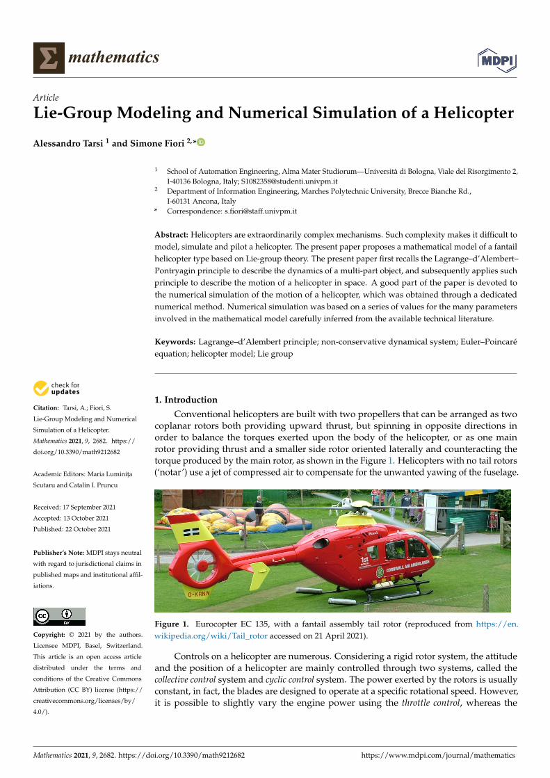
Conventional helicopters are built with two propellers that can be arranged as twocoplanar rotors both providing upward thrust, but spinning in opposite directions inorder to balance the torques exerted upon the body of the helicopter, or as one mainrotor providing thrust and a smaller side rotor oriented laterally and counteracting thetorque produced by the main rotor, as shown in the Figure 1. Helicopters with no tail rotors(‘notar’) use a jet of compressed air to compensate for the unwanted yawing of the fuselage.

Figure 1. Eurocopter EC 135, with a fantail assembly tail rotor (reproduced from https://en.wikipedia.org/wiki/Tail_rotor accessed on 21 April 2021).

Controls on a helicopter are numerous. Considering a rigid rotor system, the attitudeand the position of a helicopter are mainly controlled through two systems, called thecollective control system and cyclic control system. The power exerted by the rotors is usuallyconstant, in fact, the blades are designed to operate at a specific rotational speed. However,it is possible to slightly vary the engine power using the throttle control, whereas the

Mathematics 2021, 9, 2682. https://doi.org/10.3390/math9212682 https://www.mdpi.com/journal/mathematics

Mathematics 2021, 9, 2682 2 of 34

direction the aircraft nose points, the yaw angle, could be changed using the pedals control.A summary of helicopter controls is given in the following.

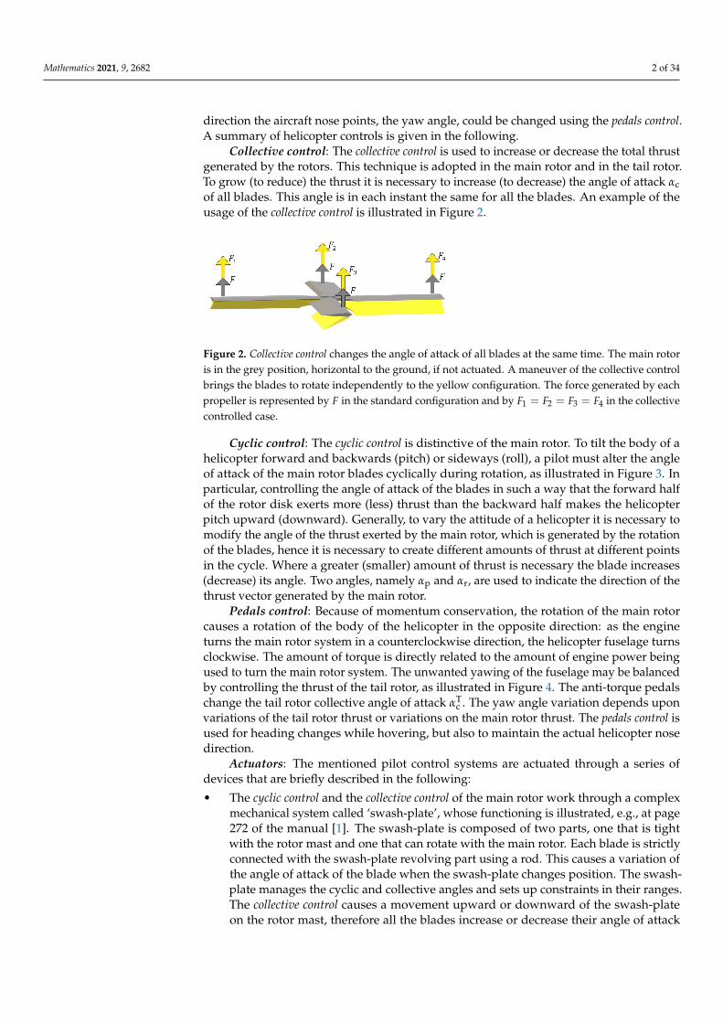
Collective control: The collective control is used to increase or decrease the total thrustgenerated by the rotors. This technique is adopted in the main rotor and in the tail rotor.To grow (to reduce) the thrust it is necessary to increase (to decrease) the angle of attack αcof all blades. This angle is in each instant the same for all the blades. An example of theusage of the collective control is illustrated in Figure 2.

Figure 2. Collective control changes the angle of attack of all blades at the same time. The main rotoris in the grey position, horizontal to the ground, if not actuated. A maneuver of the collective controlbrings the blades to rotate independently to the yellow configuration. The force generated by eachpropeller is represented by F in the standard configuration and by F1 = F2 = F3 = F4 in the collectivecontrolled case.

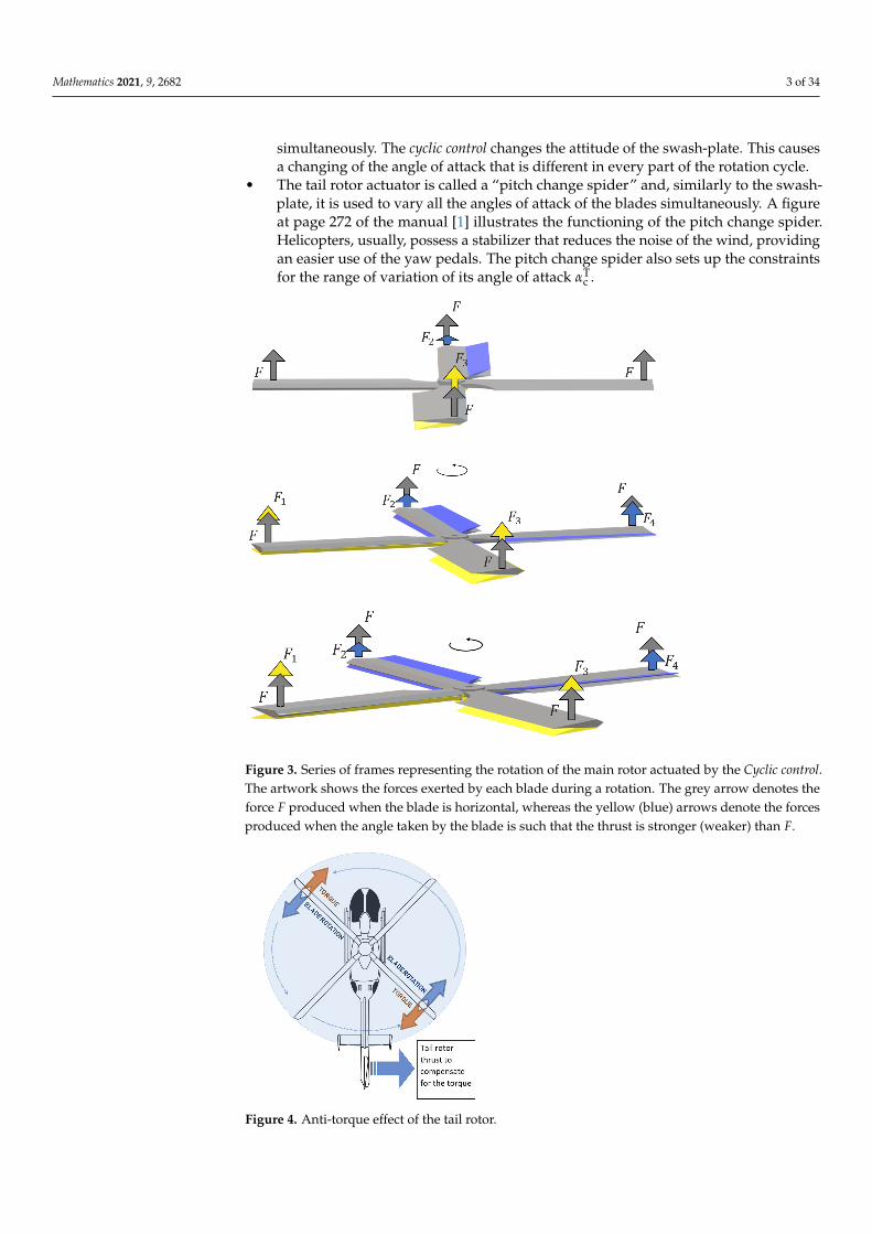
Cyclic control: The cyclic control is distinctive of the main rotor. To tilt the body of ahelicopter forward and backwards (pitch) or sideways (roll), a pilot must alter the angleof attack of the main rotor blades cyclically during rotation, as illustrated in Figure 3. Inparticular, controlling the angle of attack of the blades in such a way that the forward halfof the rotor disk exerts more (less) thrust than the backward half makes the helicopterpitch upward (downward). Generally, to vary the attitude of a helicopter it is necessary tomodify the angle of the thrust exerted by the main rotor, which is generated by the rotationof the blades, hence it is necessary to create different amounts of thrust at different pointsin the cycle. Where a greater (smaller) amount of thrust is necessary the blade increases(decrease) its angle. Two angles, namely αp and αr, are used to indicate the direction of thethrust vector generated by the main rotor.

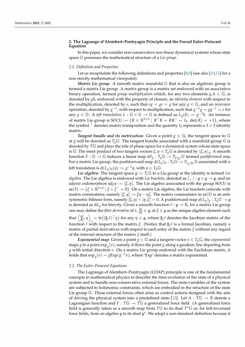
Pedals control: Because of momentum conservation, the rotation of the main rotorcauses a rotation of the body of the helicopter in the opposite direction: as the engineturns the main rotor system in a counterclockwise direction, the helicopter fuselage turnsclockwise. The amount of torque is directly related to the amount of engine power beingused to turn the main rotor system. The unwanted yawing of the fuselage may be balancedby controlling the thrust of the tail rotor, as illustrated in Figure 4. The anti-torque pedalschange the tail rotor collective angle of attack αT

c . The yaw angle variation depends uponvariations of the tail rotor thrust or variations on the main rotor thrust. The pedals control isused for heading changes while hovering, but also to maintain the actual helicopter nosedirection.

Actuators: The mentioned pilot control systems are actuated through a series ofdevices that are briefly described in the following:

• The cyclic control and the collective control of the main rotor work through a complexmechanical system called ‘swash-plate’, whose functioning is illustrated, e.g., at page272 of the manual [1]. The swash-plate is composed of two parts, one that is tightwith the rotor mast and one that can rotate with the main rotor. Each blade is strictlyconnected with the swash-plate revolving part using a rod. This causes a variation ofthe angle of attack of the blade when the swash-plate changes position. The swash-plate manages the cyclic and collective angles and sets up constraints in their ranges.The collective control causes a movement upward or downward of the swash-plateon the rotor mast, therefore all the blades increase or decrease their angle of attack

Mathematics 2021, 9, 2682 3 of 34

simultaneously. The cyclic control changes the attitude of the swash-plate. This causesa changing of the angle of attack that is different in every part of the rotation cycle.

• The tail rotor actuator is called a “pitch change spider” and, similarly to the swash-plate, it is used to vary all the angles of attack of the blades simultaneously. A figureat page 272 of the manual [1] illustrates the functioning of the pitch change spider.Helicopters, usually, possess a stabilizer that reduces the noise of the wind, providingan easier use of the yaw pedals. The pitch change spider also sets up the constraintsfor the range of variation of its angle of attack αT

c .

Figure 3. Series of frames representing the rotation of the main rotor actuated by the Cyclic control.The artwork shows the forces exerted by each blade during a rotation. The grey arrow denotes theforce F produced when the blade is horizontal, whereas the yellow (blue) arrows denote the forcesproduced when the angle taken by the blade is such that the thrust is stronger (weaker) than F.

Figure 4. Anti-torque effect of the tail rotor.

Mathematics 2021, 9, 2682 4 of 34

Throttle: The throttle controls the power of the engine which is connected to bothrotors by the transmission. The throttle setting must maintain enough engine power tokeep the rotor speed within the limits where the rotor produces enough lift for flight.The throttle changes the blades’ angular velocity in a range of few values percentage.Helicopters possess only a gear to drive both the main rotor and tail rotor, hence increasingthe speed of the main rotor causes an increase in the tail rotor speed. More throttle meansmore speed and hence a larger value of thrust. The angular velocity of the rotors is usuallyreported in percentage for a more intuitive perception, the value of 100% is the typical oneunder standard conditions.

A helicopter is an extraordinarily complicated machine, whose functioning is basedon a number of mechanical devices whose actions interact intricately to one another. Suchcomplex design make its modeling and control by a pilot a fascinating challenge. The mainchallenge encountered during the present research work was to design a mathematicalmodel that, on one hand, is able to capture the essential features of a helicopter, hence beingsufficiently accurate to predict its behavior and, on the other hand, to be simple enough forthe result to be mathematically tractable.

In the present paper, we derive, through the Euler–Poincaré formalism, the mathe-matical model of a simplified helicopter. The model concerns a helicopter with a principalrotor and a tail rotor. More accurate (and mathematically complicated) aircraft modelsare available in the specialized literature [2–4]. The structure of the present paper may beoutlined as follows:

• Section 2 presents a summary of definitions and properties regarding Lie groups,such as the tools used in this research to formalize the mathematical model of ahelicopter, i.e., tangent bundle, Lie algebra and exponential map. Moreover, thissection introduces a system of differential equations that are used to describe themotion of a helicopter.

• Section 3 introduces the structure of the helicopter, a reference system and the structureof forces used to complete the mathematical model, as the thrust of the rotors. Inaddition, this section outlines a derivation of the equations of motion starting from aLagrangian function.

• Section 4 presents a numerical scheme to simulate on a computing platform the systemof equations determined in Section 3 using a forward Euler (fEul) method tailored tothe Lie group of rotations.

• Section 5 introduces a helicopter type and shows the values of the parameters requiredto perform simulation analysis. These values are presented in tables and figures andhave been gathered (and calculated) from data-sheets.

• Section 6 illustrates eight simulation results. Each simulation is particularly focusedon a specific response, i.e., pitch response and roll response.

• Section 7 concludes this paper with a recapitulation of the obtained results and anoverview of the key points of the performed analysis.

We would like to mention that the scientific literature about system modeling (includ-ing mechanical system modeling) is rich in inventions. A few alternative techniques to themore traditional equation-based modeling and control are bond graph modeling utilized,e.g., in [5] to design a Kalman filter observer for an industrial back-support exoskeleton;closed loop identification and frequency domain analysis, utilized in [6] to determine adynamic model of a quadrotor prototype; deep neural networks, used in [7] to predict theremaining useful life (RUL) of aircraft gas turbine engines. The present authors are notfamiliar enough with the mentioned techniques to judge their advantages or disadvantagesin relation to the proposed modeling method, which arises as a more elaborated version ofthe familiar Euler–Lagrange formalism (except for the neural-network modeling approachthat provides an approximated, data-derived model in contrast to exact models).

Mathematics 2021, 9, 2682 5 of 34

2. The Lagrange–d’Alembert–Pontryagin Principle and the Forced Euler–PoincaréEquation

In this paper, we consider non-conservative non-linear dynamical systems whose statespace G possesses the mathematical structure of a Lie group.

2.1. Definition and Properties

Let us recapitulate the following definitions and properties [8,9] (see also [10,11] for anon-strictly mathematical viewpoint):

Matrix Lie group: A smooth matrix manifold G that is also an algebraic group istermed a matrix Lie group. A matrix group is a matrix set endowed with an associativebinary operation, termed group multiplication which, for any two elements g, h ∈ G, isdenoted by gh, endowed with the property of closure, an identity element with respect tothe multiplication, denoted by e, such that eg = ge = g for any g ∈ G, and an inversionoperation, denoted by g−1, with respect to multiplication, such that g−1g = gg−1 = e forany g ∈ G. A left translation L : G×G → G is defined as Lg(h) := g−1h. An instanceof matrix Lie group is SO(3) := R ∈ R3×3 | R>R = RR> = I3, det(R) = +1, wherethe symbol > denotes matrix transposition and the quantity I3 represents a 3× 3 identitymatrix.

Tangent bundle and its metrization: Given a point g ∈ G, the tangent space to Gat g will be denoted as TgG. The tangent bundle associated with a manifold-group G isdenoted by TG and plays the role of phase-space for a dynamical system whose state-spaceis G. The inner product of two tangent vectors ξ, η ∈ TgG is denoted by 〈ξ, η〉g. A smoothfunction F : G → G induces a linear map dFg : TgG → TF(g)G termed pushforward map.For a matrix Lie group, the pushforward map d(Lg)h : ThG→ TLg(h)G associated with aleft translation is d(Lg)h(η) := g−1η, with η ∈ ThG.

Lie algebra: The tangent space g := TeG to a Lie group at the identity is termed Liealgebra. The Lie algebra is endowed with Lie brackets, denoted as [·, ·] : g× g→ g, and anadjoint endomorphism adξ η := [ξ, η]. The Lie algebra associated with the group SO(3) isso(3) := ξ ∈ R3×3 | ξ + ξ> = 0. On a matrix Lie algebra, the Lie brackets coincide withmatrix commutator, namely [ξ, η] := ξη − ηξ. The matrix commutator in so(3) is an anti-symmetric bilinear form, namely [ξ, η] + [η, ξ] = 0. A pushforward map d(Lg)g : TgG→ g

is denoted as dLg for brevity. Given a smooth function ` : g→ R, for a matrix Lie groupone may define the fiber derivative of `, ∂`

∂ξ ∈ g, at ξ ∈ g as the unique algebra element such

that⟨

∂`∂ξ , η

⟩e= tr

((Jξ`)

>η)

for any η ∈ g, where Jξ` denotes the Jacobian matrix of thefunction ` with respect to the matrix ξ. (Notice that Jξ` is a formal Jacobian, namely amatrix of partial derivatives with respect to each entry of the matrix ξ without any regardof the internal structure of the matrix ξ itself.)

Exponential map: Given a point g ∈ G and a tangent vector v ∈ TgG, the exponentialmaps g to a point expg(v), namely, it flows the point g along a geodesic line departing fromg with initial direction v. On a matrix Lie group endowed with the Euclidean metric, itholds that expg(v) = gExp(g−1v), where ‘Exp’ denotes a matrix exponential.

2.2. The Euler–Poincaré Equations

The Lagrange–d’Alembert–Pontryagin (LDAP) principle is one of the fundamentalconcepts in mathematical physics to describe the time-evolution of the state of a physicalsystem and to handle non-conservative external forces. The state-variables of the systemare subjected to holonomic constraints, which are embodied in the structure of the stateLie group G. These external forces often arise as control actions designed with the aimof driving the physical system into a predefined state [12]. Let Λ : TG → R denote aLagrangian function and F : TG → TG a generalized force field. (A generalized forcefield is generally taken as a smooth map from TG to its dual T?G or, for left-invariantforce fields, from an algebra g to its dual g?. We adopt a non-standard definition because it

Mathematics 2021, 9, 2682 6 of 34

eases the notation and is more easily translated into implementation). The LDAP principleaffirms that a dynamical system follows a trajectory g : [a, b]→ G such that:

δ∫ b

aΛ(g(t), g(t))dt +

∫ b

a〈F(g(t), g(t)), δg(t)〉g(t) dt = 0, (1)

The leftmost integral is called action and the symbol δ denotes variation, namely thechange of the action value from a trajectory g to a trajectory that is infinitely close to g,whose point-by-point change is denoted as δg. The variation vanishes at endpoints andis elsewhere arbitrary. In the above expression, an over-dot (as in g) denotes derivationwith respect to the parameter t. The vanishing of the first term alone is called principle ofstationary action. The rightmost integral represents the total work achieved by the forcefield F due to the variation.

A variational formulation is based on a smooth family of curves g : U ⊂ R2 → G,where each element is denoted as g(t, ε). The index ε selects a curve in the family, and theindex t individuates a point over this curve. All the curves in the family depart from thesame initial point and arrive at the same endpoint, namely, g(a, ε) and g(b, ε) are constantwith respect to ε. The variations in (1) are defined as

δ∫ b

aΛ(g, g)dt :=

∫ b

a

∂

∂εΛ(g(t, ε), g(t, ε))dt

∣∣∣∣ε=0

, δg(t) :=∂g(t, ε)

∂ε

∣∣∣∣ε=0

. (2)

The following result, enunciated directly for matrix Lie groups, is of prime importance,as it relates a variation of velocity to velocity of variation.

Lemma 1 ([13]). Given a smooth function g : U ⊂ R2 → G on a matrix Lie group, define:

ξ(t, ε) := g−1(t, ε)∂g(t, ε)

∂t, η(t, ε) := g−1(t, ε)

∂g(t, ε)

∂ε. (3)

A variation of a trajectory induces a variation of its velocity field given by

∂ξ

∂ε= η + adξ η. (4)

Assuming that the Lagrangian as well as the generalized force field F are left invariant,we may write Λ(g, g) = `(g−1 g) and g−1F(g, g) = f (g−1 g), where ` : g→ R and f : g→ g

denote a reduced Lagrangian and a reduced force field, respectively. In addition, if the innerproduct is left-invariant, it holds that

〈F(g, g), δg〉g = 〈 f (g−1 g), g−1δg〉e. (5)

Therefore, the LDAP principle (1) reduces to

δ∫ b

a`(g−1 g)dt +

∫ b

a〈 f (g−1 g), g−1δg〉e dt = 0, (6)

where it is legitimate to replace g−1 g with ξ and g−1δg with η and then set ε to 0.By means of the Lemma 1, the variational formulation of the reduced LDAP principle

may be recast in a differential form.

Theorem 1 ([13]). Let ξ := g−1 g and η := g−1δg. The solution of the integral Lagrange–d’Alembert equation (6) under perturbations of the form ∂ξ

∂ε = η + adξ η, which vanishes atendpoints, satisfies the Euler–Poincaré equation

ddt

∂`

∂ξ= ad?

ξ

(∂`

∂ξ

)+ f , (7)

Mathematics 2021, 9, 2682 7 of 34

where ad? denotes the adjoint (The adjoint ω? of an operator ω : g→ g with respect to an innerproduct 〈·, ·〉 satisfies 〈ω(ξ), η〉 = 〈ξ, ω?(η)〉.) of the operator ad with respect to the inner productof g.

The complete system of differential equations then readg = gξ,ddt

∂`∂ξ = ad?

ξ

(∂`∂ξ

)+ f .

(8)

The above equations may be used to describe the rotational component of motion of aflying object such as a helicopter or a drone. The forcing term takes into account severalexternal driving phenomena, such as:

Energy dissipation: Energy dissipation is due, e.g., to friction with air particles. Forinstance, a linear dissipation term represents aerodynamic drag.

Control actions: Other than dissipation (which is often neglected in simplistic models),the forcing term depends on the problem under investigation. It might serve to incorporateinto the equations control terms aimed, for instance, at stabilizing the motion or to drive adynamical system [14].

2.3. Particular Case: Euclidean Space

In order to clarify the physical meaning of the Euler–Poincaré equations, let us recallthe classical version of these equations for the space Rn, which is also instrumental indescribing the translational component of motion of a flying device. The principle (1) onRn, endowed with the Euclidean inner product, reads:

δ∫ b

aΛ(p(t), p(t))dt +

∫ b

af (p(t), p(t))>δp(t)dt = 0, (9)

where Λ : Rn ×Rn → R denotes a Lagrangian function, p = p(t) a trajectory in Rn andf : Rn ×Rn → Rn a non-conservative force field. Upon computing the variation, we obtain

∫ b

a

((∂Λ∂p

)>δp +

(∂Λ∂ p

)>δ p + f>δp

)dt = 0. (10)

Integrating by parts the second term and recalling that the variations vanish at theendpoints, we obtain ∫ b

a

(∂Λ∂p− d

dt∂Λ∂ p

+ f)>

δp dt = 0. (11)

Since the variation δp is arbitrary, the dynamics of the variable p is governed by theEuler–Lagrange equation

ddt

∂Λ∂ p

=∂Λ∂p

+ f (12)

where the quantity q := ∂Λ∂ p is usually termed linear momentum.

3. Mathematical Model of a Helicopter

This section introduces a helicopter model based on the Lie group G := SO(3) of the3-dimensional rotations R.

Since, in the state space G := SO(3), it holds that (dLR)−1(ξ) = Rξ and ad?

ξ η =−adξ η [13], the Euler–Poincaré equations read

R = Rξ,ddt

∂`∂ξ = −adξ

(∂`∂ξ

)+ τ,

(13)

Mathematics 2021, 9, 2682 8 of 34

where τ denotes the resultant of all external mechanical torques. In this context, the statevariable R ∈ SO(3) denotes the attitude of a rigid body (i.e., its orientation with respectto a earth-fixed reference frame) and the state-variable ξ ∈ so(3) denotes its instantaneousangular velocity. Moreover, the quantity µ := ∂`

∂ξ represents an angular momentum andthe second Euler–Poincaré equation reads µ = [µ, ξ] + τ, which is a generalization of thewell-known angular momentum theorem, where the term [µ, ξ] represents the inertialtorque due to the internal mass unbalance of a body.

It is convenient to define the operator J·K : R3 → g as:

x :=

x1x2x3

7→ JxK :=

0 −x3 x2x3 0 −x1−x2 x1 0

. (14)

Since any skew-symmetric matrix in so(3) may be written as in (14), it is convenientto define a basis of so(3) = span(ξx, ξy, ξz) as follows:

ξx :=

0 0 00 0 −10 1 0

, ξy :=

0 0 10 0 0−1 0 0

, ξz :=

0 −1 01 0 00 0 0

. (15)

In order to shorten some relations, it is also convenient to introduce the matrix anti-commutator A, B := AB + BA. Moreover, some relations take advantage of the skew-symmetric projection · : R3×3 → so(3), defined as A := 1

2 (A− A>). It also pays

to define the ‘diag’ operator as diag(a, b, c) :=

a 0 00 b 00 0 c

.

In the present setting, we equip the algebra so(3) with the canonical metric 〈ξ, η〉e :=tr(ξ>η). With this choice, the fiber derivative of a scalar function ` : so(3) → R takes aspecial form.

Lemma 2 ([15]). The fiber derivative of a scalar function ` : so(3) → R under the canonicalmetric takes the form

∂`

∂ξ=

12(Jξ`− J>ξ `) ∈ so(3). (16)

It is immediate to verify that the fiber derivative corresponds to the orthogonal pro-jection of the Jacobian into the algebra g, namely ∂`

∂ξ = Jξ`. Moreover, it is convenientto recall a property of the matrix ‘trace’ operator, namely the cyclic permutation propertytr(ABC) = tr(BCA) = tr(CAB) for any square conformable matrices A, B, C.

Modeling a complex object to obtain the differential equations that describe its rota-tional and translational dynamics consists essentially in:

• Defining a Lagrangian function ` on the basis of the kinetic and potential energy ofits components, which accounts for the geometrical and mechanical features of eachcomponent;

• Computing the total mechanical torque τ exerted by the moving parts on the body ofthe complex object.

These descriptors, for a helicopter, are evaluated in the next subsections.

3.1. Model of a Helicopter with a Single Principal Rotor and a Tail Rotor

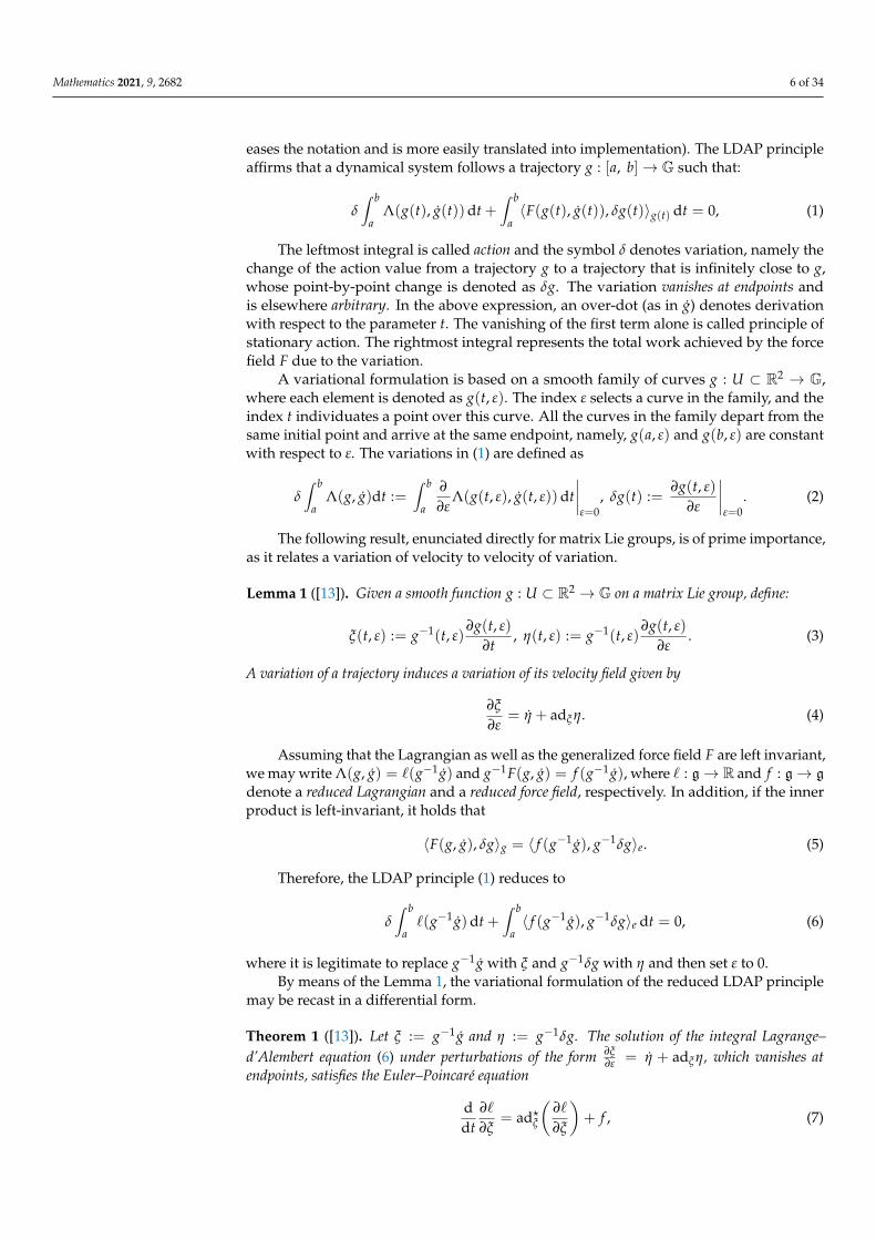
In order to formalize the behavior of a helicopter into a mathematical model, let usfix an inertial (earth) reference frame FE. Further, it is necessary to establish a body-fixedreference frame FB, as shown in Figure 5: the origin of the reference frame FB is located atthe center of gravity of the helicopter and the three axes coincide with its principal inertiaaxes. The thrust ϕm exerted by the principal rotor appears at the tip of the helicopter’sbody, which is located along the z-axis at a distance Dm from the center of gravity, whereas

Mathematics 2021, 9, 2682 9 of 34

the thrust ϕt exerted by the tail rotor appears at the tail of the helicopter’s body, which islocated along the −x axis at a distance Dt from the center of gravity.

FB

ϕt

ϕm

Dt

Dm

Figure 5. Schematic of a helicopter with a principal rotor and a tail rotor (adapted from [12]). (Theprincipal rotor to center of mass distance Dm and the tail rotor to center of mass distance Dt areexpressed in meters (m).)

Furthermore, the term 12 um represents the intensity of the thrust exerted by the main

rotor, while 12 ut denotes the thrust exerted by the tail rotor, both expressed in Newtons (N).

Considering the total thrust ϕ := ϕt + ϕm as a vector, a collective control management ofthe main rotor results in a change of the thrust intensity exerted, namely a change in um,whereas a cyclic control management changes the direction of the lift exerted, therefore thepitch angle αp (in radians (rad)) and the sideways roll angle αr (in radians). The expressionsof the thrusts (from [12]) and of their moment arms in the helicopter’s body-fixed frameFB are given by

ϕm := 12 um

sin αp cos αr− sin αr

cos αp cos αr

, bm :=

00

Dm

, (17)

ϕt := 12 ut

0−10

, bt :=

−Dt00

. (18)

The vector 2ϕmum

may be regarded as the unit normal to the rotor disk [2]. A furtherforcing term to account for the resistance of the air during forward vertical motion isdescribed in Section 3.4. Concerning the thrust generated by the principal rotor, we maynotice what follows:

• Whenever αr = αp = 0, the thrust takes the expression 12 um

001

, namely, only the

z-component is non-null and the thrust is vertical;

• Whenever αp = 0 and αr 6= 0, the thrust takes the expression 12 um

0− sin αrcos αr

,

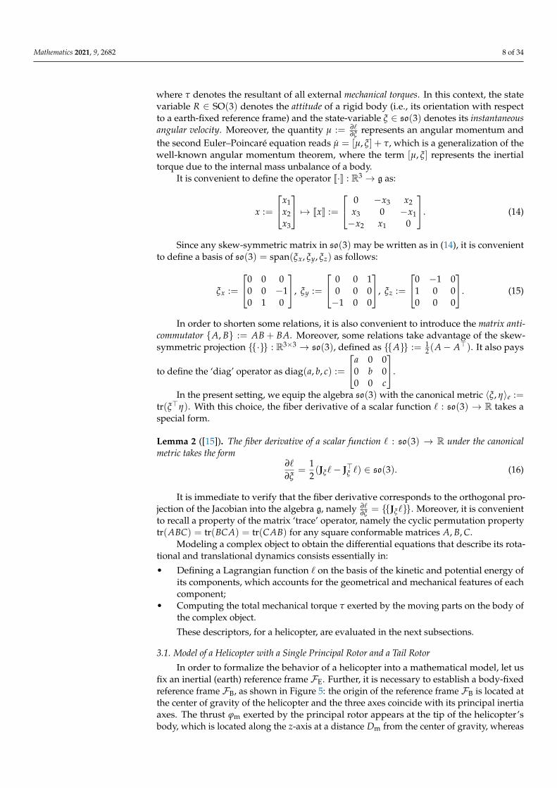
namely, the x-component is null and the thrust belongs to the y–z plane, as shown inFigure 6, hence it may only produce a rotation along the x-axis, which corresponds topure rolling. (Remark: The right-hand law defines the positive angle variation.)

Mathematics 2021, 9, 2682 10 of 34

Figure 6. Illustration of a positive variation of the angle of attack along the x-axis, where ϕy =

− 12 um sin αr and ϕz = 1

2 um cos αr are the projections of the thrust vector ϕm along the y- and z-axis,respectively. The maneuver to control rolling assigns to the blades an angle such that a greateramount of force is produced in the positive x-axis, namely fa, with respect to the force in the negativex-axis, namely fb. Those two vector forces produce a torque and a precession rotation due to thegyroscopic effect.

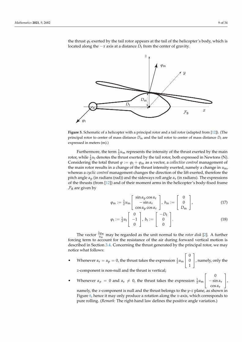
• whenever αr = 0 and αp 6= 0, the thrust takes the expression 12 um

sin αp0

cos αp

, namely,

the y-component is null and the thrust belongs to the x–z plane, as shown in Figure 7,hence it may only produce a rotation along the y-axis, which corresponds to purepitching.

Figure 7. Illustration of a positive variation of the angle of attack along the y-axis, whereϕx = 1

2 um sin αp and ϕz = 12 um cos αp are the projections of the main rotor thrust ϕm to the x-

and z-axis, respectively. The maneuver to control the pitching assigns to the blades an angle suchthat a larger amount of force is produced in the positive y-axis, namely fa, with respect to the forcealong the negative y-axis, namely fb. Those two vector forces produce a mechanical torque and aprecession of the fuselage.

Notice that the inclination of the blades influences the thrust and the torque acting onthe fuselage, but does not influence directly the roll and the pitch attitude of the helicopter.Further, notice that the thrust 1

2 um does not distribute equally across the three directionsof space and, in particular, that a change in the angles of attack of the blades weakensthe vertical component of the thrust: when a helicopter tilts, it tends to fall, unless thethrust is compensated by the pilot. It is also worth noticing that the total thrust ϕ actingon the fuselage has a y component that depends on the tail rotor thrust. This componentcauses the translation of the helicopter in the direction of ϕt: this is called drift effect (ortranslation tendency). The mechanical torque exerted by the two rotors on the helicopter’sfuselage, expressed in N·m, is termed active torque and is given by

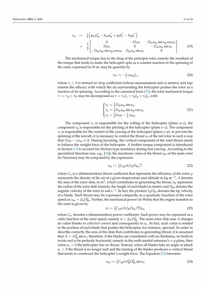
Mathematics 2021, 9, 2682 11 of 34

τA := 12

(ϕmb>m − bm ϕ>m + ϕtb>t − bt ϕ>t

)=

12

0 −Dtut Dmum sin αp cos αrDtut 0 −Dmum sin αr

−Dmum sin αp cos αr Dmum sin αr 0

. (19)

The mechanical torque due to the drag of the principal rotor, namely the resultant ofthe torque that tends to make the helicopter spin as a counter-reaction to the spinning ofthe rotor, expressed in N·m, may be quantify by

τD := − 12 γumξz, (20)

where γ > 0 is termed air drag coefficient (whose measurement unit is meters) and rep-resents the efficacy with which the air surrounding the helicopter pushes the rotor as areaction of its spinning. According to the canonical basis (15), the total mechanical torqueτ := τA + τD may be decomposed as τ = τxξx + τyξy + τzξz, with

τx = 12 Dmum sin αr,

τy = 12 Dmum sin αp cos αr,

τz =12 Dtut − 1

2 γum.

(21)

The component τx is responsible for the rolling of the helicopter (plane y–z), thecomponent τy is responsible for the pitching of the helicopter (plane x–z). The componentτz is responsible for the control of the yawing of the helicopter (plane x–y): to prevent thespinning of the aircraft, it is necessary to control the thrust ut of the tail rotor in such a waythat Dtut − γum ≈ 0. During hovering, the vertical component of the total thrust needsto balance the weight force of the helicopter. A further torque component is introducedin Section 3.3 to account for friction-type resistance during fast yawing. According to thespecialized literature (see, e.g., [16]), the maximum value of the thrust um of the main rotor(in Newtons) may be computed by the expression

um := 12 CuρA(lRΩm)2, (22)

where Cu is a (dimensionless) thrust coefficient that represents the efficiency of the rotor, ρrepresents the density of the air at a given temperature and altitude in kg·m−3, A denotesthe area of the rotor disk, in m2, which contributes to generating the thrust, lR representsthe radius of the rotor disk (namely, the length of each blade) in meters and Ωm denotes theangular velocity of the rotor in rad·s−1. In fact, the product lRΩm denotes the tip velocityof a blade. Such thrust may be expressed compactly as a quadratic function of the rotorspeed as um = βuΩ2

m. Further, the mechanical power (in Watts) that the engine transfers tothe rotor is given by

w := 12 CwρA(lRΩm)2Ωm, (23)

where Cw denotes a (dimensionless) power coefficient. Such power may be expressed as acubic function of the rotor speed, namely w = βwΩ3

m. The main rotor disk area A changesits value thanks to collective control and consequently to αc. In fact, such value is relatedto the portion of each blade that pushes the helicopter, for instance, upward. In order todescribe correctly the area of the disk that contributes to generating thrust, it is assumedthat A = πl2

R sin αc; therefore, if the blades are considered with no thickness, no built-intwists and to be perfectly horizontal, namely in the earth inertial reference’s x–y plane, thenwhen αc = 0 the helicopter has no thrust. Instead, when all blades take an angle of attackαc > 0 the thrust is no longer null and the turning of the blades produces a vertical thrustthat tends to counteract the helicopter’s weight force. The Equation (22) becomes:

um := 12 Cuρπl4

RΩ2m sin αc, (24)

Mathematics 2021, 9, 2682 12 of 34

with αc ∈ [αc,min, αc,max]. The minimum and the maximum value of the thrust dependon the range of the angle of attack of the principal rotors blades, whereas the range ofthe angle of attack is related to the shape and the built-in twist of the blades, besides theswash-plate rods mobility. The power coefficient Cw is related to the thrust coefficient Cuby the relationship

Cw =C3/2

u√2

. (25)

The mechanical power w absorbed by the helicopter’s engine at the reference speed of100% is usually provided by data-sheets. Considering w as known, it is possible to calculatethe power and the thrust coefficients, that otherwise would have to be measured throughexperiments. The value of the first coefficient, following the Equation (23), is

Cw =2 w

ρA(lRΩm)2Ωm(26)

Consequently it is possible to find the value of Cu using the Equation (25). Theexpression (24) holds for the main rotor, while a similar expression may describe the thrustexerted by the tail rotor. The equation below is based on tail rotor characteristics:

ut := 12 CT

uρπl4T Ω2

t sin αTc , (27)

where CTu denotes the thrust coefficient of the tail rotor and lT denotes the length of the tail

rotor’s blades. The drag coefficient is generally unknown, but it is possible to estimate itsvalue by assuming that the helicopter hovering and that the mechanical torque of the tailrotor balances the undesired drag torque, which would tend to make the helicopter yaw.Indeed, in hovering condition, with the tail rotor’s blades collective angle at a value set to

a half of its interval range, namely αTc,mid :=

αTc,min+αT

c,max2 (see Table 1), and at 100% of the

tail rotor speed, the helicopter should have no yawing. The drag coefficient could hencebe determined by imposing the condition e>z τ = 0, where ez := [0 0 1]>, which leads tothe expression

γ = DtCul4RΩ2

m sin αc

CTu l4T Ω2

t sin αTc,mid

. (28)

The numerical values of these (as well as others) parameters will be specified inSection 5.

Table 1. Tail rotor collective angle range, tail and main rotors weight, speed ([1], pages 303, 254 and 157), tail rotorspeed ([17], page 3) and cycling angle range ([18], page 11).

Weight Speed 100% Collective Angle Cyclic Angle

[kg] [RPM] min ÷ max [deg] Longitudinal [deg] Lateral [deg]

Main rotor 277.2 1 395 11 ÷ 31 2 −21.8 ÷ 21.8 −15 ÷ 15Tail rotor 8.2 3584 −16.8 ÷ 34.2 − −

1 The main rotor weight is the result of the addition of various components that compose the entire main rotor. These values have beentaken from [19] (page 3) which is the technical data-sheet of the helicopter AS350B3 also known as H125, that is the lower level helicopter bythe same manufacturer. The values taken have not been modified because the model is supposed to be similar. The final weight is calculatedby the sum of: anti-vibration device (28.4 kg), main rotor mast (55.7 kg), rotor hub (57.5 kg) and four blades (4× 33.9 kg = 135.6 kg). 2 Asstated in [20] (page 57) the value of the collective angle could vary in the range −5÷ 15 degrees and the negative angle could be necessaryto achieve zero lift if blades have a built-in axial twist. From Reference [1] (page 200), we know that the EC135 P2+ helicopter has a positivetwist of 16 degrees in the region where the pitch control cuff joins the airfoil section. This provides the airfoil section with a correspondingpreset pitch angle. Using the Equation (24), the collective angles range becomes 11÷ 31 degrees, the minimum angle and the maximumangle to modify the intensity of the thrust generated, respectively.

Mathematics 2021, 9, 2682 13 of 34

3.2. Lagrangian Function Associated to the Helicopter Model

To complete the present description of a helicopter motion dynamics, it is necessary towrite explicitly the Lagrangian function of a helicopter, which coincides with its kineticenergy minus its potential energy, both expressed in the inertial reference frame FE.

Kinetic energy of the fuselage: The position of the center of gravity of the helicopter inthe inertial reference frameFE at time t is denoted as p(t). The position of each infinitesimalvolume of the body (fuselage) in the body-fixed frame FB is denoted by s. Since thehelicopter’s fuselage is rigid, the position of each volume element, at time t, is p(t) + R(t)s,where R(t) ∈ SO(3) denotes a rotation matrix that takes the body-fixed frame FB tocoincide with FE. The kinetic energy of the helicopter’s body B with respect to the inertialreference frame FE may be written as

`B :=12

∫B

∥∥∥∥d(p + Rs)dt

∥∥∥∥2

dm =12

∫B

‖ p + Rs‖2dm, (29)

where dm denotes the mass content of each infinitesimal volume. Recalling that R = Rξ,with ξ ∈ so(3), we get:

`B =12

∫B

tr(( p + Rs)( p + Rs)>)dm =12

∫B

tr( p p> + Rξss>ξ>R> + 2ps>R)dm

= 12 MB‖ p‖2 + 1

2 tr(R ξ JBξ>R> ) + MBtr( pc>B R), (30)

where the cancellation is due to the cyclic permutation property of the trace operator andto the defining property of rotations (R>R = I3). The constant quantities that appear in theexpression (30) are defined as follows

MB :=∫B

dm > 0, cB :=1

MB

∫B

s dm ∈ R3, JB :=∫B

ss>dm ∈ R3×3. (31)

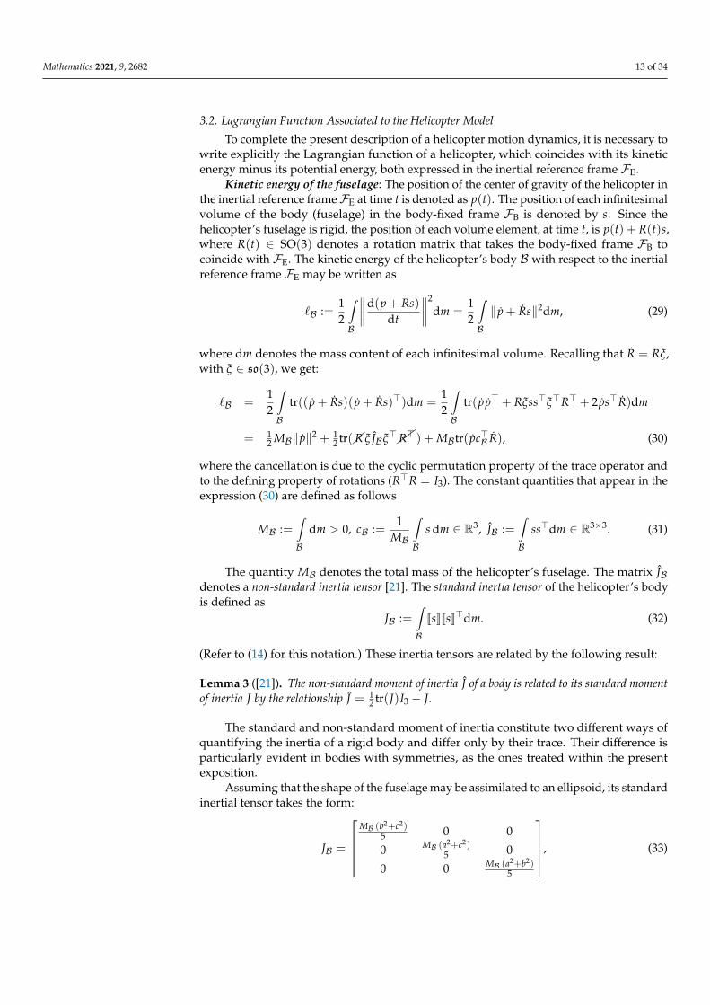
The quantity MB denotes the total mass of the helicopter’s fuselage. The matrix JBdenotes a non-standard inertia tensor [21]. The standard inertia tensor of the helicopter’s bodyis defined as

JB :=∫B

JsKJsK>dm. (32)

(Refer to (14) for this notation.) These inertia tensors are related by the following result:

Lemma 3 ([21]). The non-standard moment of inertia J of a body is related to its standard momentof inertia J by the relationship J = 1

2 tr(J)I3 − J.

The standard and non-standard moment of inertia constitute two different ways ofquantifying the inertia of a rigid body and differ only by their trace. Their difference isparticularly evident in bodies with symmetries, as the ones treated within the presentexposition.

Assuming that the shape of the fuselage may be assimilated to an ellipsoid, its standardinertial tensor takes the form:

JB =

MB (b2+c2)

5 0 0

0 MB (a2+c2)5 0

0 0 MB (a2+b2)5

, (33)

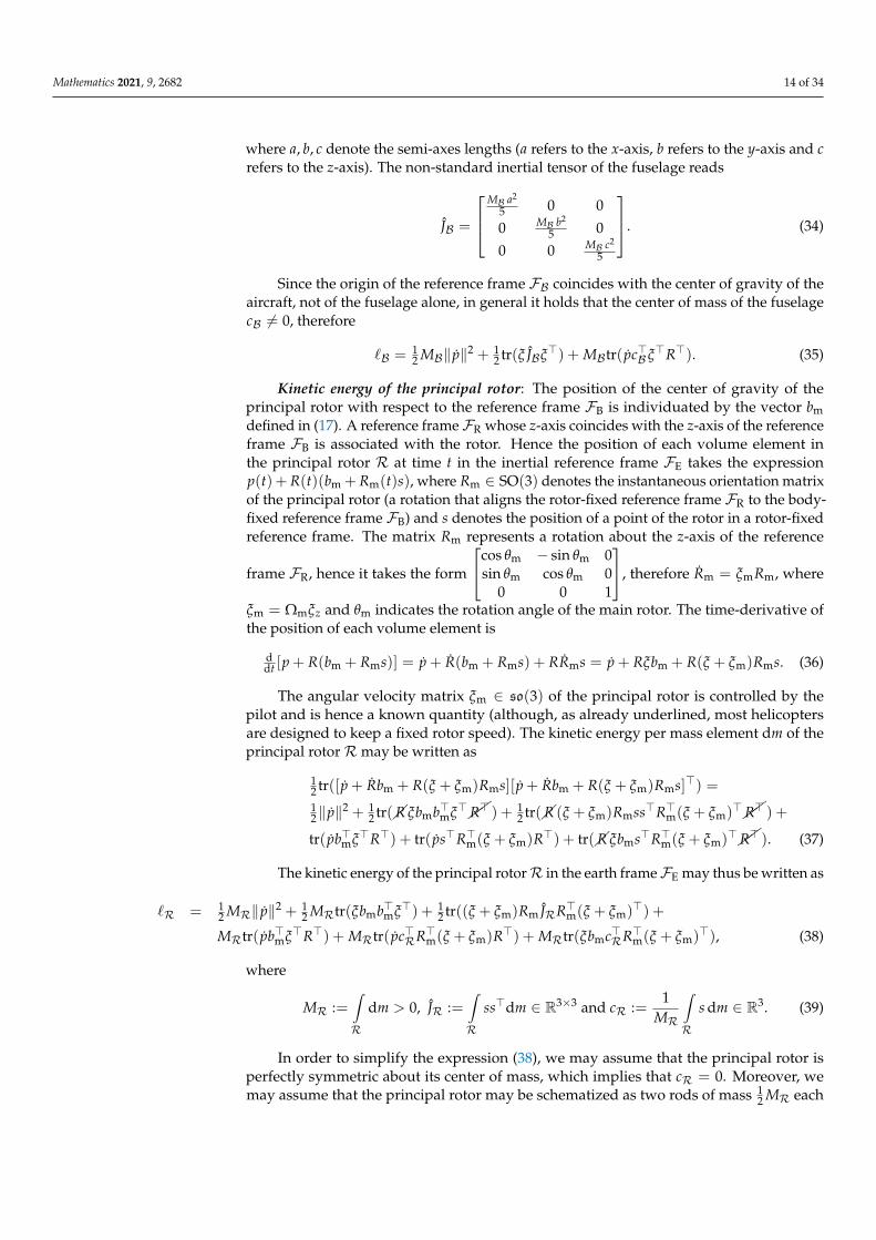
Mathematics 2021, 9, 2682 14 of 34

where a, b, c denote the semi-axes lengths (a refers to the x-axis, b refers to the y-axis and crefers to the z-axis). The non-standard inertial tensor of the fuselage reads

JB =

MB a2

5 0 0

0 MB b2

5 0

0 0 MB c2

5

. (34)

Since the origin of the reference frame FB coincides with the center of gravity of theaircraft, not of the fuselage alone, in general it holds that the center of mass of the fuselagecB 6= 0, therefore

`B = 12 MB‖ p‖2 + 1

2 tr(ξ JBξ>) + MBtr( pc>B ξ>R>). (35)

Kinetic energy of the principal rotor: The position of the center of gravity of theprincipal rotor with respect to the reference frame FB is individuated by the vector bmdefined in (17). A reference frame FR whose z-axis coincides with the z-axis of the referenceframe FB is associated with the rotor. Hence the position of each volume element inthe principal rotor R at time t in the inertial reference frame FE takes the expressionp(t) + R(t)(bm + Rm(t)s), where Rm ∈ SO(3) denotes the instantaneous orientation matrixof the principal rotor (a rotation that aligns the rotor-fixed reference frame FR to the body-fixed reference frame FB) and s denotes the position of a point of the rotor in a rotor-fixedreference frame. The matrix Rm represents a rotation about the z-axis of the reference

frame FR, hence it takes the form

cos θm − sin θm 0sin θm cos θm 0

0 0 1

, therefore Rm = ξmRm, where

ξm = Ωmξz and θm indicates the rotation angle of the main rotor. The time-derivative ofthe position of each volume element is

ddt [p + R(bm + Rms)] = p + R(bm + Rms) + RRms = p + Rξbm + R(ξ + ξm)Rms. (36)

The angular velocity matrix ξm ∈ so(3) of the principal rotor is controlled by thepilot and is hence a known quantity (although, as already underlined, most helicoptersare designed to keep a fixed rotor speed). The kinetic energy per mass element dm of theprincipal rotorRmay be written as

12 tr([ p + Rbm + R(ξ + ξm)Rms][ p + Rbm + R(ξ + ξm)Rms]>) =12‖ p‖2 + 1

2 tr(R ξbmb>mξ>R> ) + 12 tr(R (ξ + ξm)Rmss>R>m(ξ + ξm)>R> ) +

tr( pb>mξ>R>) + tr( ps>R>m(ξ + ξm)R>) + tr(R ξbms>R>m(ξ + ξm)>R> ). (37)

The kinetic energy of the principal rotorR in the earth frameFE may thus be written as

`R = 12 MR‖ p‖2 + 1

2 MRtr(ξbmb>mξ>) + 12 tr((ξ + ξm)Rm JRR>m(ξ + ξm)>) +

MRtr( pb>mξ>R>) + MRtr( pc>RR>m(ξ + ξm)R>) + MRtr(ξbmc>RR>m(ξ + ξm)>), (38)

where

MR :=∫R

dm > 0, JR :=∫R

ss>dm ∈ R3×3 and cR :=1

MR

∫R

s dm ∈ R3. (39)

In order to simplify the expression (38), we may assume that the principal rotor isperfectly symmetric about its center of mass, which implies that cR = 0. Moreover, wemay assume that the principal rotor may be schematized as two rods of mass 1

2 MR each

Mathematics 2021, 9, 2682 15 of 34

and length 2 lR, one along the x axis and one along the y-axis, spinning around the z-axis,therefore:

JR =

jR 0 00 jR 00 0 2jR

that is JR = jRdiag(1, 1, 0), (40)

by Lemma 3, with jR := 112

MR2 (2lR)2 = 1

6 MRl2R. (Refer to the beginning of the present

section for the notation used.) A consequence is that the expression Rm JRR>m simplifies toJR; therefore, the kinetic energy of the principal rotor is given by

`R = 12 MR‖ p‖2 + 1

2 MRtr(ξbmb>mξ>) + 12 tr((ξ + ξm) JR(ξ + ξm)>) + MRtr( pb>mξ>R>). (41)

Rearranging these terms shows that the kinetic energy of the principal rotor may bewritten equivalently as the quadratic form

`R = 12 MR‖ p + Rξbm‖2 + 1

2 tr((ξ + ξm) JR(ξ + ξm)>), (42)

where the first term represents the translational kinetic energy of the center of mass ofthe principal rotor in the reference system FE, whereas the second term represents therotational kinetic energy of the principal rotor in the reference system FE.

Kinetic energy of the tail rotor: The position of the tail rotor with respect to thereference frame FB is individuated by the vector bt defined in (18), hence the position ofeach point in the tail rotor T at time t is given by p(t)+ R(t)(bt + Rt(t)s), where Rt ∈ SO(3)denotes the instantaneous orientation matrix of the tail rotor with respect to a body-fixedreference frame FB and s denotes the position of a point of the tail rotor in a rotor-fixedreference frame. In this case, it holds that

ddt [p + R(bt + Rts)] = p + R(bt + Rts) + RRts = p + Rξbt + R(ξ + ξt)Rts, (43)

where Rt = ξtRt. The angular velocity matrix ξt ∈ so(3) of the principal rotor is controlledby the pilot and is hence to be held as a known quantity. Since the instantaneous axis ofrotation of the tail rotor is fixed and coincides to the −y axis, the angular matrix ξt takesthe explicit expression

ξt := −Ωtξy =

0 0 −Ωt0 0 0

Ωt 0 0

, (44)

where Ωt denotes the instantaneous rotation speed of the tail rotor.The kinetic energy of the tail rotor T in the earth frame FE has an expression which is

derived in a similar manner to (38) and may be written as

`T = 12 MT ‖ p‖2 + 1

2 MT tr(ξbtb>t ξ>) + 12 tr((ξ + ξt)Rt JT R>t (ξ + ξt)

>) +

MT tr( pb>t ξ>R>) + MT tr( pc>T R>t (ξ + ξt)R>) + MT tr(ξbtc>T R>t (ξ + ξt)>), (45)

where

MT :=∫T

dm > 0, JT :=∫T

ss>dm ∈ R3×3 and cT :=1

MT

∫T

s dm ∈ R3. (46)

In order to simplify the expression (45), we may assume that the tail rotor is perfectlysymmetric about its own center of mass cT , which implies that cT = 0. Moreover, weassume that the tail rotor may be schematized as a full disk of mass MT and radius lT ,laying over the x–z plane, spinning around the y-axis, namely that

JT =

jT 0 00 2jT 00 0 jT

, that is, JT = jT diag(1, 0, 1), (47)

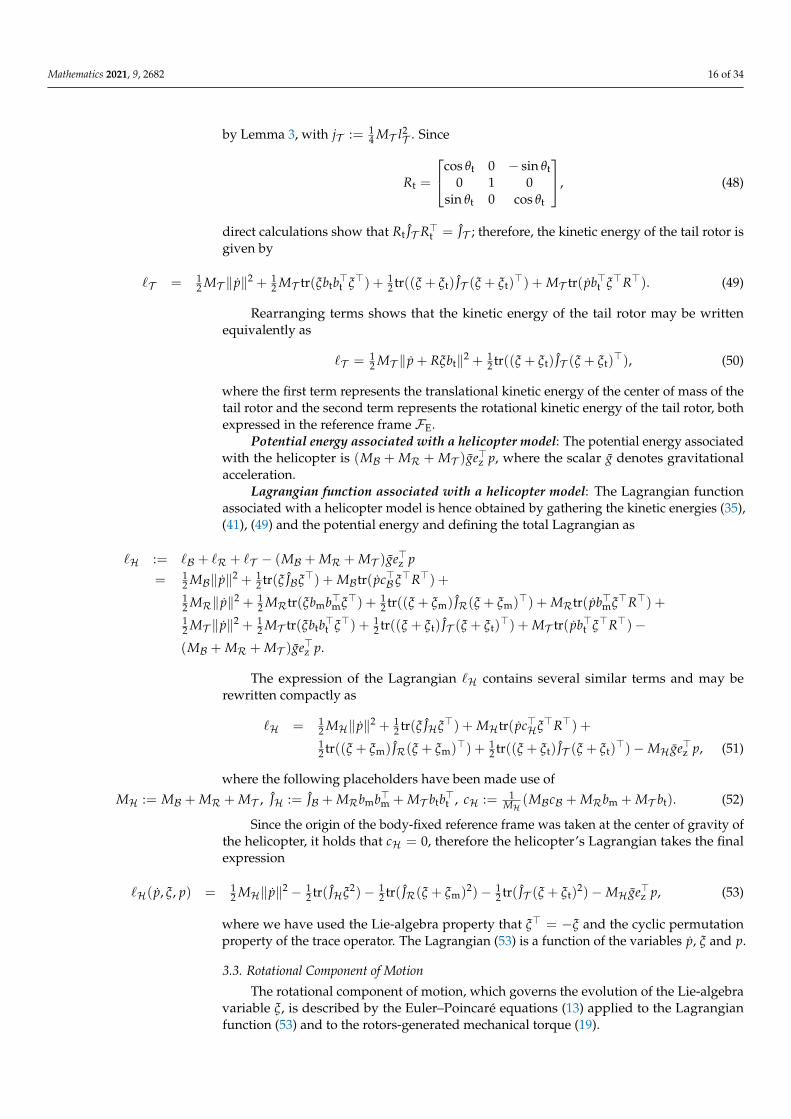
Mathematics 2021, 9, 2682 16 of 34

by Lemma 3, with jT := 14 MT l2

T . Since

Rt =

cos θt 0 − sin θt0 1 0

sin θt 0 cos θt

, (48)

direct calculations show that Rt JT R>t = JT ; therefore, the kinetic energy of the tail rotor isgiven by

`T = 12 MT ‖ p‖2 + 1

2 MT tr(ξbtb>t ξ>) + 12 tr((ξ + ξt) JT (ξ + ξt)

>) + MT tr( pb>t ξ>R>). (49)

Rearranging terms shows that the kinetic energy of the tail rotor may be writtenequivalently as

`T = 12 MT ‖ p + Rξbt‖2 + 1

2 tr((ξ + ξt) JT (ξ + ξt)>), (50)

where the first term represents the translational kinetic energy of the center of mass of thetail rotor and the second term represents the rotational kinetic energy of the tail rotor, bothexpressed in the reference frame FE.

Potential energy associated with a helicopter model: The potential energy associatedwith the helicopter is (MB + MR + MT )ge>z p, where the scalar g denotes gravitationalacceleration.

Lagrangian function associated with a helicopter model: The Lagrangian functionassociated with a helicopter model is hence obtained by gathering the kinetic energies (35),(41), (49) and the potential energy and defining the total Lagrangian as

`H := `B + `R + `T − (MB + MR + MT )ge>z p

= 12 MB‖ p‖2 + 1

2 tr(ξ JBξ>) + MBtr( pc>B ξ>R>) +12 MR‖ p‖2 + 1

2 MRtr(ξbmb>mξ>) + 12 tr((ξ + ξm) JR(ξ + ξm)>) + MRtr( pb>mξ>R>) +

12 MT ‖ p‖2 + 1

2 MT tr(ξbtb>t ξ>) + 12 tr((ξ + ξt) JT (ξ + ξt)

>) + MT tr( pb>t ξ>R>)−(MB + MR + MT )ge>z p.

The expression of the Lagrangian `H contains several similar terms and may berewritten compactly as

`H = 12 MH‖ p‖2 + 1

2 tr(ξ JHξ>) + MHtr( pc>Hξ>R>) +12 tr((ξ + ξm) JR(ξ + ξm)>) + 1

2 tr((ξ + ξt) JT (ξ + ξt)>)−MH ge>z p, (51)

where the following placeholders have been made use of

MH := MB + MR + MT , JH := JB + MRbmb>m + MT btb>t , cH := 1MH

(MBcB + MRbm + MT bt). (52)

Since the origin of the body-fixed reference frame was taken at the center of gravity ofthe helicopter, it holds that cH = 0, therefore the helicopter’s Lagrangian takes the finalexpression

`H( p, ξ, p) = 12 MH‖ p‖2 − 1

2 tr( JHξ2)− 12 tr( JR(ξ + ξm)2)− 1

2 tr( JT (ξ + ξt)2)−MH ge>z p, (53)

where we have used the Lie-algebra property that ξ> = −ξ and the cyclic permutationproperty of the trace operator. The Lagrangian (53) is a function of the variables p, ξ and p.

3.3. Rotational Component of Motion

The rotational component of motion, which governs the evolution of the Lie-algebravariable ξ, is described by the Euler–Poincaré equations (13) applied to the Lagrangianfunction (53) and to the rotors-generated mechanical torque (19).

Mathematics 2021, 9, 2682 17 of 34

As a first step in the determination of a Lie-group differential description of therotational component of motion, it is necessary to compute the fiber derivative of theLagrangian `H. The Jacobian of the Lagrangian at a point ξ may be computed easily by theproperty:

`H(ξ + ∆ξ)− `H(ξ) = tr(∆ξ>Jξ`H) + higher-order terms in ∆ξ, (54)

where ∆ξ denotes an arbitrary perturbation. It is essential to recall that, while evaluatingthe Jacobian, the matrix ξ is to be considered as unconstrained (namely, not an element ofg). Straightforward calculations yield

Jξ`H = −12

(ξ, JH> + ξ + ξm, JR> + ξ + ξt, JT >

). (55)

Plugging the above expression into the relation (16) and recalling that inertia tensors aresymmetric matrices, one gets the angular momentum

∂`H∂ξ

= Jξ`H =12(ξ, JH+ ξ + ξm, JR+ ξ + ξt, JT

). (56)

It pays to recall that the anti-commutator is a bilinear form, hence, upon defining

J?H := JH + JR + JT , (57)

the angular momentum (56) may be simplified to

µ :=∂`H∂ξ

=12(ξ, J?H+ ξm, JR+ ξt, JT

). (58)

The angular momentum µ represents the ‘quantity of rotational motion’ of the heli-copter as it is proportional to the inertia and to the rotational speed of its components. Thetime-derivative of the angular momentum may be rewritten as

µ =ddt

∂`H∂ξ

=12(ξ, J?H+ ξm, JR+ ξt, JT

), (59)

and direct calculations lead to

− adξ

(∂`H∂ξ

)=

[∂`H∂ξ

, ξ

]=

12[ J?H, ξ2] +

12[ξm, JR+ ξt, JT , ξ

]. (60)

The term µ represents the rate of change of the angular momentum that is to beequated to the total torque acting on the helicopter.

To take into account energy dissipation due to friction between the helicopter and theair molecules during rotation of the helicopter along the vertical direction, which tends tobrake the motion of the helicopter, the equation governing the rotational motion may becompleted by introducing a non-conservative force proportional to the helicopter rotationspeed along the z-axis. The resulting Euler–Poincaré equation for the helicopter modelreads

ξ, J?H = [ J?H, ξ2] +[ξm, JR+ ξt, JT , ξ

]− ξm, JR − ξt, JT + 2τ − βr〈ξ, ξz〉ξz, (61)

where βr ≥ 0 is a coefficient that quantifies the braking action of the air around thehelicopter during fast yawing.

3.4. Translational Component of Motion

The translational component of motion obeys the Euler–Lagrange equation (12) writ-ten in the inertial (earth) reference frame FE. In this case, the non-conservative force field

Mathematics 2021, 9, 2682 18 of 34

is given by the total thrust ϕm + ϕt rotated of a quantity R to express it in the earth frameFE, therefore, the Euler–Lagrange equation reads:

ddt

∂`H∂ p

=∂`H∂p

+ R(ϕm + ϕt). (62)

Notice thatddt

∂`H∂ p

= MH p,∂`H∂p

= −MH gez. (63)

To take into account energy dissipation due to friction between the helicopter andthe air molecules, that tends to brake the motion of the helicopter, the equation governingthe translational motion may be completed by introducing a non-conservative force pro-portional to the helicopter speed. Ultimately, the equation that describes the translationalmotion of a helicopter may be written as follows:

MH p = R(ϕm + ϕt)−MH gez − Bp, (64)

where B := diag(βh, 0, βv). The non-negative coefficients βh and βv quantify the brakingaction on the helicopter, which is more pronounced along the vertical direction thanhorizontally, due to the helicopter’s shape. Focusing on the Equation (64), it is clear thatwhen the helicopter fuselage is horizontal, namely R = I3, the tail rotor influences thehorizontal component of the second derivative of the position p. The tail rotor term whenthe helicopter is tilted (R 6= I3) causes an additional difficulty in controlling the position ofthe helicopter.

3.5. Explicit State-Space Form of the Equations of Motion

In order to write the equations of motion in an explicit form, we start off with a fewimportant simplifications.

• The terms related to the principal rotors may be rewritten explicitly as follows.The term Ωmξz, JR = jRΩmξz, diag(1, 1, 0) = 2jRΩmξz. Likewise, the termΩmξz, JR = 2jRΩmξz.

• The terms related to the tail rotors may be rewritten explicitly by noticing thatthe term −Ωtξy, JT = −jT Ωtξy, diag(1, 0, 1) = −2jT Ωtξy. Likewise, the term−Ωtξy, JT = −2jT Ωtξy.

• The constant J?H = JB + MRbmb>m + MT btbt> + JR + JT . Notice that bmb>m = D2m

diag(0, 0, 1) and btb>t = D2t diag(1, 0, 0). In addition, recall that the reference frame

FB has been chosen with the orthogonal axes coincident with the principal axes ofinertia of the fuselage itself, hence the tensor JB is diagonal. As a consequence, thetotal helicopter’s non-standard inertia tensor is diagonal, namely J?H = diag(jx, jy, jz).

• As a last observation, the quantity ξ, J?Hmay be written equivalently as SξS, whereS := diag(sx, sy, sz), with

sx :=

√(jx + jy)(jx + jz)

jy + jz, sy :=

√(jy + jx)(jy + jz)

jx + jz, sz :=

√(jz + jx)(jz + jy)

jx + jy. (65)

The equations of motion of the helicopter model taken into consideration in the presentpaper may be written explicitly as

Mathematics 2021, 9, 2682 19 of 34

R = Rξ,ξ = S−1([ J?H, ξ2] + 2[jRΩmξz − jT Ωtξy, ξ]− 2jRΩmξz + 2jT Ωtξy + 2τ − βr〈ξ, ξz〉ξz

)S−1,

τ := 12 Dmum sin αrξx +

12 Dmum sin αp cos αrξy +

12 (Dtut − γum)ξz,

p = 1MH

Rϕ− gez − 1MH

Bp,

ϕ :=

12 um sin αp cos αr

− 12 um sin αr − 1

2 ut12 um cos αp cos αr

.

(66)

It is interesting to consider a few special cases of motion and how the model (66)would simplify in these special instances.

Free fall: Let us assume that both rotors are blocked (ξm = ξt = 0) and that theyare isolated from the pilot control (um = ut = 0). In this case, the external torque τ (19)is null. The rotational component of motion is hence described by ξ, JB + MRbmb>m +MT btb>t + JR + JT = [ JB + MRbmb>m + MT btb>t + JR + JT , ξ2], which represents theclassical equation of a rigid body rotating freely in space under inertial forces (generallyknown as Euler’s equation of a free rigid body).

Constant rotor speed and negligible rotational inertia: Assuming constant rotationspeed for the principal and the tail rotors (namely, ξm = ξt = 0) and assuming that theangular momentum of the tail rotor and of the principal rotor are negligible with respectto the angular momentum of the helicopter, we obtain the simplified model 1

2ξ, JB +MRbmb>m + MT btb>t = 1

2 [ JB + MRbmb>m + MT btb>t , ξ2] + τ, that is the helicopter modelstudied in [12].

Hovering: Using as reference FE, hovering happens when the weight MH g balancesthe z-component of the thrust. In this situation the helicopter may only translate sidewaysin the x–y plane. Recalling that

ϕ = ϕm + ϕt =

12 um sin αp cos αr− 1

2 um sin αr − 12 ut

12 um cos αp cos αr

,

defining:

ϕw := e>z

00

−MH g

and ϕz := e>z (Rϕ)ez, (67)

the hovering condition readsϕz + ϕw = 0. (68)

In fact, the scalar ϕw denotes the (negative) intensity of gravitational pull, while thescalar term ϕz denotes the (positive) lift thrust of the main rotor. Assuming a helicopterto be horizontal (namely, with FB and FE’s z-axes aligned), the Equation (68) becomes2MH g = um cos αp cos αr. As a special case, we could for simplicity consider αp = αr = 0.Then, by the main rotor thrust Formula (24), the hovering condition could be read as4MH g = Cuρπl4

RΩ2m sin αc. Hence, the value of the collective angle needed to maintain

hovering, resulting from the hovering condition, takes the form

αc,hover = arcsin

(4MH g

ρπCul4RΩ2

m

). (69)

In general, changing the angle αp or αr causes a decrease in the z-axis thrust intensity, henceevery time the cyclic control is operated the helicopter tends to fall. The equation belowgives the value of the right collective angle with respect to αr and αp in order to prevent afall condition:

Mathematics 2021, 9, 2682 20 of 34

αc,hover = arcsin(

2MH gum cos αp cos αr

), (70)

where the thrust um comes from Equation (24).The maximum linear velocity along the x-axis could be reached provided two hypoth-

esis are met: the first is the hovering condition, in order to balance the weight force and notto decrease the helicopter height, and the second is that the horizontal component of thethrust is purely directed along the x-axis, namely αr = 0. From (68), the formula to find thecorresponding pitch angle is:

αp,maxSpeed = arccos(

2MH gum

), (71)

where um is a value of the thrust larger than the weight force of the helicopter. (Remark: Asthe collective control changes the torque exerted by the main rotor, this procedure implies anumber of concurrent actions. In fact, consider the pilot wants to change the attitude of thehelicopter using the cyclic control while keeping hovering: the cyclic control causes the needto boost the main rotor thrust by using the collective control, and the collective control causesan increase in the main rotor torque and hence a yaw effect that requires the pedals controlto be managed.)

No yawing: The condition of no yawing is achieved when the quantity 〈ξ, ξz〉 staysconstant to 0. Namely, the helicopter does not turn around the z-axis. In this case, thefriction due to rotation, βr〈ξ, ξz〉, is 0. Assuming ξ = 0 at some time, it is necessary to makesure that the first derivative of the angular velocity equals zero to ensure that no yaw ispresent, hence 〈ξ, ξz〉 = 0. From (66), it follows that

S−1(−2jRΩmξz + (Dtut − γum)ξz)S−1 = 0. (72)

As it was already underlined while discussing equations (21), in the case of constantmain rotor speed Ωm, the condition (72) will become S−1((Dtut − γum)ξz)S−1 = 0 thatcould be reduced to Dtut = γum.

No drifting: The tail thrust causes the helicopter to drift along the y-axis. This sideeffect may be compensated by choosing appropriately the roll angle αr of the main rotorthrust. The equilibrium of forces along the y-axis is reached when ϕ>ey = 0 (whereey := [0 1 0]>). Since ϕ>ey = − 1

2 um sin αr − 12 ut, in order not to have longitudinal forces

the roll angle has to be set to:

αr,noDrift = −arcsin(

ut

um

). (73)

With this value, the net drift force along the y-axis will drop to zero, meaning that noacceleration along the y-axis will be detected, although any pre-existing motions along they-axis will not cease. Moreover, setting the angle αr to this value will cause the fuselageto roll.

4. Numerical Methods to Simulate the Motion of a Helicopter

The principal aim of developing a mathematical model is to be able to carry outnumerical simulations of a physical system through a computing platform. From this per-spective, the system of differential equations (66) needs to be discretized in time in order tobe implemented on a computing platform. While the equation describing the translationalcomponent of motion may be solved through a standard numerical method, the equationdescribing the rotational component of motion needs a specific numerical method.

Mathematics 2021, 9, 2682 21 of 34

An ordinary differential equation, in which the initial value is known, could beresolved numerically using the forward Euler method fEul. The first derivative of afunction could be approximated numerically as:

fk−1 =fk − fk−1

h(74)

whereas the second derivative of a function could be approximated numerically iteratingthe fEul method as follows

fk−1 =fk − fk−1

h(75)

where k ≥ 1 denotes a discrete-time counter and h > 0 represents the step of resolutionof the numerical method. Developing the Equations (74) and (75), the second derivativeequation of a function may be approximated by fk−2 =

fk−2 fk−1+ fk−2h2 with k ≥ 2.

Using the result in Equation (66), it is possible to set up an iteration to determinenumerically the trajectory of the center of mass of the helicopter, namely:

1MH

Rk−2 ϕk−2 − gez −1

MHB(

pk−1 − pk−2h

)=

pk − 2 pk−1 + pk−2

h2 ,

which may be rewritten in explicit form as:

pk =h2

MHRk−2 ϕk−2 − h2 gez −

hMH

B(pk−1 − pk−2) + 2pk−1 − pk−2. (76)

The equation R = Rξ describes the first-order derivative of helicopter attitude. Theattitude matrix R belongs to the special orthogonal group SO(3). On manifolds it is notpossible to perform linear operations and, as a consequence, to use directly the fEul method.In this case, it is necessary to use exponential map, thus:

Rk = expRk−1(hRk−1ξk−1). (77)

Using the expression of exponential map tailored to the manifold SO(3) leads to theiteration

Rk = Rk−1Exp(h ξk−1). (78)

Since the second equation in (66) describes dynamics over the Lie algebra so(3), suchequation may be time-descritized through the classical Euler’s method: ξk = ξk−1 + h ξk−1.In particular, ξk−1 represents the angular acceleration at the step k − 1. The resultingiteration reads:

ξk =ξk−1 + h · S−1([ J?H, ξ2

k ] + 2[jRΩm,kξz − jT Ωt,kξy, ξk]

−2jRΩm,kξz + 2jT Ωt,kξy + 2τk − βr〈ξk, ξz〉ξz)S−1.

(79)

In summary, the complete set of iterations reads:

pk =h2

MHRk−2 ϕk−2 − h2 gez − h

MHB(pk−1 − pk−2) + 2pk−1 − pk−2, k ≥ 2

Rk = Rk−1Exp(h ξk−1), k ≥ 1ξk = ξk−1 + h · S−1([ J?H, ξ2

k ] + 2[jRΩm,kξz − jT Ωt,kξy, ξk]+−2jRΩm,kξz + 2jT Ωt,kξy + 2τk − βr〈ξk, ξz〉ξz

)S−1, k ≥ 1

Ωm,k = (Ωm,k −Ωm,k−1)/h, k ≥ 1Ωt,k = (Ωt,k −Ωt,k−1)/h, k ≥ 1p0 = 03×1, p0 = 03×1, p1 = 03×1,R0 = I3, ξ0 = 03,

Mathematics 2021, 9, 2682 22 of 34

where k = 0 denotes the starting time and where initial conditions have been indicated aswell. The quantities whose dynamics is not prescribed are either constants or externallycontrolled (by the pilot).

The numerical method used in the present implementation is the simplest one amongthe plethora of numerical methods available in the scientific literature. The Euler methodsare easy to implement on a computing platform, but are the least precise ones. An analysisof the precision of the Euler method on the special orthogonal group was covered in aprevious publication of the second author [22]. The precision of the numerical scheme tosimulate the dynamics of a flying body be increased by accessing higher-order numericalmethods such as those in the Runge–Kutta class.

5. Helicopter Type and Value of the Parameters

To implement the mathematical model studied, it is necessary to choose a specifichelicopter model and gather values from certification sheets and data sheets. The helicoptertype chosen for this study is the EC135 P2+ (also known as H135 P2+) manufactured byAirbusTM Corporate Helicopters. Not all parameters that appear in the equations aredirectly specified in the technical documentation, hence a careful usage of the equations toinfer those parameters values not directly available will be illustrated. The data have beengathered from the manufacturer’s flight manual [23], and other manuals [1,17–20,24–26].

The EC135 P2+ helicopter is equipped with a 4-blades bearingless main rotor and a10-blades tail rotor and is characterized by the following features:

Main rotor and Tail rotor: The main characteristics of the tail rotor and of the mainrotor are collected in Table 1. In particular, such table contains information about the rotorscollective and cyclic angle range, rotors weight and nominal spinning velocity.

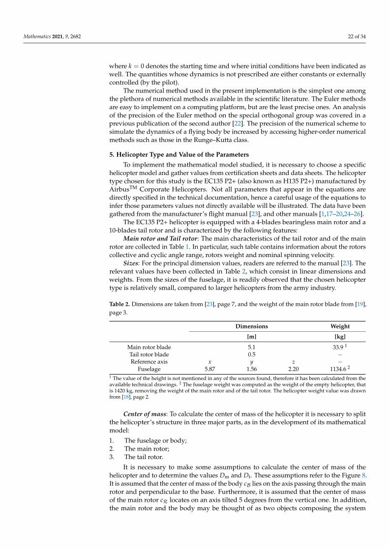
Sizes: For the principal dimension values, readers are referred to the manual [23]. Therelevant values have been collected in Table 2, which consist in linear dimensions andweights. From the sizes of the fuselage, it is readily observed that the chosen helicoptertype is relatively small, compared to larger helicopters from the army industry.

Table 2. Dimensions are taken from [23], page 7, and the weight of the main rotor blade from [19],page 3.

Dimensions Weight

[m] [kg]

Main rotor blade 5.1 33.9 1

Tail rotor blade 0.5 −Reference axis x y z −

Fuselage 5.87 1.56 2.20 1134.6 2

1 The value of the height is not mentioned in any of the sources found, therefore it has been calculated from theavailable technical drawings. 2 The fuselage weight was computed as the weight of the empty helicopter, thatis 1420 kg, removing the weight of the main rotor and of the tail rotor. The helicopter weight value was drawnfrom [18], page 2.

Center of mass: To calculate the center of mass of the helicopter it is necessary to splitthe helicopter’s structure in three major parts, as in the development of its mathematicalmodel:

1. The fuselage or body;2. The main rotor;3. The tail rotor.

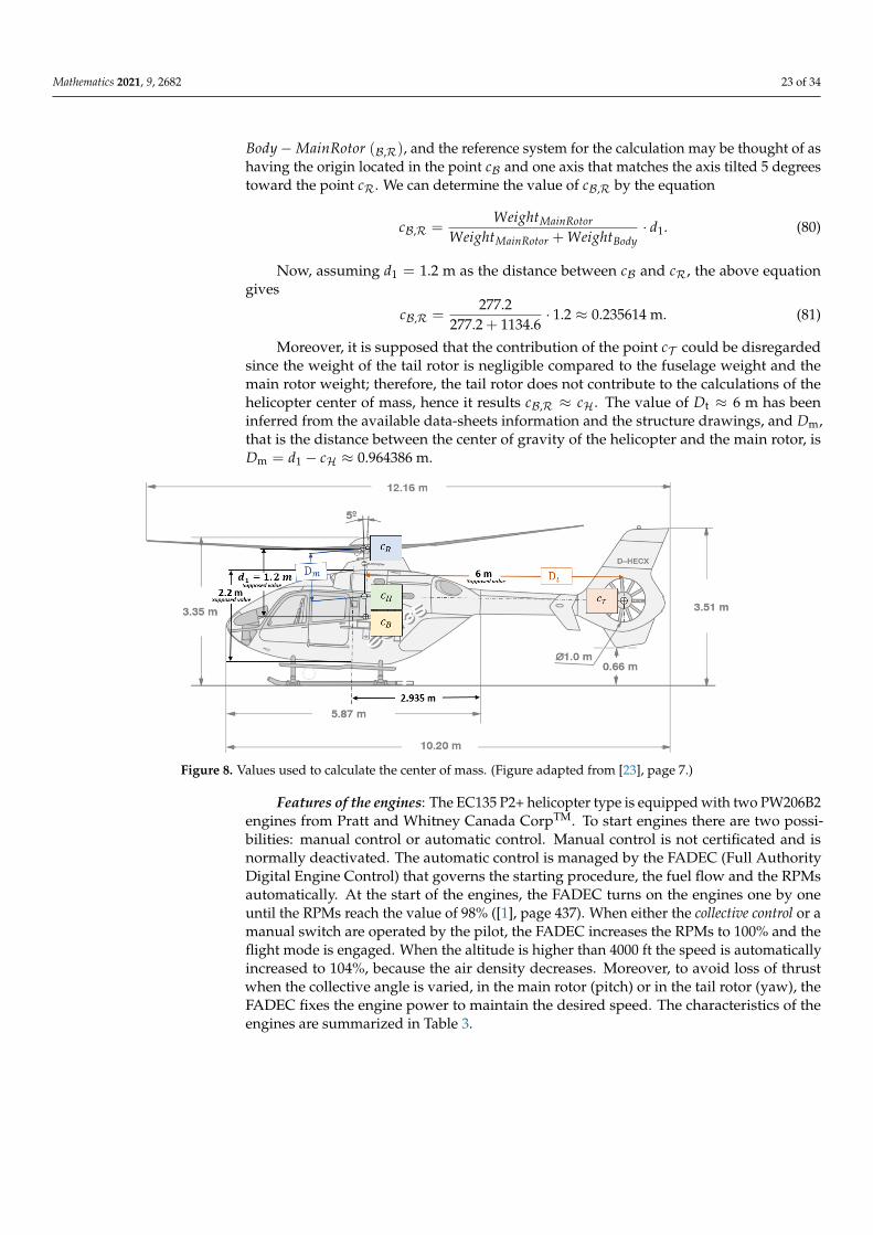
It is necessary to make some assumptions to calculate the center of mass of thehelicopter and to determine the values Dm and Dt. These assumptions refer to the Figure 8.It is assumed that the center of mass of the body cB lies on the axis passing through the mainrotor and perpendicular to the base. Furthermore, it is assumed that the center of massof the main rotor cR locates on an axis tilted 5 degrees from the vertical one. In addition,the main rotor and the body may be thought of as two objects composing the system

Mathematics 2021, 9, 2682 23 of 34

Body−MainRotor (B,R), and the reference system for the calculation may be thought of ashaving the origin located in the point cB and one axis that matches the axis tilted 5 degreestoward the point cR. We can determine the value of cB,R by the equation

cB,R =WeightMainRotor

WeightMainRotor + WeightBody· d1. (80)

Now, assuming d1 = 1.2 m as the distance between cB and cR, the above equationgives

cB,R =277.2

277.2 + 1134.6· 1.2 ≈ 0.235614 m. (81)

Moreover, it is supposed that the contribution of the point cT could be disregardedsince the weight of the tail rotor is negligible compared to the fuselage weight and themain rotor weight; therefore, the tail rotor does not contribute to the calculations of thehelicopter center of mass, hence it results cB,R ≈ cH. The value of Dt ≈ 6 m has beeninferred from the available data-sheets information and the structure drawings, and Dm,that is the distance between the center of gravity of the helicopter and the main rotor, isDm = d1 − cH ≈ 0.964386 m.

Figure 8. Values used to calculate the center of mass. (Figure adapted from [23], page 7.)

Features of the engines: The EC135 P2+ helicopter type is equipped with two PW206B2engines from Pratt and Whitney Canada CorpTM. To start engines there are two possi-bilities: manual control or automatic control. Manual control is not certificated and isnormally deactivated. The automatic control is managed by the FADEC (Full AuthorityDigital Engine Control) that governs the starting procedure, the fuel flow and the RPMsautomatically. At the start of the engines, the FADEC turns on the engines one by oneuntil the RPMs reach the value of 98% ([1], page 437). When either the collective control or amanual switch are operated by the pilot, the FADEC increases the RPMs to 100% and theflight mode is engaged. When the altitude is higher than 4000 ft the speed is automaticallyincreased to 104%, because the air density decreases. Moreover, to avoid loss of thrustwhen the collective angle is varied, in the main rotor (pitch) or in the tail rotor (yaw), theFADEC fixes the engine power to maintain the desired speed. The characteristics of theengines are summarized in Table 3.

Mathematics 2021, 9, 2682 24 of 34

Table 3. Values are taken from [25], pages 8 and 12. The helicopter state AEO denotes ‘all engineoperative’, whereas the state OEI stands for ‘one engine inoperative’. Typically, two possible workingmode could be selected: TOP (take-off power) that has a time-limit constraint, and MCP (maximumcontinuous power).

Power Maximum TorqueEngine Mode [ kW ] [ N · m ]

AEO TOP (max. 5 min) 2 × 333 2 × 519AEO MCP 2 × 321 2 × 500

OEI (max. 30 s) 547 851OEI (max. 2 min) 534 831

OEI MCP 404 629

Gear box: The gear box is a complex part that transmits power, usually reducingangular velocity and increasing torque. Both helicopter engines drive the gear box that, inturn, drives the main rotor shaft and the tail rotor shaft.

Main rotor thrust: The Equation (26) was used to calculate the power coefficientof the main rotor, that is Cw ≈ 0.006968, and its thrust coefficient Cu ≈ 0.045965. It isalso possible to determine the maximum thrust um,max generated by the main rotor usingthe Equation (24), setting the throttle at 100% and the collective angle at its maximum.

The obtained result is um,max ≈ 52, 729 kg·m·rad2

s2 . Such numerical result was obtainedby setting Ωm,max ≈ 41.364303 rad/s, αc,max = 0.541052 rad, ρ = 1.225 kg/m3 (whichdenotes, respectively, the maximum angular speed, the maximum collective angle and theair density at 15 Celsius degrees and 1 atm, from Table 1).

Tail rotor thrust: In the same way, it is possible to determine the power coefficientand the thrust coefficient for the tail rotor which are respectively CT

w ≈ 0.100974 andCT

u ≈ 0.273201. The maximum thrust generated by the tail rotor is ut,max ≈ 2601 kg ·m ·rad2/s2, whose value is calculated using the throttle at 100%, the angular velocity Ωt,max ≈375.315601 rad/s and the maximum collective angle for the tail rotor αT

c,max ≈ 0.596903 rad,from Table 1.

Drag term: According to Equation (28), the value of the drag term is γ ≈ 0.154546 m.Such numerical result was obtained by setting the middle value of the interval of the tailrotor collective angle to αT

c,mid ≈ 0.151844 rad, and the collective angle of the main rotorconsistent with hovering to αc,hover ≈ 0.268693 rad, from Equation (69).

Friction terms: Let us collect the tip velocity of the helicopter along each axis in thevector pmax. Given the maximum velocity of the helicopter, we know that, once reached thatparticular value, the acceleration of the helicopter along that axis will drop to 0, because ofthe existence of a friction force in the opposite direction. This situation can be described as:

0 = R(ϕm + ϕt)−MH gez − Bpmax. (82)

Looking closely at the term R(ϕm + ϕt), namely the propelling force of the helicopter,it is readily observed how it takes a special configuration when the tip speed is reached,in fact:

• To reach the tip speed along the z-axis, it is necessary that the z-axes of the inertialreference frame FE and of the body-fixed reference FB are aligned;

• To reach the tip speed along the x-axis, we consider a motion at maximum speed dueto a total thrust directed along the x-axis while in a horizontal attitude (R = I3). Inthis case, the thrust takes its maximum value (compatibly with the need to keep thehelicopter hovering).

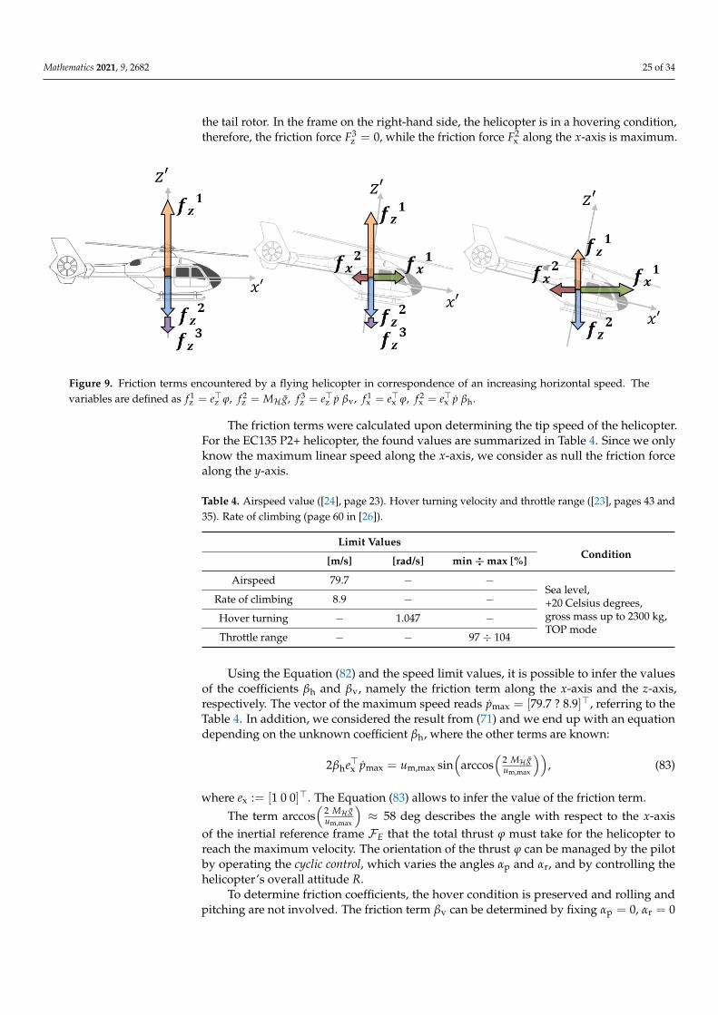
The Figure 9 shows the force components present in some particular helicopter atti-tudes. In the frame on the left-hand side of the figure, the helicopter is horizontal, namelyR = I3, and all the forces are directed along the z-axis, disregarding the force exerted by

Mathematics 2021, 9, 2682 25 of 34

the tail rotor. In the frame on the right-hand side, the helicopter is in a hovering condition,therefore, the friction force F3

z = 0, while the friction force F2x along the x-axis is maximum.

Figure 9. Friction terms encountered by a flying helicopter in correspondence of an increasing horizontal speed. Thevariables are defined as f 1

z = e>z ϕ, f 2z = MH g, f 3

z = e>z p βv, f 1x = e>x ϕ, f 2

x = e>x p βh.

The friction terms were calculated upon determining the tip speed of the helicopter.For the EC135 P2+ helicopter, the found values are summarized in Table 4. Since we onlyknow the maximum linear speed along the x-axis, we consider as null the friction forcealong the y-axis.

Table 4. Airspeed value ([24], page 23). Hover turning velocity and throttle range ([23], pages 43 and35). Rate of climbing (page 60 in [26]).

Limit Values

[m/s] [rad/s] min ÷ max [%] Condition

Airspeed 79.7 − −Sea level,+20 Celsius degrees,gross mass up to 2300 kg,TOP mode

Rate of climbing 8.9 − −Hover turning − 1.047 −Throttle range − − 97 ÷ 104

Using the Equation (82) and the speed limit values, it is possible to infer the valuesof the coefficients βh and βv, namely the friction term along the x-axis and the z-axis,respectively. The vector of the maximum speed reads pmax = [79.7 ? 8.9]>, referring to theTable 4. In addition, we considered the result from (71) and we end up with an equationdepending on the unknown coefficient βh, where the other terms are known:

2βhe>x pmax = um,max sin(

arccos(

2 MH gum,max

)), (83)

where ex := [1 0 0]>. The Equation (83) allows to infer the value of the friction term.The term arccos

(2 MH gum,max

)≈ 58 deg describes the angle with respect to the x-axis

of the inertial reference frame FE that the total thrust ϕ must take for the helicopter toreach the maximum velocity. The orientation of the thrust ϕ can be managed by the pilotby operating the cyclic control, which varies the angles αp and αr, and by controlling thehelicopter’s overall attitude R.

To determine friction coefficients, the hover condition is preserved and rolling andpitching are not involved. The friction term βv can be determined by fixing αp = 0, αr = 0

Mathematics 2021, 9, 2682 26 of 34

and R = diag(1, 1, 1), which are the conditions to reach the maximum velocity along thez-axis. From the Equation (82), we thus obtain

βve>z pmax = 12 um,max −MH g. (84)

Instantiating equations (83) and (84) with known values, the friction coefficients canbe easily computed. It has been found that βh ≈ 281 kg·s−1 and βv ≈ 1398 kg·s−1.

Using the same method, it is possible to estimate the value of βr, the friction termlinked to the yaw velocity. Let us assume the helicopter to be in the hovering condi-tion, with ξm = ξt = 0. At the maximum yaw speed the angular acceleration will benull. Since we consider a hovering condition with αr = αp = 0, the total torque τ isequal to 1

2 (Dtut,max − γ um,hover)ξz; therefore, from the second equation in (66) we obtain0 = S−1([ J?H, ξ2

max] + (Dtut,max − 2γMH g− βr〈ξmax, ξz〉)ξz)S−1, where ξmax denotes the

maximal yawing speed that, from the Table 4, is known to be ξmax = 1.047 · ξz (rad/s).Thus, isolating the friction term, this equation becomes:

βr〈ξmax, ξz〉ξz = [ J?H, ξ2max] + (Dtut,max − 2γMH g)ξz. (85)

To determine the correct value of the friction term it is necessary to fill the Equa-tion (85), namely the tip thrust of the tail rotor ut,max, the structural values, and the dragcoefficient found. The computed result for this parameter is βr ≈ 10797 N·m·s·rad−1.

6. Numerical Experiments and Results

A series of tests of the mathematical model were carried out by means of a MATLAB®

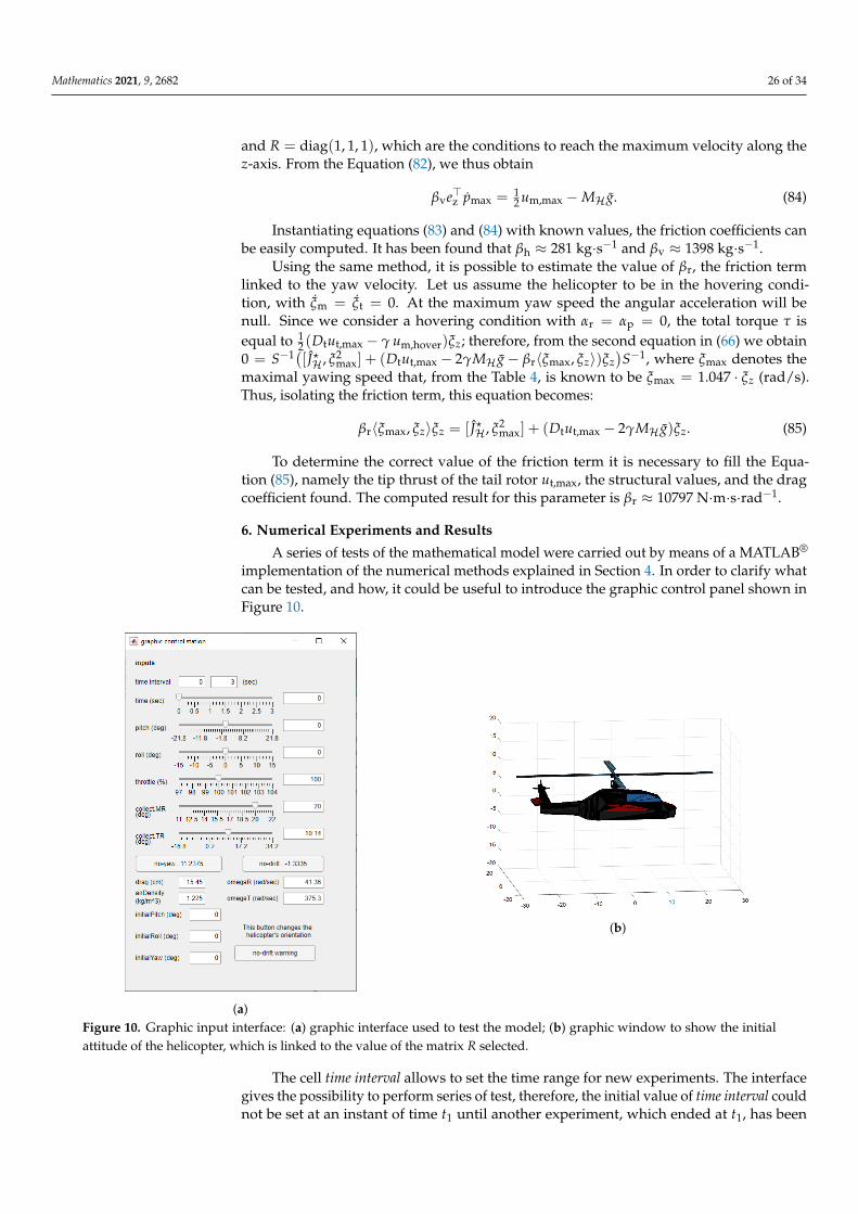
implementation of the numerical methods explained in Section 4. In order to clarify whatcan be tested, and how, it could be useful to introduce the graphic control panel shown inFigure 10.

(a)

(b)

Figure 10. Graphic input interface: (a) graphic interface used to test the model; (b) graphic window to show the initialattitude of the helicopter, which is linked to the value of the matrix R selected.

The cell time interval allows to set the time range for new experiments. The interfacegives the possibility to perform series of test, therefore, the initial value of time interval couldnot be set at an instant of time t1 until another experiment, which ended at t1, has been

Mathematics 2021, 9, 2682 27 of 34

completed. The slider named Time shows the selected instant of time in a pop-up animationwindow. Every slider is linked to an editable cell, hence, any value belonging to the correctrange could be directly set. The five sliders pitch, roll, throttle, collect.MR, collect.TR are theinterface to manage the value of the variables αp, αr, Ωm, αc, αT

c , respectively. The no-yawbutton sets the angle αT

c for a no-yawing condition, from Equation (72), whereas the buttonno-drift manages the value of the angle αr to achieve a no-drifting condition using theEquation (73). The two editable cells drag and air density allow to input the values of thecoefficients γ and ρ, respectively. The three cells initial roll, initial pitch, initial yaw interfacewith the matrix R forcing a value of attitude of the helicopter along the three axes x, y, z.The button no-drift warning changes the initial roll value in order to achieve a stationaryno-drifting condition (a technique introduced in the third test).

First test—lift response: The first test lasts 10 s and does not involve pitch and rollangles (αp = 0, αr = 0), moreover the throttle is set at 100% and the tail rotor collectiveangle at αT

c,mid. About the main rotor collective angle, it has been chosen in order to producelift along z-axis: the value chosen is 20 degrees. Figure 11 shows the result of this simulation.The position along x-axis is constant, which could seem reasonable because pitch angleis not involved. On the other hand, there is a clear decrease in the y-component of thepositional variable p due to drift effect. Notice that the direction of the tail rotor thrust isopposite to y-axis, as Figure 5 shows. The z component of the torque τ is negative, andthis is the cause of clockwise yawing. Looking closely at the entries of the position vectorp, along the x-axis it can be observed a little decrease due to the combined action of thehelicopter yawing and tail rotor drift. In fact, when the helicopter nose turns, the drift effectcauses a slight decrease in the positional x-coordinate. Note that the drift force exerted bythe tail rotor coincides with the y component of the total thrust ϕ, which is e>y ϕ. The lastremarkable observation from the first test is that the z component of the thrust ϕ has thevalue of 16,191 N, which is more than the helicopter-weight force, that could be determinedfrom Table 2 as 1420 · g ≈ 13,925 N. The resulting force along the z-axis is positive and, asdescribed by the graph of the z-coordinate of the center of gravity, the helicopter lifts up.

Figure 11. First test—lift response. Top panel: components of the position of cH. Middle panel: components of the thrust.Bottom panel: components of the active torque generated by rotors.

Remark: The x, y and z components in the torque graph have been extracted from theEquation (14) following the construction of τ, namely they are calculated by e>z τey, e>x τez

and e>y τex.

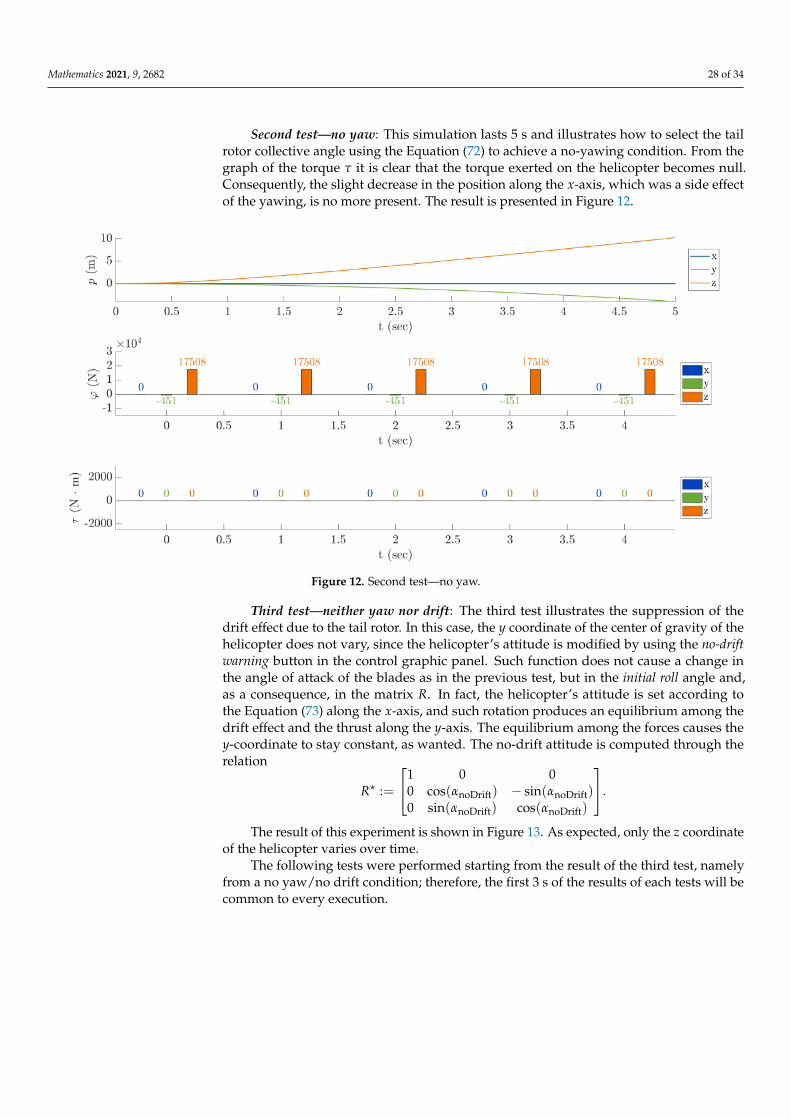
Mathematics 2021, 9, 2682 28 of 34

Second test—no yaw: This simulation lasts 5 s and illustrates how to select the tailrotor collective angle using the Equation (72) to achieve a no-yawing condition. From thegraph of the torque τ it is clear that the torque exerted on the helicopter becomes null.Consequently, the slight decrease in the position along the x-axis, which was a side effectof the yawing, is no more present. The result is presented in Figure 12.

Figure 12. Second test—no yaw.

Third test—neither yaw nor drift: The third test illustrates the suppression of thedrift effect due to the tail rotor. In this case, the y coordinate of the center of gravity of thehelicopter does not vary, since the helicopter’s attitude is modified by using the no-driftwarning button in the control graphic panel. Such function does not cause a change inthe angle of attack of the blades as in the previous test, but in the initial roll angle and,as a consequence, in the matrix R. In fact, the helicopter’s attitude is set according tothe Equation (73) along the x-axis, and such rotation produces an equilibrium among thedrift effect and the thrust along the y-axis. The equilibrium among the forces causes they-coordinate to stay constant, as wanted. The no-drift attitude is computed through therelation

R? :=

1 0 00 cos(αnoDrift) − sin(αnoDrift)0 sin(αnoDrift) cos(αnoDrift)

.

The result of this experiment is shown in Figure 13. As expected, only the z coordinateof the helicopter varies over time.

The following tests were performed starting from the result of the third test, namelyfrom a no yaw/no drift condition; therefore, the first 3 s of the results of each tests will becommon to every execution.

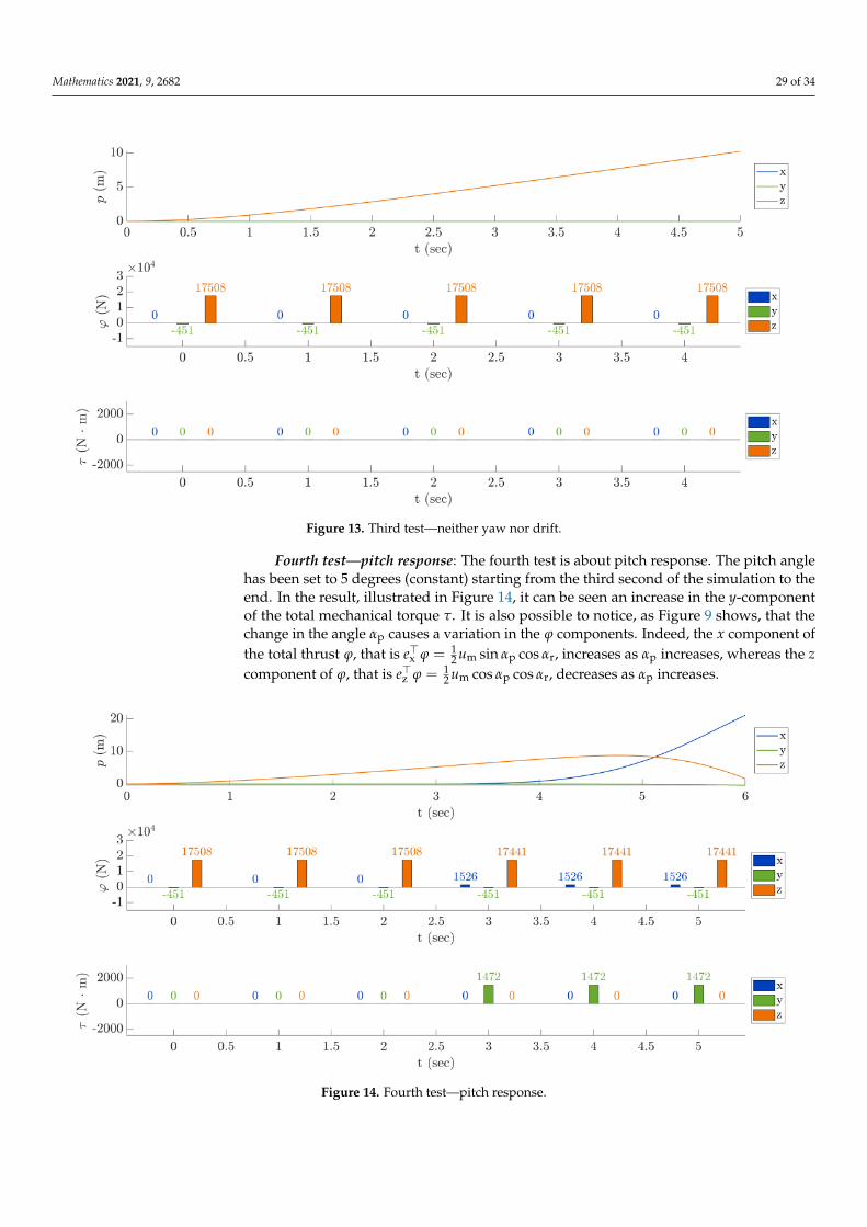
Mathematics 2021, 9, 2682 29 of 34

Figure 13. Third test—neither yaw nor drift.

Fourth test—pitch response: The fourth test is about pitch response. The pitch anglehas been set to 5 degrees (constant) starting from the third second of the simulation to theend. In the result, illustrated in Figure 14, it can be seen an increase in the y-componentof the total mechanical torque τ. It is also possible to notice, as Figure 9 shows, that thechange in the angle αp causes a variation in the ϕ components. Indeed, the x component ofthe total thrust ϕ, that is e>x ϕ = 1

2 um sin αp cos αr, increases as αp increases, whereas the zcomponent of ϕ, that is e>z ϕ = 1

2 um cos αp cos αr, decreases as αp increases.

Figure 14. Fourth test—pitch response.

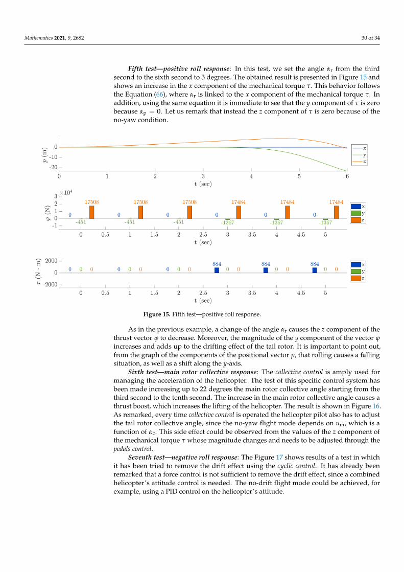
Mathematics 2021, 9, 2682 30 of 34

Fifth test—positive roll response: In this test, we set the angle αr from the thirdsecond to the sixth second to 3 degrees. The obtained result is presented in Figure 15 andshows an increase in the x component of the mechanical torque τ. This behavior followsthe Equation (66), where αr is linked to the x component of the mechanical torque τ. Inaddition, using the same equation it is immediate to see that the y component of τ is zerobecause αp = 0. Let us remark that instead the z component of τ is zero because of theno-yaw condition.

Figure 15. Fifth test—positive roll response.

As in the previous example, a change of the angle αr causes the z component of thethrust vector ϕ to decrease. Moreover, the magnitude of the y component of the vector ϕincreases and adds up to the drifting effect of the tail rotor. It is important to point out,from the graph of the components of the positional vector p, that rolling causes a fallingsituation, as well as a shift along the y-axis.

Sixth test—main rotor collective response: The collective control is amply used formanaging the acceleration of the helicopter. The test of this specific control system hasbeen made increasing up to 22 degrees the main rotor collective angle starting from thethird second to the tenth second. The increase in the main rotor collective angle causes athrust boost, which increases the lifting of the helicopter. The result is shown in Figure 16.As remarked, every time collective control is operated the helicopter pilot also has to adjustthe tail rotor collective angle, since the no-yaw flight mode depends on um, which is afunction of αc. This side effect could be observed from the values of the z component ofthe mechanical torque τ whose magnitude changes and needs to be adjusted through thepedals control.

Seventh test—negative roll response: The Figure 17 shows results of a test in whichit has been tried to remove the drift effect using the cyclic control. It has already beenremarked that a force control is not sufficient to remove the drift effect, since a combinedhelicopter’s attitude control is needed. The no-drift flight mode could be achieved, forexample, using a PID control on the helicopter’s attitude.

Mathematics 2021, 9, 2682 31 of 34

Figure 16. Sixth test—Main rotor collective response.

Figure 17. Seventh test—negative roll response.

This test was carried out using as initial setting the same setting as for the secondtest, whereas the last 2 s were simulated using the Equation (73) to change αr. Notice thatan attitude controller would ensure no drifting. Ideally, a PID controller should reducethe value of the cyclic control as the roll angle of the helicopter approaches the valuedetermined by the Equation (73).

Eight test—free flight: This last test consists in a simulation of a free flight achievedby setting multiple inputs for the cyclic control and the collective control. The obtained resultis shown in Figure 18, while Table 5 presents the time line of the controls used. The throttle

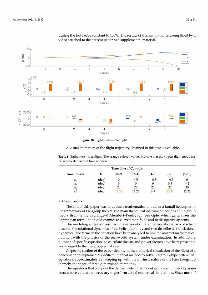
Mathematics 2021, 9, 2682 32 of 34

during the test keeps constant to 100%. The results of this simulation is exemplified by avideo attached to the present paper as a supplemental material.

Figure 18. Eighth test—free flight.

A visual animation of the flight trajectory obtained in this test is available.

Table 5. Eighth test—free flight. The orange-colored values indicate that the no-yaw flight mode hasbeen activated in that time window.

Time Line of Controls

Time Interval (s) [0–2) [2–4) [4–6) [6–8) [8–10]

αp (deg) 0 0.5 −0.5 −0.3 0αr (deg) 0 0 0 0.8 −2αc (deg) 20 22 22 22 20αT

c (deg) 11.24 11.24 8.5 12.32 12.32

7. Conclusions

The aim of this paper was to devise a mathematical model of a fantail helicopter inthe framework of Lie-group theory. The main theoretical instrument, besides of Lie-grouptheory itself, is the Lagrange–d’Alembert–Pontryagin principle, which generalizes theLagrangian formulation of dynamics to curved manifolds and to dissipative systems.

The modeling endeavor resulted in a series of differential equations, two of whichdescribe the rotational dynamics of the helicopter body and two describe its translationaldynamics. The terms in the equation have been analyzed to link the abstract mathematicalnotation with the physics of the real-world system under examination. In addition, anumber of specific equations to calculate thrusts and power factors have been presentedand merged to the Lie-group equations.

A specific section of the paper dealt with the numerical simulation of the flight of ahelicopter and explained a specific numerical method to solve Lie-group-type differentialequations approximately yet keeping up with the intrinsic nature of the base Lie-group(namely, the space of three-dimensional rotations).

The equations that compose the devised helicopter model include a number of param-eters whose values are necessary to perform actual numerical simulations. Since most of

Mathematics 2021, 9, 2682 33 of 34

such values are not directly available in the literature, a careful work of identification ofthe parameters through the devised equations has been carried out.

Numerical results have been illustrated and commented in order to elucidate someaspects of the model that were deemed of particular interest, from simple flight modesto free flight. The devised model, as the large majority of mathematical models of real-world physical phenomena, is of potential use to control engineers (who may use suchmathematical model to design a state observer and an automatic control system to assistthe pilot), to mechanical engineers (who may use the devised model to test a helicopterstructure under stress conditions) and by pilots instructing facilities (who might use thedevised model as a prototypical flight simulator).

Supplementary Materials: The following are available at https://www.mdpi.com/2227-7390/9/21/2682/s1.

Author Contributions: Conceptualization, S.F.; data curation, A.T.; writing—original draft prepa-ration, A.T. and S.F.; writing—review and editing, S.F.; supervision, S.F. All authors have read andagreed to the published version of the manuscript.

Funding: This research received no external funding.

Institutional Review Board Statement: Not applicable.

Informed Consent Statement: Not applicable.

Acknowledgments: The authors would like to gratefully thank Toshihisa Tanaka (TUAT—TokyoUniversity of Agriculture and Technology) for having hosted the author A.T. during an internshipin January–March 2020 and for having invited the author S.F. as a visiting professor at the TUAT inFebruary–March 2020.

Conflicts of Interest: The authors declare no conflict of interest.

References and Note1. Eurocopter Deutschland GmbH. EC 135—Training Manual; Eurocopter Deutschland GmbH: Donauwörth, Germany, 2002.2. Kim, S.; Tilbury, D. Mathematical modeling and experimental identification of an unmanned helicopter robot with flybar

dynamics. J. Robot. Syst. 2004, 21, 95–116. [CrossRef]3. Salazar, T. Mathematical model and simulation for a helicopter with tail rotor. In Advances in Computational Intelligence, Man-

Machine Systems and Cybernetics; World Scientific and Engineering Academy and Society: 2010; pp. 27–33. Available online:http://www.wseas.us/e-library/conferences/2010/Merida/CIMMACS/CIMMACS-03.pdf (accessed on 19 October 2021).

4. Talbot, P.; Tinling, B.; Decker, W.; Chen, R. A Mathematical Model of a Single Main Rotor Helicopter for Piloted Simulation; TechnicalReport; NASA Ames Research Center: Moffett Field, CA, USA, 1982.

5. Shojaei Barjuei, E.; Caldwell, D.G.; Ortiz, J. Bond graph modeling and Kalman filter observer design for an industrial back-supportexoskeleton. Designs 2020, 4, 53. [CrossRef]

6. Mizouri, W.; Najar, S.; Bouabdallah, L.; Aoun, M. Dynamic modeling of a quadrotor UAV prototype. In New Trends in RobotControl; Studies in Systems, Decision and Control; Ghommam, J., Derbel, N., Zhu, Q., Eds.; Springer: Singapore, 2020; Volume 270.[CrossRef]

7. Khumprom, P.; Grewell, D.; Yodo, N. Deep neural network feature selection approaches for data-driven prognostic model ofaircraft engines. Aerospace 2020, 7, 132. [CrossRef]

8. Abraham, R.; Marsden, J.; Ratiu, T. Manifolds, Tensor Analysis, and Applications; Springer: New York, NY, USA, 1988.9. Bullo, F.; Lewis, A. Geometric Control of Mechanical Systems: Modeling, Analysis, and Design for Mechanical Control Systems; Springer:

New York, NY, USA, 2005.10. Fiori, S. Nonlinear damped oscillators on Riemannian manifolds: Fundamentals. J. Syst. Sci. Complex. 2016, 29, 22–40. [CrossRef]11. Fiori, S. Nonlinear damped oscillators on Riemannian manifolds: Numerical simulation. Commun. Nonlinear Sci. Numer. Simul.

2017, 47, 207–222. [CrossRef]12. Kobilarov, M.; Desbrun, M.; Marsden, J.; Sukhatme, G. A discrete geometric optimal control framework for systems with

symmetries. In Robotics: Science and Systems; MIT Press: Cambridge, UK, 2007; pp. 161–168.13. Bloch, A.; Krishnaprasad, P.; Marsden, J.; Ratiu, T. The Euler-Poincaré equations and double bracket dissipation. Commun. Math.

Phys. 1996, 175, 1–42. [CrossRef]14. Ge, Z.M.; Lin, T.N. Chaos, chaos control and synchronization of a gyrostat system. J. Sound Vib. 2002, 251, 519–542. [CrossRef]15. Fiori, S. Model Formulation Over Lie Groups and Numerical Methods to Simulate the Motion of Gyrostats and Quadrotors.

Mathematics 2019, 7, 935. [CrossRef]

Mathematics 2021, 9, 2682 34 of 34

16. Rotaru, C.; Todorov, M. Helicopter Flight Physics. In Flight Physics—Models, Techniques and Technologies; Volkov, K., Ed.;IntechOpen Limited: London, UK, 2018.

17. Doleschel, A.; Emmerling, S. The EC135 Drive Train Analysis and Improvement of the Fatigue Strength. In Proceedings of the33rd European Rotorcraft Forum, Kazan, Russia, 11–13 September 2007; Volume 2, pp. 1275–1319.

18. Kampa, K.; Enenkl, B.; Polz, G.; Roth, G. Aeromechanical aspects in the design of the EC135. In Proceedings of the 23rd EuropeanRotorcraft Forum, Dresden, Germany, 16–18 September 1997; pp. 38.1–38.14.

19. Eurocopter. Eurocopter Training Service, Chapter 6—Main Rotor. 2006.20. Axelsson, B.E.; Fulmer, J.C.; Labrie, J.P. Design of a Helicopter Hover Test Stand. Bachelor’ Thesis, Worcester Polytechnic

Institute, Worcester, MA, USA, 2015.21. Yu, W.; Pan, Z. Dynamical equations of multibody systems on Lie groups. Adv. Mech. Eng. 2015, 7, 1–9. [CrossRef]22. Fiori, S. A closed-form expression of the instantaneous rotational lurch index to valuate its numerical approximation. Symmetry

2019, 11, 1208. [CrossRef]23. Eurocopter Deutschland GmbH. Flight Manual EC135 P2+; Eurocopter Deutschland GmbH: Donauwörth, Germany, 2002.24. EASA European Aviation Safety Agency. Type Certificate Data Sheet No. EASA.R.009 for EC135. Available online: https:

//www.easa.europa.eu/sites/default/files/dfu/TCDS_EASA_R009_AHD_EC135_Issue_07_18Mar2015.pdf. (accessed on 13October 2021).

25. EASA European Aviation Safety Agency. Type Certificate Data Sheet No. IM.E.017 for PW206 & PW207 Series Engines. Availableonline: https://www.easa.europa.eu/sites/default/files/dfu/TCDS%20IM.E.017_issue%2007_20151005_1.0.pdf (accessed on 13October 2021).

26. Eurocopter Deutschland GmbH. Eurocopter EC135 Technical Data; Eurocopter Deutschland GmbH: Donauwörth, Germany, 2006.