Sliding mesh algorithm for CFD analysis of helicopter rotor ...

INTERNATIONAL JOURNAL FOR NUMERICAL METHODS IN FLUIDSInt. J. Numer. Meth. Fluids 2008; 58:527–549Published online 18 February 2008 in Wiley InterScience (www.interscience.wiley.com). DOI: 10.1002/fld.1757

Sliding mesh algorithm for CFD analysis of helicopterrotor–fuselage aerodynamics

R. Steijl and G. Barakos∗,†

Laboratory of Computational Fluid Dynamics, Department of Engineering, University of Liverpool,Liverpool L69 3GH, U.K.

SUMMARY

The study of rotor–fuselage interactional aerodynamics is central to the design and performance analysisof helicopters. However, regardless of its significance, rotor–fuselage aerodynamics has so far beenaddressed by very few authors. This is mainly due to the difficulties associated with both experimentaland computational techniques when such complex configurations, rich in flow physics, are considered. Inview of the above, the objective of this study is to develop computational tools suitable for rotor–fuselageengineering analysis based on computational fluid dynamics (CFD).

To account for the relative motion between the fuselage and the rotor blades, the concept of slidingmeshes is introduced. A sliding surface forms a boundary between a CFD mesh around the fuselageand a rotor-fixed CFD mesh which rotates to account for the movement of the rotor. The sliding surfaceallows communication between meshes. Meshes adjacent to the sliding surface do not necessarily havematching nodes or even the same number of cell faces. This poses a problem of interpolation, whichshould not introduce numerical artefacts in the solution and should have minimal effects on the overallsolution quality. As an additional objective, the employed sliding mesh algorithms should have smallCPU overhead. The sliding mesh methods developed for this work are demonstrated for both simpleand complex cases with emphasis placed on the presentation of the inner workings of the developedalgorithms. Copyright q 2008 John Wiley & Sons, Ltd.

Received 8 August 2007; Revised 18 December 2007; Accepted 19 December 2007

KEY WORDS: sliding planes; mesh deformation; rotorcraft CFD; rotor–fuselage interaction

1. INTRODUCTION

The study of rotor and rotor–fuselage aerodynamics with computational fluid dynamics (CFD)methods, based on structured grids, requires complex multi-block topologies so that the exact

∗Correspondence to: G. Barakos, Department of Engineering, University of Liverpool, Chadwick Building, LiverpoolL69 3GH, U.K.

†E-mail: [email protected]

Contract/grant sponsor: European Union; contract/grant number: 516074

Copyright q 2008 John Wiley & Sons, Ltd.

528 R. STEIJL AND G. BARAKOS

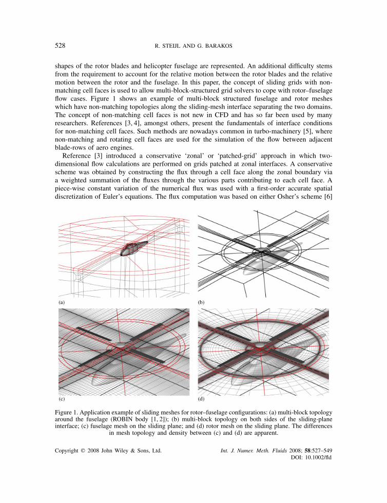
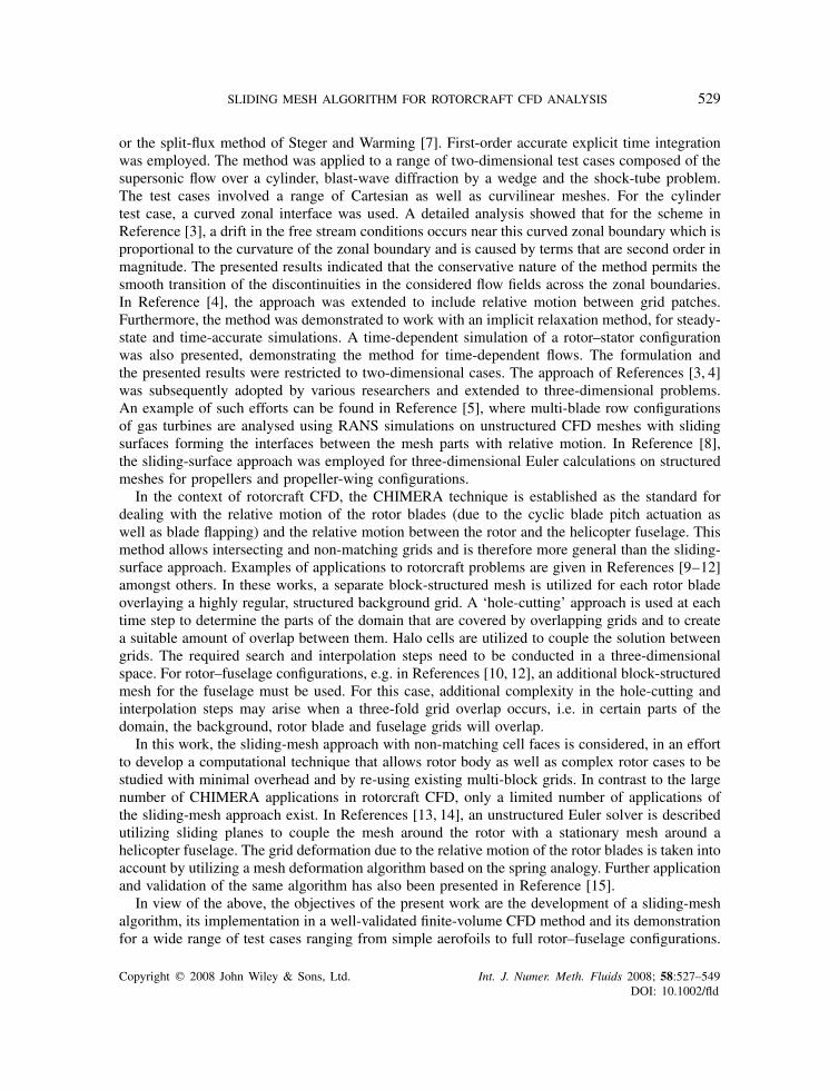
shapes of the rotor blades and helicopter fuselage are represented. An additional difficulty stemsfrom the requirement to account for the relative motion between the rotor blades and the relativemotion between the rotor and the fuselage. In this paper, the concept of sliding grids with non-matching cell faces is used to allow multi-block-structured grid solvers to cope with rotor–fuselageflow cases. Figure 1 shows an example of multi-block structured fuselage and rotor mesheswhich have non-matching topologies along the sliding-mesh interface separating the two domains.The concept of non-matching cell faces is not new in CFD and has so far been used by manyresearchers. References [3, 4], amongst others, present the fundamentals of interface conditionsfor non-matching cell faces. Such methods are nowadays common in turbo-machinery [5], wherenon-matching and rotating cell faces are used for the simulation of the flow between adjacentblade-rows of aero engines.

Reference [3] introduced a conservative ‘zonal’ or ‘patched-grid’ approach in which two-dimensional flow calculations are performed on grids patched at zonal interfaces. A conservativescheme was obtained by constructing the flux through a cell face along the zonal boundary viaa weighted summation of the fluxes through the various parts contributing to each cell face. Apiece-wise constant variation of the numerical flux was used with a first-order accurate spatialdiscretization of Euler’s equations. The flux computation was based on either Osher’s scheme [6]

Figure 1. Application example of sliding meshes for rotor–fuselage configurations: (a) multi-block topologyaround the fuselage (ROBIN body [1, 2]); (b) multi-block topology on both sides of the sliding-planeinterface; (c) fuselage mesh on the sliding plane; and (d) rotor mesh on the sliding plane. The differences

in mesh topology and density between (c) and (d) are apparent.

Copyright q 2008 John Wiley & Sons, Ltd. Int. J. Numer. Meth. Fluids 2008; 58:527–549DOI: 10.1002/fld

SLIDING MESH ALGORITHM FOR ROTORCRAFT CFD ANALYSIS 529

or the split-flux method of Steger and Warming [7]. First-order accurate explicit time integrationwas employed. The method was applied to a range of two-dimensional test cases composed of thesupersonic flow over a cylinder, blast-wave diffraction by a wedge and the shock-tube problem.The test cases involved a range of Cartesian as well as curvilinear meshes. For the cylindertest case, a curved zonal interface was used. A detailed analysis showed that for the scheme inReference [3], a drift in the free stream conditions occurs near this curved zonal boundary which isproportional to the curvature of the zonal boundary and is caused by terms that are second order inmagnitude. The presented results indicated that the conservative nature of the method permits thesmooth transition of the discontinuities in the considered flow fields across the zonal boundaries.In Reference [4], the approach was extended to include relative motion between grid patches.Furthermore, the method was demonstrated to work with an implicit relaxation method, for steady-state and time-accurate simulations. A time-dependent simulation of a rotor–stator configurationwas also presented, demonstrating the method for time-dependent flows. The formulation andthe presented results were restricted to two-dimensional cases. The approach of References [3, 4]was subsequently adopted by various researchers and extended to three-dimensional problems.An example of such efforts can be found in Reference [5], where multi-blade row configurationsof gas turbines are analysed using RANS simulations on unstructured CFD meshes with slidingsurfaces forming the interfaces between the mesh parts with relative motion. In Reference [8],the sliding-surface approach was employed for three-dimensional Euler calculations on structuredmeshes for propellers and propeller-wing configurations.

In the context of rotorcraft CFD, the CHIMERA technique is established as the standard fordealing with the relative motion of the rotor blades (due to the cyclic blade pitch actuation aswell as blade flapping) and the relative motion between the rotor and the helicopter fuselage. Thismethod allows intersecting and non-matching grids and is therefore more general than the sliding-surface approach. Examples of applications to rotorcraft problems are given in References [9–12]amongst others. In these works, a separate block-structured mesh is utilized for each rotor bladeoverlaying a highly regular, structured background grid. A ‘hole-cutting’ approach is used at eachtime step to determine the parts of the domain that are covered by overlapping grids and to createa suitable amount of overlap between them. Halo cells are utilized to couple the solution betweengrids. The required search and interpolation steps need to be conducted in a three-dimensionalspace. For rotor–fuselage configurations, e.g. in References [10, 12], an additional block-structuredmesh for the fuselage must be used. For this case, additional complexity in the hole-cutting andinterpolation steps may arise when a three-fold grid overlap occurs, i.e. in certain parts of thedomain, the background, rotor blade and fuselage grids will overlap.

In this work, the sliding-mesh approach with non-matching cell faces is considered, in an effortto develop a computational technique that allows rotor body as well as complex rotor cases to bestudied with minimal overhead and by re-using existing multi-block grids. In contrast to the largenumber of CHIMERA applications in rotorcraft CFD, only a limited number of applications ofthe sliding-mesh approach exist. In References [13, 14], an unstructured Euler solver is describedutilizing sliding planes to couple the mesh around the rotor with a stationary mesh around ahelicopter fuselage. The grid deformation due to the relative motion of the rotor blades is taken intoaccount by utilizing a mesh deformation algorithm based on the spring analogy. Further applicationand validation of the same algorithm has also been presented in Reference [15].

In view of the above, the objectives of the present work are the development of a sliding-meshalgorithm, its implementation in a well-validated finite-volume CFD method and its demonstrationfor a wide range of test cases ranging from simple aerofoils to full rotor–fuselage configurations.



The paper begins with a description of the employed solver in Section 2, and subsequently, thesliding-mesh algorithms are detailed in Section 3. Section 4 presents demonstration test cases andSection 5 presents conclusions and suggests future steps. With respect to structured multi-blockgrids, this work is the first to address sliding planes for rotor–fuselage applications.

2. NUMERICAL METHOD

2.1. The HMB flow solver

The helicopter multi-block (HMB) CFD code [16–18] was employed for this work. HMB solvesthe unsteady Reynolds-averaged Navier–Stokes equations on block-structured grids using a cell-centred finite-volume method for spatial discretization. Implicit time integration is employed, andthe resulting linear systems of equations are solved using a pre-conditioned generalized conjugategradient method [19]. For unsteady simulations, an implicit dual time-stepping method is used,based on Jameson’s pseudo-time-integration approach [20]. The method has been validated fora wide range of aerospace applications and has demonstrated good accuracy and efficiency forvery demanding flows. Examples of work with HMB can be found in References [16–18, 21, 22]and include dynamic stall [22], blade–vortex interaction [21] and rotors in hover and forwardflight [17]. Several rotor trimming methods are available in HMB along with a blade-actuationalgorithm that allows for the near-blade grid quality to be maintained on deforming meshes [17].The same algorithm is used here for the mesh deformation of the rotor mesh. The solver has alibrary of turbulence closures which includes several one- and two-equation turbulence modelsand even non-Boussinesq versions of the k–� model. Turbulence simulation is also possible usingeither the large-eddy or the detached-eddy approach. The HMB solver was designed with parallelexecution in mind. The MPI library along with a load-balancing algorithm is used to this end.Good parallel performance has been demonstrated on Beowulf clusters with up to 150 CPUsand on massively parallel machines such as the HPCx facility available to U.K. Universities.For multi-block grid generation, the ICEM-CFD Hexa commercial meshing tool is used andCFD grids with multi-million points and thousands of blocks are commonly used with the HMBsolver.

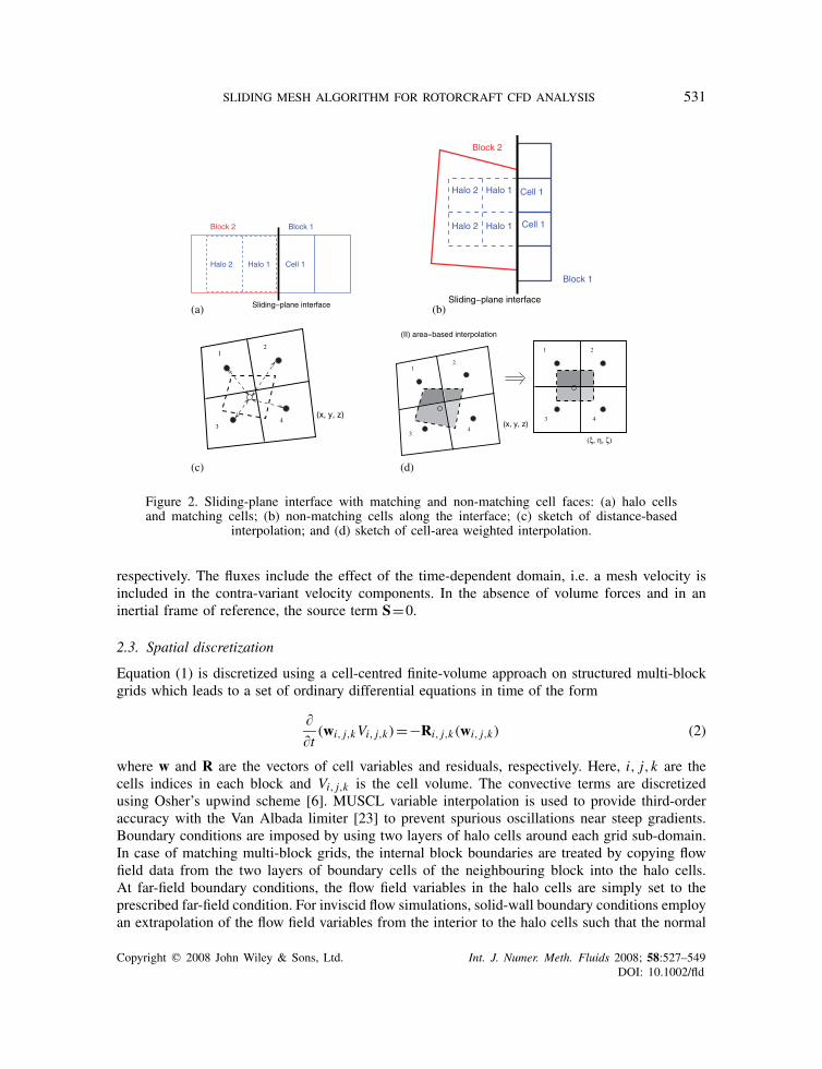
Two layers of halo cells are used in the HMB solver for imposing boundary conditions or to allowcommunication between adjacent blocks. Figure 2(a) presents a schematic of this arrangement.Each block is independent of its neighbouring blocks, and as long as the halo cells are populatedwith values of the primitive variables, the solver can compute an update of the flow solution.

2.2. Governing equations in inertial frame of reference

The Navier–Stokes equations expressed in integral form in the arbitrary Lagrangian Eulerianformulation for time-dependent domains, which may include moving boundaries, read

d

dt

∫V (t)

wdV +∫

�V (t)(F(w)−Fv(w))ndS=S (1)

The above forms a system of conservation laws for any time-dependent control volume V (t) withboundary �V (t) and outward unit normal n. The vector of conserved variables is denoted byw=[�,�u,�v,�w,�E]T, where � is the density, u,v,w are the Cartesian velocity componentsand E is the total internal energy per unit mass. F and Fv are the inviscid and viscous fluxes,



(a) (b)

(c) (d)

Figure 2. Sliding-plane interface with matching and non-matching cell faces: (a) halo cellsand matching cells; (b) non-matching cells along the interface; (c) sketch of distance-based

interpolation; and (d) sketch of cell-area weighted interpolation.

respectively. The fluxes include the effect of the time-dependent domain, i.e. a mesh velocity isincluded in the contra-variant velocity components. In the absence of volume forces and in aninertial frame of reference, the source term S=0.

2.3. Spatial discretization

Equation (1) is discretized using a cell-centred finite-volume approach on structured multi-blockgrids which leads to a set of ordinary differential equations in time of the form

��t

(wi, j,kVi, j,k)=−Ri, j,k(wi, j,k) (2)

where w and R are the vectors of cell variables and residuals, respectively. Here, i, j,k are thecells indices in each block and Vi, j,k is the cell volume. The convective terms are discretizedusing Osher’s upwind scheme [6]. MUSCL variable interpolation is used to provide third-orderaccuracy with the Van Albada limiter [23] to prevent spurious oscillations near steep gradients.Boundary conditions are imposed by using two layers of halo cells around each grid sub-domain.In case of matching multi-block grids, the internal block boundaries are treated by copying flowfield data from the two layers of boundary cells of the neighbouring block into the halo cells.At far-field boundary conditions, the flow field variables in the halo cells are simply set to theprescribed far-field condition. For inviscid flow simulations, solid-wall boundary conditions employan extrapolation of the flow field variables from the interior to the halo cells such that the normal



component of the velocity relative to the solid wall is zero. Similarly, for viscous flow simulations,halo cell values are extrapolated at solid boundaries ensuring that the velocity takes on any wallvelocity.

2.4. Temporal integration and the dual time-stepping method

For time-accurate simulations, temporal integration is performed using an implicit dual time-stepping method. Following the pseudo-time formulation [20], the updated mean flow solution iscalculated by solving the steady-state problems

R∗i, j,k = 3V n+1

i, j,kwn+1i, j,k−4V n

i, j,kwni, j,k+V n−1

i, j,kwn−1i, j,k

2�t+Ri, j,k(w

n+1i, j,k)=0 (3)

where V n−1i, j,k , V

ni, j,k and V n+1

i, j,k represent the cell volumes at different time steps. Equation (3)represents a nonlinear system of equations. This system can be solved by introducing an iterationthrough pseudo-time � to the steady state, as given by

V n+1i, j,k

wn+1,m+1i, j,k −wn+1,m

i, j,k

V n+1i, j,k��︸︷︷︸A

+3V n+1i, j,kw

n+1,mi, j,k −4V n

i, j,kwni, j,k+V n−1

i, j,kwn−1i, j,k

2V n+1i, j,k�t

+Ri, j,k(wn+1,mi, j,k )

V n+1i, j,k

=0 (4)

where the mth pseudo-time iterate at real time step n+1 is denoted by wn+1,m and the cell volumesare constant during the pseudo-time iteration. The unknown wn+1

i, j,k is obtained when term A inEquation (4) converges to a specified tolerance. An implicit scheme is used for the pseudo-timeintegration. The flux residual Ri, j,k(w

n+1i, j,k) is linearized as

Ri, j,k(wn+1) =Ri, j,k(wni, j.k)+

�Ri, j,k(wni, j.k)

�t�t+O(�t2)

≈Rni, j,k(w

ni, j.k)+

�Rni, j,k

�wni, j,k

(wn+1i, j,k−wn

i, j,k) (5)

Using this linearization in pseudo-time, Equation (4) becomes a system of linear equations. Forthe solution of this system, the generalized conjugate gradient method with a block incompletelower–upper pre-conditioner is used. Typically, the pseudo-time integration in Equation (4) iscontinued at each real time step until the residual has dropped three orders of magnitude.

3. SLIDING-MESH ALGORITHM

The underlying idea behind the sliding-mesh approach can be explained using the schematics ofFigure 2. Figure 2(a) shows the definition of two layers of halo cells around the boundary surfaceof each block. In the sliding-plane algorithm, this concept is extended to deal with grids thatare discontinuous across the interface and can also be in relative motion. Figure 2(b) presentsa situation where two adjacent blocks have non-matching cell faces. If the halo cells of eachblock could, however, be populated with interpolated values, the solver will have no difficulty in



computing the flow. The application of the sliding-plane algorithm to non-matching grids as wellas grids in relative motion will result in non-matching cell faces as sketched in Figure 2(b). Foreach pair of adjacent sliding planes, there are three main steps involved in populating the halocells: (i) identification of the neighbouring cells for each halo cell, (ii) interpolation of the solutionat the centroids of the halo cells and (iii) exchange of information between blocks associated withdifferent processors. The last step is important for computations on distributed-memory machinesonly. Regardless of the identification and interpolation methods employed, the halo-cell values arecomputed using

�halo=i=n∑i=1

wi�i (6)

where � represents any flow field variable, e.g. �,�ui , . . . , p, etc., wi is the weight associated withthe i th neighbour of the halo cell and n is the number of neighbours.

Figures 2(c) and (d) show two possible methods used to determine the halo-cell values whenneighbouring grids along a sliding-plane interface are discontinuous and may be in relative motion.The distance-based interpolation (shown in Figure 2(c)) computes a weighted sum of flow fielddata of neighbouring cells within an interaction radius. The weights are inversely proportional tothe distance of the cell centre from the projected point on the sliding plane interface and are scaledto sum up to one. Figure 2(d) shows the cell-face overlap interpolation, in which case the weight foreach neighbour is directly proportional to the fraction of the projected overlapping cell face area.In the context of finite-volume discretization methods for conservation laws based on numericalfluxes through cell faces, the cell-face overlap interpolation is the preferred method. However, aninterpolation method based on the overlap weighting of Figure 2(d) does not necessarily enforceconservation and differences in grid sizes between the sides of the sliding plane may act as aspatial filter.

3.1. Interpolation method based on overlapping areas

The present implementation of the sliding-mesh algorithm is based on the cell-face overlap inter-polation method presented in Figure 2(d). Sliding-mesh interfaces can be of arbitrary shape andfor this reason the contributing cell surfaces must all be projected on the curvilinear �,�,� axesused in the solver. This step can be combined with a transformation from primitive to conservativevariables so that flux-weighted summations can also be computed.

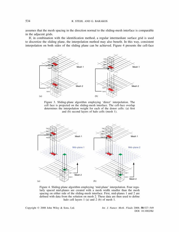
Figure 3 presents the underlying idea of the cell-face overlap interpolation used in the presentsliding-mesh algorithm. The figure shows two adjacent non-matching meshes that are separated bythe sliding-mesh interface. For both meshes, two layers of halo cells are constructed. Figure 3(a)shows how the first layer of halo cells of mesh 1 is obtained. At first, the face of each boundarycell in mesh 1 is projected onto the sliding-plane interface. Subsequently, the neighbour cellscontributing to the halo data are identified. These cells belong to mesh 2 and their faces overlapthe projected cell face from mesh 1. In the figure, three neighbours are shown. The interpolationweight assigned to each neighbour is the fraction of the projected cell face area occupied by theoverlapping area of the two cells. For the second layer of halo cells of mesh 1, the procedure ispresented in Figure 3(b). In this case, the face of the cell in mesh 1 is projected onto a planeformed by the cell faces one cell size away from the block boundary. The neighbours are nowsearched for in the second layer of cells below the block boundary of mesh 2. The present method



assumes that the mesh spacing in the direction normal to the sliding-mesh interface is comparablein the adjacent grids.

If, in combination with the identification method, a regular intermediate surface grid is usedto discretize the sliding plane, the interpolation method may also benefit. In this way, consistentinterpolation on both sides of the sliding plane can be achieved. Figure 4 presents the cell-face

(a) (b)

Figure 3. Sliding-plane algorithm employing ‘direct’ interpolation. Thecell face is projected on the sliding-mesh interface. The cell-face overlapdetermines the interpolation weight for each of the donor cells: (a) first

and (b) second layers of halo cells (mesh 1).

(a) (b)

Figure 4. Sliding-plane algorithm employing ‘mid-plane’ interpolation. Four regu-larly spaced mid-planes are created with a mesh width smaller than the meshspacing on either side of the sliding-mesh interface. First, mid-planes 1 and 2 aredefined with data from the solution on mesh 2. These data are then used to define

halo cell layers 1 (a) and 2 (b) of mesh 1.



overlap interpolation using a regular intermediate plane. The cell spacing of this intermediate planeneeds to be smaller than the cell width on both sides of the sliding-plane interface. Combined withthe need for regularity, this method requires the storage of a large number of intermediate cellvalues for large meshes with significant mesh stretching. Despite the benefits of the regularity of theintermediate-mesh interpolation in terms of identification efficiency and interpolation consistency,there is a significant memory overhead.

3.2. Identification of cell neighbours

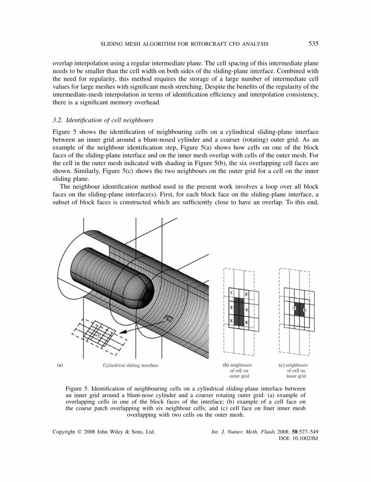
Figure 5 shows the identification of neighbouring cells on a cylindrical sliding-plane interfacebetween an inner grid around a blunt-nosed cylinder and a coarser (rotating) outer grid. As anexample of the neighbour identification step, Figure 5(a) shows how cells on one of the blockfaces of the sliding-plane interface and on the inner mesh overlap with cells of the outer mesh. Forthe cell in the outer mesh indicated with shading in Figure 5(b), the six overlapping cell faces areshown. Similarly, Figure 5(c) shows the two neighbours on the outer grid for a cell on the innersliding plane.

The neighbour identification method used in the present work involves a loop over all blockfaces on the sliding-plane interface(s). First, for each block face on the sliding-plane interface, asubset of block faces is constructed which are sufficiently close to have an overlap. To this end,

Figure 5. Identification of neighbouring cells on a cylindrical sliding-plane interface betweenan inner grid around a blunt-nose cylinder and a coarser rotating outer grid: (a) example ofoverlapping cells in one of the block faces of the interface; (b) example of a cell face onthe coarse patch overlapping with six neighbour cells; and (c) cell face on finer inner mesh

overlapping with two cells on the outer mesh.



any metric of the block-face size can be used. For planar interfaces and highly regular block faceshapes, the mean of both diagonals would suffice. This metric may have to be adjusted for blockfaces with highly stretched grids.

To check the potential of cell overlap, a search range is used which is based on the diagonalsof the cells considered. For cells within this interaction radius, the cell face overlap computationis performed. The overlap computation can handle quadrangles of arbitrary shapes and involveschecks for a range of overlap patterns.

Without the interaction radius checks, the neighbour identification for a sliding-plane interfacewith N1 cells along the interface on one side and N2 cells on the other side would involve N1×N2overlap computations. The construction of the neighbour block face list reduces the computationaloverhead. Although the cost of the above process remains O(N1×N2), it copes with complexconfigurations such as the rotor–fuselage cases. For the cases considered in the present work, theimplemented identification method was found to have an acceptable computational overhead. Forthe generic demonstration cases, the overhead was as little as 1–2% of the simulation time. Forthe more complex rotor–fuselage test cases, with significantly larger mesh sizes, the simulationneeds to be performed in parallel, leading to a more complex identification process. This problemwas addressed by developing a separate parallel pre-processor for identification and interpolationweight computation, which is described in the following section.

3.3. Parallelization of the method

The present implementation of the sliding-mesh method was designed for execution on a distributed-memory multi-processor computer, typically a low-cost Linux cluster. The method is embedded inthe HMB flow solver, which, for parallel simulations on distributed-memory computers, dividesthe sub-domains between processors, each of which stores only the flow field data and the meshfor the assigned sub-domains. In the neighbour-identification step, the mesh coordinates for cellsalong neighbouring block faces are required. The main challenge in the parallel execution arisesfrom the fact that the neighbouring block may be assigned to a different processor and, therefore,the required mesh coordinates will not be readily available. Furthermore, if the grids bordering thesliding-plane interface are moving, the multi-block topology is a function of time, and thereforethe communication pattern required for the neighbour identification step will vary for each timestep.

In the design of the parallel implementation of the neighbour-identification and weight-computation steps, the main challenge is to limit the number of message-passing communicationsand the amount of communicated data. In the present approach, a parallel pre-processor performsthe neighbour identification as well as the determination of the interpolation weights. For eachtime step in the flow simulation, the pre-processor creates a file containing, for each cell on thesliding-plane interface, a list of the neighbouring cells and corresponding weights. For each cell,its block index and the indices of the neighbouring cells on the other side of the sliding plane arestored. This out-of-core computation is necessary for large grids where storage of the whole gridon each processor during parallel execution is not possible.

Parallel computations also require an efficient approach to exchange flow field data among theprocessors which have one or more blocks assigned on the sliding plane. The parallel executionof the sliding-plane method is illustrated in Figure 6 for a simple example with a 10-block meshdistributed over four processors. A two-dimensional case is shown for clarity. In the parallelexecution, a parameter nCPU,SP defines the number of processors used to store the blocks adjacent to



(a)

(c)

(b)

Figure 6. Example of parallel execution of a 10-block mesh on four CPUs. Processors 0 and 1share the blocks along the sliding-mesh interface, whereas 3 and 4 receive the remaining blocks.Processors 0 and 1 allocate a buffer to store two cell layers of data along the interface. Collectivebroadcast operations distribute the buffer data: (a) 10-block mesh; (b) processor assignment and cell

indices in buffer; and (c) sliding-plane face list and buffer construction on two CPUs.

the sliding-plane interface (nCPU,SP=2 in the example). The parallel execution of the sliding-planemethod in the flow solver involves the following steps:

1. Load balancing: In this step, sub-domains having one or more faces along the sliding-planeinterface are identified. These sub-domains are assigned to the first nCPU,SP processors,whereas the rest are assigned to the remaining processors. Among both batches of proces-sors, the computational load is evenly distributed by a process in which the least loadedprocessor is given additional blocks until all blocks are distributed. In the present MPI-basedimplementation, an MPI_Communicator is created for the ‘sliding-plane’ processors.This communicator enables collective communications among the ‘sliding-plane’ processors,while the default MPI_Communicator, i.e. MPI_Comm_World, is used for collectivecommunications between all processors.

2. Sliding-plane buffer allocation: In this process, a linked list is constructed, in which each listelement holds the following: (i) the block index, (ii) block face index, (iii) a pointer to thepart of the flow solution buffer for this block (i.e. buffer in Figure 6(c)) and (iv) the sizeof this part of the buffer. The flow solution buffer contains the flow field variables for thetwo layers of cells adjacent to the sliding-plane interface. The need to store just two layers ofcell data means that the memory allocated on each processor for the buffer is low. It should



be noted that although the stride in the buffer index for adjacent cells is one in Figure 6,the stride used in the flow solver equals the number of unknowns per cell. The list containselements for each of the block faces on the sliding-plane interface and is allocated on eachof the first nCPU,SP processors. In Figure 6, the list has five entries. The cell indices of theneighbours pre-computed by the pre-processor are actually the indices of neighbour cells inthis buffer.

3. Sliding-plane weights allocation: In this step, a weights data structure is allocated for eachcell of the locally allocated blocks on the sliding-plane interface. The weights data typeholds (i) the number of neighbour cells, (ii) a variable-length array storing the block index,(iii) the cell index and (iv) the weight for each neighbour cell.

4. Sliding-plane buffer update: This update consists of two steps. First, each processor copiesthe most recent flow solution data into the flow solution buffers of the blocks assigned tothat processor. Figure 6 shows the parts of the buffer stored on each processor before datacommunication. The blank entries in the buffer shown in the sketch indicate the parts whichneed to be received from other processors. Collective broadcast (MPI_Bcast) operationsusing the dedicated sliding-plane MPI_Communicator are used to update the remainingflow solution buffer entries on each of the first nCPU,SP processors.

5. Sliding-plane weights update: In this step, the weights file created in the pre-processing stageis read by each one of the first nCPU,SP processors. On each processor, only the relevantinterpolation data are stored.

Steps (4) and (5) are repeated at the end of each pseudo-time step (m in Equation (4)). Followingthe above steps, the halo values required for the block faces on the sliding plane can be obtainedfrom the buffer data stored on each processor. For example, for halo cell A in Figure 6, only oneneighbour will be used (corresponding to buffer index 21), whereas for halo cell B, the halo dataare obtained from a weighted summation of buffer data at indices 2 and 3. For three-dimensionalproblems with non-matching stretched grids, the number of neighbours will range from one totens or even hundreds.

4. DEMONSTRATION OF THE METHOD AND DISCUSSION OF THE RESULTS

The technique described in the previous section has been implemented in HMB and tested for avariety of cases. The obtained results are presented in this section.

4.1. Flows over bumps and around aerofoils

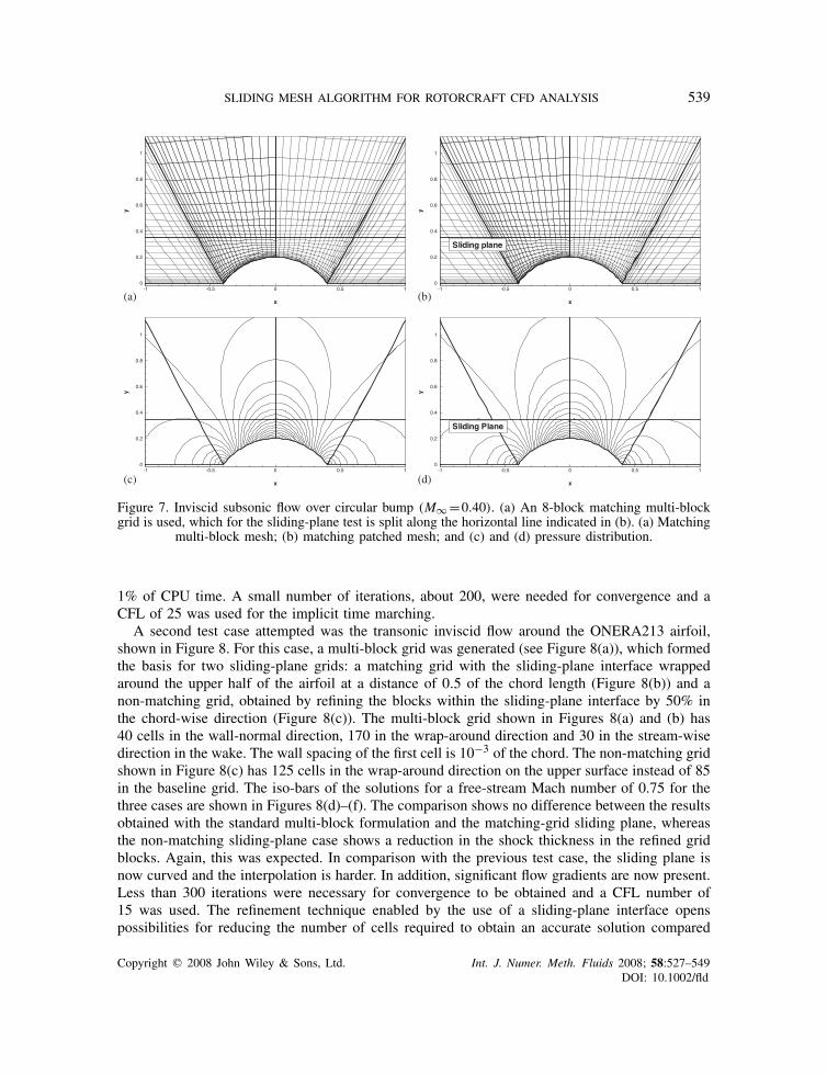
The first test case considered was the inviscid flow over a bump. For this case, a matching multi-block grid was generated with 6400 cells, as shown in Figure 7(a). The sliding-plane grid shownin Figure 7(b) was obtained by introducing a horizontal split. The solution obtained with the inter-block boundary treated as a normal block boundary is shown in Figure 7(c). The sliding-planesolution is shown in Figure 7(d). The comparison shows that there is no difference between theobtained results and this suggests that the existing interpolation method did not introduce anynumerical artefacts. This was expected since both sides of the sliding plane had matching grids.Owing to the small size of the employed grid, the computational overhead for the case where thesliding-plane algorithm is used is very low. Profiling of the solver revealed an increase of less than



(a) (b)

(c) (d)

Figure 7. Inviscid subsonic flow over circular bump (M∞ =0.40). (a) An 8-block matching multi-blockgrid is used, which for the sliding-plane test is split along the horizontal line indicated in (b). (a) Matching

multi-block mesh; (b) matching patched mesh; and (c) and (d) pressure distribution.

1% of CPU time. A small number of iterations, about 200, were needed for convergence and aCFL of 25 was used for the implicit time marching.

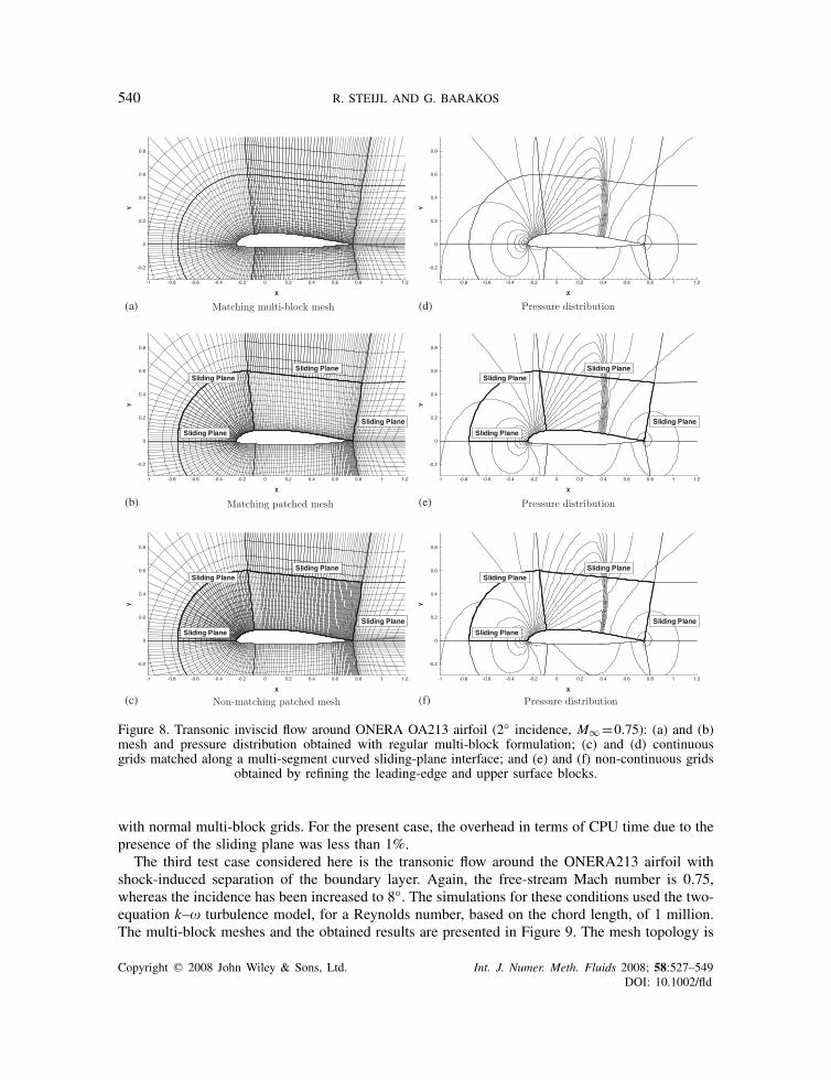
A second test case attempted was the transonic inviscid flow around the ONERA213 airfoil,shown in Figure 8. For this case, a multi-block grid was generated (see Figure 8(a)), which formedthe basis for two sliding-plane grids: a matching grid with the sliding-plane interface wrappedaround the upper half of the airfoil at a distance of 0.5 of the chord length (Figure 8(b)) and anon-matching grid, obtained by refining the blocks within the sliding-plane interface by 50% inthe chord-wise direction (Figure 8(c)). The multi-block grid shown in Figures 8(a) and (b) has40 cells in the wall-normal direction, 170 in the wrap-around direction and 30 in the stream-wisedirection in the wake. The wall spacing of the first cell is 10−3 of the chord. The non-matching gridshown in Figure 8(c) has 125 cells in the wrap-around direction on the upper surface instead of 85in the baseline grid. The iso-bars of the solutions for a free-stream Mach number of 0.75 for thethree cases are shown in Figures 8(d)–(f). The comparison shows no difference between the resultsobtained with the standard multi-block formulation and the matching-grid sliding plane, whereasthe non-matching sliding-plane case shows a reduction in the shock thickness in the refined gridblocks. Again, this was expected. In comparison with the previous test case, the sliding plane isnow curved and the interpolation is harder. In addition, significant flow gradients are now present.Less than 300 iterations were necessary for convergence to be obtained and a CFL number of15 was used. The refinement technique enabled by the use of a sliding-plane interface openspossibilities for reducing the number of cells required to obtain an accurate solution compared



(a) (d)

(b) (e)

(c) (f)

Figure 8. Transonic inviscid flow around ONERA OA213 airfoil (2◦ incidence, M∞ =0.75): (a) and (b)mesh and pressure distribution obtained with regular multi-block formulation; (c) and (d) continuousgrids matched along a multi-segment curved sliding-plane interface; and (e) and (f) non-continuous grids

obtained by refining the leading-edge and upper surface blocks.

with normal multi-block grids. For the present case, the overhead in terms of CPU time due to thepresence of the sliding plane was less than 1%.

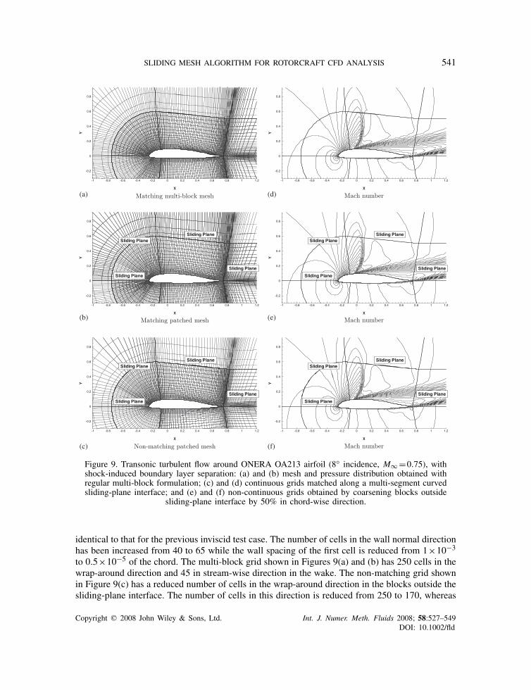
The third test case considered here is the transonic flow around the ONERA213 airfoil withshock-induced separation of the boundary layer. Again, the free-stream Mach number is 0.75,whereas the incidence has been increased to 8◦. The simulations for these conditions used the two-equation k–� turbulence model, for a Reynolds number, based on the chord length, of 1 million.The multi-block meshes and the obtained results are presented in Figure 9. The mesh topology is



(a) (d)

(b) (e)

(c) (f)

Figure 9. Transonic turbulent flow around ONERA OA213 airfoil (8◦ incidence, M∞ =0.75), withshock-induced boundary layer separation: (a) and (b) mesh and pressure distribution obtained withregular multi-block formulation; (c) and (d) continuous grids matched along a multi-segment curvedsliding-plane interface; and (e) and (f) non-continuous grids obtained by coarsening blocks outside

sliding-plane interface by 50% in chord-wise direction.

identical to that for the previous inviscid test case. The number of cells in the wall normal directionhas been increased from 40 to 65 while the wall spacing of the first cell is reduced from 1×10−3

to 0.5×10−5 of the chord. The multi-block grid shown in Figures 9(a) and (b) has 250 cells in thewrap-around direction and 45 in stream-wise direction in the wake. The non-matching grid shownin Figure 9(c) has a reduced number of cells in the wrap-around direction in the blocks outside thesliding-plane interface. The number of cells in this direction is reduced from 250 to 170, whereas



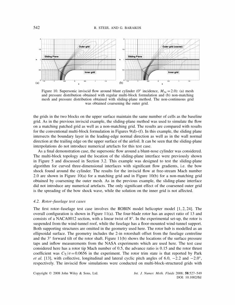
Figure 10. Supersonic inviscid flow around blunt cylinder (0◦ incidence, M∞ =2.0): (a) meshand pressure distribution obtained with regular multi-block formulation and (b) non-matchingmesh and pressure distribution obtained with sliding-plane method. The non-continuous grid

was obtained coarsening the outer grid.

the grids in the two blocks on the upper surface maintain the same number of cells as the baselinegrid. As in the previous inviscid example, the sliding-plane method was used to simulate the flowon a matching patched grid as well as a non-matching grid. The results are compared with resultsfor the conventional multi-block formulation in Figures 9(d)–(f). In this example, the sliding planeintersects the boundary layer in the leading-edge normal direction as well as in the wall normaldirection at the trailing edge on the upper surface of the airfoil. It can be seen that the sliding-planeinterpolations do not introduce numerical artefacts for this test case.

As a final demonstration case, the supersonic flow around a blunt-nose cylinder was considered.The multi-block topology and the location of the sliding-plane interface were previously shownin Figure 5 and discussed in Section 3.2. This example was designed to test the sliding-planealgorithm for curved three-dimensional interfaces with significant flow gradients, i.e. the bowshock found around the cylinder. The results for the inviscid flow at free-stream Mach number2.0 are shown in Figure 10(a) for a matching grid and in Figure 10(b) for a non-matching gridobtained by coarsening the outer mesh. As in the previous example, the sliding-plane interfacedid not introduce any numerical artefacts. The only significant effect of the coarsened outer gridis the spreading of the bow shock wave, while the solution on the inner grid is not affected.

4.2. Rotor–fuselage test cases

The first rotor–fuselage test case involves the ROBIN model helicopter model [1, 2, 24]. Theoverall configuration is shown in Figure 11(a). The four-blade rotor has an aspect ratio of 13 andconsists of a NACA0012 section, with a linear twist of 8◦. In the experimental set-up, the rotor issuspended from the wind-tunnel roof, while the fuselage has a floor-mounted wind-tunnel support.Both supporting structures are omitted in the geometry used here. The rotor hub is modelled as anellipsoidal surface. The geometry includes the 2-in rotorshaft offset from the fuselage centrelineand the 3◦ forward tilt of the rotor shaft. Figure 11(b) shows the locations of the surface pressuretaps and inflow measurements from the NASA experiments which are used here. The test caseconsidered here has a rotor tip Mach number of 0.5, the advance ratio is 0.15 and the rotor thrustcoefficient was CT/�=0.0656 in the experiment. The rotor trim state is that reported by Parket al. [13], with collective, longitudinal and lateral cyclic pitch angles of 6.0, −2.2 and −2.0◦,respectively. The inviscid flow simulations were conducted on multi-block-structured grids with



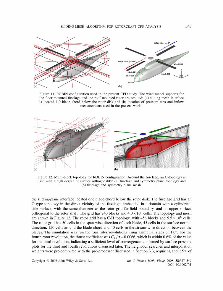
Figure 11. ROBIN configuration used in the present CFD study. The wind tunnel supports forthe floor-mounted fuselage and the roof-mounted rotor are omitted: (a) sliding-mesh interfaceis located 1.0 blade chord below the rotor disk and (b) location of pressure taps and inflow

measurements used in the present work.

Figure 12. Multi-block topology for ROBIN configuration. Around the fuselage, an O-topology isused with a high degree of surface orthogonality: (a) fuselage and symmetry plane topology and

(b) fuselage and symmetry plane mesh.

the sliding-plane interface located one blade chord below the rotor disk. The fuselage grid has anO-type topology in the direct vicinity of the fuselage, embedded in a domain with a cylindricalside surface, with the same diameter as the rotor grid far-field boundary, and an upper surfaceorthogonal to the rotor shaft. The grid has 240 blocks and 4.0×106 cells. The topology and meshare shown in Figure 12. The rotor grid has a C-H topology, with 456 blocks and 5.5×106 cells.The rotor grid has 50 cells in the span-wise direction of each blade, 45 cells in the surface normaldirection, 150 cells around the blade chord and 40 cells in the stream-wise direction between theblades. The simulation was run for four rotor revolutions using azimuthal steps of 1.0◦. For thefourth rotor revolution, the thrust coefficient was CT/�=0.0066, which is within 0.6% of the valuefor the third revolution, indicating a sufficient level of convergence, confirmed by surface pressureplots for the third and fourth revolutions discussed later. The neighbour searches and interpolationweights were pre-computed with the pre-processor discussed in Section 3.3, requiring about 5% of



the total CPU time. The sliding-plane method added an additional 5–6% communication overheadfor the parallel simulation conducted on 40 Pentium four processors of a Linux cluster. The gridblocks along the sliding-plane interface were allocated to the first six processors, i.e. the parameternCPU,SP defined in Section 3.3 was set to 6.

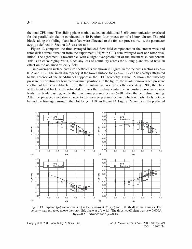
Figure 13 compares the time-averaged induced flow field components in the stream-wise androtor-disk normal direction from the experiment [25] with CFD data averaged over one rotor revo-lution. The agreement is favourable, with a slight over-prediction of the stream-wise component.This is an encouraging result, since any loss of continuity across the sliding plane would have aneffect on the obtained velocity field.

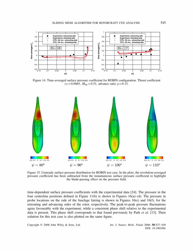
Time-averaged surface pressure coefficients are shown in Figure 14 for the cross sections x/L=0.35 and 1.17. The small discrepancy at the lower surface for x/L=1.17 can be (partly) attributedto the absence of the wind-tunnel support in the CFD geometry. Figure 15 shows the unsteadypressure distribution for four rotor azimuth positions. In the figure, the revolution-averaged pressurecoefficient has been subtracted from the instantaneous pressure coefficients. At =90◦, the bladeat the front and back of the rotor disk crosses the fuselage centreline. A positive pressure changeleads this blade passing, while the maximum pressure occurs 5–10◦ after the centreline passing.After the passage, a negative change to the average pressure occurs, which is particularly notablebehind the fuselage fairing in the plot for =110◦ in Figure 14. Figure 16 compares the predicted

(a) (b)

(c) (d)

Figure 13. In-plane (i ) and normal (�i ) velocity ratios at 0◦ (a, c) and 180◦ (b, d) azimuth angles. Thevelocity was extracted above the rotor disk plane at z/c=1.1. The thrust coefficient was cT=0.0065,

Mtip=0.51, advance ratio =0.15.



Figure 14. Time-averaged surface pressure coefficient for ROBIN configuration. Thrust coefficientcT=0.0065, Mtip=0.51, advance ratio =0.15.

Figure 15. Unsteady surface pressure distribution for ROBIN test case. In the plots, the revolution-averagedpressure coefficient has been subtracted from the instantaneous surface pressure coefficient to highlight

the blade-passing effect on the pressure field.

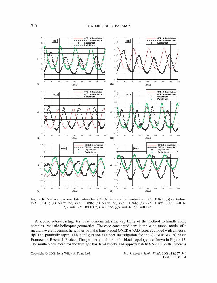
time-dependent surface pressure coefficients with the experimental data [24]. The pressure in thefour centreline positions defined in Figure 11(b) is shown in Figures 16(a)–(d). The pressure inprobe locations on the side of the fuselage fairing is shown in Figures 16(e) and 16(f), for theretreating and advancing sides of the rotor, respectively. The peak-to-peak pressure fluctuationsagree favourably with the experiment, while a consistent phase shift relative to the experimentaldata is present. This phase shift corresponds to that found previously by Park et al. [13]. Theirsolution for this test case is also plotted on the same figure.



(a) (b)

(c) (d)

(e) (f)

Figure 16. Surface pressure distribution for ROBIN test case: (a) centreline, x/L=0.096; (b) centreline,x/L=0.201; (c) centreline, x/L=0.896; (d) centreline, x/L=1.368; (e) x/L=0.896, y/L=−0.07,

z/L=0.125; and (f) x/L=1.368, y/L=0.07, z/L=0.125.

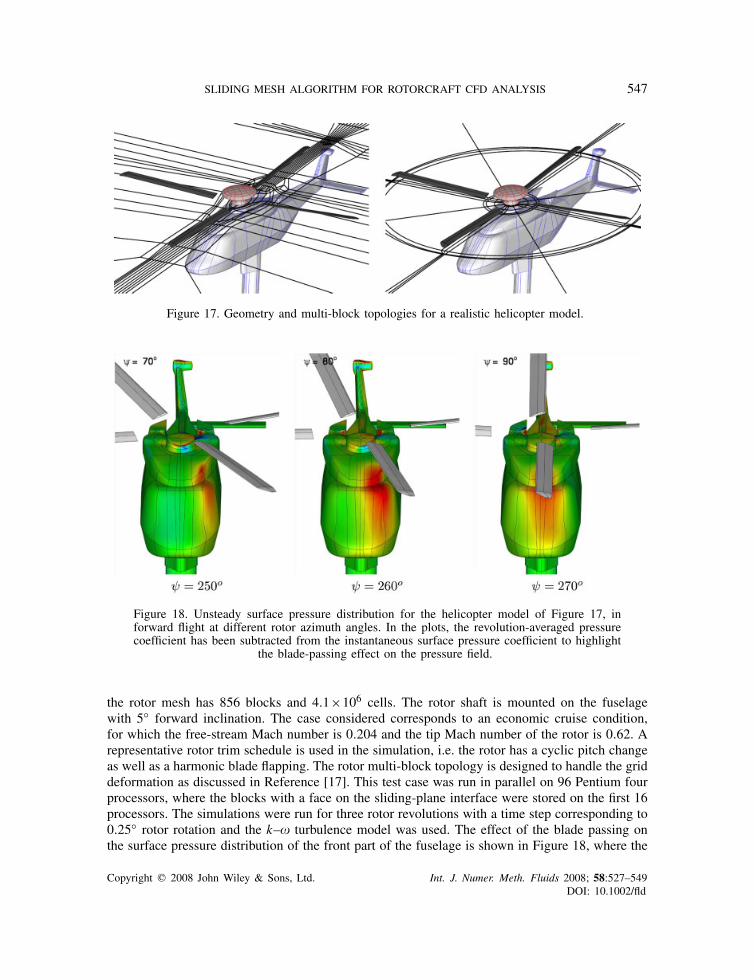
A second rotor–fuselage test case demonstrates the capability of the method to handle morecomplex, realistic helicopter geometries. The case considered here is the wind-tunnel model of amedium-weight generic helicopter with the four-bladed ONERA 7AD rotor, equipped with anhedraltips and parabolic taper. This configuration is under investigation for the GOAHEAD EC SixthFramework Research Project. The geometry and the multi-block topology are shown in Figure 17.The multi-block mesh for the fuselage has 1624 blocks and approximately 6.5×106 cells, whereas



Figure 17. Geometry and multi-block topologies for a realistic helicopter model.

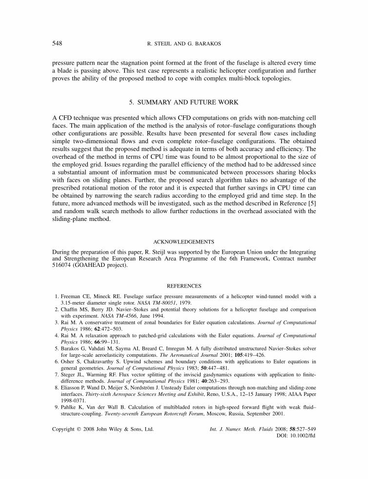
Figure 18. Unsteady surface pressure distribution for the helicopter model of Figure 17, inforward flight at different rotor azimuth angles. In the plots, the revolution-averaged pressurecoefficient has been subtracted from the instantaneous surface pressure coefficient to highlight

the blade-passing effect on the pressure field.

the rotor mesh has 856 blocks and 4.1×106 cells. The rotor shaft is mounted on the fuselagewith 5◦ forward inclination. The case considered corresponds to an economic cruise condition,for which the free-stream Mach number is 0.204 and the tip Mach number of the rotor is 0.62. Arepresentative rotor trim schedule is used in the simulation, i.e. the rotor has a cyclic pitch changeas well as a harmonic blade flapping. The rotor multi-block topology is designed to handle the griddeformation as discussed in Reference [17]. This test case was run in parallel on 96 Pentium fourprocessors, where the blocks with a face on the sliding-plane interface were stored on the first 16processors. The simulations were run for three rotor revolutions with a time step corresponding to0.25◦ rotor rotation and the k–� turbulence model was used. The effect of the blade passing onthe surface pressure distribution of the front part of the fuselage is shown in Figure 18, where the



pressure pattern near the stagnation point formed at the front of the fuselage is altered every timea blade is passing above. This test case represents a realistic helicopter configuration and furtherproves the ability of the proposed method to cope with complex multi-block topologies.

5. SUMMARY AND FUTURE WORK

A CFD technique was presented which allows CFD computations on grids with non-matching cellfaces. The main application of the method is the analysis of rotor–fuselage configurations thoughother configurations are possible. Results have been presented for several flow cases includingsimple two-dimensional flows and even complete rotor–fuselage configurations. The obtainedresults suggest that the proposed method is adequate in terms of both accuracy and efficiency. Theoverhead of the method in terms of CPU time was found to be almost proportional to the size ofthe employed grid. Issues regarding the parallel efficiency of the method had to be addressed sincea substantial amount of information must be communicated between processors sharing blockswith faces on sliding planes. Further, the proposed search algorithm takes no advantage of theprescribed rotational motion of the rotor and it is expected that further savings in CPU time canbe obtained by narrowing the search radius according to the employed grid and time step. In thefuture, more advanced methods will be investigated, such as the method described in Reference [5]and random walk search methods to allow further reductions in the overhead associated with thesliding-plane method.

ACKNOWLEDGEMENTS

During the preparation of this paper, R. Steijl was supported by the European Union under the Integratingand Strengthening the European Research Area Programme of the 6th Framework, Contract number516074 (GOAHEAD project).

REFERENCES

1. Freeman CE, Mineck RE. Fuselage surface pressure measurements of a helicopter wind-tunnel model with a3.15-meter diameter single rotor. NASA TM-80051, 1979.

2. Chaffin MS, Berry JD. Navier–Stokes and potential theory solutions for a helicopter fuselage and comparisonwith experiment. NASA TM-4566, June 1994.

3. Rai M. A conservative treatment of zonal boundaries for Euler equation calculations. Journal of ComputationalPhysics 1986; 62:472–503.

4. Rai M. A relaxation approach to patched-grid calculations with the Euler equations. Journal of ComputationalPhysics 1986; 66:99–131.

5. Barakos G, Vahdati M, Sayma AI, Breard C, Imregun M. A fully distributed unstructured Navier–Stokes solverfor large-scale aeroelasticity computations. The Aeronautical Journal 2001; 105:419–426.

6. Osher S, Chakravarthy S. Upwind schemes and boundary conditions with applications to Euler equations ingeneral geometries. Journal of Computational Physics 1983; 50:447–481.

7. Steger JL, Warming RF. Flux vector splitting of the inviscid gasdynamics equations with application to finite-difference methods. Journal of Computational Physics 1981; 40:263–293.

8. Eliasson P, Wand D, Meijer S, Nordstrom J. Unsteady Euler computations through non-matching and sliding-zoneinterfaces. Thirty-sixth Aerospace Sciences Meeting and Exhibit, Reno, U.S.A., 12–15 January 1998; AIAA Paper1998-0371.

9. Pahlke K, Van der Wall B. Calculation of multibladed rotors in high-speed forward flight with weak fluid–structure-coupling. Twenty-seventh European Rotorcraft Forum, Moscow, Russia, September 2001.



10. Renaud T, Benoit C, Boniface J-C, Gardarein P. Navier–Stokes computations of a complete helicopter configurationaccounting for main and tail rotor effects. Twenty-ninth European Rotorcraft Forum, Friedrichshafen, Germany,September 2003.

11. Pomin H, Wagner S. Aeroelastic analysis of helicopter rotor blades on deformable chimera grids. Journal ofAircraft 2004; 41(3):577–584.

12. Potsdam M, Yeo W, Johnson W. Rotor airloads prediction using loose aerodynamic/structural coupling. AmericanHelicopter Society 60th Annual Forum, Baltimore, MD, 7–10 June 2004.

13. Park Y, Nam HJ, Kwon OJ. Simulation of unsteady rotor–fuselage aerodynamic interaction using unstructuredadaptive meshes. Fifty-ninth Annual Forum of the American Helicopter Society, Phoenix, AZ, 6–8 May 2003.

14. Park Y, Kwon OJ. Simulation of unsteady rotor flow field using unstructured adaptive sliding meshes. Journalof the American Helicopter Society 2004; 49(4):391–400.

15. Nam HJ, Park Y, Kwon OJ. Simulation of unsteady rotor–fuselage aerodynamic interaction using unstructuredadaptive meshes. Journal of the American Helicopter Society 2006; 51(2):141–148.

16. Barakos G, Steijl R, Badcock K, Brocklehurst A. Development of CFD capability for full helicopter engineeringanalysis. Thirty-first European Rotorcraft Forum, Florence, Italy, 13–15 September 2005.

17. Steijl R, Barakos G, Badcock K. A framework for CFD analysis of rotors in hover and forward flight. InternationalJournal for Numerical Methods in Fluids 2006; 51:819–847.

18. Steijl R, Barakos G. CFD analysis of rotor–fuselage interactional aerodynamics. Forty-fifth AIAA AerospaceSciences Meeting and Exhibit, Reno, Nevada, U.S.A., 8–11 January 2007; AIAA Paper 2007-1278.

19. Badcock K, Richards B, Woodgate M. Elements of computational fluid dynamics on block structured grids usingimplicit solvers. Progress in Aerospace Sciences 2000; 36(5–6):351–392.

20. Jameson A. Time dependent calculations using multigrid, with applications to unsteady flows past airfoils andwings. AIAA Paper, 91-1596, 1991.

21. Morvant R, Badcock K, Barakos G, Richards BE. Aerofoil–vortex interaction using the compressible vorticityconfinement method. AIAA Journal 2004; 43(1):63–75.

22. Spentzos A, Barakos G, Badcock K, Richards BE, Wernert P, Schreck S, Raffel M. CFD investigation of 2Dand 3D dynamic stall. AIAA Journal 2005; 34(5):1023–1033.

23. Van Albada GD, van Leer B, Roberts WW. A comparative study of computational methods in cosmic gasdynamics. Astronomy and Astrophysics 1982; 108:76–84.

24. Mineck RE, Althoff Gorton S. Steady and periodic pressure measurements on a generic helicopter fuselage modelin the presence of a rotor. NASA TM 210286, 2000.

25. Elliot JW, Althoff SL, Sailey RH. Inflow measurements made with a laser velocimeter on a helicopter model inforward flight, Volume 1, Rectangular planform blades at an advance ratio of 0.15. NASA TM 100541, 1988.


Sliding mesh algorithm for CFD analysis of helicopter rotor ...

Documents

Transcript of Sliding mesh algorithm for CFD analysis of helicopter rotor ...