Research ArticleHelicopter Control Energy Reduction UsingMoving Horizontal Tail

Tugrul Oktay and Firat Sal

College of Aviation, Erciyes University, 38039 Kayseri, Turkey

Correspondence should be addressed to Tugrul Oktay; tugruloktay52@gmail.com

Received 7 November 2014; Revised 14 February 2015; Accepted 1 April 2015

Academic Editor: Zheng Zheng

Copyright © 2015 T. Oktay and F. Sal. This is an open access article distributed under the Creative Commons Attribution License,which permits unrestricted use, distribution, and reproduction in any medium, provided the original work is properly cited.

Helicopter moving horizontal tail (i.e., MHT) strategy is applied in order to save helicopter flight control system (i.e., FCS) energy.For this intention complex, physics-based, control-oriented nonlinear helicoptermodels are used. Equations ofMHT are integratedinto these models and they are together linearized around straight level flight condition. A specific variance constrained controlstrategy, namely, output variance constrained Control (i.e., OVC) is utilized for helicopter FCS. Control energy savings due to thisMHT idea with respect to a conventional helicopter are calculated. Parameters of helicopter FCS and dimensions of MHT aresimultaneously optimized using a stochastic optimization method, namely, simultaneous perturbation stochastic approximation(i.e., SPSA). In order to observe improvement in behaviors of classical controls closed loop analyses are done.

1. Introduction

Traditionally in order to control helicopters, collective andcyclic (i.e., longitudinal and lateral) rotor blade pitches areused. Presently almost all of the helicopters employ a swash-plate mechanism and pitch links (it consists of two circularplates and a ball bearing arrangement separating them; see [1]for more details) to transmit two cyclic and collective pitchcommands to the blade root. However, this mechanism isheavy and complex and also causes important drag duringhigh flight speeds. Throughout history some other controlmethods have been considered in order to avoid these draw-backs and also for some other reasons such as reduction ofcontrol energy and redundancy in case of failures. Some ofthese alternatives are using trailing edge flaps (TEFs) with(see [2–4]) andwithout (see [5–7]) classical swashplatemech-anism, passive (see [8–10]) and active (see [11–13]) helicoptermorphing, and MHT (see [14–18]). For example, in [2] TEFswere integrated into blades for the case of a failure of thepitch linkmaking the blade free float in pitch. By this methodcatastrophic results of a pitch link failure were corrected. In[5] TEFs were replacedwith a conventional swashplatemech-anism. Via eliminating swashplate mechanism and usingTEFs, important reduction in weight, drag, and cost and also

improvement in rotor performance were obtained.Moreover,in [8] passive morphing was used in order to reduce heli-copter FCS energy. In that studymany blade parameters (e.g.,blade length and blade chord length) were simultaneouslyoptimized with helicopter FCS parameters in order to saveFCS energy. Substantial reduction in helicopter FCS energywas obtained using passive morphing idea. In [11] activemorphing was used to save helicopter FCS energy. In thatstudy actively morphing parameters were blade chord length,blade length, blade twist, and main rotor angular speed. Themain difference between this and previous study (i.e., passivemorphing) was that for the active case the helicopter designparameters are able to change (except helicopter FCS) duringflight, but in prescribed interval. Using active morphing ideasignificant reduction in helicopter FCS energy was obtained.

MHT idea was firstly studied in [14] in 1953. In this studydifferential control of each side of a canted horizontal tailwas permitted. In [15] collective control of horizontal tailwas mechanically achieved. In this study it was claimed thata fixed horizontal tail is advantageous in order to improvelongitudinal stability of helicopters in forward flight, but it isnot enoughduring gliding and climbing flights.More recentlyin [16] a moveable horizontal tail to give the desired attitudeat different flight speed for UH-60 was designed. Recently

Hindawi Publishing Corporatione Scientific World JournalVolume 2015, Article ID 523914, 10 pageshttp://dx.doi.org/10.1155/2015/523914

2 The Scientific World Journal

in [17, 18] a moveable horizontal tail was designed in orderto reduce TEF deflection for swashplateless helicopters sincethe stroke capacity of existing smart material actuators isnot enough for the required TEFs inputs. Using MHT TEFsdeflections were relieved.

Numerous helicopter FCS design methods have beenstudied throughout the years, in historical sequence classicalpole placement techniques (see [19, 20]), simple feedbackcontrol methods (see [21, 22]), and modern control approa-ches depend on linear matrix algebra such as linear quadraticregulator (LQR) and linear quadratic Gaussian (LQG) tech-niques (see [23, 24]), 𝐻

∞control synthesis (see [25, 26]),

and model predictive control (MPC) (see [27, 28]). In thispaper, a modern constrained control method, namely, OVC,is chosen for the design of helicopter FCS. OVC has manyadvantages with respect to the other control strategies exist-ing in the literature. First, these controllers are modifiedLQG controllers and they benefit from Kalman filters as stateestimators. Second, variance constrained controllers applysecond-order information (i.e., state covariance matrix; see[29, 30] for details) and this kind of information is verybeneficial duringmultivariable control systemdesign becauseall stabilizing controllers are parameterized in relation to thephysically meaningful state covariance matrix. Last, for largeand strongly coupled multi-input, multi-output (MIMO)systems as in air vehicles control and especially in this paper,variance constrained control methods give guarantees onthe transient behavior of independent variables by enforcingupper limits on the variance of these variables.

Variance constrained controllers have been used formanyaerospace vehicles (e.g., helicopters, see [8, 11, 31–36]; tiltrotoraircraft, see [37]; Hubble space telescope, see [38]; tensegritystructures, see [39]) in last thirty years. For instance, in [32]variance constrained controllers were used for helicopter FCSduring maneuvers, specifically level banked turn and helicalturn. In that paper, performance of them was also consideredduring failures of some helicopter sensors. Reasonable con-sequences (meaning that variance constraints on outputs/inputs were satisfied and also closed loop systems were exp-onentially stabilized) were found in terms of helicopterFCS. Robustness of the closed loop systems (obtained viaintegration of linearized helicopter model and FCS) withrespect to some modeling uncertainties (i.e., variation offlight conditions and all helicopter inertial parameters) wasalso studied and it was found that these controllers have sta-bility robustness with respect to modeling uncertainties.

In this paper, MHT is for the first time simultaneouslydesigned with helicopter FCS. For this purpose, a specificvariance constrained controller OVC is also used for the firsttime for FCS. It is important to note that when MHT isintegrated with classical helicopter, the number of controlsincreases. This causes an important result. The number oftrim unknowns increases with additional MHT controls.Nevertheless, there are no additional trim equations. There-fore, in order to solve the resulting nonlinear trim equations,a useful optimization algorithm is required. For its solution,a stochastic optimization method specifically simultaneousperturbation stochastic approximation (i.e., SPSA) (see [40,41] for brief description of SPSA) is for the first time applied

for the simultaneous trimming and FCS design problem sinceit is computationally cheap and effective during solving con-strained optimization problems when it is impossible to com-pute derivatives such as gradients and Hessians, analyticallyas in the situation herein. This paper first presents helicoptermodels used for simultaneousMHT and FCS design. Second,MHT is illustrated andmotions of it are described.Then, def-inition of applied FCS (i.e., OVC) is given briefly. After that,trimming the system (i.e., the one obtained via integration ofhelicopter, MHT, and FCS) via simultaneous trimming andFCS design idea is explained. Then, the specific optimizationmethod, namely, SPSA, applied in order to trim the system issummarized. Finally, this simultaneous design idea is appliedfor Puma SA 330 helicopter and closed loop responses ofclassical helicopter and helicopter with MHT are compared.

2. Helicopter Model

The modeling approach of used helicopter models in thispaper is presented in detail in [31, 42].The essential modelingassumptions are given next. First of all, multibody systemapproach was used to include all helicopter components:fuselage, horizontal tail, tail rotor hub and shaft, landing gear,and fully articulatedmain rotor with 4 rigid blades with bladeflapping and lagging hinges. Secondly, a static inflow formu-lation (i.e., Pitt-Peters formulation) was applied for helicoptermain rotor downwash.Thirdly, linear incompressible aerody-namics was used for the main rotor blades, but an analyticalformulation was applied for the modeling of fuselage.

Themodeling procedure requires using physics principlesand because of the assumptions described in the previousparagraph it directly led to helicopter dynamic models thatconsisted of finite sets of ordinary differential equations(ODEs). This mathematical structure is fairly beneficial forcontrol system design since it assists the direct use of moderncontrol theory, which relies on state space representations ofthe system’s dynamics, easily obtained from ODEs.

The modeling methodology summarized above wasapplied in Maple and it led to a nonlinear helicopter modelin implicit form:

𝑓 (�̇�𝑛, 𝑥𝑛, 𝑢𝑛) = 0, (1)

where 𝑓 ∈ R28, 𝑥𝑛∈ R25, and 𝑢

𝑛∈ R4. Here 𝑥

𝑛and

𝑢𝑛are nonlinear state and control vectors, respectively, and

R∗ represents the linear space of ∗-dimensional real vectors,where “∗” can be 28, 25, or 4. It should be noted that theinconsistency between the size of 𝑓(28) and the size of𝑥𝑛(25) is due to the three static downwash equations. The

28 nonlinear equations in (1) are categorized as follows: 9fuselage equations, 8 blade flapping and 8 blade lead-laggingequations, and 3 static main rotor downwash equations. Thehelicopter models obtained have too many terms, making itsuse in fast computation impractical. For that reason, a system-aticmodel simplification technique, named ordering scheme,was applied to reduce the number of terms in the nonlinearODEs.The ordering scheme iteratively deletes terms from anequation depending on their relative magnitude with respectto the other terms in that equation. Each term’s magnitude is

The Scientific World Journal 3

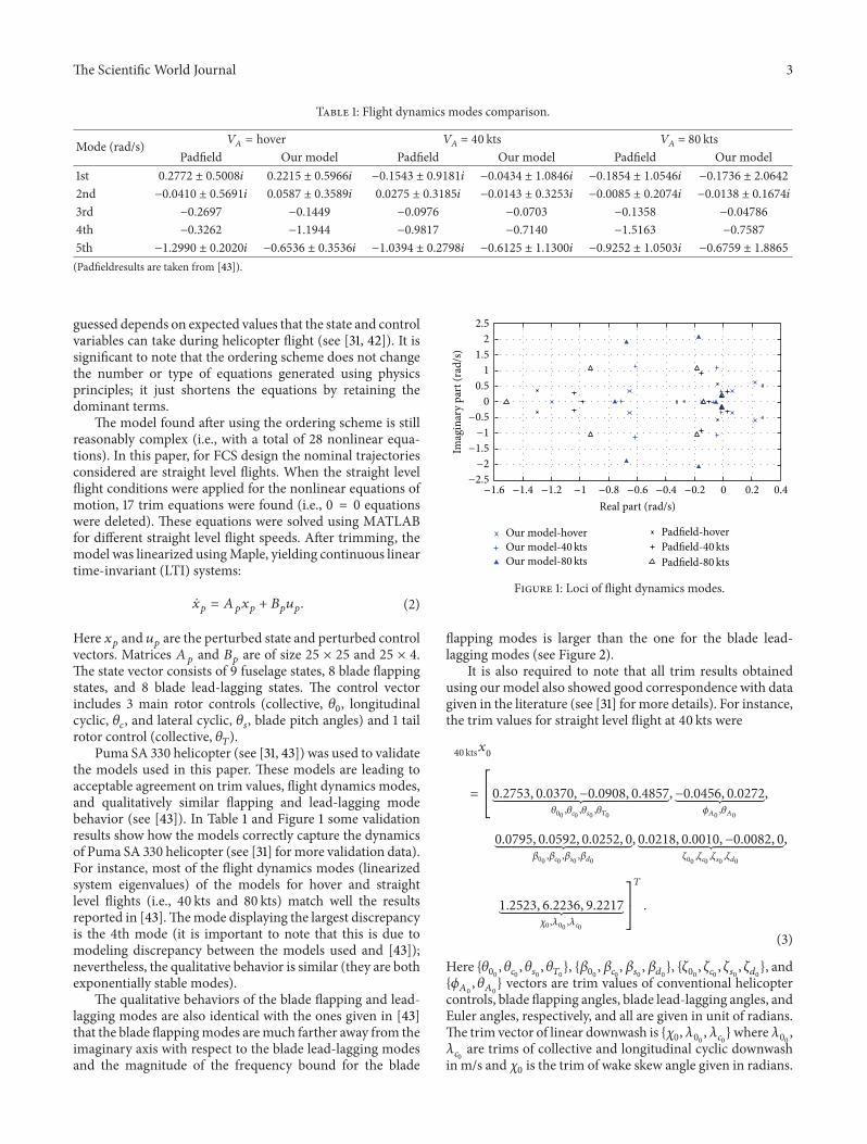
Table 1: Flight dynamics modes comparison.

Mode (rad/s) 𝑉𝐴= hover 𝑉

𝐴= 40 kts 𝑉

𝐴= 80 kts

Padfield Our model Padfield Our model Padfield Our model1st 0.2772 ± 0.5008𝑖 0.2215 ± 0.5966𝑖 −0.1543 ± 0.9181𝑖 −0.0434 ± 1.0846𝑖 −0.1854 ± 1.0546𝑖 −0.1736 ± 2.0642

2nd −0.0410 ± 0.5691𝑖 0.0587 ± 0.3589𝑖 0.0275 ± 0.3185𝑖 −0.0143 ± 0.3253𝑖 −0.0085 ± 0.2074𝑖 −0.0138 ± 0.1674𝑖

3rd −0.2697 −0.1449 −0.0976 −0.0703 −0.1358 −0.04786

4th −0.3262 −1.1944 −0.9817 −0.7140 −1.5163 −0.7587

5th −1.2990 ± 0.2020𝑖 −0.6536 ± 0.3536𝑖 −1.0394 ± 0.2798𝑖 −0.6125 ± 1.1300𝑖 −0.9252 ± 1.0503𝑖 −0.6759 ± 1.8865

(Padfieldresults are taken from [43]).

guessed depends on expected values that the state and controlvariables can take during helicopter flight (see [31, 42]). It issignificant to note that the ordering scheme does not changethe number or type of equations generated using physicsprinciples; it just shortens the equations by retaining thedominant terms.

The model found after using the ordering scheme is stillreasonably complex (i.e., with a total of 28 nonlinear equa-tions). In this paper, for FCS design the nominal trajectoriesconsidered are straight level flights. When the straight levelflight conditions were applied for the nonlinear equations ofmotion, 17 trim equations were found (i.e., 0 = 0 equationswere deleted). These equations were solved using MATLABfor different straight level flight speeds. After trimming, themodel was linearized usingMaple, yielding continuous lineartime-invariant (LTI) systems:

�̇�𝑝= 𝐴𝑝𝑥𝑝+ 𝐵𝑝𝑢𝑝. (2)

Here 𝑥𝑝and 𝑢𝑝are the perturbed state and perturbed control

vectors. Matrices 𝐴𝑝and 𝐵

𝑝are of size 25 × 25 and 25 × 4.

The state vector consists of 9 fuselage states, 8 blade flappingstates, and 8 blade lead-lagging states. The control vectorincludes 3 main rotor controls (collective, 𝜃

0, longitudinal

cyclic, 𝜃𝑐, and lateral cyclic, 𝜃

𝑠, blade pitch angles) and 1 tail

rotor control (collective, 𝜃𝑇).

Puma SA 330 helicopter (see [31, 43]) was used to validatethe models used in this paper. These models are leading toacceptable agreement on trim values, flight dynamics modes,and qualitatively similar flapping and lead-lagging modebehavior (see [43]). In Table 1 and Figure 1 some validationresults show how the models correctly capture the dynamicsof Puma SA 330 helicopter (see [31] formore validation data).For instance, most of the flight dynamics modes (linearizedsystem eigenvalues) of the models for hover and straightlevel flights (i.e., 40 kts and 80 kts) match well the resultsreported in [43].Themode displaying the largest discrepancyis the 4th mode (it is important to note that this is due tomodeling discrepancy between the models used and [43]);nevertheless, the qualitative behavior is similar (they are bothexponentially stable modes).

The qualitative behaviors of the blade flapping and lead-lagging modes are also identical with the ones given in [43]that the blade flappingmodes aremuch farther away from theimaginary axis with respect to the blade lead-lagging modesand the magnitude of the frequency bound for the blade

−1.6 −1.4 −1.2 −0.8 −0.6 −0.4 −0.2−1 0.40.2

−0.5

−1

−1.5

−2

−2.5

2.5

2

1.5

1

0.5

0

0

Imag

inar

y pa

rt (r

ad/s

)

Real part (rad/s)

Padfield-hoverOur model-hoverOur model-40ktsOur model-80kts

Padfield-40ktsPadfield-80kts

Figure 1: Loci of flight dynamics modes.

flapping modes is larger than the one for the blade lead-lagging modes (see Figure 2).

It is also required to note that all trim results obtainedusing our model also showed good correspondence with datagiven in the literature (see [31] for more details). For instance,the trim values for straight level flight at 40 kts were

40 kts𝑥0

= [

[

0.2753, 0.0370, −0.0908, 0.4857⏟⏟⏟⏟⏟⏟⏟⏟⏟⏟⏟⏟⏟⏟⏟⏟⏟⏟⏟⏟⏟⏟⏟⏟⏟⏟⏟⏟⏟⏟⏟⏟⏟⏟⏟⏟⏟⏟⏟⏟⏟⏟⏟⏟⏟⏟⏟⏟⏟⏟⏟⏟⏟⏟⏟⏟⏟⏟⏟

𝜃00,𝜃𝑐0,𝜃𝑠0,𝜃𝑇0

, −0.0456, 0.0272⏟⏟⏟⏟⏟⏟⏟⏟⏟⏟⏟⏟⏟⏟⏟⏟⏟⏟⏟⏟⏟⏟⏟⏟⏟⏟⏟⏟⏟

𝜙𝐴0,𝜃𝐴0

,

0.0795, 0.0592, 0.0252, 0⏟⏟⏟⏟⏟⏟⏟⏟⏟⏟⏟⏟⏟⏟⏟⏟⏟⏟⏟⏟⏟⏟⏟⏟⏟⏟⏟⏟⏟⏟⏟⏟⏟⏟⏟⏟⏟⏟⏟⏟⏟⏟⏟⏟⏟

𝛽00,𝛽𝑐0,𝛽𝑠0,𝛽𝑑0

, 0.0218, 0.0010, −0.0082, 0⏟⏟⏟⏟⏟⏟⏟⏟⏟⏟⏟⏟⏟⏟⏟⏟⏟⏟⏟⏟⏟⏟⏟⏟⏟⏟⏟⏟⏟⏟⏟⏟⏟⏟⏟⏟⏟⏟⏟⏟⏟⏟⏟⏟⏟⏟⏟

𝜁00,𝜁𝑐0,𝜁𝑠0,𝜁𝑑0

,

1.2523, 6.2236, 9.2217⏟⏟⏟⏟⏟⏟⏟⏟⏟⏟⏟⏟⏟⏟⏟⏟⏟⏟⏟⏟⏟⏟⏟⏟⏟⏟⏟⏟⏟⏟⏟⏟⏟⏟⏟⏟⏟⏟⏟⏟⏟

𝜒0 ,𝜆00,𝜆𝑐0

]

]

𝑇

.

(3)

Here {𝜃00, 𝜃𝑐0, 𝜃𝑠0, 𝜃𝑇0}, {𝛽00, 𝛽𝑐0, 𝛽𝑠0, 𝛽𝑑0}, {𝜁00, 𝜁𝑐0, 𝜁𝑠0, 𝜁𝑑0}, and

{𝜙𝐴0, 𝜃𝐴0} vectors are trim values of conventional helicopter

controls, blade flapping angles, blade lead-lagging angles, andEuler angles, respectively, and all are given in unit of radians.The trim vector of linear downwash is {𝜒

0, 𝜆00, 𝜆𝑐0}where 𝜆

00,

𝜆𝑐0are trims of collective and longitudinal cyclic downwash

in m/s and 𝜒0is the trim of wake skew angle given in radians.

4 The Scientific World Journal

50

0

0−50

−16 −14 −12 −10 −8 −6 −4 −2

Real part (rad/s)

Imag

inar

y pa

rt (r

ad/s

)

Flap-hoverFlap-40ktsFlap-80kts

Lag-40ktsLag-80kts

Lag-hover

Figure 2: Loci of flapping and lead-lagging modes.

𝜂0

Left Right

(a)

𝜂0 − 𝜂d 𝜂0 + 𝜂dLeft

Right

(b)

𝜂0 − 𝜂d𝜂0 + 𝜂dLeft Right

(c)

Figure 3: (a) Collective MHT angle, (b) left negative and right pos-itive differential MHT angles, and (c) right negative and left positivedifferential MHT angles.

3. Illustration of MHT

MHT angles (i.e., collective and differential) are illustrated inFigure 3. Collectivemotion refers to themovement of left andright horizontal tails in the same direction and magnitudesimultaneously. On the other hand, differential motion refersto the movement of them in the opposite direction and thesame magnitude simultaneously.

Angle of attack for left and right horizontal tails is calcu-lated using

𝛼𝑡𝑝𝑟= 𝛼𝑡𝑝+ 𝜂0+ 𝜂𝑑,

𝛼𝑡𝑝𝑙= 𝛼𝑡𝑝+ 𝜂0− 𝜂𝑑,

(4)

where 𝛼𝑡𝑝is the angle of attack of classical fixed horizontal tail

and 𝛼𝑡𝑝𝑟

and 𝛼𝑡𝑝𝑙

are angle of attack for moving right and lefthorizontal tails, respectively. Thelast MHT control (i.e., 𝑙

0) is

the control parameter of distance between helicopter centerof gravity (cg) and horizontal tail (HT).The distance between

cg andHT is found to bemultiplying distance control param-eter with the classical helicopter cg-HT distance.

4. Flight Control System (FCS)

For FCS, a variance constrained controller specifically outputvariance constrained control (OVC) is chosen. The OVCproblem’s description is given next.

For a given continuous linear time invariant (LTI) system

�̇�𝑝= 𝐴𝑝𝑥𝑝+ 𝐵𝑝𝑢𝑝+ 𝑤𝑝, 𝑦 = 𝐶

𝑝𝑥𝑝, 𝑧 = 𝑀

𝑝𝑥𝑝+ V(5)

and a positive definite input penalty matrix 𝑅 > 0, find a fullorder dynamic controller

�̇�𝑐= 𝐴𝑐𝑥𝑐+ 𝐹𝑧, 𝑢

𝑝= 𝐺𝑥𝑐

(6)

to solve the problem

min𝐴𝑐,𝐹,𝐺

𝐽 = 𝐸∞𝑢𝑇

𝑝𝑅𝑢𝑝= tr (𝑅𝐺Φ𝐺𝑇) (7)

subject to

𝐸∞𝑦2

𝑖≤ 𝜎2

𝑖, 𝑖 = 1, . . . , 𝑛

𝑦, (8)

where 𝑧 represents sensor measurements, 𝑤𝑝and V are zero-

mean uncorrelated Gaussian white noises with intensities𝑊and 𝑉, respectively, 𝜎2

𝑖is the upper bound imposed on the

𝑖th output variance, and 𝑛𝑦is the number of outputs. The

quantity 𝐽 = 𝐸∞𝑢𝑇

𝑝𝑅𝑢𝑝is referred to as the control energy (or

cost) andΦ is the state covariancematrix computed using theOVC algorithm (see [44, 45]). Here 𝐸

∞≜ lim𝑡→∞

𝐸 and 𝐸 isthe expectation operator.The solution to the OVC problem isobtained from a linear quadratic Gaussian (LQG) problem bychoosing appropriately the output penalty𝑄 > 0. Specifically,𝑄 is dictated by the constraints imposed on the outputvariances (i.e., 𝜎2

𝑖in (8)) and it can be obtained using the

iterative algorithm described in [44, 45]. After the algorithmconverges and𝑄 is found, the OVC parameters are computedusing

𝐴𝑐= 𝐴𝑝+ 𝐵𝑝𝐺 − 𝐹𝑀

𝑝,

𝐹 = 𝑋𝑀𝑇

𝑝𝑉−1

,

𝐺 = −𝑅−1

𝐵𝑇

𝑝𝐾,

(9)

where 𝑋 and 𝐾 are obtained by solving the following twoalgebraic Riccati equations:

0 = 𝑋𝐴𝑇

𝑝+ 𝐴𝑝𝑋 − 𝑋𝑀

𝑇

𝑝𝑉−1

𝑀𝑝𝑋 +𝑊, (10a)

0 = 𝐾𝐴𝑝+ 𝐴𝑇

𝑝𝐾 − 𝐾𝐵

𝑝𝑅−1

𝐵𝑇

𝑝𝐾 + 𝐶

𝑇

𝑝𝑄𝐶𝑝. (10b)

Clearly, compared to LQG where the penalties are selectedad hoc, OVC has the advantage that the penalty 𝑄 is selectedsuch that output variance constraints are satisfied.

The Scientific World Journal 5

Table 2: MHT parameters, constraints, and optimum points using SPSA.

MHT parameters Nominal trim value Lower bound Δ𝑥𝑖/𝑥𝑖

Upper bound Δ𝑥𝑖/𝑥𝑖

Optimum trim value Change Δ𝑥𝑖/𝑥𝑖

𝜂0

0 rad −0.05 0.05 0.5022 rad —𝜂𝑑

0 rad −0.05 0.05 −0.5037 rad —𝑙0

3.80m −0.05 0.05 2.9317m −0.2285

5. Trimming and SimultaneousMHT and FCS Design

Now it is required to define the simultaneous trimming andFCS design problem for the helicopter with MHT.This prob-lem makes use of the extra number of trim unknowns (i.e.,the 3 MHT control trims) and the ability to create helicopterlinearized state-space models in terms of these MHT controltrims. Let 𝑥 = {𝜂

0, 𝜂𝑑, 𝑙0} be the set ofMHT control trims.The

problem of finding optimum trim values for MHT controlscan be obtained via changing the traditional OVC designproblem summarized in Section 4 if the dependencies𝐴

𝑝(𝑥),

𝐵𝑝(𝑥) are considered. It is important to note that here 𝑥

denotes the MHT controls trim values. During the controlproblem, formulation 𝑢

𝑝represents perturbedcontrol vector

and includes the MHT controls. The FCS energy in (7) andthe expected values (i.e. 𝐸

∞𝑦2

𝑖, 𝑖 = 1, . . . , 𝑛

𝑦) in (8) are

now function of these MHT control trims also, in additionof the control matrices (𝐴

𝑐, 𝐹, 𝐺). Therefore, the following

optimization problem is created:

min𝐴𝑐,𝐹,𝐺,𝑥

𝐽 = 𝐸∞𝑢𝑇

𝑝𝑅𝑢𝑝 (11)

subject to (5), (6), and (8). Furthermore, the components of𝑥 are constrained (i.e., 𝑥

𝑖min≤ 𝑥𝑖≤ 𝑥𝑖max

, see Table 2). Thisnew optimization problem is much more complicated thantraditional OVC design and how to solve it is discussed next.

6. Simultaneous Perturbation StochasticApproximation (SPSA)

The problem of finding the optimum values of the MHTcontrol trims during the simultaneous trimming and FCSdesign problem summarized in Section 5 is much more diffi-cult than the traditional OVC design due to the introductionof the additional MHT trim optimization variables and theassociated constraints on them. Since there is complex depen-dency between 𝐽 and expected values of outputs of inter-est, computation of their derivatives with respect to thesevariables is analytically impossible. This recommends theapplication of certain stochastic optimization techniques. Inorder to solve it, a stochastic optimization method, namely,SPSA, is chosen.Thismethodwas successfully used in similarcomplex constrained optimization problems (see [8, 11, 31,41]) before. SPSA has many advantages. First, SPSA is inex-pensive because it uses only two evaluations of the objectiveto estimate the gradient (see [40]). It is also successful insolving constrained optimization problems (see [8, 11, 31, 41,46]). Moreover, under certain conditions (see [41]) strongconvergence of SPSA was theoretically proved. Its shortsummary is given next.

Let 𝑥 denote the vector of optimization variables. For theclassical SPSA, if 𝑥

[𝑘]is the estimate of 𝑥 at 𝑘th iteration, then

𝑥[𝑘+1]

= 𝑥[𝑘]− 𝑎𝑘𝑔[𝑘], (12)

where

𝑔[𝑘]= [

Γ+− Γ−

2𝑑𝑘Δ[𝑘]1

⋅ ⋅ ⋅Γ+− Γ−

2𝑑𝑘Δ[𝑘]𝑝

]

𝑇

, (13)

𝑎𝑘and 𝑑

𝑘are gain sequences, 𝑔

[𝑘]is the estimate of the

objective’s gradient at 𝑥[𝑘], Δ[𝑘]∈ 𝑅𝑝 is a vector of 𝑝mutually

independent mean-zero random variables {Δ[𝑘]1⋅ ⋅ ⋅ Δ[𝑘]𝑝}

satisfying certain conditions (see [47, 48]), and Γ+and Γ

−

are estimates of the objective evaluated at 𝑥[𝑘]+ 𝑑𝑘Δ[𝑘]

and𝑥[𝑘]−𝑑𝑘Δ[𝑘], respectively. An adaptive algorithm considering

the requirement that the optimization variables must bebetween lower and upper bounds was previously developedand combined with OVC to solve the simultaneous activelyand passively morphing helicopter and FCS design problem(see [8, 11]). The adaptation is via the gain sequences, 𝑎

𝑘and

𝑑𝑘, and they are

𝑎𝑘= min{ 𝑎

(𝑆 + 𝑘)𝜆

, 0.95min𝑖

{min (𝜑𝑙𝑖) ,min (𝜑

𝑢𝑖)}} ,

𝑑𝑘= min{ 𝑑

𝑘Θ, 0.95min

𝑖

{min {𝜗𝑙𝑖} ,min {𝜗

𝑢𝑖}}} ,

(14)

where 𝜗𝑙and 𝜗

𝑢are vectors whose components are (𝑥

[𝑘]𝑖−

𝑥min𝑖)/Δ [𝑘]𝑖 for each positive Δ[𝑘]𝑖

and (𝑥max𝑖 − 𝑥[𝑘]𝑖)/Δ [𝑘]𝑖for each negative Δ

[𝑘]𝑖, respectively. Similarly, 𝜑

𝑙and 𝜑

𝑢are

vectors whose components are (𝑥[𝑘]𝑖

− 𝑥min𝑖)/𝑔[𝑘]𝑖 for eachpositive 𝑔

[𝑘]𝑖and (𝑥

[𝑘]𝑖− 𝑥max𝑖)/𝑔[𝑘]𝑖 for each negative 𝑔

[𝑘]𝑖,

respectively, and 𝑑, 𝑎, 𝜆,Θ, and 𝑆 are other SPSA parameters.The reader interested in the details of this algorithm isreferred to [8, 11, 31].

In order to solve the simultaneous trimming and controldesign problem for optimal MHT trim values, the followingalgorithm is used in this paper.

Step 1. Set 𝑘 = 1 and choose initial values for the optimizationparameters,𝑥 = 𝑥

[𝑘], and a specific flight condition (e.g.,𝑉

𝐴=

40 kts straight level flight).

Step 2. Compute 𝐴𝑝and 𝐵

𝑝, design the corresponding OVC

using (9), (10a), and (10b), and find the current value of theobjective, Γ

𝑘using (11); note that Γ

𝑘= 𝐽𝑘for OVC.

Step 3. Perturb 𝑥[𝑘]

to 𝑥[𝑘]+ 𝑑𝑘Δ[𝑘]

and 𝑥[𝑘]− 𝑑𝑘Δ[𝑘]

andsolve the corresponding OVC problems to find Γ

+and Γ

−,

6 The Scientific World Journal

respectively. Then compute the approximate gradient, 𝑔[𝑘],

using (13) with 𝑑𝑘given by (14).

Step 4. If ‖𝑎𝑘𝑔[𝑘]‖ < 𝛿𝑥, where 𝑎

𝑘is given by (14) and 𝛿𝑥 is the

minimum allowed variation of 𝑥, or 𝑘 + 1 is greater than themaximum number of iterations allowed, exit, else calculatethe next estimate of 𝑥, 𝑥

[𝑘+1], using 𝑥

[𝑘+1]= 𝑥[𝑘]− 𝑎𝑘𝑔[𝑘], set

𝑘 = 𝑘 + 1, and return to Step 2.

7. Results

7.1. Helicopter FCS Energy Saving. It is first required to notethat, for all of the numerical results reported in this paper,the sensor measurements (𝑧 in (5)) were helicopter linearvelocities, angular velocities, and Euler angles. The outputsof interest (𝑦 in (5)) were the helicopter Euler angles. Thetolerance used for all of the OVC designs was 10−7. Firstly,the nonlinear helicopter model includingMHTwas trimmedusing simultaneous trim and FCS design idea. The outputvariance constraints on helicopter Euler angles were 𝜎2 =10−4

[1 1 0.1]while the inputs of interest were all traditionalhelicopter controls (i.e., 3 main rotor controls and 1 tail rotorcontrol) and the additional MHT controls (i.e., collectiveand differential control and distance control parameter). Thehelicopter FCS energy obtained after simultaneous trimmingand FCS design is labeled as 𝐽

𝑟. Secondly, for the same flight

condition, the same outputs and inputs of interest and thesame constraints OVC were redesigned for the helicopterwithout MHT.The resulting helicopter FCS energy is labeledas 𝐽𝑛. In order to see the benefits of usingMHTonhelicopters,

the relative variation of the helicopter FCS energy, %𝐽, wascomputed using %𝐽 = 100(𝐽

𝑛− 𝐽𝑟)/𝐽𝑛.

The adaptive SPSA algorithm summarized in Section 6was applied in order to solve the simultaneous trimmingand design problem using the SPSA parameters of 𝑆 = 5,𝜆 = 0.602, 𝑎 = 500, 𝑑 = 20, and Θ = 0.101 via MATLABsoftware. For this design problem the algorithm was veryeffective in rapidly decreasing the helicopter FCS energy, 𝐽,converging quickly to a stable value, as seen in Figure 4 (seeTable 2 for optimum MHT control trim values). Moreover,the FCS energy corresponding to the system obtained usingsimultaneous trimming and design was 59.4% lower than theFCS energy of system obtained using classical helicopter andtraditional OVC (meaning that %𝐽 = 59.4%). The vector oftrim values obtained after applying simultaneous trimmingand design situation was

MHT40 kts𝑥0

= [

[

0.2830, 0.0041, −0.1675, 0.4826⏟⏟⏟⏟⏟⏟⏟⏟⏟⏟⏟⏟⏟⏟⏟⏟⏟⏟⏟⏟⏟⏟⏟⏟⏟⏟⏟⏟⏟⏟⏟⏟⏟⏟⏟⏟⏟⏟⏟⏟⏟⏟⏟⏟⏟⏟⏟⏟⏟⏟⏟⏟⏟⏟⏟⏟⏟⏟⏟

𝜃00,𝜃𝑐0,𝜃𝑠0,𝜃𝑇0

,

−0.0620, 0.070,⏟⏟⏟⏟⏟⏟⏟⏟⏟⏟⏟⏟⏟⏟⏟⏟⏟⏟⏟⏟⏟⏟⏟⏟⏟⏟⏟

𝜙𝐴0,𝜃𝐴0

0.0849, 0.1348, −0.0027, 0⏟⏟⏟⏟⏟⏟⏟⏟⏟⏟⏟⏟⏟⏟⏟⏟⏟⏟⏟⏟⏟⏟⏟⏟⏟⏟⏟⏟⏟⏟⏟⏟⏟⏟⏟⏟⏟⏟⏟⏟⏟⏟⏟⏟⏟⏟⏟

𝛽00,𝛽𝑐0,𝛽𝑠0,𝛽𝑑0

,

0.08634, −0.0014, −0.0123, 0⏟⏟⏟⏟⏟⏟⏟⏟⏟⏟⏟⏟⏟⏟⏟⏟⏟⏟⏟⏟⏟⏟⏟⏟⏟⏟⏟⏟⏟⏟⏟⏟⏟⏟⏟⏟⏟⏟⏟⏟⏟⏟⏟⏟⏟⏟⏟⏟⏟⏟⏟⏟⏟

𝜁00,𝜁𝑐0,𝜁𝑠0,𝜁𝑑0

, 1.1942, 6.6766, 9.3000⏟⏟⏟⏟⏟⏟⏟⏟⏟⏟⏟⏟⏟⏟⏟⏟⏟⏟⏟⏟⏟⏟⏟⏟⏟⏟⏟⏟⏟⏟⏟⏟⏟⏟⏟⏟⏟⏟⏟⏟⏟

𝜒0 ,𝜆00,𝜆𝑐0

]

]

𝑇

.

(15)

0 1 2 3 4 5 6 7 8 9 10

1.51

22.53

3.5×10−3

Iteration index

J

Figure 4: Cost optimization via SPSA.

7.2. Closed Loop Simulations. In order to better evaluatethe influence of MHT on helicopter performance, closedloop performance of classical helicopter and helicopter withMHT are compared. For this purpose, helicopter linearizedstate-space model obtained after simultaneous trimming andcontrol design is used. For the discussions given next, closedloop system, which is obtained via integration of classicalhelicopter and OVC designed for it, is referred to as the 1stclosed loop system. Similarly, closed loop system, which isobtained via integration of helicopter with MHT and OVCdesigned for it using simultaneous trimming and controldesign, is referred to as the 2nd closed loop system. In thefigures given next, degrees are used to better show the behav-iors of certain variables. The labels of classical and MHTare referring to the classical helicopter and helicopter withMHT, respectively. It is also significant to note that becauselinearized models are used, variables represent perturbationsfrom their trim values in all the next set of figures.

In Figure 5, closed loop responses of helicopter Eulerangle states are given when the 1st closed loop system (solidblack line) and 2nd closed loop system (solid blue line) areboth excited by white noise perturbations. From Figure 3 itcan be easily seen that, for both classical helicopter and heli-copter with MHT, the qualitative (i.e., shape of the response)and quantitative (i.e., magnitude of the response) behaviorsof Euler angles are basically the same. This can be explainedusing the fact that the expected values (𝐸

∞𝑦2

𝑖) of outputs of

interest (i.e., helicopter Euler angles in this paper) are veryclose and satisfy the constraints (𝐸

∞𝑦2

𝑖≤ 𝜎2

𝑖).

In Figure 6, closed loop responses of helicopter linear andangular velocity states are given for the 1st closed loop system(solid black line) and 2nd closed loop system (solid blue line).Figure 6 shows that the linear and angular velocity states donot experience catastrophic behavior (meaning that fast andlarge variations do not occur). For both classical helicopterand helicopter with MHT, qualitative behaviors are similar.This nice behavior is clarified by the exponentially stabilizingeffect of OVC (see [31] for more details).

In Figure 7, closed loop responses of all traditional heli-copter controls (i.e., 3 main rotor and 1 tail rotor controls) aregiven for both classical helicopter and helicopter with MHT.The most important observation related to the traditionalhelicopter controls is that there is substantial reduction inthe peaks of the absolute values of these controls if MHTis utilized. It can be easily seen from this figure that lateralcyclic blade pitch angle (i.e., 𝜃

𝑐) experiences with smallest

The Scientific World Journal 7

0

0

0

0

0.1

0.1

0.05

0.05

1 2 3 4 5 6 7 8 9 10

0 1 2 3 4 5 6 7 8 9 10

0 1 2 3 4 5 6 7 8 9 10

−0.05

−0.1

−0.1

−0.05

𝜙A

(deg

)𝜃 A

(deg

)𝜓A

(deg

)

Time (s)

Time (s)

Time (s)

ClassicalMHT

Figure 5: Responses of helicopter Euler angle states.

reduction. Moreover, the control variations are smooth andsmall.

In Figure 8, closed loop responses of MHT controls(i.e., collective and differential angles and distance controlparameter) are given. It is clear from this figure that thepeaks of the absolute values of all these additional controls arereasonable. Furthermore, they do not experience catastrophicbehavior. Our extensive results also show that blade statesdo not experience catastrophic behavior and their qualitativebehaviour is similar with/withoutMHT.This good behaviouris also clarified by the exponentially stabilizing effect of OVC.

8. Conclusions

Moving horizontal tail (MHT) idea is investigated in order toreduce helicopter flight control system (FCS) energy. Com-plex, control-oriented, physics-based nonlinear helicoptermodels are used for this purpose. Output variance constrai-ned (OVC) controller is applied for helicopter FCS design.A stochastic optimization method is used in order to trimthe helicopter during the simultaneous trimming and FCSdesign problem. Substantial FCS energy reduction (around60%) is obtained using MHT. It is also important to notethat this energy saving is obtained using small MHT controlinputs. Nowadays such small changes are easily achievableand technologically feasible. It is also required to note thatthe FCS energy saving given in this paper is computedusing linearized state-space model. In reality due to thenonlinearities it may be slightly different than this value.

Moreover, the qualitative behaviors of fuselage and bladestates with/without MHT are similar and they do not displaycatastrophic behaviors.The outputs of interest (i.e., helicopterEuler angles) with/without MHT also display qualitatively

0

0

0.2

0.5

0.2

0.1

0.1

0.05

0

0

0

0.05

0

1

0.4

1 2 3 4 5 6 7 8 9 10

0 1 2 3 4 5 6 7 8 9 10

0 1 2 3 4 5 6 7 8 9 10

0 1 2 3 4 5 6 7 8 9 10

0 1 2 3 4 5 6 7 8 9 10

−0.4

−0.2

−1

−0.5

−0.2

−0.1

−0.05

−0.1

−0.05

−0.1

q(d

eg/s

)w

(m/s

)�

(m/s

)u

(m/s

)

ClassicalMHT

Time (s)

Time (s)

Time (s)

Time (s)

Time (s)0.4

0.2

0

−0.4

−0.2

0 1 2 3 4 5 6 7 8 9 10

Time (s)

p(d

eg/s

)r

(deg

/s)

Figure 6: Responses of helicopter linear and angular velocity states.

and quantitatively similar behaviors while satisfying all of theoutput variance constraints. The peak values of traditionalcontrols decrease withMHT clarifying the substantial reduc-tion of FCS energy seen when MHT is applied.

Nomenclature

𝑝, 𝑞, 𝑟: Helicopter angular velocities, [rad/s]𝑢, V, 𝑤: Helicopter linear velocities, [m/s]𝜙𝐴, 𝜃𝐴, 𝜓𝐴: Helicopter Euler angles, [rad]

𝐽: Control energy, []

8 The Scientific World Journal

Time (s)

ClassicalMHT

0

0

0

0

0.5

0.40.20

0.5

0.5

1 2 3 4 5 6 7 8 9 10

Time (s)0 1 2 3 4 5 6 7 8 9 10

Time (s)0 1 2 3 4 5 6 7 8 9 10

Time (s)0 1 2 3 4 5 6 7 8 9 10

−0.5

−0.6−0.4−0.2

−0.5

−0.5

𝜃0

(deg

)𝜃c

(deg

)𝜃s

(deg

)𝜃T

(deg

)

Figure 7: Responses of helicopter classical controls.

1 2 3 4 5 6 7 8 9 100

1 2 3 4 5 6 7 8 9 100

1 2 3 4 5 6 7 8 9 100

0

0

0.5

0.4

0.2

1

𝜂0

(deg

)𝜂d

(deg

)

−0.5

−1

−0.2

−0.4

0

0.01

0.02

−0.01

−0.02

l 0

Time (s)

Time (s)

Time (s)

Figure 8: Responses of helicopter MHT controls.

𝑙0: Control parameter of distance between

helicopter center of gravity andhorizontal tail, []

𝛽0, 𝛽𝑐, 𝛽𝑠: Collective and two cyclic blade flappingangles, [rad]

𝜁0, 𝜁𝑐, 𝜁𝑠: Collective and two cyclic blade lagging

angles, [rad]𝜃0, 𝜃𝑐, 𝜃𝑠: Collective and two cyclic blade pitchangles, [rad]

𝜃𝑇: Collective tail rotor angle, [rad]

𝜂0, 𝜂𝑑: Collective and differential moving

horizontal tail angles, [rad]FCS: Flight control systemMHT: Moving horizontal tailSPSA: Simultaneous perturbation stochastic

approximation.

Conflict of Interests

The authors declare that they have no conflict of interestsregarding the publication of this paper.

Acknowledgment

This work was supported by Research Fund of the ErciyesUniversity, Project no. FBA-2013-4179.

References

[1] W. J. Wagtendonk, Principles of Helicopter Flight, AviationSupplies & Academics, 2nd edition, 2006.

[2] R. Celi, “Stabilization of helicopter blades with severed pitchlinks using trailing-edge flaps,” Journal of Guidance, Control,and Dynamics, vol. 26, no. 4, pp. 585–592, 2003.

[3] O. Dieterich, B. Enenkl, and D. Roth, “Trailing edge flaps foractive rotor control aeroelastic characteristics of the ADASYSrotor system,” in Proceedings of the American Helicopter Society62nd Annual Forum, pp. 965–986, Phoenix, Ariz, USA, May2006.

[4] B. Glaz, P. P. Friedmann, and L. Liu, “Vibration reductionand performance enhancement of helicopter rotors using anactive/passive approach,” in Proceedings of the 49th AIAA/ASME/ASCE/AHS/ASC Structures, Structural Dynamics, andMaterial Conference, Schaumburg, Ill, USA, 2008.

[5] J. Shen and I. Chopra, “Swashplateless helicopter rotor withtrailing-edge flaps,” Journal of Aircraft, vol. 41, no. 2, pp. 208–214, 2004.

[6] C. Malpica and R. Celi, “Simulation-based bandwidth analysisof a swashplateless rotor helicopter,” in Proceedings of the 63rdAmerican Helicopter Society International Annual Forum, pp.2021–2042, Virginia Beach, Va, USA, May 2007.

[7] J. Falls, A. Datta, and I. Chopra, “Integrated trailing-edge flapsand servotabs for helicopter primary control,” Journal of theAmerican Helicopter Society, vol. 55, no. 3, Article ID 032005,5 pages, 2010.

[8] T. Oktay and C. Sultan, “Simultaneous helicopter and control-system design,” Journal of Aircraft, vol. 50, no. 3, pp. 911–925,2013.

The Scientific World Journal 9

[9] D. Fusato and R. Celi, “Multidisciplinary design optimizationfor aeromechanics and handling qualities,” Journal of Aircraft,vol. 43, no. 1, pp. 241–252, 2006.

[10] R. Ganguli, “Optimum design of a helicopter rotor for lowvibration using aeroelastic analysis and response surface meth-ods,” Journal of Sound andVibration, vol. 258, no. 2, pp. 327–344,2002.

[11] T. Oktay and C. Sultan, “Flight control energy saving viahelicopter rotor activemorphing,” Journal of Aircraft, vol. 51, no.6, pp. 1784–1804, 2014.

[12] H. Kang, H. Saberi, and F. Gandhi, “Dynamic blade shapefor improved helicopter rotor performance,” Journal of theAmerican Helicopter Society, vol. 55, no. 3, Article ID 32008, 11pages, 2010.

[13] S. Barbarino, F. Gandhi, and S. D. Webster, “Design of extend-able chord sections for morphing helicopter rotor blades,”Journal of IntelligentMaterial Systems and Structures, vol. 22, no.9, pp. 891–905, 2011.

[14] J. Sherry, “Helicopter stabilizer,” U.S. Patent 2,630,985, March10, 1953.

[15] J. Stuart, “Horizontal tail plane for helicopters,” U.S. Patent2,979,286, 1961.

[16] J. Howlett, “UH-60 Black Hawk engineering simulation pro-gram,” NASA Contractor Report 166309, 1981.

[17] J. E. Bluman and F. S. Gandhi, “Reducing trailing edge flapdeflection requirements in primary control with a movablehorizontal tail,” Journal of the American Helicopter Society, vol.56, no. 3, Article ID 032005, 12 pages, 2011.

[18] J. E. Bluman, Reducing trailing edge flap deflection requirementsin primary control with a moveable horizontal tail [M.S. thesis],2008.

[19] D. Fusato, G. Guglieri, and R. Celi, “Flight dynamics of anarticulated rotor helicopter with an external slung load,” Journalof the American Helicopter Society, vol. 46, no. 1, pp. 3–13, 2001.

[20] V. Sahasrabudhe, M. Tischler, R. Cheng, A. Stumm, and M.Lavin, “Balancing CH-53K handling qualities and stabilitymargin requirements in the presence of heavy external loads,”in Proceedings of the American Helicopter Society 63rd Forum,Virginia Beach, Va, USA, May 2007.

[21] P. Apkarian, C. Champetier, and J.-F. Magni, “Design of a heli-copter output feedback control law usingmodal and structured-robustness techniques,” International Journal of Control, vol. 50,no. 4, pp. 1195–1215, 1989.

[22] C. M. Ivler, M. B. Tischler, and J. D. Powell, “Cable anglefeedback control systems to improve handling qualities forhelicopters with slung loads,” in Proceedings of the AIAAGuidance, Navigation and Control Conference, Portland, Ore,USA, August 2011.

[23] Z. Jiang, J. Han, Y. Wang, and Q. Song, “Enhanced LQR controlfor unmanned helicopter in hover,” in Proceedings of the 1stInternational Symposium on Systems and Control in Aerospaceand Astronautics, pp. 1438–1443, January 2006.

[24] L. Yi-Bo, L. Wan-Zhu, and S. Qi, “Improved LQG control forsmall unmanned helicopter based on active model in uncertainenvironment,” in Proceedings of the International Conference onElectronics, Communications and Control (ICECC ’11), pp. 289–292, Zhejiang, China, September 2011.

[25] C. C. Luo, R. F. Liu, C. D. Yang, and Y. H. Chang, “Helicopter𝐻∞control design with robust flying quality,”Aerospace Science

and Technology, vol. 7, no. 2, pp. 159–169, 2003.

[26] R. Kureemun, D. J. Walker, B. Manimala, and M. Voskuijl,“Helicopter flight control law design using 𝐻

∞techniques,”

in Proceedings of the 44th IEEE Conference on Decision andControl, and the European Control Conference (CDC-ECC ’05),pp. 1307–1312, Seville, Spain, December 2005.

[27] C. L. Bottasso and L. Riviello, “Rotor trim by a neural model-predictive auto-pilot,” in Proceedings of the 31st European Rotor-craft Forum, pp. 1–12, Florence, Italy, September 2005.

[28] K. Dalamagkidis, K. P. Valavanis, and L. A. Piegl, “Nonlinearmodel predictive control with neural network optimizationfor autonomous autorotation of small unmanned helicopters,”IEEE Transactions on Control Systems Technology, vol. 19, no. 4,pp. 818–831, 2011.

[29] R. E. Skelton,Dynamic Systems Control: Linear Systems Analysisand Synthesis, chapter 8, John Wiley & Sons, 1987.

[30] R. E. Skelton, T. Iwasaki, and K. M. Grigoriadis, A UnifiedAlgebraic Approach to Linear Control Design, The Taylor &Francis Systems and Control Book Series, chapter 4, Taylor &Francis, London, UK, 1998.

[31] T.Oktay,Constrained control of complex helicoptermodels [Ph.D.dissertation], Virginia Tech, 2012.

[32] T. Oktay and C. Sultan, “Variance-constrained control ofmaneuvering helicopters with sensor failure,” Proceedings of theInstitution of Mechanical Engineers, Part G: Journal of AerospaceEngineering, vol. 227, no. 12, pp. 1845–1858, 2013.

[33] T. Oktay and C. Sultan, “Modeling and control of a helicopterslung-load system,” Aerospace Science and Technology, vol. 29,no. 1, pp. 206–222, 2013.

[34] T. Oktay and C. Sultan, “Variance constrained control ofmaneuvering helicopters,” in Proceedings of the 68th AmericanHelicopter Society International Annual Forum, FortWorth, Tex,USA, May 2012.

[35] T. Oktay and C. Sultan, “Integrated maneuvering helicoptermodel and controller design,” in AIAA Guidance, Navigation,and Control Conference, Minneapolis, Minn, USA, August 2012.

[36] T. Oktay and C. Sultan, “Robustness of variance constrainedcontrollers for complex, control oriented helicopter models,” inProceedings of the American Control Conference (ACC ’13), pp.794–799, IEEE, Washington, DC, USA, June 2013.

[37] T. Oktay, “Performance of minimum energy controllers ontiltrotor aircraft,” Aircraft Engineering and Aerospace Technol-ogy, vol. 86, no. 5, pp. 361–374, 2014.

[38] R. E. Skelton and M. DeLorenzo, “Space structure controldesign by variance assignment,” Journal of Guidance, Control,and Dynamics, vol. 8, no. 4, pp. 454–462, 1985.

[39] R. E. Skelton and C. Sultan, “Controllable tensegrity: a newclass of smart structures,” in Smart Structures and Materials1997: Mathematics and Control in Smart Structures, vol. 3039 ofProceedings of SPIE, San Diego, Calif, USA, March 1997.

[40] J. C. Spall, “Multivariate stochastic approximation using a sim-ultaneous perturbation gradient approximation,” IEEE Transac-tions on Automatic Control, vol. 37, no. 3, pp. 332–341, 1992.

[41] C. Sultan, “Proportional damping approximation using theenergy gain and simultaneous perturbation stochastic approxi-mation,” Mechanical Systems and Signal Processing, vol. 24, no.7, pp. 2210–2224, 2010.

[42] T. Oktay and C. Sultan, “Constrained predictive control ofhelicopters,”Aircraft Engineering and Aerospace Technology, vol.85, no. 1, pp. 32–47, 2013.

[43] G. D. Padfield, Helicopter Flight Dynamics, AIAA EducationSeries, AIAA, 2007.

10 The Scientific World Journal

[44] C. Hsieh, R. E. Skelton, and F. M. Damra, “Minimum energycontrollers with inequality constraints on output variances,”Optimal Control Applications and Methods, vol. 10, no. 4, pp.347–366, 1989.

[45] G. Zhu and R. E. Skelton, “Mixed L2and L

∞problems byweight

selection in quadratic optimal control,” International Journal ofControl, vol. 53, no. 5, pp. 1161–1176, 1991.

[46] C. Sultan, “Decoupling approximation design using the peak topeak gain,” Mechanical Systems and Signal Processing, vol. 36,no. 2, pp. 582–603, 2013.

[47] Y. He,M. C. Fu, and S. I.Marcus, “Convergence of simultaneousperturbation stochastic approximation for nondifferentiableoptimization,” IEEE Transactions on Automatic Control, vol. 48,no. 8, pp. 1459–1463, 2003.

[48] P. Sadegh and J. C. Spall, “Optimal random perturbations forstochastic approximation using a simultaneous perturbationgradient approximation,” IEEE Transactions on Automatic Con-trol, vol. 43, no. 10, pp. 1480–1484, 1998.