Real-time hardware simulation of a small-scale helicopter dynamics

Real-time hardware simulationof a small-scale helicopter dynamics

Agus Budiyono, Idris E. Putro, K. Yoon, Gilar B. Raharja and G.B. Kim

Department of Aerospace Information Engineering, Konkuk University, Seoul, South Korea

AbstractPurpose – The purpose of this paper is to develop a real-time simulation environment for the validation of controller for an autonomous small-scalehelicopter.Design/methodology/approach – The real-time simulation platform is developed based on the nonlinear model of a series of small-scale helicopters.Dynamics of small-scale helicopter is analyzed through simulation. The controller is designed based on the extracted linear model.Findings – The model-based linear controller can be effectively designed and tested using real-time simulation platform. The hover controller isdemonstrated to be robust against wind disturbance.Research limitations/implications – To use the real-time simulation environment to test and validate controllers for small-scale helicopters, basichelicopter parameters need to be measured, calculated or estimated.Practical implications – The real-time simulation environment can be used generically to test and validate controllers for small-scale helicopters.Originality/value – The paper presents the design and development of a low-cost hardware in the loop simulation environment using xPC targetcritical for validating controllers for small-scale helicopters.

Keywords Simulation, Helicopters, Controllers, Design and development

Paper type Research paper

I. Introduction

The design and testing of autonomous control system for

rotorcraft-based unmanned aerial vehicle (RUAV) is challenging

due to the complexity of the vehicle dynamics, flight testing risk

associated with expensive onboard system and uncertainty in the

overall flight environment. Rigorous simulations are, therefore,

necessary prior to implementing autonomous control in the

actual flight. In addition, RUAV is inherently unstable, thus its

dynamics must be understood and sufficiently modeled to

continuously control the vehicle throughout the flight envelope.The simulation phase of UAV flight control design and

development is generally aimed at identifying potential

problems that might arise during the flight test. Simulation

facility provides ways to emulate realistic environment to access

unmeasurable flight variables and to conduct sensitivity analysis

of UAV control performance with respect to flight parameters.

Despite its indispensable role of simulation, there exist classical

gaps between theoretical control synthesis and the actual

implementation. In the last several decades, hardware in the

loop simulation (HILS) has been proposed to bridge the gaps by

incorporating physical hardware into simulated system. HILS,

therefore, allows for the detection and prevention of unexpected

hardware malfunctions as well as errors in the real-time

simulation codes prior to the flight test. HILS basically

simulates realistically time-dependent signals in the UAV

system; the practical problems such as sensor noise and actuator

lag are, therefore, naturally covered. As such, one can hope thatthe UAV behavior in this real frame work closely mimic that of

the real experiment. The real-time simulation framework hasbeen used extensively in both the industry and the academia for

various applications including robotics, automation, aerospace,power systems and manufacturing. The use of the HILS in the

development of autonomous control for RUAV has been

demonstrated by various research group worldwide, includingMassachusetts Institute of Technology (Gavrilets et al., 2000),

Georgia Tech (Johnson and Fontaine, 2001), Institut TeknologiBandung (Budiyono, 2005), Korea Aerospace Research

Institute (Kim et al., 2009) and more recently NationalUniversity of Singapore (Cai et al., 2009).

This paper was focused on the development of a real-time

hardware simulation of RUAVs model for an autonomouscontrol design. This is a part of HILS setup based on real-time

environment. A developed flight dynamics small-scalehelicopter model is given in Simulink under Matlab

environment, and real-time implementation was carried outby using real-time workshop (RTW).

II. Real-time hardware simulation platform

The real-time hardware simulation includes one host personal

computer (PC) and two target PC based on Matlab/xPC targetenvironment (Mosterman et al., 2005). Host PC is connected to

each target PC to handle the simulation. First, a nonlinearsmall-scale helicopter dynamic model is developed and

implemented as plant platform target PC. Second, the control

model is implemented as controller platform target PC.The current issue and full text archive of this journal is available at

www.emeraldinsight.com/1748-8842.htm

Aircraft Engineering and Aerospace Technology: An International Journal

82/6 (2010) 360–371

q Emerald Group Publishing Limited [ISSN 1748-8842]

[DOI 10.1108/00022661011104510]

This research was supported by the faculty research fund of KonkukUniversity in 2010 and by the MKE (The Ministry of KnowledgeEconomy), Korea, under the ITRC (Information Technology ResearchCenter) support program supervised by the NIPA (National IT IndustryPromotion Agency) (NIPA-2010-C1090-1031-0003).

360

The plant platform runs the RUAV’s model in real-time

environment under DOS, while the controller platform whichuses single-board PC WAFER-8522 supports the controlimplementation of RUAVs model in real-time environment aswell. Utilizing this framework, plant platform and controllerplatform are handled by using Matlab/Simulink programmable.

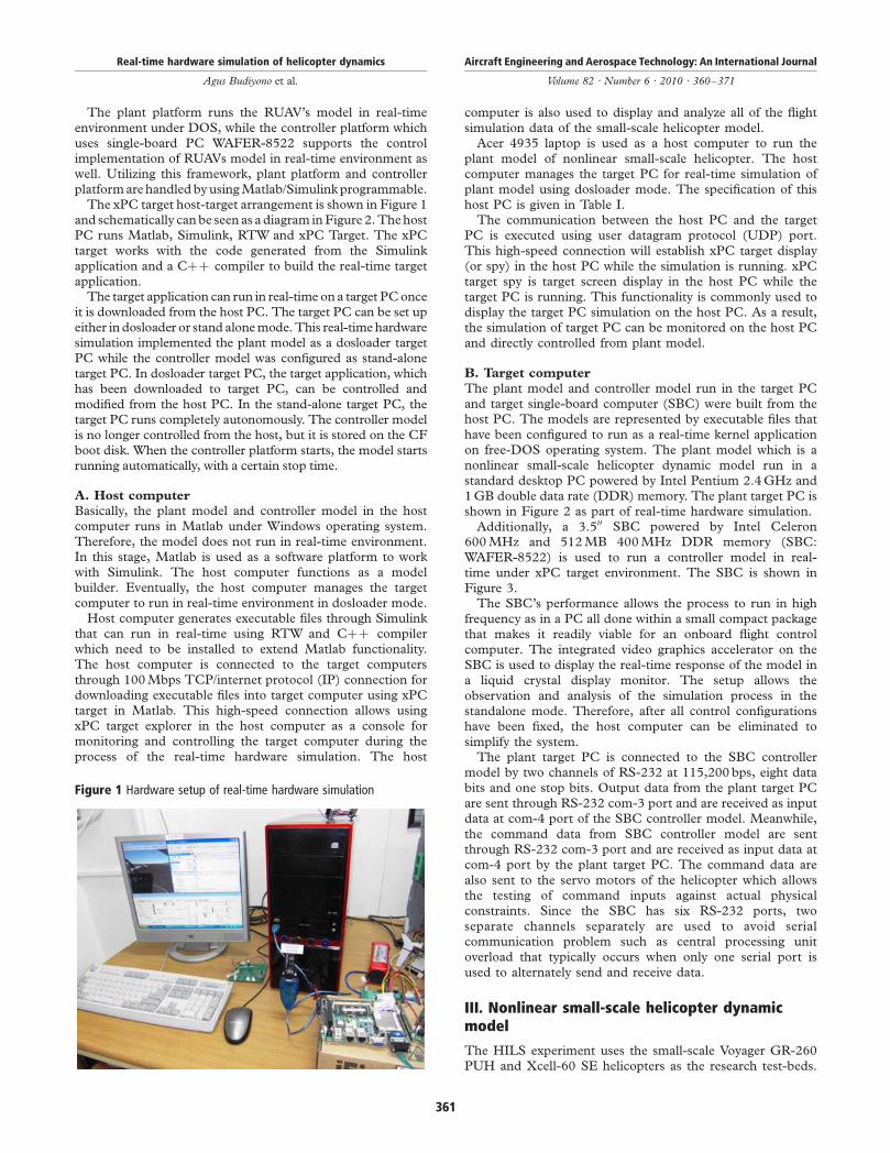
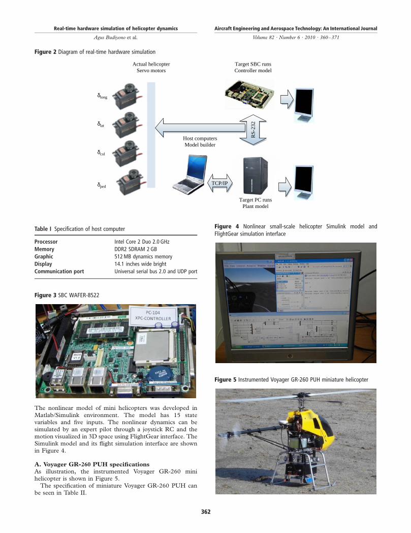
The xPC target host-target arrangement is shown in Figure 1and schematically can be seen as a diagram in Figure 2. The hostPC runs Matlab, Simulink, RTW and xPC Target. The xPCtarget works with the code generated from the Simulink

application and a Cþþ compiler to build the real-time targetapplication.

The target application can run in real-time on a target PC onceit is downloaded from the host PC. The target PC can be set up

either in dosloader or stand alone mode. This real-time hardwaresimulation implemented the plant model as a dosloader targetPC while the controller model was configured as stand-alonetarget PC. In dosloader target PC, the target application, whichhas been downloaded to target PC, can be controlled and

modified from the host PC. In the stand-alone target PC, thetarget PC runs completely autonomously. The controller modelis no longer controlled from the host, but it is stored on the CFboot disk. When the controller platform starts, the model startsrunning automatically, with a certain stop time.

A. Host computer

Basically, the plant model and controller model in the hostcomputer runs in Matlab under Windows operating system.

Therefore, the model does not run in real-time environment.In this stage, Matlab is used as a software platform to workwith Simulink. The host computer functions as a modelbuilder. Eventually, the host computer manages the targetcomputer to run in real-time environment in dosloader mode.

Host computer generates executable files through Simulinkthat can run in real-time using RTW and Cþþ compilerwhich need to be installed to extend Matlab functionality.The host computer is connected to the target computers

through 100 Mbps TCP/internet protocol (IP) connection fordownloading executable files into target computer using xPCtarget in Matlab. This high-speed connection allows usingxPC target explorer in the host computer as a console formonitoring and controlling the target computer during the

process of the real-time hardware simulation. The host

computer is also used to display and analyze all of the flight

simulation data of the small-scale helicopter model.Acer 4935 laptop is used as a host computer to run the

plant model of nonlinear small-scale helicopter. The hostcomputer manages the target PC for real-time simulation ofplant model using dosloader mode. The specification of this

host PC is given in Table I.The communication between the host PC and the target

PC is executed using user datagram protocol (UDP) port.

This high-speed connection will establish xPC target display(or spy) in the host PC while the simulation is running. xPCtarget spy is target screen display in the host PC while the

target PC is running. This functionality is commonly used todisplay the target PC simulation on the host PC. As a result,the simulation of target PC can be monitored on the host PC

and directly controlled from plant model.

B. Target computer

The plant model and controller model run in the target PCand target single-board computer (SBC) were built from thehost PC. The models are represented by executable files that

have been configured to run as a real-time kernel applicationon free-DOS operating system. The plant model which is anonlinear small-scale helicopter dynamic model run in a

standard desktop PC powered by Intel Pentium 2.4 GHz and1 GB double data rate (DDR) memory. The plant target PC isshown in Figure 2 as part of real-time hardware simulation.

Additionally, a 3.500 SBC powered by Intel Celeron600 MHz and 512 MB 400 MHz DDR memory (SBC:

WAFER-8522) is used to run a controller model in real-time under xPC target environment. The SBC is shown inFigure 3.

The SBC’s performance allows the process to run in highfrequency as in a PC all done within a small compact packagethat makes it readily viable for an onboard flight control

computer. The integrated video graphics accelerator on theSBC is used to display the real-time response of the model ina liquid crystal display monitor. The setup allows the

observation and analysis of the simulation process in thestandalone mode. Therefore, after all control configurationshave been fixed, the host computer can be eliminated to

simplify the system.The plant target PC is connected to the SBC controller

model by two channels of RS-232 at 115,200 bps, eight data

bits and one stop bits. Output data from the plant target PCare sent through RS-232 com-3 port and are received as inputdata at com-4 port of the SBC controller model. Meanwhile,

the command data from SBC controller model are sentthrough RS-232 com-3 port and are received as input data atcom-4 port by the plant target PC. The command data are

also sent to the servo motors of the helicopter which allowsthe testing of command inputs against actual physicalconstraints. Since the SBC has six RS-232 ports, two

separate channels separately are used to avoid serialcommunication problem such as central processing unitoverload that typically occurs when only one serial port is

used to alternately send and receive data.

III. Nonlinear small-scale helicopter dynamicmodel

The HILS experiment uses the small-scale Voyager GR-260PUH and Xcell-60 SE helicopters as the research test-beds.

Figure 1 Hardware setup of real-time hardware simulation

Real-time hardware simulation of helicopter dynamics

Agus Budiyono et al.


Volume 82 · Number 6 · 2010 · 360–371

361

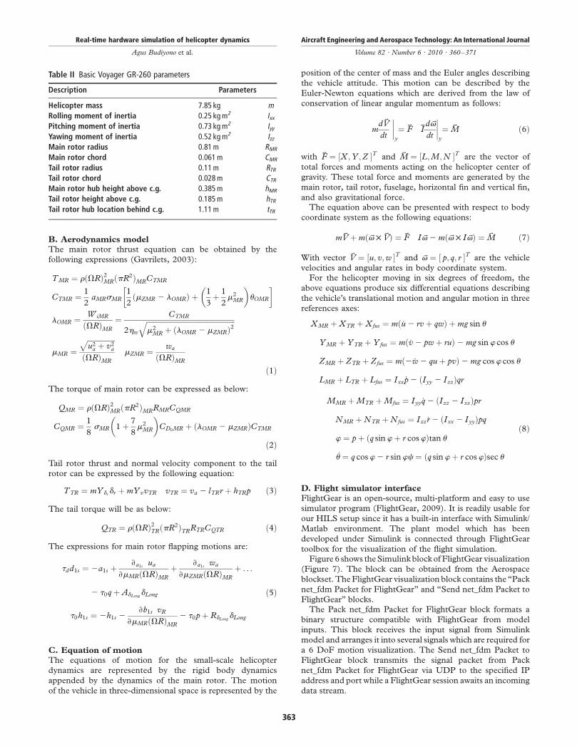
The nonlinear model of mini helicopters was developed in

Matlab/Simulink environment. The model has 15 statevariables and five inputs. The nonlinear dynamics can besimulated by an expert pilot through a joystick RC and themotion visualized in 3D space using FlightGear interface. TheSimulink model and its flight simulation interface are shownin Figure 4.

A. Voyager GR-260 PUH specifications

As illustration, the instrumented Voyager GR-260 minihelicopter is shown in Figure 5.

The specification of miniature Voyager GR-260 PUH canbe seen in Table II.

Figure 3 SBC WAFER-8522

Figure 2 Diagram of real-time hardware simulation

TCP/IP

Target SBC runsController model

Target PC runsPlant model

Host computersModel builder

Actual helicopterServo motors

RS-

232

δlong

δlat

δcol

δped

Figure 4 Nonlinear small-scale helicopter Simulink model andFlightGear simulation interface

Figure 5 Instrumented Voyager GR-260 PUH miniature helicopter

Table I Specification of host computer

Processor Intel Core 2 Duo 2.0 GHz

Memory DDR2 SDRAM 2 GB

Graphic 512 MB dynamics memory

Display 14.1 inches wide bright

Communication port Universal serial bus 2.0 and UDP port




Volume 82 · Number 6 · 2010 · 360–371

362

B. Aerodynamics model

The main rotor thrust equation can be obtained by the

following expressions (Gavrilets, 2003):

TMR ¼ rðVRÞ2MRðpR2ÞMRCTMR

CTMR ¼ 1

2aMRsMR

1

2ðmZMR 2 lOMRÞ þ

1

3þ 1

2m2MR

� �uOMR

� �

lOMR ¼ WiMR

ðVRÞMR

¼ CTMR

2hw

ffiffiffiffiffiffiffiffiffiffiffiffiffiffiffiffiffiffiffiffiffiffiffiffiffiffiffiffiffiffiffiffiffiffiffiffiffiffiffiffiffiffiffiffiffiffiffiffiffiffim2MR þ ðlOMR 2 mZMRÞ2

q

mMR ¼ffiffiffiffiffiffiffiffiffiffiffiffiffiffiffiffiu2a þ v2

a

pðVRÞMR

mZMR ¼ wa

ðVRÞMR

ð1Þ

The torque of main rotor can be expressed as below:

QMR ¼ rðVRÞ2MRðpR2ÞMRRMRCQMR

CQMR ¼ 1

8sMR 1 þ 7

8m2MR

� �CD0MR þ ðlOMR 2 mZMRÞCTMR

ð2Þ

Tail rotor thrust and normal velocity component to the tail

rotor can be expressed by the following equation:

TTR ¼ mY drdr þmYvvTR vTR ¼ va 2 lTRr þ hTRp ð3Þ

The tail torque will be as below:

QTR ¼ rðVRÞ2TRðpR2ÞTRRTRCQTR ð4Þ

The expressions for main rotor flapping motions are:

tdd1s ¼ 2a1s þ›a1s

ua

›mMRðVRÞMR

þ ›a1swa

›mZMRðVRÞMR

þ . . .

2 t0qþ AdLongdLong

t0h1s ¼ 2h1s 2›b1s vR

›mMRðVRÞMR

2 t0pþ RdLongdLong

ð5Þ

C. Equation of motion

The equations of motion for the small-scale helicopter

dynamics are represented by the rigid body dynamics

appended by the dynamics of the main rotor. The motion

of the vehicle in three-dimensional space is represented by the

position of the center of mass and the Euler angles describing

the vehicle attitude. This motion can be described by the

Euler-Newton equations which are derived from the law of

conservation of linear angular momentum as follows:

md kV

dt

��y

¼ kF kId kv

dt

��y

¼ kM ð6Þ

with kF ¼ ½X ;Y ;Z �T and kM ¼ ½L;M;N �T are the vector of

total forces and moments acting on the helicopter center of

gravity. These total force and moments are generated by the

main rotor, tail rotor, fuselage, horizontal fin and vertical fin,

and also gravitational force.The equation above can be presented with respect to body

coordinate system as the following equations:

m kVþmð kv £ kVÞ ¼ kF I kv2mð kv £ I kvÞ ¼ kM ð7Þ

With vector kV ¼ ½u; v;w �T and kv ¼ ½ p; q; r �T are the vehicle

velocities and angular rates in body coordinate system.For the helicopter moving in six degrees of freedom, the

above equations produce six differential equations describing

the vehicle’s translational motion and angular motion in three

references axes:

XMR þXTR þXfus ¼ mð_u2 rvþ qwÞ þmg sin u

YMR þ YTR þ Yfus ¼ mð_v2 pwþ ruÞ2mg sinw cos u

ZMR þ ZTR þ Zfus ¼ mð2 _w2 quþ pvÞ2mg cosw cos u

LMR þ LTR þ Lfus ¼ Ixx _p2 ðIyy 2 IzzÞqr

MMR þMTR þMfus ¼ Iyy _q2 ðIzz 2 IxxÞpr

NMR þNTR þNfus ¼ Izz_r2 ðIxx 2 IyyÞpq

w ¼ pþ ðq sinwþ r coswÞtan u

_u ¼ q cosw2 r sinwc ¼ ðq sinwþ r coswÞsec u

ð8Þ

D. Flight simulator interface

FlightGear is an open-source, multi-platform and easy to use

simulator program (FlightGear, 2009). It is readily usable for

our HILS setup since it has a built-in interface with Simulink/

Matlab environment. The plant model which has been

developed under Simulink is connected through FlightGear

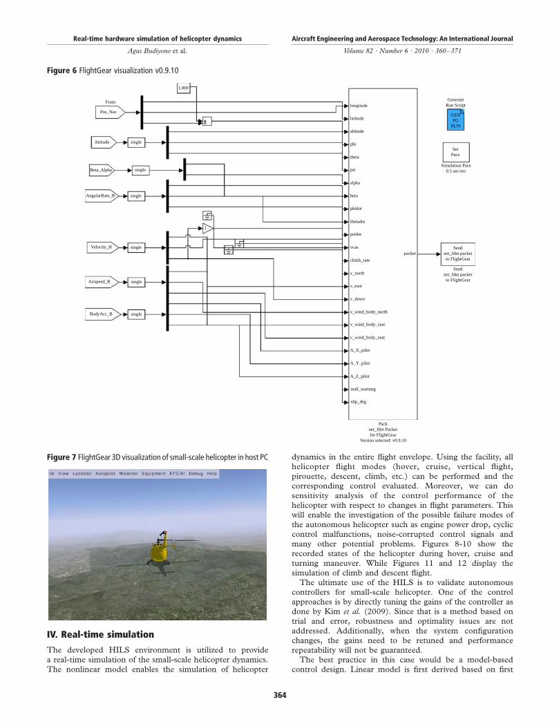
toolbox for the visualization of the flight simulation.Figure 6 shows the Simulink block of FlightGear visualization

(Figure 7). The block can be obtained from the Aerospace

blockset. The FlightGear visualization block contains the “Pack

net_fdm Packet for FlightGear” and “Send net_fdm Packet to

FlightGear” blocks.The Pack net_fdm Packet for FlightGear block formats a

binary structure compatible with FlightGear from model

inputs. This block receives the input signal from Simulink

model and arranges it into several signals which are required for

a 6 DoF motion visualization. The Send net_fdm Packet to

FlightGear block transmits the signal packet from Pack

net_fdm Packet for FlightGear via UDP to the specified IP

address and port while a FlightGear session awaits an incoming

data stream.

Table II Basic Voyager GR-260 parameters

Description Parameters

Helicopter mass 7.85 kg mRolling moment of inertia 0.25 kg m2 Ixx

Pitching moment of inertia 0.73 kg m2 Iyy

Yawing moment of inertia 0.52 kg m2 Izz

Main rotor radius 0.81 m RMR

Main rotor chord 0.061 m CMR

Tail rotor radius 0.11 m RTR

Tail rotor chord 0.028 m CTR

Main rotor hub height above c.g. 0.385 m hMR

Tail rotor height above c.g. 0.185 m hTR

Tail rotor hub location behind c.g. 1.11 m tTR




Volume 82 · Number 6 · 2010 · 360–371

363

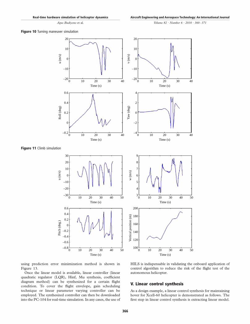
IV. Real-time simulation

The developed HILS environment is utilized to provide

a real-time simulation of the small-scale helicopter dynamics.

The nonlinear model enables the simulation of helicopter

dynamics in the entire flight envelope. Using the facility, allhelicopter flight modes (hover, cruise, vertical flight,

pirouette, descent, climb, etc.) can be performed and thecorresponding control evaluated. Moreover, we can do

sensitivity analysis of the control performance of thehelicopter with respect to changes in flight parameters. This

will enable the investigation of the possible failure modes ofthe autonomous helicopter such as engine power drop, cycliccontrol malfunctions, noise-corrupted control signals and

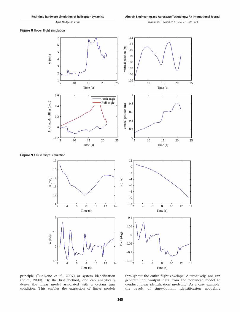
many other potential problems. Figures 8-10 show therecorded states of the helicopter during hover, cruise and

turning maneuver. While Figures 11 and 12 display thesimulation of climb and descent flight.

The ultimate use of the HILS is to validate autonomouscontrollers for small-scale helicopter. One of the control

approaches is by directly tuning the gains of the controller asdone by Kim et al. (2009). Since that is a method based on

trial and error, robustness and optimality issues are notaddressed. Additionally, when the system configuration

changes, the gains need to be retuned and performancerepeatability will not be guaranteed.

The best practice in this case would be a model-basedcontrol design. Linear model is first derived based on first

Figure 6 FlightGear visualization v0.9.10

From

1,000

longitude

latitude

altitude

phi

theta

psi

alpha

beta

phidot

thetadot

psidot

vcas

climb_rate

v_north

v_east

v_down

v_wind_body_north

v_wind_body_east

v_wind_body_east

A_X_pilot

A_Y_pilot

A_Z_pilot

stall_warning

slip_deg

Packnet_fdm Packetfor FlightGear

Version selected: v0.9.10

packetSend

net_fdm packetto FlightGeat

SetPace

GENFG

RUN

GenerateRun Script

Simulation Pace0.5 sec/sec

Sendnet_fdm packetto FlightGeat

Pos_Nav

Attitude

Beta_Alpha

AngularRate_B

Velocity_H

Airspeed_B

BodyAcc_B

single

single

single

single

1

single

single

Figure 7 FlightGear 3D visualization of small-scale helicopter in host PC




Volume 82 · Number 6 · 2010 · 360–371

364

principle (Budiyono et al., 2007) or system identification

(Shim, 2000). By the first method, one can analytically

derive the linear model associated with a certain trim

condition. This enables the extraction of linear models

throughout the entire flight envelope. Alternatively, one can

generate input-output data from the nonlinear model to

conduct linear identification modeling. As a case example,

the result of time-domain identification modeling

Figure 9 Cruise flight simulation

16

u (m

/s)

15

14

13

12

112 4 6 8

Time (s)

10 12 14

12

v (m

/s)

0

–2

–4

–12

–10

–8

–6

2 4 6 8

Time (s)

10 12 14

3

w (

m/s

)

2.5

2

1.52 4 6 8

Time (s)

10 12 14

0.1

Pitc

h (d

eg)

0.05

0

–0.15

–0.1

–0.05

2 4 6 8

Time (s)

10 12 14

Figure 8 Hover flight simulation

7

w (

m/s

)

6

5

4

3

2

15 10 15

Time (s)

Pitch angleRoll angle

20 25

112

Ver

tical

pos

ition

(m

)

111

110

109

108

107

106

1055 10 15

Time (s)

20 25

0.6

Pitc

hing

& r

ollin

g (d

eg.)

0.4

0.2

0

–0.25 10 15

Time (s)

20 25

1

Ver

tical

pos

ition

(m

) 0.8

0.6

0.4

0.2

05 10 15

Time (s)

20 25




Volume 82 · Number 6 · 2010 · 360–371

365

using prediction error minimization method is shown in

Figure 13.Once the linear model is available, linear controller (linear

quadratic regulator (LQR), Hinf, Mu synthesis, coefficient

diagram method) can be synthesized for a certain flight

condition. To cover the flight envelope, gain scheduling

technique or linear parameter varying controller can be

employed. The synthesized controller can then be downloaded

into the PC-104 for real-time simulation. In any cases, the use of

HILS is indispensable in validating the onboard application of

control algorithm to reduce the risk of the flight test of the

autonomous helicopter.

V. Linear control synthesis

As a design example, a linear control synthesis for maintaining

hover for Xcell-60 helicopter is demonstrated as follows. The

first step in linear control synthesis is extracting linear model.

Figure 10 Turning maneuver simulation

u (m

/s)

20

10

–20

–10

0

0 10 20

Time (s)

30 40

v (m

/s)

20

10

–20

–10

0

0 10 20

Time (s)

30 40

Rol

l (de

g)

0.6

0.4

–0.2

0

0.2

0 10 20

Time (s)

30 40

Yaw

(de

g)

4

2

–4

–2

0

0 10 20

Time (s)

30 40

Figure 11 Climb simulation

u (m

/s)

20

30

10

–30

–20

–10

0

0 10 20 30

Time (s)

40 50

w (

m/s

)

8

9

7

3

4

5

6

0 10 20 30

Time (s)

40 50

Pitc

h (d

eg.)

0.4

0.6

0.2

–0.2

–0.4

–0.6

–0.8

0

0 10 20 30

Time (s)

40 50

Ver

tical

pos

ition

(m

) 180

200

160

100

120

140

0 10 20 30

Time (s)

40 50




Volume 82 · Number 6 · 2010 · 360–371

366

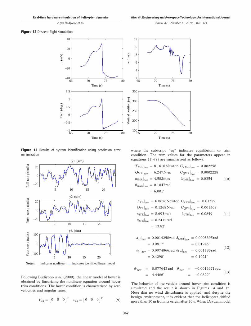
Following Budiyono et al. (2009), the linear model of hover is

obtained by linearizing the nonlinear equation around hover

trim conditions. The hover condition is characterized by zero

velocities and angular rates:

kVeq ¼ 0 0 0� �T

kveq ¼ 0 0 0� �T ð9Þ

where the subscript “eq” indicates equilibrium or trim

condition. The trim values for the parameters appear in

equations (1)-(7) are summarized as follows:

TMRjhov ¼ 81:616Newton CTMRjhov ¼ 0:002256

QMRjhov ¼ 6:247N·m CQMR

��hov

¼ 0:0002228

wiMRjhov ¼ 4:582m=s l0MRjhov ¼ 0:0354

u0MRjhov ¼ 0:1047rad

¼ 6:001+

ð10Þ

TTRjhov ¼ 6:8656Newton CTTRjhov ¼ 0:01329

QTRjhov ¼ 0:1268N·m CQTR

��hov

¼ 0:001568

wiTRjhov ¼ 8:693m=s l0TRjhov ¼ 0:0859

u0TRjhov ¼ 0:2412rad

¼ 13:82+

ð11Þ

a1sjhov ¼ 0:0014258rad dLong

��hov

¼ 0:0003395rad

¼ 0:0817+ ¼ 0:01945+

b1sjhov ¼ 0:0074866rad dLatjhov ¼ 0:001783rad

¼ 0:4290+ ¼ 0:1021+

ð12Þ

fjhov ¼ 0:077643 rad ujhov ¼ 20:0014471 rad

¼ 4:4486+ ¼ 20:08298ð13Þ

The behavior of the vehicle around hover trim condition is

simulated and the result is shown in Figures 14 and 15.

Note that no wind disturbance is applied, and despite the

benign environment, it is evident that the helicopter drifted

more than 10 m from its origin after 20 s. When Dryden model

Figure 12 Descent flight simulation

u (m

/s)

20

40

–40

–20

0

65 70 75

Time (s)

80

w (

m/s

) 8

12

10

2

4

6

65 70 75

Time (s)

80

Pitc

h (d

eg.)

1

1.5

–1

–0.5

0

0.5

65 70 75

Time (s)

80V

ertic

al p

ositi

on (

m)

250

350

300

150

200

65 70 75

Time (s)

80

Figure 13 Results of system identification using prediction errorminimization

Rol

l rat

e p

(rad

/s)

5 10 15 20

–20

0

20

y1. (sim)

Pitc

h r

ate

p (r

ad/s

)

5 10 15 20

–20

0

20

y2. (sim)

Yaw

rat

e p

(rad

/s)

5 10

Notes: indicates nonlinear; indicates identified linear model

15 20–100

0

100y3. (sim)




Volume 82 · Number 6 · 2010 · 360–371

367

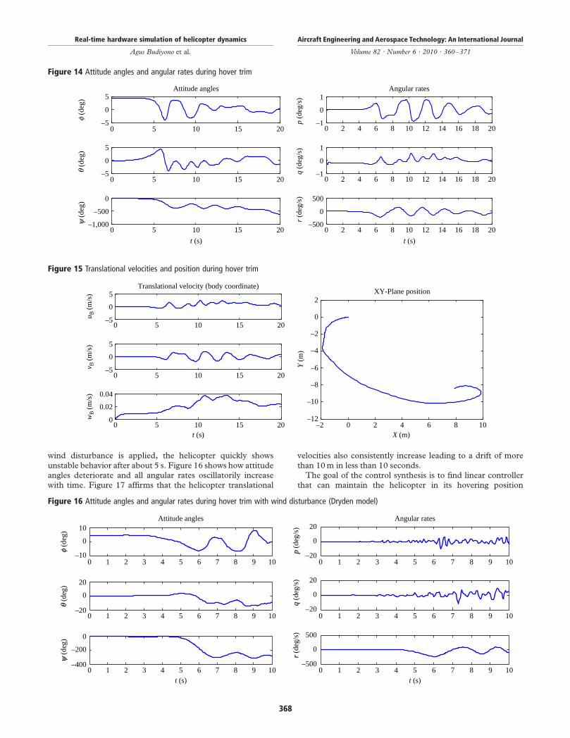
wind disturbance is applied, the helicopter quickly shows

unstable behavior after about 5 s. Figure 16 shows how attitudeangles deteriorate and all angular rates oscillatorily increasewith time. Figure 17 affirms that the helicopter translational

velocities also consistently increase leading to a drift of more

than 10 m in less than 10 seconds.The goal of the control synthesis is to find linear controller

that can maintain the helicopter in its hovering position

Figure 14 Attitude angles and angular rates during hover trim

–5

0

5Attitude angles

f (d

eg)

q (d

eg)

y (d

eg)

–5

0

5

0 5 10 15 20

0 5 10 15 20

0 5 10 15 20

–1,000

–500

0

t (s) t (s)

–1

0

1Angular rates

p (d

eg/s

)

–1

0

1

q (d

eg/s

)

0 2 4 6 8 10 12 14 16 18 20

0 2 4 6 8 10 12 14 16 18 20

0 2 4 6 8 10 12 14 16 18 20

–500

0

500

r (d

eg/s

)

Figure 15 Translational velocities and position during hover trim

–5

0

5Translational velocity (body coordinate)

u B (m

/s)

v B (m

/s)

wB

(m/s

)

–5

0

5

0 5 10 15 20

0 5 10 15 20

0 5 10 15 20

0

0.02

0.04

t (s)

XY-Plane position

–2 0 2 4 6 8 10–12

–10

–8

–6

–4

–2

0

2Y

(m

)

X (m)

Figure 16 Attitude angles and angular rates during hover trim with wind disturbance (Dryden model)

0 1 2 3 4 5 6 7 8 9 10

0 1 2 3 4 5 6 7 8 9 10

0 1 2 3 4 5 6 7 8 9 10

–10

0

10Attitude angles

–20

0

20

–400

–200

0

t (s) t (s)

f (d

eg)

q (d

eg)

y (d

eg)

0 1 2 3 4 5 6 7 8 9 10–20

0

20Angular rates

p (d

eg/s

)

0 1 2 3 4 5 6 7 8 9 10–20

0

20

q (d

eg/s

)

0 1 2 3 4 5 6 7 8 9 10–500

0

500

r (de

g/s)




Volume 82 · Number 6 · 2010 · 360–371

368

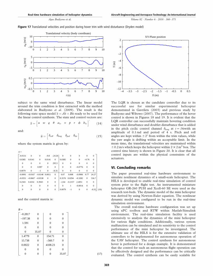
subject to the same wind disturbance. The linear model

around the trim condition is first extracted with the methodelaborated in Budiyono et al. (2009). The result is the

following state space model _�x ¼ A�xþ B �u ready to be used forthe linear control synthesis. The state and control vectors are:

~x ¼ u w q u a1s v p r f b1s

h i0

ð14Þ

and:

~u ¼ dcoll dlong dped dlath i

ð15Þ

where the system matrix is given by:

0 0 –9.8 0 0 0 0 0

0.0385 0.0141 0 0.0141 0 0.0385 0 0 0

0 0 0 0 295.5 0 0 0 0 0

0 0 0.997 0 0 0 0 0 0

0.0079 0 –1 0 –8.35 0 0 0 0 0

–0.0148 0.0011 0 0.07 0.008 9.77 24.27

–0.0538 0 0 0.3576 0.0294

A =

–0.0131 –24.26

–0.76

–0.0776

–0.0091 –0.0167 –0.0906

–0.0351 –0.0667 0 556.7

0.2343 0.4332 0.3943 0 0 –0.2157 2.4051 0 0

000 0 0 0 1 0 0

0 0 0 0 0 0.0079 –1 0 0 –8.35 (16)

–0.3282

–2.64

–0.0014

and the control matrix is:

(17)

–0.2817 0 0 0

–197.38 0 0 0

1.591 0

0 0

0

0

0

0

0 35.07 0 0

1.4779 0 154.71 0

15.738 0 –560.7 0

0.0022 0 4108.23 0

0 0 0 0

0 0 0 35.07

B =

The LQR is chosen as the candidate controller due to its

successful use for similar experimental helicopter

demonstrated in Gavrilets (2003) and previous study by

Budiyono and Wibowo (2007). The performance of the hover

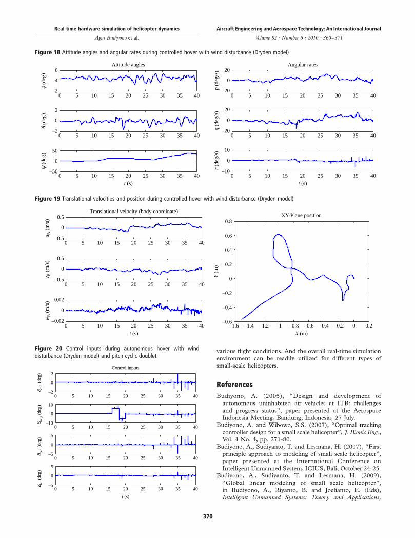
control is shown in Figures 18 and 19. It is evident that the

LQR controller can successfully maintain hovering condition

under wind disturbance and doublet disturbance that is added

in the pitch cyclic control channel dlong at t ¼ 16swith an

amplitude of 0.1 rad and period of 4 s. Pitch and roll

angles are kept within ^28 from within the trim values, while

the yaw angle is drifting within an acceptable limit. In the

mean time, the translational velocities are maintained within

^0.2 m/s which keeps the helicopter within 2 £ 2 m2 box. The

control time history is shown in Figure 20. It is clear that all

control inputs are within the physical constraints of the

actuators.

VI. Concluding remarks

The paper presented real-time hardware environment to

simulate nonlinear dynamics of a small-scale helicopter. The

HILS is developed to enable real-time simulation of control

system prior to the flight test. An instrumented miniature

helicopter GR-260 PUH and Xcell-60 SE were used as the

research test-beds. The dynamic model of the mini helicopter

was derived by using Newton-Euler equation. The nonlinear

dynamic model was configured to be run in the real-time

simulation environment.The overall real-time hardware configuration was set up

using xPC toolbox and RTW within Matlab/Simulink

environment. The real-time simulation facility is used

extensively to analysis the dynamics of the mini helicopter

for various flight conditions. Additionally, various system

malfunction can be simulated and its sensitivity to the control

performance of the mini helicopter be investigated. The

ultimate use of the HILS is for the extensive validation of

controllers to be implemented for autonomous operation of

the UAV helicopter. The control synthesis for autonomous

hover is performed for a design example. It is demonstrated

that the control for such an autonomous flight operation can

be effectively designed and the performance can be critically

evaluated. The control synthesis can be easily scalable for

Figure 17 Translational velocities and position during hover trim with wind disturbance (Dryden model)

0 1 2 3 4 5 6 7 8 9 10

0 1 2 3 4 5 6 7 8 9 10

0 1 2 3 4 5 6 7 8 9 10

–10

0

10Translational velocity (body coordinate)

u B (

m/s

)v B

(m

/s)

wB

(m

/s)

–5

0

5

–0.5

0

0.5

t (s)

XY-Plane position

–4 –3.5 –3 –2.5 –2 –1.5 –1 -0.5 0 0.5–12

–10

–8

–6

–4

–2

0

2

Y (

m)

X (m)




Volume 82 · Number 6 · 2010 · 360–371

369

various flight conditions. And the overall real-time simulation

environment can be readily utilized for different types of

small-scale helicopters.

References

Budiyono, A. (2005), “Design and development of

autonomous uninhabited air vehicles at ITB: challenges

and progress status”, paper presented at the Aerospace

Indonesia Meeting, Bandung, Indonesia, 27 July.Budiyono, A. and Wibowo, S.S. (2007), “Optimal tracking

controller design for a small scale helicopter”, J. Bionic Eng.,

Vol. 4 No. 4, pp. 271-80.Budiyono, A., Sudiyanto, T. and Lesmana, H. (2007), “First

principle approach to modeling of small scale helicopter”,

paper presented at the International Conference on

Intelligent Unmanned System, ICIUS, Bali, October 24-25.Budiyono, A., Sudiyanto, T. and Lesmana, H. (2009),

“Global linear modeling of small scale helicopter”,

in Budiyono, A., Riyanto, B. and Joelianto, E. (Eds),

Intelligent Unmanned Systems: Theory and Applications,

Figure 18 Attitude angles and angular rates during controlled hover with wind disturbance (Dryden model)

0 5 10 15 20 25 30 35 40

0 5 10 15 20 25 30 35 40

0 5 10 15 20 25 30 35 40

2

4

6Attitude angles Angular rates

–2

0

2

–50

0

50

t (s) t (s)

f (d

eg)

q (d

eg)

y (d

eg)

0 5 10 15 20 25 30 35 40–20

0

20

p (d

eg/s

)

0 5 10 15 20 25 30 35 40–20

0

20

q (d

eg/s

)

0 5 10 15 20 25 30 35 40–10

0

10

r (de

g/s)

Figure 19 Translational velocities and position during controlled hover with wind disturbance (Dryden model)

0 5 10 15 20 25 30 35 40–0.5

0

0.5Translational velocity (body coordinate)

0 5 10 15 20 25 30 35 40

0 5 10 15 20 25 30 35 40

–0.5

0

0.5

–0.02

0

0.02

t (s)

XY-Plane position

–1.6 –1.4 –1.2 –1 –0.8 –0.6 –0.4 –0.2 0 0.2–0.6

–0.4

–0.2

0

0.2

0.4

0.6

0.8Y

(m

)

X (m)

u B (

m/s

)v B

(m

/s)

wB

(m

/s)

Figure 20 Control inputs during autonomous hover with winddisturbance (Dryden model) and pitch cyclic doublet

0 5 10 15 20 25 30 35 40

0 5 10 15 20 25 30 35 40

0 5 10 15 20 25 30 35 40

0 5 10 15 20 25 30 35 40

–2

0

2Control inputs

–10

0

10

–5

0

5

–5

0

5

t (s)

d col

l (de

g)d l

ong

(deg

)d p

ed (

deg)

d lat

(de

g)




Volume 82 · Number 6 · 2010 · 360–371

370

Studies on Computational Intelligence, Vol. 192, Springer,Berlin, pp. 27-62.

Cai, G., Chen, B.M., Lee, T.H. and Dong, M. (2009),“Design and implementation of a hardware-in-the-loopsimulation system for small-scale UAV helicopters”,Mechatronics, Vol. 19, pp. 1057-66.

FlightGear (2009), Web site: www.flightgear.orgGavrilets, V. (2003), “Autonomous aerobatic maneuvering of

miniature helicopter”, PhD thesis, Massachusetts Instituteof Technology, Cambridge, MA.

Gravilets, V., Shterenberg, A., Dahleh, M. and Feron, E.(2000), “Avionics system for a small unmanned helicopterperforming aggressive maneuvers”, paper presented atDigital Avionics Systems Conference, Philadelphia, PA,October.

Johnson, E. and Fontaine, S. (2001), “Use of flight simulationto complement flight testing of low-cost UAVs”, paperpresented at the AIAA Modeling and SimulationTechnologies Conference, Montreal.

Kim, S., Budiyono, A., Lee, J.H., Kim, D. and Yoon, K.J.

(2009), “Control system design and testing for a small scale

autonomous helicopter”, paper presented at International

Symposium on Intelligent Unmanned System, ISIUS2009,

Jeju Island.Mosterman, P.J., Prabhu, S., Dowd, A., Glass, J., Erkkinen, T.,

Kluza, J. and Shenoy, R. (2005), “Embedded real-time

control via MATLAB, Simulink, and xPC target”, Handbook

of Networked and Embedded Control Systems, Birkhauser,

Boston, MA, pp. 419-46.Shim, D. (2000), “Hierarchical control system synthesis for

rotorcraft-based unmanned aerial vehicles”, PhD thesis,

University of California, Berkeley, CA.

Corresponding author

Agus Budiyono can be contacted at: agus@[email protected]




Volume 82 · Number 6 · 2010 · 360–371

371

To purchase reprints of this article please e-mail: [email protected]

Or visit our web site for further details: www.emeraldinsight.com/reprints

Real-time hardware simulation of a small-scale helicopter dynamics

Documents

Transcript of Real-time hardware simulation of a small-scale helicopter dynamics