Mapping Structures that Control Contaminant Migration using Helicopter TransientElectromagnetic Data

Louise Pellerin1, Les P. Beard2 and Wayne Mandell31Green Engineering, Inc., 2215 Curtis St., Berkeley, Calif. 94702

Email: pellerin@ak.net2Battelle-Oak Ridge Operations, 105 Mitchell Road, Suite 103, Oak Ridge, Tenn. 37830

3Army Environmental Command (Retired), Greenville, N.C. 27858

ABSTRACT

Tooele Army Depot, Tooele County, Utah has developed a hydrogeological model to

predict spatio-temporal changes in trichloroethylene contamination originating from sources on

the base. Established in 1942 to store World War II supplies, ammunition, and combat vehicles,

the Depot is situated in the Basin and Range Providence about 50 km west of Salt Lake City,

Utah. In order to better define this hydrogeological framework, a helicopter-borne, time-

domain electromagnetic system, known as SkyTEM, was used to survey a 64-km2 area of the

Depot. Areas where carbonate basement is known from prior studies to be at or near the surfacewere clearly delineated in the SkyTEM data as a high resistivity zone, which begins near the

ground surface and continues to the deepest samples at about 200 m. In some places the

basement appears to be conductive rather than resistive. In areas where unconsolidated

sedimentary cover is known to be thick, such as in the northwest part of the survey area,

resistivities were low throughout the sample intervals. The SkyTEM data supports the existence

of some, but not all, of the hydrological boundaries hypothesized from potentiometric

information. Shallow high-resistivity layers in the east and southeast portions of the survey area

appear to be underlain by more conductive sediments, and so should not necessarily beinterpreted as shallow bedrock, but possibly as resistive sediments such as dry sand and gravel.

One of the most significant results of the survey is the delineation of a narrow unit, interpreted

as a paleochannel, at depths greater than 100 m that may be responsible for migration of

contamination to the northwest.

Introduction

An airborne transient electromagnetic survey was

carried out over an area of 64 km2 at the Tooele Army

Depot (TEAD), Tooele County, Utah to better define

geological structures and hydrogeological units in the

surveyed area. Survey results were meshed with existing

geological and hydrological data to improve the TEAD

hydrogeological model. SkyTEM, a unique airborne

transient electromagnetic sounding system developed in

Denmark and designed specifically to address hydro-

geological problems (Sørensen and Auken, 2004), was

used for the survey.

The Tooele Ordnance Depot was established in

1942, and in World War II was a storage depot for

supplies, ammunition, and combat vehicles (see www.

tooele.army.mil). In 1962, the post was renamed the

Tooele Army Depot. TEAD is currently responsible for

shipping, storage, maintenance, and demilitarization of

conventional ammunition. Activities related to these

missions resulted in groundwater contamination, in

particular contamination from trichloroethylene (TCE).

A groundwater flow and contaminant transport model

was developed by Fenske et al. (2005) to better mitigate

any hazard to the public that might be associated with the

contamination.

Site Geology and Hydrogeology

The Tooele Army Depot lies in the Tooele Valley,

and is located about 55 km southwest of Salt Lake City.

The Tooele Valley is a Basin-and-Range structural

depression that comprises an area of over 700 km2. It is

filled with unconsolidated and partly-consolidated

sediments of Paleogene and Neogene ages. These

sediments range from gravels to clays, and represent a

variety of depositional environments. Basin fill sedi-

ments thicken to the north, and are reported to have a

65

JEEG, June 2010, Volume 15, Issue 2, pp. 65–75

Dow

nloa

ded

10/0

2/13

to 7

1.20

2.25

0.39

. Red

istr

ibut

ion

subj

ect t

o SE

G li

cens

e or

cop

yrig

ht; s

ee T

erm

s of

Use

at h

ttp://

libra

ry.s

eg.o

rg/

thickness greater than 3,000 m in the north-central part

of the valley (Stokes, 1988). In the area of the SkyTEM

survey, sediment thicknesses range from zero at a

bedrock outcrop to hundreds of meters throughout

much of the surveyed area.

Bedrock units consist of Paleozoic quartzite,

sandstone, limestone, and dolomite. Bedrock over much

of the survey area is covered by thick sediments, but a

limestone outcrop about 2 km northwest of the Utah

Industrial Depot suggests shallow bedrock over some

portion of the survey area. Drilling and geophysical

studies suggest a fault-bounded, uplifted, tilted fault

block dipping sharply to the north-northwest (Asch,

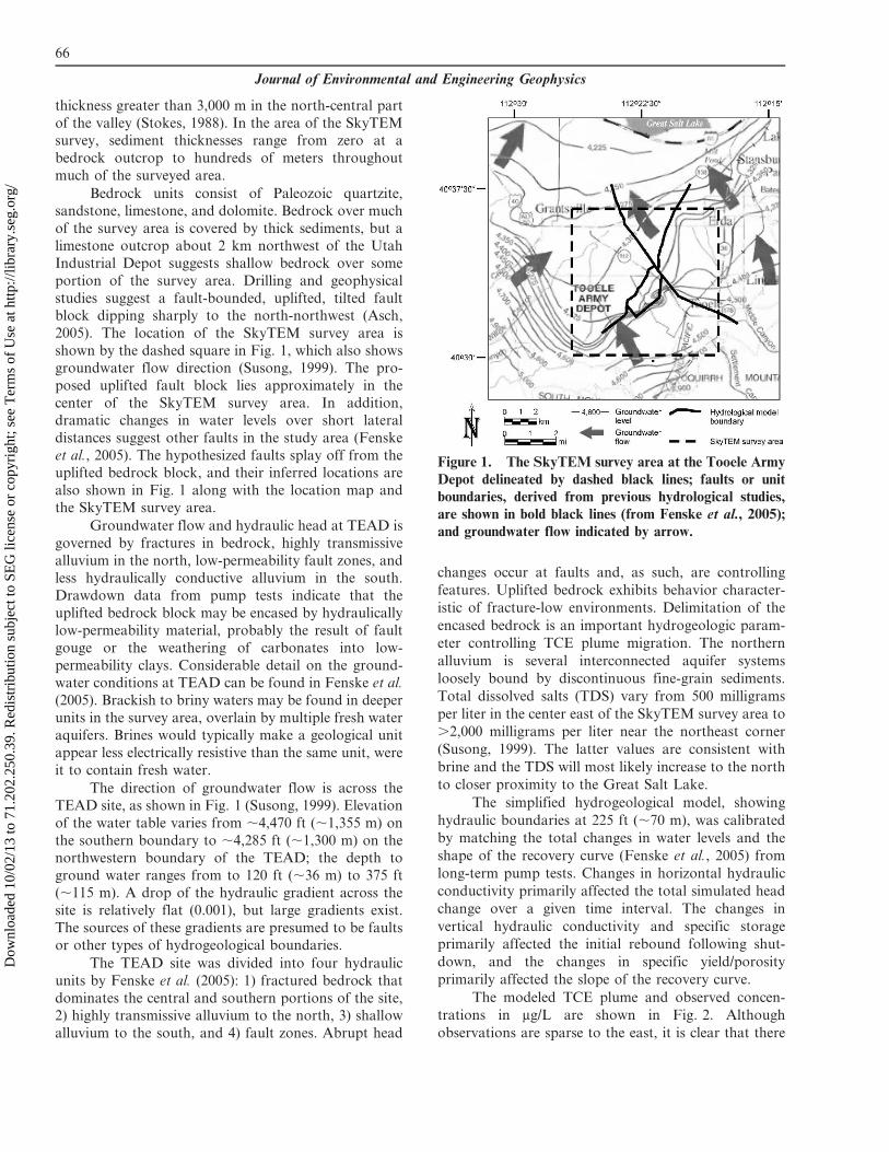
2005). The location of the SkyTEM survey area is

shown by the dashed square in Fig. 1, which also shows

groundwater flow direction (Susong, 1999). The pro-

posed uplifted fault block lies approximately in the

center of the SkyTEM survey area. In addition,

dramatic changes in water levels over short lateral

distances suggest other faults in the study area (Fenske

et al., 2005). The hypothesized faults splay off from the

uplifted bedrock block, and their inferred locations are

also shown in Fig. 1 along with the location map and

the SkyTEM survey area.

Groundwater flow and hydraulic head at TEAD is

governed by fractures in bedrock, highly transmissive

alluvium in the north, low-permeability fault zones, and

less hydraulically conductive alluvium in the south.

Drawdown data from pump tests indicate that the

uplifted bedrock block may be encased by hydraulically

low-permeability material, probably the result of fault

gouge or the weathering of carbonates into low-

permeability clays. Considerable detail on the ground-

water conditions at TEAD can be found in Fenske et al.

(2005). Brackish to briny waters may be found in deeper

units in the survey area, overlain by multiple fresh water

aquifers. Brines would typically make a geological unit

appear less electrically resistive than the same unit, were

it to contain fresh water.

The direction of groundwater flow is across the

TEAD site, as shown in Fig. 1 (Susong, 1999). Elevation

of the water table varies from ,4,470 ft (,1,355 m) on

the southern boundary to ,4,285 ft (,1,300 m) on the

northwestern boundary of the TEAD; the depth to

ground water ranges from to 120 ft (,36 m) to 375 ft

(,115 m). A drop of the hydraulic gradient across the

site is relatively flat (0.001), but large gradients exist.

The sources of these gradients are presumed to be faults

or other types of hydrogeological boundaries.

The TEAD site was divided into four hydraulic

units by Fenske et al. (2005): 1) fractured bedrock that

dominates the central and southern portions of the site,

2) highly transmissive alluvium to the north, 3) shallow

alluvium to the south, and 4) fault zones. Abrupt head

changes occur at faults and, as such, are controlling

features. Uplifted bedrock exhibits behavior character-

istic of fracture-low environments. Delimitation of the

encased bedrock is an important hydrogeologic param-

eter controlling TCE plume migration. The northern

alluvium is several interconnected aquifer systems

loosely bound by discontinuous fine-grain sediments.

Total dissolved salts (TDS) vary from 500 milligrams

per liter in the center east of the SkyTEM survey area to

.2,000 milligrams per liter near the northeast corner

(Susong, 1999). The latter values are consistent with

brine and the TDS will most likely increase to the north

to closer proximity to the Great Salt Lake.

The simplified hydrogeological model, showing

hydraulic boundaries at 225 ft (,70 m), was calibrated

by matching the total changes in water levels and the

shape of the recovery curve (Fenske et al., 2005) from

long-term pump tests. Changes in horizontal hydraulic

conductivity primarily affected the total simulated head

change over a given time interval. The changes in

vertical hydraulic conductivity and specific storage

primarily affected the initial rebound following shut-

down, and the changes in specific yield/porosity

primarily affected the slope of the recovery curve.

The modeled TCE plume and observed concen-

trations in mg/L are shown in Fig. 2. Although

observations are sparse to the east, it is clear that there

Figure 1. The SkyTEM survey area at the Tooele Army

Depot delineated by dashed black lines; faults or unitboundaries, derived from previous hydrological studies,

are shown in bold black lines (from Fenske et al., 2005);

and groundwater flow indicated by arrow.

66

Journal of Environmental and Engineering Geophysics

Dow

nloa

ded

10/0

2/13

to 7

1.20

2.25

0.39

. Red

istr

ibut

ion

subj

ect t

o SE

G li

cens

e or

cop

yrig

ht; s

ee T

erm

s of

Use

at h

ttp://

libra

ry.s

eg.o

rg/

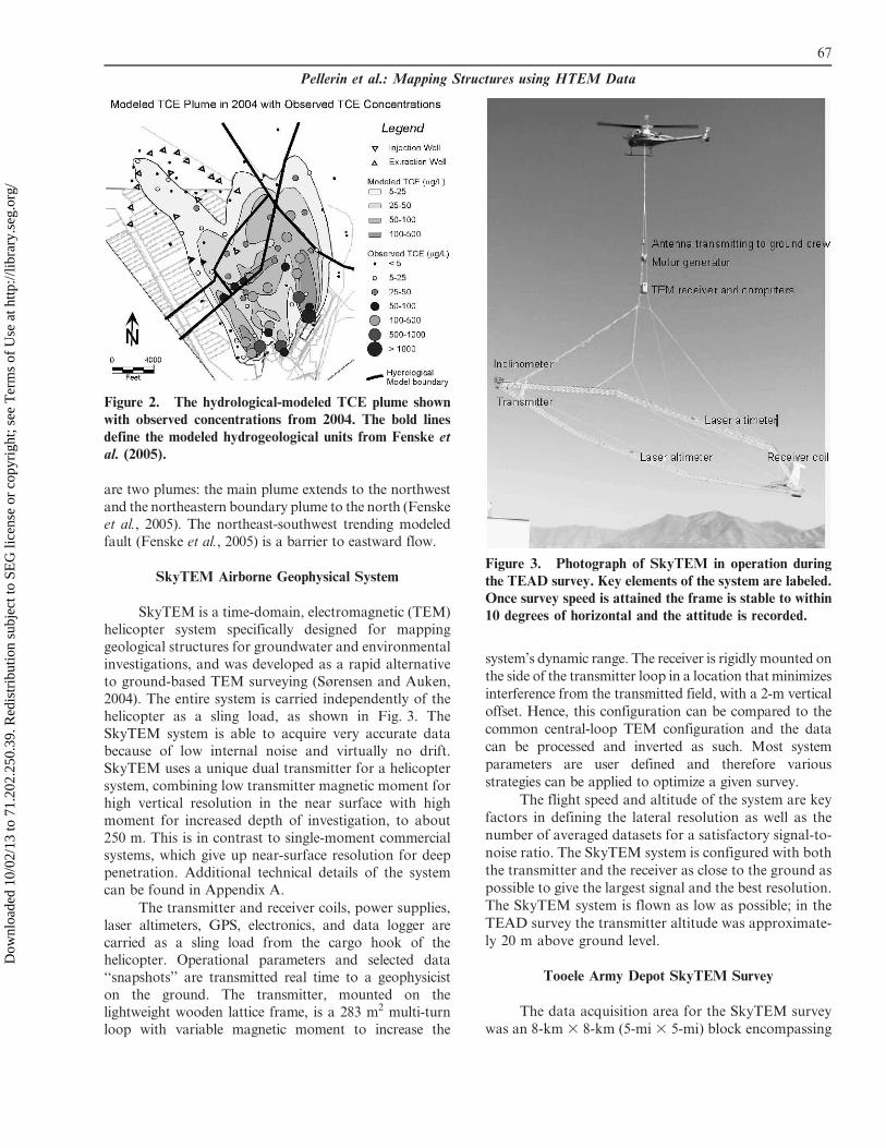
are two plumes: the main plume extends to the northwest

and the northeastern boundary plume to the north (Fenske

et al., 2005). The northeast-southwest trending modeled

fault (Fenske et al., 2005) is a barrier to eastward flow.

SkyTEM Airborne Geophysical System

SkyTEM is a time-domain, electromagnetic (TEM)

helicopter system specifically designed for mapping

geological structures for groundwater and environmental

investigations, and was developed as a rapid alternative

to ground-based TEM surveying (Sørensen and Auken,

2004). The entire system is carried independently of the

helicopter as a sling load, as shown in Fig. 3. The

SkyTEM system is able to acquire very accurate data

because of low internal noise and virtually no drift.

SkyTEM uses a unique dual transmitter for a helicopter

system, combining low transmitter magnetic moment for

high vertical resolution in the near surface with high

moment for increased depth of investigation, to about

250 m. This is in contrast to single-moment commercial

systems, which give up near-surface resolution for deep

penetration. Additional technical details of the system

can be found in Appendix A.

The transmitter and receiver coils, power supplies,

laser altimeters, GPS, electronics, and data logger are

carried as a sling load from the cargo hook of the

helicopter. Operational parameters and selected data

‘‘snapshots’’ are transmitted real time to a geophysicist

on the ground. The transmitter, mounted on the

lightweight wooden lattice frame, is a 283 m2 multi-turn

loop with variable magnetic moment to increase the

system’s dynamic range. The receiver is rigidly mounted on

the side of the transmitter loop in a location that minimizes

interference from the transmitted field, with a 2-m vertical

offset. Hence, this configuration can be compared to the

common central-loop TEM configuration and the data

can be processed and inverted as such. Most system

parameters are user defined and therefore various

strategies can be applied to optimize a given survey.

The flight speed and altitude of the system are key

factors in defining the lateral resolution as well as the

number of averaged datasets for a satisfactory signal-to-

noise ratio. The SkyTEM system is configured with both

the transmitter and the receiver as close to the ground as

possible to give the largest signal and the best resolution.

The SkyTEM system is flown as low as possible; in the

TEAD survey the transmitter altitude was approximate-

ly 20 m above ground level.

Tooele Army Depot SkyTEM Survey

The data acquisition area for the SkyTEM survey

was an 8-km 3 8-km (5-mi 3 5-mi) block encompassing

Figure 2. The hydrological-modeled TCE plume shown

with observed concentrations from 2004. The bold lines

define the modeled hydrogeological units from Fenske etal. (2005).

Figure 3. Photograph of SkyTEM in operation during

the TEAD survey. Key elements of the system are labeled.Once survey speed is attained the frame is stable to within

10 degrees of horizontal and the attitude is recorded.

67

Pellerin et al.: Mapping Structures using HTEM Data

Dow

nloa

ded

10/0

2/13

to 7

1.20

2.25

0.39

. Red

istr

ibut

ion

subj

ect t

o SE

G li

cens

e or

cop

yrig

ht; s

ee T

erm

s of

Use

at h

ttp://

libra

ry.s

eg.o

rg/

the Utah Industrial Depot, about 40% of the ordnance

storage area, and the entirety of the well injection field

described in Fenske et al. (2005), as shown Fig. 4. The

survey covered approximately 200 line-kilometers of

data, and was carried out from October 19–21, 2005.

The survey was flown with a nominal line spacing of

200 m. A large section of the southeast quadrant of the

area could not be flown safely because of industrial or

residential buildup. Additional infill lines were flown in

the area directly north of the Utah Industrial Depot to

better define the geoelectrical section in an area where

faults were thought to be responsible for abrupt changes

in measured groundwater level. Over this area of about

1.5 mi 3 1.5 mi (2.4 km 3 2.4 km), the nominal line

spacing was 100 m. Aircraft ground speed was

maintained at approximately 15 m/s (30 knots).

Resistivity Maps and Profiles

Data were processed with the Aarhus Workbench

software package (Aarhus Geophysics, 2009) developed

by the Hydrogeophysics Group of the University of

Aarhus, Denmark. The substantial amount of data

includes GPS, tilt and altitude, in addition to system

status and voltage data. The transient data are processed

with automatic filters and manual editing. Sign and

slope filters were used to cull data when sign changes

were detected, as in the presence of cultural features

such as power and pipelines (Auken et al., 2004), or if

the slope of the data curve was not within two specified

slopes. A fairly limited slope band centered at ,0.4 was

used with the hopes of culling the response caused by

buried munitions, however manual editing was neces-

sary to remove shallow TEM responses caused by

ordnance-filled revetments in the SW corner of the

survey area. Data were averaged using a trapezoid filter,

thereby increasing the signal-to-noise ratio at late times

where the signal level is relatively low while maintaining

a high resolution at earlier times, where signal levels are

relatively high. An averaged sounding consists of ten

SkyTEM transients yielding data from 10 microseconds

to up to 9 milliseconds.

In the second step, sounding data are inverted

thereby transforming the data from voltages as a

function of time to resistivities as a function of depth

(Fig. 5). A sounding consists of low- and high-moment

segments, which are two distinct datasets. Because the

two segments are slightly separated spatially, the data

sequences are inverted with somewhat different loca-

tions and corresponding altitudes. The high- and low-

moment data sequences are inverted using Mutually

Constrained Inversion (MCI) as discussed in Auken et

al. (2001) and shown in Fig. 5. This approach allows for

the different flight altitudes and any small model

discrepancies between the two spatially separated

segments. Laterally Constrained Inversion (LCI) is

used from sounding to sounding so that the models

vary smoothly over small distances. The one-dimen-

sional (1-D) inverse models are used to construct

resistivity interval plan view maps at depths from 0 to

220 m.

Eight depth interval resistivity slices are shown inFig. 6. The top slice covers only the first 20 m below the

ground surface, but some structures of geological

significance can be seen. The uppermost unit in the

NW quadrant has low earth resistivities characteristic of

saturated sediments with a high TDS content, which is

consistent with a low hydraulic gradient in proximity to

the Great Salt Lake. Low resistivities also appear in the

southwestern quadrant, and are likely of geologic origin,i.e., fluvial deposits. A high resistivity zone can be seen

trending from southwest to northeast through the

central portion of the survey area. This trend is in

agreement with geological models purporting an elevat-

ed bedrock block. In fact, the bedrock block outcrops in

this zone, about 1-km west from the reference site,

designated by a star in Fig. 4 and Fig. 6. The unit

corresponds to the fractured bedrock unit defined in thehydrological modeling. The eastern part of the survey

area appears to be the most resistive, possibly reflecting

Figure 4. The SkyTEM Tooele, Utah survey area

showing the flight lines and two selected profiles as bold

dashed lines (referred to in Figure). The underlying

topographic map highlights infrastructure in the survey

area such as roads, power lines, and the industrial depot.

68

Journal of Environmental and Engineering Geophysics

Dow

nloa

ded

10/0

2/13

to 7

1.20

2.25

0.39

. Red

istr

ibut

ion

subj

ect t

o SE

G li

cens

e or

cop

yrig

ht; s

ee T

erm

s of

Use

at h

ttp://

libra

ry.s

eg.o

rg/

drier and possibly less saline near-surface conditions

than are encountered in the northwest.

The electrical character changes with increasing

depth. The NW quadrant still shows low resistivities,

indicative of the thick sediment package in this area.

The SW-NE trend of the bedrock high is more apparent,

and appears to extend further to the southwest than in

the 0–20 m depth interval. The sizeable area of low

resistivities in the shallowest interval in the SW quadrant

has been reduced to a small circular feature. This low

resistivity unit persists to the deepest resistivity interval

and could indicate an upwelling of saline fluids. This

response being caused by a shallow anthropomorphic

conductive feature was rejected because the responses of

the buried ordnance were clearly visible and culled in the

voltage data, and there was no evidence of other

structure of the scale responsible for the anomaly.

Interpretation

The primary geological structures to be defined

with the SkyTEM survey data are: depth to basement,

or its corollary, sediment thickness; locations of major

faults or hydrological unit boundaries; and preferred

groundwater flow paths. The pertinent structures are

interpreted from the depth interval maps of Fig. 6.

Depth to Bedrock

The bedrock has no consistent resistivity signa-

ture. The shallow bedrock horst near the center of the

SkyTEM survey area appears electrically resistive, a

characteristic that would be compatible with a carbon-

ate formation. However, in many resistivity cross-

sectional profiles the lowermost electrical layer appears

conductive, and is deeper than boreholes that sampled

to depths of ,100 m, therefore the lithology and degree

of compaction is uncertain.

Resistivity cross-sections were derived from 1-D

LCI models (Auken et al., 2005) along the SkyTEM

profiles depicted in Fig. 4, and can be used to illustrate

the changes in geology from north to south in the

surveyed area. Figure 7 shows resistivity cross-sections

from two east-west profiles. The topmost profile is

located in Fig. 4, and shows the thick conductive

unconsolidated sediments in the north part of the area.

The western three-fourths of the profile show conductive

sediments that extend at least as deep as the SkyTEM

system was able to sample, about 200 m below ground

level. At position x 5 6,000 m the resistivity section

becomes more complex than the predominantly con-

ductive section, and the resistive zone at 6,500 m

corresponds to the northeast trending fault splay

predicted by the hydrological modeling (Fenske et al.,

2005) shown in the maps of Fig. 6. Line 23, the lower

panel in Fig. 7, is about 3,800 m south of Line 5 and

passes over the shallow bedrock carbonate horst in the

center of the survey area. A dense dolomite outcrop in

the area suggests a horst, as does gravity data. The horst

appears as a shallow resistive zone that continues to the

maximum SkyTEM sampling depth; west of this zone a

resistive layer overlies a more conductive zone. Because

of the local stratigraphy we interpret the resistive layer

as dry, less saline unconsolidated valley fill, rather than

carbonate bedrock.

Deeper in the fill the moisture and salinity content

increases, and the resistivity decreases. East of the horst,

the electrical section is more complex and the uncon-

solidated sediments remain resistive through the entire

depth section, probably indicative of less saline condi-

tions than in the west. The blanked out areas in both

profile cross-sections are where the helicopter had to fly

high to avoid power lines or other buildings, and the

data were not deemed reliable.

Evidence of Faulting

Few bedrock outcrops occur in the SkyTEM

survey area, and most faulting was inferred from

borehole potentiometric measurements and subsequent

modeling (Asch, 2005; Fenske et al., 2005). A number of

faults inferred from head levels modeled from potenti-

ometric data are superimposed on the depth sections in

Figure 5. (a) Average voltage data with masked data in

light gray, (b) corresponding apparent resistivity from the

edited voltage, and (c) 1-D inverse models. The dots

represent data in (a) and (b), while the smooth curve is the

response of models in (c).

69

Pellerin et al.: Mapping Structures using HTEM Data

Dow

nloa

ded

10/0

2/13

to 7

1.20

2.25

0.39

. Red

istr

ibut

ion

subj

ect t

o SE

G li

cens

e or

cop

yrig

ht; s

ee T

erm

s of

Use

at h

ttp://

libra

ry.s

eg.o

rg/

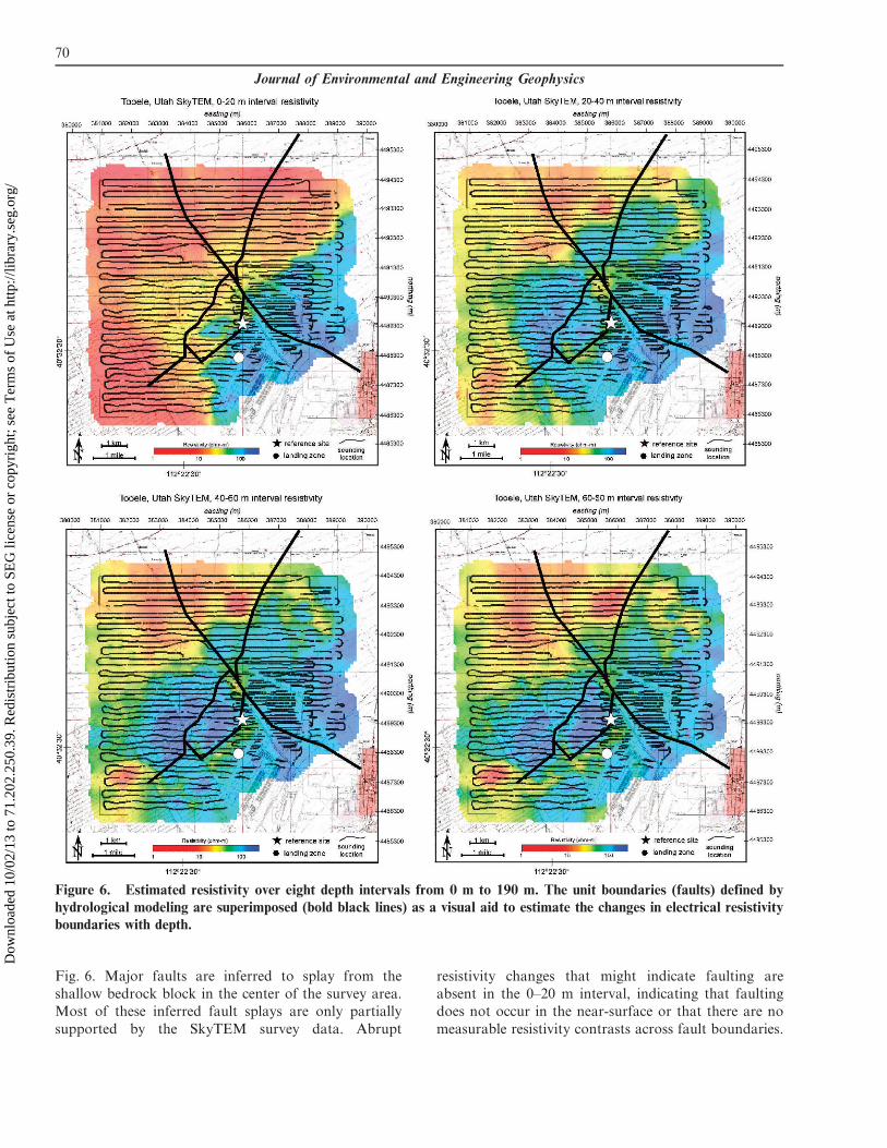
Fig. 6. Major faults are inferred to splay from the

shallow bedrock block in the center of the survey area.

Most of these inferred fault splays are only partially

supported by the SkyTEM survey data. Abrupt

resistivity changes that might indicate faulting are

absent in the 0–20 m interval, indicating that faulting

does not occur in the near-surface or that there are no

measurable resistivity contrasts across fault boundaries.

Figure 6. Estimated resistivity over eight depth intervals from 0 m to 190 m. The unit boundaries (faults) defined by

hydrological modeling are superimposed (bold black lines) as a visual aid to estimate the changes in electrical resistivity

boundaries with depth.

70

Journal of Environmental and Engineering Geophysics

Dow

nloa

ded

10/0

2/13

to 7

1.20

2.25

0.39

. Red

istr

ibut

ion

subj

ect t

o SE

G li

cens

e or

cop

yrig

ht; s

ee T

erm

s of

Use

at h

ttp://

libra

ry.s

eg.o

rg/

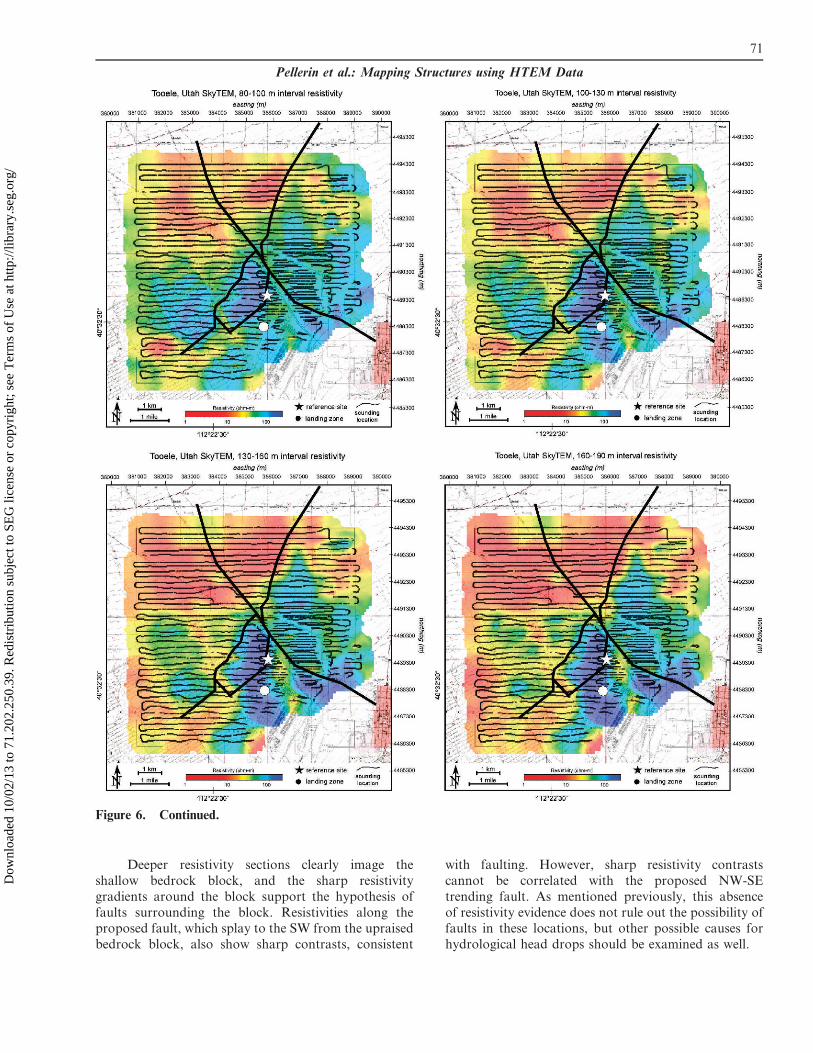
Deeper resistivity sections clearly image the

shallow bedrock block, and the sharp resistivity

gradients around the block support the hypothesis of

faults surrounding the block. Resistivities along theproposed fault, which splay to the SW from the upraised

bedrock block, also show sharp contrasts, consistent

with faulting. However, sharp resistivity contrasts

cannot be correlated with the proposed NW-SE

trending fault. As mentioned previously, this absence

of resistivity evidence does not rule out the possibility offaults in these locations, but other possible causes for

hydrological head drops should be examined as well.

Figure 6. Continued.

71

Pellerin et al.: Mapping Structures using HTEM Data

Dow

nloa

ded

10/0

2/13

to 7

1.20

2.25

0.39

. Red

istr

ibut

ion

subj

ect t

o SE

G li

cens

e or

cop

yrig

ht; s

ee T

erm

s of

Use

at h

ttp://

libra

ry.s

eg.o

rg/

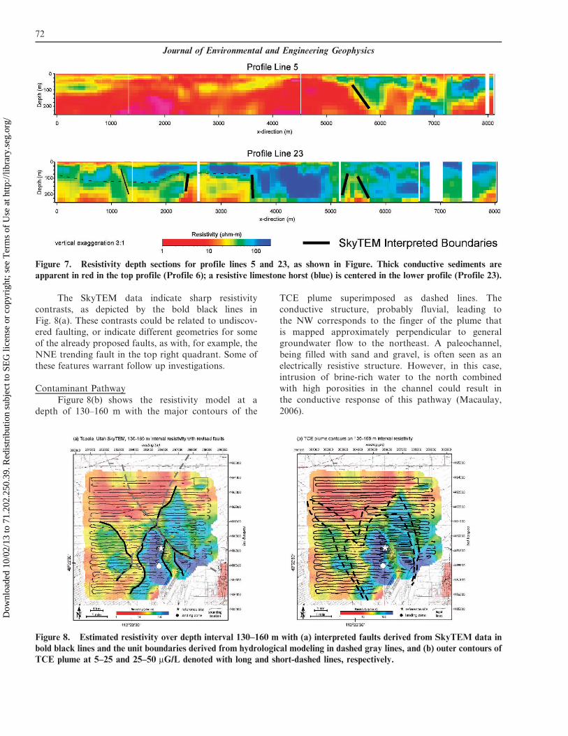
The SkyTEM data indicate sharp resistivity

contrasts, as depicted by the bold black lines in

Fig. 8(a). These contrasts could be related to undiscov-

ered faulting, or indicate different geometries for some

of the already proposed faults, as with, for example, the

NNE trending fault in the top right quadrant. Some of

these features warrant follow up investigations.

Contaminant Pathway

Figure 8(b) shows the resistivity model at a

depth of 130–160 m with the major contours of the

TCE plume superimposed as dashed lines. The

conductive structure, probably fluvial, leading to

the NW corresponds to the finger of the plume that

is mapped approximately perpendicular to general

groundwater flow to the northeast. A paleochannel,

being filled with sand and gravel, is often seen as an

electrically resistive structure. However, in this case,

intrusion of brine-rich water to the north combined

with high porosities in the channel could result in

the conductive response of this pathway (Macaulay,

2006).

Figure 7. Resistivity depth sections for profile lines 5 and 23, as shown in Figure. Thick conductive sediments are

apparent in red in the top profile (Profile 6); a resistive limestone horst (blue) is centered in the lower profile (Profile 23).

Figure 8. Estimated resistivity over depth interval 130–160 m with (a) interpreted faults derived from SkyTEM data in

bold black lines and the unit boundaries derived from hydrological modeling in dashed gray lines, and (b) outer contours of

TCE plume at 5–25 and 25–50 mG/L denoted with long and short-dashed lines, respectively.

72

Journal of Environmental and Engineering Geophysics

Dow

nloa

ded

10/0

2/13

to 7

1.20

2.25

0.39

. Red

istr

ibut

ion

subj

ect t

o SE

G li

cens

e or

cop

yrig

ht; s

ee T

erm

s of

Use

at h

ttp://

libra

ry.s

eg.o

rg/

Conclusions

The SkyTEM survey was the first wide-area

geophysical survey at TEAD, and serves as a framework

for integration of other TEAD data. The SkyTEM data

were of good quality and self-consistent. Data collected

at the calibration site were repeatable. There appears to

be good correlation of SkyTEM earth resistivity

estimates with known geology. Areas where basement

is known to be from prior studies at or near the surface

were clearly delineated in the SkyTEM data as a high

resistivity zone, which begins near the ground surface

and continues to the deepest samples. In some places,

basement may be conductive rather than resistive. In the

northwest part of the survey area, resistivities were low

throughout the sample intervals that are consistent with

brine saturation in proximity to the Great Salt Lake.

The SkyTEM data supports the existence of some,

but not all, of the faults that have been proposed based

on potentiometric studies. Although faults are a difficult

target for most geophysical methods, a few fault-like

structures defined by electrical resistivity contrasts

appear besides those that were based on groundwater

head data and modeling. Shallow high-resistivity layers

in the east and southeast portions of the survey area

appear to be underlain by more conductive sediments,

and so should not be interpreted as shallow bedrock.

One of the most significant results of the survey is the

delineation of a conductive unit, interpreted as a

paleochannel at depths .100 m in which brine may

have migrated from the north. We suggest structure may

be responsible for transport of the TCE contamination.

Acknowledgements

The authors wish to thank Jan Steen Joegensen, Lars

Jensen and Max Halkjaer of SkyTEM Aps for the data

acquisition, David Beard of Dragonfly Air for his excellent

flying, Carl Cole, U.S. Army Corps of Engineers for providing

invaluable logistical assistance and geological advice before

and during the SkyTEM survey, and Esben Auken, Hydro-

geophysics Group, University of Aarhus, DK, for his

assistance with the processing and inversion software. We

also thank Greg Hodges, an anonymous reviewer and the

JEEG associate editor Antonio Menghini for their thoughtful

comments that improved the paper.

References

Aarhus Geophysics, 2009, Aarhus Workbench Guide to

Processing and Inversion of SkyTEM Data: www.

aarhusgeo.com, 41 pp.

Asch, T., 2005, Summary and integration of geophysical

investigations of the Tooele Army Depot (TEAD), Tooele,

Utah: USGS Open-File Report 1338-2005, 53 pp.

Auken, E., Christiansen, A.V., Jacobsen, B.H., Foged, N., and

Sørensen, K.I., 2005, Piecewise 1D Laterally Con-

strained Inversion of Resistivity Data: Geophysical

Prospecting, 53, 497–506.

Auken, E., Pellerin, L., and Sørensen, K., 2001, Mutually

Constrained Inversion (MCI) of Electrical and Electro-

magnetic Data: in Expanded Abstracts: Annual Inter-

national Meeting, Society of Exploration Geophysics

1455–1458.

Auken, E., Halkjær, M., and Sørensen, K.I., 2004, SkyTEM—

Data Processing and a Survey: in Proceedings: Sympo-

sium on the Application of Geophysics to Engineering

and Environmental Problems (SAGEEP), Colorado

Springs, Colorado, USA.

Fenske, J., Grogin, L., and Andersen, P., 2005, Tooele Army

Depot Groundwater Flow and Contaminant Transport

Model: U.S. Army Corps of Engineers, Sacramento

District, Environmental Engineering Branch, PR-59.

Macaulay, S., 2006, Application of Airborne Electromagnetics

to Salt Mapping—3 Australian Case Studies: Sympo-

sium on the Application of Geophysics to Engineering

and Environmental Problems (SAGEEP).

Sørensen, K.I., and Auken, E., 2004, SkyTEM—A new high-

resolution helicopter transient electromagnetic system:

Exploration Geophysics, 35, 191–199.

Stokes, W.L., 1988, The Geology of Utah: Utah Museum of

Natural History Occasional Paper, 6, 280 pp.

Susong, D.D., 1999, Ground-water resources of Tooele Valley,

Utah Edition: USGS Library Call Number (200) F327

no.99-125.

APPENDIX A

SkyTEM SPECIFICATIONS

The SkyTEM system used a low and high

transmitter moment (Table A-1) and is based on a

central-loop array configuration. The transmitter,

mounted on a lightweight wooden lattice frame, is a

283 m2 multi-turn loop with variable moment to

increase the system’s dynamic range. The shielded,

over-damped, multi-turn receiver loop is rigidly mount-

ed on the side of the transmitter loop in a near-null

position of the primary transmitted field, which

minimizes distortions from the transmitter, with a 2-

meter vertical offset. Hence, this configuration can be

compared to a central-loop configuration and the data

are processed and inverted as such. The transmitter is

powered by a motor generator, which is placed between

the helicopter and the frame. It uses a combination of

high and low transmitter moments for high vertical

resolution in the near surface and increased depth of

investigation to ,250 m. The dual moment array has the

advantage of being able to attain measurements of time

gates shown in Table A-2.

With the system repetition frequencies, a complete

measurement cycle, including both the low and the high

73

Pellerin et al.: Mapping Structures using HTEM Data

Dow

nloa

ded

10/0

2/13

to 7

1.20

2.25

0.39

. Red

istr

ibut

ion

subj

ect t

o SE

G li

cens

e or

cop

yrig

ht; s

ee T

erm

s of

Use

at h

ttp://

libra

ry.s

eg.o

rg/

moment dataset, takes about 2 s. Hence, there is high datadensity along the flight line and several soundings can be

averaged in a running mean to enhance data quality.

The transmitted current is measured for each data

set at each moment; the exact value depends on the

ambient outdoor temperature. The complete waveform

is then scaled due to the variations caused by

temperature variations.

The transmitter waveform can be described as amodified square wave where the current builds quickly

and then turned off within a few microseconds. The very

fast turn-off time of the low-moment transmitter results

in higher vertical resolution of the upper layers.

Enhanced resolution of the upper layers results in better

resolution at depth and a greater depth of investigation.

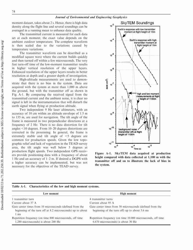
High-altitude measurements are used to demon-

strate that there is no bias in the system. Data areacquired with the system at more than 1,000 m above

the ground, but with the transmitter off as shown in

Fig. A-1. By comparing the received signal from the

transmitted current and the ambient noise, it is clear no

signal is left in the instrumentation that will disturb the

earth signal when flying at production altitude.

Two independent 9 Hz laser altimeters, with an

accuracy of 10 cm within an altitude envelope of 1.5 mto 135 m, are used for navigation. The tilt angle of the

frame is measured in two perpendicular directions at a

frequency of 2 Hz. There is no data distortion for tilt

angles ,10 degrees. From 10–20 degrees distortions are

corrected in the processing. In general, the frame is

extremely stable and tilt angle of ,5 degrees are

common for production speeds. Given the low topo-

graphic relief and lack of vegetation in the TEAD surveyarea, the tilt angle was well below 5 degrees at

production flight speeds. Two independent GPS receiv-

ers provide positioning data with a frequency of about

1 Hz and an accuracy of 1–2 m. If desired a DGPS with

a higher accuracy can be implemented, but was not

necessary for the objectives of the TEAD survey.

Figure A-1. SkyTEM data acquired at production

height compared with data collected at 1,100 m with the

transmitter off and on to illustrate the lack of bias inthe system.

Table A-1. Characteristics of the low and high moment systems.

Low moment High moment

1 transmitter turn 4 transmitter turns

Current about 37 A Current about 95 A

Gate center times from 10 microseconds (defined from the

beginning of the turn off at 8.2 microseconds) up to about

1 ms

Gate center times from 50 microseconds (defined from the

beginning of the turn off) up to about 5.6 ms

Repetition frequency (on time 800 microseconds, off time

1,280 microseconds) is about 240 Hz

Repetition frequency (on time 10.000 microseconds, off time

6.670 microseconds) is about 30 Hz

74

Journal of Environmental and Engineering Geophysics

Dow

nloa

ded

10/0

2/13

to 7

1.20

2.25

0.39

. Red

istr

ibut

ion

subj

ect t

o SE

G li

cens

e or

cop

yrig

ht; s

ee T

erm

s of

Use

at h

ttp://

libra

ry.s

eg.o

rg/

Table A-2. The center times, in microseconds, for the measurement gates.

Gate Time Gate Time Gate Time

2 10.0 11 111.8 20 911.2

3 16.3 12 145.4 21 1141.0

4 22.8 13 185.2 22 1429.2

5 29.2 14 234.4 23 1791.2

6 35.6 15 295.2 24 2246.0

7 45.2 16 370.6 25 2817.4

8 58.0 17 464.4 26 3535.6

9 71.1 18 581.4 27 4438.8

10 86.8 19 727.8 28 5575.0

75

Pellerin et al.: Mapping Structures using HTEM Data

Dow

nloa

ded

10/0

2/13

to 7

1.20

2.25

0.39

. Red

istr

ibut

ion

subj

ect t

o SE

G li

cens

e or

cop

yrig

ht; s

ee T

erm

s of

Use

at h

ttp://

libra

ry.s

eg.o

rg/