
Eindhoven University of Technology MASTER Location, location ...
Upload
khangminh22Category
view
1download
0
The Role of Amenities in the LocationDecision of Households and Firms
DissertationApproved as fulfilling the requirements for the degree of
doctor rerum politicarum (Dr. rer. pol.)by the
Department of Law and Economics ofDarmstadt University of Technology
byTorsten Kristoffer Möller, M.A.(born 19/09/1984 in Hannover)
First supervisor: Prof. Dr. Volker NitschSecond supervisor: Prof. Dr. Jens SüdekumDate of submission: 17/10/2013Date of defense: 21/05/2014Place of publication: DarmstadtYear of publication: 2014
D 17


Acknowledgements
At this point I want to thank several persons. My first supervisor and doctoral advisor Prof.Dr. Volker Nitsch discussed certain aspects related to many chapters of this dissertation duringthe last years. He provided helpful feedback which generated new ways of thinking. My secondsupervisor Prof. Dr. Jens Südekum who closely followed the development of my research overthe last years, giving useful advices.I very much would like to thank my family and friends who not only supported me during
my PhD years.A special thanks goes to my close colleague and friend Sevrin Waights for (not only) the
endless ArcGIS sessions and inspiring research discussions. Furthermore, I would like to thankDr. Gabriel Ahlfeldt for immediate feedback along the road and for making my visit at SERCat the London School of Economics and Political Science possible. I also want to thank Dr.Nicolai Wendland for his helpful comments and opinions.I want to thank the Center for Metropolitan Studies at the Berlin University of Technology
for the accommodation and great research environment. A special thanks goes to ElisabethAsche and Professor Dr. Dorothee Brantz. For constant feedback, I would like to thank mycolleagues Dr. Stefan Goldbach, Johannes Rode, Dr. Kristian Giessen, Felipe Carozzi and MrDell. Philip Savage provided excellent comments for issues related to linguistics.Finally, I want to thank all conference participants who gave useful feedback on my research.
iii


Contents
Zusammenfassung xv
1. Introduction 1
2. Literature review 32.1. Location theory and empirics . . . . . . . . . . . . . . . . . . . . . . . . . . . . 32.2. Localised goods and services . . . . . . . . . . . . . . . . . . . . . . . . . . . . . 52.3. Aesthetics and physical setting . . . . . . . . . . . . . . . . . . . . . . . . . . . . 7
2.3.1. Natural amenities . . . . . . . . . . . . . . . . . . . . . . . . . . . . . . . 72.3.2. Beauty and architectural design . . . . . . . . . . . . . . . . . . . . . . . 8
2.4. Public services . . . . . . . . . . . . . . . . . . . . . . . . . . . . . . . . . . . . . 132.4.1. Schooling . . . . . . . . . . . . . . . . . . . . . . . . . . . . . . . . . . . 132.4.2. Crime . . . . . . . . . . . . . . . . . . . . . . . . . . . . . . . . . . . . . 15
2.5. Transportation . . . . . . . . . . . . . . . . . . . . . . . . . . . . . . . . . . . . 162.6. Firm location choice . . . . . . . . . . . . . . . . . . . . . . . . . . . . . . . . . 20
3. Culturally clustered or in the cloud? Location choice of internet firms inBerlin 233.1. Motivation . . . . . . . . . . . . . . . . . . . . . . . . . . . . . . . . . . . . . . . 233.2. Internet industry in Berlin . . . . . . . . . . . . . . . . . . . . . . . . . . . . . . 25
3.2.1. (Sub-) Cultural rise after re-unification . . . . . . . . . . . . . . . . . . . 253.2.2. Berlin discovers the internet . . . . . . . . . . . . . . . . . . . . . . . . . 263.2.3. An intra-urban analysis . . . . . . . . . . . . . . . . . . . . . . . . . . . 28
3.3. Footloose start-up model . . . . . . . . . . . . . . . . . . . . . . . . . . . . . . . 283.4. Empirical approach . . . . . . . . . . . . . . . . . . . . . . . . . . . . . . . . . . 31
3.4.1. General estimation approach . . . . . . . . . . . . . . . . . . . . . . . . . 313.4.2. Identification . . . . . . . . . . . . . . . . . . . . . . . . . . . . . . . . . 34
3.5. Data . . . . . . . . . . . . . . . . . . . . . . . . . . . . . . . . . . . . . . . . . . 363.5.1. Dependent variable . . . . . . . . . . . . . . . . . . . . . . . . . . . . . . 363.5.2. Cultural amenities . . . . . . . . . . . . . . . . . . . . . . . . . . . . . . 373.5.3. Control variables . . . . . . . . . . . . . . . . . . . . . . . . . . . . . . . 403.5.4. Placebo firms . . . . . . . . . . . . . . . . . . . . . . . . . . . . . . . . . 41
3.6. Results . . . . . . . . . . . . . . . . . . . . . . . . . . . . . . . . . . . . . . . . . 423.6.1. Internet start-ups . . . . . . . . . . . . . . . . . . . . . . . . . . . . . . . 42
v

Contents
3.6.2. Robustness . . . . . . . . . . . . . . . . . . . . . . . . . . . . . . . . . . 443.6.3. Placebo firms . . . . . . . . . . . . . . . . . . . . . . . . . . . . . . . . . 48
3.7. Summary . . . . . . . . . . . . . . . . . . . . . . . . . . . . . . . . . . . . . . . 51
4. Game of zones: The economics of conservation areas 534.1. Motivation . . . . . . . . . . . . . . . . . . . . . . . . . . . . . . . . . . . . . . . 534.2. Theory and context . . . . . . . . . . . . . . . . . . . . . . . . . . . . . . . . . . 55
4.2.1. Theoretical framework . . . . . . . . . . . . . . . . . . . . . . . . . . . . 554.2.2. Institutional context . . . . . . . . . . . . . . . . . . . . . . . . . . . . . 60
4.3. Empirical strategy . . . . . . . . . . . . . . . . . . . . . . . . . . . . . . . . . . 614.3.1. Designation process . . . . . . . . . . . . . . . . . . . . . . . . . . . . . . 614.3.2. Pareto optimality . . . . . . . . . . . . . . . . . . . . . . . . . . . . . . . 63
4.4. Data . . . . . . . . . . . . . . . . . . . . . . . . . . . . . . . . . . . . . . . . . . 664.5. Empirical results . . . . . . . . . . . . . . . . . . . . . . . . . . . . . . . . . . . 67
4.5.1. Designation process . . . . . . . . . . . . . . . . . . . . . . . . . . . . . . 674.5.2. Pareto optimality . . . . . . . . . . . . . . . . . . . . . . . . . . . . . . . 71
4.6. Summary . . . . . . . . . . . . . . . . . . . . . . . . . . . . . . . . . . . . . . . 82
5. Chicken or egg? Transport and urban development in Berlin 855.1. Motivation . . . . . . . . . . . . . . . . . . . . . . . . . . . . . . . . . . . . . . . 855.2. Historical background . . . . . . . . . . . . . . . . . . . . . . . . . . . . . . . . . 87
5.2.1. S-Bahn . . . . . . . . . . . . . . . . . . . . . . . . . . . . . . . . . . . . . 875.2.2. U-Bahn . . . . . . . . . . . . . . . . . . . . . . . . . . . . . . . . . . . . 88
5.3. Data . . . . . . . . . . . . . . . . . . . . . . . . . . . . . . . . . . . . . . . . . . 895.4. Methodology . . . . . . . . . . . . . . . . . . . . . . . . . . . . . . . . . . . . . 955.5. Empirical results . . . . . . . . . . . . . . . . . . . . . . . . . . . . . . . . . . . 100
5.5.1. Main results . . . . . . . . . . . . . . . . . . . . . . . . . . . . . . . . . . 1005.5.2. Robustness . . . . . . . . . . . . . . . . . . . . . . . . . . . . . . . . . . 105
5.6. Summary . . . . . . . . . . . . . . . . . . . . . . . . . . . . . . . . . . . . . . . 110
6. Hundred years of transport in Chicago – a Panel VAR analysis 1116.1. Motivation . . . . . . . . . . . . . . . . . . . . . . . . . . . . . . . . . . . . . . . 1116.2. Historic background . . . . . . . . . . . . . . . . . . . . . . . . . . . . . . . . . . 1116.3. Data . . . . . . . . . . . . . . . . . . . . . . . . . . . . . . . . . . . . . . . . . . 1146.4. Empirical analysis . . . . . . . . . . . . . . . . . . . . . . . . . . . . . . . . . . . 116
6.4.1. Empirical approach . . . . . . . . . . . . . . . . . . . . . . . . . . . . . . 1166.4.2. Results . . . . . . . . . . . . . . . . . . . . . . . . . . . . . . . . . . . . . 117
6.5. Summary . . . . . . . . . . . . . . . . . . . . . . . . . . . . . . . . . . . . . . . 119
7. Conclusion 123
vi

Contents
A. Appendix to Chapter 3 125A.1. Data . . . . . . . . . . . . . . . . . . . . . . . . . . . . . . . . . . . . . . . . . . 125A.2. Empirical results . . . . . . . . . . . . . . . . . . . . . . . . . . . . . . . . . . . 125
B. Appendix to Chapter 4 141B.1. Introduction . . . . . . . . . . . . . . . . . . . . . . . . . . . . . . . . . . . . . . 141B.2. Theory and context . . . . . . . . . . . . . . . . . . . . . . . . . . . . . . . . . . 141B.3. Empirical strategy . . . . . . . . . . . . . . . . . . . . . . . . . . . . . . . . . . 142
B.3.1. Designation process - control variables . . . . . . . . . . . . . . . . . . . 142B.3.2. Difference-in-differences . . . . . . . . . . . . . . . . . . . . . . . . . . . 144
B.4. Data . . . . . . . . . . . . . . . . . . . . . . . . . . . . . . . . . . . . . . . . . . 149B.4.1. Data sources . . . . . . . . . . . . . . . . . . . . . . . . . . . . . . . . . . 149B.4.2. Further notes on data methods . . . . . . . . . . . . . . . . . . . . . . . 153
B.5. Estimation results . . . . . . . . . . . . . . . . . . . . . . . . . . . . . . . . . . . 154B.5.1. Designation process . . . . . . . . . . . . . . . . . . . . . . . . . . . . . . 154B.5.2. Pareto optimality . . . . . . . . . . . . . . . . . . . . . . . . . . . . . . . 162
C. Appendix to Chapter 5 171C.1. Reduced form PVAR estimates . . . . . . . . . . . . . . . . . . . . . . . . . . . 171C.2. IRF for the 300m grid model . . . . . . . . . . . . . . . . . . . . . . . . . . . . . 173C.3. Cumulative impulse response functions . . . . . . . . . . . . . . . . . . . . . . . 174C.4. Land use location choice model . . . . . . . . . . . . . . . . . . . . . . . . . . . 176
C.4.1. Motivation . . . . . . . . . . . . . . . . . . . . . . . . . . . . . . . . . . . 176C.4.2. Data . . . . . . . . . . . . . . . . . . . . . . . . . . . . . . . . . . . . . . 176C.4.3. Empirical strategy . . . . . . . . . . . . . . . . . . . . . . . . . . . . . . 178C.4.4. Results . . . . . . . . . . . . . . . . . . . . . . . . . . . . . . . . . . . . . 179
D. Appendix to Chapter 6 183D.1. Data . . . . . . . . . . . . . . . . . . . . . . . . . . . . . . . . . . . . . . . . . . 183D.2. Empirical results . . . . . . . . . . . . . . . . . . . . . . . . . . . . . . . . . . . 183D.3. Cumulative impulse response functions . . . . . . . . . . . . . . . . . . . . . . . 184
Academic career 209
Affidavit 211
vii


List of Figures
3.1. Share of internet start-ups by city. . . . . . . . . . . . . . . . . . . . . . . . . . . 283.2. Placebo Wall . . . . . . . . . . . . . . . . . . . . . . . . . . . . . . . . . . . . . 363.3. Number of internet start-ups per founding year . . . . . . . . . . . . . . . . . . 373.4. Distribution of start-ups and cultural amenities . . . . . . . . . . . . . . . . . . 393.5. Berlin Wall and access to cultural amenities . . . . . . . . . . . . . . . . . . . . 39
4.1. Expected heritage distribution with partial designation . . . . . . . . . . . . . . 574.2. RDD-DD internal estimates . . . . . . . . . . . . . . . . . . . . . . . . . . . . . 774.3. RDD-DD external estimates . . . . . . . . . . . . . . . . . . . . . . . . . . . . . 784.4. RDD-DD spatial treatment effects . . . . . . . . . . . . . . . . . . . . . . . . . . 81
5.1. Combined rail network in 1870, 1900 and 1935 . . . . . . . . . . . . . . . . . . . 915.2. Rail station density on municipality level . . . . . . . . . . . . . . . . . . . . . . 925.3. Population density on municipality level . . . . . . . . . . . . . . . . . . . . . . 935.4. Land values on block level in 1890 and 1914 . . . . . . . . . . . . . . . . . . . . 945.5. Land values on grid level (in Reichsmark) in 1890 and 1914 . . . . . . . . . . . . 965.6. Impulse responses for 2-PVAR model and total sample . . . . . . . . . . . . . . 1015.7. Impulse responses for 2-PVAR model and core sample . . . . . . . . . . . . . . . 1025.8. Impulse responses for 2-PVAR model and periphery sample . . . . . . . . . . . . 1035.9. Impulse responses for 2-PVAR anticipation model and total sample . . . . . . . 1075.10. Impulse responses for 2-PVAR anticipation model and core sample . . . . . . . . 1085.11. Impulse responses for 2-PVAR anticipation model and periphery sample . . . . . 109
6.1. Number ‘L’ stations . . . . . . . . . . . . . . . . . . . . . . . . . . . . . . . . . . 1156.2. ‘L’ station density on census tracts . . . . . . . . . . . . . . . . . . . . . . . . . 1206.3. Population density on census tracts . . . . . . . . . . . . . . . . . . . . . . . . . 1216.4. Impulse responses for 2-PVAR model . . . . . . . . . . . . . . . . . . . . . . . . 122
A.1. Distribution of squatted houses and cultural amenities. . . . . . . . . . . . . . . 126A.2. Distribution of placebo firms and cultural amenities. . . . . . . . . . . . . . . . . 126
B.1. Designation equilibrium . . . . . . . . . . . . . . . . . . . . . . . . . . . . . . . 142B.2. Semi-parametric temporal bins estimates . . . . . . . . . . . . . . . . . . . . . . 169B.3. Semi-parametric spatial bins estimates . . . . . . . . . . . . . . . . . . . . . . . 170
C.1. Impulse responses for 2-PVAR 300 m grid model . . . . . . . . . . . . . . . . . . 174
ix

List of Figures
C.2. Cumulative impulse responses (total sample) . . . . . . . . . . . . . . . . . . . . 175C.3. Cumulative impulse responses (core sample) . . . . . . . . . . . . . . . . . . . . 176C.4. Cumulative impulse responses (periphery sample) . . . . . . . . . . . . . . . . . 177C.5. Predicted land use probabilities over distance to CBD (in km) . . . . . . . . . . 182
D.1. Study area of Chicago (2010) . . . . . . . . . . . . . . . . . . . . . . . . . . . . 184D.2. Impulse responses for 2-PVAR model (individual Y-axes) . . . . . . . . . . . . . 185D.3. Cumulative impulse responses (total sample) . . . . . . . . . . . . . . . . . . . . 186D.4. Cumulative impulse responses (core sample) . . . . . . . . . . . . . . . . . . . . 186D.5. Cumulative impulse responses (periphery sample) . . . . . . . . . . . . . . . . . 187
x

List of Tables
3.1. Estimation results: Footloose start-up model . . . . . . . . . . . . . . . . . . . . 423.2. Estimation results: Robustness exercises (1) . . . . . . . . . . . . . . . . . . . . 453.3. Estimation results: Robustness exercises (2) . . . . . . . . . . . . . . . . . . . . 473.4. Estimation results: Placebo firms . . . . . . . . . . . . . . . . . . . . . . . . . . 49
4.1. Designation process . . . . . . . . . . . . . . . . . . . . . . . . . . . . . . . . . . 694.2. Conservation area premium – designation effect . . . . . . . . . . . . . . . . . . 734.3. Regression discontinuity design of differences between treatment and control
(RDD-DD) . . . . . . . . . . . . . . . . . . . . . . . . . . . . . . . . . . . . . . 754.4. Spatial regression discontinuity design of difference-in-differences (RDD-DD) . . 79
5.1. Twofold approach - three samples . . . . . . . . . . . . . . . . . . . . . . . . . . 905.2. Number of stations . . . . . . . . . . . . . . . . . . . . . . . . . . . . . . . . . . 905.3. Municipality sample summary statistics . . . . . . . . . . . . . . . . . . . . . . . 945.4. Block sample summary statistics . . . . . . . . . . . . . . . . . . . . . . . . . . 955.5. Grid (150m) sample summary statistics . . . . . . . . . . . . . . . . . . . . . . . 955.6. Panel unit root tests (separate samples) . . . . . . . . . . . . . . . . . . . . . . . 1005.7. Variance decompositions . . . . . . . . . . . . . . . . . . . . . . . . . . . . . . . 1045.8. Panel unit root tests (anticiptation model) . . . . . . . . . . . . . . . . . . . . . 1055.9. Variance decompositions (anticipation model) . . . . . . . . . . . . . . . . . . . 110
6.1. Census tract summary statistics . . . . . . . . . . . . . . . . . . . . . . . . . . . 1166.2. Panel unit root tests . . . . . . . . . . . . . . . . . . . . . . . . . . . . . . . . . 1176.3. Variance decompositions . . . . . . . . . . . . . . . . . . . . . . . . . . . . . . . 118
A.1. Estimation results: Footloose start-up model . . . . . . . . . . . . . . . . . . . . 127A.2. Estimation results: Footloose start-up model - first stage . . . . . . . . . . . . . 129A.3. Estimation results: Robustness exercises (1) . . . . . . . . . . . . . . . . . . . . 131A.4. Estimation results: Robustness exercises (2) . . . . . . . . . . . . . . . . . . . . 133A.5. Estimation results: Placebo firms . . . . . . . . . . . . . . . . . . . . . . . . . . 136A.6. Estimation results: Placebo firms - first stage . . . . . . . . . . . . . . . . . . . 138
B.1. Conditional mean prices . . . . . . . . . . . . . . . . . . . . . . . . . . . . . . . 146B.2. Variable description . . . . . . . . . . . . . . . . . . . . . . . . . . . . . . . . . . 151B.3. Land Cover Broad categories . . . . . . . . . . . . . . . . . . . . . . . . . . . . . 154
xi

List of Tables
B.4. Designation process . . . . . . . . . . . . . . . . . . . . . . . . . . . . . . . . . . 155B.5. Standard IV models – First stage regressions . . . . . . . . . . . . . . . . . . . . 156B.6. Alternative IV models . . . . . . . . . . . . . . . . . . . . . . . . . . . . . . . . 158B.7. Alternative IV models - First stage regressions . . . . . . . . . . . . . . . . . . . 158B.8. Short differences models . . . . . . . . . . . . . . . . . . . . . . . . . . . . . . . 160B.9. Short differences and income models - first stage regressions . . . . . . . . . . . 161B.10.Income models . . . . . . . . . . . . . . . . . . . . . . . . . . . . . . . . . . . . 162B.11.Conservation area premium – designation effect . . . . . . . . . . . . . . . . . . 164
C.1. Results for reduced form 2-PVAR (municipality level) . . . . . . . . . . . . . . . 171C.2. Results for reduced form 2-PVAR (block level) . . . . . . . . . . . . . . . . . . . 172C.3. Results for reduced form 2-PVAR (150m grid level) . . . . . . . . . . . . . . . . 172C.4. Results for reduced form 2-PVAR anticipation model (municipality level) . . . . 172C.5. Results for reduced form 2-PVAR anticipation model (block level) . . . . . . . . 173C.6. Results for reduced form 2-PVAR anticipation model (150m grid level) . . . . . 173C.7. Results for reduced form 2-PVAR (300m grid level) . . . . . . . . . . . . . . . . 174C.8. Land use grid sample summary statistics . . . . . . . . . . . . . . . . . . . . . . 178C.9. Results for multinomial land use model . . . . . . . . . . . . . . . . . . . . . . . 179C.10.Results for multinomial land use model (total sample) . . . . . . . . . . . . . . . 181
D.1. Results for reduced form 2-PVAR . . . . . . . . . . . . . . . . . . . . . . . . . . 183
xii

List of abbreviations
2SLS Two Stage Least Squares3SLS Three Stage Least SquareADF Augmented Dickey FullerAMM Alonso-Mills-Muth ModelCA Conservation AreaCBD Central Business DistrictCIRF Cumulative Impulse Response FunctionCRT Chicago Rapid Transit CompanyDD Differences-in-differenceGDR German Democratic RepublicGIS Geographic Information SystemGMM Generalized Method of MomentsGSOEP German Socioeconomic PanelIHK Chamber of Industry and CommerceIIA Independence of Irrelevant AlternativesIRF Impulse Response FunctionIV Instrumental VariableMAUP Modifiable Area Unit ProblemMLS Major League SoccerNBS Nationwide Building SocietyNCSA National Center for Supercomputing ApplicationsNFL Nation Football League (US)NHGIS National Historical Geographic Information SystemNHL Nation Hockey LeagueNIMBY Not In My BackyardOLS Ordinary Least SquarePP Philipps-PerronPPML Poisson Pseudo-Maximum LikelihoodPVAR Panel Vector Auto RegressionRDD Regression Discontinuity DesignSAR Spatial AutoregressionSVAR Structural Vector Auto RegressionTTWA Travel to Work Areas
xiii

List of Tables
VIF Variance Inflation FactorsVKT Vehicle Kilometres Travelled
xiv

Zusammenfassung
Städte werden traditionellerweise als Produktionszentren gesehen: Unternehmen produzierenin Städten, da ihre Produktion dort aufgrund von Agglomerationseffekten produktiver ist.Menschen leben in Städten, da ihnen dort die Unternehmen Arbeits- und Verdienstmöglich-keiten bieten. Die Existenz von Städten sowie die damit eng verknüpfte Standortentscheidungvon Haushalten und Unternehmen wird in der Regel aus Sicht dieser Produktionsverflechtun-gen erklärt. Räumliche Dichte wird mit Agglomerationsvorteilen auf der Produktionsseite undAgglomerationsnachteilen (congestion) auf der Konsumentenseite in Verbindung gesetzt. Seiteiniger Zeit haben Stadtforscher zunehmend von dieser einseitigen Betrachtung Abstand gen-ommen und Städte nicht nur als Produktions-, sondern auch als Konsumzentren betrachtet. DiePräferenzen von Arbeitern sind nachweislich heterogener geworden, das Humankapital sowiedie Einkommen gewachsen. Unternehmen sind mobiler geworden, das Güterangebot diversifiz-ierter (Brueckner et al., 1999; Kolko, 1999; Kotkin, 2000; Glaeser et al., 2001; Florida, 2002;Dalmazzo & de Blasio, 2011; Glaeser, 2011; Bauernschuster et al., 2012; Suedekum et al., 2012;Ahlfeldt, 2013). Diese Entwicklungen haben Arbeiter mehr Freizeit und Einkommen gebracht,das sie zum Konsumieren nutzen können. Daher sollten Arbeiter und Unternehmen nicht mehrnur länger auf klassische Produktionsanreize, sondern auch auf eine Reihe urbaner Annehm-lichkeiten (amenities) reagieren.Ziel dieser Dissertation ist eine detaillierte Untersuchung der “consumer city idea”. Motiviert
von einem Mangel an empirischer Evidenz durchleuchtet die Arbeit verschiedene Aspekte derRolle von Amenities bei der Standortwahl von Haushalten und Unternehmen, um auf dieseWeise zu einem noch jungen Forschungsfeld beizutragen. Die Arbeit orientiert sich dabei ander Urban Amenity Klassifizierung von Glaeser et al. (2001). Diese Einteilung sowie verwandteLiteratur werden detaillierter in Kapitel 2 behandelt. Ziel der umfangreichen Literaturzusam-menfassung ist es, dem Leser eine Basis für die späteren Analysen zu geben. Außerdem wird aufdie methodischen Entwicklungen im Forschungsfeld eingegangen, die sich vereinfacht als einenWandel von der Herstellung simpler Korrelationszusammenhänge zu Kausalität beschreibenlassen.Kapitel 3 untersucht, inwieweit kulturelle Annehmlichkeiten (cultural amenities) eine Rolle
bei der Standwortwahl von Unternehmen spielen. Dabei werden cultural amenities als lokale,nicht-handelbare Güter und Dienstleistungen (wie Bars, Cafés etc.) definiert. Die Idee ist, dassinnovative Dienstleistungsunternehmen hoch mobil sind und hauptsächlich von qualifizierterArbeit als Inputfaktor abhängen. Gleichzeitig haben Hochqualifizierte und Kreative ein großesInteresse an einem sozial und kulturell abwechslungsreichen Umfeld (Florida, 2002). Hierausableitend stellt sich die Hypothese, dass Unternehmen, die bzgl. ihrer Standortentscheidung
xv

Zusammenfassung
ihren Mitarbeitern folgen, als Amenity Maximierer agieren. Ich teste die Hypothese empirischmit Hilfe eines Location Choice Modells für Internet Start-ups in Berlin. Die Identifizierungdes cultural amenity Effekts basiert auf dem Fall der Berliner Mauer, der als quasi-natürlichesExperiment interpretiert wird. Amenities haben hiernach einen positiven Einfluss auf die Stan-dortwahl und ziehen Unternehmen aus der Web-Branche an. Ein Anstieg der Dichte an culturalamenities um 1% führt zu einer erhöhten Wahrscheinlichkeit der Unternehmensansiedlung von1,2%. Ein Vergleich mit anderen Dienstleistungsbranchen macht ferner deutlich, dass vor al-lem kreative Branchen von Amenities positiv beeinflusst werden, während die Schätzer fürtraditionelle Unternehmen nicht signifikant oder sogar negativ sind.
Kapitel 4 behandelt die Amenity Rolle in Bezug auf Ästhetik und die natürliche Schönheiteines Ortes am Beispiel von Kulturerbe. Der Ausweis von denkmalgeschützten Gebieten wirdals Lösung eines Externalitätenproblems betrachtet, das für Hauseigentümer Nutzen im Sinneeiner erhöhten Sicherheit bzgl. der Zukunft des Gebiets bedeutet, aber auch zusätzliche Kostender Weiterentwicklung- und Baumöglichkeiten, d.h. Einschränkungen, mit sich bringt. Es wirdein simples theoretisches Modell entwickelt, nach dem das optimale Ausweisniveau so bestimmtwird, dass es den Nutzen der lokalen Eigentümer Pareto-maximiert. Das Modell impliziert, dassa) mit einer erhöhten Präferenz für historische Beschaffenheiten die Wahrscheinlichkeit einesAusweis als Kulturerbe wächst, und dass sich b) marginale Neuausweise nicht signifikant inden Hauspreisen kapitalisieren. Die gewonnenen empirischen Ergebnisse entsprechen diesenErwartungen.
In Kapitel 5 wird mit Transportgeschwindigkeit eine dritte Klasse von Urban Amenitiesnach der Definition von Glaeser et al. (2001) untersucht. Die bedeutende Rolle von Verkehr istin der Ökonomie unumstritten. Die Untersuchung der Auswirkungen neuer Verkehrsprojektegestaltet sich hingegen schwierig, da die Beziehung zwischen Verkehr und wirtschaftlicher En-twicklung von einem offenkundigen Simultanitätsproblem geprägt ist. Transportallokation istnicht zufällig, sondern reagiert auf die Nachfrage nach Infrastruktur, da diese in der Regel im-mense Investitionen voraussetzt. Herkömmliche kausale Inferenz hat sich diesem Problem nurvon einer einseitigen Betrachtung der Bereitstellung neuer Infrastruktur genähert. Die Arbeitschlägt daher eine in der Makroökonomie bewährte Methode vor, um die Struktur der sichgegenseitig beeinflussenden, endogenen Variablen zu untersuchen. Ich schätze bivariate PanelVektorautoregressionsmodelle, die auf einzigartigen historischen Daten Berlins während einerhochdynamischen Periode, in der der Großteil des heutigen öffentlichen Nahverkehrs entwickeltwurde (1881-1935), basieren. Die Ergebnisse bestätigen die simultane Bestimmung von Trans-portinfrastruktur und urbaner Entwicklung. Ferner lässt sich eine Verdrängung von Haushaltendurch Unternehmen in zentralen Lagen nach einem positiven Transportschock erkennen.
Kapitel 6 ergänzt die Untersuchung des Berliner Schienennahverkehrs durch die Anwendungderselben Panel VARMethodik auf Chicago, Illinois, und der Entwicklung der Chicago Elevatedüber einen Zeitraum von über 100 Jahren (1910-2010). Die Untersuchung kann als zusätzlicherRobustheitstest sowie auch als eine Vergleichsstudie interpretiert werden. Die Ergebnisse ents-prechen den Erkenntnissen aus der Berliner Analyse.
xvi

Die Untersuchung verschiedener Aspekte der “consumer city idea” im Rahmen dieser Arbeitmacht die Bedeutung von Urban Amenities für das Verständnis, wie sich Haushalte und Un-ternehmen im Raum verhalten, wo und warum sie sich für einen Standort entscheiden, deutlich.Die räumliche Allokation von Personen sowie Unternehmen kann von mehr als nur wirtschaft-licher Aktivität erklärt werden. Neue und verbesserte empirische Methoden, eine zunehmendeVerfügbarkeit räumlicher Daten (insbesondere “open data”) sowie verbesserte Softwarepaketezur Datenaufbereitung/-analyse (wie GIS) ermöglichen Untersuchungen, die uns zu verstehenhelfen, wo wir leben und warum wir dort leben.
xvii


1. Introduction
Traditionally, cities have been regarded as centres of production: Firms produce goods in citiesbecause agglomeration economies make them more productive. People live in cities becausefirms provide jobs and income. The existence of cities and closely related location decisionsby households and firms have often been explained by these production linkages. Density isthought to offer agglomeration benefits on the production side but negative congestion effectson the consumption side. More recently, urban scholars have departed from this view andconsidered cities not only as centres of production but also of consumption (Glaeser et al., 2001).Workers have arguably become more heterogeneous in terms of taste, more educated and theirincomes have risen. Firms have become more footloose and goods more diverse (Brueckner etal., 1999; Kolko, 1999; Kotkin, 2000; Glaeser et al., 2001; Florida, 2002; Dalmazzo & de Blasio,2011; Glaeser, 2011; Bauernschuster et al., 2012; Suedekum et al., 2012; Ahlfeldt, 2013). Thesedevelopments have left workers with more leisure time and income to spend on the consumptionside so that workers and firms are no longer expected to only respond to classic productionlinks but to a wide range of amenities.This dissertation intends to shed further light on the consumer city idea. Motivated by a
lack of empirical evidence, I contribute to this young field of research by investigating differentaspects of the role of amenities in the location decision of households and firms. The work isstructured around the classification of urban amenities as suggested by Glaeser et al. (2001).This classification as well as related literature is presented in Chapter 2. The comprehensiveliterature review is intended to provide a background for the analyses carried out in this work.Moreover, it shows the field’s methodological development which is characterised by a movefrom correlations to establishing causality.Chapter 3 investigates the role of cultural amenities in the location decision of firms. I define
cultural amenities as localised goods and services, which is one of the four urban amenity cat-egories defined by Glaeser et al. (2001). The idea is that innovative service firms are highlyfootloose and mainly rely on qualified labour as input factor. At the same time, highly qualifiedand “creative” individuals have a strong preference for a rich social and cultural life (Florida,2002). It is therefore expected that firms, following its workers, act as amenity-maximisingagents. I empirically test this hypothesis by estimating a location choice model for internetstart-ups in Berlin. The identification of the cultural amenity effect is based on the fall of theBerlin Wall which is interpreted as a quasi-natural experiment. Amenities are found to posit-ively impact on the location of web firms. A comparison with other service industries moreoversuggests that amenities are significant to the location choice of creative sectors, whereas noeffect can be observed for non-creative firms.
1

1. Introduction
Chapter 4 is centred around the amenity role of aesthetics and physical setting, and onheritage preservation in particular. Heritage designation is considered to solve an externalityproblem thus providing benefits to home owners, in terms of a reduction of uncertainty regardingthe future of an area, but at the costs of development restrictions. The chapter proposes a simpletheory of the designation process, in which it is postulated that the optimal level of designationis chosen so as to Pareto-maximise the welfare of local owners. The implication of the modelis that a) an increase in preferences for historic character should increase the likelihood of adesignation, and b) new designations at the margin should not be associated with significanthouse price capitalisation effects. The empirical results are in line with these expectations.In Chapter 5 a third type of urban amenities according to the Glaeser et al. (2001) definition
is investigated in further detail, i.e. speed of transportation. Transport’s important role ineconomics is beyond controversy. The estimation of the impact of a new infrastructure projectis, however, not entirely straightforward as the relation between transport and economic de-velopment is plagued by a notorious simultaneity problem. The allocation of transport is notcompletely random and may respond to demand as infrastructure projects usually require largeinvestment costs. Conventional causal inference has approached this problem by only focusingon the uni-directional effect of transport provision. I therefore propose a method, which is wellestablished in macroeconomics, to explore the structure of mutually related endogenous vari-ables. In particular, I run bivariate Panel VAR models using unique historical data for Berlinduring a dynamic period when most of today’s public rail network was established (1881-1935).Results do indeed suggest a simultaneously determined relation between transport and urbandevelopment.Chapter 6 extends the previous analysis of the Berlin rail sector by applying the Panel VAR
methodology to the city of Chicago, Illinois, and the development of the ‘L’ train over a periodof over 100 years (1910-2010). The analysis can be interpreted as both an additional robustnesstest and a comparative study. Results are in line with the findings for Berlin.The dissertation ends with the conclusion in Chapter 7, where I summarise the main findings
and stress important contributions to the literature.
2

2. Literature review
This chapter reviews the recent literature on the role of amenities in the location decision ofhouseholds and firms. The review is intended to provide a background for the analyses carriedout in this work. The chapter begins with a very brief introduction to location theories anda quick review of the empirical workhorse models used in the literature. This is followed by amore detailed review of how the location choice is determined by different types of amenities.
2.1. Location theory and empirics
The question where people and firms locate and why they choose a particular location lies atthe centre of location theory. Combining the fields of economics and geography, the questionmarks the origins of today’s economic geography, or urban economics when dealing with cit-ies (O’Sullivan, 2009) in particular. Von Thünen (1826) is one of the first to investigate thisquestion from a more economic perspective. In his influential work “Der isolierte Staat” heintroduces a spatial dimension by looking at the transport cost of different crops from sur-rounding fields to an exogenous market square. In his models, transport costs not only dependon geographical distance but also on a crop’s weight and perishability. Assuming a (Ricardian)land rent, i.e. a renter’s maximal willingness to pay for a unit of land, he derives concentricrings of land use around a town centre where the goods are assumed to be traded. This trivialbut powerful model explains the location choice and land use allocation according to crops’transport costs to the market.Von Thünen’s early ideas were eventually picked up by Alonso (1964); Mills (1967, 1969);
Muth (1969) who replace the exogenous town centre/market square by a central business district(CBD). This CBD is assumed to host all economic activity such that the city is characterised bya single employment centre. In this monocentric city model workers are assumed to commuteto their jobs in the CBD. They face a trade-off between transport cost and space consumptionand will choose their location based on optimised utility. At the same time, firms determinetheir location based on maximised profits; they require land for production and accessibility tomarkets. While different land use types were characterised by different crops in von Thünen’s(1826) concentric ring model, it is residents and firms who compete for land in the monocentriccity model. Final land use patterns are determined by residents’ and firms’ bid-rents. Firms aregenerally expected to outbid residents in the CBD to benefit from agglomeration economies.This widely used Alonso-Mills-Muth (AMM) Model lies at the core of urban economics and hasoften been adopted to address critical assumptions. Lucas & Rossi-Hansberg (2002) introduce
3

2. Literature review
for instance an endogenously determined CBD by incorporating agglomeration economies wherefirms are assumed to be more productive in a high employment surrounding.Standard urban economic models share one common perspective on cities: A city is usually
regarded as a place of production where land use patterns are determined only by the pro-duction side. Residential utility and hence location is predominantly defined by commutingopportunities and employment. More recently, economists have departed from this view. Espe-cially applied research has increasingly investigated the role of consumption amenities. Workershave arguably become more heterogeneous in terms of taste, more educated and their incomeshave risen. Firms have become more footloose and goods more diverse, such that workers andfirms are no longer expected to respond not only to classic production links but to a wide rangeof amenities (Brueckner et al., 1999; Kolko, 1999; Kotkin, 2000; Glaeser et al., 2001; Florida,2002; Dalmazzo & de Blasio, 2011; Glaeser, 2011; Bauernschuster et al., 2012; Suedekum et al.,2012; Ahlfeldt, 2013).Glaeser et al. (2001) classify urban amenities into the following four categories1:
1. Localised goods and services
2. Aesthetics and physical setting
3. Public services
4. Speed in terms of transportation
Guided by this classification, the following sections provide an overview of the recent literatureon the spatial allocation problem with respect to different types of urban amenities. The mainquestions which arise are: How do households and firms value amenities? Are amenities ableto explain the location decision of residents and firms?The greater part of the applied spatial allocation literature addressing these questions relies
on a hedonic pricing approach which goes back to Rosen (1974). The approach allows forderiving the implicit price for specific characteristics of a composite good from the marketeven though only the composite is traded and not the sub-attributes. The idea is, that inequilibrium, the marginal benefit of an additional attribute (e.g. a flat endowed with a balcony)offsets the utility costs of the extra expenditure involved, assuming income and consumerpreferences are given. Housing expenditures are then used to derive the monetary value ofits observable attributes. The implicit price of an attribute can be determined by estimatinghow a marginal change in the attribute changes the housing expenditure (Gibbons & Machin,2008). This revealed-preference method therefore indicates how much a certain amenity isvalued by residents or firms. Following up on the hedonic pricing idea one might alternativelyinvestigate the spatial distribution of population or migration flows. If an area is characterisedby a high amenity endowment and hence by a higher (short-term) utility, people will relocateto this location since they are better off at the new place. Exploiting compensating differentials
1In a similar way, Brueckner et al. (1999) suggest the division into natural, historical and modern amenitieswhere historical and modern amenities are theoretically linked by renovation to each other.
4

2.2. Localised goods and services
and the spatial equilibrium condition one can either directly use changes in population as anindicator for a region’s attractiveness or calculate the differences in rents and wages as in thequality of life literature (Rosen, 1979; Roback, 1982; Blomquist et al., 1988; Greenwood et al.,1991; Gyourko & Tracy, 1991). Most of the research reviewed in the subsequent sections aswell as my own work are based on these very briefly summarised methodological ideas.
2.2. Localised goods and services
Manufactured goods can be considered as national or even global goods in the sense that theirconsumption is hardly limited to a certain location. These tradable goods can be ordered onlineor in catalogs and are, thanks to a significant reduction in transport cost over the last decades,available to anyone anywhere. A lot of services like restaurants, theatres, concerts, museums orhair saloons are, however, only available locally (Glaeser et al., 2001). Their product cannot beshipped and consumers need to travel to the service providers. People or firms with preferencesfor the consumption of certain non-tradables will therefore locate in its proximity.Since the provision of urban amenities like operas, bars or clubs involves high fixed costs
a critical mass is needed, which is more easily reached in dense urban areas. Producers aswell as consumers therefore benefit from agglomeration economies in dense areas. Assumingheterogeneous preferences and fixed cost in the provision of local services enables cities toagglomerate people with niche tastes which results in an even greater product variety. Specialbook stores or antique shops, Michelin star awarded restaurants or exotic cuisines are thereforeexpected to be found more in big cities than in the periphery. Theoretic models building on theDixit-Stiglitz assumption of monopolistic competition demonstrate how firms and consumersco-locate, creating concentrated consumption clusters (Fujita, 1988; Glazer et al., 2003).Empirical evidence on how local goods and services form part of the location decision process
is still rare and predominantly based on correlations. Glaeser et al. (2001) have shown that UScounties better equipped with local consumption amenities grew more quickly between 1977and 1995. In their multivariate regression approach the presence of restaurants and concertvenues in the base year significantly explains later population growth. Whilst the number of artmuseums is not significantly correlated with population growth, there is a negative associationwith the number of movie theatres and bowling alleys per capita. Glaeser et al. (2001) explainthese results by the role education plays with respect to amenity appreciation/consumption, i.eheterogenous preferences. A positive correlation between population growth and restaurants isalso reported for France (1975-1990).By finding a positive bilateral correlation between the number of museums and US metro-
politan area population in 1990, Glaeser & Gottlieb (2006) provide descriptive evidence thatconsumer amenities rely on high fixed costs and are therefore more likely to be found in biggercities. Making use of the DDB Needham Life Style Survey from 1998, they furthermore showthat city residents are significantly more likely to visit art museums, go to a bar, dine out,go to the movies or pop/rock/classical concerts. Conversely, home entertainment is negatively
5

2. Literature review
correlated. Larger cities are hence not only endowed with a higher level of amenities, theircitizens also consume urban amenities more often. In a similar exercise, Borck (2007) assessesthe importance of various kinds of consumption amenities for Germany. Based on the GermanSocioeconomic Panel (GSOEP) 1993-2003, his estimates yield an increased probability of diningout, going to the movies or a concert for people living in bigger cities. Introducing individualfixed effects, estimates stay robust for going to the cinema and to concerts. Similar findingsfor the US are reported by T. N. Clark (2004), who constructs an amenity index based on thenumber of operas, “Starbucks” coffee shops, juice bars, brew pubs, museums and whole-foodstores as well as bicycle events. Their index is positively correlated with the change in popu-lation between 1980 and 1990 as well as 1990-2000. Moreover, there is a positive associationbetween the number of high tech patents (1975-1995) and consumption amenities.
Large cities are not only equipped with a high number of restaurants and museums but areoften also home to big sports teams. Residents have the opportunity to visit home games andidentify themselves with the team. Following a compensating differential approach, Carlino& Coulson (2004) estimate people’s indirect willingness to pay for having a professional NFLfranchise in their neighbourhood. Their fixed effects estimates (on a city level) indicate thatNFL franchise raises annual rents by about 8% in central cities. But not all local amenitiesare bound to large cities. Golf courses are for instance rather located in less dense areas.Investigating house transaction prices for a suburban area of Rancho Bernardo, California, Do& Grudnitski (1995) estimate a golf course location premium of 7.6%.
With a particular focus on the amenity role of restaurants, Schiff (2013) investigates theaforementioned hypothesis that localised service and product variety increases with city size.He constructs indices for cuisine variety based on a sample of 127,000 restaurants across 726US cities. He finds that in the top quartile by land area, a one standard deviation increasein log population is correlated with a 57% rise in the number of unique cuisines. Moreover,holding population constant, a one standard deviation decrease of land area (increase in dens-ity) raises cuisine count by 10%. A positive relation between the number of restaurants andpopulation has also been found by Waldfogel (2008). He additionally provides evidence onpreference externalities, i.e., specific types of restaurants are more likely to be found in certainneighbourhoods. For instance, Chinese neighbourhoods are characterised by a high density ofChinese restaurants.
However, it is difficult to establish any causal relation between endogenous consumptionamenities and the location of firms and households. To overcome this problem, Falck et al.(2011) propose an identification strategy based on a quasi-natural experiment in German his-tory. Using proximity to baroque opera houses, they exploit the fact that opera houses werehistorically mainly built due to prestigious reasons and do not symbolise economic power. Ac-cording to their causal inference, cultural amenities explain the distribution of high humancapital employees between German city districts. A different approach to capturing the roleand the value of urban amenities is proposed by Ahlfeldt (2013). He exploits a novel dataset ofgeo-tagged photos uploaded to online communities in order to capture “urbanity” - a composed
6

2.3. Aesthetics and physical setting
measure of urban amenities. The definition of urbanity is therefore not restricted to localisedconsumption goods but is also expected to capture aesthetics and the architectural beauty ofa city. His estimates for Berlin and London yield an indirect utility elasticity with respect tourbanity of 1% and demonstrate the important role amenities play in cities.Summing up, urban consumption amenities tend to have a positive effect on the location of
households. People move to amenity-rich areas and are willing to pay for the consumption oflocal services. However, this group of amenities seems to be understudied, most probably dueto its endogenous nature.
2.3. Aesthetics and physical setting
When people think of a particular location, its physical setting or aesthetic appearance isprobably what comes first to mind: California is generally associated with a mild climate andlong beaches, New York with its skyline in Manhattan and Rome is known for its long history asexpressed by its historic building stock. Architectural design or climate conditions are thereforeoften considered as a determining factor in the spatial allocation of households and firms. Thissection reviews the recent literature on how (i) natural amenities and (ii) how pure beauty,architectural design as well as heritage conservation are valued by people.
2.3.1. Natural amenities
Natural amenities, like the proximity to the nearest coast line, an elevated location or a mildclimate might be considered as positive natural amenities by households, depending on theirpreferences. Applying a workhorse model in urban economics, Mahan et al. (2000) use hedonicregression techniques to estimate the amenity value of wetlands in Portland, Oregon. Theyfind that property prices rise with increasing distance to the nearest wetland and prices go upby US-$ 436 per 1,000 feet. Quite opposite empirical results are reported by Wu et al. (2004)who find a positive price effect of being located closer to wetlands. Portland’s inhabitants aremoreover willing to pay higher house prices for locations with more open space and which arecloser to parks and lakes. Elevation is also positively correlated with house prices. Anderson& West (2006) make further use of the hedonic price approach when examining the amenityrole of open space in the twin cities of Minneapolis and St. Paul. Their location fixed effectestimates yield a positive amenity role of open spaces which is moreover higher in denserneighbourhoods. Furthermore, the valuation of proximity to open space depends on specificneighbourhood characteristics. Neighbourhoods characterised by high incomes, high crime andchild rates value open spaces higher than average. Positive natural amenity values are alsofound within a nationwide study of one million housing transactions for England between 1996and 2008 (Gibbons et al., 2011). Gardens, green spaces, areas of water as well as broadleavedwoodland, coniferous woodland, enclosed farmland and freshwater and flood plain locationsraise house prices at a ward level. The Travel to Work Area (TTWA) fixed effect estimates
7

2. Literature review
show, moreover, that house prices are higher in proximity to rivers, National Parks as well asNational Trust sites.Another strand of literature suggests that “people vote by their feet” (Tiebout, 1956). These
mainly regional economic analyses try to capture the demand of certain location attributes byexamining where people migrate to or what places experience the strongest growth in popu-lation. Rappaport (2007) estimates partial correlation between population growth and localclimate variables on a US county level. He not only finds a positive correlation between thedaily maximum temperature in January and population growth but, amongst others, also apositive climate association with growth in employment, number of elderly people and num-ber of college graduates. Moreover, he observes a change in preferences over the last decades.People are more likely to follow nice weather, an observation in line with the consumer cityidea. Similar empirical analyses have also been carried out for Europe. Using functional urbanareas for the EU-12 countries between 1980 and 2000, Cheshire & Magrini (2006) also findthat “weather matters”. However, they conclude that climate amenities only affect populationgrowth on a national scale but not between European countries. More empirical evidence forEurope is provided by Rodríguez-Pose & Ketterer (2012). Instead of population growth theyuse net migration on a NUTS1/NUTS2 level as dependent variable. Based on Hausman-Taylorestimations they find that migrants have a preference for milder climates.A similar preference for warm coastal areas but based on a different approach is also found by
Chen & Rosenthal (2008). Following the quality of life literature (Rosen, 1979; Roback, 1982;Blomquist et al., 1988; Gyourko & Tracy, 1991), they first develop a set of quality of businessand of life indicators and then match them with US census information (1970-2000). Accordingto their estimates, young highly-qualified move to areas with a good business environmentwhereas retirees move away from economic activity to high-amenity places in terms of natureand beauty.
2.3.2. Beauty and architectural design
How architecture or a city’s “beauty” is perceived is a matter of taste and therefore not easyto generalise and value. To solve this problem Florida et al. (2011) make use of information oncommunity satisfaction from a large-scale survey covering 28,000 people and 8,000 communitiesin the US. They find a strong positive correlation between a ranking measure of communitysatisfaction and physical setting and pure beauty.Another approach to revealing residential preferences which is somehow similar to the use
of survey data is to focus on referenda for individual partly public building projects. Sportsstadia have become a very popular research subject in this regard. One example is the studyby Coates & Humphreys (2006), who investigate the outcome of the referenda held on the (re-)construction of the Lambeau Field in Green Bay, Wisconsin (professional American footballstadium), the Compaq Center and on a newly proposed arena (both professional basketballarenas) in Houston, Texas. Precincts in close distance to Lambeau Field (Green Bay) andthe newly proposed Basketball area in Houston cast a significantly larger share of positive
8

2.3. Aesthetics and physical setting
votes, whereas proximity has no particular impact for the existing arena in Houston. Matchingthe referendum data with Census tract information, Coates & Humphreys (2006) conclude forGreen Bay that urban precincts, precincts with a high share of renters and of white collar jobsshow stronger support for the stadium. In Houston, precincts characterised by a high numberof renters are conversely more likely to be against the basketball arenas, whereas a higher shareof blacks, college graduates and a higher median family income are positively correlated withpositive votes. Ahlfeldt & Maennig (2012) find contrasting results when exploiting the 2001referendum on the Allianz Arena (professional football) in Munich, Germany. Making use ofa spatial autoregressive (SAR) model their estimates show that people living in close distanceto the new grounds on average oppose the construction whereas at the overall city level thereferendum was positive. They regard the results as being in line with the NIMBY (Not In MyBackyard) hypothesis.2 Dehring et al. (2008) extend the purely referendum-based approachby additionally using data on house prices. They first estimate a hedonic price function withvariables capturing the proximity to the potentially new home stadium of NFL’s Dallas Cowboysin Arlington, Texas. They particularly look at pre-referendum events in this step to capturepotential signalling effects on homeowners. In a second step they match the market signalswith the results from a 2004 referendum on the stadium. The authors provide evidence for thehomevoter hypothesis; support for the stadium rises by between 0.9% and 1.2% for every US-$1,000 increase in house prices.There are numerous purely hedonic analyses of sport facilities and arena architecture in par-
ticular. Feng & Humphreys (2008) for instance estimate a spatial lag model, using a contiguityas well as a distance-based spatial weight matrix, to obtain residential willingness to pay formajor sport stadia. Their analysis is based on 10,000 transaction prices on family housing for2000. They examine the price effect of two different facilities in Columbus, Ohio: the Nation-wide Arena, which is home of NHL’s Blue Jackets, and the Crew Stadium, a major leaguesoccer (MLS) stadium. Their Spatial-2SLS approach with spatially lagged explanatory vari-ables as instrumental variables (IV) yields that housing values increase by 1.75% for each 10%decrease in distance to the facility. The total willingness to pay sums up to US-$ 222.54 millionsfor the Nationwide Arena and US-$ 35.7 millions for the Crew Stadium. Ahlfeldt & Maennig(2010a) also make use of hedonic regression techniques in their analysis of three multi-functionalsports arenas situated in the municipality of Prenzlauer Berg, Berlin, Germany; namely theMax-Schmeling Arena and Velodrom/Swimming Arena. As the arenas were built as part ofthe application for the Olympics 2000, special attention was paid to its architectural designs.Ahlfeldt & Maennig (2010a) find that the Velodrom has a significant positive effect on standardland values which decreases with distance. Whilst the Max-Schmeling-Arena has more ambigu-ous effects, the authors identify a total impact radius of three km for the Berlin sport arenas.Difference-in-difference estimates carried out in a follow-up study (Ahlfeldt & Maennig, 2009)3
2A NIMBY attitude describes residential opposition to a proposed new development (e.g. an airport) in closeproximity to their homes. However, they often agree to the need for this new development, but not in theirneighbourhood (“backyard”).
3Even though the initially reviewed paper was published later, it was submitted earlier.
9

2. Literature review
also yield a positive land value growth but this is only regarded as a short-run novelty effect.Similar price responses are also found for London’s 2012 Olympic stadium. Property pricesinside host boroughs rose by 2.1-3.3% after the announcement of the city’s successful bid tohost the mega event (Kavetsos, 2012). Based on year and location fixed effects price estimatesare about 5% higher in a three miles radius around the Olympic stadium. Also examiningexternal price effects of sports stadia in London but focusing on football, Ahlfeldt & Kavetsos(2013) find large effects on surrounding property prices originating from the New Wembley andArsenal’s new Emirates Stadium. With an impact area of 3-5 km, their difference-in-differenceestimates are in range of the aforementioned studies. In particular they observe an increase inprices of up to 15% in close proximity to the New Wembley. Property prices go up by 1.7% foreach distance decrease of 10% to the new Arsenal grounds.
Even though stadia provide a good example of iconic design, a large body of the literature triesto investigate architectural amenity effects of functionally less specific buildings, often makinguse of landmarks, price awarded or officially designated buildings. Professional expertise formeasuring architectural quality is used, for instance, by Vandell & Lane (1989) as well as byGat (1998). They both conclude that design impacts on the rents of office buildings in Bostonand Cambridge and in Tel Aviv, Israel, respectively. Moorhouse & Smith (1994) take anotherapproach and restrict their analysis to an arguably homogeneous neighbourhood in Boston’sSouth End which is characterised by numerous Victorian style row houses. This set-up enablesthem to estimate the premium of differentiating design features which range between 11 and20% of the price. Ahlfeldt & Mastro (2012) follow a similar approach by restricting their case-study to 24 residential buildings in Oak Park, Illinois designed by US architect Frank LloydWright. They estimate a price premium of 8.5% within a radius of 50 metres. Moreover, theyfind that the premium decreases steeply with greater distance to Wright buildings and rangesaround 5% within 50-250 m. The effects become significantly weaker and eventually diminishwith even greater distance.
Cultural heritage is another example a location’s beauty and physical appearance. Heritagedesignation has become a popular research subject, probably due its role as an important butcontroversially discussed planning policy. Following the definition of the UK Planning Act 1990,conservation areas are identified by a “special architectural or historic interest, the characteror appearance of which is desirable to preserve or to enhance” (Section 69). One of the earlystudies which estimates the price effect of being located inside a historical district of Baltimorewas carried out by Ford (1989). She observes a positive correlation between listed transactionprices for the years 1980-1985 and historic district location. A positive internal price effect hasalso been found by Schaeffer & Millerick (1991) for the Chicago neighbourhoods of BeverlyHills and Morgan Park. The effect seems, however, to depend on whether local or nationalauthorities implemented the designation. While nationally designated areas experience positiveprice effects, local designation status is associated with decreasing prices. The authors explainthe different outcomes by the fact that national designators are more likely to identify buildingsor areas of a wider importance. In a study on Philadelphia’s CBD, Asabere et al. (1994) also
10

2.3. Aesthetics and physical setting
find a negative impact of locally designated areas, looking at apartment sale prices between1980 and 1991. They estimate a negative premium on apartment prices by as much as 24%.In a similar study on owner occupied houses (1986-1990), Asabere & Huffman (1994) report,however, a premium of 26% if houses where located in federally certified historic districts. Thesefindings stress the fact that the price effect might depend on the designator being in line withSchaeffer & Millerick (1991).
There exists a long list of hedonic price analyses which mainly contribute to the previouslyreviewed literature by expanding estimations to different cities and exploiting different pricedatasets. Deodhar (2004) for example estimate the internal premium for Sidney’s upper northshore exploiting property sales between 1999 and 2000. On average property prices experiencea premium of 12%. A comparable premium of 16% is is found for single-family residences inSan Diego (2000-2006). Narwold et al. (2008) note that the premium paid exceeds the purecapitalisation due to tax savings, suggesting that built heritage generates an additional value.In Abilene, Texas, the estimated internal heritage premium is 17.6%. House prices inside acensus tract moreover rise by 0.14% per additional designation (Coulson & Leichenko, 2001).Examining a sample of nine cities in Texas, Leichenko et al. (2001) find significant price premiaranging between 5 and 20%. A range of 14-23% is reported by Coulson & Lahr (2005) forhistoric designation effects on property values in Memphis, Tennessee, for a period between1998 and 2002.
More recent analyses are on the one hand not only interested in the internal but also in theexternal effect of heritage designation. Houses in close proximity to preserved historic areas,presumingly with a direct view, are expected to experience a price increase as they indirectlybenefit from the designation without being subject to any cost such as not being able to altertheir façades. On the other hand, recent urban economic heritage literatures tries to addressendogeneity concerns such as omitted variable biases. Noonan (2007), for instance, makes use ofrepeat-sales for Chicago between 1990 and 1999. This approach enables him to take differencesin order to eliminate time-invariant characteristics which might be correlated with the variablesof interest. His SAR estimates yield an internal price effect of 2% for each additional landmarkinside a block. In a follow-up study, Noonan & Krupka (2011) introduce instrumental variableswhich are defined as interactions of historic quality and neighbourhood demographics. They findthat standard OLS overestimates the effects, suggesting that districts have been systematicallyselected into the designation program. Instrumented estimates are even negative while theyconclude that the overall policy effect for Chicago is close to zero. Noonan & Krupka (2011) alsoinvestigate the external effect and create mutually exclusive distance rings around designatedareas. Their results suggest an external effect in close proximity. However, the ring estimatesmight likely suffer from multi collinearity. There also exists a number of heritage studies forEurope. Ahlfeldt & Maennig (2010b) for instance focus on condominium apartment sales inBerlin (2007). Computing a landmark density measure for neighbourhoods defined by an areaof 600 metres, they estimate a marginal price effect of 0.10% per landmark. They test forexternal premia by separately including a distance measure to the closest landmark as well as
11

2. Literature review
a gravity-based accessibility indicator into the regression model. The distance bands yield anexternal premium of 2.8% for apartments within 50 metres of a landmark. The effect diminisheswith greater distance and lies at around 1.4% for a distance bin of 50-100 metres. A steeplydeclining external premium is also found for the Dutch city of Zaanstad. Exploiting a panelof transaction data between 1985 and 2007 and estimating a SAR model, Lazrak et al. (2013)find a premium of 0.28% within a 50-metre radius of listed heritage areas. On average, a housesells for a price which is 26.4% higher if being located inside a conserved neighbourhood.
Koster et al. (2012) and van Duijn & Rouwendal (2013) furthermore try to investigate whetherheritage appreciation depends on socio-economic attributes. Following a semi-parametric re-gression discontinuity approach, Koster et al. (2012) ask whether rich households sort them-selves into amenity-rich city centres. Exploring a house sales database which covers approxim-ately 75% of all owner-occupied housing transactions of the Netherlands between 2002-2009,they find a price difference of 5% at the boundary. They moreover observe that richer, olderand higher qualified households have a higher willingness to pay for living inside a conservationarea. Similar results for the Netherlands are found by van Duijn & Rouwendal (2013). Theirresidential sorting model accounts for the fact that residents are not only able to consume her-itage in their own but also in neighbouring municipalities. They provide additional evidence onresidential sorting into designated neighbourhoods where the highly educated have the highestmarginal willingness to pay. Final simulation exercises indicate that the price of a standardhouse in Amsterdam would decrease by 17% in the absence of cultural heritage, and by 8% inUtrecht respectively. Finally, Ahlfeldt, Möller et al. (2013)4 examine the economics of heritageconservation for England. They develop a theoretic model of the designation process in whichthey postulate that the optimal level of designation is chosen to Pareto-maximize the welfareof local owners. The implications of the model are twofold: An increase in historic preferences,proxied by education, is expected to raise the likelihood of additional heritage designation. Thisis tested and confirmed by IV Tobit estimations using UK census data between 1991 and 2011.Secondly the model implies that new designations at the margin should not be associated withsignificant house price capitalisation effects. Standard as well as spatial difference-in-differenceestimations of the benefits (externalities) and cost (restrictiveness) of heritage conservation tolocal homeowners are in line with these expectations.
To sum up, recent literature has shown that people are well aware of their surroundings andappreciate the amenity value of heritage, climate or architectural design. Most architecturalfeatures not only have an internal but also an external effect where the range of the spill-oversmight vary quite strongly. New construction projects are evaluated and supported by homeowners if they expect an increase in house prices, following the home voter analysis. Peoplemight however also be against projects in their close proximity as suggested by the NIMBYliterature. Spatial planning policies are therefore often introduced to solve coordination prob-lems inherent to free markets. Recent literature, specifically looking into the role of heritage,
4The paper is part of this thesis and is discussed in greater detail in Chapter 4.
12

2.4. Public services
has found evidence for the availability of heterogeneous preferences with respect to heritageappreciation, like the urban phenomena of gentrification.
2.4. Public services
A third type of urban amenities as categorised by Glaeser et al. (2001) is summarised under thecategory of public services. This is obviously a very broadly defined category. The followingreview is therefore restricted to schooling as well as crime - two amenities which are among themost popular in applied urban economic research.
2.4.1. Schooling
The hedonic house price approach is also popular when it comes to the valuation of schoolquality. Especially in countries where household location determines what school a pupil at-tends (catchment-areas) the hedonic price approach provides a way of estimating the parent’swillingness to pay for their children’s education. A lot of educational researchers have followedthis approach and improved and refined the methodology over time, moving from correlationto causality. The median premium of most of these studies is about 4% and an inter-quartilerange of 4% whereas refined boundary discontinuity yields a median figure of 3.5% with aninter-quartile range of 1.3% (Gibbons & Machin, 2008; Machin, 2011). According to Nguyen-Hoang & Yinger (2011), the majority of the analyses were carried out for the United States (36),followed by the United Kingdom (6), France (2) and Norway (2). The subsequent paragraphsbriefly review a selection of hedonic price regressions to assess the value of school quality.Looking into the percentage of students reaching 9th grade proficiency in Ohio 2000/2001,
Brasington & Haurin (2006) observe a positive association between house prices and schoolperformance. Prices go up by 7.6% if school performance increases by one standard deviation.Cheshire & Sheppard (2004) follow a traditional hedonic approach, attempting to capture asmany (un-)observables as possible by applying a wide range of neighbourhood and socio eco-nomic controls. Their estimates yield a premium of 9.8% for a one standard deviation increase inprimary school test performance. L. Rosenthal (2003) follows an instrumental variable strategyto establish a causal relation between house prices and school quality. Inspections by the Officeof Standards in Education are used as a source of exogeneity. Her estimates indicate a dwellingprice elasticity of 5% with respect to exam performance based on data for England between1995 and 1998.Figlio & Lucas (2004) generate a large panel dataset using repeat real estate transactions
between the mid-1980’s and 2002 for Florida. Exploiting the rich panel information and apply-ing a wide range of fixed effects as well as neighbourhood-year interactions they detect a 10%premium for schools which received an “A” as a grade in each year. Panel estimation tech-niques to deal with endogeneity are also used by Clapp et al. (2008) who examine the relationbetween property prices and school district attributes such as 8th grade math test scores forConnecticut (1994-2004). Their estimate yield a 1.3 to 1.4% price increase for a positive one
13

2. Literature review
standard deviation change in math scores. Bogart & Cromwell (2000) make use of a schoolredistriction in Shaker Heights, Ohio (1987). Their difference-in-difference estimates based ontransactions between 1983 and 1994 indicate that a disruption of neighbourhood schools lowershouse values by 9.9%.
Discontinuity designs using administrative boundaries have become a very popular tool inthe more recent literature. The idea is to compare households which are in close proximity toeach other and are hence assumed to be subject to the same observable and unobservable areaeffects but at the same time are on two sides of an administrative boundary. This boundarycan, for example, be a school attendance zone which determines the treatment. Householdsare assumed to differ only in terms of access to school quality as common neighbourhoodfactors are eliminated. The boundary discontinuity approach has, amongst others, been usedby Fack & Grenet (2010) to establish a causal link between middle-school test results andhouse prices. Looking into data for Paris (1997-2003), they find that a one standard deviationincrease in test performance leads to a rise in house prices by 2%. With 3.5%, the priceeffect is found to be significantly stronger for high-school test results in the Australian CapitalTerritory between 2003 and 2005 (Davidoff & Leigh, 2008). Similar results are also reportedfor the London area (1996-2001) using the proportion of students reaching the target grade inprimary school English, science, and maths tests by Gibbons & Machin (2006) who extend thediscontinuity approach by using changes over time within geographical school clusters and byinstrumenting school performance with salient school characteristics. A one standard deviationincrease in performance causes house prices to rise by 3.8%. More positive causal links basedon the boundary discontinuity approach are found for Boston, Massachusetts (1993-1995) usingelementary math and reading scores (Black, 1999), for British primary schools relying on gradedata from maths, science, and English tests between 1996 and 1999 (Gibbons & Machin, 2003)as well as for elementary schools in Mecklenburg County, North Carolina, exploiting math andreading scores between 1994 and 2001 (Kane et al., 2005). Machin & Salvanes (2007) make useof a quasi-experimental change in education politics in Oslo 1997, which enables school choiceindependent from living in a certain catchment area. Their discontinuity estimates yield a houseprice premium of about 2-4% for a one standard deviation increase in average marks before thereform. In a recent paper, Gibbons et al. (2013) introduce several methodological improvementsto the discontinuity approach like the matching of identical properties across boundaries, theinclusion of spatial trends and boundary effects or the re-weighting of transactions that areclosest to district boundaries. They observe prices going up by about 3% in response to a onestandard deviation change in school average value-added based on age-7 to age-11 test scoresas well as to prior achievement using a sample covering the whole of England.
A slightly different focus is used in the study by Gibbons & Silva (2008) when looking intothe relation between urban density and school performance. Exploiting the compulsory switchfrom Primary to Secondary Education and using census information for more than 1.2 millionpupils in England they find significant but small benefits on education in dense urban areas.
14

2.4. Public services
The authors explain their results by higher competition and greater school choice in denseurban areas.
2.4.2. Crime
One often-cited reason for the renewed interest in cities and urban resurgence is the drop incrime rates over the last decades. Between the 1960’s and 1980’s New York City was character-ised by historically high crime rates and workers in big cities had to be compensated for crimedisamenities by higher wages (Glaeser & Gottlieb, 2006). In fact, examining 127 US cities,Cullen & Levitt (1999) find that one additional reported crime per capita reduces populationby 1%. Their analysis is based on data covering the 1970’s till the 1980’s. They address en-dogeneity concerns by instrumenting city crime rates by lagged changes in the punitiveness ofstate criminal justice system.Crime rates are generally found to be higher in cities compared to smaller towns and rural
areas. Looking at the correlation between different types of crime and city population, Glaeser& Sacerdote (1999) report an overall elasticity of about 0.16 where the elasticity for murderis estimated to be twice as large (0.32). In their subsequent analysis, Glaeser & Sacerdote(1999) try to understand what determines higher crime rates in cities. They argue that higherpecuniary benefits, lower probabilities of arrest and recognition as well as the presence of morefemale-headed households are among the most important factors in explaining high urban crimerates.Similar to school amenities, there is a long tradition in valuing the role of crime in urban
economics. A straightforward approach to measuring the costs of crime is pursued by Brand& Price (2000), who sum up a crime-related-costs-reported-in-victimisation survey. Based onthe British Crime Survey, they derive average costs for different crimes like burglary (£2,300),robbery (£5,000) or homicide (at least £1 million). These calculations ignore any psychologicalcosts not taking into account the fear of crime or its risk. This might be one of the reasonswhy most analyses on assessing the costs of crime rely on hedonic house price estimations. Incontrast to schooling, where attendance-zones can be exploited in a boundary discontinuitydesign, for crime analyses it is difficult to eliminate unobservable neighbourhood effects. Mostestimates can therefore not be interpreted as describing a causal link.One of the early hedonic analyses was carried out by Thaler (1978) who examines crime
data from the Rochester Police Department in the state of New York of 1971. His estimatesyield a price reduction of 3% followed by a one standard deviation increase in property crimerates. A negative relation is also found by Hellman & Naroff (1979). They estimate a houseprice elasticity of -0.63 with respect to (total) crimes for the city of Boston, Massachusetts.D. E. Clark & Cosgrove (1990) apply a two-stage hedonic model for public safety, making useof the 1980 Public Use Microdata Sample for the US. A 10% increase in their public safetyindex is associated with a rise in monthly rents by 1.3%, additionally providing evidence for theexpected disamenity character of crime. A positive relation between the number of crimes andproperty prices have, against expectations, been found by Lynch & Rasmussen (2001) for data
15

2. Literature review
on Jacksonville, Florida (1994/95). They stress the importance of properly weighing a crimemeasure used in the estimations. Their improved measure, where they weigh crime offences bythe cost of crime to victims, then yields a negative elasticity of -0.05. Bowes & Ihlanfeldt (2001)investigate the effect of crime on house prices in the context of proximity to rail stations. Theyregard crime as a negative underlying factor of locations close to rail stations due to a betteraccess to a neighbourhood for outsiders. Using sale prices of single-family homes in the Cityof Atlanta and DeKalb County they observe a reduction in house prices by 3% per additionalcrime per acre and year.Schwartz et al. (2003) study the price effect of crime for New York City covering a period
ranging from 1976 to 1998. They first of all observe significant reductions in crime ratesover the years as initially stated. For New York City, murder rate fell by 69%, propertycrime by 56% and violent crime by 53% between 1988 and 1998. They address the problemsarising from unobserved location effects by using repeat-sales, which enables them to differenceout any unobserved time-invariant neighbourhood characteristics. Their panel estimates yieldan elasticity of violent crimes of 0.15. Finally, Gibbons (2004) approaches the endogeneityproblem by estimating non-parametric models jointly with instrumental variable techniques. Ina standard fixed effect fashion he uses deviations from the local spatial average of the variable.Instrumentation is built on the difference between spatially lagged values of crime rates, offencesreported on non-residential properties as well as alcohol consumption proxied by distance tonearest public house or wine bar, depending on the specification. Gibbons (2004) estimates a10% reduction in London house prices (1999/2000) for a one standard deviation increase crimedensity (incidents per square kilometre). Moreover, high incidence burglary does not impacton house prices, whereas small incidences like graffiti, vandalism or damage to property inducea negative price effect. He explains the difference by house buyers not being able to directlyobserve the first type of crime while vandalism might be a sign of an unstable neighbourhood.The reviewed studies have shown that public amenities have a significant impact on the
surrounding neighbourhood. Particularly focusing on the positive amenity of good schoolingand the disamenity of crime, the value might differ over space and time. Overall, parentsare willing to pay a certain premium for good schooling which can be estimated from houseprices. Residents also value a safe neighbourhood and high crime rates are generally associatedwith a negative premium. Similar to the local endowment of private goods and services, publicservices are subject to notable endogeneity, challenging empirical researchers who seek to obtainunbiased estimates.
2.5. Transportation
The disciplines of economic geography in general and urban economics in particular originatefrom questions regarding the costs of moving goods; crops, as in von Thünen (1826) andpeople, as in Alonso (1964); Mills (1967, 1969); Muth (1969). Glaeser et al. (2001) emphasisethe “speed” of urban transportation in their categorisation of urban amenities. In fact, the
16

2.5. Transportation
majority of transport studies examine the impact of reduced travel time due to new railroadsor new highways on house prices and population growth.5
Early hedonic price study estimates are usually based on comparisons between house pricesbefore and after a new line was constructed, being rather descriptive and far from causal in-ference. Dewees (1976) for instance cross-sectionally estimates a hedonic price function usingproperty sales for Toronto in 1961 and 1971. His analysis focuses on a 13-mile-long stretchwhere streetcar service was replaced by a new subway line. He finds an increase in the slope ofthe price function which declines perpendicularly from the tracks and diminishes at around 1/3mile from a station. Another early analysis of Toronto finds positive price effects, too, makinguse of 385 housing transactions in 1978. Bajic (1983) estimates that households using the newSpadina Subway Line save up to 34 hours in commuting time per year, an implied value ofUS-$ 120. Reviewing twenty years of the Bay Area Rapid Transit system (BART) in San Fran-cisco, Cervero & Landis (1995, 1997) generally find positive price effects: Locations close to aBART station experience, on average, a premium of 12% in contrast to freeway junctions; thepremium diminishes by US-$ 2 per meter distance from a station. Bowes & Ihlanfeldt (2001),who consider positive as well as negative underling factors of being closely located to a railtransit station, find mixed results for their analysis of sales prices in the City of Atlanta andDeKalb County. They observe negative effects in close proximity to stations which become pos-itive at a distance of about 1/2 mile. Armstrong & Rodríguez (2006) distinguish between fourmunicipalities with commuter rail service access in Eastern Massachusetts and three municip-alities without access. Their comparison relies on a total of 1,860 transactions of single-familydetached properties in 1992/1993 and yields a transport premium of 9.6-10.1%. Their spatialhedonic price estimates further indicate a reduction in prices by 1.6% per additional minute oftravel time to a station.The recent research focus has been on more carefully solving the identification problem, stat-
ing that infrastructure supply and demand are determined simultaneously: Planners have cer-tain expectations and infrastructure is not only built based on past but also on future/expectedurban development. McMillen & McDonald (2004) exploit a large dataset of repeat salesbetween 1983 and 1999 which enables them to differentiate out time-invariant characteristics.Examining the effect of a new rapid line from downtown Chicago to Midway Airport, theyobserve significant anticipation effects. The improved accessibility is already capitalised intohouse prices six years prior to the official end of the construction works. House price gradientswith respect to proximity to the nearest station decrease from -4.2% per mile before 1987 toa slope of -19.4% between 1991 and 1996, indicating the positive price effects induced by newtransport opportunities.
5The focus of this review is placed on railway- and highway transportation since it is intended to provide abackground for the rail-bound transport analyses carried out in Chapters 5 and 6. However, there exist along list of literature on other transport hubs such as airports (Feitelson et al., 1996; Carlsson et al., 2004;J. Nelson, 2004; Ahlfeldt & Maennig, 2007; Nitsch, 2009). See for instance Ahlfeldt & Maennig (2007) whoestimate a land value discount of 5-9% within a distance of 5 km along the air corridor of Berlin’s formerdowntown airport Tempelhof due to noise pollution. Investigating the disamenity effect of noise usingvoting data from a referendum on the closure of the same airport, where the closure is interpreted as naturalexperiment, Nitsch (2009) finds that airport noise is surprisingly weak in explaining voting behaviour.
17

2. Literature review
Another attempt to deal with the simultaneity problem while predicting transport effects is todirectly assume exogeneity in a quasi-experimental setting and to use a difference-in-differenceestimator. Baum-Snow & Kahn (2000) investigate the expansion of urban transit for fiveUS cities between 1980 and 1990. Their difference-in-difference estimator yields an increasesin mean prices of US-$ 4,972 when moving from 3 km to 1 km with respect to distance tonearest transit. Another prominent example, which moreover uses data on a fine spatial level,is Gibbons & Machin (2005), who interpret the extension of London’s Jubilee Line and theDocklands Light Railway during the 1990s as a quasi-experiment. Their difference-in-differenceapproach yields a positive response of house prices to improved access and a reduction in traveltime in particular. House prices increase by 1-4% per 1 km reduction in proximity to stations,depending on the specification. This translates into an upward shift of 7-20% in response to areduction in travel time by one standard deviation. Quasi-experiments have also been used byMichaels (2008), observing a trade increase in rural US counties caused by the construction ofthe Interstate Highway System, as well as by Ahlfeldt & Feddersen (2011) who find a positiveeconomic effect in two rural cities in Germany which were connected to the high speed railwaynetwork. Their estimates yield a GDP elasticity with respect to market accessibility of 0.25-0.30. The exogenous variation of the two latter studies is based on the assumption that therural locations were not connected on purpose but by accident, as the planners intended toconnect only major cities. Another paper which applies a difference-and-difference estimatorand moreover a similar dataset to the analysis carried out in Chapter 5 is Ahlfeldt et al.(2011). Exploiting a highly disaggregated dataset for Berlin covering a period between 1881and 1914, they use the inauguration of the city’s first metro line in 1902 as a quasi-experimentto disentangle the positive accessibility effects from negative noise disamenities. Their hedonicland value estimates yield an accessibility premium of 11% per km, and negative noise effectwhich declines by 0.15% per additional decibel.
One strand of literature opened up by Baum-Snow (2007) follows an instrumental variableapproach using historic infrastructure plans to generate exogenous variation. By instrumentingrecent highway development using a 1947 national interstate highway plan, he establishes acausal relation between the provision of new highways in the US and suburbanisation. Baum-Snow (2007) concludes that the construction of a new highway which passes through a centralcity depopulates the centre by 18%. Duranton & Turner (2011) extend the instrumenting lit-erature, introducing plans of historical major rail roads (1898) and expedition routes between1835 and 1850. They predict an increase in vehicle kilometres travelled (VKT) following theprovision of new roads. Duranton & Turner (2012) further find empirical evidence for a positivepopulation as well as a positive employment response caused by an increase in urban road stockfollowing a similar IV approach. These results are replicated for Spanish highways and citiesby Holl & Viladecans-Marsal (2011) and for Japan by Hsu & Zhang (2011). Baum-Snow etal. (2012) carried out similar analyses by investigating decentralisation trends in China. Theyparticularly stress the importance of infrastructure in countries which are still developing andinvest highly into their infrastructure. They find population elasticities for radial highway
18

2.5. Transportation
construction comparable to those reported for the western hemisphere. A few of the afore-mentioned studies also investigate the effect of improvements in the public transport network.Baum-Snow et al. (2012) show that railroads have a significant effect on industry location inChina. Public transportation, however, has no effect on VTK in the US (Duranton & Turner,2011) whereas urban population grows with a city’s stock of large buses (Duranton & Turner,2012).
The quasi-experimental and the IV approach of circumventing the simultaneity problemshare a common idea: They both generate exogenous variation in the transport provision toseparate supply and demand. What follows is an investigation of the isolated supply side effectof transport on the allocation of land use; a new line or road is built and the urban structureadjusts to the new situation. So far, demand side driven reactions of transport infrastructurehave been largely ignored by economists. However, as initially argued, it is very likely thatplanners take future urban development into account when planning new roads and lines, forinstance to respond to residential commuting needs. Firms could also request (lobby for)a better access to workers and customers. There is very little literature on the demand-sidedriven relation between transport and development. Levinson & Karamalaputi (2003) representan exception. Their analysis yields a positive effect of population on highway lane expansionin Minnesota (1978-1998).
However, the process must neither be exclusively supply nor exclusively demand side drivenbut could also work simultaneously. Levinson (2008) calls this joint process of infrastructure andland development co-development. In this situation, residents and firms incorporate the changesof the transport network in their location decision. At the same time rail extensions dependon the location of economic agents. Levinson (2008) empirically tests for a co-developmentprocess using a sample of 33 London boroughs for a time period between 1871 and 2001. Hefirst tests whether a change in the transport network Granger causes population to rise (fall)in the periphery (CBD). In a rather ad-hoc approach, he then reverses the estimation equationto see whether population affects station density, too. The analysis confirms the hypothesisedco-development process for London. In a follow-up study on the twin cities Minneapolis andSt. Paul, Xie & Levinson (2010) could, however, find only evidence for a supply side drivenrelationship. Unfortunately, Levinson’s approach does not allow for a simultaneous adjustmentof transport and land development. If the two variables influence each other one should accountfor simultaneous effects in order to obtain unbiased results as well as robust standard errors.Cervero & Hansen (2002) apply a three-stage least square (3SLS) approach to simultaneouslyestimate induced demand and induced supply effects. Applying and testing a wide range ofpotential instruments, they eventually conclude that road supply has been both a cause of anda reaction to vehicle miles traveled for a sample of 34 California urban counties (1976-1997).
Overall, the transport literature finds mostly positive effects of new projects on economicactivity, population growth or on house prices. For households and firms, geography and phys-ical distance matter for transporting goods, for commuting as well as for market accessibility.
19

2. Literature review
Recent literature has tried to strengthen the causal link between the provision of transport andeconomic activity, where the focus has been on a rather supply-side, unidirectional relation.
2.6. Firm location choice
Amenities might not only attract people but also determine the location of firms. So far, themajority of firm location studies has concentrated on the production side and “hard” economicfactors like access to resources and consumers, localisation economies as well as tax levels,economic activity and FDI (Guimarães et al., 2000; Kolko, 2001; List, 2001; Figueiredo et al.,2002; Guimarães et al., 2003; Crozet et al., 2004; Holl, 2004; Isaksen, 2004; S. Rosenthal &Strange, 2005; Devereux et al., 2007; Arzaghi & Henderson, 2008; Hong, 2009; Claussen et al.,2010; Brülhart et al., 2012). However, firms, especially in the service sector, might be attractedto the same type of urban amenities as households. At the end of the day, it is people whowork and run companies who themselves consider cities not only as a place of production butof consumption (Glaeser et al., 2001).The significant reduction in transport and hence shipping costs as well as an increase in the
economic importance of knowledge-based companies, with neither a capital- nor a land intensiveproduction, have made firms more flexible in deciding on where to manage their company andwhere to produce and sell their products. Service firms, especially, are becoming increasinglyfootloose thanks to portable computers and internet services. These firms and their employeesare theoretically able to live anywhere (Kotkin, 2000). As qualified labour becomes the mostimportant (and sole) input for service firms, these companies increasingly depend on the locationof their (potential) employees. This would imply that firms follow their workers and not theother way around (Kolko, 1999). If service firms follow skilled labour, they act as amenitymaximisers when deciding where to locate. Gottlieb (1995) identifies two potential channels forthis relation. On the one hand, it is a company’s executive or an entrepreneur who maximises hisown utility with respect to urban amenities and moves his firm to an amenity-rich location. Onthe other hand, workers might drive the firm location by either being irreplacable or acceptinglower wages as a compensation for living in a pleasant neighbourhood. In his subsequentempirical analysis of questionnaires, Gottlieb (1995) finds that preference for amenities wasexplicitly pronounced in high-technology firms. In a reduced form model where he regressesemployment in engineering and management services on classic firm location determinants anda wide range of urban amenities he finds (descriptive) evidence for the amenity maximising firmhypothesis (Gottlieb, 1995). A similar approach was followed by Kolko (1999) who restrictshis analysis to natural amenities as a source of exogenous variation. According to his results,natural amenities like proximity to the nearest coast and climate variables do not significantlypredict the location of firms. An early study looking into the effect of architectural designon office space in downtown Chicago is Hough & Kratz (1983). Architectural significance isdetermined as being a historic landmark in the case of an older building and by being awardedby the Chicago American Institute of Architects if it is a newer one. Hough & Kratz (1983)
20

2.6. Firm location choice
find a rent premium for “new” but not for “old” architecture. Examining the role of ratherendogenous amenities, N. Lee & Nathan (2010) make use of the 2007 London Annual BusinessSurvey to investigate the effect of cultural diversity on firm innovation. Even though theircross-sectional estimates do not permit a causal interpretation, they conclude that culturallydriven amenities can become an important economic asset for a city.Summing up, the link between urban amenities and firm location is highly understudied in
economics. Early analyses yield diverse results but generally consider amenities as an importanteconomic asset.The literature review has shown that even though the consumer city idea was recently (re-)
vitalised by Glaeser et al. (2001) amenities have been studied for a long time. Early hedonicregression analyses try to assess the value of architectural design, proximity to a transporthub or the effect of high crime rates. The more recent development can be described by adiversification in terms of research questions as well as by methodological improvements. Inparticular, this review demonstrates the tendency in applied empirical work of moving frompure correlations towards causal inference. The following chapters are intended to build on thereviewed studies by investigating different aspects of the amenity role in the location decisionprocess of households and firms.
21


3. Culturally clustered or in the cloud?Location choice of internet firms inBerlin
3.1. Motivation
In the past, manufacturing firm location was characterised by classic/first nature type locationfactors like natural advantages, cheap land and labour, or later physical infrastructure. Today’sknowledge-based economy, however, is based on the idea of generating and quickly spreadinginnovation. IT companies for instance have neither a capital- nor a land intensive production.They are highly footloose thanks to portable computers and wireless internet. Due to thesetechnological improvements as well as a significant reduction of travel and transport costs overthe last decades New Economy firms and its employees are theoretically able to live/workanywhere (Kotkin, 2000). As qualified labour becomes the most important (and sole) input forservice firms these companies increasingly depend on the location of their (potential) employees.This would imply that firms follow their workers and not the other way around (Kolko, 1999).Highly qualified and “creative” individuals have a strong preference for a rich social and
cultural life (Florida, 2002). According to social science, these creative heads can be assignedto a new social milieu which has evolved over the last years. They have been labeled “moversand shakers” (“Experimentalisten”), the unconventional creative avant-garde, the new Bohemia(Sinus Sociovision GmbH, 2011). Members of this milieu are very individualistic, digitallynetworked and highly mobile in geographical as well as in mental scope. I consider this milieuas the driver of a currently observable start-up boom in Berlin and expect them to be highlyattracted by a distinct provision of urban amenities.As reviewed in Section 2.2, the provision of urban amenities like theatres, bars or clubs
involves high fixed costs and a critical mass is needed which is easier reached in dense urbanareas. Cities have therefore been more and more regarded as a place of consumption than ofproduction (Glaeser et al., 2001). Cities are not only endowed with a higher level of amenities,their citizens also consume urban amenities more often (Glaeser & Gottlieb, 2006).If service firms follow skilled labour those firms act as amenity-maximising agents when de-
ciding where to locate (Gottlieb, 1995). Amenities can therefore become an important economicasset for a city. Even though the important role of amenities is highly accepted in the urbaneconomic literature, most amenities tested empirically do not explain the whole story. Quality
23

3. Culturally clustered or in the cloud? Location choice of internet firms in Berlin
of life indices based on compensating differentials implicitly control for amenities but do notallow for the determination of distinct effects (Gabriel & Rosenthal, 2004; Chen & Rosenthal,2008). Measures of local amenities like distance from a major coast and average annual pre-cipitation (Kolko, 1999) or other climate amenities like July/January temperature (Glaeser etal., 2010) have definitely the advantage of being purely exogenous but ignore the discussion onurban consumption amenities. It is questionable whether these amenities are able to attract ayoung footloose generation – the movers and shakers – founding and working for internet firms.As economic conditions and technology change, society changes as well.
Measures which might be more appropriate are, for instance, the cuisine variety a locationoffers (Schiff, 2013), or music nodes and clubs (Ahlfeldt, 2011a). However, since urban amenitiesare man-made, they are highly endogenous. Estimates are therefore most likely subject to severeomitted variable biases. This might be a reason why there are very few attempts to includeendogenous amenities in econometric analyses.
Motivated by this lack of empirical evidence, I contribute to the literature of firm locationand consumer cities by testing the amenity-oriented firm location hypothesis: Knowledge-basedservice industries locate at urban amenity-rich places. In particular, I concentrate on localservice/consumption goods like restaurants, bars or theatres. Throughout the chapter I labelthe composite of local consumption goods as cultural amenities.
I test the stated hypothesis empirically by looking at the rise of the internet industry in Ber-lin over the last years. First of all, internet firms provide a perfect example of the knowledge-based service sector which is highly footloose. Secondly, potential labourers as well as thefirms’ entrepreneurs can be characterised as relatively young, highly qualified and somehowcreative individuals who are expected to be attracted by urban/cultural amenities. Thirdly,limiting the analysis to start-ups enables the assumption of taking the existing economic envir-onment as given. The location choice is expected to be unconstrained by previous firm decisions(S. Rosenthal & Strange, 2003). And finally and most importantly, I use the sudden fall of theBerlin Wall as a source of exogenous variation. Nowadays, Berlin is globally known as havingan open, creative and artistic environment which is regarded as fertile ground for innovation.A specific subculture has evolved in the aftermath of German reunification which still stronglyaffects today’s cultural scene. The subcultural development originates from the open, chaoticand tolerant environment after the fall of the Berlin Wall. The “wild east” with its politicalvacuum and abandoned places became home to artists and creatives (Schwannhäußer, 2007).I make use of this very particular subcultural development and use proximity to the formerWall as well as squat density as instrumental variables for the presumably endogenous currentendowment of cultural amenities. The applied instruments are assumed to affect the locationof internet start-ups only indirectly via the cultural amenity channel conditional on a large setof controls like land values or centrality. The exclusionary restriction is strengthened by the
24

3.2. Internet industry in Berlin
time dimension and the fact that the internet was not used commercially/by the general publicduring the fall of the Iron Curtain but only became popular at the end of the 1990s.1
The next section (Section 3.2) provides an overview of the development of the internet in-dustry in Berlin as well as the city’s cultural development. I state more reasons for using Berlinas a case study. I also provide arguments in favour of an intra-urban analysis. Section 3.3introduces a footloose start-up model to motivate the empirical strategy which is outlined inSection 3.4. Section 3.5 provides an overview of the data used, followed by the discussion ofthe empirical results (Section 3.6). Previewing my results, I conclude in the final Section 3.7that cultural amenities indeed affect the internet start-up location.
3.2. Internet industry in Berlin
Today, the “Nerd Revolution” (tip, 2011) describes the growing number of internet start-upsfounded not by business students but by computer developers. Berlin seems to provide ahub function, at least in Germany, for this latest development, sometimes even compared toSilicon Valley. There are more than 5,700 firms with over 50,000 employees working in theIT and communication sector (Berlin Business Location Center, 2012b). A lot of internationalinvestors, mainly venture capitalists and business angels, not only visit Berlin but move tothe city to financially support and collaborate with local start-ups. Moreover, experts predictfurther growth of this fairly young sector and even expect that the next Facebook will comefrom Berlin.To get an idea of the movement’s origins this section sums up Berlin’s recent history with
respect to the main research questions and provides arguments in favour of an intra-urbananalysis.
3.2.1. (Sub-) Cultural rise after re-unification
The fall of the Berlin Wall in 1989, which had run through the heart of pre-WWII Berlin,reshaped the city’s geography. Former border locations like West Berlin’s Kreuzberg as well astoday’s Mitte and Prenzlauer Berg in the East were all of a sudden in the new geographicalcentre of the city, causing a re-newed interest in the historical CBD. Looking at rents, Ahlfeldtet al. (2012), for instance, observe a re-emergence of the former rent gradient towards EastBerlin’s district of Mitte.Due to the fall of the Iron Curtain Berlin’s population suddenly rose from 2.1 million (West)
or 1.3 million (East) in 1989 to 3.4 million. This implies a sudden increase in economic massand market size. Accessibility to a wide range of physical amenities (parks, water bodies),social amenities (friends and family) and cultural amenities also experienced a strong rise. Ahigher number of residents decreases the cost of provision of certain cultural and public goods.
1In fact, in 1993 the National Center for Supercomputing Applications (NCSA) at the University of IllinoisUrbana-Champaign released Mosaic - the first browser which made the internet available for the generalpublic (Vetter et al., 1994).
25

3. Culturally clustered or in the cloud? Location choice of internet firms in Berlin
This is of special interest for service industries providing local non-tradable goods since they arecharacterised by high consumer transport costs as well as by a required critical mass due to highfixed costs (Schiff, 2013). Assuming that customer’s willingness to travel to e.g. restaurants isdescribed by a steep spatial decay (i.e. they are not willing travel far), these places will clusterin central areas additionally allowing for a greater variety (Fujita, 1988; Glazer et al., 2003).Due to its history and its renewed status as German capital2, Berlin is by definition a tourist
magnet. Tourists have an additional interest in services like restaurants, bars and theatres,especially in the historic CBD. Hence, the reborn historical centre offers new potentials forservices due to the improved accessibility.Owing to underinvestments of the local GDR government in historical built-up structure, a lot
of East Berlin buildings were abandoned, rents were low. Empty houses, the political vacuumand the new tolerant, open environment drew in artists as well as squatters3 (e.g. in PrenzlauerBerg or Mainzer Straße in Friedrichshain) and eventually students. Abandoned warehouses andindustry complexes provided free/open space for artists and cultural events. A lot of technomusic clubs were established in empty buildings. Night life was young and vivid. Curfew did notexist (and still does not). This pioneering development has been increasingly commercialisedover the years: In the summer of 1999 the techno parade “Love Parade” attracted more than 1.5million visitors. Electronic music clubs like Berghain located in the district of Friedrichshainranked as number one techno club in the world in 2009 (DJ Mag, 2009). Nowadays, the cityattracts easyjetters (Rapp, 2009) from all over Europe. However, this young, mobile and oftenhighly skilled generation do not always return to their home countries but stay in Berlin, settleand look for jobs.Amongst four universities, eleven technical colleges, a great number of research institutes,
Europe’s largest fibre glass network as well as a wide range of sector specific exhibitions (e.g.Berlin Web Week, Droidcon, re:publica, Social Media Week etc.), it is the quality of life whichis an often quoted argument for start-ups locating in Berlin. As O’Leary, partner at the venturecapitalist Earlybird, puts it:
“There is no other place in the world where I can find such a bunch of creativityand freedom.”
His company as well as fellow venture capital funds invested more than in 136 mio. Eurosduring the first three quarters of 2012.
3.2.2. Berlin discovers the internet
By mid-1999 the German internet industry was lagging behind the US economy by five years(McGrane, 2000). It was exactly in that year that the German internet economy kicked off afterthe Samwer brothers sold their first German internet start-up to a US company. After havingexperienced the work and management environment in Silicon Valley, in 1999 the three brothers
2On June 20th, 1991 the German Parliament decided to move the capital of reunified Germany from Bonnback to Berlin.
3Who yet might be considered as the pioneers of today’s gentrification (Clay, 1979; Friedrichs, 2000).
26

3.2. Internet industry in Berlin
moved back to Cologne, Germany, and subsequently founded the online auction house alando.dein a backyard in Berlin-Kreuzberg. Only six months later they sold the company for US-$43million to eBay. This can be regarded as the start of the Berlin internet economy. From thatmoment on Berlin transformed itself into Germany’s Mecca for young internet entrepreneurs.
Quickly, agglomeration economies came into play. From the very beginning, the Samwerbrothers tried to establish strong linkages within the Berlin founder community. Start-upLounges, weekly breakfast rounds and seminars were supposed to foster the exchange of ideasand experience regarding the founding process. Following classic Marshallian externalities,spillovers and a highly specialised labour market support the development of the local internetindustry. In a sector which is characterised by mainly young companies bearing a high riskto failure, the exchange of experience is of even greater importance compared to “mature”industries.
Additionally, the young sector was spurred by important financial as well as technologicaldevelopments: The introduction of the “Neuer Markt” (1997) - German equivalent to USNasdaq - made it easier for the new start-ups to raise capital from venture capitalists. Moreover,internet became cheaper, faster and, with the introduction of Apple’s iBook in 1999, evenfootloose. The iBook was the first portable computer with integrated wireless network (WiFi)which not only allowed for saving costs on local cable network infrastructure but also from thatmoment on programmers were able to work from anywhere. Companies like SoundCloud forinstance even started off in bars (Sankt Oberholz), enjoying the social environment and savingon renting office space. Silicon Valley’s garages are Berlin’s bars.
According to the US technology magazine Wired (McGrane, 2000), the very first internetstart-ups settled in Berlin mainly for two reasons: (i) cheap rents in centrally located backyards,and (ii) a cultural scenery and night life which was as vivid and unshaped as the entrepreneursthemselves; both being the outcome of the reunification process.
During the past years an increasing number of internet start-ups settled in Berlin, makingthe city the nation’s biggest home to internet firms. According to the online database providedby the start-up network Gründerszene (2013), Berlin, with more than 504 internet start-ups,is by far the sector’s most important city, followed by Hamburg (138) and Munich (146, seealso Figure 3.1 on page 28). Despite it’s leading position, it’s still Berlin where the Chamber ofIndustry and Commerce (IHK) recognizes the strongest growth in innovative web firms. To sumup, the birth of the internet economy does not look like being the result of an historic accident(Krugman, 2010). Recent anecdotal evidence instead tells us that the initial firm births arehighly linked to Berlin’s rich endowment of very distinct cultural amenities. The first-moversare then expected to be followed by new start-ups which on the one hand also want to benefitfrom amenities and on the other hand from agglomeration economies of the newly createdinternet cluster. Given the above described development, Berlin serves as a perfect city toempirically test the stated firm amenity maximiser hypothesis.
27

3. Culturally clustered or in the cloud? Location choice of internet firms in Berlin
Figure 3.1.: Share of internet start-ups by city.
Notes: Data are extracted from Gründerszene (2013).
3.2.3. An intra-urban analysis
So far, most research on the determinants of firm location has been carried out on a regional ormetropolitan level. There are substantially fewer intra-urban analyses. An exception is repres-ented by S. Rosenthal & Strange (2005) as well as Arzaghi & Henderson (2008), who both usecensus tract level data from New York City. Within-city analyses, however, provide interestinginsights when it comes to the assessment of location factors. First of all, the availability ofhighly disaggregated data on a city level implies a high geographic variation compared to ananalysis which is based on a country’s variation in regions or provinces, as this number is usuallycomparably small. Secondly, there might be a lot of location factors which only affect locationsat a very close distance. Especially when thinking of cultural amenities, it is reasonable toassume that their influence diminishes with a steep decay. Thirdly, using highly disaggreg-ated data allows for including location fixed effects on a larger aggregation level to control forunobservables. And finally, as the chapter’s empirical approach builds on a conditional logitmodel, it must be ensured that the assumption of independence of irrelevant alternatives holds.An entrepreneur must theoretically be able to take all locations for setting-up his firm intoconsideration; a reasonable assumption in an intra-urban setting. After having made a case forusing Berlin for an intra-urban analysis, I present a model of a footloose start-up.
3.3. Footloose start-up model
This section introduces a model of a footloose start-up in order to derive an estimable equation.It is based on the firm model introduced by Crozet et al. (2004), which has also been used byBrülhart et al. (2012).
28

3.3. Footloose start-up model
The idea is to derive a profit function which describes a firm’s profitability depending onits location. The firm location choice model assumes an investor setting up a new firm. Thefounder then decides on a firm location given a set of alternatives. The profit function consistsof factors varying over location i and across sectors j. Quantity is set to be the strategicvariable of a representative firm. Suppose that consumer’s demand (=firm’s supply) relies ona Cobb-Douglas utility function and is given by:
Qij = αjmγji
pδjij
, (3.1)
with αj as the share of income spent on the particular good (of sector j), mi denotes the(exogenous) income of the consumers at location i, γj is the income elasticity and δj the priceelasticity for sector j. The demand is satisfied by the firms at a price pij. This is a simplifyingassumption, since in the world of internet start-ups not only workers and firms are footloosebut also consumers, i.e. demand. Now suppose that firms have identical production costs whenproducing in the same location; a reasonable assumption for internet industries. Following thatassumption, individual firms’ quantities will be equal.
Qij = Nijqij, (3.2)
where Nij is the number of firms on the market. Ignoring any taxes, a representative firm’sprofit function producing and selling at location i is given by:
πij = (pij − cij)qij, (3.3)
where cij is a unit production cost function. It is now possible to derive the total equilibriumquantity Q∗ij as well as the equilibrium price p∗ij:4
Q∗ij = Nijqij = αjmγji
Nδjij
(Nijδj − 1cijδj
)δj(3.4)
p∗ij = NijδjNijδj − 1cij (3.5)
The following profit function can be obtained when plugging in pij and qij:
πij = αjmγji
Nδj+1ij
(δj
Nijδj − 1cij)(1−δj)
(3.6)
Assuming a price elasticity greater than one, δj > 1, profits increase with consumers’ expendit-ure/market size and decrease with production costs and number of active firms/competition.
4See Crozet et al. (2004) for a more detailed derivation.
29

3. Culturally clustered or in the cloud? Location choice of internet firms in Berlin
Let firms be price takers on the input market and let the unit cost be defined as functionof the number of firms (Nij), wages (wij), which both vary over location and sector, locationvariant rents (ri) and location invariant capital cost (k):
cij = N−θNjij w
θwjij r
θrji k
θkj , (3.7)
where θNj , θwj , θrj and θkj denote the respective input shares. Unit costs rise with wages, officerents and capital cost and fall with the number of other firms due to agglomeration economies.The wage is determined by vector Ej, a composite of (unobservable) worker individual specificcharacteristics like education, work experience etc., and a location variant amenity shifter Ai,capturing the stock of cultural amenities surrounding location i. For simplicity, I assume thatEj is location invariant and identical within sectors:5
wij = EjA−τji , with τj > 0, (3.8)
where τj describes how strongly amenities are capitalised into wages and varies across sector j.Wages might decline with the endowment of amenities for two reasons: (i) workers (includingthe entrepreneur) are willing to work at lower wages if they get compensated by amenities(Rosen, 1979; Roback, 1982; Blomquist et al., 1988; Gyourko & Tracy, 1991; Gottlieb, 1995),and (ii) spill-overs due to face-to-face contact in bars, coffee shops etc.6 The latter idea isclosely related to Storper & Venables (2004) who consider the face-to-face contact as a keyelement of urban concentration. Especially creative industries require the exchange of ideasand information. Urban amenities like bars provide an external location to hold meetings. Athird-party location might be preferred due to a lack of office space (especially for young start-ups), its neutral character or due to the preference for a more relaxed, creative, stimulatingenvironment. Substituting wages into the unit cost leaves us with:
cij = N−θNjij (EjA−τji )θwj rθ
rj
i kθkj (3.9)
Plugging the unit cost into the maximised profit function and assuming a sufficiently largenumber of firms yield the following expression:
πij = αjmγji N
θNj (δj−1)−2ij r
θrj (1−δj)i (EjA−τji )θwj (1−δj)kθ
kj (1−δj) δj
δj − 1
1−δj(3.10)
Log-linearizing the maximised profit function results in:
ln πij = lnαj + γj lnmi + (θNj (δj − 1)− 2) lnNij + θwj (1− δj) lnEj − τjθwj (1− δj) lnAi
+ θrj (1− δj) ln ri + θkj (1− δj) ln k + (1− δj) ln δj1− δj
(3.11)
5Admittedly a strong assumption but reasonable when taking into account the relatively high homogeneity ofthe sector (all young, IT specialists etc.).
6The relation is more indirect where it is assumed that spill-overs boost worker productivity making labourcheaper in relative terms.
30

3.4. Empirical approach
Assuming homogeneous sectors and mobile firms, profits are equal at every location, spatialequilibrium then requires amenities to be capitalised into wages and rents. The location choiceis independent of any amenity endowment. Empirically, amenities and rents should have nosignificant effect.
∂πi∂Ai
= 0 (3.12)
However, assuming firm heterogeneity, especially with respect to amenity appreciation (τj > 0),the results are expected to differ over sectors. Since I am particularly focussing on internetstart-ups the following key hypothesis can be formulated:
∂πij∂Ai
> 0 (3.13)
A footloose start-up acts as amenity maximiser when deciding on a firm location if profits risewith cultural amenities.
3.4. Empirical approach
3.4.1. General estimation approach
Based on the log-linearized version of the profit function developed in Section 3.3 the followingestimable equation can be formulated:
ln πij = β0 + β1i lnNij + β2i lnAi + β3i ln ri + β4i lnGi + β5j + ln vij (3.14)
Capital cost and income are dropped as both factors are spatially not restricted to the city ofBerlin. Potential consumers are web users all around the world, making it impossible to controlfor their income. Employee characteristics Ej are also not included as regressors for the abovestated reasons. Gi stands for a number of controls which are going to be discussed in the datasection (Section 3.5). β5j are sector fixed effects, absorbing sector specific unobservables. Theequation can be estimated by a conditional logit model when the added stochastic term ln vijis assumed to follow an i.i.d. extreme-value type 1 distribution. As I only test the firm modelfor internet start-ups which all belong to the same sector, the estimable equation needs to beslightly adopted, where sector fixed effects are absorbed by the constant and Ni denotes thenumber of firms in all sectors.
ln πi = β0 + β1i lnNi + β2i lnAi + β3i ln ri + β4i lnGi + ln vi (3.15)
The conditional logit model serves as a well-established econometric framework when it comesto the estimation of firm location decisions. It is based on McFadden’s (1974) random utilitymaximisation which was adapted to a random profit maximisation problem by Carlton (1983).Consider an investor or entrepreneur j who chooses a location i out of a set of spatial choices
31

3. Culturally clustered or in the cloud? Location choice of internet firms in Berlin
I for setting up a new firm. The profit πij the entrepreneur j derives at location i is composedby a deterministic Uij and a stochastic term εij:
πij = Uij + εij (3.16)
Location i will be prefered over k if:
πij > πik, ∀k, k 6= i (3.17)
The probability that location i is chosen by the entrepreneur is given by:
Pij = Prob(πij > πik),∀k, k 6= i (3.18)
Assuming independently distributed error terms and additionally following a Weibull distribu-tion results in the conditional logit formulation
Pij = exp(Uij)∑Kk=1 exp(Uik)
, (3.19)
where the deterministic component Uij is assumed to be a linear combination of explanatoryvariables.
In the past, conditional logit models could not consider the full set of location choices whenthe set was large. To avoid cumbersome estimations Guimarães et al. (2000) used smaller choicesets which were selected randomly. The size of choice sets increases with the fineness of thespatial level, such as statistical blocks, as in this work. To be able to use all information andallow for the replicability of the results, Guimarães et al. (2003) have shown that it is possible toobtain equivalent coefficients for the conditional logit model when estimating it using a Poissoncount model. By assuming that each location decision is determined by a vector of choice-specific attributes which are common to groups of individuals (or in this case of firms), thelog-likelihood function of the conditional logit model is identical to the Poisson log-likelihoodup to a constant. It is therefore possible to estimate the profit function using a Poisson modelwith the number of firms in each location ni as dependent variable.
E(ni) = λi = exp(β0 + β1iNi + β2iAi + β3iri + β4iGi) (3.20)
The conditional logit model relies on the independence of irrelevant alternatives (IIA) assump-tion. This means that consistent estimates require the stochastic terms to be independentacross locations. The location decision between two alternatives is not allowed to change whena third alternative location is added or changed. An entrepreneur must therefore theoreticallybe able to compare all locations available in the choice set. The finer the spatial level, themore alternatives there are, increasing the likelihood of violating the IAA. This is in line withFigueiredo et al. (2002), who argue in their paper on location decisions of Portuguese entre-preneurs that entrepreneurs choose firm locations close to where they live. They know the area
32

3.4. Empirical approach
better and finding a new location implies additional search costs. That is another reason forinvestigating the location choice problem in an intra-city framework. I assume that within acity an entrepreneur is able to compare all potential locations.
Another violation of the IIA assumption might occur when there are unobserved locationcharacteristics that are spatially correlated. I therefore include location fixed effects to controlfor any spatially-fixed unobservables by adding a set of location dummies dv (Brülhart et al.,2012).
As previously established, the above derived profit function can be estimated using a Poissonmodel. The Poisson estimator, however, relies on the strong assumption that the conditionalmean equals the conditional variance, VAR(Y|X) = E(Y|X). In practice this assumption isoften violated and the data at hand suffer from overdispersion, i.e., the variance exceeds theexpected value. Very often there is also a larger number of zeros, as described by the Poissondistribution. I therefore weaken the Poisson assumption and apply a Poisson Pseudo-MaximumLikelihood (PPML) estimator as originally suggested by McCullagh & Nelder (1989) and laterby Santos Silva & Tenreyro (2006).
A PPML estimator requires two specifications: the functional form of the conditional ex-pectation E(Y|X) and of the conditional variance VAR(Y|X). The conditional mean is definedas above (now plus voting precinct dummies dv):
E(ni | NiAiriGidv) = exp(β0 + β1iNi + β2iAi + β3iri + β4iGi + β5idv) (3.21)
Assuming the conditional variance to be proportional to the conditional mean, VAR(Y|X) ∝E(Y|X), it is possible to estimate β by solving the following set of first-order-conditions:
N∑n=1
[ni − exp(β0 + β1iNi + β2iAi + β3iri
+β4iGi + β5idv)]NiAiriGidv = 0(3.22)
βs are a Generalized Method of Moments (GMM) estimators and consistent when the condi-tional mean is correctly specified. If the assumption about the proportional relation betweenconditional expectation and variance is violated, the standard errors of the estimates are in-efficient, whereas the estimated coefficients are not affected. All inference has therefore beenbased on Eicker-White robust standard errors.
The way the weights have been defined, the PML estimator is numerically equal to the Poissonpseudo-maximum likelihood (PPML) estimator. Therefore I obtain consistent estimates basedon a Poisson likelihood function without requiring the dependent variable to be made of integers(Gourieroux et al., 1984). Building on large sample asymptotic, the PPML approach has beenproven to be efficient and robust (Gourieroux et al., 1984; Santos Silva & Tenreyro, 2006, 2011).
33

3. Culturally clustered or in the cloud? Location choice of internet firms in Berlin
3.4.2. Identification
The inclusion of cultural amenities in the empirical model raises obvious endogeneity concernsmainly because their existence highly depends on demand from economic subjects. There aretwo potential types of endogeneity. Firstly, estimates might suffer from a simultaneity bias. Itbecomes difficult to disentangle whether cultural amenities attract firms or whether causalityruns the other way around. Secondly, the likelihood of unobservables in the error term whichaffect both internet start-ups and amenities is very high. Therefore identification becomescrucial.The suggested identification strategy to deal with the risen endogeneity concerns is twofold.
First of all, I control for location fixed effects by adding a set of location dummies. Dueto the spatial scope of the expected unobservable fixed effects, the geographic bodies of thelocation controls must be sufficiently fine. I use voting precincts from 2008 to control for fixedeffects. There are 1,201 precincts for 15,937 statistical blocks. Voting precincts are by definitionsupposed to reflect homogeneity in terms of demographics (Berliner Parlament, 2008). Theyhave previously been used by Ahlfeldt (2013) as unit of analysis to represent a self-containedneighbourhood. The voting precincts are therefore expected to soak up any unobservable fixedeffects. As there are only about 600 start-ups distributed over the whole of Berlin fixed effectsare restricted to voting precincts with at least five firms.I secondly follow an instrumental variable strategy. I make use of the fall of the Berlin
Wall and interpret it as a quasi-natural experiment. The historic event was not foreseen byany market players7 and can therefore be regarded as an exogenous shock (Redding & Sturm,2008; Redding et al., 2011; Ahlfeldt et al., 2012). I exploit German reunification as the sourceof exogenous variation from which I derive a set of instrumental variables. In particular andmost preferably, I use distance to the former Berlin Wall to instrument cultural amenities.The idea is that proximity to the former border explains the spatial endowment of currentcultural amenities sufficiently well. Municipalities like Prenzlauer Berg, Mitte, Friedrichshainand Kreuzberg which were originally located in the periphery of either East or West Berlinall of a sudden became central locations experiencing a huge accessibility shock (Redding &Sturm, 2008). There is ethnological evidence that a specific subculture has evolved in theaftermath of German reunification, predominantly in the “wild east” with its political vacuumand abandoned places (Schwannhäußer, 2007). Former border areas became home to artists,creatives, students and squatters. Bars and clubs opened. The identifying assumption isthat proximity to the Wall has no direct effect on the location choice of internet start-ups,only indirectly via the amenity channel. Identification is conditional on a large set of controlvariables, where the inclusion of a historic CBD dummy as well as land values from 1992 areof special importance. They control for the link between proximity to the Wall and today’scultural amenities neither being driven by centrality nor lower rents after re-unification. Theexclusionary restriction is backed-up by the time dimension and the fact that the internet was
7According to opinion polls, less than ten percent of the West German population expected the re-unification(Herdegen, 1992).
34

3.4. Empirical approach
not used by the general public at the beginning of the 1990s. The IV PPML estimator thensolves the following first order condition (Tenreyro, 2007):
N∑n=1
[ni − exp(Yiβ)
]zi = 0 (3.23)
For robustness reasons I suggest a second set of instruments which is admittedly weaker interms of the exclusionary restriction. Following the previous line of argumentation, I use thelocation of (i) squatted buildings since 1987 as well as (ii) historical cultural amenities for1998/1999 and (iii) for 1936 to instrument the current level of amenities. Firstly, squattersreflect the immigration into the new, open, tolerant areas. Together with artists and studentsthey are considered to be the pioneers of the gentrification (Clay, 1979; Friedrichs, 2000). Theyare the first ones to open (sub-)cultural bars and clubs. However, they develop the area forthemselves without any intentions of making the area a hip place which would drive up rentsin the long-run. Secondly, 1998/99 cultural amenities directly capture the young, open technoscene. The idea is that today’s cultural life originates from a subculture which developed duringthe 1990s provoked by German reunification. And finally, the historic amenities from 1936 aremotivated by the idea that there is some path dependency in the development of amusementareas. Neighbourhoods which were known for their endowment of bars and for their nightlifein 1936 are expected to be still equipped with urban amenities today. Even though I considerthis latter set of instrumental variables as weaker in terms of the exclusionary restriction, theyat least allow for circumventing simultaneity. Squatted houses and 1998/99 cultural amenitiesare a result of the reunification years and no direct link to internet firms can be established.By that time, the number of internet users was still very small; mobile computers and wirelessinternet connection scarcely available.
While the exclusionary restriction is fairly reasonable in terms of the time dimension, onemight be worried about the spatial dimension. Potential concerns are that the Berlin Wallonly captures centrality or/and the distance measure is correlated with unobservables drivingthe estimates. Moreover, one might question the randomness of the location of the wall. Toaddress these concerns I employ the instrumental strategy conditional on controls, whereascentrality should in particular be captured by a dummy indicating whether a block lies insidethe historic CBD from 1933. Additionally, transport controls, an East Berlin dummy, spatialtrends and, above all, the aforementioned voting precinct fixed effects are expected to pickup any remaining centrality forces determining firm location. I run a number of additionalrobustness checks, where I compare distance from a block to the CBD (centrality) to culturalamenities in terms of explaining start-up location.
Berlin’s distribution into four sectors after World War II was decided during the Conferenceof Yalta held February 4-11, 1945. It is a result of negotiations between Roosevelt, Churchilland Stalin. The sector’s border and hence the Berlin Wall followed old definitions of GrossBerlin (1920). If East and West only wanted to split the city in half, the border would alwaysrun through the centre and thus would always be correlated with centrality. If start-up location
35

3. Culturally clustered or in the cloud? Location choice of internet firms in Berlin
Figure 3.2.: Placebo Wall
Notes: The placebo Wall is indicated by the solid line, the dotted line marks the actual Berlin Wall.
was not determined via the amenity channel by the Wall but only by centrality or any otherunobservables correlated with the instrument, a placebo Wall which vertically cuts the cityin half should also give significant estimates. I therefore re-run the benchmark model using aplacebo Wall as indicated by Figure 3.2 on page 36. In alternative fixed effect specifications I usean old district definition as well as municipality location fixed effects which both share the sameborders with the former Wall. As firm location is only explained by within district/municipalityvariation a potential unobservable effect is additionally hindered.To support the case that firms/sectors are heterogeneous and therefore rely on different sets
of location factors, I re-run the benchmark specification for a set of counter-factual servicefirms. The idea is that cultural amenities more strongly drive the location of young, creativeweb start-ups than of other knowledge-based service industries. These counter-factual modelscan also be interpreted as additional robustness tests with respect to centrality or unobservableswhich might be correlated with distance to Wall.
3.5. Data
3.5.1. Dependent variable
To determine the location factors of internet start-ups I use the number of web firms perstatistical housing block as dependent variable. The regressand’s count data character furtherencourages the Poisson estimation approach. The statistical blocks are the unit of analysis.The city is structured into 15,937 of these statistical housing blocks. The firm data originatefrom two sources: As primary source, I extracted firm information of all firms listed in theonline database provided by Gründerszene (2013). Gründerszene is a magazine as well as an
36

3.5. Data
Figure 3.3.: Number of internet start-ups per founding year
Notes: Information on the founding year are only available for about 58% of the total sample.
online platform for the German web economy and its start-ups which was founded in 2006.8
The firm addresses were geocoded and processed in a geographic information system (GIS)environment. As a second source, I used the Berlin start-up map which maps Berlin Web 2.0start-ups. It is accessible via the Berlin Business Location Center (2012a), a public businesspromoter and location marketing office owned by the state of Berlin. The data from the twodifferent sources were merged and double entries deleted. The sample represents a total of 600internet start-ups listed in April 2013. 345 of these firms have information on their foundingdate. As indicated by Figure 3.3 on page 37, first internet firms started settling in Berlin atthe end of the 1990’s, whereas the development took off around 2007.
3.5.2. Cultural amenities
Data on current cultural amenities were taken from OpenStreetMap (2013). It is argued that thepotential self-selection by uploading spatial data to OpenStreetMap reflects people’s perceptionof their surroundings and, contrary to causing biases, reveals preferences. There might be abias, however, if web entrepreneurs themselves report amenities. This would further support theapplication of an IV estimator. I take into account mainstream as well as subcultural amenities.Cultural amenities include bars/pubs, cinemas, theatres, clubs, operas, beer gardens, cafés,restaurants and art places.Not the actual number of amenities is of people’s interest but the mass of cultural amenities
they are surrounded by. A potential amenity indicator should therefore be able to capture thenumber of amenities within a certain proximity, whereas amenities nearby should get a stronger
8Even though there might be a number of already more mature firms, I follow the Gründerszene classificationand consider all firms listed as start-ups, and thus as a homogeneous group of young web bound firms.
37

3. Culturally clustered or in the cloud? Location choice of internet firms in Berlin
weight. Since the definition of the amenity measure already implies a certain assumption andhence affects the results, I briefly discuss three different measures I use. First of all, I computekernel densities around each point representing a cultural amenity (Silverman, 1986), applyinga radius of 2 km. This radius goes back to Gibbons & Machin (2005) who predict a distanceof 2 km as being the maximum distance people are willing to walk to the nearest station andhas already been used in the context of urban amenities by Ahlfeldt, Möller et al. (2013). Eventhough the density measure fulfills the above stated requirements, estimate interpretation israther abstract and not intuitive. I therefore secondly employ a gravity based accessibilitymeasure as suggested by (Fujita & Ogawa, 1982):
A(i) =∑l
Ale−bd(i,l), i 6= l and dll =
13
√Areaiπ
, (3.24)
where the access to cultural amenities in block i, A(i), is defined by the number of otheramenities at all other surrounding locations l spatially discounted by a decay parameter band d(i, l) a measure of distance between i and l. As public transport plays a major role inmoving people in big and dense cities, Euclidean distances only provide a rough estimation ofproximity to other firms. However, replicating the transport network places a strong weight onthe location of public transport stations, which most likely picks up correlated unobservables.I therefore stick to the straight line distances between block centroids. Assuming that start-ups are only attracted by amenities in their close neighbourhood, I apply a distance decayparameter of two which is supposed to capture walking speed (Ahlfeldt, 2011b). For robustnesstests I thirdly create buffer rings of various radiuses around each block centroid and use thenumber of amenities which fall inside a ring.
To sum up, each of the measures suggested comes with certain advantages and disadvantages.The application of all three of them helps to get a better understanding of the forces at work.Their application is hence regarded as a robustness check, controlling whether the estimates areindependent of the measure chosen. The distribution of internet start-ups (points) and densityof cultural amenities is illustrated by Figure 3.4 on page 39. Proximity to the Berlin Wall iscomputed for every block centroid. I calculate straight line distances as well as a potentialitymeasure similar to the access to cultural amenities, as indicated by equation (3.24). To mo-tivate the first stage, illustrative evidence for today’s endowment of former border locationswith cultural amenities is given by Figure 3.5 on page 39, jointly showing the Berlin Wall andaccess to cultural amenities. A similar map motivating the application of squat density as asecondary instrument is shown in the appendix (Figure A.1 on page 126). For the second-ary set of instruments I use historical cultural amenities of 1998/1999 and squatted housessince 1987. Squatted buildings are taken from Hausbesetzungs Geschichte Berlin (2010). For1998/99, mainstream bars, clubs, theatres and restaurants were extracted from Siebenhaar etal. (1998), a guide book especially designed for young people on behalf of the state of Berlin.A detailed and ethnological analysis of Berlin’s subculture and the origins of the Berlin technounderground scene is provided by Schwannhäußer (2007). She refers to a website Verblichene
38

3.5. Data
Figure 3.4.: Distribution of start-ups and cultural amenities
Notes: Black dots denote the location of web start-ups based on Gründerszene (2013) and Berlin BusinessLocation Center (2012a). Red amenity clouds represent the amenity density measure with a radius of 2 km(Silverman, 1986), with dark red indicating a high amenity density.
Figure 3.5.: Berlin Wall and access to cultural amenities
Notes: Black solid line denotes the Berlin Wall. Cultural amenities are aggregated at a statistical block levelusing the accessibility measure from equation (3.24) with dark red indicating a high accessibility to amenities.
39

3. Culturally clustered or in the cloud? Location choice of internet firms in Berlin
Locations (1999) listing the locations of subcultural Berlin and its events before the gentri-fication process kicked in. Another list of historical amenities from 1936 was compiled fromthe guide book Baedeker (1936). The collection is significantly smaller and contains theatres,operas, operettas, vaudevilles, cabarets and cinemas. The extracted data were geocoded andprocessed as described above.
3.5.3. Control variables
According to the empirical specification (3.22) the number of internet start-ups is not onlydetermined by cultural amenities but also by the number of other firms inside a block, the rentas well as a set of control variables. The number of firms is proxied by the total employmentinside a block (i.e. across all sectors). The variable can be considered to capture localisedgeneral agglomeration/urbanization economies (Arzaghi & Henderson, 2008) as a large numberof employees suggests a strong economic activity. The coefficient is expected to be positive iflocalised agglomeration economies positively impact on internet firms. A negative coefficientwould reflect the competitive aspect of being closely located to other firms. As noted above,internet firms offer online services and users are not required to be physically close. In con-trast to offline firms I do not control for any other market potentiality in the classic sense.Anecdotal evidence sees low rents as one of the main drivers of the Berlin web 2.0 boom. Iuse standard land values from 1992 per square metre as measured by the German committeeof valuation experts (Gutachterausschuss für Grundstückswerte in Berlin, 1992). Data werespatially smoothed using an inverse distance weighting. I particularly include data from 1992to reflect the spatial pattern in land prices right after re-unification to make sure that the linkbetween instruments and amenities is not confounded with, e.g., lower prices in former borderregions. In an additional robustness specification, I replace 1992 land values by residential rentdata from 2010 (Immobilien Scout, 2012) to assess today’s role of rents for the location decisionof start-ups.I additionally control for further location factors which might determine the location of
young internet firms. I control for the number of immigrants per block. Areas characterisedby migration are expected to attract young entrepreneurs as they are signal of cultural varietyand tolerance. Data come from the statistical office Berlin Brandenburg (Amt für StatistikBerlin-Brandenburg, 2011a,b). Berlin is home of a large number of knowledge-creating and–spreading institutions. Young start-ups are often founded as spin-offs of universities. I there-fore expect a positive relation between firm location and proximity to universities and researchinstitutes. To test this I calculate Euclidean distances between all statistical blocks and re-search institutes/universities in a GIS environment. Among cultural amenities, entrepreneursmight also be attracted by natural amenities. Proximities to water bodies and green spaces aretherefore computed. Additionally, young founders might also have a need for exercising afterwork. I hence control for the number sport facilities inside a block. These facilities includegyms, outdoor sport fields, swimming baths, and tennis courts (Gelbe Seiten Deutschland,2012; OpenStreetMap, 2013). Especially in a capital like Berlin, historical districts can be of
40

3.5. Data
special interest. I therefore include a dummy variable to see whether a firm is located inside thehistorical CBD based on a definition from the historian Leyden (1933). Above all the dummyis supposed to control for centrality. As initially stated, the former eastern part of Berlin hasespecially attracted the movers and shakers, indicating a need to include a dummy variablewhich indicates whether a firm is located in the former east. In a recent review on the spatialconcentration of entrepreneurship, Chatterji et al. (2013) note that entrepreneurship clustersmight evolve from urban revitalisation projects. After re-unification 22 renewal areas wereimplemented to increase housing quality in Berlin. I therefore control for being located in oneof the areas by adding an urban renewal dummy. Data are gratefully provided by Ahlfeldt,Maennig & Richter (2013), who test whether there are any positive housing externalities ori-ginating from the planning instrument. Transport accessibility is generally another importantfactor for the location of firms. For internet start-ups, however, transport serves more forcommuting than in terms of market accessibility, since the output is usually a service goodwhich is consumed or ordered “online”. I therefore control for accessibility to public transportinfrastructure by including kernel density measures of 2 km (Silverman, 1986) for bus, trams,the underground and light rail network (BVG, 2006). Moreover, I control for the disamenityeffect of noise originating from trains, underground trains on overground tracks as well as tramand street noise. The data are taken from maps published by the Berlin Senate Department forUrban Development (2007) which indicates the level of noise on a highly disaggregated 10x10meter grid. To control for spatial trends I also add X and Y coordinates to the estimationmodel.
I note that there are numerous co-variates, such as the number of sport facilities or ofmigrants inside a block which ignore any spatial relation to the surroundings. For example,a block might very well be located inside a multi-cultural neighbourhood even though theblock’s number of migrants is low. However, the inclusion of various measures relying on thesame functional specification might cause multi-collinearity among regressors, which resultsin biased estimation results (Thill & Kim, 2005). The benchmark specification was thereforetested for multi-collinearity by computing variance inflation factors (VIF) (Kennedy, 2003).
3.5.4. Placebo firms
The selection of branches of other knowledge-based service industries is based on an overviewprovided by Eickelpasch et al. (2009) who analyse development perspectives for the servicesector in eastern Germany. I hence rerun the benchmark model of the internet start-ups forconsultancies, lawyers, insurance companies, financial advisors, agencies, engineering offices,publishers and architects. I consult the yellow pages for Berlin (Gelbe Seiten Deutschland,2012) to obtain the postal addresses of all service firms. The data were processed in the samemanner as the start-up information. Exemplary, agencies as well as of financial advisories aremapped jointly with cultural amenities in the appendix (Figure A.2 on page 126).
41

3. Culturally clustered or in the cloud? Location choice of internet firms in Berlin
3.6. Results
3.6.1. Internet start-ups
To test the implications of the footloose start-up model I begin the analysis by estimating theregression model as outlined by equation (3.22). Table 3.1 on page 42 reports the key estimatesfor five different specifications (see Table A.1 on page 128 for extended table).I initially abstract from equation (3.22) by ignoring rents (from 1992) and other firms and
by only focusing on the the effect of cultural amenities on the location of internet start-ups(column 1). I use the log of the amenities to facilitate the interpretation.9 The transformationreduces the total number of observation by 87 to 15,850 remaining blocks. Cultural amenitiessignificantly (at a 1% level) influence the location choice of internet start-ups. In particular,a 1% increase in amenity density raises the probability of a firm locating inside a block byabout 1.5%. Adding the employment and rent variable raises the attractive force of culturalamenities only slightly (column 2). Employment positively affects the location of internetstart-ups, indicating the presence of localised agglomeration economies. In line with generalintuition, rents have a negative impact on the firm location.
Table 3.1.: Estimation results: Footloose start-up model(1) (2) (3) (4) (5)
# start-up # start-up # start-up # start-up # start-uplog cult amen. 1.547*** 1.640*** 0.885*** 0.671*** 1.195***
(0.098) (0.118) (0.190) (0.157) (0.307)employment 4E-4*** 4E-4*** 4E-4*** 4E-4***
(0.000) (0.000) (0.000) (0.000)rent -5E-5** -3E-5 -3E-5 -3E-5
(0.000) (0.000) (0.000) (0.000)Controls No No Yes Yes YesFE No No No Yes YesIV No No No No YesN 15850 15850 15850 15850 15850OVERIDP 0.236F (first) 1,775.682Notes: Clustered standard errors in parentheses, * p<0.1, ** p<0.05, *** p<0.01, Instruments:distance to Wall, squat density, OVERID (OVERIDP) denotes Hansen’s J statistic of the over-identification test (and its p-value).
To control for alternative explanations, I add a set of control variables in specification (3).The likelihood of internet start-ups locating at a block due to the endowment with culturalamenities is reduced to 0.9%. Moving on to the estimates of the additional set of controls,migration positively affects the location of young web firms (see Table A.1 on page 128). Thisis very much in line with the creative class defined by Florida (2002) being highly attracted
9I also estimate the non-logarithmised density of cultural amenities as a robustness test, see Section 3.6.2.
42

3.6. Results
by a tolerant surrounding. The migration effect stays robust in all specifications. As internetstart-ups are knowledge-based firms, exchange with research institutions might be important.However, proximity to research institutes is positively correlated, i.e. the further away froma research institute the more likely a start-up location, throughout all specifications exceptthe specification in column (3) where distance to research institutes is insignificant. A similarnegative relationship is found for proximity to universities. It was said that venture capitalistsmove to Berlin as well and co-locate close to their recipients. This is found to be highly signi-ficant. Estimates indicate that the probability of a start-up locating inside a block decreasesby between 0.2% and 0.3% per km distance from venture capitalists, depending on the specific-ation. Of the two natural amenities, distance to nearest water bodies and to green space, onlythe first one is significant and positively attracts web firms. The provision of sport facilities isalso found to positively affect firm location whereas exercising can be seen as a complement tocultural amenities in terms of leisure consumption. One unfortunate drawback of the sportsmeasure is that it only takes into account the number of facilities inside a block due to the afore-mentioned multi-collinearity concerns. The transport controls are mainly insignificant with afew exceptions: Bus stops have a positive effect on firm location in specification (3). In themore demanding specifications (4) and (5), light rail stations attract start-ups. Noise disamen-ities have mixed effects. Noise originating from the underground running on overground tracksand trams positively affect start-up location. More intuitively, noise caused by the light railsystem, trains and simple streets noise drive firms out. One explanation could be that tramsand the two underground lines U1 and U2, which run on overground tracks, make relativelyless noise than for instance normal trains. As indicated by the East Berlin dummy, new webfirms are more likely to start a business in the former East, as suspected earlier. Moreover,start-ups are not particularly attracted by the historic CBD/centrality. There is no evidencethat urban renewal zones attract entrepreneurs either: Once the instruments are introduced,the urban renewal dummy becomes insignificant. Additional controls for spatial trends (bythe X-/Y-Coordinates) are all insignificant. Column (4) introduces location fixed effects at thevoting precinct level. The cultural amenity coefficient decreases to 0.67. Finally, instruments(proximity to wall, squat density) for the endogenous amenity variable are introduced in spe-cification (5). Cultural amenities continue to have a positive impact on the location decision ofinternet start-ups. A 1% increase in amenity density causes the likelihood of a firm location torise by 1.2% still with a significance level of 1%. The economic significance is slightly smallerthan in the baseline specification (1). The uninstrumented PPML estimates (3) and (4) arebiased downwards. There might for instance be a general unobservable conservative attitudeof people involved in the urban development process (planners, residents etc.) which slowsdown the creation of amenities (loud bars and clubs) and young start-ups. This attitude wouldunderestimate the causal relationship between amenities and firm location and lead to an un-derestimation of the real effect if not addressed properly. The control variables are in line withgeneral expectations indicating that start-ups are attracted by economic activity (employment,proximity to capital), tolerant (migration) and pleasant locations (proximity to water, noise
43

3. Culturally clustered or in the cloud? Location choice of internet firms in Berlin
disamenities). I consider this last specification as the most demanding one and will refer to itas benchmark model for the subsequent analysis.Instrument validity relies on two requirements: (i) instruments need to be valid, i.e. uncorrel-
ated with the error term, and (ii) relevant in terms of prediction power, so they require a highcorrelation with the endogenous regressors. The first requirement can generally not be tested.However, when the model is overidentified and there are more instruments than endogenousvariables one can perform a test of overidentifying restrictions. As I instrument current culturalamenities using two different instruments, I test the null hypothesis that the applied instru-ments are jointly valid assuming that at least one instrument is exogenous. The computedHansen’s J statistic (OVERID) and its p-values (OVERIDP) do not reject the validity of theinstruments. The evaluation of an instrument’s strength is based on the F-statistic of the firststage regression. Stock et al. (2002) argue that the F-statistic should be greater than ten for aset of instruments to be relevant. The benchmark first-stage regression passes this threshold.The full first-stage estimates are illustrated by Table A.2 on page 130, where column (1) refers tothe benchmark specification and the remaining columns belong to robustness checks discussedin the next section.
3.6.2. Robustness
To ensure the robustness of the benchmark results I first test alternative start-up model spe-cifications. I then test the amenity-maximiser hypothesis for eight alternative service sectorsand compare the outcomes to the benchmark estimates.To address the concerns that proximity to Wall only reflects centrality or is correlated with
unobservables driving the results, I perform a few robustness exercises which are shown in Table3.2 on page 45. The full table is in the appendix (Table A.3 on page 132). In column (1) Icontrol for centrality by including distance to CBD10 instead of the historic CBD dummy in theuninstrumented PPML model. Unfortunately, it is not possible to include the centrality controlvariable in the IV model due to reasons of convergence. Distance to CBD is insignificant andthe cultural amenity coefficient is almost identical to the estimates of the PPML model withoutthe distance to CBD variable (column (3) Table 3.1 on page 42). Specification (2) uses distanceto CBD and not to Wall as instrument. Centrality does not significantly attract web start-upsvia the amenity channel. Proximity to a placebo wall which cuts the city vertically in twohalves also yields insignificant estimates (column 3). Estimating the benchmark model withalternative location fixed effects that share borders with the Berlin Wall provides, however, apositive and significant amenity effect. Cultural amenities explain start-up location slightlyweaker than in the benchmark model when using district fixed effects (column 4) and slightlystronger when using municipality fixed effects (column 5).
10Following standard practice for Berlin, I define the CBD to be at the intersection of Friedrich- and Leipziger-straße (Ahlfeldt & Wendland, 2011).
44

3.6. Results
Table 3.2.: Estimation results: Robustness exercises (1)(1) (2) (3) (4) (5)
# start-ups # start-ups # start-ups # start-ups # start-upslog cult dens 0.673*** 0.573 -0.644 1.121*** 1.507***
(0.160) (1.035) (1.446) (0.405) (0.459)dist to CBD 0.007
(0.078)employment 4E-4*** 4E-4*** 4E-4*** 5E-4*** 4E-4***
(0.000) (0.000) (0.000) (0.000) (0.000)rent -4E-5 -4E-5 -3E-5 -1E-5 -3E-5
(0.000) (0000) (0.000) (0.000) (0.000)Controls Yes Yes Yes Yes YesFE voting voting voting district municipalityIV1 dist to CBD placebo Wall dist Wall dist WallIV2 d. squat p. squatN 15850 15850 15850 15850 15850OVERID 0.000 0.000 1.360 0.002OVERIDP 0.244 0.968Notes: Clustered standard errors in parentheses, * p<0.1, ** p<0.05, *** p<0.01. OVERID(OVERIDP) denotes Hansen’s J statistic of the over-identification test (p-value).
To ensure that the results are not driven by the applied indicators I re-run the benchmarkspecification using different measures of cultural amenity endowment and different instruments(Table 3.3 on page 47, extended Table A.4 on page 135). In the first column I restrict the IVestimation by only using proximity to Berlin Wall as an instrument. The amenity coefficientis insignificant with fixed effects, probably because they soak up too much variation. Column(1) illustrates the estimates without location dummies where amenities are significant at a10% level. I then use the non-logarithmised density of current cultural amenities (column 2)which allows me to run the model on the full sample of 15,937 statistical blocks. The amen-ity density variable is highly significant and still positively affects the location choice of webfirms. In columns (3)-(5) I capture the stock of current cultural amenities by a gravity-basedpotentiality measure with a distance decay of two which is supposed to capture walking speed(as suggested by Ahlfeldt (2011b)). The inherent assumption is that entrepreneurs are onlyattracted by amenities in their close neighbourhood. I first instrument current amenities usingthe benchmark instruments distance to Berlin Wall and squat density (specification 3). I thenuse distance to Wall and squat potentiality (specification 4) and both Berlin Wall and squatpotentiality (specification 5) as instrumental variables. The instrumented cultural amenity es-timates are all positive and significant at the 1% level. Finally, I make use of the historicalcultural amenities. I create buffer rings of several distances around a block centroid and countthe number of cultural amenities that fall inside a ring. This follows Arzaghi & Henderson(2008), who apply a similar indicator to capture the access to nearby advertising agencies asagglomeration measure. I define five (column 6) and four (column 7) rings moving out in incre-ments of 500 metres up to 2,000 metres whereas specification (6) has an additional ring of 250
45

3. Culturally clustered or in the cloud? Location choice of internet firms in Berlin
metres. The ring approach comes with the advantage of being intuitive to interpret. However,the variables might quite likely suffer from unobservables fixed effects in the error terms despitethe use of voting precincts dummies and instruments. For data reasons, I am additionally onlyable to use the supposedly weakest set of instruments, the count of historical cultural amenities(1998/99) inside a ring. Moreover, the definition of the blocks is relatively heterogeneous com-pared to the definition of New York City census tracts (Arzaghi & Henderson, 2008). Theremight exist large blocks with the smallest buffer rings around the centroid still inside the block.Estimates should therefore be interpreted with particular caution. Estimation results for thetwo models are very similar. One additional cultural amenity in a ring between 500 and 1000metres around a block centroid increases the probability of a firm location by 0.12%. In con-trast, in the neighbouring ring (1000-1500m) the effect is negative and the likelihood decreasesby 0.06-0.07% and the increases by 0.05-0.06% again (1500-2000m) which might indicate thepresence of multi-collinearity. In the specification reported in column (8), I use a density meas-ure of historical cultural amenities of 1936 as an instrument. Amenity estimates turn out to beinsignificant. This is most likely due to the fact that the sample of 1936 amenities is very small.Column (9) makes use of the historic cultural amenities from 1998/99 again but this time asa standard kernel density measure with a radius of 2 km. Jointly instrumenting contemporaryamenity density with the historic ones and proximity to Wall yields a positive amenity effecton the location of web firms. Their likelihood of locating inside a particular housing blockincreases by almost 1% if amenity density goes up by 1%. I eventually replace the 1992 landvalues with rent data from 2010 (column 10). The rent coefficient stays insignificant where theamenity effect is slightly larger than in the benchmark model.
46

3.6.Results
Table 3.3.: Estimation results: Robustness exercises (2)(1) (2) (3) (4) (5) (6) (7) (8) (9) (10)
start-ups start-ups start-ups start-ups start-ups start-ups start-ups start-ups start-ups start-upscult amenity 1.570* 0.021*** 0.014*** 0.032** 0.031*** 0.019 0.000 1.600 0.987** 1.590***
(0.844) (0.006) (0.004) (0.013) (0.011) (0.015) (0.006) (1.269) (0.377) (0.431)ring 250m 0.019
(0.015)ring 500m -0.007 2E-4
(0.011) (0.006)ring 1000m 0.012*** 0.012**
(0.004) (0.005)ring 1500m -0.006** -0.007***
(0.002) (0.003)ring 2000m 0.005** 0.006***
(0.002) (0.002)employment 5E-4*** 5E-4*** 5E-4*** 5E-4*** 5E-4*** 5E-4*** 5E-4*** 5E-4*** 4E-4*** 5E-4
(0.000) (0.000) (0.000) (0.000) (0.000) (0.000) (0.000) (0.000) (0.000) (0.000)land value -3E-5 -3E-5 -2E-5 -1E-5 -3E-5 -3E-5 -2E-5 -2E-5 -3E-5 0.0561992/rent (0.000) (0.000) (0.000) (0.000) (0.000) (0.000) (0.000) (0.000) (0.000) (0.059)Controls Yes Yes Yes Yes Yes Yes Yes Yes Yes Rent 2010FE No Yes Yes Yes Yes Yes Yes Yes Yes YesCult (X) ln cult dens cult dens cult pot cult pot cult pot rings rings ln cult dens ln cult dens ln cult densIV1 dist Wall dist Wall dist Wall dist Wall p. Wall hist rings hist rings cult 1936 cult 1998 dist WallIV2 d. squat d. squat p. squat p. squat dist Wall d. squatN 15850 15937 15937 15937 15937 15937 15937 15850 15850 15850OVERID 0.000 5.526 6.942 7.049 3.219 0.000 0.000 0.000 1.043 0.012OVERIDP 0.019 0.008 0.008 0.073 0.307 0.911Notes: Standard errors in parentheses, * p<0.1, ** p<0.05, *** p<0.01, OVERID (OVERIDP) denotes Hansen’s J statistic of the overidentification test (and itsp-value). IVs: dens denotes a density measure, dist a Euclidean distance measure, pot a potentiality measure, rings the amenity rings. Cult stands for the the cul-tural amenity to be instrumented. Column (10) includes rents from 2010 (Immobilien Scout, 2012) instead of 1992 land values.
47

3. Culturally clustered or in the cloud? Location choice of internet firms in Berlin
All instruments fulfill the overidentifying restrictions indicating their statistical validity. Re-ferring to the first stage regressions (Table A.2 on page 130) all instruments are also sufficientlystrong. The instruments are all individually significant and have the expected coefficients. Oneexception is shown in column (5), where distance to Wall is positively correlated to the gravity-based cultural amenity measure, probably due to multi-collinearity. Interestingly, 1936 culturalamenities are negatively correlated with today’s amenity endowment. This would imply thatamenity rich areas have changed over time and amenities moved to other locations within thecity. In fact, according to anecdotal evidence the entertainment industry was located morein the Western area around Kurfürstendamm during the 1930s (Leyden, 1933). Moreover, asstated before, the 1936 sample is very small and its application as an instrument not a verygood robustness test. Nonetheless, the overall results of the robustness checks using alternativemeasures provide evidence for the attractive role cultural amenities play for the location choiceof internet start-ups. However, I consider none of the models to be as good as the benchmarkspecification with respect to the identification.
3.6.3. Placebo firms
The work tries to establish an empirical link between cultural amenities and firm location. Itwas argued that internet start-ups provide a perfect example for a footloose and knowledge-based firm. However, there might be other service sectors affected by an area’s endowmentwith cultural amenities. I therefore re-estimate the benchmark model using eight alternative(placebo) service firms instead of the original internet start-ups. I assume that these firms faceno cost of moving and re-adjust their location when attracted by other places which offer abetter set of location factors. This, admittedly, is a simplifying assumption. However, comparedto manufacturing industries, the moving of service firms usually only involves the relocation ofoffice equipment. Moreover, it is important to note that the alternative service firms are (only)used as a placebo test to establish further robustness. Estimates are reported in Table 3.4 onpage 49 (extended in Table A.5 on page 137).
48

3.6.Results
Table 3.4.: Estimation results: Placebo firms(1) (2) (3) (4) (5) (6) (7) (8)
architects consultancies engineering insurance law publisher finance agencieslog cult dens 0.110 0.567*** -0.187 -0.221 -0.147 0.234 -0.551* 0.836**
(0.196) (0.216) (0.336) (0.465) (0.176) (0.376) (0.320) (0.333)employment 3E-4*** 3E-4*** 3E-4*** 3E-4*** 3E-4*** 3E-4*** 3E-4*** 4E-4***
(0.000) (0.000) (0.000) (0.000) (0.000) (0.000) (0.000) (0.000)rent -5E-6 1E-4*** 5E-5* 8E-5** 8E-5*** 6E-5* 1E-4*** 4E-5
(0.000) (0.000) (0.000) (0.000) (0.000) (0.000) (0.000) (0.000)Controls Yes Yes Yes Yes Yes Yes Yes YesFE Yes Yes Yes Yes Yes Yes Yes YesIV Yes Yes Yes Yes Yes Yes Yes YesN 15850 15850 15850 15850 15850 15850 15850 15850OVERID 5.102 0.677 0.001 2.167 2.510 3.117 0.014 0.241OVERIDP 0.024 0.410 0.974 0.141 0.113 0.077 0.906 0.624Notes: Standard errors in parentheses, * p<0.1, ** p<0.05, *** p<0.01. Instruments: distance to Wall, squat density, OVERID(OVERIDP) denotes Hansen’s J statistic of the overidentification test (and its p-value). There are at least ten law firms per vo-ting precincts (instead of five).
49

3. Culturally clustered or in the cloud? Location choice of internet firms in Berlin
Cultural amenities now only have an effect on the location of three out of the eight industries.In particular, cultural amenities only significantly determine the location of agencies as wellas consultancies. A 1% increase in density raises the probability of an agency locating at alocation by 0.84%, for consultancies the probability is 0.57%. The estimated probabilities aresmaller than for internet start-ups. In contrast, firms offering financial services experience onaverage a negative effect and seem to get driven out by amenities. Their likelihood decreases by0.55%.11 I cannot observe any statistically significant effects for architects, engineering offices,law firms, publishers and insurance companies.The interpretation of the remaining variables is limited as they are not at the centre of this re-
search. The majority of the coefficient estimates are comparable to the benchmark model usinginternet start-ups as dependent variable. I therefore briefly report the most striking differences.Land value estimates yield a diverse but rather positive effect on firm location (insignificant forinsurance companies, architects and agencies). Service firm location is generally independent ofthe proximity to research institutions, an intuitive result considering the research un-intensityof the firm selection. Law firms are the only type of service firms positively affected by prox-imity to universities. Interestingly, sport facilities positively affect all firms except engineeringoffices, whereas the picture of the transport role becomes rather mixed again. The importanceof light rail stations stands out and affects almost all firms except agencies. There is a signific-ant tendency to locate in former East Berlin, except for insurance companies and publishers.In contrast to web companies, the probability of locating inside an urban renewal area is higherfor all firms but publishers.Finally turning to the validity of the instruments, six out of the eight model specifications
pass the test of overidentification. For architects as well as for publishers the null hypothesis ofjoint instrument validity must be rejected. The overidentification test must to be interpretedwith care since it relies on the assumption that at least one instrument is exogenous. The testtherefore only serves as a rough indicator for the validity of the applied instruments. First-stage regressions are reported in Table A.6 on page 139. Theoretically, the first stage regressionmodels for the latter eight service industries should be equivalent to the one for the internetstart-up model. Practically however, the inclusion of voting precinct dummies slightly variesdue to the distinct distribution of firms over the city. All F-statistics confirm the IVs’ relevancefor all models.Complementing the main analysis of internet start-up location with the estimates for altern-
ative service industries allows us to draw the following conclusions: First of all, the comparisonserves as an additional robustness check in terms of the amenity effect being driven only bycentrality. If the amenity variable was highly correlated with centrality, one would expect ma-ture and financially more potent service firms to outbid young internet start-ups in the centre.Secondly, the results indicate that the endowment of an area with cultural amenities cannotbe regarded as a generalizable location determinant. The footloose start-up model as builtabove cannot be applied to any economic sector. In fact, it is only internet start-ups as well as11The positive effect of amenities on agencies and the negative one on financial advisories is also reflected by
Figure A.2 on page 126.
50

3.7. Summary
agencies and thus rather creative industries which are positively affected by the cultural amen-ities measure. The remaining firms conversely do not incorporate amenities into their locationchoice. Companies in particular offering financial or juridical advice are even driven out byamenities. These remaining service industries can be classified into rather conservative sectors.The movers and shakers are more likely to be found among web firms and agencies than amongfinancial service firms. This first group is literally the “creative class” (Florida, 2002). Thirdly,the inter-sectoral comparison provides evidence on the existence of an urban “buzz” (Storper& Venables, 2004). Concentrated urban areas are characterised by a specific atmosphere (e.g.originating from cultural amenities or tolerance) which only affects very specific industries.Even if the applied instrumental variables were correlated with unobservables I was unable tocontrol for, there would be some urban forces which particularly attract creative firms.
3.7. Summary
It was argued that especially young, highly-qualified and creative individuals are attractedby urban amenities. Knowledge-based service firms highly dependent on qualified labour aretherefore expected to act as amenity-maximising agents and to locate in amenity-rich areas.I test this hypothesis by looking at the evolving internet start-up sector in Berlin which serves
an example of knowledge-based service firms. Following an instrumental variable approachwhich makes use of the fall of the Berlin Wall as a quasi natural experiment, I try to fill the gapof missing studies empirically assessing the role of urban amenities. It was shown that culturalamenities positively impact on the location of start-ups; a one-percent increase in amenitydensity raises the probability of a start-up location by about 1.2%. These results are proven tobe robust by estimating various specifications in terms of amenity measures and instrumentsapplied.It was also shown that the results do not generally apply to all service types. Conservative
service sectors like law or financial firms are not found to be affected by an area’s endowmentwith cultural amenities. It is more creative branches like agencies and, above all, internet firmswhich act as amenity maximisers. The chapter therefore additionally provides evidence onthe existence of an urban “buzz” (Storper & Venables, 2004). Concentrated urban areas arecharacterised by a specific atmosphere (e.g. originating from cultural amenities or tolerance)which affects very specific industries and not others. I find that these affected industries areclosely related to the creative class.Entrepreneurs are generally regarded as highly beneficial for a country’s economy, both by
economists as well as by politicians. They create new jobs, promote innovation and economicgrowth. Especially the IT and software sector is considered to be a key sector with greatpotentials. Hence, there are lot of different political initiatives to support entrepreneurs suchas providing cheap office space, developing cheap credit programs or offering workshops on howto found a company. The results of this chapter enable a different perspective on how to promoteentrepreneurs. It was shown that cultural amenities play an important role in attracting start-
51

3. Culturally clustered or in the cloud? Location choice of internet firms in Berlin
ups. This suggests an implementation of cultural-political initiatives in economic policy. Eventhough subcultural diversity might not be anticipated as economically beneficial in the short-run, its destruction might, however, stop attracting footloose creative heads in the long-run.Moreover, the results stand in contrast to artificially created science and technology parks inthe periphery. Even though these parks are equipped with appealing incentives like cheap rentsor access to the public transport network, it is not very likely that young innovative firms willrelocate to the periphery but stay in developed, central and amenity-rich areas.
52

4. Game of zones: The economics ofconservation areas 1
4.1. Motivation
One of the key motivations for a variety of spatial planning policies is how to solve coordinationproblems inherent to free markets. Wherever non-traded positive or negative non-pecuniaryexternalities exist, prices no longer provide efficient signals to market actors. In such a situationindividually rational decisions may be collectively irrational which implies that it is theoreticallypossible to improve welfare by means of regulatory policies. Among such policies historicpreservation that aims at the protection of historic buildings with a particular aesthetic, culturalor historic value, occupies a leading position in terms of the rigidity of the related regulations aswell as the complexity of related social and private costs and benefits. The policy is controversialbecause the preservation of socially desirable buildings comes at the cost of restricting individualproperty rights. On the one hand, the policy would not be equitable if individual owners borethe cost of a presumed social welfare improvement. On the other hand, it can be argued thatby imposing binding standards the policy helps to overcome a coordination problem amonghomeowners. Since owners can no longer “free ride” on the character of nearby buildings whilemaking inappropriate changes to their own properties the policy helps to solve a so-calledprisoner’s dilemma and eventually benefits the owners (Holman & Ahlfeldt, 2012).With this contribution we provide a framework to empirically analyse the practice of preser-
vation policy and its impact on the utility of local homeowners. We develop a simple modelworld in which we distinguish between a heritage effect, which can be internal or external, i.e.the effect of the appearance of a historic building on the perceived value of the house itself(internal) or nearby houses (external), and a policy effect, which results from the legal treat-ment of the designation policy. We argue that with positive heritage effects, the policy benefitsthe owners by removing uncertainty regarding the future of the neighborhood, i.e. the presenceof the heritage effect. These benefits are opposed by the costs of regulation (in the form ofdevelopment restrictions and maintenance obligations) so that the net effect of the policy effectis ambiguous. Our theoretical framework predicts positive, but diminishing returns to desig-nation. We consider the policy (locally) Pareto-efficient if the designation share is maximizedunder the condition that the benefits of designation do not exceed the costs for any owner inthe neighbourhood.
1This chapter is mainly based on a revised version of Ahlfeldt, Möller et al. (2013)
53

4. Game of zones: The economics of conservation areas
From the theoretical framework we derive two empirical specifications that allow us to testthe nature and (local) welfare impact of the preservation policy. Firstly, provided that theplanner behaves as an agent of the owners, new designation will result from increases in thelocal preferences for heritage. Secondly, a Pareto-optimal designation policy implies that at themargin, the costs and benefits of designation will offset each other, resulting in a zero impactof designation on the value of designated properties. At all other locations in a neighbourhoodthe effect will be positive. We test these implications using two different empirical approaches.Firstly, we identify a causal effect of changes in neighbourhood composition, what we define asgentrification, on the likelihood of designations using a tobit IV approach. Secondly, we use ahybrid difference-in-differences (DD) and regression discontinuity design (RDD) identificationstrategy to estimate the causal effect of new designations on the market value of properties.Our analysis is based on the whole of England, making use of 1 million property transactionsfrom 1995 to 2010 and of about 8,000 designated conservation areas, of which 915 have beendesignated in the same observation period. We also make use of ward level education data fromthe UK census for 1991, 2001, and 2011 in order to analyse the effect of changing neighbourhoodcharacteristics on the designation status. Previewing our results we find that that an increasein the local share of residents holding a university or college degree leads to an expansion of thedesignated area. The property price effect inside newly designated conservation areas turns outnot to be statistically distinguishable from zero. We find evidence that the effect just outsidethe conservation area boundary is positive and significant. These results are in line with aPareto-optimal designation policy at the local neighbourhood level, which can thus be arguedto solve a coordination problem among homeowners (and landlords) within a neighbourhood.We emphasize that it is not possible to conclude from these results that the policy is globallyPareto-optimal since excessive historic preservation on a wide scale may lead to adverse welfareimpacts through supply restrictions as argued, for example, by Glaeser (2011).
Our analysis of the conservation area designation process adds to a growing body of liter-ature on the political economy of housing markets, which implicitly or explicitly assumes thatproperty owners are able to influence political outcomes in their own interest (Ahlfeldt, 2011a;Ahlfeldt & Maennig, 2013; Brunner & Sonstelie, 2003; Brunner et al., 2001; Cellini et al., 2010;Dehring et al., 2008; Fischel, 2001a,b; Hilber & Mayer, 2009; Oates, 1969). We also contributeto a literature investigating the costs and benefits of spatially targeted policies that aim atimproving neighbourhood quality (Cheshire & Hilber, 2008; Cheshire et al., 2011; Hilber &Vermeulen, 2010; Rossi-Hansberg et al., 2010) as well as research that has looked into the valueamenities add to neighbourhoods and cities more generally (Ahlfeldt et al., 2012; Brueckneret al., 1999; Cheshire & Sheppard, 1995; Glaeser et al., 2001). As reviewed in Section 2.3.2,there is also a growing body of literature that has investigated property price effects of desig-nation policies, mostly focused on the U.S. (Asabere et al., 1989, 1994; Asabere & Huffman,1994; Coulson & Lahr, 2005; Coulson & Leichenko, 2001; Glaeser, 2011; Leichenko et al., 2001;Noonan & Krupka, 2011; Schaeffer & Millerick, 1991). The key contribution of this study isto provide insights into the political economy of conservation area designation and to examine
54

4.2. Theory and context
whether the outcome is Pareto-efficient for local home-owners. We also make a number of morespecific, though still important contributions. Firstly, the theoretical framework we developlends a structure to the designation process that helps to interpret the existing evidence thathas typically been derived from ad-hoc empirical models. Secondly, our analysis of conservationarea effects on property prices is one of the few rigorous analysis of this kind available for Europe(Ahlfeldt & Maennig, 2010b; Koster et al., 2012; Lazrak et al., 2013) and the first to analyseEngland. It is unique in terms of size and spatial detail of the data set and special in its focuson spatial modelling of heritage externalities. Thirdly, our differences-in-differences analysis ofdesignation effects on property prices is the only study along with Koster et al. (2012) that usesa quasi-experimental research design to separate the policy effect of designation from correlatedlocation effects. It is unique in using particularly carefully selected control groups. Fourthly, wemake use of a novel combination of RDD and DD approaches to identify the policy effects onoutcome trends and discontinuities from quasi-experimental variation, which could be appliedmore generally to program evaluations. Fifthly, we provide the first empirical analysis of thedeterminants of heritage designation. More generally, we establish a novel connection betweenthe spatial outcome of a political bargaining process and one of the most striking contemporaryurban phenomena: gentrification.The structure of this chapter is as follows. The next Section 4.2 introduces our theoretical
model of heritage designations and the institutional setting. Section 4.3 our empirical strategy.A presentation and discussion of our empirical results is in Section 4.5. The last section sum-marizes the main findings (Section 4.6).
4.2. Theory and context
4.2.1. Theoretical framework
We assume that a linear neighbourhood exists along a spatial dimension x on the interval[0, 1]. Each parcel of land at point x is occupied by a housing structure which is endowed withh(x) units of internal heritage. The aggregate of the distribution of internal heritage gives theheritage character (external heritage) H of the neighbourhood at any point in time. Ownerscare about their initial endowment of internal heritage h(x), which is under their full control,and the long run external heritage, which may be damaged by their neighbours’ property(re)developments. Such redevelopments occur in the long run with a probability of (1 − π)where 0 ≤ π < 1 is the ‘preservation probability’ in the absence of conservation policies. Theeffect of conservation areas is to increase the preservation probability to 1 for parcels of landwithin their boundaries.2 Therefore, long-run external heritage depends on both the internalheritage distribution and the level of designation.
2Our argument does not depend on the assumption of full preservation probability, only that preservation ismore likely inside conservation areas.
55

4. Game of zones: The economics of conservation areas
Within the neighbourhood, the initial internal heritage monotonically decreases in x. Thetheoretical argument does not depend on the functional form. For simplicity we assume h(x)to be a linear function of the heritage endowment at the neighbourhood’s centre (h0):
h(x) = h0(1− x) (4.1)
One way to rationalize this distribution is to assume a neighbourhood that grew outwards fromits historical centre (at x = 0) until the neighbourhood limit (at x = 1) and an internal heritagethat strictly depends on the age of the housing unit.3
To protect the neighbourhood heritage, a planner can choose to designate a conservationarea that covers all locations in the neighbourhood from the historical centre up to a pointx = D and hence, a share 0 ≤ D ≤ 1 of the neighbourhood. Since heritage is monotonicallydecreasing in x it is always rational to start designating at x = 0. By affecting the preservationprobability, the designation share D determines the external heritage amount to be expectedin the long run. The expected long-run external heritage derived from undesignated locations(x > D) corresponds to the integral of the distribution of internal heritage multiplied by thepreservation probability,
∫ 1D πh(x)d. This is added to the amount derived from designated
locations (x ≤ D), which is simply the integral of the internal heritage as the preservationprobability is equal to one,
∫D0 h(x)d.
E[H | D] =∫ D
0h(x)dx+
∫ 1
Dπh(x)dx (4.2)
E[H | D] = h0(1− D
2 )D + π
2h0(1−D)2 (4.3)
The expected external heritage integral E[H | D] is indicated by the whole grey-shaded areain Figure 4.1 on page 57. The expected amount of external heritage saved by the preservationpolicy is illustrated as the black-dotted area H which denotes the difference in (expected)external heritage between a scenario with no designation and a scenario with a designationshare D. This amount is:
H = h0(1− π)(1− D
2 )D (4.4)
As evident from the partial derivatives, the amount of external heritage saved by the policyincreases with designation share but at a decreasing rate:
∂H
∂D= ∂E[H | D]
∂D= h0(1−D)(1− π) > 0 (4.5)
∂2H
∂D2 = ∂2E[H | D]∂D2 = −h0(1− π) < 1 (4.6)
3Alternatively, x can simply be interpreted as the rank of a property in the heritage distribution.
56
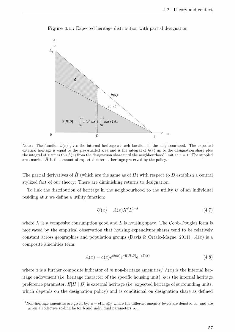
4.2. Theory and context
Figure 4.1.: Expected heritage distribution with partial designation
Notes: The function h(x) gives the internal heritage at each location in the neighbourhood. The expectedexternal heritage is equal to the grey-shaded area and is the integral of h(x) up to the designation share plusthe integral of π times this h(x) from the designation share until the neighbourhood limit at x = 1. The stippledarea marked H is the amount of expected external heritage preserved by the policy.
The partial derivatives of H (which are the same as of H) with respect to D establish a centralstylized fact of our theory: There are diminishing returns to designation.To link the distribution of heritage in the neighbourhood to the utility U of an individual
residing at x we define a utility function:
U(x) = A(x)XδL1−δ (4.7)
where X is a composite consumption good and L is housing space. The Cobb-Douglas form ismotivated by the empirical observation that housing expenditure shares tend to be relativelyconstant across geographies and population groups (Davis & Ortalo-Magne, 2011). A(x) is acomposite amenities term:
A(x) = a(x)eφh(x)eγE[H|D]e−cD(x) (4.8)
where a is a further composite indicator of m non-heritage amenities,4 h(x) is the internal her-itage endowment (i.e. heritage character of the specific housing unit), φ is the internal heritagepreference parameter, E[H | D] is external heritage (i.e. expected heritage of surrounding units,which depends on the designation policy) and is conditional on designation share as defined
4Non-heritage amenities are given by: a = bΠmaρmm where the different amenity levels are denoted am and are
given a collective scaling factor b and individual parameters ρm.
57

4. Game of zones: The economics of conservation areas
above, γ is the external heritage preference parameter, and c represents the costs of designationpolicies, which arise from the development restrictions imposed inside conservation areas. Thecost to an individual is e−cD(x) and depends on the local designation status D(x), a binaryfunction of x, which takes the value of one if x ≤ D and zero otherwise.We assume a social planner seeking a Pareto-efficient designation share, which in the model
implies maximizing the designation share (and the external heritage effects) on the conditionthat by designation utility is not reduced at any location in the neighbourhood.The positive marginal utility effect of designation at any location in the neighbourhood is
given by:dU(x)dD
= ∂U
∂E[H | D]∂E[H | D]
∂D= γU(x)h0(1− d)(1− π) (4.9)
The negative utility effect to an owner of a property changing designation status from zero toone is:
dU(x)dD
= ∂U
∂D(x)= −cU(x) (4.10)
By setting the social marginal benefit equal to the private marginal cost of an affected ownerthe planner finds the Pareto-efficient designation share D∗ by solving for D:
D∗ = 1− c
(1− π)γh0(4.11)
Based on the resulting efficiency condition we can derive some useful comparative statics (seealso Figure B.1 on page 142 in the Appendix). The (Pareto) optimal designation share isgreater when people have a greater taste for external heritage γ or where there is altogethermore heritage (determined by the heritage endowment at the neighbourhood centre h0, andimplicitly the age of the neighbourhood):
∂D∗
∂γ> 0 (4.12)
∂D∗
∂h0> 0 (4.13)
There is less optimal designation when the preservation probability π (if left undesignated)increases or if the cost of designation increases:
∂D∗
∂π< 0 (4.14)
∂D∗
∂c< 0 (4.15)
These theoretical implications are in line with intuition and can be transformed into empiricallytestable hypotheses in principle. However, the heritage at the neighbourhood centre h0, thepreservation probability π and the costs to owners of conservation policies c are all difficult toobserve in reality. For that reason we will concentrate on testing the first comparative statics
58

4.2. Theory and context
implication about taste for heritage (proxied by education level of the local population) in theempirical section.
To develop a testable hypothesis on whether the efficiency condition is fulfilled, i.e. theplanner setsD = D∗, we incorporate capitalization effects in the next step. We first assume thatindividuals maximize their utility defined above subject to a budget constraint: W = X+θ(x)L,where θ(x) is a housing bid-rent. Furthermore we assume spatial equilibrium such that alllocations offer the same level of utility U which we set equal to one:
U(x) = A(x)[δW ]δ[(1− δ)Wθ
]1−δ = U = 1 (4.16)
This can be rearranged to give the spatial equilibrium bid-rents for a representative individual:
θ(x) = (1− δ)[δδWa(x)eϕh(x)eγE[H|D]e−cD(x)]1
1−δ (4.17)
In keeping with intuition, the bid-rent increases in the expected external heritage, which de-pends on the designation share D and the internal heritage endowment h(x) and decreases inthe designation cost, which is locally constrained to x ≤ D as defined above.
The spatial equilibrium condition can be used to derive the marginal effect of an increase indesignation share on rents in the neighbourhood. At all locations in the city a marginal increasein designation share D triggers a positive effect on rent through an increase in expected externalheritage. At the margin, in addition, the change in designation status D also creates a cost.
dθ(x)dD
=
∂θ(x)
∂E[H|D]∂E[H|D]∂D
+ ∂θ(x)∂D(x)dD(x) if x = D
∂θ(x)∂E[H|D]
∂E[H|D]∂D
if x 6= D(4.18)
Substituting in the Pareto optimal designation share D = D∗ derived above we get:
dθ(x)dD
=
θ(x)1−δ [γh0(1− 1 + c
(1−π)γh0)(1− π)− c] = 0 if x = D
θ(x)1−δ [γh0(1− 1 + c
(1−π)γh0)(1− π)− c] = θ(x)
1−δ if x 6= D(4.19)
The two conditions directly translate into two testable hypotheses. If the designation process isin reality Pareto optimal, we expect the marginal effect of designation on housing rents to be zeroat newly designated locations and to be positive at all other locations in the neighbourhood.Likewise, an excessive or restrictive designation policy will be associated with negative orpositive marginal designation effects.
Assuming that the preservation probability (if undesignated) and the preservation costs areheld constant our theory predicts that, in equilibrium, (Pareto optimal) designations occuras a result of an increase in the benefits associated with (external) heritage. Such increasesin benefits will occur mechanically over time if the internal (and thus the external) heritagedepends on housing age. The effective benefits will also increase as a result of neighbourhood
59

4. Game of zones: The economics of conservation areas
turnover, if the in-migrating residents have larger heritage preferences than the incumbents.Designation then becomes a collateral effect of ‘gentrification’. The older the conservation area,the greater the accrued benefits of designation may be.Contrary to the assumption in our theory there is evidence suggesting that heritage extern-
alities (Ahlfeldt & Maennig, 2010b; Holman & Ahlfeldt, 2012) or housing externalities moregenerally (Rossi-Hansberg et al., 2010) decline quite steeply in distance. The implication isthat at the centre of a conservation area, where the effective external heritage is largest, themarginal designation benefit will be larger than at the margin. We justify our simplified theoryon the grounds that most conservation areas are small in reality even compared to the narrowscope of housing externalities. Moreover, we allow designation effects to vary in distance to theconservation area boundary and provide estimates of designation effects at the boundary, thecritical point for Pareto-efficiency as the policy benefits are presumably at their lowest.
4.2.2. Institutional context
In England, the designation of conservation areas started in 1967 and continues today underthe provisions 69 and 70 of the Planning Act 1990 (Listed Buildings and Conservation Areas).5
Conservation areas are those that have been identified as having “special architectural or historicinterest, the character or appearance of which is desirable to preserve or to enhance” (Section69). The Planning Policy Guidance Note 15 (PPG15) states that a conservation area “mayform groups of buildings, open spaces, trees, historic street patterns, village greens or featuresof historic or archaeological interest. It is the character of the areas rather than individualbuildings that conservation areas seek to enhance”. Conservation areas are designated on thegrounds of local and regional criteria. After the designation, the Local Authority has morecontrol over minor developments and the demolition of buildings (Bortrill, 2005). However,the protection an area receives when it is designated a conservation area is determined at thenational level to reflect the wider interests of society.In 2011 there were around 9,800 conservation areas in England. Conservation areas vary
in character and size. Many have strong historical links, for example an architectural styleassociated with a certain period. Besides these characteristics, designation is made based onsofter benefits said to have emanated from conservation area designation including: the creationof a unique sense of place-based identity, encouraging community cohesion, and promotingregeneration (HM Government, 2010). This ‘instrumentalisation’ of conservation policy, whichseeks to en-compass heritage values, economic values and public policy outcomes, has beenidentified as a key shift in the English policy context (Pendlebury, 2009; Strange & Whitney,2003). This is reflective of the notion of heritage not as a single definable entity, but as s
5However, the first legislation to protect the historic environment was enacted in 1882 when the AncientMonuments Protection Act was passed to protect a small number of designated ancient monuments. Morestatutory measures came into force in the ensuing years, but it was the passage of the Ancient MonumentsConsolidation and Amendment Act in 1913 that set out a more comprehensive legislative framework for theprotection of ancient monuments.
60

4.3. Empirical strategy
political, social, cultural and economic “bundle of processes” (Avrami et al., 2000, cited inPendlebury (2009) p. 7).In combination with bottom-up schemes leading to designation (e.g. community-led designa-
tion), the complex heritage preservation agenda which pursues a multitude of objectives andthe institutional setting with responsibilities shared across several institutional layers createssignificant scope for organized interest groups like property owners to influence the outcome ofa political bargaining process.
4.3. Empirical strategy
4.3.1. Designation process
The first potentially testable implications of our theoretical model are the partial derivatives(4.12) to (4.15). As mentioned in the theory section it is difficult to find feasible proxies for thevariables π, c and h0. We therefore concentrate on testing the first of these conditions, i.e., the‘taste’ for heritage γ has a positive effect on optimal designation share D∗ in a neighbourhood.We adopt the common assertion that the demand for urban consumption amenities increases ineducation and income (Brueckner et al., 1999; Carlino & Saiz, 2008; Glaeser & Gottlieb, 2006;Shapiro, 2006; van Duijn & Rouwendal, 2013). In particular, we assume that the preference forheritage γn in a neighbourhood n is related to the share of people in the neighbourhood whohold a higher education certificate (DEGi)6 with the following functional form:
γnt = DEGϑnte−εnt (4.20)
where ϑ > 0 such that the relationship is positive. Since the purpose of our empirical exerciseis to evaluate the causal impact of changes in heritage preferences on designation status - andnot the causal impact of education on heritage preference - it is sufficient to assume that ϑcaptures a correlation between education and heritage preferences. εnt is a random disturbanceterm capturing determinants of heritage preferences that are not correlated with education.Rearranging the Pareto-efficient designation share equation (4.11), substituting the educationdegree proxy relationship and taking logs we arrive at the following empirical specification:
log (1−Dnt) = α− ϑ log (DEGnt)− ωn + εnt (4.21)
where α = log (1− π)− log (c) and ωn = log (h0n) + ln (4.22)
The n subscripts correspond to the individual ‘neighbourhoods’ of our theoretical model and wechoose to represent these empirically as UK Census wards. Wards are the smallest geographicalareas that are comparable between 1991 and 2011 Censuses. Subscript t stands for time periods
6We also use income as a proxy for a subsample of our data set - results are reported in the appendix (SectionB.5.1).
61

4. Game of zones: The economics of conservation areas
for which we use the Census years of 1991 and 2011. All idiosyncratic time-invariant locationcomponents ln (location-specific determinants of designation not modelled in our theory) andthe unobserved heritage endowment h0n of a neighbourhood n as captured by ωn as well asthe preservation probability π and the costs to owners of conservation policies are removed bytaking first-differences:
∆ log (1−Dn) = ∆α− ϑ∆ log (DEGn) + ∆εn (4.23)
Our estimation equation now depicts that a neighbourhood change reflected in a positive changein (log) educational degree share causes the (logged) share of non-designated land on the left-hand side to decrease. This is just another way of saying that a positive change in educationaldegree leads to a higher designation share, although the transformation is non-linear. Notethat we implicitly assume that we are in equilibrium in the sense that all areas that should bedesignated at t are in fact designated. To support the case, we estimate our model using a longdifference between 1991 and 2011, which is more than two decades after the start of the policyand the initial wave of designations. Results for the smaller differences between 1991-2001, and2001-2011 respectively, are reported in the appendix (Section B.5.1).
Equation (4.23) evidently follows from a stylized model world. In the empirical implement-ation we add a number of covariates to control for alternative determinants of designation.The on-going designation is then only determined by the local changes in preferences and thesteady aging of buildings and the effects on heritage, which are differentiated out. To controlfor the contagion effects in designation we add the initial (1991) designation share. A num-ber of variables are added to account for heterogeneity in the net benefits of designation andabilities to express (collective) opinions in a political bargaining that may influence the desig-nation decision. These include the initial (1991) degree share, the homeownership rate, and thehousehold size (both in initial shares and changes). We alter the baseline model in a number ofrobustness checks to account for institutional heterogeneity at the TTWA level, neighbourhoodappreciation trends and, to the extent possible, the historic and physical quality of the housingstock.
In practice, however, it is difficult to control for all determinants of designation that areexternal to our model. One particular concern is that areas can be designated if the heritageis threatened by poor maintenance in a declining neighbourhood. Such derelict is likely to benegatively correlated with our explanatory variable and is unlikely to be fully captured by thecontrol variables we have at hand. At the same time, the policy itself could make it more likelythat educated people are attracted to designated areas due to a different valuation of uncertainty(reverse causality). Since an OLS estimation of equation (4.23) can result in a significant bias ineither direction we make use of instrumental variables zn, which predict changes in education,ρ(zn,∆ logDEGn) 6= 0, but must be conditionally uncorrelated with the differenced error term,ρ(zn,∆εnt) = 0. We argue that rail station (in London additionally Tube station) density aswell as effective employment accessibility (both time-invariant in levels) are good predictors of
62

4.3. Empirical strategy
neighbourhood gentrification (Florida, 2002; Glaeser et al., 2001).7 We also argue that it isunlikely that these level variables directly impact on the likelihood of designation conditionalon the unobserved heritage endowment in the fixed effects ωn.Another empirical concern is that, theoretically, a decrease in preferences for heritage must
provoke a reduction of the designated area. The abolishment of conservation areas, however, isextremely rare in England (as in most institutional contexts) so our data is left-censored (wedo not observe increases in the share of non-designated land). We therefore take the model tothe data using a tobit approach:
Y ∗n = ∆α− ϑ∆ log (DEGn) + ∆εn, ∆εn~N(0, σ2) (4.24)
Yn =
Y ∗n , if Y ∗n = ∆ log (1−Dn) < 00, if Y ∗n ≥ 0
(4.25)
4.3.2. Pareto optimality
To test whether the designation share in practice is set at the (locally) Pareto-optimal level(D∗) we estimate the effect of the event of designation on property prices within and surround-ing conservation areas. In its essence our quasi-experimental methods are a derivative of theestablished difference-in-differences (DD) methodology (Bertrand et al., 2004). We draw ele-ments of the increasingly popular regression discontinuity designs (RDD) (Imbens & Lemieux,2008), however, to relax the DD assumptions of homogeneous trends and a singular treatmentdate to separate smooth variation (e.g. externalities) and discontinuities (e.g. policy zones) intreatment effects from correlated unobservables.
Difference-in-differences
We define a group of 912 ‘treated’ conservation areas as those that were designated betweenthe years 1996 and 2010 to ensure we observe property transactions both before and after thedesignation date. Our counterfactuals are established via various control groups of housingunits that are similar to the treated units but are themselves not treated. These control groupsare discussed in more detail in the results section and in the appendix (Section B.3.2).Our baseline DD model takes the following form:
pit = βIIi + βEEi + βIPost(Ii × Postit) + βEPost(Ei × Postit) +X′
iµ+ fn + Yt + εit (4.26)
7Our measure of effective employment accessibility aggregates employment in surrounding regions weighted bydistance. We use exponential distance weights that are popular in the theoretical (Fujita & Ogawa, 1982;Rossi-Hansberg et al., 2010) and empirical literature (Ahlfeldt et al., 2012; Ahlfeldt & Wendland, 2013) andthe decay parameter estimate provided by Ahlfeldt (in press). Transport infrastructure is captured by akernel density measure (Silverman, 1986) with a radius of 2 km which is considered to be the maximumdistance people are willing to walk (Gibbons & Machin, 2005).
63

4. Game of zones: The economics of conservation areas
where pit is the natural logarithm of the transaction price for property i in time period t, Ii isa dummy variable equal to one if the observation is internal to a treated conservation area, Eiindicates observations external to the treated CA. While our standard models use a buffer areaof 500m we also experiment with various alternative spatial specifications. Postit is a dummyvariable indicating whether the transaction year t is equal to or greater than the designationyear, Xi is a vector of controls for property, neighbourhood and environmental characteristics,fn is a set of n location fixed effects and Yt are year effects. The βIPost and βEPost parametersgive the difference-in-differences estimates of the designation effect on the properties withinand just outside a conservation area. We show in Section B.3.2 that βIPost is equal to thenet marginal policy (designation costs and benefits) effect while βEPost reflects the pure (albeitspatially discounted) policy benefit.
Temporal regression discontinuity design of differences (RDD-DD)
The standard DD specification (4.26) identifies the policy treatment effect under some arguablyrestrictive assumptions. Firstly, the treatment and control groups follow the same trend beforeand after the treatment. Secondly, the treatment occurs at a singular and a priori knowndate and affects the level (and not the trend) of the outcome variable. These assumptionsare evidently violated if the outcome variable does not respond immediately to the treatment,e.g., because of costly arbitrage, or in anticipation of the treatment, for example because of aninvestment motive by buyers (Ahlfeldt & Kavetsos, 2013). In our case, a positive pre-trend canalso be associated with the gentrification that causes designation according to our theoreticalmodel, a reverse causality problem.
To address these limitations of the standard DD we refine the model to accommodate differ-ences in trends across the treatment and the control group. We borrow the functional form fromthe RDD literature where a (temporal) treatment effect is identified as an instant adjustment- a discontinuity - conditional on higher order polynomial (pre- and post-) trends, which areassumed to be unrelated to the treatment (Bento et al., 2010). In our regression discontinuitydesign of differences (RDD-DD) we combine an RDD-type polynomial specification of trendswith the control group-based counterfactual from the DD. It is therefore possible to attributepre- and post-trends to the treatment as long as it is credible to assume that treatment andcontrol groups would have followed the same trend in the absence of the treatment. It is not-able that even if this assumption is violated the RDD-DD (unlike the standard RDD) will atleast remove macro-economic shocks from the treatment effect by taking differences from thecontrol group. This improves identification so long as the control group remains unaffected bythe treatment. Our RDD-DD with linear trends takes the following form:
pit = βIIi + βIY D(Ii × Y Dit) + βEEi + βEY D(Ei × Y Dit) + βIPost(Ii × Postit)
+ βIPostY D(Ii × Postit × Y Dit) + βEPost(Ei × Postit)
+ βEPostY D(Ei × Postit × Y Dit) +X′
iµ+ fn + Yt + εit
(4.27)
64

4.3. Empirical strategy
where Y Dit is the number of years since the designation date, with the pre-designation yearshaving negative values. As in the RDD, the polynomial degree of the trend can be increasedsubject to sufficient degrees of freedom. We make use of a quadratic trend specification andevaluate the fit of the parametric polynomial function using a semi-parametric version of (4.27)that replaces the Y Dit variables with full sets of years-since-designation effects (details inSection B.3.2).
A significant ‘dis-in-diff’ parameter (βIPost or βEPost) can be entirely attributed to the treat-ment even under the existence of complex relative trends that are unrelated to the treatmentor may even have caused the treatment as the comparison is made just before and just after thetreatment date. Under the assumption of homogeneous counterfactual trends the significantpre-trend parameters (βIY D or βEY D) describe the anticipation effects. Significant post-trendparameters (βIPostY D or βEPostY D) then indicate changes in relative trends after the treatment.In conjunction, the ‘dis-in-diff’ and the pre- and post-trend parameters describe the full tem-poral structure of the treatment effect. As a program evaluation tool that is applicable to avariety of event studies, the RDD-DD thus naturally comes with a stronger test (dis-in-diff)and a weaker test (trends) of whether there exists an effect of the treatment.
Spatial regression discontinuity design of difference-in-differences (RDD-DD)
In contrast to our theory, in reality there most likely exists a spatial decay to the heritage ex-ternalities. This decay implies that the external heritage effect should be stronger at the centreof the conservation area than at the boundaries. The policy benefit, which is a transformationof the external heritage effect, should also be greater at the centre of the newly designatedconservation area. Likewise, the predicted positive policy effects just outside the boundaryshould be decaying in distance to the conservation area (CA) boundary. At the CA boundarythere may be a discontinuity as the cost of the policy ends abruptly at the boundary, whereaspotential externalities decay smoothly across it. The combination of trends and discontinuitiespotentially caused by the treatment resembles the temporal identification problem just de-scribed and will be addressed by a similar combination of RDD and DD tools. Essentially, weuse the RDD tools to capture how the difference (before and after) in the differences (treatmentvs. control) of property prices varies along the (internal and external) distances from the CAboundary. Unlike in the standard (spatial) RDD, unobserved time-invariant spatial effects canbe held constant due to the availability of spatiotemporal variation. In our spatial RDD-DDmodel it is therefore possible to attribute spatial trends (with respect to distance to the CAboundary) as well as a discontinuity (at the CA boundary) to the treatment provided that the
65

4. Game of zones: The economics of conservation areas
spatial trends are uncorrelated with unobserved temporal trends. The spatial RDD-DD weestimate takes the following form:8
pit = βITi + βID(Ti ×Di) + βIPost(Ti × Postit) + βIDPost(Ti ×Di × Postit)
+ βEOi + βOD(Oi ×Di) + βOPost(Oi × Postit) + βODPost(Oi ×Di × Postit)
+X′
iµ+ fn + Yt + εit
(4.28)
whereDi is the distance from the property to the conservation area boundary (internal distancesare negative values), Oi indicates properties outside a treated conservation area and Ti indicatesthe conservation area that is nearest to a property that is treated at any point of the studyperiod. In order to fully explore the extent of spatial externalities Oi indicates a larger areaoutside CAs rather than just within 500 m as indicated by Ei in previous models. Specifically,the empirical analysis uses properties within 1,400 m of the treated conservation area. Aswith the temporal RDD-DD specification we also estimate an expanded model specification inwhich we allow for quadratic distance trends and semi-nonparametric specifications replacingthe distance variable with some distance bin effects. The coefficient βIPost gives the interceptof the internal effect (i.e. the internal effect at the boundary) and βIDPost estimates how thischanges with respect to internal distance. Jointly, these terms capture the net policy costs andbenefits of designation for internal treated areas. A zero βIPost coefficient would be reflective ofa zero effect at the boundary and would be in line with the optimality condition derived in thetheory section. A negative βIDPost would be in line with the existence of policy benefits (dueto increased preservation probability) that spillover with decay. The parameters βOPost andβODPost allow for a spatial discontinuity treatment effect at the boundary and heterogeneityin spatial trends inside and outside the treated areas. As with βIDPost, a jointly negativeβIDPost+βODPost would be in line with the decaying policy benefits external to the conservationarea. The discontinuity at the border is measured by the external intercept term βOPost. Astatistically positive estimate would indicate a cost to the policy. A jointly positive effect ofβIPost + βOPost would in turn indicate the existence of policy benefits.
4.4. Data
We have compiled two distinct data sets for the two stages of the empirical analysis. Bothdata sets make use of data provided by English Heritage. These include a precise GIS mapof 8,167 conservation areas in England, the Conservation Areas Survey containing informationon community support and risk status (average condition, vulnerability and trajectory of aconservation) and a complete register of listed buildings.For the analysis of the determinants of designation we use UK census wards as a unit of
analysis. Shares of designated land within each Census ward are computed in a Geograph-8In models with historical CAs as control groups the following terms are also included βCD(Ci×Di)+βECECi+βECD(ECi ×Di), where Ci indicates internal to control CA and ECi external to control CA. This ensuresthat spatial effects are estimated conditional on the spatial trends in control CA.
66

4.5. Empirical results
ical Information Systems environment. Various ward level data on educational level, averagehousehold size and homeownership status and vacancy rate were obtained from the UK Census.Any changes in ward boundaries between the years were corrected for using the online conver-sion tool GeoConvert. For robustness tests we also collected a measure of the ward’s averageincome (Experian). The instrumental variables station density and employment potential areregenerated data that stem from nomis (workplace employment) and the Ordinance Survey(rail stations).For the analysis of the capitalization effects of designation we use transactions data related to
mortgages granted by the Nationwide Building Society (NBS) between 1995 and 2010. The datafor England comprise 1,088,446 observations and include the price paid for individual housingunits along with detailed property characteristics. These characteristics include floor space(m2), the type of property (detached, semi-detached, flat, bungalow or terraced), the date ofconstruction, the number of bedrooms and bathrooms, garage or parking facilities and the typeof heating. There is also some buyer information including the type of mortgage (freehold orleasehold) and whether they are a first-time buyer. Importantly, the transaction data includesthe full UK postcode of the property sold allowing it to be assigned to grid-reference coordinates.With this information it is possible within GIS to calculate distances to conservation area
borders and to determine whether the property lies inside or outside of these borders. Further-more, it is possible to calculate distances and other spatial measures (such as densities) for theamenities and environmental characteristics such as National Parks, as well as natural featureslike lakes, rivers and coastline. The postcode reference also allows a merger of transactions andvarious household characteristics (median income and ethnic composition) from the UK census,natural land cover and land use, various amenities such as access to employment opportunities,cultural and entertainment establishments and school quality. A more detailed description ofall the data used is in the appendix (Section B.4).
4.5. Empirical results
4.5.1. Designation process
Table 4.1 on page 70 reports the results of our tobit model of the designation process definedin equation (4.24). The non-instrumented baseline model is in column (1). As predicted by ourtheory, increases in educational levels that are presumably correlated with heritage preferencesare associated with reductions in the share of non-designated land. More precisely, an increasein the degree share by 1% is associated with a 0.12% reduction in the share of non-designatedland. This decrease corresponds to an 0.12% × (1 − Dt−1)/Dt−1 = 2.61% increase in theshare of designated land for a ward with the mean of the positive initial designation sharesDt−1 = 4.4%. The effect substantially increases once we instrument the change in degree shareusing rail station density and employment potential (column 2). This increase is in line withunobserved (positive) deterioration trends that a) increase the likelihood of designation andb) are negatively correlated with changes in degree share. Introducing the instruments, the
67

4. Game of zones: The economics of conservation areas
effect of a 1% increase in degree share on the share of non-designated land increases to 0.52%,which for a ward with the mean initial designation share Dt−1 corresponds to an increase in thedesignated land share of about 11%. While we have argued that our estimates are supposed toreflect a causal estimate of gentrification (proxied by degree shares) on designation probabilitiesand not necessarily a causal effect of degree share on designation share, a parameter estimate ofϑ = 0.52 is at least indicative of heritage preferences increasing relatively steeply in education.In a series of robustness checks columns (3) to (5) of the same table provide variations of the
benchmark model (2). We add TTWA effects to control for unobserved institutional heterogen-eity in column (3). Column (4) adds a measure of property price appreciation, which we obtainfrom ward-level regressions of log property prices on a time trend (and property controls, seethe appendix for details). In this specification we control for a potentially positive correlationbetween owners’ risk aversion and the value of their properties - typically their largest assets.This is a potentially important control since a larger risk aversion increases the benefit from apolicy that increases certainty regarding the future of the neighbourhood and, thus, potentiallyincreases the optimal designation share. It is a demanding control since positive price trendsare potentially endogenous to changes in neighbourhood composition and may thus absorbsome of the gentrification effect on designation. The price trends are indeed positively, thoughnot statistically significantly, associated with increases in the share of designate land. Addingcontrols capturing vacancy trends and levels, the density of listed buildings and some risk andvulnerability assessments from the Conservation Areas Survey tend to increase the educationeffect (column 5).Across all specifications we find that, besides positive changes in designation share, high initial
levels of degree shares are positively correlated with increases in the share of designated land.While high initial and positive changes in homeownership rate, ceteris paribus, are associatedwith less designation, it is notable that the (positive) impact of neighbourhood change ondesignations shares (interaction term) is particularly large in high homeownership areas (seecolumn 6). This is in line with a political economy literature that suggests that homeownerstend to form well-organized interest groups (Ahlfeldt & Maennig, 2013; Brunner & Sonstelie,2003; Dehring et al., 2008; Fischel, 2001a). Aside from the uninstrumented model (1), theresults in Table 4.1 suggest contagion effects in designation, i.e. designated land shares tend toincrease where shares were initially high.
68

4.5.Em
piricalresults
Table 4.1.: Designation process(1) (2) (3) (4) (5) (6)
Tobit IV Tobit IV Tobit IV Tobit IV Tobit IV Tobit∆ log non designation sharet
∆ log degree sharet(ϑ) -0.116*** -0.519*** -0.587*** -0.528*** -0.560*** -0.513***(0.019) (0.061) (0.105) (0.062) (0.061) (0.060)
log degree sharet−1 -0.127*** -0.276*** -0.337*** -0.280*** -0.289*** -0.269***(0.010) (0.024) (0.046) (0.024) -(0.025) (0.023)
log designation sharet−1 -0.004 -0.022* -0.027** -0.035*** -0.026* -0.025**(0.012) (0.013) (0.013) (0.013) (0.033) (0.013)
∆ log homeownershipt 0.189*** 0.263*** 0.319*** 0.262*** 0.259*** 0.255***(0.025) (0.029) (0.042) (0.029) (0.033) (0.028)
log homeownershipt−1 0.127*** 0.057*** 0.091*** 0.053*** 0.042*** 0.153***(0.015) (0.018) (0.018) (0.018) (0.018) (0.040)
∆ log aver. household 0.042 0.031 0.006 0.028 -0.009 0.047sizet (0.037) (0.040) (0.046) (0.039) (0.040) (0.040)log aver. household 0.073* -0.016 -0.122* -0.011 -0.075 -0.013sizet−1 (0.046) (0.049) (0.066) (0.049) (0.051) (0.049)log price trend -0.011
(0.021)∆ log vacancy ratet -0.021***
(0.006)log vacancy ratet−1 -0.022***
(0.010)log listed building density 1E-4
(0.004)aver. condition score -0.070***(1 best, 4 worst) (0.019)aver. vulnerability score -0.045***(1 low, 8 high) (0.017)aver. trajectory score (-2 im- 0.043proving, +2 deteriorating) (0.036)69

4.Gam
eofzones:
The
economics
ofconservationareas
∆ log degree sharet× -0.201***homeownershipt−1 (0.085)Constant 0.013 0.052 0.231* 0.018 0.039 0.096**
(0.046) (0.048) (0.119) (0.067) (0.065) (0.051)TTWA Effects No No Yes No No NoChi2 350.753 634.960 368.036 475.892 354.198ExogP 0.000 0.000 0.000 0.000 0.000Overid 0.017 0.100 0.073 0.009OveridP 0.897 0.752 0.787 0.926Observations 7965 7965 7965 7965 7965 7965Notes: ∆ log non designation sharet denotes the share of non designated land as defined by (4.23). See the data sectionfor a description of control variables. IVs are station density and employment potential in all models except model (1).Model (4) includes a dummy variable indicating 60 wards for which no price trend could be computed due to insufficienttransactions. Standard errors in parentheses and clustered on fixed effects in (3). *p< 0.05, **p< 0.01, ***p< 0.001.Chi2 is the model Wald χ2 statistic, ExogP the p-value of the Wald exogeneity test, Overid (OveridP) denotes the testof overidentifying restrictions and its p-value.
70

4.5. Empirical results
Further robustness
Our IVs comfortably pass the typical statistical tests. They are overidentified, i.e. the instru-ments are jointly valid assuming that at least one instrument is exogenous, and relevant in termsof prediction power (see first stages in Table B.5 on page 157). We have also experimented withfour alternative sets of IVs. We have moreover split up the 1991–2011 long difference into twoshorter differences (1991–2001 and 2001–2011), used the change in income as a proxy for herit-age preferences (for 2001–2011) and run the baseline model in OLS keeping only observationswith positive changes in shares of designated land. The results are presented in the appendix(Section B.4) and support those discussed here.
4.5.2. Pareto optimality
Difference-in-Differences
Table 4.2 on page 73 shows the results from an estimation of the standard DD equation (4.26)for different selections of control groups and fixed effects. Each model includes controls forproperty, location, and neighbourhood characteristics, year effects and location fixed effects tohold unobserved time-invariant effects constant. Column (1) is a naïve DD using the meanprice trend of all properties located beyond 500 m of a treated conservation area as a coun-terfactual. Columns (2) to (7) provide more credible counterfactuals by restricting the controlgroup to properties that are presumably similar to the treated properties. Column (2), withward fixed effects, and (3), with nearest CA fixed effects, provide a spatial matching by restrict-ing the sample to properties within 2 km of a treated CA, where many unobserved locationcharacteristics are likely to be similar. In column (4) we impose the additional restriction thatproperties in the control group must fall within 500 m of the boundaries of a historically des-ignated conservation area (before 1996), which increases the likelihood of unobserved propertycharacteristics being similar. While areas that are designated at any point in time are likelyto share many similarities, the diminishing returns to designation in our theoretical frameworkalso imply that heritage-richer areas should generally be designated first. To evaluate whetherthe designation date of the treated conservation areas, relative to those on the control group,influences the DD estimate, we define CA designated 1996–2002 as a treatment group and formcontrol groups based on CAs designated just before (1987–1994) or right after (2003–2010) incolumns (5) and (6). In column (7), finally, we use environmental, property and neighbour-hood characteristics to estimate the propensity of being in a treated (1996–2010) CA over ahistorical (<1996) CA. Then the treated CAs are matched to their ‘nearest-neighbour’, i.e. themost similar non-treated CA, based on the estimated propensity score (Rosenbaum & Rubin,1983). A fixed effect is defined for each treated CA and its nearest-neighbour control CA suchthat the treatment effect is estimated by the direct comparison between the treated CA andits nearest-neighbour.We anticipate that the strength of the counterfactual increases as we match the treatment and
control group based on proximity (2 and 3), proximity and qualifying for designation (4, 5 and
71

4. Game of zones: The economics of conservation areas
6) and qualifying for designation and a combination of various observable characteristics (7).As the credibility of the counterfactual increases, the statistical significance of the treatmenteffect tends to decrease. Benchmarked against the nationwide property price trend both theinternal effect (Inside × Post) and the external effect (Within 500 m × Post) are significant atthe 5% level. The magnitudes of these effects are of similar size, implying a 2.8% premium forhouses inside newly designated conservation areas and a 2.3% premium outside. The spatialmatching (2 and 3) renders the internal treatment effect insignificant (2 and 3). With furtherrefinements in the matching procedure the external effect also becomes insignificant. Table 4.2results, thus, suggest that designation does not lead to significant property price adjustments.Evidence is weak for positive (policy) spillovers to nearby areas.
72

4.5.Em
piricalresults
Table 4.2.: Conservation area premium – designation effect(1) (2) (3) (4) (5) (6) (7)
log property transaction priceInside treated CA × 0.028*** 0.014 0.014 0.003 -0.024 -0.077 -0.003Post designation (0.009) (0.009) (0.010) (0.012) (0.070) (0.111) (0.015)Within 500 m buffer of 0.023*** 0.013*** 0.012*** 0.004 0.012 -0.005 -0.005treated CA × Post des. (0.004) (0.004) (0.005) (0.006) (0.027) (0.022) (0.010)Inside treated CA -0.043*** -0.038*** -0.048*** -0.037*** -0.062 0.029 -0.024
(0.009) (0.009) (0.010) (0.012) (0.057) (0.108) (0.021)Within 500 m buffer of -0.010** -0.004 -0.011** -0.005 0.003 0.006 -0.002treated CA (0.004) (0.004) (0.005) (0.005) (0.030) (0.023) (0.013)Hedonic controls Yes Yes Yes Yes Yes Yes YesLocation controls Yes Yes Yes Yes Yes Yes YesNeighbourhood controls Yes Yes Yes Yes Yes Yes YesYear effects Yes Yes Yes Yes Yes Yes YesWard effects Yes Yes No No No No NoNearest treated CA effects No No Yes Yes Yes Yes NoMatched CA effects No No No No No No YesTreatment group: 1996-2010 1996-2010 1996-2010 1996-2010 1996-2002 1996-2002 1996-2010CAs designatedControl group Full England Within 2 km Within 2 km Within 500 m Within 500 m Within 500 m Within 500 m
sample of treated CA of treated CA of CA des- of CA des- of CA des- of pre-1996ignated before ignated before ignated before CA matched1996 & within 1987-95 & 2003-10 & on propen-2 km of treated within 2 km of within 2 km of sity score
CA treated CA treated CAR2 0.921 0.922 0.915 0.915 0.861 0.864 0.909AIC -587375 -156426 -130469 -67046 -5409 -8476 -41184Observation 1,088k 302k 302k 178k 21k 32k 133kNotes: Standard errors in parentheses are clustered on location fixed effects. Conservation area control groups in columns (4)-(7) have separate fixed effectsfor the areas inside and outside a conservation area. *p<0.10, **p<0.05, ***p<0.01.
73

4. Game of zones: The economics of conservation areas
Temporal RDD-DD
Table 4.3 on page 76 illustrates the results of the estimation of the (temporal) RDD-DD outlinedin equation (4.27). We present the results of a variety of models that feature linear (1–5)and quadratic (6–10) trends and several of the control groups utilized in Table 4.3. Oneimportant finding across these specifications is that the external (Within 500m × Post) ‘dis-in-diff’ parameter estimate is significant in four of 10 specifications at the 5% level and in one halfof the specifications at the 10% level, whereas, the internal (Inside × Post) parameter is onlysignificant in one specification at the 10% level (column 8). This suggests primarily that thereexists a significant treatment effect exactly at the treatment date only for the external area.This interpretation is in line with the predictions of our theoretical model. Another findingillustrated by Table 4.3 is the positive change in the internal price trend after a CA has beendesignated (Inside treated CA × Post designation × Years designated). The change in trend,which is significant at the 5% level in seven of the 10 models, may be regarded as evidencefor a cumulative internal effect of the designation policy. There is also a faster appreciationin the external area post-designation that is significant in four of the 10 models. In short, thetemporal RDD-DD has confirmed that designation policy causes no immediate effect insidethe conservation area but shows instead that it increases the speed of price appreciation overtime. The RDD-DD has also uncovered that areas external to the conservation area receive animmediate shift in prices at the designation date in line with our theoretical hypothesis.Figure 4.2 on page 77 provides a graphical illustration of the predicted effect of being in the
treatment group over the control group against years-since-designation. A horizontal red line isdrawn at the mean of the pre-treatment effects in order to illustrate the differences between theRDD-DD results and those of the standard DD. The positive impact of designation on (relative)price trends suggested by the RDD-DD (black lines) is supported by the functionally moreflexible semi-parametric estimates for the ‘years-since-designation bins’ (grey dots).9 However,the post-treatment effects are never statistically distinguished from the pre-period mean, whichis in line with the DD estimates.Figure 4.3 on page 78 provides an analogical illustration for the external treatment effect,
i.e. the spillovers onto areas adjacent to the designated CAs. Again, the post-period estimatesdo not deviate significantly from the pre-period mean. However, the top-left panel illustratesa large discontinuity at the treatment date that is statistically significant in Table 4.3 on page76. As with the internal effects, there is a positive trend shift post-designation.
9Confidence bands for the semi-parametric ‘bins’ model are presented in the appendix (Section B.5.2).
74

4.5.Em
piricalresults
Table 4.3.: Regression discontinuity design of differences between treatment and control (RDD-DD)(1) (2) (3) (4) (5) (6) (7) (8) (9) (10)
log property transaction priceInside treated CA × 0.015 0.022 0.024 0.027 -0.006 0.023 0.033 0.038* 0.036 0.020Post designation (0.015) (0.015) (0.015) (0.017) (0.018) (0.023) (0.021) (0.023) (0.024) (0.024)Within 500m buffer of 0.006 0.013* 0.015** 0.020** -0.007 0.013 0.017** 0.022** 0.017 0.009treated CA × Post des. (0.007) (0.007) (0.007) (0.008) (0.003) (0.008) (0.008) (0.009) (0.010) (0.014)Inside treated CA × 0.000 -0.004 -0.004 -0.007** -0.002 -0.010 -0.016* -0.019* -0.019* -0.020*Years designated (0.003) (0.003) (0.003) (0.003) (0.003) (0.010) (0.009) (0.010) (0.010) (0.011)Inside treated CA × -0.001 -0.001 -0.001 -0.001 -0.002*Years designated2 (0.001) (0.001) (0.001) (0.001) (0.001)Inside treated CA × post 0.003 0.007** 0.008** 0.009** 0.008* 0.020 0.026** 0.032** 0.031** 0.031designation × Years des. (0.003) (0.003) (0.003) (0.004) (0.004) (0.014) (0.012) (0.013) (0.013) (0.014)Inside treated CA × post 0.000 0.000 0.000 0.000 0.001designation ×Years des.2 (0.001) (0.001) (0.001) (0.001) (0.001)Within 500m of treated 0.002 -0.002* -0.002* -0.004*** -0.001 -0.001 -0.004 -0.007* -0.004 -0.009CA × Years des. (0.001) (0.001) (0.001) (0.001) (0.002) (0.004) (0.004) (0.004) (0.005) (0.007)Within 500m of treated -0.000 -0.000 -0.000 0.000 -0.001CA ×Years des.2 (0.000) (0.000) (0.000) (0.000) (0.001)Within 500m of treated CA × 0.001 0.004*** 0.004*** 0.005*** 0.003 0.003 0.007 0.011** 0.008 0.009post des. × Years des. (0.002) (0.001) (0.001) (0.002) (0.003) (0.005) (0.005) (0.005) (0.006) (0.010)Within 500m of treated CA × 0.000 0.000 0.000 -0.000 0.001post des. ×Years des.2 (0.000) (0.000) (0.000) (0.000) (0.001)Hedonic controls Yes Yes Yes Yes Yes Yes Yes Yes Yes YesLocation controls Yes Yes Yes Yes Yes Yes Yes Yes Yes YesNeighbourhood controls Yes Yes Yes Yes Yes Yes Yes Yes Yes YesYear effects Yes Yes Yes Yes Yes Yes Yes Yes Yes YesWard effects Yes Yes No No No Yes Yes No No NoNearest treated CA effects No No Yes Yes No No No Yes Yes NoMatched CA effects No No No No Yes No No No No YesControl group as in (1) (2) (3) (4) (7) (1) (2) (3) (4) (7)prev. Tab., column75

4.Gam
eofzones:
The
economics
ofconservationareas
R2 0.920 0.921 0.912 0.914 0.907 0.920 0.921 0.912 0.914 0.907AIC -547688 -147818 -120160 -64425 -39321 -548078 -147839 -120191 -64467 -39329Observation 995k 277k 277k 164k 123k 995k 277k 277k 164k 123kNotes: Standard errors in parentheses are clustered on location fixed effects. Conservation area control groups in columns (4)-(7) have separate fixed effects forthe areas inside and outside a conservation area. Observations dropped if years designated falls outside of range -10/+10 years. *p<0.10, **p<0.05, ***p<0.01.
76

4.5. Empirical results
Figure 4.2.: RDD-DD internal estimates
(a) Nearest treated CA (linear trends)Tab. 4.3, column (4)
(b) Matched CA (linear trends)Tab. 4.3, column (5)
(c) Nearest treated CA (quadratic trends)Tab. 4.3, column (9)
(d) Matched CA (quadratic trends)Tab. 4.3, column (10)
Note: The solid lines are graphical illustrations of the parametric estimates presented in Table 4.3 on page 76and estimated using equation (4.27). The dashed lines indicate the 95% CI which are calculated using standarderrors of multiplicative interaction terms presented by Aiken et al. (1991). The grey dots plot the point estimatesof ‘years-since-designation bins’ effects obtained from separate regression described and presented in more detailin the appendix (Section B.5.2). The horizontal red line illustrates the mean of the pre-treatment estimates.
Spatial RDD-DD
Table 4.4 on page 80 shows the results of the estimation of the (spatial) RDD-DD modeloutlined in equation (4.28). As with the temporal RDD-DD, we present the results of a varietyof models that feature linear (1–5) and quadratic (6–10) trends and several of the controlgroups utilized in Table 4.2. One interesting and consistent feature of Table 4.4 is that thepositive dis-continuity coefficient (Outside × Post) matches the expected (positive) sign underthe existence of a policy cost inside. However, the parameter is statistically insignificant in allmodels.
77

4. Game of zones: The economics of conservation areas
Figure 4.3.: RDD-DD external estimates
(a) Pre-1996 CA within 2 km (linear trends)Tab. 4.3, column (4)
(b) Matched pre-1996 CA (linear trends)Tab. 4.3, column (5)
(c) Pre-1996 CA within 2 km (quadratic trends)Tab. 4.3, column (9)
(d) Matched pre-1996 CA (quadratic trends)Tab. 4.3, column (10)
Note: The solid lines are graphical illustrations of the parametric estimates presented in Table 4.3 on page 76and estimated using equation (4.27). The dashed lines indicate the 95% CI which are calculated using standarderrors of multiplicative interaction terms presented Aiken et al. (1991). The grey dots plot the point estimatesof ‘years-since-designation bins’ effects obtained from separate regression described and presented in more detailin the appendix (Section B.5.2). The horizontal red line illustrates the mean of the pre-treatment estimates.
78

4.5.Em
piricalresults
Table 4.4.: Spatial regression discontinuity design of difference-in-differences (RDD-DD)(1) (2) (3) (4) (5) (6) (7) (8) (9) (10)
log property transaction priceWithin 1.4km of treat. 0.027*** 0.014 0.012 0.008 -0.003 0.026** 0.014 0.012 0.008 -0.005CA × post des. (0.010) (0.010) (0.011) (0.011) (0.014) (0.011) (0.012) (0.012) (0.012) (0.015)Within 1.4km of treat. CA × -0.057 -0.032 -0.030 -0.029 -0.070 -0.096 -0.046 -0.040 -0.040 -0.118dist. to boundary × post des. (0.081) (0.075) (0.080) (0.077) (0.068) (0.156) (0.154) (0.162) (0.157) (0.143)Within 1.4km of treat. CA × -0.059 -0.017 -0.018 -0.017 -0.099dist. to boundary2× post des. (0.132) (0.131) (0.140) (0.136) (0.130)Outside treated CA × 0.004 0.005 0.005 0.004 0.010 0.009 0.009 0.008 0.009 0.016post design. (0.010) (0.010) (0.010) (0.009) (0.011) (0.012) (0.012) (0.011) (0.011) (0.012)Outside treated CA × dist. 0.039 0.016 0.013 0.011 0.046 0.064 0.014 0.013 0.004 0.080to boundary × post des. (0.081) (0.075) (0.080) (0.078) (0.069) (0.157) (0.155) (0.163) (0.159) (0.145)Outside treated CA × dist. 0.070 0.028 0.025 0.029 0.109to boundary2× post des. (0.133) (0.132) (0.140) (0.136) (0.130)Hedonic controls Yes Yes Yes Yes Yes Yes Yes Yes Yes YesLocation controls Yes Yes Yes Yes Yes Yes Yes Yes Yes YesNeighbourhood controls Yes Yes Yes Yes Yes Yes Yes Yes Yes YesYear effects Yes Yes Yes Yes Yes Yes Yes Yes Yes YesWard effects Yes Yes No No No Yes Yes No No NoNearest treated CA effects No No Yes Yes No No No Yes Yes NoMatched CA effects No No No No Yes No No No No YesControl group Full Eng- Within Within Within Within Full Eng- Within Within Within Within
land 2 km of 2 km of 1.4 km of 1.4 km land 2 km of 2 km of 1.4 km of 1.4 kmsample treated treated CA de- pre-1996 sample treated treated CA de- pre-1996
CA CA signated CA CA CA signated CAbefore matched before matched1996 & on pro- 1996 & on pro-within pensity within pensity2km of score 2km of scoretreaded treadedCA CA79

4.Gam
eofzones:
The
economics
ofconservationareas
R2 0.921 0.922 0.915 0.914 0.905 0.921 0.922 0.915 0.914 0.921AIC -587538 -156448 -130478 -118076 -101076 -587533 -156444 -130478 -118074 -587538Observation 1,088k 302k 302k 281k 327k 1,088k 302k 302k 281k 327kNotes: Standard errors in parentheses are clustered on the location fixed effects. *p< 0.10, **p< 0.05, ***p< 0.01.
80

4.5. Empirical results
Figure 4.4.: RDD-DD spatial treatment effects
(a) Pre-1996 CA within 2 km (linear trends)Tab. 4.4, column (4)
(b) Matched pre-1996 CA (linear trends)Tab. 4.4, column (5)
(c) Pre-1996 CA within 2 km (quadratic trends)Tab. 4.4, column (9)
(d) Matched pre-1996 CA (quadratic trends)Tab. 4.4, column (10)
Note: The solid lines are graphical illustrations of the parametric estimates presented in Table 4.4 on page 80and estimated using equation (4.28). The dashed lines indicate the 95% CI which are calculated using standarderrors of multiplicative interaction terms presented by Aiken et al. (1991).
We have argued that the model predictions for capitalization effects under a (locally) efficientdesignation policy and a spatial decay in heritage externalities hold at the conservation areaboundary, i.e. we expect a zero effect just inside and a positive effect just outside the boundary.Figure 4.4 on page 81 illustrates the joint effect of the parametric estimates reported in Table4.4 on page 80 at varying (internal and external) distances from the CA boundary. With thecontrol group of historical CAs within 2 km of the treatment CA (left panels) we find a positivecapitalization effect just inside and outside the boundary, which is in line with the baseline DDresult in Table 4.2 on page 73, column (4). Moreover, the treatment effect increases towardthe centre for the CA and decreases in external distance to the boundary until it becomeszero at around 700 m. This distance is in line with existing evidence on a relatively steepdecay in heritage and housing externalities (Ahlfeldt & Maennig, 2010b; Lazrak et al., 2013;Rossi-Hansberg et al., 2010). However, the effect is statistically indistinguishable from zero at
81

4. Game of zones: The economics of conservation areas
almost all distances. The single exception is a significant (at 5% level) 1.6% effect just outsidethe CA in the quadratic model. While the effect is only significant within 100 m of the CA,this is precisely where we expect a positive effect in a world with spatial decay in heritage(housing) externalities. In the context of the model the lower and not statistically significanteffect just inside the CA indicates the presence of a cost that compensates for some of thebenefits associated with designation.With the control group of matched CAs (right panels) the treatment effect just inside the
CA boundary is remarkably close to zero. The joint effect just outside the boundary is positive,although not statistically significant. Briefly summarized, the spatial RDD-DD model suggeststhat across the treated CAs owners - at least on average - are not harmed by designation. Thereis some evidence that owners just outside a conservation area receive some benefit.
4.6. Summary
Historic preservation policies are among the most restrictive planning policies used to overcomecoordination problems in the housing market internationally. These policies aim at increasingsocial welfare at the cost of constraining individual property rights. From the perspective ofowners of properties in conservation areas, the policy may help to solve a collective actionproblem, preventing owners from free riding on the heritage character of nearby buildings whileinappropriately altering their own property. If property owners value the heritage character ofnearby buildings and can influence the designation process they will seek out a (local) level ofdesignation where the marginal costs of designation equate the marginal benefits. An increasein the marginal benefit of designation will lead to an increase in designation activity. If thepolicy is Pareto-efficient, additional designations in a neighbourhood will not lead to an adverseimpact on those being designated.We provide evidence that is supportive of this scenario using two empirical approaches that
follow from a simple model of (locally) efficient conservation area designation. First, we presenta neighbourhood level IV tobit analysis that reveals a positive impact of an increase in degreeshare, which is presumably (positively) correlated with heritage preferences, on the share ofdesignated land. Gentrification, by increasing the value of neighbourhood stability to local own-ers, can cause designation. Second, we combine the strengths of difference-in-differences (DD)and regression discontinuity designs (RDD) to estimate the capitalization effect of designationon newly designated areas as well as spillovers to adjacent areas. This RDD-DD methodologyqualifies more generally as a useful tool for program evaluations where a treatment is suspec-ted to lead to an impact on (spatial or temporal) trends and discontinuities. Within newlydesignated conservation areas we find no significant short-run effects of designation and someevidence for positive capitalization effects in the long run. There is some evidence for positivespillovers onto properties just outside.These results are in line with a Pareto-efficient designation policy, at least from the perspect-
ive of the local owners. Either, the policy is deliberately Pareto-maximizing local owner welfare
82

4.6. Summary
or, as suggested in the literature on the political economy of housing markets, homeowners areable to successfully influence the outcome of local policies in their interest. In any case, it isimportant to note that our results do not imply that the policy is necessarily welfare-enhancingon a wider geographic scale. Depending on the excessiveness of the policy and the generalrestrictiveness of the planning system, historic preservation may constrain housing supply andgenerate welfare losses. The net-welfare effect to a wider housing market area is an interestingand important question that we leave to future research.
83


5. Chicken or egg? Transport andurban development in Berlin
5.1. Motivation
As reviewed in Section 2.5, infrastructure and especially mass transit play a major role ineconomics and especially in urban economics. Transport induces welfare effects due to increasedaccessibility and reduced shipping costs and impacts on the location of households and firms.Estimating the impact of transport infrastructure is, however, not entirely straightforward sincethe relation between transport and economic activity is plagued by a notorious simultaneityproblem. While the view that an ease of access to other locations within a region should have apositive impact on the attractiveness of a location is unchallenged, it is also hard to believe thatthe allocation of transport is completely random. Due to the demand required to recover largeinvestment costs, new infrastructure is more likely to connect economically successful places.Recent research has approached this problem by only focusing on the uni-directional effect oftransport provision, building causal inference on quasi-experimental and instrumental variablestrategies.
However, it is very difficult to address the simultaneity problem entirely with conventionalmodels. It is challenging to assess to which extent the reverse causation is an empiricallyrelevant phenomenon because instruments for this direction are particularly difficult to find.Moreover, it is a priori unclear whether the planner responds to economic activity broadlydefined – and reflected in land values – or absolute demand from potential passengers – reflectedin population. Effectively, the relation can be described by a complex structure of variousendogenous variables whose mutual causal links are difficult to model with the standard toolsets of causal inference. Theory offers some guidance on the potential directions and temporalsequence of the dependencies, but ultimately fails in producing predictions that would allowus to describe the whole dynamic process by a causal relationship of X on Y . A methodthat is well established to explore the structure of mutually related endogenous variables is thestructural vector auto regression (SVAR) model. Commonly used in macroeconomics whereisolated shocks are hard to observe and models consist of many endogenous variables, VARmodels have become a well-established method to describe complex dynamic relations. Themethod can be adopted to incorporate spatial information in a Panel VAR (PVAR), where theregions form a cross-sectional dimension. This method is proposed as an informative tool to go
85

5. Chicken or egg? Transport and urban development in Berlin
beyond the state of knowledge that has been achieved in the transport economics literature onthe uni-directional effects of transport on land (or property) value.
Unfortunately, as with most applications of empirical methods, the benefits do not comewithout costs. Causality in a narrow sense is an issue, and while the PVAR strength is tomodel the simultaneous relationships of the most important variables conditional on each other,it is vulnerable to variables that belong to the (unknown) full model, but are omitted fromthe analysis. Also it is difficult to parameterize the strength of the (mutual) dependenciesanalysed. Acknowledging the strength and weaknesses, I believe that the novel applicationof the established PVAR method to a well-known estimation problem has the potential tocomplement existing uni-directional causal research by providing a better picture of the generaldynamics.
In line with the macroeconomic approach, a dynamic study area is required characterisedby a battery of shocks. These criteria can typically be found in massively growing developingcountries and their metropolises. However, reliable data for a spatially fine level and a suffi-ciently long time period is difficult to find for these cities. I therefore look into the history of aby now developed city and employ a unique historic dataset for Berlin between 1881 and 1935for the analysis. This period is characterised by great infrastructure projects as well as a stronggrowth in population, which enables me to empirically address the research question. I try tofill a gap of studies fully exploiting changes in the transport infrastructure, most probably dueto a scarcity of projects, as noted by Gibbons & Machin (2008). In line with Baum-Snow et al.(2012) I argue that the analysis of public infrastructure during that time is of special interestas the city was industrialising, economically developing and characterised by huge transport in-vestments somehow comparable to the process developing countries experience today. Moreoverautomobiles can largely be ignored as transport mode.
The analysis follows a twofold approach: Firstly, I estimate the interaction between popu-lation and transport. Secondly, the analysis is extended by looking into the relation betweenland values and transport. I separately estimate the empirical model for a core and a peripheralsample in order to allow for potential outbidding. The estimates suggest a simultaneous relationbetween transport and urban development. Planners, however, follow only economic activitybut not residents. I find evidence for an outbidding of residents due to transport innovations.The results are proven robust to price anticipation effects.
The remainder of this chapter is structured as follows. The next Section 5.2 provides ahistorical overview of the Berlin transport sector. This is followed by an introduction of ourhistorical dataset in Section 5.3 as well as of the PVAR methodology in Section 5.4. In Section5.5, the empirical findings of the benchmark models as well as of additional robustness tests arereported and interpreted. Section 5.6 briefly summarizes and comments on the main findings.
86

5.2. Historical background
5.2. Historical background
The public rail network in Berlin is made up of two different modes, namely a rapid transitsystem (“S-Bahn”) and the underground (“U-Bahn”). This section provides a brief overviewof its historical development.
5.2.1. S-Bahn
Berlin’s rapid transit system as it is known today is a result of combining various suburbanlines (“Vorortsbahn”), the original city line (“Stadtbahn”) and the circular line (“Ringbahn”)in 1930. Therefore, there are various reasons and purposes why, where and how the S-Bahnwas developed over the years (Klünner, 1985; Gottwaldt, 1994; Kiebert, 2004, 2008).The suburban lines connected Berlin with surrounding cities and its suburbs. Especially the
early lines originate from long-distance connections to major cities like Potsdam (“Stammbahn”1838), Hamburg (“Hamburger Bahn” 1846) or Dresden (“Dresdner Bahn” 1887). Initially, thelong-distance lines had to share their tracks with the new upcoming suburban lines. In 1891a new tariff system for local mass transit was introduced, pushing up the passenger numbersby about 30% and the suburban lines increasingly started to run on their own tracks. Themajority of these lines were developed by public companies and planned by the government.For instance, the “Ostbahn”, which was intended to go through the Prussian regions of Pom-mern and East Prussia, was built in order to develop the periphery along the tracks. The“Görlizer Bahn” (1866/67) or the “Wetzlarer Bahn” (also “Canon Train”), linking Berlin withMetz at the French border, were planned by the military in order to move troops more rap-idly. Later on, new lines were directly built for local mass transit in order to improve accessfrom the periphery, like the North-South connection (1934-39). However, private developerslike J.A.W. Carsten, who financed the station “Lichterfelde” (1868) in order to sell his newlyestablished country estates in that area, intervened in the expansion of the S-Bahn networkas well. The electronics company Siemens further financially supported the exploitation of thesection between Fürstenbrunn and Siemensstadt (1905) in order to improve the commutingsituation for its workers. Moreover, Spindler Brothers, who ran a laundry and drying factoryin Köpenick at the Eastern border of the city, were strongly in favour of building a transportline between Schöneweide and Spindlersfelde (1891). Hence, the suburban lines were driven byboth public and private interests.The city line went from Stralau-Rummelsburg to Westkreuz, Halensee and was built in 1882.
This East-West connection running through the historical city centre was planned to decongestthe traffic between Berlin’s terminal stations. The tracks were mainly built on land owned bythe government and the project was carried out publicly.The first sections of the circular line Moabit-Gesundbrunnen-Potsdamer-Ringbahnhof and
Moabit-Charlottenburg-(Westend)-Grunewald-Tempelhof were opened in 1881, and 1882 re-spectively. The circular line was financed by the state of Prussia but run by the Niederschlesisch-Märkische Eisenbahn, a public company owned by Prussia. The idea behind the circular line
87

5. Chicken or egg? Transport and urban development in Berlin
was to connect radian lines extending from the centre with each other and the important ter-minal stations. Various parts of the new line were built on undeveloped land and thus outsidethe city border. Or, as Elkins & Hofmeister (1988) state: “The actual position of the ringline was a compromise between the desire to maximise utilization by being as close as possibleto the core of the city and the desire to minimize land-acquisition costs by avoiding areas ofexisting urban development” (p. 114).Like the circular line, many other lines of the light rail system were extended into undeveloped
areas, connecting Berlin with other villages. Only the East-West and North-South connectionswent through the city centre. New villages were founded close to the new lines, such as “Gli-enicke an der Nordbahn”. Companies like AEG or Borsigwerke in Tegel built new factories inclose proximity to the new stations (e.g. “Kremmener Bahn”). Even though a few rapid transitlines were developed at the request of the private sector, most of the lines were developed by thepublic sector. In the 1880s the majority of the long-distance lines, which were closely related tothe rise of the suburban lines, were nationalised. However, most of the nationalised lines werestill run independently. They had their own management as well as their own trains/coaches.From 1920 on, all lines were eventually nationalised under the “Reichseisenbahn”.
5.2.2. U-Bahn
The underground was developed about a third of a century later than the rapid transit system.The first line was opened in 1902 and went from Stralauer Tor (later Warschauer Brücke) toPotsdamer Platz and then to Zoo. The first underground was constructed on elevated trackssince the Berlin government was afraid of damaging its newly installed drainage system. Theproject was pushed forward by the company “Siemens & Halske”, which as far back as 1891proposed a densely linked network, connecting the historic city centre to its surrounding mu-nicipalities. The new line was eventually developed by the “Hochbahngesellschaft” a companyjointly founded by Siemens & Halske and Deutsche Bank as the main funder. While the line’sEastern section to Nollendorf Platz was built on viaducts, the city of Charlottenburg success-fully negotiated the tracks to run under ground when passing though its territory. Not obscuringthe view of the prominent church “Kaiser-Wilhelm-Gedächtniskirche” was one of Charlotten-burg’s reasons for the changed routing. In the West (Westend), the line was extended into anundeveloped area where Deutsche Bank owned land. Driven by financial speculations the bankwas expecting rising land rents due to improved access. As a result of the newly establishedconnection, Western Charlottenburg turned into an attractive business area. The extensionof the first underground line leading into central Berlin was initially hampered by the tramoperator “Große-Berliner-Straßenbahn” being afraid of losing its monopolistic role in that area.Despite the concerns, the line eventually went via Mohrenstraße and Spittelmarkt through thecity centre (Gottwaldt, 1994).Especially the municipalities in the South West had great interest in developing their un-
developed land. They competed for wealthy citizens by turning it into attractive residen-tial areas. The underground played a crucial role in developing these areas. The city of
88

5.3. Data
Schöneberg (“Schöneberger Linie” 1910) even planned and financed its own line between Nol-lendorfplatz and Hauptstraße (today Innsbrucker Platz) in order to develop its Western ter-ritory. As the “Hochbahngesellschaft” did not expect any profits from the new line it wascompletely planned as a public enterprise. The area through which Schöneberger Linie ranchanged significantly. Individually designed stations were built at prominent squares. A sim-ilar approach was followed by the villages of Wilmersdorf and Dahlem. Newly planned countryestates and academic institutes were supposed to benefit from improved access by construct-ing the “Wilmersdorf-Dahlemer U-Bahn” (1913). The line was divided into three sectionsregarding ownership: While the section between Wittenbergplatz and Nürnberger Platz be-longed to the Hochbahngesellschaft, Nürnberger Platz-Breitenbachplatz was owned by the cityof Wilmersdorf and Breitenbachpatz-Thielplatz by Domäne Dahlem. The line was extended tothe lake “Krumme Lanke” in 1929. This extension was mainly financed by the land speculatorand private developer Adolf Sommerfeld in order to connect his newly established residentialquarters in Dahlem. Moreover, he wanted to improve the access to the surrounding woods,establishing them as recreational areas (Kurpjuweit & Meyer-Kronthaler, 2009).
In contrast to the S-Bahn network, Berlin’s underground was intended to serve local masstransit from the beginning. The lines were extended into more central areas. Moreover, the net-work was developed later than the rapid transit system; the technology was superior, allowingfor an underground system, and planners as well as investors had already gained experience byevaluating the effects of the S-Bahn. Anecdotal evidence suggests that the rise of the U-Bahnwas mainly driven by the idea of developing new land in close proximity to the historical core(especially in the South West). Public as well as private planners competed for wealthy citizensand increasing land rents.
Summing up, even though the link between transport and land development is not completelyclear when analysing the history of Berlin’s transport system, the majority of the projects andnewly constructed lines seemed to lead the development in an area and not the other wayaround.
5.3. Data
This section provides a brief overview of the historic data used in the main analysis. Thedata differ in time as well as in spatial coverage and level of detail. Since spatial aggrega-tion/disaggregation might result in a loss of information or biased estimates (modifiable areaunit problem, MAUP) I decided to work with distinct panels. I end up with three samples:(i) I estimate the interaction between transport and population at a municipality (“Ortsteile”)level of 93 municipalities using data for every five years from 1870 to 1935 (14 time periods),(ii) the relation between transport and land values is estimated on a block level covering 2,481blocks of an inner sample of historical land value maps between 1881 and 1914 (7 time periods),as well as on (iii) a grid square level (length of 150 m, 12,596 grid squares) making use of the
89

5. Chicken or egg? Transport and urban development in Berlin
full extent of the historical sources which are further explained in the next paragraphs (see alsoTable 5.1 on page 90).1
Table 5.1.: Twofold approach - three samplesPanel Development indicator Unit of analysis Spatial coverage Time period1 Population Municipality Gross Berlin 1870-19352 Land values Historical city block Inner Müller sample 1881-19143 Land values Grid (150 m) Müller sample 1881-1914
Table 5.2.: Number of stationsYear S-Bahn U-Bahn Total1870 18 0 181875 31 0 311880 55 0 551885 64 0 641890 65 0 651895 88 0 881900 96 0 961905 103 15 1181910 109 28 1371915 109 46 1551920 112 46 1581925 113 60 1731930 120 94 2141935 127 94 221
To compute rail densities, the historic transport network of Berlin has been reconstructedfor the entire observation period (1870-1935/36) in a geographic information system (GIS)environment (Schomacker, 2009; Mauruszat, 2010; Straschewski, 2011). Similar to Levinson(2008) and in line with the density measures used in the previous analyses, station densities forthe combined network are computed using a kernel with a radius of 2 km (Silverman, 1986).By choosing this radius I follow Gibbons & Machin (2005) who estimate a distance of 2 kmas the maximum distance people are willing to walk to the nearest station. By definition, thedensity measure reflects the degree of network concentration. It is high in areas which arecharacterised by a high number of stations in close distance, and low vice versa. The measuredoes not, however, incorporate the number of lines which run through a station, the traveltime/speed and the frequency for which I do not have data for either. I compute a joint stationdensity since the two rail systems cannot be regarded as substitutes for each other: The rapid
1To address any concerns regarding the modifiable area unit problem, the grid sample approach has additionallybeen carried out for a 300 m grid sample (Appendix Section C.2).
90

5.3. Data
Figure 5.1.: Combined rail network in 1870, 1900 and 1935
Notes: The lines indicate the combined rail network, i.e. the rapid transit system and the underground linesthat were added up to each respective year.
transit system was developed earlier and originates from inter-city connections. Conversely,the underground was built as public transport mode from the very beginning and runs throughmore central areas.
Figure 5.1 on page 91 and Figure 5.2 on page 92 provide an overview of the development ofthe total rail network during the observation period. In 1870, there existed only seven linesconnecting surrounding cities with Berlin, whereby each line had its own terminus station. Thelines did not reach the very centre of the city and only a few stations were built along the tracks.Turning to 1935, one can observe a massive development of the transport network. By thattime, the circular line as well as the East-West and North-South connections were merged withthe suburban lines. From 1902 onwards, underground tracks were added to the rail network.One can also observe the strong growth in accessibility of the South West up to 1935. The totalnumber of stations increased from 18 in 1870 to 221 in 1935 (see also Table 5.2 on page 90).
The population data for Berlin refer to 93 municipalities (“Ortsteile”) as they were structuredin 1935. The data were collected from the Statistical Yearbook of Berlin (Statistisches Amtder Stadt Berlin, 1920) and Leyden (1933) and aggregated to the municipality level. Theobservation area covers the entire Greater Berlin. Between 1870 and 1935 population grewstrongly from more than 900,000 up to about 4,200,000 inhabitants. Figure 5.3 on page 93illustrates the population density over the observation period. Apart from a general increasefor the whole of Berlin, a slight decentralisation pattern becomes visible.
The technician Gustav Müller (1881-1914) produced maps of land values at the plot level forBerlin between 1881 and 1914. The historical maps were georeferenced in a GIS environment
91

5. Chicken or egg? Transport and urban development in Berlin
Figure 5.2.: Rail station density on municipality level
(a) 1870 (b) 1890
(c) 1910 (d) 1935
(e) Legend
Notes: Station densities were computed using a kernel radius of 2 km and a quadratic kernel function (Silverman,1986).
and land values were extracted for seven time periods at a plot level.2 The values were aggreg-ated at the 1910 block level for inner Berlin. Figure 5.4 on page 94 illustrates the developmentof the land values in Reichsmark between 1890 and 1914. I additionally aggregated the com-plete coverage of the historical maps at a grid square level, where each grid square has a lengthof 150 m, i.e. an area of 0.0225 square km (Figure 5.5 on page 96). There are several rathertechnical advantages of using grid squares. First of all, they do not imply a density bias. Thatmeans if for instance an area was made up of a high number of smaller blocks, this specific
2The land value data were extracted for 1881, 1890, 1896, 1900, 1904, 1910 and 1914. Data for 1885 areunfortunately not available.
92

5.3. Data
Figure 5.3.: Population density on municipality level
(a) 1870 (b) 1890
(c) 1910 (d) 1935
(e) Legend
Notes: Population are extracted from Statistisches Amt der Stadt Berlin (1920) and Leyden (1933).
area would be weighted more strongly in the econometric analysis due to the higher numberof observations. Furthermore, the grid approach yields a balanced panel over space and time.However, one cannot deny the fact that grids provide only an abstract picture of reality. Onealso needs to pay attention to not generating too many artificial observations when creatingthe variables/distributing the available spatial information on the grid squares. The size of thegrid squares is chosen to represent an average sized housing block. The Müller maps were usedpreviously by Ahlfeldt & Wendland (2011); Ahlfeldt et al. (2011); Ahlfeldt & Wendland (2013).
93

5. Chicken or egg? Transport and urban development in Berlin
Figure 5.4.: Land values on block level in 1890 and 1914
(a) 1890 (b) Legend
(c) 1914
Notes: Land values (in Reichsmark) were extracted from Müller (1881-1914).
In the analysis, I distinguish between a core and peripheral region to capture the presumablydistinct behaviour of economic agents in the city. The idea is explained in greater detail in thenext section. I follow the definition of “Berlin City” introduced by Leyden (1933) to determinethe boundaries of the core.3
Tables 5.3, 5.4 and 5.5 provide the summary statistics for the different samples.
Table 5.3.: Municipality sample summary statisticsVariable Mean Std. Dev. Min Max Observations
railDens overall 0.211 0.354 0 1.995 N=1302between 0.268 0 0.834 n=93within 0.233 -0.503 1.372 T=14
3Throughout this and throughout the next chapter the terms core and CBD are used synonymously.
94

5.4. Methodology
population overall 29743.77 56296.1 0 354.684 N=1302between 47686.4 0 216.328.3 n=93within 30298.21 -146107.2 221449.6 T=14
Table 5.4.: Block sample summary statisticsVariable Mean Std. Dev. Min Max ObservationsrailDens overall 0.389 0.247 0 1.248 N=15034
between 0.145 0 0.735 n=2486within 0.207 -0.209 1.096 T=6.047
land value overall 159.523 239.052 0 2348 N=15034between 199.025 0 1502.143 n=2486within 117.688 -1043.33 1522.384 T=6.047
Table 5.5.: Grid (150m) sample summary statisticsVariable Mean Std. Dev. Min Max ObservationsrailDens overall 0.219 0.251 0 1.769 N=88172
between 0.193 0 0.856 n=12596within 0.160 -0.529 1.272 T=7
land value overall 81.839 159.151 1 2180 N=52254between 118.221 1 1665.429 n=12596within 65.084 -1103.589 1335.422 T=4.15
5.4. Methodology
Panel vector autoregression is an adaption of the vector autoregression (VAR) methodology(Sims, 1980). A VAR model consists of a system of equations which are estimated simultan-eously. Each variable in this system is explained by its own lags and lagged values of the othervariables (Gravier-Rymaszewska, 2012). VARs have become very popular in applied empiricalresearch mainly because they treat all variables as being endogenous and independent and allowfor a simultaneous determination. Causality is allowed to run in any direction, from transportto urban development and from urban development to transport infrastructure (Drakos & Kon-stantinou, 2011). Since the observation period does not allow for any identification relying onthe idea of natural experiments but is characterised by a battery of shocks - such as in a moremacroeconomic set-up - the PVAR approach allows for setting up a model with only a smallset of assumptions in order to interpret the impact of transport/development shocks.
95

5. Chicken or egg? Transport and urban development in Berlin
Figure 5.5.: Land values on grid level (in Reichsmark) in 1890 and 1914
(a) 1890
(b) 1914
Notes: Land values (in Reichsmark) were extracted from Müller (1881-1914).
The panel VAR incorporates spatial information by using municipalities as a cross-sectionaldimension. Exploiting rich panel data sets, PVARs extend the standard VARs model by al-lowing for unobserved individual heterogeneity. Even short panels improve asymptotic resultsas the sampling properties do not depend on the number of time-series observations but oncross-sectional observations (Gilchrist & Himmelberg, 1999).
96

5.4. Methodology
PVARs are still more popular in macro- than in microeconomic research. They have for in-stance been applied in analyses of monetary policy and investment behaviour (Love & Zicchino,2006; Assenmacher-Wesche & Gerlach, 2008), the supply of development aid (Osei et al., 2005;M’Amanja & Morrissey, 2006; Gillanders, 2011; Gravier-Rymaszewska, 2012) or security eco-nomics (Drakos & Konstantinou, 2011). An extensive overview of PVAR models used in mac-roeconomics and finance is provided by Canova & Ciccarelli (2013). In urban economics PVARsare not yet in common use. Exceptions are Miller & Peng (2006) who look, for example, intoUS housing price volatility as well as C.-I. Lee (2007), who investigates the question of whetherthe provision of public rental housing crowds out private investment. However, to the author’sknowledge this is the first work applying PVAR techniques in an intra-urban context.
Building on Holtz-Eakin et al. (1988) and Canova & Ciccarelli (2004) the PVAR is specifiedas follows:
yi,t = A0ai,t +M1yi,t−1 + ...+Mpyi,t−p + ui,t,(i = 1, ..., N ; t = 1, ..., T )
(5.1)
ui,t = µi + vt + εi,t (5.2)
where yi,t is a κx1 vector of κ panel data variables, the M ’s are κxκ coefficient matrices of thelagged variables yi,t, p denotes the number of lags and ai,t is a vector of deterministic terms(linear trend, dummy or a constant) with the associated parameter matrix A0. The unobservedindividual effect µi, the time fixed effect vt and the disturbance term εi,t jointly compose theerror process ut. It is assumed that ut has zero mean, i.e. E(ut) = 0, independent ut’s and atime invariant covariance matrix. As the panels are rather short (due to the availability of thehistoric data) lag length p is a priori determined to be one.
I begin by estimating the reduced form VARs using system GMM (Arellano & Bover, 1995).Writing the reduced form as a system of single equations gives the following equations: For themunicipality sample equations (5.3) and (5.4) and for the block/grid samples equations (5.5)and (5.6) where the error process is defined as above:
Ri,t = δ1 + β11Popi,t−1 + β12Ri,t−1 + u1i,t (5.3)
Popi,t = δ2 + β21Popi,t−1 + β22Ri,t−1 + u2i,t (5.4)
Rj,t = ϑ1 + α11LVj,t−1 + α12Rj,t−1 + u1j,t (5.5)
LVj,t = ϑ2 + α21LVj,t−1 + α22Rj,t−1 + u2j,t (5.6)
with Ri,t denoting rail station density in municipality i (statistical block/grid square j) at timet, Pop population and LV land values.
97

5. Chicken or egg? Transport and urban development in Berlin
After having estimated the unknown parameters of the reduced form and computed themoving average representation of the VAR model (Wold decomposition), the impulse responsefunctions (IRF) can be derived. The IRFs indicate how a variable reacts to a unit innovationin the disturbance term in period t holding all shocks constant. In particular, I am interestedin the reaction of urban development to transport shocks and vice versa. The importance ofthat particular shock is determined by decomposing the variance. However, the IRFs do notallow for a structural interpretation since the models have not been identified. The variablesonly respond to the reduced form disturbances but not to the structural innovations. Onetherefore needs to isolate the shocks in the IRF by orthogonalising the residuals. The identifyingrestriction imposes a recursive ordering of causality (Choleski decomposition): The earlier avariable appears in the system the more exogenous it presumably is.I adopt the identifying restriction (recursive order) by assuming that (i) transport is not
affected by a contemporaneous population shock, whereas population is subject to contempor-aneous rail shocks, and for the secondary set of panels that (ii) transport is not affected by acontemporaneous shock in land values, whereas land values responds to contemporaneous railshocks. The idea is that new stations are subject to physical constraints/“time-to-build effects”(Love & Zicchino, 2006; Kilian, 2011) and do no instantly respond to population or land valueshocks. There might also be information delays (Inoue et al., 2009) which impose a reactiontime of one period in the system. In contrast, population and land values are assumed to reactinstantaneously to contemporaneous transport shocks. Assuming that markets incorporate allrealizations of relevant outcomes (weak form efficient market hypothesis), prices in particularare expected to adjust immediately to transport shocks. Moreover, the construction of newlines is usually made public in advance so that residents/firms have time to adjust their loc-ation according to their preference for accessibility. A stricter interpretation of the (strong)efficient market hypothesis would even imply that prices adjust directly after the constructionof a new line has been announced. Investors anticipate a future rise in land values and thevalues increase even before the station has officially been inaugurated. To control for anticip-ation effects I re-estimate the model using announced station density instead of actual stationdensity.The estimation model controls for individual heterogeneity by including individual fixed ef-
fects µi. Applying standard mean-differencing procedures, however, generates biased estimates.This is because the fixed effects are correlated with the regressors due to the auto-correlateddependent variables (Arellano & Bond, 1991; Arellano & Bover, 1995; Blundell & Bond, 1998).I therefore use forward-mean-differencing (also Helmert transformation) to eliminate the fixedeffects. This way it is possible to remove the mean of all future observations available foreach municipality/block-time pair.4 The Helmert transformation preserves the orthogonalitybetween the variables and their lags which is essential for the use of lags as instruments in thesystem GMM estimation (Arellano & Bover, 1995).5 I time-demean the series by subtracting
4See also Gilchrist & Himmelberg (1999), p. 257 f. for details.5I adopt the Stata routines pvar and helm by Inessa Love who developed the programs for her paper Love& Zicchino (2006). The original programs are available at http://go.worldbank.org/E96NEWM7L0.
98

5.4. Methodology
the mean of each variable computed for each spatial unit-year pair. This final transformationcontrols for time fixed effects ϑt. The PVAR is estimated in logs. Since I look at the relativeeffects (log differences), it does not matter whether population enters in levels or densities.
The analysis of the impulse response functions requires an estimate of their confidence bands.Standard errors for the IRFs are obtained by Monte Carlo simulations: I generate random drawsof the VAR coefficients and recalculate the impulse responses using the estimated covariancematrix of the errors and the estimated coefficients. Repeating this procedure several timesallows for the generation of 5th and 95th percentiles of the distribution. These percentiles arethen used as confidence intervals for the IRFs (Love & Zicchino, 2006).
The empirical analysis follows a twofold approach: Firstly, I look into the interaction betweenpopulation and transport, secondly between land values and transport. However, this approachonly explains how people/land values react to changes in the transport network. These resultswould hardly allow us to derive any adjustments in the actual land use pattern, i.e. it is notpossible to draw any insights on how firms react and whether, for instance, an outbiddingof residents occurs. Since I am unfortunately not in the possession of historic firm data, analternative strategy is required. I distinguish between a core region and the periphery as definedby Leyden (1933) and estimate the model for the two spatial samples separately. Assumingthat businesses strongly depend on agglomeration economies in order to use land productively,they will pay a higher price for land than residents would do. They are therefore expected tooutbid residents in the core who face a trade-off between commuting and space consumption.Overall, residents value centrality not as much as firms do, use land less productively and arethus only able and willing to pay a lower price. Therefore the relationship between land rentsand transport development indicates how intense land is actually used. This argument couldalso work in a reverse way (simultaneity).
Panel VAR estimations require stationary variables since non-stationary data lead to incon-sistent estimates. There are a number of unit root tests, like Levin et al. (2002); Im et al.(2003) etc., which test for stationarity. However, most of these tests are designed for longmacroeconomic panels whereas this dataset is a rather short microeconomic one (N large, Tsmall). I therefore apply a modified Fisher type test which combines the test results of testingeach panel individually for a unit-root based on a Philipps-Perron test. As suggested by Choi(2001) for a large number of cross-sectional observations, I use the modified version of theinverse χ2 transformation in order to test the null hypothesis of all panels having a unit root.All aforementioned tests are first generation tests which assume cross-sectional independence,i.e. being independently and identically distributed across individuals. But particularly whenworking with spatial data this assumption is likely to be violated. Ignoring the problem ofcross-sectional dependence could result in biased test statistics. I therefore additionally ap-ply the second generation Pesaran (2007) test, which allows for some form of cross-sectionaldependence.
Unit root test as well as regression results are reported and discussed in the next section.
99

5. Chicken or egg? Transport and urban development in Berlin
5.5. Empirical results
5.5.1. Main results
The analysis begins with the unit root tests. The test results are given by Table 5.6 on page100. I run the individual unit root tests of the modified Fisher type test as Philipps-Perron test(Phillips & Perron, 1988). The inverse χ2 transformed test statistic (Choi, 2001) rejects thenull hypothesis of all panels being non-stationary at a significance level of 1%. Hence, assumingcross-section independence the tests yield stationary series.The Pesaran (2007) unit root test, to control for potential cross-section dependence, rejects
the null hypothesis of the series being non-stationary, I(1), for population and rail stationdensity of the municipality-level dataset at a 1% level. Unfortunately, the land value samplesare too short to perform a Pesaran unit root test. However, according to Sarafidis & Robertson(2009) the bias caused by potential cross-section dependence can be reduced when the series aretime-demeaned prior to the estimation. I therefore expect the variables of the city block andgrid datasets to sufficiently fulfil the stationarity requirements, too, as the PVAR is estimatedusing time-demeaned and forward-mean-differed series.
Table 5.6.: Panel unit root tests (separate samples)Panel Variable Phillips-Perron (Choi 2001) Pesaran (2007)1 pop test statistic 3.099*** -4.552***
p-value 0.001 0.000railDens test statistic 87.988*** -4.646***
p-value 0.000 0.0002 LV test statistic 197.555*** –
p-value 0.000 –railDens test statistic 183.268*** –
p-value 0.000 –3 LV test statistic – –
p-value – –railDens test statistic 114.779*** –
p-value 0.000 –Notes: (1) Variables shown are logarithmised, time-demeaned and Helmert transformed, (2) standarderror in parentheses *** p<0.01, ** p<0.05, * p<0.1.
Interpretation is restricted to the identified impulse response functions. The reduced formestimates are reported in the appendix (Section C.1). The IRFs are illustrated jointly with5% confidence bands generated by Monte Carlo simulations in Figure 5.6 on page 101 for thetotal sample, Figure 5.7 on page 102 for the core, and Figure 5.8 on page 103 for the peripherysubsample respectively. The top three graphs in each figure show the often investigated responseof economic activity to transport shocks which represents the rather conventional supply-sidedriven perspective. Each column stands for a different panel, the municipality panel on the left
100

5.5. Empirical results
hand side, followed by the block and grid panel (on the right hand side). The bottom graphsillustrate the reverse transport response.
Figure 5.6.: Impulse responses for 2-PVAR model and total sample
Notes: Dotted lines indicate 5% error bands generated by Monte-Carlo with 500 repetitions.
Beginning the analysis with the reaction to transport innovations for the total sample (Figure5.6), one can observe a positive population response (top left), as well as a positive land valueresponse to transport shocks (for both, the block and the grid sample). A one standard deviationincrease in rail station density raises population relatively constantly over time by about 0.04standard deviations in each period, and land values by about 0.05 respectively in the initialperiods. The cumulative response over six periods in standard deviations is about 0.3 forthe population response and between 0.08 and 0.3 for the land value response (see also thecumulative IRF which are presented in Section C.3 in the appendix). The land value responsedeclines more quickly than the population one and is generally stronger for the block samplecompared to the grid sample (top right). This might be due to the fact that the historic blocksamples only covers an inner sample of the city with a higher share of central areas and isthus slightly biased by centrality. Generally, the response to transport improvement is verymuch in line with expectations and the literature. Moving on to the reverse relation and thequestion whether transport also follows economic activity, the bottom left IRF in Figure 5.6
101

5. Chicken or egg? Transport and urban development in Berlin
Figure 5.7.: Impulse responses for 2-PVAR model and core sample
Notes: Dotted lines indicate 5% error bands generated by Monte-Carlo with 500 repetitions.
102

5.5. Empirical results
Figure 5.8.: Impulse responses for 2-PVAR model and periphery sample
Notes: Dotted lines indicate 5% error bands generated by Monte-Carlo with 500 repetitions.
103

5. Chicken or egg? Transport and urban development in Berlin
indicates a negative but insignificant reaction. Conversely, new infrastructure is attracted byhigh-valued areas as transport reacts positively to land values (bottom middle and left). Theestimates for the block and the grid sample are, moreover, very similar. Assuming that land isused efficiently, a positive response to land value and a negative response to population can beinterpreted as (an unconditional) positive transport reaction to commercial activity or firms.Based on this interpretation, planners therefore do not follow residents but only firms.To further exploit this this idea, the Berlin sample is split into two geographic subsamples for
the core and the periphery. Population now responds negatively in the core (top left in Figure5.7) but positively in the periphery (Figure 5.8). This can be interpreted as the outbiddingof residents in central areas by firms as a results of a land use intensification triggered by thetransport shock. Land value response is positive for the block sample, with the effect beingimmediate in the core and slightly lagged in the periphery. Land value response is also positivefor the grid sample estimates but only in the periphery. In the core, transport has a negativeeffect on land values which is significant from period one onwards but small in magnitudes. Asfor the total sample, transport planners do not follow residents, neither in the core nor in theperiphery. They are, however, attracted by economic activity expressed by high land values.This effect is particularly strong in the core, where a one stand deviation increase in land valuesraises station density by up to 0.12 stand deviations (second period) which accumulates up to0.5 standard deviations over all six periods.Overall, there is indeed evidence for a simultaneously determined relationship between urban
development and transport. In fact, transport planners only follow businesses but they do notfollow residents. An isolated focus on the supply-side driven relation of how transport affectsurban development hence ignores important effects. Moreover, once can observe an outbiddingof residents by businesses in response to transport shocks which is in line with traditionalmodels.In a next step, the variance decompositions (Table 5.7 on page 105) try to explain what shocks
are most important in explaining a variable through time. Population hardly explains variationin rail station density two periods (about 10 years) ahead in the total sample, whereas transportexplains about 0.6% of the population variation. Looking at the subsamples, explanation poweris much higher in the core for both models. Here, station density explains about 5.3% ofthe population variation and about 0.8% in the periphery. The variance decomposition yieldssignificantly smaller explanation power for the reverse relation. Overall the relationship betweentransport development and population is much stronger in the CBD than in the periphery.
Table 5.7.: Variance decompositionsPanel Municipality Block Grid
pop railDens LV railDens LV railDensTotal pop 0.994 0.006 LV 0.976 0.024 0.997 0.003
railDens 0.000 1.000 railDens 0.007 0.993 0.008 0.992Core pop 0.947 0.053 LV 0.914 0.086 0.997 0.003
railDens 0.004 0.996 railDens 0.106 0.894 0.025 0.975
104

5.5. Empirical results
Periphery pop 0.992 0.008 LV 0.978 0.022 0.996 0.004railDens 0.000 1.000 railDens 0.008 0.992 0.012 0.988
Notes: Percent of variation in the row variable explained by column variable (2 periods ahead).
The variance decomposition of the city block sample generally yields higher variations interms of explanation power (also the number of observations is greater). Transport explainsabout 2.4% of variation in land values two periods ahead whereas it is only 0.7% for thereverse relation. Explanation power is significantly higher in the core again. In central areasalmost 10.6% of transport variation is explained, conversely the explanation power is 8.6%.Interestingly, by explanation power, the relation is rather demand-side driven in the core andrather supply-side driven in the periphery. Finally, looking at the variance decomposition ofthe grid level data, variation is smaller in magnitudes but generally similar to the block sample.The explanation power is also higher in the core again. Overall, the variance decompositionsreflect the simultaneity between transport and development.
5.5.2. Robustness
As stated earlier, one might be worried about price anticipation effects. Information might enterthe market in advance and prices adjust directly after the construction of a new line has beenannounced. Investors anticipate a future rise in land values and the values increase even beforethe station has been officially inaugurated. To control for anticipation effects, I re-estimate theland value PVAR model using announced station density instead of actual station density.The anticipation approach requires a careful collection of all announcement dates for each
station constructed during the observation period. I use the first construction year for stationsfor which I do not find any information on the announcement date.6
I re-run the unit root tests for the updated land value sample. Like the other variables,announced station density, AnRailDens, is generally stationary when being time-demeanedand Helmert transformed (see Table 5.8 on page 106). However, only the Phillips-Perron testconsistently rejects the null hypothesis of having a unit root for all panels, but not the Pesarantest. The following analysis, however, ignores any potential problems resulting from cross-dependence and treats the series as being stationary, relying only on the Phillips-Perron test.
Table 5.8.: Panel unit root tests (anticiptation model)Panel Variable Phillips-Perron (Choi 2001) Pesaran (2007)1 AnRailDens test statistic 41.515*** -4.104***
p-value 0.000 1.0002 AnRailDens test statistic 183.278*** –
p-value 0.000 –6Research on the announcement dates of new stations is based on: Dudczak & Dudczak (2012); Kurpjuweit& Meyer-Kronthaler (2009); Mauruszat (2010); Loop (2012); Luisenstädtischer Bildungsverein e.V. (2012);Senatsverwaltung für Stadtentwicklung und Umwelt (2012); Straschewski (2011).
105

5. Chicken or egg? Transport and urban development in Berlin
3 AnRailDens test statistic 354.749*** –p-value 0.000 –
Notes: (1) Variables shown are logarithmised, time-demeaned and Helmert transformed, (2) standard errorin parentheses *** p<0.01, ** p<0.05, * p<0.1.
The impulse response functions of the anticipation PVAR models are shown in Figure 5.9 onpage 107 for the total sample, Figure 5.10 on page 108 for the core and Figure 5.11 on page 109for the periphery, the reduced VAR estimates are reported in the appendix. Using announcedstation density instead of the actual construction year does not severely change the overallfindings. Most IRFs are in line with the ones reported earlier. The following interpretationtherefore only highlights major differences.Residential response to shock is only significant in the spatial subsamples (top left graphs).
Residents negatively respond to the announcement of rail stations in the core and positivelyin the periphery. The IRF of the periphery sample moreover suggest that residents do notanticipate transport improvements. In contrast to the main models, announced station density,i.e. forward-looking planners, do now significantly respond to shocks in population. Transportreacts positively in the total as well as in the peripheral sample and negatively in the core one(bottom left graphs). This supports the tendencies presumed in the main models that plannersfollow economic activity in the core and, based on the magnitude of the shocks, less stronglyfollow residents in the periphery.Block samples estimates of the anticipation model are very similar to the main model estim-
ates except in core areas where announced station density’s response to land values is insignific-ant for the anticipation model (bottom middle graph in Figure 5.10 on page 108). Estimatingthe anticipation model for the grid sample yields comparable results, too. In contrast to themain grid model, announced station density responds, however, negatively to land value shocks(bottom right graph in Figure 5.10 on page 108).It is important to note that the idea of this robustness exercise is to control for price anti-
cipation effects and thus motivated from a supply side driven perspective. Is there any price orpopulation reaction due to the announcement of constructing new stations? The reverse rela-tion of how station announcement responds to changes in land values/population is, however,less intuitive and mainly reported for completeness.Overall, the anticipation models are mostly in line with our main models, rejecting any
worries that the results are driven by anticipation effects.The variance decomposition of the price anticipation models is also mainly in line with the
standard model (Table 5.9 on page 110). However, transport explains population in the core,as well as land values in all spatial grid samples comparably well two periods ahead, indicatingthat anticipation is at work. Nonetheless anticipation effects are not strong enough to driveour results.
106

5.5. Empirical results
Figure 5.9.: Impulse responses for 2-PVAR anticipation model and total sample
Notes: Dotted lines indicate 5% error bands generated by Monte-Carlo with 500 repetitions.
107

5. Chicken or egg? Transport and urban development in Berlin
Figure 5.10.: Impulse responses for 2-PVAR anticipation model and core sample
Notes: Dotted lines indicate 5% error bands generated by Monte-Carlo with 500 repetitions.
108

5.5. Empirical results
Figure 5.11.: Impulse responses for 2-PVAR anticipation model and periphery sample
Notes: Dotted lines indicate 5% error bands generated by Monte-Carlo with 500 repetitions.
109

5. Chicken or egg? Transport and urban development in Berlin
Table 5.9.: Variance decompositions (anticipation model)Panel Municipality Block Grid
pop railDens LV railDens LV railDensTotal pop 0.999 0.001 LV 0.966 0.034 0.992 0.008
railDens 0.002 0.998 railDens 0.009 0.991 0.006 0.994Core pop 0.865 0.135 LV 0.982 0.018 0.952 0.048
railDens 0.019 0.981 railDens 0.001 0.999 0.009 0.991Periphery pop 0.998 0.002 LV 0.957 0.043 0.985 0.015
railDens 0.009 0.991 railDens 0.012 0.098 0.007 0.993Notes: Percent of variation in the row variable explained by column variable (2 periods ahead).
To address any multiple areal unit problem (MAUP) concerns, the raw land value and trans-port data have alternatively been aggregated to grid squares with a length of 300 m instead of150 m. The reduced form estimates and the IRF are shown in the appendix (Section C.2) andreject any MAUP concerns.I finally control for different land use types to make up for the lack of firm data in interpreting
adjustments in the land use pattern due to transport innovations. Land use data and resultsare explained and interpreted in greater detail in Section C.4. The distinction by land use isin line with the outbidding of residents.
5.6. Summary
This chapter was intended to provide a new and purely empirical perspective on the chicken-and-egg-problem of transport economics. It was argued that despite conventional models’power in establishing causality, they lack of a demand side driven and hence a more complete,simultaneous perspective. Most analyses focus only on the uni-directional supply side driveneffect of transport on an adjustment of prices and people. The reverse relation from urbandevelopment/economic activity to the attraction of new transport links is, however, highlyunderstudied. Therefore, a method which is well suited to explore the structure of mutuallyrelated endogenous variables was proposed. In particular, I run a panel VAR analysis usingmunicipality, block and grid level data for land values, population and rail stations. The modelswere estimated for historic Berlin between 1881 and 1935, a dynamic period characterised bya battery of shocks.I find empirical evidence that the relation between urban development and transport is not
uni-directional but highly simultaneous. In fact, transport planners follow economic activityin core areas but tend to ignore residential development. In line with traditional models, theestimates suggest an outbidding of residents by firms due to transport improvements.
110

6. Hundred years of transport inChicago – a Panel VAR analysis
6.1. Motivation
The previous chapter highlighted the important role of transport amenities for urban develop-ment. Moreover, it was said that there is a lack of studies which incorporate the simultaneousdetermination of transport facilities and economic activity. In this chapter I extend the previ-ously carried out empirical analysis of the Berlin rail sector by applying a similar methodologyfor the city of Chicago, Illinois. The motivation for this extension is two-fold: First of all, it canbe interpreted as an additional robustness test. Similar results for Chicago would back-up theBerlin findings and could further support the applicability of the earlier Panel VAR approach.Secondly, extending the empirical investigation to Chicago results in a unified comparative ana-lysis of this question which provides significant benefits over individual case studies. Previousstudies into the question have all employed different methodologies and the results may differfor this reason and not due to the fundamental processes at hand. A consistent approach wouldensure that differences in results reflect real differences in situations.In particular, I look into the interaction between Chicago’s ‘L’ (=Elevated) train and popu-
lation for a period of 100 years, ranging from 1910 to 2010. Applying a similar PVAR approachas in the previous chapter, also distinguishing between a core and a periphery, yields resultssimilar to those found for Berlin. Again, rail developers do not follow people but presuminglyeconomic activity. Moreover residents are driven out of core areas and move to the periphery(outbidding).The chapter proceeds as follows: Section 6.2 provides a brief introduction to the history of
Chicago’s famous ‘L’. Section 6.3 introduces the data which will be used for the analysis carriedout in Section 6.4. Finally, Section 6.5 sums up the insights gained from the analysis andcompares them to the results described in the previous chapter.
6.2. Historic background
Chicago was officially founded in 1833.1 Only four years later it was granted city rights andthe City of Chicago was incorporated. The former village near Fort Dearborn quickly became
1For a more comprehensive summary of the history of Chicago see Pierce (1937, 1940); Andreas (1975);Grossman et al. (2004); Emmett (2012) and Cudahy (1982); Young (1998); Borzo (2007); Chicago“L”.org(2013a) for the evolution of the ‘L’ in particular.
111

6. Hundred years of transport in Chicago – a Panel VAR analysis
the fastest growing city in the world. Population grew from about 4,000 in the 1830’s up toalmost 1.1 million people in 1890 (Borzo, 2007). This massive growth was accompanied by arapid expansion of the city border, stressing the need for mass transportation. Horse-drawnomnibuses were introduced in 1850, horse-drawn streetcars followed in 1859. Many attemptswere made to introduce a (heavy) rapid transit line, with the first attempt failing in 1869. Ittook an additional 23 years until the first rapid transit line opened in 1892 (Chicago“L”.org,2013a). This was the birth of Chicago’s ‘L’, which got its nickname from the all-elevatedbeginnings of the transport system (Chicago Transit Authority, 2013).The first line (1892) was constructed and operated by the Chicago and South Side Rapid
Transit Railroad Company. The so-called South Side ‘L’ went from a terminal at CongressStreet to 39th Street. The route followed a straight line of 3.6 miles and ran through a com-pletely city-owned alley. The Chicago citizens quickly adopted to the new means of intra-urbantravel and public demand required an extension of the new line. The tracks were extended toJackson Park, where the World’s Colombian Exposition was held during the summer of 1893.Additional branches were opened subsequently: The Englewood Elevated Railroad Companymade the Englewood neighboorhood accessible in 1905, the Normal Park Branch was built toserve a growing real estate development (1907), similar to the Kenwood Branch (1907) whichwas characterised by a massive residential development between 1905 and 1915, when the oldhousing stock was replaced by new apartment buildings. Anecdotal evidence suggests thatearly lines were constructed to respond to residential development, often in conjunction withgreat public events like the World’s Colombian Exposition. Commuter demand is said to beresponsible for the Stock Yard Branch which opened in 1908. The line went to “Packingtown”to transport “the vast quantity of workers to and from their south side homes” (Chicago“L”.org,2013a). The aforementioned branches jointly made up the South Side Elevated.The Lake Street Elevated opened for service in 1893. It initially went from 52nd Avenue to
Market & Madison. The franchise was owned by Michael C. McDonald (“King Mike”), whosemain motive for developing new branches was to make a fortune via land speculations. His‘L’ line served many factories along the track and became an important transport mode forworkers to commute to their jobs. The Metropolitan Westside Elevated (1895) was the firstbranch serving a steadily growing population in the west. It was moreover the first ‘L’ to useelectric traction technology. The franchise initially connected Franklin Street Terminal withGarfield Park, Douglas Park and Logan Square, splitting into three lines at Marshfield Avenue.The line was extended to Oak Park and to Garfield Park in 1913.The early ‘L’ lines had one drawback: They did not share a joint terminal in the CBD
but all ended outside the city centre.2 The Union Loop (or just Loop) was supposed to solvethis problem by connecting the early three ‘L’ lines. The first part of the Loop opened in1895 (Lake Street ‘L’) and the first full circuit journey around the CBD could be made in1897. It took about 25 minutes to circle through the Union Loop’s twelve stations. Initially,companies along the planned route needed to be persuaded since they were worried that rail
2This is similar to the origins of Berlin’s rapid transit system, which was a result of terminus stations connectingBerlin with other major cities.
112

6.2. Historic background
disamenities could have a negative effect on their business. They were quickly proven wrong andridership numbers rose rapidly together with their market potential. The Loop provided newopportunities to residents; the CBD was suddenly made accessible for commuting or shoppingtrips.
The fourth ‘L’, the North Western Elevated, started operations in 1900. After initial prob-lems the line connected Wilson Avenue with the Loop. By 1907 the growing Ravenswoodneighbourhood was linked to the system by a new branch line. Ridership numbers went up to10,000 per day already within the first two months. The original four ‘L’s radiated from thecity centre via the Loop into surrounding residential neighbourhoods, industrial as well as farmland being the backbone of Chicago’s ‘L’. But the system got further extended and in 1919 itwas possible to go from downtown Chicago to Milwaukee.
Different attempts were made over the years to unify the various ‘L’ companies. The con-sortium Chicago Surface Lines (1913) was replaced by the Chicago Rapid Transit Company(CRT) in 1924, which completely consolidated all ‘L’ lines. The CRT experienced the ‘L”shistoric peak in terms of rail service in the early 1930s, with 5,306 scheduled trains serving627,157 passengers per day. The network consisted of 227 stations and a total track lengthof 227.49 miles (363.98 km). However, as far back as the 1940’s Chicago’s ‘L’ faced numerousdifficulties. The CRT was no longer profitable as a private company and became public in 1945.The newly formed Chicago Transit Authority (CTA) took over business. The Elevates Lines’biggest problem was the increasing competition from the automobile. The CRT failed to in-tegrate the former private (sometimes parallelly running) lines, to close down old traffic routesor to convert them to bus operations, to adjust routes with respect to traffic-usage and to setfares which would allow the generation of funds for reinvestments and necessary modifications.The new CTA’s focus was on the repayment of debts and interests, which made importantre-investments difficult. However, the CTA was facing the problem that 50% of its revenuehad to originate from fare boxes. Another problem rose from the construction of the CongressExpressway (later Eisenhower Expressway) which was the first expressway within city bordersand which provided a new and fast way of commuting into the city centre by car. The neworganisation mainly responded to the rising problems by closing down stations and lines. By1960, about one fourth of the rapid transit system had been abandoned.
In 1964, a new project, the Skokie Swift, was supposed to revitalise the ‘L’ and deal with theincreasing car competition. The demonstration project was jointly carried out by the federalgovernment and the mass transit agency. The Skokie Swift’s main intention was to complementcar usage. The new line was built in proximity to the Edens Expressway, space was reserved forPark’n’Ride as well as Kiss’n’Ride and rail stations were connected by buses. The Skokie linewas, moreover the fastest rapid transit in the world by the time. The new line was a success sinceit responded to the demand for good rapid transit service in the suburbs. This “prototype” wasemulated by the Dan Ryan Line (1969), built in the centre of the new Dan Ryan Expressway,connecting the South Side with the West Side of the city as well as the suburbs of Oak Park.The line started on the 95th and joined the Loop at 18th Street. It facilitated the commuting of
113

6. Hundred years of transport in Chicago – a Panel VAR analysis
low-income households from the city centre to the suburbs (reverse commuting). The KennedyExpressway (1970) was an extension of the Milwaukee Line to Jefferson Park. In 1984, the linesgot further extended to O’Hare Airport. This was the first extension into new territory for morethan fifty years. Against the planners’ expectations not only airport workers but also airlinepassengers were using the new service. The new rapid transit lead urban development andnew office parks and retail outlets located in proximity to the line.3 Despite the adjustments,ridership significantly declined over the 1970s and CTA failed to cover operating costs. Thenumber of commuters strongly decreased due to the outmigration of people and jobs. In 1973,the Regional Transit Authority was created as overseer and included representatives of thesurrounding counties. However, the CTA continued its downward trend during the 1980s.Several raises in fares which were intended to cover the ‘L”s operating costs drove away moreriders. In the 1990s the CTA tried to reinvent itself. Changes like the reconfiguration of theNorth-South and West-South Routes (1993) as well as the introduction of color instead of namecodes were supposed to make the service more attractive to customers. The Orange line wasbuilt between the Loop and Midway Airport based on the good O’Hare experience. The newline was inaugurated in 1993. In 1997, a private consulting company proposed further cuts viachanges in services. After its implementation, CTA was eventually able to cover its costs again.Ridership numbers eventually increased again over the last years. In the fourth quarter of
2012, an average number of 728,800 riders were taking the ‘L’. The CTA manages America’sthird biggest heavy rail systems in terms of ridership. Only the Washington Metro Area TA(901,300) and the MTA New York City Transit counted more passengers (8,373,100) (Dickens,2013). Today’s ‘L’ system consists of 144 stations which are distributed over a network ofabout 242.2 miles (387.52 km) of track. There are eight rapid transit routes which run elevatedabove ground, in tubes and subway tunnels as well as in expressway medians (Chicago TransitAuthority, 2013).Overall, anecdotal evidence suggests that Chicago rail developers had similar motives to
those of their counterparts in Berlin. New rapid transit lines were constructed to connectresidential areas, to provide commuting opportunities to industrial areas and for reasons offinancial speculation. In contrast to the period investigated in Berlin, this analysis covers longperiods of decline where the ‘L’ was facing strong competition with the automobile and itsexpressways. However, as with Berlin, the historic review does not uncover the link betweentransport and urban development and further empirical investigations will therefore be carriedout in the subsequent sections.
6.3. Data
The empirical analysis of the interaction between transport and development is based on UScensus tract data for Chicago. The tract definition of 1990 is used as the baseline geography. Ithas the highest number of individual census tracts (i.e. 1,352) and covers the largest geographical
3O’Hare Airport’s role as a new and important employment centre for Chicago has also been investigated andempirically confirmed by McMillen (1996).
114

6.3. Data
area facilitating the (dis-)aggregation of the data for the other years. Overall, the panel coverseleven time periods (every ten years) between 1910 and 2010. Transport data for the ‘L’ networkare provided by the City of Chicago (Chicago Transit Authority, 2012) and by Chicago“L”.org(2013b). The evolution of the number of stations is illustrated by Figure 6.1 on page 115. Onecan clearly see the rapid transit system’s peak in 1930/1940, as mentioned in the history review.The number of stations drastically declines from 230 (1940) down to 135 in 1960. During thelast fifty years the number of ‘L’ stations has been roughly stable at around 150 stops.
Figure 6.1.: Number ‘L’ stations
As in the transport analysis of Berlin (Chapter 5), I compute station densities for the ‘L’stations using a kernel with a radius of 2 km (Silverman, 1986) reflecting the maximal walkingdistance (Gibbons & Machin, 2005). Figure 6.2 on page 120 provides an overview of thedevelopment of the rail network during the observation period. The four years are chosen toreflect the beginning and the end of the period as well as it’s bust and boom periods in termsof the number of stations. One can clearly observe the network’s extension until 1940 followedby it’s decline and stabilisation process.Population data come from the National Historical Geographic Information System database
(Minnesota Population Center, 2011, NHGIS) and are depicted for a selection of years in Figure6.3 on page 121. Between 1910 and 2010 the number of inhabitants of the study area rises from2.2 to almost 5.2 million. The figure clearly describes a strong decentralisation pattern, wherethe historic city centre becomes depopulated over the years. Population density declines incentral and rises in peripheral areas. Moreover, there seems to be a tendency of residents tomove north.In the analysis I distinguish between the CBD as defined by City of Chicago (2010) and the
periphery to capture the presumably distinct behaviour of economic agents in the city.4 Anoverview of the study area as well as the definition of the CBD is given in the appendix (FigureD.1 on page 184). Summary statistics of the panel data are shown in Table 6.1 on page 116.The next section briefly reviews the empirical approach and discusses its results.
4As in the previous chapter, core and CBD are used synonymously.
115

6. Hundred years of transport in Chicago – a Panel VAR analysis
Table 6.1.: Census tract summary statisticsVariable Mean Std. Dev. Min Max Observations
L Dens overall 0.321 0.777 0 10.676 N=14872between 0.718 0 8.791 n=1352within 0.298 -1.883 3.991 T=11
population overall 3233.668 2708.459 0 21726.000 N=14872between 1665.356 27.450 12567.520 n=1352within 2136.400 -6366.936 20861.150 T=11
Notes: LDens denotes the density of “L” stations.
6.4. Empirical analysis
6.4.1. Empirical approach
The subsequent analysis follows the empirical strategy as outlined in Section 5.4 and buildson the estimation of a Panel VAR as defined by equation (5.1). Translating the reduced formVAR into a system of single equations with a lag length a priori determined to be one yields:
Li,t = δ1 + β11Popi,t−1 + β12Li,t−1 + µi + vt + ε1i,t (6.1)
Popi,t = δ2 + β21Popi,t−1 + β22Li,t−1 + µi + vt + ε2i,t (6.2)
with Li,t denoting Elevated line station density in census tract i at time t and Pop denotingpopulation.I control for individual fixed effects (µi) via Helmert transforming the data as well as for
period effects (vt), which are removed by time demeaning. Since all variables are in logs andidentification comes from variation over time a transformation into density becomes empiric-ally obsolete. The estimation of the reduced form VAR is followed by a Wold decompositionto derive the impulse response functions (IRF). For a structural interpretations a recursivecorrelation scheme (Cholesky decomposition) needs to be assumed. Identification builds on theassumption that transport is not affected by a contemporaneous population shock due to phys-ical constraints (time-to-build) but only responds with a one period lag. Population, however,is subject to contemporaneous rail shocks and allowed to respond immediately.The analysis is initially carried our for the total sample and then separately for the CBD
as well as for the periphery. The idea is to disentangle residential and firm behaviour in theabsence of explicit firm data. This approach has also been followed by Levinson (2008); Xie& Levinson (2010) as well as in Chapter 5. Because the estimations require the series to bestationary, a modified Fisher type unit root test based on a Philipps-Perron test (Choi, 2001;Phillips & Perron, 1988) precedes the PVAR estimations. Test as well as estimation results arepresented in the next section.
116

6.4. Empirical analysis
6.4.2. Results
The results of the unit root test are shown in Table 6.2 on page 117. Population data fulfil thestationary requirements and the inverse χ2 transformed test statistic rejects the null hypothesisof all panels being non-stationary at a 1% significance level. Unfortunately, the ‘L’ systemcovers only a smaller part of the city (see again Figure D.1 on page 184) such that the majorityof the census tracts is characterised by an excess of zeros. This makes a unit root testing of the‘L’ density variable virtually impossible. However, to get a rough indication for the presenceof stationarity, I restrict the unit root test for the transport variable for a sample which has adensity of at least 0.14, i.e. 25% of the density distribution. This subsample estimate rejectsthe null hypothesis of all panels containing a unit root at a 1% level. In contrast to the analysisof Berlin, I cannot control for cross-sectional dependence. I therefore need to rely on theassumption that the time-demeaning and forward-mean-differentiation sufficiently eliminatesany unit root.
Table 6.2.: Panel unit root testsVariable Phillips-Perron (Choi 2001)pop test statistic 286.336***
p-value 0.000L Dens test statistic 9.8762***
p-value 0.000Notes: (1) Variables shown are logarithmised, time-demeaned and Helmert transformed,(2) LDens testing is reduced to a subsample which at least has a density value that isequivalent to 25% of the density distribution due to an excess of zeros, (3) standarderror in parentheses, *** p<0.01, ** p<0.05, * p<0.1.
The interpretation of the empirical results is restricted to the impulse response functions andthe variance decomposition. Reduced form estimates are moved to the appendix (Table D.1on page 183). Figure 6.4 on page 122 illustrates the IRFs with 5% confidence bands generatedby Monte Carlo simulations.5 The impulse responses for the total sample are given by thegraphs on the left-hand side. Population positively follows transport shocks over time (top left)whilst transport planners respond negatively to population shocks (bottom left). However, theestimated rail IRFs are statistically insignificant as shown by the confidence intervals. Theseinitial results suggest a clearly supply-side driven relation between transport and development,where only population responds to transport improvements. This view is strengthened by thecumulated impulse response which is about 0.23 standard deviations for the population responseand only -0.026 for the transport sector (cumulative IRFs are presented in Section D.3 in theappendix).
5The IRFs shown in the main text share a common Y-axis to make the responses comparable. Alternativelysee Figure D.2 on page 185 where the IRFs have individual Y-axes.
117

6. Hundred years of transport in Chicago – a Panel VAR analysis
Moving on to the geographic subsamples, impulse responses of ‘L’ station density to popu-lation shocks in the core (bottom middle) as well as in the periphery (bottom right) turn outto be insignificant. There are, however, significant population reactions. Residents seem toget driven out of the CBD due to transport improvements. A one standard deviation increasein station density leads to a population decline of about 0.1 standard deviations in the initialperiods. The effect declines over time (note that a period denotes one decade, i.e. 10 years) andseems to converge back to zero (top middle). Cumulated over all six periods, the populationresponse is -0.6 standard deviations (see Figure D.4 on page 186). In the periphery, popula-tion responds positively to shocks in the ‘L’ system. A one standard deviation increase in railstation density raises population by 0.06 standard deviations in the second period (top right,accumulated response of 0.3 standard deviations). Overall, people seem to follow transport buttransport does not responds to residents. Moreover, the negative population response in theCBD and positive one in the periphery suggest an outbidding of residents by firms. The vari-ance decomposition in Table 6.3 on page 118 confirms the earlier presumed weak demand-sidedriven link between transport and population: Population does not explain ‘L’ station densityvariation two periods ahead for any of the samples. Conversely, transport has the strongestexplanation power in the periphery, explaining about 2.5% of the future variation while it isonly 0.2% in the core. Overall, the variance decomposition yields relatively weak links betweenthe location of residents and of the ‘L’ network. This might be due to the fact that the ‘L’system only covers a smaller part of Chicago, being the potential transport mode of only aminority of residents.
Table 6.3.: Variance decompositionspop L Dens
Total pop 0.992 0.008L Dens 0.000 1.000
Core pop 0.997 0.003L Dens 0.000 1.000
Periphery pop 0.975 0.025L Dens 0.000 1.000
Notes: Percent of variation in the row variable explainedby column variable (2 periods ahead).
To conclude, the interaction between the Elevated network and population development inChicago is not simultaneous but supply side driven. People follow transport but plannersextend/reduce the rapid transit network independent of people. In line with urban economicliterature transport innovations lead to a decentralisation of residential activity, most probablybecause residents are outbid by firms in the CBD (land use densification).
118

6.5. Summary
6.5. Summary
The second chapter studying transport was motivated by the idea of extending the Panel VARanalysis previously carried out on Berlin to a second city. Applying the same methodology, butfor the city of Chicago, Illinois, the investigation not only provides an additional robustnesstest but also allows for a comparison of the two cities.First of all, the estimates for Chicago are mainly in line with the results for Berlin. Both cities
are characterised by a presumed outbidding of residents by firms due to transport improvements:Population declines by 0.1 standard deviations in Chicago and by about 0.06 in Berlin followinga one standard deviation increase in rail station density in the core. In the periphery, thetransport shocks lead to increases in population which are comparable between the two citiesin terms of their magnitudes (both between 0.05 and 0.06 standard deviations). The similarreactions are quite astonishing when taking into account the different historical developmentof the (public) transport system in the two cities. While the rapid transit as well as theunderground system have always played an important role for residents in Berlin and moreoverbeen crucial for the development of the city, Chicago’s ‘L’ faced severe competition from intra-urban expressways and the automobile resulting in a decline of the system. Moreover thestudy periods are quite different; the investigation of Berlin is restricted to the early yearsof massive transit until 1935 while the analysis of the US city makes use of a temporallylarger sample. Despite all these facts, the long-run relation between population and transportdescribes comparable patterns.Only restricting the analysis to population, transport planners in Berlin as well as in Chicago
do not responds to urban development and do not follow residents. The provision of transportis rather supply-side driven with people responding to new commuting opportunities. Theinclusion of land values in the study of Berlin, however, yields positive transport responses.Chapter 5 therefore concludes that planners only follow economic activity in core areas buttend to ignore residential development. Based on the comparable interaction of transport andpopulation in the two cities, which moreover originates from a consistent investigation approach,one might infer that transport planners in Chicago also only follow firms but ignore residentialneeds.The two transport studies carried out in this work both provide comparable results for the
spatial allocation of transport, households and indirectly firms/commercial activity. By apply-ing a consistent empirical investigation approach to another study area, the work leaves thedomain of individual case studies and moves towards a unified comparative analysis. Imple-menting a consistent method across a large number of cities would eventually help to providea categorical answer to transport questions and would facilitate the derivation of more generalpolicy implications.
119

6. Hundred years of transport in Chicago – a Panel VAR analysis
Figure 6.2.: ‘L’ station density on census tracts
(a) 1910 (b) 1940
(c) 1960 (d) 2010
(e) Legend
Notes: Transport data come from Chicago Transit Authority (2012) and Chicago“L”.org (2013b).
120

6.5. Summary
Figure 6.3.: Population density on census tracts
(a) 1910 (b) 1940
(c) 1960 (d) 2010
(e) Legend
Notes: Population are extracted from Minnesota Population Center (2011).
121

6. Hundred years of transport in Chicago – a Panel VAR analysis
Figure 6.4.: Impulse responses for 2-PVAR model
Notes: Dotted lines indicate 5% error bands generated by Monte-Carlo with 500 repetitions.
122

7. Conclusion
This dissertation’s goal is to elaborate on the consumer city idea by investigating differentaspects of the role of urban amenities in the location decision of households and firms. In thefollowing, the main findings of the empirical analyses are summarised. I also highlight keycontributions and limitations which leave room for future research.The first analysis, which is carried out in Chapter 3, explains firm location by an area’s
endowment with localised consumption amenities. Berlin internet start-ups are found to beattracted by cultural amenities: An increase in the amenity density by 1% causes an increasein the probability of a young web firm to locate in a block by 1.2%. The positive impact remainssignificant across a number of robustness checks, testing for alternative explanations such ascentrality and for the validity of the applied instrumental variables. Moreover, according torobustness specifications using placebo firms, it is indeed creative firms like agencies (probabilityincrease of 0.84% as a response to a 1% rise in amenity density) and consultancies (with anincreased probability of 0.57%) which are attracted by cultural amenities, whilst traditionalservice industries such as financial advisories (-0.55%) respond negatively. I contribute to anunderstudied field of research by being the first to explain firm location with highly endogenousurban amenities. It is shown that cultural amenities, a city’s diversity and tolerance play animportant role in attracting start-ups. It is therefore not very likely that young innovativefirms will (re-)locate at (to) artificially created science parks in the periphery but will stay inmore central and amenity-rich areas. Due to data availability this analysis is limited to cross-sectional estimation techniques. Time-variation would allow for estimating the start-up modelin differences differentiating out time invariant unobservables and also for investigating thedynamics of the amenity effect. This could also enable us to disentangle potential agglomerationeffects from the amenity effects. Moreover, it would be interesting not just to distinguishbetween service sectors but also between types of amenities. This is left for further research.The analysis in Chapter 4 is centered around heritage as an example for aesthetic amenities.
The key contribution is to provide insights into the political economy of conservation areadesignation. It is shown that the outcome is Pareto-efficient for local home-owners based onthe following findings: An increase in preferences for historic character, proxied by the localshare of residents holding a university degree, leads to an increase in the designated share ofland area. Moreover, the property price effect inside newly designated conservation areas isnot statistically distinguishable from zero, whereas the effect just outside the conservation areais positive and significant. Conservation area designation is therefore interpreted as solvinga coordination problem among homeowners (and landlords) within a neighbourhood, i.e. thepolicy is Pareto-optimal at the local level. However, the analysis does not allow for conclusions
123

7. Conclusion
regarding any global welfare effects. Future research must therefore depart from the localisedmobility assumption and needs to consider potential supply restrictions due to the heritagepreservation.The idea of the two transport analyses carried out in Chapter 5 for Berlin and Chapter 6
for Chicago is to propose and apply a new methodology borrowed from macroeconomics whichallows for the simultaneous estimation of transport and urban development. The intentionis not to reject existing uni-directional causal inference but to complement and provide analternative view on the link between transport and economic activity. The Panel VAR estimatesindeed suggest that the above stated relation is not uni-directional but simultaneous. In fact,concluding from the land value analysis of Berlin, transport planners follow economic activityin core areas but tend to ignore residential development. In line with traditional models, theestimates for both Berlin and Chicago suggest an outbidding of residents in the CBD by firmsdue to transport improvements. Future research could follow up on the comparative study ideaand extend the analysis to additional cities. Moreover, an extension to a multi variable VARwould allow for the estimation of conditional effects over time.To conclude, the elaboration of the consumer city idea and the analysis of various different
aspects makes clear that amenities are important when explaining how households and firms actin space, where they locate and why. The spatial allocation of people and firms can thereforebe explained by more than just economic activity. Potential determinants are as manifoldas the aspects one can study. Novel and improved empirical methods, an increase in theavailability of spatial data (such as open data triggered by the availability of GPS devices), aswell as improved data analysis and management software (like GIS) provide valuable researchopportunities which help us to understand where we live and why we live there.
124

A. Appendix to Chapter 3
This appendix complements Chapter 3. Section A.1 provides additional information on the dataused. The full tables of the empirical analyses providing all coefficient estimates are presentedin Section A.2.
A.1. Data
To motivate the first stage of the secondary instrument used in the analysis in the main text,squat density, Figure A.1 jointly maps the location of squatted houses, represented by the blackdots, and the kernel density measure of cultural amenities. As reviewed in Section 3.2.1, a lotof abandoned buildings in proximity to the Berlin Wall and above all in the former Easternpart were squatted during the 1990s. There is a high number of squats (black dots) in thedistricts of Mitte, Prenzlauer Berg, Friedrichshain as well as Kreuzberg, whereas there are veryfew squatted houses in the proximity to Kurfürstendamm. The squats in the east are visuallycorrelated with the red amenity clouds, strengthening the applicability of squat density as aninstrument for cultural amenities.Figure A.2 on page 126 shows the location of agencies (white dots) as well as financial
advisories (black dots) jointly mapped with amenity density. Generally, the two service firms,which are used as placebos to test the robustness of the footloose start-up model, are distributedmore equally over the city compared to internet start-ups (Figure 3.3 on page 37). Bothexemplary sectors seem to be slightly clustered around Kurfürstendamm in the South West.Additionally, agencies are clustered in the northern red amenity cloud around Mitte/PrenzlauerBerg. Overall, visual inference suggests that agencies are more likely be affected by the culturalamenity distribution than financial advisories.
A.2. Empirical results
This section complements the estimation results from Section 3.6 by showing the full regressiontables, i.e. including all control variables. Table A.1 on page 128 reports the estimates of themain models, starting with an uninstrumented baseline specification in column (1) and endingwith the benchmark specification in column (5). The respective first stage regressions for thebenchmark as well as for the remaining IV robustness models are given by Table A.2 on page130. To address the concerns that proximity to Wall only reflects centrality or is correlated withunobservables driving the results, Table A.3 on page 132 presents the results of a first set of
125

A. Appendix to Chapter 3
Figure A.1.: Distribution of squatted houses and cultural amenities.
Notes: Black dots denote the location of squatted houses extracted from Hausbesetzungs Geschichte Berlin(2010). Red amenity clouds represent the amenity density measure with a radius of 2 km (Silverman, 1986),with dark red indicating a high amenity density.
Figure A.2.: Distribution of placebo firms and cultural amenities.
Notes: White dots denote the location of agencies and black dots of financial advisories respectively, bothextracted from Gelbe Seiten Deutschland (2012). Red amenity clouds represent the amenity density measurewith a radius of 2 km (Silverman, 1986), with dark red indicating a high amenity density.
126

A.2. Empirical results
robustness exercises. In a second set of robustness tests, I verify the validity of the measures andindicators used in the analysis and experiment with alternative instrumental variables. Resultsare shown in Table A.4 on page 135. The estimates using the placebo firms are eventuallyreported in Table A.5 on page 137 with their respective first stage results in Table A.6 on page139.
Table A.1.: Estimation results: Footloose start-up model(1) (2) (3) (4) (5)
# start-up # start-up # start-up # start-up # start-uplog cult dens 1.547*** 1.640*** 0.885*** 0.671*** 1.195***
(0.098) (0.118) (0.190) (0.157) (0.307)employment 4E-4*** 4E-4*** 4E-4*** 4E-4***
(0.000) (0.000) (0.000) (0.000)rent -5E-5** -3E-5 -3E-5 -3E-5
(0.000) (0.000) (0.000) (0.000)migrants 0.004*** 0.004*** 0.004***
(0.001) (0.001) (0.001)dist research inst 0.024 0.166* 0.269**
(0.115) (0.101) (0.115)dist university 0.209** 0.176** 0.203**
(0.097) (0.084) (0.095)dist VC -0.284*** -0.291*** -0.215***
(0.079) (0.074) (0.080)dist to water -0.512*** -0.392*** -0.384***
(0.119) (0.109) (0.110)dist to green space 0.593 0.655 0.654*
(0.458) (0.425) (0.359)sport 0.209*** 0.191*** 0.208***
(0.073) (0.064) (0.061)bus dens 0.100** -0.006 -0.035
(0.042) (0.040) (0.045)light rail dens 0.316 0.721* 0.790*
(0.509) (0.432) (0.427)undergr. dens -0.350 0.216 -0.086
(0.223) (0.264) (0.283)tram dens 0.010 -0.034 -0.128
(0.073) (0.068) (0.087)U/tram noise 0.015*** 0.010** 0.010**
(0.005) (0.005) (0.005)train noise -0.046*** -0.034*** -0.035***
(0.012) (0.010) (0.011)street noise -0.021** -0.021** -0.019**
(0.009) (0.009) (0.009)
127

A. Appendix to Chapter 3
East Berlin 1.457*** 0.896*** 1.114***(0.402) (0.302) (0.386)
historic CBD 0.076 0.019 0.081(0.284) (0.283) (0.247)
urban renewal 0.314 0.370* 0.296(0.234) (0.204) (0.211)
x coord -0.013 0.047 0.021(0.033) (0.036) (0.036)
y coord -0.017 -0.037 -0.036(0.031) (0.028) (0.031)
Constant -8.026*** -8.315*** -3.143** -3.856*** -5.024***(0.370) (0.427) (1.311) (1.261) (1.492)
Controls No No Yes Yes YesFE No No No Yes YesIV No No No No YesN 15850 15850 15850 15850 15850OVERID 1.407OVERIDP 0.236Notes: Clustered standard errors in parentheses, * p<0.1, ** p<0.05, *** p<0.01, Instruments:distance to Wall, squat density, OVERID (OVERIDP) denotes Hansen’s J statistic of the over-identification test (and its p-value).
128

A.2.
Empiricalresults
Table A.2.: Estimation results: Footloose start-up model - first stage(1) (2) (3) (4) (5) (6) (7)
log cult dens log cult dens cult dens cult pot cult pot cult pot log cult densdist wall -0.022*** -0.023*** -0.062*** -0.163*** 0.239***
(0.002) (0.002) (0.021) (0.032) (0.039)pot squats 1.317*** 1.195***
(0.029) (0.029)pot wall 0.460***
(0.059)cult1936 -0.523***
(0.031)squat density 0.115*** 8.025*** 11.759***
(0.007) (0.083) (0.129)employment -3E-5* -3E-5** -0.001*** -0.001** -0.001** -0.001** -2E-5
(0.000) (0.000) (0.000) (0.000) (0.000) (0.000) (0.000)rent 3E-5*** 3E-5*** 0.003*** 0.005*** 0.005*** 0.005*** 9E-5***
(0.000) (0.000) (0.000) (0.000) (0.000) (0.000) (0.000)migrants 0.001*** 0.001*** 0.016*** 0.031*** 0.035*** 0.034*** 0.001***
(0.000) (0.000) (0.001) (0.002) (0.002) (0.002) (0.000)dist research inst -0.054*** -0.057*** 0.105** -0.025 -0.331*** -0.267*** -0.052***
(0.004) (0.004) (0.046) (0.071) (0.082) (0.082) (0.004)dist university 0.011*** 0.024*** 0.390*** 0.562*** 0.788*** 0.802*** 0.030***
(0.003) (0.003) (0.042) (0.066) (0.078) (0.078) (0.003)dist VC -0.060*** -0.068*** -0.436*** -0.723*** -0.144** -0.166*** -0.073***
(0.003) (0.003) (0.032) (0.050) (0.064) (0.064) (0.003)dist to water -0.101*** -0.109*** -0.289*** -0.414*** -0.513*** -0.469*** -0.117***
(0.005) (0.005) (0.056) (0.087) (0.101) (0.101) (0.005)dist to green space -0.157*** -0.170*** 1.780*** 3.011*** 1.839*** 1.593*** -0.146***
(0.018) (0.018) (0.219) (0.341) (0.395) (0.393) (0.018)sport 0.021** 0.018* -0.275** -0.401** -0.365* -0.329 0.014
(0.009) (0.010) (0.117) (0.182) (0.211) (0.211) (0.010)129

A.Appendix
toChapter
3
bus dens 0.096*** 0.099*** 0.097*** 0.039 0.206*** 0.040 0.109***(0.002) (0.002) (0.028) (0.043) (0.050) (0.049) (0.002)
light rail dens 1.268*** 1.242*** 3.610*** 5.578*** -0.125 0.436 1.157***(0.036) (0.037) (0.449) (0.698) (0.811) (0.810) (0.037)
undergr dens 1.070*** 1.134*** 21.365*** 30.483*** 28.238*** 28.907*** 1.245***(0.020) (0.020) (0.249) (0.387) (0.481) (0.486) (0.021)
tram dens 0.276*** 0.311*** 0.929*** 0.526*** 2.118*** 2.112*** 0.321***(0.006) (0.005) (0.069) (0.107) (0.123) (0.123) (0.005)
U/tram noise 0.001** 0.000 -0.018*** 0.004 -0.053*** -0.048*** 0.000(0.000) (0.000) (0.005) (0.007) (0.008) (0.008) (0.000)
train noise 0.003*** 0.003*** 0.049*** 0.075*** 0.091*** 0.087*** 0.004***(0.001) (0.001) (0.007) (0.011) (0.013) (0.013) (0.001)
street noise -0.002** -0.002*** -0.112*** -0.145*** -0.256*** -0.251*** -0.002**(0.001) (0.001) (0.009) (0.013) (0.016) (0.016) (0.001)
East Berlin -0.598*** -0.602*** 2.710*** 4.118*** 4.668*** 5.201*** -0.621***(0.025) (0.026) (0.310) (0.482) (0.560) (0.548) (0.025)
historic CBD -0.326*** -0.212*** -6.896*** -9.114*** -7.478*** -8.853*** -0.072*(0.037) (0.037) (0.459) (0.713) (0.841) (0.861) (0.037)
urban renewal 0.047 0.159*** 3.031*** 7.596*** 14.857*** 15.235*** 0.157***(0.034) (0.034) (0.420) (0.653) (0.749) (0.751) (0.034)
x coord 0.011*** 0.012*** 0.010 0.038 -0.209*** -0.267*** 0.020***(0.001) (0.001) (0.018) (0.028) (0.034) (0.032) (0.001)
y coord -0.011*** -0.012*** -0.051*** -0.057*** -0.163*** -0.221*** -0.007***(0.001) (0.001) (0.012) (0.019) (0.022) (0.021) (0.001)
Constant 1.008*** 0.994*** 2.125*** 3.708*** 3.803** 8.637*** 0.397***(0.067) (0.067) (0.822) (1.270) (1.478) (1.244) (0.056)
F 1775.682 1772.545 2617.249 2440.989 1735.954 1738.901 1786.564R2 0.851 0.849 0.894 0.887 0.848 0.848 0.850N 15850 15850 15937 15937 15937 15937 15850Standard errors in parentheses, * p<0.1, ** p<0.05, *** p<0.01.
130

A.2. Empirical results
Table A.3.: Estimation results: Robustness exercises (1)(1) (2) (3) (4) (5)
# start-ups # start-ups # start-ups # start-ups # start-upslog cult dens 0.673*** 0.573 -0.644 1.121*** 1.507***
(0.160) (1.035) (1.446) (0.405) (0.459)dist to CBD 0.007
(0.078)employment 4E-4*** 4E-4*** 4E-4*** 5E-4*** 4E-4***
(0.000) (0.000) (0.000) (0.000) (0.000)rent -4E-5 -4E-5 -3E-5 -1E-5 -3E-5
(0.000) (0.000) (0.000) (0.000) (0.000)migrants 0.004*** 0.004*** 0.004*** 0.004*** 0.004***
(0.001) (0.001) (0.001) (0.001) (0.001)dist research inst 0.164 0.144 -0.191 0.058 0.095
(0.105) (0.255) (0.503) (0.130) (0.143)dist university 0.177** 0.172* 0.112 0.265** 0.228
(0.084) (0.094) (0.146) (0.112) (0.139)dist VC -0.297*** -0.308 -0.559 -0.110 -0.092
(0.093) (0.194) (0.344) (0.097) (0.098)dist to water -0.393*** -0.391*** -0.328* -0.495*** -0.628***
(0.111) (0.105) (0.172) (0.141) (0.154)dist to green space 0.648 0.655* 0.352 0.567 0.665
(0.437) (0.375) (1.449) (0.469) (0.460)sport 0.190*** 0.189*** 0.172*** 0.217*** 0.225***
(0.063) (0.065) (0.060) (0.076) (0.077)bus dens -0.006 -0.001 0.082 0.114** 0.076
(0.040) (0.067) (0.161) (0.057) (0.063)light rail dens 0.727* 0.709 0.566 0.238 0.483
(0.440) (0.457) (0.538) (0.626) (0.464)undergr dens 0.221 0.268 0.873 -0.619* -0.550*
(0.278) (0.610) (0.622) (0.338) (0.316)tram dens -0.035 -0.018 0.182 -0.019 -0.105
(0.068) (0.184) (0.279) (0.092) (0.093)U/tram noise 0.010** 0.010** 0.012* 0.009** 0.016***
(0.005) (0.005) (0.007) (0.005) (0.005)train noise -0.035*** -0.034*** -0.032*** -0.048*** -0.055***
(0.011) (0.011) (0.011) (0.013) (0.014)street noise -0.020** -0.021** -0.027** -0.018** -0.021**
(0.009) (0.010) (0.013) (0.009) (0.009)East Berlin 0.890*** 0.864* 0.495 1.791*** 0.816*
(0.308) (0.513) (0.544) (0.580) (0.428)historic CBD 0.019 0.003 -0.263 0.001 0.188
(0.283) (0.294) (0.466) (0.319) (0.387)urban renewal 0.372* 0.387 0.620 0.415 0.199
(0.203) (0.264) (0.381) (0.269) (0.221)x coord 0.050 0.053 0.137 0.021 -0.012
(0.045) (0.068) (0.130) (0.050) (0.042)y coord -0.035 -0.037 -0.055 0.044 -0.053
(0.032) (0.027) (0.047) (0.051) (0.047)
131

A. Appendix to Chapter 3
Constant -3.981** -3.635 -1.196 -8.042*** -4.372**(1.755) (2.578) (2.829) (2.232) (1.707)
Controls Yes Yes Yes Yes YesFE voting voting voting district municipalityIV1 dist to CBD placebo Wall dist Wall dist WallIV2 d. squat p. squatN 15850 15850 15850 15850 15850OVERID 0.000 0.000 1.360 0.002OVERIDP 0.244 0.968Notes: Clustered standard errors in parentheses, * p<0.1, ** p<0.05, *** p<0.01. OVERID(OVERIDP) denotes Hansen’s J statistic of the over-identification test (p-value).
132

A.2.
Empiricalresults
Table A.4.: Estimation results: Robustness exercises (2)(1) (2) (3) (4) (5) (6) (7) (8) (9) (10)
start-ups start-ups start-ups start-ups start-ups start-ups start-ups start-ups start-ups start-upscult amenity 1.570* 0.021*** 0.014*** 0.032** 0.031*** 0.019 0.000 1.600 0.987** 1.590***
(0.844) (0.006) (0.004) (0.013) (0.011) (0.015) (0.006) (1.269) (0.377) (0.431)ring 250m 0.019
(0.015)ring 500m -0.007 2E-4
(0.011) (0.006)ring 1000m 0.012*** 0.012**
(0.004) (0.005)ring 1500m -0.006** -0.007***
(0.002) (0.003)ring 2000m 0.005** 0.006***
(0.002) (0.002)employment 5E-4*** 5E-4*** 5E-4*** 5E-4*** 5E-4*** 5E-4*** 5E-4*** 5E-4*** 4E-4*** 5E-4
(0.000) (0.000) (0.000) (0.000) (0.000) (0.000) (0.000) (0.000) (0.000) (0.000)land value -3E-5 -3E-5 -2E-5 -1E-5 -3E-5 -3E-5 -2E-5 -2E-5 -3E-51992 (0.000) (0.000) (0.000) (0.000) (0.000) (0.000) (0.000) (0.000) (0.000)rent 2010 0.056
(0.059)migrants 0.004*** 0.004*** 0.004*** 0.004*** 0.004*** 0.004*** 0.004*** 0.004*** 0.004*** 0.004***
(0.001) (0.001) (0.001) (0.001) (0.001) (0.001) (0.001) (0.001) (0.006) (0.001)dist research 0.162 -0.162 -0.148 0.014 -0.019 -0.113 -0.090 0.167 0.236* 0.155institute (0.166) (0.106) (0.107) (0.163) (0.145) (0.105) (0.105) (0.223) (0.123) (0.123)dist univer- 0.269* 0.201** 0.195* 0.270** 0.275** 0.171* 0.156 0.271 0.197** 0.284***sity (0.143) (0.100) (0.101) (0.127) (0.119) (0.103) (0.100) (0.171) (0.091) (0.110)dist VC -0.170 -0.426*** -0.435*** -0.373*** -0.370*** -0.359*** -0.335*** -0.166 -0.244** -0.155*
(0.134) (0.071) (0.073) (0.084) (0.080) (0.097) (0.095) (0.184) (0.091) (0.093)dist to water -0.522*** -0.395*** -0.371*** -0.267** -0.295** -0.369*** -0.372*** -0.522*** -0.390*** -0.487***
(0.128) (0.119) (0.121) (0.119) (0.116) (0.124) (0.124) (0.129) (0.108) (0.128)133

A.Appendix
toChapter
3
dist to green 0.704 0.603 0.534 0.233 0.165 0.563 0.652 0.709 0.649* 0.516space (0.487) (0.459) (0.476) (0.474) (0.476) (0.437) (0.430) (0.442) (0.364) (0.449)sport 0.228*** 0.197*** 0.189** 0.194** 0.196** 0.131 0.146* 0.229** 0.203*** 0.232***
(0.077) (0.073) (0.075) (0.088) (0.084) (0.094) (0.088) (0.089) (0.062) (0.071)bus dens 0.063 0.080* 0.067 0.020 0.021 0.079* 0.086** 0.061 -0.020 0.043
(0.060) (0.044) (0.044) (0.042) (0.040) (0.043) (0.043) (0.085) (0.049) (0.045)light rail dens 0.642 0.665 0.420 1.132 1.123 0.504 0.583 0.657 0.755* 0.466
(0.695) (0.532) (0.552) (0.967) (0.867) (0.584) (0.577) (0.679) (0.432) (0.465)undergr dens -0.629 -0.449* -0.435 -1.116** -0.986** -0.542* -0.574* -0.641 0.039 -0.731***
(0.408) (0.265) (0.265) (0.524) (0.441) (0.280) (0.297) (0.562) (0.335) (0.263)tram dens -0.088 -0.035 -0.000 -0.172 -0.181 -0.035 -0.036 -0.093 -0.089 -0.114
(0.142) (0.085) (0.081) (0.138) (0.124) (0.081) (0.082) (0.198) (0.103) (0.087)U/tram noise 0.015*** 0.010** 0.008 0.000 0.004 0.014** 0.016*** 0.015*** 0.010** 0.015***
(0.005) (0.005) (0.005) (0.008) (0.007) (0.006) (0.005) (0.005) (0.005) (0.005)train noise -0.051*** -0.045*** -0.044*** -0.059*** -0.057*** -0.046*** -0.048*** -0.051*** -0.034*** -0.046***
(0.015) (0.013) (0.012) (0.018) (0.016) (0.013) (0.014) (0.014) (0.011) (0.013)street noise -0.017 -0.013 -0.013 0.004 0.001 -0.018* -0.016 -0.017 -0.019** -0.019**
(0.011) (0.010) (0.010) (0.013) (0.012) (0.010) (0.010) (0.012) (0.009) (0.009)East Berlin 1.748*** 1.269*** 1.194*** 1.957*** 1.983*** 1.488*** 1.434*** 1.761** 1.043*** 1.704***
(0.568) (0.429) (0.452) (0.751) (0.664) (0.439) (0.426) (0.717) (0.390) (0.437)historic 0.277 -0.097 -0.047 0.084 0.023 -0.240 -0.260 0.285 0.056 0.292CBD (0.320) (0.288) (0.308) (0.281) (0.271) (0.307) (0.304) (0.432) (0.248) (0.272)urban 0.202 0.265 0.234 -0.156 -0.134 -0.056 0.052 0.198 0.344 0.222renewal (0.280) (0.254) (0.256) (0.395) (0.359) (0.280) (0.309) (0.265) (0.220) (0.232)x coord -0.050 0.064** 0.061* 0.052 0.038 0.019 0.014 -0.052 0.301 -0.040
(0.055) (0.032) (0.032) (0.037) (0.033) (0.038) (0.038) (0.068) (0.039) (0.037)y coord -0.022 -0.017 -0.016 -0.029 -0.022 -0.019 -0.019 -0.022 -0.344 -0.027
(0.042) (0.028) (0.028) (0.030) (0.028) (0.027) (0.027) (0.046) (0.029) (0.039)Constant -4.812* -2.529** -2.402** -3.394** -3.057** -1.669 -1.862 -4.883 -4.657*** -5.380***
(2.476) (1.232) (1.215) (1.641) (1.480) (1.182) (1.195) (3.418) (1.558) (1.707)Controls Yes Yes Yes Yes Yes Yes Yes Yes Yes Rent 2010FE No Yes Yes Yes Yes Yes Yes Yes Yes Yes
134

A.2.
Empiricalresults
Cult (X) ln cult dens cult dens cult pot cult pot cult pot rings rings ln cult dens ln cult dens ln cult densIV1 dist Wall dist Wall dist Wall dist Wall p. Wall hist rings hist rings cult 1936 cult 1998 dist WallIV2 d. squat d. squat p. squat p. squat dist Wall d. squatN 15850 15937 15937 15937 15937 15937 15937 15850 15850 15850OVERID 0.000 5.526 6.942 7.049 3.219 0.000 0.000 0.000 1.043 0.012OVERIDP 0.019 0.008 0.008 0.073 0.307 0.911Notes: Standard errors in parentheses, * p<0.1, ** p<0.05, *** p<0.01, OVERID (OVERIDP) denotes Hansen’s J statistic of the overidentification test (and itsp-value). IVs: dens denotes a density measure, dist a Euclidean distance measure, pot a potentiality measure, rings the amenity rings. Cult stands for the the cul-tural amenity to be instrumented. Column (10) includes rents from 2010 (Immobilien Scout, 2012) instead of 1992 land values.
135

A.Appendix
toChapter
3
Table A.5.: Estimation results: Placebo firms(1) (2) (3) (4) (5) (6) (7) (8)
architects consultancies engineering insurance law publisher finance agencieslog cult dens 0.110 0.567*** -0.187 -0.221 -0.147 0.234 -0.551* 0.836**
(0.196) (0.216) (0.336) (0.465) (0.176) (0.376) (0.320) (0.333)employment 3E-4*** 3E-4*** 3E-4*** 3E-4*** 3E-4*** 3E-4*** 3E-4*** 4E-4***
(0.000) (0.000) (0.000) (0.000) (0.000) (0.000) (0.000) (0.000)rent -5E-6 1E-4*** 5E-5* 8E-5** 8E-5*** 6E-5* 1E-4*** 4E-5
(0.000) (0.000) (0.000) (0.000) (0.000) (0.000) (0.000) (0.000)migrants 0.003*** 0.003*** 0.003*** 0.003*** 0.003*** 0.004*** 0.003*** 0.003***
(0.000) (0.000) (0.000) (0.000) (0.000) (0.001) (0.001) (0.000)dist research inst 0.039 0.071 -0.004 -0.022 0.033 0.162 0.011 0.012
(0.048) (0.047) (0.063) (0.082) (0.040) (0.132) (0.062) (0.108)dist university -0.042 -0.054 -0.002 0.039 -0.085*** 0.041 -0.007 -0.010
(0.030) (0.038) (0.046) (0.062) (0.025) (0.083) (0.059) (0.080)dist VC -0.089** 0.021 -0.099** -0.087 -0.051 -0.128 -0.147*** -0.025
(0.035) (0.043) (0.049) (0.084) (0.036) (0.106) (0.055) (0.086)dist to water 0.005 0.081 -0.082 -0.055 -0.027 -0.017 0.005 0.052
(0.041) (0.049) (0.070) (0.097) (0.037) (0.098) (0.074) (0.095)dist to green space 0.197 0.180 -0.001 -0.230 -0.138 -0.237 -0.260 -0.235
(0.169) (0.207) (0.226) (0.392) (0.156) (0.490) (0.492) (0.457)sport 0.133*** 0.125*** 0.062 0.242*** 0.124*** 0.199** 0.194*** 0.124*
(0.045) (0.047) (0.068) (0.057) (0.037) (0.091) (0.061) (0.067)bus dens -0.004 -0.032 0.021 0.019 0.052** 0.030 0.080 0.043
(0.024) (0.028) (0.043) (0.054) (0.023) (0.052) (0.058) (0.048)light rail dens 1.429*** 1.260*** 1.123** 1.481** 1.576*** 1.574*** 1.837*** 0.760
(0.269) (0.285) (0.488) (0.609) (0.245) (0.521) (0.601) (0.474)undergr dens 0.362 -0.292 0.343 0.570 0.717*** 0.619* 0.830** -0.695**
(0.220) (0.240) (0.402) (0.538) (0.180) (0.321) (0.370) (0.307)tram dens -0.126** -0.210*** -0.129 -0.028 0.007 -0.018 0.005 -0.219**
(0.059) (0.059) (0.108) (0.123) (0.050) (0.091) (0.116) (0.086)
136

A.2.
Empiricalresults
U/tram noise 0.009*** 0.008** 0.012*** 0.010** 0.009*** 0.007 0.002 0.010**(0.003) (0.003) (0.004) (0.005) (0.002) (0.006) (0.004) (0.005)
train noise -0.025*** -0.034*** -0.015** -0.033*** -0.046*** -0.053*** -0.039*** -0.044***(0.005) (0.006) (0.007) (0.011) (0.005) (0.016) (0.009) (0.013)
street noise -0.055*** -0.028*** -0.016** -0.013 -0.023*** -0.053*** 0.002 -0.025**(0.005) (0.006) (0.007) (0.011) (0.004) (0.013) (0.008) (0.011)
East Berlin 0.747*** 1.012*** 0.709* 0.395 0.468*** 0.565 0.649* 1.257***(0.220) (0.244) (0.374) (0.449) (0.175) (0.433) (0.382) (0.410)
historic CBD -0.035 0.092 -0.895** -1.128** -0.779*** -0.294 -0.916** 0.687**(0.191) (0.211) (0.394) (0.546) (0.183) (0.346) (0.427) (0.288)
urban renewal 0.701*** 0.563*** 0.782*** 0.702** 1.027*** 0.378 0.681** 1.001***(0.144) (0.163) (0.251) (0.345) (0.149) (0.379) (0.318) (0.254)
x coord -0.056*** -0.067*** -0.011 0.004 -0.026* -0.015 -0.001 -0.072**(0.015) (0.017) (0.022) (0.032) (0.014) (0.041) (0.024) (0.034)
y coord -0.032*** -0.017 0.004 -0.008 -0.027*** -0.045 -0.008 -0.022(0.010) (0.012) (0.013) (0.016) (0.008) (0.028) (0.018) (0.025)
Constant 2.350*** -0.437 -2.143*** -2.594*** 1.352*** -0.433 -2.539*** -1.895(0.436) (0.537) (0.692) (0.918) (0.366) (1.136) (0.834) (1.180)
Controls Yes Yes Yes Yes Yes Yes Yes YesFE Yes Yes Yes Yes Yes Yes Yes YesIV Yes Yes Yes Yes Yes Yes Yes YesN 15850 15850 15850 15850 15850 15850 15850 15850OVERID 5.102 0.677 0.001 2.167 2.510 3.117 0.014 0.241OVERIDP 0.024 0.410 0.974 0.141 0.113 0.077 0.906 0.624Notes: Standard errors in parentheses, * p<0.1, ** p<0.05, *** p<0.01. Instruments: distance to Wall, squat density, OVERID (OVERIDP)denotes Hansen’s J statistic of the overidentification test (and its p-value). There are at least ten law firms per voting precincts (instead offive).
137

A.Appendix
toChapter
3
Table A.6.: Estimation results: Placebo firms - first stage(1) (2) (3) (4) (5) (6) (7) (8)
architects consultancies engineering insurance law publisher finance agencieslog cult dens log cult dens log cult dens log cult dens log cult dens log cult dens log cult dens log cult dens
dist wall -0.021*** -0.023*** -0.023*** -0.023*** -0.024*** -0.023*** -0.023*** -0.023***(0.002) (0.002) (0.002) (0.002) (0.002) (0.002) (0.002) (0.002)
squat density 0.095*** 0.104*** 0.107*** 0.104*** 0.108*** 0.105*** 0.102*** 0.112***(0.007) (0.006) (0.006) (0.006) (0.007) (0.006) (0.006) (0.006)
employment -3E-5* -3E-5** -3E-5** -3E-5* -1E-5 -3E-5** -3E-5** 3E-5**(0.000) (0.000) (0.000) (0.000) (0.000) (0.000) (0.000) (0.000)
rent 5E-5*** 5E-5*** 2E-6 5E-6 5E-5*** 2E-5*** 4E-5*** 3E-5***(0.000) (0.000) (0.000) (0.000) (0.000) (0.000) (0.000) (0.000)
migrants 0.001*** 0.001*** 0.001*** 0.001*** 0.001*** 0.001*** 0.001*** 0.001***(0.000) (0.000) (0.000) (0.000) (0.000) (0.000) (0.000) (0.000)
dist research inst -0.053*** -0.055*** -0.056*** -0.056*** -0.053*** -0.055*** -0.055*** -0.056***(0.004) (0.004) (0.004) (0.004) (0.004) (0.004) (0.004) (0.004)
dist university 0.011*** 0.013*** 0.015*** 0.015*** 0.014*** 0.013*** 0.012*** 0.012***(0.003) (0.003) (0.004) (0.004) (0.003) (0.003) (0.003) (0.003)
dist VC -0.060*** -0.064*** -0.071*** -0.071*** -0.064*** -0.066*** -0.066*** -0.064***(0.003) (0.003) (0.003) (0.003) (0.003) (0.003) (0.003) (0.003)
dist to water -0.099*** -0.099*** -0.100*** -0.101*** -0.100*** -0.102*** -0.101*** -0.101***(0.005) (0.005) (0.005) (0.005) (0.005) (0.005) (0.005) (0.005)
dist to green space -0.152*** -0.157*** -0.141*** -0.144*** -0.149*** -0.151*** -0.149*** -0.147***(0.018) (0.018) (0.018) (0.018) (0.018) (0.018) (0.018) (0.018)
sport 0.020** 0.022** 0.023** 0.022** 0.021** 0.022** 0.023** 0.022**(0.009) (0.010) (0.010) (0.010) (0.009) (0.010) (0.010) (0.010)
bus dens 0.095*** 0.096*** 0.095*** 0.095*** 0.096*** 0.095*** 0.095*** 0.096***(0.002) (0.002) (0.002) (0.002) (0.002) (0.002) (0.002) (0.002)
light rail dens 1.256*** 1.172*** 1.138*** 1.125*** 1.159*** 1.170*** 1.170*** 1.215***(0.038) (0.037) (0.037) (0.037) (0.038) (0.037) (0.037) (0.037)
undergr dens 1.053*** 1.044*** 1.097*** 1.097*** 1.051*** 1.065*** 1.049*** 1.045***(0.022) (0.021) (0.020) (0.020) (0.022) (0.020) (0.020) (0.020)
138

A.2.
Empiricalresults
tram dens 0.282*** 0.267*** 0.252*** 0.253*** 0.268*** 0.261*** 0.261*** 0.262***(0.006) (0.006) (0.006) (0.006) (0.006) (0.006) (0.006) (0.006)
U/ram noise 0.001** 0.001*** 0.001*** 0.001*** 0.001*** 0.001*** 0.001*** 0.001***(0.000) (0.000) (0.000) (0.000) (0.000) (0.000) (0.000) (0.000)
train noise 0.002*** 0.003*** 0.003*** 0.003*** 0.003*** 0.003*** 0.003*** 0.003***(0.001) (0.001) (0.001) (0.001) (0.001) (0.001) (0.001) (0.001)
street noise -0.002** -0.002** -0.001 -0.001 -0.002** -0.001* -0.001** -0.002**(0.001) (0.001) (0.001) (0.001) (0.001) (0.001) (0.001) (0.001)
East Berlin -0.633*** -0.607*** -0.655*** -0.652*** -0.612*** -0.649*** -0.636*** -0.643***(0.025) (0.025) (0.025) (0.025) (0.025) (0.025) (0.025) (0.025)
historic CBD -0.370*** -0.473*** -0.727*** -0.713*** -0.428*** -0.584*** -0.565*** -0.575***(0.039) (0.036) (0.033) (0.033) (0.037) (0.034) (0.035) (0.034)
urban renewal 0.093*** 0.014 0.056* 0.058* 0.048 0.034 0.036 0.065*(0.034) (0.034) (0.034) (0.034) (0.035) (0.034) (0.034) (0.034)
x coord 0.012*** 0.013*** 0.016*** 0.016*** 0.014*** 0.015*** 0.015*** 0.014***(0.001) (0.001) (0.002) (0.002) (0.001) (0.001) (0.001) (0.001)
y coord -0.011*** -0.011*** -0.010*** -0.010*** -0.011*** -0.010*** -0.010*** -0.010***(0.001) (0.001) (0.001) (0.001) (0.001) (0.001) (0.001) (0.001)
Constant 0.968*** 0.964*** 0.977*** 0.971*** 0.939*** 0.967*** 0.974*** 0.981***(0.067) (0.068) (0.069) (0.069) (0.068) (0.068) (0.068) (0.068)
F 856.351 1856.923 3059.642 3419.338 1093.501 3356.475 3017.632 3036.796R2 0.855 0.849 0.844 0.844 0.852 0.847 0.847 0.848N 15850 15850 15850 15850 15850 15850 15850 15850Standard errors in parentheses, * p<0.1, ** p<0.05, *** p<0.01.
139


B. Appendix to Chapter 4
B.1. Introduction
This appendix complements Chapter 4. Section B.2 provides an illustration of how a plannerdetermines the Pareto-efficient designation share and adds to the theory section of the mainchapter. Section B.3 complements the empirical strategy section of the main text by providinga more detailed discussion of the control variables in tobit designation process models. Thesection also links the reduced form difference-in-differences parameters to the marginal policyeffect in the theoretical model. Section B.4 provides a detailed overview of the data we use, itssources, and how they are processed. Finally, Section B.5 complements the empirical resultssection of the main text by showing the results of a variety of robustness tests and modelalterations not reported in the main chapter.
B.2. Theory and context
This section briefly illustrates how a planner determines the Pareto-efficient designation share.The equilibrium between the social marginal benefits (MB) of designation (equation (4.9) inthe main text) and the marginal costs (MC) (equation (4.10)) is depicted by Figure B.1 on page142. At point A the designation share D is Pareto-efficient. Social marginal benefits equal theprivate marginal costs associated with designation. A further extension would benefit all ownersto the left of A as they would profit from increasing the expected heritage in the neighbourhoodwithout experiencing a change in marginal cost. To the right of A, however, the social marginalbenefit would also increase, but the increase would not compensate for the private marginalcosts associated with a change in the designation status from undesignated to designated. Theexpansion would not be Pareto-optimal.
If there is, for instance, a change in preferences and residents develop a greater taste forexternal heritage γ their marginal benefits curve shifts to the right. A Pareto-optimal planneradapts to this situation and raises the designation share to set marginal benefits equal tomarginal costs again. This new Pareto-optimal equilibrium is illustrated by point B where thedesignation share increases to D′ .
141

B. Appendix to Chapter 4
Figure B.1.: Designation equilibrium
B.3. Empirical strategy
B.3.1. Designation process - control variables
This section provides a detailed description and motivation of the control variables we useto account for the determinants of conservation area designation that are unrelated to themechanisms modelled in our theory. In particular we try to control for composition effects,neighbourhood sorting, heterogeneity in terms of homeownership, and whether the heritage ina neighbourhood is at particular risk.We add the initial period (1991) degree share for two reasons. First, we assume that the
highly educated derive higher (net-)benefits from neighbourhood heritage. To the extent thatthis group is capable of more efficiently articulating their will in a political bargaining a higherdegree share will make the designation more likely. It is important to control for the initialdegree share since levels and changes may be correlated in either direction. On the one handthere may be catch-up growth in the degree share of less educated regions, i.e. mean reversion.On the other hand, people with degrees may be more likely to move to areas with an alreadyhigh share of people with degrees, which would imply a self-reinforcing process leading to spatialsegregation.We also include a control for the extent of designation in the initial period (1991). The
share of designated land area in the total ward area would be (positively) correlated with thechange in the designation share if designations spark further designations as in a contagionmodel. Initial designation also helps to control for the possibility that the skilled may beattracted to areas with a lot of designated land. Another set of controls is driven by the interestin homeowners within the designation process. Homeowners experience extra benefits/costsfrom designation since, unlike renters, they are not compensated for changes in neighbourhood
142

B.3. Empirical strategy
quality by increases in degrees or rents. Homeowners, thus have additional incentives to engagein political bargaining. Similar to the other controls, homeownership status enters in laggedlevels and differences. In a final specification we also add an interaction of the logged change indegree with homeownership (rescaled to a zero mean to make coefficients comparable). We useaverage household size (both in differences and lagged levels) to control for the presumptionthat larger households are more likely to lobby against designation and the resulting constrainton available floor space.We add a measure of property price appreciation, which we obtain from ward-level regressions
of log property prices on a time trend (and property controls).A larger risk aversion increases the benefit from a policy that increases certainty regarding the
future of the neighbourhood and, thus, potentially increases the optimal designation share. Tocontrol for a potentially positive correlation between owners’ risk aversion and the value of theirproperties - typically their largest assets - we add a measure of neighbourhood appreciation.We generate ward-level property price trends in n separate auxiliary regressions of the followingtype:
log (Pitn) = an +Xinbn + βnTt + εitn (B.1)
where X is a vector of property and neighbourhood characteristics and T is a linear time trend.To avoid a reverse effect of designation on the property price trend we only consider transactionsthat occur outside conservation areas.A second set of controls deals with potential development risk. Areas that experience devel-
opment pressure or are in poor and/or declining condition may be more likely to be designatedin order to protect against the threats to the heritage character of the neighbourhood. We usethe vacancy rate, a density measure of listed buildings as well as score measures for a conser-vation area’s condition, vulnerability and trajectory provided by English Heritage to capturedevelopment pressure. We expect that neighbourhoods with few vacancies will be put underhigher development pressure. Vacancies enter the specification both in differences and laggedlevels. The reason for the differenced term is that a change in development pressure is likely tolead to a change in designation status as a result. We argue that the lagged level may also cap-ture changes (not just levels) in development pressure. This is because of external factors andconditions (i.e. population growth) that effect areas unevenly depending on their level in cer-tain attributes (e.g. vacant housing). It seems likely that general population growth would putgreater development pressure on neighbourhoods with lower vacancy rates. The score measuresreflect the development risk inside a conservation area and come from a survey provided byEnglish Heritage. The higher the condition score, the worse the heritage conditions. A highervulnerability as well as a higher trajectory are also indicated by higher scores. Except for thescore variables, all control variables enter our empirical specification in logs.While taking first-differences of the empirical specification will remove all time-invariant
ward-specific effects that might impact on the level of designation (including the heritage itself),it will not help if there are location-specific effects that impact on the changes in designationstatus. For example, if there is heterogeneity across Local Authorities (LAs) about how difficult
143

B. Appendix to Chapter 4
or easy it is to designate arising from different bureaucratic practices then this would affectchanges in designation for all wards within a particular LA. We therefore estimate a fixed effectsspecification for the 166 English Travel To Work Areas (TTWAs). The TTWAs are designedto approximate city regions which can be described as somehow self-contained economic areasfrom a job market perspective. By applying a TTWA fixed effect model we are therefore ableto control for socio-economic heterogeneity across TTWAs.
B.3.2. Difference-in-differences
This section motivates the difference-in-differences approach for the estimation of the marginalpolicy effect. Firstly, we illustrate how the policy and heritage effects are difficult to disentanglein a simple cross-sectional hedonic estimation. Secondly, we lay out how the difference-in-differences treatment effect is used to estimate the marginal policy effect laid out in terms ofthe structural parameters of our model.
Cross-sectional hedonics
Taking logs of the spatial equilibrium price equation (4.17) from the main text gives:1
log θ(x) = τ + 11− δ logα(x) + ϕh(x)
1− δ + γE[H | D]1− δ − cD(x)
1− δ (B.2)
The following heritage and policy effects determine the bid rent:
Policy cost = cD(x)1− δ (B.3)
External heritage effect (conditional on designation) = γE[H | D]1− δ (B.4)
Internal heritage effect = ϕh(x)1− δ (B.5)
Consider the cross-sectional reduced form equation:
pit = ℵIi +X′
iµ+ fn + Yt + εit (B.6)
where pit is the natural logarithm of the transaction price for property i in time period t,Ii is a dummy variable equal to one if the observation is internal to a treated conservationarea, Xi is a vector of controls for property, neighbourhood, and environmental characteristics,fn is a set of n location fixed effects and Yt are year effects. The coefficient ℵ on the CAidummy identifies the policy cost associated with the location of a property inside a conservationarea D(x) = 1. The policy cost should have a negative effect on logged house prices. Thecoefficient also partly identifies the internal heritage effect. Specifically, it identifies the value
1Where τ is a constant and equal to: log(1− δ) + δ1−δ log δ + 1
1−δ logW .
144

B.3. Empirical strategy
of the difference between the mean internal heritage inside conservation areas and the meaninternal heritage outside conservation areas (i.e. ϕ/(1 − δ)(hCAi=1 − hCAi=0). This should bepositive because the policymaker would normally designate areas that have the most heritage.Finally, under the existence of some spatial decay in externalities, it will also identify thevalue of the difference inside and outside conservation areas in the external heritage effect(i.e. γ(1− δ)(E[H | D]CAi=1 − E[H | D]CAi=1). This is a function of internal heritage and willtherefore also be positive.The coefficient ℵ thus reflects a composite effect of policy costs, policy benefits, and correl-
ated internal heritage effect. Furthermore, in reality the actual distribution of internal heritageis unknown and there is likely a spatial decay to externalities, further complicating the estim-ate.2 In practice, ℵ will also be affected by unobserved neighbourhood characteristics that arecorrelated with the distance to the conservation area. A positive ℵ parameter, at best, tells usonly that the overall higher levels of heritage (internal and external) combined with the policybenefits of conservation outweigh the policy costs. This does not provide a comprehensive eval-uation of the policy effect itself. To try and disentangle these effects we implement a differentempirical approach.
Difference-in-differences
Using the difference-in-differences (DD) approach to estimate the marginal effect of a changein designation status offers an improved identification.Our empirical difference-in-differences specification is equation (4.26) from the main paper:
pit = βIIi + βEEi + βIPost(Ii × Postit) + βEPost(Ei × Postit) +X′
iµ+ fn + Yt + εit (B.7)
Table B.1 on page 146 illustrates the conditional mean prices (after controlling for time effects)for the treatment and control group in the pre- and post-treatment periods. It is important tonote that the year fixed effects Yt capture the general development of price over time. Withoutthis feature it would be necessary to control for the overall growth in price between the pre-and post-treatment periods via the inclusion of a non-interacted version of Postit.Our treatment coefficient βIPost essentially differentiates across the treatment and control
groups before and after designation and is, thus defined as follows:
βIPost = (pTreatPost − pTreatPre )− (pConPost − pConPre ) (B.8)
Let us assume that the relationship between the observed conditional mean and the theoreticalbid rent is given by:
pTreatPost = θTreatPost + uTreatPost (B.9)
where uTreatPost are partially unobservable factors specific to properties in the Treated-Post cell.The same relationship applies for the other cells (Treated-Pre, Control-Post and Control-Pre).
2In a general case the estimate would be equal to:ℵ = ϕ
1−δ (hCAi=1 − hCAi=0) + γ1−δ (E[H | D]CAi=1 − E[H | D]CAi=1)
145

B. Appendix to Chapter 4
At the heart of our identification strategy we assume that the price trends unrelated to the policyare the same within the treatment and the control group. The typical identifying assumptionon which the difference-in-differences identification strategy relies can be expressed as follows:
(uTreatPost − uTreatPre ) = (uConPost − uConPre ) (B.10)
The credibility of the counterfactual rests on the likelihood that the treatment group, in theabsence of the intervention, would have followed a trend that is similar to that of the controlgroup. An appropriate definition of the control group is therefore a critical element of theidentification strategy. We therefore consider a number of different control groups in whichwe try to reduce the potential heterogeneity between properties in the treatment and controlgroup.
Table B.1.: Conditional mean pricesConditional mean of prices Pre PostTreated (internal) pTreatPre = βI pTreatPost = βI + βIPost
Control pConPre = 0 pConPost = 0Treatment effect = (pTreatPost − pTreatPre )− (pConPost − pConPre )Treatment effect = ([βI + βIPost]− [βI ])− ([0]− [0])Treatment effect = βPost
Notes: The conditional mean of prices in the treatment group in the pre-period is denoted pTreatPre .This represents the log of prices conditional on fixed and year effects (fn + Yt) and controls Xi.The same notation is used for the other groups.
The first treatment group is a spatial match where we choose the observations that fall withina 2 km buffer surrounding conservation areas that changed designation status during the ob-servation period (1995–2010). As an alternative, we consider a number of matching proceduresthat rest on the idea that properties inside conservation areas generally share similarities. Prop-erties in conservation areas that did not change designation status therefore potentially qualifyas a control group. To make the areas in the treatment and control group more similar, weselect conservation areas based on similarities with those in our treatment group (Rosenbaum& Rubin, 1983). For the matching procedure we only make use of variables that turn out tohave significant impact in the auxiliary propensity score matching regression.3 We use a nearestneighbour matching procedure, which produces a broader and a narrower group.
Under the assumptions made it is straightforward to demonstrate that the DD treatmentcoefficient gives the pure policy effect we are interested in. Combining the theoretical bid rentof equation (4.17) from the main paper with the definition of pTreatPost in equation (B.9) gives
3A list of significant controls in propensity score matching regressions is included in the next subsection.
146

B.3. Empirical strategy
the conditional mean price of (treated) properties inside newly designated conservation areasbefore (pre) and after (post) designation can be expressed as follows:4
pTreatPre = τ + 11− δ logαi + ϕhi
1− δ + γE[H | D]1− δ + uTreatPre (B.11)
pTreatPost = τ + 11− δ logαi + ϕhi
1− δ + γ
1− δ
(E[H | D] + dE[H | D]
dD
)− cDi
1− δ + uTreatPost (B.12)
where a new designation is represented as an increase in designation share D. For a controlgroup sufficiently far away to not be exposed to the heritage externality we similarly get:
pConPre = τ + 11− δ logαi + γE[H | D]
1− δ + uConPre (B.13)
pConPost = τ + 11− δ logαi + γE[H | D]
1− δ + uConPost (B.14)
where there is (by definition) no new designation. Given the common trend assumption ofequation (B.10), βIPost identifies the pure net policy effect of designation:
βIPost = γ
1− δdE[H | D]
dD − cDi
1− δ (B.15)
In the empirical implementation of the DD strategy we also consider alternative treatmentgroups that consist of properties just outside conservation areas, which are potentially exposedto spillovers, but not to the cost of designation. The interpretation of the external treatmentco-efficient can be derived analogically where designation leads to benefits but without theassociated costs:
pTreatPre = τ + 11− δ logαi + γE[H | D]
1− δ + uTreatPre (B.16)
pTreatPost = τ + 11− δ logαi + γ
1− δ
(E[H | D] + dE[H | D]
dD
)+ uTreatPost (B.17)
Under the common trends assumption the treatment coefficient reflects the pure policy benefitassociated with the reduction in uncertainty as predicted by the stylized theory:
βEPost = γ
1− δ + dE[H | D]dD (B.18)
Propensity score matching regression
In order to determine the control group for the difference-in-differences specification a propensityscore matching approach was employed. We used a stepwise elimination approach in order todetermine which variables have a significant impact on propensity score. With a significance
4Where the theoretical locations x have been replaced by observed housing transactions i.
147

B. Appendix to Chapter 4
level criterion of 10% the following variables remained in the final CA propensity score estim-ation:CA characteristics: Urban, Commercial, Residential, Industrial, World Heritage Site, At
Risk and Article 4 Status.Environmental characteristics: Land Cover Type 9 (Inland bare ground), Land Cover
Type 3 (Mountains, moors and heathland), distance to nearest National Nature Reserve, dis-tance to nearest National Park, National Park (kernel density) and Area of Outstanding NaturalBeauty (kernel density).Neighbourhood characteristics: Median Income and Ethnicity Herfindahl index.Amenities: Distance to nearest Bar, distance to nearest Underground Station, distance to
nearest Hospital, distance to nearest Motorway and distance to nearest TTWA centroid.
Semi-parametric temporal and spatial estimations of treatment effects
We estimate a semi-parametric version of (4.27) that replaces the Y Dit variables with a fullset of years-since-designation bins. We group transactions into bins depending on the numberof years that have passed since the conservation area they fall into or are near to had beendesignated. Negative values indicate years prior to designation. These bins (b) are captured bya set of dummy variables PTb:
pit =∑b
βIb (PT bi × Ii) +∑b
βEb (PT bi × Ei) +∑b
βbPTbi +X
′
iµ+ fn + Yt + εit (B.19)
The parameters βIb and βEb give the difference in prices between treatment and control groupsin each years-since-designation bin b. The results of this semi-parametric estimation are plottedin Figure B.2 on page 169 in Section B.5.2. In order to allow for a casual inspection of the fitof the parametric models the semi-parametric point-estimates are also plotted in Figure 4.2 onpage 77 (internal) and Figure 4.3 on page 78 (external) of the main text.As with the temporal models, we relax the parametric constraints of the spatial estimations
by replacing the distance variable in equation with distance bins:
pit =∑d
βd(DBdi × Ti) +
∑d
βPostd (DBdi × Ti × Postit) +X
′
iµ+ fn + Yt + εit (B.20)
where DBdi are positive (external) and negative (internal) distance bins from the designation
area boundary and βPostd are d treatment effect parameters at different distances inside andoutside the conservation area. If the planner designates in a Pareto-optimal manner then thebin that corresponds to the locations just inside the treated conservation area should indicatea zero treatment effect. This may or may not be associated with a positive effect for thebins deepest inside the conservation area. Furthermore, if there are significant externalitiesassociated with the designation (and heritage in general) then the bins just outside the boundaryshould indicate a positive effect. A lower effect for further out bins would indicate a spatial
148

B.4. Data
decay to this externality. The results from this specification are presented Figure B.3 on page170 in Section B.5.2 and in Figure 4.4 on page 81 of the main text.
B.4. Data
B.4.1. Data sources
Housing transactions
The transactions data relates to mortgages for properties granted by the Nationwide BuildingSociety (NBS) between 1995 and 2010. The data for England comprise 1,088,446 observa-tions and include the price paid for individual housing units along with detailed propertycharacteristics. These characteristics include floor space (m2), the type of property (detached,semi-detached, flat, bungalow or terraced), the date of construction, the number of bedroomsand bathrooms, garage or parking facilities and the type of heating. There is also some buyerinformation including the type of mortgage (freehold or leasehold) and whether they are afirst-time buyer.Importantly, the transaction data includes the full UK postcode of the property sold allowing
it to be assigned to grid-reference coordinates. With this information it is possible within a Geo-graphical Information System environment to calculate distances to conservation area bordersand to determine whether the property lies inside or outside these borders. Furthermore it ispossible to calculate distances and other spatial measures (e.g. densities) for the amenities andenvironmental characteristics that will be used as control variables. Since the data set refersto postcodes rather than individual properties, it is not possible, however, to analyze repeatedsales of the same property. This is a limitation shared with most property transaction datasets available in England, including the land registry data.
Neighbourhood characteristics
The main variables used for estimating capitalization effects of neighbourhood characteristicsare median income and ethnic composition. The income data is a model-based estimate ofmedian household income produced by Experian for Super Output Areas of the lower level(LSOA). This is assigned to the transaction data based on postcode. The data on ethnicitywas made available by the 2001 UK Census at the level of Output Area (OA). Shares of each ofthe 16 ethnic groups and a Herfindahl index were computed to capture the ethnic compositionof neighbourhoods. The Herfindahl index (HI) is calculated according to the following relation:HI = ∑N
i=1 s2i , where si is the share of ethnicity i in the LSOA, and N is the total number of
ethnicities.
Environmental variables
The environmental variables capture the amenity value of environmental designations, featuresof the natural environment, different types of land cover and different types of land use.
149

B. Appendix to Chapter 4
Geographical data (in the form of ESRI shapefiles) for UK National Parks, Areas of Out-standing Natural Beauty, and National Nature Reserves are available from Natural England.National Parks and Areas of Outstanding Natural Beauty are protected areas of countrysidedesignated because of their significant landscape value. National Nature Reserves are “estab-lished to protect sensitive features and to provide ‘outdoor laboratories’ for research” (NationalEngland website). Straight line distances to these designations were computed for the hous-ing units as geographically located by their postcodes. Furthermore, density measures thattake into account both the distance to and the size of the features were created. We apply akernel density measure (Silverman, 1986) with a radius of 2 km which is considered to be themaximum distance people are willing to walk (Gibbons & Machin, 2005).The location of lakes, rivers and coastline are available from the GB Ordinance Survey. The
distance to these features is also computed for the housing units from the transaction data.The UK Land Cover Map produced by the Centre for Ecology and Hydrology describes landcoverage by 26 categories as identified by satellite images. We follow Mourato et al. (2010)who construct nine broad land cover types from the 26 categories. Shares of each of these ninecategories in 1 km grid squares are calculated and the housing units take on the value of thegrid square in which they reside.The generalized Land Use Database (GLUD) available from the Department for Communities
and Local Government gives area shares of nine different types of land use within Super OutputAreas, lower level (LSOA). These nine land use types are domestic buildings, non-domesticbuildings, roads, paths, rail, domestic gardens, green space, water, and other land use. Theseshares are assigned to the housing units based on the LSOA in which they are located.
Amenities
The locational amenities variables capture the benefits a location offers in terms of accessibility,employment opportunities, schools quality, and the proximity of cultural and entertainmentestablishments.Employment accessibility is captured both by the distance to Travel to Work Area (TTWA)
centroid and a measure of employment potentiality. TTWAs are defined such that 75 per centof employees who work in the area also live within that area. Thus they represent independentemployment zones and the distance to the centre of these zones is a proxy for accessibility toemployment locations. A more complex measure of accessibility is the employment potentialityindex (Ahlfeldt, 2011b).5 This is computed at the Super Output Area, lower level (LSOA) andrepresents an average of employment in neighbouring LSOAs weighted by their distance.Key Stage 2 (ages 7–11) assessment scores are available from the Department for Education
at the Super Output Area, middle layer (MSOA). School quality is thus captured at the hous-ing unit level by computing a distance-weighted average of the KS2 scores of nearby MSOAcentroids.6
5Further detail on the construction of the employment potentiality measure is provided in Section B.4.2.6This is calculated as an Inverse Distance Weighting (IDW) with a threshold distance of 5 km and a power oftwo.
150

B.4. Data
Geographical data on the locations of motorways, roads, airports, rail stations and rail tracksare available from the GB Ordinance Survey. Distances were computed from housing units tomotorways, A-roads, B-roads and rail stations to capture accessibility. Buffer zones were createdaround the motorways and roads along with distance calculations to rail tracks and airports inorder to capture the disamenity noise effects of transport infrastructure.Further data on local amenities were taken from the Ordinance Survey (police stations, places
of worship, hospitals, leisure/sports centers) and OpenStreetMap (cafés, restaurants/fast foodoutlets, museums, nightclubs, bars/pubs, theatres/cinemas, kindergartens and monuments,memorials, monuments, castles, attractions, artwork). The number of listed buildings wasprovided by English Heritage. Kernel densities for these amenities were computed for housingunits using a kernel radius of 2 km and a quadratic kernel function (Silverman, 1986). Theradius of 2 km is consistent with amenities having a significant effect on property prices onlywhen they are within walking distance.
Table B.2.: Variable descriptionVariable DescriptionDependent variablePrice Per square meter transaction price in Euro of the correspond-
ing plot of land (expressed as natural logarithm). Transactiondata from the Nationwide Building Society (NBS).
Independent variablesCA Effects Dummy variables denoting property transactions taking place
within the boundaries of an currently existing conservationarea, in a conservation area at the time when designated orwhere the designation date is unknown as well as various buf-fer areas surrounding current or treated conservation areas.
Fixed Effect Control Travel to Work Areas, nearest conservation area catchmentareas and interactives with year effects.
Housing information Set of property variables from the NBS including: Number ofbedrooms, number of bathrooms, floor size (in square meter),new property (dummy), building age (years), tenure (lease-hold/freehold), central heating (full: gas, electric, oil, solidfuel), central heating (partial: gas, electric, oil, solid fuel),garage (single or double), parking space, property type (de-tached, semi-detached, terraced, bungalow, flat-maisonette).
151

B. Appendix to Chapter 4
Neighbourhood information Set of neighbourhood variables including: media income(2005, LSOA level), share of white population at total popu-lation (2001 census, output area level), share of mixed pop-ulation at total population (2001 census, output area level),share of black population at total population (2001 census,output area level), share of Asian population at total popu-lation (2001 census, output area level), share of Chinese pop-ulation at total population (2001 census, output area level),Herfindahl of ethnic segregation (including population sharesof White British, White Irish, White others, Mixed Carib-bean, Mixed Asian, Mixed Black, Mixed other, Asian In-dian, Asian Pakistani, Asian others, Black Caribbean, BlackAfrican, Black other, Chinese, Chinese other population, 2001census output area).
Conservation area Charac-teristics
Set of characteristic variables for conservation areas from Eng-lish Heritage including: Conservation area land use (dummyvariables for residential, commercial, industrial or mixed landuse), conservation area type (dummy variable for urban, sub-urban or rural type), conservation area size (dummy for areaslarger than mean of 128,432.04 square meters), conservationarea (square meter), conservation area has an Article 4 Dir-ection implemented (dummy), oldness of conservation area(dummy for areas older than mean of 1981), conservation areaat risk (dummy), conservation area with community support(dummy), conservation area is World Heritage Site (dummy),score measures on the condition, vulnerability and trajectory.
Environment Characterist-ics and Amenities
Set of locational variables processed in GIS including: Na-tional Parks (distance to, density), Areas of OutstandingBeauty (distance to, density), Natural Nature Reserves (dis-tance to, density), distance to nearest lake, distance tonearest river, distance to nearest coastline, land cover in 1 kmsquare: Marine and coastal margins; freshwater, wetland andflood plains; mountains, moors and heathland; semi-naturalgrassland; enclosed farmland; coniferous woodland; broad-leaved/mixed woodland; urban; inland bare ground.
152

B.4. Data
Other amenities Set of locational variables created in GIS including: Averagekey stage 2 test score (MSOA averages as well as interpolatedin GIS), distance to electricity transmission lines, A-Roads(distance to, buffer dummy variables within 170m), B-Roads(distance to, buffer dummy variable within 85m), motorway(distance to, buffer dummy variable within 315m; buffer dis-tances refer to the distance were noise of maximum speeddrops drown to 50 decibel), distance to all railway stations,distance to London Underground stations, distance to railwaytracks, distance to bus stations, distance to airports, densitiesof cafés, restaurants/fast food places, museums, nightclubs,bars/pubs, theatres/cinemas, kindergartens, monuments (me-morial, monument, castles, attraction, artwork), hospitals,sports/leisure centres, police stations and worship locations,distance to Travel to Work Areas, employment potentiality(based on Travel to Work Areas with an time decay para-meter of 0.073).
Neighbourhood DistanceControls
Set of neighbourhood distance dummy variables created inGIS including: Distances outside conservation area border(up to 50 m, 100 m, 150 m, 200 m, 250 m, 300 m, 350 m, 400m, 1 km, 2 km and 3 km), distances inside conservation areaborder (up to 50 m, 100 m, 150 m, 200 m).
B.4.2. Further notes on data methods
Employment potentiality
The employment potentiality index is computed at the Super Output Area, lower level (LSOA)and represents an average of employment in neighbouring LSOAs weighted by their distances.Employment potentiality is calculated for each Lower Layer Super Output Area i (LSOA) basedon employment in all other LSOAs j using the following equation:
EPi =∑j
Eje−adij , with i 6= j (B.21)
where d measures the straight line distance converted into travel time assuming an overallaverage speed of 25km/h (Department for Transport, 2009) and Employment the absolutenumber of workers in the respective LSOA. The indicator is weighted by a decay parameter ofa = −0.073 estimated by Ahlfeldt (in press). Internal distances are calculated as:
dii = 13
√Areaiπ
(B.22)
153

B. Appendix to Chapter 4
Kernel densities for National Parks, Areas of Outstanding Natural Beauty andNational Nature Reserves
The kernel density is a measure that takes into account both the proximity and the size ofNational Parks (NPs), Areas of Outstanding Natural Beauty (AONBs) and National NatureReserves (NNRs). Every 100x100 m piece of designated area is assigned a point and the densityof these resulting points calculated for 10 km kernels and a quadratic kernel function (Silverman,1986, p. 76, equation 4.5) around each housing unit using a kernel density method. The result issimilar to calculating a share of NP area within a circle, the one difference being that the pointsare additionally weighted by distance to the housing units according to a normal distribution.
Buffers for motorways and roads
The buffer sizes for the different roads are as follows: B-Road (85 m), A-Road (170 m) andMotorway (315 m). These distances are calculated based on how far it is expected that thenoise from traffic travelling at the speed limit of the respective roads (Steven, 2005) woulddecline to an assumed disamenity threshold level of noise of 50 db (J. P. Nelson, 2008).
Land cover map Broad Categories
Table B.3.: Land Cover Broad categories1 Marine and coastal margins2 Freshwater, wetlands, and flood plains3 Mountains, moors, and heathland4 Semi-natural grasslands5 Enclosed farmland6 Coniferous woodland7 Broad-leaved/mixed woodland8 Urban9 Inland bare groundBroad categories as defined by Mourato et al. (2010).
B.5. Estimation results
B.5.1. Designation process
In order to test our theoretical implication that changes in heritage preferences lead to changesin designation we estimate the regression model as outlined in Section 4.3.1. The prediction ofthe model is that positive changes in heritage preferences should lead to negative changes in theshare of non-designated land in a neighbourhood. OLS regression results are reported in TableB.4 on page 155. We drop all zeros and identify the effect based on the sample of observationswith observable changes in conservation area shares. The standard OLS estimates without (1)
154

B.5. Estimation results
and with a basic set of composition controls (2) are insignificant. Due to the potential sourcesof bias in OLS discussed in the main part we re-estimate the two models using our instrumentalvariables. The 2SLS estimates (3) and (4) are in line with the tobit results reported in the mainpaper and support the theory that a positive change in degree share leads to higher designation.
Table B.4.: Designation process(1) (2) (3) (4)OLS OLS 2SLS 2SLS
∆ log non designation sharet∆ log degree sharet(ϑ) -0.009 -0.017 -0.674*** -0.279***
(0.012) (0.015) (0.113) (0.085)log degree sharet−1 -0.009 -0.106***
(0.013) (0.033)log designation sharet−1 0.169*** 0.147***
(0.010) (0.023)∆ log homeownershipt 0.120*** 0.148***
(0.029) (0.035)log homeownershipt−1 0.025 -0.030
(0.022) (0.026)∆ log aver. household sizet -0.015 -0.067
(0.064) (0.052)log aver. household sizet−1 0.005 -0.041
(0.030) (0.064)Constant -0.044*** -0.033 0.430*** -0.017
(0.012) (0.031) (0.081) (0.062)IV No No Yes YesControls No Yes No YesR2 0.000 0.075 -1.023 0.015F 0.604 139.420 35.637 19.008AIC -931.737 -1045.816 210.758 -944.019Overid 0.966 2.372OveridP 0.326 0.124Observations 1621 1621 1621 1621Notes: See the data section for a description of control variables. IVs are station densityand employment potential. Standard errors in parentheses and clustered on fixed effectsin (3). *p< 0.05, **p< 0.01, ***p< 0.001.
Table B.5 on page 157 reports the first stage results to the second-stage results reported inTable 4.1 on page 70 in the main text. Both IVs are (conditionally) positively correlated withthe change in degree share, as expected.
155

B.Appendix
toChapter
4
Table B.5.: Standard IV models – First stage regressions(1) (2) (3) (4) (5) (6)
∆ log degree sharet ∆ log degreesharet×
homeowner-shipt−1
rail station density 0.124*** 0.112*** 0.124*** 0.103*** 0.128*** -0.007***(0.014) (0.014) (0.013) (0.013) (0.013) (0.002)
employment potentiality 3.2E-08*** 2.5E-08*** 3.2E-08*** 3.8E-08*** 3.2E-08*** 9.5E-10***(0.000) (0.000) (0.000) (0.000) (0.000) (0.000)
predicted ∆ log degree sharet × homeownershipt−1 -0.403*** 1.118***(0.048) (0.009)
log degree sharet−1 -0.409*** -0.454*** -0.409*** -0.429*** -0.400*** 0.002***(0.013) (0.009) (0.004) (0.004) (0.004) (0.001)
log designation sharet−1 -0.021 -0.20 -0.021*** -0.001 -0.025*** -0.005***(0.017) (0.015) (0.008) (0.008) (0.008) (0.001)
∆ log homeownershipt 0.293*** 0.339*** 0.294*** 0.376*** 0.275*** 0.012***(0.060) (0.065) (0.016) (0.017) (0.016) (0.003)
log homeownershipt−1 0.016 0.054 0.016* 0.073*** 0.210*** -0.060***(0.021) (0.031) (0.011) (0.011) (0.025) (0.005)
∆ log aver. household sizet -0.075 -0.140* -0.075*** -0.032* -0.052*** 0.020***(0.084) (0.055) (0.024) (0.024) (0.024) (0.004)
log aver. household sizet−1 -0.170 -0.315*** -0.169*** -0.070*** 0.171*** 0.018***(0.087) (0.090) (0.028) (0.005) (0.028) (0.005)
log price trend 0.004(0.012)
∆ log vacancy ratet 0.024***(0.004)
log vacancy ratet−1 0.070***(0.005)
log listed building density 0.017***(0.002)
156

B.5.Estim
ationresults
aver. condition score (1 best, 4 worst) 0.011(0.014)
aver. vulnerability score (1 low, 8 high) -0.013(0.013)
aver. trajectory score (-2 improving, 0.002+2 deteriorating) (0.027)Constant 0.017 0.136 0.025 0.316*** 0.106*** -0.032***
(0.098) (0.107) (0.039) (0.034) (0.030) (0.005)Controls Yes Yes Yes Yes Yes YesFE No Yes No No No NoPrice trend No No Yes No No NoHousing Conditions No No No Yes No NoF 420.662 123.00 1756.16 1320.37 2093.28 18708.76R2 0.688 0.732 0.688 0.699 0.703 0.955Observations 7965 7965 7965 7965 7965 7965Notes: See the data section for a description of control variables. IVs are station density and employment potential in all models. Model (4) includesa dummy variable indicating 60 wards for which no price trend could be computed due to insufficient transactions. We derive the instrument (predicted∆ log degree sharet × homeownershipt−1) for the interaction term in model (5) by interacting homeownershipt−1 with the predicted values of an auxiliaryregression where we regress ∆ log degree share on the exogenous variables, i.e. on the standard IVs and controls. Standard errors in parentheses andclustered on fixed effects, *p< 0.05, **p< 0.01, ***p< 0.001.
157

B. Appendix to Chapter 4
We have tried four alternative IV models which are based on the benchmark model, i.e.including the set of controls (Table 4.1, column 2 in the main text). The coefficient estimatesreported in Table B.6 on page 158 remain qualitatively similar and quantitatively close to themain model. First stage results are reported in Table B.7 on page 159. The alternative instru-ments, again, pass the validity tests. Only the overidentification test is failed by specification(1) using employment potentiality and museum density as instruments.
Table B.6.: Alternative IV models(1) (2) (3) (4)
∆ log non designation sharet∆ log degree sharet(ϑ) -0.488*** -0.512*** -0.502*** -0.557***
(0.063) (0.065) (0.063) (0.070)log degree sharet−1 -0.265*** -0.274*** -0.270*** -0.291***
(0.025) (0.025) (0.025) (0.027)log designation sharet−1 -0.020 -0.022* -0.022* -0.021
(0.013) (0.013) (0.013) (0.013)∆ log homeownershipt 0.259*** 0.263*** 0.262*** 0.251***
(0.029) (0.029) (0.029) (0.028)log homeownershipt−1 0.065*** 0.061*** 0.061*** 0.046**
(0.018) (0.018) (0.018) (0.019)∆ log aver. household sizet 0.033 0.033 0.032 0.013
(0.040) (0.040) (0.040) (0.039)log aver. household sizet−1 -0.009 -0.014 -0.012 -0.010
(0.049) (0.050) (0.049) (0.050)Constant 0.049 0.052 0.051 0.040
(0.048) (0.048) (0.048) (0.048)IV Yes Yes Yes YesControls Yes Yes Yes YesChi2 340.356 341.226 342.655 331.908EXOGP 0.000 0.000 0.000 0.000Overid 3.544 0.078 0.752 0.201OveridP 0.060 0.780 0.386 0.654Observations 7965 7965 7965 7968Instruments (as densities except Employment Employment Employment Rail stationemployment potentiality) potentiality potentiality potentiality
Museum Coffee place Bar Coffee placeNotes: See the data section for a description of control variables. Standard errors in parentheses andclustered on fixed effects, *p< 0.05, **p< 0.01, ***p< 0.001.
Table B.7.: Alternative IV models - First stage regressions(1) (2) (3) (4)
∆ log degree sharetemployment potentiality 4.4E-08*** 4.3E-08*** 4.1E-08***
(0.000) (0.000) (0.000)
158

B.5. Estimation results
museum density 0.142***(0.034)
coffee place density 0.004*** -0.011***(0.001) (0.003)
bar density 0.006**(0.002)
rail station density 0.282***(0.022)
log degree sharet−1 -0.406*** -0.406*** -0.408*** -0.399***(0.012) (0.012) (0.012) (0.010)
log designation sharet−1 -0.019 -0.022 -0.018 -0.031*(0.015) (0.016) (0.016) (0.012)
∆ log homeownershipt 0.285*** 0.274*** 0.285*** 0.260***(0.065) (0.063) (0.068) (0.061)
log homeownershipt−1 0.007 -0.002 0.011 -0.038(0.024) (0.024) (0.025) (0.031)
∆ log aver. household sizet -0.101 -0.098 -0.088 -0.040(0.078) (0.077) (0.079) (0.108)
log aver. household sizet−1 -0.192* -0.204* -0.188* -0.127(0.083) (0.084) (0.082) (0.086)
Constant 0.039 0.051 0.035 -0.015(0.092) (0.094) (0.091) (0.091)
Controls Yes Yes Yes YesF 396.188 517.118 441.850 552.553R2 0.686 0.685 0.686 0.681Observations 7965 7965 7965 7968Notes: See the data section for a description of control variables. Standard errors in parentheses andclustered on fixed effects, *p< 0.05, **p< 0.01, ***p< 0.001.
Furthermore, we have split the long difference between 1991 and 2011 into two shorter differ-ences of 1991 to 2001 and 2001 to 2011 (Table B.8 on page 160). For the latter short differencewe moreover used the change in income instead of change in degree as a proxy for heritagepreferences (Table B.10 on page 162). The coefficient estimates remain qualitatively similar tothe main model. Their first stages are reported in Table B.9 on page 161. The coefficient ofthe key variable is slightly smaller in the benchmark specification of the short different between1991 and 2001 (Table B.8, column 4) and considerably larger for the period between 2001 and2011 (column 8). This could be explained with an increase in gentrification over time. In TableB.10 we use income as a proxy of heritage preference. Focusing on the benchmark specifica-tion in the final column, doubling income more than quadruples the designation share. Therespective instruments are valid and sufficiently strong. Overall, the results are in line with ourtheory; increases in heritage preferences, proxied by change in degree or change in income, leadto increases in designation shares.
159

B.Appendix
toChapter
4
Table B.8.: Short differences models1991-2001 2001-2011
∆ log non designation sharet ∆ log non designation sharet(1) (2) (3) (4) (5) (6) (7) (8)
∆ log degree sharet(ϑ) -0.013 -0.229*** -0.064*** -0.193*** 0.464*** 1.618*** -0.066 -2.790***(0.008) (0.022) (0.011) (0.031) (0.051) (0.124) (0.077) (0.910)
log degree sharet−1 -0.063*** -0.291*** -0.140*** -0.689***(0.005) (0.027) (0.022) (0.036)
log designation sharet−1 -0.034*** -0.021 0.022 0.036(0.011) (0.013) (0.018) (0.022)
∆ log homeownershipt 0.109*** 0.251*** 0.225*** 0.895***(0.024) (0.028) (0.084) (0.236)
log homeownershipt−1 0.061*** 0.046** 0.185*** 0.390***(0.010) (0.019) (0.025) (0.074)
∆ log aver. household sizet 0.039 0.013 -0.220* -0.813***(0.034) (0.039) (0.132) (0.257)
log aver. household sizet−1 0.090*** -0.010 0.108 -0.140(0.031) (0.050) (0.068) (0.107)
Constant 0.153*** 0.231*** -0.011 0.040 0.311*** -0.125*** 0.246*** 0.615***(0.005) (0.010) (0.031) (0.048) (0.021) (0.042) (0.066) (0.140)
IV No Yes No Yes No Yes No YesControls No No Yes Yes No No Yes YesChi2 106.812 215.197 171.695 169.534EXOGP 0.000 0.000 0.000 0.000Overid 2.165 1.118 1.485 15.948OveridP 0.141 0.276 0.223 0.000Observations 7968 7965 7968 7965 7969 7966 7969 7966Notes: See the data section for a description of control variables. Standard errors in parentheses and clustered on fixed effects, *p< 0.05,**p< 0.01, ***p< 0.001.
160

B.5.Estim
ationresults
Table B.9.: Short differences and income models - first stage regressions1991-2001 2001-2011 2001-2011
∆ log degree sharet ∆ log degree sharet ∆ log incomet(1) (2) (3) (4) (5) (6)
rail station density 0.117*** 0.102*** -0.061*** 0.038*** -0.012 0.018(0.032) (0.012) (0.010) (0.007) (0.037) (0.029)
employment potentiality 5.14E-8*** 4.99E-8*** -1.87E-9 5.69E-9* 5.44E-9(0.000) (0.000) (0.000) (0.000) (0.000)
log degree sharet−1 -0.262*** -0.209***(0.011) (0.009)
log incomet−1 -0.095***(0.020)
log designation sharet−1 -0.040* 0.006 -0.011*(0.018) (0.006) (0.005)
∆ log homeownershipt 0.411*** 0.253*** -0.017(0.083) (0.029) (0.064)
log homeownershipt−1 -0.038 0.092*** 0.040*(0.022) (0.009) (0.017)
∆ log aver. household sizet -0.145* -0.217*** 0.220***(0.064) (0.065) (0.037)
log aver. household sizet−1 -0.236** -0.069* 0.130**(0.077) (0.030) (0.044)
Constant 0.327*** -0.036 0.390*** 0.112*** 0.255*** 0.741***(0.008) (0.083) (0.005) (0.004) (0.004) (0.113)
Controls No Yes No Yes No YesF 34.876 443.629 74.997 544.976 8.308 12.770R2 0.103 0.504 0.095 0.602 0.004 0.068Observations 7965 7965 7966 7966 7966 7966Notes: See the data section for a description of control variables. Standard errors in parentheses and clustered on fixedeffects, *p< 0.05,**p< 0.01, ***p< 0.001.
161

B. Appendix to Chapter 4
Table B.10.: Income models2001-2011
∆ log non designation sharet(1) (2) (3) (4)
∆ log incomet -0.204*** -9.152*** -0.210*** -4.357***(0.068) (1.981) (0.067) (0.959)
log incomet−1 -0.201*** -0.498***(0.026) (0.078)
log designation sharet−1 0.032* -0.019(0.018) (0.028)
∆ log homeownershipt 0.278*** 0.134(0.082) (0.113)
log homeownershipt−1 0.225*** 0.244**(0.026) (0.036)
∆ log aver. household sizet -0.227* 0.774***(0.130) (0.276)
log aver. household sizet−1 0.198*** 0.671***(0.070) (0.145)
Constant 0.535*** 2.825*** 1.702*** 4.203***(0.026) (0.513) (0.179) (0.630)
IV No Yes No YesControls No No Yes YesChi2 21.347 122.739EXOGP 0.000 0.000Overid 13.591 0.061OveridP 0.000 0.000Observations 7969 7966 7969 7966Notes: See the data section for a description of control variables. Standard errors in paren-theses and clustered on fixed effects, *p< 0.05, **p< 0.01, ***p< 0.001.
B.5.2. Pareto optimality
Table B.11 on page 167 reports the conservation area effects as well as the full set of hedoniccontrols, housing characteristics in particular, for the difference-in-differences estimation givenby equation (4.26) in the main text. Column (7) shows that housing units with more bath-rooms and bedrooms fetch higher prices, as do detached, semi-detached, and bungalows (overthe omitted category flats/maisonettes). The sales price of terraced housing is insignificantlydifferent from flats/maisonettes. Larger floor spaces are associated with higher price but withsignificant diminishing effects. There is a premium for new properties. Leased properties areof less value than those owned. Properties with parking spaces, single garages and doublegarages sell for higher prices than those without any parking facilities. There is a house pricepremium for properties with central heating over other types of heating. In order to controlfor a potentially non-linear relationship between housing age and house prices we included aseries of house age bins. In order to separate the effects of pure building age (which may be
162

B.5. Estimation results
associated with deterioration) from the build date (which may strongly determine the architec-tural style) we allow for age cohort and building data cohort effects. Since the ‘New property’variable identifies all properties where the build age is zero years, the omitted category fromthe age variables is 1–9 years. All of the bins for properties older than this indicate significantnegative premiums. The negative premium increases with age, mostly quickly over the firstfew categories and then more slowly until the penultimate category and finally decreases forbuildings over 100 years. The effect of the build date is also non-linear. The general tendencyis for buildings built in earlier periods to have higher prices than buildings built in the omittedperiod 2000–2010. However, this effect becomes insignificant in the 60s and 70s; periods asso-ciated with the architectural styles of the post-ward reconstruction phase that are today lessappreciated than other styles. The greatest premium is attached to houses built pre-1900, theearliest category.
163

B.Appendix
toChapter
4
Table B.11.: Conservation area premium – designation effect(1) (2) (3) (4) (5) (6) (7)
log property transaction priceInside treated CA × 0.028*** 0.014 0.014 0.003 -0.024 -0.077 -0.003Post designation (0.009) (0.009) (0.010) (0.012) (0.070) (0.111) (0.015)Within 500m buffer of 0.023*** 0.013*** 0.012*** 0.004 0.012 -0.005 -0.005treated CA × Post des. (0.004) (0.004) (0.005) (0.006) (0.027) (0.022) (0.010)Inside treated CA -0.043*** -0.038*** -0.048*** -0.037*** -0.062 0.029 -0.024
(0.009) (0.009) (0.010) (0.012) (0.057) (0.108) (0.021)Within 500m buffer -0.10** -0.004 -0.011** -0.005 0.003 0.006 -0.002of treated CA (0.004) (0.004) (0.005) (0.005) (0.030) (0.023) (0.013)No. of bathrooms 0.007*** 0.007*** 0.006*** 0.013*** 0.057*** 0.059*** 0.014***
(0.000) (0.001) (0.001) (0.002) (0.008) (0.006) (0.002)No. of bedrooms 0.166*** 0.172*** 0.169*** 0.165*** 0.170*** 0.179*** 0.158***
(0.002) (0.004) (0.005) (0.005) (0.014) (0.011) (0.006)No. of bedrooms2 -0.019*** -0.020*** -0.020*** -0.019*** -0.019*** -0.019*** -0.018***
(0.000) (0.001) (0.001) (0.001) (0.002) (0.002) (0.001)Detached house 0.254*** 0.222*** 0.211*** 0.194*** 0.235*** 0.216*** 0.193***
(0.003) (0.005) (0.008) (0.007) (0.015) (0.014) (0.007)Semi-detached house 0.119*** 0.097*** 0.088*** 0.070*** 0.082*** 0.066*** 0.073***
(0.003) (0.004) (0.007) (0.006) (0.014) (0.012) (0.006)Terraced house / 0.040*** 0.026*** 0.015** 0.001 0.002 -0.013 -0.000country cottage (0.003) (0.004) (0.006) (0.006) (0.013) (0.012) (0.006)Bungalow 0.311*** 0.285*** 0.281*** 0.257*** 0.292*** 0.269*** 0.257***
(0.003) (0.006) (0.008) (0.009) (0.019) (0.016) (0.009)Floor size (m2) 0.006*** 0.006*** 0.007*** 0.007*** 0.008*** 0.007*** 0.007***
(0.000) (0.000) (0.000) (0.000) (0.000) (0.000) (0.000)Floorsize2 -0.000*** -0.000*** -0.000*** -0.000*** -0.000*** -0.000*** -0.000***
(0.000) (0.000) (0.000) (0.000) (0.000) (0.000) (0.000)New property 0.084*** 0.087*** 0.088*** 0.088*** 0.047*** 0.076*** 0.077***
(0.002) (0.004) (0.005) (0.006) (0.024) (0.017) (0.006)
164

B.5.Estim
ationresults
Leasehold -0.054*** -0.067*** -0.065*** -0.073*** -0.100*** -0.104*** -0.070***(0.003) (0.004) (0.006) (0.006) (0.014) (0.012) (0.006)
Single garage 0.112*** 0.097*** 0.100*** 0.097*** 0.096*** 0.097*** 0.098***(0.001) (0.002) (0.003) (0.003) (0.007) (0.005) (0.003)
Double garage 0.190*** 0.162*** 0.161*** 0.159*** 0.160*** 0.156*** 0.158***(0.002) (0.003) (0.005) (0.005) (0.015) (0.010) (0.005)
Parking space 0.076*** 0.063*** 0.065*** 0.061*** 0.052*** 0.049*** 0.063***(0.001) (0.002) (0.003) (0.003) (0.007) (0.005) (0.003)
Central heating 0.089*** 0.094*** 0.098*** 0.100*** 0.085*** 0.094*** 0.095***(0.001) (0.002) (0.003) (0.003) (0.007) (0.007) (0.003)
Building age: 10-19 -0.047*** -0.063*** -0.062*** -0.075*** -0.071*** -0.068*** -0.069***years (0.002) (0.003) (0.004) (0.005) (0.016) (0.015) (0.005)Building age: 20-29 -0.079*** -0.106*** -0.104*** -0.125*** -0.133*** -0.126*** -0.113***years (0.002) (0.005) (0.007) (0.008) (0.026) (0.021) (0.007)Building age: 30-39 -0.092*** -0.127*** -0.123*** -0.150*** -0.169*** -0.141*** -0.133***years (0.003) (0.006) (0.010) (0.011) (0.032) (0.027) (0.009)Building age: 40-49 -0.104*** -0.148*** -0.142*** -0.180*** -0.199*** -0.165*** -0.158***years (0.004) (0.008) (0.012) (0.013) (0.036) (0.031) (0.011)Building age: 50-59 -0.121*** -0.171*** -0.167*** -0.207*** -0.232*** -0.204*** -0.175***years (0.004) (0.009) (0.015) (0.016) (0.044) (0.038) (0.014)Building age: 60-69 -0.135*** -0.198*** -0.194*** -0.238*** -0.320*** -0.265*** -0.215***years (0.005) (0.011) (0.019) (0.020) (0.051) (0.042) (0.018)Building age: 70-79 -0.136*** -0.213*** -0.207*** -0.263*** -0.326*** -0.273*** -0.234***years (0.006) (0.013) (0.021) (0.022) (0.053) (0.046) (0.019)Building age: 80-89 -0.132*** -0.218*** -0.213*** -0.277*** -0.339*** -0.313*** -0.243***years (0.007) (0.014) (0.023) (0.024) (0.062) (0.054) (0.021)Building age: 90-99 -0.111*** -0.208*** -0.204*** -0.280*** -0.360*** -0.304*** -0.248***years (0.008) (0.016) (0.025) (0.027) (0.068) (0.063) (0.023)Building age: over 100 -0.083*** -0.176*** -0.176*** -0.261*** -0.348*** -0.284*** -0.227***years (0.009) (0.017) (0.027) (0.030) (0.074) (0.065) (0.025)Build date: 1900-1909 0.040*** 0.121*** 0.128*** 0.208*** 0.256*** 0.222*** 0.173***
(0.009) (0.018) (0.028) (0.031) (0.077) (0.067) (0.025)165

B.Appendix
toChapter
4
Build date: 1910-1919 0.074*** 0.153*** 0.158*** 0.226*** 0.262*** 0.256*** 0.196***(0.008) (0.016) (0.027) (0.028) (0.071) (0.059) (0.024)
Build date: 1920-1929 0.093*** 0.157*** 0.162*** 0.215*** 0.225*** 0.189*** 0.190***(0.007) (0.014) (0.024) (0.025) (0.062) (0.050) (0.021)
Build date: 1930-1939 0.082*** 0.128*** 0.130*** 0.168*** 0.187*** 0.163*** 0.151***(0.006) (0.013) (0.021) (0.023) (0.058) (0.045) (0.020)
Build date: 1940-1949 0.040*** 0.078*** 0.078*** 0.111*** 0.063*** 0.053*** 0.096***(0.005) (0.012) (0.018) (0.021) (0.058) (0.048) (0.018)
Build date: 1950-1959 0.017*** 0.033*** 0.041*** 0.057*** 0.017 -0.004 0.046***(0.004) (0.010) (0.016) (0.018) (0.047) (0.039) (0.015)
Build date: 1960-1969 0.001 0.007 0.018 0.023 -0.017 -0.012 0.011(0.004) (0.009) (0.013) (0.015) (0.044) (0.037) (0.013)
Build date: 1970-1979 -0.015*** -0.016*** -0.008 -0.004 -0.059 -0.046 -0.011(0.003) (0.007) (0.011) (0.012) (0.042) (0.033) (0.011)
Build date: 1980-1989 0.013*** 0.017*** 0.025*** 0.029*** -0.023 -0.010 0.024***(0.003) (0.006) (0.008) (0.010) (0.038) (0.029) (0.008)
Build date: 1990-1999 0.022*** 0.020*** 0.022*** 0.029*** -0.020 -0.008 0.017**(0.002) (0.005) (0.006) (0.008) (0.034) (0.025) (0.008)
Build date: pre 1900 0.098*** 0.149*** 0.162*** 0.244*** 0.312*** 0.259*** 0.216***(0.009) (0.018) (0.029) (0.031) (0.081) (0.070) (0.026)
Location controls Yes Yes Yes Yes Yes Yes YesNeighbourhood controls Yes Yes Yes Yes Yes Yes YesYear effects Yes Yes Yes Yes Yes Yes YesWard effects Yes Yes No No No No NoNearest treated CA effects No No Yes Yes Yes Yes NoMatched CA effects No No No No No No YesTreatment group: 1996-2010 1996-2010 1996-2010 1996-2010 1996-2002 1996-2002 1996-2010CAs designatedControl group Full England Within 2km Within 2km Within 500m Within 500m Within 500m Within 500m
sample of treated CA of treated CA of CA des- of CA des- of CA des- of pre-1996ignated before ignated before ignated before CA matched1996 & within 1987-95 & 2003-10 & on propen-
166

B.5.Estim
ationresults
2km of treated within 2km of within 2km of sity scoreCA treated CA treated CA
R2 0.921 0.922 0.915 0.915 0.861 0.864 0.909AIC -587375.2 -156426.4 -130469.1 -67046.3 -5408.8 -8475.7 -41184.2Observation 1,088k 302k 302k 178k 21k 32k 133kNotes: Standard errors in parentheses are clustered on location fixed effects. Conservation area control groups in columns (4)-(7) have separate fixed effectsfor the areas inside and outside a conservation area. * p < 0.10, ** p < 0.05, *** p < 0.01.
167

B. Appendix to Chapter 4
Semi-parametric temporal and spatial treatment effects
Figure B.2 on page 169 reports the results for the semi-parametric estimation of the temporaleffects of designation using equation (B.19). Instead of simply presenting our two strongestspecifications, as we do in the main text, here we present a different dimension to the resultsbin by comparing the bin estimates for the naïve DD in the left panels to the matched CAcontrol group in the right panels. The left charts show that the post-period internal andexternal estimates deviate significantly from the pre-period mean (hence the significant DDestimates) but that this is driven by a general upward trends. This corroborates the resultsin Table 4.2 on page 73, column (1) of the main text where no significant discontinuity norshift in trend for the naïve control group exists and hence the advantages of the RDD-DD overthe standard DD method is high-lighted. The charts in the right panels also corroborate theevidence presented using the parametric trends equations in the main text. Specifically, theyshow that for the internal effects the post-treatment estimates tend not to deviate significantlyfrom the pre-treatment effects but that there are upward shifts in the trend when comparedto the pre-treatment trend. For the external effects there is a general upward trend in the lesscarefully matched control groups and a downward trend in the stronger control groups but noshift in the trend at the designation date.Figure B.3 on page 170 demonstrates the semi-parametric spatial effects using different bin
sizes of 100 m and 200 m using appendix equation (B.20). These semi-parametric charts closelyresemble their parametric counterparts. Notably, there is no significant and positive effect inthe first bin outside the conservation area when using the preferred specification of column (7)from Table B.11 on page 167. This is consistent with the parametric findings and baseline DDfindings that there is no significant external policy effect and that our second hypothesis cannotbe accepted. There is, however, one significant bin inside the conservation area at 200-300 m.This provides some support for the idea that heritage externalities are stronger deeper withinthe conservation areas such that there may be a positive policy effect. This effect then declinesto zero for the deepest bin of greater than 300 m.
168

B.5. Estimation results
Figure B.2.: Semi-parametric temporal bins estimates
(a) Internal effects: Full datasetTab. B.11, column (1)
(b) Internal effects: Matched CATab. B.11, column (7)
(c) External effects: Full datasetTab. B.11, column (1)
(d) External effects: Matched CATab. B.11, column (7)
Note: The solid black line plots the estimated differences between treatment group and control group againstyear since designation date using equation (B.19). The dashed lines indicate the 5% confidence intervals. Theleft charts show results for the control group used in column (1) of appendix Table B.11 on page 167. The rightcharts show results for the control group used in column (7) of appendix Table B.11. The horizontal red lineillustrates the mean of the pre-treatment estimates.
169

B. Appendix to Chapter 4
Figure B.3.: Semi-parametric spatial bins estimates
(a) 200 m bins: Full datasetTab. 4.4, column (1) (b) 200 m bins: Matched CATab. 4.4, column (5)
(c) 100 m bins: Full datasetTab. 4.4, column (1) (d) 100 m bins: Matched CATab. 4.4, column (5)
Note: The solid black line plots estimate the difference-in-differences treatment effect at different distances fromthe conservation area boundary using appendix equation (B.20). The dashed lines indicate the 5% confidenceintervals. The left charts show results for the control group used Table 4.4 on page 80, column (1). The rightcharts show results for the control group used in Tab. 4.4, column (5). The horizontal red lines illustrate themean of the pre-treatment estimates, the final pre-period bin and the first post-period bin.
170

C. Appendix to Chapter 5
The appendix to Chapter 5 is structured as follows: I begin by reporting the reduced form PVARestimates in Section C.1 which complement the results from Section 5.5. As the reduced formresults cannot be interpreted structurally, the interpretation is limited to the correspondingIRF in the main text. This is followed by a robustness test of modifiable areal unit problem(Section C.2), the presentation of the cumulative IRF (Section C.3) and finally the introductionand discussion of a land use location choice model which serves as an additional robustness test(Section C.4).
C.1. Reduced form PVAR estimates
Table C.1.: Results for reduced form 2-PVAR (municipality level)(1) (2) (3) (4) (5) (6)total core periphery total core peripherypop pop pop railDens railDens railDens
popt−1 0.800*** 0.818*** 0.792*** -0.029 -0.0139 -0.022***(0.030) (0.049) (0.031) (0.031) (0.118) (0.035)
railDenst−1 0.029** -0.086*** 0.036** 0.745*** 0.803*** 0.739***(0.015) (0.020) (0.016) (0.079) (0.072) (0.084)
Observations 1015 132 883 1015 132 883Notes: (1) 1-lag VAR is estimated by GMM, (2) variables are estimated in logs, (3) variables aretime-demeaned and Helmert transformed prior to estimation, (4) standard errors in parentheses,*** p<0.01, ** p<0.05, * p<0.1.
171

C. Appendix to Chapter 5
Table C.2.: Results for reduced form 2-PVAR (block level)(1) (2) (3) (4) (5) (6)total core periphery total core peripheryLV LV LV railDens railDens railDens
LVt−1 0.529*** 0.524*** 0.515*** 0.079*** 0.571*** 0.073***(0.012) (0.025) (0.014) (0.006) (0.028) (0.008)
railDenst−1 0.157*** 0.076*** 0.200*** 0.738*** 0.641*** 0.677***(0.013) (0.015) (0.019) (0.024) (0.022) (0.030)
Observations 7759 1992 5767 7759 1955 5767Notes: (1) 1-lag VAR is estimated by GMM, (2) variables are estimated in logs, (3) variables aretime-demeaned and Helmert transformed prior to estimation, (4) standard errors in parentheses,*** p<0.01, ** p<0.05, * p<0.1.
Table C.3.: Results for reduced form 2-PVAR (150m grid level)(1) (2) (3) (4) (5) (6)total core periphery total core peripheryLV LV LV railDens railDens railDens
LVt−1 0.512*** 0.593*** 0.503*** 0.128*** 0.588*** 0.054***(0.004) (0.014) (0.005) (0.015) (0.006) (0.005)
railDenst−1 0.039*** -0.024*** 0.054*** 0.537*** 0.624*** 0.470***(0.004) (0.003) (0.005) (0.063) (0.018) (0.019)
Observations 26083 3192 22886 26083 3192 22886Notes: (1) 1-lag VAR is estimated by GMM, (2) variables are estimated in logs, (3) variables aretime-demeaned and Helmert transformed prior to estimation, (4) standard errors in parentheses,*** p<0.01, ** p<0.05, * p<0.1.
Table C.4.: Results for reduced form 2-PVAR anticipation model (municipality level)(1) (2) (3) (4) (5) (6)total core periphery total core peripherypop pop pop railDens railDens railDens
popt−1 0.796*** 0.850*** 0.772*** 0.049** -0.727*** 0.077***(0.033) (0.059) (0.037) (0.027) (0.334) (0.022)
railDenst−1 0.045*** -0.029*** 0.089** 0.517*** 0.484*** 0.481***(0.016) (0.013) (0.026) (0.067) (0.162) (0.072)
Observations 993 123 810 933 123 810Notes: (1) 1-lag VAR is estimated by GMM, (2) variables are estimated in logs, (3) variables aretime-demeaned and Helmert transformed prior to estimation, (4) standard errors in parentheses,*** p<0.01, ** p<0.05, * p<0.1.
172

C.2. IRF for the 300m grid model
Table C.5.: Results for reduced form 2-PVAR anticipation model (block level)(1) (2) (3) (4) (5) (6)total core periphery total core peripheryLV LV LV railDens railDens railDens
LVt−1 0.547*** 0.472*** 0.546*** 0.153*** -0.078* 0.163***(0.012) (0.030) (0.013) (0.012) (0.060) (0.015)
railDenst−1 0.037*** 0.026*** 0.043*** 0.250*** 0.282*** 0.250***(0.006) (0.001) (0.008) (0.024) (0.032) (0.029)
Observations 7590 1955 5635 7590 1955 5635Notes: (1) 1-lag VAR is estimated by GMM, (2) variables are estimated in logs, (3) variables aretime-demeaned and Helmert transformed prior to estimation, (4) standard errors in parentheses,*** p<0.01, ** p<0.05, * p<0.1.
Table C.6.: Results for reduced form 2-PVAR anticipation model (150m grid level)(1) (2) (3) (4) (5) (6)total core periphery total core peripheryLV LV LV railDens railDens railDens
LVt−1 0.514*** 0.586*** 0.503*** 0.113*** -0.311*** 0.110***(0.004) (0.014) (0.005) (0.011) (0.036) (0.006)
railDenst−1 0.027*** -0.043*** 0.044*** 0.334*** 0.310*** 0.367***(0.003) (0.005) (0.004) (0.025) (0.021) (0.015)
Observations 25856 3091 22765 25856 3091 22765Notes: (1) 1-lag VAR is estimated by GMM, (2) variables are estimated in logs, (3) variables aretime-demeaned and Helmert transformed prior to estimation, (4) standard errors in parentheses,*** p<0.01, ** p<0.05, * p<0.1.
C.2. IRF for the 300m grid model
To address any multiple areal unit problem (MAUP) concerns, the raw land value and transportdata have alternatively been aggregated to grid squares with a length of 300 m instead of 150m. The reduced form estimates are given by Table C.7 on page 174 and the respective IRFby Figure C.1 on page 174. The IRF patterns are very similar to the 150m grid sample IRFderived in the main text, rejecting any MAUP concerns regarding the aggregation of the gridlevel data.
173

C. Appendix to Chapter 5
Table C.7.: Results for reduced form 2-PVAR (300m grid level)(1) (2) (3) (4) (5) (6)total core periphery total core peripheryLV LV LV railDens railDens railDens
LVt−1 0.547*** 0.604*** 0.542*** 0.147*** 0.608*** 0.158***(0.008) (0.026) (0.008) (0.012) (0.045) (0.013)
railDenst−1 0.019*** -0.028*** 0.026*** 0.490*** 0.613*** 0.437***(0.007) (0.006) (0.005) (0.008) (0.046) (0.041)
Observations 7817 828 6989 7817 828 6989Notes: (1) 1-lag VAR is estimated by GMM, (2) variables are estimated in logs, (3) variables aretime-demeaned and Helmert transformed prior to estimation, (4) standard errors in parentheses,*** p<0.01, ** p<0.05, * p<0.1.
Figure C.1.: Impulse responses for 2-PVAR 300 m grid model
Notes: Dotted lines indicate 5% error bands generated by Monte-Carlo with 500 repetitions.
C.3. Cumulative impulse response functions
The cumulative impulse responses (CIRF) for the total sample are illustrated by Figure C.2on page 175, for the core sample by Figure C.3 on page 176 and for the periphery sample by
174

C.3. Cumulative impulse response functions
Figure C.4 on page 177. The curves illustrate the response to a shock accumulated over alltime periods.
Looking at the CIRF based on the total sample (Figure C.2), population over time respondspositively to transport shocks (almost up to 0.3 standard deviations after six periods) whilethe planner’s response to population shocks is negative over time. The CIRF for the land value- transport relationship is positive in both ways. The CIRF for the block sample estimatesindicate again that the inner block sample is slightly biased by centrality. In the core, populationand transport respond negatively to each other (Figure C.3) which is in line with transportbeing more responsive to economic as opposed to residential activity. The CIRF for the landvalue samples are positive again where the land value response is significantly less pronouncedthan the transport response, which constantly increases over time. The CIRF derived fromthe periphery estimates (Figure C.4) further illustrate the positive population response dueto the decentralisation partly driven by the outbidding of residents by firms. Land values andtransport responses accumulated over time also stay positive in both directions in the periphery.
Figure C.2.: Cumulative impulse responses (total sample)
Notes: Cumulative IRFs illustrate accumulated effect of a one standard deviation shock (in logs) on the responsevariable (in logs) in units of standard deviation.
175

C. Appendix to Chapter 5
Figure C.3.: Cumulative impulse responses (core sample)
Notes: Cumulative IRFs illustrate accumulated effect of a one standard deviation shock (in logs) on the responsevariable (in logs) in units of standard deviation.
C.4. Land use location choice model
C.4.1. Motivation
As a robustness test and accompanying the PVAR models a multinomial choice model ofdifferent land use is developed in order to predict actual land use patterns. The discrete model’sintention is to confirm the expectations about the distinct behaviour of firms and residents andthe assumed outbidding process in particular. Owing to the nature of discrete models, I onlytest the supply-sided relationship of transport affecting land use. Moreover, it is important tonote that only correlations are reported to shed some light into the outbidding process but itis not the author’s intention to establish any causal relations.
C.4.2. Data
This section gives a brief overview of additional land use data I make use of to estimate alocation choice model of different land use patterns.
176

C.4. Land use location choice model
Figure C.4.: Cumulative impulse responses (periphery sample)
Notes: Cumulative IRFs illustrate accumulated effect of a one standard deviation shock (in logs) on the responsevariable (in logs) in units of standard deviation.
The data were extracted from specific land use maps (Aust, 1986/1987) of Berlin for 1850,1880, 1910 and 1940. These historical maps illustrate areas of different land use types, eachdevoted to either industrial, public, residential, business or mixed use. To control for naturalamenities which could drive the results, water bodies and green spaces were also extracted fromthe Aust maps. Proximity to water, green space and overground tracks were computed in theGIS environment.Over time, land use does not only change by designation but also by location and size.
Therefore a unit of analysis is required which is able to capture these changes. Housing blocksas well as land value plots would not be able to describe the evolution appropriately. A gridsquare is able to take on a different land use type in every period; clustered grid squaresthen reflect spatial adjustments. Above all, the grid approach enables me to derive initiallyundeveloped land. I designate all grids as being undeveloped if they are covered by neitherbuilt-up structure (including streets), nor green space, nor water. Moreover, there are severaltechnical advantages of using grid squares as discussed in Section 5.3. The selection of areasonable grid size is based on the smallest land use areas in the data. The smallest areasrange between 150 and 1,136 square meters. Based on this, grids with an area of 650 square
177

C. Appendix to Chapter 5
meters were chosen, hence with a length of 25 meters. A grid square takes on a land use type ifat least 50% of the square is covered with that respective land use. The grid panel is stronglybalanced over 4 periods and consists of 215,600 observations per period, covering a total areaof 140.14 square kilometres (entire Gross-Berlin: 891.85 square kilometres).As for the PVAR models, I distinguish between a core and peripheral region within the ana-
lysis to capture the presumably distinct behaviour of economic agents in the city. As suggested(and tested) by Ahlfeldt & Wendland (2011), I define the underground station “Stadtmitte”(downtown) as centroid of the CBD. The station lies in the prestigious Friedrichstraße, sur-rounded by the boulevards Unter den Linden and Leipziger Straße.Table C.8 on page 178 reports the number of grid squares for each land use type and time
period. Public land use has been excluded due to its broad definition. The indicated publicareas range from governmental buildings to military zones. It is important to note that thereare two independent grid samples for distinct empirical models. To clarify, in one instance I use150 m grid squares for estimating the relation between transport and land values in a PVARmodel (300 m grid squares in a robustness test) and in another 25 m grids for the land uselocation choice model.
Table C.8.: Land use grid sample summary statisticsLand use 1850 1880 1910 1940
Business 197 453 2,869 4,789Mixed 7,688 11,756 7,788 7,990Residential 4,252 10,179 39,006 54,194Industry 2,407 7,141 10,680 13,387Undeveloped 78,088 66,187 27,481 17,050Total 92,612 95,716 87,824 97,410Notes: A grid square takes on a land use type if at least50% of the square is covered with that respective landuse. Grids are considered to be undeveloped if they areneither covered by built-up structure (including streets),nor green space, nor water.
C.4.3. Empirical strategy
Similar to the location choice model for footloose start-ups established in Section 3.4 the multi-nomial choice model is derived from utility theory. In random utility models, an urban economicagent (either resident or firm) chooses a location i over all other locations if location i’s utility isat least as high as the utility of all other locations, i.e. if ui ≥ uj, for all j 6= i. The probabilityof an agent choosing i over j can then be expressed by:
Pi = Prob{ui ≥ uj;∀j 6= i} (C.1)
178

C.4. Land use location choice model
In this context, utility is assumed to be mainly defined by the local transport infrastructure.Hence, the choice model predicts the probability of a certain type of land use to locate at locationi, conditional on the transport network at that particular location. I expect the increase instation density to have a larger effect on businesses than on residents (land use intensification).In fact, in central locations residents are expected to be driven out by high rail density.The multinomial logit model describes a choice situation where the values have no natural
order, γm ∈ {1, 2, . . . J}. The empirical specification takes the following form:
LUi = αi + βrailDensi + γ∑i
Li + δ∑i
Tt + εi (C.2)
where LUi indicates the type of land use, railDensi is station density, Li a vector of locationalcontrols and Tt time fixed effects. The discrete land use variable LUi is defined by:
LUi =
1 if business2 if mixed3 if residential4 if industry5 if undeveloped
(C.3)
The estimation results of the land use model as well as further robustness exercises are reportedand discussed in the next part.
C.4.4. Results
The estimates of the multinomial logit model are reported in Table C.10 on page 181. Themodel is estimated separately for the core and the periphery sample.
Table C.9.: Results for multinomial land use modelCore Periphery
(1) (2) (3) (4) (5) (6)BusinessrailDens 1.901*** 1.139*** 1.105*** 3.659*** 2.536*** 2.128***
(0.036) (0.087) (0.089) (0.031) (0.035) (0.038)MixedrailDens 0.193*** -0.930*** -1.062*** 3.116*** 2.549*** 2.075***
(0.032) (0.083) (0.086) (0.019) (0.022) (0.024)ResidentialrailDens 0.808*** -2.209*** -2.092*** 2.725*** 1.443*** 1.041***
(0.031) (0.083) (0.085) (0.014) (0.016) (0.017)IndustrialrailDens 1.440*** -2.030*** -2.510*** 1.936*** 0.722*** 0.092***
(0.036) (0.095) (0.102) (0.017) (0.020) (0.023)Time fixed effects No Yes Yes No Yes YesControls No No Yes No No Yes
179

C. Appendix to Chapter 5
Observations 41253 41253 41253 239697 239697 239697pseudo R2 0.073 0.144 0.153 0.114 0.160 0.203Notes: Base outcome 5 (undeveloped). Constants are significant in all models but not reported for bre-vity. Standard errors in parentheses, *** p<0.01, ** p<0.05, * p<0.1
Starting with the core area, the probability that a location is of business land use increaseswith station density compared to undeveloped areas (column 1). Station density also increasesthe likelihood of being a mixed, a residential and an industrial area compared to the baseoutcome. Nevertheless, the effect is largest for business areas, followed by residential andindustrial areas. When controlling for time fixed effects, see column (2), the probability oflocations being mixed, residential or industrial decreases significantly and is even negativecompared to undeveloped land. Only the likelihood of business land use increases with higherstation density. The estimates stay relatively robust when additionally controlling for locationalamenity effects (column 3). The amenity controls are distance to the nearest overground tracks(considered as disamenity due to negative noise/view effects (Ahlfeldt et al., 2011)), nearestgreen space and nearest water body (positive amenities). The individual effects are not reportedin the table for reasons of brevity. Overall, the improved transport only increases the likelihoodfor areas to be used as business land (compared to the base outcome). This is not surprisingsince the choice model is only estimated for the core area.In the baseline model of the sample covering only peripheral Berlin (same table, column 4),
increased transport density raises the probability of being developed compared to undeveloped.The effect is still the largest for business areas but not as strong as in the core-area estimation.Controlling for time fixed effects and amenity controls slightly changes the picture. While thelikelihood of being a business area stays high, its effect decreases relatively compared to mixedland use. When time dummies are added (column 5) the likelihood of being a location ofmixed land use is even slightly higher than being a business location as a response to transportshocks. The probabilities of the two land use categories are fairly similar when adding theamenity controls. In contrast to the core-model, the likelihood of residential or industriallocation increases with transport improvement. Comparing the estimates for the core andperiphery one can observe the assumed outbidding of residents due to transport shocks. Inthe core, businesses are attracted by an increase in station density whereas all other land usetypes experience a negative effect. In the periphery, however, transport also attracts residential,industrial and especially mixed land use.Table ?? on page ?? reports a rather flexible distinction between core and periphery by
interacting each transport variable with distance to CBD (and distance to CBD2). In all threemodels the probability of a business location is described by a positive binomial interactionbetween land use and distance to CBD, whereas mixed, residential and industrial land use isdescribed by a negative binomial one. In all models the probability of a business location ishighest in the CBD. This likelihood decreases with distance until the parabola is upward sloped
180

C.4. Land use location choice model
again. The other land use categories’ probabilities decline continuously with distance due totheir negative slope.
Table C.10.: Results for multinomial land use model (total sample)(1) (2) (3)
BusinessrailDens 4.931*** 4.863*** 4.039***
(0.053) (0.056) (0.052)railDens x distCBD -0.875*** -1.107*** -1.104***
(0.027) (0.028) (0.027)railDens x distCBD2 0.063*** 0.068*** 0.077***
(0.004) (0.004) (0.004)MixedrailDens 2.734*** 3.272*** 2.432***
(0.051) (0.054) (0.050)railDens x distCBD 0.172*** -0.105*** -0.087***
(0.025) (0.026) (0.025)railDens x distCBD2 -0.098*** -0.054*** -0.048***
(0.003) (0.003) (0.003)ResidentialrailDens 2.187*** 2.007*** 1.450***
(0.047) (0.049) (0.045)railDens x distCBD 0.246*** -0.019*** -0.044*
(0.020) (0.021) (0.020)railDens x distCBD2 -0.098*** -0.054*** -0.048***
(0.003) (0.003) (0.003)IndustrialrailDens 1.559*** 1.421*** 0.169**
(0.055) (0.057) (0.056)railDens x distCBD 0.263*** -0.013 0.214***
(0.025) (0.026) (0.026)railDens x distCBD2 -0.037*** -0.034*** -0.058***
(0.003) (0.003) (0.003)Time fixed effects Yes YesControls YesObservations 280950 280950 280950pseudo R2 0.073 0.144 0.153Notes: Base outcome 5 (undeveloped). Constants are significantin all models but not reported to save space. Standard errors inparentheses, *** p<0.01, ** p<0.05, * p<0.1.
Interpretation is restricted to the more demanding model, the estimates of which are reportedin column (3). Plotting the estimated probability against distance to CBD (see Figure C.5 onpage 182) results in a picture which shares similarities with the Alonso-Mills-Muth Model(AMM). Starting from the CBD, a location is most likely to be of business land use. The effectdeclines with distance. At approximately 2 km from the CBD, mixed land use takes over, i.e.
181

C. Appendix to Chapter 5
between 2 km and 4.5 km an increase in station density most likely results in an area becoming“mixed”. After that, improved transport has the strongest effect on residential land use, i.e. upto a distance of about 6.8 km from the CBD station density is most likely to attract residents.The estimated probability for industrial land use is relatively low and becomes negative ataround 4.25 km. This means that improved transport does not attract any industry withinthe city. As the land use sample covers a rather central area, it contains only a few industrialareas, which most probably results in an underestimation of industrial land use probability.Summing up, the estimates from the multinomial land use model provide further evidence
for the outbidding process. In line with traditional models, a transport improvement leads toan outbidding of residents by firms in the core.
Figure C.5.: Predicted land use probabilities over distance to CBD (in km)
Notes: Land use probability estimates come from Table C.10.
182

D. Appendix to Chapter 6
The appendix complements Chapter 6 and is structured as follows: First of all, the study areaof Chicago is illustrated on a map (Section D.1). Secondly, the appendix reports the reducedform PVAR estimates in Section D.2. And finally Section D.3 presents the cumulative IRF.
D.1. Data
The empirical analysis on the interaction between transport and development is based on UScensus tract data for Chicago. The tract definition of 1990 is used as the baseline geography(Minnesota Population Center, 2011). Figure D.1 on page 184 provides an overview of thestudy area. As one can see, the ‘L’ network does not cover the entire study area but only thearea framed in black by Figure (a). In Figure (c) the Central Business District is indicated bya red border. I hereby follow the definition from City of Chicago (2010). The Union Loop,which circulates though downtown Chicago, is located in the middle of the CBD.
D.2. Empirical results
The following tables complement the estimation results from Section 6.4.2. As the reduced formresults cannot be interpreted structurally, the interpretation is limited to the correspondingIRF in the main text. Figure D.2 on page 185 illustrated the IRF from the main text but withindividual Y-axes.
Table D.1.: Results for reduced form 2-PVAR(1) (2) (3) (4) (5) (6)total core periphery total core peripherypop pop pop L Dens L Dens L Dens
popt−1 0.567*** 0.544*** 0.562*** -0.008 -0.139 -0.006(0.260) (0.078) (0.026) (0.011) (0.118) (0.012)
L Denst−1 0.072*** -0.134*** 0.088*** 0.795*** 0.795*** 0.795***(0.013) (0.068) (0.012) (0.038) (0.105) (0.040)
Observations 3603 251 3352 3603 251 3352Notes: (1) 1-lag VAR is estimated by GMM, (2) variables are estimated in logs, (3) variables aretime-demeaned and Helmert transformed prior to estimation, (4) standard errors in parentheses,*** p<0.01, ** p<0.05, * p<0.1.
183

D. Appendix to Chapter 6
Figure D.1.: Study area of Chicago (2010)
(a) Census tracts (b) The “L” network
(c) Central Business District (d) Legend
D.3. Cumulative impulse response functions
The cumulative impulse responses (CIRF) for the total sample are illustrated by Figure D.3on page 186, for the core sample by Figure D.4 on page 186 and for the periphery sample byFigure D.5 on page 187. The curves illustrate the response to a shock accumulated over sixtime periods.
184

D.3. Cumulative impulse response functions
Figure D.2.: Impulse responses for 2-PVAR model (individual Y-axes)
Notes: Dotted lines indicate 5% error bands generated by Monte-Carlo with 500 repetitions.
Looking at the CIRF based on the total sample (Figure D.3), population over time respondspositively to transport shocks (about 0.23 standard deviations after six periods) while theplanner’s response to population shocks is negative over time. In the core, population andtransport respond negatively to each other (Figure D.4) which is in line with transport be-ing more responsive to economic instead of residential activity. The CIRF derived from theperiphery estimates (Figure D.5) further illustrate the positive population response due to thedecentralisation partly driven by the outbidding of residents by firms.
185

D. Appendix to Chapter 6
Figure D.3.: Cumulative impulse responses (total sample)
Notes: Cumulative IRFs illustrate accumulated effect of a one standard deviation shock (in logs) on the responsevariable (in logs) in units of standard deviation.
Figure D.4.: Cumulative impulse responses (core sample)
Notes: Cumulative IRFs illustrate accumulated effect of a one standard deviation shock (in logs) on the responsevariable (in logs) in units of standard deviation.
186

D.3. Cumulative impulse response functions
Figure D.5.: Cumulative impulse responses (periphery sample)
Notes: Cumulative IRFs illustrate accumulated effect of a one standard deviation shock (in logs) on the responsevariable (in logs) in units of standard deviation.
187


References
Ahlfeldt, G. (2011a, January). Blessing or curse? appreciation, amenities and resistance tourban renewal. Regional Science and Urban Economics, 41 (1), 32-45.
Ahlfeldt, G. (2011b, 05). If alonso was right: Modeling accessibility and explaining the resid-ential land gradient. Journal of Regional Science, 51 (2), 318-338.
Ahlfeldt, G. (2013). Urbanity. SERC Discussion Paper , 136 .
Ahlfeldt, G. (in press). If we build it, will they pay? pridicting property price effects oftransport innovations. Environment and Planning A.
Ahlfeldt, G. & Feddersen, A. (2011, September). From periphery to core: Economic adjustmentsto high speed rail (ERSA conference papers No. ersa11p545). European Regional ScienceAssociation.
Ahlfeldt, G. & Kavetsos, G. (2013). Form or function?: the effect of new sports stadia onproperty prices in London. Journal of the Royal Statistical Society: Series A (Statistics inSociety).
Ahlfeldt, G. & Maennig, W. (2007). Assessing external effects of city airports: Land values inBerlin (Working Papers No. 011). Chair for Economic Policy, University of Hamburg.
Ahlfeldt, G. & Maennig, W. (2009). Arenas, arena architecture and the impact on locationdesirability: The case of ‘Olympic Arenas’ in Prenzlauer Berg, Berlin. Urban Studies, 46 (7),1343-1362.
Ahlfeldt, G. & Maennig, W. (2010a). Impact of sports arenas on land values: evidence fromBerlin. The Annals of Regional Science, 44 (2), 205-227.
Ahlfeldt, G. & Maennig, W. (2010b). Substitutability and complementarity of urban amenities:External effects of built heritage in Berlin. Real Estate Economics, 38 (2), 285-323.
Ahlfeldt, G. & Maennig, W. (2012). Voting on a NIMBY facility: Proximity cost of an “iconic”stadium. Urban Affairs Review, 48 (2), 205-237.
Ahlfeldt, G. & Maennig, W. (2013). Homevoters vs. leasevoters: A spatial analysis of aircraftnoise (Working Paper No. 4301). CESifo.
Ahlfeldt, G., Maennig, W. & Richter, F. (2013). Urban renewal after the Berlin Wall.
189

References
Ahlfeldt, G. & Mastro, A. (2012). Valuing iconic design: Frank Lloyd Wright architecture inOak Park, Illinois. Housing Studies, 27 (8), 1079-1099.
Ahlfeldt, G., Möller, K., Waights, S. & Wendland, N. (2013, Sep). Game of zones: Theeconomics of conservation areas (Tech. Rep. No. SERC Discussion Paper 143). SERC.
Ahlfeldt, G., Nitsch, V. & Wendland, N. (2011). Ease vs. noise: On the conflicting effects oftransportation infrastructure. In 51st european congress of the regional science associationinternational. Barcelona, Spain.
Ahlfeldt, G., Redding, S. J., Sturm, D. M. & Wolf, N. (2012, June). The economics of density:Evidence from the Berlin Wall (CEP Discussion Papers No. dp1154). Centre for EconomicPerformance, LSE.
Ahlfeldt, G. & Wendland, N. (2011). Fifty years of urban accessibility: The impact of urbanrailway network on the land gradient in Berlin 1890-1936. Regional Science and UrbanEconomics, 41(2), 77-88.
Ahlfeldt, G. & Wendland, N. (2013). How polycentric is a monocentric city? centers, spilloversand hysteresis. Journal of Economic Geography, 13 (1), 53-83.
Aiken, L., West, S. & Reno, R. (1991). Multiple regression: Testing and interpreting interac-tions. SAGE Publications.
Alonso, W. (1964). Location and land use: Toward a general theory of land rent. Cambridge,Massachusetts: Harvard University Press.
Amt für Statistik Berlin-Brandenburg. (2011a). Arbeitslose in Berlin. Berlin.
Amt für Statistik Berlin-Brandenburg. (2011b). Einwohnerstatistik Berlin. Berlin.
Anderson, S. T. & West, S. E. (2006). Open space, residential property values, and spatialcontext. Regional Science and Urban Economics, 36 (6), 773 - 789.
Andreas, A. (1975). History of Chicago (No. Bd. 2). Arno Press.
Arellano, M. & Bond, S. (1991, April). Some tests of specification for panel data: Monte carloevidence and an application to employment equations. Review of Economic Studies, 58 (2),277-97.
Arellano, M. & Bover, O. (1995, July). Another look at the instrumental variable estimationof error-components models. Journal of Econometrics, 68 (1), 29-51.
Armstrong, R. J. & Rodríguez, D. A. (2006). An evaluation of the accessibility benefits ofcommuter rail in Eastern Massachusetts using spatial hedonic price functions. Transportation,33 (1), 21-43.
190

References
Arzaghi, M. & Henderson, J. V. (2008, October). Networking off Madison Avenue. Review ofEconomic Studies, 75 (4), 1011-1038.
Asabere, P. K., Hachey, G. & Grubaugh, S. (1989). Architecture, historic zoning, and thevalue of homes. The Journal of Real Estate Finance and Economics, 2 (3), 181-195.
Asabere, P. K., Huffman, F. & Mehdian, S. (1994). The adverse impacts of local historicdesignation: The case of small apartment buildings in Philadelphia. The Journal of RealEstate Finance and Economics, 8 (3), 225-234.
Asabere, P. K. & Huffman, F. E. (1994, July). Historic designation and residential marketvalues. The Appraisal Journal, 62 (3), 396-401.
Assenmacher-Wesche, K. & Gerlach, S. (2008, October). Monetary policy, asset prices andmacroeconomic conditions : a panel-VAR study (Working Paper Research No. 149). NationalBank of Belgium.
Aust, B. (1986/1987). Die städtebauliche entwicklung Berlins - Berlin um 1850, 1880, 1910,1940 [Computer software manual].
Avrami, E., Mason, R. & de la Torre, M. (2000). Values and heritage conservation Los Angeles(Tech. Rep.). The Getty Conservation Institute.
Baedeker, K. (1936). Berlin und Potsdam. Karl Baedeker, Leipzig.
Bajic, V. (1983). The effects of a new subway line on housing prices in metropolitan Toronto.Urban Studies, 20 (2), 147-158.
Bauernschuster, S., Falck, O., Heblich, S. & Suedekum, J. (2012, September). Why are edu-cated and risk-loving persons more mobile across regions? (IZA Discussion Papers No. 6860).Institute for the Study of Labor (IZA).
Baum-Snow, N. (2007). Did highways cause suburbanization? The Quarterly Journal ofEconomics, 122 (2), 775-805.
Baum-Snow, N., Brandt, L., Henderson, J. V., Turner, M. A. & Zhang, Q. (2012). Roads,railroads and decentralization of Chinese cities (Tech. Rep.).
Baum-Snow, N. & Kahn, M. E. (2000). The effects of new public projects to expand urbanrail transit. Journal of Public Economics, 77 (2), 241 - 263.
Bento, A. M., Kaffine, D. & Roth, K. (2010). Clearing the air by promoting hybrids? theunintended consequences of allowing solo-hybrid drives in high (Tech. Rep.). Working Paper.
Berlin Business Location Center. (2012a). Berlin Startup Map. Retrieved from http://www.businesslocationcenter.de/web2zero (retrieved: 27/06/2012)
191

References
Berlin Business Location Center. (2012b). Informations- und Kommunikationstechnik. Re-trieved from http://www.businesslocationcenter.de/ikt (retrieved: 01/11/2012)
Berlin Senate Department for Urban Development. (2007). Lärmkartierung nach Umgebungs-richtlinie - Ballungsraum Berlin. Berlin.
Berliner Parlament. (2008). Berliner Landeswahlgesetzs. Retrieved from http://www.parlament-berlin.de/pari/web/wdefault.nsf/vFiles/D14/$FILE/LWahlG_Times%2014.pdf (retrieved: 06/02/2013)
Bertrand, M., Duflo, E. & Mullainathan, S. (2004, February). How much should we trustdifferences-in-differences estimates? The Quarterly Journal of Economics, 119 (1), 249-275.
Black, S. E. (1999). Do better schools matter? parental valuation of elementary education.The Quarterly Journal of Economics, 114 (2), pp. 577-599.
Blomquist, G. C., Berger, M. C. & Hoehn, J. P. (1988, March). New estimates of quality oflife in urban areas. American Economic Review, 78 (1), 89-107.
Blundell, R. & Bond, S. (1998, August). Initial conditions and moment restrictions in dynamicpanel data models. Journal of Econometrics, 87 (1), 115-143.
Bogart, W. T. & Cromwell, B. A. (2000). How much is a neighborhood school worth? Journalof Urban Economics, 47 (2), 280 - 305.
Borck, R. (2007). Consumption and social life in cities: Evidence from Germany. UrbanStudies, 44 (11), 2105-2121.
Bortrill, C. (2005). Homes in historic conservation areas in Great Britain: Calculating theproportion of residential dwellings in conservation areas (Tech. Rep.). Environmental ChangeInstitute.
Borzo, G. (2007). The Chicago “L”. Chicago: Arcadia Publishing.
Bowes, D. R. & Ihlanfeldt, K. R. (2001). Identifying the impacts of rail transit stations onresidential property values. Journal of Urban Economics, 50 (1), 1 - 25.
Brand, S. & Price, R. (2000). The economic and social costs of crime (Vol. 217; Tech. Rep.No. 217). Home Office Research Development and Statistics Directorate.
Brasington, D. & Haurin, D. R. (2006). Educational outcomes and house values: A test of thevalue added approach. Journal of Regional Science, 46 (2), 245-268.
Brueckner, J. K., Thisse, J.-F. & Zenou, Y. (1999, January). Why is central Paris rich anddowntown Detroit poor?: An amenity-based theory. European Economic Review, 43 (1),91-107.
192

References
Brülhart, M., Jametti, M. & Schmidheiny, K. (2012, 09). Do agglomeration economies reducethe sensitivity of firm location to tax differentials? Economic Journal, 122 (563), 1069-1093.
Brunner, E. & Sonstelie, J. (2003, September). Homeowners, property values, and the politicaleconomy of the school voucher. Journal of Urban Economics, 54 (2), 239-257.
Brunner, E., Sonstelie, J. & Thayer, M. (2001, November). Capitalization and the voucher: Ananalysis of precinct returns from California’s proposition 174. Journal of Urban Economics,50 (3), 517-536.
BVG. (2006). Berliner Verkehrsbetriebe Liniennetz. Berlin.
Canova, F. & Ciccarelli, M. (2004, June). Forecasting and turning point predictions in aBayesian panel VAR model. Journal of Econometrics, 120 (2), 327-359.
Canova, F. & Ciccarelli, M. (2013, March). Panel vector autoregressive models: A survey(CEPR Discussion Papers No. 9380). C.E.P.R. Discussion Papers.
Carlino, G. & Coulson, N. E. (2004). Compensating differentials and the social benefitsoftheNFL. Journal of Urban Economics, 56 (1), 25-50.
Carlino, G. & Saiz, A. (2008). Beautiful city: Leisure amenities and urban growth (Tech. Rep.No. 08-22). FRB of Philadelphia Working Paper.
Carlsson, F., Lampi, E. & Martinsson, P. (2004). The marginal values of noise disturbance fromair traffic: Does the time of the day matter? Transportation Research Part D: Transport andEnvironment, 9 (5), 373 - 385.
Carlton, D. W. (1983). The location and employment choices of new firms: An econometricmodel with discrete and continious endogenous variables. Review of Econo, 65 , 440-449.
Cellini, S. R., Ferreira, F. & Rothstein, J. (2010). The value of school facility investments: Evid-ence from a dynamic regression discontinuity design. The Quarterly Journal of Economics,125 (1), 215-261.
Cervero, R. & Hansen, M. (2002). Induced travel demand and induced road investment: Asimultaneous equation analysis. Journal of Transport Economics and Policy, 36 (3), 469-490.
Cervero, R. & Landis, J. (1995). Development impacts of urban transport: A US perspective(D. Banister, Ed.). London: E & F. N. Spon.
Cervero, R. & Landis, J. (1997). Twenty years of the Bay Area Rapid Transit system: Landuse and development impacts. Transportation Research Part A: Policy and Practice, 31 (4),309 - 333.
Chatterji, A., Glaeser, E. L. & Karr, W. (2013). Clusters of entrepreneurship and innovation.NBER Working Paper Series, 19013 .
193

References
Chen, Y. & Rosenthal, S. (2008, November). Local amenities and life-cycle migration: Dopeople move for jobs or fun? Journal of Urban Economics, 64 (3), 519-537.
Cheshire, P. & Hilber, C. (2008, 06). Office space supply restrictions in Britain: The politicaleconomy of market revenge. Economic Journal, 118 (529), F185-F221.
Cheshire, P., Hilber, C. & Kaplanis, I. (2011). Evaluating the effects of planning policies on theretail sector: Or do town centre first policies deliver the goods? (Discussion Paper No. 66).SERC.
Cheshire, P. & Magrini, S. (2006). Population growth in European cities: Weather matters -but only nationally. Regional Studies, 40 (1), 23-37.
Cheshire, P. & Sheppard, S. (1995, May). On the price of land and the value of amenities.Economica, 62 (246), 247-67.
Cheshire, P. & Sheppard, S. (2004). Capitalising the value of free schools: The impact ofsupply characteristics and uncertainty. The Economic Journal, 114 (499), F397–F424.
Chicago Transit Authority. (2012). CTA - ‘L’ (rail) stations - shapefile.
Chicago Transit Authority. (2013, July). Our services. Retrieved from http://www.transitchicago.com/riding_cta/service_overview.aspx
Chicago“L”.org. (2013a, July). “L” system history. Retrieved from http://www.chicago-l.org/history/index.html
Chicago“L”.org. (2013b, July). Stations. Retrieved from http://www.chicago-l.org/stations/
Choi, I. (2001, April). Unit root tests for panel data. Journal of International Money andFinance, 20 (2), 249-272.
City of Chicago. (2010). Boundaries - Central Business District.
Clapp, J. M., Nanda, A. & Ross, S. L. (2008). Which school attributes matter? the influenceof school district performance and demographic composition on property values. Journal ofUrban Economics, 63 (2), 451 - 466.
Clark, D. E. & Cosgrove, J. C. (1990). Hedonic prices, identification, and the demand for thepublic safety. Journal of Regional Science, 30 (1), 105–121.
Clark, T. N. (2004). The city as an entertainment machine. In T. N. Clark (Ed.), (p. 103-140).Amsterdam: Elsevier.
Claussen, J., Falck, O. & Grohsjean, T. (2010, August). The strength of direct ties: Evidencefrom the electronic game industry (Discussion Papers in Business Administration No. 11745).University of Munich, Munich School of Management.
194

References
Clay, P. L. (1979). Neighborhood renewal. middle-class resettlement and incumbent up-gradingin American neighbourhood. Lexingtion, MA: Lexington Books.
Coates, D. & Humphreys, B. R. (2006). Proximity benefits and voting on stadium and arenasubsidies. Journal of Urban Economics, 59 (2), 285 - 299.
Coulson, N. E. & Lahr, M. L. (2005, 09). Gracing the land of Elvis and Beale Street: Historicdesignation and property values in Memphis. Real Estate Economics, 33 (3), 487-507.
Coulson, N. E. & Leichenko, R. (2001). The internal and external impact of historical des-ignation on property values. The Journal of Real Estate Finance and Economics, 23 (1),113-124.
Crozet, M., Mayer, T. & Mucchielli, J.-L. (2004, January). How do firms agglomerate? a studyof FDI in France. Regional Science and Urban Economics, 34 (1), 27-54.
Cudahy, B. J. (1982). Destination Loop: The story of rapid transit railroading in and aroundChicago. Brattleboro, VT: S. Greene Press.
Cullen, J. B. & Levitt, S. D. (1999). Crime, urban flight, and the consequences for cities. TheReview, 81 (2), 159-169.
Dalmazzo, A. & de Blasio, G. (2011). Amenities and skill-biased agglomeration effects: Someresults on Italian cities. Papers in Regional Science, 90 (3), 503–527.
Davidoff, I. & Leigh, A. (2008, 06). How much do public schools really cost? estimatingthe relationship between house prices and school quality. The Economic Record, 84 (265),193-206.
Davis, M. A. & Ortalo-Magne, F. (2011, April). Household expenditures, wages, rents. Reviewof Economic Dynamics, 14 (2), 248-261.
Dehring, C. A., II, C. A. D. & Ward, M. R. (2008). A direct test of the homevoter hypothesis.Journal of Urban Economics, 64 (1), 155 - 170.
Deodhar, V. (2004, March). Does the housing market value heritage? some empirical evidence(Research Papers No. 0403). Macquarie University, Department of Economics.
Department for Transport. (2009). Transport statistics bulletin, road statistics 2008: Traffic,speeds and congestion. London.
Devereux, M. P., Griffith, R. & Simpson, H. (2007, April). Firm location decisions, regionalgrants and agglomeration externalities. Journal of Public Economics, 91 (3-4), 413-435.
Dewees, D. (1976). The effect of a subway on residential property values in Toronto. Journalof Urban Economics, 3 (4), 357 - 369.
195

References
Dickens, M. (2013). Public transport ridership report (Tech. Rep.). Washington, DC: AmerianPublic Transport Association.
DJ Mag. (2009). Top 100 clubs. Retrieved from http://www.djmag.com/top100clubs/ (re-trieved: 01/11/2012)
Do, A. & Grudnitski, G. (1995). Golf courses and residential house prices: An empiricalexamination. The Journal of Real Estate Finance and Economics, 10 (3), 261-270.
Drakos, K. & Konstantinou, P. T. (2011). Terrorism shocks and public spending: Panel VARevidence from Europe (Economics of Security Working Paper Series No. 48). DIW Berlin,German Institute for Economic Research.
Dudczak, J. & Dudczak, U. (2012). Berliner-bahnen.de – Bahnen im Berliner Raum. Retrievedfrom http://www.berliner-bahnen.de (Retrieved August 14th, 2012)
Duranton, G. & Turner, M. A. (2011, September). The fundamental law of road congestion:Evidence from US cities. American Economic Review, 101 (6), 2616-52.
Duranton, G. & Turner, M. A. (2012). Urban growth and transportation. Review of EconomicStudies, 79 (4), 1407-1440.
Eickelpasch, A., Brenke, G. K., K. & Gornig, M. (2009). Wachstums- und Beschäftigungschan-cen in wissensintensiven Dienstleistungsmärkten in Ostdeutschland. DIW Politikberatungkompakt, 54 .
Elkins, T. & Hofmeister, B. (1988). Berlin: The spatial structure of a divided city. Methuen.
Emmett, D. (2012). Fabulous Chicago: A great city’s history and people. Garrett CountyPress.
Fack, G. & Grenet, J. (2010). When do better schools raise housing prices? evidence fromParis public and private schools. Journal of Public Economics, 94 (1–2), 59 - 77.
Falck, O., Fritsch, M. & Heblich, S. (2011). The phantom of the opera: Cultural amenities,human capital, and regional economic growth. Labour Economics, 18 (6), 755-766.
Feitelson, E. I., Hurd, R. E. & Mudge, R. R. (1996). The impact of airport noise on willingnessto pay for residences. Transportation Research Part D: Transport and Environment, 1 (1), 1- 14.
Feng, X. & Humphreys, B. R. (2008, August). Assessing the economic impact of sports facil-ities on residential property values: A spatial hedonic approach (Working Papers No. 0812).International Association of Sports Economists & North American Association of SportsEconomists.
196

References
Figlio, D. N. & Lucas, M. E. (2004, September). What’s in a grade? school report cards andthe housing market. American Economic Review, 94 (3), 591-604.
Figueiredo, O., Guimarães, P. & Woodward, D. (2002, September). Home-field advantage:location decisions of Portuguese entrepreneurs. Journal of Urban Economics, 52 (2), 341-361.
Fischel, F. A. (2001a). The homevoter hypothesis. Cambridge, MA.: Harvard University Press.
Fischel, F. A. (2001b). Why are there NIMBYs? Land Economics, 77 (1), 144-152.
Florida, R. (2002). The rise of the creative class - and how it’s transforming work, leisure,community and everyday life. New York: Basic Books.
Florida, R., Mellander, C. & Stolarick, K. (2011). Beautiful places: The role of perceivedaesthetic beauty in community satisfaction. Regional Studies, 45 (1), 33 - 48.
Ford, D. A. (1989). The effect of historic district designation on single-family home prices.Real Estate Economics, 17 (3), 353–362.
Friedrichs, J. (2000). Gentrification (Vol. Großstadt. SoziologischeStichwort; H. Häußermann,Ed.). Opladen: Leske + Budrich.
Fujita, M. (1988). A monopolistic competition model of spatial agglomeration: Differentiatedproduct approach. Regional Science and Urban Economics, 18 (1), 87 - 124.
Fujita, M. & Ogawa, H. (1982, May). Multiple equilibria and structural transition of non-monocentric urban configurations. Regional Science and Urban Economics, 12 (2), 161-196.
Gabriel, S. A. & Rosenthal, S. (2004, February). Quality of the business environment versusquality of life: Do firms and households like the same cities? The Review of Economics andStatistics, 86 (1), 438-444.
Gat, D. (1998). Urban focal points and design quality influence rents: The Tel Aviv officemarket. Journal of Real Estate Research, 16 (2), 229-247.
Gelbe Seiten Deutschland. (2012). Gelbe Seiten.
Gibbons, S. (2004). The costs of urban property crime. The Economic Journal, 114 (499), pp.F441-F463.
Gibbons, S. & Machin, S. (2003, March). Valuing english primary schools. Journal of UrbanEconomics, 53 (2), 197-219.
Gibbons, S. & Machin, S. (2005, January). Valuing rail access using transport innovations.Journal of Urban Economics, 57 (1), 148-169.
197

References
Gibbons, S. & Machin, S. (2006). Paying for primary schools: Admission constraints, schoolpopularity or congestion? The Economic Journal, 116 (510), C77–C92.
Gibbons, S. & Machin, S. (2008). Valuing school quality, better transport, and lower crime:evidence from house prices. Oxford Review of Economic Policy, 24 (1), 99-119.
Gibbons, S., Machin, S. & Silva, O. (2013). Valuing school quality using boundary discontinu-ities. Journal of Urban Economics, 75 (0), 15 - 28.
Gibbons, S., Mourato, S. & Resende, G. (2011, March). The amenity value of English nature:A hedonic price approach (SERC Discussion Papers No. 0074). Spatial Economics ResearchCentre, LSE.
Gibbons, S. & Silva, O. (2008). Urban density and pupil attainment. Journal of UrbanEconomics, 63 (2), 631 - 650.
Gilchrist, S. & Himmelberg, C. (1999, July). Investment: Fundamentals and finance. InNber macroeconomics annual 1998, volume 13 (p. 223-274). National Bureau of EconomicResearch, Inc.
Gillanders, R. (2011, August). The effects of foreign aid in Sub-Saharan africa (Working PapersNo. 201116). School Of Economics, University College Dublin.
Glaeser, E. L. (2011). Triumph of the city: How our greatest invention makes US richer,smarter, greener, healthier, and happier. Penguin Group US.
Glaeser, E. L. & Gottlieb, J. D. (2006). Urban resurgence and the consumer city. UrbanStudies, 43 (8), 1275-1299.
Glaeser, E. L., Kerr, W. R. & Ponzetto, G. A. (2010, January). Clusters of entrepreneurship.Journal of Urban Economics, 67 (1), 150-168.
Glaeser, E. L., Kolko, J. & Saiz, A. (2001, January). Consumer city. Journal of EconomicGeography, 1 (1), 27-50.
Glaeser, E. L. & Sacerdote, B. (1999). Why is there more crime in cities? Journal of PoliticalEconomy, 107 (S6), pp. S225-S258.
Glazer, A., Gradstein, M. & Ranjan, P. (2003). Consumption variety and urban agglomeration.Regional Science and Urban Economics, 33 (6), 653 - 661.
Gottlieb, P. D. (1995). Residential amenities, firm location and economic development. UrbanStudies, 32 (9), 1413-1436.
Gottwaldt, A. (1994). Das Berliner U- und S-Bahnnetz: eine Geschichte in Streckenplänen.Argon.
198

References
Gourieroux, C., Monfort, A. & Trognon, A. (1984, May). Pseudo maximum likelihood methods:Applications to poisson models. Econometrica, 52 (3), 701-20.
Gravier-Rymaszewska, J. (2012). How aid supply responds to economic crises: A panel VARapproach (Working Papers No. UNU-WIDER Research Paper). World Institute for Devel-opment Economic Research (UNU-WIDER).
Greenwood, M. J., Hunt, G. L., Rickman, D. S. & Treyz, G. I. (1991, December). Migration,regional equilibrium, and the estimation of compensating differentials. American EconomicReview, 81 (5), 1382-90.
Grossman, J., Keating, A., Reiff, J., Library, N. & Society, C. H. (2004). The encyclopedia ofChicago. University of Chicago Press.
Gründerszene. (2013). Datenbank. Retrieved from http://www.gruenderszene.de/datenbank/unternehmen (retrieved : 25/04/2013)
Guimarães, P., Figueirdo, O. & Woodward, D. (2003, February). A tractable approach to thefirm location decision problem. The Review of Economics and Statistics, 85 (1), 201-204.
Guimarães, P., Figueiredo, O. & Woodward, D. (2000, January). Agglomeration and thelocation of foreign direct investment in Portugal. Journal of Urban Economics, 47 (1), 115-135.
Gutachterausschuss für Grundstückswerte in Berlin. (1992). Bodenrichtwertatlas.
Gyourko, J. & Tracy, J. (1991, August). The structure of local public finance and the qualityof life. Journal of Political Economy, 99 (4), 774-806.
Hausbesetzungs Geschichte Berlin. (2010). Über 200 besetzte Häuser in Berlin seit 1987. Blog.(retrieved: 29/06/2012)
Hellman, D. A. & Naroff, J. L. (1979). The impact of crime on urban residential propertyvalues. Urban Studies, 16 , 105-112.
Herdegen, G. (1992). Einstellungen zur Deutschen Einheit (Vol. Handwörterbuch zur deutschenEinheit; W. Weidenfeld & K.-R. Korte, Eds.). Frankfurt am Main: Campus.
Hilber, C. & Mayer, C. (2009, January). Why do households without children support localpublic schools? linking house price capitalization to school spending. Journal of UrbanEconomics, 65 (1), 74-90.
Hilber, C. & Vermeulen, W. (2010). The impacts of restricting housing supply on house pricesand affordability (Tech. Rep.). Department for Communities and Local Governmnet Report.
HM Government. (2010). The government’s statement on the historic environment for England.London: DCMS.
199

References
Holl, A. (2004, May). Manufacturing location and impacts of road transport infrastructure:Empirical evidence from Spain. Regional Science and Urban Economics, 34 (3), 341-363.
Holl, A. & Viladecans-Marsal, E. (2011). Infrastructure and cities: The impact of new highwayson urban growth (Tech. Rep.). Universitat de Barcelona d’Institut d’Economia de BarcelonaWorking Paper.
Holman, N. & Ahlfeldt, G. (2012). No escape? the coordination problem in heritage preserva-tion.
Holtz-Eakin, D., Newey, W. & Rosen, H. S. (1988). Estimating vector autoregressions withpanel data. Econometrica, 56 (6), pp. 1371-1395.
Hong, J. (2009). Firm heterogeneity and location choices: Evidence from foreign manufacturinginvestments in China. Urban Studies, 46 (10), 2143-2157.
Hough, D. E. & Kratz, C. G. (1983). Can “good” architecture meet the market test? Journalof Urban Economics, 14 (1), 40 - 54.
Hsu, W.-T. & Zhang, H. (2011). The fundamental law of highway congestion: Evidence fromJapanese expressways (Tech. Rep.). Chinese University of Hong Kong Working Paper.
Im, K. S., Pesaran, M. H. & Shin, Y. (2003, July). Testing for unit roots in heterogeneouspanels. Journal of Econometrics, 115 (1), 53-74.
Imbens, G. W. & Lemieux, T. (2008, February). Regression discontinuity designs: A guide topractice. Journal of Econometrics, 142 (2), 615-635.
Immobilien Scout. (2012). Immobilienpreise in Kartenform. Retrieved from http://www.immobilienscout24.de/de/immobilienbewertung/immobilienpreise.jsp (retrieved:26/06/2012)
Inoue, A., Kilian, L. & Kiraz, F. B. (2009, October). Do actions speak louder than words?household expectations of inflation based on micro consumption data. Journal of Money,Credit and Banking, 41 (7), 1331-1363.
Isaksen, A. (2004). Knowledge-based clusters and urban location: The clustering of softwareconsultancy in Oslo. Urban Studies, 41 (5-6), 1157-1174.
Kane, T. J., Staiger, D. O. & Riegg, S. K. (2005, May). School quality, neighborhoods andhousing prices: The impacts of school desegregation (NBER Working Papers No. 11347).National Bureau of Economic Research, Inc.
Kavetsos, G. (2012). The impact of the London Olympics announcement on property prices.Urban Studies, 49 (7), 1453-1470.
Kennedy, P. (2003). A guide to econometrics. The MIT Press.
200

References
Kiebert, W. (2004). Die Berliner S-Bahn 1924 bis heute: Geschichte, Technik, Hintergründe.Transpress-Verlag.
Kiebert, W. (2008). Die Berliner Nordsüd-S-Bahn. Transpress Verlag.
Kilian, L. (2011, August). Structural vector autoregressions (CEPR Discussion Papers No.8515). C.E.P.R. Discussion Papers.
Klünner, H. (1985). S- und U-Bahnarchitektur in Berlin. Berlin (West): Der Senator für Bau-und Wohnungswesen.
Kolko, J. (1999, November). Can i get some service here? information technology, serviceindustries, and the future of cities.
Kolko, J. (2001). Silicon mountain, Silicon molehills. Discussion Paper , 2001/2 .
Koster, H. R. A., Van Ommeren, J. N. & Rietveld, P. (2012). Upscale neighbourhoods: Historicamenities, income and spatial sorting of households (Tech. Rep.). VU Unversity Amsterdam.
Kotkin, J. (2000). The New Geography: How the digital revolution is reshaping the Americanlandscape. Random House.
Krugman, P. (2010). Increasing returns in a comparative advantage world. IPC Working PaperSeries, 91 .
Kurpjuweit, K. & Meyer-Kronthaler, J. (2009). Berliner U-bahn: in Fahrt seit über hundertJahren. Edition Q.
Lazrak, F., Nijkamp, P., Rietveld, P. & Rouwendal, J. (2013). The market value of culturalheritage in urban areas: an application of spatial hedonic pricing. Journal of GeographicalSystems, 1-26.
Lee, C.-I. (2007, March). Does provision of public rental housing crowd out private housinginvestment? a panel VAR approach. Journal of Housing Economics, 16 (1), 1-20.
Lee, N. & Nathan, M. (2010). Knowledge workers, cultural diversity and innovation: Evidencefrom London. Int. J. Knowledge-Based Development, 1 , 53-78.
Leichenko, R. M., Coulson, N. E. & Listokin, D. (2001). Historic preservation and residentialproperty values: An analysis of Texas cities. Urban Studies, 38 (11), 1973-1987.
Levin, A., Lin, C.-F. & James Chu, C.-S. (2002, May). Unit root tests in panel data: asymptoticand finite-sample properties. Journal of Econometrics, 108 (1), 1-24.
Levinson, D. (2008, January). Density and dispersion: the co-development of land use and railin London. Journal of Economic Geography, 8 (1), 55-77.
201

References
Levinson, D. & Karamalaputi, R. (2003, September). Induced supply: A model of highwaynetwork expansion at the microscopic level. Journal of Transport Economics and Policy,37 (3), 297-318.
Leyden, F. (1933). Gross-Berlin. Geographie der Weltstadt. Breslau: Ferdinand Hirt.
List, J. A. (2001, May). US county-level determinants of inbound FDI: evidence from a two-step modified count data model. International Journal of Industrial Organization, 19 (6),953-973.
Loop, A. (2012). Untergrundbahn. Retrieved from http://www.untergrundbahn.de (Re-trieved August 14th, 2012)
Love, I. & Zicchino, L. (2006, May). Financial development and dynamic investment behavior:Evidence from panel VAR. The Quarterly Review of Economics and Finance, 46 (2), 190-210.
Lucas, R. E. J. & Rossi-Hansberg, E. (2002). On the internal structure of cities. Econometrica,70 (4), pp. 1445-1476.
Luisenstädtischer Bildungsverein e.V. (2012). Berlin von A bis Z. (Retrieved August 14th,2012)
Lynch, A. K. & Rasmussen, D. W. (2001). Measuring the impact of crime on house prices.Applied Economics, 33 (15), 1981.
Machin, S. (2011). Houses and schools: Valuation of school quality through the housingmarket. Labour Economics, 18 (6), 723 - 729. (European Association of Labour Economists,3rd World Conference EALE/SOLE, London UK, 17-19 June2010)
Machin, S. & Salvanes, K. (2007). Valuing school choice and social interactions: Evidence froman admissions reform.
Mahan, B. L., Polasky, S. & Adams, R. M. (2000). Valuing urban wetlands: A property priceapproach. Land Economics, 76 (1), pp. 100-113.
M’Amanja, D. & Morrissey, O. (2006). Foreign aid, investment, and economic growth inKenya: A time series approach. University of Nottingham. Centre for research in economicdevelopment and international trade (CREDIT).
Mauruszat, A. (2010). Bahnstrecken im Land Brandenburg - interaktive Karte. Retrieved fromhttp://www.bahnstrecken.de (Retrieved February 25th, 2011)
McCullagh, P. & Nelder, J. A. (1989). Generalized linear models. London: Chapman and Hall.
McFadden. (1974). Conditional logit analysis of qualitative choice behaviour. In P. Zarembka(Ed.), Frontiers in econometrics. Academic Press.
McGrane, S. (2000). GO TO: Berlin. (retrieved: 01/11/2012)
202

References
McMillen, D. P. (1996). One hundred fifty years of land values in Chicago: A nonparametricapproach. Journal of Urban Economics, 40 (1), 100 - 124.
McMillen, D. P. & McDonald, J. (2004). Reaction of house prices to a new rapid transit line:Chicago’s Midway Line, 1983–1999. Real Estate Economics, 32 (3), 463–486.
Michaels, G. (2008, November). The effect of trade on the demand for skill: Evidence from theinterstate highway system. The Review of Economics and Statistics, 90 (4), 683-701.
Miller, N. & Peng, L. (2006, August). Exploring metropolitan housing price volatility. TheJournal of Real Estate Finance and Economics, 33 (1), 5-18.
Mills, E. S. (1967). An aggregative model of resource allocation in a metropolitan area. TheAmerican Economic Review, 57 (2), pp. 197-210.
Mills, E. S. (1969). The value of urban land (H. Perloff, Ed.). Baltimore: Resources for theFuture, Inc.
Minnesota Population Center. (2011). National historical geographic information system: Ver-sion 2.0. Minneapolis, MN.
Moorhouse, J. C. & Smith, M. S. (1994). The market for residential architecture: 19th centuryrow houses in Bostons South End. Journal of Urban Economics, 35 (3), 267 - 277.
Mourato, S., Atkinson, G., Collins, M., Gibbons, S., MacKerron, G. & Resende, G. (2010).Economic analysis of cultural services (Tech. Rep.). U. N. E. A. Report.
Müller, G. (1881-1914). Karte zur Berechnung des Grund- und Bodenwertes in Berlin, Char-lottenburg und Westend. Map. Berlin.
Muth, R. F. (1969). Cities and housing: The spatial pattern of urban residential land use.Chicago: University of Chicago Press.
Narwold, A., Sandy, J. & Tu, C. (2008). Historic designation and residential property values.International Real Estate Review, 11 (1), 83-95.
Nelson, J. (2004). Meta-analysis of airport noise and hedonic property values. Journal ofTransport Economics and Policy, 38 (1), 1-27.
Nelson, J. P. (2008). Hedonic property value studies of transportation noise: Aircraft and roadtraffic. In A. Baranzini, J. Ramirez, C. Schaerer & P. Thalmann (Eds.), Hedonic methods inhousing markets (p. 57-82). Springer New York.
Nguyen-Hoang, P. & Yinger, J. (2011). The capitalization of school quality into house values:A review. Journal of Housing Economics, 20 (1), 30 - 48.
Nitsch, V. (2009). Fly or cry: Is airport noise costly? (CESifo Working Paper Series No. 2732).CESifo Group Munich.
203

References
Noonan, D. S. (2007). Finding an impact of preservation policies: Price effects of historiclandmarks on attached homes in Chicago, 1990-1999. Economic Development Quarterly,21 (1), 17-33.
Noonan, D. S. & Krupka, D. J. (2011). Making - or picking - winners: Evidence of internaland external price effects in historic preservation policies. Real Estate Economics, 39 (2),379–407.
Oates, W. E. (1969, Nov./Dec.). The effects of property taxes and local public spendingon property values: An empirical study of tax capitalization and the Tiebout hypothesis.Journal of Political Economy, 77 (6), 957-71.
OpenStreetMap. (2013). OpenStreetMap-Projekt. (Data provided as download provided byGeofabrik GmbH; retrieved: 22/01/2013)
Osei, R., Morrissey, O. & Lloyd, T. (2005). The fiscal effects of aid in Ghana. Journal ofInternational Development, 17 (8), 1037-1053.
O’Sullivan, A. (2009). Urban economics. New York: McGraw-Hill.
Pendlebury, J. (2009). Pendlebury. London: Routledge.
Pesaran, M. H. (2007). A simple panel unit root test in the presence of cross-section dependence.Journal of Applied Econometrics, 22 (2), 265-312.
Phillips, P. C. B. & Perron, P. (1988). Testing for a unit root in time series regression.Biometrik, 75 , 335-346.
Pierce, B. L. (1937). The beginning of a city, 1673 - 1848. a history of Chicago. New York,London: Knopf.
Pierce, B. L. (1940). From town to city, 1848 - 1871. a history of Chicago. New York, London:Knopf.
Rapp, T. (2009). Lost and sound: Berlin, Techno und der Easyjetset. Frankfurt (Main):Suhrkamp Verlage.
Rappaport, J. (2007, May). Moving to nice weather. Regional Science and Urban Economics,37 (3), 375-398.
Redding, S. J. & Sturm, D. M. (2008, December). The costs of remoteness: Evidence fromGerman division and reunification. American Economic Review, 98 (5), 1766-97.
Redding, S. J., Sturm, D. M. & Wolf, N. (2011, August). History and industry location:Evidence from German airports. The Review of Economics and Statistics, 93 (3), 814-831.
Roback, J. (1982). Wages, rents, and the quality of life. Journal of Political Economy, 90 (6),pp. 1257-1278.
204

References
Rodríguez-Pose, A. & Ketterer, T. D. (2012, October). Do local amenities affect the appeal ofregions in Europe for migrants? Journal of Regional Science, 52 (4), 535-561.
Rosen, S. (1974). Hedonic prices and implicit markets: Product differentiation in pure com-petition. Journal of Political Economy, 82 (1), pp. 34-55.
Rosen, S. (1979). Wage-based indexes of urban quality of life (S. Miezkowski, Ed.). Baltimore:Johns Hopkins University Press.
Rosenbaum, P. R. & Rubin, D. B. (1983). The central role of the propensity score in observa-tional studies for causal effects. Biometrika, 70 (1), 41-55.
Rosenthal, L. (2003). The value of secondary school quality. Oxford Bulletin of Economics andStatistics, 65 (3), 329–355.
Rosenthal, S. & Strange, W. C. (2003, May). Geography, industrial organization, and agglom-eration. The Review of Economics and Statistics, 85 (2), 377-393.
Rosenthal, S. & Strange, W. C. (2005). The geography of entrepreneurship in the New Yorkmetropolitan area. Economic Policy Review(Dec), 29-53.
Rossi-Hansberg, E., Sarte, P.-D. & Owens, R. (2010, 06). Housing externalities. Journal ofPolitical Economy, 118 (3), 485-535.
Santos Silva, J. & Tenreyro, S. (2006, November). The log of gravity. The Review of Economicsand Statistics, 88 (4), 641-658.
Santos Silva, J. & Tenreyro, S. (2011, August). Further simulation evidence on the performanceof the Poisson pseudo-maximum likelihood estimator. Economics Letters, 112 (2), 220-222.
Sarafidis, V. & Robertson, D. (2009, 03). On the impact of error cross-sectional dependence inshort dynamic panel estimation. Econometrics Journal, 12 (1), 62-81.
Schaeffer, P. V. & Millerick, C. A. (1991). The impact of historic district designation onproperty values: An empirical study. Economic Development Quarterly, 5 (4), 301-312.
Schiff, N. (2013, October). Cities and product variety [Computer software manual].
Schomacker, M. (2009). Berliner-Untergrundbahn.de. (Retrieved February 25th, 2011)
Schwannhäußer, A. (2007). Kosmonauten des Underground, Ethnografie einer Berliner Szene.Berlin: Campus Verlag. (Diss. Humboldt-Universität Berlin)
Schwartz, A. E., Susin, S. & Voicu, I. (2003). Has falling crime driven New York City’s realestate boom? Journal of Housing Research, 14 (1), 101-135.
Senatsverwaltung für Stadtentwicklung und Umwelt. (2012). Denkmalliste, Denkmalkarte,Denkmaldatenbank. (Retrieved August 14th, 2012)
205

References
Shapiro, J. M. (2006). Smart cities: Quality of life, productivity, and the growth effects ofhuman capital. The Review of Economics and Statistics, 88 (2), pp. 324-335.
Siebenhaar, K., Blisse, M., Golz, R. & Lehmann, U. (1998). Berlin für junge Leute(H. V. G. im Auftrag des Landes Berlin, Ed.). Druckhaus Berlin-Mitte.
Silverman, B. (1986). Density estimation for statistics and data analysis. New York: Chap.
Sims, C. A. (1980, January). Macroeconomics and reality. Econometrica, 48 (1), 1-48.
Sinus Sociovision GmbH. (2011). Sinus-Milieus [Computer software manual]. Heidelberg.
Statistisches Amt der Stadt Berlin. (1920). Statistisches Jahrbuch der Stadt Berlin. Berlin.
Steven, H. (2005). Investigations on noise emission of motor vehicles in road traffic: Re-search project 200 54 135, final report (Tech. Rep.). RWTUEV Fahrzeug, Inst. for VehicleTechnology, Division noise, measurement technique, modelling.
Stock, J. H., Wright, J. H. & Yogo, M. (2002). A survey of weak instruments and weak iden-tification in generalized method of moments. Journal of Business and Economic Statistics,20 (4), 518-529.
Storper, M. & Venables, A. J. (2004). Buzz: face-to-face contact and the urban economy.Journal of Economic Geography, 4 (4), 351-370.
Strange, I. & Whitney, D. (2003). The changing roles and purposes of heritage conservation inthe UK. Planning Practice and Research, 18 (2-3), 219-229.
Straschewski, M. (2011). Geschichte und Geschichten rund um die Berliner S-Bahn. (RetrievedFebruary 25th, 2011)
Suedekum, J., Wolf, K. & Blien, U. (2012). Cultural diversity and local labour markets.Regional Studies, 0 (0), 1-19.
Tenreyro, S. (2007, March). On the trade impact of nominal exchange rate volatility. Journalof Development Economics, 82 (2), 485-508.
Thaler, R. (1978). A note on the value of crime control: Evidence from the property market.Journal of Urban Economics, 5 (1), 137 - 145.
Thill, J.-C. & Kim, M. (2005, 06). Trip making, induced travel demand, and accessibility.Journal of Geographical Systems, 7 (2), 229-248.
Tiebout, C. M. (1956). A pure theory of local expenditures. Journal of Political Economy, 64 ,416.
tip. (2011, 09). Berlin [Computer software manual]. Berlin.
206

References
Vandell, K. D. & Lane, J. S. (1989). The economics of architecture and urban design: Somepreliminary findings. Real Estate Economics, 17 (2), 235–260.
van Duijn, M. & Rouwendal, J. (2013). Cultural heritage and the location choice of Dutchhouseholds in a residential sorting model. Journal of Economic Geography, 13 (3), 473-500.
Verblichene Locations. (1999). (retrieved: 16/01/2012)
Vetter, R., Spell, C. & Ward, C. (1994, oct.). Mosaic and the world wide web. Computer ,27 (10), 49 -57.
von Thünen, J. H. (1826). Der isolierte Staat in Beziehung auf Landwirtschaft und Nation-alökonomie, oder Untersuchungen über den Einfluss, den die Getreidepreise, der Reichtumdes Bodens und die Abgaben auf den Ackerbau ausüben. Hamburg: Perthes.
Waldfogel, J. (2008). The median voter and the median consumer: Local private goods andpopulation composition. Journal of Urban Economics, 63 (2), 567 - 582.
Wu, J., Adams, R. M. & Plantinga, A. J. (2004). Amenities in an urban equilibrium model:Residential development in Portland, Oregon. Land Economics, 80 (1), 19-32.
Xie, F. & Levinson, D. (2010, May). How streetcars shaped suburbanization: a Grangercausality analysis of land use and transit in the Twin Cities. Journal of Economic Geography,10 (3), 453-470.
Young, D. (1998). Chicago Transit: An illustrated history. Northern Illinois University Press.
207


Academic career
Kristoffer MöllerTechnical University DarmstadtInternational EconomicsMarktplatz 15 - ResidenzschlossD-64283 [email protected] | www.kristoffer-moeller.de
Research interestsUrban Economics, Economic Geography, International Economics
Education08/2010 - 05/2014 PhD in Economics, Technical University Darmstadt, Germany
Thesis: The Role of Amenities in the Location Decision of Householdsand Firms
10/2007 - 03/2007 Master of Arts in International Economics, Georg-August-Universityof Göttingen, GermanyThesis: Determinants of Export Diversification in Brazil
10/2004 - 03/2007 Bachelor of Arts in International Economics, Georg-August-Universityof Göttingen, GermanyThesis: Development and Perspectives of the ASEAN
Profess. experience03/2013 - Research assistant at the Centre for Economic Performance, London
School of Economics and Political Science, UK08/2010 - 08/2013 Research assistant at the Chair for International Economics,
Technical University Darmstadt, Germany04/2008 - 04/2010 Student research assistant at the Chair of Economic Policy and
SME Research, Georg-August-University of Göttingen, Germany
Stays abroad01/2013 - 04/2013 Visiting PhD, Spatial Economic Research Centre, London
School of Economics and Political Science, UK09/2007 - 04/2008 Studies abroad at the University of Sevilla, Spain
209

Academic career
Presentations08/2013 53rd European Congress of the Regional Science Association,
(ERSA), Urban Economics Association, Palermo, Italy06/2013 6th Summer Conference in Regional Science, Dortmund, Germany05/2013 5th Annual SERC Conference, LSE, London, UK03/2013 SERC work in progress seminar, LSE, London, UK02/2013 Research Workshop Economic Geography and International
Trade (EGIT), Berlin, Germany08/2012 52nd European Congress of the Regional Science Association,
(ERSA), Bratislava, Slovakia02/2012 Research Workshop Economic Geography and International
Trade (EGIT), Duisburg, Germany09/2011 51st European Congress of the Regional Science Association,
(ERSA), Barcelona, Spain03/2011 Research Workshop Economic Geography and International
Trade (EGIT), Munich, Germany
210

Affidavit
I hereby declare that the dissertation entitled
The role of amenities in the location decision of households and firms
is my own work. I have used only the sources indicated and have not made unauthorizeduse of services of a third party. Where the work of others has been quoted or reproduced, thesource is always given. I have not presented this thesis or parts thereof to a university as partof an examination or degree.
211
Copyright © 2022 FDOKUMEN