
Measuring Amenities and Disamenities in the Housing Market
178
Web Book of Regional Science Regional Research Institute 2021 Measuring Amenities and Disamenities in the Housing Market: Measuring Amenities and Disamenities in the Housing Market: Applications of the Hedonic Method Applications of the Hedonic Method Joshua Hall West Virginia University Kerianne Lawson North Dakota State University--Fargo Jacob Shia West Virginia University Follow this and additional works at: https://researchrepository.wvu.edu/rri-web-book Recommended Citation Recommended Citation Hall, Joshua, Kerianne Lawson, and Jacob Shia (eds.). (2021). Measuring Amenities and Disamenities in the Housing Market: Applications of the Hedonic Method. Edited by Randall Jackson. WVU Research Repository, 2021. This Book is brought to you for free and open access by the Regional Research Institute at The Research Repository @ WVU. It has been accepted for inclusion in Web Book of Regional Science by an authorized administrator of The Research Repository @ WVU. For more information, please contact [email protected].
-
Upload
khangminh22 -
Category
Documents
-
view
0 -
download
0
Transcript of Measuring Amenities and Disamenities in the Housing Market

Web Book of Regional Science Regional Research Institute
2021
Measuring Amenities and Disamenities in the Housing Market: Measuring Amenities and Disamenities in the Housing Market:
Applications of the Hedonic Method Applications of the Hedonic Method
Joshua Hall West Virginia University
Kerianne Lawson North Dakota State University--Fargo
Jacob Shia West Virginia University
Follow this and additional works at: https://researchrepository.wvu.edu/rri-web-book
Recommended Citation Recommended Citation Hall, Joshua, Kerianne Lawson, and Jacob Shia (eds.). (2021). Measuring Amenities and Disamenities in the Housing Market: Applications of the Hedonic Method. Edited by Randall Jackson. WVU Research Repository, 2021.
This Book is brought to you for free and open access by the Regional Research Institute at The Research Repository @ WVU. It has been accepted for inclusion in Web Book of Regional Science by an authorized administrator of The Research Repository @ WVU. For more information, please contact [email protected].

The Web Book of Regional ScienceSponsored by
Measuring Amenities andDisamenities in the HousingMarket: Applications of the
Hedonic MethodEdited By
Joshua HallKerianne Lawson
Jacob ShiaPublished: 2021
Web Series Editor: Randall JacksonDirector, Regional Research InstituteWest Virginia University

<This page blank>

The Web Book of Regional Science is offered as a service to the regional research community in an effortto make a wide range of reference and instructional materials freely available online. Roughly three dozenbooks and monographs have been published as Web Books of Regional Science. These texts covering diversesubjects such as regional networks, land use, migration, and regional specialization, include descriptions ofmany of the basic concepts, analytical tools, and policy issues important to regional science. The Web Bookwas launched in 1999 by Scott Loveridge, who was then the director of the Regional Research Institute atWest Virginia University. The director of the Institute, currently Randall Jackson, serves as the Series editor.
When citing this book, please include the following:
Hall, Joshua, Kerianne Lawson, and Jacob Shia (eds.). (2021). Measuring Amenities and Disamenitiesin the Housing Market: Applications of the Hedonic Method. Edited by Randall Jackson. WVU ResearchRepository, 2021.
i

Contents
1 Measuring Amenities and Disamenities in the Housing Market:Applications of the Hedonic Method . . . . . . . . . . . . . . . . . . . . . . . . . . . . 1Joshua Hall, Kerianne Lawson, and Jacob Shia1.1 Introduction . . . . . . . . . . . . . . . . . . . . . . . . . . . . . . . . . . . . . . . . . . . . . . 11.2 Introduction . . . . . . . . . . . . . . . . . . . . . . . . . . . . . . . . . . . . . . . . . . . . . . 1
1.2.1 Environment . . . . . . . . . . . . . . . . . . . . . . . . . . . . . . . . . . . . . . 21.3 Crime . . . . . . . . . . . . . . . . . . . . . . . . . . . . . . . . . . . . . . . . . . . . . . . . . . . 31.4 Location . . . . . . . . . . . . . . . . . . . . . . . . . . . . . . . . . . . . . . . . . . . . . . . . . 41.5 Locally provided goods . . . . . . . . . . . . . . . . . . . . . . . . . . . . . . . . . . . . 41.6 Conclusion . . . . . . . . . . . . . . . . . . . . . . . . . . . . . . . . . . . . . . . . . . . . . . . 5References . . . . . . . . . . . . . . . . . . . . . . . . . . . . . . . . . . . . . . . . . . . . . . . . . . . . . 5References . . . . . . . . . . . . . . . . . . . . . . . . . . . . . . . . . . . . . . . . . . . . . . . . . . . . . 5
2 Open Space at the Rural-Urban Fringe: A Joint Spatial HedonicModel of Developed and Undeveloped Land Values . . . . . . . . . . . . . . . 11Andres Jauregui, Diane Hite, Brent Sohngen, and Greg Traxler2.1 Introduction . . . . . . . . . . . . . . . . . . . . . . . . . . . . . . . . . . . . . . . . . . . . . . 112.2 Analytical Framework . . . . . . . . . . . . . . . . . . . . . . . . . . . . . . . . . . . . . 13
2.2.1 General spatial hedonic price model . . . . . . . . . . . . . . . . . . 142.2.2 Spatial weight matrices . . . . . . . . . . . . . . . . . . . . . . . . . . . . . 152.2.3 Seemingly Unrelated Regression (SUR) models . . . . . . . . 15
2.3 Data . . . . . . . . . . . . . . . . . . . . . . . . . . . . . . . . . . . . . . . . . . . . . . . . . . . . 152.3.1 Neighborhood land characteristic variables . . . . . . . . . . . . 18
2.4 Empirical Results . . . . . . . . . . . . . . . . . . . . . . . . . . . . . . . . . . . . . . . . . 182.5 Discussion . . . . . . . . . . . . . . . . . . . . . . . . . . . . . . . . . . . . . . . . . . . . . . . 202.6 Simulations . . . . . . . . . . . . . . . . . . . . . . . . . . . . . . . . . . . . . . . . . . . . . . 232.7 Conclusion . . . . . . . . . . . . . . . . . . . . . . . . . . . . . . . . . . . . . . . . . . . . . . . 24References . . . . . . . . . . . . . . . . . . . . . . . . . . . . . . . . . . . . . . . . . . . . . . . . . . . . . 25References . . . . . . . . . . . . . . . . . . . . . . . . . . . . . . . . . . . . . . . . . . . . . . . . . . . . . 25
3 Neighborhood Sorting Dynamics in Real Estate: Evidence from theVirginia Sex Offender Registry . . . . . . . . . . . . . . . . . . . . . . . . . . . . . . . . 27Xun Bian, Raymond Brastow, Michael Stoll, Bennie Waller and ScottWentland3.1 Introduction . . . . . . . . . . . . . . . . . . . . . . . . . . . . . . . . . . . . . . . . . . . . . . 273.2 Motivating Literature and Contribution . . . . . . . . . . . . . . . . . . . . . . . 293.3 Neighborhood Tipping Dynamics — A Simple Model . . . . . . . . . . 31
v

vi Contents
3.4 Data . . . . . . . . . . . . . . . . . . . . . . . . . . . . . . . . . . . . . . . . . . . . . . . . . . . . 343.5 Methodology . . . . . . . . . . . . . . . . . . . . . . . . . . . . . . . . . . . . . . . . . . . . . 36
3.5.1 Hedonic Diff-in-Diff Approach . . . . . . . . . . . . . . . . . . . . . . 363.5.2 Heterogeneous Effects by Number of Bedrooms . . . . . . . . 383.5.3 Simultaneous Equation (3SLS) Model . . . . . . . . . . . . . . . . 383.5.4 Parametric (Weibull) Hazard Model – A Censoring
Correction . . . . . . . . . . . . . . . . . . . . . . . . . . . . . . . . . . . . . . . 393.5.5 Geospatial Analysis of Tipping and Clustering . . . . . . . . . 40
3.6 Results -– The Effects of Clustering and the Role of the PriceMechanism . . . . . . . . . . . . . . . . . . . . . . . . . . . . . . . . . . . . . . . . . . . . . . 413.6.1 The Price of (Sex Offender) Clustering . . . . . . . . . . . . . . . 413.6.2 The Different Price of RSO Clustering for Families . . . . . 433.6.3 The Liquidity (or Time on Market) Effect — 3SLS . . . . . 433.6.4 The Liquidity Effect and Probability of Sale – A
Parametric (Weibull) Hazard Model . . . . . . . . . . . . . . . . . . 443.7 Results -– Tipping and Clustering Evidence from GIS Spatial
Analysis . . . . . . . . . . . . . . . . . . . . . . . . . . . . . . . . . . . . . . . . . . . . . . . . . 443.8 Conclusion and a Discussion of Efficiency Implications . . . . . . . . . 46References . . . . . . . . . . . . . . . . . . . . . . . . . . . . . . . . . . . . . . . . . . . . . . . . . . . . . 47References . . . . . . . . . . . . . . . . . . . . . . . . . . . . . . . . . . . . . . . . . . . . . . . . . . . . . 47
4 The Rental Next Door: The Impact Of Rental Proximity On HomeValues . . . . . . . . . . . . . . . . . . . . . . . . . . . . . . . . . . . . . . . . . . . . . . . . . . . . . 49Wendy Usrey4.1 Introduction and Background Information . . . . . . . . . . . . . . . . . . . . . 494.2 Analytical Framework . . . . . . . . . . . . . . . . . . . . . . . . . . . . . . . . . . . . . 534.3 Hypothesis and variable selection . . . . . . . . . . . . . . . . . . . . . . . . . . . . 554.4 Data sources and summary statistics . . . . . . . . . . . . . . . . . . . . . . . . . . 574.5 Empirical Results . . . . . . . . . . . . . . . . . . . . . . . . . . . . . . . . . . . . . . . . . 584.6 Policy Implications . . . . . . . . . . . . . . . . . . . . . . . . . . . . . . . . . . . . . . . . 614.7 Conclusion . . . . . . . . . . . . . . . . . . . . . . . . . . . . . . . . . . . . . . . . . . . . . . . 62References . . . . . . . . . . . . . . . . . . . . . . . . . . . . . . . . . . . . . . . . . . . . . . . . . . . . . 62References . . . . . . . . . . . . . . . . . . . . . . . . . . . . . . . . . . . . . . . . . . . . . . . . . . . . . 62
5 Airport Noise and House Prices: Evidence from Columbus, Ohio . . . 65Kerianne Lawson5.1 Introduction . . . . . . . . . . . . . . . . . . . . . . . . . . . . . . . . . . . . . . . . . . . . . . 655.2 Literature Review . . . . . . . . . . . . . . . . . . . . . . . . . . . . . . . . . . . . . . . . . 665.3 Data . . . . . . . . . . . . . . . . . . . . . . . . . . . . . . . . . . . . . . . . . . . . . . . . . . . . 685.4 Empirical Methodology . . . . . . . . . . . . . . . . . . . . . . . . . . . . . . . . . . . . 705.5 Empirical results . . . . . . . . . . . . . . . . . . . . . . . . . . . . . . . . . . . . . . . . . . 715.6 Conclusion . . . . . . . . . . . . . . . . . . . . . . . . . . . . . . . . . . . . . . . . . . . . . . . 75References . . . . . . . . . . . . . . . . . . . . . . . . . . . . . . . . . . . . . . . . . . . . . . . . . . . . . 76References . . . . . . . . . . . . . . . . . . . . . . . . . . . . . . . . . . . . . . . . . . . . . . . . . . . . . 76
6 Homeowner evaluation of crime across space . . . . . . . . . . . . . . . . . . . . 79Eliot Alexander6.1 Introduction . . . . . . . . . . . . . . . . . . . . . . . . . . . . . . . . . . . . . . . . . . . . . . 796.2 Model . . . . . . . . . . . . . . . . . . . . . . . . . . . . . . . . . . . . . . . . . . . . . . . . . . . 826.3 Data . . . . . . . . . . . . . . . . . . . . . . . . . . . . . . . . . . . . . . . . . . . . . . . . . . . . 836.4 Empirical results . . . . . . . . . . . . . . . . . . . . . . . . . . . . . . . . . . . . . . . . . . 866.5 Conclusion . . . . . . . . . . . . . . . . . . . . . . . . . . . . . . . . . . . . . . . . . . . . . . . 89

Contents vii
References . . . . . . . . . . . . . . . . . . . . . . . . . . . . . . . . . . . . . . . . . . . . . . . . . . . . . 90References . . . . . . . . . . . . . . . . . . . . . . . . . . . . . . . . . . . . . . . . . . . . . . . . . . . . . 90
7 The Effects of Zebra Mussel Infestations on Property Values:Evidence from Wisconsin . . . . . . . . . . . . . . . . . . . . . . . . . . . . . . . . . . . . . 93Martin E. Meder and Marianne Johnson7.1 Introduction . . . . . . . . . . . . . . . . . . . . . . . . . . . . . . . . . . . . . . . . . . . . . . 937.2 Methodology . . . . . . . . . . . . . . . . . . . . . . . . . . . . . . . . . . . . . . . . . . . . . 95
7.2.1 Model . . . . . . . . . . . . . . . . . . . . . . . . . . . . . . . . . . . . . . . . . . . 957.2.2 Study Area and Data . . . . . . . . . . . . . . . . . . . . . . . . . . . . . . . 96
7.3 Analysis . . . . . . . . . . . . . . . . . . . . . . . . . . . . . . . . . . . . . . . . . . . . . . . . . 1007.4 Conclusion . . . . . . . . . . . . . . . . . . . . . . . . . . . . . . . . . . . . . . . . . . . . . . . 102References . . . . . . . . . . . . . . . . . . . . . . . . . . . . . . . . . . . . . . . . . . . . . . . . . . . . . 103References . . . . . . . . . . . . . . . . . . . . . . . . . . . . . . . . . . . . . . . . . . . . . . . . . . . . . 103
8 A Case for Amenity-Driven Growth? The Value of Lake Amenitiesand Industrial Disamenities in the Great Lakes Region . . . . . . . . . . . 105Heather M. Stephens8.1 Introduction . . . . . . . . . . . . . . . . . . . . . . . . . . . . . . . . . . . . . . . . . . . . . . 1058.2 Literature Review . . . . . . . . . . . . . . . . . . . . . . . . . . . . . . . . . . . . . . . . . 1078.3 Empirical specification . . . . . . . . . . . . . . . . . . . . . . . . . . . . . . . . . . . . . 1088.4 Data . . . . . . . . . . . . . . . . . . . . . . . . . . . . . . . . . . . . . . . . . . . . . . . . . . . . 109
8.4.1 Housing Transactions . . . . . . . . . . . . . . . . . . . . . . . . . . . . . . 1098.4.2 Amenities . . . . . . . . . . . . . . . . . . . . . . . . . . . . . . . . . . . . . . . . 1108.4.3 Disamenities . . . . . . . . . . . . . . . . . . . . . . . . . . . . . . . . . . . . . 111
8.5 Results and discussion . . . . . . . . . . . . . . . . . . . . . . . . . . . . . . . . . . . . . 1128.5.1 Sensitivity analysis . . . . . . . . . . . . . . . . . . . . . . . . . . . . . . . . 116
8.6 Conclusion . . . . . . . . . . . . . . . . . . . . . . . . . . . . . . . . . . . . . . . . . . . . . . . 116References . . . . . . . . . . . . . . . . . . . . . . . . . . . . . . . . . . . . . . . . . . . . . . . . . . . . . 116References . . . . . . . . . . . . . . . . . . . . . . . . . . . . . . . . . . . . . . . . . . . . . . . . . . . . . 116
9 The Impact of Controlled Choice School Assignment Policy onHousing Prices: Evidence from Rockford, Illinois . . . . . . . . . . . . . . . . . 119Tammy Batson9.1 Introduction . . . . . . . . . . . . . . . . . . . . . . . . . . . . . . . . . . . . . . . . . . . . . . 1199.2 Background . . . . . . . . . . . . . . . . . . . . . . . . . . . . . . . . . . . . . . . . . . . . . . 1219.3 Methodology . . . . . . . . . . . . . . . . . . . . . . . . . . . . . . . . . . . . . . . . . . . . . 1239.4 Data . . . . . . . . . . . . . . . . . . . . . . . . . . . . . . . . . . . . . . . . . . . . . . . . . . . . 1259.5 Empirical results . . . . . . . . . . . . . . . . . . . . . . . . . . . . . . . . . . . . . . . . . . 1289.6 Conclusion . . . . . . . . . . . . . . . . . . . . . . . . . . . . . . . . . . . . . . . . . . . . . . . 132References . . . . . . . . . . . . . . . . . . . . . . . . . . . . . . . . . . . . . . . . . . . . . . . . . . . . . 134References . . . . . . . . . . . . . . . . . . . . . . . . . . . . . . . . . . . . . . . . . . . . . . . . . . . . . 134
10 Public High-School Quality and House Prices: Evidence from aNatural Experiment . . . . . . . . . . . . . . . . . . . . . . . . . . . . . . . . . . . . . . . . . 137Edward Hearn10.1 Introduction . . . . . . . . . . . . . . . . . . . . . . . . . . . . . . . . . . . . . . . . . . . . . . 13710.2 Data . . . . . . . . . . . . . . . . . . . . . . . . . . . . . . . . . . . . . . . . . . . . . . . . . . . . 13910.3 Estimation Strategy . . . . . . . . . . . . . . . . . . . . . . . . . . . . . . . . . . . . . . . 146
10.3.1 Exogeneity of CMS school-zone reassignments . . . . . . . . 14610.3.2 Model Specification . . . . . . . . . . . . . . . . . . . . . . . . . . . . . . . 149
10.4 Empirical Results . . . . . . . . . . . . . . . . . . . . . . . . . . . . . . . . . . . . . . . . . 150

viii Contents
10.4.1 Non-Linear Treatment Results . . . . . . . . . . . . . . . . . . . . . . . 15510.5 Heterogeneity Test: Condominium Prices . . . . . . . . . . . . . . . . . . . . . 15610.6 Conclusion . . . . . . . . . . . . . . . . . . . . . . . . . . . . . . . . . . . . . . . . . . . . . . . 158References . . . . . . . . . . . . . . . . . . . . . . . . . . . . . . . . . . . . . . . . . . . . . . . . . . . . . 160References . . . . . . . . . . . . . . . . . . . . . . . . . . . . . . . . . . . . . . . . . . . . . . . . . . . . . 160
11 Hospitals and Housing Prices in Small Towns in Wisconsin . . . . . . . . 163Russell Kashian, Michael Kashian and Logan O’Brien11.1 Introduction . . . . . . . . . . . . . . . . . . . . . . . . . . . . . . . . . . . . . . . . . . . . . . 16311.2 Literature Review Methods . . . . . . . . . . . . . . . . . . . . . . . . . . . . . . . . . 164
11.2.1 Housing Characteristics . . . . . . . . . . . . . . . . . . . . . . . . . . . . 16411.2.2 Community Amenities . . . . . . . . . . . . . . . . . . . . . . . . . . . . . 165
11.3 Data and Empirical Model . . . . . . . . . . . . . . . . . . . . . . . . . . . . . . . . . . 16511.4 Regression Results . . . . . . . . . . . . . . . . . . . . . . . . . . . . . . . . . . . . . . . . 16611.5 Discussion . . . . . . . . . . . . . . . . . . . . . . . . . . . . . . . . . . . . . . . . . . . . . . . 166References . . . . . . . . . . . . . . . . . . . . . . . . . . . . . . . . . . . . . . . . . . . . . . . . . . . . . 168References . . . . . . . . . . . . . . . . . . . . . . . . . . . . . . . . . . . . . . . . . . . . . . . . . . . . . 168

List of Contributors
Eliot AlexanderOhio State University Newark, Newark, OH, 43005, USA e-mail: [email protected]
Tammy BatsonNorthern Illinois University, DeKalb, IL 60115, USA e-mail: [email protected]
Joshua HallWest Virginia University, Morgantown, WV 26506-6025, USA e-mail:[email protected]
Diane HiteAuburn University, Auburn, AL 36849 e-mail: [email protected]
Edward HearnResolution Economics, Los Angeles, CA, 90067, USA e-mail:[email protected]
Andres JaureguiCalifornia State University Fresno, Fresno, CA 93740 e-mail: [email protected]
Marianne JohnsonUniversity of Wisconsin Oshkosh, Oshkosh, WI 54901, USA e-mail: [email protected]
Michael KashianMarquette University, Milwaukee, WI 53233, USA e-mail: [email protected]
Russell KashianUniversity of Wisconsin-Whitewater, Whitewater, WI 53109, USA e-mail:[email protected]
Kerianne LawsonNorth Dakota State University, Fargo, ND, 58108, USA e-mail: [email protected]
Martin E. MederNicholls State University, Thibodaux, LA 70301, USA e-mail: [email protected]
ix

x List of Contributors
Logan O’BrienUniversity of Wisconsin-Whitewater, Whitewater, WI 53109, USA e-mail:[email protected]
Jacob ShiaWest Virginia University, Morgantown, WV 26506-6025, USA e-mail:[email protected]
Brent SohngenOhio State University, Columbus, OH 43210 e-mail: [email protected]
Heather M. StephensWest Virginia University, Morgantown, WV 26506 e-mail: [email protected]
Greg TraxlerUniversity of Washington, Seattle, WA 98195 e-mail: [email protected]
Wendy UsreyKansas State University, Manhattan, KS 66506, USA e-mail: [email protected]

Chapter 1Measuring Amenities and Disamenities in theHousing Market: Applications of the HedonicMethod
Joshua Hall, Kerianne Lawson, and Jacob Shia
1.1 Introduction
1.2 Introduction
The hedonic method is an econometric technique used to measure the value of ordemand for a good. By considering the characteristics of the good, the method al-lows for analysis of how each part contributes to the good’s value (Lancaster, 1966;Rosen, 1974). Houses have many attributes that are not directly sold but which af-fect their value. This can include parts of a house – such as a pool or half bathroom– but also publicly-provided goods whose usage is associated with the home, suchas public schools. This explains the widespread use of the hedonic method in eco-nomics. There are thousands of research articles that employ the hedonic model andthere are various modifications and contexts studied (Ekeland et al., 2004; Good-man and Thibodeau, 2003; Maclennan, 1977; Malpezzi, 2002; Simons and Saginor,2006).
The hedonic method is useful when researchers want to understand how someexternal factor that can not be directly purchased affects house prices. The externalfactors are often broken down into two categories, amenities and disamentities. Intheory, amenities should be incorporated into the value of a home. An amenity hasa positive relationship with house prices if it is desirable to a specific group, orgroups, that have a higher willingness to pay for the home due to its relationshipwith or proximity to the amenity. A disamenity would have a negative relationshipwith house prices.
In many cases, distance to the amenity affects house prices, or the amenity isspecific to a certain area or neighborhood. Therefore, the real estate economics liter-ature has extended the general hedonic method to include spatial analysis (Anselin,1998; Anselin and Lozano-Gracia, 2009; Basu and Thibodeau, 1998; Bourassaet al., 2007). Locational aspects of the home are related to an amenity and aretherefore incorporated into the econometric model. First, these models may include
Joshua HallWest Virginia University, Morgantown, WV 26506-6025, USA e-mail: [email protected] LawsonNorth Dakota State University, Fargo, ND 58108-6050, USA e-mail: [email protected] ShiaWest Virginia University, Morgantown, WV 26506-6025, USA e-mail: [email protected]
1

2 Joshua Hall, Kerianne Lawson, and Jacob Shia
a dummy variable to designate whether the observations are positioned in a geo-graphic area. Additionally, models can use the relative positioning of an observationor distance from an observation to the amenity in question to understand the spatialrelationships.
Aside from physical attributes of the house itself, there are many external fac-tors that could affect an individual’s willingness to pay for a house. Therefore, thereare many opportunities for research that applies the hedonic method. The follow-ing chapters of this book identify various amenities and disamenities, discuss whichhouses would be impacted by their presence, and then measure the relationship be-tween the amenity or disamenity with house values. This book’s objective is to bea guide of the current real estate economics literature through applications of thehedonic method. It is our hope that readers can gain a better understanding of thehedonic method and feel inspired to contribute new research to the field.
1.2.1 Environment
Many articles in the hedonic literature focus on the relationship between environ-mental factors and real estate (Boyle and Kiel, 2001). This is because the environ-ment can be affected by human activity or nature, and there are many componentsof the environment. To name a few, scholars study the effect of storms and wildfires(Cohen and Coughlin, 2009; Gourley, 2021; Hansen et al., 2014), air quality (Aminiet al., 2021; Chattopadhyay, 1999; Chay and Greenstone, 2005; Lang, 2015; Nelson,1978; Nourse, 1970; Zabel and Kiel, 2000), water quality (Walsh et al., 2011), andinvasive species (Hansen and Naughton, 2013; Zhang and Boyle, 2010) on houseprices.
Cohen and Coughlin (2009) examine the differences in the expectations of flood-ing (based on the FEMA flood zones) and actual flooding in New York City afterHurricane Sandy in 2012. For those who were further from the storm surge thanexpected, there was no price effect. However, for those who experienced a nega-tive shock, which meant their homes were closer to the storm surge than expected,there was a significant difference in house prices depending on their distance fromthe storm surge, about 6-7% for every mile. With time this effect dissipates, as theshock of the storm wears off.
Liu et al. (2017) study the impact of water quality on house prices in NarragansettBay on the north side of Rhode Island. They find that poor coastal water quality cor-responds with negative house prices, and this effect diminishes with distance to theshoreline. They also find evidence that house prices are most impacted by extremeenvironmental conditions, which make the poor water quality more noticeable.
In Chapter 6 of this volume, Meder and Johnson (2021) measure the effect ofthe zebra mussel infestation of lakes in Wisconsin on local house prices. Whilezebra mussels are devastating to the native species, they are also associated withincreased water clarity. Meder and Johnson (2021) find no measurable effect onlakefront properties on infested lakes. This finding may explain the difficulty aroundenforcing policies aimed at containing the spread of zebra mussel infestation.
When the environment is affected by an industry, or accident, it may be difficultto accurately measure the environmental impact. Yet, it is still possible to measurehow this event has affected house prices. For example, after the Three Mile Islandaccident, proximity to the nuclear plant meltdown would be considered a disamenity(Nelson, 1981). Additionally, the environmental externalities associated with animal

1 Measuring Amenities and Disamenties in the Housing Market 3
agriculture facilities has a negative impact on house prices (Kuethe and Keeney,2012).
Noise is another externality associated with industry, construction, and devel-opment. There is a large literature that uses the hedonic method to measure thedisamenity value of noise. For example, airports (Nelson, 1980), windmills (Jensenet al., 2014), and traffic (Swoboda et al., 2015; Theebe, 2004), are all sources ofnoise that can affect house prices.
Jensen et al. (2014) employ a dataset of over twelve thousand homes within 2,500meters of a wind turbine and find that wind turbines pose significant and negativeeffects on house prices. They look at two different ways in which wind turbines mayaffect the desirability of a home. First, visual pollution, which means that the windturbines are visible from the home. This could have a negative impact as it makesthe surrounding land seem less rural and perhaps ruin a good view of the terrain.Next, they measure the impact of the noise pollution generated when the turbinesrun on house prices. They find that there is a negative impact of about 3% for visualpollution and 3-7% for noise pollution, depending on the specification.
In Chapter 4, Lawson (2021) measures the impact of an addition of a runwayat the airport in Columbus, Ohio on house prices. The airport’s runways only runeast-west, making a cone of noise pollution projecting from each side of the airport,but very little noise pollution occurs to the north and south of the airport. This pro-vided a control group of homes that are a similar distance to the airport, but are notexperiencing the same noise pollution. Lawson finds that the airport’s expansion ledto an increase in air traffic and noise, which resulted in a decline in house prices by2-10%, depending on the distance from the airport.
1.3 Crime
Many studies have shown that proximity to registered sex offenders is negativelyrelated to house prices (Caudill et al., 2015; Linden and Rockoff, 2008; Pope, 2008).Criminal activity in general is also associated with lower house prices, and can evenoffset the value of other amenities, like parks (Troy and Grove, 2008). House pricesare negatively associated with drug-related deaths (Ajzenman et al., 2015), violence(Bishop and Murphy, 2011), terrorism (Besley and Mueller, 2012), when they occurwithin a close distance to a house.
In Chapter 2, Bian et al. (2021) expand on the existing literature about the nega-tive relationship between the proximity to registered sex offenders and house prices.Their contribution looks at the effects of clusters in a neighborhood and discuss thesorting mechanisms at work, as registered sex offenders would not be uniformlydistributed across a city or neighborhood. The study finds that there is a discountassociated with homes near a cluster of 4 or more registered sex offenders.
In Chapter 5, Alexander (2021) uses data from Baltimore to measure variousimpacts of crime on house prices. First, the overall level of crime, based on historicalaverages is not significantly related to house prices. However, when crimes occurnear the house while the house is listed for sale do decrease house prices and thiseffect varies with the distance to the house. Additionally, there are differential effectson house prices depending on the type of crime that occurs nearby.

4 Joshua Hall, Kerianne Lawson, and Jacob Shia
1.4 Location
There are many outdoor amenities and land-use that can positively affect the value ofa home (Fischel, 2004; Heimlich and Anderson, 2001). In Chapter 1, Jauregui et al.(2021) contribute to this area of the hedonic literature by highlighting how openspace amenities change over time. Their study shows that preferences surroundingland use are dynamic and the impact on land values depends on the use, but also thesurrounding areas. There are a number of papers in the economics literature that sup-port this finding. Open and green space can be an amenity, depending on quality. Forexample, the literature finds that people are willing to pay a premium for proxim-ity to parks (Espey and Lopez, 2000; Hoshino and Kuriyama, 2010; Poudyal et al.,2009). This is also the case with golf courses (Do and Grudnitski, 1995), woodlands(Garrod and Willis, 1992; Tyrvainen and Miettinen, 2000), lakes (Lansford Jr andJones, 1995a,b; Nelson, 2010).
In Chapter 7, Stephens (2021) discusses the possible amenity and disamenityeffects of living near a lake by examining houses on or near Lake Erie in Ohio. Theprevious literature suggests that buyers are willing to pay a premium for proximityto bodies of water, but in the Great Lakes Region, living near the lake may meanliving near industrial sites or factories. Stephens (2021) finds that there is a positiveeffect on house prices for homes located directly on Lake Erie, but as the homesget further away from the lakefront, the effects begin to shift, depending on theproximity to manufacturing facilities. These results are meaningful for the GreatLakes Region as residents may positively value less industrialization near the lakeand view the lake as a natural and recreational amenity instead.
Depending on the preferences of the buyers, neighbors can also influence thevalue of a home. For example, purchasing a home near a foreclosed or vacant prop-erty is often viewed as a disamenity (Immergluck and Smith, 2005; Mikelbank,2008). On the other hand, there are many other neighborhood attributes that can beviewed as amenities. For example, residential community associations (Grace andHall, 2019), historic landmark designation (Noonan, 2007), and historical districts(Zhou, 2021), correspond with higher property values.
In Chapter 3, (Ursey, 2021) examines how the proximity of rental homes mayaffect the value of homes sold in a neighborhood. Utilizing an econometric approachthat is new to the literature with this research question, Ursey (2021) finds thatrentals within a quarter mile of a sold home had a negative impact on price, whilerentals between a quarter and half mile had a positive impact on price.
1.5 Locally provided goods
There is also a substantial literature associated with proximity to establishmentsthat provide goods and services to the community. Some establishments may bevaluable to those living nearby, but the congestion and noise associated with theestablishment may harm house prices. For example, proximity to places of worship,are associated with house price premiums (Carroll et al., 1996; Do et al., 1994; Si-mons and Seo, 2011; Makovi, 2019; Babawale and Adewunmi, 2011). The literatureabout living near hospitals is mixed. It may be desirable if individuals value beingclose to where they can receive medical treatment, but on the other hand, noise from

1 Measuring Amenities and Disamenties in the Housing Market 5
ambulances and helicopters can be seen as a drawback (Peng and Chiang, 2015;Rivas et al., 2019).
In Chapter 10, Russell Kashian et al. (2021) study the relationship between thedistance to the nearest hospital and house price. In a contribution the existing liter-ature on this research question, the article focuses on homes in rural and exurbanlocations in Wisconsin. Their results suggest that in rural communities living near ahospital is an amenity.
For schools, there are various factors that determine if the school is viewed as anamenity or disamenity. The literature finds that quality, type, and distance to schoolsare positively related to real estate prices (Bayer et al., 2007; Black, 1999; Bogartand Cromwell, 2000; Downes and Zabel, 2002; Figlio and Lucas, 2004; Jud andWatts, 1981). Whereas school district consolidation contributes to a drop in houseprices (Brasington, 2004).
In Chapter 8, Batson (2021) studies a policy in Rockford, Illinois in 1996. Theschool district implemented a Controlled Choice school assignment policy, whichresulted in students moving schools. There was considerable variation in the qualityof schooling prior to the policy, and Batson (2021) finds that when the neighborhoodschool was high quality, homes in that neighborhood lost an average of 9.3% oftheir value. Alternatively, there was a positive effect on price for homes previouslyassigned to poor quality schools.
In Chapter 9, Hearn (2021) discusses the relationship between public-schoolquality and house prices. Using a natural experiment from Charlotte, NC, Hearn(2021) finds that people were willing to pay a premium to live in areas with higherexam scores, especially in the areas that were experiencing large increases in thepass rates on the standardized examinations. And unlike the results in Batson (2021),there is no evidence that there is a negative impact on price for houses that were re-assigned for lower quality public high schools.
1.6 Conclusion
The papers in this volume provide an overview of how the hedonic method canbe used to measure a number of amenities and disamenties. While some of thesetopics have been studied before, it is important to remember that willingness to paydepends on the tastes and preferences of individuals living and purchasing homes inan area. Empirical estimates from hedonic studies will therefore vary across spaceand over time. For this reason, there will always be a need for well done empiricalwork measuring amenities and disamenties using the hedonic method.
References
Ajzenman, N., Galiani, S., and Seira, E. (2015). On the distributive costs of drug-related homicides. The Journal of Law and Economics, 58(4):779–803.
Alexander, E. (2021). Homeowner evaluation of crime across space. In Hall, J.,Lawson, K., and Shia, J., editors, Measuring Amenities and Disamenities in theHousing Market: Applications of the Hedonic Method, chapter 5, pages 77–90.Morgantown: Regional Research Institute.

6 Joshua Hall, Kerianne Lawson, and Jacob Shia
Amini, A., Nafari, K., and Singh, R. (2021). Effect of air pollution on house prices:Evidence from sanctions on Iran. Regional Science and Urban Economics.
Anselin, L. (1998). Research infrastructure for spatial analysis of real estate mar-kets. Journal of Housing Research, 9(1):113–133.
Anselin, L. and Lozano-Gracia, N. (2009). Spatial hedonic models. In Mills, T. andPatterson, K., editors, Palgrave Hanbook of Econometrics. Macmillan, London.
Babawale, G. K. and Adewunmi, Y. (2011). The impact of neighbourhood churcheson house prices. Journal of Sustainable Development, 4(1):246–253.
Basu, S. and Thibodeau, T. (1998). Analysis of spatial autocorrelation in houseprices. The Journal of Real Estate Finance and Economics, 17:61–85.
Batson, T. (2021). The impact of controlled choice school assignment policy onhousing prices: Evidence from Rockford, Illinois. In Hall, J., Lawson, K., andShia, J., editors, Measuring Amenities and Disamenities in the Housing Market:Applications of the Hedonic Method, chapter 8, pages 121–140. Morgantown:Regional Research Institute.
Bayer, P., Ferreira, F., and McMillan, R. (2007). A unified framework for measur-ing preferences for schools and neighborhoods. Journal of Political Economy,115(4):588–638.
Besley, T. and Mueller, H. (2012). Estimating the peace dividend: The impactof violence on house prices in Northern Ireland. American Economic Review,102(2):810–833.
Bian, X., Brastow, R., Stoll, Michael Waller, B., and Wentland, S. (2021). Neigh-borhood sorting dynamics in real estate: Evidence from the Virginia sex offenderregistry. In Hall, J., Lawson, K., and Shia, J., editors, Measuring Amenities andDisamenities in the Housing Market: Applications of the Hedonic Method, chap-ter 2, pages 19–44. Morgantown: Regional Research Institute.
Bishop, K. and Murphy, A. (2011). Estimating the willingness to pay to avoidviolent crime: A dynamic approach. American Economic Review, 101(3):625–629.
Black, S. E. (1999). Do better schools matter? Parental valuation of elementaryeducation. The Quarterly Journal of Economics, 114(2):577–599.
Bogart, W. and Cromwell, B. (2000). How much is a neighborhood school worth?Journal of Urban Economics, 47(2):280–305.
Bourassa, S., Cantoni, E., and Hoesli, M. (2007). Spatial dependence, housing sub-markets, and house price prediction. The Journal of Real Estate Finance andEconomics, 35:143–160.
Boyle, M. and Kiel, K. (2001). A survey of house price hedonic studies of the impactof environmental externalities. Journal of Real Estate Literature, 9(2):117–144.
Brasington, D. (2004). House prices and the structure of local government: An ap-plication of spatial statistics. The Journal of Real Estate Finance and Economics,29:211–231.
Carroll, T., Clauretie, T., and Jensen, J. (1996). Living next to godliness: Residentialproperty values and churches. Journal of Real Estate Finance and Economics,12:319–330.
Caudill, S., Affuso, E., and Yang, M. (2015). Registered sex offenders and houseprices: A hedonic analysis. Urban Studies, 52(13):2425–2440.
Chattopadhyay, S. (1999). Estimating the demand for air quality: New evidencebased on the Chicago housing market. Land Economics, 75(1):22–38.
Chay, K. Y. and Greenstone, M. (2005). Does air quality matter? Evidence from thehousing market. Journal of Political Economy, 113(2):376–424.
1 Measuring Amenities and Disamenties in the Housing Market 7
Cohen, J., Barr, J., and Kim, E. (2021). Storm surges, informational shocks, and theprice of urban real estate: An application to the case of Hurricane Sandy. RegionalScience and Urban Economics, 90.
Do, A. and Grudnitski, G. (1995). Golf courses and residential house prices: Anempirical examination. Journal of Real Estate Finance and Economics, 10:261–270.
Do, A. Q., Wilbur, R., and Short, J. (1994). An empirical examination of the ex-ternalities of neighborhood churches on housing values. Journal of Real EstateFinance and Economics, 9:127–136.
Downes, T. and Zabel, J. (2002). The impact of school characteristics on houseprices: Chicago 1987-1991. Journal of Urban Economics, 52:1–25.
Ekeland, I., Heckman, J., and Nesheim, L. (2004). Identification and estimation ofhedonic models. Journal of Political Economy, 112(S1):S60–S109.
Espey, M. and Owusu-Edusei, K. (2001). Neighborhood parks and residential prop-erty values in Greenville, South Carolina. Journal of Agricultural and AppliedEconomics, 33(3):487–492.
Figlio, D. and Lucas, M. (2004). What’s in a grade? School report cards and thehousing market. The American Economic Review, 94(3):591–604.
Fischel, W. (2004). An economic history of zoning and a cure for its exclusionaryeffects. Urban Studies, 41(2):317–340.
Garrod, G. and Willis, K. (1992). The environmental economic impact of woodland:A two-stage hedonic price model of the amenity value of forestry in Britain. Ap-plied Economics, 24(7):715–728.
Goodman, A. and Thibodeau, T. (2003). Housing market segmentation and hedonicprediction accuracy. Journal of Housing Economics, 12:181–201.
Gourley, P. (2021). Curb appeal: How temporary weather patterns affect houseprices. The Annals of Regional Science, 67:107–129.
Grace, K. and Hall, J. (2019). The value of residential community associations:Evidence from South Carolina. International Advances in Economic Research,25:121–129.
Hansen, W. D., Mueller, J. M., and Naughton, H. T. (2014). Wildfire in hedonicproperty value studies. Western Economics Forum: Western Agricultural Eco-nomics Association, 13(1):1–14.
Hansen, W. D. and Naughton, H. T. (2013). The effects of a spruce bark beetle out-break and wildfires on property values in the wildland–urban interface of south-central Alaska, USA. Ecological Economics, 96:141–154.
Hearn, E. (2021). Public high-school quality and house prices: Evidence from anatural experiment. In Hall, J., Lawson, K., and Shia, J., editors, MeasuringAmenities and Disamenities in the Housing Market: Applications of the HedonicMethod, chapter 9, pages 141–168. Morgantown: Regional Research Institute..
Heimlich, R. and Anderson, W. (2001). Development at the urban fringe and be-yond: Impacts on agriculture and rural land. Economic Research Service, U.S.Dept. of Agriculture, AER-803.
Hoshino, T. and Kuriyama, K. (2010). Measuring the benefits of neighbourhoodpark amenities: Application and comparison of spatial hedonic approaches. En-vironmental Resource Economics, 45:429–444.
Immergluck, D. and Smith, G. (2005). Measuring the effect of subprime lendingon neighborhood foreclosures: Evidence from Chicago. Urban Affairs Review,40(3):362–389.
Jauregui, A., Hite, D., Sohngen, B., and Traxler, G. (2021). Open space at therural-urban fringe: A joint spatial hedonic model of developed and undeveloped

8 Joshua Hall, Kerianne Lawson, and Jacob Shia
land values. In Hall, J., Lawson, K., and Shia, J., editors, Measuring Amenitiesand Disamenities in the Housing Market: Applications of the Hedonic Method,chapter 1, pages 1–18. Morgantown: Regional Research Institute.
Jensen, C. U., Panduro, T., and Lundhede, T. H. (2014). The vindication of DonQuixote: The impact of noise and visual pollution from wind turbines. LandEconomics, 90(4):628–644.
Jud, D. and Watts, J. (1981). Schools and housing values. Land Economics,57(3):459–470.
Kuethe, T. and Keeney, R. (2012). Environmental externalities and residential prop-erty values: Externalized costs along the house price distribution. Land Eco-nomics, 88(2):241–250.
Lancaster, K. J. (1966). A new approach to consumer theory. Journal of PoliticalEconomy, 74(2):132–157.
Lang, C. (2015). The dynamics of house price responsiveness and locational sorting:Evidence from air quality changes. Regional Science and Urban Economics,52:71–82.
Lansford Jr, N. and Jones, L. (1995a). Marginal price of lake recreation and aes-thetics: A hedonic approach. Journal of Agricultural and Applied Economics,27(1):212–223.
Lansford Jr, N. and Jones, L. (1995b). Recreational and aesthetic value of waterusing hedonic price analysis. Journal of Agricultural and Resource Economics,20(2):341–355.
Lawson, K. (2021). Airport noise and house prices: Evidence from Columbus, Ohio.In Hall, J., Lawson, K., and Shia, J., editors, Measuring Amenities and Disameni-ties in the Housing Market: Applications of the Hedonic Method, chapter 4, pages63–76. Morgantown: Regional Research Institute.
Linden, L. and Rockoff, J. (2008). Estimates of the impact of crime risk on propertyvalues from Megan’s laws. American Economic Review, 98(3):1103–1127.
Liu, T., Opaluch, J. J., and Uchica, E. (2017). The impact of water quality in Narra-gansett Bay on housing prices. Water Resources Research, 53(8):6454–6471.
Maclennan, D. (1977). Some thoughts on the nature and purpose of house pricestudies. Urban Studies, 14(1):59–71.
Makovi, M. (2019). The price of walking: Orthodox Jewish synagogues and resi-dential property values. Working paper.
Malpezzi, S. (2002). Hedonic pricing models: A selective and applied review. InO’Sullivan, T. and Gibb, K., editors, Housing Economics and Public Policy, chap-ter 5. Wiley-Blackwell.
Meder, M. E. and Johnson, M. (2021). The effects of zebra mussel infestations onproperty values: Evidence from Wisconsin. In Hall, J., Lawson, K., and Shia, J.,editors, Measuring Amenities and Disamenities in the Housing Market: Applica-tions of the Hedonic Method, chapter 6, pages 91–104. Morgantown: RegionalResearch Institute.
Mikelbank, B. A. (2008). Spatial analysis of the impact of vacant, abandoned, andforeclosed properties. Federal Reserve Bank of Cleveland.
Nelson, J. (1978). Residential choice, hedonic prices, and the demand for urban airquality. Journal of Urban Economics, 5:357–369.
Nelson, J. (1980). Airports and property values: A survey of recent evidence. Jour-nal of Transport Economics and Policy, 14:37–52.
Nelson, J. (1981). Three Mile Island and residential property values: Empiricalanalysis and policy implications. Land Economics, 57:363–372.

1 Measuring Amenities and Disamenties in the Housing Market 9
Nelson, J. (2010). Valuing rural recreation amenities: Hedonic prices for vacationrental houses at Deep Creek Lake, Maryland. Agricultural and Resource Eco-nomics Review, 39(3):485–504.
Noonan, D. (2007). Finding an impact of preservation policies: Price effects ofhistoric landmarks on attached homes in Chicago, 1990-1999. Economic Devel-opment Quarterly, 21(1):17–33.
Nourse, H. (1970). The effect of air pollution on house values. Land Economics,46:435–446.
Peng, T.-C. and Chiang, Y.-H. (2015). The non-linearity of hospitals’ proximity onproperty prices: Experiences from Taipei, Taiwan. Journal of Property Research,32(4):341–361.
Pope, J. (2008). Fear of crime and housing prices: Household reactions to sex of-fender registries. Journal of Urban Economics, 64(3):601–614.
Poudyal, N., Hodges, D., and Merrett, C. (2009). A hedonic analysis of the demandfor and benefits of urban recreation parks. Land Use Policy, 26(4):975–983.
Rivas, R., Patil, D., Hristidis, V., Barr, J. R., and Srinivasan, N. (2019). The impactof colleges and hospitals to local real estate markets. Journal of Big Data, 6(7).
Rosen, S. (1974). Hedonic prices and implicit markets: Product differentiation inpure competition. Journal of Political Economy, 82(1):34–55.
Russell Kashian, R., Kashian, M., and O’Brien, L. (2021). Hospitals and hous-ing prices in small towns in Wisconsin. In Hall, J., Lawson, K., and Shia, J.,editors, Measuring Amenities and Disamenities in the Housing Market: Applica-tions of the Hedonic Method, chapter 10, pages 169–175. Morgantown: RegionalResearch Institute.
Simons, R. and Saginor, J. (2006). A meta-analysis of the effect of environmentalcontamination and positive amenities on residential real estate values. Journal ofReal Estate Research, 28(1):71–104.
Simons, R. and Seo, Y. (2011). Relgious value halos: The effect of a Jewish or-thodox campus on residential property values. International Real Estate Review,14(3):330–353.
Stephens, H. M. (2021). A case for amenity-driven growth? The value of lakeamenities and industrial disamenities in the Great Lakes region. In Hall, J.,Lawson, K., and Shia, J., editors, Measuring Amenities and Disamenities in theHousing Market: Applications of the Hedonic Method, chapter 7, pages 105–120.Morgantown: Regional Research Institute.
Swoboda, A., Nega, T., and Timm, M. (2015). Hedonic analysis over time andspace: The case of house prices and traffic noise. Journal of Regional Science,55(4):644–670.
Theebe, M. (2004). Planes, trains, and automobiles: The impact of traffic noise onhouse prices. The Journal of Real Estate Finance and Economics, 28:209–234.
Troy, A. and Grove, J. M. (2008). Property values, parks, and crime: A hedonicanalysis in Baltimore, MD. Landscape and Urban Planning, 87:233–245.
Tyrvainen, L. and Miettinen, A. (2000). Property prices and urban forest amenities.Journal of Environmental Economics and Management, 39(2):205–223.
Ursey, W. (2021). The rental next door: The impact of rental proximity on homevalues. In Hall, J., Lawson, K., and Shia, J., editors, Measuring Amenities andDisamenities in the Housing Market: Applications of the Hedonic Method, chap-ter 3, pages 45–62. Morgantown: Regional Research Institute.
Walsh, P. J., Milton, J. W., and Scrogin, D. (2011). The spatial extent of waterquality benefits in urban housing markets. Land Economics, 87(4):628–644.

10 Joshua Hall, Kerianne Lawson, and Jacob Shia
Zabel, J. E. and Kiel, K. (2000). Estimating the demand for air quality in four U.S.cities. Land Economics, 76(2):174–194.
Zhang, C. and Boyle, K. (2010). The effect of an aquatic invasive species (Eurasianwatermilfoil) on lakefront property values. Ecological Economics, 70(2):394–404.
Zhou, Y. (2021). The political economy of historic districts: The private, the public,and the collective. Regional Science and Urban Economics, 86.

Chapter 2Open Space at the Rural-Urban Fringe: A JointSpatial Hedonic Model of Developed andUndeveloped Land Values
Andres Jauregui, Diane Hite, Brent Sohngen, and Greg Traxler
Abstract We examine the impacts of different open space amenities on sales pricesof developed and undeveloped land in two time periods ten years apart in a rapidlyurbanizing county in central Ohio. Buffers within 0.25 and 0.5 miles are created thatinclude percentages of agricultural, residential, park and golf course uses aroundeach land sale and are used as explanatory variables. We contribute to the literatureby estimating a unified model that accounts for spatial heterogeneity as well as forcross-correlations in developed and undeveloped land sales. Our findings suggestinteractions between the land markets examined are complex and dynamic.
2.1 Introduction
There is widespread concern that the largely unplanned production of new housingstock at the urban frontier reduces open space and other amenities, and that exter-nalities associated with development ultimately lead to a reduction in the value ofsuburban residences (Fischel, 1999). Given that most land use decisions that shiftland from agricultural to developed uses are “irreversible,” at least within a 20–50year period, if developers make decisions that do not account for the spillovers fromdevelopment, the effects are capitalized into land values for long periods of time(Heimlich and Anderson, 2001). Numerous studies (e.g., Irwin (2002); Ready andAbdalla (2003)) have used the traditional hedonic price model to estimate home-owners’ valuations of environmental amenities surrounding their homes. Their find-ings suggest that development processes that cause too much development at therural fringe can have negative consequences. However, they have not addressed thefundamental questions posed by Fischel (1999) and Heimlich and Anderson (2001):Do unplanned development processes accumulate over time, and reduce the valueof other nearby houses and land, and if there are effects, are they irreversible?
Andres JaureguiCalifornia State University Fresno, Fresno, CA 93740e-mail: [email protected] HiteAuburn University, Auburn, AL 36849 e-mail: [email protected] SohngenOhio State University, Columbus, OH 43210 e-mail: [email protected] TraxlerUniversity of Washington, Seattle, WA 98195 e-mail: [email protected]
11
12 Andres Jauregui, Diane Hite, Brent Sohngen, and Greg Traxler
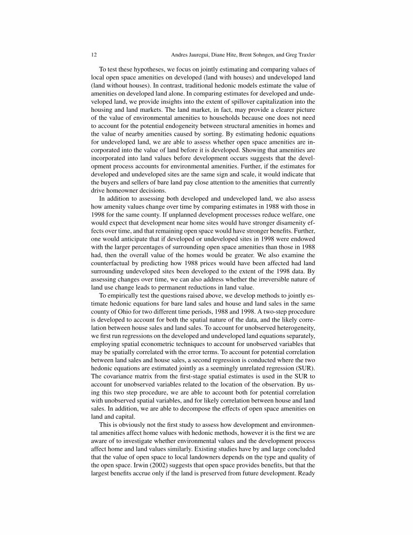
To test these hypotheses, we focus on jointly estimating and comparing values oflocal open space amenities on developed (land with houses) and undeveloped land(land without houses). In contrast, traditional hedonic models estimate the value ofamenities on developed land alone. In comparing estimates for developed and unde-veloped land, we provide insights into the extent of spillover capitalization into thehousing and land markets. The land market, in fact, may provide a clearer pictureof the value of environmental amenities to households because one does not needto account for the potential endogeneity between structural amenities in homes andthe value of nearby amenities caused by sorting. By estimating hedonic equationsfor undeveloped land, we are able to assess whether open space amenities are in-corporated into the value of land before it is developed. Showing that amenities areincorporated into land values before development occurs suggests that the devel-opment process accounts for environmental amenities. Further, if the estimates fordeveloped and undeveloped sites are the same sign and scale, it would indicate thatthe buyers and sellers of bare land pay close attention to the amenities that currentlydrive homeowner decisions.
In addition to assessing both developed and undeveloped land, we also assesshow amenity values change over time by comparing estimates in 1988 with those in1998 for the same county. If unplanned development processes reduce welfare, onewould expect that development near home sites would have stronger disamenity ef-fects over time, and that remaining open space would have stronger benefits. Further,one would anticipate that if developed or undeveloped sites in 1998 were endowedwith the larger percentages of surrounding open space amenities than those in 1988had, then the overall value of the homes would be greater. We also examine thecounterfactual by predicting how 1988 prices would have been affected had landsurrounding undeveloped sites been developed to the extent of the 1998 data. Byassessing changes over time, we can also address whether the irreversible nature ofland use change leads to permanent reductions in land value.
To empirically test the questions raised above, we develop methods to jointly es-timate hedonic equations for bare land sales and house and land sales in the samecounty of Ohio for two different time periods, 1988 and 1998. A two-step procedureis developed to account for both the spatial nature of the data, and the likely corre-lation between house sales and land sales. To account for unobserved heterogeneity,we first run regressions on the developed and undeveloped land equations separately,employing spatial econometric techniques to account for unobserved variables thatmay be spatially correlated with the error terms. To account for potential correlationbetween land sales and house sales, a second regression is conducted where the twohedonic equations are estimated jointly as a seemingly unrelated regression (SUR).The covariance matrix from the first-stage spatial estimates is used in the SUR toaccount for unobserved variables related to the location of the observation. By us-ing this two step procedure, we are able to account both for potential correlationwith unobserved spatial variables, and for likely correlation between house and landsales. In addition, we are able to decompose the effects of open space amenities onland and capital.
This is obviously not the first study to assess how development and environmen-tal amenities affect home values with hedonic methods, however it is the first we areaware of to investigate whether environmental values and the development processaffect home and land values similarly. Existing studies have by and large concludedthat the value of open space to local landowners depends on the type and quality ofthe open space. Irwin (2002) suggests that open space provides benefits, but that thelargest benefits accrue only if the land is preserved from future development. Ready

2 Open Space at the Rural-Urban Fringe 13
and Abdalla (2003), Palmquist et al. (1997), and Irwin et al. (2003) find that sometypes of farming operations, even though they provide open space for neighbors,can have negative consequences. Garrod and Willis (1992), Tyrvainen and Mietti-nen (2000), Espey and Owusu-Edusei (2001), and Paterson and Boyle (2002) showthat the value of open space depends on the quality of the open space. In the contextof this study, we account for differences between permanent and temporary pro-tection of open space, although we do not account for different types of land use(i.e. livestock versus crop operation, or forest versus agricultural land.1 There havebeen some hedonic studies investigating the value of agricultural land (e.g., Boisvertet al. (1997); Roka and Palmquist (1997); Xu et al. (1993); Kennedy et al. (1997),but these studies did not consider local environmental amenities located around thesite. Bastian et al. (2002) and Pearson et al. (2002) examined the influence of scenicviews on farmland values, but these studies were conducted in locations with par-ticularly scenic viewing opportunities.
Thus, this paper innovates in several ways. First, it innovates by considering howopen space amenities change over time. Over the 10 year period in the study region(Delaware County, Ohio), population and per capita income increased by around60%, and 80% respectively, and around 8,843 agricultural parcels were developedinto residential uses (Hite et al., 2003). One would expect in this context that thevalue of environmental amenities would change. Not only would the nature of thelandscape be altered, but new urban migrants with different sets of values would in-creasingly inhabit the area. Most studies to date have only considered a single timeslice, but the results in this study show that environmental values are susceptible topotentially large changes over time. Second, the paper accounts for likely correla-tion between land sales and house and land sales that occur in the urban frontier.Third, the paper shows how open space values and local residential developmentinfluence the value of two different types of sales that are important in regions withsubstantial development-–land sales and house and land sales. Our results indicatethat local amenities are capitalized into both types of sales in similar ways and thatthe amenities are about the same proportion of the total value of the sale. This im-plies that farmers not only provide open space, but also receive a share of the benefitsof open space.
2.2 Analytical Framework
Following Rosen (1974) we apply the hedonic framework to the markets for un-developed and developed land characteristics. The traditional (non-spatial) hedonicundeveloped price model is specified as:
lnVi = Liα1 +Oiα2 +Niα3 +Siα4 + εi (2.1)
where lnV is a vector of natural logarithms of undeveloped land prices, L is a matrixof land characteristics, O is a matrix of neighboring land use variables, N is a matrixof neighborhood characteristics, S is a vector of structural and other environmentalvariables, and the s represent parameters to be estimated for properties i = 1...M.
The traditional hedonic developed land price model adds H, a matrix of housecharacteristics, to the land only equation:
1 The agricultural land in the study area is primarily row crop. Examination of different types ofagricultural land uses in the area uncovers very few livestock operations of any kind.

14 Andres Jauregui, Diane Hite, Brent Sohngen, and Greg Traxler
lnPj = L jβ1 +H jβ2 +O jβ3 +N jβ4 +Si jβ5 + ε j (2.2)
where O, N and S are as before, the β s are parameters, and lnP represents a vectorof natural logarithms of house prices for houses j = 1...N. Both the traditional he-donic undeveloped and developed price models are most frequently estimated usingOrdinary Least Squares (OLS), corrected for heteroskedasticity.
The majority of previous undeveloped and developed land hedonic studies donot account for the possible spatial nature of housing and land data. The literatureon spatial econometrics focuses on two types of spatial effects that can arise whensample data has a locational component: (1) spatial dependence and (2) unobservedspatial heterogeneity (LeSage, 1999). Spatial dependence refers to the fact that oneobservation associated with a location depends on other observations in adjacentlocations. For example, the price of a house in a particular location depends on theprices and characteristics of neighboring houses. Unobserved spatial heterogeneityrefers to variation in relationships over space. Anselin (1988) suggests that spatialeffects lack uniformity, that is, the impact of spatial characteristics on the spatialunits vary from one region to another. For example, the impact of house characteris-tics on house prices located close to a forest is different from the impact of housingcharacteristics on house prices located close to a lake. Traditional hedonic pricemodels that use Ordinary Least Squares fail to account for these effects which inturn may result in biased, inefficient and inconsistent parameter estimates (Anselin,1988; Brasington and Hite, 2005). In order to incorporate spatial effects into a re-gression model we consider a series of spatial model specifications, all derived froma general spatial model.
2.2.1 General spatial hedonic price model
The general spatial model is considered a point of departure for a series of specificspatial models that are obtained by constraining some of its parameters (Anselin,1988). The general spatial model takes the form:
lnVi = ρW1lnVi +Liα1 +Oiα2 +Niα3 +Siα4 + εi
εi = λW2εi +µi (2.3)
where ρ is a spatial lag coefficient, W1 is a spatial autoregressive weight matrix,λ is a spatial error coefficient, W2 is a spatial weight matrix of disturbances, µi isassumed to be a vector of i.i.d. errors, and all other variables and parameters aredefined as before. In this paper we also consider the following model specifications:the spatial lag model, which is found by imposing λ = 0 into the general spatialmodel, the spatial error model, which is obtained by imposing ρ = 0, and the spatialDurbin model, which is specified as:
lnVi = ρW1lnVi +Liα11 +Oiα21 +Niα31 +Siα41
+W2Liα12 +W2Oiα22 +W2Niα32 +W2Siα42 + εi (2.4)

2 Open Space at the Rural-Urban Fringe 15
From all these model specifications, we perform a series likelihood ratio tests todetermine the best fitting models in each year for both developed and undevelopedland transactions.
2.2.2 Spatial weight matrices
To capture spatial dependence in the house and land hedonic models, spatial weightmatrices must be constructed. Each land and house transaction coordinates can beused to find the nearest neighbors to each property and construct spatial weightmatrices. The matrices are then normalized to have row-sums of unity. FollowingKim et al. (2003), we experimented with a series of different weights and reportresults from the best fitting models.
2.2.3 Seemingly Unrelated Regression (SUR) models
Previous empirical studies have assumed that the impact of transactions in the un-developed land market is independent of transactions occurring in the developedland market and vice versa. It was argued earlier in this study that the literaturefails to account for the link between these two markets. The main argument forassuming linkage of the two markets comes from the fact that land is continuous.For example, the price of land-only transactions may be affected by the price ofhouse transactions if they share common boundaries. Therefore the impact of dif-ferent land uses on house prices is not independent of the impact of land uses onland prices. Though the impact of land use variables is accounted for individually inboth single equations, it is reasonable to believe contemporaneous correlations existbetween the two markets through the unexplained portions of the equations. Giventhat both the undeveloped land price equation and the developed land price equationshare similar characteristics that affect one another, as well as possible existence ofcommon omitted factors that are not accounted for in each equation, we can arguethat the errors between the two equations may be contemporaneously correlated. Amodel of this structure calls for a seemingly unrelated regression estimation (SURE)approach.
2.3 Data
The dataset used in this paper consists of undeveloped (land only) and developed(house included) land transactions that took place in two time periods in DelawareCounty, Ohio: first, a total of 705 undeveloped land transactions and 1,595 devel-oped land transactions from July 1987 to June 1988, and second, a total of 1,236 un-developed land transactions and 1,915 developed land transactions from July 1997to June 1998. Delaware County is located north of the city of Columbus, and is afast-growing part of Ohio. It contains not only high quality agricultural land, but alsohigh value land for development (Sohngen et al., 2000). Table 2.1 presents variablesdefinitions and sources, while Table 2.2 and Table 2.3 presents summary statistics

16 Andres Jauregui, Diane Hite, Brent Sohngen, and Greg Traxler
by time period and type of transaction on structural housing characteristics, parcelcharacteristics, and neighborhood characteristics used in the hedonic regressions.
Table 2.1 Definitions and sources of hedonic regression variables
Name Definition
PRICE Price of undeveloped and developed land transactions in 1988 and 1998*NOTINACITY 1 for properties not in a city, 0 otherwiseCORNYIELD Yield of corn on land (bushels per acre)SLOPE Average percentage slope of property*AREA Property area in acresSQFT Square footage of house (1000s)AGE HOUSE Age of house in years, up to the transaction year*STORYHGT Number of stories in house*BASEMENT Size of basement coverage*ROOMS TOT Total number of rooms in house*BATHS TOT Total number of bathrooms in house (half bath=0.5)*GARAGE CAP Cars fitting in garage*ATTIC 1 for houses with an attic, 0 otherwise*POP DENS Population density in census block**INCPRCAP Income per capita in block, in dollars**SOUTHBND Distance to the southern boundary in miles***PCT AG % of agricultural land in 0.25 and 0.50 radii buffer, in 1988 and 1998****PCT GOLF % of golf courses land in 0.25 and 0.50 radii buffer, in 1988 and 1998****PCT PARK % of park land in 0.25 and 0.50 radii buffer, in 1988 and 1998****PCT RES % of residential land in 0.25 and 0.50 radii buffer, in 1988 and 1998****Note: Prices is deflated by the average quarterly Ohio Housing Price Index (I QTR 1988=100)from Federal Housing Enterprise Oversight. Sources: * Delaware County Auditor, **US Cen-sus Bureau, *** Calculated using ArcGIS®.
It can be seen from Table 2.2 that the average price for undeveloped transactionsincreased by 45.38% over the ten years under study, while Table 2.3 shows the aver-age price for developed transactions increased by 19.46%. The average parcel sizefor undeveloped transactions decreased by 78% while the average parcel size fordeveloped transactions slightly decreased. All this suggests that considerable parcelfragmentation occurred over the ten years period, resulting in more transactions in agiven year but highly reduced area transacted. Further, the percentage increase in percapita income at the census tract level over the ten years period of study (41.65% forundeveloped transactions and a 45.02% for developed transactions) is much higherthan the average percentage increase at the state level.2
Several sources comprise the dataset. All house and land information comes fromthe Delaware County Auditor.3 Housing characteristics include the total number ofrooms in a house, the total number of bathrooms (the sum of full baths and halfbaths), the total garage capacity, and the age of a house in years, as well as dummyvariables for the presence of an attic, basement, and central air conditioning.
The land characteristics include parcel area in acres and the percentage slope(measured by rise/run) and soil type of the parcel. Also included is a dummy vari-able for whether the parcel is located in a city area. Further, since most land pricestudies are concerned with the impact of land characteristics, such as productivity,
2 Calculated at 20.21% for the 1989-99 period; data obtained from the US Census Bureau.3 The Delaware County Office operates a project named Delaware Appraisal Land InformationSystem (DALIS) whose mission is to collect GIS data in Delaware County, OH. Special thanks goto Shoreh Elhami, GIS Director of DALIS Project, for her assistance with the data.

2 Open Space at the Rural-Urban Fringe 17
Table 2.2 Hedonic variable means for undeveloped land
1988 1998
Variable Mean Std. Dev. Mean Std. DevPRICE $60,589.52 $118,729.09 $88,086.39 $230,599.47NOTINACITY 0.33 0.47 0.77 0.42CORNYIELD 93.72 11.01 94.58 16.67SLOPE 3.61 1.72 3.38 4.03AREA 7.16 19.82 1.78 5.87SQFT - - - -AGE-HOUSE - - - -STORYHGT - - - -BASEMENT - - - -ROOMS TOT - - - -BATHS TOT - - - -GARAGE CAP - - - -POP DENS 1,025.25 677.06 289.44 720.95INCPRCAP $14,377.72 $3,577.34 $20,308.83 $8,873.36SOUTHBND 4.96 4.66 4.70 4.45PCT AG (0.25 mi buffer) 41.27 34.13 24.40 26.39PCT GOLF (0.25 mi buffer) 1.42 6.63 1.60 7.67PCT PARK (0.25 mi buffer) 3.39 8.94 2.40 6.91PCT RES (0.25 mi buffer) 34.53 24.93 51.31 23.45PCT AG (0.50 mi buffer) 41.26 29.91 31.20 25.57PCT GOLF (0.50 mi buffer) 1.39 4.06 1.76 6.54PCT PARK (0.50 mi buffer) 5.27 8.47 3.51 7.64PCT RES (0.50 mi buffer) 36.90 21.82 41.72 18.71Number of observations 705 705 1,236 1,236
Table 2.3 Hedonic variable means for developed land
1988 1998
Variable Mean Std. Dev Mean Std. Dev.PRICE $101,498.89 $81,020.66 $121,249.74 $67,952.14NOTINACITY 0.14 0.35 0.60 0.49CORNYIELD 92.61 6.89 93.42 17.60SLOPE 3.91 1.62 3.81 4.30AREA 1.96 8.77 1.84 6.83SQFT 2.22 0.87 2.20 0.74AGE-HOUSE 16.62 29.34 17.05 29.09STORYHGT 1.64 0.45 1.75 0.40BASEMENT 0.85 0.36 0.90 0.29ROOMS TOT 7.26 1.87 7.34 1.49BATHS TOT 2.49 1.02 2.63 0.84GARAGE CAP 1.75 1.01 1.91 0.90POP DENS 1,293.02 494.59 894.76 1,795.07INCPRCAP $13,825.80 $1,883.41 $20,050.19 $9,133.43SOUTHBND 4.65 4.35 4.63 4.15PCT AG (0.25 mi buffer) 26.84 28.69 18.65 21.38PCT GOLF (0.25 mi buffer) 1.91 6.77 1.72 7.09PCT PARK (0.25 mi buffer) 3.95 10.35 2.84 7.03PCT RES (0.25 mi buffer) 43.20 22.92 55.11 19.34PCT AG (0.50 mi buffer) 42.26 29.15 26.93 21.90PCT GOLF (0.50 mi buffer) 1.81 4.94 1.78 6.25PCT PARK (0.50 mi buffer) 4.96 8.30 4.55 8.36PCT RES (0.50 mi buffer) 36.64 20.96 43.18 16.46Number of observations 1,595 1,595 1,915 1,915

18 Andres Jauregui, Diane Hite, Brent Sohngen, and Greg Traxler
on land prices, we include the potential average corn yield of the transacted parcel.Neighborhood demographic characteristics include income per capita and popula-tion density collected at the census block group level. These variables come fromthe US Census Bureau. Following the urban economics literature, a set of distancemeasures is included to capture proximity to urbanized areas. These variables, cal-culated using ArcGIS®, are the distances in miles from each transacted house andparcel to the city of Columbus and the city of Delaware.
2.3.1 Neighborhood land characteristic variables
The primary variables of interest in this study are the percentages of land use typesin buffers around a transacted property. A review of the literature does not suggesta specific number or size of buffers to be included in the hedonic regressions. Irwin(2002) suggests that a visual inspection of the land use distribution could be a firstindicator to determine the specification of the neighborhood extent; she uses a 0.25-mile radius buffer (400-meters); Patterson and Boyle (2002) use a 0.62-mile radiusbuffers (1-kilometer); Espey and Owusu-Eudsei (2001) use various buffer sizes fordifferent park types. To avoid collinearity problems, the hedonic regressions in thisessay do not include all of the land uses calculated within the buffers. Since it isof interest to determine the impact of open space lands and residential land on landand house prices, the regressions only include the percentage of agricultural land,residential land, parks, and golf courses within a buffer of 0.25 miles radii. A secondbuffer of 0.5 miles radii is also created. The percentages of land uses in the buffersare calculated using ArcGIS®.
2.4 Empirical Results
Table 2.4 and Table 2.5 presents the estimates of the spatial undeveloped and devel-oped land price equations in 1988 and 1998. Table 2.4 presents the 0.25 mile bufferand Table 2.5 the 0.50 mile buffer. The undeveloped land equations in 1998 presenthigher adjusted R2 than the undeveloped land equations in 1988; further, they com-paratively have a greater number of explanatory variables that are statistically differ-ent from zero. The same result is observed in the developed land equations, yet the1988 equations present several explanatory variables that are statistically differentfrom zero. With respect to the land use variables, their impact on the undevelopedland prices is not statistically significant, yet significant on developed land prices(except in 1988).
Table 2.6 and Table 2.7 presents results for the undeveloped and developed landprice equations in 1988 and 1998 treated as seemingly unrelated regressions. Table2.6 presents the results for the 0.25 mile buffer and Table 2.7 for the 0.50 barrier.In order to estimate these coefficients, we proceed as follows: First, we obtain thevector of disturbances from a first stage spatial regression with undeveloped anddeveloped land transactions pooled together for a given year. Second, we estimatethe variance-covariance matrix of disturbances using Judge et al.’s (1985) procedurewhen each equation has different number of observations. This variance-covariancematrix of disturbances is used to re-estimate the equations as seemingly unrelatedregressions without directly accounting for spatial effects.

2 Open Space at the Rural-Urban Fringe 19
Table 2.4 Results for the spatial hedonic models, 0.25 mile buffer
Undeveloped Developed1988 1998 1988 1998
Variable Estimate t-stat Estimate t-stat Estimate t-stat Estimate t-statINTERCEPT 4.48*** 2.84 5.88*** 3.94 11.11*** 140.90 9.47*** 512.92NOTINACITY -0.075 -0.43 0.294** 2.37 0.127 0.69 0.008 0.30LN CORNYIELD 0.023 0.90 0.008 0.71 - - - -LN SLOPE -0.160** -2.00 0.044 1.06 0.106*** 2.78 0.031*** 2.57AREA 0.008*** 3.80 0.000 0.05 0.002 1.12 -0.005*** -3.41SQFT - - - - 0.184*** 4.68 0.217*** 9.71LN AGE HOUSE - - - - 0.029*** 8.76 0.012* 1.72STORYHGT - - - - 0.128*** 2.49 -0.053* -1.76BASEMENT - - - - 0.113* 1.84 0.076* 2.02ROOMS TOT - - - - -0.072*** -4.37 0.019* 1.90BATHS TOT - - - - 0.156*** 4.43 0.093*** 4.44GARAGE CAP - - - - 0.103*** 3.93 0.088*** 5.78LN POP DENS -0.136** -2.35 -0.202*** -5.28 -0.013 -0.22 -0.018*** -2.43LN INCPRCAP 0.756*** 3.21 0.662*** 4.58 0.008 0.17 0.007 0.75LN SOUTHBND -0.165** -2.43 -0.090* -1.90 -0.216*** -7.12 -0.070*** -7.06PCT AG -0.003 -1.07 -0.011*** -4.36 -0.003 -2.36 0.002*** 2.44PCT GOLF 0.002 0.31 -0.011** -1.93 -0.004 -0.92 0.006*** 3.75PCT PARK -0.001 -0.22 -0.011* -1.87 -0.003 -1.14 0.004*** 2.44PCT RES -0.005 -1.25 -0.019*** -7.34 -0.002 -1.55 0.003*** 4.08RHO -0.008 -0.43 0.029*** 3.22 -0.022*** -3.27 0.076*** 15.89LAMBDA 0.598*** 23.96 0.474*** 21.28 0.356*** 26.65 0.076*** 5.67
N 705 1,236 1,595 1,915Adjusted R2 0.40 0.46 0.31 0.45Note: a series of likelihood ratio test comparing the general spatial model to the spatial errormodel, the spatial lag model, and the spatial Durbin model suggest that the general specifica-tion best.
All estimated equations resulted in high adjusted R2, yet the number of statis-tically significant variables varies from one equation to another. In particular, theland use variables present differing results across years and type of transaction. Theprice of undeveloped land transactions in 1988 is positively impacted only by thepercentage of golf area within 0.25 miles from the property, and negatively impactedby the percentage of residential land within the same distance. None of the percent-ages of land use variables statistically impact the price of undeveloped land within0.50 miles from the property. In 1998, only the percentage of residential land within0.25 miles from the property has a negative impact on the price of undeveloped landtransactions, though the estimated coefficient is considerably higher than in 1988.The percentages of golf course area and park area within a distance of 0.50 milesfrom the undeveloped land property have a positive impact on its price, while thepercentage of residential land has a negative impact, yet smaller in size compared tothe impact within 0.25 miles from the property.
The percentages of agricultural land, park areas, and residential land have a neg-ative impact on the price of developed land transactions in 1988 within 0.25 milesfrom the property, yet no significant impact is found within 0.50 miles from theproperty. These effects are reverted in 1998; all land uses have a positive impact ondeveloped land prices with the percentage of park areas having the greatest impact.

20 Andres Jauregui, Diane Hite, Brent Sohngen, and Greg Traxler
Table 2.5 Results for the spatial hedonic models, 0.50 mile buffer
Undeveloped Developed1988 1998 1988 1998
Variable Estimate t-stat Estimate t-stat Estimate t-stat Estimate t-statINTERCEPT 4.65*** 1.65 5.61*** 2.95 10.79*** 122.42 9.56*** 514.08NOTINACITY -0.111 -1.13 0.182 1.47 0.105 0.57 -0.005 -0.19LN CORNYIELD 0.019 0.77 0.008 0.68 - - - -LN SLOPE -0.155** -1.94 0.045 1.03 0.105*** 2.77 0.027** 2.27AREA 0.008*** 3.55 -0.000 -0.11 0.002 1.06 -0.005*** -3.52SQFT - - - - 0.179*** 4.55 0.199*** 8.87LN AGE HOUSE - - - - 0.028*** 9.06 0.016** 2.22STORYHGT - - - - 0.134*** 2.61 -0.045 -1.48BASEMENT - - - - 0.116* 1.89 0.081** 2.16ROOMS TOT - - - - -0.068*** -4.18 0.017* 1.72BATHS TOT - - - - 0.152*** 4.33 0.093*** 4.42GARAGE CAP - - - - 0.098*** 3.75 0.087*** 5.77LN POP DENS -0.150*** -3.32 -0.213*** -4.67 -0.002 -0.04 -0.012*** -2.70LN INCPRCAP 0.722** 1.94 0.662*** 3.10 0.019 0.39 -0.009 -0.96LN SOUTHBND -0.181*** -2.92 -0.056 -0.99 -0.231*** -8.75 -0.083*** -7.78PCT AG 0.001 0.41 -0.011*** -3.35 -0.001 -0.44 0.003*** 4.17PCT GOLF -0.004 -0.42 0.010 1.45 0.002 0.49 0.010*** 5.24PCT PARK -0.001 -0.18 -0.005 -0.83 -0.001 -0.56 0.005*** 3.46PCT RES -0.000 -0.03 -0.015*** -3.73 -0.000 -0.12 0.006*** 6.58RHO -0.015 -1.15 0.036*** 2.84 -0.024** -2.40 0.074*** 15.63LAMBDA 0.597*** 14.26 0.459*** 15.00 0.364*** 27.82 0.070*** 5.26
N 705 1,236 1,595 1,915Adjusted R2 0.40 0.45 0.31 0.49Note: a series of likelihood ratio test comparing the general spatial model to the spatial errormodel, the spatial lag model, and the spatial Durbin model suggest that the general specifica-tion best.
2.5 Discussion
Results from the seemingly unrelated regressions are used to compare marginal im-pacts from land use changes on undeveloped and developed land prices over timewhere land changes are measured as percentage changes in land uses in buffersaround each property. Table 2.8 and Table 2.9 present marginal values for the fourcategories of land uses.4 The impact of changes in the percentage of agriculturalland is positive in both years on undeveloped and developed land values. In 1988, a1% increase in agricultural land in the 0.25 mile radii buffer increases undevelopedland values by $186.51, while it increases developed land prices by $368.10. Theseeffects are considerably larger in 1998. A 1% increase in agricultural land increasesundeveloped land values by $2,438.47, while it increases developed land prices by$5,287.06. While the average value of land-only transactions increased in real termsby nearly 18% per year, the value of agricultural open space around land-only trans-actions increased 18-25% per year (0.50-0.25 mi. radius respectively).
The value of developed parcels increased substantially more slowly over the 10year time period, only 2.4% per year when considered on a $/acre basis, and 1.9%per year when considered on a %/ f t2 basis. In contrast, the value of agriculturalopen-space increased by 14–27% per year 0.50-0.25 mi. radius respectively). Taken
4 We calculated the marginal implicit prices of each of the land uses assuming that the area of eachproperty remains constant at the sample average.
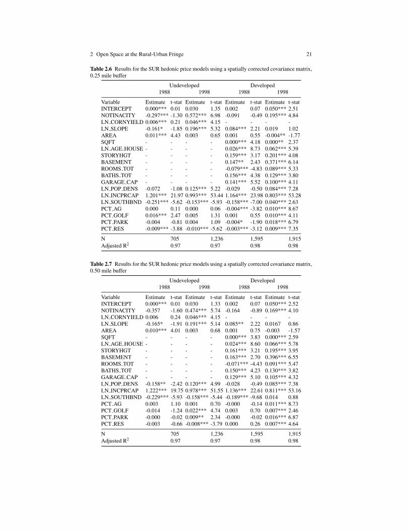
2 Open Space at the Rural-Urban Fringe 21
Table 2.6 Results for the SUR hedonic price models using a spatially corrected covariance matrix,0.25 mile buffer
Undeveloped Developed1988 1998 1988 1998
Variable Estimate t-stat Estimate t-stat Estimate t-stat Estimate t-statINTERCEPT 0.000*** 0.01 0.030 1.35 0.002 0.07 0.050*** 2.51NOTINACITY -0.297*** -1.30 0.572*** 6.98 -0.091 -0.49 0.195*** 4.84LN CORNYIELD 0.006*** 0.21 0.046*** 4.15 - - - -LN SLOPE -0.161* -1.85 0.196*** 5.32 0.084*** 2.21 0.019 1.02AREA 0.011*** 4.43 0.003 0.65 0.001 0.55 -0.004** -1.77SQFT - - - - 0.000*** 4.18 0.000** 2.37LN AGE HOUSE - - - - 0.026*** 8.73 0.062*** 5.39STORYHGT - - - - 0.159*** 3.17 0.201*** 4.08BASEMENT - - - - 0.147** 2.43 0.371*** 6.14ROOMS TOT - - - - -0.079*** -4.83 0.089*** 5.33BATHS TOT - - - - 0.156*** 4.38 0.129*** 3.80GARAGE CAP - - - - 0.141*** 5.52 0.100*** 4.11LN POP DENS -0.072 -1.08 0.125*** 5.22 -0.029 -0.50 0.084*** 7.28LN INCPRCAP 1.201*** 21.97 0.993*** 53.44 1.164*** 23.98 0.803*** 53.28LN SOUTHBND -0.251*** -5.62 -0.153*** -5.93 -0.158*** -7.00 0.040*** 2.63PCT AG 0.000 0.11 0.000 0.06 -0.004*** -3.82 0.010*** 8.67PCT GOLF 0.016*** 2.47 0.005 1.31 0.001 0.55 0.010*** 4.11PCT PARK -0.004 -0.81 0.004 1.09 -0.004* -1.90 0.018*** 6.79PCT RES -0.009*** -3.88 -0.010*** -5.62 -0.003*** -3.12 0.009*** 7.35
N 705 1,236 1,595 1,915Adjusted R2 0.97 0.97 0.98 0.98
Table 2.7 Results for the SUR hedonic price models using a spatially corrected covariance matrix,0.50 mile buffer
Undeveloped Developed1988 1998 1988 1998
Variable Estimate t-stat Estimate t-stat Estimate t-stat Estimate t-statINTERCEPT 0.000*** 0.01 0.030 1.33 0.002 0.07 0.050*** 2.52NOTINACITY -0.357 -1.60 0.474*** 5.74 -0.164 -0.89 0.169*** 4.10LN CORNYIELD 0.006 0.24 0.046*** 4.15 - - - -LN SLOPE -0.165* -1.91 0.191*** 5.14 0.085** 2.22 0.0167 0.86AREA 0.010*** 4.01 0.003 0.68 0.001 0.75 -0.003 -1.57SQFT - - - - 0.000*** 3.83 0.000*** 2.59LN AGE HOUSE - - - - 0.024*** 8.60 0.066*** 5.78STORYHGT - - - - 0.161*** 3.21 0.195*** 3.95BASEMENT - - - - 0.163*** 2.70 0.396*** 6.55ROOMS TOT - - - - -0.071*** -4.43 0.091*** 5.47BATHS TOT - - - - 0.150*** 4.23 0.130*** 3.82GARAGE CAP - - - - 0.129*** 5.10 0.105*** 4.32LN POP DENS -0.158** -2.42 0.120*** 4.99 -0.028 -0.49 0.085*** 7.38LN INCPRCAP 1.222*** 19.75 0.978*** 51.55 1.136*** 22.61 0.811*** 53.16LN SOUTHBND -0.229*** -5.93 -0.158*** -5.44 -0.189*** -9.68 0.014 0.88PCT AG 0.003 1.10 0.001 0.70 -0.000 -0.14 0.011*** 8.73PCT GOLF -0.014 -1.24 0.022*** 4.74 0.003 0.70 0.007*** 2.46PCT PARK -0.000 -0.02 0.009** 2.34 -0.000 -0.02 0.016*** 6.87PCT RES -0.003 -0.66 -0.008*** -3.79 0.000 0.26 0.007*** 4.64
N 705 1,236 1,595 1,915Adjusted R2 0.97 0.97 0.98 0.98

22 Andres Jauregui, Diane Hite, Brent Sohngen, and Greg Traxler
Table 2.8 Average marginal implicit prices for changes in the percentage land uses within 0.25 mibuffer, in real dollars
1988 Undeveloped 1998 Undeveloped
Mean Lower 95% Upper 95% Mean Lower 95% Upper 95%Agricultural land $186.51 $116.93 $256.09 $2,438.47 $1,497.27 $3,379.68Golf courses $1,141.11 $715.42 $1,566.80 $2,662.75 $1,634.98 $3,690.52Parks -$53.00 -$72.78 -$33.23 $4,496.86 $2,761.16 $6,232.56Residential Land -$432.61 -$593.99 -$271.23 $3,174.19 $1,949.01 $4,399.37
1988 Developed 1998 DevelopedMean Lower 95% Upper 95% Mean Lower 95% Upper 95%
Agricultural Land $368.10 $252.34 $483.87 $5,287.06 $4,947.34 $5,626.77Golf Courses $2,252.17 $1,543.89 $2,960.45 $5,773.33 $5,402.37 $6,144.29Parks -$104.61 -$137.51 -$71.71 $9,750.02 $9,123.54 $10,376.50Residential Land -$853.82 -$1,122.34 -$585.31 $6,882.24 $6,440.03 $7,324.45
together, the results for both developed and undeveloped land indicates that a largeproportion of the growth in value over the time period is due to open space. Forinstance, while the value of developed parcels has increased only slowly, the valueof the open-space around developed parcels appears to be an increasingly importantcomponent of the value of developed parcels.
Further, these effects are considerably larger when considering a greater buffersize. The process of land transformation from agricultural land into residential landprogressively impacts how undeveloped and developed land owners value the agri-cultural land left.
Table 2.9 Average marginal implicit prices for changes in the percentage land uses within 0.50 mibuffer, in real dollars
Undeveloped
1988 Undeveloped 1998 UndevelopedMean Lower 95% Upper 95% Mean Lower 95% Upper 95%
Agricultural land $754.43 $580.90 $927.96 $3,657.23 $1,822.42 $5,492.04Golf courses $152.36 $117.32 $187.41 $5,872.10 $2,926.11 $8,818.10Parks $706.96 $544.35 $869.57 $6,245.43 $3,112.14 $9,378.72Residential Land $588.14 $452.86 $723.42 $5,328.24 $2,655.10 $8,001.38
1988 Developed 1998 Developed
Mean Lower 95% Upper 95% Mean Lower 95% Upper 95%Agricultural land $1,752.03 $1,312.70 $2,191.36 $6,843.43 $6,393.26 $7,293.59Golf courses $353.83 $265.11 $442.56 $10,987.91 $10,265.12 $11,710.70Parks $1,641.78 $1,230.09 $2,053.46 $11,686.49 $10,917.74 $12,455.23Residential Land $1,365.84 $1,023.35 $1,708.33 $9,970.23 $9,314.38 $10,626.08
The same effect is observed for the percentage of golf courses surrounding aproperty, yet in 1988 a 1% increase in this type of land has a considerably largerimpact than the percentage of agricultural land. Over time, the impact of additionalland dedicated to golf course follows the same pattern as agricultural land, as wellthe marginal impact equalize. An increase in 1% in the percentage area dedicated toparks within 0.25 miles from both undeveloped and undeveloped land properties in1998 has a negative impact; yet extending the area to 0.50 miles from the propertyresults in a positive impact. This effect is inverted in 1998: both undeveloped and

2 Open Space at the Rural-Urban Fringe 23
developed land prices are positively impacted by the percentage of land dedicated toparks. Combining these two effects, it can be observed that the marginal impact ofopen space lands increases as time passes and the relative abundance of these typesof land are reduced at the expense of residential land. Land owners and homeown-ers considerably value agricultural land, golf course and parks, and their valuationincreases over time.
The marginal impact of a 1% increase in the area dedicated to residential landhas a negative impact of $432.61 within a 0.25 miles distance from undevelopedland properties in 1988, yet the marginal effect becomes positive considering a 0.50mi distance. This effect is reversed in 1998; a 1% increase in the percentage areadedicated to residential land increases undeveloped land values by $3,174.19 con-sidering a 0.25 miles distance from the property, whereas it marginally increasesundeveloped land prices by $5,328.24 within 0.50 miles from the property.
2.6 Simulations
The undeveloped and developed land price equations estimated in this paper areused to predict the impact of land use changes on property values as urbanizationinto predominantly agricultural areas takes place. Concerns over the impact of in-creased urban and suburban growth on agricultural areas and open space lands haveled many cities and counties in the United States to pass laws to protect farmlandand the environment discouraging the expansion of suburban areas. It is arguablethat these policies have unpredictable effects on land and house prices. Further, asthis expansion continues, the relative abundance of land amenities decreases withrespect to other types of land areas. It is therefore useful to determine whether thechanging conditions in the area dedicated to a particular land use capitalizes intoproperty values. One way to asses this impact is to simulate price changes in thehedonic price models imposing certain conditions on the land use variables. Specif-ically, we are interested in assessing how the actual predicted value of developed orundeveloped parcels in 1998 (with 1998 amenities) compare to the predicted valueof these same parcels assuming they have 1988 amenities.
Table 2.10 Actual predicted prices in 1998 versus simulated predicted prices in 1998 within 0.25and 0.50 miles buffer
Undeveloped 0.25 mi buffer Developed 0.25 mi buffer
Mean Lower 95% Upper 95% Mean Lower 95% Upper 95%
Actual Price Prediction $46,321 $44,681 $47,961 $122,266 $118,462 $126,070Simulated Price Prediction $54,984 $53,084 $56,884 $120,610 $117,082 $124,138% Change 19.16 18.66 19.65 0.27 -0.30 0.84
Undeveloped 0.50 mi buffer Developed 0.50 mi buffer
Mean Lower 95% Upper 95% Mean Lower 95% Upper 95%
Actual Price Prediction $46,605 $44,889 $48,322 $121,899 $118,148 $125,650Simulated Price Prediction $49,153 $47,443 $50,863 $137,232 $133,241 $141,224% Change 6.58 6.28 6.88 14.17 13.53 14.81
Table 2.10 present simulations of undeveloped and developed land prices in 1998assuming that the average percentage area of the different land uses in 1998 approx-

24 Andres Jauregui, Diane Hite, Brent Sohngen, and Greg Traxler
imate the averages in 1988. These results are compared to the actual undevelopedand developed predictions from the estimated model in 1998. The average percent-age of land dedicated to agriculture in this sample of transactions decreased con-siderably from 1988 to 1998, especially surrounding undeveloped land transactions.The average percentage area dedicated to residential land also increased, while theaverage percentage of area dedicated to golf course and parks were not considerablyaffected.
Two effects are considered here. First, residential expansion may adversely cap-italize into property prices due to increased housing congestion and other resultingexternalities. Second, because open space amenities are positive valued, and openspace amenities are larger in 1988, one would expect houses and land in 1998 tobe more valuable if they have 1988 amenities. For the 0.25 mi. buffer, undevel-oped land transactions are estimated to be 19% more valuable if they have the 1988amenities in 1998, whereas developed land transactions are estimated to be aboutthe same value. Thus, open-space within a relatively short distance of an agricul-tural property tends to enhance that properties value, however, it does not appearto enhance the value of a developed property. Looking at the 0.50 mi. buffer, unde-veloped land transactions would have only been about 7% more valuable with theamenities of 1988 around them, whereas developed transactions would have been14% more valuable. These results help explain observed tendencies in the Midwest,where there is strong reliance on minimum lot size zoning. Minimum lot size zon-ing would appear to substantially benefit agricultural land owners because it wouldhelp preserve open space near existing farms, while at the same time allowing fordevelopment to occur. The results also imply that nearby open space does not sub-stantially benefit developed land if that open space is close. Open space appearsto have its greatest effects on developed land if it is not located in the immediatevicinity of the house.
Results from calculating the percentage difference between the simulated pricesand the predicted prices indicate that in close proximity to the property, residentialexpansion has a greater negative impact on the price of undeveloped land transac-tions than developed land transactions. Assuming that the land use averages in 1998remain at the same averages than in 1988, ceteris paribus, undeveloped land priceswould have been 19.16% higher than the actual predictions, whereas developed landprices would have been only 0.27% greater considering the impact within 0.25 milesfrom the property. This means that the negative impact of urbanization outweighedthe positive impact of increased relative area dedicated to open space lands, but theimpact is greater on undeveloped land properties than in developed ones.
2.7 Conclusion
This paper addresses concerns over the impact of urban and suburban expansioninto predominantly agricultural areas. We consider that the negative impact fromexternalities generated by increased residential areas counteracted by the positiveexternality generated from an increase in the relative abundance of open space landsaccumulate into property price over time. Results from the estimated undevelopedand developed land prices in two different time periods are used to shed light intowhether the negative impact of urbanization outweigh the positive impacts of theremaining open space land. These results are relevant policy making tools that al-

2 Open Space at the Rural-Urban Fringe 25
low us to predict how land use changes affect the value of land and house pricetransactions.
This paper represents a contribution to the literature because it estimates house-holds’ valuations of different types of land uses on land and house transactionsconsidering the fact that both markets are linked by the continuity and fixity of land.Empirical results determine that households’ valuation of open space lands differbetween land only transactions and transactions that include a house. Further, wecan predict changing preferences over time: residential movers in 1988 have differ-ent preferences compared to those in 1998.
The following concerns need to be addressed in future research. First, the landuses in this paper do not provide information about whether the parcels are po-tentially developable or idle. Further, it was not possible to determine whether theparcels classified as agricultural land are actually being used for agricultural produc-tion. The marginal impact of additional agricultural land most likely differs by typesof agricultural operations. It has been found in the literature that certain agriculturalactivities have a negative impact on property values, such as swine production farms,whereas others might have positive impacts. The last concern relates to the impactof congestion externalities on property values. Most conversion of agricultural landinto residential land accompanies fragmentation of large plots into smaller plots.The increase in housing congestion as measured by density of built structures perunit of land, for example, is not captured within the percentage of residential landsurrounding a property. Over time the percentage increases, but at the same timethe number of houses built on the parcels also increases. It is possible that the im-pact of residential land use on property values may differ by the capital intensitysurrounding the property, an effect which is outside the scope of this study.
References
Anselin L (1988) Spatial Econometrics: Methods and Models. Kluwer AcademicPublishers, Boston
Bastian CT, McLeod DM, Germino MJ, Reiners WA, Blasko BJ (2002) Environ-mental amenities and agricultural land values: A hedonic model using GeographicInformation Systems data. Ecological Economics 40(3):337–349
Boisvert RN, Schmit TM, Regmi A (1997) Spatial, productivity, and environmentaldeterminants of farmland values. American Journal of Agricultural Economics79(5):1657–1664
Brasington DM, Hite D (2005) Demand for environmental quality: A spatial hedo-nic analysis. Regional Science and Urban Economics 35(1):57–82
Espey M, Owusu-Edusei K (2001) Neighborhood parks and residential property val-ues in Greenville, South Carolina. Journal of Agricultural and Applied Economics33(3):487–492
Fischel WA (1999) Zoning and land use regulation. In: Bouckaert B, De Geest G(eds) Encyclopedia of Law and Economics, Edward Elgar, Cheltenham
Garrod GD, Willis KG (1992) Valuing goods’ characteristics: An application ofthe hedonic price method to environmental attributes. Journal of EnvironmentalManagement 34(1):59–76
Heimlich RE, Anderson WD (2001) Development at the Urban Fringe and Beyond:Impacts on Agriculture and Rural Land. Economic Research Service, US Depart-ment of Agriculture, Agricultural Economic Report No. 803

26 Andres Jauregui, Diane Hite, Brent Sohngen, and Greg Traxler
Hite D, Sohngen B, Templeton J (2003) Zoning, development timing, and agricul-tural land use at the suburban fringe: A competing risks approach. Agriculturaland Resource Economics Review 32(1):145–157
Irwin EG (2002) The effects of open space on residential property values. LandEconomics 78(4):465–480
Irwin EG, Bell KP, Geoghegan J (2003) Modeling and managing urban growth atthe rural-urban fringe: A parcel-level model of residential land use change. Agri-cultural and Resource Economics Review 32(1):83–102
Judge G, Griffiths W, Hill RC, Lutkepohl H, Lee TC (1985) The Theory and Practiceof Econometrics. Wiley, New York
Kennedy GA, Henning SA, Vandeveer LR, Dai M (1997) An empirical analysis ofthe Louisiana rural land market. Louisiana State University Agricultural Center,Bulletin Number 857
Kim CW, Phipps TT, Anselin L (2003) Measuring the benefits of air quality im-provement: A spatial hedonic approach. Journal of Environmental Economics andManagement 45(1):24–39
LeSage JP (1999) The Theory and Practice of Spatial Econometrics. University ofToledo Department of Economics, Toledo
Palmquist RB, Roka FM, Vukina T (1997) Hog operations, environmental effects,and residential property values. Land Economics 73(1):114–124
Paterson RW, Boyle KJ (2002) Out of sight, out of mind? Using GIS to incorporatevisibility in hedonic property value models. Land Economics 78(3):417–425
Pearson L, Tisdell C, Lisle A (2002) The impact of Noosa National Park on sur-rounding property values: An application of the hedonic price method. EconomicAnalysis and Policy 32(2):155–171
Ready R, Abdalla C (2003) GIS analysis of land use on the rural-urban fringe: Theimpact of land use and potential local disamenities on residential property valuesand on the location of residential development in Berks County, Pennsylvania.Northeast Regional Center for Rural Development, Pennsylvania State Univer-sity, University Park
Roka FM, Palmquist RB (1997) Examining the use of national databases in a hedo-nic analysis of regional farmland values. American Journal of Agricultural Eco-nomics 79(5):1651–1656
Rosen S (1974) Hedonic prices and implicit markets: product differentiation in purecompetition. Journal of Political Economy 82(1):34–55
Sohngen B, Hite D, Simpson J, Templeton J (2000) The Value of Open Space andAgricultural Land to Rural Non Farm Residents. Paper presented at the AnnualMeetings of the American Agricultural Economics Association, Tampa, FL
Tyrvainen L, Miettinen A (2000) Property prices and urban forest amenities. Journalof Environmental Economics and Management 39(2):205–223
Xu F, Mittelhammer RC, Barkley PW (1993) Measuring the contributions of sitecharacteristics to the value of agricultural land. Land Economics 69(4):356

Chapter 3Neighborhood Sorting Dynamics in Real Estate:Evidence from the Virginia Sex OffenderRegistry
Xun Bian, Raymond Brastow, Michael Stoll, Bennie Waller and Scott Wentland
Abstract Given the potential risk of recidivism, recent research has found that reg-istered sex offenders impose external costs that are capitalized into the value (lowerprices) and liquidity (longer time on market) of nearby residential real estate. Usingmore than a decade of real estate listings data and a unique data set of registeredsex offenders (RSOs) in Virginia, we extend this literature by investigating how realestate markets respond to clustering of this particular group and whether there is ev-idence of market prices facilitating clustering phenomena. Employing a difference-in-difference approach within a hedonic empirical framework, the results show thatthe housing market has a nonlinear response to clusters, as it considerably discountsprices of homes located near a cluster (4+) of RSOs, providing a market incentivefor further sorting/clustering. Our empirical findings and supplemental geospatialanalysis are consistent with a sorting/tipping model in which individuals chooseresidential locations according to preferences and price incentives. Insofar as clus-tering of negative externalities is efficient, we further discuss the market efficiencyimplications in this context.
3.1 Introduction
Thomas Schelling (1971) showed that residents will tend to sort into segregatedneighborhoods, even when individuals within those neighborhoods are relativelytolerant and do not have extreme preferences for such segregation as the group dy-
Xun BianLongwood University, Farmville, VA 23909, USA e-mail: [email protected]
Raymond BrastowFederal Reserve Bank of Richmond, Richmond, VA 23261, USA e-mail: [email protected]
Michael StollAmplify Geo e-mail: [email protected]
Bennie WallerLongwood University, Farmville, VA 23909, USA e-mail: [email protected]
Scott WentlandBureau of Economic Analysis and Longwood University, Washington, DC 20233, USA e-mail:mailto:[email protected]
27
28 Xun Bian, Raymond Brastow, Michael Stoll, Bennie Waller and Scott Wentland
namics suggest. In his model segregation is produced by individuals who chose tolocate in areas where they are not surrounded by large numbers of neighbors fromanother group. In the presence of a critical mass of ‘others’ a neighborhood may‘tip’ in one direction as residents move out.1 A number of studies have investigatedthe dynamics of Schelling’s tipping model in different contexts. In this chapter, weapply the insights of the Schelling tipping model to another group dynamic, cluster-ing among sex offenders and non-sex offenders, a group of great concern to partic-ipants in the real estate market (which also happens to have transparent public dataon where they live and when they move). In particular, using a hedonic pricing ap-proach, we examine whether there is evidence that the price mechanism incentivizesthese groups to cluster and the broader housing market implications of this result.
Following the passage of Megan’s Law and related statutes at both the state andnational level, convicted sex offenders must register their residences with local au-thorities each time they move (Virginia State Police, 2020).2 Each state operates itsown online registry, which is searchable by the general public. When a registeredsex offender moves in nearby, studies have consistently shown that the neighbor-hood takes note, which affects the local real estate market in turn. The purpose ofthis chapter is to study the incremental effects that sex offenders (and sex offenderclusters) have on home prices and liquidity, determining whether there is evidenceof distinct price signals that facilitate tipping in the market for real estate. Using astraightforward nearest-neighbor GIS analysis, we further explore the implicationsof these pricing dynamics, examining the locational choices of sex offenders andhomeowners (i.e. non-sex offenders), looking at whether these groups tend to sepa-rate from one another and whether sex offenders exhibit a tendency to cluster amongother sex offenders over time.
Motivating our empirics analytically, we first explore household preferences thatmay lead to clustering dynamics. Some households may have preferences to moveout in the event that one or more registered sex offenders move in nearby. On theother side of the same coin, sex offenders may be more likely than the general pop-ulation to move near other sex offenders for a variety of reasons (e.g. discountedhousing, less aversion to living near a fellow offender, etc.). Over time, neighbor-hood composition will tend to ‘tip’ toward segregation of these two groups, based ontheir preferences, market conditions, and, as we explore empirically, pricing incen-tives. Moreover, there may be considerable variation of individual or family-levelpreferences toward sex offenders within the general populace, which we test using aproxy potentially correlated with intensity of these preferences. Specifically, we usea proxy for children to explore whether pricing dynamics are different for ‘family’vs. ‘non-family’ homes.
To summarize our results, we find evidence that the real estate market steeplydiscounts the price of homes near clusters (4+) of registered sex offenders by asmuch of 16%, on average, along with a substantial adverse effect on nearby homeliquidity. This result is consistent across multiple specifications, including a three-stage-least-squares (3SLS) simultaneous equations analysis; and, when the prefer-ences of the treated group are heightened (i.e., for more family-friendly 3+ bedroomhomes), we find a pronounced effect accordingly. This result helps explain further
1 One insight from Schelling’s model is that trends and patterns of residential mobility for thegroup may be more extreme than the preferences of the individual within that group. We returnto a related point later when we investigate effects among individuals with stronger preferences(proxied by the number of bedrooms within the home).2 For more information on the sex offender registry in Virginia, which is a key source of our data,see: https://sex-offender.vsp.virginia.gov/sor/.

3 Neighborhood Sorting Dynamics in Real Estate 29
sorting/clustering of sex offenders over time found in the literature and in our owngeospatial analysis, as market prices provide an additional incentive for RSOs tocluster and concentrate this negative externality in a particular area. We conclude bydiscussing the market efficiency implications of these results in more detail.
3.2 Motivating Literature and Contribution
There are several streams of literature that have analyzed the primary elements ofthis paper (neighborhood segregation, tipping, and real estate market response to sexoffenders), but one opportunity we take in this study is to combine the insights fromthese strands of literature to investigate market response to RSO clusters specificallyand the further sorting that is incentivized by this home price response. Below, webriefly discuss a number of geography and regional sciences studies that have estab-lished that registered sex offenders tend to cluster spatially. These papers generallyfocus on the degree to which local or state restrictions limit locational choices andessentially force sex offenders to live in clusters in the relatively few areas that areopen to them. Another strand of literature has focused on forces that lead to neigh-borhood segregation. These papers model the existence of stable equilibria and tip-ping points at which a neighborhood may change from high to low income or fromone ethnic or religious group to another. Finally, economics and real estate studieshave established that living near a sex offender creates negative consequences inreal estate markets — lower selling price and reduced liquidity. Given that these aresizable (and growing) literatures, the review in this section is not comprehensive;but, we attempt to integrate some of these insights as we summarize closely relatedliterature below.
When a registered sex offender (RSO) moves into a neighborhood, it presentsa potential ‘shock’ to the neighborhood that elevates perceptions of crime risk ofnearby residents, which has shown to have a measurable impact on very localizedreal estate markets. Given the nature of this shock, which represents a ‘treatment’ tonearby homes that is differentiated from the control group across both space (nearvs. far) and time (post-RSO move in), the real estate and urban economics aca-demic literature has generally estimated this effect using a difference-in-differencesapproach. The study closest to this paper is by Wentland et al. (2014), which alsoutilizes multiple listing service (MLS) data estimates the effect of nearby RSOs onreal estate when there is endogenous determination of housing liquidity and price.Controlling for home and property characteristics as well as property and time fixedeffects, three stage least squares results indicated that the presence of a registeredsex offender within 0.1 miles resulted in a 7% decrease in selling price and an 80%increase in the time a home takes to sell. The authors also found significant but de-clining effects on price and liquidity of sex offenders located in larger radii up to onemile around a listed property relative to the control group (i.e., homes not presentlywithin a mile of a sex offender). Results were robust across a number of specifica-tions and identification strategies, including correction for sample selection and apre-trend, placebo analysis of housing outcomes before a nearby offender moves inor after he/she moves out. Finally, they also show that the treatment varies hetero-geneously based on the intensity of the preferences of potential homebuyers, wherehomes with more bedrooms, a proxy for households with more children, sufferedlarger price and liquidity effects. Perhaps most relevant for the present study, the

30 Xun Bian, Raymond Brastow, Michael Stoll, Bennie Waller and Scott Wentland
authors also estimate (linear) effects of additional nearby sex offenders, but did notinvestigate potential nonlinear effects of clusters.
Wentland et al. (2014) extended a growing literature that has also found thatsex offenders residing nearby had a significant impact on home prices. Linden andRockoff (2008) analyzed housing effects in Mecklenberg County, NC, a large areawhich contains Charlotte. Data on the move-in date for the most recent address ofeach offender was matched to a data set of home sales over a ten year period. Theyfound significant reductions in home prices across radii of less than 0.1 miles and 0.1to 0.3 miles when an offender moves in. Results indicated that the presence of a sexoffender within 0.1 miles reduces home prices by roughly 4.0% after the offender’smove-in date. Living beyond one-third of a mile from an offender had no signifi-cant effect on price in their study. Another influential study in this literature, Pope(2008), analyzed the effect of proximity to a sex offender in Hillsborough County,Florida which contains Tampa. His data set included move-in and move-out datesfor every house an offender has occupied since being placed on the registry. Con-trolling for housing characteristics, time, and neighborhood fixed effects, regressionresults indicated that a location within 0.1 miles of a registered sex offender reducedhousing values by 2.3%. He also found that prices rebound when an offender movesout. Like the Linden and Rockoff (2008) study, the effect dissipated quickly beyond0.1 mile, as there was no significant effect on price for homes located between 0.1and 0.2 miles from an offender.
A somewhat older study by Larsen et al. (2003) found similar results in Mont-gomery County (Dayton area), Ohio. They matched data on sex offender addresseswith home sales during one year, 2000. Controlling for a vector of house character-istics and neighborhood fixed effects, regression results indicate that living within0.1 miles of a registered sex offender reduces property values by 17.4%. Significantbut diminishing price effects were estimated out to a distance of 0.3 miles.
A more recent paper by Brastow et al. (2018) analyzed the effect of nearby sexoffenders with a focus on housing liquidity. They use both survival analysis and adifference-in-difference framework, and their empirical results show that registeredsex offenders have a large adverse impact on nearby home liquidity on average,where this effect is largely driven by ‘surprises’ of sex offenders moving in or outduring the marketing period. However, for homes near offenders who reside nearbythrough the entire marketing period, the results indicate that sellers steeply discountthe initial list price and may actually sell their homes more quickly.
Geography and regional science studies have employed a variety of spatial tech-niques to demonstrate the degree to which registered sex offenders cluster. The anal-ysis generally focusses on local or state restrictions on the location of sex offenderresidences. Grubesic (2010) calculates several measures of sex offender clustering inIllinois and compares the results to residency restrictions and regional demographiccharacteristics. The techniques produced general correspondence in the identifica-tion of clusters. The study identifies several characteristics of the identified clustersincluding the existence of relatively low priced housing.
Rey et al. (2014) introduced a Markov chain framework to analyze residentialmovement patterns of registered sex offenders in Hamilton County, Ohio, from2005 to 2007. The authors analyze sex offender location choices relative to spatialrestrictions. Results indicate a 46 percent reduction in offenders violating spatial re-striction zone policy as compared to a counterfactual case where offenders move inpatterns that correspond to existing housing distributions. Strong legacy effects arealso found as offenders previously in violation of restriction policies move into otherrestricted zones at a higher rate than offenders who were previously in compliance

3 Neighborhood Sorting Dynamics in Real Estate 31
with the policy. Generally, registered sex offenders continue to locate in restrictedzones at a higher rate than expected, despite the policy restrictions.
Finally, the economics literature of residential sorting, segregation, and tippinghas its roots largely in the work of Thomas Schelling (1971). In Schelling’s model,a resident’s preference for neighborhood characteristics is expressed as the degreeof tolerance for existing or potential residents who differ on some important mar-gin. A resident moves when the number of different neighbors exceeds the individ-ual’s threshold. Schelling’s models demonstrated that tipping and segregation canoccur even if individuals have relatively high thresholds (are willing to live in in-tegrated neighborhoods), segregation is a stable equilibrium and is likely to occur.Economists continue to develop new models of spatial segregation. In a more re-cent article, O’Sullivan (2009) models neighborhood preferences as bid-rent offerswhere vacant properties are sold to the highest bidder. Even though bid-rent curvesmaximize in integrated neighborhoods, inefficient segregation is the stable outcome.
Card et al. (2008) use a regression discontinuity methodology with Census tractdata to test for the dynamics of neighborhood racial composition. They find ev-idence of white residential flows consistent with tipping behavior in most cities.Tipping points range from 5% to 20% minority portion of city population. Whilethere is evidence of white population flows in urban areas, the authors do not findCensus tract rental or housing sale price effects around the tipping point.3 Thus,while tipping and sorting dynamics have been investigating in these other contexts(usually by race), these studies often use more aggregated data on the compositionof a particular geography, rather than microdata identifying the exact membershipof a household to a particular group that is sorting. The uniqueness of data fromsex offender registries is that it allows researchers to analyze this type of sortingand clustering phenomenon at a very micro-level with data where we know the ad-dress, move-in, and move-out dates of each member of this particular group, whichcontributes to the sorting/tipping literature more broadly. Further, we are able to ex-tend the narrower literatures on the impact of sex offenders by helping explain howprice responses can facilitate clustering and further sorting, which is the primarycontribution of this paper.
3.3 Neighborhood Tipping Dynamics — A Simple Model
In this section, we sketch a simple theoretical model to motivate our empirical anal-ysis. Imagine an open city in a featureless plain. A registered sex offender randomlyselects a point in the city to reside, and our model examines location choices aroundthis point. Additionally, our model will show that such location choices can impactthe value of nearby properties. We assume that each individual has a utility function:
Ui =U(Q(x,q),c) (3.1)
3 Two additional studies have modeled neighborhood dynamics and real estate outcomes. Basedon a model developed in Bond and Coulson (1989), the neighborhood turnover process dependson the hedonic bid functions for housing and neighborhood quality. Coulson and Bond (1990) useFHA data from six cities from 1979 and 1980 to estimate inverse demand functions for housingquality attributes. They find significant differences among income groups in the bid for floor space,suggesting that segregation could occur as higher income groups bid for larger properties. Theauthors did not find differences in bid functions for racial composition.

32 Xun Bian, Raymond Brastow, Michael Stoll, Bennie Waller and Scott Wentland
where individual utility U is a strictly increasing function of the overall quality ofhousing services Q and the consumption of a composite good c. For simplicity, theprice of the composite good c is assumed to be the same everywhere in the city,and the price of c is normalized to unity. Quality of housing services is determinedby two things: 1) x, the intensity of the nearby sex offender(s) and 2) other hous-ing attributes q, which include physical characteristics of the residence (e.g. squarefootage, number of bedrooms, etc.) and other location characteristics (e.g. schoolquality).4 A greater x could result from closer proximity to the sex offender (or eachadditional sex offender). It may also be a consequence of the nearby sex offenderbeing one who committed a violent offense that is perceived as a higher or moreserious recidivism risk by his or her neighbors. Assuming a sex-offender-free en-vironment is strictly preferred by everyone, we must have Qx < 0. Additionally,assuming high-quality housing attributes are desirable, we have Qq > 0.
Following Rosen (1974), preferences for the overall quality of housing servicescan be expressed by the bids for different levels of housing quality, θ , that yield thesame level of utility U . Assuming an individual exhausts his or her endowment yon housing and the composite good c, we must have c = y−θ . Substitute this intoequation 3.1 and invert, we obtain the bidding function:
θ = θ(Q(x,q),y,U) (3.2)
Equation 3.2 suggests that the willingness-to-pay for location depends on thelevel of reservation utility, the endowment y, and overall housing quality Q, whichis determined by both x and q. To examine the impact of sex offenders on propertyprices, we implicitly differentiate θ with respect to x holding utility level constant.We obtain
θx =UQ
UcQx < 0 (3.3)
Because UQ and Uc are strictly positive, and Qx is strictly negative, we must haveθx < 0. Intuitively, θx is the marginal price an individual is willing to pay for oneunit increase of sex offender intensity x. Not surprisingly, Equation 3.3 indicatesthat such a marginal price is negative. In other words, a nearby sex offender is a‘bad’, or a neighborhood disamenity in this model. Individuals would be willing topay to get rid of it. This also implies people must be compensated for acceptinga greater x. In housing markets, such compensation takes the form of lower houseprices. Therefore, Equation 3.3 generates our first testable hypothesis:
Prediction 1: An increase in sex offender intensity x reduces the willingness-to-pay for a particular location. Property prices fall as x increases.
The first prediction is rather simple and intuitive. Any exogenous shock that in-creases sex offender intensity would reduce property prices. Such shocks could be asex offender moving into a sex-offender-free neighborhood. It could also be a newsex offender entering a community where some sex offenders already reside. Ourmodel predicts that such shocks would hurt property value, which is straightforwardand expected, but to this point we have only assumed homogeneous preferences.Yet, given a fall in value for these properties, the more interesting question is whathappens next with regard to locational choices, particularly if individuals perceive
4 By other location characteristics, we mean location characteristics other than the intensity of thenearby sex offender, x. Because x is the focus of our analysis here, we single it out from otherlocation characteristics.

3 Neighborhood Sorting Dynamics in Real Estate 33
risks differently and have heterogeneous preferences over this particular type of dis-amenity.
To analyze location choices, we introduce heterogeneous preferences. We nowassume individuals are identical except for their preference for sex offender inten-sity x. While everyone prefers a smaller x, the degree to which people dislike xcould be different. A strong preference for a sex-offender-free environment can berepresented by a smaller (more negative) value of Qx. Intuitively, a more negativeQx implies that each unit of increase in x reduces overall housing quality Q moresignificantly for individuals with a stronger distaste for, or risk aversion toward, sexoffenders. Suppose there are two types of individuals, type i and j. Type i individu-als are more strongly averse to living near sex offenders than type j. Thus, we musthave Qi
x < Q jx. Together with Equation 3.3, we must have
UQ
UcQi
x <vQ
UcQ j
x ⇒ θix < θ
jx (3.4)
The implication of Equation 3.4 can be more easily understood via a simpleillustration. θx < 0 suggests that the bidding function θ must be downward slopingif plotted in the (x,θ) space. Equation 3.4 implies θ i must be steeper than θ j.
of type 𝑖𝑖 individuals, who vigorously dislike or have a strong aversion toward 𝑥𝑥. The dashed line,
𝜃𝜃𝑗𝑗, represents the bidding function of type 𝑗𝑗 individuals, who also favor a sex-offender-free
environment, but not as strongly as type 𝑖𝑖 individuals. As shown in Figure I, type 𝑖𝑖 individuals
would outbid type j for locations with lower sex offender intensity. On the other hand, type 𝑗𝑗
individuals would outbid type 𝑖𝑖 for locations with greater sex offender intensity. Because
ownership goes to who offers the highest bid, sorting based on preference for 𝑥𝑥 occurs.
Specifically, type 𝑖𝑖 individuals will reside at places with lower sex offender intensity, and locations
with greater sex offender intensity will be occupied by type 𝑗𝑗 individuals. Thus, we obtain the
second testable hypothesis:
Prediction 2: individuals with a stronger preference for a sex-offender-free neighborhood will
reside at locations with lower sex offender intensity.
Figure I
Although the model we presented here is not a dynamic one, it is not hard to envision that
an exogenous change of sex offender intensity would affect mobility. Imagine a sex offender
entering a community. This, as indicated by our first prediction, will hurt nearby house values.
Fig. 3.1 Difference in willingness to pay between different types of individuals
This difference in willingness to pay between type i and j individuals for dif-ferent levels of sex offender intensity is illustrated in Figure 3.1. The solid line,θ i, represents the bidding function of type i individuals, who vigorously dislike orhave a strong aversion toward x. The dashed line, θ j, represents the bidding func-tion of type j individuals, who also favor a sex-offender-free environment, but notas strongly as type i individuals. As shown in Figure 3.1, type i individuals wouldoutbid type j for locations with lower sex offender intensity. On the other hand, typej individuals would outbid type i for locations with greater sex offender intensity.Because ownership goes to who offers the highest bid, sorting based on preferencefor x occurs. Specifically, type i individuals will reside at places with lower sex of-

34 Xun Bian, Raymond Brastow, Michael Stoll, Bennie Waller and Scott Wentland
fender intensity, and locations with greater sex offender intensity will be occupiedby type j individuals. Thus, we obtain the second testable hypothesis:
Prediction 2: individuals with a stronger preference for a sex-offender-freeneighborhood will reside at locations with lower sex offender intensity.
Although the model we presented here is not a dynamic one, it is not hard toenvision that an exogenous change of sex offender intensity would affect mobility.Imagine a sex offender entering a community. This, as indicated by our first pre-diction, will hurt nearby house values. Then, the mechanism outlined in our secondprediction will lead people to rethink and modify their location choices made beforesuch an exogenous shock. Residences who dislike sex offenders the most will havethe strongest incentive to relocate and, most likely, be one of the first to do so. Fur-thermore, distaste for sex offenders will make a lot of potential buyers shun awayfrom buying in the neighborhood. Increased supply and low demand may furthercause house prices to drop. Other sex offenders, who perhaps have less of an aver-sion to their own group are attracted by the lowered prices, are more likely to moveinto the community. As a result, the relocation of sex offenders, then, becomes anon-random process, creating further shocks to the areas in which they move. Thus,this market process implies that price signals from declining home values associatedwith each additional sex offender precipitate a tipping dynamic, where a neighbor-hood may tip toward a critical mass of sex offenders, resulting in clustering.
3.4 Data
To explore clustering dynamics of registered sex offenders, we have obtained datafrom several sources. Our sample of real estate data consist of transactions fromresidential properties on the market between July 1999 and June 2009 and comefrom a central Virginia multiple listing service (MLS). The initial housing data con-tained 21,453 observations of both sold and unsold properties. As noted by otherstudies, MLS data are ‘organic data’ in the sense that it was initially collected andmaintained for commercial purposes, entered by real estate agents, which means itcan contain some incorrect or incomplete data. As a result, the data were carefullyculled for incomplete, missing, or illogical outliers.5 The final sample consists of12,426 sold and 7,295 unsold properties.
The data collected from the MLS include typical property characteristics (squarefootage, bedrooms, baths, etc.), location, and market and calendar information (listdate, sale date, length of listing contract). Specifically, our data includes numerousproperty characteristics, which we use as controls in our hedonic analysis below(e.g., square footage, age of the structure, acreage, number of bedrooms, bathrooms,length of the listing contract, indicators for whether the home is a one-story, new,vacant, whether it has a brick exterior, has hard wood floors, a pool, a fenced yard,or a walk-in closet). In addition, we control for the year and what time of yearit was sold in (i.e. the season), macroeconomic controls (the unemployment ratein Virginia, Leading Economic Indicators Index, Consumer Sentiment Index), and
5 Consistent with other studies using MLS data, we culled mobile homes and other outliers fromour data set, confining our data to more ‘typical’ range of homes from $25,000 to $750,000. How-ever, the findings of this study are not sensitive to dropping these observations. As an additionalquality check, a sample of the MLS data was compared to county government records which con-tain data on price and housing characteristics and MLS data were 100% consistent with the taxdata for our sub-sample.

3 Neighborhood Sorting Dynamics in Real Estate 35
area/neighborhood fixed effects (Census Block Groups). These control variables arecommonly used within the real estate literature. Hence, we limit our discussion inthis paper primarily to the variable of interest: the incremental effect of registeredsexual offenders. We do include the summary statistics of our control variables (withthe exception of the time and location fixed effects variables) in the summary statis-tics table, Table 3.4.
Table 3.1 Summary statistics for sold homes
Variable Mean Std. Dev. Min Max
Sale Price ($) 165,874.10 89,949.70 25,500.00 749,000.00Time on Market (days) 110.55 88.79 0.00 963.00Sold 0.61 0.48 0 1Number of Sex Offenders ≤ 0.25 mile 0.08 0.38 0 9First Sex Offender ≤ 0.25 mile 0.04 0.20 0 1Second Sex Offender ≤ 0.25 mile 0.01 0.11 0 1Third Sex Offender ≤ 0.25 mile 0.003 0.05 0 1Four or More Sex Offenders ≤ 0.25 mile 0.002 0.04 0 1Square Feet 1,924.02 782.09 417.00 8,418.00Age (years) 26.42 28.15 0 267.00Vacant 0.33 0.47 0 1Bedrooms 3.20 0.78 1 8.00Baths 2.04 0.69 1 6.00Length of Contract (days) 186.83 102.98 0 990.00One Story 0.39 0.49 0 1New 0.16 0.37 0 1Finished basement 0.27 0.44 0 1Hardwood 0.55 0.50 0 1Brick 0.54 0.50 0 1Pool 0.17 0.37 0 1Fenced Yard 0.17 0.37 0 1Walk-in Closet 0.21 0.41 0 1Acreage 2.04 7.67 0 248.66Avg. Fixed Rate Mortgage at Sale Date 6.13 0.49 4.81 8.64Virginia Unemployment Rate 3.57 0.59 2.20 7.10Consumer Sentiment Index 86.17 10.45 55.30 112.00Leading Economic Indicators Index 99.04 6.04 84.20 104.90Fall 0.19 0.39 0 1Winter 0.26 0.44 0 1Spring 0.30 0.46 0 1Summer 0.25 0.43 0 1
The Virginia Sex Offender and Crimes Against Minors Registry contains detailedinformation about registered sexual offenders and is available on a public websitemaintained by the Commonwealth of Virginia. However, the publicly available dataon the website only relays a snapshot of sex offenders’ current addresses at the timethe website is accessed. While this is sufficient for homebuyers and real estate agentsto check the registry when purchasing a property, from a research standpoint, thisis problematic because a number of registered sex offenders move often and theirhistory of addresses is not maintained on the public site. To overcome this issue,we have obtained a unique archived data set from the Virginia State Police whichcontains each of the registered sex offender’s past addresses, including all move-in and move-out dates. Each observation also contains a registered sex offender’scurrent address, along with a number of other personal characteristics (e.g., age,

36 Xun Bian, Raymond Brastow, Michael Stoll, Bennie Waller and Scott Wentland
sex, race, description of the perpetrated crime, and whether that crime was a violentcrime) that appear on the registry.
Over approximately ten years, there were 2,031 sex offenders who resided at4,601 different addresses in the geographic area we focus on in Virginia.6 Thearchived data we have obtained allows us to utilize historical real estate data ef-fectively, essentially replicating the data that would have been accessible to home-buyers and sellers at any time during a property’s marketing period, including atthe time of the transaction. Analysis without such archived data is at best incom-plete and is potentially biased. Unlike other studies, we did not cull the data set fortransient sex offenders based on length of stay at a residence alone, although wedid remove some whose obvious transient indicators did not seem useful for thepurposes of our study. For example, we removed offenders if they were listed ashomeless or as staying at a hotel or some other institution.
We obtain our variables of interest (i.e., whether a property listing was locatednear sex offenders), we use the great-circle distance formula to calculate the straight-line distance from a given house on the market to each sex offender.7 From that, wetabulate the number of sex offenders that reside within a quarter-mile radius (i.e. ≤0.25 mile).8 To explore the incremental impact of each offender, we then separatedout this tabulation into subgroups. Dummy variables were created to correspondto each increment up to four offenders (with the fourth increment including eachnumber of sex offenders beyond 4). Table 3.4 shows the breakout of each increment.The reference group, zero sex offenders, corresponds to the vast majority of homesthat were sold in our sample (approximately 93%). In our sample, there were 584(sold) homes that were located within a quarter-mile of a registered sex offender,167 located near two, 38 located near three, and 23 located within a quarter-mile offour or more offenders.9
3.5 Methodology
3.5.1 Hedonic Diff-in-Diff Approach
We first employ a traditional OLS hedonic pricing model that accounts for hetero-geneous characteristics of each property listing, its location, and time of sale. Weuse the following functional form:
6 Because our MLS covers a smaller subset of the Virginia real estate market (in central Virginia),the number of sex offenders corresponding to our area is smaller.7 This distance calculation (see below) approximates a straight line (“crow flies”) distance, ratherthan a driving distance. To illustrate why this might be preferable for this study, consider anexample where a sex offender lives in an adjacent property behind a home. That sex offendermight actually be relatively far away in terms of driving time. Yet, the sex offender in that sit-uation would likely be perceived just as risky as a sex offender next door (on the same street),as they may pose equal risk to, for example, children playing in the yard. Distance = 69.1 *180/π*arcos[sin(LAT1)*sin(LAT2)+ cos(LAT1)*cos(LAT2)*cos(LAT )*cos(LON2–LON1)].8 In a previous study, we explored different radii, finding an impact of registered sex offenders up toone mile. The impact, however, was a declining function in distance. For this study we confine ouranalysis to registered sex offenders with a quarter-mile, which is the smallest radius the producesreasonable variation in the number of sex offenders that reside within that range.9 These figures are higher for all categories when the data set it expanded to incorporate unsoldhomes in the Weibull hazard analysis below.

3 Neighborhood Sorting Dynamics in Real Estate 37
SP = β0 +∑βiSOi +∑βiXi +αi + εP (3.5)
where SPi is a vector for property selling price,10 Xi is a vector of property specificcharacteristics11 and macroeconomic control variables,12 αi represents location andyear fixed effects, SOi, the variable of interest, indicates the presence of registeredsex offenders who live (contemporaneously) within a quarter-mile of a homei, andε is an error term. We estimate SOi in two forms. First, we estimate the effect thenumber itself has on sale price; and, second we look at the effect of each incrementindividually (i.e., first, second, third, and 4+ RSOs). The latter measures will help usinvestigate the increment at which a neighborhood might tip or the pricing dynamicsthat would lead to clustering.
Because location itself is a key source of differences in housing prices, hedonicanalysis of the housing market must control for spatial heterogeneity. FollowingPope (2008) and Wentland et al. (2014), we chose census block groups to control fortime-invariant unobserved heterogeneity across these areas so that the explanatoryvariables’ effects are identified from variation within a given area (or even in a givenyear, as is the case for time fixed effects).13 This study uses block groups from the2000 census, which on average contain between 600 to 3,000 people, usually around1,500. Our sample of houses falls within a total of 163 census block groups in centralVirginia. Like Wentland et al. (2014), we follow Davis (2004) and Heintzelman(2010) and cluster standard errors at the census block group level and use robust,heteroscedastic-consistent standard errors.
Note that like Wentland et al. (2014) and Brastow et al. (2018), this research de-sign is a variation of a difference-in-difference (diff-in-diff) approach within a he-donic regression framework,14 leveraging two sources of variation or ‘differences’for the variable(s) of interest in comparison to the control group. That is, the controlgroup is differentiated from the treatment by 1) presence of a sex offender in a timedimension (i.e., a listing that appears on the market ‘post’ or after a sex offendermoves in nearby) and 2) the severity of the treatment along a distance dimension(near vs. far — a quarter mile in this study). Hence, the interpretation of the treat-ment effects below relative to the control group can be interpreted similarly to theseother studies. Using a very similar data set to these studies (although with somedifferences in design choices), we refer the reader to these papers for evidence of
10 Following Wentland et al. (2014), we use a linear form of sale price, but we also explored anumber of non-linear functional forms and our results remain robust. Kuminoff et al. (2010) survey69 hedonic studies and find no single dominant functional form, as 80% rely on linear, semi-log,or log-log functional form.11 We use the following property specific variables: square footage, age, acreage, number of bed-rooms, bathrooms, length of the listing contract, whether the home is a one-story, new, vacant,whether it has a brick exterior, hardwood floors, a pool, fenced yard, walk-in closet.12 In addition to year fixed effects, we use the following macroeconomic controls: season thehome sold, Consumer Sentiment Index, fixed rate mortgage interest rate at the sale date, Virginiaunemployment rate, and the Leading Economic Indicator Index. The macro controls are monthlyaggregates, which correspond to the month the home was sold.13 According to the U.S. Census, census tracts are “small, relatively permanent statistical sub-divisions of a county ... designed to be homogenous with respect to population characteristics,economic status, and living conditions.” Yet, census block groups are subsections of census tractsand the smallest spatial area for which the U.S. Census tabulates sample data. For more detail, see:http://www.census.gov/geo/www/cob/tr metadata.htmlgad.14 See both Pope (2008) and Linden and Rockoff (2008) for a similar approach. For more detailabout this approach, see their explanation for how this research design can exploit quasi-randomvariation in sex offender movements.

38 Xun Bian, Raymond Brastow, Michael Stoll, Bennie Waller and Scott Wentland
parallel trends and placebo tests that support our identification strategy, which weomit here for brevity.
3.5.2 Heterogeneous Effects by Number of Bedrooms
One test proposed by Roberts and Whited (2013), among others, is to exploit sys-tematic variation in the treatment or among treated groups as a check on the internalvalidity of a difference-in-difference treatment design. If the design here is properlyidentified, then we should observe whether effects of nearby sex offenders vary withthe intensity of household preferences (as predicted by our theoretical framework)that would show an exacerbated response. To this end, we attempt to differentiate themarket response by introducing ‘family’ homes vs. ‘non-family’ treatment groups(akin to introducing an additional ‘difference’ or diff-in-diff-in-diff approach). Weproxy for family-oriented preferences (i.e. whether the home has children or plansto have children) based on the number of bedrooms the home has. Based on ev-idence from the 2009 American Housing Survey, we can reasonably assume thathomeowners with more children would be interested in homes with three or morebedrooms, all else equal, and would exhibit greater risk aversion to residing nearsex offenders.15 If a potential homeowner has children or plans to have children,then perceived risk associated with living more sex offenders, and thus heightenednegative disamenities, should be larger for this subsection of the market.
Therefore, we build on the baseline model (Equation 3.5) by extending it in thefollowing way:
SP = β0 +∑βiSOi ∗3Bedrooms+i +∑βiSOi +∑βiXi+ ∝i +εP (3.6)
where SOi ∗ 3Bedrooms+i is an interaction term, multiplying the sex offender vari-ables of interest by a dummy variable proxy for ‘family homes’ (which equals 1 ifa listed property has 3 or more bedrooms, 0 otherwise). This additional ‘difference’incorporated into the model allows the incremental impact of sex offenders to differbased on whether the home is a ‘family’ home or not (as proxied by bedrooms),allowing two and one bedroom homes to be among the potentially ‘less treated’control.
3.5.3 Simultaneous Equation (3SLS) Model
Following a strand of papers in the hedonic real estate literature, including Brastowet al. (2018) and Wentland et al. (2014) discussed above, we also specify two equa-tions in which sales price and liquidity are jointly determined (Krainer, 2001). Anempirical complication in this literature is the fact that a home’s price and liquidity,as measured by time on market, are simultaneously determined largely by identi-
15 Our estimates hold attributes such as square footage constant. So, additional bedrooms, holdingsquare footage constant, essentially means that homebuyers are getting more, albeit smaller bed-rooms. There are a number of reasons why they might want additional bedrooms holding squarefeet constant, but the most straightforward explanation is additional children (or openness to havingchildren in the future).
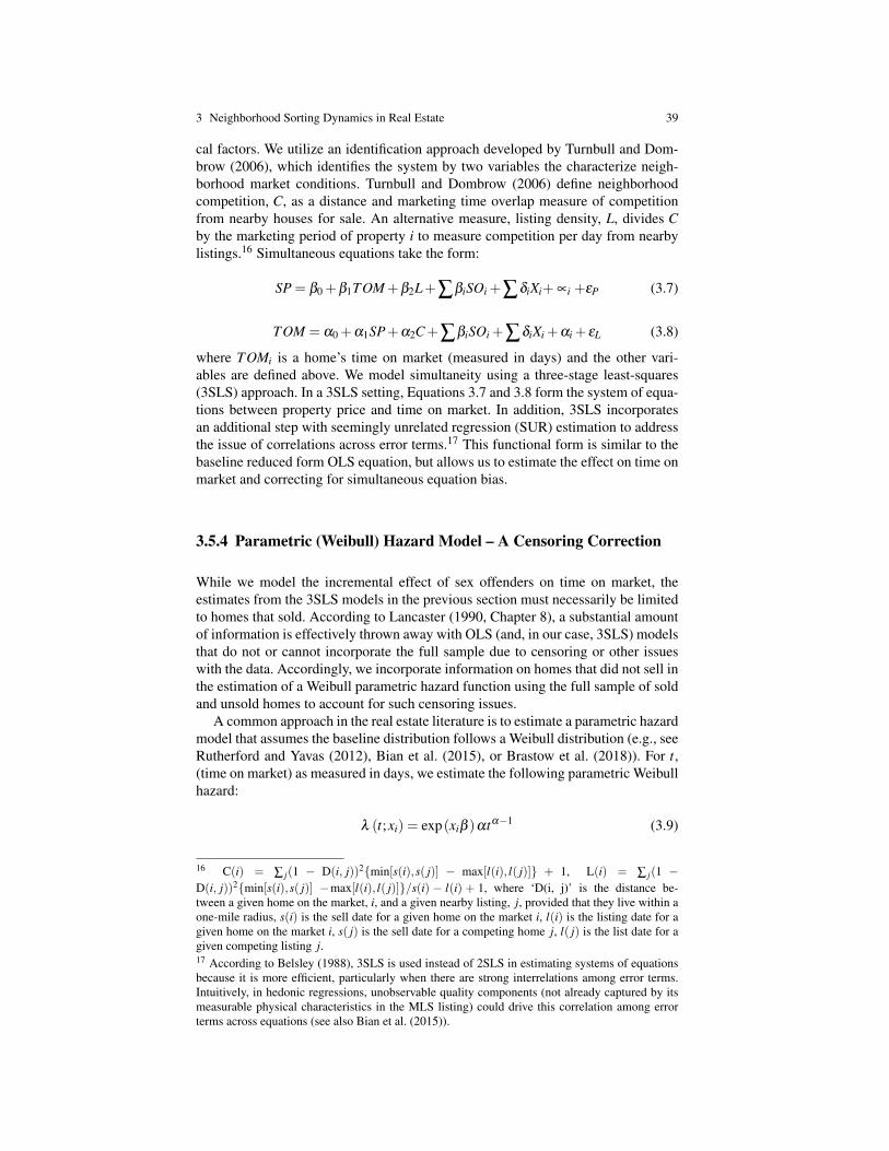
3 Neighborhood Sorting Dynamics in Real Estate 39
cal factors. We utilize an identification approach developed by Turnbull and Dom-brow (2006), which identifies the system by two variables the characterize neigh-borhood market conditions. Turnbull and Dombrow (2006) define neighborhoodcompetition, C, as a distance and marketing time overlap measure of competitionfrom nearby houses for sale. An alternative measure, listing density, L, divides Cby the marketing period of property i to measure competition per day from nearbylistings.16 Simultaneous equations take the form:
SP = β0 +β1TOM+β2L+∑βiSOi +∑δiXi+ ∝i +εP (3.7)
TOM = α0 +α1SP+α2C+∑βiSOi +∑δiXi +αi + εL (3.8)
where TOMi is a home’s time on market (measured in days) and the other vari-ables are defined above. We model simultaneity using a three-stage least-squares(3SLS) approach. In a 3SLS setting, Equations 3.7 and 3.8 form the system of equa-tions between property price and time on market. In addition, 3SLS incorporatesan additional step with seemingly unrelated regression (SUR) estimation to addressthe issue of correlations across error terms.17 This functional form is similar to thebaseline reduced form OLS equation, but allows us to estimate the effect on time onmarket and correcting for simultaneous equation bias.
3.5.4 Parametric (Weibull) Hazard Model – A Censoring Correction
While we model the incremental effect of sex offenders on time on market, theestimates from the 3SLS models in the previous section must necessarily be limitedto homes that sold. According to Lancaster (1990, Chapter 8), a substantial amountof information is effectively thrown away with OLS (and, in our case, 3SLS) modelsthat do not or cannot incorporate the full sample due to censoring or other issueswith the data. Accordingly, we incorporate information on homes that did not sell inthe estimation of a Weibull parametric hazard function using the full sample of soldand unsold homes to account for such censoring issues.
A common approach in the real estate literature is to estimate a parametric hazardmodel that assumes the baseline distribution follows a Weibull distribution (e.g., seeRutherford and Yavas (2012), Bian et al. (2015), or Brastow et al. (2018)). For t,(time on market) as measured in days, we estimate the following parametric Weibullhazard:
λ (t;xi) = exp(xiβ )αtα−1 (3.9)
16 C(i) = ∑ j(1 − D(i, j))2{min[s(i),s( j)] − max[l(i), l( j)]} + 1, L(i) = ∑ j(1 −D(i, j))2{min[s(i),s( j)] −max[l(i), l( j)]}/s(i) − l(i) + 1, where ‘D(i, j)’ is the distance be-tween a given home on the market, i, and a given nearby listing, j, provided that they live within aone-mile radius, s(i) is the sell date for a given home on the market i, l(i) is the listing date for agiven home on the market i, s( j) is the sell date for a competing home j, l( j) is the list date for agiven competing listing j.17 According to Belsley (1988), 3SLS is used instead of 2SLS in estimating systems of equationsbecause it is more efficient, particularly when there are strong interrelations among error terms.Intuitively, in hedonic regressions, unobservable quality components (not already captured by itsmeasurable physical characteristics in the MLS listing) could drive this correlation among errorterms across equations (see also Bian et al. (2015)).

40 Xun Bian, Raymond Brastow, Michael Stoll, Bennie Waller and Scott Wentland
where xi are the same covariates from the prior TOM equation and incorporateslist price (LPi) instead of sale price (SPi) so that the full sample could be used in thehazard estimation. Further, all models cluster standard errors by census block groupand report heteroscedastic-consistent robust standard errors. We report the resultsin both the accelerated failure time form and log-relative hazard form to interpretthe hazard results in regards to time on market and the probability of sale (failure),respectively. The coefficients can be interpreted as semi-elasticities with regard toright-hand side variable by exponentiating the coefficients, analogous to a semi-loginterpretation in OLS.
3.5.5 Geospatial Analysis of Tipping and Clustering
If the presence of nearby sex offenders has an incremental impact on real estate,then subsequent tipping of neighborhoods toward clusters of sex offenders shouldbe an observable geospatial phenomenon. In this section, we briefly outline how wemay exploit basic GIS techniques to explore implications of the pricing dynamicsthat may flow from our theoretical and empirical models above.18
Following Clark and Evans (1954), we begin by conducting a simple NearestNeighbor Analysis (NNA) in order to determine the pattern and distribution of apopulation in precise and meaningful terms. A Nearest Neighbor Analysis is oftenutilized as a procedure to classify the geographic distribution of a set of points ac-cording to their spatial pattern and proximity (Griffith and Arnrhein, 1991). Thisanalysis has been applied to a diverse variety of fields including the study of spatialdispersion patterns for individuals suffering from dengue fever in Malaysia (Azizet al., 2012). Second, we also incorporate a preliminary, broad spatial distributionanalysis of registered sex offenders in order to conduct an Average Nearest NeighborAnalysis (ANNA).19 The average nearest neighbor classification is particularly ef-fective at looking at a large data set and understanding the hypothetical random dis-persion compared to the observed positioning. The average nearest neighbor anal-ysis determines whether a set of spatial points can be classified as distributed ina dispersed pattern, random pattern, or a clustered pattern. This is accomplishedon the basis of the Average Nearest Neighbor Ratio (ANNR) value. Two distancesmake up the two key components of the Average Nearest Neighbor Ratio (ANNR).The ANNA tool measures what the distance to the nearest neighbor centroid is, andwhat it should be hypothetically if the dispersion is random. These are referred toas the observed mean distance (OMD) and the estimated mean distance (EMD) re-spectively. If the average distance is less than hypothetical random distribution, theANNR is less than 1, and the distribution is considered clustered. If the averagedistance is greater than the hypothetical distance for random clustering, then theANNR is greater than 1, and the distribution is considered dispersed. The point atwhich these two values meet can be construed as a ‘tipping point’ or critical periodin which the points move from dispersed to clustered or clustered to dispersed.
18 The GIS analysis uses the full Virginia data set of sex offenders, including areas both inside andoutside our MLS geographical area.19 Average Nearest Neighbor Ratio is given as follows: ANN = Do/DE where Do is the observedmean distance between each feature and the nearest neighbor: Do =
∑ni=1 di
n and DE is the expectedmean distance given a random pattern: DE = 0.5/
√n/A. In the previous equations di equals the
distance between feature i and its nearest feature, n corresponds to the total number of features,and A is the total study area.

3 Neighborhood Sorting Dynamics in Real Estate 41
The distance between points was measured as a Euclidean distance or ‘as thecrow flies’ in meters. The precise field area was set as the minimum enclosing rect-angle around the features. The null hypothesis for the ANNA is that all the pointsare randomly distributed. The null hypothesis is tested by Z statistic. The Z scorevalue is a measure of statistical significance which tells us whether or not to rejectthe null hypothesis. Higher and lower numbers identify virtually no chance of ran-dom distribution. The ANNA also identifies a P value for the data set. This P valueis the probability that null hypothesis will be falsely rejected.
For the initial analysis, we divided the registered sex offender data into 6 monthincrements. Each 6 month grouping identifies the registered sex offenders who livedwithin Virginia at that time regardless of the duration they lived at that particularaddress. The first grouping, designated (a), includes those registered sex offenderswho were living in Virginia during the time of January 1st to June 30th. The secondgrouping, designated (b), includes those registered sex offenders who were living inVirginia during the time of July 1st to December 31st. Each 6 month increment madeup a single layer feature class, and we utilized the average nearest neighbor analysisto all points within that layer. We applied the ANNA to 24 total data layers. Theutilization of the ANNA in this fashion identified a general trend of clustering overtime with a specific tipping point apparent. This preliminary analysis also identifieda time in which a significant number of registered sex offenders were present withinthe study area.
3.6 Results -– The Effects of Clustering and the Role of the PriceMechanism
3.6.1 The Price of (Sex Offender) Clustering
The initial set of results reveals a significant relationship between the number ofsex offenders and real estate outcomes, namely price and liquidity (as measuredby days on market). While there are some differences in model specifications, theinitial results are qualitatively consistent with Wentland et al. (2014). The first twocolumns of Table 3.6.1 show the general impact on sale price. Column 1 indicatesthat an additional sex offender located nearby (i.e. within 0.25 mile) lowers the saleprice of a home by approximately $5,455. This provides preliminary evidence thatregistered sex offenders present a negative externality and the negative externalityis an increasing function in sex offenders, which is generally consistent with theliterature discussed in section two. However, the incremental impact of each sexoffender may be more nuanced, which is the primary focus of this paper.
Column 2 breaks out the variable of interest into four increments (with the refer-ence group being zero) that allow the effect to vary across increments in a nonlinearfashion. Column 2 shows that the first nearby sex offender has a large, significanteffect on the sale price of a home, amounting to a discount of $8,338 or approxi-mately 5% for the average home. The second and third nearby sex offenders do nothave a statistically significant impact on price, however, implying a discontinuousor non-linear preference for living near additional sex offenders. While this does notnecessarily confirm an equilibrium (or equilibrium-like behavior) at some low num-ber of sex offenders, this evidence would be consistent with the idea that the firstsex offender has a large initial effect on home prices, but an equilibrium may exist

42 Xun Bian, Raymond Brastow, Michael Stoll, Bennie Waller and Scott Wentland
Table 3.2 The incremental effect of sex offenders on a home’s sale price and days on market –OLS and 3SLS models
Variable
OLS ModelDependentVariable:Sale Price
OLS ModelDependentVariable:Sale Price
OLS ModelDependentVariable:Sale Price
3SLS ModelDependentVariable:Sale Price
OLS ModelDependentVariable:Days onMarket
Number of Sex Offenders≤ 0.25 mile
-5,454.72***
(-2.81)
First Sex Offender≤ 0.25 mile
-8,337.78***
(-3.30)
-14,843.68***
(-2.68)
-7,692.50***
(-3.99)
51.94***
(3.39)
Second Sex Offender≤ 0.25 mile
-6,861.99
(-1.19)
-2,543.79
(-0.30)
-6,395.65*
(-1.84)
46.81**
(2.01)
Third Sex Offender≤ 0.25 mile
-10,697.24
(-1.28)
-14,613.54
(-0.89)
-8,181.99
(-1.16)
61.78
(1.36)
Four or More Sex Offenders \leq 0.25 mile-25,099.07**
(-2.07)
7,830.07
(0.89)
-26,016.15***
(-2.73)
163.95**
(2.43)
Bedrooms (3+) * First Sex Offender8,908.58
(1.08)
Bedrooms (3+) * Second Sex Offender-5,481.68
(-0.60)
Bedrooms (3+) * Third Sex Offender4,498.29
(0.24)
Bedrooms (3+) * Four or More Sex Offenders-43,765.75***
(-4.21)
Property Characteristics ✓ ✓ ✓ ✓ ✓Macroeconomic Controls ✓ ✓ ✓ ✓ ✓Season Fixed Effects ✓ ✓ ✓ ✓ ✓Census Block Groups ✓ ✓ ✓ ✓ ✓Year Fixed Effects ✓ ✓ ✓ ✓ ✓Observations 12,426 12,426 12,426 12,362 12,362Notes: This table presents results of OLS and 3SLS estimations of the incremental impact of registered sex offenderson sale price and days on market (time on market) across different specifications (OLS and 3SLS); t-statistics (z-statistics) in parentheses; ***, **, and * denote significance at the 1%, 5% and 10% levels, respectively. Coefficientson controls are omitted for brevity.
in neighborhoods with a low number of sex offenders (three or less). A low numberof sex offenders may be consistent with a stable, initial discount of approximately5% with a potential noisier discount associated with additional offenders.
If a neighborhood tips toward a critical mass of sex offenders, we would expectthis to be reflected by (or precipitated by) the pricing of these homes. Indeed, we seethat the equilibrium (or quasi-equilibrium) appears to break down once the fourthsex offender moves in. Table 3.6.1 shows that a cluster of four or more sex offenderscoincides with a much larger, statistically significant discount on sale price. Specifi-cally, a cluster of four or more offenders is associated with a sharp $25,099 (or 16%)drop in price of nearby homes. Given the steep discount on home prices, the clusterof sex offenders provides a stronger incentive to sort based on the theoretical frame-work outlined previously. All else equal, this strong price signal coupled with thelikelihood that sex offenders are likely to be less averse to living near one of theirown group members, we would expect additional sex offender clustering aroundareas with multiple sex offenders as a result of the sharp discount associated withthis clustering. Thus, this provides initial evidence that pricing dynamics illustratea mechanism through which a clustering or tipping dynamic could occur in housing

3 Neighborhood Sorting Dynamics in Real Estate 43
markets. Whether we find evidence of additional clustering over time in this data isa hypothesis that will be explored with GIS spatial analysis.
3.6.2 The Different Price of RSO Clustering for Families
Household preferences for living near sex offenders are not likely to be uniform.Households with children may be particularly averse to living near sex offenders,which will be reflected in their bid functions for housing. After creating a simpli-fied proxy for ‘family homes’ (i.e. a variable indicating whether a home has threeor more bedrooms), we attempt to disentangle some of the tipping dynamics of themarket by interacting this proxy with our variables of interest. The results are shownin Column 3 of Table 3.6.1. The estimates of this model show that the discount forthe initial sex offender for ‘non-family’ homes is $14,844. Each additional sex of-fender does not have a statistically significant effect, implying an approximatelyuniform discount for living near sex offenders (regardless of the number) for ‘non-family’ homes.20 The most striking result of this column is that ‘family’ homes havea very large discount, approximately $43,765 or 26%, associated with living near acluster of four or more sex offenders. Given the potentially greater risk/externalitythat sex offender recidivism imposes for families with children, this result is consis-tent with the prediction of both intuition and our theoretical framework. More gen-erally, given that we find that an intensified (nonlinear) treatment effect on a moresensitive treatment group, this also serves as additional evidence that our results areproperly identified.
3.6.3 The Liquidity (or Time on Market) Effect — 3SLS
The incremental effect of sex offenders may not be capitalized solely in price, par-ticularly as price and liquidity are jointly determined in this market. The estimated3SLS model, shown in Columns 4 and 5 in Table 3.6.1, shows that the externalityassociated with additional sex offenders is reflected by both price and liquidity. Theimpact of the initial offender on price is slightly smaller (-$7,692), as the effect isalso capitalized into liquidity by extending the time it takes to sell the home by 52days (or 47%) on average. There is a smaller (less statistically significant) effectfor the second sex offender, but no statistically significant impact for the third of-fender. Generally, this is consistent with the previous results like Wentland et al.(2014) and Brastow et al. (2018), suggesting a significant, moderate external liquid-ity effect associated with living near a few sex offenders. Moreover, there is also alarge, significant effect associated with living near four or more offenders. Whilethe price discount is approximately the same as the OLS estimate, the striking resultis the massive effect on a home’s liquidity. A cluster of four or more nearby offend-ers increases a home’s time on market by 164 days, or 147% on average. While itis not surprising that homes located near a cluster of sex offenders sell for a siz-
20 The coefficients that are not individually significant in this regression are also not jointly signifi-cant, at conventional levels of statistical significance. For all intents and purposes, the insignificantcoefficients are treated as zero in this analysis. Also note that the specification here is somewhatdifferent from Wentland et al. (2014), which has a linear interacted bedrooms specification. Thisanalysis suggests that there may also be a nonlinear effect.

44 Xun Bian, Raymond Brastow, Michael Stoll, Bennie Waller and Scott Wentland
able discount and are much harder to sell in a reasonable amount of time, the sheermagnitude of the effect remains striking, possibly reflecting a much smaller pool ofpotential buyers willing to bid on one of these homes.
3.6.4 The Liquidity Effect and Probability of Sale – A Parametric(Weibull) Hazard Model
Using the full sample of sold and unsold properties, a parametric hazard functionwas estimated to account for related selection issues (which were explained in fur-ther detail in the methodology section above). The results in Table 3.6.4 are gener-ally consistent with the three stage findings, with a couple notable exceptions. Themagnitude for the effect on time on market appear to be more modest across theboard as compared to the three stage results, but in this specification, the larger ex-ternality may be the reflected by the presence of the third offender, not the forth. Thethird offender represents a substantially longer time on market, and correspondingly,a much lower probability of sale in the hazard model specifications. The cluster offour or more still represents a large, negative externality based on the Weibull haz-ard model results, which we interpret as qualitatively consistent with the three stageresults from the previous sub-section.
3.7 Results -– Tipping and Clustering Evidence from GIS SpatialAnalysis
We conduct a basic geospatial analysis of our sample, finding initial evidence ofadditional clustering of registered sex offenders over time. The result of an averagenearest neighbor analysis gives several values, which include the Average Near-est Neighbor Ratio (ANNR), the observed mean distance (OMD), the estimatedmean distance (EMD), a z-score and a p-value. The initial Average Nearest Neigh-bor Analysis begins at a starting point of three registered sex offenders in the lastsix months of 1997. This initial analysis produces an ANNR value of 3.847748. Thesame analysis was completed on each six month grouping. We identified a poten-tial tipping point within the first six months of 2003. Around the tipping point atwhich the observed mean distance reached the estimated mean distance, the ANNRreached 1.007778. The ANNR generally continued to decrease as seen in Figure 3.2,with the smallest ANNR is found in the 2009a data set. The Z score values identifythat the RSO distribution pattern within the study area has a less than 1% chance ofbeing the result of chance. Figure 3.3 shows the dramatic dip, as increasing cluster-ing of registered sex offenders occurs on a state-wide level.21
To summarize, the GIS analysis shows a clear trend of clustering, as some neigh-borhoods tip toward being more densely populated by sex offenders. This offers
21 In untabulated analysis, we created census blocks as a way to normalize the ANN analysis forpopulated areas within Virginia. We are able to statistically identify traits of those census blockswhich contain RSOs with our sample. We compare the location of the RSOs to the census blocksin order to develop a general temporal trend and identify if any other ‘tipping point’ exists. Ouranalysis showed that despite the potential for the RSOs to live in any of the 285,762 census blocks,there is a spatial clustering within certain small census blocks over time. We leave more in-depthspatial analysis to future research.

3 Neighborhood Sorting Dynamics in Real Estate 45
Table 3.3 The incremental effect of a registered sex offender on a home’s time on market andprobability of sale – Weibull accelerated failure-time form and log relative-hazard form
Variable
Weibull DistributionCoefficientsDependent Variable:Time on Market
Weibull DistributionCoefficientsDependent Variable:Sold
First Sex Offender≤ 0.25 mile
0.098**
(1.98)
-0.146**
(-1.99)Second Sex Offender
≤ 0.25 mile
0.012
(0.17)
-0.018
(-0.17)Third Sex Offender
≤ 0.25 mile
0.794***
(3.30)
-1.179***
(-3.29)
Four or More Sex Offenders≤ 0.25 mile
0.538**
(2.50)
-0.798**
(-2.50)
/ln p0.394***
(28.35)
0.394***
(28.35)p 1.48 1.48Property Characteristics ✓ ✓Macroeconomic Controls ✓ ✓Season Fixed Effects ✓ ✓Census Block Groups ✓ ✓Year Fixed Effects ✓ ✓Observations 19,701 19,701Sold Homes 12,406 12,406Notes: This table estimates the external effects an RSO on home liq-uidity using a parametric hazard that follows a Weibull distribution.Results in Column 1 report accelerated failure-time coefficients, whilethe results in Column 2 report log relative hazard form coefficients.Robust z-statistics in parentheses (Errors Clustered by Census BlockGroup) *** p¡0.01, ** p¡0.05, * p¡0.10.
values identify that the RSO distribution pattern within the study area has a less than 1% chance
of being the result of chance. Figure II shows the dramatic dip, as increasing clustering of
registered sex offenders occurs on a state-wide level.21
Figure II. ANNA statistic results by 6 month increment
Figure III. ANNA Z score statistical results by 6 month increment
21 In untabulated analysis, we created census blocks as a way to normalize the ANN analysis for populated areas within Virginia. We are able to statistically identify traits of those census blocks which contain RSOs with our sample. We compare the location of the RSOs to the census blocks in order to develop a general temporal trend and identify if any other “tipping point” exists. Our analysis showed that despite the potential for the RSOs to live in any of the 285,762 census blocks, there is a spatial clustering within certain small census blocks over time. We leave more in-depth spatial analysis to future research.
0
0.5
1
1.5
2
2.5
3
3.5
4
4.5
1997
b
1998
a
1998
b
1999
a
1999
b
2000
a
2000
b
2001
a
2001
b
2002
a
2002
b
2003
a
2003
b
2004
a
2004
b
2005
a
2005
b
2006
a
2006
b
2007
a
2007
b
2008
a
2008
b
2009
a
AN
NA
(R
) V
alue
Fig. 3.2 ANNA statistic results by 6 month increment
additional, complementary evidence that the pricing dynamics are consistent withsex offender sorting.

46 Xun Bian, Raymond Brastow, Michael Stoll, Bennie Waller and Scott Wentland
To summarize, the GIS analysis shows a clear trend of clustering, as some neighborhoods
tip toward being more densely populated by sex offenders. This offers additional, complementary
evidence that the pricing dynamics are consistent with sex offender sorting.
VIII. Conclusion and a Discussion of Efficiency Implications
Prior real estate research has found that registered sex offenders (RSOs) impose external
costs, given potential risks of recidivism, which are capitalized into the value and liquidity of
nearby residential real estate. Several studies have shown that registered sex offenders lower
nearby residential home prices significantly. In this study, we find that sex offenders have a
tendency to cluster in certain areas. To explain this phenomenon, we investigated whether there is
evidence that market prices facilitate this process, given that RSOs could be attracted by lower
prices and being less concerned with living near other sex offenders (as compared to non-
offenders’ concerns about living near offenders). Using a decade of multiple listing service (MLS)
data in Virginia, along with corresponding sex offender data obtained with the help of the Virginia
State Police, we found that the initial sex offender that moves in nearby has a significant negative
effect on a home’s price and liquidity. We find evidence of nonlinear effects, where each
-70
-60
-50
-40
-30
-20
-10
0
10
20
1997
b
1998
a
1998
b
1999
a
1999
b
2000
a
2000
b
2001
a
2001
b
2002
a
2002
b
2003
a
2003
b
2004
a
2004
b
2005
a
2005
b
2006
a
2006
b
2007
a
2007
b
2008
a
2008
b
2009
a
Z S
core
Fig. 3.3 ANNA Z score statistical results by 6 month increment
3.8 Conclusion and a Discussion of Efficiency Implications
Prior real estate research has found that registered sex offenders (RSOs) impose ex-ternal costs, given potential risks of recidivism, which are capitalized into the valueand liquidity of nearby residential real estate. Several studies have shown that regis-tered sex offenders lower nearby residential home prices significantly. In this study,we find that sex offenders have a tendency to cluster in certain areas. To explain thisphenomenon, we investigated whether there is evidence that market prices facilitatethis process, given that RSOs could be attracted by lower prices and being less con-cerned with living near other sex offenders (as compared to non-offenders’ concernsabout living near offenders). Using a decade of multiple listing service (MLS) datain Virginia, along with corresponding sex offender data obtained with the help ofthe Virginia State Police, we found that the initial sex offender that moves in nearbyhas a significant negative effect on a home’s price and liquidity. We find evidence ofnonlinear effects, where each successive sex offenders that move in nearby have lit-tle significant impact until the neighborhood reaches a critical ‘tipping point,’ wherea cluster of four or more sex offenders has much larger negative effects on the priceand liquidity of nearby homes. A within-neighborhood analysis shows that livingnear a cluster of four or more sex offenders may reduce a home’s sale price by ap-proximately $26,000 (or 16%) and increase the time a home spends on the marketby 164 days (or 147%), on average.
Overall, the results provide evidence consistent with the hypothesis that marketprices facilitate the sorting/tipping process we observe, where individuals operat-ing within the market sort according to their preferences and incentives, resultingin segmentation of these two groups (i.e. sex offenders vs. general populace). Thegeospatial evidence is consistent with increasing clustering of registered sex offend-ers and segregation of these two groups. This research may help real estate aca-demics and practitioners understand the locational choices/tendencies of registeredsex offenders and the implications for real estate and residential mobility.
While these results are striking, it raises a broader question about whether thisprocess is efficient. We can offer a brief discussion based on the findings here. Thesteep negative externality associated with living near a cluster of sex offenders atfirst gives one pause that a negative externality is leading to a serious issue for realestate markets. However, note that in Table I.B., the number of homes that are lo-cated nearby clusters is very small. So, while the externality effect is large for anindividual listing on the market, it is not necessarily the case that the overall ef-

3 Neighborhood Sorting Dynamics in Real Estate 47
fect on the market is larger. The opposite could be true, depending on how manyhomes are affected by this externality. Intuitively, if the external impact of an RSOis spatial in nature (i.e., a decreasing function in distance), then a cluster containsoverlapping externalities that are concentrated in a particular area. Conceptually,this runs parallel to the idea that it might be more efficient to concentrate pig farms,or some other spatially-specific negative externality like a paper mill, in a particulararea or cluster rather than scattering them randomly next to housing developments,for example. While this may not be applicable for all externalities (nor is efficiencythe only value policymakers need to take into account), this reasoning is a key mo-tivating idea behind local zoning restrictions. However, while states and localitiesdo have restrictions on where RSOs can live and work to induce a similar sort ofclustering, the evidence from Virginia from our study suggests that the market pro-vides an additional incentive to cluster, which is unplanned and decentralized. Thus,the extent to which real estate markets provide a price incentive to cluster negativeexternalities could be an extension of classic ideas in economics, whether it is AdamSmith’s ([1776] 1937) invisible hand metaphor more generally, or Coase’s (1960)idea more specifically, that market exchange can lead to efficient outcomes througha decentralized price mechanism (even when externalities are present, dependingon the circumstances). We leave further exploration of this in real estate and otherapplications to future research.
Acknowledgements Disclaimer: Any views expressed here are those of the authors and not neces-sarily those of the Federal Reserve Bank of Richmond or the Federal Reserve System. The authorswould like to thank participants and discussants at the 2013 American Real Estate Society AnnualMeeting, 2015 American Real Estate and Urban Economics International Conference, and the 2016Eastern Economics Association Annual Meeting for helpful comments. This paper was the recip-ient of the 2013 Best Paper Award from the American Real Estate Society Annual Meeting for‘Innovative, Outside-The-Box Research.’ We also thank Lt. William Reed, Jr of the Criminal Jus-tice Information Services Division of the Virginia State Police for providing the historical recordof sex offender residences.
References
Aziz S, Ngui R, Lim Y, Sholehah I, Nur Farhana J, Azizan A, Wan Yusoff W (2012)Spatial pattern of 2009 dengue distribution in Kuala Lumpur using GIS applica-tion. Tropical Biomedicine 29(1):113–120
Belsley DA (1988) Two-or three-stage least squares? Computational Economics1(1):21–30
Bian X, Waller BD, Turnbull GK, Wentland SA (2015) How many listings are toomany? Agent inventory externalities and the residential housing market. Journalof Housing Economics 28(1):130–143
Bond EW, Coulson NE (1989) Externalities, filtering, and neighborhood change.Journal of Urban Economics 26(2):231–249
Brastow RT, Waller BD, Wentland SA (2018) Temporally dynamic externalities andreal estate liquidity. Journal of Real Estate Research 40(2):199–240
Card D, Mas A, Rothstein J (2008) Tipping and the dynamics of segregation. Quar-terly Journal of Economics 123(1):177–218
Clark PJ, Evans FC (1954) Distance to nearest neighbor as a measure of spatialrelationships in populations. Ecology 35(4):445–453

48 Xun Bian, Raymond Brastow, Michael Stoll, Bennie Waller and Scott Wentland
Coase R (1960) The problem of social cost. Journal of Law and Economics 3(1):1–44
Coulson NE, Bond E (1990) A hedonic approach to residential succession. Reviewof Economics and Statistics 72(3):433–44
Davis LW (2004) The effect of health risk on housing values: Evidence from acancer cluster. American Economic Review 94(5):1693–1704
Griffith D, Arnrhein C (1991) Statistical Analysis for Geographers. Prentice Hall,Englewood Cliffs, NJ
Grubesic TH (2010) Sex offender clusters. Applied Geography 30(1):2–18Heintzelman MD (2010) Measuring the property-value effects of local land use and
preservation referenda. Land Economics 86(1):22–47Krainer J (2001) A theory of liquidity in residential real estate markets. Journal of
Urban Economics 49(1):32–53Kuminoff NV, Parmeter CF, Pope JC (2010) Which hedonic models can we trust to
recover the marginal willingness to pay for environmental amenities? Journal ofEnvironmental Economics and Management 60(3):145–160
Lancaster T (1990) The Econometric Analysis of Transition Data. Cambridge Uni-versity Press, New York, NY
Larsen JE, Lowrey KJ, Coleman JW (2003) The effect of proximity to a registeredsex offender’s residence on single-family house selling price. The Appraisal Jour-nal 71(3):253
Linden L, Rockoff JE (2008) Estimates of the impact of crime risk on propertyvalues from Megan’s laws. American Economic Review 98(3):1103–27
O’Sullivan A (2009) Schelling’s model revisited: Residential sorting with competi-tive bidding for land. Regional Science and Urban Economics 39(4):397–408
Pope JC (2008) Fear of crime and housing prices: Household reactions to sex of-fender registries. Journal of Urban Economics 64(3):601–614
Rey SJ, Murray AT, Grubesic TH, Mack E, Wei R, Anselin L, Griffin M (2014) Sexoffender residential movement patterns: A Markov chain analysis. The Profes-sional Geographer 66(1):102–111
Roberts MR, Whited TM (2013) Endogeneity in empirical corporate finance1. In:Constantinides GM, Harris M, Stulz RM (eds) Handbook of the Economics ofFinance, vol 2, Elsevier, pp 493–572
Rosen S (1974) Hedonic prices and implicit markets: Product differentiation in purecompetition. Journal of Political Economy 82(1):34–55
Rutherford R, Yavas A (2012) Discount brokerage in residential real estate markets.Real Estate Economics 40(3):508–535
Schelling TC (1971) Dynamic models of segregation. Journal of Mathematical So-ciology 1(2):143–186
Smith A ([1776] 1937) The Wealth of Nations: An Inquiry into the Nature andCauses of the Wealth of Nations. Modern Library, New York, NY
Turnbull GK, Dombrow J (2006) Spatial competition and shopping externalities:Evidence from the housing market. Journal of Real Estate Finance and Economics32(4):391–408
Virginia State Police (2020) Sex Offenders and Crimes Against Minors Registry.Virginia State Police, North Chesterfield, VA
Wentland S, Waller B, Brastow R (2014) Estimating the effect of crime risk onproperty values and time on market: Evidence from Megan’s law in Virginia.Real Estate Economics 42(1):223–251

Chapter 4The Rental Next Door: The Impact Of RentalProximity On Home Values
Wendy Usrey
Abstract The literature on the spillover effects of rental properties mainly focuseson the impacts of multi-unit complexes and low income housing. Little has beendone specifically looking at the relationship between single-family rental homesand sales price. This paper extends the literature by modeling the impact of single-family rental proximity on home sales price using a spatial approach. Through theuse of GIS software, I was able to specifically measure the density of single-familyrental properties for each sold home, rather than following the “blanket approach”of measuring density as the ‘percent of rentals in the census tract’ typical in the lit-erature. With data collected for 2,766 homes sold between January 1, 2011 and July1, 2012 in Fort Collins, Colorado, a hedonic price model was used to empiricallytest for the impacts of rental proximity on home values. I find strong evidence thatproximity to single-family rental homes plays an important role in determining ahome’s selling price. Rentals within 1/4 mile of a sold home had a negative impacton price, while rentals between 1/4 and 1/2 mile had a positive impact on price. Ifrentals are considered an alternative to foreclosure or short sale, these results suggestthe negative impacts of distressed sales are greater than those of rental properties onsurrounding home values.
4.1 Introduction and Background Information
People generally tend to believe that rental properties will impact their neighbor-hood negatively as more and more homes in the subdivision turn into rental proper-ties. Many homeowners’ associations attempt to reduce the number of rental proper-ties by regulating the placement of signs, restricting the number of rental propertiesin the subdivision, and in some cases, outright banning rental properties. In somecities, policy makers try to reduce the number of rental properties by passing ordi-nances (such as the three unrelated ordinance in Fort Collins, CO), requiring rentalinspections, regulating sign placement, and charging registration and/or licensingfees. Even the mortgage industry is “anti- rental,” with larger down payments re-quired for non-owner occupied homes and “Fannie Mae and Freddie Mac refus[ing]
Wendy UsreyKansas State University, Manhattan, KS 66506, USA e-mail: [email protected]
49
50 Wendy Usrey
to underwrite mortgages in condo projects where a majority of units are rentals”(Reagan, 2009).
The general public is quick to assume a rental property will “ruin” their neigh-borhood, and this is traditionally the assumption in most literature. This oppositionhas been well documented and takes many forms. Some of the most common argu-ments against rental housing include: rentals attract low-income residents and lessdesirable neighbors, lead to an increase in crime and traffic and place an additionalfinancial burden on local governments and schools. Opposition also stems from thebelief that rental properties are not as well-maintained as owner-occupied homesand will overall lead to a decline in property values (Ellen et al., 2007; Obrinskyand Stein, 2007; Sirmans, 1996). These arguments have been supported in some ofthe empirical literature. Wang et al. (1991) concluded that “an inverse relationshipexists between the value of a house and the presence of rental properties in the area.”Specifically, they found that the presence of rental properties within close proximity(defined as the group of 5-8 surrounding homes) reduced a home’s selling price byapproximately 2% (Wang et al., 1991). Similar results were found in several studieslooking at the impact of subsidized and multi-family rental housing developments,though the results were mixed and varied widely between the studies (Goetz et al.,1996).
While at first glance it would appear that rental homes are “bad” for a neigh-borhood and property values, the evidence is mixed overall. A study analyzingthe impact of federally subsidized rental housing on property values found that inmost cases, property values were not reduced by federally-subsidized developmentsand in many instances the developments actually led to increases in property val-ues (Ellen et al., 2007). Grether and Mieszkowski (1980)Grether and Mieszkowskifound that proximity to “low-density apartment developments [were] relativelyharmless” in terms of their impact on residential property values, and a documentproduced for the National Policy Summit on Rental Housing summarized numer-ous studies in which the authors determined property values were higher in areasnear multi-family housing or “proximity to subsidized housing made no differencein housing values...” (Obrinsky and Stein, 2007).
A recent addition to the debate is how economic conditions are playing a role inthe desirability of rental homes. With the housing crisis plaguing the United States,home prices are down in many areas which means many homeowners can no longersell their properties without taking a loss, or bringing money to the table. As ofMarch 1, 2012, an estimated 11.1 million homeowners were underwater on theirmortgage.1 That’s approximately 22.8% of mortgages and is at the highest levelsince the third quarter of 2009, when the data was first tracked (Reuters, 2012).Stricter lending requirements, along with higher rates of unemployment, meansfewer people are willing or able to buy. As a result, many homeowners are facedwith tough choices: sell at a loss, attempt a short sale, let the home go to foreclo-sure, leave the home vacant, or rent it out until conditions improve. For homeownersin these situations, rental restrictions limits their options. If they can’t afford to makepayments on two homes or don’t have money to bring to the closing table while un-able to rent out the home due to rental restrictions, their only option left is to attempta short sale or let the home go to foreclosure.
It is commonly assumed that foreclosures and vacant homes decrease propertyvalues, and many studies have shown that this is assumption is accurate. Immergluck
1 A borrower is considered to be underwater when their loan balance is higher than the currentmarket value of the property.

4 The Rental Next Door: The Impact Of Rental Proximity On Home Values 51
and Smith (2005) determined that in Chicago, each foreclosure within 1/8 mile ofa single-family home results in a decrease in value of approximately 1%, and Linet al. (2009) also focused on the City of Chicago and found that a foreclosure within0.9 kilometers of a home reduces its value by 8.7%. Mikelbank (2008) analyzedthe impact of foreclosures and vacant/abandoned properties in Columbus, Ohio anddetermined that each foreclosure negatively impacted sold homes between 1% and2%, while vacant or abandoned properties negatively impacted sold homes between0.5% and 3.5% depending upon their on distance from the homes. For many loca-tions, the debate has turned into choosing between the ‘lesser of two evils.’ Allowrentals, keeping homes occupied with fewer foreclosures, and accept the “problems”that come from non-owner occupied homes or ban rentals, and instead deal with theempty properties and increased foreclosures.
Fig. 4.1 Larimer County foreclosure filings and sales
4
Figure 1: Foreclosure Filings and Sales Data Source: Colorado Division of Housing
644 806
974 1253
1588 1493
2134 1824
1329 1296
500
1006 759 817 903 781 726
0
500
1000
1500
2000
2500
2003 2004 2005 2006 2007 2008 2009 2010 2011 2012
Larimer County Foreclosures
Foreclosure Filings Foreclosure Sales
vacant or abandoned properties negatively impacted sold homes between 0.5% and
3.5% depending upon their on distance from the homes (Mikelbank, 2008).
For many locations, the debate has turned into choosing between the ‘lesser
of two evils.’ Allow rentals, keeping homes occupied with fewer foreclosures, and
accept the “problems” that come from non-owner occupied homes or ban rentals,
and instead deal with the empty properties and increased foreclosures.
The foreclosure crisis has not only impacted property values and
homeowners. Along with falling homeownership rates, the increase in foreclosures
has led to a large number of households transitioning from homeowners to renters.
Across the nation, rental vacancy rates have reached a ten year low, while rents
continue to climb, and the rental market in Fort Collins, Colorado is no exception2
(Callis & Kresin, 2012). Figures 1 and 2 below show the relationship between
foreclosures and rental demand in Fort Collins.3,4
2 See Appendix A: Figures A1 and A2. 3 Values for 2012 are estimates based on the monthly data available at the time of the analysis. 4 See Appendix A for foreclosure filings and foreclosure sales definitions.
Source: Colorado Division of Housing (2012).
The foreclosure crisis has not only impacted property values and homeowners.Along with falling homeownership rates, the increase in foreclosures has led to alarge number of households transitioning from homeowners to renters. Across thenation, rental vacancy rates have reached a ten year low, while rents continue toclimb, and the rental market in Fort Collins, Colorado is no exception (Callis andKresin, 2012). Figures 4.1 and 4.2 show the relationship between foreclosures andrental demand in Fort Collins.2
In 2009, foreclosure filings in Larimer County peaked, creating higher demandfor rental housing. Between 2009 and 2012, as fewer rentals were available (indi-cated by the decreasing vacancy rates), the average rent increased by 17.9%. Rentalhousing policy typically focuses on balancing the need for affordable housing withthe needs of homeowners’ concerned with preserving the quality of their neigh-borhood and protecting the value of their homes. Policy discussion tends to largelyfocus on low-income affordable housing (i.e. subsidized housing, Section 8 housing,etc) despite the fact that such types of rental properties make up a small percentageof overall rental housing in most communities.3 Single-family rental homes play animportant role in providing quality housing to people who are unable or unwillingto purchase their own homes, and are “essential for households at middle-incomeand lower-income levels” (Colorado Division of Housing, 2011).
2 Values for 2012 are estimates based on the monthly data available at the time of the analysis.3 For example, in Larimer County, affordable rental units (including income restricted, senior anddisabled housing) make up just 10.8% of renter-occupied units (Community Strategies Institute,2009).

52 Wendy Usrey
Fig. 4.2 Fort Collins rent and vacancy rates
5
$753 $743 $726 $740 $749 $759 $760
$861 $867 $925
$1,015
8.6%
13.1% 12.4%
1.2%
8.7%
6.2% 5.7%
6.3%
5.0%
3.9% 3.1%
0.0%
2.0%
4.0%
6.0%
8.0%
10.0%
12.0%
14.0%
$-
$200
$400
$600
$800
$1,000
$1,200
2002 2003 2004 2005 2006 2007 2008 2009 2010 2011 2012
Vac
ancy
Rat
e
Ave
rage
Re
nt
Average Rent and Vacancy Rates in Fort Collins
Average Rent Vacancy Rate
Figure 2: Fort Collins Rent and Vacancy Rates
Data Source: Colorado Division of Housing
In 2009, foreclosure filings in Larimer County peaked, creating higher
demand for rental housing. Between 2009 and 2012, as fewer rentals were
available (indicated by the decreasing vacancy rates), the average rent increased by
17.9%.
Rental housing policy typically focuses on balancing the need for affordable
housing with the needs of homeowners’ concerned with preserving the quality of
their neighborhood and protecting the value of their homes. Policy discussion tends
to largely focus on low-income affordable housing (i.e. subsidized housing, Section 8
housing, etc) despite the fact that such types of rental properties make up a small
Source: Colorado Division of Housing (2011).
According to the American Housing Survey, in 2010, 34.5% of occupied housingunits in Fort Collins were home to renters. The estimated median household incomefor renter-occupied housing was $33,803, while the estimated median household in-come for owner-occupied housing was $70,441. In general, housing is consideredaffordable when housing expenses do not exceed 30% of a family’s gross income(Wallace, 1995). Based on data obtained from the 2011 American Community Sur-vey, it was estimated that 28% of owner-occupied households and 53% of renter-occupied households in Fort Collins had housing costs that exceeded 30% of theirincome.
Due to the high cost of housing (relative to income), and the overall dynamicsof the housing market in Fort Collins, the rental-housing debate is a particularlycontentious issue. With high home prices, rock bottom vacancy rates and increas-ing rents, local policy makers are faced with concern from both homeowners andrenters. Finding a balance between supporting home prices and providing afford-able housing within the community requires that policy makers have access to asmuch information as possible. This study aims to provide additional insight into thespecific dynamics of the housing market in Fort Collins, in terms of the relationshipbetween single-family rental homes and home sales prices. With so much mixedevidence, and so much at stake, further investigation is required to make sound de-cisions about the impact of non-owner occupied homes in a subdivision.
While this issue receives a lot of public attention and policy interest, the majorityof research in this area has focused on multi-family rental properties, governmentsubsidized housing and concentration of poverty in large cities. Little has been doneto look at how the presence of single family rental homes in a neighborhood for acommunity like Fort Collins, Colorado will impact property values. Literature in thisarea typically uses the percent of rental properties in the census tract as a measureof rental density. In doing so, the authors are implicitly assuming that the impactof rental composition will be identical across the tract. This paper expands uponthe current literature by using a unique spatial approach where the location andconcentration of rental properties is identified and explicitly considered, allowingthe impact to be unique for each home. It is also different in that it looks at single

4 The Rental Next Door: The Impact Of Rental Proximity On Home Values 53
family rental properties rather than focusing specifically on multi-unit complexes orsubsidized housing developments. Using a hedonic pricing model, the analysis willestimate the way rental properties affect home values by looking at how propertyvalues change depending upon their proximity to rental homes.
4.2 Analytical Framework
Rosen (1974) provided the framework for the hedonic price regressions that is typ-ically used to measure housing market impacts and externalities. These models usethe characteristics of a property as independent variables to explain or predict thesales price of a house. The basic intuition in hedonic valuation is that the price ofa good (in this case, a house) is a function of a bundle of attributes unique to thatspecific good (property). However, the prices of the individual characteristics arenot directly observed; they are implicit in the sales price of the house (which isobservable).
Thus the hedonic price of a house is defined as the “set of implicit prices” re-lated to the home’s specific characteristics and its observed price (Rosen, 1974).In equation form, the hedonic price of house Pi is a function of its characteristics,represented by the vector Xi.
Pi = f (Xi) (4.1)
For simplicity, assume a linear function of the form:
Pi = β0 +β1X1i +β2X2i + ...+βkXki (4.2)
Taking the partial derivative of price with respect to each characteristic yields thecharacteristic’s marginal cost:
δP/δx1 = β1 (4.3)
In this case, the marginal price of an additional unit of characteristic X1 is equal toβ1. For example, if X1 represented the number of bedrooms, this equation is tellingus that for each additional bedroom, the price of the house increases by β1, holdingother things constant.
In addition to structural characteristics, (square footage, number of bedrooms,lot size, etc.), the location of a house is considered to play an important role indetermining its value, so the characteristics of the neighborhood (location) must alsobe considered. Depending on the analysis, other factors expected to affect the priceof a home are also added to the model (for example: environmental characteristics,proximity to amenities, etc.).
For this analysis, the hedonic model, Pi j = f (Xi j,Ni j,Ri), measures the value of ahome as a function of its structural characteristics, its neighborhood characteristics,and the rental density characteristics of its location. In semi-log functional form, theregression model can be written as follows:
ln(Pricei j) = β0 +β1Xi j +B2N j +β3Ri + εi (4.4)
Where Pricei j = price of house i in neighborhood j, Xi j=a vector of structural char-acteristics of house i in neighborhood j, N j=a vector of characteristics for neighbor-hood j, and Ri=rental density characteristics of the location of house i. The variables

54 Wendy Usrey
that make up each of these characteristics, their definitions, and their expected rela-tionship with the dependent variable are shown in Table 4.1.
Table 4.1 Variable descriptions
Variable DescriptionExpectedSign
ln (Sales Price) Natural log of home sale price, in real dollars n/a
Age Age of house at time of sale in years* -Stories Number of stories (does not include basement)*Square Footage square feet of total above grade living space* +Basement SF Number of square feet in basement (finished or unfinished)* +Rooms Number of rooms above grade (does not include bathrooms)*Bedrooms Number of bedrooms* +Bathrooms Number of bathrooms* +Fireplace Number of fireplaces* +Lot Lot size in acres* +Central Air Dummy=1 if central air conditioning* +Loveland Schools Dummy=1 if located inside Loveland School District** +/-In City Limits Dummy=1 if located inside Fort Collins city limits** +/-Owner Occupied Dummy=1 if owner occupied* +/-
Attached Garage Home has an attached garage* +carport Home has a carport* +Detached Garage Home has a detached garage* +Multiple Garages Home has multiple garages and/or types* +Garage SF Square feet of garage space* +
Bank Owned Property was bank owned/foreclosure*** -Short Sale Property was a short sale*** -
Q1,Q2,Q3,Q4 Quarter home was sold*Sold 2012 Home was sold in 2012* +Distance to CSU Distance to CSU’s Lory Student Center**** -Distance to Shopping Distance to popular shopping area**** -
Rentals 500 Number of rentals within 500 ft **** +/-Rentals 14 Number of rentals within 500 ft and 1/4 mile radius **** +/-Rentals 12 Number of rentals within 1/4 and 1/2 mile radius **** +/-
Population Total population in census tract**** +/-% College % Census tract pop. with college degree or higher**** +Median Age Median age in census tract in years**** +/-Families Husband and wife with own child**** +Dad Male with own child less than 18, no wife**** -Mom Female with own child less than 18, no husband**** -% White % of tract population that is white**** +Income Average annual income in census tract in real$**** +Vacant Vacant housing units in census tract**** -% Rentals % of rental homes in census tract**** +/-% Students % of tract population enrolled in 4-yr public college**** -Sources: * Larimer County Assessor’s Office; ** Author’s calculations using GIS; *** RealList searchoption through Fort Collins multi-list service; **** All neighborhood characteristics come from the USCensus Bureau.
The semi-logarithmic functional form used here was selected because it is themost commonly used functional form in hedonic studies of housing markets due tothe inseparable nature of the characteristics of housing. As Coulson noted, “physicalhousing characteristics are for the most part, tied together in an inseparable bundle.

4 The Rental Next Door: The Impact Of Rental Proximity On Home Values 55
One cannot detach a bathroom from a house and sell it on ebay. Because of this,linearity should not be assumed in a housing hedonic function ... .” (Coulson, 2010).
4.3 Hypothesis and variable selection
The purpose of this study is to determine how proximity to rental homes affects thevalue of nearby homes by estimating the magnitude and direction of the rentals’impacts on nearby homes. Thus, the hypothesis being tested is that the proximity torental homes does not affect the price of homes in the neighborhood, all else equal.
This study focuses specifically on properties with a postal delivery address ofFort Collins, Colorado. The sample was chosen so that general city characteristicssuch as, public service provisions, tax rates, etc. are the same for all properties in thesample, and can therefore be excluded from the model. In addition to the variables inTable 4.1, squared variables such as Age2 and Lot2 are included, a common practicein hedonic studies, to account for the notion of diminishing returns. These variablescapture the fact that as size of the home, size of the lot or age of the home increase,the price of the house will increase, but at a decreasing rate. Numerous indicatoror dummy variables are also included to indicate whether prices change as a resultof the presence of different attributes. For example, the dummy variable CentralAirallows us to test whether the presence of air conditioning in a home has an impacton the home’s price.
The structural characteristics included in this model that are standard in mosthousing price regression models include: square footage, age, number of bedroomsand bathrooms, lot size, garage and/or carport spaces, presence of a fireplace, centralair conditioning, number of stories, and presence of a basement. Many of these mod-els are limited in the number of structural characteristics they can include becausethey lack sufficient data. My sample includes data on additional characteristics thatcould affect the price of a home including: basement square footage, number of totalrooms above grade, age of the home at the time of sale, garage type, school district,location inside city limits, and type of occupancy at the time of sale (non-owner vs.owner occupied). Based on the literature, I have also included an indicator variableto indicate whether a sold property was a fair market sale, foreclosure or short sale(which theoretically would result in a lower sales price).
It is largely considered common knowledge among real estate professionals thatthe time of year a home sells has an impact on its price. The seasonality of thereal estate market is supported in the literature as well (Goodman, 1993). For thisreason, dummy variables were included for both the year and quarter during whichthe home sold.
Neighborhood characteristics that theoretically could affect a neighborhood’shome values include both demographic and location variables. As already discussed,the presence of rentals in a neighborhood is a main interest of this study. In additionto the rental proximity variables discussed below, the subdivision’s overall occu-pancy composition may also have an impact on home values. Therefore, a variablefor the percent of homes occupied by renters has been included. Previous studieshave found that lower home prices were associated with higher percentages of mi-norities, presence of single parent households and higher numbers of vacant homes(Chiodo et al., 2010). For this reason, variables for the percent of population that iswhite only in a neighborhood, single parent households (with both male and femaleheads of household) and number of vacant homes were included. Other included

56 Wendy Usrey
variables that are traditionally associated with higher property values include edu-cation levels, age of residents, and income.
A study on Fort Collins, conducted by Corona Research (2005) found that 71% ofrenter households with more than three unrelated persons living in a single dwellingunit were college students. While the study specifically analyzed the impact ofsingle-family rentals on neighborhood property values, it used the percent of single-family homes in a census block group, rather than the total number of rental homeswithin a certain distance of the subject property, which is the focus of this paper. Theauthors found four characteristics with a significant impact on neighborhood homevalues: percent of rentals, average number of rooms in each house in the subdivi-sion, distance from the CSU campus to the approximate center of the neighborhood,and the average age of the homes (Corona Research, 2005). Based on this informa-tion, variables for the number of college students in the census tract and distance toCSU (measured from the sold home to Lory Student Center) were included.
Typical to these types of analysis, the distance to Central Business District isincluded; however, the Central Business District in Fort Collins, known as “OldTown” is very close to the Colorado State University Campus (already being mea-sured with the Distance to CSU variable). Furthermore, while Old Town is a populararea of town, it provides more of a “destination” type shopping and nightlife expe-rience. The majority of everyday retail shopping occurs along the Harmony Roadcorridor which is also home to a large number of technology-oriented employers.With location to Old Town already being largely accounted for in the Distance toCSU variable, a variable for the home’s distance to a major shopping center wasadded to the model.4
Fig. 4.3 Example of proximity rings around each sold home
17
Figure 4: Close up of rental properties located near CSU Campus
Figure 5: Proximity “rings” for each sold home
In order to test the hypothesis that proximity to rental homes will affect a home’s
value rental density characteristics were constructed. These variables were createdusing a list of non-owner occupied homes obtained from the Larimer County As-sessor’s office. While it would be ideal to have information on whether a home
4 The shopping center selected for this analysis was the Front Range Village, a lifestyle-shoppingcenter anchored by several big box stores (including Lowe’s, Super Target, and Sport Authority).

4 The Rental Next Door: The Impact Of Rental Proximity On Home Values 57
is specifically being used as a rental property, this information was not available.Therefore, the assumption was made that a home listed as non-owner occupied inthe county tax records is being used as a rental property.
The homes identified as non-owner occupied were plotted, along with single-family homes sold between January 1, 2011 and July 1, 2012, using ArcGIS soft-ware. The number of rental homes within 1/2 mile of each sold home were iden-tified, then grouped and totalled according to distance from the subject property.Rentals that were located within 500 feet of the subject make up Rentals500 cate-gory. Rentals that were located within a radius of 500 feet to 1/4 mile, were includedin Rentals14. Similarly, rentals located between a 1/4 and 1/2 mile radius from thesubject make up Rentals12. A visual representation of the construction is providedin Figure 4.3.
4.4 Data sources and summary statistics
The data for this paper came from multiple sources. Property characteristics wereobtained from the Larimer County Assessor’s office and the local multi-list service(MLS). Both sources provided detailed structural information on each property, aswell as transaction data for single-family homes sold between January 1, 2011 andJuly 1, 2012. In order to ensure a consistent, quality data set, I compared the asses-sor’s property information with the multi-list information for every property. If aninconsistency was found, I examined that specific property in both systems to checkfor typographical and/or data errors. In most cases, the inconsistency was due to anerror in the input of data in one of the two systems and was easily corrected in thefinal data set. If there were inconsistencies that could not be resolved, or significantamounts of data were missing for the property, it was eliminated from the data set.
Sales that were not arms-length transactions were identified by examining boththe sale price and the type of deed used in the transaction. 5 Property transfers thatinvolved deed types that are not used for arms-length real estate sales were removedfrom the data set.6 Sales for unusually low dollar amounts were also examined asthey typically involved the “sale” of a home to a relative (for example, a home wassold to a family member for $100).
Data for neighborhood characteristics and demographic information was ob-tained from the U.S. Census Bureau and matched to the individual properties basedon Census blocks and tracts (the geographic unit used to represent a “neighbor-hood”, a common practice in the literature). GIS shapefiles for Colorado school dis-trict boundaries and Fort Collins’ city limits were used to identify whether propertieswere located within the city limits as well as within the boundaries of Fort Collins’school district (Poudre R-1) or the city of Loveland’s school district (Thompson R2-J). Table 4.2 present summary statistics for non-categorical/binary variables. Table4.3 contains summary statistics for categorical/binary variables.
5 An arms-length transaction is defined as, “a transaction in which the parties are dealing fromequal bargaining positions” (Reilly, 2000).6 For example, it is common to use Quit Claim Deeds to transfer or “gift” property to anotherindividual (for example to a spouse or child) as they do not contain any language of warranty.There are a variety of other deeds that generally indicate a transaction was not an arms-length sale,examples include: Beneficiary Deeds, Trustee Deeds, Bargain and Sale Deeds, and AdministrativeDeeds

58 Wendy Usrey
Table 4.2 Summary statistics for non-categorical/binary variables
Variable Mean Std. Dev. Min. Max.
Sales Price 272553 117376 25500 825000Age 30.32 24.22 1 126Square Footage 1783.56 648.85 464 7559Basement SF 812.96 620.53 0 7279Rooms 6.90 1.85 2 15Bedrooms 3.33 0.87 1 7Bathrooms 2.40 0.89 0.75 8Fireplaces 0.67 0.49 0 2Garage SF 498.90 268.85 0 3316Lot Size 0.74 4.32 0 98.73Distance to CSU 3.53 1.95 0.22 11.36Distance to Shopping 4.04 2.07 0.33 15.26Population 4526.46 2095.72 1214 11580Median Age 34.29 6.22 19.50 53.10% White 90 3 69 96% College 9 0 37Income 77419 23528 19699 132402% Students 17 13 3 90Families 405.59 2.81 30 1218Dad 36.34 17.48 2 102Mom 85.74 41.133 14 160Vacant 81.95 44.03 24 313% Rentals 32 17 6 90Rentals 500 139.55 134 0 802Rentals 14 58.89 52 0 548Rentals 12 8.51 8 0 59
The price of homes sold during this time period ranged from $25,500 to $825,000,with a mean sales price of $272,553. Average square footage (above grade) was1,783 and average basement square footage was 812. Most homes had 3 bedroomsand 2 bathrooms and garage square footage of 498 (which roughly translates intoa 2 car garage). The majority of sold properties were located within city limits andwithin the boundaries of the Poudre R-1 School District. Five percent of the homeswere foreclosures, 2.0% were short sales, and 75% were owner occupied.
The average census tract had a population of 4,526 people, 90% of which werewhite, and consisted of 405 families, 36 single-dad households and 85 single-momhouseholds. On average, 15% of the census-tract population held a bachelor’s de-gree. Annual income ranged between $19,699 and $132,402 with the average being$77,419. The percent of students in each census tract ranged between 3% and 90%,with a mean of 17%. Sold homes had an average of 8 rentals within 500 feet, 59rentals between 500 feet and 1/4 mile, and 139 rentals between 1/4 and 1/2 mile.The average percent of rentals overall in each census tract was 32%.
4.5 Empirical Results
Initially a semi-log specification was considered, however based on the relationshipbetween sales price and rental density, the specification that best fit the data and un-derlying intuition was a model examining the non-linear effects of proximate rentalproperties on sales price. The model specification is presented below and examines

4 The Rental Next Door: The Impact Of Rental Proximity On Home Values 59
Table 4.3 Summary statistics for categorical/binary variables
Variable Frequency Percent
Owner Occupied 2059 75%Bank Owned 142 5%Short Sale 63 2%Sold in 2012 1028 37%Q1 655 24%Q2 1149 42%Q3 594 22%Q4 361 13%Central Air 1325 48%No Garage 167 6%Attached Garage 2290 83%Carport 13 0%Detached Garage 218 8%Multiple Garages 71 3%Outside City Limits 478 17%In City Limits 2281 83%Loveland School District 196 7%
the non-linear effects of rental proximity on home sales price by log-transformingthe rental proximity variables.
This model considers the possibility that as the number of proximate rentals rises,the marginal impact on a home’s price will increase, but at a decreasing rate, andallows for interpretation of the coefficients as elasticities. The rest of the model waskept in the semi-log functional form, with sales price being the only other variablethat was log-transformed. The regression was corrected for heteroskedasticity usingrobust standard errors. Results are presented in Table 4.4.
Overall, the model was highly significant, with a p-value of less than 0.0001. Themodel’s adjusted r-squared was 0.692, indicating that the model explains 69.2% ofthe variation in sales price after adjusting for degrees of freedom. The majority ofthe structural characteristics variables were statistically significant with the expectedsign. Square Footage, Basement SF , Rooms, Bathrooms and Fireplaces were pos-itive, representing a percentage increase in home price per unit increase in the char-acteristic. While Multiple Garages was the only variable for specific garage typethat was significant, Garage SF was significant and positive. This indicates that inthe real estate market for Fort Collins, CO the size of the garage is more importantto buyers than the type of garage, all other things being equal.
As expected, the size of the home had a positive impact on price. Sales priceincreased 0.027% for every additional square foot above grade, and by 0.018% forevery additional basement square foot. While at first glance this appears to be a verysmall number, when one puts this into the context of an example the amount appearsmore appropriate. Because the variables are interpreted as the change in price dueto a one square foot increase, we would expect the price difference between twohouses that differ only by one square foot to be very small. In other words, a housethat has 1,000 square feet above grade and a house that is 1,001 square feet abovegrade would not be expected to differ substantially in price.
Rooms and Bathrooms also positively impacted home sales price by 1.9% and5.6%, respectively, for each additional room or bathroom. Additionally, the pres-ence of Central Air increased the home’s price by 3.8%, all else equal. Significantvariables that were predicted to have a negative impact on sales price were Age and

60 Wendy Usrey
Table 4.4 Regression results with dependent variable being ln(sales price)
Variable Coefficient Variable Coefficient
Age -0.003*** Owner Occupied 0.035***Stories -0.048** Bank Owned -0.144***Square Footage 0.0003*** Short Sale -0.111***Basement SF 0.0001*** Q2 0.038***Rooms 0.018*** Q3 0.047***Bedrooms -0.027*** Q4 0.028*Bathrooms 0.055*** Sold 2012 0.003Fireplaces 0.045*** Distance to CSU -0.065***Lot Size -0.007 Distance to Shopping -0.050***Central Air 0.036*** ln (Rentals 12) 0.056***Attached Garage -0.056 ln (Rentals 14) -0.053***Carport 0.073 ln (Rentals 500) -0.044***Detached Garage -0.018 Population -6.14E-05***Multiple Garages -0.178** Median Age 0.001Garage SF 0.000*** % White 0.698***In City Limits -0.025 % College -0.008Loveland Schools 0.090*** Families 0.000***Dad 0.002** Square Footage2 -1.93E-08Mom 0.000 Basement SF2 -2.04E-08Vacant 0.000*** Lot2 6.87E-05Rentals 0.038 Distance to CSU2 0.003Income 8.20E-07 Distance to Shopping2 0.005***% Students 0.331*** Constant 11.170***Age2 4.48E-05***
Observations 2266Adjusted R2 0.692Notes: Table shows the estimated coefficients from one OLS regression of listed co-variates on ln (Sales Price). Standard errors are not shown for space considerations.Heteroskedasticity-adjusted robust standard errors used. *** indicates statistical sig-nificance at the 1% level and ** at the 5% level, respectively.
if the sale was a foreclosusre (Bank Owned) or a Short Sale. As expected, homesthat were bank owned sold for 15% less than those that were a fair market sale, andhomes that were a short sale sold for 11% less than fair market sales, all else equal.There was also evidence of seasonality in the market, with homes sold during thesecond and third quarters of the year selling for approximately 4% more than homessold during the first quarter of the year.
Two of the house characteristic variables that had unexpected outcomes werenumber of Stories and Bedrooms, however further consideration provides some in-sight into the results. If one considers the fact that adding a bedroom takes awayfrom the size of other rooms in the house, it seems appropriate that increasing thenumber of bedrooms would negatively impact the sales price overall (Boxall et al.,2005; Coulson, 2010). Lot Size and In City Limits were not statistically significant.Distance to CSU, as well as distance to the shopping district, were both significant.In both cases, home price decreased for each additional mile from CSU or the shop-ping district, falling by 6.5% as distance from CSU increased and by 5% as distancefrom the shopping district increased.
Neighborhood characteristics also played a role in determining the sales priceof a home. As predicted in the literature, % White, College, Families and Incomeall positively impacted a home’s sales price. The rental proximity variables were allsignificant at the 0.0001 level. A 1% increase in the number of rentals located within

4 The Rental Next Door: The Impact Of Rental Proximity On Home Values 61
500 feet decreased the home’s price by 0.0439%. Price decreased by 0.0532% foreach additional percent of rentals within a radius of 500 feet to 1/4 mile, while a1% increase in rentals located between 1/4 mile and 1/2 mile of the home increasedprice by .0559%, all else equal. Putting this in the context of an example provides aclearer picture of what these results are saying. If a home has 100 rental propertieswithin a 1/4 to 1/2 mile radius, and 10 more homes become rentals (equivalent toa 10% increase), the sales price of the property is predicted to increase by 5.59%,holding other things constant. For a home that would have sold for $250,000, thistranslates into an increase in sales price of nearly $14,000.
Overall, these results indicate that while rental homes that are closely located toa property detract from its selling price, as distance from the home increases, thepresence of rental homes increase its price. This relationship can be explained byconsidering how many home buyers shop for properties. If there is a rental directlyacross the street that perhaps is not well maintained, it is considered an eyesore,but a rental a block away, which the buyer doesn’t see from the driveway, may notmatter as much to the buyer. At the same time, if rental properties are considered analternative to a short sale or foreclosure, an increase in the number of rentals wouldmean a decrease in the number of distressed sales, effectively increasing prices forsurrounding homes overall if the negative impacts of foreclosure are greater thanthe negative impacts of rentals. An interesting extension of this study would be toanalyze proximity of foreclosures to the same sold homes to test for this type ofscenario.
4.6 Policy Implications
In general, these findings can be used to assist policy makers, homeowner’s associa-tions and mortgage lenders in making sound decisions on rental regulation. The pol-icy implications of these findings may be of particular interest to Fort Collins’ policymakers given the three-unrelated ordinance. Passed in 2007, the three-unrelated or-dinance (often referred to as U+2), limits the number of unrelated occupants in res-idential properties to no more than three. The ordinance was intended to reduce thenumber of people living in a single property, with the goal of reducing neighborhoodproblems and complaints, and preserving property values. A 2005 impact study con-ducted by Corona Research (2005) for the city predicted that “2/3 of householdsthat would be considered in violation of the ordinance were living in single-familyhomes.”
While the ordinance may have limited the number of people living in any onerental property, (theoretically reducing complaints and problems), it likely lead toan increase in the number of rental homes overall, as households that were made upof more than three unrelated people were forced to split up. This appears to be thecase based on interviews conducted in a 2009 follow up study during which severalpeople commented that they had “seen a marked increase in the number of rentalproperties where they live”(Corona Research, 2009). Another consequence of theordinance is that it likely contributed to the decrease in vacancy rates. Basic supplyand demand theory tells us that as the number of available properties falls, rents willincrease. This means that in Fort Collins, the U+2 ordinance very likely exacerbatedaffordable housing problems.
Furthermore, if the ordinance resulted in additional rental households forming(which appears to be the case), the results of this analysis suggest that the U+2 or-

62 Wendy Usrey
dinance may not have had the intended impact of preserving property values. Giventhese results, further research examining the full impact of the U+2 ordinance onboth property values and housing affordability would be beneficial to local policymakers.
4.7 Conclusion
Single-family rental homes play a crucial role in providing quality, affordable hous-ing to households that are unwilling or unable to purchase their own home. Liter-ature in this area often overlooks the majority of the rental housing market as ittypically focuses on low-income affordable housing or multi-unit apartment com-plexes. Sound housing policy requires a balance between the need for quality, af-fordable housing with the needs of homeowners seeking to preserve the quality oftheir neighborhood and protect the value of their homes.
This analysis extends the current literature by specifically measuring the impactof proximity to single-family rental homes on home sales price. In developing thismodel, GIS software was used to measure precise distances between rental prop-erties and sold homes. This method resulted in rental density variables that wereunique to each individual home, rather than taking the “blanket approach” of usingcensus tract data typically found in the literature. By measuring both the number ofrentals and their distance from each sold single family home, I was able to explicitlyidentify both the location and concentration of rental homes for each sold property,rather than implicitly assuming a uniform impact as seen in most literature. Overall,these findings suggest that rental properties do have an impact on the selling priceof nearby homes.
I find strong evidence that rental density plays an important role in determininga home’s overall selling price; with rentals located within 1/4 mile of a propertynegatively affecting price and rentals located between 1/4 and 1/2 mile positivelyaffecting selling price. If rental homes are considered an alternative to a foreclosureor short sale for sellers that are underwater on their homes, these results suggestthat while an increase in the number of rental properties may negatively affect theprice of homes within close proximity, by lowering the number of properties sold inshort sale or foreclosure, they have a positive effect on the price of homes in the areaoverall. These findings suggest areas for additional research, including an analysisof the proximity of distressed sales on sold home prices. To the extent policymakersseek to preserve property values through rental restrictions, the results of this papersuggest that these restrictions may not necessarily be having the intended effect.
References
Boxall, P. C., Chan, W. H., and McMillan, M. L. (2005). The impact of oil and nat-ural gas facilities on rural residential property values: A spatial hedonic analysis.Resource and Energy Economics, 27(3):248–269.
Callis, R. R. and Kresin, M. (2012). Residential Vacancies and Homeownership inthe First Quarter 2014. US Census Bureau, Washington DC.
Chiodo, A., Hernandez-Murillo, R., and Owyang, M. T. (2010). Nonlinear effects ofschool quality on house prices. Federal Reserve Bank of St. Louis Review, 92(2).

4 The Rental Next Door: The Impact Of Rental Proximity On Home Values 63
Colorado Division of Housing (2011). Housing Need and Rent Burden in Coloradoand its Metropolitan Areas. Colorado Division of Housing, Denver.
Colorado Division of Housing (2012). Foreclosure Reports and Statistics. ColoradoDivision of Housing, Denver.
Community Strategies Institute (2009). Larimer County Housing Needs and Assess-ment. Community Strategies Institute, Denver.
Corona Research (2005). Impact Analysis of “Three Unrelated Persons” OrdinanceEnforcement in the City of Fort Collins. Corona Research, Denver.
Corona Research (2009). Follow-Up Study: Impact of the “Three Unrelated PersonsOrdinance” Enforcement. Corona Research, Denver.
Coulson, E. (2010). A Brief Survey and Interpretation of Hedonic Parameters. Penn-sylvania State University, University Park.
Ellen, I. G., Schwartz, A. E., Voicu, I., and Schill, M. H. (2007). Does federally sub-sidized rental housing depress neighborhood property values? Journal of PolicyAnalysis and Management, 26(2):257–280.
Goetz, E. G., Lam, H. K., and Heitlinger, A. (1996). There Goes the Neighborhood?The Impact of Subsidized Multi-Family Housing on Urban Neighborhoods. Cen-ter for Urban and Regional Affairs, University of Minnesota, Minneapolis.
Goodman, J. (1993). A housing market matching model of the seasonality in geo-graphic mobility. Journal of Real Estate Research, 8(1):117–137.
Grether, D. M. and Mieszkowski, P. (1980). The effects of nonresidential land useson the prices of adjacent housing: Some estimates of proximity effects. Journalof Urban Economics, 8(1):1–15.
Immergluck, D. and Smith, G. (2005). There Goes the Neighborhood: The Effect ofSingle-family Mortgage Foreclosures on Property Values. Woodstock Institute,Chicago.
Lin, Z., Rosenblatt, E., and Yao, V. W. (2009). Spillover effects of foreclosures onneighborhood property values. Journal of Real Estate Finance and Economics,38(4):387–407.
Mikelbank, B. A. (2008). Spatial Analysis of the Impact of Vacant, Abandoned andForeclosed Properties. Federal Reserve Bank of Cleveland, Cleveland.
Obrinsky, M. and Stein, D. (2007). Overcoming Opposition to Multifamily RentalHousing. National Multi Housing Council, White Paper.
Reagan, B. (2009). New battle affects home values: No-rental rules. Smart Money,page online.
Reilly, J. W. (2000). The Language of Real Estate. Dearborn Financial Publishing,Chicago.
Reuters (2012). Share of US Mortgages Underwater Up in Q4 – CoreLogic. Thom-son Reuters, Toronto.
Rosen, S. (1974). Hedonic prices and implicit markets: Product differentiation inpure competition. Journal of Political Economy, 82(1):34–55.
Sirmans, J. (1996). Depreciation, maintenance, and housing prices. Journal ofHousing Economics, 5(4):369–389.
Wallace, J. E. (1995). Financing affordable housing in the United States. HousingPolicy Debate, 6(4):785–814.
Wang, K., Grissom, T. V., Webb, J. R., and Spellman, L. (1991). The impact of rentalproperties on the value of single-family residences. Journal of Urban Economics,30(2):152–166.

Chapter 5Airport Noise and House Prices: Evidence fromColumbus, Ohio
Kerianne Lawson
Abstract The John Glenn International Airport in Columbus, Ohio opened a newrunway in 2013. This expansion made it possible for Columbus to nearly doubleits air traffic. The added noise from this expansion was a concern for the city, andspecifically residents in the surrounding neighborhoods. I use a difference in differ-ences approach to examine the effect of the added noise pollution. I find that afterthe runway expansion, house prices in noisier areas decreased compared to those inareas not as affected by aircraft noise. Depending on the area specification, decreasein home sale price ranges from approximately 2-10%.
5.1 Introduction
Living near an airport, or at least under the flight paths, can be very loud. Aircraftnoise is a negative externality caused by airports that, in theory, should affect houseprices. Moreover, an expansion of an airport that increases noise should be a concernas it could impact home values in noise-affected areas.
The John Glenn International Airport is located about seven miles east of down-town Columbus, Ohio. On August 22, 2013 the airport opened a new runway thatwas 702 feet further south than the previous runway. This move allowed for enoughspace between the north and south runways so that for the first time, planes couldtake off and/or land on both runways at once. Representatives from the airport statedin numerous news articles that the goal of the airport was to meet increasing demandand allow for more planes to get in and out of Columbus faster than ever before(Weese, 2013). The increase in air travel demand could be attributed to Columbus’population growth in recent years. It was reported in 2018 that Columbus is one ofthe fastest growing cities in the country, and appears to be booming compared toother northern and midwestern cities (Millsap, 2018). As Columbus Mayor MichaelColeman put it, “as the city grows, the airport needs to grow with it” (Weese, 2013).
As the demand for air travel continues to increase, many cities must decide ifit is beneficial to expand their airports to accommodate more traffic. For example,the Heathrow Airport in London discussed adding a third runway in 2013 as well.The new runway would bring an additional 250,000 planes to Heathrow a year.
Kerianne LawsonWest Virginia University, Morgantown, WV, 26506, USA e-mail: [email protected]
65
66 Kerianne Lawson
Opponents to the expansion argued that the noise levels would be simply unbearablewith the new runway. The airport is already a source of strife in south-east London.The concern that the affected areas would be under a “louder sky of sound” ledto a debate about moving the entire airport to the outskirts of the city where theadditional noise would affect fewer people (The Guardian, 2013). There are manystories like this, and as cities struggle with the decision to expand or move airports todeal with the increasing number of flights per year, economists should be concernedwith the consequences of these decisions. In particular, the potentially increasingnoise pollution may affect the housing market.
This paper examines the effects of an airport expansion on house sale pricesin Columbus, Ohio. After the new south runway opened at John Glenn Interna-tional Airport in Columbus, home values in areas under the flight paths decreased.Although, it is not clear that the decrease in home sales prices is due to the ac-tual increase in noise from the airport, or just the expectation of new noise. Menseand Kholodilin (2014) looked at the anticipation of noise based on the release offlight path plans released two years before the scheduled opening of the Berlin-Brandenberg airport and the house prices in that area. They found a decrease inhome values from the expected increase in noise.1
The majority of the literature uses a hedonic price model to study the relationshipbetween airport noise and house prices. Several papers have noted that it is moreimportant to consider flight paths rather than distance from the airport (Boes andNuesch, 2011; Mense and Kholodilin, 2014; Tomkins et al., 1998). This is whyI use a difference in differences approach to compare the homes under the flightpaths to homes not under the flight paths before and after the new runway opened.I use two different methods to identify which homes are affected by airport noise.The first is using homes located in certain ZIP codes and the second using latitudeand longitude coordinates.
5.2 Literature Review
City and regional airports have been regarded as amenities that benefit the surround-ing area. For example, in terms of economic growth (Bilotkach, 2015; Blonigenand Cristea, 2015; Brueckner, 2003; Button and Yuan, 2013; Green, 2007; Tittleet al., 2013), and increased employment (Appold and Kasarda, 2013; Button andLall, 1999; Sheard, 2014). However, there has been mixed evidence the nature ofspillovers from nearby airports. Despite evidence that airports are associated withincreased employment and economic activity, others are concerned about possiblenegative externalities generated from airports. In this paper, I will focus on noisepollution. Excessive noise from air traffic must be considered when we evaluate thecosts and benefits of an airport’s location and activities. One of the ways one canmeasure the social costs of airport noise is looking at prices of homes around theairport.
Studying the effects of airport noise, and other negative externalities associatedwith airports, on house prices is not new to the economics literature (Nelson, 1980;Suksmith and Nitivattananon, 2015). Most of the literature uses hedonic price mod-els and studies decibel levels across cities to evaluate the effects of noise on house
1 The airport has still not opened despite the plans being released in 2011, further showing thatexpectations of noise matter.
5 Airport Noise and House Prices: Evidence from Columbus, Ohio 67
prices (Cohen and Coughlin, 2003; Dekkers and van der Straaten, 2009; Espey andLopez, 2000; Nelson, 1979). Nearly all have found a negative relationship betweenhome prices and noise levels. The estimates on these effects vary, because some arelooking at airport openings and others at expansions.
Cohen and Coughlin (2008, 2009) look at houses around Hartsfield-Jackson Ata-lanta International Airport. They found that while proximity to the airport is posi-tively related to house prices, after controlling for proximity and house characteris-tics, the homes in noisy areas sold for less than homes in less noisy areas. In Cohenand Coughlin (2008), they consider spatial effects and use a model that includesspatial autocorrelation and autoregressive parameters and find a strong negative re-lationship between noise and house prices. Cohen and Coughlin (2009) build onO’Byrne et al. (1985) that also looked at Atlanta’s airport and house prices, but inthe 1970s. They find similar results, but look at how the impact of noise has changedover time at the specific airport.
Nelson (1980) conducts a survey of the literature using thirteen empirical studiesand finds that the noise discount in urban areas is commonly about 0.5% to 0.6%per decibel. The increase in sound from being near an airport is approximately 20decibels, resulting in a 10-12% decrease in home values in noisy areas. These studiesdo not necessarily look at the opening or expansion of the airport, but just compareseemingly identical homes that are close to and far away from the airport, or lie indifferent noise contour zones. Despite the large number of papers that have founda negative relationship between noise and house price, it still up for debate aboutwhether airports are an urban amenity or disamenity.
One study suggested that as aircraft technology improves, planes make far lessnoise than they ever have before and additional air traffic does not significantlyaffect noise levels or home sale prices (McMillen, 2004). McMillen (2004) looksat the expansion of the Chicago O’Hare airport and finds that homes in the areaswith severe noise experience about a 10% decrease in their home values. However,the size of the area of noise concern is shrinking as planes get quieter. He estimatesthat in order for airport expansions to have an impact on home values, the expectedincrease in air traffic must exceed 60%. One could argue that John Glen InternationalAirport’s new runway meets this requirement, as the new south runway has thepotential to double Columbus’ air traffic and the increase in flights possible wasoften discussed in the local news.
This is connected to some of the more recent literature that argues that it is moreabout the anticipation of noise than the noise itself. Jud and Winkler (2006) studythe effects on house prices after the announcement of the airport expansion in NorthCarolina, the Piedmont Triad International Airport, a hub for cargo and passengerair travel. They find that within a 2.5 mile band of the airport, house prices declinedabout 9.2%. They effect is still significantly negative, 5.7%, when the band is ex-tended another mile and a half. This suggests that the anticipation of air noise couldaffect house prices, before the increased noise levels caused by the airport expansioneven occur. Conversely, if residents near the airport do not perceive the expansion tobe a major one, then this will not affect home prices as much. McMillen (2004) ar-gues that the shrinking affected area because of quieter planes, and lack of reactionto relatively small expansions should be a good sign to airports who wish to growin the coming years.
Others have argued that airports are an amenity to the nearby neighborhoods.Tomkins et al. (1998) found in a study conducted about the Manchester airport thathome owners may actually experience house price premiums if they locate close to

68 Kerianne Lawson
airports. They found a 4 to 12% increase in home price depending on the level ofnoise observed.
Some papers have suggested that using identifying homes under flight paths is abetter method than distance from the airport (Boes and Nuesch, 2011; Mense andKholodilin, 2014; Tomkins et al., 1998). The reasoning behind this is because twohomes that are equivalent in distance from the airport may experience vastly differ-ent noise levels depending on the flight patterns above them. Mense and Kholodilin(2014) uses the release of the new flight patterns from the Berlin-Brandenburg air-port. They find that home values decrease between a 8.3 to 12.8% because of therelease of the plans for the new flight paths, not the actual increased noise itself, asthe airport is yet to open. They propose that perhaps it is the anticipation of addednoise that affects home values more than the actual noise after the airport’s opening.Because Columbus’ airport did not double its traffic overnight with the opening ofthe new runway but expanded for the increasing demand, then expectations of theadded noise may be a driving factor of the results of this paper.
In a similar study, Almer et al. (2017) used a change in regulation in Germanythat affected the Zurich airport’s flight patterns for a quasi-experimental analysis ofthe aircraft noise on housing prices. They use online advertisements for apartmentsand use a difference-in-differences approach with time varying treatment effects andfind the rental market experienced about a 13% decrease in the average apartment’srent for about two years after the policy change and then reached a new lower equi-librium for the rest of the observed period. Almer et al. (2017); Boes and Nuesch(2011) both use a difference-in-differences approach to estimate the effect of theincrease or change in airport noise on the areas under flight paths, which should bethe most affected by sound, after the policy went into effect or expansion was an-nounced. In this paper, I will use a similar approach and use the opening date of thenew runway as the beginning of the treatment period.
Unlike previous work, this paper is the first to use the difference-in-differencesmethod to estimate the effect of opening of a new runway at an airport on houseprices. While not very many cities are considering opening up new airports, newrunways are an option for lots of airports that are trying to accommodate increasingdemand for air travel. Airport expansions that include adding runways are happeningin smaller cities like Columbus, but also major cities all over the world (Cowin,2018). The homes potentially affected by these new runways are already near theairport, so this effect should be interpreted differently than the results in Boes andNuesch (2011) which is considering placing an airport in an entirely new area. Theeffect of an opening at a new site, or a major change in flight paths like in the case ofAlmer et al. (2017), should be viewed differently than increasing the intensity andfrequency of sound in an already noisy area. The results in this paper could be moreuseful in cases where airports are considering an expansion via new runway(s).
5.3 Data
The data on house sale price and characteristics comes from the Franklin CountyAuditor. The home sale information covers the years 2009-2017 and excludes con-dominiums, mobile homes and duplex dwellings. Included in the data are severalvariables about the location, condition, and house characteristics (Mingo, 2018).Homes that are affected by sound are identified using two methods: ZIP codes, andareas created using latitude and longitude coordinates.

5 Airport Noise and House Prices: Evidence from Columbus, Ohio 69
The John Glenn International Airport only has runways that run east-west. So Ilook at homes to the east and west that are in the flight path zone, and compare themto homes to the north and south of the airport, as well as the rest of Franklin County.Just measuring distance from the airport would not be an accurate way to determinewhich homes are impacted by the sound.
On the Columbus airport’s website, it says that they have started programs tomonitor and track noise levels (Columbus Regional Airport Authority, 2018). Theyhave devices to measure sound in the areas they believe will be most impacted by theever increasing volume of air traffic in Columbus. They provide an interactive mapthat has circles where the monitors are located, and the current sound levels at anygiven time (Fly Columbus, 2018). As the planes move you can see the increasingsound levels denoted by the change in color and size of the circles, as shown inFigure 5.2.
Fig. 5.1 Circles indicate sound tracking monitors around the airport
Fig. 5.2 Example of a plane approaching the airport

70 Kerianne Lawson
5.4 Empirical Methodology
This paper’s difference in differences approach rests on the plausibly exogenousvariation in sound due to the flight paths over the city. I identified the noisiest areasusing maps from the sound tracking website provided by the Columbus airport.Then, I used the opening of the airport runway as the date to determine the post-treatment period and the ZIP code and latitude/longitude areas to determine thetreated homes.
The model is as follows:
log(SalePrice) = α + γ(Treatedareai ∗Posti)+βXi + εi (5.1)
where Xi is a vector of home characteristics including the year the home was built,the number of bedrooms, full baths and stories, the condition2, the style of thehome3, and the school district in which the home is located. γ is the coefficientthat can be interpreted as the percent change in home sale prices for homes in agiven treatment area.
I used several different specifications to determine which homes are included inthe “treated” group. That is, the homes that are under the path of the planes comingand going from the airport. The first three specifications are based on ZIP codelocation and the second three are based on latitude and longitude location.
The airport is located in the south central part of the 43219 ZIP code. First, I onlyincluded homes in 43219, as they would be closest to the airport. Next, I added theZIP codes directly east and west of where the airport was located, 43211 and 43230.Next, I added two more ZIP codes that were west of 43219, but not directly westof the airport. However, as you can see in Figure 5.3, many homes that are northof the airport, and presumably not as affected by airport noise, are included in thisspecification.
To ensure I was truly capturing the homes most affected by airport sound, I usedthe latitude and longitude coordinates of each home sold. Area 1 is drawn to includeall of the sound monitoring devices that the Columbus airport has placed in its im-mediate vicinity to measure sound. Area 1 extends about 4 miles on either side ofthe airport. It seems reasonable to assume that this is the area that the airport is mostconcerned about and is therefore tracking the noise. The next two areas are drawn tocapture homes slightly further out of this area but who are almost certainly affectedby the sound. Area 2 adds approximately 2 miles on either side of Area 1, and Area3 is an additional 3 miles out. These areas are based on anecdotal evidence from thecity’s residents as well as the previous literature. The true shape of the area affectedis more like two cones fanning out to the east and west of the airport. However, forthis paper, I will just use the same height for all three areas, because I do not knowhow far the cone shape fans out to the north and south. It is possible that there aremore homes being affected by sound that are not included in the three areas.
2 The condition of the home is determined by the county auditor’s office. Homes can be coded asone of the following: Excellent, Very Good, Good, Fair, Average, Poor or Very Poor3 Some examples of the style of the home are bungalow, Cape Cod, and colonial

5 Airport Noise and House Prices: Evidence from Columbus, Ohio 71
Fig. 5.3 The three ZIP code specifications: 1 ZIP is blue, 3 ZIP is blue and purple, 5 ZIP is blue,purple, and green.
Fig. 5.4 The three area specifications, the shade of blue indicating each area. Area 1 is the darkestand Area 3 is the lightest.
5.5 Empirical results
First, a concern is that the proximity to the airport in the treated group homes iscorrelated with some unobservable factors that will affect house prices. One way tosee if this is a valid concern is to compare home characteristics between the treatedand untreated groups. Table 5.5 has the summary statistics for the three ZIP codearea specifications compared to the rest of Franklin County.
There are slight differences in the characteristics and quality of the homes be-tween the ZIP code areas and the rest of the sample. However, it does not looklike the differences are not large enough to explain the difference between aver-

72 Kerianne Lawson
Table 5.1 Home characteristics comparison for the ZIP code areas
ZIP 1vs rest of sample
ZIP 3vs rest of sample
ZIP 5vs rest of sample
Year Built 1983 1974 1977 1974 1966 1975Stories 1.586 1.565 1.526 1.568 1.484 1.578Sale Price 126,662 214,373 159,803 217,317 155,435 220,360Full Baths 1.640 1.808 1.656 1.818 1.577 1.576Bedrooms 3.157 3.292 3.220 3.296 3.152 3.308Acres 0.178 0.255 0.239 0.256 0.209 0.260Very Good 0.005 0.039 0.006 0.041 0.021 0.040Good 0.076 0.176 0.153 0.176 0.179 0.174Fair 0.083 0.030 0.052 0.028 0.059 0.027Average 0.831 0.7513 0.783 0.750 0.736 0.755Poor 0.003 0.003 0.004 0.003 0.005 0.003Very Poor 0.001 0 0.001 0.001 0.001 0.001
Observations 1,873 104,731 8,313 98,291 12,360 94,244
age sale price in the two groups. I believe a lot of this difference can be explainedby the school district in which the schools are located. In the rest of the sample,there are 5 school districts that rank in the top 15 in the state of Ohio (Niche.com,2018). The treated ZIP codes are all located in the Columbus or Gahanna-Jeffersonschool districts (Ohio Development Services Agency, 2018). Given the poor qualityof Columbus city schools and the relatively small number of private schools in thearea, many central Ohio residents are willing to pay a premium for homes in certainschool districts even though they are not much nicer or bigger. Because of this, Iinclude controls for school district in the model.
Table 5.2 Diff-in-Diff results for the ZIP code areas
Log Sale Price(1) (2) (3) (4) (5) (6)
1ZIP*Post-0.043**(0.016)
-0.0002(0.011)
3ZIP*Post-0.049***
(0.007)-0.035***
(0.005)
5ZIP*Post-0.081***
(0.007)-0.041***
(0.005)
Year Built0.001***(0.000)
0.001***(0.000)
0.001***(0.000)
Bedrooms0.008***(0.001)
0.007***(0.001)
0.008***(0.001)
Full Baths0.138***(0.001)
0.136***(0.001)
0.137***(0.001)
Stories0.107***(0.002)
0.101***(0.002)
0.101***(0.002)
Acres0.032***(0.001)
0.031***(0.001)
0.032***(0.001)
Condition No No No Yes Yes YesStyle No No No Yes Yes YesSchool District No No No Yes Yes YesObservations 106,604 106,604 106,604 93,642 93,642 93,642R2 0.015 0.013 0.027 0.498 0.502 0.500
Significance codes: ‘***’ 0.001, ‘**’ 0.01, ‘*’ 0.05, ‘ˆ’ 0.1

5 Airport Noise and House Prices: Evidence from Columbus, Ohio 73
Table 5.5 is the difference in differences results for the three ZIP code specifi-cations. Even when controlling for style, condition, school district, and house char-acteristics, the house prices in the 3 ZIP and 5 ZIP areas are still negatively andsignificantly affected after the runway opens. However, because of the shape of theZIP code areas, many homes north of the airport are included in these areas. And aspreviously discussed, planes can only take off and land over the homes to the eastand west of the airport. These ZIP code areas may be considering homes largely un-affected by aircraft noise as a part of the treated group, which would be problematicfor this study’s analysis.
Table 5.3 Home characteristic comparison for the three areas
Area 1vs rest of sample
Area 2vs rest of sample
Area 3vs rest of sample
Year Built 1974 1974 1982 1974 1972 1974Stories 1.563 1.565 1.650 1.558 1.706 1.547Sale Price 156,920 213,090 185,943 214,851 201,877 213,999Full Baths 1.758 1.806 1.809 1.804 1.792 1.806Bedrooms 3.279 3.290 3.255 3.292 3.257 3.295Acres 0.236 0.255 0.213 0.257 0.190 0.262Very Good 0.023 0.038 0.011 0.040 0.035 0.039Good 0.156 0.175 0.099 0.180 0.154 0.177Fair 0.056 0.030 0.064 0.028 0.053 0.028Average 0.760 0.753 0.819 0.748 0.754 0.753Poor 0.003 0.003 0.005 0.003 0.004 0.003Very Poor 0.001 0.001 0.001 0.001 0.001 0.001
Observations 3,889 102,651 8,088 98,452 11,803 94,737
Table 5.5 is a comparison of the homes in the three areas to the rest of the sam-ple. Like the three ZIP code areas, these homes sell for less than the rest of thesample despite being very similar in size and age of the home. Again, I control forschool district and style of the homes in hopes of controlling for differences in theneighborhoods that can affect house prices. Table 5.5 is the difference in differencesresults for the three areas. Even as far out from the airport as Area 3, house pricesare still affected negatively and significantly after the opening of the airport runway.In column 4, the result is negative, but loses significance once the controls are addedto the regression. There are mostly industrial buildings to the east of the airport inArea 1, and those properties are not included in the data. This could contribute to thenot significant result. Next, I check to see if my results are only due to the size of theareas I have created. I change three areas to different longitude ranges, but the samelatitude ranges. I expand and shrink the three areas by a quarter of a mile (or 0.005longitudinal degrees). These results are presented in Table 5.5 and are consistentwith Table 5.5.
My estimates include all homes in Franklin County outside of the specifiedtreated area as the control group. Some of these homes are nearly 25 miles awayfrom the airport and in newer suburban areas that are very different, in many un-observed ways, from the older neighborhoods downtown that are affected by theairport sound. To attempt to include homes that are most comparable geographi-cally and in neighborhood composition, I restrict the sample of home sales and runthe same analysis with the three latitude/longitude areas. The observations includedin this analysis include homes located the ZIP codes where the three areas are, and

74 Kerianne Lawson
Table 5.4 Diff-in-Diff Results for the three areas
Log Sale Price(1) (2) (3) (4) (5) (6)
Area1*Post-0.053***
(0.010)-0.007(0.008)
Area2*Post-0.054***
(0.008)-0.022***
(0.006)
Area3*Post-0.037***
(0.006)-0.027***
(0.005)
Year Built0.001***(0.000)
0.001***(0.000)
0.001***(0.000)
Bedrooms0.008***(0.001)
0.007***(0.001)
0.008***(0.001)
Full Baths0.139***(0.001)
0.139***(0.001)
0.139***(0.001)
Stories0.139***(0.002)
0.103***(0.004)
0.103***(0.002)
Acres0.032***(0.001)
0.032***(0.001)
0.032***(0.001)
Condition No No No Yes Yes YesStyle No No No Yes Yes YesSchool District No No No Yes Yes YesObservations 106,540 106,540 106,540 93,580 93,580 93,580R2 0.007 0.010 0.005 0.497 0.498 0.495
Significance codes: ‘***’ 0.001, ‘**’ 0.01, ‘*’ 0.05, ‘ˆ’ 0.1
other ZIP codes close to the treated areas and the airport.4 Table 5.5 shows the re-sults when using a smaller area as a control group. These are homes that still shouldbe unaffected by the airport noise, but may be a more suitable control group thanusing the entire county. When controlling for school district and housing character-istics, I find slightly larger negative results.
Table 5.5 Diff-in-Diff Results for the three areas with adjusted sizes
Log Sale Price(1) (2) (3) (4) (5) (6)
Area1*Post-0.017*(0.008)
-0.012(0.008)
Area2*Post-0.025***
(0.005)-0.019***
(0.006)
Area3*Post-0.026***
(0.005)-0.028***
(0.005)
Size Change +0.005 +0.005 +0.005 -0.005 -0.005 -0.005Controls Yes Yes Yes Yes Yes YesObservations 93,580 93,580 93,580 93,580 93,580 93,580R2 0.497 0.497 0.495 0.496 0.499 0.495
Significance codes: ‘***’ 0.001, ‘**’ 0.01, ‘*’ 0.05, ‘ˆ’ 0.1
4 43201, 43202, 43205, 43206, 43209, 43210, 43211, 43212, 43213, 43214, 43219, 43221, 43224,43227, and 43230

5 Airport Noise and House Prices: Evidence from Columbus, Ohio 75
Table 5.6 Diff-in-Diff Results for the three areas with restricted control group
Log Sale Price(1) (2) (3) (4) (5) (6)
Area1*Post-0.044**(0.014)
-0.010(0.009)
Area2*Post-0.108***
(0.012)-0.069***
(0.009)
Area3*Post-0.063***
(0.010)-0.041***
(0.007)
Controls No No No Yes Yes YesObservations 32,715 32,715 32,715 32,654 32,654 32,654R2 0.005 0.026 0.004 0.503 0.511 0.501
Significance codes: ‘***’ 0.001, ‘**’ 0.01, ‘*’ 0.05, ‘ˆ’ 0.1
5.6 Conclusion
John Glenn International Airport opened a new runway to accommodate increaseddemand. August 22, 2013 was the first time that planes could simultaneously takeof and/or land on the two runways. This addition allows for Columbus’ airport topossibly double its number of flights a day in the coming years. The increased sound,or at least the anticipation of the increased sound, may affect house prices to thehomes under the flight paths. I used a difference in differences approach to examinethe effect of the increased sound after the new runway’s opening on the homes tothe east and west of the airport. The results indicate that there is a negative andsignificant effect on home sale prices to the affected areas after the runway opens.
My results are smaller (about a third to fourth of the size) than the effects foundby Mense and Kholodilin (2014), but that study was looking at the introduction ofa brand new airport. Since I am only concerned with the opening of a new runwayin a much smaller airport and city, it makes sense that the impact of additionalsound is not as large. The Berlin-Brandenburg airport has a projected number ofannual passengers that is five times the size of Columbus. In comparison to the otherhedonic price models in the literature, my preliminary results are slightly smaller aswell. These results could be contributed to the findings of McMillen (2004) thatsuggests that newer planes are quieter than ever before.
My results suggest that the Columbus airport’s increasing air traffic has a negativeimpact on the housing market in areas that are most affected by the sound. With thedifferent area specifications, my estimates range from about a 2% to 10% declinein house sale price after the opening of the south runway in Columbus. The projectcost about $140 million dollars, and is a part of a larger effort by the airport toincrease the number of planes visiting John Glenn International Airport each year.As Columbus’ Mayor Coleman said in 2013, the city continues to grow in size, theairport plans to expand with it (Weese, 2013). In addition to the construction costs,increasing airport noise is a another cost of this growth, which has the potential toreduce housing prices in the loudest areas.

76 Kerianne Lawson
References
Almer, C., Boes, S., and Nuesch, S. (2017). Adjustments in the housing marketafter an environmental shock: Evidence from a large-scale change in aircraft noiseexposure. Oxford Economic Papers, 69(4):918–938.
Appold, S. J. and Kasarda, J. D. (2013). The airport city phenomenon: Evidencefrom large US airports. Urban Studies, 50(6):1239–1259.
Bilotkach, V. (2015). Are airports engines of economic development? a dynamicpanel data approach. Urban Studies, 52(9):1577–1593.
Blonigen, B. A. and Cristea, A. D. (2015). Air service and urban growth: Evi-dence from a quasi-natural policy experiment. Journal of Urban Economics,86(March):128–146.
Boes, S. and Nuesch, S. (2011). Quasi-experimental evidence on the effect of air-craft noise on apartment rents. Journal of Urban Economics, 69:196–204.
Brueckner, J. (2003). Airline traffic and urban economic development. Urban Stud-ies, 40(8):1455–1469.
Button, K. and Lall, S. (1999). The economics of being an airport hub city. Researchin Transportation Economics, 5:75–105.
Button, K. and Yuan, J. (2013). Airfreight transport and economic development: Anexamination of casuality. Urban Studies, 50(2):329–340.
Cohen, J. and Coughlin, C. (2008). Spatial hedonic models of airport noise, prox-imity, and housing prices. Journal of Regional Science, 48(5):859–878.
Cohen, J. and Coughlin, C. (2009). Changing noise levels and housing prices nearthe Atlanta airport. Growth and Change, 40(2):287–313.
Cohen, J. P. and Coughlin, C. C. (2003). Congestion at airports: The economics ofairport expansions. Federal Reserve Bank of St. Louis Review, 85:9–26.
Columbus Regional Airport Authority (2018). Noise Reducing Initiatives. Colum-bus Regional Airport Authority, Columbus, OH.
Cowin, L. (2018). 7 giant airport projects around the world take flight. ConstructionDive, 11 October.
Dekkers, J. E. and van der Straaten, J. W. (2009). Monetary valuation of aircraftnoise: A hedonic analysis around Amsterdam airport. Ecological Economics,68(1):2850–2858.
Espey, M. and Lopez, H. (2000). The impact of airport noise and proximity onresidential property values. Growth and Change, 31(3):408–419.
Fly Columbus (2018). WebTrak Interactive Flight Tracking. Fly Columbus, Colum-bus OH.
Green, R. (2007). Airports and economic development. Real Estate Economics,35:91–112.
Jud, G. D. and Winkler, D. T. (2006). The announcement effect of an airport expan-sion on housing prices. Journal of Real Estate Finance and Economics, 33(2):91–103.
McMillen, D. P. (2004). Airport expansions and property values: The case ofChicago O’Hare airport. Journal of Urban Economics, 55(3):627–640.
Mense, A. and Kholodilin, K. A. (2014). Noise expectations and house prices: Thereaction of property prices to an airport expansion. Annals of Regional Science,52(3):763—-797.
Millsap, A. (2018). Columbus, Ohio is booming but will it last? Forbes, 6 August.Mingo, C. E. (2018). Franklin County Auditor Web Reporter. Franklin County
Auditor, Columbus, OH.

5 Airport Noise and House Prices: Evidence from Columbus, Ohio 77
Nelson, J. P. (1979). Airport noise, location rent, and the market for residentialamenities. Journal of Environmental Economics and Management, 6(4):320–331.
Nelson, J. P. (1980). Airports and property values: A survey of recent evidence.Journal of Transport Economics and Policy, 14(1):37–52.
Niche.com (2018). Best school districts in Ohio. niche.com, accessed 7 July.O’Byrne, P., Nelson, J., and Seneca, J. (1985). Housing values, census estimates,
disequilibrium, and the environmental cost of airport noise: A case study of At-lanta. Journal of Environmental Economics and Management, 12(2):169–178.
Ohio Development Services Agency (2018). School Districts. Ohio DevelopmentServices Agency, Columbus, OH.
Sheard, N. (2014). Airports and urban sectoral employment. Journal of UrbanEconomics, 80(March):133–152.
Suksmith, P. L. and Nitivattananon, V. (2015). Aviation impacts on property valuesand management: The case of Suvarnabhumi International Airport. InternationalAssociation of Traffic and Safety Sciences Research, 39:58–71.
Tittle, D., McCarthy, P., and Xiao, Y. (2013). Airport runway capacity and economicdevelopment: A panel data analysis of metropolitan statistical areas. EconomicDevelopment Quarterly, 27(3):230–269.
Tomkins, J., Topham, N., J, T., and Ward, R. (1998). Noise versus access: Theimpact of an airport in an urban property market. Urban Studies, 35(2):243–258.
Weese, E. (2013). Port columbus ‘staying ahead of demand curve’ with new southrunway. Columbus Business First.


Chapter 6Homeowner evaluation of crime across space
Eliot Alexander
Abstract I analyze how a homeowner’s evaluation of crime is affected by the typeof crime committed and the spatial distribution of crime around a home. Nearbycrime is capitalized into house prices, but it is not well understood how the degreeof that capitalization varies with the crime incident’s distance from the house. Iemploy a simple hedonic model of house prices in Baltimore City using a micro-level dataset of location-specific crimes and houses to shed light on this relationship.Because crime is potentially correlated with a myriad of spatial unobservables, ascrime could be attracted to areas of greater property value, I estimate a Hausman-Taylor model with nearby tree-canopy density and distance to the nearest park asinstruments for neighborhood crime. I find that, though the historical average ofneighborhood-wide crime does not significantly impact house prices, nearby crimesthat occur during the homeowner’s search period do decrease house prices, and thiseffect varies with the distance of the crime to the house. There is also significantheterogeneity of the impact of different types of crime on housing prices.
6.1 Introduction
Safety from crime is an important aspect of the bundle of amenities that local gov-ernments provide in an effort to attract new citizens and retain existing ones. Thisgoal of minimizing the impact of crime on its citizens is, however, only one goalamongst many that must be supported by a limited budget. Because crime not onlyvaries by type but has a non-uniform spatial distribution, understanding the impactof crime on citizens by type and space will enable policymakers to better allocatescarce funds to best serve its citizens. In this way, local police departments couldplace a greater emphasis on preventing crimes in areas that have the greatest impacton the overall well-being of residents.
To be sure, all crime is a dis-amenity. However, until a local government caneliminate crime altogether, it can maximize the utility of its citizens by targetingcrime in a way that best reduces the crimes that residents want most strongly toavoid. In order to maximize law enforcement policy in this way, we must investigateresident preference heterogeneity across crime types and over the spatial distribution
Eliot AlexanderOhio State University Newark, Newark, OH, 43005, USA e-mail: [email protected]
79

80 Eliot Alexander
of crime that affects them. Numerous studies have utilized hedonic analysis to studythe cost of crime.
Before Rosen’s (1974), Kain and Quigley (1970) estimated implicit prices of spe-cific aspects of the bundles of residential services in St. Louis. They found strongeffects for building and neighborhood characteristics but insignificant effects forcrime. They explained that including a neighborhood crime index is more a state-ment of good intentions than any serious effort to come to grips with the conceptualand measurement problems of defining a neighborhood’s perceived safety, and ar-gued that insignificance of crime was likely due to its high correlation with the resi-dential quality data and the relatively low variance of crime within the city. Harrisonand Rubinfeld (1978) control for neighborhood crime in their estimate of marginalwillingness to pay for clean air in Boston. They found that marginal pollution dam-ages are indeed increasing with total pollution level and with consumer income.They also found that the hedonic price of clean air exhibits large variance with dif-ferent specifications of the hedonic housing price model: with plausible specifica-tions of the relationship among air pollution, housing attributes, and housing values,aggregate benefit estimates may be reduced as much as 60% below the figure basedon a constant marginal valuation. The study, which included FBI data on crime rateby town, incidentally found it had a higher effect than that of pollution (in annualaverage pphm of nitrogen oxide). Dubin and Goodman (1982) estimated the valueof education and crime in the Baltimore area using 12 neighborhood crime vari-ables and 21 neighborhood schools variables in addition to variables for housingcharacteristics. Using a Box-Cox transformation, they found that a semi-log modelof price provided the best fit. They compared the results between Baltimore Countyand Baltimore City subsets of their data. In the city, a one unit change in non-violentproperty loss implied a $795 fall in house price, the violent crime component im-plied a decrease of $3,143, and “shopping center crime” implied a price decreaseof $3,721. In the county subset, crime had a much smaller impact. Of the coeffi-cients on the three crime variables, only the one for murder was significant, and anincrease by one unit lead to a $1,184 decline in house price. They suggested thatcrime could indeed have a smaller cost in the county but also proposed that lowervariation of crime in the county was more likely the reason. In concluding, theystressed that their findings only show marginal effects and warned that dynamic ef-fects across the city could lead to different results if education or crime policy wereimplemented.
In an analysis of migration, Berger and Blomquist (1992) used a hedonic modelas one of many steps towards determining which factors, such as wages and qualityof life, most strongly affect an individual’s choice to move. Their results showed thatalthough rate of violent crime did not affect an individual’s probability of moving,it did affect the individual’s decision of to which location he or she will move, givena decision to move. They found that individuals on average were willing to accept$1.07 in combined compensation via wages and housing prices in response to a one-unit increase from the mean in the violent crime rate. Bowes and Ihlanfeldt (2001)used hedonic analysis to study various effects of proximity in Atlanta to a MARTArail transit station. They proposed that transit stations could increase crime due toincreased access to new areas for criminals. They found strong, significant effectsof crime density on property value as well as a strong correlation between crimedensity and proximity to transit stations, supporting the theory that stations lead tohigher crime. For higher-income areas, they found evidence that the potential forincreased “booty” slightly outweighed the supposed increased probability of arrest.The increase in crime due to greater access was stronger for transit stations nearer

6 Homeowner evaluation of crime across space 81
downtown, the area of highest criminal activity, suggesting that criminals do nottravel far outside high-crime areas.
In a similar context, Troy and Grove (2008) performed a hedonic analysis to in-vestigate the relationship between violent crime and city parks in Baltimore. Theyfound that public parks maintain a positive market value until the crime of the sur-rounding neighborhoods reaches a certain threshold, at which point they maintaina negative value. They compared the results of a linear model, a semi-log model, aBox- Cox transformation, and a spatially adjusted model to test for potential spatialauto- correlation, and obtained similar results for all four models.
Bishop and Murphy (2011) expanded the hedonic model to incorporate dynamicdecision-making and applied the model to a dataset of violent crime, consumer raceand income, and housing characteristics across multiple counties in the Bay Area ofCalifornia. Their results held that, on average, households were willing to pay $472a year to avoid a 10% percent increase in violent crime, and by comparison, staticmodels underestimate willingness to pay to avoid crime by 21%. They also foundheterogeneity of WTP for avoiding crime across incomes and races.
Bishop and Murphy (2011) develop a new econometric method for finding theunderlying marginal willingness-to-pay function that avoids the problems of endo-geneity described by Brown and Rosen (1982). By specifying a parametric form ofthis function, they derive an estimator and apply it to violent crime data from LosAngeles and San Francisco. They found that MWTP is indeed increasing in totallevel of crime; with each additional increase in violent crime per 100,000 residents,MWTP increased by between 20 to 30 cents. They hold that by assuming constantWTP across all levels of crime, the researcher will find severely biased estimates,which in this case would underestimate the total value of a non-marginal shift incrime levels.
Ihlanfeldt and Mayock (2010) also argue that researchers should be concernedabout the endogeneity of crime in these models. A few studies attempt to correct forthis issue by using instrumental variables (Rizzo, 1979; Naroff et al., 1980; Burnell,1988; Tita et al., 2006), but only two test the validation of their instruments. Theinstrument of the first, the lags of explanatory variables in Buck et al. (1993) failsthe overidentification test. Only Gibbons (2004) and Ihlanfeldt and Mayock (2010)give support for their instruments as appropriate ones. As I am also concerned aboutthe endogeneity of crime on house prices, I estimate a Hausman-Taylor model withtwo instrumental variables in addition to a hedonic model.
Ihlanfeldt and Mayock (2010) address two additional issues in estimating the ef-fect of various types of crime: multicollinearity and the specification of the crimevariable. First, multicollinearity is likely an issue for our study. Ihlanfeldt and May-ock (2010) address this by transforming crime type variables from levels to annualchanges, which are much less correlated. Because I use house-specific measures ofcrime in addition to the annual, neighborhood-level crime measures that Ihlanfeldtand Mayock employ, this method will not apply to all of our crime variables, and soinstead we difference each individual crime variable with the corresponding census-tract-wide average, which decreases the collinearity of the variables. Using differentmeasures of local crime -– specifically crime density, crime rate, and crime counts— can yield different results. The results of Ihlanfeldt and Mayock suggest thatcrime density — crime per area — best explains local price variation, and this studywill examine both crime counts and crime density.

82 Eliot Alexander
6.2 Model
As a basis, a simple hedonic model of housing prices for household i in neighbor-hood n is estimated in which houses vary by such as square footage and age as wellas by their provision of local amenities such as tree cover, proximity to open space,and amount of nearby crime incidents:
lnPin = β0 +βCXCi +βHXHi +µn + εi (6.1)
where XC and XH are vectors of local crime and housing characteristics, respec-tively. Neighborhood fixed-effects control for time-invariant factors that influencehouse prices by neighborhood. Additionally, we estimate a Hausman-Taylor modelto correct for endogeneity of crime variables and to compare the effects of recent andhouse-specific measures of crime to neighborhood-wide measures of crime acrossthe entire dataset. The Hausman-Taylor model uses both within neighborhood andbetween neighborhood variation to explain observed housing prices and is given by:
ln¶in = β0 +X1inβ1 +X2inβ2 +Z1nδ1 +Z2nδ2 +µn + εin (6.2)
for variables X1in and Z1n that are assumed to be exogenous and variables X2in andZ2n that are possibly correlated with unobserved neighborhood effects µn. In the cur-rent context, Z1n is the average distance to downtown of houses by neighborhood,Z2n is the total number of crimes committed in the neighborhood over the four yearspan, X2in is a vector of house characteristics that includes individual measures oflocal crime, and X1in consists of two variables that will act as instruments for neigh-borhood crime: distance in feet to the nearest park, and average tree canopy coverof the house. We obtain robust standard errors that are clustered by neighborhood,as it is likely that house prices are spatially correlated. The BPD delineated theseneighborhood boundaries, which presumably constitute some level of contiguousareas that are separate from one another.
A consistent estimate of neighborhood crime can be identified if the number ofvariables in X1in is at least as large as the number of variables in Z2i and if there issufficient correlation between the instruments — distance to the nearest park andtree canopy cover -– and neighborhood crime i.e., the instruments are not weak.Further, the neighborhood averages of tree canopy, the distance to the nearest park,and the distance to downtown must be uncorrelated with the random effect µn.
It is reasonable to think that unobserved neighborhood-level factors that affecthouse prices do not significantly vary with neighborhood-level distance to parks,tree cover, or distance to downtown. The provision of parks across space in Balti-more City has been set for many years; public efforts concerning the provision ofparks in Baltimore City focus on renovating existing parks rather than establishingnew ones. Baltimore is a relatively old city, and most of its parks were founded inthe 19th century. These historical connections are likely too old to have any remain-ing correlation to current neighborhood unobservables. Similarly, tree canopy coverin Baltimore City has gone largely unchanged in recent years except for small-scaleefforts by private citizens that likely have a negligible effect on overall canopy cover.
Figure 6.1 shows that tree cover in Baltimore is sparse and appears to be corre-lated with park location. Public support of additional tree cover in Baltimore Cityfocuses on subsidizing plantings by individuals rather than a larger-scale provisionof trees in new areas of the city. Thus, it is likely that the spatial distribution of treecanopy cover in the city is based on older policies that are exogenous to current

6 Homeowner evaluation of crime across space 83
Fig. 6.1 Baltimore City tree canopy density
93
neighborhood unobservables. Tree cover and distance to open space, however, arecorrelated with neighborhood-level crime; the correlation coefficients with crimeare -0.40 and -0.2 for average neighborhood tree cover and distance to the nearestpark, respectively. Though these relationships are perhaps the opposite of expected,they nevertheless entail a significant correlation. Rather than constituting a haven forcriminals, perhaps parks attract residents to an extent that deters crime, as there aremore potential witnesses in the surrounding area. It is possible that the same effectholds for tree cover. Tests for weak instruments and for overidentification confirmthat these instruments are valid.
6.3 Data
The dataset employed is a panel of mortgage transactions in Baltimore City, Mary-land between 2007 and 2010 that was matched with house-level measures of localcrime, parks, and tree canopy cover. Figure 6.2 shows the distribution of the roughly3,500 house and park locations across the city. The housing data includes detailedcharacteristics obtained from the Maryland Department of Planning’s MDPropertyView electronic GIS parcel data. The data includes US state plane coordinates fortransacted houses, which were converted to latitude and longitude. We observe ac-curate spatial locations for both homes and local amenities and so can estimate theeffect on house prices of crime as it varies spatially around the household. Table 6.1shows summary statistics for the dataset.
The crime data was compiled by the Baltimore Police Department and containslongitude and latitude coordinates, the incident date, and the neighborhood wherethe crime took place. It is possible that there is a correlation between property val-
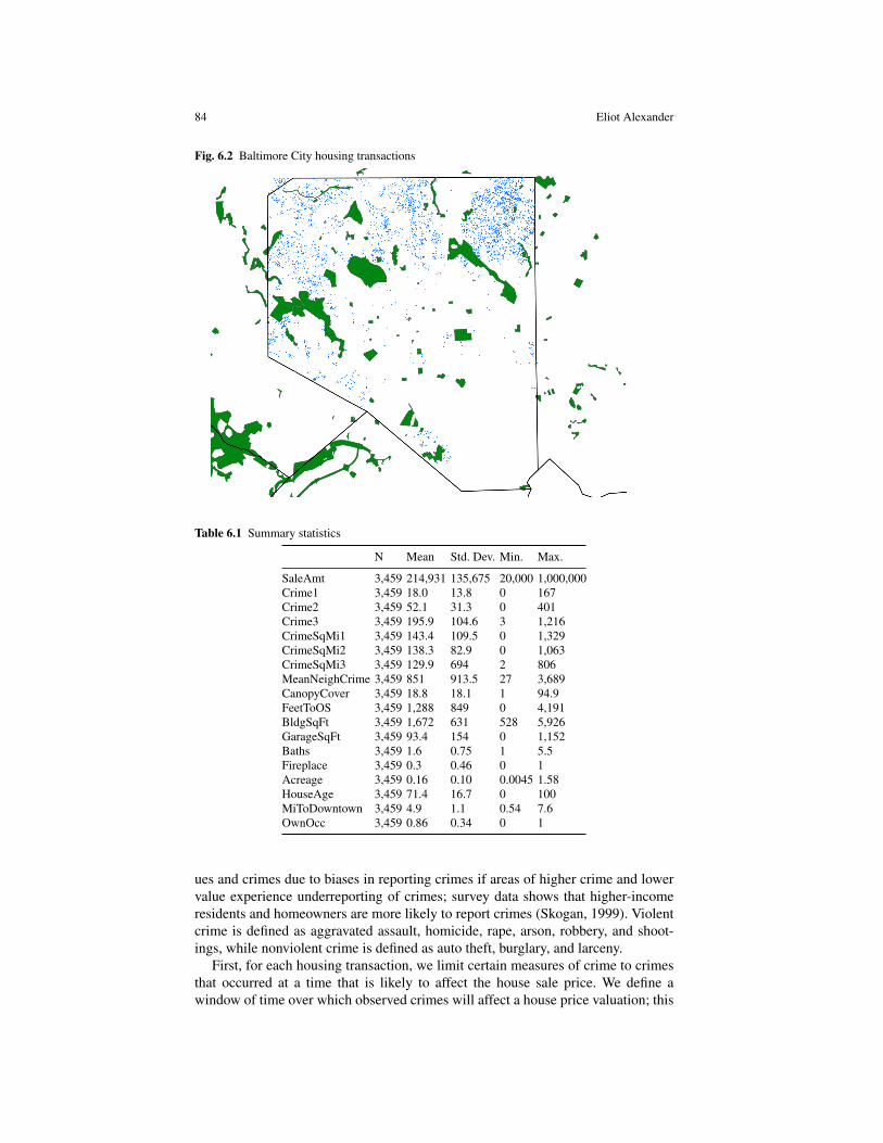
84 Eliot Alexander
Fig. 6.2 Baltimore City housing transactions
91
3.7 Figures
Table 6.1 Summary statistics
N Mean Std. Dev. Min. Max.
SaleAmt 3,459 214,931 135,675 20,000 1,000,000Crime1 3,459 18.0 13.8 0 167Crime2 3,459 52.1 31.3 0 401Crime3 3,459 195.9 104.6 3 1,216CrimeSqMi1 3,459 143.4 109.5 0 1,329CrimeSqMi2 3,459 138.3 82.9 0 1,063CrimeSqMi3 3,459 129.9 694 2 806MeanNeighCrime 3,459 851 913.5 27 3,689CanopyCover 3,459 18.8 18.1 1 94.9FeetToOS 3,459 1,288 849 0 4,191BldgSqFt 3,459 1,672 631 528 5,926GarageSqFt 3,459 93.4 154 0 1,152Baths 3,459 1.6 0.75 1 5.5Fireplace 3,459 0.3 0.46 0 1Acreage 3,459 0.16 0.10 0.0045 1.58HouseAge 3,459 71.4 16.7 0 100MiToDowntown 3,459 4.9 1.1 0.54 7.6OwnOcc 3,459 0.86 0.34 0 1
ues and crimes due to biases in reporting crimes if areas of higher crime and lowervalue experience underreporting of crimes; survey data shows that higher-incomeresidents and homeowners are more likely to report crimes (Skogan, 1999). Violentcrime is defined as aggravated assault, homicide, rape, arson, robbery, and shoot-ings, while nonviolent crime is defined as auto theft, burglary, and larceny.
First, for each housing transaction, we limit certain measures of crime to crimesthat occurred at a time that is likely to affect the house sale price. We define awindow of time over which observed crimes will affect a house price valuation; this

6 Homeowner evaluation of crime across space 85
window spans from 180 days prior to the sale date through 30 days prior to the saledate. It is reasonable to expect that a homeowner would spend a period of roughlysix months in the search of a house over which he/she observes characteristics of theprospective purchases. The last month prior to the sale date is excluded, as the finalhousing decision has likely been made already before this time while the relevantpaperwork is carried out before the actual transaction date. Results are robust tochanges in the specification of this time window.
Fig. 6.3 Baltimore City neighborhoods
92
A measure of crime is then calculated for each house as the total number ofcrime incidents by type that occurs within this time window prior to the sale dateand within various exclusive radii of the house. For example, each house is assignedmeasures of the total number of violent and nonviolent crimes that occur within therelevant time window and occur within 0.2, 0.2 to 0.4, and 0.4 to 0.8 miles of thehouse. Each house is also assigned to a neighborhood, determined by that of thenearest crime to the house over the entire four-year dataset. Figure 6.3 plots eachcrime incident over the four-year span, color-coded by neighborhood to show therough location of the nearly 150 neighborhoods as defined by the Baltimore PoliceDepartment. For a more long-term measure of crime across space, I also includedin estimations the average number of crime incidents per neighborhood over thefour-year span. In addition to a count of crime, I also calculate a measure of crimedensity for each house, defined as the count of crimes by type divided by the area insquare miles of each concentric, exclusive band.
I must also address the potential for multicollinearity across different measuresof crime, either by crime type or by distance from the house. It is not uncommonin the hedonic literature to exclude property crime and use only one measure of vi-olent crime (Berger and Blomquist, 1992; Troy and Grove, 2008; Bishop and Mur-phy, 2011; Bishop and Timmins, 2011). However, when possible I include multiple

86 Eliot Alexander
types of both violent and non-violent crimes in order to reduce omitted variable biasand to compare the effects of different crime types. Table 6.2 shows the correlationcoefficient between different measures of crime in the sample. Using a measure ofcrime counts above the census-tract mean decreases the collinearity of variables.
Table 6.2 Crime correlation
Total crime count within Crime count above mean within
0.2mi 0.4mi 0.8mi 0.2mi 0.4mi 0.8mi
0.2mi 1 0.2mi 10.4mi 0.72 1 0.4mi 0.35 10.8mi 0.52 0.72 1 0.8mi 0.12 0.37 1
A measure of local tree cover is also estimated using a dataset on tree canopydensity from the National Land Cover Database. This includes an index of treecanopy cover as it is spatially distributed across the US. This index ranges from0 (representing no canopy cover) to 100 (maximal canopy cover). Figure 6.1 showsthe spatial distribution of tree cover for the city as a color gradient with green rep-resenting maximal cover and red representing minimal cover. The dataset is quitegranulated, as it consists of multiple index values per city block. Each house is as-signed the average index value of the nearest ten data points, representing roughlya city-block-wide measure of tree cover. The nearest canopy data point is also usedas a robustness check. Data on parks from the United States Geological Survey wasused to assign the distance to the nearest public park for each house.
6.4 Empirical results
Table 6.3 shows the results of the hedonic model of house prices in BaltimoreCity using three measures of crime within concentric, exclusive bands around eachhouse. A quick check of the variance inflation factors for the various models sug-gests that multicollinearity is not likely an issue. The largest VIF value for the crimecount and density variables is 7.94, and the largest VIF value for the crime countabove the mean is 1.73. Measuring crime by count suggests that the homeowner dis-count of house prices for increased crime fades with the crime’s distance from thehouse. However, these three bands cover increasingly large areas, so these measuresdo not account for crime density surrounding each house.
By adjusting each count for the area over which it consists, we obtain measures ofcrime counts per square mile. A model of these measures suggests that homeownersdo not monotonically decrease their valuation of crime as it increases in distancefrom their house. Using crime counts and crime densities results in an equal fit ofthe variation in house prices. Estimation of these models while excluding countsof burglary and robbery, shown in table 3.6, generates more significant effects ofcrime. In this case, all three counts of crime are significant, and the effect of crimedecreases as the crimes extend farther in distance from the house. Adjusting fordensity however, suggests that the density of crimes within 0.2, between 0.2 and0.4, and between 0.4 and 0.8 miles around the house have similar effects on houseprices. We cannot reject that these effects are equal.

6 Homeowner evaluation of crime across space 87
Table 6.3 Hedonic crime model
Variable Crime Count Crime Density Count Above Mean
Crime1 -0.0016* -0.00021* -0.0015*Crime2 -0.00052 -0.00023 -0.00055Crime3 -0.00027* -0.00040* -0.00013AverageCanopy 0.0024*** 0.0024*** 0.0025***FtToOS 0.000027* 0.000027* 0.000024*OwnOcc 0.19*** 0.19*** 0.19***BldgSqFt 0.00016*** 0.00016*** 0.00016***GarageSqFt 0.00012*** 0.00012*** 0.00012***MiToDowntown 0.033 0.033 0.067***Fireplace 0.068*** 0.068*** 0.067***Acreage 0.44*** 0.44*** 0.44***Baths 0.072*** 0.072*** 0.07***Age -0.00089* -0.00089* -0.00094*Constant 11.25*** 11.25*** 10.99***SaleMonth FE Yes Yes YesSaleYear FE Yes Yes YesNeighborhood FE Yes Yes Yes
N 3,459 3,459 3,459R2 0.6451 0.6451 0.6445Notes: *, **, *** indicate statistical significance at the .10%, .05%,and .01%, respectively.
Table 6.4 Hedonic model without robberies or burglaries
Variable Crime Count Crime Density Count Above Mean
Crime1 -0.0032*** -0.00040** -0.0029**Crime2 -0.0011* -0.00040* -0.00098Crime3 -0.00043** -0.00065** -0.00021AverageCanopy 0.0023*** 0.0023*** 0.0024***FtToOS 0.000027** 0.000027** 0.000024*OwnOcc 0.19*** 0.19*** 0.19***BldgSqFt 0.00016*** 0.00016*** 0.00016***GarageSqFt 0.00011** 0.00011* 0.00012***MiToDowntown 0.030 0.030 0.067***Fireplace 0.068*** 0.068*** 0.067***Acreage 0.44*** 0.44*** 0.44***Baths 0.071*** 0.071*** 0.07***Age -0.00089* -0.00089* -0.00094*Constant 11.30*** 11.30*** 10.99***SaleMonth FE Yes Yes YesSaleYear FE Yes Yes YesNeighborhood FE Yes Yes Yes
N 3,459 3,459 3,459R2 0.6460 0.6460 0.6452Notes: *, **, *** indicate statistical significance at the .10%, .05%,and .01%, respectively.
Table 6.5 shows a comparison of estimates between OLS, fixed-effects, random-effects, and Hausman-Taylor models. The results are fairly consistent between themodels, except for estimates of the coefficient on neighborhood historical crime.Most models result in an insignificant effect except for the random-effects model,which, surprisingly, shows a positive effect of neighborhood crime on house prices.

88 Eliot Alexander
Table 6.5 Comparison of OLS, fixed effects, random effects, and Hausman-Taylor models
OLS FE RE H-T
CrimeDensity1 -0.00043*** -0.00043*** -0.00035*** -0.00043***CrimeDensity2 -0.00044** -0.00040* -0.00037* -0.00040*CrimeDensity3 -0.00064*** -0.0010*** -0.00055** -0.0010***NeighCrimes -5.12E-6 No 0.000068* -0.00041Notes: *, **, *** indicate statistical significance at the .10%, .05%,and .01%, respectively. For brevity, stimates of AverageCanopy,FtToOS, MiToDowntown, BldgSqFt, GarageSqFt, Acreage, Baths,Age, Fireplace, and year effects are omitted.
Tables 6.6 and 6.7 show the results of the Hausman-Taylor model. The effects ofcrime count and density are very similar to those found in the hedonic model. Wedo not find a significant effect for total neighborhood crime, however. It is possiblethat the instruments used to estimate this endogenous variable are weak. Table 6.7shows estimations that include each crime by time within certain radii. This not onlyprovides further evidence that households value different types of crime differently,but that they treat various types of crime in different ways as they vary across space.
Table 6.6 Hausman-Taylor crime model
Spatially-Varying Exogenous FeetToOS 0.000028*** 0.000028***
AverageCanopy 0.0023*** 0.0023***Crime1 -0.0033*** -0.00041***Crime2 -0.0011** -0.00043**Crime3 -0.00051** -0.00078**OwnerOcc 0.19*** 0.19***
Spatially-Varying Endogenous BldgSqFt 0.00016*** 0.00016888GarageSqFt 0.00011** 0.00011**Acreage 0.44*** 0.44***Baths 0.071*** 0.071***Fireplace 0.068*** 0.068***Age -0.00096** -0.00096**
Spatially-Invariant Exogenous MeanDistToDowntown -0.024 0.024Spatially-Invariant Endogenous MeanNeighCrime -0.00053 -0.00053
Constant 12.18*** 12.18***
SaleMonth FE Yes YesSaleYear FE Yes YesN 3,459 3,459
Notes: *, **, *** indicate statistical significance at the .10%, .05%, and .01%,respectively.
Auto theft and rape are the only crime types that consistently decrease housevalues across multiple radii. Arson and burglary never appear to have a significanteffect within any radius. Some variables such as larceny do not have a consistentpattern in the way they are valued at increasing radii.

6 Homeowner evaluation of crime across space 89
Table 6.7 Hausman-Taylor crime by type model
VariableDensity within0.2 miles
Density within0.4 miles
Density within0.8 miles
FeetToOS 0.000027** 0.000026** 0.000022**AverageCanopy 0.0025*** 0.0024*** 0.0024***Homicide -0.0056** 8.06E-6 0.0052Rape -0.0091*** -0.013*** -0.022**Robbery 0.0014*** 0.0011* 0.0017AggrAsslt -0.00082* -0.0012* -0.00077Burglary -0.00022 -0.00004 -0.00024Larceny -0.00054*** -0.00041 -0.0011**AutoTheft -0.00082** -0.0015*** -0.0018**Arson 0.0021 0.00074 -0.0021Shooting 0.0024 -0.0042* -0.0069MeanDistToDowntown 0.036 0.012 -0.0091MeanNeighCrime -0.00060 -0.00057 -0.0055Constant 11.83*** 12.0*** 12.12***
SaleMonth FE Yes Yes YesSaleYear FE Yes Yes YesN 3,459 3,459 3,459Hansen’s J stat 0.255 0.275 0.474Notes: *, **, *** indicate statistical significance at the .10%, .05%,and .01%, respectively.
6.5 Conclusion
This study provides evidence that there is significant heterogeneity not only in theway homeowners value different types of crime but also in the way they value thespatial distribution of crime surrounding their house. This study represents an initiallook into the way homeowners value safety spatially. Spatial proximity is indeed asignificant component of how homeowners evaluate local crime; homeowners have agreater willingness-to-pay for avoiding crimes that are located closer to their homes.
In an attempt to address the potential endogeneity of crime on housing prices,we find that tree canopy cover and distance to the nearest park constitute valid can-didates. Multiple model estimations strongly fail to reject the hypothesis that theseinstruments are uncorrelated with the error term and also are correctly excludedfrom the price equation. However, it is possible that these are weak instruments -–that they are not jointly significant in explaining endogenous crime.
This study is a first step towards understanding how residents view the spatialcomponent of crime. Because residents do not treat crimes of all types and in all lo-cations equally, policy-makers and law enforcement agencies should similarly con-sider type and spatial heterogeneity of crimes when planning and enacting policy toreduce crime. This is not to say that certain crime types or certain areas should beignored but that a greater focus should be placed on crime types and areas that havea greater negative impact on residents.
Residents do not appear to evaluate crimes categorized within perhaps arbitraryspatial boundaries like neighborhoods. Instead, homeowners do take into accountphysical distance from their home when evaluating safety from crime. For somecrimes such as homicides, residents appear to only be affected by incidents that arewithin a small distance from their house, while for other crimes like automobiletheft, larceny, and rape, homeowners are averse to incidents farther away.

90 Eliot Alexander
Policymakers can use these results and those of further studies to implementlaw enforcement that accounts for the spatial distribution of houses and crime intoaccount to not just maximize the safety of residents but the well-being of residents,measured by the willingness-to-pay to avoid crime by type and space. For crimetypes that appear to harm residents over large distances, such as auto theft and rape,law enforcement could focus on city-wide efforts to reduce incidents. However, forsome crimes, such as homicide, law enforcement could focus on areas that havea large density of residents. In this way, in a time of tight state and city budgets,law enforcement could enact measures that are both more cost-effective and betterimpact residents.
References
Berger MC, Blomquist GC (1992) Mobility and destination in migration decisions:The roles of earnings, quality of life, and housing prices. Journal of HousingEconomics 2(1):37–59
Bishop KC, Murphy AD (2011) Estimating the willingness to pay to avoid violentcrime: A dynamic approach. American Economic Review 101(3):625–29
Bishop KC, Timmins C (2011) Hedonic Prices and Implicit Markets: EstimatingMarginal Willingness to Pay for Differentiated Products Without InstrumentalVariables. National Bureau of Economic Research, Working paper No. 17611
Bowes DR, Ihlanfeldt KR (2001) Identifying the impacts of rail transit stations onresidential property values. Journal of urban Economics 50(1):1–25
Brown JN, Rosen HS (1982) On the estimation of structural hedonic price models.Econometrica pp 765–768
Buck AJ, Hakim S, Spiegel U (1993) Endogenous crime victimization, taxes, andproperty values. Social Science Quarterly 74(2):334–334
Burnell JD (1988) Crime and racial composition in contiguous communities as neg-ative externalities: Prejudiced household’s evaluation of crime rate and segrega-tion nearby reduces housing values and tax revenues. American Journal of Eco-nomics and Sociology 47(2):177–193
Dubin RA, Goodman AC (1982) Valuation of education and crime neighborhoodcharacteristics through hedonic housing prices. Population and Environment5(3):166–181
Gibbons S (2004) The costs of urban property crime. Economic Journal114(499):441–463
Harrison D, Rubinfeld DL (1978) Hedonic housing prices and the demand for cleanair. Journal of Environmental Economics and Management 5(1):81–102
Ihlanfeldt K, Mayock T (2010) Panel data estimates of the effects of different typesof crime on housing prices. Regional Science and Urban Economics 40(2-3):161–172
Kain JF, Quigley JM (1970) Measuring the value of housing quality. Journal of theAmerican Statistical Association 65(330):532–548
Naroff JL, Hellman D, Skinner D (1980) Estimates of the impact of crime on prop-erty values. Growth and Change 11(4):24–30
Rizzo M (1979) Cost of crime to victims: An empirical analysis. Journal of LegalStudies 8(1):177–205
Rosen S (1974) Hedonic prices and implicit markets: Product differentiation in purecompetition. Journal of Political Economy 82(1):34–55

6 Homeowner evaluation of crime across space 91
Skogan W (1999) Measuring what matters: Crime, disorder, and fear. In: Langwor-thy R (ed) Measuring What Matters: Proceedings from the Policing ResearchInstitute Meetings, US Department of Justice, Washington DC, pp 37–53
Tita GE, Petras TL, Greenbaum RT (2006) Crime and residential choice: A neigh-borhood level analysis of the impact of crime on housing prices. Journal of Quan-titative Criminology 22(4):299
Troy A, Grove JM (2008) Property values, parks, and crime: A hedonic analysis inBaltimore, MD. Landscape and Urban Planning 87(1):233–245


Chapter 7The Effects of Zebra Mussel Infestations onProperty Values: Evidence from Wisconsin
Martin E. Meder and Marianne Johnson
Abstract Containment strategies for invasive species often require significant changesin behavior. Success in fostering these changes requires that individuals correctlyperceive the costs and benefits. Yet, while both the ecological and aesthetic impactsof some invasive species are universally negative it less clear how lakefront prop-erty owners might view zebra mussel infestations. Zebra mussels negatively affectthe local ecology, crowd out native species, and deposit sharp shells on beaches.However, they are also associated with increased water clarity, a reduction in sus-pended pollutants, and increased numbers of popular game fish. We use a spatial lagand spatial error hedonic model to estimate the impact of zebra mussel infestationson lakefront property prices in Waupaca County, Wisconsin. We find no evidencethat homes on infested lakes incur a penalty at sale; consequently, it may be difficultto generate compliance with containment strategies to effectively halt the spread ofzebra mussels.
7.1 Introduction
Climate change and increased ease of transportation have accelerated the spreadof invasive species with deleterious ecological consequences (Thomas and Hanson,2007; Rahel and Olden, 2008; Zipp et al., 2019). As species such as the emeraldash borer, the spruce bark beetle, the lionfish, and Asian carp expand their range,national, state and local environmental groups have aggressively moved to imple-ment a range of containment and mitigation strategies. Yet despite uniformly neg-ative publicity, recent studies suggest that people form complex and multifacetedviews of infestations. For example, Hansen and Naughton (2013) find that sprucebark beetle infestations are associated with an increase in property values in Alaska.Kovacs et al. (2011) document that Sudden Oak Death sometimes negatively andsometimes positively effects property values. Zhang and Boyle (2010) are unableto conclusively demonstrate that lakefront homeowners penalize properties on lakesinfested with Eurasian watermilfoil, though these owners do care about the totalamount of plant growth in the lake. In other cases, infestations have had an over-
Martin E. MederNicholls State University, Thibodaux, LA 70301, USA e-mail: [email protected] JohnsonUniversity of Wisconsin Oshkosh, Oshkosh, WI 54901, USA e-mail: [email protected]
93

94 Martin E. Meder and Marianne Johnson
whelmingly negative impact on property values, such as that identified for the in-sect, the hemlock woolly adelgid (Holmes et al., 2006). These studies suggest thatperceptions of the economic impact of invasions may be an empirical question. Thismay be especially true for zebra mussels (Dreissena polymorpha), where the eco-logical and scientific evidence does not convincingly tell us whether the invasivespecies should be perceived as “a good” or “a bad” by lakefront homeowners andrecreational boaters.
Native to Eastern and Central Europe, zebra mussels were first detected in theUnited States in 1988 in Lake St. Clair near Detroit, Michigan. It took barely twentyyears for them to spread to more than thirty states, endangering ecologies as diverseas Lake Okeechobee in Florida (Adams and Lee, 2012) and the Great Lakes in thenorth central United States (Timar, 2008). Primarily spread by transient recreationalboating, zebra mussels are associated with significant environmental disturbances.They alter ecosystems by crowding out native species, particularly fish such as carpand sturgeon, and by increasing water clarity (Klerks et al., 2001; Strayer et al.,2004; McCabe et al., 2006). In addition to the ecological harm, zebra mussels gen-erate millions of dollars in direct annual costs by inhibiting the functioning of intakepipes and cooling systems and by affecting the operation of other permanent sub-mersed structures (Timar and Phaneuf, 2009).
Previous research on zebra mussels has focused modeling human-induced spread(Timar and Phaneuf, 2009), predicting contaminations (Timar, 2008), and optimalmitigation strategies (Adams and Lee, 2012). However, containment and mitigationstrategies for invasive species such as zebra mussels are costly and often requiresignificant changes in behaviors and practices (Cobourn et al., 2019; Eiswerth et al.,2011; Roberts et al., 2018). Practices such as hot washes and boat dry-outs canbe effective, though all require financial and time investments from boaters andhomeowners. Their incentive to conform with containment policies is complicatedby the nature of the ecological changes engendered by zebra mussels. In additionto the negative implications discussed, Zebra mussels are also associated with in-creased water clarity, which is highly valued by lakefront property owners. For fish-ermen they disadvantage some unpopular species, such as carp, while encouragingmore popular species such as smallmouth bass (Strayer et al., 2004).1 For swim-mers, they decrease the concentration of suspended pollutants in the water columnthrough biosequestration, yielding cleaner water. However, the sharp shells of zebramussels can mar beaches and encrust partially submerged structures such as piersin an unattractive layer of shells. Hence, despite consistently negative publicity, itis not clear that lakefront homeowners would necessarily place an implicitly nega-tive value on zebra mussel infestation. Where ecological disturbances are associatedwith both positive and negative amenities, this makes the combined effect an empir-ical question. To convince individuals to modify their lake-use habits, it is thereforeimportant to develop accurate estimates of the costs as perceived by lakefront prop-erty owners as a first step to designing response strategies.
1 Negatively, zebra mussels impede the feeding habits of lake sturgeon, around which an entireseasonal tourism industry has developed in some areas of Wisconsin (McCabe et al., 2006).

7 The Effects of Zebra Mussel Infestations on Property Values 95
7.2 Methodology
7.2.1 Model
We employ a hedonic model to estimate the empirical impact that zebra musselshave on lakefront property prices. Such estimates are highly useful to policy makersand for constructing cost-benefit analyses of containment and mitigation strategies.In hedonic pricing models, the implicit values consumers place on the individualfeatures of a property can be identified by regressions of sales price on the variouscharacteristics of the product (Rosen, 1974). These characteristics generally includethe features of the structure and of the land, as well as additional location and envi-ronmental characteristics. In an estimated model, the slope coefficient on a partic-ular characteristic represents the marginal willingness to pay. Hedonic models arecommonly used to assess legislated or other land-use policy changes, as the modelallows researchers to isolate the effect of the policy variable on housing prices, andhence estimate the additional value or penalty as perceived by consumers. Only ahandful of studies have attempted to use hedonic price models to estimate the impactof invasive species (Halstead et al., 2003; Hansen and Naughton, 2013; Horsch andLewis, 2009; Zhang and Boyle, 2010). While there are clearly a number of limitsto hedonic pricing models in generating welfare estimates for environmental policychanges, these models can provide useful empirical evidence of the value that con-sumers place on an environmental amenity or dis-amenity (Hansen and Naughton,2013; Holmes et al., 2006; Leggett and Bockstael, 2000).
One complicating factor of hedonic models is there is little theoretical basis todrive the functional form of the estimation equation. This has been extensively dis-cussed with in the literature; the general consensus is that simpler forms perform aswell or better as more complex variations, with the additional advantage of provid-ing more intuitive relationships and explanations (Cropper et al., 1988; Leggett andBockstael, 2000). Following the common strategy in literature, we adopt a specifi-cation where the dependent variable is the sales price of a property as determined bythe market (Pi); see Equation 7.1. While hedonic models often focus on isolating theeffect of a policy change or an environmental amenity or disamenity, a number ofadditional explanatory variables are generally included to capture the main factorsthat influence property values. Like Rosen (1974), we speculate that the sales priceof a property is a function of the property’s structural (H), land (L), geographic (G)and time (T ) characteristics. Price is also influenced by presence/absence of zebramussels (Z), as indicated in Equation 1.
P = f (H,L,G,T,Z) (7.1)
Hedonic pricing models frequently suffer from the econometric problem of en-dogeneity. For example, zebra mussels are spread by contaminated boats or otherrecreational vehicles moving between bodies of water. Higher demand lakes—lakeswith features that make it attractive for recreational use or lakes which are closer topopulation centers—are more likely to become infested. Simultaneously, these samelakes tend to evidence higher property values. Previous studies of aquatic invasivespecies have grappled with endogeneity in different ways. Horsch and Lewis (2009))employ a difference-in-difference methodology to assess the impact of Eurasian wa-termilfoil, whereas Zhang and Boyle (2010) utilize lake fixed effects to address thesame problem. However, neither of these approaches addresses the underlying spa-

96 Martin E. Meder and Marianne Johnson
tial interdependence that is inherent in this type of hedonic model. Spatial interde-pendence implies that the sales prices of neighboring properties are more relatedthan the sales prices of properties further away. Failing to account for the fact thatproperties near each other are more related than properties more distant generatesbiased results, as the error terms from the Ordinary Least Squares regression (Equa-tion 7.2) will not be normally distributed and likely will be correlated with eachother.
Pit = β0 +β1Hit +β2Lit +β3Git +β4Zit +β5Tt +uit (7.2)
We can address the problem of endogeneity engendered by spatial interdepen-dence through the use of a spatial lag and spatial error term. This strategy has beenused effectively to examine the impact of spruce bark beetle infestations (Hansenand Naughton, 2013) and air pollution (Carriazo et al., 2013) on property values.Our spatial maximum likelihood model therefore estimates the sales price of prop-erty i in time period t, Pit (Equation 7.3) as a function of the same structural, land,and geographic characteristics as used in Equation 7.2
Pit = ρΣ j =iw jt lnPjt + γ0 + γ1Hit + γ2Lit + γ3Git + γ4Zit + γ5Tt +uit (7.3)
but where
uit = λΣ j =iw jtu jt + eit (7.4)
The spatial lag represented by Σ j =iw jt lnPjt is the weighted average of other prop-erties’ sales prices. Weights (w) are assigned based on the inverse distance betweenthe properties included in our sample, as identified using GIS determined latitudeand longitude measured at the center of each property. The estimated coefficienton the spatial lag term, ρ , illustrates how the sales price of one property is influ-enced by the sales prices of neighboring properties. Additionally, the spatial error,Σ j =iw jtu jt , is the weighted average of the other observations’ error terms, using thesame weights (w) as the spatial lag, with eit representing the error term. The esti-mated coefficient, λ , does not have a useful interpretation in this case (LeSage andPace, 2009). By directly incorporating spatial location into the model, we can thusdisentangle the impact of zebra mussel infestations from consumer preferences forlakes with particular location attributes.
7.2.2 Study Area and Data
Hedonic pricing models rely on the assumption that all property sales occur in thesame housing market and hence prices represent the market equilibrium price, con-ditional on house and land characteristics. This is problematic when studying in-vasive species. Properties located on a single lake would constitute a single hous-ing market but would not evidence variation in infestation status. Infestation sta-tus varies across lakes, but these lakes may not exist in the same property market.Hence, researchers face a difficult task appropriately identifying a market to study,

7 The Effects of Zebra Mussel Infestations on Property Values 97
as no agreed upon theoretical tests of market boundaries exists.2 This leaves re-searchers to empirically identify reasonable markets for study.
We focus our study on the north central Wisconsin region of the United States.The region’s reputation as a vacation destination as well as its proximity to the re-gional metropolitan areas of Madison, Milwaukee, Chicago and Minneapolis helpidentify it as a well-defined market (see Figure 7.2.2). Chi and Marcouiller (2012)argue that this area represents a “contiguous remote rural region” with most countiesnonadjacent to a significant urban center. These counties are classified as “recre-ational” and are likely to include substantial numbers of second homes (Chi andMarcouiller, 2012). For our purposes, by choosing to purchase lakefront propertyin this area, owners have self-selected for an interest in aquatic recreational activi-ties. Further, by indicating a premium on lake use, these buyers are likely sensitiveto invasive species infestation. Unlike dis-amenities such as water pollution, whichcan be difficult for property owners to discern, the infestation status of lakes arewell known to owners and potential buyers and is required by state of Wisconsindisclosure laws.
Fig. 7.1 Map of Waupaca County
While the expansion of zebra mussels may seem like a dynamic problem, severalissues mean that it is difficult to statistically treat it as such. First, expansion islimited by the availability and suitability of ecosystems that can support them; e.g.,not all lakes provide the appropriate environment for zebra mussels to thrive. Thecorollary is that infestations spread much faster to popular lakes that provide suitablehabitats. This demonstrates itself in the data, where infestations are observed tooccur in waves. A second issue is that Wisconsin Department of Natural Resourcesampling practices are highly inconsistent and rely on a mix of random checks andhomeowner reporting. Thus, while the true number of infestations every year islikely not zero, and therefore not entirely static, the level of dynamism—or even theextent or direction of invasion—cannot be practically observed.
This makes Waupaca County in north central Wisconsin of particular interest. Itszebra mussel invasion, which has gradually made headway in a large chain of lakes
2 Additional issues with hedonic pricing models have been extensively discussed (Leggett andBockstael, 2000; Horsch and Lewis, 2009). These include the absence of a theoretical basis for thefunctional form of the model and difficulties with omitted variable bias (Palmquist, 1991).

98 Martin E. Meder and Marianne Johnson
in the county in the years since the establishment of the Wisconsin Integrated Prop-erty Assessment System in 2009 provides us with a natural case study. While the firstzebra mussel infestation in the county was identified in Partridge Lake in 2005, allfurther infestations occurred between 2010 and 2014. Consequently, a large numberof houses sold on infested lakes, while others with similar attributes sold in closeproximity on non-infested lakes, often within the same township. While this kindof invasion has occurred in other regions of Wisconsin, such as the Spread EagleChain of Lakes in Florence County, Waupaca County’s relative population densityand affluence allows for a greater number of observations owing to a thicker market.
According to the U.S. Census, Waupaca County is home to roughly 52,000 peo-ple, its population remaining highly stable across recent decades. With 126 lakes anda land area of 747 square miles, Waupaca County is decidedly rural, averaging 70.1persons per square mile. The population is overwhelmingly white with a medianhousehold income of $49,777, slightly below the national median. The homeown-ership rate is nearly 77%. The county is home to twelve incorporated cities and avariety of smaller villages and townships. Waupaca County records roughly 25,364housing units, 14.8% of which are in multi-unit structures. However, because of thenature of our question, we focus solely on single-family lakefront properties thatsold between 2009 and 2014. We exclude unimproved properties as well as prop-erties with temporary structures. Property transactions whose real estate transferreturns indicate a transfer fee exemption were excluded from the data set to ensurethat all observed transactions occurred at arm’s-length. Our sample thus includes102 properties from 16 cities, towns and villages on 43 different lakes. In our dataset, 30.4% of the lakefront properties sold in Waupaca County were on lakes in-fested with zebra mussels, which is notably higher than the state-wide average.
Data were collected from the state’s Wisconsin Integrated Property AssessmentSystem which makes available the sales of all properties, sales price, date of sale,as well as some additional in formation. The system is designed to publicly pro-vide information as required by state open records laws. Additional data is from theWisconsin Department of Natural Resources lake database, county-level propertyassessments and the Geographic Information System (GIS). Summary statistics arereported in Table 7.1. Sales prices were adjusted to pre-recession values using theWisconsin House Price Index of the St. Louis Federal Reserve Bank as a way to ac-count for the recent instability in home prices in the United States. The mean salesprice in 2007 dollars is nearly $385,000, with a median price of $270,457.
Structural characteristics (H) include the number of bedrooms, number of bath-rooms and half baths, square footage and year in which the house was built. Wealso have dummy variables indicating whether the home has central heating and/ora basement. As is common in the literature, we include a measure of the distancefrom the center of the property to the closest highway, measured in miles, deter-mined by GIS mapping. Land characteristics (L) include measures of acreage andlake-frontage.
The geographic characteristics (G) merit some additional discussion. We includeseveral measures designed to capture buyer preferences for recreational lake fea-tures such as lake area, lake depth and whether the lake has been endorsed for sportfishing. Empirically, lakefront homeowners have also exhibited strong preferencesfor clearer lakes (Leggett and Bockstael, 2000; Zhang and Boyle, 2010), so we in-clude Secchi depth as a measure of water clarity. However, zebra mussels are knownto improve water clarity over time. Thus, we establish a baseline for water clarityby adopting the 1999 Secchi depth measure for each lake, dating Secchi depth to aperiod prior to the arrival of zebra mussels in this county. In this way, subsequent im-
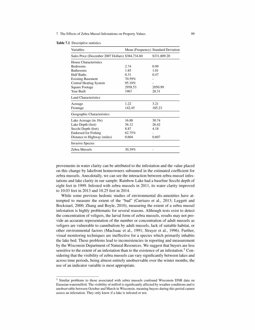
7 The Effects of Zebra Mussel Infestations on Property Values 99
Table 7.1 Descriptive statistics
Variables Mean (Frequency) Standard Deviation
Sales Price (December 2007 Dollars) $384,734.60 $331,809.20
House CharacteristicsBedrooms 2.74 0.99Bathrooms 1.85 1.01Half Baths 0.31 0.47Existing Basement 70.59% -Central Heating System 95.10% -Square Footage 2958.53 2050.99Year Built 1967 28.31
Land Characteristics
Acreage 1.22 3.21Frontage 142.45 185.23
Geographic Characteristics
Lake Acreage (in 10s) 16.88 30.74Lake Depth (feet) 36.12 26.42Secchi Depth (feet) 8.87 4.18Endorsed for Fishing 62.75% -Distance to Highway (miles) 0.604 0.607
Invasive Species
Zebra Mussels 30.39% -
provements in water clarity can be attributed to the infestation and the value placedon this change by lakefront homeowners subsumed in the estimated coefficient forzebra mussels. Anecdotally, we can see the interaction between zebra mussel infes-tations and lake clarity in our sample: Rainbow Lake had a baseline Secchi depth ofeight feet in 1999. Infested with zebra mussels in 2011, its water clarity improvedto 10.03 feet in 2013 and 10.25 feet in 2014.
While some previous hedonic studies of environmental dis-amenities have at-tempted to measure the extent of the “bad” (Carriazo et al., 2013; Leggett andBockstael, 2000; Zhang and Boyle, 2010), measuring the extent of a zebra musselinfestation is highly problematic for several reasons. Although tests exist to detectthe concentration of veligers, the larval form of zebra mussels, results may not pro-vide an accurate representation of the number or concentration of adult mussels asveligers are vulnerable to cannibalism by adult mussels, lack of suitable habitat, orother environmental factors (Maclsaac et al., 1991; Strayer et al., 1996). Further,visual monitoring techniques are ineffective for a species which primarily inhabitsthe lake bed. These problems lead to inconsistencies in reporting and measurementby the Wisconsin Department of Natural Resources. We suggest that buyers are lesssensitive to the extent of an infestation than to the existence of an infestation.3 Con-sidering that the visibility of zebra mussels can vary significantly between lakes andacross time periods, being almost entirely unobservable over the winter months, theuse of an indicator variable is most appropriate.
3 Similar problems to those associated with zebra mussels confound Wisconsin DNR data onEurasian watermilfoil. The visibility of milfoil is significantly affected by weather conditions and isunobservable between October and March in Wisconsin, meaning buyers during this period cannotassess an infestation. They only know if a lake is infested or not.

100 Martin E. Meder and Marianne Johnson
7.3 Analysis
To provide a benchmark for analysis, we first estimate the standard Ordinary LeastSquares (OLS) model as specified in Equation 7.2, exclusive of the spatial lag andspatial error term. This is equivalent to assuming that λ and ρ are simultaneouslyzero.4 These results are compared to a specification that includes only the spatiallag or the spatial error and then finally a specification that includes both the spatiallag and the spatial error. Our estimation results are presented in Table 7.2. As iscommon in hedonic studies, we transform the dependent variable to be the naturallog of real sales price, which we measure in December 2007 dollars (lnPit ). We alsoincorporate a month time trend to ensure that differences in sales prices across timethat are common in all properties will not bias estimates.
As expected, across all four regressions, square footage, the number of full bath-rooms, and the year in which a house was built are of central importance to homebuyers, their estimated coefficients evidencing positive and statistically significantassociations with sales price. Additionally, home buyers place a premium on con-venient access to the property. For each additional mile that a property is locatedfrom a main highway, home price decreases by about 12 to 15% (p ≈ 0.05). Ourestimated coefficients for these factors are highly consistent with the ranges foundby other hedonic studies and are robust to specification and estimation procedure.The number of bedrooms and acreage also contribute positively to sales price in allcases, though they are not statistically significant in any of the four specifications.We retain these variables to maintain consistency with other studies in the hedonicpricing literature.5 We find that buyers are also sensitive to the amount of lake-frontage available on the property, though the relationship is nonlinear. While theestimated coefficients on frontage are consistently negative and the estimated coef-ficients are quite small for the frontage-squared term, across Regressions 1 through4, they are in fact logical. The estimates indicate that for most standard frontages,an extra foot or so has very little impact (negative, but essentially zero). However,particularly large expanses of frontage command notably higher prices.6
Home buyers exhibit a strong preference for deeper lakes (p < 0.01); lakes en-dorsed for fishing command an additional premium of 23% to 31% of sales price(p < 0.05). Neither result is surprising given the strong revealed preferences byproperty owners in this region for sport fishing. Our measure of baseline water clar-ity, 1999 Sechi depth, is positively associated with sales price, though not statisti-cally significant in either of the regressions that use a spatial lag.
As previously discussed, zebra mussels generate both positive and negative ef-fects on their environment, when viewed from the perspective of lakefront propertyowners.7 Thus we have no intuitive guide to evaluate the estimated effect generatedby a hedonic model, nor any presumption as to whether the sign should be positive
4 The heteroskedastic robust OLS estimates, clustered by township/village yields, nearly identicalresults to the basic OLS model, hence we only report the most basic model.5 We do not find a statistically significant relationship between property sales price and number ofhalf bathrooms, the existence of a basement or whether the property has improved central heating.We do not retain these variables in the final regressions for parsimony.6 The estimates indicate that after roughly 393 feet of frontage, each additional foot of frontagecontributes positively to sales price. Note that one meter is equivalent to 3.28 feet.7 Johnson and Meder (2013) use a non-standard hedonic model and basic OLS to estimate theimpact of zebra mussels in 17 counties in north central Wisconsin (n = 1072). They find that lakesinfested with zebra mussels evidence 10% higher sales prices than comparable properties on un-infested lakes. We know of no other hedonic model estimates for zebra mussels.

7 The Effects of Zebra Mussel Infestations on Property Values 101
Table 7.2 Hedonic regression results
Variables OLSSpatialLag
SpatialError
MixedSpatial Lag&Spatial Error
House
Bedrooms 0.081 0.036 0.062 0.024(0.058) (0.051) (0.055) (0.051)
Full Bathrooms 0.183*** 0.142*** 0.171*** 0.125**(0.061) (0.053) (0.058) (0.052)
ln(Square Footage) 0.176* 0.183** 0.175** 0.182**(0.092) (0.079) (0.096) (0.075)
Year Built 0.006*** 0.007*** 0.006*** 0.007***(0.002) (0.001) (0.002) (0.001)
Land
Acreage 0.015 0.020 0.013 0.022(0.020) (0.017) (0.018) (0.017)
Frontage -0.001 -0.001** -0.001* -0.001*(0.000) (0.000) (0.000) (0.000)
Frontage Squared 106e-6 1.18e-6* 1.26e-6* 1.06e-6*(7.03e-7) (6.00e-7) (6.77e-7) (5.90e-7)
Geographic
Lake Depth 0.011*** 0.009*** 0.011*** 0.009(0.003) (0.002) (0.003) (0.002)
Lake Acres 0.001 0.002 0.002 0.003*(0.002) (0.002) (0.002) (0.001)
Secchi Depth 0.026* 0.017 0.025* 0.012(0.014) (0.012) (0.014) (0.011)
Endorsed for Fishing 0.307** 0.250** 0.301** 0.229**(0.134) (0.115) (0.131) (0.107)
Distance to Highway -0.139* -0.136* -0.151** -0.127**(0.075) (0.064) (0.074) (0.060)
Zebra Mussels 0.238* 0.089 0.162 0.066(0.131) (0.118) (0.150) (0.155)
Month Time Trend 0.006** 0.006*** 0.006*** 0.006***(0.003) (0.002) (0.002) (0.002)
Spatial Lag (ρ) - 0.506*** - 0.707***- (0.129) - (0.144)
Spatial Error (λ ) - - 0.357 -0.330- - (0.328) (0.267)
Observations 102 102 102 102R2/Squared Correlation 0.79 0.82 0.79 0.82Notes: Dependent variable is ln(Adjusted Sales Price). Constantincluded but omitted for space. * indicates statistical signifi-cance at the 10% level, ** at the 5% level, and *** at the 1%level.
or negative. Our standard OLS model, as reported in Regression 1 in Table 7.2, sug-gests that zebra mussel infestations are associated with a 26.9% increase in propertyvalues (p = 0.07).8 However, this model fails to incorporate spatial effects, which
8 This comes from using the standard transformation 100∗ [ex −1] transformation for interpretingthe coefficients of dummy variables in models with the dependent variable being transformed bythe natural log (Wooldridge, 2010).

102 Martin E. Meder and Marianne Johnson
likely causes our estimate to be upward biased. Diagnostic tests for spatial depen-dence suggest the use of a mixed spatial lag and spatial error model. The need for aspatial lag is highly recommended by diagnostic tests (Lagrange Multiplier = 12.03,p = 0.001). Moran’s I for the spatial error (= 1.54, p = 0.124) is suggestive but notdefinitive.
The spatial lag coefficient (ρ) is both positive and statistically significant in re-gressions 2 and 4, providing evidence of spatial spillovers between the sales price ofa property and that of its neighbors. For example, a 1% increase in neighboring salesprices is associated with an increase in sales price of 0.51% (Spatial Lag regression)to 0.71% (Mixed Spatial Lag & Spatial Error regression). This demonstrates that thefactors that influence the sales price of one property such as neighborhood amenitiesand/or infrastructure development will spillover to affect the value of neighboringproperties as well. The use of the spatial lag thus captures these underlying omit-ted variables that contribute to the endogeneity problem inherent in hedonic studies.The spatial error performs less well in our estimated equations. In neither of the tworightmost columns is the estimated coefficient statistically significant (p = 0.28 andp = 0.22), suggesting that the Spatial Lag in column 2 is the preferred specification.
Across all specifications, zebra mussel infestations are associated with highersales prices for lakefront homes, suggesting that the visible effects of an infestation,in including clearer water and more high-value fishing, outweigh the negative per-ceptions of an infestation. The spatial lag model reported in column 2 posits thathomes on infested lakes will command a 9.3% premium over otherwise compara-ble houses on un-infested lakes (the mixed spatial lag and spatial error specificationsuggests 6.8%). This corresponds to a welfare gain of approximately $25,000 on amedian lakefront property. Note that both estimated values are substantially smallerand less statistically significant than that generated by standard OLS, which failsto account for spatial interconnections. In neither case is the estimated coefficientstatistically significant, suggesting that the true impact of an infestation cannot bedifferentiated from zero. This implies that even in areas where zebra mussels com-mand significant attention in the local news, consumers do not prioritize infestationstatus when selecting recreational lakefront properties.
7.4 Conclusion
The absence of hedonic studies of zebra mussels is surprising given the attention de-voted to invasive and potentially invasive species in the United States and Canada.One of the reasons for this absence may be the confounding effects that zebra mus-sels have on their environment. An infestation engenders both visible positive andnegative effects on a lake. Zebra mussels improve water clarity and sports fishingwhile reducing suspended pollutants in the water. Zebra mussels also crowd outsome fish species important to the Wisconsin fishing industry, notably sturgeon,and deposit sharp shells along beaches. It therefore becomes an empirical question,whether lakefront homeowners suffer from an infestation.
In this study, we evaluate how the spread of zebra mussels through a chain oflakes in Waupaca County, Wisconsin has influenced the sales prices of lakefrontproperties. In spite of their uniformly negative reputation, we find no evidence thatzebra mussels are associated with decreased prices for lakefront properties. Rather,using a Maximum Likelihood estimation strategy with a spatial lag, we find thatan infestation is associated with positive but not statistically significant increases in

7 The Effects of Zebra Mussel Infestations on Property Values 103
lakefront property values. Our finding of a zero or slightly positive association be-tween zebra mussel infestations and property values has an important policy impli-cation. Since most mitigation and control mechanisms require substantial changes inuser behavior, the lack of a negative effect on property values suggests that it mightbe difficult to generate substantial levels of compliance. If lakefront home ownersdo not perceive a negative effect from zebra mussels, they are much less likely toregularly practice hot boat washes or regularly clean their boats, both of which areinconvenient and engender significant opportunity costs. These results may also in-dicate that mechanical or chemical control methods employed by lake associationsfor invasive species such as zebra mussels are unnecessary from a homeowner per-spective. We caution readers that this paper is an initial attempt to assess the impactof zebra mussel infestations on lakefront property values; as such, it unavoidablyhas a number of limitations. The most important is the small sample size, whilecarefully selected and suggestive, demands further replication, both in Wisconsinand in other states.
Acknowledgements We would like to thank Chad Cotti, Russ Kashian and Kevin McGee forhelpful comments and suggestions.
References
Adams DC, Lee DJ (2012) Technology adoption and mitigation of invasivespecies damage and risk: Application to zebra mussels. Journal of Bioeconomics14(1):21–40
Carriazo F, Ready R, Shortle J (2013) Using stochastic frontier models to mitigateomitted variable bias in hedonic pricing models: A case study for air quality inBogota, Colombia. Ecological Economics 91:80–88
Chi G, Marcouiller DW (2012) Recreational homes and migration to remoteamenity-rich areas. Journal of Regional Analysis and Policy 42(1):47–60
Cobourn KM, Amacher GS, Haight RG (2019) Cooperative management of inva-sive species: A dynamic Nash bargaining approach. Environmental and ResourceEconomics 72(4):1041–1068
Cropper ML, Deck LB, McConnell KE (1988) On the choice of funtional form forhedonic price functions. Review of Economics and Statistics 70(4):668–675
Eiswerth ME, Yen ST, van Kooten GC (2011) Factors determining awareness andknowledge of aquatic invasive species. Ecological Economics 70(9):1672–1679
Halstead JM, Michaud J, Hallas-Burt S, Gibbs JP (2003) Hedonic analysis of effectsof a nonnative invader (myriophyllum heterophyllum) on new hampshire (usa)lakefront properties. Environmental Management 32(3):391–398
Hansen WD, Naughton HT (2013) The effects of a spruce bark beetle outbreakand wildfires on property values in the wildland–urban interface of south-centralAlaska, USA. Ecological Economics 96(1):141–154
Holmes TP, Murphy EA, Bell KP (2006) Exotic forest insects and residential prop-erty values. Agricultural and Resource Economics Review 35(1):155–166
Horsch EJ, Lewis DJ (2009) The effects of aquatic invasive species on propertyvalues: Evidence from a quasi-experiment. Land Economics 85(3):391–409
Johnson M, Meder M (2013) Effects of aquatic invasive species on home prices:Evidence from Wisconsin. University of Wisconsin-Oshkosh, Oshkosh

104 Martin E. Meder and Marianne Johnson
Klerks PL, Fraleigh PC, Sinsabaugh R (2001) The impact of zebra mussels on thedynamics of heavy metals. Ohio Sea Grant College Program, Technical SummaryOHSU-TB-055
Kovacs K, Holmes TP, Englin JE, Alexander J (2011) The dynamic response ofhousing values to a forest invasive disease: Evidence from a sudden oak deathinfestation. Environmental and Resource Economics 49(3):445–471
Leggett CG, Bockstael NE (2000) Evidence of the effects of water quality onresidential land prices. Journal of Environmental Economics and Management39(2):121–144
LeSage J, Pace RK (2009) Introduction to Spatial Econometrics. CRC PressMaclsaac HJ, Sprules WG, Leach J (1991) Ingestion of small-bodied zooplankton
by zebra mussels: Can cannibalism on larvae influence population dynamics?Canadian Journal of Fisheries and Aquatic Sciences 48(11):2051–2060
McCabe D, Beekey Ph D M, Mazloff A, Marsden I (2006) Negative effect of ze-bra mussels on foraging and habitat use by lake sturgeon. Aquatic Conservation:Marine and Freshwater Ecosystems 16(5):493–500
Palmquist R (1991) Hedonic methods. In: Braden J, Kolstad C (eds) EnvironmentalBenefit Measurement, North-Holland, Amsterdam
Rahel FJ, Olden JD (2008) Assessing the effects of climate change on aquatic inva-sive species. Conservation Biology 22(3):521–533
Roberts M, Cresswell W, Hanley N (2018) Prioritising invasive species control ac-tions: Evaluating effectiveness, costs, willingness to pay and social acceptance.Ecological Economics 152:1–8
Rosen S (1974) Hedonic prices and implicit markets: Product differentiation in purecompetition. Journal of Political Economy 82(1):34–55
Strayer DL, Powell J, Ambrose P, Smith LC, Pace ML, Fischer DT (1996) Arrival,spread, and early dynamics of a zebra mussel (dreissena polymorpha) populationin the Hudson River estuary. Canadian Journal of Fisheries and Aquatic Sciences53(5):1143–1149
Strayer DL, Hattala KA, Kahnle AW (2004) Effects of an invasive bivalve (dreissenapolymorpha) on fish in the Hudson River estuary. Canadian Journal of Fisheriesand Aquatic Sciences 61(6):924–941
Thomas MH, Hanson TR (2007) Evaluating the policy to restrict the potentially in-vasive black carp (mylopharyngodon piceus): A decision protocol with assurancebonding. Journal of Environmental Planning and Management 50(1):153–162
Timar L (2008) Modeling the Anthropogenic Spread of an Aquatic Invasive Species:The Case of Zebra Mussels and Transient Recreational Boating in Wisconsin.University of Wisconsin Madison, PhD Dissertation
Timar L, Phaneuf DJ (2009) Modeling the human-induced spread of an aquaticinvasive: The case of the zebra mussel. Ecological Economics 68(12):3060–3071
Wooldridge JM (2010) Econometric Analysis of Cross Section and Panel Data. MITPress, Cambridge
Zhang C, Boyle KJ (2010) The effect of an aquatic invasive species (eurasian wa-termilfoil) on lakefront property values. Ecological Economics 70(2):394–404
Zipp KY, Lewis DJ, Provencher B, Vander Zanden MJ (2019) The spatial dynamicsof the economic impacts of an aquatic invasive species: An empirical analysis.Land Economics 95(1):1–18

Chapter 8A Case for Amenity-Driven Growth? The Valueof Lake Amenities and Industrial Disamenitiesin the Great Lakes Region
Heather M. Stephens
Abstract In advanced economies, such as the United States, people increasinglyvalue quality of life and are willing to pay for access to natural amenities. In theOhio Great Lakes region, residents enjoy access to an abundance of fresh water andnatural and recreational amenities. At the same time, however, they are confrontedwith the artifacts of the region’s industrial legacy in disamenities, including factoriesand other industrial sites. Given the economic restructuring of many of the region’sindustries, there is interest in understanding how the competing effects from naturalamenities and industrial disamenities affect housing demand and regional growth.To assess this, we utilize a unique dataset that includes over 300,000 housing trans-actions in the Greater Cleveland (Ohio) region and detailed geographically-locateddata on industrial disamenities, urban amenities, and natural and related built ameni-ties. Using the hedonic pricing method, we estimate the value that residents placeon these amenities and disamenities. We find a positive capitalization effect frombeing directly on Lake Erie. However, away from houses in close proximity to thelake, the effects are more heterogeneous. Additionally, there is evidence that prox-imity to manufacturing is associated with lower house values, especially near thelake. This suggests that, as the region’s economy transitions, residents may posi-tively value less industrialization near the lake and a focus on Lake Erie as a naturaland recreational amenity.
8.1 Introduction
Lake Erie has long been the driving force behind economic development in theGreater Cleveland, Ohio, region; from the early settlements on the shore of the lake,to the growth of ports to transport goods from the markets of the East Coast to theMississippi River and the West, to the growth of the automobile and other manufac-turing businesses. The presence of high quality housing along the shoreline, alongwith the presence of beaches and marinas, also suggests that people in the regionvalue the lake beyond its role in creating employment. In recent years, as globalcompetition and economic restructuring have put pressure on the industrial sectorsthat led to the growth of this region, there is a renewed interest in exploring the role
Heather M. StephensWest Virginia University, Morgantown, WV, 26506, USA e-mail: [email protected]
105

106 Heather M. Stephens
of the lake in attracting households who are value the lake amenities. Policymakersseek to understand how and if people value Lake Erie in order to determine whethereconomic development policies focused on the lake amenities make sense.
In advanced economies, such as the United States, there is evidence that peo-ple increasingly value quality of life (QOL) and are willing to pay for access tonatural amenities (Rappaport, 2004; McGranahan, 2008; Partridge and Ali, 2008).However, due to the fact that proximity to Lake Erie was one of the drivers behindthe industrialization of the Cleveland area, a complicating factor in this region isthat there is pollution and environmental degradation near Lake Erie. In other con-texts, there is evidence that housing values are negatively affected by proximity toenvironmental disamenities such as power plants, superfund sites, and air pollution(Smith and Huang, 1995; Hite et al., 2001; Davis, 2011).
This research thus considers the potential for QOL-oriented Lake Erie devel-opment in Greater Cleveland. We hypothesize that, if households value access toLake Erie, they will be willing to pay a higher housing price, all else equal. Wealso will test whether industrialization has made it less desirable to live close toLake Erie, offsetting any positive aesthetic or recreational benefits, and reducinghousing prices. Using residential sales transactions data from the Greater Clevelandregion, we use a hedonic price model to measure the capitalization effect on housesin proximity to Lake Erie and its recreational amenities as well as the proximityto industrialized sites or pollution. Our unique dataset includes over 300,000 hous-ing transactions from 1992 to 2006 as well as detailed geographically-located dataon industrial disamenities and industrial emissions, and natural and related builtamenities, including parks, and Lake Erie and its beaches and marinas. To controlfor unobserved characteristics, we also include both time and spatial fixed effects.
This research contributes to the literature by providing insight into the value oflake amenities in a highly-industrialized, developed, and transitioning region. Muchof the previous literature on lake amenities has focused on resort communities alongthe coasts and in the South. Thus, a priori, it was unclear whether and how muchhouseholds in this region value these lake amenities. However, there is some limitedevidence that at least high-income people in the Great Lakes region may value lakeproximity (Stephens and Partridge, 2015). Additionally, we consider the differenttypes of lake amenities — including lake views as well as access to boat ramps andbeaches. And, we also consider the role of industrialization and abandoned facilities.We find strong evidence that, consistent with other studies which have found thataccess to lake views and being very close to water is valuable to households, housingvalues in immediate proximity to Lake Erie are higher. However, away from that,the results are more mixed, perhaps due to the fact that the lake amenities are withindriving distance of all households in the region.
There is also evidence that households do notice industrialization and that it isreflected in a price decrease for houses near manufacturing facilities and especiallyfor those located near the lake. However, the negative effect on price of being closeto air pollution or Superfund sites is much lower, suggesting that it may be thevisible nature of smokestacks that drives prices lower.
In what follows, we detail the previous literature. Next, we describe our empir-ical model and data; followed by the empirical results. The final section presentssome concluding thoughts and a discussion about the implications for the regionand policy.

8 A Case for Amenity-Driven Growth? 107
8.2 Literature Review
Valuing non-market attributes of a region such as natural or built amenities or pollu-tion or environmental disamenities using the hedonic pricing framework has a longhistory starting with Rosen (1974). By using a single housing market (such as ametropolitan area), the assumption is that wages are held constant in a region andthat housing prices can be used to uncover the change in value associated with thevarious attributes of a house, including proximity to natural amenities and industrialand environmental disamenities, as consumers will maximize their utility by theirchoice of a house (Rosen, 1974; Taylor, 2003; Palmquist, 2006).
In an early application of the hedonic method to look at access to lake amenities,Brown Jr et al. (1977) found that property values decrease with distance from thelake. Feather et al. (1992) examined the relationship between water amenities andhousing prices in Orange County, Florida, and saw evidence that the land value oflakefront property is greater than property away from a lake, and that the effect ofbeing close to a lake diminishes with distance.
A number of other papers have also found a link between either access to lakeamenities or proximity to a lake and housing values, including Lansford Jr and Jones(1995a,b), Nelson (2010), and Abbott and Klaiber (2013).Lansford Jr and Jones(1995a,b) also found that adjacency to the lake is the strongest effect and that thelake effect dies off quickly. White and Leefers (2007) looked at a rural housingmarket in Michigan and found that the only natural amenity that affected housingvalues in their study area was proximity to the major lake. Looking specifically atthe Northeast Ohio Lake Erie lakefront, Bond et al. (2002) found some evidence ofa willingness to pay a premium to live in housing that has a view of Lake Erie. How-ever, they also qualify their results by noting that they fail to control for a number ofimportant factors including access to recreational amenities and proximity to urbanamenities and downtown Cleveland.
Among other natural amenities that may affect housing prices are open spaceand parklands. A number of previous studies have looked at the effect of open spaceon housing prices, including Smith et al. (2002) and Irwin (2002), among others.Results from Poudyal et al. (2009) showed that access to larger urban parks wasassociated with increased house values. In their study of urban areas in Finland,Tyrvainen and Miettinen (2000) found that proximity to forests increases housingsales prices, and there is a premium for being within view of those forests. Otherstudies have shown that the benefits from certain natural amenities (including na-tional monuments and other public open space) extend a significant distance beyondtheir boundaries (Irwin, 2002; Schmidt and Courant, 2006).
In the environmental economics literature, the hedonic price method has beenused to quantify the negative effects of pollution and proximity to hazardous wastesites and other environmental disamenities. Many studies have provided evidencethat housing values are negatively affected by proximity to environmental disameni-ties such as power plants, Superfund and other hazardous waste sites, and air pollu-tion (Kiel and McClain, 1995; Smith and Huang, 1993; Chattopadhyay, 1999; Hiteet al., 2001; Beron et al., 2001; Ihlanfeldt and Taylor, 2004; Davis, 2011). In anotherstudy focused on Ohio, Brasington and Hite (2005) looked at proximity to what theycall ‘hazards’ or sites that have been identified as possible brownfields or future Su-perfund sites. They found that proximity to such hazards is negatively correlatedwith housing prices. Smith and Huang (1993, 1995) looked at 25 years of hedonicanalysis considering a link between housing prices and air quality which, in general,

108 Heather M. Stephens
showed there is a positive relationship. However, a related study by Boyle and Kiel(2001) found that the values on air quality are generally statistically insignificant;perhaps due to the fact that air quality variables are correlated with both includedand omitted variables. This study also provided evidence that studies which includedmultiple environmental variables tended to have higher significance, perhaps due tofewer omitted variables, although they suggested that further research is needed.
Looking at the relationship between toxic releases as measured by the U.S. En-vironmental Protection Agency (EPA) Toxic Release Inventory (TRI), Fonseca andNoonan (2006) saw almost no statistical relationship between proximity to the near-est toxic release and housing price. However, they suggested that future work maywant to consider the amount of the releases, not just what is closest.
In other research, there is evidence that proximity to certain businesses or thepresence of congestion may be associated with changes in housing prices. Forexample, proximity to industrial businesses is negatively correlated with housingprices (Franklin and Waddell, 2003). Perhaps it is that people are more likely to beconcerned with smokestacks rather than with air quality or pollution, which theymay not be able to observe (unless it is coming out of the previously mentionedsmokestacks). Timmins and Murdock (2007) found that congestion was importantwhen considering the willingness to pay for access to recreational amenities. And,hedonic methods have uncovered a link between the effects of traffic congestion andhousing prices (Wilhelmsson, 2000; Davis, 2004).
The work by McConnell (1990) suggested that there may be multiple driversof the price of houses close to natural amenities, including water. These factorsinclude the view, the recreational opportunities, and environmental benefits, if theair quality is better close to the water, or environmental disamenities, if there isindustrialization or more pollution near the water. And, these factors can interact:Stephens and Weinstein (2019) found that the positive impact from proximity tonatural amenities can be negatively affected by energy development.
8.3 Empirical specification
Following Rosen (1974), a general hedonic model is:
P(z) = f (H,A,ε) (8.1)
where, H includes housing characteristics, A are community or locational charac-teristics (including amenities and disamenities), and ε is an standard error term.
In specifying our empirical model, we attempt to address the concerns raised inthe previous literature related to functional form and the potential omitted variablebias from missing housing and community characteristics, especially when usingspatially-delineated variables (Rosen, 1974; Palmquist, 2006; Kuminoff et al., 2010;Coulson, 2012). Following Kuminoff et al. (2010), we use spatial fixed effects, anda somewhat flexible functional form, which they found was the most robust in theface of omitted variable bias.
Thus, to estimate our model we use equation 8.2:
ln(Pi) = β0 +Σh1βh1Hih1 +Σh2βh2Hih2 +Σh3βh3(Hih2)2 +ΣaβaAia (8.2)
+βcCi +βsc(Ci)2 +Ti +Si + εi

8 A Case for Amenity-Driven Growth? 109
In equation 8.2, the vector of housing characteristics is split into two vectors, H1and H2, due to the inclusion of quadratic terms of some of the variables. H1 containsthe total number of bathrooms, bedrooms, and dummy variables indicating if thereis a garage or fireplace. H2 consists of age, hundreds of square feet in the building,and lot acres. The housing characteristics in H2 enter the equation both linearly andas quadratic terms. The distance to downtown Cleveland (C) is split from the rest ofthe original community characteristics vector and its square is also included in theestimation equation. The rest of the community characteristics, namely the naturalamenities and industrial disamenities, are included in the final vector, A. T and Sare the time (sales year) and spatial (block group) fixed effects, respectively. Theyear fixed effect will control for changes in the overall housing market, changesin environmental conditions in the overall region, and policy changes that wouldaffect all houses in a given year. The block group fixed effect will control for otherneighborhood or community characteristics that do not change over time, includinglocal school quality and the quality of the neighborhood. In the next section, wefurther describe the data and the variables used in this analysis.
When estimating the models, we will test the sensitivity of our results to theinclusion of specific amenity and disamenity variables. We also correct for het-eroskedasticity by using robust standard errors.
We also test whether the results could be pooled across the decades using themethod outlined in Ohta and Griliches (1976), in which the standard error of theregression (SEE) of the pooled, full model was compared to that of the separate, un-pooled models (results not shown). The results indicate that use of pooled regressionof the data from all of the years is appropriate.
8.4 Data
This research focuses on six counties in the Greater Cleveland (Ohio) region,Ashtabula, Cuyahoga, Geauga, Lake, Lorain, and Medina Counties. A map of thestudy area is shown in Figure 8.1. This area includes the Cleveland Metropolitan Sta-tistical Area (MSA) and the adjacent Ashtabula Micropolitan Area which, together,form a single regional labor market and, by assumption, a regional housing mar-ket. Thus, housing prices in this region can be used to uncover the marginal valueof non-traded amenities and disamenities. The market is likely comprised of sev-eral overlapping local markets. However, since they are all part of a single greatermetropolitan area, with connections by major roads and lack of physical featuresthat would separate the areas, we expect significant overlap in these markets andbelieve the housing market is best modeled as a single regional market. This is con-sistent with the work by Irwin (2002) in looking at the housing market in Maryland.
8.4.1 Housing Transactions
We use sales data for single-family houses from the six-county region from 1992 to2006 compiled from data provided by the Center for Urban and Regional Analysis(CURA) at The Ohio State University and purchased from Corelogic Data Services.The data are matched to parcel shapefiles using ArcGIS obtained from the six coun-ties. Compared to relying on geocoding of addresses, this provides more accurate

110 Heather M. Stephens
9
market is best modeled as a single regional market. This is consistent with the work by Irwin
(2002) in looking at the housing market in Maryland.
Figure 1. Map of the six-county region, Northeast Ohio Fig. 8.1 Map of the six-county region, Northeast Ohio
locations of the sales transactions, and increases the accuracy of our calculationsof spatially-defined variables such as distance to lake amenities and environmentaldisamenities (as explained below).
Our dataset includes the sale price of the house and the following housing char-acteristics, which are likely to be predictors of house attractiveness: lot acres andhundreds of square feet in the building, total number of bathrooms, age of the house,whether the house has a garage, and whether the house has a fireplace (generally asign of higher quality). The use of these characteristics is consistent with other he-donic studies and, based on the available data, provides the best set of controls forheterogeneous housing characteristics. House prices are normalized in 2006 dollarsusing the CPI for the Cleveland-Akron region in order to account for inflation. Sincewe need accurate information on these characteristics for all transactions in the sam-ple, we eliminate transactions with missing or zero values for the relevant variablesin the estimation. We also follow Klaiber (2008) in using approximately the 1st and99th percentiles as the limits of the bounds of those transactions we retain. The finaldataset includes 303,907 transactions.
8.4.2 Amenities
Since we are interested in proximity to Lake Erie, we use ArcGIS to measure thedistance between each parcel in our transactions data and the closest point on the
8 A Case for Amenity-Driven Growth? 111
lake. We then construct a dummy variable that indicates whether or not the house iswithin 100 meters of the Lake Erie, to proxy for those houses that are adjacent toor have a view of the lake. Data on recreational amenities on Lake Erie, includingbeaches and boat ramps, were obtained from the Ohio Department of Natural Re-sources. We measure the distance from each parcel in our transactions data to thenearest Lake Erie beach and boat ramp.1 We combine the distance to beach and boatramp into a single variable, distance to nearest boat ramp or beach, due to the highcollinearity between the two distance measures (0.986). We also construct dummyvariables indicating whether or not a house is within 250 meters of a boat or beach,i.e. within close walking distance of these amenities. The number of parking spacesat the closest boat ramp is also included in the data and is interacted with the dummyvariable that indicates if a boat ramp is within 250 meters, to get a measure of thenumber of parking spaces near a house. This will measure congestion related to theboat facilities.
Additional data on public parks and recreational lands were provided by OhioDucks Unlimited. We construct a measure of the number of park acres (in tens ofacres) within one kilometer of the parcel as a proxy for other natural amenities inthe neighborhood of a house.
We recognize that the recreational amenities could be endogenous. Unfortu-nately, detailed data on the actual construction date for each facility was not avail-able. However, most of the public recreational infrastructure in the region was con-structed before 1990, minimizing this endogeneity.
To control for proximity to urban amenities and business opportunities, we in-clude a measure of the distance to downtown Cleveland. Downtown Cleveland con-tains or is near many of the urban amenities in the region including the sports sta-diums for the major professional sports teams, as well as museums and restaurants.Additionally, classical urban growth theory would suggest that housing prices are(negatively) correlated with distance to downtown Cleveland, assuming that work-ers are generally commuting there (Muth, 1961; Alonso, 1964; Mills, 1967).
8.4.3 Disamenities
Data on businesses, by location, in the region are available by two-digit NAICScode, by year. These data are used to measure the number of manufacturing busi-nesses, defined as businesses with NAICS code 31, 32, or 33, within one kilometerof each parcel. Since these manufacturing businesses could be heterogeneous interms of building size and structure, we also tested several other specifications andfound similar results. We hypothesize that households are more likely to notice uglybuildings or ‘smokestacks,’ thus the presence of a manufacturing facility in closeproximity to a house will be likely to be associated with lower housing prices. Tocontrol for endogeneity, we include one-year lagged values of the numbers of busi-nesses; for example, for a transaction in the year 2002, we use the number of nearbymanufacturing businesses in 2001.
To control for other local industrial disamenities, we utilize U.S. EPA toxic re-lease inventory (TRI) data on aggregate toxic air releases, by company, by year. We
1 Because of available data, all distance measures here are straightline distances, not driving dis-tances. Given the extensive road network in this highly urbanized region, straightline distancesshould approximate driving distances. However, we recognize that there could be some differencesnot controlled for here.

112 Heather M. Stephens
then use ArcGIS to measures the distance between each parcel in our transactionsdata to the releasing companies. To avoid counting small releases that may not beobvious to households we only consider companies whose annual air toxic releasestotal over 1000 pounds. We then aggregate the toxic releases (in tens of thousandsof pounds) within one kilometer of a parcel and create a measure of the amountof toxic releases over 5000 pounds per year. We also tested other cut-offs, but theresults were similar. For the TRI data, we also lag the values by one year.2
To control for proximity to abandoned hazardous industrial sites, we measure thedistance to the nearest Superfund site in a particular year, using data from the U.S.EPA. Then, we created a dummy variable that indicates whether or not the parcelis located within one kilometer of a Superfund site and include that measure in ourmodels.
Table 8.1 contains summary statistics for the data used in our analysis.
Table 8.1 Descriptive statistics, Northeast Ohio housing transactions
Variable Mean St. Dev. Min Max
Log sales price in 2006 dollars 11.51 0.585 8.876 14.28Price in 2006 dollars 118,178 76,964 7,159 1,587,000Number of bedrooms 3.159 0.716 1 8Number of bathrooms 1.615 0.694 1 6House has a garage (0/1) 0.831 0.375 0 1House has a fireplace (0/1) 0.234 0.423 0 1House size (hundreds of square feet) 16.75 6.650 6 45Lot size in acres 0.438 0.847 0.0500 15Age of house 44.61 27.55 0 130Distance to downtown Cleveland (km) 24.37 16.92 0.862 107.2Distance to Lake Erie (km) 8.461 8.271 0.000106 51.69Distance to nearest beach or boat access (km) 10.13 8.888 0.0300 55.53Acreage of parks within 1 km (tens of acres) 1.059 4.212 0 121.8Number of manufacturing businesses within 1 km 1.680 1.121 0 3TRI air releases within 1 km (in 10,000s of pounds) 0.856 9.572 0 634.7Notes: Number of sales within 100 meters of Lake Erie = 2,779. Number of sales with 250meters of a beach of boat ramp = 769. Number of sales within 1 km of a Superfund site =348. Number of sales within 1 km of a manufacturing business = 240,362. Number of saleswithin 1 km of TRI releases = 27,410. Total number of Observations = 303,907. Numberof block groups = 1,938.
8.5 Results and discussion
The results of our hedonic analysis are presented in Tables 8.2 and 8.3. In all models,the core housing characteristics are statistically significant and of the expected signs.The number of bathrooms, the number of bedrooms, the presence of a garage orfireplace, the building size and the lot size all are associated with an increase in theprice of the house. Also, as shown by the squared terms for building size and lotacres, the residential housing price is increasing at a decreasing rate in terms of thesize of the house and the size of the lot. Additionally, as expected, older houses,
2 We recognize that the lag of one year may not fully account for the potential endogeneity ofour emissions and business variables. However, due to data availability, further lags would haverequired us to drop many of the observations in our dataset.

8 A Case for Amenity-Driven Growth? 113
Table 8.2 Northeast Ohio hedonic basic regression results
Variable Model (1) Model (2) Model (3)
Number of bedrooms 0.019*** 0.019*** 0.019***(0.001) (0.001) (0.001)
Number of bathrooms 0.077*** 0.077*** 0.077***(0.001) (0.001) (0.001)
House has a garage (0/1) 0.061*** 0.061*** 0.061***(0.002) (0.002) (0.002)
House has a fireplace (0/1) 0.027*** 0.027*** 0.027***(0.001) (0.001) (0.001)
House size (hundreds of square feet) 0.023*** 0.023*** 0.023***(0.000) (0.000) (0.000)
House size, squared -0.000 -0.000 -0.000(0.000) (0.000) (0.000)
Lot size in acres 0.078*** 0.078*** 0.078***(0.003) (0.003) (0.003)
Lot size, squared -0.005*** -0.005*** -0.005***(0.000) (0.000) (0.000)
Age of house -0.007*** -0.007*** -0.007***(0.000) (0.000) (0.000)
Age squared 0.000*** 0.000*** 0.000***(0.000) (0.000) (0.000)
Distance to downtown Cleveland (km) -0.005** -0.004* -0.004*(0.002) (0.002) (0.002)
Distance to downtown Cleveland, squared -0.000* -0.000** -0.000**(0.000) (0.000) (0.000)
Distance to Lake Erie (km) 0.002 0.006** 0.006**(0.001) (0.002) (0.002)
Lake Erie within 100 meters (0/1) 0.212*** 0.213*** 0.214***(0.009) (0.009) (0.009)
Distance to nearest beach or boat access (km) -0.005** -0.005*(0.002) (0.002)
Beach within 250 meters (0/1) -0.034** -0.035** -0.035**(0.016) (0.016) (0.016)
Boat access with 250 meters (0/1) 0.050** 0.048** 0.012(0.024) (0.023) (0.026)
Number of parking spots at nearby boating access 0.003***(0.001)
Acreage of parks within 1 km (tens of acres) 0.001*** 0.001*** 0.001***(0.000) (0.000) (0.000)
Number of manufacturing businesses within 1 km -0.006*** -0.006*** -0.006***(0.001) (0.001) (0.001)
TRI air releases within 1 km (in 10,000s of pounds) -0.000*** -0.000*** -0.000***(0.000) (0.000) (0.000)
Superfund site within 1 km (0/1) -0.016 -0.016 -0.017(0.021) (0.021) (0.021)
Adjusted R-squared 0.815 0.815 0.815Note: Robust standard errors in parentheses. *** p¡0.01, ** p¡0.05, * p¡0.1. Con-stant included but not reported for space. All regressions include year and blockgroup fixed effects. Number of observations = 303,858 in all models.
on average, have lower prices, however, the quadratic term is positive, suggestingthat the price is decreasing at a decreasing rate (as expected). As predicted by theurban bid rent model, housing prices are decreasing with the distance to downtownCleveland.
Focusing on the lake amenities, we find strong evidence that being on or veryclose to Lake Erie (within 100 meters) is significantly positively capitalized intohousing prices, and this is consistent across all models. Using the results from model3, being within 100 meters of the lake is associated with a 21.4% increase in homevalue. Based on the average home value in our sample, this is more than a $25,000increase in home value. It could be that this value is picking up characteristics ofthe lakefront homes that are not included in our analysis, given that houses on the

114 Heather M. Stephens
water may be more luxurious, have Lake Erie piers, private beaches or foundations.3
However, discussions with local leaders confirmed that similar houses do sell formore simply by being on the lake.
Table 8.3 Northeast Ohio hedonic additional regression results
Variable Model (4) Model (5) Model (6) Model (7)
Number of bedrooms 0.019*** 0.019*** 0.019*** 0.018***(0.001) (0.001) (0.001) (0.001)
Number of bathrooms 0.077*** 0.077*** 0.077*** 0.077***(0.001) (0.001) (0.001) (0.002)
House has a garage (0/1) 0.061*** 0.061*** 0.061*** 0.050***(0.002) (0.002) (0.002) (0.002)
House has a fireplace (0/1) 0.026*** 0.026*** 0.026*** 0.030***(0.001) (0.001) (0.001) (0.002)
House size (hundreds of square feet) 0.023*** 0.023*** 0.023*** 0.025***(0.000) (0.000) (0.000) (0.001)
House size, squared -0.000 -0.000* -0.000 -0.000***(0.000) (0.000) (0.000) (0.000)
Lot size in acres 0.078*** 0.078*** 0.078*** 0.081***(0.003) (0.003) (0.003) (0.003)
Lot size, squared -0.005*** -0.005*** -0.005*** -0.005***(0.000) (0.000) (0.000) (0.000)
Age of house -0.007*** -0.007*** -0.007*** -0.007***(0.000) (0.000) (0.000) (0.000)
Age squared 0.000*** 0.000*** 0.000*** 0.000***(0.000) (0.000) (0.000) (0.000)
Distance to downtown Cleveland (km) -0.004* -0.004* -0.004* -0.004*(0.002) (0.002) (0.002) (0.003)
Distance to downtown Cleveland, squared -0.000** -0.000** -0.000** -0.000(0.000) (0.000) (0.000) (0.000)
Distance to Lake Erie (km) 0.008*** 0.008*** 0.008*** 0.006**(0.002) (0.002) (0.002) (0.003)
Lake Erie within 100 meters (0/1) 0.233*** 0.281*** 0.233*** 1.296***(0.009) (0.013) (0.009) (0.155)
Lake Erie within 100 and 250 meters (0/1) 0.043*** 0.043*** 0.043***(0.005) (0.005) (0.005)
Distance to nearest beach or boat access (km) -0.007*** -0.007*** -0.007*** -0.005*(0.002) (0.002) (0.002) (0.003)
Beach within 250 meters (0/1) -0.048*** -0.048*** -0.048*** -0.049***(0.016) (0.016) (0.016) (0.017)
Boat access with 250 meters (0/1) 0.001 0.009 0.001 -0.053**(0.026) (0.026) (0.026) (0.026)
Number of parking spots at nearby boating access 0.003*** 0.003*** 0.003*** 0.004***(0.001) (0.001) (0.001) (0.001)
Acreage of parks within 1 km (tens of acres) 0.001*** 0.001*** 0.001*** 0.001***(0.000) (0.000) (0.000) (0.000)
Number of manufacturing businesses within 1 km -0.006*** -0.005*** -0.006*** -0.006***(0.001) (0.001) (0.001) (0.001)
TRI air releases within 1 km (in 10,000s of pounds) -0.000*** -0.000*** -0.000*** -0.000***(0.000) (0.000) (0.000) (0.000)
Superfund site within 1 km (0/1) -0.015 -0.015 -0.016 -0.020(0.021) (0.021) (0.021) (0.021)
Number of manuf. bus. within 1 km if on the coast -0.037***(0.007)
TRI air releases within 1 km if on the coast -0.000(0.000)
Elevation if along the coast (DEM) -0.002***(0.000)
Adjusted R-squared 0.815 0.815 0.815 0.811Note: Robust standard errors in parentheses. *** p¡0.01, ** p¡0.05, * p¡0.1. Constant includedbut not reported for space. All regressions include year and block group fixed effects. Number ofobservations = 303,858 for models 4-5, 205,166 for Model 7.
In models 4-6 in Table 8.3, we also include a control for houses slightly fartheraway (100 to 250 meters) and there is a smaller (approximately 4%), yet statistically
3 Looking at Google Maps, we saw that houses near Lake Erie seem very different than those onlya short distance away.

8 A Case for Amenity-Driven Growth? 115
significant, capitalization effect. This suggests that the lake effects may extend atleast a few blocks. However, away from those homes immediately located on ornear to Lake Erie, our results indicate there is at least a small premium on housingprices from being farther away, as demonstrated by the positive and statisticallysignificant coefficient on the distance to Lake Erie variable in most models (evenwhen our control for those slightly farther away is included). For example, housesprices are approximately 6-8% higher (or about $7,000 to $9,000 higher) if they are10 kilometers away. The overall negative relationship between proximity and pricemay be evidence that people like living in the Greater Cleveland area because theycan access Lake Erie when they want to enjoy its recreational and other benefits butthat, unless they live directly on the lake (or within walking distance), they are notwilling to pay to be close.
We further explore this by considering the proximity to beach and boat access. Inthis case, there is an offsetting, but small, negative capitalization effect from livingfarther from one of these access points, suggesting that people do not want to livetoo far away. Yet, the negative and statistically significant price effect (3-4%) fromliving within 250 meters of a beach, indicates that people would rather not livetoo close to the congestion of a beach. Interestingly, while models 1 and 2 pointto positive price effects from being close (within 250 meters) to a boat access, itappears that it is boat access with parking that is the most valuable. This may bebecause boat owners (even those who live nearby) will drive to the boat access andwant to be able to park their car after launching their boat. Initially, we had thoughtthat the number of parking spaces could be seen as a measure of congestion, whichwould likely make it less desirable (all else equal) to have a house nearby. But, inaddition to the convenience of parking at the boat ramp, it is also likely that thereare additional amenities associated with boat ramps with lots of parking spaces thatare not controlled for by our model; in other words, boat ramps with lots of parkingspaces might also be nicer boat ramps.
We also find a small, but positive and statistically significant, capitalization effectfrom proximity to parks, consistent with other studies which have looked at a vari-ety of open space types. This is further evidence that households in the region valueproximity to natural and recreational amenities. There is some concern that indus-trialization may be reducing the attractiveness of portions of the region. Consistentwith these hypotheses, we find evidence that proximity to manufacturing businessesis negatively related to housing prices. In models 5 and 6, there is also evidence ofan additional negative impact on house prices near Lake Erie from nearby manu-facturing facilities, suggesting that industrialization near the lake could drive downprices more than similar industrialization farther away from the lake. Based on theseresults, for the average house, prices are 4.2% lower for each manufacturing facilitynear houses on Lake Erie, reducing prices by about $5,000.
The industrial legacy has also left abandoned hazardous waste sites, includingSuperfund sites, and those manufacturing businesses and other industrial sites thatcreate air pollution that is tracked by the TRI. However, we observe a statisticallyinsignificant relationship between proximity to a Superfund site and home price,perhaps due to the use of our spatial fixed effects. And, the coefficient on nearbyTRI air releases is very small, although it is negative and statistically significant.In model 6, we explore whether air pollution near the coast has a bigger negativeimpact (as we found for manufacturing). In this case, the coefficient is statisticallyinsignificant.

116 Heather M. Stephens
8.5.1 Sensitivity analysis
Finally, on inspection of the housing along the Lake, it appears that much of thehigh-end private development is in areas with cliffs rather than beach access. To testfor this, we considered a measure of elevation using Digital Elevation Model (DEM)data in ArcGIS for those houses within 100 meters of the lake, results are in model7. As shown, the relationship was negative but small (a reduction in price of about0.2%) compared to the large capitalization effect from being next to the lake. Thissuggests that the key effect is from being on or close to the lake, not whether thereis a beach or cliff.
8.6 Conclusion
Results from this analysis suggest that households in the Greater Cleveland regionvalue being on or close to Lake Erie, at least if they are close enough to have aview or within walking distance. Beyond that, the results are more mixed. However,away from those houses in close proximity to Lake Erie, the lake has little to noeffect on housing values, perhaps because everyone in the region can benefit fromthe amenities being within driving distance.
Consistent with our hypothesis that industrial disamenities may play a role inrepelling households, we find evidence of a negative effect on house prices fromnearby manufacturing facilities, especially when houses are close to the lake. How-ever, the effect is much smaller when we consider air pollution levels. Consistentwith previous research, this may be due to the fact that households are able to seethe smokestacks or industrial sites but may not necessarily notice pollution other-wise.
Overall, our findings suggest that, even in a highly industrialized region, natu-ral and related built amenities are valued by households and increase their qualityof life. As the region transitions from its historic reliance on heavy industry andmanufacturing, it appears that investments in environmental quality and increasedrecreational facilities, especially boat access, would be valued by residents. Addi-tionally, as there is a large capitalization effect from being directly next to the lake,perhaps due to the view, efforts to clean up past industrial sites could pay off.
While these results are based on the Greater Cleveland region, they should pro-vide insight into the value of natural amenities and industrial disamenities in othercities and regions located on coastlines or with other natural amenities who have anindustrial legacy. It appears that even in the face of that legacy, policies to enhancequality of life enhancing amenities are worth pursuing.
References
Abbott JK, Klaiber HA (2013) The value of water as an urban club good: A match-ing approach to community-provided lakes. Journal of Environmental Economicsand Management 65(2):208–224
Alonso W (1964) Location and Land Use: Towards a General Theory of Land Rent.Harvard University Press, Cambridge MA

8 A Case for Amenity-Driven Growth? 117
Beron K, Murdoch J, Thayer M (2001) The benefits of visibility improvement: Newevidence from the Los Angeles metropolitan area. The Journal of Real EstateFinance and Economics 22(2-3):319–337
Bond M, Vicky S, Michael S (2002) Residential real estate prices: A room with aview. Journal of Real Estate Research 23(1-2):129–138
Boyle M, Kiel K (2001) A survey of house price hedonic studies of the impact ofenvironmental externalities. Journal of Real Estate Literature 9(2):117–144
Brasington DM, Hite D (2005) Demand for environmental quality: A spatial hedo-nic analysis. Regional Science and Urban Economics 35(1):57–82
Brown Jr GM, Pollakowski HO, et al. (1977) Economic valuation of shoreline. TheReview of Economics and Statistics 59(3):272–278
Chattopadhyay S (1999) Estimating the demand for air quality: New evidence basedon the Chicago housing market. Land Economics 75(1):22–38
Coulson E (2012) Chapter 2: A brief survey and interpretation of housing parame-ters. In: Coulson E (ed) Hedonic Methods and Housing Markets: A Monograph,Book Manuscript, State College, PA
Davis AF (2004) The Impact of Traffic Congestion on Household Behavior: ThreeEssays on the Role of Heterogeneity. North Carolina State University, PhD Dis-sertation
Davis LW (2011) The effect of power plants on local housing values and rents.Review of Economics and Statistics 93(4):1391–1402
Feather TD, Pettit EM, Ventikos P (1992) Valuation of Lake Resources throughHedonic Pricing. US Army Corps of Engineers, IWR Report 92-R-8
Fonseca C, Noonan D (2006) Living Near an Environmental Disamenity: Do TRI fa-cilities affect negatively Chicago housing prices? Georgia Tech University, Work-ing Paper
Franklin JP, Waddell P (2003) A Hedonic Regression of Home Prices in KingCounty, Washington, using Activity-Specific Accessibility Measures. Transporta-tion Research Board, 2003 Annual Meeting
Hite D, Chern W, Hitzhusen F, Randall A (2001) Property-value impacts of an envi-ronmental disamenity: The case of landfills. The Journal of Real Estate Financeand Economics 22(2-3):185–202
Ihlanfeldt KR, Taylor LO (2004) Externality effects of small-scale hazardous wastesites: Evidence from urban commercial property markets. Journal of Environmen-tal Economics and Management 47(1):117–139
Irwin EG (2002) The effects of open space on residential property values. LandEconomics 78(4):465–480
Kiel KA, McClain KT (1995) House prices during siting decision stages: The caseof an incinerator from rumor through operation. Journal of Environmental Eco-nomics and Management 2(28):241–255
Kuminoff NV, Parmeter CF, Pope JC (2010) Which hedonic models can we trust torecover the marginal willingness to pay for environmental amenities? Journal ofEnvironmental Economics and Management 60(3):145–160
Lansford Jr NH, Jones LL (1995a) Marginal price of lake recreation and aesthetics:An hedonic approach. Journal of Agricultural and Applied Economics 27(1):212–223
Lansford Jr NH, Jones LL (1995b) Recreational and aesthetic value of water us-ing hedonic price analysis. Journal of Agricultural and Resource Economics20(2):341–355
McConnell K (1990) Double counting in hedonic and travel cost models. Land Eco-nomics 66(2):121–127

118 Heather M. Stephens
McGranahan DA (2008) Landscape influence on recent rural migration in the US.Landscape and Urban Planning 85(3-4):228–240
Mills ES (1967) An aggregative model of resource allocation in a metropolitan area.The American Economic Review 57(2):197–210
Muth RF (1961) The spatial structure of the housing market. Papers in RegionalScience 7(1):207–220
Nelson JP (2010) Valuing rural recreation amenities: Hedonic prices for vacationrental houses at Deep Creek Lake, Maryland. Agricultural and Resource Eco-nomics Review 39(3):485–504
Ohta M, Griliches Z (1976) Automobile prices revisited: Extensions of the hedonichypothesis. In: Terleckyi N (ed) Household production and consumption, Na-tional Bureau of Economic Research, Cambridge MA, pp 325–398
Palmquist RB (2006) Property value models. In: Maler KG, Vincent J (eds) Hand-book of Environmental Economics Volume 2, Elsevier, Amsterdam, pp 763–819
Partridge M, Ali K (2008) Amenity-driven Growth: Recent Trends and Future Di-rections. Federal Reserve Bank of Chicago, Detroit Branch, Presented at the FreshWater and the Great Lakes Economic Future Workshop
Poudyal NC, Hodges DG, Merrett CD (2009) A hedonic analysis of the demand forand benefits of urban recreation parks. Land Use Policy 26(4):975–983
Rappaport J (2004) Why are population flows so persistent? Journal of Urban Eco-nomics 56(3):554–580
Rosen S (1974) Hedonic prices and implicit markets: product differentiation in purecompetition. Journal of Political Economy 82(1):34–55
Schmidt L, Courant PN (2006) Sometimes close is good enough: The value ofnearby environmental amenities. Journal of Regional Science 46(5):931–951
Smith VK, Huang JC (1993) Hedonic models and air pollution: Twenty-five yearsand counting. Environmental and Resource Economics 3(4):381–394
Smith VK, Huang JC (1995) Can markets value air quality? A meta-analysis ofhedonic property value models. Journal of Political Economy 103(1):209–227
Smith VK, Poulos C, Kim H (2002) Treating open space as an urban amenity. Re-source and Energy Economics 24(1-2):107–129
Stephens HM, Partridge MD (2015) Lake amenities, environmental degrada-tion, and Great Lakes regional growth. International Regional Science Review38(1):61–91
Stephens HM, Weinstein AL (2019) Household valuation of energy development inamenity-rich regions. Growth and Change 50(4):1375–1410
Taylor LO (2003) The hedonic method. In: Champ P, Brown T, Boyle K (eds) APrimer on Nonmarket Valuation, Springer, New York, pp 331–393
Timmins C, Murdock J (2007) A revealed preference approach to the measurementof congestion in travel cost models. Journal of Environmental Economics andManagement 53(2):230–249
Tyrvainen L, Miettinen A (2000) Property prices and urban forest amenities. Journalof Environmental Economics and Management 39(2):205–223
White EM, Leefers LA (2007) Influence of natural amenities on residential propertyvalues in a rural setting. Society and Natural Resources 20(7):659–667
Wilhelmsson M (2000) The impact of traffic noise on the values of single-familyhouses. Journal of Environmental Planning and Management 43(6):799–815

Chapter 9The Impact of Controlled Choice SchoolAssignment Policy on Housing Prices: Evidencefrom Rockford, Illinois
Tammy Batson
Abstract In 1996, in response to a court order, the Rockford School District imple-mented a Controlled Choice school assignment policy to desegregate their schooldistrict. This paper investigates the impact of the Controlled Choice policy on thehousing prices within the city of Rockford. The extent to which the loss of certaintyin the school assignment process impacted housing prices within three policy zonesis examined using a hedonic model and data from 1993 to 2000. Once the quality ofthe previously assured neighborhood school is added the results show that formerlyhigh quality schools lost an average of 9.3 percent of their value whereas homespreviously assigned to poor quality schools saw increases in values.
9.1 Introduction
For many people who are deciding to buy a home, the quality and proximity oflocal schools is an important consideration. The theoretical framework supportingthis observation comes from the Tiebout (1956) model in which homeowners in-corporate the quality of local public services into their decision when purchasing aresidential property. In the example of Rockford, traditional neighborhood schoolassignment is replaced by a Controlled Choice assignment policy following a courtorder after a desegregation lawsuit. Under this new policy, parents submitted a list ofpreferred schools, which could include their neighborhood school. However, thereis no guarantee that they would receive their first choice. The inability of schooldistricts to provide everyone with their first choice left many homeowners uncertainof school assignment and, therefore, unable to incorporate the quality of this localpublic good into the value of their property. Many economists argue that changes toschool choice programs can be an informative source of changes in housing mar-kets (Bogart and Cromwell, 1997; Brennan and Buchanan, 1980; Hoxby, 2000;Oates, 1969, 1985). Using data from Rockford, Illinois housing transactions from1993–2000, this paper investigates the connection between Controlled Choice andthe changes in the housing market.
Schools are an important component of the bundle of public services in a local-ity, and because of this, the relationship between public schools and housing prices
Tammy BatsonNorthern Illinois University, DeKalb, IL 60115, USA e-mail: [email protected]
119

120 Tammy Batson
has attracted considerable interest from researchers. The hedonic methodology usedby Rosen (1974) gathers cross-sectional data on neighborhood characteristics toexamine how taxes or public services are capitalized into the value of the house(Black, 1999; Hayes et al., 1996; Reback, 2005). In Reback’s (2005) work, a schoolchoice program that allowed for inter-district choice in Minnesota is reviewed. Re-back found houses appreciated significantly when students are given a choice toattend a “preferred school,” but values declined in districts that accepted these trans-ferred students. Some researchers have focused on housing data in which propertiesare sold more than once over an observed time period to observe the link betweenschools and housing prices (Bogart and Cromwell, 2000; Downes and Zabel, 2002;Figlio and Lucas, 2004). Figlio and Lucas found that, in the Florida School System,once school quality measures are made available to the public, this information hasa significant effect on housing prices. Housing prices are about 6% higher on aver-age in areas where the local elementary schools received an “A” rating than prices ofhouses where local schools received a “B” rating. What is attractive about the repeatsales approach is that it allows analysts to ignore the fixed elements that determinehome prices, limits missing variable bias, and allows analysts to focus on the policychange.
Results of this chapter show that home buyers under Controlled Choice haveevaluated this policy differently based on their proximity to a school, its historicalquality, and the zone assigned to residents by the district. Since giving all studentsthe school of their choice may conflict with racial guidelines, the certainty of schoolassignment is difficult for many residents to accurately evaluate. Therefore, the cap-italization effects on these houses decrease due to the uncertainty in school assign-ment. Using repeat sales, homeowners for whom the assignment policy changedduring ownership saw prices fall an average of 5.59%. In addition, when homeprices are reviewed introducing a spatial dummy variable indicating the zone eachhome is assigned to, the policy impact ranges from a 1.49% to 9.19% decrease, de-pending on the zone. Finally, these interactions are included along with a new vari-able introduced to represent former school quality based on local scores relative tothe state average. This variable for school quality becomes very important; not onlyis it significant at 1%, but all three policy-created zone variables appear to be signif-icant factors in falling home prices. Houses located near formerly well-performingschools lost, on average, 9.3% after the policy change. This is an indication thatproperties formerly included a premium to neighborhood schools of an average of2.9%, if the school performed at least one standard deviation above the district aver-age. In contrast, some houses that located next to schools with lower school qualityhad discounts capitalized into current values. Formerly poor-performing schools un-der neighborhood assignment combined with the zones result in some positive im-pacts to houses located close to schools performing two standard deviations lowerthan the district average. This chapter is devoted to the examination of a school dis-trict ordered to desegregate its schools and how the element of uncertainty, as wellas the limiting of selection based on residency, caused capitalization effects. Theseresults emphasize that under Controlled Choice the removal of certainty in schoolassignment make potential home buyers unable to evaluate school quality.

9 The Impact of Controlled Choice School Assignment Policy on Housing Prices 121
9.2 Background
Rockford, Illinois is located about 70 miles west of Chicago in Winnebago County.Rockford is the second-largest city in the state of Illinois with approximately150,115 residents according to the 2000 census. The Rock River acts as a naturaldivider of the city: the central city’s older housing and neighborhoods are locatedwest of the river, while a significant amount of recent growth has occurred on theeast side of the river. This geographical division has also led to some controversybetween the Westside and the Eastside residents. This controversy is often com-pounded by the single school district of approximately 27,000 students that servesthe entire central city.
Rockford School District #205 (RSD) is one of many districts that have dealtwith the challenge of desegregating their public schools after Brown v. Board ofEducation of Topeka (347 US 483) in 1954. The United States, for years, attemptedto integrate students with a form of school choice referred to as “freedom of choice.”This, however, failed to attract African American students to white schools or whitestudents to African American schools. In 1976, a federal judge “ordered the Depart-ment of Health, Education and Welfare (HEW) to begin enforcement proceedingsagainst certain Northern and Western school districts for violations of school de-segregation requirements” (Times, 1976, p. 13) to increase efforts to desegregateschools. RSD was included in the list of school districts required to take action todesegregate the district. Along with many areas in the country, a number of initia-tives were introduced in Rockford to bring about desegregation including changes inschool boundaries, magnet schools, and school bussing. The original results showthat in Rockford, by 1980, the number of elementary students attending raciallyidentifiable schools had declined. Following these improvements, and with similarresults occurring all across the country, many school districts included in the 1976ruling were released from oversight. By 1981, RSD was dismissed from its deseg-regation lawsuits.
By the late 1980s and early 1990s, with forced busing on the decline across thecountry, the schools within the RSD began to look more like the neighborhoods thatsurrounded the schools and therefore, showed signs of residential segregation. Nolonger under the watchful oversight of the federal government, and in an attemptto ease budget problems, the RSD subsequently made plans to close 10 schoolslocated on the west side of town which served primarily minority students. Localresidents, who had followed an ongoing Eastside/Westside of the river debate foryears, were already exasperated when the district decided to close a large Westsidehigh school in 1988. The decision one year later to close 10 elementary schoolsand turn the aforementioned high school into a super elementary school, knownas Together Toward a Brighter Tomorrow, attracted considerable controversy. Thismove by the RSD seemed to show a disregard for the earlier warnings they hadreceived from HEW and resulted in some Rockford parents creating a coalitionknown as People Who Care.
In 1989, in response to the proposed closings under Together Toward a BrighterTomorrow, the People Who Care sued the district over the proposal on behalf ofAfrican American and Hispanic students. The court found the school district guiltyof systematic discrimination against African American and Hispanic students, andthe closings were stopped (Taylor and Alves, 1999). United States Magistrate JudgeP. Michael Mahoney directed the district to make a number of improvements. First,the school district was directed to close the achievement gap between white and

122 Tammy Batson
minority students by 50%. Second, it was directed to meet strict racial quotas incourses across the curriculum.1 The Court Remedial Order gave the district fulldiscretion in how to achieve these directives. In late 1996, the school board approveda system known as Controlled Choice to facilitate the desegregation process for thedistrict.
Controlled Choice is a system that attempts to provide open choice while stillmaintaining ethnic and racial integration. The system replaces neighborhood atten-dance districts with zones and allows families to choose schools according to theirzone. Alves and Willie (1990), the creators of the system, state that the policy allowsfor parental choice so long as that choice does not upset the racial and ethnic balanceat the school in question. Only a few cities have adopted Controlled Choice, withmost programs patterned after a pilot program implementation in Cambridge, Mas-sachusetts. The Cambridge plan developed into the following system: New familieswould visit a central registration area where they would choose four schools andrank them in order of preference. The district would then review the lists and ev-ery effort would be made to assign students to one of their top choices while stillensuring all schools reflected the district’s racial and ethnic composition without ex-ceeding capacity (Tan, 1990). Though not every student would be able to attend theirfirst choice, the policy succeeded in striking a balance between providing students’families with some choice while ensuring school improvement overall (Yanofskyand Young, 1992). At the beginning of the 1997/98 school year, the RSD had beendivided into three zones: Northeast, Southeast, and West.
Students are no longer assigned to neighborhood schools, but instead, parents areasked to submit a list of preferred schools based on the new attendance zones. Fam-ilies in the West Zone, where the minority population is concentrated, are allowedto choose schools from any of the three zones. Families in the Southeast and North-east Zones are asked to choose from two zones, their own zone or the West Zone.The Racial Fairness Guidelines used for assignment are determined according tothe court’s remedial order (CRO). These guidelines defined racial balance as beingwhen the minority enrollment is plus or minus 15% of the minority student pop-ulation of the district. Minority students in this court order are defined as AfricanAmerican and Hispanic, with all other groups considered part of the majority interms of student assignment.
Under the former neighborhood school assignment, parents knew exactly whatschool their children would attend based on where they purchased their house. AfterControlled Choice is implemented, it creates uncertainty even though the majorityof students received their first-choice school. Research conducted by Taylor andAlves (2000) found that in 1999, only 24% of all Kindergarten students did not re-ceive their first choice, while 8% of students did not receive one of their top threechoices. Prior to Controlled Choice, parents had certainty over the school their childwould attend once they purchased a home. After Controlled Choice, there was con-siderable uncertainty, in addition to many many students now faced increased traveltime to and from school as well as to after-school activities because many studentsare assigned to schools located a significant distance from their residence. Parentswho were unhappy with the assignment for their children sorted themselves out ofthe district as predicted by Tiebout (1956). This should change the demand to live indifferent neighborhoods in Rockford. Families living in the West Zone have a widerrange of choice, while families living in the Northeast and Southeast Zones are lim-
1 These guidelines defined racial balance as being when the minority enrollment is plus or minus15% of the minority student population of the district.

9 The Impact of Controlled Choice School Assignment Policy on Housing Prices 123
ited to choosing among schools located within their zones or the West Zone.2 Thissuggests there will be a higher preference for families residing in the West Zone be-cause residents are offered a larger choice of schools. This should create a premiumfor residing in the West Zone implying that, everything else being equal, the valueof homes in the West Zone would increase. Instead of parents finding the West Zonemore attractive because of its higher quality, they demand housing in the West Zonedue to its larger choice set compared to the other zones. As a result, the remainingzones would theoretically see little-to-no premium in housing price after the imple-mentation of Controlled Choice or a decline due to the increased uncertainty andconsequent reduced demand.
9.3 Methodology
The hedonic method is often difficult to estimate, based on constraints of the datasample. Therefore, the repeat sales regression is a special case of the hedonic methodwhere one can create a hedonic price function to estimate implicit prices of char-acteristics of residential property when data are limited. Therefore, by focusing theanalysis on repeat sales, these unique comparables will allow for comparing thevalue of a property to itself over time. This allows for the estimation of what a con-sumer is willing to pay for a good whose attributes have changed during the sampleand should help track the changing value given to this public good. This analysisfollows Bogart and Cromwell (2000), who, using several techniques including re-peat sales, estimated the changes in prices due to new school assignment for someresidents after redistricting of the neighborhood schools. Properties are assigneddichotomous variables based on whether or not they are considered part of the treat-ment group sold after November 1996, following the policy implementation.
The typical hedonic estimation regresses the value of a property against a set ofvariables controlling for characteristics, location, and other factors that may affectprice:
ln(Pit) = P[Zit ,Lit ,Dit ] (9.1)
Here, P is the residential property of i value at time t, and Zit is a vector of phys-ical attributes of property i at time t, such as the number of rooms, the lot size,and whether or not the unit is attached. The location of the property, Lit , describesthe location of property i value at time t, with Dit describing the dummy variablefor the policy i at time t. This function is based on the basic assumption that theprice of a composite good is a linear function of the prices of its characteristics. AsPalmquist (1984) showed, the repeat sales technique allows for a considerably sim-plified model specification since many of the characteristics do not change over timeand are omitted for estimation. Repeat sales measures, initially proposed by Baileyet al. (1963), provide an alternative estimation method based on price changes ofhouses sold more than once. This model is frequently used to create price indices, atechnique that has been refined by Palmquist (1984) and Case and Shiller (1989). Inparticular, if the restricted hedonic model in Equation 9.1 is differenced with respect
2 The rationale for this requirement is that the students from West Zone schools are mainly fromminority groups while the student bodies at Northeast and Southeast Zone schools are primarilyfrom non-minority groups.

124 Tammy Batson
to consecutive sales of houses that have sold more than once in the sample period;it follows that
lnPt+1[Zit ,Lit ,Dit ]− lnPt [Zit ,Lit ,Dit ] = lnP[∆DPC] (9.2)
What remains is a subset of variables observed to be those that change betweensales. The assumption in which relevant elements of Z and L are constant betweensales is supported since the time between sales is sufficiently short. With the creationof dummy variables to indicate DPC=1 if a policy change occurred between salesand DPC=0 for those houses otherwise as the same policy is in effect for both sales.This clearly exogenous policy impact makes the use of repeat sales a very attractiveoption. Equation 9.2 is then estimated as
lnPt+1 − lnPt = b2DPC + e
= b1 +b2DPC if DPC = 1 (9.3)= b1 if DPC = 0
The estimated coefficients are then transformed using the technique created byHalvorsen et al. (1980) and Kennedy et al. (1981) to interpret dummy variables thatare regressed against the natural log of the dependant variable as shown in Equation9.4:
bi = 100(exp(bi −V (bi)/2)−1) (9.4)
Next, a matrix of dummy variables, denoted as DZonePC, is created to indicate theControlled Choice policy zone assigned to each household. It is assumed that thesezones are created arbitrarily as they are bounded by the Rock River and Broadway, aroad that bisects the north and south ends of Rockford. The study tests to determinewhether the impact to the district is experienced uniformly across the different zonesby estimating equation (2). Since this policy ties residential locations (Li) to schoolchoice zones, with some zones having more choices than others, this policy effectneeds to be interacted with the different zones. Estimation of a model that failsto account for the potential interactions among the independent variables may notprovide an accurate estimation of the true relationship between the dependent andindependent variables. Friedrich (1982) argues it is a low-risk strategy to determinewhether the product term is significant. If it is significant, it is kept in the model;otherwise, an analyst can drop the product term out of the model. The inclusion of aninteraction term is nonadditive; therefore, the effect of one set of dummy variableson the dependent variable varies according to the value of a second set of dummyvariables.
The second set of regressions can then be run as shown in Equation 9.5:
lnPt+1 − lnPt = f (b∗) = b1 +b2dPC +b3DZonePC + e (9.5)
Finally, a crude measure of former school quality of the neighborhood schoolpreviously assigned to each home is added. This may help to capture the responseby homeowners who had previously paid a premium or discount to be located neara high or low quality school.
lnPt+1 − lnPt = f (b∗) = b1 +b2dPC +b3DZonePC +b4SQ+ e (9.6)

9 The Impact of Controlled Choice School Assignment Policy on Housing Prices 125
One possible critique of the repeat sales method is its failure to control for tem-poral market trends. Toward this end, the above equations estimates using a fixedeffects methodology as a check of robustness. Omitted variable bias occurs whena study lacks crucial information primarily due to data set constraints (Leventhaland Brooks-Gunn, 2000). Thus, the fixed effects model allows one to control forvariables that are unobserved and are more permanent or the same across houses. Inthis case, the fixed effects model is used as a test for consistency. The fixed effectsmodel measures differences in intercepts for each group and allows a researcher toinclude time dummies to control specifically for annual market fluctuations, whilethe repeat sales approach does not.
lnPit = bit +bit(PC ∗Zone)+ γ2Dy2i + ...+ γnDyni + eit (9.7)
This new indicator Dy2i=1 for sales occurring within the second year, and 0 ifotherwise, and Dy3i= ..., etc. for all years in the sample. These binary regressorsfor each year help account for bias that may show up in the estimated coefficientswithin the data.3
9.4 Data
The Winnebago Township House Sales is used to determine the number of housessold in Rockford and for what amounts. The core housing price data from Win-nebago Township House Sales for the years 1993 to 2000 include the following:the sale price every time a property is sold, households’ assessed values, tax codes,neighborhood codes, addresses, and an assortment of other house characteristics.The data, which consist of a little over 18,000 records, yield a mean house priceof $93,315, a standard deviation of $55,525, and a median house price of $82,227.These house prices are adjusted to 2000 values using the consumer price index notseasonally adjusted (NSA) calculated by the United States Bureau of Labor Statis-tics. The policy variable splits the data among the houses that sold before the policychange in November 1996 and those sold after.
Table 9.1 Descriptive statistics for houses in data set, before and after Controlled Choice
Houses sold before Nov. 1996 Houses sold after Nov. 1996
Mean Price $95,947.50 $90,655.10Median Price $83,951.42 $80,594.09Standard Deviation $56,344.60 $48,215.95Notes: The Controlled Choice policy begins in Nov. 1996. Data is Winnebago Countyhousing data from 1993-2000.
Table 9.1 shows summary statistics for housing sale prices before and after Con-trolled Choice. The county database also includes parcel identifiers, making it pos-sible to match sales of the same house over time. The data refocused contain onlyrepeat sales occurring in the RSD and only houses that sold twice within a mini-mum of 12 months between sales, and for greater than the NSA-Adjusted price of
3 The summary statistics for the characteristics are not shown due to the use of the repeat salesmodel.

126 Tammy Batson
$20,000. The resulting repeat sales data are 2,540 paired observations that contain2,362 individual properties.4
Table 9.2 Dummy variable definitions and observations
Variable No. of obs.
Repeat sales data sample size 2,540Houses sold twice with former neighborhood assignment,prior to change in assignment policy-neighborhood assignment policy (NAP) 455
Houses sold twice once prior to change in assignment policy and onceafter-neighborhood assignment policy changed to controlled choiceassignment policy (NAPCCAP)
1,741
Houses sold twice after change in assignment policy-controlled choiceassignment policy (CCAP) 344
This repeat sales data set is divided into the school assignment policy that is inplace when the home is originally purchased (first sale) and sold (second sale). Table9.2 shows the size of each group. Of the 2,540 pairs, 18% are bought and sold underthe neighborhood school assignment policy, 69% are bought under neighborhoodassignment and sold under Controlled Choice, and the remaining 13% bought andsold under Controlled Choice.
Table 9.3 Summary statistics for each zone
Zone Obs Mean Std. Dev. Min Max
West Zone (W) 599 71,480 37,922 20,230 477,173Southeast Zone (S) 624 84,452 33,157 20,531 264,885Northeast Zone (N) 1,317 125,627 64,426 21,502 581,480Note: Winnebago County Housing Data in 2000 dollars.
Next, each home is assigned to its Controlled Choice zone according to its loca-tion with the use of ArcGIS® (an integrated collection of Geographical InformationSystem software). Table9.3 indicates the amount of observations available for eachzone as well as some differences in the mean value of housing in each zone. Analysisof repeat sales data allows one to better control for housing characteristics.
Finally, the former school attendance boundaries are attached to the repeat salesobservations and merged with the Illinois Report Card data. Figure 9.1 presentsthe RSD mean meet and exceed ratio during the Controlled Choice policy and theyears following. The 3rd grade reading scores in 2000/2001 reflect the first classusing the Controlled Choice assignment criteria as students apply for choice as theyenter kindergarten, the 6th grade, and the 9th grade. During the first 2 years, gradesimprove. This may indicate that the desegregation policy has had a positive effecton those students who chose to change out of their neighborhood schools. However,despite the public support for school choice policies, it is possible that the decreasesexperienced are a result due to the sort and may prevent these policies from workingas intended.4 Properties sold in less than 12 months and for less than $20,000 are omitted because repeatsales measures are estimated on the premise that house characteristics (that is, quality) have notchanged over time. Given the potential for renovation or other reasons for homes selling below thisthreshold, these two restrictions are put in place. This is similar to Figlio and Lucas (2004) whoeliminate all sales of less than $10,000.

9 The Impact of Controlled Choice School Assignment Policy on Housing Prices 127
Fig. 9.1 School quality measure of meet and exceed variable for third grade reading scores fromthe Illinois Report Card Data 1997–2004
26
Figure 2. School quality measure of meet and exceed variable for third grade reading scores from the Illinois Report Card Data 1997–2004. The ratio score in yellow are the mean results of the district level variable used for meet and exceed 1996–1997(me97), meet and exceed of the zone at the time of the second sale (mezo2nd), and meet and exceed of the attendance zone at the time of the second sale (meatzo2nd).
66.0
68.0
70.0
72.0
74.0
76.0
78.0
80.0
82.0
84.0
86.0
88.0
0
10
20
30
40
50
60
70
80
96/97 97/98 98/99 99/00 2000/01 2001/02 2002/03 2003/04
Rat
io S
core
(dis
trict
to s
tate
)
STATE DISTRICT Ratio
zz
Note: The ratio score in yellow are the mean results of the district level variable used for meet andexceed 1996–1997 (me97), meet and exceed of the zone at the time of the second sale (mezo2nd),and meet and exceed of the attendance zone at the time of the second sale (meatzo2nd).
Assessing the impact of a school choice policy on the quality of education is notthe main intention of this research. However, what is tested is how houses previ-ously assigned to high quality schools are impacted under Controlled Choice, basedon the expectation that houses formerly attached to high quality schools will see thelargest price drop. The Illinois Report Card data, which is available for each elemen-tary school in the district before and after the policy, indicate a students’ abilities tomeet and exceed established subject guidelines. In Figure 9.2, these variables aresummarized by zone and illustrate the decreasing measures of school quality expe-rienced in the Northeast Zone (N) and increases in the West Zone (W).
Once the new policy has been implemented, parents will factor the new qualityof education into the utility of their current housing decision, giving rise to the fol-lowing question: “Does the community feel school quality has decreased due to thisnew assignment policy?” Theoretically, the new policy should cause school qual-ity to increase since it is implemented to improve the education for both AfricanAmerican and Hispanic children. If this coefficient is negative, it means that parentsconsider school quality an important factor contributing to housing values. There-fore, given changes in school quality, with repeat sales data the within-district policyeffects are calculated. After merging data from the RSD assignment policy and thehousing data, it is possible to determine the within-district differences and changesin housing values based on former school quality.

128 Tammy Batson
Fig. 9.2 School quality changes by zone
27
020
4060
8010
0
N S W
mean of me97 mean of mezo2ndmean of meatzo2nd
Figure 3. School quality changes by zone. Variables are from Illinois report card data 1997, 1998, 1999, and 2000.
Once the new policy has been implemented, parents will factor the new quality of
education into the utility of their current housing decision, giving rise to the following question:
“Does the community feel school quality has decreased due to this new assignment policy?”
Theoretically, the new policy should cause school quality to increase since it is implemented to
improve the education for both African American and Hispanic children. If this coefficient is
negative, it means that parents consider school quality an important factor contributing to
housing values. Therefore, given changes in school quality, with repeat sales data the within-
district policy effects are calculated. After merging data from the RSD assignment policy and
the housing data, it is possible to determine the within-district differences and changes in
housing values based on former school quality.
Note: Variables are from Illinois report card data 1997, 1998, 1999, and 2000.
9.5 Empirical results
In order to determine whether changing the school assignment policy has an impacton the capitalized value of housing, the repeat sales data are used to estimate thecoefficients of the policy dummy (DPC). The first regression, shown in Table 9.4,shows that having a change in policy leads to a significant decrease in home valuesat -5.59%. The intercept is also revealing; it represents the coefficient for housesthat did not experience a change in policy, and it showed a 3.46% increase in price.
Table 9.4 Regression results for repeat sales change in housing price in Rockford
Variable Difference ln(sale price) Difference ln(sale price)
Sale and policy -0.055 -0.060change (NAPCCAP) (-5.59) (-6.15)
[0.005]** [0.007]**Both sold after -0.012change (CCAP) (-1.67)
[0.0096]Constant 0.036 0.041
(3.46) (3.85)[0.004]** [0.0063]**
Observations 2540 2540R2 0.0351 0.0357Note: Robust standard errors in brackets []. Interpretation of log in ().* denotes statistical significancce at 5% and ** at 1%.

9 The Impact of Controlled Choice School Assignment Policy on Housing Prices 129
This suggests that the policy change in the district led to a decrease in housingvalues. Given that choice removes the consideration of school quality from the loca-tion decision as outlined previously, this result is not surprising. The constant termin the first regression contains both types of assignment policy; therefore, the secondregression (both are in Table 9.4) distinguishes between houses that are bought andsold under the neighborhood assignment policy and houses that are bought and soldunder Controlled Choice. These results show that the marginal impact of switch-ing from neighborhood assignment to Controlled Choice decreases homes’ valuesabout 6.15% compared to not experiencing a change. In addition, when ControlledChoice policy is in place, houses appeared to decrease in value 1.67%, relative to the3.85% increase estimate for homes under neighborhood assignment. This decrease,however, is not significant, with a p-value of 0.202, indicating the decrease mayhave occurred without Controlled Choice. Note that the R2 values of the first andsecond regression are small; that is often seen in repeat sales analysis (i.e., 0.033and 0.035, respectively). This, however, does not represent a threat to the validityof these results as low R2 values are common in behavioral science research (Chauand Hu, 2002; Cohen, 1988). Overall, the first and second regressions indicate anonpreference of the homebuyers for the new policy.
Table 9.5 Subset results by policy change and zone
VariableDifferenceln(sale price)
Differenceln(sale price)
Differenceln(sale price)
Northwest Zone -0.049 -0.050 -0.028(-5.40) (-5.21) (-3.49)[0.013]** [0.007]** [0.015]
West Zone 0.029 0.031 0.041(2.07) (2.63) (2.58)[0.017] [0.010]** [0.031]
Constant 0.060 -0.001 0.038(5.55) (-0.39) (3.20[0.012]** [0.006] [0.013]**
Subsample NAP NAPCCAP CCAPObservations 455 1741 344R2 0.08 0.06 0.04Note: Robust standard errors in brackets []. Interpretationof log in (). * denotes statistical significancce at 5% and **at 1%.
Because Controlled Choice creates three zones, the policy implication on housingis likely not unilateral, but differential by zone. An additional set of dummies arecreated based on the zones designated by the choice program in the district. Asmentioned previously, parents in the West Zone are able to pick any school in thedistrict, whereas parents in the Northeast and Southeast Zones are limited to theirown zone and the West Zone. Additionally, households that exist in the SoutheastZone are more likely to be assigned to their neighborhood school since most of thepreferred schools are in the Northeast Zone. Table 9.5 contains in the first columna regression where the data used are a subset of the repeat sales data where thehomes sold had the neighborhood assignment policy (NAP). The general trend forSoutheast Zone housing prices is positive at 5.55%, with no significant change in theWest Zone. The Northeast Zone appears to already experience a decrease of 5.21%

130 Tammy Batson
in housing values. This may reflect anticipation of the change in attendance policysince the district had been dealing with a desegregation lawsuit since 1990.
The second column in Table 9.5 examines the houses sold both before and after achange in policy (NAPCCAP). This indicates that the change in policy has little im-pact on the houses in the Southeast Zone (constant), and the result is not significant.However, the Northeast Zone and West Zone both have significant results at 1%(p-value of 0.00 for the Northeast Zone and 0.001 for the West Zone). The housesdecrease in the Northeast Zone at 5.2% and increase in the West Zone at 2.43%.
Finally, the third column includes houses that are purchased after the ControlledChoice assignment policy (CCAP) is in place. The only significant result is a generaltrend showing an increase of 3.2% within the Southeast Zone. In contrast, the dropin the Northeast Zone values of 3.49%, or the increase in the West Zone of 2.58%,are results that are just under a significance level with p-values of 0.090 and 0.053,respectively. This is an indication that, under this policy, zones are no longer a factor.In essence, only the Southeast Zone saw any premium from having this policy inplace. This result coincides with the increased demand for housing in the SoutheastZone that appears to be a result of the growth of the Hispanic population.
Table 9.6 Regression results from interactions of zone and change in policy
VariableDifference ln ofsale price
Difference ln ofsale price
Northeast Zone-(NAPCCAP)-0.093(-9.19)[0.007]**
-0.083(-8.27)[0.007]**
Northeast Zone-(CCAP)-0.032(-3.63)[0.008]**
-0.021(-2.60)[0.008]*
West Zone-(NAPCCAP)-0.042(-4.5)[0.008]**
-0.048(-5.04)[0.008]**
West Zone-(CCAP)-0.004(-1.12)[0.014]
-0.006(-1.36)[0.014]
Southeast Zone-(NAPCCAP)-0.011(-1.49)[0.010]
-0.026(-3.05)[0.010]**
e Southeast Zone-(CCAP)0.038(4.51)[0.028]
0.02(3.34)[0.028]
Meet and exceed 1997(Me97)
-0.0011(-0.12)[0.0002]**
Constant0.041(3.87)[0.006]**
0.131(12.98)[0.018]**
Observations 2540 2540R2 0.0855 0.1041Note: Robust standard errors in brackets []. Interpretationof log in (). * denotes statistical significancce at 5% and **at 1%.
In Table 9.6, interaction dummies are used to determine the zone impact wheninteracted with the policy. If the interactions exist and are not included in the estima-tion, this would introduce a specification error in the form of omitted variable bias.
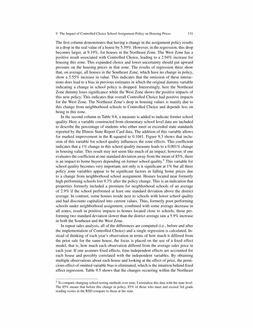
9 The Impact of Controlled Choice School Assignment Policy on Housing Prices 131
The first column demonstrates that having a change in the assignment policy resultsin a drop in the real value of a house by 5.59%. However, in the regression, this dropbecomes larger, at 9.19%, for houses in the Northeast Zone. The West Zone has apositive result associated with Controlled Choice, leading to a 2.94% increase forhousing this zone. This expanded choice and lower uncertainty should put upwardpressure on the housing prices in that zone. The results of regression three showthat, on average, all houses in the Southeast Zone, which have no change in policy,show a 5.55% increase in value. This indicates that the omission of these interac-tions does lead to a bias in previous estimates in which the original dummy variableindicating a change in school policy is dropped. Interestingly, here the NortheastZone dummy loses significance while the West Zone shows the positive impacts ofthis new policy. This indicates that overall Controlled Choice had positive impactsfor the West Zone. The Northeast Zone’s drop in housing values is mainly due tothis change from neighborhood schools to Controlled Choice and depends less onbeing in this zone.
In the second column in Table 9.6, a measure is added to indicate former schoolquality. Here a variable constructed from elementary school level data are includedto describe the percentage of students who either meet or exceeded state standardsreported by the Illinois State Report Card data. The addition of this variable allowsfor marked improvement in the R-squared to 0.1041. Figure 9.3 shows that inclu-sion of this variable for school quality influences the zone effects. This coefficientindicates that a 1% change in this school quality measure leads to a 0.001% changein housing value. This result may not seem like much of an impact; however, if oneevaluates the coefficient at one standard deviation away from the mean of 85%, thereis an impact to home buyers depending on former school quality.5 This variable forschool quality becomes very important; not only is it significant at 1% but all threepolicy zone variables appear to be significant factors in falling home prices dueto a change from neighborhood school assignment. Houses located near formerlyhigh performing schools lost 9.3% after the policy change. This is an indication thatproperties formerly included a premium for neighborhood schools of an averageof 2.9% if the school performed at least one standard deviation above the districtaverage. In contrast, some houses reside next to schools with lower school qualityand had discounts capitalized into current values. Thus, formerly poor performingschools under neighborhood assignment, combined with some average decrease inall zones, result in positive impacts to homes located close to schools, those per-forming two standard deviation slower than the district average saw a 5.9% increasein both the Southeast and the West Zone.
In repeat sales analysis, all of the differences are computed (i.e., before and afterthe implementation of Controlled Choice) and a single regression is calculated. In-stead of thinking of each year’s observation in terms of how much it differed fromthe prior sale for the same house, the focus is placed on the use of a fixed effectmodel, that is, how much each observation differed from the average sales price ineach year. If one assumes fixed effects, time-independent effects are accounted foreach house and possibly correlated with the independent variables. By obtainingmultiple observations about each house and looking at the effect of price, the perni-cious effect of omitted variable bias is eliminated, which is the intuition behind fixedeffect regression. Table 9.5 shows that the changes occurring within the Northeast
5 To compare changing school testing methods over time, I normalize this data with the state level.The 85% means that before this change in policy, 85% of those who meet and exceed 3rd gradereading scores in the RSD compare to those at the state

132 Tammy Batson
Fig. 9.3 Graphical depiction of empirical results by zone
34
Figure 4. Zone results based on former school quality and data from Table 7 regression 7.
In repeat sales analysis, all of the differences are computed (i.e., before and after the
implementation of Controlled Choice) and a single regression is calculated. Instead of
thinking of each year’s observation in terms of how much it differed from the prior sale for the
same house, the focus is placed on the use of a fixed effect model, that is, how much each
observation differed from the average sales price in each year. If one assumes fixed effects,
time-independent effects are accounted for each house and possibly correlated with the
independent variables. By obtaining multiple observations about each house and looking at
the effect of price, the pernicious effect of omitted variable bias is eliminated, which is the
intuition behind fixed effect regression. Table 6 shows that the changes occurring within the
Note: Zone results base on former school quality and data from Table 9.6. All results in the figureare significant at the 1% level.
Zone and the West Zone in the third column hold true when tested against the fixedeffect model, which controls for the time trend occurring in the data, shown here inTable 9.7.
Coefficients from regression 8 show the fixed effects model to yield the same co-efficient from the repeat sales coefficient (regression 5) in which the Northeast Zonedrop of 0.028 are similar to impact under the fixed effects coefficient for ControlledChoice of 0.029. In addition, the West Zone coefficient of a 0.041 increase, seen inregression 5, compares to 0.040, in regression 8. When factored in with repeat salesresults, any unobserved bias does not appear to affect the coefficients associatedwith this change.
9.6 Conclusion
Education policies involving some form of school choice are of great interest andconcern to parents, taxpayers, educators, and policymakers alike. In order to deter-mine the impact of the capitalization of public goods into housing prices, this study

9 The Impact of Controlled Choice School Assignment Policy on Housing Prices 133
Table 9.7 Fixed Effect Regression Results-Interactions with Dpczone
Variable ln of Sales Price
Northeast Zone-(CCAP)-0.029(.006)**
West Zone-(CCAP)0.040(.008)**
Dy2= 19940.022(.007)**
Dy3= 19950.032(.007)**
Dy4= 19960.026(.007)**
Dy5= 19970.012(.007)
Dy6= 1998-0.004(.007)
Dy7= 1999-0.003(.007)
Dy8= 20000.013(.0097)**
Constant11.382(.009)**
Observations 4857Number of pid 2362R2-within, between, overall 0.05, 0.17, 0.10Note: Robust standard errors in (). * denotesstatistical significancce at 5% and ** at 1%.
adopted an approach of using repeat sales. This control for heterogeneity in prop-erty characteristics allowed for the introduction of choice program dummies thatare significant to show reduced values of houses that experience a change in policyof 5.59%. In Rockford, the policy aligned all schools to the racial composition ofthe district while making improvements to the gap between the schools and the per-centage of students meeting the state’s reading goals. However, house prices dropapproximately 9.3% when located near high quality schools following the removalof the guaranteed attendance, unlike houses near former poor-performing schoolsthat have marginal positive effects due to the school choice policy.6 These resultsindicate removal of neighborhood assignment removes any premium or discountthat previously had been capitalized into housing values. However, the next chapterwill examine the idea that this policy impact to housing is caused when residentsreevaluate the utility received from schooling. This sorting can lead to increasedsegregation as homogenous patterns emerge as residents vote with their feet avoid-ing the RSD Controlled Choice guidelines.
Acknowledgements This paper is drawn from Chapter 2 of my dissertation. I would like to thankmy primary advisor, Jeremy Groves, who challenged me. My committee, Virginia Wilcok-Gok andSusan Porter-Hudak, were always been there to listen and give advice. And finally, to my husband,Levi, thank you for being patient and giving me words of encouragement when I needed themmost.
6 Variable based on Illinois Report Card data on 3rd grade students’ achievement scores during thepolicy.

134 Tammy Batson
References
Alves M, Willie C (1990) Choice, decentralization, and desegregation: The Boston‘controlled choice plan’. In: Witte JF, Clune WH (eds) Choice and Control inAmerican Education, Volume 2: The Practice of Choice, Decentralization, andSchool Restructuring, Falmer Press, New York, pp 17–75
Bailey MJ, Muth RF, Nourse HO (1963) A regression method for real estate priceindex construction. Journal of the American Statistical Association 58(304):933–942
Black SE (1999) Do better schools matter? Parental valuation of elementary educa-tion. Quarterly Journal of Economics 114(2):577–599
Bogart WT, Cromwell BA (1997) How much more is a good school district worth?National Tax Journal 50(2):215–232
Bogart WT, Cromwell BA (2000) How much is a neighborhood school worth? Jour-nal of Urban Economics 47(2):280–305
Brennan G, Buchanan JM (1980) The Power to Tax: Analytic Foundations of aFiscal Constitution. Cambridge University Press, New York
Case K, Shiller R (1989) The efficiency of the market for single-family homes.American Economic Review 79(1):125–37
Chau PY, Hu PJ (2002) Examining a model of information technology acceptanceby individual professionals: An exploratory study. Journal of Management Infor-mation Systems 18(4):191–229
Cohen J (1988) Statistical Power Analysis for the Behavioral Sciences. LawrenceErlbaum Associates, Hillsdale, NJ
Downes TA, Zabel JE (2002) The impact of school characteristics on house prices:Chicago 1987–1991. Journal of Urban Economics 52(1):1–25
Figlio DN, Lucas ME (2004) What’s in a grade? School report cards and the housingmarket. American Economic Review 94(3):591–604
Friedrich RJ (1982) In defense of multiplicative terms in multiple regression equa-tions. American Journal of Political Science 26(4):797–833
Halvorsen R, Palmquist R, et al. (1980) The interpretation of dummy variables insemilogarithmic equations. American economic review 70(3):474–475
Hayes KJ, Taylor LL, et al. (1996) Neighborhood school characteristics: what sig-nals quality to homebuyers? Economic Review-Federal Reserve Bank of Dallaspp 2–9
Hoxby CM (2000) Does competition among public schools benefit students andtaxpayers? American Economic Review 90(5):1209–1238
Kennedy PE, et al. (1981) Estimation with correctly interpreted dummy variablesin semilogarithmic equations [the interpretation of dummy variables in semilog-arithmic equations]. American Economic Review 71(4):801–801
Leventhal T, Brooks-Gunn J (2000) The neighborhoods they live in: the effects ofneighborhood residence on child and adolescent outcomes. Psychological bulletin126(2):309
Oates WE (1969) The effects of property taxes and local public spending on prop-erty values: An empirical study of tax capitalization and the tiebout hypothesis.Journal of political economy 77(6):957–971
Oates WE (1985) Searching for leviathan: An empirical study. The American Eco-nomic Review 75(4):748–757
Palmquist RB (1984) Estimating the demand for the characteristics of housing. TheReview of Economics and Statistics pp 394–404

9 The Impact of Controlled Choice School Assignment Policy on Housing Prices 135
Reback R (2005) House prices and the provision of local public services: capitaliza-tion under school choice programs. Journal of Urban Economics 57(2):275–301
Rosen S (1974) Hedonic prices and implicit markets: product differentiation in purecompetition. Journal of political economy 82(1):34–55
Tan N (1990) The Cambridge Controlled Choice program: Improving educationalequity and Integration. Manhattan Institute, Center for Educational Innovation
Taylor DG, Alves MJ (1999) Controlled Choice: Rockford, Illinois, desegregation.Equity & Excellence 32(1):18–30
Taylor DG, Alves MJ (2000) Implementing Controlled Choice and the search foreducational equity in the Rockford, Illinois, public schools: A survey of parentswho withdrew from the Rockford public schools after the 1998-99 school year.Equity & Excellence in Education 33(2):81–94
Tiebout CM (1956) A pure theory of local expenditures. Journal of political econ-omy 64(5):416–424
Times NY (1976) Sirica gives H.E.Y. order on schools. New York Times, 22 JulyYanofsky SM, Young L (1992) A successful parents’ choice program. Phi Delta
Kappan 73(6):476


Chapter 10Public High-School Quality and House Prices:Evidence from a Natural Experiment
Edward Hearn
Abstract Are changes in local public-school quality capitalized into house prices?In 2002, the Charlotte-Mecklenburg School district CMS rezoned 50% of Charlottehouses to different public schools after the court-ordered end of race-based bus-ing. This chapter contributes to the literature on public-school quality and housingprices by exploiting this natural experiment from Charlotte, NC. Using a difference-in-differences model to identify the causal effect of reassignment into a better orworse public high school on the sale prices of affected houses, my results indicatethat people willingly pay between $3,300 and $4,700 per percentage point increasein passing rates on the North Carolina Department of Public Instruction’s End-of-Course exams. This effect is limited to houses in neighborhoods experiencing largeincreases in EOC passing rates after the 2002 reassignments. The positive effectsof school quality on selling prices increase non-linearly among houses experiencingthe largest increases in EOC passing rates. There is no solid evidence that moder-ate or small increases in EOC passing rates that occurred after the 2002 citywidereassignment are capitalized into house prices in the affected school zones. There isalso no evidence to suggest negative price shocks exist for houses CMS reassigns tolow-quality public high schools.
10.1 Introduction
Are changes in local public-school quality capitalized into house prices? This isthe central question in Oates (1969) regarding the mechanism by which people’spreferences for public goods are expressed. Individuals are predicted to move intoareas that reflect most closely their desires for public goods. Since people do notpay for these public goods outright, variations in property taxes levied representdifferences in the costs to individuals of the amount and quality of local publicservices they prefer. In most areas of the United States, property-tax-funded servicesinclude public schools. Where public schools are of higher quality, houses zoned forthese schools are predicted to have higher prices relative to houses zoned for lower-quality schools, holding all else constant.
Edward HearnResolution Economics, Los Angeles, CA, 90067, USA e-mail: [email protected]
137

138 Edward Hearn
Oates (1969), in the spirit of Tiebout (1956), finds that house prices capitalizeboth property taxes and the value of the public services these taxes finance. Black(1999) finds a positive relationship between house prices and public-school qualityfor houses along school-zone boundaries in Massachusetts. Bayer et al. (2007) findthe same result for houses located along school-zone boundaries in the San Fran-cisco Bay Area. Downes and Zabel (2002) and Figlio and Lucas (2004) concludethat families reveal their preferences for better-quality public schools by sorting intohigher-priced houses assigned to these schools. Moreover, Hoxby (2000) finds thatcities with more school districts enjoy more productive public schools than citieswith fewer school districts. Parental sorting forces greater inter-district competitionamong public schools when families have more public-school options.
Untangling the effects of school quality and sorting complicates the identificationof how school quality impacts house prices. Zahirovic-Herbert and Turnbull (2009)control for sorting by examining how an exogenous change in school-attendancezones in East Baton Rouge Parish, Louisiana affects the price and time-to-sale ofaffected houses. They find evidence that people pay higher prices for houses as-signed to schools with better test scores. However, the East Baton Rouge rezoningpales in comparison to the massive reassignment the Charlotte-Mecklenburg School(CMS) district implemented in 2002. In Charlotte, those neighborhoods reassignedby CMS to better schools are predicted to experience positive price shocks relativeto neighborhoods retaining their pre-2002 assignments. People express their prefer-ences for public schools of higher quality through the prices they pay for propertiesassigned to better performing schools, holding property-tax rates constant. The con-verse should be true of neighborhoods CMS reassigned into worse schools. Homesin these adversely affected neighborhoods should experience negative price shocks,reflecting the implicit compensation required by residents to consume lower publicschool quality.
Kane et al. (2006) use the CMS changes in school zones as a natural experimentto investigate how differences in school quality affect house prices, independent ofsorting. They examine houses located along school-assignment borders and housesthat changed school assignments in Charlotte. The primary difficulty with their iden-tification strategy is that they have a limited time frame in which to study the fulleffects of the court-ordered rezoning. They used data through 2001, which was priorto the citywide redistricting CMS instituted in 2002. Because it appealed the school-busing reversal all the way to the Supreme Court, CMS did not implement its schoolreassignment plan until after the citywide rezoning that occurred in April 2002.1
This chapter contributes to the existing literature by exploiting this natural ex-periment from Charlotte, NC. I use this experiment to test whether people paymore for houses assigned to better public schools. In 2002, CMS rezoned 50% ofCharlotte houses to different public schools (Hastings et al., 2006) after the court-ordered end of race-based busing. CMS rezoned some neighborhoods into differentschool zones, but left other neighborhoods’ school assignments unchanged. Thus,the district-wide rezoning provides natural treatment and control neighborhoods foran investigation of whether house prices reflect public-school quality.
Because the 2002 school reassignments were plausibly exogenous, they allowfor a sharper identification of citywide causal effects than does previous work. Moststudies of house-price capitalization use either boundary discontinuity designs or he-donic pricing models. My study has a cleaner identification strategy because Char-
1 On April 15, 2002, the Supreme Court refused to hear CMS’s appeal, thereby upholding theoriginal ruling to end busing.
10 Public High-School Quality and House Prices: Evidence from a Natural Experiment 139
lotte has only one school district, unlike other large cities that have multiple schooldistricts within city limits. Mecklenburg County also has uniform property tax rates.Since CMS is the sole school district in Charlotte, citywide changes in school atten-dance zones prior to the 2002-2003 academic year affected all Charlotte neighbor-hoods similarly. Most other studies do not have citywide levels of treatment withinone school district. Rather, these studies typically focus on houses located near aschool boundary (Black and Machin, 2011). I examine changes in the prices of allhouses in the city of Charlotte and Mecklenburg County, instead of just those houseswithin narrow geographical bands around school-zone boundaries. In doing so, I amable to capture citywide effects of school quality on house prices in a large urbanarea.
I use a difference-in-differences model to identify the causal effect of reassign-ment into a better or worse public school on the sale prices of affected houses. Ifocus exclusively on changes in the quality of high schools, whereas most studieshave examined changes in elementary-school quality. High schools typically havelarger catchment areas than elementary and middle schools. School catchment sizeis important because it permits the inclusion of the many different neighborhoodsthat CMS assigned to a single high school, and facilitates estimation of the effectsof school reassignments on house prices across the citywide price distribution. Thisvariation helps isolate the causal effect of school reassignment on the median houseprice in a variety of neighborhoods. Also, high-school assignment is arguably moreimportant in terms of student outcomes than assignment to elementary or middleschool. High-school quality affects if and where a student attends college, whethera student drops out of formal schooling, and even if a student turns to criminal ac-tivity (Billings et al., 2014). Parents (and students) pay close attention to the qualityof the high school to which their children (or they) are assigned. My results in-dicate that people willingly pay between $3,300 and $4,700 per percentage pointincrease in passing rates on the North Carolina Department of Public Instruction’sEnd-of-Course (EOC) exams. This effect, however, is limited to houses in neigh-borhoods experiencing large increases in EOC passing rates after the 2002 CMSreassignments.
Because of this limitation, I also test for non-linear effects of changes in theEOC passing rate. My results are similar to those of Chiodo et al. (2010), who con-clude that the premium parents pay for houses in better-quality public school zonesincreases as school quality increases. The positive effects of school quality on sell-ing prices increase non-linearly among houses experiencing the largest increases inEOC passing rates. There is no solid evidence that moderate or small increases inEOC passing rates that occurred after the 2002 citywide reassignment are capital-ized into house prices in the affected school zones. There is also no evidence tosuggest negative price shocks exist for houses CMS reassigns to low-quality publichigh schools.
10.2 Data
I used data on house prices from the Charlotte, NC and surrounding-area Multi-ple Listing Service (MLS). The MLS is an online database containing house-pricepostings from Realtors, mortgage brokers, property appraisers, and other real-estatespecialists. The Charlotte MLS contains data on houses that have been listed any-

140 Edward Hearn
time within the past fourteen years. Because it is a rolling aggregate, the 2014 MLSwould include data back to 2000.
The data consist of observations of houses sold in Charlotte and MecklenburgCounty between 1997 and 2010. Only houses listed in the MLS are in these data,however, over 90% of all houses for sale appear in the MLS.2 The data include bothquantitative and qualitative house attributes that fall into three categories: historical,structural, and locational. Historical variables include the year of construction andthe selling date. Structural variables include the architectural style, square foot age,type of residence, and so forth. Locational attributes consist of the house’s neigh-borhood, address, zoning code, assigned public schools, and tax location. The dataalso include the list price and selling price of the house.
I separate these data into neighborhoods containing houses with sell dates beforeand after April 15, 2002. On this date, implementation of citywide school reassign-ments took effect for the next school year after CMS lost its appeal to maintainforced busing. I use selling price, rather than list price, because selling price rep-resents the price that the buyer and seller willingly agreed upon. It is, therefore,more indicative of the market price for a house. I follow the recent literature by notlimiting the sample to houses with three or more bedrooms. The resulting sampleconsists of 46,957 houses in 969 neighborhoods. After cleaning the data, I end upwith a sample consisting of 44,729 houses in 838 neighborhoods.3 Table 10.1 con-tains average selling price and other summary statistics for these houses from theMLS data. It also contains data on EOC test passing-rate averages and differences.4
Table 10.1 Summary statistics
Variable N Mean Std. Dev. Min Max
House Attributes
House Price in 2010 $ 44,729 309,372 260,133 10,909 6,645,636Beds 44,729 3.6 0.7 1 8Baths 44,729 2.3 0.7 1 6Half-Baths 44,729 1.0 0.2 1 5Total Heated Living Area 44,729 2,358.3 982.2 106 13,359Acres 44,729 0.3 0.3 0 9.41New 44,729 0.2 0.4 0 1Age 44,729 23.1 17.7 1 149Age2 44,729 845.4 1,363.6 1 22,201Rezone 44,729 0.4 0.5 0 1Post-2002 44,729 0.8 0.4 0 1
School Attributes
% Pass EOC 43,833 66.9 12.3 26.7 95.4∆EOC2001 43,348 3.0 10.9 -37.7 34.5∆EOC2001 (Positive) 10,292 17.5 11.6 3.16 34.5∆EOC2001 (Negative) 4,530 -11.4 10.0 -37.7 -1.0
2 Houses may not appear in the MLS for a number of reasons: a house may be undergoing fore-closure proceedings and the seller does not want it advertised; a house may be purchased withina family; or, the seller may simply not want to price compete with similar properties listed on theMLS server. In any case, there appears to be no systematic bias in the prices of houses listed in theMLS (Higgins, 2013).3 I clean the data by eliminating observations with nonsensical values: negative ages, houses over200 years old, zero bedrooms, more than 6 or no full bathrooms, lot sizes over 10 acres, and houseselling prices less than $1,0004 EOC passing-rate data come from the North Carolina Department of Public Instruction.

10 Public High-School Quality and House Prices: Evidence from a Natural Experiment 141
From this sample, I identify neighborhoods that experienced public high-schoolreassignments and those which experienced no such school reassignments. The for-mer comprise the “treatment” group of neighborhoods and the latter the “control”group. I consider separately two types of treatments: one where a neighborhoodexperienced a negative shock to high-school quality as a result of high-school reas-signment, and one where a neighborhood received a positive shock to high-schoolquality. A positive school-quality shock occurred when CMS reassigned a neigh-borhood in 2002 to a better-performing high school. I refer to this group of neigh-borhoods as having been positively treated. Correspondingly, reassignment induceda negative shock to neighborhood school quality when CMS rezoned the neighbor-hood into a lower-performing high school than it previously enjoyed. I refer to thisgroup of neighborhoods as having been negatively treated. Control neighborhoodsretained their pre-2002 school assignments.
As a measure of school quality, I use EOC test passing rates for every high schoolin the CMS district. North Carolina state law requires students in grades 9 through12 to take EOC tests at school-year’s end. These tests cover subject material fromten specific courses in the fields of mathematics, science, English, and social studies.I use scores from the Algebra I, English I, and Biology EOC tests for two reasons:the North Carolina Department of Public Instruction mandates that all students inthese courses take EOC tests, and high-school students take English I, Algebra I,and/or Biology courses during their 9th and 10th grades. Since the legal age to dropout of high school in North Carolina is 16 years old (with a parent’s permission),every student, regardless of ability, takes at least one of these courses. This meansthat every student in CMS takes these three EOC tests. Taking high-school averagesacross years in the three subject areas yields estimates of annual school quality basedon a population of high-school students before attrition. Since every student musttake these EOC tests before they can drop out, Algebra I, English I, and Biologytest scores contain information regarding student performance before self-selectionof the least-able students becomes an issue.
Table 10.2 Average EOC passing rates by subject and school, 1996-2002
High School English I Algebra I Biology AverageD.W. Butler 62.8 40.0 66.2 56.3E.E. Wadell 50.1 29.9 54.9 43.3East Mecklenburg. 62.4 41.6 62.8 55.6Garinger 51.0 23.9 33.8 36.2Independence 70.4 35.7 60.2 55.4Myers Park 70.7 30.4 68.8 56.6North Mecklenburg 78.1 33.4 64.0 58.5Olympic 49.8 25.4 48.7 41.3Providence 81.3 59.7 80.5 73.8South Mecklenburg 71.6 35.7 64.4 57.2West Charlotte 39.4 15.5 37.1 30.7West Mecklenburg 54.9 53.5 45.8 51.4Z.B. Vance 67.5 26.7 58.7 51.0
Table 10.2 aggregates EOC passing-rate averages across subjects by year lead-ing up to Charlotte’s citywide rezoning. Using EOC test scores from 1996-1997to 2009-2010 provides multiple years of data before and after April 15, 2002.From these averages, I determine which neighborhoods experienced positive school-quality treatments and which neighborhoods experienced negative treatments. I ex-

142 Edward Hearn
pect average house prices in negatively treated neighborhoods to fall relative tothe prices of similar houses in their control-neighborhood counterparts, and aver-age house prices in positively treated neighborhoods to rise relative to the prices ofcontrol-neighborhood houses.
Table 10.3 Differences in mean prices: Positively and negatively treated and control houses
Positive Treatment(N)
Control(N)
Differences inGroups
Pre-2002257,112.7(1,554)
298,796(4,980) -41,683.3
Post-2002338,364.1(9,223)
323,118(23,592) 15,246.1
Differences in Years 81,251.4 24,322 56,929.4
Negative Treatment(N)
Control(N)
Differences inGroups
Pre-2002225,253.3(707)
298,796(4,980) -73,542.7
Post-2002232,903.3(3,823)
323,118(23,592) -90,214.7
Differences in Years 7,650 24,322 -16,672
Table 10.3 shows that reassignment of a neighborhood into a better public highschool from a worse one increases that neighborhood’s average house price by$56,929. A reassignment from a better public high school to a worse one, on theother hand, has a negative effect on average price of $16,672. These results rep-resent aggregated selling-price averages in all neighborhoods before and after theApril 15, 2002 Supreme Court decision and in both treatment and control neighbor-hoods.
Figure 10.1 depicts annual EOC test passing rates for houses in positively treatedand control neighborhoods. Before April 15, 2002, control neighborhood EOCscores lie below those neighborhoods experiencing no rezoning by about ten per-centage points. After April 15, 2002, this gap narrows substantially.
The graph illustrates that houses in positively-treated neighborhoods experiencesignificant improvements in school EOC passing rates, and this effect lasts over theentire sample period after the rezoning. Figure 10.2 provides similar graphical evi-dence that houses in negatively treated neighborhoods suffer in school quality fromthe CMS rezoning in the entire post-2002 period. The EOC passing rates in nega-tively treated neighborhoods actually lie above the control group annual averages,but fall below the control-group averages after 2002. The negative shock to schoolquality for negatively treated neighborhoods never recovers after the Supreme Courtdecision.
Figure 10.3 presents monthly average selling prices of houses in both positivelytreated and control neighborhoods from June 1997 until April 2010. During the eraof race-based busing (1997-2002), treatment and control trends are roughly parallel.Even in 2000, where a lack of data makes monthly averages for both treatment andcontrol houses fluctuate significantly, monthly control averages lie above positivelytreated averages. However, after the April 15, 2002 Supreme Court decision, posi-tive treatment and control monthly averages tighten, and treatment averages beginovertaking control averages. Eventually, almost all the monthly averages of houseprices in positively treated neighborhood lie above their control group counterparts.

10 Public High-School Quality and House Prices: Evidence from a Natural Experiment 143
Fig. 10.1 EOC passing rates for positively treated and control houses
52
2.6 Tables and Figures
Figure 2.1: EOC Passing Rates for Positively Treated and Control Houses
4/15/200240
50
60
70
80
EO
C P
assin
g R
ate
(%
)
1995 2000 2005 2010Year
Control Houses Positively Treated Houses
EOC Passing Rates for Positive Treatment and Control
Fig. 10.2 EOC passing rates for negatively treated and control houses
53
Figure 2.2: EOC Passing Rates for Negatively Treated and Control Houses
4/15/2002
50
60
70
80
EO
C P
assin
g R
ate
(%
)
1995 2000 2005 2010Year
Control Houses Negatively Treated Houses
EOC Passing Rates for Negative Treatment and Control
Figure 10.4 plots monthly average selling prices for houses in negatively treatedand control neighborhoods. The pattern in monthly house price averages observedprior to 2002 remains unchanged after 2002. Negatively treated houses neverachieve price parity with control-group houses. There is no visual evidence in thescatter plot to suggest that the Supreme Court decision on April 15, 2002 had anyimpact on houses reassigned to lower-quality high schools relative to non-reassignedhouses.

144 Edward Hearn
Fig. 10.3 Log house sale prices of positively treated and control houses
54
Figure 2.3: Log House Sale Prices of Positively Treated and Control Houses
4/15/2002
11.5
12
12.5
13
Lo
g H
ouse S
ale
Price
1997m7 2000m1 2002m7 2005m1 2007m7 2010m1Month in Year
Control Houses Positively Treated Houses
Positive Treatment and Control Log House Prices
Fig. 10.4 Log house sale prices of negatively treated and control houses
55
Figure 2.4: Log House Sale Prices of Negatively Treated and Control Houses
4/15/2002
11.5
12
12.5
13
Lo
g H
ouse S
ale
Price
1997m7 2000m1 2002m7 2005m1 2007m7 2010m1Month in Year
Control Houses Negatively Treated Houses
Negative Treatment and Control Log House Prices
Figure 10.5 minimizes the monthly averages and plots positively treated and con-trol house price trends. During the era of race-based busing (1997-2002), treatmentand control trends are roughly parallel, so there is no strong visual evidence thatCharlotteans moved into houses in higher quality school zones prior to the SupremeCourt decision. There is a small drop in the control neighborhood house price trendfrom the pre-2002 period to the post-2002 period. This magnifies the upward jump

10 Public High-School Quality and House Prices: Evidence from a Natural Experiment 145
in trend prices for the positively treated neighborhoods between the two periods. Byplotting a simple linear fit, in the pre-2002 and post-2002 periods for both positivelytreated and control houses, the graphical evidence of a positive effect suggests asmall but distinct degree of household sorting into homes that CMS reassigned intobetter schools. Further, the slope of the post-2002 positively treated house trendsteepens. The effects of school rezoning in the wake of the Supreme Court case maynot have all occurred immediately after April 15, 2002. These effects could havebeen spread out over several subsequent years.
Fig. 10.5 Trends in log house sale prices of positively treated and control houses
56
Figure 2.5: Trends in Log House Sale Prices of Positively Treated and Control Houses
4/15/2002
11.5
12
12.5
13
Lo
g H
ouse S
ale
Price
1997m7 2000m1 2002m7 2005m1 2007m7 2010m1Month in Year
Control Houses Positively Treated Houses
Control House Trend
Positively Treated House Trend
Positive Treatment and Control Log House Sale Price Trends
Conversely, graphical evidence of house price capitalization of school quality isnot apparent from the plot in Figure 10.6 of the price trends for negatively treatedand control houses. There is almost no change in the trend line for negatively treatedhouses before and after April 2002. The only difference between the two fitted linesis that the slope of the trend line for negatively treated houses becomes slightlyless positive after April 15. This graph predicts no significant effects from the CMSschool reassignment on house prices in negatively treated neighborhoods. It appearsthat Charlotteans experiencing a negative school-quality shock did not move to getinto a better area. This makes sense considering, as the next section details, theseCharlotteans had a chance to win a school choice lottery and gain admittance to ahigher quality school within CMS with out having to pay a house price premium.

146 Edward Hearn
Fig. 10.6 Trends in log house sale prices of negatively treated and control houses
57
Figure 2.6: Trends in Log House Sale Prices of Negatively Treated and Control Houses
4/15/2002
11.5
12
12.5
13
Lo
g H
ouse S
ale
Price
1997m7 2000m1 2002m7 2005m1 2007m7 2010m1Month in Year
Control Houses Negatively Treated Houses
Control House Trend
Negatively Treated House Trend
Negative Treatment and Control Log House Sale Price Trends
10.3 Estimation Strategy
10.3.1 Exogeneity of CMS school-zone reassignments
There are two justifications for interpreting the CMS school reassignments as anexogenous change in the Charlotte housing market: the nature of the legal battle toend busing and the structure of the CMS school-choice plan. The legal battle be-gan in 1997 when a parent sued CMS over its race-based busing policy. In 1999,CMS administrators proposed a new school-choice plan which the elected schoolboard rejected in January 2000. From February until June 2000, CMS proposed,debated, and was in the process of instituting a second school-choice plan that wasidentical to the plan the school board subsequently implemented in 2002. However,in November 2000 the fourth circuit court of appeals in Richmond (VA) reversedits previous ruling and reinstated forced busing. CMS then scrapped its reassign-ment plan and went back to race-based busing (Charlotte Observer, 2001). The firstattempt to legally overturn race-based busing had failed.
In early 2001, a group of parents sued CMS over its race-based student-assignmentpolicy in an attempt to keep legal battle alive. As the case languished in the fourthcircuit court, CMS initiated a third reassignment plan that was approved in July2001, pending the fourth circuit court’s decision. On July 15, 2001 the appellatecourt reversed again and ruled that CMS must dismantle race-based busing (Char-lotte Observer, 2001). CMS immediately appealed this decision to the SupremeCourt. The school board put implementation of the school-choice reassignment planon hold until the Supreme Court ruled on whether to hear the appeal.
The lead-up to the Supreme Court’s decision took nearly a year. Uncertainty overwhether the Court would hear the case abounded. Predictions were mixed: somelegal experts said the Supreme Court would not take the case, while others noted
10 Public High-School Quality and House Prices: Evidence from a Natural Experiment 147
that the Court had not heard a school desegregation case in many years and, so,would agree to hear it.
The plaintiffs’ case was comprised of two issues: the first challenged the consti-tutionality of race-based school assignment policies and the second addressed theissue of whether CMS should have to pay the suing parents’ legal fees. The dualnature of the case rendered it difficult, if not impossible, to say with any confidencewhether the Supreme Court was going to take the case or defer to the fourth circuitcourt’s ruling to overturn race-based busing.5 As Vanderbilt School of Law Centen-nial Professor James Blumstein stated, “To say anything is clear in this area is anoverly optimistic statement” (Smith, 2002).
Given the legal background of the court case from 1997-2002, Charlotte home-owners’ expectations of the Supreme Court decision would have been even lesscertain than the legal experts’. All of this uncertainty dissolved after April 15, 2002.The Supreme Court ruled on that day not to hear CMS’s appeal. This ruling ef-fectively upheld the fourth circuit court’s 2001 decision which forced CMS to dis-mantle race-based busing. The Supreme Court’s decision essentially codified thenew school-choice plan, which had already been put in place prior to the final deci-sion, and resolved any lingering doubts Charlotteans might have had about whetherthere would be school reassignments for the 2002-2003 school year. According tothe Charlotte Observer, parents were simply relieved that the uncertainty had beenresolved (Smith and Helms, 2002).
Although most parents were likely familiar with earlier proposals and reassign-ment plans before April 15, 2002, what parents knew about the 2002 plan’s structureclouded their expectations concerning new school assignments. The school boardused a lottery system, in conjunction with a parental-choice plan, to rezone students(Hastings et al., 2006). Parents gave CMS their preferences for the top three schoolsthey wanted their student(s) to attend. Concurrently, CMS assigned Charlotte homesinto “neighborhood” schools at all levels of education. CMS rezoned 35% of allhouses into different high schools and guaranteed students a seat in their neighbor-hood school, along with transportation to and from neighborhood schools. Therewas no longer a racial basis for school assignments based on county demographicsin which, as was the case under forced busing, CMS could rezone any houses to anypublic school at any time for the ensuing school year.
The board assigned school seats by lottery if the number of parental requestsoutnumbered available seats in a high school (assuming that the school the par-ents chose was not their neighborhood school). Because of the lottery, parentshad a chance to enroll their child at a high-performing public high school even iftheir neighborhood was not assigned to that school. This was true for everyone inCharlotte-Mecklenburg schools, including students just entering CMS (Rothackerand Smith, 2002).
Furthermore, the lottery only applied if a school was oversubscribed. If parentsdid not “win the lottery” for their first-choice school, they also had a chance toenroll their child in their second- or third-choice school by the same lottery as-signment mechanism. Students who did not receive their first-choice assignmentsjoined “waiting pools,” while CMS drew their second or third choices from city-wide lotteries. CMS conducted the first round of school-choice lotteries and mailedreassignment letters to homes on February 28, 2002 (Rothacker and Smith, 2002).Parents had until March 22, 2002 to appeal reassignment decisions.
5 Another reason for a lack of confident predictions before the April 15 Court decision was thatonly four of nine justices must vote affirmatively for the case to be taken by the Supreme Court.

148 Edward Hearn
Many parents complained about the school assignments before this deadline.This forced CMS to revamp its plan, which it did twice after parents received ini-tial assignments but before the Supreme Court decision. The school board voted togive higher priority to students in waiting pools whose first choice was their pre-2002 school, but who had been reassigned to another public school. This alterationoccurred on March 8, 2002 after the initial round of rezoning decisions (Helms,2002b).
The lotteries concluded on March 22, 2002. Subsequently, just four days priorto the Supreme Court’s refusal to hear its appeal, CMS altered the plan again byallowing high-school juniors to remain in their pre-2002 public schools, regardlessof previous reassignment decisions (Helms, 2002a). After April 15, 2002, the schoolboard made no further changes to the school-choice reassignment plan.
Charlotteans knew about the school choice plan but did not know whether itwould be implemented until after the Supreme Court decision. Because of this un-certainty and given prior school reassignment failures, parents would have had lit-tle, if any, incentive to move to another house based on predictions about CMSneighborhood reassignments. Even if parents did not get their first-choice schoolstraightaway, there was a possibility that they would “win the lottery” or benefitfrom a last-minute reassignment plan alteration and their student would be assignedto their first-choice school. After CMS implemented its reassignment plan, 74%of parents got their first-choice school for the 2002-2003 school year (Smith andHelms, 2002).
The choice plan’s provision that parents could enter the assignment lottery forany high school in Mecklenburg County became a problem, however, because high-quality public high schools quickly became over-subscribed. While most parentsgot their first-choice schools in the 2002-2003 school year, many high schools withhigh EOC passing rates had to turn away “choice-in” students in subsequent years.The odds of being denied entry versus gaining a seat at these high schools rangedfrom 11:1 to 43:1 by the 2003 school year and became longer in subsequent years.Concurrently, CMS schools with low EOC passing rates suffered diminishing en-rollments and increased poverty levels as students who won the lottery for reassign-ment into better schools disenrolled (Helms, 2003).
By 2005, CMS began considering alterations to the school choice lottery todeal with the dual problems of over-crowding in high-performing high schools andshrinking student populations in low-performing high schools. The school boardannounced its solution in Fall 2005 for the 2006-2007 school year. CMS electedto keep the lottery in place so parents still had the option to transfer to non-over-subscribed schools. But, CMS dramatically scaled back the options of which highschools parents could choose for their children (Helms, 2005b). The school boardremoved 75% of county high schools from its reassignment options list due to over-subscription (Helms, 2005a). The only remaining options were those high schoolsunder-subscribed prior to Fall 2006. Because these high schools also had the lowestEOC passing rates citywide, most parents sent their kids to neighborhood schools(Helms, 2006). There was no longer an incentive for parents to participate in thechoice lottery after the 2005-2006 school year. The only way for parents to securea seat at a high EOC-passing-rate high school was to move into that school’s catch-ment area.
To examine the possibility of bias arising from the selection of neighborhoodsfor school reassignments based on pre-2002 school quality, I estimated Probit re-gressions of three alternative school-quality measures on the likelihood of a housebeing reassigned to a better or worse school. First, I found that the marginal effect

10 Public High-School Quality and House Prices: Evidence from a Natural Experiment 149
of a one-standard-deviation increase in the three-subject EOC composite test pass-ing rate diminished the probability of a house being rezoned into a better schoolzone after 2002 by 4.5%. As an alternative measure of school quality, I also used acomposite EOC test-performance measure for the other seven subject areas the NCDepartment of Public Instruction covers with such tests. The estimated effect wassmall and not statistically significant. The last school-quality measure I used wasaverage SAT score. The marginal effect of a one-standard-deviation increase in thisscore resulted in an increase in the probability of receiving a positive treatment by4.4%. The size and precision of these effects before CMS reassigned neighborhoodswere not large enough to indicate a systematic bias by the school board of reassign-ing neighborhoods assigned previously to lower-quality schools into better schoolcatchment areas.
I repeated this analysis for houses in neighborhoods that were reassigned tolower-quality schools. The marginal effect of a one-standard-deviation increase inthe EOC passing rate led to a decrease of 7.1% in the probability of negative treat-ment. The marginal effect of a one-standard-deviation increase in SAT score de-creased the likelihood of reassignment to a worse-performing school by 3.3%. Theseven-test composite EOC’s marginal effect was 6.1% and also statistically signifi-cant. The magnitudes of these effects, while larger than for positively rezoned neigh-borhoods, are still not large enough to suggest a systematic bias toward reassign-ing neighborhoods initially assigned to high-quality schools to lower-performingschools in the lead up to the Supreme Court decision.
The direction of the bias indicates that, if endogeneity was present in the selec-tion of neighborhoods receiving positive treatment, then removing the bias wouldincrease the effect of school reassignments on house prices after April 15, 2002.That is, if CMS was more likely to pick worse performing students for reassignmentinto better performing schools, that would diminish those schools’ quality. This re-duction in the quality of better high schools from endogenous selection would alsoreduce the importance of positive sorting on house prices in newly reassigned neigh-borhoods.
The converse is true of negatively treated neighborhoods. If CMS was more likelyto pick higher performing students for reassignment into worse performing schools(before 2002), the quality of schools in negatively treated neighborhoods wouldhave increased. This increase in school quality would have mitigated any negativesorting effects on house prices in those neighborhoods. Endogeneity in school reas-signments biases the results towards finding no effects. This fact, and the small mag-nitudes of the Probit results, suggest that endogenous assignment of CMS houses topositive and negative treatments is not of great concern.
10.3.2 Model Specification
I use a difference-in-differences model to identify the causal effect of a change inschool quality on house price. My initial specification is
yi jt = α + γ(rezone j)+θ(post2002t (10.1)+δ (rezone j ∗ post2002t)+X ′
i jtβ +Ztζ + εi jt

150 Edward Hearn
where yi jt is the log of average selling price of house i in neighborhood j and yeart, α is the intercept term, rezone j is a dummy variable equal to one if a house lies ina neighborhood that CMS rezoned, post2002t is a dummy variable equal to one if ahouse sells after the end of school year 2001-2002 (with April 15, 2002 designatedas the threshold date), Xi jt contains house and/or neighborhood characteristics, Ztcontains year fixed effects, and εi jt is a random error term. The coefficient δ on theinteraction of the two dummy variables measures the causal effect of a neighborhoodhigh-school rezoning on house prices. I identify which houses received a positivetreatment and which houses received a negative treatment based on their respectiveneighborhoods’ school reassignments. Since the school reassignment occurred atthe neighborhood level, I do not include fixed effects for neighborhoods becausethese would be perfectly collinear with the rezone j variable.
To further refine the degree to which changes in EOC test passing rates influencehouse prices, I interact the treatment dummy variable with the change in an EOCtest-score measure:
yi jt = α +π(∆EOC j,2001)+θ(post2002t) (10.2)+τ(∆EOC j,2001 ∗ post2002t)+X ′
i jtβ +Ztζ + εi jt
All variables are defined as before, with the exception of the newly added variable∆EOC j,2001. This variablerepresents the difference in 2001 between neighborhoodj’s pre-2002 public high-school passing rate on the three-subject EOC compositeand neighborhood j’s post-2002 public high-school passing rate on the same EOCtest composite. Neighborhoods not reassigned in 2002 have zero change becausethere is no difference in passing rates. Rezoned neighborhoods register non-zerodifferences for this variable because their EOC passing rates change with their newschool assignments. Parents knew the public high school into which CMS rezonedtheir students. In order to assess the school quality shock their children would ex-perience, parents would have had to assess the difference between the 2001 EOCpassing-rate differences because students take EOC exams in early June. Therefore,the pertinent comparison of EOC passing rates between pre-2002 and post-2002public high school assignments would have been the 2001 difference in EOC pass-ing rates. I interact the difference in the 2001 EOC passing rates with the treatmentvariable to estimate the effect of an increase in the size of the school-quality shockon house prices. If CMS did not reassign a neighborhood, then houses in that neigh-borhood experienced no school-quality shock. These houses remain in the controlgroup as they would under the dichotomous specification of the treatment using therezone dummy variable.
10.4 Empirical Results
10.4.0.1 Initial Results
Column 1 of Table 10.4 contains the results of estimating Equation 10.1 using thedata for positively treated houses. There are no statistically significant treatmenteffects on the prices of houses in neighborhoods that CMS transferred to schoolsof higher quality. This holds for the results from estimating a model containing just

10 Public High-School Quality and House Prices: Evidence from a Natural Experiment 151
the causal variables and a model containing hedonic house variables and year fixedeffects.
Table 10.4 The effect of the 2002 CMS rezoning on log selling price of positively treated houses
Full Sample†(Std. Errors)
Repeat-Sales Sample(Robust Standard Errors)
post2002.0534(.0484)
.0016(.0148)
.0518**(.0259)
.0792*(.0454)
rezone-.1044(.0967)
-.0363(.0432)
-.0901***(.0332)
-.0741***(.0234)
post2002*rezone.0785(.0884)
.0411(.0374)
.0760(.0515)
.0378(.0340)
acres.2559***(.0365)
.2740***(.0387)
beds.2288***(.0131)
.2473***(.0133)
baths.4114***(.0249)
.3287***(.0166)
half-baths.3309***(.0264)
.3445***(.0567)
new.0298(.0287)
-.0108(.0263)
age-.0082***(.0027)
-.0163***(.0023)
age2 .0002***(3.01e-5)
.0003***(2.96e-5)
constant12.44***(.0546)
10.27***(.1125)
12.53***(.0184)
10.58***(.0935)
Year FE N Y N YF(k, N-k) 6.53 119.26 6.42 112.08N 39,349 39,349 2,250 2,250Notes: † indicates standard errors clustered at neighborhoodlevel. *, **, *** indicate p< .10, .05, .01, respectively.
Results from estimating Equation 10.1 for houses in negatively treated neigh-borhoods are reported in the first column of Table 10.5. Here, again, there are nostatistically significant effects on average house price of having been rezoned into alower quality public high school. This is true whether or not I control for hedonicvariables and year fixed-effects. I conclude that the results from the difference-in-differences model provides no evidence that people pay less for houses reassignedinto worse school zones.
I replace the rezone dummy with a measure of the difference between positively-treated neighborhoods’ pre-reassignment and post-reassignment high schools’ 2001EOC passing rates to estimate Equation 10.2. The first column of Table 10.6 con-tains the results. Estimates of these treatments in both the basic and hedonic regres-sions indicate positive and statistically significant house-price effects after account-ing for the magnitude of the difference in EOC passing rates. Using the hedonicresults, the marginal effect of an increase in the EOC passing rate in a positivelytreated neighborhood increases the average house price by about $4,711 per one-percentage point increase in EOC passing rate. This effect is large and statisticallysignificant at the 1% level, and provides evidence that people price in the size of theschool-quality increase when purchasing (and selling) a house.

152 Edward Hearn
Table 10.5 The effect of the 2002 CMS rezoning on log selling price of negatively treated houses
Full Sample†(Std. Errors)
Repeat-Sales Sample(Robust Standard Errors)
post2002.0534(.0484)
.0192(.0137)
.0518**(.0259)
.0595(.0444)
rezone-.2247(.0805)
-.0591(.0399)
-.1548***(.0482)
-.0434***(.0344)
post2002*rezone-.0642(.0695)
-.0344(.0372)
.0040(.0711)
-.0161(.0499)
acres.3094***(.0402)
.3535***(.0463)
beds.2310***(.0155)
.2493***(.0151)
baths.3833***(.0217)
.3132***(.0174)
half-baths.2800***(.0245)
.2736***(.0540)
new-.0004(.0308)
-.0314(.0296)
age-.0128***(.0027)
-.0230***(.0026)
age2 .0002***(3.68e-5)
.0004***(3.62e-5)
constant12.44***(.0547)
10.48***(.1050)
12.53***(.0184)
10.73***(.1000)
Year FE N Y N YF(k, N-k) 5.55 106.58 8.00 95.39N 33,102 33,102 1,880 1,880Notes: † indicates standard errors clustered at neighborhoodlevel. *, **, *** indicate p< .10, .05, .01, respectively.
The first column of Table 10.7 provides estimates using data for negativelytreated neighborhoods in a model where I interact the treatment dummy variablewith the difference in EOC passing rates. These estimates contrast with the evi-dence associated with the previous results for positively treated houses. There is noevidence to suggest that people pay less for houses CMS rezones into worse schools.Even after I account for EOC passing rate differences, the conclusion is the same aswith the treatment indicator variable: no statistically significant results of negativetreatment.
These results are similar to results for East Baton Rouge (Zahirovic-Herbert andTurnbull, 2009). These authors found that a one-standard-deviation increase in testperformance scores resulted in a 2.5% increase in average house price. Their resultsfor negatively treated neighborhoods, however, were inconclusive, as they are here.
As striking as these results are, they may, in fact, represent a lower bound onTiebout movement in the wake of the 2002 CMS school reassignments. The lotteriespredating April 15, 2002 were the largest, but CMS kept the lottery system in placeuntil October 2005, when they dramatically limited lottery system school choices(draws occurred once per year). At the beginning of the 2006-2007 school year,CMS radically scaled back lottery assignments. In so doing, CMS effectively guttedits choice lottery in favor of assigning students solely to high schools closest totheir residence (Helms, 2005c). For this reason, some parents may have applied tothe lotteries each year instead of purchasing a new (higher-priced) home in a betterquality school zone. CMS transferred students into their school of choice if they

10 Public High-School Quality and House Prices: Evidence from a Natural Experiment 153
Table 10.6 The effect of changes in EOC passing rates on log selling price of positively treatedhouses
Full Sample†(Std. Errors)
Repeat-Sales Sample(Robust Standard Errors)
post2002.0292(.0457)
-.0064(.0138)
.0372(.0241)
.0766*(.0433)
∆EOC2001.0018(.0061)
.0014(.0033)
.0059***(.0018)
.0019(.0014)
(post2002*∆EOC2001)
.0090***(.0031)
.0045***(.0014)
.0079***(.0026)
.0052***(.0018)
acres.2614***(.0349)
.2819***(.0402)
beds.2346***(.0131)
.2559***(.0134)
baths.4035***(.0202)
.3210***(.0166)
half-baths.3227***(.0240)
.3517***(.0545)
new.0200(.0284)
-.0252(.0255)
age-.0073***(.0024)
-.0137***(.0022)
age2 .0002***(2.61e-5)
.0003***(2.94e-5)
constant12.41***(.0515)
10.26***(.0926)
12.49***(.0170)
10.52***(.0904)
Year FE N Y N YF(k, N-k) 10.57 132.42 24.54 113.45N 38,802 38,802 2,226 2,226Notes: † indicates standard errors clustered at neighborhoodlevel. *, **, *** indicate p< .10, .05, .01, respectively.
won the yearly lottery without their parents having to relocate. Lotteries representedan alternative mechanism for parents and students to fulfill their preferences forhigher quality education without having to pay a house price premium for it. Inthis way, Tiebout sorting may have been attenuated by the presence of the annualschool choice lottery. Household sorting may also have been deferred until after the2005-2006 school year, when CMS effectively scrapped its lottery system in favorof neighborhood school assignments.
This idea gains credence from recent work on the educational outcomes for stu-dents who “won the lottery” for their first-choice school. On average, students whowere selected for reassignment from low-quality schools to high-quality schoolsthrough the lottery showed increases in post-secondary achievements. In contrast,students already in high-quality school zones who won lotteries for their first-choiceschools exhibited declines in the quality of post-secondary outcomes (Deming et al.,2014). Since lottery draws occurred annually from 2002-2005, parents in low-performing school zones had a yearly incentive to apply for their first-choice schoolthrough the lottery system rather than moving between school zones.
As a robustness exercise, I repeat the analysis above using an alternative sampleof MLS data. I do so to try and capture neighborhood fixed effects without theproblem of multicollinearity arising between fixing effects at the neighborhood leveland my difference-in-difference variables. I match addresses before and after April15, 2002 to form a repeat-sales sample. This significantly cuts down on sample size,

154 Edward Hearn
Table 10.7 The effect of changes in EOC passing rates on log selling price of negatively treatedhouses
Full Sample†(Std. Errors)
Repeat-Sales Sample(Robust Standard Errors)
post2002.0384(.0463)
.0120(.0132)
.0493*(.0251)
.0573*(.0442)
∆EOC2001.0143***(.0053)
.0018(.0038)
.0086***(.0028)
.0027(.0044)
(post2002*∆EOC2001)
-.0034***(.0042)
-.0019(.0022)
-.0020***(.0047)
.0003(.0039)
acres.3144***(.0408)
.3552***(.0464)
beds.2341***(.0155)
.2492***(.0150)
baths.3848***(.0218)
.3133***(.0175)
half-baths.2802***(.0245)
.2755***(.0540)
new.0011(.0304)
-.0324(.0295)
age-.0128***(.0028)
-.0235***(.0026)
age2 .0002***(4.14e-5)
.0004(3.66e-5)
constant12.43***(.0524)
10.46***(.1049)
12.53***(.0177)
10.73***(.1000)
Year FE N Y N YF(k, N-k) 6.09 108.17 6.11 95.35N 33,040 33,040 1,880 1,880Notes: † indicates standard errors clustered at neighborhoodlevel. *, **, *** indicate p< .10, .05, .01, respectively.
but allows me to control for unobserved fixed effects at the neighborhood level.Using identical houses before and after the end of race-based busing also allowsa more exact causal interpretation to my estimates, since individual houses do notchange much over time. I also control for household attributes and year fixed effects.
The second columns of Tables 10.4 and 10.5 contain repeat-sales sample es-timates from Equation 10.1. Like the full-sample estimates, the repeat-sales sam-ple treatment effects are not statistically significant either with or without hedonichousehold-level variables and year fixed effects. The second columns of Tables 10.6and 10.7 present results that resemble those from the full-sample regressions. A pos-itively treated house experiences a marginal effect of $3,313 per percentage pointincrease in the EOC passing rate of its assigned public high school. This premiumis smaller than, but roughly similar to, the estimate from the full sample. Estimatedpremiums for negatively-treated houses are, like the full sample, not statisticallysignificant.
The estimated effects of both the dummy-variable and EOC-interacted treatmentsare robust in both the full and repeat-sales MLS samples. Because school qualityis so closely intertwined with neighborhood characteristics, controlling for the lat-ter isolates the effects of the treatment from the post-busing school reassignments.There is no consistent evidence that the rezonings affected citywide house prices.Positive EOC-interacted treatments, on the other hand, are always positively signed,statistically significant, and of roughly the same magnitudes. There is scant evidence

10 Public High-School Quality and House Prices: Evidence from a Natural Experiment 155
of negative EOC-interacted treatment effects. By controlling for the magnitude ofthe school-quality shock, it becomes clear that families relocate based on how muchschool quality they gain or lose as measured by the differences in school EOC pass-ing rates.
10.4.1 Non-Linear Treatment Results
Following Chiodo et al. (2010), I test for non-linear treatment effects. To do so, I usesplit-sample regressions by dividing the EOC-interacted treatments in my full andrepeat-sales samples into three bins based on quantiles of the differences in 2001EOC passing rates. The “Bottom” bin represents differences up to the 25th quantileof the distribution of EOC passing-rate differences. This bin represents houses thatexperienced a small positive or negative school-quality shock. I bin “Middle” asEOC passing rate differences from the 25th to the 75th quantiles. There are surpris-ingly few passing-rate differences that fall into the middle of the distribution, andthis is why I aggregate the middle two quartiles in filling the middle bin. Finally,the “Top” bin contains EOC passing-rate differences above the 75th quantile of the2001 EOC test-score difference distribution.
Table 10.8 The effects of non-linear changes in EOC passing rates on log selling price, positivelytreated houses
Bottom‡(Std. Errors)
Middle‡(Std. Errors)
Top‡(Std. Errors)
Full Sample†-.0036(.0047)
-.0061*(.0036)
.0048***(.0012)
N 33,008 29,650 33,161
Repeat-Sales Sample-.0117**(.0053)
.0017(.0047)
.0053***(.0019)
N 1,931 1,738 1,878Notes: † Indicates standard errors clustered at neighbor-hood level. *, **, *** indicate p< .10, .05, .01, respec-tively. ‡ Bottom, Middle, and Top represent the bins of<25th, 25th-75th, and >75th quantiles of the differences in2001 EOC passing rates between positively-treated neigh-borhoods’ pre-2002 and post-2002 high school assignments.
As Table 10.8 shows, the top bins of the EOC-interacted treatment drive mostof the regression results from the previous sections. There is weak evidence fromboth the full and repeat-sales samples that, in the middle and bottom bins, there isa negative effect on house prices from positive treatment. This evidence, however,is inconsistent across samples. The results for “Top” treatments are all positivelysigned, statistically significant, and resemble the results of Chiodo et al. (2010).Houses experiencing the largest increases in school quality pay premia for bet-ter schools. Houses experiencing small-or medium-sized increases in EOC pass-ing rates display no evidence of price effects. This translates into price premia forhouses for which high school reassignment results in EOC passing-rate increases of25 percentage-points or more. These price premia are essentially equal to those inthe EOC-interacted results from Table 10.6.

156 Edward Hearn
Table 10.9 The effects of non-linear changes in EOC passing rates on log selling price, negativelytreated houses
Bottom‡(Std. Errors)
Middle‡(Std. Errors)
Top‡(Std. Errors)
Full Sample†.0134(.0138)
-.0019(.0038)
-.0036**(.0017)
N 29,725 30,333 29,270
Repeat-Sales Sample-.0033(.0211)
-.0012(.0054)
.0014(.0050)
N 1,716 1,791 1,694
Notes: † Indicates standard errors clustered at neighbor-hood level. *, **, *** indicate p< .10, .05, .01, respec-tively. ‡ Bottom, Middle, and Top represent the bins of<25th, 25th-75th, and >75th quantiles of the differences in2001 EOC passing rates between positively-treated neigh-borhoods’ pre-2002 and post-2002 high school assignments.
Because CMS took away all of its top quality high schools as lottery choices after2005, the only way to get into a high EOC-passing-rate school was to move housesprior to the 2006-2007 school year. The marginal effects may reflect this movement.For the full sample, there is a price premium of $4,734 for a one-point increasein EOC passing rates and for the repeat-sales sample there is a price premium of$2,694. Most of the effect of CMS’s neighborhood reassignment policy probablyoccurs after there is not the mitigating impact of a lottery to win admittance to anypublic school in Mecklenburg County.
Table 10.9 presents split-sample results of EOC-interacted treatment estimatesfor houses in negatively treated neighborhoods. The evidence is much weaker thanin Table 10.8. The only statistically significant treatment effect has the correct sign,but is sample-specific, and, so, is not generalizable.
10.5 Heterogeneity Test: Condominium Prices
As a further check on the robustness of my results, I regress the same sets of covari-ates and treatments I used previously on condominium prices. Since families withschool-aged children are more likely to own detached houses rather than condo-miniums, sorting along school quality lines should not affect condominium pricesto the same extent. Gallagher et al. (2013) proposed a similar test. They posit that theprices of small houses do not capitalize differences in public school quality becausepeople in these houses generally do not have school-aged children. If small housesare less likely to contain public school students, then condominiums are similarlyunlikely to contain families with public school children.
I control for neighborhood and fixed effects by matching condominium sales byaddress before and after the end of race-based busing on April 15, 2002. This limitsmy sample size because condominiums’ neighborhoods are unlisted in the MLS dataprior to 2003. However, matching controls for confounding neighborhood and loca-tional attributes. Since I cannot narrow my sample to condominiums least likely tohave school-aged kids (i.e., one-room condominiums), families with public school

10 Public High-School Quality and House Prices: Evidence from a Natural Experiment 157
students may reside in some of my sample properties. Any bias in this direction,though, works to the benefit of a statistically non-significant result. Because fam-ilies would sort into condominiums located in better public school zones for whatwould probably be a much lower price premium than for detached houses in thesezones, treatment estimates will tend toward being significantly different than zero.6
My results include less structural attributes of condominiums than of houses.The excluded variables do not translate from house attributes to condominium at-tributes. For instance, lot size is solely a detached-housing attribute. I also includetotal heated living area instead of the number of bathrooms, since inclusion of bothbathrooms and bedrooms provides less variation. Condominiums vary by size, butfew have more than two bathrooms or three bedrooms.
Table 10.10 The effect of the 2002 CMS rezoning on log selling price of condominiums
PositivelyTreated
PositivelyTreated
NegativelyTreated
NegativelyTreated
post2002.1899**(.0814)
.1652***(.0523)
.1899**(.0815)
.1658***(.0527)
rezone-.0031(.1052)
.1897**(.0918)
-.1758(.2759)
-.3228***(.0634)
post2002*rezone.0477(.1716)
.0497(.1480)
-.0564(.5093)
-.0640(.1722)
beds-.1697***(.0589)
-.0868(.0579)
total heated living area.8037***(.0613)
.7411***(.0530)
new-.1513*(.0798)
-.1454*(.0763)
age-.0180***(.0046)
-.0226***(.0047)
age2 .0002***(4.15e-5)
.0002***(5.30e-5)
constant11.52***(.0553)
11.27***(.1986)
11.21***(.1986)
F(k, N-k) 2.65 44.20 2.15 76.02N 161 161 141 141Note: *, **, *** indicate p<.10, .05, .01, respectively. Huber-Whitestandard errors.
Table 10.10 provides the results of estimating equation (1) using data on the sell-ing prices of condominiums in Charlotte from 1997-2010. For both positively andnegatively treated units, there are no statistically significant effects of school-zonechanges on selling prices. This is true for both basic (columns 1 and 3) and hedonic(columns 2 and 4) regressions. Also, some of the signs of estimated hedonic co-efficients are different than their household counterparts. Condominium purchasershave different preferences than house purchasers in the data, and this may be whythe coefficients on characteristics like “new” and “beds” have different signs thanthe coefficients on these variables in the house regressions.
6 This bias works identically for foreclosed houses. To the extent that banks price these propertiesto sell quickly, parents can move into a foreclosed house in a higher-quality school zone at a lowerprice than a non-foreclosed house (Saccacio, n.d.). While I cannot identify foreclosed houses inmy MLS sample, omitting foreclosures induces a bias toward finding statistically non-significanttreatment estimates.

158 Edward Hearn
Table 10.11 The effect of changes in EOC passing rates on log selling price of condominiums
PositivelyTreated
PositivelyTreated
NegativelyTreated
NegativelyTreated
post2002.1813**(.0795)
.1555***(.0511)
.1791**(.0824)
.1627***(.0538)
∆EOC2001.0039(.0032)
.0103***(.0022)
-.0165***(.0057)
.0097*(.0054)
(post2002*∆EOC2001)
.0040(.0050)
.0039(.0036)
-.0188(.0119)
-.0163(.0095)
beds-.1457**(.0654)
-.0305(.0657)
total heated living area.8122***(.0640)
.6740***(.0582)
new-.1626*(.0671)
-.1234(.0788)
age-.0178***(.0044)
-.0228***(.0050)
age2 .0002***(4.17e-5)
.0002***(4.97e-5)
constant11.50***(.0533)
11.21***(.1933)
11.14***(.2244)
F(k, N-k) 4.81 44.49 7.76 67.57N 161 161 137 137Note: *, **, *** indicate p<.10, .05, .01, respectively. Huber-Whitestandard errors.
Results from estimating Equation 10.2 are reported in Table 10.11. The estimatesare nearly identical to those of Table 10.10. The only statistically significant effectfrom a change in school EOC score occurs for negatively-treated condominiums,and it is only marginally statistically significant. Recall that the results from neg-atively treated houses indicated only one statistically significant result, by way ofthe neighborhood-attribute sample. There is scant consistent evidence for a negativetreatment effect for either houses or condominiums.
10.6 Conclusion
The results reported here indicate that houses receiving positive, EOC-interactedtreatments in assigned-school quality experienced increases in prices. This effectis non-linear, however, and is precisely estimated only for those houses in neigh-borhoods which experience a twenty-five percentage-point or higher jump in theirschool EOC passing rates. Negative treatment effects are never consistently sta-tistically significant, and neither are positive or negative treatment estimates fromequation (1). Simply put, Charlotteans paid premia for houses reassigned to higherquality high schools, given the quality increased enough. On the other hand, thereis no convincing empirical evidence that Charlotteans receive price discounts forhouses reassigned to lower quality high schools after April 2002.
There would have been no incentive to sell a house in a negatively treated neigh-borhood, especially during the first three years of the school choice plan. A schoolchoice lottery provided Charlotteans a method by which they could potentially gettheir students into high-quality high schools without incurring a house price pre-

10 Public High-School Quality and House Prices: Evidence from a Natural Experiment 159
mium from moving to a house in a higher EOC-passing school’s neighborhood.However, after CMS took away 75% of the high school parents with public high-school kids could apply for, including all of the public high schools with the bestEOC passing rates in the city, the effects of house-price capitalization are obviousin those high-performing schools’ zones. Furthermore, my results suggest that mostof the house-price premia occurs after a threshold level of increase in EOC-passingrates. The marginal effects on house prices in the “Top” bin of EOC passing ratedifferences are essentially the same as the marginal effects on house prices in theEOC-treatment regressions.
Robustness checks confirm these conclusions. Using full and repeat-sales sam-ples of MLS data confirms that, although the results vary in magnitude, they arequalitatively consistent: the marginal effects of an EOC passing rate increases houseprices in positively treated neighborhoods. This result is non-linear in both samplesI analyze. My findings are broadly consistent with Zietz et al. (2008) and Liao andWang (2012) who find evidence, using quantile regressions, that houses from dif-ferent quantiles of the price distribution value identical private amenities differently.The rezoning of a house into a higher-performing school zone has no effect on houseprice unless the newly assigned school is sufficiently better than the previously as-signed school.
A comparison with average private school tuition rates sheds light on the will-ingness to pay house-price premia for better quality public schools. In Charlotte,there are eighteen denominational and non-denominational private high schools.The average annual tuition for the twelfth grade in all of the private high schoolswas $13,180 in 2012. The maximum private high-school tuition is $21,200 and theminimum is $6,307 (Colwell and Thurmond, 2012). Parents with the ability to movehouses would do so rather than pay private tuition every year. Parents with studentsnewly entering or having recently entered high school would benefit more from amove to a significantly better school zone rather than from sending their childrento private school. However, this may not be the case for parents with students intheir last year or two of high school. In this case, it may be more cost-effective toenroll their students in private schools, depending on how much of an additionalpost-threshold increase in EOC-passing rates parents seek.
Possible extensions of this study would involve using the MLS data in several dif-ferent ways. Future work could examine school-reassignment effects on the pricesof small houses (those with fewer than three bedrooms). These properties shouldexhibit smaller premia for public-school quality. I could also incorporate additionalmeasures of high-school quality, such as graduation rates or SAT scores. Unlikethe three-subject EOC-composite measure, however, these alternative school-qualitymetrics are subject to selection biases because they reflect only those students whohave elected to not drop out of high school or who take the SAT. A natural extensionof this paper would be to investigate the yearly effects of the rezoning variable inan event-study framework. This type of analysis could examine the annual shiftsin house prices over the time frame following the 2002 Supreme Court decision tomore exactly estimate how changes in CMS policy impacted area house prices. Theapplication of MLS data to examine the effects of the CMS post-busing rezoning onCharlotte house prices would enable empirical investigations of these questions andmany others.

160 Edward Hearn
References
Bayer P, Ferreira F, McMillan R (2007) A unified framework for measuring prefer-ences for schools and neighborhoods. Journal of Political Economy 115(4):588–638
Billings SB, Deming DJ, Rockoff J (2014) School segregation, educational attain-ment, and crime: Evidence from the end of busing in Charlotte-Mecklenburg.Quarterly Journal of Economics 129(1):435–476
Black SE (1999) Do better schools matter? Parental valuation of elementary educa-tion. Quarterly Journal of Economics 114(2):577–599
Black SE, Machin S (2011) Housing valuations of school performance. In:Hanushek EA, Machin S, Woessmann L (eds) Handbook of the Economics ofEducation, vol 3, Elsevier, pp 485–519
Charlotte Observer (2001) Third time’s a charm. Charlotte Observer 1 AugustChiodo A, Hernandez-Murillo R, Owyang MT (2010) Nonlinear effects of school
quality on house prices. Federal Reserve Bank of St Louis Review 92(2):185–204Colwell L, Thurmond R (2012) A guide to private schools. Charlotte Magazine 8
JanuaryDeming DJ, Hastings JS, Kane TJ, Staiger DO (2014) School choice, school quality,
and postsecondary attainment. American Economic Review 104(3):991–1013Downes TA, Zabel JE (2002) The impact of school characteristics on house prices:
Chicago 1987–1991. Journal of Urban Economics 52(1):1–25Figlio DN, Lucas ME (2004) What’s in a grade? School report cards and the housing
market. American Economic Review 94(3):591–604Gallagher RM, Kurban H, Persky JJ (2013) Small homes, public schools, and prop-
erty tax capitalization. Regional Science and Urban Economics 43(2):422–428Hastings JS, Kane TJ, Staiger DO (2006) Gender and performance: Evidence
from school assignment by randomized lottery. American Economic Review96(2):232–236
Helms A (2002a) Juniors to stay at current schools—-news thrills rising 11th graderswho were not assigned to first choice. Charlotte Observer 11 April
Helms A (2002b) School board tinkers with wait-list priorities-—change favors stu-dents who might be bumped from current schools. Charlotte Observer 13 March
Helms A (2003) In-demand schools shut choice door-–most students got schoolsthey picked, but some totally out of luck. Charlotte Observer 23 March
Helms A (2005a) The assignment season brings less paperwork-–CMS strives forcandor, simplicity this time in campus shuffle. Charlotte Observer 22 November
Helms A (2005b) How new CMS plan affects you; students still have a choice inschools, but menu will be smaller. Charlotte Observer 27 October
Helms A (2005c) School board drops choice experiment-—with students now as-signed, magnet programs revised. Charlotte Observer 26 October
Helms A (2006) School choice: More changes, fewer options. Charlotte Observer 1January
Higgins M (2013) For your ears only. New York Times 22 SeptemberHoxby CM (2000) Does competition among public schools benefit students and
taxpayers? American Economic Review 90(5):1209–1238Kane TJ, Riegg SK, Staiger DO (2006) School quality, neighborhoods, and housing
prices. American Law and Economics Review 8(2):183–212Liao WC, Wang X (2012) Hedonic house prices and spatial quantile regression.
Journal of Housing Economics 21(1):16–27

10 Public High-School Quality and House Prices: Evidence from a Natural Experiment 161
Oates WE (1969) The effects of property taxes and local public spending on prop-erty values: An empirical study of tax capitalization and the Tiebout hypothesis.Journal of Political Economy 77(6):957–971
Rothacker J, Smith C (2002) Notification letters mailed on school assign-ments—notes will also include whether transportation is provided for student.Charlotte Observer 28 February
Saccacio JJ (n.d.) Uncovering bargains in bank-owned real estate. MLScom URLhttp://www.mls.com/uncovering-bargains-in-bank-owned-real-estate.mvc
Smith C (2002) Top court to decide on hearing CMS case soon—school-choice plan,desegregation policy could change lawsuit would end if supreme court justicesdecline to hear appeal. Charlotte Observer 14 April
Smith C, Helms A (2002) High court won’t hear school case-—lower court rulingstands history-making era of busing is over refusal clears the way for choice planthat does not consider race in school assignments. Charlotte Observer 16 April
Tiebout CM (1956) A pure theory of local expenditures. Journal of Political Econ-omy 64(5):416–424
Zahirovic-Herbert V, Turnbull GK (2009) Public school reform, expectations, andcapitalization: What signals quality to homebuyers? Southern Economic Journal75(4):1094–1113
Zietz J, Zietz EN, Sirmans GS (2008) Determinants of house prices: A quantileregression approach. Journal of Real Estate Finance and Economics 37(4):317–333


Chapter 11Hospitals and Housing Prices in Small Towns inWisconsin
Russell Kashian, Michael Kashian and Logan O’Brien
Abstract Research has determined that hospitals often have significant impacts onreal estate housing prices. The objective of this study is to refine and add to thegrowing literature on the proximity-based effect that hospitals have on surroundinghome values due to their semi-obnoxious characteristics. By limiting this inquiry tothe population of all home sales in Wisconsin Cities and Villages with a populationof under 10,000 persons and hospital with an emergency room, other desirable (andundesirable) externalities are limited. The results suggest that, when controlling forthe individual housing qualities, proximity to the hospital is desirable.
11.1 Introduction
Hospitals often have significant impacts on real estate housing prices. The devel-opment of a hospital can have positive effects, whether it be increasing the rate ofeconomic development, or access to healthcare, especially urgent health care at anemergency room. Facilities that provide desirable services like these are often re-ferred to as ‘yes-in-my-backyard (YIMBY) facilities’ and generally yield increasedhome values based on proximity to a YIMBY facility. Living too close to a hospitalcan also produce negative externalities for residents, through hospital-related traf-fic as well as noise pollution from ambulances, emergency helicopters, etc. Otherfacilities that cause negative externalities are referred to as ‘not-in-my-backyard(NIMBY) facilities’ and usually correlate with lowered property values based onproximity to them (Peng and Chiang, 2015). Facilities, like hospitals for example,that provide the positive resources as well as the undesirable externalities are knownas ‘semi-obnoxious facilities.’ Other examples of semi-obnoxious facilities includelarge sports stadiums, airports, and police/fire stations, among many others. Ideallyfor homebuyers, living near an ER/Hospital brings valuable accessibility, but living
Russell KashianUniversity of Wisconsin-Whitewater, Whitewater, WI 53109, USA e-mail: [email protected]
Michael KashianMarquette University, Milwaukee, WI 53233, USA e-mail: [email protected]
Logan O’BrienUniversity of Wisconsin-Whitewater, Whitewater, WI 53109, USA e-mail:[email protected]
163

164 Russell Kashian, Michael Kashian and Logan O’Brien
too close brings undesirable externalities. Therefore there is a zone in which prop-erty values are maximized, based on an ideal distance from the nearest hospital.
The objective of this study is to refine and add to the growing literature onthe proximity-based effect that hospitals have on surrounding home values due totheir semi-obnoxious characteristics. Drawing from a database of over 3,000 homeswithin a two mile radius of each hospital, we were able to determine the effect onhouse values through proximity to the main entrance of the hospital. This study ex-pands the body of housing research by assessing the impact of hospitals on local realestate without the clutter of other external variables, and utilizes spline variables fordistance from the hospital to allow for non-linearities. Surprisingly, the results showthat the home sales price is maximized nearest to the hospital.
The remainder of this paper continues as follows: related literature review, ex-planation of the models and methodologies, summary of the data, interpretation ofthe empirical results, and conclusions.
11.2 Literature Review Methods
Hedonic analysis describes commodities as consisting of differentiated characteris-tics, which together determine total value. Hedonic analysis has roots in the early20th century in non-housing studies, however it has since expanded into use forreal estate, more specifically, the analysis of housing. The concept for the empiri-cal hedonic analysis developed around the idea that goods, previously thought of ashomogenous, are actually comprised of a multitude of differentiated components.Through this concept researchers use hedonic analysis to estimate the contributionderived from the components of a unit and the value offered by the componentsto the overall value of the unit (Rosen, 1974). Importantly, hedonic analysis cap-tures the implicit and explicit contributions of the characteristics that comprise thecommodity. To do this, a majority of hedonic models explain total value (e.g., saleprice) as either a semi-log or a linear combination of the attributes comprising thecommodity.
Each characteristic of a commodity provides a unique level of utility to buyers.As a commodity, any home then provides a total utility based on the values thedifferentiated characteristics take on (Harding et al., 2003). The market for single-family housing units does not contain a supply of homogeneous homes, but ratherit contains the demand for and supply of differentiated attributes determined on thepurchasing side of the market (Epple, 1987).
11.2.1 Housing Characteristics
Outside of proximity to semi-obnoxious facilities, the value of individual housingcharacteristics is important in determining the overall value of properties (Hard-ing et al., 2003). In an analysis of roughly 125 studies, the number of bedrooms,bathrooms, and square feet generally yielded positive coefficients, the home agecommonly had a negative coefficient, and none of the studies found a negative co-efficient for the lot size or presence of a garage (Sirmans et al., 2006). Comparinghedonic research results directly to one another is often difficult, because severalmethods for measuring and incorporating housing attributes exist in a hedonic anal-

11 Hospitals and Housing Prices in Small Towns in Wisconsin 165
ysis, including binary dummy variables, complex dummy variables, and utilizing acount to indicate more than one unit.
11.2.2 Community Amenities
Location can be a benefit or a detriment to a home’s value. Determining how loca-tion causes the impact on the value of a house can be difficult. In turning the locationinto a variable, the impact of the location can become influenced by other variables(Malpezzi, 2002). This study was limited to exurban and smaller suburban com-munities throughout Wisconsin that contain an ER/Hospital, because larger, morecondensed urban communities are affected by other attractions and facilities thatsubsequently have their own effect on home values.
11.3 Data and Empirical Model
The data was limited to single-family home sales within two miles of a hospital,located within towns or cities with a minimum of 674 residents and a maximum of39,114 residents, for the years from 2013 to 2019. This approach yielded a sampleof 3,013 home sales with complete information on all variables.
Following Peng and Chiang (2015), the distance from the nearest hospital, mea-sured in miles, was split into splines with the provided distances in a fixed range(less than .25 miles, or between .25 and .5 miles), such that coefficients could be in-terpreted as slopes within the range. Peng and Chiang (2015) present a single set ofspline variables but, given that the ranges are necessarily arbitrary, we instead con-sidered splines with only two ranges (less than .5 miles to at least .5 miles), three(less than .33 miles, and .33 to .66 miles), four (less than .25 miles), five (less than.2 miles) or 10 ranges (less than .1 miles). This experimentation allows the identifi-cation of appropriate ranges. Splines for ranges above one mile were considered andrejected since only 157 home sales, approximately 5% of the entire sample, were inthat range.
As is standard in hedonic models, we regress the natural logarithm of housingprices against a series of independent variables, such that coefficients () can be in-terpreted with a 1 unit change in an independent variable yielding a proportionalchange in the dependent variable. The specific formulation is:
ln(price) = α +β (X)+η (year, month) + ε (11.1)
where price is the sales price, β a vector of coefficients, X a series of independentvariables including the hospital distance spline variables, η is a vector of coefficientsfor year and month dummy variables utilized to control for any fixed effects ofeither, and ε is the error term.
For this study, we were concerned that hospitals might be located near the centerof these small cities and towns such that measured distance from the hospital mightactually measure the distance from the city or town center. To control for this possi-bility, a variable is included for the distance from the town or city post office to thehospital, using the assumption that the post office is in fact located at the center.

166 Russell Kashian, Michael Kashian and Logan O’Brien
Table 11.1 Descriptive statistics
Variable Mean Std. Dev.
Price $124,260 72,090Hospital Distance .449 miles .294Post office distance to hospital .771 miles .514Square feet of house 1,761 698.5Full baths in house 1.626 .682Half baths in house .327 .484Bedrooms in house 3.146 .774Attached garage (proportion) .541 .498Population in town/city 7,721 8345Note: n=3,013.
Descriptions for the variables are provided in Table 11.3. Note that square feetand population are entered in quadratic form in the regression to allow for decliningmarginal effects.
11.4 Regression Results
Regression results for either 3, 4 or 5 splines are presented in Table 11.4. Resultsfor 2 or 10 splines are not provided because, for the prior, both coefficients wereinsignificant, while for the latter only 3 of 10 coefficients were significant, and thesedid not yield any clear pattern, meaning the significant coefficients were not con-tiguous with each other.
Overall explanatory power is reasonable for each regression, with R2 statisticsabove .5 in each. Other results are also as expected, with larger homes yieldinghigher prices with a declining marginal effect, and with full and half baths andattached garages yielding significantly higher sales prices. The distance between thehospital and the post office provides a positive, significant coefficient, which mightbe due to hospitals located further from the city center being newer and in newerdevelopments. In unreported results, the year fixed effects suggest prices tended torise over time, while the month effects show peak selling prices between June andSeptember.
Turning to the splines themselves, none are significant with either 3 or 5 splines,but three are significant in the regression with 4 splines, which is also the regressionwith the highest R2 statistic. Those results suggest that price declines for housesfurther away from the hospital, with the largest effect for houses within .25 milesof the hospital, and with the effect dissipating thereafter and becoming insignificantfor houses more than .75 miles from the hospital.
11.5 Discussion
The analysis here sought to understand the relationship between the distance to thenearest hospital in rural and exurban locations in Wisconsin and the home sellingprice. The results for control variables were quite reasonable and consistent withprior research. The distance result is surprising, in that we found home price drop-

11 Hospitals and Housing Prices in Small Towns in Wisconsin 167
Table 11.2 Selling price regression
Variable 3 Splines 4 Splines 5 Splines
Hospital distance range 1 of 3 0.015(0.120)
Hospital distance range 2 of 3 0.007(0.060)
Hospital distance range 3 of 3 0.026(.033)
Hospital distance range 1 of 4 -0.511**(0.205)
Hospital distance range 2 of 4 -0.220**(0.094)
Hospital distance range 3 of 4 -0.135**(0.062)
Hospital distance range 4 of 4 -0.034(0.037)
Hospital distance range 1 of 5 -0.242(0.279)
Hospital distance range 2 of 5 -0.122(0.129)
Hospital distance range 3 of 5 -0.073(0.085)
Hospital distance range 4 of 5 -0.096(0.064)
Hospital distance range 5 of 5 0.015(0.039)
Post office 0.171*** 0.174*** 0.175***(0.019) (0.019) (0.019)
Square feet 0.001*** 0.001*** 0.001***(0.000) (0.000) (0.000)
Square feet2 -0.000*** -0.000*** -0.000***(0.000) (0.000) (0.000)
Full baths 0.230*** 0.229*** 0.230***(0.016) (0.016) (0.016)
Half baths 0.129*** 0.129*** 0.128***(0.017) (0.017) (0.017)
Bedrooms -0.008 -0.008 -0.008(0.013) (0.013) (0.013)
Attached garage 0.233*** 0.232*** 0.229***(0.016) (0.016) (0.017)
Population 0.000 0.000 0.000(0.000) (0.000) (0.000)
Population2 -0.000 -0.000 -0.000(0.000) (0.000) (0.000)
Year and Month Fixed Effects ✓ ✓ ✓Observations 3,013 3,013 3,013R2 0.538 0.540 0.539
ping at a decreasing rate as the distance increases from the hospital, with the largesteffect being on the closest spline (0 to .25 miles).
It was expected that close proximity to a hospital would reduce selling pricedue to the high levels of noise and traffic associated with hospitals. Further, eachhospital in the sample had an emergency room, so noise and traffic are expected.The results suggest instead that proximity to the hospital is desirable. There are twoplausible and complementary explanations for this finding. First, hospital employeesmay value locations within short walking distance to the hospital. Second, given the

168 Russell Kashian, Michael Kashian and Logan O’Brien
hospitals are in rural and exurban location, they may be small and generate relativelyinfrequent noise from ambulances or helicopters. Nonetheless, it is still possible thathome locations in very close proximity to these hospitals (e.g., across the street)are associated with reduced home prices, but there are an insufficient number ofobservations for those locations in this data.1
A limitation of this study is that it does not include urban locations. Parallel testsof home real estate markets and hospital location in medium and large urban areasmight yield very different results.
References
Epple D (1987) Hedonic prices and implicit markets: estimating demand and supplyfunctions for differentiated products. Journal of Political Economy 95(1):59–80
Harding JP, Rosenthal SS, Sirmans CF (2003) Estimating bargaining power in themarket for existing homes. Review of Economics and statistics 85(1):178–188
Malpezzi S (2002) Hedonic pricing models: A selective and applied review. WileyOnline Library, pp 67–89
Peng TC, Chiang YH (2015) The non-linearity of hospitals’ proximity on prop-erty prices: Experiences from Taipei, Taiwan. Journal of Property Research32(4):341–361
Rosen S (1974) Hedonic prices and implicit markets: Product differentiation in purecompetition. Journal of Political Economy 82(1):34–55
Sirmans GS, MacDonald L, Macpherson DA, Zietz EN (2006) The value of housingcharacteristics: A meta analysis. Journal of Real Estate Finance and Economics33(3):215–240
1 The closest the analysis comes to testing very close location is the regression with 10 splines.The coefficient on location within one-tenth of a mile of the hospital is negative (-.697) and in-significant.