The Reliability of the Fetal Magnetocardiogram

The Reliability of the Fetal Magnetocardiogram

Jeroen Gustaaf Stinstra

2001

Ph.D. thesisUniversity of Twente

Also available in print:http://www.tup.utwente.nl/uk/catalogue/technical/fetal-mcg/

T w e n t e U n i v e r s i t y P r e s s

http://www.tup.utwente.nl/uk/catalogue/technical/fetal-mcg/

RELIABILITY OF THE FETALMAGNETOCARDIOGRAM

Jeroen Gustaaf Stinstra

Electronic full color version

Acknowledgement

This research was financially supported by:• The Netherlands Heart Foundation• The Institute for Biomedical Engineering (BMTI), University of Twente

J.G. Stinstra,Reliability of the fetal MagnetocardiogramProefschrift Universiteit Twente, Enschede.ISBN 90-365-1658-7Copyright c© J.G. Stinstra, [email protected], 2001

RELIABILITY OF THE FETALMAGNETOCARDIOGRAM

PROEFSCHRIFT

ter verkrijging vande graad van doctor aan de Universiteit Twente,

op gezag van de rector magnificus,prof. dr. F.A. van Vught,

volgens besluit van het College voor Promotiesin het openbaar te verdedigen

op vrijdag 2 november 2001 te 16.45 uur.

door

Jeroen Gustaaf Stinstrageboren op 7 oktober 1974

te Leeuwarden

Dit proefschrift is goedgekeurd door:

prof. dr. M. J. Peters (promotor) enprof. dr. H. Rogalla (promotor)

voor mijn ouders

Contents

1 Introduction 111.1 Reliability of the fetal magnetocardiogram . . . . . . . . . . . . . . . 111.2 Layout of this thesis . . . . . . . . . . . . . . . . . . . . . . . . . . . 121.3 Monitoring the fetal heart . . . . . . . . . . . . . . . . . . . . . . . . 141.4 Fetal magnetocardiography . . . . . . . . . . . . . . . . . . . . . . . . 18

2 Signal-processing 292.1 Objectives signal-processing . . . . . . . . . . . . . . . . . . . . . . . 292.2 The signal-processing procedure . . . . . . . . . . . . . . . . . . . . . 302.3 Description of the recorded signals . . . . . . . . . . . . . . . . . . . 312.4 Filtering . . . . . . . . . . . . . . . . . . . . . . . . . . . . . . . . . . 402.5 Detection and averaging of fetal complexes . . . . . . . . . . . . . . . 48

3 Modeling fetal MCG 533.1 Physical model . . . . . . . . . . . . . . . . . . . . . . . . . . . . . . 533.2 Boundary element method . . . . . . . . . . . . . . . . . . . . . . . . 563.3 Fetoabdominal compartments . . . . . . . . . . . . . . . . . . . . . . 613.4 Conductivity of fetoabdominal compartments . . . . . . . . . . . . . 663.5 Modeling the fetal heart . . . . . . . . . . . . . . . . . . . . . . . . . 75

4 The vernix caseosa and its effects on fetal MCG and ECG 854.1 The vernix caseosa . . . . . . . . . . . . . . . . . . . . . . . . . . . . 854.2 Modeling thin highly resistive layers . . . . . . . . . . . . . . . . . . . 894.3 Modeling thin highly resistive layers and holes . . . . . . . . . . . . . 984.4 The influence of the vernix caseosa . . . . . . . . . . . . . . . . . . . 1034.5 Capacitive effects due to the vernix caseosa . . . . . . . . . . . . . . . 113

5 The forward problem in fetal magnetocardiography 1215.1 Fetoabdominal volume conduction . . . . . . . . . . . . . . . . . . . . 1215.2 The layer of subcutaneous fat and amniotic fluid . . . . . . . . . . . . 1235.3 Inter-individual differences during gestation . . . . . . . . . . . . . . 1265.4 The P-wave to QRS-complex ratio . . . . . . . . . . . . . . . . . . . . 1345.5 An effective model for volume conductor plus source . . . . . . . . . 1375.6 Comparison between measurement and simulations . . . . . . . . . . 146

CONTENTS 7

6 Database of normal values 1516.1 The intracardiac time intervals . . . . . . . . . . . . . . . . . . . . . . 1516.2 Statistics . . . . . . . . . . . . . . . . . . . . . . . . . . . . . . . . . . 1546.3 Comparison with previously measured data . . . . . . . . . . . . . . . 1566.4 Factors influencing intracardiac time intervals . . . . . . . . . . . . . 1606.5 Application of intracardiac time intervals . . . . . . . . . . . . . . . . 163

7 The classification of arrhythmia by fetal magnetocardiography 1697.1 Fetal arrhythmia . . . . . . . . . . . . . . . . . . . . . . . . . . . . . 1697.2 Complete atrioventricular block . . . . . . . . . . . . . . . . . . . . . 1707.3 Atrial flutter . . . . . . . . . . . . . . . . . . . . . . . . . . . . . . . . 1757.4 Premature atrial contractions . . . . . . . . . . . . . . . . . . . . . . 1787.5 Bundle branch block . . . . . . . . . . . . . . . . . . . . . . . . . . . 1807.6 Discussion . . . . . . . . . . . . . . . . . . . . . . . . . . . . . . . . . 184

8 Conclusions and discussion 1858.1 Influence of the signal-processing . . . . . . . . . . . . . . . . . . . . 1858.2 Models . . . . . . . . . . . . . . . . . . . . . . . . . . . . . . . . . . . 1858.3 Amplitude of the fetal MCG . . . . . . . . . . . . . . . . . . . . . . . 1868.4 Ratios of the amplitudes in the fetal MCG . . . . . . . . . . . . . . . 1878.5 Field distribution of the fetal MCG . . . . . . . . . . . . . . . . . . . 1878.6 Field distribution of the fetal ECG . . . . . . . . . . . . . . . . . . . 1888.7 The intracardiac time intervals . . . . . . . . . . . . . . . . . . . . . . 1888.8 Classification of arrhythmia . . . . . . . . . . . . . . . . . . . . . . . 189

References 191

Abbreviations 199

Samenvatting (summary in dutch) 201

Summary 205

Dankwoord 209

Curriculum Vitae 211

8

Chapter 1

Introduction

According to Barker’s theorem disease originates in the womb. Barker (1999) and his teamuncovered a relation between abnormal fetal growth and the development of diseases likecoronary artery disease, hypertension, and diabetes in later life. According to his theorem,those children who are already suffering from health problems in their prenatal life are thesame persons that suffer most health problems in adult life. Therefore Barker stressesthe need for preventing abnormal fetal development. This implies the need for an accuratemeans of monitoring fetal well-being. Congenital anomalies of the heart are more commonthan anomalies in any other organ with about one percent of the children affected. Thence,this calls for monitoring the fetal heart. One way of monitoring the fetal heart activity is fetalmagnetocardiography. Fetal magnetocardiography (MCG) is the recording of the magneticfields generated by the fetal heart’s electric activity. The scope of this thesis is to evaluatethis technique and its ability to reflect the electrical phenomena taking place within the fetalheart. An important aspect for fetal magnetocardiography in order to become a clinicalaccepted tool, is that it is not only able to measure fetal heart activity, but it has alsoto be a method, whose readings are reliable for diagnosis. This reliability aspect will bethe central theme throughout this thesis. Although this thesis will focus on the reliabilityof fetal magnetocardiography, other methods like fetal electrocardiography and Doppler-ultrasound will be discussed as well as they provide important clues on the origin of themagnetic field measured.

1.1 Reliability of the fetal magnetocardiogram

For a proper operation, a fetal magnetocardiogram (MCG) has to reflect the elec-trophysiological processes taking place in the fetal heart. If not, the fetal MCG hasto be used cautiously in the diagnosis of fetal heart diseases. Moreover, it needs tobe investigated, which aspects of the recorded signals can be trusted and which not.This reliability aspect is not restricted to the fetal MCG magnetometer system asthere are other factors involved. The question is whether the changes in the magneticfield over the maternal abdomen can be predominately ascribed to the fetal heart and

Introduction 11

which other factors play a role in the formation of the magnetic field over the mater-nal abdomen. As the magnetic data recorded over the maternal abdomen containsmuch more than fetal heart data alone, the fetal heart signals need to be extractedfrom the recorded signals. Hence, the algorithms in this signal-processing stage needto be robust and their flaws need to be known. In order to evaluate the reliability offetal magnetocardiography, three aspects are considered, the duration, the amplitudeand the ratio of the different depolarisation/repolarisation waves in the fetal magne-tocardiogram. As the field of fetal magnetocardiography is developing, the questionis raised how to spot irregularities in the fetal heart functioning. For this purpose thesignals need to be compared with other methods such as postnatal ECGs. Althoughthe techniques are alike the differences need to be known. Throughout this thesis thedifferent aspects of fetal magnetocardiography mentioned will be addressed in orderto answer the question whether the fetal magnetocardiogram is reliable for diagnosis.

In the next section the layout of this thesis will be described, followed by a shorthistoric overview of the methods used to monitor the fetal heart and a description offetal magnetocardiography.

1.2 Layout of this thesis

In chapter 2, the signal-processing techniques will be discussed as currently used in theBiomagnetic Center Twente. The averaging and filtering techniques will be discussedas well as the influence of the magnetometer system itself. It will be investigated towhat extent the signals will be dependent on the signal processing algorithms.

In chapter 3 the volume conduction problem will be introduced. The volume conduc-tor consists of all tissues surrounding the fetal heart. As the currents generated in thefetal heart flow through these tissues, the differences in conductivity of these tissuesinfluences the magnetic field over the maternal abdomen. Direct measurements ofthe volume conductor influence are not feasible, as it is not possible to separate thecontributions to the magnetic field generated by the fetal heart from those due to thecurrents in the other tissues in the maternal abdomen. Hence, the volume conductionmay compromise the reliability. The direct measurement of the current density in thefetus and maternal abdomen is not possible due to practical reasons. Hence, simula-tions are used to estimate the effects of the volume conductor. These simulations areused to answer the question whether the amplitudes or the amplitude ratios in thefetal magnetocardiogram can be trusted. In chapter 3, the volume conductor mod-els will be introduced which are used in these simulations, as well as the numericaltechniques needed to perform the simulations. The bounds of the conductivity of thetissues present in fetoabdominal volume conductor will be estimated.

The vernix caseosa is a fatty layer, which covers the skin of the fetus in the lasttrimester of gestation. Since this layer plays an important role in the volume con-duction problem, chapter 4 will be dedicated to its role in the volume conductionproblem. As this thin layer covering the fetus demands a refinement of the modelingtechniques, these modeling techniques are introduced in this chapter and a new one

12 Chapter 1

will be introduced which allows for modeling thin layers which contain holes and arenot homogeneous. Simulations using this technique show that the vernix caseosa hasa profound effect on the volume conduction problem. These simulations are used toestimate the influence of this layer on the intracardiac time intervals, the amplitudesand amplitude ratios of the various waves in the PQRST-complex. As the modelscan be used to compute both the magnetic field as well as the electric potential, bothfetal ECG and MCG are considered. It will be shown that holes in the vernix caseosaneed to accounted for in the model in order to produce a simulated fetal ECG mapwhich is similar to the ones measured.

Chapter 5 is also dedicated to the volume conduction problem. In this chapter theinfluence of the changing volume conductor throughout gestation will be discussed aswell as inter-individual differences. In this chapter the models of chapter 4 are ex-tended with realistic geometrical data obtained from MRI-images of pregnant women.This chapter will be dedicated to two questions, namely whether the amplitude of thefetal MCG signals can be used for diagnostic purposes and up till which accuracy theratios between the amplitudes can be estimated. Because in some cardiac diseaseslarge P-waves are encountered in comparison to healthy cases, a large P-to-QRS ratiomay point to a fetus a risk. Thence, the discussion on the accuracy of the ratioswill focus on the P-to-QRS ratio. In order estimate the variability of the amplitudeand the ratios, models of the second and third trimester of gestation have been madewhich include the vernix caseosa and the amniotic fluid. At the end of this chapter itwill be shown that the field near the maternal abdomen can be described as the fieldof a magnetic dipole, where this magnetic dipole is located in the vicinity of the fetalheart. Hence, this model can be used optimise the pickup-coil of the magnetometersystem.

In chapter 6, measurements that are obtained during normal pregnancy and the vari-ations observed between the different individuals will be discussed. A database ispresented consisting of data collected by a number of research groups in various coun-tries, that can be used as reference. This database contains the intracardiac timeintervals, which can be used for establishing what values can be expected to be nor-mal during uncomplicated pregnancy and hence for determining which values are notexpected to be normal. This database is the first study, which compares the datameasured by the various research groups involved in fetal MCG studies and is thefirst attempt to come to a measure that is independent of the magnetometer systemand the interpreter of the signals.

In chapter 7, several malfunctions of the fetal heart and their reflections in the fetalMCG will be considered. Apart from being reliable, fetal magnetocardiography hasto provide data that is useful for classifying fetal cardiac disorders. Therefore, thesecond question to be answered is whether fetal MCG enables the distinction betweendifferent cardiac disorders. Four examples will demonstrate new insights in the abilityof fetal MCG in detecting live-threatening heart conditions as well as less serious ones.The importance of detecting the P-wave in the fetal MCG will be demonstrated.

Finally, in chapter 8 conclusions will be formulated and recommendations for furtherimprovement.

Introduction 13

1.3 Monitoring the fetal heart

Monitoring the fetal heart dates back more than a century. In the late 19th centuryit was recognised that the fetal heart rate could be found by means of ausculation.The first attempt to record the electrical activity of the fetal heart directly was in1906 by Cremer (Cremer, 1906). By means of a set of electrodes attached to thematernal abdomen, fetal heart activity was picked up and amplified, showing the firstrecorded fetal QRS-peaks. During the remaining part of the 20th century numerousimprovements have been made in fetal ECG equipment as well as improvements in theunderstanding of the propagation of the fetal heart signal (Bolte, 1961; Hon and Lee,1964; Oldenburg and Macklin, 1977; Brambati and Pardi, 1980; Pardi et al., 1986;Oostendorp et al., 1989; Pieri et al., 2001). However, despite the advantage of beinga cheap and non-invasive method, transabdominal fetal electrocardiography (ECG)suffers from the fact that the acquisition of the fetal ECG cannot be guaranteed.Pieri et al. (2001) found an average success rate of about 60 percent during the lasttrimester of gestation and a reduced measurability around weeks 28 until 34 withsuccess rates as low as 30 percent. In this case the success rate was defined as thepercentage of the total recording time, in which a reliable fetal heart rate could beobtained. Apart from the low overall average success rate of about 60 percent largeindividual differences in success rate were found between recordings. In figure 1.1,an example of a fetal ECG is given. In this case the signals have an amplitude ofabout 20 µV, which is large for a fetal ECG. In most cases the R-peaks are difficultto discern from the background noise.

The discovery of the Josephson-effect in 1962 (Josephson, 1962) led to the invention ofSQUID-magnetometer systems in the late sixties. These systems made it possible forthe first time to record very tiny magnetic fields such as the magnetic field originatingfrom the fetal heart, which is of the order of a picotesla at a few centimeters distancefrom the maternal abdomen, see figure 1.1. The first fetal magnetocardiogram wasmeasured in 1974 by Kariniemi et al. (1974). In the following 25 years the interest infetal magnetocardiography slowly grew. At first most biomagnetometer systems in theworld were focused on the adult heart and brain, however at the start of the ninetiesfetal MCG became more popular. At the moment about ten groups in the world arecollecting fetal MCGs on a regular basis. Most of them use systems originally designedfor the measurement of magnetoencephalograms or adult magnetocardiograms. How-ever some groups are now using or are planning to use magnetometer arrays speciallydesigned for fetal magnetocardiography (Kandori et al., 1999; Robinson et al., 2001;Rijpma et al., 1999). The present activity in the field focuses on improving the currentsystems for fetal magnetocardiography, the investigation of fetal heart defects and theestablishment of a reference database. The latter consists of values measured duringnormal pregnancies that can be used for comparison with the measurements obtainedin ill fetuses (Stinstra et al., 2001b). Over the last ten years, the first documentedcases of arrhythmia (Achenbach et al., 1997; Wakai et al., 1998; van Leeuwen et al.,1999; Menendez et al., 2000; Quartero et al., 2001; Menendez et al., 2001) and con-genital heart disease (Hamada et al., 1999; Golbach et al., 2001; Kahler et al., 2001)

14 Chapter 1

Figure 1.1. Recordings of various methods to monitor the fetal heart. Upper row is a fetalMCG obtained using a magnetometer at approximately 2 cm from the maternal abdomen(week 36). The second and third row represent simultaneous recordings of a fetal MCG andECG (M=maternal and F=fetal). The fourth row is a fetal CTG in which the fetal heartrate is measured during several minutes. The lower two graphs represent recordings of theultrasound imaging technique.

Introduction 15

investigated by means of fetal magnetocardiography have been reported in literature.Not only cardiac diseases have been investigated, intrauterine growth retarded fetuseshave been investigated as well as twin pregnancies (van Leeuwen et al., 2001a). Wakaiet al. (2000b) even investigated a case of ectopia cordis, a condition in which the heartis developing outside the chest of the fetus.

Other methods of monitoring the fetal heart rate include methods such as the directrecording of the sound produced by the fetal heart and echocardiography. Talbertet al. (1984) reported the development of a microphone system, which attached tothe abdominal wall could register the opening and closing of the valves in the heart.Apart from a couple of literature citations in the 1980s, this technique remains mainlyunused.

At the moment ultrasound is the most common technique used to study the fetal heartrate. This technique became popular in the 1980s and still dominates the centersfor fetal surveillance. Currently, the realm of ultrasound consists of a wide varietyof techniques and devices ranging from a Doppler-ultrasound device for obtaining acardiotocogram (CTG) displaying the fetal heart rate, to ultrasound imaging deviceswith color-Doppler imaging possibilities and options to reconstruct three-dimensionalimages. The latter reconstruct an image of the anatomy of the fetus within the womband attempt to map movements of, for instance, blood flow on top of this image.The technique is based on ultrasonic waves with frequencies in the MHz range thatare reflected at the different interfaces within the maternal abdomen and fetus. Anultrasound image is created by focusing the ultrasound transducer array along a lineand recording the reflected waves. In this way an ultrasonic image is created alongthis line in the body. In the so called B-mode ultrasound scan, the line along whichthe ultrasound scan is made is varied in angle and a two dimensional image is created.By scanning this two dimensional plane continuously, a moving image is created ofthe fetus and for instance the heart. In order to increase the temporal resolution, theM-mode scan has been created. In this mode the ultrasonic beam is not varied indirection, but the angle under which the ultrasonic beam is insonated is kept constant.Hence instead of having to make multiple scans under different directions in order tomake one two-dimensional image, each scan along the same direction is a sample intime. In order to make variations more clear the ultrasonic image along this beamis displayed as a function of time. In this way a two-dimensional image is created inwhich the structure along a line is depicted as a function of time. Hence, this modeis often used to study moving structures such as the heart. The B-mode is used tostudy the morphology of the heart and the M-mode is used to study, for instance,arrhythmia. The latter scan is performed by focusing the ultrasonic beam in sucha way that the image crosses the fetal heart and preferably both the ventricles andatria. In figure 1.1, such an M-mode scan is depicted. In this figure, an M-modetracing of an atrioventricular heart block is shown in which the atrial and ventricularrate differ by a factor 2, see chapter 7.

Another way of studying movements is using Doppler-ultrasound. In this techniqueDoppler shifts are recorded of the reflected ultrasonic waves. These shifts occur whenparticles such as blood cells or structures such as the heart wall move towards or

16 Chapter 1

away from the transducer. This allows for monitoring the fetal heart as well as thedetection of fetal arrhythmias. This technique is used in two kinds of devices, one builtfor the sole purpose of obtaining the fetal heart rate lacking any imaging possibilities.In the other devices this technique is integrated with imaging ultrasound machines.Despite the common use of Doppler-ultrasound devices for obtaining the fetal heartrate, these devices have a number of disadvantages. For instance, the elastic belt thatholds the ultrasonic transducer in place for long term usage is found to be unpleasant(Pieri et al., 2001) and needs continuous repositioning in order to keep the fetal heartin line with the transducer. To complicate matters the received signal is subjectedto a lot of noise and artifacts, therefore a lot of signal-processing is used in order todetermine the fetal heart rate. However, these signal processing techniques are farfrom flawless and they are known to produce erroneous fetal heart rate data undercertain circumstances (Dawes et al., 1990). They are notorious for doubling or halvingthe fetal heart rate or making educated guesses during those short intervals in whichnoise inhibits the fetal heart rate detection. Especially during episodes of high fetalheart rate variability problems can occur. Furthermore, due to the signal-processingstrategies employed, the beat-to-beat variability may not be observed at all. Anotherapplication of Doppler-ultrasound is the integration of the technique with ultrasoundimaging. In this way, moving particles can be localised and be used for instance tomeasure the blood flow in the fetal aorta, whose velocity will relate to the mechanicalaction of the heart. In this way the heart rate can be established as well.

Safety is a matter of concern as the fetus is subjected to a beam of ultrasonic waves.For instance, Stanton et al. (2001) found that diagnostic ultrasound induces a changein the number of mitotic and apoptotic cells in the small intestines of mice and theyhypothesise that DNA may be damaged by intense ultrasonic waves. In a study byTarantal et al. (1995) monkey fetuses that were frequently exposed to ultrasound,showed for instance a smaller birth weight and a reduction in the number of neu-trophils in the blood (type of white blood cell). Especially the Doppler-ultrasoundmode in modern equipment produces ultrasonic beams with a high power density,some over 0.5 W/cm2 (Harrington and Campbell, 1995). Hence, these kinds of mon-itoring the fetal heart should be limited in order to avoid heating up of the tissueinsonated with the ultrasonic beam.

Each technique has its own advantages and drawbacks. For instance, ultrasoundimaging allows for investigating the morphology of the fetal heart and studying itsmechanical functioning using the M-mode. Although techniques like fetal ECG andMCG cannot reveal the morphology of the fetal heart, they allow for studying theelectrical activation of the fetal heart, which is origin of the mechanical functioningof the fetal heart. Although these techniques are all labeled as being non-invasive,the ultrasound techniques still rely on the insonation of sound waves into the body,whereas the fetal MCG is a truly non-invasive technique in which the body is not eventouched. Whereas fetal ECG and Doppler-ultrasound data are obtained for longerperiods (extending up to 24-hour monitoring), fetal MCG and ultrasound imaging canonly be obtained for short periods of time, as mother and child are not allowed to moveduring measurement. Fetal MCG is at the moment performed in magnetically shielded

Introduction 17

rooms with complex magnetometer systems requiring a lot of technical attention.Ultrasound imaging is still in need of an expert to operate the transducer and a skilledoperator is needed to detect arrhythmias using M-mode. Although the temporalresolution of ultrasound is improving, the proper diagnosis of fetal arrhythmia is stillnot flawless. For instance, Kleinman et al. (1985) describe a case where an arrhythmiacaused by retrograde atrial activation was mistaken for sustained supraventriculartachycardia by the M-mode tracings. Due to this incorrect diagnosis a treatment of thetachycardia was initiated with medication that was potentially harmful for the fetus incase of an arrhythmia caused by retrograde atrial activation. Most medication directlyinvokes on the underlying electrical activation of the fetal heart, i.e. the behaviourof the ionic channels in the cardiac cells are often the target of the medication inorder to increase or slow down the electrical activation. Fetal MCG can improve theclassification and thence the treatment as it reflects the electrical activation directly.

1.4 Fetal magnetocardiography

1.4.1 The origin of the fetal MCGThe origin of the magnetic field and the potential measured at the abdominal surfaceis located within the heart muscle. The heart muscle, like other tissues in the humanbody, consists of cells surrounded by a membrane. This membrane separates twoelectrolytes, i.e. the interstitial fluid and the intracellular fluid. Both fluids exchangeions, like potassium, sodium and chloride ions through the cell membrane, whichis selectively permeable for these ions. Normally, the sodium concentration in theinterstitial fluid is at least a factor ten larger than in the intracellular fluid and viceversa for the potassium concentration. These concentration differences are the drivingforces behind the current source in the fetal heart. When the myocardiac cells are inrest the cell membrane is permeable for potassium ions, but not for the other ions.Due to the difference in potassium concentration, potassium ions diffuse from theintracellular fluid towards the extracellular fluid. As a result, the cell gets negativelycharged stopping the efflux of potassium ions. Hence, in equilibrium the potentialacross the cell membrane is about -90 mV (Berne and Levy, 1993).When a cell is excited, the transmembrane potential difference becomes less negative.This causes the cell membrane to become more permeable to sodium. This triggers aninflux of sodium ions into the cell, charging the cell with positive charges. Since thecell membrane is now more permeable to sodium, the potential difference over the cellmembrane rises to +30 mV (depolarisation). The influx of sodium is counterbalancedby an electrical force opposite in the direction of the concentration gradient. Theraise in potential causes the cell membrane to become more permeable to potassiumand less to sodium again lowering the potential difference over the cell again. Incardiac cells, the repolarisation due to the efflux of potassium is temporarily cancelledby an additional influx of calcium ions keeping the potential at a level of about -10 mV for about 150 ms. However, the efflux of potassium progresses and ensuresa return to the resting potential. These transmembrane potential changes due to

18 Chapter 1

Figure 1.2. The cardiac muscle of an adult as current source.

activation are called the action potential. The depolarisation process is illustrated infigure 1.2. As the activation of cardiac cells reduces the differences in concentrationsbetween the intracellular and extracellular fluids, each cell membrane contains anactive mechanism, which pumps the potassium and sodium ions back, maintainingthe concentration gradients. This pump consists of an integral membrane proteincalled Sodium-Potassium-ATPase. This protein uses chemical energy stored in thecell to pump potassium and sodium against their concentration gradients allowing analmost infinite sequence of activation and deactivation.

When a cell is activated at one side and not at the other, it causes a current flow inthe intra- and extracellular fluid, see figure 1.2. At the activated side sodium ions

Introduction 19

Figure 1.3. The volume currents originate from the depolarisation front and from therepolarisation of cells and spread through the extracellular volume of the fetoabdominalbody. All these currents together generate the magnetic field measured outside the body.

enter the cell charging the cell positively. This charge is carried away again by theoutward flow of potassium ions in the non-activated part of the cell. Not only doesthe activation at one side cause volume currents to flow, it also raises the potentialover the cell membrane between the activated and non-activated parts. This raise inthe transmembrane potential, causes this part to be activated as well. Hence, due tothe activation at one side, the activation spreads along the cell membrane depolarisingthe entire cell interior. As a result the current source for the volume currents movesalong the depolarisation front. In normal cells, the depolarisation front would stop atthe other end of the cell. However in heart tissue, special gap junctions between themuscle cells exist which allow the depolarisation front to move from the cell membraneof one cell to the cell membrane of the next cell. In fact, these gap-junctions consist

20 Chapter 1

Figure 1.4. The relative magnitudes ofthe magnetic field in tesla.

10-14

10-12

10-10

10-8

10-6

10-4

Magnetic field of the earth

Disturbances due to traffic,electrical equipment, etc.

QRS-complex fetal heart

QRS-complex adult heart

Instrumental noise

P-wave fetal heart

of tiny tubes linking the different cells. As they link all the muscle cells in the heart,a continuous depolarisation front starts at one side of the heart and will subsequentlydepolarise all the cells in the heart. The repolarisation of the cardiac cells is causedby the closure of the sodium channels and the opening of the potassium ones in thecell membrane and also coincides with volume currents. However, the role of thegap-junctions in the repolarisation is not completely understood.

The simultaneous depolarisation of many heart cells cause volume currents that canbe measured at the surface of the maternal abdomen, see figure 1.3. These volumecurrents flow primarily in the extracellular volume of the tissues surrounding the fetalheart. As the density of cells varies for the different tissues in the fetoabdominalvolume, the volume current distribution is highly dependent on the properties of thesurrounding tissue. The volume currents that reach the surface of the abdomen giverise to potential differences at the abdominal surface. The fetal electrocardiogramthence reflects the fetal heart activity.

Not only do the volume currents ensure the existence of the fetal ECG, they contributeas well to the magnetic field. The magnetic field measured outside the maternalabdomen consists of a contribution of the volume currents spreading through thebody as well as the currents flowing within the cardiac muscle cells. This magneticfield is called the fetal MCG. That this magnetic field can be measured is a result ofthe synchronous activity of many heart cells, the magnetic field of a single cell cannotbe measured. However, the resulting magnetic fields are still weak and thereforeextremely sensitive sensors are needed to measure the fetal MCG. A comparison withother magnetic field strengths is given in figure 1.4. As a consequence, special careis required in obtaining the fetal MCG signals in order to reduce disturbances, suchas fluctuations of the earth’s magnetic field and the magnetic fields generated byelectrical devices and power-lines.

Introduction 21

Figure 1.5. Artistic impression of the measurement setup. In the upper figure the patientin supine position underneath the magnetometer is shown. The distance between the fetalheart and the pickup coils is in the order of 10 to 15 cm. In the lower figure the layoutof the 19-channel magnetometer system is shown. In this figure a cross section is depictedwith five channels for measuring the magnetic field.

1.4.2 Measuring the fetal MCG

In figure 1.5 an overview is given of the measurement setup. The magnetic field sensoris a low Tc DC-SQUID which is cooled by means of liquid helium. In order to beas close as possible to the fetal heart, the mother is asked to lie in a supine positionunderneath the cryostat filled with liquid helium. The measurements take place ina magnetically shielded room and the recorded signals are fed to a computer systemlocated outside the shielded room. The magnetometer system can be repositioned

22 Chapter 1

nΦ0

(n+1/2)Φ0

I bias

<V>

0 0.2 0.4 0.6 0.8 10

1

2

3

4

5

6

7

8

0 0.2 0.4 0.6 0.8 10

1

2

3

4

5

6

7

8

<V>

Φ0 2Φ0

Average potential over the DC-SQUID as function of the flux induced in the SQUID

I-V characteric of a SQUID

amplifier

phase sensitivedetector

oscillator

I bias

SQUID

feedbackcoil

to pickup coil

<V>

Vread out

Flux locked loop read out scheme

Figure 1.6. The SQUID system. In the upper left graph, the I-V characteristic of a DC-SQUID is shown for two values of applied flux. In the upper right graph the flux-to-voltagetransfer of a SQUID is shown for a bias current large enough to ensure a potential differenceover the junctions. In the lower graph the SQUID read-out scheme is drawn, showing thefeedback loop and the phase-sensitive detection system.

over the maternal abdomen using a wooden gantry, which holds the magnetometer ina position above the abdomen. By means of this gantry the magnetometer system isrepositioned between measurements in order to find a good position for obtaining afetal MCG.

The heart of the magnetometer system is the SQUID (Superconducting QuantumInterference Device). This extremely sensitive sensor for magnetic flux needs to becooled by liquid helium (4.2 K) in order to become superconducting. It consistsof a superconducting ring with one or two weak links. The DC-SQUID used tomeasure the fetal MCG consists of a ring with two identical weak links (Weinstock,

Introduction 23

1996). Although the two superconducting parts of the SQUID are separated by anon-superconducting domain, a superconducting current is able to tunnel throughthe junction, when the gap is small enough (Josephson, 1962). In order to measurethe magnetic flux that passes through this superconducting ring, the ring is con-nected to a current source generating a bias current through the SQUID. When thecurrent through the junctions exceeds the amount of current that can pass throughthe junctions resistanceless, a potential difference across the junction is created. Thispotential difference over the junctions is a high frequent signal and only the aver-age potential over the junction is measured. When a magnetic flux is applied to thering, a screening current in the superconducting ring will compensate the change inthe flux and the average potential difference measured over the junction is changed.If the flux applied through the superconducting ring is changed by exactly one fluxquantum (Φ0 = h/2e) the average potential difference over the junction is the same.In figure 1.6 the I-V characteristic for a DC-SQUID is given. This I-V characteristicis depending on the externally applied flux. In case exactly n flux quanta are appliedthe upper curve is attained and for n + 1

2the lower curve. All other cases have an

I-V characteristic somewhere in between the two former cases. The SQUID is nowoperated with a bias current chosen such that the voltage changes periodically withthe applied flux as shown in the upper right graph of figure 1.6. The flux-to-voltagetransfer is non-linear, the sensor is operated in a flux-locked loop. By introducing afeedback system in which the measured flux is applied to a feedback coil next to theSQUID, the system can be used as zero-detector, see lower graph of figure 1.6. In thiscase the flux through the SQUID is kept constant. Often a phase-sensitive detectionscheme is used in which a reference signal is applied to the feedback coil and a phase-sensitive detector is present in the feedback loop. Using this technique the frequencyof the signal that needs to be amplified is shifted to an operating bandwidth wherethe amplifier is more sensitive. In our case an oscillator with a frequency of 100 kHzis used for the phase-sensitive detection scheme. A more detailed description of theSQUID system used is given by Houwman (1990).

In order to couple the magnetic flux present above the maternal abdomen into theSQUID a flux transformer is used. A fluxtransformer consists of a superconductingwire wound such as depicted in figure 1.7. As the superconducting wire is kept in asuperconducting state by means of liquid helium, each change in the magnetic fieldinduces a current that keeps on flowing due to the lack of any resistance in the super-conducting wire. This superconducting current induces a magnetic flux opposing theinduced flux. Thence, the total flux through the fluxtransformer is kept constant thisway. Hence, flux entering the fluxtransformer must be compensated by the super-conducting current, which generates a counterbalancing flux. This counterbalancingflux is distributed between the pickup coils and the coil on top of the SQUID. A partof the applied flux is inductively coupled into the SQUID by the coil on top of theSQUID. The configuration given in figure 1.7 is a gradiometer. This configurationconsists of two coils at a certain distance wound in opposite direction. In case thisgradiometer is subjected to a homogeneous magnetic field, the net flux coupled intothe fluxtransformer is zero. Hence, the fluxtransformer is sensitive for sources close

24 Chapter 1

Figure 1.7. Scheme of a fluxtrans-former in gradiometric setup. A gra-diometer consists of two coils woundin the opposite direction of eachother connected in series with a coilon top of the SQUID in order to cou-ple flux into the SQUID. The flux-transformer is made of a supercon-ducting wire and hence the total fluxthrough the loop is constant.

SQUID

superconductingshield

Magnetic flux

superconductingwire

to the pickup coil and not sensitive for sources far away as these will render magneticfields, which approach a homogeneous field at these distances.

A variety of fluxtransformers has been used to measure the fetal MCG. In figure 1.8,three different sets of fluxtransformers are shown. The first is a vector-gradiometer.This fluxtransformer consists of three sets of coils. In order to measure the magneticfield vector, the coils are wound in such way that they pick up the magnetic fluxin three perpendicular directions. The fluxtransformer consists of three ellipticallyshaped coils, which are engraved in a cylinder under an inclination. The coils are underan angle of 120 degrees with the other coils. Hence, recording the actual magneticfield vector is only approached by this configuration as the magnetic field that passesthrough each of the coils is not homogeneous and only a spatial average is recorded.In order to reject homogeneous fields, a second set of coils wound in the oppositedirection is located at distance of 6 cm along the axis of the cylinder. Hence, thisconfiguration will be referred as a “vector”-gradiometer. The second fluxtransformertested consists of two magnetometers of which the upper coil can be moved up anddown along the vertical axis. Hence, a gradiometer signal with a variable baselinecan be made with this system by combining measurements obtained with the upperand lower coil. The last configuration used is the 19-channel system, which wasoriginally constructed for magnetoencephalography measurements. Hence, the arrayof 19 gradiometers are located in an array in which the axis of the gradiometers areperpendicular to a sphere of a radius of 125 mm, representing the head. All threesystems have been used in such a way that the vertical axis of the fluxtransformer is

Introduction 25

Figure 1.8. Overview of the different kinds of fluxtransformers used at the BiomagneticCenter Twente for obtaining a fetal MCG. In the upper left corner the vector-gradiometersystem is shown. In this system three elliptic coils are wound around a cylinder to mea-sure the gradient along the z-axis of the three components of the magnetic field. In theupper right corner the variable baseline gradiometer is shown. This system consists of twomagnetometers which can be repositioned along the z-axis during measurement in order tosimulate a baseline change. The lower one is the 19-channel system, which was originallydesigned for brain measurements. It consists of 19 gradiometers covering a circular surfacewith a diameter of approximately 10 cm.

26 Chapter 1

oriented more or less perpendicular to the maternal abdomen.The measurements take place in a magnetically shielded room, in order to avoid anabundance of environmental noise. This magnetically shielded room consists of alayer of aluminum and two layers of µ-metal. The layer of aluminum is used to shieldagainst the higher frequencies by means of eddy currents induced in the layer. The twolayers of µ-metal serve to shield the room against low frequency fields. The µ-metallayers have such a high magnetic permeability that the magnetic field lines prefer toflow through these metal layers instead of through the magnetically shielded roomitself. The shielding factor of the two layers of µ-metal for DC-fields is about 1200,while for AC-fields at 0.1 Hz it is only a factor 70 (Wieringa, 1993). For frequenciesabove 1 kHz the shielding factor is more than 60 dB due to the aluminum layer.

Introduction 27

Chapter 2

Signal-processing

This chapter deals with the signal-processing procedures applied during our investigationof fetal magnetocardiography. The fetal MCG measurements are contaminated by a con-siderable amount of noise if, for instance, compared to an adult ECG. Hence, the signalshave to be processed in order to help their interpretation. Since every method of signalenhancing is based on a set assumptions, the reliability of the processed signals may becompromised when these assumptions represent a poor description of the real situation.In this chapter I will elucidate some of these assumptions and their impact on the reliabilityof the fetal magnetocardiogram. The procedures in this chapter are part of the automatedalgorithm used to process the fetal magnetocardiograms.

2.1 Objectives signal-processing

The primary objective of processing fetal magnetocardiograms is the extraction ofparameters to be used for the diagnosis and classification of a heart disease. Moreover,the signal-processing procedures should simplify the read-out of these parameters andhelp to estimate how reliable the measurement is. The following parameters arethought to be of interest for the interpretation of the fetal magnetocardiogram.

• Fetal heart rate. The fetal heart rate, for instance, provides informationwhether the fetal heart is activated from the central nervous system or maypoint to a conduction disorder in the fetal heart.

• Intracardiac time intervals. The intracardiac time intervals are the durationsof the different waves in the cardiac complex, see figure 2.1. These intracardiactime intervals play a role in the detection of diseases like the long-QT-syndrome,first degree heart block and other conduction disorders. A more elaborate dis-cussion on intracardiac time intervals can be found in chapter 6.

• Shape and amplitude of the cardiac complex. In adult ECG analysis, theshape and amplitude play an important role in detecting heart diseases. How-ever, the role of the amplitude in fetal magnetocardiography is limited due to

Signal-processing 29

complicated volume conduction effects and the lack of accurate knowledge onfetal lie and especially on the position of the fetal heart in relation to the mag-netometer system. Volume conduction effects and the difficulties in interpretingthe amplitudes are discussed in chapter 5.

• Amplitude ratios within the cardiac complex. As the amplitudes of thevarious waves depend considerably on the volume conductor, analysing the ratiosof the various waves may provide an alternative. For instance, a large P-to-QRSratio may point to atrial hypertrophy, i.e. thickening of the atrial wall, and thismay reveal an underlying congenital heart disease.

• Fetal heart rate and cardiac complex. Finally, all of these parametersmentioned above interact with each other. For instance a change in the fetalheart rate may be accompanied by complexes that show different shapes, am-plitudes and intracardiac time intervals. Examples of such cases are describedin chapter 7.

2.2 The signal-processing procedure

In figure 2.2, the general signal-processing scheme is given. Most techniques used toextract the fetal MCG are adapted from fetal ECG. For instance, several methodshave been described using a coherent averaging technique to reconstruct the cardiaccomplex from noisy data (Hon and Lee, 1964; Rompelman and Ros, 1986). Also fordetecting cardiac complexes within a noisy signal many methods have been devisedover the years (e.g. van Oosterom, 1986; Woolfson et al., 1990). In this chapter, theapplication of such techniques in the fetal MCG research and its impact on obtainingreliable signals is discussed.The signal-processing scheme starts by filtering the signal by means of a band-passfilter in the range from 2 to 120 Hz. This frequency range is chosen as most of thesignal energy of the fetal MCG is concentrated in this bandwidth, as will be shownin the next section. By this filter the baseline wandering, which is predominantlydue to breathing, is suppressed as well as the noise from the measuring system. Asthe signals are obtained in a magnetically shielded room, the contribution of 50 Hzinterference is minimal. Hence, often no 50 Hz filter is applied. Only when a clear50 Hz contribution is visible in the signal, a 50 Hz filter is used.As the signal energy of the maternal signal and fetal signal largely coincide, the ma-ternal MCG is suppressed using information from the time-domain. For this purpose,the maternal ECG is measured simultaneously with the fetal MCG (usually betweenboth wrists). From the ECG, the time instants are retrieved at which the maternalR-peaks occur in the maternal ECG. As the maternal MCG is coherent with thematernal ECG, these time instants do indicate when a maternal R-peak is observedin the recorded magnetic signal. By averaging the maternal complexes in the mag-netic signal, a template of the maternal cardiac complex is made. This complex issubsequently subtracted at all the time instants where a maternal complex is found.

30 Chapter 2

-0.2 -0.1 0 0.1 0.2 0.3

P

QRS

T

time (s)

intracardiactime interval

amplitude

Figure 2.1. Some of theparameters retrieved fromthe fetal cardiac complex.

Detection of maternal R-peaks

mECG

Band-pass filterof 2 - 100Hz

MCG Subtract maternalMCG

Detect fetal cardiaccomplexes

Average fetal MCG

fetal heart rate

fetal PQRST complex

Figure 2.2. General signal-processing scheme used forobtaining the fetal heartrate and an averaged fetalPQRST-complex.

In the next the step the fetal R-peaks are detected in the magnetic signals by meansof a threshold and a matched filter. The detected R-peaks are subsequently used toderive a graph of the fetal heart rate. In the last step of the process, the detectedR-peaks are used for coherently averaging the fetal MCG. This average is again usedto derive the parameters such as the intracardiac time intervals and the ratios betweenthe different waves. An example of a signal processed with the procedure describedabove is given in figure 2.3.

2.3 Description of the recorded signals

2.3.1 Variety in signals

This section will exemplify the variety of signals that are encountered in fetal mag-netocardiography. To start with, different magnetometer systems have been used, allhaving a different resolution and a different set of pickup-coils. In order to visualisethe variety in signals recorded, several recordings have been depicted in figures 2.4and 2.5. The first figure lists five recordings obtained with the vector-gradiometersystem. All of these examples show the time traces from three channels, representing


0 10 20 30 40 500

50

100

150

200

250

300

time (s)

Hea

rt R

ate

(bpm

)

fetal heart rate

-0.2 -0.1 0 0.1 0.2 0.3time (s)

Ave

rage

P-wave

QRS-complex

T-wave

Figure 2.3. Example of a fetal MCG recording and how these signals are processed.Upper graph: time traces of the maternal ECG, the measured MCG signal, the MCGsignal after filtering with a band-pass filter and 50 Hz filter, and of the MCG signal afterfiltering and subtraction of the maternal signal. Lower left graph: the fetal heart rateextracted from the measurement expressed in beats per minute (bpm). Lower right graph:an average cardiac complex (109 complexes).

three components of the magnetic field vector. All of the signals display a repeatingpattern of maternal and fetal QRS-complexes. As both have a different shape andamplitude, a distinction can be made between both. The fetal heart displays a rateof about 130 beats per minute (bpm) and that of the mother is in the range of 70 to90 bpm.

The five examples show that the signal-to-noise ratio is not constant and may varyper channel and week of gestation. In general it is believed that recordings duringearly pregnancy are more noisy due to a small fetal signal, however this is not alwaysthe case. For instance, the first recording in figure 2.4, displays a signal-to-noise ratioachieved in the 22nd week of gestation that is better than the one in most recordingsobtained at the end of gestation. Repeating the measurement of this patient fourweeks later, resulted in a poorer signal-to-noise of the fetal MCG.

The conditions under which a fetal MCG has to be recorded are often not the same.

32 Chapter 2

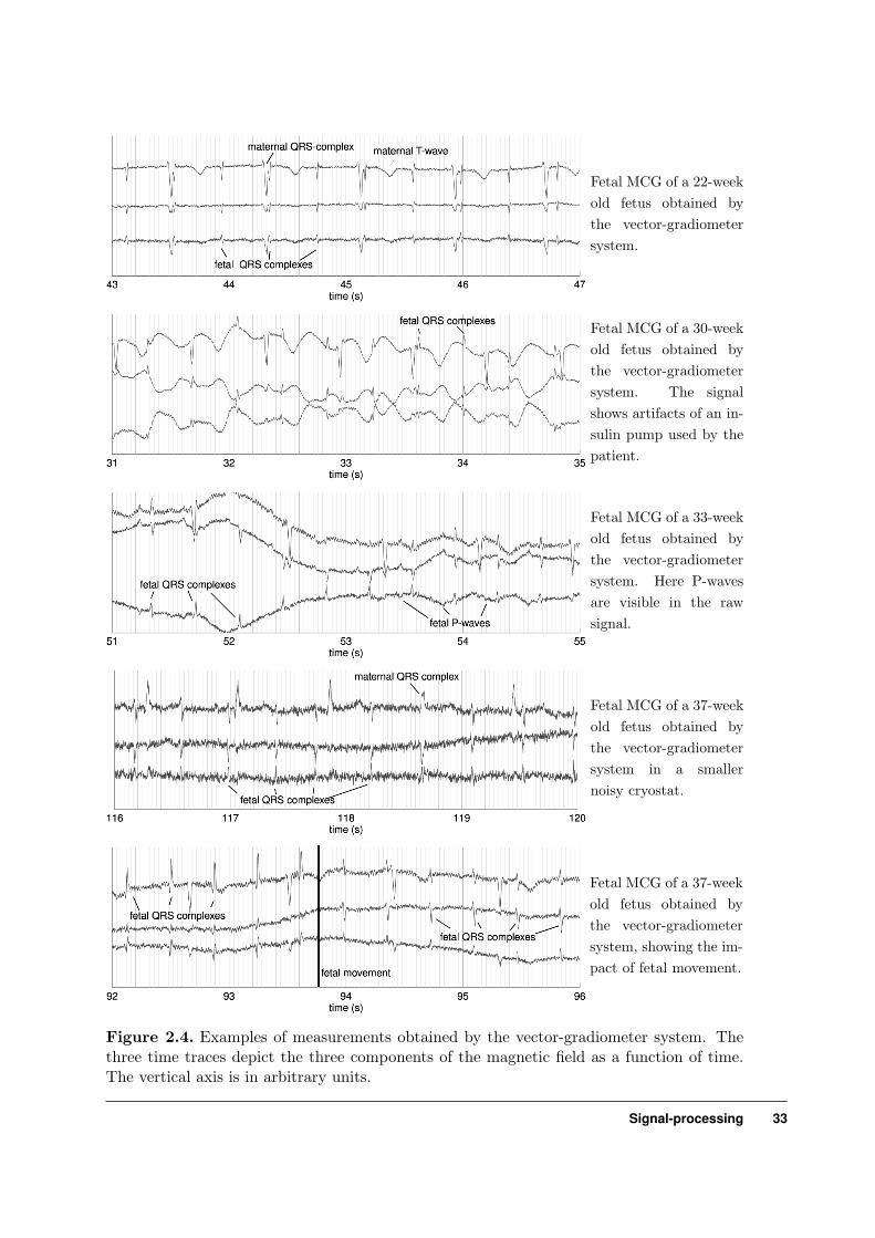
Fetal MCG of a 22-weekold fetus obtained bythe vector-gradiometersystem.

Fetal MCG of a 30-weekold fetus obtained bythe vector-gradiometersystem. The signalshows artifacts of an in-sulin pump used by thepatient.

Fetal MCG of a 33-weekold fetus obtained bythe vector-gradiometersystem. Here P-wavesare visible in the rawsignal.

Fetal MCG of a 37-weekold fetus obtained bythe vector-gradiometersystem in a smallernoisy cryostat.

Fetal MCG of a 37-weekold fetus obtained bythe vector-gradiometersystem, showing the im-pact of fetal movement.

Figure 2.4. Examples of measurements obtained by the vector-gradiometer system. Thethree time traces depict the three components of the magnetic field as a function of time.The vertical axis is in arbitrary units.


In the Biomagnetic Center Twente the measurements normally take place in a mag-netically shielded room in order to block out variations in the earth’s magnetic fieldand in magnetic fields generated by electrical equipment and moving magnetic ob-jects. For example, one of our patients was diabetic and carried an implant for insulininjection. Although switched off, the device produced a lot of artifacts. The result ofthis measurement is shown in the second recording of figure 2.4. Although the fetaltrace is still visible, a lot of baseline wandering is measured. As children of diabeticpatients are thought to have a higher risk for cardiac abnormalities (Greene, 1999;Ryan, 1998), this kind of patients will be indicated for fetal MCG screening whenfetal MCG will enter the clinic. Hence, a signal-processing program should be flexibleenough to cope with this kind of signals.A more common form of baseline wandering is shown in the third recording. Thesource of these changes in the amplitude is not exactly known. Most probably theyare due to movements of mother or child. In most cases the baseline wandering islinked to maternal breathing. Recordings of movement due to breathing, showed ahigh correlation with the baseline wandering in the MCG.That the signal-to-noise ratio is not only depending on the magnitude of the fetalsignal is shown in the fourth example. In this case a smaller cryostat was used tokeep the vector-gradiometer at a temperature of 4.2 K. The metallic layers of theradiation-shield inside the wall of this cryostat, did produce a lot of white noise, ascan be seen in the figure. The last example also shows a phenomenon often recorded.In this fetal MCG, the sign of the R-peak suddenly changes due to fetal movement.In figure 2.5, examples of measurements with the variable baseline system and the 19-channel system are shown. The variable baseline system was designed for experimentaluse only. As it is fitted in a smaller noisier cryostat, the signal-to-noise ratio ispoorer. However the use of this smaller cryostat enabled us to move the pickup-coils more easily over the abdomen. The variable baseline system consists of twomagnetometers at a variable distance. Combining both channels electronicly createsagain a gradiometer. As magnetometers are used in the system, it is more sensitivefor 50 Hz interference. Normally the 50 Hz sources are at a large distance from thepickup-coils and hence in a gradiometer setup both coils will record about the sameamount of 50 Hz and these contributions will cancel each other. As for a magnetometerchannel this is not the case the 50 Hz component will be seen and its contributionis only diminished after electronicly subtracting both channels. The examples of the19-channel system show recordings of a similar quality (the level noise in the signalsis about a factor 2 larger)as the vector-gradiometer system. With both systems it wasoccasionally possible to distinguish P-waves in the raw signal, even before filtering oraveraging the data.

2.3.2 Noise sources

In order to detect fetal cardiac disorders, the signal-processing procedures should beflexible. To make a distinction between the fetal signal and all the other sources, thesesources should be identified. The more is known about a noise source, the higher the

34 Chapter 2

Fetal MCG of a 34-week old fetus obtainedby the variable baselinesystem.

Fetal MCG of a 27-weekold fetus obtained bythe 19-channel system.This fetus is sufferingfrom a complete atrio-ventricular block.

Fetal MCG of a 39-week old fetus obtainedby the 19-channel sys-tem. This fetus has pre-mature atrial contrac-tions.

Figure 2.5. Examples of measurements obtained by the variable baseline system and the19-channel system. The upper graph depicts the two magnetometer channels of the variablebaseline system. In this case the coils are 8 cm apart. The lower two graphs depict the fourchannels of the 19-channel system with the best signal-to-noise ratio.

chance is that it is recognised in the fetal MCG signal. In figure 2.6 the major noisesources are listed.

In every fetal MCG measured in the Biomagnetic Center Twente, the maternal MCGcould be distinguished as well. The amplitude of the maternal QRS-complex is com-parable to that of the fetal QRS-complex. The amplitude of the fetal QRS-complexvaries in amplitude and shape for each channel as can be seen in figure 2.4.

Other sources of noise include, for instance, movements due to breathing and fetalmovement. In figure 2.7, two examples of such influences are depicted. In the uppergraph simultaneous recordings are shown of an adult MCG and the movement ofthe chest due to breathing. The latter was recorded using a system consisting of aDC-light-source and a light-sensor. The resistance of this sensor is dependent on the


Figure 2.6. Illustration of themain sources of noise in the fe-tal MCG.

intensity of the light, and therefore it is dependent on the distance between the light-source and the sensor. With the light-source at a distance of 0.5 m, this measurementsetup had a sensitivity of 0.02 V/cm. The relation between the light intensity and thedistance is not linear. However, for movements of a few centimeters at a distance of0.5 m from the source, the relation could be approximated by a linear one. The sensorwas attached to the subject lying underneath the magnetometer-system with the light-source mounted at a distance of around 0.5 m. Measurements with and without thesensor were made to assure that the light-sensor did not interfere with the MCGmeasurement. When looking at the graphs in figure 2.7, a striking similarity is foundbetween the low-frequent baseline wandering of the MCG and the motions recordedby the light sensor. Hence, it is concluded that most of the low-frequent signalsoriginate from breathing. The measurements were repeated for different subjects.The amplitude of the breathing artifacts was different for each person. For somealmost no baseline wandering was found and for others it was about a factor fivetimes as large as the one shown in figure 2.7. A number of factors may explain thesedifferences, such as food with a high content of metal that was consumed before themeasurements, or some magnetic object moving along with the subject’s movements.

In the lower graph of figure 2.7, a completely different influence of movements is shown.In this case, it is the fetus that is moving and the fetal MCG signal changes abruptlyin shape and amplitude (within a few seconds). The fetal movement could not bemeasured itself, because a measurement with, for instance, ultrasound would interferewith the fetal MCG. However, fetal movement is the most probable explanation of thischange in signal. Hence, when averaging fetal MCG data, one should be aware thatthe fetal cardiac complex could change its shape and amplitude due to fetal movement.Especially, in the early weeks of gestation the fetus is able to move freely within theuterus. Measurements suggest that the periods in which movements are absent have amean duration of 4 minutes (with a maximum of 11 minutes) for the gestational age of8-20 weeks, 5 minutes (maximal 17 minutes) for weeks 20-30 (Nijhuis, 1994), therebylimiting the number of complexes that can be used in the averaging procedure.

Not all noise results from the body, the magnetometer system also produces noise.This noise consists of thermal noise of the cryostat and noise of the SQUID-system.

36 Chapter 2

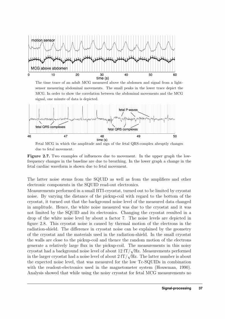
The time trace of an adult MCG measured above the abdomen and signal from a light-sensor measuring abdominal movements. The small peaks in the lower trace depict theMCG. In order to show the correlation between the abdominal movements and the MCGsignal, one minute of data is depicted.

Fetal MCG in which the amplitude and sign of the fetal QRS-complex abruptly changesdue to fetal movement.

Figure 2.7. Two examples of influences due to movement. In the upper graph the low-frequency changes in the baseline are due to breathing. In the lower graph a change in thefetal cardiac waveform is shown due to fetal movement.

The latter noise stems from the SQUID as well as from the amplifiers and otherelectronic components in the SQUID read-out electronics.

Measurements performed in a small BTI-cryostat, turned out to be limited by cryostatnoise. By varying the distance of the pickup-coil with regard to the bottom of thecryostat, it turned out that the background noise level of the measured data changedin amplitude. Hence, the white noise measured was due to the cryostat and it wasnot limited by the SQUID and its electronics. Changing the cryostat resulted in adrop of the white noise level by about a factor 7. The noise levels are depicted infigure 2.8. This cryostat noise is caused by thermal motion of the electrons in theradiation-shield. The difference in cryostat noise can be explained by the geometryof the cryostat and the materials used in the radiation-shield. In the small cryostatthe walls are close to the pickup-coil and thence the random motion of the electronsgenerate a relatively large flux in the pickup-coil. The measurements in this noisycryostat had a background noise level of about 12 fT/

√Hz. Measurements performed

in the larger cryostat had a noise level of about 2 fT/√

Hz. The latter number is aboutthe expected noise level, that was measured for the low Tc-SQUIDs in combinationwith the readout-electronics used in the magnetometer system (Houwman, 1990).Analysis showed that while using the noisy cryostat for fetal MCG measurements no


Figure 2.8. The power spec-tral density measured withthe same system under simi-lar conditions using two dif-ferent cryostats. The up-per graph is obtained usinga small BTI-cryostat and thelower graph using a largerCTF-cryostat. In the lastcase the noise is limited bythe SQUID-system.

P-waves were observed in the raw data and P-waves were hardly discernible afterfiltering with a band-pass filter from 2 to 120 Hz. In case the noise was limited bythe SQUID and its read-out system at a level of 2 fT/

√Hz more often a P-wave was

found in the raw data. Although averaging helps to reduce the noise level and mayreveal P-waves in noisy signals, there are some diseases where P-waves need to bedetected independently from the R-peaks in order to make a proper diagnosis, as willbe explained in chapter 7.

2.3.3 Frequency contents

In order to determine the frequency range of the fetal MCG signal, a fetal MCGrecording of a 22-week old fetus was divided into the signal from the maternal heart,the signal from the fetal heart and the remaining noise. The division is made bydetermining an averaged maternal PQRST-complex. Using this averaged complexand the time instants where a maternal R-peak was detected, the maternal signal isrecreated. This signal is subsequently subtracted from the recorded signal. In thenext step the fetal QRS-complexes are detected in the remaining signal and again areconstruction is made of the fetal signal, which is subtracted from the recorded signal.The remaining signal is assumed to contain noise only. The power spectral densityof all three signals was computed. This spectrum was computed by dividing thesignal into intervals of 4096 ms and computing the power spectrum for each interval.Subsequently all these spectra were averaged. In figure 2.9, the power spectra of thematernal MCG, the fetal MCG and the remaining noise are shown. The signal powerof the fetal MCG is mostly confined to a frequency range between 10 and 100 Hz, witha peak at 2 Hz, the fetal heart rate. The maternal signal has a lower frequency content,although there is a large overlap in the frequency range. Repeating the analysis forother channels revealed a similar graph. The graph shows that the frequency rangeof 10 to 100 Hz is the best range for detecting the fetal MCG, as the signal-to-noiseratio in this range is largest. In the latter case, it is assumed that the maternal MCGis suppressed before detecting the fetal signal.

38 Chapter 2

Figure 2.9. The power spec-tral density of the maternalMCG, the fetal MCG and theremaining noise. This graphhas been obtained by split-ting a measured signal intothese three components.

2.3.4 The influence of the magnetometer system

The magnetometer system is a complex system, which may cause deformations in thefetal MCG signal. Before the signal is digitised, it is amplified and filtered. After theSQUID-electronics, the signal is amplified by a factor 10, low-frequency disturbancesare suppressed by applying a high-pass filter and the signal is led through an anti-aliasing filter and subsequently the signal is processed digitally. The high-pass filteris an RC-network with a cut-off frequency of 0.01 Hz and the anti-aliasing filter is afifth-order Bessel filter with a cut-off frequency of 220 Hz. After sampling the signalwith a frequency of 4 kHz, the signal is then electronically resampled to a sample-frequency of 1 kHz. As this system contains many components, they all may interferewith the fetal MCG and change its shape and amplitude. Another issue of concernis the feedback loop in the SQUID-electronics, which may give rise to higher orderharmonics in the recorded signal.In order to examine the influence of this measurement setup, an artificial magneticsignal was generated that resembled the signal of the fetal heart. This signal wastransmitted by a coil positioned underneath the magnetometer system at a distanceof about 10 cm. In figure 2.10 an example of the input and the output signal isdepicted. The shape of the signal was obtained from an averaged fetal MCG near theend of gestation. This artificial fetal PQRST-complex was repeated with a frequencyof about 120 bpm. The rhythm of the signal was composed after a rhythm observed ina real fetal MCG. The experiment was repeated with different amplitudes of the seriesof R-peaks. The amplitude of this series was varied in such a way that they resembledthe amplitudes of fetal R-peaks (from 0.5 to 2 pT). The latter range coincides withthe range of R-peak amplitudes, which is normally observed.The recorded artificial PQRST-complexes are detected in the signal and subsequentlyaveraged in order to reduce the noise in the signal. In this case 120 complexes weregenerated and subsequently averaged. The resulting average has been compared withthe original input. In figure 2.11, a comparison between the transmitted signal and theretrieved signal is made. This comparison has been made after fitting the amplitudeof the input signal to that of the retrieved signal. As can be seen in figure 2.11,


Figure 2.10. In the lower time trace the signal is depicted, which is transmitted by meansof a coil into the magnetometer system (input). This signal is generated artificially by meansof a computer. In the upper time trace the signal recorded by the magnetometer system isshown (output).

0 0.1 0.2 0.3 0.4-1

0

1

2

3

4

5 x 10�-12

time (s)

B (T

)

Applied signal Measured signal Figure 2.11. In black the artificial

cardiac complex is depicted that wastransmitted by a coil into the mag-netometer system. In gray the av-eraged cardiac complex is depictedwhich was reconstructed out of therecorded signal. In the upper leftand lower right corner enlargementsof the signal are shown, which showonly minute changes in the complex.

almost no differences between the original and the retrieved signal can be found. Asa diagnosis is drawn from an average by examining its shape, these small differencesshould not be of any influence on the diagnosis made by a physician. The analysishas been repeated with different input signals and different amplitudes of the signals.It turned out that the system scales linearly in the measurement range and that theshape of the complex was not affected by the magnetometer system. Hence, thesystem can be used for obtaining a reliable fetal MCG.

2.4 Filtering

2.4.1 Band-pass filter

The first stage of the signal-processing procedure is applying a band-pass filter. Thefilter is used to suppress baseline wandering and to reduce the noise and interferencein the frequency band from 120 to 500 Hz. Baseline wandering needs to be suppressed

40 Chapter 2

0 0.05 0.1 0.15 0.2 0.25 0.3 0.35 0.4 0.45time (s)

Pre-detection filter 10-60Hz

Pre-detection filter 10-40Hz

The detected maximumshifts to the left

fetal MCG

Power-line interference

fetal MCG +50 Hz interference

Figure 2.12. Influence of 50 Hz interference. left: This graph shows two averaged fetalcardiac complexes (n = 100). The upper is computed after detecting the R-peaks witha pre-detection filter of 10-60 Hz. The lower is the average in case a pre-detection filterof 10-40 Hz is used. Depending on the bandwidth of the pre-detection filter the 50 Hz issuppressed. right: The cause of the poor suppression of the 50 Hz in case it is not removedin the pre-detection filter. Due to the 50 Hz interference the detected R-peak shifts towardsthe top of the 50 Hz sine-wave. Due to the increased number of R-peaks detected near thetop of the 50 Hz sine wave, coherently averaging does not suppress the 50 Hz interference.

in order to be able to detect the fetal R-peaks and for enhancing the coherent average.For these two purposes the filter has to meet different specifications. In case of detect-ing the fetal R-peaks, it does not matter whether PQRST-complexes are deformedby the filter as long as the R-peak becomes clearly identifiable. In case the filter isused for removing noise and interference before coherent averaging, the filter shouldnot alter the shape of the averaged PQRST-complex. As both specifications differ,two band-pass filters are used.

As pre-detection filter a finite impulse response (FIR) filter is used with 50 coefficientsand a bandwidth from 10 to 40 Hz. This frequency range is chosen, because it excludesthe power-line frequency of 50 Hz and it does coincide with the bandwidth in whichthe fetal cardiac complex has most of its signal energy. That the cut-off frequencyshould be well below 50 Hz, is demonstrated in figure 2.12. With a moderate 50 Hzcontribution (about 25 percent of the amplitude of the R-peak), the location, wherethe top of the R-peak is detected, may be shifted to an earlier or later time instant ifthe R-peak and top of the 50 Hz sine-wave more or less coincide. Due to this processthe number of events detected near the top of the 50 Hz wave is larger than it shouldbe, as illustrated in figure 2.12. Hence, the phase of the 50 Hz interference is notuniformly distributed. And as a consequence this interference is not averaged out ascan be seen in figure 2.12.

The pre-averaging filter consists of a separate high-pass and low-pass filter. Togetherthey form a band-pass filter with a bandwidth from 2 to 120 Hz. The low-pass filteris again a finite impulse response (FIR) filter. In order to determine the number of


0 0.05 0.1 0.15 0.2 0.25 0.3 0.35 0.4 0.45 0.5-10

-8

-6

-4

-2

0

2

4 x 10�-3

time (s)

aver

age

(V)

original

LP�

FIR: order 10LP

�

FIR: order 25LP FIR: order 50

order 50

order 10order 10

order 50,25

order 25

0 0.05 0.1 0.15 0.2 0.25 0.3 0.35 0.4 0.45 0.5-10

-8

-6

-4

-2

0

2

4 x 10�-3

time (s)

aver

age

(V)

��

original HP FIR: 1HzHP FIR: 2HzHP FIR: 4Hz

�

4Hz

2Hz1Hz

Figure 2.13. Left graph: the influence of the low-pass filter with a cut-off frequency of120 Hz on the PQRST-complex. In this figure the number of coefficients used in the FIRfilter is varied. Right graph: the influence of the cut-off frequency of the high-pass filteron the PQRST-complex.

coefficients to be used in this filter, the effect of the filter on the averaged PQRST-complex is analysed. For this purpose a fetal MCG measurement is taken with largecardiac complexes and almost no baseline wandering. The filter is applied beforeaveraging the fetal MCG and the average is compared to the one obtained in caseno filter would have been applied. In this case both should be about same. Infigure 2.13, the averages are depicted. In case the number of coefficients is low, theamplitude of the R-peak decreases. When a larger number of coefficients is taken,small fluctuations are found succeeding the R-peak (impulse response). Hence, forthis finite impulse response filter the number of coefficients is a compromise. A filterwith 25 coefficients has only a minor influence on the average. The analysis wasrepeated for other measurements. As most QRS-complexes are not as steep as theone in figure 2.13, a cut-off filter of 100 Hz is also sufficient in those cases. For thegraphs in this thesis, a pre-averaging filter with a cut-off frequency of 120 Hz and25 coefficients is used.

In order to use a FIR filter as high-pass filter, a lot of coefficients are needed. In orderto detect the slow variations on the baseline, the filter needs a large time window. Asthis requires a lot of coefficients, the filtering process would be a time consuming one.Hence, the signal is resampled before filtering and the sample-frequency is decreasedfrom 1 kHz to 0.1 kHz. This process of decimating the signal by a factor 10 and theinterpolation of the signal after the filtering process has been described by Mosher etal. (1997). After decimating the signal it is passed through a low-pass filter of 2 Hz,after which the baseline wandering remains. This signal is interpolated to the originalsample-frequency of 1 kHz and subsequently subtracted from the original signal. Infigure 2.13, the effect of a cut-off frequency of 1, 2 or 4 Hz on the average PQRST-complex is shown. It turns out that for a cut-off frequency larger than 2 Hz, thehigh-pass filter changes the appearance of the average. Hence, for the fetal MCGs inthis thesis a high-pass filter with a cut-off frequency of 2 Hz is used.

42 Chapter 2

Figure 2.14. An example of a signal filtered with the pre-detection filter and the pre-averaging filter.

Figure 2.15. The signal of a patient who had an insulin pump as implant. Filtering thesignal within a bandwidth from 2 to 120 Hz did not remove the noise. However in thiscase the noise was correlated to the maternal heart beat and could be removed by coherentaveraging using the maternal R-peak as trigger.

In figure 2.14, the effect of the pre-detection and the pre-averaging filter on a fetalMCG recording is depicted. That the noise cannot always be removed in this manneris shown in figure 2.15. This figure shows the recorded signal of a diabetes patient,who had an insulin pump as implant. The pump was switched off during the measure-ment, but did cause baseline wandering. However the frequency of the interference isover 2 Hz and using a band-pass filter with a higher frequency would interfere withthe fetal signal. The interference was however coupled to the maternal heart beat.Possibly, the blood pressure waves coming from the maternal heart moved the implantslightly up and down. As the implant is probably a bit magnetic, it results in thecoherent movement of this magnetic object with the maternal heart. The interfer-ence was suppressed by coherent averaging on the R-peaks of the maternal signal andsubtracting an average maternal MCG that in this case was contaminated with theinterference. In the lower trace of figure 2.15, the result is shown.


2.4.2 Filtering 50 Hz

When measuring by means of magnetometers instead of gradiometers, the signalsoften show a strong 50 Hz component (about the size of the fetal R-peak). Hence,this component should be removed before averaging. There are several ways to removethe 50 Hz interference. For instance, using a digital notch filter. These filters canbe constructed in several ways, for instance using a finite impulse response scheme oran infinite impulse response scheme. However, applying these filters on the recordedsignal interferes with the fetal QRS-complex. One difficulty encountered in the fetalMCG signal is that it is not stationary in frequency contents. Only at a time scaleof a few seconds does the signal become stationary. Hence, whenever a QRS-peakpasses the filter, an impulse response of the filter will be triggered. The effect ofsuch a response is demonstrated in figure 2.16. Prior to averaging, the signal wasfiltered with a Chebychev II notch-filter with a bandwidth of 1 Hz. Compared to thenon-filtered case the filtered average shows strong artifacts in the complex. Otherdigital notch-filters have been tested but they all resulted in some type of impulseresponse following the QRS-complex, although not as strong as in the example shownin figure 2.16. Hence, when using this kind of filters, the QRS-complex may appearto be prolonged.

In order to avoid this unwanted prolongation of the QRS-complex, a different 50 Hzsuppression scheme has been used. The scheme starts by detecting fetal and mater-nal QRS-complexes in the pre-detection filtered signal. By means of averaging thePQRST-complexes are removed from the signal and the signal is band-pass filteredfrom 40 to 60 Hz. This leaves the 50 Hz interference as the largest signal in therecorded signal. Now the amplitude, exact frequency and phase of this 50 Hz inter-ference are estimated. The frequency is estimated using a fast fourier transform ofthe signal. The signal is now divided into segments of 2 seconds and for each segmentthe best fitting phase and amplitude are determined. By means of comparing thephase information of the segments it is possible to check whether the estimated fre-quency is correct. When between the different segments small shifts in phase occur,the frequency of the fitted sine wave differs slightly from the interference. Using thesephase differences a better frequency can be estimated. The process of estimating theamplitude and phase of the interference is now repeated. Subsequently the phase andamplitude information is used to construct the 50 Hz interference signal and subtractit from the measurement. Simulations with artificial 50 Hz interference (about 20 per-cent of the amplitude of the fetal R-peak) showed that after two steps the frequencyof the interference was found with an error of 0.02 Hz. The results of applying thisnoise suppression scheme is shown in figure 2.16 as well.

Although the 50 Hz suppression scheme does not always perfectly remove the 50 Hzinterference in the signal, it does not introduce artifacts in the averaged fetal cardiaccomplexes. Most of the time, the reduction of the 50 Hz interference is enough toproduce useful cardiac complexes. The amplitudes and intracardiac time intervals arenot affected by this filter.

44 Chapter 2

0.1 0.2 0.3 0.4 0.5

fetal MCG with 50 Hz noise

notch filter

suppression by subtracting 50 Hz sine wave

time (s)

Figure 2.16. Influence of 50 Hz on fetalMCG traces and averages. Upper graph:The first trace is a measurement contaminatedby 50 Hz, the second trace is after applyinga notch-filter, the last trace is obtained af-ter reconstruction of the 50 Hz sine wave andsubtracting it from the signal. Left graph:Averaged complexes obtained from the threesignals shown in the graph above (100 com-plexes).

2.4.3 Non-linear filter

Another method to extract reoccurring events, i.e. fetal or maternal heart complexes,from a single channel recording is the use of a state-space projection, such as thealgorithm described by Richter et al. (1998). They applied a state-space projectionto improve the signal quality of a fetal electrocardiogram in order to enhance theaccuracy of fetal heart rate detection.

In this non-linear filtering technique the signal is first reconstructed in the state-space. The vectors in the state-space are extracted from a time series of a singlechannel recording using delay coordinates. In such a description a single sample attime t and m− 1 samples preceding this sample at times t− iτ describe one point inthe state-space. Hence a vector in the state-space reads

Sn = (xn−(m−1)τ , xn−(m−2)τ , · · · , xn) (2.1)


Here Sn is a vector in an m-dimensional space and xn−(m−1)τ are the signal valuespreceding the current value by a time difference of (m− i)τ . Following this procedurea trajectory in an m-dimensional space represents the signal. An example of sucha trajectory is given in figure 2.17(c). This is in fact a two-dimensional projectionof the first two delay coordinates of the multi-dimensional trajectory. If a fetal ormaternal signal is the dominant ingredient in a recording and each complex is basiclythe same complex, a closed trajectory will appear that will be followed each time afetal or maternal complex is found in the signal. However this trajectory will differfor each complex due to the presence of additional noise. Under the assumptionof all complexes being equal in shape and amplitude, the signal is now filtered byreconstructing this trajectory and making a local projection on a local basis using aprincipal component analysis. The filter processes the points in the state-space, pointby point. For each point in the state-space, the reconstruction starts by finding thosepoints in the state-space that are close to this point.

U =

{Sk

∣∣∣∣ ∥∥∥Sk − Sn

∥∥∥ ≤ ε

}(2.2)

For this collection of neighbouring points, the local center of mass is computed

Smean =∑Sk∈U

Sk

|U |(2.3)

Subsequently, a q-dimensional volume is fitted in the m-dimensional space that locallyapproaches the trajectory. This volume can be described as following

Strajectory(α1, . . . , αq) = Smean + α1Sdir 1 + . . . + αqSdir q (2.4)

In this equation the vectors Sdir i define in which direction the q-dimensional figurestretches. For instance, if q = 2 a plane is used to describe the trajectory locally.This plane intersects the center of mass and its direction vectors are derived using aprincipal component analysis of the points in this local neighbourhood. After estab-lishing this local plane, the point that is processed is projected on this plane. Thisprocedure is carried out for each point in the state-space. A more detailed descriptionof this procedure is given by Richter et al. (1998). The result of such a reconstruc-tion is shown in figure 2.17(c) (red line). Hence, the result shown may represent adenoised signal and the trajectory in the state-space is now translated back into asingle channel recording.In order to test the performance of this state-space reconstruction, a signal was takenof a 39 week old fetus. This fetus was diagnosed with a bundle branch block, aswill be described in chapter 7. As the magnetic signal should be comparable tothe fetal electrocardiogram, the same parameters in the reconstruction are used as

46 Chapter 2

(a) Time traces

-0.2 -0.1 0 0.1 0.2time (s)

I

V

IV

III

II

(b) Averages over 43 complexes

(c) State space reconstruction

Figure 2.17. Non-linear state-space reconstruction of a fetal magnetocardiogram measuredin week 39 of gestation. The lower right graph is the trajectory in the state space. The blueline is the raw signal and the red line is the reconstructed signal. In the upper graph signalI represents the raw signal, signal II is filtered by a band-pass filter between 2 and 120 Hz,signal III is a non-linear reconstruction using a two-dimensional state-space projection,signal IV is a non-linear reconstruction using a four-dimensional state-space projection andsignal V is the same as signal III except that the local neighbourhood for reconstructing alocal basis is halved. Finally, the lower left graph displays the averages extracted from thefive time traces.


Richter et al. (1998) used in their reconstruction of the fetal electrocardiogram, i.e.

an 11-dimensional state-space and a delay of 4 ms between the samples in vector Sn.The results of the procedure are shown in figure 2.17(a). In total 20 seconds of dataare processed, as this type of non-linear filter requires a huge computational effort.From the results it becomes clear that the complexes become better visible in thetime trace after applying the non-linear filter. However after applying the non-linearfilter, details like the P-wave are still difficult to identify and averaging seems still tobe necessary in determining parameters like PR-intervals. Of all five time traces infigure 2.17(a) an average fetal complex is constructed. These complexes are shownin figure 2.17(b). From these complexes it becomes apparent that the non-linearfilter has difficulty to distinguish between P-wave and noise and consequently theamplitude of the P-wave is smaller for the average reconstructed out of the non-linearfiltered signal. Using more degrees of freedom in the state-space reconstruction onlyexaggerates this effect. However decreasing the volume in which neighbouring pointsare taken for constructing a local basis on which the projection is made, makes themethod less vulnerable for decreasing the amplitude of the P-wave. On the otherhand it decreases as well the effectiveness in removing noise from the time traces andthe performance is not better than a band-pass filter (second time trace and average).The decrease in amplitude of the P-wave is observed in other measurements as well.

Hence, this state-space reconstruction may help to improve the accuracy of the fetalheart rate tracings as the R-peaks are more clearly visible. However as long as theP-wave and the T-wave remain obscured by the background noise in the recordings,the state-space reconstruction will not help to improve the determination of the in-tracardiac time intervals, as the P-wave and T-waves will be considered noise and sub-sequently will be removed. Increasing the dimension of the state-space reconstructiondoes not seem to improve the signal quality. Increasing the local projection dimensionfrom two to three or four does result in better signals, however the apparently cleanersignals lack even more details of the P- and T-wave. For a reconstruction dimension offour hardly a P-wave remains in the average, rendering this kind of filtering unsuitablefor diagnosing abnormalities in the cardiac complex.

2.5 Detection and averaging of fetal complexes

2.5.1 Detection of fetal complexes

In figure 2.18, the detection scheme used at the Biomagnetic Center Twente is de-picted. The detection algorithm starts by filtering the signal with the pre-detectionband-pass filter. The next step in the process is detecting the R-peaks in the signal.The R-peak of the QRS-complex is the part of the cardiac complex that is easiestrecognised in the signal. The peaks are detected by means of a threshold. Thisthreshold is acquired by dividing the signal in pieces of two seconds. For each of thetwo second intervals, the largest peak (positive or negative) in relation to the meanvalue over this interval is selected. Of all these local extrema the median value is

48 Chapter 2

Pre-detection filter data with a band-pass filter of10 Hz to 40 Hz

Divide the signal into sections of 2 secondsFind the maximum amplitude in each sectionTake the median of all R-peak amplitudes asas a representative R-peak amplitude

Detect R-peaks in the signal using a threshold of 0.65 x median of the R-peak amplitudes

Create a template with detected peaks anduse the template for a matched filter

Detect peaks again after the matched filter

Reject R-peaks that are closer together than 200 ms

Figure 2.18. Detection scheme usedto detect the fetal complexes in thefetal MCG.

selected. This value represents the size of the average R-peak. The threshold fordetection is now set to 65% of the median size of the R-peak. The latter value wasobtained by trial and error and works in most cases. Almost all the events in the fetalMCG signals that are processed at the Biomagnetic Center Twente are detected inthis way.

In the next step the cardiac complexes are extracted from filtered signal. These com-plexes are used to construct a template of the cardiac complex. Using this templatethe signal is filtered again and the template serves here as a matched filter. Usingthe algorithm described above the events are again detected and a threshold of 65%of the median value is used again.

The last step in the detection process is checking what the minimum time intervalbetween two detected R-peaks is. Whenever the interval is shorter than 200 ms,the R-peak with the lowest correlation in the matched filter is rejected. The latterassumption that R-peaks cannot follow each other within 200 ms is based on therefractory period of the ventricular pacemaker cells, which cannot sustain a fastercontraction rate than 300 bpm (van Wezel-Meijler et al., 1997).

2.5.2 Averaging fetal complexes

After detecting where fetal R-peaks are possibly located. An averaging procedure isapplied in which complexes are rejected for averaging if they do not resemble the othercomplexes. The procedure is drawn in figure 2.19. The scheme starts by retrievingthe detected complexes and defining an interval surrounding the detected R-peaksas being the interval of the fetal PQRST-complex. For each of these intervals themaximum and minimum value reached by the signal (the fetal MCG recording) isdetermined. It is assumed that baseline wandering and the maternal complexes are


Reject complexes with a small or a large amplitude0.8 x median(ampl) < amplitude < 1.2 x median(ampl)

Make a global template by averaging complexesand correct baseline template by subtracting linear function

Correct R-peak detection by a cross-correlation ofeach complex with the template

Obtain individual complexes and do a baseline correction

Reject complexes which do not resemble the template based on a residue measure

Create average from the remaining complexes

Figure 2.19. Averaging scheme ap-plied to obtain an average fetal MCGfrom which intracardiac time inter-vals can be derived.

removed by the pre-averaging filter and that the fetal R-peak is the largest peakwithin the interval. The difference between maximum and minimum thence reflectsthe amplitude of the QRS-complex. From these differences between the maximumand minimum, the median difference is chosen and all intervals that show a largerdifference between maximum and minimum are rejected if this value is more than20 percent. The same procedure is followed for complexes that are smaller and theintervals are rejected if the value is 20 percent smaller than the median value. In thisway intervals with large fluctuations due to movements or the patient touching thecryostat are not considered in the averaging procedure. These fluctuations are notalways removed by the band-pass filter, as in these sudden movements frequencieshigher than 2 Hz are present.

In the next step of the process, a template of the PQRST-complex is created byaveraging the individual PQRST-complexes. The complexes in this case are alignedon their R-peaks. After averaging, the template is further modified by flatteningits baseline. The latter is done by taking the first and last 15 ms of the interval inwhich the PQRST-complex is located and fitting a straight line through the valuescontained by these small intervals of 15 ms. In this case it is assumed that during thefirst and last 15 ms no fetal heart activity is present and thence these periods in thePQRST-complex should represent the iso-electric line. The fitted line is subtractedfrom the template in order to flatten its baseline.

The template is used to make a cross-correlation with the individual complexes. Thiscross-correlation is used to do a final correction in the time domain. This correctionnormally leads to corrections on the position of the R-peak of an order of a fewmilliseconds. Due to noise peaks the maximum of the R-peak sometimes shifts witha few milliseconds. After these corrections, baseline corrections are made in theindividual complexes. Subsequently the difference between the individual complex

50 Chapter 2

100 101 102 10310-17

10-16

10-15

10-14

10-13

frequency (Hz)

pow

er s

pect

ral d

ensi

ty (T

/ √ H

z)

Figure 2.20. The power spec-tral density after removing thefetal and maternal MCG andthe low-frequency noise.

and the template is expressed in the form of a residue

R =n∑

i=1

(Si,complex − Si,template)2

n(2.5)

Here, R is the residue and Si is the ith sample of the signal. This expected residueis based on knowledge of the background noise level plus the fact that the complexesare not similar. All the complexes with a residue larger than expected are rejectedand not used in the final average

R ≤ 2× V ar(Snoise) + ((0.1)× Ampl(R-peak))2 (2.6)

After this step, the final average is computed and the intracardiac time intervals aremanually extracted from the average.

2.5.3 Noise reduction due to averaging

In order to estimate the noise reduction achieved the distribution of the noise hasto be estimated. After removal of the low-frequency components due to movementand breathing and after the removal of the maternal signal, the remaining noise inthe frequency band from 2 Hz to 120 Hz is primarily caused by thermal noise ofthe cryostat or the intrinsic noise of the SQUID-system. In order to estimate theproperties of this noise contribution in the frequency domain, a power spectrum ismade from the noise. This signal is defined as the signal that remains after removalof the maternal and fetal complexes and the low-frequency components below 2 Hz.The power spectral density of this signal is given in figure 2.20. It turns out thatin the frequency range from 10 to 120 Hz the noise is around a level of 3 ft/

√Hz.


In the lower-frequency range, the noise level is somewhat higher, possibly due to anincomplete removal of maternal or fetal complexes.In order to describe the noise reduction by the averaging process the following modelis posed for each individual complex

si(t) = fmcg(t) + ni(t) (2.7)

Here, si(t) is the individual cardiac complex retrieved from the fetal MCG recordingand fmcg(t) is the fetal complex that is assumed not to change during the recording.Since the noise ni(t) is assumed to be mainly due to thermal noise or noise in theSQUID-system it is assumed to be gaussian distributed. In order to determine whetherit is gaussian distributed a goodness-of-fit test has been performed (Stinstra et al.,2001a). In this test, a histogram is made of the noise distribution and the hypothesisis tested whether this distribution can be explained by gaussian noise. It turned outthat the noise was gaussian distributed (p=0.05).

ni ∼ N(0, σ) ⇒ V ar

[ n∑i=1

si/n

]= σ2/n (2.8)

Hence, the signal-to-noise ratio improves by a factor n, where n is the number ofcomplexes. The goodness-of-fit test was performed for each sample in the cardiaccomplex and it turned out that the estimated standard variance for each sample didnot depend on the position in the QRS-complex (the noise contribution during theQRS-complex is the same as the one during the P-wave). Hence, the more complexesare used in an average the less noise remains, however the effectiveness of includingmore complexes decreases since the variance scales with n. The number of complexescannot be increased indefinitely as the fetal complexes change over time. As the fetusmoves on average every 4 minutes for the gestational age of 8-20 weeks and 5 minutesfor weeks 20-30 (Nijhuis, 1994), the number of complexes that can be averaged ismaximal about 500 (assuming an average fetal heart rate of 120bpm). The averagereduction in noise amplitude thence is about a factor

√500 ≈ 20.

52 Chapter 2

Chapter 3

Modeling fetal MCG

In adult ECG the electrical activity of the heart is measured by means of a set of electrodesattached to the skin at standardised locations. Because the currents from the heart haveto travel through tissues like lung, muscle and skin to reach the electrodes, these tissuedo influence the measured signals. In order to rule out the influence of these tissues, theadult ECG is measured at fixed positions. The latter ensures that the influence of the so-called volume conductor is about the same for each person, as for every individual thesame tissues are encountered. Because of the many years of experience in this field,physicians are able to distinguish between effects due to the volume conductor and dueto cardiac disorders. In case of fetal MCG and ECG no such experience is present andthere are no standard positions where the fetal ECG or MCG is measured. To complicatematters, the fetus is able to move within the maternal abdomen changing layout the volumeconductor. Thence, to allow for a reliable diagnosis by means of fetal MCG or fetal ECG,the influence on the measured signal of the tissues surrounding the fetal heart shouldbe estimated. As it is difficult to assess the effect of the surrounding tissues from themeasurements themselves, simulations are used. These simulations are based on volumeconductor models of the maternal abdomen. In this chapter the numerical models aredescribed, which will be used to estimate the magnetic field distribution as well as thepotential distribution at the abdominal surface.

3.1 Physical model

To estimate the effects of the volume conduction, a mathematical model is constructedfor which the magnetic field distribution near the maternal abdomen (MCG) andpotential distribution at the abdominal surface (ECG) are calculated. The modelsdescribed in this thesis for estimating the volume conduction effects, divide the bodyinto discrete volumes and each of these volumes is assigned an effective conductivityand dielectric permittivity. An example of such a subdivision is given in figure 3.1.As the magnetic permeability of biological tissues is only slightly different from themagnetic permeability of free space, changes in magnetic permeability due to thepresence of various kinds of tissues are ignored. The following linear equations are

Modeling fetal MCG 53

Figure 3.1. Example of a volumeconductor subdivided into three ho-mogeneous compartments, the fetus,the amniotic fluid and the maternalabdomen.

Homogeneous and isotropiccompartments

Volume currents in the volume conductor

Current source

taken to describe the properties of the compartments

J = σ(ω)E

D = ε(ω)E

B = µ0H

(3.1)

Here σ(ω) is the effective conductivity of the tissue and ε(ω) is the effective dielectricpermittivity of the tissues involved. Because at a microscopic scale tissue is veryinhomogeneous, only taking a volume much larger than the cellular scale will allowfor the use of effective properties (Peters et al., 2001b; Peters et al., 2001a). Althoughit seems that both σ(ω) and ε(ω) are independent functions, they are correlated by theKronig-Kramer relation. In the model used capacitive effects are taken into account.Inductive effects and wave properties are assumed to be negligible. These lattereffects do not play a significant role in the volume conduction related to bioelectricalsources in the body (Plonsey and Heppner, 1967). Hence the Maxwell equations inthis approach read

∇ ·D = ρ ∇ ·B = 0

∇× E = 0 ∇×H = J + ∂∂t

D(3.2)

It is convenient to write the current density as a sum of two terms

J = −σ(ω)∇Φ + Js (3.3)

The first term at the right-hand side describes the Ohmic currents outside the sourceregions. The second term is non-zero within the source region and consists of thesource currents. The first term represents the current that flows in the extracellularvolume and the second the currents within the cell. A more extensive descriptionof the source will follow at the end of this chapter. Only when a large number ofcells display synchronous electrical activity the source currents will contribute to the

54 Chapter 3

macroscopic magnetic field or electrical potential. Inserting equation 3.3 into theMaxwell equations results in

∇ · ∇ ×H = −∇ · [σ(ω)∇Φ] +∇ · Js + ∂∂t∇ ·D = 0 (3.4)

Applying a Fourier transformation, yields

∇ · [σ(ω) + iωε(ω)]∇Φ(r, ω) = ∇ · Js(r, ω) (3.5)

In this equation a complex effective conductivity is introduced to describe the electricalproperties of a certain part of the volume conductor

σ(ω) = σ(ω) + iωε(ω) (3.6)

Assuming σ(ω) to be independent of the position within a compartment results in thefollowing equation for each compartment

σ(ω)∇2Φ(r, ω) = ∇ · Js(r, ω) (3.7)

Because the complex conductivity is different for each frequency component, equa-tion 3.5 will result in a different equation for each frequency. This means that theforward problem has to be solved for each frequency component of the source. Thesuperposition principle allows for adding up the resulting solutions of each frequencycomponent in obtaining the final solution.In order to solve the partial differential equation 3.7 for each compartment, boundaryconditions have to be taken into account. The first boundary condition is the require-ment that the potential is continuous across each interface, implying that both thereal and imaginary part of the potential have to be continuous. The second boundarycondition is the requirement that the total current density, including the displace-ment current ∂

∂tD, perpendicular to the interface separating different compartments

is continuous, yielding the following conditions

Φi(r, ω) = Φj(r, ω) and σi∇Φi(r, ω) · n = σj∇Φj(r, ω) · n r ∈ Sij (3.8)

In this equation Sij is the interface separating compartment i and j. The magneticpermeability of biological tissue is presumed to be the same as the permeability ofvacuum. Hence, H has to be continuous across every interface

Hi(r, ω) = Hj(r, ω) r ∈ Sij (3.9)


Note that using the complex conductivities, the appropriate boundary conditions andthe Poisson equations for Φ and H are similar to the ones used in the case that ca-pacitive effects are neglected. Consequently, the electrical potential and the magneticfield can be calculated in the same way as in the non-capacitive case (Stinstra andPeters, 1998). Depending on the geometry of the volume conductor model, differentmethods will be used to solve the forward problem. Because the capacitive case issimilar to the non-capacitive case except for the complex numbers involved, capacitiveeffects are implicitly incorporated in the description of the boundary element methodin the next section.

3.2 Boundary element method

3.2.1 Numerical approximation

In order to solve equation 3.7 for an arbitrary set of compartments, the boundaryelement method is applied. This method is based on Green’s theorem and expressesthe potential at an arbitrary point in space in an integral over the surfaces separatingthe different compartments and into an integral over the impressed currents (Barnardet al., 1967). The following equation was derived for the potential

σiΦ(r) =

∫∫∫g(r, r′)∇ · Js(r

′)dV ′

−n∑

p=1

[σ+p − σ−p ]

∫∫Sp

Φ(r′)∇g(r, r′) · ndS ′ r ∈ Vi

(3.10)

and for the potential at the interface between the compartments

[σ+q + σ−q ]

2Φ(r) =

∫∫∫g(r, r′)∇ · JsdV ′

−n∑

p=1

[σ+p − σ−p ]

∫∫Sp

Φ(r′)∇g(r, r′) · ndS ′ r ∈ Sq

(3.11)

The latter equation differs from the first one as a consequence of the discontinuityin the conductivity at the interfaces. In these equations Sp are the interfaces sep-arating the volumes with a different conductivity and n is the outwards pointingnormal to this surface. The conductivities σ−i and σ+

i are the conductivities of thevolumes separated by the interface. The first conductivity is the one found at theinside of interface Sp and the latter the one found at the outside. Commonly, thefirst integral at the righthand-side is referred as the primary source and the secondintegral as the secondary sources. The primary source refers to the potential distribu-tion due to a current source in an infinitely large homogeneously conducting medium

56 Chapter 3

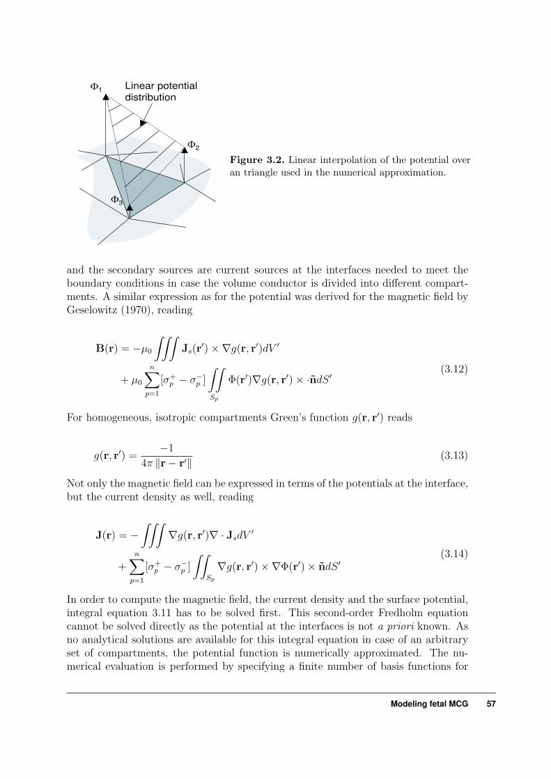
Φ1

Φ2

Φ3

Linear potentialdistribution

Figure 3.2. Linear interpolation of the potential overan triangle used in the numerical approximation.

and the secondary sources are current sources at the interfaces needed to meet theboundary conditions in case the volume conductor is divided into different compart-ments. A similar expression as for the potential was derived for the magnetic field byGeselowitz (1970), reading

B(r) = −µ0

∫∫∫Js(r

′)×∇g(r, r′)dV ′

+ µ0

n∑p=1

[σ+p − σ−p ]

∫∫Sp

Φ(r′)∇g(r, r′)× ·ndS ′(3.12)

For homogeneous, isotropic compartments Green’s function g(r, r′) reads

g(r, r′) =−1

4π ‖r− r′‖(3.13)

Not only the magnetic field can be expressed in terms of the potentials at the interface,but the current density as well, reading

J(r) = −∫∫∫

∇g(r, r′)∇ · JsdV ′

+n∑

p=1

[σ+p − σ−p ]

∫∫Sp

∇g(r, r′)×∇Φ(r′)× ndS ′(3.14)

In order to compute the magnetic field, the current density and the surface potential,integral equation 3.11 has to be solved first. This second-order Fredholm equationcannot be solved directly as the potential at the interfaces is not a priori known. Asno analytical solutions are available for this integral equation in case of an arbitraryset of compartments, the potential function is numerically approximated. The nu-merical evaluation is performed by specifying a finite number of basis functions for


the potential at the interfaces and finding the linear combination of these basis func-tions that best fits the integral equation. Commonly, the interfaces are described bytriangulated surfaces and the potential is assumed to be a linear function over eachtriangle. An example of such a linear interpolation function is given in figure 3.2.Hence the potential over a triangle reads

Φ4(q)(Φq1, Φq2, Φq3, r) = Φq1hq1(r) + Φq2hq2(r) + Φq3hq3(r) (3.15)

In this equation hqi are unit interpolation functions over triangle 4(q) for each po-tential at the corner of a triangle as defined by de Munck (1992). Inserting theseinterpolation functions hqi into the boundary element equation, will result in thefollowing expression for a point at an interface

[σ+q + σ−q ]

2Φ(r) +

n∑p=1

[σ+p − σ−p ]

∑4t∈Sp

∫∫4t

Φ4t(Φt1, Φt2, Φt3, r′)∇g(r, r′) · ndS ′

=

∫∫∫g(r, r′)∇ · JsdV ′ r ∈ Sq

(3.16)

By means of this equation, the potential at each node point of the tesselated surfacescan be expressed in a sum of the potential values of the other node points and anintegral over the impressed currents. As the impressed currents are assumed to beknown, the latter integral can be solved analytically. Moreover, the potential at eachnode point is expressed as a weighted sum of all other potentials and one source term.Thence, this will result in a set of linear equations that can be solved using a matrixinversion

(S− E)Φ = Φ∞ ⇒ Φ = (S− E)−1Φ∞ (3.17)

In this equation Φ is a vector over all potentials at the node points and Φ∞ is thepotential at these node points if the volume conductor was an infinite large conductingmedium. Here S is an matrix with diagonal elements (σ+

i + σ−i )/2 and E is a matrixcontaining all the integrals over the triangular elements. De Munck (1992) derivedanalytical solutions for these integrals in matrix E. These analytical solutions are usedto numerically evaluate the elements of this matrix. In order to solve the equationa reference potential has to be defined, as otherwise matrix (S − E) will have aneigenvalue of zero and no unique solution can be obtained. A reference potentialis obtained by stating that the surface integral of the potential over the outermostinterface is equal to zero.

∫∫Sout

Φ(r)dS = 0 (3.18)

58 Chapter 3

In the this equation Sout is the outermost interface. Assuming that this interface isclosed and that all current sources are located within the volume enclosed by the sur-face, this definition is equal to stating that the potential is zero at a point infinitelyfar from the volume conductor. All simulations described in this thesis will use thisequation to define the reference potential. A difficulty in calculating the diagonalelements of matrix E is the singularity in Green’s function at r = r′ (Barnard et al.,1967). To avoid this problem these diagonal elements are calculated using the ref-erence potential condition, because equation 3.18 implies that the sum of all rowsmust be one. In order to improve the matrix inversion process, multiple deflations areperformed. This process of multiple deflations has been described by Lynn and Tim-lake (1980). The formulation of the boundary element method applied achieved thesmallest numerical errors for non-spherical geometries in a comparison of numericalprocedures performed by Ferguson and Stroink (1997). They compared a linear inter-polation approach versus a constant potential approach and applied different methodsto obtain the diagonal elements of matrix E.When the potential at the interfaces is known, this potential distribution can be usedto evaluate the magnetic field at an arbitrary point in space. Because the magneticfield can be directly calculated from the potentials at the interfaces no additionalnumerical approaches have to be applied

B(r) = µ0

∫∫∫Js(r

′)×∇g(r, r′)dV ′

+ µ0

n∑p=1

[σ+p − σ−p ]

∑4t∈Sp

∫∫4t

Φ4t(Φt1, Φt2, Φt3, r′)∇g(r, r′)× ndS ′

(3.19)

For integrals over the triangular elements, Ferguson (1994) derived analytical expres-sions. These are used in the computation of the magnetic field.

3.2.2 Accuracy of the boundary element methodThe boundary element method will be used to predict the magnetic field distribu-tions surrounding the maternal abdomen. Apart from the obvious errors made inapproximating the body by a set of homogeneous compartments, the boundary ele-ment method is also vulnerable to numerical errors. There are two sources for thesenumerical instabilities. The first is the inversion of matrix (S−E). When the changesin the conductivity at the interfaces are large or the interfaces are spaced closely to-gether, the matrix will become ill-conditioned. Due to a limited numerical accuracy,the inverse of this ill-conditioned matrix will be subjected to large numerical errors.The second source of errors is located in the evaluation of the magnetic field. For aspherical volume conductor the primary and secondary sources will counterbalanceeach other and cancel each other in the calculation of the magnetic field of a radialsource. Due to this phenomenon geometries approaching a sphere in combinationwith sources in a radial direction will be subjected to large rounding errors as in thelast step of the calculation two large counterbalancing numbers are subtracted.


RDM RDM∗ MAG ME

Φsurf 0.060 0.039 1.045 0.119Bx 0.007 0.006 1.005 0.007By 0.014 0.014 1.000 0.028Bz 0.007 0.003 0.994 0.009Br 0.0002 0.0001 0.999 0.0003

Table 3.1. Error indices for a three-layermodel having radii of 0.6, 0.8 and 1.0 andconductivities of 0.5, 1.7 and 0.2. Thelayers represent the fetus, the amnioticfluid and maternal tissue, respectively.As source a tangential dipole at an ec-centricity of 0.5 was used. This sourceeccentricity is larger than in reality in or-der not to underestimate the numericalerror. These errors serve as lower boundestimates on the error made in the for-ward and inverse calculations.

In order to estimate the order of numerical errors in the calculations of the nextchapter, the surface potential and the magnetic field are computed by the boundaryelement method for a model consisting of three concentric spheres. As for a sphericalmodel the potential can be expressed by an expansion in spherical harmonics (Stok,1986) and an analytical formula exists for the magnetic field outside such a concen-tric model (Grynspan and Geselowitz, 1973), the results obtained by the boundaryelement method can be scrutinized. Since the numerical errors are dependent on theconductivities, the geometry, the location of the source, and number of elements in-volved, a spherical model was constructed comparable with the models used in thenext chapter. This spherical model had approximately the same dimensions, numberof elements, and conductivity distribution as the models used in the next chapters.The current source in the model was a current dipole representing the fetal heart, aswill be discussed later on.For comparison of the numerical solution with the analytical solution, the relativedifference measure RDM , the modified relative difference measure RDM∗ and themagnification measure MAG are used, which read (van Burik, 1999)

RDM =‖xn − xa‖‖xa‖

RDM∗ =

∥∥∥∥ xn

‖xn‖− xa

‖xa‖

∥∥∥∥ MAG =‖xn‖‖xa‖

(3.20)

In this equation xn is a vector containing the numerical solution of the surface po-tential or the magnetic field at the node points used in the numerical calculation andthe vector xa is the analytical solution at the same locations. The modified relativedifference measure is used to express the differences in the distribution of the poten-tials or magnetic fields and the magnification expresses the presence of a systematicmagnification factor. Apart from these measures defined to express errors on a globalscale, a fourth measure is defined to state the maximum absolute error occurring,reading

ME =max(xn − xa)

max(xa)(3.21)

60 Chapter 3

The results are shown in table 3.1. These numerical errors, will be used as a lowerlimit for the simulations in the next two chapters. Hence, for the surface potentiala relative numerical error of about 10 percent is expected and the magnetic field issubjected to even smaller numerical errors of about 3 percent. The accuracy of thesimulations will not be more accurate than these numbers and effects of comparablemagnitude will be flawed by numerical artifacts and thence need not to be considered.

3.3 Fetoabdominal compartments

3.3.1 Division into compartments

The fetoabdominal anatomy is depicted in figure 3.3. All the tissues together formthe volume conductor surrounding the fetal heart. In order to be able to use theboundary element method in computing the magnetic field and the surface potential,the fetoabdominal volume needs to be divided into compartments with a homoge-neous conductivity. This division is based on knowledge of the conductivity and themorphology within the fetoabdominal volume. The highest conductivity in the ab-dominal volume is found in the amniotic fluid and the lowest in the vernix caseosa, afatty layer surrounding the fetus. Not only do these layers have the lowest and high-est conductivity values, but they also surround the fetus completely. Hence, it seemslogical to split the abdominal volume conductor into four compartments being thefetus, a layer of vernix caseosa, the amniotic fluid and the remainder of the maternalabdomen. This division in compartments is sketched in figure 3.3.

Most simulations will be performed using these four compartments, as the compu-tational load is already huge for four compartments. However, in order to furtheranalyse the volume conduction problem, these compartments are split again. In thematernal abdomen the skin and the subcutaneous fat are considered as one separatecompartment, because both are poorly conducting, the conductivity being about afactor 10 less than that of muscle tissue. Because the skin and the fat layer under-neath form the interface between the abdominal ECG leads and the other tissues inthe body, they may have a profound influence on the fetal ECG. The layers of skin andfat are considered to be one compartment at the outer skirts of the model. This layermay also represent and include the pelvis bone, which is found at the bottom of thevolume that is modeled. Other tissues that are a factor 10 to 50 times less conductingare for example the bone in the spinal column. By defining an outer compartmentwith a varying thickness, these less conducting layers can be included into the model.This compartment has for example a thickness of about 2 to 4 cm underneath theabdominal surface, which represents the skin and a variable layer of subcutaneous fat.At the bottom this layer is thicker in order to include the pelvis bone.

The volume of the placenta may be as large as the volume of the fetus it self. Theconductivity of the placenta will be less than that of the amniotic fluid, but maybe larger than that of the other tissues in the maternal abdomen. Hence, it will beconsidered whether it may be modeled by assigning a part of the placenta volume to


Cross section of the maternal abdomen indicating the position of the different tissues relative to thefetus.

Division of the fetoabdominal volume into compartments as used in the simulations.

Figure 3.3. Fetoabdominal anatomy

62 Chapter 3

the volume of the amniotic fluid and a part to the volume of the maternal abdomen.Thereby, assuming that this process will in a sense average the local conductivity.

3.3.2 Changes throughout gestation

The fetoabdominal volume conductor is not a steady conductor. It changes through-out gestation and its electrical properties and the geometry of the compartments needto be gestational age dependent. Since we are investigating the influence of the fetoab-dominal volume conductor on the fetal MCG and ECG, only the gestational periodfrom the 20th week onward needs to considered. For instance, the layer of vernixcaseosa does not form before the 28th week of gestation (Bolte, 1961) and thence doesnot have to be included in a model of the second trimester of gestation.

The change in amniotic fluid volumes is given by Brace and Wolf (1989) and byMagann (1997). The values they reported are summarised in figure 3.4. Both thefitted curves to the data as well as the 90 percent prediction interval are given. Lookingat the data in the period between approximately the 26th week and the 40th week ofgestation huge differences between the highest and lowest values are reported. Thehighest value reported reads about 4200 ml and the lowest about 150 ml. Apartfrom this huge variance, the fitted curve from Brace and Wolf (n=706) displays amaximum around 34 weeks of gestation, whereas the data of Magann et al. (n =144) seem to suggest that the volume increases until the end of gestation. Looking atthe data points of Brace and Wolf who fitted a third-order polynomial through theirdata, the data up to the 40th week does not seem to predict a maximum around 34week gestation. A series of measurements after the 41st week of gestation causes thefitted curve to bend down at the end of gestation. Hence, it remains questionablewhether the volume tops at 34 weeks gestation, since only measurements performedafter week 41 seem to imply this tendency of a decrease in fluid amounts. Thereforethe curve of Magann seems reasonable, because they used data until the 41st week ofgestation. For the simulations in the next chapters the mean curves serve as a meansto estimate the amount of amniotic fluid in an average pregnancy.

In the same period of gestation the average fetus will grow from 630 g to a weight of3400 g at the end of gestation. In figure 3.5 the average fetal volume is displayed asa function of the gestational age. These values were obtained by MR-images (Bakeret al., 1995) or based on the weights of deceased fetuses (Cunningham et al., 1993).Assuming the specific density of the fetus is about that of water of 1 g/ml, it is possibleto estimate the fetal volume from its weight. The results show a good agreement andthese curves will be used to estimate the average size of the fetal compartment.

The placental volume was obtained by Baker et al. (1995). Their results are shownin figure 3.6. From this graph it becomes apparent that the placental volume is abouthalve of that of the fetus. Hence, it is the second largest volume within the uterus.


15 20 25 30 35 400

500

1000

1500

2000

2500

3000

3500

gestation age (week)

amni

otic

flui

d vo

lum

e (m

l)

Magann et al.Brace et al.

Figure 3.4. The amount of amni-otic fluid as function of the gesta-tional age. The green curve repre-sents the data measured by Magannet al. (1997) and the blue curvethe data by Brace and Wolf (1989).The dashed lines indicate the 95 and5 percent prediction interval.

15 20 25 30 35 400

500

1000

1500

2000

2500

3000

3500

4000

gestational age (week)

feta

l vol

ume

(ml)

Cunningham et al.Baker et al.

Figure 3.5. The fetal volume asfunction of gestational age. The bluegraph is obtained by Baker et al.(1995) using MR-images. The meanvalue is indicated by the solid lineand the 5 to 95 percent predictioninterval by the dashed lines. The redgraph is based on the fetal weightdata of fetuses that have been fixedin formalin for about two weeks. Thedata is obtained from Cunninghamet al. (1993) and it was assumed thatthe fetal specific density is about1 g/ml.

15 20 25 30 35 400

200

400

600

800

1000

1200

1400

1600

1800

2000

gestational age (week)

plac

enta

l vol

ume

(ml)

Figure 3.6. The placental volumeas function of the gestational age.The solid line is the average placentalvolume and the dashed lines indicatethe 5 to 95 percent prediction inter-val. The data was obtained fromBaker et al. (1995) who used MR-images to estimate this volume.

64 Chapter 3

Vertex 96.8 % Breech 2.5 % Shoulder 0.4 %

Face 0.2 % Brow 0.1 %

The fetal presentation. The part of the fetus facing the birth channel is used to describe the fetalposition. The numbers indicate the incidence of this position at the end of gestation Symonds (1992).

ROP 8%

ROT 24%

ROA 10% LOA 15%

LOT 40%

LOP 3%

Pelvic bone

z-axis

The fetal position. The six vertex positions and their relative frequency. In the abbreviations Lstands for left, R for right, O for occiput, A for anterior, T for transverse and P for posterior. In theleft graph the LOA position is drawn.

Figure 3.7. Classifying the fetal position in relation to the maternal abdomen.


3.3.3 Fetal lie, presentation and position

Whereas the fetus can move relatively easy within the uterus at 24 weeks, near theend of gestation the fetus gets stuck within the uterus and cannot move that easy. Inobstetrics it is common use to describe the fetal position and orientation by meansof fetal lie, presentation and position. The fetal lie is the orientation of the fetus,defined by the axis from head to bottom, in relation to the longitudinal axis of theuterus and describes whether the fetus is in a longitudinal, oblique, or transverse lie.The presentation of the fetus reflects the part of the fetus that is orientated towardsthe birth channel. Common presentations are sketched in figure 3.7. The percentagein which they occur is indicated in the figure as well (Symonds, 1992). Thence mostfetuses will be in the vertex position at the end of gestation. The fetal position refersto how the fetus is rotated in relation to the pelvic bone. The fetal position can beexpressed for each fetal presentation. Here, only the subdivision for a fetus in vertex(often referred as occiput) presentation is given. A subdivision is made in facing leftor right side of the abdomen with a subclassification in posterior (towards the back),anterior (towards the front of the abdomen) or transverse (towards the side of themother). This subdivision is depicted in figure 3.7. The percentage in which thesepositions occur are indicated (Symonds, 1992). The fetal position that prevails isthe left occiput transverse position in which the fetus is facing the right side of themother with its spinal column at the left side of the uterus. The fetal location withinthe maternal abdomen is often expressed in the terms described above and should beconsidered in the modeling.

3.4 Conductivity of fetoabdominal compartments

In order to estimate the effective conductivity of the different compartments, twoapproaches can be followed. First of all, the conductivity of tissue can be measuredin vitro or in vivo by applying a potential difference by means of a set electrodesand measuring the resulting current. A second approach is applying knowledge of thechemical and biological composition and morphology of tissue in order to compute theeffective conductivity. As measured values of the effective conductivities of tissue varywidely in literature and the conductivity of fetal tissues is still largely unexplored, acombination of both approaches is followed in order to estimate the conductivitiesinvolved in the fetoabdominal volume conduction problem.However, measurements of the conductivity of the different tissues encountered in thematernal abdomen are abundant. In table 3.2 a overview is given for conductivitiesencountered in literature for the fetoabdominal volume conduction problem. Thesevalues represent measurements of the conductivity performed in the frequency rangeof 1 to 100 Hz and at a temperature of 37◦C.The uncertainty in measured conductivity values is high, because the measurementsare very complicated. The currents used for the measurements have to be low (about 1mA) in order not to trigger a response from the cells. If the measurements are carriedout in vitro, the accuracy may be low because tissue properties change rapidly outside

66 Chapter 3

Tissue Conductivity S/m Tissue Conductivity S/m

Placenta 6× 10−1 d (25◦C) Bladder 1× 10−1 a

Uterus 5× 10−1 a Liver 2× 10−2 a

Kidney 1× 10−1 c Spleen 1× 10−1 a

Muscle 2× 10−1 a Ovary 3× 10−2 a

Bone (cortical) 2× 10−2 a Cartilage 2× 10−1 c

Skin (dry) 2× 10−5 a Adipose tissue 1.2× 10−2 a

Skin (wet) 2× 10−1 a Fetal membranes 0.40 b

Vernix caseosa 2× 10−6 b Wharton’s jelly 1.4 b

Table 3.2. Conductivity values of tissues surrounding the fetus at 37◦C. These values havebeen taken from literature: aGabriel et al. (1996), bOostendorp et al. (1989), cGeddes andBaker (1967), dStinstra et al. (1999a).

the body once it is deprived of blood. For instance, osmotic pressures may changecausing some cells to swell and burst. Cell membranes after death allow currents topass more easily. If the measurements are carried out in vivo, commonly animal tissueis used instead of human tissue. However, it is not clear whether the animal tissue hasthe same electrical properties as human tissue. Moreover, the in vivo measurementsdepend on the surrounding tissues. When electrodes are stuck into the living tissuethe currents are not solely confined to the tissue that is measured, but spread outthrough all surrounding tissues. Hence, it is difficult to estimate which part of thecurrent will flow through the tissue of interest. Some investigators try to avoid thisproblem by measuring the conductivity with two electrodes spaced closely together(less than a millimeter apart) (Organ and Kwan, 1970). However this raises thequestion whether on such a scale the inhomogenity of the tissue itself does not spoil themeasurement of an effective macroscopic conductivity. Another problem experiencedis a relatively large capacitance and resistance at the interface between electrode andtissue for low frequencies (below 3 kHz) (Schwan and Takashima, 1993). This effectis most prominent for tissues with a high conductivity and low relative permittivity.Moreover, the effective conductivity cannot be determined unambiguously, becausethe conductivity is dependent on the direction, the uniformity, the frequency andstrength of the applied current. It is common practice, to assume that the electricfield applied in order to generate a current is initially uniform. Measurements showthat the conductivity increases with frequency. For low frequencies, this effect isascribed to the formation of counter-ions in the extra cellular volume surrounding thecharged cell membranes (Pethig, 1984). If an electric field is applied to a suspension ofcells the counter-ions move along the surface of the cell. However their movements arerestricted to the vicinity of the surface of the cell. For high frequencies, this limitationis no problem as there is no time to accumulate a charge in this cloud of counter-ions surrounding the cell, but for low frequencies there is, which limits the movementof the counter-ions. Hence, for low frequencies less of these ions will participate inthe conduction process and therefore for lower frequencies the conductivity is lower.


Commonly, this phenomenon is not taken into account and both the conductivity anddielectric constant are presumed to be frequency independent for frequencies lowerthen 1 kHz. In this frequency range, most tissues like heart muscle, skin liver, lungand fat do not show a strong frequency dependence (Schwan and Foster, 1980; Gabrielet al., 1996). Thence, the conductivity and relative permittivity will be assumed tobe frequency independent. However, for certain tissues even in this low frequencyrange a change in conductivity is found. For instance, Gabriel et al. (1996) found anincrease of a factor 4 for grey matter, which has an influence on the volume conductormodels of the head (Stinstra and Peters, 1998). However for the tissues found in thefetoabdominal volume conductor no literature has been found showing large frequencydependencies for the conductivity or the dielectric permittivity.

In order to be able to estimate the conductivity in case no values or contradictingvalues were found in literature, a theory has been developed in order to predict thebounds of the effective conductivity for low frequencies (below 100 Hz). This theoryhas been based on knowledge of the shape and size of the cells, the way cells arestacked and the extracellular conductivity. In the next section a short overview ofthis theory will be given and subsequently the conductivities within the fetoabdominalvolume conductor are estimated.

3.4.1 Model of the effective conductivity

Human tissue consists of cells and fibers that are surrounded by an aqueous conduct-ing medium. Thence, tissues are inhomogeneous materials on a cellular scale withtwo domains i.e. the extracellular and the intracellular space. For low frequenciesand low current densities, currents will circumvent the cells. Therefore tissue canbe modeled as a suspension of non-conducting particles surrounded by a solvent. Inorder to define an effective conductivity, this suspension is subjected to an externallyapplied electrical field or current. On a cellular scale this field will change in directionand amplitude due to the charge density at the surface of the polarised cells and thepresence of counter-ions near the surface. In order to obtain a macroscopic conduc-tivity the field is averaged over regions large enough to contain many thousands ofcells or fibers, so that microscopic fluctuations are smoothed. The graininess of thematerial is blurred by distance and the material acts as a continuum with an effectivemacroscopic conductivity. Although the cells are of microscopic size, they are muchlarger than the ions in the extracellular fluid, so that this fluid can be considered asa continuum.

A sphere is a good approximation for many colloidal particles, including various bi-ological cells. However, biological cells often have a more complex geometry. Manycells are better described by ellipsoids. Cylindrical particles in an aqueous mediumare a model for capillaries, muscle fibers or white matter. Maxwell (1891) derived anexpression for a dilute suspension of spheres within a uniform electric field. Later thistheory was extended for ellipsoidal particles that are all aligned along the same axis.(Fricke, 1953). However, most human tissues consist of a densely-packed mediumof several types of cells, which are more or less randomly oriented. The effective

68 Chapter 3

conductivity of a concentrated suspension of particles can be calculated using a pro-cedure proposed by Bruggeman (Bruggeman, 1935; Hanai, 1960). If the particles arenon-conducting an expression is obtained known as Archie’s law, which was foundempirically in geology (Archie, 1942).Because a biological cell is far from homogeneous,i.e. it is surrounded by a poorconducting cell membrane but its intracellular fluid is relatively good conducting,the cells are assigned an apparent conductivity. This apparent conductivity is thatconductivity that produces nearly the same current density and electric field outsidethe cell as in the case that the cell were to be described by different compartments witha different conductivity. At low frequencies and small current densities, the currentstend to flow around the cell membranes rather than through them. This can bemodeled by describing the cell as a particle with an apparent conductivity σpart = 0.To evaluate whether this approximation is allowed, the apparent conductivity of asingle cell was modeled as a spherical compartment representing the intracellularfluid being surrounded by a thin shell describing the cell membrane. The latter onits turn is embedded in a homogeneous medium. Based on the conductivity of theintra- and extracellular medium, size of an average cell and the resistivity of the cellmembrane, it turns out that the apparent conductivity of the cell is about 10−5 timessmaller than the conductivity of the surrounding medium, i.e. the extracellular fluid(Peters et al., 2001a).If a homogeneous electric field is applied on a tissue described by ellipsoidal particleswith conductivity σpart in an aqueous surrounding with conductivity σsolv, and if allparticles have the same orientation, and the applied field is along the a-axes of theparticles, then the effective conductivity reads (Boyle, 1985)

σeff − σpart

σsolv − σpart

(σsolv

σeff

)La = 1− p (3.22)

where p is the volume fraction occupied by the particles and La is the so-calleddepolarisation factor. Inserting σpart = 0 in expression 3.22 yields Archie’s law, being

σeff = σsolv(1− p)m (3.23)

where m = 1/(1 − La) is the cementation factor that depends on the shape andorientation of the particles, but not on their sizes. The apparent conductivity of acell turned out to be 10−5 times less conducting than the surrounding extracellularvolume. Inserting this apparent conductivity in expression 3.22 and comparing σeff

with that obtained with expression 3.23 shows that σpart can be ignored. Thence,it will be assumed that for most types of tissues, the cells can be described as non-conducting particles.There are three cases of interest: spheres, needle-shaped ellipsoids (cylinders) anddisk-like particles (plates). For a needle-shaped ellipsoid or a cylinder with a = b � c,La, Lb and Lc tend to 1

2, 1

2and 0 respectively. For a sphere with a = b = c, La = Lb =

Lc = 13, leading to m = 3

2. For a disk-shaped ellipsoid with a = b � c, La, Lb and Lc


tend to 0, 0 and 1 respectively. Archie’s law can also be found for a solution of severaltypes of particles, which differ in shape (i.e. the ratio a : b : c is different for eachgroup of particles in the suspension). When different types of particles are presentand these particles are randomly oriented, the cementation factor reads (Peters et al.,2001a)

m =n∑

i=1

mipi

p, where p =

n∑i=1

pi and mi =1

3(

c∑j=a

1

1− Lj

) (3.24)

where pi is the volume fraction of particle type i and mi the cementation factor foreach type of particle. In most cases, it is very difficult to actually calculate theeffective conductivity of a composite material due to a lack of detailed informationon the micro-geometric structure. However, lower and upper bounds for the effectiveconductivity can be given based on the information available. The range between thesebounds decreases with increasing knowledge about the constituents of the compositemedium. For a material consisting of n phases, denoted by the index i = 1, 2, 3, . . . , nwith volume fractions pi, it is assumed that σi increases with i. The first and mostsimple limits are obtained for the situation that only the conductivities of the phasesare known. For a multi-phase material, the limits are

σ1 ≤ σeff ≤ σn (3.25)

Stricter bounds are found when apart from the conductivities also the volume fractionsof all phases are known. These bounds were derived by Wiener in 1912 reading (Hashinand Shtrikman, 1962)

(n∑

i=1

pi

σi

)−1 ≤ σeff ≤n∑

i=1

piσi (3.26)

The upper bound is, for instance, attained for a two-phase composite medium consist-ing of a suspension of needle-shaped particles with the applied field in the directionof their principal axes. The lower bound is, for instance, attained when this mediumconsists of a suspension of thin disks that are stacked and where the applied field isperpendicular to the disks. In case it is known that the distribution of the constituentsis homogeneous and the medium is isotropic (particles randomly distributed), morerigorous limits are applicable (Hashin and Shtrikman, 1962). In this case, the upperand lower bound for a two-phase material is given by

σ1 +p2

1σ2−σ1

+ p1

3σ1

≤ σeff ≤ σ2 +p1

1σ1−σ2

+ p2

3σ2

(3.27)

If the composite constitutes of homogeneously distributed and randomly orientatedparticles within a conducting medium, and the particles are non-conducting spheroids

70 Chapter 3

(Lb = Lc), the upper and lower bounds can be obtained from Archie’s law. Thedepolarisation factors are restrained to La + Lb + Lc = 1 and La > 0, Lb > 0, Lc > 0.The cementation factor m in Archie’s law reads

m =1

3(

1

1− La

+2

1− Lb

) =1

3(

1

1− La

+4

1 + La

) (3.28)

The maximum effective conductivity is found when

∂σeff

∂La

= σsolv(1− p)m ln(1− p)∂m

∂La

= 0 (3.29)

yielding an upper bound for La = Lb = Lc = 13, thence

σeff ≤ σsolv(1− p)32 (3.30)

In other words, the upper bound is attained when the particles are spheres. Appar-ently, such a suspension has the least impact on the flow of currents through thematerial. The lower bound σeff = 0 is attained when the particles are thin disks(La = 1, Lb = Lc = 0). Often the ratio between the axes of the spheroidal particlesis not known, but it is known that a > b = c. In that case the lower bound is foundfor cylinders, where La = 0, Lb = Lc = 1

2, leading to

σsolv(1− p)53 ≤ σeff (3.31)

In summary, for elongated homogeneously-distributed and randomly-orientated non-conducting spheroids the effective conductivity is limited by the following bounds (Pe-ters et al., 2001a)

σsolv(1− p)53 ≤ σeff ≤ σsolv(1− p)

32 (3.32)

3.4.2 Amniotic fluid and extracellular space

The fluids such as the extracellular (interstitial) fluid, the cerebrospinal fluid, theamniotic fluid and the blood plasma, are electrolytes whose conductivity depends onthe amount of cations and anions dissolved in the fluid. The conducting propertiesof these electrolytic fluids are mainly due to the presence of Na+ and Cl− ions. Onlyin the intracellular space the role of the Na+ ion is replaced by K+ ion. For lowfrequencies the conductivity of the intracellular space is not playing a role in theconductivity of tissues, as it is shielded by the cell membrane. Thence, this fluid is


blood interstitial cerebrospinal λi

ion plasma fluid fluid (10-4 Sm2/mol)

Na+ 142 145 153 63.9K+ 4 4 2 95.7Mg2+ 2 1 3 142.4Ca2+ 5 4 3 154.9Cl− 102 116 123 95.4HCO−

3 26 29 55∗

PO3−4 2 2 286∗

Table 3.3. The ionic concentrations in mmol/l of different fluids encountered in the bodyand the specific conductivity of each ion in a dilute solution at 37 ◦C. The values wereobtained from Aseyev (1998). ∗ These values are only available for 25 ◦C and have beencorrected by an average increase of 2 percent/◦C.

blood interstitial cerebrospinalplasma fluid fluid

Computed conductivity at 37 ◦C (S/m) 2.08 2.22 2.12Measured conductivity at 37 ◦C (S/m) 1.58a 2.0b 1.79c

Table 3.4. Calculated and measured values of the conductivity of the various body fluids at37 ◦C. The measured values are taken from literature: aGeddes and Baker (1967), bSchwanand Takashima (1993), cBaumann et al. (1997)

not considered here further. Using the ionic concentrations of the different cationsanions, the conductivity can be approached by

σ =∑

i

λici (3.33)

Here λi are the ionic conductivities at 37 ◦C and ci are the molar concentrations ofthe different ions. In table 3.3 the ionic concentrations in the interstitial fluid, thecerebrospinal fluid and the blood plasma are given. Using the ionic conductivities,as given in table 3.3, the conductivity of these fluids can be estimated. In table 3.4the computed values are compared with the values cited in literature. From thesevalues it becomes apparent that the computed values are about 15 to 25 percenthigher than the measured values. This overestimation may be caused by presenceof counter-ions surrounding the cells and the charged proteins in the solution. Thecounter-ions are clouds of ions that surround the charges in proteins and at the sur-faces of cell membranes. As these counter-ions form complicated networks with thepolar water molecules around the charges neutralising the fluid, the ion mobility may

72 Chapter 3

locally change. This may explain why lower values are found in the measurement ofthe conductivity of the body fluids. The extracellular conductivity is an importantparameter in the theory of estimating the conductivity of tissues. The value used forestimating the tissue conductivity is the measured value at 37 ◦C.The conductivity of the amniotic fluid was measured by De Luca et al. (1996).However this conductivity was measured at a temperature of 20 ◦C. The mayor con-tributors to the conductivity are again the Na+ and Cl− ions. The ionic conductivityof the former increases by 2.1 percent per ◦C and that of the latter by 1.9 percent per◦C (Aseyev, 1998). An overall increase of 17× 2 percent for the amniotic fluid is thusexpected. The same rate of increase was also obtained by Baumann et al. (1997),who measured the conductivity of cerebrospinal fluid at 25 and 37 ◦C. Since the ioniccomposition of the amniotic fluid is expected to be comparable with the cerebrospinalfluid, this rate of 2 percent per ◦C was applied on the data of De Luca.De Luca et al. (1996) measured conductivity values ranging from 1.25 to 1.30 S/m forthe gestation period of week 15 to 32. After this period a decrease in conductivity wasobserved with values ranging between 1.15 and 1.30 S/m with an exceptional valueas low as 1.10 S/m. This change in conductivity De Luca et al. (1996) ascribe to thematuring lungs of the fetus, which release phospholipids (lecithin) into the amnioticfluid from the 24th week onward. Correcting the conductivities to body temperatureleads to a conductivity in the range from 1.67 to 1.74 S/m for the period before the32nd week and a range from 1.54 to 1.74 S/m after this week. Hence for the simulationsa value of 1.7 S/m will be taken for the second trimester and a value of 1.6 S/m forthe third trimester.

3.4.3 The fetusAs no measured values for the conductivity of the human fetus are available, itsconductivity is computed, based on the volume fraction of the extracellular volumeand the conductivity of the extracellular volume. In order to be able to use the theorypresented above, the fetus is assumed to be a homogeneous conductor. It is assumedthat the cells in the fetus are randomly distributed and randomly orientated and havea shape somewhere between a sphere and a cylinder. Looking at the histology of thefetus most tissues consist of elongated spheroids or spheres and disc-like cells are lesscommonly encountered. And according to Rush et al. (1984) many tissues in thehuman body such as lung, liver and fat do not show a preferred direction. Hence, theassumption of randomly distributed and randomly orientated is reasonable. Based onthese assumptions the conductivity of the fetus can be estimated to be between thefollowing limits

σextracellular(1− p)53 ≤ σfetus ≤ σextracellular(1− p)

32 (3.34)

The volume fraction of the extracellular fluid as function of gestational age is presentedby Brace (1998) and Costarino and Brans (1998). Both compiled a graph from thevarious values given in literature and they present averaged data. The values they


0 5 10 15 20 25 30 35 400

10

20

30

40

50

60

70

80

90

100

week of gestation

perc

enta

ge o

f bod

y w

eigh

ttotal body water

extracellular water

intracellular water

Figure 3.8. The total body watercontents, the extracellular water con-tents and the intracellular water con-tents as a function of the week ofgestation. The values have beenobtained from Brace (1998), darkgraphs and Costarino and Brans(1998), bright graphs.

obtained are plotted in figure 3.8. The volume fraction of the extracellular space atthe end of gestation is in both cases around 40 percent of the total body volume.However at the end of second trimester Brace reports a value of 60 percent whereasthe Costarino and Brans state a value of 40 percent. In both cases the extracellularspace includes besides the interstitial fluid the fluids in the body cavities like thecerebrospinal fluid and the blood plasma. The blood plasma is about 18 percent ofthe total extracellular water content. As the fetus is considered as one single entity, itmakes sense to take all the extracellular fluid in account in estimating the conductivity,as all fluids contribute to the conductivity. In comparison the extracellular fluidfraction of an adult tissue is about 20 percent. Thence, the fetus is at least a factor2 more conducting than the maternal abdomen. Assuming the conductivity of theextracellular volume in both fetus and adult to be comparable at a value of 1.9 S/mequation 3.34 predicts a range of

1.9× (0.4)53 ≈ 0.41 ≤ σfetus ≤ 1.9× (0.6)

32 ≈ 0.88 S/m (3.35)

Assuming that volume fraction will be somewhere between 40 and 60 percent andwill approach 40 percent at the end of gestation a value of 0.5 S/m is taken for theconductivity of the fetus.

3.4.4 Conductivity of the maternal abdomen

In order to estimate the conductivity of the maternal abdominal compartment litera-ture values are used. The values reported in literature for tissues like the kidney, theuterus, the bladder, the spleen and muscle tissue are of the same order of magnitude.As these tissues are modeled by one homogeneous compartment, its conductivity willbe an average value of these conductivities. Its conductivity is estimated in the orderof 0.1 to 0.2 S/m. The latter value of 0.2 S/m is chosen for the simulations. Thesevalues correspond as well to theoretical values. As the average interstitial volume(the extra cellular volume between the cells) is about 20 percent of the total volume

74 Chapter 3

(Shier et al., 1996), a p of about 0.2 is estimated. Assuming most tissues consists ofelongated particles or spherical like particles the conductivity averaged over a largevolume of the maternal abdomen would be in the order of

1.9× (0.2)53 ≈ 0.13 ≤ σabdomen ≤ 1.9× (0.2)

32 ≈ 0.17 S/m (3.36)

This is of the order of the measured values at 37◦C for low frequencies of the differ-ent kinds of tissues found in the abdomen. Hence, a value of 0.2 S/m should be areasonable estimation of the conductivity.In some additional simulations the outer layer of the volume conductor is treatedseparately. This layer includes several centimeters of fat and skin. From table 3.2,it can be read that these kind of tissues are at least a factor 10 less conducting thanthe average value taken for the maternal abdomen. This layer is expected to havethe most profound influence on the fetal ECG, as the layer of fat and skin separatesthe electrodes attached to the skin from the remaining conducting layers within theabdomen. Hence, the value of 2 × 10−2 S/m of adipose tissue (fat) is taken as theconductivity of these layers. A theoretical upper limit for the conductivity of fat canbe estimated as well. Since fat tissue consists of about 9 percent water (Foster andSchwan, 1989) and the interior of the cells is mostly filled with fat, the interstitialspace occupies about 9 percent of the volume (upper limit). Histology shows that fatcells are spherical shaped particles, hence an upper limit for the conductivity is

1.9× (0.09)32 ≈ 0.05 S/m (3.37)

Since the fat cells do occupy some water and the cells are not perfectly sphericallyshaped, a lower value may be expected. Thence, a value of the order of 0.02 S/m isa reasonable choice and is not a gross over or underestimation of the real value.

3.5 Modeling the fetal heart

Up till now, the volume conduction problem has been described in terms of currentsflowing through the extracellular volumes of the tissues surrounding the fetal heart.However all these currents find their origin within the fetal heart. Hence, the modelcannot do without a description of the current sources within the heart.

3.5.1 The fetal heart as current source

In chapter 1, the processes taking place at a cellular level have been described, whichcause cardiac cells to generate currents in the body. The delicate process of openingand closing of different ion channels causes the transmembrane potential to vary asindicated in figure 3.9. The shape indicated is typical for cardiac cells. After a fastinitial increase in potential, the transmembrane potential is kept at a stable level for


Figure 3.9. left: the distribution of the currents within the myocardiac tissue of an adult,when it is being depolarised. middle: action potential, and right: current dipole layer model.

about 200 ms. The cardiac cells are activated at one side causing the transmembranepotential in this activated region to change according to the action potential. For theneighbouring parts of the cell membrane, this activation results in a small increase ofthe transmembrane potential, which triggers the generation of the action potential inthese parts of the cell membrane as well. Hence, the action potential spreads throughthe cardiac muscle tissue with a speed of about 1 m/s. This spread is accommodatedby the presence of gap junctions between the different cardiac cells.

In this activation process the sodium currents enter the cell in the activated regionand potassium currents leave the cell at the other end. This causes a circulatingcurrent. The electrical currents leave the cell at one side of the activation front andenter the cell again at the other side. In figure 3.9 this process is illustrated. As thecells are activated in a continuous wave the currents leaving the cells enter the cellagain after traveling within the extracellular volume surrounding the cell. However asmall part of this current returns after flowing through the body. Often the activationfront is described by a current dipole layer as shown in figure 3.9.

3.5.2 The fetal heart as a current dipole

In the last section the process was described where the electrical currents leave thecell at one side of the activation front and enter the cell again at the other side andreturn through the intracellular space. According to this image, the currents in theloop can be divided into two parts, the currents in the intracellular volume and thecurrents flowing in the extracellular volume, see figure 3.10. The former are consideredto be the source currents in the volume conductor model. The on and offset of thesesource currents form the sources and sinks in the model. The volume currents inthe extracellular volume start in the sources and end in the sinks. The source of thevolume conductor model is expressed as the divergence of the source currents and

76 Chapter 3

Cell

JsJv

source

sink

Cell

JsJv

source

sink

Figure 3.10. The source current density Js within the cell is thesource for the volume currents. Alternatively, the on and offsetof the source current can be thought of as a sink and source forthe volume currents.

reads

Φsource(r) = − 1

4πσ

∫∫∫Vsource

∇ · Js(r′)

‖r− r′‖dV ′ (3.38)

In case of the magnetic field the complete path of the source currents needs to beconsidered as every current contributes to the magnetic field. Hence the magneticfield source contribution reads

Bsource(r) = ∇× µ0

4π

∫∫∫Vsource

Js(r′)

‖r− r′‖dV ′ (3.39)

Both equations express the magnetic field and the surface potential for a homogeneousvolume conductor of infinite extent. In case of a compartment model, the boundaryelement method can be used to transform the fields to meet the boundary conditionsat the interfaces between the compartments. Hence, both are needed in order tocompute the magnetic field.Both expressions are still difficult to evaluate as the actual distribution of the sourcecurrents is unknown. In fact the problem of the source current distribution is againlinked to the distribution of volume currents flowing in the extracellular volume. Inorder to reduce the complexity a parametric approach is followed. Using an expan-sion in Legendre polynomials, the source terms can be decomposed in the so-calledmultipole expansion. This expansion in the Legendre components reads

1

‖r− r′‖=

∞∑n=0

(r′)n

rn+1Pn(cos γ) where ‖r‖ > ‖r′‖ (3.40)

where Pn is a Legendre polynomial of the nth order and γ the angle between vector r′

and r. The Legendre polynomial of cos γ can be further subdivided into a part thatonly depends on vector r and a part that depends on vector r′

Pn(cos γ) = Re

[ n∑m=0

Ynm(θ, φ)Ynm(θ′, φ′)

](3.41)

with Ynm(θ, φ) =√

2(n−m)!(n+m)!

+ δ0m Pnm(cos θ)eimφ


In the latter equation the spherical coordinates with a prime indicate the position ofthe current source density and the other spherical coordinates the observation point.Inserting equation 3.40 and 3.41 into the expressions of the current sources, leads tothe following expressions

Φsource(r) = −Re

[1

4πσ

∞∑n=0

n∑m=0

[Ynm(θ, φ)

rn+1

] ∫∫∫(r′)nYnm(θ′, φ′)∇·Js(r

′)dV ′]

(3.42)

Bsource(r) = Re

[µ0

4π

∞∑n=0

n∑m=0

∇[Ynm(θ, φ)

rn+1

]×

∫∫∫(r′)nYnm(θ′, φ′)Js(r

′)dV ′]

(3.43)

From these equations follows that the higher-order Legendre polynomials will fall offwith the distance much faster than the lower-order polynomials due to the dependenceon 1/rn+1. Hence, for an observation point r with a large radius in comparison tothe distances within the heart r′ the expansion is approximated by the first non-zeroterm. In case of the potential the first-order term reads

Φsource(r) = − 1

4πσr

∫∫∫∇ · Js(r

′)dV ′ (3.44)

This term is assumed to be zero as the amount of current leaving the myocardiac cellsshould equal to the amount of current entering these cells. Moreover, rewriting equa-tion 3.42 and 3.43 and omitting the higher order polynomials results in the followingexpressions

Φsource(r) =r ·Q4πσr3

where Q =

∫∫∫Js(r

′)dV ′ (3.45)

and

Bsource(r) =µ0Q× r

4πr3(3.46)

Here Q is the current dipole moment. This current dipole model is used to simulatethe fetal heart activity. The dipole is positioned in the center of the heart in orderminimise the contributions of the higher-order moments. In the next section theelectrical conduction system of the heart will be discussed as well as the resultingcurrent dipole moment as a function of time which will simulate this activity. Whenlooking at figure 3.9, the current distribution within the myocardium changes directionon a cellular scale, i.e. the currents in the intracellular and extracellular volume arepointing in an opposite direction. Hence, high-order moments are probably presentin the multipole expansion and only at a relatively large distance from the heart theassumption of a current dipole is feasible.

78 Chapter 3

3.5.3 The electrical conduction system

The heart possesses an underlying activation structure that serves the mechanicalfunction of the heart as pump. In this section a brief description is given. Theanatomy of the fetal heart is given in figure 3.11. It differs from the adult heart inits mechanical functioning. As oxygen is supplied to the fetus by the placenta, theneed for pumping blood through the lungs is not there. Postnatally, the left ventricleof the heart is pumping blood to the body and the right ventricle blood to the lungs.In the fetus both ventricles operate together and both pump blood to both the bodyand the lungs. For this purpose an additional connection is present between bothatria, the foramen ovale, and the ductus arteriosus links the outgoing vessels of bothventricles.

Not all myocardiac cells in the heart show the same response to activation. Generally,two classes of cell responses are distinguished, being the slow and fast response (Berneand Levy, 1993). The myocardiac cells that display the slow response lack the fastopening of the sodium channels. These cells however have the property of generatingan action potential briefly after the last one ended and are therefore the pacemakersof the heart. In the right posterior wall of the right atrium a cluster of cells isfound labeled the sinoatrial (SA) node. These cells are the first to trigger an actionpotential in the heart. The subsequent depolarisation spreads through both atriadepolarising the myocardiac cells. This activation front is however not able to continueinto the ventricles as the tissue separating ventricles and atria cannot conduct thedepolarisation front. The only pathway through which the activation front can spreadfrom atria to ventricles is through the atrioventricular (AV) node. This node is locatedin the lower posterior wall of the right atrium and connects to the ventricular septum.The AV-node again consists of cells showing the slow response and the depolarisationfront is conducted slowly through this node. At the other end of the AV-node thedepolarisation front enters the bundle of His, which later on branches into a left anda right bundle and ends in the Purkinje fibers. These bundles consist of specialisedmyocardiac cells with a high conduction velocity for the depolarisation front. Thence,the depolarisation front travels along these bundles and initiates a depolarisationfront from within the ventricular walls. From here the depolarisation front spreadsfrom within to the inner and outer surface of the ventricular muscle. After thisdepolarisation phase, in the repolarisation phase all cells return to their resting state.The time it takes to return to the resting state depends on the duration of the actionpotential. Once in rest the cells in the sinoatrial node are the first ones to generateanother action potential and the process repeats itself. In figure 3.11, this process isillustrated.

When measuring an ECG, this stage-wise activation pattern results in a so-calledPQRST-complex. Such a complex is shown in figure 3.11 The latter name dates backto Einthoven (1908), who labeled the subsequent peaks in the electrocardiogram al-phabetically starting with P. The first wave encountered is the P-wave, which is thespreading of the depolarisation front through the atria. In the next 50 ms no signalis measured as it takes some time for the depolarisation front to travel through the


Left atrium

Left ventricle

Right atrium

Right ventricle

SA-node

AV-node

His bundle

Purkinje fibres

Left bundle branch

Anatomy of the fetal heart

Foramen ovale

Ductus arteriosus

Slow response

Fast response

P-wave

QRS-complex

PQ-interval

Start

Activation sequence of the fetal heart

Typical ECG signal

PQ

R

S

T

actio

n po

tent

ial

actio

n po

tent

ial

Figure 3.11. The anatomy of the fetal heart. The upper figure shows the anatomy of thefetal heart and the lower figure illustrates the activation sequence, resulting in the typicalPQRST-waveform seen in both fetal ECG and MCG.

80 Chapter 3

Figure 3.12. The three planes on which theorientation of the current dipole is projected.

z-axis

x-axisy-axis

Frontal plane

horizontal plane

sagittal plane

anterior

left

superior

right

inferior

posterior

AV-node. As only a small number of myocardiac cells take part in the atrioventric-ular conduction the signal is too small to be measured. Subsequently, the ventriclesare depolarised, which results in the QRS-complex. In the mean time the atria arerepolarised, however this repolarisation is obscured by the depolarisation of the ven-tricles. Finally, the ECG shows a T-wave, which corresponds to the repolarisation ofthe ventricles.

3.5.4 The heart as a rotating dipole

The activation sequence of the heart, can be modeled using the dipole model. Asthe depolarisation front travels through the heart, it can be modeled by an in timerotating current dipole. As the distances within the fetal heart are small in com-parison to the distance between heart and observation point, only the current dipolemoment is considered. Although the dipole component of the multipole expansion isindependent of the location where the expansion is made, the higher-order momentsare not. Thence the center of the heart is used as the dipole position, as this ensuresthat the higher-order components become negligible.

In order to obtain the current dipole model as a function of time from measurementssuch as fetal ECG or MCG, the inverse problem has to be solved. Hence, a validvolume conductor model is needed. This illustrates, how the description of the volumeconductor and the model of the electrical activity of the fetal heart are interlocked.When an adequate volume conductor model is used it will lead to a model descriptionof the heart that is correct. However in case it is not, the errors in the volumeconductor model will translate to the obtained rotation of the current dipole. Thisdemonstrates the need of an adequate volume conductor model, if fetal MCG is everto be used to obtain the rotation of the source dipole for diagnostic purposes, ascurrently is done in adult ECG.

As will be shown in the next two chapters, the volume conductor in both fetal MCGand ECG has a considerable influence. Thence, for a suitable current dipole model, Ihave used vector ECGs obtained shortly after birth. These vector ECGs are recordings


of three potential differences at the chest one for each principal direction. Two ofthese potentials are subsequently plotted against each other to depict the currentdipole rotation in the horizontal, frontal and sagittal plane of the chest. These planesare defined in figure 3.12.

A rotating current dipole model was constructed based on the observation made byNamin (1966) who measured a vector ECG in 100 subjects 30 hours after birth and onobservations made by DePasquale and Burch (1963) who measured 50 subjects withinthe first week of life. The rotating dipole model is shown in figure 3.13. In this figurethe pathways are shown along which the far end of the current dipole vector rotatesin time. The figures are in arbitrary units, as the vector ECGs are obtained fromthe potential differences found over the chests of children and a volume conductoris still in between. The dipole orientations differ with respect to those obtained inadults. The maximum amplitude of the QRS-complex is found when it points tothe right-anterior-inferior octant, whereas for adults it is rotated over 90 degrees andpoints to the left. The reason behind this shift, is the distribution of the mechanicalload between the left and right ventricle (Namin and Miller, 1966). In the fetal heartconfiguration the right ventricle pumps blood to body, through the additional ductusateriosus. Hence, this part of the heart has to generate the highest pressures. Afterbirth the ductus arteriosus and the foramen ovale close and the right ventricle pumpsthe blood to the lungs and the left pumps the blood now through the body. So,the pressure in the left ventricle is now the highest. In order to generate this largerpressure, the heart adapts by increasing the thickness of the heart wall of the leftventricle. Since the depolarisation front travels from within the ventricular muscle tothe outer surface of the ventricles, it takes now more time in the left ventricle. As aconsequence the depolarisation front in this part of the heart will dominate the netcurrent dipole and force it to the left side. At birth the left ventricular wall has notyet adapted and the fetal heart dipole is still seen, in which the right side dominatesover the left side.

The vector ECGs of children show a large variety. Namin and Miller (1966) reportthat the angle with the positive horizontal axis under which the vector ECG displaysits largest amplitude in the frontal plane ranges between 110 to 170 degrees (80 per-cent probability interval). A similar range is found for this angle in the left sagittalplane (DePasquale and Burch, 1963). All data seem to indicate that the largest vectoris pointing towards the right, anterior, inferior octant, with a wide variety of angles.DePasquale and Burch (1963) even report some cases where the vector representingthe QRS-complex is pointing upward instead of downward.

For the P-wave also a wide variety is seen. For instance the amplitude of the P-waveafter birth ranges from 0.05 mV to 0.3 mV, the direction varies as well (DePasqualeand Burch, 1963). However in general the same direction as in the adult heart isobserved pointing from the right to the left atrium. The latter direction is taken forthe model of the current dipole. The vector ECGs of newborns show a ratio of about1:6 for the amplitude of the P-wave and the R-wave, each measured in the directionthey display the largest amplitude. The same ratio is found for the T-wave. Hence,the amplitude of the current dipole representing both P and T-wave is about one sixth

82 Chapter 3

-1 -0.5 0 0.5 1-1

-0.8

-0.6

-0.4

-0.2

0

0.2

0.4

0.6

0.8

1Right Sagittal Plane

X

Z

-1 -0.5 0 0.5 1

-1

-0.8

-0.6

-0.4

-0.2

0

0.2

0.4

0.6

0.8

1

Horizontal Plane

Y

X

P-wave

anterior

superior

inferior

posteriorleftright

anterior

posterior

-1 -0.5 0 0.5 1

-1

-0.8

-0.6

-0.4

-0.2

0

0.2

0.4

0.6

0.8

1

Horizontal Plane

Y

X

-1 -0.5 0 0.5 1-1

-0.8

-0.6

-0.4

-0.2

0

0.2

0.4

0.6

0.8


X

Z

QRS-complex

anterior

superior

inferior

posteriorleftright

anterior

posterior

-1 -0.5 0 0.5 1

-1

-0.8

-0.6

-0.4

-0.2

0

0.2

0.4

0.6

0.8

1

Horizontal Plane

Y

X

-1 -0.5 0 0.5 1-1

-0.8

-0.6

-0.4

-0.2

0

0.2

0.4

0.6

0.8


X

Z

T-wave

anterior

superior

inferior

posteriorleftright

anterior

posterior

Figure 3.13. An equivalent current dipole model of the P-wave, QRS-complex and T-wave. The graphs represent the orientation and strength of the current dipole as a functionof time. The arrows indicate the direction in which the loop is followed by the currentdipole. The two graphs for each wave in the PQRST-complex are the projections of thethree-dimensional loop in the horizontal and right sagittal plane.


of that of the QRS-complex.After birth the T-wave shows the largest variety in duration and amplitude in thePQRST-complex. Several hours after birth it may point in any direction, but af-ter 30 hours it settles down in a direction towards the left-inferior quadrant eitherpointing anteriorly or posteriorly. After one month the range in which the T-wave ispointing varies from 20 degrees anteriorly or 60 degrees posteriorly in the horizontalplane (Namin and Miller, 1966).The data show that it is likely that both P and T-wave point in more or less thesame direction and that the R-peak is more or less under an angle of 90 degrees withthese other two. In this configuration it is primarily the QRS-complex that show adifferent direction in comparison to the adult case. This current dipole model stillassumes that the postnatal case resembles the prenatal case. At least the heart of thenewborn has not had any time to adapt to the different pressure distribution in theheart. Thence the case of the newborn should resemble the fetus better than that ofthe adult heart.

84 Chapter 3

Chapter 4

The vernix caseosa and its effects onfetal MCG and ECG

One of the layers that is thought to have a distinctive influence on the volume conductionproblem is the vernix caseosa. This layer, which is segregated from the fetal skin some-where between the 28th and 32nd week of gestation, distinguishes itself from the othertissues by its extreme low conductivity. This layer covers most of the skin of the fetus.However fetal ECGs suggest that holes may appear in this layer, ensuring measurablepotential differences over the maternal abdomen. In this chapter the techniques are de-scribed that were used to simulate the influences of this layer on both the fetal ECG andMCG. As the vernix caseosa has a poor conductivity, it is suspected that capacitive effectsplay a role in the volume conduction. By means of simulations, it will be checked whetherthese capacitive effects can explain the rather small amplitudes of T-waves in the cardiaccomplexes obtained by fetal MCG.

4.1 The vernix caseosa

In early pregnancy, the currents generated by the fetal heart spread out in the fetus,the amniotic fluid, and the maternal abdomen. After about 30 weeks of gestationthe fetal ECG signal usually decreases, and around 32 weeks it is often immeasur-able (Bolte, 1961; Oostendorp et al., 1989; Pieri et al., 2001). A study by Oldenburgand Macklin (1977) reveals that the fetal vector cardiogram shows a spatially rotatingdipole until approximately the 28th week of gestation and a closed loop afterwards. Intheir paper, the authors explain this change of the vector cardiogram by a change inthe conduction of the fetal ECG to the abdominal surface from a uniform conductionto a non-uniform one. These changes in the fetal vector cardiogram are ascribed toa change in the conductivity in the fetoabdominal volume conductor. Bolte (1961)found a significant decrease in the amplitude of the fetal ECG after the 28th weekof gestation. He ascribed this effect to the presence of vernix caseosa. The vernixcaseosa is a fatty layer surrounding the fetus, which is formed somewhere betweenthe 28th and 32th week of gestation. The layer of vernix caseosa is a mixture of dead

The vernix caseosa and its effects on fetal MCG and ECG 85

keratinocytes and a fatty secretion from the sebaceous glands. It protects the skinfrom the effect of amniotic fluid and from abrasions and hardening. The layer coversthe entire fetal skin, as indicated in figure 4.1. The amount of vernix caseosa on thefetal skin after a Caesarean section suggests that the thickness of this layer of vernixis in the order of a few millimeters. The layer is found to be a mechanical barrierthrough which bacteria do not pass in order to protect the child (Joglekar, 1980).Generally, the vernix caseosa can be described as a stack of closely packed disk-likedead keratinocytes emerged in a fatty substance from the sebaceous glands, see fig-ure 4.2. The dead keratinocytes originate from the keratinization of the cells in theupper epidermis. In this process the cell fills with cytokeratin filements and flattensout. What remains is a robust compact mass of keratin, which acts as a physical bar-rier and makes the skin impermeable to water (Stevens, 1992). The keratin disks aremore or less aligned parallel to the fetal skin, from which they have been segregated.Hence, the layer of vernix caseosa is anisotropic and has a poor conductivity in thedirection perpendicular to the skin (Peters et al., 2001a).

Due to the insulating effect of the vernix caseosa, the currents are presumably con-strained within the fetus and only a small part of the current flows to the surfaceof the maternal abdomen. Consequently, practically no potential differences can bemeasured at the abdomen. In pregnancies of more than 34 weeks of gestation, thetransfer of the current towards the maternal abdomen occurs probably through pre-ferred pathways, possibly holes in the layer of vernix caseosa. This explains as wellthe changes in the vector cardiograms observed by Oldenburg and Macklin (1977).Kahn (1963) assumed that there were two preferred pathways involved through thelayer of vernix caseosa, one close to the oronasal cavities and one through the um-bilical cord. However measurements by Roche and Hon (1965) could not find anyevidence for a strong fetal ECG signal just over the placenta and concluded that theumbilical cord could not be a preferred pathway. In order to find the location of thepreferred pathways involved in the conduction, Oostendorp et al. (1989) tried to fitfetal ECG data on a model containing two monopoles, representing both ends of thepreferred pathways. They found a wide spread in the location of the monopoles andconcluded that the preferred pathways were randomly spread holes in the layer ofvernix caseosa. Near term, in approximately the 37th to 38th week of pregnancy, thislayer slowly dissolves from the surface of the fetal skin into the amniotic fluid. Chil-dren born after this period are covered by much less vernix than those prematurelyborn. In conclusion, the electrical properties of the layer of vernix caseosa play a dom-inant role in the transfer of currents from the fetal heart to the maternal abdomen,although other tissues may also have a considerable effect (Oostendorp et al., 1989;Wakai et al., 2000b).

Normally, capacitive effects are not taken into account in the realm of modeling thevolume conduction effect on ECG. Moreover, the electrical conductivities and dielec-tric constants are assumed to be frequency-independent for a frequency range of 1 to1000 Hz. Although the frequencies that are important in biomagnetism do not exceed1000 Hz, these assumptions are only approximately true. Capacitive effects are onlynegligible when ε0εrω/σ � 1 (Plonsey and Heppner, 1967). However, at a frequency

86 Chapter 4

vernix caseosa

amniotic fluid

uterus Figure 4.1. The vernix caseosa coversthe fetal skin and divides the volume con-ductor in two, i.e. the fetal body andthe maternal abdomen including amni-otic fluid and uterus.

dead keratinocytes

fatty secretion from the sebaceous glands

Figure 4.2. Composition of the vernixcaseosa.

of 10 Hz this value is about 0.6 for adipose tissue and at 100 Hz it may be as high as500 for the vernix caseosa. The conductivity of vernix caseosa in the frequency rangeof 1 to 100 Hz as reported by Oostendorp et al. (1989) is 10−6 S/m and that of therelative dielectric constant 105. The latter has a value that is not exceptionally high.For instance, the relative dielectric constants at 10 Hz of brain tissue, heart muscle,kidney, or liver are higher than 107 (Gabriel et al., 1996). However, the conductivityof the vernix caseosa is exceptionally low. For example, the conductivity at 10 Hz ofdry skin is about 5 × 10−4 S/m and that of adipose tissue 10−2 S/m (Gabriel et al.,1996). Consequently, the layer of vernix caseosa is not only highly resistive, but itwill act as a leaky capacitor. Other values reported for the conductivity of the vernixcaseosa are 1.4× 10−6 S/m (Wimmer, 1954) and 1.1× 10−6 S/m (Bolte, 1961). Bothdid not mention any phase shifts encountered during the measurement.To get a confirmation on the fact that for vernix caseosa ε0εrω/σ > 1, measurementsof the conductivity of vernix caseosa were repeated, using a lock-in amplifier to coverthe frequency range of 1 to 1000 Hz. Samples were scraped from the skin of normalinfants immediately after birth. Their gestational age varied between 36 and 41 weeks.(At 41 weeks the amniotic fluid that surrounded our sample was contaminated withmeconium.) Some samples showed small traces of blood. The consistency of thevarious samples seemed to vary. The vernix caseosa was put in a small cylinder ofperspex. The samples were fitted between tubes filled with an isotonic saline solution(NaCl 9 gram/litre), as shown in figure 4.3. The latter solution is comparable to theextracellular fluid and prevents the swelling of the cells in the tissue due to a change inthe osmotic pressure and a change in the extracellular conductivity. Care was taken toensure that no minute openings were present in the layer of vernix caseosa that couldform salt-water junctions between the tubes filled with the saline solution. Samplesobtained from different newborns were used to measure the electrical properties. The


Figure 4.3. Measurement setup used to determine the conductivity of the vernix caseosa

100 101 102 103 10410-6

10-5

10-4

10-3

frequency (Hz)

σ (S

/m)

week 39week 37week 41

100 101 102 103 104102

103

104

105

frequency (Hz)

ε r

Figure 4.4. Three measurements of the conductivity of vernix caseosa. Three differentsamples were obtained postnatally and their conductivity and relative permittivity is shownas a function of the frequency.

time interval between the measurement and the instant of birth varied between fourand seven days. The thickness of the samples was 10±1 mm and 5±1 mm, dependingon the amount of vernix that could be recovered. The measurements were conductedat a temperature of 25◦C. To ensure a linear relationship between the conductivityand the potential gradient over the sample, the latter was kept as small as possible.An example of a measured conductivity and relative dielectric permittivity is shown asa function of frequency in figure 4.4. It was noticed that the electrical properties of thevarious samples differ a lot. Probably, the properties vary between individuals, theydepend on the gestational age, on the contamination with blood or other fluids, andon the number of days after birth at which the sample was measured. Measurementswere also carried out for a sample of 1 cm3 of vernix caseosa, the specimen was keptin a freezer at −18◦C for some months. Presumably, due the breaking-up of the cell

88 Chapter 4

membranes and loss of fluid, no phase shift was found. At 10 Hz the value of theconductivity was 9× 10−4 S/m.

The next section of this chapter will focus on the numerical methods needed to es-timate the effect of the thin, but highly resistive layer of vernix caseosa. Then thequestion how to describe holes in this layer is addressed. Subsequently, the influenceof this layer on the fetal MCG and fetal ECG will be discussed. The last topic coveredis the influence of the capacitive effects on the fetal MCG and ECG.

4.2 Modeling thin highly resistive layers

4.2.1 Introduction

The boundary element method is known to produce inaccurate results when modelingthin highly resistive layers. Examples of such resistive layers are the skull, that isabout 80 times less conductive than its surrounding tissues (Geddes and Baker, 1967),and the layer of vernix caseosa, which is about a million times less conducting (Stinstraet al., 1999a). Several numerical approaches have already been suggested to improvethe accuracy of the boundary element method, such as the isolated problem approachproposed by Meijs et al. (1989). This approach indeed improves the accuracy, butin case of the vernix caseosa additional measures have to be taken, because the layeris only a few millimeters thick. To assure an accurate solution, a great number ofelements have to be used, increasing the computational effort. A different way is toassume the thickness of the layer to be larger than in reality and compensating thisenlargement by increasing the conductivity of the layer (Stinstra and Peters, 1998).

However, in spite of the use of all these measures the method is still limited for usein case of a homogeneous layer with a constant thickness. In reality, biological tissueis very heterogeneous and the thickness of layers may vary considerably. In case ofthe vernix caseosa the thickness variations are not known. The remainder of vernixcaseosa on the fetal skin after a Caesarean section is not constant, suggesting thatthe layer is probably not of a constant thickness throughout pregnancy. Bolte (1961)suggests that after the formation of this layer around the 28th week of gestation holesappear in this layer. Since holes or thickness variations in highly resistive tissue mayinfluence the conduction of electrical currents through the volume conductor, modelingthese effects will help to understand what is going on. A hybrid approach combininga boundary element model with a layer modeled by a large array of resistors allowsfor the modeling of these thin layers. Moreover, it allows for local changes in thethickness of the layer. In the following sections this method is evaluated in its abilityto incorporate thin resistive layers into the model, e.g. a layer of vernix caseosa.

4.2.2 Isolated problem approach

One way to improve the numerical accuracy of the boundary element method in han-dling layers with a relative low electrical conduction is the isolated problem approach.


Due to the poor conducting properties of a such a layer, the potential within the vol-ume surrounded by the poor conducting layer will be large compared to the potentialfound outside this layer. Due to these large differences in amplitude the numericalerrors in the volume outside the poor conducting layer are considerable. In order toimprove the numerical accuracy a scheme was deduced in which first the potentialdistribution is solved in case the layer is not conducting (isolated problem) and sub-sequently a correction is computed for the case that the layer is poorly conductive(Meijs et al., 1989; Hamalainen and Sarvas, 1989). The advantage of this approachis that large potential values are handled first and that the correction is more com-parable to the potential values found outside the poor-conducting layer. Hence thepotential is written as

Φq = Φq,iso + Φq,cor q ≤ m and Φq = Φq,cor q ≥ m (4.1)

In this equation Φq,iso is the solution of the isolated problem at interface q and Φq,cor

is a correction potential for the total problem. In this case it is assumed that theinnermost interface is labeled 1 and the interface at which the poor conducting layerstarts is labeled m. The isolated problem reads

[σ+q + σ−q ]

2Φq,iso(rq) =

n∑p=1

[σ+p − σ−p ]

∫∫Sp

Φp,iso(r′)∇g(rq, r

′) · ndS ′ + σ−1 Φq,∞

(4.2)

σ+m = 0 and σ+

l = σ−l = 0 for l ≥ m

and the corrected potential is solved by inserting equation 4.1 and 4.2 into boundaryelement equation 3.11. This results in the following expressions (Zanow, 1997; Meijset al., 1989)

for m = 1

[σ+q + σ−q ]

2Φq,cor(rq) =

n∑p=1

[σ+p − σ−p ]

∫∫Sp

Φp,cor(r′)∇g(rq, r

′) · ndS ′

+ σ+1 Φq,∞ − δq1σ

+1 Φq,iso(rq) (4.3)

for m > 1

[σ+q + σ−q ]

2Φq,cor(rq) =

n∑p=1

[σ+p − σ−p ]

∫∫Sp

Φp,cor(r′)∇g(rq, r

′) · ndS ′

+ σ+m

∫∫Sm

Φm,iso(r′)∇g(rq, r

′) · ndS ′ − 1

2δqmσ+

1 Φq,iso(rq)

(4.4)

90 Chapter 4

Note that in case the poor conducting layer is surrounding more than one compart-ment, an additional integral must be evaluated numerically, compromising the effec-tiveness of the method.

4.2.3 Hybrid method

A thin, highly resistive layer may be modeled by assuming it to be a separate com-partment. However, this way of modeling often results in numerical problems. Toovercome these problems the layer can be modeled using a resistor model of this thinlayer, as shown in figure 4.5. Based on the knowledge that the layer is thin and highlyresistive in comparison to neighboring tissue, one can assume that the currents willcross the layer almost perpendicular to its surface. Hence, the following model isproposed:Both the inner and outer surfaces of the thin layer are triangulated. The inner surfaceis connected to a boundary element model of the inner volume and the outer surfaceto a boundary element model of the space outside the thin layer. The potentialdistribution over each triangle is assumed to be a linear interpolation based on thevalues found at its three corners. A similar linear interpolation model is used for thenormal current density at both the inner and outer surface. Both the inner and theouter surface are discretised with the same number of vertices. And care is taken thatthe vertices of the inner surface of the layer are located just opposite to the ones atthe outer surface. In practice, this is achieved by using the same grid for the innersurface and the outer surface. In this case the vertices of both inner and outer surfaceare the same. Because the layer is thin and the physical position of the vertices is onlyof importance to the inner and outer boundary element model, using the same gridfor inner and outer interface of the thin layer does not lead to any problems in thedescription of the thin layer. The corresponding vertices on the inside and the outsideof the layer are now connected by resistors. Since it is assumed that the currents flowperpendicular to the surface, the resistor model, which assumes a linear change in thepotential across the layer, is a good approximation. The resistors are calculated usingthe conductivity value of the tissue and the thickness of the layer as follows

R =dlayer

σlayer

(4.5)

Here, R is the resistance per square meter. The following expression is assumedbetween the potential on the in- and outside of the surface and the current density ofthe current passing through this layer

Ji,⊥ =1

R[Φi,in − Φi,out] i ∈ vertices (4.6)

The current density Ji,⊥ is assumed to flow from the inside to the outside of the thinlayer.


Surface 2Resistor

Surface 1

Figure 4.5. Illustration of the resistorsconnecting the inner and outer surface ofthe thin layer

volume conductor outside

volume conductor inside

12 cm

16.5 cm

source

Figure 4.6. Volume conductor layout.As the volume conductor is split into tworegions by the thin layer, both the inner(Vin) and outer compartment (Vout) aremodeled separately by the boundary ele-ment method.

Two boundary element models are constructed; one for the volume at the inside ofthe inner surface of the thin layer and one for the volume at the outside of the outersurface of the thin layer, see figure 4.6. In order to link the volumes described by theboundary element method and the thin layer described by a large array of resistors, theboundary element method is extended by including the currents entering and leavingthe volumes described by the boundary element method. The boundary elementmethod is extended in the following manner

[σ+i + σ−i ]

2Φ(r) = −

n∑p=1

[σ+p − σ−p ]

∫∫Sp

Φ(r′)∇g(r, r′) · ndS ′ +

∫∫∫g(r, r′)∇ · JidV ′

+

∫∫S1

g(r, r′)J(r′) · ndS ′ −∫∫

Sn

g(r, r′)J(r′) · ndS ′ r ∈ Sij

(4.7)

In this equation it is assumed that S1 is the innermost surface of the model and thevolume within S1 is not part of the model. The same is true for the volume outsideSn, where Sn is the outermost interface. The conductivity of the volumes inside S1

and outside Sn are assumed to have a conductivity zero.In order to solve this boundary element model, a similar approach as in the closed

92 Chapter 4

models is used. In the same way as the integral over the surface potentials is splitinto tiny integrals over each triangle, the last two integrals in equation 4.7 can besplit in integrals over each triangle as well. Assuming a linear interpolation over thesetriangles, these integrals can be solved analytically by a Radon integration.By means of the boundary element method the potentials at the tesselated surfacecan be expressed. Both for the volume surrounded by the resistive thin layer (Vin) andfor the volume outside this thin resistive (Vout) layer the potentials can be expressedby the boundary element method

SinΦin = EinΦin − ZinJ⊥ + Φ∞ (4.8)

SoutΦout = EoutΦout + ZoutJ⊥ (4.9)

In this equation matrices Ein and Eout are the matrices formulated by the boundaryelement method and both matrices Zin and Zout represent the contribution of thecurrents flowing in and out the volumes Vin and Vout, i.e. the currents flowing throughthe thin layer. In this case the current density J⊥, represents the current throughthe thin layer. Note that the infinite medium potential, representing the primarysources, is only included in the first equation. Since, it is assumed that all sources arelocated within the inner compartment, there is only a primary source contribution inthe inner model. Finally, the current density J⊥ can be expressed using Ohm’s law

HJ⊥ = GinΦin − GoutΦout (4.10)

In this equation G is a matrix with 1/R at the diagonal for those vertices that make upthe surface of the thin layer and H is the identity matrix. The latter will be adaptedin order to incorporate holes within the layer of vernix caseosa. As both the innersurface and the outer surface are represented by different vertices in both the inner andouter volume, matrix G may be different for the in- and outside. Equations 4.8, 4.9,and 4.10 are now solved simultaneously using a matrix inversion

Φin

J⊥Φout

=

(Sin − Ein) Zin 0Gin −H −Gout

0 −Zout (Sin − Eout)

−1 Φ∞00

(4.11)

This approach can be improved by including a form of the isolated potential approach.In this approach the potential in the isolated case is calculated first, i.e. the potentialsin case the thin layer was not conducting at all. The isolated case consists of theinner boundary element model with no currents leaving or entering this inner volume.Hence, the isolated problem reads

(Sin − Ein)Φiso = Φ∞ (4.12)


The potential distribution at the inner volume can now be written as

Φin = Φiso + Φcorr (4.13)

Inserting equation 4.13 and 4.12 into matrix equation 4.11 will now result in

Φcorr

J⊥Φout

=



−1 0

−GinΦiso

0

(4.14)

Adding all together will now result in the following equation

Φin

J⊥Φout

=



−1 0

−GinΦiso

0

+

Φiso

00

(4.15)

The remaining problem to be solved is the definition of a reference potential. As longas no reference potential is defined matrix equations 4.12 and 4.15 cannot be solvedsince the matrix to be inverted still contains an eigenvalue zero. As it is desirableto define a common reference potential for both equations, the mean potential of allthe vertices of the inner model is set to zero. This reference potential is added usinga single deflation for matrix (Sin − Ein), by which the zero eigenvalue is eliminated,see for instance Lynn and Timlake (1980). For the final results the potential is re-calibrated assuming that the potential integrated over the outermost surface is zero.This definition of the reference potential is similar to defining the potential to be zeroat an infinitely large distance from the volume conductor.

4.2.4 Magnetic field and highly resistive thin layers

Although thin resistive layers complicate the computation of surface potentials, thecomputation of the magnetic field is less hampered by these layers. Once the po-tentials at the surfaces are calculated, the magnetic field can be computed using theboundary element method as described by equation 3.19. Since in the determinationof the magnetic field no matrix inversion has to be performed, problems such as in-dicated in the calculation of the surface potential will not be present. The source ofthe inaccuracies of the magnetic computation is the inaccuracy of the potentials atthe interfaces. However, as the surface potentials become smaller and smaller withincreasing resistance of the thin layer, the magnetic field will become less and lessdependent on the potential at the interfaces outside the resistive layer. Hence as thesurface potential may become very inaccurate, the magnetic field values may still beaccurate.

94 Chapter 4

10-6

10-4

10-2

1000

0.1

0.2

0.3

0.4

0.5

RD

M Φ

Hybrid method

BEM method

Hybrid method

Conductivity ratio σ2 /σ1

(a) RDM surface potential

10-6

10-4

10-2

100

0.8

0.9

1

1.1

1.2

1.3

MA

G Φ


Hybrid method

BEM method

(b) MAG surface potential

10-6

10-4

10-2

1000

0.02

0.04

0.06

0.08

0.1

0.12

0.14

0.16

0.18

0.2

RD

M |B

|

Hybrid method

BEM method


(c) RDM magnetic field

10-6

10-4

10-2

1000.95

0.96

0.97

0.98

0.99

1

1.01

1.02

1.03

1.04

1.05

MA

G |B

| Hybrid method

BEM method


(d) MAG magnetic field

(e) Layout model

Figure 4.7. Effectiveness of the boundary element method vs. the hybrid model approach(both using the isolated problem approach). The graphs show the result of a three-layerspherical model with radii of 0.120, 0.121, and 0.165 m. The inner and the outermost layerhave an equal conductivity and the conductivity of the thin layer is varied. The upper twographs show the relative difference measure and the magnification for the surface potentialof a central dipole (dark line) and a tangential dipole at a radius of 0.075 (bright line). Inthe middle graphs the relative difference measure and magnification of the strength of themagnetic field are shown. These errors are computed at a distance of 0.035 from the outershell. Finally, the lower graph shows the model and tesselated surfaces used in both theboundary element method as well as the hybrid method.


4.2.5 Comparison of methods

In order to test the effectiveness of the hybrid method compared to the boundaryelement method, a three-layer model is constructed in which the middle layer is athin layer of 1 mm whose conductivity can be changed. The radii chosen for theinner and outer compartment are 12 cm and 16.5 cm, respectively. This model is arough representation of the fetus and the maternal body separated by a thin layerof vernix caseosa. A total of 1722 vertices is used to describe the three layers theisolated problem approach is used. The analytical solution is used as a reference. Infigure 4.7 the numerical errors are shown as function of the ratio of the conductivitiesin the model. In case of the surface potential the results show that if the conductivityof the thin layer is 1000 times smaller than that of the surrounding tissues the hybridmethod will result in more accurate values than the boundary element method. Thisresult is found for all dipoles up to eccentricities of 10 cm. For smaller differences inthe conductivity the boundary element method will give more accurate results. Hence,for these relative small differences in conductivity the assumption that the currentscross the thin layer perpendicular to its surface is no longer valid, and consequentlythe resistor model is not a good model anymore. In case of the magnetic field thehybrid method will result in smaller errors for conductivity ratios of 10−5 and smaller.However the difference is marginal and for ratios larger than 10−5 the potentialsobtained by the boundary element method are better for estimating the magnetic fieldoutside the volume conductor. The surface potential in the boundary element methodis troubled by large numerical errors for conductivity ratios of 10−3 and smaller.However these potentials do not play a role in the determination of the magnetic fieldfor these small ratios.

4.2.6 Variations in thickness

Up till now, the vernix caseosa has been described as a homogeneous layer with auniform thickness. The vernix caseosa can be described as a layer of densely packedcells, see figure 4.2. As the layer is a segregation of the fetal skin, the distributionof vernix caseosa over the skin is probably not homogeneous. In order to estimatethe effect of inhomogeneous distributions of vernix caseosa, the hybrid model can beadjusted to cope with such variations in thickness. By adjusting the resistances ofthe resistors in the model, variations in thickness can be simulated.

Postnatal observations of vernix caseosa suggest that the layer is about one or twomillimeters thick. Hence, a simulation is performed in which the layer is allowedto vary in thickness between 0.5 and 2.5 mm. The lower boundary of 0.5 mm ischosen to avoid holes in the layer, which have a profound influence on the potentialdistribution at the abdominal surface as will be shown in the next section. As thedistribution of thickness is unknown, 50 random distributions are generated. Thesedistributions are generated with a spatial correlation length of about 1 cm and anoverall average thickness of 1.5 mm. An example of such a spatial distribution isshown in figure 4.8. For each of the 50 distributions the surface potential is computed

96 Chapter 4

(a) spatial distribution of vernixlayer

(b) potential distribution at abdomen

Figure 4.8. In the left graph an example of the simulated vernix thickness is given. Thecolor scale displays the thickness ranging from 0.5 mm to 2.5 mm. In the right graph thepotential distribution at the outermost surface is given, for the thickness variations shown inthe left figure. As source a central dipole directed along the z-axis is taken with an unitarystrength. Despite the thickness variations a clear dipole pattern is observed.

using the hybrid model for a radial dipole at the center of the sphere and a tangentialdipole at an eccentricity of 10 cm. Although substantial changes in the layer thicknesswere introduced, no mayor effects could be observed in the potential distribution atthe surface of the outer sphere apart from displacements of both the maximum andthe minimum of about a centimeter. These displacements depend on the underlyingdistribution.

As no mayor influence is found, it is checked whether the layer could be described by alayer of uniform thickness. In this case two models are proposed. In the first method,the effective layer thickness has the average layer thickness. This can be achieved bytaking the average resistance of the resistor model and replacing all resistors with theaverage one. The second method is taking the average of the reciprocal thickness incalculating the effective layer thickness. As the currents cross this thin layer almostperpendicular to its surface, the resistors form locally a parallel network. Thence, theequivalent resistor should be computed by taking into account this local arrangementof resistors in respect to the currents. So the method of taking the reciprocal of thethickness in the averaging process may be a better way for predicting the effectivelayer thickness.

In table 4.1 the results are shown in comparing the 50 individual models with theeffective layer thickness models. Both the average RDM and MAG are given as wellas their standard deviation. From these results it becomes clear that both methods


eff. layer thickness (m) RDM MAG

central dipole

average resistance model 0.0015 0.11± 0.03 0.90± 0.03parallel resistance model 0.0013 0.07± 0.02 1.04± 0.03

tangential dipole at 10 cm

average resistance model 0.0015 0.14± 0.04 0.89± 0.04parallel resistance model 0.0013 0.09± 0.03 1.04± 0.04

Table 4.1. Errors made by assuming a layer with a uniform thickness instead of a layerwith thickness variations. A total of 50 thickness distributions were generated and theaverage errors are given as well as their standard deviation. Two methods are applied toobtain the effective layer thickness. The first method is by assuming the effective layerthickness to be the average layer thickness. The second method is taking the average of thereciprocal thickness in calculating the effective layer thickness. This approach assumes thatthe resistors form a parallel network within the model.

give reasonable results and that within the modeling accuracy the variations in thelayer thickness can be ignored. Secondly, the results clearly show that taking intoaccount that the current flows perpendicular to the thin layer is advantageous overtaking just the average thickness. This observation coincides with the conclusionsobtained from simulations in which the effective conductivities of structured layerswere estimated (Peters et al., 2001b). In these simulations the direction of currentspassing through the layer was the mayor indicator in how an average conductivityshould be obtained.

4.3 Modeling thin highly resistive layers and holes

In order to estimate the effect of holes in the vernix caseosa, the boundary elementmethod may be applied. However, the presence of holes may compromise the accuracyof the boundary element method. As the hole links the volume inside and outsidethe thin layer, the surface between the thin layer and the inner and outer volume isa continuous surface. Assuming both inner and outer volumes have an equal conduc-tivity the model will have only two compartments. An example of such a geometricalmodel is given in figure 4.9. This inhibits the use of the isolated problem approach.

4.3.1 Hybrid method and holes

In order to model holes in a thin layer the hybrid method introduced in the last sectioncan be adapted. Because this method allows for local changes in the conductivity,as discussed earlier, this approach can be extended by making the layer thicknessapproach to zero. In this way a part of the layer will behave as a hole, as its thickness

98 Chapter 4

σ1

σ2

thin layer

hole in layer

σ1

σ2

thin layer

hole in layer

Figure 4.9. Model consisting of two compart-ments in which the second volume forms a thinlayer with a hole inside.

is infinitely small. Thence, equation 4.6 will have to be altered as R will approachzero

limR→0

Ji,⊥R = [Φi,in − Φi,out] ⇒ Φi,in = Φi,out (4.16)

In a similar way as a hole can be created by letting the resistance approach zero, anon-conducting thin layer can be achieved by letting the resistance approach infinity.This leads to the following expression

Ji,⊥ = limR→∞

1

R[Φi,in − Φi,out] ⇒ Ji,⊥ = 0 (4.17)

Both expressions can be used to simulate the fetal skin covered with vernix caseosa incombination with a couple of holes in this layer. In order to incorporate equation 4.16or 4.17 in the hybrid model, matrix H will include a zero at the diagonal for thevertices that model the hole and for the non-conducting layer matrices Gin and Gout

will have to be adapted.

4.3.2 Axial symmetric finite element method and holes

In order to check the validity of modeling holes with the hybrid method, the methodwill be compared with the results of other methods. As no analytical expression (oran expansion in analytical functions) is available for the case of a thin layer withholes punched into this layer, another way has to be found for assessing the numericalstability of the method. Therefore, the boundary element method, the hybrid methodand the finite element method will be compared in order to scrutinize the validity ofthe methods for modeling holes.For this purpose, an axial symmetric case is chosen, because this allows for modelingthe problem in its full three-dimensional shape as well as decreasing the number ofelements by taking advantage of the rotational symmetry in the system. The latterensures that the finite element method can be applied without a huge computationalload, which would be needed for a full three-dimensional finite element mesh. Themodel chosen consists of an inner sphere with a radius of 12 cm, which is surrounded


(a) Model with one hole (b) Model with two holes

Figure 4.10. Axial symmetric model consisting of three layers in which the two innermostsurfaces are linked by respectively one or two holes. This model represents the fetus (innersphere) surrounded by a layer of vernix caseosa in which holes are present all containedwithin the maternal abdomen (outer sphere).

by a thin non-conducting layer and an outer sphere with a radius of 16.5 cm. Theseparameters are chosen as the dimensions may represent the fetus surrounded by a layerof vernix caseosa within the maternal abdomen of diameter 33 cm. The latter valuewas obtained from MR-images of a 36-week old fetus. Two cases will be evaluated, acase with one hole and a case with two holes. The first model has a hole with a radiusof 5 cm at the top of the inner sphere. The second model also includes a hole of thesame dimensions opposite to the other hole. Both models are depicted in figure 4.10.A current dipole serves as a source for the model. This current dipole is located at theaxis connecting the centers of both holes and is oriented along this axis. This sourceis chosen as it preserves the axial symmetry present in the geometry of the model.

The model described above is axial symmetric, hence the potential distribution followsthe same symmetry. Using a cylindrical coordinate system, this special case can besolved in the rz halve plane, since the solution does not depend on the azimuthalangle θ. Thence, a finite element method can be applied with elements that aresymmetric around the symmetry axis and have a potential distribution across theelements with constant potential in the θ direction. This reduces the number ofelements and therefore it is less likely that the model collapses under numerical errors.In figure 4.11 an example of a rotational element is shown. A mesh consisting ofthese kind of elements has been generated containing a thin non-conducting layer of0.5 cm thickness. A cross section of this mesh is shown in figure 4.12. The potentialfunction is assumed to be linear over the triangular cross sections. In order to solvethe potential distribution in the finite element method, the singularity of the currentdipole is removed prior to solving the potential numerically. The singularity is removedby splitting the potential in a part which is equal to the potential that arises fromthe source in an infinite conducting medium and a correction that has to be made tocope with the volume conductor. In this process described by van den Broek (1997)

100 Chapter 4

r

z

Figure 4.11. Example of an element that issymmetric around the z-axis

(a) One hole (b) Two holes

Figure 4.12. Finite element mod-els with respectively one hole andtwo holes in the layer of vernixcaseosa. The potential distributionis depicted in color . The color scaleis truncated near the center in theinner volume, in order to show thedetails in the potential distributionin the outer sphere. In both casesthe dipole is located at the z-axis atthe center of the inner sphere andis pointing towards the upper hole.The color scale in both figures isequal.

the primary source is replaced by secondary sources at the interfaces between thedifferent compartments of the model. Subsequently the potential is solved using theGalerkin method. More details on the finite element method can be found in the PhDthesis of van den Broek (1997). The finite element method in that report is given fortetrahedral elements, here it is rewritten for ring shaped elements.

This axial symmetric finite element method is applied for both the model containingone hole and the model with two holes. In figure 4.12 the potential distribution in therz-plane is given for both models. The potential is indicated by the color scale. Notethat for large values near the center of the model the color scale is truncated in orderto show more details in the outer regions of the model, where the potential differencesare relatively small. The results clearly show the influence of the presence of holes.In case only one hole is present the currents from the current dipole have to enter andleave the outer sphere through the same hole. As a result only at the points over thehole changes in the amplitude of the potential are found. In the remaining volume ofthe outer sphere almost no currents will flow and hence the potential at this surface isnearly constant. The situation completely changes when a second hole is present and


0 0.1 0.20.2

0.1

0

0.1

0.2

z

r

Φsurface(z)z=0.165

z=-0.165

z=0

0.2 0.15 0.1 0.05 0 0.05 0.1 0.15 0.24

3

2

1

0

1

2

3

4

5

z (m)

Φsu

rface

(V)

BEM (3D)

FEM (2D)

Hybrid Method

(a) Surface potential for one hole

0.2 0.15 0.1 0.05 0 0.05 0.1 0.15 0.250

40

30

20

10

0

10

20

30

40

50

z (m)

Φsu

rface

(V)

BEM (3D)

FEM (2D)

Hybrid Method

(b) Surface potential for two holes

Figure 4.13. The three different numerical models are compared using the potential at theoutermost surface. Due to symmetry this potential function is constant in the θ direction.As a consequence the potential is only dependent on the z-axis, as shown in the left figure.For both the one and two hole case the dependence on the z-axis is shown. The results ofthe boundary element method are indicated by the red line, the results of the finite elementmethod by the blue line and the results of the hybrid method by the green line.

the currents leave the inner sphere through one hole and return through the other.This clearly demonstrates the influence of holes and their distribution.

4.3.3 Comparison of different methods

The potential distributions found using the finite element method will be comparedwith both the boundary element method and the hybrid method. For the boundaryelement method a three-dimensional mesh is generated in which the layer of vernixcaseosa is 5 mm thick and the layer of vernix is separated by an interface folded

102 Chapter 4

around this compartment, as shown in figure 4.9. In this model the mesh is refinedaround the holes. In case of the hybrid method the layer of vernix caseosa is modeledby an infinite thin layer, which is normally conducting at the position of the holesand not conducting everywhere else. At the position of a hole the inner and outerboundary element models are linked by a resistor of zero resistance. This impliesthat the current density normal to a hole is continuous and the potentials on bothsides of a hole are equal. For the vertices facing the non-conducting part of thelayer the current density perpendicular to the surface is put to zero. The results ofboth methods are compared with the results of the finite element method and areshown in figure 4.13. In this figure, the potential at the outer surface is given as afunction of the z-coordinate, describing the potential from the top of the outer sphereto the bottom of this sphere. From this figure it becomes clear that both the finiteelement method as well as the hybrid method give the same results for both methods.However the boundary element method fails to produce accurate results in case of asingle hole. The reason for these inaccurate results can be ascribed to the divisionof the potential in one due to the primary and one due to the secondary sources. Inthis case the potential of the primary source is the potential in case the source waslocated in an infinite homogeneous conductor and the secondary sources provide thecorrection of this potential. In case of a single hole the infinite medium potential is apoor estimator for the potential distribution found in the outer sphere of the model.Hence in the outer layer the secondary sources have to produce a potential distributionopposite in sign to that of the primary source to produce a potential distribution thatis almost zero. As this involves subtracting two almost equal potentials, the remainingpotential is inaccurate. The result is a potential distribution in the single hole casethat strongly correlates to the infinite potential distribution. In order to avoid theseproblems in the next sections the hybrid method is used to model the influence ofholes in the vernix caseosa.

4.4 The influence of the vernix caseosa

4.4.1 Simulations with holes in the vernix caseosaIn order to study the effects of preferred pathways through the vernix caseosa, be-ing for instance the mouth and the onset of the umbilical cord, a model has beenconstructed to study this case. The model consists of four compartments describingthe fetus, the vernix caseosa, the uterus filled with amniotic fluid and the maternalabdomen. The model is depicted in figure 4.14 and represents the fetus somewherearound week 36. The fetus is lying in a left occiput transverse position, being themost common fetal position with the mouth and umbilicus facing the left side of themother. At this side, two large holes were made in the layer of vernix caseosa in ordersimulate the effect of the currents leaving and entering the fetus. Care was taken thatthe volume of the fetus is that of a real fetus. In order to avoid numerical problemsthe layer of amniotic fluid was taken larger than in the average pregnancy, but wellbeneath the 95 percent curve. This volume is also thought to partly represent the


Figure 4.14. Overview of the model used to examine the influence of holes in the layer ofvernix caseosa on the fetal MCG and fetal ECG. In the model of the fetus, the two holesrepresenting the mouth and the umbilicus of the fetus are indicated. In the last figure thepick-up coils of the magnetometer are indicated.

104 Chapter 4

placenta. In figure 4.14 the positions of the two holes are indicated that are thought tobe the preferred pathways within the fetoabdominal volume conductor. In the model,the fetus has a volume of 3500 ml, the amount of amniotic fluid is 2500 ml. The latteris including about halve of the placenta, which has a volume of 1000 ml at week 36of gestation. Dividing this volume equally between maternal abdomen and amnioticfluid, leaves a volume of about 2000 ml for the amniotic fluid. In order to simulate thefetal MCG measurements the component perpendicular to the abdominal surface iscomputed at a distance of about 2 cm from this surface. This distance approximatesthe distances at which the measurements are performed. In the model the distancebetween pickup coil and heart is 11.5 cm. The fetal heart lies at a depth of about 8to 10 cm underneath the abdominal surface. This depth was obtained by means ofultrasound measurements, which were performed routinely before measuring a fetalMCG. Adding up the 2 cm from the abdominal surface to the pickup coil, the distancein the model should be comparable to the real situation at the end of gestation.

The numerical model consists of four tesselated interfaces, of which the interfacesbetween the vernix caseosa and the fetus and that between the vernix caseosa andthe amniotic fluid are modeled by the same tesselated surface. This latter surfacehas been refined around the locations of the holes in the layer of vernix and consistedof 545 vertices. The interface between the amniotic fluid and the maternal abdomenconsists of 440 vertices and the abdominal surface of 633 vertices. Thence the matrixequation to be solved consists of 2708 linear equations, which are solved by directmatrix inversion.

In this volume conductor model the potential and magnetic field are computed usingthe hybrid method, in which the vernix caseosa is described as a 2 mm thick layerwhose conductivity is 2 × 10−5 S/m and where the holes directly linked the amni-otic fluid compartment to the fetal compartment. The holes are given a large area,probably a couple of times larger than the area of real holes in the vernix caseosa.However the model is used to estimate the upper limit of the influence caused by thepresence of the holes in the layer of vernix caseosa. The case of two holes is comparedto the case of no holes at all. Therefore, a second model is constructed with the samecompartments as sketched in figure 4.14. In this model the fetus is completely coveredby a layer of vernix caseosa. In the next sections both the surface potential and themagnetic field simulations will be compared.

The goal of the simulation is to estimate the influence of the volume conductor on thefetal MCG and ECG. Hence, the model of fetoabdominal volume conductor is used tocompute the transfer function from the current dipole, representing the fetal heart, tothe magnetic field measured over the maternal abdomen. Because the amplitude of themagnetic field scales linearly with the amplitude of the current dipole, three currentdipoles with a unitary strength have been used to compute this transfer function (onealong each axis of a cartensian coordinate system). These three transfer functionsrepresent the influence of the volume conductor and will be used in this chapter toestimate volume conduction effects.

In figure 4.15 the potential distributions are given for three current dipoles along theprincipal axis of the model. The white lines on top of the figure, display the position


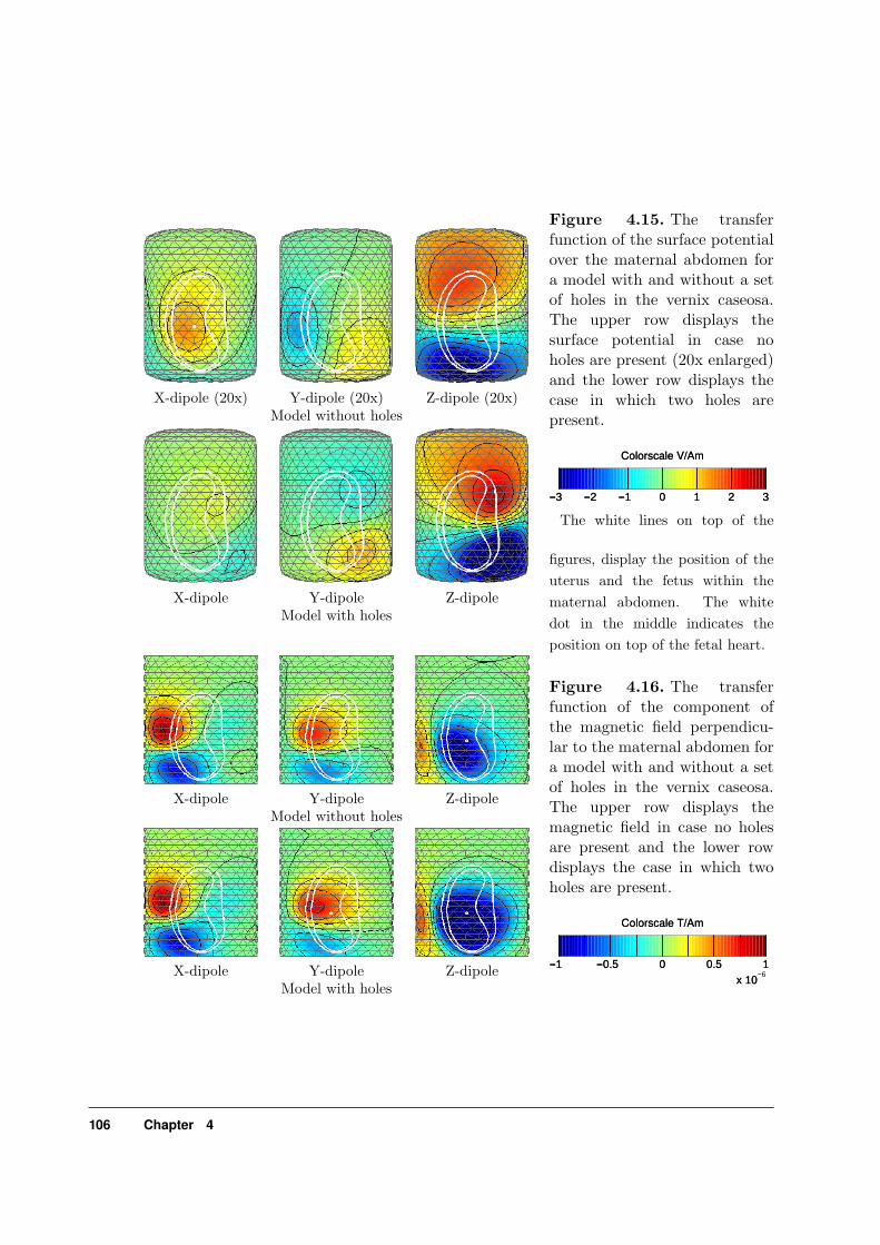
X-dipole (20x) Y-dipole (20x) Z-dipole (20x)Model without holes

X-dipole Y-dipole Z-dipoleModel with holes

Figure 4.15. The transferfunction of the surface potentialover the maternal abdomen fora model with and without a setof holes in the vernix caseosa.The upper row displays thesurface potential in case noholes are present (20x enlarged)and the lower row displays thecase in which two holes arepresent.

−3 −2 −1 0 1 2 3

Colorscale V/Am

The white lines on top of the

figures, display the position of theuterus and the fetus within thematernal abdomen. The whitedot in the middle indicates theposition on top of the fetal heart.

X-dipole Y-dipole Z-dipoleModel without holes

X-dipole Y-dipole Z-dipoleModel with holes

Figure 4.16. The transferfunction of the component ofthe magnetic field perpendicu-lar to the maternal abdomen fora model with and without a setof holes in the vernix caseosa.The upper row displays themagnetic field in case no holesare present and the lower rowdisplays the case in which twoholes are present.

−1 −0.5 0 0.5 1x 10

−6

Colorscale T/Am

106 Chapter 4

of the uterus and the fetus within the maternal abdomen. The white dot in the middleindicates the position on top of the fetal heart. From this figure it becomes clear thatin case no holes are present the amplitude of the measured signals is at least a factor 20times lower than in the case with holes. However it should be noted that the area ofthe holes is overestimated and in reality the difference is possibly smaller. Both modelsalso show that the potential distribution of the vertical component of the heart dipolehas a maximum that is a factor 3 larger than the maximum amplitude for a dipolein both other directions for the model with no holes. In case holes are present, thisfactor even becomes a factor 10. Therefore reconstructing the current dipole strengthusing a homogeneous volume conductor will overestimate the vertical component anda volume conductor model will be needed to derive the vector cardiogram. As thevertical component is expected to be the largest component of the current dipolerepresenting the heart (see chapter 3), only this component will dominate the fetalECG maps and the maps will display the same fetal complex all over the abdomen.

Another conclusion that can be drawn from these model studies is that in case thefetus is lying on the right side of the abdomen the maximum and minimum in thepotential map will be over the fetus in line with the fetal heart in case of no holes,however as soon as holes appear the maximum and minimum in the potential mapshift to the left side of the abdomen. This effect is caused by the location of the holesbeing the main pathways for the currents to the abdominal surface. As the holes facethe left side of the fetus the currents are drawn towards the left side of the abdomen.

In figure 4.16 the magnetic field maps are drawn for the same two cases of a modelwith and without holes. Only in the maps for a dipole along the z-axis, differencesin the magnetic field distribution are found. For the other two dipole directions thedipolar source is not pointing along a line connecting both holes and as a consequencethe currents are primarily confined within the fetus compartment. That these currentsare primarily confined in the fetus compartment can also be derived from the potentialmaps where the surface potential amplitude is small for the dipoles along the x andy-axis for a model containing holes. Only for the model with holes and a dipolealong the z-axis the surface potential displays larger potential differences. Hence, thepresence of holes in the vernix caseosa will influence the inverse calculations of thedipole strength and orientation from the fetal MCG if this effect is not taken intoaccount. However the effect is depending on the location where the fetal MCG ismeasured. In case it is just over the lower hole (the hole whose distance is closest tothe abdominal surface) changes in the magnitude of the magnetic field are expectedfor the vertical component of the dipole. The changes could be as large as a factor 2depending on the position of measurement.

As the magnetic field is hardly influenced by the currents in the outermost compart-ments, the question rises whether these compartments can be omitted in the model.In order to test the hypothesis of omitting compartments, the maternal compartmentand subsequently the amniotic fluid compartment have been removed from the model.So far the largest influence on the magnetic field has been found for a dipole alongthe z-axis. Hence, these stripped models are evaluated for a dipole along the z-axis.As the vernix caseosa is poorly conducting anyway, this compartment was removed


Model without holes

complete model amniotic fluid only fetusand fetus

Model with holes

complete model amniotic fluid only fetusand fetus

Figure 4.17. The transferfunction of the component ofthe magnetic field perpendicu-lar to the maternal abdomenfor a model with and withouta set of holes in the vernixcaseosa. In the first column theresults obtained with a modelconsisting of the maternalabdomen, amniotic fluid andfetus is shown, in the secondcolumn the model consistingof only the amniotic fluid andfetus and in the last columnthe model is solely based on thefetus.

−1 −0.5 0 0.5 1x 10

−6

Colorscale T/Am

Model without holes

Abdomen 0.2 S/m Abdomen 0.5 S/m

Model with holes

Abdomen 0.2 S/m Abdomen 0.5 S/m

Figure 4.18. The transfer function of thecomponent of the magnetic field perpendic-ular to the maternal abdomen for a modelwith and without a set of holes in the vernixcaseosa. The first column shows the resultsfor the model, in which the maternal abdomencompartment has a conductivity 0.2 S/m andthe second column for a conductivity value of0.5 S/m.

−1 −0.5 0 0.5 1x 10

−6

Colorscale T/Am

108 Chapter 4

too in the case the amniotic fluid compartment and the maternal compartment wereremoved from the model. When these compartments were removed from the model,their volume is considered to be non-conducting. In figure 4.17 the results are shown.It becomes apparent that independent of the question whether a hole is present, theouter compartment of the maternal abdomen can be removed without changing themagnetic field distribution or strength. For the amniotic fluid compartment the caseis more complicated, as in the case of holes changes in the magnetic field distributionare found. The changes in the magnetic field are again over the location of both holeson the left side of the abdomen. As a consequence the maternal abdomen (everythingoutside the uterus) does not need to be modeled in order to predict the strength anddistribution of the magnetic field. Of course this effect is depending on the effectiveconductivity of the maternal abdomen compartment and its conductivity distribu-tion. In order to verify the results the conductivity of the maternal abdomen hasbeen raised up to values of 0.5 S/m. The latter value is obtained by assuming thetotal extracellular water content (including fluids like the ones found in the stomach,intestines and bladder as well as the blood volume and the cerebrospinal fluid) to bearound 37 percent (Shier et al., 1996). The latter was the highest value encounteredin literature. Taking this value and assuming all cells to be spherical and the conduc-tivity of the extracellular fluids to be of an order of 2 S/m, an upper limit of 0.5 S/mis found for the conductivity. In figure 4.18, the magnetic field maps are depicted fora model with a conductivity of 0.2 and 0.5 S/m for the maternal compartment. Themaps show the magnetic field for a current dipole along the z-axis. Despite takingthis unlikely value, the maternal abdomen compartment can still be ignored in themagnetic field computations.

From the simulations it becomes clear that the maternal abdomen compartment doesnot play a significant role in the volume conductor problem for the fetal MCG, whena layer of vernix caseosa shields the fetus. Thence, the models do not need a moreelaborate subdivision of this compartment.

4.4.2 Comparison with measured fetal ECG data

In order to validate the results from the models, fetal ECGs have been measured inorder to confirm the potential distributions obtained by the simulations. As from theprevious section followed that the holes in the vernix had the largest influence on thepotential distribution, the surface potential will be used instead of the magnetic field.

As real fetal ECGs are dependent on the volume conductor and the fetal heart as cur-rent source, both have to be considered. So far, the potential distribution has beenconsidered as a function from current dipoles with a unitary strength and orientedalong the axis of the cartesian coordinate system. In order to compare real measure-ments with the simulations, the simulations need to include a model of the currentdipole. For this purpose the depolarisation sequence of the fetal heart is described asa current dipole, which rotates at the center of the fetal heart. This current dipolemodel has been described in the previous chapter. As the model was derived from


−0.03 −0.02 −0.01 0 0.01 0.02 0.03

Colorscale V/Am

closed layer of vernix caseosa(1x)

−0.2 −0.1 0 0.1 0.2 0.3

Colorscale V/Am

holes in layer of vernixcaseosa (10x)

−3 −2 −1 0 1 2 3

Colorscale V/Am

no layer of vernix caseosa(100x)

closed layer of vernix caseosa holes in layer of vernixcaseosa

no layer of vernix caseosa

Figure 4.19. Comparison between a model with no vernix caseosa, a model with a closedlayer of vernix caseosa and a model with a layer containing two holes. In the upper row thepotential distributions due to a vertical dipole are shown for all three models. The secondrow shows the predicted shapes of the complexes measured over the maternal abdomen.The latter figures are not depicted on the same scale.

postnatal ECGs, it does not include an absolute dipole strength. Hence, the simu-lations are only compared by means of the distributions and the shape of the fetalheart complexes.

So far the simulations have been performed with dipoles along the principal axis ofthe coordinate system. In order to compute what the different models would predictfor the surface potential measured at the abdominal surface, three models have beenselected and the surface potential maps have been evaluated. These models include, amodel without a layer of vernix caseosa, a model with a closed layer of vernix caseosaand a model containing holes. The results of the simulations with these models aredepicted in figure 4.19. In the upper row the fetal ECG due to a dipole along the z-axisis shown. From this figure it becomes clear that the results of the three models differin amplitude more than two decades. The three models give a different distribution as

110 Chapter 4

well, for example with a layer of vernix and holes the maximum and minimum lie ona vertical line approximately connecting the two holes, in this case over the left sideof the maternal abdomen. In case no layer of vernix caseosa is present, the oppositeis the case and the maximum and minimum are located at the left side. Here, thelayer of amniotic fluid shields the left side better than the right side of the abdomen.Finally, in case that the layer of vernix caseosa is closed the maximum and minimumare located along a vertical line over the center of the abdomen. In the lower row offigure 4.19 the corresponding results are shown when the previously described currentdipole that was obtained from neonatal ECGs is inserted in the model. In the casesthat a layer of vernix caseosa is present, the vertical component of the current dipoledominates the maps and in the case of no vernix caseosa the other components alsocontribute to the map. In case of holes in the vernix the maps also show the largestR-peaks over the holes, whereas in case of a closed layer it is more over the center ofthe fetus.

In order to be able to obtain usable fetal ECG maps, simultaneous fetal ECG andMCG measurements have been carried out. As the potentials at the abdominal surfaceare overshadowed by noise, the fetal R-peaks obtained from the fetal MCG serve asa trigger for averaging the fetal ECG. In this way four usable fetal ECG maps wereobtained ranging from week 36 to 39. The four fetal ECG maps as well as the positionof the fetus and the maternal umbilicus are shown in figure 4.20. The maps show amaximum over the fetal mouth. This maximum potential in the R-peak is of theorder of 1 to 2 µV in all four maps. As a reference potential for the maps the averagepotential of all electrodes is used. In all four cases the fetuses were lying in a positionin which the fetal back was on the left side and the head was located near the bottomof the uterus. For comparison the results of a model with holes in the layer of vernixcaseosa near the mouth and the umbilical cord are shown. The fetus is in the sameposition and this simulated map especially resembles the maps obtained in week 36and 38. The deflections of the P-wave and QRS-complex are similar in both the modeland the fetal ECG maps. And both show a similar distribution.

In figure 4.21, maps are shown with holes at different positions over the fetus. Themap on the right side is again the one with two holes aligned along the z-axis. Theother two display the potential distributions due to a couple of holes aligned onrespectively the x-axis and the y-axis. In comparing these maps with the measuredones, it becomes clear that if there are preferred pathways they are aligned along thez-axis, as the other two patterns do not resemble the distributions found in the fetalECGs.

In conclusion, it can be said that the measurements confirm the model with two holes.The exact position of the holes cannot be determined by means of fetal ECG, butthe maps and simulations indicate that they are on a vertical line. From the mapsit becomes clear that one maximum is over the head, probably a hole is formed bythe oronasal cavities that are in open contact with the amniotic fluid. The otherpathway must be at the other end of the fetal torso and the umbilicus may be agood candidate, as large veins leave the body here and currents can pass through theonset of the umbilical cord and then diffuse into the amniotic fluid, which is better


9cm

6cm

5cm

6cm

fECG week 36 fECG week 377cm

6cm 5cm

5cm

fECG week 38 fECG week 39

Simulation

Figure 4.20. Four fetal ECG maps measuredat the end of gestation. In all four cases theposition of the fetus is indicated as well asthe position of the maternal umbilicus. Thefetuses were all in the same lying in a sim-ilar position in relation to the maternal ab-domen. In the right figure a fetal ECG map isdepicted based on simulations using a modelwith the fetus whose back is on the left side.This model is a mirrored version of the modelin the second column of figure 4.19.

112 Chapter 4

Holes on X-axis Holes on Y-axis Holes on Z-axis

Figure 4.21. Simulated fetal ECG maps with a couple of holes along the z-axis(mouth,umbilicus), along the x-axis and along the y-axis. The latter two couples are placedon the fetal torso so that the connecting line between the two holes crosses the heart.

conducting than blood itself. The umbilical cord is surrounded by Wharton’s jelly.Oostendorp (Oostendorp, 1989) measured its conductivity to be in the order 1 S/m,hence it does not pose a barrier to the ionic currents as the vernix caseosa does. Andthence, the onset of the umbilicus is a likely candidate to be one of the preferredpathways.

Looking at the amplitudes obtained in the measurements, the amplitudes for themodels with holes should be of the order of a few µV. In case no vernix is present theamplitudes are expected to be a factor 10 higher. Such a case is described by Wakaiet al. (2000b) who measured the fetal ECG in case of ectopia cordis. In this conditionthe fetal heart is located outside the fetal chest and thence it is not shielded by vernixcaseosa. The amplitudes they measure in week 30 are of the order of 65 µV. Thisis even higher than predicted. However this may be due to the fact that the fetalheart is located more to the front of the abdomen and thence closer to the abdominalwall. Moreover, the fetal heart is not functioning normally and is surrounded byother tissues than usual. Hence, this may lead to a different source strength. Anotherreason is that in the vernix caseosa model the size of the holes is overestimated.

4.5 Capacitive effects due to the vernix caseosa

4.5.1 Capacitive effects

It was suspected that the absence of a pronounced T-wave in the measured signals ofboth ECG and MCG (see, chapter 2) could be ascribed to a temporal filtering effectof the vernix caseosa (Peters et al., 1998). Because the layer of vernix caseosa can bedescribed as a leaky capacitor, it is not only the ohmic current that passes throughthe layer of vernix caseosa, but also the dielectric displacement current. As charge


Amniotic fluid

FetusResistor + Capacitor

Figure 4.22. Modeling the vernix caseosa asa parallel network of a resistor and a capacitor.

gets built up at the inside of the layer of vernix caseosa due to the electric activityof the heart, an opposite charge will build up on the other side of the layer of vernixcaseosa. This implies currents to flow in the maternal abdomen. These currentswill be out of phase with respect to the source, as the spatial charges surroundingthe vernix caseosa have to be built up. There will be a frequency dependency aswell, because the accumulation of charge is limited in time and hence changes withfrequency. Hence, the layer of vernix caseosa may act as a temporal filter for boththe magnetic field and the surface potential.In order to estimate the characteristics of this filter, simulations were performed. Forthis purpose the same model as in the previous section was used, representing thefetus near the end of gestation. The simulations were performed in order to answerthe question whether the absence of a pronounced T-wave could be explained bythis effect and to estimate whether the fetal MCG is influenced by the displacementcurrents.The measurements of the vernix caseosa and its conductivity result in a wide rangeof values from a very poor conductivity 10−6 S/m and high relative permittivity 105

(Oostendorp, 1989) to a 10 times higher conductivity and a lower relative permit-tivity (Stinstra et al., 1999a) 4 × 104. Both limits have been used to model theconductivity of the layer. Since the layer is poor conducting, the layer is modeled bya network of resistor and capacitors. For this purpose the hybrid method has beenextended by replacing the ohmic resistors in the poor conducting layer with compleximpedances. These impedances are nothing more than a parallel network of resistorsand capacitors, see figure 4.22. As discussed previously, the capacitance and the re-sistance are given a value to match the thickness of the real layer of vernix caseosa,whereas in the geometric model the layer is infinitely small. The impedance of theelements now reads

Z =1

1R

+ iωC=

1Aσd

+ iωAε0εr

d

=d

Aσ(ω)(4.18)

As the thickness of the vernix caseosa varies throughout gestation, simulations withthicknesses of 0.5 mm as well as of 2 mm are performed. As the frequency range ofinterest is approximately from 0.1 Hz to 1 kHz, this range is chosen for the simulations.As fetal ECG measurements indicated the likelihood of holes present in the vernix

114 Chapter 4

10−1

100

101

102

103

10−2

10−1

100

101

102

Am

plitu

de (

V/A

m)

10−1

100

101

102

103

0

0.5

1

1.5

2

2.5

3

Pha

se s

hift

(rad

)

frequency (Hz)

σ = 2 10−5 S/m, εr = 4 104, no holes

σ = 2 10−5 S/m, εr = 4 104, holes

σ = 10−6 S/m, εr = 5 105, no holes

σ = 10−6 S/m, εr = 5 105, holes

Figure 4.23. The potential as afunction of the frequency for fourdifferent volume conduction models.The source in the model is a cur-rent dipole oriented along the z-axis, which was driven at frequenciesranging from 0.1 to 1000 Hz. The po-tential is calculated at the positionwhere the surface potential reachesthe maximum value for a frequencyof 1 kHz. The graph shows the trans-fer function for two different conduc-tivities of the vernix caseosa and forboth the case without holes in thelayer of vernix caseosa and with holesin this layer.

caseosa, the simulations are repeated, but now with two large holes present in thelayer of vernix caseosa.

4.5.2 Influence on fetal ECG

In figure 4.23 the results of the simulations of the surface potential are shown. This fig-ure depicts the transfer function, i.e. the relation between the current dipole strengthand the potential at the abdominal surface. Because the abdominal surface potentialchanges in amplitude and phase over the abdomen, each position of the maternalabdomen has its own transfer function. For each node point on the abdominal surfacethis transfer function was computed. In figure 4.23 this transfer function is depictedfor the position at which the largest amplitude is observed for 1 kHz. In this case thethickness of the layer of vernix caseosa was 2 mm. Not depicted here are the results for0.5 mm, but they do not differ substantially. In that case, the main difference is thatthe amplitudes of the signals are about a factor 4 larger and the cut-off frequenciesare slightly lower. A more in depth discussion in the dependence on the thickness ofthe layer is given by Stinstra et al. (1998).In figure 4.23 four cases are discussed, a case of a conductivity of 10−6 S/m and arelative permittivity εr of 5 × 105 and a case of a conductivity of 2 × 10−5 and arelative permittivity εr of 4 × 104 both having holes in the vernix caseosa and nothaving any holes in the vernix caseosa. From the figure, it becomes clear that bothconductivity values have their influence on the frequency domain investigated. Thelarger the relative permittivity gets the more the amplitude changes as a function ofthe frequency. For instance, in the case of εr = 5×105 and no holes present the change


1 Hz no holes 100 Hz no holes

1 Hz two holes 100 Hz two holes

Figure 4.24. The surface potential distribu-tions at the front side of the abdomen. Thesedistributions were computed for a vernix con-ductivity of 10−6 S/m and a permittivity of5× 105. All graphs are displayed at the samecolor scale. The two upper graphs representthe case in which no holes are present in thevernix caseosa and the lower ones in case twoholes would be present near the mouth andumbilical chord.

−10 −5 0 5 10

Colorscale V/Am

10−1

100

101

102

103

1

1.2

1.4

1.6

1.8x 10

−6

Am

plitu

de (

T/A

m)

10−1

100

101

102

103

−1.5

−1

−0.5

0

0.5

1

1.5

Pha

se s

hift

(rad

)

frequency (Hz)

σ = 2 10−5 S/m, εr = 4 104, no holes

σ = 2 10−5 S/m, εr = 4 104, holes

σ = 10−6 S/m, εr = 5 105, no holes

σ = 10−6 S/m, εr = 5 105, holes

Figure 4.25. The transfer functionof the radial component of the mag-netic field computed at 2 cm from theabdominal surface as a function ofthe frequency for four different vol-ume conduction models. The sourcein the model is a current dipole ori-ented along the z-axis, which wasdriven at frequencies ranging from0.1 to 1000 Hz. The magnetic fieldis calculated at the position where itreaches the maximum value for a fre-quency of 1 kHz. The graph showsthe transfer function for two differentconductivities of the vernix caseosaand for both the case without holesin the layer of vernix caseosa as wellas for the case with holes in thislayer.

116 Chapter 4

may be a factor 100 between 1 Hz and 100 Hz. Hence, in this case the layer of vernixcaseosa acts as a high-pass filter. However as soon as holes in the layer of vernixcaseosa are present, this high-pass filtering is reduced and between 10 Hz and 1 kHzthe amplitude only changes about a factor 4. For the smaller relative permittivityhardly any frequency dependency is found in case two holes are present in the layervernix caseosa. For the case no holes are present the cut-off frequency of the high-passfiltering appears to be shifted to a higher frequency.

In order to determine whether the frequency dependency influences the distributionof the potential, the distributions at 1 Hz and 100 Hz for a case with no and a casewith two holes are computed. These surface potential distributions at the maternalabdomen are depicted in figure 4.24. Although not visible, the distribution in the caseof no holes at 1 Hz and that at 100 Hz are almost similar apart from the apparentgain in amplitude. However for the case of the two holes, the maximum seems to shiftfrom a position at the left of the abdominal surface to the right of this surface. Ata frequency of 1 Hz, the holes in the vernix caseosa cause the currents to enter andleave the fetus at the left side and here the maximum and minimum are found. At100 Hz, the layer of vernix caseosa becomes more transparent for currents and themaximum and minimum are now found to be in line with the fetal heart instead ofthe holes in the vernix. The latter distribution is similar to the distribution in case noholes are present. Hence, the frequency dependency influences the surface potentialdistribution.

4.5.3 Influence on fetal MCG

Similar simulations were performed for the magnetic field. The magnetic field wasevaluated for the frequency range from 0.1 to 1000 Hz as well. Again two complexconductivity values were taken for the case that two holes were present and for the casethat no holes were present. The component of the magnetic field perpendicular to thematernal abdomen was computed at a distance of 2 cm from the abdominal surfacefor three current dipole dipoles each along one of the principal axes. In figure 4.25 theresults of this simulation are shown for a dipole along the z-axis of the model. Theresults for the dipoles along the x-axis and y-axis revealed a similar graph. In thefigure, the component of the magnetic field perpendicular to the abdominal surface isgiven as a function of the frequency. The graphs represent the magnetic field at thatposition where the observed field reaches a maximum at 1 kHz.

The figure clearly demonstrates that the magnetic field is influenced differently byfrequency dependent effects. For the fetal MCG a change in amplitude is found incase the conductivity of the vernix caseosa is as low as 10−6 S/m and the relativepermittivity is as high as 5 × 105. Here the magnetic field strength for a frequencyof 200 Hz is about a 20 percent larger than it was for 1 Hz. Whereas a high-passfilter was found in case of the fetal ECG, for the fetal MCG a band-pass filteringeffect is found that starts to have its influence from about 10 Hz onward. First theobserved amplitudes rise until a frequency of about 200 Hz and subsequently dropagain. Like in the previous case the presence of holes in the vernix caseosa reduces


1 Hz no holes 100 Hz no holes

1 Hz two holes 100 Hz two holes

Figure 4.26. The transfer functionof the component of the magneticfield perpendicular to the abdominalsurface at the front side of the ab-domen. These distributions are com-puted for a vernix conductivity of10−6 S/m and a relative permittiv-ity of 5 × 105. All graphs are dis-played at the same color scale. Thetwo upper graphs represent the casein which no holes are present in thevernix caseosa and the lower ones incase two holes are present near themouth and the other at the begin-ning of the umbilical chord.

−1 −0.5 0 0.5 1x 10

−6

Colorscale T/Am

the temporal filtering effect and the change in amplitude strength is now less than2 percent between 1 Hz and 100 Hz. For the case of a higher conductivity of thevernix caseosa and a lower relative permittivity a much smaller filtering effect is seen.

As changes in the distribution of the surface potential were observed for differentfrequencies, it is checked whether the magnetic field shows changes in distribution aswell. In figure 4.26 the magnetic field distribution is shown for frequencies of 1 Hzand 100 Hz for both the case of holes and no holes present. The figure displays themagnetic field in case the conductivity is 10−6 S/m and the relative permittivity is5× 105. In this case the current dipole is orientated along the z-axis. A small changein the distribution of the magnetic field strength is found for both cases. The largestchange in distribution is found in case no holes are present in the vernix caseosa. Thischange in field pattern can be ascribed to a change in the distribution of the currentsin the abdomen. In case of a frequency of 100 Hz, more currents will flow in theamniotic fluid as for 1 Hz. The latter explains as well that for 100 Hz the patterns ofthe cases with and without holes are more alike. Because the two holes are locatedto the side where most of the amniotic fluid is, the currents will flow within the fetusand through the amniotic fluid leaving the fetus at one hole and returning throughthe other.

Although a very small amplitude of the T-wave in the fetal ECG could be explainedby a high-pass filtering effect of the vernix caseosa, this still cannot explain the lowamplitude of the T-wave in the fetal MCG. Simulations show that even for very lowvalues of the conductivity of vernix caseosa (down to 10−6 S/m) capacitive effectswill take place for frequencies over 10 Hz. However for the fetal MCG, only smallincreases in amplitude are found and they display a band-pass filtering characteristic.

118 Chapter 4

The simulations suggest, that the decrease in T-wave amplitude should only be about10 percent for the fetal MCG measurements, which is lower than the variance ob-served in the amplitude of the T-wave. Moreover, our own measurements also show adependence of the relative permittivity of the vernix caseosa on the frequency, whichwas not taken into account in the simulations. For higher frequencies the value of thepermittivity drops by an order of a decade (from 1 Hz to 1 kHz). This reduces thecapacitive effect even further. Hence, for the fetal MCG the measured signals shouldhardly be affected by any frequency dependent behaviour of the volume conductor.For the fetal ECG a small filtering effect may be expected. However, the holes presentin the layer of vernix caseosa will minimise the capacitive effect of the layer vernix.How much the vernix caseosa will influence the fetal ECG signals in the frequencyrange of 1 to 100 Hz is still dependent on the size of the holes. The smaller the holes,the lower the cut-off frequency of the high-pass filter becomes. Hence for smallerholes, the frequency range in which the capacitive effects will play a role, is lower andshifts to the frequency range of the fetal PQRST-complex. On the other hand if theholes become too tiny almost no currents will reach the abdominal surface and thenceno potential differences can be measured.


Chapter 5

The forward problem in fetalmagnetocardiography

In the previous chapter the problem how to model the vernix caseosa was discussed, inthis chapter the implications of the volume conductor on the fetal MCG will be studied. Inchapter 4 only a model for the last period of gestation was introduced, this approach will beextended with volume conductor models of the second trimester. The differences betweenpregnancies and hence the differences in fetoabdominal volume conductors can be exam-ined by creating volume conductor models based on the different anatomical morphologiesencountered. Using MR-images of pregnant women, the variability in the fetoabdominalvolume conductor is simulated and evaluated. Fetal heart activity is modeled by a heartvector obtained from newborns. Using this source model in combination with realisticallyshaped volume conductor models fetal MCGs are simulated. The results of the simula-tions will be compared with the results obtained in fetal MCG. The influence on fetal MCGparameters such as the P-to-QRS ratio and the intracardiac intervals will be estimated. Fi-nally, the computed field patterns will be examined in order to answer the question whetherit is possible to determine a good measurement position.

5.1 Fetoabdominal volume conduction

In order to improve and to assess the reliability of the MCG several issues need to beaddressed. For instance, the question remains where to measure the fetal magneto-cardiogram above the maternal abdomen. It is advantageous, if the position can bepredicted, where a clear P-wave or QRS-complex can be measured over the maternalabdomen. As devices for clinical application should preferably have a small numberof channels, information on good measuring positions is needed. A good measuringposition refers to the position, where the signal-to-noise ratio of the signal is as largeas possible. Apart from this position, simulations can also be used to determine whichparameters should be recorded as well in order to increase the reliability of the signal.An example of such a parameter is the position of the fetal heart.

In order to address these issues, simulations are presented in this chapter. Since

The forward problem in fetal magnetocardiography 121

the modeling techniques used in the simulations predict both the magnetic field aswell as the potential distribution, similar items on the reliability of the fetal ECGcan be addressed. The models used to predict the magnetic field distribution overthe abdomen consist of two parts, i.e. a model of the fetal heart represented by arotating current dipole and a model describing the transfer function. In case of thesurface potential a similar subdivision can be made. Often knowledge on the transferfunction is enough to answer certain questions.

In order to derive this transfer function a model of the volume conductor is needed.The construction of such a model raises new questions such as how to subdivide thevolume conductor into regions with the same conductivity, or whether it is necessaryto include inter-individual differences in this model. These questions are addressed inthe next two sections.

Knowledge on the transfer function is also needed in order to predict the reliability ofthe intracardiac time intervals, the amplitude of the various waves and the amplituderatios which are obtained from the fetal MCG. The transfer function can be usedto estimate the variations in these parameters due to the volume conductor and canbe used to set the bounds of the reliability. In this chapter, the influence on theamplitudes and the amplitude ratios will be discussed.

Another reason for studying the transfer function, would be the solution of the inverseproblem, so that the measurements obtained outside the maternal abdomen can betranslated into the rotation of a current dipole at the center of the heart. Informationon the rotating dipole would be a more direct translation of the processes taking placein the fetal heart. Hence, it could be of help in the quest for obtaining reliable dataon the fetal heart’s functioning. Such inverse calculations are used to for instance intracking down the location of brain activity out of adult EEG measurements or theestimation of electrical activity in the adult heart from ECG/MCG measurements.In a paper by Oostendorp and van Oosterom (1989) an example of such an inversecomputation is given for the reconstruction of the current dipole from fetal ECGmeasurements. However, the transfer function has to be evaluated more extensivelybefore the inverse solution can be trusted.

As described in the previous chapter, the vernix caseosa has a profound influenceon the volume conduction problem. As this layer develops at the end of the secondtrimester (from week 28 and onward) it marks a significant change in the volumeconduction problem as noted before by for instance Kahn et al. (1963). Thence,the volume conduction problem will be divided into two, one for the period beforethe segregation of vernix caseosa and one for the period it covers the fetus. Someinvestigators claim that the vernix caseosa first covers the fetus completely and thatafterwards holes appear in the layer (Oostendorp, 1989). This assumption is based onthe fact that only in about 20 to 30 percent of the fetal ECGs measured in this perioda usable recording is obtained, in which fetal R-peaks can be discerned (Bolte, 1961).However, there is no solid evidence that the vernix caseosa is completely coveringthe fetus and no holes are present at all, as it seems unlikely that the fetus keeps itsmouth closed for this entire period. Thence, one hole is probably always there. Thesimulations in the last chapter showed that when one hole is present in the poorly

122 Chapter 5

Figure 5.1. Cross section of amodel with a layer of fat at theouter regions of the volume conduc-tor. The model is based on the oneused in the previous chapter. In thiscase the maternal compartment is di-vided in a fat layer and the remainingvolume.

conducting layer, it is still shielding the currents within the fetus. In order to obtainlarger current densities in the volume outside the vernix caseosa, at least two holesare needed. Hence, the question remains whether there is a second preferred pathwayto the opposite side to the mouth in respect to the fetal heart. The latter conditionassures that the currents induced by the fetal heart leave the fetus compartment atone side and return at the other side.

5.2 The layer of subcutaneous fat and amniotic fluid

In the previous chapter it was concluded that the layers outside the fetus did nothave a profound influence on the magnetic field, but did have an influence on the fetalECG. In order to further examine the influence of the outer regions of the model anadditional layer of fat will be introduced. Furthermore, the influence of the presenceof the amniotic fluid will be studied.

The model that was introduced in the previous chapter consisting of a fetal compart-ment surrounded by a layer of vernix with two holes, an amniotic fluid compartmentand one for the maternal abdomen, has been extended with a layer of fat. In thismodel, the maternal abdomen compartment is split into two, the outer part of thiscompartment is assumed to represent both the skin and the subcutaneous fat and theinner part the other remaining tissues in the maternal abdomen. In the model thecompartment of fat (and skin) is estimated to have a thickness of about 2 cm near theabdominal wall. Towards the bottom and top of the model the layer is thicker andhas an average thickness of 3 cm. A cross section of the model is given in figure 5.1.In the model the layer of vernix caseosa was assigned a value of 2× 10−5 S/m. Boththe surface potential and the magnetic field strength perpendicular to the abdominalsurface are calculated by means of the boundary element method. The results aredepicted in figure 5.2. In this figure the case with an additional layer of subcuta-neous fat is compared with the case without this fat. In the same figure the case isshown, where the amniotic fluid is replaced by a compartment with a conductivityof 0.2 S/m. This reflects the case in which the volume conductor outside the vernixcaseosa is considered to be homogeneous.

The results depicted in figure 5.2 show a two-fold effect for the surface potential.Firstly, in the inner part of the volume conductor the amniotic fluid is shielding


Surface potential

fat - abdomen - abdomen - abdomen -amniotic fluid - amniotic fluid - vernix caseosa -vernix caseosa - vernix caseosa - fetus

fetus fetus

Magnetic field

fat - abdomen - abdomen - abdomen -amniotic fluid - amniotic fluid - vernix caseosa -vernix caseosa - vernix caseosa - fetus

fetus fetus

Figure 5.2. Upper row: thetransfer function of the surfacepotential for a model in whichthe maternal compartment hasbeen subdivided into a com-partment of subcutaneous fatand a compartment representingthe other tissues in the mater-nal abdomen, a model withoutthis subdivision and a model inwhich the amniotic fluid layeris replaced by a layer with thesame conductivity as that ofthe maternal abdomen. Lowerrow: the transfer function ofthe component of the magneticfield perpendicular to the mater-nal abdomen calculated for thethree models mentioned above.The current dipole is orientedalong the z-axis. Note that theposition of the fetus and the am-niotic fluid are indicated by thewhite lines.

−30 −20 −10 0 10 20 30

Colorscale V/Am

−1 −0.5 0 0.5 1x 10

−6

Colorscale T/Am

the surface potential by forcing more currents to flow through the inner part of thevolume conductor, namely the amniotic fluid instead of flowing through the outerparts of the abdominal volume. Hence, in case the amniotic fluid is replaced bya compartment having the same conductivity as the rest of the abdominal volumelarger potential values can be measured. However, a lower conductivity at the surfaceof the model, representing the layer of fat, causes the currents to follow a pathwaymore to the interior of the model. Despite this reduction in current density in theouter layers, the drop in conductivity is larger than the reduction in current density.As a consequence, slightly larger potentials are found at the abdominal surface in casea poorer conductive layer is present at the surface.

In case of the magnetic field no significant difference has been found between the modelwith and without the fat layer and once again only a small deviation was found in themagnetic field due to a dipole along the z-axis. This confirms again the conclusionmade in the last chapter that in case of a layer of vernix caseosa, the tissues outside

124 Chapter 5

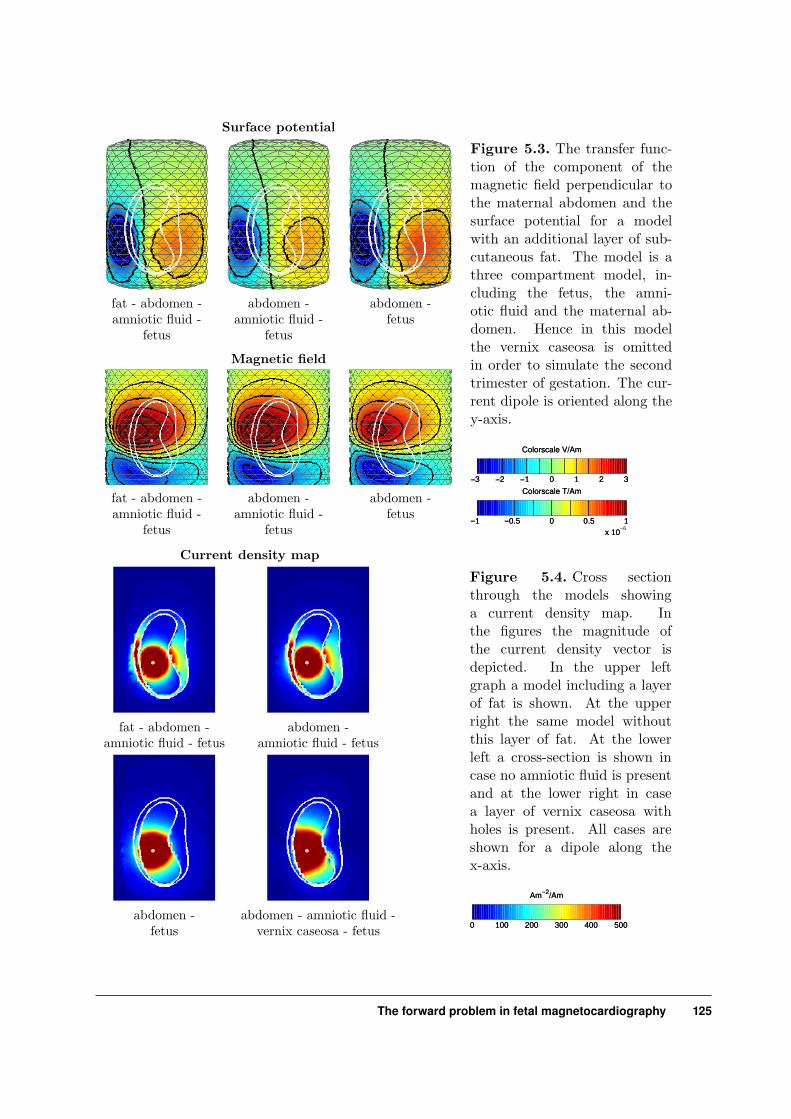
Surface potential

fat - abdomen - abdomen - abdomen -amniotic fluid - amniotic fluid - fetus

fetus fetus

Magnetic field

fat - abdomen - abdomen - abdomen -amniotic fluid - amniotic fluid - fetus

fetus fetus

Figure 5.3. The transfer func-tion of the component of themagnetic field perpendicular tothe maternal abdomen and thesurface potential for a modelwith an additional layer of sub-cutaneous fat. The model is athree compartment model, in-cluding the fetus, the amni-otic fluid and the maternal ab-domen. Hence in this modelthe vernix caseosa is omittedin order to simulate the secondtrimester of gestation. The cur-rent dipole is oriented along they-axis.

−3 −2 −1 0 1 2 3

Colorscale V/Am

−1 −0.5 0 0.5 1x 10

−6

Colorscale T/Am

Current density map

fat - abdomen - abdomen -amniotic fluid - fetus amniotic fluid - fetus

abdomen - abdomen - amniotic fluid -fetus vernix caseosa - fetus

Figure 5.4. Cross sectionthrough the models showinga current density map. Inthe figures the magnitude ofthe current density vector isdepicted. In the upper leftgraph a model including a layerof fat is shown. At the upperright the same model withoutthis layer of fat. At the lowerleft a cross-section is shown incase no amniotic fluid is presentand at the lower right in casea layer of vernix caseosa withholes is present. All cases areshown for a dipole along thex-axis.

0 100 200 300 400 500

Am−2/Am


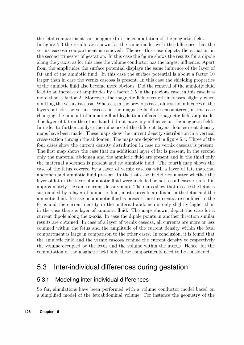
the fetal compartment can be ignored in the computation of the magnetic field.In figure 5.3 the results are shown for the same model with the difference that thevernix caseosa compartment is removed. Thence, this case depicts the situation inthe second trimester of gestation. In this case the figure shows the results for a dipolealong the y-axis, as for this case the volume conductor has the largest influence. Apartfrom the amplitudes the surface potential displays the same influence of the layer offat and of the amniotic fluid. In this case the surface potential is about a factor 10larger than in case the vernix caseosa is present. In this case the shielding propertiesof the amniotic fluid also become more obvious. Did the removal of the amniotic fluidlead to an increase of amplitudes by a factor 1.5 in the previous case, in this case it ismore than a factor 2. Moreover, the magnetic field strength increases slightly whenomitting the vernix caseosa. Whereas, in the previous case, almost no influences of thelayers outside the vernix caseosa on the magnetic field are encountered, in this casechanging the amount of amniotic fluid leads to a different magnetic field amplitude.The layer of fat on the other hand did not have any influence on the magnetic field.In order to further analyse the influence of the different layers, four current densitymaps have been made. These maps show the current density distribution in a verticalcross-section through the abdomen. The maps are depicted in figure 5.4. Three of thefour cases show the current density distribution in case no vernix caseosa is present.The first map shows the case that an additional layer of fat is present, in the secondonly the maternal abdomen and the amniotic fluid are present and in the third onlythe maternal abdomen is present and no amniotic fluid. The fourth map shows thecase of the fetus covered by a layer of vernix caseosa with a layer of fat, maternalabdomen and amniotic fluid present. In the last case, it did not matter whether thelayer of fat or the layer of amniotic fluid were included or not, as all cases resulted inapproximately the same current density map. The maps show that in case the fetus issurrounded by a layer of amniotic fluid, most currents are found in the fetus and theamniotic fluid. In case no amniotic fluid is present, most currents are confined to thefetus and the current density in the maternal abdomen is only slightly higher thanin the case there is layer of amniotic fluid. The maps shown, depict the case for acurrent dipole along the x-axis. In case the dipole points in another direction similarresults are obtained. In case of a layer of vernix caseosa, all currents are more or lessconfined within the fetus and the amplitude of the current density within the fetalcompartment is large in comparison to the other cases. In conclusion, it is found thatthe amniotic fluid and the vernix caseosa confine the current density to respectivelythe volume occupied by the fetus and the volume within the uterus. Hence, for thecomputation of the magnetic field only these compartments need to be considered.

5.3 Inter-individual differences during gestation

5.3.1 Modeling inter-individual differencesSo far, simulations have been performed with a volume conductor model based ona simplified model of the fetoabdominal volume. For instance the geometry of the

126 Chapter 5

fetus was approximated by a smoothed surface. To be able to estimate the influ-ence of the inter-individual differences between pregnancies, four MR-images of thelast period of gestation (from week 36 until 39) were selected. The reasons for fo-cusing on this period is that the mobility of the fetus within the uterus is small,the fetus is confined to certain positions and orientations in respect to the maternalabdomen (Symonds, 1994). This allows for classification of the fetal position intodifferent classes as described in chapter 3. Thence, by classifying the fetal positionthe amount of parameters to be estimated is reduced. In all four cases examined, thefetuses were lying in a left occiput position. Moreover, using these four MR-imagesthe inter-individual differences can be estimated in case the position of the fetus isknown. In order to study the volume conduction problem during the second trimester,three MR-images were used obtained in the period from 21 to 30 weeks of gestation.The models created for this period did not contain any layer of vernix caseosa andthence show a different behaviour.

In order to estimate the expected differences when using a realistically-shaped vol-ume conductor model for the fetoabdominal volume in different pregnancies, sevenindividually shaped models have been constructed. MR-images of the lower abdomenof pregnant women were used to subdivide the abdominal volume into three com-partments. These compartments consist of a compartment representing the fetus,one of the amniotic fluid and one of the remainder of the abdominal volume. Theamniotic fluid and the structures within the fetus could be reasonably well distin-guished in the MR-images. However the details in the maternal abdomen like a layerof fat or skin could not be distinguished. Hence, no further subdivision is made ofthe maternal volume. The results in figure 5.2 however show that these regions ofthe maternal abdomen hardly influence the magnetic field and thence the need for afurther subdivision is not there. The placenta and the amniotic fluid are both whitein the MR-images, nevertheless a distinction could be made between both. In order tokeep the computational effort within the limits of a modern PC, no separate placentalvolume is included in the model. The placental volume is divided between both theamniotic fluid and the maternal abdomen. In order to avoid the use of large amountsof elements the volume of arms and legs of the fetus are divided between fetus andamniotic fluid in a similar procedure. Apart from avoiding a huge computationaleffort, the arms and legs are difficult to distinguish as some parts fall within the gapbetween two MRI-slices, which makes it difficult to exactly define where a hand or afoot is. In order to include holes in the layer of vernix, the position of the mouth andthe umbilicus are estimated. The first can be obtained easily, as the oronasal cavitiesare clearly visible, however the position of the umbilical chord is more difficult as itcan not be discerned on the MR-images. Thence, it is estimated based on the positionof the liver, lungs and heart within the fetus. The position of the heart on the otherhand can be obtained without any problem and the current dipole is thence positionedat the center of the heart.

In figure 5.5, all seven models are depicted. The first four are of the third trimester andthence include a layer of vernix caseosa. The latter layer has an estimated thicknessof about 2 mm. These four models are selected because the fetus is in about the same


Model I, 39-weeks-old fetus. Model II, 37-weeks-old fetus.

Model III, 39-weeks-old fetus. Model IV, 36-weeks-old fetus.

Model V, 30-weeks-old fetus. Model VI, 21-weeks-old fetus.

Model VII, 26-weeks-old fetus.

Figure 5.5. The seven volume conductor models used to study the inter-individuality inthe second and third trimester. The first four models are used to study the third trimester ofgestation and the last three for the second trimester. As for the models of the third trimesterthe position of mouth and umbilicus are important, they are indicated in the model. Theinner volume represents the fetus (covered by vernix in the third trimester), the other twothe amniotic fluid and the maternal abdomen, respectively.

position in all four cases. In these cases, the fetus is lying with its head down and itsback to the right side of the mother. However the fetal presentation is not equal foreach fetus. In model I and IV the fetus has turned its head towards the front of theabdomen. In model II its head is just facing the mother’s back and in model III itis facing the left side of the mother. Apart from the position of the head the modelsdiffer in amniotic fluid distribution, some have more fluid on the left side and othersmore on the right side. In the second trimester the fetus has more space to swimaround, however still most fetuses are found with the head down and the back facingone of two sides of the mother. In these models there is clearly more amniotic fluid

128 Chapter 5

relative to the fetal volume in comparison to the models of the third trimester.

5.3.2 The influence of inter-individual differences

For all seven models the abdominal surface potential and the magnetic field distri-bution have been calculated. The latter have been computed at a distance of 2 cmfrom the abdominal wall. In figures 5.6 and 5.7 the surface potential distributionsare shown for all three components of the current dipole. Likewise, in figures 5.8and 5.9 the x-component of the magnetic field is depicted for all three current dipolecomponents. This x-component of the magnetic field is the component perpendicularto the front of the abdomen and is the one that is usually measured.In case the fetus is surrounded by a layer of vernix caseosa with two distinctive holespresent in this layer, the surface potential is dominated by the z-component of thecurrent dipole representing the heart. Hence, a distribution is expected in which themaximum and minimum of the potential are aligned along the z-axis. The lattereffect is observed in the simulations. The potential maximum is found 5 to 10 cmabove the position that is right on top of the fetal heart and the minimum is found atapproximately the same distance below this point. In the simulations of the previouschapter the largest potential was found at the side the fetus was facing. For instance,when the back of the fetus is located to the right, the largest potential difference isfound at the left side of the abdominal surface. However this was assuming that thefetus faces toward the left side and the mouth opening is pointing to the left side ofthe abdomen. However the present models show that the case is more complicated. Incase the fetus has turned its head towards the front of the abdomen or to the left side,the minimum is still found at a position on top of the mouth, however the positionof the maximum is more variable, but it is found more to the left than the minimum.In case the mouth is facing toward the back of the mother, the simulation revealsonly a weak potential difference and no clear minimum can be distinguished near thehead of the fetus. On the other hand when the fetus is facing the front a more clearerminimum is seen over the maternal abdomen than in the other three cases.The magnetic maps are shown in figures 5.8 and 5.9 and display a wide variety inpatterns. For dipoles oriented along the y and z-axis the overall pattern is the same,whereas for a dipole along the x-axis the patterns seem to be rotated over a widevariety of angles. Not only do the patterns change, the amplitudes of the distributionsvary over a wide range. For instance, the amplitude of the field generated by a dipolealong the z-axis in model I and model III differs from that in model III by at least afactor 10.In order to get a better understanding why these models show such a diversity in themagnetic field distribution, the magnetic field is split up into a contribution of theprimary source (current dipole) and a contribution of the secondary sources (volumeconductor contribution). In figure 5.10 both contributions are depicted for models Iand V. From the figure it becomes clear that both contributions tend to counterbalanceeach other. This effect decimates the observed amplitudes of the magnetic field incomparison with a homogeneous volume conductor of infinite extent. It turns out


Surface potential

X-dipole Y-dipole Z-dipole

Mod

elI

Mod

elII

Mod

elII

IM

odel

IV

Figure 5.6. The surfacepotential due to unitarycurrent dipoles along the x,y and z-axis for four mod-els of the third trimester ofgestation in which the fetusis lying in a left occiput po-sition.

−3 −2 −1 0 1 2 3

Colorscale V/Am

Surface potential


Mod

elV

Mod

elV

IM

odel

VII

Figure 5.7. The surfacepotential due to unitarycurrent dipoles along the x,y and z-axis for three mod-els of the second trimesterof gestation in which the fe-tus is lying in an arbitraryposition.

−30 −20 −10 0 10 20 30

Colorscale V/Am

130 Chapter 5

magnetic field along the x-axis


Mod

elI

Mod

elII

Mod

elII

IM

odel

IV

Figure 5.8. The compo-nent of the magnetic fieldalong the x-axis due to uni-tary current dipoles alongthe x, y and z-axis forfour models of the thirdtrimester of gestation inwhich the fetus is lying ina left occiput position.

−1 −0.5 0 0.5 1x 10

−6

Colorscale T/Am

magnetic field along the x-axis


Mod

elV

Mod

elV

IM

odel

VII

Figure 5.9. The compo-nent of the magnetic fieldalong the x-axis due to uni-tary current dipoles alongthe x, y and z-axis forthree models of the secondtrimester of gestation.

−1 −0.5 0 0.5 1x 10

−6

Colorscale T/Am

that slight changes in the geometry of the volume conductor change the degree inwhich both the primary and secondary source contribution tend to cancel each other.Hence, the maxima and minima in the magnetic field distribution of the differentmodels are also found at a different position due to the contribution of the secondarysources. Hence, this explains why in model III hardly any magnetic field is founddue to a dipole along the z-axis. In this case, both contributions almost perfectlycounterbalance each other resulting in magnetic fields that are only a tenth of the size


Magnetic field along x-axis

Primary source Secondary source TotalM

odel

I

+ =

Mod

elV

Figure 5.10. The magnetic field of a current dipole oriented along the z-axis split up inthe contribution of the primary source and that of the secondary sources. Together bothsources account for the final magnetic field. The contributions are depicted for a model inthe second trimester and for one in the third trimester.

of the magnetic field due to the primary source.

5.3.3 The influence of the volume conductor on amplitudes

In the maps shown in figures 5.8 and 5.9, both the volume conduction and the positionof the fetal heart are of influence for the amplitudes and the field patterns observed.When the fetal heart is further away from the pickup-coil, the magnetic field strengthis smaller. Since it is possible to determine the position of the fetal heart, for instanceby means of ultrasound imaging, this problem can be overcome. Hence, the questionremains to what extent the volume conductor is of influence if we correct for thisdistance. For this purpose, the simulations have been repeated with a magneticsensor array that is at 12 cm distance from the fetal heart and is centered over theposition of the fetal heart. In this case not the shape of the maternal abdomendetermines where the magnetic field is computed, but a rigid distance from the heartis chosen. In figure 5.11 the results are shown for all seven models. The figure displaysthe magnetic field along the x-axis for a sensor array of 61 points, which covers thefront of the abdomen. Although in the latter case the sensor array is positionedat a constant distance from the fetal heart, the maps still show a large spread inamplitudes. For instance the difference in amplitudes between model I and model IIIis about a factor 10.

Comparison between the models of the second trimester and the third trimester showsthat on average the volume conductor in the second trimester allows a larger gaindue to the transfer of the volume conductor. Although the volume conductor has ahigher transfer coefficient for the magnetic field in the second trimester, the measured

132 Chapter 5

Magnetic field along the x-axis


Mod

elI

Mod

elII

Mod

elII

IM

odel

IVM

odel

VM

odel

VI

Mod

elV

II

Figure 5.11. The compo-nent of the magnetic fieldalong the x-axis due to uni-tary current dipoles alongthe x, y and z-axis for allseven models. In this casethe magnetometer grid ispositioned at a fixed dis-tance of 12 cm from the fe-tal heart.

−1 −0.5 0 0.5 1x 10

−6

Colorscale T/Am


amplitudes are smaller, as the size of the fetal heart is smaller and thus the amountof currents released by the myocardiac cells.

Moreover, considering that the fetus is in the same position for the first four mod-els, for an accurate estimation of the size of the current dipole more information isneeded than the lie of the fetus and the position of the fetal heart. Under the presentmeasurement setup we are only able to determine the position of the fetus and theposition of the fetal heart by means of ultrasound imaging. Hence, the amplitude ofthe current dipole which would be retrieved by an inverse computation based on thisinformation is not reliable for diagnosis. To carry out an analysis of the amplitudes,more extensive modeling is needed as well as comparison with measured distributions.The models may be derived from 3D-ultrasound, a new field emerging in ultrasoundimaging which is able to generate three-dimensional reconstructions of the anatomicallayout of the uterus and everything inside. However, an extensive ultrasound scanwould complicate the measurement procedures in fetal magnetocardiography, whereasthe advantages of knowing the current dipole strength for making a diagnosis is stillquestionable. For instance, the amplitude of the various complexes in pediatric car-diology are hardly used, as they show a wide spread. For example, Namin and Miller(1966) report a spread in the amplitudes of the QRS-complex in lead V6 in the rangeof 0.2 to 1.0 mV (90 percent confidence interval). These numbers were obtained frompostnatal ECGs 30 hours after birth and are similar for other leads. This large spreadof a factor five in amplitude is probably the reason why the amplitudes are not com-monly used in diagnosis. Apart from volume conduction effects the spread in currentdipole strengths is probably large when looking at the data measured in newbornsand its advantages in diagnosing fetal cardiac diseases is unknown.

5.4 The P-wave to QRS-complex ratio

The previous sections showed that the amplitude of the PQRST-complex is heavilydependent on the symmetries in the volume conductor. Hence, these amplitudes arenot suited for diagnostic purposes. A way to avoid the use of the amplitudes, is lookingat the ratios of the amplitudes within a PQRST-complex. For instance, if one is ableto prove that the amplitude of the P-wave is large in comparison to the amplitudeof the R-peak this may indicate that there is some kind of atrial hypertrophy. Thelatter may be the result of a severe arrhythmia or a congenital heart defect. In caseof an atrioventricular block (n = 4) or an atrial flutter (n = 2) our measurementsshowed an exceptionally large P-wave amplitude in comparison to the QRS-complex,see chapter 6. However, if this kind of analysis is to be used, the P-to-QRS ratiomeasured in the fetal magnetocardiogram should reflect the ratio in current dipolestrength of the P-wave and the QRS-complex. Moreover, if this ratio depends on theposition where the fetal magnetocardiogram is measured, the variability of this ratioover the abdomen should be small enough, so that abnormal ratios can be detected.

In order to acquire insight in the ratio of the P-wave amplitude in respect to theQRS-complex amplitude, simulations have been performed in order to estimate the

134 Chapter 5

Vector VectorMagnetometer Gradiometer Magnetometer Gradiometer

Mod

elI

Mod

elII

Mod

elII

IM

odel

IV

0 0.1 0.2 0.3 0.4

P/QRS

Figure 5.12. Ratio of P-wave amplitude to QRS-complex amplitude as a function of theposition over the maternal abdomen. Four different measurement configurations are de-picted. The first is a magnetometer, the second a gradiometer along the x-axis with abaseline of 6 cm. This baseline is more or less perpendicular to the maternal abdomen.The third system is a vector magnetometer, which measures the three components of themagnetic field and combines the three to obtain the magnitude of the magnetic field vector.And the fourth system is a vector gradiometer along the x-axis with a baseline of 6 cm.In this system, the difference between the magnitudes of the magnetic field vector at twopositions is subtracted. The ratio between the current dipole generating the P-wave andthe one generating QRS-complex is 0.2. The latter value was obtained from vector ECGmeasurements in newborns, from which a model for the current dipole in the fetal heart wasderived, see chapter 3.


Vector VectorMagnetometer Gradiometer Magnetometer Gradiometer

Mod

elI

Mod

elII

Mod

elII

IM

odel

IV

0 0.1 0.2 0.3 0.4

P/QRS

Figure 5.13. The P-to-QRS ratio as a function of the position over the maternal abdomen,see figure 5.12. In this case only a distribution is given for the locations where the R-peakis at least 20 percent of the largest R-peak found over the abdomen.

influence of the measurement position and the volume conductor on this ratio. In thesesimulations the current dipole is assumed to be rotating as described in chapter 3. Inthis model the largest current dipole vector of the P-wave is more or less perpendicularto the largest vector in the QRS-complex. In these simulations the four volumeconductor models of the third trimester of gestation are used.

In figure 5.12, the results of the simulations are depicted. In this figure four typesof fluxtransformers are described. The first fluxtransformer is a magnetometer andthe second one is a gradiometer with a baseline of 6 cm. Both measure the magneticfield component along the x-axis. The gradiometer is simulated by subtracting themagnetic field component at a distance of 6 cm from the one just above the abdomen.Both fluxtransformers display large fluctuations in the P-to-QRS ratio.

In order to diminish the dependence on the measurement position, a fluxtransformerwas designed that measures all three components of the magnetic field. This vector

136 Chapter 5

gradiometer system has been described in chapter 1. Both a vector-magnetometerand a vector-gradiometer setup have been included into the simulations. The formermeasures the three components of the magnetic field just above the maternal abdomenand the latter subtracts the three components of magnetic field at a distance of 6 cmfrom the field measured above the abdomen. The P-to-QRS ratio is now defined as theratio between the maximum strength of the magnetic field vector during respectivelythe P-wave and the QRS-complex. The results are shown in the two columns at theright-hand side of figure 5.12. A substantial improvement can be seen when using allthree components of the magnetic field, as the P-to-QRS ratio shows less dependenceon the measurement location. However, the spread is still large being a factor 2 to 3in magnitude.

However in obtaining a fetal MCG with a single channel vector-gradiometer, thesystem is moved to different locations in order to find a position where the R-peaksare good visible. Hence, the comparison over the whole abdominal area is not fair, asthose position with a small R-peak are not selected for diagnostic purposes. In orderto include this procedure a selection is made based on the size of the amplitude of theR-peak. In figure 5.13 only those node points are plotted whose R-peak is at least20 percent of the amplitude of the maximum amplitude found over the abdomen.This figure displays the same distribution as the previous figure, however only thearea in which a good measurement can be obtained, is shown.

The results show that with a vector-magnetometer or vector-gradiometer a larger areaover the abdomen will produce large R-peaks in one of the three channels of such asystem and secondly, the P-to-QRS ratio is more stable over this region and will varyin a range of about 0.07 to 0.20. This range is experimentally found as well in themeasurements with the vector gradiometer system. Only in model II a larger ratio isfound near the edges of the region in which the R-peak is over 20 percent. Hence, inthese models the P-to-QRS ratio may exceed a ratio of about 0.25. Ratios of the lattervalue were only obtained in measurements in which the fetus was not healthy and wassuffering from a cardiac disease. Except from model II, the normal gradiometer andmagnetometer also show a similar range of fluctuations in the obtained P-to-QRSratio, the area in which this is obtained is much smaller. In shifting the measurementsystem over different areas of the abdomen, this region is easily missed and as a resultthe measurements are poor and do not show consistent P-to-QRS ratios.

5.5 An effective model for volume conductor plus source

5.5.1 The magnetic dipole

The simulations in the previous section, did show that the contribution to the mag-netic field of the volume conductor and the contribution of the source counterbalanceeach other and that the currents are confined within a small volume. In case of thethird trimester the presence of the vernix caseosa ensures that the majority of thecurrents is confined in the compartment of the fetus. In case of the second trimester


and no vernix caseosa, the amniotic fluid takes over the role of the vernix caseosa andconfines the currents in the volume occupied by the fetus and the amniotic fluid.

On average the distance between the heart and the pickup-coil will be larger than thedistance between the heart and the uterus. At the end of gestation the heart is at adepth in the range of 12 to 15 cm from the abdominal wall. Adding another 3 to 4 cmfor the wall of the cryostat and for the distance between abdomen and cryostat, thedistance from the fetal heart to the pickup-coil will be at least 15 to 18 cm. The sizeof the fetus in the same period of gestation will be about 34 cm (crown-rump length)(Cunningham et al., 1993) and the heart will be in the center of the fetal volume.Hence the radius of the volume in which the currents are confined is smaller than thedistance from the fetal heart to the pickup-coil, as illustrated in figure 5.14. Assumingthat this is the case, a multipole expansion can be made of the total current densityin the fetus. The magnetic field due to all the currents in the volume conductor reads

B(r) = ∇× µ0

4π

∫∫∫Vsource

J(r′)

‖r− r′‖dV ′ (5.1)

In this case J is the sum of both the volume currents and the source currents in thefetal heart itself

J = Js − σ∇Φ (5.2)

The magnetic field as a function of the total current density can now be expandedusing a multipole expansion

B(r) = Re

[µ0

4π

∞∑n=0

n∑m=0

∇[Ynm(θ, φ)

rn+1

]×

∫∫∫V ′

(r′)nYnm(θ′, φ′)J(r′)dV ′]

(5.3)

This expansion is in principal the same as introduced for the current source in chap-ter 3. For the distribution of the current density within the fetal heart no assumptionsare made. In case of the total current density J, it is assumed that the currents areconfined within a volume with radius r′ and that the magnetic field is computed ata radius r which is larger than r′. In order to comply with condition that r′ < r,the origin of the multipole expansion is positioned at the center of the fetal heart.Hence outside this confined volume the current density is assumed to be zero. Sincethe currents in the volume conductor are assumed to be the result of a quasi-staticprocess, the charges in the volume conductor are assumed to be quasi-static. Hence

∇ · J = 0 (5.4)

138 Chapter 5

As in the source regions the currents are not necessary ohmic, i.e. in the cell membranediffusion due to ionic concentration differences plays a role as well, the current densitydistribution is not rotation free. Hence,

∇× J 6= 0 (5.5)

The changes in conductivity between compartments also lead to singularities in thecurrent density. In this case the current density parallel to the interfaces is discontin-uous. This can be interpreted as a sheet of vortex sources along this interface. Hence,the current density field within the confined region is divergence free, but not rota-tion free. This conclusion has its impact on the different moments in the multipoleexpansion. For example the first term in the multipole expansion reads

Bn=0 =µ0

4π

[∇1

r×

∫∫∫V ′

J(r′)dV ′]

(5.6)

In case of the current source this term provides the current dipole (Chapter 3). How-ever in this case

∫∫∫V ′

J(r′)dV ′ = 0 (5.7)

Which can be proven under the assumption that the field is divergence free and thatthe current density is zero at the edge of the volume. This can be shown as following

∫∫∫V ′

∇ · (xJ)dV ′ =

∫∫∫V ′

[∇x] · JdV ′ +

∫∫∫V ′

x[∇ · J]dV ′ =

∫∫∫V ′

JxdV ′ + 0

(5.8)∫∫∫V ′

∇ · (xJ)dV ′ =

∫∫∂V ′

xJ · ndS ′ = 0 ⇒∫∫∫

V ′

JxdV ′ = 0

This procedure can be repeated for the two other components. The next terms in theexpansion are the quadrupole moments, which include the current quadrupole andthe magnetic dipole moments. The former can be shown to be zero again and onlythe magnetic dipole moments remain. The magnetic dipole reads

Bn=1 =µ0

4π

[− m

‖r‖3 +3(m · r)r‖r‖5

](5.9)

The fact that the first moment in the expansion is zero, explains why in the lastparagraph the contribution to the magnetic field of the current dipole and the one of


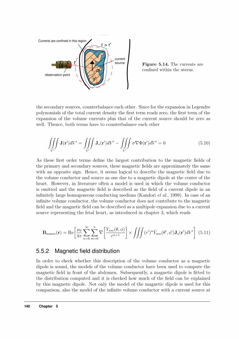
r'

r

Currents are confined in this region

current source

observation point

r > r'

Figure 5.14. The currents areconfined within the uterus.

the secondary sources, counterbalance each other. Since for the expansion in Legendrepolynomials of the total current density the first term reads zero, the first term of theexpansion of the volume currents plus that of the current source should be zero aswell. Thence, both terms have to counterbalance each other

∫∫∫V ′

J(r′)dV ′ =

∫∫∫V ′

Js(r′)dV ′ −

∫∫∫V ′

σ∇Φ(r′)dV ′ = 0 (5.10)

As these first order terms define the largest contribution to the magnetic fields ofthe primary and secondary sources, these magnetic fields are approximately the samewith an opposite sign. Hence, it seems logical to describe the magnetic field due tothe volume conductor and source as one due to a magnetic dipole at the center of theheart. However, in literature often a model is used in which the volume conductoris omitted and the magnetic field is described as the field of a current dipole in aninfinitely large homogeneous conducting medium (Kandori et al., 1999). In case of aninfinite volume conductor, the volume conductor does not contribute to the magneticfield and the magnetic field can be described as a multipole expansion due to a currentsource representing the fetal heart, as introduced in chapter 3, which reads

Bsource(r) = Re

[µ0

4π

∞∑n=0

n∑m=0

∇[Ynm(θ, φ)

rn+1

]×

∫∫∫(r′)nYnm(θ′, φ′)Js(r

′)dV ′]

(5.11)

5.5.2 Magnetic field distribution

In order to check whether this description of the volume conductor as a magneticdipole is sound, the models of the volume conductor have been used to compute themagnetic field in front of the abdomen. Subsequently, a magnetic dipole is fitted tothe distribution computed and it is checked how much of the field can be explainedby this magnetic dipole. Not only the model of the magnetic dipole is used for thiscomparison, also the model of the infinite volume conductor with a current source at

140 Chapter 5

the center. The magnetic dipole model reads

B =µ0

4π

[3(m · r)r‖r‖5 − m

‖r‖3

](5.12)

where m is the magnetic dipole moment and the current dipole model reads

B =µ0

4π

[Q× r

‖r3‖

](5.13)

where Q is the current dipole moment. Both models have been compared with thevolume conductor models. Both a magnetic dipole moment m and a current dipolemoment Q are fitted to the magnetic field of the volume conductor simulations usinga linear least squares optimalisation. The fit is performed using the magnetic fieldcomputed at 427 points, which are scattered in a cylindrical volume covering the ma-ternal abdomen and stretching 12 cm in the direction perpendicular to the abdominalwall. This is the region in which normally the measurements take place.In table 5.1 the results are shown. As both the magnetic field and the current dipoledo not fully describe the fields computed using the volume conductor model, both havebeen extended with the magnetic quadrupole moments and the current quadrupolemoments. The position of the fetal heart is taken as the origin of the multipoleexpansion. A linear least squares fit has been performed in order to obtain the dipoleand quadrupole moments in the multipole expansion. For this analysis the magneticfield component along the x-axis has been used. Although not depicted here, theanalysis showed similar results when using another component of the magnetic field.How well the multipole expansion model explains the magnetic field obtained by thevolume conductor model, is expressed by the amount of explained variance

explained variance =

n∑i=1

(Bx,i,volume conductor −Bx,i,multipole)2

n∑i=1

(Bx,volume conductor)2

(5.14)

In this equation Bx,i,volume conductor is the component of the magnetic field along thex-axis computed at position i. This measure describes how well the data can beexplained by the proposed model. When the explained variance approaches 1, itexplains most of the data, for lower values the model does not fit the data well.In the first column of table 5.1 the current dipole moment is given, which is usedin the volume conductor model for the forward computation of the magnetic field.The next column lists the magnetic dipole moment and the current dipole moment,which were fitted to the magnetic field distribution. The next two columns list, howwell the computed field can be described by a dipole or by a combination of dipoleand quadrupole. In both columns the fraction of the data, which is explained by the


Expl. Var. Expl. Var. AngleSource dipole Magnetic dipole dipole dipole+quadrp (degrees)

Model I(1,0,0) (-0.2,-0.72,0.67) 0.908 0.995 102(0,1,0) (0.49,0.049,0.87) 0.961 0.985 87(0,0,1) (-0.66,-0.74,0.096) 0.984 0.996 84

Model II(1,0,0) (-0.17,-0.28,-0.95) 0.762 0.992 100(0,1,0) (-0.19,-0.74,0.64) 0.731 0.974 138(0,0,1) (0.45,-0.67,0.59) 0.935 0.977 54

Model III(1,0,0) (-0.14,-0.95,-0.29) 0.622 0.995 98(0,1,0) (0.54,-0.014,0.84) 0.974 0.994 91(0,0,1) (-0.4,-0.69,0.6) 0.922 0.964 53

Model IV(1,0,0) (0.34,-0.93,0.13) 0.567 0.983 70(0,1,0) (0.49,-0.17,0.85) 0.923 0.976 100(0,0,1) (-0.3,-0.76,0.58) 0.819 0.985 55

Source dipole Current dipole

Model I(1,0,0) ( 0,0.7,0.71) 0.705 0.908 90(0,1,0) ( 0, 1,-0.041) 0.437 0.568 2(0,0,1) ( 0,0.15,0.99) 0.302 0.351 9

Model II(1,0,0) ( 0,-0.94,0.33) 0.666 0.924 90(0,1,0) ( 0,0.52,0.85) 0.478 0.884 58(0,0,1) ( 0,0.68,0.73) 0.489 0.61 43

Model III(1,0,0) ( 0,-0.28,0.96) 0.51 0.94 90(0,1,0) ( 0, 1,0.0025) 0.384 0.514 0(0,0,1) ( 0,0.66,0.75) 0.637 0.66 41

Model IV(1,0,0) ( 0,0.13,0.99) 0.338 0.814 90(0,1,0) ( 0,0.98,0.21) 0.379 0.572 12(0,0,1) ( 0,0.63,0.78) 0.573 0.826 39

Table 5.1. Results of fitting a magnetic dipole and a current dipole to the computed mag-netic fields of models I to IV. first column: the current dipole moment, which is usedin the volume conductor model for the forward computation of the magnetic field. sec-ond column: the magnetic/current dipole moment which was fitted to the magnetic fielddistribution. third and fourth column: the amount of variance explained by a mag-netic/current dipole or by a combination of magnetic/current dipole and quadrupole. fifthcolumn: the angle between the current dipole in the volume conductor model and themagnetic/current dipole moment of the expansion.

142 Chapter 5

Volume conductor Magnetic dipole Magnetic dipolesimulation and quadrupole

Current dipole Current dipoleand quadrupole

Figure 5.15. Magnetic field distribution due to a current dipole along the z-axis in ModelII. In the upper left corner the result of the volume conductor simulation is shown. Inthe upper right graphs are the distributions shown due to a magnetic dipole and due toa magnetic dipole in combination with a quadrupole. In the lower graph the distributionsdue to a current dipole in an infinite large medium and a current dipole together with aquadrupole are shown.

model, is given. The last column lists the angle between the current dipole in thevolume conductor model and the dipole moment of the expansion. As the magneticfield was fitted to the component of magnetic field along the x-axis, the current dipolemoment along this axis is always zero as it gives no contribution. Hence, for thecurrent dipole the fitted data for a dipole along the x-axis is always at an angle of90 degrees. In the expansion of the current dipole to higher order terms, the magneticdipole moments are omitted to allow for a fairer comparison.

For the four models in the third trimester, the magnetic dipole model explains about75 to 90 percent of the data, whereas the current dipole model often explains lessthan 50 percent of the data. Hence, the assumption that currents are confined withinthe uterus is justified. Including the magnetic quadrupole moments will increase theratio of explained data to a range of 97 to 99 percent of the data. Hence, the fieldsurrounding the maternal abdomen is shaped like that of a magnetic dipole plus amagnetic quadrupole. This result can be used for optimising the pickup-coil geometry.These field geometries should be used instead of the current dipole field, which wereused previously. Also, a comparison between different measurement systems for fetalMCG can be made based on the notion that the magnetic field is that of a magneticdipole and its quadrupole moments.


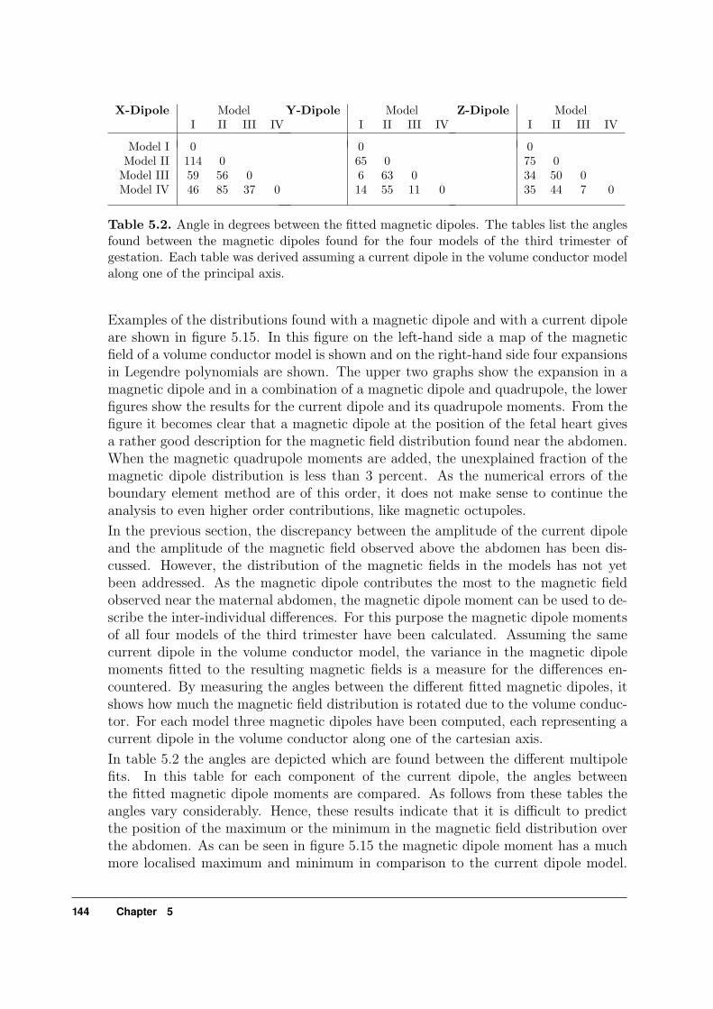
X-Dipole ModelI II III IV

Model I 0Model II 114 0

Model III 59 56 0Model IV 46 85 37 0

Y-Dipole ModelI II III IV

065 06 63 014 55 11 0

Z-Dipole ModelI II III IV

075 034 50 035 44 7 0

Table 5.2. Angle in degrees between the fitted magnetic dipoles. The tables list the anglesfound between the magnetic dipoles found for the four models of the third trimester ofgestation. Each table was derived assuming a current dipole in the volume conductor modelalong one of the principal axis.

Examples of the distributions found with a magnetic dipole and with a current dipoleare shown in figure 5.15. In this figure on the left-hand side a map of the magneticfield of a volume conductor model is shown and on the right-hand side four expansionsin Legendre polynomials are shown. The upper two graphs show the expansion in amagnetic dipole and in a combination of a magnetic dipole and quadrupole, the lowerfigures show the results for the current dipole and its quadrupole moments. From thefigure it becomes clear that a magnetic dipole at the position of the fetal heart givesa rather good description for the magnetic field distribution found near the abdomen.When the magnetic quadrupole moments are added, the unexplained fraction of themagnetic dipole distribution is less than 3 percent. As the numerical errors of theboundary element method are of this order, it does not make sense to continue theanalysis to even higher order contributions, like magnetic octupoles.

In the previous section, the discrepancy between the amplitude of the current dipoleand the amplitude of the magnetic field observed above the abdomen has been dis-cussed. However, the distribution of the magnetic fields in the models has not yetbeen addressed. As the magnetic dipole contributes the most to the magnetic fieldobserved near the maternal abdomen, the magnetic dipole moment can be used to de-scribe the inter-individual differences. For this purpose the magnetic dipole momentsof all four models of the third trimester have been calculated. Assuming the samecurrent dipole in the volume conductor model, the variance in the magnetic dipolemoments fitted to the resulting magnetic fields is a measure for the differences en-countered. By measuring the angles between the different fitted magnetic dipoles, itshows how much the magnetic field distribution is rotated due to the volume conduc-tor. For each model three magnetic dipoles have been computed, each representing acurrent dipole in the volume conductor along one of the cartesian axis.

In table 5.2 the angles are depicted which are found between the different multipolefits. In this table for each component of the current dipole, the angles betweenthe fitted magnetic dipole moments are compared. As follows from these tables theangles vary considerably. Hence, these results indicate that it is difficult to predictthe position of the maximum or the minimum in the magnetic field distribution overthe abdomen. As can be seen in figure 5.15 the magnetic dipole moment has a muchmore localised maximum and minimum in comparison to the current dipole model.

144 Chapter 5

Expl. Var. Expl. Var. AngleSource dipole Magnetic dipole dipole dipole+quadrp (degrees)

Model V(1,0,0) (0.051,-0.45,-0.89) 0.981 0.999 87(0,1,0) (0.54,-0.059,0.84) 0.986 0.997 93(0,0,1) (0.85,-0.52,0.017) 0.993 0.997 89

Model VI(1,0,0) (0.018,-0.98,0.18) 0.984 0.999 89(0,1,0) (0.8,-0.059,0.6) 0.975 0.989 93(0,0,1) (0.09,-0.94,0.32) 0.959 0.993 71

Model VII(1,0,0) (-0.17,-0.59,0.79) 0.98 0.997 100(0,1,0) (0.37,0.053,0.93) 0.985 0.995 87(0,0,1) (-0.5,-0.87,0.0071) 0.987 0.994 90

Source dipole Current dipole

Model V(1,0,0) ( 0,-0.89,0.45) 0.9 0.992 90(0,1,0) ( 0, 1,0.041) 0.415 0.503 2(0,0,1) ( 0,-0.0016, 1) 0.115 0.138 0

Model VI(1,0,0) ( 0,0.17,0.99) 0.929 0.997 90(0,1,0) ( 0, 1,0.098) 0.155 0.196 6(0,0,1) ( 0,0.31,0.95) 0.808 0.97 18

Model VII(1,0,0) ( 0,0.82,0.57) 0.851 0.932 90(0,1,0) ( 0, 1,-0.053) 0.61 0.727 3(0,0,1) ( 0,0.018, 1) 0.482 0.559 1

Table 5.3. Results of fitting a magnetic dipole and a current dipole to the computed mag-netic fields of models V to VII. first column: the current dipole moment, which is usedin the volume conductor model for the forward computation of the magnetic field. sec-ond column: the magnetic/current dipole moment which was fitted to the magnetic fielddistribution. third and fourth column: the amount of variance explained by a mag-netic/current dipole or by a combination of magnetic/current dipole and quadrupole. fifthcolumn: the angle between the current dipole in the volume conductor model and themagnetic/current dipole moment of the expansion.

Together with the large angles found between different volume conductors, this makesit difficult to predict a good measurement position over the abdomen.

When considering the models of the second trimester of gestation, similar results areobtained. In table 5.3 the explained fraction of the field by a magnetic and currentdipole are shown. The numbers are about equal in comparison to the model of thethird trimester. The only difference is that the angle between the different magneticdipoles and current dipoles is smaller. Hence, the prediction of a good measurementposition in this case is somewhat easier.


Mag. Dipole Mag. Dipole + Quadrup.Week of gestation Expl Var. Depth (m) Expl Var. Depth (m)

Measurement I 38 0.974 0.16 0.996 0.12Measurement II 42 0.948 0.11 0.990 0.10

Measurement III 38 0.874 0.15 0.985 0.19Measurement IV 36 0.976 0.11 0.985 0.09Measurement V 35 0.971 0.10 0.992 0.04

Cur. Dipole Cur. Dipole + Quadrup.Week of gestation Expl Var. Depth (m) Expl Var. Depth (m)

Measurement I 38 0.966 0.12 0.991 0.17Measurement II 42 0.903 0.08 0.987 0.14

Measurement III 38 0.847 0.12 0.972 0.14Measurement IV 36 0.78 0.10 0.905 0.09Measurement V 35 0.944 0.06 0.956 0.04

Table 5.4. Comparison between two magnetic field models and the observed magnetic field.The models are the expansion in a magnetic dipole and higher-order terms and the expansionin a current dipole and higher-order terms. Both the explained variance by the magneticfield model and the depth of the dipole that explains the distribution best are given.

5.6 Comparison between measurement and simulations

5.6.1 Fetal MCG maps

In order to validate some of the results obtained in the previous sections. The resultsare compared with measurements. In order to check the magnetic dipole description,fetal MCG maps measured at the Institute of Microtherapy in Bochum have beencompared with a magnetic field distribution due to a magnetic dipole. The fetalMCG maps have been obtained using a 61-channel system, which covers an area witha cross section of about 30 cm. Five of these maps obtained near the end of gestation(between 36 and 42 weeks of gestation) are used for comparison.

In order to fit a magnetic dipole distribution to the maps, a non-linear least squaresfit is made, in which the position and strength of the dipole and its higher-ordermoments are fitted to the measured distribution. In this least squares fit the linearparameters are fit using a standard projection matrix. This linear fit is done foreach position of the magnetic dipole and the position of this dipole is varied to findan overall minimum. In the latter optimalisation the Nelder-Mead simplex methodis used. The magnetic dipole is fitted for the time instant the R-peak shows themaximum amplitude. In order to extend the comparison to other models, a currentdipole in an infinite homogeneous medium was used as well. In table 5.4, the goodnessof fit is described by the fraction of explained variance by the model. In order to beable to estimate whether the fit is fair the depth of the dipole is given also.

From the data it becomes apparent that the magnetic dipole moment results in aslightly better description of the magnetic field. In the comparison the simulations

146 Chapter 5

Measurement Magnetic dipole Magnetic dipoleand quadrupole

Current dipole Current dipoleand quadrupole

Figure 5.16. Magnetic field distribution of measurement II. In the upper left corner themeasured field is shown. In the upper right graphs the distributions are shown due to amagnetic dipole and due magnetic dipole in combination with a quadrupole. In the lowergraph the distributions are shown due to a current dipole and a current dipole together witha quadrupole.

with the volume conductor models resulted in a large difference between the explainedfraction of the current dipole model and the magnetic dipole model. In these casesthe current dipole model is only slightly worse. However, both the current dipole andthe magnetic dipole model show a different location for the dipole. Hence, this isthe reason why the comparison resulted in different numbers, as both dipoles werethought to be at the center of the heart. Another difference is that the measurementtook place on a shell for which most measurements coils had an approximately equaldistance to the fetal heart. Hence, the measurement is not selective for the radialdependency of the magnetic field. Therefore, less distinction can be made between amagnetic dipole and a current dipole.

The depth of the fitted dipoles and quadrupoles changes when including the higherorder moments as well. For the magnetic dipole, except for measurement III, disre-garding the higher order moment leads to a deeper source. For the current dipolethe opposite effect is found and the inclusion of higher order terms leads to deepersources. However it is difficult to say which of these dipoles is closest to the real fetalheart position, as the distance between abdominal wall to the fetal heart ranges from8 cm to 15 cm. The latter numbers are estimates obtained by ultrasound. Hence, allmodels will fit the dipole in the range of where the fetal heart is.

In figure 5.16, the results are shown for measurement II. In the figure the measureddistribution and the fields due to a magnetic and current dipole are shown. In this


y-axis

z-axis

upper coil

lower coilfetal heart

cryostat

Figure 5.17. Overview of the measurementsetup in order to obtain the magnetic field asa function of the distance to the fetal heart. Inorder to fit a model on the measurements a lo-cal coordinate system is introduced consistingof a y and z-axis.

case there is a striking similarity between the field of a magnetic dipole and that of themeasurement. What can be noticed is that both the measurement and the magneticdipole distribution show a localised minimum, whereas for the current dipole model amore gradual change is seen from the minimum to the area where the magnetic fieldis almost zero. This feature is found for the other measurements as well, although notas strikingly as in this measurement.The measurements demonstrate that the magnetic field surrounding the abdomen canbe described by the field of a magnetic dipole and its quadrupole moments. Thence, forcomparison of different measurement systems using different fluxtransformer arrays,a decomposition into the magnetic dipole and its quadrupole would be sufficient.

5.6.2 Dependence on distance

In the previous section, the models were compared with a fetal MCG map in whichthe pickup-coils were approximately at the same distance from the fetal heart. Inorder to verify the magnetic field strength as a function of the distance from thefetal heart, another experiment has been performed. The magnetic field strength hasbeen measured as a function of the distance to the fetal heart. For this purpose ameasurement system was designed with two magnetometers, one at a fixed distancefrom the bottom of the cryostat, and another coil that was able to move along the axisof the cryostat, see figure 5.17. The lower coil is used to detect movements of the fetusbetween consecutive measurements of the fetal MCG. In case the fetus would move toa different position, this would imply a change of the fetal cardiac complex as found inthe lower coil. Hence, this coil will be used to ensure that the fetus did not move. Theupper coil is used to measure the dependence of the amplitude of the QRS-complexas a function of the distance. For this purpose seven fetal MCG measurements werecarried out for positions along the vertical axis. Each measurement took one minuteand the amplitude of the R-peak was determined after averaging all the fetal MCGcomplexes in this one minute measurement. During these measurements the fetus

148 Chapter 5

10 12 14 16 18 20 22 24 260

0.5

1

1.5

2

2.5

3 x 10-12

Mag

netic

fiel

d (T

)

Distance to fetal heart (cm)

Measurement Magnetic dipoleCurrent dipole

Figure 5.18. The magnetic fieldstrength as function of the dis-tance of the fetal heart. Thefigure includes as well a currentdipole and a magnetic dipole fit.

was at the same position as followed from measurements by means of the lower coiland hence the distance to the fetal heart is a reliable parameter. As the lower coilalso performed a measurement, a total of eight amplitudes were obtained. In orderto relate the amplitude dependence to the distance of the heart, the position of thefetal heart was determined using ultrasound. This position determination is accurateup to one or two centimeters and was performed before the measurement.

In figure 5.18, the R-peak amplitude as a function of distance to the heart is given.The measurement was obtained in a 34-week old fetus. In order to test the magneticdipole and the current dipole model, a second measurement of the dependence onthe distance was included but at another position above the abdomen. The lattermeasurement series was added as simulations revealed that fitting a current dipole ora magnetic dipole on a series of measurements that line up is not stable. Errors inthe range of 7 or 8 cm are expected for this case. Both the magnetic dipole and thecurrent dipole model could be fitted on the data explaining in both cases 98 percentof the variance in the measured magnetic fields. In order to test the stability ofthis solution, the amplitudes of the measured R-peaks were randomly altered by amaximum of 10 percent. This order of magnitude for the error was encountered whenvarying the number of complexes in a measurement used in the averaging process.The results of the fit are described in table 5.5. From these results it becomes clearthat the magnetic dipole is closer to the fetal heart and that its location is withinerror limits of where the fetal heart was located. The current dipole is shifted toa shallower position and more to the side of the abdomen. However both give anaccurate description of the magnetic field. That the current dipole is found at adifferent position in comparison with the fetal heart, also follows from figure 5.17.This reconstruction shows that the pickup-coil is more or less in alignment with thefetal heart, as a consequence only a small magnetic field is expected. In case of aperfect alignment no magnetic field would be observed for a current dipole model.As this measurement position proved to be one of the best places to measure a fetalMCG, the interpretation of the current dipole in an infinite homogeneous volume asbeing the current source in the fetal heart is not correct. This current dipole fit is a


position X (cm) Y (cm) Z (cm)

magnetic dipole -1.2±2.7 -4.9±2.2 +3.3±0.7current dipole +2.43± 3.0 -6.9±3.3 +0.8±1.4

fetal heart -3.0±1.5 -3.7±1 0±3

Table 5.5. The position of the fitted magnetic and current dipole in comparison with thelocalisation with ultrasound imaging. The standard deviation of the dipole fit was obtainedby adding 10 percent noise to the measurement. The latter amount is about the accuracywith which the amplitude of the QRS-complexes could be determined. The error limitson the ultrasound imaging was estimated based on the procedure followed to obtain thisposition.

mere parametric fit of the magnetic field of both the volume and the source currents.Although actual measurements can be nicely described by both a current dipole or amagnetic dipole, the simulations showed that these dipoles are only weakly correlatedto the source current dipole in the volume conductor. Hence, is seems tempting todescribe the fetal heart by one of both dipoles. However, since the field is heavilydependent on the volume conductor the expected spread in the dipoles is huge. Thisconfirmed by measurements conducted by Kandori et al. (1999) who fitted a currentdipole in a infinite half space to the fetal measurements they obtained. The lattermodel is similar to a dipole in an infinite volume conductor. The difference is thatin case of an infinite half space there is no contribution to the magnetic field of thecurrent dipole perpendicular to the half space. Their measurements show a largespread in amplitudes observed. Another disadvantage is that the current dipole inan infinite plane suggests that the fitted current dipole represents the current dipolewithin the fetal heart. However the simulations with the volume conductor modelclearly demonstrated that the current dipole representing the heart is underestimatedwhen this approach is followed, see for instance figure 5.10. The current dipole modelin an infinite conductor should be considered as parametric models, whose parametersdo only weakly link to the parameters of the fetal heart.

150 Chapter 5

Chapter 6

Database of normal values

In order to discriminate between pathological and healthy fetuses, reference values of theparameters describing the cardiac waveforms are needed. Commonly, the duration of theintracardiac time intervals are extracted from averaged fetal MCGs and are screened forany abnormal interval durations. Knowledge on these interval durations within the fetal car-diac waveform is scarce. Apart from fetal MCG recordings, these parameters are obtainedby means of fetal ECG measured using electrodes attached to the maternal abdomen(Brambati and Pardi, 1980), using ECG recordings in newborns (Hastreiter and Abella,1971), or using ECG recordings obtained during labour by means of a pair of electrodeswhere one is attached to the scalp of the child. In this chapter our effort is described tocollect and join the cardiac parameters measured at different centers involved in fetal MCGmeasurements (Stinstra et al., 2001b). The parameters collected include the duration ofthe P-wave, the PR-interval, the PQ-interval, the QRS-complex, the QT-interval and theT-wave.

6.1 The intracardiac time intervals

In the determination of reference values of the intracardiac time intervals five centersare involved, i.e. the Department of Biomagnetism of the Research and Develop-ment Center for Microtherapy in Bochum (Germany), the Departments of InternalMedicine II and Obstetrics and Gynecology and Pediatric Cardiology of the Univer-sity of Erlangen (Germany), the Biomagnetic Center and Department of Gynecologyand Obstetrics of the Friedrich Schiller University in Jena (Germany), and the De-partment of Pediatrics and the Institute of Clinical Medicine of the University ofTsukuba in Ibaraki (Japan). A total of 575 fetal MCGs have been used for the ex-traction of the intracardiac intervals. The MCGs were recorded in uncomplicatedpregnancies, which means that no maternal or fetal complications were noticeable.As the intracardiac time intervals are extracted from fetal MCGs measured at thevarious cooperating centers, they were obtained under different conditions, i.e. dif-ferent measurement arrays, flux transformers, magnetic field components, and signal

Database of normal values 151

-0.2 -0.1 0 0.1 0.2 0.3

PR

QT

PQRS

T

time (s)

Figure 6.1. Definition of the intracardiac time intervals. The P-interval is defined as theduration of the P-wave. The PR-interval is the duration from the start of the P-wave untilthe start of the QRS-complex. The PQ-interval is the duration from the end of P-wave untilthe start of the QRS-complex. The QRS-interval is the duration of the QRS-complex. TheQT-interval is the duration from the start of the QRS-complex until the end of the T-wave.The T-interval is the duration of the T-wave. In case the T-wave was biphasic the endingof the last wave (often referred to as U-wave) was taken as reference point.

processing techniques.Every intracardiac time interval recorded is extracted from an averaged fetal MCG,based on two to five minutes of fetal MCG data. Due to the lack of a reliable auto-mated algorithm for extracting the intracardiac time intervals from the averaged fetalMCGs, all centers extract the intracardiac time intervals manually. A definition ofthese time intervals is indicated in figure 6.1.As the QT-interval is dependent on the fetal heart rate, the mean RR-interval isincluded as well. To overcome this dependence on the fetal heart rate, Bazett’sformula (Bazett, 1920) is used to obtain the QTc, the corrected QT-interval. Bazett’sformula for the QTc reads (Bazett, 1920)

QTc =QT√

RRpreceding

(6.1)

As the fetal QT-interval is extracted from an averaged complex, the mean RR-intervalis taken instead of the preceding RR-interval. The reason that the QT-interval de-pends on the heart rate, is caused by the fact that the activation rate of the cardiaccells shortens the action potential duration (Berne and Levy, 1993).A complication is the definition of what is an uncomplicated pregnancy. For instance,Leuthold et al. (1999) included mothers with diabetes, gestational diabetes and lowamniotic fluid when the birth weight was normal. However, the thickness of thecardiac walls increases faster for fetuses of diabetic mothers than for normal fetuses

152 Chapter 6

15 20 25 30 35 40 450

10

20

30

40

50

60

70

80

90

Week of Gestation

Duration P−wave [ms]

Bochum ErlangenJena Twente

(a) Duration of the P-wave

15 20 25 30 35 40 450

20

40

60

80

100

120

140

160

180

Week of Gestation

Duration PR−Interval [ms]

Bochum ErlangenJena Tsukuba Twente

(b) Duration of the PR-interval

15 20 25 30 35 40 450

10

20

30

40

50

60

70

80

Week of Gestation

Duration QRS−Complex [ms]


(c) Duration of the QRS-complex

15 20 25 30 35 40 4540

60

80

100

120

140

160

180

200

Week of Gestation

Duration T−Wave [ms]

BochumTwente

(d) Duration of the T-wave

15 20 25 30 35 40 4550

100

150

200

250

300

350

Week of Gestation

Duration QT−Interval [ms]


(e) Duration of the QT-interval

15 20 25 30 35 40 450

0.1

0.2

0.3

0.4

0.5

0.6

Week of Gestation

QTc−value

Bochum ErlangenTsukuba Twente

(f) QTc-value

Figure 6.2. The duration of the various intracardiac time intervals against the week ofgestation. The gray lines mark the 90%, 95%, and 98% prediction interval.


irrespective of fetal size (Romanini et al., 1995) and therefore the duration of variouswaves may grow faster with gestational age than normally.

In order to make the data globally available, the data is pooled in a database,which can be consulted through the internet. This internet database is availableat http://bct.tn.utwente.nl/database and includes all individual data of the groupsreferred to, as well as data available from the literature.

6.2 Statistics

Posing a linear regression model, the dependence of the duration of the various timeintervals on the gestational week is analysed. Assuming that the data of the differentgroups are comparable, the influence of different measurement conditions is ignoredand the data of the different groups are pooled into one set of data. Assuming thatthe fetal age is the only independent parameter, the regression model reads

D = β0 + β1 × week + ε, ε ∼ N(0, σ) (6.2)

where D is the duration of the interval and ε the variability, having a normal distri-bution that is independent of the week. In reality the duration will be a function ofmore than one parameter, such as the diameter of the heart or the thickness of theheart wall and the heart rate. Including the latter in the regression model did increasethe explained variance only by a couple of percents and is therefore not included inthe model. No data is available on the other parameters. Hence, the data will beanalysed in regard to the fetal age, which is indirectly linked to parameters such asthe ones mentioned above.

The regression coefficients (β0 and β1) obtained by a least squares fit for the sevenintracardiac intervals and the QTc-value are given in table 6.1. In order to check howmuch of the variance in the data can be explained by the linear regression model ofequation 6.2, the correlation coefficient r2 is given as well. By means of the F-test itis checked whether the regression parameter (β1) is needed to explain the data, i.e.whether the duration is dependent on the fetal age. The outcome of this F-test isgiven in table 6.1 as well as the probability p of falsely rejecting the hypothesis thatonly β0 is sufficient to explain the data. When this probability is less than 1 percent,the hypothesis is rejected and a linear regression model is chosen, which includes thefetal age into the model. From the given probability values one can conclude that theduration of the P-wave, PR-interval, QRS-complex and QT-interval are dependent onthe fetal age, whereas the duration of the PQ-interval, the QTc-value and the T-waveare independent of the fetal age. However, looking at the correlation coefficient r2,only a small percentage of the variance in the data is explained by the inclusion of theweek of gestation into the model. For instance, for the QRS-complex only 36 percentof the variance is explained by the fetal age and for the P-wave only 24 percent. Incase of the T-wave and the QT-interval even a smaller fraction is explained, which may

154 Chapter 6

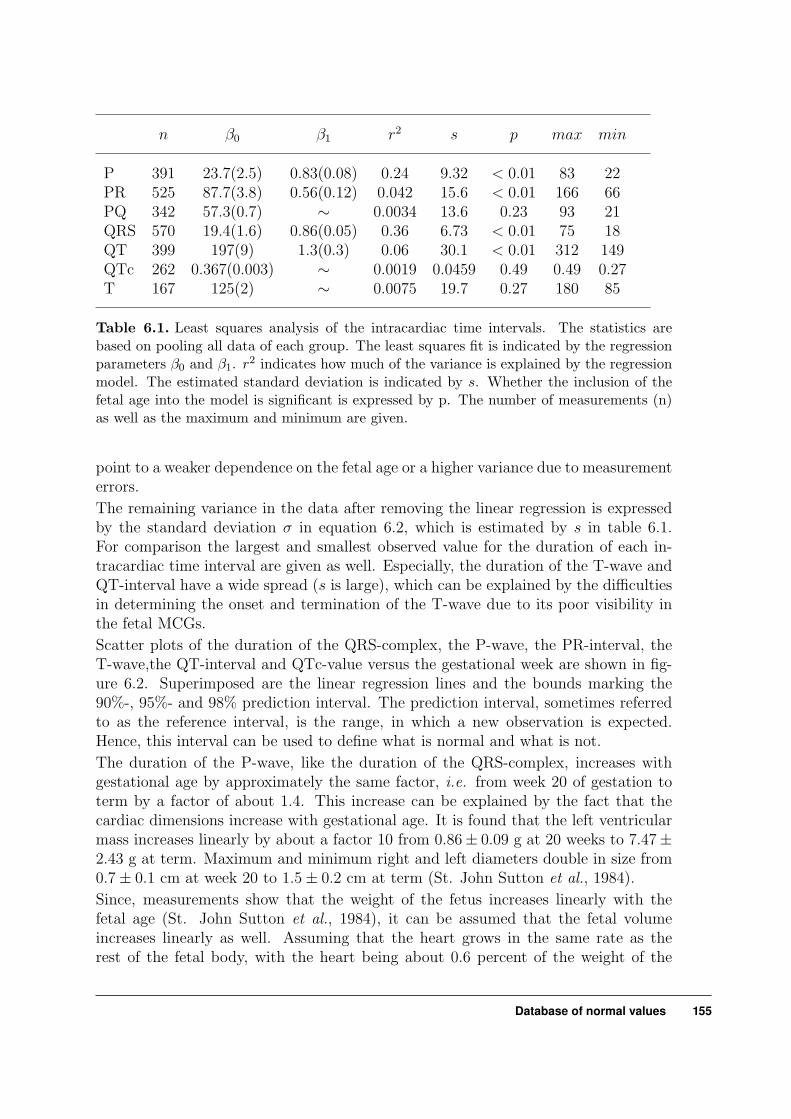
n β0 β1 r2 s p max min

P 391 23.7(2.5) 0.83(0.08) 0.24 9.32 < 0.01 83 22PR 525 87.7(3.8) 0.56(0.12) 0.042 15.6 < 0.01 166 66PQ 342 57.3(0.7) ∼ 0.0034 13.6 0.23 93 21QRS 570 19.4(1.6) 0.86(0.05) 0.36 6.73 < 0.01 75 18QT 399 197(9) 1.3(0.3) 0.06 30.1 < 0.01 312 149QTc 262 0.367(0.003) ∼ 0.0019 0.0459 0.49 0.49 0.27T 167 125(2) ∼ 0.0075 19.7 0.27 180 85

Table 6.1. Least squares analysis of the intracardiac time intervals. The statistics arebased on pooling all data of each group. The least squares fit is indicated by the regressionparameters β0 and β1. r2 indicates how much of the variance is explained by the regressionmodel. The estimated standard deviation is indicated by s. Whether the inclusion of thefetal age into the model is significant is expressed by p. The number of measurements (n)as well as the maximum and minimum are given.

point to a weaker dependence on the fetal age or a higher variance due to measurementerrors.

The remaining variance in the data after removing the linear regression is expressedby the standard deviation σ in equation 6.2, which is estimated by s in table 6.1.For comparison the largest and smallest observed value for the duration of each in-tracardiac time interval are given as well. Especially, the duration of the T-wave andQT-interval have a wide spread (s is large), which can be explained by the difficultiesin determining the onset and termination of the T-wave due to its poor visibility inthe fetal MCGs.

Scatter plots of the duration of the QRS-complex, the P-wave, the PR-interval, theT-wave,the QT-interval and QTc-value versus the gestational week are shown in fig-ure 6.2. Superimposed are the linear regression lines and the bounds marking the90%-, 95%- and 98% prediction interval. The prediction interval, sometimes referredto as the reference interval, is the range, in which a new observation is expected.Hence, this interval can be used to define what is normal and what is not.

The duration of the P-wave, like the duration of the QRS-complex, increases withgestational age by approximately the same factor, i.e. from week 20 of gestation toterm by a factor of about 1.4. This increase can be explained by the fact that thecardiac dimensions increase with gestational age. It is found that the left ventricularmass increases linearly by about a factor 10 from 0.86± 0.09 g at 20 weeks to 7.47±2.43 g at term. Maximum and minimum right and left diameters double in size from0.7± 0.1 cm at week 20 to 1.5± 0.2 cm at term (St. John Sutton et al., 1984).

Since, measurements show that the weight of the fetus increases linearly with thefetal age (St. John Sutton et al., 1984), it can be assumed that the fetal volumeincreases linearly as well. Assuming that the heart grows in the same rate as therest of the fetal body, with the heart being about 0.6 percent of the weight of the


fetus (van Wezel-Meijler et al., 1997), the dimensions of the heart wall should increaseby approximately the cubic root of the fetal age. Both the duration of the P-wave andthe QRS-complex are thought to be linear dependent on the diameter of the heartwall. Therefore, based on this assumption one might prefer a model which reads,

D = α0 + α1 × week13 + ε (6.3)

However, taking into account that the intracardiac time intervals are obtained betweenthe 20th and 40th week of gestation, this function may be linearised as follows

D = α0 + α1

[20

13 +

4013 − 20

13

40− 20(week − 20)

]+ ε (6.4)

The relative error made by substituting equation 6.4 for equation 6.3 is about onepercent. This means that without any prior knowledge on which set of regressioncoefficients is preferred, both models can be used to describe the duration of theQRS-complex and P-wave. The linear relation between fetal weight and fetal age isin fact a linear fit on the measured data, simplifying an even more complex situation.The linear model will be used to describe the dependency of the duration of theP-wave and QRS-complex on the week of gestation.Although the duration of the QT-interval is slightly increasing with fetal age, the QTc-value, which is corrected for the duration of the RR-interval, is not dependent on thefetal age. Apparently, the duration of the QT-interval is not noticeable influencedby an increase in the dimensions of the fetal heart, but only by the fetal heart rate,which decreases as the fetus grows older and increases the QT duration.In the preceding, it was assumed that the influence of the cooperating research groupswas negligible. However inspecting figures 6.2(a) and 6.2(b) suggests a considerableinfluence. To elucidate this dependence, the 98%-prediction intervals for both theduration of the QRS-complex and the P-wave have been plotted for each researchgroup in figure 6.3. The regression coefficients for each group are listed in table 6.2.Whereas in case of the QRS-complex most lines coincide, in case of the P-wave boththe inclination as well as the spread of the data show a wide variation, resulting in alarge overall spread. However in this case the overall statistics do not fit the individualcases.

6.3 Comparison with previously measured data

Fetal MCG is not the only method for obtaining the intracardiac time intervals. Inthe literature also values obtained by means of fetal ECG can be found. Also ECGs ofprematurely born children may provide values for comparison. In the latter case, thequestion remains whether these children can be considered healthy. Another sourceof values of the durations of the intracardiac time intervals, are the ECGs obtainedduring labour and shortly after labour. As during labour, the fetus experiences a lotof stress and may be for instance aenemic, this may alter the durations of the various

156 Chapter 6

15 20 25 30 35 40 450

10

20

30

40

50

60

70

80

Week of Gestation

Duration QRS−Complex [ms]


(a) QRS-interval

15 20 25 30 35 40 450

10

20

30

40

50

60

70

80

90

Week of Gestation

Duration P−Complex [ms]

Bochum ErlangenJena Twente

(b) P-interval

Figure 6.3. The prediction intervals of the various groups vs gestational age. The coloredlines indicate the 99-percentile, the least squares fit and the 1-percentile, whereas the blacklines indicate the overall prediction interval.

QRS-complex P-wave

group β0 β1 β0 β1

Bochum 17.2± 1.8 1.00± 0.06 11.7± 2.3 1.42± 0.08Erlangen 12.7± 4.7 1.05± 0.15 24.1± 6.4 0.55± 0.20Jena 19.6± 2.8 0.75± 0.08 26.2± 4.6 0.71± 0.13Tsukuba 13.0± 4.2 1.11± 0.12Twente 19.0± 13.5 0.94± 0.39 −9.6± 12.5 1.70± 0.36

Table 6.2. Regression coefficients for the different research groups

intracardiac time intervals. Schwartz et al. (1998) measured the postnatal ECG inthe third or fourth day after birth, because they observed that the ECG is stable inthis period.

6.3.1 Measurements during gestationIn figure 6.4 a comparison of the duration of the various intracardiac time intervalswith values previously reported in literature is made. The values found in literaturecomprise values for the QRS-complex, the PR-interval, the QT-interval and the QTc-values. The regression line, which was fitted to the data in the previous section,is indicated by the black line and the individual measurements by the grey dots.The 98 percent prediction interval and the 98 percent confidence interval for thecollected data are given by the thin gray lines. Brambati and Pardi (1980) obtainedthe durations of the QRS-complex from fetal ECGs. They measured a total of 421 fetal


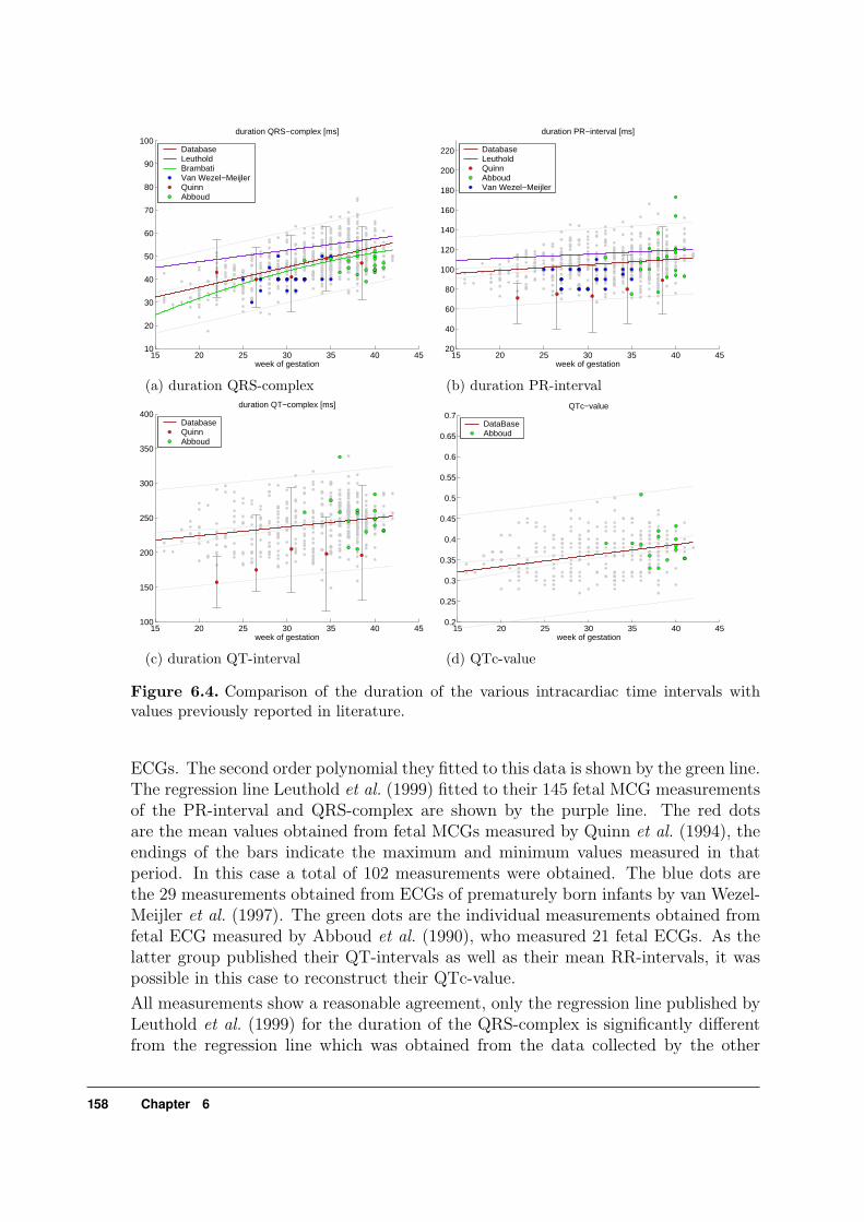
15 20 25 30 35 40 4510

20

30

40

50

60

70

80

90

100

week of gestation

duration QRS−complex [ms]

Database Leuthold Brambati Van Wezel−MeijlerQuinn Abboud

(a) duration QRS-complex

15 20 25 30 35 40 4520

40

60

80

100

120

140

160

180

200

220

week of gestation

duration PR−interval [ms]

Database Leuthold Quinn Abboud Van Wezel−Meijler

(b) duration PR-interval

15 20 25 30 35 40 45100

150

200

250

300

350

400

week of gestation

duration QT−complex [ms]

DatabaseQuinn Abboud

(c) duration QT-interval

15 20 25 30 35 40 450.2

0.25

0.3

0.35

0.4

0.45

0.5

0.55

0.6

0.65

0.7

week of gestation

QTc−value

DataBaseAbboud

(d) QTc-value

Figure 6.4. Comparison of the duration of the various intracardiac time intervals withvalues previously reported in literature.

ECGs. The second order polynomial they fitted to this data is shown by the green line.The regression line Leuthold et al. (1999) fitted to their 145 fetal MCG measurementsof the PR-interval and QRS-complex are shown by the purple line. The red dotsare the mean values obtained from fetal MCGs measured by Quinn et al. (1994), theendings of the bars indicate the maximum and minimum values measured in thatperiod. In this case a total of 102 measurements were obtained. The blue dots arethe 29 measurements obtained from ECGs of prematurely born infants by van Wezel-Meijler et al. (1997). The green dots are the individual measurements obtained fromfetal ECG measured by Abboud et al. (1990), who measured 21 fetal ECGs. As thelatter group published their QT-intervals as well as their mean RR-intervals, it waspossible in this case to reconstruct their QTc-value.

All measurements show a reasonable agreement, only the regression line published byLeuthold et al. (1999) for the duration of the QRS-complex is significantly differentfrom the regression line which was obtained from the data collected by the other

158 Chapter 6

fetal MCG postnatal ECG postnatal ECG

mean SD n mean SD n mean SD nP-wave 56 10 84 592 10 126PR-interval 109 16 110 1131 13 13442 1082 15 126PQ-interval 57 16 73 492 12 126QRS-complex 52 8 113 571 7 13442 622 9 126QT-interval 243 27 100 2741 28 13442 2842 50 126QTc-value 0.37 0.04 46 0.4001 0.002 13442T-wave 131 20 21

Table 6.3. Comparison between the means of the intracardiac time intervals during the38th week until the 41st week of gestation and postnatal ECGs and the ECGs recordedduring labour. 1ECG of mature newborn infants, recorded during the third or fourth dayafter birth (Schwartz et al., 1998). 2ECG of mature newborn infants 1-7 days after birth(DePasquale and Burch, 1963)

groups. The values of the PR-interval obtained from Quinn et al. (1994) and thedata obtained from Leuthold et al. (1999) are significantly different from the meanobtained in the previous section. The QT-intervals and the values of the QTc obtainedfrom fetal ECGs measured in 21 fetuses by Abboud et al. (1990) agree within onestandard deviation. However, the duration of the QT-interval as measured by Quinnet al. (1994) by means of fetal MCG is significantly lower.Brambati and Pardi (1980) found a linear relationship between the duration of QRS-complex and the weight at birth. The average birth weight may differ between thecooperating centers, as it depends for instance on the sex, the ethnic group, the factthat the mother smokes or the fact that the country has a high altitude (Gardosiet al., 1994). Also the PR-interval and QT-interval increase linearly with gestationalage, as is the case during normal development after birth.Janse et al. (1976) measured the duration of the PR-interval in three isolated heartsof fetuses in the 12th-16th week of gestation. In their experiments they artificiallystimulated the atria and measured when the ventricles were activated as a functionof the pace in which the atria were triggered. Their values of 85-100 ms agree withours.

6.3.2 Postnatal ECG and ECG during labour

In table 6.3, a comparison is made between the values obtained in the last weeks ofgestation (week 38-41) by means of fetal MCG and those values obtained postna-tally or during gestation. Comparing the durations of the various waves of fetuses inweek 38-41 with those measured in newborns shows that these values agree withinone standard deviation. Comparing the duration of the QRS-complex found in thedatabase (figure 6.2) with those obtained from fetal ECG during labour shows thatboth are in agreement. Hence, although the blood flow through the heart has altered


from a system where the pulmonary system is mainly bypassed and an additionalpathway exists between both atria to a normal double looped system, it has no im-mediate influence on the intracardiac time intervals recorded. The durations of thevarious waves are also measured during labor. By attaching a pair of electrodes tothe scalp of the child and a reference electrode to the maternal thigh an ECG ofthe child is measured. Marvell et al. (1980) measured the duration of the P-waveand the PR-interval. They devised an average P-wave duration of 52±10 ms andan average PR-interval of 103±10 ms (n=37). They measured also the duration ofthe QRS-complex, however they defined this duration as the interval between Q-peakand S-peak. For this interval they found a value of 31 ms, which is less than theaverage found in the database, but the difference is mainly due to the definition ofthe interval. The P-interval and PR-interval values do coincide with the values foundin the database.

6.4 Factors influencing intracardiac time intervals

6.4.1 Different measurement systems

As the data was gathered at different centers, the magnetometer systems variedconsiderably, from multi-channel magnetometer systems to a one-channel vector-gradiometer system. A multi-channel system usually measures the magnetic fieldcomponent perpendicular to the maternal abdomen at several positions over the ma-ternal abdomen, simultaneously. A one-channel vectorgradiometer measures all threecomponents of the magnetic field at one position over the maternal abdomen. Thedrawback of the systems covering only a small part of the abdomen, is that the mea-surement position might not be ideal, resulting in a poor signal-to-noise ratio. Inorder to cope with this drawback, the system is repositioned to look for the optimalmeasuring position, which is in general the position where a prominent QRS-complexis seen in the time trace. In other words, this is not necessarily a position with a highsignal-to-noise ratio for the P-wave or T-wave. At the University of Erlangen twodifferent 37-channel systems were used, at the Biomagnetism Center in Bochum a 37-channel system and recently a 67-channel system and at the University of Tsukuba a32-channel system measuring two components of the magnetic field at 16 positions ora 9-channel system measuring 3 components and at the Friedrich Schiller Universityin Jena a 31-channel system and at the University of Twente a homemade 19-channelsystem or a one-channel vector-gradiometer.

A question that arises when using a multi-channel system, is which channel to usefor the determination of the various intracardiac time intervals. Van Leeuwen etal. (2001a) showed that the determination of the duration of the P-wave may differby an amount of about 20 ms for two different channels separated by about 15 cmfrom each other. In this case the component of the magnetic field perpendicular tothe maternal abdomen was measured. The more channels were included in the deter-mination of the duration of the P-wave, the longer the P-wave interval became (van

160 Chapter 6

Figure 6.5. Fetal MCG of a 29-week-old fe-tus measured by a 1-channel vector-gradiometer,see chapter 1. The vertical lines indicate wherethe P-wave and the QRS-complex start andend. The grey line indicates how the durationof the P-wave was estimated, if only the upperchannel would have been used.

-0.1 -0.05 0 0.05 0.1 0.15 0.2 0.25

QRSP

P

time (s)

Leeuwen et al., 2001b). A similar inaccuracy was observed using the one-channel vec-torgradiometer system. In figure 6.5 an example is given in which the three measuredcomponents of the magnetic field are shown. When estimating the duration of theP-wave based on the middle channel, a duration of 63 ms is found, when the upperchannel is used only a duration of 29 ms is found. The difference between both is34 ms. Using the same measurement a difference in QRS-duration of 10 ms can befound. Apart from this measurement three other measurements were performed at adifferent positions over the maternal abdomen, in these cases smaller differences werefound between the different channels. One way to reduce this problem is taking intoaccount all the channels available and not relying on one channel for the determina-tion of the duration of the various waves. The procedure to be followed should detectthe first onset of a P-wave in whatever channel this occurs and should measure thetime interval until in none of the channels a P-wave can be observed.The P-wave and the QRS-complex can be easily identified in averaged fetal MCGs,whereas the detection of the T-wave is difficult. The beginning of the T-wave is oftenhardly definable, as it may be biphasic and its shape varies from channel to channel.

6.4.2 Interpretation of waveforms

Another important factor is the subjective interpretation of the complexes. All groupsuse a manual inspection of the complexes for extracting the intracardiac time inter-vals. Because everyone interprets the data differently small differences occur. Forinstance, it is difficult to determine where a P-wave starts especially when the base-line is noisy. In order to examine how accurate the interpretation is, three observershave interpreted about 40 fetal MCGs, measuring their intracardiac time intervals.The difference in their interpretation results in the order of magnitude this subjec-tive interpretation has. All three observers work at Biomagnetic Center Twente andthence influence each other in the interpretation and thence are not fully independent


n P (ms) PQ (ms) PR (ms) QRS (ms) QT (ms) T (ms)

Mean ± Standard deviationObs 1 ⇔ Obs 2 47 2±5 -3±7 -1±5 2±4 19±13 11±19Obs 1 ⇔ Obs 3 29 2±8 -4±10 -3±8 6±4 32±21 24±18Obs 2 ⇔ Obs 3 23 1±10 0±11 1±8 -2±7 10±10 16±20

MedianObs 1 ⇔ Obs 2 47 1 -2 0 1 20 17Obs 1 ⇔ Obs 3 29 3 -5 -3 0 30 20Obs 2 ⇔ Obs 3 23 -2 0 -1 -2 8 12

Table 6.4. Difference in measured intracardiac time intervals. The mean, the median andstandard deviation of the differences between the durations of the intervals measured bytwo observers are depicted. Here, n indicates the number of measurements that that wasused for the analysis (a T-wave was not observed for each measurement).

observers.In table 6.4, the mean, the median and the standard deviation of the differencesbetween the interval durations measured by two observers are given. In this table,the results obtained by one observer are compared with those obtained by the othertwo. For the QRS-complexes these differences are the smallest, although the numbersstill suggest a wide variance in the observed values. A difference of 10 ms in theobserved value can be easily accounted for by the subjectivity of the interpretation.A systematic error of a few milliseconds is found for most intervals and a randomerror of about 8 ms. In case of the QT-interval and the T-duration the interpretationis more subjective and large differences occur. An error in the order of 30 ms is notunusual. The latter accounts for the wide spread in the observed values. Becausethe T-waves are small in amplitude and start and end smoothly, they are difficultto discern from noise, leading to many different interpretations on where the T-wavestarts and ends. All these measurements used in this survey were obtained with thevectorgradiometer in the Biomagnetic Center Twente and do depend on the signal-to-noise ratio of that system. For the determination of the starting point and terminationof the P-wave and the QRS-complex van Leeuwen et al. (2001a) obtained a mediandifference between two observers of about 1 ms. These results are similar to thedifferences found between observer 1 and 2.

6.4.3 Filters

As shown in chapter 2, a filter can alter the shape of a PQRST-complex and thence thedurations of the intracardiac time intervals. For instance, applying a high-pass maytrigger an impulse response on a QRS-complex and broaden the complex. However,the results of chapter 2 suggest that filters can be applied with minimal distortion.The interval durations are prolonged or shortened by a few milliseconds due to the

162 Chapter 6

filters. However for P or T-waves that start or end very smoothly, the filters mayalter the appearance of the complexes, because after removing most of the noise it iseasier to determine the onset and termination of the wave. The latter may lead to adifferent estimation of the duration of the complex.

6.4.4 Physiology

Changes in the P-wave morphology have been reported during decelerations in thefetal heart rate. Decelerations usually are absent in the third trimester in case ofa healthy fetus. The interval between the ending of the P-wave to the beginningof the QRS-complex is variable and depends on the duration of the P-wave. If thisinterval is short it is most often due to a long P-wave with a normal PR-interval.The PR-interval of children normally increases with age and decreases with heartrate. A common cause for a short PR-interval in a normal heart is a low right atrialpacemaker. The PR-interval fluctuates as a result of variations in the conductiontime of the AV-node (Heethaar, 1972). These fluctuations give rise to trigger jitter,which in turn effects the morphology of the averaged fetal MCG in the same way asa low-pass filter (Rompelman, 1987; Woolfson et al., 1990), resulting in a longer P-wave. Under normal physiological conditions it is found that the RR-interval and thePR-interval are positive related (Symonds, 1994). The fetal heart rate is characterizedby a normal baseline frequency of 110-150 bpm. A baseline variability of more than10 bpm and presence of acceleration in relation to fetal movements is regarded as asign of fetal well being (van Woerden and van Geijn, 1994). Factors that may influencethe fetal heart rate are fetal age, the behavioral state, the fact that the mother is insupine position. During quiet sleep the fetal heart rate hardly changes (bandwidth7 bpm), the bandwidth increases during breathing movements.

Moreover, the spread in the intracardiac time intervals, is mainly due to the inter-pretation of the complexes and the fact that some fluxtransformer arrays are “blind”to a current dipole in a certain direction, hereby underestimating the duration of acomplex. In order to minimise the differences due to the fluxtransformer array, oneshould estimate the duration of the intervals based on all channels available. In orderto overcome the differences with the manual interpretation an automated algorithm(see for instance, Marvell and Kirk, 1980a) may be developed, which estimates theduration of the intervals.

6.5 Application of intracardiac time intervals

In the previous section a wide spread in the time intervals was observed. Thence,this leads to a large prediction interval. This means that only values that differsubstantially from the mean can be indicated as being abnormal. For these referencevalues to be useful in the diagnosis, congenital heart defects or abnormalities in theelectrical conduction system of the fetal heart should coincide with abnormal intervals


exceeding the prediction interval based on the reference values, e.g. exceeding the 99-percentile. Although the intervals of healthy and pathological fetuses may have adifferent mean value, when both have a large overlap in the distribution of theirvalues, it renders the evaluation of the intracardiac time intervals ineffective in thediagnosis for certain heart diseases. The usefulness of the intracardiac time intervalsanalysis will be illustrated in the next sections by means of a few examples.In order to express the deviation from the reference values, it is assumed that the errorε is normally distributed. This allows for estimating the likelihood of an encounteredvalue. This likelihood is expressed by the chance p that the observed value is largerthan the value expected in case the pregnancy was uncomplicated. Hence, p reads

p = P(Dinterval < β0 + β1 × week) (6.5)

Moreover if a p value of 0.99 is found the value must be on the 99-percentile. Thisdefinition was used for the QRS-complex and the QT-interval, where the regressionlines of the different centers coincided, as was concluded in section 6.2. For the P-wave and the PR-interval, all the centers show a different regression line, i.e. boththe constant and the linear parameter differ substantially. Hence, the data sets arenot combined into one set, but the observed values are compared with the individualregression line of each center and the center, which comes closest to explaining thedata is chosen for comparison. In this case the definition of p reads

p = mini

[ P(D < β0,i + β1,i × week) ] for D > β0,i + β1,i × week

p = maxi

[ P(D < β0,i + β1,i × week) ] for D < β0,i + β1,i × week (6.6)

p = 0.50 for all other cases

In this equation β0,i and β1,i refer to the regression coefficients of each individual re-search group. In this comparison with individual centers the Twente data is discarded,as not enough reference values were available for a reliable comparison. However asthe regression line of our data falls between the other regression lines for the gesta-tional period of 27 weeks until term, there is no apparent reason for the intracardiacintervals to exceed the range of the other centers in case more measurements weretaken.

6.5.1 The duration of the P-waveFetal conditions that coincided with abnormal durations of the P-wave are the con-genital complete AV-block and the fetal atrial flutter. In both cases a dissociation ofatrial and ventricular rate takes place. For a more elaborate description of these casessee chapter 7. Measuring the duration of the P-wave in two atrial flutter cases andfour third degree AV-block cases, a significant increase in P-wave duration was found,see table 6.5. In this table both the durations of the P-waves and the probabilities p

164 Chapter 6

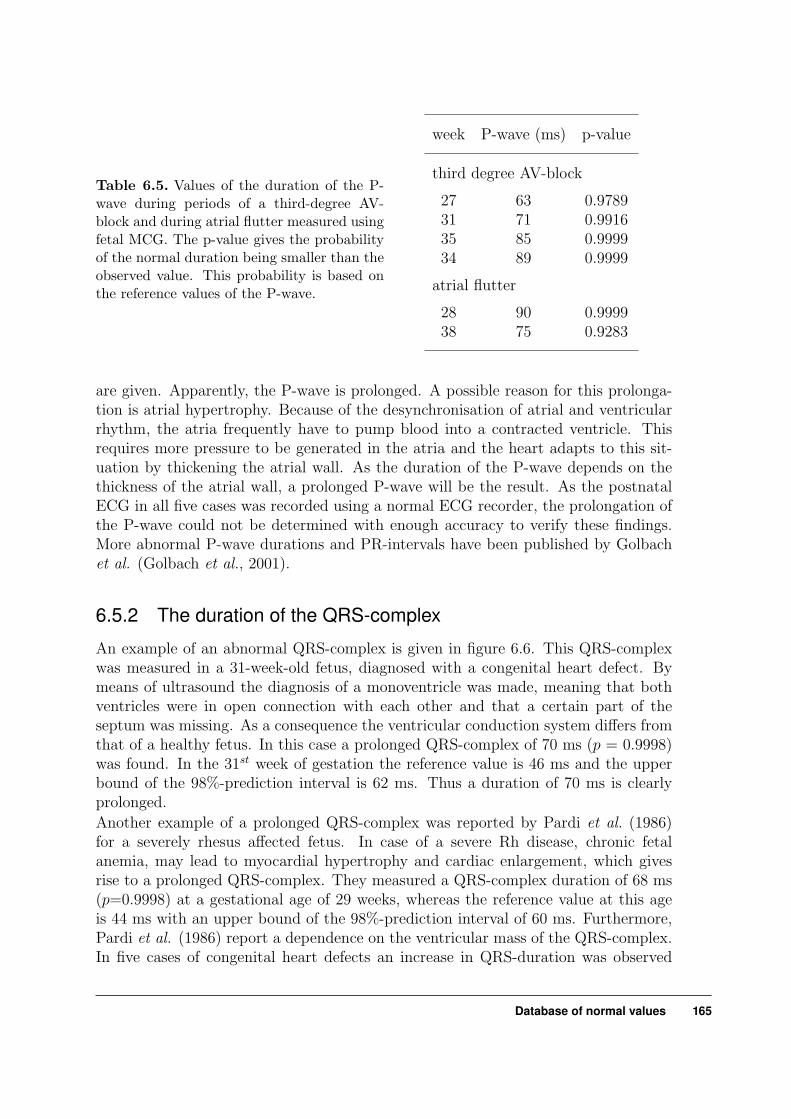
Table 6.5. Values of the duration of the P-wave during periods of a third-degree AV-block and during atrial flutter measured usingfetal MCG. The p-value gives the probabilityof the normal duration being smaller than theobserved value. This probability is based onthe reference values of the P-wave.

week P-wave (ms) p-value

third degree AV-block

27 63 0.978931 71 0.991635 85 0.999934 89 0.9999

atrial flutter

28 90 0.999938 75 0.9283

are given. Apparently, the P-wave is prolonged. A possible reason for this prolonga-tion is atrial hypertrophy. Because of the desynchronisation of atrial and ventricularrhythm, the atria frequently have to pump blood into a contracted ventricle. Thisrequires more pressure to be generated in the atria and the heart adapts to this sit-uation by thickening the atrial wall. As the duration of the P-wave depends on thethickness of the atrial wall, a prolonged P-wave will be the result. As the postnatalECG in all five cases was recorded using a normal ECG recorder, the prolongation ofthe P-wave could not be determined with enough accuracy to verify these findings.More abnormal P-wave durations and PR-intervals have been published by Golbachet al. (Golbach et al., 2001).

6.5.2 The duration of the QRS-complex

An example of an abnormal QRS-complex is given in figure 6.6. This QRS-complexwas measured in a 31-week-old fetus, diagnosed with a congenital heart defect. Bymeans of ultrasound the diagnosis of a monoventricle was made, meaning that bothventricles were in open connection with each other and that a certain part of theseptum was missing. As a consequence the ventricular conduction system differs fromthat of a healthy fetus. In this case a prolonged QRS-complex of 70 ms (p = 0.9998)was found. In the 31st week of gestation the reference value is 46 ms and the upperbound of the 98%-prediction interval is 62 ms. Thus a duration of 70 ms is clearlyprolonged.

Another example of a prolonged QRS-complex was reported by Pardi et al. (1986)for a severely rhesus affected fetus. In case of a severe Rh disease, chronic fetalanemia, may lead to myocardial hypertrophy and cardiac enlargement, which givesrise to a prolonged QRS-complex. They measured a QRS-complex duration of 68 ms(p=0.9998) at a gestational age of 29 weeks, whereas the reference value at this ageis 44 ms with an upper bound of the 98%-prediction interval of 60 ms. Furthermore,Pardi et al. (1986) report a dependence on the ventricular mass of the QRS-complex.In five cases of congenital heart defects an increase in QRS-duration was observed


-0.2 -0.1 0 0.1 0.2

QRS = 70 ms

Monoventricle

time (s)

Figure 6.6. Average fetal MCG obtained in afetus diagnosed with monoventricle (31 weeks).The prolonged duration of the QRS-complexis indicated. The average was obtained using180 complexes.

-0.2 0 0.2 0.4 0.6time (s)

QT = 394 ms

393

Figure 6.7. Average fetal MCG obtained ina fetus diagnosed with a persistent bradycar-dia (27 weeks). The prolonged QT-interval(including U-wave) is indicated. The averagewas obtained using 243 complexes.

and in four other cases the congenital heart defect accounts for smaller ventricularmasses and as a consequence these values belong to the observations with the lowestdurations of the QRS-complex. However, all of these observations are within thedetermined 95%-prediction interval.

Another possible application for the determination of the duration of the QRS-complex, is the detection of fetal growth retardation. Van Leeuwen et al. (2001a)showed that the mean QRS-duration of 9 intra-uterine growth retarded fetuses is sig-nificantly different from their control group (n = 172). However, their data show thatonly a few of the individual measurements exceed the 98%-prediction interval. Apartfrom the growth retarded fetuses, they showed that the duration of the QRS-complexof twins is shortened as well, however not as severe as the growth retarded fetuses.The same observation was made for the duration of the P-wave for both twins andgrowth retarded fetuses.

6.5.3 The duration of the QT-interval

The idiopathic long-QT-syndrome is a congenital disease often with a familial trans-mission characterised by a prolonged QT-interval and is thought to be associated

166 Chapter 6

with the sudden infant death syndrome (Schwartz et al., 1993). The condition isoften accompanied by the occurrence of life-threatening tachyarrhythmia or brady-cardia (Surawicz, 1992). In a multicenter study in Italy (Schwartz et al., 1998), halfof the newborns who died of the sudden infant death syndrome, were suffering from aprolonged QT-interval in the postnatal ECG. As the T-wave is difficult to distinguisheven in the postnatal ECG and a clear definition of when the QTc is prolonged islacking, Schwartz et al. (1993) drew a list of secondary diagnostic criteria to enablethe diagnosis of what has become known as the long-QT-syndrome. Secondary crite-ria include the existence of a tachy- or bradycardia or the unexplained cardiac deathof family member at an early age. In the last couple of years, several genetic defectshave been located that are associated with the presence of the long-QT-syndrome. Forinstance, long-QT-type III is associated with genetic defects in the genes that decodethe sodium channels of the cardiac cells (Augustus, 2001). As these ionic channelsplay an important role in depolarising and repolarising the cardiac cells, flaws in theinactivation mechanism of these ionic channels may prolong the depolarised state ofthe cell, prolonging the QT-interval or even trigger arrhythmia. The latter are thoughtto be caused by early afterdepolaristions of the cardiac cells (Clancy and Rudy, 1999)and may lead to ventricular tachycardia or even ventricular fibrilation, which rendersthis condition life-threatening.

Hamada et al. (1999) were able to diagnose a long-QT-syndrome in the 37th week of

gestation using fetal MCG. The QTc-value measured by Hamada et al. was 0.57 s12

(p = 0.999), which according to the durations given in figure 6.2(f) is clearly pro-longed. A second report on prenatal detection of a long-QT-syndrome is given byMenendez et al. (2000), who measured two cases with a QTc-value of 0.54 and 0.51-

0.57 s12 (p > 0.98).

During our research only one case of prolonged QT interval was encountered. Awoman in her 27th week of gestation referred to the Biomagnetic Center Twenteafter ultrasound analysis demonstrated a persistent bradycardia, showed a prolongedQT-interval with a QTc-value of at least 0.53 s

12 (p = 0.998). Several fetal MCGs

were recorded using a 1-channel vector-gradiometer, confirming the presence of thebradycardia. The averages obtained from all recordings showed a small T-wave with aprolonged QT-interval showing QTc-values of about 0.53 and more. As the ending ofthe U-wave was difficult to obtain, a cautious estimate was made in which the durationof the QT-interval was rather underestimated than overestimated. An example of suchan average is shown in figure 6.7. In comparison with the reference database all valuesobtained from the measurements showed a prolonged QT and therefore the diagnosisof long-QT-syndrome was issued. Postnatal examination did confirm this finding,however a compelling diagnosis in this case has not yet been made on the basis of thepostnatal ECG.

Up till now, a possible case of long-QT-syndrome, could only be suspected by means ofthe detection of unexplainable fetal arrhythmia using ultrasound, as fetal arrhythmiaoften coincide with the long-QT-syndrome. Hence, the determination of the QTc-value prenatally is presently only possible by means of fetal MCG. As presently thecause of the long-QT-syndrome is not always clear and diagnosis relies on the detection


of several symptoms associated with the disease, the prenatal detection of prolongedQT-intervals may help the early detection of fetuses at risk for sudden cardiac death.Moreover, if fetal MCG becomes available in the clinic, prenatal screening of prolongedQT-intervals may help to determine which fetuses are at risk and these children maybe born in centers with expertise in pediatric cardiology. As the mechanisms behindthe prolongation of the QT interval are beginning to be understood, treatments andmedicine may follow.

168 Chapter 6

Chapter 7

The classification of arrhythmia by fetalmagnetocardiography

So far fetal magnetocardiography has been discussed in the light of the healthy fetus. Thischapter will illustrate the diagnostic value of the fetal magnetocardiogram by means offour types of arrhythmias. Apart from the detection, it is also important to classify the ar-rhythmia. The four cases discussed are a complete atrioventricular block, an atrial flutter,a case of premature atrial contractions and a bundle branch block. The first two condi-tions are rarely seen, whereas premature atrial contractions are considered to be morecommon. The arrhythmia will be classified and the diagnosis will be compared with thepostnatal evaluation. After a case-wise description of the arrhythmias and the correspond-ing measurements, fetal magnetocardiography is evaluated in its ability to obtain a reliablediagnosis.

7.1 Fetal arrhythmia

The most common fetal arrhythmia is an irregular rhythm due to isolated extrasys-toles, in particular premature atrial contractions. Premature beats are beats thatoccur earlier than expected and briefly interrupt the normal sinus rhythm. Thesearrhythmias rarely cause hemodynamic problems and often disappear before term orwithin a few days after birth. However about one percent of the fetuses having prema-ture atrial contractions, have a concomitant structural heart disease as well and about0.5 percent of these fetuses are found to develop a reentrant tachycardia later on in thepregnancy (Friedman et al., 1993). Van Leeuwen et al. (1999) observed different typesof abnormal heart rates in about half of 155 fetal magnetocardiography recordings.These arrhythmias included supraventricular and ventricular ectopic beats as well asbradycardia and tachycardia. In another study by Richards and Southall (1979) usingechocardiography in 963 fetuses in week 36 to 40 of gestation an incidence of 1.9%was found for bradycardia and 0.5% for tachycardia. Strasburger (2000) estimates theincidence of malignant arrhythmias to be 1:5000 pregnancies. The fetal heart rate isconsidered normal when the heart rate is between 100 bpm and 160 bpm (Friedman

The classification of arrhythmia by fetal magnetocardiography 169

et al., 1993). Tachycardia are considered mild when the baseline rate is between 160and 180 bpm and severe when it exceeds 180 bpm. The rhythm is considered to be abradycardia when the fetal heart rate falls below 100 bpm. Depending on the originof the tachycardias they are divided in supraventricular and ventricular tachycardia.Ventricular tachycardia are rarely observed in the fetus, whereas supraventriculartachycardia are more common. About two-thirds of the fetal arrhythmias are foundin the last trimester of pregnancy (Strasburger, 2000).

As arrhythmias come in different forms, from innocent to life threatening, the clas-sification is crucial to the treatment. It may, for instance, help in the determinationof which drugs to use in order to restore the fetal heart to normal sinus rhythm. Asthe recent advances in prenatal heart monitoring start to unleash their possibilities indetecting arrhythmias, such treatments are currently under investigation. Choosinga therapy appropriate to the arrhythmia reduces the chance of causing accelerationsof the fetal heart rate or the chance of degeneration to a life-threatening arrhythmia(Kleinman et al., 1985). For this reason, it is important to know the origin of atachycardia. In case it is supraventricular, one may for example use the drug digoxinto treat the arrhythmia, however in case of a ventricular origin, this therapy couldpotentially exacerbate the arrhythmia (Clark and Case, 1990). Another reason for adiagnosis as precise as possible is that intra-uterine pharmacologic treatment involvesthe administration of the cardiac medicine to the mother. This involves exposing themother to potential side effects these potent agents have.

In the next sections the classification of four types of arrhythmias will be discussedand demonstrated. The arrhythmias in these four patients were first discovered duringa routine ultrasound investigation. Subsequently, fetal magnetocardiography was ap-plied in order to test its ability to scrutinize the origin of the arrhythmia. In each caseabout five measurements of two to three minutes were taken, the best recording wassubsequently taken for further analysis. In this case the best recording refers to thatrecording that shows the largest QRS-complexes in combination with the abnormalitywe were looking for, like additional P-waves.

7.2 Complete atrioventricular block

This section describes the use of fetal magnetocardiography in patients with a congen-ital complete atrioventricular block, a condition that is manifest in one of 20,000 livebirths (Somville and Morgenstern, 1994; Michaelsson and Engle, 1972), but probablytwice as much in utero (Ferrer, 1998). Three types of AV-blocks are distinguished, thefirst degree AV-block refers to a slow conduction of the depolarisation front throughthe AV-node. In a second degree AV-block only one out of several depolarisationfronts is conducted through the AV-node, thence the ventricles are stimulated onlyonce for several atrial beats. A complete, or third degree, AV-block refers to a con-dition of the heart, in which the depolarisation front is not conducted through theAV-node and as a consequence the ventricles are not activated by the electrical im-pulse traveling down the atria. The heart compensates for this loss by triggering

170 Chapter 7

the depolarisation of the ventricles using an independent pacemaker in the ventricles.Hence, this condition reveals itself by an independent pace of the atrial and ventric-ular contraction. The atria contract at a normal rate as they are triggered by theSA-node, however the pacemaker in the ventricles is often more slowly, compromis-ing the fetal cardiac output and thereby the fetal condition (Michaelsson and Engle,1972). This disease is either associated with structural cardiac abnormalities or thepresence of maternal antibodies in relation to a maternal connective tissue disorderlike systemic lupus erythematosus (McCue et al., 1977; Clark and Case, 1990). Thelatter relation is thought to be caused by an inflammatory process in the heart dueto transplacental transfer of maternal auto-antibodies (anti-Ro and anti-La) from the14th or 16th week of gestation onward (Rosenthal et al., 1998). In this process muscletissue at the location of the AV-node is replaced by granulation tissue. It is thoughtthat from this time on the AV-block progresses into a third degree block, for instanceCopel et al. (1995) found in one patient a progression from a second degree AV-blockinto a complete AV-block. However in two other cases they observed an improvementfrom a second degree AV-block into normal sinus rhythm and an improvement froma third degree AV-block to a second degree AV-block. In both cases the motherswere treated with 4 mg of dexamethasone in order to stop the inflammatory processin the fetal heart. Hence a second degree AV-block may still be reversed to normalsinus rhythm and information on the progression towards a complete AV-block maylead to an understanding of how these patients have to be treated. Especially, thosechildren showing a slow ventricular rate (50 bpm or less) are at risk and often requirethe implantation of a pacemaker shortly after birth (Michaelsson and Engle, 1972).

Currently, the prenatal detection of a complete AV-block is obtained from ultrasoundimages. As the mechanical contraction of the heart can be monitored step-by-stepon a modern ultrasound machine, a complete AV-block shows up as a desynchronisedcontraction of the atria and ventricles. By obtaining a four-chamber view of thefetal heart showing both ventricles and atria the contraction rate of both can becompared and a desynchronised rhythm can be demonstrated (Fouron et al., 2000).However, this detection still relies on the mechanical action of the heart to detect adisorder in the electrical conduction system of the heart. Furthermore, the detectionof a fetal AV-block by means of ultrasound is difficult, especially the classification ofthe type of block. Therefore fetal magnetocardiography may provide an alternativeto detect this condition, as it directly relates to the electrical phenomena takingplace in the heart. Using fetal electrocardiography as a means to detect a fetal AV-block is often not feasible, because the signal-to-noise ratio is poor and it is usuallyimpossible to distinguish the P-wave in the raw data trace, which complicates theprecise interpretation of the signals, in particular the classification of a third degreecongenital atrioventricular block (Brambati and Pardi, 1980). The detection of acomplete AV-block by means of fetal magnetocardiography has been described beforeby Wakai et al. (2000a) and Menendez et al. (2001). Wakai et al. depicted onlythe overall atrial and ventricular rates of one case. Menendez et al. report theobservation of three complete AV-blocks and two second degree ones. Hosono et al.(2001) reported a case of complete AV-block measured in the 32nd week and performed


0 10 20 30 40 50 60 70 80 90 1000

200

400

600

800

1000R

R In

terv

al (m

s)

time (s)

2:1 complete

Atria

Ventricles

(a) Fetal Heart Rate. Upper trace shows the RR-interval against time and the lower tracethe PP-interval

(b) Time trace during the period of second degree AV-block

(c) Time trace during the period of complete AV-block

Figure 7.1. Fetal heart rate and time traces of a 35-week old fetus showing the progressionof a second degree AV-block into a complete (third degree) AV-block

a direct fetal ECG with needles attached to the fetus confirming the fetal MCG.

Four cases of fetal complete congenital AV-block were encountered since the startof fetal magnetocardiographic recordings in the Biomagnetic Center Twente. All ofthem were diagnosed with an AV-block of a certain degree (not necessarily a completeAV-block) using echocardiography previously to the magnetocardiogram recording.Later postnatal electrocardiography confirmed the diagnosis of a complete AV-block(Quartero et al., 2001). In this section the case of one patient will be discussed. This

172 Chapter 7

-0.2 -0.1 0 0.1 0.2 0.3 0.4time (s)

P PQRS

(a) Average during the period of seconddegree AV-block

-0.2 -0.1 0 0.1 0.2 0.3 0.4time (s)

QRS

(b) Average during the period of completeAV-block

Figure 7.2. Averages triggered on the R-peaks during the period of second degree AV-blockand complete AV-block

patient was referred to the local hospital Medisch Spectrum Twente in the 27th weekof gestation with a persistent fetal bradycardia. With ultrasound a complete AV-block was diagnosed and SS-B antibodies were found. A fetal magnetocardiogramwas measured in week 35 of gestation. The child was born at a gestational age of38 weeks and the complete AV-block was confirmed.In order to distinguish P-waves in the time traces, the fetal magnetocardiogram traceswere filtered using a band-pass filter from 2 to 120 Hz. After subtraction of thematernal PQRST-complexes, fetal QRS-complexes and P-waves could be observed inthe time traces. However, not all P-waves could be seen in these traces. To enhancethe detection of the P-waves, the best channels were summed to cancel even morenoise and a stronger band-pass filter was applied for visual inspection. After thesemeasures, it was possible to detect the individual P-waves. The fetal QRS-complexeswere subtracted in the summed channel to allow the detection of the P-waves usingan automated algorithm, as discussed in chapter 2. About 95 percent of the P-wavescould be identified this way, the others had to be detected manually.In figure 7.1(a), the ventricular and atrial rate during 100 s of the measurement areshown. In this figure an abrupt change in ventricular and atrial rate can be observed.In the first period of 40 s, the P-waves and QRS-complexes are coupled with a meanRR-interval of 77 bpm and a mean PP-interval of 154 bpm, suggesting a two to oneblock, see figure 7.1(b), whereas during the next 60 s, they are uncoupled with anentirely irregular PR-interval, suggesting complete AV-block, see figure 7.1(c). Theaveraged signals were calculated using the R-peak for the alignment of the complexes.Figure 7.2 shows the averaged complexes. When a P-wave was found in the averagedsignal, it was concluded that the P-wave and R-peak were coupled in time. Note thattwo P-waves were found, one preceding the QRS-complex and one following it, clearlyshowing the presence of two P-waves for each QRS-complex. When no P-wave wasfound, it was concluded that the P-wave and R-peak were uncoupled in time.The change in atrioventricular conduction (from a second to a third degree AV-block)


0 0.1 0.2 0.3 0.4 0.5 0.6 0.7time (s)

10 complexes20 complexes30 complexes40 complexes50 complexes

(a) Averages during the period of seconddegree AV-block

0 0.1 0.2 0.3 0.4 0.5 0.6 0.7time (s)

10 complexes20 complexes30 complexes40 complexes50 complexes

(b) Averages during the period of completeAV-block

Figure 7.3. The average as function of the number of complexes.

coincided with a change of the ventricular rhythm from 77 bpm to a rate of 62 bpm. Asimilar change in atrial rate was observed from 152 bpm to 130 bpm. The variabilityof the ventricular rate was less than the atrial one and the atrial variability showeda larger variability during the second degree AV-block. The duration of the QRS-complex was 58 ms and the duration of the P-wave was 85 ms, during the periodwith a complete AV-block. The P-to-QRS amplitude ratio was 0.31, which is largein comparison to the ratio normally observed. The duration is clearly prolonged(p=0.999) and may indicate a certain degree of atrial hypertrophy, see chapter 6.The patient was born at full term with a normal intracardiac anatomy, with an atrialrate of 136 bpm and a ventricular rate of 64 bpm. No pacemaker was necessary.

In order to determine how many complexes are needed in the averaging procedure fordetecting, whether the P-wave is coupled to the QRS-complex or not, five averageshave been computed from respectively 10, 20, 30, 40 and 50 complexes. The complexeshave been computed for both the uncoupled and the coupled case. The results aredepicted in figure 7.3. From these graphs it becomes apparent that 20 complexes arealready sufficient for discriminating between both cases. However more complexeswill enhance the signal-to-noise ratio of the averages.

In the other cases of complete AV-block it was possible to detect the P-waves in thetime traces from the 27th week onward. An earlier attempt to detect P-waves in the25th week of gestation was unsuccessful and averages using the R-peaks as triggers onlyrevealed that no P-waves could be observed, which may in it self point to a completeAV-block, especially in combination with the observed bradycardia. However, even foruncomplicated pregnancies measurements taken before the 27th week of gestation, donot always show a P-wave in the average as the P-wave is obscured by environmentalnoise.

174 Chapter 7

7.3 Atrial flutter

Atrial flutter, a potentially lethal arrhythmia (Lisowski et al., 2000), is an uncommonform of a supraventricular tachycardia constituting one to two percent of all fetalarrhythmias (Calvin et al., 1992; Friedman et al., 1993). It may occur in normalindividuals, however, there is usually an underlying heart disease. It is a reentrantsupraventricular tachycardia with an atrial rate of more than 250 bpm. The ventric-ular rhythm is most often regular and not as fast as the atrial rate with a varyingdegree of AV-block, usually 2:1. However, the ventricular rate is usually above the200 bpm (Strasburger, 2000). Postnatally, this arrhythmia displays an electrocar-diogram showing typical flutter waves with a sawtooth-like pattern superimposed onthe baseline of the ECG. This pattern consists of a fast sequence of atrial depolari-sations and the succeeding repolarisations. Due to reentry of the atrial impulse intothe atrial wall, the atrial depolarisation front travels up and down the atria in a cir-cular perpetual motion, reactivating itself after completing one cycle. Prenatally, anechocardiographic diagnosis of atrial flutter is usually made on the basis of an atrialcontraction rate in the range of 300 to 500 bpm. This atrial rate is determined usingM-mode echocardiography, while the ventricular rate is determined with the use ofM-mode and echo Doppler. One case of atrial flutter is described by Menendez etal. (2001). Blumenthal et al. (1968) describe a case of fetal atrial flutter detected bymeans of fetal ECG. However the lack of details in the averaged fetal ECGs, rendersthe technique not reliable for the detection of P-waves and thus the detection of fetalflutter may be difficult. Recently, Oudijk et al. (2000) found a conversion rate of 80percent for atrial flutter with Sotalol and this may become the in utero treatment.

In total two cases of atrial flutter were encountered in our group. Both cases werereferred to the Biomagnetic Center Twente after routine ultrasound analysis revealeda severe intermittent tachycardia of a fetal heart rate of 280 and 230 bpm, respectively.One patient had a fetal MCG recording in the 32nd week of gestation and the other inthe 36th and 37th week of gestation. All fetal MCG recordings were able to demonstratethe existence of a fetal atrial flutter. One case will be presented in this section.

In the patient, episodes of tachycardia were discovered in the 36th week of pregnancyduring a routine prenatal evaluation by the obstetrician. Ultrasound analysis showedno evidence of fetal structural anomalies, particularly no cardiac anomalies. Thus far,the pregnancy had been uncomplicated. Fetal magnetocardiograms were obtained inweeks 36 and 37 of gestation. The patient was referred to the hospital in the 38th

week of gestation, where the existence of a fetal atrial flutter was diagnosed by meansof echocardiography. An atrial rate of 400 bpm was observed and a ventricular rateof 280 bpm. No signs of congestive heart failure or hydrops fetalis were noticed.

In order to distinguish P-waves in the time traces, the same procedure as in the case ofthe congenital complete AV-blocks was chosen. The fetal magnetocardiogram traceswere filtered using a band-pass filter from 2 to 120 Hz. Subsequently, the maternalcomplexes were subtracted and to enhance the detection of the P-waves the bestchannels were summed. After these measures it was possible to detect the individualP-waves in the time traces. In figure 7.4(a) the fetal heart rate is displayed, showing


0 50 100 150 200 250 3000

200

400

600

800

1000R

R In

terv

al (m

s)

time (s)

(a) Fetal Heart Rate

(b) Time trace during sinus rhythm

(c) Time trace during atrial flutter

(d) Time trace during sinus rhythm with a short interval of atrial flutter

Figure 7.4. Fetal magnetocardiogram heart rate and time traces of a 36-week old fetusdiagnosed with periods of atrial flutter

176 Chapter 7

-0.3 -0.2 -0.1 0 0.1 0.2 0.3time (s)

(a) Average during atrial flutter

-0.3 -0.2 -0.1 0 0.1 0.2 0.3time (s)

(b) Average during normal sinus rhythm

Figure 7.5. Averages during atrial flutter and sinus rhythm

periods of the RR-interval of about 400 ms as well as abrupt changes to episodes ofabout 200 ms, the latter corresponds to a fetal heart rate of about 240 bpm. Hence,the arrhythmia is a severe intermittent tachyarrhythmia. Examples of time tracesduring three different episodes are given in figures 7.4(b), 7.4(c) and 7.4(d). The firsttrace, figure 7.4(b), shows a heart rate during a period of normal sinus rhythm ofabout 150 bpm, whereas figure 7.4(c) corresponds to a period of atrial flutter witha tachycardia of about 240 bpm. In the latter time trace flutter waves are present,whereas in the former trace only one P-wave is preceding every QRS-complex. Thethird time trace shows normal sinus rhythm interrupted by a short period of fetalflutter of about 12 flutter waves interrupted by abnormal QRS-complexes. Theseabnormal QRS-complexes are most probably ventricular extrasystoles. A ventricularextrasystole occurs when the normal activation of the ventricles is interrupted by anactivation within the ventricle itself. This results in abnormal looking ventricularcomplexes that once in a while disturb the normal pattern, not preceded by a P-wave.However in this case it is difficult to determine whether the atrial activity triggers theventricular activity, as the atrial flutter is present.

In order to improve the visibility of the atrial flutter waves averaged heart complexestriggered on R-peaks are constructed. The mechanism of the atrial flutter imposes acertain degree of AV-block in the AV-conduction system. It is therefore expected thatthe flutter waves are correlated with the QRS-complexes in the rhythm. Whenever theatrial rhythm is stable, this correlation to the ventricular rhythm should produce anaverage in which both the atrial flutter waves are present as well as the QRS-complex.Hence, the signal is divided into episodes of suspected atrial flutter and normal sinusrhythm. The R-peaks in each episode are detected and subsequently an average of700 ms for each episode is calculated. The length of this average is chosen in such waythat multiple QRS-complexes are visible in the averaged complexes, making it easierto judge the degree of AV-block. An average during an episode of tachycardia (intervalof 100-180 s) is shown in figure 7.5(a). The first and third QRS-complex shown are


seemingly smaller than the middle one. This is due to the averaging procedure andcan be explained by the fact the RR-interval is not perfectly regular during thisepisode of atrial flutter resulting in a slightly broadening of the QRS-complex anda smaller amplitude, see chapter 2. The averaged fetal MCG shows waves that aretypical for atrial flutter. For each QRS-complex two P-waves are seen (2:1 AV-block)with a mean RR-interval of 253 ms and PP-interval of 122 ms. The duration of theP-wave itself is 75 ms (p=0.928), which is slightly prolonged. Like in the case of theatrioventricular block, the observed P-to-QRS ratio is about 0.25, which is large incomparison to the values observed for healthy fetuses. The average calculated usingthe PQRST-waveforms in the interval of 0-80 s during the episode of normal sinusrhythm is shown in figure 7.5(b). In this figure no atrial flutter waves nor a 2:1AV-block are present. Hence, the conclusion of normal sinus rhythm is confirmed.At 39 weeks of gestation a child was born with a regular sinus rhythm alternatedwith episodes of atrial flutter and a 2:1 AV-block. Ventricular rhythm varied between200 and 250 bpm. Sotalol was given as a treatment and the episodes of tachycardiadiminished. Finally, the patient had a sinus rhythm of 130 bpm.

7.4 Premature atrial contractions

The most common fetal arrhythmia is an irregular rhythm due to isolated extrasys-toles, particularly premature atrial contractions. Premature beats are beats that occurearlier than expected and briefly interrupt the normal sinus rhythm. Premature beatsoften originate from the atria, within the myocardium but outside the SA-node, i.e.premature atrial contraction, near the AV-node junction, i.e. premature junctionalbeats, or from the ventricle i.e. premature ventricular contraction. Most prematureatrial contractions are detected in the last trimester of gestation and are found in oneto three percent of the pregnancies, they resolve within the first month of extrauterinelife (Strasburger, 2000).

Several cases of fetal premature atrial contractions were found. In this section, acase of premature atrial contractions will be described. During repeated ultrasoundevaluations premature fetal heart beats were observed. No evidence of structural fetalanomalies was found. Fetal MCG was performed at 38 weeks of gestation. The fetalheart rate, measured during this recording, is shown in figure 7.6(a). The RR-rateis about 130 bpm and very irregular. Time traces during two different intervals aredepicted in figures 7.6(b) and 7.6(c). The rhythm as shown in figure 7.6(b) can bedescribed as two normal beats (numbered 1 and 2) followed by a premature atrialcontraction (labeled 3) followed by a compensatory pause after which the patternrepeats. Once in a while the pattern is interrupted by abnormal complexes, as shownin figure 7.6(c). These abnormal beats are probably ventricular extra systoles, i.e.ventricular depolarisation waves triggered by a pacemaker in the ventricles and not bythe AV-node. This explains why these beats are not preceded by a P-wave and showa prolonged duration. These kind of extrasystoles are encountered once in a while. Inthree out of the seven cases of premature atrial contractions, premature ventricular

178 Chapter 7

50 100 150 200 250 3000

200

400

600

800

1000

RR

-inte

rval

(ms)

time (s)

(a) Fetal Heart Rate

(b) Example time trace 1

(c) Example time trace 2

(d) Postnatal ECG time trace

Figure 7.6. Fetal magnetocardiogram heart rate and time traces of a 38-week old fetusdiagnosed with premature atrial contractions as well as a postnatal ECG trace


-0.4 -0.2 0 0.2 0.4time (s)

(a) Average of the beats indicated by 1

-0.4 -0.2 0 0.2 0.4time (s)

(b) Average of the beats indicated by 3

Figure 7.7. Averages obtained by separately averaging the first and third beats in therepeating pattern

contractions are observed, whereas postnatally only four percent of patients with ec-topic beats are found to have premature ventricular contractions (Strasburger, 2000).

The time traces shown are processed in a similar way as the two previous examples andin this case the P-waves are hardly discernible in the time traces. In order to checkwhether the QRS-complexes are indeed preceded by a P-wave, thereby confirmingthe supraventricular origin, the cardiac complexes numbered 1, 2, and 3 are averagedseparately. The results are shown in figure 7.7. In figure 7.7(a) the average of thebeats labeled 1 are shown and in figure 7.7(b) the beats labeled 3. The average ofthe beats labeled 2 is equal to the average of the beats numbered 1, and thereforenot depicted. However a different shape and polarity of the P-wave is found in thelast average. Therefore, the premature atrial beats originate from somewhere outsidethe SA-node, as the P-wave has a different shape and polarity. The diagnosis of apremature atrial contraction is thereby confirmed.

A boy was born after 39 weeks of pregnancy. A postnatal ECG was made 4 daysafter delivery showing a normal sinus rhythm alternated with some premature atrialcontractions followed by a normal QRS-complex and a compensatory pause 7.6(d).No abnormal complexes were found.

In other cases of premature atrial contractions, the P-waves were hardly distinguish-able and averaging was needed to confirm the diagnosis. For instance, averaging allbeats followed by a compensatory pause in a case where R-peaks seemed to be miss-ing the rhythm, revealed a premature P-wave too premature to trigger a ventricularcontraction (Quartero et al., 2001).

7.5 Bundle branch block

An unusual arrhythmia had been observed during a routine investigation by ultra-sound in the 24th week of gestation in a woman, who consumed three liters of coca-coladaily as a pregnancy habit. Some beats seemed to succeed each other inexplicably

180 Chapter 7

0 10 20 30 40 50 60 70 80 900

200

400

600

800

1000

RR

Inte

rval

(ms)

time (s)

Figure 7.8. Fetal MCG heart rate, showing a tachycardia

fast. In order to classify this very irregular rhythm, a fetal magnetocardiogram hasbeen recorded in the 24th week of gestation. The fetal heart rate, which is derivedfrom the fetal magnetocardiogram, is shown in figure 7.8. In this figure the sameinexplicably fast rhythm is found. This rhythm is inexplicably fast, as the refractoryperiod of the cardiac cells in the ventricles should be at least 200 ms (Janse et al.,1976). In figure 7.8 this minimum interval between ventricular stimulation has beenindicated by the dotted line. In order to find the cause of this arrhythmia, more fetalmagnetocardiograms were made during the pregnancy.

After discontinuing the daily intake of three liters of cola, the arrhythmias disap-peared. Fetal magnetocardiography was repeated in the 34th and 39th week of gesta-tion, see figure 7.9 and only a regular rhythm was observed. A fetal electrocardiogramwas recorded simultaneously with the fetal MCG as well during the last session. Al-though the signal-to-noise ratio of the electrocardiogram measured by means of elec-trodes attached to the maternal abdomen was very low, an averaged signal could beextracted using time information obtained from the fetal magnetocardiogram. Neona-tal electrocardiograms were recorded immediately after birth and two weeks later.

In figure 7.10, averaged complexes of the recorded magnetocardiograms and electro-cardiogram are shown. In case of the fetal magnetocardiogram recorded during the24th week of gestation, only those beats were averaged that were part of the regularsinus rhythm, separated from the previous and next QRS-complex by about 400 ms.The averages of both the magnetocardiograms and the electrocardiograms show anenlarged QRS-complex duration. The QRS-complex durations are indicated in fig-ure 7.10. Comparing these values with the normal values found in chapter 6, thesevalues exceed the 99-percentile. Thence this prolongation is significant. Apart fromthe length, the shape of the QRS-complexes is unusual as well, because an additionalpeak is seen in the QRS-complex. This additional peak is especially noticeable in theaverage of the electrocardiogram.

Such a prolonged and notched QRS-complex generally refers to an additional pathwaybetween the atria and the ventricles bypassing the AV-node or to a block in the left or


(a) Time trace magnetocardiogram in week 24

(b) Time trace magnetocardiogram in week 34

(c) Time trace magnetocardiogram in week 37

(d) Time trace electrocardiogram in week 37

Figure 7.9. Time traces of the magnetocardiogram and electrocardiogram measured atthree different time instances during gestation

right bundle branch within the ventricles. In the first case the ventricles are stimulatedthrough an additional pathway, i.e. the bundle of Kent, preceding the stimulationof the ventricles through the AV-node, causing the ventricular depolarisation frontto start at a different position and not through the fast tract of the His-bundle. Inthe latter case the depolarisation front is not conducted along one of the two bundlebranches, which inhibits a fast conduction of the depolarisation front through one ofthe ventricles. A distinction between both cases is often made on the shape of bothcomplexes and the duration of the PR-interval. However the normal values of the

182 Chapter 7

-0.2 -0.1 0 0.1 0.2 0.3time (s)

(a) MCG Average in week 26

-0.2 -0.1 0 0.1 0.2 0.3time (s)

(b) MCG average in week 34

-0.2 -0.1 0 0.1 0.2 0.3time (s)

(c) MCG Average in week 39

-0.2 -0.1 0 0.1 0.2 0.3time (s)

(d) ECG average in week 39

Figure 7.10. Average MCG/ECG complexes obtained during different stages of gestation

PR-interval, as discussed in the previous chapter, allow for a large variation in valuesrendering it difficult to prove that the PR-interval is shortened in comparison to a nor-mal case, which could indicate an additional pathway. As a result the existence of anadditional pathway cannot be excluded. The prolonged QRS-complex is also observedpostnatally and a QRS-width of 79 ms is observed as well as the additional peak inthe QRS-complex. Even postnatally it remains unclear whether the heart containsan additional pathway or some kind of bundle branch block, as the interpretation ofthe postnatal ECGs by different experts resulted in different diagnoses.

Retrospection of the fetal magnetocardiogram recorded in the 24th week shows that insome beats the left and right ventricle did contract successively. In figure 7.9(a), twoexamples of such beats are indicated by an A. The time interval observed between thetwo peaks of these beats is shorter than the refractory period. Whether this behaviouris triggered by activation due to an additional pathway or due to a conduction blockin the ventricles remains unclear.


7.6 DiscussionThe four examples demonstrate that important parameters in the classification ofarrhythmias are the fetal heart rate and the shape of the fetal cardiac complexes.These parameters predict the hemodynamic consequences as well as the potential fordeterioration of rhythm into a life threatening form.Apart from the viewpoint of ensuring a good classification of the arrhythmia, thereis also the need to detect the arrhythmia. About 40 percent of the abnormalities aredetected using modern echocardiography in centers of excellence. And these rates areeven lower in regular clinical settings (Buskens et al., 1996). As a consequence, thearrhythmia will be found postnatally, whereas an intra-uterine treatment may benefitthe fetus, as the uterus is a protective environment and the fetus does not yet rely onits own pulmonary system (Kleinman et al., 1985).The cases of the congenital AV-block and the atrial flutter demonstrate the need forthe detection of the P-wave in the fetal MCG. So far, it has not been possible todetect an AV-block before the 27th week of gestation, due to the insufficient signal-to-noise ratio. However a possible cure to the congenital complete AV-block linked tomaternal connective tissue disorders like systemic lupus erythematosus requests thedetection of the progression of a second degree AV-block into a complete AV-block inan early stage of the disease (Copel et al., 1995). However it is not certain when acomplete block exactly arises during gestation and whether they can be cured by anappropriate treatment. At the moment the only way to monitor the progression ofAV-blocks is by means of echocardiography, hence magnetocardiography offers a nicepossibility to improve diagnostics as it offers a reliable way to classify arrhythmias.In case of an atrial flutter or an atrioventricular block it is important to observethe individual P-waves in time traces. In a way nature helps detecting these P-waves, as that the P-to-QRS ratio and the P-wave duration in these measurementsis larger than those of healthy fetuses (the P-to-QRS ratios are larger than 0.2).Although the variations in the P-to-QRS ratio depends on the volume conductor(see chapter 5), the cases of atrial flutter (2) and complete atrioventricular block (4)showed ratios that were rarely encountered in uncomplicated pregnancies. Hence,a certain degree of atrial hypertrophy might raise the chance of detecting an atrialflutter or an atrioventricular block. A similar example of a large P-to-QRS ratio isreported by Wakai et al. (2001), who observed unusually large P-waves in a fetuswith an intermittent supraventricular tachycardiaAlthough fetal MCG offers an adequate method to classify arrhythmias, it will notrule out the need for echographic analysis, as the detection of an arrhythmia maypoint to the presence of an underlying structural heart disease.

184 Chapter 7

Chapter 8

Conclusions and discussion

8.1 Influence of the signal-processing

It turned out that the digital filters and the magnetometer system did hardly affectthe measured signals when applied properly. The differences in the durations ofvarious intracardiac time intervals after filtering and averaging differed only a fewmilliseconds, which was far less than the inter-observer variability. The amplitudes ofthe averaged signals did change only by a few percents. In comparison to the influenceof the volume conduction effects on the amplitudes these differences can be ignored.The maternal ECG measurement provided an easy means to get rid of the maternalMCG contribution in the fetal MCG recordings. Despite the fact that averaging thematernal complexes and subtracting these complexes from the signal did not result ina perfect removal of the maternal MCG, it was sufficient to obtain an averaged fetalMCG without any noticeable influence of the maternal MCG.

8.2 Models

Models of the volume conductor in the last trimester of gestation were designed toinclude a layer of vernix caseosa containing two holes. The fetal ECG maps that werecalculated using these models resembled the fetal ECG maps that were measured.The holes in the vernix caseosa were constructed over the mouth of the fetus andat its abdomen near the onset of the umbilical cord. Hence, the assumption thatthe preferred pathways for the currents generating the fetal ECG are the mouth andthe onset of the umbilical cord, is reinforced by these measurements and simulations.However, more maps should be obtained to come to a more definite conclusion.For the magnetic field, the outer regions in the volume conductor do not play a role,as the currents are mainly confined within the uterus. In case of the second trimester,the amniotic fluid is shielding the fetus, whereas in the third trimester the vernixcaseosa shields the fetus. Hence, the magnetic field is generated mainly by currentswithin the uterus. As a consequence, a further refinement of the model should focuson differentiating more compartments within the fetus.

Conclusions and discussion 185

As the volume currents are mainly confined within a volume which is smaller indiameter than the distance between the fetal heart and the pickup-coil, the magneticfield outside the volume conductor resembles the field of a magnetic dipole at thelocation of the fetal heart. This equivalent magnetic dipole moment depends on thevolume conductor and not solely on the currents within the fetal heart.

That the boundary element method is not suited for modeling thin layers with holeswas confirmed by simulations. The introduction of a hybrid method helped to over-come the numerical difficulties of the boundary element method. The hybrid methodwas used for the models in which a thin highly-resistive layer with holes was present.The thin highly-resistive layers could be modeled as a set of resistors as the currentscross this layer almost perpendicularly. For conductivity ratios of 10−3 or less betweenthe surrounding medium and the thin layer, the hybrid method proved to give betterresults than the boundary element method.

Another advantage of the hybrid method is that the influence of local variations in theconductivity and thickness of the layer vernix caseosa could be studied. Simulationsshowed that as long as the vernix caseosa surrounds the fetus completely, the magneticfield is not influenced by these variations, for the simple reason that the layer of vernixcaseosa confines the currents within the volume within this layer. The currents thatescape through the layer are not contributing noticeably to the magnetic field.

8.3 Amplitude of the fetal MCG

The simulations performed show that the amplitudes of the PQRST-complex obtainedfrom the fetal MCG strongly depend on the volume conductor. Simulations basedon the MR-images of four fetuses in the same position within the maternal abdomenshowed that the observed amplitudes at the same distance of the heart could still differa factor 5. The inter-individual differences between the pregnant women cause thesedifferences in the observed amplitudes. The reason for these large differences is thatthe contribution of the primary and the secondary sources more or less counterbalanceeach other. Depending on subtle differences in the symmetry of the volume conductor,both contributions will cancel each other in a higher or lesser degree. In order to derivea reliable diagnosis from the amplitude, more information is needed than the magneticfield provides. The location of the heart and the lie of the fetus are definitely needed.The latter is needed, as the heart can be modeled by a rotating dipole within thefetal heart. It is important whether the current dipole is pointing to the feet or tothe head of the fetus.

In case of the fetal ECG, the simulations showed that the higher frequency compo-nents in the signal may be influenced by capacitive effects. However, holes in thelayer of vernix caseosa will minimise these capacitive effects and shift the frequencydependency to frequencies above 100 Hz. The latter frequency range is not importantfor fetal ECG analysis. For the magnetic field, the influence is minimal and in theworst case scenario, the influence is no more than a change in amplitude of 20 percentfor frequencies well over 50 Hz. Hence, this effect is negligible in comparison with the

186 Chapter 8

volume conductor uncertainties and its influence on the amplitudes in the fetal MCG.Thus this effect cannot explain the small T-wave amplitudes observed in fetal ECGsand MCGs. Since the influence of the magnetometer system and the signal-processingprocedures on the amplitude of the T-wave is small, these cannot explain the smallT-wave amplitudes either. Hence, a likely explanation is that these small T-waves areintrinsic to the fetal heart and that the explanation has to be found in the physiologyof the fetal heart.

8.4 Ratios of the amplitudes in the fetal MCG

The ratios of the amplitudes in the simulations do not as strongly depend on thevolume conductor as the amplitudes themselves. Hence, the use of ratios should bepreferred over the use of the actual amplitudes, as long as no volume conductor modelexists, which can be used for inverse computations. From simulations it followedthat using a vector-gradiometer in determining the P-to-QRS ratio, leads to morereliable ratio than using a magnetometer or gradiometer. The computed variationsin this ratio turned out to be comparable with those found during measurements inuncomplicated pregnancies, when using a current dipole model that was derived fromneonatal vector ECGs. In fetuses with a heart block (4), atrial flutter (2) or somekind of congenital heart disease (2) this ratio was found to be higher (> 0.25) thanencountered in healthy fetuses. So far, a large ratio has only be found for fetuses witha serious heart disease. Hence, the P-to-QRS ratio may prove to be important indetecting cardiac diseases. If this is the case, the use of a vector-gradiometer systemmay help to determine a reliable diagnosis.

8.5 Field distribution of the fetal MCG

The field patterns computed outside the maternal abdomen are similar in the sensethat they can primarily be described as the field of a magnetic dipole. Also the mea-sured maps can be described as that of a magnetic dipole. In that sense the fieldpatterns are similar. However, simulations with different volume conductor modelsdemonstrated that the orientation of this magnetic dipole depends on the volume con-ductor. Different volume conductor models describing the fetus in the same positionand lie with the current dipole pointing in the same direction were used to calculatethe magnetic fields. The equivalent magnetic dipole sources describing these fieldsdiffered in orientation. The angles between these equivalent dipoles showed a widespread ranging from 6 to 114 degrees.

This finding makes it difficult to predict a good measuring position over the maternalabdomen. In the simulations the fetus is at the same position, but in reality the fetuscan twist and turn resulting in even a larger variety of the field distributions. Apartfrom the uncertainty in the fetal position within the volume conductor, the variabilityin orientation of the fetal heart within the fetus adds up to the variety in the field


distribution. The latter can be overcome by measuring the orientation of the fetalheart by means of ultrasound.

8.6 Field distribution of the fetal ECG

For fetal ECG measurements it is important to stick electrodes to those positionsat the maternal abdomen that result in a relatively large potential difference. Inorder to overcome the poor signal-to-noise ratio in this technique information onthese positions is essential. The fetal ECG maps in the third trimester of gestationthat where obtained using a trigger from the fetal MCG suggest that the extremain the potential distribution can be found over the mouth of the fetus and the onsetof the umbilical cord at the fetal abdomen. In both these locations holes in thelayer of vernix caseosa are present. A fetal ECG measurement should thus measurethe potential difference between both positions. The simulations modeling the effectof these holes on the fetal ECG point out that the position of the fetal mouth isimportant. For instance when it is facing the back of the maternal abdomen themaximum potential difference at the abdomen is a factor three lower than in caseit would be facing the abdomen. Moreover, the influence of the volume conductoron the amplitude of the fetal ECG is large as well and depends for instance on theamount of amniotic fluid and positions of fetus within the uterus.

8.7 The intracardiac time intervals

The intracardiac time intervals depend on fetal age and show a wide spread in theirdurations. Despite this wide spread several diseases coincide with an interval durationexceeding the 95 percent prediction interval. Hence, measuring these parameters inthe fetal MCG makes sense. For instance, in all cases of atrial flutter and completecongenital AV-block a prolonged P-wave was found.

The wide spread in the durations is mainly due to the inter-observer variability. Onaverage these variations are about 10 ms for the P-wave, the PR-interval and theQRS-complex and even larger for the QT-interval and the T-wave. Another factor ofimportance is the way the interval durations are measured. It turns out that takingmore channels into account leads to longer durations. Especially, when measuring theduration of the P- or T-wave in one channel, their width may be underestimated. Thereason for this underestimation is the fact that current dipoles in certain directions aresilent when measuring certain magnetic field components in certain positions. Whenthis, for instance occurs during the last part of the P-wave, its width is underestimated.

In order to reduce the variation, better definitions of the start and termination of acardiac wave should be derived and the analysis should be based on measurementswith multiple channels. These channels should be far apart or should measure differentmagnetic field components.

188 Chapter 8

8.8 Classification of arrhythmiaIt was shown in chapter 7 that arrhythmia can be classified by means of fetal mag-netocardiography. For a good classification the detection of a P-wave turned out tobe essential. For instance, in case of an atrioventricular block, the detection of theP-wave is needed to classify the block e.g. first, second or third degree. From the datacollected in the Biomagnetic Center Twente it followed that P-waves were only seenin the raw data when the noise level was below 2 fT/

√Hz. In all measurements of a

complete atrioventricular block that were carried out after the 27th week of gestation,a P-wave could be identified after applying a strong band-pass filter. It is suspectedthat nature helps in a way to detect these P-waves. This is due to the fact that theP-to-QRS ratio in these measurements is higher than in those in healthy fetuses (theP-to-QRS ratio is about 0.25). The reason for this enhancement is probably atrialhypertrophy as the atria often have to pump blood into a contracted ventricle. Thesame effect is observed for atrial flutter. But also for less serious arrhythmia, such aspremature atrial contractions, it is important to classify a premature QRS-complexby detecting a premature P-wave just in front of it. In the latter case the P-waveamplitude was not exceptionally large.

In conclusion: it was shown that the observed intracardiac time intervals are reli-able, whereas the measured amplitudes are not. However, the first steps were takenin creating a model predicting the magnetic field distribution surrounding the ma-ternal abdomen. Such model will be needed if the amplitude of the magnetic field isever to be used for clinical diagnosis. Despite these incertainties in the amplitudes,it turned out that fetal magnetocardiography can already be used for diagnostic pur-poses. Moreover, the four examples given show that arrhythmia can be classifiedreliably.


References

Abboud S, Barkai G, Mashiach S, and Sadeh D, “Quantification of the fetal electrocardiogram usingaveraging technique”, Comput Biol Med, 20, 147–155. 1990.

Achenbach S, Moshage W, Menendez T, Beinder E, Bittl A, Hofbeck M, Kollert A, Singer H, andBachmann K, “Investigation of foetal cardiac arrhythmias by magnetocardiography”, BiomedTech, 42, 253–256. 1997.

Archie GE, “The electrical resistivity log as an aid in determining some reservoir characteristics”,Trans Am Instit Min Metal Eng, 146, 54–62. 1942.

Aseyev CG, Electrolytes. Interparticle interactions. Theory, calculation methods and experimentaldata. New york: Begell House inc. 1998.

Augustus OG, “Molecular biology of sodium channels and their role in cardiac arrhythmias”, Am JMed, 110, 296–305. 2001.

Baker PN, Johnson IR, Gowland PA, Hykin J, Adams V, Mansfield P, and Worthington BS, “Mea-surement of fetal liver, brain and placental volumes with echo-planar magnetic resonance imag-ing”, Brit J Obstet Gynaecol, 102, 35–39. 1995.

Barker DJ, “Fetal origins of cardiovascular disease”, Ann Med, Suppl 1, 3–6. 1999.

Barnard ACL, Duck IM, and Lynn MS, “The application of electromagnetic theory to electrocardi-ology. I Derivation of the integral equations”, Biophys J, 7, 433–462. 1967.

Baumann SB, Wozny DR, Shawn KK, and Mena FM, “The electrical conductivity of human cere-brospinal fluid at body temperature”, IEEE T Biomed Eng, 44(3). 1997.

Bazett HC, “An analysis of the time-relations of electrocardiogram”, Heart, 7, 353–370. 1920.

Berne RM, and Levy MN, Physiology. third edn., St. Louis, Missouri: Mosby. 1993.

Blumenthal S, Jacobs JC, Steer CM, and Williamson SW, “Congenital atrial flutter: report of a casedocumented by intra-uterine electrocardiogram”, Pediatrics, 41(3), 659–661. 1968.

Bolte A, “Zur Ableitung und Bewertung foetaler Hertzaktionspotentiale bei schwangeren Frauen”,Archiv Gynakol, 194, 594–611. 1961.

Boyle MH, “The electrical properties of heterogeneous mixtures containing an oriented spheroidaldispersed phase”, Colloid Polym Sci, 263, 51–57. 1985.

Brace RA, “Fluid distribution in the fetus and neonate”, pp. 1703–1713 In: Polin RA, and Fox WW(eds), Fetal and neonatal physiology, second edn., Philadelphia: Saunders company. 1998.

Brace RA, and Wolf EJ, “Normal amniotic fluid changes throughout pregnancy”, Am J ObstetGynecol, 161(2), 382–388. 1989.

Brambati B, and Pardi G, “The intraventricular conduction time of foetal heart in uncomplicatedpregnancies”, Brit J Obstet Gynaecol, 87, 941–948. 1980.

REFERENCES 191

van den Broek SP, Volume conduction effects in EEG and MEG, Ph.D. thesis, University of Twente,The Netherlands. 1997.

Bruggeman DAG, “Berechnung verschiedener physikalischer Konstanten von heterogener Sub-stanzen”, Annalen der Physik, 25, 636–664. 1935.

van Burik MJ, Physical aspects of EEG, Ph.D. thesis, University of Twente, The Netherlands. 1999.

Buskens E, Grobbee DE, Frohn-Mulder IM, Stewart PA, Juttmann RE, Wladimiroff JW, and HessJ, “Efficacy of routine fetal ultrasound screening for congenital heart disease in normal preg-nancy”, Circulation, 94(1), 67–72. 1996.

Calvin SE, Gaziano EP, Bendel RP, Knox GE, and Brandt DG, “Evaluation of fetal cardiac arrhyth-mias. Ultrasound findings and neonatal outcome”, Minn Med, 75(12), 29–31. 1992.

Clancy CE, and Rudy Y, “Linking a genetic defect to its cellular phenotype in a cardiac arrhythmia”,Nature, 400, 566–569. 1999.

Clark JM, and Case CL, “Fetal arrhythmias”, pp. 293–302 In: Gilette PC, and Garson A (eds),Pediatric arrhythmias, Philadelphia: Saunders. 1990.

Copel JA, Buyon JP, and Kleinman CS, “Successful in utero therapy of fetal heart block”, Am JObstet Gynecol, 173(5), 1384–1390. 1995.

Costarino AT, and Brans YW, “Fetal and neonatal body fluid composition with reference to growthand development”, pp. 1713–1721 In: Polin RA, and Fox WW (eds), Fetal and neonatalphysiology, second edn., Philadelphia: Saunders company. 1998.

Cremer M, “Uber die Direkte Ableitung der Aktionstrome des Menschlichen Herzens von Oesphagusand uber die Elektrokardiogram des Fetus”, Munchener Medizinischen Wochenschrift, 53, 811–813. 1906.

Cunningham FG, MacDonald PC, Gant NF, Leveno KJ, and Gilstrap LC, Williams Obstetrics. 19th

edn., Norwalk, Connecticut: Appleton & Lange. 1993.

Dawes GS, Moulden M, and Redman CWG, “Limitations of antenatal foetal heart rate monitors”,Am J Obstet Gynecol, 162, 170–173. 1990.

De Luca F, Cametti C, Zimatore G, Maraviglia B, and Pachi A, “Use of low-frequency electricalimpedance measurements to determine phospholopid content in amniotic fluid”, Phys Med Biol,41, 1863–1869. 1996.

DePasquale NP, and Burch GE, “The electrocardiogram, ventricular gradient and spatial vectorcar-diogram during the first week of life”, Am J Cardiol, 482–493. 1963.

Einthoven W, Fahr G, and de Waast A, “Weiteres uber das Elektrokardiogram”, Pflugens ArchPhysiol, 122, 517–558. 1908.

Ferguson AS, Zhang X, and Stroink G, “A complete linear discretization for calculating the magneticfield using the boundary element method”, IEEE T Biomed Eng, 41(5), 455–459. 1994.

Ferguson AS, and Stroink G, “Factors affecting the accuracy of the boundary element method inthe forward problem I: calculating surface potentials”, IEEE Biomed Eng, 44(11), 1139–1155.1997.

Ferrer PL, “Fetal arrhythmias”, pp. 17–63 In: Deal BJ, Wolff GS, and Gelband H (eds), Currentconcepts in diagnosis and management of arrhythmias in infants and children, Armonk NY:Futura. 1998.

Foster KR, and Schwan HP, “Dielectric properties of tissues and biological materials: a criticalreview”, Crit Rev Biomed Eng, 17, 25–104. 1989.

192

Fouron JC, Proulx F, Miro J, and Gosselin J, “Doppler and M-mode ultrasonography to time fetalatrial and ventricular contractions”, Obstet Gynecol, 95(5), 732–736. 2000.

Fricke H, “The Maxwell-Wagner dispersion in a suspension of ellipsoids”, J Phys Chem, 57, 934–937.1953.

Friedman AH, Copel JA, and Kleinman CS, “Fetal echocardiography and fetal cardiology: indica-tions, diagnosis and management”, Semin Perinatol, 17(2), 76–88. 1993.

Gabriel S, Lau RW, and Gabriel C, “The dielectric properties of biological tissue: II Measurementsin the frequency range 10Hz to 20GHz, III Parametric models for the dielectric spectrum oftissues”, Phys Med Biol, 41, 2251–2293. 1996.

Gardosi J, Mongelli M, Wilcox M, and Chang A, “Screening and assessment of fetal growth”,pp. 437–448 In: van Geijn HP, and Copray FJA (eds), A critical appraisal of fetal surveillance,Amsterdam: Elsevier Science. 1994.

Geddes LA, and Baker LE, “The specific resistance of biological material - A compendium of datafor the biomedical engineer and physiologist”, Med Biol Eng, 5, 271–293. 1967.

Geselowitz DB, “On the magnetic field generated outside an inhomogeneous volume conductor byinternal current sources”, IEEE T Magnetics, MAG-6(2), 346–347. 1970.

Golbach EGM, Stinstra JG, Quartero HWP, and Peters MJ, “Magnetocardiography and fetal heartdisease”, It Heart J, Under review. 2001.

Greene MF, “Spontaneous abortions and major malformations in women with diabetes mellitus”,Semin Reprod Endocrinol, 17(2), 127–136. 1999.

Grynspan F, and Geselowitz DB, “Model studies of the magnetocardiogram”, Biophys J, 13, 911–925. 1973.

Hamada H, Horigome H, Asaka M, Shigemitsu S, Mitsui T, Kubo T, Kandori A, and Tsukada K,“Prenatal diagnosis of long QT syndrome using fetal magnetocardiography”, Prenatal Diag,19(7), 677–680. 1999.

Hamalainen MS, and Sarvas J, “Realistic conductivity geometry model of the human head for theinterpretation of neurologic data”, IEEE T Biomed Eng, 36(2), 165–171. 1989.

Hanai T, “Theory of the dielectric dispersion due to the interfacial polarization and its applicationto emulsion”, Kolloid Z, 171, 23–31. 1960.

Harrington K, and Campbell S, A color atlas of Doppler ultrasonography in obstetrics. London:Arnold. 1995.

Hashin Z, and Shtrikman S, “A variational approach to the theory of the effective magnetic perme-ability of multiphase materials”, J Appl Phys, 33(10), 3125–3131. 1962.

Hastreiter AR, and Abella JB, “The electrocardiogram in the newborn period I. The normal infant”,J Pediatr, 78(1), 146–156. 1971.

Heethaar RM, A mathematical model of AV conduction in the rat heart, Ph.D. thesis, University ofUtrecht, The Netherlands. 1972.

Hon EH, and Lee ST, “Averaging techniques in fetal electrocardiography”, Med Electr Biol Eng, 2,71–76. 1964.

Hosono T, Chiba Y, Shinto M, Miyashita S, Muramaki K, Kandori A, and Tsukada K, “A caseof fetal complete heart block recorded by magnetocardiography, ultrasound and direct fetalelectrocardiography”, Fetal Diag Ther, 16, 38–41. 2001.

Houwman E, Development of DC-SQUID sensors for multichannel magnetometry, Ph.D. thesis,University of Twente, The Netherlands. 1990.

REFERENCES 193

Janse MJ, Anderson RH, Van Capelle FJL, and Durrer D, “A combined electrophysiological andanatomical study of the human fetal heart”, Am Heart J, 91(5), 556–562. 1976.

Joglekar VM, “Barrier properties of vernix caseosa”, Arch Dis Child, 55, 817–819. 1980.

Josephson BD, “Possible new effects in superconductive tunneling”, Phys Rev Lett, 1, 251. 1962.

Kahler C, Grimm B, Schleussner E, Schneider A, Schneider U, and Nowak H, “The application offetal magnetocardiography to investigate fetal arrhythmia and congenital heart defects”, PrenatDiagn, 21, 176–182. 2001.

Kahn AR, “Transmission characteristics in fetal electrocardiography”, pp. 134–135 In: 16th annualconference on engineering in medicine and biology. 1963.

Kandori A, Miyashita T, Tsukada K, Horigome H, Asaka M, Shigemitsu S, Takahashi M, Terada Y,Mitsui T, and Chiba Y, “A vector fetal magnetocardiogram system with high sensitivity”, RevScient Instrum, 70(12), 4702–4705. 1999.

Kariniemi V, Ahopelto J, Karp JP, and Katila TE, “The fetal magnetocardiogram”, J Perinat Med,2(3), 214–216. 1974.

Kleinman CS, Copel JA, Weinstein EM, Santulli TV, and Hobbins JC, “In utero diagnosis andtreatment of fetal supraventricular tachycardia”, Semin Perinatol, 9, 113–129. 1985.

Kleinman CS, and Donnerstein RL, “Ultrasonic Assessment of cardiac function in the intact humanfetus”, J A Coll Cardiol, 5(1), 84S–94S. 1985.

van Leeuwen P, Hailer B, Bader W, Geissler J, Trowitzsch E, and Gronemeyer DH, “Magnetocar-diography in the diagnosis of fetal arrhythmia”, Brit J Obstet Gynaecol, 106(11), 1200–1208.1999.

van Leeuwen P, Lange S, Hackmann J, Klein A, Hatzmann W, and Gronemeyer D, “Assessment ofintra-uterine growth retardation by fetal magnetocardiography”, pp. 603–606 In: Biomag2000Proceedings 12th Int Conf on Biomagnetism. 2001a.

van Leeuwen P, Klein A, Geue D, Lange S, and Gronemeyer D, “Bestimmung der fetalen Herzzeiten-intervalle anhand der Magnetokardiographie: Einfluss der Anzahl der evaluierten Messkanale”,Biomed Tech, 43 Suppl 1, 256–257. 2001b.

Leuthold A, Wakai RT, and Martin CB, “Noninvasive in utero assessment of PR and QRS intervalsfrom the fetal magnetocardiogram”, Early Hum Dev, 54(3), 235–243. 1999.

Lisowski LA, Verheijen PM, Benatar AA, Soyeur DJ, Stoutenbeek P, Brenner JI, Kleinman CS, andMeijboom EJ, “Atrial flutter in the perinatal age group: diagnosis, management and outcome”,J Am Coll Cardiol, 35(3), 771–777. 2000.

Lynn MS, and Timlake WP, “The use of multiple deflations in the numerical solution of singularsytems of equations with applications of potential theory”, SIAM J Numer Anal, 2, 303–322.1980.

Magann EF, Bass JD, Chauhan SP, Young RA, Withworth NS, and Morrison JC, “Amniotic fluidvolume in normal singleton pregnancies”, Obstet & Gynecol, 90(4), 524–528. 1997.

Marvell CJ, Kirk DL, Jenkins HML, and Symonds EM, “The normal condition of the fetal electro-cardiogram during labour”, Br J Obstet Gynaecol, 87(9), 786–796. 1980.

Marvell CJ, and Kirk DL, “A simple software routine for the reproducible processing of the electro-cardiogram”, J Biomed Eng, 2, 216–220. 1980.

Maxwell JC, A treatise of electricity and magnetism. Vol. 1, New York: Dover Publ. 1891.

McCue CM, Mantakas ME, Tingelstad JB, and Ruddy S, “Congenital heart block in newborn ofmothers with connective tissue disease”, Circulation, 56(1). 1977.

194

Meijs JWH, Weier OW, Peters MJ, and van Oosterom A, “On the numerical accuracy of the boundaryelement method”, IEEE T Biomed Eng, 36, 1038–1049. 1989.

Menendez T, Achenbach S, Beinder E, Hofbeck M, Schmid O, Singer H, Moshage W, and DanielWG, “Prenatal diagnosis of QT prolongation by magnetocardiography”, PACE, 23, 1305–1307.2000.

Menendez T, Achenbach S, Beinder E, Hofbeck M, KLinghammer L, Singer H, Moshage W, andDaniel W, “Usefulness of magnetotocardiography for the investigation of fetal arrhythmias”,Am J Cardiol, 88, 334–336. 2001.

Michaelsson M, and Engle MA, “Congenital complete heart block: an international study of thenatural history”, Cardiovasc Clin, 4(3), 85–101. 1972.

Mosher JC, Flynn ER, Quinn A, Weir A, Shahani U, Bain RJP, Maas P, and Donaldson GB, “Fetalmagnetocardiography: methods for rapid data reduction”, Rev Sci Instrum, 68, 1587–1595.1997.

de Munck JC, “A Linear discretization of volume conductor boundary integral equation using ana-lytically intergrated elements”, IEEE T Biomed Eng, 39(9), 987–990. 1992.

Namin PE, and Miller RA, “The normal electrocardiogram and vectorcardiogram in children”,pp. 99–115 In: Cassel DE, and Zugler RF (eds), Electrocardiography in infants and children.1966.

Nijhuis JG, “Fetal motility and fetal behavior”, pp. 183–187 In: van Geijn HP, and Copray FJA(eds), A critical appraisal of fetal surveillance, Amsterdam: Elsevier Science. 1994.

Oldenburg JT, and Macklin M, “Changes in the conduction of fetal electrocardiogram to the maternalabdominal surface during gestation”, Am J Obstet Gynecol, 129(4), 425–433. 1977.

Oostendorp TF, Modeling the fetal ECG, Ph.D. thesis, University of Nijmegen, The Netherlands.1989.

Oostendorp TF, van Oosterom A, and Jongsma HW, “Electrical properties of biological tissuesinvolved in the conduction of foetal ECG”, Med Biol Eng Comput, 322–324. 1989.

Oostendorp TF, and van Oosterom A, “Source parameter estimation in inhomogeneous volumeconductors of arbitrary shape”, IEEE Trans Biomed Eng, 36, 382–391. 1989.

van Oosterom A, “Spatial filtering of the fetal electrocardiogram”, J Perinat Med, 14, 411–419.1986.

Organ LW, and Kwan HC, “Electrical impedance variation along a tract of brain tissue”, Ann of theNew York Acad of Sciences, 70, 491–508. 1970.

Oudijk MA, Michon MM, Kleinman CS, Kapusta L, Stoutenbeek P, Visser GH, and EJ Meijboom,“Sotalol in the treatment of fetal dysrhythmias”, Circulation, 101(23), 2721–2726. 2000.

Pardi G, Ferrazzi E, Cetin I, Rampello S, Baselli G, Cerutti S, and Civardi S, “The clinical relevanceof the abdominal fetal electrocardiogram”, J Perinat Med, 14(6), 371–377. 1986.

Peters MJ, Stinstra JG, van den Broek SP, Huirne JAF, Quartero HWP, ter Brake HJM, and RogallaH, “On the fetal magnetocardiogram”, Bioelectroch Bioener, 47(2), 273–281. 1998.

Peters MJ, Stinstra JG, and Hendriks M, “Estimation of the electrical conductivity of human tissue”,Electromagnetics, 21, 545–557. 2001a.

Peters MJ, Hendriks M, and Stinstra JG, “The passive DC conductivity of human tissues describedby cells in solution”, Bioelectrochemistry, 53, 155–160. 2001b.

Pethig R, “Dielectric properties of biological materials: biophysical and medical applications”, IEEET Electr Insul, 5(5), 453–474. 1984.

REFERENCES 195

Pieri JF, Crowe JA, Hayes-Gill BR, Spencer CJ, Bhogal K, and James DK, “Compact long-termrecorder for the transabdominal foetal and maternal electrocardiogram”, Med Biol Eng Comput,39, 118–125. 2001.

Plonsey R, and Heppner DB, “Considerations of quasi-stationarity in electrophysiological systems”,Bulletin of mathematical Biophysics, 29, 657–664. 1967.

Quartero HWP, Stinstra JG, Golbach EGM, Meijboom EJ, and Peters MJ, “Clinical implications offetal magnetocardiography”, Ultrasound Obstet Gynecol, Accepted for publication. 2001.

Quinn A, Weir A, Shahni U, Bain R, Maas P, and Donaldson G, “Antenatal fetal magnetocardiog-raphy: a new method for fetal surveillance?”, Brit J Obstr Gynaecol, 101, 866–870. 1994.

Richards J, Southall DP, Johnston GB, and Shinebourne EA, “Study to determine normal fetal heartrate and rhythm”, Brit Heart J, 42, 234. 1979.

Richter M, Schreiber T, and Kaplan DT, “Fetal ECG extraction with nonlinear state-space projec-tions”, IEEE T Biomed Eng, 45(1), 133–137. 1998.

Rijpma AP, ter Brake HJM, Borgmann J, Krooshoop HJG, and Rogalla H, “Design aspects ofthe FHARMON fetal heart monitor”, pp. 561–564 In: Obradors X, Sandiumenge F, andFontcuberta J (eds), Proceedings of EUCAS 1999. 1999.

Robinson SE, Burkank MB, Fife AA, Haid G, Kubik PR, Sekachev I, Taylor B, Tillotson M, Vbra J,Wong G, Lowery C, Eswaran H, Wilson D, Murphy P, and Preissl H, “A biomagnetic instrumentfor human reproductive assessment”, pp. 919–922 In: Biomag2000 Proceedings 12th Int Confon Biomagnetism. 2001.

Roche JB, and Hon EH, “The fetal electrocardiogram”, Am J Obstet Gynecol, 92, 1149–1159. 1965.

Romanini C, Rizzo G, and Arduini D, “Cardiac function in fetuses of insulin dependent diabeticmothers”, pp. 109–118 In: Arduini D (ed), Fetal cardiac function, New York: The ParthenonPublisher Group. 1995.

Rompelman O, Hartritme variabiliteit, Ph.D. thesis, Technical University of Delft, the Netherlands.1987.

Rompelman O, and Ros HH, “Coherent averaging technique: A tutorial review. Part 1: Noisereduction and the equivalent filter”, J Biomed Eng, 8, 24–29. 1986.

Rosenthal D, Druzin M, Chin C, and Dubin A, “A new therapeutic approach to the fetus withcongenital complete heart block: preemptive, targeted therapy with dexamethasone”, ObstetGynecol, 92(4), 689–691. 1998.

Rush S, Mehtar M, and Baldwin AF, “Normalisation of body impedance data: a theoretical study”,Med Biol Eng Comput, 22, 285–286. 1984.

Ryan EA, “Pregnancy in diabetes”, Med Clin North Am, 82(4), 823–845. 1998.

Schwan HP, and Foster KR, “RF-Field Interactions with biological systems: electrical propertiesand biophysical mechanisms”, Proc of the IEEE, 68(1), 104–113. 1980.

Schwan HP, and Takashima S, “Electrical conduction and dielectric behaviour in biological systems”,Encyclopedia of Applied Physics, 5, 177–199. 1993.

Schwartz PJ, Moss AJ, Vincent GM, and Crampton RS, “Diagnostic criteria for the Long QTSyndrome An update”, Circulation, 88(2), 782–785. 1993.

Schwartz PJ, Stramba-Badiale M, Segantini A, Austoni P, Bosi G, Giorgetti R, Grancini F, MarniED, Perticone F, Rosti D, and Salice P, “Prolongation of the QT interval and the sudden infantdeath syndrome”, New Engl J Med, 338(24), 1709–1714. 1998.

196

Shier D, Butler J, and Lewis R, Hole’s Human anatomy & Physiology. Boston: WCB McGraw-Hill.1996.

Somville T, and Morgenstern J, “Fetal arrhythmias”, pp. 297–302 In: van Geijn HP, and CoprayFJA (eds), A critical appraisal of fetal surveillance, Amsterdam: Elsevier Science. 1994.

St. John Sutton MG, Gewitz MH, Shah B, Cohen A, Reichek N, and Gabbe S, “Quantitativeassessment of growth and function of the cardiac chambers in the normal human fetus: aprospective longitudinal echocardiographic study”, Circulation, 69(4), 645–654. 1984.

Stanton MT, Errarh R, Arango D, Tonra M, and Brennan PC, “Diagnostic ultrasound induceschange within numbers of cryptal mitotic and apoptotic cells in small intestine”, Life Sci, 68,1471–1475. 2001.

Stevens A amd Lowe JS, Histology. London: Gower Medical Publishing. 1992.

Stinstra JG, Krooshoop HJG, Muis B, Huirne JAF, Quartero HWP, and Peters MJ, “The influenceof the vernix caseosa on foetal magnetocardiograms”, pp. 1070–1073 In: Yoshimoto T, KotaniM, Kuriki S, Karibe H, and Nakasato N (eds), Recent Advances in Biomagnetism, Sendai,Japan: Tohoku University Press. 1999a.

Stinstra JG, Selen LPJ, and Peters MJ, “The processing of the foetal magnetocardiograms”, pp. 971–974 In: Yoshimoto T, Kotani M, Kuriki S, Karibe H, and Nakasato N (eds), Recent Advancesin Biomagnetism, Sendai, Japan: Tohoku University Press. 1999b.

Stinstra JG, Golbach EGM, Peters MJ, and Quarteo HWP, “Extracting reliable data from the fetalMCG”, pp. 591–594 In: Biomag2000 Proceedings 12th Int Conf on Biomagnetism. 2001a.

Stinstra JG, Golbach EGM, van Leeuwen P, Lange S, Menendez T, Moshage W, Schleußner E,Kaehler C, Horigome H, Shigemitsu S, and Peters MJ, “Multicentre study on the fetal cardiactime intervals using magnetocardiography”, Br J Obstet Gyneacol, Under review. 2001b.

Stinstra JG, and Peters MJ, “The volume conductor may act as a temporal filter on the ECG andEEG”, Med Biol Eng Comput, 36(6), 711–716. 1998.

Stok CJ, The inverse problem in EEG and MEG with application to the visual evoked responses,Ph.D. thesis, University of Twente, The Netherlands. 1986.

Strasburger JF, “Progress in Pediatric Cardiology”, Prog Pedeatr Cardiol, 11, 1–17. 2000.

Surawicz B, “Bradycardia-dependent Long QT Syndrome, sudden death and late potentials”, J AmColl Cardiol, 19(3), 550–551. 1992.

Symonds EM, Essential Obstetrics and Gynaecology. 2nd edition edn., London: Churhill Lingstone.1992.

Symonds EM, “The P wave and the PR interval”, pp. 381–387 In: van Geijn HP, and Copray FJA(eds), A critical appraisal of fetal surveillance, Amsterdam: Elsevier Science. 1994.

Talbert DG, Dewhurst J, and Southall DP, “New transducer for detecting fetal heart sounds: use ofcompliance matching for maximum sound transfer”, Lancet, 426–427. 1984.

Tarantal AF, Gargorsky SE, Ellis DS, O’Brien WD, and Hendrickx AG, “Hematologic and growth-related effects of frequent prenatal ultrasound exposure in the long-tailed macaque”, UltrasoundMed Biol, 21(8), 1072–1081. 1995.

Wakai RT, Leuthold AC, and Martin CB, “Atrial and ventricular fetal heart rate patterns in isolatedcongenital complete heart block detected by magnetocardiography”, Am J Obstet Gynecol, 179,258–260. 1998.

Wakai RT, Leuthold AC, Cripe L, and Martin CB, “Assessment of fetal rhythm in complete con-genital heart block by magnetocardiography”, PACE, 23, 1047–1050. 2000a.

REFERENCES 197

Wakai RT, Lengle JM, and Leuthold AC, “Transmission of electric and magnetic fetal cardiac signalsin a case of ectopia cordis: the dominant role of vernix caseosa”, Phys Med Biol, 45, 1989–1995.2000b.

Wakai RT, Chen M, Zhao H, van Veen B, and Strasburger J, “Assessment of fetal rhythm at 20weeks’ gestation by fetal magnetocardiography”, Biomed Tech, 46, 188–190. 2001.

Weinstock H, SQUID Sensors: Fundamentals, fabrication and applications. NATO ASI series 329.1996.

van Wezel-Meijler G, van Genderingen HR, and Meijler FL, “Atrioventriculaire geleidingstijd bij tevroeg geborenen ongeveer de helft van die bij volwassenen”, Ned Tijdschr Geneeskd, 141(5),244–247. 1997.

Wieringa HJ, MEG, EEG and the integration with Magnetic Resonance Images, Ph.D. thesis, Uni-versity of Twente, The Netherlands. 1993.

Wimmer P, “Ergebnisse der Abdominal-Elektrokardiographie”, Geburtsh u Frauenheilk, 14, 115.1954.

van Woerden EE, and van Geijn HP, “Factors influencing the fetal heart rate”, pp. 211–220 In: Acritical appraisal of fetal surveillance, Amsterdam: Elsevier Science. 1994.

Woolfson MS, Peasgood W, Sahota DS, and Crowe JA, “Signal processing of the fetal electrocardio-gram”, J of Electrocardiol, 23, 51–57. 1990.

Zanow F, Realistically shaped models of the head and their application to EEG and MEG, Ph.D.thesis, University of Twente, The Netherlands. 1997.

198

Abbreviations

Abbreviation description

AV AtrioventricularBEM Boundary element methodbpm beats per minuteCTG CardiotocogramDC Direct currentECG ElectrocardiogramFEM Finite element methodFHR Fetal heart rateFIR Finite Impulse ResponseIIR Infinite Impulse ResponseMCG Magnetocardiogram, MagnetocardiographySA SinoatrialSD Standard deviationSQUID Superconducting quantum interference deviceWPW Wolff-Parkinson-White-syndrome

Symbol description

x pseudo vector in cartesian space∗

x vector not indicating a position in cartesian spaceX matrixx unit pseudo vectorn unit vector normal to surfaceP (x) ProbabilityPn(x) Legendre polynomialS, dS SurfaceV, dV Volume

∗referring to a right handed coordinate system

Abbreviations 199

Samenvatting

Het meten van het magnetisch veld boven de buik van de moeder, dat het gevolg is vande elektrische activiteit in het foetale hart wordt foetale magnetocardiografie genoemd.De cellen in het foetale hart genereren elektrische stromen. Deze stromen blijvenniet beperkt tot het hart, maar verspreiden zich door alle aangrenzende weefsels.Al deze stromen geven een bijdrage tot het magnetisch veld dat buiten het lichaammeetbaar is. De registratie van dit veld als functie van de tijd gedurende de hartcyclusnoemt men het foetale magnetocardiogram. Dit foetale magnetocardiogram wordtgemeten met behulp van een magnetometer systeem, dat boven het bed hangt waaropde moeder ligt. Dit magnetometer systeem bestaat uit een cryostaat, waarin desupergeleidende sensoren, de zogenaamde SQUIDs, gekoeld worden. Door middelvan oppik-spoelen onderin de cryostaat wordt het magneetveld boven de moederbuikgemeten. De meting wordt vervolgens met de computer bewerkt en weergegeven ineen magnetocardiogram.

In het magnetocardiogram wordt de elektrische activiteit in het hart uitgedrukt dooreen reeks opeenvolgende golven, die achtereenvolgens de depolarisatie van de boezems(P-golf), de depolarisatie van de kamers (QRS-complex) en de repolarisatie van dekamers (T-golf) weerspiegelen. De centrale vraag in dit proefschrift is, welke aspectenvan het foetale magnetocardiogram betrouwbare informatie leveren en kunnen wordengebruikt voor de diagnose van hartafwijkingen in het foetale hart.

Om deze vraag op te lossen is er gekeken naar drie aspecten, namelijk de duur,de amplitudes en de verhouding in amplitude van de verschillende golven in hetmagnetocardiogram. Om de invloed van de meetapparatuur op deze drie aspectente bestuderen wordt in hoofdstuk twee gekeken of de apparatuur (magnetometersysteem en de electronica nodig om het signaal uit te lezen) het gemeten magnetischveld boven de buik nauwkeurig weergeeft. Tevens wordt ook naar de invloed vanhet signaal-verwerkings algoritme gekeken. In hoofdstuk drie tot en met vijf wordtvervolgens gekeken naar de invloed op het foetale magnetocardiogram van de weefsels,die het foetale hart omringen. Omdat de elektrische stromen vanuit het hart doordeze weefsels gaan, heeft de geleidbaarheid van deze weefsels invloed op de verdelingvan de stromen en daarmee op de verdeling van het magnetisch veld boven demoederbuik. Hoe de elektrische stromen zich verdelen over de weefsels die hetfoetale hart omringen, wordt ook wel het volume geleider probleem genoemd. Naastde betrouwbaarheid van de signalen is het van belang, dat men op basis van hetfoetale magnetocardiogram ook onderscheid kan maken tussen zieke en gezonde foetale

Samenvatting 201

hartjes. Hiertoe wordt in hoofdstuk zes gekeken naar de duur van de verschillendegolven in het magnetocardiogram bij gezonde kinderen en in hoofdstuk zeven wordter gekeken naar ziektegevallen. In dit hoofdstuk wordt besproken hoe verschillendehartziekten kunnen worden gedetecteerd met behulp van foetale magnetocardiografie.

Het blijkt dat de meetapparatuur de gemeten foetale magnetocardiogrammennauwelijks beınvloedt. Om het magnetisch signaal ten gevolge van bijvoorbeeldademhaling in het foetale magnetocardiogram te onderdrukken, wordt gebruiktgebruik gemaakt van een band-pass filter met een doorlaatband van 2 tot 120 Hz.Daarnaast wordt er gebruik gemaakt van middeling over meerdere hartslagen omde signaal-ruis-verhouding te verbeteren. Het blijkt dat deze procedures het foetalemagnetocardiogram nauwelijks beınvloeden en dat het gemeten signaal een reflectieis van het magnetisch veld boven de moederbuik.

Om de invloed van de omliggende weefsels op het magnetocardiogram af te schatten,is er van simulaties gebruik gemaakt. Deze simulaties beschrijven het foetale hartals een stroomdipool en de omliggende weefsels worden beschreven door homogene,isotrope compartimenten. In de modellen wordt de volume geleider opgedeeld inde foetus, de vernix caseosa, het vruchtwater en de rest van de moederbuik. Dezeindeling is gebaseerd op de geleidbaarheid van deze verschillende weefsels. Omdat ditmodel de verdeling van elektrische stromen in de moederbuik simuleert, worden zowelhet magnetisch veld boven de buik als de elektrische potentiaal op de buik berekend.De elektrische potentiaal kan worden gemeten met behulp van electroden, die opde buik van de moeder geplakt worden (foetaal electrocardiogram). De registratievan het potentiaalverschil tussen twee elektroden als functie van de tijd wordt eenfoetaal ECG genoemd. Daarom leveren de simulaties zowel informatie over het foetalmagnetocardiogram als over het foetale ECG. De informatie over het foetale ECGkan gebruikt worden om te voorspellen waar op de buik gemeten moet worden. Ditlaatste is van belang vanwege de slechte signaal-ruis verhouding en informatie over degrootste potentiaalverschillen te verwachten zijn kan de kans op het meten van eenfoetaal ECG vergroten.

Om numerieke problemen te vermijden met de traditionele methoden, die ge-bruikt worden om de potentiaal verdeling te berekenen, is een nieuwe methodegeıntroduceerd. Het probleem ligt bij een dun laagje dat de foetus omringt, devernix caseosa genaamd. Dit laagje wordt aan het begin van het derde trimestervan de zwangeschap afgescheiden door de huid van de foetus en is een miljoen keerslechter geleidend dan de andere weefsels. In dat laatste punt liggen ook de numeriekeproblemen. Deze problemen zijn omzeild door aan te nemen dat de elektrische stromendeze laag loodrecht oversteken in een methode die gebruik maakt van zowel de “finitedifference method” als de “boundary element method”. Het bleek nu mogelijk te zijnom aannemelijk te maken dat variaties in de dikte van deze laag geen invloed hebbenop de potentiaal verdeling gemeten op de buik van de moeder. Echter gaten in devernix caseosa laag hebben wel degelijk invloed. Wanneer de invloed van deze gaten(het ene gat is de mond en het andere het aanhechtingspunt van de navelstreng) wordtmeegenomen, lijken de uitkomsten van de berekeningen op de potentialen gemetenop de moederbuik. Zowel de simulatie als de metingen tonen een extremum in de

202

potentiaal verdeling boven het mondje van de foetus en een boven het begin van denavelstreng. Daar de laag vernix caseosa ervoor zorgt dat de elektrische stromenvoornamelijk binnen de foetus blijven, blijkt het magnetisch veld voornamelijk teworden bepaald door deze stromen binnen de foetus. Stromen daar buiten hebben eenverwaarloosbare invloed. Daar in de literatuur een vermoeden wordt uitgesproken datde naar verhouding geringe amplitude van de T-golf in het foetale magnetocardiogram(in vergelijk met het ECG van een volwassene) zijn oorzaak kan hebben in eenfilterende werking door de vernix caseosa, is dit effect ook gesimuleerd. Uit desimulaties volgt dat de aanwezigheid van de vernix caseosa niet de reden is voorhet meten van een kleine T-golf. Daar het ook niet het gevolg is van manco’s in demeetapparatuur, lijkt het waarschijnlijk dat de oorzaak van de geringe amplitude vande T-golf gezocht moet worden in de fysiologie van het foetale hart.

Om iets meer te kunnen zeggen over de betrouwbaarheid van de amplitudes, zijnzeven individuele modellen gemaakt van de foetus in de moederschoot op basis vanMRI beelden (alle foetussen liggen in ongeveer dezelfde houding). Simulaties metdeze modellen tonen aan, dat de amplitudes nogal afhankelijk zijn van hoe de foetusin de moederbuik ligt. Het blijkt, dat de verhouding tussen de P-golf en het QRS-complex minder variatie vertoont dan de variaties in de absolute amplitudes. Bijhet bepalen van deze verhouding lijkt het gebruik van een meetsysteem, dat alledrie de componenten van het magnetisch veld meet, voordelig te zijn wat betreftbetrouwbaarheid. Door de P-tot-QRS ratio te baseren op alle drie de componentenvan het magnetisch veld, gemeten op een positie boven de buik, is deze ratio minderafhankelijk van de plaats waar er boven de buik wordt gemeten. Voorts blijkt hetveld buiten de moederbuik bijna volledig te kunnen worden beschreven door dat vaneen magnetische dipool. Dit laatste model kan gebruikt worden om het meetapparaatverder te optimaliseren.

Een database op internet is gemaakt dat de duur van de verschillende golven in hetmagnetocardiogram gemeten door verschillende groepen in de wereld bevat. Hetblijkt dat variaties groot zijn, maar de gemiddelde waarden komen overeen. Devoornaamste reden voor deze variabiliteit is de interpretatie van de duur van de golvendoor verschillende mensen. Deze variabiliteit bedraagt ongeveer 10 ms en is nog grotervoor de T-golf en het QT-interval. Ondanks de grote spreiding blijken bij een aantalziektes zulke grote afwijkingen in de duur van de verschillende golven op te tredendat ze toch te onderscheiden zijn van gezonde foetussen.

Als laatste worden er een viertal voorbeelden getoond, die laten zien dat foetalemagnetocardiografie geschikt is voor het classificeren van ritmestoornissen. In hetgeval van een hartblok, een atriale flutter, premature atriale contracties en eenbundeltakblok bleek het mogelijk om de ritmestoornis te bepalen. Het blijkt vooralvan belang te zijn om P-golven te herkennen in het foetale magnetocardiogram(onafhankelijk van de detectie van de P-golf door middel van middeling van een reekshartslagen).

Al met al bleek foetale magnetocardiografie een uitermate geschikte manier voor hetclassificeren van ritmestoornissen. Wat betreft de grootte van de signalen, deze iserg afhankelijk van de volume geleider en een individueel model is nodig om de

Samenvatting 203

grootte van stromen in het hart te reconstrueren. Echter de duur van de verschillendegolven is betrouwbaar en eveneens lijkt de ratio tussen de P-golf en het QRS-complexdiagnostische informatie te bevatten. Kortom foetale magnetocardiografie is eenwaardevolle techniek om ritmestoornissen op te sporen en te classificeren.

204

Summary

In fetal magnetocardiography the magnetic field over the maternal abdomen is mea-sured in order to measure the electrical activity of the fetal heart. Cardiac cells inthe fetal heart generate electric currents within the fetal heart. These currents arenot confined to the fetal heart itself, but also spread through the tissues surroundingthe fetal heart. All these currents together give rise to a magnetic field observed overthe maternal abdomen. A measurement of this magnetic field as a function of timeis called the fetal magnetocardiogram. This fetal magnetocardiogram is measuredusing a magnetometer system in points near the maternal abdomen with the motherin a supine position underneath this system. The magnetometer system consists ofa cryostat containing the superconducting sensors, the so-called SQUIDs. By meansof a series of pickup-coils at the bottom of the cryostat the magnetic field is coupledinto the SQUID. The signal is subsequently processed by means of a computer and itis displayed in the magnetocardiogram.

In this fetal magnetocardiogram the electrical activation of the heart is reflected asa succession of waves in the time trace. The first one, the P-wave reflects the depo-larisation of the atria, the second, the QRS-complex reflects the depolarisation of theventricles and the third one, the T-wave reflects the repolarisation of the ventricles.The central question in this thesis is which aspects of the fetal magnetocardiogramare to be trusted for a reliable diagnosis of cardiac disorders.

In order to solve this question, three aspects are considered, the duration, the ampli-tude and the amplitude ratio of the different depolarisation/repolarisation waves inthe fetal magnetocardiogram. In order to study the influence of the magnetometersystem on the fetal magnetocardiogram, chapter two describes whether the magneticfield measured is distorted by the signal-processing procedures (both in hardware andsoftware). In chapter three to five the influence on the fetal magnetocardiogram of thetissues surrounding the fetal heart is discussed. Because the currents that originatein the heart flow through the tissues surrounding the fetal heart, the conductivityof these tissues influences the distribution of the currents and thence the magneticfield. These tissues together are referred to as the volume conductor. Apart fromthe reliability aspect, the recorded signals also need to be able to distinguish betweenhealthy and ill fetuses. For this purpose the duration of the various waves in healthyfetuses are discussed in chapter six and in chapter seven examples of cardiac diseasesare discussed and how they can be detected by means of fetal magnetocardiography.

Summary 205

It turns out that the magnetometer system hardly influences the fetal magnetocar-diograms. In order to suppress breathing artifacts from the magnetocardiograms, aband-pass filter is used width a bandwidth from 2 Hz to 120 Hz. Apart from that anaveraging procedure is used to improve the signal-to-noise ratio. These procedureswhen applied properly do not influence the information contained in fetal magneto-cardiograms that is relevant for diagnostic purposes.

In order to estimate the influence of the volume conductor on the fetal magnetocar-diogram, simulations are used. These simulations describe the fetal heart as a currentdipole and divide the maternal abdomen in homogeneous, isotropic compartments. Inthe simulations used a subdivision is made consisting of the fetus, the vernix caseosa(a fatty layer surrounding the fetus having a poor conductivity), the amniotic fluidand the maternal abdomen. A rotating current dipole is used to model the fetalheart. The rotation and strength of the current dipole as a function of time is basedon vector ECG measurements obtained in newborns. Based on this model the elec-trical potential over the maternal abdomen is computed as well as the magnetic fieldoutside the abdomen. The former simulates the fetal ECG, which is measured usingelectrodes attached to the maternal abdomen and the latter represents the fetal MCG.The simulated fetal ECG can be used to predict where electrodes should be stuck inorder to obtain a reasonable potential difference.

In order to avoid numerical problems in the computation of the potential at thematernal abdomen, a new method is introduced. Customarily the boundary elementmethod is used, however this method produces large numerical errors when highlyresistive layers are present. And the vernix caseosa is just such a layer. In orderto circumvent the problems with the boundary element method, a hybrid method isapplied in which the parts of the model that are suited for boundary element modelingis simulated using this method and in which the vernix caseosa is modeled using afinite difference approach. In the latter approach it is assumed that the electriccurrents cross this layer perpendicular, this assumption will be approximately trueas the currents tend to avoid regions with a low conductivity. As this layer confinesmost of the currents within the fetus, the magnetic field is mainly determined bythe currents within the fetus. Thence, all tissues which are located outside of thevernix caseosa do hardly influence the magnetic field. The hybrid method also allowsfor modeling thickness variations in the layer of vernix caseosa. Simulations withthickness variations between 0.5 and 2.5 mm did hardly influence the potential atthe maternal abdomen nor the magnetic field. However, when holes are simulatedwithin the layer of vernix caseosa (one near the mouth and one near the onset of theumbilical cord) a profound influence on the fetal ECG is found. It turns out thatthe simulations of the surface potential do coincide with fetal ECG maps measuredover the abdomen in the third trimester of gestation. In both the measured and thecomputed fetal ECG maps extrema are found over the mouth of the fetus and theonset of the umbilical cord at fetal abdomen. the Hence the presence of holes inthis layer seems likely. As in literature a suspicion is raised that the small amplitudeof the T-wave in regard to the QRS-complex is due to a filter effect of the vernixcaseosa, this is also investigated by means of simulations. In this theory the filtering

206

of vernix caseosa is due to its low conductivity which causes this layer to act as aleaky capacitor. However, simulations exclude this as the cause of the presence ofa relatively small T-wave. As the signal-processing cannot be the cause either, thesmall amplitude of the T-wave is probably due to the physiology of the fetal heart.In order to estimate the reliability of the amplitudes of the various waves in the fetalmagnetocardiogram, seven models have been constructed based on MRI-images ofpregnant women. In all cases the fetuses are in about the same position within thematernal abdomen. Simulations with these models show that the amplitudes dependconsiderably on inter-individual differences. Hence, the amplitudes are not reliablein case these inter-individual differences are not taken into account. Moreover, itturns out that the ratios between the P-wave and QRS-complex are less affectedby the volume conductor. Using a system that measures all three components ofthe magnetic field turns out to be beneficial in the determination of the P-to-QRSratio. The overall ratio taking into account all three components does less depend onthe measurement position in comparison to a system where only one component ismeasured. Finally, the simulations show that the magnetic field outside the maternalabdomen can be described pretty well by a magnetic dipole. The latter model can beused to optimise the measurement system.The duration of the various waves of the magnetocardiogram as measured by variousresearch groups all over the world are collected into a database. This database isavailable on internet. Some of these durations turn out to be dependent on fetalage. They show a considerable variability. The primary reason for this variabilityis the subjective interpretation of the various waves in the fetal magnetocardiogram.This variability is about 10 ms and is even larger for the T-wave and the QT-interval.However, comparison with the durations obtained from ill fetuses shows that in certaincases a congential heart disease can be detected using these intracardiac time intervals.Finally, four cases of fetal arrhythmia are shown, which show that fetal magnetocar-diography can be used for classifying fetal arrhythmia. In case of a complete congenitalAV-block, an atrial flutter, a bundle branch block and premature atrial contractions,it turned out to be possible to classify the arrhythmia. Important for diagnosis wasthe detection of the P-wave in the time trace of the fetal magnetocardiogram.In conclusion, fetal magnetocardiography turns out to be a valuable tool for thediagnosis of congenital heart diseases and for classifying arrhythmia in the fetus.

Summary 207

Dankwoord

Allereerst zou ik Michiel willen bedanken voor de manier, waarop hij mij enthousiastheeft gemaakt voor bioelectromagnetisme. Zonder mijn stage toendertijd in Graz,die hij begeleidde en de lange discussies die wij over het volumegeleidingsprobleemvoerden, zou ik nooit aan een promotie op dit gebied zijn begonnen. Voorts wil ikEllen bedanken voor de prettige samenwerking in het BCT en voor alle chocolade,die zij me als dokter voorschreef, telkens wanneer ik niet genoeg opschoot met hetschrijven van dit proefschrift.Ook wil ik Erik-Jan bedanken voor de begeleiding op het gebied van de kindercardi-ologie en Erik voor de onophoudelijke technische ondersteuning, waardoor van zulkemooie foetale MCG metingen mogelijk zijn geweest.Ook denk ik met vreugde terug aan de samenwerking met Maikel en de lange dis-cussies, die we hadden over hoe we de weefselmodellen nu precies moesten inter-preteren. Sander, jou moet ik bedanken voor je onophoudelijke inzet, die je hebtgetoond voor het onderzoek en de frisse moed, waarmee je elk keer weer aan de gangging als ik weer een idee had hoe we het model misschien konden verbeteren. Verderwil ik Ibolya, Luuk, Ramon, Olaf, Hermerik, Luc, Benjamin, Peter, Richard, Przemeken Micha bedanken voor hun gezelschap op het BCT.Sairhei, I want to thank you for the smart remarks you always make, which often didme realise that we could improve the fetal MCG system. I also want to thank you foryour suggestions that improved this thesis. John, I want to thank you for my stayin Nottingham during which I greatly improved my english and which inspired meto continue with the modeling. Jean-Francois, I want to thank you for showing mearound in Nottingham and in Cannes. Rachel, I want to thank you for supplying mewith the nice MR-images of pregnant women.

Jeroen Stinstra

Dankwoord 209

Curriculum Vitae

Jeroen Stinstra was born in Leeuwarden on the 7th of October 1974. In 1993, hestarted studying applied physics at Twente University. In 1998 he graduated aftercompleting his masters thesis on volume conductor models. The same year, he startedworking at the same university as a PhD-student in the biomagnetism group of the lowtemperature division. During the next three and a halve year he continued workingon volume conductor models of the fetoabdominal anatomy and embedding them inthe fetal MCG measurements taking place at the Biomagnetic Center Twente. Inthis thesis some of these model simulations are described and their impact on thereliability of fetal magnetocardiography as a diagnostic tool.

Papers

Stinstra JG, and Peters MJ, “The volume conductor may act as a temporal filter on the ECG andEEG”, Med Biol Eng Comput, 36(6), 711–716. 1998.

Peters MJ, Stinstra JG, van den Broek SP, Huirne JAF, Quartero HWP, ter Brake HJM, and RogallaH, “On the fetal magnetocardiogram”, Bioelectroch Bioener, 47(2), 273–281. 1998.

Peters MJ, Hendriks M, and Stinstra JG, “The passive DC conductivity of human tissues describedby cells in solution”, Bioelectrochemistry, 53, 155–160. 2001.

Peters MJ, Stinstra JG, and Hendriks M, “Estimation of the electrical conductivity of human tissue”,Electromagnetics, 21, 545–557. 2001.

Quartero HWP, Stinstra JG, Golbach EGM, Meijboom EJ and Peters MJ, “Clinical implications offetal magnetocardiography”,Accepted for publication in: Ultrasound Obstet Gynecol. 2001.

Golbach EGM, Stinstra JG, Quartero HWP and Peters MJ, “Magnetocardiography and fetal heartdisease”, To be published in: It Heart J. 2001.

Peters MJ, Crowe JA, Pieri JF, Quartero HWP, Hayes-Gill BR, James DK, Stinstra JG and Shake-speare SA, “Monitoring the fetal heart non-invasively: A review of methods”, Accepted forpublication in: J Perinat Med, 29. 2001.

Stinstra JG, Golbach EGM, van Leeuwen P, Lange S, Menendez T, Moshage W, Schleußner E,Kaehler C, Horigome H, Shigemitsu S, and Peters MJ, “Multicentre study on the fetal cardiactime intervals using magnetocardiography”, Submitted to: Br J Obstet Gyneacol. 2001.


Conference papers and books

van Burik MJ, Mulder MC, Stinstra JG and Peters MJ, “Inward continuation of the scalp potentialdistribution by means of the (vector) BEM ”, pp. 2131–2134 In: Proc 20th Ann Int Conf ofthe IEEE Eng in Medicine and Biology Society, Hongkong. 1998.

van Burik MJ, Mulder MC, Stinstra JG and Peters MJ, “The application of the (vector) boundaryelement method for the reconstruction of the cortical potential distribution”, pp. 21–23 In:Proc of the Dutch Ann Conf on Biomedical Eng, Papendal. 1998.

Stinstra JG and Peters MJ, “The frequency dependence of the volume conductor of foetal cardio-grams”, pp. 94–96 In: Proc of the Dutch Ann Conf on Biomedical Eng, Papendal. 1998.

Stinstra JG, Krooshoop HJG, Muis B, Huirne JAF, Quartero HWP, and Peters MJ, “The influenceof the vernix caseosa on foetal magnetocardiograms”, pp. 1070–1073 In: Yoshimoto T, KotaniM, Kuriki S, Karibe H, and Nakasato N (eds), Recent Advances in Biomagnetism, Sendai,Japan: Tohoku University Press. 1999.

Stinstra JG, Selen LPJ, and Peters MJ, “The processing of the foetal magnetocardiograms”, pp. 971–974 In: Yoshimoto T, Kotani M, Kuriki S, Karibe H, and Nakasato N (eds), Recent Advancesin Biomagnetism, Sendai, Japan: Tohoku University Press. 1999.

Peters MJ, van Burik MJ and Stinstra JG, “On the effective conductivity of human tissue at lowfrequencies”, Biomed Tech, 44, 83–86. 1999.

Stinstra JG, Quartero HWP and Peters MJ, “Monitoring the foetal heart”, Med Biol Eng Comput,37, 564–565. 1999.

Peters MJ, Stinstra JG, Hendriks M and van Burik MJ, “The influence of inhomogeneities of theconductivity of the head on the EEG”, Med Biol Eng Comput, 37, 1642–1643. 1999.

Quartero HWP, Stinstra JG, Krooshoop HJG and Peters MJ, “Clinical applications for fetal mag-netocardiography present and future”, Frontiers in fetal health, 1(5), 6–7. 1999.

Stinstra JG, Peters MJ and van Leeuwen P, “Using simulations to estimate the reliability of fetalmagnetocardiograms”, Frontiers in fetal health, 1(5), 10–11. 1999.

Peters MJ, van Burik MJ and Stinstra JG, “On the effective passive conductivity of tissues withinthe head”, Neuro Image, 10, A3. 1999.

Stinstra JG, Quartero HWP and Peters MJ, “Monitoring the foetal heart rate”, pp. 126–128 In:Proc of the Dutch Ann Conf on Biomedical Eng, Papendal. 1999.

Golbach EGM, Stinstra JG and Peters MJ, “Reference values for fetal MCG/ECG recordings inuncomplicated pregnancies”, pp. 41–43 In: Proc of the Dutch Ann Conf on Biomedical Eng,Papendal. 2000.

Stinstra JG, Peters MJ, “The influence of fetoabdominal volume conduction on the fetal MCG”,pp. 130–132 In: Proc of the Dutch Ann Conf on Biomedical Eng, Papendal. 2000.

Peters MJ, Stinstra JG and Hendriks M, “Estimation of the electrical conductivity of human tissue”,pp. 184–190 In: Proc Int Conf Mechatronics, Warschau. 2000.

Peters MJ, Stinstra JG, Quartero HWP and ter Brake M, “The foetal magnetocardiogram”, pp. 41–54 In: Res Adv in Biomedical Eng, 1. 2000.

Stinstra JG, Veenstra RR and Peters MJ, “The influence og fetoabdominal volume conduction onthe fetal MCG”, pp. 831–834 In: Nenonen J, Ilmoniemi RJ and Katila T (eds), Biomag2000Proceedings 12th Int Conf on Biomagnetism, Helsinki University of Technology, Espoo, Finland.2001.

212

Stinstra JG, Golbach EGM, Peters MJ and Quarteo HWP, “Extracting reliable data from the fetalMCG”, pp. 591–594 In: Nenonen J, Ilmoniemi RJ and Katila T (eds), Biomag2000 Proceedings12th Int Conf on Biomagnetism, Helsinki University of Technology, Espoo, Finland. 2001.

Golbach EGM, Stinstra JG, Grot P and Peters MJ, “Reference values for fetal MCG/ECG recordingsin uncomplicated pregnancies”, pp. 495–498 In: Nenonen J, Ilmoniemi RJ and Katila T (eds),Biomag2000 Proceedings 12th Int Conf on Biomagnetism, Helsinki University of Technology,Espoo, Finland. 2001.

Stinstra JG and Peters MJ, “Modeling inhomogeneities in highly resistive layers”, pp. 160–162 In:Proc of the Dutch Ann Conf on Biomedical Eng, Papendal. 2001.

Stinstra JG, Golbach EGM, Peters MJ, Quartero HWP, Klumper FJCM and Meijboom EJ, “Mag-netocardiography in the detection of fetal arrhythmias”, pp. In:, Proc 3rd World Congress ofPediatric Cardiology and Cardiac Surgery, Toronto, Canada, 2001.

Uzunbajakau SA, Golbach EGM, Stinstra JG and Peters MJ, “A sensitive magnetocardiograph forfetal surveillance” To be published in: Proceedings IEEE Eng in Medicine and Biology, Istanbul.2001.

Stinstra JG and Peters MJ, “Modelling Inhomogeneities in highly resistive Layers”, Biomed Tech,46, 156–158. 2001.

Stinstra JG and Peters MJ, “On the Influence of inhomogeneous Layers that have a low Conductivityand that vary in Thickness ”, Biomed Tech, 46, 194–196. 2001.


The Reliability of the Fetal Magnetocardiogram

Documents

Transcript of The Reliability of the Fetal Magnetocardiogram