The relationship between Regional Growth and Regional Inequality in EU and transition countries-a...
26
1 Regional Growth and Regional Inequality in EU and Transition Countries: a Spatial Econometric Approach. Giuseppe Arbia Faculty of Economics, “G. d’Annunzio” University, Pescara, Italy Laura de Dominicis * Faculty of Economics, Tor Vergata University, Rome, Italy and Department of Spatial Economics, Vrije Universiteit, Amsterdam, The Netherlands Gianfranco Piras Faculty of Economics, Tor Vergata University, Rome, Italy Preliminary version, please do not quote. In preparation for the 45 th Congress of the European Regional Science Association, 23-27 August 2005, Amsterdam. * Corresponding author: Laura de Dominicis, Department of Spatial Economics, Free University, De Boelelaan 1105, 1081HV, Amsterdam, The Netherlands. E-mail: [email protected]
-
Upload
independent -
Category
Documents
-
view
1 -
download
0
Transcript of The relationship between Regional Growth and Regional Inequality in EU and transition countries-a...
1
Regional Growth and Regional Inequality in EU and
Transition Countries: a Spatial Econometric Approach. Giuseppe Arbia Faculty of Economics, “G. d’Annunzio” University, Pescara, Italy Laura de Dominicis* Faculty of Economics, Tor Vergata University, Rome, Italy and Department of Spatial Economics, Vrije Universiteit, Amsterdam, The Netherlands Gianfranco Piras Faculty of Economics, Tor Vergata University, Rome, Italy
Preliminary version, please do not quote. In preparation for the 45th Congress of the European Regional Science Association, 23-27 August 2005, Amsterdam. *Corresponding author: Laura de Dominicis, Department of Spatial Economics, Free University, De Boelelaan 1105, 1081HV, Amsterdam, The Netherlands. E-mail: [email protected]
2
Abstract Is inequality good or bad for growth? This issue, with its important political bearings, has attracted much attention in the past in the economic literature. Starting from the seminal work of Kuznet (1955), in the literature there is some empirical evidence that economies with unequal distribution of income grow faster than those with an even income distribution.
Such a belief has been heavily criticised by recent studies, and some contrasting views, supported by empirical evidence, were expressed e.g. by Aghion et al. (1999). Barro (2000) also argues in this direction, but empirically found little overall relation between income inequality on one side and growth rates and investment on the other. The debate, thus, seems still open.
In our analysis we aim at investigating whether space and spatial relationships play a significant role in the specification of the relationship between regional inequality and regional growth. In particular, we analyse the case of European Regions, including the transition countries that recently joined the EU.
Keywords: Economic Growth, Income Inequality, European Regions and Transition Countries, Spatial Econometrics.
JEL classification: C21, C23, C52, O11, O18, O52.
3
Colore, l'elemento dello spazio, suono, l'elemento del tempo, il movimento che si sviluppa nel tempo e nello
spazio, sono le forme fondamentali dell'arte nuova, che contiene le dimensioni dell'esistenza.
Tempo e spazio. 1
Lucio Fontana, Italian sculptor and painter
Manifesto Blanco, 1946
1. Introduction
The European Union (EU) is one of the world’s most prosperous economic areas, but there
are large economic disparities between its Member States. These disparities are even larger if
we look at the EU at regional level. The aim of regional policy is to gradually reduce the gap
between countries. Apart from the efforts of local, regional and national authorities, article
158 of the Treaty of Amsterdam states that "... the Community shall aim at reducing
disparities between the levels of development of the various regions and the backwardness of
the least favoured regions or islands, including rural areas".
Moreover, one of the challenges facing the European Union’s regional policy is the
accession of new countries to the Single Market and to Economic and Monetary Union. As
conditions in many of these Eastern European countries are worse than in the least developed
regions of the 15 existing Member States, the enlargement process is likely to have a marked
effect on the geographical distribution of economic performances in the rest of the EU
regions.
A number of studies have appeared which investigates the evolution of inequality in
Europe during the enlargement process. While they agree that Europe as a whole is
experiencing a downward trend in the level of inequality, the same is not true when one
looks at the intra-national dynamics, in particular for those countries directly involved in the
transition. A frequent general interpretation is that economic integration may, at least
initially, give input to the development of regional competition, with the creation of core
regions opposed to weaker peripheral areas. Policy makers are challenged to find a way to
give balance to the emerging trade-off between intra-country and inter-countries disparities.
Together with the evolution of disparities over time and space, several studies have
analyzed the convergence process in Europe. Starting from classical growth models, more 1 Colour, the element of space, sound, the element of time, the movement which develops in time and space, they are the fundamental expressions of the new art, containing the dimensions of the existence. Time and space.
4
recent years have seen strengthened the tendency to make use of spatial econometrics
techniques (Le Gallo et al., 2003, Arbia and Paelinck, 2003a, 2003b ). They have drawn the
attention to the issue that regional income data and growth rates are highly spatially
correlated, and inference based on traditional econometrics methods are likely to provide
inefficient results.
Standard growth literature (Alesina and Rodrik, 1994, Forbes, 2000, Barro, 2000
among others) has often claimed that economic growth and income inequality are linked
each other, giving origin in some cases to a positive, in others to a negative relationship.
We aim at integrating the two approaches, by including the inequality component
inside the regional convergence framework. In doing so, we are aware that ignoring the
presence of spatial effects can be misleading.
The paper is organized as follows. In section 2 we review the concepts of
convergence and inequality, and their spatial implications. Section 3 gives a description of
the data used for the empirical analysis. In section 4 we present a measure to capture
regional disparities within and between countries and we present the results for our sample
of European regions. Section 5 proposes an empirical model to integrate the impact of
inequality on the growth process, considering the importance of spatial interactions among
regions. Section 6 concludes with some summary comments.
2. Convergence, Inequality and the role of space.
The concepts of convergence among economies and income disparities are intrinsically
associated each others. Rey and Janikas (2005) observe that the traditional literature has
often examined the issue of regional inequality as an isolated phenomenon, without
considering in a formal way its impact on the convergence process. At the same time they
stress the attention on the important role played by space and spatial dependence in the
context of inequality and economic growth, and provide an hypothetical agenda for future
investigations in the field. Three are the area which offer potential enrichment inside the
convergence literature: “[1] spatial effect in regional inequality and convergence analysis;
[2] new measures for space-time analysis; [3] comparative regional dynamics”2
The present work aims at bridging the gap by examining the first point of their
agenda, namely the relationship between regional economic growth and regional inequality
in Europe. 2 Rey and Janikas (2005), forthcoming in Journal of Economic Geography.
5
The role of space inside the theoretical and empirical literature of economic growth
have attracted an increasing interest among researchers3. At the same time, several empirical
studies have analyzed the process of convergence among European regions (Le Gallo et al.,
2003, Arbia and Piras, 2004). From our knowledge there is no attempt to study the link
between growth and inequality at regional level taking also into account the important role
played by the presence of spatial interactions among units.
The standard methodologies for analysing the convergence hypothesis are the sigma
and beta analyses as introduced in the literature by Sala-i-Martin (1990) and further
discussed in Barro and Sala-i-Martin (1992).
The σ-convergence shows how the dispersion of real per capita income (in
logarithms) across a group of countries (or regions) evolves over time. Therefore, if the
dispersion - as measured by the variance of income per capita - decreases, there exists σ-
convergence between the countries (regions). Both Barro and Sala-i-Martin (1991) and Sala-
i-Martin (1996) derive the relation between sigma and beta and show that β-convergence is a
necessary but not sufficient condition for σ-convergence to occur, therefore σ-convergence
analysis is often used as a first approximation to the existence of β-convergence.
Absolute β-convergence tests the neo-classical hypothesis that poorer countries (or
regions) grow faster than richer ones. If this is the case, there will be a negative relationship
between the initial level of income and the average rate of growth of income for the period
under consideration. Interest in unconditional β-convergence derives from interest in the
hypothesis that all countries (regions) are converging to the same growth path. Typically, the
unconditional model is supported when applied to data from relatively homogeneous groups
of economic units such as the states of US, the OECD, or the regions of Europe.
Conditional β-convergence, as opposed to absolute β-convergence, analyses the
incomes per capita of countries (or regions) that have identical structural characteristics and
converge in the long-run to their own steady states. Conditional β-convergence can be
analysed by introducing variables that account for differences among the regions or countries
(Mankiw et al., 1992). These might include education levels, infant mortality rates,
inequalities in income, assets or human capital, fiscal deficits, among other variables that
might be considered relevant for the analysis.
Two are the crucial parameters to judge the convergence of an economy, namely the
speed of convergence, and the so-called half-life. The former refers to the speed at which an
3 Abreu, et al. (2004) provide an in-depth exposition of the literature on “growth and space”.
6
economy is converging towards the steady-state, the latter refers to the time that is necessary
for half of the initial gap in the per-capita output to be eliminated.
The literature in theme of inequality and growth offers a variegate picture. At the
early stage, the consensus has been unanimous and the empirical results confirmed the belief
that inequality is detrimental for growth (Alesina and Rodrik ,1994, Persson and Tabellini,
1994). In this phase studies are carried out at country level and are based on cross-section
econometric techniques. The conclusion is that on the long-run economies with a higher
level of initial inequality are likely to experience lower rates of growth. The compilation of a
more complete dataset (Deininger and Squire, 1996) with country-level observations and a
panel structure has allowed researchers to make use of more sophisticated techniques. The
results have been shocking. They predict a positive relationship between inequality and
growth, starting the well-known debate which can be perfectly summarized by the
Shakespearian dilemma “is inequality harmful/not harmful for growth?”. Forbes (2000),
which also find a positive relationship between inequality and growth, concludes that the
positive findings do not directly contradict the previous as [1] panel techniques look at
changes within countries over time, while cross-section studies look at differences between
countries (with the possibility that the within-country and cross-country relationship might
work through different channels of opposite sign), and [2] panel studies look at the issue
from a short/medium viewpoint, while cross-sections studies investigate the relationship in
the long-run period.
3. Description and characteristics of regional data.
Spatial data availability remains the most serious problem when dealing with economic
phenomena at European level. Lately, empirical studies have known a substantial boost due
to the efforts done by the European statistical office (Eurostat) in order to produce reliable
data at sub-national level.
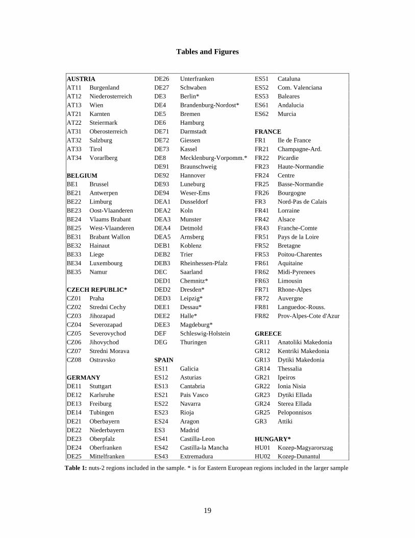
In the present work, data are based on the Eurostat regional classification. The
Nomenclature of Territorial Units for Statistics (NUTS) has been established by Eurostat at
the beginning of the 1970’s in order to provide a single uniform breakdown of territorial
units for the production of regional statistics. NUTS subdivides each Member State into a
whole number of regions at NUTS 1 level. Each of these is then subdivided into smaller
regions at NUTS level 2, and these in turn into smaller areas at NUTS level 3.
The empirical analysis is based on data extracted from the Cambridge
Econometrics’(CE) regional database, which provides comparable regional data at NUTS-2
7
and NUTS-3 level on real gross value-added (GVA)4 per capita and per worker, private
sector investment, employment and labour participation rates, and the economy’s sectoral
structure. The data are annual and cover the period from 1977 to 2002.
We analyse two distinct samples of regions drawn from the CE, characterized by a
different territorial and time coverage. Data used in the following are per capita annual GVA
measured in purchasing power standards, to account for differences in standard of living
among territorial units. The first group contains observations on 162 regions from 13
countries (Austria, Belgium, Germany, Spain, France, Greece, Ireland, Italy, Netherlands,
Norway, Portugal, Sweden and United Kingdom) and covers the period from 1977 to 2002.
A second sample is then considered, which includes 203 regions from 16 countries (the
former 13, plus Hungary, Poland, Czech Republic, and Eastern German regions) and a
shorter time period, from 1991 to 2002. For both series, the time span have been selected to
account for most of the crucial economical and historical events which have taken place
during the European integration process. In 1973, with the inclusion of Denmark, Ireland and
the United Kingdom, the first step of the enlargement took place, widening the composition
of the European space from the original EU6 to EU9. Greece joined EU in 1981, and Spain
and Portugal in 1986. This southern enlargement to a EU12 has been crucial, as it brought
inside Europe a relatively poorer set of regions. The subsequent 1995 enlargement to EU15
caused even more diversity, but in the opposite direction, due to the inclusion of relatively
affluent states of Austria, Finland and Sweden. The most recent phase in May 2004 have
enlarged the European space up to 25 countries, with the inclusion of a much poorer group
of acceding countries than those in 1986. Furthermore, the regions of these countries display
wide economic diversity, and have had very mixed experiences of operating the liberal
economic system required by membership of the EU.
Throughout our analysis data are at level NUTS-2 of desegregation, with the
exception of United Kingdom, where data are at NUTS-1 level. The region of Groningen in
Netherlands is not here considered because of anomalies dues to oil revenues accounting.
We are aware that the choice of the spatial scale may have some impact on our
results. The issue is well known among geographers as MAUP, or “modifiable unit area
problem” (Arbia, 1989). Nevertheless, the choice of the NUTS-2 level appears to be the
most appropriate unit for modelling and analysing European data as [1] it allows one to
consider phenomena at meso-levels, [2] it is sufficiently small, in most cases, to capture sub-
4 GVA equals GDP net of taxes on and subsidies for production.
8
national variations, and [3] from a policy viewpoint, it is the unit adopted by the EU to
define Objective 1 regions when allocating Structural Funds.
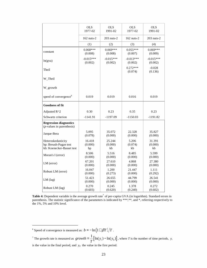
In the following we present the results of the estimate of unconditional beta-
convergence for our sample of regions. Table 4, columns (1) displays results for 162 regions
(without considering Eastern European countries) and a longer time period (1977-2001);
column (2) shows results for the sample containing data on 203 regions, and a shorter time
coverage (1992-2001). In both cases the speed of convergence is close to the notorious “2
percent” considered almost a constant by the traditional growth literature.
4. Measuring Regional Income Inequality in Europe
Theories of regional inequality as well as empirical evidence of its evolution over space and
time has been largely examined and debated in the economic literature. In particular, if we
look at the European space, the analysis of regional inequalities has attracted an increasing
interest among researchers in the last years (Petrakos, 2001, Magrini, 1999, Duro, 2004).
Duro (2004) points out some factors which are helpful to explain this trend. First, the
deepening of European integration have raised some concern about the regional distribution
of its consequences and costs; second the “new wave” of growth theories in the nineties has
been partially devoted to the analysis of regional cases, and third, the improvement in term
of quality and availability of European regional data have favoured the development of a
large body of empirical studies.
Several studies agree on the conclusion that the process of enlargement is likely to
cause deep transformations inside the European texture, both at international and intra-
national level. Moreover, while the within countries disparities are decreasing inside the “old
Europe”, accessing countries are experiencing a period of boost in terms of economic
growth, accompanied by an unquestionable intensification of regional disparities.
In this section we present a measure of regional inequality able to disentangle the two
spatial components (inter and intra) at the basis of the overall inequality present in Europe.
Inequality is often measured by mean of an index able to reflect the degree of
dispersion of the income among agents (individuals, regions, industrial sectors). The
theoretical and empirical literature largely debated about the characteristics and properties of
distinct measures5. In the present work we measure the level of inequality by mean of the
Theil index. The index possesses the desirable property to be perfectly decomposable into 5 See Cowell (1995) for a methodological discussion on inequality measures.
9
additive components. Such a characteristics turns out to be very useful when the aim of a
study is to investigate the impact of the different components of inequality within the
economic space. In the following of the analysis, the population-weighted formulation of the
index has been used, as it is more sensitive to the transfers occurring at the bottom of the
income distribution.
We apply to our data the one-stage decomposition method as reported in Akita
(2003), here adapted for the case of European regions. Let us consider the following
hierarchical structure for Europe (in crescent order of desegregation):
Europe → Countries → Regions
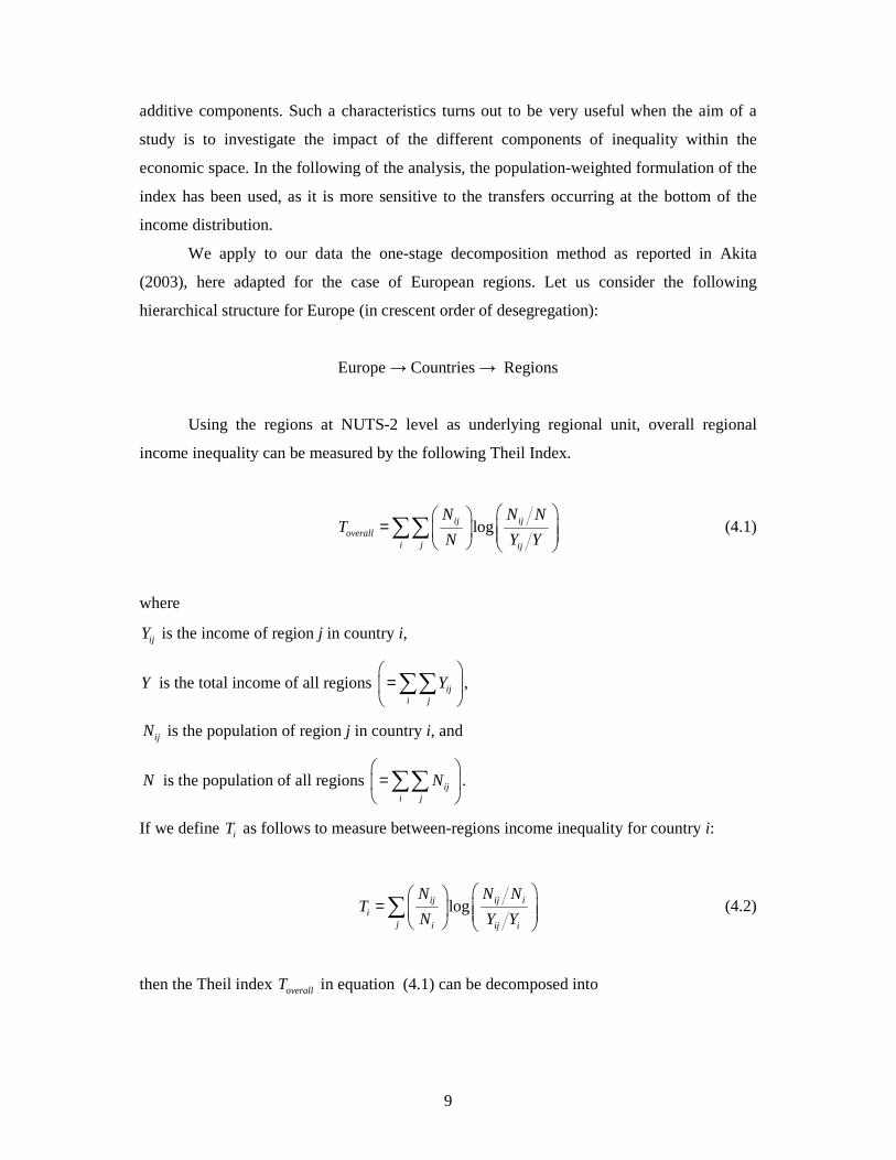
Using the regions at NUTS-2 level as underlying regional unit, overall regional
income inequality can be measured by the following Theil Index.
logij ijoverall
i j ij
N N NT
N Y Y
= ∑∑ (4.1)
where
ijY is the income of region j in country i,
Y is the total income of all regions iji j
Y
= ∑∑ ,
ijN is the population of region j in country i, and
N is the population of all regions iji j
N
= ∑∑ .
If we define iT as follows to measure between-regions income inequality for country i:
logij ij ii
j i ij i
N N NT
N Y Y
= ∑ (4.2)
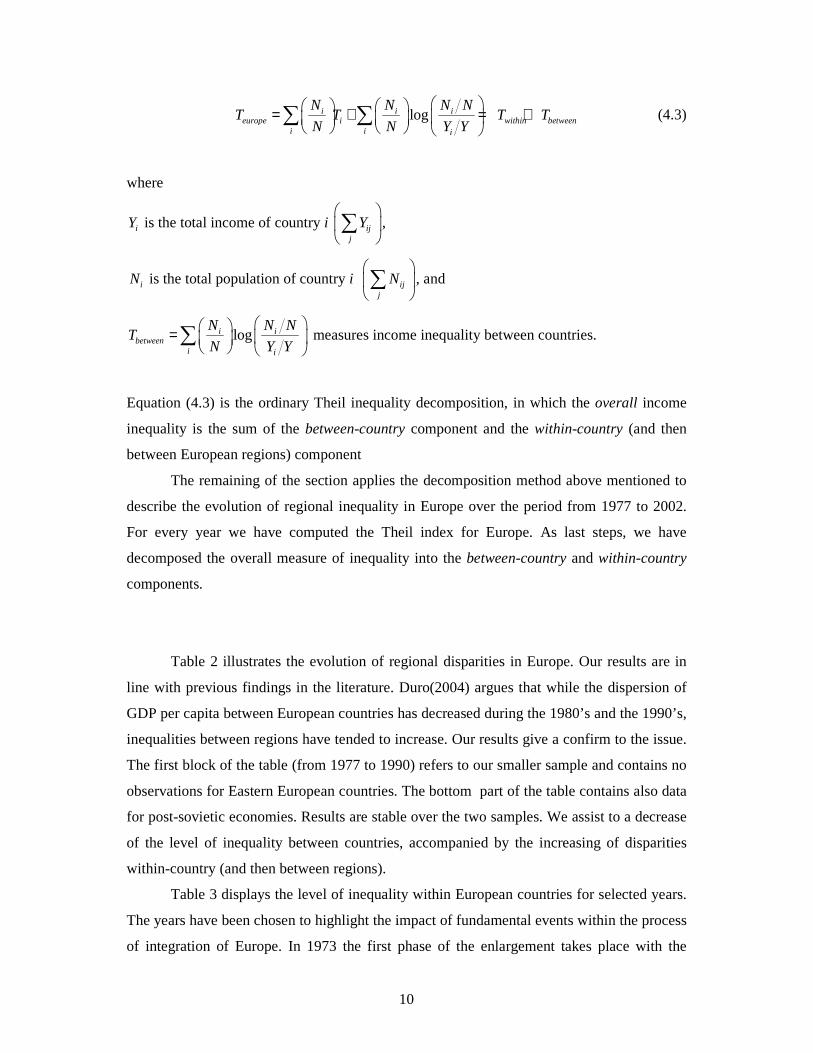
then the Theil index overallT in equation (4.1) can be decomposed into
10
logi i ieurope i within between
i i i
N N N NT T T T
N N Y Y
= + = +
∑ ∑ (4.3)
where
iY is the total income of country i ijj
Y ∑ ,
iN is the total population of country i ijj
N ∑ , and
logi ibetween
i i
N N NT
N Y Y
=
∑ measures income inequality between countries.
Equation (4.3) is the ordinary Theil inequality decomposition, in which the overall income
inequality is the sum of the between-country component and the within-country (and then
between European regions) component
The remaining of the section applies the decomposition method above mentioned to
describe the evolution of regional inequality in Europe over the period from 1977 to 2002.
For every year we have computed the Theil index for Europe. As last steps, we have
decomposed the overall measure of inequality into the between-country and within-country
components.
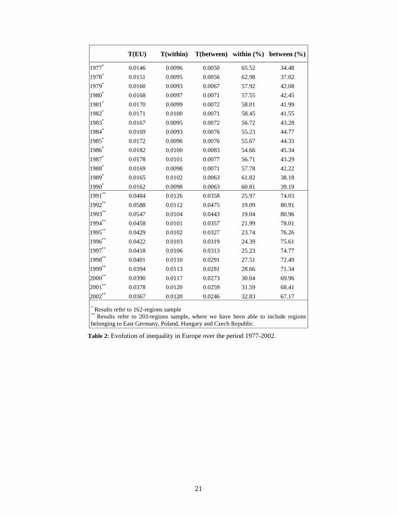
Table 2 illustrates the evolution of regional disparities in Europe. Our results are in
line with previous findings in the literature. Duro(2004) argues that while the dispersion of
GDP per capita between European countries has decreased during the 1980’s and the 1990’s,
inequalities between regions have tended to increase. Our results give a confirm to the issue.
The first block of the table (from 1977 to 1990) refers to our smaller sample and contains no
observations for Eastern European countries. The bottom part of the table contains also data
for post-sovietic economies. Results are stable over the two samples. We assist to a decrease
of the level of inequality between countries, accompanied by the increasing of disparities
within-country (and then between regions).
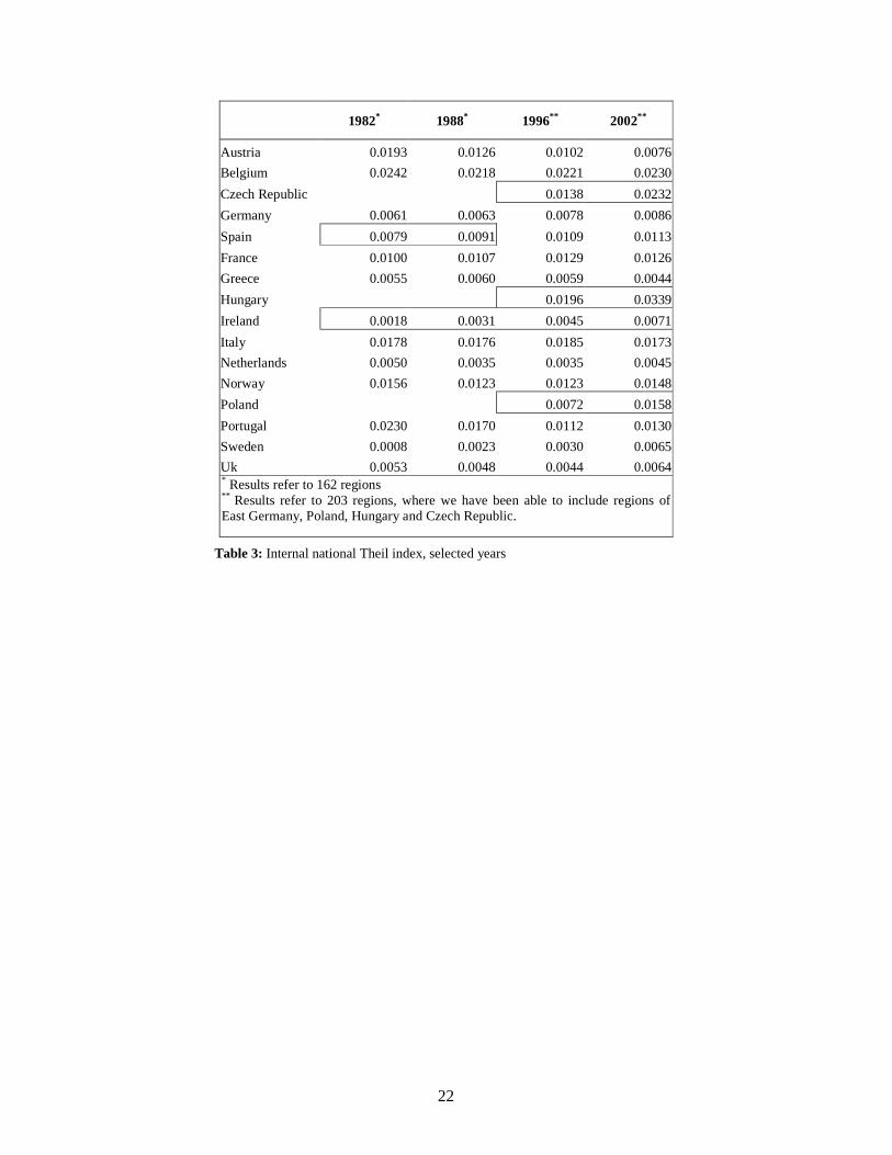
Table 3 displays the level of inequality within European countries for selected years.
The years have been chosen to highlight the impact of fundamental events within the process
of integration of Europe. In 1973 the first phase of the enlargement takes place with the
11
inclusion of Denmark, United Kingdom and Ireland, the 1980’s witness the entrance of
relatively poor southern European countries (Greece, Spain and Portugal) accompanied by a
strong campaign of allocation of structural funds by the European Community; last, the
1990’s have started with the falling of most of the communist governments, the following
opening to the west of the post-soviet economies, and the entrance of Sweden, Finland and
Austria, in 1996, within the EU.
[Table 3 about here]
Columns (3) and (4) from show the rising trend in the level of inequality in those
countries actively involved in the process of integration. If we look at the value of the Theil
of Spain, during the transition to EU, it exhibits an increase from 0.0079 in 1982 to 0.0091 in
1988. The same holds for Ireland, where inequality goes up from 0.0018 in 1982 to 0.0071
in 2002. The situation in Eastern European countries is nearly similar. In order to facilitate
the interpretation of the results, we have highlighted in table 3 the most interesting results.
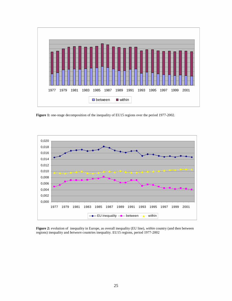
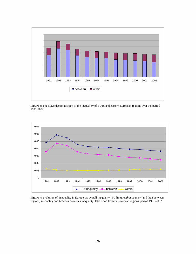
[figure 1 and figure 3 about here]
Figure 1 and Figure 3 illustrate the contribution given by the within-country and
between-country component to the overall inequality in Europe for the two samples of
regions. What is immediately clear is that inequality in the European area, when no Eastern
European regions are considered, is due by disparities within countries. Once data for
Eastern European regions are added the picture changes dramatically. The scenario is even
more clear if we look at the time pattern of the evolution of inequality in Europe as shown in
Figure 2 and Figure 4.
[figure 2 and figure 4 about here]
When we compare the two, we see that the lines corresponding to the between country
component (yellow line) and the within country component (red line) change their position.
5. Regional growth and regional inequality in EU regions and accession countries: an
empirical analysis.
A natural starting point when one analyzes the impact of inequality on growth is the
seminal work of Kuznets (1955). Kuznets was among the first to speculate about the
12
existence of a systematic relationship between inequality and the process of development.
According to him, inequality increases in the early stages of development, when the
economy experiences the passage from the rural to the industrial organization, and decreases
when the modern structure has taken over the entire social-economic texture. The result is
the inverted U-shaped relation between inequality and per-capita income, well known as
“Kuznets curve”.
The theoretical literature is divided between those who suggest that inequality is
detrimental for growth, and those who predict that the presence of an unequal distribution of
resources is an important determinant for the development of an economy.
The empirical literature is even less unanimous and shows the same division that the
theoretical models suggest. The standard procedure for estimating the impact of inequality
upon economic growth is to assume a simple linear relationship between the two
components. The equation estimated in the earliest studies is based on cross-country growth
regressions on the type:
0 1 0 2i i i i ig y Ineq Xβ β β β ε= + + + + (5.1)
where gi is the average growth rate of GDP per capita over the period under consideration,
0β is the constant, 1 0yβ is the level of gdp at the beginning of the period to account for
convergence among regions, Ineq is a measure of income inequality and Xk is a vector of
other control variables of interest.
In 1996 Deininger and Squire compile a new cross-country dataset in which they put
together a much larger and comprehensive sample of data on income distribution than
hitherto available, giving the researcher the opportunity to make use of more sophisticated
techniques. Forbes (2000), Li and Zou (1998) all look at this relationship using fixed effects
panel methods. They argue that OLS estimates result to be biased, as they do not consider
country specific effects which can be omitted. Banerjee and Duflo (2003) investigate and
conclude for the existence of a non-linear relationship between the two variables. Barro
(2000) uses a three-stage least square estimator which treats country specific effects as
random. Differently from the previous works, he doesn’t find the presence of an overall
(positive nor negative) effect of income inequality on economic growth.
Studies on the relationship between growth and inequality using regional data are less
common. Panizza uses a cross-state panel for the United States to assess the relationship
between inequality and growth. The paper shows that the relationship is not robust and that
13
small differences in the method used to measure inequality can result in large differences in
the estimated coefficients.
In our study we estimate the relationship between inequality and growth by means of
regional data at NUTS-2 level in the period 1977-2002. As in the previous sections, two
different sample of regions are considered, with or without the inclusion of eastern European
countries. Before presenting our final model we proceed by steps, moving away from the
unconditional beta convergence model and gradually including the inequality index and the
spatially lagged variables.
We first estimated, by means of Ordinary Least Square, a conditional beta-
convergence model, when we introduce as additional explanatory variable, the Theil index.
For every country of our samples we have computed a Theil index reflecting the level of
internal inequality among the regions.
[Table 4 about here]
Columns (3) and (4) show the results. At lest for the sample without Eastern
European regions, the effect of inequality on growth is positive and significant. It seems to
be in contrast with the empirical findings in the traditional literature on growth and
inequality based on cross-section data, where a trade-off between the two variables is
presented as to be a constant.
We can at glance conclude that the use of regional data has lead to opposite results if
compared to those found in cross-country based studies. Growth is associated with higher
initial levels of (within country) regional inequality. This is in line with the recent literature
in theme of spatial economics. Countries which experience high levels of growth rates are
also the ones where inequalities are rising up, due to processes of agglomeration and
concentration of economic activities.
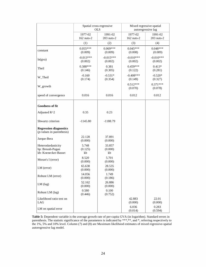
In the next step we have estimates a cross-regressive model, where the lagged value
of the Theil index is included in the regression. The aim is that we want to check how
proximity to regions with a certain level of inequality can affect the growth process of
European regions. Table 5, columns (1) and (2), shows the results. Looking at the estimated
values we see that inequality in the regions and inequality in the neighbours work on the
growth of a region in a different way. While a region receive benefit for experiencing a
phase of high disparities inside the country it belongs to, the same doesn’t hold for the fact of
being located close to regions with an high level of inequality.
14
As final model we have estimated a mixed-regressive spatial autoregressive lag
model (Florax and Folmer, 2002; Anselin, 2003). The model takes the following form
*y Wy X WXρ β λ ε= + + + (5.2)
where y is a vector of (R x 1) stochastic dependent variables, W is the binary contiguity
matrix, X the (R x k) matrix of non-stochastic regressors, *X the (R x (k-1)) matrix of
explanatory variables with the constant term deleted, ρ is the autocorrelation coefficient, β
the (k x 1) vectors of the non-weighted independent variables, λ is the ((k-1) x 1) vector of
the cross-correlation components. By using our variables of interest the model estimated
takes the form:
0 1 0 2growth y Wgrowth Ineq WIneq uβ β ρ β λ= + + + + + (5.3)
where 0y is the initial level if income to account for the presence of convergence among
regions. Table 5, columns (3) and (4), presents the results for the mixed regressive spatial
autoregressive lag model. The estimates confirm that the process of growth is positively
influenced by the presence of regions with high level of growth rates. The relationship
between regional growth and regional inequality is positive. The trade-off between growth
and the lagged value of inequality holds, and it is now significant even when Eastern
European regions are considered.
One can conclude that as long as disparities are within a region, this can be see as
consequence of agglomeration processes and the consequent growth of the economy. On the
other side, we observe that regions does not take any advantage by being located close to
regions with high level of inequality. In this case the traditional findings on the relationship
between inequality and growth are confirmed. 4 shows the results.
As argued by Petrakos et al. (2005) “the direction of the relationship is critical in
term of policy choice. A negative relationship implies that in the long-term inequalities will
disappear, and, as a result, there is limited scope and a declining need for regional policy. On
the other hand, a positive relation between growth and inequality implies that, no matter
what other factors may affect the evolution of inequalities, economic growth will always
generate new inequalities”.
15
6. Conclusions
In the present work we have analyzed the evolution of income disparities in European
regions and transition countries in the period 1977-2002.
Our result have confirmed the tendency in overall European inequality to decrease
over time, accompanied by an expansion of the intra-country (and then between regions)
disparities. The entrance of Eastern regions has caused at a first stage a consistent increase
in the level of inequality in Europe, with a tendency of attenuation over time.
The empirical literature in theme of convergence have argued that European regions
are characterized by a high level of spatial dependency in income levels and growth rates. In
our analysis we have tested that also inequality cannot be considered as an isolated
phenomenon, and it requires to be modelled in association with space and the concept of
spatial interaction.
Estimates from cross-country data have shown that the relationship between
inequality and growth is positive, indicating that the process of development requires the
presence of initial disparities to start. The impact is consistent when we introduce data for
Eastern European countries. When we look at the effect of inequality in neighbouring
regions, we have found evidence of a trade-off with the process of growth. A plausible
interpretation could be that inequality within a country is useful for growth, while unequal
realities in the neighbours have a detrimental impact.
For the future, we are confident that the availability of longer time series for
transition countries will give us the opportunity to further investigate the relationship
between growth and inequality in those regions.

16
References Abreu, M., de Groot, H. and Florax, R. (2004) Growth and Space, Tinbergen Institute
Discussion Paper, 2004-129/3.
Aghion, P., Caroli E. and Garcia-Penalosa, C. (1999) Inequality and Economic Growth: the
Perspective of the New Growth Theories, Journal of Economic Literature, 37 (4)
1615-1660.
Akita, T. (2003) Decomposing Regional Income Inequality in China and Indonesia using
Two-Stage Nested Theil Decomposition Method, Annals of Regional Science, 37 (1)
55-77.
Alesina, A. and Rodrik, D. (1994) Distributive Politics and Economic Growth, Quarterly
Journal of Economics, 109 (2) 465-490.
Anselin, L. (1988) Spatial Econometrics: Methods and Models. Dordrecht: Kluwer
Academic Publishers.
Anselin (2003), Spatial Externalities, Spatial Multipliers and Spatial Econometrics,
International Regional Science Review, 26 (2), 153-166.
Arbia, G. (1989) Spatial Data Configuration in the Statistical Analysis of Regional
Economics and Related Problems. Dordrecht: Kluwer Academic Publishers.
Arbia, G. and Paelinck, J. (2003) Economic Convergence or Divergence? Modelling the
Interregional Dynamics of Eu Regions, 1985-1999, Journal of Geographical
Systems, 5 (3) 291-314.
Arbia, G. and Paelinck, J. (2003) Spatial Econometric Modelling of Regional Convergence
in Continuous Time, International-Regional-Science-Review, 26 (3) 342-362.
Arbia, G. and Piras, G. (2004) Convergence in Per-Capita Gdp across European Regions
Using Panel Data Models Extended to Spatial Autocorrelation Effects, paper
presented at the European Regional Science Association (ERSA) conference, Porto.
Azzoni, C. (2001) Economic Growth and Regional Income Inequality in Brazil, Annals of
Regional Science, 35 (1) 133-152.
Banerjee, A. V. and Duflo, E. (2003) Inequality and Growth: What Can the Data Say,
Journal of Economic Growth, 8 267-299.
Barro, R. (2000) Inequality and Growth in a Panel of Countries, Journal of Economic
Growth, 5 5-32.
Barro, R. and Sala-I-Martin, X. (1991) Convergence across States and Regions, Brookings
Papers on Economic Activity, 1 107-158.
17
Barro, R. J. and Sala-I-Martin, X. (1992) Convergence, Journal of Political Economy, 100
(2) 223-251.
Barro, R. and Sala-I-Martin, X. (2003) Economic Growth. Boston: The MIT Press.
Bénabou, R. (1996) Inequality and Growth, NBER Working Paper No. 5658.
Cowell, F. (1995) Measuring Inequality. London; New York and Toronto: Simon and
Schuster International, Harvester Wheatsheaf/Prentice Hall.
Dall’erba, S. and Le Gallo, J. (2003) Regional Convergence and the Impact of Structural
Funds over 1989-1999: A Spatial Econometric Analysis, University of Illinois at
Urbana-Champaign Discussion Paper 03-T-14.
Deininger, K. and Squire, L. (1996) Measuring Inequality: a New Database, World Bank
Economic Review, 10 (3), 565-591
Deininger, K. and Squire, L. (1998) New Ways of Looking at Old Issues: Inequality and
Growth, Journal of Development Economics, 57 259-287.
Duro, J. A. (2004) Regional income inequalities in Europe: An Updated Measurement and
Some Decomposition Results, Working Paper n. 04-11, Departament d'Economia
Aplicada, Universitat Autònoma de Barcelona.
Duro, J. A. and Esteban, J. (1998) Factor Decomposition of Cross-Country Income
Inequality, 1960-1990, Economics-Letters, 60 (3) 269-275.
European Commission (2004) Catching-up, Growth and Convergence of the New Member
States, European Economy, no. 6.
Florax, R. And Folmer, H. (1992) Specification and estimation of spatial linear regression
models: Monte Carlo evaluation of pre-test estimators, Regional Science and Urban
Economics,22, 405-32.
Forbes, K. J. (2000) A Reassessment of the Relationship between Inequality and Growth,
American Economic Review, 90 (4) 869-887.
Kuznet, S. (1955) Economics Growth and Income Inequality, American Economic Review,
45 (1) 1-28.
Le Gallo, J. and Ertur, C. (2003) Exploratory Spatial Data Analysis of the Distribution of
Regional Per Capita Gdp in Europe, 1980-1995, Papers in Regional Science (82)
175-201.
Le Gallo, J., Ertur, C. and C., B. (2003) A Spatial Econometric Analysis of Convergence
across European Regions: 1980-1995, in European Regional Growth, ed. by B.
Fingleton. Berlin: Springer, 99-129.
18
Li, H. and Zou, H. (1998) Income Inequality Is Not Harmful for Growth: Theory and
Evidence, Review of Development Economics, 2 (3) 318-334.
Lopez-Bazo, E., Vayà, E., Mora, A. J. and Suriñach, J. (1999) Regional Economic Dynamics
and Convergence in the European Union, Annals of Regional Science (33) 343-370.
Magrini, S. (1999) The Evolution of Income Disparities among the Regions of the European
Union, Regional Science and Urban Economics (29) 257–281.
Mankiw, N., Romer, D. and Weil, D. (1992) A Contribution to the Empirics of Economic
Growth, Quarterly Journal of Economics, 107 (2) 407-437.
Milanovic, B. (1999) Explaining the Increase in Inequality During the Transition, Economics
of Transition, 7 (2) 299-341.
Panizza, U. (2002) Income Inequality and Economic Growth: Evidence from American
Data, Journal of Economic Growth, 7 25-41.
Persson, T. and Tabellini, G. (1994) Is Inequality Harmful for Growth?, American Economic
Review, 84 600-621.
Petrakos, G. (1996) The Regional Dimension of Transition in Central and East European
Countries, Eastern European Economics, 34 (5) 5-38.
Petrakos, G. (2001) Patterns of Regional Inequality in Transition Economics, European
Planning Studies, 9 (3) 359-383.
Petrakos, G. and Saratsis, Y. (2000) Regional Inequalities in Greece, Papers in Regional
Science, 79 (1) 57-74.
Petrakos, G., Rodriguez-Pose, A. and Rovolis, A. (2005) Growth, Integration and Regional
Disparities in the European Union, Environment and Planning A, 37.
Rey, S. and Janikas, M. (2005) Regional Convergence, Inequality, and Space, Journal of
Economic Geography, forthcoming.
Sala-i-Martin, X. (1990) On Growth and States: Phd Dissertation, Harvard University.
Sala-I-Martin, X. (1996) Regional Cohesion: Evidence and Theories of Regional Growth
and Convergence, European Economic Review, 40 1325-1352.
19
Tables and Figures
AUSTRIA DE26 Unterfranken ES51 Cataluna AT11 Burgenland DE27 Schwaben ES52 Com. Valenciana AT12 Niederosterreich DE3 Berlin* ES53 Baleares AT13 Wien DE4 Brandenburg-Nordost* ES61 Andalucia AT21 Karnten DE5 Bremen ES62 Murcia AT22 Steiermark DE6 Hamburg AT31 Oberosterreich DE71 Darmstadt FRANCE AT32 Salzburg DE72 Giessen FR1 Ile de France AT33 Tirol DE73 Kassel FR21 Champagne-Ard. AT34 Vorarlberg DE8 Mecklenburg-Vorpomm.* FR22 Picardie DE91 Braunschweig FR23 Haute-Normandie
BELGIUM DE92 Hannover FR24 Centre BE1 Brussel DE93 Luneburg FR25 Basse-Normandie BE21 Antwerpen DE94 Weser-Ems FR26 Bourgogne BE22 Limburg DEA1 Dusseldorf FR3 Nord-Pas de Calais
BE23 Oost-Vlaanderen DEA2 Koln FR41 Lorraine BE24 Vlaams Brabant DEA3 Munster FR42 Alsace BE25 West-Vlaanderen DEA4 Detmold FR43 Franche-Comte BE31 Brabant Wallon DEA5 Arnsberg FR51 Pays de la Loire BE32 Hainaut DEB1 Koblenz FR52 Bretagne BE33 Liege DEB2 Trier FR53 Poitou-Charentes BE34 Luxembourg DEB3 Rheinhessen-Pfalz FR61 Aquitaine BE35 Namur DEC Saarland FR62 Midi-Pyrenees
DED1 Chemnitz* FR63 Limousin
CZECH REPUBLIC* DED2 Dresden* FR71 Rhone-Alpes CZ01 Praha DED3 Leipzig* FR72 Auvergne CZ02 Stredni Cechy DEE1 Dessau* FR81 Languedoc-Rouss. CZ03 Jihozapad DEE2 Halle* FR82 Prov-Alpes-Cote d'Azur CZ04 Severozapad DEE3 Magdeburg* CZ05 Severovychod DEF Schleswig-Holstein GREECE CZ06 Jihovychod DEG Thuringen GR11 Anatoliki Makedonia CZ07 Stredni Morava GR12 Kentriki Makedonia CZ08 Ostravsko SPAIN GR13 Dytiki Makedonia
ES11 Galicia GR14 Thessalia
GERMANY ES12 Asturias GR21 Ipeiros DE11 Stuttgart ES13 Cantabria GR22 Ionia Nisia DE12 Karlsruhe ES21 Pais Vasco GR23 Dytiki Ellada DE13 Freiburg ES22 Navarra GR24 Sterea Ellada DE14 Tubingen ES23 Rioja GR25 Peloponnisos
DE21 Oberbayern ES24 Aragon GR3 Attiki DE22 Niederbayern ES3 Madrid DE23 Oberpfalz ES41 Castilla-Leon HUNGARY* DE24 Oberfranken ES42 Castilla-la Mancha HU01 Kozep-Magyarorszag DE25 Mittelfranken ES43 Extremadura HU02 Kozep-Dunantul
Table 1: nuts-2 regions included in the sample. * is for Eastern European regions included in the larger sample

20
HU03 Nyugat-Dunantul NL22 Gelderland PORTUGAL HU04 Del-Dunantul NL23 Flevoland PT11 Norte HU05 Eszak-Magyarorszag NL31 Utrecht PT12 Centro HU06 Eszak-Alfold NL32 Noord-Holland PT13 Lisboa e V.do Tejo HU07 Del-Alfold NL33 Zuid-Holland PT14 Alentejo NL34 Zeeland PT15 Algarve
IRELAND NL41 Noord-Brabant IE01 Border NL42 Limburg SWEDEN IE02 Southern and Eastern SE01 Stockholm NORWAY SE02 Ostra Mellansverige
ITALY NO01 Oslo og Akershus SE04 Sydsverige IT11 Piemonte NO02 Hedmark og Oppland SE06 Norra Mellansverige IT12 Valle d'Aosta NO03 Sor-Ostlandet SE07 Mellersta Norrland IT13 Liguria NO04 Agder og Rogaland SE08 Ovre Norrland IT2 Lombardia NO05 Vestlandet SE09 Smaland med oarna IT31 Trentino Alto Adige NO06 Trondelag SE0A Vastsverige IT32 Veneto NO07 Nord-Norge IT33 Fr.-Venezia Giulia UK IT4 Emilia-Romagna POLAND* UKC North East IT51 Toscana PL01 Dolnoslaskie UKD North West IT52 Umbria PL02 Kujawsko-Pomorskie UKE Yorkshire and the Humber IT53 Marche PL03 Lubelskie UKF East Midlands IT6 Lazio PL04 Lubuskie UKG West Midlands IT71 Abruzzo PL05 Lodzkie UKH Eastern IT72 Molise PL06 Malopolskie UKI London IT8 Campania PL07 Mazowieckie UKJ South East IT91 Puglia PL08 Opolskie UKK South West IT92 Basilicata PL09 Podkarpackie UKL Wales IT93 Calabria PL0A Podlaskie UKM Scotland ITA Sicilia PL0B Pomorskie UKN Northern Ireland ITB Sardegna PL0C Slaskie PL0D Swietokrzyskie NETHERLANDS PL0E Warminsko-Mazurskie NL12 Friesland PL0F Wielkopolskie NL13 Drenthe PL0G Zachodniopomorskie NL21 Overijssel
Table 1: continued
21
T(EU) T(within) T(between) within (%) between (%)
1977* 0.0146 0.0096 0.0050 65.52 34.48
1978* 0.0151 0.0095 0.0056 62.98 37.02
1979* 0.0160 0.0093 0.0067 57.92 42.08
1980* 0.0168 0.0097 0.0071 57.55 42.45
1981* 0.0170 0.0099 0.0072 58.01 41.99
1982* 0.0171 0.0100 0.0071 58.45 41.55
1983* 0.0167 0.0095 0.0072 56.72 43.28
1984* 0.0169 0.0093 0.0076 55.23 44.77
1985* 0.0172 0.0096 0.0076 55.67 44.33
1986* 0.0182 0.0100 0.0083 54.66 45.34
1987* 0.0178 0.0101 0.0077 56.71 43.29
1988* 0.0169 0.0098 0.0071 57.78 42.22
1989* 0.0165 0.0102 0.0063 61.82 38.18
1990* 0.0162 0.0098 0.0063 60.81 39.19
1991** 0.0484 0.0126 0.0358 25.97 74.03
1992** 0.0588 0.0112 0.0475 19.09 80.91
1993** 0.0547 0.0104 0.0443 19.04 80.96
1994** 0.0458 0.0101 0.0357 21.99 78.01
1995** 0.0429 0.0102 0.0327 23.74 76.26
1996** 0.0422 0.0103 0.0319 24.39 75.61
1997** 0.0418 0.0106 0.0313 25.23 74.77
1998** 0.0401 0.0110 0.0291 27.51 72.49
1999** 0.0394 0.0113 0.0281 28.66 71.34
2000** 0.0390 0.0117 0.0273 30.04 69.96
2001** 0.0378 0.0120 0.0259 31.59 68.41
2002** 0.0367 0.0120 0.0246 32.83 67.17
* Results refer to 162-regions sample
** Results refer to 203-regions sample, where we have been able to include regions belonging to East Germany, Poland, Hungary and Czech Republic.
Table 2: Evolution of inequality in Europe over the period 1977-2002.
22
1982* 1988* 1996** 2002**
Austria 0.0193 0.0126 0.0102 0.0076
Belgium 0.0242 0.0218 0.0221 0.0230
Czech Republic 0.0138 0.0232
Germany 0.0061 0.0063 0.0078 0.0086
Spain 0.0079 0.0091 0.0109 0.0113
France 0.0100 0.0107 0.0129 0.0126
Greece 0.0055 0.0060 0.0059 0.0044
Hungary 0.0196 0.0339
Ireland 0.0018 0.0031 0.0045 0.0071
Italy 0.0178 0.0176 0.0185 0.0173
Netherlands 0.0050 0.0035 0.0035 0.0045
Norway 0.0156 0.0123 0.0123 0.0148
Poland 0.0072 0.0158
Portugal 0.0230 0.0170 0.0112 0.0130
Sweden 0.0008 0.0023 0.0030 0.0065
Uk 0.0053 0.0048 0.0044 0.0064 * Results refer to 162 regions
** Results refer to 203 regions, where we have been able to include regions of East Germany, Poland, Hungary and Czech Republic.
Table 3: Internal national Theil index, selected years
23
OLS 1977-02
OLS 1991-02
OLS 1977-02
OLS 1991-02
162 nuts-2 203 nuts-2 162 nuts-2 203 nuts-2
(1) (2) (3) (4)
constant 0.068*** (0.008)
0.069*** (0.008)
0.055*** (0.007)
0.069*** (0.009)
ln(gva) -0.015***
(0.002) -0.015***
(0.002) -0.013***
(0.002) -0.015***
(0.002)
Theil 0.272*** (0.074)
-0.028 (0.136)
W_Theil
W_growth
speed of convergence6 0.019 0.019 0.016 0.019
Goodness of fit
Adjusted R^2 0.30 0.23 0.35 0.23
Schwartz criterion -1141.91 -1197.09 -1150.03 -1191.82
Regression diagnostics (p-values in parenthesis)
Jarque-Bera 5.095
(0.078) 35.072 (0.000)
22.328 (0.000)
35.827 (0.000)
Heteroskedasticity bp: Breush-Pagan test kb: Koenecker-Basset test
16.418 (0.000)
bp
25.244 (0.000)
kb
5.206 (0.074)
kb
31.391 (0.000)
kb
Moran's I (error) 8.506
(0.000) 5.516
(0.000) 8.485
(0.000) 5.599
(0.000)
LM (error) 67.201 (0.000)
27.610 (0.000)
4.868 (0.000)
27.380 (0.000)
Robust LM (error) 16.047 (0.000)
1.200 (0.273)
21.447 (0.000)
1.111 (0.292)
LM (lag) 51.423 (0.000)
26.655 (0.000)
44.799 (0.000)
26.541 (0.000)
Robust LM (lag) 0.270
(0.603) 0.245
(0.620) 1.378
(0.240) 0.272
(0.602)
Table 4: Dependent variable is the average growth rate7 of per-capita GVA (in logarithm). Standard errors in parenthesis. The statistic significance of the parameters is indicated by ***,**, and *, referring respectively to the 1%, 5% and 10% level.
6 Speed of convergence is measured as: ( )ln 1b T Tβ= − + .
7 The growth rate is measured as [ ]0
1ln( ) ln( )tgrowth y y
T= − , where T is the number of time periods, yt
is the value in the final period, and y0 the value in the first period.
24
Spatial cross-regressive OLS
Mixed regressive-spatial autoregressive lag
1977-02 162 nuts-2
1991-02 203 nuts-2
1977-02 162 nuts-2
1991-02 203 nuts-2
(1) (2) (3) (4)
constant 0.055*** (0.009)
0.069*** (0.009)
0.045*** (0.008)
0.048*** (0.009)
ln(gva) -0.013***
(0.002) -0.015***
(0.002) -0.010***
(0.002) -0.010***
(0.002)
Theil 0.388*** (0.146)
0.381 (0.305)
0.459*** (0.122)
0.413* (0.281)
W_Theil -0.160 (0.174)
-0.531* (0.354)
-0.408*** (0.149)
-0.520* (0.327)
W_growth 0.512*** (0.070)
0.371*** (0.078)
speed of convergence 0.016 0.016 0.012 0.012
Goodness of fit
Adjusted R^2 0.35 0.23
Shwartz criterion -1145.80 -1188.79
Regression diagnostics (p-values in parenthesis)
Jarque-Bera 22.128 (0.000)
37.891 (0.000)
Heteroskedasticity bp: Breush-Pagan kb: Koenecker-Basset
5.748 (0.125)
kb
33.857 (0.000)
kb
Moran's I (error) 8.520
(0.000) 5.701
(0.000)
LM (error) 65.638 (0.000)
28.535 (0.000)
Robust LM (error) 14.056 (0.000)
1.749 (0.186)
LM (lag) 52.162 (0.000)
26.886 (0.000)
Robust LM (lag) 0.580
(0.446) 0.100
(0.752)
Likelihood ratio test on LAG
42.883 (0.000)
22.01 (0.000)
LM on spatial error 6.036
(0.014) 0.283
(0.594)
Table 5: Dependent variable is the average growth rate of per-capita GVA (in logarithm). Standard errors in parenthesis. The statistic significance of the parameters is indicated by ***,**, and *, referring respectively to the 1%, 5% and 10% level. Column (7) and (8) are Maximum likelihood estimates of mixed regressive-spatial autoregressive lag model.
25
0,0000,0020,0040,0060,0080,0100,0120,0140,0160,0180,020
1977 1979 1981 1983 1985 1987 1989 1991 1993 1995 1997 1999 2001
between within
Figure 1: one-stage decomposition of the inequality of EU15 regions over the period 1977-2002.
0,000
0,002
0,004
0,006
0,008
0,010
0,012
0,014
0,016
0,018
0,020
1977 1979 1981 1983 1985 1987 1989 1991 1993 1995 1997 1999 2001
EU inequality between within
Figure 2: evolution of inequality in Europe, as overall inequality (EU line), within country (and then between regions) inequality and between countries inequality. EU15 regions, period 1977-2002
26
0
0,01
0,02
0,03
0,04
0,05
0,06
0,07
1991 1992 1993 1994 1995 1996 1997 1998 1999 2000 2001 2002
between within
Figure 3: one-stage decomposition of the inequality of EU15 and eastern European regions over the period 1991-2002.
0
0,01
0,02
0,03
0,04
0,05
0,06
0,07
1991 1992 1993 1994 1995 1996 1997 1998 1999 2000 2001 2002
EU inequality between within
Figure 4: evolution of inequality in Europe, as overall inequality (EU line), within country (and then between regions) inequality and between countries inequality. EU15 and Eastern European regions, period 1991-2002