Retrospective Theses and Dissertations Iowa State University Capstones, Theses andDissertations

1967

Factor demand in the United States agriculture:econometric simulationAn-Yhi LinIowa State University

Follow this and additional works at: https://lib.dr.iastate.edu/rtd

Part of the Agricultural and Resource Economics Commons, Agricultural Economics Commons,and the Econometrics Commons

This Dissertation is brought to you for free and open access by the Iowa State University Capstones, Theses and Dissertations at Iowa State UniversityDigital Repository. It has been accepted for inclusion in Retrospective Theses and Dissertations by an authorized administrator of Iowa State UniversityDigital Repository. For more information, please contact digirep@iastate.edu.

Recommended CitationLin, An-Yhi, "Factor demand in the United States agriculture: econometric simulation" (1967). Retrospective Theses and Dissertations.3405.https://lib.dr.iastate.edu/rtd/3405

This dissertation has been

microfilmed exactly as received bo—4oo7

LIN, An-Yhi, 1933-FACTOR DEMAND IN THE UNITED STATES AGRICUL­TURE: ECONOMETRIC SIMULATION.

Iowa State University, Ph.D,, 1967 Economics, general Economics, agricultural

University Microfilms, Inc., Ann Arbor, Michigan

FACTOR DEMAND IN THE UNITED STATES AGRICULTURE:

ECONOMETRIC SIMULATION

by

A Dissertation Submitted to the

Graduate Faculty in Partial Fulfillment of

The Requirements for the Degree of

DOCTOR OF PHILOSOPHY

Major Subject: Economics

An-Yhi Lin

Approved:

In Charge of Major Work

Iowa State University Of Science and Technology

Ames, Iowa

1967

Signature was redacted for privacy.

Signature was redacted for privacy.

Signature was redacted for privacy.

ii

TABLE OF CONTENTS Page

I. INTRODUCTION AND OBJECTIVES 1

A. Introduction - 1 B. Objectives .7 5

II. ECONOMIC NORMS 9

A. Some Theories of Investment Behavior 9 _ 1. Marginal investment theory 10

2. The acceleration approach 12 3. Institutional and empirical generalizations 19 4. The eclectic approaches. 20

B. Review of Some Econometric Investigations 22 1. The studies 22

III. THE ECONOMIC STRUCTURE OF THE DEMAND FOR FACTORS 31

A. The Static Framework of Resources Demand 32 B. Some Modifications toward the Dynamic and

Interregional Competitive System 37 C. Specification of Output Supply and Input Demand

Functions 42 1. Aggregate commodity market 44 2. Factor markets 49

IV. THE RECURSIVE MODELS AND ECONOMETRIC CONSIDERATIONS 63

A. The Proposed Models 63 1. A tentative model 67 2. The final model 84

B. The Econometric Considerations 91 1. Recursive versus simultaneous systems 92 2. Use of least-squares techniques 94

V. EMPIRICAL ESTIMATION OF THE FUNCTIONAL RELATIONS 105

A. Variable and Data Sources 105 B. Results of National Model 1924-1965 116

1. Aggregate commodity market ...116 2. Factor markets .^121

C. Results of Regional Models 1946-1965 137

iii

TABLE OF CONTENTS (Continued)

Page

VI. THE COMPUTER SIMULATION MODEL OF THE DEMAND FOR FACTORS (NATIONAL MODEL) 158

A. Simulation of Factors Demand Under the Existing Economic Structure 158

1. Simulation of the historical period and model validation 158

2. Simulation of alternative historical demand for factors 168

B. Projection of National Demand for Factors, 1980 17 6 1. Estimation of exogenous variables 176 2. Simulated endogenous variables 181

VII. SUMMARY AND CONCLUSIONS 183

VIII. BIBLIOGRAPHY 190

IX. ACKNOWLEDGEMENTS 200

1

I. INTRODUCTION AND OBJECTIVES

A. Introduction

This study is an investigation of the aggregate demand for investment

expenditure on farm machinery and farm buildings. The demand for farm

labor is also included. The study includes the econometric analysis of

the investment demand for above-mentioned factors and the related under­

lying variables affecting those demands. The data used in the study are

aggregate times series data from 1924 to 1965 for national analysis and

from 1946 to 1965 for regional analysis.

The usefulness of the study is obvious : The problem of overcapacity

and low incomes in agriculture has been one of the major problems in U.S.

society over the three decades. The problems of agriculture have been

somewhat reflected in a large supply of crop and livestock products and

low level of farm incomes as compared to those in non-farm sectors.

Although the problems of agriculture are directly those commodity

supply and price, fundamentally they are problems of resource demand and

supply. More basically, the farm problems stem from economic growth which

is reflected in the relatively stable price for non-farm produced items

and increasing productivity of resources.

Through economic growth, capital has increased in supply to agricul­

ture sector at sufficiently low real price, resulting in large-scale sub­

stitution for land and labor. With rapid adoption of productive capital

inputs, opportunities for growth in output and productivity of resources

is large. But if opportunities for adjusting redundant labor resources

2

out of agriculture are low because of values,social attachments, abilities

and other characteristics of farm peofLe, the returns to farm labor may be

low indeed. Whether this is the case, depends upon the developing struc­

ture and organization of agriculture.

The organization of agriculture is a reflection of parameters in the

structure of agriculture. The organization involves the numbers and sizes

of farms which make up the industry, the size of the labor force and the

amount and composition of capital used etc. To explain why a particular

organization might emerge, it is necessary to know the structure of agri­

culture. It is a systematic framework of institutional, behavioral and

technological relationships that go to determine output, efficiency and

returns in agriculture.

Understanding of structure in agriculture can be useful for example,

in answering a number of fundamental questions which depend heavily on the

nature of the resources market in agriculture. Whether a return to an

agriculture free of government controls will eventually raise farm income

per worker depends on the responsiveness of farm workers to a fall in

relative income. The interrelationships of policies affecting national

employment and farm labor mobility cannot be accurately judged without

gaging the ma^itude of parameters in the farm labor function. The de­

mand and supply function for a particular resource obviously is inter­

related, through resource prices, technical coefficients and substitution

rates, with the demand and supply functions for other resources. Thus

the estimation of the basic structure of parameters of demand and supply

functions for other resources are also needed.

3

The close relationship between factor demand and the organization of

resources in agriculture along with the importance of factor demand to

commodity supply further suggests that the research into agricultural re­

sources is a relevant area for study. However, studies of the basic

structure of agriculture and the parameters of supply and demand are

limited. Past discussions and econometric studies regarding the re­

sources demand have often been based largely on particular resources.

Only Heady and Tweeten's excellent study (50) has investigated quantitative­

ly the interrelationships among the different categories of resources in

agriculture. More important, their study has explicitly integrated the

products and inputs markets of the agricultural and the non-farm variables.

There are several reasons why an integrated study is necessary. Product

markets determine gross income, resource markets determine expenses and

the two markets determine net income in farming. From a causal and

statistical standpoint, many decisions in farming are interdependent. It

is almost impossible to determine how much family labor, for example, will

remain in agriculture without estimates of farm product prices, national

unemployment and factory wages.

There are some difficulties in extending Heady and Tweeten's study

(50) much beyond its current contributions. These possibilities, if any,

lie in two major aspects of economic structure. The first of these is

the intertemporal structure, or, in short, dynamics. The second is the

spatial interconnecte dne s s of demand and supply either in resources or

products markets. For many agricultural commodities, production decisions

4

take place many months before supplies reach markets. Given supplies

are determined by past production decisions and the intervening hand of

weather. The recursive models seem appropriate in describing this kind

of nature both as a basis for practical forecasting and as a tool of

realistic economic theory. The recursive system is composed of a sequence

of causal relationships. It consists of a set of equations each contain­

ing a single endogenous variable other than those that have been treated

as dependent in prior equations. The endôgêhous variables enter the sys­

tem one by one, like links in an infinite chain where each link is ex­

plained in terms of earlier links.

For the interregional relationships, the regional commodity demand

functions shift over time. But at the time when supplies are forthcoming

they are relatively stable. With supplies predetermined, a transportation

model, augmented by regional demand functions, might well represent the

temporary equilibrium of spatial marketing structure, yielding interregion­

al commodity flows and regional prices received and paid for agricultural

commodities (3.1, 98 )

By temporary equilibrium one does not mean static or normative

equilibrium. It implies that the economic function of distributing pre­

determined supplies among various regions is performed in an efficient,

manner with respect to costs that clears the market. The interregional

prices and commodity flows may vary widely from one period of temporary

equilibrium to the next, in cyclical, in an explosive or even (because

of weather) in an erratic manner.

!

5

Synthesizing the recursive production, factor demand and the tem­

porary market equilibrium feature to formulate a dynamic regional inter­

dependence model for the U.S. agriculture would be desirable. By em­

phasizing the factor market, a better understanding of the structure and

organization of agriculture resources for policy purposes will become

attainable. Furthermore as an alternative econometric model, it can be

subjected to testing and to observing how well it describes the invest­

ment behavioral pattern of farmers.

The quantitative results and the structural parameters which will be

presented in this study refer to specific types of investment, namely

farm machinery and farm buildings. Demand for farm labor will also be

estimated. The words "resource, factor, and input" will be used inter-

changeabJ.y_ in the following chapters.

B. Objectives

The general objective of this study is to describe and analyze the

resource structure of American agriculture. A major portion of the study

is devoted to developing the econometric models and derivation of quanti­

tative estimates of structural parameters determining farm resources al­

location. Specific objectives are (1) to identify the causal and related

variables affecting the historic changes in investment demand, (2) to

develop a model or models to describe the aggregate demand for farm

machinery, farm buildings investment and the farm labor using the causal

and related variables, (3) to estimate the parameters of the models de­

veloped using the available data for the time period under study, and

6

(4) to use the models developed .and the estimated parameters to simulate

and project the national aggregate demand for the above-mentioned factors

(based upon certain assumptions to be indicated later).

The organization and contents of this study will be in the following

order. After this introductory chapter a broad examination of investment

theory and brief review of past econometric studies for durable goods

will be presented in Chapter II. The demand theory, supply-demand relation­

ships, spatial and dynamic interrelationships of the agriculture '-resources

will be discussed and developed in Chapter III. Further a review of past

studies and hypotheses directly concerned with agriculture resources also

will be discussed in this chapter. The econometric models for this study

will be the subject of Chapter IV. This chapter will be composed of a

proposed model and the final model. The proposed model will be developed

on the theoretical basis which will be discussed and developed in Chapter

III. It will incorporate tha.dynamic, spatial relationships of resources

demand and further integrating it with the commodity market.. The final

model will be the workable model based on the proposed model taking care of

the forseeable data limitations. The final model will further be divided

into national and regional models. Econometric consideration then will be

at the end of this chapter.

After this background material the empirical analysis will be presented

in Chapters V and VI. The national recursive model of resources demand

bases on time-series estimates along with the sources of data will be pre­

sented in Chapter V. Linear regional model estimated with times-series

and cross—sectional data (10 farm production regions, see Figure 1),

FARM PRODUCTION REGIONS

l&DAK 1 NORTHERN

I PLAINS I NEBR.

PACinC

MOUNT)

ACHIAN

SOUTHERN PLAINS

Figure 1. Farm production regions

8

using the combination of the analysis of covariance and multiple regression

techniques also will be presented in Chapter V.

The national model and the parameters of the model after statistical

estimation will be used for simulation and projection Chapter VI. The

historical values of investment will be simulated with the model developed

and the parameters estimated in order to verify the model. Two different

exogenous variables, technology and farm policy also will be simulated

with different value and different practice than the prevailing one. Under

free market system (free from price support and production control programs)

and lower technological advancements (one half of original rates), the

national model will be simulated for the resources demand. Further the

national model also will be used to project the investment demand for those

factors in agriculture up to year 1980. Certain basic assumptions about

the general economy and specific assumptions about the individual variables

will be made. These assumptions will be stated in Chapter VI on investment

projections. The final chapter, i.e., Chapter VII, is devoted to con­

clusions .

9

II, ECONOMIC NORMS

At the beginning of this chapter, some theories of investment be­

havior will be discussed briefly. Then recent innovations in connection

with these investment theories will be examined. Following this some

economic investigations based on these models will be discussed. The

central elements of modern investment theories will provide a basis for

specification and integration of individual resource demand functions in

the next chapter. Emphasis throughout the remainder of this chapter and

the thesis will be on the decision to invest as viewed from the standpoint

of the individual entrepreneur. Consequently the discussion revolves

around investment theory of the firm.

It will be made clear in the subsequent sections that one has to ad­

mit that a simple conceptualization of the investment process is called

into question, both by conflicting views among economists themselves and

by businessmen*s expression of their own ideas of the investment process.

A. Some Theories of Investment Behavior

Investment is the time rate of change in a stock of durable assets.

The investment decisions of a firm are likely to involve a number of

considerations including expectations about future prices, outputs and re^

actions oë major rivals, current rates of capacity utilization as well as a

variety of constraints such as technological conditions and availability

of finance.

Investment theories, for purposes of discussion, can be grouped into

10

four categories:

(1) The profit maximization or marginal theories: the profit motive

is the fundamental propelling drive in both static marginal

theories and the more recent adaptation of marginalism contained

in uncertainty, risk and expectation theories;

(2) The technically oriented acceleration approach: The technical

need for greater capacity to meet an increase in demand for

final product are the main motives;

(3) Inductive generalizations based upon institutional and empirical

studies ;

(4) The eclectic theories, based on integration of several of the

above theories.

1. Marginal investment theory

Marshall has fully developed the theory of marginal analysis including

the marginal theory of investment (82, pp. 351-367). Investment will be

made by entrepreneurs in such a way that the return from investment in all

enterprises will be the same.

There are certain assumptions (86) in the marginal approach: (1) pro­

ducers are maximizing profit; (2) all future product and factor prices are

known; (3) the production function is given; (4) there is no change in

technology; and (5) the availability of funds and the rate of interest is

known.

Under pure competition, the amount of investment will shift be­

tween enterprises until an equilibrium is reached where the value of mar­

ginal products of capital for all enterprises are equal. At the same time

11

the average return to capital will also be equal to the marginal return.

This equilibrium situation has seldom been reached. The reasons are

many. First of all ^ure competition does not exist in most economies.

Varying degrees of monopoly exist in almost all classes of enterprises.

Secondly there are continual shifts and disturbances in the economy which

occur at intervals shorter than the time lags needed to make the required

marginal adjustments. There are other reasons such as most capital stock

is constrained to very specific use, the durability of capital, the per­

sonal preference and the store of personal experience and individual

training which give the variation in return to capital in different enter-

prises.

In the short-run, capital investment rarely reaches that theoretical

equilibrium indicated above. Yet, marginal analysis remains one of the

most powerful tools for economic planning and decision-making. The mar­

ginal values (shadow prices) which result from programming models, one

of the practical uses of marginal analysis, become important decision cri­

teria. The application of marginal theory to investment has revealed many

important variables, such as the cost of capital stock and the value of

the product by capital stock, which need to be subjected to careful in­

vestigation.

The marginal theories, recently, have been subjected to modification.

In the real world, those objective conditions that are put ceteris paribus

by the marginal theories are really the crucial determinants of investment.

It should be recognized that the choice of what properly belong to

ceteris paribus is itself an institutional variable and subject to change.

12

The partial recognition of this institutional change has led to efforts

to shift the theory of the firm from a profit maximization orientation

to that of utility maximization. Specifically, the use of the utility

maximization assumption enables the theoretician to bring the entrepre­

neurial desire for flexibility into a theoretical model. In other words,

if uncertainty about the future exists, a premium is placed on being able

to adapt to changing circumstances.

Of course, all investment theories taking uncertainty into account

will contain some theory of expectations. These theories usually fall

into two distinct categories. For example? in the first category a set of

objectives (utility or profit maximization) are characterized as the goals

of behavior but in a very broad, general way. . In the second category, a

subjective desire, say the desire for flexibility, is linked to an ob­

jectively measurable variable presumed capable of satisfying the objective

desire, for example, a particular type of asset structure.

2. The acceleration approach

The acceleration principle is one of the post-Keynesian approaches to

investment theory. The other Keynesian approach is marginal efficiency

of capital. Most of their considerations, however, are oriented toward the

macro effects. The following is a brief discussion of the marginal ef­

ficiency of capital.

"The marginal efficiency of capital is the rate of discount which

equates the present worth of the receipt stream to the present worth of

the expense stream (67, p. 140)."

13

The net present worth of an investment is :

-J(t) V = I (R-t Et) e dt

4) = r cRt -- o

where is the receipt stream at time t, is the expense stream, j is

rd the discount rate, which is treated as variable here and J = J j(t) dt

• o

is a function representing the variation in the discount rate (83, p . 16).

(R-E)^;is the net return. The marginal efficiency of capital is equal to

the discount rate when the discount rate is such that the present worth

of the investment V is equal to the cost of the investment.

Several decision criteria for selection of an investment using the

marginal efficiency of capital have been suggested (102, pp. 18-20). In

general, at least theoretically, the interest rate plays an important role

in making economic choices in the area of investment just as prices of

other commodities affect the choices made by consumers. Through this mar­

ginal efficiency of capital theory, the investment decision is also based

upon some expected future net incomes and the cost of the capital stock.

Thus investment decision theory is quickly linked to the expectation

theory.

There are many possible expectation models. One of the most frequently

used is the continuity type. The last observed variable is the value pre­

dicted for the future. This method is based upon the assumption of con­

tinuous development of the variable in question (106, p. 44)

Another type of expectation model is the stationary type. The degree

of uncertainty is hypothesized to fluctuate around the average (106, pp.44—

45).

14

If expectations are going to be included in the theory of invest­

ment for better description of the real world, they must be related in

some way to past events and/or present datum, Haavelmo made the similar

argument that expectations must be a function of some other known relation

in developing a workable theory of investment (43, p. 10).

a. The acceleration principle The acceleration principle in­

volves the relationships between the changes in gross output and the in­

duced investment occurring as a result of. the changes in gross output.

The accelerator for investment is given by Allen (1, p. 62) as;

= k dy/dt, or for discrete analysis, as 1^. = kCY^-Y^^i),

where is investment, (Yf-Y^t^^) is the change in gross income or output

from one period to the next, and k is the accelerator coefficient relating

investment per period with the change in output.

The acceleration principle, in Ehis rigid construction, asserts that

the change in the capital stock per unit of time is a linear function of

the rate of change in output. Thus the acceleration principle has little

or no motivational content.

The most critical and basic accelerator assumption is that firms,

prior to an increase in output, must have no excess capacity. Since ex­

cess capacity is frequently observed in reality, attempts have been made

to adapt the accelerator to these facts. The most common solution has

been to view excess capacity primarily as a cyclical phenomenon so that

the accelerator works in an upswing but becomes inoperative during a down­

swing. Others, go further and suggest that secular excess capacity is

15

often needed for profit maximization in an industry with increasing re­

turns to scale and growing output.

Since the accelerator, technically, deals only with net investment,

it might appear unwarranted to suggest that it should also take into ac­

count replacement investment. In recognition of this, two schools of

thought emerged, the first holding that replacement investment depends on

the level of output and the second that it depends on the age distribution

of the capital stock.

Still another major difficulty with the simple accelerator is its

assumption that firms can obtain funds with little or no difficulty. Since

unlimited financial availability does not exist in actuality, profits are

generally the major sources of business funds. As a consequence it has

been suggested that profits be incorporated into attractive simple ac­

celeration theory.

The original and attractively simple acceleration principle has, in

recent years, become complex and rather confused. Emerging from the ac­

celerator discussion are three different theories of investment: the

original theory based on change in sales, a capacity oriented theory in­

volving the ratio of absolute sales or output to capacity stock, and a

profit model.

b. Modified acceleration approach Capacity utilization theories

are; (1) The acceleration principle has been fundamentally modified in

two related cases, a) The first modification is toward a level of output;

rather than the rate of change of output, b) The second is the introduc­

tion of distributed lags.

16

The simple capacity model is shown in equation (1).

It = " 2^t~l

Hollis Ghenery (10) in a theory very similar to one proposed by Richard

M. Goodwin (1, pp. 240-251) suggests how to rationalize the coefficients

a^ and a2 in terms of pure acceleration reasoning plus a reaction coef­

ficient that indicates how rapidly the capital stock will adjust to a

disequilibrium relation between output and capital stock. In Ghenery's

case, the equation is

It = bCBXt - Kt-P (2)

where I^ is investment, is output, K is capital stock, b is the reac­

tion coefficient, 0<b^l and the B is the desired capital co­

efficient, i.e. the desired capital-output relation.

Investment is proportional to the difference between the optimal

capital stock (BX^) and the actual capital stock at the beginning of the

period, where the desired capital stock is predicted on the assumption

that the current levels of sales will continue into the future. The theory

merely stating that investment is proportional to the difference between

the actual and desired capital stock. The lagged nature of decision­

making in addition to the doubt that 'truly* current sales are expected to

continue indefinitely causes the reaction coefficient 'b' to be fractional.

Once the identification of current sales with expected sales is made, the

theory acquires operational content. Equation (1) can be written as a

difference equation (3 )

Kt = + CI ~ 2^^t-l (3)

with its solution shown in (4)

17

= (1 — a-2)^KQ+ a2 2 (1-52 ) Xgi C^) T=1

using notation from Chenery model

t K^. = (l-b)%o + bB 2 (l-b)^"^Xp (5)

T=1

on the assumption that b in (5) is a positive fraction, the first term in

equation (3) will gradually drop out. The dominant part of the expression

is contained in the second term. It is the sum of an exponentially de­

clining set of weights applied to previous period outputs. Since 0<b:$l,

the discrepancy between desired and actual capital stock is never totally

eliminated, so that past outputs continually influence current investment.

Koyck provides some worthwhile insights into the explicitly dynamic

aspects of investment theory (76). He makes two main theoretical points.

(1) There are distributed lag effects of adjusting the capital stock

in response to a change in output.

(2) If one assumes that the distributed lag declines exponentially

in time after a certain point, one can then interpret the estimated coef­

ficient in a regression model involving the capital stock, output, and in­

vestment as reflecting the parameters of the distributed lag.

A simplified version of Koyck's model can be represented as

Kt XX-1 ' (!') i=0

Equation (1*) represents the capital stock as an exponentially weighted

sum of previous outputs. It has been assumed that the exponential declin­

ing occurs immediately after the current period. From this relation, Koyck

shows that investment defined as the rate of change in capital stock can

18

be represented as ;

It = Vt-H = (2-)

This is virtually identical with the capacity model presented in equation

(2). In (2*) X is a speed of adjustment coefficient. In Ghenery's model

(2) it is clear X = 1 - b. For values of near zero, investment will ad­

just rapidly to the capital stock so that the capital stock will always

be approximately proportional to output according to cK Q which can be

identified as * the' capital coefficient. This result corresponds to the

instantaneous or strict rate of change accelerator. In the case when X is

near unity, the capital stock adjusts very slowly to changes in output.

An example, take- the case where the gestation lag occurs after the decision

lag. The gestation lag refers to the lags between capital goods produc­

tion and the time when these new assets are in place and operations can

begin. Gestation lags may prove unimportant in some situations, particu­

larly when they are short relative to the period of observation, which or­

dinarily is a year,

A limitation common to all the linear capacity models is the assump­

tion of exponential weights. A *more realistic' description of reaction

pattern might be a declining rate of reaction for several periods, with

no effect of any other periods. --

Profit theories: In real world the capital market is imperfect. This

is either due to the self-imposed restrictions on the business firm de­

signed to avoid external financing or limited availability of funds. Then

the actual investment rate is restricted predominantly to gross profit

19

levels. There are several divergent views concerning the formulation of

this gross profit function.

(1) Profit theorists contended that since the entrepreneur should

maximize the present value of expected future profits through investment

activity, he will invest according to present profits because these closely

reflect future profits (64, 71). This is moreco if future profits are

not expected to diverge greatly from present profits and most revenues

from an investment are paid back rapidly,

(2) Others look to cost-revenue relations to provide rationale.

When total revenue and cost functions are linear, total profits will be

a linear function of output (114t). According to this view, profit theories

are actually a subsidiary hypothesis under the capacity utilization theories.

(3) A third view stresses the supply effects, as well as institution­

al barriers and entrepreneurial caution as the reasons for profits' in­

fluence on the rate of investment (71).

3. Institutional and empirical generalizations

Many empirical studies of firm investment behavior have been under­

taken with the 'model-free investigations' guided by a priori concepts

but in a somewhat more causal, flexible manner. Furthermore, in these

studies, direct interview and questionnaire techniques have generally been

preferred to strict econometric models.

By far the most outstanding aspect of the direct inquiries is their

virtual unanimity in finding that internal liquidity considerations and

a strong preference for internal financing are prime factors in determin­

ing the volume of investment (2, W). The main causes are explained as

20

the disadvantages, risk and higher expense in extending the external debt.

Institutional-empirical approaches have served several functions.

For one thing, they have uncovered negative evidence concerning some hy­

potheses. More positively, they have stressed the importance of the

liquidity restraint and trade position. The main shortcomings of this ap­

proach have been an absence of a theoretical framework for explaining the

investment process.

4. The eclectic approaches

Many theories formulated under this approach have been the consequence

of the recognition of the fact that there is a varying amount of empirical

truth in each theory mentioned but nothing to justify which is the most

superior. Eclectic theories are compounded from many theories. They

differ from the institutional and empirical generalization approaches in

degree of theoretical rigor. A few micro investment theories can be put

into this category. Only two of them will be discussed in this section.

a. Residual-funds theory Meyer and Kuh (86, pp. 190-205) have

formulated the hypotheses of investment decision within the framework of

a modern industrial economy typified by oligopolistic markets, large cor­

porations distinctly separated in management and ownership, and highly im­

perfect equity and monetary markets.

They have recognized that the investment decisions are subjected to

highly complex and volatile economic environment. As a consequence, none

of the principal existing theories of investment was found to be completely

m adequate or inadequate. There is a varying amount of empirical truth in

21

each theory but nothing to justify any claim to absolute superiority for

any one theory above all others.

Their proposed theory is thus compounded from many sources. The

technological relationships center on the acceleration principle defining

the long-run objectives of investment policy. In the short-run, the in­

vestment outlay on fixed and working capital are treated as a residual de­

fined to be the difference between the total net flow of funds realized

from current operations less the established or conventional dividend pay­

ments. Investment will often exceed or fall short of this residual. These

excesses and deficiencies should be primarily related to changes in the

sales picture since the long-run policy is centered around the accelera­

tion principle. Finally, the profit motive, has been considered to be the

main entrepreneural motive which is closely linked in a world of oligo­

polistic markets to long-run retention of market share and trade position.

b. Price-ratio-profit approach Heady and Tweeten (50) suggested

that many of the macro models may not be applicable in agriculture because

of the small percentage of the agriculture investment in the total invest­

ment. Data limitations are also one of the reasons prohibiting the use

of more elaborate investment models used in other economic sectors. The

mixture of business decisions with consumption decisions in agriculture

and the influence of net farm income on investment in agriculture is such

that it is not easy to delineate it there as in other economic sectors.

They used net farm income in the investment demand function assuming that

in many cases part of farm family consumption is purchase of productive

22

assets for prestige or other non-monetary utility reasons.

There are some behavior differences expected between farmers and

businessmen in regard to investment decisions. Prices and price ratios are

seriously considered by farmers attempting to formulate expectations of

their ability to pay for a particular factor of production and the rela­

tionship of price of the factor to the price of other factor is of inter­

est at the time of purchases. Furthermore, the price ratios, that is the

substitution effects, net farm income, equity ratio, stock of productive

capital, farm size and interest rate formulate the main explanatory vari­

ables of the investment demand functions of agriculture.

The price-ratio-profit model thus also has highly eclectic nature in

terms of theory. It even has integrated the marginal theories which have

been discussed in the earlier section. The price-ratio model is unique

in the studies for agriculture sector. It has appeared in most of agri­

culture investment studies which have been rewarding (18, 19, 40, 88, 102).

B. Review of Some Econometric Investigations

There are several types of investment models which are based on those

investment theories discussed. All econometric models of the investment

studied were linear in nature except for the exponential model estimated

by Greenberg (3 9). The following discussions are limited to some of those

models which have been thought to have some empirical appeals to this

study,

1. The s tudies

Eisner (28) studied investment demand using the distributed-lag

23

accelerator. The accelerator in his model differs from the Keynesian

accelerator in terms of an accelerator combining the change in gross inw

come with the capacity concept of other writers. He based the use of the

accelerator approach on the assumption that business firms try to maxi­

mize some monotonically increasing function of profits subject to a pro­

duction with diminishing marginal returns to factors.

Eisner's main hypotheses are; (1) Increases in investment are

generated by the increase in sales over a period of years ; (2) the ac­

celerator coefficient is higher the greater the proportion of the change

in sales is thought to be permanent; (3) in those firms operating closer

to capacity the accelerator coefficients should be higher than otherwise;

(4) expectations should influence investment decisions. Since investment

is made in response to expectations of the future return on investment,

past profits per se should not be relevant to investment except for im­

perfections in the capital market (28, p. 2). Some other known values,

either taken from past experience or from presently known business indi­

cators, should be used as a basis for expectations; (5) the accelerator

coefficient should be higher for firms with rising sales. (This is a

restatement of (1)).

The empirical results obtained by his study, estimated with two dif­

ferent time periods for the distributed lag, were relatively good. The

empirical results showed that the accelerator coefficients tended to get

smaller with greater lags.

Diamond reformulated the Eisner models (26). Eisner used the change

in sales to a specified high sales ratiq_as a distributed-lag accelerator

24

while Diamond used the following accelerator variable;

where S refers to sales and F is fixed assets. The model is

4 a + :a_^bi[CSt„2*l/Ft-i/St«i/Ft«i«l)-l]+b^(Ft-i-Ft„5/4Ft^) +

^6 t-2 ) 7 (Dt-l/Ft-2 ) +Ut

where I = gross investment, F = gross fixed assets, S = net sales, P =

profit before tax, D = depreciation change, u = disturbance term. The

equation was estimated by ordinary least squares for a number of industry

groups.

The results are consistent with those of Eisner*s findings, that is,

there is an accelerator relationship with sales, and profits are also

significantly affected.

R 's for various equations range from .19 to .3 8.

With the main concern of developing the effect of capacity upon in­

vestment, Ghenery presented a theoretical and empirical study of the ef­

fects of the accelerator and plant capacity on the demand for investment

(10). He hypothesized that for industries where overcapacity was the

general rule, a measure of capacity utilization would have greater causal

effect upon investment activity than the accelerator.

Ghenery used two models ; one model was the usual accelerator, another

was a model containing a measure of under- or overcapacity without the

inclusion of the accelerator. The estimation procedure used was ordinary

least squares. Ghenery found that the accelerator gave good results on

25

industries where, on any industry-wide basis, there was little or no

overcapacity.

Greenberg based his study on the hypothesis that the most important

variable affecting the demand for investment is the difference between

existing and desired plant capacity (3 9). His model, with the formulation

of Bourneuf and Kuh (8, 78), belongs to the capacity adjustment models.

The Greenberg model was;

Ci,t+1= ^it"^if^^itf^^i,t+l~^^it-"^it>^'

where is the actual stock of plant and equipment, refers to de­

preciation, C* ^2 is desired plant and equipment. Expected sales from

Moody's survey data were used as a proxy variable for desired capacity 'G*'.

However, the equations estimated were linear in logarithms and differ

from the exponential form in his proposed model,

Greenberg found that (a) profit was not a significant variable;

(b) liquidity and a modified accelerator should be considered; and (c)

the relationship between desired capital and capital stock was signifi­

cantly affected.

Bourneuf proposed that plant capacity is one of the most important

variables in the determination of investment (8). She estimated two models

with the same set of data. Model I (similar to a capacity-adjustment

model) is

It = + bG^jt+cAY^+K ,

where I refers to the investment, G is the capacity, Y is the output,

Gbt is the capacity at the beginning of year t, and G refers to the aver­

26

age capacity for the year t.

Model II (capacity equation) is

^bt ~ *It-l*bGbt-l+ K.

Bourneuf claims that model I has better results.

Kuh advocates the capacity utilization theories (78). He argued that

the growth rate of a firm will range between a lower and an upper bound.

The lower bound is determined by the amount of retained earnings and the

upper bound is restricted only by the use and availability of external

funds. Heady had essentially the same arguments in his earlier work (47,

pp. 550-557).

The capacity-adjustment models developed along this line hypothesized

that producers wish to adjust their presently existing capital to some de-

D T sired amount. The general model is I^ = b(l^ - I^_^^), with I^ being net

investment in capital for the period t, I^ the total amount of investment

T desired for period t, the total amount of investment at the end of

the previous period t-1, and b the coefficient of adjustment or speed of

adjustment.

This model is conceptually different from the accelerator model. In

using this kind of model, there are some difficulties in finding t^ ap­

propriate data for the desired capital variable. Some function of gross

output could be used as a proxy variable for the desired amount of capi­

tal, i.e. assume that the past year's capital-output ratio will be the

desired future relationship. Under these circumstances, this model turns

out to be a mere modification of accelerator models (102, pp. 66-68).

Kuh*s empirical results supported the hypotheses of the effects of

desired capital, internal funds, and equity ratio,

Meyer—Kuh*s residual fund theory (86) was discussed in the earlier

theoretical section under the heading of 'the eclectic approaches*. Meyer-

Kuh used the cross-section data for a large number of firms in fifteen

different industries instead of the aggregated time series data used by

most of the other investment studies. However, a combination of cross-

section and time-series data was utilized by employing an interesting

technique. They fitted linear functions using the distributed-lag ac­

celerator in some models and a distributed-lag measure of capacity in

others. Their findings indicated preference for the capacity utilization

variables. They found that liquidity, formulated more like an equity

ratio, was one of the statistically significant variables affecting capi­

tal investment.

The conclusions from this empirical studyare that although short-run

behavior might reflect either predominantly profit or capacity influences

depending upon the rate of growth and levels of liquidity flows, in the

long-run it was a capacity oriented model which most accurately repre­

sented entrepreneurial action.

Heady and Tweeten made a most extensive study in the area of demand

estimation for capital investment in agriculture (50). The investments

included farm machinery, capital stock, equipment and farm buildings. The

demand for hired and family labor was also included.

Heady and Tweeten developed some behavioral hypotheses for testing

in the agricultural sector. The general hypothesis was discussed in the

28

earlier theoretical section under the heading of 'the eclectic approach—

price-ratio-profit approach'.

A number of models using different combinations of the proposed vari­

ables were estimated from available aggregate time-series data (50). The

statistical techniques used are the ordinary least squares method and the

1 imited-information-maximum-1ikelihood method.

The statistical results on the whole were very good. The general

hypothesis supported by the empirical results was that the demand for

capital investment in agriculture is dependent upon the price of capital,

prices received by farmers, prices paid for hired labor, net farm income,

the equity ratio, the stock of capital on hand, the size of farm, the rate

of interest, government payments, and technology.

Griliches used two price-ratio models in his study of demand for farm

tractors (40);

Model I. Total stock of tractors = f(the ratio of price paid for a

tractor to the price received by farmers, rate of interest, lagged stock

of tractors).

Model II, The annual investment in tractors = f(current tractor

prices, the rate of interest, the stock of tractors at the beginning of

the year).

Both models were estimated by the least squares method. Each of the

variables was reported to be significant at the 5 percent probability level

in at least one or more of the equations.

Cromarty published his studies of the demand for farm machinery, farm

tractors and farm trucks in 1959 (18, 20). The ordinary least squares and

29

the limited information maximum-!ikelihood methods were the estimation

procedures for his single equation and simultaneous equation models re­

spectively.

The price—ratio was introduced in his model as the explanatory vari«

able. The statistically significant variables (at or over the 5 percent

probability level) in either models were the net farm income and the ratio

of the price paid for different capital items to prices received by farmers.

Among the variables reported significant in either study, price-ratios ,

excepted, are the asset position of farmers at the beginning of the year

and trade-in value of old capital items.

The Cromarty studies were among the first and most extensive work

done on the demand for farm equipment. The published equations generally

show good results.

The authors DeLeeuw and Klein and co-authors Gehrels and Wiggins used

the ordinary linear models, though with different dependent and independent

variables, for the study of the demand for investment in several different

industrial sectors (2 5, 71, 3 6).

The empirical results show various degrees of success. The common ex­

planatory variable, interest rate, was found to be a significant explana­

tory variable (at the 5 percent probability level) in the Deleeuw and

'Gehrels and Wiggins' investment studies while it does not appear signifi­

cant in the Klein's investment studies. However,—in Klein's studies there

was significant negative correlation between the interest rate and invest­

ment in the railroad and utilities industries. Both of these industries

have high capital-output ratios and high capital-labor ratios. The pro-

30

portion of the total input cost attributable to capital is perhaps larger

in railroads and utilities than in any other industry which was studied

by Klein. The increasing capital intensity in modern agriculture probably

would suggest the inclusion of interest rate as one of the explanatory

variables in investment demand.

31

III. THE ECONOMIC STRUCTURE OF THE DEMAND FOR FACTORS

The formulation of hypotheses concerning the variables affecting the

demand for farm inputs relys on underlying economic theory and the economic

models used to represent economic relationships. It has been shown that

the aggregate supply response of farm products depends fundamentally on

the flexibility of resources in agriculture (50). The net farm income

in farming is determined both by product markets and by resources markets.

Product markets determine gross income, and resources markets determine

expenses. Hence, it is logical for this study of resources demand to

culminate in an explanation of aggregate farm products market. To a con­

siderable extent, farm input and output prices are determined by non-

farm variables such as wage rates, national income and population. In­

tegrated models which include these non-farm variables are necessary for"

understanding the economic system and hence resource demand relationships

in agriculture. In view of the fact that economic processes are enacted

over time and among different regions one can expect that the temporal

and spatial structure also are crucial in the study of economic structure.

This chapter contains the economic considerations relating to the

dynamic interregional supply and demand for farm product, and demand and

supply of resources. The procedure is to begin with concepts suggested

by static economic theory of the firm and industry. Djmamic conditions

and the spatial aspects of the real world then introduce questions con­

cerning the nature of causality, degree of interdependence among variables,

regions, time lags, and other fundamental concepts. The theoretical

framework for dynamic interregional competitive economic structure of

32

resources demand will be generated in this ehapten. In the last section,

some theoretical bases of those significant variables in relating to out­

put and individual input markets will be discussed.

A. The Static Framework of Resources Demand

The static framework is an oversimplification of the economic struc­

ture for the agricultural industry. However, the static formulation of

the theory of a perfectly competitive firm under perfect knowledge with

the goal of profit maximization is a useful starting point for construc­

tion of a structural model. Henceforth the structure will refer to the

demand, supply and production functions which reflect technology, goals,

values, institutions, etc. Certainly, the firm is the logical starting

point for analysis of the aggregate product supply and resources demand.

Furthermore, under certain assumptions, the agricultural industry is analo

gous to a farm firm.

The following arguments are developed along the lines of a general

Walrasian type model with multiple outputs and generalized production func

tion. Some of the restrictive assumptions made here will be dropped in

the next section in order to formulate the more realistic operational the­

orem for investigating the economic structure of resources demand in agriw

culture.

Let us assume that firm A has a transformation function which allows

it to produce more than one output per activity. For convenience, let us

assume also that we have a fully general transformation function which

allows all outputs to be produced from all inputs:

33

"^Am' ^1' "'^n^ ~ °

where Y^^'s are outputs, X^*s are inputs and Y^*s are intermediate outputs.

Outputs here are treated as negative inputs.

For simplicity, we shall drop the subscript A from the function and

convert it to an explicit function with an arbitrary good (say Yi) chosen

as dependent variable.

Y^ = f (Yg Y^, Y^,"--Y^)

where outputs are considered negative inputs. We further assume that some

of the inputs are fixed, such as management ability, which leads to a U«

shaped average cost curve and a rising marginal cost curve. The U-shaped

cost curve is required in order for a maximum profit equilibrium at zero

profits to exist. In reality, the firm's capital capacity may be one of

these fixed inputs. Assumed also is the continuous cost function. Also

for every set of positive and assume that minimum cost of producing

every feasible set of outputs is obtained.

The firm will be maximizing profits subject to the production con­

straint of the above production function; ~

J J = Z PR.Yj-2 Px.X.-2 Pj^.Y-X(Yi-fCY2, .Y^, ,%)) j=l i=l ^ ^ j=l J

This is maximized, when:

2. U- = "PR.+ = 0, j=l, .n 3 Y j 3

34

^ ' âH = PR.+ Xf," = j=2, ,n 3Yj J

5. ^ =-Yi + f(Yg , ,Yn,Xi,^-«,X^,Yi, ,Y^) = 0

when an interior maximum is assumed.

Also, the second-order conditions require that

d Tf — 2Sf dX^dYj'«cO, .i=2 «"^n, j=l,~-"—,m ij

subject to conditions (1) to (5) i.e., d T[ = 0. This condition can be

put in bordered Hessian form (77, p. 182). Where single- and double-

barred f-terms denoted differentiation with respect to production function

once and twice respectively.

Four sets of conditions are set forth here for the multi-output firm

which wants to maximize profits ;

(a) in equilibrium, the ratio of prices to marginal products for all

inputs must be equal;

(b) the ratios of prices to marginal outputs must be equal;

(c) the factor of proportionality in (a) must be equal and opposite

in sign to the factor of proportionality in (b); and

(d) the factor of proportionality in (b) must equal the price of

Yj^, i.e. "

These translate further into the conditions that the marginal cost of any -

output be equal to a common value whatever input is used to produce the

marginal output, and that the marginal output of every good yield a zero

35

marginal profit in equilibrium.

The firmes demand function for resources can be derived accoding

to the conditions 1, 2, and 3 : solving f^ simultaneously for

3 f X£(i=l ,m), where f = , the derived demand function for these in-

puts becomes

Xi = G( ,£xi' ^i'^j' "^3' i'=i, —,m except for the .th PRi 'pRi 1 term.

This can be rewritten as

.Xi = Sp, PRV , Tech. , U), j*=l, ,n except PRj PRj

m ^ where the u is the residual term and Sp = 2 X^, i'=l, —,m except the i ,

i=l

is the stock of productive farm assets.

The industrial demands for the i^^ input is then the sum of all firm's

demands for the i^^ input as given in the above equation

~ ^Rj » T®Gh, , U).

This resources demand function gives the general hypothesis that the

demand for the specific input under study depends upon the price ratios

of that input to price received by farmers and prices paid for related

inputs to price received by farmers, prices received by farmers, net in­

come, the stock of productive assets and the technology. The functional

relationships derived here is nothing new. Heady and Tweeten (50) have

derived quite the same hypotheses. And the former is merely a generaliza­

tion of the latter.

36

The resources demand functions derived above are the result of the

Walrasian general equilibrium system. According to the Walrasian system,

prices and quantities of commodities are determined interdependently by

a system of demand and supply equations. This is true either for the

commodity market or resources market. The complete Walrasian system in­

volves demand and supply functions in the entire economy. By this vein

of argument, the interrelated simultaneous equations system will be the

appropriate framework for studying the static resources demand and market

structure.

Even if the simultaneous system is considered pertinent in the theo­

retical context, empirical models of particular market necessarily must

abstract from the remote markets in the entire economy. The operational

theory and manageable models, as in this study for example, must emphasize

the market for agricultural inputs and outputs. An investigation taking

care of the demands for different types of investment expenditures in

agriculture should be made instead of individual demand study. The de­

pendent variables in a simultaneous equation system might be investment

in machinery, investment in farm : b uil dings and so on. Such an integrated

over-all study, as implied in the above theoretical context, should give

greater insight into the economic and other variables affecting the total

investment decision in agriculture than individual demand studies. A more

complete study should show the underlying structure and combination of

variables affecting investment expenditures for all the various types of

agricultural investment.

Economic theory of the competitive industry introduces additional

37

concepts which must be considered in any empirical estimation of the re­

sources structure. For agriculture, the price of several non-farm factors

may be assumed as given or exogenous, i.e., determined by forces outside

the system being examined. That is, the actions of the group of farmers

has little influence on the magnitudes of certain variables determined by

the whole economy or mainly by the non-farm sector.

B. Some Modifications toward the Dynamic and Inter­

regional Competitive System

The type of economic model chosen to represent the market structure

of agriculture depends strongly on the underlying causal framework. A

direct relationship exists between the nature of causality specified in

the economic model and the type of statistical model chosen to estimates

the parameters. So far, the static equilibrium model of Walras stresses

the interdependence of supply and demand in determining equilibrium price

and quantity. This basic premise of simultaneity is doubtful when one

introduces the dynamic economic theory which is thought to be a better

description of the real world. The fact that decisions take time led some

of the economists (the Stockholm school) to conclude that economic de­

cisions are not made simultaneously. Instead, they conceive of the re­

cursive model as the most fundamental at an abstract level of economic

theory. The introduction of the variable uncertainty is one of the reasons

for suggesting a recursive model. The recursive model is composed of a

sequence of causal relationships. The values of economic variables during

a given period are determined by equations in terms of values already cal-

38

culated, including the initial values of the system.

Much intuitive appeal lies in the disequilibrium nature of the re­

cursive system. For example, in agriculture it seems logical that the

current supply quantity often is determined by past price and the current

year price is a function of the predetermined current quantity. Inputs

are indispensable in any agricultural production. Farmers must make de­

cisions of how much resources to use on the basis of expected rather than

actual product prices because of the length of the farm production period.

In formulating the output prices considerable uncertainty is involved.

The methods of formulation of these expected prices are various, it could

be by some weighted averages of the past prices or many others. Simul­

taneous equations with time, subscript and which include price and quantity

of the same time period, are dynamic equilibrium models. But they may

not be appropriate when production, as in-agriculture, is predetermined.

The economic structure of the agricultural production and resources de­

mand suggest the possibility of a recursive model. Recursive models seem

appropriate in agriculture, both as a basis for practical forecasting and

as tools of realistic economic theory (90, 133). For these reasons the

use of static resources demand functions as derived above are not justi­

fied in all cases in a dynamic economy. It should be modified along the

lines of the dynamic conditions of the real world. The first necessary

modifications in the formulation of the model have been suggested to be

the introduction of recursive economic models.

So far we have based the arguments on the profit-maximization

assumptions of the firm and the competitive structure of the markets. This

normative approach bases its inference for a solution solely on a profit-

maximizing criterion. The other approach, the behavioral approach, at­

tempts to predict the solutions based on the description of past actual

reactions subjected to the same stimuli. In the real world, the firms

and industries•are acting with some degree of deviation from the normative

assumptions. Prcsducers have many different, conflicting goals, and their

decisions are influenced by numerous forces. All operate under imperfect

knowledge, and each one's knowledge situation differs. Under such condi­

tions, none of the approaches mentioned above will yield completely ac­

curate predictions. Nevertheless, it is argued that the behavioral ap­

proach is more useful compared with the normative path when short- or

intermediate-run market predictions are desired. It is hypothesized here,

without elaboration at this moment, that the degree of deviation from the

profit-maximizing position depends upon the size of the producing units,

(represented by an index of the value of land and buildings) the farmer's

equity, and the lagged unemployment rate etc. The signs and the magnitude

of the parameter can be determined by empirical data. The relevance of

these variables in products and inputs markets of agriculture are clear,

even though it is difficult to say, a priori, whether the relationship is

direct or inverse. More discussion of the relevance of these variables,

and others, to the product and input markets will be taken care of in the

next section.

In addition to the above modification of introducing the intertemporal

structure, there is another modification which should be made to the logic

behind the theory of the structure of agriculture. That is the regional

40

uniqueness and the interconnectedness of production, transportation, and

demand among regions. As mentioned previously, the production decisions

of many agricultural commodities take place many months before supplies

reach markets. Hence supplies are determined by past production decisions

and some other natural variables. For this reason, regional supplies are

independent of temporary market equilibrium. But not the converse.

Apparently, the implicit assumption is that the shipping decisions by

producers are based on the profit-maximizing goals. Analogous arguments

are applied to the resources markets. That is the regional price differ­

entials of outputs and inputs are based on the normative assumption. This

is not an unrealistic assumption concerning the shipping pattern. While

the absolute price level and producer and consumer reactions are dictated

by past reactions to the same stimuli as formulated in the regional demand

and supply functions, interregional prices, and commodity and inputs flows

may vary widely from one period of temporary equilibrium to the next in a

cyclical or in an explosive manner. These temporary equilibrium prices

of inputs and outputs at time t will then affect the regional production,

consumption and resources demand for the next period. The general idea of

moving temporary equilibrium has been proposed by Goodwin (3 8). As a syn­

thesis of recursive production, inputs demand and temporary equilibrium

shipping patterns, the static equilibrium theory of last section has sup­

posedly now been modified toward a better description of the real world.

The production decisions in agriculture are made before products

shipments are made, profit expectations cannot be based on thfe prices that

41

will result from the forthcoming supply. As the derived demand, the in­

puts demand has the same characteristics. The recursive production and

inputs demand models of the regional farm types at the beginning of a

production period are therefore independent of the marketing process for

that period. Thus on the basis of prices, yields and inputs requirements,

expected profits for the various enterprises in each regional farm type

model can be computed for period t^. Under the given initial stock of

productive farm assets and prevailing government policy, the family of

behavioral (or econometric)equations can then be solved for that time

period. This gives the regional production and investment demand for the

period. Thus regional supplies are a result of adjustments for govern­

ment and farmers' policies of storage and some other natural effects.

By assuming market clearance for each time period, an estimate for total

demand is also available. Now, it follows that given the transportation

costs these regional supplies will form the initial conditions for deter­

mining the interregional commodity flows and prices. The regional demands

can then be determined simultaneously with current regional products prices

under the given exogenous variables such as population, index of per capita

food consumption and personal disposable income. The resulting prices be­

come information for formulating profit expectation in the succeeding year's

production at time t^+1. The whole process can then be repeated an in­

definite number of times.

In the same way, the investments demand which is generated from the

recursive production and investment demand functions in the interregional

42

system, will determine the interregional flows and prices of inputs under

similar given conditions, namely, the given transportation costs and mar­

ket clearance conditions. All the demand functions are separate from one

another but they are similar to the extent that they are all dependent up­

on the current prices of inputs which are computed at the same time as the

quantities demanded. The resulting prices become information for formula -

ting profit expectations for the succeeding year's production and invest­

ment demand at time t^+l, and the process may be repeated indefinitely.

A schematic diagram of the economic structure of resources and commodity

markets is presented in Figure 2. Although it is, of course, a highly

simplified representation of the system, it suffices to emphasize that

even though production decisions are independent of the current period's

market equilibrium they are not independent of past market equilibrium.

Also, it shows implicitly how interregional demand does affect interre­

gional shifts in production and investment and how these effects are dis­

tributed over time by a dynamic adjustment process.

G. Specification of Output Supply and Input Demand Functions

The main purpose, here, is to conceptualize a simple and, hopefully,

workable set of supply and demand functions for domestic farm machinery,

farm buildings and farm labor markets in agriculture. While main emphasis

is in the factors market, aggregate behavior equations in the commodity

market are also discussed as an integrated part of this study.

There are some behavior differences expected between farmers and

Temporary Inpu't market equilibriurn model

Prices (inputs

Jnvestr.ient^"^ der.'anded

Inputs ^ supplied /

Input market

(inputs)

Interregional •flows

Transportation costs

•Res ourcos s toclcs Econometric equation: Realized

profits Firr.i's

Production Policy instl'unents

Sales

inputs i'equj.ro!;ien' Temporary product r^ai-'cet equilibriuiti model

Products na rl'.et " ^Existing fan-i-^

Temporary/ interre^^ional'j supplies Ilia rl-e t cquiliV>riv

Prices pa (outputs)

Final de'and functions

Intermediate supplies % • -.Cntorrs^ional floT.' Trans poi-ta t i on

costs Final

Temporary interregional

Production,• Investment Storage activities; Profits of alternative activities.

Figure 2. Schematic diagram of the economic structure of the resources demand and products supply

44

businessmen in regard to investment decisions. These differences, apart

from those which have been discussed in the last chapter, will be discussed

along with the variables hypothesized for the demand functions of factors.

1. Aggregate commodity market

a. Aggregate production response function The aggregate produc­

tion response function of farm products depends fundamentally on the re­

source flexibility in agriculture (50).

There is a simple and useful approach to estimate the aggregate out­

put and price variables in macroi-economic functions. This approach does

provide a basis for inferences about the aggregate production response as

compared to a number of studies which dealt exclusively with the supply

response of many individual farm commodities (62, 63, 84, 92).

In here, the aggregate production response function for farm products

is specified as;

Q-j- — f[ C'PR / ' t» ^Ct), G^]

Si where agricultural output,is the production of feed and livestock

during the current year, excluding interfarm sales, seed and crops fed to

livestock. It represents the current product of agricultural resources

available for eventual human consumption. The concept is considered rele­

vant for long-run measure of quantity produced since it is closely tied

with the resource structure and is not influenced by fluctuations of non­

productive farm inventories.

The assumptions are that current product(s) produced is predetermined

45

by past prices ratio (P^/Pp)^_^, stock of productive farm assets at the

beginning of the year, government's programs G^, weather W^, level of

technology ^(t), structure dummy variables and time T.

Given the level of aggregate inputs and technology A(t), the output

is also known. It follows that the variables (PR/Pp)t-l ^t Primarily

are concerned with predicting the aggregate input level in agriculture.

But with the beginning year stock of productive farm assets^Sp^ ,in the

function, only operating inputs, labor and current inputs of durables are

left to be determined by and G.

Since durable assets and labor have little short-run effect on output,

the price variable primarily reflects the short-run influence of operating

inputs. The above equation may be regarded as a dynamic agricultural

production response function with price substituted for the quantity of

operating inputs. This response function is extremely simplified. The

function is specified in a highly simplified form to avoid statistical com­

plications later on. But from knowledge of the input structure (invest­

ment functions) much can be learned about the nature of supply elasticity

in agriculture. Whatever the short-run nature of this response function

long run also can be made by substituting an investment function for Sp

into this response function.

b. Stock of productive farm assets The stock of productive farm

b assets, Sp^, has been included in the aggregate production response func­

tion as mentioned in the last section. The inclusion of Sp allows the

changes in scale of the farm plant. In the very short-run, the Sp^ is

46

more or less fixed, but in the longer run, prices influence plant size.

The amount of commodities produced, and the last year's stock of produc­

tive farm assets, also, come into the picture for determining the necessary

adjustment in the total stock of productive farm assets. Hence, in this

study, the stock of productive farm assets functionhas been specified as:

where the Sp is the current stock of productive farm assets at the be-^t

' b • ginning of the year. The Sp^ is the amount of stock at the beginning of

S1 last year. Qt-1 the quantity of farm products produced in the previous

year and T is the time variable. It is more or less an adjustment model,

where the firm views the services which are able to be rendered by a cer­

tain level of total productive farm assets as essential in determining the

current amount (stock) of productive farm assets.

c. Products supply function The quantity of farm commodities

entering the market system in a given year, > is useful in explaining

current farm prices. It is not an indication of the production potential

because inventory changes obscure the true output-input relationships.

Since there is no production period for farm inventories, decisions re­

garding the level of inventories can be based on the current amount of

products produced and the demand situations in the farm products market.

However, the data for inventory changes in farm products, especially for

time series data, are not complete during the period under study. In view

of this, it has been hypothesized that the quantity supplied of farm

47

products depend on the quantity produced and time variables. The latter

is a catchall for variables, which include inventory changes, export and

some other time effects. The aggregate products supply function is

specified as ;

So , 8i Qt = f(Qt ' T)

So s 1 where Q is the amount of commodities supplied, Q. is the amount produced

t ^

and T is the time variable.

d. Aggregate agriculture price function In this study, the aggre­

gate demand function for agricultural commodities is viewed as depending on

the prices of agriculture commodities, prices of consumer goods and services

other than foods, disposable personal income per capita, and changes in

tastes and preferences_. _However, tastes and preferences are not readily

measureable. An alternative has been to put them in residual term in

empirical testing.

As has been explained in previous sections, the agricultural economic

system might well be represented by a recursive type of model. And the

aggregate commodity production can be described as a cobweb model where

price in one period affects production in the next, which in turn affects

price, and so on. Accordingly, also under the assumption of consumption

equal to amounts supplied, the price function for the aggregate agricul­

tural commodity can be specified as ;

48

where is the current price of the commodity received by farmers,

is the current index of per capita food consumption, is disposable

personal income, and is the current price of non-food commodities.

The net farm income (definitional equation) is

b %t - (pp ^t' ^Pt ' R't' Ft~l' (-"t)

where the is the current net farm income. The logic in deriving this

equation is as follows. By definition,

Ypt = Qt^%t ~ Opt^Pt

S2 where = quantity of farm products sold,

Pg^^= current prices received by farmers,

Qp^= total farm inputs,

Pp^= prices paid for inputs.

It can be visualized from this equation that the current net farm income

is a function of the relative price and efficiency. The level of the cur­

rent net farm income also depends on the amount of the stock of productive

farm assets which is a proxy variable for the quantity of inputs available

at the beginning of the production period.

Statistics show that although there were changes in net farm income

before and after the world war years while there were no erratic year by

year changes. As an integrated part of the entire economic situation,

net farm income depends on the levels of non-farm products prices P^^.

Consequently, the approximated definitional equation for net farm income

can be specified as the equation which is stated at the beginning of this

49

section. Where (P^/Pp) is the ratio of prices received and paid by

farmers, Sp^j. is the stock of productive farm assets at the beginning of

the year. is the level of non-farm products. Ypt-l the last

year's net farm income and is structure variable.

2. Factor markets

a. Farm machinery market (1) Machinery supply (or price) function;

Machinery supply depends on factories' production and price policies. Pro­

duction policy, in turn, depends on production planning which is the conse­

quence of long-range market forecasts and the estimated sales for the forth­

coming year.

Production restrictions of particular machines as well as those due

to decreased demands are important factors in pricing farm machinery. In

addition, material prices, direct labor costs, transportation charges,

factory overhead and margins of retailers and manufacturers all contribute

to the level of machinery prices.

Cromarty (18) has pointed out that the pricing policies in the farm

machinery industry seldom follow principles outlined in theoretical com­

petitive economics except in a very indirect manner. In general, estimates

of price are made on the basis of costs of materials, labor, and past

profit. Revisions are made by comparing this price with the price of

competitive machines, the level of technological improvements and the level

of sales. Still further price revisions may be made on the basis of in­

ternal and external economies of scale and on the intentions of some firms

to maintain a certain share of the total market.

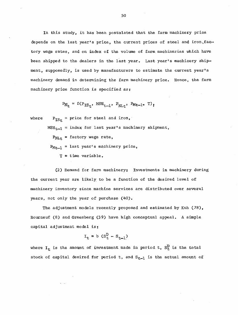
50

In this study, it has been postulated that the farm machinery price

depends on the last year's price, the current prices of steel and iron,fac­

tory wage rates, and on index of the volume of farm machineries which have

been shipped to the dealers in the last year. Last year's machinery ship­

ment, supposedly, is used by manufacturers to estimate the current year's

machinery demand in determining the farm machinery price. Hence, the farm

machinery price function is specified as:

~ ^®®t-l' NLt' t-l" ;

where ^ISt ~ price. for steel and iron,

= index for last year's machinery shipment,

= factory wage rate,

- last year's machinery price,

T = time variable,

(2) Demand for farm machinery: Investments in machinery during

the current year are likely to be a function of the desired level of

machinery inventory since machine services are distributed over several

years, not only the year of purchase (40).

The adjustment models recently proposed and estimated by Kuh (78),

Bourneuf (8) and Greenberg (3 9) have high conceptual appeal. A simple

capital adjustment model is;

It = b cs? - s^_i)

where I^ is the amount of investment made in period t, is the total

stock of capital desired for period t, and is the actual amount of

51

total capital stock that existed in period t-1. Stocks of productive

farm assets on the farm at the beginning of an investment period have an

effect on the current year^ investment activity. If stocks of assets are

high at the end of the preceding investment period, it may signify the

presence of excess machine capacity which allows a moderate output ex­

pansion without additions to the stock of machinery items.

Few variables are attributed to formulate the desired level of the

stock of farm machinery. Prices and price ratios are seriously considered

by farmers attempting to formulate expectations of their ability to pay

for a particular item of machinery. The price of a particular factor of

production is of interest only at the time of purchases. Once the factor

has been, purchased, the price of that factor and the relationship of the

price of the factor to the price of other factors is of no concern. The

ability to pay for an input depends upon what happens to wage rates, land

price and product prices (50). This justifies the inclusion of prices

as variables in the domestic farm machinery investment function. At the

time the decision to purchase farm machinery is made not only the level of

machine prices, but also the relationships between the machine prices and

prices of other factors or prices of products are considered. These latter

prices are more likely candidates for expectation variables. Although

past efforts to measure the influence of wage rates on farm investment

demand have been largely unrewarding (18, 42, 66), the farm wage rate

might be singled out as a separable variable in the investment processes

because of the large substitution of capital for labor.

Recent investment studies by Meyer and Kùh (86) depend heavily upon

52

net income to explain nonfarm investment patterns. Most agricultural in­

vestment demand equations, have also included net farm income as an ex­

planatory variable. This is the important variable from the standpoint

of motivation for investment and a variable for expectations. In another

study of the demand for agriculture inputs, Griliches (42) could find

no good theoretical reason for including income in the demand equations

for factors. He says income is usually introduced as a proxy variable

for expectations and liquidity in reality, but income has little to do

with liquidity (42). Income is a function of prices, quantities marketed

etc. Theoretically, each of the determinants of income should be specified

independently in the model. Since it is difficult to define all factors

determining annual income, the estimates obtained from ordinary least

squares procedures break down if the number of explanatory variables be­

comes very large.

Assets other than investment stock of the particular demand asset are

important in the investment function. The demand for a durable asset de­

pends on the form and abundance of farm assets since many assets are

technically related.

The ratio of proprietors? fixed assets to total liabilities, the

equity ratio, reflects several influences on demand in a dynamic agri- •

culture. It is a measure of the vulnerability of the farm firm to uncer­

tain outcomes. A given loss causes little concern if equity is high,

but if equity is low the same loss may increase liabilities above assets,

creating an insolvent firm. The equity ratio is a measure of this influence

both psychologically for the farmer and actually for outside credit sources.

53

The equity ratio may be regarded as the culmination of the income

generating process. Periods of high income provide an opportunity for

farmers to pay debts and build equity. In the long run a large portion of

these gains is likely to find its way into additional investment. Hence,

the equity ratio is a kind of proxy variable for past income. This is

more so because of the probable lagged adjustment of consumption and durable

purchases to higher income.

The level of technology represented by the production function also

has a bearing on the tendency of farmers to invest. If new technology in

the form of machinery items or other durable goods are to be employed

farmers need to be able to form expectations as to the increases in pro­

duction possible from new capital investment.

Interest rates have been regarded as the prime quantifiable motivator

of investment in durable goods (18, 24, 36, 40, 67, 86, 13 6). These re­

sults draw exclusively from the reflection of businessmen. Farmers seldom

invest to the upper and lower bounds specified by the availability of ex­

ternal and internal capital constraints. Consequently, the interest rates

may not be so relevant to farmers as to businessmen.

Other variables such as average farm size, the number of hired agri­

cultural workers, cropland harvested and time, to some extent, all have

influences on farm machinery investment. Consequently, the postulated in­

vestment function for farm machinery is as follows ;

™t-l- SMt- T)

where Qjyj^ is the annual purchases or gross investment in farm machinery.

54

is the ratio of the current machinery price to the price of farm

products, is the lagged equity ratio, is the stock of farm

machinery at the beginning of the year and T is the time variable.

The demand for motor vehicles and other farm machinery are assumed

not to differ.much from this specification.

An alternative specification of the demand function for farm machinery

could emerge from the following observations. Effective machinery demand

in recent years is a function only of replacement requirements and not

of a gap between current and desired stocks. Many researchers have ob­

tained certain significant results by including lagged values of machine

purchases as independent variables (40, 76, 91), Most of the techniques

employed by these authors included a distributed lag scheme to allow the

influences of certain variables to be spread out over a period of time.

Consequently, the alternative specification for the machinery demand

function may be as ;

%^t ^ ^ QMt-1»

where is the annual gross purchase of farm machinery, (Pj^/Pg^)^ is the

ratio of current machinery price to the price of farm products, ^ is

lagged purchase of farm machinery and T is the time variable.

b. Demand for farm building investment The expected life of farm

buildings is much longer than the expected life of other durable goods in

agriculture. The adjustment models discussed in the last section for

farm machinery still have high conceptual appeal in explaining building

investment. An accelerator model would be difficult to estimate, because

55

a model used to describe farm building investment would need to be an

extended-lag accelerator such as ;

n QBIt ~ 2 ^^(Yt-n+l "" Yt-l)

1=1

where n may be ten or more years. The explanatory variables of an ex­

tends d-lag net farm income would probably be so highly intercorrelated

that reliable estimation by least squares might prove impossible. In a

model with other variables this problem could be solved by arbitrarily

weighting the accelerator coefficient in some logical pattern describing

a response curve such as those suggested by Koyck (76) and used by DeLeeuw

(25). The synthesis might use the weighted (e.g. decreasing geometrical

average) net farm income as an explanatory variable in the stock adjustment

model.

In a number of previous investment demand studies, price ratios have

been used as variables to estimate possible substitution effects between

inputs and relative price effects between inputs and outputs (50). From

the standpoint of motivation one might expect the price ratio of output

and building material to be one of the explanatory variables.

The equity ratio, the ratio of the value of long-term assets (real

estate and buildings) to farm mortgage debt outstanding is believed to

be quite a relevant variable. In addition to those reasons mentioned

with the specification for the machinery demand function, the equity ratio

may be even more relevant for farmers than in the nonagricultural sector

for the following reasons. The farmer is usually an individual owner and

does not have a group of stockholders to share his financial risk. Con­

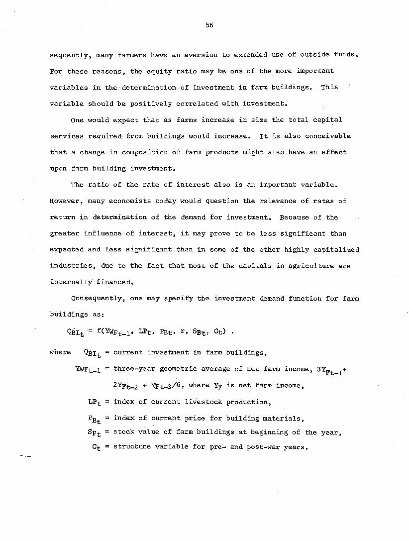
56

sequently, many farmers have an aversion to extended use of outside funds.

For these reasons, the equity ratio may be one of the more important

variables in the. determination of investment in farm buildings. This

variable should be positively correlated with investment.

One would expect that as farms increase in size the total capital

services required from buildings would increase. It is also conceivable

that a change in composition of farm products might also have an effect

upon farm building investment.

The ratio of the rate of interest also is an important variable.

However, many economists today would question the relevance of rates of

return in determination of the demand for investment. Because of the

greater influence of interest, it may prove to be less significant than

expected and less significant than in some of the other highly capitalized

industries, due to the fact that most of the capitals in agriculture are

internally financed.

Consequently, one may specify the investment demand function for farm

buildings as;

Qfilt = LPt, PBt, r, SB%, Gt) .

where = current investment in farm buildings,

YWFt.,1 = three-year geometric average of net farm income,

2YF.|._2 Ypt-o/®» where Yp is net farm income,

LP.(- = index of current livestock production,

= index of current price for building materials,

Sp.|. = stock value of farm buildings at beginning of the year,

G-j- = structure variable for pre- and post-war years.

57

c. Farm labor market

(1) Demand functions: Demand for labor in agriculture results

from the demand for factors in agriculture and indirectly from economic

conditions in the non-farm economy. This relationship can be envisioned

from the general demand function for factors formulated in the first sec­

tion of this chapter. The variables which have been hypothesized as af­

fecting demand for labor are; 1) the wage rate in agriculture (as a price

of the labor factor), 2) price and quantities of competing resources, 3)

price and quantity of agricultural production, 4) technological changes

in agriculture, 5) general non-farm economic activity, 6) unemployment

rate in the non-farm economy, 7) market structures in the non-farm economy.

In Cromarty's study of the demand for farm machinery, the farm wage

rate was a significant variable, however, the sign was negative (18).

This shows that under farm wage rate increases, a substitution of machinery

for labor did not take place. Heady and Tweeten found that the farm wage

rate was not a significant factor in the substitution of machinery for

labor in the analysis of the demand for farm machinery and equipment (50).

Bishop regressed migration against the price of farm products and

found a positive relationship (6). In relating migration to the farm-

nonfarm income ratio, the coefficient was positive and significant. These

results led Bishop to suggest that job opportunity was more important than

farm or non-farm returns. Where migration was used as a dependent vari­

able against unemployment in the economy, a significantly negative rela­

tionship was observed.

Johnson estimated demand and supply functions for hired and family

labor (59). The results from this study showed that the demand for hired

58

labor was a function of farm wage rate with a negative sign and, with

the prices of agricultural products variable indicated a positive sign.

The demand function for hired labor showed a positive sign for the value

of machinery not indicating substitutability. Where machinery prices were

included in the demand for hired labor, the results also did not indicate

substitutability. For family labor the results showed a negative sign

with respect to the farm wage rate but the prices received variable was

inconsistent.

In Schuh's study (100), the demand for hired farm labor was related

to the farm wage rate with a negative sign, positively with farm product

prices, and negatively with technology.

In Heady and Tweeten's analysis of family and hired farm labor a

number of variables were hypothesized as affecting demand for labor (50).

Family labor was hypothesized as a function of 1) ratio of wages of fac­

tory workers to income per farm family, 2) ratio of proprietors equity

to liability in agriculture, 3) stock of productive farm machinery, 4)

percentage of farm sales forced through bankruptcy, 5) index of govern­

ment policy, 6) an interaction term between unemployment and the ratio

of wages of factory worker to income per farm family, and 7) time. The

sign of the ratio of factory wage to income per farm family variable was

negative. The ratio of proprietor's equity to liabilities in agriculture

was positively related to family labor demand.

In Helmers' study (52), the results of the demand equations estimated

for total farm employment show a number of influences affecting total

59

farm employees. These are: 1) the positive effect of the farm wage rate

on the demand for total farm labor, 2) positive influences of net farm

income on total labor in agriculture, 3) the negative operation of non-

farm earning opportunities or non-farm employment opportunities on total

farm employmentand 4) strong negative technological influences on total

farm labor.

Comparing hired and family farm labor demand with respect to the

farm wage rate the negative relationship on hired labor demand and the

positive effect on family labor is notable. Sign differences also exist

for demand elasticities between family and hired farm labor with respect

to net farm income and net income per farm.

Technical change has affected the demand for farm labor in two ways.

It has increased labor productivity and thus increased the demand for

farm labor. But it has increased farm output also, and thus decreased

the demand for farm labor through the resulting decline in farm product

prices. It is probably that the output increasing effects of technical

change have offset the rising productivity of labor resulting in a net

decline in the demand for labor in agriculture. Several econometric

studies of the farm labor market have supported these observations (59,

100, 101).

In this study, demand for total farm labor is hypothesized as de­

pending on the following specific variables: 1) lagged net farm income,

2) lagged index of mechanical powers on farm, 3) lagged ratio of ma­

chinery price to farm wage rates, 4) technological changes index, 5)

non-farm factory wage rates, 6) lagged ratio of machinery price to farm

wage rates.

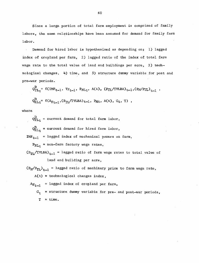
60

Since a large portion of total farm employment is comprised of family

labors, the same relationships have been assumed for demand for family farm

labor.

Demand for hired labor is hypothesized as depending on: 1) lagged

index of cropland per farm, 2) lagged ratio of the index of total farm

wage rate to the total value of land and buildings per acre, 3) tech­

nological changes, 4) time, and 5) structure dummy variable for post and

pre-war periods.

QTLt= f(IMPt-l, PNLf A(t), (Ptl/TVLBA)^^!,CPM/PrL)t«l '

QHLt" PMt, A(t), Gt, T) ,

where

QTL-J. == current demand for total farm labor,

= current demand for hired farm labor,

~ lagged index of mechanical powers on farm,

^NL-t ~ non-farm factory wage rates,

CP.PL/IVLBA)^__^ = lagged ratio of farm wage rates to total value of

land and building per acre,

= lagged ratio of machinery price to farm wage rate,

A(t) = technological changes index,

Ap^^^ = lagged index of cropland per farm,

= structure dummy variable for pre- and post-war periods,

T = time.

61

(1) Labor supply: Although primary emphasis in this study lies on

demand, supply plays a related role in the determination of labor use.

Labor in contrast to other agricultural input, such as machinery, is not

the output of another firm. Rather, it is a primary input. Economic

theory suggests that an individual supply function for labor is derived

from the utility function of the individual (53, pp. 23, 13 7, 129-131).

Current economic thinking postulates that the supply of farm labor is a

function of the price of farm labor and alternative non-farm job oppor­

tunities. Alternative non-farm job opportunities are a function of non-

farm wage rates and various impediments to the farm-nonfarm labor flow.

Various variables have been suggested as impediments to farm-nonfarm

mobility. Among those cited are unemployment conditions in the non-farm

economy, transportation costs, non-farm job rationing, asset fixities of

farm operators, imperfect knowledge, and the preference for farm and rural

life on the part of farm people.

With the exception of the evidence on unemployment conditions, evi«

dence with respect to the other hypothesized impediments seems to be tenu­

ous, conflicting or absent. Bishop (6) refers to the magnitude of recent

migration rates to refute the imperfect knowledge hypothesis, whereas

Johnson (58) has doubted that unions have distorted the wage structure

sufficiently to act as an effective impediment.

Quite comprehensive evidence on farm-nonfarm mobility, however, has

been presented by Perkins in his study of farm-nonfarm job mobility for

the 1955-1959 period (94). His study shows that unemployment in the non-

farm sector, age, and lack of nonfarm job experience are the important

impediments to farm-nonfarm job migration. Clearly, the agricultural

62

labor force has become a shock absorber for the non-farm labor market.

The burdens of deficient demand conditions in the non-farm economy and

structural change in the non-farm labor market in part have been placed on

members of the farm labor force.

In this study, the total farm wage rate has been hypothesized as

positively depending on number of labor demands, non-farm factory wage

rate, lagged unemployment rate, technology, farm machinery price,

structure dummy variable and time. The hired labor wage rate has been

hypothesized as solely a function of total farm wage rate,

^TLt^^^^TLt' ^NLt' t-1' ' P-Mt» ^t» T)

where

= current total farm wage rate,

~ current amount of labor demanded

= non-farm, factory wage rate,

= lagged unemployment rate,

A(t) = technology,

PM^ = farm machinery price,

= structure dummy variable for post- and pre-war years,

T = time.

63

IV. THE RECURSIVE MODELS AND ECONOMETRIC CONSIDERATIONS

A. The Proposed Models

The ultimate goal of agricultural economic research should be a

definite, integrated model of the product and resource structure of agri­

culture. There are several reasons why an integrated model is necessary,

product markets determine gross income, resource markets determine ex­

penses and the two markets determine net income in farming. From a causal

and statistical standpoint, many decisions in farming are interdependent.

It is almost impossible to determine how many hired workers, for example,

will remain in agriculture without estimates of farm product prices,

national unemployment and factory wages. To a considerable extent, farm

input and output prices are determined by non-farm variables such as wage

rates, national income and population. The mobility of farm labor is

conditioned by the rate of national unemployment. Integrated models which

include these nonfarm variables are necessary for predicting farm income,

output and efficiency.

The studies of Brandow (9), Cromarty (17) and Fox (31) have emphasized

the totality and interdependence of farm product markets. While there are

few notable quantitative studies of the resources markets, such as

Griliches (40, 41), Johnson (59), Heady and Yeh (51), Cromarty (3), Heady

and Tweeten (50), Maudon (84), Schuh (100), Scott (102), Helmers (52),

Minden (88) and Reynolds (96), only Heady and Tweeten's study has sup­

plemented and integrated with commodity studies to provide adequate know­

64

ledge of prices, quantities and efficiency in agriculture.

The regional interdependence is one of the other factors which is

crucial in the study of economic structure. There has been progress in

the application of interregional models to policy analysis. In agricul­

tural economics, one must cite among other pioneers the works of Mighell

and Black (87). Fox (31), Heady and Egbert (49), and Judge (61, 62).

While their studies are exclusively in the product markets and are static

analysis. In the studies of resources markets, either due to the data

limitations or technical difficulties, the studies of Scott (102), Minden

(88), Helmers (52), Heady and Tweeten (50) and Reynolds (96)studies are

in terms of separated regional analyses.

There are difficulties for any future work to extend these basic

studies much beyond their current contributions. These possibilities

are in the two major aspects of economic structure. The first of these

is the intertemporal structure or, in short, dynamics. The second is the

interconnectedness of production, transportation, and demand.

Economic theories may be categorized as static or dynamic. Most work

in economic structure has been static in nature. However, as economic

processes are enacted over time, we should expect that temporal structure

is crucial in economic understanding. Only in special cases should we

find that static tools are sufficient to gain an adequate understanding

of economic events. For many agricultural commodities, production de­

cisions take place many months before supplies reach markets. Given

supplies are determined by past production decisions and the intervening

hand of weather. For this reason, regional supplies are independent of

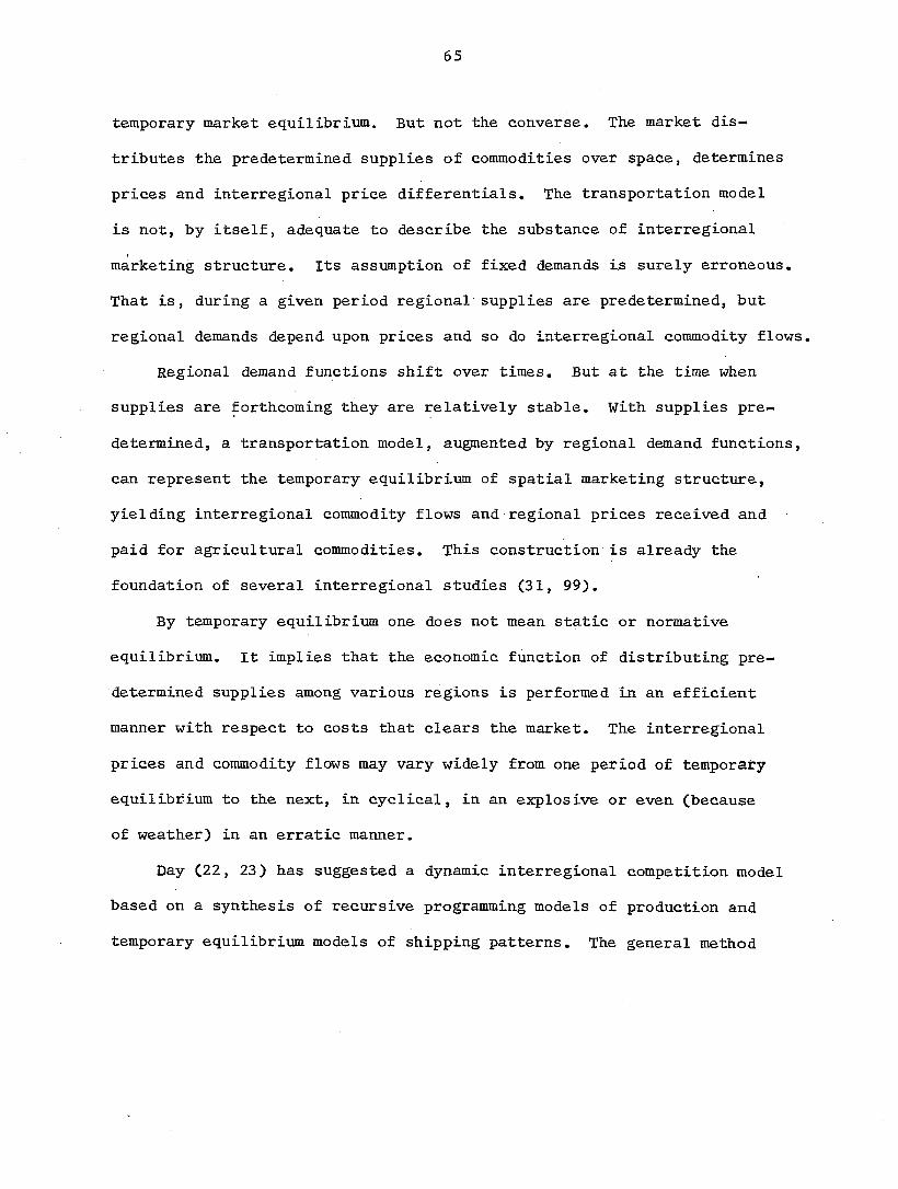
65

temporary market equilibrium. But not the converse. The market dis­

tributes the predetermined supplies of commodities over space, determines

prices and interregional price differentials. The transportation model

is not, by itself, adequate to describe the substance of interregional

marketing structure. Its assumption of fixed demands is surely erroneous.

That is, during a given period regional supplies are predetermined, but

regional demands depend upon prices and so do interregional commodity flows.

Regional demand functions shift over times. But at the time when

supplies are forthcoming they are relatively stable. With supplies pre­

determined, a transportation model, augmented by regional demand functions,

can represent the temporary equilibrium of spatial marketing structure,

yielding interregional commodity flows and regional prices received and

paid for agricultural commodities. This construction is already the

foundation of several interregional studies (31, 99).

By temporary equilibrium one does not mean static or normative

equilibrium. It implies that the economic function of distributing pre­

determined supplies among various regions is performed in an efficient

manner with respect to costs that clears the market. The interregional

prices and commodity flows may vary widely from one period of temporary

equilibrium to the next, in cyclical, in an explosive or even (because

of weather) in an erratic manner.

Day (22, 23) has suggested a dynamic interregional competition model

based on a synthesis of recursive programming models of production and

temporary equilibrium models of shipping patterns. The general method

66

proposed follows the so called'dynamic coupling of Goodwin (38). The

production decisions are interdependent on past market equilibriums, be­

cause market prices do enter production decisions through expectations,

with a lag. Interregional demand does affect interregional shifts in pro­

duction, investment and land utilization, but these effects are distributed

over time by a dynamic adjustment process.

D. Lee Bawden (4) has recently completed a regional interdependence

study for the turkey industry in the United States based on the same

feature of 'dynamic coupling'. However, it differs from Day's proposed

model with respect to supply. His model exploits dynamic behavioral sup­

ply equations rather than a recursive programming formulation. The quanti­

tative forecasts indicate that his model is well suited for short-run

predictions.

The synthesis of recursive production hence recursive resources de­

mand (as the derived demand) and temporary market equilibrium models to

formulate a general dynamic regional interdependence model for the U.S.

agriculture would be desirable. A dynamic interregional model, based on

the theoretical formulation developed in Chapter III and aimed at accurate

prediction in the immediate future will be developed. The model will be

descriptive (behavioral) in nature with emphasis on adjustment in resources

demand—both in quantity and location—through time. However, it can be

readily conceived that many of the regional data are either not available

or limited in time-series. Due to these reasons, the following proposed

models will be separated into the tentative and the final model. The

final model, which has dropped the aspects of the integration of the inter­

67

regional relationships developed in the tentative model, will then be sub"

jected to empirical testing for describing the resources demand structures

in United States agriculture.

1. A tentative model

In formulating an econometric model, the nature of the economic

system to be analyzed should determine the type of equations to be used

and the method used in fitting them.

In this tentative model, as is true also in the final model, the com­

modities supplied are assumed to be given by past production decisions

and the intervening hand of weather.

Wold (13 7, 138) believes that many economic systems are of the recursive

type, whereas certain other econometricians believe that systems of simul­

taneous relations are typical. The recursive system is composed of a se­

quence of causal relationships. It consists of a set of equations each

containing a single endogenous variable other than those that have been

treated as dependent in prior equations (45). The endogenous variables

enter the system one by one, like links in an infinite chain, where each

link is explained in terms of earlier links.

Recursive models seem appropriate in agriculture, both as a basis for

practical forecasting and as tools of realistic economic theory (29, 133,

p. 734). It seems logical that the current prices are a function of the

predetermined quantity. As an extremely simplified example, agricultural

production can be described as a cobweb model, which in turn is considered

to fall into a recursive pattern, where price in one period affects pro­

68

duction in the next, which in turn affects price, and so on. Of course,

a more complete model would include more variables and more relationships

represented in equational forms. The recursive model also seems appro­

priate for the resources demand market.

For these reasons, regional supplies are independent of temporary

market equilibrium. The market distributes the predetermined supplies of

commodities over space, determines prices and interregional price differ­

entials . A transportation model augmented by regional demand functions,

as proposed in this tentative model, can adequately describe the substance

of interregional marketing structure. The essence is that the regional

demand functions are not assumed fixed; rather they are assumed to shift

over time.

This tentative model differs from Day's recursive programming models

(23) with respect to supply. The dynamic behavioral supply equations are

employed here rather than a recursive programming formulation.

This model consists of the separate regional aggregate commodity

supply and demand functions, separate regional supply .and demand for fac­

tors' functions and the transportation submodels for commodity and factor.

The logic and specification for the commodity demand, supply functions

and the factor demand, supply functions has been fully treated in section

3 of the last chapter (Chapter III). The theoretical framework for this

has also been developed in Chapter li. Consequently, to avoid repetition,

only a brief description of those behavioral equations are given in this

section. The logic, specifications and formulation of the interregional

relationships and modified transportation model, will be discussed more

69

fully in this section. These interregional aspects, incidentally, have

been dropped in the final model for lack of data.

As stated, the given supplies of farm commodities are determined by

past production decisions and the intervening hand of weather. For this

reason, regional supplies are independent of temporary market equilibrium.

But not the converse. The market distributes the predetermined supplies

of commodities over space, determines prices over regions. The regional

aggregate production and supply function for farm products are specified as

Qt£ - f( (2R/Pp)(t"l)i' ^t,i ' ®t' Wt,i,T,A(t)^, G),

Q^2 = f( (f ] , T) , ti_ T-l

g

where we have; = quantity of commodities produced; (PR/Pp)t-1 ~

lagged ratio of price received and paid by farmers; = stock of pro-

ductive assets at the beginning of the year; = government's price policy

= current weather index, T = time; A(t) = technological index; G-j- =

dummy variable, refers to the structure change pre- and post-war; =

amount of farm commodity supplied. Subscript i refers to regional numbers.

The regional demand functions for agriculture commodities are speci­

fied as;

Qtj = f j' ^'t,j' %t, j)'

where Q® = quantity demanded; Pj^^ = current price of agriculture commodity;

Pg^,^ = current price of commodities excluding agriculture commodities ;

FGjj^ = index of per capita food consumption; = personal disposable

income; j = consuming regions.,;.

70

Regional demand functions shift over time. But at the time when sup­

plies are forthcoming they are relatively stable. With supplies prede­

termined, a transportation model, augmented by these regional demand func­

tions might represent the temporary equilibrium of spatial marketing struc­

ture, yielding interregional commodity flows and regional prices received

and paid for agricultural commodities. The temporary equilibrium here,

refers to the economic function of distributing predetermined supplies

among various regions in an efficient manner with respect to cost that

clears the market. The implicit assumption is that the shipping decisions

by producers are based on the profit-maximizing goal and, hence, regional

price differentials are based on normative assumptions. The absolute price

level and producer and consumer reactions are dictated by past reactions

to the same stimuli (as discussed and specified in the recursive nature

of the supply and demand of agriculture commodities). These behavioral

equations are estimated by regression analysis. The formulation attempts

to predict on the basis of a description of past actual market behavior.

Although Day (22) has favored the normative path, the present approach is

argued to be the more useful approach when short- or intermediate-run

market predictions are desired.

In an attempt to reduce this sub-model concerning the interregional

shipping pattern and price differentials to a simplified version of reality,

the following restrictive assumptions are also made. Thus perfect com­

petition assumptions dictate the requirements for the regional pattern of

prices and flows of the commodity. Therefore, each firm is assumed to

have the objective of maximizing profits. The supply source and market

71

I for each region is assumed to be represented by a fixed point. All regions

are connected by transportation costs and flows of agricultural commodi­

ties among regions are assumed unhampered by governmental or other inter-

ference. It is further assumed that consumers are indifferent as to

source of supply and that the product is homogeneous. Also, it is as­

sumed that for any time period, t, that total production and total con­

sumption of farm products are equal.

There are some other obvious assumptions. The production and consump­

tion of farm products can take place in all regions and farm products con­

sumed out of local production does not require transporting since each

region is represented by a point. There are no negative shipments and no

cross-hauling.

The normative assumption for shipping decisions by producers appears

reasonable and probably approximates actual conditions, but the assumption

of perfect knowledge by the shipper is clearly fallacious. On this ac­

count, the model is expected to yield perhaps useful forecasts of area

prices, and probably unreliable prognostications of the shipping pattern.

The sub-model which embraces the above arguments is developed below:

The primal solution can be formulated as follows:

Let: subscript i indicate the producing region (i=l, —,n), subscript j

indicates the consuming region (j=l, —,m). In this submodel, it is

assumed that n = m = 10 since each region can be both a producing and

a consuming region. Each region can be categorized as a surplus

(origin) or a deficit (destination) region by comparing their and

Çp at each time t. .

72

Subscript t indicates time in years

X^j = quantity shipped from region i to region j

TG^j= transfer cost from region i to region j

TGij= 0, when i = j

= agriculture commodity price in producing region i at the

producer level

= agriculture commodity price in consuming region j.

The other variables are defined previously.

Given: = f((PR/Pp)t_i,i, Sp^^, G^, W^, T, C^)

qS2 = fCQ^l,T) ti *-3-

Qtj ~ f(2Rtj'FCNtj'%btj'2R'tj

%(t-l)j

TGij

is an unknown and is determined by the complete solution,

but it is considered exogenous to the primal solution. As a prac­

tical procedure one might choose to substitute with

and to start the computation.

The problem then is:

Find X"(t)j Eor all i and j (shipping pattern); n m

Which minimizes: 2 2 X(t)fi'TCii 1=1 j=l

73

Subject to : ij 0 (a)

m

«cl)i =

dct)j °

(b)

(c)

(d)

for all 1, j.

There are many solutions to (b) and (c) subject to (a) and (d), and

given any feasible solution of n+m-1 shipments, the simplex method provides

a means of converging the above problem to the optimum program (21) in

terms of satisfying the objective function. The equilibrium prices are

tied together by a specific set of transportation costs used, and the rele­

vant transport costs used in obtaining the optimum set of flows, are less

than for every possible alternative delivery which is not made. Thus the

solution obtained will be unique except for the case when two or more

sources find two or more markets equally profitable.

The regional (equilibrium) prices, are still unknown at

this stage. In the real world, the regional prices constitute one of the

unknowns necessary for solution, since it is conditioned by the demand func­

tion specified previously. In practical problems, however, with a finite

number of regions an initial approximate set of regional prices can be

So obtained. With given and known transportation costs TC^j and by

utilizing the information (just information) about - given by the

consumption functions, one can derive a unique set of regional prices with

74

the aid of the duality theorem of linear programming. This set of shadow

prices will correspond to the equilibrium set of flows and which may be

used as the approximation value to check and facilitate the procedures to

reach the equilibrium solution.

The dual solution of this problem is ;

D n S Maximizing W=2 ^^ti" 2 Q^.DP .

j=l i=l

Subject to

DR(t)j > 0

Find: Eor all j (shadow prices)

DP^t)i Eor all i (shadow prices) .

Where the DR^^^. and DP^^^^ are dummy variables at this moment and will

be given the interpretation below.

This dual problem has been constructed from the primal solution of

minimizing the total transportation costs. The objective then can be

thought of as that of finding the DR^^jj and DP^^)^ that will maximize

the total gain in value of amounts shipped subject to nonpositive profits

on each shipment. By this formulation, it is possible to interpret the

DR^t)j and that will maximize the total gain in value of amounts

shipped subject to nonpositive profits on each shipment. By this formula­

tion, it is possible to interpret the DR(t)j and DR^^^^ as the value of

the product at supply origin i and as the value of the product delivered

at destination j. The first equation for the restriction on the above

75

can be written as

DK(t)j ^P(t)i-^ TCij.

This is implying that for routes in the basis, destination value equals

supply point value plus transportation costs. For those routes not in the

basis, destination value is equal to or less than the supply point value

plus transport costs.

With the and found from the dual solution, one can pro»-»

ceed to solve the regional prices (t)i and Here, the

known. The formulation is

Minimize Z PR(t)j - S - ZPgct).

Subject to: Q(t) ,• = £<PR(t)i. PRCtJi'^^NCt) j. YoCtji) — Regional demand function.

^ g ^ g

^&(t)a" P&(t)b= °Kt)a- °^(t)b Cj=a,b)

^R(t)c" RCt)d~ DP(t)c~ DP(t)d (i=c,d)

PR(t)j" PR(t)i= DR(t)j" D2(t)i '

This is a corollary solution. These restrictions are set up so that

regional demand function and the total consumption are equal to the total

production. Other restrictions are trying to keep the regional prices and

their corresponding shadow prices consistent among the regions.

76

Complete solution of the problem encompasses all three phases;

primal, dual, and corollary. The procedure includes the sequential solu­

tion:

I, Time (t)

A. Stage I; Use the known value of solve the regional supply

equations for

B, Stage 2 ;

(1). Trial I

(a) Arbitrarily start with Q(t,;.i),j and through the primal,

dual and corollary solutions find X(t)ij: ^(t)i» D&(t)j'

(2). Trial 2:

(a) Use the found above to solve Q(t)j through demand

equations.

(b) Solve for the X^j, and ^ through the primal

and dual solutions.

(c) Compare these new shadow prices with those in the pre­

vious trial. If they are identical, a final solution

for year t has been reached. Solve for regional

(equilibrium) prices PR(t)j and P&(t)i through corollary

solution and proceed for the solution of year t+i with

the same procedure as for year t.

(d) If they differ, a final solution has not been reached;

77

repeat the same procedures as in trial 2, and continue

new trials until an equilibrium solution for year t has

been reached.

This procedure may be repeated until answers to the desired number of

time periods are obtained. This procedure has been called reactive pro­

gramming (62, 113). For ordinary cases, the final solution can be obtained

at the trial 2. While with careful selection of initial j' say if

it is equilibrium value, then trial I is enough to yield the satisfactory

solutions for year t and the subsequent years.

Conceptually analogous procedures can be developed for regional farm

input prices. Regional demand for different individual farm inputs depend,

as discussed in Chapter III, on the nature of the supply and demand func­

tions of farm products. While supply functions for farm inputs especially

for durable goods, depends more on the non-farm variables—for example, de­

mand for farm machinery depends most probably on past machinery prices,

farm commodity prices and farmer's equity position—the other influencing

variables may be the levels of production technology and the stock of farm

machinery at the beginning of the year. The regional demand function for

total farm machinery can be specified as;

^M(t)i^ fC(PM/I'R)(t-l)i> A(t)^, T, SMCt)i>,"the demand

region i=l, —, 10.

The regional machinery supply functions can be specified as

g

% ( t ) j ' ^ l S ( t ) j ' MSH ( t - . l ) j > P N L t j » T ) , t h e n u m b e r o f j un d e -

78

termine d, depends on the location of machinery manufacturing plants.

Where, is the regional farm machinery supply; P^Ct) the re­

gional farm machinery price; Pjg^^) is the regional wholesole price for

iron and steel ; the index of farm machinery shipment in the

previous year; P l-j- is the factory wage rate; T is time.

It can be visualized that QM(t)i predetermined at the beginning

of the year. It is mainly determined by last year's regional farm product

prices and farm machinery prices. Given and TG^j (transportation

S D costs) for farm machinery, the Qi^(t)i QM(t)i^ and the P]^(t)i can be

solved analogously, and the farm commodity prices, by the primal, dual

and corollary programs as are formulated at the beginning of this section.

Without going into the logic about specifications of other behavioral

equations, the whole (tentative) model is presented in the following. The

model is immediately followed by brief description of the variables. The

logic behind the specifications of behavioral equations has been treated

in section 3 of the last chapter (Chapter III).

The Model :

Regional stock of productive farm assets including money capital

®Pti (Q(t-l)i' P(tyl)i'

Regional aggregate production response function

Qti = ^((PR/Pp)t«l,i, 8pt,i. Gt, Wt,i, T,A(t)i, Gt)

Regional aggregate commodity supply function

79

= f (Qtb T)

Regional aggregate products demand function

Qtj ~ ^ ^Rt, j' %'t, j' ^"^Nt, j' t, j)

reactive programming (transportation) submodel;

I i i are. solved via a.(revised I K\, , i. , J

1 reactive programming (transportation) submodel

Definitional equations;

Net farm income = = f ^R'^t, ^Rt'(

Weighted net farm income = YwFt ~ /

Farm machinery market;

Regional demand for all farm machinery

QM(t)i = ^(CPM/PR)(t«l)A(t)i, ER(t„l)£» S]yi(t)i> T)

Regional demand for farm motor vehicles

<^V(t)i~ ^(C%v/PR)(t"l) ,i'A(t)i,ER(t_2)j^,AF(t"l) , i'^MVt, i.

Regional demand for other farm machinery and equipment

(&(t)i = " V(t)i

Regional machinery supply functions

9M(t)j = ^^PMCt)j>^IS(t)' ^^(t-l)j' %Lt,j' T)

80

S W(t)j ~ j' %L(t)j, T)

PlS(t)j. T)

Reactive programming (transportation) submodel

%(t).i'j. %V(t),i,j, PME(t)i,j are solved via a

revised programming (Transportation) submodel

Regional demand for farm building investment

W t)i =^(^W(t^l) , i, i'ER(t-1 )i, A(t).g^, PBti, Gti)

Farm labor market;

Regional demand for total farm employees

"7 I I

QTL(t)i = ÊCYF(t-i)i,]âlP(t-l)i, A(t)i, )(PTL/TV1BA). , . (iM >> \ t-i,i

Regional supply of total farm labor

^TL(t) j ~ i'^NLt, i'%(t-l)i»Ut-l'

Regional demand for hired farm employees

QHLt,i=fCPTL/TVLBA)t,i, Ap(t"l),i, Ct), Gt, T)

Regional demand for family farm employees

QFLt,i = QTLt,i"^Lt,i

Regional hire farm wage rate

%Lt,i =

81

The Variables:

Endogenous variables:

= Quantity of farm products produced

Q 2 = Quantity of farm products supplied

Sp = Stock of productive farm assets at beginning of year

Q® = Quantity of farm products demanded

= Net farm income

Y pt ~ Weighted net farm income for last three years

= Quantity of total farm machinery demanded

D Qj y = Quantity of farm motor vehicles demanded

= Quantity of other farm machinery and equipment demanded

g

Q = Quantity of total farm machinery supplied

= Quantity of farm motor vehicles supplied -

g

Qj g = Quantity of other farm machinery and equipment demanded

Qgg. = Value of investment for service buildings on farm

Q Lt - Quantity of total labor demanded

= The farm wage rate

Q 2, = Quantity of hired labor demanded

Q t ~ Quantity of family labor demanded

= Farm wage rate for hired labor

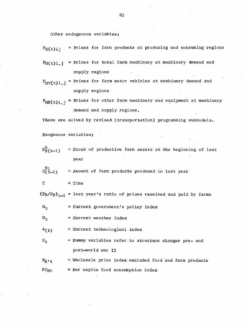
82

Other endogenous variables:

R(t)ij ~ Prices for farm products at producing and consuming regions

P]yi(t)i,j ~ Prices for total farm machinery at machinery demand and

supply regions

MV(t)i j ~ Prices for farm motor vehicles at machinery demand and

supply regions

ME(t)i j ~ Prices for other farm machinery and equipment at machinery

demand and supply regions.

These are solved by revised (transportation) programming submodels.

Exogenous variables;

P(t-l) ~ Stock of productive farm assets at the beginning of last

year

Si Q(t-l) = Amount of farm products produced in last year

T = Time

CPr/Pp) „1 = last year*s ratio of prices received and paid by farms

= Current government's policy index

= Current weather index

A- t) ~ Current technological index

Cj. = Dummy variables refer to structure changes pre— and

post-world war II

Pg t = Wholesale price index excluded food and farm products

^ Nt ~ Per capita food consumption index

83

"5 , = Personal disposable income

T' = Index for production efficiency, i.e., total output

divided by total input

Ypt l ~ Net farm income for last year

YFt-2 = Net farm income for the year before last

YFt-3 = Net farm income for three years ago

(P]yi/PR)-t>.i = Last year's ratio of farm machinery prices to prices

received by farmers

ER't"! Last year's farmers' equity ratio

MCt) - Stock of total farm, machinery at beginning of year

CPMV"/l'R)t-l = Last year*s ratio of farm motor vehicles prices to

prices received by farmers

Apt„i = Last year's cropland index

MVt ~ Stock of farm motor vehicles at beginning of year

PjSt ~ Current price index for iron and steel

~ Index for the amount of machinery shipped, lagged one year

%Lt - Factory wage rate

LP f- = Current index for livestock production

Pg = Current price for farm building

Pp.(. = Price paid by farmers for aggregate inputs

= Last year's indè& :of fmechan:ical -powders :Qn farm

U-t„i = Last year's national unemployment rate

%t-.l ~ Last year's price for total farm, machinery

TVLBA = Index of the total value of farm land and buildings per

acre

84

2. The final model

In the last section, an interregional factor demand model in agri­

culture has been proposed which integrates factors and products markets.

However for some of the important variables, the data needed in the em«

pirical analysis are either very difficult to find or not available. For

example, a complete set of data for the transportation costs among ten

production regions for a period 1924 to 1965 are very difficult to obtain.

In order to operationalize the model under the constraints of these

data limitations, the proposed model has been separated into the national

and regional models.

In the final national model all of the features which were incor*"

porated in the proposed model, except the modified transportation submodel,

are maintained. In the regional models the multiple covariance analysis

models, instead of the simple equation for each region, are employed.

These models are essentially the results of combining the techniques of

covariance analysis and multiple regression with certain algebraic re­

combinations of intercept and dummy variable.

a. The national model On the basis of economic theory and logic

developed for the proposed model in the last section, the final model has

the same set of functional relationships and similar specifications of

the variables as in the proposed model except for the modified transporta­

tion submodel which has been dropped. Without loss of precision, the

model is presented here in functional form. All variables have been de­

fined in the last sections. The model is;

85

Stock of productive farm assets including money capital

s|t = Spt-r T)

Aggregate production response function

= fCCPR/Pp)t-irs| ^ , G , Wt, A(t), T, G)

Aggregate commodity supply function

= fCQ-J, T)

Aggregate products demand function

PRt = fCFCjgt' YDt, Qt^, Gt, PÉt)

Definitional equations :

Net farm income

Ypt = fCPR.t'T'CPR/Pp)t. sjt' CPR/Pp)t. Ypt)

Weighted net farm income

WFt = OYpt + YF _2) / ®

Farm machinery market

Demand for all farm machinery

Qm-(- — PM/PR) t—l ' ' ® t-»l '

Demand for farm motor vehicles

^Vt ~ ^(^^t"l ' -^Ft^lJ ACt), S]y[y^, T)

Demand for other farm machinery and equipment

^ MEt ~ t " Vt

Total machinery supply functions

%r = PNLt» %t-l»

Demand for farm building investment

QBIt = f(ERt-l,LPt, PBt, Sfit, YWFt-l» ^t)

86

Farm labor market

Demand for total farm employees

qÇl = fClMPt-i, PNLt. A(t), (PTL/rVHLA)t„lX )t_i)

Supply of total farm labor

TL ~ ( t) t-l» QTLT»

Demand for hired farm employees

( Lt = (Pn/rVBLA) ] , T, 0%)

Demand for family farm employees

QpLt TLt " Sht

b. Regional models Even less census data is available for region­

al analysis than for national analysis. For a number of important vari-.

ables, data on a regional basis are available annually only since World

War II. When a proposed economic behavioral model suggests lagging cer­

tain variables for one year or more, the length of the time series for

analysis and consequently the statistical degrees of freedom are further

reduced. On the basis of economic theory for the national model approxi­

mately the same variables are included in the regional model.

The usual method for regression analysis of regional data is to esti­

mate separate regression equations from each area. With this procedure

the length of the series available for this study would limit the total

degrees of freedom (with reduction due to lags) to approximately 16.

Assuming that four to six independent variables would be needed to ex­

plain a substantial proportion of the variance of the dependent variable,

the residual sum of squares from regression would be associated with ap­

87

proximately 10 degrees of freedom. This would be insufficient to get

good statistical results where a separate equation is used for each region.

The final regional models used in this study include all regions

simultaneously in one equation (for each factor, each region and year

providing an observation). The models are essentially the combination

of the analysis of covariance (93, pp. 43 7-465) with multiple regression

(14). With further incorporation of the algebraic recombination of cer­

tain intercept and dummy variables, the models become multiple covariance

analysis with additional regression variables. Slopes and differences

of slopes as well as intercept differences are obtained for testing. This

kind of model has several advantages over the usual simple equation model.

First, it provides an immediate statistical test for differences found

between regions ; Comparison by general inspection of separate equations

is more fallible and less precise, while statistical comparison of

separate regression equations is more difficult and time consuming.

The second advantage is that inclusion of all regions in one equa­

tion gives a much higher number of observations. Although the number of

independent variables are also increased because of the addition of dummy

variables, not all differences for all variables and all regions are ex­

pected to be significant and there would be a greater relative increase

in the degrees of freedom associated with the residual sum of squares

rather than the increase in the number of explanatory variables. An

underlying statistical assumption in following this procedure requires

that observations from all regions are drawn from a common population.

This, however, is an assumption which must be made if separate equations

88

are estimated in the usual way and statistical tests performed between

regressions. If there is no significant increase in the variance of

variables, the relative increase in degrees of freedom for the residual

sum of squares should increase the probability of obtaining good statis­

tical results. More precise statistical results lend greater credence to

subsequent economic analysis and interpretation.

Regional demand for total farm machinery; The following model

is used to obtain regression equations for the ten production regions;

m—1 m—1 m-l OBt = bg + S bi + G OMt-l+ ? < iQMt-l,i+® t-l+|_ iEî t-l,i

+ gC M/ R t + h.T + TJ

where b is the overall intercept; b is the difference in intercept be­

tween the i region and b i=l ,2 , ——,m-l) , and m is_the number of regions

(10 in this study). is the current investment in total farm machinery

deflated by the -wholesale price index; Q t-l one year lagged investment

in total farm machinery deflated by the wholesale price index; d is the

slope difference for between the i region and the m region

given by c; f is the slope difference for ERt-l between the i region

and the m region given by e; (PM/PR)t the index of the ratio of the

farm machinery price to the price received by farmers for farm products

(1957-'59 = 100). T is the time trend, and is represented by the last two

digits of the year. TJ is the error term.

The alternative stock adjustment model for the total machinery demand

89

is as follows;

m-1

where is the technological index; S t the stock value of the total

farm machinery at the beginning of the year; the ratio (Pm/Pr)t-i is a

one year lagged index of the ratio of farm machinery price paid to the

prices received by farmers for farm products (1957-*59 = 100); and the

remaining variables and coefficients as defined in the preceding equation.

Regional demand for motor vehicles; The expectation and stock ad«

justment models for the demand of motor vehicles are presented separately

below.

The expectation model;

D m-l m-1 m-1 Pmv. 9MVt= o+ 2=1 1+ cQMVt-i" f=i' i MVt-.l,i''® ^ t-l+ =i i t-l,

+ h T + U-j

The stock adjustment model ;

J) m» l m l m - l QMVt= c 2 diAti+ e ERt_i+ iERt i, i.+g S vt

m—1 + S h-iSMVti* j(PM/PR)t i+kT +Ut. i=l

is the current investment in farm motor vehicles (including tractor,

truck and auto vehicles) deflated by wholesale price index. CPMv/ 'R t

the index of the ratio of the price of motor vehicles to the prices re­

ceived by farmers for farm products (1957-'59=100); the value of

the stock of farm motor vehicles at the beginning of the year; (P]y[/PR)t-.l

is the one year lagged index of the ratio of farm machinery prices to

pieces received by farmers for farm products (1957-*59 = 100).

90

Regional demand for total farm labors ; The regional model for

the demand of total farm labors is as follows ;

J) m—1 m—1 QTLt= o+2 bj_+c(lMP)t«l+dYpt_i+2 YFt„i,i+ NLt + S t

L-i 1=1 '

m—1 m +?_ h£A i+j(P L/T"VBLA)t„i+? ki(P L/TVBLA)t-l, i+l(%/P'rL)t i+Ut.

b is the overall intercept, b is the difference between the i region

and bg (where i=l,2,—,m-l), and m is the number of regions (10 in this

study). is the quantity of the total farm labor demanded;

a one year lagged index of the mechanical power on farms ; is net farm

income lagged one year; e is the slope difference for between the

ith region and the region given by d. NLt the index of the fac­

tory wage rate (1957-'59=100); is the technological change index (1957-

*59=100); h is the slope difference for between the i region and

the m region given by g; (Pij A'VBLA)is the index of the ratio of

farm wage rate to total value of buildings and land per acre, lagged one

year (1957-* 59=100) ; is the slope difference for (Pg j/TVBLA)between

the i region and the m h- region given by j; (PTL/rVBLA) „] is the index

of the ratio of farm machinery to farm wage rate (1957-*59=100), lagged

one year; and is the error term.

The demand for hired farm labor;

Tj m-1 m-1 m-1 QjjL ~ o+|_j bi+cPMt+ At+Ç_eAt,i+fAF .„j +Ç_gj- A-pt-l, i

m—1 +h(P,jL/TVLBA)t„i+?_ : PTL/TVL®A)t-l,i+' +

91

where is the quantity of hired labor demanded; is the index

of cropland per farm in acres, lagged one year; with other variables and

the relationships between the coefficients defined as in the demand for

total labor.

Regional demand for farm building investment:

T\ n-l m-1 m-l BIt~ * ' PBt+ ® WFt-l, i+g t-l'*'f=i' ' B&t-l,i

+ J T + Ut ,

where is the annual gross investment in productive farm buildings;

Pg is the index of the price of farm building materials (1957-*59=100);

is the stock value of productive farm buildings at the beginning of

the year; T is time trend; and U is the error term. Ywpt-l the lagged

geometric average of the net farm income; f is the slope difference for

WFt-l t»etween the i region and the m region given by e; is the

one year lagged equity ratio; h is the slope difference for ERt-i be­

tween the i region and the m region given by g. All variables are de­

flated by the wholesale price index.

B. The Econometric Considerations

Economic variables are frequently interdependent. The existence of

a system of equations including both the equations upon which main inter­

est centers (say the production response function) and equations which

generate its determining variables (say the price generating equations)

may lead to a biased single equation estimate of the former relationship.

92

Marshak and Andrews (81) and Hoch. (54) show, however, that no such biases

will occur if the price generating functions are separable from the pro­

duction response function (i.e., if prices are in no way dependent on the

disturbance term of the production response function). A time lag between

the decision period and time of final output suggests that this may be an

appropriate assumption for agriculture, though it may not be appropriate

for certain non-agricultural industries where there is mutual interde­

pendence between the current price and output variables. Supply in the

latter situation should theoretically be estimated using simultaneous

equation methods, though in practice much will depend upon the period over

which prices and output are aggre-gated. This has important implications

for what will be appropriate estimation procedures for alternative formu­

lations of the system of equations. The time period chosen and the produc­

tion processes involved determine whether the model is recursive, simul"

taneous or both (recursive with simultaneous subsets),

1. Recursive versus simultaneous systems

Suppose one has the system of equations

By . + CZ = U.J. 1

The above system is a recursive system if the following properties hold;

B is lower triangular 2

E(Uit; yjt) = 0 for ic j for all t 3

This implies that the stochastic disturbances in the equations are dis­

tributed independently. Assumptions 2 and 3 permit one to estimate y . .

yit = "5+ibj,tyj,t-3=iCjZjt+ Uit

93

from the conditional likelihood function derivable from equation 4. In

that estimation procedure the problem of identification does not arise

as it would if one estimated the reduced form without the assimptions 2

and 3 from equation

Yt + C 5

Recursive systems are frequently given a causal interpretation. There

continues to be an intensive discussion on the concept of causality in

econometric investigations (5, 104, 107, 13 7). Causality in recursive

systems is understood to imply an asymmetric relationship. Controlling

an endogenous variable y implies that one exerts at least stochastic

control on a variable y , if i < j. The converse does not hold. In pure

simultaneous relationships it is generally held that this division cannot

be imposed. A recursive system, as defined above, always possesses the

property of causality as defined. Recursive systems can be subdivided

into pure causal chains and conditional chains, pure causal chains, after

appropriate substitution, transfor the matrix B into a diagonal matrix.

The cobweb theorem, as applied to the supply and demand for hogs, is an

example at the micro level. Conditional causal chains are formally simi­

lar to interdependent systems (simultaneous equation systems), with the

important difference being that the behavioral relations of the equation

systems are specified in terms of conditional expectations. Following

this line of argument, Strotz and Wold (107) have argued that a simul­

taneous equation can be seen as the limiting form of a recursive system,

where the adaptation process of the economy is instantaneous. The question

94

then remains whether causality exists in a non-recursive system. Wold

(13 7) argues that a causal-chain model, where some types of simultaneous

systems could be used to construct a model on the basis of behavioral

relations, might synthesize the recursive and interdependent systems.

This model would accept other relations and approximations that might

break the pattern of the triangular coefficient matrix and yet maintain

the stimulus-response interpretation.

It can be easily visualized that the proposed final model in this

study is a recursive model. This model has been constructed on the lag-

causal ordering of the commodity markets and the causal structure of the

demand for factors markets which are discussed in detail in the previous

sections.

2. Use of least-squares techniques

Wold and Jureen have shown that least-squares regression will yield

unbiased estimates of the parameters in a system of linear equations if

the system is recursive and if all the residuals are uncorrelated (140,

p. 51).

In the recursive system specified by the triangular coefficient matrix

of the endogenous variables, the covariance matrix of the residuals is

also assumed to be a diagonal matrix. Wold and Jureen (140, p. 203) as­

sert that intercorrelation of these off-diagonal residuals can be reduced

to negligible proportions if the relationships are arranged as a series

of lag relationships.

Other arguments have been advanced for use of least-squares techniques,

even if the assumption of a diagonal covariance matrix is invalid. Klein

95

(70, p. 866) endorsed least squares for cobweb models and also concurred

with Fox's argument for least squares estimation of market demand rela­

tions of farm products where supply varies much more than demand (31).

Waugh (135, p. 386) reviewed the use of least squares and simultaneous

systems in operational uses of the past decade and concluded that least

squares, as often as not, give superior estimates. On the other hand,

Chirst (11) noted that specification errors, other than simultaneity,

often invalidated interdependent estimates.

Least-squares regression techniques were used to estimate the para­

meters of the recursive model developed in this study. Possible difficul­

ties in the assumption of uncorrelated error terms of the recursive model

was taken into account in making this decision.

a. Least-squares The least-squares regression model is of the

following form;

" i = 1 ?2 2i + + PK %i *

where is the dependent variable, the X*s are the independent (explana­

tory) variables, the p's are the coefficients of the model and U is the

error term. This model can be stated more compactly in matrix notation;

Y = X B + U (A)

where Y is a vector of n observations on the dependent variable, X is an

(n X k) matrix of n observations on K independent variables, B is a vec­

tor of unknown coefficients and TJ is a vector of errors.

To estimate the vector of coefficients by least-squares, the following

assumptions are made (60, p, 107);

96

(a) E(u) = 0, i.e., the are random variables with zero expectation;

2 n (b) E(u U» ) = i.e., the have constant variance ( homo s ce das-

ticity) and E(U U +g) = 0 for S X 0 (independent errors);

(c) X is a nonsingular matrix;

(d) X is a fixed set of numbers; and

(e) the number of observations exceeds the number of parameters to

be estimated.

We are interested in estimating the parameters of Equation (A). Let

denote a vector of estimates of B, . Now we may rewrite Equation (A) as

Y = X + e

where e denotes the vector of n residuals (Y-3ffi ).

The principle of least squares is that the value of B should be chosen

so as to minimize the sum of squared residuals, e'e.

e'e = (Y-XB)'(Y-xê)

By differentiating e'e with respect toand equating the result to

zero, we obtain;

X'3ffi = X'Y

By premultiplying both sides by (X'X)" , we obtain;

•B" = (X'X)~ X*Y

where (X*X)~ is the inverse of (X'X). The variance of can be shown to

be;

Var (B) =(?\ (X'X)-

and the variance of any coefficient may be obtained by taking the i h

term, from the principal diagonal of (X'X)" and multiplying by the

variance of (60, p. 110). , the least-squares estimate o£ , can

97

be shown to be;

- e'e/(n-K) = ( Y ' Y - B'X'Y) / n-K.

It can be shown that least-squares estimators are linear, unbiased

and that they possess a smaller variance than any other linear unbiased

estimator (60, p. 110). Therefore, the best, linear, unbiased estimator

of B is the least-squares estimate ( ) given in' = (X'X)'" X*Y.

In addition to our earlier set of assumptions, it must be assumed

that the are normally distributed if we are going to use the F- or

t-tests of significance (60, p. 115). The t-test is the ratio of the es­

timated regression coefficient to its standard error. This t-test is used

to test whether the regression coefficient is significantly different from

zero. The F-test is the ratio of the regression mean square to the residu­

al mean square. The F-test is used to test the significance of the over­

all regression. That is, the F-test is used to test the hypothesis that

the explanatory variables do not influence the dependent variable.

values are used to indicate the percent of variation in the dependent vari-

O able that is explained by the explanatory variables. R is called the co­

efficient of determination.

Multico11inearity Multicollinearity is the high correlation be­

tween two (or more) explanatory variables. Multicollinearity makes it

difficult to disentangle the separate influences of the explanatory vari­

ables and obtain a reasonably precise estimate of their separate effects

(60, p. 201). Subsequently, the assumption (G) for using the least squares

technique is not met. Multicollinearity is often a problem in economic

98

time-series, especially whenever a larger number of explanatory variables

are used. The problem becomes greater when lagged variables are used and

the coefficient of the lagged variables are estimated by least squares

along with the coefficients of the other explanatory variables. It is

possible to have a relationship that fits very well (a high R ) while

no coefficient tests to be significantly different from zero (37, p. 193).

In some cases, as Haavelmo (43) argues, the estimate of (sum of squares

of error) will be impaired by highly correlated independent variables. The

inflated standard errors of the regression coefficients will, hence,

present difficulties in rejecting very diverse hypotheses about the re­

gression coefficients.

In using the ordinary least-squares estimation method, there are cer­

tain ways to alleviate the problem. Where two explanatory variables

(other than lagged variables) are highly correlated, a common practice is

to remove one of the variables from the equation. Experience indicates

that the multicollinearity problem is not severe if the correlation between

any two explanatory variables is less than .8. Lagged variables are

usually significantly correlated with one another and with the associated

current variable. In that case, the general method is to enter a func­

tion of the lagged variables as a single variable in the regression equa­

tion. A number of possible functions of the lagged variables can be de­

vised. The declining geometric weighted average of lagged variables will

be used in this study whenever weighting of lagged variables will be re­

quired.

Recently, another weighting function which may be used to replace

99

intercorrelated variables in cases of either with or without lagged ex­

planatory variables has been suggested. It is a linear combination of the

intercorrelated variables based on the first principal component (55, 57,

72, 134). This method, quite appropriate when no a priori knowledge about

a weighting scheme is available, is quite useful in some cases.

b. Autocorrelation of errors Autocorrelated error terms exist when

the error term of one period is not independent of the error of previous

periods. When autocorrelated errors are present, assumption (b) for es­

timation by least-squares regression is not met. The least-squares esti­

mators remain unbiased and consistent but they are inefficient when auto­

correlation exists (115).

Time-series regression equations quite often have positive autocor­

related error terms, Klein (68) has shown that the problem of autocor­

relation increases with shorter time periods. Autocorrelation may be

caused by 1) omission of important variables either due to incorrect

specification or deliberate omission of some variables due to limited

length of time series data, 2) incorrect specification of the form of

the relationship between economic variables and 3) errors of measurement

in the explanatory variables. There is a strong likelihood that an error

of observation committed in one time period is likely to be repeated in

the next time period and hence give rise to autocorrelated errors.

Two generally accepted tests for autocorrelation are the Von-Neuman

ratio (132) and the Durb in-Wats on test (2 7).

The Durb in-Watson test is:

100

d = s ( N

t=2

where u (t=l-,n) are the residuals from a fitted least-squares regres­

sion. Tables of significance have been worked out by Durbin-Watson for

up to five independent variables and 100 observations (27). Exact sig­

nificance levels are not available but upper (d ) and lower (d ) bounds

to test for positive autocorrelation are calculated. The tables are sym­

metric for negative autocorrelation in the range of 2 to 4.

If the computed d value is less than table value of d^, the hypothe­

sis of random disturbance is rejected in favor of positive autocorrelation.

If the computed d value is greater than d^, the hypothesis of random dis­

turbances is not rejected. If the computed d value falls between d^ and

d the test for positive autocorrelation is inconclusive (60, p. 192).

Theil and Nagar (111) have obtained a more accurate approximation for

the distribution of the Durbin-Watson statistic. This criterion defines

as significant those values of d which are significant or inconclusive in

the Durbin-Watson test.

Both the Von-Neuman ratio and the Durbin-Watson tests are considered

questionable for errors from equations containing lagged endogenous vari­

ables. The presence of lagged endogenous variables violates the assump­

tion of the fixed regressors in using the ordinary least square estimation

method. Consequently, the coefficients of the lagged variables carry

away part of the autocorrelation in the residuals with biased coefficients,

invalidating the use of the test criteria which are based on residuals.

When lagged endogenous variables are included as explanatory variables,

101

one should proceed to estimate the structural coefficients as if auto­

correlation was present. Koyck proposes a technique to obtain consistent

estimators which depend on the assumption that the error term, u , is

generated by an autoregressive scheme,

"t ~ P"t-1 t •

The assumptions are that u has a zero mean and a constant variance, e

is npt correlated with u ^ and there is no autocorrelation among the e's

(76, p. 34). Further, he assumes specific values of f?. Estimation by

this technique is referred to as autoregressive least squares.

m an equation such as the following, (assuming that a first-order

autoregressive scheme applies) the cases in which an estimated coefficient

(b') is a consistent estimator of the real regression coefficient (b),

has been outlined by Fuller (33). He shows that, given Koyck's basic

equation, y = ax +by _ +u combines with the first-order autoregressive

scheme of u = + e leads to;

"t = f(yt-l - t-1 - b y ^ g) + e .

By substituting this equation into = ax + by ^ + shows that

the probability limit of b' is given by plim b'=b+ —Ê_ IC V tYt " 1 » I l-r tYt-l J

Under these assumptions, b' is a consistent estimator of b only when p= 0.

These results indicate that a more accurate estimate of b can be obtained

if the value of P is known.

Methods for estimating have been presented by Klein (68) and

Cochrane and Orcutt (13). A simplified method for estimating and the

regression coefficients by an iterative process has been developed by

102

Fuller and Martin (34, 3 5).

The essences of the Fuller-Martin method is as follows; Assume a

basic equation of the following from = ax + by _ + u , and combining

with the assumed first-order autoregressive scheme of u = leads

to •— =P(yt„i - - byt-2> + t '

By substituting the last equation into the first equation, the next

equation will yield the result

yt = ax +(b +f)yt-l ~ r t-1 - yPyt-2 +

A regression on those variables provides initial values of estimation of

a, b, and p . By a method of non-linear regression (79), a function of the

estimates of the coefficients is expanded in a first-order Taylor expansion

about the point defined by the initial values above. The sums of squares

and cross products for Taylor expansion become linear combinations of the

parameters in the above equation. The results of the Taylor expansion

yield:

y = y + z A'a + 22"=" + 3- , where

y = y - y , the residuals in the equation

yt = axt +(b +/0) yt-l"^r^t-l " ^ yt-2 + ^t'

Zi = Xt- pZt-1

Z2 = yt_i- pyt-2.

Z3 = yt-i-' t-1- yt-2'

where 'a, 'b', are the initial estimates of the coefficients, and the a,

, and-=a.p represent changes in the estimates for each iteration. The least-

squares method applied to y = y + zj -A'a' + Z2 produces

103

further changes in the estimates, and the iterative procedure continues

until the change becomes sufficiently small. The final values are consis­

tent estimates of the coefficient.

This technique has advantages, however, it only guarantees a local

minimum of the residual sum of squares.

Another method which is among the easiest has been suggested by Theil

and Nagar (111) and is used in estimating most of the equations in this

study. The calculated d-statistic can be used to give a simple estimate

of P by the simple formula p = 1 - % d . The first-order autoregressive

scheme; u = p t-l"*" t' P J with the estimated ( ) then, could

be used to transform the original data and the transformed data are re-

estimated by ordinary least squares. If the original equation is

y = b + u , the re-estimated equation after transformation is

(y Yt-l) ~ (xt "'P t-l + ®t* a time consuming method because

with most existing computer programs it is necessary to go on and off the

machine and transform the data between each trial. However it is far

cheaper in terms of computer time.

a. Dummy variables Phase plane shifts or substantial changes in

all economic parameters do occur in economies at certain times. Changes

may occur between wartime and peacetime, or between economic booms and

depressions. Usually these kinds of discrete changes can be accounted

for by using appropriate dummy variables.

Dummy variables are used to permit changes in the intercept, changes

in the slope coefficient or both (108). The use of dummy variables in a

single equation usually has the advantage of a larger number of degrees

104

of freedom. If dummy variables are used for estimating both the intercept

and the slope coefficients, there is no "degrees of freedom" advantage.

If one wants to differentiate a change in the intercept between the

pre-war (e.g., explanatory variable A) and post-war, one could construct

the simplest dummy variable in the following manner.

= 0 in each pre-war (including war) year

1 in all post-war years.

If one wants to estimate the change in the slope of pre-war (including

war years) and post-war for an explanatory variable (e.g., explanatory

variable A), one could follow the following procedure;

Xg = explanatory variable A.in each year,

X3 =(0 in all years except post-war year

explanatory variable A in post-war year.

The estimated coefficient of the explanatory variable A would be

p2 + 3 for post-war year and 2 :Eor other years.

Dummy variables will also be used in the cross-sectional analysis of

this study to represent regional variation.

b. Trend The question of time trend *hisch>has often arisen

when handling time-series data. The suggested methods for removing time

trend include the use of orthogonal polynominals (112, p. 189) and in­

clusion of a function of time in the regression equation with the remain­

ing explanatory variables (48). The second method may not be as adequate

as the use of the first method when time seems to have a complex trend.

The second method has been adopted in this study.

105

V, EMPIRICAL ESTIMATION OF THE FUNCTIONAL RELATIONS

A. Variable and Data Sources

Limitations in the research resources and time have been main reasons

for estimating the economic relationships which are based mainly on the

theory of the firm using the aggregate data. The other reason could be

the attempt to condense the multifarious and random appearing behavior of

individuals into a few meaningful, consistent relationships useful for

predictive purposes.

Serious discrepancies can arise in predicting the micro relationships,

for example the effect of a rise in farm income on farm machinery purchases,

from aggregate income and sales data. The problems of achieving consistent

estimation of micro relationships with aggregate approach, thus become

the central issue.

Klein and Theil (59, 109) have suggested to estimate the macro para­

meter from macro variables formed from micro variables weighed to insure

consistency. Whereas May (85) has suggested analyzing the type of under­

lying economic relationships which must necessarily hold to allow con­

sistent statistical estimation and prediction from simple available ag­

gregates. 'Simple aggregates' may be arithmetic sums of homogeneous inputs

or weighted sums of less than homogeneous data.

Theil's proposed criteria for economic aggregation and the so-called

'perfect aggregation procedure* (109) have been extended by Allen (1)

and Foote (30, pp. 84-87). However, it is conceivable that the criteria

for economic aggregation, since it might involve the aggregation over

non-homogeneous commodities, largely are superimposed on the index number

106

criteria. Theil's 'perfect aggregation* is not feasible since in most

instances the micro parameters are unknown and considerable costs are

involved in their estimation. For the most part, it is necessary to rely

on simple aggregate of prices, quantities and income based on index number

procedures when the variables are non-homogeneous.

The grouping already used by USDA conform reasonably with the above

mentioned aggregation criteria. Reasonably consistent results are ob­

tainable by simple aggregation if inputs are relatively homogeneous with

respect to the variables which influence the economic relationship. Data

limitations require use of- some input groups which are aggregated over

types of farms and regions in violation of the aggregation criteria.

Throughout this study, main sources of data come from the publications

of the United States Department of Agriculture supplemented by the pub­

lished data from the Department of Commerce. The description of data and

their sources are as follows. Unless otherwise stated, the data are avail­

able both for nation and 10 production regions.

Total farm employment (hired plus family) measured in million

persons.

a. Historical statistics of the United States (130).

b. U.S.D.A. Farm Labor (117).

c. U.S.D.A. Farm Employment (128).

Demand for hired farm employees measured in million persons.

Same as the total farm employment.

Demand for family farm employees, measured in million persons.

Same as the total farm employment.

QTLt

Sources:

(&.t

Sources:

QPLt

Sources:

107

Quantity of all farm machinery purchased (gross investment)

by farmers in the current year, deflated, in millions of

dollars. Regional data will be explained later.

Source: U.S.D.A. The Farm Income Situation.(124 ) .

Qjyjy Amount of motor vehicles purchased during the current year.

The variable includes tractors, trucks and the productive por­

tion of automobile purchases (40 percent) (deflated value in

millions of dollars) Regional data will be explained later.

Sources: Same as the total farm machinery.

Amount of farm machinery and equipment purchases during the

current year for productive purposes. The variable includes

planting, harvesting and tillage machines, farm wagons, sprayers,

gas and electric engines, and dairying and haying equipment.

Motor vehicles are excluded (deflated value in millions of

dollars). Regional data will be explained later.

Sources; Same as the total farm machinery.

Annual investment expenditures (gross investment) on new and

remodeled farm buildings, in millions of dollars deflated by

the wholesale price index.

Source: U.S.D.A. The Farm Income Situation (124).

Sp Beginning year stock of productive farm assets including farm

real estate, less value of operator's dwellings ; livestock;

machinery; motor vehicles less 60 percent of the value of auto»

108

mobiles; stocks of feed crops held for subsequent use on farms

and working capital, in index form and deflated by the whole­

sale price index (1957-59=100),

Sources: a. Historical statistics of the United States (130).

b. Statistical Abstract of the United States (116).

c. U.S.D.A. The Balance Sheet of Agriculture (123).

O 3 1 Index of the farm output (1957-'59=100).

Source; U.S.D.A. Changes in Farm Production and Efficiency.

Sources;

Index of the volume of farm products marketed, for consumption,

non-farm and government storage, and export.

a. U.S.D.A. National Food Situation (125).

b. U.S.D.A. The Farm Income Situation (124).

Rt Index of the prices received by farmers for crops and livestock,

deflated. Regional analysis used the national data.

Sources; a. U.S.D.A. Agriculture Prices (118).

b. U.S.D.A. Agriculture Statistics (119).

'Ft

Source ;

%Ft

Total net farm income, deflated, including cash form receipts,

nonfarm income, and government payments minus production ex­

penses, in millions of dollars.

U.S.D.A. Farm Income Situation (124).

Declining geometric average of the net farm income (deflated).

WFt - 3Yf + + ' Ft-2/ ®

109

P-PLt Composite farm wage rate, in index form deflated by the whole­

sale price index (1957-'59=100).

Sources: a. U.S.D.A. Farm Labor (117).

b. U.S.D.A, Farm Employment (128).

PjjLt Wage rate of hired farm employees, in index form deflated by

the wholesale price index (1957-*59=100).

Source; U.S.D.A. Farm Labor (117).

Pjyj Index of the current price of all farm machinery. Regional

analysis used the national data.

Sources: Same as the prices received by farmers.

(P L/rVLBA)t: Index of the ratio of the composite farm wage rate to the

total value of land and building per acre, 1957-'59=100.

Sources: a. Same as (a) and (b) in P-JL»

b. U.S.D.A. Current Developments in the Farm Real Estate Market

(121).

(P /Pijj ) Index of the ratio of the farm machinery price to the composite

farm wage rate. (1957-'59=100).

Sources: Same as Pjyj and

MSH _2 Value of farm machines and equipment sold last year for domestic

uses (deflated value in index form (1957-'59=100)). Regional

analysis also used the national data.

Sources: a. Statistical Abstract of the United States (116).

b. Agriculture Statistics (119).

110

Index of the stock of mechanical power and machines (1957—

'59=100), lagged one year. Regional analysis also used the

national data.

U.S.D.A. Changes in Farm Production and Efficiency (120).

Wholesale price index. Regional analysis also used the nation­

al data.

Statistical Abstract of the United States (116).

Index of the prices paid by the farmers for items used in pro­

duction, including interest, taxes and wage rates with current

value deflated by the wholesale price index. Regional analysis

also used the national data.

U.S.D.A. Agriculture Prices (118).

Index of the price paid for farm building materials (1957-'59=

100) (deflated by the wholesale price index). Regional analysis

also used national data.

U.S.D.A. Agri. Prices (118).

Index of the government agriculture policy. During those years

when acreage allotment or production controls are in force, with

flexible price supports, the value of -1 is given. If price

supports are fixed, with rigid support of 85% or over, the value

of +1 is given. For those years when soil bank and subsequent

agriculture adjustment act provisions are in force, an addi­

tional -1 is given. The values are summed to form index Gt-

Ill

Source: Constructed by this writer based on the article which is

written by Wayne D. Rasmussen and Gladys L. Baker, titled

"A Short History of Price Support and Adjustment Legislation

and Programs for Agriculture, 1933-'65" (95).

(Pg^/Pp)^_2 Previous year's index of the ratio of prices received by farm­

ers for crops and livestock to prices paid by farmers for items

used in production, including interest, taxes and wage rates.

Regional analysis also used the national data.

Sources: Same as the prices received by farmers.

WFt-1 Geometric average of the net farm income for the preceding

three years, deflated and in millions of dollars.

Sources: Same as the

Wj- S tailings* index of the influence of weather on farm output.

Sources; a. Stailings, James L. Weather indexes (105).

b. The data for years 1958-*65 have been indexed by this

writer using Stailings' formulation.

T Time, an index composed of the last two digits of the respec­

tive years.

T' Index of productivity, the ratio of farm output to all farm

inputs in the respective years.

Source: U.S.D.A, Changes in Farm production and Efficiency (120).

P Wholesale price index other than food.

Source: Statistical Abstract of the United States (116).

112

FG Index of per capita food consumption, 1957-'59=100,

Source; U.S.D.A, National Food Situation (125).

Disposable personal income, deflated, for the U.S. in re­

spective years.

Sources; a. Historical Statistics of the United States (130).

b. Statistical Abstract of the United States (116).

Index of cropland per farm, in acres, lagged one year. 1957-

'59=100.

Sources ; a. U.S.D.A. Crop Production (12 7).

b. U.S.D.A. Number of Farms and Land in Farms (129).

(Pij.] /TVLBA) Index of the ratio of composite farm wage rate to total

value of land and building per acre, 1957-'59=100, lagged one

year.

Sources; a. Same as (a) and (b) in

b. U.S. Dept. of Agriculture Current Developments in the Farm

Real Estate Market (121).

U _2 Preceding year's national rate of unemployment, in percent.

Source; Statistical Abstract of the United States (116).

NLt Index of the deflated non-farm wage rate (1957-'59=100).

Source; U.S.D.A. Farm Income Situation (124).

Variable reflecting the once-for-all shift in structure. During

the World War II period and pre-war years the variable is zero,

while during the post-war period the variable is 1.

113

ER t"-*! Farmers' equity ratio, lagged one year. Computed from the

total value of land and building divided by outstanding mort­

gage debt.

Sources; a. U.S. Dept. of Agriculture. Agriculture Finance Review

(122) .

b. Agriculture Statistics (119),

•ISt Wholesale price index of iron and steel. Deflated by wholesale

price index (1957-'59=100).

Source; The Handbook of Basic Economic Statistics (131).

t-1 Rate of interest on new farm mortgage, in percent, lagged one

year. Regional analysis also used the national data.

Source; U,S. Dept. of Agriculture, Agriculture Finance Review (122).

LP Index of the gross production of livestock and livestock products

(1957"'59=100).

Source; U,S,D.A. Changes in Farm Production and Efficiency (120).

- Bt

Sources;

Stock value of farm buildings at the beginning of year, ex­

cluding operators* dwellings. Deflated by wholesale price in­

dex (1957-'59=100). Regional analysis also used the national

data.

a. Agriculture Statistics (119).

b. U.S.D.A. Current Developments in the Farm Real Estate Market

(121).

William G. Murray. Farm Appraisal and Valuation (89).

114

S]yj Stock value of total farm machinery at the beginning of year.

Deflated by wholesale price index (1957-'59=100).

Source; U.S. Dept. of Agriculture. Farm Income Section (126).

Sj Vt Stock value of productive motor vehicles on farms (estimated as

40 percent of the total value) at the beginning of year. De­

flated by wholesale price index (1957-'59=100).

Source: U.S.D.A. Farm Income Section (126).

(Pj /Pl'l,) _] Ratio of the farm machinery price to the composite farm wage

rate in index form lagged one year (1957-'59=100).

Sources; Same as (Pm/ TlH*

A(t) Technological change index (1957-'59=100),

Sources; a, Hiromitu Kaneda. Regional Patterns of Technical Change in

U.S. Agriculture. 1950-1963 (65). The basic model used

in his study is as follows;

(V/L)t = AW G(t),

where V/L is value added per unit of labor input (in man-

hours) and W is the real wage rate. This model recognizes

explicitly the relationships between labor input and labor

cost, and underlies the constant elasticities of substi­

tution in the above function. The equation incorporates

a variable G(t) (accounting for the influence of time, in­

cluding weather conditions and the level of technology),

which is not necessarily a simple (regular) function of time.

115

The GCt), technological change index, was estimated by-

pooling the time-series and the cross-section data.

b. The national time-series data and regional data other than

1950-*63 were computed by this writer following the proce­

dures suggested by Kaneda. National annual average rate of

technological change was computed as 0.03 percent.

Annual regional purchases (gross investment) of the total farm

machines deflated by wholesale price index. These figures were

derived by dividing the stock value of total farm machines in

a given region (126) by the U.S. total stock values (126).

This percentage was then multiplied by the total U.S. purchases

to give a regional purchase figure.

OMti = QMt * %ti/ Mt

where refers to stock value of total farm machines in the

i region; Sjyj is the national stock values of total farm

machines.

Annual regional purchases (gross investment) of the motor ve­

hicles deflated by wholesale price index. These figures were

derived in the same fashion as the Q ti* The S ; and

data were from the same sources as the S t .nd SMti-

Annual regional purchases (gross investment) of other farm

machines deflated by wholesale price index.

OMEti = OMti " OMVti'

116

Annual regional gross investment in farm buildings. Deflated

by wholesale price index. Derived in the same fashion as the

using the ratio of regional stock value of farm real estate

(121) and national stock value of farm real estate (121).

Annual regional gross investment for total farm machines,

lagged one year. Data sources are the same as

Annual regional gross investment for farm motor vehicles,

lagged one year. Data sources are the same as Qyivti*

Annual regional gross investment for other farm machines,

lagged one year.

QMEi(t-l) = ?Mi(t-l) - QMVi(t-l) •

B. Results of National Model 1924-1965

1. Aggregate commodity market

The production (response) function; The production response function

estimated with 1924 to 1965 annual data is as follows :

qSi= „43.52882 + 0.123264(PR/Pp) _2 +0.21986 SPb + 0.776164 Gt (3.24797) (7.13526) (1.575314)

+0.248210 Wt+1.13 7410 T+0.119460 A(t) - 2.534415 Gt . (5.893801) (16.81066) (2.00517) (-1.47674)

R2 = 0.9873

d = 1.92 998*

The variable Q lis the index of the commodity produced. The equation is

linear in original values of variables defined in the first section of this

chapter. The coefficient of each variable is highly significant and displays

9BIti

QMi(t-l)

QMVi(t-l)

QMEi(t-l)

117

the anticipated sign in the equation. The student t—values are presented

in the parenthesis below each coefficient. The hypothesis that the residu­

als are not autocorrelated is accepted at the one percent probability

level. In the remainder of this study one asterisk on Durbin-Watson d-

statistic will indicate the insignificant autocorrelation.

The elasticity of output Q lwith respect to CPR/Pp)t-1 computed at

the 1924 to 1965 mean is 0.17. This is essentially a production response

elasticity with respect to one year lag index of the parity ratio. The

elasticity with respect to is 0.33 and 0.15 with respect to A(t).

The variables in the equation provide the basis for ascertaining two

general sources of the increased output; (a) changes in the input levels

indicated by the variable and Sp ; (b) changes in the output due

to technological improvements. The technological index indicates the

changes in output due to management and efficiency. If A(t) is at the 1965

value and other variables are at the 1924 value, the elasticity indicates

output would have been 3.7 percent greater than the predicted 1924 output.

This computed contribution of the technological improvements to the agri-.

culture production would have been greater if one uses the output-input

or productivity index (of U.S.D.A.) as the technological variable. The

productivity index puts all of the effects of weather, management and ef­

ficiency together. The separate effect of the technological improvements

is hard to assess by employing such kind of variable.

The above equation further indicates that output was increased 2 7

percent from 1924 to 1965 due to increased investment in agriculture (Sp ).

To summarize, the major portion of the increase in output from 1924

118

to 1965 is associated with investment and technological improvements.

Short run price influence had lesser effect on the secular increase in

output.

Aggregate commodity supply function; The estimated commodity supply

function using the time series from 1924 to 1965 is as follows:

QS2= _12.19 + 0.61 T + 0.78 . (3.60) (6.93)

R2 = 0.98

d = 1.73*

The variable Q 2 is the predicted supply quantity, including changes in

inventories. The student t-values are presented in the parenthesis. The

coefficients of the variables explain a high proportion of the annual vari-

S ation in Ç 2. The hypothesis that the residuals are not autocorrelated is

accepted at the one percent probability level.

The time variable, T, which includes the inventory changes, have

been significant in explaining the annual variation of aggregate quantity

supplied. The supply elasticity with respect to time variable computed at

the mean is 0.3 5. This magnitude is less than one-half of the supply

elasticity with respect to the index of the commodity produced (0.81).

Aggregate commodity price function; The estimated aggregate com­

modity price function using the annual data from 1924 to 1965 is as follows;

P- = 220.9714 + 2.137803 FGNT + 0.117606 Y^T " 1.101805 Q^2 (3.34) (2.08) («4.02)

+ 2.449223 - 2.5506 . (1.56) (-7.54) = 0.93

d = 1.39*

119

The variable is the index of commodity price received by farmers; FGN

is the index of per capita food consumption; Yjj is the disposable personal

income for the U.S.; is the index of agriculture commodity supplied;

G is an index of government agriculture policy; and is the wholesale

price index other than food. All variables except G and FGN are deflated

by wholesale price index. The figures in parentheses are student t-values

of the coefficients above them.

All variables are significant at the one percent probability level

and have the expected sign. The hypothesis of non-autocorrelated error

term is also accepted. All independent variables together explained 93

percent of the annual variation in commodity prices.

The variable, Q 2 is among the significant explanatory variables in

explaining the annual variation of commodity prices. The price flexibility

of Pg with respect to Q®2 computed at the mean is -0.78. A one percent

increase in the index of commodity supplied, the index of price received

by farmers decreases more than 0.78 percent on the long run. The price

flexibility with respect to FGN computed also at the mean is 1.86. Hence,

the estimated demand elasticity is 0.51. it has to be noted that the co­

efficient of the quantity variable in the price equation is the constant

price flexibility. It is not strictly correct to assume that the inverse

is the price elasticity of demand. That is, the price flexibility gener­

ally is defined as the coefficient of quantity when price is the dependent

variable. Price elasticity of demand generally is defined as the coef­

ficient of price when quantity is the dependent variable. The two concepts

are equivalent only if there is no error in the model or the equation is

independent of the direction of normalization. This price equation is not

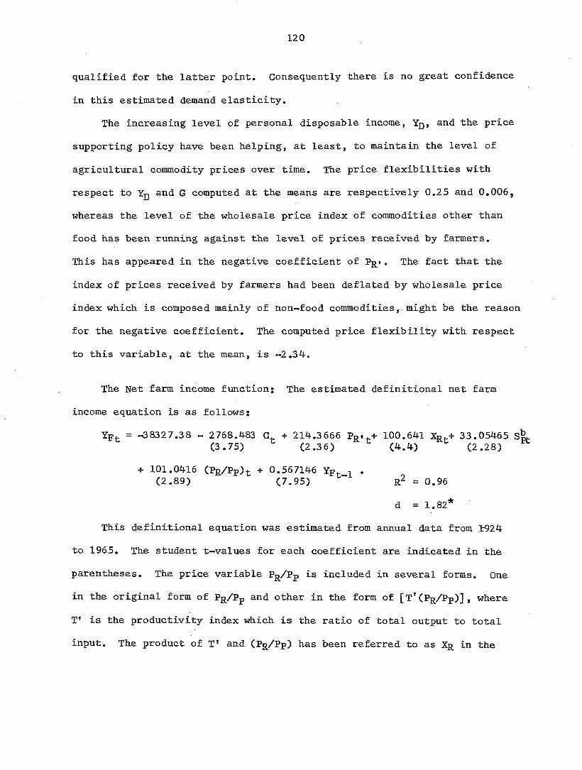
120

qualified for the latter point. Consequently there is no great confidence

in this estimated demand elasticity.

The increasing level of personal disposable income, Yq, and the price

supporting policy have been helping, at least, to maintain the level of

agricultural commodity prices over time. The price flexibilities with

respect to Yp and G computed at the means are respectively 0.25 and 0,006,

whereas the level of the wholesale price index of commodities other than

food has been running against the level of prices received by farmers.

This has appeared in the negative coefficient of Pg t. The fact that the

index of prices received by farmers had been deflated by wholesale price

index which is composed mainly of non-food commodities, might be the reason

for the negative coefficient. The computed price flexibility with respect

to this variable, at the mean, is -2,34.

The Net farm income function; The estimated definitional net farm

income equation is as follows;

= -383 2 7.38 - 2768.483 + 214.3666 Ppt + 100.641 Xr .+ 33.05465 sL (3.75) (2.3 6) (4.4) (2.28)

+ 101.0416 (PR/Pp)t + 0.567146 Yp. . . (2.89) (7.95) " r2 = 0,96

d = 1.82*

This definitional equation was estimated from annual data from 1924

to 1965, The student t-values for each coefficient are indicated in the

parentheses. The price variable Pg /Pp is included in several forms. One

in the original form of P /Pp and other in the form of [T'(P /Pp)], where

T' is the productivity index which is the ratio of total output to total

input. The product of T' and (P /Pp) has been referred to as Xr in the

121

above equation. The results indicate that a one percent increase in

PR/PP increases 1.49 percent Yp in the 1924 to 1965 period. With a one

percent increase in the interaction term of T' and P /Ppj Yp increases

0.68 percent.

b The results indicate also that increasing Sp contributes to the in­

crement of Yp, whereas the structure variable indicates that Yp declines

more in real value over the post-war years than pre-war years.

2. Factor markets

The demand for total farm machinery: The estimated demand function

for total farm machinery is as follows :

= -3 9 1 0 . 7 50 - 1.19 1 53 2 8 (PM/PR)t-l+ 33.321269 A(t) + 29.38883 T (0.44) (3.13) (1.91)

+132.5875 ERt-1 + 0 . 032 1 888 SM .- = 0.898 (3.47) (1.26)

d = 1.329*

The variable is the demand for total farm machinery in dollars term;

(P]y[/Pg ) „] is the one year lagged index of the ratio of farm machinery to

price received by farmers. ER ^ is the one year lagged equity ratio;

Mt the stock value of total farm machinery at the beginning of the

year and T is time variable. All variables except A(t) and T are deflated

by the wholesale price index. All variables have the expected sign. The

t-value for the coefficients are indicated in parenthesis below each co­

efficient. Except for (Pm/Pr) ^ and all variables are significant

at the one percent probability level, though is significant at five

percent probability level.

122

Level of technology ACt), and lagged Cone year) equity ratio are the

most significant variables in influencing the demand for total farm

machinery. It is quite conceivable that the technological change has

lead to the utilization of more machinery than labor. Certainly, the sub­

stitution of machinery for labor has been taking place over time. One

percent improvement in technology led the demand for total farm machinery

to increase 1.6 percent.

Lagged equity ratio is also an influential variable in determining

the demand for total farm machinery. The t-value for the coefficient of

equity ratio is significant at one percent probability level.

By this equation, which is based on the stock adjustment model as

discussed in Chapter III, the regression coefficient of is the dif­

ference between depreciation rate and the adjustment coefficient (50).

The average depreciation rate of the total farm machinery had been com­

puted from the separate set of data as 0.138 (18). Consequently the ad­

justment coefficient of the total farm machinery was computed as 0.106.

This implies that the average increment of the total farm machinery in­

vestment has been approximately 11 percent per year of the stock value of

farm machinery at the beginning of each year.

The elasticities of demand for annual investment of total farm

D machinery, Q with respect to prices ratio (PM/PR) ] is approximately

-0.05 measured at the mean.

Supply of all farm machinery: The estimated supply functions of all

farm machinery is as follows:

123

= 11.95938 + 0.39262 - 0.735667T + 0.003607MSH „j +0 2623PNLt (3.46) (-2.23) (1.29) (1.94)

r2 = 0.883

+ 0.576885 PMt-1 (5.35) d = 1,586*

The variable P is the price index of farm machinery; Pjg is the wholesale

price of iron and steel; the index of machinery shipment; P

is price index of non-farm wage rate and T is time variable. All vari­

ables except T and MSH are deflated by wholesale price index, and are

expressed as a percentage of the 1957 to 1959 average. The annual data

extend from 1924 to 1965.

All variables except are significant at one percent probability

level. significant at the five percent probability level. All

variables have the expected sign.

The price flexibility of machinery shipment (supply) computed from

the equation is 0.02. Since it is near zero, the supply elasticity

(1/price flexibility) is very large.

The result was consistent with the hypothesis that machinery supply

is highly elastic. Although this equation indicates supply is less than

perfectly elastic, it does indicate that price is relatively unresponsive

to quantity changes in the short-run.

That farmers are price takers (quantity a function of price) and

manufacturers are price setters (price a function of quantity) should be

inferred from this supply equation.

A variable significantly explaining machinery prices is Pj-g. A one

percent increase in iron and steel price raises machinery price 0.34 per­

cent according to "this equation. The result is not surprising, since

124

steel and iron are the important raw materials in farm machinery. Non-

farm wage rates affect the cost of machinery production and the empirical

result in this study shows that it has a very significant effect on

machinery price.

The short-run year to year variation in total farm machinery price

is very small. The coefficient for one year lagged farm machinery price

is 0.58, and is a significant variable by the t-test (at the one percent

probability level).

Demand for motor vehicles estimated by least squares; Variables con­

sidered to be important influences on demand quantities of motor vehicles

are the level of technology, lagged one year equity ratio, time variable,

lagged index of cropland and the stock of motor vehicles on farm at the

beginning of the year. The logic of the specification and the nature of

expectations and adjustments are discussed previously in Chapter III.

Coefficients, student t-values and related statistics for motor ve­

hicle demand equation are as follows:

QMVt = -2138.35 + 17.76596A(t) + 83 .28165ERt„i+8.3 8613 6T+3 . 918741Af (2.41) (5.01) " (0.73) (0.36)

+ 0.012950S]yivt . = 0.8384 (0.3 5)

d = 1.22

Student t-value for the coefficient of each variable is presented in the

parentheses. All variables have the expected signs. The Durbin-Watson

d-statistic falls in the inconclusive range.

Lagged (one year) equity ratio and the level of technology are again

highly significant (at the one percent probability level) in explaining

125

the demand for motor vehicles as in the demand for total farm machinery

equation.

The stock of motor vehicles is not significant in this demand equation

as compared to the significant influence of the stock value for the demand

of total farm machinery. The average depreciation rate of the motor ve­

hicles was computed as 0.132 from the separate set of data. Though it is

doubtful to infer with the insignificant coefficient, the adjustment co­

efficient for motor vehicles was computed as 0.10 in this empirical re­

sult. This adjustment coefficient is as high as in the demand for total

farm machinery.

Demand for other farm machinery and equipment; The definitional

equation of the demand for other machinery and equipment is as follows;

&t ~ Tt " Vt *

The demand for other farm machinery and equipment are treated as the

residual in terms of subtracting the demand for motor vehicles from the

demand for total farm machinery. No estimation of the parameters was

made since it is a definitional equation.

Shifts in machinery demand: Total machinery demand equation indicates

that total farm machinery purchases would have been 6 7 percent greater in

1924 if farmers would have experienced the financial or equity position

present in 1965, ceteris paribus. More efficient methods of production,

substitution of cheap operating inputs for farm labor and horsepower,

improved management and inflation permitted a slight increase in net farm

income and a considerable improvement in the equity of farmers from 1924

to 1965 despite the rise in the ratio of (Pm/Pr). An 'acceleration*

126

influence may be evident; since adoption of machinery in early years par­

tially was responsible for the increased efficiency and improved financial

position of farmers, this permitted greater machinery purchases in later

years. Table 1 indicates that the major sources of the increased machinery

demand have been due to the equity positions of farmers, the level of tech­

nology and the structural changes represented by the time variable. Effects

of the technological level are more than offset by the effects of,price on

the demand for total farm machinery, consequently leaving the equity and

'structure' to explain almost the entire shift in machinery demand since

1924. The situation is quite similar in the demand for motor vehicles.

The most notable structural changes embodied in the time variable are the

continuous improvement in the quality and adaptability of machinery.

Table 1. Estimate percentage changes in annual gross investment in farm machinery from. 1924- to 1965 attributed to prices, technology, demand structure and equity

Inputs Variables C M/ R t-l A(t) T ® t-l

Demand for total farm machinery -0.049 1.58 0.62 0.52

Demand for motor vehicles - 1.59 0.33 0.61

Concurrent with these improvements is the increased awareness by farmers

of the returns and convenience from using improved machinery. Of course,

it is well to remember that the structural and financial categories are

not entirely independent.

Perhaps the most basic indirect source of the structural increase in

12 7

demand for machinery is the growth of the American education. Without

the large investment in education, it is unlikely that engineering and

other talents of human resources would have been able to develop rapidly

the steel, coal and automobile industries so vital to the growth of the

farm machinery industry.

The non-farm sector has performed an important role in farm mech­

anization. If the supply of farm machinery were not highly elastic and

if small increase in farm demand would have brought sharp machinery price

increases, farm mechanization undoubtedly, would have progressed less

rapidly. The fact that manufacturers have made farm machines available

in quantities and of the quality desired by farmers, has been an important

element explaining the rapid growth of farm machinery investment. In turn,

using the stock of farm machinery and substitution of machinery for farm

produced power has been a significant element in the rising farm labor

efficiency.

Thus, the development of America's agriculture is an interdependent

accomplishment. The basic ingredients are the natural resources, educa­

tional attainment and technological know-how for building farm machines

and the desire and ability to use them profitably on farms. On this

foundation, the total economy grows as the machines have been made avail­

able to farmers. This allows financial surpluses for farmers to purchase

more machines. Simultaneously, workers who are freed from farming, pro­

vide the basis for further expansion of industry and improved standards

of living for both the farm and non-farm sectors. Although the growth

of America's agricultural plant principally was financed internally from

128

net farm income, a strong non-farm sector, undoubtedly, can be an import­

ant source of credit in times of rapid expansion of farm investment.

Demand for farm building investment; The deflated total value of

real estate increased by 288 percent during 1924-1965 period (121). Ihe

increase is largely due to annual investment in building improvements, in­

cluding fences, windmills, and wells. In this study, the quantity de­

manded (annual gross investment of building materials) is specified as a

function of prices, index of livestock production, interest rate, stock

of productive farm building assets, three years' weighted average of the

net farm income, the structure variable for pre- and post world war years.

All indexes are expressed as a percentage of the 1957 to 1959 aver­

age. All variables are annual data for the U.S. from 1924 to 1965.

The six independent variables in the following equation, explain 87

percent of the annual variation about the mean of Qgi . Coefficients of

all variables except the index of livestock production are highly signifi­

cant (at the one percent probability level). The signs of all the variables

are consistent as expected.

QbI^=. 81 7.9438 + 3 75.2 62 70% + 34.1892ER% .+2 .049107LP^-9.858559Pg (6.20) (4.56) " (1.75) (4.07)

T-I0,004864S-R) + 1 = 0.98 (1,82) (3.70)

d =1.2 7*

The weighted three years' average of the net farm income is the most

significant variable. The price for building materials and stock of farm

building also are highly significant. As mentioned in the demand for

total farm machinery the regression coefficient of the stock value of farm

building is the depreciation rate h minus the adjustment coefficient

12 9

g (50), Hence, the negative coefficients of indicate that g ex­

ceeds h by 0,005, The exact depreciation rate is unknown (data not avail­

able), but probably is considerably below the machinery depreciation rate.

If the depreciation rate is 0.10, the adjustment rate is 0.10 + 0.005 =

0.1005. The level of adjustment coefficients are quite compatible with

the demand for farm machinery.

According to this equation, the price elasticity of estimated

at the mean is -1.0. Income elasticity of with respect to lagged

three years* weighted average of the net farm income YwFt-l> 0.19,

Shifts in building investment demand; In 1965, annual gross invest­

ment in building improvements was 97 percent above the 1924 level. Three

hypothetical sources of the investment increases are; (a) equity ratio,

(b) livestock production index, and (c) structure Gf If 1965 values are

given these variables, the farm building demand equation indicates that

demand would have been 166 percent greater than in 1924. If price Pg had

been at the 1965 level in 1924, other things equal, the demand quantity

would have been 70 percent less than the actual demand in 1924 according

to the.equation. The large building investment needed to store and house

the increased inventories of livestock and feed also need large building

investment to store and house them. The index of livestock production

might be the proxy variable for these changes. The t-value of this proxy

variable appeared to be significant at the one percent probability level.

If livestock production had been at the 1965 value in 1924, demand would

have been 34 percent above the 1924 level, other things equal.

13 0

The agriculture production efficiency has been increased over time,

with relatively stable inputs prices farmers apparently improved their

financial status sufficiently to increase purchases of building improve­

ments by a sizeable amount. But the influence of both building material

prices and equity would reduce demand by a net of about 25 percent.

The structural changes only explain about 120 percent increase in

building investment during 1924-1965. Structural changes are a broad

range of physical and technological influences. Technological influence

may not be as dramatic as for farm machinery; nevertheless, changes in

methods of storing feeds, handling dairy cattle, etc, have influenced de­

mand for buildings. Influences tending to reduce farm numbers and replace

labor with other resources also have created an impact on the investment

in real estate. Some of these influences reduce demand, others increase

demand, but the net influence according to above equation is to shift de­

mand to the right for post-war years.

The empirical analysis for the demand for farm machinery and farm

building indicates that increasing annual investment in machinery and

buildings may be explained substantially by (a) level of technology,

(b) financial structure, and (c) slowly changing influences reflected by

a time variable. For machinery input, the influence shifting demand to

the right at the most rapid rate was (a), the improvement in financial

status due to greater efficiency, lower prices of operating inputs and

inflation, tended to increase annual investment for durable inputs.

Structure and time variables include improvements in quality, adaptability

and convenience of durables. Other components of the time variable are

the gradual awareness by farmers of better management practices and of

131

the profitability and convenience of investment in durable resources.

The structure and time variables are also influential in the demand for

all other durable inputs in this study.

The supply of farm machinery is analyzed as part of an recursive

model. The long run price flexibility is approximately 0.02. Thus, supply

prices are quite unresponsive to changes in quantity. In this elastic

supply function, the most influential variable appears to be the price of

iron and steel. A one percent increase in the price of iron and steel

tends to increase the supply price about 3.5 percent. It should be noted

that the price of non-farm labor is also highly significant.

Demand for total farm employees; The time-series data of the total

farm employment is that of the sum of hired and family employment data.

It might be expected that the demand for total farm employment would be

an average or aggregate of the demands for hired and family labor. The

total farm employment data represent the total number of persons employed

in agriculture.

The estimated demand equation for total farm employment is as follows;

( Lt = 17640,22 - 17.872 16 IMP i+0.0756263 .44567? -11,42658A(t) (-1.90) (1.07) ~ («9.26) (-1.05)

-17.56882 (PT;.L/rVLBA)t„i + 3.3 04025 (PM/PTLH-I- = 0.97 (-1.27) (1.20)

d = 1.62*

The lagged index of the price ratio of farm machinery to farm wage

rate is a significant explanatory variable (at the five percent probability

level). The positive coefficient suggests that total demand for farm

labor declines on farms in response to a fall in the relative price of

132

farm machinery. This is consistent with the hypothesis that machinery

substitutes for labor with a relative decline in the machinery price.

However, the long-run elasticity measured at the mean for the total labor

demanded with respect to this price ratio is lower than expected. The

computed elasticity was 0.004.

The demand for total farm labor showed, in this equation, a negative

relationship with the lagged index of the mechanical power on farms. A one

percent increase in the index of the mechanical power on farms in the

previous year reduced the current year*s total labor demand by more than

1.11 percent. This empirical result provides the evidence that modern

mechanization on farms gives an increasing impact on the declining demand

for total farm labor.

The lagged net farm income, Ypt-l» exhibits the expected positive

relationships with total farm employment. In aggregate, therefore, it

appears that total employment in agriculture tends to increase in response

to increase in previous year's net farm income. This increase in total

farm labor would be expected to be manifested through an increase in the

family fàrm. labor force rather than the hired labor force.

The effects of technological improvements have a significant (at the

five percent probability level) negative effect on the demand for family

farm labor and consequently reduce the demand for total farm labor. The

technological improvements lead to the substitution of farm machinery for

labor. From this empirical analysis, a one percent increase in tech­

nological index will reduce the demand for farm labor (in terms of the

number of persons) over 1.12 percent.

133

The negative coefficient for index of the one year lagged ratio of

the farm wage rate to the price of land and buildings per acre suggests

that as the price of labor rises relative to the price of land and build­

ings per acre, total labor declines on farms. With a one percent increase

in the ratio of the price of labor to the price of land, and buildings,

in a given year, total farm labor will decline roughly 1.5 percent in

the next year.

The result also indicates that the wage rate for factory workers is

a significant explanatory variable in total farm labor demand. A sustained

one percent increase in tends to reduce the total farm labor demand

by approximately 4.8 percent. This apparently is exerted through the

farm migration process. With job opportunities growing in the non-farm

economy farm laborers tend to migrate from agriculture.

The supply function of total labor: The supply function of total

labor estimated with annual time series from 1924 to 1965 is as follows;

= 3 . 8 6 93 6 0 - 0 . 6 1873 6 p -0.0453 59A(t) + 1.3 71446P , (4.64) (0.41) (4.39)

-1.211193 UT_I+ 0 . 003 1 75 QS. +0.199450T - 1.3 723 080 . = 0.96 (6.24) (1.66) (0.31) (0.27)

d =1.53*

f = 0.33

The variable is a structure variable with values of zero from 1924 to

1946, and values of 1 from 1947 to 1965. P is the index of farm

machinery price, A(t) is technological index, P is the wage rate of

factory workers and U is the proportion of the national labor force un­

employed. qÇl i-s the amount of total farm labor demanded and T is time

134

variable. All price indexes were deflated by wholesale price index (1957-

1959=100). p is the autoregressive coefficient. Student t-values are

indicated in parentheses below the coefficients. All coefficients display

the expected signs.

The long run price flexibility with respect to labor demand computed

at the mean is 0.42. With this low price flexibility, the labor demand

and/or supply did not exert a significant effect on the farm wage rate.

The insignificant effects of labor demand and/or supply of farm labor on

farm wage rates, probably is one of the main causes for excessive labor

supply, excessive products supply and hence the result is low farm income

in the agriculture sector. This is due to the failures of farm wage

rates to reflect the market conditions.

The result with a negative coefficient for also indicates that

there are more competitive relationships between labor and machinery than

complementary, and both significant explanatory variables

for farm wage rate. A sustained one percent rise in tends to increase

more than one percent when at the 1924-1965 average level.

As indicated by the positive coefficient of the time variable T,

time trend for real farm wage rate displayed a slight annual increase over

time. The structure variable, G , appeared insignificant in this function.

It is very possible that the effects of structure changes on farm wage

rate have been taken care of by the time variable T.

The technological index, A(t), has the expected negative sign. The

elasticity of farm wage rate with respect to technological index computed

at the mean is -0.06. The substitutional effects of machinery on farm

135 .

labor are again supported by this empirical result.

The demand for hired farm labor; The estimated demand equations for

hired farm employees is as follows;

Q§t . = 3583.077 + 9.282995 A(t) + 5.407297AFt_i+0.804702 % (3.85) (1.44) (0.26)

« 3 .659986(P™, AVLBA) ._;[-51.41593T + 188.4969 Gf (2.26) " (7.13) (2.76) = 0.968

d = 1.64978*

= 0.23

A number of independent variables reflecting price of agricultural

re sources-were -significantly influential on the demand for hired farm em­

ployees. These included both resource prices independently and in ratio

form.

Index of the price of farm machinery also is a significant explana­

tory variable. The positive coefficient suggests that hired labor de­

clines on farms in response to a fall in the price of farm machinery.

This is consistent with the hypothesis that machinery substitutes for

labor with a decline in machinery price. The estimated elasticity com­

puted at the mean is 0.03.

The negative coefficient for the lagged index of the ratio of the

farm wage rate to the price of land and buildings per acre suggests that

as the price of labor rises relative to the price of land, hired labor

declines on farms.

The lagged index of cropland per farm Ap __ , are significantly posi­

tive in the demand for hired farm labor equation. The elasticity of hired

labor demand with respect to this variable computed at the mean is 0.18.

136

The level of technology, A(t), is also an influential variable.

However, it has a quite small positive coefficient as compared to the co­

efficient of the demand for total farm machinery and motor vehicle func­

tions. The technological improvements in agriculture have been in favor

of mechanization. The effects of technological improvements have a sig­

nificant negative effect on the demand for family farm labor and conse­

quently the demand for total farm labor. Its effect on hired farm labor

is not clear. Improvements in technology will increase the labor effi­

ciency which induces higher demand for labor. On the other hand, the

technological improvements lead to the substitution of farm machinery for

labor. In the demand for hired farm labor, the latter effects might have

been offset by the former.

Time is a significant explanatory variable. The elasticity of the

demand for hired farm labor with respect to time variable, T, is roughly

-0.9. Despite the relative decline in the annual demand for the hired

labor over time, the absolute amount of the demand for hired labor has in­

creased in post-war years. This can be identified from the significant

positive coefficient for the structure variable, G .

The demand for family farm labor; The demand for family farm labor

is defined as follows;

Q?t = TLt " %Lt'

The variable is the quantity demanded (in terms of persons employed)

of the family farm labor; demand for total farm labor; and

is the demand for hired farm labor. More than 75 percent out of the total

farm labor (in terms of persons employed) demanded in the period under

13 7

study belongs to family farm labor. The quantity demanded (in terms of

persons employed) for family labor is treated as the residual of the de­

mand for total labor after subtracting the hired labor. Thus, the para­

meters for the demand function of family farm labor is not estimated

since it is a definitional equation,

G. Results of Regional Models 1946-1965

Demand for total farm machinery; The regression results reported in

Table 2 included all variables of the demand for total farm machinery

function which were found to be statistically significant (see the foot­

notes for table 2). The Durbin-Watson statistic also indicated that the

errors were not autocorrelated in the equation.

The stock adjustment model was tried for regional machinery demand.

However, the high multicollinearity among the stock value of farm machinery,

time trend and technological index led to the nonsignificance of the co­

efficients of many variables. Consequently the regression reported in

Table 2 was the expectation model.

The overall coefficient for the time trend is significant. The over­

all coefficient for the ratio of farm machinery prices to prices received

by farmers also is significant and with the expected negative sign.

The overall coefficient for one-year-lagged farm machinery investment

is significant. For the coefficient of the same variable, only the Delta

States region coefficient was significantly different from the overall

coefficient.

The overall coefficient for the lagged equity ratio is a significant

138

Table 2. Regression equation and related statistics for regional total farm machinery demand

Statistics and Names of variables regression and statistics Notation coefficients

Overall regression *F' ratio 3 79.886 Coefficient of determination R 0.986 Durbin-Watson statistics d 1.648** Overall intercept bo -745.54

(-4.40)*** Diff. in the intercept for Lake States ^3 164.67

Reg. ^3

( 1.30)* Diff. in the intercept for Corn Belt b4 321.94

Reg. C 2.65)*** Diff. in the intercept for Northern ^5 283.55

plains Reg. C 2.47)** Diff. in the intercept.for Appalachian bg 166.24

Reg, ( 1.38)* Overall time trend T 14.72

C 4.59)*** Overall coeff. Qbt-i 0.867 Overall coeff. Qbt-i

( 3.34)*** Diff. in the coeff. of for Owt-i ,7 -0.690

Delta States Reg. Owt-i

(-1.34)* Overall coeff. of ER. | .__2 B&t-l 15.87

C 2.88)*** Diff. in the coeff. of ER ^ E%t_l ,2 24.04

North-east Reg. ( 2.01)** Diff. in the coeff. of ER ^ for E&t-l ,5 -9.67

Northern Plains Reg. (-1.60)* Diff. in the coeff. for Appalachian E&t-l ,6 -9.44

Reg. (-1.56)* Overall coeff. for M R -2.56 Overall coeff. for M R

(-3.29)***

Indicates coefficients significant at probability, level 00.01.

**Indicates coefficients significant at probability level O.Olc Pc5 0.05.

*Indicates coefficients significant at probability level 0.05<lP<0.20.

13 9

explanatory variable in the farm machinery demand with the positive re­

lationships. The significant regional differences from the overall co­

efficient are found for the Northeast, Northern plains and Appalachian

regions. It has to be noted that the regional regression coefficients

are the difference between overall coefficient and the regional differences.

To illustrate the broader aspects of regression results from the

model, the coefficients and variables for 10 farm production regions in the

United States are presented in Table 3. It provides estimates for total

farm machinery demand functions in each of the ten farm production re­

gions in the United States. Thus one aggregate regression was used to

derive 10 different and complete equations, one for each region.

Elasticities for variables in those equations were calculated at

the respective means and are reported in Table 4.

General results obtained in this regional estimation are consistent

with the national function. The regional results further indicate that

the Appalachian and Northern Plains regions have a lesser response in

farm machinery investment with respect to lagged equity ratio. The Ap­

palachian Region is generally considered as having a depressed agricul­

tural sector. Areas or sectors suffering from chronic income depression

are often characterized by large personal debts. As a consequence, the

low equity ratio generally leads to the lower elasticity of farm machinery

investment with respect to equity ratio.

Demand for farm motor vehicles ; The same types of analyses were per­

formed for the regional demand for farm motor vehicles. The stock adjust­

ment model also was tried unsuccessfully for the regional farm motor

140

Table 3. Regression coefficients for the regional total farm machinery demand

Regression coefficients for Region Constant T QMt-1 B&t-l %/PR

Pacific Region -745.54 14.72 0.867 15.87 -2 .56

North-east Region -745.54 14.72 0.867 39.91 «2.56

Lake States Region -580.87 14.72 0.867 15.87 -2.56

Corn Belt Region -423.60 14.72 0.867 15.87 -2.56

Northern Plains Region -462.99 14.72 0 . 8 6 7 6.20 —2.56

Appalachian Region -579.30 14.72 0.867 6.43 -2.56

South-east Region -745.54 14.72 0.867 15.87 -2.56

Delta States Region -745.54 14.72 0.177 15.87 -2.56

So, plains Region -745.54 14.72 0.867 15.87 -2.56

Mountain States Region -745.54 14.72 0.867 15.87 —2.56

Table 4. Elasticities computed at the means of the variables for total farm machinery demand

Names of variables Notation Elasticities

Time trend T 2.610

Q t-i for Pacific Reg. QMt-1 0.021

for Delta States Reg. Q t-1,7 0.006

ERt-i for pacific Reg. ERt-1 0.015

E&t l for N.E. Reg. ^ t-1,2 0.023

ERt-1 for N.P. Reg. ERt-1,5 0.003

ERt-1 for Appalachian Reg. B&t-1,6 0.005

for pacific %/PR -0.72 7

141

vehicles demand. High multicollinearity among stock values of motor

vehicles, technological index and the time trend were evidenced. Hence,

only the results for the expectation model were reported.

All variables of the demand for motor vehicles functions which Were

found to be statistically significant (see the footnotes for Table 5) were

reported in Table 5. The Durbin-Watson statistic indicated that the errors

were unautocorrelated in the equation.

The overall coefficients for the one-year-lagged investment, the

lagged equity ratio and the lagged ratio of motor vehicles prices to price

received by farmers are statistically significant and all have expected

signs. For the lagged equity ratio, the regression results indicated

that there were significant differences in the coefficients for the North­

east, Corn Belt and Appalachian regions. Regional regression coefficients

are the difference between overall coefficients and the regional differences.

To illustrate the broader aspects of regression results from the

model, the coefficients and variables for 10 farm production regions in the

United States also are presented in Table 6. It provides estimates for

farm motor vehicles demand functions in each of the ten farm production

regions. Thus, one aggregated regression was used to derive 10 different

and complete equations, one for each region.

Elasticities for variables in those equations were calculated at

the respective means and are reported in Table 7.

The results obtained in the regional analysis are generally con­

sistent with the national analysis and the general hypotheses except there

is an inconsistent sign for the coefficient of lagged equity ratio in the .

142

Table 5. Regression equation and related statistics for regional farm motor vehicles demand

Statistics and Names of variable and regression statistics Notation coefficients

Overall regression 'F* ratio F 238.10 Goeff. of determination R2 0.978 Durbin-Watson statistics d 2.130** Overall intercept bo -140.8

(-1.45)* Diff. in the intercept for Corn Belt b4 186.16

( 2.54)** Overall coeff. for Qjyjyt-l OMVt-l 65.01 Overall coeff. for Qjyjyt-l

( 2.31)** Overall coeff. for ERt-1 5.05

( 1.43)* Diff. in the coeff. of ER j for ® t-l,2 14.13

North-east Reg. ( 1.86)* Diff. in the coeff. of ER __2 for ERt-l,4 -6.24

Corn Belt Reg. (-1.28)* Diff. in the coeff. of ER ^ for ^ t-1,6 -4.82

Appalachian Reg. (-1.23)* Overall coeff. for =Ô.5§)'

Indicates coefficients significant at probability level 0 -< P 0.01.

Indicates coefficients significant at probability level 0-< Pr<0.05,

*Indicates coefficients significant at probability level 0.05 xrp < 0.20.

143

Table 6. Regression coefficient for the regional farm motor vehicles demand

Regression coefficients for

Region Constant Q t.1 r—1 Pmv/PR

Pacific Region -140.8 65.01 5.05 -0.55

North-east Region -140.8 65.01 19.18 -0.55

Lake States Region -140.8 65.01 5.05 -0.55

Corn Belt Region 45.36 65.01 -1.19 -0.55

Northern Plains Region -140.8 65.01 5.05 -0.55

Appalachian Region -140.8 65.01 0.23 -0.55

South-east Region -140.8 65.01 5.05 -0.55

Delta States Region -140.8 65.01 5.05 -0.55

Southern Plains Region -140.8 65.01 5.05 -0.55

Mountain States Region -140.8 65.01 5.05 -0.55

Table 7. Elasticities computed at the motor vehicles demand

meatis of the variables for farm

Names of variables Notation Elasticities

Ratio of machine prices received by farmers

Lagged equity ratio for

to prices

Pacific Reg. %V/pr

B&t-l

-0.294

0.055

Lagged equity ratio for east Reg.

Lagged equity ratio for

North-

Corn Belt Reg. ^ t-1,2

^ t-1,4

0.110

-0.003

Lagged equity ratio for Appalachian Reg. ERt-1,6 0.002

Lagged investment QMVt-1 6.220

144

Corn Belt. The high coefficient value for the lagged farm machinery in­

vestment suggests that if there were no high multicollinearity among stock

value of motor vehicles, technological index and the time trend, the stock

variable instead of the lagged investment variable would yield statistical­

ly and economically more meaningful results in the analysis.

Regional farm buildings investment: The regression results reported

in Table 8 included all variables of the demand for farm building function

which proved statistically significant (see the footnotes for Table 8).

The Durbin-Watson statistic also indicated that the errors were not auto-

correlated in the equation.

The overall coefficient for weighted net farm income (one year lagged)

is positive and is significant at the 1 percent probability level. The

regional coefficients of income variable in other regions (except the

Mountain region) indicate slightly different responses from the overall

income effect.

The overall coefficient for the equity ratio (one year lagged) is

not significant. All regions, except the Pacific region, have significant

positive coefficients for the lagged equity ratio. These results are evi­

dence that the equity ratio as a basis for making long-term investment does

have a strong effect on building demand.

The effects of a higher equity ratio on farm building investments

will likely enable farmers to couple with the other forces of change; for

example the increase in gross physical production, than as the direct

motivating force.

145

Table 8. Regression equation and related statistics for regional farm buildings demand

Names of variables Statistics and re-and statistics Notation gression coefficients

Overall regression 'F' rat io F 601.51 Coefficient of determination R 0.992 Durbin-Watson statistic d 1.870** Overall intercept b 463.91

C 9.22)*** Diff. in the intercept for Corn b3 -42.12 State Reg. (-1.59)* Diff. in the intercept for Ap- b5 -70.65 palachian Reg. (-3.29)*** Overall time trend T -4.09

(-4.58)*** Price of farm building materials % -1.49 %

(-2.3 8)** Stock value of farm buildings SB 0.00128 SB

( 2.09)** Overall coeff. for %Ft-l 0.105

( 4.82)*** Diff. in the coeff. of WFt-1 for %Ft-.1 ,2 -0.100 North-east Reg.

WFt-1 %Ft-C-3.24)***

Diff. in the coeff. of WFt-1 for WFt-.1 ,3 -0.089

Lake States Reg. WFt-1 WFt-

(-3.92*** Diff. in the coeff. of %Ft-l for YWFt-1 ,4 -0.040 Corn Belt Reg.

%Ft-l (-1.85)*

Diff. in the coeff. of Northern Plains Reg.

WFt-1 for WFt_ •1 ,5 -0.89

(-3.98)*** Diff. in the coeff. of %Ft«l for %Ft_ .1 ,6

-0.074 Appalachian Reg.

%Ft«l %Ft_ (-3.20)***

Diff. in the coeff. of WFt-1 for WFt-.1 , 7 -0.103

South-east Reg. WFt-1 WFt-(-3.92)***

Diff. in the coeff. of WFt-1 for WFt.. ,8 -0.142

Delta State Reg. WFt-1 WFt.. ,8

(-4.57)*** Diff. in the coeff. of " Ft-l for %Ft-.1 9

-0.0680 Southern plains Reg.

" Ft-l %Ft-(-2.74***

Coeff. of ® t-.l for North-east Reg. ERt-1,2 11.31 ( 1.61)*

Coeff. of ERt-1 for Lake States Reg. ® t-l,3 7.56 ( 1.90)*

Coeff. of ERt-1 for Corn Belt Reg. ERt-1,4 9.53 ( 2.84)**

Coeff. of E t-l for Northern Plains Reg. R-t-l, 5 12.05 ( 3.77)***

Coeff. of t-1 for Appalachian Reg. ^ t-1,6 11.43 ( 3.55)***

please see footnotes under Table 5 for explanation of asterisks.

146

Table 8. (Continued)

Names of variables Statistics and re« and statistics Notation gression coefficients

6.72 ( 2.05)**

7.61 ( 2.31)**

8.88 ( 2.61)*** 5.53

( 1.19)*

Goeff. of ERt-l for Southeast Reg. ERt_l ,7

Goeff. of ERt-1 for Delta State Reg. ERt-1 ,8

Goeff. of ERt_i for Southern Plains Reg. t-1 ,9

Goeff. of ERt_l for Mountain Reg. ERt_i ,10

The time trend and price of farm building materials proved to be

significant and negative in the euqation. The stock value of farm build­

ings also was significant in explaining the annual gross investment of

farm buildings. The magnitudes of adjustment coefficients could not be

computed because the regional depreciation rates of farm buildings were

not available.

To illustrate the broader aspects of regression results from the

model, the coefficients and variables for 10 farm production regions in

the United States are presented in Table 9. It provides estimates for

farm building demand functions in each of the ten farm production regions.

Thus, one aggregate regression equation was used to derive 10 different

and complete equations, one for each region.

Elasticities for variables in those equations were calculated at the

respective means and are reported in Table 10.

In the farm buildings investment demand functions, the most significant

147

Table 9. Regression coefficients for the regional buildings investment

Regression coefficients for Region Constant Y Pt l T Sg ER i

pacific Reg. 463 .91 0. 105 «1 .49 -4. 09 0. 00128

North-east Reg. 463 .91 0. 005 -1 .49 -4. 09 0. 00128 11 .31

Lake States Reg. 463 .91 0. 016 -1 .49 -4. 09 0. 00128 7 .56

Corn Belt Reg. 421 .79 0. 065 .49 -4. 09 0. 00128 9 .53

Northern Plains Reg.

463 .91 0. 016 -1 .49 09 0. 00128 12 .05

Appalachian Reg. 383 .26 0. 031 -1 .49 "4. 09 0. 00128 11 .43

Southeast Reg. 463 .91 0. 002 .49 -4. 09 0. 00128 6 .72

Delta States Reg. 463 .91 —0, 03 7 -1 .49 —4. 09 0. 00128 7 .61

Southern plains 463 .91 0. 03 7 -1 .49 -4. 09 0. 00128 8 .88

Mountain States Reg,.

463 .91 0. 105 -1 .49 -4. 09 0. 00128 5 .53

148

Table 10. Elasticities computed at the means of the variables for farm buildings investment

Names of variables Notation Elasticities

Price of farm building materials B 1 .3 7

Stock values of farm building SB 0 .32

Lagged weighted income %Ft-l 0 .146

Ywpt-1 :Eor North-east Reg. " WFt-1,2 0 .00485

Y t„i for Lake States Reg. %Ft-l ,3 0 .0244

WFt-l Corn Belt Reg. YwFt-1,4 0 .083 7

WFt-1 Northern Plains Reg. YWFt-1,5 0 .01996

%Ft-l Appalachian Reg. YWFt-1,6 0 .058

WFt-1 South-east Reg. • WFt-1,7 0 .0034

WFt 1 Delta States Reg. YWFt-1,8 0 .074

Y t„i Southern plains Reg. WFt-l,9 0 .046

Y jpt i Mountain States Reg. YWFt-1,10 0 .114

Time trend T 2 .16

Lagged equity ratio for North-east E&t-1,2 0 .097

Lagged equity ratio for Lake States EBt-1,3 0 .071

Lagged equity ratio for Corn Belt B&t-1,4 0 .048

Lagged equity ratio for Northern Plains B&t-l,5 0 .159

Lagged equity ratio for Appalachian B&t-1,6 0 .184

Lagged equity ratio for South-east ERt-1,7 0 .13 98

Lagged equity ratio for Delta States t-1,8 0 .187

Lagged equity ratio for Southern Plains t-1,9 0 .111

Lagged equity ratio for Mountain States E&t-l, 10 0 .080

149

variables included the weighted net farm income, equity ratio, time trend,

price for building materials and stock value of farm buildings. As ex­

pected, regional differences in the farmers' responses with respect to

the same set of variables for the farm buildings investment were not sig­

nificant.

Regional demand for total farm labor; The regression results reported

in Table 11 included all variables of the demand for total farm labor func­

tion which were found to be statistically significant (see the footnotes

for Table 11). The Durbin-Watson statistic indicated that the errors

were not autocorrelated in the euqation.

The overall coefficient for the technological change index was nega­

tive and was significant at 1 percent probability level. The regional

differences of the same variable also were significant but with a positive

sign. However, the regional regression coefficients, which were the dif­

ferences between overall and the regional difference, had consistent nega­

tive signs.

The weighted net farm income, lagged one year, was tried as an ex­

planatory variable but proved to be nonsignificant. The lagged ratio of

composite farm wage rate to total value of building and land per acre were

negative and significant for the Northern Plains and Appalachian regions.

An inconsistent sign for the Mountain region was found. The positive

relations for the lagged ratio of machinery prices to farm labor wages were

found for the Northeast and Lake States regions in contrast with the in­

consistent sign found for the Southeast region.

150

Table 11. Regression equation and related statistics for regional total farm labor demand

Names of variables and Statistics and re-statistics Notation gression coefficients

Overall regression 'F' ratio F 1602.06 Coefficient of determination R2 0.998 Durbin-Watson statistics d 1.58** Overall intercept o 3371.98

( 4.97)*** Diff. in the intercept for 2 -2186.79 North-east Reg. (-3.11)*** Diff. in the intercept for 3 -1764.42 Lake States Reg. (-2.45)** Diff. in the intercept for b -1091.34 Corn Belt Reg. (_1.44)* Diff. in the intercept for bg -1590.38 Northern Plains Reg, (-1.95)* Diff. in the intercept for 6 -899,48 Appalachian Reg. (-1.28)* Diff. in the intercept for by -949.52 South-east Reg. (-1.3 9)* Diff. in the intercept for bg -2119.45 Delta States Reg. (-3.09)*** Diff, in the intercept for bg -1699.32 Southern Plains Reg, (-2.41)** Diff, in the intercept for 10 -941.08 Mountain Reg.

10 (-1.33)*

Overall coeff. of A(t) -15.56 (-2.65)***

Diff. in the coeff. of A(t) for A(t)2 15.75 Northeast Reg.

A(t)2 ( 2.68)***

Diff. in the coeff. of A(t) for ACt)3 15.40 Lake States Reg.

ACt)3 ( 2.61)***

Diff. in the coeff. of >

rt

for A(t) 13.00 Corn Belt Reg. ( 2.13)** Diff. in the coeff. of A(t) for ACt)5 16.45 Northern plains Reg. ( 2.76)*** Diff. in the coeff. of A(t) for A(t)6 12.96 Appalachian Reg. ( 2.16)** Diff. in the coeff. of A(t) for A( t) 7 5.00 South-east Reg. ( 2.54)** Diff. in the coeff. of A(t) for A(t)g 15.70 Delta States Reg.

A(t)g ( 2.66)***

Please see footnote under Table 5 for explanations of asterisks.

151

Table 11. (Continued)

Names of variables and statistics Notation

Statistics and re­gression coefficients

Diff. in the coeff. of A(t) for A(t)9 15.71 Southern Plains Reg. ( 2.66)*** Diff. in the coeff. of A(t) for A(t)io 1.56 Mountain Reg. ( 2.62)*** Coeff. of (PJLA'VBLA) for (PTL/TVBLA) -4.01 Northern Plains Reg.

(PTL/TVBLA) (-1.53)*

Coeff. of (Pipj^/rVBLA) for (P,JLAVBLA) 3.25 Appalachian Reg.

(P,JLAVBLA) ( 1.29)*

Coeff. of (PijL/TVBLA) for (Pg /TV&LA) -5.30 Mountain Reg.

(Pg /TV&LA) (-2.2 7)**

Overall coeff. for NL -9.22 Overall coeff. for NL

(-13.67)*** Overall coeff. for IMP - I IMPt-1 -i.S5

(-2.96)*** Coeff. of (Pm/P l) North­ (PM/PTL)t-l,2 5.26 east Reg. ( 1.49)* Coeff. of (Pm/P L for Lake (PM/PTLH-1,3 6.03 States Reg. ( 1.69)* Coeff. of (P /Pqi ) for South­ (Pjyi/PTL^t-l,? -4.43 east Reg. (-1.43)*

The overall coefficients for non-farm wage rates and lagged index

of mechanical power were found to be significant and with consistent nega­

tive signs in explaining the demand for total farm labor.

To illustrate the broader aspects of regression results from the model,

the coefficients and variables for 10 farm production regions in the United

States are presented in Table 12. It provides estimates for total farm

labor demand functions in each of the 10 farm production regions. Thus,

one aggregate equation was used to derive 10 different and complete

equations, one for each region.

Elasticities for variables in those equations were calculated at the

respective means and are reported in Table 13.

152

Table 12. Regression coefficients for the regional total farm labor demand

Regression coefficients for Region Constant A(t) (PTL/rVBLA:| l %L ™%.i CPM/PTLH-I

pacific Reg. 3371.98 -15.56 -9.22 -1.85

North-east Reg. 1185.19 0.19 -9.22 -1.85 5.26

Lake States Reg. 1507.56 -0.16 -9.22 -1.85 6.03

Corn Belt Reg. 2280.64 -2.56 -9.22 -1.85

Northern Plains Reg.

1781.60 0.89 -4.01 -9.22 -1.85

Appalachian Reg. 2472.50 -2.60 3 .25 -9.22 -1.85

South-east Reg. 2322.46 -10.56 -9.22 -1.85 -4.43

Delta States Reg. 1252.53 0.14 -9.22 -1.85

Southern Plains Reg.

1672.66 0.15 -9.22 -1.85

Mountain States 2430.90 -13.99 -5.30 -9.22 -1.85

In the regional demand for total labor functions, the most signifi­

cant variables included the technological index, non-farm wage rate,

lagged index of machanical power on farm, lagged ratio of composite farm

wage rate to total value of land and buildings per acre and lagged ratio

of machinery prices to farm labor wages.

The results for the 10 farm production regions show a close similarity

to the national results. Therefore, the general effects of each set of

independent variables need not be repeated again. However, the regional

analysis revealed that technological advancement has exerted differing

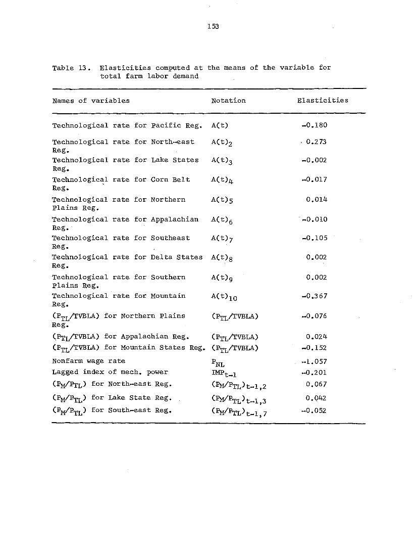
153

Table 13. Elasticities computed at the means of the variable for total farm labor demand

Names of variables Notation Elasticities

Technological rate for Pacific Reg. A(t) -0 .180

Technological rate for North-east ACt)2 : 0 .2 73 Reg. Technological rate for Lake States A(t^ -0 .002 Reg.

Technological rate for Corn Belt A(t)4 -0 .017 Reg.

Technological rate for Northern A(t)5 0 .014 Plains Reg.

Technological rate for Appalachian A(t) g -0 .010 Reg.

Technological rate for Southeast A(t)y -0 .105 Reg.

Technological rate for Delta States A(t)g 0 .002 Reg.

Technological rate for Southern ACt)g 0 .002 Plains Reg.

Technological rate for Mountain ACt)io -0 .367 Reg.

ACt)io

(PTLA'VBLA) for Northern plains CPtlAvbla) -0 .076 Reg.

(P^^^/rVBLA.) for Appalachian Reg. (Ptl/ÏVBLA) 0 .024

(P ] /TVBIA) for Mountain States Reg. «0 .152 Nonfarm wage : rate %L -1 .057 Lagged index ( Df mech. power -0 .201

(Pni/Ptl) Eor- North--east Reg. (PM/PTLH-1,2 0 .067

Lake State Reg. (PM/P.JJ )T„IJ3 0 .042 (P]y[/P L ' 3outh--east Reg. %/PTL t-l, 7 -0 .052

154

effects in reducing the total farm labor demand in the various regions.

In those areas such as the pacific, Southeast and Mountain regions where

the agriculture sector was depressed, the effects were more evident than

in other regions.

Regional demand for hired farm labor: The same types of analyses were

performed for the regional demand function for hired farm labor as for the

total farm labor. However, most of the coefficients were insignificant due

to the fact that there was high multicollinearity among the technological

index, time trend and lagged ratio of farm wage rates to the value of

land and building per acre. Consequently the original regional model

(which was proposed in the last chapter) for the hired farm labor was re­

vised as follows ; r. m—l m—l HLt i=l i + ' Ft«l' , i + CPm/PtlH I

m-1 + |_ g(PM/PTL)t„l,i + Ut*

All variables are as described in the previous chapter.

All variables of the demand for hired farm labor function which proved

statistically significant are reported in Table 14.

To illustrate the broader aspects of regression results from the model,

the coefficients and variables for 10 farm production regions in the United

States also are presented in Table 15. It provides estimates for the de­

mand of hired farm labor functions in each of the 10 farm production re­

gions. Thus, the one aggregate equation was used to derive 10 different

and complete equations, one for each region.

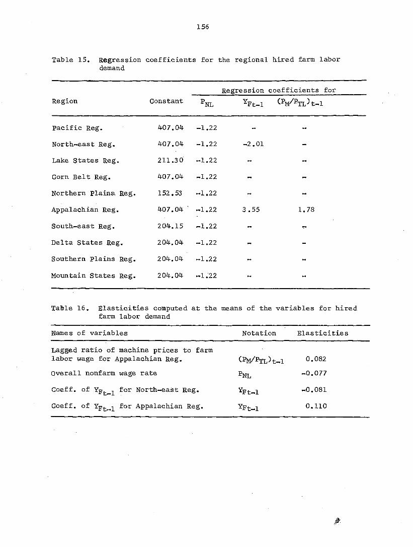
156

Table 15. Regression coefficients for the regional hired farm labor demand

Regression coefficients for

Region Constant CFn/ TL t-l

Pacific Reg. 407. .04 -1.22 - -

North-east Reg. 407. .04 -1.22 -2.01

Lake States Reg. 211. .3 0 -1.22 - -

Corn Belt Reg. 407. .04 -1.22 - —

Northern plains' Reg. 152. ,53 -1.22 - -

Appalachian Reg. 407. ,04 • -1.22 3 .55 1.78

South-east Reg. 204. ,15 -1.22 —

Delta States Reg. 204. ,04 -1.22 - -

Southern Plains Reg. 204. ,04 -1.22 - -

Mountain States Reg. 204. ,04 -1.22 —

Table 16. Elasticities computed at the means of the variables for hired farm labor demand

Names of variables Notation Elasticities

Lagged ratio of machine prices to farm labor wage for Appalachian Reg. (PM/PTLH-1 0.082

Overall nonfarm wage rate NL -0.077

Goeff. of for North-east Reg. %t-l -0.081

Goeff. of for Appalachian Reg. Ypt-l 0.110

157

tivities in the demand for hired labor with respect to weighted net farm

income and the ratio of farm machinery prices to farm labor wages than other

regions. The Appalachian region has a depressed agriculture sector. Farm

laborers are more sensitive in comparing the farm wage rates and the non-

farm wage rates. Farmers also are more sensitive in comparing the farm

wage rates to machinery prices. Net farm income relative to non-farm in­

come could be one of the many yardsticks for farm operators and farm

laborers to check their future in farming.

158

VI. THE COMPUTER SIMULATION MODEL OF THE DEMAND FOR

FACTORS (NATIONAL MODEL)

A. Simulation of Factors Demand Under the Existing Economic Structure

1. Simulation of the historical period and model validation

In this study, a computer simulation model is used for explanatory

or positive analysis. The primary concern here is to explain how the

structure of the demand for factors in agriculture behaves. Conclusions

or predictions implied by data generated by this model must be subjected

to direct empirical observation for either verification or refutation.

Verification lends support to the model as a whole. It implies that the

underlying assumptions in the model are adequate to explain the behavior

of the actual system.

Koopmans (74, p. 134) has suggested historical and forecasting veri­

fication as two alternative approaches for testing the degree to which data

generated by computer simulation models conform to observed data. Further,

among several approaches to historical verification, Clarkson (12, p. 34)

has suggested one of the most difficult and rigorous methods. The model

as a whole, as he suggested, can be subjected to statistical tests by

matching the time-series of the variables under consideration. In this

way a measure of 'goodness of fit* can be obtained and the model as a

whole can be confirmed on its ability to predict the time series.

Of course, no model is expected to fit the data exactly; the question

is whether the residual errors are sufficiently small to be tolerable and

sufficiently unsystematic to be treated as random.

159

Concerning the goodness of fit in attempting to fit data generated

by computer simulation experiments to actual time series data, Cohen and

Cyert (16) have suggested three general testing procedures. One of the

procedures suggested by them is to regress the generated time-series on

actual time-series data, and then proceed to check whether the resulting

equations have intercepts which are not significantly different from zero

and slopes which are not significantly different from unity.

In this study, the behavioral and definitional relations developed in

the previous chapters for national models were rewritten in computer language.

Given the time-series data for the exogenous variables and the lagged en­

dogenous variable at the beginning of the time period (1924), the endogenous

variables for the entire historical period (1924-1965) were then automatic­

ally generated by the recursive model without any additional constraints.

The generated time-series data were, then regressed on the respective actual

time-series. The results are presented as follows; Where all variables

were defined in Chapter V:

-Pt - 6.03 + 0.95 Spt R2 = 0.93

0.66 + 0.99 Q l = 0.99

1.82 + 0.97 q|2 = 0.97

%t = 17.50 + 0.84 Pg R2 = 0.95

/V (PR/Pp)t= 18.31 + 0.83 (Pj /Pp)t R2 = 0.94

/N CYF)t = 2 903 . 72 + 0 . 70 %'t R2 = 0.75

11 19.62 + 0.79 Pfjt R2 = 0.75

160

' t = 167.23 + 0.95 Qjyit

= 5.53 + 0.94 XRt

(%/Pg) = 14.69 + 0.82 (PM/PR)t

OMEt = 132.71 + 0.95 Qp t

QTLt ~ 236.16 + 0.96 QjLt

TLt ~ TLt

(PijL/TVLAB)t = 2.07 + 0.98 (PTL/TVLAB)t

QHLt ~ -13.18 + Qhl

^FLt = 234.3 9 + 0.95 Çp t

%Ft = 2908.36 + 0.71 Y pt

= 0. 93

= 0. 94

R2 = 0. 91

R = 0. 95

R = 0. 96

R2 = 0. 96

R = 0. 95

R = 0. 98

R2 = 0. 95

R = 0. 77

R = 0. 97

r2 0. 89

R2 — 0. 89

Qfilt ~ 28.23 + 0.96 Qgj

QjyiVt - 70.74 + 0.91

A CP]y[/PTL t ~ 7.07 + 0.91 C M/ 'TL t

Out of the twenty variables which were tested, the coefficient of the

déterminent ranges from 0.75 to 0.99. The intercepts vary from 0.66 to

2908 and depend on the different units of measurement for each variable,

and the slopes vary from 0.70 to 0.99 quite close to unity. The production

response function has the best fit, whereas the definitional net farm in -

come function has the least.

The actual and predicted time-series of the quantities demanded for

five kinds of resources are presented on Figures 3 to Figure 9. As can

be visualized from these figures, the height and turning point are reason­

ably well predicted.

161

S 03 _j

C3 O

<\i C3.

X

Ss

il o

OZO yj-;

o Œ

cc -

C3 03'

g I

fLCT cr X fim irHRT(prn. lct'

X x\< - r V X

> x

o 1 1920 1930 19U0 .950 1950

Figure 3 . Actual and predicted values of total farm machinery-purchases for the United States

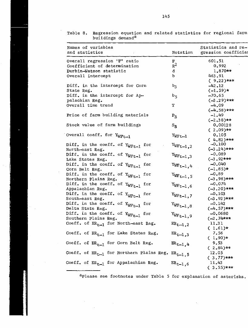
145

Table 8. Regression equation and related statistics for regional farm buildings demand

Names of variables and statistics Notation

Statistics and re­gression coefficiei

Overall regression 'F' ratio Coefficient of determination Durbin-Watson statistic Overall intercept

Diff. in the intercept for Corn State Reg. Diff. in the intercept for Ap­palachian Reg. Overall time trend

Price of farm building materials

Stock value of farm buildings

Overall coeff. for

Diff. in the coeff. of North-east Reg. Diff. in the coeff. of Y __2 for Lake States Reg. Diff. in the coeff. of for Corn Belt Reg. Diff. in the coeff. of Y _ for Northern plains Reg. "" Diff. in the coeff. of for Appalachian Reg. " Diff. in the coeff. of Y . , for South-east Reg. " Diff. in the coeff. of Y . for Delta State Reg. "" Diff. in the coeff. of Yyp for Southern Plains Reg. "

R" d b

•B

"B

%Ft-l

%Ft-l,2

%Ft-l,3

YWFt-1,4

WFt-1,5

WFt-1,6

WFt-1,7

t-1,8

WFt.,1,9

Coeff. of ERt-i for North-east Reg. ERt-1 ,2

Coeff. of ERt-1 for Lake States Reg. ERt-1 ,3

Coeff. of ERt-1 for Corn Belt Reg. ERt-1

Coeff. of ERt-1 for Northern Plains Reg. ERt-l ,5

Coeff. of ERt-1 for Appalachian Reg. E&t-l ,6

601.51 0.992 1.870**

463.91 ( 9.22)*** -42.12 (-1.59)* -70.65 (-3.29)*** -4.09

(-4.58)*** -1.49

(-2.38)** 0.00128

( 2.09)** 0.105

( 4.82)*** -0.100 C-3.24)*** -0.089

(-3 .92*** «0.040

(-1.85)* -0.89

(-3.98)*** -0.074

(-3.20)*** -0.103

(-3.92)*** -0.142

(-4.57)*** -0.0680

(-2.74*** 11.31 ( 1.61)*

7.56 ( 1.90)*

9.53 ( 2.84)** 12.05 ( 3.77)*** 11.43 ( 3.55)***

Please see footnotes under Table 5 for explanation of asterisks.

146

Table 8. (Continued)

Names of variables Statistics and re~ and statistics Notation gfession coefficients

6.72 C 2.05)**

7.61 ( 2.31)**

8.88 ( 2.61)***

5.53 C 1.19)*

Goeff. of E t-1 for Southeast Reg. ERt_i ,7

Goeff. of ERt_i for Delta State Reg. E&t-l ,8

Goeff. of ERt-1 for Southern Plains Reg. ERt-1 ,9

Goeff. of ERt-1 for Mountain Reg. ERt-l ,10

The time trend and price of farm building materials proved to be

significant and negative in the euqation. The stock value of farm build­

ings also was significant in explaining the annual gross investment of

farm buildings. The magnitudes of adjustment coefficients could not be

computed because the regional depreciation rates of farm buildings were

not available.

To illustrate the broader aspects of regression results from the

model, the coefficients and variables for 10 farm production regions in

the United States are presented in Table 9. It provides estimates for

farm building demand functions in each of the ten farm production regions.

Thus, one aggregate regression equation was used to derive 10 different

and complete equations, one for each region.

Elasticities for variables in those equations were calculated at the

respective means and are reported in Table 10.

In the farm buildings investment demand functions, the most significant

147

Table 9. Regression coefficients for the regional buildings investment

Regression coefficients for Region Constant %Ft«l T ER^^i

pacific Reg. 463 .91 0. 105 -1 .49 -4. 09 0 .00128 —

North-east Reg. 463 .91 0. 005 -1 .49 -4. 09 0 .00128 11.31

Lake States Reg. 463 .91 0. 016 -1 .49 «4. 09 0 .00128 7.56

Corn Belt Reg. 421 .79 0. 065 -1 .49 -4. 09 0 .00128 9.53

Northern Plains Reg.

463 .91 0. 016 -1 .49 -4. 09 0 .00128 12.05

Appalachian Reg. 383 .26 0. 031 ~1 .49 -4. 09 0 .00128 11.43

Southeast Reg. 463 .91 0. 002 -1 .49 -4. 09 0 .00128 6.72

Delta States Reg. 463 .91 —O. 03 7 -1 .49 -4. 09 0 .00128 7.61

Southern Plains 463 .91 0. 03 7 -1 .49 -4. 09 0 .00128 8.88

Mountain States Reg..

463 .91 0. 105 -1 .49 -4. 09 0 .00128 5.53

148

Table 10, Elasticities computed at the means of the variables for farm buildings investment

Names of variables Notation Elasticities

Price of farm building materials B 1 .3 7

Stock values of farm building SB 0 .32

Lagged weighted income '%Ft-l 0 .146

YwFt-1 North-east Reg. %Ft-l,2 0 .00485

WFt 1 Lake States Reg. WFt-1,3 0 .0244

WFt-l Corn Belt Reg. YwFt-1,4 0 .083 7

WFt-l Northern Plains Reg. YWFt-1,5 0 .01996

WFt~l Appalachian Reg. YWFt-1,6 0 .058

WFt-l South-east Reg. YWFt-1,7 0 .0034

WFt 1 Delta States Reg. YWFt-1,8 0 .074

Y t„i Southern Plains Reg. %Ft-l, 9 0 .046

WFt-1 Mountain States Reg. YWFt-1,10 0 .114

Time trend T 2 .16

Lagged equity ratio for North-east E&t_l,2 0 .097

Lagged equity ratio for Lake States EBt-1,3 0 .071

Lagged equity ratio for Corn Belt B&t-1,4 0 .048

Lagged equity ratio for Northern Plains ERt-1,5 0 .159

Lagged equity ratio for Appalachian B&t-1,6 0 .184

Lagged equity ratio for South-east ^ t-1,7 0 .13 98

Lagged equity ratio for Delta States t-1,8 0 .187

Lagged equity ratio for Southern Plains t-1,9 0 .111

Lagged equity ratio for Mountain States E&t-l,10 0 .080

149

variables included the weighted net farm income, equity ratio, time trend,

price for building materials and stock value of farm buildings. As ex­

pected, regional differences in the farmers' responses with respect to

the same set of variables for the farm buildings investment were not sig­

nificant.

Regional demand for total farm labor; The regression results reported

in Table 11 included all variables of the demand for total farm labor func­

tion which were found to be statistically significant (see the footnotes

for Table 11). The Durbin-Watson statistic indicated that the errors

were not autocorrelated in the euqation.

The overall coefficient for the technological change index was nega­

tive and was significant at 1 percent probability level. The regional

differences of the same variable also were significant but with a positive

sign. However, the regional regression coefficients, which were the dif­

ferences between overall and the regional difference, had consistent nega­

tive signs.

The weighted net farm income, lagged one year, was tried as an ex­

planatory variable but proved to be nonsignificant. The lagged ratio of

composite farm wage rate to total value of building and land per acre were

negative and significant for the Northern Plains and Appalachian regions.

An inconsistent sign for the Mountain region was found. The positive

relations for the lagged ratio of machinery prices to farm labor wages were

found for the Northeast and Lake Statés regions in contrast with the in­

consistent sign found for the Southeast region.

150

Table 11. Regression equation and related statistics for regional total farm labor demand

Names of variables and statistics Notation

Statistics and re­gression coefficients

Overall regression 'F* ratio F 1602.06 Coefficient of determination R2 0.998 Durbin-Watson statistics d 1.58** Overall intercept t)o 3371.98

C 4.97)*** Diff. in the intercept for b2 -2186.79 North-east Reg. (-3.11)*** Diff. in the intercept for bs -1764.42 Lake States Reg. (-2.45)** Diff. in the intercept for b4 -1091.34 Corn Belt Reg. (-1.44)* Diff. in the intercept for 5 -1590.3 8 Northern Plains Reg, (-1.95)* Diff. in the intercept for 6 -899.48 Appalachian Reg. (-1.28)* Diff. in the intercept for by -949.52 South-east Reg. (-1.3 9)* Diff. in the intercept for bg -2119.45 Delta States Reg.

bg (-3.09)***

Diff. in the intercept for bg -1699.32 Southern plains Reg, (-2.41)** Diff. in the intercept for O

I—1 -941.08

Mountain Reg.

O

I—1

(«1.33)* Overall coeff. of A(t) -15.56

(-2,6 5)*** Diff. in the coeff. of A(t) for A(t)2 15.75 Northeast Reg.

A(t)2 ( 2.68)***

Diff. in the coeff. of A(t) for ACt)3 15.40 Lake States Reg.

ACt)3 ( 2.61)***

Diff. in the coeff. of A(t) for ACt) 13.00 Corn Belt Reg. ( 2 .13)** Diff. in the coeff. of A(t) for A(t)5 16.45 Northern Plains Reg.

A(t)5 ( 2.76)***

Diff. in the coeff. of A(t) for A(t)6 12.96 Appalachian Reg. ( 2.16)** Diff. in the coeff. of A(t) for A(t)y 5.00 South-east Reg. ( 2.54)** Diff. in the coeff. of >

rt

for A(t) g 15.70 Delta States Reg.

A(t) g

( 2.66)***

^Please see footnote under Table 5 for explanations of asterisks.

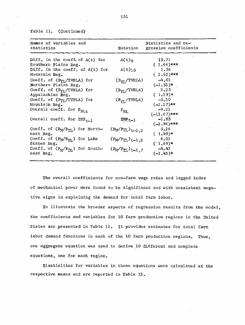
151

Table 11. (Continued)

Names of variables and Statistics and re-statistics Notation gression coefficients

Diff. in the coeff. of A(t) for A(t)9 15.71 Southern Plains Reg.

A(t)9 ( 2.66)***

Diff. in the coeff. of A(t) for A(t)io 1.56 Mountain Reg. ( 2.62)*** Coeff. of (Pjl/TVBLA) for (P,JL/TVBLA) -4.01 Northern Plains Reg.

(P,JL/TVBLA)

(-1.53)* Coeff. of (P j A'VBLA) for CP-JL/IVBLA) 3.25 Appalachian Reg.

CP-JL/IVBLA) ( 1.29)*

Coeff. of (Pij.l/TVBLA) for (P /TVBLA) -5.30 Mountain Reg.

(P /TVBLA)

(-2.2 7)** Overall coeff. for

NL -9.22 Overall coeff. for NL

(-13.6 7)*** Overall coeff. for IMP.t-1 -1.85 IMP.t-1

(-2.96)*** Coeff. of CP / TL for North­ CPM/PTL)t-l,2 5.26 east Reg. ( 1.49)* Coeff. of for Lake (%/FTL)t-l,3 6.03 States Reg. ( 1.69)* Coeff. of (P /PG ) for South­ < %/ TL t«l, 7 -4.43 east Reg. (-1.43)*

The overall coefficients for non-farm wage rates and lagged index

of mechanical power were found to be significant and with consistent nega­

tive signs in explaining the demand for total farm labor.

To illustrate the broader aspects of regression results from the model,

the coefficients and variables for 10 farm production regions in the United

States are presented in Table 12. It provides estimates for total farm

labor demand functions in each of the 10 farm production regions. Thus,

one aggregate equation was used to derive 10 different and complete

equations, one for each region.

Elasticities for variables in those equations were calculated at the

respective means and are reported in Table 13.

152

Table 12. Regression coefficients for the regional total farm labor demand

Regression coefficients for Region Constant A(t) (Pn/rvBLA: ! %L IMPj l (PM/PTLH-1

Pacific Reg. 33 71.98 -15.56 -9.22 -1.85

North-east Reg. 1185.19 0.19 -9.22 -1.85 5.26

Lake States Reg. 1507.56 -0.16 -9.22 -1.85 6.03

Corn Belt Reg. 2280.64 -2.56 -9.22 -1.85

Northern Plains Reg.

1781.60 0.89 -4.01 -9.22 -1.85

Appalachian Reg. 2472.50 -2.60 3.25 -9.22 -1.85

South-east Reg. 2322.46 -10.56 -9.22 -1.85 -4.43

Delta States Reg. 1252.53 0.14 -9.22 -1.85

Southern plains Reg.

1672.66 0.15 "9.22 -1.85

Mountain States 243 0.90 -13.99 -5.30 -9.22 -1.85

In the regional demand for total labor functions, the most signifi­

cant variables included the technological index, non-farm wage rate,

lagged index of machanical power on farm, lagged ratio of composite farm

wage rate to total value of land and buildings per acre and lagged ratio

of machinery prices to farm labor wages.

The results for the 10 farm production regions show a close similarity

to the national results. Therefore, the general effects of each set of

independent variables need not be repeated again. However, the regional

analysis revealed that technological advancement has exerted differing

153

Table 13. Elasticities computed at the means of the variable for total farm labor demand

Names of variables Notation Elasticities

Technological rate for Pacific Reg. ACt) -0 .180

Technological rate for North-east A(t)2 : 0 .2 73 Reg. Technological rate for Lake States A(t)3 -0 .002 Reg.

Technological rate for Corn Belt A(t) -0 .017 Reg.

Technological rate for Northern A(t)5 0 .014 Plains Reg.

Technological rate for Appalachian A(t)6 -0 .010 Reg. Technological rate for Southeast A(t)y -0 .105 Reg.

Technological rate for Delta States A(t) g 0 .002 Reg.

Technological rate for Southern ACt)g 0 .002 plains Reg.

Technological rate for Mountain «0 .367 Reg.

(Ptl/TVBLA) for JîTorthern plains (PTLAVBLA) -0 .076 Reg.

(P'JlA'VBLA.) for Appalachian Reg. (Ptl/TVBLA) 0 .024

CP jl/IVBLA) for Mountain States Reg. (PTL/TVBLA) -0 .152

Nonfarm wage ; rate %L -1 .057 Lagged index ( DF mech. power IMPt-1 -0 .201

(PJ /PXL) for North--east Reg. (PM/PTL)t-l,2 0 .067

CPM/PTL for : Lake State Reg. ^ /%L t-l,3 0 .042

(P] /PQ, ) for 1 South--east Reg. (P /PTL t-l,7 -0 .052

154

effects in reducing the total farm labor demand in the various regions.

In those areas such as the pacific, Southeast and Mountain regions where

the agriculture sector was depressed, the effects were more evident than

in other regions.

Regional demand for hired farm labor; The same types of analyses were

performed for the regional demand function for hired farm labor as for the

total farm labor. However, most of the coefficients were insignificant due

to the fact that there was high multicollinearity among the technological

index, time trend and lagged ratio of farm wage rates to the value of

land and building per acre. Consequently the original regional model

(which was proposed in the last chapter) for the hired farm labor was re­

vised as follows;

•Q m—1 m—l HLt f=i i ^ Nt + ^ Ft l"*" i=i ^ t-l,i + fCPM/PTL t l

m-1 + |_lg(PM/î'TLH-l,i + t*

All variables are as described in the previous chapter.

All variables of the demand for hired farm labor function which proved

statistically significant are reported in Table 14.

To illustrate the broader aspects of regression results from the model,

the coefficients and variables for 10 farm production regions in the United

States also are presented in Table 15. It provides estimates for the de-

mand of hired farm labor functions in each of the 10 farm production re­

gions. Thus, the one aggregate equation was used to derive 10 different

and complete equations, one for each region.

155

Table 14. Regression equation and related statistics for regional hired farm labor demand

Names of variable and Statistics and re-statistics Notation gression coefficients

Overall regression 'F' ratio F 205 .32 Coefficient of determination R2 0 .97 Durbin-Watson statistics d 1 .58** Overall intercept bo 407 .04

( 5 .56)*** Diff. in the intercept for 3 -195 .74 Lake States Reg. (-1 .57)* Diff. in the intercept for 5 -254 .51 Northern Plains Reg. (-1 .49)* Diff. in the intercept for -202 .89 South-east Reg. (-1 .45)* Goeff. of for North-east Reg. Ftrl,2 -2 .01 Goeff. of for North-east Reg.

(-1 .61)* Goeff. of Appalachian Reg. Ft_l,.6 3 .55 Goeff. of Appalachian Reg.

C 1 .75)* Overall coefficient for P %L -1 .22 %L

(-2 .14)** Goeff. of (Pjyj/Pipj ) for (%/FTL)t-l,6 1 .78 Appalachian Reg. ( 1 .30)*

***Indicates coefficients significant at probability level 0 <P< 0.01.

**Indicates coefficients significant at probability level 0-= P 0.05.

*Indicates coefficients significant at probability level 0.05-cp<0.20.

Elasticities for variables in those equations were calculated at the

respective means and are reported in Table 16.

The coefficients of all variables, except the coefficient of

for the Northeast region, had the expected sign. There were no significant

regional differences about the farm firms' responses on the demand for

hired farm labor. However, the Appalachian region showed its high sensi-

156

Table 15. Regression coefficients for the regional hired farm labor demand

Regression coefficients for

Region Constant NL ?Ft_l C%/PTLH-I

pacific Reg. 407. 04 -1.22 - -

North-east Reg. 407. 04 -1.22 -2.01 -

Lake States Reg 211. 3 0 -1.22 - -

Corn Belt Reg. 407. 04 -1.22 -

Northern plains Reg. 152. 53 -1.22 -

Appalachian Reg. 407. 04 • -1.22 3 .55 1.78

South-east Reg. 204. 15 -1.22 —

Delta States Reg. 204. 04 -1.22 - -

Southern Plains Reg. 204. 04 -1.22 - -

Mountain States Reg. 204. 04 -1.22 — -

Table 16. Elasticities computed at the means of the variables for hired farm labor demand

Names of variables Notation Elasticities

Lagged ratio of machine prices to farm labor wage for Appalachian Reg. Cpm/ TLH-I 0.082

Overall nonfarm wage rate NL -0.077

Goeff. of for North-east Reg. Ypt-l -0.081

Goeff. of Appalachian Reg. " Ft-1 0.110

157

tivities in the demand for hired labor with respect to weighted net farm

income and the ratio of farm machinery prices to farm labor wages than other

regions. The Appalachian region has a depressed agriculture sector. Farm

laborers are more sensitive in comparing the farm wage rates and the non-

farm wage rates. Farmers also are more sensitive in comparing the farm

wage rates to machinery prices. Net farm income relative to non-farm in­

come could be one of the many yardsticks for farm operators and farm

laborers to check their future in farming.

158

VI. THE COMPUTER SIMULATION MODEL OF THE DEMAND FOR

FACTORS (NATIONAL MODEL)

A. Simulation of Factors Demand Under the Existing Economic Structure

1. Simulation of the historical period and model validation

In this study, a computer simulation model is used for explanatory

or positive analysis. The primary concern here is to explain how the

structure of the demand for factors in agriculture behaves. Conclusions

or predictions implied by data generated by this model must be subjected

to direct empirical observation for either verification or refutation.

Verification lends support to the model as a whole. It implies that the

underlying assumptions in the model are adequate to explain the behavior

of the actual system.

Koopmans (74, p. 134) has suggested historical and forecasting veri­

fication as two alternative approaches for testing the degree to which data

generated by computer simulation models conform to observed data. Further,

among several approaches to historical verification, Glarkson (12, p. 34)

has suggested one of the most difficult and rigorous methods. The model

as a whole, as he suggested, can be subjected to statistical tests by

matching the time-series of the variables under consideration. In this

way a measure of 'goodness of fit' can be obtained and the model as a

whole can be confirmed on its ability to predict the time series.

Of course, no model is expected to fit the data exactly; the question

is whether the residual errors are sufficiently small to be tolerable and

sufficiently unsystematic to be treated as random.

159

Concerning the goodness of fit in attempting to fit data generated

by computer simulation experiments to actual time series data, Cohen and

Cyert (16) have suggested three general testing procedures. One of the

procedures suggested by them is to regress the generated time-series on

actual time-series data, and then proceed to check whether the resulting

equations have intercepts which are not significantly different from zero

and slopes which are not significantly different from unity.

In this study, the behavioral and definitional relations developed in

the previous chapters for national models were rewritten in computer language.

Given the time-series data for the exogenous variables and the lagged en­

dogenous variable at the beginning of the time period (1924), the endogenous

variables for the entire historical period (1924-1965) were then automatic­

ally generated by the recursive model without any additional constraints.

The generated time-series data were, then regressed on the respective actual

time-series. The results are presented as follows; Where all variables

were defined in Chapter V;

-Pt - 6.03 + 0.95 Spt = 0.93

0.66 + 0.99 Q|I = 0.99

% - 1.82 + 0.97 Q 2 R2 = 0.97

II

+J 17.50 + 0.84 = 0.95

/V

(PR/Pp) = 18.31 + 0.83 (Pg /Pp)t R2 = 0.94

CYF)t = 2903.72 + 0.70 ÏFt R2 = 0.75

II

19.62 + 0.79 PMt R2 0.75

160

Ont " = 167.23 + 0.95 R2 = 0.93

XRt = = 5,53 + 0.94 XRt = 0.94

(PM/PR)t = 14.69 + 0.82 CPM/PR)t R2 = 0.91

OMEt - 132.71 + 0.95 R2 = 0.95

QTLt = 236.16 + 0,96 QxLt R2 = 0.96

TLt — 2.48 + 0,97 P'jL-j- R2 = 0.96

(PQnLAVLAB)t = 2.07 + 0.98 (PTL/TVLAB)t R2 = 0.95

QHLt - -13.18 + QjiLt R2 = 0.98

= 234.39 + 0.95 Qp t R2 = 0.95

%Ft = 2908.36 + 0,71 R2 = 0.77

/V

Qsit = 28.23 + 0.96 R2 = 0.97

/V

OMVt = 70.74 + 0.91 R2 = 0.89

A (P /PTL t ~ 7.07 + 0.91 CPM/ TL t R2 = 0.89

Out of the twenty variables which were tested, the coefficient of the

déterminent ranges from 0.75 to 0.99. The intercepts vary from 0.66 to

2908 and depend on the different units of measurement for each variable,

and the slopes vary from 0.70 to 0.99 quite close to unity. The production

response function has the best fit, whereas the definitional net farm in­

come function has the least.

The actual and predicted time-series of the quantities demanded for

five kinds of resources are presented on Figures 3 to Figure 9. As can

be visualized from these figures, the height and turning point are reason­

ably well predicted.

161

o a 03-4

o . <\i o.

2^ X

5(3 rf O

o

azS yj_: c\i'

O cc

CC D —

c_3

C3 03"

o C3

fLCT cr r(actual' FLO! cr rtiRT(p ''i

o t 1920 1930 19U0 1950 1930

Figure 3. Actual and predicted values of total farm machinery-purchases for the United States

162

rim Or X FLOT Gr

Q O =r. ru

S <M £3.

X

1.0 A 48 g 2-

; ; C3 o

b_! CV_J

LU >-azB

ID

g

i

X

X X

% X

-4 X X

X

K

g 1920 1230 isyo 1950 1900

Figure 4. Actual and predicted values of farm motor vehicle. . purchases for the United States

163

Figure 5, Actual and. predicted values of other farm machinery-purchases for the United States

164

fLST Et rCcctusl) X FLOT Gr THRTCprc.: Vc

Figure 6. Actual and predicted values of farm building investment for the United States

165

S (0_J

S =i*-4

' o o rJ. M —« î-i G eu C O

3s O-

OC E3 CD CE

_lo Eaî-»

o o <â'

o o

FLOT CT r (actual) X FLOT QF THfifvpredicted)'

X

± 1920 1930 IMÔ 1950

YEAR I960

Figure 7. Actual and predicted numbers of total farm employees for the United States

165

a D

a c

I S C 03. 'P (V

(-• o

S S . rvj

az ED GO

@1-

g cô-i

Q

fj.

PLOT Gr r ci-.-ol)X PLOT CF rHRlCprncicto-;)-

XX

1920 1930 19%0 1350 IS3Q YPf P

Figure 8. Actual and predicted numbers of hired farm employees for the United States

167

fLQT ^ Kactivai) % • PLOT CSr THRT( prodi. cted ) -

Q o d_

V XX

O C3 OJ

•H

So

o CD cr

—la •—c • (O Œ L_

o

in

a o

îsSô imo =* 1920 I960 1930

Figure 9. Actual and predicted numbers of family farm employees for the United States

168

In general, the performance of the model in reproducing the histori­

cal period was deemed satisfactory considering the degree of accuracy

needed for each variable.

2. Simulation of alternative historical demand for factors

Total agricultural production in the United States has been increasing

rapidly over the past three decades. The production index increased from

51 in 1924 to 115 in 1965, but the total of the inputs in agriculture has

been increasing at a lower rate. The composition of the inputs, however,

has been changing markedly. The input of labor, which used to be the

largest item, has been declining rapidly. The input of labor (in terms

of persons employed) was 13 million in 1924 to only 5.6 million in 1965.

The input of capital measured in real value rose, offsetting the decline

in labor, from 1924 to 1965. The index of stock value of productive farm

assets rose from 110 in 1924 to 180 in 1965 with the 1957-'59 average of

100.

Agriculture supply is believed to be excessive in relation to demand

as a result of excessive inputs of productive factors in agriculture.

Current programs to reduce production do not, in fact, control agriculture

supply (the position of the supply curve) and leave the position of the

supply curve unaffected. The over-production problem is only pushed back

and not solved. The production control programs, at most, will reduce the

current short-run problem,namely the excessive supply of farm products,

while the basic long-run problem of inelastic inputs supply in agriculture,

mainly an excessive supply of farm labor and management, remains unsolved.

169

The basic long-run problem appears in the form of low price and low

income per farmer relative to those in other industries. The fact that

prices remain low, in the face of massive and expensive government pro­

grams designed to raise them, means to some advocators that the efforts

need to be further increased (15) in order to increase the prices and

hence, solve the agriculture problem.

Still others believe that the real problem in agriculture is over­

capacity resulting from rapid and widespread adoption of new technology

in agricultural production and that measures to support agricultural prices

and incomes do not relieve this, but instead make it worse (103).

The basic problem of agriculture should be an adjustment problem re­

sulting from continued overproduction of farm products relative to the

demand and excessive supply of farmers (46, 103, pp. 43-44).

The increase in agricultural production does not result from any in­

crease in acreage. The overproduction results mainly from rapid technologic

cal advances and the addition and substitution of capital resources. The

inelastic demand for farm products has limited the total U.S. gross farm

income to a slow rise. With the elastic supply and the farmers' increased

demand in the quantity of commercial inputs, the net effect of using more

efficient production techniques is to decrease total national net farm in­

come. Along with the overproduction of farm products, the inelastic supply

of factors, especially the labor and management, keeps income per farmer

declining further.

The effects of both production control and the technological advances

on the parameters of the existing economic structure will be developed in

the following two sections. However, the main emphasis is to illustrate the

170

meaning of the supply and demand elasticities found in the last chapter

and to illustrate broadly some of the adjustments that would occur rather

than to trace the exact implications of free market and technological

effects.

a. Alternative rate of technological change The technological

strides in agriculture have caused the supply of agricultural products

to be shifted ahead faster than the increases in demand (46). These

technological gains (at an annual average rate of 0,03%, see Chapter V),

in association with the low price elasticity of demand for agricultural

commodities (0,51, see the last chapter), create downward pressure on

resource returns in agriculture,

•Public investment in research has had an important part not only in

increasing production functions in agriculture but in fostering low rela­

tive prices of commercial inputs. Economic development with the ability

to produce capital items at low prices along with increased returns to

laborers is a factor in increasing capital substitution for labor.

The problem of low returns in agriculture arises from the transfer of

resources which are in excess supply in agriculture. By the nature of

land, labor, and impediments to the movement of these resources from agri­

culture, the presence of excess resources in the form of land and labor

adds to depressed economic conditions in agriculture.

The technological index was a significant explanatory variable in the

production response function as explained in the last chapter. The produc­

tion response elasticity with respect to technology was computed as 0,15.

Had the technological advancement in agriculture increased at a

171

slower rate (say at one half of the prevailing rate which is at an annual

average rate of 0.03 percent, see description of A(t) in Chapter V, Sec­

tion 1) and ceteris paribus, the problem of excessive supply of commodities

in agriculture would have been reduced to some extent. By the parameters

computed for technological index A(t) in the last chapter, the demand for

total labor is likely to increase and the demand for farm machineries to

decrease.

The national recursive model was simulated with the computed para­

meters in the last chapter. The simulated results for the demand of fac­

tors for selected years are presented in Table 17.

The results showed that the decrease in the demand for total farm

machines varied approximately from 1 to 3 0 percent in different years.

The increase in the demand for total farm labor varied approximately from

1 to 10 percent in different years. The effects on the demand in farm

building investments were unnoticeable.

In addition, the results showed that the drop in machinery demand was

largely due to the drop in demand for motor vehicles. This included the

tractor, truck and the automobile. The percentage, decrease in total

farm machines was far higher than the percentage increase in the demand

for total farm labor. While the demand for total farm labor and family

farm labor increased, the demand for hired labor decreased.

Different rates of technological advancement, as indicated by these

results, have quite different impacts on both the magnitude and composi­

tion of the demand for factors in agriculture. Consequently, it affected

the returns for factor and hence, the net farm income. The latter will be

investigated briefly in the next section.

Table 17. Simulated results for the demand of factors under the lower rate of technological changes (onehhalf of the prevailing rate)

Year QMT QMT° QMV QMV° QTL QTL° QHLb QTL° QBib QBic

1924 713.8 713.8 440.8 440.8 13369.5 13369.5 3441.7 3441.7 311.9 311.9

1930 893 .4 1004.4 488.9 547.5 12799.0 12748.3 3118.5 3148.9 285.4 288.6

193 5 1168.7 720.1 619.6 3 79.8 123 56.7 12511.0 3044.6 2920.5 150.2 148.1

1940 1672.1 1270.9 874.9 659.9 10895.5 1103 8.3 2681.4 2568.9 266.5 268.1

1945 2147.5 2128.0 723 .2 723 .2 9780.4 9794.6 2184.0 2177.8 552.5 555.3

1950 3245.8 3219.4 1673.9 1659.7 9524.1 9539 .9 2199.0 2193.2 1054.7 1055.5

1955 3111.3 3181.7 1584.3 1621.6 8267.0 8244.6 2019.9 2039.1 919.5 920.1

1960 3202.1 3205.7 1614.1 1615.8 7533 .7 7535.2 1890.4 1892.0 827.1 827.2

1961 3288.9 3200.0 1661.5 1613 .6 7522.1 7554.1 1927.2 1902.1 816.3 816.5

1962 3274.3 3169.0 1634.0 1577.1 7297.6 733 5.1 1866.5 1836.1 792.9 793.3

1963 3884.9 3191.8 1945.2 1573 .9 6896.3 7137.8 1991.7 1796.9 787.7 788.7

1964 3607.7 3424.4 1778.6 1785.7 6074.2 6076.5 1684.7 1783 .5 776.3 779.9

1965 3897.4 3612.1 1932.3 1779.5 6003.8 6114.7 183 7.8 1758.0 765.0 768.2

All values are in terms of a million dollars, except QTL and QHL are in thousands persons.

Simulated results under the prevailing system.

Simulated results under the lower rate of technological changes (one half of the prevailing rate, i.e. 0.015% per year).

173

b. Free market system Direct measurement of income changes in­

duced by government programs is difficult, if not impossible. In this

study, the possible effects on income and factors demand of the following

types of government activity have been dealt with;

(1) price-support programs, which, of course, have altered price

relationships as well as the general level of farm commodity

prices ;

(2) allotment and land-retirement programs; and

(3) direct-payment programs.

The first two of these three programs were combined to formulate

the policy index, G , in estimating the structure parameters in the last

chapter.

The formulation of the policy index can be briefly summarized as

follows: During those years when acreage allotment or production controls

are in force with flexible price support, the value of -1 is given. If

price supports are fixed, with rigid support of 85 percent or over, the

value of +1 is given. Years when soil bank and subsequent agriculture

adjustment act provisions are in force, an additional -1 is given. The

values are summed to the index G .

In simulating the effects on income and factors demand under the

existing structure without the above-mentioned government activities, the

time-series G . had been replaced with zero-value and further the. amount

of the government direct payments were subtracted from the net farm income.

The results were presented in Table 18.

174

Table 18. Simulated results for the net farm income

Variable Year YF YF Ypd

1924 10853.8 10853.8 10853.8

1930 1123 8.9 11296.2 11238.9

193 5 7605.4 7789.5 7303 .0

1940 10209.1 10465.7 9479.0

1945 18834.1 18910.5 16597.9

1950 15193.0 15228.4 13 767.8

1955 15421.1 15405.1 14111.8

1960 13 772.4 13 786.9 13 503 .8

1961 13345.7 13412.1 123 94.0

1962 13217.5 13313 .0 11617.4

1963 12914.0 133 81.1 10990.5

1964 14087.2 142 51.8 11494.6

1965 13 852.9 14155.2 10598.9

All values are in terms of a million dollars.

Simulated results under prevailing market system.

' Simulated results under one half of the prevailing technological rate.

" Simulated results under the free market system.

175

The initial effects of support programs supposedly had been to alter

price relationships among commodities as well as to maintain a somewhat

higher level of product price than otherwise might have prevailed. How­

ever, as indicated in thé T le ,19,, the latter effect did not last long.

Starting from 1955, the commodity prices were slightly higher (approxi­

mately 3 percent) when the government activities of those above-mentioned

were absent. This was due to the fact that substantial increases in the

personal disposable income and a bit increased in the per capita food

consumption had more than offset the negative effect of increasing com­

modity supply on price level. Furthermore, the functions of government

programs greatly reduced the excess supply and indirectly raised the

price level. It also had the effect of stabilizing the price fluctuations

or even limiting the upward movement of price levels. The later effect

was brought about through the governmental attempts to equate the supply

and demand of commodities and by the psychic effects the farmers had re­

ceived for their unfavored position to bargain. When prices were not

allowed to fluctuate, producers were not able to determine which line of

production the market favored. The effect had been further compounded by

the atomistic nature of the agriculture commodity market.

The simulated results for free market indicated that price levels

would have been 2 to 3 percent higher from 1956 to 1965 if there were no

governmental activities such as soil bank, market quotas and flexible price

support. However, the net farm income, as indicated in Table 18, would

have been substantially lower (4 to 3 0 percent) had there been no govern­

ment support programs, since it involved a large amount of direct payments

made by the government. The simulated results under the slower technologi-

176

cal advancement (one half of the prevailing rate) indicated, as in

Table 18, that net farm income increased 1 to 4 percent more than under

the prevailing rate. It is as expected that the slower technological ad­

vancement will reduce the excessive supply and hence increase the price

level which is one of the components to determine the net farm income.

In the absence of support programs, the prices of those factors with

an inelastic supply schedule such as total farm labor declined relative

to those with more elastic supply schedules such as farm machines. Prices

of factors that are largely 'cost determined' and hence, have relatively

flat supply schedules, declined much less than prices of factors which

have few alternative uses outside of agriculture and therefore have supply

schedules which are steeply declined. As indicated in Table 19, the ratio

of farm machine prices to composite farm wage rates declined 0.1 to 0.5

percent.

Changes in the price ratio between factors and the reduction in net

farm income had caused the changes in composition of factors demanded. As

indicated in Table 20, the demand for total farm machines had increased

less than 1 percent whereas the demand for total farm labor had decreased

from 1 to 8 percent under the simulated free market system. The demand for

farm building investments also decreased from 1 to 4 percent due to the

decrease in net farm income under the simulated free market system.

B. Projection of National Demand for Factors, 1980

1. Estimation of exogenous variables

Certain assumptions about the national economy are required for making

the projections. The projection of the national demand for factors was

177

Table 19. Quantity produced and the commodity and factor prices simulated under the free market system

Variable Year QgA° QSA QSB QSB PR PRC

1924 58.2 58.2 51.7 47.6 110.0 110.0 191.2 191.2

193 0 58.9 58.9 51.7 51.7 115.3 115.3 144.9 144.9

193 5 64.2 65.3 58.9 59.7 98.2 99.7 241.4 241.5

1940 65.7 67.3 63.1 64.3 94.9 95.9 174.5 174,9

1945 82.6 82.0 79.3 78.8 135.5 133.5 84.5 84.9

1950 89.6 88.4 87.7 86,8 123.7 122.3 91.7 92.0

1955 98.2 96.5 97.4 96.1 113.0 112.0 96.9 97.2

1960 103.7 105.4 104.7 106.1 100.3 103.7 107.3 107.4

1961 105.8 107.8 107.0 108.5 99.0 102.2 101.9 102.0

1962 10 7..1 109.3 108.6 110.3 100.5 103.5 99.6 99.8

1963 111.5 114.0 112.6 114,5 99.4 102.2 99.6 100.0

1964 110.0 112.6 112.0 114.1 105.4 108.0 96.1 96.5

1965 114.2 117.1 115.9 118.1 97.7 100.2 97.1 97.6

All values are in index form (1957-* 59=100).

Simulated results under prevailing market system.

' Simulated results under the free market system.

Table 20. Simulated results for the demand of factors under the free market system

Variable Year QMT" • QMV QMV QTL QTLC QHLt> QHL QBI QBiC

1924 713.8 713.8 440.8 440.8 13369.5 13369.5 3441.7 3441.7 311.9 311.9

1930 893 .4 893 .4 488.9 488.9 12799.0 12799.0 3118.5 3118.5 285.4 285.4

193 5 1168.7 1170.8 619.6 619.6 123 56.7 12349.5 3044.6 3 044.4 150.2 150.4

1940 1672.1 16 73 .6 874.9 874.9 10895.5 10854.7 2681.4 2681.6 266.5 261.9

1945 2147.5 2146.3 723.2 723.2 9780.4 9629.4 2184.0 2186.1 552.5 526.8

1950 3245.8 3244.9 1673 .9 1673 .9 9524.1 9423.4 2199.4 2201.1 1054.7 1033 .9

1955 3111.3 3110.5 1584.3 1584.3 8267.0 8173.5 2019.9 2021.1 919.5 902.3

1960 3202.1 3206.6 1614.1 1614.1 7533.7 7501.9 1890.4 1891.1 827.1 818.6

1961 3288.9 32 93.3 1661.5 1661.5 7522.1 7503 .9 1927.2 1927.5 816.3 810.7

1962 3274.3 3278.5 1634.0 1634.0 7297.6 7226.7 1866.5 1866.7 792.9 784.6

1963 3884.9 3888.8 1945.2 1945.2 6896.3 6779.2 1991.7 1992.4 787.7 772.8

1964 3607.7 3611.4 1778.6 1778.6 6074.2 5934.9 1684.7 1685.7 776.3 755.1

1965 3897.4 3900.5 1932.3 1732 .3 56 03 .8 5414.7 143 7.8 143 9 .0 765.0 73 6 .6

All values are in the unit of a million dollars except QTL and QHL which are in terms of a thdu's'and persons.

Simulated results under prevailing market system.

'Simulated results under the free market system.

179

made for the year 1980 under the following assumptions: (1) it is assumed

that the past trends in productivity and technological development will

continue; (2) there will be no general war and the foregoing general

economic environment of 1946 to 1965 are going to prevail ; (3) national

economic growth is projected at approximately the same rate as the actual

growth rate which occurred from 1946 to 1965; (4) an unemployment rate of

4,5 percent (which is lower than 1965 level of 5.7 percent) and an interest

rate of 6.0 percent (which is higher than 1965 level of 5.3 percent) were

assumed to be sustained through 1980; (5) the midpoint of the Census

Bureau*s high and low population projection for 1980 (255 million); (6)

there will be a government policy of no greater restriction in agricultural

output than there has been in the past; and (7) weather condition (index)

will be that of the 1963 to 1965 average from 1966 through 1980; (8) the

level of per capita food consumption will remain at the 1965 level through

1980.

It is necessary, to project all of the exogenous variables to the year

1980 in order to use the model developed and the parameters estimated in

the national model.

In this study, based on assumption (-2), four regressions were fitted

for each exogenous variable for the 1946 to 1965 period with one independent

variable in each regression. The four different independent variables

used were; (a) time variable (T); (b) log of time variable (log T);

(c) square root of time variable (a/7); and (d) square of time variable

(T ). One out of the four regressions, which has the best fit and highest

F ratio, is then chosen to generate the respective exogenous variable.

180

The historical data for each exogenous variable also was plotted in

order to check whether the time trend was well represented by the regression

chosen.

The regressions chosen for representing the time trend of exogenous

variables are presented below. All variables have been described in the

last sections.

AF . = -30.01 + 2.21 T = 0.98 F = 1073 .69

Pgt = -65.20 + 92.70 log gT = 0.75 F = 54.78

Sgt = -4558.51 + 549.35 T r2 = 0.69 F = 39.98

Pp = 92.72 + 0.18 T R2 = 0.71 F = 32.28

PIS = -377.07 + 267.01 log gT R = 0.91 F = 188.71

= 25.68 - 0.25 T r2 = 0.64 F = 31.78

MSH . T -134.23 + 28.96 T R2 = 0.76 F = 36.42

LP = -87.21 + 24.75 //r R = 0.96 F = 465.42

%Lt -54.45 + 2.68 T r2 = 0.97 F = 665.68

TVLBAt = -94.16 + 3.45 T R = 0.90 F = 166.90

(Pg/Pp)t = -10.3 9 + 62.19 log qT r2 = 0.90 F = 154.41

Yj)t = -3 6 6 . 03 + 2.10 T r2 = 0.94 F = 2 73.98

= —147118.23 + 95210.98 log gT R = 0.88 F = 130.30

181

SMVt = -100820.93 + 63601.77 log gT R2 = 0.91 F = 183.32

= 6.62 + 1.61 T r2 = 0.95 F = 359.42

IMPt_i = -401.26 + 281.76 log Q? r2 = 0.73 F = 49.08

2, Simulated endogenous variables

The projected values of factors demand for 1966, 1970, 1975 and 1980

(as well as actual values for 1946 and 1965) for the national model are

presented in Table 21. All of the projected values are deflated by the

wholesale price index and in terms of a million dollars except labor de­

mands which are in terms of a million persons.

By 1980 the total labor demand will decrease 57 percent of the 1965

level, and the total farm machines demand will increase 12 percent of

the 1965 level. Among the components of the total labor demand, the

family farm labor will decrease most, approximately 80 percent of the

1965 level; whereas the hired farm labor will decrease at a lower percentage

of 66 percent. The farm building investments will decrease 25 percent of

the 196 5 level by 1980 in real value. It is generally consistent with

the results of Scott's study on the demand for investment in farm build­

ings .

182

Table 21. Projections of factors demand for 1980 (National data)"

Year Actual Projected Items 1946 1965 1966 1970 1975 1980

Total farm labor 10295.0 5609. 0 52 70 .9 4477.8 3464.1 2432 .5

Hired farm labor 2189.0

00 1—1

0 1401 .6 1280.4 1116.8 950.5

Family farm labor 8106.0 412 5. 0 3869 .2 3197.4 2347.3 1482.0

Total machinery 1564.3 4190. 1 4202 .2 4281.8 43 67.3 4457.2

Motor vehicles 848.7 2183 . 3 2179 .6 2210.6 2240.5 22 78.9

Other farm machines 715.6 2006. 8 2222 .6 2271.2 2326.8 23 78.3

Farm buildings 113 7.7 704. 0 732 .7 679.3 600.1 525.4

All of the values are deflated by the wholesale price index and in terms of a million dollars except labor demands which are in terms of a thousand ,i persons.

183

VII. SUMMARY AND CONCLUSIONS

The main objective of this study was to describe and analyze the re­

source structure of American agriculture. Results of the study have been

discussed pertaining to the specific objectives, i.e. estimating structur­

al coefficients in aggregate demand and supply equations of resources,

projecting future quantities, determining aggregate product supply and im«

plications of policy alternatives. The quantitative results and the

structural parameters presented in this study referred to specific types

of investment: farm machinery, farm labor and the farm buildings. The

farm machinery was further subdivided into two categories; farm motor

vehicles and other farm machinery. Farm labor was also further sub­

divided into two categories; hired labor and family labor.

The dynamic nature of production, hence dynamic resources demand (as

the derived demand) in agriculture has been emphasized and was integrated

explicitly with the spatial interrelationships to formulate the proposed

econometric model. However, due to the data limitations, the final models

for empirical testing were separated into the national and the regional

models.

National models were fitted from 1924 to 1965. Regional resources

demand functions were fitted for the period of 1946 to 1965.

National model has recursive features and was estimated with least

squares and the modified autoregressive least squares techniques. Func­

tions were fitted using annual original data.

Regional models were estimated with the multiple regression techniques

184

in combination with the covariance and algebraic combinations of dummy

variables.

The national model and the parameters of the model after statistical

estimation were used for simulation and projection. The historical values

for investment were simulated with the model developed and the parameters

estimated in order to verify the model. Further, the resources demand

under the slower rate of technological advancements (one half of the pre­

vailing rate) and the free market system were simulated. The projection

of national resources demand was made up to the year 1980.

In general, the results for the United States as a whole and the ten

selected farm regions obtained from the analysis appeared to conform to

the rationale presented for the specification of the resources demand

functions and causal relationships presented in Chapters III and IV. The

general impression is that the analysis was successful, although some

shortcomings can be cited. The recursive model has well described the

dynamic natures of the farmers decision processes of production and re­

sources demand in the United States. If the quarterly time series data were

available better empirical results could be expected than the annual time

series data used in this study.

The results for both national and regional investigations of the de­

mand for farm resources have been discussed in Chapters V and VI. These

- need not be repeated in detail again. However, a few general comments on

the results might give a general picture for the quantitative results and

the interrelationships between farm and non-farm sectors.

The empirical demand equations provide meaningful estimates of the

response of input demand quantities to own-price and product price. The

185

input demand equations indicate that historic trends cannot contribute

entirely to declining own-price relative to output price. Much of the

secular rise in demand for machinery, for example, is associated with

other input price, improvements in.input quality and other variables not

specifically identified in the demand equations. The analysis further in­

dicates that the growth in machinery inventories is consistent with sub-

stitutability with labor. That is, the prices of labor have increased

relative to machinery prices. However, the substitutability is iaorre than

unity. The percentage decrease in farm labor demand was higher than the

percentage increase in farm machinery demand as indicated in Chapter IV.

The input demand functions estimated in this study further suggested

that there are strong non-price influences such as the technological im­

provements, equity ratio and the time trend. In some instances the forces

other than price overshadow the price effects. Even drastic reductions in

farm prices may not be able to offset the input increasing effects of

these forces, as for example, on the machinery demand. It follows that

one cannot be too optimistic aboutthe ability of the price system to cope

with the resource and income adjustments needed in agriculture.

Increasing prices paid by farmers for inputs also have some impact

on the declining net farm income observed (as relative to that of non-farm

sectors) and have induced the need for resource adjustments. During the

period from 1924 to 1965, prices paid by farmers for items used in pro­

duction, including interest, taxes and wage rates, increased 51 percent in

nominal price and 8 percent in real price with both 1957-1959 average as

100. Rising input prices like falling output prices depress the net farm

186

income. This, to some extent, puts additional burdens on the price

mechanism to cope with needed adjustments.

Some implications of direct supports for farm prices, , without

controls or diversionary purchases are apparent from the estimated supply-

elasticities, The output increasing effect of price supports act against

the intended purpose. It is apparent that because of the inelastic demand

for farm products, the intended price and income benefits to farmers would

soon be dissipated unless farm output is controlled. However, as the

simulation results indicate, the net farm income would have been substantial-,

ly lower (4 to 30 percent in different years) had there been no government

support programs.

The functions estimated in this study also provide quantitative measures

of the influence of non-farm variables such as wage rates, unemployment

rates and technology etc., on the farm economy. The input supply equations

of farm machinery and farm labor indicate the relationship between farm

input prices and non-farm wages and prices. The results indicate that a

one percent increase in non-farm wage rates is associated with more than

one percent increase in farm wage rates. Similarly, a one percent increase

in the wholesale price of iron and steel tends to be reflected in a 0.34

percent increase in farm machinery prices.

A very high supply elasticity of farm machinery was found in this

study. The result was consistent with the hypothesis that machinery supply

is highly elastic. Although the result indicated that it was less than

perfectly elastic, it did show that price was relatively unresponsive to

quantity changes in the short-run. It can be inferred from this result

that farmers are price takers (quantity a function of price) and manufac­

turers are price setters (price a function of quantity). The impacts of

187

non—farm sectors on farm sectors have been manifested by the technological

advancements through the elastic machinery supply function. Changes in

the non—farm variables will determine the cost and amount of farm

machinery prices and the demand. As a substitutional factor for farm

labor, the magnitude of farm machinery demanded affects, to quite a great

extent, the amount of farm labor employed. Machinery prices have effects

on prices paid by farmers, hence the net farm income. The consequent

results of the amount of farm labor remaining on the farm also will deter­

mine the per capita net farm income to a considerable extent.

Further effects of the non-farm sector on farm sector could indirectly

come through the effects of national disposable income. The average flexi­

bility of disposable income on farm price is 0.25. When economic condi­

tions in the non-farm sectors are depressed, the economic condition in

the farm sector will also be depressed. The national disposable income

has a greater chance to fall faster than non-farm wage rates due to the

downward rigidity of non-farm wages caused by the institutionalized wage

structure. The reduced disposable income is more likely to result in un­

employed workers than in lower wage rates. The result is that machinery

prices and other prices paid by farmers will fall less than the price

received by farmers. This also could partially be due to the elastic

machinery supply function. The increased unemployment rates might reduce

the farm wages further. The consequent increase in the ratio of machinery

prices to farm wages further functions to accommodate more labor, as can be

visualized by the estimated labor demand functions. The result is more

likely that the farm sector will become a shock absorber of depressed

188

economy. The high correlation between the farm and non-farm sectors also

impedes the effectiveness of the agricultural price support programs in

bringing the needed resource adjustments.

Other variables which have some elements exogenous to the farm sector

and remain to be mentioned are interest rates and the technological ef­

fects. The interest rates, however, did not exert a direct significant

influence on resource demand in agriculture as can be inferred from this

study.

Public investment in research has had an important part not only in

increasing production in agriculture but in fostering low relative prices

of commercial inputs. Economic development with the ability to produce

capital items at low prices along with increased returns to labor is a

factor in increasing capital substitution for labor.

The problem of low returns in agriculture arises from the transfer

of resources which are in excess supply in agriculture. By the nature of

land, labor and impediments to the movement of these resources from agri-

culture, the presence of excess resources in the form of land and labor

adds to depressed economic conditions in agriculture.

If the technological advancement in agriculture increased at one half

of prevailing rate (which was computed as annual average rate of 0.03 per­

cent) and ceteris paribus, the results of this study indicated that de­

crease in the demand for total farm machines varied approximately from 1

tb 3 0 percent in different years. The increase in the demand for total

farm labor varied approximately from 1 to 10 percent in different years.

The effects on the demand for farm buildings were small or unnoticeable.

The net farm income could increase 1 to 4 percent over the prevailing rate.

189

It is, as expected, the slower technological advancement which will re-

duce the excessive supply and hence increase the price level which is one

of the main components in determining the net farm income.

190

VIII. BIBLIOGRAPHY

1. Allen, R. G. D. Mathematical economics. 2nd edition. New York, N.Y., St. Martin's Press. 1960.

2. Andrews, Philip W. S. A further inquiry into the effects of interest rates. Oxford Economic Paper 3; 33«73. 1940.

3. Basmann, R. L. A generalized classical method of linear estimation of coefficients in a structural equation. Econometrica 25: 77-83. 1957.

4. Bawden, D. Lee, A dynamic interregional programming model. University of Wisconsin Social Systems Research Institute [Publication] 640110. 1964.

5. Bentzel, R. and Hansen, B. On recursiveness and interdependency in economic models. Review of Economic Studies 22 ; 153-168. 1955.

6. Bishop, G. E. Economic aspects of changes in farm labor force. In Iowa State University of Science and Technology. Center for Agricul­tural and Economic Adjustment. Labor mobility and population in agri* culture. Pp. 36-49. Ames, Iowa, Iowa State University Press. 1961.

7. Boulding, K. E. Time and investment. Economica New Series, 3: 196-22 0. 1936.

8. Bourneuf, Alice. Investment, excess capacity, and growth. American Economic Review 54; 607-625. 1964.

9. Brandow, G. E. Interrelations among demands for farm products and im­plications for control of market supply. Pennsylvania Agricultural Experiment Station Bulletin 680. 1961.

10. Ghenery, Hollis B. Overcapacity and the acceleration principle. Econometrica 20; 1-28. 1952.

11. Christ, Carl F. Simultaneous equations, estimation, any verdict yet. Econometrica 28; 83 5-845. 1960.

12. Glarkson, G. P. E. Portfolio selection; a simulation of trust in­vestment. Englewood Cliffs, N.J., Prentice-Hall. 1962.

13. Cochran, D. and Orcutt, G. H. Application of least squares regression to relationships containing autocorrelated error terms. American Statistical Association Journal 44; 3 6-61. 1949.

14. Cochran, W. G. and Cox, G. M. Experimental designs. Second edition. New York, N.Y., John Wiley and Sons, Inc. 1957.

191

15. Cochrane, Willard W. Some further reflections on supply control. Journal of Farm Economics 41; 697-98. 1959.

16. Cohen, Kalman J. and Gyert, Richard M. Computer models in dynamic economics. Quarterly Journal of Economics 125; 112-127. 1961.

17. Cromarty, William A. An econometric model for United States agri­culture. American Statistical Association Journal 54: 556-574. 1957.

18. . The demand for farm machinery and tractors. Michigan Agricultural Experiment Station Bulletin 2 75. 1959.

19. . The farm demand for tractors, machinery and trucks. Journal of Farm Economics 41 ; 323-331. 1959.

20. . The market for farm trucks. Michigan Agricultural Ex­periment Station Technical Bulletin 2 71. 1959,

21. Dantiz, G. B. Application of the simplex method to a transportation problem. Cowles Commission Monograph 13 ; 357-374. 1951.

22. Day, Richard H. Dynamic coupling, optimizing, and regional inter­dependence. Journal of Farm Economics 46 : 442-445. 1964.

23. . Recursive programming and production response. Amsterdam, Holland, North-Holland Publishing Company. 1963.

24. Dean, Joel. Measuring the productivity of capital. Harvard Business Review 32: 120-180. 1954.

25. DeLeeuw, Frank. The demand for capital goods by manufacturers: a study of quarterly time series. Econometrica 30: 407-423. 1960.

26. Diamond, James J. Further development of a distributed lag function. Econometrica 3 0: 788-800. 1962.

27. Durbin, J. and Watson, G. S. Testing for serial correlation in least-squares regression. II. Biometrica 38: 159-178. 1951.

28. Eisner, Robert. .A distributed lag investment function. Econometrica 28: 1-29.

29. Ezekiel, Mordecai. The cobweb theorem. Quarterly Journal of Economics 53 : 2 55-2 80. 1938.

3 0. Foote, Richard J. Analytical tools for studying demand and price structures. U.S. Dept. of Agr. Handbook 146, 1958.

192

31. Fox, Karl A. A spatial equilibrium model of the livestock-feed economy in the United States. Econometrica 21: 547-566. 1953.

32. . The study of interactions between agriculture and the non-farm economy: local, regional and national. Journal of Farm Economics 44: 1-34. 1962.

33. Fuller, Wayne. A non-static model of the beef and pork economy. Unpublished Ph.D. thesis. Ames, Iowa, Library, Iowa State University of Science and Technology. 1959.

34. . and Martin, James E. The effects of autocorrelated errors on the statistical estimation of distributed lag models. Journal of Farm Economics 44: 71-82. 1961.

35. and . A note on the effects of autocorrelated errors on the statistical estimation of distributed lag models. Journal of Farm Economics 44: 407-410. 1962.

36. Gehrels, Franz and Wiggins, Suzzanne. Interest rates and manufac­turer's fixed investment. American îîconomic Review 47: 79-92. 1957.

37. Goldbergen, Arthur-Sn.— Econometric theory. New York, N. Y., John Wiley and Sons, Inc. 1964.

38. Goodwin, Richard M. Dynamic coupling with special reference to mar­kets having production lags. Econometrica 15: 181-204. 1947.

39. Greenberg, Edward. A stock-adjustment investment model. Econometrica 32: 338-357. 1964.

40. Griliches, Zvi. The demand for a durable input: farm tractors in the United States, 1921-57. In Harberger, Arnold C., ed. The demand for durable goods. Pp. 181-207. Chicago, Illinois, The University of Chicago Press. 1960.

41. . The demand for fertilizer: an economic interpretation of a technical change. Journal of Farm Economics 40: 591-606. 1958.

42. . The demand for inputs in agriculture and a derived supply elasticity. Journal of Farm Economics 41: 309-322. 1959.

43. Haavelmo, Trygve. Remarks on Frisch's confluence analysis and its use in econometrics, in statistical inference in dynamic economic models. Cowles Commission Monograph 10: 258-265. 1950.

44. . A study in the theory of investment. Chicago, Illinois, The University of Chicago Press. 1961.

193

45. Harlow, Arthur A. A recursive model of the hog industry. Agricul­tural Economic Research 14: 1-12. 1962.

46. Heady, E. 0. Agriculture policy under economic development. Ames, Iowa, Iowa State University Press. 1962.

47. . Economics of agricultural production and resource use. Englewood Cliffs, N.J., Prentice-Hall, Inc. 1960.

48. and Dillon, John L. Agricultural production functions. Ames, Iowa, Iowa State University Press. 1961.

49. and Egbert, A. C. Programming regional adjustments in grain production to eliminate surpluses. Journal of Farm Economics 41: 718-733. 1959.

50. and Tweeten, Luther G. Resource demand and structure of the agricultural industry. Ames, Iowa, Iowa St"â:te University Press. 1963.

51. and Yeh, Martin H. National and regional demand functions for fertilizer. Journal of Farm Economics 41: 332-348. 1959.

52. Helmers, Glenn A. Factors affecting the demand for farm labor. Un­published Ph.D. thesis. Ames, Iowa, Library, Iowa State University of Science and Technology. 1965.

53. Henderson, James M. and Quandt, Richard E. Microeconomic theory. New York, New York, McGraw-Hill Book Co., Inc. 1958.

54. Hoch, J. Simultaneous equation bias in the context of the Cobb-Douglas production function. Econometrica 26: 566-578. 1958.,

55. Hoizinger, Karl J. and Harman, Harry H. Factor analysis: a synthesis of factorial methods. Chicago, Illinois, University of Chicago Press. 1941.

56. Hoover, Edgar M. Some institutional factors in business investment decisions. American Economic Review 44: 201-213. 1954.

57. Hotelling, Harold. Simplified calculation of principal components. Psychometrika 1: 27-35. 1936.

58. Johnson, D. Gale. The functioning of the labor market. Journal of Farm Economics 33: 75-87. 1951.

59. Johnson, Stanley Spann. A quantitative analysis of the demand for and supply of farm labor. Unpublished Ph.D. thesis. Ames, Iowa, Library, Iowa State University of Science and Technology. 1961.

60

61

62

63

64

65

66

67

68

69

70

71

72

194

Johnston, J. Econometric methods. New York, New York, McGraw-Hill Book Co., Inc. 1963.

Judge, George G. Competitive position of the Connecticut poultry industry: a spatial equilibrium model for eggs. Connecticut Ag­ricultural Experiment Station Bulletin 318. 1956.

. Spatial price equilibrium analyses of the livestock economy: 3. Spatial price equilibrium models of the pork marketing sector. Oklahoma Agricultural Experiment Station Technical Bulletin 81. 1960.

and Wallace, Thomas D. Econometric analysis of the beef and pork sectors of the economy. Oklahoma Agricultural Experiment Station Technical Bulletin T-75. 1958.

Kalechi, Michael. A new approach to the problem of business cycle. Review of Economic Studies 16: 57-64. 1950.

Kaneda, Hiromitu. Regional patterns of technical change in U.S. agriculture, 1950-63. I. Journal of Farm Economics. 49: 199-212. 1967.

Kendrick, John W. and Jones, Card E. Farm capital outlays and stock. Survey of Current Business 33, No. 8: 16-23. 1953.

Keynes, J. M. The general theory of employment, interest, and money. New York, N.Y., Harcourt, Brace, and Company. 1936.

Klein, L. R. Econometrics. Evanston, Illinois, Row, Peterson and Co. 1953.

. Notes on the theory of aggregation. Econometrica 14: 303-312. 1946.

. Single equation versus equation system methods of estima­tion in econometrics. Econometrica 28: 866-871. 1960.

. Studies in investment behavior. In Universities: National Bureau Committee for Economic Research Conference on Business Cycles. Pp. 233-303. New York, N.Y., National Bureau of Economic Research, Inc. 1951.

Klock, T. and Mennes, L. B. M. Simultaneous estimation based on principal components of predetermined variables. Econometrica 28: 45-61. 1960.

73

74

75

76

77

78

79

80

81

82

83

84

85

195

Knight, Dale A. Evaluation of time series as data for estimating supply parameters. In Heady, Harl 0., Baker, G. B., Diesslin, Howard G., Kehrberg, Earl and Staniforth, Sydney, eds. Agricultural supply functions. Pp. 74-104. Ames, Iowa, Iowa State University Press. 1961.

Koopmans, T. G. Three essays on the state of economic science. New York, New York, McGraw-Hill Book Go. 1957.

and W. G. Hood. The estimation of simultaneous linear economic relationships. Gowles Gommission Monograph 14: 147-151. 1953.

Koyck, L. M. Distributed lags and investment analysis. Amsterdam, Holland, Netherlands, North Holland Publishing Go. 1954.

Kuenne, Robert E. The theory of general economic equilibrium. Princeton University Press. Princeton, New Jersey. 1963.

Kuh, Edwin. Gapital stock growth: a micro economic approach. Amsterdam, Holland, North Holland Publishing Gompany. 1963.

Levenberg, Kenneth. A method for the solution of certain non-linear problems in least squares. Quarterly of Applied Mathematics 2: 164-168. 1945.

Mann, H. B. and Wald, A. On the statistical treatment of linear stochastic difference equations. Econometrica 11: 173-220. 1943.

Marschak, J. and Andrews, Vf. H., Jr. Random simultaneous equations and the theory of production. Econometrica 12: 143-202. 1944.

Marshall, Alfred. Principles of economics. Vol. 1. New York, N.Y., The Macmillan Gompany. 1961.

Massé,: Pierre. Optimum investment decisions: rules for action and criteria for choice. Englewood Cliffs, N.J., Prentice-Hall', Inc. 1962.

Mauldon, Roger G. An econometric analysis of the supply of livestock products and demand for feed grains. Unpublished Ph.D. thesis. Ames, Iowa, Library, Iowa State University of Science and Technology. 1962.

May, K. The aggregation problem for a one industry model. Econo­metrica 14: 285-298. 1946.

196

86. Meyer, John R. and Kuh, Edwin. The investment decision. Cambridge, Massachusetts, Harvard University Press. 1957.

87. Mighell, R. L. and Black, J. D. Interregional competition in agri­culture. Cambridge, Massachusetts, Harvard University Press. 1951.

88. Minden, A. J. Domestic demand functions for new farm machinery. Unpublished Ph.D. thesis. Ames, Iowa, Library, Iowa State University of Science and Technology. 1965.

89. Murray, W. G. Farm appraisal and valuation. Iowa State University Press. 1961.

90. Nerlove, Marc. Adaptive expectations and cobweb phenomena. Quarterly Journal of Economics 73: 227-240. 1958.

91. . Distributed lags and demand analysis for agricultural- and other commodities. U.S. Department of Agriculture Agricultural marketing service. Agricultural Handbook 141. 1958.

92. . and Bachman, Kenneth L. The analysis of changes in agri­cultural supply. Journal of Farm Economics 42: 531-554. 1960.

93. Ostle, Bernard. Statistics in research. Ames, Iowa, The Iowa State University Press. 1963.

94. Perkins, B. B. Labor mobility between the farm and nonfarm sector. Unpublished Ph.D. thesis. East Lansing, Michigan, Library, Michigan State University. 1954.

95. Rasmussen, Wayne D. and Baker, Gladys L. A short history of price support and adjustment legislation and programs for agriculture, 1933-1965. Agricultural Economic Research 18: 69-78. 1966.

96. Reynolds, John E. An econometric investigation of farmland values in the United States. Unpublished Ph.D. thesis. Ames, Iowa, Library, Iowa State University of Science and Technology. 1966.

97. Ross, Charles F. Survey of economic forecasting techniques. Econo-metrica 23: 363-395. 1955.

98. Schaller, W. N. Improving the predictive reliability of regional analysis through the use of recursive programming. Unpublished paper delivered, at Western Farm Economics Association, Laramie, Wyoming, July, 1963. Ames, Iowa, Department of Economics, Iowa State Uni­versity of Science and Technology. 1963.

99. Schraeder, Lee F. and King, Gordon A. Regional location of beef cattle feeding. Journal of Farm Economics 44: 64-81. 1962.

197

100. Schuh, G. E. An econometric investigation of the market for hired labor in agriculture. Journal of Farm Economics 44: 307-321. 1962.

101. and Leeds, J. R. A regional analysis of the demand for hired agriculture labor. Production Economics Paper 6218. Purdue University. April 1963.

102. Scott, J. T., Jr. The demand for investment in farm buildings. Un­published Ph.D. thesis. Ames, Iowa, Library, Iowa State University of Science and Technology. 1965.

103. Shepherd, G., Beneke, R., Heifner, R. and Uhrig, W. Controlling agriculture production by controlling inputs. Missouri Agricultural Experiment Station Bulletin 7 98. 1963.

104. Simon, H. A. Causal ordering and identifiability. In Hood, W. C. and T. C. Koopmans, eds. Studies in econometric method. Pp. 49-74. New York, N.Y., John Wiley and Sons, Inc. 1953.

105. Stallings, James L. Weather indexes. Journal of Tarm Economics 42: 180-86. 1960.

106. Steindl, J. On risk. Oxford Economic Papers New Series, 5: 43-53. 1941.

107. Strotz, R. H. and Wold, H. 0. Recursive versus nonrecursive systems: an attempt at synthesis. Econometrica 28: 417-463. 1960.

108. Suits, D. B. Use of dummy variables in regression equations. American Statistical Association Journal 52: 548-551. 1957.

109. Theil, H. Economic forecasts and policy. Amsterdam, Holland, North Holland Publishing Co. 1958.

110. . Linear aggregation of economic relations. Contributions to economic analysis. Amsterdam, Holland, North-Holland Publishing Company. 1954.

Ill- and Nagar, H. L. Testing the independence of regression disturbances. American Statistical Association Journal 56: 793-806. 1961.

112. Tintner, G. Econometrics. New York, N-Y., John Wiley and Sons, Inc. 1963.

113. Tramel, T. B. and Seale, A. D., Jr. Reactive programming of supply and demand relations: applications to fresh vegetables. Journal of Farm Economics 41: 1012-1022. 1959.

198

114. Tsiang, S. G. Accelerator theory of the firm and the business cycle. Quarterly Journal of Economics 65: 325-341. 1956.

115. Tweeten, Luther G. Determining factor shares: discussion. In Iowa State University of Science and Technology. Center for Agri­cultural and Economic Development. Farmers in the market economy. Pp. 214-220. Ames, Iowa, Iowa State University Press. 1964.

116. U.S. Bureau of the Census. Statistical Abstract of the United States. 1939 through 1965.

117. U.S. Department of Agriculture Agriculture Marketing Service. Farm Labor. Dec., 1950 through Jan. 1960; Jan. 1963; Jan. 1965; Jan. 1966.

118. . Agriculture Prices, Annual Summaries. 1959; 1960; 1962; 1963; 1965; 1966.

119. . Agriculture Statistics, 1939-1963; 1940-1964; 1941-1965.

120. . Changes in Farm Production and Efficiency: a Summary Report. 1964; 1965; 1966.

121. . Current Development in the Farm Real Estate Market. March 1956; Aug. and Nov. 1958; Feb. and May 1960 ; July 1961 ; Aug. 1963; Aug. 1965; Feb. 1966.

122. . Economic Research Service. Agriculture Finance Review. Nov. 1939; May 1940; Sept. 1960; July 1961; June 1963; Feb. 1966.

123. . Economic Research Service. The balance sheet of agri­culture. U.S. Department of Agriculture Information Bulletin 314. 1966.

124. . Economic Research Service. Farm Income Situation No. FIS-77. June 1946; No. FIS-203, July 1966; No. FIS-203, Supplement. Aug. 1966.

125. . Economic Research Service. National Food Situation No. NFS-110. Nov. 1964; No. NFS-118. Nov. 1966.

126. . Farm Income Section. Data on the stock values of Farm machineries. Unpublished tables. Washington, D.C., author. 1967.

127. . Statistical Reporting Service. Crop Reporting Board. Crop production. Annual Summary. 1961; 1962; 1963; 1964; 1965.

128. Statistical Reporting Service. Farm employment. U.S. Department of Agriculture Bulletin 334. 1963.

199

129. . Statistical Reporting Service. Number of Farms and Land in Farms. 1962; 1966.

130. U.S. Department of Commerce. Bureau of Census. Historical statistics of the United States, 1789-1945. Washington, D.C., U.S. Government Printing Office. 1949.

131. U.S. Economic Statistic Bureau. Handbook of basic economic statis­tics. Vol. 20. Washington, D.C., author. 1966.

132. Von-Neuman, J. Distribution of ratio of the mean successive differ­ence to the variance. Annals of Mathematical Statistics 12: 367-395. 1941.

133. Waugh, F. V. Cobweb models. Journal of Farm Economics 46: 732-750. 1964.

134. . Factor analysis: some basic principles and an application. Agriculture Economic Research 14: 77-80. 1962.

135. . The place of least squares in econometrics. Econometrica 29: 386-396. 1961.

136. White, W. H. The rate of interest, the marginal efficiency of capital, and investment programming. Economic Journal 68: 51-59. 1958.

137. Wold, H. Causal inference from observational data: a review of ends and means. Royal Statistics Society Journal 119: 28-61. 1956.

138. . Dynamic systems of the recursive type; economic and statistical aspects. Sankhya 11: 205-216. 1951.

139. . A generalization of causal chain models. Econometrica 28: 443-463. 1960.

140. . and Jureen, L. Demand analysis. New York, New York, John Wiley and Sons, Inc. 1953.

200

IX. AGECNOWLEDGEMENTS

The author expresses his sincere appreciation to Dr. Earl 0. Heady

in the course of this study and through his graduate program.

• Appreciation also is expressed to other members of his Graduate Com­

mittee, Drs. Donald Kaldor, David Huntsberger, Eugene Brady, Walter We din

and John Scott for their valuable suggestions; and to fellow graduate

students at Iowa State University who provided a stimulating intellectual

environment.

Finally, the author is indebted to his wife, Yen-Yen for her encourage­

ment in the preparation of this dissertation.