The Ramsey growth model

The Ramsey growth model

Paulo [email protected]

25.3.2020(revised 26.3.2020)

A short history of the model

▶ Frank Ramsey (seehttps://en.wikipedia.org/wiki/Frank_P._Ramsey)made several important contributions in his short life (hedied at 26) one of them Ramsey (1928)

▶ His contribution was only fully recognized in the early 60’s( Cass (1965), Koopmans (1965)) as presenting a rigorousalternative to the ad-hoc aspects (dynamic inefficiency) ofthe Solow (1956) model (now we call it exogenousgrowth theory)

▶ It was rejoined again in the middle of the 1980’s which sawthe onset of endogenous growth theory

▶ It is also the founding rock of the DGE (dynamic generalequilibrium theory) of macroeconomics

https://en.wikipedia.org/wiki/Frank_P._Ramsey

The Ramsey modelThe basic idea

▶ output is a function of the capital stock and can be usedfor investment or for consumption (everything in per capitaterms): this introduces a intratemporal budgetconstraint

▶ savings is determined by a arbitrage between presentand future consumption: it balances two effects:▶ present consumption is a good thing, although its utility

decreases with the amount consumed;▶ however, if people sacrifice present consumption to save and

increase the capital stock they improve their prospects formore consumption in the future;

▶ this idea can be formalized by a intertemporaloptimization problem

The Ramsey modelAssumptions

▶ Production:▶ closed economy producing a single composite good▶ production uses two factors: labor and physical capital▶ production technology: neoclassical (increasing, concave,

Inada, CRTS)▶ Reproducible factor:

▶ physical capital (machines)▶ Population:

▶ exogenous and constant

The Ramsey modelAssumptions: cont

▶ Households: optimizing behavior▶ maximize an intertemporal utility functional with

consumption as the control variable▶ subject to a budget constraint▶ labor is supplied inelastically▶ they have perfect foresight

▶ Equilibrium is Pareto optimal, therefore it is equivalent toa central planer problem

Ramsey modelThe model: production technology

▶ in aggregate terms

Y(t) = F(A,K(t),L(t)) = AK(t)αL(t)1−α, 0 < α < 1

where: A TFP productivity, K stock of capital, L = Nloabor input = population

▶ In per capita terms:

y(t) = Ak(t)α

where y = Y/N and k = K/N

Ramsey modelThe model: preferences

Preferences: for the representative agent▶ the intertemporal utility functional is

V[c] =∫ ∞

0u(c(t))e−ρtdt

▶ c = C/N per capita consumption, [c] =

(c(t)

)t∈[0,∞)

▶ ρ > 0 is the rate of time preference▶ the instantaneous utility function is

u(c) =

c1−θ − 1

1 − θ, if θ ∈ (0,∞)/{1}

ln(c), if θ = 1

where 1/θ is the elasticity of intertemporal substitution

Ramsey modelVersions

▶ We are assuming an homogeneous agent (orrepresentative) economy

▶ There are two versions of the model▶ centralized version: maximization of social welfare given

the budget constraint▶ decentralized (DGE) version: individual maximization of

households an firms coordinated by market equilibrium▶ because there are no externalities the are equivalent (in

the sense that generate the same allocations, ofconsumption and capital through time)

Ramsey modelThe centralized version

▶ The central planner solves the problem

max(c)t≥0

∫ ∞

0

c(t)1−θ − 11 − θ

e−ρtdt

▶ subject tok = Ak(t)α − c(t)− δk(t),

▶ k(0) = k0 given▶ limt→∞ h(t)k(t) ≥ 0 physical capital is asymptotically

bounded (h(t) is any discount factor)

Ramsey modelSolving by using the Pontriyagin’s max principle

▶ The current-value Hamiltonian is

H(c, k, q) = c1−θ − 11 − θ

+ q(Akα − c − δk)

▶ the optimality conditions are

∂H∂c = 0 ⇔ c−θ(t) = q(t), t ∈ [0,∞)

q = ρq − ∂H∂k ⇔ q = q(t)

(ρ+ δ − αAk(t)α−1) , t ∈ [0,∞)

limt→∞

q(t)k(t)e−ρt = 0

▶ the admissibility conditions

k = Ak(t)α − c(t)− δk(t), t ∈ [0,∞)

k(0) = k0, t = 0

Ramsey modelThe modified Hamiltonian dynamic system

▶ An optimum path (c∗(t), k∗(t))t∈[0,+∞) is the solution of the(MHDS)

c =cθ(r(k(t))− ρ− δ))

k = Ak(t)α − c(t)− δk(t)0 = lim

t→∞c(t)−θk(t)e−ρt

k(0) = k0 given

▶ with the (gross) rate of return for capital

r(k) = αAkα−1

The Ramsey modelSteady states

▶ they are fixed points of the systemc∗θ(r(k∗)− ρ)) = 0,

c∗ = A(k∗)α − δk∗.

▶ there are three steady states(c∗, k∗) = {(0, 0), (0, (A/δ)1/(1−α)), (c, k)}

for

k =

(αAδ + ρ

)1/(1−α)

, c =ρ+ δ(1 − α)

αk

▶ the last one verifies the transversality condition (the secondnot: check)

▶ then steady state GDP levels

y = Akα =

[A(

α

δ + ρ

)α]1/(1−α)

. (1)

The Ramsey modelSolving the Ramsey model

▶ In general the Ramsey does not have an explicitsolution (also called exact or closed form)

▶ We can only find an exact solution for the case θ = α(which is counterfactual)

▶ Analytical methods for finding the solution:▶ get a linear approximate system and force the solution

to converge to the steady state;▶ use exact methods by transforming the MHDS into a

known differential equation (only for that very special case)▶ In all cases, it is always a good idea to build the

phase diagram

Ramsey modelCase θ = α: approximate solution

▶ there is no explicit solution▶ we study dynamics of the approximate system in a

neighbourhood of (c, k)▶ the linearised MHDS is(

ck

)=

0 cr′(k)θ

−1 ρ

(c(t)− ck(t)− k

)

▶ where r′= (α− 1)αAkα−2|k=k = −(1 − α)ρ

k< 0

▶ and cr′(k)θ

= −d ≡ −(1 − α) ρ

(ρ+ δ(1 − α)

)αθ

< 0


▶ the system is of type x = Jx▶ where the Jacobian matrix is

J =

(0 −d−1 ρ

)

▶ the solution is of type

x(t) = hsVseλst + huVueλut

▶ where λj are the eigenvalues and Vj are the associated

eigenvectors of J and hs are arbitrary constants


▶ the eigenvalues of J are

λu =ρ

2 +

[(ρ2

)2+ d

]1/2> ρ > 0

λs =ρ

2 −[(ρ

2

)2+ d

]1/2< 0

▶ satisfying λs + λu = ρ > 0, λsλu = −d▶ then (c, k) is a saddle-point


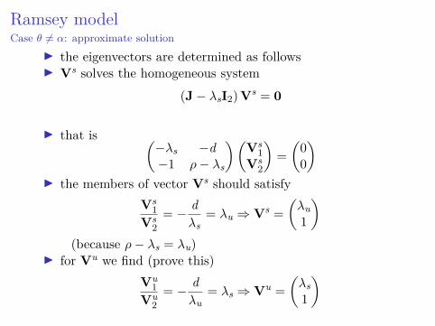
▶ the eigenvectors are determined as follows▶ Vs solves the homogeneous system

(J − λsI2)Vs = 0

▶ that is (−λs −d−1 ρ− λs

)(Vs

1Vs

2

)=

(00

)▶ the members of vector Vs should satisfy

Vs1

Vs2= − d

λs= λu ⇒ Vs =

(λu1

) (because ρ− λs = λu)

▶ for Vu we find (prove this)Vu

1Vu

2= − d

λu= λs ⇒ Vu =

(λs1

)


▶ Then the general solution is(c(t)− ck(t)− k

)= hs

(λu1

)eλst + hu

(λs1

)eλut

▶ We determine hs and hu by forcing the general solution to

satisfy the two remaining conditions

limt→∞

h(t)c(t)θ e−ρt = 0, and k(0) = k0

▶ the first condition holds if

limt→∞(c(t)− c) = limt→∞(k(t)− k) = 0, i.e., they convergeto the steady state, which is obtained by eliminating theeffect of eλut (wich converges to ∞) by setting hu = 0

▶ the second condition holds if

k(0) = k + hs − k = k0 → hs = k0


▶ the approximate solution is, for t ∈ [0,∞)

c(t) = c + λu(k0 − k)eλst,

k(t) = k + (k0 − k)eλst.


▶ at t = 0 we have(c(0)k(0)

)=

(c + λu(k0 − k)

k0

)observe that λu gives the variation of consumption asc(0)− c = λu(k0 − k) and the initial consumption isdetermined from future data (c and k)

▶ asymptotically (i.e., in the long run)

limt→∞

(c(t)k(t)

)=

(ck

)=

(ρ+δ(1−α)

α kk

)the solution converges to the steady state (this means thatthe transversality condition is satisfied)

▶ the saddle path dynamics implies that the solutionis unique

Ramsey modelCase θ = α: phase diagrams for θ < α and θ > α

Ramsey para alpha>theta

c

k’=0

c’=0

k

Ws

Es

Ramsey para alpha<theta

Es

c

k’=0

c’=0

k

Ws

Figure: Exact (dark) and approximate (light) solutions

Ramsey modelCase θ = α: exact solution

▶ there is an explicit solution:

c(t) =δ + ρ(1 − α)

αk(t),

r(t) =r(0)(δ + ρ)

r(0) + (δ + ρ− r(0))e−[(1−α)(δ+ρ)/α]t ,

with k(t) = (αA/r(t))1/(1−α)

▶ given k(0) we get explicitly

c(0) = δ + ρ(1 − α)

αk(0)

▶ convergences asymptotically to the steady state,

limt→∞

c(t) = c

limt→∞

r(t) = r = δ + ρ

limt→∞

k(t) = k

Ramsey modelCase θ = α: phase diagram

Ramsey para alpha=theta

cWs

k’=0

c’=0

k

Ramsey modelProperties of the solution paths

1. if k(0) = k then limt→∞ k(t) = k,2. given any initial value for k, k(0), there is only a value for

c, c(0) which is determined endogenously such thatlimt→∞ c(t) = c;

3. the solution is determinate, i.e, unique: this is theonly solution for the ode system such that thetransversality condition holds;

4. the saddle path is asymptotically tangent to the straightline

c(t)− c = λu(k(t)− k)

5. the approximate per-capita output path is

y(t) =[y1/α + (y(0)1/α − y1/α)eλst

]α(2)

the model only displays transitional dynamics as λs < 0.

Ramsey modelCase θ = α: GDP exact dynamics

▶ the exact per-capita output path is

y(t) = A[

αAk(0)α−1(δ + ρ)

αAk(0)α−1 + (δ + ρ− αAk(0)α−1)e−[(1−α)(δ+ρ)/α]t

]α,

▶ the solution converges asymptotically to the steady state

limt→∞

y(t) = y =

[A(

α

δ + ρ

)α]1/(1−α)

The Ramsey modelGrowth implications

▶ there is no long-run growth g = 0▶ the long-run level y depends on (A, δ, ρ, α): productivity,

the rate of depreciation, the rate of time preference(impatience) and on the income shares (see equation (1));

▶ there is only transitional dynamics: the speed andthe pattern of convergence depends on the relationshipbetween the capital share, α, in income and theintertemporal elasticity of substitution θ (see equation (2)).This is because

λs =ρ

2 −

[(ρ2

)2+

(1 − α) ρ(ρ+ δ(1 − α)

)αθ

] 12< 0

the higher |λs| is the faster the transition speed is.

The Neoclassical DGE modelAssumption

▶ Representative household: has initial financial wealth b andgets financial income (rb), and decides on consumption (c)and savings (b) ;

▶ Households own firms with physical capital (k) which isonly financed by bonds: thus b = k. Firms transformcapital and labor into output (y)

▶ There are accounting restrictions.▶ All markets are competitive▶ Other assumptions: infinite-lived households with isoelastic

utility and Cobb-Douglas production, function and nofrictions.

The Neoclassical DGE model▶ Household’s problem: maximize discounted intertemporal

utility subject to a financial constraint

maxc(.)

∫ ∞

0

c(t)1−θ

1 − θe−ρtdt

subject to: change in assets = income minus consumption

b = r(t)b(t) + w(t)− c(t), t ≥ 0b(0) = b0

limt→∞

e−∫∞

t r(s)ds ≥ 0

where b =bonds, w =wage▶ Optimality conditions

c = c(t)(r(t)− ρ)

θ

limt→∞

e−ρtc(t)−θb(t) = 0

The Neoclassical DGE model

▶ Firm’s problem (price taker in all the markets): maximizespresent value of profits

maxi

∫ ∞

0(Ak(t)α − w(t)− i(t)) e−

∫∞t r(s)dsdt

subject to net investment = gross investment minusddepreciation

k = i − δkk(0) = k0

▶ F.o.c

r(t) = αAk(t)α−1 − δ

The Neoclassical DGE model

▶ Micro-macro constraints:▶ Accounting identity b(t) = k(t),▶ Then b(t) = k(t),▶ Wage determination w = y − rk = (1 − α)Akα,

▶ Then get the same dynamic system as in the Ramsey model

c = c(t)(r(t)− ρ)

θ

k = Ak(t)α − c(t)− δk(t)

▶ Then the allocations of c and k are equal: we say that theequilibrium is Pareto efficient)

References▶ Ramsey (1928), Cass (1965) Koopmans (1965)▶ (Acemoglu, 2009, ch. 8) , (Aghion and Howitt, 2009, ch.

1), (Aghion and Howitt, 2009, ch. 1), (Barro andSala-i-Martin, 2004, ch. 2)

Daron Acemoglu. Introduction to Modern Economic Growth.Princeton University Press, 2009.

Philippe Aghion and Peter Howitt. The Economics of Growth.MIT Press, 2009.

Robert J. Barro and Xavier Sala-i-Martin. Economic Growth.MIT Press, 2nd edition, 2004.

D. Cass. Optimum growth in an aggregative model of capitalaccumulation. Review of Economic Studies, 32:233–40, 1965.

T. Koopmans. On the concept of optimal economic growth. InThe Econometric Approach to Development Planning.Pontificiae Acad. Sci., North-Holland, 1965.

Frank P. Ramsey. A mathematical theory of saving. EconomicJournal, 38(152):543–559, December 1928.

The Ramsey growth model

Documents

Transcript of The Ramsey growth model