The Local Solow Growth Model

Steven N Durlauf∗, Andros Kourtellos, Artur MinkinDepartment of Economics, University of Wisconsin

October 6, 2000

1 IntroductionThis paper is designed to contribute to our understanding of the capacity of the Solowgrowth model to explain cross-country growth patterns. In a seminal paper, Mankiw,Romer and Weil (1992) demonstrated that the Solow model has impressive empiricalexplanatory power. We mean this in two respects. First, the empirical version ofthe model produces parameter estimates whose signs and statistical signiÞcance arepredicted by the associated theory. Second, by conventional goodness-of-Þt measures,the Solow model �explains� over 40% of the cross-country variation in growth rates.For these reasons, the Solow growth model has become the baseline from which avery large part of the new empirical growth literature has developed. Typically, theevaluation of a new causal determinant of growth consists of adding an empiricalproxy of the determinant to the basic Solow regression.As a careful reading of Solow (1956, 1970) makes clear, the stylized facts for which

this model was developed were not interpreted as universal properties for every coun-try in the world. In contrast, the current literature imposes very strong homogeneityassumptions on the cross-country growth process as each country is assumed to havean identical (and Cobb-Douglas) aggregate production function. This is surprising,as modern growth theory, suggests that different countries should be described bydistinct aggregate production functions, in the sense that the new causal theories ofgrowth will presumably affect the aggregate production function of countries ratherthan constitute additive components of the growth process. To us, this suggests thatfor a given parsimonious growth regression, whether it is based on the Solow modelor some other theory, one should explicitly account for parameter heterogeneity. Inthis paper, we provide some estimates of a local generalization of the Solow growth

∗Durlauf thanks the National Science Foundation, John D. and Catherine T. MacArthur Foun-dation, Vilas Trust, and Romnes Trust for Þnancial support.

1

model. By local, we refer to the idea that a Solow model applies to each country, butthe model�s parameters vary across countries. In particular, we allow these parame-ters to vary according to a country�s initial income. While this restricts the form ofparameter heterogeneity, it is an appealing way to generalize current empirical prac-tice, in that new growth theories such as Azariadis and Drazen (1990) suggest thatinitial conditions can index countries so as to produce behaviors that, near a steadystate, are similar to that predicted by the Solow model. Our approach also providesa simple way of evaluating the local goodness-of-Þt of the Solow model.Our Þndings of parameter heterogeneity have several possible interpretations.

First, our results may simply imply that the identical Cobb-Douglas technology as-sumption is unsatisfactory. Duffy and Papageorgiou (1999) Þnd evidence in supportof an alternative production function rather than the standard Cobb-Douglas spec-iÞcation; at least qualitatively we are consistent with this Þnding. Second, it maybe the case that the parameter heterogeneity we Þnd is induced by omitted growthdeterminants. Third, our results may indicate general nonlinearities in the growthprocess. Evidence of this has already been found by Durlauf and Johnson (1995),Desdoigts (1999), Kourtellos (2000), and Rappaport (2000) among others. Thisrange of possible explanations does not mean, of course, that additional work cannotdiscriminate between them. This paper demonstrates the importance of explicitlyaccounting for parameter heterogeneity in evaluating how the Solow growth modelapproximates cross-country data.

2 A Local Generalization of the Solow Growth ModelMuch of the new empirical growth literature is based on the regression

gi = γ0Xi + ²i (1)

where gi is real per capita growth in economy i over a given time period, Xi is a p-dimensional vector of country-speciÞc controls which includes a constant and ²i is anunexplained residual. When this regression represents the growth process implied bythe standard Solow model, the controls consist of a constant, the log of yi,0, the realper capita income of the country at the beginning of the period over which growthis measured, the log of sk,i, the savings rate for physical capital accumulation outof real output, the log of sh,i, the analogous savings rate for human capital, and thelog of (ni + ρ + δ), where ni is the population growth rate of country i and ρ and δrepresent common rates of technical change and depreciation of human and physicalcapital stocks. Following standard practice we assume that (ρ+ δ) equals 0.05. Thederivation of this regression (see Mankiw, Romer, and Weil (1992)) assumes that eachcountry is associated with a common aggregate production function which (unless onewishes to claim that all countries are near their steady states) is Cobb-Douglas.One way to think about a localized generalization of the Solow regression is to

assume that each country obeys the Solow model, but that the aggregate production

2

function which characterizes the country varies. Assuming that this variation can beindexed by a scalar index variable zi, one can generalize the Solow regression to

gi = γ(zi)0Xi + ²i (2)

where γ(zi)0 = (γ1(zi), . . . , γp(zi)) is a function which maps the index into a set of

country-speciÞc Solow parameters and p is the number of Solow-type variables. Here,zi is interpretable as some measure of development of the country. This type of de-pendence can be justiÞed in several ways. For example, if one believes that thereare threshold effects due to capital externalities of the type studied by Azariadis andDrazen (1990), then γ(·) will behave as a step function with respect to a capitalstock. Alternatively, the index may proxy for omitted growth determinants. For ex-ample, if democracy causally affects growth (Barro (1996)), then a democracy indexcan be introduced in this way. Durlauf (2000) provides some additional discussionof this functional form. As stated earlier, this type of parameter heterogeneity isnot completely general. On the other hand, this formulation provides a simple wayof modelling cross-country differences in the way aggregate economic growth is inßu-enced by physical capital accumulation, human capital accumulation and populationgrowth.

3 DataWe employ the Heston -Summers data as used in Mankiw, Romer, Weil (1992). Thevarious savings and growth rates we use are computed for the period 1960 to 1985for 98 countries, which are identiÞed in Table 1 in the appendix. The Þve variablesemployed are (i) g, the change in the log of income per capita over the period 1960to 1985; (ii) log(n+ .05), average growth rate of the working age population (deÞnedas population between ages of 15 and 64); (iii) log(sk), average proportion of realinvestments (including government) to real GDP; (iv) log(sh), average percentageof working age population that is in secondary school; (v) log(y0), initial per capitaincome. Following Durlauf and Johnson (1995), we use log(y0) as our developmentindex. We plan to explore other indices in subsequent work; estimates with initialliteracy produced qualitatively similar results. In estimating the model, we also allowfor a country varying intercept term.

4 Estimation IssuesThe varying coefficient model we apply is based on the work of Hastie and Tibshirani(1993) and follows the conditional linear structure given by equation (2) with

E(gi | Xi = Xi, zi = zi) = γ(zi)0Xi (3)

V ar(gi | Xi = Xi, zi = zi) = σ2gi(zi) (4)

3

The sampling model is assumed to be a random sample {zi,Xi}ni=1 drawn from a

distribution Fz,X .For each given point z0, we approximate the functions γj(z), j = 1, . . . p, locally

asγj(z) ≈ aj + bj(z− z0) (5)

for sample points z in a neighborhood of z0. This results in the following weightedleast squares problem:

mina0s, b0s

nXi=1

gi −pX

j=1

(aj + bj(zi − z0)) xij

2

Kh(zi − z0) (6)

where Kh(·) = 1hK³ ·

h

´is some kernel. In this paper we use the Epanechnikov kernel

K(z) = 34(1−z2)I(|z|≤ 1).

While this estimation is very simple, it implicitly assumes that the functionalcoefficients have the same degrees of smoothness and hence can be approximatedequally well in the same interval. In practice, though, the functional coefficientsmay possess different degrees of smoothness, rendering estimators derived from themore conventional one-step weighted least squares estimation suboptimal. In orderto avoid this problem we adopt a two-stage estimation method proposed by Fan andZhang (1999) that ensures that the optimal rate of convergence for the asymptoticmean-squared error is achieved.The two-step estimation procedure assumes that γp(·) is smoother (that is it

possesses a bounded fourth derivative) than the other coefficient functions and hence asecond-step is needed to correct for bias of the Þrst step estimation1. In particular, theÞrst step produces an initial estimate of γ1(·), ..., γp−1(·) by solving (6) and obtainingthe partial residuals r−p

r−p = g − γ1(z)x1 − ...− γp−1(z)xp−1 (7)

Fan and Zhang (1999) recommend choosing the initial smoothing parameter so thatthe estimate is undersmoothed, which ensures that the bias of the initial estimator issmall. The two step estimation procedure is not sensitive to the choices of the initialbandwidth. In the second step, one solves2

minap,bp,cp,dp

nXi=1

hri,−p −

³ap + bp(zi − z0) + cp(zi − z0)

2 + dp(zi − z0)3´xip

i2Kh2(zi − z0)

(8)

1In practice one does not know in advance which coefficient function is smoother so we apply thetwo-step for all the coefficients. Fan and Zhang (1999) show that the two-step procedure is alwaysmore reliable than the one-step approach.

2In theory a local cubic Þt should be used in the second step. In our reported results, however,we use a local linear Þt which performs equally well.

4

where h2 is the second step bandwidth. Following suggestions by Fan and Zhang(1999), for the Þrst step we use 10% of the data range for all the coefficients andfor the second step we use 25%, 25%, 30% and 30% of the data range for γ1, . . . , γ4,respectively.

5 ResultsFigures 1a-1d report3 our point estimates and associated 95% conÞdence intervalsfor the varying coefficient functions for (2). Table 1 in the appendix presents theassociated point estimates together with standard errors for these functions for thedifferent countries in the sample. The superimposed horizontal line in the graphsrefers to the least square coefficients of the Solow model (see table V, pp. 426,Mankiw, Romer, and Weil (1992)). A number of general conclusions may be drawn.First, evidence of parameter heterogeneity is strongest for the poorer economies

in the sample. For the varying coefficients associated with the intercept, popula-tion growth, and human capital variables, our estimates of the Solow parametersare relatively stable for economies with per capita GDP in 1960 above $944, whichcorresponds to Kenya, the 24th poorest country in our sample.Second, our estimates of the physical capital coefficient are highly unstable through-

out the sample, and do not exhibit any sort of monotonicity. Interestingly, the highestvalues of the physical capital coefficient are associated with the higher per capita in-come economies. For the majority of economies with a per capita income higher than$1794, which corresponds to Sri Lanka, the point estimate for the physical capitalcoefficient is higher than that produced by the Solow model.Third, we note that the varying intercept term exhibits substantially lower values

for the poorest economies than the rest of the sample. This suggests that there maybe a latent determinant of low growth by poor countries that is omitted from theSolow model.

6 Local Goodness-of-fitAssociated with our varying coefficient estimates are local measures of the goodness-of-Þt of the Solow model. The local goodness-of-Þt measure we employ is the corre-lation curve due to Bjerve and Doksum (1993) and Doksum, Blyth, Bradlow, Mengand Zhao (1994). An important virtue of the correlation curve is that it representsa natural generalization of the standard statistic R2.The local goodness-of-Þt measure we employ is based on the following idea. Con-

sider the regression (2). If the parameters γ(zi) which hold for a given zi were to

3Tanzania is omitted from the graphs as it acts as an outlier and would render the graphsunreadable given space constraints. Parameter estimates are given in Table 1; complete graphs areavailable upon request.

5

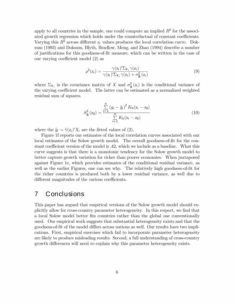
apply to all countries in the sample, one could compute an implied R2 for the associ-ated growth regression which holds under the counterfactual of constant coefficients.Varying this R2 across different zi values produces the local correlation curve. Dok-sum (1993) and Doksum, Blyth, Bradlow, Meng, and Zhao (1994) describe a numberof justiÞcations for this goodness-of-Þt measure, which can be written in the case ofour varying coefficient model (2) as

ρ2(zi) =γ(zi)

0ΣXiγ(zi)

γ(zi)0ΣXiγ(zi) + σ2

gi(zi)

(9)

where ΣXiis the covariance matrix of X and σ2

gi(zi) is the conditional variance of

the varying coefficient model. The latter can be estimated as a normalized weightedresidual sum of squares.

bσ2gi(z0) =

nPi=1(gi − bgi)

2Kh(zi − z0)

nPi=1Kh(zi − z0)

(10)

where the bgi = bγ(zi)0Xi are the Þtted values of (2).

Figure 1f reports our estimates of the local correlation curves associated with ourlocal estimates of the Solow growth model. The overall goodness-of-Þt for the con-stant coefficient version of the model is .42, which we include as a baseline. What thiscurve suggests is that there is a monotonic tendency for the Solow growth model tobetter capture growth variation for richer than poorer economies. When juxtaposedagainst Figure 1e, which provides estimates of the conditional residual variance, aswell as the earlier Figures, one can see why. The relatively high goodness-of-Þt forthe richer countries is produced both by a lower residual variance, as well due todifferent magnitudes of the various coefficients.

7 ConclusionsThis paper has argued that empirical versions of the Solow growth model should ex-plicitly allow for cross-country parameter heterogeneity. In this respect, we Þnd thata local Solow model better Þts countries rather than the global one conventionallyused. Our empirical work suggests that substantial heterogeneity exists and that thegoodness-of-Þt of the model differs across nations as well. Our results have two impli-cations. First, empirical exercises which fail to incorporate parameter heterogeneityare likely to produce misleading results. Second, a full understanding of cross-countrygrowth differences will need to explain why this parameter heterogeneity exists.

6

References[1] Azariadis, C. and A. Drazen (1990), �Threshold Externalities in Economic De-

velpment�, Quarterly Journal of Economics, 105, 2, 501-526.

[2] Barro, R., (1996), �Democracy and Growth,� Journal of Economic Growth, 1,1-27.

[3] Bjerve, S. and K. Doksum, (1993), �Correlation Curves: Measures of Associationas Functions of Covariate Values,� Annals of Statistics, 21, 2, 890-902.

[4] Desdoigts, A., (1999), �Patterns of Economic Development and the Formationof Clubs,� Journal of Economic Growth, 4, 3, 305-330.

[5] Doksum, K., S. Blyth, E. Bradlow, X.-L. Ming, and H. Zhao, (1994), �Correla-tions Curves as Local Measures of Variance Explained by Regression,� Journalof the American Statistical Association, 89, 426, 571-582.

[6] Duffy, J. and C. Papageorgiou, (1999), �Cross-Country Empirical Investigationof the Aggregate Production Function SpeciÞcation,� mimeo, University of Pitts-burgh.

[7] Durlauf, S., (2000), �Econometric Analysis and the Study of Economic Growth:A Skeptical Perspective,� in Macroeconomics and the Real World, R. Backhouseand A Salanti, eds., Oxford, Oxford University Press.

[8] Durlauf, S. and P. Johnson, (1995), �Multiple Regimes and Cross-CountryGrowth Behavior,� Journal of Applied Econometrics, 10, 365-384.

[9] Fan, J. and Zhang, W. (1999), �Statistical Estimation in Varying-CoefficientModels�, Annals of Statistics, 27, no. 5, 1491�1518.

[10] Hastie, T. and R. Tibshirani, (1993), �Varying Coefficient Models (with discus-sion),� Journal of the Royal Statistical Society, series B, 55, 757-796.

[11] Kourtellos, A., (2000), �A Projection Pursuit Approach to Cross CountryGrowth Data,� mimeo, University of Wisconsin.

[12] Mankiw, N. G., D. Romer and D. Weil, (1992). �A Contribution to the Empiricsof Economic Growth,� Quarterly Journal of Economics, CVII, 407-437.

[13] Rappaport, J., (2000), �Is the Speed of Convergence Constant?,� mimeo, FederalReserve Bank of Kansas City.

[14] Solow, R., (1956), �A Contribution to the Empirics of Economic Growth,� Quar-terly Journal of Economics, 70, 65-94.

[15] Solow, R., (1970), �Growth Theory�, Oxford, Oxford University Press.

7

Appendix

Figure 1a - intercept

6 7 8 9log(y0)

-20

-10

010

gam

ma0

(log(

y0))

Figure 1c - coefficient of investments

6 7 8 9log(y0)

0.5

11.

5

gam

ma2

(log(

y0))

Figure 1e - conditional variance

6 7 8 9log(y0)

05

10

sigm

a^2(

log(

y0))

Figure 1b - coefficient of population growth

6 7 8 9log(y0)

-50

gam

ma1

(log(

y0))

Figure 1d - coefficient of initial human capital

6 7 8 9log(y0)

-2-1

01

gam

ma3

(log(

y0))

Figure 1f - squared correlation curve

6 7 8 9log(y0)

00.

20.

40.

60.

8

r^2(

log(

y0))

Figure 1: Varying Coefficient Model and Correlation Curve

8

Table 1. Variable Coefficient Estimates Countries

GDP60 (y0)

γ0(y0) γ1(y0) γ2(y0) γ3(y0) CountriesGDP60

(y0)γ0(y0) γ1(y0) γ2(y0) γ3(y0)

Tansania 383 -93.78 -23.91 1.55 -6.63 Botswana 959 0.09 -0.92 0.29 0.549.38 2.12 0.28 0.75 0.76 0.20 0.04 0.09

Malawi 455 -16.39 -4.37 0.67 -1.45 India 978 0.30 -0.84 0.29 0.533.26 0.75 0.09 0.28 0.72 0.19 0.03 0.09

Rwanda 460 -13.83 -3.71 0.63 -1.26 Congo 1009 0.65 -0.72 0.28 0.503.14 0.72 0.09 0.27 0.67 0.18 0.03 0.08

Sierra 511 2.82 0.54 0.40 0.00 Ghana 1009 0.65 -0.72 0.28 0.50Leone 2.53 0.58 0.07 0.23 0.67 0.18 0.03 0.08Myanmar 517 3.94 0.81 0.38 0.10 Morocco 1030 0.86 -0.64 0.28 0.48

2.50 0.57 0.07 0.23 0.64 0.18 0.03 0.08Burkina 529 5.83 1.27 0.35 0.27 Nigeria 1055 1.09 -0.56 0.28 0.46Faso 2.43 0.56 0.06 0.23 0.61 0.17 0.03 0.08Ethiopia 533 6.33 1.39 0.34 0.32 Pakistan 1077 1.27 -0.49 0.28 0.45

2.41 0.56 0.06 0.23 0.58 0.17 0.03 0.08Niger 539 7.04 1.56 0.33 0.40 Haiti 1096 1.43 -0.43 0.27 0.45

2.38 0.55 0.06 0.22 0.57 0.17 0.03 0.07Zaire 594 9.82 2.08 0.28 0.79 Benin 1116 1.61 -0.35 0.27 0.45

2.08 0.49 0.06 0.20 0.56 0.16 0.03 0.07Uganda 601 9.79 2.05 0.28 0.82 Zimbabwe 1187 2.12 -0.15 0.27 0.45

2.04 0.48 0.06 0.20 0.54 0.16 0.03 0.07Mali 737 5.45 0.53 0.30 0.81 Madagascar 1194 2.16 -0.13 0.27 0.45

1.33 0.33 0.05 0.14 0.54 0.16 0.03 0.07Burundi 755 4.65 0.29 0.30 0.79 Sudan 1254 2.60 0.04 0.28 0.45

1.26 0.31 0.05 0.13 0.54 0.16 0.03 0.06Mauritania 777 3.68 0.01 0.30 0.76 South 1285 2.85 0.15 0.29 0.45

1.18 0.29 0.04 0.13 Korea 0.54 0.17 0.03 0.05Togo 777 3.68 0.01 0.30 0.76 Thailand 1308 2.98 0.20 0.29 0.44

1.18 0.29 0.04 0.13 0.53 0.17 0.03 0.05Nepal 833 1.65 -0.56 0.30 0.68 Ivory 1386 3.40 0.40 0.32 0.42

1.01 0.26 0.04 0.11 Coast 0.51 0.16 0.04 0.05Central 838 1.50 -0.61 0.30 0.67 Senegal 1392 3.44 0.42 0.32 0.42Afr. Rep. 1.00 0.25 0.04 0.11 0.51 0.16 0.04 0.05Bangladesh 846 1.26 -0.67 0.30 0.66 Zambia 1410 3.57 0.47 0.32 0.42

0.98 0.25 0.04 0.11 0.51 0.16 0.04 0.05Liberia 863 0.79 -0.79 0.30 0.64 Mozambique 1420 3.64 0.50 0.33 0.41

0.94 0.24 0.04 0.10 0.50 0.16 0.04 0.05Indonesia 879 0.37 -0.90 0.30 0.63 Honduras 1430 3.69 0.52 0.33 0.41

0.91 0.23 0.04 0.10 0.50 0.16 0.04 0.05Cameroon 889 0.12 -0.96 0.29 0.61 Angola 1588 3.69 0.57 0.41 0.34

0.89 0.23 0.04 0.10 0.42 0.14 0.04 0.05Somalia 901 -0.17 -1.03 0.29 0.60 Bolivia 1618 3.69 0.58 0.43 0.32

0.87 0.23 0.04 0.10 0.41 0.14 0.04 0.05Egypt 907 -0.32 -1.06 0.29 0.60 Tunisia 1623 3.68 0.58 0.43 0.31

0.86 0.22 0.04 0.10 0.40 0.14 0.04 0.05Chad 908 -0.35 -1.07 0.29 0.59 Philippines 1668 3.65 0.59 0.46 0.29

0.86 0.22 0.04 0.10 0.38 0.13 0.04 0.05Kenya 944 -0.09 -0.98 0.29 0.56 Papua 1781 3.54 0.57 0.54 0.20

0.79 0.21 0.04 0.09 New Guinea 0.33 0.12 0.04 0.05

Sri Lanka 1794 3.52 0.57 0.55 0.19 Mexico 4229 -0.79 -0.91 0.87 -0.140.33 0.12 0.04 0.05 0.31 0.11 0.06 0.07

Brazil 1842 3.47 0.56 0.58 0.15 Ireland 4411 -1.22 -1.05 0.83 -0.120.31 0.12 0.04 0.05 0.29 0.10 0.06 0.07

Dominican 1939 3.36 0.53 0.65 0.08 South 4768 -2.03 -1.32 0.75 -0.07Rep. 0.29 0.11 0.04 0.04 Africa 0.27 0.09 0.06 0.07Paraguay 1951 3.34 0.52 0.66 0.07 Israel 4802 -2.10 -1.35 0.74 -0.06

0.29 0.11 0.04 0.04 0.27 0.09 0.06 0.07Mauritius 1973 3.31 0.51 0.68 0.06 Argentina 4852 -2.20 -1.38 0.73 -0.05

0.29 0.11 0.04 0.04 0.27 0.09 0.06 0.07El Salvador 2042 3.21 0.48 0.72 0.01 Italy 4913 -2.31 -1.42 0.72 -0.04

0.28 0.11 0.04 0.04 0.26 0.09 0.06 0.07Malaysia 2154 3.05 0.44 0.80 -0.06 Uruguay 5119 -2.65 -1.53 0.67 -0.01

0.28 0.11 0.04 0.04 0.26 0.09 0.06 0.07Jordan 2183 3.02 0.43 0.82 -0.08 Chile 5189 -2.75 -1.57 0.66 0.00

0.28 0.11 0.04 0.05 0.26 0.09 0.06 0.07Ecuador 2198 3.00 0.43 0.83 -0.09 Austria 5939 -3.05 -1.68 0.54 0.12

0.28 0.11 0.04 0.05 0.23 0.08 0.06 0.08Greece 2257 2.94 0.41 0.87 -0.12 Finland 6527 -2.86 -1.61 0.51 0.17

0.28 0.11 0.05 0.05 0.23 0.07 0.06 0.08Portugal 2272 2.92 0.40 0.88 -0.13 Belgium 6789 -2.67 -1.55 0.52 0.18

0.28 0.11 0.05 0.05 0.23 0.07 0.06 0.08Turkey 2274 2.92 0.40 0.88 -0.13 France 7215 -2.24 -1.40 0.57 0.17

0.28 0.11 0.05 0.05 0.23 0.07 0.06 0.08Syrian 2382 2.81 0.37 0.94 -0.18 United 7634 -1.70 -1.22 0.63 0.16Arab Rep. 0.29 0.11 0.05 0.05 Kingdom 0.24 0.07 0.06 0.08Panama 2423 2.78 0.36 0.96 -0.20 Netherlands 7689 -1.62 -1.20 0.64 0.15

0.29 0.11 0.05 0.05 0.24 0.07 0.06 0.08Guatemala 2481 2.73 0.34 0.99 -0.22 West 7695 -1.61 -1.20 0.65 0.15

0.30 0.11 0.05 0.05 Germany 0.24 0.07 0.06 0.08Algeria 2485 2.73 0.34 0.99 -0.22 Sweden 7802 -1.44 -1.14 0.67 0.15

0.30 0.11 0.05 0.05 0.24 0.08 0.06 0.08Colombia 2672 2.51 0.27 1.06 -0.26 Norway 7938 -1.22 -1.07 0.69 0.15

0.31 0.12 0.05 0.06 0.25 0.08 0.06 0.08Jamaica 2726 2.45 0.25 1.06 -0.26 Australia 8440 -0.24 -0.78 0.80 0.14

0.32 0.12 0.05 0.06 0.26 0.08 0.06 0.07Singapore 2793 2.33 0.20 1.06 -0.25 Denmark 8551 0.00 -0.71 0.83 0.14

0.32 0.12 0.05 0.06 0.26 0.08 0.06 0.07Hong Kong 3085 1.72 -0.03 1.08 -0.24 Trinidad & 9253 1.74 -0.23 1.00 0.15

0.32 0.12 0.05 0.06 Tobago 0.30 0.10 0.05 0.07Nicaragua 3195 1.48 -0.12 1.08 -0.24 New 9523 2.40 -0.05 1.08 0.17

0.33 0.12 0.05 0.06 Zealand 0.31 0.10 0.05 0.07Peru 3310 1.21 -0.22 1.07 -0.23 Canada 10286 4.24 0.42 1.30 0.24

0.32 0.12 0.05 0.06 0.36 0.12 0.06 0.07Costa 3360 1.11 -0.26 1.07 -0.23 Switzerland 10308 4.29 0.43 1.30 0.24Rica 0.32 0.12 0.05 0.06 0.36 0.12 0.06 0.07Japan 3493 0.83 -0.36 1.05 -0.22 Venezuela 10367 4.42 0.46 1.32 0.25

0.32 0.12 0.05 0.06 0.37 0.12 0.06 0.07Spain 3766 0.27 -0.55 0.99 -0.19 United 12362 6.51 1.06 1.56 0.37

0.32 0.11 0.05 0.06 States 0.97 0.30 0.15 0.18