Electronic copy available at: http://ssrn.com/abstract=1956543

CEIS Tor Vergata RESEARCH PAPER SERIES

Vol. 9, Issue 12, No. 216 – November 2011

Corruption, growth and ethnic

fractionalization: a theoretical model

Roy Cerqueti, Raffaella Coppier and Gustavo Piga

This paper can be downloaded without charge from the Social Science Research Network Electronic Paper Collection

http://papers.ssrn.com/paper.taf?abstract_id=19565 43

Electronic copy available at: http://ssrn.com/abstr act=1956543

Electronic copy available at: http://ssrn.com/abstract=1956543

Corruption, growth and ethnic fractionalization: a

theoretical model∗

Roy Cerqueti

Department of Economic and Financial Institutions

University of Macerata

Raffaella Coppier

Department of Economic and Financial Institutions

University of Macerata

Gustavo Piga†

Department of Economics and Territory

University of Rome Tor Vergata

Abstract

This paper analyzes the existing relationship between ethnic fractional-ization, corruption and the growth rate of a country. We provide a sim-ple theoretical model. We show that a nonlinear relationship betweenfractionalization and corruption exists: corruption is high in homoge-neous or very fragmented countries, but low where fractionalizationis intermediate. In fact, when ethnic diversity is intermediate, con-stituencies act as a check and balance device to limit ethnically-basedcorruption. Consequently, the relationship between fractionalizationand growth rate is also non-linear: growth is high in the middle rangeof ethnic diversity, low in homogeneous or very fragmented countries.

Keywords: corruption, ethnic fractionalization, monitoring cost, economicgrowth.JEL Codes: D73, K42, O43.

∗The authors would like to thank Elisabetta Iossa, Arsen Palestini, the seminar par-ticipants at the 24th Annual Congress of the European Economic Association, August23-27, 2009 and at the 15th World Congress of the International Economic Association,June 25-27, 2008, Istanbul, for their very helpful suggestions.

†Corresponding author: Gustavo Piga, Department of Economics and Territory, Uni-versity of Rome Tor Vergata, Via Columbia 2, 00133, Rome, Italy,E-mail:gustavo.piga@uniroma2.it

Electronic copy available at: http://ssrn.com/abstract=1956543

1 Introduction

Much research has been directed at explaining the causes and theconsequences of corruption. Different levels of corruption have beenattributed to differences in religious tradition, colonial experiences (see e.g.Treisman, 2000), level of development (see e.g. Blackburn et al., 2010), levelsof decentralization (Treisman, 2000, Fisman and Gatti, 2002 and Lessmannand Markwardt, 2010), competition among bureaucracies (see e.g. Drugov,2010) or to the availability of natural resources (see e.g. Vicente, 2010and Bhattacharyya and Hodler, 2010). Researchers have also investigatedthe effects of corruption on investment and growth (see e.g Mauro, 1995),on international trade (see e.g. Lambsdorff, 1998 and Musila and Sigue,2010), on income inequality (see e.g. Dobson and Ramlogan-Dobson, 2010),on the volatility of the economic growth rate (see Evrensel, 2010) and onmisallocation of resources (see e.g. Acemoglu and Verdier, 1998 and 2000).Our paper tries to provide additional light on the causes and consequencesof corruption by suggesting that a further determinant of it, ethnic diversity,can produce a novel and non-linear impact on output growth.In recent years, the economic interest in ethnic fractionalization1 hasincreased, in part due to greater cross-border movements. Althoughethnic diversity is an omnipresent theme throughout history, economistsare only recently starting to pay attention to it. Journalists report onethnic diversity mostly when it erupts into bloodshed, although ethnicfractionalization does not automatically, nor exclusively, imply ethnicconflict. The recent literature has claimed that cross-country differencesin ethnic diversity explain a substantial part of cross-country differences inpublic policies, political instability and other economic factors associatedwith long-run growth (see Easterly and Levine 1997). Political economymodels suggest that polarized societies will be both prone to competitiverent-seeking by different groups and have difficulty agreeing on publicgoods like infrastructure, education and good policies (Alesina and Drazen1991; Shleifer and Vishny 1993; Alesina and Spoloare 1997). Alesina andDrazen (1991) describe how a war of attrition between interest groups canpostpone macroeconomic stabilization. Alesina et al. (1999) present a

1In our paper we will consider as ethnic group one of human beings whose membersidentify with each other usually on the basis of common cultural, linguistic, religious,behavioral or biological traits. In this respect, we will use interchangeably term ethnicfractionalization or ethnolinguistic fractionalization since in the definition of the concept of“ethnic group” it is difficult to distinguish between ethnic and linguistic variables. In fact,language is a fundamental part of the criterion used by ethnologists and anthropologists todefine the concept of ethnicity. Indeed, Alesina et al. (2003) compute a measure of ethnicfractionalization, “ethnicity”, the definition of which involves a combination of racial andlinguistic characteristics. Also, Atlas Norodov Mira (1964), in order to compute the ELFindex, mainly used language to define groups, even if it sometimes refers to notions of raceor national origin in order to distinguish between different groups.

1

model linking heterogeneity of preferences across ethnic groups in a cityto the amount and type of public goods the city supplies. Results show thatthe shares of spending on productive public goods are inversely related tothe city ethnic fragmentation. Mauro (1995), La Porta et al. (1999) andAlesina et al. (2003)2, amongst others, show that ethnic fractionalizationis negatively correlated with measures of infrastructure quality, literacy andschool attainment.

Ethnolinguistic fractionalization appears to be responsible for a varietyof corruption-related phenomena (Shleifer and Vishny 1993; Svensson 2000).Svensson (2000) and Mauro (1995) find that corruption is higher the higherethnic diversity. Svensson (2000) also finds that corruption increases wherethere is more foreign aid in an ethnically-divided society although this is notthe case in an ethnically-homogeneous one. In Shleifer and Vishny (1993)corruption may be particularly damaging when there is more than one bribe-taker. If each independent bribe-taker does not internalize the effects ofher/his bribes on the other bribe-takers’ revenues, then the result is morebribes per unit of output and less output. Ethnically-diverse societies maybe more likely to yield independent bribe-takers, since each ethnic groupis responsible for a region or ministry in the power structure. For thisreason Mauro (1995) regresses growth on corruption assuming an indexof ethnolinguistic fractionalization as an instrumental variable to test thehypothesis that more fractionalization (and therefore more corruption) isassociated with lower economic growth3.The literature has thus stressed the negative role of ethnic fragmentation oncorruption and therefore on economic growth. But alongside this negativerole, there is the possibility of a positive role for ethnic diversity. In fact asAlesina and La Ferrara (2005) say:

“ Is ethnic diversity “good” or “bad” from an economic point of view,and why? Its potential costs are fairly evident. Conflict of preferences,racism, prejudices often lead to policies which are suboptimal from the pointof view of society as a whole, and to the oppression of minorities whichcan explode in war or least in disruptive political instability. But an ethnicmix also brings about variety in abilities, experiences, cultures which may beproductive and may lead to innovation and creativity. The United States arethe quintessential example of these two faces of racial relations in a “meltingpot”. ”

Analogously to Tangeras and Lagerlof (2009), the role of the degree of

2These results are very strong in regressions without income per capita (which may beendogenous to ethnic fractionalization). They lose some of their significance when on theright-hand side one controls for GDP per capita.

3“Sociological factors may contribute to rent-seeking behavior. An index ofethnolinguistic fractionalization (societal divisions along ethnic and linguistic lines) hasbeen found to be correlated with corruption. Also, public officials are more likely to dofavors for their relatives in societies where family ties are strong”. Mauro (1997)

2

ethnic diversity of a country (i.e. the number of ethnic groups) has beenexplored to describe and explain an economic phenomenon. While Tangerasand Lagerlof’s analysis is related to the probability of the occurrence of acivil war, we discuss the level of corruption of a country and its relationshipto ethnic fragmentation. In particular, we contribute to this debate byanalyzing how ethnolinguistic fractionalization can influence the extent ofcorruption.We propose a descriptive model since, as Collier (2001) and Alesina et al.(2003) emphasize, it is hard to see any policy implications arising fromfractionalization, because there is little that a country can legitimately doabout its ethnic composition without affecting other non-economic variableswhich are not the object of this study.Indeed, our descriptive paper does not aim at suggesting optimal ethnicpolicies directed at reducing corruption or at allowing growth to increase.One might note however that, for a given ethnolinguistic fractionalization, apolicy aspiring to achieve a fair and balanced representation of ethnic groupswithin the administrative public sector machine (even in the presence ofconstituencies with a majority of votes) could help not only in reinforcingmutual understanding and muting fake stereotypes but also in making thefight against corruption more credible. Minority rights in this respect couldprove helpful.In our model, we rely on a society populated by bureaucrats, controllers andentrepreneurs, producing a single good. The population is fractionalized inn different ethnic groups. A theoretical game is constructed as follows:the entrepreneur has to choose between the traditional technology and themodern technology. We assume that the modern technology has higherproductivity than the traditional technology. In order to access to themodern technology, the entrepreneur has to request a concession from thebureaucrat. Since the concession has an expiration date, the entrepreneurneeds to submit the project to the Public Administration in each period,and each concession submission is independent from the previous ones. Tocapture these characteristics of the problem, we develop a one-shot game.We also assume that the entrepreneur must acquire a bureaucrats approvalfor the project (see Yoo, 2008). The bureaucrat can ask the entrepreneurfor a bribe in exchange for providing the concession. The entrepreneur canagree or refuse to pay the bribe. Moreover, we consider the presence ofmonitoring activity. Monitoring activity is related to the intervention of thecontrollers in order to penalize illegal interactions between entrepreneursand bureaucrats.In our work, the optimal monitoring level is endogeneously derived. Weassume that ethnic fractionalization has two opposite effects: on the onehand, it increases the cost of monitoring but, on the other hand, high ethnicfractionalization generates an increase in the probability of being reported,because the controller reports the corrupt transaction only if the bureaucrat

3

belongs to a different ethnic group from that of the controller. Indeed,for certain levels of ethnic diversity, fragmentation takes on a positive rolein controlling corruption because it increases the level of control betweendifferent ethnic groups.The findings of the present paper are comparable to the ones in Tangerasand Lagerlof (2009): indeed, in both cases, the influence of the degree ofethnic diversity seems to be more powerful when the country is neitherhomogeneous nor highly fragmented. The common root of these results canbe found in the presence of two competitive effects due to the number ofethnic groups. In particular, in our paper, the effect of monitoring corruptionis low either in homogeneous or very fragmented countries, while it is highwhen the level of ethnic diversity is intermediate.In this context, we also find a non-linear relationship between ethnicdiversity, corruption and growth: in fact, homogeneous and fragmentedsocieties are characterized by high corruption and low economic growth.In the middle range of ethnic diversity, the ethnic factor acts as a “control”on corruption thus producing greater economic growth.In Figures 1a, 1b, 1c, we scatter the growth rate in 2007 against themeasure of ethnic fractionalization proposed in Alesina et al. (2003) forWorld Countries, Democratic Countries and OECD Countries, respectively4.As the Figures indicate, intermediately fractionalized countries have thehighest growth rate. The Figures also show the implementation of a formalregression between the ethnic fractionalization index and the growth rate viaquadratic polynomial function. There is evidence that a reversed U-shapedfunction seems to fit the scatter plot well5.The rest of the paper is organized as follows. In section 2, we presentthe model and the related theoretical game. In section 3, the relationshipbetween the monitoring level, corruption and economic growth is studied.In section 4, using the results of the previous sections, we endogeneizethe monitoring level of controllers and prove that a non-linear relationshipbetween fractionalization -via corruption- and growth exists. Section 5concludes.

4See Appendix A for the list of the countries.5The R-squared are 0.03327, 0.07805 and 0.1309 for World, Democratic and OECD

Countries, respectively. The second-order best fit polynomial is P (x) = −14.86x2 +11.96x + 2.627, P (x) = −21.3x2 + 16.81x + 1.675 and P (x) = −0.102x2 + 0.9078x + 2.511for World, Democratic and OECD Countries, respectively. We point out that the analysisdeveloped in our model does not aim at providing forecasts, but only at stating therelationship between variables. In particular, the relationship between growth rate andfractionalization is under scrutiny in our paper. In this situation, standard statisticsarguments guarantee that the fit parameters such as R-squared are less relevant, becauseno one would expect fractionalization to explain a high percentage of the growth rate, asthe growth rate of a country is affected by many other factors. The best fit parameters, asexpected, improve when restricting from World Countries to Democratic Countries, andthen to OECD Countries.

4

0 0.1 0.2 0.3 0.4 0.5 0.6 0.7 0.8 0.9

−10

−5

0

5

10

15

20

25

Fractionalization

Gro

wth

ra

te

World Countries: 2007

0.1 0.2 0.3 0.4 0.5 0.6 0.7

−5

0

5

10

15

Fractionalization

Gro

wth

ra

te

Democratic Countries: 2007

4 5 6 7 8 9

−2

0

2

4

6

8

10

Fractionalization

Gro

wth

ra

te

OECD Countries: 2007

Figure 1: The scatter plot is the growth rate versus the ethnic coefficient.The line is the best fit quadratic function.

2 The theoretical game model

Let us consider an economy producing a single homogeneous good andcomposed of a continuum of 3 types of agents: bureaucrats, controllers andentrepreneurs. The controllers monitor bureaucrats’ behavior in order toweed out or reduce corruption. Firms manufacture a homogeneous producty using either one of two technologies6 with constant return to scale: themodern technology and the traditional technology. Each entrepreneur isassumed to have the same quantity of capital k. The product may either bemanufactured for consumption purposes or for investment purposes.The modern technology output is:

y = aMk (1)

Here we deal with the grant of a concession7 to the entrepreneurs. In orderto obtain their concession, the entrepreneurs need to submit a project tothe Public Administration.The entrepreneur may access the traditional technology without anyconcession being issued by the Public Administration. In this case theoutput is:

y = aT k (2)

From here on, it will be assumed that aM > aT and therefore that themodern technology is more profitable than the traditional technology.

6As in Li et al. (2000) an agent can produce in either the traditional or the moderntechnology. Productivity of the modern technology is greater than that of the traditionaltechnology. The advantage of the traditional technology is that it is not subject toexpropriation, while that of the modern technology is. The rationale is that entrepreneurswith the modern technology must obtain permits and concessions and are vulnerable tothe effects of corruption. This hypothesis could be interpreted by regarding the moderntechnology as an innovative technology (e.g. telecommunications) which is still in need ofState regulation.

7The concession, once granted, has an expiration date and must be renewed at theend of its lifetime. As we will see, we construct and develop a one-shot game, and so theone-period concession seems to be suitable for modelling purposes. After the expirationdate, the game is repeated in an identical manner.

5

The bureaucrat receives a salary w8. In this model, the bureaucrat maydecide to issue a concession only in exchange for a bribe. Since the grossprofit resulting from the investment in the modern technology is higherthan the one in the traditional technology, the entrepreneur may find itworthwhile to negotiate and accept the bribe requested by the corruptbureaucrat in order to obtain the necessary concession to access the moderntechnology. The bureaucrat may decide not to ask for a bribe and to issuethe concession to all those who submit a project, or s/he may decide toask for a bribe in exchange for such a concession. The State monitorsbureaucrats -via controllers- in such a way that qi is the probability that thebureaucrat belonging to the i-th ethnic group is reported9. In our model,we assume that the bureaucrat detected in a corrupt transaction will bepunished with a fine mk10. In contrast, the loss of reputation incurred by theentrepreneur detected in a corrupt transaction may affect her/his business.More precisely, it is common knowledge11 that the j-th entrepreneur incursa specific value cjk to the loss of reputation derived from being caught in acorrupt transaction12 where cj ∈ [0, 1].The controller must monitor the bureaucrat’s behavior and s/he puts a levelof monitoring p in place. Since the pioneer work of Allport (1954) on thetheory of prejudice and following the Social Identity Theory (Tajfel andTurner, 1986), early work established that patterns of intergroup behaviorcan be understood considering that individuals may attribute positive utilityto the well-being of members of their own group and negative utility to thatof members of others group (see e.g. Tajfel et al. 1971). The simple fact ofbelonging to a group can lay foundations of prejudice, judgmental biases and

8It is assumed that no arbitrage is possible between the public and the private sectorand that therefore there is no possibility of the bureaucrats becoming entrepreneurs, evenif their salary w were lower than the entrepreneur’s net return. This happens because thebureaucrat individuals in the population have no access to the capital markets, but onlya job, and therefore may not become entrepreneurs.

9In our model, there is an implicit public budget constraint so that the State usesrevenues which derive from a lump sum taxation and fines imposed on bureaucrats caughtin corrupt transaction, to pay the wages and to put in place redistributive policies.However, there is no space for financing public productive expenditure. Since this isnot the focus of our work, we do not make that public constraint explicit.

10The punishment for the detected bureaucrat is not a constant, but following Rose-Ackerman (1999), it is a function of the bureaucrat’s payoff. In fact, in the suggestedmodel, since the obtained bribe is a function of k, the punishment is assumed to be afunction of k.

11The entrepreneurs experience different reputation costs when they are detected incorrupt transactions. The differences derive from the economic relevance of entrepreneurialactivity. Hence, it is possible to attach a specific value to the entrepreneurs’ reputationcosts, and such values belong to the bureaucrats’ information set.

12Based on the statements of Rose-Ackerman (1999), the punishment for theentrepreneur is not a constant, but rather a function of the entrepreneur’s payoff. Thepunishment for the entrepreneur is considered as a function of the investment determiningthe size of the profits.

6

intergroup discrimination towards outgroups13. Following this literature, weassume that only if the controller meets a corrupt bureaucrat belonging toa different ethnic group will s/he report the corruption14. We hypothesizethat “The Department of Controllers” is divided in proportion to ethnicgroups15. Let ωi ∈ [0, 1] the probability that an individual belongs to thei-th ethnic group, with i = 1, . . . n.16 Following Alesina and La Ferrara(2005), we rely on a country where the different ethnic groups are of thesame size. Therefore

ωi = ω =1

n. (3)

The controller earns αp from the State for the monitoring level p ands/he encounters increasing difficulty in monitoring entrepreneurs as thenumber of ethnic groups grows. The optimal monitoring level p will bederived endogenously in the model and it will be a non linear function ofethnolinguistic fractionalization n. In the rest of the paper, we refer to theentrepreneur payoff by a superscript (E) and to the bureaucrat payoff by asuperscript (B).Our model can be formalized by introducing the following three-perioddynamic game:

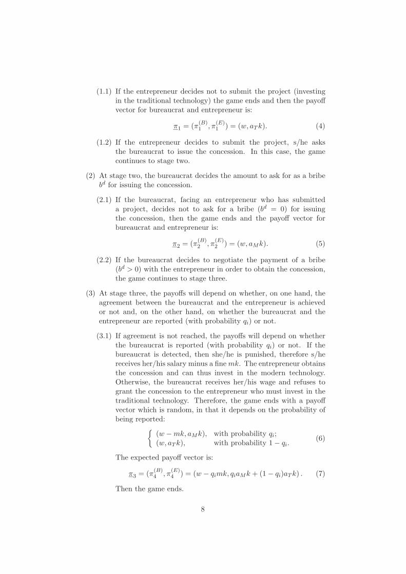
(1) At stage one of the game, the entrepreneur should decide in whichtechnology to invest, i.e. whether to invest her/his capital in themodern or in the traditional technology. Such a decision is tantamountto the decision of whether or not to submit the project to the PublicAdministration, considering that a concession is needed to invest inthe modern technology. Project submission does not result in theautomatic issue of the concession by the bureaucrat, in that thebureaucrat may refuse to grant the concession unless a bribe bd ispaid.

13This prejudice is reinforced by the nationalist attitude of a population. Corneo (2010)stresses in his theoretical and empirical analysis that ability is an explanatory factor ofnationalism: in fact, parents of low-ability children instill nationalism in their offspringwhich will have, therefore, more hostile relations with immigrants.

14It is worth noticing that the controllers do not have information about the bureaucrat’sethnic group before the check. In fact, we do not deal with political corruption butbureaucratic corruption (petty corruption). In this case, the controller does not knowwhich entrepreneurs to control until a superior tells her/him the assigned tasks and s/hecannot refuse to control the entrepreneurs which have been allocated.

15Notice that our model does not apply if ethnic fractionalization is not reflected alsoin institutions, as it is often the case in dictatorships.

16This assumption we make allows us to derive closed form formulas for the analysis ofthe growth rate and the reputation of the entrepreneurs with respect to fractionalizationand the probability of being detected. We can only say that whenever the ethnic group i isdominant then, ceteris paribus, the probability qi to be detected is lower and corruption isgreater. In the case of non homogeneous ethnic groups, our model should be interpretedas a normative model highlighting the impact of electoral and administrative systemswhere ethnic representation in government and/or civil servants is proportional to thedemographic base.

7

(1.1) If the entrepreneur decides not to submit the project (investingin the traditional technology) the game ends and then the payoffvector for bureaucrat and entrepreneur is:

π1 = (π(B)1 , π

(E)1 ) = (w, aT k). (4)

(1.2) If the entrepreneur decides to submit the project, s/he asksthe bureaucrat to issue the concession. In this case, the gamecontinues to stage two.

(2) At stage two, the bureaucrat decides the amount to ask for as a bribebd for issuing the concession.

(2.1) If the bureaucrat, facing an entrepreneur who has submitteda project, decides not to ask for a bribe (bd = 0) for issuingthe concession, then the game ends and the payoff vector forbureaucrat and entrepreneur is:

π2 = (π(B)2 , π

(E)2 ) = (w, aMk). (5)

(2.2) If the bureaucrat decides to negotiate the payment of a bribe(bd > 0) with the entrepreneur in order to obtain the concession,the game continues to stage three.

(3) At stage three, the payoffs will depend on whether, on one hand, theagreement between the bureaucrat and the entrepreneur is achievedor not and, on the other hand, on whether the bureaucrat and theentrepreneur are reported (with probability qi) or not.

(3.1) If agreement is not reached, the payoffs will depend on whetherthe bureaucrat is reported (with probability qi) or not. If thebureaucrat is detected, then she/he is punished, therefore s/hereceives her/his salary minus a fine mk. The entrepreneur obtainsthe concession and can thus invest in the modern technology.Otherwise, the bureaucrat receives her/his wage and refuses togrant the concession to the entrepreneur who must invest in thetraditional technology. Therefore, the game ends with a payoffvector which is random, in that it depends on the probability ofbeing reported:

{

(w − mk, aMk), with probability qi;(w, aT k), with probability 1 − qi.

(6)

The expected payoff vector is:

π3 = (π(B)4 , π

(E)4 ) = (w − qimk, qiaMk + (1 − qi)aT k) . (7)

Then the game ends.

8

(3.2) If agreement is not reached, the payoffs will depend onwhether the bureaucrat and the entrepreneur are reported (withprobability qi) or not. If they are detected, then the bureaucratreceives her/his salary minus the fine mk and the entrepreneurpays the reputation cost cj , but she/he is refunded the cost of thebribe paid to the bureaucrat. Otherwise, the bureaucrat receivesher/his wage plus the bribe, which the entrepreneur must pay.Therefore, the game ends with a payoff vector which is random,in that it depends on the probability of being reported:

{

(w − mk, aMk − cjk), with probability qi;(w + bNB, aMk − bNB), with probability 1 − qi.

(8)

The expected payoff vector is:

π4 = (π(B)4 , π

(E)4 ) =

(

w + (1 − qi)bNB − mkqi, aMk − (1 − qi)b

NB − qicjk)

.(9)

When a controller monitors a corrupt transaction, s/he decides to bring acharge only if the bureaucrat belongs to a different ethnic group from that ofthe controller. The probability of a controller, belonging to the i-th ethnicgroup, meeting a bureaucrat belonging to the i-th ethnic group as well, willbe equal to 1

n. Then qi is the probability of the bureaucrat belonging to

the i-th ethnic group being reported and it derives from the probability pof being monitored and from the probability of the controller belonging toan ethnic group different from i. Then

qi = q = p

(

1 −1

n

)

, ∀ i = 1, . . . , n. (10)

The optimum level of p derives from maximization by the controller ofher/his own expected payoff (see section 4).

3 The solution of the game

The game may be solved by backward induction, starting from the laststage. The bribe resulting as the Nash solution to a bargaining game inthe last subgame needs to be determined. Such a bribe is the outcome ofa negotiation between the bureaucrat and the entrepreneur, who will beassumed to share a given surplus on an equal basis. We first determine theequilibrium bribe (see Appendix B for the proof).

Proposition 3.1. Let q 6= 1.17 Then there exists a unique non-negativebribe bNB

j , as the Nash solution to a bargaining game, given by:

bNBj =

[

(aM − aT )k

2−

qcjk

2(1 − q)

]

. (11)

17If q = 1 this stage of the game is never reached.

9

Proposition 3.1 shows that, when the equilibrium is reached, theentrepreneur gives half of the surplus to the bureaucrat, such a surplusbeing the difference in the expected return on the investment in the twodifferent technologies (modern and traditional), net of the entrepreneur’sexpected costs for being detected in a corrupt transaction.

Remark 3.2. We notice that a straightforward computation gives thatthe equilibrium bribe bNB

j is decreasing with respect to the probability ofbeing detected in a corrupted transaction. Therefore, increasing q, reducesthe potential surplus that the bureaucrat and entrepreneur can share, thusreducing the bribe.

3.1 The static equilibrium

The game has been solved in Appendix C by using the backward inductionmethod starting from its last stage. The solution of the game is formalizedby the following proposition.

Proposition 3.3. Let 0 ≤ (aM−aT )(1−q)q

− 2m = c◦ ≤ 118.

(a) If cj ∈ [0, c◦) then the equilibrium expected payoff vector is:

π4 =

(

w − mkq +(aM − aT )(1 − q)k

2−

cjkq

2, aMk −

(aM − aT )(1 − q)k

2−

cjkq

2

)

.

(12)This is the expected payoff vector connected to equilibrium C (seebelow);

(b) if cj ∈ [c◦, 1] then the equilibrium expected payoff vector is:

π2 = (w, aMk) . (13)

This is the expected payoff vector connected to equilibrium NC (seebelow).

The previous proposition shows that we obtain two perfect Nash equilibriain the sub-games, depending on the parameter values:

• Equilibrium C: if cj < c◦, the difference in gross profits between themodern sector and the traditional technology is such as to make upfor the expected cost of corruption. Thus, the surplus to be sharedbetween the entrepreneur and the bureaucrat will keep a negotiationgoing, the outcome of which is the bribe corresponding to the Nashsolution to a bargaining game;

18Actually, this requirement allows us to avoid the trivial cases of corner solutions: whenc◦ < 0, then the entrepreneurs are honest, while c◦ > 1 implies that the entrepreneurs arecorrupt.

10

• Equilibrium NC: if cj ≥ c◦, i.e. the “reputation cost” is so high thatthe entrepreneur would turn down a request for a bribe. Realizing thisfact, the bureaucrat will refrain from asking for a bribe for issuing theconcession. Thus the entrepreneur will choose the modern technologyand will not be asked for a bribe by the bureaucrat.

Substantially, there are two ranges of cj which correspond to differentcorruption levels: in equilibrium C corruption is widespread, while it isabsent in equilibrium NC.As we have stated, our model assumes that reputation costs may varyacross different entrepreneurs (cj for the j-th entrepreneur), depending onher/his own “reputation loss” when the corrupt transaction is detected. Thisargument applies to each ethnic group.The distribution of individual costs is described through a probabilitydistribution function F (cj), where j is the specific entrepreneur. Thisfunction represents the fraction of entrepreneurs who agree to be corrupted.By definition, F is a distribution function associated to a random variablewhose density function f has support [0, 1]. The shape of the function fgives good information about the general level of entrepreneurs’ honesty. Inparticular, the symmetry properties of the function f provide informationabout the distribution of the entrepreneurs between those with a high orlow reputation costs, in short the honest and the corrupt. If f is a centeredsymmetric function, then the country has an average level of corruption,and the number of corrupted entrepreneurs balances the number of honestentrepreneurs. The case of f asymmetric to the left can be associated to acountry where most entrepreneurs are corrupt, while f is asymmetric to theright in countries where most entrepreneurs are honest. Therefore, so thatour analysis is complete, we need to provide a random law for the reputationcosts which may describe the generality of the cases, depending on the valueof some parameters. This purpose can be achieved by incurring the cost ofadopting an unusual probability law, which is commonly used in a rathermathematical context: namely the Kumaraswamy distribution. In fact, ofall the distribution functions of random variables with support in [0, 1], theKumaraswamy law seems to be the more appropriate choice for F , since ithas some features that make it suitable for modeling the different reputationcosts of the entrepreneurs belonging to a given country19. However, as wewill see below in Remark 3.4, the results concerning the behavior of theaggregate expected growth rate with respect to the monitoring level q canbe obtained, regardless of the particular shape of cost distribution.Given the heterogeneity of entrepreneurs, their behavior will be influenced

19Further details of the mathematical definition of the Kumarawamy law with somegraphical examples, together with some supporting arguments on why we use this randomvariable for modelling the reputation costs distribution, are provided in Appendix D.

11

by their own reputation cost cj . In this hypothesis we have

F (c◦) = 1−(1−(c◦)α1)α2 = 1−

(

1 −

(

(aM − aT )(1 − q)

q− 2m

)α1)α2

(14)

is the fraction of entrepreneurs belonging to the i-th ethnic group with areputation cost cj < c◦, while

1 − F (c◦) = (1 − (c◦)α1)α2 =

(

1 −

(

(aM − aT )(1 − q)

q− 2m

)α1)α2

(15)

is the fraction of entrepreneurs belonging to the i-th ethnic group with areputation cost cj ≥ c◦.In contrast with the static case, in a dynamic context, as we will seein the next section, corruption influences the accumulation of capital byentrepreneurs, and thus economic growth.

3.2 Dynamic equilibrium

The game perspective is now expanded to review the dynamic consequencesof corruption on growth and, therefore, on investment, while analyzing theentrepreneur’s behavior in this respect. As noted, a manufactured product

may be either consumed C or invested•k.

We consider a constant elasticity utility function:

U =C1−σ − 1

1 − σ. (16)

Each entrepreneur maximizes utility over an infinite period of time subjectto a budget constraint. This problem is formalized as:

maxC∈[0,+∞)

∫ ∞

0e−ρtU(C)dt (17)

subject to•k = ΠE − C, (18)

where C is consumption, e−ρ is the uniperiodal discount factor and ΠE isthe return on the investment for the entrepreneur.Since ΠE is different across equilibria, the problem is solved for the twocases20.This model predicts that the j-th entrepreneur belonging to the i-th ethnicgroup will have only one optimum equilibrium -and only one correspondingexpected growth rate- depending on her/his own reputation cost.

20In the interest of clarity, we report the computation of the expected growth rate inAppendix E.

12

• The entrepreneur with a reputation cost cj ≤ c◦, will find it worthwhileto be corrupted and then the optimal equilibrium will be C. In thisequilibrium, the entrepreneur will obtain a consumption expectedgrowth rate equal to:

γCj =

1

σ

[

aM −(aM − aT )(1 − q)

2−

qcj

2− ρ

]

. (19)

• The entrepreneur with a reputation cost cj > c◦, will find it worthwhileto be honest and then, the optimal equilibrium will be NC. In thisequilibrium, the entrepreneur will obtain a constant consumptiongrowth rate equal to:

γNC =1

σ[aM − ρ]. (20)

Furthermore, it can easily be demonstrated that capital and income alsohave the same expected growth rate21.Then, at aggregate level, we obtain an income expected growth rateγ weighting over different expected growth rates for correspondingentrepreneurs. Then, in the equilibrium C, there will be F (c◦) corruptedentrepreneurs, each with her/his own expected growth rate γC

j ; in theequilibrium NC there will be [1 − F (c◦)] honest entrepreneurs, all withthe same growth rate γNC . At the aggregate level, we have:

γ =1

σ· [1 − (1 − (c◦)α1)α2 ] ·

[

aM −(aM − aT )(1 − q)

2− ρ

]

−

−1

2σ

[

q

∫ c◦

0cdc

]

+1

σ· [1 − (c◦)α1 ]α2 (aM − ρ) =

=(aM − aT )(1 − q)

2σ·[1−(c◦)α1 ]α2−

q

4σ·(c◦)2+

1

σ·

[

aM −(aM − aT )(1 − q)

2− ρ

]

.

(21)

By substituting c◦ = (aM−aT )(1−q)q

− 2m into (21), we obtain the economyexpected growth rate as

γ =(aM − aT )(1 − q)

2σ·

[

1 −

(

(aM − aT )(1 − q)

q− 2m

)α1]α2

−

−q

4σ·

(

(aM − aT )(1 − q)

q− 2m

)2

+1

σ·

[

aM −(aM − aT )(1 − q)

2− ρ

]

. (22)

A straightforward computation gives that

∂γ

∂q> 0. (23)

21See Appendix F for the proof.

13

This means that the expected growth rate of the economy increases as theprobability of being reported grows.

Remark 3.4. Relation in (23) holds, for each chosen probability distributiondescribing the cost function. Indeed, for a generic cumulative function F ,we can write:

γ =1

σ·{

1 − F

(

(aM − aT )(1 − q)

q− 2m

)

·(aM − aT )(1 − q)

2−

−q

4σ·

[

(

(aM − aT )(1 − q)

q− 2m

)2

+ aM −(aM − aT )(1 − q)

2− ρ

]

}

,

(24)and also in this case γ increases with respect to q, since F increases bydefinition.

Despite the argument laid out in Remark 3.4, we prefer to show a verygeneral but specific density function which applies to a multitude of cases,in order to avoid results that can be difficult to interpret. In this respect,the next section contains an explanation of how the relationship betweenthe expected growth rate and the monitoring level works, by considering anendogenous optimal monitoring level.

4 Endogenous monitoring

As we have stated, q is the probability of being reported and it derives fromthe probability p of being monitored and from the probability 1−1/n of thebureaucrat belonging to a different ethnic group from that of the controller(see formula (10)).So far, we have taken the monitoring level p as exogenous, but now we makethe analysis more realistic, considering that the monitoring level set by thecontroller results from maximization of her/his payoff Vp:

Vp = αp − χ(n, p). (25)

where αp are the benefits of a certain monitoring level p for the controllerand χ(n, p) are monitoring costs, dependent on n and p.The optimum level of p, named p∗, is derived by maximization of thecontroller’s expected payoff function in (25).The controller decides the optimal level of monitoring p∗ comparing themarginal benefit of a certain monitoring level with the cost of doing it.We state some assumptions about the cost function: costs are assumedto be null in the case of absence of monitoring, as it naturally should be.Moreover, we assume that the marginal costs increase as the monitoring levelincreases. In fact, comprehensive monitoring activity implies increased costs,

14

since it requires a more sophisticated action and the specialist knowledgeabout complex corrupted transactions. As a further requirement, wehypothesize that the costs related to a fixed monitoring level grows as ethnicfractionalization n increases. This assumption is driven by the growingcomplexity for any given group of interacting with a larger number of ethnicgroups, also considering the evident presence of linguistic difficulties ofmonitoring members of different ethnic groups22. Wrong (2009), describingthe “artificial” increase in ethnic groups which was forced onto Kenya bycolonialism, makes a forceful supporting argument:“by 1938, Kenya had been partitioned into twenty-four overcrowded nativereserves “Kamba” for the Kamba people, “Kikuyu” for the Kikuyu, and soon and the fertile “White Highlands” for exclusive European use, whereAfricans could not own land. [...] The settlers wanted Africans to actsmall, think local. It made them so more manageable. [...] To those on thereserves, who increasingly viewed their communities as mini-nations in fiercecompetition with one another, Kenyans from outside were “foreigners”.“Most of us on the farm rarely met people from other communities, spoketheir language or participated in their cultural practices”[the future NobelPeace Prize-winner Wanri Maathai remarked].”.The necessity of summing up the above statements and remarks drives thechoice of an appropriate cost function. In this respect, we achieve our targetby introducing the mathematical concept of Orlicz functions23. In doingso, we incur the cost of a rather complicated mathematical tool, but wealso admit that it is worth incurring this cost. Indeed, the constitutiveelements of the concept of Orlicz functions are so general and basic thatOrlicz functions may be suitable for modeling purposes. In this respect, aswe will see below, an Orlicz function describes well the main features of themonitoring costs.24

The costs χ are defined as:

χ(n, p) = g(n)M(p), (26)

where:

• g : N → [0, +∞) describes how the monitoring level cost dependson the number of ethnic groups. We point out that, in our analysis,

22See, e.g., Ortega and Tangeras (2008).23For the concept of Orlicz functions and kernels see Appendix G, where some illustrative

examples are also provided.24It is worth noting that we are not the pioneers of the use of special functions like

those of Orlicz type for economic modeling purposes, even if this technique is ratherrecent. In this respect, we refer to Boucekkine and Ruiz-Tamarit (2008) and Boucekkineet al. (2008) where it is shown that the solution to a two-sector Lucas-Uzawa modelof endogenous growth can be expressed in terms of hypergeometric-type function. InBenchekroun and Withagen (2010), the exponential integrals are applied for modeling aneconomy with resource constraints.

15

the trivial case of a single ethnic group is not considered, and thepopulation is made up of at least two different ethnic groups. We canassume that we know the value of g in the case of two different ethnicgroups, with value g(2) = g2 > 0. Function g is also assumed to beincreasing;

• M has support in [0, 1], M([0, 1]) ≡ [0, H], H > 0 and M is atruncation of an Orlicz function as follows:

M(x) := 1{x∈[0,1]} · Γ(x),

where 1A is the usual characteristic function of the set A and Γ(x) isan Orlicz function such that Γ(1) ≡ M(1) = H. We assume that thekernel function of Γ, named h, is strictly increasing.

The concept of Orlicz function is not new in the economic literature. Inthis respect, it is well-known that the properties of this mathematical toolare suitable to characterize a class of risk measures used in actuarial science(Haezendock and Goovaerts, 1982; Schmidt, 1989; Goovaerts et al., 2004;Bellini and Rosazza Gianin, 2008). As already stressed in the discussiondeveloped above, we feel that the Orlicz functions can be also used todescribe well the cost functions introduced in our model, with a particularfocus on the relationship between monitoring level and fractionalization.In our framework, the highest monitoring level is attained for m = 1. Inthis case the cost function is:

χ(n, 1) = g(n)H,

and it depends on the ethnic fractionalization within the country in that itdepends on the term g(n).The function Vp of the monitoring activity, for the controller, is maximizedfor an optimal monitoring level p∗, which can be found by imposing the firstorder condition:

∂Vp

∂p= α − g(n)h(p∗) = 0.

Since h is strictly increasing, then there exists the inverse function h−1. Weassume hereafter the following condition for the weights g(n).

g(n) ≥α

h(1), ∀n ∈ N. (27)

Condition (27) states that the cost adjustment factor g(n) is not less thana certain threshold depending on the monitoring costs and the marginalbenefit of monitoring.By imposing (27), we can find the optimal monitoring level p∗ ∈ [0, 1] givenby:

p∗ = h−1

(

α

g(n)

)

. (28)

16

By considering the continuous version of the function g : [0, +∞) → [0,+∞),assuming that g is differentiable and replacing the discrete variable n withthe continuous variable x, we can compute the first derivative of p∗,

(p∗)′(x) =1

h′(α/g(x))·−αg′(x)

g2(x)< 0, (29)

since g is increasing respect to n.Thus, the assumption that g is increasing implies that the optimalmonitoring level decreases as the number of ethnic groups grows. This is dueto the fact that the monitoring costs grow as the number of ethnic groupsincreases.By substituting the optimal p∗ of (28) into (10), we find the optimalprobability of being reported q∗:

q∗ = h−1

(

α

g(n)

)

·

(

1 −1

n

)

. (30)

Then the optimal probability of being reported q∗ depends on ethnolinguisticfractionalization through two channels:

(1) the optimal monitoring level: as ethnic diversity increases, we haveshown that the monitoring cost also increases and thus the optimalmonitoring level p∗ declines;

(2) the probability of the bureaucrat belonging to a different ethnic groupfrom that of the controller: as the number of ethnic groups increases,the probability of the bureaucrat belonging to the same ethnic groupdecreases. Therefore the probability of the bureaucrat belonging to adifferent ethnic group from that of the controller increases.

More intuitively, on the one hand, as ethnic diversity increases, themonitoring cost increases and then the optimal monitoring level decreases,thus the optimal q∗ decreases. On the other hand, as ethnic diversityincreases, the probability of the bureaucrat belonging to a different ethnicgroup from that of the controller increases. Uniting these two oppositechannels we will show (see Theorem 4.1.) that, subject to a non restrictiveassumption regarding g, there is a threshold value of ethnic diversity n∗

where the probability of being reported reaches a maximum. For lowerfractionalization levels, i.e. before n∗, the probability of being reportedq∗ increases with respect to ethnic diversity n. Indeed, the increase inthe probability of being reported -due to the fact that the bureaucratbelongs to a different ethnic group from that of the controller- overtakesthe reduction in monitoring level -due to the increasing monitoring cost-.For high fractionalization levels, i.e. after n∗, the growing monitoring costsovertake the increase in the probability of being reported.

17

These results are reflected in the aggregate expected growth rate. We defineby γ∗ the expected growth rate computed at the optimal monitoring levelp∗ (and so at the optimal level q∗) by substituting (30) and (28) into (21)as follows:

γ∗ =(aM − aT )(1 − q∗)

2σ·

[

1 −

(

(aM − aT )(1 − q∗)

q∗− 2m

)α1]α2

−

−q∗

4σ·

(

(aM − aT )(1 − q∗)

q∗− 2m

)2

+1

σ·

[

aM −(aM − aT )(1 − q∗)

2− ρ

]

.

(31)We measure the corruption level with the fraction of corruptedentrepreneurs, given by (14). By substituting (30) into (14), we have:

F (c◦)∗ = 1 −

(

1 −

(

(aM − aT )(1 − q∗)

q∗− 2m

)α1)α2

. (32)

This formula shows that, before n∗, as ethnic diversity increases, corruption-via the increasing probability of being reported q∗- decreases; conversely,after n∗ as ethnic diversity increases, corruption also increases, due to thedecreasing probability of being reported q∗.

In the next result, the previous arguments are formalized:

Theorem 4.1. Consider a function g such that

g(n∗) =α

h(

Kn∗

n∗−1

) , (33)

for n∗ ∈ N, withK = h−1(α/g2). (34)

Moreover, suppose that

h′′(

αg(n∗)

)

< 0;

g′′(n∗)g′(n∗) > 2g′(n∗)

g(n∗) .

(35)

Then n∗ is the unique absolute maximum point for q∗ and for γ∗, and it isthe unique absolute minimum point for (c◦).

For the proof see Appendix H.

Remark 4.2. The hypotheses contained in (35) are rather general: the firstone is implied by the concavity of h, while the second one can be interpretedas a condition on the risk-aversion, whenever g is assumed to be an utilityfunction. In this respect, it is worth recalling that the ratio −g′′/g′ is theArrow-Pratt risk-aversion coefficient of the utility function g.

18

In Theorem 4.1, we showed that ethnolinguistic diversity increases themonitoring activity level, up to a critical ethnolinguistic threshold n∗. In thiscase, the expected growth rate increases and the corruption level declines.For high fractionalization levels, i.e. after n∗, the growing monitoring costsreduce the monitoring level and thus economic growth.Moreover, the dynamic analysis shows an inverted U-curve betweenethnolinguistic fractionalization and the expected growth rate. Indeed,we showed that, in the case of very fragmented countries or, conversely,in a homogeneous society, the economy has a low expected growth rateand widespread corruption, while in intermediate fragmented countries, theeconomy has a high expected growth rate and limited corruption.

5 Conclusion

In this work, we have analyzed the influence of cultural and ethnic factorson the spread of corruption. The theoretical and empirical literaturehas stressed how greater ethnolinguistic fractionalization can producegreater corruption; in our model, as a further result, we have shown thatintermediate ethnolinguistic fractionalization makes the control system moreincisive on the bureaucrat’s behavior, and thus might reduce corruption.A theoretical game model is presented, in order to explore the relationshipbetween ethnolinguistic fractionalization, corruption and the growth rate.Very general conditions on the model’s parameters are assumed. Inparticular, we state that the reputation costs follow a Kumaraswamydistribution, which belongs to the family of two-parameter distribution but,differently from the Beta law, it is explicitly tractable from a mathematicalpoint of view.We find an ethnolinguistic threshold n∗ such that before n∗ the expectedgrowth rate grows and the corruption level declines. For higherfractionalization levels, i.e. after n∗, the growing monitoring costs drivegrowing corruption and a low economic growth and monitoring level.The dynamic analysis shows a U-curvebetween ethnolinguistic fractionalization and the expected growth rate: inthe case of a highly fractionalized society or, conversely, in a homogeneoussociety, the economy has a low expected growth rate, while in the middle ofthe range of ethnic diversity, the economy has a high expected growth rateand limited corruption.

19

A Appendix

World Countries are:Afghanistan; Albania; Algeria; Angola; Antigua and Barbuda; Argentina;Armenia; Australia; Austria; Azerbaijan; Bahamas; Bangladesh; Barbados;Belarus; Belgium; Belize; Benin; Bermuda; Bhutan; Bolivia; Bosnia andHerzegovina; Botswana; Brazil; Brunei; Bulgaria; Burkina Faso; Burundi;Cambodia; Cameroon; Canada; Cape Verde; Central African Republic;Chad; Chile; China; Colombia; Comoros; Congo, Dem. Rep.; Congo,Republic of; Costa Rica; Cote d‘Ivoire; Croatia; Cuba; Cyprus; CzechRepublic; Denmark; Djibouti; Dominica; Dominican Republic; Ecuador;Egypt; El Salvador; Equatorial Guinea; Eritrea; Estonia; Ethiopia; Fiji;Finland; France; Gabon; Gambia, The Georgia; Germany; Ghana; Greece;Grenada; Guatemala; Guinea; Guinea-Bissau; Guyana; Haiti; Honduras;Hong Kong; Hungary; Iceland; India; Indonesia; Iran; Iraq; Ireland;Israel; Italy; Jamaica; Japan; Jordan; Kazakhstan; Kenya; Kiribati;Korea, Republic of; Kuwait; Kyrgyzstan; Laos; Latria; Lebanon; Lesotho;Liberia; Libya; Lithuania; Luxembourg; Macao; Macedonia; Madagascar;Malawi; Malaysia; Mali; Malta; Marshall Islands; Mauritania; Mauritius;Mexico; Micronesia, Fed. Sts.; Moldova; Mongolia; Morocco; Mozambique;Namibia; Nepal; Netherlands; New Zealand; Nicaragua; Niger; Nigeria;Norway; Oman; Pakistan; Panama; Papua New Guinea; Paraguay; Peru;Philippines; Poland; Portugal; Qatar; Romania; Russia; Rwanda; Sao Tomeand Principe; Saudi Arabia; Senegal; Seychelles; Sierra Leone; Singapore;Slovak Republic; Slovenia; Solomon Islands; Somalia; South Africa; Spain;Sri Lanka; St. Kitts & Nevis; Sudan; Suriname; Swaziland; Sweden;Switzerland; Syria; Taiwan; Tajikistan; Tanzania; Thailand; Togo; Tonga;Trinidad; Tobago; Tunisia; Turkey; Turkmenistan; Uganda; Ukraine; UnitedArab Emirates; United Kingdom; United States; Uruguay; Uzbekistan;Vanuatu; Venezuela; Vietnam; Zambia; Zimbabwe.Democratic countries, considering the indications of Freedom House(http://www.democracyweb.org/new-map/), are:Antigua and Barbuda; Argentina; Australia; Austria; Bahamas; Barbados;Belgium; Belize; Benin; Botswana; Brazil; Bulgaria; Canada; Cape Verde;Chile; Costa Rica; Croatia; Cyprus; Czech Republic; Denmark; Domenica;Dominican Republic; El Salvador; Estonia; Finland; France; Germany;Ghana; Greece; Grenada; Hungary; Iceland; India; Indonesia; Ireland;Israel; Italy; Jamaica; Japan; Kiribati; Latria; Lithuania; Luxembourg;Mali; Malta; Marshall Islands; Mauritius; Mexico; Micronesia, Fed. Sts.;Mongolia; Namibia; Netherlands, New Zealand; Norway; Panama; Peru;Poland; Portugal; Romania; Slovak Republic; Slovenia; South Africa; Spain;Suriname; Sweden; Switzerland; Taiwan; Trinidad & Tobago; Ukraine;United Kingdom; United States; Uruguay; Vanuatu.OECD Countries are:

20

Australia, Austria, Belgium, Canada, Czech Republic; Denmark, Finland;France; Germany; Greece; Hungary; Iceland; Ireland; Italy; Japan;Korea; Luxembourg; Mexico; Netherlands; New Zealand; Norway; Poland;Portugal; Slovak Republic; Spain; Sweden; Switzerland; Turkey; UnitedKingdom; United States.

B Appendix

Let π∆ = π4 − π3 = (π(E)∆ , π

(B)∆ ) be the vector of the differences in the

expected payoffs where π4 is the agreement about the bribe and whereπ3 is disagreement between bureaucrat and entrepreneur. The bribe bNB

associated to the Nash solution to a bargaining game is the solution of thefollowing maximum problem

maxb∈(0,+∞)

(π(E)∆ · π

(B)∆ ),

i.e.

maxb∈(0,+∞)

{[aMk − (1 − q)b − qcjk − qaMk − aT k(1 − q)] · [w − mkq + (1 − q)b − w + mkq]} ,

that is the maximum of the product between the elements of π∆ and where[qaMk +(1− q)aT k, w−mkq] is the point of disagreement, i.e. the expectedpayoffs that the entrepreneur and the bureaucrat respectively would obtainif they did not come to an agreement. Since the objective function is concavewith respect to b, a sufficient condition for b being a maximum is the firstorder condition

∂(

π(E)∆ · π

(B)∆

)

∂b= 0,

that leads in this case to:

(aM − aT )k(1 − q)2 − cjq(1 − q)k − 2b(1 − q)2 = 0 ⇔

⇔ 2b(1 − q)2 = (aM − aT )k(1 − q)2 − cjq(1 − q)k,

bringing to:

bNB =

[

(aM − aT )k

2−

cjkq

2(1 − q)

]

(36)

that is the unique equilibrium bribe in the last subgame, ∀q 6= 1.

C Appendix

The static game is solved with the backward induction method. Startingfrom stage 3, the entrepreneur needs to decide whether to negotiate withthe bureaucrat. Both expected payoffs are then compared, because thebureaucrat asked for a bribe.

21

(3) At stage three the entrepreneur negotiates the bribe if and only if

π(E)4 > π

(E)3 ⇔ aMk − (1 − q)bNB − cjkq > qaMk + (1 − q)aT k (37)

i.e. the entrepreneur expected payoff negotiated is greater thanher/his expected payoff in the case of refusal. Since under a perfectinformation hypothesis, the entrepreneur knows the final equilibriumbribe bNB then we substitute this value in the previous inequality and,by simplification, we obtain

aMk −(aM − aT )(1 − q)k

2−

cjkq

2> qaMk + (1 − q)aT k,

that is equivalent to:

(aM − aT )(1 − q)k

2−

cjkq

2> 0 (38)

that is verified ∀ cj < (aM−aT )(1−q)q

= c⋆.Notice that in order to have an admissible probability set, cj mustbelong to [0, 1]. Since aM > aT , then we have

c⋆ =(aM − aT )(1 − q)

q≥ 0. (39)

Generally, if cj < c⋆ the entrepreneur negotiates the bribe, while ifcj ≥ c⋆ s/he refuses the bribe.

(2) Going up the decision-making tree, at stage two, the bureaucratdecides whether to ask for a bribe.• If cj ≥ c⋆ then the bureaucrat knows that the entrepreneur will notaccept any bribe. Therefore, s/he will be honest and s/he will pursuethe concession without any bribe: indeed the bureaucrat expectedpayoff if not asking for a bribe w is greater than her/his expectedpayoff if s/he asks for a bribe w − mkq.• If cj < c⋆ then the bureaucrat knows that if s/he asks for a bribethen the entrepreneur will enter into negotiation and the final bribewill be bNB. Then at stage two the bureaucrat asks for a bribe if andonly if

π(B)4 > π

(B)2 ⇔ w − mkq + (1 − q)bNB > w

i.e. the bureaucrat expected payoff if asking for a bribe is greaterthan her/his expected payoff if s/he does not ask for a bribe. Bysubstituting bNB in the previous inequality and after some algebra,we obtain

cj < c◦ =(aM − aT )(1 − q)

q− 2m.

22

Because c◦ < c⋆, so we can conclude that if cj < c◦ then the bureaucratasks for the bribe bNB and the entrepreneur accepts. If, cj ≥ c◦, thebureaucrat will not find it worthwhile to ask for a bribe.

(1) At stage one the entrepreneur has to decide whether to submit theproject.• If cj ≥ c◦ then the entrepreneur knows that if s/he submits a projectno bribe will be asked for. So s/he will submit the project if and onlyif

π(E)2 > π

(E)1 ⇔ aM < aT

The previous inequality is always verified by hypothesis.• If cj < c◦ then the entrepreneur knows that the bureaucrat will askfor the bribe bNB which s/he will accept. So, at stage one, s/he hasto decide whether to invest in the modern technology. S/he will investin the modern technology if and only if

π(E)1 < π

(E)4 ⇔ aMk −

(aM − aT )(1 − q)k

2−

kqcj

2> aT k,

hence:

cj < c⋆⋆ =(aM − aT )(1 + q)

q. (40)

Because c⋆⋆ > c⋆ > c◦, so we can conclude that if cj < c◦ theentrepreneur invests in the modern technology with corruption, whileif cj ≥ c◦ the entrepreneur invests in the modern technology withoutcorruption.

D Appendix

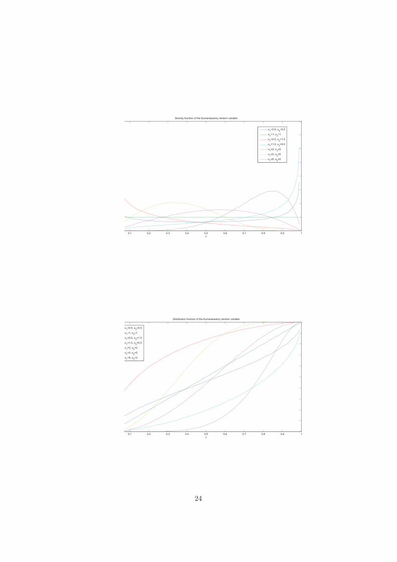
The Kumaraswamy law belongs to the family of the two-parametersdistributions, being the Beta distribution the most famous. A veryimportant feature of the Kumaraswamy random variable is its mathematicaltractability, since an explicit form of its distribution function is available.Indeed, given α1, α2 ∈ (0, +∞), the density function f and the distributionfunction F of a Kumaraswamy random variable are, respectively:

f(c) = α1α2cα1−1(1 − cα1)α2−1, c ∈ [0, 1]; (41)

F (c) = 1 − (1 − cα1)α2 , c ∈ [0, 1]. (42)

To be more exhaustive, the graphs of the Kumaraswamy density anddistribution functions related to some choices of α1 and α2 are shown inFigures 2 and 3. As the Figures show, the shape of the Kumaraswamydensity function changes as the values of α1 and α2 vary. Therefore, thisprobability law is suitable for describing different types of ethical behaviors

23

0.1 0.2 0.3 0.4 0.5 0.6 0.7 0.8 0.9 1

c

Density function of the Kumaraswamy random variable

α1=0.5, α

2=0.5

α1=1, α

2=1

α1=0.5, α

2=1.5

α1=1.5, α

2=0.5

α1=2, α

2=2

α1=2, α

2=5

α1=5, α

2=2

0.1 0.2 0.3 0.4 0.5 0.6 0.7 0.8 0.9 1

c

Distribution function of the Kumaraswamy random variable

α1=0.5, α

2=0.5

α1=1, α

2=1

α1=0.5, α

2=1.5

α1=1.5, α

2=0.5

α1=2, α

2=2

α1=2, α

2=5

α1=5, α

2=2

24

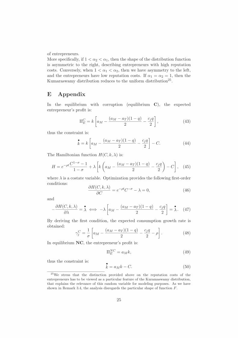
of entrepreneurs.More specifically, if 1 < α2 < α1, then the shape of the distribution functionis asymmetric to the right, describing entrepreneurs with high reputationcosts. Conversely, when 1 < α1 < α2, then we have asymmetry to the left,and the entrepreneurs have low reputation costs. If α1 = α2 = 1, then theKumaraswamy distribution reduces to the uniform distribution25.

E Appendix

In the equilibrium with corruption (equilibrium C), the expectedentrepreneur’s profit is:

ΠCE = k

[

aM −(aM − aT )(1 − q)

2−

cjq

2

]

, (43)

thus the constraint is:

•k = k

[

aM −(aM − aT )(1 − q)

2−

cjq

2

]

− C. (44)

The Hamiltonian function H(C, k, λ) is:

H = e−ρt C1−σ − 1

1 − σ+ λ

[

k

(

aM −(aM − aT )(1 − q)

2−

cjq

2

)

− C

]

, (45)

where λ is a costate variable. Optimization provides the following first-orderconditions:

∂H(C, k, λ)

∂C= e−ρtC−σ − λ = 0, (46)

and

−∂H(C, k, λ)

∂λ=

•λ ⇐⇒ −λ

[

aM −(aM − aT )(1 − q)

2−

cjq

2

]

=•λ . (47)

By deriving the first condition, the expected consumption growth rate isobtained:

γCj =

1

σ

[

aM −(aM − aT )(1 − q)

2−

cjq

2− ρ

]

. (48)

In equilibrium NC, the entrepreneur’s profit is:

ΠNCE = aMk, (49)

thus the constraint is:•k = aMk − C. (50)

25We stress that the distinction provided above on the reputation costs of theentrepreneurs has to be viewed as a particular feature of the Kuramaswamy distribution,that explains the relevance of this random variable for modeling purposes. As we haveshown in Remark 3.4, the analysis disregards the particular shape of function F .

25

The Hamiltonian function H(C, k, λ) is:

H = e−ρt C1−σ − 1

1 − σ+ λ[aMk − C]. (51)

A straightforward computation gives the following expression for theconstant consumption growth rate:

γNC =1

σ[aM − ρ]. (52)

F Appendix

At a steady state, everything grows at the same rate and therefore•

kk

isconstant. At equilibrium C we know that

•k

k= aM −

(aM − aT )(1 − q)

2−

cjq

2−

C

k.

Since•

kk

is constant, then the difference between both terms on the rightshould also be constant, and because aM , aT , c and q are constant, then Cand k should grow at the same rate. Similarly, since y = aMk, at a steadystate income grows at the same rate as capital. The same applies in the caseof equilibrium NC.

G Appendix

M : [0, +∞) → [0, +∞) is an Orlicz function if and only if it is continuous,convex and nondecreasing in [0, +∞), M(0) = 0, M(x) > 0 for x > 0and lim

x→+∞M(x) = +∞. Krasnoselskii and Rutitsky (1961) proved a

representation theorem, stating that given an Orlicz function M , there existsa function h : [0, +∞) → [0, +∞) such that

M(x) =

∫ x

0h(t)dt, (53)

where h(t) is right-differentiable for t ≥ 0, h(0) = 0, h(t) > 0 for t > 0, h isnondecreasing and lim

t→+∞h(t) = +∞. h is known as the kernel of the Orlicz

function M . In our model, the analysis is restricted to the case of h strictlyincreasing.We now list some noticeable examples of Orlicz functions M together withthe related kernel h. The derivation of the kernel is obtained by applying

26

formula (53).

M(x) = x2, with h(x) = 2x;M(x) = axk with h(x) = akxk−1, a > 0 and k > 1;M(x) = x2ex with h(x) = x(x + 2)ex;M(x) = xαeβx with h(x) = (αxα−1 + βxα)eβx, α > 1 and β > 0.

(54)As examples in (54) show, the set of Orlicz function is rather wide, andcontains some types of polynomials as well as exponentials.

H Appendix

Define the function q∗ : [2,+∞) → R such that

q∗(x) = h−1

(

α

g(x)

)

·

(

1 −1

x

)

. (55)

The first order condition is

(q∗)′(x) =1

h′(α/g(x))·−αg′(x)

g2(x)·

(

1 −1

x

)

+ h−1

(

α

g(x)

)

·1

x2= 0.

Then1

h′(α/g(x))·

1

h−1(α/g(x))·−αg′(x)

g2(x)=

1

x(1 − x).

By integrating, we obtain

log(h−1(α/g(x))) − log(h−1(α/g(2))) = log

(

x

x − 1

)

, x ≥ 2. (56)

A straightforward computation allows us to rewrite (56) as follows:

h−1(α/g(x)) =Kx

x − 1, (57)

where K = h−1(α/g(2)). By (57) we have that:

∃(q∗)′(x∗) = 0 ⇐⇒ g(x∗) =α

h(

Kx∗

x∗−1

) .

The second order conditions can be written as follows:

(q∗)′′(x) =2

x2·

d

dx

(

h−1

(

α

g(x)

))

−

−2

x3h−1

(

α

g(x)

)

+x − 1

x·

d2

dx2

(

h−1

(

α

g(x)

))

. (58)

27

By (58), we get that a sufficient condition for (q∗)′′(x) < 0 is that

d2

dx2

(

h−1

(

α

g(x)

))

< 0. (59)

By conditions in (35) and after some algebra, we obtain that condition (59)holds.Returning to the discrete variable n and imposing the boundary conditiong(2) = g2, we have that g(n∗) can be written as in (33), with K given by(34) and

n∗ ∈ {[x∗], [x∗] + 1} | q(n∗) = max{q([x∗]), q([x∗] + 1)}.

n∗ is the unique absolute maximum point for q∗.The optimal expected growth rate γ∗ can be written as γ∗(n) := γ(q∗(n)).Directly by formula (31), we observe that a straightforward computationgives that γ∗ has the same behavior as q∗, i.e. it has a unique maximumpoint in n∗ as well.The costs at the optimal monitoring level m∗ are:

(c◦)∗(n) =(aM − aT )(1 − q∗(n))

q∗(n)− 2m.

Therefore

((c◦)∗)′(n) = −(aM − aT )

(q∗)2(n)· (q∗)′(n). (60)

The coefficient of (q∗)′(n) in (60) is negative, and so n∗ is the uniqueminimum point for (c◦)∗.

28

References

[1] Acemoglu D, Verdier T (1998) Property rights, Corruption and theAllocation of Talent: A General Equilibrium Approach. The EconomicJournal 108: 1381-1403.

[2] Acemoglu D, Verdier T (2000) The Choice Between Market Failuresand Corruption. American Economic Review 90(1): 194-211.

[3] Alesina A, Baqir R, Easterly W (1999) Public Goods and EthnicDivisions. Quarterly Journal of Economics 114(4): 1243-1284.

[4] Alesina A, Devlseschawuer A, Easterly W, Kurlat S, Wacziarg R (2003)Fractionalization. Journal of Economic Growth 8(2): 155-94.

[5] Alesina A, Drazen A (1991) Why are Stabilizations Delayed? AmericanEconomic Review 81(5): 1170-1188.

[6] Alesina A, La Ferrara E (2005) Ethnic Diversity and EconomicPerformance. Journal of Economic Literature 43: 762-800.

[7] Alesina A, Spolaore E (1997) On the Number and Size of Nations. TheQuarterly Journal of Economics 112(4): 1027-56.

[8] Allport G W (1954) The Nature of Prejudice. Beacon Press, Boston.

[9] Atlas Narodov Mira (1964) Moscow: Glavnoe upravlenie geodezii icartografii.

[10] Bellini F, Rosazza Gianin E (2008) On Haezendonck risk measures.Journal of Banking and Finance 32(6): 986-994.

[11] Benchekroun H, Withagen C (2010) The Optimal Depletion ofExhaustible Resources: A Complete Characterization. Cahiers derecherche 04-2010, Centre interuniversitaire de recherche en conomiequantitative, CIREQ.

[12] Bhattacharyya S, Hodler R (2010) Natural Resources, Democracy andCorruption. European Economic Review 54(4): 608-21.

[13] Blackburn K, Bose N, Haque M Emranul (2010) EndogenousCorruption in Economic Development. Journal of Economic Studies37(1): 4-25.

[14] Boucekkine R, Ruiz-Tamarit J (2008) Special functions of the study ofeconomics dynamics: The case of the Lucas-Uzawa model. Journal ofMathematical Economics 44: 33-54.

29

[15] Boucekkine R, Martinez B, Ruiz-Tamarit J (2008) Global dynamicsand imbalance effects in the Lucas-Uzawa model. International Journalof Economic Theory 4(4): 503-518.

[16] Collier P (2001) Implications of Ethnic Diversity. Economic Policy32(16): 127-66.

[17] Corneo G (2010) Nationalism, cognitive ability, and interpersonalrelations. International Review of Economics 57: 19-41.

[18] Dobson S, Ramlogan-Dobson C (2010) Is There a Trade-Off betweenIncome Inequality and Corruption? Evidence from Latin America.Economics Letters 107(2): 102-04.

[19] Drugov M (2010) Competition in Bureaucracy and Corruption. Journalof Development Economics 92(2): 107-14.

[20] Easterly W, Levine R (1997) Africa’s Growth Tragedy: Policies andEthnic Divisions. Quarterly Journal of Economics 112(4): 1203-1250.

[21] Evrensel A Y (2010) Corruption, Growth, and Growth Volatility.International Review of Economics and Finance 19(3): 501-14.

[22] Fisman R, Gatti R (2002) Decentralization and Corruption: Evidenceacross Countries. Journal of Public Economics 83(3): 325-45.

[23] Goovaerts M J, Kaas R, Dhaene J, Tang Q (2004) Some new classesof consistent risk measures. Insurance: Mathematics and Economics34(3): 505-516.

[24] Haezendonck J, Goovaerts M (1982) A new premium calculationprinciple based on Orlicz norms. Insurance: Mathematics andEconomics 1(1): 41-53.

[25] Krasnoselskii M A, Rutitsky Y B (1961) Convex Function and OrliczSpaces. Groeningen, Netherlands.

[26] Lambsdorff J G (1998) An Empirical Investigation of Bribery inInternational Trade. European Journal of Development Research 10:40-59.

[27] La Porta R, Lopes de Silanes F, Shleifer A, Vishny R (1999) The Qualityof Government. Journal of Law, Economics and Organization 15(1):222-79.

[28] Lessmann C, Markwardt G (2010) One Size Fits All? Decentralization,Corruption, and the Monitoring of Bureaucrats. World Development38(4): 631-46.

30

[29] Li H, Xu C L, Zou H (2000) Corruption, Income Distribution andGrowth. Economics and Politics 12(2): 155-182.

[30] Mauro P (1995) Corruption and Growth. Quarterly Journal ofEconomics 110: 681-712.

[31] Mauro P (1997) The Effects of Corruption on Growth, Investment,and overnment Expenditure: a Cross-Country Analysis. In: Elliot K AEditor, Corruption in the Global Economy (Washington: Institute forInternational Economics).

[32] Musila J W, Sigue S P (2010) Corruption and International Trade: AnEmpirical Investigation of African Countries. World Economy 33(1):129-146.

[33] Ortega J, Tangeras T P (2008) Unilingual Versus Bilingual Education:A Political Economy Analysis. Journal of the European EconomicAssociation 6(5): 1078-1108.

[34] Rose-Ackerman S (1999) Corruption and Government. CambridgeUniversity Press.

[35] Shleifer A, Vishny R (1993) Corruption. The Quarterly Journal ofEconomics 108(3): 599-617.

[36] Schmidt K D (1989) Positive Homogeneity and Multiplicativity ofPremium Principles on Positive Risks. Insurance: Mathematics andEconomics 8(4): 315-319.

[37] Svensson J (2000) Foreign Aid and Rent-seeking. Journal ofInternational Economics 51: 437-461.

[38] Tajfel H, Billig M, Bundy R P, Flament C (1971) Social Categorizationand Intergroup Behavior. European Journal of Social Psychology 1:149-178.

[39] Tajfel H, Turner J C (1986) The Social Identity Theory of Inter-groupBehavior. In: Worchel S, Austin L W (eds.), Psychology of IntergroupRelations. Chigago: Nelson-Hall.

[40] Tangeras T P, Lagerlof N P (2009) Ethnic Diversity, Civil War andRedistribution. Scandinavian Journal of Economics 111(1): 1-27.

[41] Treisman D (2000) The Causes of Corruption: A Cross-National Study.Journal of Public Economics 76(3): 399-457.

[42] Vicente P C (2010) Does Oil Corrupt? Evidence from a NaturalExperiment in West Africa. Journal of Development Economics 92(1):28-38.

31

[43] Wrong M (2009) It’s Our Turn to Eat: The Story of a Kenyan Whistle-Blower. New York: Harper.

[44] Yoo S H (2008) Petty Corruption. Economic Theory 37: 267-280.

32