ISSN 1444 8866

CORRUPTION, POLITICAL COMPETITION AND ENVIRONMENTAL POLICY

John K. Wilson Richard Damania

Working Paper 03-9

SCHOOL OF ECONOMICS University of Adelaide SA 5005 AUSTRALIA

CORRUPTION, POLITICAL COMPETITION AND ENVIRONMENTAL POLICY

John K. Wilson

Richard Damania

ABSTRACT

There is a growing literature on the causes and consequences of corruption. A common and often unsubstantiated assertion is that countries which exhibit a low level of political competition are more likely to suffer higher levels of corruption. In this paper we examine the effects of corruption on environmental policy under varying degrees of political competition. An important feature of the model, which has been neglected in the existing literature, is that corruption may occur at different levels of government, such as the payment of bribes to politicians who determine policies, or bureaucrats who administer environmental regulations. We analyse the relationship between political competition and environmental outcomes in a model of stratified corruption and identify the benefits and limits of political competition. Our results suggest that while political competition may yield policy improvements, it cannot eliminate corruption at all levels of government.

JEL Classifications: D72, D78, Q28. Keywords: Corruption, lobbying, political competition, regulatory compliance, bribery. Contact authors: John K. Wilson Richard Damania School of Economics School of Economics University of Adelaide University of Adelaide SA 5005 AUSTRALIA SA 5005 AUSTRALIA Tel: +61 8 8303 5540 Tel: +61 8 8303 4933 Fax: +61 8 8223 1460 Fax: +61 8 8223 1460 john.wilson@adelaide.edu.au richard.damania@adelaide.edu.au We would like to thank Alex Robson, Ralph Bayer and John Whitley for comments on an earlier version of this paper and the participants of the 31st Australian Conference of Economists, Adelaide, October 2002 and the Inaugural National Workshop of the Economics and Environment Network, Australian National University, May 2003. The usual disclaimers apply.

1. Introduction

A growing body of evidence suggests that corruption is one of the major

causes of environmental degradation in developing countries. The large rents

associated with resource extraction can be used to evade environmental regulations in

a number of ways, with significant economic and environmental costs (World Bank

1997, Callister, 1999). For instance, the surpluses can be used to influence policies

through the payment of political contributions to policy makers (Ascher 1999).

Alternatively, environmental regulations can be evaded by paying bribes to lower

level bureaucrats who are responsible for administering policies (Desai 1998).

Despite growing evidence of different forms of corruption, the existing

environmental policy literature has neglected the problem of stratified corruption, and

has focused mainly upon the economic and environmental consequences of bribes

paid to policy makers (Fredriksson (1997),(1999), (2001)). This paper attempts to

augment this literature by examining corruption in the political and administrative

branches of government. We also examine the effects of political competition on the

different forms of corruption. While there is general acceptance in the literature that

political competition reduces corruption (Treisman (2000), Deacon (2002), Rose

Ackerman (1999), Johnston (1999), Jain (2001) and World Bank (1997,2000)), there

is little formal modelling to support this conjecture. This paper attempts to address

this issue in a model of stratified corruption.1

We adopt the definitions proposed by the World Bank (2000), and distinguish

between “grand” and “petty” corruption. The former is defined as an attempt to

influence the setting of policy by making payments to politicians, while the latter

reflects payments made in an attempt to avoid the consequences of a given policy. It

1 Recent empirical work by the World Bank has begun to look at grand and petty corruption separately (See World Bank, 2000; Hellman et al., 2000).

1

is clear that grand corruption will impinge on the setting of policy, while petty

corruption will determine the level of compliance. Both issues are important when

evaluating the effectiveness of environmental policy.

We consider a polluting firm which can adopt one or both of the following

strategies to minimise the costs associated with environmental policy. First, it can

make contributions to political parties in return for more favourable policy outcomes

(grand corruption). A second strategy is to avoid compliance with policy by bribing an

inspector to under-report emission levels (petty corruption). We evaluate the effects

of political competition on environmental and policy outcomes, and examine its role

in the elimination of petty and grand corruption. It is shown that increasing political

competition will yield more stringent policy and better environmental outcomes. In

addition, political competition may lead to lower levels of petty corruption, however

this is not assured. In particular, if enforcement mechanisms and judicial institutions

are weak, rather than promoting less petty corruption, a more competitive political

system induces an increase in both non-compliance and the bribe paid to downstream

bureaucrats. We also find that even under intense political competition, grand

corruption may persist. In particular, when the welfare cost of environmental damage

is sufficiently high, the policies of political parties converge. Policy convergence

allows the political parties to minimise the political costs associated with neglecting

public welfare and thus insulates them from the effects of political competition.

These results are arguably of considerable policy significance, particularly in

the formation of global reform programs designed to combat corruption. Corruption

is usually defined as the “use of public office for private gain” (World Bank 1997,

Bardhan, 1997). Our analysis suggests the need for a more precise definition of

corruption that takes account of the economic effects of bribery. Since political

2

competition may lead to both policy improvements and higher bribes being paid, the

results suggests that there is no necessary relationship between the level of bribery

(i.e. the degree of rent extraction, or abuse of public office for private gain) and the

resulting economic distortions. Depending on the level of political competition,

corruption may simply lead to a transfer of rents, rather than policy distortions. This

finding has implications for the way in which corruption is defined and measured by

organisations such as the World Bank and Transparency International, which focus on

subjective measures of the amount of money paid in bribes.

This paper combines elements from two distinct strands of literature:

environmental policy models of grand corruption and principal-agent models of

administrative corruption. The grand corruption component of the model is most

closely related to the work of Fredriksson (1997, 1999, 2001), which has its origins in

Grossman and Helpman (1994). However, our model extends upon this literature in

two important ways. First, we explore the possibility that political competition acts to

constrain the corrupt behaviour of policy makers and second, the model endogenises

the weight that policy makers place upon social welfare when determining optimal

policies. The petty corruption component of the model is related to the work of

Border and Sobel (1995) and Damania (2002).2

The remainder of this paper is organised as follows: section 2 provides an

overview of the model and derives the equilibrium properties. Section 3, examines

the effects of political competition on bribes, policies and compliance levels. Section

4 provides some concluding remarks and discussion.

2 A similar literature on tax evasion includes, Mookherjee and Png (1995) and Chander and Wilde (1992).

3

2. The Model

In this section we present a model in which a polluting firm seeks to evade

regulations either by bribing politicians who determine policies (i.e. grand corruption),

and/or bribing bureaucrats who administer policies (i.e. petty corruption). For

simplicity we focus on the case of a single firm that discharges pollution, which is

controlled through an emissions tax.3 The analysis is based on the following sequence

of events.

There are two political parties i and j who compete for power. In the first

stage the polluting firm simultaneously offers each political party a bribe, or

contribution schedule. This consists of a continuous function that maps every policy

vector that each party might choose into a specific political contribution or bribe. In

stage 2 given knowledge of the firm’s contribution schedule offered to it, each party

announces its optimal policies. Once policies have been announced, an election or

political struggle occurs, and the winner of the political struggle implements the

announced policy vector. Finally, given knowledge of the policy settings, the firm and

an inspector who administers the tax, interact and bargain over the level of

compliance and the bribe that will be paid.

Figure 1 provides an overview of the game and the sequence of events. The

model is solved by backwards induction, hence we begin by describing the firm

inspector interaction.

3 While the results here hold for any form of environmental regulation, we use an emissions tax for reasons of simplicity. Further, as noted in Fredriksson (2001) many countries use this as the instrument of choice to deal with environmental problems.

4

Figure 1

Firm

Contributions paid to i

Contributions paid to j

Party i Party j

Policy Announcements (ti,θi and tj,θj)

Election *Outcome a function of

political bias and ρ(Wi,Wj)

Party i wins

Party j wins

Implement policy Implement policy

Firm –Inspector interaction

5

2.1 Firm –Inspector Interaction

Consider a firm (ƒ) which as a result of its production process, discharges emissions

(e). These emissions result in environmental damage D(e), with ' 0 and '' 0D D> > .

For simplicity, production costs are assumed to be zero.

To combat the problem of environmental damage, the government can levy a

tax (t) on each unit of emissions. An informational asymmetry exists such that the

government must rely on the services of an inspector (m) to report pollution levels. In

return for a fixed wage (w), the inspector reports the level of emissions of the firm to

the government. The tax is thus levied on the level of emissions reported by the

inspector.

In order to reduce its tax burden, the firm may offer a bribe (B), to the

inspector to induce a report of emission levels ê ≤ e. This form of bribery is referred

to as ‘petty’ corruption. The level of under-reporting is defined by v = (e – ê), ê ≤ e.4

The government can commission an audit to deter non-compliance. The

probability of being audited is given as σ(ê), σ∈(0,1), with, ' 0; '' 0σ σ< > , which

implies that the probability of being audited is ceteris paribus higher (lower) when the

level of reported emissions is lower (higher). This audit rule is consistent with

previous literature which demonstrates that the optimal audit frequency is declining in

the report (see for example, Border and Sobel (1995), Damania (2002)). With

probability, η the audit uncovers the actual level of emissions and leads to a

successful prosecution of both the firm and the inspector. The parameter η captures

two practical problems associated with the enforcement of environmental regulation:

4 We exclude the possibility that the level of reported emissions could be higher than actual emissions (ê>e). This implies that if required, the firm can provide incontrovertible evidence of emission levels, thus precluding extortion by the inspector.

6

the ability of the policy maker to detect cheating and the ability of the legal system to

convict guilty offenders (i.e. the efficiency of the judiciary). Both are of relevance,

especially in developing countries, where evidence of polluting activities is often

difficult to obtain (for example, due to the activity being undertaken in a remote

location) and where the judicial infrastructure is weak and underdeveloped. The

expected probability of a conviction is thus defined by: λ(ê) = σ(ê)η. The expected

fine payable is: ( ) ( ) ( ) ( )gˆ , , gE F e h v g f,mλ θ= = ; where gθ is the fine rate on

agent g = m, f and ˆv e e= − is the level of non-compliance. It is assumed that

2 2 2 20, 0 ; 0, 0h h h v h vθ θ∂ ∂ > ∂ ∂ > ∂ ∂ > ∂ ∂ > . The latter assumption implies that

the penalty is increasing in the degree of non-compliance (i.e. ‘the punishment fits the

crime’).

We begin by establishing the equilibrium bribe and reported level of

emissions. In considering its prospective bribe, the firm must consider the benefits

from reducing its tax burden and the expected costs of non-compliance. Let gross

profits when a bribe is paid be given by π(e) = P(e)e, where P(e) is the price of the

good.5 Further, let B be the bribe paid to the inspector, and e be the resulting

reported emissions level. The emission tax paid by the firm on reported emissions is

t e . It follows that the payoffs to the firm from corrupt behaviour are given by:

( )ˆ( ) ( , )f fe B te h vπ λ θ− + + . On the other hand, if the firm complies with regulations

and correctly report emissions, gross profits are given by π(eh) = P(eh)eh and the

payoffs from compliance are: π(eh) - teh. Thus the expected gains to the firm from

bribery are:6

5 Notice that production and abatement costs are ignored and one unit of output results in one unit of emissions. 6 For notational brevity, the arguments of λ are ignored.

7

fΨ = ( ) ( ) ( )ˆ( ) ( , )f f h he B te h v e t eπ λ θ π − + + − − (1a)

The inspector faces a similar trade off. The payoffs from accepting a bribe

are: ( ),m mw B h vλ θ + − . Hence the expected gains from bribery are:

( ),m m mw B h v wλ θ Ψ = + − − (1b)

Taking the tax and penalty rates as given, reported and actual emissions are

chosen to maximise the expected joint payoffs from the bribe:

( )mf Ψ+Ψ≡e,e

JMax (2)

The first order conditions are:

( ) ( ),J t , 0ˆ ˆe

TTh v

h vv eθ σλ η θ

∂∂ ∂= − + − =∂ ∂ ∂

(3a)

( ) ( )G e ,J 0e e

Th vvθ

λ∂ ∂∂ = − =

∂ ∂ ∂ (3b)

where hT= hƒ + hm. Note that equation (3a) specifies that in equilibrium, reported

emissions are set such that the marginal cost of compliance (i.e. the marginal rate of

tax) is equated to the marginal expected cost of non-compliance (i.e. the expected

marginal fine). By equation (3b) actual emissions are determined by equating

marginal revenue from production with the marginal expected penalty.

The equilibrium bribe is determined by a Nash bargain between the firm and

the inspector, where both are assumed to have equal bargaining power. This implies

that the firm and the inspector share equally the benefits from corruption. The bribe is

determined by the following Nash bargain,

( )mf ΨΨB

Max (4)

Using (1a) and (1b), the equilibrium bribe is given as:

( ) ( ) ( ) ( ) ( )( )h h1 ˆB e e t e e , ,2

f f m mh v h vπ π λ θ θ = − + − − − (5)

8

To ensure that higher fines always reduce the equilibrium bribe, the following

regularity condition is adopted: f mh h> . This assumption requires that penalties on

the bribe giver are more severe than those on the recipient. 7

Appendix A summarises some useful equilibrium properties of the firm–

inspector interaction. It is shown that: (i) An increase in the tax rate will reduce the

level of emissions (property 2). This occurs because higher taxes raise costs and thus

lower production and pollution levels. (ii) However, a higher tax will increase the

level of under-reporting (property 3). Intuitively, since a higher tax raises the payoffs

from tax evasion, the level of non-compliance rises. We also show that, (iii) an

increase in the fine decreases the level of emissions (property 5) and (iv) reduces the

level of under-reporting (property 6). The latter occurs because higher fines dilute the

gains from bribery and thus induce greater levels of compliance.

2.2 Political Equilibrium: Grand Corruption and Political Competition

Having examined the firm-inspector outcome, attention is now turned to the

political equilibrium. There are two political parties i and j who compete for political

power. Consistent with Grossman and Helpman (1994), Aidt (1998) and Fredriksson

(1997), the firm lobbies policy makers in each party by offering political contributions

that are contingent upon announced policies. In contrast to previous work, our

lobbying model incorporates political competition and also allows the firm to lobby

both parties in the electoral contest.8

7 To see why this is necessary note that an increase in the marginal fine on the inspector may increase the level of the bribe. To see this, consider the case where the marginal fine increases and

mmff hh θ∂∂<θ∂∂ . Provided (1a) remains positive, the firm will simply offer a larger bribe to the inspector in order to compensate her for the greater expected loss. 8 These features represent an extension of the standard common agency model of environmental lobbying (see, e.g. Fredriksson (1997)).

9

Politicians value the political contributions received from lobby groups and the

rewards of winning power. Ceteris paribus, the probability that a party wins the

political contest is increasing in the level of welfare that voters expect to receive from

the party’s announced policies. Accordingly the level of aggregate welfare is defined

as the sum of all agents utility in the model:9

( ) ( )θCeDdePWe

−−= ∫0

(6)

where C(θ) represents the costs of administering the penalty and judicial regime with

' 0C > and '' 0C > and D(e)is environmental damage which is increasing and convex

in emissions ( )' 0, '' 0D D> > .

Let ρ(Wi,Wj)∈ (0,1) be the policy dependent level of support for party i. The

following reasonable assumptions are made, which are consistent with the literature

on political competition: 0 , iWρ∂ >

∂

2

2 0 ,iWρ∂ <

∂ 0 ,jW

ρ∂ <∂

2

2 0,jWρ∂ >

∂

2

0.i jW Wρ∂ ≤

∂10 These assumptions imply that support for party i increases when it

announces welfare improving policies, and decreases when its rival does the same.

Concavity of ρ in Wi (and convexity in Wj) captures the idea of diminishing marginal

political returns to welfare enhancing policies.

We further allow for the possibility that the political contest may be influenced

by possible ideological bias. Without loss, assume that voters have a preference for

9 Aggregate welfare is the sum of consumer surplus ( ) ( )

−∫ eePdeeP

e

0

, the firm’s profits ((P(e)-t)e), the

government’s revenue from the tax, the cost of imposing fines (C(θ)) and environmental damage (D(e)). Taxes and contributions paid by the firm are received by the government, the wage received by the inspector is paid by the government and the firm pays bribes received by the inspector. These obviously cancel out in aggregate. Aggregate welfare is increasing in both the tax and the marginal fine.

10

party i which is captured by a parameter α ∈[0, 1]11 12. The probability that party i

wins the political struggle is thus given by: ( )(1 ) ( , )i jW Wα α ρΩ ≡ + − . Similarly,

the probability that party j wins the election is: ( )(1 ) 1 (1 ) ( , )i jW Wα α ρ − Ω = − + − .

Thus, the probability of electoral success of each party is to some degree determined

by the welfare implications of their policies. The policy dependent level of support

for party i is given by ρ(Wi,Wj)∈ (0,1). However, this is tempered by the ideological

bias for party i (α∈(0,1)). A high bias in favour of party i has the effect of lowering

the importance of gaining political support by adopting welfare enhancing policies.

Recall the sequence of events in the model. First, the firm makes policy

contingent contributions to both political parties. Following this, the parties announce

their tax and penalty rate to maximise expected utility. After the announcement of

policies, an election occurs. It is assumed that the victor of the political struggle

faithfully implements its policies.13 Each political party announces an emission tax

policy ( , ,kt k i j= )and penalty policy ( , ,k k i jθ = ) to maximise expected utility.14 The

expected utility to each party from winning office is:

( ),i i i iG R S t θ= Ω + (7a)

[ ]1 ( , )j j j jG R S t θ= − Ω + (7b)

10 There is a significant literature regarding the nature of political competition (see for example: Downs (1957), Romer (1975), Roemer (2002), Johnson (1988), Grofman (1993)). In this paper, the exact details of the political struggle are not explicitly modelled. 11 Grossman and Helpman (1996) also model political bias in a similar manner. 12 In this model ideological bias is used to measure a party’s ability to avoid the political effect of its policies. For example, it may measure incumbency bias, ethnic preferences or the effectiveness of a party in preventing certain groups from voting, or the ability to rig an election outcome. 13 An important side issue is the assumption that politicians do not renege on their promises. In a one shot game, there exists a motive to implement policies which diverge from those promised. This default could be against the firm (different policy once contributions are accepted) or against the public at large (different policy after the political struggle is fought and won). As noted by Grossman and Helpman (1996), honestly implementing policies can be motivated in a repeated game where credible punishments are imposed on agents who break promises. 14 The analysis could be extended to also include an audit policy or a prosecution policy. However, for brevity we focus on only one aspect of compliance policy. This may also be justified on the grounds

11

where R denotes the exogenous returns to being in office. Sk(tk,θk) are the

contributions received from the firm by party k = i ,j, which are contingent upon the

announced policies Φk = tk, θk. 15 Thus, the weight apportioned to general welfare vis

à vis contributions will be determined by Ω which captures the political costs

associated with abandoning the public interest. These costs are determined in the

model by the political bias and the responsiveness of the electorate to changes in

environmental policy. For simplicity, R is set to zero when a party is not in office.

Observe that equations (7a) and (7b) are based on the assumption that political

contributions convey private benefits to the recipients, but have no effect on the

outcome of the political struggle. This is consistent with a large volume of empirical

work examining the effect of campaign spending on outcomes. Most find spending

by the incumbent government has no significant effect on electoral prospects (e.g.

Glantz et al (1976); Erikson and Palfrey (1993), Levitt (1994)). Similarly, Schulze

and Ursprung (2001) and Grossman and Helpman (1994) argue that political

contributions are used by lobbyists to influence policy positions, rather than the

election outcome.

Maximising (7a) and (7b) yields the following first order conditions:

( ) 01 =Φ∂

∂+Φ∂

∂∂∂−=

Φ∂∂

i

i

i

i

ii

i SRWW

G ρα i i iΦ t ,θ= (8a)

( ) 01 =Φ∂

∂+Φ∂

∂∂∂−=

Φ∂∂

j

j

j

j

jj

j SRWW

G ρα j j jΦ t ,θ= (8b)16

that judicial changes involve institutional reforms that are slow to undertake and uncertain in their impacts while our focus is on predictable short run policies. 15 Φ is adopted to represent either the tax rate or the marginal fine for notational brevity. 16 Having derived the first order conditions, we can provide an heuristic argument of the assumption that the welfare maximising policy level will never be exceeded. Let α=0 and assume that the parties make no contributions. The parties will maximise (9a) and (9b) by setting policy to maximise political support. This involves setting policy at the welfare maximising level. Contributions are only made by the firm in return for more favourable policy outcomes. It thus follows that in the presence of grand corruption, policy is set below the welfare maximising rate. Thus W′(Φ)>0.

12

Equations (8a) and (8b) reveal that in each party, policies are determined by equating

the politically relevant marginal benefits and costs. Thus, each party sets its policy

such that the marginal benefit in the form of a greater bribe is equated to the marginal

political cost of the policy, which is defined by the change in the probability of losing

power. Ceteris paribus the greater the welfare loss from a policy change, the greater

will be the probability of losing power to a rival and hence the higher are the political

costs of the policy. Accordingly, in equilibrium the weight given to the welfare costs

of a policy is determined endogenously by the intensity of political competition. This

contrasts with the standard common agency lobbying model where the weight given to

social welfare is assumed to be exogenous.

Totally differentiating the system of equations in (8a) and (8b) yields the

slopes of each party’s policy reaction function, which is given by:

0 and 0.i i

j jdt ddt d

θθ

> > (9)

Thus under political competition, policies are strategic complements.

Intuitively, as the second mover political parties take contributions/bribes as given. If

party i sets more stringent policies, this increases its chances of electoral success.

This compels a rival seeking power to also raise the stringency of its policies. Thus,

in general, electoral competition tends to induce policies to move in the same

direction.

In the first stage of the game the firm determines contributions by maximising

its expected payoffs (equation (8)), taking account of the political parties optimal

responses and the anticipated interaction with the inspector. The expected payoffs to

the firm from lobbying are:

(1 ) ( , ) ( , )f i j i i i j j jU S t S tθ θ= ΩΠ + − Ω Π − − (10)

13

where Πk k = i, j is defined as: ( ) ( )kkfkkkkkk vfBeteeP ,ˆ θλ−−−=Π are profits

under policies of party k.

The first-order conditions from maximising equation (10) are:

( )(1 ) 1 (1 ) 1 0i i j j

i ji i i j

dA AS d

α γ α γ ∂Φ ∂Π Φ ∂ΠΩ + − + − Ω + − − = ∂ ∂Φ Φ ∂Φ

(11a)

( )1 (1 ) (1 ) 1 0j j i i

j ij j j i

dA AS d

α γ α γ ∂Φ ∂Π Φ ∂Π− Ω + − + Ω + − − = ∂ ∂Φ Φ ∂Φ

(11b)

where ( ),k

kk k

W k i jWργ ∂ ∂≡ =

∂ ∂Φ and i jA = Π − Π .

Equations (11a) and (11b) imply that the firm pays contributions to each party, for

each policy, to equate the expected marginal benefits from a policy change to the

marginal costs of increased lobbying.17 There are three components to the expected

marginal benefits of a policy change by a party. We summarise each below with

reference to equation (11a).18 First, policy concessions made by party i have a direct

effect on the firms profits expected under that party (i.e. i

i∂ΠΩ∂Φ

). Second, as policies

are strategic complements, a policy change by party i will induce a policy change by

the rival party j. Hence, ceteris paribus, contributions to party i will alter expected

17 The equilibrium described here is consistent with the concept of ‘local truthfulness’. Given knowledge of its own contributions each party will announce policies to maximise its expected utility. From lemma 2 of Bernheim and Whinston (1986) and Proposition 1 of Grossman and Helpman (1994), the optimal policies of each party satisfy the following criteria:

( ) ( )arg maxK k i i iΦ G k i, j Φ t ,θ∈ = = (B1)

( ) ( )arg maxK f k j j jΦ U G k i, j Φ t ,θ∈ + = = (B2)

( ) ( )1f i j i j i jU S S E S S= ΩΠ + − Ω Π − − = Π − − Condition (B1) implies that each party chooses the equilibrium tax rate and penalty rate are chosen to maximise its expected utility given the offered contributions from the firm. (B2) requires that the joint utilities of the firm and the political parties are maximised. Performing appropriate substitutions into

(B1) and (B2) and rearranging yields ( ) ( ),

k

k k

dE dS k i jd d

Π= =

Φ Φ.

This condition tells us that the contribution are offered to equate the marginal cost of changing policy with the marginal effect on expected profits.

14

profits under party j. (i.e. j j

i j

d dd d

Φ ΠΩ Φ Φ ). Finally, changes in policy by both parties

alter welfare levels and hence the outcome of the election. This electoral effect is

captured by the terms ( ) ( )( )1 and 1j

i ji

dA Ad

α γ α γΦ− −Φ

. As a first mover, the firm

will take into account these electoral effects.

Finally, for completeness it is useful to note that by total differentiation of

(11a) and (11b) contributions to each political party are strategic complements

(i.e. 0j

idSdS

> ). Intuitively, political competition ensures that the firm must consider

the electoral effects of paying bribes to political parties. Specifically, to offset the

effects of political competition, the firm must secure more favourable policies from

both parties. Hence higher contributions to (say) party i are accompanied by higher

contributions to the rival party. Thus, ceteris paribus, bribes (contributions) are used

to distort policies of both the incumbent and rival parties simultaneously.

3. Policies, Corruption and Political Competition

Having defined the political equilibrium in this section we examine how the

level of contributions and policy platforms of the parties change when the level of

political competition varies. We also investigate the effects of political competition

on the level of petty corruption. All proofs are presented in Appendix B.

Recall that the parameter α is a measure of political bias. A large α implies

that the electoral prospects of party i are less effected by the welfare consequences of

its policies. Thus α may be used as a proxy for the intensity of political competition,

with lower levels implying a more competitive environment.

18 The same intuition holds for equation (11b).

15

We begin by considering the effects of political competition on policy

positions.

Proposition 1a

If the returns to winning government (R) are sufficiently large, an increase in political

bias for a party (i.e. a rise in α), results in both parties announcing less stringent

policies. (i.e. 0id

dαΦ < , 0<

αΦd

d j

( ),i i i j j jΦ t , Φ t , i jθ θ= = ≠

The intuition for this result is straightforward. As the political advantage of

party i grows, there is less political competition. Hence the political cost of lowering

the stringency of environmental controls falls. As a result, each of the political

parties has less incentive to adopt welfare improving policies. An alternative way of

expressing this result is that the parties are completely self interested and only care

about welfare from the perspective of political gain. Greater political bias for a party

lowers the importance of improving welfare compared with procuring contributions

from the firm. Conversely, this implies that policy will become more stringent when

political competition increases (i.e. α diminishes).

Proposition 1b

An increase in political competition results in a decrease in the level of emissions and

thus brings about better environmental outcomes (i.e. 0>αd

de ).

An increase in political competition results in more stringent policy in terms of

both the marginal fine and the tax rate. This raises the costs of polluting for the firm,

so that the level of emissions fall. Hence political competition always leads to

environmental improvements. However, as Proposition (1c) shows the effects of

political competition on petty corruption and compliance levels may be ambiguous.

16

Proposition 1c

When political competition increases, the effects on compliance levels and the

equilibrium bribe are ambiguous. (i.e. 0<>

αddv , 0dB

dα><

)

An increase in political competition leads to a higher tax rate and a higher

marginal fine (Proposition 1a). Higher taxes increase the benefits from under-

reporting emissions. This ‘evasion effect’ acts as an incentive for the firm to under-

report emissions. However, at the same time an increase in the fine dilutes the benefits

of under-reporting. This is the ‘deterrent’ effect, which reduces the incentive to

under-report emissions. As these effects work in opposite directions, the overall

effect of an increase in the level of political competition is ambiguous. Similarly, the

effects of political competition on the equilibrium bribe are determined by the change

in compliance levels (v), and the marginal effects each policy instrument has on the

bribe, which is in general ambiguous. In the special case when judicial institutions are

weak so that the expected probability of being convicted is low, political competition

induces higher levels of bribery and lower compliance. This result is summarised in

the following proposition:

Proposition 1d

When the exogenous prosecution rate (η) is sufficiently low and/or the costs

associated with enforcement are sufficiently high, an increase in political competition

will increase the level of under-reporting and the equilibrium bribe will be higher.

(i.e. 0, 0 , dv dB dCwhen sufficiently low sufficiently highd d d

ηα α θ

< < .)

The intuition for this results rests upon the incentives for engaging in petty

corruption. When political competition increases, both the marginal fine and the tax

rate increase. The effect this has on the level of petty corruption depends on the

17

relative size of the evasion and deterrent effects. In the case where the enforcement

infrastructure is weak (e.g. η small), an increase in the fine has little effect on the

expected costs of being corrupt and hence the evasion effect dominates.

The equilibrium bribe is also shaped by similar forces. A higher tax rate

implies that the firm will be willing to increase the bribe offer. Conversely, higher

expected penalties decrease the expected payoffs from petty corruption and thus

decrease the equilibrium bribe. Again, when the prosecution rate is low, the evasion

effect dominates the deterrent effect so that the equilibrium bribe increases. In this

case, increased political competition, while leading to policy improvements, induces

greater down-stream corruption.

Proposition 2

When the welfare costs of environmental damage are sufficiently high, the policies of

the political parties tend to converge:(i.e. i jΦ = Φ when γk is large k=(i,j))

When environmental policy has a sufficiently large effect on welfare, in

equilibrium the parties adopt policies which are identical. The intuition is

straightforward. When the welfare costs of a policy are large, so too are the electoral

costs to the party of deviating from the welfare maximising equilibrium. In such

circumstances, the parties are able to insulate themselves from these costs by allowing

their policies to converge (and thus offering the electorate no real choice between

parties). As noted below, this creates an environment where grand corruption can

persist, even though the public care “sufficiently” about environmental damage.

Corollary 1

Even when the political system is at its most competitive (α=0), and the public are

sufficiently sensitive to environmental damage, grand corruption may persist.

18

With greater political competition, deviations in policy from the welfare

maximising level impose greater costs on the parties. This effectively increases the

weight that the parties place upon aggregate welfare relative to contributions and leads

the parties to adopt more stringent policy. Further, as political costs are higher, more

of the lobbying dollar goes towards compensating the parties for the political costs.

The persistence of grand corruption can be explained by the following. First, the

policy maker will always be prepared to accept a bribe, provided she is adequately

compensated for the political costs. Political competition forces the parties to attach a

lower weight to contributions vis-à-vis aggregate welfare in determining their policy

responses, however, this weight will not in general be zero. Further, as noted in

Proposition 2, if the public sensitivity to environmental damage is sufficiently high,

the parties set convergent policies. This simultaneously insulates them against the

electoral effects of abandoning public welfare and perpetuates grand corruption.

Taken together, these two results reveal that even when political competition is

at its maximum, the firm still offers payments in exchange for less stringent policy.

Thus, grand corruption persists. Moreover, if the welfare effects of policy are large,

the parties protect their relative political positions by setting policies which are

identical to each other. The firm and the parties find themselves in a position whereby

they are insulated from the political ramifications of grand corruption, allowing the

practice to persist.

4. Conclusion

This paper presents a model where a polluting firm can use different forms of

corruption and minimise the effect of environmental policy. The model combines the

earlier work of Fredriksson (1997; 1999; 2001), Grossman and Helpman (1994; 1996)

19

and Border and Sobel (1995). The focus of the paper is on whether political

competition has a role in combating environmental damage, petty and grand

corruption, and if so, under what circumstances.

The results suggest that higher levels of political competition will lead to the

adoption of more stringent environmental policy and higher fines for evading their

effects. Importantly, more stringent policy always reduces emission levels. In this

respect, the model suggests political competition to be important in achieving a

reduction in environmental damage. However, corruption in all of its forms has the

capacity to temper the magnitude of this outcome.

We find that political competition by no means guarantees the elimination of

either form of corruption. Where the prosecution rate is very low, as is likely where

judicial institutions are weak, an increase in political competition will actually

increase petty corruption. This is because the gains from avoiding more stringent

policy are large and the chances of being prosecuted for doing so are small. Thus,

even if penalties are severe, the overall enforcement system is ineffectual. Such

regimes will also see a rise in the amount of the down-stream bribe and the level of

under-reporting.

Grand corruption, which takes the form of contributions to each of the parties,

may not be eliminated when political competition is at a maximum. This is because,

provided they are sufficiently compensated, policy makers are willing to trade off the

welfare of citizens. Further, if the public care deeply about environmental damage,

policy matching by the parties minimises the electoral impacts of deviating from the

welfare maximising level. The model presented here thus provides an explanation for

the circumstances under which policy convergence will occur – a reason which to our

knowledge is new to the literature.

20

There has been considerable debate about how corruption is defined. Our

results indicate the importance of this debate. On the one hand, political competition

unambiguously brings about more stringent environmental policy and better

environmental outcomes. This implies that political competition forces politicians to

better consider the welfare of the citizens they purport to represent. This outcome

may be taken to imply that policy makers have thus become less corrupt. However,

at the same time, we find that there are circumstances where the level of non-

compliance (under-reporting) and the bribes paid to both policy makers and

bureaucrats either persist or increase when political competition is strong. If

corruption is measured by the size of bribes, one must conclude that corruption levels

have increased. Overall, political competition yields an environment where policy

makers are more sensitive to the welfare of citizens and thus set policies that are

closer to the welfare maximising equilibrium. At the same time, if the enforcement

mechanisms are weak, political leaders may be powerless to stop petty corruption and

their efforts to improve public welfare lead to a more corrupt bureaucracy.

Despite the fact that we examine the effect of political competition in a

simplified setting, the results are instructive in considering the complexities that

surround the issue of corruption. The effects of political competition on corruption,

even in this model, are not unambiguous. In particular, they are sensitive to

exogenous factors such as the quality of the judiciary and upon how corruption is

defined. Several useful extensions are suggested. First, political competition, as

defined in this paper, is a reduction in the incumbent government’s ability to ignore

the welfare consequences of its policies. A worthwhile extension would be to allow

for more complex political systems. There is a vast literature detailing the nature of

political competition and the inclusion of a more complex system of political

21

determination may yield interesting results. The model here is also restricted to the

analysis of an incumbent party and a single rival. A clear extension would be to allow

for a larger number of challengers. Similarly, environmental interests may also be

represented by special interest groups and could, in the same manner as the firm,

attempt to influence policy decisions by making payments to incumbent and rival

policies.

22

References Aidt, T. (1998), ‘Political internalization of economic externalities and environmental policy’, Journal of Public Economics, 69 1-16. Ascher, W. (1999), Why Governments Waste Natural Resources: Policy Failures in

Developing Countries. Johns Hopkins University Press, Baltimore. Bardhan, P (1997), ‘Corruption and development: a review of the issues’, Journal of Economic Literature, Vol. XXXV, September, 1320-1346. Bernheim B. D. and Whinston M. D. (1986), ‘Menu auctions, resource allocation and economic influence’, Quarterly Journal of Economics, 101(1), 1-31. Border K. and J. Sobel (1995), ‘Samurai accountant: a theory of auditing and plunder’, in Levine D.K. Lippman S.A. (Eds.), The Economics of Information, vol.1 pp 363-78. Callister D. J., (1999), Corrupt and Illegal Activities in the Forestry Sector, World Bank Discussion Paper, May 1999. Chander P. and Wilde L. (1992), ‘Corruption in tax administration’, Journal of Public Economics, vol. 49, iss 3, 333-49. Damania R. (2002), ‘Environmental controls with corrupt bureaucrats’, Environment and Development Economics, 7: 407-427. Deacon, R., (2002), Dictatorship, Democracy and the Provision of Public

Goods, Department of Economics, University of California at Santa Barbara, Working Paper

Desai, U. (1998), Ecological Policy and Politics in developing Countries: Economic Growth, Democracy and Environment, Albany, New York: State University of New York Press. Downs A. (1957), An Economic theory of Democracy, New York, Harper and Row. Erikson R. S. and Palfrey, T. (1993), ‘The Puzzle of Incumbent Spending in

Congressional Elections’, Social Science Working Paper no. 806, Pasadena Inst. of Technology.

Fredriksson P. G. (1997), ‘The political economy of pollution taxes in a small open economy’, Journal of Environmental Economics and Management, 33, 44- 58. Fredriksson P. G. (1999), ‘The political economy of trade liberalization and environmental policy’, Southern Econom. J., 65, 513-525. Fredriksson P. G. (2001), ‘How pollution taxes may increase pollution and reduce net revenue’, Public Choice, 107: 65-85. Grofman B (Ed.) (1993), ‘Information, participation and choice: an economic theory of democracy in perspective’, Ann Arbor: University of Michigan Press. Glantz S. A., Abramowitz A. I., and Burkart M. P. (1976), ‘Election outcomes: whose money matters?’ J. Politics 38 1033-38. Grossman G. M. and Helpman E. (1994), ‘Protection for sale’, American Economic Review, Vol 84, number 4, 833-850. Grossman G. M. and Helpman E. (1996), ‘Electoral competition and special interest politics’, Review of Economic Studies, 63, 265-286.

23

Hellman J. S., G Jones, D Kaufmann, and M Schankerman (2000), Measuring Governance, Corruption and State Capture: How Firms and Bureaucrats Shape the Business Environment in Transition Economies, Policy Research Working Paper 2312, World Bank, Washington. Jain A. (2001), ‘Corruption: a review’, Journal of Economic Surveys,Vol. 15, No. 1, 71-121. Johnson (1988), ‘On the theory of political competition: comparative statics from a general allocative perspective’, Public Choice, vol. 58, iss. 3, 217-35. Johnston M (1999), Corruption and Democratic Consolidation, Department of Political Science, Colgate University, Hamilton, N.Y. Levitt S D. (1994), ‘Using Repeat Challengers to Estimate the Effect of Campaign Spending on Election Outcomes in the US House’, J. Pol. Economy, vol 102, no. 4 p777-798. Mookherjee D., and Png I.P.L. (1995), ‘Corruptible Law Enforcers: How Should They Be Compensated?’, Economic Journal, 105: 145-59. Roemer J E (2002), Political Competition, Theory and Applications, Harvard University Press. Romer T. (1975), ‘Individual Welfare, Majority Voting, and the Properties of Linear Income Tax’, Journal of Public Economics, vol. 4 issue 2, pp 163-85. Rose Ackerman S. (1999), Corruption and Government: Causes, Consequences and Reform, Cambridge University Press. Schulze, G. and H. Ursprung (2001), “The Political Economy of International Trade and the Environment,” in G. Schulze and H. Ursprung, eds., International Environmental Economics: A Survey of the Issues, Oxford University Press, pp. 62-83. Treisman D. (2000), ‘The Causes of Corruption: a Cross National Study’, Journal of Public Economics, 76: 399-457. World Bank (1997), Helping Countries Combat Corruption: The Role of the World Bank, World Bank, Washington. World Bank (2000), Anticorruption in Transition: A Contribution to the Policy Debate, World Bank, Washington.

24

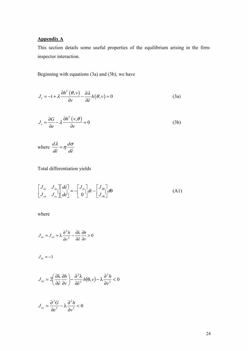
Appendix A

This section details some useful properties of the equilibrium arising in the firm-

inspector interaction.

Beginning with equations (3a) and (3b), we have

( ) ( )ˆ,

t , 0ˆ

T

e

h vJ h v

v eθ λλ θ

∂ ∂= − + − =∂ ∂

(3a)

( ),0

T

e

h vGJe v

θλ

∂∂= − =∂ ∂

(3b)

where ˆ ˆ

d dde deλ ση=

Total differentiation yields

θ

−

−=

θ

θ dJJ

dtJ

deed

JJJJ

e

ete

eeee

eeee ˆˆ

ˆ

ˆˆˆ

0ˆ

(A1)

where

0ˆ2

2

ˆˆ >∂∂

∂λ∂−

∂∂λ==

vh

evhJJ eeee

1te −=J

( ) 0,ˆˆ

2 2

2

2

2

ˆˆ <∂∂λ−θ

∂λ∂−

∂∂

∂λ∂=

vhvh

evh

eJ ee

02

2

2

2

<∂∂λ−

∂∂=

vh

eGJ ee

25

eeeeeeeeeeee JJJJJJ ˆˆˆˆˆˆ and,0,0 >><< 19, ensuring a unique and stable

solution. This ensures the determinant of the coefficient matrix, defined as 2

ˆˆˆ eeeeee JJJ −=∆ is positive.

0;0ˆ

22

ˆ <θ∂∂

∂λ−=>θ∂∂

∂λ+θ∂

∂∂λ∂−= θθ v

hJv

hhe

J ee

Property 1

ˆˆ0et ee eeJ J Jde

dt−= = <

∆ ∆

Property 2

ˆ ˆ 0et eeJ Jdedt

= <∆

Property 3

( )ˆˆ0ee eeJ Jdv de de

dt dt dt− +

= − = >∆

Property 4

0ˆ ˆˆ >

∆−

=θ

θθ eeeeee JJJJd

ed

Property 5

0ˆˆˆˆ <∆−

=θ

θθ eeeeee JJJJdde

It is assumed that eeee JJ ˆˆˆ > by a sufficient amount to ensure

θθ > eeeeee JJJJ ˆˆˆˆ .

Property 6

( ) ( )0

ˆ ˆˆˆˆˆ <∆

+−+=

θ−

θ=

θθθ eeeeeeeeee JJJJJJ

ded

dde

ddv

which follows directly from the properties (4) and (5)

19 eeee JJ ˆ> requires v

heeG ∂

∂∂

λ∂>∂∂ ˆ22 which is assumed.

26

Appendix B

Expanding terms in (8a) and (8b), using (11a, b):

( ) ( ) ( ) ( )1 1 1i j j

i ji i i j

dZ A R Ad

α γ α γ ∂Π Φ ∂Π= Ω + − + + − Ω + − ∂Φ Φ ∂Φ

=0 ,i i it θΦ =

(A2)

[ ] ( ) ( ) ( )1 1 1j i i

j ij j j i

dZ A R Ad

α γ α γ ∂Π Φ ∂Π= − Ω + − − + Ω + − ∂Φ Φ ∂Φ

=0 ,j j jt θΦ =

(A3)

Totally differentiating the above system of equations yields

α

−=

ΦΦ

α

α dZZ

dd

ZZZZ

jj

ii

j

i

jjj

jji

iij

iii , , ,,i j i j i jt θΦ =

For the SOCs to hold it is assumed that: i

ijj

jjj

jij

jjj

jii

iii

iji

iij

jji

ii ZZZZZZZZZZ >>>><< and,,;0,0

These conditions also assure that the determinant of the coefficient matrix is positive:

0>−=Ω iij

jji

jjj

iii ZZZZ

Proposition 1a

Ω+−

=α

Φ ααi

ijj

jj

jji

ii ZZZZ

dd ,i i it θΦ =

where,

( ) ( ) ( )1 1 0i j j

i i ji i i j

dZ A R Adα ρ γ ρ γ

∂Π Φ ∂Π= − − + + − − < ∂Φ Φ ∂Φ when R is large.

(A4)

( ) ( ) ( )1 1 0j i i

j j ij j j i

dZ A R Adα ρ γ ρ γ

∂Π Φ ∂Π= − − − − + − − < ∂Φ Φ ∂Φ when R is large.

(A5)

and,

27

( ) ( ) ( ) ( )2 2

2 21 1 1 1 0j i j j j

i j i jji ij j i i j j j

d d WZ Z Ad dW

ρα γ α γ α ∂Π ∂Π Φ ∂ Π ∂= = − + − + − Ω + − > ∂Φ ∂Φ Φ ∂Φ ∂Φ

(A6)

thus,

0<αd

dt i

and 0<αθ

dd i

Proposition 1b

From properties 2 and 5, in Appendix A 0and0 <θ< dde

dtde . As

0and0 <αθ<α d

dd

dt , then 0de dt de d ded d dt d d

θα α α θ

= + > .

Proposition 1c

a. When political competition increases, the effect on under-reporting is

ambiguous: 0<>

αddv

where dv dv dt dv dd dt d d d

θα α θ α

= + (A6)

From Proposition 1a, 0 0i jd d

d dα αΦ Φ< <

Ambiguity in the sign results from Properties 3 and 6 in Appendix A which reveal:

0>dtdv 0<

θddv

b. dB dB dt dB d dB dvd dt d d d dv d

θα α θ α α

= + + (A7)

using Proposition (1a), 0, 0, 0dB dt dB d dB dvanddt d d d dv d

θα θ α α

>< >

<

Thus, the sign of (A7) is ambiguous.

28

Proposition 1d

dv dv dt dv dd dt d d d

θα α θ α

= +

0dvdα

< if the first term dominates since ( )ˆ 0ee eeJ Jdvdt

− += >

∆

and 0dtdα

< , while ( ) ( )

0ˆˆˆˆˆ <∆

+−+=

θθθ eeeeeeeeee JJJJJJ

ddv and 0d

dθα

<

Expanding these equations, it is evident that dvdα

< 0 requires that θ

>ddv

dtdv which

occurs when θθ ee JJ ˆand are very small in size. This occurs when η is small in

magnitude.20 Performing relevant substitutions for eeJ ˆ and eeJ , we get,

2

200dv GLim

dt eη→

∂= − >∂

and also 0

0dvLimdη θ→

=

An identical argument establishes that 0dBdα

< as η→0 or C(θ) is sufficiently large.

Proposition 2 and Corollary 1

Let political competition be at the maximum (α=0), 0, 0i jS S> > :

Setting α=0, equation (11a) can be written as,

( )1i i j j

i ji i i j

S dA Ad

ρ γ ρ γ ∂ ∂Π Φ ∂Π= + + − + ∂Φ ∂Φ Φ ∂Φ (A8)

where i jA = Π − Π . Further note that from (11a) for an interior solution we require

that 0i

idSd

<Φ

. The sign of the RHS of (A8) will depend on the sign of A. We

therefore begin by considering equilibrium contributions in 3 cases: A = 0, A > 0 and

A<0 and show that when iγ is large, then A=0 and hence that , 0i jS S > .

Note that when A=0, then all terms on the RHS of (A8) are negative so that 0i

idSd

<Φ

,

implying that an interior solution exists and contributions are always paid. Suppose

next that A>0, and let iγ be sufficiently large, such that 0i

idSd

>Φ

. In this case by the

29

FOC in (A8) Si = 0. However, when Si=0, then from equation (7a) (with α=0):

0i

ii

dG Rd

γ= =Φ

which implies that party i sets policies at the welfare maximising level

denoted : Φi=Φw . Furthermore A>0, implies that i jΠ − Π > 0 which can only occur

if Φj>Φi=Φw. But since no party has an incentive to set policies which are more

stringent than the welfare maximising policies, it follows that Φj ≤ Φw. This implies

that A ≤ 0, which contradicts the assumption that A > 0. Hence A > 0 is not feasible

when γi is sufficiently high. QED.

By an identical argument it also follows that A < 0 is not feasible when γj is

sufficiently high. Hence A = 0, which implies that Φj = Φi for sufficiently high γi

(and γj).

When political competition is at a maximum (α=0), and γi (γj) is sufficiently

high, it has been shown that A=0. This implies that the policies of the parties must

converge under such circumstances (i.e. A = 0). Moreover when A=0, then the

conditions for an interior equilibrium of (A8) are satisfied hence , 0i jS S > .

20 Note for Proposition 1a to hold, η≠0.