Corruption, Trade and Resource Conversion

Edward B Barbier1,2

Richard Damania3

Daniel Léonard4

October, 2004

Paper presented at the Workshop on "Trade, Biodiversity and Resources", University of Tilburg, the Netherlands, September 5-6, 2002. Acknowledgements: We are grateful for the comments and suggestions of Chris Costello, Joe Herriges, Anthony Heyes, Patrik Hultberg, Carol McAusland, Wallace Oates, Linwood Pendleton, Cees Withagen and two anonymous reviewers, and for the research assistance of Lee Bailiff.

1 Department of Economics and Finance, University of Wyoming, PO Box 3985, Laramie, WY 82071-3985, tel: 1 307 766 2178; fax: 1 307 766 5090; email: ebarbier@uwyo.edu 2 External Associate, Centre for Environment and Development Economics, University of York, Heslington, York, YO1 5DD, tel: 44 1904 432 999; fax: 44 1904 432 998 3 School of Economics, University of Adelaide, Adelaide, Australia. email: richard.damania@adelaide.edu.au 4 School of Business Economics, Flinders University, Adelaide, Australia. email: daniel.leonard@flinders.edu.au

2

Abstract

Recent evidence suggests that special interest groups significantly affect tropical

deforestation through lobbying. We develop an open-economy model in which resource

conversion is determined by a self-interested government that is susceptible to the influences of

the political contributions it receives from the profit-maximizing economic agent responsible for

land conversion. We investigate the effects of lobbying on the cumulative level of resource

conversion and examine how trade policy influences the distortions created by political

corruption. We derive testable predictions that are analyzed through a panel analysis of

cumulative agricultural land expansion over 1960-99 for low and middle-income tropical

countries. Our findings suggest that increased corruption and resource dependency directly

promote land conversion, whereas rising terms of trade reduce conversion.

JEL classification: Q23, Q28, D78, F19

Keywords: corruption, developing countries, lobbying, open economy, political economy,

resource conversion, resource-trade dependency, terms of trade.

3

1. Introduction

Concerns over the loss of tropical forests and global biodiversity have intensified in

recent years. Over the past decade, forest cover in the tropics has decreased by 12.3 million

hectares (ha) annually, a deforestation rate of 0.7% per annum (FAO, 2001a). The continual loss

of tropical forests has important implications for biodiversity. It has been estimated that more

than four-fifths of many groups of plants and animals are found in tropical forests

(CIFOR/Government of Indonesia/UNESCO, 1999). Moderate estimates of future species

extinction rates due to tropical deforestation range from one to five percent per decade

(Matthews et al., 2000).

Across the tropics, the principal activity responsible for deforestation appears to be the

direct conversion of forests to permanent agriculture (FAO, 2001a). Stratified random sampling

of 10% of the world's tropical forests reveals that direct conversion by large-scale agriculture

may be the main source of deforestation, accounting for around 32% of total forest cover change,

followed by conversion to small-scale agriculture, which accounts for 26%. Intensification of

agriculture in shifting cultivation areas comprises only 10% of tropical deforestation, and

expansion of shifting cultivation into undisturbed forests only 5%. However, there are important

regional differences. In Africa, the major process of deforestation (around 60%) is due to the

conversion of forest for the establishment of small-scale permanent agriculture, whereas direct

conversion of forest cover to large-scale agriculture, including raising livestock, predominates in

Latin America and Asia (48% and 30%, respectively). Although agricultural conversion is the

principal cause of tropical deforestation, in many forested regions uncontrolled timber harvesting

is responsible for initially opening up previously inaccessible forested frontiers to permanent

4

agricultural conversion and for causing widespread timber-related forest degradation and loss

(Ascher, 1999; Barbier et al., 1994; Matthews et al., 2000).

There is also growing recognition that tropical deforestation due to forestry activities and

agricultural conversion, especially for large-scale economic activity, is influenced by

government policy. In Central America and Amazonia, government support for cattle ranching,

forestry and large-scale agriculture has played a prominent role in deforestation (Ferraz and

Serôa da Motta, 1998; Kaimowitz, 1995; Mahar and Schneider, 1994; Young, 1998), while in

Asia, South America and Africa policy-induced expansion of large scale plantations, timber

harvesting and cash crops have been responsible for the destruction of large tracts of forested land

(Ascher, 1999; Broad, 1998; Hafner, 1998). Common to all these cases is the role of governments

in providing both tacit and overt support for the incursion of agricultural and logging activities into

forests.

Numerous studies suggest that the lobbying activities of special interest groups in many

developing countries have played a significant role in influencing key government policies that

determine land use decisions in these countries (Ascher, 1999; Desai, 1998; Broad, 1998; FAO,

2001b; Hafner, 1998). As argued by Ascher (1999, pp. 52-3), the result of such lobbying is that

governments in turn will deliberately create rent-seeking opportunities for those special interests

that benefit from favorable land use policies: As a consequence, government corruption – the use

of public office for private gain - is now seen to be an endemic problem dictating forest land use

policies in developing countries:

Despite the prevalence of this link between rent-seeking, corruption and government land

use policy, the existing literature in economics has failed to examine the consequences of special

interest lobbying pressures on agricultural land conversion. We develop a model in which the

5

amount of land converted to agricultural uses is determined by a self-interested government. The

government is assumed to care about the political contributions it receives from private

economic agents as well as social welfare. The relative weight given to welfare considerations

thus provides a measure of the degree of government honesty. The other player in the game is

the land conversion agent. The players have different objectives and interact noncooperatively.

We investigate the effects of bribes and corruption on rates of cumulative land conversion and

examine whether trade policy reforms enhance or correct these distortions. The main predictions

of our model appear to be supported by our empirical results. Our findings suggest that

increased corruption, terms of trade and resource dependency increase agricultural conversion

directly.

The contribution of this paper extends the varied and growing literature that examines the

effects of rent-seeking activities on environmental policy outcomes in general. For instance,

using the common agency framework Eliste and Fredriksson (2000) investigate the effects of

special interest lobbying on subsidies in the agricultural sector. They find that more

environmentally damaging sectors receive greater compensation for the costs associated with

environmental protection. Leidy and Hoeckman (1994) explore the interaction between

environmental policy efficiency and trade barriers, and demonstrate that polluters may prefer

inefficient policies since they increase the implicit level of protection. Rauscher (1994)

examines lobbying incentives in a polluting industry and finds that trade openness may have

ambiguous effects on lobbying intensity. López and Mitra (2000) investigate the impact of

corruption on the empirical relationship between income and pollution - the Environmental

Kuznets Curve (EKC). It is shown that corruption increases the income level at which the EKC

begins to decline.1

6

This paper differs from previous work in several significant ways. Most notably, and in

contrast to existing work, we deal explicitly with resource dynamics. Thus our model applies to

resource-based environmental problems such as tropical deforestation and habitat loss, which

have hitherto been ignored in the environmental political economy literature. In addition, we

extend the literature by investigating the interaction between corruption and trade openness on

policy outcomes. Finally, from our theoretical model we derive testable predictions concerning

lobbying, trade and resource conversion in developing countries. The empirical section of the

paper tests these predictions, employing a panel analysis of agricultural land expansion over

1960-99 for low and middle-income economies.

These issues are arguably of economic significance for at least two reasons. Firstly, as

noted above, political factors appear to be responsible for a major change in the use of global

resources, especially tropical forests and biodiversity. Thus, an understanding of the effects of

bribes and corruption on land conversion and deforestation rates is of considerable economic

relevance. Secondly, tropical forests may confer significant cross-border external benefits,

through their role as stores of carbon, genetic material, habitat for endangered species, etc. This

has prompted calls for the use of various trade-based policies to coerce these nations to reduce

the level of resource exploitation. It is clearly important to determine whether trade policies

strengthen or weaken the distorting influence of lobby groups on domestic land use decisions.

This paper represents a first but significant step in analyzing these issues in a political economy

context.

The remainder of the paper is organized as follows. The next two sections outline the

basic model of resource conversion and the lobbying decisions of the private economic agent

and the government’s responses, while section 4 examines the effects of trade openness and

7

corruption on the resource conversion decisions of the government and presents four basic

predictions concerning the influence of trade and lobbying on resource conversion. In the

following section we test these predictions through an empirical analysis of agricultural land

expansion in developing countries. The final section concludes the paper and discusses the

wider implications of the analysis.

2. Lobbying and Resource Conversion Decisions of the Private Economic Agent

The focus of our model is a small open economy that contains a homogenous stock of a

finite, available natural resource, F(t) ≥ 0. In the following analysis, we treat the stock as a land

resource, such as forests, wetlands or other natural habitat, which is subject to irreversible

conversion by an economic activity, such as agriculture or timber felling. Alternatively, F could

also be a non-renewable stock, such as mineral ores or energy reserves, which is depleted

through mining, and so the model that follows could equally be applied to a conventional

exhaustible resource problem.2 However, in what follows, we will focus on resource conversion

as the principal economic activity and thus consider F(t) to be a stock of natural habitat or land

subject to agricultural conversion, or depletion through timber harvesting.

To illustrate the potential influences of lobbying on the resource conversion (or

depletion) decision, we build in two distinct features. First, government is responsible for the

management of the resource and determines the rate of conversion by issuing quotas. The quotas

define the maximum allowable conversion rate in any period. Second, the profit-maximizing

economic agent responsible for converting the resource seeks to influence the government’s

decisions through political contributions.

8

Denoting h(t) as the amount of resource conversion and hk as the government quota,

changes in the resource stock over time F(t) are therefore determined by

0 t0

( ) (0) ( ) or ( ), (0) , lim ( ) 0t

F t F h d F h t F F F t→∞

− = − τ τ = − = ≥∫ (1)

and

0)(,)( ≥≤ thhth k . (2)

In what follows, it is assumed that the constraint in (2) always binds so that actual resource

conversion depends on the government’s allocation decision. Attention is therefore focused on

the political decisions of the government.

Irreversible resource conversion occurs as the result of some economic activity, such as

agriculture or timber felling. Output of this activity, Q, is therefore assumed to be a function of

the current flow of resource conversion, h(t), as well as cumulated conversion over time,

∫ −=ττt

tFFdh0

0 )()( . The reason for this specification is twofold. First, current resource

conversion may influence output, as it is assumed that there is an immediate gain in production

from current conversion. For example, if the converting activity is agriculture, then the clearing

and burning that usually accompany land conversion will release nutrients that will boost current

agricultural productivity. Cumulative resource conversion also affects output of the conversion

activity, because it is generally assumed that production is dependent on the converted resource.

Again returning to the example of agriculture, cumulative conversion of wetlands, forests and

other natural habitat means more arable land for agricultural production. A second implication

of the above specification is that helps to avoid corner solutions.

To focus the analysis further on the effects of lobbying on resource conversion, it will be

convenient to express the production function of the conversion activity as3

9

( ) 0,0),()(0 <′′>′−= qqthtFFqQ . (3)

The way the economic agent engaged in resource conversion can influence the setting of

the quota is through expenditures, S(h), on political contributions or bribes. Specifically,

following Grossman and Helpman (1994), we assume that in each period the resource-converting

agent offers the incumbent government a political contribution schedule (S(h)), which consists of

a continuous function that maps resource conversion rates the government chooses, into a bribe.4

Given knowledge of the bribe schedule, the government then proceeds to set its optimal policies.

The discounted profits, Π, received by the resource converting agent from resource conversion is

given by

( )[ ] 0,))((),;,(0

0 >−−=Π ∫∞

−h

QtQ SdthShtFFqpephF δδ (4)

Note that in (4) the time argument has been dropped for most variable to simplify notation, δ is

the discount rate and pQ is the price of the output produced from the resource conversion activity.

We also assume that the amount of political contributions or bribes required by the government

increases with the level of resource conversion, Sh > 0. In essence, Sh is the marginal cost to the

private rent-seeking agent of “lobbying” the government for more resource conversion.

3. Political Decision Making by the Government

We assume that the economy is small and open and trades some of its output from the

resource converting activity in order to finance its imports. Let x(t) be the exports of output from

the resource conversion activity, and m(t) is consumption of a composite imported good. It

follows that domestic consumption of the remaining output from the resource converting activity

can be defined as c(t) = Q(t) – x(t). As the terms of trade, p, of the small open economy are

10

exogenously determined on international markets, and all the output of the resource converting

activity is sold at world prices, we can define the balance of trade condition of the economy as

m

Q

m

x

pp

pppmpx === , . (5)

The political decision-making of the government in setting the optimal amount of

resource conversion in the economy will be influenced by the lobbying efforts of the economic

agent engaged in resource conversion. However, the government may also have wider social

welfare concerns, such as maintaining domestic consumption and protecting the ecological and

other values of the remaining stock of the natural habitat, F. Finally, the government is also

responsible for managing the open economy, which involves ensuring that sufficient exports are

generated from the resource converting activity to allow an optimal flow of imported

consumption goods.

We follow Lόpez and Mitra (2000) and assume that the government's utility function, G,

is a discounted weighted sum of political contributions and citizens’ welfare. To determine the

optimal amount of resource conversion, exports and imports each period, the government

chooses to

[ ] ),,(,)()1(Max0

,,FmcWWdtWhSeG t

mxh=α+α−= ∫

∞δ− , (6)

subject to (1) and (5).

The government’s objective function (6) is therefore a weighted sum of social welfare

and political contributions (or bribes). 5 W is the aggregate social welfare function, which is

assumed to depend on domestic consumption, c(t), imports, m(t) and the remaining natural

resource stock, F(t). The inclusion of the resource stock in W indicates the presence of positive

stock externalities associated with F, which may consist of watershed protection, salinity

11

prevention, soil conservation, wildlife habitat, tourism, carbon store, biodiversity preservation,

and other possible ecological values. The function W is assumed to be additively separable and

concave with respect to its arguments, i.e. .,,,0,0 22

FmciiW

iW =<

∂∂>∂

∂

Finally, the parameter 10 ≤α≤ is the weight given to aggregate social welfare, W,

relative to political contributions or bribes, S, in the government's objective function. As lower

values of α indicate the government's willingness to set policies that diverge from the welfare-

maximizing level of resource conversion in return for political contributions. The parameter (1 -

α) can be interpreted as an indicator of the level of corruption. The latter interpretation is similar

to Schulze and Ursprung (2001), who note that in such models political contributions or bribes

are given in order to influence government policy, not the election outcome. The level of

corruption in the model is reflected by the government’s willingness to allow lobby groups to

influence policies, e.g., the propensity to sell policies for personal gains in the form of monetary

transfers. This view of corruption is also consistent with Bardhan (1997, p. 1321), who defines

corruption as “the use of public office for private gain”. Our formulation also closely follows the

government’s objective function in Grossman and Helpman (1995). However, in contrast to all

the existing work on the political economy of environmental policy, our model explicitly

incorporates the dynamic characteristics of the problem.

In the game that forms the basis of this model the government selects the resource

conversion rate, h, while the private agent chooses the contribution schedule, S(h), that is offered

to the government (and taken as given). Thus, an equilibrium for this game is a contribution

schedule and a conversion rate for each period, such that: (i) the contribution is feasible;6 (ii) the

conversion policy h maximizes the government’s welfare, G, taking the contribution as given

(Grossman and Helpman (1994)). We do not discuss the well known necessary conditions for

12

equilibrium since these have been extensively discussed in the political economy literature

(Grossman and Helpman 1994, Bernheim and Whinston 1986). The necessary conditions for an

equilibrium conditions are defined by:

(MI) h maximizes [ ] ),,(,)()1(0

FmcWWdtWhSeG t =+−= ∫∞

− ααδ ; subject to

.F h= − , h ≥ 0 and px = m.

(MII) h maximizes J = G + Π; subject to .

F h= − , h ≥ 0 and px = m

where [ ]∫ −−=Π∞

−

00 )())(( dthShtFFqpe Qtδ

Condition (MI) asserts that the equilibrium conversion rate h must maximize the government’s

payoff, given the contribution offered. Condition (MII) requires that h must also maximize the

joint payoffs of the private agent and the government. If this condition is not satisfied, agents

have an incentive to alter their strategy to capture more of the surplus.7

The current-value Hamiltonian for the government’s payoff problem (MI) is

[ ]( ) hFpxxhFFqWhSH µ−−−α+α−= ,,)()()1( 0 (7)

which is maximized with respect to choice of h and x. Note that µ is the shadow value of the

resource, defined in terms of its marginal contribution to the government's objective function.

The corresponding first order conditions for an interior solution to (7) are (1) and8

(1 ) 0 or (1 )h c c hH S W q W q Sh

α α µ µ α α∂= − + − = = + −

∂ (8)

[ ] mccm pWWWpWxH

==−α=∂∂ or0 . (9)

[ ]or F cH W W hqF

µ δµ µ δµ α∂ ′− = − = − −∂

(10)

0)()(lim =−

∞→tFte t

tµδ . (11)

13

Condition (8) indicates that the marginal cost of additional resource conversion, µ, must equal

the marginal benefits. The latter consist of the weighted sum in the government's utility

calculation of welfare gain in the economy from the additional consumption resulting from

conversion, αWcq, plus the additional political contributions that the government receives from

the economic agent lobbying for more resource conversion, (1-α)Sh. Equation (9) is the open

economy equilibrium condition, which states that the marginal welfare contribution of domestic

consumption from resource conversion relative to the marginal welfare contribution of imported

consumption, must equal the terms of trade, p. Equation (10) states that, from the government's

perspective, any change in the shadow value of the resource stock must equal the marginal cost

of conserving that stock, δµ, less the net marginal social benefits from conserving the resource.

The latter include the stock externality benefits of resource conservation, WF, minus the marginal

welfare contribution of the additional consumption from cumulative resource conversion, Wchq'.

Finally, condition (11) is the transversality condition corresponding to the government's infinite

horizon utility-maximizing problem.

Taking the time derivative of (8) and substituting it into (10) yields an expression for the

change over time in the optimal amount of resource conversion set by the government

[ ] [ ] [ ] [ ]qhWWqWSxqWFqWqhWhqWS cFchccccccchh ′−α−α+α−δ=α−′+α−α+α− )1()1( 2

[ ] [ ]( ) .0)1(,)1(1 2 <+−=+′+−+−= qWSxqWhqQWWqpWSh cchhccccFmh ααηααααδη

(12)

Note that η < 0 follows from the necessary second order condition for maximizing (7) with

respect to h.

Similarly, the Hamiltonian for the problem MII is:

[ ]( ) ( ) hhShFFqpFpxxhFFqWhSH x λ−−−+−−α+α−= )(,,)()()1( 00 (13)

where λ is the costate variable.

14

The necessary conditions are equation (11) and:

(1 ) 0xh c h

H S W q p q Sh

α α λ∂= − + + − − =

∂ (14)

[ ] mccm pWWWpWxH

==−α=∂∂ or0 . (15)

[ ]or 'xF c

H W W hq p q hF

λ δλ λ δλ α∂ ′− = − = − − +∂

(16)

Denoting the joint-payoff maximizing rate of resource conversion as he, we can again

obtain an expression for eh

( ) 21 , 0.e x eh m F cc cc hh cch S pW q p q W W Qq h W qx S W qδ α α α α η α α

η′⎡ ⎤ ⎡ ⎤= − + + − + + = − + <⎣ ⎦ ⎣ ⎦

(17)

Since in the political equilibrium the optimal rate of resource conversion, hhe = . Hence

combining equations (8) and (14), yields: xhS p qµ λ= + − . Differentiating with respect to time

and simplifying using (10) and (16): ( )xhh hhS S p qδ= − , one solution which satisfies this

condition is: xhS p q= and 0hhS = . Moreover when hhe = this implies that

. .eh h= must satisfy

both equations (12) and (17), , which holds if xhS p q= and 0hhS = . By concavity of the

objective function this is the unique solution to the problem. Furthermore, observe that from

equation (4): xh p qΠ = and 0hhΠ = . Hence, Sh = Πh. That is, in equilibrium the change in

contributions from the resource-converting agent (Sh) truthfully reflect the profits obtained by the

agent from greater access to the resource ( hΠ ). These conditions are the dynamic counterparts of

the local truthfulness condition of the common agency lobbying model. Using these conditions

in equation (12), resource conversion rates are given by:

15

[ ] [ ]( ).)1(12 xqWhqQWWqpWS

qWh ccccFmh

cc

ααααδα

+′+−+−= (17’)

Equation (17’) defines the political equilibrium level of resource conversion for ehh = .

It suggests that in equilibrium the government determines the level of resource conversion by

comparing the politically relevant marginal benefits and marginal costs. The benefits from

resource conversion include two components: the discounted welfare gains from increased

imports, [ ]( )qpWmαδ , and discounted bribes paid to the government, [ ]( ).)1( hSαδ − The benefits

of conversion are equated to the net benefits from conservation. The latter are defined by the

stock externality benefits of the resource, less the marginal utility from consumption of the

resource: [ ]( )hqQWW ccF ′+α , plus an additional term representing the marginal welfare effects of

resource-based exports, xqWccα . In what follows this latter term is denoted as the “resource

trade dependence” effect. Observe that the marginal benefits from bribes are given a weight of

(1 - α), while the marginal welfare effects are given a weight of α. This suggests that in highly

corrupt regimes (with a low α), bribes have a greater influence on the amount of resource

conversion.

4. Model Predictions for the Political Equilibrium

Having defined the political equilibrium we now investigate the effects of corruption and

variations in the terms of trade and the degree of resource-dependence of the economy on

resource conversion levels. We also examine how corruption affects the influence of changes in

the terms of trade and lobbying pressure on conversion. However, to derive more precise

predictions about the interaction between resource conversion levels and the key parameters of

economic significance it is necessary to specify the structure of the model in greater detail.9

16

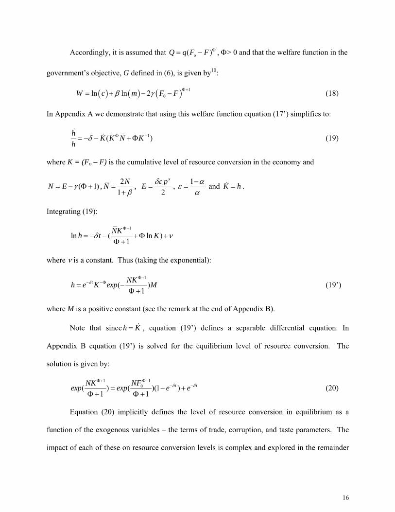
Accordingly, it is assumed that ( )oQ q F F Φ= − , Φ> 0 and that the welfare function in the

government’s objective, G defined in (6), is given by10:

( ) ( ) ( ) 10ln ln 2W c m F Fβ γ Φ+= + − − (18)

In Appendix A we demonstrate that using this welfare function equation (17’) simplifies to:

1( )h K K N Kh

δ Φ −= − − +Φ (19)

where K = (Fo – F) is the cumulative level of resource conversion in the economy and

( 1)N E γ= − Φ + , 21

NNβ

=+

, 2

xpE δε= , 1 αε

α−

= and K h= .

Integrating (19):

1

ln ( ln )1

NKh t Kδ νΦ+

= − − +Φ +Φ +

where ν is a constant. Thus (taking the exponential):

1

( )1

t NKh e K exp MδΦ+

− −Φ= −Φ +

(19’)

where M is a positive constant (see the remark at the end of Appendix B).

Note that since h K= , equation (19’) defines a separable differential equation. In

Appendix B equation (19’) is solved for the equilibrium level of resource conversion. The

solution is given by:

110( ) ( )(1 )

1 1t tNFNKexp exp e eδ δ

Φ+Φ+− −= − +

Φ + Φ + (20)

Equation (20) implicitly defines the level of resource conversion in equilibrium as a

function of the exogenous variables – the terms of trade, corruption, and taste parameters. The

impact of each of these on resource conversion levels is complex and explored in the remainder

17

of the paper. We use these predictions to form the basis of our empirical work in the next

section. Since the aim of this paper is to examine resource conversion incentives in corrupt

regimes and the empirical analysis in the following section focuses on countries afflicted with

high levels of corruption, hence we consider the case where the government is sufficiently

corrupt such that in equation (20) N > 0. However, we also discuss the consequences of

eschewing this assumption. All proofs are in Appendix C.

Prediction 1: In a political equilibrium, if the government is sufficiently corrupt, then an

improvement in the terms of trade leads to an increase in the equilibrium cumulative level of

resource conversion, i.e. 0>xdpdK .

An improvement in the terms of trade could have two reinforcing effects that lead to

higher levels of cumulative resource conversion. Firstly, a rise in the terms of trade allows for a

higher level of domestic consumption, for any given level of resource conversion. Hence the

marginal welfare gains from resource conversion rise and the government responds by increasing

the level of conversion. In addition, by the local truthfulness property of the equilibrium, an

improvement in the terms of trade implies that the government receives higher bribes and this

too encourages further conversion. An equivalent interpretation is that with an improvement in

the terms of trade the private agent has more at stake and therefore increases the bribe offer.

Prediction 2: In a political equilibrium, greater corruption leads to an increase in the

cumulative level of resource conversion, i.e. 0dK dε > .

Intuitively, an increase in corruption implies that the government places a greater weight

on bribes, relative to social welfare. If the government releases more of the resource for

18

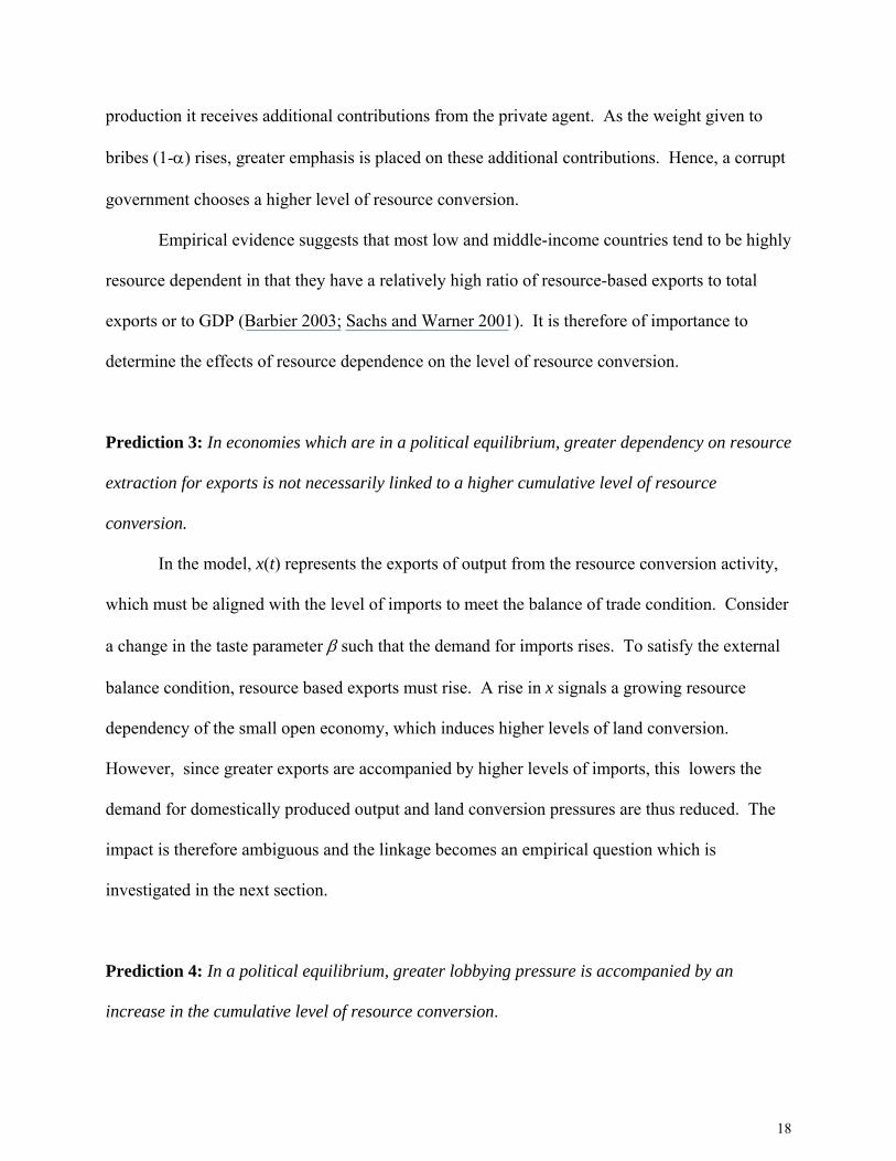
production it receives additional contributions from the private agent. As the weight given to

bribes (1-α) rises, greater emphasis is placed on these additional contributions. Hence, a corrupt

government chooses a higher level of resource conversion.

Empirical evidence suggests that most low and middle-income countries tend to be highly

resource dependent in that they have a relatively high ratio of resource-based exports to total

exports or to GDP (Barbier 2003; Sachs and Warner 2001). It is therefore of importance to

determine the effects of resource dependence on the level of resource conversion.

Prediction 3: In economies which are in a political equilibrium, greater dependency on resource

extraction for exports is not necessarily linked to a higher cumulative level of resource

conversion.

In the model, x(t) represents the exports of output from the resource conversion activity,

which must be aligned with the level of imports to meet the balance of trade condition. Consider

a change in the taste parameter β such that the demand for imports rises. To satisfy the external

balance condition, resource based exports must rise. A rise in x signals a growing resource

dependency of the small open economy, which induces higher levels of land conversion.

However, since greater exports are accompanied by higher levels of imports, this lowers the

demand for domestically produced output and land conversion pressures are thus reduced. The

impact is therefore ambiguous and the linkage becomes an empirical question which is

investigated in the next section.

Prediction 4: In a political equilibrium, greater lobbying pressure is accompanied by an

increase in the cumulative level of resource conversion.

19

Recall from our theoretical model that Sh is the marginal cost to the private rent-seeking

agent of lobbying for more resource conversion. Thus, Sh also represents the degree of

“lobbying pressure” exerted by the agent on the government. Consider an exogenous increase in

lobbying pressure, perhaps caused by a decline in lobbying costs. A more corrupt government is

likely to be susceptible to any increase in lobbying pressure and thus allows more resource

conversion by economic agents to take place.

The next section develops a panel analysis of cumulative agricultural land expansion over

1961-99 for tropical low and middle-income economies to explore further the four predictions

concerning corruption, trade and resource conversion that we have derived from our model.

5. Empirical Analysis of Agricultural Land Expansion in Tropical Developing Countries

The predictions derived above stated in terms of changes in the cumulative level of

resource conversion in the economy, K = (Fo – F). Assuming that conversion of forest habitat to

agricultural land is the main resource conversion activity, then the appropriate dependent

variable in an econometric analysis of the four theoretical predictions is the cumulative level of

agricultural land expansion, ( )0K A A= + .11 This implies the following empirical model:

0 1 2 30

4 5

6

1 ( ) ( ) ( )

( * ) ( * )( )

it

i

A b b terms of trade b control of corruption b resource trade dependenceA

b control of corruption terms of trade b termsof trade resource trade dependenceb other variables

+ = + + +

+ ++

with the dependent variable being a (scaled) measure of the cumulative expansion of agricultural

land area, Ait, over a given time period, t, for each country i, relative to land area in some initial

period, Ai0.12

Prediction 1 implies that b1 > 0, i.e. an improvement in the terms of trade (TOT) will lead

to greater cumulative agricultural expansion. Prediction 2 suggests b2 < 0, i.e. greater control of

20

corruption will result in less agricultural land expansion. Prediction 3 queries the sign of b3, i.e.

in a more resource trade-dependent economy the impact on cumulative land conversion is

ambiguous. As noted in the previous section, to derive these predictions about the direct effects

of terms of trade, corruption and resource trade dependence on resource conversion required

specifying the structure of the theoretical model in greater detail. It is possible that a more

general model may produce interaction effects between these three explanatory variables. To

explore this possibility, we have included two additional interaction terms in the empirical

model. However, we cannot specify a priori what the signs of the coefficients on these

interaction terms, b4 and b5, might be, since these interactions do not appear in the theoretical

model. They are added as possible statistical controls in the regressions, and as will discussed

further below, they also have important intuitive explanations.

A number of additional variables that explain cumulative agricultural land expansion are

also included in the model as exogenous controls in the regression model. Following Barbier

(2001), the controls chosen were growth in agricultural value added, cereal yield, rural

population growth, real gross domestic product (GDP) per capita and the percentage share of

arable plus permanent cropland in total land area.

Finally, it is difficult to construct a reliable test of Prediction 4 of our theoretical model.

Although there are no direct indicators of lobbying pressure by the agricultural sector in

developing countries, this variable could be proxied by two of the exogenous controls in our

empirical model, the growth in agricultural value added and the share of cropland in total land

area. Recall that in the political equilibrium of the theoretical model that lobbying pressure must

equal the gross payoffs to the private agent engaged in resource conversion, i.e. qpS xh = . It is

21

likely that the returns to conversion are in turn positively related to the growth in agricultural

value added in the economy or to simply the scale of total agricultural activity in the economy.13

The above model was applied to a panel analysis of agricultural land expansion over

1961-99 for tropical low and middle income countries in Africa, Asia and Latin America, with

the dependent variable being the (scaled) measure of the cumulative expansion of agricultural

land area every year in each country relative to land area in the initial year 1961.14 The terms of

trade for a country is represented by an index of export to import prices (1995 =100), and

resource-trade dependence is indicated by the share of agricultural and raw material exports as a

percentage of total exports. The source of data used for these variables, plus the control

variables of growth in agricultural value added, cereal yield, rural population growth, GDP per

capita and the percentage share of cropland in total land area, was the World Bank’s World

Development Indicators, which has the most extensive data set for key land, agricultural and

economic variables for developing countries over the period of analysis.

The final variable required in the model is an indicator of control of corruption. The

source used for these data is a recent project on governance conducted by the World Bank, which

puts together a measure of the control of corruption and other governance indicators indexed on

a scale of –2.5 (lowest value) to 2.5 (highest value) for 178 developing and advanced economies

(Kaufmann, Kraay and Zoido-Lobaton (1999a,b)). As the control of corruption indicator covers

the broadest range of developing countries to date of any comparable indicator, it is ideal for our

analysis. However, as this indicator is a single point estimate in time (based on survey data

corresponding for 1997-8 according to the authors), including this time-invariant institutional

index essentially amounts to incorporating a "weighted" country-specific dummy variable in the

panel regression (Baltagi 1995, pp. 11-12).15

22

Table 1 provides a summary of the descriptive statistics of the variables, and Table 2

reports the regression results. Recall that the predictions of the theoretical model derived in the

previous section apply to countries that were considered “highly corrupt”. In our cross-country

data set, these appear to be countries that have a control of corruption indicator less that 0.1.16

We therefore applied our empirical model to both the full sample of all tropical developing

countries and to those countries that are designated as “highly corrupt”. As a further check for

robustness, we also examined the regression results for a key sub-sample, those countries with

total land area greater than 15,000 km2.17 For this sub-sample we again examined the results for

all countries in the sample as well as just the highly corrupt countries.

Both one-way and two-way fixed and random effects models were applied, and the usual

panel tests for comparing these models against each other and ordinary least squares were

conducted. Table 2 displays the results for the preferred models and the relevant statistics. The

chi-squared and F-tests for the pooled models as well as the LM test are significant, suggesting

the presence of individual effects and thus rejection of the ordinary least squares model.

Although the Hausman test was significant for each regression, the random effects model is

preferred over fixed effects because the latter cannot estimate reliably the effects of the time-

invariant control of corruption variable (Baltagi 1995, pp. 11-12).18 The two-way random effects

specification was chosen over the one-way model based on the significance of individual

coefficients and the overall explanatory power of each specification.

The results in Table 2 suggest that the model is strongly robust with respect to the

influence of the direct effects of control of corruption, the terms of trade (TOT) and agricultural

export share on agricultural land expansion. The two interacted terms involving these three

23

variables are also consistently significant in all samples. Three of the exogenous controls are

also highly significant: cereal yield, cropland share and GDP per capita.

The regressions results confirm Prediction 2 of our theoretical model. For all countries –

and not just “highly corrupt” countries – increased corruption (more control of corruption) has a

direct and positive (negative) effect on cumulative agricultural land expansion. This result

provides empirical support of the main result derived from our theoretical model. A more

corruptible government places a greater weight on bribes relative to social welfare, and as a

consequence, will allow private agents paying these bribes to engage in more land conversion.

However, the regressions contradict Prediction 1. In contrast to the prediction, a rise in the terms

of trade of a country has a direct and negative impact on agricultural land expansion. While

Prediction 3 is ambiguous, the empirical results indicate that increased resource-trade

dependency leads to greater agricultural land expansion in a tropical developing economy.

Finally, with regard to Prediction 4, if we accept cropland share as a proxy for lobbying pressure,

then there is strong support for this prediction from the regression results as cumulative land

conversion increases with the share of cropland to total land area. However, if we consider

growth in agricultural value added as the appropriate proxy for lobbying pressure, then there is

little support for Prediction 4 as this variable is not significant in all regressions.

Our regression results also indicate that an improvement in the TOT not only has a direct

impact on increasing agricultural land expansion but also interacts with the influence of

corruption and agricultural export share on agricultural land expansion. The sign of the

interaction term between the TOT and control of corruption is negative, suggesting that the

impact of a rise in the TOT on reducing cumulative land conversion is dissipated if the country is

more corrupt and amplified if there is less corruption. The interaction term between the TOT

24

and agricultural export share is also negative, indicating that the impact of a TOT increase on

lowering cumulative land conversion is enhanced if the country is more dependent on resource-

based exports and reduced if the country is less resource-dependent in its exports.19

Further insights from the regression results can be gained by Table 3, which indicates the

effects of the significant variables influencing tropical land conversion, including any interacting

effects. The latter effects are particularly important in determining the various components

comprising the total effects of control of corruption, terms of trade and resource trade-

dependency on agricultural land expansion. Note that the effects reported in Table 3 are in terms

of elasticities, or percentage changes, which are evaluated at the sample regression means for the

relevant variables.

A 1% rise in the terms of trade has a direct impact on decreasing cumulative agricultural

land expansion ranging from 0.06% to 0.09%. This elasticity effect will be reinforced by any

increase in agricultural export share and greater control of corruption. The result is that the total

elasticity effect of 1% rise in the TOT is a reduction in agricultural land conversion of between

0.11% and 0.19%, depending on the type of country.

The direct effect of greater control of corruption appears to be a reduction in cumulative

agricultural land expansion of between 0.11% to 0.22%. The interaction between the terms of

trade and greater control of corruption reinforces the latter’s direct influence on limiting land

conversion, so that a 1% reduction in corruption may decrease cumulative land conversion by

0.17% to 0.30% in tropical developing countries.

A 1% rise in the agricultural export share of a country may have a direct impact of raising

agricultural land conversion by around 0.02%. However, the moderating effect of the level of

25

the terms of trade on agricultural export share suggests that the total effects of a 1% rise in

resource trade dependency on land conversion may be only 0.01%.

Finally, a 1% increase in GDP per capita and cropland share raises cumulative land

conversion by 0.03% to 0.04% and 0.25% to 0.311% respectively. In contrast, a 1% rise in crop

yields, reduces land expansion by 0.02% to 0.04%.

6. Conclusion

The theoretical and empirical findings of the paper confirm that “bribes” by economic

agents that benefit from resource converting activities will have a substantial effect on the

control of conversion by a government that is corruptible. We specifically find that

improvements in the terms of trade, greater resource trade-dependency and increased “lobbying

pressure” also provide additional incentives for cumulative resource conversion in corrupt

countries. Overall, these results support the many studies suggesting that special interest groups

have a played a significant role in determining land use decisions in developing countries,

particularly the conversion of forests and other natural habitat to agriculture.

Our empirical results confirm Prediction 2 from our theoretical model that corruption

appears to be associated with cumulative land expansion in tropical developing economies. The

direct effect is as expected; increased corruption leads to greater land conversion. In this regard,

our empirical analysis conforms not only with the theoretical prediction of this paper but also

with the propositions of others, notably López and Mitra (1999), who suggest that greater

corruption is associated with increased environmental degradation. Of course the latter authors

were concerned with the influence of corruption on pollution flows, whereas we have confirmed

26

this relationship both theoretically and empirically for a decline in an environmental stock

(cumulative resource conversion) in developing countries.

Although our empirical analysis suggests opposite terms of trade effects on cumulative

tropical land expansion compared to Prediction 1 from the theoretical model of resource

conversion, this is possibly due to the necessary simplification of the model’s structure to obtain

the latter prediction. In a more general version of our model, Prediction 1 may be ambiguous,

and as a result the direct effect of a change in the TOT, i.e. the sign of the coefficient b1 in our

regression, could be positive or negative empirically. Our estimation results suggest that this

effect is negative, i.e. across tropical countries an improvement in the terms of trade reduces

cumulative land conversion.

The direct influence of the agricultural export share also suggests that greater resource

dependency is associated with land conversion. Developing countries that are more structurally

dependent on non-oil primary products for their exports are more susceptible to processes of

agricultural land expansion. However, these resource dependency effects on land conversion

may depend on what happens to a country’s terms of trade. There is some statistical evidence

from the regression analysis that countries with higher TOT may reduce the resource dependency

effects on land expansion. 20 In addition, we find that the level of corruption also asserts an

indirect effect on land conversion in tropical countries via interaction with the terms of trade.

The impact of a rise in the TOT in reducing cumulative land conversion is dissipated if the

country is more corrupt and amplified if there is less corruption. One possible reason is that

increasingly corrupt government officials may siphon off any additional foreign exchange

earnings, thus reducing the incentives of private agents to slow down cumulative conversion in

response to a TOT increase.21

27

Finally, the presence of these significant interaction effects between the terms of trade

and corruption and primary product export dependency suggest caution in assuming that an

important policy mechanism by which the rest of the world can reduce resource conversion in

developing economies is through sanctions, taxation and other trade interventions that reduce the

terms of trade of these economies. First, our empirical analysis suggests that such a decline in

the TOT would have a direct impact of increasing, rather than reducing cumulative agricultural

land expansion in tropical countries. Second, as Table 3 shows, the direct and some interactive

effects of a TOT change can work in opposite directions. In addition, for low and middle-

income economies especially, any reduction in TOT is likely to have additional economic

consequences not captured in our model, such as the loss of foreign exchange earnings that could

be employed to import advanced technology and capital, or to be invested in human capital to

put the developing economy on a path that reduces its dependence on resource-based exports.

Thus the long run consequences of trade interventions may be that these economies will have

little opportunities to diversify away from a resource-dependent pattern of growth and trade.

At the end of the day, there may be very little that other countries can do to influence the

linkages between special interest lobbying, trade and resource conversion within a developing

economy, other than continue to point out the economic losses that the economy is likely to incur

as a result of such linkages. Whether such negative publicity is likely to change domestic

policies within the developing economy is doubtful. As our model has shown, if a government is

corruptible, a resource-converting agent producing a tradable good has considerable incentives to

influence the resource conversion decisions of that government.

28

References

Ascher, W. (1999), Why Governments Waste Natural Resources: Policy Failures in Developing Countries. Johns Hopkins University Press, Baltimore.

Baltagi, B. (1995). Econometric Analysis of Panel Data. Chichester: John Wiley. Barbier, E. B. (2001), The Economics of Tropical Deforestation and Land Use: Introduction to

the Special Issue" Land Economics77, (2): 155-171. Barbier, E.B., 2003, "The Role of Natural Resources in Economic Development." Australian

Economic Papers, 42(2):253-272. Barbier, E.B., Burgess, J.C., Bishop, J.T. and Aylward, B.A. (1994). The Economics of the

Tropical Timber Trade. Earthscan Publications, London. Bardhan, P. (1997), “Corruption and Development: A Review of the Issues,” Journal of

Economic Literature 35(3): 1320-46. Bernheim, B.D. and M.D. Whinston (1986). “Menu Auctions, Resource Allocation, and

Economic Influence.” Quarterly Journal of Economics 101(1):1-31. Broad, R. (1995) "The Political Economy of Natural Resources: Case Studies of Indonesia and

the Phillipines" Journal of Developing Areas, 29: 317- 340. Center for International Forestry Research (CIFOR)/Government of Indonesia/UNESCO (1999)

World Heritage Forests: The World Heritage Convention as a Mechanism for Conserving Tropical Forest Biodiversity. CIFOR, Bogor, Indonesia.

Damania R (2001) "When the Weak Win: The Role of Investment in Environmental Lobbying " Journal of Environmental Economics and Management, (42):1 - 22.

Desai, U (1998) Ecological Policy and Politics in Developing Countries, SUNY Press, New York.

Ehui S and T.W. Hertel (1989) Deforestation and agricultural productivity in the Côte d'Ivoire. Amer. J. Agric. Econ. (71): 703-711.

Eliste P and P. Fredriksson (2000) "Environmental Regulations,Transfers and Trade" Journal of Environmental Economics and Management, (41):33-57.

Ferraz, C. and Serôa da Motta, R. (1998). "Economic Incentives and Forest Concessions in Brazil" Planejamento e Políticas Públicas. 18:259-286.

Food and Agricultural Organization of the United Nations (FAO) (2001a). Global Forest Resources Assessment 2000: Main Report. FAO Forestry Paper 140. FAO, Rome.

Food and Agricultural Organization of the United Nations (FAO) (2001b). State of the World's Forests 2001. FAO, Rome.

Fredriksson, P.G. (1999), “The Political Economy of Trade Liberalization and Environmental Policy,” Southern Economic Journal 65(3): 513-25.

Grossman, G.M. and E. Helpman (1994), “Protection for Sale,” American Economic Review 84(4): 833-50.

Hafner, O (1998) "The Role of Corruption in the Misappropriation of Tropical Forest Resources and in Tropical Forest Destruction" Transparency International Working Paper, October.

Hillman, A.L. and H.W. Ursprung (1994), “Greens, Supergreens, and International Trade Policy: Environmental Concerns and Protectionism,” in The International Dimension of Environmental Policy, edited by C. Carraro, Dordrecht: Kluwer.

Kaimowitz, D. (1995). “Livestock and Deforestation in Central America in the 1980s and 1990s: A Policy Perspective.” EPTD Discussion Paper, No. 9, Environment and Production Technology Division, International Food Policy Research Institute, Washington DC.

29

Kaufmann, D., Kraay, A. and Zoido-Lobaton, P. (1999a). "Aggregating Governance Indicators". World Bank Policy Research Department Working Paper No. 2195. The World Bank, Washington DC.

Kaufmann, D., Kraay, A. and Zoido-Lobaton, P. (1999b). "Governance Matters". World Bank Policy Research Department Working Paper No. 2196. The World Bank, Washington DC.

Leidy, M.P. and B.M. Hoekman (1994), “’Cleaning Up’ while Cleaning Up? Pollution Abatement, Interest Groups and Contingent Trade Policies,” Public Choice 78: 241-58.

López, R. and S. Mitra (2000), “Corruption, Pollution and the Kuznets Environment Curve,” Journal of Environmental Economics and Management 40(2): 137-50.

Mahar, D. and Schneider, R.R. (1994). “Incentives for Tropical Deforestation: Some Examples from Latin America.” In K. Brown and D.W. Pearce (eds.). The Causes of Tropical Deforestation. University College London Press, London.

Matthews, E., Payne, R., Rohweder, M. and Murray, S. (2000), Pilot Analysis of Global Ecosystems: Forest Ecosystems. World Resources Institute, Washington DC.

Rauscher, M. (1994), “On Ecological Dumping,” Oxford Economic Papers 46: 822-40. Sachs, Jeffrey D. and Andrew M. Warner. (2001). "The Curse of Natural Resources." European

Economic Review 45:827-838. Schulze, G. and H. Ursprung (2001), “The Political Economy of International Trade and the

Environment,” in G. Schulze and H. Ursprung, eds., International Environmental Economics: A Survey of the Issues, Oxford University Press, pp. 62-83.

Shleifer, A. and R.W. Vishny (1993), “Corruption,” Quarterly Journal of Economics 108(3): 599-617.

United Nations, Food and Agricultural Organization (FAO). 2001. Forest Resources Assessment 2000: Main Report. FAO Forestry Paper 140. Rome.

Wunder, S. (2003). Oil Wealth and the Fate of the Forest: A Comparative Study of Eight Tropical Countries. Routledge, London.

Young, C.E.F. (1998). "Public Policies and Deforestation in the Brazilian Amazon." Planejamento e Políticas Públicas. 18:201-222.

30

Appendix A: Derivation of Equation (19)

The FOCs for the problem in MI simplify as follows:

( ) 01 =−+−=∂∂ µαα

cqS

hH

h (A1)

0=∂∂

xH ⇒ x = βc;

1qhcβ

=+

, 1

qhx ββ

=+

(A2)

Substituting (A2) in (A1) to eliminate c:

( ) µαβα =+

+−h

Sh)1(1 (A3)

Differentiating (A3) with respect to time:

( ) µαβα =+

−− hh

hShh 2

)1(1 (A4)

Using (10)

( 1) '2 ( 1) qKq

βµ δµ α γ Φ⎡ ⎤+= − Φ + −⎢ ⎥

⎣ ⎦t (A5)

where K = (Fo – F).

Using Shh = 0 and Sh = pxq we get:

1( )h K K N Kh

δ Φ −= − − +Φ (19)

where K = (Fo – F), K h= , 21

NNβ

=+

, (1 )2

xpE δ αα

−= ( 1)N E γ= − Φ + .

Appendix B: Solution to Equation (20)

Substituting h = K in (19’) yields the separable equation:

1

( )1

tNKK exp dK e MdtδΦ+

Φ −=Φ +

(B1)

31

where M is a positive constant

Integrating (B1) with respect to time:

1

( ) ( )1

tNK e Mexp Nδ

υδ

Φ+ −

= −Φ +

(B2)

where υ is a constant. The boundary conditions are:

At t = 0, F = Fo and K = 0 hence in (B2) 1 = ( )MN υδ−

+ ⇒ 1 MN Nυδ

+ =

At t = ∞, F =0 and K = Fo hence in (B2) 1

0( )1

NFexpΦ+

Φ += Nυ

The specific solution is then:

110( ) ( )(1 )

1 1t tNFNKexp exp e eδ δ

Φ+Φ+− −= − +

Φ + Φ + (20)

Remark:

Taking the total derivative of (20) with respect to time we can obtain the exact form of equation (19’):

0

11

exp( )[ (exp( ) 1]1 1

t FKh e N NN

δ δκΦ+Φ+

− −Φ= − −Φ + Φ +

where the square bracket is the constant M which depends on N .

Appendix C

Taking the total derivative of (20) wrt N and t respectively yields:

110( ) (1 )

1 1tFK dKA NK B e

dNδ

Φ+Φ+Φ −+ = −

Φ + Φ + (C1)

where 1

exp( )1

NKAΦ+

=Φ +

; 1

exp( )1

oNFBΦ+

=Φ +

and ( 1)tANK h e BδδΦ −= − (C2)

Rearranging (C1):

32

1 10( 1) (1 ) ( )tdKA NK BF e AK t

dNδΦ Φ+ − Φ+Φ + = − − ≡ Ω (C3)

To evaluate the sign of this expression it is necessary to determine the sign of Ω for all [0, ]t∈ ∞ .

Note that at t = 0, K(0)=0 and hence Ω(0) = 0 and at t = ∞, K=Fo, A = B and Ω(∞) = 0. Next

we must evaluate the sign of Ω(t) over (0, )t∈ ∞ . Differentiating:

1 10

( ) ( ( 1))td t BF e AhK NKdt

δδΦ+ − Φ Φ+Ω= − + Φ + (C4)

Thus

10

(0) 0d BFdt

δΦ+Ω= > (C5)

10 0

( ) ( ( 1))d AhF NFdt

Φ Φ+Ω ∞= − + Φ + < 0 if N > 0 (C6)

Using (C2) to simplify (C4):

110( ) 10

1BFd t K

dt B N

Φ+Φ+Ω Φ +

= ⇒ = +−

(C7)

Since K is monotone then (C7) can only hold once. Evaluating 2

2

( )d tdtΩ when ( ) 0d t

dtΩ

= we

have ( 1) 0te K hδδ − Φ− Φ + < . Hence (C7) defines the maximum point. It follows that Ω(t) > 0

over (0, )t∈ ∞ hence 0 (0, )dK tdN

> ∀ ∈ ∞ if N > 0.

Prediction 1:

Recall that ( 1)2

xpN δε γ= − Φ + and 21

NNβ

=+

. Thus 01x

dNdp

δεβ

= >+

and x

dKdp

= x

dK dNdN dp

> 0

when N > 0. The assumption that N > 0 summarizes the condition that the government is

sufficiently corrupt.

33

Prediction 2:

By a similar procedure: dKdε

= dK dNdN dε

> 0 when N > 0.

Prediction 3:

Since x is endogenously determined in the model, it is not possible to determine directly the

causality relation from x to K. Instead we infer the impact of greater resource dependency

indirectly by examining the correlation between cleared land and exports when β increases.

Note that by the balance of trade condition, a rise in the taste parameter β induces higher imports

and an equivalent rise in exports.

Define the level of cumulative exports as:

0

( ) ( )X t x dτ

τ τ= ∫

where 11K hxβ

Φ

−=+

. Then using h K= :

1

1

1(1 )(1 )

dKXdtβ

Φ+

−=+Φ +

Equilibrium levels of cumulative exports are:

1

1(1 )(1 )KX

β

Φ+

−=+Φ +

Observe that when β increases then 21

NNβ

=+

decreases as does K (Prediction 1), but the

denominator of X also increases, hence the outcome is ambiguous.

Prediction 4:

The proof is similar to that of Prediction 1: Consider an exogenous lobbying efficiency

34

parameter denoted as ρ. The political equilibrium requires that xhS p qρ = . It follows that

( ) ( )1 12 2

xhSp qN

qδερδε β β= − Φ + = − Φ + . Thus sign dK

dρ= sign x

dKdp

> 0.

Table 1. Summary Statistics of Variables

Variables Mean

Standard Deviation

Number of Observations

Cumulative agricultural land expansion (1 + Ait/Ai0)

2.19 0.35 3773

Terms of trade (1995 = 100)

113.07 38.73 2450

Control of corruption (no control = -2.5; no corruption = 2.5)

-0.35 0.60 2880

Agricultural export share (% of merchandise exports)

10.65 15.22 2503

Control of corruption × Terms of trade -44.85 61.96 2078Terms of trade × Agricultural export share 1185.78 1887.49 1776Growth in agricultural value added (% annual change)

2.70 8.71 2672

Cereal yield (kg per hectare)

1530.15 925.37 3532

Rural population growth (% annual change)

1.42 1.43 3822

Gross domestic product per capita ($/person)

2035.30 3619.08 3167

Cropland share (% of total land area)

16.14 15.47 3774

Table 2. Panel Analysis of Corruption and Tropical Agricultural Land Expansion, 1960-99

Dependent Variable: Cumulative agricultural land expansion (1 + Ait/Ai0) Cross-Country Estimationsa Full Sample Large Land Areab

Explanatory Variables

All Countries (N = 1,363) (Y = 2.255)d

Highly Corruptc

(N = 1,204) (Y = 2.262)

All Countries

(N = 1,267) (Y = 2.271)

Highly Corruptc

(N = 1,149) (Y = 2.271)

Terms of trade/103 (1995 = 100)

-1.207 (-4.246)**

-1.759 (-5.153)**

-1.415 (-4.331)**

-1.801 (-4.913)**

Control of corruption/101 (no control = -2.5; no corruption = 2.5)

-9.668 (-7.396)**

-9.339 (-4.348)**

-5.559 (-3.794)**

-8.881 (-4.400)**

Agricultural export share/103 (% of merchandise exports)

3.758 (3.209)**

4.766 (3.720)**

3.767 (3.118)**

4.708 (3.604)**

Control of corruption × Terms of trade/103

-2.191 (-5.862)**

-2.951 (-6.591)**

-2.475 (-5.865)**

-3.018 (-6.364)**

Terms of trade × Agricultural export share/105

-1.698 (-1.959)*

-1.963 (-2.109)*

-1.569 (-1.755)†

-1.866 (-2.109)*

Growth in agricultural value added/104 (% annual change)

5.756 (1.144)

6.315 (0.984)

5.474 (1.010)

6.208 (0.919)

Cereal yield/105 (kg per hectare)

-5.094 (-3.502)**

-2.954 (-1.659)†

-5.238 (-3.186)**

-3.352 (-1.791)†

Rural population growth/103 (% annual change)

6.201 (0.759)

1.782 (0.197)

9.289 (1.091)

3.024 (0.326)

Gross domestic product per capita/105 ($/person)

5.962 (4.165)**

6.218 (3.324)**

8.164 (5.134)**

7.046 (3.643)**

Cropland share/102 (% of total land area)

3.957 (17.853)**

3.443 (14.518)**

3.646 (15.724)**

3.358 (13.634)**

χ-test for pooled model 2252.185** 1974.509** 2046.968** 1833.741** F-test for pooled model 57.165** 52.868** 52.900** 48.769** Breusch-Pagan (LM) test 4693.85** 4171.62** 4398.08** 4061.77** Hausman test 159.51** 147.16** 157.78** 132.78**

Preferred model Two-way random effects

Two-way random effects

Two-way random effects

Two-way random effects

Notes: a t-ratios are indicated in parentheses. b Countries with total land area greater than 15,000 km2. c Countries with a control of corruption indicator of less than 0.1.

d N = number of observations. Y = mean of dependent variable for the regression sample. ** Significant at 1% level, * significant at 5% level, † significant at 10% level.

Table 3. Total Elasticity Effects

Full Sample Large Land Area All Highly All Highly Effects a/ Countries Corrupt Countries Corrupt 1. Terms of trade Terms of trade only -0.061 -0.089 -0.071 -0.091 Agricultural export share effect -0.009 -0.011 -0.009 -0.011 Control of corruption effect -0.045 -0.079 -0.056 -0.084 Total effects -0.114 -0.179 -0.136 -0.186 2. Agricultural export share Agricultural export share only 0.018 0.024 0.019 0.024 Terms of trade effect -0.009 -0.011 -0.009 -0.011 Total effects 0.009 0.012 0.010 0.013 3. Control of corruption Control of corruption only -0.175 -0.217 -0.110 -0.214 Terms of trade effect -0.045 -0.079 -0.056 -0.084 Total effects -0.220 -0.296 -0.166 -0.298 4. Cereal yield -0.036 -0.020 -0.036 -0.022 5. Cropland share 0.311 0.262 0.270 0.252 6. GDP per capita 0.032 0.029 0.041 0.032 Notes:

a/ Only effects significant at 10% level or better are indicated. All effects are indicated as elasticities evaluated at the means of the respective regression samples

Notes

1A growing number of related studies examine the link between special interest group lobbying and environmental policy outcomes. Examples of papers that use the common agency framework include Fredriksson (1999) and Damania (2001), and examples of studies that use the political competition framework include Hillman and Urpsrung (1994) and Schulze and Urpsrung (2000). 2 In fact our model can equally be applied to the case of a minerals resource where the quality of the output declines with the amount extracted. 3 Ehui and Hertel (1989) use a similar specification. 4 Following the common agency lobbying literature we assume that optimal bribe schedule is determined outside of the model. However, this schedule is assumed to be contingent upon the amount of conversion. Observe that if the assumption does not hold so that the private agent does not offer a bribe schedule and instead offers a single bribe amount, then the payment can have no marginal incentive effects on the government’s decisions. 5 Following Lόpez and Mitra (2000), we could assume that the government objective function (6) is

[ ] ),,(,)()1(Max0

,,FmcWdthSeG t

mxhπ=παπ+α−= ∫

∞δ−

where W is the aggregate social welfare function as defined in (6) and π is the probability of the government being re-elected, which is assumed to be linear and increasing in W. This would make our model compatible with voting models that take into account the motive of democratically elected government is to elections. In equation (6), to sharpen the analysis, we drop π but note that our model could easily be extended to include the re-election motive. In addition we also exclude profits from W following Lopez and Mitra. Inclusion of this term complicates but does not alter the analysis. Moreover as shown later in the paper by local truthfulness bribes reflect profits thus profits enter the government’s objective function but with a different weight attached than other terms in the welfare function. 6 In this context this is taken to imply that the contribution must be non-negative. That is the private economic agent cannot "tax" the government. 7 See Grossman and Helpman (1994) for an extensive discussion of this condition. 8 In what follows we show that h > 0 prevails. 9 Note that (17’) defines a nonlinear differential equation which does not have an analytical solution. Hence we adopt specific functional forms that yield closed form solutions to the problem. The empirical analysis presented in the next section provides a test of the suitability of the model given the assumed specifications. 10 It is not possible to derive an explicit solution for h unless ( )oF F− appears in the objective function W in a form related to the production function ( )oQ q F F= − . 11 Ideally, to make the empirical model an exact test of the theoretical predictions would suggest expressing the dependent variable in terms of changes in the cumulative level of resource conversion in the economy, K = (F0 – F), rather in terms of the cumulative level of agricultural expansion, K = (A0 + A). However, as discussed in Barbier (2001), since 1990 the United Nations Food and Agricultural (FAO), which has been the international agency responsible for compiling forest area data across all tropical developing countries has based its periodic global forest resource assessment on population growth projections in order to overcome an inadequate forest data base for some countries and regions. As the econometric literature on tropical deforestation has pointed out (see Barbier (2001)), this means that the FAO tropical forest cover data are inappropriate for cross-country data are inappropriate for cross-country analyses of deforestation, such as the one we are conducting in this paper, that use demographic factors as explanatory variables. However, the assumption that agricultural conversion is the main resource conversion activity responsible for deforestation in tropical countries is supported by independent studies. Stratified random sampling of 10% of the world's tropical forests reveals that direct conversion by large-scale agriculture may be the main source of deforestation, accounting for around 32% of total forest cover change, followed by conversion to small-scale agriculture, which accounts for 26% (FAO 2001). Intensification of agriculture in shifting cultivation areas comprises 10% of tropical deforestation, and expansion of shifting cultivation into undisturbed forests 5%.

12 The effect of the scaling is to eliminate the influence of cross-country differences in land endowment on the dependent variable by effectively turning it into an index of cumulative agricultural land expansion in period t compared to the initial period 0. Moreover, this index is easily translated into a percentage change in cumulative agricultural land expansion, e.g. via (K – 2)*100%. For example, in Table 1 across all countries, the average cumulative expansion in agricultural land compared to the base year 1961 is 19.3%. 13 Alternative proxies for the lobbying pressure indicator were also employed in the regression analysis, such as the percentage share of agricultural value added in the GDP of a country, agricultural value added per hectare and agricultural value added per worker. However, none of these alternative proxy indicators for lobbying pressure performed well in the regressions. In addition, for our sample the number of panel observations of the three alternative proxy indicators was considerably smaller, which may explain why they performed so poorly in the regressions. 14 Annual data on permanent and arable cropland over 1960-1999 for each country is from the World Bank’s World Development Indicators, which was used to calculate the annual percentage change dependent variable. Permanent cropland is land cultivated with crops that occupy the land for long periods and need not be replanted after each harvest, such as cocoa, coffee, and rubber. This category includes land under flowering shrubs, fruit trees, nut trees, and vines, but excludes land under trees grown for wood or timber. Arable land (in hectares) includes land defined by the Food and Agricultural Organization of the World Bank as land under temporary crops (double-cropped areas are counted once), temporary meadows for mowing or for pasture, land under market or kitchen gardens, and land temporarily fallow. Land abandoned as a result of shifting cultivation is excluded. 15 As pointed out by Baltagi (1995, pp. 11-12), including a time-invariant explanatory variable, such as the corruption index we have used, can sometimes lead to collinear regressors in fixed effects estimation. As indicated in note 17, this occurred when we applied our model to certain sub-samples of the data set. Also, as a time-invariant institutional index is in itself a “weighted” country-specific dummy variable, including the corruption index in an OLS regression will essentially imitate a fixed effects model. However, as reported in Table 2, our χ-tests and F-tests for the pooled model are highly significant, and therefore we cannot reject the hypothesis of the presence of individual effects. Given these factors, it is therefore not surprising that the random effects model was the preferred specification to either the OLS or fixed effects models. 16 As indicated above and in Table 1, the control of corruption indicator ranges from -2.5 (no control) to 2.5 (no corruption). Although Table 1 shows that the average level of corruption across the tropical developing countries of our sample is -0.35, the minimum value for a country is -1.57 and the maximum value is 1.95. The median for the entire sample is -0.40. Given this distribution, designating the countries that have a control of corruption indicator less than 0.1 as “highly corrupt” eliminates the top 15% “least corrupt” countries from the sample. 17 Attempts to apply the empirical model to other sub-samples, notably just Latin American and Asian countries and countries with GDP per capita (1995$) of less than $3,000 during any time period of the analysis, led to problems of collinear regressors in the fixed effects versions of the regressions. This particularly occurred when the sub-sample was further reduced to “highly corrupt” countries only. As discussed in note 15, this problem can arise due to the combination of including a time-invariant explanatory variable (the control of corruption indicator) in a regression with a smaller number of observations, as suggested by Baltagi (1995, pp. 11-12). 18 Although we report the Hausman test statistic for each regression in Table 2, we did not use this statistic in deciding whether or not the fixed effects version is the preferred model for several reasons. First, as indicated in notes 15 and 17, Baltagi (1995, pp. 11-12) points out that the fixed effects model “cannot estimate the effect of any time-invariant variable like sex, race, religion, schooling or union participation.” The fixed effects and random effects models and relevant test statistics, including the Hausman test, were estimated using the LIMDEP 8 software package. In all regression results the fixed effects model and the random effects model generated similar estimates and standard errors for the coefficients of all explanatory variables except for the control of corruption indicator. The main difference between the two versions is that the fixed effects model produced extremely large standard errors and widely fluctuating coefficient estimates for the control of corruption indicator, confirming Baltagi’s contention that fixed effects is indeed inappropriate for regressions incorporating this time-invariant variable. Baltagi (1995, p. 70) states that “if either heteroskedasticity or serial correlation is present, the variances of the Within and GLS estimators are not valid and the corresponding Hausman test statistic is inappropriate.” We found high serial correlation for the fixed effects estimations corresponding to each of the four regressions reported in

Table 2. For example, the estimated autocorrelation of the fixed effects estimation for all countries of the full sample was 0.884, for highly corrupt countries of the full sample was 0.875, for all countries with large land area was 0.879 and for highly corrupt countries with large land area was 0.875. Thus, although a Hausman test is the standard procedure for determining whether a fixed effects model should be preferreto a random effects model, it is a less reliable test for the panel analysis conducted in this paper. 19 According to Wunder (2003), this phenomenon is particularly relevant for oil producing tropical countries. For example, when a tropical country experiences an oil-price boom or discovers new oil reserves, there is a real appreciation of the booming country’s currency. This is also equivalent to a price shift in favor of non-traded goods. The result is a “Dutch disease” effect, in that the oil and non-traded sectors of the economy expand at the expense of those facing declining competitiveness. In most tropical developing countries, the latter non-oil trade sectors are typically agriculture, fisheries, forestry and non-oil mining, which are also the sectors most associated with forest conversion. As a consequence, a country with a large non-oil primary product export sector is likely to experience a greater slow down in forest land conversion as a result of the rising terms of trade from an oil price boom. 20 Evidence of this phenomenon is found in a study of eight tropical oil producing countries, which found that these countries faced fewer pressures for conversion or degradation of their forests than non-oil producing countries, and that forest loss was particularly less pronounced during periods of oil booms (Wunder 2003). As the author points out (p. 30), the most important causal factor was “a real appreciation of the booming country’s currency”, and the decline in land conversion is likely to be greater given the importance of the traded non-oil primary product sector of the economy. The eight countries studied by Wunder (2003) were Cameroon, Ecuador, Gabon, Indonesia, Mexico, Nigeria, Papua New Guinea and Venezuela. 21 Wunder (2003) suggests that there may be another explanation of this interaction effect for some oil-producing tropical countries. For example, if the TOT appreciation is due to an oil boom, then one consequence is higher rents in the oil and non-trade good sectors. Corruptible officials will therefore be able to enrich themselves by diverting more resources away from non-oil primary product sectors, including agriculture, that are mainly responsible for deforestation. The result is again a slowing down of cumulative agricultural land expansion and forest conversion.