The Quantum Spheres and their Embedding into Quantum Minkowski Space-Time
22
THE QUANTUM SPHERES AND THEIR EMBEDDING INTO QUANTUM MINKOWSKI SPACE-TIME M. LAGRAA Received 3 November 2001 and in revised form 12 April 2002 We recast the Podleś spheres in the noncommutative physics context by showing that they can be regarded as slices along the time coordinate of the different regions of the quantum Minkowski space-time. The inves- tigation of the transformations of the quantum sphere states under the left coaction of the SO q (3) group leads to a decomposition of the trans- formed Hilbert space states in terms of orthogonal subspaces exhibiting the periodicity of the quantum sphere states. 1. Introduction A great variety of works based on the quantum spheres have been developed since the appearance of Podleś spheres [11] and their sym- metries [12]. Most part of these studies have been done either in the quantum bundle formalism where the quantum spheres provide con- crete examples to test the different structures of this formalism [1, 5, 6] or, more recently, in quantum field theories on quantum spheres which should respect the SU q (2) quantum symmetries (see, e.g., [2, 3, 4, 10] and the references therein). On the other hand, the evolution of a free particle in the quantum Minkowski space-time has been analysed in [8] and the transformations of its quantum velocity under the Lorentz subgroup of boost transfor- mations in [7]. In Section 2 of this paper, we pursue these studies by recasting the quantum spheres in the noncommutative special relativity where we show that we can regard them as quantum manifolds embedded into the quantum Minkowski space-time. This embedding preserves the reality Copyright c 2002 Hindawi Publishing Corporation Journal of Applied Mathematics 2:7 (2002) 315–335 2000 Mathematics Subject Classification: 16W30, 22E43, 20G45, 81R05 URL: http://dx.doi.org/10.1155/S1110757X0211103X
-
Upload
independent -
Category
Documents
-
view
5 -
download
0
Transcript of The Quantum Spheres and their Embedding into Quantum Minkowski Space-Time

THE QUANTUM SPHERES AND THEIREMBEDDING INTO QUANTUMMINKOWSKI SPACE-TIME
M. LAGRAA
Received 3 November 2001 and in revised form 12 April 2002
We recast the Podleś spheres in the noncommutative physics context byshowing that they can be regarded as slices along the time coordinate ofthe different regions of the quantum Minkowski space-time. The inves-tigation of the transformations of the quantum sphere states under theleft coaction of the SOq(3) group leads to a decomposition of the trans-formed Hilbert space states in terms of orthogonal subspaces exhibitingthe periodicity of the quantum sphere states.
1. Introduction
A great variety of works based on the quantum spheres have beendeveloped since the appearance of Podleś spheres [11] and their sym-metries [12]. Most part of these studies have been done either in thequantum bundle formalism where the quantum spheres provide con-crete examples to test the different structures of this formalism [1, 5, 6]or, more recently, in quantum field theories on quantum spheres whichshould respect the SUq(2) quantum symmetries (see, e.g., [2, 3, 4, 10]and the references therein).
On the other hand, the evolution of a free particle in the quantumMinkowski space-time has been analysed in [8] and the transformationsof its quantum velocity under the Lorentz subgroup of boost transfor-mations in [7].
In Section 2 of this paper, we pursue these studies by recasting thequantum spheres in the noncommutative special relativity where weshow that we can regard them as quantum manifolds embedded into thequantum Minkowski space-time. This embedding preserves the reality
Copyright c© 2002 Hindawi Publishing CorporationJournal of Applied Mathematics 2:7 (2002) 315–3352000 Mathematics Subject Classification: 16W30, 22E43, 20G45, 81R05URL: http://dx.doi.org/10.1155/S1110757X0211103X

316 The quantum sphere
structure and the commutations rules of the quantum Minkowski space-time coordinates. In particular, we show that in the time-like region ofthe quantum Minkowski space-time the Hilbert spaceH(L) of states de-scribing the noncommutative relativistic evolution of a free particle hav-ing a quantum velocity of length |v|2q = (1 +Q2c(L)), c(L) = −1/(q(L+1) +q−(L+1))2 with L ≥ 1 is an integer, q is the deformation parameter andQ = q+ q−1 are precisely, for fixed time, the space of irreducible represen-tations of the Podleś quantum spheres S2
qc with c = c(L). We also showin this section that the Hilbert space of representations of the space-likeregion of the quantum Minkowski space-time corresponds, for partic-ular fixed time, to the Hilbert space of representations of the quantumspheres S2
qc, where c ∈ [0,∞] or S2q∞.
In Section 3, we show that the state transformations under the coac-tion of the SOq(3) group exhibits the periodicity of the quantum spherestates through a decomposition of the transformed Hilbert space in termsof orthogonal subspaces, each describes the same quantum sphere.
2. The quantum spheres
Before embedding the different quantum spheres into the quantumMinkowski space-time, we recall briefly some properties of the noncom-mutative special relativity presented in [8]. First, it was shown in [9] thatthe generators ΛN
M (N,M = 0,1,2,3) of quantum Lorentz group may bewritten in terms of those of quantum SL(2,C) group as
ΛNM =
1Qεγ̇δ̇σN
δ̇αMασσM
σρ̇Mβ̇ρ̇εγ̇β̇, (2.1)
where Mαβ (α,β = 1,2) and Mα̇
β̇ = (Mαβ)� are the generators of the quan-
tum SL(2,C) group subject to the unimodularity conditions
εαβMγαMδ
β = εγδ, εγδMγαMδ
β = εαβ,
εα̇β̇Mγ̇α̇Mδ̇
β̇ = εγ̇δ̇, εγ̇ δ̇Mγ̇α̇Mδ̇
β̇ = εα̇β̇, Q = q+ q−1(2.2)
and the spinor metrics are taken to be εαβ = −εβ̇α̇ =( 0 −q−1/2
q1/2 0
), where q ∈
]0,1[ is a real deformation parameter. σNαβ̇
are a set of four independentmatrices composed by the Pauli matrices σn
αβ̇(n = 1,2,3) and the identity
matrix σ0αβ̇
and
σIα̇β± = εα̇λ̇R−σρ̇λ̇νε
νβσIσρ̇ = q1/2ελ̇ρ̇R−σλανενβσI
σρ̇. (2.3)

M. Lagraa 317
The R-matrices are given by
R±δβαγ = δδαδ
βγ + q±1εδβεαγ , Rα̇γ̇
±δ̇β̇ = δδ̇α̇δ
β̇γ̇ + q±1εδ̇β̇εα̇γ̇ (2.4)
satisfying R±δβαγR∓ρσδβ = δραδ
σγ and R±δ̇β̇α̇γ̇R∓ρ̇σ̇ δ̇β̇ = δ
ρ̇α̇δ
σ̇γ̇ . They induce the
commutation rules
MαρMβ
σR±γδρσ = R±ρσαβMργMσ
δ,
Mα̇ρ̇Mβ̇
σ̇R±γ̇ δ̇ ρ̇σ̇ = R±ρ̇σ̇ α̇β̇Mρ̇γ̇Mσ̇
δ̇.(2.5)
The Lorentz group generators are real, (ΛNM)� = ΛN
M, and generatea Hopf algebra L endowed with a coaction ∆, a counit ε, and an an-tipode S acting as ∆(ΛN
M) = ΛNK ⊗ΛK
M, ε(ΛNM) = δM
N , and S(ΛNM) =
GNKΛLKGLM, respectively. GNM is an invertible and hermitian quantum
metric given by
G IJ =(
1Q
)εανσI
αβ̇σJβ̇γ εγν =
(1Q
)εν̇γ̇σ
Iγ̇ασJαβ̇ε
ν̇β̇. (2.6)
The form of the antipode of ΛNM implies the orthogonality conditions
GNMΛLNΛK
M = G LK and G LKΛLNΛK
M = G NM of the generators ofthe quantum Lorentz group.
The quantum metric GNM can be considered as a metric of a quantumMinkowski space-timeM4 equipped with real coordinates XN , (XN)� =XN . X0 represents the time operator and Xi (i = 1,2,3) represent thespace right invariant coordinates, ∆R(XI) = XI ⊗ I, which transform un-der the left coaction as
∆L
(XI
)= ΛI
K ⊗XK. (2.7)
From the hermiticity of the Minkowskian metric and the orthogonalityconditions, we can see that the four-vector length GNMXNXM = −τ2 isreal and invariant. It was also shown in [9] that τ2 is central; it commuteswith the Minkowski space-time coordinates and the quantum Lorentzgroup generators. ΛN
M and XN are subject to the commutation rulescontrolled by the RNM
PQ matrix as
ΛLPΛK
QRNMPQ =RPQ
LKΛPNΛQ
M, (2.8)
XNXM =RPQNMXPXQ, (2.9)

318 The quantum sphere
where the R-matrix of the Lorentz group is constructed out of those ofSL(2,C) group and satisfies the relationsRNM
KL GKL=GNM andRNMKL GNM
= GKL which show the quantum symmetrization of the Minkowskianmetric GNM and its inverse.
To make an explicit calculation of the different commutation rules ofthe generators of the quantum Lorentz group, we take the followingchoice of Pauli hermitian matrices
σ0αβ̇
=(
1 00 1
), σ1
αβ̇=(
0 11 0
),
σ2αβ̇
=(
0 −ii 0
), σ3
αβ̇=(q 00 −q−1
).
(2.10)
This choice leads us to a quantum metric form GLK exhibiting two inde-pendent blocks, one for the time index and the others for space compo-nents indices (k = 1,2,3) whose nonvanishing elements are G00 = −q−3/2,G11 = G22 = G33 = q1/2, G12 = −G21 = −iq1/2((q − q−1)/Q). The nonvanish-ing elements of its inverse are G00 = −q3/2, G11 =G22 = q−1/2(Q2/4), G33 =q−1/2, and G12 = −G21 = iq−1/2((q − q−1)Q/4). In the classical limit q = 1,this metric reduces to the classical Minkowski metric with signature(−,+,+,+). Explicitly, the length of the four-vector XN reads
GNMXNXM = −τ2 = −q−3/2X20 + q1/2
(qXzXz + q−1XzXz
Q+X2
3
), (2.11)
where Xz =X1 + iX2 and Xz =X1 − iX2. An explicit computation of (2.9)gives
[X0,XN
]= 0,
X3Xz − q2XzX3 =(q− q−1)X0Xz,
X3Xz − q−2XzX3 = −q−2(q − q−1)X0Xz,
(2.12)
XzXz −XzXz =(q− q−1)Q(X2
3 + q−1X0X3). (2.13)
The Pauli matrices satisfy σ0α̇β = −σ0
αβ̇= −δβ
α, σNα̇α = σN1̇1 +σN2̇2 = −Qδ0N
and σNαα̇ = QδN0 which make explicit the restriction of the quantum
Lorentz group to the quantum subgroup of the three-dimensional spacerotations by restricting the quantum SL(2,C) group generators to thoseof the SU(2) group. In fact when we impose the unitarity conditions,Mα̇
β̇ = S(Mβα), in (2.1) we get
ΛN0 = δ0
N, ΛM0 = δM
0 , (2.14)

M. Lagraa 319
which lead us to the restriction of the Minkowski space-time transfor-mations under the quantum Lorentz group to the orthogonal transfor-mations group SOq(3). This subgroup leaves invariant the three-dimen-sional quantum subspace R3 ⊂ M4 equipped with the real coordinatesystem Xi (i = 1,2,3) and the Euclidean metric Gij . More precisely as aconsequence of (2.14), (2.7) reduces to
∆L
(X0)= Λ0
0 ⊗X0 = I ⊗X0, ∆L
(Xi
)= Λi
j ⊗Xj, (2.15)
where ∆(L) is the restriction of (2.7) to the three-dimensional quantumsubspace R3 of M4. Λi
j = (1/Q)σiγ̇αMα
σσjσρ̇S(Mρ
β)εγ̇β̇ generate anSOq(3) Hopf subalgebra L whose axiomatic structure is derived fromthose of L as ∆(Λi
j) = Λik ⊗Λk
j , ε(Λij) = δi
j and S(Λij) = GiKΛL
KG Lj =GikΛl
kG lj , where G ij is the restriction of G IJ satisfying G ikGkj = δij =
GjkGki, GijRkl
ij = Gkl and GklRklij = Gij which are the quantum symmet-
rization of the Euclidean metric Gij and its inverse. The form of the an-tipode S(Λi
j) implies the orthogonality properties of the generators ofthe quantum subgroup SOq(3) as G ijΛi
lΛjk = G lk and GlkΛi
lΛik = Gij .
The commutation rules of the coordinate Xi of R3 satisfy the same com-mutation rules (2.13), where X0 is taken to be a constant parameter re-calling that it commutes with the spacial coordinates Xi.
Therefore, Λij = (1/Q)σiγ̇
αMασσj
σρ̇S(Mρβ)εγ̇β̇ establishes a corre-
spondence between SUq(2), Mαβ =(α −qγ�γ α�
)with the commutation rela-
tion
αα� + q2γγ� = 1, α�α+ γγ� = 1, γγ� = γ�γ,
αγ� = qγ�α, αγ = qγα(2.16)
and SOq(3) group. In the three-dimensional space R3 spanned by the ba-sis Xz, Xz, and X3, where the SOq(3) coacts, the generators Λi
j =(1/Q)σiγ̇
αMασσj
σρ̇S(Mρβ)εγ̇β̇ read
(Λi
j) =−2qγγ 2α�α� Qγα�
2αα −2qγ�γ� Qαγ�
−2αγ −2γ�α� 1− qQγγ�
∈M3 ⊗C
(SUq(2)
), (2.17)
where the indices i, j run over z = 1+ i2, z = 1− i2 and 3.In the case τ2 > 0, time-like region, it was shown in [8] that the evolu-
tion of a free particle in the Minkowski space-time is described by statesbelonging to the Hilbert spaceH(L) whose basis is spanned by common

320 The quantum sphere
eigenstate of X0 and X3
X0|t,L,n〉 = t|t,L,n〉, x3|t,L,n〉 = x(L,n)3 |t,L,n〉, (2.18)
where τ2 = q−3/2(t2/γ2(L)), x(L,n)3 = q−1t(q−(L−2n)/γ (L) − 1), γ (L) = (q(L+1) +
q−(L+1))/Q, L = 0,1,2, . . . ,∞, and n runs by integer steps over the range0 ≤ n ≤ L. Xz and Xz act on the basis elements ofH(L) as
Xz|t,L,n〉 = λq−1t
γ (L)q−(L−n)
(1− q2(n+1))1/2(1− q2(L−n))1/2|t,L,n+ 1〉, (2.19)
Xz|t,L,n〉 = λq−1t
γ (L)q−(L−n+1)(1− q2n)1/2(1− q2(L−n+1))1/2|t,L,n− 1〉, (2.20)
respectively, where λλ = 1. In what follows, we will take λ = −1. Thelength of velocity of the particle is given by |�v|2q = q2((qVzVz + q−1VzVz)/Q+V 2
3 ) = 1− 1/γ2(L) ≤ 1.The light-cone, τ2 = 0, corresponds to L =∞ leading to |�v|2q = 1 which
is the velocity of the light. In this region, the evolution of the particle isdescribed by states |t,n〉 (n = 0,1, . . . ,∞) satisfying
X0|t,n〉 = t|t,n〉,X3|t,n〉 = q−1t
(q2n+1Q− 1
)|t,n〉,Xz|t,n〉 = −qntQ
(1− q2(n+1))1/2|t,n+ 1〉,
(2.21)
Xz|t,n〉 = −q(n−1)tQ(1− q2n)1/2|t,n− 1〉. (2.22)
In what follows, we will take the length of the quantum three-vector as| �X|2q = (qXzXz + q−1XzXz)/Q +X2
3. The quantum group SOq(3) acts onthe spatial coordinates Xi as (2.15) and lives invariant both X0 and τ2,then q−2X2
0 − q−1/2τ2 =R2 =q−1/2GijXiXj =((qXzXz + q−1XzXz)/Q +X23)=
| �X|2q. For fixed t2, we have
R2(L)|L,n〉 = q−2t2(
1− 1γ2(L)
)|L,n〉, (2.23)
and the relations (2.18) and (2.20) for finite L ≥ 1 and
R2|n〉 = q−2t2|n〉 (2.24)

M. Lagraa 321
and the relations (2.22) for L =∞, where the orthonormal states |L,n〉and |n〉, 〈L,n′|L,n〉 = δn′,n, n′,n = 0,1, . . . ,L, and 〈n′|n〉 = δn′,n, n′,n =0,1, . . . ,∞, denote the states satisfying (2.18), (2.20), and (2.22), respec-tively. The unique state |t,0,0〉 corresponding to L = 0 describes a parti-cle at rest at the origin of the spacial coordinate system, for t = 0, thenτ2 = 0 represents the origin of the four coordinate system of the quan-tum Minkowski space-time, XN |0,0,0〉 = 0|0,0,0〉. Therefore, the (L+ 1)-dimensional Hilbert subspace H(L) of states describing the evolutionof a free particle of a given length of the velocity in the noncommu-tative Minkowski space-time can be identified, for fixed time, with theHilbert spaceH(L)
S2q
of irreducible representations of the quantum spheresof radius R(L) = q−1t(1 − 1/γ2(L))1/2. This observation leads us to statethe following theorem.
Theorem 2.1. The Podleś spheres S2qλρ
are slices along the time coordinate ofthe different regions of the quantum Minkowski space-timeM4
S2qλρ =
{XN ∈M4 |X0 = t0, τ
2 = τ20
}. (2.25)
The quantum spheres S2qc where c = c(n) = −1/(qn + q−n)2, n = 2,3, . . . ,∞, cor-
respond to slices at t0 = −q and τ20 = q1/2/γ2(L), where n = L+ 1, L ≥ 1.
The quantum spheres S2qc where c ∈ [0,∞] correspond to slices at t0 = −q
and τ20 = −q1/2Q2c and S2
q∞ corresponds to a slice at t0 = 0 and τ20 = −q1/2Q2.
Proof. Due to the fact that X0 and τ2 commute with the spacial coordi-nates Xz, Xz and X3, X0 and τ2 can be taken to be constants withoutcontradicting the commutation rules (2.13). If we set Xz =Qe1, X3 = e0,Xz = Qe−1, λ = (q − q−1)X0 = (q − q−1)t and ρ = q−2t2 − q−1/2τ2 into (2.11)and (2.13), we see that we recover the algebra generators of the quan-tum sphere A(S2
q) given by [11, (2a)-(2b)].For t0 = −q and τ2
0 = q1/2/γ2(L) ≥ 0, L ≥ 1, we have λ = 1 − q2 and ρ =R2 = 1 − 1/γ2(L) =Q2c + 1 giving c = c(L) = −1/Q2γ2(L) = c(n) = −1/(qn +q−n)2 where n = L + 1. These constraints correspond to slices of the pasttime-like region for finite L or a slice of the past light-cone region forL =∞. They fit with the quantum spheres S2
qc with c = c(n) ≤ 0 whichare described by states satisfying (2.18), (2.20), and (2.23) for finite L ≥ 1and (2.22) and (2.24) for L =∞.
We follow the same procedure presented in [8] to investigate theHilbert space Hs of space of representations of the space-like region ofthe Minkowski space-time. The elements |t,n〉, n = 0,1, . . . ,∞, of the basis
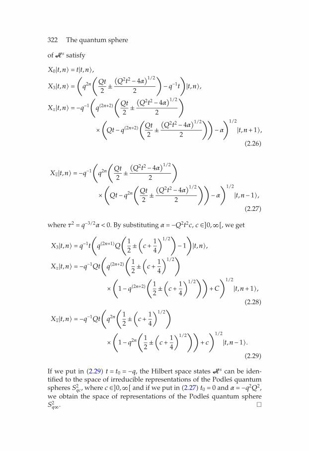
322 The quantum sphere
ofHs satisfy
X0|t,n〉 = t|t,n〉,
X3|t,n〉 =(q2n
(Qt
2±(Q2t2 − 4α
)1/2
2
)− q−1t
)|t,n〉,
Xz|t,n〉 = −q−1
(q(2n+2)
(Qt
2±(Q2t2 − 4α
)1/2
2
)
×(Qt− q(2n+2)
(Qt
2±(Q2t2 − 4α
)1/2
2
))−α)1/2
|t,n+ 1〉,(2.26)
Xz|t,n〉 = −q−1
(q2n
(Qt
2±(Q2t2 − 4α
)1/2
2
)
×(Qt− q2n
(Qt
2±(Q2t2 − 4α
)1/2
2
))−α)1/2
|t,n− 1〉,(2.27)
where τ2 = q−3/2α < 0. By substituting α = −Q2t2c, c ∈]0,∞[, we get
X3|t,n〉 = q−1t
(q(2n+1)Q
(12±(c +
14
)1/2)− 1
)|t,n〉,
Xz|t,n〉 = −q−1Qt
(q(2n+2)
(12±(c+
14
)1/2)
×(
1− q(2n+2)
(12±(c+
14
)1/2))
+C
)1/2
|t,n+ 1〉,(2.28)
Xz|t,n〉 = −q−1Qt
(q2n
(12±(c +
14
)1/2)
×(
1− q2n
(12±(c +
14
)1/2))
+ c
)1/2
|t,n− 1〉.(2.29)
If we put in (2.29) t = t0 = −q, the Hilbert space states Hs can be iden-tified to the space of irreducible representations of the Podleś quantumspheres S2
qc, where c ∈]0,∞[ and if we put in (2.27) t0 = 0 and α = −q2Q2,we obtain the space of representations of the Podleś quantum sphereS2q∞. �

M. Lagraa 323
We may also consider, as for the time-like region, that the HilbertspaceHs spanned by |t,n〉 satisfying (2.29) as space of states describingthe evolution in the space-like region of the quantum Minkowski space-time of a free particle moving with an operator velocity of componentsVz =Xx/t, Vz =Xz/t, and V3 =X3/t. In this case, we obtain from (2.29) alength of the velocity |�v|2q = −(Gij/G00)ViVj = 1+Q2c > 1 greater than thevelocity of the light |�v|2q = 1 [8].
Note that from (2.29), (2.18), (2.20), and (2.22), we have
limc→0Hs −→H(∞)←− lim
L→∞H(L). (2.30)
To investigate the transformations of the quantum sphere states underthe SOq(3) quantum group, we have to construct the Hilbert space statesHSOq(3), where the generators Λi
j act. Since the X′0 = ∆(L)(X0) = I ⊗X0
and X′i = ∆(L)(Xi) = Λij ⊗ Xj fulfil the same commutation rules (2.13)
the transformed states of the quantum sphere satisfy the same relations(2.18) and (2.20) in the time-like region, (2.22) in the light-cone and(2.27) in the space-like region. Since the coordinates Xi transform un-der the tensorial product of SOq(3) and S2
q, the transformed states alsobelong to the tensorial product HSOq(3) ⊗HS2
q[8] which needs the con-
struction of the Hilbert spaceHSOq(3).To construct HSOq(3), we are not obliged to compute explicitly the
complicated commutation rules (2.8) where we impose (2.14) but wesimply consider the action of the SUq(2) generators on the orthonormalHilbert space states; γ |n〉 = qn|n〉, γ�|n〉 = qn|n〉, α|n〉 = (1 − q2n)1/2|n − 1〉and α�|n〉 = (1− q2(n+1))1/2|n+ 1〉 (n = 0,1,2, . . . ,∞) which, combined with(2.17), give the action of the generators of SOq(3) on the basis |n〉 of theHilbert spaceHSOq(3) as
Λ33|n〉 = (1− q(2n+1)Q
)|n〉,Λz
z|n〉 = −2q(2n+1)|n〉,Λz
z|n〉 = −2q(2n+1)|n〉,Λ3
z|n〉 = −2qn(1− q2n)1/2|n− 1〉,
Λ3z|n〉 = −2q(n+1)(1− q2(n+1))1/2|n+ 1〉,
Λz3|n〉 =Qq(n+1)(1− q2(n+1))1/2|n+ 1〉,
Λz3|n〉 =Qqn
(1− q2n)1/2|n− 1〉,
Λzz|n〉 = 2
(1− q2(n+1))1/2(1− q2(n+2))1/2|n+ 2〉,
Λzz|n〉 = 2
(1− q2n)1/2(1− q2(n−1))1/2|n− 2〉.
(2.31)

324 The quantum sphere
Now, we are ready to investigate the transformations of the quantumsphere states under the SOq(3) group.
3. The transformations of the quantum sphere states
To investigate the transformed quantum sphere states under the SOq(3)quantum group, we follow the study of the quantum boost transforma-tions in noncommutative special relativity presented in [7]. We recallthat in the boost transformation the four coordinates transform by yield-ing a change of the time operator X0, the length of the three spacial-vector (qXzXz + q−1XzXz)/Q+X2
3 and the component X3 which leads toa change of the quantum number L and n in the transformed states. Un-der the SOq(3) transformations, the spacial coordinates transform but thelength | �X|q of the three-vector and the time operator X0 remain invari-ant. Then under the SOq(3) group the quantum number L remains fixedbut n changes and, therefore, the transformed states |L,p〉, p = 0,1, . . . ,Lmay be given either in the Hilbert subspace states H(L)
S2q
or in the tenso-
rial productHSOq(3) ⊗H(L)S2q
. More precisely, if we consider the orthonor-
mal basis |m,L,n〉 = |m〉 ⊗ |L,n〉 of the Hilbert space HSOq(3) ⊗H(L)S2q
or
|m,n〉 = |m〉 ⊗ |n〉 of the Hilbert spaceHSOq(3) ⊗H(∞)S2q
, we have
⟨m′,L,n′ |m,L,n
⟩= δm′,mδn′,n,
m=∞∑m=0
n=L∑n=0
|m,L,n〉〈m,L,n| = 1(3.1)
for finite L and ⟨m′,n′ |m,n
⟩= δm′,mδn′,n,
m=∞∑m=0
n=∞∑n=0
|m,n〉〈m,n| = 1(3.2)
for L =∞ from which we deduce that under the coaction of SOq(3) quan-tum group, the transformed sphere states may be written as
|L,p〉 =m=∞∑m=0
n=L∑n=0
|m,L,n〉⟨m,L,n | L,p⟩, p = 0,1, . . . ,L (3.3)
for finite L and
|p〉 =m=∞∑m=0
n=∞∑n=0
|m,n〉⟨m,n | p⟩, p = 0,1, . . . ,∞ (3.4)
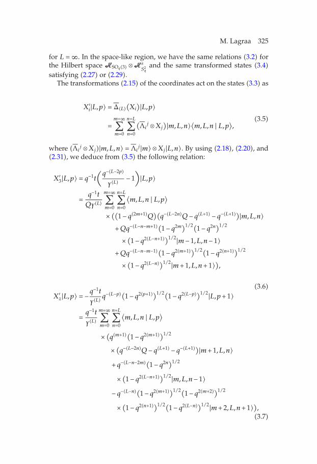
M. Lagraa 325
for L =∞. In the space-like region, we have the same relations (3.2) forthe Hilbert space HSOq(3) ⊗Hs
S2q
and the same transformed states (3.4)satisfying (2.27) or (2.29).
The transformations (2.15) of the coordinates act on the states (3.3) as
X′i|L,p〉 = ∆(L)(Xi
)|L,p〉=
m=∞∑m=0
n=L∑n=0
(Λi
j ⊗Xj
)|m,L,n〉⟨m,L,n | L,p⟩, (3.5)
where (Λij ⊗Xj)|m,L,n〉 = Λi
j |m〉 ⊗Xj |L,n〉. By using (2.18), (2.20), and(2.31), we deduce from (3.5) the following relation:
X′3|L,p〉 = q−1t
(q−(L−2p)
γ (L)− 1)|L,p〉
=q−1t
Qγ (L)
m=∞∑m=0
n=L∑n=0
⟨m,L,n | L,p⟩
× ((1− q(2m+1)Q)(q−(L−2n)Q− q(L+1) − q−(L+1))|m,L,n〉
+Qq−(L−n−m+1)(1− q2m)1/2(1− q2n)1/2
× (1− q2(L−n+1))1/2|m− 1,L,n− 1〉+Qq−(L−n−m−1)(1− q2(m+1))1/2(1− q2(n+1))1/2
× (1− q2(L−n))1/2|m+ 1,L,n+ 1〉),(3.6)
X′z|L,p〉 = −q−1t
γ (L)q−(L−p)
(1− q2(p+1))1/2(1− q2(L−p))1/2|L,p+ 1〉
=q−1t
γ (L)
m=∞∑m=0
n=L∑n=0
⟨m,L,n | L,p⟩
× (q(m+1)(1− q2(m+1))1/2
× (q−(L−2n)Q− q(L+1) − q−(L+1))|m+ 1,L,n〉+ q−(L−n−2m)(1− q2n)1/2
× (1− q2(L−n+1))1/2|m,L,n− 1〉− q−(L−n)(1− q2(m+1))1/2(1− q2(m+2))1/2
× (1− q2(n+1))1/2(1− q2(L−n))1/2|m+ 2,L,n+ 1〉),(3.7)

326 The quantum sphere
X′z|L,p〉 = −q−1t
γ (L)q−(L−p+1)(1− q2p)1/2(1− q2(L−p+1))1/2|L,p− 1〉
=q−1t
γ (L)
m=∞∑m=0
n=L∑n=0
⟨m,L,n | L,p⟩
× (qm(1− q2m)1/2(q−(L−2n)Q− q(L+1) − q−(L+1))|m− 1,L,n〉
+ q−(L−n−2m−1)(1− q2(n+1))1/2(1− q2(L−n))1/2|m,L,n+ 1〉
− q−(L−n+1)(1− q2(m−1))1/2(1− q2m)1/2(1− q2n)1/2
× (1− q2(L−n+1))1/2|m− 2,L,n− 1〉).(3.8)
By applying 〈m,L,n| from the left, we get, because of linear indepen-dence, the following conditions on 〈m,L,n | L,p〉:
(q2p − q2n − q2m(1− q2n)+ q(2m+2n+2)(1− q2(L−n)))⟨m,L,n | L,p⟩
= q(m+n+1)(1− q2(m+1))1/2(1− q2(n+1))1/2
× (1− q2(L−n))1/2⟨m+ 1,L,n+ 1 | L,p⟩
+ q(m+n−1)(1− q2m)1/2(1− q2n)1/2
× (1− q2(L−n+1))1/2⟨m− 1,L,n− 1 | L,p⟩
(3.9)
from (3.6),
− q−(L−p)(1− q2(p+1))1/2(1− q2(L−p))1/2⟨m,L,n | L,p+ 1
⟩= qm
(1− q2m)1/2(
q−(L−2n)Q− q(L+1) − q−(L+1))⟨m− 1,L,n | L,p⟩+ q−(L−n−2m−1)(1− q2(n+1))1/2(1− q2(L−n))1/2⟨
m,L,n+ 1 | L,p⟩− q−(L−n+1)(1− q2(m−1))1/2(1− q2m)1/2(1− q2n)(1− q2(L−n+1))1/2
× ⟨m− 2,L,n− 1 | L,p⟩(3.10)

M. Lagraa 327
from (3.7), and
− q−(L−p+1)(1− q2p)1/2(1− q2(L−p+1))1/2⟨m,L,n | L,p− 1
⟩= q(m+1)(1− q2(m+1))1/2(
q−(L−2n)Q− q(L+1) − q−(L+1))⟨m+ 1,L,n | L,p⟩+ q−(L−n−2m)(1− q2n)1/2(1− q2(L−n+1))1/2⟨
m,L,n− 1 | L,p⟩− q−(L−n)(1− q2(m+1))1/2(1− q2(m+2))1/2(1− q2(n+1))(1− q2(L−n))1/2
× ⟨m+ 2,L,n+ 1 | L,p⟩(3.11)
from (3.8). The relations (3.9), (3.10), and (3.11) are the recursion for-mulas which permit to compute the coefficients 〈m,L,n | L,p〉 giving thetransformed states |L,p〉 in terms of basis elements of the Hilbert spacestatesHSOq(3) ⊗H(L)
S2q
.
To investigate the different coefficients 〈m,L,n | L,p〉, we start by in-serting 〈0,L,n | L,0〉, and then 〈m,L,0 | L,0〉 into (3.9), the result can beiterated K times to get
⟨K,L,n+K | L,0⟩ = qK(n+K)
k=K∏k=1
( (1− q2(L+1−n−k))1/2
(1− q2k
)1/2(1− q2(n+k))1/2
)
× ⟨0,L,n | L,0⟩, 0 ≤ n+K ≤ L,
⟨m+K,L,K | L,0⟩ = qK(m+K)
k=K∏k=1
( (1− q2(L+1−k))1/2
(1− q2k
)1/2(1− q2(m+k))1/2
)
× ⟨m,L,0 | L,0⟩, 0 ≤K ≤ L.
(3.12)
By combining the relations (3.10) and (3.11) with (3.9), we can deduceby a recursive way the coefficients 〈m+K,L,K | L,p+ 1〉, 〈K,L,n+K | L,p + 1〉, 〈m+K,L,K | L,p − 1〉, and 〈K,L,n+K | L,p − 1〉 in terms of thoseof the development of |L,p〉 as
⟨m,L,n | L,p+ 1
⟩= −q(n−p+1)
(1− q2(n+1))1/2(1− q2(L−n))1/2
(1− q2(p+1)
)1/2(1− q2(L−p))1/2
⟨m,L,n+ 1 | L,p⟩
− q−(m+p−1)
(1− q2m)1/2(
q2p − qn)(1− q2(p+1)
)1/2(1− q2(L−p))1/2
⟨m− 1,L,n | L,p⟩,

328 The quantum sphere⟨m,L,n | L,p− 1
⟩= −q(n−p+1)
(1− q2n)1/2(1− q2(L−n))1/2
(1− q2p
)1/2(1− q2(L+1−p))1/2
⟨m,L,n− 1 | L,p⟩
− q−(m+p+1)
(1− q2(m+1))1/2(
q2p − qn)(1− q2p
)1/2(1− q2(L+1−p))1/2
⟨m− 1,L,n | L,p⟩.
(3.13)
Therefore all the coefficients in the development (3.3) of states can beobtained in terms of 〈m,L,0 | L,0〉 and 〈0,L,n | L,0〉.
Now we are in position to state the following theorem.
Theorem 3.1. The Hilbert spaceHSOq(3) ⊗H(L)S2q
admits the decomposition
HSOq(3) ⊗H(L)S2q=
m=∞∑m=−L
⊕H(L,m), (3.14)
where the (L+ 1)-dimensional Hilbert subspacesH(L,m) are spaces of represen-tations of the same quantum spheres S2
qc, where c = c(L).
Proof. First, we may see that
P(L,m) =K=L∑K=0
|m+K,L,K〉〈m+K,L,K|, m = −L, . . . ,∞ (3.15)
are projectors, P†(L,m) = P(L,m) and P(L,m)P(L,m′) = δm,m′P(L,m), leading tothe decomposition
HSOq(3) ⊗H(L)S2q=
m=∞∑m=−L
⊕H(L,m). (3.16)
For m < 0 the sum starts from K = −m because for K +m < 0 the states|m +K,L,K〉 vanish implying that the dimension of H(L,m) is L + 1 +mfor −L ≤m < 0. In this case, we have
|L,p〉(n) =L−n∑K=0
|K,L,n+K〉⟨K,L,n+K | L,p⟩
=L∑
K=n
|K −n,L,K〉⟨K −n,L,K | L,p⟩ ∈H(L,n), n = (1,2, . . . ,L),
(3.17)
where n = −m.

M. Lagraa 329
Now let in the Hilbert spacesH(L,m) the states
|L,p〉(m) =K=L∑K=0
|m+K,L,K〉⟨m+K,L,K | L,p⟩. (3.18)
The normalization condition of these states |L,0〉n, 0 ≤ n ≤ L, and |L,0〉m,m ≥ 0, gives from (3.12)
(⟨0,L,n | L,0⟩)2
(K=L−n∑K=0
q2K(n+K)k=K∏k=1
( (1− q2(L+1−n−k))1/2
(1− q2k
)1/2(1− q2(n+k))1/2
))= 1,
(3.19)
(⟨m,L,0 | L,0⟩)2
(K=L∑K=0
q2K(m+K)k=K∏k=1
( (1− q2(L+1−k))1/2
(1− q2k
)1/2(1− q2(m+k))1/2
))= 1,
(3.20)
respectively. The restriction of (3.6) to the states (3.18) gives
∆L
(X3)|L,p〉(m)
=q−1t
γ (L)Q
K=L∑K=0
⟨m+K,L,K | L,p⟩
× ((1− q2(m+K)+1Q)
× (q−(L−2K)Q− q(L+1) − q−(L+1))|m+K,L,K〉
+Qq−(L−m−2K+1)(1− q2(m+K))1/2
× (1− q2K)1/2(1− q2(L−K+1))1/2|m+K − 1,L,K − 1〉
+Qq−(L−m−2K−1)(1− q2(m+K+1))1/2(1− q2(K+1))1/2
× (1− q2(L−K))1/2|m+K + 1,L,K + 1〉).(3.21)
We evaluate this sum by parts. Each part contains a sum constructed bysetting K in the first term of the second hand, K + 1 in the second termand K − 1 in the third term and gives the same state |m +K,L,K〉 with
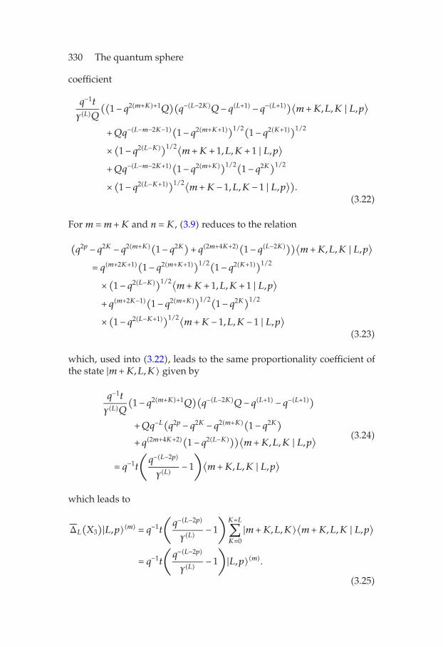
330 The quantum sphere
coefficient
q−1t
γ (L)Q
((1− q2(m+K)+1Q
)(q−(L−2K)Q− q(L+1) − q−(L+1))⟨m+K,L,K | L,p⟩
+Qq−(L−m−2K−1)(1− q2(m+K+1))1/2(1− q2(K+1))1/2
× (1− q2(L−K))1/2⟨m+K + 1,L,K + 1 | L,p⟩
+Qq−(L−m−2K+1)(1− q2(m+K))1/2(1− q2K)1/2
× (1− q2(L−K+1))1/2⟨m+K − 1,L,K − 1 | L,p⟩).
(3.22)
For m =m+K and n =K, (3.9) reduces to the relation
(q2p − q2K − q2(m+K)(1− q2K)+ q(2m+4K+2)(1− q(L−2K)))⟨m+K,L,K | L,p⟩
= q(m+2K+1)(1− q2(m+K+1))1/2(1− q2(K+1))1/2
× (1− q2(L−K))1/2⟨m+K + 1,L,K + 1 | L,p⟩
+ q(m+2K−1)(1− q2(m+K))1/2(1− q2K)1/2
× (1− q2(L−K+1))1/2⟨m+K − 1,L,K − 1 | L,p⟩
(3.23)
which, used into (3.22), leads to the same proportionality coefficient ofthe state |m+K,L,K〉 given by
q−1t
γ (L)Q
(1− q2(m+K)+1Q
)(q−(L−2K)Q− q(L+1) − q−(L+1))
+Qq−L(q2p − q2K − q2(m+K)(1− q2K)
+ q(2m+4K+2)(1− q2(L−K)))⟨m+K,L,K | L,p⟩= q−1t
(q−(L−2p)
γ (L)− 1
)⟨m+K,L,K | L,p⟩
(3.24)
which leads to
∆L
(X3)|L,p〉(m) = q−1t
(q−(L−2p)
γ (L)− 1
)K=L∑K=0
|m+K,L,K〉⟨m+K,L,K | L,p⟩
= q−1t
(q−(L−2p)
γ (L)− 1
)|L,p〉(m).
(3.25)

M. Lagraa 331
Now if we apply ∆(Xz) on the states (3.18), we obtain
∆(Xz)|L,p〉(m)
=q−1t
γ (L)
K=L∑K=0
⟨m+K,L,K | L,p⟩
× (q(m+K+1)(1− q2(m+K+1))1/2
× (q−(L−2K)Q− q(L+1) − q−(L+1))|m+K + 1,L,K〉
+ q−(L−2m−3K)(1− q2K)1/2(1− q2(L−K+1))1/2|m+K,L,K − 1〉
− q−(L−K)(1− q2(m+K+1))1/2(1− q2(m+K+2))1/2
× (1− q2(K+1))1/2(1− q2(L−K))1/2|m+K + 2,L,K + 1〉).(3.26)
The computation of each part of this sum corresponding to K for the firstterm of the right-hand side of (3.26), K + 1 for the second term and K − 1for the third term leads to a proportionality coefficient of a same state|m+ 1+K,L,K〉 given by
q−1t
γ (L)q(m+K+1)(1− q2(m+K+1))1/2(
q−(L−2K)Q− q(L+1) − q−(L+1))
× ⟨m+ 1+K − 1,L,K | L,p⟩+ q−(L−2m−3K−3)(1− q2(K+1))1/2
× (1− q2(L−K))1/2⟨m+ 1+K,L,K + 1 | L,p⟩
− q−(L−K+1)(1− q2(m+K))1/2(1− q2(m+K+1))1/2(1− q2K)1/2
× (1− q2(L+1−K))1/2⟨m+ 1+K − 2,L,K − 1 | L,p⟩.
(3.27)
By replacing into (3.10) m by m + 1 +K and n by K, we see that (3.27)reduces to
−q−1t
γ (L)q−(L−p)
(1− q2(p+1))1/2(1− q2(L−p))1/2⟨
m+ 1+K,L,K | L,p⟩ (3.28)

332 The quantum sphere
which shows that (3.26) reads
∆L
(Xz
)|L,p〉(m) = −q−1t
γ (L)q−(L−p)
(1− q2(p+1))1/2(1− q2(L−p))1/2
×K=L∑K=0
|m+ 1+K,L,K〉⟨m+ 1+K,L,K | L,p+ 1⟩
= −q−1t
γ (L)q−(L−p)
(1− q2(p+1))1/2(1− q2(L−p))1/2|L,p+ 1〉(m+1).
(3.29)
The same way gives
∆L
(Xz
)|L,p〉(m) = −q−1t
γ (L)q−(L−p+1)(1− q2p)1/2(1− q2(L−p+1))1/2
×K=L∑K=0
|m− 1+K,L,K〉⟨m− 1+K,L,K | L,p− 1⟩
= −q−1t
γ (L)q−(L−p+1)(1− q2p)1/2(1−q2(L−p+1))1/2|L,p−1〉(m−1).
(3.30)
By using (3.25), (3.29), and (3.30), we can show from a straightforwardcomputation that the states |L,p〉(m), m=−L,−L+1, . . . ,∞, are eigenstatesof (qXz + q−1Xz)/Q +X2
3 with the same eigenvalue q−2t2(1 − 1/γ2(L)) =R2(L).
Note that for m = 0 and n = L (3.9) gives (q2p − 1)〈0,L,L | L,p〉 = 0yielding
⟨0,L,L | L,p⟩ = 0 if p > 0. (3.31)
On the other hand, (3.19) leads to
(⟨0,L,L | L,0⟩)2 = 1 (3.32)
yielding 〈0,L,L | L,0〉 = λ with λλ = 1. If we take λ = 1, we get
|L,0〉(L) = |0,L,L〉⟨0,L,L | L,0⟩ = |0,L,L〉 (3.33)

M. Lagraa 333
which is the unique state of the one-dimensional Hilbert subspaceH(L,−L). On the other hand, for m = 0, (3.13) gives
⟨0,L,n | L,p+ 1
⟩= −q(n−p+1)
(1− q2(n+1))1/2(1− q2(L−n))1/2
(1− q2(p+1)
)1/2(1− q2(L−p))1/2
⟨0,L,n+ 1 | L,p⟩
(3.34)
which shows that 〈0,L,L− 1 | L,p + 1〉 = 0 if p > 0 or 〈0,L,L− 1 | L,p〉 = 0if p > 1. By iteration, we get from (3.34)
⟨0,L,L− k | L,p⟩ = 0 if p > k. (3.35)
Now by substituting (3.35) into the left-hand side of (3.9), we get
⟨K,L,L− k +K | L,p⟩ = 0 if p > k (3.36)
and by setting L− k = n, we obtain
⟨K,L,n+K | L,p⟩ = 0 =⇒ |L,p〉(n) = 0 for L−n < p ≤ L. (3.37)
Then the Hilbert subspace states H(L,m), −L ≤ m ≤ 1, do not describethe whole of the quantum sphere but only its parts described by thestates |L,0〉, . . . , |L,L +m〉. Equations (3.29) and (3.30) show that Xz is alinear mapping Xz :H(L,m) →H(L,m+1) and Xz is a linear mapping Xz :H(L,m) →H(L,m−1). To obtain the Hilbert space of representations, weconsider the orthogonal subspacesH(L,m) m = −L, . . . ,∞ spanned by thebases |L,p〉(m+p) with p = 0,1, . . . ,L which are the Hilbert subspaces in thedecomposition (3.14). The (L + 1)-dimensional subspaces H(L,m) are ir-reducible space representations of the same quantum sphere S2
qc, wherec = c(L). �
Note that by using the eigenstate relations (2.22) and the relations(2.31), the same procedure shows that in the light-cone (L = ∞), thestates
|p〉(m) =K=∞∑K=0
|m+K,K〉⟨m+K,K | p⟩, m+K ≥ 0 (3.38)
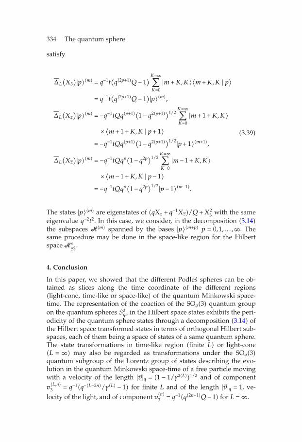
334 The quantum sphere
satisfy
∆L
(X3)|p〉(m) = q−1t
(q(2p+1)Q− 1
)K=∞∑K=0
|m+K,K〉⟨m+K,K | p⟩= q−1t
(q(2p+1)Q− 1
)|p〉(m),
∆L
(Xz
)|p〉(m) = −q−1tQq(p+1)(1− q2(p+1))1/2K=∞∑K=0
|m+ 1+K,K〉
× ⟨m+ 1+K,K | p+ 1⟩
= −q−1tQq(p+1)(1− q2(p+1))1/2|p+ 1〉(m+1),
∆L
(Xz
)|p〉(m) = −q−1tQqp(1− q2p)1/2
K=∞∑K=0
|m− 1+K,K〉
× ⟨m− 1+K,K | p− 1⟩
= −q−1tQqp(1− q2p)1/2|p− 1〉(m−1).
(3.39)
The states |p〉(m) are eigenstates of (qXz + q−1Xz)/Q +X23 with the same
eigenvalue q−2t2. In this case, we consider, in the decomposition (3.14)the subspaces H(m) spanned by the bases |p〉(m+p) p = 0,1, . . . ,∞. Thesame procedure may be done in the space-like region for the HilbertspaceHs
S2q.
4. Conclusion
In this paper, we showed that the different Podleś spheres can be ob-tained as slices along the time coordinate of the different regions(light-cone, time-like or space-like) of the quantum Minkowski space-time. The representation of the coaction of the SOq(3) quantum groupon the quantum spheres S2
qc in the Hilbert space states exhibits the peri-odicity of the quantum sphere states through a decomposition (3.14) ofthe Hilbert space transformed states in terms of orthogonal Hilbert sub-spaces, each of them being a space of states of a same quantum sphere.The state transformations in time-like region (finite L) or light-cone(L = ∞) may also be regarded as transformations under the SOq(3)quantum subgroup of the Lorentz group of states describing the evo-lution in the quantum Minkowski space-time of a free particle movingwith a velocity of the length |�v|q = (1 − 1/γ2(L))1/2 and of componentv(L,n)3 = q−1(q−(L−2n)/γ (L) − 1) for finite L and of the length |�v|q = 1, ve-
locity of the light, and of component v(n)3 = q−1(q(2n+1)Q− 1) for L =∞.

M. Lagraa 335
Acknowledgment
I am particularly grateful to the Abdus Salam International Centre forTheoretical Physics, Trieste, Italy, for hospitality.
References
[1] T. Brzeziński and S. Majid, Quantum group gauge theory on quantum spaces,Comm. Math. Phys. 157 (1993), no. 3, 591–638, Erratum: Comm. Math.Phys. 167 (1995), no. 1, 235.
[2] C.-S. Chu, P.-M. Ho, and B. Zumino, Some complex quantum manifolds andtheir geometry, Quantum Fields and Quantum Space Time (Cargèse, 1996),NATO Advanced Science Institutes Series B: Physics, vol. 364, Plenum,New York, 1997, pp. 281–322.
[3] H. Grosse, J. Madore, and H. Steinacker, Field theory on the q-deformedfuzzy sphere II: Quantization, preprint, 2001, http://arxiv.org/abs/hep-th/0103164.
[4] , Field theory on the q-deformed fuzzy sphere. I, J. Geom. Phys. 38 (2001),no. 3-4, 308–342.
[5] P. M. Hajac, Strong connections on quantum principal bundles, Comm. Math.Phys. 182 (1996), no. 3, 579–617.
[6] P. M. Hajac and S. Majid, Projective module description of the q-monopole,Comm. Math. Phys. 206 (1999), no. 2, 247–264.
[7] M. Lagraa, The boosts in the noncommutative special relativity, preprint, 2001,http://arxiv.org/abs/math-ph/0103033.
[8] , Measurability of observables in the noncommutative special relativity,preprint, 2001, http://arxiv.org/abs/math-ph/9904014.
[9] , On the quantum Lorentz group, J. Geom. Phys. 34 (2000), no. 3-4, 206–225.
[10] A. Pinzul and A. Stern, Dirac operator on the quantum sphere, Phys. Lett. B 512(2001), no. 1-2, 217–224.
[11] P. Podleś, Quantum spheres, Lett. Math. Phys. 14 (1987), no. 3, 193–202.[12] , Symmetries of quantum spaces. Subgroups and quotient spaces of quantum
SU(2) and SO(3) groups, Comm. Math. Phys. 170 (1995), no. 1, 1–20.
M. Lagraa: Laboratoire de Physique Théorique, Université d’Oran Es-Sénia,31100, Algérie
Current address: Abdus Salam International Centre for Theoretical Physics, Tri-este, Italy
Boundary Value Problems
Special Issue on
Singular Boundary Value Problems for OrdinaryDifferential Equations
Call for Papers
The purpose of this special issue is to study singularboundary value problems arising in differential equationsand dynamical systems. Survey articles dealing with interac-tions between different fields, applications, and approachesof boundary value problems and singular problems arewelcome.
This Special Issue will focus on any type of singularitiesthat appear in the study of boundary value problems. Itincludes:
• Theory and methods• Mathematical Models• Engineering applications• Biological applications• Medical Applications• Finance applications• Numerical and simulation applications
Before submission authors should carefully read overthe journal’s Author Guidelines, which are located athttp://www.hindawi.com/journals/bvp/guidelines.html. Au-thors should follow the Boundary Value Problems manu-script format described at the journal site http://www.hindawi.com/journals/bvp/. Articles published in this Spe-cial Issue shall be subject to a reduced Article Proc-essing Charge of C200 per article. Prospective authorsshould submit an electronic copy of their completemanuscript through the journal Manuscript Tracking Sys-tem at http://mts.hindawi.com/ according to the followingtimetable:
Manuscript Due May 1, 2009
First Round of Reviews August 1, 2009
Publication Date November 1, 2009
Lead Guest Editor
Juan J. Nieto, Departamento de Análisis Matemático,Facultad de Matemáticas, Universidad de Santiago de
Compostela, Santiago de Compostela 15782, Spain;[email protected]
Guest Editor
Donal O’Regan, Department of Mathematics, NationalUniversity of Ireland, Galway, Ireland;[email protected]
Hindawi Publishing Corporationhttp://www.hindawi.com