The Project Outline: A Year In Retrospect

The Project Outline

A Year In Retrospect

Johar M. Ashfaque1

String PhenomenologyDivision of Theoretical Physics

University of Liverpool

Contents

1 Introduction 2

2 The Aim 2

3 The Superstring Theory 23.1 The Superstring Action: The Basics . . . . . . . . . . . . . . . . . . . . . . . . . . . . . . 23.2 Constraints and Light-Cone Coordinates . . . . . . . . . . . . . . . . . . . . . . . . . . . . 33.3 Closed Strings and Mode Expansions . . . . . . . . . . . . . . . . . . . . . . . . . . . . . . 43.4 Quantization . . . . . . . . . . . . . . . . . . . . . . . . . . . . . . . . . . . . . . . . . . . 43.5 The Spectrum of States . . . . . . . . . . . . . . . . . . . . . . . . . . . . . . . . . . . . . 53.6 Heterotic Strings and Compactification . . . . . . . . . . . . . . . . . . . . . . . . . . . . . 53.7 The Partition Function . . . . . . . . . . . . . . . . . . . . . . . . . . . . . . . . . . . . . 6

4 Free-fermionic Construction and The ABK Rules 64.1 The ABK Rules for the Basis Vectors . . . . . . . . . . . . . . . . . . . . . . . . . . . . . 74.2 Rules for the One-Loop Phases . . . . . . . . . . . . . . . . . . . . . . . . . . . . . . . . . 74.3 Rules for the GGSO Projection . . . . . . . . . . . . . . . . . . . . . . . . . . . . . . . . . 74.4 The Massless Spectrum: Virasoro Level-Matching Conditions . . . . . . . . . . . . . . . . 8

5 The NAHE Set: {1,S,b1,b2,b3} 85.1 1: The Non-Supersymmetric Case . . . . . . . . . . . . . . . . . . . . . . . . . . . . . . . 85.2 S: The SUSY Generator . . . . . . . . . . . . . . . . . . . . . . . . . . . . . . . . . . . . . 95.3 b1 . . . . . . . . . . . . . . . . . . . . . . . . . . . . . . . . . . . . . . . . . . . . . . . . . 95.4 b2 . . . . . . . . . . . . . . . . . . . . . . . . . . . . . . . . . . . . . . . . . . . . . . . . . 95.5 b3 . . . . . . . . . . . . . . . . . . . . . . . . . . . . . . . . . . . . . . . . . . . . . . . . . 95.6 From SO(44) To SO(10) . . . . . . . . . . . . . . . . . . . . . . . . . . . . . . . . . . . . . 10

6 The Standard-Like Model: A Composite 106.1 From SO(44) To SU(3)× U(1)× SU(2)× U(1) . . . . . . . . . . . . . . . . . . . . . . . . 10

7 Phenomenology Based On The Standard-Like ModelSU(3)C × U(1)C × SU(2)L × U(1)L 107.1 Higgs Boson Mass Matrix . . . . . . . . . . . . . . . . . . . . . . . . . . . . . . . . . . . . 117.2 One Loop RGEs . . . . . . . . . . . . . . . . . . . . . . . . . . . . . . . . . . . . . . . . . 11

8 The Extracurricular Activities 118.1 Teaching and Marking . . . . . . . . . . . . . . . . . . . . . . . . . . . . . . . . . . . . . . 118.2 Talks . . . . . . . . . . . . . . . . . . . . . . . . . . . . . . . . . . . . . . . . . . . . . . . . 118.3 Conferences I Attended . . . . . . . . . . . . . . . . . . . . . . . . . . . . . . . . . . . . . 11

9 Conclusion 12

[email protected]

1

1 Introduction

In this report, I present a review of the first year of my PhD study. Having joined the TheoreticalPhysics division at the University of Liverpool after gaining a BSc in Mathematics and a postgraduatecertificate from King’s College London opened a gateway to new horizons.

As a newcomer, it was very important for me to acquire the relevant background knowledge andto get up to speed with the latest research in the area. Having studied modules like supersymmetry,string theory and standard model physics with Lie algebras and manifolds at King’s college in London, Iwanted to speed up my progress. Having that in mind, I went on the quest of understanding superstrings.However, I soon realized that the path taken will not be as easy as planned due to time constraints andmy own interests. Here, I must add that the lectures by Dr. Mohaupt on the conformal field theoryaspects of string theory were a delight and I thoroughly enjoyed them as they widened my understandingof the area. Eventually, I got the opportunity to work with Hasan Sonmez, a third year student, whogave me the opportunity to work with him in order to tackle the various models that were being explored.

Within the string phenomenology division I got the opportunity to explore free fermionic formulationbased on the heterotic string models.

For the interested reader, good references to the subject of free fermionic formulation can be found in[1, 2, 3] and [4]. This progress report will focus on the theory followed by some of the key ideas thatunderlie the free fermionic construction and present a brief discussion on the Standard-Like model beforemoving to phenomenology based on the Standard-Like model.

2 The Aim

Our aim is to construct realistic models with 4 flat space-time dimensions, chiral matter fields and N = 1SUSY.

3 The Superstring Theory

String theory is the only known consistent theory that incorporates gravity. Therefore, the motivation isto be able to do phenomenology based on superstrings.

3.1 The Superstring Action: The Basics

In string theory, the string propagates in D-dimensional flat Minkowski spacetime. As this string movesthrough spacetime it traces out a worldsheet, which is a two-dimensional surface in spacetime. The pointson the worldsheet are parametrized by the two coordinates σ0 = τ , which is time-like and σ1 = σ, whichis spacelike. Therefore the action is given by

S = − 1

4πα′

∫d2σ

(∂αXµ∂

αXµ + iψµρα∂αψµ

)(1)

where Xµ = Xµ(σ, τ) and ψµ = ψµ(σ, τ) are the two-dimensional bosonic and fermionic fields respectivelyand µ = 0, 1, . . . , D − 1.Furthermore, the term ρα is a 2-dimensional Dirac matrix with α = 0, 1, which we can choose to be aMajorana representation, where a convenient choice will be

ρ0 =

(0 −11 0

), ρ1 =

(0 11 0

). (2)

These matrices can also be seen to satisfy the Clifford algebra. Moreover taking this choice of ρα, wededuce that

2

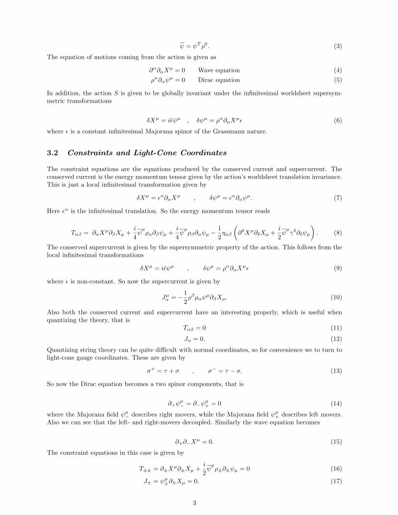
ψ = ψT ρ0. (3)

The equation of motions coming from the action is given as

∂α∂αXµ = 0 Wave equation (4)

ρα∂αψµ = 0 Dirac equation (5)

In addition, the action S is given to be globally invariant under the infinitesimal worldsheet supersym-metric transformations

δXµ = iεψµ , δψµ = ρα∂αXµε (6)

where ε is a constant infinitesimal Majorana spinor of the Grassmann nature.

3.2 Constraints and Light-Cone Coordinates

The constraint equations are the equations produced by the conserved current and supercurrent. Theconserved current is the energy momentum tensor given by the action’s worldsheet translation invariance.This is just a local infinitesimal transformation given by

δXµ = εα∂αXµ , δψµ = εα∂αψ

µ. (7)

Here εα is the infinitesimal translation. So the energy momentum tensor reads

Tαβ = ∂αXµ∂βXµ +

i

4ψµρα∂βψµ +

i

4ψµρβ∂αψµ −

1

2ηαβ

(∂δXµ∂δXµ +

i

2ψµγδ∂δψµ

). (8)

The conserved supercurrent is given by the supersymmetric property of the action. This follows from thelocal infinitesimal transformations

δXµ = iεψµ , δψµ = ρα∂αXµε (9)

where ε is non-constant. So now the supercurrent is given by

Jµα = −1

2ρβραψ

µ∂βXµ. (10)

Also both the conserved current and supercurrent have an interesting properly, which is useful whenquantizing the theory, that is

Tαβ = 0 (11)

Jα = 0. (12)

Quantizing string theory can be quite difficult with normal coordinates, so for convenience we to turn tolight-cone gauge coordinates. These are given by

σ+ = τ + σ , σ− = τ − σ. (13)

So now the Dirac equation becomes a two spinor components, that is

∂+ψµ− = ∂−ψ

µ+ = 0 (14)

where the Majorana field ψµ− describes right movers, while the Majorana field ψµ+ describes left movers.Also we can see that the left- and right-movers decoupled. Similarly the wave equation becomes

∂+∂−Xµ = 0. (15)

The constraint equations in this case is given by

T±± = ∂±Xµ∂±Xµ +

i

2ψµρ±∂±ψµ = 0 (16)

J± = ψµ±∂±Xµ = 0. (17)

3

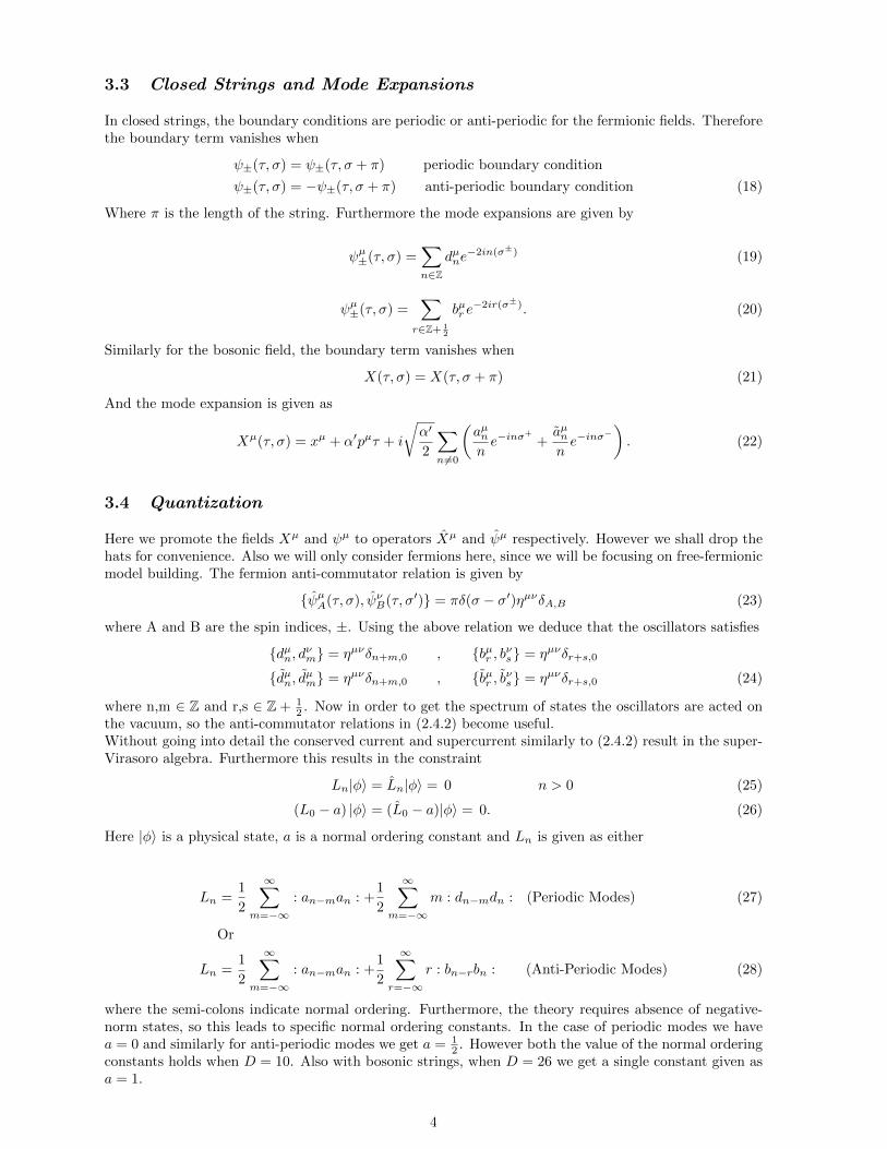
3.3 Closed Strings and Mode Expansions

In closed strings, the boundary conditions are periodic or anti-periodic for the fermionic fields. Thereforethe boundary term vanishes when

ψ±(τ, σ) = ψ±(τ, σ + π) periodic boundary condition

ψ±(τ, σ) = −ψ±(τ, σ + π) anti-periodic boundary condition (18)

Where π is the length of the string. Furthermore the mode expansions are given by

ψµ±(τ, σ) =∑n∈Z

dµne−2in(σ±) (19)

ψµ±(τ, σ) =∑

r∈Z+ 12

bµr e−2ir(σ±). (20)

Similarly for the bosonic field, the boundary term vanishes when

X(τ, σ) = X(τ, σ + π) (21)

And the mode expansion is given as

Xµ(τ, σ) = xµ + α′pµτ + i

√α′

2

∑n 6=0

(aµnne−inσ

+

+aµnne−inσ

−). (22)

3.4 Quantization

Here we promote the fields Xµ and ψµ to operators Xµ and ψµ respectively. However we shall drop thehats for convenience. Also we will only consider fermions here, since we will be focusing on free-fermionicmodel building. The fermion anti-commutator relation is given by

{ψµA(τ, σ), ψνB(τ, σ′)} = πδ(σ − σ′)ηµνδA,B (23)

where A and B are the spin indices, ±. Using the above relation we deduce that the oscillators satisfies

{dµn, dνm} = ηµνδn+m,0 , {bµr , bνs} = ηµνδr+s,0

{dµn, dµm} = ηµνδn+m,0 , {bµr , bνs} = ηµνδr+s,0 (24)

where n,m ∈ Z and r,s ∈ Z + 12 . Now in order to get the spectrum of states the oscillators are acted on

the vacuum, so the anti-commutator relations in (2.4.2) become useful.Without going into detail the conserved current and supercurrent similarly to (2.4.2) result in the super-Virasoro algebra. Furthermore this results in the constraint

Ln|φ〉 = Ln|φ〉 = 0 n > 0 (25)

(L0 − a) |φ〉 = (L0 − a)|φ〉 = 0. (26)

Here |φ〉 is a physical state, a is a normal ordering constant and Ln is given as either

Ln =1

2

∞∑m=−∞

: an−man : +1

2

∞∑m=−∞

m : dn−mdn : (Periodic Modes) (27)

Or

Ln =1

2

∞∑m=−∞

: an−man : +1

2

∞∑r=−∞

r : bn−rbn : (Anti-Periodic Modes) (28)

where the semi-colons indicate normal ordering. Furthermore, the theory requires absence of negative-norm states, so this leads to specific normal ordering constants. In the case of periodic modes we havea = 0 and similarly for anti-periodic modes we get a = 1

2 . However both the value of the normal orderingconstants holds when D = 10. Also with bosonic strings, when D = 26 we get a single constant given asa = 1.

4

3.5 The Spectrum of States

In order to examine the spectrum of states, the number operator N is introduced. For the periodic sectorthis is given as

N =

∞∑n=1

ηµνaµ−na

νn +

∞∑m=1

mdµ−mdνmηµν

= Na +Nd. (29)

Similarly for the anti-periodic sector it is given as

N =

∞∑n=1

ηµνaµ−na

νn +

∞∑r= 1

2

rbµ−rbνrηµν

= Na +N b. (30)

Now using the constraint (L0 − a) |φ〉 = 0 and working with anti-periodic sector i.e.(L0 − 1

2

)|φ〉 = 0.

The L0 − 12 operator expansion in terms of oscillators gives

L0 −1

2=

1

2

∑n

: aµ−naνn : ηµν +

1

2

∑r

r : bµ−rbνr : ηµν −

1

2

=1

2aµ0a

ν0ηµν +

1

2

∞∑n=1

aµ−naνnηµν +

1

2

∞∑r= 1

2

rbµ−rbνrηµν −

1

2

=1

4α′pµpµ +N − 1

2(31)

where aµ0 =√

α′

2 pµ for closed strings. Moreover comparing (2.5.3) with the Klein-Gordan equation, the

spacetime mass-squared of a physical state is the eigenvalue of the operator

M2 =4

α′

(N − 1

2

)(32)

Similarly for the periodic sector, the spacetime mass-squared of a physical state is an eigenvalue of

M2 =1

α′N. (33)

3.6 Heterotic Strings and Compactification

The discussion up till now was on based on N = 2 world-sheet supersymmetry. However, closed stringsallow the supersymmetric transformations to decouple in the left and right-movers. For instance theinfinitesimal transformations become

δψµ− = −2∂−Xµε+ , δψµ+ = −2∂+X

µε−. (34)

Furthermore, this corresponds to two different supersymmetric transformations. So it is now possibleto get the N = 2 world-sheet supersymmetry and express it as an N = 1 world-sheet supersymmetryon the left-movers and on the right-movers. The idea here is that we can construct a model wherethe string has a N = 1 world-sheet supersymmetry on the left-movers and no supersymmetry on theright-movers, which will at the end generate a N = 1 space-time supersymmetry. Until now we workedon superstrings, but all the results apply to a non-supersymmetric strings (bosonic strings). This couldseem quite weird at first glance because cancelling the conformal anomaly requires that the space-timedimension for right-movers is 26 and 10 for the left-movers, although one would expect to have the samespace-time dimension. However, using compactification, we can reduce the two number of dimensionsto the same value, which can be taken as equal to four in order to match with our real 4-dimensional

5

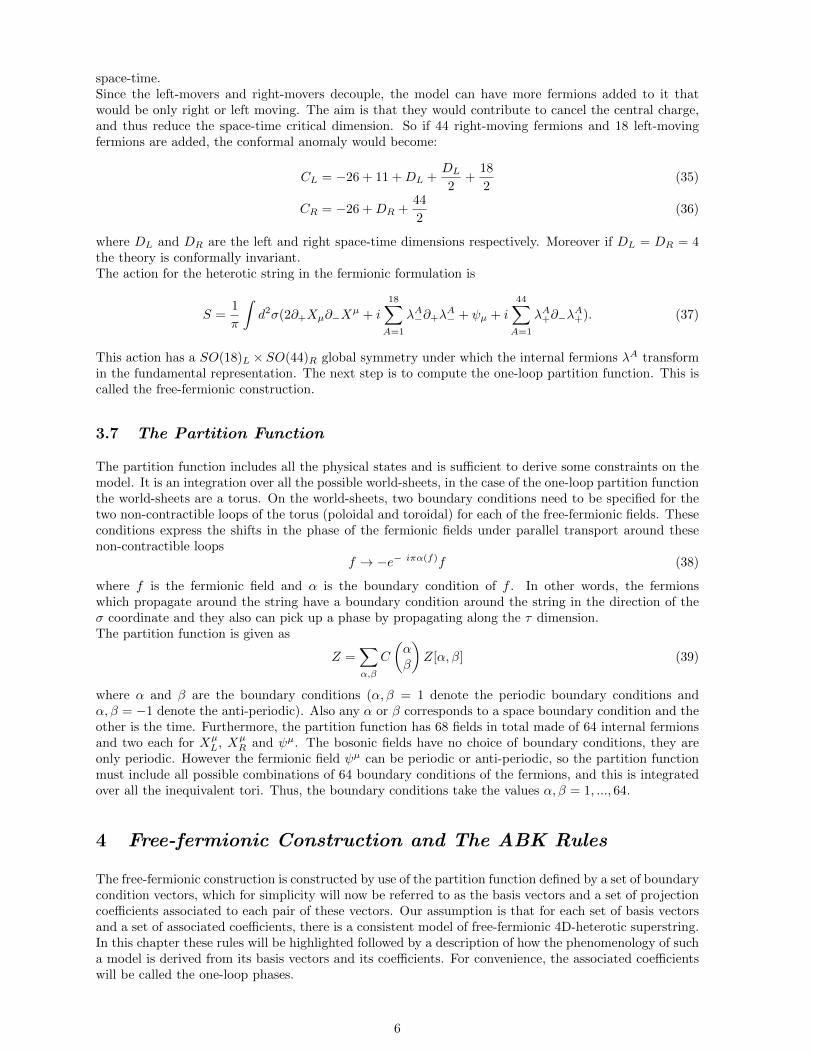
space-time.Since the left-movers and right-movers decouple, the model can have more fermions added to it thatwould be only right or left moving. The aim is that they would contribute to cancel the central charge,and thus reduce the space-time critical dimension. So if 44 right-moving fermions and 18 left-movingfermions are added, the conformal anomaly would become:

CL = −26 + 11 +DL +DL

2+

18

2(35)

CR = −26 +DR +44

2(36)

where DL and DR are the left and right space-time dimensions respectively. Moreover if DL = DR = 4the theory is conformally invariant.The action for the heterotic string in the fermionic formulation is

S =1

π

∫d2σ(2∂+Xµ∂−X

µ + i

18∑A=1

λA−∂+λA− + ψµ + i

44∑A=1

λA+∂−λA+). (37)

This action has a SO(18)L × SO(44)R global symmetry under which the internal fermions λA transformin the fundamental representation. The next step is to compute the one-loop partition function. This iscalled the free-fermionic construction.

3.7 The Partition Function

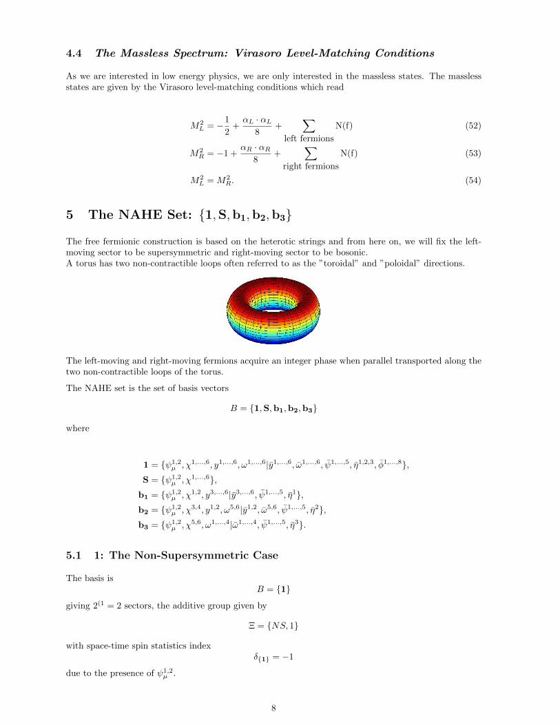
The partition function includes all the physical states and is sufficient to derive some constraints on themodel. It is an integration over all the possible world-sheets, in the case of the one-loop partition functionthe world-sheets are a torus. On the world-sheets, two boundary conditions need to be specified for thetwo non-contractible loops of the torus (poloidal and toroidal) for each of the free-fermionic fields. Theseconditions express the shifts in the phase of the fermionic fields under parallel transport around thesenon-contractible loops

f → −e− iπα(f)f (38)

where f is the fermionic field and α is the boundary condition of f . In other words, the fermionswhich propagate around the string have a boundary condition around the string in the direction of theσ coordinate and they also can pick up a phase by propagating along the τ dimension.The partition function is given as

Z =∑α,β

C

(αβ

)Z[α, β] (39)

where α and β are the boundary conditions (α, β = 1 denote the periodic boundary conditions andα, β = −1 denote the anti-periodic). Also any α or β corresponds to a space boundary condition and theother is the time. Furthermore, the partition function has 68 fields in total made of 64 internal fermionsand two each for Xµ

L, XµR and ψµ. The bosonic fields have no choice of boundary conditions, they are

only periodic. However the fermionic field ψµ can be periodic or anti-periodic, so the partition functionmust include all possible combinations of 64 boundary conditions of the fermions, and this is integratedover all the inequivalent tori. Thus, the boundary conditions take the values α, β = 1, ..., 64.

4 Free-fermionic Construction and The ABK Rules

The free-fermionic construction is constructed by use of the partition function defined by a set of boundarycondition vectors, which for simplicity will now be referred to as the basis vectors and a set of projectioncoefficients associated to each pair of these vectors. Our assumption is that for each set of basis vectorsand a set of associated coefficients, there is a consistent model of free-fermionic 4D-heterotic superstring.In this chapter these rules will be highlighted followed by a description of how the phenomenology of sucha model is derived from its basis vectors and its coefficients. For convenience, the associated coefficientswill be called the one-loop phases.

6

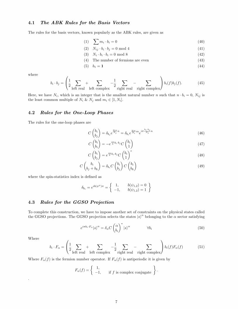
4.1 The ABK Rules for the Basis Vectors

The rules for the basis vectors, known popularly as the ABK rules, are given as

(1)∑

mi · bi = 0 (40)

(2) Nij · bi · bj = 0 mod 4 (41)

(3) Ni · bi · bi = 0 mod 8 (42)

(4) The number of fermions are even (43)

(5) b1 = 1 (44)

where

bi · bj =

1

2

∑left real

+∑

left complex

−1

2

∑right real

−∑

right complex

bi(f)bj(f). (45)

Here, we have Ni, which is an integer that is the smallest natural number n such that n · bi = 0, Nij isthe least common multiple of Ni & Nj and mi ∈ [1, Ni].

4.2 Rules for the One-Loop Phases

The rules for the one-loop phases are

C

(bibj

)= δbje

2iπNj

n= δbie

2iπNi

meiπbi·bjNj

n(46)

C

(bibi

)= −e iπ4 bi·bjC

(bi1

)(47)

C

(bibj

)= e

iπ2 bi·bjC

(bi1

)∗(48)

C

(bi

bj + bk

)= δbiC

(bibj

)C

(bibk

)(49)

where the spin-statistics index is defined as

δbi = eib(ψµ)π =

{1, b(ψ1,2) = 0−1, b(ψ1,2) = 1

}

4.3 Rules for the GGSO Projection

To complete this construction, we have to impose another set of constraints on the physical states calledthe GGSO projections. The GGSO projection selects the states |s〉α belonging to the α sector satisfying

eiπbi·Fα |s〉α = δαC

(αbi

)∗|s〉α ∀bi (50)

Where

bi · Fα =

1

2

∑left real

+∑

left complex

−1

2

∑right real

−∑

right complex

bi(f)Fα(f) (51)

Where Fα(f) is the fermion number operator. If Fα(f) is antiperiodic it is given by

Fα(f) =

{1,−1, if f is complex conjugate

}.

.

7

4.4 The Massless Spectrum: Virasoro Level-Matching Conditions

As we are interested in low energy physics, we are only interested in the massless states. The masslessstates are given by the Virasoro level-matching conditions which read

M2L = −1

2+αL · αL

8+

∑left fermions

N(f) (52)

M2R = −1 +

αR · αR8

+∑

right fermions

N(f) (53)

M2L = M2

R. (54)

5 The NAHE Set: {1,S,b1,b2,b3}

The free fermionic construction is based on the heterotic strings and from here on, we will fix the left-moving sector to be supersymmetric and right-moving sector to be bosonic.A torus has two non-contractible loops often referred to as the ”toroidal” and ”poloidal” directions.

The left-moving and right-moving fermions acquire an integer phase when parallel transported along thetwo non-contractible loops of the torus.

The NAHE set is the set of basis vectors

B = {1,S,b1,b2,b3}

where

1 = {ψ1,2µ , χ1,...,6, y1,...,6, ω1,...,6|y1,...,6, ω1,...,6, ψ1,...,5, η1,2,3, φ1,...,8},

S = {ψ1,2µ , χ1,...,6},

b1 = {ψ1,2µ , χ1,2, y3,...,6|y3,...,6, ψ1,...,5, η1},

b2 = {ψ1,2µ , χ3,4, y1,2, ω5,6|y1,2, ω5,6, ψ1,...,5, η2},

b3 = {ψ1,2µ , χ5,6, ω1,...,4|ω1,...,4, ψ1,...,5, η3}.

5.1 1: The Non-Supersymmetric Case

The basis isB = {1}

giving 2(1 = 2 sectors, the additive group given by

Ξ = {NS, 1}

with space-time spin statistics indexδ{1} = −1

due to the presence of ψ1,2µ .

8

5.2 S: The SUSY Generator

The basis isB = {1,S}

giving 22 = 2 sectors, the additive group given by

Ξ = {NS, 1 + S, 1, S}

with space-time spin statistics indexδ{S} = −1


5.3 b1

The basis isB = {1,S,b1}


Ξ = {NS, 1 + S, 1 + b1, S + b1, 1 + S + b1, 1, S, b1}

with space-time spin statistics indexδ{b1} = −1


5.4 b2

The basis isB = {1,S,b1,b2}


Ξ = {NS, 1 + S, 1 + b1, 1 + b2, S + b1, S + b2, b1 + b2, 1 + S + b1,

1 + S + b2, 1 + b1 + b2, S + b1 + b2, 1 + S + b1 + b2, 1, S, b1, b2}



5.5 b3

The basis isB = {1,S,b1,b2,b3}


Ξ = {NS, 1 + S, 1 + b1, 1 + b2, 1 + b3, S + b1, S + b2, S + b3, b1 + b2, b1 + b3, b2 + b3,

1 + S + b1, 1 + S + b2, 1 + S + b3, 1 + b1 + b2, 1 + b1 + b3, 1 + b2 + b3, S + b1 + b2, S + b1 + b3,

S + b2 + b3, b1 + b2 + b3, 1 + S + b1 + b2, 1 + S + b1 + b3, 1 + S + b2 + b3, 1 + b1 + b2 + b3, S + b1 + b2 + b3,

1 + S + b1 + b2 + b3, 1, S, b1, b2, b3}



9

5.6 From SO(44) To SO(10)

The NAHE set consists of five basis vectors. The basis vectors 1 and S, generate a model with the SO(44)gauge symmetry and N = 4 space–time supersymmetry. The vectors bi for i = 1, 2, 3 correspond to theZ2×Z2 orbifold twists. The vector b1 breaks the SO(44) gauge group to SO(28)×SO(16) and the N = 4space–time supersymmetry to N = 2. The vector b2 then reduces the group to SO(10)×SO(22)×SO(6)2

gauge group and the N = 2 supersymmetry is further reduced to N = 1 . Furthermore, the basis vectorb3 gives the decomposition SO(10) × SO(16)1 × SO(6)3 where we fix the GGSO projection coefficientin order to preserve the N = 1 space–time supersymmetry. Moreover, the sector, ξ, given by the linearcombination

ξ = 1 + b1 + b2 + b3 ≡ {φ1,...,8}

together with the NS–sector form the adjoint representation of E8 thereby enhancing the SO(16)1. Asa result, we obtain

SO(10)× E8 × SO(6)3

as the gauge group with N = 1 space–time supersymmetry at the NAHE level.

6 The Standard-Like Model: A Composite

The Standard-like model we consider will be generated by a set of 12 basis vectors defined as

v1 = S = {ψµ, χ12, χ34, χ56},v1+i = ei = {yi, ωi|yi, ωi}, i = 1, . . . , 6,

v8 = b1 = {χ34, χ56, y34, y56|y34, y56, η1, ψ1,...,5},

v9 = b2 = {χ12, χ56, y12, y56|y12, y56, η2, ψ1,...,5},

v10 = z = {φ1,...,8},

v11 = α = {ψ4,5, φ

1,2},

v12 = β = {η1,2,3 = − 12 , ψ

1,...,5= 1

2 , φ1,...,8

= 12}.

6.1 From SO(44) To SU(3)× U(1)× SU(2)× U(1)

The basis vector S generates a model with the SO(44) gauge symmetry and N = 4 space–time super-symmetry. The vectors e1,. . . ,e6, corresponding to all the possible symmetric shifts of the six internalfermionic coordinates, break the SO(44) gauge group to SO(32)×U(1)6 and preserve the N = 4 space–time supersymmetry. The vectors b1 and b2 correspond to the Z2 × Z2 orbifold twists, which breakN = 4 to N = 1 supersymmetry and reduce the rank of the group as the U(1)6 is broken completely,leaving the SO(32) symmetry to decompose to the SO(10) × U(1)2 × SO(18) group. Moreover, thebasis vector z results in a further decomposition of the gauge group to SO(10) × U(1)3 × SO(16). Fur-thermore, the group SO(10) × U(1)3 corresponds to the observable gauge group whilst the SO(16)corresponds to the hidden. The Pati-Salam basis vector α then breaks the observable gauge group toSO(6)×SO(4)×U(1)3 and the hidden to SO(12)×SO(4). The flipped SU(5) vector β reduces the gaugegroups to SU(3)C × U(1)C × SU(2)L × U(1)L × U(1)3 and SU(6)× U(1)× SU(2)× U(1), respectively.

7 Phenomenology Based On The Standard-Like ModelSU(3)C × U(1)C × SU(2)L × U(1)L

Last but not the least, I would take a moment to briefly mention a mini-project on the BSM (Beyond theStandard Model) phenomenology. The first task I was set involved the computation of the Higgs bosonmass matrix.

10

7.1 Higgs Boson Mass Matrix

We restrict our attention to the part of the scalar potential involving only the Higgs fields and the singletunder the assumption that squark and slepton fields have vanishing vacuum expectation values.

ConsiderW = H1H2N

whereH1 = (H0

1 , H−),

H2 = (H+, H02 )

are the Higgs fields and N denotes a singlet.

7.2 One Loop RGEs

This is the next stage after the computation of the Higgs boson mass matrix which is being studied now.

8 The Extracurricular Activities

In this section, I will highlight some of the activities that I actively took part in.

8.1 Teaching and Marking

In this section, I will briefly highlight the highs and the lows of being a graduate teaching assistantfrom a personal perspective.

To round up, I will say that being a graduate teaching assistant was challenging yet interesting.

• Field Theory and PDEs

• Engineering Mathematics II

• Dynamic Modelling

• Engineering Mathematics

• Introduction to Financial Maths

8.2 Talks

• (First Year Development Workshop): Heterotic Strings and Free Fermionic Construction

• Morse Theory

• Clifford Algebras and Dirac Operators

• Laplace Transform and ODEs

8.3 Conferences I Attended

• Annual Theory Meeting: Durham University

• Kent Spectral Theory Meeting

11

9 Conclusion

All in all, the first year of my PhD studies has been a productive one. The highlight of this year wasthe several talks that I gave in the journal clubs which helped me develop my communication skills. Inconclusion, I would like to emphasize on how wonderful this year has been regardless of all the difficultiesthat were faced. I would like to take a moment to acknowledge the work I did with Hasan and wouldlike to thank him for sharing his expertise in order to make me realise the true essence of the theory thatunderlies our research.

To sum up, I would like to finish with a quote: ”Not failure, but low aim is definitely a crime.”

References

[1] B. Assel, K. Christodoulides, A.E. Faraggi, C. Kounnas, J. Rizos, Classification of Heterotic Pati-Salam Models, Nucl.Phys. B844 (2011), 365-396.

[2] I. Antoniadis, C.P. Bachas, C. Kounnas, Four Dimensional Superstrings, Nuclear Physics B (1987),Volume 289, Pages 87108.

[3] I. Antoniadis, C.P. Bachas, 4D Fermionic Superstrings With Arbitrary Twists, Nuclear Physics B(March 1988), Volume 298, Issue 3, Pages 586612.

[4] S. Nooij, Classification of the Chiral Z2 × Z2 Heterotic String Models, arXiv: hep-th/0603035

12

http://arxiv.org/abs/hep-th/0603035

The Project Outline: A Year In Retrospect

Documents

Transcript of The Project Outline: A Year In Retrospect