
The Pennsylvania State University - ETDA
80
The Pennsylvania State University The Graduate School Department of Aerospace Engineering NUMERICAL SIMULATION AND EXPERIMENTAL INVESTIGATION OF THRUST PRODUCED BY A HOBBY–SCALE PULSEJET ENGINE A Thesis in Aerospace Engineering by Mengyao Zhu 2015 Mengyao Zhu Submitted in Partial Fulfillment of the Requirements for the Degree of Master of Science August 2015
-
Upload
khangminh22 -
Category
Documents
-
view
0 -
download
0
Transcript of The Pennsylvania State University - ETDA

The Pennsylvania State University
The Graduate School
Department of Aerospace Engineering
NUMERICAL SIMULATION AND EXPERIMENTAL INVESTIGATION OF THRUST
PRODUCED BY A HOBBY–SCALE PULSEJET ENGINE
A Thesis in
Aerospace Engineering
by
Mengyao Zhu
2015 Mengyao Zhu
Submitted in Partial Fulfillment
of the Requirements
for the Degree of
Master of Science
August 2015

ii
The thesis of Mengyao Zhu was reviewed and approved* by the following:
Michael M. Micci
Professor of Aerospace Engineering
Thesis Advisor
Cengiz Camci
Professor of Aerospace Engineering
George A. Lesieutre
Professor of Aerospace Engineering
Head of the Department of Aerospace Engineering
*Signatures are on file in the Graduate School

iii
ABSTRACT
The pulsejet is a type of jet engine in which combustion occurs in pulses. It was
introduced to the world in the 1860s and the most famous previous application was the “V-1 buzz
bomb” during World War II. Because of its high thrust to weight ratio, low cost and simple
design, the pulsejet has recently received more research interest, like micro-scale propulsion
devices for UAVs, or even large-scale propulsion devices for single stage to orbit Launchers.
The objectives of this research include investigating the thrust a hobby scale pulsejet can
deliver and its operating frequency, and develop a numerical simulation model for future study.
This project investigated pulsejet operation in a combined numerical and experimental
approach. The working mechanism of pulsejet engine was studied and a numerical simulation
code based on a shock tube model with a quasi-one-dimensional assumption was built using
second-order accurate Lax–Wendroff scheme. The code was capable of predicting flow
parameters at various locations of the pulsejet engine with different lengths and diameters.
A test bed with mounting clamps was manufactured; 10 tests were run on gaseous
propane with assistance from an air compressor.
The simulation model estimated the 40 cm pulsejet can deliver an average 4.18 N thrust
with a 232 Hz operating frequency and the maximum instantaneous thrust was 32N. When the
pulsejet was running on different fuel–air equivalence ratios, the working frequency was
different. The load-cell was proved to be capable of detecting and recording each combustion
events; and the operating frequency could be derived from the thrust data with high accuracy.

iv
TABLE OF CONTENTS
List of Figures .......................................................................................................................... vi
List of Tables ........................................................................................................................... ix
Acknowledgements .................................................................................................................. x
Dedication…………………………………………………………………………….………xi
Chapter 1 Introduction ............................................................................................................. 1
1.1 Literature Review ....................................................................................................... 1 1.1.1 Background and History .................................................................................. 1 1.1.2 Recent Research .............................................................................................. 3
1.2 Valved Pulsejet Combustion Cycle ............................................................................ 5 1.3 Objectives................................................................................................................... 6
Chapter 2 Numerical Model ..................................................................................................... 8
2.1 Description of the Shock Tube Problem .................................................................... 8 2.2 Euler Equations of Gas Dynamics ............................................................................. 10
2.2.1 Dimensionless Equations ................................................................................ 10 2.2.2 Exact Solution for shock tube problem ........................................................... 11
2.3 Numerical Solution .................................................................................................... 14 2.3.1 Lax-Wendroff Centered Scheme ..................................................................... 14 2.3.2 Artificial Dissipation ....................................................................................... 17
2.4 Numerical Model for Pulsejet and Boundary Conditions .......................................... 18 2.4.1 Numerical Model for Pulsejet ......................................................................... 18 2.4.2 Boundary Conditions ....................................................................................... 21
Chapter 3 Experimental Apparatus and Setup ......................................................................... 23
3.1 Test Bed Design ......................................................................................................... 23 3.2 Strain Gauge and Calibration ..................................................................................... 25
3.2.1 Strain Gauge .................................................................................................... 25 3.2.2 Calibration ....................................................................................................... 26
3.3 Thermocouple ............................................................................................................ 31 3.4 Other Instruments and Systems .................................................................................. 33
3.4.1 Fuel Delivery System ...................................................................................... 33 3.4.2 Ignition System ............................................................................................... 34 3.4.3 Sound Measurement System ........................................................................... 35
3.5 Procedures .................................................................................................................. 35 3.5.1 Data Collection ................................................................................................ 35 3.5.2 Engine run procedure ...................................................................................... 36 3.5.3 After Treatment ............................................................................................... 37
Chapter 4 Results and Discussions .......................................................................................... 38

v
4.1 Experiment results ...................................................................................................... 38 4.1.1 Test-7 ............................................................................................................... 39 4.1.2 Test-10 ............................................................................................................. 45
4.2 Numerical simulation results...................................................................................... 51 4.3 Comparison and Overview ......................................................................................... 57
Chapter 5 Conclusions and Future Work ................................................................................. 59
5.1 Summary and Conclusions ......................................................................................... 59 5.2 Future Work ............................................................................................................... 60
Bibliography ............................................................................................................................ 61
Appendix A Exact solution Code .................................................................................... 63 Appendix B Pulsejet Geometry Model Code .................................................................. 66 Appendix C Numerical Model Code ............................................................................... 67

vi
LIST OF FIGURES
Figure 1-1. Humphrey cycle. ................................................................................................... 1
Figure 1-2. Marconnet's valveless engine design. .................................................................... 2
Figure 1-3. Sketch German V-1 Pulsejet Powered Cruise Missile [8]. ................................... 3
Figure 1-4. Pulsejet schematic diagram [2]. ............................................................................ 5
Figure 1-5. The combustion cycle of a valved pulsejet [13]. ................................................... 5
Figure 1-6. 40cm hobby scale pulsejet..................................................................................... 6
Figure 2-1. Sketch of the initial configuration of the shock tube (t = 0) and waves
propagating in the tube after the diaphragm breaks (t > 0) [14]. ..................................... 9
Figure 2-2.Plots of different waves which are formed in the tube once the diaphragm
breaks (t > 0). ................................................................................................................... 9
Figure 2-3. Diagram in the (x, t) plane of the exact solution of the shock tube problem. ....... 12
Figure 2-4. Exact solution of the shock tube problem with Sod’s initial condition, at
t=0.2. ................................................................................................................................ 13
Figure 2-5. Computational stencil for the two-step Lax-Wendroff scheme. ........................... 15
Figure 2-6. Comparison between exact solution and Lax-Wendroff scheme solution of the
shock tube problem with Sod’s initial condition, at t=0.2. .............................................. 16
Figure 2-7. Comparison between exact solution and Lax-Wendroff scheme (with artificial
dissipation) solution of the shock tube problem with Sod’s initial condition, at t=0.2. ... 18
Figure 2-8. Pulsejet engine’s geometric profile. ...................................................................... 20
Figure 3-1. Test bed. ................................................................................................................ 24
Figure 3-2. Aluminum mounting clamps and ceramic tapes. .................................................. 24
Figure 3-3. Strain Gauge. ......................................................................................................... 25
Figure 3-4. Full bridge strain gauge circuit.............................................................................. 26
Figure 3-5. Pulley system. ....................................................................................................... 27
Figure 3-6. Data collecting and analysis system for calibration. ............................................. 27
Figure 3-7. Plots of pulley drag test, weights versus voltages. ................................................ 28
Figure 3-8. Plots of pulley thrust test, weights versus voltages. .............................................. 29

vii
Figure 3-9. Unsheathed TC type K thermocouple (indicated by green circle) accuracy
testing. .............................................................................................................................. 31
Figure 3-10. HH (High Temperature Fiberglass) SLE type K thermocouple. ......................... 32
Figure 3-11.Original fuel delivery system (left) and improved fuel delivery system
(right). .............................................................................................................................. 33
Figure 3-12. Model-T Ford ignition coil and spark plug. ........................................................ 34
Figure 3-13. Microphone and analog electrical filter. ............................................................. 35
Figure 3-14. Data acquisition Labview code front panel. ........................................................ 36
Figure 4-1. Plot of thrust vs time in test-7. .............................................................................. 39
Figure 4-2. Plot of temperature vs time in test-7. .................................................................... 39
Figure 4-3. Plot of sound vs time in test-7. .............................................................................. 40
Figure 4-4. Plot of temperature vs time (46 s to 46.1s) in test-7. ............................................. 41
Figure 4-5. Plot of sound data from (39.16s to 39.26s) in test-7. ............................................ 42
Figure 4-6. Plot of thrust vs time (39.16s to 39.26s) in test-7.................................................. 42
Figure 4-7. Plot of thrust vs average temperature (12s to 40s) in test-7. ................................. 43
Figure 4-8. Plot of magnitude vs frequency of the thrust data (39.16s to 39.26s) in test-7. .... 44
Figure 4-9. Plot of thrust vs time in test-10. ............................................................................ 45
Figure 4-10. Plot of temperature vs time in test-10. ................................................................ 45
Figure 4-11. Plot of sound vs time in test-10. .......................................................................... 46
Figure 4-12. Plot of temperature vs time (112.45 s to 112.55s) in test-10. .............................. 46
Figure 4-13. Plots of sound data from (105.5s to 105.6s) in test-10. ....................................... 47
Figure 4-14. Plot of thrust vs time (105.5s to 105.6s) in test-10.............................................. 47
Figure 4-15. Plot of thrust vs average temperature (86s to 106s) in test-10. ........................... 48
Figure 4-16. Plots of sound data from (90.1s to 90.2s) in test-10. ........................................... 49
Figure 4-17. Plot of thrust vs time (90.1s to 90.2s) in test-10.................................................. 50
Figure 4-18. Plot of pressure vs location in numerical simulated test-7. ................................. 51

viii
Figure 4-19. Plot of parameters vs time at pulsejet valve inlet in numerical simulated test-
7. ....................................................................................................................................... 52
Figure 4-20. Plot of parameters vs time at pulsejet exit in numerical simulated test-7. .......... 53
Figure 4-21 Plot of pressure vs location in numerical simulated test-10. ................................ 54
Figure 4-22. Plot of parameters vs time at pulsejet valve inlet in numerical simulated test-
10. ..................................................................................................................................... 55
Figure 4-23. Plot of parameters vs time at pulsejet exit in numerical simulated test-10. ........ 56

ix
LIST OF TABLES
Table 2-1. The measurement of the pulsejet engine. ............................................................... 19
Table 3-1. Residuals in set1-test 3. .......................................................................................... 29
Table 3-2. Residuals in set 2- test 2. ........................................................................................ 30
Table 4-1. Table of different frequency results from experiments and simulation study. ....... 57
Table 4-2. Table of different average thrust results from experiments and simulation
study. ................................................................................................................................ 58

x
ACKNOWLEDGEMENTS
First, I would like to express gratitude and thanks to my advisor, Dr. Michael M. Micci.
His support and guidance made this thesis possible. I am very grateful for his encouragement,
knowledge and patient.
Thanks to my thesis committee, Dr. Cengiz Camci, not only for his help reading drafts
and providing good feedback and suggestions, but also for his help with my curriculum study.
Thanks to Lab supervisor Mr. Richard Auhl and his team for their technical support,
manufacturing and calibrating the test bed. Thanks the team for their hard work on setting up and
running the experiment with me.
Thanks to all my friends at Penn State and overseas, who have all encouraged and
supported me.
Finally, I would like to thank my family, Ping Zhu, Lihua Yao and Guizhen Liu for their
love and support through my whole life.

xi
DEDICATION
-To my grandfather, Yu Yao-

1
Chapter 1
Introduction
1.1 Literature Review
1.1.1 Background and History
The pulsejet is one of the simplest propulsion devices and it belongs to a class of resonant
thermo-acoustic devices in which heat released by combustion is coupled with the acoustic field
[1]. It operates on the Humphrey cycle, where an isochoric (a constant-volume process) heat
addition process (b-c) follows isentropic compression (a-b) and isobaric heat rejection (d-a)
follows isentropic expansion (c-d) [2], see Fig 1-1. However the thermodynamic efficiency is low
because of weak wave compression and this limits the practical application of this engine type.
Figure 1-1. Humphrey cycle.
The concept of pulse combustion can be traced back to Professor Le Conte. He observed
the flames would pulsate according to notes in music because of the pressure field was interfered

2
by the acoustic waves. Conte’s studies of sensitive flames were followed by Schaffgotch and
Tyndall who independently investigated the response of flames in an enclosed tube to external
sound excitation [3]. And it was not until the early twentieth century that pulsed combustion was
actually used in areas of air breathing propulsion. In 1906 the Russian engineer V.V Karavodin
started to investigate how the tube length and diameter affect pulsejet performance [4]. Two years
later, Georges Marconnet designed the first valveless pulsejet engine, which is shown in Fig 1-2
[5]. The working mechanism behind Marconnets's design is the Kade-nacy effect, which is a
high pressure wave resulting from a combustion event will result in negative pressure as it leaves
the combustion chamber [5].
Figure 1-2. Marconnet's valveless engine design.
Influenced by Marconnet's design, Paul Schmidt in conjunction with a German
manufacturer developed the most famous pulsejet to power the “V-1 buzz bomb” in 1939 [6], see
Fig 1-3. The engine used a series of one-way valves at the injection duct to intake a volume of air
to mix with the vaporized fuel before its ignition. The cruise missile was launched using a steam
catapult; reflected pressure waves from the jet exhaust nozzle opened the valves, compressed the
new intake air-fuel mixture, and ignited it. Once the pulsejet had reached operating temperature
and minimum air flow velocity, it became self-sustaining without its electrical ignition system.
The pulsejet produced 650 lbs. of thrust at an altitude of 3000 ft. with a cruise speed of 400 mph
[5].

3
The USAF was very interested in the V-1; they studied captured parts of the engine and
built their own pulsejet. There were parallel development programs undertaken in Russia, France,
and the United States to produce new pulsejet rockets by the end of World War II [7].
Figure 1-3. Sketch German V-1 Pulsejet Powered Cruise Missile [8].
Interest in pulsejets slowly died after WW II as more reliable and efficient gas turbine
engines were developed.
Due to the increasing popularity of UAV's in the early 70's and its demands on small,
lightweight, and affordable propulsion devices, interest in pulsejets was renewed [9]. And today
the pulsejet is used in several areas such as military research, industrial and hobby models.
1.1.2 Recent Research
Some of the most extensive fundamental research on pulsejets was done during the late
1960's by Hiller Aircraft Corporation under Ray Lockwood [10]. There are a few research groups
in universities and institutions conducting various researches on different kinds of pulsejets from
early 20th century to today.
V-1
pulsejet

4
R. Erickson and B.T. Zinn at Georgia Institute of Technology studied the effect of energy
addition processes on operating characteristics and performance of a pulsejet in terms of average
thrust generated. They developed a numerical model simulating the unsteady operation of the
pulsejet with explicit finite differencing of quasi one-dimensional conservation equations, and
integrated turbulent mixing field using Linear Eddy Mixing (LEM). They proved that the average
thrust produced by a pulsejet is sensitive to small changes in the operating parameters; and the
operating frequency decreases as the time lag between the start of mixing and the injection of
reactants increases [11].
D. Paxson at NASA Glenn Research Center and Paul J. Litke, et al at the Air Force
Research Laboratory conducted a comparison investigation on the performance of a pulsejet with
a pulsed-detonation engine (PDE). Their results show PDE has more potential in terms of
compression ratio and fuel efficiency than optimized pulsejet, but pulsejet still suits for the
condition where an inexpensive, simple, low-thrust engine is desired [12].
A series of studies on pulse combustion engines was sponsored by the Defense Advanced
Research Projects Agency (DARPA) under the supervision of Dr. R L. Rosenfeld in North
Carolina State University. T. Geng, et al. did a combined numerical and experimental
investigation of a 50cm hobby pulsejet, including testing average thrust, operating frequency,
valve working mechanism and characteristics of the combustion event. Their study shows the
valves open approximately 30% of the cycle duration; the location and size of the vortex in the
combustion chamber generated by the injection of the fuel-air mixture. They also prove that the
pulsejet can be modeled as a 1/6-wave tube acoustically [2]. Their study of the lengthening effect
will help validate the numerical model developed in this study.
5
1.2 Valved Pulsejet Combustion Cycle
To this day, pulsejet engines have many different appearances and sizes, and they are
divided into two main categories: valved pulsejets and valveless pulsejets. This research focuses
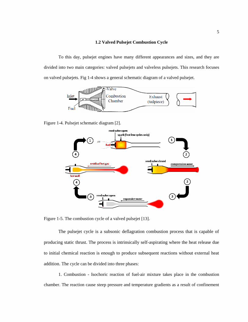
on valved pulsejets. Fig 1-4 shows a general schematic diagram of a valved pulsejet.
Figure 1-4. Pulsejet schematic diagram [2].
Figure 1-5. The combustion cycle of a valved pulsejet [13].
The pulsejet cycle is a subsonic deflagration combustion process that is capable of
producing static thrust. The process is intrinsically self-aspirating where the heat release due
to initial chemical reaction is enough to produce subsequent reactions without external heat
addition. The cycle can be divided into three phases:
1. Combustion - Isochoric reaction of fuel-air mixture takes place in the combustion
chamber. The reaction cause steep pressure and temperature gradients as a result of confinement

6
of the flow. In turn the rise of pressure and temperature accelerates the reaction. The pressure rise
causes the inlet valves to close, preventing backflow.
2. Expansion - The hot, high-pressure combustion products in the combustion chamber
expand, forcing flow through the exhaust.
3. Ingestion - Not all the combustion products are discharged; some are reserved as
residual to flow back upstream. At the same time, the momentum of the exhaust gases causes the
combustion chamber pressure to drop below the ambient pressure. The inlet valves open and suck
in a fresh charge of air mixed with fuel. Then the exhaust residual mixes with the fresh charge.
Therefore, the combination of compressed high temperature waves and the hot combustion
chamber wall are sufficient to initiate a new reaction and the cycle begins again.
1.3 Objectives
Although many studies have been done on pulsejet engines, the design parameters of
pulsejets have not been fully investigated and understood. Equations need to be developed to
scale pulsejets in a highly predictable manner.
Figure 1-6. 40cm hobby scale pulsejet.

7
Previous developed numerical simulation models are based on each research groups’ in-
house code or CFX software packages, some of them include turbulent models in order to study
the turbulent mixing field, they all require long computing time. Develop a simple numerical
model to simulate a real experiment and estimate average and maximum thrust produced by a
pulsejet was the primary objective of this work. Secondary goals of this project were to conduct a
numerical and experimental combined study on the operating frequency of a 40 cm hobby scale
pulsejet and the thrust produced by it.

8
Chapter 2
Numerical Model
In this chapter, the shock tube problem is used to study a one-dimensional Euler system
of PDEs (partial differential equations). Its exact solution will be presented to validate a Lax-
Wendroff Centered Schemes based numerical model. Then this model is modified with boundary
conditions to simulate a pulsejet engine.
2.1 Description of the Shock Tube Problem
Consider a long one-dimensional tube with closed ends, and divided by a thin diaphragm
into two equal regions. Each region contains the same gas, but with different thermodynamic
parameters (temperature, pressure, density). The region with the higher pressure is called the
driven section of the tube, which is shown on the left side in Fig 2-1.While the other part is the
working section. The gas in the tube is initially stationary, here we define the thermodynamic
parameters on the left side as pressure pL, density ρL, temperature TL, and the initial velocity
UL=0. Similarly, the thermodynamic parameters on the right side are pR , ρR, TR and UR=0.
At t=0 the diaphragm breaks, and generates a process that naturally tends to unify the
pressure in the tube. An expansion wave propagates to the left; the region of the expansion wave
(expansion fan) grows in time. While compression of the low pressure gas generates a shock
wave, which propagates to the right. Between the expanded and compressed gas is a contact
discontinuity travelling to the right side at constant speed, which is represented by a red dash line
in Fig 2-2.

9
Figure 2-1. Sketch of the initial configuration of the shock tube (t = 0) and waves propagating in
the tube after the diaphragm breaks (t > 0) [14].
Figure 2-2.Plots of different waves which are formed in the tube once the diaphragm breaks (t >
0).

10
2.2 Euler Equations of Gas Dynamics
To simplify the study of the shock tube problem, the gases on both sides are considered
as ideal gases. The other assumptions are: infinitely long tube perfectly isolated (no heat transfer
to the ambient environment); viscous effects are neglected. Then the compressible flow in the
shock tube is described by the one-dimensional Euler equations [15]
𝜕
𝜕𝑡(
𝜌𝜌𝑈𝐸
) +𝜕
𝜕𝑥(
𝜌𝑈
𝜌𝑈2 + 𝑝
(𝐸 + 𝑝)𝑈
) = 0 (2.1)
In which, E is the total energy:
𝐸 =𝑝
𝛾 − 1+
𝜌
2𝑈2 (2.2)
Equation of state for ideal gas is used to close this system:
𝑝 = 𝜌𝑅𝑇 (2.3)
R is the gas constant, 𝛾 is the ratio of specific heat coefficient. Local speed of sound a, Mach
number M, and the total enthalpy H are defined in the following equations:
𝑎 = √𝛾𝑅𝑇 = √𝛾𝑝
𝜌 (2.4)
𝑀 =
𝑈
𝑎 (2.5)
𝐻 =
𝐸 + 𝑝
𝜌 (2.6)
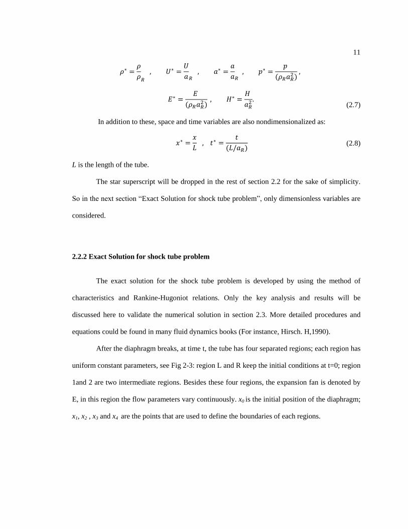
2.2.1 Dimensionless Equations
To save computational time and reduce errors, the parameters of the driven section are
used as a reference state. Thus all the parameters are nondimensionalized as:
11
𝜌∗ =
𝜌
𝜌𝑅
, 𝑈∗ =𝑈
𝑎𝑅 , 𝑎∗ =
𝑎
𝑎𝑅 , 𝑝∗ =
𝑝
(𝜌𝑅𝑎𝑅2 )
,
𝐸∗ =𝐸
(𝜌𝑅𝑎𝑅2 )
, 𝐻∗ =𝐻
𝑎𝑅2 .
(2.7)
In addition to these, space and time variables are also nondimensionalized as:
𝑥∗ =
𝑥
𝐿 , 𝑡
∗ =𝑡
(𝐿/𝑎𝑅) (2.8)
L is the length of the tube.
The star superscript will be dropped in the rest of section 2.2 for the sake of simplicity.
So in the next section “Exact Solution for shock tube problem”, only dimensionless variables are
considered.
2.2.2 Exact Solution for shock tube problem
The exact solution for the shock tube problem is developed by using the method of
characteristics and Rankine-Hugoniot relations. Only the key analysis and results will be
discussed here to validate the numerical solution in section 2.3. More detailed procedures and
equations could be found in many fluid dynamics books (For instance, Hirsch. H,1990).
After the diaphragm breaks, at time t, the tube has four separated regions; each region has
uniform constant parameters, see Fig 2-3: region L and R keep the initial conditions at t=0; region
1and 2 are two intermediate regions. Besides these four regions, the expansion fan is denoted by
E, in this region the flow parameters vary continuously. x0 is the initial position of the diaphragm;
x1, x2 , x3 and x4 are the points that are used to define the boundaries of each regions.

12
Figure 2-3. Diagram in the (x, t) plane of the exact solution of the shock tube problem.
The shock tube problem is a common test for the accuracy of computational fluid codes
[16], the initial condition data is used here:
(
𝜌𝐿
𝑝𝐿
𝑈𝐿
) = (1.01.00.0
), (
𝜌𝑅
𝑝𝑅
𝑈𝑅
) = (0.125
0.10.0
) . (2.9)
And the results are shown in Fig 2-4.

13
Figure 2-4. Exact solution of the shock tube problem with Sod’s initial condition, at t=0.2.
The three plots are all labeled: at t=0.2, region L and R are not influenced by breakdown
of the diaphragm; the parameters in region E vary continuously between region L and region 2
and are calculated by the following equations:
𝑈𝐸 =
2
𝛾 + 1(𝑎𝐿 +
𝑥 − 𝑥0
𝑡)
(2.10)
𝑎𝐸 = 𝑎𝐿 − (𝛾 − 1)
𝑈
2 (2.11)
𝑝𝐸 = 𝑝𝐿 (𝑎𝐸
𝑎𝐿)
2𝛾𝛾−1
(2.12)
the contact discontinuity between regions 1 and 2 is a discontinuity of density, the pressure and
the velocity are continuous; the shock wave between region 1 and R is represented by the jump of
parameters’ valve in all three plots.

14
2.3 Numerical Solution
2.3.1 Lax-Wendroff Centered Scheme
The second-order accurate scheme for Euler equations were historically the first to be
derived and still form the basis and the reference for all the other schemes derived since then [15].
The most popular scheme, the Lax-Wendroff scheme, will be studied and used to develop the
numerical solution for pulsejet engine model.
The independent variables in the Lax-Wendroff scheme are x and t, which represent
space and time respectively. The time domain is discretized as:
𝑡 ∈ [0, 𝑇], 𝑛 = 1,2, … , 𝑁, 𝛿𝑡 =
𝑇
𝑁 − 1 , 𝑡𝑛 = (𝑛 − 1)𝛿𝑡 (2.13)
And the space domain is discretized as:
𝑥 ∈ [0,1], 𝑗 = 1,2, … , 𝑀, 𝛿𝑥 =
1
𝑀 − 1 , 𝑥𝑗 = (𝑗 − 1)𝛿𝑥 (2.14)
The Euler equations can be written in conservative form:
𝜕𝑊
𝜕𝑡+
𝜕𝐹(𝑊)
𝜕𝑥= 0 (2.15)
with
𝑊 = (𝜌𝐴
𝜌𝑈𝐴𝐸𝐴
) , 𝐹(𝑊) = (𝜌𝐴
𝜌𝑈𝐴𝐸𝐴
) (2.16)

15
Figure 2-5. Computational stencil for the two-step Lax-Wendroff scheme.
As shown in Fig2-5, the scheme uses a three point stencil to reach second-order accuracy
in time and space. It contains two steps: a predictor and a corrector step. At point 𝑥𝑗 with the
information at time step n, 𝑊𝑗𝑛+1 is calculated by:
�̃�
𝐽+12
=
𝑊𝑗𝑛 + 𝑊𝑗+1
𝑛
2−
𝛿𝑡
2𝛿𝑥[𝐹(𝑊𝑗+1
𝑛 ) − 𝐹(𝑊𝑗𝑛)] (2.17)
𝑊𝑗
𝑛+1 = 𝑊𝑗𝑛 −
𝛿𝑡
𝛿𝑥[𝐹 (�̃�
𝑗+12
𝑛 ) − 𝐹 (�̃�𝑗−
12
𝑛 )] (2.18)
Obviously, the two points j=1 and j=M which represents inlet boundary and exhaust
boundary are not calculated, appropriate boundary conditions need to be specified. For the
solution for the shock tube problem, which we assume the tube is infinitely long, the vectors on
both boundaries are assumed to be constant and keep the initial values.
At last the stability condition is set as:
(|𝑈| + 𝑎)
𝛿𝑡
𝛿𝑥≤ 1 (2.19)

16
This condition is then used to compute the time step:
𝛿𝑡 = 𝑐𝑓𝑙 ∗
𝛿𝑥
|𝑈| + 𝑎 (2.20)
cfl is called the Courant number, and must be less than 1.
Figure 2-6. Comparison between exact solution and Lax-Wendroff scheme solution of the shock
tube problem with Sod’s initial condition, at t=0.2.
Unnatural oscillations are spotted around the sharp discontinuities from the Lax-
Wendroff solution plot (red) in Fig2-6, which can be minimized by adding in artificial dissipation
term into the solutions.

17
2.3.2 Artificial Dissipation
To improve previous the results, an artificial viscous flux is added into the Lax-Wendroff
scheme predictor step as:
𝐹(�̌�𝑛)̅̅ ̅̅ ̅̅ ̅̅ ̅ = 𝐹(�̌�𝑛) − 𝐷𝛿𝑥2𝛿𝑊
𝛿𝑥 (2.21)
The dissipation term is proportional to the gradient𝛿𝑊
𝛿𝑥, so will have an important smoothing effect
in the shock discontinuity region.
An original method developed by Von Neumann and Richtmyer [17] can be written for
quasi-linear flow in the above form by adding pressure term into momentum and energy
equations:
𝐷𝛿𝑥2𝛿𝑊
𝛿𝑥= 𝛼 ∗ 𝛿𝑥2 ∗ 𝜌 ∗ [
𝑜1𝑢
] |𝛿𝑢
𝛿𝑥|
𝛿𝑢
𝛿𝑥 (2.22)
𝛼 in the equation is an adjustable coefficient.
Fig 2-7 shows the results obtained with the artificial dissipation term, the oscillations near
the shock and expansion fan are reduced significantly, and overall have a good match with the
exact solution.

18
Figure 2-7. Comparison between exact solution and Lax-Wendroff scheme (with artificial
dissipation) solution of the shock tube problem with Sod’s initial condition, at t=0.2.
2.4 Numerical Model for Pulsejet and Boundary Conditions
2.4.1 Numerical Model for Pulsejet
The numerical model for the pulsejet engine is based on the numerical solution for the
shock tube discussed previously with additional quasi one-dimensional assumptions. The higher
pressure on the left side will represent the pressure rise because of chemical energy release from
the combustion.

19
The cross sectional area of the engine is modeled as a function of the axial coordinate,
A=A(x); and all flow parameters are functions of the axial coordinate and are equal in all other
directions:
𝑈 = 𝑈(𝑥), 𝑝 = 𝑝(𝑥), 𝑇 = 𝑇(𝑥), 𝜌 = 𝜌(𝑥) (2.23)
Table 2-1. The measurement of the pulsejet engine.
unit(inches) unit(centimeters)
Length of Combustion Chamber 2.5 6.35 Length of Taper Part 1.5 3.81
Length of Exhaust Pipe 11 27.94 Length of Flared Nozzle 0.5 1.27
Diameter of Combustion Chamber 1.625 4.1275 Diameter of Exhaust Pipe 0.875 2.2225 Diameter of Flared Nozzle 1 2.54
The measurement of the engine is shown in the table; the taper section diameter is
modeled by:
𝑑(𝑥) = (4.1275 + 2.2225)/2 +
(4.1275 − 2.2225)
2𝑡𝑎𝑛ℎ(
8.255 − 𝑥
0.005) (2.24)
and the flared nozzle diameter is modeled by:
𝑑(𝑥) = 2.2225 +
19.7
2(𝑥 − 38.1)2 (2.25)

20
Figure 2-8. Pulsejet engine’s geometric profile.
A MATLAB code was used to model the pulsejet engine’s geometric profile. The
derivative of equations (2.24) and (2.25) which represent 𝑑𝐴
𝑑𝑥 is shown in Fig2.8, to ensure that
intersections between different sections are continuous.
Then the governing equations with the no heat transfer and no viscous effects assumption
become:
𝜕
𝜕𝑡(
𝜌𝐴𝜌𝑈𝐴𝐸𝐴
) +𝜕
𝜕𝑥(
𝜌𝐴𝜌𝑈𝐴𝐸𝐴
) = (0
𝑃𝛿𝐴𝛿𝑥0
) (2.26)
And the conservative form becomes:
𝜕𝑊
𝜕𝑡+
𝜕𝐹(𝑊)
𝜕𝑥= 𝐺 (2.27)

21
With:
𝑊 = (𝜌𝐴
𝜌𝑈𝐴𝐸𝐴
) , 𝐹(𝑊) = (𝜌𝐴
𝜌𝑈𝐴𝐸𝐴
) , 𝐺 = (0
𝑃𝛿𝐴𝛿𝑥0
) (2.28)
The predictor and corrector step of Lax-Wendroff scheme become [18]:
�̃�
𝐽+12
=
𝑊𝑗𝑛 + 𝑊𝑗+1
𝑛
2−
𝛿𝑡
2𝛿𝑥[𝐹(𝑊𝑗+1
𝑛 ) − 𝐹(𝑊𝑗𝑛)] +
𝛿𝑡
4(𝐺𝑗+1
𝑛 + 𝐺𝑗𝑛) (2.29)
𝑊𝑗
𝑛+1 = 𝑊𝑗𝑛 −
𝛿𝑡
𝛿𝑥[𝐹 (�̃�
𝑗+12
𝑛 )̅̅ ̅̅ ̅̅ ̅̅ ̅̅ ̅̅
− 𝐹 (�̃�𝑗−
12
𝑛 )̅̅ ̅̅ ̅̅ ̅̅ ̅̅ ̅̅
] +𝛿𝑡
2(𝐺𝑗+1/2
𝑛+1/2+ 𝐺𝑗−1/2
𝑛−1/2) (2.30)
with the artificial dissipation term included in equation (2.30).
2.4.2 Boundary Conditions
As illustrated in Chapter 1, the reed valve remains closed when the inlet pressure is
higher than the ambient pressure and open when the inlet pressure is lower than the ambient
pressure to ingest more fuel and air mixture.
The infinite long tube assumption doesn’t hold here: the expansion fan will reflect back
from the closed valve, and the shock wave will reflect back from the flared nozzle exit. So the
inlet boundary needs to be modeled as a partially open valve and the exit boundary needs to be
modeled as an open and pressure release surface. Then the inlet and exhaust condition are
calculated using characteristic representation of the Euler equations following the formulation by
Poinsot and Lele [19], which is presented in Zinn’s paper [11].
First when the valves are closed, the inlet is modeled as a perfectly reflecting wall:
𝜕𝜌
𝜕𝑡= −
1
𝑎2 [𝑈 (𝑎2𝜕𝜌
𝜕𝑥−
𝜕𝑝
𝜕𝑥) + (𝑈 − 𝑎) (
𝜕𝑝
𝜕𝑥− 𝜌𝑎
𝜕𝑈
𝜕𝑥)]
(2.31)

22
𝜕𝑝
𝜕𝑡= −(𝑈 − 𝑎) (
𝜕𝑝
𝜕𝑥− 𝜌𝑎
𝜕𝑈
𝜕𝑥)
(2.32)
𝑈1 = 0 (2.33)
And the temperature is calculated from the perfect gas state equation; when the reed valves are
open, the inlet velocity is modeled by:
𝜕𝑈
𝜕𝑡=
1
𝜌𝑎(
𝜕𝑝
𝜕𝑡+ (𝑈 − 𝑎) (
𝜕𝑝
𝜕𝑥− 𝜌𝑎
𝜕𝑈
𝜕𝑥))
(2.34)
The pressure derivative in the equation requires another equation relating inlet pressure and
velocity for a closure:
∆𝑝 =1
2𝝃𝜌𝑈2[20] (2.35)
The equation is based on the Bernoulli equation, and relates the pressure gradient across the
valves and the inlet velocity. ∆𝑝 is the pressure difference between the stagnation pressure in the
fuel-air mixing area and the pressure at the combustion chamber inlet. 𝝃 is a parameter which
represents the resistance of the valves.
For the exhaust boundary, pressure always equals ambient pressure; velocity and density
are calculated by:
𝜕𝑈
𝜕𝑡= −
1
𝜌𝑎((𝑈 + 𝑎) (
𝜕𝑝
𝜕𝑥+ 𝜌𝑎
𝜕𝑈
𝜕𝑥))
(2.36)
𝜕𝜌
𝜕𝑡= −
𝑈
𝑎2(𝑎2
𝜕𝜌
𝜕𝑥−
𝜕𝑝
𝜕𝑥)
(2.37)
The simulation results and discussions will be shown in chapter 4.

23
Chapter 3
Experimental Apparatus and Setup
The goal of this experiment was to measure the average thrust the red head pulsejet can
produce and the working frequency. For these purposes, a test bed was built from scratch to hold
the pulsejet and measure the thrust by using strain gauge based load cell; a simple ignition system
and fuel delivery system were assembled; two thermocouples were used to measure the
combustion chamber temperature, and an infrared camera was used to insure the accuracy of data;
a microphone was used to measure the frequency. The fuel used in the experiment was gaseous
propane for good mixing and simplicity. The 40cm hobby scale pulsejet was purchased online.
3.1 Test Bed Design
A test bed was designed and machined by Mr. Richard Auhl and his team, which is
shown in Fig 3-1. The test bed base was a thick rectangular steel plate; two identical stair-shaped
modules were screwed in the shallow ditch on the plate surface, which were also made of steel.
Two identical aluminum mounting clamps were made to hold the jet, and they were fixed
on the beginning and ending point of the exhaust pipe separately by screws. Considering
combustion heat may increase the temperature in the exhaust pipe above the melting point of
Aluminum, which is 660.3°C, ceramic tapes were purchased from Cotronics Corp. to add a
thermal insulation layer between the engine and the clamps, see Fig 3-2. The tapes can be used in
conditions with high temperature exceeding 1260°C and offer good thermal insulation, low
thermal conductivity and heat storage.

24
Figure 3-1. Test bed.
Figure 3-2. Aluminum mounting clamps and ceramic tapes.
Ceramic tapes

25
3.2 Strain Gauge and Calibration
3.2.1 Strain Gauge
As shown in Fig 3-1, the two mounting clamps were attached to the stair-shaped modules
through two spring steel flexures. Four strain gauges were glued on the flexure piece close to the
flared nozzle, two on each side to form a full bridge configuration.
Figure 3-3. Strain Gauge.
When a force is applied on strain gauge and it is stretched within the limits of its
elasticity, it will become narrower and longer and its electrical resistance increases. With a full
bridge circuit, the output voltage is directly proportional to applied force. This was designed so as
to measure the thrust and drag force produced by the pulsejet during the experiment.

26
Figure 3-4. Full bridge strain gauge circuit.
Fig 3-4 shows the full bridge strain gauge circuit applied in this experiment. “Front”
indicates the side facing the combustion chamber, while “Back” indicates the side facing the
flared nozzle. And the output voltage can be calculated by:
𝑉 = 𝑉𝐼𝑛𝑝𝑢𝑡 [(
𝑅1
𝑅1 + 𝑅4) − (
𝑅2
𝑅2 + 𝑅3)]
(3.1)
𝑅1, 𝑅2, 𝑅3 and 𝑅4 represent the resistances of four strain gauges respectively, and 𝑉𝐼𝑛𝑝𝑢𝑡 is the
input voltage.
3.2.2 Calibration
To obtain the relation between output voltage of the strain gauge and the force applied on
the flexure, two sets of experiments were performed. The test bed was clamped to a stationary
cart. The pulsejet head was removed, and the combustion chamber inlet was covered by a steel
cap, which was attached by a thick nylon cord to a pulley system. Different weights were added
to the other end of the pulley system to mimic various thrust and drag force.

27
Figure 3-5. Pulley system.
The strain gauge was connected to a signal conditioning amplifier input port; the output
port was connected to a Fluke 179 multi-meter. The output voltage data is displayed in Fig 3-6;
the output port was also connected to HP 35670A dynamic signal analyzer to measure the natural
frequency of the test bed.
Figure 3-6. Data collecting and analysis system for calibration.

28
Negative values read on the multi-meter stands for drag force, positive values read on the
multi-meter stands for thrust, range of measurement: -10 to 10 volts.
Figure 3-7. Plots of pulley drag test, weights versus voltages.
The first set of tests was designed to test the relationship between the drag force and
strain gauge output voltage, and contained 3 tests:
Test 1: Kept adding weights without manually zeroing the amplifier. After removing all
the weights, -0.011 volts was read on the multi-meter;
Test 2: Kept adding weights without manually zeroing the amplifier. After removing all
the weights, - 0.009 volts was read on the multi-meter;
Test 3: Manually zeroed the amplifier between each step. The following table shows the
residuals in this test.
y_test1= -0.1542x + 0.0285
y_test2 = -0.1558x + 0.0291
y_test3 = -0.1663x + 0.0889
-8
-7
-6
-5
-4
-3
-2
-1
0
1
0 5 10 15 20 25 30 35 40
volt
s
lbs.
test 1 test 2 test 3

29
Table 3-1. Residuals in set1-test 3.
weight(lbs.) volts histories
0 0 0
1 -0.146 0
2 -0.291 0
3 -0.437 0.001
4 -0.585 0
5 -0.734 0
6 -0.884 0.001
7 -1.039 0.001
10 -1.503 0.002
15 -2.3 0
20 -3.127 -0.017
40 -6.68 -0.152
From Fig 3-7, the results from the first two tests were similar, results from test 3 had
good agreement with the previous two tests when the weights was lighter than 15 lbs. Since the
maximum drag force from both Zinn’s paper and the numerical simulation code prediction are
less than 11.5 lbs., y_test2 function was chosen to process experiment data in Chapter 4.
Figure 3-8. Plots of pulley thrust test, weights versus voltages.
y_test1 = 0.1661x - 0.017
y_test2= 0.1615x - 0.0371
-1
0
1
2
3
4
5
6
7
0 5 10 15 20 25 30 35 40
volt
s
lbs.
test 1 test 2

30
The second set of tests was designed to see the relationship between thrust and strain
gauge output voltage, and contained 2 tests:
Test 1: Kept adding weights without manually zeroing the amplifier. After removing all
the weights, 0.113 volts was read on the multi-meter
Test 2: Manually zeroed the amplifier between each step. The following table shows the
residuals in this test.
Table 3-2. Residuals in set 2- test 2.
weight(lbs.) volts histories
0 0 0
1 0.147 0
2 0.297 0
3 0.448 0
4 0.601 0
5 0.758 0
6 0.917 0
7 1.077 0.001
10 1.557 0.002
15 2.377 0.008
20 3.188 0.009
40 6.443 0
From Fig 3-8, the results from the two tests had good agreement with each other when
the weights were lighter than 15lbs. Since the maximum thrust from both Zinn’s paper and the
numerical simulation code prediction are higher than 11.5 lbs., y_test2 function was used to
process experimental data in Chapter 4.
During these calibration tests, as the weight was increased over 6lbs., the force might be
higher than the elastic limits of the material used in the flexure ( spring steel), and the force bent
it. The flexure could restore the original shape slowing, but not entirely recovered. Considering

31
the residuals read on the multi-meter because of the bending, the accuracy of the experiment
results may be off between 0.05 lbs. to 0.1 lbs.
During the experiment, data was transferred to a computer via a National Instruments
BNC-2100 low channel count single device.
3.3 Thermocouple
Two different thermocouples were purchased from OMEGA Engineering Inc. The first
one is an Unsheathed TC type K thermocouple, which is simply using the junction of two
dissimilar conducting metals to produce a temperature dependent voltage. Ice water was used to
calibrate the thermocouple. The original method to measure the combustion chamber was putting
the thermocouple on the chamber outside surface, and measuring the surface temperature. A test
was applied to test the accuracy of the thermocouple and also the possibility of the method. The
red head was removed and the thermocouple was placed on the upper surface of the combustion
chamber, a heat gun was used to heat the air in the chamber.
Figure 3-9. Unsheathed TC type K thermocouple (indicated by green circle) accuracy testing.

32
Fig 3-9 shows the infrared image of the pulsejet during the testing, taken by a FLIR T620
infrared camera, the glowing bright part is a wielding seam. At that time, the temperature tested
from the thermocouple was 156.5°C, while the temperature from the high accuracy camera was
237°C (spot 2). Also during the testing, if the two wires had any connection besides the junction
(measuring point), the measured value would drop further.
Figure 3-10. HH (High Temperature Fiberglass) SLE type K thermocouple.
This test proved that measuring the surface temperature was not an ideal method. So the
second thermocouple was purchased, which is a HH (High Temperature Fiberglass) SLE type K
thermocouple, see Fig 3-10. This one was placed inside the combustion chamber through the
exhaust pipe to measure the chamber temperature directly. To prevent the exhaust flow blow out
the thermocouple, a metal wire was twined around the thermocouple and formed a ring with a
diameter larger than the diameter of the exhaust pipe. The thermocouple was also calibrated by
using ice water. And because the wire was covered by a fiberglass sleeve, error from connecting
with other metal material was prevented.

33
3.4 Other Instruments and Systems
3.4.1 Fuel Delivery System
A propane tank was used as the fuel source, and was originally connected to a grill
regulator, which had three flow rates. The design was proved not functional when we first
attempted to initiate the combustion. To have higher flow rate, a valve that simply linearly
increase the flow rate and tubing with larger diameter were used to replace the original design,
see Fig 3-11.
Figure 3-11.Original fuel delivery system (left) and improved fuel delivery system (right).
To initiate the combustion, an air compressor was used to blow in compressed air with 40
psi into the inlet. The compressed air not only mixed with propane but also opened the reed valve
and the fuel-air mixture was injected into the combustion chamber.

34
3.4.2 Ignition System
The pulsejet used a miniature “champion V-2” spark plug to provide the necessary
temperatures to start the combustion process. The spark plug was connected to a Model-T Ford
ignition coil which transforms low voltage electricity to a higher voltage suitable for the spark
plug. The system was powered by a 12V battery.
The system was disconnected from the battery after the pulsejet engine combustion
chamber temperature was hot enough to sustain the combustion by itself.
Figure 3-12. Model-T Ford ignition coil and spark plug.

35
3.4.3 Sound Measurement System
A highly sensitive microphone was used to measure the frequency of the pulsejet engine
operating cycle. During a pre-testing, the microphone also picked up a noise signal, and the
frequency was 30Hz. So a Krohn-Hite analog electrical filter was used to filter out frequencies
lower than 30 Hz.
Figure 3-13. Microphone and analog electrical filter.
3.5 Procedures
3.5.1 Data Collection
The strain gauge was connected to a signal conditioning amplifier input port; the output
port was connected to a computer via a National Instruments BNC-2100 low channel count single
device. Two thermocouples were connected to the low channel count single device directly. The
microphone signal was filtered first, and then connected to the low channel count single device. A
LabView code was used to communicate to the BNC-2100 low channel count single device and

36
transfer the data off of it. This code collected at a sample rate of 5,000 Hz, and the range of data
is -10 volts to 10 volts.
Figure 3-14. Data acquisition Labview code front panel.
3.5.2 Engine run procedure
Considering the noise and possibility of fire accident, all the experiments were conducted
at an outside open area, and a fire extinguisher was prepared.
First the air compressor was started. When the pressure level became stable, the data
acquisition system was started. Next the ignition system was connected to the 12v battery and the

37
spark plug started to generate a continuous electrical spark. Finally the valve of the propane tank
was opened slowly and the flow rate was increased slowly until the fuel-air mixture was ignited.
During the experiment, 10 tests were made: the first five had the SLE type K
thermocouple inside the combustion chamber, and the other five had it on the outside surface.
The valve of the propane tank was controlled by a team member, and the flow rate was deceased
and increased during the combustion process in different tests to get a good fuel-air mixture.
Unfortunately, in none of the tests, the combustion was self- sustainable without the air
compressor forcing air into the inlet.
The results will be discussed in the Chapter 4.
3.5.3 After Treatment
In each test, after the propane valve was closed, the data acquisition system was stopped.
The air compressor was left on for a few more minutes to kept blowing cool air into the pulsejet
engine to cool down the engine.
When the engine was cooled to a temperature under 40°C, the inlet was removed. The
spark plug and the reed valve were examined to make sure they were still functional for the next
test.

38
Chapter 4
Results and Discussions
4.1 Experiment results
As mentioned in the previous chapter, the sample rate was set to be 5,000 Hz and the
recorded data was saved as a text document. The experimental data were initially plotted by using
Excel, which gave a quick overview of the data quality.
The second thermocouple was placed inside the combustion chamber in the first 5 tests,
and none of these 5 tests had successful continuous combustion longer than a few seconds. It’s
clear that to have a better combustion, the chamber must be clear; otherwise the acoustic wave
would be affected. So in the last 5 tests, the second thermocouple was placed on the outside
surface of the chamber.
The output data that represents the instantaneous thrust from the load-cell were recorded
as a voltage; it was converted to lbs. by using the calibration relation functions obtained in section
3.2.2. The microphone's output was in volts and the selected data were moved to a MATLAB
code where it went through a Fast Fourier Transform (FFT) and then plotted to find the peak that
represents the dominating frequency. Some continuous peaks of the thrust data where the
combustion occurred were picked out to calculate the operating frequency and compare to the
frequency received from the FFT of the microphone output data. The temperature data was
converted to Celsius by multiplying by 130°C/V, and the average maximum temperature was
calculated.
2 tests were selected for discussion because they had a longer combustion time compared
to the others. Test-7 and Test-10 represent the chosen tests respectively in the following
discussion.
39
4.1.1 Test-7
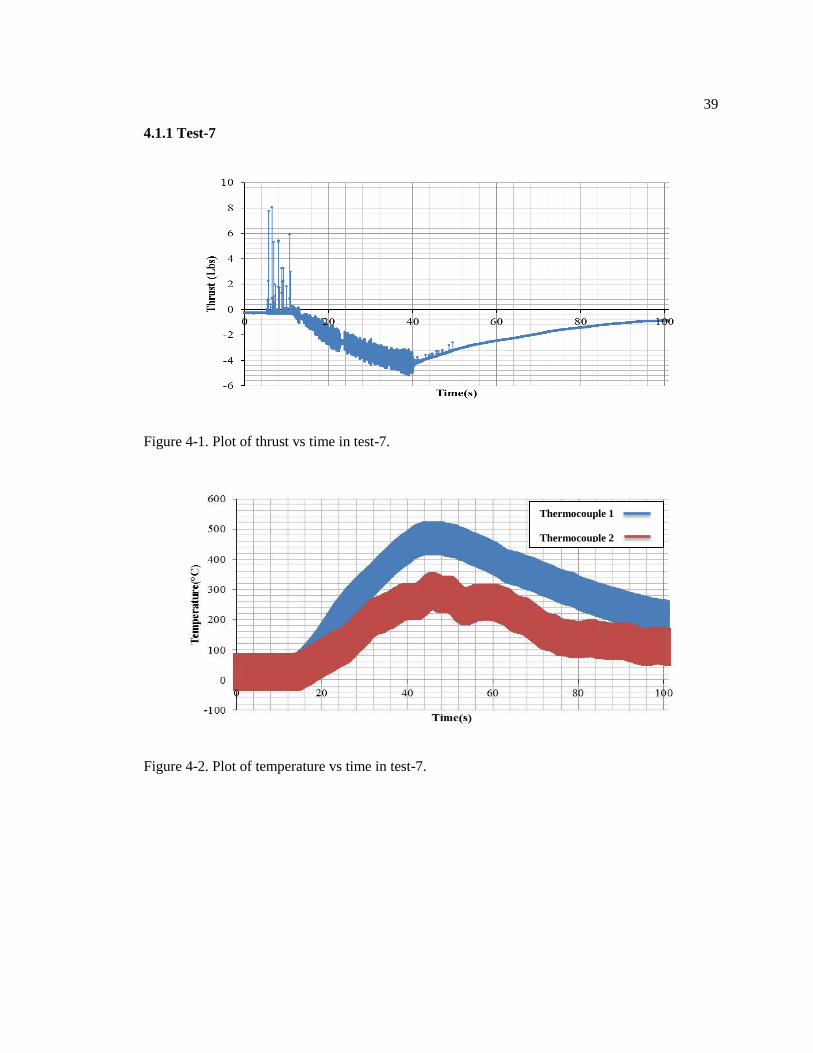
Figure 4-1. Plot of thrust vs time in test-7.
Figure 4-2. Plot of temperature vs time in test-7.
Thermocouple 1
Thermocouple 2

40
Figure 4-3. Plot of sound vs time in test-7.
From Fig 4-1 and Fig 4-3, major combustion events were spotted between 12s and 40s,
while in Fig 4-2, the measured temperature started to increase from 14s, and kept increasing until
44s. So because of the thermocouples were measuring the outside chamber surface temperature
instead of measuring the mixture temperature inside the chamber, the temperature measurement
could not reflect the instantaneous temperature inside the chamber. But after the pulse jet engine
reached the stable working cycle, the temperature measurement could reflect the maximum
temperature inside the chamber.
The next observation was when the two thermocouples were placed on the outside
surface, compared to the reference temperature measured by the infrared camera, thermocouple 1
had better measurement than thermocouple 2. For this reason, temperature measured by
thermocouple 2 was neglected in the rest of the discussion.
As the temperature increased, the strain gauge zero shifted to a negative value; after the
combustion stopped, the strain gauge zero shifted back. Although a full bridge circuit strain gauge
was used in the experiment, which should compensate the temperature effects on the strain
measurement, clearly the compensation didn’t work. The heat was transferred from the engine
body to the mounting clamp and the flexure through conduction and radiation. And because the

41
flexure was fixed between the mounting clamp and stair-shaped base by screws, it expanded
unevenly when it was heated.
Based on these discussions, thrust and sound data collected from time 39.16s to 39.26s
were selected. While temperature data from time 46s to 46.1s were selected since the maximum
temperature was our primary concern.
Figure 4-4. Plot of temperature vs time (46 s to 46.1s) in test-7.
Average maximum temperature from 46s to 46.1s was 471.8148 °C. This value will be
needed in the numerical study section 4.2.

42
Figure 4-5. Plot of sound data from (39.16s to 39.26s) in test-7.
Figure 4-6. Plot of thrust vs time (39.16s to 39.26s) in test-7.
The operating frequency measured from the microphone was 305.6 Hz. In Fig 4-6, two
red circles were used to indicate two groups of combustion events which could also be identified
43
in Fig 4-5. Three continuous peaks of the thrust data in Fig 4-6 were picked out to calculate the
operating frequency. The frequency calculated from the selected data was 310Hz. So the load-cell
was capable of picking up each combustion event, and the frequency could be derived from the
thrust data with a small error.
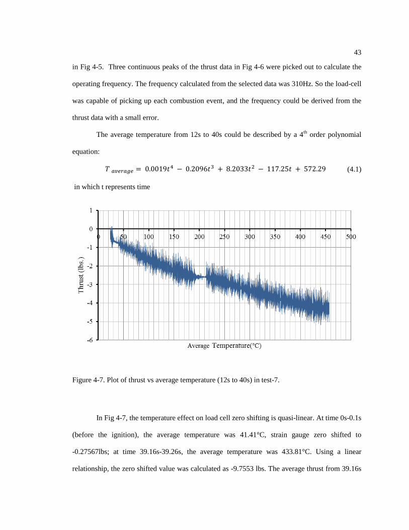
The average temperature from 12s to 40s could be described by a 4th
order polynomial
equation:
𝑇 𝑎𝑣𝑒𝑟𝑎𝑔𝑒 = 0.0019𝑡4 − 0.2096𝑡3 + 8.2033𝑡2 − 117.25𝑡 + 572.29 (4.1)
in which t represents time
Figure 4-7. Plot of thrust vs average temperature (12s to 40s) in test-7.
In Fig 4-7, the temperature effect on load cell zero shifting is quasi-linear. At time 0s-0.1s
(before the ignition), the average temperature was 41.41°C, strain gauge zero shifted to
-0.27567lbs; at time 39.16s-39.26s, the average temperature was 433.81°C. Using a linear
relationship, the zero shifted value was calculated as -9.7553 lbs. The average thrust from 39.16s

44
to 39.26s was -4.2797 lbs. So using this value to make temperature compensation to the average
thrust, the result was 5.4765 lbs.
Figure 4-8. Plot of magnitude vs frequency of the thrust data (39.16s to 39.26s) in test-7.
Thrust data from 39.16s to 39.26s also went through a FFT, and the result was plotted in
Fig 4-8. Clearly the dominating frequency in the test was 65.13 Hz which was the test bed natural
frequency; and the engine operating frequency was 305.6 Hz. A Butterworth filter was used to
damp the test bed natural frequency; unfortunately it also filtered out the average DC signal.
X 65.13, Y 81.69
X 305.6, Y 7.5

45
4.1.2 Test-10
Figure 4-9. Plot of thrust vs time in test-10.
Figure 4-10. Plot of temperature vs time in test-10.

46
Figure 4-11. Plot of sound vs time in test-10.
Compared to test-7, similar results were observed from test-10.
From Fig 4-9 and Fig 4-11, major combustion events were spotted between 86s and 106s,
while in Fig 4-10, the measured temperature started to increase from 87.5s, and kept increasing
until 110s.
Based on previous discussion and analysis, thrust and sound data collected from time
105.5s to 105.6s was selected. Temperature data from time 112.45s to 112.55s was selected since
the maximum temperature was our primary concern.
Figure 4-12. Plot of temperature vs time (112.45 s to 112.55s) in test-10.

47
Average maximum temperature from 112.45 s to 112.55s was 548.67 °C. This value will
be needed in the numerical study section 4.2.
Figure 4-13. Plots of sound data from (105.5s to 105.6s) in test-10.
Figure 4-14. Plot of thrust vs time (105.5s to 105.6s) in test-10.

48
In Fig 4-13, the operating frequency measured from the microphone was 355.7 Hz; two
red circles were used to indicate two groups of combustion events which could also be identified
in Fig 4-14. Five continuous peaks of the thrust data in Fig 4-14 were picked out to calculate the
operating frequency. The frequency calculated from the selected data was 340Hz. Again, this
proved the load-cell was capable of picking up each combustion event, and the frequency could
be derived from the thrust data with a small error.
The average temperature from 86s to 106s could be described by a 4th order polynomial
equation:
𝑇 𝑎𝑣𝑒𝑟𝑎𝑔𝑒 = 0.0029𝑡4 − 1.1341𝑡3 + 167.34𝑡2 − 10920𝑡 + 265685 (4.2)
in which t represents time.
Figure 4-15. Plot of thrust vs average temperature (86s to 106s) in test-10.
In Fig4-15, the temperature effect on load cell zero shifting was quasi-linear. At time 0s-
0.1s (before the ignition), the average temperature was 73.81°C, strain gauge zero shifted to
-1.07978 lbs.; at time 105.5s-105.6s, the average temperature was 489.8624°C. Using a linear
relationship, the zero shifted value was calculated as -12.0756 lbs. The average thrust from 105.5s

49
to 105.6s was -6.7951 lbs. So use this value to make compensation to the average thrust, the
result was 5.2815 lbs.
Test-10 had the longest continuous combustion among all the tests. During this test time
86s to 106s, to reach a better combustion, a team member controlled the air compressor and
turned down the pressure gradually from 40 psi to 25 psi; while another team member controlled
the fuel flow rate, and increased it slowing. This resulted in a fuel-air mixture with a different
fuel–air equivalence ratio. To see the influence of fuel–air equivalence ratio on the combustion,
sound and thrust data from 90.1s to 90.2 s was selected.
Figure 4-16. Plots of sound data from (90.1s to 90.2s) in test-10.

50
Figure 4-17. Plot of thrust vs time (90.1s to 90.2s) in test-10.
In Fig 4-16, the operating frequency measured from the microphone was 325.7 Hz; two
red circles were used to indicate two combustion events which could also be identified in Fig
4-17. Three continuous peaks of the thrust data in Fig 4-17 were picked out to calculate the
combustion frequency. The frequency calculated from the selected data was 333Hz.
So comparing to the results from 105.5s to 105.6s, when the pulse jet was running on
different fuel–air equivalence ratios, the operating frequency was also different.
51
4.2 Numerical simulation results
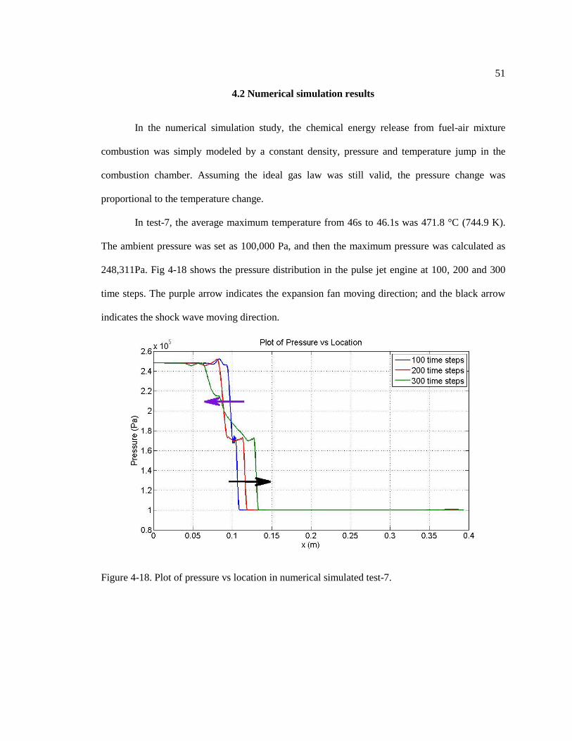
In the numerical simulation study, the chemical energy release from fuel-air mixture
combustion was simply modeled by a constant density, pressure and temperature jump in the
combustion chamber. Assuming the ideal gas law was still valid, the pressure change was
proportional to the temperature change.
In test-7, the average maximum temperature from 46s to 46.1s was 471.8 °C (744.9 K).
The ambient pressure was set as 100,000 Pa, and then the maximum pressure was calculated as
248,311Pa. Fig 4-18 shows the pressure distribution in the pulse jet engine at 100, 200 and 300
time steps. The purple arrow indicates the expansion fan moving direction; and the black arrow
indicates the shock wave moving direction.
Figure 4-18. Plot of pressure vs location in numerical simulated test-7.

52
Figure 4-19. Plot of parameters vs time at pulsejet valve inlet in numerical simulated test-7.
The reed valve was modeled by two pressure conditions: when the pressure at the valve
inlet dropped below ambient pressure (100,000Pa), the valve opened and sucked in more fuel-air
mixture for the next combustion event; the pressure rise above ambient pressure as next
combustion occurred, and the valve closed. Fig 4-19 shows pressure and velocity at the inlet, and
add-in pressure represents the pressure rise because of new combustion event.

53
Figure 4-20. Plot of parameters vs time at pulsejet exit in numerical simulated test-7.
Fig 4-20 shows the velocity and momentum at the pulsejet engine exit during 5 operating
cycles (0.00148s-0.024s). The operating frequency was calculated as 222Hz and the average
thrust was 3.9616N (0.8906 lbs.); the maximum instantaneous thrust was 30N (6.74 lbs.).

54
In test-10, average maximum temperature from 112.45 s to 112.55s was 548.7 °C
(821.8 K). The ambient pressure was set as 100,000 Pa, and then the maximum pressure was
calculated as 273,930Pa. Fig 4-21 shows the pressure distribution in the pulse jet engine at 100,
200 and 300 time steps. The purple arrow indicates the expansion fan moving direction; and the
black arrow indicates the shock wave moving direction.
Figure 4-21 Plot of pressure vs location in numerical simulated test-10.

55
Figure 4-22. Plot of parameters vs time at pulsejet valve inlet in numerical simulated test-10.

56
Figure 4-23. Plot of parameters vs time at pulsejet exit in numerical simulated test-10.
Fig 4-23 shows the velocity and momentum at the pulsejet engine exit during 5 operating
cycles (0.00245s-0.024s). The working frequency was calculated as 232Hz and the average thrust
was 4.1732N (0.9382 lbs.); the maximum instantaneous thrust was 32N (7.2 lbs.).

57
4.3 Comparison and Overview
To have a better view of the previous results, the operating frequency from both
experiments and the simulation study are shown in Table 4-1.
Table 4-1. Table of different frequency results from experiments and simulation study.
Frequency(microphone) Frequency(thrust) Frequency(simulation)
test-7 305.6 Hz 310 Hz 222 Hz
test-10 355.7 Hz 340 Hz 232 Hz
Comparing the results from the sound measurement and numerical simulation study, the
difference is obvious. As stated in Chapter 3, during the experiment, in none of the 10 tests the
engine was able to run without the air compressor. The air compressor was constantly blowing
compressed air into the inlet, and opening the reed valve. So before and after the ignition, the
pressure in the combustion chamber was higher than ambient pressure. During the combustion,
because of the pressure at the valve inlet was higher than ambient pressure, the reed valve opened
more easily and frequently. Naturally the flow rate was higher and the combustion frequency was
higher.
Even though the frequency calculated from simulation needs more support from an
improved experiment in the future, it can be validated by Geng’s paper, in which he did a study
on ‘effect of pulsejet length on frequency’, which shows that 232Hz is a good prediction of the
40cm length pulsejet engine operating frequency.

58
Table 4-2. Table of different average thrust results from experiments and simulation study.
Average thrust
( experiment) Average thrust
(simulation)
test-7 5.4765 lbs. 0.8906 lbs.
test-10 5.2815 lbs. 0.9382 lbs.
Average thrust from both the experiments and simulation study are shown in Table 4-2.
Again difference is large between the experiment and numerical simulation study. Besides the
effect of the constant high pressure air flow from the compressor, the temperature effect on the
strain gauge also needs more future study to be compensated for. Also the experiments were
conducted at an outdoor open area, convection heat transfer from the pulsejet to ambient
environment might be accelerated by the wind, and this would further affect the temperature
measurement.
The numerical computation related errors mainly come from the ideal gas and energy
addiction assumptions. In the model, the energy released from new combustion cycle was simply
modeled as pressure and temperature rise in the combustion chamber, yet the combustion product
was unknown. So the specific heat of the mixture inside the chamber was not specified
accurately. To have a better and direct simulation, chemical reaction model integration is
necessary.
Comparing average thrust from the simulation study to previous study in published
papers, 4.18 N (0.94 lbs.) is a reasonable estimation of the average thrust that the 40 cm pulsejet
engine can deliver. And the maximum instantaneous thrust was 32N (7.2 lbs.).
59
Chapter 5
Conclusions and Future Work
5.1 Summary and Conclusions
The purpose for this project was to study the working mechanism of a pulsejet engine,
and conduct a combined numerical simulation and experimental thrust study of a 40 cm pulsejet
engine.
A numerical simulation code based on the shock tube model with additional quasi one-
dimensional assumptions was built using the second-order accurate Lax–Wendroff scheme. The
code was capable of predicting flow parameters at various locations of a pulsejet engine with
different lengths and diameters.
The simulation model estimated the 40 cm pulsejet can deliver an average 4.18 N (0.94
lbs.) thrust with a 232 Hz operating frequency. And the maximum instantaneous thrust was 32N
(7.2 lbs.).
A test bed with mounting clamps was manufactured with a full bridge circuit strain gauge
to measure thrust; two different thermocouples were used to measure temperature; a highly
sensitive microphone was used to collect sound data to calculate the operating frequency of the
pulsejet. A simple fuel delivery system with an air compressor and an ignition system were also
assembled.
10 tests were run on gaseous propane. Two tests achieved more than 20s of continuous
combustion time, and they were selected to be simulated by the developed model. Unfortunately,
none of these tests could sustain the combustion without assistance from an air compressor.
Because of this, the operating frequency and average thrust from the experiment were higher than

60
the results from the simulation model. Also, the thermal energy radiated and conducted from the
combustion chamber had a large effect on the thrust measurement; the load cell zero shifted to a
negative value and the effect was quasi-linear. Temperature compensation was made to the
measured thrust.
The load cell was proved to be capable of detecting and recording each combustion
event; and the operating frequency could be derived from the thrust data with reasonable
accuracy. Also, when the pulse jet was running on different fuel–air equivalence ratios, the
working frequency was different.
5.2 Future Work
The numerical simulation model needs improved experimental data for better validation.
To get the engine running without the help from the air compressor and have a better thrust
measurement, some adjustment and improvement of the experimental test bed needs to be done:
1. Improve the fuel delivery system by using more controllable and precise valves, and
integrating flow rate measurement equipment into the system to measure the fuel flow rate.
2. Redesign the thrust measurement system by mounting the thrust stand on a rail, and
connecting on side of the sand to a low-friction linear bearing assembly system.
3. Run the pulsejet on different fuels, ethanol, gasoline, etc.
4. Redesign and manufacture a new pulsejet with thicker and strong material so that holes
can be drilled at combustion chamber. Put different probes and thermocouples inside the chamber
to measure the pressure, velocity and temperature.
The numerical simulation model can also be improved by integrating a chemical reaction
model.

61
Bibliography
[1] Yungster, Shaye, Daniel E. Paxson, and Hugh D. Perkins. "Computational Study of
Pulsejet-Driven Pressure Gain Combustors at High-Pressure." AIAA paper 3709 (2013).
[2] Geng, Tao, et al. "Combined numerical and experimental investigation of a hobby-
scale pulsejet." Journal of propulsion and power 23.1 (2007): 186-193.
[3] ZINN, BENT. "Pulsating combustion." Advanced combustion methods (A 87-50643
22-25). London and Orlando, FL, Academic Press, 1986, (1986): 113-181.
[4] Ordon, Robert Lewis. "Experimental Investigations into the operational parameters of
a 50 Centimeter Class Pulsejet Engine." (2006). PhD thesis, North Carolina State University.
[5] Reynst, François Henri. "Pulsating combustion: the collected works of FH Reynst."
Pergamon Press, 1961.
[6] Foa, Joseph V. "Elements of flight propulsion." Wiley, 1960.
[7] Goebel, Greg. "The V-1 Flying Bomb." Excerpt from an unpublished article,
http://www. vectorsite. net/twcruz2. html 1 (2004).
[8] http://media.iwm.org.uk/iwm/mediaLib//26/media-26724/large.jpg
[9] Choutapalli, Isaac, Anjaneyulu Krothapalli, and Luiz M. Lourenco. "Pulsed jet:
ejector characteristics." 44th AIAA Aerospace Sciences Meeting & Exhibit, Reno, Nevada, USA.
2006.
[10] Lockwood, R. M. "Pulse reactor lift-propulsion system development program." No.
ARD-308. HILLER AIRCRAFT CORP. PALO ALTO CA, 1963.
[11] Erickson, R., and B. T. Zinn. "A Numerical Investigation of the Effect of Energy
Addition Processes on Pulsejet Wave Engine Performance." 42 nd AIAA Aerospace Sciences
Meeting and Exhibit. 2004.

62
[12] Litke, Paul J., et al. "Assessment of the Performance of a Pulsejet and Comparison
with a Pulsed-Detonation Engine." AIAA paper 228 (2005): 2005
[13] Beers, Benjamin R. "Investigating Geometrical Configurations of a Hobby-scale
Pulsejet Engine for Maximum Thrust Efficiency." Diss. Pennsylvania State University, 2011.
[14] Danaila, Ionut, et al. "An introduction to scientific computing: Twelve
computational projects solved with MATLAB." Springer Science & Business Media, 2007.
[15] Hirsch, H. "Numerical computation of internal and external flows."Computational
methods for inviscid and viscous flows 2 (1990): 536-556.
[16] Sod, Gary A. "A survey of several finite difference methods for systems of nonlinear
hyperbolic conservation laws." Journal of computational physics 27.1 (1978): 1-31.
[17] VonNeumann, John, and Robert D. Richtmyer. "A method for the numerical
calculation of hydrodynamic shocks." Journal of applied physics 21.3 (1950): 232-237.
[18] Warren, M. D. "Calculation of the reflected wave from a pipe with a nozzle end by
the Lax-Wendroff method." International journal of heat and fluid flow 6.3 (1985): 205-211.
[19] Poinsot, T. J. A, and S. K. Lelef. "Boundary conditions for direct simulations of
compressible viscous flows." Journal of computational physics 101.1 (1992): 104-129.
[20] Benelli, G., G. De Michele, V. Cossalter, M. Da Lio, and G. Rossi. "Simulation of
large non-linear thermo-acoustic vibrations in a pulsating combustor." InSymposium
(International) on Combustion, vol. 24, no. 1, pp. 1307-1313. Elsevier, 1992.

63
Appendix A
Exact solution Code
function [data] = exact_solution_shocktube(t) % | | | | % L | E | 2 | 1 | R % | | | | %___|_______|___*_____|_________|__________ % x1 x2 x0 x3 x4 % E is the expansion fan % Between 2 and 1 is the discontinuity, it is a discontinuity of the % density function, so v_2=v_1 P_2=P_1 % Between 1 and R is the shock wave % t (time) t =0.2; %Initial conditions gamma = 1.4; x0 = 0.5;
P_R = 0.1; %pa %T_R =300; %k %R_AIR=286.9; %j/kg.k rho_R = 0.125;%P_R/(R_AIR*T_R); u_R = 0;
rho_L = 1.0;%rho_R; P_L = 1.0;%2*P_R; u_L = 0; x_min =0.0; x_max = 1.0;
%speed of sound a_L = (gamma*P_L/rho_L)^(0.5); %local speed of sound in zone L a_R = (gamma*P_R/rho_R)^(0.5); %local speed of sound in zone R
v_shock = fzero('sod_func',pi); %shock wave speed
P_1=(( 2*gamma* (v_shock^2)-(gamma-1))/(gamma+1) )*P_R; % pressure in
zone 1 v_1 = (2/(gamma+1))*(v_shock-1/v_shock); % velocity in zone 1*a_R rho_1 =rho_R/( 2/((gamma+1)* (v_shock^2))+(gamma-
1)/(gamma+1) ); %density in zone 1 rho_2 = (rho_L)*power((P_1/P_L),1/gamma); %density in zone 2
%Key Positions x1 = x0 - a_L*t; x3 = x0 + v_1*t; x4 = x0 + v_shock*t;

64
c_2 = a_L*power(P_1/P_L,(gamma-1)/(2*gamma)); x2 = x0 + (v_1 - c_2)*t;
%start setting values n_points = 501; x = linspace(x_min,x_max,n_points); data.x = x'; data.rho = zeros(n_points,1); %density data.P = zeros(n_points,1); %pressure data.u = zeros(n_points,1); %velocity data.T = zeros(n_points,1); %temperature data.v_shock=sod_func(v_shock);
for index = 1:n_points if data.x(index) < x1 %Solution before x1 data.rho(index) = rho_L; data.P(index) = P_L; data.u(index) = u_L;
elseif (x1 <= data.x(index) && data.x(index) <= x2) %Solution expansion fan, between x1 and x2 data.u(index) =( 2/(gamma+1))*(a_L+(data.x(index)-x0)/t); c = a_L-((gamma-1)*data.u(index))/2; data.P(index) = P_L*power((c/a_L),((2*gamma)/(gamma-1))); data.rho(index) = gamma*data.P(index)/(c^2); elseif (x2 < data.x(index) && data.x(index) <= x3) %Solution in zone 2, between x2 and x3 data.rho(index) = rho_2; data.P(index) = P_1; data.u(index) = v_1; elseif (x3 <= data.x(index) && data.x(index) <= x4) %Solution in zone 1, between x3 and x4 data.rho(index) = rho_1; data.P(index) = P_1; data.u(index) = v_1; elseif (x4 < data.x(index)&& data.x(index)<= 1) %Solution after x4 data.rho(index) = rho_R; data.P(index) = P_R; data.u(index) = u_R;
end data.T(index) = data.P(index) / data.rho(index); end
end

65
function y = sod_func(v_shock) %defines function to be used in analytic_sod %Initial conditions gamma = 1.4;
P_R = 0.1; %pa %T_R =300; %k %R_AIR=286.9; %j/kg.k rho_R = 0.125;%P_R/(R_AIR*T_R);
rho_L = 1.0;%rho_R; P_L = 1.0;%2*P_R;
a_L = (gamma*P_L/rho_L)^(0.5); a_R = (gamma*P_R/rho_R)^(0.5);
y=v_shock-1/v_shock-a_L*((gamma+1)/(gamma-1))* (1-
(power(((P_R/P_L)*(( 2*gamma* (v_shock^2)-(gamma-
1))/(gamma+1) )),(gamma-1)/(2*gamma))));
end

66
Appendix B
Pulsejet Geometry Model Code
clear all %initial parameters j = 1001; %number of grid points x1=0; x2=0.0635; %unit: m, equals 2.5 inches, the starting point of the taper
section x3=0.1016; %unit: m, equals 4 inches, the ending point of the taper
section x4=38.1e-2; %unit: m, equals 15 inches, x5=39.37e-2; %unit: m, equals 15 1/2 inches, y1=(4.1275e-2)/2; % 1 5/8inches combustion chamber y2=(0.022225)/2; %7/8 inch diffuser x = linspace(x1,x5,j);
data.x = x'; data.r= zeros(1,j); data.d= zeros(1,j); L=x5-x1; dx = L/(j-1); for index = 1:j
if (x1 <= data.x(index) && data.x(index) <x2) %combustion chamber data.r(index)=y1; % 1 5/8inches
data.d(index)=0;
elseif (x2 <= data.x(index) && data.x(index) < x3) %taper data.r(index)=(y2+y1)/2+0.5*(y1-y2)*tanh((8.255e-2-
data.x(index))/0.005); data.d(index)=2*pi*data.r(index)*((y2-y1)/0.01)*sech((8.255e-2-
data.x(index))/0.005)^2;
elseif (x3 <= data.x(index) && data.x(index) < x4) %exhuast tube data.r(index)=y2; %7/8 inch
data.d(index)=0;
elseif (x4 <= data.x(index) && data.x(index) <= x5) %flared nozzle data.r(index)=y2+19.7*(data.x(index)-x4)^2/2;%*39.37e-2; data.d(index)=2*pi*data.r(index)*19.7*(data.x(index)-x4); end end
A(1:j)=pi*(data.r(1:j)).^2;

67
Appendix C
Numerical Model Code
%Shock tube numerical solution Lax-Wendroff method with artificial %dissipation CFL= 0.2; %CFL number for stability alpha=0.009; %coefficient for artificial viscosity gamma=1.4;
%initial parameters on the right side of the tube at t=0 p_r=100000; %pa T_r =303.15; %k R_air=286.9; %j/kg.k rho_r = p_r/(R_air*T_r); u_r=0; %initial parameters on the left side of the tube at t=0 rho_l = rho_r; p_l =2.74*p_r; %depends on the experiment result u_l = 0; b=0.000005; c=0.000005; d=0.000005; p(1:j)=(p_l+p_r)/2+(p_l-p_r)/2*tanh((x3-x)/b); rho(1:j)=(rho_l+rho_r)/2+(rho_l-rho_r)/2*tanh((x3-x)/c); u(1:j)=(u_l+u_r)/2+(u_l-u_r)/2*tanh((x3-x)/d); e = p./((gamma-1)*rho); E = (e + u.^2/2).*rho; a=sqrt(gamma*p./rho); % speed of sound dt=CFL*dx/max(a+abs(u)); %time step based on CFL number t_final=0.024; %final time n=round(t_final/dt); rho_1(1:n)= zeros(n,1); u_1(1:n) = zeros(n,1); m_1(1:n)=zeros(n,1); T_1(1:n)=zeros(n,1); p_1(1:n)=zeros(n,1); E_1(1:n)=zeros(n,1); ADD(1:n)=zeros(n,1); rho_j(1:n)= zeros(n,1); u_j(1:n) = zeros(n,1); m_j(1:n)=zeros(n,1); T_j(1:n)=zeros(n,1); t=0:dt:t_final; zi=500; % reed valve resistance parameter
for step=1:n+1 %define W and F matrix z(1:j)=p(1:j).*data.d(1:j); %diff(A,1,2)/dx; W=[rho.*A; rho.*u.*A; E.*A]; F=[rho.*u.*A; (rho.*u.^2+p).*A; u.*(E+p).*A]; H=[zeros(1,j);z;zeros(1,j)];

68
%boundary condition of the right side of the tube with open end
subsonic %condition p(j)=p_r; u(j)=u(j)-
dt/(rho(j)*sqrt(gamma*p(j)./rho(j)))*((u(j)+sqrt(gamma*p(j)./rho(
j)))*( (p(j)-p(j-1))/dx+
(rho(j)*sqrt(gamma*p(j)./rho(j)))*((u(j)-u(j-1))/dx) ) ); rho(j)=rho(j)-
dt/(gamma*p(j)./rho(j))*( u(j)*( (gamma*p(j)./rho(j))*(rho(j)-
rho(j-1))/dx -(p(j)-p(j-1))/dx ) ); E(j)=( p(j)/(rho(j)*(gamma-1)) + u(j)^2/2)*rho(j);
if u(j)>=-1.7 m(j)=rho(j)*u(j)*u(j)*A(j); rho_j(step)=rho(j); u_j(step)=u(j); m_j(step)=m(j); T_j(step)=p(j)./(rho_j(step)*R_air); else T(j)=500;% ratio2:500 ; rho(j)=p(j)/(R_air*T(j)); E(j)=( p(j)/(rho(j)*(gamma-1)) + u(j)^2/2)*rho(j); m(j)=-rho(j)*u(j)*u(j)*A(j); rho_j(step)=rho(j); u_j(step)=u(j); m_j(step)=m(j); T_j(step)=T(j); end
%add artificial dissipation in predictor step F_visc=F; %calculate W_tilde W_tilde(:,1:j-1)=0.5*(W(:,2:j)+W(:,1:j-1))-(dt/(2*dx))*(F_visc(:,2:j)-
F_visc(:,1:j-1))+0.25*dt*(H(:,1:j-1)+H(:,2:j)); %update flow parameters rho(1:j-1)=W_tilde(1,1:j-1)./A(1:j-1); u(1:j-1)=(W_tilde(2,1:j-1)./A(1:j-1))./(W_tilde(1,1:j-1)./A(1:j-1)); E(1:j-1)=W_tilde(3,1:j-1)./A(1:j-1); p(1:j-1)=(gamma-1)*(E(1:j-1)-0.5*u(1:j-1).^2.*rho(1:j-1)); %calculate F_tilde F_tilde(:,1:j-1)=[rho(1:j-1).*u(1:j-1).*A(1:j-1); (rho(1:j-1).*u(1:j-
1).^2+p(1:j-1)).*A(1:j-1); u(1:j-1).*(E(1:j-1)+p(1:j-1)).*A(1:j-1)]; %add artificial dissipation in corrector step
vis=[zeros(1,j-1);ones(1,j-1);u(1:j-1)]; for i=1:3 q(i,1:j-1)=alpha*dx^2*rho(1:j-1).*abs((u(2:j)-u(1:j-1))/dx).*
((u(2:j)-u(1:j-1))/dx).*vis(i,1:j-1); end
F_tilde_visc=F_tilde-q; z(1:j-1)=p(1:j-1).*data.d(1:j-1); H_tilde=[zeros(1,j-1); z(1:j-1) ;zeros(1,j-1)]; %calculate W in next time step

69
W(:,2:j-1) = W(:,2:j-1)- (dt/dx)*(F_tilde_visc(:,2:j-1) -
F_tilde_visc(:,1:j-2))+0.5*dt*(H_tilde(:,2:j-1)+H_tilde(:,1:j-2)); rho(2:j-1)= W(1,2:j-1)./A(2:j-1); u(2:j-1)=W(2,2:j-1)./W(1,2:j-1); E(2:j-1)=W(3,2:j-1)./A(2:j-1); p(2:j-1)=(E(2:j-1)-0.5*u(2:j-1).^2.*rho(2:j-1))*(gamma-1);
%boundary condition of the right side of the tube with closed end rho(1)=rho(1)-
dt/(gamma*p(1)/rho(1))*( u(1)*( (gamma*p(1)/rho(1))*(rho(2)-rho(1))/dx-
(p(2)-p(1))/dx )+ (u(1)-sqrt(gamma*p(1)/rho(1)))*( (p(2)-p(1))/dx -
sqrt(gamma*p(1)/rho(1))*rho(1)*(u(2)-u(1))/dx ) ); p(1)=p(1)-dt*(u(1)-sqrt(gamma*p(1)/(W(1,1)/A(1))))*( (p(2)-p(1))/dx -
sqrt(gamma*p(1)/(W(1,1)/A(1)))*(W(1,1)/A(1))*(u(2)-u(1))/dx ); if p(1)>=100000 u(1)=0; m(1)=rho(1)*u(1)*u(1)*A(1);
u_1(step)=u(1); m_1(step)=m(1);
E(1)=( p(1)/(rho(1)*(gamma-1)) + u(1)^2/2)*rho(1); if step<17620 % ratio2: 17620 p(1)=p(1); else ADD(step)=0.18*(1+tanh((step-27480)/20))*p(1); p(1)=p(1)+0.18*(1+tanh((step-27480)/20))*p(1); %ratio2: 0.11
27480
end p_1(step)=p(1); rho_1(step)=rho(1); E_1(step)=E(1); T_1(step)=p(1)./(rho_1(step)*R_air); else u(1) =((0.9*p_r-p(1))/(0.5*zi*rho(1)))^0.5; E(1)=( p(1)/(rho(1)*(gamma-1)) + u(1)^2/2)*rho(1 rho_1(step)= rho(1); u_1(step)=3.6*u(1); %ratio2: 3.6 T_1(step)=p(1)./(rho_1(step)*R_air); p_1(step)=p(1); E_1(step)=E(1);
end end