The Pennsylvania State University The Graduate School ... - ETDA

The Pennsylvania State University

The Graduate School

Intercollege Graduate Program in Agricultural and Biological Engineering

MODELING ENERGY AND GREENHOUSE GAS EMISSIONS FOR FARM

SCALE PRODUCTION

A Thesis in

Agricultural and Biological Engineering

by

Gustavo Garcia de Toledo Camargo

2009 Gustavo Garcia de Toledo Camargo

Submitted in Partial Fulfillment of the Requirements

for the Degree of

Master of Science

December 2009

ii

The thesis of Gustavo Garcia de Toledo Camargo was reviewed and approved* by the following:

Tom L. Richard Associate Professor of Agricultural and Biological Engineering Thesis Adviser

C. Alan Rotz Adjunct Professor of Agricultural and Biological Engineering

Gregory W. Roth Professor of Agronomy

Roy E. Young Professor of Agricultural and Biological Engineering Head of the Department of Agricultural and Biological Engineering

*Signatures are on file in the Graduate School.

iii

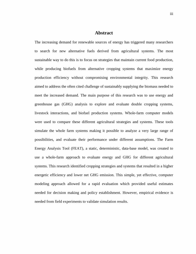
Abstract

The increasing demand for renewable sources of energy has triggered many researchers

to search for new alternative fuels derived from agricultural systems. The most

sustainable way to do this is to focus on strategies that maintain current food production,

while producing biofuels from alternative cropping systems that maximize energy

production efficiency without compromising environmental integrity. This research

aimed to address the often cited challenge of sustainably supplying the biomass needed to

meet the increased demand. The main purpose of this research was to use energy and

greenhouse gas (GHG) analysis to explore and evaluate double cropping systems,

livestock interactions, and biofuel production systems. Whole-farm computer models

were used to compare these different agricultural strategies and systems. These tools

simulate the whole farm systems making it possible to analyze a very large range of

possibilities, and evaluate their performance under different assumptions. The Farm

Energy Analysis Tool (FEAT), a static, deterministic, data-base model, was created to

use a whole-farm approach to evaluate energy and GHG for different agricultural

systems. This research identified cropping strategies and systems that resulted in a higher

energetic efficiency and lower net GHG emission. This simple, yet effective, computer

modeling approach allowed for a rapid evaluation which provided useful estimates

needed for decision making and policy establishment. However, empirical evidence is

needed from field experiments to validate simulation results.

iv

Table of Contents List of Figures ................................................................................................................... vii List of Tables ..................................................................................................................... xi Acknowledgments............................................................................................................ xvi Chapter 1. Introduction and Objectives .............................................................................. 1

1.1. Introduction .............................................................................................................. 1

1.2. Research Objectives ................................................................................................. 6

1.3. Document Organization ........................................................................................... 6

Chapter 2. Literature Review .............................................................................................. 7

2.1. Energy analysis ........................................................................................................ 7

2.2. Greenhouse gas emissions ..................................................................................... 10

2.3. Biofuels .................................................................................................................. 14

2.4. Cropping systems ................................................................................................... 15

2.5. Computer modeling ............................................................................................... 20

2.5.1. Whole-farm modeling ..................................................................................... 20

2.5.2. Dairy feeding model ....................................................................................... 22

Chapter 3. Farm Energy Analysis Tool (FEAT) ............................................................... 23

3.1. FEAT description ................................................................................................... 23

3.1.1. FEAT crops ..................................................................................................... 26

3.1.2. Crop Farm System description........................................................................ 26

3.1.3. Dairy Farm System description ...................................................................... 27

3.1.4. Biofuel Farm System description.................................................................... 28

3.2. FEAT methodology ............................................................................................... 29

3.2.1. Energy Analysis .............................................................................................. 30

3.2.1.1. Crop production characteristics ............................................................... 30

3.2.1.2. General energy inputs .............................................................................. 50

3.2.1.3. Dairy Farm System specific inputs .......................................................... 55

3.2.1.4. Biofuel Farm System specific inputs ....................................................... 56

v

3.2.1.5. Crop Farm System outputs....................................................................... 58

3.2.1.6. Dairy Farm System outputs ..................................................................... 60

3.2.1.7. Biofuel Farm System outputs................................................................... 63

3.2.2. Greenhouse gases emissions ........................................................................... 66

3.2.2.1. GHGs for general crop production: ......................................................... 67

3.2.2.2. Dairy Farm System specific GHGs production ....................................... 71

3.2.2.3. Biofuel Farm System GHG emissions ..................................................... 73

3.3. FEAT results .......................................................................................................... 76

Chapter 4. Energy and Greenhouse Gas Analyses of Cropping Systems for Feed, Heat and Biofuel Production in Northern US.......................................................... 91

4.1. Introduction ............................................................................................................ 91

4.2. Methods.................................................................................................................. 93

4.2.1. Energy and greenhouse gas analyses .............................................................. 93

4.2.2. Cropping system characteristics ..................................................................... 94

4.2.3. Cropping system yield assessment.................................................................. 94

4.3. Results and discussion ........................................................................................... 97

4.3.1 Yield modeling results ..................................................................................... 97

4.3.2. Energy analysis ............................................................................................. 101

4.3.3. Greenhouse Gas (GHG) Analysis ................................................................. 110

4.4. Conclusions .......................................................................................................... 117

Chapter 5. Energy and Greenhouse Gas Analysis of a Pennsylvania Dairy Farm ......... 119

5.1. Introduction .......................................................................................................... 119

5.2. Material and methods ........................................................................................... 122

5.2.1. Energy and greenhouse gas analysis ............................................................. 122

5.2.2. Cropping system descriptions ....................................................................... 123

5.2.3. Dairy characteristics ...................................................................................... 125

5.3. Results and discussion ......................................................................................... 126

5.3.1. Dairy feed consumption ................................................................................ 126

5.3.2. Energy analysis results .................................................................................. 126

5.3.3. Greenhouse gas emissions analysis .............................................................. 129

vi

5.4. Conclusions .......................................................................................................... 132

Chapter 6. Modifying Northern Dairy Farms for Productivity, Greenhouse Gas Reductions, and Potential Biomass Supply .................................................. 134

6.1. Introduction .......................................................................................................... 134

6.2. Materials and methods ......................................................................................... 135

6.2.1. Model methodology ...................................................................................... 135

6.2.2. Dairy farming systems description ............................................................... 135

6.2.3. Dairy feeding methodology .......................................................................... 137

6.3. Results and discussion ......................................................................................... 138

6.3.1. Feed ration balance ....................................................................................... 138

6.3.2. Energy results................................................................................................ 141

6.3.3. Greenhouse gas emissions ............................................................................ 144

6.4. Conclusions .......................................................................................................... 147

Chapter 7. Conclusions ................................................................................................... 149

7.1. Summary .............................................................................................................. 149

7.2. Scope and limitations ........................................................................................... 150

7.3. Potential improvements and future work ............................................................. 150

References ………………………………………………………………………………152

Appendix A : Fuel consumption for agricultural operations .......................................... 162

Appendix B: Crop bushel weight and moisture, fuel density and unit conversions ....... 171

vii

List of Figures

Figure 3-1. Overall Farm Energy Analysis Tool diagram. ............................................... 24

Figure 3-2. Crop Farm System schematic and boundary. ................................................. 25

Figure 3-3. Dairy Farm System schematic and boundary. ................................................ 25

Figure 3-4. Biofuel Farm System schematic and boundary. ............................................. 25

Figure 3-5. Crop Farm System greenhouse gas sources and sinks diagram. .................... 66

Figure 3-6. Livestock Farm System greenhouse gas sources and sinks diagram. ............ 66

Figure 3-7. Biofuel Farm System greenhouse gas sources and sinks diagram. ................ 66

Figure 3-8. Crop energy inputs for the Crop, Livestock, and Biofuel Farm Systems per

year. ........................................................................................................................... 82

Figure 3-9. Feedstock energy output in net energy for lactation (NEL) for the Crop Farm

System per year. ........................................................................................................ 83

Figure 3-10. Feedstock energy output in higher heating value (HHV) for the Crop Farm

System per year. ........................................................................................................ 84

Figure 3-11. Greenhouse gas emissions from farm inputs for the Crop, Livestock, and

Biofuel Farm Systems per year. ................................................................................ 85

Figure 3-12. Greenhouse gas net crop assimilation for the Crop Farm System per year. 86

Figure 3-13. Farm inputs, feedstock transportation, and biorefinery energy inputs for the

Biofuel Farm System per year. ................................................................................. 87

Figure 3-14. Biofuel and biofuel co-products energy outputs from the Biofuel Farm

System per year. ........................................................................................................ 88

Figure 3-15. Greenhouse gas emissions from farm inputs, feedstock transportation, and

the biorefinery for the Biofuel Farm System per year. ............................................. 89

Figure 4-1. Rye silage yield after first year corn silage regression based on annual mean

temperature from Integrated Farm System Model (Rotz et al. 2009). ...................... 99

Figure 4-2. Rye silage yield after corn silage regression based on annual mean

temperature from Integrated Farm System Model (Rotz et al. 2009). .................... 100

Figure 4-3. Rye silage yield after soybean regression based on annual mean temperature

from Integrated Farm System Model (Rotz et al. 2009). ........................................ 100

viii

Figure 4-4. Centre County Pennsylvania net energy for lactation (NEL) balance per year.

................................................................................................................................. 104

Figure 4-5. Cayuga County New York net energy for lactation (NEL) balance per year.

................................................................................................................................. 104

Figure 4-6. Huron County Michigan net energy for lactation (NEL) balance per year. . 105

Figure 4-7. Penobscot County Maine net energy for lactation (NEL) balance per year. 105

Figure 4-8. Centre County Pennsylvania higher heating value (HHV) energy balance per

year. ......................................................................................................................... 106

Figure 4-9. Cayuga County New York higher heating value (HHV) energy balance per

year. ......................................................................................................................... 106

Figure 4-10. Huron County Michigan higher heating value (HHV) energy balance per

year. ......................................................................................................................... 107

Figure 4-11. Penobscot County Maine higher heating value (HHV) energy balance per

year. ......................................................................................................................... 107

Figure 4-12. Centre County Pennsylvania biofuel and co-products energy balance per

year. ......................................................................................................................... 108

Figure 4-13. Cayuga County New York biofuel and co-products energy balance per year.

................................................................................................................................. 108

Figure 4-14. Huron County Michigan biofuel and co-products energy balance per year.

................................................................................................................................. 109

Figure 4-15. Penobscot County Maine biofuel and co-products energy balance per year.

................................................................................................................................. 109

Figure 4-16. Centre County Pennsylvania crop greenhouse gas assimilation balance per

year. ......................................................................................................................... 112

Figure 4-17. Cayuga County New York crop greenhouse gas assimilation balance per

year. ......................................................................................................................... 113

Figure 4-18. Huron County Michigan crop greenhouse gas assimilation balance per year.

................................................................................................................................. 113

Figure 4-19. Penobscot County Maine crop greenhouse gas assimilation balance per year.

................................................................................................................................. 114

ix

Figure 4-20. Centre County Pennsylvania biofuel greenhouse gas credit balance per year.

................................................................................................................................. 114

Figure 4-21. Cayuga County New York biofuel greenhouse gas credit balance per year.

................................................................................................................................. 115

Figure 4-22. Huron County Michigan biofuel greenhouse gas credit balance per year. 115

Figure 4-23. Penobscot County Maine biofuel greenhouse gas credit balance per year. 116

Figure 5-1. Farm system evaluation boundary. .............................................................. 122

Figure 5-2. Recycled energy embodied in manure nutrients and plant N fixation for

control and double / cover cropping systems per year. ........................................... 127

Figure 5-3. Straight vegetable oil energy recycling for control and double / cover

cropping systems per year. ...................................................................................... 128

Figure 5-4. Net energy input for control and double / cover cropping systems per year.

................................................................................................................................. 129

Figure 5-5. Control cropping system greenhouse gas (GHG) emission balance per year.

................................................................................................................................. 130

Figure 5-6. Double / cover cropping system greenhouse gas (GHG) emission balance per

year. ......................................................................................................................... 131

Figure 6-1. Farm system evaluation boundary. .............................................................. 135

Figure 6-2. Centre County Pennsylvania energy balance per year. ................................ 142

Figure 6-3. Cayuga County New York energy balance per year. ................................... 142

Figure 6-4. Huron County Michigan energy balance per year. ...................................... 143

Figure 6-5. Penobscot County Maine energy balance per year. ..................................... 143

Figure 6-6. Centre County Pennsylvania greenhouse gas (GHG) emissions balance per

year. ......................................................................................................................... 145

Figure 6-7. Cayuga County New York greenhouse gas (GHG) emissions balance per

year. ......................................................................................................................... 145

Figure 6-8. Huron County Michigan greenhouse gas (GHG) emissions balance per year.

................................................................................................................................. 146

Figure 6-9. Penobscot County Maine greenhouse gas (GHG) emissions balance per year.

................................................................................................................................. 146

x

Figure 6-10. Crop greenhouse gas (GHG) assimilation for current (CT) and double (DC)

cropping system for each county per year. ............................................................. 147

xi

List of Tables Table 3-1. Crop fuel consumption for FEAT crops based on tillage practices from IFSM

(Rotz et al. 2009), I-FARM (van Ouwerkerk et al. 2009), and literature values (Rcrop

fuel). ............................................................................................................................ 32

Table 3-2. Crop fuel consumption for pesticide application and field residue removal. .. 33

Table 3-3. Corn production: input application rate per year (Rinput). ................................ 35

Table 3-4. Corn for silage production: input application rate per year (Rinput). ................ 35

Table 3-5. Soybean production: input application rate per year (Rinput). .......................... 36

Table 3-6. Rye for silage production: input application rate per year (Rinput). ................. 36

Table 3-7. Wheat for silage production: input application rate per year (Rinput). ............. 37

Table 3-8. Barley production: input application rate per year (Rinput). ............................. 37

Table 3-9. Alfalfa production: input application rate per year (Rinput). ............................ 38

Table 3-10. Red clover production: input application rate per year (Rinput). .................... 38

Table 3-11. Canola production: input application rate per year (Rinput). .......................... 39

Table 3-12. Switchgrass production: input application rate per year (Rinput). ................... 39

Table 3-13. Miscanthus production: input application rate per year (Rinput). ................... 40

Table 3-14. Sugar beet production: input application rate per year (Rinput). ..................... 40

Table 3-15. FEAT crop default yields per year (Ycrop). .................................................... 41

Table 3-16. Residue to crop ratio (Rresidue). ....................................................................... 42

Table 3-17. Crop and residue moisture content (Cmoist). ................................................... 43

Table 3-18. Dairy farm livestock ratio management. ....................................................... 44

Table 3-19. Dairy farm outputs (Rmilk, Rmanure). ................................................................ 44

Table 3-20. Dairy feed requirements per cow per year[2]. ................................................ 45

Table 3-21. Dairy manure nutrient content and use efficiency. ........................................ 46

Table 3-22. Dairy farm livestock weight. ......................................................................... 47

Table 3-23. Dairy farm livestock unit (LU[2]). .................................................................. 47

Table 3-24. Dairy management annual requirements. ...................................................... 48

Table 3-25. Energy inputs for energy balance analysis. ................................................... 49

Table 3-26. Energy output distribution for energy balance analysis, for each type of

system. ...................................................................................................................... 50

xii

Table 3-27. Embodied energy in crop inputs (Einput). ....................................................... 51

Table 3-28. Crop input energy embodied in seed production (Einput). .............................. 52

Table 3-29. Embodied fuel energy (Efuel). ........................................................................ 53

Table 3-30. Energy associated with transport of farm inputs (Einput transport). .................... 54

Table 3-31. Drying energy (Edrying). .................................................................................. 54

Table 3-32. Crushing oil seed energy for straight vegetable oil production (Ecrushing). .... 55

Table 3-33. Energy transportation of feedstock to a biorefinery (Etranspfeedstock). .............. 57

Table 3-34. Biorefinery feedstock processing energy (Eprocessing). .................................... 58

Table 3-35. Net energy for lactation (NEL) for FEAT crops and residues (Ecrop). .......... 59

Table 3-36. Higher heating value (HHV) for FEAT crops and residues (Ecrop). .............. 60

Table 3-37. Food energy content of milk (Emilk). .............................................................. 61

Table 3-38. Straight vegetable oil (SVO) yield (YSVO). ................................................... 62

Table 3-39. Diesel and straight vegetable oil energy content (ESVO). .............................. 62

Table 3-40. Feed meal yield and energy content (Ymeal ; Efeed meal). ................................. 63

Table 3-41. Biofuel yield (Ybiofuel). ................................................................................... 64

Table 3-42. Biofuel energy content (Ebiofuel). .................................................................... 64

Table 3-43. Biofuel co-product yield and energy content (Ybiofuel co-product ; Eco-product). .... 65

Table 3-44. Greenhouse gas global warming potential (GWP). ....................................... 67

Table 3-45. Greenhouse gas emissions from crop input production and nitrous oxide

(N2O) soil emission (Eminput). ................................................................................... 68

Table 3-46. Greenhouse gas emissions from seed production (Eminput). .......................... 69

Table 3-47. Greenhouse gas emissions from diesel fuel (Emfuel). .................................... 70

Table 3-48. Greenhouse gas emissions from transportation of farm inputs (Eminput transport).

................................................................................................................................... 70

Table 3-49. Greenhouse gas net crop assimilation parameters. ........................................ 71

Table 3-50. Greenhouse gas emissions from animals and housing (Emdairy). .................. 72

Table 3-51. Greenhouse gas emissions from manure storage and manure carbon dioxide

emission from soil (Emmanure storage; Emmanure carbon). ................................................... 73

Table 3-52. Greenhouse gas emissions from feedstock transportation (Emtransport). ......... 74

Table 3-53. Greenhouse gas emission from biorefinery processing (Emprocessing). ........... 75

xiii

Table 3-54. Gasoline / ethanol and diesel / biodiesel energy content ratio (Eratio). .......... 76

Table 3-55. Biofuel co-product greenhouse gas credit (Embiofuel co-prod). .......................... 76

Table 3-56. Crop energy input and output for the FEAT Crop Farm System. ................. 77

Table 3-57. Energy dynamics for each crop for the FEAT Biofuel Farm System. .......... 78

Table 3-58. Biofuel yield and co-product for each FEAT feedstock. ............................... 79

Table 3-59. FEAT crop GHG input production and crop assimilation [1] for Crop Farm

System. ...................................................................................................................... 80

Table 3-60. FEAT net greenhouse gas (GHG) emission for the Biofuel Farm System. .. 81

Table 4-1. Statistical yields for selected counties (10-yr average 1999-2008). ................ 95

Table 4-2. Soil information used for each selected county. .............................................. 95

Table 4-3. Yield adjustment parameter for corn silage and soybean based on statistical

yields. ........................................................................................................................ 96

Table 4-4. Rye silage yields (Mg DM ha-1) from Duiker and Curran (2005). .................. 96

Table 4-5. Rye silage yield adjustment parameters for Centre County based on Duiker

and Curran (2005) study. .......................................................................................... 96

Table 4-6. Crop farm input requirements. ........................................................................ 97

Table 4-7. Centre County Pennsylvania modeled yields per year. ................................... 98

Table 4-8. Cayuga County New York modeled yields per year. ...................................... 98

Table 4-9. Huron County Michigan modeled yields per year. ......................................... 98

Table 4-10. Penobscot County Maine modeled yields per year. ...................................... 99

Table 4-11. Overall average annual yield of cropping systems for each county (Mg DM

ha-1yr-1). ................................................................................................................... 101

Table 4-12. Livestock feed energy balance (NEL[1]) per year. ....................................... 102

Table 4-13. Biomass heating energy balance (HHV[1]) per year. ................................... 102

Table 4-14. Biofuel production energy balance per year. ............................................... 103

Table 4-15. Net energy increase from double cropping system versus control cropping

system. .................................................................................................................... 110

Table 4-16. Livestock feed and heating greenhouse gas (GHG) emissions balance (g

CO2e ha-1 yr -1). ....................................................................................................... 111

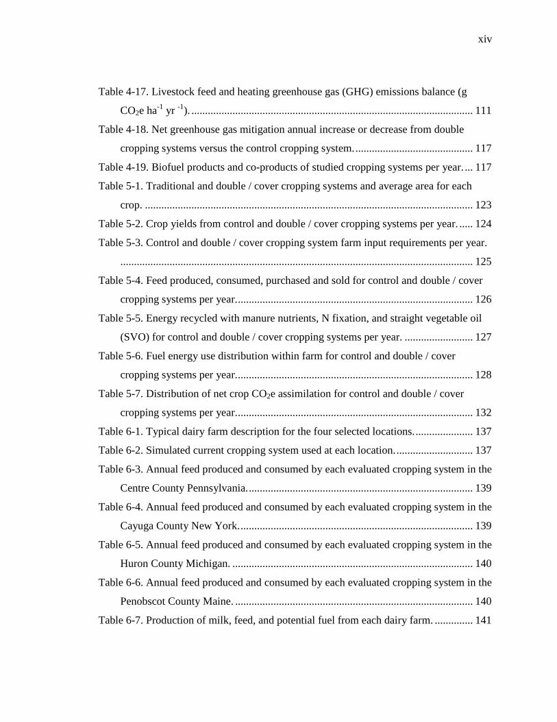
xiv

Table 4-17. Livestock feed and heating greenhouse gas (GHG) emissions balance (g

CO2e ha-1 yr -1). ....................................................................................................... 111

Table 4-18. Net greenhouse gas mitigation annual increase or decrease from double

cropping systems versus the control cropping system. ........................................... 117

Table 4-19. Biofuel products and co-products of studied cropping systems per year. ... 117

Table 5-1. Traditional and double / cover cropping systems and average area for each

crop. ........................................................................................................................ 123

Table 5-2. Crop yields from control and double / cover cropping systems per year. ..... 124

Table 5-3. Control and double / cover cropping system farm input requirements per year.

................................................................................................................................. 125

Table 5-4. Feed produced, consumed, purchased and sold for control and double / cover


Table 5-5. Energy recycled with manure nutrients, N fixation, and straight vegetable oil

(SVO) for control and double / cover cropping systems per year. ......................... 127

Table 5-6. Fuel energy use distribution within farm for control and double / cover


Table 5-7. Distribution of net crop CO2e assimilation for control and double / cover


Table 6-1. Typical dairy farm description for the four selected locations. ..................... 137

Table 6-2. Simulated current cropping system used at each location. ............................ 137

Table 6-3. Annual feed produced and consumed by each evaluated cropping system in the

Centre County Pennsylvania. .................................................................................. 139


Cayuga County New York. ..................................................................................... 139


Huron County Michigan. ........................................................................................ 140


Penobscot County Maine. ....................................................................................... 140

Table 6-7. Production of milk, feed, and potential fuel from each dairy farm. .............. 141

xv

Table 6-8. Annual greenhouse gas balances for the selected counties for current and

double / cover cropping systems. ............................................................................ 144

Table A.1. Studies of moldboard plow fuel consumption (n=17). ................................. 163

Table A.2. Studies of chisel plow fuel consumption (n=12). ......................................... 163

Table A.3. Studies of offset disk fuel consumption (n=10). ........................................... 164

Table A.4. Studies of sub-soiling fuel consumption (n=2). ............................................ 164

Table A.5. Studies of disk fuel consumption (n=7). ....................................................... 164

Table A.6. Studies of field cultivate fuel consumption (n=5). ....................................... 165

Table A.7. Studies of pesticide application fuel consumption (n=7). ............................. 165

Table A.8. Studies of fertilizer application fuel consumption (n=5). ............................. 165

Table A.9. Studies of planter fuel consumption (n=8). .................................................. 166

Table A.10. Studies of grain drill fuel consumption (n=6). ............................................ 166

Table A.11. Studies of no-till planting fuel consumption (n=9). .................................... 166

Table A.12. Studies of cultivator fuel consumption (n=7). ............................................ 167

Table A.13. Studies of rotary hoe fuel consumption (n=4). ........................................... 167

Table A.14. Studies of spring tooth fuel consumption (n=4). ........................................ 167

Table A.15. Studies of mower fuel consumption (n=3). ................................................. 167

Table A.16. Studies of mower conditioner fuel consumption (n=3). ............................. 168

Table A.17. Studies of rake fuel consumption (n=4). ..................................................... 168

Table A.18. Studies of baler fuel consumption (n=5). .................................................... 168

Table A.19. Studies of forage harvesting and green chop fuel consumption (n=4). ...... 168

Table A.20. Studies of corn silage harvesting fuel consumption (n=3). ........................ 169

Table A.21. Studies of grain and row crop harvesting fuel consumption (n=5). ............ 169

Table A.22. Studies of corn combine fuel consumption (n=5). ...................................... 169

Table A.23. Studies of miscellaneous operations fuel consumption. ............................. 170

Table B.1. Crop bushel weight and moisture content. .................................................... 172

Table B.2. Fuel density. .................................................................................................. 172

Table B.3. Conversions used in calculations. ................................................................. 173

xvi

Acknowledgments

I would like to express my sincere gratitude to my adviser, Dr. Tom Richard, for

providing excellent guidance, and encouraging me to push my research expectations to

high levels. As he once said: “I want you to be one of the top experts in your area of

expertise, in the world”. I would also like to thank my thesis committee Dr. C. Al Rotz

and Dr. Greg Roth, for their assistance, and for making my work more realistic and

interesting. Thanks also to Dr. Harvey B. Manbeck who gave me great guidance and

strength in the beginning of this journey. Additional thanks to Dr. Paul Walker, Virginia

Ishler, and extension educators: Craig Altemose, Bob Batel, Brian Aldrich, and Gleason

Gray.

My family, you are the base for everything that I conquered. Remembering an old

saying, I got here because I am standing on the shoulders of giants. A special thanks for

my grandparents Jose Maria and Isis (in memorium), George (in memorium) and

Carmen, to my mother Vivian, to my father Eduardo, and to my brother Rogério. Mom,

thanks for the amazing love that you gave me through my life and especially for

encouraging me to go to graduate school. Dad, you are the most intelligent person that I

know, and I am thankful to be able to mirror in someone like you. STRENGTH, this is

the word that I heard the most from both of you, and with it, I succeed one more step in

my life. I would like to thank my girlfriend Liane for the support, care and love. Thank

you also to all of my friends here in US and Brasil. Unique thanks to Matt Ryan that

helped me to edit and generate good ideas. Thank you God.

xvii

This thesis is dedicated to the memory of

my grandfather George Anthony Garcia

and grandmother Isis Marques de Toledo Camargo.

1

Chapter 1

Introduction and Objectives

1.1. Introduction

Over the past decade, there has been an incredible transformation in the interest,

acceptance, and support of renewable energy resources, as society has largely realized the

important future role they will play in maintaining healthy ecosystems, global security,

and vibrant economic growth. This transformation has been driven by growing interest in

reducing dependency on fossil fuels and associated greenhouse gas emissions that

contribute to global warming. Diverse energy alternatives are being researched and

developed such as wind, solar and hydro power, but one option that currently captures

significant attention is biomass energy. The majority of agricultural crops provide food,

fiber or feed for animals. Crops can also provide a wide range of fuels including pellets

for combustion and liquid transportation fuels such as ethanol and biodiesel.

Some biomass energy technologies are well developed and common, such as

ethanol production from sugar cane and corn, but new research is focusing on novel and

innovative technologies that are more efficient and utilize cellulosic biomass materials.

Cellulosic ethanol is a novel technology that is being developed to use cellulose-rich

material such as vegetative parts of plants and waste food products to produce ethanol

(Lynd, 1996). Although cellulosic ethanol is still under development, it is a promising

fuel technology that could replace part of US petroleum based fuels.

The benefits from a transition to renewable biofuels include economic aspects in

addition to energy security and sustainability. For local rural economies, the

2

development of biofuel infrastructure would lead to more opportunities for rural

businesses, and possibly increase farmers’ profits as well.

Changes in current cropping systems are needed to obtain the amount of biomass

required to meet anticipated biofuel feedstock demand. A new equilibrium between food

and energy use of the land must be achieved. This equilibrium will be mostly dictated by

the market, but its implementation will require optimization and transformation of current

cropping systems and land use in ways that are barely imagined today.

Most farmers usually follow traditional practices, with incremental changes

depending on their area of interest. Specialization has resulted in such examples as crop

farms that only produce corn and soybeans, or animal farms that import much, if not all

of their feed. Transitioning to more integrated systems involves risk, but realistic

simulations of future scenarios can be helpful in minimizing that risk. Such simulations

can also be useful for identifying opportunities to integrate crop and livestock systems, or

to create incentives for beneficial practices like double and cover cropping (Rotz et al.

2001b).

Regardless of the type of farm, there are usually environmental and economic

benefits from having crops growing throughout the whole year (PSU Agronomy guide,

2008). Sometimes this is not possible, especially in very cold climates, where the winter

is harsh and crops cannot survive. However in much of the temperate agricultural regions

certain winter crops can be grown, and year-round cropping can increase productivity

(Heggenstaller et al. 2008).

More than ever before, it is clear there is a need to overcome challenges to

increase agricultural and bioenergy system sustainability. This goal combined with the

3

national support to increase energy security will require research on diverse farm systems

that break from traditional paradigms in order to achieve greater efficiency. Integrated

systems of the future will need to focus on improving sustainability, profitability,

productivity, food safety, the environment and the community when compared with

traditional cropping systems (NRC, 1989).

Double cropping systems, which consist of two harvested crops grown in the

same field over the course of a single year (Heggenstaller et al. 2008), and cover

cropping systems in which the winter crop is not harvested, are two promising

approaches farmers are using to increase overall sustainability. With cover crops the

winter crop replenishes nutrients and organic matter, and in the case of double crops an

additional harvest of grain, oil seed, and or cellulosic biomass is obtained in the spring.

The downside of these systems is a potentially lower yield of the main summer cash crop

and lower quality of the products. This is especially true in regions prone to unfavorable

climatic conditions. For example, in the Northeastern United States, most field crops such

as corn and soybean are not irrigated. In some years, drought conditions occur, which can

drastically reduce soybean yields if they are delayed by (or double cropped after) wheat

or barley harvest. This difficulty requires research to evaluate the feasibility of

implementing new double cropping systems in the Northeast, and to compare their

sustainability relative to traditional systems, such as a corn-soybean two-year rotation.

The integration of oil seed crops is another change in traditional cropping

practices that has potential to help contribute to meeting bioenergy goals. Because they

are not already commonly grown, they are also touted as a feasible way to diversify

cropping systems, unlike corn derived ethanol. These crops have relatively high oil

4

contents, which is extracted to make vegetable oil. When used directly as fuel this oil is

commonly referred to as straight vegetable oil (SVO) (Cauffman, 2008). Farmers can

use SVO as fuel in farm machinery after some adjustment (Emberger et al. 2009). Thus,

integrating oil seed crops can provide farmers with an opportunity to be more self

sufficient.

As fossil fuels are becoming an input subjected to high variation in prices, fuel-

saving practices like no-till are gaining more attention. Besides being more fuel efficient,

no-till is beneficial for controlling soil erosion, maintaining soil moisture, and increasing

soil organic matter. No-till management is gaining popularity among farmers in the

Northeast and throughout the US (Duiker and Curran, 2005).

No-till, and double/cover cropping systems provide more options for farmers to

harvest parts of crop plants that have traditionally been designated as crop residues,

without damaging the environment. There are many types of unused crop plant

components, or residues, that are not being directly utilized. For example, corn stover

(stalks, cobs and leaves after corn harvest) is a residue that is abundantly available.

There are a number of studies currently underway to evaluate soil erosion effects, plant

material properties, harvesting equipment, and harvesting fuel consumption (Lockeretz,

1981; Hoskinson et al. 2007; Zhou et al. 2008).

As the need to find more alternatives for biomass production increases, some

dedicated energy crops are starting to be considered. Switchgrass, a perennial grass

native to North America, with high yield levels and low input requirements is already

widely planted for conservation purposes (McLaughlin and Kszos, 2005). Miscanthus

(Miscanthus x giganteus), also a perennial grass from Asia that produces large amounts

5

of biomass with low inputs is gaining increasing attention (Lewandowski et al. 2000;

Clifton-Brown et al. 2001; Heaton et al. 2004). The relationship between crop input

requirements and crop output production is an important consideration, and has been also

widely evaluated in previous literature (IFIAS, 1973; Leach, 1975; Pimentel, 1980).

While the productivity of different farming systems has long been evaluated with

respect to nutrient cycles and impacts on soil and water quality, energy analysis and

greenhouse gas emissions have more recently been added to the list of environmental

sustainability concerns. Energy analysis of a system is the energetic accounting of the

major inputs and outputs from a defined system. A system could represent a farm, or

include a larger boundary such as a biofuel system, including farm, transportation and

biorefinery components (Pimentel and Patzek, 2005; Farrell et al. 2006). Energy analysis

is a useful tool to evaluate various systems. The ability to convert system components to

the same units of energy creates an analytical coherence and flexibility that is very

practical for evaluating systems that typically exchange inputs and products outside the

system.

As with energy analysis, greenhouse gas (GHG) analysis is an increasingly

important tool for evaluating cropping and bioenergy systems, mainly because of the

threat of global warming (Kim and Dale, 2005a; Farrell et al. 2006; Chianese et al.

2009d). GHG analysis converts the major inputs and outputs of a particular system into a

mass unit of carbon dioxide equivalent (CO2e). Results from GHG and energy analyses

provide useful results that parallel one another, although the relationships vary depending

on the fossil or renewable energy sources involved. Energy and GHG analysis are useful

to understand, compare, and improve the overall operation of agricultural systems. Using

6

the same units of measurement, such as mega-joule and carbon dioxide equivalent, allows

for direct comparisons of different alternatives.

1.2. Research Objectives

The overall objective of this research was to use energy and GHG analyses to

evaluate complex cropping systems, livestock interactions, on-farm fuel production, and

biofuel production systems. This evaluation was accomplished through the use of whole-

farm computer models. The research objectives were:

1. Develop a model to calculate energy and GHG emission balances.

2. Assess energy and GHG emissions of 11 feedstocks.

3. Evaluate how double and cover crops can contribute to overall energy and GHG

benefits in dairy farm, heat production, and biofuel production scenarios.

4. Assess on-farm fuel production through oil seed use.

5. Evaluate manure nutrient recycling in dairy farms in terms of energy and GHG

emissions.

6. Evaluate double cropping impact on Northern US dairy farms.

1.3. Document Organization

This work is organized in seven chapters. In Chapter 2 important literature is reviewed in

terms of energy analysis, greenhouse gas (GHG) emissions, biofuel production, cropping

systems, and computer modeling. Chapter 3 quantifies energy and GHG parameters for

model development, encompassing objectives 1 and 2. Chapter 4 focuses on objective 3,

Chapter 5 examines objectives 4 and 5, and Chapter 6 explores objective 6. Finally,

Chapter 7 states the conclusions from this research.

7

Chapter 2

Literature Review

There are several important parameters to consider when conducting agricultural

systems analysis. In this chapter, a literature review is provided to introduce relevant

areas of study on such research. Several topics are covered, including energy analysis,

greenhouse gas emissions analysis, biofuel production, cropping systems design, and

whole-farm computer modeling.

2.1. Energy analysis

Energy is a broad term that is linked with a large range of applications. In food

and agricultural systems, energy inputs and outputs can be used as a measure to evaluate

the efficiency and productivity of systems. Agricultural mechanization and rural

electrification enabled dramatic transformations of agriculture in the 20th century, but the

abundant low-cost energy that enabled this modernization was long taken as a given.

Energy analysis on farming systems started to get greater attention after the 1973 oil

embargo (Stanhill, 1984). As supplies of petroleum became scarce, the understanding of

energy use relationships in fuels, fertilizers and chemicals became more relevant. Due to

demanding circumstances, many researchers started to develop energy analysis

methodologies for crop and livestock production (Pimentel et al. 1973; Leach, 1975;

IFIAS, 1974; Pimentel, 1980).

More recently, these energy analysis methodologies have been used to evaluate

different types of biofuel production systems (Ahmed et al. 1994, Shapouri et al. 2004;

8

Pimentel and Patzek, 2005; Farrell et al. 2006). This tendency toward greater scrutiny of

energetic efficiency was also motivated by increasing energy prices, foreign dependency,

and rising energy demand. Currently, energy analysis is considered an important tool in

the evaluation of agricultural systems for food, fiber, feed and now biofuel production

(Gopalakrishnan, 1994; Brown, 2003).

Energy and mass balance analyses are two components of life cycle assessment

(LCA), which in the most extreme cases involves quantifying energy transfer from the

origin of raw materials to the disposal of waste products, otherwise known as “cradle to

grave” analyses (SETAC, 1993). In an LCA evaluation, it is possible to characterize the

overall efficiency and environmental impact of systems to produce various products

(Pradham et al. 2008). Energy analysis in agriculture usually has a reduced boundary that

ends well before the product “grave”, and consequently is not considered a complete

LCA. Typical bioenergy analysis defines the downstream boundary at the farm gate or

biorefinery exit.

A clear methodology is essential for effective system-level comparisons.

Typically, energy analysis involves six steps, as defined by the International Federation

of Institutes for Advanced Studies (IFIAS) in 1975; 1) definition of the objective of

analysis; 2) definition of system boundaries; 3) identification of inputs; 4) assignment of

energy requirements of all inputs; 5) identification of all outputs; and 6) establishment of

a criteria for partition.

When conducting an energy analysis, there are two methods that can be used to

account for the input energy flows: 1) the thermodynamic method; and 2) the sequestered

method (Fluck and Baird, 1980). In the thermodynamic method, all forms of energy are

9

included, including their respective inefficiencies. The sequestered method accounts for

fossil fuel and other primary energy sources, however, it does not account for natural

energy inputs such as solar and muscular energy (Fluck and Baird, 1980). The

sequestered method has a higher level of acceptance in energy analysis studies and is

more common in the literature.

Energy analysis methodology divides energy use in two categories: 1) direct

energy use; and 2) indirect energy use (Uhlin, 1998). Direct energy use is employed to

convert an input into another form of energy, such as fuel, electricity, and drying. Indirect

energy use is employed to produce an input that is not considered an energy resource,

such as fertilizers, pesticides, and machinery.

Farm system inputs are diverse and include fertilizers, fuel, pesticides, electricity,

seed, labor, and infrastructure. Outputs in a farm system are also diverse, ranging from

crops to livestock products and renewable energy production. In a biofuel system, in

addition to the farm requirements, the inputs could include the fuel to transport the

feedstock, and the energy to process the biofuel. Biofuels and their respective co-

products are the outputs in a bioenergy system (Morris, 2005; Farrell et al. 2006). Many

authors have reported energy analyses for corn and cellulosic ethanol (Wang 2001;

Graboski, 2002; Shapouri et al. 2004; Pimentel and Patzek, 2005; de Oliveira et al. 2005;

Farrell et al. 2006), and for biodiesel (Ahmed et al. 1994; Sheehan et al. 1998; Hill et al.

2006). Co-products from biofuel processes could include DDGs (distillers dried grains

and solubles) from corn ethanol, soybean meal and glycerin from biodiesel production,

and electricity from cellulosic ethanol. The results of biofuel energy analyses are often

reported on the basis of energy outputs (MJ or gallons of gasoline equivalent) but for

10

agricultural systems can also be standardized per unit of area (hectare) for a specific

period of a time (year) (Ziesemer, 2007).

Despite the need for a system to evaluate energy use and efficiency, energy

analyses have received a great deal of criticism. One of the primary criticisms is because

of the non-homogeneity of energy from different forms (Webb and Pearce, 1975; Leach,

1975; Hill and Walford, 1975). This condition makes the addition of energy flows from

different sources difficult. Energy sources could have the same joule (or calorific)

content, but definitely different applications, quality, economic value, cleanliness, and

concentration (Fluck and Baird, 1980). Others criticisms include: 1) undefined system

boundaries (Fluck and Baird, 1980; Daalgaard, 2000); 2) unequal comparisons among

agricultural products (Breimyer, 1975); 3) inaccurate energy-use data (Daalgaard, 2000);

and 4) undefined analysis scope and goals (Gopalakrishnan, 1994; Daalgaard, 2000).

Nevertheless, energy analysis is gaining attention because of its utility to evaluate

alternatives for fossil fuel reduction, and consequently strategies to decrease the

greenhouse gas emissions that contribute to global warming (IPCC, 2007).

2.2. Greenhouse gas emissions

Greenhouse gas (GHG) analyses are typically linked with energy analyses (West

and Marland, 2000; Wang, 2001; Nelson et al. 2001; Kim and Dale, 2005a; Farrell et al.

2006; Adler et al. 2007). The importance of global warming and GHG emissions was

heightened after the Kyoto protocol, which was drafted in 1997 and aimed for the

stabilization of emissions to a level that would prevent dangerous anthropogenic

11

interference with the world climate. Since then agriculture has been considered an

important sector to evaluate and identify potential problems and solutions.

GHG emissions from agriculture can be divided into primary, secondary, and

tertiary sources (Gifford, 1994). Primary sources are related to operations such as

fertilization, tillage, planting, irrigation, harvesting, and drying. Secondary sources are

related to the production and transportation of inputs such as fertilizers, pesticides, and

diesel fuel. Tertiary sources are related to the acquisition of raw materials to produce

items such as machinery and buildings.

The three main GHGs from agricultural production are carbon dioxide (CO2),

methane (CH4), and nitrous oxide (N2O) (Robertson et al. 2000; Kim and Dale, 2005a).

The methodology for GHG evaluation is similar to energy analysis, where all the inputs

and outputs are converted to one mass unit of carbon (C), or carbon dioxide (CO2) (Lal,

2004; Farrell et al. 2006). GHGs (CO2, CH4, and N2O) have different global warming

potentials (GWP); in other words, each GHG impacts differently in terms of global

warming, and GWP is used as an indicator to equalize each gas in terms of global

warming (IPCC, 2007). After GWP conversion, GHGs have the same units: either

kilograms of carbon dioxide equivalent (CO2e), or carbon equivalent (CE) (Chianese et

al. 2009d).

There are several sources of data on GHG emissions: 1) empirical experiments

(Hansen et al. 2006); 2) mechanistic or process-based modeling (Kim and Dale, 2005a;

Del Grosso et al. 2005; Adler et al. 2007); and 3) database approaches (Chianese et al.

2009d). A highly controlled environment, where all the gas fluxes can be measured, is

required to measure GHGs by experimentation. In a process-based model, the majority of

12

fluxes are simulated using equations. In a database approach, a meta-analysis of

published values is used to determine GHG fluxes.

Soil and its various processes is important to consider in agricultural GHG

evaluations. The soil emits or sequesters GHGs depending on management factors. For

example, after nitrogen fertilization on cropland, part of the fertilizer can be transformed

into nitrous oxide (N2O) in the soil, which can be a large source of global warming

potential (Robertson et al. 2000; Kim and Dale, 2005a). Sequestration can occur during

crop growth when root systems are formed and when crop residues are left on the soil,

which then contribute to the formation of soil organic carbon (SOC). Consequently, CO2

is sequestered in soil as soil organic carbon (SOC). The extent of sequestration and SOC

accumulation varies due to management practices such as tillage method, and crop

residue quantity (Paustian et al. 2000; Six et al. 2004).

The type of farming operation also has a large impact on GHGs. Livestock

operations are considered a significant source of GHGs. Livestock farms usually grow

crops and thus produce emissions through all the same mechanisms as specialized crop

farms, but also include methane production from animals and their manure. Livestock

farms have also been evaluated using mechanistic modeling (Chianese et al. 2009a;

Chianese et al. 2009b; Chianese et al. 2009c), database modeling (Chianese et al. 2009d),

and experimental evaluations (Hansen et al. 2006).

Crop assimilation, the carbon assimilated in plant material, is considered another

form of GHG reduction. To determine crop assimilation, it is necessary to consider the

net ecosystem production (NEP), which is the sum of the carbon dioxide assimilated by

plant through photosynthesis, minus plant and soil respiration (Chianese et al. 2009d).

13

Combining the emissions (from farm inputs and soil), assimilation (from crops), and

sequestration (from soils), it is possible to calculate net farm GHG emissions.

Expanding from and building on farm systems, biofuel production has been

identified as one strategy for GHG mitigation (Pacala and Socolow, 2004). Biofuel

systems have a particular method to account for GHGs. The inputs remain the same as on

farm systems, but biofuel outputs are considered differently. The methodology considers

the carbon in bio-based products such as ethanol, biodiesel, distillers dried grains, to be

“carbon free”. This assumption is made because the CO2 produced from bio-based

products is considered to be assimilated by crops (Kim and Dale, 2005a). However, there

are GHGs associated with growing, harvesting, and processing those crops.

Bioenergy production is complex and has been the focus of many studies, as

unintended consequences from bioenergy production have been called into question.

Some studies that have been critical of bioenergy production have modeled systems with

the assumption that if an area that is currently producing food is transitioned to bioenergy

production, a similar amount of land would need to be cleared somewhere else to balance

the food production void. This effect is commonly called indirect land use, and has fueled

the “food vs. fuel” debate. The assumption that indirect land use often requires forest

clearing or conversion of other native ecosystems for maintenance of food production

leads to the generation of a significant amount of GHGs (Searchinger et al. 2008;

Fargione et al. 2008). As sustainability, in terms of environmental quality and human

welfare, becomes more important, frameworks for evaluating GHGs become critical.

14

2.3. Biofuels

Biofuel production and the use of renewable energy alternatives are bringing

agriculture back to the attention of the broader society. The main biofuel produced in the

US is corn ethanol, produced by yeast fermentation of starch. Biodiesel is also an

established fuel, produced by the transformation of vegetable oil or animal fats into a fuel

through a process called transesterfication. Biodiesel can be used in a variety of farm

engines such as tractors, combines, trucks, and boilers.

Cellulosic ethanol, however, is a breakthrough fuel technology that is still under

development. This biofuel is made from lignocellulosic biomass, a feedstock that could

consist of anything from residues from crops or wood processing to high-yielding energy

crops designated for this purpose. Two technological gaps are slowing the development

of a cellulosic fuel industry. First, the pretreatment methods used to break down the

lignin that encapsulates cellulose and hemicelluloses is expensive, and second, the

saccharification and conversion of 5 and 6 carbon sugars in cellulose and hemicellulose

to produce ethanol through fermentation requires improved enzymes and

microorganisms. Cellulosic ethanol is not currently available at a large scale mainly

because of the processing costs (Lynd et al. 2008). As these costs drop, feedstock

availability is likely to be the next limiting constraint.

As biofuels become more available, a new relationship will be established

between farms and biorefineries. This interaction might benefit both sides, with the

industrial wastes turning into agricultural nutrients (Anex et al. 2007). This type of

synergy between agriculture and industry can help address waste concerns at the

biorefinery and improve organic matter and nutrient recycling for the farm.

15

Biofuel is one of the factors that is making scientists re-think cropping systems.

Innovative cropping systems are being developed to maintain levels of food production,

while increasing biomass production. Advances in plant genetics, machinery, and

agronomic management, along with the revival of old practices, are some of the

components of these new cropping systems.

2.4. Cropping systems

Cropping systems are being tested to increase primary productivity, and to

augment on-farm resource recycling. Some strategies used are 1) double / cover crops; 2)

on-farm fuel production; 3) livestock and crop integration; and 4) crop residue

harvesting; 5) energy cropping systems with dedicated energy crops.

Double cropping is a system of consecutively producing, and harvesting, two

crops on the same land in a single year (Tollenaar et al. 1992; Heggenstaller et al. 2008).

When the second crop (fall planted) is not harvested (but killed), it is called a cover crop

or green manure. The benefits of double/cover cropping are: erosion control, nitrate

leaching prevention, organic matter increase, soil structure improvement, nitrogen

fixation, weed control, reduction of production risk, labor spreading, opportunities for

manure spreading, and in case of double crop, increase of overall crop production.

Several studies have investigated double/cover cropping and the benefits of this strategy

(Zhu et al. 1989; Tollenaar et al. 1992; Kaspar et al. 2001; Rotz et al. 2002; Duiker and

Curran, 2005; PSU agronomy guide, 2008; Heggenstaller et al. 2008).

Double / cover cropping systems require more inputs for a given area than a

single annual crop. This is due to the increase in field operations and inputs required for

16

the additional crop. Before deciding to undertake double cropping, it is important to

estimate the likely yield, check the selling prices, and evaluate implementation viability.

In a short growing season region, winter crops might not reach full maturity before the

harvest time necessary for the establishment of the summer cash crop. Silage is likely to

be the best method to store and conserve biomass at this immature stage (Heinz et al.

2001). Silage has many benefits that include: 1) the time of harvest may coincide with the

crop growth stage with the highest dry matter yield, which is earlier than at grain harvest

for most crops; 2) pesticides can be reduced or omitted; and 3) the flexibility to use the

silage as livestock feed or as an energy feedstock. Most weeds do not reduce the quality

of silage for animal feed, and for thermal energy conversion, they have a similar calorific

content as crops (Stülpnagel et al. 1992; Heinz et al. 2001). Silage could be made from

summer crops such as corn, winter crops such as small grains, and perennials such as

alfalfa. The flexibility of silage allows it to be marketed as feed for livestock or as the

raw material for cellulosic ethanol production.

A complementary benefit of double/cover cropping systems is the possibility to

increase the amount of corn stover removal (stalks, cobs and leaves left after corn

harvest), or other crop residues (Kim and Dale, 2005b; Clark, 2007) without decreasing

soil quality. By having a second crop planted covering the land over the winter, high

levels of erosion will be less likely to occur.

Double / cover cropping has three potential drawbacks. First, the main summer

crop yields might be reduced due to the potentially shorter period for plant development.

Second, the forage could have reduced quality, depending on the crop and required

harvest time. Third, silage made from double crops could have lower protein content and

17

higher levels of fiber (Rotz et al. 2002), which is suboptimal for livestock feeding.

Nonetheless, even considering these potential drawbacks the advantages of double crops

and cover crops deserve careful evaluation.

Another approach to improving farm efficiency is on-farm fuel production, which

is a viable solution for some farms today and is expected to become more common in the

future. Oil seed crops, like soybeans (Glycine max) and canola (Brassica napus and

Brassica campestris), can serve as feedstocks straight vegetable oil (SVO) production on

farms or in local communities. In Germany, farm machinery is currently being adapted to

run on 100% SVO (Emberger et al. 2009). In Pennsylvania, researchers are also adapting

tractors, and evaluating the long-term impact of SVO use (Cauffman, 2008). Engine

power has been reported to be higher than conventional diesel fuel (Emberger et al.

2009). A second product from the oil seed crushing is the meal. After the oil is removed

from the seed, the remaining meal could be fed to livestock. This strategy allows the

farmer to increase fuel self-sufficiency by allocating part of their land to biofuel crop

production.

When developing more efficient and productive farming systems, it is important

to consider crops and livestock as an integrated system. The specialization of agricultural

operations created separation of crop and livestock production, and led to a decoupling of

nutrient flows. This decoupling has resulted in serious environmental problems such as

eutrophication of watersheds and hypoxic zones in the Gulf of Mexico and Chesapeake

Bay. Returning to an integrated crop and livestock system would improve agroecosystem

function (Liebig et al. 2007). Integrated systems provide more options for nutrient

management, crop allocation, and residue use (Tanaka et al. 2006).

18

Many winter crops and energy crops can be used to integrate traditional farming

systems. Small grains are a good option for winter cover. Rye (Secale cereale) is a

winter-hardy crop that performs well in places with cold winters (Clark, 2007). Barley

(Hordeum vulgare) has more drought tolerance, and develops fast, which improves the

prospects of double cropping barley in a corn soybean rotation (Roth, 2008). Barley

grain could also be converted to ethanol using similar processes as corn, while also

producing distillers grain as an animal feed co-product (Flores et al. 2005; Kim et al.

2008). Sugar beets (Beta vulgaris) are another crop with high starch and sugar content,

that could be grown in summer or winter as a feedstock for ethanol, while also providing

pulp as animal feed co-product (Harland et al. 2006).

Dedicated energy crops such as switchgrass (Panicum virgatum), and miscanthus

(Miscanthus x giganteus) are gaining a lot of research attention. Switchgrass is a native

grass in much of the US, and produces high yields with low nutrient requirements due to

efficient fertilizer use (McLaughlin and Kszos, 2005). Miscanthus is a perennial grass

native to East Asia, which grows to heights of 3-4 meters in one growing season,

providing yields from 10 to 30 t ha-1 y-1 (Clifton-Brown et al. 2001). Some researchers

have reported that that nitrogen fertilizer has no affect on miscanthus yields

(Lewandowski et al. 2000), and this is believed to be a result of efficient internal

recycling (Lewandowski and Schmid, 2006).

The downside of dedicated perennial grass energy crops is that they require at

least two years growth to achieve full yields. This initial lack of income sometimes

makes farmers reluctant to adopt perennial energy crops. One interesting strategy would

be locating energy crops in areas where the land is not so favorable for traditional crops,

19

such as in sloping topography. This strategy could maintain land for food crop production

and protect steep slopes from erosion, with the potential for conservation payments

helping to support crop establishment.

Recognizing the advantages of a diverse feedstock supply, scientists are looking

for flexible methods to convert these high yielding grasses and double crops into

cellulosic ethanol and livestock feed (Lynd, 1996; Carolan et al. 2007). The ammonia

fiber expansion (AFEX) process can be used to pretreat the energy feedstock (Dale et al.

1996). AFEX creates a feedstock with more accessible sugars for ethanol production, and

also makes the biomass more digestible to livestock. AFEX treatment could be performed

in a regional bioprocessing center, where the biomass would be pretreated and go to

biorefineries for ethanol production, or be returned to farms with added value as a

livestock feed. Corn stover and switchgrass are two feedstocks currently being evaluated

in the AFEX process (Carolan et al. 2007), but the hope is that this process will work for

many different feedstocks.

With increased crop production expected from dedicated energy crops, double /

cover crops, and crop residues, scientists have already started to design possible energy

cropping systems (Kim and Dale, 2005b; Adler et al. 2007; Boehmel et al. 2007;

Heggenstaller et al. 2008). The sustainability of many of these systems has been

evaluated in terms of yields, input requirements, economics, environmental impacts,

potential bioenergy production, and greenhouse gas emissions.

There are an enormous range of farming system alternatives that could be

implemented in order to increase the sustainability of diverse agroecosystems. One

20

strategy used to evaluate a large number of these possibilities in a very short period of

time is through the use of whole-farm models to simulate real situations.

2.5. Computer modeling

Computer modeling of agricultural systems has been designed to represent and

help understand certain types of phenomena. It provides a framework to interpret the

problem holistically (Dent and Thorton, 1987), and is a fast and cost-effective method to

analyze and improve management strategies (Rotz et al. 2009). Models usually focus on

specific tasks or issues within agricultural systems. In the agricultural sector, models

have developed for many specific applications including soil erosion (Renard et al. 1991;

Nearing et al. 1991), soil and ground water management (Leonard et al. 1987; Neitsch et

al. 2001), greenhouse gas emissions (Williams et al. 1990; Wang, 2001; Kim and Dale,

2005a; Chianese et al. 2009a), and energy consumption (Farrell et al. 2006).

2.5.1. Whole-farm modeling

Models of specific agricultural functions can be gathered in sub-models or

routines inside a larger model to create a whole-farm model (Dent and Thorton, 1987).

Few models have this capability to aggregate different agroecosystem components, and

treat the farm as a whole system. Two user-friendly models that are available for free on-

line, the Integrated Farm System Model (IFSM) (Rotz et al. 2009) and I-FARM (van

Ouwerkerk et al. 2009), have this capability.

IFSM is a mechanistic model that estimates how variations in farm inputs and

practices affect various farm outcomes (Rotz et al. 2009). IFSM has the following user-

adjustable variables: local weather, type of farm (crop, dairy or beef), land area

21

designated for each crop, predominant soil, farm topography, field crops, livestock (dairy

and beef), machinery, farm operations (harvest, feeding, tillage, planting), fertilizer

application, manure handling and economic information. IFSM is public domain

software, and is accessible at http://www.ars.usda.gov.

IFSM includes a collection of sub-routines that predict each of the output

variables desired. The simulation runs over a 25 year period, with each year treated

individually, allowing either an average output or a detailed result year by year. In a crop

simulation, the model predicts the following results: yield, feed production, nutrient

availability and economics of the farm.

I-FARM (van Ouwerkerk et al. 2009) can be used by farmers and decision makers

in order to apply different farm management strategies, and evaluate the resulting effects.

I-FARM is a web-based model, available at http://i-farmtools.org. The model has the

following adjustable variables: location, crop, livestock (dairy, beef, swine and poultry),

single year crop rotation, fertilizers, biomass management, machinery and economics. I-

FARM has been used to evaluate biomass sustainability issues on a simulated

Midwestern corn farm. The parameters of the analysis included environmental impacts,

production capacity, and energy consumption of several crop rotations (van Ouwerkerk,

2009).

Many studies used models to evaluate energy and greenhouse gases impacts from

farming systems, but few of them evaluated energy from double / cover cropping systems

and the associated GHGs (Kim and Dale, 2008). Given the increasing importance of

those two impact variables, and the small number of studies, there is a clear need to

examine integrated farm systems that include diverse crop rotations, manure nutrient

22

recycling, and on-farm fuel production. A database model would be a fast and cost-

effective approach to evaluate scenarios that need more investigation.

2.5.2. Dairy feeding model

Database models can also be used for specific purposes such as dairy feeding.

Ishler and Beck (1999) developed the Dairy Farm Feed Cost Control Worksheets, a

database model on MS Excel, capable to determine the feed requirements of a dairy herd,

and respective economic impacts. The model divides feed in three types: 1) grain; 2)

forages; and 3) concentrates. For each type of feed it is required to enter information of

dry matter (DM); crude protein (CP); neutral detergent fiber (NDF), and net energy for

lactation (NEL). In addition, the model is also able to characterize feed losses with

storage and animal feeding.

Herd types are divided in milking cows early dry cows, close up dry cows, calves

(1 – 6 months), heifers (7 – 11 months), and heifers (12 – 24 months). For each herd

category there is a specific livestock ration that is formulated. In conclusion, the model is

capable to evaluate economic impacts of different management strategies.

23

Chapter 3

Farm Energy Analysis Tool (FEAT)

3.1. FEAT description

The Farm Energy Analysis Tool (FEAT) was developed to evaluate energy use,

energy efficiency, and greenhouse gas (GHG) emissions of farming systems. The FEAT

is a static, deterministic, database-driven model that is based on a comprehensive

literature review. The objective in developing the FEAT was to create a framework to

evaluate sustainable strategies for different farm and biofuel systems. The FEAT is

unique in that it compares systems that employ various sustainable farming system

practices such as double/cover cropping, manure nutrient recycling, and on-farm biofuel

production (straight vegetable oil). Microsoft Excel software is used to store data,

perform calculations, and present graphs. The model structure is divided in to crop

characteristics, dairy characteristics, biofuel characteristics, energy conversions, and

GHG conversions (Figure 3-1). The FEAT is divided in three primary systems: 1) the

Crop Farm System (Figure 3-2); 2) the Dairy Farm System (Figure 3-3); and 3) the

Biofuel Farm System (Figure 3-4). This system division was created to explore different

system boundaries, and the use of materials provided on-farm. Appendix B provides

additional unit conversions for this study.

24

Figure 3-1. Overall Farm Energy Analysis Tool diagram.

Crop characteristics: - Yields - Nitrogen, phosphate, potash, lime, seed, herbicide, insecticide rates. - Transportation of inputs. - Drying. - Oil seed pressing.

Dairy characteristics: - Milking cows; dry cows; heifers. - Milk and manure production. - Fuel for feed and manure handling. - Electricity. - Manure storage - Manure nutrients and application efficiency.

Biofuel characteristics: - Transportation of feedstock. - Biorefinery energy consumption. - Biomass recycled energy (lignin combustion). - Biodiesel production. - Corn, sugar beet and cellulosic ethanol production. - Co-products production.

Energy conversion: - Convert all previous elements to an energy unit of mega-joule (MJ).

Greenhouse gas (GHG) conversion: - Convert all previous elements to a GHG unit of kilogram of carbon dioxide equivalent (kg CO2e).

25

Figure 3-2. Crop Farm System schematic and boundary.

Figure 3-3. Dairy Farm System schematic and boundary.

Figure 3-4. Biofuel Farm System schematic and boundary.

26

3.1.1. FEAT crops

The FEAT includes a set of 11 crops and three crop residues. FEAT crops consist

of grains, oil seeds, and grasses that can be used as food, livestock feed, and biofuel

feedstock. The crops are: 1) corn (Zea mays) (grain) and (silage); 2) soybean (Glycine

max); 3) barley (Hordeum vulgare) (grain); 4) rye (Secale cereale) (silage); 5) wheat

(Triticun) (silage); 6) alfalfa (Medicago sativa); 7) red clover (Trifolium pratense); 8)

canola (Brassica napus and Brassica campestris); 9) switchgrass (Panicum virgatum);

10) miscanthus (Miscanthus x giganteus); and 11) sugar beet (Beta vulgaris). The

residues are: 1) corn stover; 2) barley straw; and 3) sugar beet top. The crop biomass,

including corn silage, rye silage, wheat silage, red clover, alfalfa, switchgrass,

miscanthus, and crop residues, is also considered as cellulosic feedstocks.

3.1.2. Crop Farm System description.

The FEAT Crop Farm System is restricted to a boundary that includes the

production of inputs and crops (Figure 3-1). This system is a framework just for cropping

systems evaluation, in other words, a system without livestock and biofuel components.

Crop energy value outputs are accounted using two methodologies: 1) net energy value

for lactation (NEL) – that is the net energy value in the feed for lactation (Tyrrell, 2005);

and 2) higher heating value (HHV) – that is the energy released after reaction with

oxygen under isothermal conditions (Brown, 2003). The user inputs required for the Crop

Farm System are: 1) area of the crop fields; 2) crop yields (default); and 3) selection of a

tillage system.

27

3.1.3. Dairy Farm System description

The parameters used in the Dairy Farm System include: 1) production of inputs,

2) crop production and 3) dairy production (Figure 3-2). This system creates an integrated

crop / livestock framework to evaluate the energy and GHG balance of two unique

strategies, one that emphasizes on-farm nutrient recycling, and another that emphasizes

liquid fuel self-sufficiency using oil seed crops. The Dairy Farm System is intended to

represent a typical dairy operation in the Northeastern United States. Crops grown in this

system provide feed for dairy livestock. Oil seed crops grown in this system were

assumed to be processed on the farm, which would provide feed meal for animals and

straight vegetable oil (SVO) for machinery. It is assumed that farm diesel machinery

could operate on SVO. The SVO produced on the farm would then provide part or all of

the farm liquid fuel requirement.

A fixed dairy diet could be used, which is similar to the methodology used in I-

FARM (van Ouwerkerk et al. 2009). In any specific defined farm system, if the crops

grown could not provide the whole feed requirements, it was assumed that off-farm feed

was purchased. This procedure of purchasing off-farm feed is also adapted from I-

FARM and IFSM (van Ouwerkerk et al. 2009; Rotz et al. 2009). The FEAT does not

account for the energy and greenhouse gas emissions associated with the off-farm feed

purchased.

In the FEAT Dairy Farm System, manure produced by dairy livestock is spread

on crop fields. This strategy reduces off-farm fertilizer requirements, therefore reducing

fossil fuel energy consumption and reducing greenhouse gases from fertilizer production.

Depending on manure application methods, the nutrient incorporation efficiency varies.

28

These values can be changed by the user, and default values provided are 30% for

nitrogen, 100% for phosphate and 100% for potash (Hansen, 2006). The user inputs

required for the Dairy Farm System are: 1) the area of crop fields; 2) crop yields

(default); 3) selection of a tillage system; 4) number of milking cows; 5) dairy livestock

feed consumption and 6) manure nutrient incorporation efficiency (default).

3.1.4. Biofuel Farm System description.

The FEAT Biofuel Farm System includes production of inputs, crop production,

feedstock transportation and biofuels production (Figure 3-3). This system has a structure

for cropping systems evaluation in terms of biofuel production. The focus of this

evaluation is the farm, and the other components (feedstock transportation and

biorefinery) are accounted for with a lower level of detail. The Biofuel Farm System

assumes that crops are converted into two types of biofuels (ethanol and biodiesel) from

six feedstock sources: 1) corn ethanol; 2) barley ethanol; 3) sugar beet ethanol; 4)

cellulosic ethanol; 5) soybean biodiesel; and 6) canola biodiesel. The following co-

products from biofuel production are also accounted: 1) distillers dried grain with

solubles (DDGs) from corn and barley ethanol; 2) feed meal from soybean biodiesel,

canola biodiesel, and sugar beet ethanol; 3) glycerine from soybean biodiesel and canola

biodiesel; and 4) electricity from cellulosic ethanol. The user inputs required for the

Biofuel Farm System are: 1) area of crop fields; 2) crop yields (default); and 3) selection

of tillage system.

29

3.2. FEAT methodology

Data and equations used in the FEAT are presented in this section. The

methodology is organized by the general parameters that apply to all of the systems

(crop, dairy, and biofuels), and the specific parameters of a single system. The

methodology is divided in to three major parts: 1) farm production; 2) energy balance

analysis; and 3) GHG emission balance analysis. Farm production focuses on the crop

input requirements, crop yields, crop residue management, and dairy livestock

management. Energy balance analysis converts the systems components into energy

units (mega-joule, MJ). The GHG emission balance uses similar methodology to the

energy balance, converting system components into units of mass of carbon dioxide

equivalent (kg CO2e). Results of the energy and GHG analyses are provided in tables

and graphs.

The majority of the information contained in the FEAT comes from literature

sources. To increase the accuracy of parameter estimates, several cited values were

compared. Out of the list of values available, a single value was selected to represent a

specific parameter. In order to acknowledge the other values from the literature, most of

the tables state ranges of values, and a respective mean with a 95% confidence interval

(CI). Statistical information such as range, mean, and confidence interval allow for

independent evaluation of the parameters selected for FEAT, and allow the user to

understand the possible variability of a determined parameter.

30

3.2.1. Energy Analysis

3.2.1.1. Crop production characteristics

Each of the FEAT crops has specific production input requirements that are

quantified as: 1) nitrogen rate (N); 2) phosphate rate (P2O5); 3) potash rate (K2O); 4) lime

rate (CaCO3); 5) seed rate; 6) herbicide rate; 7) insecticide rate; and 8) diesel fuel

consumption per crop and tillage practice.

For diesel fuel consumption per crop and tillage practice, an evaluation was

performed using three sources: 1) literature review; 2) IFSM simulation; and 3) I-FARM

simulation. Field fuel consumption depends on variables such as tillage practices, soil

moisture, field slope, number of trips to the field, soil type, crop type, and machinery

power. Simulations and literature values for crop fuel consumption were structured into

several categories including: 1) conventional tillage (CT); 2) reduced tillage (RT); and 3)

no-till (NT). Before performing the simulations on I-FARM and IFSM, a sensitivity

analysis of model parameters was performed. The sensitivity criteria were the impact of

parameter variation on fuel consumption.

I-FARM fuel consumption is not sensitive to changes in: field slope, soil type,

weather, fertilizer application, field area, percentage of stover removal, and machinery

size. IFSM fuel consumption is not sensitive to changes in: fertilizer application. Table 3-

1 presents values for simulated fuel consumption (I-FARM and IFSM) and literature

references. Field fuel consumption has significant variability, due to the lack of consistent

definition of soil types, tillage practices, with different equipment representing the same

tillage nomenclature in different sources. FEAT diesel fuel usage values for crop

production are primarily from IFSM simulations for the respective crops: corn grain, corn

31

silage, soybean, small grain, alfalfa, red clover, small grain silage and switchgrass.

Literature values are used for the remaining crops: sugar beet, canola and miscanthus. For

IFSM simulations, State College, PA was selected as the location, and the soil type was

selected to be medium clay loam.

To quantify fuel consumption for pesticide applications and corn stover

harvesting, an I-FARM simulation was performed (Table 3-2). Fuel for pesticide

applications is added separately in the overall fuel consumption for each crop type.

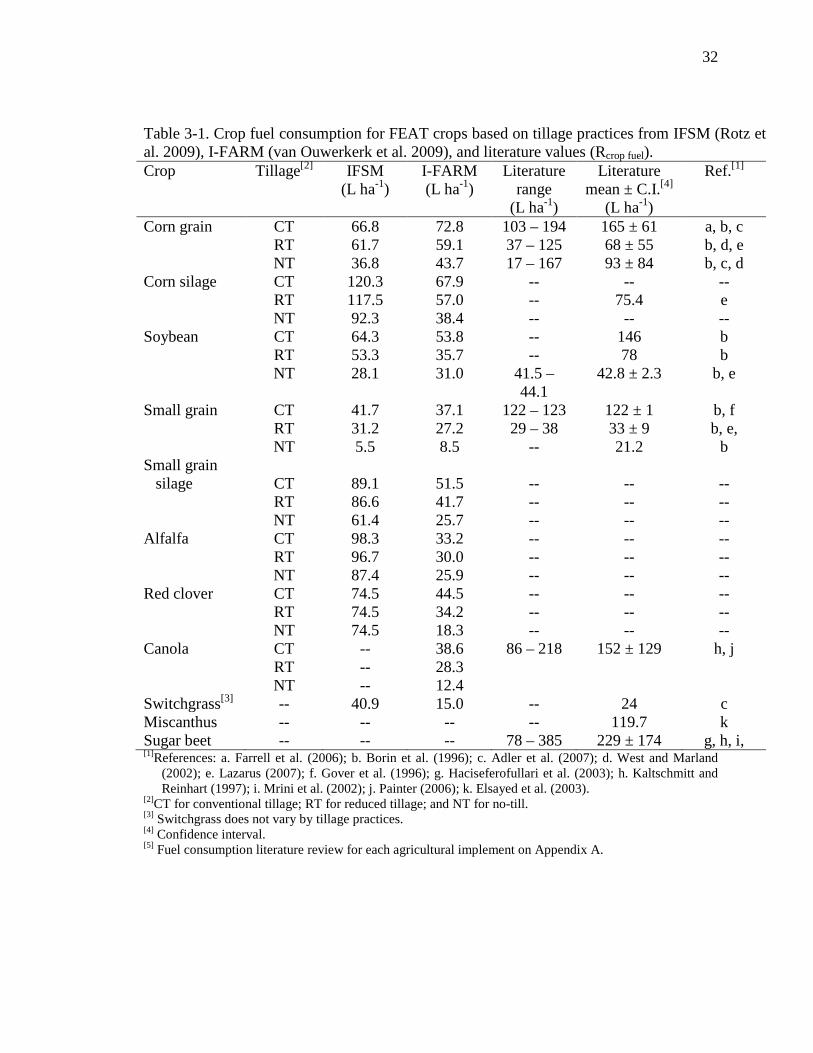
32

Table 3-1. Crop fuel consumption for FEAT crops based on tillage practices from IFSM (Rotz et al. 2009), I-FARM (van Ouwerkerk et al. 2009), and literature values (Rcrop fuel). Crop Tillage[2] IFSM

(L ha-1) I-FARM (L ha-1)

Literature range

(L ha-1)

Literature mean ± C.I.[4]

(L ha-1)

Ref.[1]

Corn grain CT 66.8 72.8 103 – 194 165 ± 61 a, b, c RT 61.7 59.1 37 – 125 68 ± 55 b, d, e NT 36.8 43.7 17 – 167 93 ± 84 b, c, d Corn silage CT 120.3 67.9 -- -- -- RT 117.5 57.0 -- 75.4 e NT 92.3 38.4 -- -- -- Soybean CT 64.3 53.8 -- 146 b RT 53.3 35.7 -- 78 b NT 28.1 31.0 41.5 –

44.1 42.8 ± 2.3 b, e

Small grain CT 41.7 37.1 122 – 123 122 ± 1 b, f RT 31.2 27.2 29 – 38 33 ± 9 b, e, NT 5.5 8.5 -- 21.2 b Small grain

silage

CT

89.1

51.5

--

--

-- RT 86.6 41.7 -- -- -- NT 61.4 25.7 -- -- -- Alfalfa CT 98.3 33.2 -- -- -- RT 96.7 30.0 -- -- -- NT 87.4 25.9 -- -- -- Red clover CT 74.5 44.5 -- -- -- RT 74.5 34.2 -- -- -- NT 74.5 18.3 -- -- -- Canola CT -- 38.6 86 – 218 152 ± 129 h, j RT -- 28.3 NT -- 12.4 Switchgrass[3] -- 40.9 15.0 -- 24 c Miscanthus -- -- -- -- 119.7 k Sugar beet -- -- -- 78 – 385 229 ± 174 g, h, i, [1]References: a. Farrell et al. (2006); b. Borin et al. (1996); c. Adler et al. (2007); d. West and Marland

(2002); e. Lazarus (2007); f. Gover et al. (1996); g. Haciseferofullari et al. (2003); h. Kaltschmitt and Reinhart (1997); i. Mrini et al. (2002); j. Painter (2006); k. Elsayed et al. (2003).

[2]CT for conventional tillage; RT for reduced tillage; and NT for no-till. [3] Switchgrass does not vary by tillage practices. [4] Confidence interval. [5] Fuel consumption literature review for each agricultural implement on Appendix A.

33

Table 3-2. Crop fuel consumption for pesticide application and field residue removal. Operation I-FARM[2]

(L ha-1) Literature range

(L ha-1) Literature mean ± C.I.[4]

(L ha-1) Ref.[1]

Pesticide application

1.87 0.9 – 3.1 1.7±0.57 a, b, c, d, e, f, g

Corn stover harvesting[3]

16.6

--

--

[2]

[1] References: a. Stout (1984); b. West and Marland (2002); c. Ayres (2000); d. Lobb (1989); e.Vaughan et al. (1977); f. Frye and Phillips (1981); g. Nix (1996).

[2] van Ouwerkerk et al. 2009. [3] Value also used for barley straw and sugar beet top removal. [4] Confidence interval.

In addition to field fuel consumption, the remaining crop input requirements of

different crops also vary significantly. Input rates may vary in terms of crop variety, soil

type, weather, crop rotation and tillage practices. Input rates are listed for the following

crop types included in the FEAT: corn for grain (Table 3-3), corn for silage (Table 3-4),

soybean (Table 3-5), barley for grain (Table 3-6); rye for silage (Table 3-7), wheat for

silage (Table 3-8), alfalfa (Table 3-9) red clover (Table 3-10), canola (Table 3-11),

switchgrass (Table 3-12), miscanthus (Table 3-13), and sugar beet (Table 3-14).

Lime is a particular input that has high application variability. There are few

citations relating lime application on soil to grow specific crops, making it difficult to

model diverse crops. FEAT assumes a fixed lime application rate that was estimated for

those crops for which no cited value was found. Given the fact that FEAT runs in an

annual basis, rates are assumed to be applied every year. Default annual lime rates for

crops without a cited value are 300 kg/ha for annual crops and 150 kg/ha for perennials.

Electricity for crop production is generally a minor parameter with low

significance, and it is not included in the FEAT input defaults, although is possible to set

this value manually. I-FARM, with a similar methodology, does not account for

electricity consumption for crop production IFSM accounts for electricity in harvest but

34

is a negligible parameter. In addition, there are few citations that relate electricity

consumption and crop production.

Machinery for crop production is not included in the FEAT analysis. The energy

embedded in machinery is a variable that has a small impact in the total energy and GHG

production. Farrell et al. (2006) reported that machinery accounted for only 1.7% of total

energy, and 0.8% of total GHG emissions associated with corn production.

The following parameters reported by Farrell et al. (2006) were also not included

in FEAT calculations: 1) labor; 2) input packaging; 3) gasoline; and 4) electricity used in

irrigation. First, labor was reported as energy per area, and different crops in FEAT might

use different amounts of labor, making it unrealistic to use the same amount of labor for

each crop. Labor, as muscular energy, is often excluded from energy analyses for that

reason as well. Second, input packaging has a slight impact, estimated by Farrell et al.

(2006) at 0.4% of total energy for farm production, making this parameter negligible.

Third, fuel consumption for crop production was based on IFSM simulations which

reports only diesel fuel consumption. Furthermore, most of the literature used for fuel

consumption evaluation (Table 3-1), did not state values for gasoline usage. Lastly,

irrigation is not a common practice in the northeast US, and thus this parameter was not

included.

In order to perform FEAT analyses, input rates need to be set at a fixed level. For

a more realistic analysis, or a case study to mimic a real operation, the input values could

be changed accordingly. However, having default input values facilitates the use of the

model by users not familiar with those rates, and thus speeds the generation of results.

35

Table 3-3. Corn production: input application rate per year (Rinput).

Value

(kg ha-1yr-1)

Ref.[1]

Range

(kg ha-1yr-1)

Mean ± C.I.[2]

(kg ha-1yr-1)

References[1]

Nitrogen

145

a

32 – 150 140 ± 10.3 a, b, c, d, e, f,

g

Phosphate 56 a 35 – 66 58 ± 8.1 a, b, c, f, g

Potash 34 a 34 – 99 76 ± 16.1 a, b, c

Lime 448 f 23 – 3800 1121 ± 1759 b, e, h

Seed

20

b

17 – 23.6 21 ± 1.4 b, c, f, g, i, j, k, l, m

Herbicide

2.71

b

2.7 – 6.2 3 ± 0.6 b, f, g, h, i, j,

k, l, m, n

Insecticide

0.99

b

0.99 – 2.8 0.9 ± 0.4 b, c, f, g, i, j,

k, l, m, n [1] References: a. PSU Agronomy guide (2008); b. West and Marland (2002); c. Chancellor (1978); d. Adler

et al. (2007); e. Liska et al. (2009); f. Farrell et al. (2006); g. Pimentel and Patzek (2005); h. Kim et al. (2009); i. Pimentel (1980); j. Patzek (2004); k. Shapouri et al. (2004); l. Graboski (2002); m. de Oliveira et al. (2005); n. Wang (2001).

[2] Confidence interval. Table 3-4. Corn for silage production: input application rate per year (Rinput). Value (kg ha-1yr-1) References[1]

Nitrogen 168 a

Phosphate 123 a

Potash 257 a

Lime 448 b

Seed 20 c

Herbicide 3.63 c

Insecticide 0.68 c [1] References: a. PSU Agronomy guide (2008); b. Farrell et al. (2006); c. West and Marland (2002). [2] No statistical analysis because of few references of corn silage input application.

36

Table 3-5. Soybean production: input application rate per year (Rinput).

Value

(kg ha-1yr-1)

Ref.[1]

Range

(kg ha-1yr-1)

Mean ± C.I.[2]

(kg ha-1yr-1)

References[1]

Nitrogen 0 a 0 – 35 19 ± 15.5 a, b

Phosphate 45 a 45 – 67 57 ± 9.2 a, b

Potash 67 a 67 – 108 90 ± 16.8 a, b

Lime 300 -- 0 – 4000 -- b

Seed 81.2 b 63 – 81 72 ± 10.6 b, c, d

Herbicide 1.5 b 0.22 – 3.0 1.7 ± 0.8 b, d

Insecticide 0.39 b 0.3 – 4.9 1.6 ± 2.2 b, d [1] References: a. PSU Agronomy guide (2008); b. West and Marland (2002); c. NDSU (2009); d. Pimentel (1980). [2] Confidence interval. Table 3-6. Rye for silage production: input application rate per year (Rinput).

Value

(kg ha-1yr-1)

Ref.[1]

Range

(kg ha-1yr-1)

Mean ± C.I.[3]

(kg ha-1yr-1)

References[1]

Nitrogen 67 a 34 – 67 -- a, d

Phosphate 67 a 34 – 67 -- a, d

Potash 123 a -- -- --

Lime 300 - -- -- --

Seed 126 b 67 – 126 93 ± 25.5 b, d, e, f

Herbicide[2] 0.4 c 0.28 – 0.4 0.7 ± 0.8 c, d

Insecticide[2] 0.33 c -- 2.1 ± 3.1 c, d, g [1] References: a. PSU Agronomy guide (2008); b. Duiker and Curran (2005); c. West and Marland (2002); d.

Pimentel (1980); e. Clark (2007); f. Nemecek and Erzinger (2003); g. Gover et al. (1996). [2] Values cited in literature for wheat grain. [3] Confidence interval.

37

Table 3-7. Wheat for silage production: input application rate per year (Rinput).

Value

(kg ha-1yr-1)

Ref.[1]

Range

(kg ha-1yr-1)

Mean C.I.[3]

(kg ha-1yr-1)

References[1]

Nitrogen[2] 67 a 37 – 195 102 ± 43.9 a, b, f, g, h, i

Phosphate[2] 67 a 21 – 77 57 ± 12.9 a, b, g, h, i

Potash[2] 123 a 20 – 123 75 ± 20.4 a, b, g, h, i

Lime 300 - 0 – 3800 -- b

Seed[2]

175

b

84 – 185

132 ± 31.9 b, c, d, e, f, g,

h

Herbicide[2] 0.4 b 0.2 – 1.9 0.71 ± 0.79 b, h

Insecticide[2] 0.33 b 0.3 – 8.4 2.1 ± 3.1 b, g, h [1] References: a. PSU Agronomy guide (2008); b. West and Marland (2002); c. Borjesson (1996); d. Nemecek

and Erzinger (2003); e. Clark (2007); f. Richards (2000); g. Gover et al. (1996); h. Pimentel (1980); i. Elsayed et al. (2003).

[2] Values cited on literature for wheat grain. [3] Confidence interval. Table 3-8. Barley production: input application rate per year (Rinput).

Value

(kg ha-1yr-1)

Ref.[1]

Range

(kg ha-1yr-1)

Mean ± C.I.[4]

(kg ha-1yr-1)

References[1]

Nitrogen 67 a -- -- --

Phosphate 56 a -- -- --

Potash 134 a -- -- --

Lime 300 -- -- -- --

Seed 100 b 84 – 100 -- b, c

Herbicide[3] 0.4 b -- -- --

Insecticide[3] 0.33 b -- -- -- [1] References: a. PSU Agronomy guide (2008); b. West and Marland (2002); c. Clark (2007). [2] Reduced till. [3] Value from wheat grain production. [4] Confidence interval.

38

Table 3-9. Alfalfa production: input application rate per year (Rinput).

Value

(kg ha-1yr-1)

Ref.[1]

Range

(kg ha-1yr-1)

Mean ± C.I.[3]

(kg ha-1yr-1)

References[1]



Potash 279 a -- -- --

Lime 150 -- -- -- --

Seed[2] 5.6 b 4.1 – 5.6 -- b, c

Herbicide 0 -- -- -- --

Insecticide 0 -- -- -- -- [1] References: a. PSU Agronomy guide (2008); b. Rankin (2008); c. NDSU (2009). [2] 3-year standing assumption. [3] Confidence interval. Table 3-10. Red clover production: input application rate per year (Rinput).

Value

(kg ha-1yr-1)

Ref.[1]

Range

(kg ha-1yr-1)

Mean ± C.I.[2]

(kg ha-1yr-1)

References[1]



Potash 179 a -- -- --

Lime 150 -- -- -- --

Seed 8 b 7.8 – 10.1 8.2 ± 1.6 b, c, d, e

Herbicide 0 -- -- -- --

Insecticide 0 -- -- -- -- [1] References: a. PSU Agronomy guide (2008); b. West and Marland (2002); c. Clark (2007); d. Borjesson (1996);

e. Nemecek and Erzinger (2006). [2] Confidence interval.

39

Table 3-11. Canola production: input application rate per year (Rinput).

Value

(kg ha-1yr-1)

Ref.[1]

Range

(kg ha-1yr-1)

Mean ± C.I.[2]

(kg ha-1yr-1)

References[1]

Nitrogen 145 a 145 – 204 172 ± 26.6 a, d, e

Phosphate 39 a 39 – 50 46 ± 7.1 a, d, e

Potash 56 a 40 – 56 48 ± 9.0 a, d, e

Lime 19 b -- -- --

Seed 6 a 5.0 – 8.4 6.2 ± 1.3 a, b, e, f, g

Herbicide 3.4 c 2.8 – 3.4 -- c, d

Insecticide 0 -- -- -- -- [1] References: a. NDSU (2009); b. Kaltschmitt and Reinhardt (1997); c. Monsanto (2009); d. Elsayed et al.

(2003); e. Richards (2000); f. Borjesson (1996); g. Clark (2007). [2] Confidence interval. Table 3-12. Switchgrass production: input application rate per year (Rinput).

Value

(kg ha-1yr-1)

Ref.[1]

Range

(kg ha-1yr-1)

Mean ± C.I.[3]

(kg ha-1yr-1)

References[1]

Nitrogen 50 a 50 – 158 78 ± 51.9 a, c, b, d

Phosphate 2.1 b -- -- --

Potash 3.4 b -- -- --

Lime 150 -- -- -- --

Seed[2] 0.11 c 0.1 – 0.4 0.37 ± 0.26 c, e, f

Herbicide 0.42 b 0 – 3 -- b, c

Insecticide 0 b 0 – 4.2 -- b, g [1] References: a. McLaughlin and Kszos (2005); b. Wang (2001); c. Pimentel and Patzek (2005); d. Adler et al.

(2007); e. Walsh and Becker (1996); f. Teel and Barnhart (2003); g. Mehdi et al. (2000). [2]15-year stand assumption. [3] Confidence interval.

40

Table 3-13. Miscanthus production: input application rate per year (Rinput).

Value

(kg ha-1yr-1)

Ref.[1]

Range

(kg ha-1yr-1)

Mean ± C.I.[2]

(kg ha-1yr-1)

References[1]

Nitrogen 84 a 80 – 100 93 ± 8.8 a, b, c, d, e

Phosphate 14 a 14 – 100 53 ± 36.9 a, b, c, d, f

Potash 113 a 60 – 200 122 ± 46.0 a, b, c, d, f

Lime 158 b -- -- --

Seed 52.6 b 19.2 – 52.6 -- b, f

Herbicide 0.72 b -- -- --

Insecticide 0 -- -- -- -- [1] References: a. Gibson and Barnhart (2007); b. Bullard and Metcalfe (2001); c. Lewandowski et al. (1995); d.

Jones and Walsh (2001); e. Collura et al. (2006); f. Christian et al. (1997). [2] Confidence interval.

Table 3-14. Sugar beet production: input application rate per year (Rinput).

Value

(kg ha-1yr-1)

Ref.[1]

Range

(kg ha-1yr-1)

Mean ± C.I.[2]

(kg ha-1yr-1)

References[1]

Nitrogen 145 a 145 – 255 170 ± 41.7 a, b, d, e, g

Phosphate 45 a 45 – 159 87 ± 42.9 a, b, d, e, g

Potash 61 a 60 – 141 77 ± 31.3 a, b, d, e, g

Lime 150 -- -- -- --

Seed 3.25 b 3.20 – 10 5.4 ± 2.5 b, d, e, f, g

Herbicide 0.12 c 0.1 – 4.0 1.7 ± 1.5 b, c, d, e, g

Insecticide 0.15 b -- -- -- [1] References: a. Cattanach et al. (1993); b. Erdal et al. (2007); c. OMAFRA (2002); d. Haciseferofullari et al.

(2003); e. Kaltschmitt and Reinhardt (1997); f. Harris and Barry (2004); g. Mrini et al. (2002). [2] Confidence interval.

In order to facilitate FEAT simulations, a data-set of crop yields was organized

(Table 3-15). Crop yield is a very sensitive parameter that has significant variability, due

to conditions such as weather, soil, location, input intensity, irrigation, tillage, seed

41

variety and rotation. Literature values for each crop yield were assumed to be the default

FEAT values.

Table 3-15. FEAT crop default yields per year (Ycrop). Crops

Value

(Mg DM[3] ha-1yr-1)

Ref.[1]

Range

(Mg DM ha-1yr-1)

Mean ± C.I.[2]

(Mg DM ha-1yr-1)

Ref.[1]

Corn for grain

7.40

a

6.18 – 7.99 7.1 ± 0.4 a, b, c, d, e,

f, g, h, t, l

Corn for silage 17.90 i 17.9 – 19.9 18.6 ± 1.2 i, l, q

Soybean 2.91 a 2.33 – 2.91 2.6 ± 0.6 a, l

Barley 4.17 a 3.48 – 4.17 3.8 ± 0.7 a, l

Rye for silage 5.19 l 0.8 – 5.2 2.62 ± 1.1 j, l, r

Wheat for

silage 5.19 l

5.2 – 5.4

5.31 ± 0.3

l, q

Alfalfa 10.09 l 10.7 – 11.1 10.9 ± 0.4 k, l

Red clover 7.78 l 7.78 – 8.30 8.04 ± 0.5 k, l

Canola 2.5 a 1.94 – 3.07 2.6 ± 0.7 a, o, p

Switchgrass 9.88 a 8.92 – 13.5 10.8 ± 2.7 a, m, n

Miscanthus

20.00

w

15 – 41 24.6 ± 8.0 o, w, y, z,

aa, bb

Sugar beet

18.75

x

15.2 – 21 17.3 ± 1.8 a, b, o, u, v,

x [1] References: a. Roth (2008); b. Icoz et al. (2009); c. Shapouri et al. (2004); d. Patzek (2004); e. Pimentel and Patzek

(2005); f. Graboski (2002); g. de Oliveira et al. (2005); h. Wang (2001); i. Lauer et al. (2004); j. Kaspar and Singer (2007); k. Smith (1965); l. PSU agronomy guide (2008); m. McLaughlin and Walsh (1998); n. Adler et al. (2006); o. Elsayed et al. (2003); p. Canada Council (2008); q. Brown (2006); r. Snapp et al. (2005); t. Heggenstaller et al. (2008); u. Haciseferofullari et al. (2003); v. Erdal et al. (2007); x. Milford (2006); w. Collura et al. (2006); y. Lewandowski et al. (1995); z. Christian et al. (1997); aa. Clifton-Brown et al. (2001); bb. Heaton et al. (2004).

[2] Confidence interval. [3] Dry matter.

Residue removal rate is a required user input. The residue/crop ratio is the mass

ratio of crop residue per crop (grain) production. FEAT crop residues are corn stover,

42

barley straw and sugar beet tops (Table 3-16). The crop residue harvested is calculated

as:

Cresidue = ∑ Ycrop . A. Rremoval . Rresiduecropi=1 (3.1)

where Cresidue is the annual crop residue [Mg yr-1], Ycrop is the annual crop yield [Mg ha-

1yr-1], A is the field area [ha], Rremoval is the crop removal percentage (user input) [%], and

Rresidue is the ratio between crop and residue production [dimensionless].

Table 3-16. Residue to crop ratio (Rresidue). Type Value Units References[1]

Corn stover 1 kg WM kg-1 WM[3] a

Barley straw[2] 0.53 kg WM kg-1 WM[3] b

Beet top 1 kg DM kg-1 DM[4] c [1] References: a. Posselius and Stout (1982); b. Elsayed et al. (2003); c. Harland et al. (2006). [2] This ratio was referred to wheat residue in the study. [3] kg of residue (wet matter) per kg of crop (wet matter). [4] kg of residue (dry matter) per kg of crop (dry matter).

Both, dry and wet matter crop production, are used throughout FEAT

calculations. Each crop and residue has different moisture contents at harvest (Table 3-

17). The dry and wet matter content was assessed using:

CDM = CWM . (1 − Cmoist ) (3.2)

where CDM is crop or residue dry matter [kg DM], CWM is crop or residue wet matter [kg

WM], and Cmoist is crop or residue moisture content [kg water kg crop-1].

43

Table 3-17. Crop and residue moisture content (Cmoist). Type Value Unit References[1]

Corn 0.155 kg water kg-1crop a

Corn silage[2] 0.65 kg water kg-1crop e

Soybean 0.13 kg water kg-1crop a

Barley 0.14 kg water kg-1crop d

Canola 0.09 kg water kg-1crop c

Switchgrass 0.15 kg water kg-1crop f

Miscanthus 0.30 kg water kg-1crop g

Sugar beet 0.75 kg water kg-1crop h

Corn stover 0.30 kg water kg-1crop b [1] References: a. Beuerlein (2008); b. Nielsen (1995); c. Boyles (2009); d. Hall (2009); e. PSU Agronomy

guide (2008); f. McLaughlin et al. (1996); g. Danalatos et al. (2006); h. Kumhala et al. (2008). [2] Corn silage half milk line. This value was also used for rye silage and wheat silage.

3.2.2. Dairy livestock production

The Dairy Farm System represents a dairy operation in FEAT. The user is

required to provide the number of cows as an input factor. With this input, FEAT

automatically calculates herd size (lactating cows, dry cows, heifers and calves), milk

production, manure production, manure storage, manure nutrients (N, P, K), dairy

livestock labor, fuel for manure handling, fuel for feed handling, and dairy livestock

electricity consumption. Straight vegetable oil production, meal, and electricity for oil

extraction is also calculated when oil seeds are present on the farm.

Herd type distribution is calculated using values in Table 3-18. For example, if a

farm has 100 cows (Ncow), that translates to 85 lactating cows, 15 dry cows, 38 heifers

(over one year) and 42 heifers (under one year). Milk and manure production results are

calculated using number of animals (Ncow) (Table 3-19).

44

Table 3-18. Dairy farm livestock ratio management. Type Value Unit Variable References[1]

Cows 1 -- Ncow a

Lactating cows 0.85 -- -- a

Dry cows 0.15 -- -- a

Older heifers (over one year) 0.38 -- -- a

Young heifers (under one year) 0.42 -- -- a [1] References: a. Chianese et al. (2009d). Table 3-19. Dairy farm outputs (Rmilk, Rmanure). Type Value Unit Variable References[1]

Milk 8,791 L cow-1 yr-1 Rmilk a[2]

Lactating cow manure 24,820 L cow-1 yr-1 Rmanure b

Dry cow manure 13,870 L cow-1 yr-1 Rmanure b

Heifer manure 8,030 L cow-1 yr-1 Rmanure b

Calf manure 3,103 L cow-1 yr-1 Rmanure b [1] References: a. van Ouwerkerk et al. (2009); b. ASAE (2005). [2] Target milk production.

The dairy feed requirement is another parameter that has large variability.

Depending on the crop and nutritional strategy, different quantities of diverse feed

options can be used. In order to simplify this real-world complexity, a default fixed diet

could be used (Table 3-20). Salt, minerals and fat supplements were purchased and

imported to the farm. Protein supplements were soybean or canola meal. The dairy

livestock diet is a user input, and could be changed once the user knows another type of

diet.

45

Table 3-20. Dairy feed requirements per cow per year[2]. Feed type Value Units References[1]

Corn grain 2.6 Mg WM[3] a

Corn silage 7.3 Mg WM a

Forage 5.5 Mg WM a

Protein supplement 0.9 Mg WM a

Salt and mineral supplements 0.11 Mg a

Fat supplement 0.012 Mg a [1] Reference: a. van Ouwerkerk et al. (2009). [2] Target milk production of 8,791 L cow-1 yr-1. [3] Wet matter. Manure produced on-farm is stored and applied to crop fields. The amount of

plant nutrients present in a cubic meter of manure is shown on Table 3-21. Depending

upon the type of manure application, the soil nutrients available for the plant varies.

These nutrient application efficiency values (Table 3-21) are default inputs that can be

changed by the user. The recycled manure nutrients (N, P, and K) reduce off-farm

fertilization requirements for crop production.

46

Table 3-21. Dairy manure nutrient content and use efficiency.

Type value Units[3] Ref.[1]

Efficiency

value[2] Ref.[1]

Lactating cow nitrogen 6.62 kg m-3[4] a 30% b

Lactating cow potash 1.15 kg m-3[4] a 100% b

Lactating cow phosphate 1.51 kg m-3[4] a 100% b

Dry cow nitrogen 6.05 kg m-3[4] a 30% b

Dry cow potash 0.79 kg m-3[4] a 100% b

Dry cow phosphate 3.89 kg m-3[4] a 100% b

Heifer nitrogen 5.45 kg m-3[5] a 30% b

Heifer potash 0.91 kg m-3[5] a 100% b

Heifer phosphate -- kg m-3[5] a 100% b

Calf nitrogen 3.41 kg m-3[5] a 30% b

Calf potash -- kg m-3[5] a 100% b

Calf phosphate -- kg m-3[5] a 100% b [1] References: a. ASAE (2005); b. Hansen (2006). [2] Percent of nutrients available for the plant. [3] kg of nutrient per cubic meter of manure. [4] 87% moisture. [5] 83% moisture.

For some dairy management parameters, it is necessary to calculate livestock

units (LU). Dairy livestock weight (Table 3-22) is required in order to calculate livestock

units. One livestock unit equals 500 kg of livestock weight (Chianese et al. 2009d). The

dairy livestock LU distribution of each type of animal was also pre-calculated (Table 3-

23).

47

Table 3-22. Dairy farm livestock weight. Type Value Units References[1]

Lactating cows 650 kg a

Dry cows 650 kg a

Older heifers(over one year) 470 kg a

Young heifers (under one year) 200 kg a [1] References: a. Chianese et al. (2009d). Table 3-23. Dairy farm livestock unit (LU[2]). Type Value Unit Reference[1]

Lactating cows 1.30 LU a

Dry cows 1.30 LU a

Older heifers (over one year) 0.94 LU a

Young heifers cows (under one year) 0.4 LU a [1] Reference: a. Chianese et al. (2009d). [2] Livestock unit is 500 kg of live body mass.

Dairy management requirements are comprised of labor, fuel for manure

handling, fuel for feed handling, electricity consumption from dairy facilities, and volume

of manure storage (Table 3-24). Labor and electricity consumption are calculated using

cow units (Ncow). Livestock unit (LU) is a parameter used to calculate fuel for feed

handling (RFH). Manure storage volume per cow (Rmanure storage) is used to calculate the

fuel for manure handling (RMH). Electricity used on a dairy farm is comprised of: 1) milk

harvest; 2) milk cooling; 3) lighting; 4) circulation and ventilation; 5) washing and

watering; 6) water systems; and 7) compressed air systems (Ludington et al. 2005). The

FEAT dairy livestock electricity value used was 2,959 MJ cow-1year-1 (Ludington and

Johnson, 2005). Fuel for feed handling accounts for feed transported to dairy livestock.

Fuel for manure handling accounts for removal, storage, and spreading.

48

Table 3-24. Dairy management annual requirements. Type Value Units[2] Variable References[1]

Labor 70 hrs cow-1year-1 -- a

Electricity consumption 2,959 MJ cow-1year-1 Relectr b

Fuel for feed handling 31.6 L LU-1 year-1 RFH c, d

Fuel for manure handling 0.58 L m-3manure RMH c, d

Manure storage 11 m3 cow-1year-1 RMS d [1] References: a. van Ouwerkerk et al. (2009); b. Ludington and Johnson (2005); c. Lazarus (2007); d. Chianese et

al. (2009d). [2] Livestock unit (LU) is 500 kg of live body mass.

3.2.3. Energy balance methodology

FEAT calculates the energy balance using a methodology adapted from Farrell et

al. (2006). The concept is to convert the main elements of the studied system into a

common unit of energy, in this case mega-joule (MJ). With the same energetic unit, all of

the system elements can be compared. Net energy value (NEV) and net energy ratio

(NER) are the two measurements typically used in energy balance evaluations. Net

energy value is the sum of energy content of the outputs minus the sum of the energy

contents of the inputs (Eq. 3.3). Net energy ratio is the sum of energy outputs divided by

the sum of energy inputs (Eq. 3.4). Farrell et al. (2006) stated that NER is not a strong

metric due to challenges with co-product allocation, concluding that NEV is a more

consistent measurement. Net energy value (NEV) and net energy ratio (NER) are

calculated as:

NEV = Eoutputs − Einputs (3.3)

NER = Eoutputs

Einputs (3.4)

49

where NEV is net energy value [MJ], NER is net energy ratio [dimensionless], Eoutputs is

the sum of energy outputs [MJ] and Einputs is the sum of fossil fuel energy inputs [MJ].

Due to different boundaries and characteristics of each system (Crop – Figure 3-1;

Dairy – Figure 3-2, and Biofuels – Figure 3-3), the assessment was divided into sections

to estimate energy inputs (Table 3-25) and outputs (Table 3-26). The energy inputs were

divided as: 1) general inputs; 2) dairy specific inputs; and 3) biofuel specific inputs. The

energy outputs for each system were milk, crops, excess straight vegetable oil, excess

feed meal production, biofuels and biofuel co-products.

Table 3-25. Energy inputs for energy balance analysis. Energy Inputs

Crop Farm

System

Dairy Farm

System

Biofuel Farm

System

General inputs

Farm inputs[1] x x x

Fuel for crop production x x x

Farm inputs transportation x x x

Crop drying x x x

Dairy specific inputs

Oil seed processing -- x --

Fuel for feed handling -- x --

Fuel for manure handling -- x --

Electricity for dairy -- x --

Biofuel specific inputs

Transport feedstock to biorefinery -- -- x

Biorefinery processing -- -- x [1] Nitrogen, phosphate, potash, lime, seed, herbicide, and insecticide.

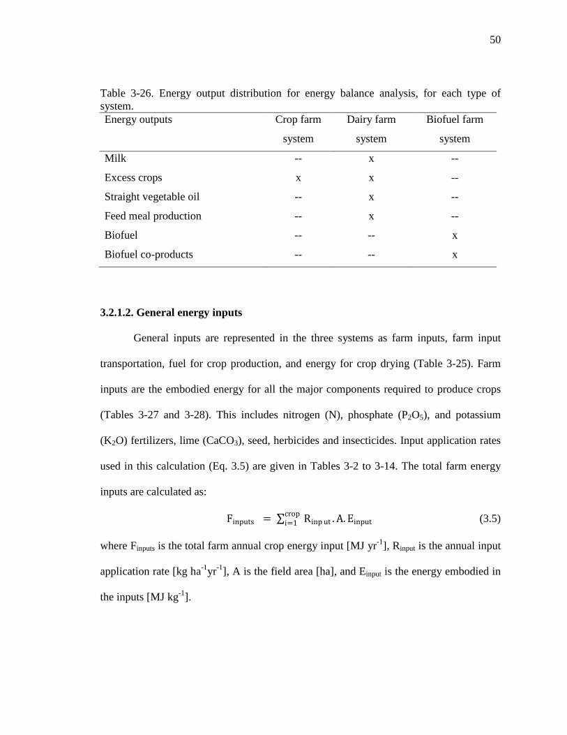
50

Table 3-26. Energy output distribution for energy balance analysis, for each type of system. Energy outputs

Crop farm

system

Dairy farm

system

Biofuel farm

system

Milk -- x --

Excess crops x x --

Straight vegetable oil -- x --

Feed meal production -- x --

Biofuel -- -- x

Biofuel co-products -- -- x

3.2.1.2. General energy inputs

General inputs are represented in the three systems as farm inputs, farm input

transportation, fuel for crop production, and energy for crop drying (Table 3-25). Farm

inputs are the embodied energy for all the major components required to produce crops

(Tables 3-27 and 3-28). This includes nitrogen (N), phosphate (P2O5), and potassium

(K2O) fertilizers, lime (CaCO3), seed, herbicides and insecticides. Input application rates

used in this calculation (Eq. 3.5) are given in Tables 3-2 to 3-14. The total farm energy

inputs are calculated as:

Finputs = ∑ Rinp ut . A. Einputcropi=1 (3.5)

where Finputs is the total farm annual crop energy input [MJ yr-1], Rinput is the annual input

application rate [kg ha-1yr-1], A is the field area [ha], and Einput is the energy embodied in

the inputs [MJ kg-1].

51

Table 3-27. Embodied energy in crop inputs (Einput). Type

Value

(MJ kg-1)

Ref.[1]

Range

(MJ kg-1)

Mean ± C.I.[2]

(MJ kg-1)

Ref.[1]

Nitrogen

56.95

a

40.6 – 80.0

58.3 ± 4.4

a, b, d, e, f, g,

h, i, j, k, l, m,

n, o, p, q, r, s,

t, v

Phosphate

9.30

a

6.8 – 18.1

11.4 ± 2.0 a, b, d, g, h, k,

l, n, o, p, q, r, t,

u, v, x, w

Potash

6.97

a

4.7 – 13.6

7.9 ± 1.0 a, b, d, g, h, l,

n, o, p, q, r, t,

u, v, x, y

Lime 0.12 a 0.12 – 8.2 2.1 ± 2.1 a, b, d, g, o, p

Insecticide

358

a

100 – 418

313 ± 42 a, b, d, e, g, l,

n, o, p, q, t

Herbicide

356

a

100 – 418

302 ± 47 a, b, c, d, e, g,

l, n, o, p, q, t, v [1] References: a. Farrell et al. (2006); b. West and Marland (2002); c. Nemecek and Erzinger (2003); d. Pimentel

and Patzek (2005); e. Pimentel (1980); f. FAO (1999a); g. Patzek (2004); h. Muller (1992); i. Stout (1990); j. Bertilson (1992); k. Spatari et al. (2005); l. Wang (2001); m. Snyder et al. (2007) ; n. Shapouri et al. (2004); o. Graboski (2002); p. de Oliveira et al. (2005); q. Chancellor (1978); r. Lewis (1982); s. Coxworth et al. (1994); t. Sheehan et al. (1998); u. Southwell et al. (1977); v. Ahmed et al. (1994); x. Kaltschmitt and Reinhardt (1997); w. Kongshaug (1998); y. Borin et al. (1996).

[2] Confidence interval.

52

Table 3-28. Crop input energy embodied in seed production (Einput). Type

Value

(MJ kg-1yr-1)

Ref.[1]

Range

(MJ kg-1yr-1)

Mean ± C.I.[6]

(MJ kg-1yr-1)

References[1]

Corn

53.36

a

9.7 – 104

45.5 ± 30.1 a, b, e, f, g, h,

i,

Soybean 12.86 a 4.7 – 33.5 17.0 ± 16.8 a, j, o

Wheat [2]

5.87

a

3.0 – 18.2

9.3 ± 4.1 a, b, k, l, m,

n, o

Barley 5.57 a 3.0 – 12.7 7.1 ± 4.0 a, b, l, o

Alfalfa [3] 44.36 a -- -- --

Red clover 87.01 a 20.0 – 87.0 41.5 ± 44.6 a, b, k

Canola 13 b 5.0 – 28.0 13.5 ± 7.8 b, k, l, m, p

Switchgrass 26.15 e 6.0 – 45.1 25.8 ± 22.1 e, t, u

Miscanthus [4,5] 8.00 c 8.0 – 160

84.2 ± 149 c, q

Sugar beet 50 d 22.0 – 85.0 48.5 ± 20.6 b, d, p, r, s [1] References: a. West and Marland (2002); b. Nemecek and Erzinger (2003); c. Bullard and Metcalfe (2001);

d. Erdal et al. (2007); e. Pimentel and Patzek (2005); f. Shapouri et al. (2004); g. Graboski (2002); h. de Oliveira et al. (2005); i.Chancellor (1978); j. Sheehan et al. (1998) ; k. Borjesson (1996); l. Zentner and Sontag (1998); m. Richards (2000); n. Gover et al. (1996); o. Pimentel (1980); p. Kaltschmitt and Reinhardt (1997); q. Lewandowski et al. (1995); r. Mrini et al. (2002); s. Haciseferofullari et al. (2003); t. Walsh and Becker (1996); u. Shmer et al. (2008);

[2] Value used for rye silage. [3] Assuming 3 year standing. [4] Assuming 19-year average. [5] MJ per hectare. [6] Confidence interval.

Fuel needed for crop production includes the diesel used to power machines and

field implements for each crop type (Table 3-1). The energy associated with this fuel is

the sum of the embodied energy of the diesel fuel (38.66 MJ L-1) plus the energy required

to process and transport the fuel to the farm (6.17 MJ L-1) (West and Marland, 2002). The

fuel energy is calculated as:

53

Ffuel = ∑ Rcrop fuel . A. Efuelcropi=1 (3.6)

where Ffuel is the fuel energy for annual crop production [MJ yr-1], Rcrop fuel is the annual

fuel consumed per crop [L ha-1yr-1], A is area [ha], and Efuel is the energy embodied in the

fuel [MJ L-1].

Table 3-29. Embodied fuel energy (Efuel). Type

Value

(MJ L-1)

Ref.[1]

Range

(MJ L-1)

Mean ± C.I.[2]

(MJ L-1)

References[1]

Diesel 38.66 a, b -- -- --

Diesel processing

and transporting 6.17 a, c 3.27 – 17.71

7.54 ± 2.8

d, e, f, g, h, i,

j, k

Total diesel energy 44.83 a -- -- -- [1] References: a. West and Marland (2002); b. EIA (1999); c. US Office of Technology Assessment (1990); d.

Pimentel (1980); e. Southwell and Rothwell (1977); f. Pimentel and Patzek (2005); g. Frischknecht and Jungbluth (2007); h. Coxworth et al. (1994); i. Rosa (2007); j. Sheehan 1998; k. Prabhu et al. (2009).


Farm transportation input is the energy required to transfer farm inputs from

manufacturing facilities to the farm. This calculation is based on Equation 3.7 and Table

3-30. Shapouri et al. (2004) used the GREET model (Wang, 2001) to report an energy

requirement of 0.64 MJ per kg of inputs for fuel consumption associated with farm input

transportation. Energy for transportation is a parameter with great variability, depending

on location and distance. FEAT uses a value that accounts for 634 km for barge and

1,207 km for rail from manufacturing plants to bulk terminals, 80 km for transportation

from bulk terminals to mixing centers, and 48 km for transportation from mixing centers

to farms. The total energy for farm input transportation is determined as:

Ftransp = ∑ Einput transport . Rinput . Ainputi=1 (3.7)

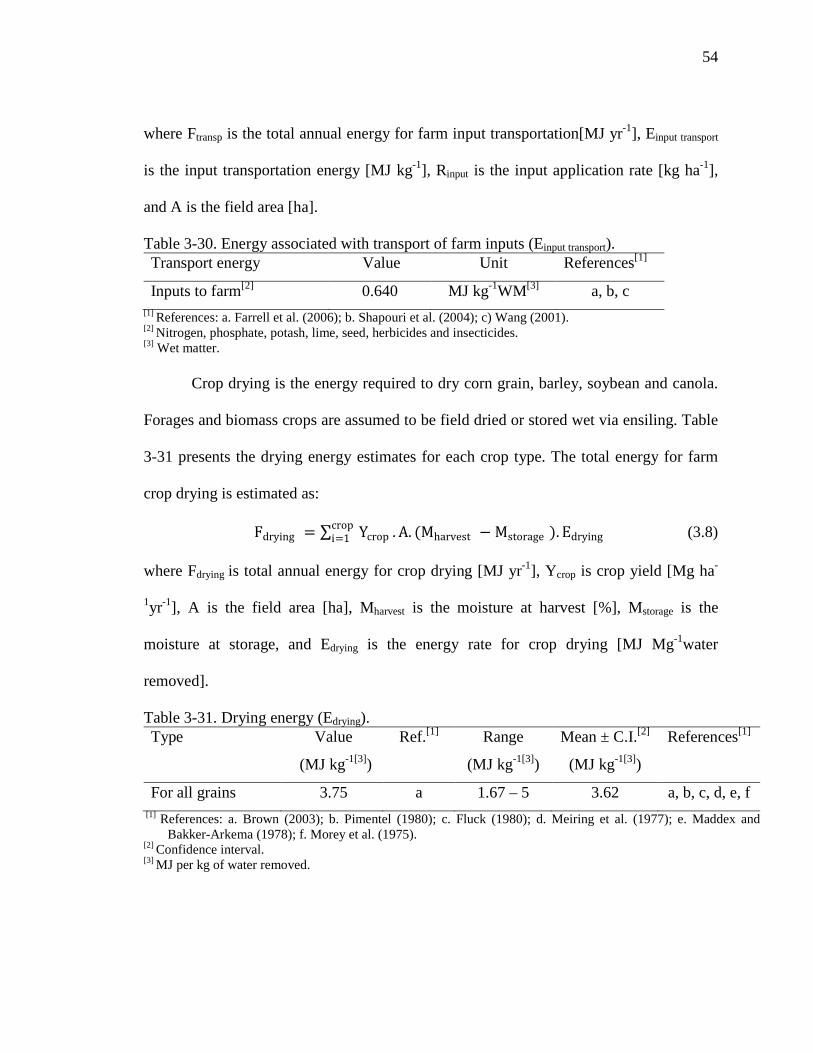
54

where Ftransp is the total annual energy for farm input transportation[MJ yr-1], Einput transport

is the input transportation energy [MJ kg-1], Rinput is the input application rate [kg ha-1],

and A is the field area [ha].

Table 3-30. Energy associated with transport of farm inputs (Einput transport). Transport energy Value Unit References[1]

Inputs to farm[2] 0.640 MJ kg-1WM[3] a, b, c [1] References: a. Farrell et al. (2006); b. Shapouri et al. (2004); c) Wang (2001). [2] Nitrogen, phosphate, potash, lime, seed, herbicides and insecticides. [3] Wet matter.

Crop drying is the energy required to dry corn grain, barley, soybean and canola.

Forages and biomass crops are assumed to be field dried or stored wet via ensiling. Table

3-31 presents the drying energy estimates for each crop type. The total energy for farm

crop drying is estimated as:

Fdrying = ∑ Ycrop . A. (Mharvest − Mstorage ). Edryingcropi=1 (3.8)

where Fdrying is total annual energy for crop drying [MJ yr-1], Ycrop is crop yield [Mg ha-

1yr-1], A is the field area [ha], Mharvest is the moisture at harvest [%], Mstorage is the

moisture at storage, and Edrying is the energy rate for crop drying [MJ Mg-1water

removed].

Table 3-31. Drying energy (Edrying). Type

Value

(MJ kg-1[3])

Ref.[1]

Range

(MJ kg-1[3])

Mean ± C.I.[2]

(MJ kg-1[3])

References[1]

For all grains 3.75 a 1.67 – 5 3.62 a, b, c, d, e, f [1] References: a. Brown (2003); b. Pimentel (1980); c. Fluck (1980); d. Meiring et al. (1977); e. Maddex and

Bakker-Arkema (1978); f. Morey et al. (1975). [2] Confidence interval. [3] MJ per kg of water removed.

55

3.2.1.3. Dairy Farm System specific inputs

The dairy specific energy inputs are: 1) Pressing oil seed; 2) fuel for feed

handling; 3) fuel for manure handling; and 3) electricity for dairy facilities. Soybean and

canola are the oil seed crops that, in the Dairy Farm System, are assumed to be converted

into straight vegetable oil (SVO) and meal. Table 3-32 gives the energy used for crushing

oil seed. The total farm energy to crush the oil seeds is calculated as:

Fcrushing = ∑ Ycrop . A. Ecrushingoil seedi=1 (3.9)

where Fcrushing is the total annual farm energy to crush oil seeds [MJ yr-1], Ycrop is annual

crop yield [Mg ha-1yr-1], A is area [ha], and Ecrushing is energy rate for oil seed crushing

[MJ Mg-1].

Table 3-32. Crushing oil seed energy for straight vegetable oil production (Ecrushing). Type Value Unit Reference[1]

Canola[2] 1,640 MJ Mg-1 [3] a [1] Reference: a. Smith et al. (2007). [2] Value used for soybean. [3] Mega-joule per mega-gram of seed. Fuel for feed handling, fuel for manure handling, and electricity for dairy are also

part of the Dairy Farm System specific energy inputs. This part of the analysis requires

previous information such as the fuel consumption for manure handling (Table 3-24),

fuel consumption for feed handling (Table 3-24), electricity for dairy production (Table

3-24), livestock live unit distribution (Table 3-23), and fuel energy embodied (Table 3-

29). Farm fuel energy for feed handling is calculated as:

Ffeed handling = LU. RFH . Efuel (3.10)

where Ffeed handling is the farm annual fuel energy required for feed handling [MJ yr-1], LU

is total livestock live units [LU], RFH is the annual rate of fuel use for feed handling [L

56

LU-1yr-1], and Efuel is energy embodied in fuel [MJ L-1]. Farm fuel for manure handling is

estimated as:

Fmanure handling = Ncow . Rmanure . RMH . Efuel (3.11)

where Fmanure handling is the annual farm fuel energy for manure handling [MJ yr-1], Ncow is

the number of cows (user input) [cow], Rmanure is manure production rate[Lmanure cow-1yr-

1], RMH is the rate of fuel use per unit of manure handled [Lfuel Lmanure-1yr-1] and Efuel is

the energy embodied in fuel [MJ L-1]. Farm energy from dairy electricity is computed as:

Fdairy electr = Ncow . Relectr (3.12)

where Fdairy electr is the annual farm energy from dairy electricity [MJ], Ncow is the number

of cows [cow], and Relectr is electricity rate required per cow [MJ cow-1yr-1].

3.2.1.4. Biofuel Farm System specific inputs

In the Biofuel Farm System, with broader boundaries, it is necessary to account

for feedstock transportation from the farm to a biorefinery as well as biorefinery

operations. The feedstock transportation component assumed a fixed distance for all

FEAT crops. Shapouri et al. (2004) used GREET (Wang, 2001) to estimate corn

transportation (Table 3-30). The general value of 0.234 MJ kg-1 accounts for 64 km from

farm to collector terminals, 563 km for barge transport to ethanol plants, or 644 km for

rail to ethanol plants. In order to maintain some uniformity, the same transportation rate

was used for soybean and canola. For biomass transportation, which accounts for corn

silage, rye silage, wheat silage, red clover, switchgrass, alfalfa, barley stover, sugar beet,

sugar beet top, and miscanthus, FEAT uses the value of 0.205 MJ kg-1 (Table 3-33), as

estimated for switchgrass by Farrell et al. (2006) using the GREET model (Wang, 2001).

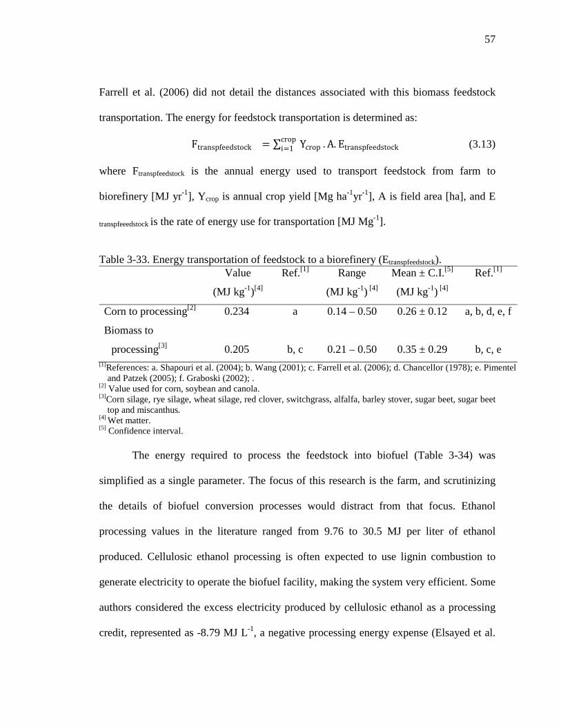
57

Farrell et al. (2006) did not detail the distances associated with this biomass feedstock

transportation. The energy for feedstock transportation is determined as:

Ftranspfeedstock = ∑ Ycrop . A. Etranspfeedstockcropi=1 (3.13)

where Ftranspfeedstock is the annual energy used to transport feedstock from farm to

biorefinery [MJ yr-1], Ycrop is annual crop yield [Mg ha-1yr-1], A is field area [ha], and E

transpfeeedstock is the rate of energy use for transportation [MJ Mg-1].

Table 3-33. Energy transportation of feedstock to a biorefinery (Etranspfeedstock).

Value

(MJ kg-1)[4]

Ref.[1]

Range

(MJ kg-1) [4]

Mean ± C.I.[5]

(MJ kg-1) [4]

Ref.[1]

Corn to processing[2] 0.234 a 0.14 – 0.50 0.26 ± 0.12 a, b, d, e, f

Biomass to

processing[3] 0.205 b, c 0.21 – 0.50

0.35 ± 0.29

b, c, e [1]References: a. Shapouri et al. (2004); b. Wang (2001); c. Farrell et al. (2006); d. Chancellor (1978); e. Pimentel

and Patzek (2005); f. Graboski (2002); . [2] Value used for corn, soybean and canola. [3]Corn silage, rye silage, wheat silage, red clover, switchgrass, alfalfa, barley stover, sugar beet, sugar beet

top and miscanthus. [4] Wet matter. [5] Confidence interval.

The energy required to process the feedstock into biofuel (Table 3-34) was

simplified as a single parameter. The focus of this research is the farm, and scrutinizing

the details of biofuel conversion processes would distract from that focus. Ethanol

processing values in the literature ranged from 9.76 to 30.5 MJ per liter of ethanol

produced. Cellulosic ethanol processing is often expected to use lignin combustion to

generate electricity to operate the biofuel facility, making the system very efficient. Some

authors considered the excess electricity produced by cellulosic ethanol as a processing

credit, represented as -8.79 MJ L-1, a negative processing energy expense (Elsayed et al.

58

2003). Other authors (Wang, 2001; Farrell et al. 2006) use a different approach, such that

after cellulosic ethanol electricity requirement is fulfilled, the excess electricity is

considered as a co-product (Wang, 2001, Farrell et al. 2006). The total energy to process

the feedstock into biofuel is computed as:

Ebiorefinery = ∑ Ycrop . A. Eprocessingcropi=1 (3.14)

where Ebiorefinery is the total energy to process the feedstock into biofuel annually [MJ yr-

1], Ycrop is annual crop yield [Mg ha-1yr-1], A is field area [ha], and Eprocessing is the energy

rate for feedstock conversion to biofuels[MJ Mg-1].

Table 3-34. Biorefinery feedstock processing energy (Eprocessing). Biofuel type

Value

(MJ L-1)

Ref.[1]

Range

(MJ L-1)

Mean ± C.I.[4]

(MJ L-1)

References[1]

Corn ethanol

14.65

a

9.76 - 30.5

16.3 ± 4.3 a, c, f, g, h, i,

k, l, m

Wheat ethanol[2] 10.08 b -- -- --

Cellulosic ethanol[3] 1.09 a, c -8.37 - 1.09 -3.6 ± 9.3 a, b, c

Soybean biodiesel 17.41 d 9.68 - 42.03 19.1 ± 11.5 d, e, i, h, j

Canola biodiesel 3.33 e 3.33 - 9.67 6.5 ± 6.2 b, e

Sugar beet ethanol 9.85 b -- -- -- [1]References: a. Farrell et al. (2006); b. Elsayed et al. (2003); c. Wang (2001); d. Ahmed et al. (1994); e. Smith et al.

(2007); f. Gover et al. (2000); g. Liska et al. (2009); h. Prabhu et al. (2009); i. Pimentel and Patzek (2005); j. Richards (2000); k. Graboski (2002); l. de Oliveira et al. (2005); m. Shapouri et al. (2004).

[2] Value used for barley ethanol. [3] Net energy to process the cellulosic ethanol. The energy required to process is 27.41MJ L-1 and the energy

recycled is 26.32 MJ L-1. Transportation energy is not accounted in this value. This value was used for rye (silage), wheat (silage), corn stover, switchgrass, alfalfa, sugar beet top, barley stover and miscanthus.


3.2.1.5. Crop Farm System outputs

The energy embodied in the crops is the only output of the Crop Farm System.

There are two types of energy outputs considered: 1) net energy for lactation (NEL)

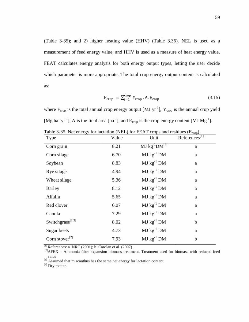
59

(Table 3-35); and 2) higher heating value (HHV) (Table 3.36). NEL is used as a

measurement of feed energy value, and HHV is used as a measure of heat energy value.

FEAT calculates energy analysis for both energy output types, letting the user decide

which parameter is more appropriate. The total crop energy output content is calculated

as:

Fcrop = ∑ Ycrop . A. Ecropcropi=1 (3.15)

where Fcrop is the total annual crop energy output [MJ yr-1], Ycrop is the annual crop yield

[Mg ha-1yr-1], A is the field area [ha-1], and Ecrop is the crop energy content [MJ Mg-1].

Table 3-35. Net energy for lactation (NEL) for FEAT crops and residues (Ecrop). Type Value Unit References[1]

Corn grain 8.21 MJ kg-1DM[4] a

Corn silage 6.70 MJ kg-1 DM a

Soybean 8.83 MJ kg-1 DM a

Rye silage 4.94 MJ kg-1 DM a

Wheat silage 5.36 MJ kg-1 DM a

Barley 8.12 MJ kg-1 DM a

Alfalfa 5.65 MJ kg-1 DM a

Red clover 6.07 MJ kg-1 DM a

Canola 7.29 MJ kg-1 DM a

Switchgrass[2,3] 8.02 MJ kg-1 DM b

Sugar beets 4.73 MJ kg-1 DM a

Corn stover[2] 7.93 MJ kg-1 DM b [1] References: a. NRC (2001); b. Carolan et al. (2007). [2]AFEX – Ammonia fiber expansion biomass treatment. Treatment used for biomass with reduced feed

value. [3] Assumed that miscanthus has the same net energy for lactation content. [4] Dry matter.

60

Table 3-36. Higher heating value (HHV) for FEAT crops and residues (Ecrop). Type Value Unit References[1]

Corn grain 17.20 MJ kg-1 DM[4] a

Soybean 23.79 MJ kg-1 DM b

Wheat 16.6 MJ kg-1 DM b

Canola 20.39 MJ kg-1 DM d

Switchgrass 18.64 MJ kg-1 DM a

Miscanthus 17.74 MJ kg-1 DM c

Corn stover 17.65 MJ kg-1 DM a

Alfalfa straw[2] 18.45 MJ kg-1 DM a

Wheat straw[3] 17.51 MJ kg-1 DM a [1]References: a. Brown (2003); b. Auri fuels initiative (2009); c. Collura et al. (2006); d. Aakre (2009) [2] Value used for corn silage, rye silage, wheat silage, red clover, and alfalfa. [3] Value used for barley straw. [4] Dry matter.

3.2.1.6. Dairy Farm System outputs

Milk, straight vegetable oil, recycled nutrients in manure, and excess feed and

meal are accounted for as Dairy Farm System outputs. For excess feed, there is currently

no energy accounting in the Dairy Farm System. If necessary, this could be calculated

separately in the FEAT Crop Farm System section. Table 3-37 presents the milk energy

content. Consequently, the total milk energy is determined as:

Fmilk = Ncow . Rmilk . Emilk (3.16)

where Fmilk is the total annual food energy embodied in milk produced on the farm in a

year [MJ yr-1], Ncow is the number of milking cows [cow], Rmilk is milk production rate

per cow [kg cow-1yr-1], and Emilk is embedded milk energy [MJ kg-1].

61

Table 3-37. Food energy content of milk (Emilk). Type Value Unit References[1]

Milk 2.63 MJ kg-1 a, b [1] References: a. FAO (2002); b. Jensen (1995). The amount of nutrients (N, P, K) in manure was calculated in Section 3.2.2 using

data from Table 3-21. To account for the energy content of each nutrient, the nutrient

values are multiplied by the efficiency of application and by the embodied energy in their

respective chemical fertilizer equivalents (Table 3-27), thus crediting the manure for the

substitution value of its nutrients. The embodied energy from these manure nutrients is

subtracted from initial off-farm fertilizer crop requirements. After this calculation, a

graph is generated showing the percentage of off-farm fertilizer that has been saved. The

manure recycling feature makes it possible to evaluate the benefits of manure spreading

and manure application efficiencies.

Straight vegetable oil (SVO) produced on-farm is used to run machinery to reduce

or fulfill the overall fuel requirements. When selecting oil seed crops for this purpose, it

is important to evaluate the oil content of different crops. Canola seed, for instance, has a

higher oil content than soybean seed (Table 3-38). SVO and diesel have similar energy

contents. To perform a straightforward comparison between SVO and diesel, SVO is set

to have the same energy content as diesel fuel, which assumes that processing and

transportation energy are also similar (Table 3-39). Although no published data were

available, the SVO probably has lower embedded transportation energy but more

processing energy than diesel given the limited economies of scale available on a farm.

The farm fuel sufficiency analysis is also graphed, making it possible to evaluate crop

choice strategies. The total straight vegetable oil energy is calculated as:

62

Fstraight vegetable oil = ∑ Ycrop . A. YSVO . ESVOoil seedi=1 (3.17)

where Fstraight vegetable oil is the total annual energy content of straight vegetable oil [MJ yr-

1], Ycrop is the annual oil seed crop yield [Mg ha-1yr-1], A is the field area [ha], YSVO is the

straight vegetable oil yield per crop [L Mg-1], and ESVO is the energy content of straight

vegetable oil [MJ L-1].

Table 3-38. Straight vegetable oil (SVO) yield (YSVO). Type Value Unit References[1]

Canola 351 L Mg-1 WM[2] a

Soybean 206 L Mg-1 WM b [1] References: a. Karpenstein-Machan (2001); b. Ahmed et al. (1994). [2] Wet matter. Table 3-39. Diesel and straight vegetable oil energy content (ESVO). Type Value Unit References[1]

Total diesel 44.83 MJ L-1 a

Canola straight vegetable oil 38.25 MJ L-1 b

Adapted straight vegetable oil [2] 44.83 MJ L-1 -- [1] References: a. West and Marland (2001); b. Windman (2009). [2] Value used for soybean and canola straight vegetable oil. Dairy livestock feed meal production follows the same methodology as straight

vegetable oil. Table 3-40 presents the meal rates for canola and soybean. The meal

calculation is only performed for the amount of meal that is in excess. The total feed meal

energy on the farm is estimated as:

Ffeed meal = ∑ Yoil seed . A. Ymeal . Efeed mealoil seedi=1 (3.18)

where Ffeed meal is the total energy of feed meal produced annually on the farm [MJ yr-1],

63

Yoil seed is the oil seed annual crop yield [Mg ha-1yr-1], A is the field area [ha], Ymeal is the

meal yield [Mgmeal Mgcrop-1], and Efeed meal is the energy content of feed meal [MJ Mg-1].

Table 3-40. Feed meal yield and energy content (Ymeal ; Efeed meal). Type

Value

(Mg Mg-1)[2]

References[1]

Energy content

(MJ kg-1)

Reference[1]

Soybean meal 0.812 a 5.67 a[3]

Canola meal 0.580 b 5.67 [4]

[1] References: a. Ahmed et al. (1994); b. Richards (2000). [2] Mega-gram of meal per mega-gram of oil seed. [3] Assumed that meal has the same energy as in the industry production. [4] Assumed that canola meal and soybean meal have the same energy content.

3.2.1.7. Biofuel Farm System outputs

Biofuel Farm System energy outputs are: 1) ethanol (from corn, cellulosic

biomass, sugar beet and barley); 2) biodiesel (from soybean and canola); 3) ethanol co-

products (DDGs, sugar beet pulp, lignin from cellulosic biomass); and 4) biodiesel co-

products (meal and glycerine). Table 3-41 shows the biofuel yield per mass of crop, and

Table 3-42 presents the amount of energy per liter of each type of biofuel. Conventional

ethanol and cellulosic ethanol have the same energy content; however, biodiesel from

different feedstocks may have different values. Ahmed et al. (1994) reported 36.95 MJ L-

1for soybean biodiesel, and Richards (2000) reported 39.3 MJ L-1 for canola biodiesel. US

EPA (2002) reported 32.98 MJ L-1 as the average biodiesel energy content in the US. In

order to standardize the biodiesel energy content, a single value for soybean and canola

biodiesel were used (Table 3-42). The total biofuel energy content is calculated as:

Fbiofuel = ∑ Ycrop . A. Ybiofuel . Ebiofuelcropi=1 (3.19)

64

where Fbiofuel is the total annual biofuel energy content [MJ yr-1], Ycrop is the annual crop

yield [Mg ha-1yr-1], A is the field area [ha], Ybiofuel is the biofuel yield per crop mass [L

Mg-1], and Ebiofuel is the biofuel energy content [MJ L-1].

Table 3-41. Biofuel yield (Ybiofuel).

Type Value

(L Mg-1)[4] Ref.[1]

Range

(L Mg-1)[4] Mean ± C.I.[5]

(L Mg-1)[4] Ref.[1]

Corn ethanol

400

a

354 – 423

389 ± 13 a, g, h, i, j, k, l, m, n

Sugar beet ethanol 114 b 89 – 114 103 ± 11 b, m, o, p Biomass ethanol[2]

330

c

240 – 380

333 ± 26 c, g, j, n, q, r, s, t, u

Small grain ethanol[3] 358 d 350 – 410 386 ± 22 b, d, m, v Soybean biodiesel 204 e 195 – 204 200 ± 5 e, w, x Canola biodiesel 351 f -- -- --

[1] References: a. Shapouri et al. (2004); b. Elsayed et al. (2003); c. Spatari et al. (2005); d. Roth (2008); e. Ahmed et al. (1994); f. Karpenstein-Machan (2001); g. Pimentel and Patzek (2005); h. Graboski (2002); i. Prabhu et al. (2009); j. Wallace et al. (2005); k. Liska et al. (2009); l. de Oliveira et al. (2005); m. Icoz et al. (2009); n. McLaughling and Walsh (1998); o. Leroudier (2002); p. Acharya and Young (2008); q. Spatari et al. (2005); r. Sheehan et al. (2002); s. USDOE (2006); t. Wang (2001); u. Saha et al. (2005); v. Gover et al. (1996); w. Peterson (2005); x. Sheehan et al. (1998).

[2] Original values are for switchgrass, corn stover and wheat straw. This value is used for switchgrass, corn silage, corn stover, rye silage, wheat silage, red clover, alfalfa, barley stover, sugar beet top and miscanthus.

[3] Original values are for wheat, triticale, rye and barley. This value is used for barley ethanol. [4] Wet matter. [5] Confidence interval. Table 3-42. Biofuel energy content (Ebiofuel). Type Value Unit References[1]

Ethanol[2] 21.20 MJ L-1 a

Biodiesel 32.98 MJ L-1 b [1] References: a. Farrell et al. (2006); b. US EPA (2002). [2] Lower heating value (LHV).

In order to calculate the energy of biofuel co-products, an energy credit is

assigned to the co-product, similar to the credit for manure nutrients, with the credit equal

to the energy required for manufacturing an equivalent product that would provide the

same service (Ahmed et al. 1994). The biofuel co-products are replacements for 1)

65

livestock feed (DDGs, wheat meal, sugar beet pulp, soybean meal, and canola meal), 2)

chemicals (soybean and canola glycerine); and 3) electricity (lignin combustion from

cellulosic ethanol). Biofuel co-product yields are presented on Table 3-43. The total

biofuel co-product energy content is calculated as:

Fbiofuel co−products = ∑ Ycrop . A. Ybiofuel −coproduct . Eco−productcropi=1 (3.20)

where Fbiofuel co-products is the total annual biofuel co-product energy content [MJ yr-1], Ycrop

is the annual crop yield [kg ha-1yr-1], A is the crop field area [ha], Ybiofuel co-product is the

biofuel co-product yield [kg kg-1], and Eco-product is the energy content of the biofuel co-

product(s) [MJ kg-1].

Table 3-43. Biofuel co-product yield and energy content (Ybiofuel co-product ; Eco-product). Type

Yield value

(kg kg-1)[2]

References[1]

Energy content

(MJ kg-1)[3]

References[1]

Distillers dried grains

and solubles (DDGs)

0.15

a

11.16 a

Livestock feed (wheat) 0.43 b 11.16 [5]

Sugar beet pulp (feed) 0.067 b 11.13 g

Soybean meal 0.81 c 5.67 c

Canola meal 0.58 d 3.1 --

Soybean glycerin 0.0195 c 49.41 c

Canola glycerin 0.0490 e 49.41 c

Cellulosic ethanol CP[4] -- -- 1.58 f [1] References: a. Graboski (2002); b. Elsayed et al. (2003); c. Ahmed et al. (1994); d. Richards (2000); e.

Smith et al. (2007); f. Wang (2001); g. Harland et al. (2006). [2] kg of co-product per kg of feedstock (wet matter). [3] Mega-joule per kg of co-product. [4] Cellulosic ethanol co-product is excess electricity produced sent to the grid. [5] Assumption, same value as corn distillers dried grains and solubles.

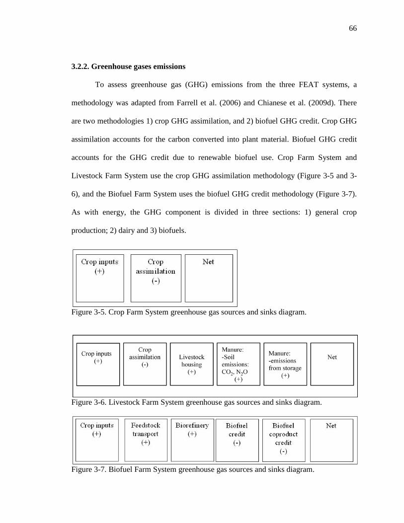
66

3.2.2. Greenhouse gases emissions

To assess greenhouse gas (GHG) emissions from the three FEAT systems, a

methodology was adapted from Farrell et al. (2006) and Chianese et al. (2009d). There

are two methodologies 1) crop GHG assimilation, and 2) biofuel GHG credit. Crop GHG

assimilation accounts for the carbon converted into plant material. Biofuel GHG credit

accounts for the GHG credit due to renewable biofuel use. Crop Farm System and

Livestock Farm System use the crop GHG assimilation methodology (Figure 3-5 and 3-

6), and the Biofuel Farm System uses the biofuel GHG credit methodology (Figure 3-7).

As with energy, the GHG component is divided in three sections: 1) general crop

production; 2) dairy and 3) biofuels.

Figure 3-5. Crop Farm System greenhouse gas sources and sinks diagram.

Figure 3-6. Livestock Farm System greenhouse gas sources and sinks diagram.

Figure 3-7. Biofuel Farm System greenhouse gas sources and sinks diagram.

67

3.2.2.1. GHGs for general crop production:

The three major greenhouse gas (GHG) types accounted for in FEAT systems are

carbon dioxide (CO2), methane (CH4) and nitrous oxide (N2O). Each component of the

system produces a percentage of each greenhouse gas. Global warming potential (GWP)

was used to convert each type of GHG to carbon dioxide equivalent (CO2e) (IPCC,

2007). The total overall greenhouse gas emission equivalent conversion is estimated as:

GHGe = EmCO 2 . GWPCO 2 + EmCH 4 . GWPCH 4 + EmN2O. GWPN2O (3.21)

where GHGe is the annual overall greenhouse gas emission equivalent [kg CO2e yr-1],

EmCO2 is the annual carbon dioxide emissions [kg CO2 yr-1], GWPCO2 is carbon dioxide

global warming potential [kg CO2e kg-1 CO2], EmCH4 is the annual methane emissions

[kg CH4 yr-1], GWPCH4 is methane global warming potential [kg CO2e kg-1 CH4], EmN2O

is annual nitrous oxide emissions [kg N2O yr-1], and GWPN2O is nitrous oxide global

warming potential [kg CO2e kg-1 N2O].

Table 3-44. Greenhouse gas global warming potential (GWP). Type Value Units Variable Reference[1]

CO2 1 kg CO2e kg-1 CO2 GWPCO2 a

CH4 25 kg CO2e kg-1 CH4 GWPCH4 a

N2O 298 kg CO2e kg-1 N2O GWPN20 a [1] Reference: a. IPCC (2007). Following the energy methodology, farm inputs (nitrogen, phosphate, potash,

lime, herbicide, insecticide, and seed), nitrous oxide soil emission, and input

transportation emissions are converted to common units of carbon dioxide equivalent

(CO2e) (Table 3-45 and 3-46). All of these inputs were converted to kilograms of CO2e

(Eq. 3.21). In the case of the Dairy Farm System, before converting fertilizer inputs to

68

GHG emissions, FEAT subtracts the amount of manure nutrients recycled, reducing

emissions from off-farm input production. The total farm greenhouse gas emissions from

inputs are calculated as:

GHGinput = ∑ Rinput . A. Eminputinputi=1 (3.22)

where GHGinput is the total annual greenhouse gas emissions from input production [kg

CO2e yr-1], Rinput is the input application rate [kg ha-1 yr-1], A is the field area [ha], Eminput

is the input GHG emission [kg CO2e kg-1].

Table 3-45. Greenhouse gas emissions from crop input production and nitrous oxide (N2O) soil emission (Eminput). Type

Value

(kg CO2e kg-1yr-1)

Ref.[1]

Range

(kg CO2e kg-1yr-1)

Mean ± C.I.[4] (kg CO2e kg-1yr-1)

Ref.[1]

Nitrogen

4.0

a

2.6 – 5.5

3.7 ± 0.7 a, b, d, e, f, g,

h

N2O soil

emissions[2] 7.0 a 2.8 – 7.0

4.7 ± 2.0

a, i, j, k

Phosphate 1.6 a 0.6 – 1.6 1.0 ± 0.3 a, b, d, e, f, h

Potash 0.71 b 0.44 – 0.86 0.62 ± 0.13 a, b, d, e, f, h

Lime 0.13 d 0.13 – 0.59 0.13 ± 0.60 a, b, e, f, k

Herbicide 25.0 a 5.4 – 25 17.6 ± 6.5 a, b, e, f, h

Insecticide 26.0 a 18 – 29 24.5 ± 4.5 a, b, e

Electricity[3] 0.069 a 0.069 – 0.275 0.18 ± 0.06 a, b, l, m, n [1] References: a. Wang (2001); b. West and Marland (2002); c. Flessa et al. (2002); d. Reinhardt (1992); e. Prabhu

et al. (2009); f. Lal (2004); g. Snyder et al. (2007); h. Kaltschmitt and Reinhardt (1997); i. Friedrich et al. (1993); j. Liska et al. (2009); k. Mortimer et al. (2002); l. Lewandowski et al. (1995); m. Shapouri et al. (2002); n. Heller et al. (2004).

[2] Soil emission from nitrogen fertilization per kg of N applied. [3] Values in CO2e per MJ of electricity. [4] Confidence interval.

69

Table 3-46. Greenhouse gas emissions from seed production (Eminput). Type Value Unit References[1]

Corn 3.80 kg CO2e kg-1yr-1 a

Soybean 0.91 kg CO2e kg-1yr-1 a

Barley 0.40 kg CO2e kg-1yr-1 a

Wheat[4] 0.40 kg CO2e kg-1yr-1 a

Alfalfa[2] 3 kg CO2e kg-1yr-1 a

Red clover[2] 2.08 kg CO2e kg-1yr-1 a

Canola 0.61 kg CO2e kg-1yr-1 b

Switchgrass[3] 0.62 kg CO2e kg-1yr-1 a

Miscanthus 0.28 kg CO2e kg-1yr-1 b

Sugar beet 2.12 kg CO2e kg-1yr-1 b [1] References: a. West and Marland (2002); b. Kaltschmitt and Reinhardt (1997). [2] Assumed 3 years stand life. [3] Calculation based on red clover value of 6.24 (West and Marland, 2002) with a 10 year stand life. [4]Value used for wheat silage, and rye silage.

Diesel fuel emissions are also a system input, but for this study were accounted

separately. Diesel emissions from farm operations are also converted to a kg of carbon

dioxide equivalent (Table 3-47). The diesel GHG emissions are estimated as:

GHGfarm fuel = FC. Efuel . Emfuel (3.23)

where GHGfarm fuel is the total annual greenhouse gas emission from diesel fuel

combustion in farm operations [kgCO2e yr-1], FC is the total annual farm fuel

consumption [L yr-1], Efuel is the fuel energy embodied [MJ L-1], and Emfuel is the fuel

greenhouse gas emission [kg CO2e L-1].

70

Table 3-47. Greenhouse gas emissions from diesel fuel (Emfuel). Type

Value

(kg CO2e L-1)

Ref.[1]

Range

(kg CO2e L-1)

Mean ± C.I.[2]

(kg CO2e L-1)

References[1]

Diesel

3.48

a

2.68 – 3.48

3.4 ± 0.4 a, b, c, d, e, f,

g, h, i

Gasoline[3] 2.85 a -- -- -- [1] References: a. Wang (2001); b. West and Marland (2002); c. Flessa et al. (2002); d. Lal (2004); e.

Lewandowski et al. (1995); f. Shapouri et al. (2002); g. Elsayed et al. (2003); h. Sheehan et al. (2004); i. EIA (2007).

[2] Confidence interval. [3] Value used for further biofuel greenhouse gas methodology as comparison to ethanol.

In the Dairy Farm System, if SVO is produced, the amount of diesel GHG

emission is reduced or eliminated. The combustion of SVO is considered “GHG free”

because it comes from a renewable source (Kim and Dale, 2008), although the production

of the SVO will generate emissions.

Greenhouse gases emissions for transportation of farm inputs to the farm is also

accounted separately (Table 3-48). The total farm greenhouse gas emissions from input

transportation of inputs is calculated as:

GHGinput transportation = ∑ Rinput . Rinput . A. Eminput transportinputi=1 (3.24)

where GHGinput transportation is the annual greenhouse gas emission from input transportation

[kg CO2e yr-1], Rinput is the annual input application rate [kg ha-1 yr-1], A is the field area

[ha], and Eminput transport is the input transportation emission [kg CO2e kg-1].

Table 3-48. Greenhouse gas emissions from transportation of farm inputs (Eminput transport). Type Value Unit References[1]

Transportation of farm inputs 0.05 kg CO2e kg-1 a, b [1] References: a. Wang (2001); b. Farrell et al. (2006).

71

During plant growth, net greenhouse gases are assimilated as carbon-based plant

material. The parameters used for calculation are shown on Table 3-49. The total

greenhouse gas assimilation is calculated as:

GHGnet crop assimilation = ∑ Ycrop . A. EmC. EmC−CO 2cropi=1 + A . EmCH 4 (3.25)

where GHGnet crop assimilation is the total annual crop greenhouse gas assimilation [kg CO2e

yr-1], Ycrop is the annual crop yield [kg yr-1], A is the field area [ha], EmC is the carbon

content in plant material [kg C kg-1], EmC-CO2 is the molecular weight conversion of

carbon to carbon dioxide [dimensionless], and EmCH4 is the annual methane plant

assimilation [kg CO2e ha-1 yr-1].

Table 3-49. Greenhouse gas net crop assimilation parameters. Value Variable Units Ref.[1]

Carbon content in plant material 0.40 EmC kg C kg-1 DM[2] a

Methane plant assimilation

average[3] 37

EmCH4 kg CO2e ha-1yr-1 b

Molecular weight carbon

conversion to carbon dioxide 3.67

EmC-CO2 dimensionless c [1] References: a. Chianese et al. (2009a); b. Chianese et al. (2009b); c. Blasing et al. (2004). [2] kg of carbon per kg of dry matter plant material. [3]Averaged reported values for methane assimilations for grass, alfalfa, corn grain, corn silage, soybeans

and wheat.

3.2.2.2. Dairy Farm System specific GHGs production

Dairy operations have three additional sources of major greenhouse gas

emissions: 1) animals and housing, 2) manure carbon emissions from soil, and 3) manure

storage. Tables 3-50 and 3-51 present the quantity of each type of gas per livestock unit

72

(LU) per year. Dairy GHG emissions were also converted to carbon dioxide equivalents

(Eq. 3.21). To calculate manure storage GHG emission, it is necessary to know the

storage volume. FEAT methodology followed the approach of Chianese et al. (2009d),

using 1100 m3 for 100 cows, and consequently 11m3 per cow as the average amount of

manure in storage throughout the year. The total GHG emission from animal and housing

are computed as:

GHGanimal and housing = LU . Emdairy (3.26)

where GHGanimal and housing is the annual GHG emissions from animals and housing [kg

CO2e yr-1], LU is the total livestock units [LU], and Emdairy is the GHG emissions rate per

livestock unit [kg CO2e LU-1 yr-1]. The total GHG emission from manure is calculated as:

GHGmanure = Ncow . Rmanure storage . Emmanure storage + Rtotal manure . Emmanure carbon (3.27)

where GHGmanure is the total annual GHG emission from manure [kg CO2e yr-1], Ncow is

the number of cows (user input) [cow], Rmanurestorage is the manure storage rate per cow

[m3 cow-1 yr-1], Emmanure storage is the storage GHG emission per volume of manure storage

[kg CO2e m-3], Rtotal manure is the total manure produced [kg DM yr-1], and Emmanure carbon is

the carbon dioxide manure emission from soil after manure application [kg CO2 kg-1

DM].

Table 3-50. Greenhouse gas emissions from animals and housing (Emdairy). Type Value Units Reference[1]

Carbon dioxide (CO2) 3,138 kg CO2 LU-1 yr-1 a

Methane (CH4) 84 kg CH4 LU-1 yr-1 a

Nitrous oxide (N2O) 0.3 kg N2O LU-1 yr-1 a

Carbon dioxide equivalent (CO2e) 5,327 kg CO2e LU-1 yr-1 a [1] Reference: a. Chianese et al. (2009d).

73

Table 3-51. Greenhouse gas emissions from manure storage and manure carbon dioxide emission from soil (Emmanure storage; Emmanure carbon). Type Value Units Reference[1]

Manure storage carbon dioxide (CO2) 17 kg CO2 m-3 yr-1 a

Manure storage methane (CH4) 5.6 kg CH4 m-3 yr-1 a

Manure storage nitrous oxide (N2O) 0.13 kg N2O m-3 yr-1 a

Manure storage carbon dioxide

equivalent (CO2e) 196 kg CO2e m-3 yr-1 a

Manure carbon dioxide emission

from soil 1.468 kg CO2 kg-1 DM a [1] Reference: a. Chianese et al. (2009d).

3.2.2.3. Biofuel Farm System GHG emissions

The additional Biofuel Farm System GHG emissions are categorized as: 1)

feedstock transportation to biorefinery, 2) biofuels processing, 3) biofuel credit, and 4)

biofuel co-product credit. Table 3-52 presents the two different parameters for feedstock

transportation. The corn transportation GHG emission value was used for soybean,

barley, canola, and sugar beet transportation. Similarly, the biomass transportation GHG

emission value was used for corn silage, rye silage, wheat silage, corn stover,

switchgrass, alfalfa, barley stover, sugar beet top, and miscanthus transportation. The

total feedstock transportation greenhouse gas emissions are calculated as:

GHGfeedstock tranport = ∑ Ycrop . A. Emtransportcropi=1 (3.28)

where GHGfeedstock transport is the total annual GHG emissions from feedstock transportation

from farm to biorefinery [kg CO2e yr-1], Ycrop is the annual crop yield [kg ha-1 yr-1], A is

74

the field area [ha], and Emtransport is the GHG emission rate for feedstock transportation

per crop mass to the biorefinery [kg CO2e kg-1WM].

Table 3-52. Greenhouse gas emissions from feedstock transportation (Emtransport). Type Value Unit References[1]

Corn transportation[2] 0.0196 kg CO2e kg-1WM[4] a, b

Biomass transportation[3] 0.0164 kg CO2e kg-1 WM [4] a, b [1] References: a. Farrell et al. (2006); b. Wang (2000). [2] Value used for corn, soybean, canola, barley and sugar beet. [3] Value used for corn(silage), rye (silage), wheat (silage), corn stover, switchgrass, alfalfa, barley stover,

sugar beet top and miscanthus. [4] kg of CO2 equivalent per kg of feedstock (wet matter content). Feedstock processing follows the same methodology as energy, in other words,

the process emission details are not deeply scrutinized, since that is not the primary focus

of this research. Table 3-53 presents the CO2e values for biofuel processing of corn

ethanol, cellulosic ethanol, sugar beet ethanol, canola and soybean biodiesel, and wheat

ethanol. Corn silage, rye silage, wheat silage, red clover, switchgrass, alfalfa, barley

stover, sugar beet top, and miscanthus are considered cellulosic materials that are

consequently converted into cellulosic ethanol. A cellulosic ethanol processing value of -

0.033 kgCO2e L-1 (Farrell et al. 2006) was used in this analysis for switchgrass feedstock.

The total emissions from feedstock processing are calculated as:

GHGprocessing = ∑ Ycrop . A. Ybiofuel . Emprocessingcropi=1 (3.29)

where GHGprocessing is the total annual GHG emissions for processing feedstock [kg CO2e

yr-1], Ycrop is the annual crop yield [kg ha-1 yr-1], A is field area [ha], Ybiofuel is the biofuel

yield per crop mass, and Emprocessing is the GHG emissions rate per volume of biofuel

processed [kg CO2e L-1].

75

Table 3-53. Greenhouse gas emission from biorefinery processing (Emprocessing). Type Value Unit References[1]

Corn ethanol processing 0.778 kg CO2e L-1[5] a

Cellulosic ethanol processing[2] -0.033 kg CO2e L-1 a

Sugar beet ethanol processing 0.108 kg CO2e L-1 b

Canola biodiesel processing[3] 0.595 kg CO2e L-1 b

Wheat ethanol processing[4] 0.504 kg CO2e L-1 b [1] References: a. Farrell et al. (2006); b. Elsayed et al. (2003). [2] Value used for corn (silage), rye (silage), wheat (silage), red clover, switchgrass, alfalfa, barley stover,

sugar beet top and miscanthus. [3] Value used for canola and soybean. [4] Value used for barley. [5] kg of CO2 equivalent per liter of biofuel.

Biofuel Farm System uses biofuel GHG methodology where biofuels and biofuels

co-products are considered carbon neutral due to atmospheric carbon dioxide recycling

(Kim and Dale, 2008; Lal 2009). The reduced energy content from biofuels is accounted

in Table 3-54. The biofuels and biofuel co-products greenhouse gas credit is calculated

as:

GHGbiofuel = ∑ (Ycrop . A. Ybiofuel . Eratio . Emfuel + Ycrop . A. Ybiofuelcropi=1 . Embiofuel coprod ) (3.29)

where GHGbiofuel is the total annual greenhouse gas credit by biofuels and biofuel co-

products [kg CO2e yr-1], Ycrop is the annual crop yield [Mg ha-1 yr-1], A is the field area

[ha], Ybiofuel is the biofuel yield per crop mass [L Mg-1], Eratio is the fuel and biofuel

energy ratio [dimensionless], Emfuel is the fuel greenhouse gas emission [kg CO2e L-1],

and Embiofuel co-prod is the biofuel co-product GHG credit.

76

Table 3-54. Gasoline / ethanol and diesel / biodiesel energy content ratio (Eratio). Type Value Units References[1]

Gasoline / ethanol 0.73 -- a

Diesel / biodiesel 0.95 -- a [1] References: a. ORNL (2008).

Table 3-55. Biofuel co-product greenhouse gas credit (Embiofuel co-prod). Type Value Units References[1]

Distillers dried grains and soluble 0.525 kg CO2e L-1 a

Cellulosic ethanol excess electricity 0.106 kg CO2e L-1 a

Soybean meal 0.677 kg CO2e L-1 [2]

Canola meal 0.578 kg CO2e L-1 [2]

Sugar beet pulp 0.567 kg CO2e L-1 [2]

[1] References: a. Farrell et al. (2006). [2] Assumption based on distillers dried grains and soluble values. 3.3. FEAT results

The FEAT overall results were divided as 1) crop energy input and output for the

Crop Farm System (Table 3-56); 2) energy input and output for the Biofuel Farm System

(Table 3-57); 3) biofuel yields and co-products for each crop (Table 3-58); 4) crop GHG

input and assimilation (Table 3-59); 5) biofuel GHG balance for each feedstock; 6) crop

input energy distribution (Figure 3-8); 7) net energy for lactation (NEL) energy outputs

(Figure 3-9); 8) higher heating value (HHV) energy outputs (Figure 3-10); 9) GHG from

crop production inputs (Figure 3-11); 10) net GHG crop assimilation (Figure 3-12); 11)

biofuel energy input distribution (Figure 3-13); 12) biofuel energy output distribution

(Figure 3-14); 13) GHG emissions from biofuel system inputs (Figure 3-15); and 14)

GHG credit from biofuel outputs (Figure 3-16).

77

Table 3-56. Crop energy input and output for the FEAT Crop Farm System. Crop / energy Input

(MJ ha-1 yr-1)

Output (NEL)

(MJ ha-1 yr-1)

Output (HHV)

(MJ ha-1 yr-1)

Corn grain 16,494 60,723 127,276

Corn silage 21,286 119,910 330,255

Soybean 6,798 25,747 69,350

Barley 9.695 33,903 69,288

Rye silage 10,840 25,626 95,700

Wheat silage 11,169 27,798 95,700

Alfalfa 7,785 57,017 205,072

Red Clover 6.249 47,234 143,550

Canola 15,157 18,496 51,768

Switchgrass[2] 5,110 79,251 118,163

Miscanthus[2] 11,923 160,428 248,416

Sugar beet 19,836 99,353 --

Corn stover[1] 0 24,303[2] 54,097

Barley straw[1] 0 7,098[2] 15,674

S. beet top[1] 0 53,284[2] 117,667 [1]50% residue removal. [2] Ammonia fiber expansion (AFEX) treatment (Dale et al. 1996).

78

Table 3-57. Energy dynamics for each crop for the FEAT Biofuel Farm System. Crop / Energy Input

(MJ ha-1 yr-1)

Input recycled[4]

(MJ ha-1 yr-1)

Output biofuel

(MJ ha-1 yr-1)

Output

biofuel co-product

(MJ ha-1 yr-1)

Corn grain[2] 69,859 0 74,260 14,467

Corn silage[3] 193,681 155,472 125,228 28,295

Soybean[1] 16,874 0 22,480 18,651

Barley[2] 28,237 0 36,623 23,152

Rye silage[3] 60,804 25,539 20,568 4,647

Wheat silage[3] 61,125 45,052 36,288 8,199

Alfalfa[3] 101,985 96,540 77,761 17,569

Red Clover[3] 78,821 67,578 54,432 12,299

Canola[1] 23,039 0 32,292 15,930

Switchgrass[3] 96,861 85,814 69,120 15,617

Miscanthus[3] 198,686 121,598 97,944 22,130

Sugar beet[2] 63,258 0 50,208 15,612 [1] Biodiesel. [2] Ethanol. [3] Cellulosic ethanol. [4] Energy recycled through lignin combustion in cellulosic ethanol processing.

79

Table 3-58. Biofuel yield and co-product for each FEAT feedstock. Feedstock Biofuel yield

(L ha-1 yr-1) Biofuel co-products yield

Feed[1] ( Mg ha-1 yr-1)

Chemical[2] ( Mg ha-1 yr-1)

Electricity[3] ( MJ ha-1 yr-1)

Corn grain 3,503 1.30 0 0

Corn silage 5,907 0 0 28,295

Soybean 682 2.72 0.07 0

Barley 1,728 2.07 0 0

Rye silage 1,712 0 0 4,647

Wheat silage 1,712 0 0 8,199

Alfalfa 3,668 0 0 17,569

Red Clover 2,568 0 0 12,299

Canola 979 1.62 0.14 0

Switchgrass 3,260 0 0 15,617

Miscanthus 4,620 0 0 22,130

Sugar beet 2,392 1.4 0 0 [1] Feed are DDGs (corn), Livestock feed (barley), sugar beet pulp, soybean meal, and canola meal. [2] Chemical is glycerine from biodiesel processing. [3]Excess electricity generated from lignin combustion on cellulosic ethanol processing.

80

Table 3-59. FEAT crop GHG input production and crop assimilation [1] for Crop Farm System. Feedstock Input GHG production

(g CO2e m-2 yr-1) Crop Assimilation (g CO2e m-2 yr-1)

Net emission (g CO2e m-2 yr-1)

Corn grain 13.2 98.8 85.7

Corn silage 17.7 251.4 233.7

Soybean 6.0 43.2 37.1

Barley 8.3 57.0 48.7

Rye silage 9.2 71.8 62.6

Wheat silage 9.4 71.8 62.4

Alfalfa 7.5 148.5 141.0

Red Clover 5.6 114.6 109.0

Canola 11.4 27.5 16.1

Switchgrass 3.9 141.9 138

Miscanthus 9.3 288.1 278.8

Sugar beet 15.6 298.5 282.9 [1] Conventional tillage fuel consumption.

81

Table 3-60. FEAT net greenhouse gas (GHG) emission for the Biofuel Farm System. Feedstock Inputs for production

(g CO2e m-2 yr-1) Biofuel and co-product credits

(g CO2e m-2 yr-1) Net emission

(g CO2e m-2 yr-1) Corn grain 52.3 -67.7 -14.4

Corn silage 35.9 -87.8 -51.9

Soybean 10.7 -27.1 -16.3

Barley 22.6 -32.9 -10.3

Rye silage 15.8 -25.4 -9.7

Wheat silage 16.0 -25.4 -9.4

Alfalfa 8.7 -49.5 -40.7

Red Clover 6.5 -38.1 -31.7

Canola 26.3 -37.9 -11.6

Switchgrass 8.3 -48.4 -40.2

Miscanthus 17.7 -98.1 -80.4

Sugar beet 44.8 -46.6 -1.8 [1] Conventional tillage fuel consumption.

82

Figure 3-8. Crop energy inputs for the Crop, Livestock, and Biofuel Farm Systems per year.

0

5,000

10,000

15,000

20,000

25,000En

ergy

(MJ h

a-1yr

-1)

Transp. inputs

Drying

On farm fuel useInsecticide

Herbicide

Seed

Lime

K

P

N

83

Figure 3-9. Feedstock energy output in net energy for lactation (NEL) for the Crop Farm System per year.

0

20,000

40,000

60,000

80,000

100,000

120,000

140,000

160,000

180,000

Ener

gy (M

J ha-1

yr-1

)

84

Figure 3-10. Feedstock energy output in higher heating value (HHV) for the Crop Farm System per year.

0

50,000

100,000

150,000

200,000

250,000

300,000

350,000

400,000

Ener

gy (M

J ha-1

yr-1

)

85

Figure 3-11. Greenhouse gas emissions from farm inputs for the Crop, Livestock, and Biofuel Farm Systems per year.

0

2

4

6

8

10

12

14

16

18

20

GH

G (g

CO

2e m

-2yr

-1)

Drying

Transport. inputs

On farm fuel use

Insecticide

Herbicide

Seed

Lime

K

P

N

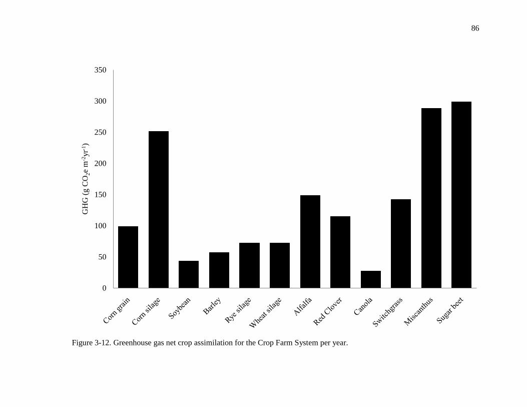
86

Figure 3-12. Greenhouse gas net crop assimilation for the Crop Farm System per year.

0

50

100

150

200

250

300

350

GH

G (g

CO

2e m

-2yr

-1)

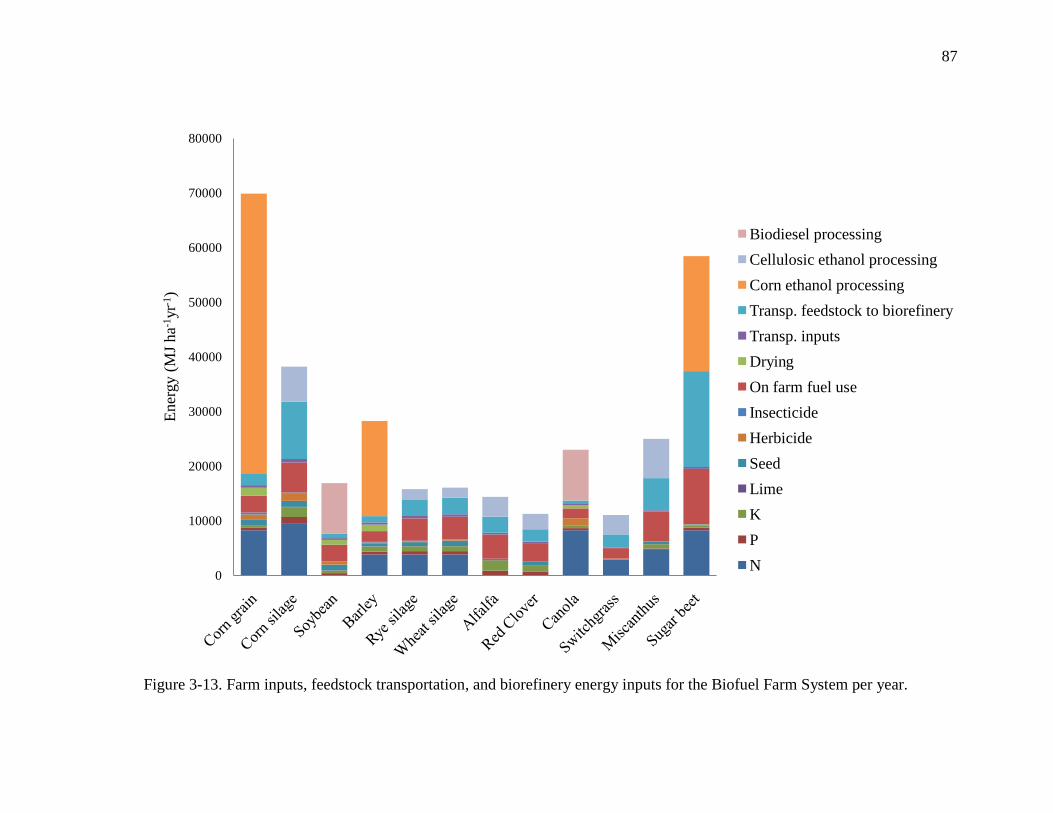
87

Figure 3-13. Farm inputs, feedstock transportation, and biorefinery energy inputs for the Biofuel Farm System per year.

0

10000

20000

30000

40000

50000

60000

70000

80000

Ener

gy (M

J ha-1

yr-1

)

Biodiesel processingCellulosic ethanol processingCorn ethanol processingTransp. feedstock to biorefineryTransp. inputsDryingOn farm fuel useInsecticideHerbicideSeedLimeKPN

88

Figure 3-14. Biofuel and biofuel co-products energy outputs from the Biofuel Farm System per year.

0

20000

40000

60000

80000

100000

120000

140000

160000

180000

200000

Ener

gy (M

J ha-1

yr-1

) Sugar beet pulpSugar beet ethanolCellulosic ethanol co-productsDDGsGlycerineMealCellulosic ethanolCorn ethanolBiodiesel

89

Figure 3-15. Greenhouse gas emissions from farm inputs, feedstock transportation, and the biorefinery for the Biofuel Farm

System per year.

-10

0

10

20

30

40

50

60

GH

G (g

CO

2e m

-2yr

-1)

BiorefineryTransport. feedstockNitrous oxideDryingTransport. inputsOn farm fuel useInsecticideHerbicideSeedLimeKPN

90

Figure 3-16. Greenhouse gas credit from biofuel and biofuel co-products for the Biofuel Farm System per year.

0

20

40

60

80

100

120

GH

G (g

CO

2e m

-2yr

-1)

Biofuel co-productsBiofuel

91

Chapter 4

Energy and Greenhouse Gas Analyses of Cropping Systems for Feed,

Heat and Biofuel Production in Northern US.

4.1. Introduction

As demand for renewable energy increases, new agricultural cropping systems are

being designed to increase productivity and benefit the environment. Biofuel feedstock

production has given farmers an alternative market opportunity in addition to the

traditional food, feed and fiber markets. This transition to alternative agricultural

production has prompted an increased interest in evaluating cropping system performance

and efficiency. Energy and greenhouse gas (GHG) emissions are two criteria that have

received a great deal of attention, because of their relevance to concerns about peak oil

production and global climate change.

Feedstocks to produce biofuels can be divided into three broad categories: 1)

crops with starch; 2) crops with oil; and 3) cellulosic materials. Starch crops such as corn,

barley, wheat and rye are used to produce ethanol. Oil crops such as soybeans and canola

are used to produce biodiesel. Cellulosic materials such as crop residues and high

yielding biomass crops are used to produce three major products: 1) heat; 2) electricity;

and 3) cellulosic ethanol. There are exceptions to these categories, like the use of corn

grain or as a home heating fuel, but nonetheless this simplified framework will be used

for the present investigation.

Energy and GHG analyses are relatively simple, straight-forward evaluations that

convert the majority of system components into units of energy or carbon dioxide,

92

respectively. Using these analytical frameworks, different farming practices can be

simulated and evaluated on a comparative basis. This flexibility of analysis allows for

direct comparisons of agricultural inputs and outputs that are normally purchased or sold

in different units.

There are many cropping system options, and their selection depends mainly on

the types of products produced, in a context of regional soils, climate, and markets. In

the Northeast US, large farms are typically either field crop or livestock operations. Corn-

soybean rotations are commonly used on field crop farms that are producing only grain

for cash, whereas corn-soybean-alfalfa rotations are commonly implemented on dairy

farms.

As demand increases for agricultural production, and with simultaneous

encouragement of more environmentally sound agricultural practices, nutrient and soil

conserving practices like double and cover cropping are becoming more common.

Double cropping is a system of consecutively producing, and harvesting, two crops on

the same land in a single year (Tollenaar et al. 1992; Heggenstaller et al. 2008). When a

crop (typically planted in the fall) is killed and left as mulch or tilled under rather than

harvested, it is called a cover crop or green manure. The benefits of double / cover

cropping are many, including erosion control, reduced nitrate leaching, increased soil

organic matter, improved soil structure, nitrogen fixation, weed control, reduced

production risk, spreading labor over the year, increased opportunities for manure

spreading, and in the case of double crops, increased overall crop production (Zhu et al.

1989; Kaspar et al. 2001; Rotz et al. 2002; Duiker and Curran, 2005; PSU agronomy

guide, 2008; Heggenstaller et al. 2008).

93

The objectives of this study were to evaluate three cropping systems 1) a

traditional corn-soybean-alfalfa system as a control; 2) double cropping with rye; and 3)

double cropping with rye and spring canola; energy and greenhouse gas (GHG) emission

balances are compared in four northern counties. Cropping system outputs are reported in

three forms: 1) livestock feed, 2) heating value, and 3) biofuel products.

4.2. Methods

4.2.1. Energy and greenhouse gas analyses

The Farm Energy Analysis Tool (FEAT) was developed to evaluate energy usage

and greenhouse gas (GHG) emissions of farming systems (Chapter 3). FEAT is a static,

deterministic, database-driven model that is based on a comprehensive literature review

(see Chapters 2 and 3). FEAT was used in this study as a framework to evaluate cropping

system options in terms of: 1) livestock feed, 2) biomass heating value, and 3) biofuel

production. For livestock feed and biomass heating purposes, the Crop Farm System was

selected, which includes production of inputs and crop production (see Chapter 3). For

biofuel purposes, the Biofuel Farm System was selected whith production of inputs, farm

crop production, feedstock transportation, and biofuel production (see Chapter 3).

FEAT calculates the energy balance using a methodology adapted from Farrell et

al. (2006). The concept is to convert the main elements of the studied system into a

common unit of energy, in this case the mega-joule (MJ). With the same energetic unit,

all of the system elements can then be aggregated and compared.

On the energy output side there are three different types of energy end uses

considered: 1) net energy for lactation (NEL) for livestock feed; 2) higher heating value

94

(HHV) for biomass heat and power; and 3) biofuel and co-product energy content for

biofuel systems. Net energy for lactation (NEL) is the net energy value in the feed for

producing milk in dairy animals (Tyrrell, 2005). Higher heating value is the energy

released after a combustion reaction with oxygen under isothermal conditions (Brown,

2003). Biofuel energy content is the energy embodied in the biofuel, and co-product

energy content is the energy used to produce an equivalent product to the biofuel co-

product in a separate, conventional process (Ahmed et al. 1994).

To assess greenhouse gas (GHG) emissions from the three studied systems, a crop

GHG assimilation method (see Chapter 3) was used for NEL and HHV systems, and a

Biofuel GHG credit method (see Chapter 3) was used for biofuel system.

4.2.2. Cropping system characteristics

Three cropping systems were evaluated in this study, 1) control (CT); 2) double

cropping (DC1); and 3) double cropping with spring canola (DC2). The control cropping

system was a seven year rotation with corn silage, soybean, corn silage, and alfalfa (C-S-

C-A-A-A-A). The double cropping system was a seven year rotation with corn silage, rye

silage, soybean, rye silage, corn silage, rye silage, and alfalfa (C/R-S/R-C/R-A-A-A-A).

The double cropping with spring canola was a seven year rotation with corn silage, rye

silage, corn silage, rye silage, spring canola, and alfalfa (C/R-C/R-Cn-A-A-A-A).

Cropping systems were standardized in a 100 ha area using conventional tillage practices.

4.2.3. Cropping system yield assessment

Four US northern counties were selected to represent the region: 1) Centre

County, PA; 2) Cayuga County, NY; 3) Huron County, MI; and 4) Penobscot County,

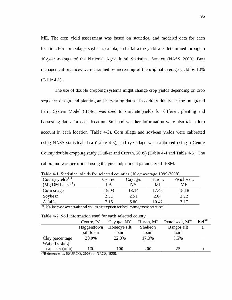
95

ME. The crop yield assessment was based on statistical and modeled data for each

location. For corn silage, soybean, canola, and alfalfa the yield was determined through a

10-year average of the National Agricultural Statistical Service (NASS 2009). Best

management practices were assumed by increasing of the original average yield by 10%

(Table 4-1).

The use of double cropping systems might change crop yields depending on crop

sequence design and planting and harvesting dates. To address this issue, the Integrated

Farm System Model (IFSM) was used to simulate yields for different planting and

harvesting dates for each location. Soil and weather information were also taken into

account in each location (Table 4-2). Corn silage and soybean yields were calibrated

using NASS statistical data (Table 4-3), and rye silage was calibrated using a Centre

County double cropping study (Duiker and Curran, 2005) (Table 4-4 and Table 4-5). The

calibration was performed using the yield adjustment parameter of IFSM.

Table 4-1. Statistical yields for selected counties (10-yr average 1999-2008). County yields[1] (Mg DM ha-1yr-1)

Centre, PA

Cayuga, NY

Huron, MI

Penobscot, ME

Corn silage 15.03 18.14 17.45 15.18 Soybean 2.51 2.51 2.64 2.22 Alfalfa 7.15 6.80 10.42 7.17

[1]10% increase over statistical values assumption for best management practices.

Table 4-2. Soil information used for each selected county.

Centre, PA Cayuga, NY Huron, MI Penobscot, ME Ref[a]

Haggerstown silt loam

Honeoye silt loam

Shebeon loam

Bangor silt loam

a

Clay percentage 20.0% 22.0% 17.0% 5.5% a Water holding

capacity (mm) 100 100 200 25 b

[a]References: a. SSURGO, 2008; b. NRCS, 1998.

96

Table 4-3. Yield adjustment parameter for corn silage and soybean based on statistical yields.

Centre, PA Cayuga, NY Huron, MI Penobscot, ME

Corn silage 117% 166% 115% 232% Soybean 96% 100% 100% 111%

Table 4-4. Rye silage yields (Mg DM ha-1) from Duiker and Curran (2005). Studied years 2000-2001 2001-2002 2002-2003 Rye planting date / Corn planting date 22 May 11 May 22 May 23 October 1.833 -- -- 3 October -- 3.740 -- 25 September -- -- 7.075

Table 4-5. Rye silage yield adjustment parameters for Centre County based on Duiker and Curran (2005) study. Studied years 2000-2001 2001-2002 2002-2003 Rye planting dates / Corn planting dates 22 May 11 May 22 May 23 October 19% -- -- 3 October -- 73% -- 25 September -- -- 63%

The rye silage yield adjustment parameter of 19% (Table 4-5) was considered an

outlier because IFSM did not appropriately account for reduced yields due to late rye

planting. The remaining rye silage yield adjustment parameters, 73 % and 63%, were

averaged into 68%. This same yield adjustment parameter value was used for the rest of

the locations to assess rye silage yields.

Input requirements for crop production include nitrogen, phosphate, potash, lime,

seed, herbicide, insecticide, grain drying, and the transportation associated with those

inputs. Inputs for each crop evaluated are described on Table 4-6.

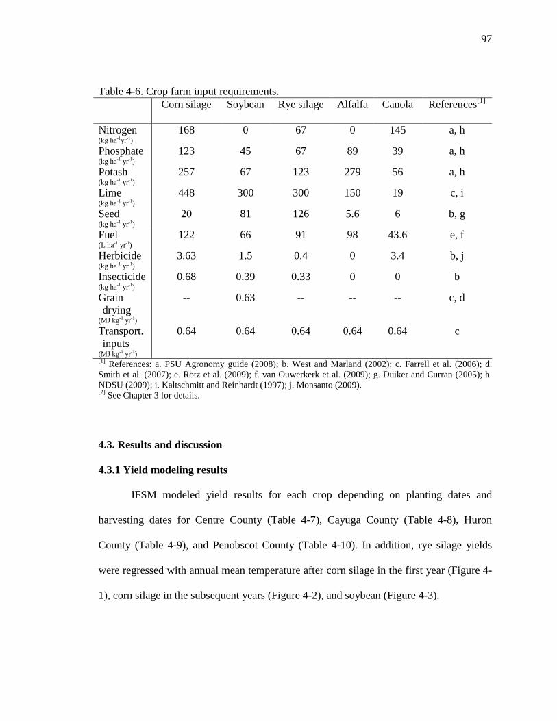
97

Table 4-6. Crop farm input requirements.

Corn silage Soybean Rye silage Alfalfa Canola References[1]

Nitrogen (kg ha-1yr-1)

168 0 67 0 145 a, h

Phosphate (kg ha-1 yr-1)

123 45 67 89 39 a, h

Potash (kg ha-1 yr-1)

257 67 123 279 56 a, h

Lime (kg ha-1 yr-1)

448 300 300 150 19 c, i

Seed (kg ha-1 yr-1)

20 81 126 5.6 6 b, g

Fuel (L ha-1 yr-1)

122 66 91 98 43.6 e, f

Herbicide (kg ha-1 yr-1)

3.63 1.5 0.4 0 3.4 b, j

Insecticide (kg ha-1 yr-1)

0.68 0.39 0.33 0 0 b

Grain drying

(MJ kg-1 yr-1)

-- 0.63 -- -- -- c, d

Transport. inputs

(MJ kg-1 yr-1)

0.64 0.64 0.64 0.64 0.64 c

[1] References: a. PSU Agronomy guide (2008); b. West and Marland (2002); c. Farrell et al. (2006); d. Smith et al. (2007); e. Rotz et al. (2009); f. van Ouwerkerk et al. (2009); g. Duiker and Curran (2005); h. NDSU (2009); i. Kaltschmitt and Reinhardt (1997); j. Monsanto (2009). [2] See Chapter 3 for details.

4.3. Results and discussion

4.3.1 Yield modeling results

IFSM modeled yield results for each crop depending on planting dates and

harvesting dates for Centre County (Table 4-7), Cayuga County (Table 4-8), Huron

County (Table 4-9), and Penobscot County (Table 4-10). In addition, rye silage yields

were regressed with annual mean temperature after corn silage in the first year (Figure 4-

1), corn silage in the subsequent years (Figure 4-2), and soybean (Figure 4-3).

98

Table 4-7. Centre County Pennsylvania modeled yields per year. Yields

(Mg DM ha-1yr-1) Planting dates Harvesting dates

Corn silage 1 15.05 25 April 14 September Corn silage 2 11.98 20 May 10 October Soybean 1 2.51 10 May 5 October Soybean 2 2.20 20 May 15 October Rye silage 1[a] 7.46 17 September 17 May Rye silage 2[b] 5.24 4 October 17 May Rye silage 3[c] 4.19 18 October 17 May [a] After corn 1st year. [b] After corn 2nd and 3rd year. [c] After soybean. Table 4-8. Cayuga County New York modeled yields per year. Yields


Corn silage 1 18.19 1 May 20 September Corn silage 2 13.53 23 May 1 October Soybean 1 2.51 10 May 5 October Soybean 2 2.20 20 May 15 October Rye silage 1[a] 8.22 23 September 20 May Rye silage 2[b] 5.29 4 October 20 May Rye silage 3[c] 3.56 18 October 20 May [a] After corn 1st year. [b] After corn 2nd and 3rd year. [c] After soybean. Table 4-9. Huron County Michigan modeled yields per year. Yields


Corn silage 1 17.47 1 May 20 September Corn silage 2 11.49 26 May 1 October Soybean 1 2.64 10 May 5 October Soybean 2 2.28 26 May 15 October Rye silage 1[a] 6.56 23 September 23 May Rye silage 2[b] 5.71 4 October 23 May Rye silage 3[c] 3.99 18 October 23 May [a] After corn 1st year. [b] After corn 2nd and 3rd year. [c] After soybean.

99

Table 4-10. Penobscot County Maine modeled yields per year. Yields


Corn silage 1 15.19 5 May 25 September Corn silage 2 12.95 26 May 1 October Soybean 1 2.22 10 May 5 October Soybean 2 1.97 26 May 15 October Rye silage 1[a] 2.82 28 September 23 May Rye silage 2[b] 2.64 4 October 23 May Rye silage 3[c] 1.97 18 October 23 May [a] After corn 1st year. [b] After corn 2nd and 3rd year. [c] After soybean late planted.

Figure 4-1. Rye silage yield after first year corn silage regression based on annual mean

temperature from Integrated Farm System Model (Rotz et al. 2009).

ME

MI NY

PA

y = 0.4319x + 5.5488R² = 0.7948

0

1

2

3

4

5

6

7

8

9

10

0 1 2 3 4 5 6 7 8 9

Ann

ual m

ean

tem

pera

ture

(C)

Yield (Mg DM ha-1 yr-1)

100

Figure 4-2. Rye silage yield after corn silage regression based on annual mean

temperature from Integrated Farm System Model (Rotz et al. 2009).

Figure 4-3. Rye silage yield after soybean regression based on annual mean temperature

from Integrated Farm System Model (Rotz et al. 2009).

ME

MINY

PA

y = 0.697x + 4.9648R² = 0.7092

0

1

2

3

4

5

6

7

8

9

10

0 1 2 3 4 5 6

Ann

ual m

ean

tem

pera

ture

(C)

Yield (Mg DM ha-1yr-1)

ME

MINY

PA

y = 1.0822x + 4.5462R² = 0.8801

0

1

2

3

4

5

6

7

8

9

10

0 0.5 1 1.5 2 2.5 3 3.5 4 4.5

Ann

ual m

ean

tem

pera

ture

(C)

Yield (Mg DM ha-1yr-1)

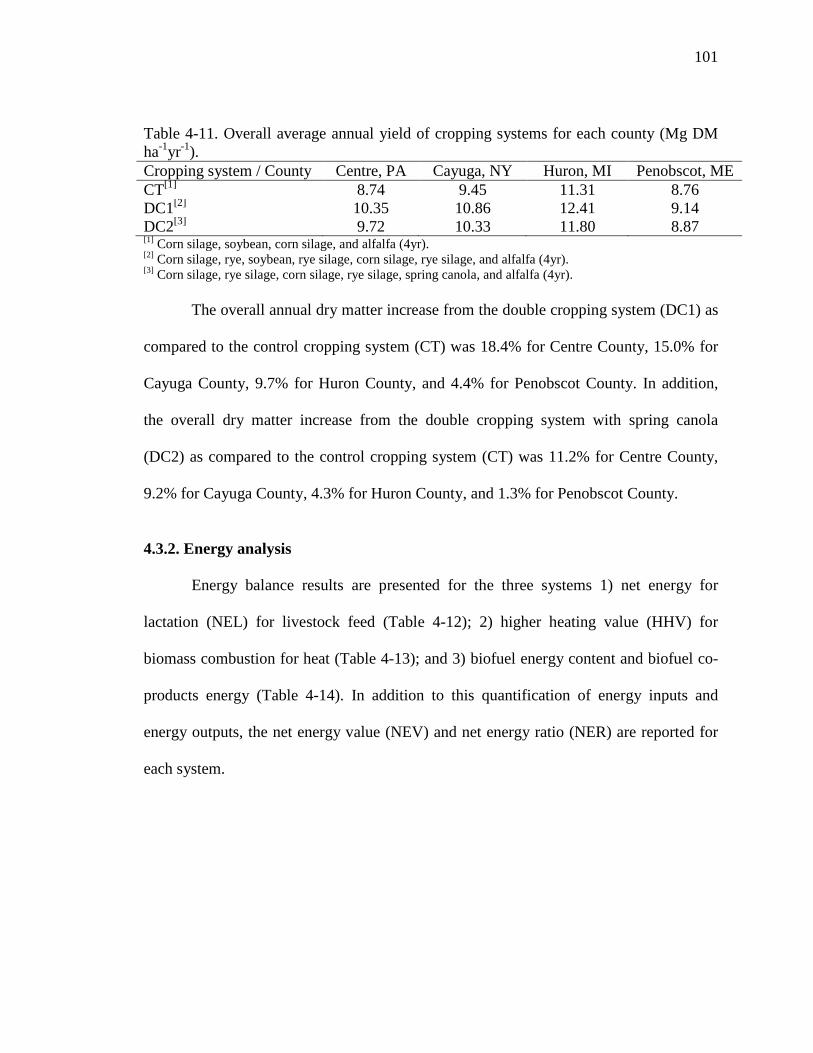
101

Table 4-11. Overall average annual yield of cropping systems for each county (Mg DM ha-1yr-1). Cropping system / County Centre, PA Cayuga, NY Huron, MI Penobscot, ME CT[1] 8.74 9.45 11.31 8.76 DC1[2] 10.35 10.86 12.41 9.14 DC2[3] 9.72 10.33 11.80 8.87 [1] Corn silage, soybean, corn silage, and alfalfa (4yr). [2] Corn silage, rye, soybean, rye silage, corn silage, rye silage, and alfalfa (4yr). [3] Corn silage, rye silage, corn silage, rye silage, spring canola, and alfalfa (4yr).

The overall annual dry matter increase from the double cropping system (DC1) as

compared to the control cropping system (CT) was 18.4% for Centre County, 15.0% for

Cayuga County, 9.7% for Huron County, and 4.4% for Penobscot County. In addition,

the overall dry matter increase from the double cropping system with spring canola

(DC2) as compared to the control cropping system (CT) was 11.2% for Centre County,

9.2% for Cayuga County, 4.3% for Huron County, and 1.3% for Penobscot County.

4.3.2. Energy analysis

Energy balance results are presented for the three systems 1) net energy for

lactation (NEL) for livestock feed (Table 4-12); 2) higher heating value (HHV) for

biomass combustion for heat (Table 4-13); and 3) biofuel energy content and biofuel co-

products energy (Table 4-14). In addition to this quantification of energy inputs and

energy outputs, the net energy value (NEV) and net energy ratio (NER) are reported for

each system.

102

Table 4-12. Livestock feed energy balance (NEL[1]) per year.

Cropping system nomenclature

Energy input

(MJ ha-1 yr-1)

Energy output (NEL)[1]

(MJ ha-1 yr-1) NEV[2]

(MJ ha-1 yr-1) NER[3]

Centre CT 11,376 55,060 43,685 4.84 Centre DC1 16,025 61,839 45,814 3.86 Centre DC2 15,440 60,048 44,607 3.89 Cayuga CT 11,129 59,971 48,743 5.34 Cayuga DC1 15,830 65,410 49,581 4.13 Cayuga DC2 15,265 64,004 48,739 4.19 Huron CT 11,376 70,422 59,046 6.19 Huron DC1 16,025 75,434 59,409 4.71 Huron DC2 15,440 72,155 56,715 4.67 Penobscot CT 11,129 55,013 43,784 4.90 Penobscot DC1 15,830 56,000 40,170 3.54 Penobscot DC2 15,265 56,060 40,795 3.67

[1] Net energy for lactation. [2] Net energy value. [3] Net energy ratio. [4] See Chapter 3 for details. Table 4-13. Biomass heating energy balance (HHV[1]) per year.

Cropping system nomenclature

Energy input

(MJ ha-1 yr-1)

Energy output (HHV)[1]

(MJ ha-1 yr-1) NEV[2]

(MJ ha-1 yr-1) NER[3]

Centre CT 11,376 163,234 151,858 14.35 Centre DC1 16,025 192,685 176,660 12.02 Centre DC2 15,440 186,041 170,601 12.05 Cayuga CT 11,129 176,199 164,930 15.69 Cayuga DC1 15,830 202,090 186,260 12.77 Cayuga DC2 15,265 196,940 181,675 12.90 Huron CT 11,376 210,920 199,544 18.54 Huron DC1 16,025 236,570 220,545 14.76 Huron DC2 15,440 224,483 209,043 14.54 Penobscot CT 11,129 163,159 151,930 14.53 Penobscot DC1 15,830 170,116 154,287 10.75 Penobscot DC2 15,265 170,090 154,825 11.14

[1] Higher heating value. [2] Net energy value. [3] Net energy ratio. [4] See Chapter 3 for details.

103

Table 4-14. Biofuel production energy balance per year. Cropping systems nomenclature

Energy input

(MJ ha-1 yr-1)

Energy recycled[5] (MJ ha-1 yr-1)

Energy output (biofuel source)[1]

(MJ ha-1 yr-1)

Energy output (co-product)[2] (MJ ha-1 yr-1)

NEV[3] (MJ ha-1 yr-1)

NER[4]

Centre CT 91,930 72,830 61,427 15546 58,498 4.17 Centre DC1 72,654 17,874 72,654 17,874 66,433 3.76 Centre DC2 71,997 17,257 71,997 17,257 65,799 3.81 Cayuga CT 98,857 78,938 66,344 16,657 63,081 4.17 Cayuga DC1 117,413 91559 76,212 18,707 69,064 3.67 Cayuga DC2 114,975 89,917 76,129 18,191 69,263 3.76 Huron CT 116,358 95,075 79,485 19,713 77,915 4.66 Huron DC1 134,947 107,721 89,278 21,688 83,740 4.08 Huron DC2 128,925 102,883 86,573 20,551 81,083 4.11 Penobscot CT 92,369 73,273 61,454 15,355 57,714 4.02 Penobscot DC1 101,007 76,938 64,138 15,800 55,868 3.32 Penobscot DC2 100,899 77,277 65,948 15,891 58,217 3.46

[1] Energy content in biofuel. [2] Energy content in biofuel co-products. [3] Net energy value (Energy output biofuel source, energy output co-product, minus energy input, and

energy recycled. [4] Net energy ratio. (Energy output biofuel source, energy output co-product, divided by energy input, and

energy recycled. [5] Energy recycling through lignin combusting in cellulosic ethanol processing. [6] See Chapter 3 for details.

The net energy for lactation distribution balance are presented for Centre County

(Figure 4-4), for Cayuga County (Figure 4-5), for Huron County (Figure 4-6), and for

Penobscot County (Figure 4-7). The higher heating value energy distribution balance are

presented for Centre County (Figure 4-8), for Cayuga County (Figure 4-9), for Huron

County (Figure 4-10), and for Penobscot County (Figure 4-11). The biofuel energy

distribution balance are presented for Centre County (Figure 4-12), for Cayuga County

(Figure 4-13), for Huron County (Figure 4-14), and for Penobscot County (Figure 4-15).

104

Figure 4-4. Centre County Pennsylvania net energy for lactation (NEL) balance per year.

Figure 4-5. Cayuga County New York net energy for lactation (NEL) balance per year.

-70,000

-60,000

-50,000

-40,000

-30,000

-20,000

-10,000

0

10,000

20,000

CT input

DC1 input

DC2 input

CT output

DC1 output

DC2 output

CT net DC1 net

DC2 net

Ene

rgy

(MJ

ha-1

yr-1

)Net

Canola

Alfalfa

Rye (silage)

Corn (silage)

Soybean

Transp. inputs

Drying

On farm fuel use

Insecticide

Herbicide

Seed

Lime

K

P

N

-70,000

-60,000

-50,000

-40,000

-30,000

-20,000

-10,000

0

10,000

20,000

CT input

DC1 input

DC2 input

CT output

DC1 output

DC2 output

CT net DC1 net

DC2 net

Ene

rgy

(MJ

ha-1

yr-1

)

NetCanolaAlfalfaRye(silage)Corn(silage)SoybeanTransp. inputsDryingOn farm fuel useInsecticideHerbicideSeedLimeKPN

105

Figure 4-6. Huron County Michigan net energy for lactation (NEL) balance per year.

Figure 4-7. Penobscot County Maine net energy for lactation (NEL) balance per year.

-80,000

-70,000

-60,000

-50,000

-40,000

-30,000

-20,000

-10,000

0

10,000

20,000

CT input

DC1 input

DC2 input

CT output

DC1 output

DC2 output

CT net DC1 net

DC2 net

Ene

rgy

(MJ

ha-1

)yr-1

)

Net

Canola

Alfalfa

Rye(silage)

Corn(silage)

Soybean

Transp. inputs

Drying

On farm fuel use

Insecticide

Herbicide

Seed

Lime

K

P

N

-60,000

-50,000

-40,000

-30,000

-20,000

-10,000

0

10,000

20,000

CT input

DC1 input

DC2 input

DCT output

DC1 output

DC2 output

CT net DC1 net

DC2 net

Ene

rgy

(MJ

ha-1

yr-1

)


106

Figure 4-8. Centre County Pennsylvania higher heating value (HHV) energy balance per

year.

Figure 4-9. Cayuga County New York higher heating value (HHV) energy balance per

year.

-250,000

-200,000

-150,000

-100,000

-50,000

0

50,000

CT input

DC1 input

DC2 input

CT output

DC1 output

DC2 output

CT net DC1 net

DC2 net

Ene

rgy

(MJ

ha-1

yr-1

)NetCanolaAlfalfaRye (silage)Corn(silage)SoybeanTransp. inputsDryingOn farm fuel useInsecticideHerbicideSeedLimeKPN

-250,000

-200,000

-150,000

-100,000

-50,000

0

50,000

CT input

DC1 input

DC2 input

CT output

DC1 output

DC2 output

CT net DC1 net

DC2 net

Ene

rgy

(MJ

ha-1

yr-1

)


107

Figure 4-10. Huron County Michigan higher heating value (HHV) energy balance per

year.

Figure 4-11. Penobscot County Maine higher heating value (HHV) energy balance per

year.

-250,000

-200,000

-150,000

-100,000

-50,000

0

50,000

CT input

DC1 input

DC2 input

CT output

DC1 output

DC2 output

CT net DC1 net

DC2 net

Ene

rgy

(MJ

ha-1

yr-1

)NetCanolaAlfalfaRye(silage)Corn(silage)SoybeanTransp. inputsDryingOn farm fuel useInsecticideHerbicideSeedLimeKPN

-200,000

-150,000

-100,000

-50,000

0

50,000

CT input

DC1 input

DC2 input

CT output

DC1 output

DC2 output

CT net DC1 net

DC2 net

Ene

rgy

(MJ

ha-1

yr-1

)


108

Figure 4-12. Centre County Pennsylvania biofuel and co-products energy balance per

year.

Figure 4-13. Cayuga County New York biofuel and co-products energy balance per year.

-100000

-80000

-60000

-40000

-20000

0

20000

40000

CT input

DC1 input

DC2 input

CT output

DC1 output

DC2 output

CT net

DC1 net

DC2 net

Ene

rgy

(MJ

ha-1

yr-1

)NetCellulosic ethanol coproductsGlycerineMealCellulosic ethanolBiodiesel Biodiesel processingCellulosic ethanol processingTransp. feedstock to biorefineryTransp. inputsDryingOn farm fuel useInsecticideHerbicideSeedLimeKPN

-120,000

-100,000

-80,000

-60,000

-40,000

-20,000

0

20,000

40,000

CT input

DC1 input

DC2 input

CT output

DC1 output

DC2 output

CT net

DC1 net

DC2 net

Ene

rgy

(MJ

ha-1

yr-1

)

NetCellulosic ethanol coproductsGlycerineMealCellulosic ethanolBiodiesel Biodiesel processingCellulosic ethanol processingTransp. feedstock to biorefineryTransp. inputsDryingOn farm fuel useInsecticideHerbicideSeedLimeKPN

109

Figure 4-14. Huron County Michigan biofuel and co-products energy balance per year.

Figure 4-15. Penobscot County Maine biofuel and co-products energy balance per year.

-120,000

-100,000

-80,000

-60,000

-40,000

-20,000

0

20,000

40,000

CT input

DC1 input

DC2 input

CT output

DC1 output

DC2 output

CT net

DC1 net

DC2 net

Ene

rgy

(MJ

ha-1

yr-1

)NetCellulosic ethanol coproductGlycerineMealCellulosic ethanolBiodiesel Biodiesel processingCellulosic ethanol processingTransp. feedstock to biorefineryTransp. inputsDryingOn farm fuel useInsecticideHerbicideSeedLimeKPN

-100,000

-80,000

-60,000

-40,000

-20,000

0

20,000

40,000

CT input

DC1 input

DC2 input

CT output

DC1 output

DC2 output

CT net

DC1 net

DC2 net

Ene

rgy

(MJ

ha-1

yr-1

)

NetCellulosic ethanol coproductGlycerineMealCellulosic ethanolBiodiesel Biodiesel processingCellulosic ethanol processingTransp. feedstock to biorefineryTransp. inputsDryingOn farm fuel useInsecticideHerbicideSeedLimeKPN

110

The net energy increase for each studied cropping system and each energy type

are shown on Table 4-15. Higher heating value in double cropping systems had the

highest overall net energy increase followed by biofuel and net energy for lactation.

Table 4-15. Net energy increase from double cropping system versus control cropping system. Cropping systems

Energy type Centre PA

Cayuga NY

Huron MI

Penobscot ME

DC1 NEL[1] 4.6% 1.6% 0.5% -8.2% DC2 NEL 1.2% -0.8% -4.6% -7.5% DC1 HHV[2] 16.2% 12.8% 10.4% 1.5% DC2 HHV 12.0% 9.8% 4.5% 1.7% DC1 Biofuel[3] 13.2% 9.3% 7.3% -3.2% DC2 Biofuel 11.6% 9.0% 3.5% 0.3% [1] Net energy for lactation. [2] Higher heating value. [3] Biofuel and co-products energy.

4.3.3. Greenhouse Gas (GHG) Analysis

The GHG results are presented using two methodologies (see Chapter 3) 1) crop

GHG assimilation for livestock feed and biomass heating (Table 4-16), and 2) biofuel

GHG credit for biofuel production (Table 4-17).

111

Table 4-16. Livestock feed and heating greenhouse gas (GHG) emissions balance (g CO2e ha-1 yr -1). Cropping systems

County Total input production

Net crop assimilation

Net emissions

CT Centre 9.3 -125.4 -116.0 DC1 Centre 13.3 -147.1 -133.8 DC2 Centre 12.8 -141.9 -129.1 CT Cayuga 9.2 -135.7 -126.5 DC1 Cayuga 13.2 -154.6 -141.4 DC2 Cayuga 12.7 -150.6 -137.9 CT Huron 9.3 -163.2 -153.9 DC1 Huron 13.3 -182.0 -168.7 DC2 Huron 12.8 -172.5 -159.7 CT Penobscot 9.3 -125.5 -116.2 DC1 Penobscot 13.2 -129.3 -116.1 DC2 Penobscot 12.7 129.2 -116.5

[1] See Chapter 3 for details.

Table 4-17. Livestock feed and heating greenhouse gas (GHG) emissions balance (g CO2e ha-1 yr -1). Cropping systems

County Farmland production

Farm nitrous oxide Biorefinery[1]

Biofuel credit

Co-product credit

Net

CT[2] Centre 8.7 3.4 2.7 -40.9 -3.5 -29.8 DC1[2] Centre 12.2 5.4 3.3 -48.1 -4.0 -31.3 DC2[2] Centre 11.9 6.1 3.3 -48.1 -4.1 -30.8 CT Cayuga 9.2 3.4 3.0 -44.1 -3.7 -32.4 DC1 Cayuga 13.2 5.4 3.5 -50.5 -4.2 -32.6 DC2 Cayuga 12.7 6.1 3.6 -50.8 -4.3 -32.7 CT Huron 9.3 3.4 3.2 -52.7 -4.4 -41.3 DC1 Huron 13.3 5.4 3.7 -59.0 -4.9 -41.5 DC2 Huron 12.8 6.1 3.6 -57.6 -4.8 -39.8 CT Penobscot 9.3 3.4 2.6 -40.8 -3.5 -29.1 DC1 Penobscot 13.2 5.4 2.8 -42.5 -3.5 -24.7 DC2 Penobscot 12.7 6.1 3.0 -44.2 -3.8 -26.1

[1] Includes feedstock transportation and lignin combustion emissions credit. [2] Control (CT), Double cropping (DC) systems.

To provide a better understanding of the allocation of the GHG inputs, outputs

and net balance for the three evaluated systems, graphs are presented for 1) livestock feed

112

and biomass heating (Figure 4-16, 4.17, 4.18, 4.19), and 2) biofuels systems (Figure 4-20,

4-21, 4-22, 4-23) for each studied county.

Figure 4-16. Centre County Pennsylvania crop greenhouse gas assimilation balance per

year.

-160

-140

-120

-100

-80

-60

-40

-20

0

20

40

CT input

DC1 input

DC2 input

CT output

DC1 output

DC2 output

CT net DC1 net

DC2 net

GH

G (g

CO

2e m

-2yr

-1)

NetCanolaAlfalfaRye (silage)Corn (silage)SoybeanDryingTransport. inputsOn farm fuel useInsecticideHerbicideSeedLimeKPN

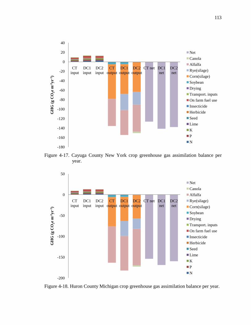
113

Figure 4-17. Cayuga County New York crop greenhouse gas assimilation balance per

year.

Figure 4-18. Huron County Michigan crop greenhouse gas assimilation balance per year.

-180

-160

-140

-120

-100

-80

-60

-40

-20

0

20

40

CT input

DC1 input

DC2 input

CT output

DC1 output

DC2 output

CT net DC1 net

DC2 net

GH

G (g

CO

2e m

-2yr

-1)

NetCanolaAlfalfaRye(silage)Corn(silage)SoybeanDryingTransport. inputsOn farm fuel useInsecticideHerbicideSeedLimeKPN

-200

-150

-100

-50

0

50

CT input

DC1 input

DC2 input

CT output

DC1 output

DC2 output

CT net DC1 net

DC2 net

GH

G (g

CO

2e m

-2yr

-1)


114

Figure 4-19. Penobscot County Maine crop greenhouse gas assimilation balance per year.

Figure 4-20. Centre County Pennsylvania biofuel greenhouse gas credit balance per year.

-140

-120

-100

-80

-60

-40

-20

0

20

40

CT input

DC1 input

DC2 input

CT output

DC1 output

DC2 output

CT net DC1 net

DC2 net

GH

G (g

CO

2e m

-2yr

-1)


-60

-50

-40

-30

-20

-10

0

10

20

30

CT input

DC1 input

DC2 input

CT output

DC1 output

DC2 output

CT net DC1 net

DC2 net

GH

G (g

CO

2e m

-2yr

-1)

NetBiofuel co-productsBiofuelBiorefineryTransport. feedstockNitrous oxideDryingTransport. inputsElectricityOn farm fuel useInsecticideHerbicideSeedLimeKPN

115

Figure 4-21. Cayuga County New York biofuel greenhouse gas credit balance per year.

Figure 4-22. Huron County Michigan biofuel greenhouse gas credit balance per year.

-60

-50

-40

-30

-20

-10

0

10

20

30

CT input

DC1 input

DC2 input

CT output

DC1 output

DC2 output

CT net DC1 net

DC2 net

GH

G (g

CO

2e m

-2yr

-1)


-70

-60

-50

-40

-30

-20

-10

0

10

20

30

CT input

DC1 input

DC2 input

CT output

DC1 output

DC2 output

CT net DC1 net

DC2 net

GH

G (g

CO

2e m

-2yr

-1)


116

Figure 4-23. Penobscot County Maine biofuel greenhouse gas credit balance per year.

The net greenhouse gas mitigation increase for each studied double cropping

system, and each energy methodology type are shown on Table 4-18. The majority of

counties had positive greenhouse gas mitigation with double cropping practices, with for

the exception of Penobscot County.

To illustrate the energy and GHG values in terms of real products from a biofuel

system, a list of biofuels and their respective co-products for each cropping system are

provided in Table 4-19.

-60

-50

-40

-30

-20

-10

0

10

20

30

CT input

DC1 input

DC2 input

CT output

DC1 output

DC2 output

CT net DC1 net

DC2 net

GH

G (g

CO

2e m

-2yr

-1)


117

Table 4-18. Net greenhouse gas mitigation annual increase or decrease from double cropping systems versus the control cropping system. Cropping system

Energy type Centre PA

Cayuga NY

Huron MI

Penobscot ME

DC1 NEL[1]/HHV[2] 15.3% 11.8% 9.6% -0.1% DC2 NEL/HHV 11.2% 9.0% 3.7% 0.2% DC1 Biofuel[3] 5.1% 0.9% 0.4% -15.0% DC2 Biofuel 3.6% 1.1% -3.6% -10.1% [1] Net energy for lactation. [2] Higher heating value. [3] Biofuel and co-products energy.

Table 4-19. Biofuel products and co-products of studied cropping systems per year.

Cropping system county

Biodiesel (L ha-1 yr-1)

Cellulosic ethanol

(L ha-1 yr-1) Feed meal (Mg ha-1 yr-1)

Glycerine (Mg ha-1 yr-1)

Excess electricity (MJ ha-1 yr-1)

Centre CT 84 2,767 0.33 0.01 13,255 Centre DC1 73 3,313 0.29 0.01 15,870 Centre DC2 112 3,221 0.19 0.02 15,430 Cayuga CT 84 2,999 0.33 0.01 14,366 Cayuga DC1 75 3,479 0.30 0.01 16,663 Cayuga DC2 112 3,416 0.19 0.02 16,364 Huron CT 88 3,612 0.35 0.01 17,303 Huron DC1 76 4,093 0.30 0.01 19,604 Huron DC2 112 3,909 0.19 0.02 18,724 Penobscot CT 74 2,784 0.29 0.01 13,335 Penobscot DC1 66 2,923 0.26 0.01 14,002 Penobscot DC2 112 2,836 0.19 0.02 14,064


4.4. Conclusions

Energy and greenhouse house gas analyses were effective and direct indicators to

evaluate cropping systems. In general, the addition of rye double crop presented better

energy and GHG results.

Successful implementation of double cropping systems depends on the amount of

extra output produced per additional input required. For the double cropping systems

analyzed in this chapter, the additional dry matter production required to “break-even” or

118

compensate for the additional inputs of fertilizer, fuel, etc. was calculated. Break-even

production for net energy for lactation required a 10 to 11% increase in the overall dry

matter production of the double cropping system. For higher heating value, the required

increase ranged from 1 to 5%, and for biofuels it ranged from 1 to 7%. For greenhouse

gas, emissions required to break-even ranged from 1 to 5% additional dry matter increase

for the crop assimilation method, and from 9-10% for biofuel credit method for the

double cropping systems.

Additional empirical data are needed in order to validate the modeled yield

results. Furthermore, an economic analysis for implementing these double cropping

systems is also required.

Energy and greenhouse gas analyses, plus other benefits such as ecological

services, are useful drivers to evaluate and promote more diverse cropping systems. New

technologies are coming available such as cellulosic ethanol, and plant genetics, which

could improve the incentives for and implementation of double cropping systems, giving

farmers more options to improve their operations.

119

Chapter 5

Energy and Greenhouse Gas Analysis of a Pennsylvania Dairy Farm

5.1. Introduction

As agricultural operations are looking for ways to maximize internal resources,

strategies that promote integration and multi-functionality are being revitalized to provide

environmental and productivity benefits. One set of strategies, double cropping systems,

are being designed to maximize land production to both fulfill livestock feed

requirements, and also to produce on-farm biofuels for energy self-sufficiency. Energy

and greenhouse gas analyses are useful tools to evaluate integrated farm systems in terms

of energy efficiency and global warming impact.

The majority of dairy farms in Pennsylvania are integrated operations that

produce both livestock feed and dairy products. Usually those farms are operated by one

or two families, with herd sizes ranging from 20 to 100 milking cows (NASS, 2007). In

such operations it is common for farmers to purchase additional livestock feed beyond

what is produced on the farm.

Alfalfa, hay, and corn are common crops grown on dairy farms (Borton et al.

1997). Perennial forage crops such as alfalfa and hay are cultivated for three or four

years, and annual crops such as corn are harvested as silage or grain. Other crops such as

soybean are also grown in some cases for use as dairy feed and to include an annual

nitrogen-fixing legume in crop rotations (Rotz et al. 2001a). Although exceptions exist,

120

most Pennsylvania dairy farms have traditionally used crop rotations that include corn,

soybean, and alfalfa.

Typical crop rotations with summer annual crops such as corn and soybeans have

unutilized periods when the soil is bare during late fall, winter, and early spring periods.

One way to take advantage of this unutilized window of opportunity is to employ double

crop or cover cropping strategies. Double cropping is a system of consecutively

producing and harvesting two crops on the same area of land in a single year (Tollenaar

et al. 1992; Heggenstaller et al. 2008). When the second crop (usually fall planted) is not

harvested (but simply killed and left in the field), it is called a cover crop or green

manure. These strategies can provide benefits such as decreased soil erosion and reduced

nitrate leaching, increased soil organic matter, and weed suppression, and in the double

crop case, increased farmland productivity (Zhu et al. 1989; Kaspar et al. 2001; Rotz et

al. 2002; Duiker and Curran, 2005; PSU agronomy guide, 2008).

When double / cover cropping systems are implemented, there is more biomass

produced, so the overall farm nutrient requirements are augmented. Phosphorus and

potassium demand is increased, while nitrogen requirements will increase or decrease

depending on whether the double / cover crop fixes nitrogen. Increased P and K demand

can be a benefit in cases where dairy operations have excess manure production, given

the cost of manure transport and water quality concerns.

In integrated systems, manure recycling provides essential nutrients for crop

growth, but also improves soil organic matter, soil structure, and soil water and nutrient

holding capacity (Madison et al. 1986). Furthermore, when winter crops are used it

creates an additional opportunity to spread the manure.

121

Integrated farm operations allow farmers to have a diverse crop mix creating the

flexibility in livestock feeding. Small grains such as wheat, rye and barley are winter

crops that have historically been grown in Pennsylvania dairy farm rotations and are now

generating renewed interest (Rotz et al. 2002). Small grains are harvested as grain or

silage, depending on the double crop production strategy. Small grains are often used as

livestock feed; however, the energy and protein contents can be lower than those of corn

and alfalfa (NRC, 2001).

Canola (Brassica napus L. and B. campestris L.) is an oil seed crop that is

becoming more popular in Pennsylvania (Frier and Roth, 2009). There are spring and

winter varieties of canola, and consequently this can be easily integrated in a double /

cover cropping system in many different crop rotations. There are two main products

from canola: meal and oil. Canola meal can be used as a protein supplement in livestock

rations as an alternative to soybean meal, distiller dried grains, or commercial concentrate

(Newkirk, 2009). The oil extracted from the seed can be used as food grade oil, as

biodiesel feedstock, or as an on-farm fuel alternative. When the extracted oil is used pure

and without further processing as a source of fuel for internal combustion engines, it is

called straight vegetable oil (SVO) (Caufmann, 2008). Farmers can use SVO in diesel-

powered farm machinery after some adjustment (Emberger et al. 2009). Thus, integrating

canola in livestock and double / cover cropping systems, could provide farmers an

alternative feed material and an opportunity to be more fuel self-sufficient.

Various types of energy analyses have been used to assess livestock (Spedding,

1981; Oltenacu and Allen, 1981), single crop systems (Fluck and Baird, 1979; Pimentel,

1981), and double / cover cropping systems (Kim and Dale, 2008). GHG analysis has

122

also been widely used to evaluate livestock (Chianese et al. 2009d), cash grain (Adler et

al. 2007); and double / cover cropping systems (Kim and Dale, 2008).

The objective of this study was to use energy and greenhouse gas analyses,

nutrient recycling, and on-farm fuel production to evaluate a theoretical Pennsylvania

dairy farm operation with two cropping system scenarios. First, corn, soybean, and alfalfa

were grown as a control cropping system, which represented the majority of current

rotations. Second, double / cover cropping systems integrated rye, wheat, and canola in

the standard corn, soybean, and alfalfa rotation.

5.2. Material and methods

5.2.1. Energy and greenhouse gas analysis

The Farm Energy Analysis Tool (FEAT) was used to evaluate energy usage and

greenhouse gas (GHG) emissions of two crop rotations in a livestock operation (Chapter

3). The analysis was restricted to a boundary that included production of inputs, crop

production, and dairy production (Figure 5-1). The methodology used to assess energy

and greenhouse gases was described earlier in Chapter 3.

Figure 5-1. Farm system evaluation boundary.

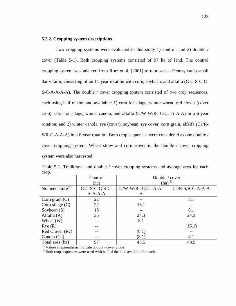
123

5.2.2. Cropping system descriptions

Two cropping systems were evaluated in this study 1) control, and 2) double /

cover (Table 5-1). Both cropping systems consisted of 97 ha of land. The control

cropping system was adapted from Rotz et al. (2001) to represent a Pennsylvania small

dairy farm, consisting of an 11-year rotation with corn, soybean, and alfalfa (C-C-S-C-C-

S-C-A-A-A-A). The double / cover cropping system consisted of two crop sequences,

each using half of the land available: 1) corn for silage, winter wheat, red clover (cover

crop), corn for silage, winter canola, and alfalfa (C/W-W/Rc-C/Ca-A-A-A) in a 6-year

rotation; and 2) winter canola, rye (cover), soybean, rye cover, corn grain, alfalfa (Ca/R-

S/R-C-A-A-A) in a 6-year rotation. Both crop sequences were considered as one double /

cover cropping system. Wheat straw and corn stover in the double / cover cropping

system were also harvested.

Table 5-1. Traditional and double / cover cropping systems and average area for each crop. Control

(ha) Double / cover

(ha)[2] Nomenclature[1] C-C-S-C-C-S-C-

A-A-A-A C/W-W/Rc-C/Ca-A-A-

A Ca/R-S/R-C-A-A-A

Corn grain (C) 22 -- 8.1 Corn silage (C) 22 16.1 -- Soybean (S) 18 -- 8.1 Alfalfa (A) 35 24.3 24.3 Wheat (W) -- 8.1 -- Rye (R) -- (16.1) Red Clover (Rc) -- (8.1) -- Canola (Ca) -- (8.1) 8.1 Total area (ha) 97 48.5 48.5 [1] Values in parenthesis indicate double / cover crops. [2] Both crop sequences were used with half of the land available for each.

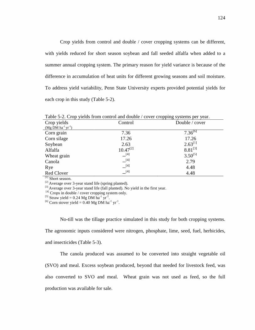
124

Crop yields from control and double / cover cropping systems can be different,

with yields reduced for short season soybean and fall seeded alfalfa when added to a

summer annual cropping system. The primary reason for yield variance is because of the

difference in accumulation of heat units for different growing seasons and soil moisture.

To address yield variability, Penn State University experts provided potential yields for

each crop in this study (Table 5-2).

Table 5-2. Crop yields from control and double / cover cropping systems per year. Crop yields (Mg DM ha-1 yr-1)

Control Double / cover

Corn grain 7.36 7.36[6] Corn silage 17.26 17.26 Soybean 2.63 2.63[1] Alfalfa 10.47[2] 8.81[3] Wheat grain --[4] 3.50[5] Canola --[4] 2.79 Rye --[4] 4.48 Red Clover --[4] 4.48 [1] Short season. [2] Average over 3-year stand life (spring planted). [3] Average over 3-year stand life (fall planted). No yield in the first year. [4] Crops in double / cover cropping system only. [5] Straw yield = 0.24 Mg DM ha-1 yr-1. [6] Corn stover yield = 0.40 Mg DM ha-1 yr-1.

No-till was the tillage practice simulated in this study for both cropping systems.

The agronomic inputs considered were nitrogen, phosphate, lime, seed, fuel, herbicides,

and insecticides (Table 5-3).

The canola produced was assumed to be converted into straight vegetable oil

(SVO) and meal. Excess soybean produced, beyond that needed for livestock feed, was

also converted to SVO and meal. Wheat grain was not used as feed, so the full

production was available for sale.

125

Table 5-3. Control and double / cover cropping system farm input requirements per year.

Corn grain

Corn silage

Soybean Canola Wheat grain

Rye Hairy vetch

Alfalfa Ref.[1]

Nitrogen (kg ha-1 yr-1)

145 168 0.0 145 67 0.0 0.0 0.0 a, h,

Phosphate (kg ha-1 yr-1)

56 123 45 39 56 0.0 0.0 89 a, h

Potash (kg ha-1 yr-1)

34 257 67 56 134 0.0 0.0 279 a, h

Lime (kg ha-1 yr-1)

448 448 300 19 300 0.0 0.0 150 c, i

Seed (kg ha-1 yr-1)

20 20 81 6 100 126 8 5.6 b, g,

Fuel (L ha-1 yr-1)

38.7 94.2 30 7.4 7.4 7.4 5.5 87.4 e, f,

Herbicide (kg ha-1 yr-1)

2.71 3.63 1.5 3.4 0.4 0.4 0.4 0.0 b, j

Insecticide (kg ha-1 yr-1)

0.99 0.68 0.39 0.0 0.33 0.0 0.0 0.0 b [1] References: a. PSU Agronomy guide (2008); b. West and Marland (2002); c. Farrell et al. (2006); d.

Smith et al. (2007); e. Rotz et al. (2009); f. van Ouwerkerk et al. (2009); g. Duiker and Curran (2005); h. NDSU (2009); i. Kaltschmitt and Reinhardt (1997); j. Monsanto (2009).


5.2.3. Dairy characteristics

The evaluated cropping systems were used on a dairy farm. The main objective of

the cropping systems was to provide feed to dairy livestock. To assess the amount of feed

required by the dairy herd, the Dairy Farm Feed Cost Control model was used (Ishler and

Beck, 1999). A target milk production of 10,886 kg of milk per milking cow per year was

used to assess the feed requirements. The dairy herd consisted of 60 cows and 60 heifers.

All rations took into account 4-5% feeding loss for forages, and 2% feeding loss for

grains. The energy and greenhouse gas emission methodologies for the dairy production

system were previously described in Chapter 3.

126


5.3.1. Dairy feed consumption

The control cropping system was more efficient in producing larger quantities of

dairy feed (Table 5-4). The double / cover cropping system had 10% lower production

and 23% lower excess biomass after feed consumption.

Table 5-4. Feed produced, consumed, purchased and sold for control and double / cover cropping systems per year. Control Double / cover Crop (Mg DM yr-1)

Produced[1] Consumed Purchased / Sold[2]

Produced Consumed Purchased / Sold

Corn grain 144 58 87 53 43 10 Corn silage 342 218 124 252 226 25 Soybean 43 40 3[3] 19 18 1[3] Alfalfa[4] 341 204 137 385 127 259 Wheat straw -- -- -- 23 23 0 Canola meal[5] -- -- -- 20 21 -1 Milk cow grain

mix[6] -- 89 -89 -- 112 -112

Dry cow grain mix[6]

-- 5 -5 -- 6 -6

Heifer grain mix[6]

-- 25 -25 -- 25 -25

Wheat grain[7] -- -- -- 28 -- 28 Total 870 639 232 780 601 179

[1] Adjusted values including feed losses. [2] Negative values are purchased products and positive values are sold products and carry over. [3] Converted to straight vegetable oil. [4] Includes both silage and hay. [5] 10% moisture content (Grant et al. 1983). [6] 15% moisture content as this is a mixture of grains, byproducts, protein, minerals, and vitamins. [7] Not used as dairy feed. 5.3.2. Energy analysis results

Double / cover cropping systems had higher input energy requirements; however,

due to greater energy recycling, the net input energy was lower than the control cropping

system (Table 5-5). Recycled energy that substituted for external inputs included straight

vegetable oil, manure nutrients, and nitrogen fixation by legume crops.

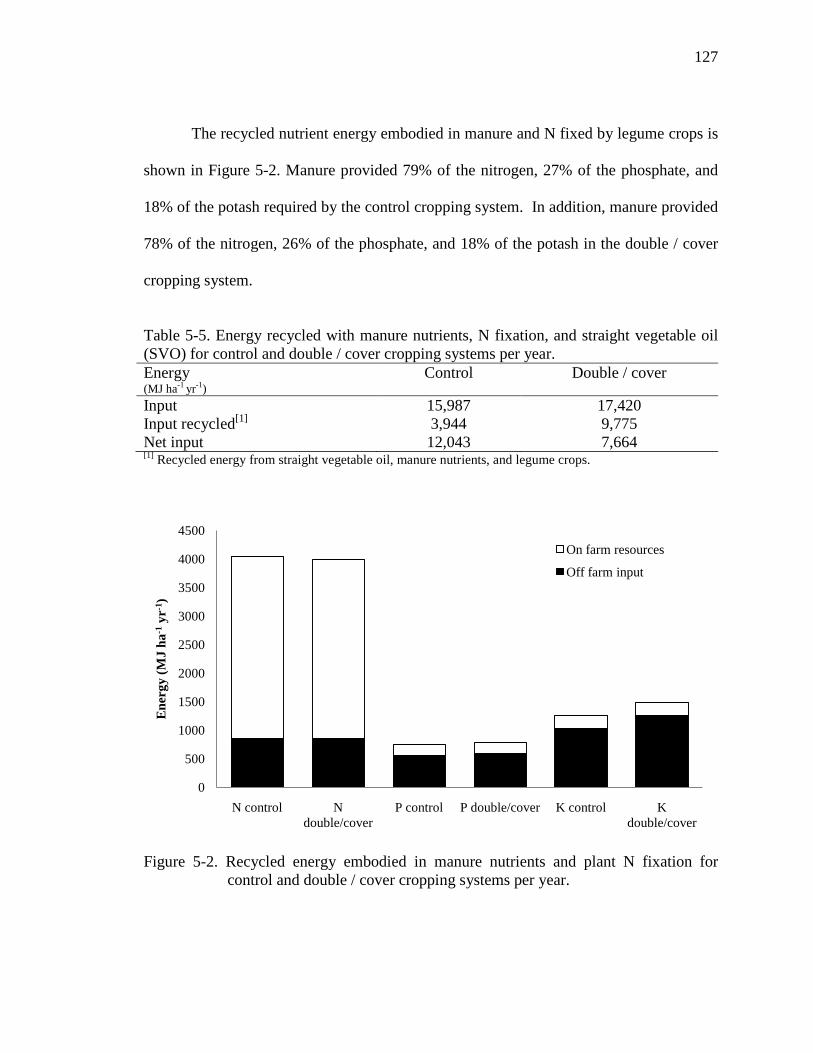
127

The recycled nutrient energy embodied in manure and N fixed by legume crops is

shown in Figure 5-2. Manure provided 79% of the nitrogen, 27% of the phosphate, and

18% of the potash required by the control cropping system. In addition, manure provided

78% of the nitrogen, 26% of the phosphate, and 18% of the potash in the double / cover

cropping system.

Table 5-5. Energy recycled with manure nutrients, N fixation, and straight vegetable oil (SVO) for control and double / cover cropping systems per year. Energy (MJ ha-1 yr-1)

Control Double / cover

Input 15,987 17,420 Input recycled[1] 3,944 9,775 Net input 12,043 7,664 [1] Recycled energy from straight vegetable oil, manure nutrients, and legume crops.

Figure 5-2. Recycled energy embodied in manure nutrients and plant N fixation for

control and double / cover cropping systems per year.

0

500

1000

1500

2000

2500

3000

3500

4000

4500

N control N double/cover

P control P double/cover K control K double/cover

Ene

rgy

(MJ

ha-1

yr-1

)

On farm resources

Off farm input

128

Straight vegetable oil, as a component of input energy recycling, provided 6% of

the fuel needed for the control cropping systems, and 121% of the fuel for the double /

cover cropping system (Figure 5-3). The majority of the fuel was used for field crop

operations, followed by feed handling, and manure handling (Table 5-6).

Table 5-6. Fuel energy use distribution within farm for control and double / cover cropping systems per year. Control Double / cover Field crop operations 56 % 62 % Feed handling 35 % 30 % Manure handling 9 % 8 %

Figure 5-3. Straight vegetable oil energy recycling for control and double / cover

cropping systems per year.

0

1000

2000

3000

4000

5000

6000

7000

8000

Fuel control Fuel double/cover

Ene

rgy

(MJ

ha-1

yr-1

)

Excess beyond farm needs

On farm resources

Off farm input

129

After energy in the straight vegetable oil, manure nutrients, and legume N fixation

were accounted, the net input energy distribution for the control and double / cover

cropping system are shown on Figure 5-4. Fuel consumption input was the highest energy

input for the control cropping system, and electricity was the highest energy input for the

double / cover cropping system.

Figure 5-4. Net energy input for control and double / cover cropping systems per year.

5.3.3. Greenhouse gas emissions analysis

The control cropping system had higher farmland GHG production (10.2 g CO2e

m-2 yr-1) relative to the double / cover cropping system (6.6 g CO2e m-2 yr-1) (Figures 5-5

and 5-6). GHG assimilation by crops was 6% higher for the double / cover cropping

0

2000

4000

6000

8000

10000

12000

14000

Control inputs Double/cover inputs

Ene

rgy

(MJ

ha-1

yr-1

)

Oil grain Crushing

Transportation of inputs

Drying

Electricity

On farm fuel use

Insecticide

Herbicide

Seed

Lime

K

P

N

130

system than the control rotation. The double / cover cropping system had -154.0 g CO2e

m-2 yr-1 net crop assimilation and the control system had -145.4 g CO2e m-2 yr-1 net crop

assimilation. Both cropping systems had the same amount of emissions from dairy

housing (70.0 g CO2e m-2 yr-1) and manure (58.0 g CO2e m-2 yr-1) since the same herd size

and housing/manure management system was used. Overall, the double / cover cropping

system had lower net GHG emissions on an area basis (-19.7 g CO2e m-2 yr-1) than the

control system (-7.3 g CO2e m-2 yr-1).

Figure 5-5. Control cropping system greenhouse gas (GHG) emission balance per year.

-200.0

-150.0

-100.0

-50.0

0.0

50.0

100.0

150.0

Farmland Crop assimilation

Livestock and manure

Net

GH

G (g

CO

2e m

-2yr

-1)

NetMaure N2O emissionsManure soil CO2 emissionsManure storageLivestock housingCrop assimiliationOil grain crushingDryingTransport. inputsElectricityOn farm fuel useInsecticideHerbicideSeedLimeKPN

131

Figure 5-6. Double / cover cropping system greenhouse gas (GHG) emission balance per

year.

The use of double and cover crops contributed to a higher overall crop

assimilation in the double / cover cropping system (Figure 5-6). The overall crop

distribution is shown in Table 5-7. Winter crops such as canola contributed to farm

energy self-sufficiency and reduced of fuel related GHG emissions.

-200

-150

-100

-50

0

50

100

150

Farmland Crop assimilation Livestock and manure

Net

GH

G (g

CO

2e m

-2 y

r-1)

Double / cover GHG balanceNetMaure N2O emissionsManure soil CO2 emissionsManure storageLivestock housingCrop assimiliationOil grain crushingDryingTransport. inputsElectricityOn farm fuel useInsecticideHerbicideSeedLimeKPN

132

Table 5-7. Distribution of net crop CO2e assimilation for control and double / cover cropping systems per year. Crops Control Double / cover Corn grain 17% 6% Corn silage 39% 27% Soybean 5% 2% Alfalfa 39% 42% Canola -- 4% Wheat grain -- 3% Rye (cover crop) -- 7% Red clover (cover crop) -- 4% Corn stover[1] -- 4% Wheat straw[1] -- 2% [1] Only the amount of residue collected were accounted as net crop assimilation.

5.4. Conclusions

The double / cover cropping system outperformed the traditional cropping system

in terms of net biomass production, net input energy, farmland input GHG, and net GHG

emission. However, the control cropping system was able to provide a higher dairy feed

amount than the double / cover cropping system.

Additional factors must be also taken into account when implementing double /

cover cropping systems. Available labor and machinery and economic impacts could

create constraints for implementation.

Double / cover cropping systems such as those simulated might provide some

additional benefits that were not accounted for, such as environmental enhancement

through reduced nutrient and soil losses and increased soil quality, reduced economic

risks associated with growing just a few primary crops, and higher crop yields over the

long term.

As agricultural carbon markets expand, cropping systems such as double / cover

crops, which assimilate more GHG, might gain an economic incentive that could

133

encourage implementation. In addition, as oil prices become increasingly unstable,

farmers might adapt practices such as the production of SVO to protect themselves from

high fuel prices.

134

Chapter 6

Modifying Northern Dairy Farms for Productivity, Greenhouse

Gas Reductions, and Potential Biomass Supply

6.1. Introduction

Alternative cropping systems utilizing double cropping strategies have been

evaluated in terms of biomass for direct combustion (heating), livestock feed, and biofuel

production (Chapter 4). The effects of integrating these practices into a typical

management program for a small Pennsylvania dairy operation were also previously

described (Chapter 5). In this chapter, dairy farm site-specific analyses were performed to

address regional variability and to provide a broader assessment of sustainable cropping

practices such as double cropping.

This study simulated typical agricultural operations in the northeast and north

central regions of the US. Dairy farms are common agricultural enterprises in these

northern regions. Out of the 23 major milk-producing states, Pennsylvania accounted for

6.03% of total US milk production, New York accounted for 6.97%, and Michigan 4.4%

in 2008 (NASS, 2009).

To evaluate site specific differences, four counties in different northern states

were chosen: 1) Centre County in Pennsylvania; 2) Cayuga County in New York; and 3)

Huron County in Michigan, and Penobscot County in Maine. Centre County is situated in

central Pennsylvania, and the primary operations include dairy and cow / calf farms.

Cayuga County is located in central New York, where dairy, and cash crop farms

predominate. Huron County is located in Michigan’s northeastern lower peninsula (“the

135

thumb”), where dairy, beef, and cash crop farms are common. Penobscot County is

located in central Maine, where the main agricultural operations include dairy and potato

farms.

The objective of this study was to evaluate dairy farm operations in the selected

states and to compare common current cropping systems with alternative double cropping

management scenarios. Energy and greenhouse gas (GHG) analyses were used as

evaluation criteria.

6.2. Materials and methods

6.2.1. Model methodology

The Farm Energy Analysis Tool (FEAT) was used to assess cropping systems,

dairy energy and greenhouse gas emission balances. The restricted boundary in this study

was production of input, crop production, and dairy production (Figure 6-1). Yields

results obtained for each county with Integrated Farm System Model from Chapter 4

were also used in this chapter.

Figure 6-1. Farm system evaluation boundary. 6.2.2. Dairy farming systems description

In each of the four selected counties, local county extension educators were

interviewed to assess the characteristics of typical agricultural operations. Dairy farms

136

were a common type of operation in all of the selected counties, and thus were used as

the baseline for comparisons with double cropping systems scenarios. Extension

educators helped to parameterize typical dairy farm operations for each county, and these

recommendations provided the basis for the simulated farms described.

In Centre County, PA, typical dairy farms were assumed to have 160 milking

cows, 26 dry cows, and 156 heifers. Farms were assumed to have 154 ha of available

land with no tillage practices used for crop production. Corn and soybeans were rotated

with alfalfa. Corn production was assumed to include 30 ha harvested as grain and 40 ha

as silage. Soybean was assumed to be produced on 28 ha, and alfalfa was established and

grown for 4 years with 56 ha in production.

In Cayuga County, NY, typical dairy farms were assumed to have 200 cows, 35

dry cows, and 198 heifers. Farms were assumed to have 200 ha of available land with

reduced tillage practices used for crop production. Corn was harvested as silage, with

alfalfa grown for four years in an eight year rotation.

In Huron County, MI, typical dairy farms were assumed to have 200 cows, 35 dry

cows, and 198 heifers. Farms were assumed to have 400 ha of available land, and

conventional tillage practices were used for crop production. The current cropping system

was assumed to fulfill all the dairy feed requirements, with the excess production sold as

cash crops. Corn was assumed to be harvested as both grain and silage, and was rotated

with alfalfa in an eight year rotation.

In Penobscot County, ME, typical dairy farms were assumed to have 100 milking

cows, 15 dry cows, and 96 heifers. Farms were assumed to have 80 ha of available land,

and reduced tillage practices were used for crop production. The typical cropping system

137

included corn, harvested as silage, with alfalfa grown in four years out of an eight year

rotation.

Summary data on the farm herd size, tillage, area, and area per milking cow for

each simulated typical dairy in each county is shown on Table 6-1, while the crop area

for each county cropping system scenario is shown on Table 6-2.

Table 6-1. Typical dairy farm description for the four selected locations. County No. Cows Tillage[1] Area (ha) Area per cow

(ha cow-1) Centre, PA 160 NT 154 0.94 Cayuga, NY 200 RT 200 1.00 Huron, MI 200 CT 400 2.00 Penobscot, ME 100 RT 80 0.80 [1] CT – conventional tillage; RT – reduced tillage; NT – no tillage. Table 6-2. Simulated current cropping system used at each location. Crop/county Centre, PA

(ha) Cayuga, NY

(ha) Huron, MI

(ha) Penobscot, ME

(ha) Corn grain 30 0 164 -- Corn silage 40 100 36 40 Soybean 28 -- -- -- Alfalfa 56 100 200 40 Total 154 200 400 80

Simulations were based on yields modeled in Chapter 4. Studied double cropping

systems consisted of current cropping system, plus double cropped rye silage with corn

silage and soybeans. In the Huron County scenario, a rye cover crop was assumed with

corn grain production.

6.2.3. Dairy feeding methodology

The model Dairy Farm Feed Cost Control model (Ishler and Beck, 1999) was

used to estimate the amount of feed required for each herd size, depending on feeds

138

available in each county. In addition, the model calculated feed losses from feeding and

storage (see Chapter 3).


6.3.1. Feed ration balance

Feed production from current cropping systems and double cropping systems and

requirements to produce the same amount of milk are shown for Centre County (Table 6-

3), Cayuga County (Table 6-4), Huron County (Table 6-5), and Penobscot County (Table

6-6). Double cropping systems had higher rates of feed consumption mainly because of

the availability of extra forage provided by rye silage (Table 6-7). In addition, double

cropping systems had lower amounts of feed purchased which can be considered an

indirect potential source of food, feed, or fuel. In addition, the positive difference

between biomass production in double crop versus control systems would directly allow

additional production of fuel, in this case biodiesel, corn ethanol, and cellulosic ethanol

(Table 6-7).

139

Table 6-3. Annual feed produced and consumed by each evaluated cropping system in the Centre County Pennsylvania. Current Double Crop (Mg DM yr-1)



Corn grain 174 110 63 174 140 33 Corn silage 542 537 4 468 453 15 Alfalfa[3] 360 350 10 332 280 52 Soybean 63 61 2 55 47 8 Rye silage -- -- -- 322 290 33 Milk cow grain mix[4]

-- 356 -356 -- 368 -368


-- 13 -13 -- 13 -13

Heifer grain mix[4]

-- 71 -71 -- 53 -53

Grass hay -- 236 -236 -- 119 -119 Total 1,139 1,734 -597 1,351 1,763 -412 [1] Adjusted values including feed losses. [2] Negative values are purchased products and positive values are sold products or carry over. [3] Includes both silage and hay. [4] 15% moisture content as this is a mixture of grains, byproducts, protein, minerals, and vitamins. Table 6-4. Annual feed produced and consumed by each evaluated cropping system in the Cayuga County New York. Current Double Crop (Mg DM yr-1)



Corn silage 1,637 897 740 1,322 707 615 Alfalfa[3] 613 555 58 563 435 128 Rye silage -- -- -- 542 380 163 Milk cow grain mix[4]

-- 660 -660 -- 660 -660


-- 25 -25 -- 25 -25

Heifer grain mix[4]

-- 113 -113 -- 113 -113

Total 2,250 2,250 0 2,427 2,320 108 [1] Adjusted values including feed losses. [2] Negative values are purchased products and positive values are sold products or carry over. [3] Includes both silage and hay. [4] 15% moisture content as this is a mixture of grains, byproducts, protein, minerals, and vitamins.

140

Table 6-5. Annual feed produced and consumed by each evaluated cropping system in the Huron County Michigan. Current Double Crop (Mg DM yr-1)



Corn grain 1,255 398 827 1,195 398 797 Corn silage 566 390 176 467 390 77 Alfalfa[3] 1,876 626 1,249 1,856 626 1,229 Rye silage -- -- -- 237 -- 237 Milk cow grain mix[4]

-- 330 -330 -- 330 -330


-- 19 -19 -- 19 -19

Heifer grain mix[4]

-- 66 -66 -- 66 -66

Total 3,697 1,829 1,838 3,755 1,829 1,925 [1] Adjusted values including feed losses. [2] Negative values are purchased products and positive values are sold products or carry over. [3] Includes both silage and hay. [4] 15% moisture content as this is a mixture of grains, byproducts, protein, minerals, and vitamins. Table 6-6. Annual feed produced and consumed by each evaluated cropping system in the Penobscot County Maine. Current Double Crop Produced[1] Consumed Purchased

/ Sold[2] Produced[1] Consumed Purchased

/ Sold[2] Corn silage 547 412 135 486 402 83 Alfalfa[3] 258 244 14 238 203 35 Rye silage -- -- -- 97 85 11 Milk cow grain mix[4]

-- 330 -330 -- 330 -330


-- 10 -10 -- 10 -10

Heifer grain mix[4]

-- 59 -59 -- 59 -59

Grass hay -- 73 -73 -- 11 -11 Total 805 1,128 -323 821 1,100 -281 [1] Adjusted values including feed losses. [2] Negative values are purchased products and positive values are sold products or carry over. [3] Includes both silage and hay. [4] 15% moisture content as this is a mixture of grains, byproducts, protein, minerals, and vitamins.

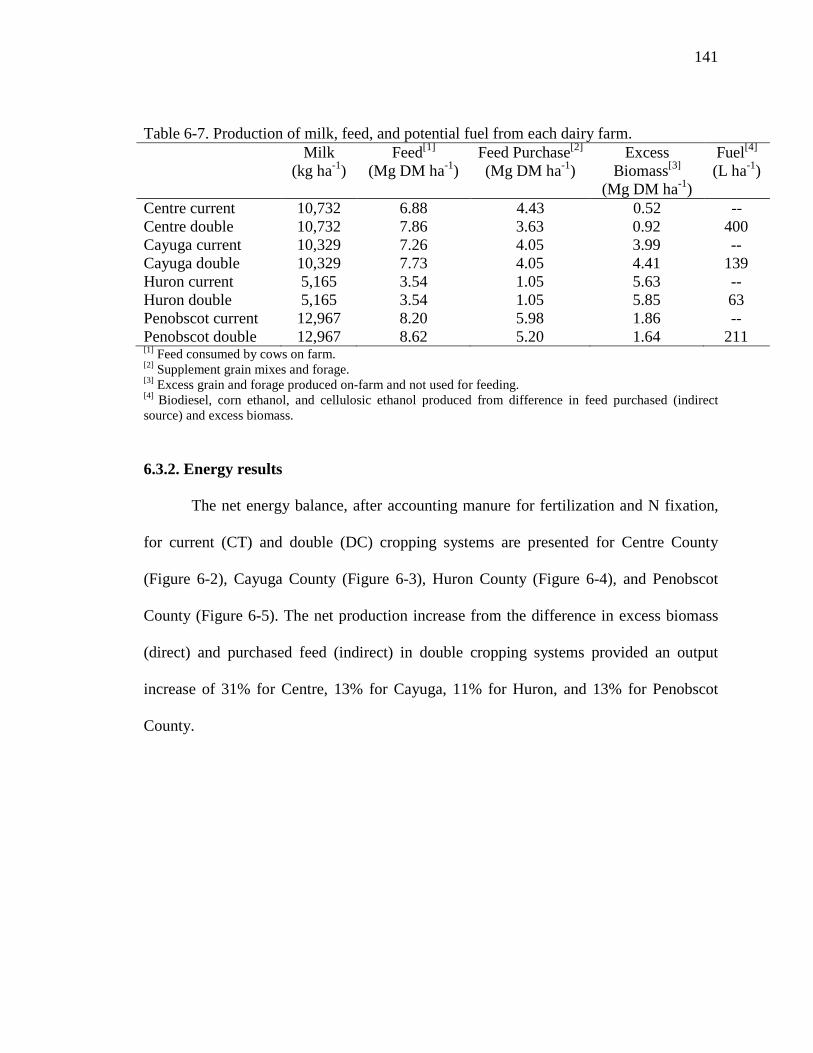
141

Table 6-7. Production of milk, feed, and potential fuel from each dairy farm. Milk

(kg ha-1) Feed[1]

(Mg DM ha-1) Feed Purchase[2] (Mg DM ha-1)

Excess Biomass[3]

(Mg DM ha-1)

Fuel[4] (L ha-1)

Centre current 10,732 6.88 4.43 0.52 -- Centre double 10,732 7.86 3.63 0.92 400 Cayuga current 10,329 7.26 4.05 3.99 -- Cayuga double 10,329 7.73 4.05 4.41 139 Huron current 5,165 3.54 1.05 5.63 -- Huron double 5,165 3.54 1.05 5.85 63 Penobscot current 12,967 8.20 5.98 1.86 -- Penobscot double 12,967 8.62 5.20 1.64 211 [1] Feed consumed by cows on farm. [2] Supplement grain mixes and forage. [3] Excess grain and forage produced on-farm and not used for feeding. [4] Biodiesel, corn ethanol, and cellulosic ethanol produced from difference in feed purchased (indirect source) and excess biomass.

6.3.2. Energy results

The net energy balance, after accounting manure for fertilization and N fixation,

for current (CT) and double (DC) cropping systems are presented for Centre County

(Figure 6-2), Cayuga County (Figure 6-3), Huron County (Figure 6-4), and Penobscot

County (Figure 6-5). The net production increase from the difference in excess biomass

(direct) and purchased feed (indirect) in double cropping systems provided an output

increase of 31% for Centre, 13% for Cayuga, 11% for Huron, and 13% for Penobscot

County.

142

Figure 6-2. Centre County Pennsylvania energy balance per year.

Figure 6-3. Cayuga County New York energy balance per year.

-40,000

-30,000

-20,000

-10,000

0

10,000

20,000

30,000

Input CT Output CT Input DC Output DC

Ene

rgy

(MJ

ha-1

yr-1

)Biodiesel

Ethanol

Milk


Drying

Electricity

On Farm fuel use

Insecticide

Herbicide

Seed

Lime

K

P

N

-40,000

-30,000

-20,000

-10,000

0

10,000

20,000

30,000


Ene

rgy

(MJ

ha-1

yr-1

)

Ethanol

Milk


Drying

Electricity

On Farm fuel use

Insecticide

Herbicide

Seed

Lime

K

P

N

143

Figure 6-4. Huron County Michigan energy balance per year.

Figure 6-5. Penobscot County Maine energy balance per year.

-20,000

-15,000

-10,000

-5,000

0

5,000

10,000

15,000

20,000


Ene

rgy

(MJ

ha-1

yr-1

)Ethanol

Milk


Drying

Electricity

On Farm fuel use

Insecticide

Herbicide

Seed

Lime

K

P

N

-50,000

-40,000

-30,000

-20,000

-10,000

0

10,000

20,000

30,000


Ene

rgy

(MJ

ha-1

yr-1

)

Ethanol

Milk


Drying

Electricity

On Farm fuel use

Insecticide

Herbicide

Seed

Lime

K

P

N

144

6.3.3. Greenhouse gas emissions

Net greenhouse gas (GHG) emissions were calculated based on farmland

emissions, net crop assimilation, and dairy production emissions from animal housing

and manure (Table 6-8). Each county had higher farmland GHG emissions from the

double cropping systems than current cropping systems. Net crop assimilation in double

cropping systems was also higher than current cropping systems. The overall net

emission from double cropping systems was 17% lower in Centre County (Figure 6-6),

19% lower in Cayuga County (Figure 6-7), 213% lower in Huron County (Figure 6-8),

and 3% higher in Penobscot County (Figure 6-9).

Table 6-8. Annual greenhouse gas balances for the selected counties for current and double / cover cropping systems. Emissions Centre, PA Cayuga, NY Huron, MI Penobscot, ME (g CO2e m-2 yr-1) CT[2] DC[2] CT DC CT DC CT DC Farmland 11.8 15.1 14.1 18.7 11.3 12.4 14.8 19.2 Net crop assimilation

-120.9

-142.1

-182.9

-195.2

-147.4

-184.7

-164.3

-165.8

Dairy production[1]

216.4

216.4

208.3

208.3

104.2

104.2

261.5

261.5

Net production

107.4

89.5

39.5

31.8

-31.9

-68.1

112.0

114.9

[1] Includes livestock emissions (CO2, CH4, and N2O) from housing and manure. [2] Current (CT) and double (DC) cropping systems.

145

Figure 6-6. Centre County Pennsylvania greenhouse gas (GHG) emissions balance per

year.

Figure 6-7. Cayuga County New York greenhouse gas (GHG) emissions balance per

year.

-200

-150

-100

-50

0

50

100

150

200

250G

HG

(g C

O2e

m-2

yr-1

)NetMaure N2OManure soil CO2Manure storageLivestock housingCrop assimiliationDryingTransport. InputsElectricityOn Farm fuel useInsecticideHerbicideSeedLimeKPN

-250

-200

-150

-100

-50

0

50

100

150

200

250

GH

G (g

CO

2e m

-2yr

-1)

NetMaure N2OManure soil CO2Manure storageLivestock housingCrop assimiliationDryingTransport. InputsElectricityOn Farm fuel useInsecticideHerbicideSeedLimeKPN

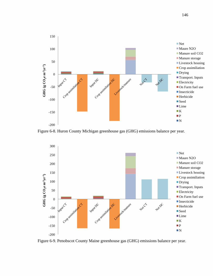
146

Figure 6-8. Huron County Michigan greenhouse gas (GHG) emissions balance per year.

Figure 6-9. Penobscot County Maine greenhouse gas (GHG) emissions balance per year.

-200

-150

-100

-50

0

50

100

150

GH

G (g

CO

2e m

-2yr

-1)


-200

-150

-100

-50

0

50

100

150

200

250

300

GH

G (g

CO

2e m

-2yr

-1)


147

The distribution of net crop assimilation for each crop in these different farming

scenarios is shown in Figure 6-10. Cropping systems had a different crop assimilation

distribution for each county because of different county yields.

Figure 6-10. Crop greenhouse gas (GHG) assimilation for current (CT) and double (DC)

cropping system for each county per year. 6.4. Conclusions

Double cropping systems were estimated to produce more dairy livestock feed

than current cropping systems for all counties evaluated. This higher production gave

overall better results for energy and greenhouse gas emissions.

In conclusion, there are opportunities to implement double cropping systems in

Pennsylvania, New York, Michigan, and Maine to improve land sustainability by

reducing energy inputs and net GHG emissions. However, double cropping systems

0

50

100

150

200

250

GH

G (g

CO

2e m

-2yr

-1)

RyeSoybeanAlfalfaCorn silageCorn grain

148

should be implemented when increased overall outputs surpass the higher costs of

execution. In addition, experimental data is required to validate the modeling results.

149

Chapter 7

Conclusions

7.1. Summary

The overall objective of this research was to evaluate cropping and dairy systems

in terms of energy use and greenhouse gas (GHG) emissions. To accomplish this

objective in an efficient and accurate manner, the Farm Energy Analysis Tool (FEAT)

was developed. This spreadsheet tool is database driven, and is based on leading whole-

farm agroecosystem models and a thorough literature review. The FEAT was then used

to evaluate cropping systems used for livestock feed production, biomass heating

purposes, and biofuel production. The FEAT was also used to compare different dairy

farm scenarios for typical farms located in Pennsylvania, New York, Michigan, and

Maine. Double cropping strategies were shown to improve some aspects of farm

sustainability through on-farm fuel production with the use of oil seed crops, manure

nutrient recycling, and dedicated energy crops.

The FEAT successfully created useful energy and greenhouse gas balances for the

various scenarios. The FEAT was able to identify and scrutinize critical points of energy

consumption and production, and also of GHG emission and assimilation. This allowed

for a more thorough evaluation of the impact of the strategies used in the study.

Double cropping systems evaluated in this project were successful at improving

energy efficiency and reducing net greenhouse gas emission. Double cropping systems

also allowed dairy operations to maintain milk production, and provided excess biomass

150

for additional livestock or biofuel production. Very promising upcoming technologies

such as cellulosic ethanol (Lynd, 1996) would allow farmers to implement more

productive double cropping systems to employ the excess biomass produced.

Analyses performed in FEAT provided an estimate of the percentage of fertilizer

requirements that were provided by manure recycling. Furthermore, adding oil seed crops

such as canola to crop rotations created the potential for fuel self-sufficiency in dairy

operations.

7.2. Scope and limitations

Applications of the FEAT are restricted to energy and greenhouse gas emissions.

While the FEAT focuses on farm-level evaluations, it also accounts for agricultural

inputs to the farm, and if desired also for biofuel feedstock transportation and processing.

The FEAT is a static data-base model and does not account for farm-scale changes,

ecosystem benefits of different crop rotations, and economics.

7.3. Potential improvements and future work

The FEAT could be improved by adding additional features including 1)

economic analysis; 2) new crops; 3) new livestock operations; 4) soil carbon GHG

sequestration, and 5) anaerobic digestion. Including an economic analysis within the

FEAT would be very useful for evaluating the profitability of different cropping systems.

New crops and different livestock operations would increase the applicability of the

FEAT. Soil carbon sequestration is an important parameter that is affected by tillage

151

practices and crop residue management. Accounting for manure anaerobic digestion

could improve energy efficiency of farm systems.

Alternatively, the FEAT could be combined or incorporated in with other farm

decision tools such as I-FARM (van Ouwerkerk et al. 2009) to explore a broader range,

including economic impacts, soil erosion, and labor availability. Furthermore, results

from this research could be compared with results from the Integrated Farm System

Model (IFSM) (Rotz et al. 2009), a whole-farm process model, which can address

additional farming system complexities such as soil type and weather variation. In

conclusion, the FEAT is a useful contribution to the whole farm analytical evaluation of

energy and greenhouse gas emissions.

152

References

Aakre, P. 2009. Farm scale biodiesel / SVO research. University of Minnesota. Online presentation. Available at: http://www.cleanenergyresourceteams.org/files/CERTs_presntations_NWCERT_CampusForum_Aakre_Biodiesel.pdf. Accessed 7 May 2009.

Acharya, V., and B.R. Young. 2008. A review of the potential of bio-ethanol in New Zealand. Bulletin of science technology society 28:143-149.

Adler, P.R., M.A. Sanderson, A.A. Boateng, P.J. Weimer, and H.G. Jung. 2006. Biomass yield and biofuel quality of switchgrass harvested in fall or spring. Agron.J. 98. pp. 1518-1525.

Adler, P.R., S.J. Del Grosso, and W.J Parton. 2007. Life-cycle assessment of net greenhouse-gas flux for bioenergy cropping systems. Ecological applications 17(3): 675-691.

Ahmed, I., J. Deeker, and D. Morris. 1994. How much energy does it take to make a gallon of soydiesel. Institute for local self-reliance. Minneapolis, Minnesota,USA.

Anex, R. P., L.R. Lynd, M.S. Laser, A.H. Heggenstaller and M. Liebman. 2007. Potential for enhanced nutrient cycling through coupling of agricultural and bioenergy systems. Crop Sci. 47:1327-1335.

ASAE. 2005. Manure Production and characteristics. Standard D384.2. American Society of Agricultural Engineers.

Auri Fuels Initiative.2009. Agricultural Renewable Solid Fuels Data. Available at: http://www.auri.org/research/fuels/pdfs/fuels.pdf. Accessed 7 May 2009.

Ayres, G.E. 2000. Fuel required for field operations. Iowa State University Extension. Available at http://www.extension.iastate.edu/Publications/PM709.pdf accessed 29 May 2009.

Bertilsson, G. 1992. Environmental consequences of different farming systems using good agriculture practices. Proceedings no. 332. The Fertilizer Society, Peterborough, 1992.

Beuerlein, J. 2008. Bushels, test weights and calculations. Ohio State University fact sheet. Available at: http://ohioline.osu.edu/agf-fact/0503.html. Accessed 25 August 2008.

Blasing, T.J., C.T. Broniak, and G. Marland, 2004. Estimates of monthly carbon dioxide emissions and associated δ13C values from fossil-fuel consumption in the U.S.A. In Trends: A Compendium of Data on Global Change, Carbon Dioxide Information Analysis Center, Oak Ridge National Laboratory, U.S. Department of Energy, Oak Ridge, TN, U.S.A.

Boehmel, C., I. Lewandowski, and W. Claupein. 2008. Comparing annual and perennial energy cropping systems with different management intensities. Agricultural Systems 96:224-236.

Borin, M., C. Menini, and L. Sartori. 1996. Effects of tillage systems on energy and carbon balance in northeastern Italy. Soil & Tillage research 40:209 – 226.

Borjesson, P.I.I. 1996. Energy analysis of biomass production and transportation. Biomass and Bioenergy 11(4): 305 – 318.

Borton, L.R., C.A. Rotz, J.R. Black, M.S. Allen, and J.W. Lloyd. 1997. Alfalfa and corn silage systems compared on Michigan dairy farms. J Dairy Sci 80:1813-1826.

Bowers, C.G. 1989. Tillage draft and energy measurements for twelve southeastern soil series. Trans ASAE 32:1492-502.

Boyles, M. 2009. Canola Project Specialist. Oklahoma State University. Available at: http://www.canola.okstate.edu/commonquestions/index.htm. Accessed 7 May 2009.

Brown, B.D. 2006. Winter cereal-corn double crop forage production and phosphorus removal. Soil Science society of America Journal 70:1951-1956.

Breimyer, H.F. 1975. The food-energy balance. Agricultural Economics, Department of Agricultural Economics, University of Missouri, paper 50 pp.9, prepared for delivery at Symp. On Population and Food, December. Rome.

Brown, R.C. 2003. Biorenewable resources: engineering new products from agriculture. Blackwell publishing company.

153

Bullard, M., and P. Metcalfe. 2001. Estimating the energy requirements and CO2 emissions from production of the perennial grasses miscanthus, switchgrass and reed canary grass. Report ETSU, Energy technology support unit, Harwell, United Kingdom.

Canada Council. 2008. Canadian canola yield. Field crop reporting series - statistics Canada. Available at: http://www.canola-council.org/acreageyields.aspx. Accessed 7 May 2009.

Carolan, J.E., S.V. Joshi and B.E. Dale. 2007. Technical and financial feasibility analysis of distributed bioprocessing using regional biomass pre-processing centers. Journal of agricultural and food industrial organization 5(2):1-27.

Cattanach, A., W.C. Dahnke, and C. Fanning. 1993. Fertilizing sugar beet. North Dakota State University. Available at: http://www.ag.ndsu.edu/pubs/plantsci/soilfert/sf714w.htm. Accessed at 7 May 2009.

Cauffman, G. 2008. Tractors without tankers. Presentation at Energy on the Farm: how to reduce costs and generate revenue. Penn State and the Lancaster center. Available at: http://www.keeplancastercountyfarming.com/images/stories/docs/Lancaster-Energy-Farm-(Glen-Cauffman).ppt. Accessed 8 May 2009.

Chancellor, W.J. 1978. The role of fuel and electrical energy in increasing production from traditionally based agriculture. Trans. ASAE 21:1060 – 1067.

Chianese, D.S., C.A. Rotz, and T.L. Richard. 2009a. Simulation of carbon dioxide emissions from dairy farms to assess greenhouse gas reduction strategies. Trans. ASABE 52:1301-1312.

Chianese, D.S., C.A. Rotz, and T.L. Richard. 2009b. Simulation of methane emissions from dairy farms to assess greenhouse gas reduction strategies. Trans. ASABE 52:1313-1323.

Chianese, D.S., C.A. Rotz, and T.L. Richard. 2009c. Simulation of nitrous oxide emissions from dairy farms to assess greenhouse gas reduction strategies. Trans. ASABE 52:1325-1335.

Chianese, D.S., C.A. Rotz, and T.L. Richard. 2009d. Whole-farm greenhouse gas emissions: a review with application to a Pennsylvania dairy farm. Applied Engineering in Agriculture 25: 431-442.

Christian, D.G., P.R. Poulton, A.B. Riche, and N.E. Yates. 1997. The recovery of 15N-labelled fertilizer applied to miscanthus x giganteus. Biomass and Bioenergy 12: 21-24.

Clark, A. 2007. Managing cover crops profitably. Sustainable Agriculture Network. Available at: http://www.sare.org/publications/covercrops/covercrops.pdf. Accessed 3 April 2009.

Clifton-Brown, J.C., I. Lewandowski, B. Andersson, G. Basch, D.G. Christian, J.B. Kjeldsen, U. Jorgensen, J.V. Mortensen, A.B. Riche, K. Schwarz, K. Tayebi, and F. Teixeira. 2001. Performance of 15 Miscanthus genotypes at five sites in Europe. Agron. J. 93:1013-1019.

Collura, S., B. Azambre, G. Finqueneisel, T. Zimny, and J.V. Weber. 2006. Miscanthus x giganteus straw and pellets as sustainable fuels, combustion and emission tests. Environ. Chem. Lett. 4: 75-78.

Collins, N.E., L.J. Kemble and T.H. Williams. 1977. Energy requirements for tillage on coastal plains soils. In: Agriculture and energy. Lockeretz, W. pp.233-43.

Coxworth, E., G. Hultgreen, and P. Leduc. 1994. Net carbon balance effects of low disturbance seeding systems on fuel, fertilizers, herbicides and machinery usage in western Canadian agriculture. Report for TransAlta Utilities Corp., Calgary Canada.

Daalgaard, T. 2001. A model for fossil energy use in Danish agriculture used to compare organic and conventional farming. Agriculture, Ecosystems and Environment 87:51-65.

Dale, B.E., C.K. Leong, T.K. Pham, V.M. Esquivel, I. Rios, and V.M. Latimer. 1996. Hydrolysis of lignocellulosics at low enzyme levels: applications of the AFEX process. Bioresource technology 56:111-116.

Danalatos, N.G., S.V. Archontoulis, and I. Mitsios. 2006. Potential growth and biomass productivity of Miscanthus x giganteus as affected by plant density and N-fertilization in central Greece. Biomass and bioenergy 31:145-152.

Del Grosso, S.J., A.R. Mosier, W.J. Parton, and D.S. Ojima. 2005. DAYCENT model analysis of past and contemporary soil N2O and net greenhouse gas flux for major crops in the USA. Soil Tillage Research 83:9-24.

Dent, J.B., and P.K. Thorton. 1987. The role of biological simulation models in farming systems research. Agric. Admin. and Extension 29:111-122.

Downs, H.W. 2007. Estimating Farm fuel requirements. Colorado State. Available at: http://www.ext2.colostate.edu/PUBS/FARMMGT/05006.html. Accessed 20 August 2009.

154

Duiker, S.W., and W.S. Curran. 2005. Rye cover crop management for corn production in the northern mid-atlantic region. Agron. J. 97:1413-1418.

EIA. 1999. Annual energy outlook 2000, Apendendix H, DOE/EIA-0383 p.243. U.S. Department of Energy, Energy Information Administration, Washington, DC.

EIA. 2007. Voluntary reporting of greenhouse gases program: fuel and energy sources codes and emission coefficients. Washington, D.C.: Energy Information Administration. Available at: http://www.eia.doe.gov/oiaf/1605/coefficients.html. Accessed at 23 February 2009.

Elsayed, M.A., N.D. Mortimer and R. Matthews. 2003. Carbon and energy balances for a range of biofuels options. Interin report. Report no. 21. Resources Research Unit, Sheffield Hallan University, Sheffield, United Kingdon. Available at: http://www.berr.gov.uk/files/file14925.pdf. Accessed 8 January 2009.

Emberger, P., K. Thuneke, and T. Gassner. 2009. Operation characteristics of rapeseed oil fuelled tractors in practice. Landtechnik 64:37-39.

Erdal, G., K. Esengun, H. Erdal, and O. Gunduz. 2007. Energy use and economical analysis of sugar beet production in Tokat province of Turkey. Energy 32: 35-41.

FAO. 1999a. Food Balance Sheets. Food and Agriculture Organization. United Nations, Rome, Italy. FAO. 2002. Food energy - Methods of analysis and conversion factors. pp. 32. Food and Agriculture

Organization. United Nations, Rome, Italy. Available at: ftp://ftp.fao.org/docrep/fao/006/y5022e/y5022e00.pdf. Accessed 7 May 2009.

Fargione, J., J. Hill, D. Tillman, S. Polasky, and P. Hawthorne. 2008. Land clearing and the biofuel carbon debt. Science 319:1235-1238.

Farrell, A.E., R.J. Plevin, B.T. Tuner, A.D. Jones, M. O’Hare, and D.M. Kamen. 2006. Ethanol can contribute to energy and environmental goals. Science 301: 506 – 508.

Flessa, H., R. Ruser, P. Dörsch, T. Kamp, M.A. Jimenez, J.C. Munch, and F. Beese. 2002. Integrated evaluation of greenhouse gas emissions (CO2, CH4, N2O) from two farming systems in southern Germany. Agr. Ecosyst. Environ. 91: 175-189.

Flores, R.A., R.B. Hicks, D.W. Eustace, and J. Philips. 2005. High-starch and high-β-glucan barley fractions milled with experimental mills. Cereal Chemistry vol. 82 n.6 pp. 727-733.

Fluck, R.C., and C.D. Baird. 1980. Agricultural energetics. AVI Publishing Company, inc. Westport, Connecticut.

Friedrich, A., F. Glante, C. Schliiter, C. Golz, I. Noh, G. A. Reinhardt, U. Hopfner, U. Sartorius, R. Benndorf, H. Blumel, B. Scharer, and S. Rodt. 1993. Okologische Bilanz von Rapsol bzw. Rapsolmethylester als Ersatz von Dieselkraftstoff (Okobilanz Rapsol). Unweltbundesamt, Berlin, Germany.

Frier, M.C., and G.W. Roth. 2009. Canola or rapeseed production in Pennsylvania. Department of crop and soil sciences, Penn State University. Available at http://downloads.cas.psu.edu/RenewableEnergy/CanolaProduction.pdf. Accessed 13 June 2009.

Frischknecht, R., and N. Jungbluth.2007. Ecoinvent report number 1. Overview and methodology. Available at http://www.ecoinvent.org/fileadmin/documents/en/01_OverviewAndMethodology.pdf. Accessed 1 June 2009.

Frye, W.W., and S.H. Phillips. 1981. How to grow crops with less energy. In: Cutting energy costs. Hayes, J. (ed.). USDA Washington, DC.

Gibson, L., and S. Barnhart. 2007. Miscanthus hybrids for biomass production. Department of agronomy. Iowa State University. Available at: http://www.extension.iastate.edu/Publications/AG201.pdf. Accessed at 7 May 2009.

Gifford, R.M. 1984. Energy in different agricultural systems: renewable and non-renewable sources. In: Stanhill, G. ed. pp.84-112. Energy and agriculture. Berlin: Springer-Verlag.

Gopalakrishnan, C. 1994. Economics of energy in agriculture. Avebury publishing limited. Gover, M.P., S.A. Collings, G.S. Hitchcock, D.P. Moon and G.T. Wilkins. 1996. Alternative Road

Transport Fuels – A preliminary Life Cycle Study for the UK. Vol. 2. ETSU, London, HMSO. Graboski, M.S. 2002. Fossil energy use in the manufacture of corn ethanol. National Corn Growers

Association.Washington, DC. Available at:

155

http://www.oregon.gov/ENERGY/RENEW/Biomass/docs/FORUM/FossilEnergyUse.pdf. Accessed 7 May 2009.

Grant, D.R., R.C. Eager, J.M. Pepper. 1983. Factors affecting the desolvention of canola meal. JAOCS 60:1867-1875).

Griffith, D.R., J.V. Mannering and C.B. Richey. 1977. Energy requirements and areas of adaptation for eight tillage-planting systems for corn. In: Agriculture and Energy. Lockeretz,W. pp.261 – 76. Academic Press.

Haciseferofullari, H., M. Acaroglu, and I. Gezer. 2003. Determination of the energy balance of the sugar beet plant. Energy sources 25: 15 – 22.

Hall, R.G. 2009.Grain moisture conversion to standard weights. South Dakota State University. Available at: http://plantsci.sdstate.edu/rowcrops/files/Grain%20moisture%20conversions%20to%20standard%20weights.pdf. Accessed 23 February 2009.

Hansen, D.J. 2006. Manure as a nutrient source. In: The mid-atlantic nutrient management handbook. Haering, K.C. and G.K. Evanylo eds. Available at: http://www.mawaterquality.org/Publications/manmh/MANMH_complete.pdf. Accessed 7 May 2009.

Harland, J.I., C.K. Jones, and C. Hufford. 2006. Co-products. In: Sugar beet, 443-463, Draycott, A.P.,ed. World agriculture series. Blackwell publishing.

Harris, B., and P. Barry. 2004. The effects of seed treatment and seedling rate on the yield and quality of sugar beet. DAF, Backweston, Leixlip, Co, Kildare and University College Dublin, Lyons, New Castle, Co Dublin. Available at: http://www.agresearchforum.com/publicationsarf/2004/page060.pdf. Accessed 7 May 2009.

Heaton, E.A., J. Clifton-Brown, T.B. Voigt, M.B. Jones, and S.P. Long. 2004. Miscanthus for renewable energy generation: European union experience and projections for Illinois. Mitigation and Adaptation Strategies for Global Change 9:433-451.

Heggenstaller, A.H., R.P. Anex, M. Liebman, D.N. Sundberg, and L.R. Gibson. 2008. Productivity and nutrient dynamics in bioenergy double-cropping systems. Agronomy Journal 100:1740 - 1748.

Heinz, A., M. Kaltschmitt, R. Stülpnagee, and K. Scheffer. 2001. Comparison of moist vs. air-dry biomass provision chains for energy generation from annual crops. Biomass and Bioenergy 20:197-215.

Heller, M.C., G.A. Keoleian, M.K. Mann, and T.A. Volk. 2004. Life cycle energy and environmental benefits of generating electricity from willow biomass. Renewable Energy 29:1023 - 1042.

Helsel, Z., and T. Oguntunde. 1981. Fuel requirements for field operations. Energy facts Cooperative Extension Service Michigan State University.

Hensen, A., T.T. Groot, W.C.M. van den Bulk, A.T. Vermeulen, J.E. Olesen, and K. Schelde. 2005. Dairy farm CH4 and N2O emissions, from one square metre to the full farm scale. Agriculture, Ecosystems and Environment 112:146-152.

Hill, J., E. Nelson, D. Tillman, S. Polasky, and D. Tiffany.2006. Environmental, economic, and energetic costs and benefits of biodiesel and ethanol biofuels. PNAS vol. 103 pp. 11206-11210.

Hill, K.M., and F.J. Walford. 1975. Energy analysis of a power generating system. Energy Policy 3:306-317.

Icoz,E., K.M. Tugrul, A. Saral, and E. Icoz. 2009. Research on ethanol production and use from sugar beet in Turkey. Biomass and Bioenergy 33(1):1-7.

IFIAS. 1975. Workshop on energy analysis and economics. International Federation of Institutes for Advanced Studies. Report. no. 9, Stockholm.

IPCC. 2007. Climate change 2007: The physical science basis. Contribution of working group I to the fourth assessment report of the Intergovernmental panel on climate change. Chapter 2, Changes in atmospheric constituents and in radiative forcing. Available at: http://www.ipcc.ch/pdf/assessment-report/ar4/wg1/ar4-wg1-chapter2.pdf. Accessed 8 May 2009.

Ishler, V., and T. Beck. 1999. Dairy farm feed cost control. Penn State University College of Agricultural Sciences. Available at http://pubs.cas.psu.edu/FreePubs/pdfs/ud008.pdf. Accessed 15 June 2009.

Jones, M.B., and M.Walsh. 2001. Miscanthus for energy and fibre. Earthscan, 208pp. ISBN 1-902916-07-7.

http://www.ipcc.ch/pdf/assessment-report/ar4/wg1/ar4-wg1-chapter2.pdf�

156

Jensen, R.G. 1995. Handbook of milk composition. Academic Press, San Diego, California, 919 pages. ISBN: 0123844304.

Kaltschmitt, M., and G.A. Reinhardt. 1997. "Nachwachsende energietrager - Grudlagen, verfaben, okologische bilanzierung". (Renewable energy sources, basis, processes and ecological balance). Vieweg, Branschweig/Weisbaden, Germany.

Karpenstein-Machan, M. 2001. Sustainable cultivation concepts for domestic energy production from biomass. Critical reviews in plant sciences 20:1-14.

Kaspar, T.C., and J.W. Singer. 2007. Rye cover crops in a corn silage - soybean rotation. ASA-CSSA-SSSA Annual meeting abstracts, Nov. 4-8, 2007, New Orleans, LA.

Kim, S., and B.E. Dale. 2005a. Environmental aspects of ethanol derived from no-tilled corn grain: nonrenewable energy consumption and greenhouse gas emissions. Biomass and Bioenergy 28:475-489.

Kim, S., and B.E. Dale. 2005b. Life cycle assessment of various cropping systems utilized for producing biofuels: Bioethanol and biodiesel. Biomass and Bioenergy 29:426-439.

Kim, S., and B.E. Dale. 2008. Life cycle assessment of fuel ethanol derived from corn grain via dry milling. Bioresource Technology 99: 5250 – 5260.

Kim, S., B. Dale, and R. Jenkins. 2009. Life cycle assessment of corn grain and corn stover in the United States. Int. J. Life Cycle Assess. 14:160 - 174. doi 10.1007/s11367-008-0054-4.

Kim, T.A., F. Taylor, and K.B. Hicks. 2008. Bioethanol production from barley hull using SAA (soaking in aqueous ammonia) pretreatment. Bioresource technology 99(13):5694-5702.

Koller, K. 1996. Production de cereals sous labor. Rev. Suisse Agric. 28:30. Kongshaug, G. 1998. Energy Consumption and Greenhouse Gas Emissions in Fertilizer Production. IFA

Technical Conference, Marrakech, Morocco, 28 September-1 October, 1998. Kumhala, F., V. Prosek, M. Kroulik, and Z. Kviz. 2008. Parallel plate mass flow sensor for forage and

sugar beet. 200 ASABE Annual International meeting. Providence, Rhode Island. Lal, R. 2004. Carbon emissions from farm operations. Environmental International 30: 981 - 990. Lal, R. 2009. Sequestering atmospheric carbon dioxide. Critical Reviews in Plant Science 28:90-96. Lauer, J. G., G.W. Roth, and M.G. Bertram. 2004. Impact of defoliation on corn forage yield. Agronomy

Journal 96:1459 - 1463. Lazarus, W. 2007. Machinery cost estimates. University of Minnesota. Available at:

http://www.extension.umn.edu/distribution/businessmanagement/DF6696.pdf . Accessed 5 February 2009.

Leach, G. 1975. Energy and food production. Food Policy 1:62-73. Leonard, R.A., W.G. Knisel, and D.A. Still. 1987. GLEAMS: Grondwater Loading Effects of Agricultural

Management Systems. Trans. ASAE 30: 1403 – 1418. Leroudier, J.P. 2002. Perspectives for the development of bioethanol in the European Union.

Zuckerindustrie 127:614 - 616. Lewandowski, I., A. Kicherer, and P. Vonier. 1995. CO2 - Balance for the cultivation and combustion of

Miscanthus. Biomass and Bioenergy 8(2): 81-90. Lewandowski, I., J.C. Clifton-Brown, J.M.O. Scurlock, and W. Huisman. 2000. Miscanthus: European

experience with a novel energy crop. Biomass and Bioenergy 19:209-227. Lewandowski, I., and U. Schmid. 2006. Nitrogen energy and land use efficiencies of miscanthus, reed

canary grass and triticale as determined by the boundary line approach. Agriculture Ecosystem Environment 112:335-346.

Lewis, D.A. 1982. The role of energy in UK agriculture. In: Energy Management and Agriculture 43-65, D.W. Robinson, and R.C. Mollan eds. Proceedings 1st Summer School in Agriculture, Dublin, Ireland. Elsevier Science Publishers, Amsterdam.

Liebig, M.A., D.L. Tanaka, J.M. Krupinsky, S.D. Merril and J.D. Hanson. 2007. Dynamic Cropping Systems: Contributions to improve Agroecosystem Sustainability. Agron. J. 99: 899-903.

Liska, A.J., H.S. Yang, V.R. Bremer, T.J. Klopfenstein, D.T. Walters, G.E. Erickson, and K.G. Cassman. 2009. Improvements in life cycle energy efficiency and greenhouse gas emissions of corn-ethanol. Journal of Industrial Ecology 00(0): doi: 10.1111/j.1530-9290.2008.105.x.

Lobb, D. 1989. A study of the impact of no-till on tractor fuel cost vs. crop returns. Agricultural Energy Centre, Guelph, Ont., 19pp.

157

Lockeretz, W. 1981. Cropp residues for energy: comparative costs and benefits for the farmer, the energy facility, and the public. Energy in Agriculture 1 pp. 71-89. Elsevier Publishing Company, Amsterdam.

Lockeretz, W. 1983. Energy implications of conservation tillage. J. Soil Water Conserv.38:207-211. Ludington, D. and E.L. Johnson. 2003. Dairy farm energy audit summary. FlexTech Services. New York

State Energy Research and Development Authority. Albany, NY. http://www.nyserda.org/publications/dairyfarmenergysummary.pdf Accessed 17 August 2009.

Ludington, D.C., E.L. Johnson, J.A. Kowalski, and A.L. Mage. 2005. Dairy farm energy management guide California. Dltech, inc. Prepared for Southern California Edison. Available at: http://www.dairyfarmenergy.com/Chapter_PDFs/Introduction.pdf. Accessed 7 May 2009.

Lynd, L.R. 1996. Overview and evaluation of fuel ethanol from cellulosic biomass: technology, economics, the environment, and policy. Annual Rev. Energy Environ. 21:403-465. Lynd, L.R., M.S. Laser, B. Bransby, B.E. Dale, B. Davison, R. Hamilton, M. Himmel, M. Keller, J.D.

McMillan, J. Sheehan and C.E. Wyman. 2008. How biotech can transform biofuels. Nature Biotechnology 26:169-172.

Maddex,R.L. and F.W. Bakker-Arkema.1978. Reducing energy requirements for harvesting, drying and storing grain. Energy fact no.18, Extension Bull. E-1168, Mich. State Univ., East Lansing.

Madison, F., K. Kelling, J. Petersen, T. Daniel, G. Jackson, and L. Massie. 1986. Managing Manure and Waste: Guidelines for Applying Manure to Pasture and Cropland in Wisconsin. Report A3392. Madison: University of Wisconsin-Extension.

McLaughlin, N.B., C.F. Drury, W.D. Reynold, X.M. Yang, Y.X. Li, T.W. Welacky, and G. Steward. 2008. Energy inputs for conservation and conventional primary tillage implements in a clay loam soil. Trans. ASABE 51:1153-1163.

McLaughlin, S.B., R. Samson, D. Bransby, and A. Weislogel. 1996. Evaluating physical, chemical, and energetic properties of perennial grasses as biofuels. Proc. Bioenergy 96, Nashville, TN.

McLaughlin, S.B., and M.E. Walsh. 1998. Evaluating environmental consequences of producing herbaceous crops for bioenergy. Biomass and bioenergy 14:317-324.

McLaughlin, S.B., and Kszos, L.A. 2005. Development of switchgrass (Panicum virgatum) as a bioenergy feedstock in the United States. Biomass and bioenergy 28:515-535.

Mehdi, B., P. Duxbury, and R. Samson. 2000. Resource Efficiency Agricultural Production Canada. Development of Bioenergy Feedstocks: Agronomy Data from Eastern Canada. Final Report. Contract 23348-9-4068/001/SQ. REAP-Canada: Ste. Anne de Bellevue, QC.

Meiering,A.G., T.B. Daynard, R. Brown and L. Otten.1977. Drier performance and energy use in corn drying. Can.Agric.Eng. 19:49-54.

Milford, G.F.J. 2006. Plant structure and crop physiology. In: Sugar beet, Draycott, A.P., ed. World agricultural series. Blackwell publishing.

Monsanto. 2009. Roundup ready winter canola. Available at: http://www.monsanto.com/monsanto/ag_products/pdf/input_traits/winter_Canola.pdf. Accessed 7 May 2009.

Morey, R.V., H.A. Cloud and W.E. Leuschen. 1976. Practices for the efficient utilization of energy for drying corn. Trans. ASABE 19:151-155.

Morris, D. 2005. The carbohydrate economy, biofuels and the net energy debate. The Institute for local self-reliance.

Mortimer, N.D., P. Cormack, M.A. Elsayed, and R.E. Horne. 2002. Evaluation of the comparative energy, global warming and social costs and benefits of biodiesel. Resources research unit, Sheffield Hallan University, United Kingdom.

Mrini, M., F. Senhaji, and D. Pimentel. 2002. Energy analysis of sugar beet production under traditional and intensive farming systems and impacts on sustainable agriculture in Morocco. Journal of sustainable agriculture 20(4): 5 – 28.

Muller, R. E. 1992. Energy input-output simulations of crop production. In Energy in World Agriculture, Peart, R. M. and Brook, R. C., eds. vol. 5. Elsevier, Amsterdam, 1992.

NASS. 2009. National Agricultural Statistics Service. US Department of Agriculture, Washington, DC. Available at http://www.nass.usda.gov/. Accessed 25 June 2009.

158

NDSU Extension Service. 2009. Bushel weights and suggested seeding rates for various crops. North Dakota State University. Available at: http://www.ag.ndsu.edu/procrop/sds/susrvc04.htm . Accessed 5 January 2009.

Nearing, M.A., G.R. Foster, L.J. Lane, and S.C. Finkner. 1989. A processed-based soil erosion model for USDA soil erosion prediction project technology. Trans. ASAE 32:1587–1593.

Neitsch, S.L., J.G. Arnold, J.R. Kiniry, and J.R. Williams. 2001. Soil and Water Assessment Tool (SWAT) user’s manual version 2000. Grassland Soil and Water Research Laboratory. Temple,TX: ARS.

Nelson, R.G., C.M. Hellwinckel, C.C. Brandt, T.O. West, D.G. De La Torre Ugarte, and G. Marland. 2009. Energy use and carbon dioxide emissions from cropland production in the United States, 1990-2004. J. Environ. Qual. 38:418-425.

Nemecek, T., and S. Erzinger. 2003. Agricultural production systems. Ecoinvent. Available at: http://www.ecoinvent.org/fileadmin/documents/en/presentation_papers/agriculture_DF_eng.pdf. Accessed 25 November 2008.

Newkirk, R. 2009. Canola meal. Canadian International Grains Institute. Available at http://www.canola-council.org/uploads/feedguide/Canola_Guide_ENGLISH_2009_small.pdf. Accessed 13 June 2009.

Nielsen, R.L. 1995. Questions relative to harvesting & storing corn stover. Agronomy Extension publication AGRY - 95-09. Purdue University. Available at: http://www.agry.purdue.edu/ext/corn/pubs/agry9509.htm. Accessed 7 May 2009.

Nix, J. 1996. Farm Management Pocketbook. Wye College, University of London. NRC. 1989. Alternative Agriculture. National Research Council. Washington, D.C.:National Academy

Press. NRC. 2001. Nutrient requirements of dairy cattle. National research council (U.S.) - Committee on animal

nutrition. National academy of sciences. NRCS. 1998. Assessment of Water Holding Capacity of Soils. Natural Resources Conservation Service.

Available at http://soils.usda.gov/use/worldsoils/mapindex/whc.html. Accessed 18 September 2009.

de Oliveira, M. E. D., B. E. Vaughan, and E. J. Rykiel Jr. 2005. Ethanol as Fuel: Energy,Carbon Dioxide Balances, and Ecological Footprint. BioScience 55:593 – 602.

Oltenacu, P.A., and M.S. Allen. 1981. Resource-cultural energy requirements of the dairy production system. In Handbook of Energy Utilization in Agriculture, pp. 363-378 Pimentel, D., CRC Press, Inc., Boca Raton, Florida.

OMAFRA. 2002. Herbicide recommendation for sugar beets: postemergence broadleaf herbicide. Ontario Ministry of Agriculture Food and Rural affairs. Available at: http://www.omafra.gov.on.ca/english/crops/pub75/13sbepbh.htm. Accessed 7 May 2009.

ORNL. 2008. Bioenergy feedstock development. Oak Ridge National Laboratory. Available at: http://bioenergy.ornl.gov/papers/misc/energy_conv.html. Accessed 7 May 2009.

van Ouwerkerk, E.N.J., D.E. James, T.L. Richard, and M. Liebman 2003. A multi-model approach for sustainable agriculture in the US corn belt. ASAE Meeting presentation n. 033009, pp 13.

van Ouwerkerk, E.N.J. , R.P. Anex, and T.L. Richard. 2009. I-FARM integrated crop and livestock production and biomass planning tool. Available at: http://www.i-farmtools.org. Accessed 7 May 2009.

Pacala, S., and R. Socolow. 2004. Stabilization wedges: solving the climate problem for the next 50 years with current technologies. Science 305:968-972.

Painter, K. 2006. Economics of irrigated winter canola production. Biofuels summit. Washington State University. Available at: http://www.columbiabasin.edu/docs/ag_bs1_pdf_wsu-katepainter11-3new.pdf. Accessed 5 February 2009.

Patzek, T.W. 2004.Thermodynamics of the corn-ethanol biofuel cycle. Critical Reviews in Plant Sciences 23(6):519-567.

Paustian, K., J. Six, E. T. Elliot, and H.W. Hunt. 2000. Management options for reducing CO2 emissions from agricultural soils. Biogeochemistry 48:147-163.

Peterson, C. 2005. Potential production of biodiesel. In: The biodiesel handbook, 231-238. Knothe,G., J. Krahl, and J.van Gerpen, eds. Champaign, Ill.: AOCS Press. Available at: http://www.uiweb.uidaho.edu/bioenergy/BiodieselEd/publication/02.pdf. Accessed 7 May 2009.

159

Pimentel, D., L.E. Hurd, A.C. Bellotti, J. Forster, I.N. Oka, O.D. Sholes, and R.J. Whitman. 1973. Food production and the energy crisis. Science 182: 443-449.

Pimentel, D. 1980. Handbook of Energy Utilization in Agriculture. CRC Press. Boca Raton, FL. Pimentel, D. and T. W. Patzek. 2005. Ethanol Production Using Corn, Switchgrass, and Wood; Biodiesel

Production Using Soybean and Sunflower. Natural Resources Research 14 (1). Posselius, J.H. and B.A. Stout. 1982. Crop residue availability for fuel. In: Energy management and

agriculture, Robinson, D.W. and R.C. Mollan, eds. Proceedings of the first international summer school in agriculture held in co-operation with the W.K. Kellogg foundation.

Prabhu, A., C. Pham, A. Glabe, and J. Duffy. 2009. Detailed California-Modified GREET pathway for corn ethanol. California environmental protection agency. Air resources board. Available at: http://www.arb.ca.gov/fuels/lcfs/022709lcfs_cornetoh.pdf. Accessed 7 May 2009. (in press).

Pradhan, A., D.S. Shrestha, J. Van Gerpen, and J. Duffield. 2008. The energy balance of soybean oil biodiesel production: a review of past studies. Trans ASAE 51:185-194.

PSU Agronomy guide. 2008. College of Agricultural sciences. The Pennsylvania State University. Available at http://agguide.agronomy.psu.edu/. Accessed 5 March 2008.

Rankin, M. 2008. Determining the optimum alfalfa seeding rate . Focus on forage 10(5):1-2. College of Agricultural and Life Sciences, University of Wisconsin-Madison. Available at: http://www.uwex.edu/ces/crops/uwforage/AlfSeedingRate-FOF.pdf. Accessed 7 May 2009.

Renard, K.G., G.R. Foster, G.A. Wessies, and J.P. Porter. 1991. RUSLE: Revised Universal Soil Loss Equation. J. Soil and Water Conservation 46:30-33.

Reinhardt, G.A. 1992. Energie- und CO2-Bilanzierung nachwachsender Rohstoffe. Theoretische Grundlagen und Fallstudie Raps.

Richards, I.A. 2000. Energy balances in the growth of oilseed rape for biodiesel and wheat for bioethanol. British Association for Bio Fuels and Oils. Available at: http://bloomingfutures.com/uploads/Levington%20Agricultural%20Report%202000.pdf. Accessed at 23 February 2009.

Robertson, G.P., E.A. Paul, and R.R. Harwood. 2000. Greenhouse gases in intensive agriculture: Contributions of individual gases to the radiative forcing of the atmosphere. Science 289:1922-1925.

Rosa, F. 2007. IFECO - Modeling the agro-fuel chain for energy co-generation. Presentation for the 1st International European Forum on Innovation and System Dynamics in Food Networks. Available at http://ageconsearch.umn.edu/bitstream/6578/2/sp07ro01.pdf. Accessed 1 June 2009.

Roth, G. 2008. Assessment of Pennsylvania crops and biofuels. Penn State crop management extension group. Online presentation. Available at: http://www.extension.psu.edu/Powerpoints/Energy%20Inservice%20Roth%20Crops.1MB.ppt. Accessed 7 May 2009.

Rotz, C.A., G.W. Roth, K.J. Soder, and R.R. Schnabel. 2001a. Economic and environmental implications of soybean production and use on Pennsylvania dairy farms. Agronomy Journal 93:418-428.

Rotz, C.A., K.J. Soder, and G.W. Roth. 2001b. Environmental and economic impacts of a corn and rye double crop system on a Pennsylvania dairy farm. Proceedings/Reports American Forage and Grassland Council. Vol. 10. Springdale, Arkansas.

Rotz, C.A., G.W. Roth, and W.L. Stout. 2002. Economic and environmental implications of small grain production and use on Pennsylvania dairy farms. ASAE Meetings papers. Paper No. 021069. 11 pp.

Rotz, C.A., M.S. Corson, D.S. Chianese, and C.U. Coiner. 2009. Integrated Farm System Model, Reference Manual. Pasture Systems and Watershed Management Research Unit. Agricultural Research Service. Unite States Department of Agriculture. Available at: http://www.ars.usda.gov/SP2UserFiles/Place/19020000/ifsmreference.pdf. Accessed on 07 July 2009.

Hoskinson, R.L., D.L. Karlen, S.J. Birrel, C.W. Radtke, and W.W. Wilhelm. 2007. Engineering, nutrient removal, and feedstock conversion evaluations of four corn stover harvest scenarios. Biomass and Bioenergy 31:126-136.

Saha, B.C., L.B. Iten, M.A. Cotta and Y.V. Wu. 2005. Dilute acid pretreatment, enzymatic saccharification and fermentation of wheat straw to ethanol. Process Biochem. 40: 3693-3700.

160

Schrock, M.D., J.K. Kramer, S.J. Clark. 1985. Fuel requirements for field operations in Kansas. Trans. ASAE 28:669-874.

Searchinger, T., R. Heimlich, R.A. Houghton, F. Dong, A. Elobeid, J. Fabiosa, S. Tokgoz, D. Hayes, T. Yu. 2008. Use of U.S. for biofuels increases greenhouse gases through emissions from land use change. Science 319:1238-1240.

SETAC. 1993. Guidelines for life cycle assessment: A code of practice. Society of Environmental Toxicology and Chemistry, Brussels and Penscola.

Shapouri, H., J.A. Duffield, M. Wang. 2002. The energy balance of corn ethanol: an update. Washington, DC. Office of energy policy and new uses. Agricultural Economics report no. 814.

Shapouri, H., J. A. Duffield, and A. Mcaloon. 2004. The 2001 Net Energy Balance of Corn-Ethanol. Corn Utilization and Technology Conference. Indianapolis, June 7-9, 2004.

Sheehan J., V. Camobreco, J. Duffield, M. Graboski, H. Shapouri. 1998. Life cycle inventory of biodiesel and petroleum diesel for use in an urban bus. NREL/SR-580-24089. National Renewable Energy Laboratory. Colorado, United States.

Sheehan, J., A. Aden, C. Riley, K. Paustian, J. Brenner, D. Lightle, R. Nelson, M. Walsh, and J. Cushman. 2002. Is ethanol from corn stover sustainable? Adventures in cyber-farming: a life cycle assessment of the production of ethanol from corn stover for use in a flex fuel vehicle. Draft report for peer review. Colorado: National Renewable Energy Laboratory.

Sheehan, J., A. Aden, K. Paustian, K. Killian, J. Brenner, M. Walsh, and R. Nelson. 2004. Energy and environmental aspects of using corn stover for fuel ethanol. Journal of Industrial Ecology 7: 117 - 146.

Shelton, D.P., K. Von Burgen, A.S. Al-Jiburi.1980. Nebraska on-farm fuel use survey. Trans ASAE 23:1089-92. Shmer, M.R., K.P. Vogel, R.B. Mitchell, and R.K. Perrin. 2008. Net energy of cellulosic ethanol from

switchgrass. PNAS 105: 464-469. Six, J., S.M. Ogle, F.J. Breidt, R.T. Conant, A.R. Mosier, and K. Paustian. 2004. The potential to mitigate

global warming with no-tillage management is only realized when practiced in the long term. Global Change Biology 10:155-160.

Smith, D. 1965. Forage production of red clover and alfalfa under differential cutting. Agronomy Journal 57: 463 - 465.

Smith, E. G., H.H. Janzen, and N.K. Newlands. 2007. Energy balances of biodiesel production from soybean and canola in Canada. Canadian Journal of Plant Science 87(4):793-801.

Snapp, S.S., S.M. Swinton, R. Labarta, D. Mutch, J.R. Black, R. Leep, J. Nyiraneza, and K. O'Neil. 2005. Evaluating cover crops for benefits, costs, and performance within cropping system niches. Agronomy Journal 97:322 - 332.

Snyder, C.S., T.W. Bruulsema, and T.L. Jensen. 2007. Greenhouse gas emissions from cropping systems and the influence of fertilizer management – a literature review. International Plant Nutrition Institute. Norcross, Georgia, U.S.A.

Southwell, P.H., and T.M. Rothwell. 1977. Analysis of output / input energy ratios of food production in Ontario. School of Engineering, University of Guelph, Guelph, Ont.

Spatari, S., Y. Zhang , and H. L. Maclean . 2005. Life cycle assessment of switchgrass- and corn stover-derived ethanol-fueled automobiles. Environ. Sci. Technol. 39: 9750-9758.

Spedding, C.R.W. 1982. Energy use in livestock production. In: Energy management and agriculture. Robinson, D.W. and R.C. Mollan eds. pp. 337-349. Royal Dublin Society.

SSURGO. 2008. Natural Resources Conservation Service, United States Department of Agriculture. Soil Survey Geographic (SSURGO) Database for [Centre County, PA; Cayuga County, NY; Huron County, MI; Penobscot County, ME]. Available online at http://soildatamart.nrcs.usda.gov accessed 18 September 2009.

Stanhill, G. 1984. Introduction to the role of energy in agriculture. In: Energy and Agriculture, pp. 1-7, Stanhill, G. (ed.), Springer, Berlin.

Stout, B.A. 1984. Energy use and management in agriculture. Massachusetts: Breton. Stout, B. A. 1990. Handbook of Energy for World Agriculture.Elsevier science publishers ltd.

161

Stülpnagel, R., T. Behringer, W. Klose, F. Reufer, V. Stucke. 1992. Investigations for a cheap estimation of the net calorific values of different biomasses. Proceedings of the Seventh European Conference on Biomass for Energy and Industry, Florence, Italy. pp. 969-973.

Tanaka, D.L., J.F. Karn, M.A. Liebig, S.L. Kronberg, and J.D. Hanson.2006. An integrated approach to crop/livestock systems: Forage and grain production for swath grazing. Renew. Agric. Food Syst. 20: 223-231.

Teel, A., and S. Barnhart. 2003. Switchgrass seeding recommendation for the production of biomass fuel in southern Iowa. Iowa State University Extension. PM-1773. Available at: http://www.extension.iastate.edu/Publications/PM1773.pdf. Accessed 24 February 2009.

Tollenaar, M., M. Mihajlovic, and T.J. Vyn. 1992. Annual phytomass of a rye-corn double-cropping system in Ontario. Agonomy J. 84:963-967.

Uhlin, H. 1998. Why energy productivity is increasing: an I-O analysis of Swedish agriculture. Agric. Ecosyst. Environ. 56:443-465.

U.S. Census of Agriculture. 1997. U.S. Department of Agriculture, Washington, DC. Available at http://www.agcensus.usda.gov/. Accessed 25 June 2009.

U.S. Department of Energy. 2006. Theoretical ethanol yield calculator. Available at: http://www.eere.energy.gov/biomass/ethanol_yield_calculator.html. Accessed 7 May 2009.

U.S. EPA. 2002. A comprehensive analysis of biodiesel impacts on exhaust emissions. U.S. Environmental Protection Agency, EPA420-P-02-001.

U.S. Office of Technology Assessment. 1990. Energy use and the US Economy, OTA-BP-E-57. US Congress, Washington, DC.

Vaughan, D.H., E.S. Smith, and H.A. Hughes. 1977. Energy requirements of reduced tillage practices for corn and soybean production in virginia.In: Agriculture and energy. Lockeretz,W. (ed). Academic press. pp. 245-60.

Wallace, R., K. Ibsen, A. McAloon, and W. Yee. 2005. Feasibility study for co-locating and integrating ethanol production plants from corn starch and lignocellulosic feedstocks. TP-510-37092. National Renewable Energy Lab., Golden, CO.

Walsh, M.E., and D. Becker. 1996. Biocost: A Software program to estimate the cost of producing bioenergy crops. BIOENERGY ’96 -Proceedings of the Seventh National Bioenergy Conference:Partnerships to Develop and Apply Biomass Technologies.Nashville, TN. September 15-20, 1996.

Wang, M. Q. 2001. Development and use of GREET 1.6 fuel cycle model for transportation fuels and vehicle technologies. Technical Report ANL/ESD/TM-163. Argonne National Laboratory, Argonne, Illinois, USA. Available at: http://www.transportation.anl.gov/pdfs/TA/153.pdf. Accessed 7 May 2009.

Webb, M. and D. Pearce. 1975. The economics of energy analysis. Energy Policy 3: 318-331. West, T. O., and G. Marland. 2002. A synthesis of carbon sequestration, carbon emissions, and net carbon

flux in agriculture: comparing tillage practices in the United States. Agriculture, Ecosystems & Environment 91:217–232.

Williams, J.R., J.M. Shaffer, K.G. Renard, G.R. Foster, J.M. Laflen, L. Lyles, C.A. Onstad, A.N. Sharpley, A.D. Nicks, C.A. Jones, C.W. Richardson, P.T. Dyke, K.R. Cooley, and S.J. Smith. 1990. EPIC – Erosion / productivity impact calculator: 1. Model documentation. Technical Bulletin no. 1789. Washington, D.C.: USDA-ARS.

Windmann, B.2009. Work-Session on decentral vegetable oil production Weihenstephan. Available at: http://www.journeytoforever.org/biodiesel_svostd.html. Accessed 8 February 2009.

Zentner, R.P., and G.J. Sonntag. 1998. Alternative crop production systems: Economic and energy analysis component. CSAGPA Final Report, AAFC/SPARC, Swift Current.

Ziesemer, J. 2007. Energy use in organic systems. Natural resources management and environment department. Food and agriculture organization for the united nations (FAO).

Zhou, B., K.E. Ileleji, and G. Ejeta. 2008. Physical property relationships of bulk corn stover particles. Transactions of ASABE 51:581-590.

162

Appendix A : Fuel consumption for agricultural operations

163

Table A.1. Studies of moldboard plow fuel consumption (n=17). Measured value

(L ha-1) Range (L ha-1)

References

17.5 -- Shelton et al. (1980) -- 15 - 38 Lockeretz (1983)

18.9 -- Schrock et al. (1985) -- 15.1 - 25.1 Bowers (1989)

16.92* 32.7 - 8.4 Helsel and Oguntunde (1981) 49.4 -- Koller (1996) 15.90 -- Ayres (2000) 12.40 -- Lobb (1989) 21.80 -- West and Marland (2002) 20.05 -- Adler et al. (2007) 18.30 -- Collins et al. (1977) 26.86 -- Vaughan et al. (1977) 32.90 -- Griffith et al. (1977) 17.22 -- Frye and Phillips (1981) 24.00 -- Nix (1996) 21.60 -- McLaughlin et al. (2008) 15.70 -- Downs (2007)

* Average value. Table A.2. Studies of chisel plow fuel consumption (n=12).

Measured value (L ha-1)

Range (L ha-1)

References

9.3 -- Shelton et al. (1980) -- 10.3 - 16.9 Lockeretz (1983)


12.7* 7.5 - 32.7 Helsel and Oguntunde (1981) 31.3 -- Koller (1996) 10.3 -- Ayres (2000) 9.2 -- Lobb (1989) 13.5 -- Collins et al. (1977) 23.4 -- Griffith et al. (1977) 10.48 -- Frye and Phillips (1981) 13.9 -- McLaughlin et al. (2008)

* Average value.

164

Table A.3. Studies of offset disk fuel consumption (n=10). Measured value


References

7.9 -- Ayres (2000)

10.4* 8.4 - 11.2 Helsel and Oguntunde (1981) 8.9 -- Downs (2007) -- 7.2 - 11.7 Bowers (1989)

6.5 -- Lobb (1989) 6.7 -- West and Marland (2002) 5.48 -- Adler et al. (2007)

-- 6.74 - 7.7 Vaughan et al. (1977) 5.9 -- Frye and Phillips (1981) 11.8 7.3 – 11.8 McLaughlin et al. (2008)

*Average value. Table A.4. Studies of sub-soiling fuel consumption (n=2).


Range (L ha-1)

References

14.4* 10.3 - 21.5 Helsel and Oguntunde (1981) 15.9 -- Ayres (2000)

* Average value. Table A.5. Studies of disk fuel consumption (n=7).


Range (L ha-1)

References

7.4 -- Shelton et al. (1980) -- 4.7 - 7.5 Lockeretz (1983)


8.7* 2.9 - 30.9 Helsel and Oguntunde (1981) 28.4 -- Koller (1996) 5.1 -- Ayres (2000)

* Average value.

165

Table A.6. Studies of field cultivate fuel consumption (n=5). Measured value


References

-- 6.1 - 6.5 Ayres (2000)

7.3* 2.8 - 16.8 Helsel and Oguntunde (1981) 5.6 -- Downs (2007) 10.3 -- Vaughan et al. (1977) 3.93 -- Frye and Phillips (1981)

* Average value. Table A.7. Studies of pesticide application fuel consumption (n=7).


Range (L ha-1)

References

3.1* 0.9 – 27.1 Helsel and Oguntunde (1981) 1.2 -- West and Marland (2002) 0.9 -- Ayres (2000) 1.9 -- Lobb (1989) 1.12 -- Vaughan et al. (1977) 1.21 -- Frye and Phillips (1981) 2.2 -- Nix (1996)

* Average value. Table A.8. Studies of fertilizer application fuel consumption (n=5).


Range (L ha-1)

References

(L ha-1) 2.8* 0.9 - 4.7 Helsel and Oguntunde (1981) 9.8 -- West and Marland (2002) 1.6 -- Adler et al. (2007) 6.1 -- Downs (2007) 2.2 -- Nix (1996)

* Average value.

166

Table A.9. Studies of planter fuel consumption (n=8). Measured value


References

-- 3.7 - 5.1 Ayres (2000)

4.7 -- Downs (2007) -- 3.7 - 5.6 Lockeretz (1983)

4.9 -- West and Marland (2002) 4.64 -- Adler et al. (2007) 5.43 -- Vaughan et al. (1977) 4.02 -- Frye and Phillips (1981) 4.8* 1.9 - 9.4 Helsel and Oguntunde (1981)

* Average value. Table A.10. Studies of grain drill fuel consumption (n=6).


Range (L ha-1)

References

2.8 -- Ayres (2000) 3.3 -- Downs (2007) 3.7 -- Lockeretz (1983) 3.57 -- Adler et al. (2007) 10 -- Nix (1996)

5.2* 0.9 - 21.6 Helsel and Oguntunde (1981) * Average value. Table A.11. Studies of no-till planting fuel consumption (n=9).


Range (L ha-1)

References

13.4 -- Koller (1996) 4.2 -- Ayres (2000) 3.3 -- Downs (2007) -- 5.6 - 9.4 Lockeretz (1983)

11.25 -- Adler et al. (2007) 12.64 -- Collins et al. (1977) 5.9 -- Vaughan et al. (1977) 4.68 -- Frye and Phillips (1981) 6.4 -- Helsel and Oguntunde (1981)

167

Table A.12. Studies of cultivator fuel consumption (n=7). Measured value


References

(L ha-1) 3.6* 0.9 - 17.8 Helsel and Oguntunde (1981) 3.7 -- Ayres (2000) 4.2 -- Downs (2007)

2.8 - 5.6 -- Lockeretz (1983) 3.6 - 4 -- Lobb (1989)

3.3 -- West and Marland (2002) 5.12 -- Adler et al. (2007)

* Average value. Table A.13. Studies of rotary hoe fuel consumption (n=4).


Range (L ha-1)

References

2.2* 0.9 - 6.5 Helsel and Oguntunde (1981) 1.9 -- Ayres (2000) 2.3 -- Lockeretz (1983) 2.9 -- Lobb (1989)

* Average value. Table A.14. Studies of spring tooth fuel consumption (n=4).


Range (L ha-1)

References

6.8* 1.87 - 16.8 Helsel and Oguntunde (1981) 3.7 -- Downs (2007)

1.9 - 3.7 Lockeretz (1983)

5.43 -- Vaughan et al. (1977) * Average value. Table A.15. Studies of mower fuel consumption (n=3).


Range

References

2.8 -- Ayres (2000)

3.3 - 7.5 Downs (2007)

4.73 - 8.65 Adler et al. (2007)

168

Table A.16. Studies of mower conditioner fuel consumption (n=3). Measured value


References

6.7* 2.8 - 16.8 Helsel and Oguntunde (1981) 5.1 -- Ayres (2000) 5.6 -- Downs (2007)

* Average value. Table A.17. Studies of rake fuel consumption (n=4).


Range (L ha-1) References

4.3* 1.9 - 11.8 Helsel and Oguntunde (1981) 2.3 -- Downs (2007) 1.1 -- Adler et al. (2007) 1.4 -- Ayres (2000)

* Average value. Table A.18. Studies of baler fuel consumption (n=5).


Range (L ha-1)

References

6.0* 0.9 - 27.1 Helsel and Oguntunde (1981) 3.7 -- Ayres (2000) 4.2 -- Downs (2007) -- 3.05 - 11.58 Adler et al. (2007)

6.0 -- Nix (1996) * Average value. Table A.19. Studies of forage harvesting and green chop fuel consumption (n=4).


Range (L ha-1)

References

14.7* 1.8 - 18.7 Helsel and Oguntunde (1981) 7.9 -- Ayres (2000) 8.9 -- Downs (2007) -- 3.7 - 9.4 Lockeretz (1983)

* Average value.

169

Table A.20. Studies of corn silage harvesting fuel consumption (n=3). Measured value


References

25.4* 15.9 - 62.6 Helsel and Oguntunde (1981) 30.4 -- Ayres (2000) 33.7 -- Downs (2007)

* Average value. Table A.21. Studies of grain and row crop harvesting fuel consumption (n=5).


Range (L ha-1)

References

11.5 6.5 - 16.8 Helsel and Oguntunde (1981) 9.4 -- Ayres (2000) 15.5 -- Nix (1996) 10.3 -- Downs (2007) 31.3 -- Adler et al. (2007)

* Average value. Table A.22. Studies of corn combine fuel consumption (n=5).


Range (L ha-1)

References

14.1 6.5 - 20.6 Helsel and Oguntunde (1981) 13.6 -- Ayres (2000) 15.0 -- Downs (2007) 11.1 -- West and Marland (2002) 33.2 -- Adler et al. (2007)

* Average value.

170

Table A.23. Studies of miscellaneous operations fuel consumption. Miscellaneous operations

Measured value


References

Sweep plow 5.6 -- Downs (2007) Rotary till -- 16.7 - 38.4 Lockeretz (1983) Deep zone till 17 -- McLaughlin et al. (2008) Chisel sweep 18 -- McLaughlin et al. (2008) Shallow zone till 7 -- McLaughlin et al. (2008) Fluted coulter 4 -- McLaughlin et al. (2008) Broadcastseeder 1 1.4 -- Ayres (2000) Broadcastseeder 2* 2.6* 0.9 - 10.8 Helsel and Oguntunde (1981) Airdrill 6.5 -- Ayres (2000) Ridge plant 25.2 -- Koller (1996) No-till grain drill 8.53 -- Adler et al. (2007) Rolling Cultivator 3.3 -- Downs (2007) Seedbed conditioner 1 8.4 -- Ayres (2000) Seedbed conditioner 2 5.15 -- Adler et al. (2007) Spike tooth harrow 1 2.8 -- Downs (2007) Mulch treader 2.8 -- Downs (2007) Mulch tiller 8.5 -- Nix (1996) Rod weeder 2.8 -- Downs (2007) Haylage 1 10.8 -- Ayres (2000) Haylage 2 11.7 -- Downs (2007) Swather 5.1 -- Downs (2007) Swath 10 -- Nix (1996) shred stalks 6.7 -- Downs (2007) Stack wagon 4.7 -- Downs (2007) Corn picker 1 17.2* 11.2 - 28.1 Helsel and Oguntunde (1981) Corn picker 2 10.8 -- Downs (2007) Pull+ windrow beans 4.9* 2.8 - 10.3 Helsel and Oguntunde (1981) Beat harvester 12.8* 8.4 - 17.8 Helsel and Oguntunde (1981) Topping beets 7.8* 3.7 - 11.2 Helsel and Oguntunde (1981) Potato harvester 25.2* -- Helsel and Oguntunde (1981) forage blower 1 8.3* 3.4 - 23.5 Helsel and Oguntunde (1981) forage blower 2 -- 2.3 - 11.7 Ayres (2000) Irrigation 12.9* 4.2 - 16.7 Helsel and Oguntunde (1981) Grinding 14.5* 8.3 - 16.1 Helsel and Oguntunde (1981) hauling small grains 5.6 -- Downs (2007)

* Average value.

171

Appendix B: Crop bushel weight and moisture, fuel density and

unit conversions

172

Table B.1. Crop bushel weight and moisture content. Crop Bushel weight

(lbs bu-1) References[1] Bushel moisture

(%) References[1]

Corn 56 a 15.5 b Soybean 60 a 60 b Canola 50 a 50 c Barley 48 a 48 d [1]References: a. NDSU Extension Service (2009); b. Beuerlein (2008); c. Boyles (2009); d. Hall (2009). Table B.2. Fuel density. Fuel type Density

(kg L-1) References[1]

Diesel 0.84 a

Ethanol 0.79 b

Biodiesel 0.88 a

Straight vegetable oil 0.92 c [1]References: a. ORNL (2008); b. Wang (2001); c. Windmann (2009).

173

Table B.3. Conversions used in calculations. Conversion Value Reference[1]

Gallon per acre to liter per hectare 9.36 --

Mega-calories to mega-joules 4.19 --

Pounds per acre to kilogram per hectare 1.12 --

BTU per acre to Mega-joule per hectare 0.00261 --

BTU per gallon to Mega-joule per liter 0.000278 --

BTU per pound to Mega-joule per

kilogram

0.002326 --

Ton per acre to Mega-gram per hectare 2.24 --

Acre to hectare 0.4046863 --

Pounds to kilogram 0.4535924 --

Gallon to liter 3.785412 --

Ton to Mega-gram 0.9071847 --

CWT (hundred weight) to kilogram 45.35924 --

Mega-joule to kWh 0.2777778 --

Carbon to carbon dioxide 3.67 a [1]Reference: a. Blasing et al. (2004).

174

GUSTAVO CAMARGO 220 Homan Ave. State College, PA 16801 - [email protected]

EDUCATION

M.S., Agricultural and Biological Engineering, The Pennsylvania State University, December 2009. Thesis: Modeling Energy and Greenhouse Gas Emissions for Farm Scale Production.

B.S., Agricultural Engineering, State University of Campinas (UNICAMP), Brazil, December 2005.

PERSONAL Age: 27. Nationality: USA and Brazil.

WORK EXPERIENCE U.S. Department of Agriculture – Beltsville, MD

October – January 2010: Agricultural Research Science Technician. Evaluation of energy and greenhouse gas emissions of conventional and organic cropping systems.

Cutrale Citrus Juices – Auburndale, FL October – March 2007: Supervisor Orange Oil Production. Responsibilities: Plan, direct and coordinate activities of employees engaged in production. July – October 2006: Engineer of fresh orange juice production and storage.

RELEVANT COURSES

1st Brazil – U.S. Biofuels short course. Fulbright Commission. July 2009. Customer Relationship Management. July 2005.

COMPUTER SKILLS: AutoCAD, MS Office, MATLAB, Minitab. LANGUAGE SKILLS: English; Portuguese; Spanish (basic); German (pre-basic). OVERSEAS EXPERIENCE: France, Spain, Germany, Italy, Netherlands and Paraguay. PROFESSIONAL INVOLVEMENT / HONORS

• Reimagining agriculture to accommodate large scale energy production. • Fresh tomato and orange handling for classification, packing, and processing. • Second place on presentation entitled Modeling Sustainable Strategies for Farm Scale

Biomass Production. Penn State University Graduate Exhibition. Jan. 2009. • Second place on presentation entitled Integrating a Northeast livestock farm with the

emerging bioenergy industry. NABEC Conference. July 27-30, 2008. • Best paper presented at the Brazilian Agricultural Engineering Conference. July 2004.

HOBBIES: Soccer, swimming, guitar and world backpacking.

The Pennsylvania State University The Graduate School ... - ETDA

Documents

Transcript of The Pennsylvania State University The Graduate School ... - ETDA