The origins of olivine fabric transitions and their effects on seismic anisotropy in

the upper mantle

Dissertation Zur Erlangung des Grades eines

Doktors der Naturwissenschaften

-Dr. Rer. Nat.-

Bayreuther Graduiertenschule für Mathematik und Naturwissenschaften der Universität Bayreuth

„Experimental Geosciences“

vorgelegt von Sushant Shekhar

Int. M.Sc. (Exploration Geophysics) Aus

Kharagpur (Indien)

May 2011

Prüfungssausschuß: Prof. F. Langenshorst, Universität Jena (1. Gutachter) Prof. David Rubie, Universität Bayreuth (2. Gutachter)

Prof. L. Dubrovinsky, Universität Bayreuth

Dr. Henri Samuel, Universität Bayreuth

Prof. Jurgen Senker, Universität Bayreuth

Prof. Ludwig Zöller, Universität Bayreuth

Prof. S. Peiffer, Universität Bayreuth

Table of Contents

Acknowledgements ............................................................................................................................................................................. I

Abstract .................................................................................................................................................................................................. II

Zusammenfassung ....................................................................................................................................................................... V

List of Images ........................................................................................................................................................................................X

List of Tables .................................................................................................................................................................................... XVI

1 Introduction .................................................................................................................................................................... 1

1.1 Seismic anisotropy in the earth ...................................................................................................................... 3

1.2 CPO in Olivine ........................................................................................................................................................ 6

1.3 CPO relationship with microstructure ...................................................................................................... 10

1.4 CPO, mantle flow and anisotropy ................................................................................................................ 12

1.5 Mineral description - Olivine ......................................................................................................................... 15

1.5.1 Crystal-chemistry ..................................................................................................................................... 15

1.6 Aim of the thesis ................................................................................................................................................. 17

2 Methodology ................................................................................................................................................................. 19

2.1 Deformation experiments under extreme conditions ........................................................................ 19

2.1.1 High pressure deformation apparatus ............................................................................................ 20

2.2 Sample Preparation ........................................................................................................................................... 36

2.2.1 Hot pressing San Carlos olivine .......................................................................................................... 36

2.2.2 Placing platinum Shear strain marker ............................................................................................. 36

2.3 Analytical Methods ............................................................................................................................................ 37

2.3.1 Measurement of crystallographic preferred orientation using Electron backscatter diffraction technique (EBSD) ................................................................................................................................. 38

2.3.2 Study of dislocation structure using Transmission electron microscope (TEM)........... 44

2.3.3 FTIR ................................................................................................................................................................ 49

2.3.4 Piezoelectric measurements of stress in the Multianvil apparatus ..................................... 53

3 Results ............................................................................................................................................................................. 58

3.1 Deformation experiments on San-Carlos olivine using the D-DIA ................................................. 58

3.1.1 Simple shear deformation experiments on dry San Carlos olivine ...................................... 58

3.2 Characterization of the starting material ................................................................................................. 59

3.3 Measurement of sample strain ..................................................................................................................... 61

3.4 SEM and EBSD characterization ................................................................................................................... 67

3.4.1 LPO determinations of dry San Carlos olivine samples ............................................................ 67

3.4.2 Estimation of the mean grain size ..................................................................................................... 74

3.4.3 TEM characterization .............................................................................................................................. 77

3.4.4 Measurement of sample stress ........................................................................................................... 79

3.5 Experiments under wet condition .............................................................................................................. 83

3.5.1 Measurement of water content using FTIR ................................................................................... 85

3.5.2 NMR spectroscopy on hydrous Forsterite ..................................................................................... 88

3.5.3 General microstructures ........................................................................................................................ 92

3.5.4 SEM and EBSD characterization ......................................................................................................... 95

3.5.5 TEM characterization ........................................................................................................................... 100

3.6 Deformation experiment on Peridotite modal composition ......................................................... 103

In-situ measurement of stress using piezoelectric sensor ........................................................................... 104

4 Discussion ................................................................................................................................................................... 107

4.1 Effects of stress and pressure on the slip systems in olivine: Evidence from deformation experiments on “dry” olivine .................................................................................................................................... 109

4.2 Fabric types under water rich conditions ............................................................................................. 116

4.3 Physical basis for slip system changes in olivine ............................................................................... 117

4.3.1 Dominance of (010)[001] slip system at higher stresses ..................................................... 118

4.3.2 Higher (100)[001] activity at higher water content ............................................................... 125

4.4 Viscoplastic self consistent modelling of fabric development in olivine .................................. 130

4.4.1 Modelling the pole fabric for dry specimen DD455 ................................................................ 131

4.4.2 Modelling the pole fabric for dry specimen DD456 ................................................................ 134

Seismic anisotropy in the upper mantle – Implications from this study ............................................... 136

Seismic anisotropy in the upper mantle ......................................................................................................... 137

Olivine LPO transitions and changes in seismic anisotropy with depth ........................................... 138

5 Conclusion ................................................................................................................................................................... 143

References .............................................................................................................................................................................. 145

Appendix ................................................................................................................................................................................. 152

Erklärung ............................................................................................................................................................................... 165

[X]

LIST OF IMAGES FIGURE 1-1: PYROLITIC MANTLE MINERALOGY AS A FUNCTION OF MINERAL VOLUME FRACTION AND DEPTH VARIATION. (FIGURE COURTESY: DAN FROST)

.................................................................................................................................................................................................................................................................... 2 FIGURE 1-2: A WAVE TRAVELLING THROUGH A ELASTICALLY ANISOTROPIC MEDIA SPLITS INTO TWO ORTHOGONALLY POLARIZED WAVE. MAGNITUDE OF

THE SHEAR WAVE SPLITTING IS GIVEN BY THE TIME DELAY (ΔT) BETWEEN THE FAST WAVE AND THE SLOW WAVE. FIGURE SOURCE: - ED GARNERO - HTTP://GARNERO.ASU.EDU/RESEARCH_IMAGES ........................................................................................................................................................................... 4

FIGURE 1-3: PHYSICAL AND CHEMICAL STRUCTURE AND RADIAL SEISMIC ANISOTROPY OBSERVED IN THE EARTH. SOURCE OF SIGNIFICANT ANISOTROPY IN THE UPPER MANTLE IS BELIEVED TO BE THE CRYSTALLOGRAPHIC PREFERRED ORIENTATION OF MANTLE MINERAL, MAINLY OLIVINE (COURTESY: D. MAINPRICE). ................................................................................................................................................................................................................ 5

FIGURE 1-4: CRYSTALLOGRAPHIC PREFERRED ORIENTATION DEVELOPMENT IN OLIVINE DUE TO SHEARING NATURE OF THE MANTLE FLOW. CPO OF ELASTICALLY ANISOTROPIC MINERALS IS THE PRINCIPAL CAUSE FOR SEISMIC ANISOTROPY OBSERVED IN THE UPPER MANTLE. ................................... 7

FIGURE 1-5: DOMINANT SLIP SYSTEMS IN OLIVINE AS A FUNCTION OF STRAIN RATE AND TEMPERATURE (AT P = 1.5 GPA) (FROM CARTER & AV´E LALLEMANT 1970). RESULTS SHOWN HERE SUGGEST STRESS-INDUCED TRANSITIONS IN THE DOMINANT SLIP SYSTEMS. (B) A COMPARISON OF CREEP STRENGTH FOR DIFFERENT ORIENTATIONS OF SINGLE CRYSTAL AND POLYCRYSTAL AT ˙Ε ≈ 10−5 S−1 (FROM GOETZE 1978). THE [110]C ACTIVATES THE [100] (010) SLIP SYSTEM, THE [101]C ORIENTATION, THE [100] (001) AND [001] (100) SLIP SYSTEMS, AND THE [011]C AND [001] (010) SLIP SYSTEMS. FIGURE SOURCE: KARATO (2008) .................................................................................................................................................. 8

FIGURE 1-6: DOMINANT SLIP SYSTEM IN OLIVINE AS A FUNCTION OF STRESS AND WATER CONTENT [T = 1400 TO 1570K]. AS EVIDENT FROM THE PLOT, HIGHER CONTENT OF WATER PROMOTES (100)[001] SLIP WHEREAS AT HIGHER STRESS PROMOTES (010)[001] SLIP SYSTEM. FIGURE SOURCE: JUNG & KARATO (2001) ....................................................................................................................................................................................................................... 9

FIGURE 1-7: LIKELY DISTRIBUTION OF OLIVINE FABRICS IN THE UPPER MANTLE AS A RESPONSE TO CHANGING STRESS, TEMPERATURE AND WATER CONTENT OF THE PARTS OF UPPER MANTLE (FIGURE SOURCE: KARATO 2008). .................................................................................................................... 12

FIGURE 1-8: IDEALIZED FORSTERITE STRUCTURE PROJECTED ON (100) PLANE (REDRAWN FROM DEER ET AL., 1997). SI ATOMS ARE AT THE CENTRE OF THE TETRAHEDRONS. SMALL BLACK CIRCLE, SI; LARGER GRAY CIRCLE, OXYGEN; BLACK CIRCLE, M1; DIAGONALLY HATCHED CIRCLE, M2 ................... 16

FIGURE 1-9: FORSTERITE STRUCTURE PERPENDICULAR TO (100) SHOWING THE APPROXIMATELY HEXAGONAL CLOSE-PACKING STRUCTURE (REDRAWN FROM DEER ET AL., 1997) .................................................................................................................................................................................................................. 16

FIGURE 2-1: SCHEMATIC DIAGRAMS OF ORIGINAL DIA AND DEFORMATION-DIA. A) ORIGINAL DIA CONSISTS OF UPPER AND LOWER GUIDE BLOCKS, FOUR WEDGE SHAPE SIDE WEDGES AND SIX TUNGSTEN CARBIDE ANVILS. B) A DEFORMATION-DIA HAS TWO ADDITIONAL HYDRAULIC ACTUATORS CALLED DEFORMATION RAMS WHICH PROVIDES A MEAN TO ACHIEVE CONTROLLED DEFORMATION. (SOURCE: Y. WANG) ........................................... 22

FIGURE 2-2: A VERTICAL CROSS-SECTION OF D-DIA SHOWING THE TWO SIDE WEDGES AND THE DIFFERENTIAL RAM. PRESENCE OF DIFFERENTIAL RAMS PROVIDES CONTROLLED DEFORMATION OF THE CUBIC SAMPLE AT A CONSTANT PRESSURE. ................................................................................................ 22

FIGURE 2-3: PRESSURE-TEMPERATURE-STRAIN PROFILE OF TYPICAL EXPERIMENTAL RUN IN D-DIA PRESS. AFTER COMPRESSING THE PRESSURE CELL TO THE REQUISITE PRESSURE, SAMPLE IS HEATED UP TO THE DESIRED TEMPERATURE AND IT IS ALLOWED TO HEAT FOR AT LEAST 30 MIN TO RELEASE THE INITIAL STRESS BUILD-UP, IF ANY PRESENT IN THE SAMPLE. THEN, THE SAMPLE IS DEFORMED AT A CONSTANT STRAIN RATE. ONCE THE TARGET AMOUNT OF STRAIN IS ACHIEVED, DEFORMATION IS STOPPED AND THE SAMPLE IS QUENCHED RIGHT AFTER THAT. THEREAFTER THE PRESSURE IS RELEASED SLOWLY. ....................................................................................................................................................................................................... 23

FIGURE 2-4: CARTOON COMPARING DEFORMATION BY PURE SHEAR AND SIMPLE SHEAR .................................................................................................................. 26 FIGURE 2-5: ORIENTATION CONTRAST IMAGE OF AN EXCESSIVELY DEFORMED SAMPLE AT 8GPA (SAMPLE NO. DD407). ALUMINA PISTONS HAVE FAILED,

OWING TO THE LARGE SHEARING STRESS ACTIVE ON THE WEDGE SHAPED ALUMINA PISTONS. THE APPLIED SHEAR STRAIN WAS MORE THAN 200%. ..................................................................................................................................................................................................................................................... 28

FIGURE 2-6: SCHEMATIC DIAGRAM OF AN 8/6 MM D-DIA ASSEMBLY. ................................................................................................................................................... 29 FIGURE 2-7 : A SCHEMATIC DIAGRAM OF A 4/6 MM D-DIA ASSEMBLY SHOWING ITS MAJOR COMPONENTS ................................................................................. 30 FIGURE 2-8: SCHEMATIC OF ASSEMBLY USED FOR PRESSURE CALIBRATION USING BISMUTH AND MANGANIN ............................................................................. 31 FIGURE 2-9: CALIBRATED CELL PRESSURE HAS BEEN PLOTTED AS A FUNCTION OF OIL PRESSURE. ROOM TEMPERATURE CALIBRATION HAS BEEN DONE BY

USING PHASE TRANSITIONS IN BISMUTH AND MANGANIN RESISTIVITY METHOD. HIGH TEMPERATURE (1000°C) PRESSURE CALIBRATION WAS DONE USING PHASE TRANSITION IN QUARTZ (QUARTZCOESITE AND COESITESTISHOVITE). 700 BAR OIL PRESSURE IS EQUIVALENT TO 500 TONNE LOAD FOR D-DIA PRESS AT BGI. .......................................................................................................................................................................................... 33

FIGURE 2-10: MEASURED TEMPERATURE ALONG THE SAMPLE LENGTH. CENTER OF THE SAMPLE RECORDED THE HIGHEST TEMPERATURE WITH APPROX. 85°C/MM TEMPERATURE GRADIENT AS WE MOVE TOWARDS THE EXTREMITIES. .................................................................................................................. 34

FIGURE 2-11: EMPLACEMENT OF PLATINUM STRAIN MARKER FOR SHEAR STRAIN MEASUREMENT. APPROXIMATELY 100 NM THICK PLATINUM-LAYER IS SPUTTER COATED ON THE SIDES OF THE TWO CUT HALVES OF THE HOTPRESSED SAMPLE. ROTATION OF THE STRAIN MARKER IS DIRECTLY RELATED TO THE SHEAR STRAIN ........................................................................................................................................................................................................ 37

FIGURE 2-12: FORMATION OF BACKSCATTERED KIKUCHI PATTERNS BY EBSD IN THE SEM. (A) ORIGIN OF KIKUCHI LINES FROM THE EBSD (I.E., TILTED SPECIMEN) PERSPECTIVE. (B) EBSD PATTERN FROM OLIVINE (ACCELERATING VOLTAGE 20 KV)..................................................................................... 39

FIGURE 2-13: SCHEMATIC SETUP OF AN EBSD SYSTEM SHOWING ITS PRINCIPAL COMPONENTS ..................................................................................................... 40 FIGURE 2-14: DIAGRAM ILLUSTRATING THE EVALUATION OF AN EBSD PATTERN. SAMPLE COORDINATE HAS BEEN REPRESENTED BY SUPERSCRIPT “S”

WHERE AS SCREEN COORDINATE HAS BEEN REPRESENTED BY SUPERSCRIPT “SCREEN”. SPECIMEN-TO-SCREEN DISTANCE IS . (X*I ,Y*I) ARE COORDINATES OF THE CENTER OF THE PATTERN AND (XPC,YPC ) ARE THE COORDINATES OF THE CENTER OF THE SCREEN. ................................ 42

FIGURE 2-15 : SCHEMATIC ILLUSTRATION OF DIFFRACTION AROUND A DISLOCATION CORE. IN THIS CASE THE ELECTRON BEAM IS DIFFRACTED MORE STRONGLY TILED LATTICE PLANES TO ONE SIDE OF THE DISLOCATION CORE THAN IN THE UNDISTORTED PARTS OF THE CRYSTAL. THE TRANSMITTED BEAM IS DEPLETED AROUND THE DISLOCATION LINE, AND IN A BRIGHT-FIELD IMAGE THE DISLOCATION LINE WILL APPEAR DARKER

[XI]

THAN THE REST OF THE CRYSTAL. ON THE OTHER HAND, THE DIFFRACTED INTENSITY IS GREATER AROUND THE DISLOCATION LINE AND IN A DARK FIELD IMAGE USING THE DIFFRACTED BEAM; THE DISLOCATION LINE WILL APPEAR LIGHTER THAN THE REST OF THE CRYSTAL. UNDER WEAK BEAM (WBDF) CONDITION, THE OVERALL INTENSITY OF THE IMAGE IS REDUCED IN COMPARISON TO A DARK FIELD IMAGE. ..................................... 45

FIGURE 2-16: ILLUSTRATION OF EDGE AND SCREW DISLOCATIONS IN A HYPOTHETICAL CRYSTAL. BURGERS VECTOR “B”, THE LATTICE VECTOR THAT CLOSES THE CIRCUIT AROUND THE DISLOCATION CORE AND DISLOCATION LINE HAS BEEN REPRESENTED BY “DL”, A). IN CASE OF EDGE DISLOCATION, BURGERS VECTOR IS NORMAL TO THE DISLOCATION LINE. IN THIS CASE, SLIP PLANE IS DEFINED AS THE PLANE CONTAINING THE DISLOCATION LINE AND THE BURGERS VECTOR, B). IN CASE OF SCREW DISLOCATION, THE DISLOCATION LINE AND BURGERS VECTOR ARE PARALLEL. ............................................................................................................................................................................................................................................... 49

FIGURE 2-17: DETAILS OF THE FTIR MICROSCOPE (REDRAWN FROM BOLFAN-CASANOVA, 2000) .............................................................................................. 50 FIGURE 2-18: PIEZOELECTRIC CRYSTAL CONFIGURATIONS SHOWING DIFFERENT ORIENTATIONS OF THE APPLIED FORCE WITH RESPECT TO THE CHARGE

POLARIZATION. ...................................................................................................................................................................................................................................... 54 FIGURE 2-19: A SIMPLIFIED CIRCUIT DIAGRAM OF THE CHARGE AMPLIFIER PRODUCED BY COMBINING AN OPERATIONAL AMPLIFIER WITH AN RC

NETWORK. ............................................................................................................................................................................................................................................... 55 FIGURE 2-20: FINAL ASSEMBLY DESIGN FOR PIEZOELECTRIC EFFECT MEASUREMENTS AT HIGH PRESSURE IN THE D-DIA AND 6-AXIS MULTIANVIL

PRESSES. CUBE IS 8 MM IN EDGE LENGTH AND IS COMPRESSED USING 6 MM EDGE LENGTH TRUNCATIONS. THE CRYSTAL IS 1.2 MM IN DIAMETER AND 0.4 MM THICK AND IS COATED WITH AU USING VAPOUR DEPOSITION. .............................................................................................................................. 57

FIGURE 3-1: TOP: SPECIMEN ID B206 – POLE FIGURE FOR POLYCRYSTALLINE OLIVINE SAMPLE HOT-PRESSED AT 1 𝑮𝑷𝒂 AND 1200°C USING PISTON CYLINDER PRESS (TALC-PYREX ASSEMBLY). WE FOUND NO LPO IN THIS SPECIMEN. BOTTOM: SPECIMEN ID H3115 – POLE FIGURE FOR OLIVINE SAMPLE HOT PRESSED AT 8.5 𝑮𝑷𝒂 AND 1200°C USING AN 8-6 MULTI-ANVIL APPARATUS. THIS HOT PRESSED SPECIMEN EXHIBITS A WEAK LPO RESULTING FROM THE ACTIVITY OF THE (𝟎𝟏𝟎)[𝟏𝟎𝟎] SLIP SYSTEM. ........................................................................................................................................ 60

FIGURE 3-2: PLATINUM SHEAR MARKER IN THE SAMPLE DD402 IS SHOWN. A). SIDEWISE DISPLACEMENT (140 µM) OF THE ALUMINA PISTONS CAN BE SEEN. B) FAINTLY VISIBLE PLATINUM MARKER IS SHOWN FOR THE SAME ASSEMBLY. C). A CLOSE-UP LOOK AT THE PLATINUM AND ITS AVERAGE ROTATION DUE TO SAMPLE SHEAR (16.4°); NOTE THAT THE ROTATION OF THE MARKER IS MORE PRONOUNCED NEAR THE PISTON. ...................... 62

FIGURE 3-3: ROTATION OF PLATINUM STRAIN MARKER Θ AND AMOUNT OF SHEAR ∆L FOR A STRAIN MARKER INITIALLY ORIENTED AT 45° TO THE BASE OF THE SPECIMEN. DOTTED PARALLELOGRAM DEPICTS THE INITIAL ORIENTATION OF A HYPOTHETICAL PLANAR ELEMENT OF THICKNESS “T” THAT UNDERGOES SHEARING DUE TO THE SIDEWISE MOVEMENT OF THE ALUMINA PISTONS. SOLID LINES INDICATE THE NEW ROTATED POSITION OF THE SAME ELEMENT AFTER THE SHEAR STRAIN OF Γ. ............................................................................................................................................................................ 63

FIGURE 3-4: VARIATION IN STRAIN EXPERIENCED BY THE SAMPLE DD402 ALONG ITS THICKNESS. TOP-LEFT: THE PARTS CLOSER TO THE ALUMINA PISTON ARE STRAINED MORE THAN THOSE ARE CLOSE TO THE NEUTRAL LINE N´N. LOCAL ORIENTATION OF THE PT STRAIN MARKER IS SHOWN USING A SOLID WHITE LINE WHEREAS ORIGINAL ORIENTATION OF PT-MARKER IS SHOWN USING A DOTTED RED LINE. SENSE OF SHEAR IS AS INDICATED BY THE TWO RED ARROWS ON THE TOP AND BOTTOM. TOP-RIGHT: LOCAL INCREASE IN THE SHEAR STRAIN IN THE SAMPLE NEAR ALUMINA PISTON HAS BEEN MARKED BY A CURLY BRACKET. BOTTOM (LEFT AND RIGHT): THESE IMAGES SHOW THE DIFFERENCE IN THE ROTATION ANGLE AS WE MOVE AWAY FROM THE NEUTRAL LINE TOWARDS THE ALUMINA PISTON. ....................................................................................................... 64

FIGURE 3-5: REACTION OF OLIVINE WITH ALUMINA FORMS A LAYER OF SPINEL AND GARNET AT THEIR INTERFACE. THIS MAY ENHANCE THE COUPLING BETWEEN THE PISTON AND THE SPECIMEN MATERIAL (OLIVINE) .............................................................................................................................................. 65

FIGURE 3-6: DRY SAMPLES DEFORMED AT 3 GPA AND 1300°C. SAMPLE DEFORMED AT LOWER STRAIN RATE (TOP) SHOWS DOMINANT SLIP SYSTEM TO BE (𝟎𝟏𝟎)[𝟏𝟎𝟎]. OLIVINE A-AXES ARE PREFERENTIALLY ALIGNED SUB-PARALLEL TO THE SHEAR DIRECTION WHEREAS B-AXES ARE ALIGNED SUBNORMAL TO THE SLIP PLANE. (BOTTOM) SAMPLE DEFORMED UNDER HIGHER STRAIN RATE ALSO SHOW THE PRESENCE OF (𝟎𝟏𝟎)[𝟏𝟎𝟎] SLIP SYSTEM ALONG WITH (𝟎𝟏𝟎)[𝟎𝟎𝟏] SLIP SYSTEM. ......................................................................................................................................................................... 67

FIGURE 3-7 : DRY SAMPLES DEFORMED AT 5 GPA AND 1300°C. SAMPLE DEFORMED AT LOWER STRAIN RATE (TOP) SHOWS DOMINANT SLIP SYSTEM TO BE (𝟎𝟏𝟎)[𝟏𝟎𝟎]. OLIVINE A-AXES ARE PREFERENTIALLY ALIGNED SUB-PARALLEL TO THE SHEAR DIRECTION WHEREAS B-AXES ARE ALIGNED SUBNORMAL TO THE SLIP PLANE. (BOTTOM) SAMPLE DEFORMED UNDER HIGHER STRAIN RATE ALSO HAS BOTH (𝟎𝟏𝟎)[𝟏𝟎𝟎] SLIP AND (𝟎𝟏𝟎)[𝟎𝟎𝟏] SLIP SYSTEM ACTIVE. 20° GAUSSIAN SMOOTHING WAS APPLIED TO THE POLE FIGURE OF SPECIMEN DD350. ...................................... 68

FIGURE 3-8: DRY SAMPLES DEFORMED AT 5 GPA AND 1400°C. SAMPLE DEFORMED AT LOWER STRAIN RATE (TOP) SHOWS HAS AN LPO RESULTANT OF SIGNIFICANT STRAIN CONTRIBUTION FROM BOTH (𝟎𝟏𝟎)[𝟏𝟎𝟎] AND 𝟎𝟏𝟎𝟎𝟎𝟏 SLIP SYSTEM. (BOTTOM) SAMPLE DEFORMED UNDER HIGHER STRAIN RATE HAS (𝟎𝟏𝟎)[𝟎𝟎𝟏] SLIP SYSTEM DOMINANT. .......................................................................................................................................................... 69

FIGURE 3-9: DRY SAMPLES DEFORMED AT 8.5 GPA AND 1300°C. SAMPLE DEFORMED AT SLOWER STRAIN RATE (BOTTOM) SHOWS DOMINANT SLIP SYSTEM TO BE (𝟎𝟏𝟎)[𝟏𝟎𝟎] AND (𝟎𝟏𝟎)[𝟎𝟎𝟏]. OLIVINE A-AXES AND C-AXES ARE PREFERENTIALLY ALIGNED SUB-PARALLEL TO THE SHEAR DIRECTION WHEREAS B-AXES ARE ALIGNED SUBNORMAL TO THE SLIP PLANE. (BOTTOM) SAMPLE DEFORMED UNDER HIGHER STRAIN RATE SHOW THE PRESENCE OF (𝟎𝟏𝟎)[𝟎𝟎𝟏] SLIP SYSTEM. 20° GAUSSIAN SMOOTHING WAS APPLIED TO THE POLE FIGURE OF DD335. ..................................... 70

FIGURE 3-10: SUBSETS OF POLE FIGURES INDICATED A PARTICULAR CRYSTALLOGRAPHIC AXIS PARALLEL TO A SELECTED SPECIMEN AXIS. [100] || X0 IMPLIES THAT THE SUBSET CONTAINS ONLY THE DATA POINTS SUCH THAT OLIVINE [100] AXES ARE ALIGNED PARALLEL (OR SUB-PARALLEL) TO X-AXIS OF THE SPECIMEN. ........................................................................................................................................................................................................................ 71

FIGURE 3-11: DRY SAMPLES DEFORMED AT 8GPA AND 1500°C. NO RECOGNISABLE LPO IS PRESENT IN THESE SAMPLES. .................................................... 73 FIGURE 3-12 : TOP: EBSD MAP FOR SPECIMEN DD350 WITH NON-INDEXED DATA POINTS; GRAINS HAVE BEEN ASSIGNED COLOUR ACCORDING TO THEIR

EULER ANGLES 1 TO 3; BOTTOM: EBSD MAP AFTER GRAIN RECONSTRUCTION USING THE NEAREST NEIGHBOUR NOISE-REDUCTION METHOD...... 74 FIGURE 3-13: TOP -TEM MICROGRAPH FOR SPECIMEN D384 THAT WAS DEFORMED AT 8.5 GPA AND 1300°C. C-DISLOCATIONS (ONLY EDGE SEGMENTS

ARE VISIBLE) ARE VISIBLE IN THE TOP-LEFT IMAGE (𝒈 = [𝟎𝟎𝟒]). NO A-DISLOCATION COULD BE SEEN FROM 𝒈 = [𝟏𝟏𝟎] IMAGING DIRECTION, WHICH IMPLIES THAT C-SLIP WAS THE DOMINANT SLIP SYSTEM. BOTTOM – TEM MICROGRAPHS FOR SPECIMEN DD391 DEFORMED AT 8.5 GPA AND 1500°C. BOTH A- AND C-DISLOCATIONS CAN BE SEEN IN THE LEFT IMAGE. RIGHT IMAGE SHOWS ONLY THE C-DISLOCATION FOR THE SAME SPECIMEN. WHITE DOUBLE-ARROWS IN THE PICTURE INDICATE THAT SENSE OF SHEAR FOR THE BULK SAMPLE............................................................ 78

FIGURE 3-14: TEM MICROGRAPHS FOR THE DRY SAMPLE DD455 DEFORMED SLOWLY AT 1300°C. ACTIVE SLIP SYSTEMS ARE (010)[100], (100)[001] AND (010)[001]. FIGURE ON THE LEFT SIDE SHOWS LARGE NUMBER OF B = [100] DISLOCATIONS PRESENT IN ONE GRAIN. WHITE DOUBLE-ARROWS IN THE PICTURE INDICATE THAT SENSE OF SHEAR FOR THE BULK SAMPLE. ............................................................................................................. 79

[XII]

FIGURE 3-15: DISLOCATION DENSITY VERSUS STRESS RELATIONSHIP [JUNG AND KARATO, 2001A]. THE SOLID LINE IS THE STRESS VERSUS DISLOCATION DENSITY RELATIONSHIP FOR A SINGLE CRYSTAL WITH THE SCHMIDT FACTOR = 0.5 [KOHLSTEDT ET AL., 1976B]. ....................................................... 80

FIGURE 3-16: LEFT-DURING ARGON MILLING PROCESS, ARGON STREAM BOMBARDS THE SAMPLE FROM TOP AND BOTTOM (ONLY TOP STREAM IS SHOWN IN THE FIGURE). THIS GIVES THE MILLED GRAIN SHAPE OF A WEDGE (MARKED BY THE PRESENCE OF THICKNESS FRINGES) WITH HALF-ANGLE BEING EQUAL TO THE ANGLE OF INCIDENCE OF ARGON STREAM (~5°). APPROXIMATE THICKNESS OF THE PLATEAU OF THE GRAIN CAN BE CALCULATED FROM THIS SIMPLE MODEL. RIGHT-WEDGE SHAPED PART AND PLATEAU TOP (REGION ENCLOSED BY WHITE RECTANGLE) OF ARGON-MILLED OLIVINE GRAIN FOR SPECIMEN DD384 IS SHOWN HERE. THIS SAMPLE WAS DEFORMED AT 8.5 GPA AND 1300°CNOTE THAN BASE (B) OF THE WEDGE PART IS APPROXIMATELY 2 µM. .................................................................................................................................................................................... 81

FIGURE 3-15 SHOWS THIS RELATIONSHIP FOR DRY AND WET SPECIMENS [JUNG AND KARATO, 2001B]. FIGURE 3-17: STRESS VERSUS RECRYSTALLIZED GRAIN-SIZE RELATIONSHIP FROM JUNG AND KARATO 2001. STRESS MAGNITUDES IN THE SAMPLES FROM THIS STUDY WERE ESTIMATED FROM DISLOCATION DENSITIES. THE SOLID LINES INDICATE THE RESULTS OF THE LEAST SQUARE FIT FOR THE ‘DRY’ AND ‘WET’ CONDITION. THE SIZE OF RECRYSTALLIZED OLIVINE DEFORMED UNDER ‘WET’ CONDITIONS IS SIGNIFICANTLY LARGER THAN THAT UNDER ‘DRY’ CONDITIONS AT THE SAME STRESS. .................................................................................................................................................................................................................................................... 82

FIGURE 3-18: BACKGROUND CORRECTION OF THE RAW FTIR DATA. A BASELINE WAS CREATED USING PIECEWISE CUBIC INTERPOLATION METHOD. WATER SOLUBILITY VALUES ARE SENSITIVE TO THE CHOICE OF THE BASELINE AND RANGE OF WAVENUMBER USED FOR INTEGRATION (2950 TO 3780 CM-1 IN OUR CASE). .................................................................................................................................................................................................................... 85

FIGURE 3-19: FTIR SPECTRA OF HYDROUS OLIVINE SPECIMEN AFTER THE EXPERIMENTS. ABSORBANCE OF THE SPECTRA WAS NORMALIZED FOR 1 CM THICK SPECIMEN. ................................................................................................................................................................................................................................... 86

FIGURE 3-20: WATER SOLUBILITY IN SAN CARLOS OLIVINE (MODIFIED AFTER KEPPLER AND BOLFAN-CASANOVA [2006]). OUR RESULTS ARE SHOWN ALONG WITH THE EXPERIMENTAL DATA FROM MOSENFELDER ET AL. (2006; BLUE DIAMOND) AND KOHLSTEDT ET AL. (1996; RED SQUARES). THE H2O CONTENTS FROM THIS STUDY EMPLOY THE PATERSON CALIBRATION SO AS TO COMPARE THEM DIRECTLY WITH THE WORK OF KOHLSTEDT ET AL., 1996 WHERE OLIVINE WAS SATURATED WITH EXCESS H2O.THIS COMPARISON INDICATES THAT THE OLIVINE FROM THIS STUDY HAD H2O CONTENTS LESS THAN THE SATURATION LEVEL (25-35%). THE STUDY OF MOSENFELDER ET AL (2006) REPORTED HIGHER H2O CONTENTS MAINLY BECAUSE OF USING THE NEWER BELL ET AL CALIBRATION. ............................................................................................................ 87

FIGURE 3-21: NMR SPECTRA FOR GYPSUM AND SYNTHETIC FORSTERITE SAMPLE. GYPSUM WITH ITS KNOWN WATER CONTENT HAS BEEN USED AS THE STANDARD. SYNTHETIC FORSTERITE WAS SYNTHESIZED BY ADDING SMALL AMOUNT OF EQUIMOLAR MIXTURE OF BRUCITE AND SILICA WITH FORSTERITE (SEE TABLE 3-2) AT 11 GPA AND 1150°C USING 8-6 TYPE MA APPARATUS. SAMPLE Z769 WAS ADDED WITH 4 TIMES MORE BRUCITE-SILICA MIXTURE THAN Z771. CHEMICAL SIFT FOR PEAKS ARE MARKED BY THE ARROW. THE VALUE IN THE PARENTHESIS FOR Δ 6.73 IS THE CORRESPONDING VALUE OF THE ORDINATE. ........................................................................................................................................................................... 89

FIGURE 3-22: LEFT: RELATION BETWEEN O-H STRETCHING FREQUENCY AND D (O...O) [LIBOWITZKY, 1999]. OPEN SYMBOLS REPRESENT STRAIGHT H BONDS, SHADED SYMBOLS MARK BENT H BONDS, AND FILLED ONES DENOTE COPPER COMPOUNDS; CIRCLES - SILICATES, SQUARES - (OXY)HYDROXIDES, HEXAGONS - CARBONATES, DIAMONDS - SULFATES, TRIANGLES - PHOSPHATES AND ARSENATES. RIGHT: ISOTROPIC CHEMICAL SHIFTS VERSUS O – H...O DISTANCE FOR VARIOUS CRYSTALLINE COMPOUNDS (ECKERT ET AL. 1988)............................................................................. 90

FIGURE 3-23: FTIR SPECTRA OF THE SPECIMEN Z769 CONTAINING FE-FREE SYNTHETIC FORSTERITE WITH TWO WT. PERCENTAGE BRUCITE-SIO2 EQUIMOLAR MIXTURE. WATER CONTENT IN THIS SAMPLE WAS MEASURED USING FTIR IS 559 WT. PPM USING CALIBRATION BY PATERSON (1982) .................................................................................................................................................................................................................................................... 91

FIGURE 3-24: SEM ORIENTATION CONTRAST IMAGES OF THE SPECIMENS DEFORMED UNDER WET CONDITION. IN GENERAL, THE AVERAGE GRAIN SIZES IN THE HYDROUS SPECIMENS ARE SMALLER IN COMPARISON TO THEIR DRY COUNTERPARTS IN TERMS OF P-T CONDITIONS. GRAINS IN WET SPECIMENS HAVE SERRATED BOUNDARIES. ...................................................................................................................................................................................... 93

FIGURE 3-25: WET SAMPLES DEFORMED AT 3 GPA AND 1300°C. SAMPLE DEFORMED AT LOWER STRAIN RATE (TOP) SHOWS TWO ACTIVE SLIP SYSTEMS – (010)[100] AND (100)[001]. (BOTTOM) SAMPLE DEFORMED UNDER HIGHER STRAIN SHOWS ONLY (100)[001] SLIP SYSTEM TO BE ACTIVE. .................................................................................................................................................................................................................................................................. 96

FIGURE 3-26: WET SAMPLES DEFORMED AT 5 GPA AND 1300°C. BOTH THE HIGH STRAIN RATE AND LOW STRAIN RATE SAMPLE EXHIBIT ONLY ONE ACTIVE SLIP SYSTEM – (100)[001]. ................................................................................................................................................................................................. 96

FIGURE 3-27: WET SAMPLES DEFORMED AT 5 GPA AND 1400°C. SAMPLE DEFORMED AT LOWER STRAIN RATE (TOP) SHOWS MAINLY ONE ACTIVE SLIP SYSTEMS – (100)[001]. WHEREAS, (BOTTOM) SAMPLE DEFORMED UNDER HIGHER STRAIN HAS TWO (010)[001] AND (100)[001] SLIP SYSTEMS ACTIVE. ................................................................................................................................................................................................................................... 97

FIGURE 3-28: WET SAMPLES DEFORMED AT 8.5 GPA AND 1300°C. IRRESPECTIVE OF THE STRAIN RATE, BOTH THE SPECIMENS DEFORMED AT 8.5 GPA AND 1300°C SHOW TWO ACTIVE SLIP SYSTEMS –(010)[100] AND (100)[001]. THIS OBSERVATION IS CONSISTENT WITH ACTIVITY OF (010)[001] SLIP SYSTEM AT RELATIVELY HIGHER STRESSES AND (100)[001] SLIP SYSTEM UNDER HYDROUS CONDITION. ..................................... 98

FIGURE 3-29: WET SAMPLES DEFORMED AT 5 GPA AND 1500°C. SAMPLE DEFORMED AT LOWER STRAIN RATE (TOP) SHOWS TWO ACTIVE SLIP SYSTEMS – (010)[100] AND (100)[001]. (BOTTOM) SAMPLE DEFORMED UNDER HIGHER STRAIN SHOWS ONLY (100)[001] SLIP SYSTEM TO BE ACTIVE. .................................................................................................................................................................................................................................................................. 99

FIGURE 3-30: TEM MICROGRAPHS FOR THE WET SPECIMEN DD456. DEFORMATION EXPERIMENT WAS CARRIED OUT AT 8.5 GPA AND 1300°C WITH A STRAIN RATE OF 5X10-4. TOP FIGURE SHOWS THE PRESENCE OF C-DISLOCATIONS. (100)[001] DISLOCATIONS ARE MOSTLY OF EDGE NATURE WHERE AS THE [001] SCREW DISLOCATIONS ARE MOST LIKELY FROM (010)[001] DISLOCATION. EVIDENCE OF CROSS-SLIP CAN BE ALSO SEEN AS INDICATED BY MARKER 1 IN TOP IMAGE AND WHITE ARROW IN THE BOTTOM-LEFT IMAGE. BOTTOM-RIGHT FIGURE ALSO SHOWS STRAIGHT C-SCREW DISLOCATION FROM (010)[001] SLIP SYSTEM. ............................................................................................................................................................. 101

FIGURE 3-31: A TYPICAL HRTEM IMAGE (UPPER AND LOWER RIGHT) AND THE FAST FOURIER TRANSFORMED IMAGE (LOWER RIGHT) OF THE DISSOCIATED C-EDGE DISLOCATION VIEWING ALONG THE {110} ZONE AXIS OF A DEFORMED HYDROUS OLIVINE. THE IMAGE CONTRAST IN THE DISLOCATION CORE REGIONS IS DIFFERENT FROM THAT IN THE SURROUNDING BULK, WHICH INDICATES THAT THE CORE IS EXPANDED. .............. 102

FIGURE 3-32: PERIDOTITE SAMPLES DEFORMED AT 8.5GPA AND 1300°C. OLIVINE IN THE SLOWLY DEFORMED AGGREGATE LIKELY HAS BOTH (010)[100] AND (010)[001] SLIP SYSTEMS ACTIVE WHEREAS IN THE EXPERIMENT CONDUCTED AT HIGHER STRAIN RATE THE SLIP SYSTEM IS (010)[001]. PYROXENE IN BOTH THE CASES SHOW (100)[001] SLIP SYSTEM .................................................................................................................. 103

[XIII]

FIGURE 3-33: OUTPUT VOLTAGE FROM THE CHARGE AMPLIFIER AS A FUNCTION OF TIME FOR AN EXPERIMENT WHERE A GAPO4 CRYSTAL WAS COMPRESSED TO 2 GPA AND THEN HELD AT CONSTANT STATIC PRESSURE FOR 80 MIN. ................................................................................................... 104

FIGURE 3-34: OUTPUT VOLTAGE AS A FUNCTION OF TIME FOR AN EXPERIMENT HELD STATICALLY AT 2 GPA AND THEN DEFORMED BY DRIVING OUT THE ANVILS IN THE HORIZONTAL DIRECTION SIMULTANEOUSLY AFTER APPROXIMATELY 60 S BY 20 MICRONS. THE DRIFT BEFORE 60 S IS LINEAR AND IS REMOVED BY SUBTRACTING A LINEAR BACKGROUND AS SHOWN IN B. ............................................................................................................................... 105

FIGURE 3-3-35: STRESS AND ANVIL DISPLACEMENT VERSUS TIME FOR 4 DEFORMATION EVENTS PERFORMED AT 2 GPA. .................................................... 106 FIGURE 4-1: SUMMARY OF FABRICS OBSERVED IN SAN-CARLOS OLIVINE DEFORMED UNDER DRY AND WET CONDITION AT DIFFERENT STRAIN RATES.

EXPERIMENTS WERE PERFORMED BETWEEN 3 TO 8.5 GPA AND 1300°C TO 1500°C. WIDTH OF EACH COLOUR BAR IS PROPORTIONAL TO THE APPROXIMATE NUMBER OF GRAINS THAT WERE PRESENT IN THE SUBSET CONTAINING DATA POINTS FOR THAT SLIP SYSTEM. REFER TO SECTION 3.4.14 FOR MORE DETAILS. AS SHOWN IN THE TABLE AT TOP-RIGHT CORNER OF THE PAGE, THE LOWER ROW IN THE 2X2 MATRIX CONTAINS RESULTS FROM DRY EXPERIMENTS WHILE UPPER ROW CONTAINS RESULTS FROM WET EXPERIMENTS. THE LEFT COLUMN IN 2X2 MATRICES HAS RESULTS FROM SLOWLY DEFORMED SAMPLES WHEREAS SAMPLES DEFORMED AT RELATIVELY HIGHER STRAIN RATE HAVE THEIR FABRICS SHOWN IN THE RIGHT COLUMN. ..................................................................................................................................................................................................................... 111

FIGURE 4-2: POLE FIGURES FOR TWO POLYCRYSTALLINE OLIVINE SPECIMEN HOTPRESSED AT 8.5 GPA (H3115) AND 11 GPA (H3354). SPECIMENS WERE ANNEALED AT 1400°C. BOTH POLE FIGURES RESEMBLE A-TYPE FABRIC WHICH IS OFTEN OBSERVED UNDER LOW STRESS AND DRY DEFORMATION ENVIRONMENT. PRESENCE OF A-TYPE FABRIC IN THESE HOTPRESSED SPECIMEN IS INDICATIVE OF (010)[100] SLIP SYSTEM ACTIVITY. .............................................................................................................................................................................................................................................. 113

FIGURE 4-3: DEFORMATION DATA FROM THIS STUDY AND OTHER STUDIES ARE SHOWN AS A FUNCTION OF STRESS AND WATER CONTENTS (T ∼ 1470–1670 K). LARGER SYMBOLS WITH BLACK BOUNDARIES REPRESENT DATA FROM THIS STUDY WHEREAS REST OF DATA ARE FROM KATAYAMA ET AL. 2004. EXCEPT, ONE OF THE DATA FOR D-TYPE FABRIC IS FROM BYSTRICKY ET AL. (2001). WATER CONTENT WAS ESTIMATED USING THE PATERSON (1982) CALIBRATION. BROKEN GRAY LINES INDICATE THE LIKELY TRANSITION LINE BETWEEN TWO DIFFERENT FABRIC TYPES (MODIFIED AFTER KARATO ET AL., 2008) ................................................................................................................................................................................... 115

FIGURE 4-4: CRITICAL RESOLVED SHEAR STRESSES (CRSS) OF THE (010)[100] AND (010)[001] SLIP SYSTEMS AS A FUNCTION OF TEMPERATURE. DATA (CORRESPONDING TO A STRAIN RATE OF 10-5 S-1) FROM EXPERIMENTS PERFORMED ON SINGLE CRYSTALS ORIENTED ALONG [011]C (BLACK-FILLED SYMBOLS) TO PROMOTE [001](010) GLIDE AND ALONG [110]C (OPEN SYMBOLS) TO PROMOTE [100](010) GLIDE. (SOURCE- PHD THESIS – HELEN COUVY, 2005) ............................................................................................................................................................................................ 118

FIGURE 4-5: TEMPERATURE DEPENDENCE OF THE CRITICAL SHEAR STRESS ΤC(T) OF COVALENT CRYSTALS MEASURED UNDER HIGH OR ATMOSPHERIC PRESSURE. THE DATA ARE TAKEN FROM THE REFERENCES: LAGERLOF ET AL. (1994) FOR Α-AL2O3, CASTAING ET AL. (1981B) FOR SI AND BOIVIN ET AL. (1990) FOR GAAS OF INTRINSIC AND P-TYPE. (FIGURE SOURCE: KOIZUMI ET AL., 1994) ..................................................................... 119

FIGURE 4-6: LEFT IMAGE SHOWS A KINK (DARK LINE) LYING ACROSS A POTENTIAL VALLEY. BROKEN LINES INDICATE THE POTENTIAL MAXIMA WITH MINIMA REPRESENTED BY THE SOLID LINES. RIGHT: A KINK IN THE PRESENCE OF EXTERNAL STRESS HAS ITS EQUILIBRIUM POSITION DISPLACED AWAY FROM THE UNSTRESSED POSITION. SIZE OF THE KINK IS REPRESENTED BY KINK HEIGHT H AND WIDTH 2K+L IN CASE OF A TRAPEZOIDAL KINK MODEL. (SOURCE: SUZUKI ET AL. 1995) ............................................................................................................................................................................. 120

FIGURE 4-7: ENTHALPY CHANGE ASSOCIATE WITH THE CONTRIBUTION FROM THERMAL PERTURBATION AT TEMPERATURE T AND MECHANICAL WORK DONE BY STRESS Σ. ............................................................................................................................................................................................................................. 121

FIGURE 4-8: THE FUNCTION G(X) GIVING THE SHAPE OF THE PEIERLS POTENTIAL. IT IS SINUSOIDAL FOR A = 0, DAM-LIKE WITH A ROOF TOP FOR A=0.5, AND CAMEL-HUMP SHAPED, WITH AN INTERMEDIATE MINIMUM FOR A = 0.8. (SOURCE: KOIZUMI 1994) ................................................................... 122

FIGURE 4-9: PREDICTED CRSS VALUES FOR A-SLIP AND C-SLIP USING DOUBLE KINK NUCLEATION THEORY. AT AROUND 1300°C, 300 MPA STRESS WOULD BARELY ACTIVATE C-SLIP WHEREAS AT AROUND 600 MPA, BOTH C-SLIP AND A-SLIP ARE ACTIVE. IN THIS CASE, ACTIVITY OF (010)[001] SLIP SYSTEM WOULD BE HIGHER BECAUSE THIS SLIP SYSTEM HAS EXTRA THERMAL ENERGY AVAILABLE AT ITS DISPOSAL. ....................................... 124

FIGURE 4-10: (001) PROJECTION OF THE OLIVINE STRUCTURE. ONLY THE OXYGEN IONS ARE SHOWN, BUT THE POSITIONS OF THE SILICON IONS ARE INDICATED BY THE SI 04 TETRAHEDRA. PERIODIC JOGS IN A (100) PLANE ARE INDICATED BY THE BROKEN LINE. THE ATOM POSITIONS ARE THOSE OF THE PAPER BY HANKE (1965). (FIGURE SOURCE: OLSEN AND BIRKELAND, 1973) ..................................................................................................... 127

FIGURE 4-11: FTIR SPECTRA FOR HYDROUS SAMPLES SHOW PEAKS AT 3477, 3448, 3629 AND 3676 CM-1. THESE PEAKS COULD BE ARISING FROM HYDROGEN ASSOCIATED WITH VACANT SILICON SITES. .............................................................................................................................................................. 128

FIGURE 4-12: DRY SAMPLES DEFORMED AT 8.5 GPA AND 1300°C. SAMPLE DEFORMED AT SLOWER STRAIN RATE SHOWS DOMINANT SLIP SYSTEM TO BE (𝟎𝟏𝟎)[𝟏𝟎𝟎] AND (𝟎𝟏𝟎)[𝟎𝟎𝟏]. ............................................................................................................................................................................................. 131

FIGURE 4-13: POLE FIGURES FOR MODELS DESCRIBED IN THE TABLE 5-3. MODELS WHICH ASSUME VERY SIMILAR CRSS VALUE FOR (010)[100] AND (010)[001] AND AT LEAST THREE TIMES HIGHER CRSS VALUE FOR OTHER TWO SLIP SYSTEMS CAN MIMIC THE EXPERIMENTAL POLE FIGURE. 133

FIGURE 4-14: NORMALIZED ACTIVITY VERSUS EQUIVALENT STRAIN PLOT FOR VARIOUS MODEL. MODEL 1 TO 6 IS SHOWN HERE. ACTIVITY OF SLIP SYSTEMS CAN CHANGE WITH INCREASING STRAIN BECAUSE OF GEOMETRICAL CONSTRAINTS. IN THIS SENSE, MODEL 4 AND 5 APPEAR VERY STABLE ............................................................................................................................................................................................................................................................... 134

FIGURE 4-15: WET SAMPLES DEFORMED AT 8.5 GPA AND 1300°C. THE SPECIMENS SHOWS TWO LIKELY ACTIVE SLIP SYSTEMS – (010)[100] AND (100)[001] WHICH HAS ALSO BEEN CONFIRMED BY TEM STUDY ON THIS SAMPLE........................................................................................................... 135

FIGURE 4-16: POLE FIGURES FOR MODELS DESCRIBED IN THE TABLE 5-4. MODELS WHICH ASSUME (100)[001] TO BE THE EASIEST AND (010)[100] AS SLIGHTLY HIGHER THAN THE FORMER ALONG WITH VERY HIGH VALUE OF CRSS FOR (010)[100] AND (001)[100] I.E. FOR A-SLIP CAN REPRODUCE WELL THE POLE FIGURE FOR THE SPECIMEN DD456. ......................................................................................................................................... 135

FIGURE 4-17: LEFT: SHEAR WAVE ANISOTROPY IN THE UPPER MANTLE AS A FUNCTION OF DEPTH. RIGHT: P-WAVE ANISOTROPY AS A FUNCTION OF DEPTH (SOURCE: PHD THESIS – HELEN COUVY, 2005). .......................................................................................................................................................... 138

FIGURE 4-18: VARIATION OF WATER CONTENT OF MAJOR MINERAL PHASES IN THE UPPER MANTLE. CHANGES IN THE WATER CONTENT ARE RESULT OF VARIATION IN THE PORTIONING COEFFICIENT OF WATER FOR VARIOUS PHASES WITH DEPTH. ......................................................................................... 140

FIGURE 4-19: VARIATION IN OLIVINE FABRIC WITH CHANGES IN WATER CONTENT AS A FUNCTION OF DEPTH. PRESENCE OF C-TYPE FABRIC CAN EXPLAIN THE NATURE OF THE SEISMIC ANISOTROPY IN THE LOWER PARTS OF THE UPPER MANTLE. NUMBERS IN THE PARENTHESIS ARE THE VSH/VSV RATIOS (FROM KARATO ET AL., 2008) THAT ARE OBSERVED IN NATURAL OLIVINE SPECIMENS EXHIBITING CORRESPONDING FABRIC TYPES. ..... 141

LIST OF TABLES

TABLE 1-1: FABRIC TYPE AND NATURE OF SLIP SYSTEM (JUNG AND KARATO, 2001) .............................................................................................. 9 TABLE 1-2: SUMMARY OF SLIP SYSTEM (DURHAM AND GOETZE, 1977) ................................................................................................................. 11 TABLE 1-3: SHEAR WAVE SPLITTING (DIRECTION OF THE POLARIZATION OF THE FASTER, VERTICALLY TRAVELING SHEAR WAVES) (FROM

KARATO, 2008) .................................................................................................................................................................................................. 13 TABLE 1-4: VSH/VSV ANISOTROPY (FROM KARATO, 2008) .................................................................................................................................... 13 TABLE 1-5: LATTICE CONSTANTS AND DENSITIES OF OLIVINES (DEER ET AL., 1997) ........................................................................................... 16 TABLE 2-1: LIST OF DEFORMATION DEVICES AND PROPERTIES (MODIFIED AFTER KARATO 2008) .................................................................... 21 TABLE 2-2: LIST OF EXPERIMENTS AND THE END PRODUCTS - CALIBRATION OF CELL PRESSURE AT 1000°C USING PHASE TRANSITION IN

QUARTZ ................................................................................................................................................................................................................ 32 TABLE 2-3 : OPTICS SETTINGS FOR DIFFERENT FREQUENCY RANGES USED TO ANALYZE WATER SPECIES ............................................................. 50 TABLE 3-1: EXPERIMENTAL CONDITIONS AND RESULTS OF DRY SAN CARLOS OLIVINE EXPERIMENTS .................................................................. 59 TABLE 3-2: MEASUREMENT OF STRESS USING RECRYSTALLIZED GRAIN SIZE ........................................................................................................... 76 TABLE 3-3: LIST OF EXPERIMENTS AND EXPERIMENTAL CONDITIONS UNDER WET CONDITION ............................................................................. 83 TABLE 3-4: STARTING MATERIAL FOR DEFORMATION EXPERIMENTS ON HYDROUS OLIVINE .................................................................................. 84 TABLE 3-5: DESCRIPTION OF THE STARTING MATERIAL AND WATER CONTENT FROM 1H MAS NMR AND FTIR MEASUREMENTS ................ 89 TABLE 3-6: O – H...O DISTANCE FOR DIFFERENT STRETCHING FREQUENCIES PRESENT IN THE FTIR SPECTRA OF THE HYDROUS FORSTERITE

(Z769) AND OLIVINE SAMPLE USING RELATION CORRELATION PROPOSED BY LIBOWITZKY (1999). CHEMICAL SHIFT VALUES

OBSERVED USING 1H MAS NMR AND CORRESPONDING O – H...O DISTANCE IN THE HYDROUS FORSTERITE SAMPLE (ECKERT,1988)

HAS BEEN SHOWN IN THE BOTTOM TWO ROWS. ............................................................................................................................................... 90 TABLE 3-7: DEGREE OF RECRYSTALLIZATION AND RECRYSTALLIZED GRAIN SIZE FOR WET SPECIMENS ................................................................ 93 TABLE 3-8: EXPERIMENTAL CONDITIONS FOR PERIDOTITE DEFORMATION EXPERIMENTS AND LIKELY ACTIVE SLIP SYSTEMS ........................ 103 TABLE 4-1: FABRIC TYPE AND NATURE OF SLIP SYSTEMS (JUNG AND KARATO, 2001) ........................................................................................ 110 TABLE 4-2: VALUE OF CONSTANTS THAT DESCRIBE WELL THE CRSS-TEMPERATURE RELATION FOR THE TWO SLIP SYSTEMS IN OLIVINE ... 123 TABLE 4-3: CHOICE OF RELATIVE CRSS VALUES USED FOR VARIOUS MODELS IN ORDER TO SYNTHETICALLY GENERATE THE POLE FIGURE FOR

SPECIMEN DD455 ............................................................................................................................................................................................ 131 TABLE 4-4: CHOICE OF RELATIVE CRSS VALUES USED FOR VARIOUS MODELS IN ORDER TO SYNTHETICALLY GENERATE THE POLE FIGURE FOR

SPECIMEN DD456 ............................................................................................................................................................................................ 135 TABLE 4-5: VSH /VSV ANISOTROPY FOR VARIOUS OLIVINE FABRICS AS A FUNCTION OF MANTLE FLOW DIRECTION (FROM KARATO, 2008)

............................................................................................................................................................................................................................. 137

[I]

ACKNOWLEDGEMENTS I feel immense pleasure in availing this opportunity for expressing my deepest sense of gratitude

and regards to my supervisors - Dr. Dan Frost, Prof. Falko Langenshorst and Prof. Dave Rubie for

their continuous support, invaluable suggestions and untiring effort extended during my entire

doctoral research work at the Bayerisches Geoinstitut, Universität Bayreuth, Germany.

But above all, if it was not for the constant motivation provided by my acting supervisor Dan Frost

since the inception of this project, this work may never have been completed within the given

timeframe and as per the desired quality.

I am acknowledging my obligations to the Elitenetzwerk Bayern, International Graduate School

program for funding my research projects and the administration of the Bayerisches Geonistitut, for

providing me necessary facilities to pursue my work.

More so I am indebted to Dr. Florian Heidelbach for his substantial help and invaluable suggestions

apart from his assistance in SEM and EBSD studies. I am greatly appreciative of Dr. Nobuyohi

Miyajima for his help in performing TEM studies. I must acknowledge the instructions by Dr.

Nicolas Walte while using Deformation-DIA and his continued support in the form of valuable

inputs to this study. I also take this opportunity to express my gratitude to Prof. Hans Keppler for

providing me an opportunity to work at BGI and his subsequent support in FTIR studies. Dr. Andrea

Tommassi and Dr. Dave Mainprice from Geoscience Montpellier provided useful insights into

interpretations of results from this study and VPSC modeling was also performed under their

supervision. I also must thank Prof. Jurgen Senker for his support in conducting NMR studies.

This work would have been far from complete if it was not for the crucial support from technical

staff at Bayerisches Geoinstitut.

Last but not least I thank all who have directly or indirectly sympathized with me in completing my

entire dissertation.

Sincerely

Sushant Shekhar

Bayreuth, May 2011

[II]

ABSTRACT

Convecting mantle plays a central role in the thermal and geochemical evolution of the

Earth. It provides the principal force responsible for major geological features such as

mountains and ocean basins. Plate tectonics and its violent consequences such as

earthquakes and volcanoes are all manifestations of the dynamics of the convective mantle.

Shearing forces generated by mantle convection leads to lattice preferred orientation (LPO)

of the major upper mantle mineral phases. LPO that develops in this way is thought to be

the principal cause behind seismic anisotropy in the upper mantle, which can consequently

be used to chart convective flow of the mantle.

Strong changes in seismic anisotropy occur in the top 300 km of the upper mantle where

olivine is the principal mineral. In this study a solid media high pressure deformation

apparatus, called the deformation-DIA or D-DIA, has been used to deform aggregates of San

Carlos olivine in simple shear geometry at pressures between 3 and 8.5 GPa and

temperatures from 1300-1500°C. As part of this project a high pressure and temperature

solid-media cubic assembly was developed to facilitate these experiment that employed

alumina pistons cut at 45° to shear the sample but minimized cold deformation of the

sample by employing initially porous alumina in the sample column. Once stable high

pressures and temperature were reached the cubic assembly was deformed by

compressing two vertically oriented anvils of the D-DIA, while the four horizontally

oriented anvils were maintained at a constant loading force. This assembly shortening led

to shearing of the olivine sample. Recovered samples were analyzed for fabric development

employing electron backscattered diffraction (EBSD) and microstructure was observed

using transmission electron microscopy (TEM).

Experiments were performed at each pressure and temperature as a function of strain rate

and H2O content. In dry olivine deformation experiments performed at slower strain rates

an A-type fabric dominated at all pressures and temperatures, implying deformation by

[III]

dislocation glide through the (010)[100] slip system. At higher strain rates evidence for the

B-type fabric was observed, suggesting increased activity of the (010)[001] slip system at

higher stresses. Recrystallization grains size and dislocation densities were used to

estimate stresses in the samples and a good correlation was observed between strain rate

and estimated flow stresses. Dry experiments from 8.5 GPa and 1500°C exhibited no LPO,

which may be an indication for deformation through diffusion accommodated grain

boundary sliding at these conditions. No indication was found that pressure influences the

dominant slip system in olivine, in contrast to previous studies. It is considered that

previously reported incidences of pressure effects can in fact be attributed to the

development of higher stresses in experiments performed at higher pressures.

Fabrics in H2O bearing olivine deformed at similar conditions revealed the overriding

dominance of the C-type fabric, developed through action of the (100)[001] slip system.

Variations in pressure, temperature and strain rate had little influence on this fabric

development. TEM observations confirmed the presence of dislocations with slip systems

consistent with the development of the macroscopic fabrics. Viscoplastic self consistent

modeling was employed to understand the development of fabric in the samples and to

estimate the relative contributions of variations slip systems to the developed fabrics.

These results are used to construct an olivine fabric map which is found to be consistent

with some previous studies at lower pressures. It is argued that the decrease in seismic

anisotropy observed in the top 300 km of the upper mantle cannot originate from a

pressure induced change in the dominant olivine deformation fabric. Instead it is argued

that changes in the H2O content of olivine with depth cause a shift in the dominant fabric

from A-type to C-type, with a possible excursion through the E-type fabric, dominant slip

system (001)[100], which was, however, not observed in this study. Modeling is used to

show that this variation in fabric with depth can cause the observed weakening the seismic

anisotropy in the upper mantle if the olivine H2O content increases from below 100 ppm at

50 km to 250 ppm at 300 km. Rather than implying an increased in the H2O content of the

mantle with depth, however, it is argued that this change in olivine H2O content can be

[IV]

caused by changes in the H2O olivine-pyroxene partition coefficients with depth, for a fixed

bulk mantle H2O content of 200 ppm.

Similar deformation experiments performed on a peridotite assemblage at 8.5 GPa and

1300°C indicate identical olivine fabrics to those observed in monomineralic experiments

at the same conditions. Fabrics for diopside and enstatite were found to be similar to those

found in previously performed lower pressure experiments.

Experiments on a piezoelectric single crystal of GaPO4 were performed in the D-DIA and 6-

ram MAVO press at high pressures in order to measure charge on the crystal developed

through the application of deviatoric stresses. Electrical charges were measured through

the use of an operational amplifier. Experiments performed at room temperature using a

developed cubic assembly were successful in measuring quantifiable electrical charges

resulting from the advancement of the deformation anvils by as little as 0.5 µm. Although

the piezoelectric constant for this material is not yet calibrated at high pressures, stresses

were estimated from the measured charges and measureable values were in the range 4-

350 MPa.

[V]

ZUSAMMENFASSUNG Mantelkonvektion spielt eine zentrale Rolle in der thermischen und geochemischen

Entwicklung der Erde. Sie stellt die Hauptenergiequelle für die Bildung von geologischen

Grossstrukturen wie Gebirgsketten und Ozeanbecken dar. Die Plattentektonik und ihre

gewaltigen Folgen wie Erdbeben und Vulkanismus sind Manifestationen der Dynamik des

konvektiven Erdmantels. Von der Mantelkonvektion generierte Scherkräfte bewirken eine

kristallographische Vorzugsorientierung („lattice preferred orientation“, LPO) der

mineralogischen Hauptphasen des oberen Erdmantels. Eine auf diese Art gebildete LPO

wird als Hauptursache für die seismische Anisotropie des oberen Erdmantels angesehen,

welche somit zur Kartierung der Mantelströmungen verwendet werden kann.

In den ersten 300 km des oberen Erdmantels, in dem das Mineral Olivin dominiert,

verändert sich die seismische Anisotropie besonders stark. In der vorgelegten Studie

wurde eine Hochdruck-Verformungspresse, der sogenannte Deformation-DIA (D-DIA),

eingesetzt, um Aggregate aus San Carlos Olivin in einfacher Schergeometrie bei Drücken

zwischen 3 und 8,5 GPa und Temperaturen von 1300-1500 ° C zu verformen. Zur

Durchführung der Experimente wurde als Teil dieses Projektes eine kubische Hochdruck

und -temperaturzelle entwickelt, in der mit einem Winkel von 45° geschnittene Al2O3

Stempel benutzt werden, um die Probe zu scheren. Die Kaltverformung während des

Druckaufbaus wird durch den Einsatz von porösem Aluminiumoxid minimiert. Nach dem

Erreichen von stabil hohen Druck- und Temperaturbedingungen während eines

Experiment wurde die kubische Zelle durch Komprimierung der zwei vertikal

ausgerichteten Stempel der D-DIA verformt, während die vier horizontal ausgerichteten

Stempel bei konstanter Kraft gehalten wurden. Diese Verkürzung der gesamten Zelle führt

zu einer Scherdeformation der Olivinprobe. Die Texturentwicklung der extrahierten

Proben wurde mithilfe von rückgestrahlter Elektronenbeugung (EBSD) analysiert und die

Mikrostruktur wurde mit Transmissionselektronenmikroskopie (TEM) untersucht.

[VI]

Bei jedem Druck und Temperatur wurden Experimente in Abhängigkeit von

Deformationsrate und Wassergehalt durchgeführt. In Verformungsexperimenten mit

trockenem Olivin entwickelte sich bei niedriger Deformationsrate (niedrige Spannung)

eine LPO des Typs A bei allen experimentellen Drücken und Temperaturen, was auf ein

dominantes Gleitsystem (010) [100] hindeutet. Bei höherer Deformationsraten (höheren

Spannungen) entwickelten sich LPOs des Typs B, was auf eine erhöhte Aktivität des (010)

[001] Gleitsystems hindeutet. Die rekristallisierte Korngrösse und die Versetzungsdichten

wurden dazu benutzt, die Spannungen in den Proben abzuschätzen und ergaben eine gute

Korrelation mit den Deformationsraten. Experimente mit trockenen Proben bei 8.5 GPa

und 1500 ° C ergaben keine LPO, was möglicherweise den Übergang zur Verformung durch

Diffusions-gestütztes Korngrenzgleiten bei diesen Bedingungen anzeigt. Im Gegensatz zu

früheren Studien gab es keinen Hinweis darauf, dass Druck das dominante Gleitsystem in

Olivin beeinflusst. Die in diesen Arbeiten postulierte Druckabhängigkeit der Gleitsysteme

im Olivin könnte daher in Wirklichkeit durch die höheren Spannungen bei den höheren

experimentellen Drücken verursacht sein.

Texturen in H2O-haltigen Olivinproben, die bei ähnlichen Bedingungen wie die trockenen

Proben deformiert wurden, offenbart die Dominanz des Texturtyps C, charakterisiert durch

die Einregelung des (100) [001] Gleitsystems. Änderungen von Parametern wie Druck,

Temperatur und Deformationsrate hatte dabei nur sehr geringen Einfluss auf diese

Texturentwicklung. TEM Beobachtungen bestätigten das Vorhandensein von Versetzungen

der jeweiligen Gleitsysteme, die mit der Entwicklung der makroskopischen Texturen in

Einklang stehen. Modellierungen der Texturentwicklung mithilfe eines viskoplastisch-

selbskonsistenten Deformationsmodells wurden benutzt, um die Textur der Proben zu

verstehen und die anteiligen Beiträge der verschiedenen Gleitsysteme zu ihrer Entwicklung

abzuschätzen.

Diese Ergebnisse werden verwendet, um eine Olivintexturkarte zu erstellen, die mit den

vorherigen Deformationsstudien von Olivin bei niedrigerem Druck im Einklang steht. Es

[VII]

wird argumentiert, dass der Rückgang der seismischen Anisotropie, der in den obersten

300 km des oberen Mantels beobachtet wird, nicht durch eine druckinduzierte Änderung

des dominanten Gleitsystems in Olivin verursacht wird. Stattdessen wird vorgeschlagen,

dass Änderungen im H2O-Gehalt des Olivins mit der Tiefe eine Verschiebung der Textur

von Typ A nach Typ C bewirken, mit einem möglichen Umweg über die Textur des Typs E

(charakterisiert durch das Gleitsystem (001) [100]), die in dieser Studie jedoch nicht

beobachtet wurde. Modellierungen wurden durchgeführt, um zu zeigen, dass diese

Änderung im dominanten Gleitsystem die Verringerung der seismischen Anisotropie mit

der Tiefe im oberen Erdmantel verursachen kann. Der H2O-Gehalt von Olivin steigt von

unter 100 ppm bei 50 km Tiefe auf 250 ppm bei 300 Kilometern Tiefe an. Allerdings wird

nicht argumentiert, dass der gesamte H2O-Gehalt des Mantels mit der Tiefe ansteigt,

sondern, dass diese Änderung im H2O-Gehalt des Olivins durch die Änderung des

Verteilungskoeffizienten von H2O zwischen Olivin und Pyroxen mit der Tiefe bei einem

konstanten H2O Konzentration von 200 ppm im oberen Erdmantel verursacht werden

kann.

Ähnliche Verformungsexperimente wurden mit einer Probe peridotitischer

Zusammensetzung bei 8.5 GPa und 1300 ° C durchgeführt und ergaben identische

Olivintexturen wie die monomineralischen Experimente. Texturen für Diopsid und Enstatit

in diesen Experimenten sind ähnlich mit denen, die zuvor in Experimenten bei niedrigerem

Druck produziert wurden.

Experimente mit einem piezoelektrischen Einkristall aus GaPO4 wurden in der D-DIA und

der 6-Stempel MAVO Presse bei hohen Drücken durchgeführt, um die elektrische Ladungen

zu messen, die durch die deviatorischen Spannungen erzeugt werden. Die elektrische

Ladung des Kristalls wurde mithilfe eines Operationsverstärkers gemessen. In

Experimenten bei Raumtemperatur wurden unter Verwendung der kubischen Zelle

erfolgreich quantifizierbare elektrische Ladungen gemessen, die bei absoluten

Bewegungen der Deformationsstempel von weniger als 0,5 µm erzeugt wurden. Obwohl

[VIII]

die piezoelektrische Konstante für GaPO4 bei hohen Drücken noch nicht kalibriert ist,

konnten aus den gemessenen elektrischen Ladungen mechanische Spannungen im Bereich

von 4-350 MPa abgeschätzt werden.

[1]

1 Introduction

Only rocks of the earth’s outer crust are directly accessible to analysis but this surface

reservoir accounts for less than 1% of Earth's total volume. Clues to the chemical and

physical state of the Earth’s underlying mantle can be obtained through the study of

xenoliths i.e. rocks brought to Earth's surface in basalt flows or by more exotic magmas

such as diamond-bearing kimberlite pipes. In addition larger sections of the oceanic

lithospheric mantle can become tectonically attached to the continental crust during

mountain building episodes and meteorites also provide some clues about the likely

chemical composition of the bulk Earth and its metallic core. The deep interior of the Earth

remains directly inaccessible, however, and it can only be studied indirectly, using tools

provided by geophysics – such as analysis of seismic waves and the measurement of

gravity, heat flow, and magnetism.

Seismology has been the most important tool for the determination of the Earth’s deep

structure and likely chemical composition. Seismic body wave data has been employed to

produce one dimensional global model for S and P wave velocities in the Earth [Dziewonski

and Anderson, 1981]. These one-dimensional profiles have been compared with mineral

seismic velocities determined as a function of pressure, temperature and composition in

the laboratory in order to determine the likely mineralogy and composition of the mantle

as a function of depth [Frost, 2008; Stixrude and Lithgow-Bertelloni, 2005]. Such

comparisons are generally consistent with an ultramafic upper mantle composed of olivine,

ortho- and clinopyroxene and garnet to depths of approximately 410 km. The velocities for

the mantle at greater depths are consistent with a bulk mantle of similar composition to the

upper mantle, although undergoing phase transformations to denser mineral polymorphs

with increasing depth. Seismic discontinuities at 410, 520 and 660 km, where waves are

reflected and converted at sharp boundaries in mineral elastic properties, are consistent

with experimental studies that show phase transformations of olivine to higher pressure

[2]

structures at pressure corresponding to these depths. Seismic observations are therefore

consistent with the upper mantle being comprised dominantly of olivine, ∼60 volume %

(Fig 1-1), which is also in agreement with the majority of mantle xenoliths which show the

upper mantle to be olivine dominated.

Figure 1-1: Pyrolitic mantle mineralogy as a function of mineral volume fraction and depth variation. (Figure courtesy: Dan Frost)

Velocities of seismic body waves in the Earth increase with depth as a result of both the

effect of pressure on mineral elastic properties and phase transformations to denser

mineral structures. While the former effect causes a gradual increase in velocity with depth

the later introduces discontinuous changes in velocity. However, seismic wave velocities

[3]

also change as a function of the direction of propagation in some regions of the mantle. This

anisotropic behaviour is a phenomenon of great significance because it results from the

development of fabric in mantle rocks caused by convective flow driven by heat flow in the

earth.

Convection in the earth’s mantle has a direct bearing on the motion of tectonic plates,

which in turn governs the evolution of the most prominent geological features on the

earth’s surface, such as mountains, oceans, volcanoes etc. The study of seismic anisotropy

can therefore be used to understand the direction of mantle convection, to investigate the

coupling between the lithosphere and the asthenosphere and to delineate structures in the

interior such as continental roots.

1.1 Seismic anisotropy in the earth

Seismic anisotropy arises from anisotropic elastic properties of rocks and minerals and

can result from two main processes in the Earth, both related to deformation. Shape

preferred orientation (SPO) arises from layering, caused, for example, by mineral banding

or melt channelling, while crystallographic preferred orientation (CPO) arises from the

alignment of elastically anisotropic minerals. Seismic anisotropy due to SPO would infer

banding of minerals into layers with strongly different elastic properties. Most mantle

mineral, however, do not have sufficiently different elastic properties to cause strong

seismic anisotropy through SPO [Shearer, 1999]. The exception would be banding involving

melt layers, although these could only occur in the very top of the mantle, potentially

beneath ridges, or possibly in the D’’ layer. Anisotropy in the bulk of the mantle is generally

attributed to CPO.

Seismic anisotropy is measured using two main techniques:

1. Azimuthal anisotropy is the variation in wave velocity, both S and P waves, with the

direction of wave propagation. This was first detected from the azimuthal

dependence of waves (a P wave that travels along the boundary between the

crust and mantle) in the oceanic lithosphere, beneath the Pacific Ocean [Hess, 1964].

This type of anisotropy is measured by determining the directional dependence of

wave velocities through a region of the earth. For this purpose a series of different

[4]

sources (e.g. earthquakes) are required to send waves to one or more receivers so

that suitable directional coverage of the region in question is obtained. The

differences in velocity as a function of the direction that the wave travelled through

the region of interest are then analyzed. The main drawbacks in studying azimuthal

anisotropy are that many source-receiver pairs are required and heterogeneities

can also cause apparent anisotropy because rays travel through different regions on

their way to the region of interest. Azimuthal anisotropy can also be studied using

Surface waves (Rayleigh and Love waves).

2. Polarization anisotropy is similar to birefringence in optical mineralogy and leads to

shear-wave splitting in seismograms. S-wave particle motion is normal to the

propagation direction and the velocity is therefore a function of the material elastic

properties in directions normal to the propagating direction. In an anisotropic

medium S-waves therefore become polarized with a fast S-wave direction

orthogonal to a slow one. The velocity difference between the polarized S-waves

causes shear wave splitting, where the two polarized waves develop a delay time. At

a single receiver station the polarization direction (φ) of the fast shear wave and the

time delay (𝛿𝑡) between the two pulses can be measured (Fig. 1-2).

Figure 1-2: A wave travelling

through a elastically anisotropic media splits into two orthogonally polarized wave. Magnitude of the shear wave splitting is given by the time delay (δt) between the fast wave and the slow wave. Figure source: - Ed Garnero - http://garnero.asu.edu/research

_images

In addition to these

different measurement

techniques, seismologists

often model anisotropy in the

mantle assuming transverse isotropy, which considers an elastic medium to have a

[5]

symmetry axis normal to the propagation direction. In most instances the symmetry axis is

considered to be vertical and this type of anisotropy is therefore often termed radial

anisotropy. Differences in properties are implied in the horizontal and vertical directions. P

waves are then resolved into PH and PV components in the horizontal and vertical

directions and SH and SV are the corresponding polarized S-waves. The first reference

model for seismic structure of earth, PREM (Dziewonski and Anderson, 1981), includes this

kind of anisotropy in the top 220 km of the Earth (Fig 1-3). The value VSH/VSV or VSH2/VSV2

or inequalities such as VSH>VSV are frequently used to quantify anisotropy in the mantle as

shown in figure 1-3.

Figure 1-3: Physical and chemical structure and Radial seismic anisotropy observed in the earth. Source of significant anisotropy in the upper mantle is believed to be the crystallographic preferred orientation of mantle mineral, mainly olivine (Courtesy: D. Mainprice).

Significant seismic anisotropic is observed in the upper mantle and the D’’ layer

(between lower mantle and the outer core) (Fig 1-3). Major source of the seismic

anisotropy in the upper mantle is the CPO of major mineral phases e.g. olivine and

[6]

pyroxene. Out of these two mineral phases, olivine has much larger contribution to the

overall anisotropy in the upper mantle because of its larger intrinsic anisotropy and the

volume. Anisotropy in the crustal regions is generally caused by the shaped preferred

orientation and presence of melts and fluids.

1.2 CPO in Olivine

Creep within the earth’s convecting mantle results in the non-random distribution of

crystallographic orientations of major mantle minerals such as olivine, pyroxene and

garnet because these minerals have anisotropic mechanical properties (Karato, 1989). As

these minerals, particularly olivine, also have intrinsic elastic anisotropy the development

of CPO makes the mantle seismically anisotropic in places. Therefore, seismic anisotropy in

the mantle reflects the strain field prevailing in the past (frozen-in anisotropy) within the

lithosphere or present convective processes in the asthenosphere and deeper mantle. As

shown in Figure 1-3, the bulk of mantle below 200 km appears seismically isotropic, which

could be interpreted as a result of diffusion creep or superplastic flow (Karato, 1995),

because such diffusive processes do not lead to CPO development. CPO results from

dislocation glide which acts to rotate the orientation of a crystal to match the imposed

deformation regime. CPO depends on the deformation geometry and the active dislocation

slip systems of the crystal. A slip system is related to the motion of the dominant

dislocations active in the mineral. Natural olivine –bearing rocks show a deformation fabric

dominated by alignment of the [100] axis parallel with the direction of apparent shear

deformation, abbreviated as a-slip, while the (010) plane is parallel to the shear plane (Fig

1-4).

[7]

Figure 1-4: Crystallographic preferred orientation development in olivine due to shearing nature of the mantle flow. CPO of elastically anisotropic minerals is the principal cause for seismic anisotropy observed in the upper mantle.

The olivine fabric database compiled by (Ben Ismaїl and Mainprice 1998) indicates that

up to 50% of naturally deformed samples possess this (010)[100] CPO olivine fabric. Apart

from the most common (010)[100] slip system, other known slip systems in olivine are

(001)[100], (010)[001] and (100)[001] [Carter and Ave'lallemant, 1970]. In the past,

experimental studies have been performed on natural and synthetic samples in order to

understand the effect of deformation conditions on the CPO development in olivine and

other minerals (Carter and Ave'Lallemant 1970, Nicolas et al. 1973, Zhang & Karato 1995).

Initial works on experimental deformation on San Carlos olivine indicated that slip

systems in olivine change with changing stress and temperature [Carter and Ave'lallemant,

1970; Goetze, 1978]. At lower stresses (or higher temperatures) (010)[100] slip system

was found to be most active where as higher stresses (or lower temperatures) (010)[001]

slip system was most active. Under intermediate stress and temperature conditions,

{0kl}[100] slip system was the easiest (Fig. 1-5). Later works by Karato and co-workers

[8]

also proposed a change in slip system at from (010)[100] to (010)[001] slip system at

higher stresses [Jung and Karato, 2001a]. Change in slip system has also been observed

with change in water content of olivine [Jung and Karato, 2001a; Katayama et al., 2004]. At

moderate water content (less than 60 wt. ppm), (001)[100] slip system was found to be

dominant slip system while it changed to (100)[001] slip system at higher water contents

(Fig. 1-5).

Figure 1-5: Dominant slip systems in olivine as a function of strain rate and temperature (at P = 1.5 GPa) (from Carter & Av´e Lallemant 1970). Results shown here suggest stress-induced transitions in the dominant slip systems. (b) A comparison of creep strength for different orientations of single crystal and polycrystal at ˙ε ≈ 10−5 s−1 (from Goetze 1978). The [110]c activates the [100] (010) slip system, the [101]c orientation, the [100] (001) and [001] (100) slip systems, and the [011]c and [001] (010) slip systems. Figure Source: Karato (2008)

Previous works at Bayerisches Geoinstitut [Couvy et al., 2004] indicated that at higher

pressures (11 GPa), the deformation was mainly caused by slip of dislocation with [001]

burgers vectors, indicating that c-slip was easier under these conditions. Deformation of

single crystal olivine specimens also reaffirmed this conclusion where [001]-slip over

[100]-slip progressively becomes easier with increasing pressure [Raterron et al., 2007].

Theoretical modelling of dislocation core structure by first principal calculations indicated

that this change in slip system with pressure can be explained by change in dislocation core

structure with pressure [Durinck et al., 2005].

[9]

Figure 1-6: Dominant slip system in olivine as a function of stress and water content [T = 1400 to 1570K]. As evident from the plot, higher content of water promotes (100)[001] slip whereas at higher stress promotes (010)[001] slip system. Figure source: Jung & Karato (2001)

Table 1-1: Fabric type and nature of slip system (Jung and Karato, 2001)

Fabric type A-Type E-Type B-Type C-Type D-Type

Dominant Slip system (010)[100] (001)[100] (010)[001] (100)[001] (100){0kl}

However, recent results have indicated that this pressure related transition in slip

system could occur at much lower pressures of approximately 3 GPa [Jung et al., 2009b].

Whereas other reports on olivine deformation have put this pressure related transition

point around 7.6 GPa at 1400°C [Ohuchi et al., 2011]. Such conflicting reports along with

the difficulty in accurate measurement of flow stresses in the sample, have put a question

[10]

mark if there is indeed a pressure related transition in slip system or is it simply the

variation in stress and water content that would have lead to change in this slip system, as

reported in the earlier studies [Carter and Ave'lallemant, 1970; Goetze, 1978; Jung and

Karato, 2001a; Jung et al., 2006]?

In other studies, Holtzman et al. [2003] have reported that presence of melt rich band

affects the LPO development in olivine due to the difference in the deformation geometry

between the solid and partially molten part. This implies that even if deformation regimes

are similar, LPO that develops in a partially molten region is different from that in a melt

free region.

1.3 CPO relationship with microstructure

TEM studies have been performed on deformed single crystals of olivine. In these

studies, force on single crystals is applied along known crystallographic directions of

olivine so as to preferentially activate certain slip systems (Table 1-2). Results from Bai

and Kohlstedt (1992) for crystal oriented along [110]c and [011]c shows that the

dislocation were generally short, curved edge or of mixed nature. For the crystal orientated

along [101]c, annealing had little effect on the dislocation structure, unlike for other two

orientations. The density of dislocations decreased much less for these [101]c samples than

for the [110]c and [011]c samples, indicating that dislocation recovery processes operated

much slower for (100)[001] and (001)[100] slip system. These results appear consistent

with those form Durham and Goetze (1977), where they found that stress exponent for

crystals oriented along [101]c were higher than for te other two orientation. This in turn

also implies that (100)[001] and (001)[100] are difficult to activate slip system because

slip on these slip systems may involve breaking of tetrahedral Si-O bonds. Results from

Durham and Goetze (1977) also suggest that these two harder slip systems had significant

contribution (20-30%) to the overall strain from dislocation climb. straight [100] screw

dislocations in the quenched samples appear to become curved due to dislocation climb

and under these conditions low-angle (100) tilt boundaries develop [Bai and Kohlstedt,

1992; Durham and Goetze, 1977; Durham et al., 1977].

[11]

Olivine crystals strained beyond ~50% tend to recrystallise dynamically. Evidence from

such specimens also suggests the LPO development is caused by lattice rotation due to

dislocation glide, and nucleation and growth of new grains. Correlation between the LPO

and the strain field indicates that lattice rotation due to dislocation glide might be the more

important of the two phenomenon [Toriumi and Karato, 1985].

Table 1-2: Summary of slip system (Durham and Goetze, 1977)

Orientation (σ1) Primary slip system Secondary slip system

[110]C (010)[100] (100)[010]

[101]C (001)[100] (100)[001]

[011]C (010)[001] (001)[010]

Detailed TEM work by Sharp et al. [2004] on experimentally deformed olivine specimen

has confirmed that hydrous specimens exhibiting C-type fabric (Table 1-1) with dominant

slip system (100)[001], shows tilt boundaries along (100) and (001), consisting of edge

dislocations with b = [100] and b = [001], respectively, suggest presence of the both

(001)[100] and (100)[001] slip systems. Results from HRTEM imaging of [100] and [001]

edge dislocations cores along [010] showed no dissociation for [100] dislocations, whereas

the [001] dislocations were found to be dissociated into 1/2[-101] and 1/2 [101] partial

dislocations. In a B-type fabric sample, presence of [100] and [001] dislocations with mixed

character indicates that both (010)[001] and (010)[100] slip systems were active. HRTEM

imaging of dislocations with [001] dislocations indicated that these dislocations were also

dissociated in similar way as in the case of dislocations present in specimens exhibiting C-

type fabric. These samples also show another kind of dissociation with burgers vector of

partial dislocation being 1/2[001] and 1/2[00-1]. The A-type fabric sample contained

(100) tilt boundaries and [100] edge dislocations, suggesting in the (010)[100] slip system.

This sample also contained many b = [001] with predominantly screw character. However,

a-dislocations in this case were found to be un-dissociated. Summary of these results is that

(100)[001], (010)[001] and (010)[100] slip systems are dominant slip system in the C-, B-,

and A-type fabrics, respectively.

[12]

Studies on natural olivine specimens also confirm the dissociated nature of dislocations

in water containing sample. Presence of water seems to enhance the climb dissociation of

[001] dislocations in planes which are not the typical slip planes for olivine [Drury, 1991].

C-dislocation dissociated into (001) and {021} planes with Burgers vectors approximately

equal to 1/x (011), should inhibit their glide on (100) and (010) planes.

Results from these studies suggest that olivine does not exhibit only three independent

slip systems (010)[100], (010)[001], (100)[001] and (001)[100] with the last two slip

systems always appearing as a couplet. Absence of five independent slip system, which are

necessary to satisfy Von Mises criteria for homogeneous deformation, will require

processes like dislocation climb, dynamic recrystallization and other intercrystalline

deformation processes to play crucial role in overall deformation of olivine polycrystal.

1.4 CPO, mantle flow and anisotropy

Spatial variation of seismic anisotropy is intricately related to the variation of CPO as a

function of temperature, stress, water content and also pressure [Karato et al., 2008;

Mainprice et al., 2005]. Model proposed by Karato (2008) discards any pressure related

change in olivine fabric. In this model, A-type and/or E-type fabric are the most likely

source of seismic anisotropy in most parts of the asthenosphere mantle (Fig. 1-7).

Figure 1-7: Likely distribution of olivine fabrics in the upper mantle as a response to changing stress, temperature and water content of the parts of upper mantle (Figure source: Karato 2008).

[13]

If upper mantle contains anywhere between 50 to 150 ppmw water then these part of

mantle is likely to have E- or C-type fabric rather than A-type fabric. Moreover, presence of

E-type fabric might be able to explain the weaker VSH/VSV anisotropy in asthenosphere in

spite of larger straining of the rock mass in the asthenosphere [Karato et al., 2008].

With the pressure induced change in slip system in the hindsight, Mainprice et al.

(2005) have proposed weak nature of the seismic anisotropy below the 250 KM depth in

the upper mantle can very well be explained by the CPO resulting from the activity of

{0kl}[001] slip system (Table 1-3 and 1-4).

Table 1-3: Shear wave splitting (direction of the polarization of the faster, vertically traveling shear waves) (From Karato, 2008)

Fabric type Horizontal flow Vertical planar flow

A-type Parallel to flow Small splitting

B-type Normal to flow Parallel to the plane

C-type Parallel to flow Normal to the plane

D-type Parallel to flow Small splitting

E-type Parallel to flow Small splitting

This explanation does not require that diffusion creep be the dominant deformation

mechanism in these lower parts of the upper mantle to generate the kind of seismic

anisotropy observed there [Karato, 1992].

Table 1-4: VSH/VSV anisotropy (From Karato, 2008)

Fabric type Horizontal flow Vertical planar flow

A-type VSH/VSV > 1 VSH/VSV < 1

B-type VSH/VSV > 1 VSH/VSV > 1 (weak)

C-type VSH/VSV < 1 VSH/VSV > 1 (weak)

D-type VSH/VSV > 1 VSH/VSV < 1

E-type VSH/VSV > 1 (weak) VSH/VSV < 1

[14]

The conclusion of these studies is that the olivine [100] axes are aligned sub-parallel to

the flow direction, and the olivine (010) planes become sub-parallel to the flow plane. The

resultant seismic anisotropy due to this fabric is characterized by VSH/VSV > 1 for

horizontal flow and VSH/VSV < 1 for vertical flow, whereas the direction of polarization of

the faster shear wave becomes parallel to the flow direction. Studies performed in past 10

years have revealed that CPO development in olivine is a complex interplay between stress,

temperature, water fugacity and pressure. (100)[001] slip system becomes dominant in

olivine under water reach condition whereas higher stresses favour (010) [001] slip

system (Figure 1-2) [Jung & Karato 2001, Katayama et al. 2004, Jung et al. 2006, Katayama

& Karato 2006].

Evident from the discussion above is the fact that the relation between mantle flow and

the direction of the fast axis is not as simple as was initially thought to be. The fast axis

direction derived from the seismic anisotropy studies is not always parallel to the mantle

flow direction. According to Ribe [1992], LPO development in minerals like olivine, with

one dominant slip system, is a function of resultant strain ellipsoid integrated over the

whole deformation path. And, hence it is not possible to infer the deformation history

based upon present day seismic anisotropy data. Moreover, there is no simple and unique

relation between the present day mantle flow pattern and the finite strain ellipsoid

[Mckenzie, 1979]. Hence, barring the simpler deformation regimes like subducting slabs,

beneath the lithosphere and in boundary layers, seismic anisotropy does not definitely

represent the present day mantle flow (Fig. 1-7).

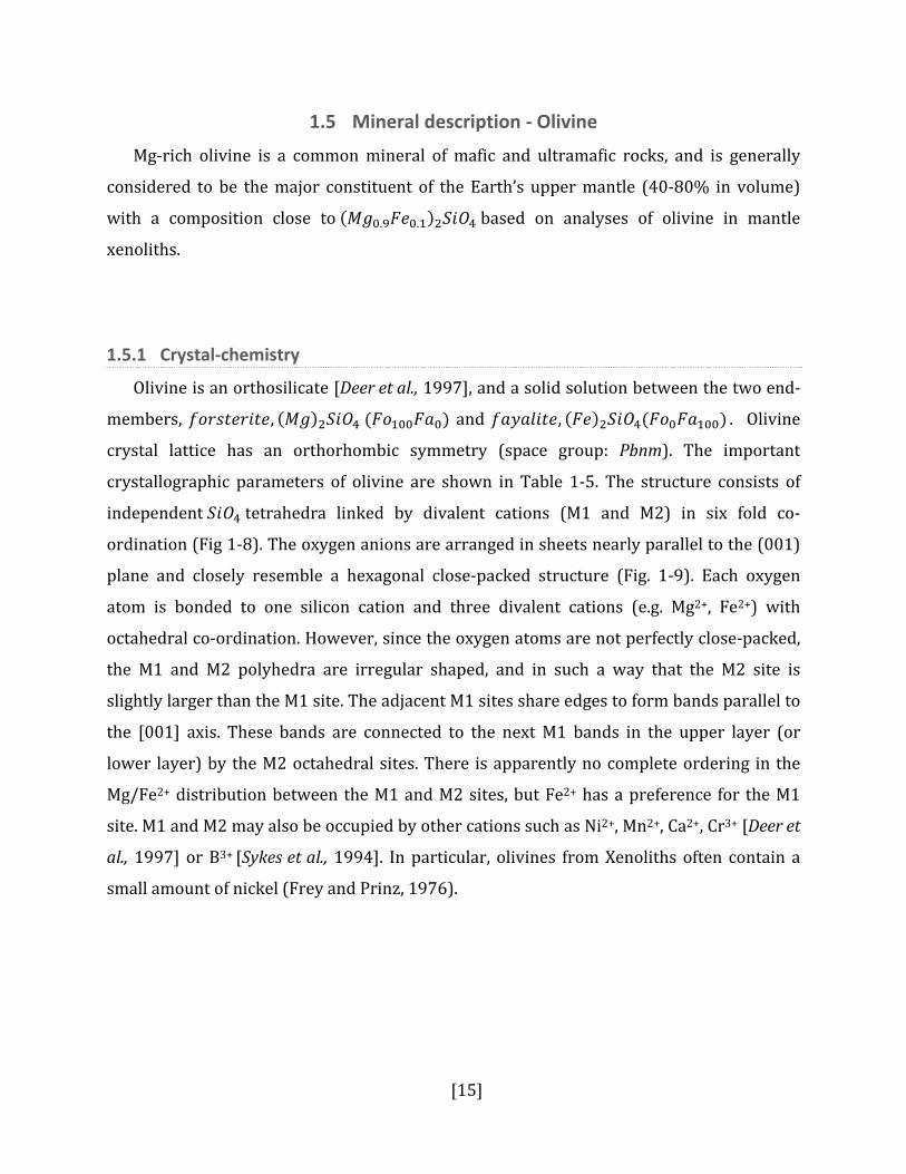
[15]

1.5 Mineral description - Olivine

Mg-rich olivine is a common mineral of mafic and ultramafic rocks, and is generally

considered to be the major constituent of the Earth’s upper mantle (40-80% in volume)

with a composition close to (𝑀𝑔0.9𝐹𝑒0.1)2𝑆𝑖𝑂4 based on analyses of olivine in mantle

xenoliths.

1.5.1 Crystal-chemistry

Olivine is an orthosilicate [Deer et al., 1997], and a solid solution between the two end-

members, 𝑓𝑜𝑟𝑠𝑡𝑒𝑟𝑖𝑡𝑒, (𝑀𝑔)2𝑆𝑖𝑂4 (𝐹𝑜100𝐹𝑎0) and 𝑓𝑎𝑦𝑎𝑙𝑖𝑡𝑒, (𝐹𝑒)2𝑆𝑖𝑂4(𝐹𝑜0𝐹𝑎100) . Olivine

crystal lattice has an orthorhombic symmetry (space group: Pbnm). The important

crystallographic parameters of olivine are shown in Table 1-5. The structure consists of

independent 𝑆𝑖𝑂4 tetrahedra linked by divalent cations (M1 and M2) in six fold co-

ordination (Fig 1-8). The oxygen anions are arranged in sheets nearly parallel to the (001)

plane and closely resemble a hexagonal close-packed structure (Fig. 1-9). Each oxygen

atom is bonded to one silicon cation and three divalent cations (e.g. Mg2+, Fe2+) with

octahedral co-ordination. However, since the oxygen atoms are not perfectly close-packed,

the M1 and M2 polyhedra are irregular shaped, and in such a way that the M2 site is

slightly larger than the M1 site. The adjacent M1 sites share edges to form bands parallel to

the [001] axis. These bands are connected to the next M1 bands in the upper layer (or

lower layer) by the M2 octahedral sites. There is apparently no complete ordering in the

Mg/Fe2+ distribution between the M1 and M2 sites, but Fe2+ has a preference for the M1

site. M1 and M2 may also be occupied by other cations such as Ni2+, Mn2+, Ca2+, Cr3+ [Deer et

al., 1997] or B3+ [Sykes et al., 1994]. In particular, olivines from Xenoliths often contain a

small amount of nickel (Frey and Prinz, 1976).

[16]

Table 1-5: lattice constants and densities of Olivines (Deer et al., 1997)

Forsterite Mantle olivine Fayalite

Chemical Formula Mg2SiO4 (Mg0.9,Fe0.1)2SiO4 Fe2SiO4

a (Å) 4.754 4.755 4.8211

b Å 10.197 10.21 10.4779

c (Å) 5.9806 5.985 6.0889

Density (g/cm3) 3.222 3.4 4.392

Figure 1-8: Idealized forsterite structure projected on (100) plane (Redrawn from Deer et al., 1997). Si atoms are at the centre of the tetrahedrons. Small black circle, Si; larger gray circle, oxygen; black circle, M1; diagonally hatched circle, M2

Figure 1-9: Forsterite structure perpendicular to (100) showing the approximately hexagonal close-packing structure (redrawn from Deer et al., 1997)

[17]

1.6 Aim of the thesis

Principal goal of this PhD work is to determine the origin of changes in the dominant

slip systems at high pressure and high temperature environment prevalent in the upper

mantle. For this purpose, we plan to conduct simple shear deformation experiments on San

Carlos olivine and Peridotite modal composition, using Deformation-DIA. Experiments are

designed to delineate the influences of pressure, temperature, strain rate and H2O content

on slip systems in olivine.

At the initial stages of this PhD work, a new high pressure assembly will be designed

which should allow us to reliable conduct deformation experiments at pressures above 8

GPa under high temperature conditions.

Deformed specimens are to be analyzed using a variety of analytical tools that includes

SEM & EBSD, TEM, FTIR and NMR.

1. Effect of stress and pressure on slip systems in olivine

A range of experiments has been conducted at various pressure and

temperatures to explore the effect of stress on the slip systems in olivine. In this

way, we also ascertained the role played by pressure on changes in olivine slip

systems. Pressure has been varied between 3 to 8.5 GPa at temperatures between

1300 to 1500°C.

Determination of stress in the sample, for some experiments, has been

performed Ex-Situ using dislocation densities obtained by Transmission electron

microscopy. Alternatively, stresses have also been measured using recrystallized

grain size data obtained by EBSD technique and comparing them with known

recrystallized grain size versus stress calibration. TEM studies were also be

employed for detailed study of dislocation microstructure.

2. Effect of water on slip systems in olivine

A similar range of experiments have been performed on “wet” olivine specimens

to determine the effect of H2O on slip systems in olivine. Water content of the

hydrous specimens has been analyzed using FTIR spectroscopy. Some of these

[18]

specimens have also been studied by TEM to understand the role of water on

dislocations.

3. Olivine is the most voluminous phase in the upper mantle rocks. Other important

mineral phases in the upper mantle are Pyroxenes, Spinel and Garnet. Deformation

studies have been performed on Peridotite modal composition, which represents

the upper mantle rock composition, to understand the role of other mineral phases

e.g. pyroxenes on the overall fabric development in a upper mantle.

4. Stress is the most crucial parameter in a controlled deformation experiment. Yet, it

is one of the most poorly constrained. In-situ measurement of stress, in most cases,

is either performed using externally (external to the pressure cell) placed load cell

or using x-ray radiography. The former method often gives a measured value of

stress that can be far off from the actual value experienced by the sample material.

This difference is caused by the frictional forces active throughout the pressure cell.

Other method of stress measurement using the x-ray radiography relies upon

synchrotron based radiation source. This approach is not suitable for day-to-day use

in a standard laboratory environment. Therefore, attempt has been made to develop

a stress sensor based upon piezoelectric property of GaPO4 crystal. Once this

technique has fully developed, it should provide us a mean to make in-situ stress

measurements.

[19]

2 Methodology

2.1 Deformation experiments under extreme conditions

Many types of equipment have been used to deform mineral assemblages at ambient

and high pressure and temperature conditions. For many years the gas media Paterson rig

and the Griggs apparatus were the main devices used to deform samples but could only be

employed at conditions equivalent to the crust and very shallow mantle (see table 1).

However the need to investigate rheological properties at higher pressures resulted in

initial attempts using the 6-8 Kawai-type multianvil, DIA and diamond anvil cell [Karato,

2008a]. These devices were not designed for applying controlled deformation at high

pressure but they could expose samples to high deviatoric stresses as a result of

anisotropic compression. In the diamond cell this occurs quite normally when a poorly

hydrostatic pressure medium is employed, while in multianvil devices deviatoric stresses

can be applied by placing harder materials in the sample column direction compared to the

perpendicular direction. In these devices high deviatoric stresses then develop during

compression. Once high pressures are reached the application of temperature softens the

pressure medium and the stresses relax.

The need to provide a better control over the sample deformation environment,

however, lead to the development of new high pressure deformation devices such as the

Rotational Drickamer device (Karato, 2008) and the deformation DIA apparatus. In order

to study the development of Crystallographic preferred orientation (CPO) of mineral

assemblages at mantle conditions, deformation experiments must be able to satisfy the

criterion given below:

1. The method must provide the ability to generate and maintain extreme states of

pressure (for upper mantle 1-14 GPa) and temperature (above 1000-1600°C)

conditions prevalent in the earth’s mantle, for time durations that allow fabrics to

develop at suitable strain rates (1-48 hours).

[20]

2. Such a method should also provide control over strain rate (or stress) which is essential

for any meaningful understanding of the fabric development.

3. The ability to measure strain rate and stress.

4. Provide control over chemical environment e.g. water and oxygen fugacity is also

required.

5. Allow recovery of the sample for fabric and textural analysis. And,

6. Ensure that the sample does not deform during compression and decompression phase

of the experiment.

2.1.1 High pressure deformation apparatus

Understanding the role of deviatoric stress (and several other physical & chemical

parameters) on the development of texture in material is a prerequisite to the

understanding of anisotropic behaviour of minerals. Material scientists also use such

studies for establishing relations between various manufacturing processes and the

mechanical performance of the product material. The immense scope of such studies has

led to the development of a series of high pressures apparatuses with each having a unique

set of advantages and drawbacks.

Simple dead weight loading experiments are an effective way to perform precise

deformation experiments under ambient pressure condition [Carter et al., 1980] whereas

at the other extreme of pressure diamond-anvil cells can be used to deformed materials up

to 200 GPa pressure but with poor control over strain rate and stress distribution [Kinsland

and Bassett, 1977]. At intermediate pressures, a range of devices exist which all tend

towards a compromise in terms of maximum pressure and the control over deformation

and sample environment. Some salient features of various deformation apparatus are given

below in the table 2-1. For experiments to address olivine fabric development pressures of

between 1-15 GPa are required. Though, the 6-8 multianvil configurations can achieve

these pressures, only stress relaxation experiments can be performed and no control over

strain rate is possible [Bussod et al., 1993; Karato and Rubie, 1997]. The Rotational

Drickamer device (e.g. [Yamazaki and Karato, 2001] can provide control of strain rate over

the pressures of interest, however, it is very limited in sample size and control over

[21]

pressure and temperature is limited accept when used in conjunction with in situ X-rays.

Consequently the deformation-DIA appears to embody a suitable compromise between

allowing control over strain rate, pressure and temperature and also achieving a range of

pressure of interest to the study of olivine fabric development in the upper mantle.

Table 2-1: List of deformation devices and properties (Modified after Karato 2008)

Type of apparatus Max. P (GPa)

Max. T(K)

In-situ Stress measurement

Comment

Dead-weight creep apparatus

10-4 2000 From applied load

Low ƒH2O

Gas-medium apparatus (e.g. Paterson rig)

0.5 1600 Internal load cell Limited ƒH2O

Griggs-type apparatus 3 1600 External load cell

Limited strain

Deformation-DIA 23 1700 X-ray diffraction Limited strain Rotational Drickamer apparatus

18 2000 X-ray diffraction Unlimited strain

6-8 Multianvil stress-relaxation

23 2000 X-ray diffraction Non-steady state, relaxation experiments only

Diamond anvil 200 1000 X-ray diffraction Non-steady state, very high stress, Study of LPO difficult due to small sample size

6- ram cubic press 25 2000 X-ray diffraction Limited strain

Deformation-DIA

The Deformation-DIA (or D-DIA) is a modified form of DIA cubic-anvil apparatus [Osugi

et al., 1964]. The D-DIA incorporates two additional hydraulic actuators; here referred to as

differential rams, which provide independent control of the displacement of two vertically

opposing anvils [Wang et al., 2003]. The original DIA consists of upper and lower guide

blocks, four wedge-shaped side wedges, and six tungsten carbide anvils. The six anvils of

the D-DIA define a cubic volume due to their square shaped truncation. Four out of six

anvils are attached to the side wedges whereas one each of the other two anvils is mounted

to the upper and lower guide blocks.

[22]

DifferentialRam

SideWedge

DisplacementTransducer

Main loadFrom Press

HydraulicOil line

Sample

GuideBlock

Anvil

Figure 2-2: A vertical cross-section of D-DIA showing the two side wedges and the differential ram. Presence of differential rams provides controlled deformation of the cubic sample at a constant pressure.

Original DIA Deformation DIA

Figure 2-1: Schematic diagrams of original DIA and Deformation-DIA. A) Original DIA consists of upper and lower guide blocks, four wedge shape side wedges and six tungsten carbide anvils. B) A deformation-DIA has two additional hydraulic actuators called deformation rams which provides a mean to achieve controlled deformation. (source: Y. Wang)

[23]

As the main guide block of the DIA is compressed the vertically opposing anvils are

advanced. The 45° surfaces of the side wedges, however, ensure that a component of the

vertical displacement is converted to a horizontal displacement which advances the 4

horizontal anvils. Once high pressure has been achieved through the advancement of the

main ram, the vertical differential rams can be advanced thus applying a principle stress on

the cubic sample assembly.

D-DIA’s unique design provides a way to advance the differential rams into the sample

assembly without raising the confining pressure in the process. A typical experimental run

in the D-DIA is illustrated below in Figure 2-2. One starts by hydrostatically compressing

the sample assembly, with differential rams fully withdrawn to maintain the oil pressure in

the main ram at a constant value. The action of the guide block transfers the vertical

compressional force into horizontal compression via the side wedges. Then the sample is

heated up to the requisite temperature and kept in this state for approximately 30 min,

with a view to achieve thermal equilibrium. Then the differential rams are advanced so as

to bring a non-cubic shape change to the assembly while simultaneously withdrawing the

main ram at an appropriate rate. This ensures that total force exerted by the main ram

stays constant and hence the volume of the sample assembly is also conserved (Wang et al.,

2003).

Figure 2-3: Pressure-Temperature-Strain profile of typical experimental run in D-DIA press. After compressing the pressure cell to the requisite pressure, sample is heated up to the desired temperature and it is allowed to heat for at least 30 min to release the initial stress build-up, if any present in the sample. Then, the sample is

deformed at a constant strain rate. Once the target amount of strain is achieved, deformation is stopped and the sample is quenched right after that. Thereafter the pressure is released slowly.

[24]

The onset of movement of the differential rams occurs only when the differential ram

pressure is sufficient enough to overcome the confining force and the friction. Hence, the

higher the confining pressure, higher is the initial differential ram pressure required to

move the differential rams. This imposes a limit to the maximum confining pressure at

which deformation can be achieved without breaking the anvils. Using the 500 tonne

Voggenreiter D-DIA press available at the Bayerisches Geoinstitut with 4 mm square

truncations tungsten carbide (WC) anvils, it is possible to perform deformation

experiments up to 10 GPa confining pressure, at temperatures as high as 1500°C.

The displacement of the two differential anvils is measured relative to the guide block

using displacement transducers. The transducers employ a magnetic response to measure

displacement to a precision of 0.2 µm.

Sample assembly design

As stated earlier, in the D-DIA a wide range of pressure and temperature conditions can

be achieved (up to 10 GPa and 1700°C). In order to access higher pressures the truncation

size on the tungsten carbide anvils can be reduced, however, this also reduces the sample

size as the dimensions of the cubic pressure assembly must also be reduced. For the work

performed in this thesis two assembly configurations were developed. The 6/8 assembly

employs 6 mm edge length square faceted tungsten carbide anvil truncations with a cubic

sample assembly that is 8 mm in edge length. It was used to achieve pressures up to 3.5

GPa. The 4/6 assembly, used between 3.5 and 10 GPa, employs 4 mm anvil truncations and

a 6 mm edge length cube.

The experimental set-up for deformation experiments consists of a cubic pressure

medium composed of fired or unfired pyrophyllite. The cube is drilled out along one axis

for the insertion of a furnace separated by a thermally insulating sleeve. The resistive

materials graphite and rhenium are used as furnaces, while zirconia is used as a thermally

insulating sleeve around the furnace to make the experimental set-up thermally efficient. A

number of attempts were made to employ lanthanum chromite as a furnace material,

[25]

however, it was found to be prone to mechanical damage and subsequent thermal

instability during deformation.

Gaskets form during the experiment as material from the pressure assembly is

squeezed between the anvils. For fired pyrophyllite cubes this action is less efficient due to

the use of stiffer material. This may help the attainment of higher pressures however it also

leads to more blow outs due to the more brittle nature of the gaskets formed. For this

reason the 4/6 assembly design employs preformed gaskets of Teflon, which are attached

to the anvils using glue prior to the experiment.

The sample material is sandwiched between cylindrical pistons of alumina cut at 45°

(Fig 2-4). A softer crushable alumina is also required to absorb the initial shortening of the

sample assembly during hydrostatic compression. During compression the entire assembly

is shortened. In order that the sample is not deformed in the process, crushable alumina is

added to the sample column to accommodate this compressional strain. During

deformation, the majority of the sample column needs to be comprised of fully dense

alumina such that the sample is the weakest material. However, the proportion of

crushable and dense alumina in the sample column needs to be carefully adjusted by trial

and error experiments such that minimal sample deformation occurs during compression.

Determining this ratio between crushable and dense alumina in the sample column is one

of the most important factors when developing a D-DIA assembly.

Alumina pistons can either be cut at 45° to the axis of the cylindrical rod or at 90° to it.

The first kind of pistons are used in performing simple shear deformation experiment,

whereas pistons cut at right angle to the axis of cylinder are used for plane-strain

compression (pure shear) deformation experiments.

[26]

Plane-strain compression (Pure shear) Simple Shear

Figure 2-4: Cartoon comparing deformation by pure shear and simple shear

The shape of the finite strain ellipsoid may be the same at the end of deformation in the

case of both, pure and simple shear but in the case of simple shear deformation; the finite

strain ellipsoid is inclined at some angle to the shear. It has direct implication on the

representation of CPO using pole figures. For pure shear case, one should expect an

orthorhombic pole figure, whereas simple shear leads to monoclinic or triclinic pole

figures. More importantly, it’s easier to obtain larger strain using simple shear

configuration (γ > 1), whereas strain due to pure shear is generally limited to 30-40%, in

the best of cases. Apart from that, dominant deformation regimes in the upper mantle are

either simple shear or plane combinations of simple and pure shear [Tommasi et al., 1999].

In this thesis shear deformation experiments were performed in order to maximize strain

and fabric development.

Demerits of the Deformation-DIA

The D-DIA has been an important step forward towards conducting deformation

experiment at pressures in excess of 3GPa. However, as outlined below, there are some

limitations to the amount of achievable strain and accurate measurement of strain rate and

stress.

D-DIA allows the user to control the rate and amount of advancement of the differential

rams and hence the deformation anvil. If the softest material in the assembly happens to be

the sample being deformed, then it is safe to assume that deformation caused by the

[27]

advancing anvils has been absorbed by the sample. In such a scenario, it is very easy to

quantify the bulk strain rate of the sample along with the strain experienced by it.

However, due to the fact that some amount of the deformation is always lost in the elastic

and plastic deformation of the materials surrounding the sample, the aforementioned

assumption is not always valid. The way to minimize this inefficiency in transferring strain

is by insuring that the parts surrounding the sample e.g. pistons, thermocouple tube,

furnace and insulating materials (for instance, zirconia) have considerably higher strength

than the sample. On the other hand, total strain experienced by the sample can also be

characterized using a strain marker. Though, the presence of a strain marker cannot insure

that externally applied strain rate, measured as the rate of deformation ram advancement,

is the same as that being experienced by the sample.

The total amount of strain that can be applied to the sample is always limited by the

strength of the materials surrounding the sample. In case of a non-porous sample,

deformation can only be achieved if the surrounding material gives way to the sample and

the piston, as the volume needs to be conserved. In case of simple shear, owing to the

excessive shearing force at the tip of the wedge shaped pistons the alumina pistons fail

after a certain point (shear strain = 2). It is also noteworthy that the amount of the sample

that stays sandwiched between the wedge-shaped pistons decreases with increasing

amount of strain. Due to the geometrical constraints imposed by the anvils which are cut at

45°, such limitations are only important for the case of simple shear deformation

experiments. Referring to the orientation contrast image of the sample DD407 (Fig. 2-5),

one can see the effect of large shearing stress causing the alumina pistons to fail at along

the maximum shear stress direction. Evidence of necking and breaking in the assembly can

also be seen.

[28]

Figure 2-5: orientation contrast image of an excessively deformed sample at 8GPa (Sample No. DD407). Alumina pistons have failed, owing to the large shearing stress active on the wedge shaped alumina pistons. The applied shear strain was more than 200%.

D-DIA coupled with a synchrotron radiation source provides a direct way to measure

the microscopic stresses that are active in the sample. In the absence of such a facility, user

needs to apply indirect ways to estimate stress (e.g. measuring dislocation density using

oxidation-coloration method and TEM). Such off-situ approaches discount the possibility of

studying flow laws of materials which cannot be performed without continuous

measurement of strain rate and stress.

8/6 mm Assembly description

The 8/6mm assembly consists of a cubic unfired pyrophyllite pressure cell drilled to

contain a graphite furnace surrounded by a zirconia sleeve. The sample slice, along with the

alumina pistons, is jacketed using Pt-foil (25 micron thick) and inserted into the furnace in

an MgO sleeve (Fig. 2-6).

[29]

Figure 2-6: Schematic diagram of an 8/6 mm D-Dia assembly.

A suitable length of 4-hole alumina tube and crushable alumina plugs are inserted

above and below the pistons to minimize the deformation during hydrostatic compression

phase of experiment. Crushable and fully dense alumina is therefore distributed

symmetrically about the central piston assemblage. The assembly is self-gasketing.

4/6mm Assembly description

The 4/6 assembly was developed to performed experiments in simple shear

configuration up to a confining pressure of 8 GPa and 1500°C. The assembly consists of a

pyrophyllite pressure cell, fired at 1000°C for 5 hours. Firing makes the assembly

mechanically strong and it helps generate much higher pressure than a similar sized

unfired pyrophyllite pressure cell. One important difference between the 6/8 and 4/6

assembly is the use of a rhenium metal foil furnace (25 µm thick). A foil furnace was found

to be more stable than graphite at high pressure during deformation, most likely due to it

being more malleable.

[30]

In the 4/6 design the sample column above and below the piston-set comprises dense

and crushable alumina as shown in figure 2-7. The length ratio of crushable and dense

alumina cylinders has been carefully optimized to minimize the deformation of sample

during cold compression. The lengths of the dense alumina thermocouple tube and solid

cylinder below the lower alumina piston are identical (in this case 0.5 mm), as are the

crushable alumina cylinders above and below the pistons (1.7 mm). This ensures a

symmetric configuration in the assembly, so that during deformation the sample material

remains in the centre of the furnace hot-spot. Pre formed Teflon gaskets are attached to the

anvils for the 4/6 assembly. 12 such gaskets, each 1.5 mm wide are glued to the 12 pairs of

anvil faces.

Figure 2-7 : A schematic diagram of a 4/6 mm D-DIA assembly showing its major components

[31]

Pressure and temperature calibration of the Sample assembly

Pressure calibration at room temperature

The sample pressure must be calibrated in each D-DIA assembly against the oil

pressure using phase transitions that occur at well-determined pressures. Initially room

temperature calibrations were employed to identify the approximate pressure range for

further high temperature calibrations and to define the gradient of the pressure calibration.

Bismuth undergoes phase transitions at 2.54 GPa (Bi I-II), 2.7 GPA (Bi II-III) and 7.7 GPa

(Bi III-IV) which causes a change in the resistivity of bismuth [Getting, 1998; Lloyd, 1971],

whereas the resistivity of Manganin wire (Cu86/Mn12/Ni2) changes linearly with

pressure. In order to calibrate the pressure achievable with the 6 mm pyrophyllite

pressure cell, a thin wire of Bismuth

was placed

between two AgCl disks as shown in Fig

2-8. Thin copper foils which served the

purpose of electrode, were placed at the

two ends of the Bismuth wire. A

constant current was supplied through

the bismuth wire and the voltage across

the Cu-electrodes was measured during

the compression.

Bi I-II transition was observed at around 17 bar oil pressure. For obtaining the

pressure-resistivity relationship of Manganin, the same setup was used but with Manganin

wire replacing the Bismuth wire. The change in Manganin

resistivity with the confining pressure can be expressed as the pressure coefficient of the

resistance change given by �𝛿𝑅 𝑅0� � �1𝑃� � = (2.322 ± 0.008) × 10−2 𝐺𝑃𝑎−1 where 𝛿𝑅 is

the change in resistance and R is the resistance at any given pressure P measured in GPa

(Robert J. Zeto and H. B. Vanfleet). The pressure dependence of resistivity must be

Figure 2-8: Schematic of assembly used for pressure calibration using Bismuth and Manganin

[32]

calibrated using a known pressure point, for which we used the Bi I-II transition. As shown

in Fig 2-8 the pressure at room temperature determined using Manganin wire reaches a

plateau just over 7 GPa, consistent with the observation that we were unable to observe the

Bi III-IV transition at 7.7 GPa. This plateau is typical of most multianvil assemblies and

results from the gasket supporting an ever-increasing proportion of the load.

Figure 2-9 shows that data from calibration experiments at room temperature and

1000°C. The assembly is more efficient at generating pressure at 1000°C than at room

temperature as shown by the Coesite/Stishovite transition, which occurs at approximately

110 bars oil pressure (78.6 tonnes of applied load).

Pressure calibration at high temperature

Phase transition in quartz to its high pressure polymorphs, coesite and stishovite, is

pressure and temperature dependent. At 1000°C, quartz transforms to coesite at ~ 2.95

GPa; whereas the coesite to stishovite transition pressure at 1000°C is at ~9.25 GPa

(Akaogi & Navrotsky, 1984).

A fine grained mixture of fibrous quartz was placed in the standard assembly (but in

pure shear configuration). The sample assembly was brought up to the requisite pressure

and then it heated at 1000°C for ~5 hours. After quenching and decompression, the end

product was sectioned and polished and analyzed using Raman spectroscopy to identify

the SiO2 polymorph in the run products.

Table 2-2: List of experiments and the end products - Calibration of cell pressure at 1000°C using phase transition in Quartz

Experiment Run Oil pressure(bars) Observation

DD451 17.1 Quartz

DD452 19.6 Quartz and Coesite coexist

DD387 78.6 Coesite

DD400 85.7 Stishovite

[33]

Figure 2-9: Calibrated cell pressure has been plotted as a function of oil pressure. Room temperature calibration has been done by using phase transitions in Bismuth and Manganin resistivity method. High temperature (1000°C) pressure calibration was done using phase transition in Quartz (quartzcoesite and coesitestishovite). 700 bar oil pressure is equivalent to 500 tonne load for D-DIA press at BGI.

Temperature calibration of the sample assembly

The sample temperature distribution within the 4/6 deformation cell assembly was

measured using a two-pyroxene thermometer assemblage, employing the calibration of

Nickel & Brey, (1984). An equimolar powdered mixture of Al-free enstatite and diopside

were placed between the alumina deformation pistons at 45° to the axial direction. 4 wt%

PbO was added to the sample as a flux. The sample powder was compacted before the

second deformation piston was placed on top, but the sample was not hot pressed. The

experiment was heated at 1300°C (thermo-couple temperature) and 8 GPa pressure for

approx. 6 hrs. No deformation was applied. Chemical compositions of fully reacted

neighbouring pairs of enstatite and diopside grains were measured using a JEOL JXA – 8200

electron microprobe at BGI.

[34]

The recovered sample slice was approximately 200 µm thick in the axial direction. The

calibration employs the distribution of Ca and Mg between the two-pyroxene minerals. The

determined mean temperature in the central portion of the sample slice was

approximately 150°C higher than the temperature measured at the thermocouple. The

difference between the mean temperature at the middle of the sample and at the extreme

points of the sample was found to be ~75°C (Fig 2-10). This results in a temperature

gradient of 84° C/mm along the sample length. The variation in temperature likely reflects

the thermal gradient along the furnace; with the centre of the sample, therefore, placed will

in the hottest part of the furnace, while the thermocouple and sample extremities next to

the furnace are slightly out of the hot spot.

Figure 2-10: Measured temperature along the sample length. Center of the sample recorded the highest temperature with approx. 85°C/mm temperature gradient as we move towards the extremities.

Oxygen fugacity of the experiments

The oxygen fugacity is an important parameter in deformation experiments as it

controls the concentration and mobility of point defects in Fe-bearing minerals [Demouchy

and Mackwell, 2006; Kohlstedt and Mackwell, 1998]. The oxygen fugacity is not controlled

1300

1350

1400

1450

1500

1550

-0.85 -0.65 -0.45 -0.25 -0.05 0.15 0.35 0.55 0.75

Tem

pera

ture

(°C)

Distance from the center of the sample (mm)

Temperature (°C) along the sample length

Standard Deviation = 43°

[35]

in D-DIA experiments but it is influenced by the type of furnace employed and by the

nature of the starting material. The use of graphite or metal furnaces generally leads to

more reducing conditions because the furnaces can only be oxidized during the experiment

and has no mechanism to release oxygen or oxidized species. The oxygen fugacity can be

measured in the experiment however particularly in the region of the Pt capsule or Pt

strain markers where the proportion of Fe alloying with the Pt can be measured.

𝐹𝑒2𝑆𝑖𝑂4 = 𝐹𝑒𝑆𝑖𝑂3 + 𝐹𝑒 + 𝑂2

𝑂𝑙𝑖𝑣𝑖𝑛𝑒 𝑒𝑛𝑠𝑡𝑎𝑡𝑖𝑡𝑒 𝐴𝑙𝑙𝑜𝑦

The equilibrium can be used to determine the oxygen fugacity from the thermodynamic

relationship

2 4 32log log log 2log

ln(10)olivine orthopyroxene metal

Fe SiO FeSiO Fe

oGfo

RT a a a−∆= + − −

Where, 2 4

olivine

Fe SiOa ,ametal

Fe and 3

orthopyroxene

FeSiOa are the activities of the Fe2SiO4 component in

olivine, Fe in the Pt-Fe alloy and FeSiO3 in pyroxene respectively. ∆G0 is the free energy of

the end-member equilibrium, which was taken from thermodynamic data reported by

[Stagno et al., 2011]Stagno and Frost (2011). In some deformation experiments where

pyroxene was observed and the Fe content of Pt foil or strain marker was measured it was

possible to calculate the oxygen fugacity in the experiment. For this activity composition

relations for Fe in Pt alloy were required, which were taken from Mann et al. (submitted).

The determined oxygen fugacity at 8 GPa and 1500°C was -0.8±0.5 log units or

approximately at the fayalite-magnetite-quartz (QFM) oxygen buffer. This value is within

the range found for mantle rocks, although it may be considered slightly more oxidised

than many samples from the deep mantle, >100 km, which are in general closer to QFM –2

[Frost and Mccammon, 2008].

[36]

2.2 Sample Preparation

2.2.1 Hot pressing San Carlos olivine

A fine grained powder of (𝑀𝑔0.9,𝐹𝑒0.1)2𝑆𝑖𝑂4 San Carlos olivine with grain size below

10 µ𝑚 was loaded into a 12 𝑚𝑚 long and 5 𝑚𝑚 outer Diameter cylindrical Platinum

capsule. Using ¾” Talc-Pyrex glass assembly and 200t piston cylinder press at Bayerisches

Geoinstitut, the assembly was cold pressed to 10𝑘𝑏 confining pressure. Thereafter it was

heated to a temperature of 1100°𝐶 and kept as such for 30 𝑚𝑖𝑛. Then the assembly was

slowly decompressed over 12 ℎ𝑜𝑢𝑟𝑠 period along with simultaneously cooling to room

temperature. Slow decompression with simultaneous cooling was performed in order to

avoid decompression cracks.

Hydrous olivine samples were prepared by adding an equimolar mixture of Brucite and

Silica to the powdered olivine and then hotpressed in the 6-8 multianvil device. In some

instance, Brucite-Silica aggregate was added to the pre-hotpressed samples while

assembling process before the experiment.

2.2.2 Placing platinum Shear strain marker

After hot pressing the sintered samples were carefully removed from the high-pressure

assembly and the top and bottom of the capsule removed. 1.2mm diameter cylindrical

cores were prepared from these samples in the thin section laboratory by H. Schulze. Using

a diamond wire saw, 200µm thick elliptical slices of hot pressed olivine sample were then

cut from the core each of which were oriented at 45° to the core axis. Each olivine slice was

then cut into two symmetrical halves, with the direction of cutting oriented parallel to the

original cylindrical core (Fig 2-11). The exposed surfaces of this cut were then sputter

coated with a ~100nm Pt layer. Putting a Pt marker in this way, on a cross-section cut

parallel to the cylindrical axis minimizes the marker rotation due to axial compression of

the sample.

[37]

0.2 mm

Sample

Pt StrainMarker

Alumina Piston

Pt capsule

Figure 2-11: Emplacement of platinum strain marker for shear strain measurement. Approximately 100 nm thick Platinum-layer is sputter coated on the sides of the two cut halves of the hotpressed sample. Rotation of the strain marker is directly related to the shear strain

2.3 Analytical Methods

As the central theme of this thesis has been to study of the effects of physical and

chemical parameters on the crystallographic preferred orientation of olivine, electron

backscatter diffractometer (EBSD) has been the primary analysis technique. It is also crucial

however to relate the determined CPO, or lack thereof, to the underlying deformation

mechanism and active slip system in the crystal and for this purpose Transmission electron

microscope (TEM) has been a vital analysis technique.

Water content in the starting sample and the recovered sample has been measured

using Fourier Transform Infrared (FTIR) spectroscopy. A brief introduction to these three

important instruments is provided in the next paragraphs.

The Electron probe micro-analyzer (EPMA) was used for analyzing the chemical

composition of recovered samples and to examine the equilibrium distribution of Ca and

Mg between enstatite and diopside aggregates employed in experiments to calibrate the

temperature in the pressure cell. Raman spectroscopy has also been utilized for phase

[38]

identification in the run products from experiments performed to calibrate cell pressure

using quartz-coesite and coesite-stishovite phase transformations.

2.3.1 Measurement of crystallographic preferred orientation using Electron backscatter diffraction technique (EBSD)

Electron backscattered diffraction (EBSD); sometimes also referred to as backscatter

Kikuchi diffraction (BKD) is a technological add-on to a scanning electron microscope. It

provides an SEM with a microstructural-crystallographic analysis capability. Primarily,

EBSD is used to study texture or preferred orientation of any crystalline or polycrystalline

material. This is achieved by indexing and identifying the crystal systems. Apart from

structure and orientation information, EBSPs (Electron back scatter patterns; See figure

No. 2-12 for an example of such a pattern in mineral olivine) contain additional information

on crystal lattice perfection, local strain, deformation, and grain boundaries.

Traditionally these types of studies have been carried out using x-ray diffraction (XRD),

neutron diffraction and/or electron diffraction in a TEM.

[39]

Figure 2-12: Formation of backscattered Kikuchi patterns by EBSD in the SEM. (a) Origin of Kikuchi lines from the EBSD (i.e., tilted specimen) perspective. (b) EBSD pattern from olivine (accelerating voltage 20 kV).

EBSD system consists of a phosphor screen, compact lens and low light CCD camera

attached to a Scanning Electron Microscope (SEM) (Fig. 2-13). A polished sample specimen

is placed into the normal position in the specimen chamber, and is tilted to ~70° from the

normal position. Doing so boosts the contrast of EBSPs.

EBSPs are generated if a stationary beam interacts with the surface of a crystal [Alam et

al., 1954],[Venables and Harland, 1973]. The electrons while interacting with an atom

undergo inelastic scattering. It results in a fraction of the electrons losing a small part of

their energy. This process creates a divergent source of electrons close to the surface of the

sample. Some of these electrons are incident on atomic planes at angles which satisfy the

Bragg equation. For each given plane, these electrons emanate in diffraction cones from

both the front and back surface of the plane. When these cones intersect the phosphor

screen, the Kikuchi lines are formed. The Kikuchi lines appear as almost straight lines

because the cones are very shallow as the Bragg angle is of the order of 1°. Small Bragg

angle results from the fact that incident electrons have very high energy and hence very

small wavelength (λ ≈ 8 pm for a 25 KeV electron beam). Hence, Kikuchi bands are

effectively the trace of the plane from which they are formed and the EBSD pattern is

therefore a gnomonic projection of the crystal structure.

[40]

Figure 2-13: Schematic setup of an EBSD system showing its principal components

Thus, the whole Kikuchi pattern consists of pairs of parallel lines where each pair, or

“band,” has a distinct width and corresponds to a distinct crystallographic plane. The

intersection of bands corresponds to a zone axis (pole), and major zone axes are

recognized by intersection of several bands. The Kikuchi pattern therefore essentially

embodies all the angular relationships in a crystal—both the - and inter-planar angles—

and hence implicitly contains the crystal symmetry. Figure 2-12 shows an EBSD Kikuchi

pattern from mineral San-Carlos olivine. The orientation of the pattern and hence of the

volume from which it has arisen is evaluated by “indexing,” that is, identifying the poles and

bands in the pattern, and calculating the relationship between these and some chosen

reference axes.

From Kikuchi bands to pole figure

Automated identification of a crystal orientation involves identifying the kikuchi lines in

the gray scale image containing EBSPs. First step towards this process involves the pre-

processing stage of edge detection. This is a non-trivial task because contrast normal to the

kikuchi lines rarely change abruptly. The pattern of Kikuchi lines on the phosphor screen is

electronically digitized and processed to recognize the individual Kikuchi lines. These data

are used to identify the phase, to index the pattern, and to determine the orientation of the

[41]

crystal from which the pattern was generated. Individual mineral grains can be selected for

identification and determination of crystal orientation, or data may be acquired on a grid

over a selected area of the surface of the sample to determine the identity, orientations, and

spatial relations between a large numbers of grains.

These data can be used to make statistical studies of the micro-fabric of the sample, to

reveal systematic textural relations between individual grains or phases, and even to

determine relative abundances of phases in a poly-phase sample.

Principles of Orientation Determination

From the information about the crystallographic indices with

(where is the number of identified bands or poles) and the angles

between each band or pole and the beam normal, the orientation of the sample normal in

terms of its crystallographic indices can be expressed as

The root term in the equation given above normalizes the indices of the bands or axes,

which are typically given as integers, for example or to unity. Hence the

resulting vector is directly normalized to unity. It is seen that three equations are

necessary to determine the vector , which means that three bands or poles have to be

indexed.

Automation of Pattern Indexing and Orientation

To relate the characteristic features of an EBSD pattern – typically zone axes or bands—

from the 2-D computer screen to the 3-D sample coordinate system (denoted by the

superscript s in equation below), the 2-D screen coordinates are transformed into

3-D vectors by

[42]

Figure 2-14: Diagram illustrating the evaluation of an EBSD pattern. Sample coordinate has been represented by superscript “s” where as screen coordinate has been represented by superscript “screen”. Specimen-to-screen distance is . (X*i,Y*i) are coordinates of the center of the pattern and (XPC,YPC ) are the coordinates of the center of the screen.

With an appropriate calibration of the hardware setup, the coordinates of the pattern

centre and the specimen-to-screen distance are known (Figure 2-14). The

rotation matrix contains all necessary geometrical corrections, most notably the tilting

angle α of the sample (usually as well as additional angles between sample and

phosphor screen, which may occur in the various EBSD setups.

After indexing the pattern, the orientation of the sampled crystal volume with respect

to the external specimen coordinate system can be determined (e.g. [Schwarzer and

Weiland, 1988]; [Dingley et al., 1987]. The crystallographic orientation is usually given in

terms of its orientation matrix g that transforms the specimen coordinate system into the

coordinate system of the crystal (indexed by the superscript c in the following equations):

[43]

Thus, for each vector (zone axis or band normal), its vector in the sample frame

and, after the indexing, its crystallographic direction

are known. It follows from definition of (with :

Finally, a pattern can be recalculated from the orientation matrix and overlaid on the

original pattern. If the solution is judged by the operator to be correct, the orientation

matrix g is stored in a computer file for further evaluation and representation of the data.

Sample preparation for EBSD measurement

At the end of a deformation experiment the entire recovered sample assembly is cut

either normal to the shear plane or parallel to it. The sample is then mounted in epoxy

resin and the surface of the assembly and sample is polished to microprobe quality

polished section using standard mechanical polishing methods with a finish of

approximately 0.5 µm.

The electrons that generate EBSD patterns are diffracted from a depth of 10-50nm from

the surface of the crystallites, and any residual surface deformation introduced during the

mechanical polishing must be minimized to obtain high quality EBSD pattern. Typically

standard metallography does not require such a fine surface. It should be noted that while

these traditional methods can produce EBSD patterns that can be analyzed; the goal of

EBSD sample preparation is to produce a flat deformation free surface that maximizes the

pattern quality from the entire surface.

The next polishing stage uses a colloidal silica suspension in a mildly acidic medium.

This chemical polishing removes the top surface of the sample that is mechanically

damaged during standard polishing with grits. Thereafter the sample is carbon coated up

to a thickness of 4-6 nm to minimize charge accumulation during the analysis.

[44]

2.3.2 Study of dislocation structure using Transmission electron microscope (TEM)

Plastic deformation of crystals occurs through the development and motion of lattice

defects such as dislocations. Transmission electron microscopy (TEM) is by far the most

important technique for studying such defects in great detail. TEMs are capable of imaging

at a significantly higher resolution than light microscopes, owing to the small de Broglie

wavelength of electrons. This enables the instrument's user to examine fine detail—even as

small as a single column of atoms, which is tens of thousands times smaller than the

smallest resolvable object in a light microscope.

Imaging methods in TEM utilize the information contained in the electron waves exiting

from the sample to form an image. Different imaging methods attempt to modify the

electron waves exiting the sample in a form that is useful to obtain information with

regards to the sample, or beam itself. The observed image depends not only on the

amplitude of beam, but also on the phase of the electrons, although phase effects may often

be ignored at lower magnifications.

Diffraction contrast imaging is the most widely applicable way of studying dislocations,

although high resolution microscopy produces more direct and spectacular images.

Amplitude contrast imaging can be done by either using the direct beam or one of the

diffracted beams. In the former case it is called bright field (BF) imaging, in the latter case

dark field (DF) imaging. These names originate from the fact that in DF imaging, holes in

the foil appear black and the picture is generally darker than for BF imaging. These two

imaging techniques can be used to image strain fields within crystals. “Contrast” is the

appearance of a feature in an image. Contrast in bright-field (BF) and dark-field (DF) TEM

images is usually “diffraction contrast” or the variations in intensity of diffraction across

the sample. Crystal defects like dislocations induce local bending of crystal planes close to

the defects. This bending of crystal planes modifies the way in which the electron beam is

locally diffracted. To illustrate this point further, let us consider the case of a hypothetical

thin crystal flake containing an edge dislocation (Fig 2-15). The electron beam direction is

now approximately at right angles to both the dislocation line (which is normal to the page)

and the Burgers vector. In the immediate vicinity of the dislocation core the orientation of

[45]

the lattice planes is slightly different to that in the rest of the crystal. This means that the

ways in which these lattice planes diffract electrons will be different in the distorted and

undistorted parts of the crystal.

Figure 2-15 : Schematic illustration of diffraction around a dislocation core. In this case the electron beam is diffracted more strongly tiled lattice planes to one side of the dislocation core than in the undistorted parts of the crystal. The transmitted beam is depleted around the dislocation line, and in a bright-field image the dislocation line will appear darker than the rest of the crystal. On the other hand, the diffracted intensity is greater around the dislocation line and in a dark field image using the diffracted beam; the dislocation line will appear lighter than the rest of the crystal. Under Weak beam (WBDF) condition, the overall intensity of the image is reduced in comparison to a dark field image.

By slightly tilting the crystal relative to the beam it is possible to set the undistorted

planes in the exact Bragg reflection (Bragg angle for short wavelength electrons is very

small), in which case the planes around the dislocation core will not diffract strongly.

Alternatively, a slight adjustment of the crystal will set the distorted planes into the exact

[46]

diffracting condition, while the other lattice planes will only weakly diffract. A bright field

image taken in this latter position will show depleted intensity in those parts of the crystal

strongly diffracting i.e. around the dislocation line. The dislocation line will appear as a

dark string against a paler background. In a dark field image, using the diffracted beam, the

dislocation line will appear brighter against a dark background.

Determination of the Burgers vector

As mentioned above, a dislocation bends the lattice planes near the dislocation core.

This can be described by a displacement field 𝑅�⃗ . The displacement field generates an

additional phase shift ~ 𝑒2𝜋𝑖𝑔�⃗ .𝑅�⃗ of the Bragg diffracted beam, which leads to a diffraction

contrast in the image. The phase shift 𝑒2𝜋𝑖𝑔�⃗ .𝑅�⃗ only comes into effect if �⃗� .𝑅�⃗ ≠ 0. This

means, if �⃗� . 𝑏�⃗ = 0 ⇒ �⃗� .𝑅�⃗ = 0 and the dislocation line is not visible, then the

displacement field is parallel to the exploited hkl plane and does not change in phase. This

relation is called �⃗� . 𝑏�⃗ criterion. If �⃗� . 𝑏�⃗ = 0, the dislocation line is not visible, otherwise the

dislocation is visible in the WBDF (Weak beam dark field) image. This enables the Burgers

vector determination and identification of the dislocation type by taking WBDF images of

the same sample area by using different �⃗� reflections.

Sample preparation

To be able to observe the sample under the TEM one needs to thin it to a thickness

where it becomes transparent to electrons, which means it needs to be thinned from ~ 30

µm, the typical thickness of a thin section, to a thickness of ~100 nm. The step of sample

preparation is one of most important steps in obtaining good data for a TEM study,

especially when studying interfaces within materials, since these get amorphized

preferentially [Barna et al., 1999; Malherbe, 1994]. Several techniques are available for

reducing the thickness of a sample, however, all of them use in one way or another beam of

ionized atoms that are accelerated to an energy of several keV to tens of keV, after which

they strike the sample and ablate material from the surface of the sample. In the studies

presented in this thesis, Argon ion-milling technique has been used to thin a prepared thin

section to electron transparency.

[47]

In an Ar ion-milling device the sample is loaded on a stage and lowered into a vacuum

chamber. In this vacuum there are two argon ion guns, on opposing sides of the sample.

Each gun consists of an anode inside of a cathode tube with small hole in it. The anode is

connecting to an Ar supply, and since there is a several kV difference between the anode

and cathode, Ar is ionized and accelerated through a hole in the cathode tube and directed

at the specimen. As the accelerated Ar ions hit the surface of the specimen, they sputter the

top surface layer of then specimen away, by which the specimen is thinned. Ion milling

usually results in two kinds of damage to the specimen, creation of topography on a initially

flat surface and secondly the creation of an amorphous layer of material on the surface

(Barna et al., 1999). The first kind of damage can be reduced by rotating the sample while

thinning and using a low incidence angle of the ion beam on the specimen, however due to

the geometry of the holder, the lowest incidence angle that can be used for thinning in the

ion milling device is 12 degrees. Rotation of the specimen reduces the creation of

topography since the sputtering rate is dependent on the orientation of the incident ion

beam relative to the crystal lattice of the crystallites in an aggregate [Barna and Menyhard,

1994]. Rotation of the specimen thus averages out (or at least reduces) the orientation

dependent sputtering rate. Creation of a damaged or amorphous layer is harder to reduce.

Typical operating conditions of ion miller are 2 – 5 kV, in this range ionization of the target

can happen by electron exchange between the incident electron and specimen, and thus

modifying the direct surface layer of the specimen (Malherbe, 1994). As the incident ions

impinge on the surface, the ion will lose its energy in two different way, either through

electron interactions with atoms of the specimen, or by nuclear interaction (momentum

transfer) with specimen atoms before it finally becomes trapped (implanted) within the

specimen. Electronic interaction results in the ionization of specimen atoms. Nuclear

interaction, or collision, between the incident ion and atoms of the specimen result in a

momentum or energy transfer from the impinging ion to a specimen atom. Momentum

transfer sets the atoms of the specimen in motion and leads to sputtering of the specimen

atoms if the atoms is freed from the surface, or otherwise may lead to a cascade of

collisions inside the specimen. If the impinging ion transfers enough energy, not a single

cascade of collision will occur, but a group of atoms will be set simultaneously in motion, a

so-called 'spike', which may completely amorphize a portion of the lattice (Malherbe,

[48]

1994). The above mentioned processes are dependent on the incident angle, charge, mass

and energy of the incident ion, and the properties of the target (Barna and Menyhard, 1994;

Barna et al., 1999). The thickness of the damaged or amorphized layer thus will also vary

with these variables. A higher energy of the incident ion increases penetration depth and

thus the thickness of the damaged layer, whereas as higher mass of the incident ion

decreases it penetration depth. A lower incident angle will decrease the thickness, though

below an incident angle of 10° the dependence on incident angle becomes very weak

(Barna et al., 1999). A multiply ionized incident ion will have a higher energy and thus

create a thicker damage layer. Next to this, energy transfer of the incident ion to the

specimen may also result in heating of the specimen, which may also damage or modify the

specimen, cooling therefore is required for some specimens.

Screw and edge dislocations

Strain is defined by the displacement of an atom from its position that would be

expected from the ordinary periodicity of the crystal. Causes of such a strain field can be

dislocations, planar defects or other imperfections in the crystal lattice. In the case of

dislocations two different types, or end types since most dislocations have a mixed

character, of dislocations can be distinguished, i.e. screw and edge dislocations. Edge

dislocations can be seen as the insertion of an additional lattice half plane in the otherwise

regular crystal lattice. At the place where this additional half plane ends, the lattice will be

distorted around the end of the edge dislocation, called the dislocation core, due to

relaxation of the lattice around the core (Figure 2-16a). Screw dislocation the lattice is

sheared on a plane such that part of the lattice above this plane has an offset to the lattice

below the plane, the direction of the offset also lies in this plane (figure 2b). Dislocation are

described by the Burgers vector b, the lattice vector that closes the circuit around the

dislocation core (figure 2-16), and the dislocation line (direction DL) around which the

lattice is deformed strongest. For an edge dislocation the dislocation line and the Burgers

vector are perpendicular, for a screw dislocation they are parallel.

[49]

The distortion of the lattice around the dislocation core may alter the lattice is such a

way that diffracted beams that are in the undistorted lattice not excited, become exited in

the distorted lattice.

Figure 2-16: Illustration of edge and screw dislocations in a hypothetical crystal. Burgers vector “b”, the lattice vector that closes the circuit around the dislocation core and dislocation line has been represented by “DL”, a). In case of edge dislocation, burgers vector is normal to the dislocation line. In this case, slip plane is defined as the plane containing the dislocation line and the burgers vector, b). In case of screw dislocation, the dislocation line and burgers vector are parallel.

2.3.3 FTIR

The hydroxyl distribution within the samples were analyzed with unpolarized Fourier

transform infrared (FTIR) using a Bruker™ IFS 120 HR high-resolution FTIR spectrometer

with a Bruker™ IR microscope.

A schematic picture of the interferometer is shown in fig 2-17. The spectrometer is

coupled with a Brucker IR microscope containing all reflecting Cassegrain optics that

allows measurements of small areas with apertures down to 10 µm. Measurements in the

near infrared region were carried out using tungsten light source, CaF2 beam/splitter and

high sensitivity, narrow-band MCT detector. The standard optic settings for the different

frequency ranges of interest for analyzing water species are also shown in table 2-3.

[50]

1. IR beam in transmission mode

2. Condenser mirror

3. Sample holder

4. Cassegranian objective

5. Objective

6. Aperture

7. Moving mirror

8. Ocular

9. MCT detector

Figure 2-17: Details of the FTIR microscope (Redrawn from Bolfan-Casanova, 2000)

Table 2-3 : Optics settings for different frequency ranges used to analyze water species

Optic

parameter

Frequency Range

Near infrared

Mid Infrared

Beam splitter setting CaF2 KBr

Detector setting MCT microscope MCT microscope

Source setting W lamp Globar

Several hundred scans were accumulated for each spectrum with 1 or 4 cm-1 resolution.

During the measurements, the optics of the spectrometer was evacuated and the

microscope was purged with a stream of H2O and CO2—free purified air. Polarized infrared

[51]

radiation was generated using a metal-strip polarizer on a KRS-5 substrate. Background

corrections of absorbance spectra were carried out by a piecewise continuous cubic fit of

the baseline defined by points outside the OH-stretching region.

Calculation of the water content

The measurement of water content by IR spectroscopy is based on the Beer Lambert

law:

𝐴 = 𝜀 × 𝑐 × 𝑡

Where,

𝐴 is the absorbance, 𝜀 is the extinction coefficient, in cm-1 /(mol/L), 𝑐 is the concentration of the absorber, in mol/L, and 𝑡 is the sample thickness, in cm.

Thus, to obtain quantitative data the extinction coefficients of the OH bands must be

known. These are determined by the calibration of the infrared data with an independent

analytical method. For most of the mantle phases, however, 𝜀 is not precisely known

because its calibration is difficult for two reasons:

Analytical techniques, such as Karl Fisher titration and gas extraction manometry, are

limited to high water contents and thus require a large amount of homogeneous material,

which, for high pressure synthetic samples, is extremely difficult to obtain. 1H MAS NMR

(Magic-Angle-Spinning Nuclear magnetic resonance) spectroscopy is an intrinsically

quantitative technique which has recently been used for the study of water in mantle NAMs

(Kohn, 1996). The main disadvantage of this technique, however, is that the samples must

be iron-free.

H2O bound to mineral surfaces and contained in inclusions can lead to inaccurate

values. Thus the water content of the sample can easily be overestimated by such bulk

techniques.

[52]

In the present study, because of the absence of specific calibration for most high-

pressure phases, the concentration of hydroxyl groups were determined by integrating the

absorption using the calibration of extinction coefficients by Paterson (1982).

𝐶 =𝑋𝑖

150𝜉�

𝐾(�̅�)(3780 − �̅�)𝑑�̅�

Where,

𝐶 is the concentration of hydroxyl (in H/106 or ppm wt H2O), 𝜉 is an orientation factor, equal to 1 3� for unpolarized measurement on olivine [Mackwell and Kohlstedt, 1990], 𝐾(�̅�) is the absorption coefficient (in cm-1) for a given wavenumber �̅� , and 𝑋𝑖 is a density factor. Its value is chemical composition dependent. 𝑋𝑖 = 4.39 ×104 𝐻 106𝑆𝑖 ⁄ or 2695 wt ppm H2O for olivine (Fo90).

[53]

2.3.4 Piezoelectric measurements of stress in the Multianvil apparatus

Quantitative rheological measurements and the determination of mineral and rock flow

laws rely on the ability to measure deviatoric stresses in materials under well-defined

conditions. In room or low pressure devices stress measurements are achieved through the

use of a load cell which must be mechanically coupled to the loaded sample but which

resides outside of the sample environment or high pressure chamber. A load cell uses the

strain response of a calibrated material to measure force, with strain converted into

variations in electrical conductivity using a strain gauge. In the Griggs solid media

deformation apparatus, which operates to pressures of approximately 3 GPa, the stress in

the deformation piston is measured by means of a load cell in mechanical contact with the

sample through the piston and hard alumina rods [Holyoke and Kronenberg, 2010].

However, at pressures higher than 3 GPa where multianvil devices are employed stress

measurements are extremely challenging. Ex-situ measurements can be made to determine

average stresses using sample specific calibrations of dislocation densities or

recrystallization grain size. However, such methods can only be calibrated at lower

pressures with devices that use load cells and their application at high pressure is

uncertain and limited. In situ x-ray diffraction measurements to examine the distortion of

diffracted Debye Scherrer rings can be used to determined lattice strain from which

stresses can be determined. However, the accuracy of such measurements is currently of

the order of at least 100 MPa and a rigorous internally consistent treatment of such

diffraction data has yet to be demonstrated [Durham et al., 2009].

A load cell that can be used internally in solid media pressure assemblies would be a

significant advantage, particularly if it could preserve the accuracy in stress demonstrated

by low-pressure devices. Mechanical strain gauges placed internally in a solid media devise

would be extremely difficult to calibrate and to separate changes in pressure from those of

deviatoric stress. The calibration of the charge developed on the surface of piezoelectric

crystals as a function of force, however, may be one promising alternative.

A piezoelectric charge develops on the surface of a non-centrosymmetric crystal in

response to the application of mechanical strain. Piezoelectric crystals and ceramics find

[54]

uses in an enormous range of devices such as transducers, microphones, igniters and

micro-actuators. One of the most common piezoelectric crystals employed is quartz, which

is used for example as a piezoelectric resonant oscillator to produce an electric signal with

a precise frequency.

The charge polarization of a crystal caused by the application stress is related to the

applied force through the piezoelectric charge constant, dab, where “a” is the direction of

the polarization and b is the direction of the applied stress. It is convention to describe the

crystallographic directions x, y, z with subscripts 1, 2, 3, with shear about one of these axes

being referred to by 4, 5, 6. Piezoelectric crystals have different responses depending on

the direction of stress with respect to the direction of charge polarization as shown in

figure 2-18.

Figure 2-18: Piezoelectric crystal configurations showing different orientations of the applied force with respect to the charge polarization.

The relationship between change Q and force F varies with the configuration but only

for transverse operation is it a function of crystal shape.

Longitudinal 𝑄 = 𝐹𝑑11

2.a

Transverse Q= 𝐹𝑑13 𝐿 𝑇�

2.b

Shear Q = 𝐹𝑑14 2.c

[55]

d11 for quartz, for example, is –2.3x10-12 C/N. The charge developed on a crystal can be

determined by measuring the voltage; however, as the charge is very small the discharge

time would be of the order of nano-seconds. A method of amplification is required in order

to convert the charge on the crystal into a measurable voltage. This can be performed by

constructing a charge amplifier or integrator amplifier. An integrator amplifier uses an

operational amplifier circuit with a resistor and capacitor in series, a so called RC network.

The circuit produces an output voltage, which is proportional to the integral of the input

voltage as a function of time. A charge of equal magnitude to that on the piezoelectric

crystal builds up on the range capacitor and the output voltage is a function of the range

capacitance and the charge.

Op amp

V

C = 10 nFr

PiezoelectricCrystal Cables

Cc Rc

Ri

Vo

Charge Amplifier

Figure 2-19: A simplified circuit diagram of the charge amplifier produced by combining an

operational amplifier with an RC network.

In figure 2-19, Cr is the range capacitor, Ri is an insulating input resistance and Rc and

Cc are the resistance and capacitance of the cables connecting the crystal to the charge

amplifier. The output voltage 𝑉𝑜 is

Shear 𝑉0 = −𝑄𝐶𝑟� 2.d

[56]

An important aspect in the use of a charge amplifier in the measurement of small

charges is the elimination of drift, which is an undesirable change in the output signal over

time. Drift originates from leakage of current or charge through the cabling (Cc,Rc), the

crystal itself or the operational amplifier (although modern MOSFET op amps have an

extremely high gain that eliminates drift). If a piezoelectric charge is to be measured from

within a high pressure multianvil assembly, then the cabling within the cell assembly needs

to have a very high Rc. As many ceramics can contain H2O or C extreme caution has to be

taken to ensure the resistance across the cables remains extremely high in order to

eliminate drift.

Choice of Piezoelectric crystal

For high pressure and potentially high temperature measurements in a multianvil

assembly a piezoelectric crystal needs to be selected with a suitable thermodynamic

stability. Although quartz is stable to at least 15 GPa at room temperature, at 573°C it

transforms to β-quartz and the piezoelectric effect is lost. GaPO4 is isomorphic with quartz

but has a piezoelectric coefficient (𝑑11 =– 4.5𝑥10 − 12 𝐶/𝑁) that is twice as large [Krempl

et al., 1997]; [Damjanovic, 1998]. The comparable β-quartz high temperature phase

transition occurs at 930°C at room pressure, enabling GaPO4 to be used as a piezoelectric

material to much higher temperatures than quartz. High pressure studies have indicated

that at room temperature GaPO4 is stable in the quartz structure to at least 9 GPa [Sowa,

1994]; [Badro et al., 1998] Two x-plates of GaPO4 single crystal (a plate with the thickness

in x-direction to measure d11 in the longitudinal configuration) were kindly donated by

Piezocryst GmBH. The plates were 0.4 and 1 mm thick and could be cored to any diameter.

High pressure sample assembly for piezoelectric measurements

The main consideration in the development of a high pressure cell assembly for

piezoelectric measurements is eliminating or minimizing drift by ensuring that no current

can leak across the piezoelectric crystal through the assembly material. Drift causes the

output voltage to rise steadily and often rapidly with time. Once the saturation voltage of

10 V is reached Cr is fully charged and is discharged automatically by the closing of the

switch across Cr. Many different assembly and cable configurations were tested in order to

[57]

minimize the drift. In early attempts an unfired pyrophyllite cubic assembly was used

which resulted in high drift due to conductivity through the pyrophyllite. Similarly the use

of MgO around the crystal also caused drift. Unshielded cable configurations and

connections also led to drift. In many instances it was difficult to identify the origin of drift,

however, in many experiments drift worsened on the addition of pressure and electrical

conductivity through the assembly was the most likely cause.

FiredPyrophyllite

ZrO2

GaPO4

Au foil

Cu foil electrode

PVC

MgO

Figure 2-20: Final assembly design for piezoelectric effect measurements at high pressure in the D-DIA and 6-axis multianvil presses. Cube is 8 mm in edge length and is compressed using 6 mm edge length truncations. The crystal is 1.2 mm in diameter and 0.4 mm thick and is coated with Au using vapour deposition.

Figure 2-20 shows a successful assembly design. An 8mm pyrophyllite cube is

employed which has been fired to 1000°C for 1 hour to ensure dehydration. The GaPO4

single crystal of 1.2mm diameter and 0.4mm thick is within a PVC cylinder with a 1.2 mm

diameter hole which is also filled with PVC rods. PVC has an extremely high resistivity and

provides a relatively soft pressure medium. Gold layers of a few nm thick were vapour

deposited onto each face of the crystal, with care taken to mask off the cylindrical surface.

Au foil discs 25 μm thick were placed on each phase and copper foil electrodes 15 μm thick

connected the crystal faces with the upper surface of the cube. The opposing cube faces

[58]

were in contact with anvils of the D-DIA or 6-axis Mavo press. The anvils in contact with the

cube were connected to the charge amplifier using shielded coaxial cables.

3 Results

3.1 Deformation experiments on San-Carlos olivine using the D-DIA

3.1.1 Simple shear deformation experiments on dry San Carlos olivine

Deformation experiments on hot pressed dry olivine in simple shear configuration were

performed at the conditions given in Table 3-1. All experiments employed the D-DIA

apparatus with slices of polycrystalline San Carlos olivine approximately 200 microns thick

cut at 45° from previously hot pressed cylinders. Olivine slices were deformed in simple

shear configuration between alumina pistons because of the advancement of independent

deformation anvils once the experimental pressure and temperature had been reached.

Samples were first compressed over a period of approximately 10 hours then heated to

target temperature over a period of 30 mins. After annealing at target temperature for

approximately 2-3 hours, in order to remove microstructure potentially developed during

compression, the samples were deformed at a strain rate governed by the advancement

rate of the independent deformation anvils. Recovered samples were analyzed with the

SEM and TEM in order to determine the sample strain, grain size evolution, lattice

preferred orientation and deformation microstructure. The results of these analyses are

reported in this section along with a description of the methods used to estimate sample

stresses from grain size and microstructure observations. Strain rates were then

determined from the total strain measured within the recovered sample from the rotation

of strain marker assuming that strain was proportioned constantly over the deformation

period of the experiment. When the total strain imparted on the cubic D-DIA assembly is

compared with the sample strain measured after the experiments it is clear that

[59]

approximately 25% of the assembly strain is not transferred to the sample, although this

loss is highly variable and ranges between 5-30%.

Table 3-1: Experimental conditions and results of dry San Carlos olivine experiments

Run ID Starting material P(GPa) T(°C) Strain rate (x10-5 s-1)

Shear

Strain

Strain measurement

Stress (MPa)

DD344 Hot-pressed(1 GPa) 3 1300 2.5 1.5 Pt strain marker 242

DD319 Powder 3 1300 50 1.2 Piston displacement

280

DD474 Hot-pressed (1 GPa) 5 1300 2.5 1.1 Pt strain marker 248

DD350 Powder 5 1300 40 0.7 Piston Displacement

286

DD403 Hot-pressed (1 GPa) 5 1400 4 1.4 Pt strain marker 177

DD404 Hot-pressed (1 GPa) 5 1400 50 1.5 Piston Displacement

196

DD455 Hot-pressed (1 GPa) 8.5 1300 2.5 1.4 Pt strain marker 250

DD335 Powder 8.5 1300 50 1.2 Piston Displacement

318

DD405 Hot-pressed (1 GPa) 8.5 1500 10 0.6 Piston Displacement

153

DD402 Hot-pressed (1 GPa) 8.5 1500 50 0.7 Pt strain marker 180

3.2 Characterization of the starting material

Deformation experiments are particularly sensitive to the grain size of the starting

material because smaller grain sizes tend to promote diffusion creep at the expense of the

dislocation creep [Karato et al., 1986; Karato et al., 1993; Mei and Kohlstedt, 2000]. It is

equally important to know beforehand the fabric of the hot-pressed starting material, with

[60]

respect to crystallographic preferred orientation. Knowledge of the CPO in the starting

material is necessary if we want to interpret meaningfully the CPO observed in the

deformed sample. In addition it is important to determine the OH- content of the starting

material.

After hot pressing of the San Carlos olivine powder, cylindrical cores of the requisite

diameter were drilled out from the recovered specimens. These cylinders were then cut at

an angle of 45° to the vertical axis into thin elliptical slices of 200 µm thickness using a

diamond wire saw. A slice of the remaining core was polished and prepared for EBSD

analysis. Poles figures of two such specimens are shown below.

Figure 3-1: Top: Specimen ID B206 – Pole figure for polycrystalline olivine sample hot-pressed at 1 𝑮𝑷𝒂 and 1200°C using piston cylinder press (Talc-Pyrex assembly). We found no LPO in this specimen. Bottom: Specimen ID H3115 – Pole figure for olivine sample hot pressed at 8.5 𝑮𝑷𝒂 and 1200°C using an 8-6 Multi-anvil apparatus. This hot pressed specimen exhibits a weak LPO resulting from the activity of the (𝟎𝟏𝟎)[𝟏𝟎𝟎] slip system.

No appreciable fabric could be observed in specimens that had been hot pressed at

1 𝐺𝑃𝑎 (Specimen ID B206; Figure 3-1: Top) in the piston cylinder press using a Talc-Pyrex

assembly. Mean grain size of the hotpressed sample was found to be approximately 31 µm.

[61]

FTIR spectra of this hot pressed specimen revealed that no detectable amount of water was

present. EBSD results of hot pressing experiments performed at higher pressure (8.5 𝐺𝑃𝑎)

show that some of the samples have weak LPO present. Figure 3-1: Bottom shows the pole

figure for one such specimen (ID H3315). The presence of LPO in this sample results from

the deviation from truly hydrostatic conditions during hot pressing in the 6-8 multianvil

assembly. During compression anisotropy in the ceramic multianvil assembly materials

results in shortening of the sample as pressure increases and dislocations are introduced in

the olivine specimen. Once the assembly is heated to high temperature, dislocation

recovery processes start. This leads to a minor amount of straining of the sample and a

fabric develops that resembles fabrics formed under pure shear strain. Such hot pressed

samples prepared in the multianvil have been avoided as starting materials for

deformation experiments. Nevertheless, this pole figure provides crucial information about

the easiest slip system present in olivine at 8.5 𝐺𝑃𝑎 pressure. The pole figure is consistent

with slip in the a-direction on the (010) plane, which is counter to arguments that c-slip is

activated at high pressures (Couvy et al. 2004). In the discussion chapter, this observation

will be employed to further understand the effect of pressure on the dominant olivine slip

system.

3.3 Measurement of sample strain

The strength of LPO development is directly related to the amount of strain experienced

by the sample. In natural olivine samples the strength of the LPO does not generally reflect

shear strains significantly over a value of 300%, because once this level of strain is

approached dynamic recrystallization slows the further strengthening of the fabric

[Bystricky et al., 2000; Tommasi et al., 2000]. In experimental studies starting with olivine

samples without initial fabric shear stains as low as 30% is sufficient to generate

recognizable LPO [Couvy et al., 2004]. Although, a clear relation between LPO and the sense

of shear is not observed for strains less than 70% [Karato et al., 1998]. Moreover, starting

material with redeveloped LPO may require shear strains as high as 150% before they start

to reflect the new deformation conditions [Warren et al., 2008].

[62]

Figure 3-2: Platinum shear marker in the sample DD402 is shown. A). Sidewise displacement (140 µm) of the alumina pistons can be seen. B) Faintly visible platinum marker is shown for the same assembly. C). A close-up look at the platinum and its average rotation due to sample shear (16.4°); Note that the rotation of the marker is more pronounced near the piston.

Strain in the simple shear configuration is measured using a platinum strain marker

vapour deposited onto two cut halves of the olivine sample slice (Figure 3-2A). Initially the

strain markers are parallel to the direction of principal stress. Specimens recovered after

annealing under pressure showed no measureable rotation of the strain marker. Shear

strain 𝛾 is related to the strain marker rotation angle 𝜃 (Figure 3-1) as follows:

A

C B

[63]

Figure 3-3: Rotation of platinum strain marker θ and amount of shear ∆l for a strain marker initially oriented at 45° to the base of the specimen. Dotted parallelogram depicts the initial orientation of a hypothetical planar element of thickness “t” that undergoes shearing due to the sidewise movement of the alumina pistons. Solid lines indicate the new rotated position of the same element after the shear strain of γ.

𝐶𝑎𝑠𝑒 𝐼: 𝑖𝑓 𝜃 ≤ 45°

𝛾 = �∆𝑙𝑡 �

= 1 − tan (45° − 𝜃) 3.a.

𝐶𝑎𝑠𝑒 𝐼𝐼 ∶ 𝑖𝑓 𝜃 > 45°

𝛾 = �∆𝑙𝑡 �

= 1 + tan (𝜃 − 45°) 3.b.

𝐻𝑒𝑛𝑐𝑒, 𝑖𝑛 𝑔𝑒𝑛𝑒𝑟𝑎𝑙, 𝑠ℎ𝑒𝑎𝑟 𝑠𝑡𝑟𝑎𝑖𝑛

𝛾 = �∆𝑙𝑡 �

= 1 − tan(|45° − 𝜃|) 3.c.

𝑤ℎ𝑒𝑟𝑒 |𝑥| 𝑖𝑠 𝑚𝑜𝑑𝑢𝑙𝑢𝑠 𝑜𝑓 𝑥.

In a reference frame attached to the alumina piston, rotational component of the strain

matrix is absent. Hence, the equivalent strain matrix can be represented as:

�𝜖𝑖𝑗� = �

0 𝜀12 0𝜀21 0 00 0 0

� 3.d.

𝑤ℎ𝑒𝑟𝑒 𝜀12 = −𝜀21 = 𝛾 2⁄

[64]

Figure 3-4: Variation in strain experienced by the sample DD402 along its thickness. Top-Left: The parts closer to the alumina piston are strained more than those are close to the neutral line N´N. Local orientation of the Pt strain marker is shown using a solid white line whereas original orientation of Pt-marker is shown using a dotted red line. Sense of shear is as indicated by the two red arrows on the top and bottom. Top-Right: Local increase in the shear strain in the sample near alumina piston has been marked by a curly bracket. Bottom (Left and Right): These images show the difference in the rotation angle as we move away from the neutral line towards the alumina piston.

The platinum strain marker also preserves evidence that in most instances the sample

experiences non-uniform strain along its thickness. The shear strain close to the alumina

piston is generally slightly larger than the strain near the centre or neutral line of the

[65]

sample, N´N in Figure 3-4. This occurs because the polycrystalline specimen, unlike a single

crystal, does not behave as a perfect rigid body. Transference of shear force between two

adjacent flow layers occurs via the interlayer friction, similar to a fluid column. This

variation in shear strain should be more marked when grains are polygonal shaped and

have straight edges. In this case, grains can easily slip past each other with lesser effect of

inter-granular friction than in the case of irregular shaped grains (as is the case with

hydrous olivine sample).

Employing the Pt strain marker and equation 3.c the shear strain determined for the

edge of the sample is calculated from,

𝛾𝑚𝑎𝑥 = 1 − tan(45° − 26.7°) = 0.67

However in the centre of the sample the angle of the strain marker is only 16.4° and the

determined shear strain is 0.44. Inhomogeneities in shear strain of the order of 30% occur

through most samples and the shear strain reported is the maximum value recorded.

Figure 3-5: Reaction of olivine with alumina forms a layer of spinel and garnet at their interface. This may enhance the coupling between the piston and the specimen material (olivine)

It is also possible to estimate

shear strain from the sidewise

displacement of the alumina pistons.

This assumes that the pistons are

mechanically coupled to the sample because slip at the sample pistons interface would

result in erroneously large maximum strain estimates. The maximum shear strain

experienced by sample DD402 can be calculated from the piston displacement from:

𝛾𝑚𝑎𝑥 =𝐷𝑖𝑠𝑝𝑙𝑎𝑐𝑒𝑚𝑒𝑛𝑡 𝑜𝑓 𝑡ℎ𝑒 𝑎𝑛𝑣𝑖𝑙

𝑆𝑎𝑚𝑝𝑙𝑒 𝑡ℎ𝑖𝑐𝑘𝑛𝑒𝑠𝑠≅

140 µ𝑚200 µ𝑚

= 0.7

[66]

This is in excellent agreement with the strain marker estimate and implies good

mechanical coupling between the sample and pistons.

The shear strain imparted to the sample decreases as the distance from the piston

increases even though there is no appreciable sliding between the alumina piston and the

sample material, unlike in other studies ( [Zhang et al., 2000] ) where loss of strain has

been observed quite frequently. We have made no special attempts at enhancing the

coupling between the piston and the specimen material. All alumina pistons were cut using

diamond wire saw.

In our case, the better coupling could be result of higher confining pressures (3 to 8.5

GPa) which should ensure a much better frictional contact by localized deformation of the

alumina pistons and the olivine sample along their interface. Reaction between olivine and

alumina leading to the formation of layer of spinel and garnet at the olivine-alumina

interface could be another factor that might be responsible for a better coupling (Figure 3-

5).In some instances it was not possible to place a Pt strain marker in the sample due to the

sample being too fragile. In these cases it was also possible, to estimate the shear strain by

measuring the lateral displacement of the top and bottom alumina pistons (Figure 3-2B).

[67]

3.4 SEM and EBSD characterization

Recovered samples were cut and polished for SEM observations to determine the grain

size distribution and lattice-preferred orientation. 5° cluster size and 15° Gaussian

smoothing has been applied for generating the pole figures from EBSD data, unless

otherwise specified.

3.4.1 LPO determinations of dry San Carlos olivine samples

3 𝑮𝑷𝒂 pressure and 1300°C

Strain-rate: 2.5x10-5; No. Of grains: 1835; Shear strain ≈ 1.5

Figure 3-6: Dry samples deformed at 3 GPa and 1300°C. Sample deformed at lower strain rate (Top) shows dominant slip system to be (𝟎𝟏𝟎)[𝟏𝟎𝟎]. Olivine a-axes are preferentially aligned sub-parallel to the shear direction whereas b-axes are aligned subnormal to the slip plane. (Bottom) Sample deformed under higher strain rate also show the presence of (𝟎𝟏𝟎)[𝟏𝟎𝟎] slip system along with (𝟎𝟏𝟎)[𝟎𝟎𝟏] slip system.

EBSD patterns from samples recovered from experiments performed at 3 GPa and

1300°C are shown in Figure 3-4 for fast and slow strain rates. The experimental shear

direction is indicated horizontal to the page. The sample deformed at a slower strain rate of

2.5x10-5 s-1 exhibits alignment of olivine a-axes sub-parallel to the shear direction whereas

the olivine (010) is aligned sub-parallel to the shear plane, as evident from the alignment of

olivine [010] axes normal to the shear direction. The specimen deformed at a higher strain

rate of 50x10-5 s-1 also shows a strong fabric originating from the (010)[100] slip system.

[68]

However, there is also an evidence for a weaker texture originating from slip on

(010)[001] slip system as indicated by the partial alignment of [001] axes sub parallel to

the shear direction. Observation of (010)[001] along with (010)[100] is in line with the

observation of Jung and Karato (2001) where they found (010)[001] slip system to be

dominant at higher stresses.

5 𝑮𝑷𝒂 pressure and 1300°C

The sample deformed at 5 GPa and 1300°C at a strain rate of 2.5x10-5 has (010)[100] as

the dominant slip system, similar to experiments at 3 GPa. Whereas the sample deformed

under similar condition but with a faster strain rate of 50x10-5 appears to have the

(010)[001] slip system also making an important contribution to the overall deformation.

In this case, the overall LPO in the sample becomes weaker. This weakness may result from

the competing actions of more than one slip system.

Strain-rate: 2.5x10-5; No. Of grains: 1675; Shear strain ≈ 1.1

Strain-rate: 40x10-5; No. Of grains: 1520; Shear strain ≈ 0.7

Figure 3-7 : Dry samples deformed at 5 GPa and 1300°C. Sample deformed at lower strain rate (Top) shows

dominant slip system to be (𝟎𝟏𝟎)[𝟏𝟎𝟎]. Olivine a-axes are preferentially aligned sub-parallel to the shear direction whereas b-axes are aligned subnormal to the slip plane. (Bottom) Sample deformed under higher strain rate also has both (𝟎𝟏𝟎)[𝟏𝟎𝟎] slip and (𝟎𝟏𝟎)[𝟎𝟎𝟏] slip system active. 20° Gaussian smoothing was applied to the pole figure of specimen DD350.

[69]

5 𝑮𝑷𝒂 pressure and 1400°C

Samples deformed at 5 GPa, but at a slightly higher temperature of 1400°C show a

similar mix of the two slip systems as found at lower temperatures. While at the slower

strain rate both (010)[100] and (010)[001] slip systems are sub equally active, at the

higher strain rate of 50x10-5, the (010)[001] slip system appears to dominant deformation.

Interestingly, the LPOs at this temperature appear to be stronger than at 1300°C. This may

be a result of slightly higher strains in these samples.

8.5 𝑮𝑷𝒂 pressure and 1300°C

The LPO for the sample deformed at 8.5 GPa, 1300°C and a strain rate of 2.5x10-5 shows

evidence for contribution from (010)[100] , (010)[001] and (100)[001] slip system.

Presence of (010)[100] and (010)[001] slip system is consistent with deformation under

moderately high stress (285 MPa). Presence of (100)[001] may be result of the activation

of harder slip system as per the Von Mises criteria.

Strain-rate: 4x10-5; No. Of grains: 2320; Shear strain ≈ 1.4

Strain-rate: 50x10-5; No. Of grains: 1980 ; Shear strain ≈ 1.5

Figure 3-8: Dry samples deformed at 5 GPa and 1400°C. Sample deformed at lower strain rate (Top) shows has an LPO resultant of significant strain contribution from both (𝟎𝟏𝟎)[𝟏𝟎𝟎] and (𝟎𝟏𝟎)[𝟎𝟎𝟏] slip system. (Bottom) Sample deformed under higher strain rate has (𝟎𝟏𝟎)[𝟎𝟎𝟏] slip system dominant.

[70]

Specimen DD335, which was also deformed at 8.5 GPa and 1300°C but at a higher strain

rate (50x10-5) indicates that the (010)[001] slip system was predominately active. This

observation is also consistent with the reports of (010)[001] being easy slip system under

higher stresses (395 MPa).

Specimen DD455 and active slip systems

HKL Channel™ 5 program which has been used for EBSD data analysis allows for

selection of subsets of a few data points. A new data file is created by using an elliptical

subset selection tool shows by red-dotted like in figure 3-10-A. Such a subset can be

created in a way to include grains with a particular orientation. Figure 3-10-A shows

selection where only the grains with their [010]-axes oriented sub-parallel to the specimen

Y0 axis. The selected data points marked by red-dotted ellipse are used for drawing a new

EBSD pole-figure as shown in figure 3-10-B. The purpose of analyzing such subsets is to

establish the simultaneous activity of more than one slip system.

Strain-rate: 2.5x10-5; No. Of grains: 1850 ; Shear strain ≈ 1.4

Strain-rate: 5x10-4; No. Of grains: 2500 ; Shear strain ≈ 1.2

Figure 3-9: Dry samples deformed at 8.5 GPa and 1300°C. Sample deformed at slower strain rate (Bottom) shows dominant slip system to be (𝟎𝟏𝟎)[𝟏𝟎𝟎] and (𝟎𝟏𝟎)[𝟎𝟎𝟏]. Olivine a-axes and c-axes are preferentially aligned sub-parallel to the shear direction whereas b-axes are aligned subnormal to the slip plane. (Bottom) Sample deformed under higher strain rate show the presence of (𝟎𝟏𝟎)[𝟎𝟎𝟏] slip system. 20° Gaussian smoothing was applied to the pole figure of DD335.

[71]

Subset selection – Only grains oriented sub-parallel to b-axis

[010] || y0

No. of data points in the

subset;

N = 46918

[001] || x0

N = 43663

[100] || x0

N = 22546

[100] || z0

N = 27094

[001] || z0

N = 28081

[100] || y0

N = 2733

Figure 3-10: Subsets of pole figures indicated a particular crystallographic axis parallel to a selected specimen axis. [100] || x0 implies that the subset contains only the data points such that olivine [100] axes are aligned parallel (or sub-parallel) to x-axis of the specimen.

X

Y

A

B

C

D

E

F

G

[72]

Taking the example of DD455, the [010] || y0 subset i.e. a subset consisting of grains

with their b-axes aligned (sub-)parallel to the y0 specimen axes, we observe that some of

these grains have their a-axes aligned sub-parallel to x0 –specimen direction or shear

direction. This particular subset also includes grains with their c-axes aligned sub-parallel

to shear direction. This observation can be construed to be indicative of comparative

activity of the two slip systems – (010)[100] and (010)[001]. A more refined understanding

of slip system activity can be obtained by analyzing several such subsets and counting the

number of grains (or data points) present in those subsets. Figure 3-10-E shows mostly the

grains with dominant slip system being (010)[001]. We can make such an assumption

because all such grains with their a-axes aligned parallel to z0-axis of the specimen also

have their b-axis aligned sub-normal to the shear direction and c-axis aligned sub-parallel

to the shear direction. Such a configuration develops due to the dominant activity of

(010)[001] slip systems with number of data points being 27094. On the other, figure 3-10-

B shows the pole figure for those grains who are neither deformed preferably either in

(010)[100] slip system or (010)[001] slip system and the number of data points in this case

is 46918. Hence, the number of data points indicative of (010)[100] slip system is (46918 –

27094) = 19824. Hence, we can say that the relative activity of (010)[100] to (010)[010] is

19824/27094 = 0.73:1. Similarly, from figure 3-10-D the relative activity of (001)[100] to

(010)[100] is (22546 – 19824)/19824 = 0.137:1. From figure 3-10-G, we can derive the

relativity activity of (100)[001] slip system with respect to (010)[100] which is equal to

(2733 / 19824 ) = 0.138:1. Hence, the activity of 4 major slip systems is as follows:

Slip system (010)[100] (010)[001] (100)[001] (001)[100]

Activity 1 1.37 0.138 0.137

[73]

8.5 𝑮𝑷𝒂 pressure and 1500°C

Specimens deformed at 8.5 GPa but at much higher temperature (1500°C) display no

recognizable LPO. Mean grain sizes in these specimens are much higher than samples

deformed at 1300°C and 1400°C (See figure 3-11). The maximum shear strain in these

specimens was no more than 60%. Due to the shorter life of the assembly at 1500°C, it was

not possible to continue deforming the sample for longer duration of time because of

failure of the furnace.

Strain-rate: 10 x10-5; No. Of grains: 320 ; Shear strain ≈ 0.6

Strain-rate: 50x10-5; No. Of grains: 450 ;Shear strain ≈ 0.55

Figure 3-11: Dry samples deformed at 8GPa and 1500°C. No recognisable LPO is present in these samples.

[74]

3.4.2 Estimation of the mean grain size

Before grain size and distribution can be determined from EBSD sample maps non-

indexed data points need to be assigned a crystallographic orientation. This can be

performed using the grain-area determination module of the HKL Channel 5 software suite.

Non-indexed data points are assigning the same orientation as nearest neighbour point,

under the condition that all of these neighbours have the same orientation. The number of

neighbours requiring the same orientation can be varied but in this study a value of 4 was

employed. This is essentially a noise reduction procedure that filters out un-indexed data

points by assigning them to the most likely orientation. This process is repeated until

almost all the non-indexed points have been assigned an orientation. This algorithm

performs optimally (with an accuracy better than 10%) when the data collection step size

is lower than one-fifth of the grain size [Humphreys, 2001]. Figure 3-10: top shows the raw

data with several non-indexed points (Grey colour) whereas the bottom figure shows the

same orientation map with reconstructed grains using the nearest neighbour noise-

reduction algorithm in the HKL Channel 5 software-suites.

Figure 3-12 : Top: EBSD map for specimen DD350 with non-indexed data points; grains have been assigned colour according to their Euler angles 1 to 3; Bottom: EBSD map after grain reconstruction using the nearest neighbour noise-reduction method.

Recrystallized grain size and fraction of recrystallization

Estimation of the mean value of recrystallized grains size and fraction of

recrystallization can be performed after grains have been reconstructed according to the

procedure described in the last section (Figure 3-10). The programme Tango which is a

part of the HKL Channel 5 software suite, initiate the following procedure to differentiate

between deformed, substructured and recrystallized grain fractions:

[75]

1. Tango initially performs a grain reconstruction using the user-defined parameters

in the grain-area determination window, e.g. critical misorientation angle, 𝜃𝑐 = 10°R

for olivine. Individual grains are defined to be separated by this difference in

orientation angle.

2. In the next step, the programme measures the internal average misorientation angle

within each grain.

3. If the average angle in a grain exceeds the user-defined minimum angle to define a

subgrain, (𝜃𝑐), the grain is classified as being “deformed”, which simply implies that

the sub-grain structure is as yet poorly developed.

4. Some grains consist of subgrains whose internal misorientation is under 𝜃𝑐 but the

misorientation from subgrain to subgrain is above 𝜃𝑠𝑢𝑏 = 2°R. In that case, the grain

is classed as “substructured” i.e. composed of subgrains.

5. All the remaining grains are classified as “recrystallized”.

6. A geometric correction factor of 1.5 [Gifkins, 1970] has been used to account for 3-D

nature of the grains.

Dynamic recrystallization plays an important role in the deformation of olivine. It often

leads to grain size reduction due to nucleation of smaller strain free grains from the

strained ones. Reduction in grain size may change the dominant deformation mechanism

from grain-size-insensitive (GSI) dislocation creep to grain-size-sensitive (GSS) diffusion

creep, leading to weakening and strain localization [Drury, 2005; Karato and Wu, 1993;

Michibayashi et al., 2006; Schmid, 1982]. It has been suggested that weakening effect

related to dynamic recrystallization could be minor and the transition from GSI to GSI may

not happen if grain growth is an active phenomena [De Bresser et al., 2001]. Rather, a

switch from GSI power law dislocation creep to GSS power law creep (instead of GSS linear

diffusion creep) is more likely to occur in the case of olivine [Drury, 2005; Montesi and

Hirth, 2003].

[76]

Table 3-2: Measurement of stress using recrystallized grain size

Run ID P (GPa)

T (°C)

Strain rate (x10-5 s-1)

Shear Strain

Grain size (µm) Stress (MPa)

All

Recrystallized

DD344 3 1300 2.5 1.5 15.4 7.1 242 DD319 3 1300 50 1.2 14.5 5.5 280 DD474 5 1300 2.5 1.1 8.1 6.8 248 DD350 5 1300 40 0.7 7.8 5.3 286 DD403 5 1400 4 1.4 17.4 12.4 177 DD404 5 1400 50 1.5 23 10.3 196 DD455 8.5 1300 2.5 1.4 8.7 6.7 250 DD335 8.5 1300 50 1.2 9.5 4.4 318 DD405 8.5 1500 10 0.6 24.5 16 153 DD402 8.5 1500 50 0.55 24.3 12 180

Comparison of results from simple shear deformation experiments and VPSC modelling

of LPO development suggests that dynamic recrystallization results in further reorientation

of the LPO [Tommasi et al., 2000]. Significant presence of dynamic recrystallization

eliminates the need for strain contributions from hard slip systems and in such a scenario,

only the easiest slip system may control the fabric development and flow behaviour of

olivine [Zhang et al., 2000]. Furthermore, in the presence of dynamic recrystallization,

developed texture in olivine has been found to be symmetric in nature. In the absence of

significant contribution from dynamic recrystallization, the developed texture has

asymmetry (for example, one can see the rotation of [100] direction away from the shear

direction in Figure 3-6) [Wenk and Tome, 1999; Zhang et al., 2000].

Recrystallized grain size in the dislocation creep regime is strongly stress dependent

[Jung and Karato, 2001b; Karato et al., 1980; Nicolas, 1978; Ross et al., 1980; Twiss, 1977;

Van Der Wal et al., 1993] and as such presents a potential method for stress determination

as discussed earlier. Theoretical models for recrystallized grain size also propose

temperature dependence [De Bresser et al., 2001; Derby and Ashby, 1987]. Furthermore,

recrystallized grain size in olivine is also affected by the presence of water [Jung and

Karato, 2001b].

[77]

In general, recrystallized grain size 𝐷 can be expressed as:

𝐷 = 𝐾𝜎−𝑐 exp(∆𝑄 𝑅𝑇⁄ ) 3.e.

𝑤ℎ𝑒𝑟𝑒 𝐾 𝑎𝑛𝑑 𝑐 𝑎𝑟𝑒 𝑐𝑜𝑛𝑠𝑡𝑎𝑛𝑡𝑠

𝜎 = 𝑓𝑙𝑜𝑤 𝑠𝑡𝑟𝑒𝑠𝑠

∆𝑄 = 𝑎𝑐𝑡𝑖𝑣𝑎𝑡𝑖𝑜𝑛 𝑒𝑛𝑡ℎ𝑎𝑙𝑝𝑦 𝑓𝑜𝑟 𝑑𝑦𝑛𝑎𝑚𝑖𝑐 𝑟𝑒𝑐𝑟𝑦𝑠𝑡𝑎𝑙𝑙𝑖𝑧𝑎𝑡𝑖𝑜𝑛 𝑎𝑛𝑑

𝑇 = 𝑡𝑒𝑚𝑝𝑒𝑟𝑎𝑡𝑢𝑟𝑒

In the case of olivine, value of ∆𝑄 has been found to be ≈ 30 𝑘𝐽/𝑚𝑜𝑙 for dry specimen

and ∆𝑄 ≈ −30 𝑘𝐽/𝑚𝑜𝑙 for wet specimen with low water content [Drury, 2005]. Hence, the

temperature dependence of recrystallized grain size for olivine can most likely be ignored

because of small activation enthalpy. This implies that recrystallization grain size can be a

useful indicator for stress provided that H2O contents are also considered.

3.4.3 TEM characterization

TEM observations have been made on several of the recovered samples in order to

correlate the developed CPO with the action of specific dislocations (Figure 3-11). Sample

DD384 deformed at 8.5 GPa and 1300°C shows straight edge dislocations with b = [001].

Absence of screw segments indicates that screw segments were more mobile than the edge

segment. Top-right figure shows that no dislocation with b = [100] are present in this grain.

Most of the c-dislocations are short and straight. In the samples deformed at 8.5 GPa and

1500°C (Figure 3-11: Bottom), both a-dislocation and c-dislocations are present in almost

equal density. Low-angle grain boundaries (tilt walls) are also visible in the bottom-left

image. Unlike c-dislocations which appear to be very straight, a-dislocations appear wavy.

Most of the c-dislocations in this case are short and straight edge segments. Abundance of

low angle tilt walls in this sample points to the presence of numerous small subgrains.

[78]

Figure 3-13: Top -TEM micrograph for specimen D384 that was deformed at 8.5 GPa and 1300°C. C-dislocations (only edge segments are visible) are visible in the top-left image (𝒈��⃗ = [𝟎𝟎𝟒]). No a-dislocation could be seen from 𝒈���⃗ = [𝟏𝟏𝟎] imaging direction, which implies that c-slip was the dominant slip system. Bottom – TEM micrographs for specimen DD391 deformed at 8.5 GPa and 1500°C. Both a- and c-dislocations can be seen in the left image. Right image shows only the c-dislocation for the same specimen. White double-arrows in the picture indicate that sense of shear for the bulk sample.

TEM micrograph for the specimen DD455, which was deformed at a slower rate at 8.5

GPa and 1300°C, shows that active slip systems in this case are (010)[100], (100)[001] and

(010)[001] (Fig 3-12-left). Dislocation with b = [001] are short and straight and appear to

be of mainly edge nature. The image on the right (Fig 3-12) shows high density of

dislocation with b = [100]. These dislocation appear wavy unlike most of the b = [001]

dislocations in previous images. This indicates that Peierls barrier to the movement of c-

dislocations is generally higher than those for a-dislocations.

[79]

Figure 3-14: TEM micrographs for the dry sample DD455 deformed slowly at 1300°C. Active slip

systems are (010)[100], (100)[001] and (010)[001]. Figure on the left side shows large number of b = [100] dislocations present in one grain. White double-arrows in the picture indicate that sense of shear for the bulk sample.

3.4.4 Measurement of sample stress

Dislocation density method

In this work, we have taken two different approaches for measuring flow stress in the

sample. The first approach is based upon the relationship between dislocation density and

flow stress, whereas the second approach relies upon the fact that the recrystallized grain

size in materials that have deformed plastically, is a function of stress as has been

discussed in the last section.

Wherever, TEM micrographs are available, stress has been estimated using the Taylor’s

equation (Eq. 3.f), which relates flow stress to the dislocation density in the specimen

[Kohlstedt et al., 1976b].

𝜎1 − 𝜎3 = 𝛼𝑏𝜇𝜌1 2� 3.f.

Where; 𝛼 ≈ 3

𝑏 = 𝑏𝑢𝑟𝑔𝑒𝑟′𝑠 𝑣𝑒𝑐𝑡𝑜𝑟

𝜇 = 𝑠ℎ𝑒𝑎𝑟 𝑚𝑜𝑑𝑢𝑙𝑢𝑠

𝜌 = 𝑑𝑖𝑠𝑙𝑜𝑐𝑎𝑡𝑖𝑜𝑛 𝑑𝑒𝑛𝑠𝑖𝑡𝑦

[80]

Figure 3-15: Dislocation density versus stress relationship [Jung and Karato, 2001a]. The solid line is the stress versus dislocation density relationship for a single crystal with the Schmidt factor = 0.5 [Kohlstedt et al., 1976b].

The critical step in adopting this procedure is the estimation of dislocation density, ρ,

which in turn is defined as the total length of dislocation in a unit volume of the specimen.

Several methods have been proposed for the measurement of total length of dislocation

which involve manual processing of the micrographs [Bailey and Hirsch, 1960; Ham, 1961].

It is also noteworthy that the dislocation density in polycrystalline aggregate may differ

from a single crystal because of heterogeneous deformation near grain-boundaries [De

Bresser, 1996] and grain boundary migration [Jung and Karato, 2001b]. Jung and Karato

2001) have proposed a new calibration curve for the relationship between dislocation

densities and stress (Fig 3-16).

Measurement of the sample thickness: As described in the last chapter, our TEM

specimens have been thinned using Argon milling process. This process results in a wedge

shaped grain with a plateau top as shown in Figure 3-15 for the specimen DD384 deformed

[81]

at 8.5 GPa and 1300°C. Wedge shaped region can be identified easily by the presence of

thickness fringes at the edge of the grain.

Figure 3-16: Left-During argon milling process, argon stream bombards the sample from top and bottom (only top stream is shown in the figure). This gives the milled grain shape of a wedge (marked by the presence of thickness fringes) with half-angle being equal to the angle of incidence of argon stream (~5°). Approximate thickness of the plateau of the grain can be calculated from this simple model. Right-Wedge shaped part and plateau top (region enclosed by white rectangle) of argon-milled olivine grain for specimen DD384 is shown here. This sample was deformed at 8.5 GPa and 1300°CNote than base (b) of the wedge part is approximately 2 µm.

Argon milling has been done at varying voltage with an angle of incidence of Argon

stream being ~5°.

From figure 3-14, we have:

𝑇ℎ𝑖𝑐𝑘𝑛𝑒𝑠𝑠 𝑜𝑓 𝑡ℎ𝑒 𝑝𝑙𝑎𝑡𝑒𝑎𝑢, 𝑡 = 2𝑏 tan𝜃

𝐹𝑜𝑟 𝑏 ≅ 2µ𝑚 𝑎𝑛𝑑 𝜃 = 5°; 𝑠𝑎𝑚𝑝𝑙𝑒 𝑡ℎ𝑖𝑐𝑘𝑛𝑒𝑠𝑠 ≈ 350 𝑛𝑚

Total length of dislocations: Projected length of dislocation in the area of interest

(white rectangular region marked in Figure 3.14-right) can be estimated manually or using

an image processing program. Assuming that dislocations are a straight line and are

inclined to the surface of the micrograph (Figure 3.14-left), the true length of a

[82]

dislocation, 𝑙 = �(𝑙𝑝)2 + (𝑡)2 where 𝑙𝑝 is the projected length of a dislocation and 𝑡 is the

thickness of the grain. Total length in this case, as measured from the 2-D micrograph,

turns out to be ~17.34 µ𝑚.

Dislocation Density: Now the dislocation density in the volume corresponding to the

white rectangular area in the Figure 3.14 is

𝑙 (𝑎𝑟𝑒𝑎 × 𝑡ℎ𝑖𝑐𝑘𝑛𝑒𝑠𝑠) = 17.34 µ𝑚12.92 µ𝑚2×0.35 µ𝑚

= � 3.84 µ𝑚−2 = 3.84 × 1012 𝑚−2

𝐻𝑒𝑛𝑐𝑒,𝑓𝑟𝑜𝑚 𝐸𝑞. 3.𝑓; 𝑭𝒍𝒐𝒘 𝒔𝒕𝒓𝒆𝒔𝒔,𝜎1 − 𝜎2 = 𝟐𝟕𝟐 𝑴𝑷𝒂 𝑎𝑡 8.5 𝐺𝑃𝑎 𝑎𝑛𝑑 1300°𝐶.

Measurement of stress using recrystallized grain size piezometer

As has been discussed in the previous sections, mean recrystallized grain size in a deformed specimen varies with flow stress.

Figure 3-15 shows this relationship for dry and wet specimens [Jung and Karato, 2001b]. Figure 3-17: Stress versus recrystallized grain-size relationship from Jung and Karato 2001. Stress magnitudes in the samples from this study were estimated from dislocation densities. The solid lines indicate the results of the least square fit for the ‘dry’ and ‘wet’ condition. The size of recrystallized olivine deformed under ‘wet’ conditions is significantly larger than that under ‘dry’ conditions at the same stress.

Referring back to the same sample

DD384 (See figure 3-14 for a TEM

micrograph of the same sample),

recrystallized grain size in this sample has been found to be ~7.6 𝜇𝑚 . The stress

corresponding to this value of recrystallized grain size is ~230 𝑀𝑃𝑎 . This value is 40 𝑀𝑃𝑎

lower than the calculated value from the dislocation density method in the last section. The

source of this discrepancy in the flow stress value could be the error in estimating grain

sizes from EBSD measurement or due to the error in the thickness measurement of the

grain from TEM micrograph. In this case, a step size of 4 µ𝑚 has been used for data

collection whereas the mean grain size is 7.6 𝜇𝑚.

[83]

3.5 Experiments under wet condition

Deformation experiments on wet olivine samples were performed at 3, 5 and 8.5 GPa

pressures with the maximum value of the pressure corresponding to ~250 KM of depth in

the upper mantle (Table 3-2). At least two experiments were performed at each pressure-

temperature condition with the strain rate differing by an order of magnitude. For each of

the three pressure points, experiments were carried out at 1300°C. Additionally,

experiments were also performed at 1400°C at 5GPa and 1500°C at 8.5GPa.

The starting material for each deformation experiment consisted of polycrystalline San

Carlos olivine powder mixed with equimolar mixture of brucite and silica as the source of

water (Table 3-3). After achieving the desired pressure, the assembly was heated up and

left to anneal for 2-3 hours at 1150°C, a temperature value less than the target

temperature, to avoid excessive grain growth during annealing. This period also provides

sufficient time for hydration of the olivine sample because of the breakdown of brucite

during heating. Thereafter, the temperature was raised to the final target level for that

experiment and deformation commenced through the advancement of the deformation

anvils.

Table 3-3: List of experiments and experimental conditions under wet condition

Run ID Pressure (GPa)

Temperature (°C)

Strain rate (x10-5 s-1)

Shear1 Strain

Water Content2 (wt. ppm)

Stress3 (MPa)

DD430 3 1300 3.2 1.2 90 250 DD477 3 1300 55 1.3 74 340 DD463 5 1300 4 1.1 279 210 DD461 5 1300 50 0.9 214 325 DD462 5 1400 5 2.4 168 310 DD466 5 1400 50 1.0 189 365 DD457 8.5 1300 2.5 1.1 419 310 DD456 8.5 1300 50 1.2 461 370 DD473 8.5 1500 15 1.1 401 300 DD460 8.5 1500 60 1.3 340 325 1 Shear strain has been determined using sidewise displacement of the pistons. 2 Estimation of water content is based upon calibration by Paterson (1982).

3Stress has been determined using recrystallized grain size versus stress relation except for DD456 which has been calculated using the dislocation-density obtained from TEM micrograph.

[84]

The shear strain for each experiment was calculated from the sideward displacement of

the top and bottom alumina shear-pistons from post-mortem observation of the deformed

assembly. This method had to be employed because hot pressed H2O-bearing olivine

aggregates proved to be far too fragile to cut into slices or added Pt strain markers. The

totally strain applied to the cubic assembly, measured using the transducers attached to the

independent deformation anvils, was always greater than that determined from the

sideward displacement of the alumina shear pistons. This implies that the strain rate

initially applied to the cubic assembly was actually moderately faster than those

experiences by the sample. This difference results from the minor deformation of assembly

parts other than the sample material. Hence, the nominal target strain on the cubic

assembly was accordingly replaced by the determined sample strain and then the true

strain rate experienced by the sample was calculated and given in Table 3-1. The

corrections in strain between those measured on the entire cubic assembly and those

actually experienced by the sample where generally within 10% of each other. This is in

better agreement with what was observed for the dry samples and likely results from

significant softening of the samples in the presence of H2O.

Table 3-4: Starting material for deformation experiments on hydrous olivine

Sample ID Starting material

DD477 Hotpressed San Carlos olivine (1 GPa) +

0.1 wt % Brucite+SiO2 equimolar mixture

DD466 Hotpressed San Carlos olivine (1 GPa) +

0.5 wt % Brucite+SiO2 equimolar mixture

Others Polycrystalline olivine aggregate +

0.5 wt % Brucite+SiO2 equimolar mixture

[85]

3.5.1 Measurement of water content using FTIR

The water content of each deformed specimen has been analyzed using FTIR

spectroscopy. Two hundred scans are collected for each spectrum at a resolution of 1 cm-1.

Background correction has been made using a baseline obtained by piecewise cubic

interpolation method (Fig. 3-16). Absorbance values for each specimen are normalized for

hypothetical specimen of 1 cm thickness. Integration has been performed between

wavenumbers 2950 to 3780 cm-1. The calibration proposed by Paterson (1982), instead of

the relatively newer one proposed by Bell et a. (2003), has been employed to relate the

total integrated absorbance with wavenumber to the water content. This choice of

calibration makes it possible to compare our water content data with results from

Kohlstedt et al. (1996) and also directly compare with results from previous deformation

studies (Jung et al. 2001; Karato et al., 2008) which have routinely employed the Paterson

calibration.

Figure 3-18: Background correction of the raw FTIR data. A baseline was created using piecewise cubic interpolation method. Water solubility values are sensitive to the choice of the baseline and range of wavenumber used for integration (2950 to 3780 cm-1 in our case).

The Bell et al. (2003) calibration most likely provides a better estimate of the H2O

content of olivine because it was performed specifically on olivine. The Bell calibration

would imply H2O contents that are approximately 3 times higher in comparison to that

250030003500400045005000-0.4

-0.35

-0.3

-0.25

-0.2

-0.15

-0.1

-0.05

0

0.05

Wavenumber (cm -1)

Abs

orba

nce

(for 1

00 µ

m th

ick

spec

imen

)

Background corrected dataBaselineRaw data (DD461)

[86]

measured by the Paterson calibration for H20 content. However, rather than correcting

data previous studies using an arbitrary correction parameter the H2O contents are simply

reported using the older calibration. Ultimately, the absolute H2O contents are less

important than the degree of saturation, which can be determined from comparison with

the study of Kohlstedt et al. (1996), which also used the older calibration. Measurement of

water content by either of the above-mentioned approaches, results in solubility values

that are sensitive to both the choice of baseline and the range of wavenumber selected for

the integration.

As shown in the figure 3-17, strong IR absorbance peaks can be observed at

wavenumbers (in cm-1) 3612, 3599, 3579, 3568 and 3568 for 8.5 GPa experiments (DD456,

DD457 and DD460). Minor peaks at 3504, 3475 and 3450 cm-1 can also be seen. In the 5

GPa run products (DD461, DD463 and DD462), peaks at 3579 cm-1 and 3568 cm-1 are not

so well resolved. IR spectra for neither of the samples exhibit any recognizable presence of

group II bands that has been reported to occur below 3450 cm-1 [Bai and Kohlstedt, 1993;

Matveev et al., 2001].

Figure 3-19: FTIR spectra of hydrous olivine specimen after the experiments. Absorbance of the spectra was normalized for 1 cm thick specimen.

3400345035003550360036500

50

100

150

200

250

Wavenumber (cm-1)

Abs

orba

nce

(cm

-1)

DD456DD457DD460DD461DD462DD463DD466DD430DD473DD477

3568

3504

3475 3450

3612

3548

35993579

[87]

Figure 3-20: Water solubility in San Carlos olivine (modified after Keppler and Bolfan-Casanova [2006]). Our results are shown along with the experimental data from Mosenfelder et al. (2006; blue diamond) and Kohlstedt et al. (1996; red squares). The H2O contents from this study employ the Paterson calibration so as to compare them directly with the work of Kohlstedt et al., 1996 where olivine was saturated with excess H2O.This comparison indicates that the olivine from this study had H2O contents less than the saturation level (25-35%). The Study of Mosenfelder et al (2006) reported higher H2O contents mainly because of using the newer Bell et al calibration.

Comparison of our water solubility results with previous works indicates that solubility

values observed in our samples are lower than the saturation level reported by Kohlstedt

et al. (1996) from 1100°C (Fig. 3-18). The water content in olivines recovered from this

study varies between 25 and 35 % of the saturation level. Saturated H2O olivine contents

are expected to rise slightly with temperature but then drop at higher temperatures due to

the presence of silicate melting. Some idea of how temperature may influence H2O

saturation levels can be gained by examining experiments performed by Smyth et al.

(2006) on forsterite. The H2O saturation limit in pure forsterite at 1250°C is almost double

the value at 1100°C but it drops to almost half of the 1100°C value by 1500°C. The H2O

contents reported for San Carlos olivine in this study from 1500°C are lower than the

saturated values reported by Kohlstedt et al. (1996) at 1100°C but may still be close to the

[88]

saturation limit, which may be lower at this higher temperature. Data from Mosenfelder et

al. (2006) yield saturated H2O contents for temperatures between 1100-1300°C are 2-4

times higher than the water contents from Kohlstedt et al. (1996), but most of this increase

can be attributed to the use of the newer FTIR H2O calibration proposed by Bell et al.

(2003).

3.5.2 NMR spectroscopy on hydrous Forsterite

Positions of the resonance peaks obtained from 1H MAS (magic angle spinning) NMR

are extremely sensitive to the minute differences in the chemical environment around a

nucleus. Differences in the position of the resonance peaks are referred as chemical shift,

which is measured in ppm. A known weight of powdered sample material is loaded in a

ceramic rotor of length 1.2 cm and inner diameter 1.5 mm. After being placed in the NMR

probe, such that the angle between the direction of the external magnetic field and rotor

axis is 54.7° (the magic angle), the rotor is spun at very high speed (30 KHz). This choice of

angle coupled with high rotation speed, minimizes the broadening of resonance peaks.

In nominally anhydrous minerals, H should be strongly bonded to the adjacent oxygen

[Kohn, 2006]. Results from hydroxyl containing minerals and other materials indicate that

a strong correlation exists between not only between chemical shift (𝛿) and 𝑂 − 𝐻 distance

(𝑟𝑂𝐻) [Brunner and Sternberg, 1998] but also between 𝛿 and 𝑂 − 𝐻. .𝑂 distance (𝑟𝑂..𝑂)

[Eckert et al., 1988]. Moreover, the area under an NMR resonance curve is directly

proportional to the number of resonating nuclei. Hence, position of the resonance peaks,

expressed as chemical shift with respect to the resonance peak of reference material

Tetramethylsilane ((CH3)4Si, usually referred to as TMS), gives us information regarding

the chemical environment of the hydrogen. On the other hand, calculating the area under

the resonance curve and comparing it with NMR spectra of a standard material with known

water content (e.g. Gypsum), we can find out the absolute number of the H nuclei present in

the sample. This approach of measuring water content using 1H MAS NMR has a detection

limit as small as 1 ppm of H2O by weight [Kohn, 2006].

Hydrous forsterite samples were prepared at 11 GPa and 1150°C using 6-8 type multi-

anvil apparatus. In case of sample Z771, 2 wt% of equimolar mixture of brucite and silica

[89]

was added to the synthetic forsterite powder whereas 0.5 wt% of brucite-silica mixture

was added to the sample in case of the specimen Z769. Annealing time for both the samples

was approx. 4 hours.

Table 3-5: Description of the starting material and water content from 1H MAS NMR and FTIR measurements

Sample ID Starting material Weight – sample

material (gms)

Resonance peak area

(x106 units )

Water content (1H MAS NMR)

(wt %)

Water content (FTIR)

(wt ppm) Gypsum (Standard)

Powdered Gypsum 0.0152 2.0738 20.93

Z771 Synthetic Forsterite (11 GPa, 1150°C) With 0.5 wt% rucite-SiO2 equimolar mixture

0.0224 0.2725 1.87

Z769 Synthetic Forsterite (11 GPa, 1150°C) With 2.0 wt% Brucite-SiO2 equimolar mixture

0.0209 1.0292 7.55 559

Figure 3-21: NMR spectra for gypsum and synthetic forsterite sample. Gypsum with its known water content has been used as the standard. Synthetic forsterite was synthesized by adding small amount of equimolar mixture of Brucite and Silica with forsterite (see Table 3-2) at 11 GPa and 1150°C using 8-6 type MA apparatus. Sample Z769 was added with 4 times more brucite-silica mixture than Z771. Chemical sift for peaks are marked by the arrow. The value in the parenthesis for δ 6.73 is the corresponding value of the ordinate.

Figure 3-21 shows the NMR

spectra for the standard material,

gypsum and two synthetic

hydrous forsterite samples.

Gypsum shows resonance peaks

at chemical shifts 𝛿 𝑎𝑡 4.90 𝑝𝑝𝑚.

-200-10001002000

0.5

1

1.5

2

2.5

x 105

-10123456780

0.5

1

1.5

2

2.5x 10

6

0510150

1

2

3

4

5

x 104

Chemical shift (ppm)

Gypsum

Z769

Z771

1.14

4.90

3.89

0.94

4.69

* ** *

6.73(3.589x104)

6.73(4.001x104)

[90]

Hydrous forsterite Z769 specimen with higher amount of added water (as brucite) to start

with, shows peaks at 𝛿 1.14, 3.89, 4.69 𝑎𝑛𝑑 6.73 𝑝𝑝𝑚. Specimen Z771, with four times lower

water added water in the beginning, shows peaks at 𝛿 0.94 𝑎𝑛𝑑 6.73. In the case of

specimen Z769, relative contribution of peak at 𝛿 6.73 𝑝𝑝𝑚 is far lower than that in

specimen Z771. Interestingly, the absolute contribution of this 𝛿 6.73 𝑝𝑝𝑚 for both cases

has stayed the same, around 4x104 units (Z769 -> 3.59x104 and Z771 -> 4.01x104) and

minor difference in the value could be related to slight difference in the probe conditions

during measurements of the two specimens.

Table 3-6: O – H...O distance for different stretching frequencies present in the FTIR spectra of the hydrous Forsterite (Z769) and olivine sample using relation correlation proposed by Libowitzky (1999). Chemical shift values observed using 1H MAS NMR and corresponding O – H...O distance in the hydrous forsterite sample (Eckert,1988) has been shown in the bottom two rows.

Wavenumber (cm-1) Z769

3612 3579 3566 3541 3533 3477 3396 3232 3066 2927

Wavenumber (cm-1) Olivine

3612

3599

3579

3568

3548

3504

3475

3450

rO..O (Å) 3.22 3.10 3.02 2.99 2.98 2.95 2.93 2.92 2.88 2.86 2.85 2.83 2.80 2.72 2.68 2.65

δ (ppm) Z771 1.14 3.89 4.69 6.73 δ (ppm) Z769 0.94

Figure 3-22: Left: relation between O-H stretching frequency and d (O...O) [Libowitzky, 1999]. open symbols represent straight H bonds, shaded symbols mark bent H bonds, and filled ones denote copper compounds; circles - silicates, squares - (oxy)hydroxides, hexagons - carbonates, diamonds - sulfates, triangles - phosphates and arsenates. Right: isotropic chemical shifts versus O – H...O distance for various crystalline compounds (Eckert et al. 1988)

[91]

Figure 3-23: FTIR spectra of the specimen Z769 containing Fe-free synthetic forsterite with two wt. percentage brucite-SiO2 equimolar mixture. Water content in this sample was measured using FTIR is 559 wt. ppm using calibration by Paterson (1982)

As has been mentioned above, chemical shift 𝛿 and 𝑂 − 𝐻. .𝑂 distance (𝑟𝑂..𝑂) have a

correlation [Eckert et al., 1988] (Fig 3-22) and it can be expressed using the following

relation.

𝑟𝑂..𝑂�Å� = (79.05 − 𝛿)/25.5

where; 𝛿 is the chemical shift in

ppm

3.g.

Alternatively, one can use estimate 𝑂 − 𝐻. .𝑂 distance (𝑟𝑂..𝑂) from O-H stretching

frequencies (from infrared spectroscopy) using the relation proposed by Libowitzky

(1999) for silicates (Fig 3-22), expressed as:

𝑟𝑂..𝑂(Å) = −0.1346 × ln

(3622 − 𝜈)2.38 × 1011

where; 𝜈 is the wavenumber in cm-1 3.h.

Table 3-6 shows the likely 𝑟𝑂..𝑂 values for the stretching peaks observed in the FTIR

spectra of the specimen Z769 and other olivine samples and the corresponding relation

2700280029003000310032003300340035003600370038000

100

200

300

400

500

600

700

800

Wavenumber (cm-1)

Abs

orba

nce

(cm

-1)

3579

3612

3566

35333541

34773396 3232 3066 2927

[92]

with the chemical shift from two specimens Z771 and Z769 are shows in the table 3-6 in

the last two rows.

3.5.3 General microstructures

In general, the average grain sizes for the wet specimens are smaller in comparison to

their dry counterparts deformed under similar P, T and strain rate conditions. Grains are

rarely polygonal shaped and they have serrated boundaries (e.g. Fig 3-8:DD462). The

degree of recrystallization is much higher for wet specimens (Table 4-3), on average more

than 50%, whereas for dry specimens recrystallization was limited to 20% for most of the

samples. Moreover, a clear foliation is visible in all the specimens with the long axes of the

grains parallel to the plane of foliation (e.g. Fig 3-8:DD462).

As has been discussed before, the strain partitioned into the wet specimens was in

general larger than that in the dry specimens for the same amount of deformation anvil

displacement. For the dry samples, a larger proportion of the strain was accommodated by

deformation of other assembly components. This apparent weakening of hydrous olivine is

correlated with higher degrees of dynamic recrystallization in these samples. If this is the

case weakening due to H2O is unlikely to be because of so-called hydrolytic weakening as

observed in quartz for examples where Si-O-Si bonds are broken through hydrolysis. In

olivine, it is more likely that H2O is enhancing dynamic recrystallization, which is pushing

the specimen into the GSS diffusion creep regime, leading to weakening and strain

localization.

[93]

Figure 3-24: SEM orientation contrast images of the specimens deformed under wet condition. In

general, the average grain sizes in the hydrous specimens are smaller in comparison to their dry counterparts in terms of P-T conditions. Grains in wet specimens have serrated boundaries.

Table 3-7: Degree of recrystallization and recrystallized grain size for wet specimens

DD43

0

DD4

DD

DD

DD

DD

DD

DD

DD

DD4

[94]

Run ID Press-ure

(GPa)

Temperature (°C)

Strain rate (x10-5

s-1)

Shear Strai

n

Water Content

(wt. ppm)

Stress (MPa)

Fraction of grains

recrystallized (%)

Recrystallized grain size

(µm)

DD430 3 1300 3.2 1.2 90 250 62.8 10.70 DD477 3 1300 55 1.3 74 340 55.3 6.92 DD463 5 1300 4 1.1 279 210 51.3 12.32 DD461 5 1300 50 0.9 214 325 32 7.2 DD462 5 1400 5 2.4 168 310 65.8 6.84 DD466 5 1400 50 1.0 189 365 55.7 4.8 DD457 8.5 1300 2.5 1.1 419 310 35.9 7.35 DD456 8.5 1300 50 1.2 461 370 52.5 4.65 DD473 8.5 1500 15 1.1 401 300 43.6 7.65 DD460 8.5 1500 60 1.3 340 325 54.8 7.2

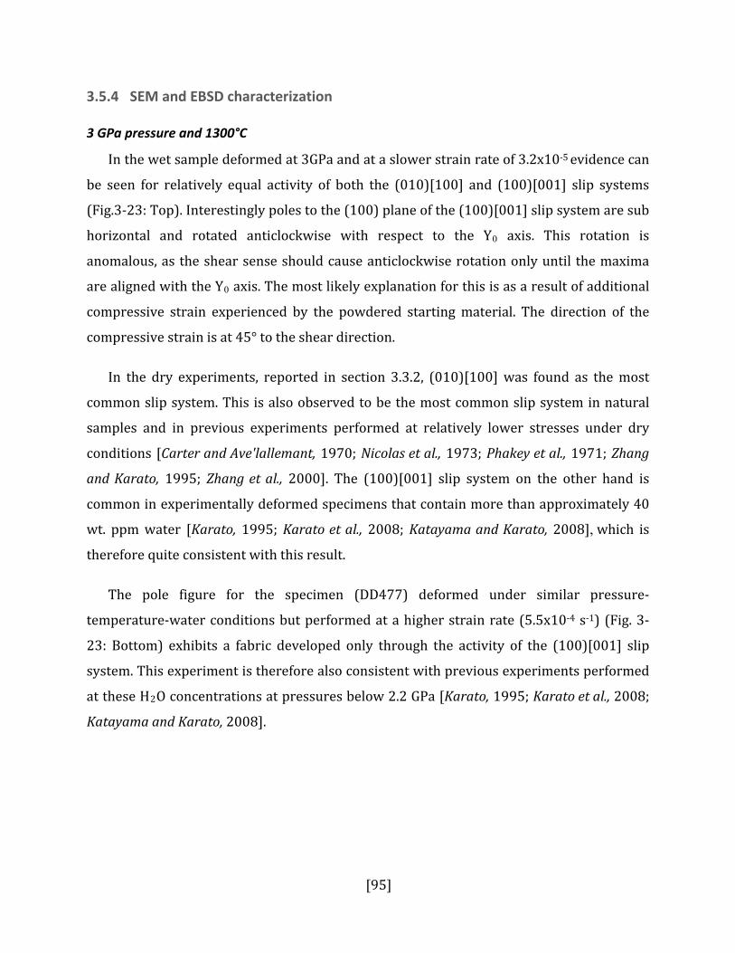
[95]

3.5.4 SEM and EBSD characterization

3 GPa pressure and 1300°C

In the wet sample deformed at 3GPa and at a slower strain rate of 3.2x10-5 evidence can

be seen for relatively equal activity of both the (010)[100] and (100)[001] slip systems

(Fig.3-23: Top). Interestingly poles to the (100) plane of the (100)[001] slip system are sub

horizontal and rotated anticlockwise with respect to the Y0 axis. This rotation is

anomalous, as the shear sense should cause anticlockwise rotation only until the maxima

are aligned with the Y0 axis. The most likely explanation for this is as a result of additional

compressive strain experienced by the powdered starting material. The direction of the

compressive strain is at 45° to the shear direction.

In the dry experiments, reported in section 3.3.2, (010)[100] was found as the most

common slip system. This is also observed to be the most common slip system in natural

samples and in previous experiments performed at relatively lower stresses under dry

conditions [Carter and Ave'lallemant, 1970; Nicolas et al., 1973; Phakey et al., 1971; Zhang

and Karato, 1995; Zhang et al., 2000]. The (100)[001] slip system on the other hand is

common in experimentally deformed specimens that contain more than approximately 40

wt. ppm water [Karato, 1995; Karato et al., 2008; Katayama and Karato, 2008], which is

therefore quite consistent with this result.

The pole figure for the specimen (DD477) deformed under similar pressure-

temperature-water conditions but performed at a higher strain rate (5.5x10-4 s-1) (Fig. 3-

23: Bottom) exhibits a fabric developed only through the activity of the (100)[001] slip

system. This experiment is therefore also consistent with previous experiments performed

at these H2O concentrations at pressures below 2.2 GPa [Karato, 1995; Karato et al., 2008;

Katayama and Karato, 2008].

[96]

5 GPa pressure and 1300°C

Strain-rate: 3.2x10-5; Water content: 90 wt. ppm; No. Of grains: 3320; Shear strain ≈ 1.2

Strain-rate: 5.5x10-4; Water content: 74 wt. ppm; No. Of grains: 3500; Shear strain ≈ 1.3

Figure 3-25: Wet samples deformed at 3 GPa and 1300°C. Sample deformed at lower strain rate (Top) shows two active slip systems – (010)[100] and (100)[001]. (Bottom) Sample deformed under higher strain shows only (100)[001] slip system to be active.

Strain-rate: 4x10-5; Water content: 279 wt. ppm; No. of grains: 4010; Shear strain ≈ 1.1

Strain-rate: 5x10-4; Water content: 214 wt. ppm; No. of grains: 3800; Shear strain ≈ 0.9

Figure 3-26: Wet samples deformed at 5 GPa and 1300°C. Both the high strain rate and low strain rate sample exhibit only one active slip system – (100)[001].

[97]

5 GPa pressure and 1400°C

The (100)[001] slip system is the only active slip system observed in the specimens

deformed at 5 GPa and 1300°C irrespective of the strain rate at which they were deformed

(Fig 3-24). In this case the [001] axis poles appear in a girdle pattern which likely results

from a component of compressive strain of the powdered aggregate sample. Compression

causes alignment in the [001] direction but as there is no unique shear direction a girdle

develops. Deformation experiments on powdered aggregates often result in a non-zero

contribution from compressive strain to the overall deformation during compaction of the

sample material.

At 5 GPa and slightly higher temperature of 1400°C the slower strain rate experiment

exhibits the same fabric as that observed at lower temperature i.e. (100)[001]. At the same

conditions but at higher strain rate the fabric of the recovered sample is again dominated

by the (100)[001] slip system (Fig 3-25). In addition, however, a weaker fabric resulting

from activity of the (010)[001] slip system is also present. While the (100)[001] slip

Strain-rate: 5x10-5; Water content: 168 wt. ppm; No. Of grains: 4670; Shear strain ≈ 2.4

Strain-rate: 5x10-4; Water content: 189 wt. ppm; No. Of grains: 3920; Shear strain ≈ 1.0

Figure 3-27: Wet samples deformed at 5 GPa and 1400°C. Sample deformed at lower strain rate (Top) shows mainly one active slip systems – (100)[001]. Whereas, (Bottom) Sample deformed under higher strain has two (010)[001] and (100)[001] slip systems active.

[98]

system has been previously observed to be active at high H2O content, the (010)[001] slip

system has been previously documented under higher stress conditions irrespective of the

H2O content. (Karato 1995; Karato et al. 2008; Katayama et al. 2008) report the (010)[001]

slip system as dominant over a range of H2O contents at stresses over 300 MPa, from

experiments performed at pressures <2.2 GPa. This would again be consistent with the

experiments performed at these conditions where evidence for the (010)[001] slip system

appears in the experiment performed with a faster strain rate and therefore under higher

stresses.

8.5 GPa pressure and 1300°C

Fabrics developed in samples deformed at 8.5 GPa and 1300°C (Fig 3-26) are in general

very similar to those found in the wet samples at 3 and 5 GPa. The sample at low strain rate

shows evidence for the dominant slip system being (100)[001], however either (010)[100]

or (010)[001] or both may also be active, albeit with much lower activity than the

(100)[001] slip system.

Strain-rate: 2.5x10-5; Water content: 419 wt. ppm; No. Of grains: 3850; Shear strain ≈ 2.4

Strain-rate: 5x10-4; Water content: 461 wt. ppm; No. Of grains: 4350; Shear strain ≈ 1.0

Figure 3-28: Wet samples deformed at 8.5 GPa and 1300°C. Irrespective of the strain rate, both the specimens deformed at 8.5 GPa and 1300°C show two active slip systems –(010)[100] and (100)[001]. This observation is consistent with activity of (010)[001] slip system at relatively higher stresses and (100)[001] slip system under hydrous condition.

[99]

Sample DD456, which was deformed at the same pressure and temperature conditions

but at a higher strain rate, has also developed a fabric dominated by the (100)[001] slip

system but again a weak contribution from the (010)[001] slip system also seems to be

present. This two-slip system combination appears consistent with dislocation activity

under higher stresses and hydrous condition as also proposed in previous studies [Karato,

1995; Karato et al., 2008; Katayama and Karato, 2008]. TEM observation on the sample

DD456 confirms the presence of these two slip systems (See section 3.1.2).

8.5 GPa pressure and 1500°C

Unlike the pole figures for dry experiments deformed at 8.5 GPa and 1500°C, where no

appreciable LPO was detected, most likely as a result of deformation occurring in the

diffusion creep regime and likely assisted by grain boundary sliding, wet experiments have

developed strong fabrics under both slow and fast strain rates.

Strain-rate: 1.5x10-4; Water content: 401 wt. ppm; No. Of grains: 1600; Shear strain ≈ 1.1

Strain-rate: 6x10-4; Water content: 340 wt. ppm; No. Of grains: 1920; Shear strain ≈ 1.3

Figure 3-29: Wet samples deformed at 5 GPa and 1500°C. Sample deformed at lower strain rate (Top) shows two active slip systems – (010)[100] and (100)[001]. (Bottom) Sample deformed under higher strain shows only (100)[001] slip system to be active.

[100]

At the relatively slower strain rate of 1.5x10-4 the (010)[001] slip system appears to

have led to a slightly stronger fabric than the sub equally present (100)[001] slip system.

At the faster strain rate of 6x10-4, however, the (100)[001] slip system dominates with only

a faint indication that (010)[001] slip may also be present.

3.5.5 TEM characterization

In order to relate the observed fabric with the dislocation microstructure a TEM

investigation was carried out on sample DD456, which was deformed under a higher

strain-rate of 5x10-4 at 8.5 GPa and 1300°C and contained a water content of 958 wt. ppm.

It was considered unnecessary to examine multiple wet samples from various conditions

using the TEM as EBSD measurements show all wet samples to have essentially similar LPO

fabric and therefore should all show evidence for dislocations with [001] Burgers vectors

slipping on either the (010) or (100) planes. The LPO for sample DD456 is typical of this

wet fabric, which is dominated by the (100)[001] slip system but with evidence for weaker

activity of the (010)[001] slip system.

TEM micrographs of DD456 show evidence for c-dislocations with slip planes being

(010) and (100). Edge segments for the (010)[001] dislocations are more mobile whereas

for the (100)[001] slip system dislocations, screw segments are more mobile. Cross-slip is

an active process as marked by the pointer 1 in the top image (Fig 3-28) and some of the

edge (100)[001] dislocations are kinked (pointer 2 in Fig 3-28). Evidence of cross-slip can

also be seen in the bottom-left image as indicated by the white arrows. The bottom-right

image shows long and straight screw dislocations from (010)[001] slip system. There is

fewer sub grain boundaries observed in comparison to samples deformed under dry

conditions. Presence of long and straight screw segments could also indicate resistance to

the glide of dislocation.

Although potentially also showing the tops of dislocation loops, the structures in the

HRTEM image shown in Fig 3-29 seem to be more consistent with being the cores of a

weakly dissociated c-dislocations. The Fast Fourier transformed image (Fig 3-29: lower

right) of the dissociated c-edge dislocation when viewed along the {110} zone axis, shows a

[101]

variation in contrast. The image contrast in the dislocation core regions is different from

that in the surrounding bulk, indicating the core is expanded.

Figure 3-30: TEM micrographs for the wet specimen DD456. Deformation experiment was carried

out at 8.5 GPa and 1300°C with a strain rate of 5x10-4. Top figure shows the presence of c-dislocations. (100)[001] dislocations are mostly of edge nature where as the [001] screw dislocations are most likely from (010)[001] dislocation. Evidence of cross-slip can be also seen as indicated by marker 1 in top image and white arrow in the bottom-left image. Bottom-right figure also shows straight c-screw dislocation from (010)[001] slip system.

[102]

Figure 3-31: A typical HRTEM image (upper and lower right) and the Fast Fourier transformed

image (lower right) of the dissociated c-edge dislocation viewing along the {110} zone axis of a deformed hydrous olivine. The image contrast in the dislocation core regions is different from that in the surrounding bulk, which indicates that the core is expanded.

[103]

3.6 Deformation experiment on Peridotite modal composition

Deformation experiments performed were performed on a peridotite assemblage at 8.5

GPa and 1300°C. In the low strain rate sample, the likely active slip systems are (010)[100]

and (010)[001] whereas the dominant slip system in olivine in the high strain rate sample

is (010)[001]. In case of pyroxene assemblage (100)[001] slip system is the only likely

active slip system in both high and low strain rate sample (Table 3-8).

Table 3-8: Experimental conditions for Peridotite deformation experiments and likely active slip systems

Run ID Pressure (GPa)

Temperature (°C)

Strain rate (x10-5 s-1)

Stress (MPa)

Likely Active slip systems

DD495 8.5 1300 5 230 Olivine: (010)[100] and (010)[001] Pyroxene : (100)[001]

DD483 8.5 1300 40 325 Olivine: (010)[001] Pyroxene : (100)[001]

Strain-rate: 5x10-5; Shear strain ≈ 1.6

Strain-rate: 50x10-5; Shear strain ≈ 1.3

Figure 3-32: Peridotite samples deformed at 8.5GPa and 1300°C. Olivine in the slowly deformed aggregate likely has both (010)[100] and (010)[001] slip systems active whereas in the experiment conducted at higher strain rate the slip system is (010)[001]. Pyroxene in both the cases show (100)[001] slip system

[104]

These results indicate an identical olivine fabrics to those observed in monomineralic

experiments at the same conditions. Fabrics for diopside and enstatite were found to be

similar to those found in previously performed lower pressure experiments.

In-situ measurement of stress using piezoelectric sensor

Piezoelectric stress measurements were made using GaPO4 single crystals within a 8/6

multianvil assembly. Many test experiments were made in the D-DIA however the most

successful runs, where drift was minimal, were performed using the 6-axis MAVO press.

The success of the MAVO press in these experiments most likely originates from the highly

resistive electrical insulation of each individual anvil. In the D-DIA press the top and

bottom guide blocks are electrically connected via the oil lines to the deformation rams.

Figure 3-33: Output voltage from

the charge amplifier as a function of time for an experiment where a GaPO4 crystal was compressed to 2 GPa and then held at constant static pressure for 80 min.

The anvils therefore cannot be

used as part of the circuit and

crystals must, therefore, be

connected via separate cables that

pass through the gasket. The use of

the cables that have to pass

through the gaskets that form as

the cubic assembly is compressed probably results in current leakage.

Figure 3-33 shows the output voltage from the charge amplifier for an experiment

compressed to 2 GPa, which remained under static conditions for 80 min. This voltage

change would correspond to changes in stress of the order of 5 GPa over this time period

and more likely results from drift. The origin of this drift is unclear. Drift is positive for the

first 30 min but eventually goes through a maximum and decreases. However, the slope of

[105]

the drift is relatively linear over periods of a few minutes such that drift can be eliminated

from the data through fitting of a linear background over short periods.

Figure 3-34: Output voltage as a function of time for an experiment held statically at 2 GPa and then

deformed by driving out the anvils in the horizontal direction simultaneously after approximately 60 s by 20 microns. The drift before 60 s is linear and is removed by subtracting a linear background as shown in B.

Figure 3-34 shows the output voltage as a function of time in seconds for an experiment

at 2 GPa were the cubic assembly has been deformed by 40 μm at approximately 60s after

the start of data recording. The assembly is deformed by driving the 4 horizontally aligned

anvils in the decompression direction by 20 μm. As the pressure on the vertical anvils

remains constant this results in a concurrent compression of the vertical anvils by

approximately the same distance. As deformation of the assembly occurs, a break in slope

of the output voltage is observed. In figure 3-32A the background drift has been subtracted

from the voltage measurements by fitting a linear background to the data recorded just

before deformation. This drift corrected voltage shows a clear and sharp signal generated

by the piezoelectric crystal as a result of the deformation.

The charge Q on the crystal, developed as a result of deformation, can be calculated

from 𝑄 = 𝑉𝑜.𝐶𝑟 where 𝐶𝑟 = 10𝑥10−9𝐹 and 𝑉𝑜 is the drift corrected voltage. The force on

the crystal can then be calculated using equation 2.a. The stress on the crystal is

determined by diving the force by the surface area of the crystal which is 1.2 mm in

diameter.

Four examples of assembly deformation are shown in Figure 3-33 where the stresses

determined from the piezoelectric crystal can be compared with the corresponding anvil

A B

[106]

displacement. Figure 3-35A shows the stress determined from the same deformation event

as shown in Figure 3-34. The vertical anvils were each compressed by 20 μm and the

corresponding stress reached approximately 80 MPa.

The timescale for the increase in stress is longer than the deformation event as the anvils displace in a matter of a few seconds. Figure 3-35B shows the piezoelectric stress developed as a result of retracting the horizontal anvils, which lead to advancement of the vertical anvils, by 0.5 μm each. Although the signal is noisy an increase in stress of the order of 2-3 MPa can be observed indicating that the technique is extremely sensitive.

Figure 3-3-35: Stress and anvil displacement versus time for 4 deformation events performed at 2

GPa.

Figure 3-35C shows a test where the horizontal anvils were advanced rather than compresses leading to a retraction of the anvils in the vertical direction. This release of the anvils in the vertical direction caused a negative stress pulse, demonstrating that the effect is sensitive to the direction of the applied stress. In Figure 3-35D an advancement of the vertical anvils by approximately 50 μm, i.e. a combined deformation of 100 μm, has caused a large stress to develop of the order of 300 MPa. Therefore the determined piezoelectric stress is not only sensitive to direction of the stress but is also seemingly proportional to the strain of the assembly.

[107]

4 Discussion

Randomly oriented grains deforming plastically develop crystallographic preferred

orientation or CPO as a result of anisotropic mechanical properties. The primary reason for

the preferred alignment of the crystals is the mismatch between the rotational component

of the crystal and the macroscopic strain [Karato et al., 2008]. Although phenomena such as

dynamic recrystallization also play an important role in the overall deformation of a

polycrystalline aggregate, dislocation glide is often the primary agent of deformation.

The total intercrystalline deformation in a polycrystalline aggregate generally results

from slip on more than one slip system. For an individual crystal to deform in a

homogeneous manner, a minimum of five independent slip systems are required. This

condition is called ‘Von Mises criteria’. If this condition is satisfied then a crystal can take

any arbitrary shape in response to the external force field. Olivine does not possess five

independent slip systems (Durham et al. 1977), in addition the three available slip systems

that olivine has, are of varying strength. Onset of deformation occurs when the shearing

force acting on a given slip system exceeds a critical value called the “Critical resolved

shear stress” or CRSS. The requirement for homogeneous deformation drives olivine

crystals to deform also on the harder slip planes. Sometimes, harder slip planes are

activated first because they are oriented most favorably with respect to the external stress

field (Lister et al. 1978). The need for slip on harder slip systems, on the other hand, can be

minimized if additional deformation processes are also active. Dislocation, climb which is

another intercrystalline deformation process, is one such process. In fact the results of

Durham et al. (1977) suggest a significant contribution from climb processes during

deformation for olivine grains oriented along [101]c. This orientation activates two harder

slip systems – (001)[100] and (100)[001]. Other intercrystalline deformation processes

such as, grain boundary migration and grain boundary sliding can also accommodate some

amount of strain, thereby reducing the need for slip on harder slip system (Lister et al.

1978; Paterson 1969).

[108]

Based upon the observation that a significant portion of the strain can be generated by

diffusive processes (e.g. dislocation climb and grain boundary sliding), the need for 5

independent slip systems can be relaxed. For this reason Karato has argued that dislocation

glide on only the easiest slip system can in many cases accommodate sufficient strain such

that a simple relationship exists between the LPO and this easiest slip system [Karato,

1986; 1998; Karato et al., 2008]. However, the results obtained in this thesis imply that this

is likely to be an over simplification. With the aid of VPSC (Visco-plastic self consistent)

modeling, the results of which will be discussed in section 4.4, it can be shown that many of

the LPOs observed in this study require sufficient strain on more than one slip system to

explain their development. Although, some of these specimens display LPO resultant from

high stress deformation, stresses which are unrealistic for the upper mantle, the complex

LPO development is, never the less, apparently due to significant strain on more than one

slip system. The activation of multiple slip systems is likely also to occur in the mantle,

particularly in regimes which are transitional between dominant slip systems, such as

resulting from changes in the H2O content of the mantle rocks. It has also been shown that

the activity of three independent slip systems may be sufficient to accommodate enough

strain by dislocation glide if modest strain heterogeneity is allowed. Results from Paterson

(1969) suggest that in the case of olivine, strain accommodated by the fourth and fifth

hardest slip systems was around 15% and 1% respectively.

As this study is focused on changes in the olivine fabric resulting from changes in

various physical-chemical conditions (stress, temperature, water and pressure), it is

important to understand how these changes in the relative activity of slip systems

translates in to changes in the LPO. A crucial aspect in studying LPO transitions is to

understand if changes are gradual or abrupt. Based upon a Taylor-Bishop-Hill model Lister

and coworkers have simulated the possible LPOs with a given set of active slip systems

[Lister and Hobbs, 1980; Lister and Paterson, 1979; Lister et al., 1978]. They found that a

range of smoothly varying CRSS values can produce very similar LPOs, but there are critical

CRSS ratios where abrupt changes in the LPO may occur. This model allows for a complex

kind of LPOs with abrupt changes in it as the (relative) CRSS values change with changing

state of stress, water and other parameters. Moreover, merely the relative ease (or

[109]

difficulty) of slip activity does not necessarily guarantee that a set of slip systems should be

active together. Geometric constraints on deformation by dislocation glide, imposed by the

need for homogeneous strain, may prevent a set of slip systems being active together even

if their CRSS values permit their activity. For example, for olivine the (001)[100] LPO

pattern should not develop when the (010)[001] slip system is active, even when

(001)[100] is an easy slip system [Tommasi et al., 2000], unless significant contribution to

strain is made by phenomena such as dynamic recrystallization, grain boundary sliding etc.

In the following section the results of high pressure and temperature deformation

experiments on olivine will be summarized and the main findings discussed. The main

observation is that changes in pressure have a minor influence on olivine LPO development

compared to changes in olivine H2O content and flow stresses. Explanations for these

effects will be examined.

4.1 Effects of stress and pressure on the slip systems in olivine: Evidence from deformation experiments on “dry” olivine

As has been discussed previously, stress, water and pressure can have all be reported to

have strong effects on the slip systems in olivine. Results from previous studies suggest

that higher stresses tend to promote the (010)[001] slip system whereas (100)[001] slip

systems are more active under water rich conditions [Jung et al., 2006; Karato et al., 2008].

Reports also indicate that the (001)[100] slip system can also be the dominant slip system

under moderately hydrous conditions [Katayama et al., 2004]. It has also been proposed

based upon experimental results and computer modeling that c-slip becomes easier at

higher pressures [Couvy et al., 2004; Durinck et al., 2005; Jung et al., 2009a; Raterron et al.,

2007]. Although doubts have been raised about the validity of the last conclusion, mainly

due to uncertainties related to stress and water content under which these experiments

were performed [Karato et al., 2008]. The results obtained in this thesis, however,

apparently indicate that pressures up to 11 GPa may not actually cause any change in the

major slip system (Fig 4-1 and 4-2), as discussed below.

[110]

Figure 4-1 shows a summary of the active slip systems in various specimens deformed

under wet and dry conditions in this study. Each slip system has been assigned a separate

color for clarity. As shown on the top-right part of the image, the four rectangular boxes

show the data from four experiments that were performed at same pressure-temperature

conditions. Two rectangles on the bottom show results from the experiments performed

under dry conditions whereas the top two rectangles show data from wet experiments.

Two rectangles on the left side show the samples deformed at relatively slower strain rates

(lower stresses) whereas the other two rectangles on the right show the fabric observed in

experiments conducted at higher strain rates (higher stresses). Evidence for four slip

systems was observed in the experiments and the width of the colour bars is proportional

to the number of grains in each sample that show evidence for activity of that particular

slip system.. At 1300°C and 3 GPa, for example, the first rectangle at the bottom-left is

colored in only green, implying that the fabric in this specimen is of the A-type which

results from the dominant activity of the (010)[100] slip system. The top-right rectangle at

3GPa and 1300°C contains green and blue coloured rectangles of equal width, which

implies that approximately half of the data points display an A-type fabric (green colored),

indicative of (010)[100] slip system activity, while the other half , (blue), indicate activity of

(100)[001] i.e. producing a C-type fabric (Table 4-1). The presence of both of these fabrics

in this specimen indicates that physical and chemical conditions are suitable for the activity

of both (010)[100] and (100)[001] slip systems.

Table 4-1: Fabric type and nature of slip systems (Jung and Karato, 2001)

Fabric type A-type E-type B-type C-type D-type Dominant Slip system

(010)[100] (001)[100] (010)[001] (100)[001] (100){0kl}

Based upon the summary of fabrics shows in the image below, it is clear that under dry

conditions, mainly two kinds of slip systems dominate the deformation by dislocation glide

in olivine, (010)[100] and (010)[001]. Every specimen deformed under similar P-T

condition but at a different strain rate has a different proportion of data points indicating

A-type and B-type fabrics. In addition, every specimen which was deformed at a higher

[111]

strain rate (and hence higher flow stress) has a larger proportion of data points indicating

the B-type fabric.

Figure 4-1: Summary of fabrics observed in San-carlos olivine deformed under dry and wet condition at different strain rates. Experiments were performed between 3 to 8.5 GPa and 1300°C to 1500°C. Width of each colour bar is proportional to the approximate number of grains that were present in the subset containing data points for that slip system. Refer to section 3.4.14 for more details. As shown in the table at top-right corner of the page, the lower row in the 2x2 matrix contains results from dry experiments while upper row contains results from wet experiments. The left column in 2x2 matrices has results from slowly deformed samples whereas samples deformed at relatively higher strain rate have their fabrics shown in the right column.

Hence, it can be concluded that under high stress deformation conditions the B-type

fabric dominates i.e. the (010)[001] slip system contributes to most of the strain. Although,

[112]

the proportion of data points with the B-type fabric increases at 5 GPa and 1400°C with

respect to 5GPa and 1300°C , this is actually in line with a slightly higher strain rate and

hence higher flow stresses in specimens deformed at 1400°C.

Equally important is the observation that at 8.5 GPa and 1300°C, the specimen

deformed at a slower strain rate shows a larger proportion of data points with the A-type

fabric. There have been reports that at higher pressures c-slip, slip with a Burgers vector

[001], becomes easier than a-slip. The approximate transition pressure between a-slip and

c-slip apparently varies between studies with Jung et al. (2009) reporting this transition at

approximately 3.6 GPa whereas Raterron et al. (2007) place the transition at approximately

7.6 GPa. If there was indeed a pressure related easing of the b = [001] slip then it would be

hard to reconcile this with the results in Fig. 4-1, which show dominant (010)[100] slip

system activity at slower strain rates at 8.5 GPa. These results are rather more in line with

the observation that a change from a-slip (b = [100] slip) to c-slip (b = [001] slip) can occur

at higher stresses [Jung et al., 2006]. Another piece of strong evidence that a-slip continues

to be the dominant slip mechanism at high pressures, comes from analysis of specimens

that were hot-pressed in the 6-8 multianvil under pseudo-hydrostatic conditions i.e.

without the inclusion of alumina hard parts in the multianvil assembly that can lead to

strong deformation (Fig 4-2). In two such hot-pressing experiments, dry olivine powder

was hotpressed at 1400°C at pressures of 8.5 GPa and 11 GPa. During cold compression of

the multianvil assembly, some dislocations are introduced in the olivine sample. Once, the

sample is heated up to high temperatures, dislocation recovery processes start, leading to

deformation of the sample and development of a weak LPO. As seen in the pole figures on

the next page, the A-type fabric are clearly present both of these specimens.

[113]

Figure 4-2: Pole figures for two polycrystalline olivine specimen hotpressed at 8.5 GPa (H3115) and 11 GPa (H3354). Specimens were annealed at 1400°C. Both pole figures resemble A-type fabric which is often observed under low stress and dry deformation environment. Presence of A-type fabric in these hotpressed specimen is indicative of (010)[100] slip system activity.

The LPO fabrics observed in Fig 4-2 could have only developed in these samples if a-slip

was dominant. Interestingly, the first report of a pressure induced transition in olivine LPO

was by Couvy et al. (2004) from deformation experiments performed at BGI using a similar

multi-anvil apparatus. The assembly setup was in simple shear configuration, however,

unlike that reported here where no deliberate attempt was made to deform the olivine

sample during hot-pressing. The peak stress that would have developed during the initial

stages of annealing must be lower than in the experiments of Couvy et al. (2004). Hence,

the hot-pressing fabric in specimens H3115 and H3354 must result from deformation

under low stresses and thus it can be concluded that a-slip continues to be the easiest slip

mechanism even up to 11 GPa pressure under low stress deformation conditions.

The observations in previous studies where a transition of a-slip to c-slip has been

attributed to increasing pressure are more likely to result from higher stresses which may

inevitably increase in experiments at higher pressures.. Pole figures shown by Jung et al.

(2008) do not show strong LPOs despite large amounts of strain that their samples

[114]

experienced. Results from Raterron et al. [2007] where they observed a pressure related

transition in the slip system, are based upon experiments performed at stresses varying

between 300 MPa to 1800 MPa. Similarly in the study of Ohuchi et al. [2011] most

specimens exhibiting the presence of c-slip have estimated stresses in excess of 350 MPa.

Only in one specimen are stresses reported to have been less than 300 MPa but this sample

actually indicates dominant activity of the (100)[001] slip-system under dry conditions.

Additionally the observation that various studies have placed the pressure of the transition

at widely varying values can also be explained if this transition in fact results from

increasing flow stresses.

Figure 4-3 shows the fabrics observed in this study compared with those reported in

previous studies. Larger symbols with black boundaries are data points from this study.

The results are in very good agreement with variations in fabric reported by Karato et al.

[2008]. At higher stresses, under dry condition the B-type fabric was observed, whereas

under lower stresses and dry conditions deformation resulted in the dominance of A-type

fabric. Hydrous specimens exhibit C-type fabric which also agrees with previous reports

from lower pressure deformation studies. None of the specimens characterized in this

study showed evidence of E-type or D-type fabric because experimental conditions in were

never entered these regions of stress-water content space. Broken grey lines in the image

are the likely transition boundaries between two different fabric types.

The main conclusion of the results obtained from deformation experiments under dry

condition is that pressure apparently plays no direct role in the slip system transition in

olivine. (010)[001] slip system contributes most to the overall strain at higher stresses and

the B-type fabric should be observed under such environment. A-type fabric should be the

most dominant type fabric that we would expect to see in the lithospheric mantle because

stresses are expected to be too low (<10 MPa) to generate B-type fabric. However, in the

mantle wedge near subducting slabs it is possible that regions exist where B-type fabric

could occur as these regions are most likely deforming at relatively high stresses.

[115]

Figu

re 4

-3: D

efor

mat

ion

data

from

this

stu

dy a

nd o

ther

stu

dies

are

sho

wn

as a

func

tion

of s

tres

s an

d w

ater

co

nten

ts (

T ∼

147

0–16

70 K

). La

rger

sym

bols

wit

h bl

ack

boun

dari

es r

epre

sent

dat

a fr

om t

his

stud

y w

here

as

rest

of

data

are

fro

m K

atay

ama

et a

l. 20

04. E

xcep

t, on

e of

the

dat

a fo

r D

-typ

e fa

bric

is

from

Bys

tric

ky e

t al

. (2

001)

. Wat

er c

onte

nt w

as e

stim

ated

usi

ng t

he P

ater

son

(198

2) c

alib

rati

on. B

roke

n gr

ay l

ines

ind

icat

e th

e lik

ely

tran

siti

on li

ne b

etw

een

two

diffe

rent

fabr

ic ty

pes

(Mod

ified

aft

er K

arat

o et

al.,

200

8)

[116]

Lack of LPO in the dry samples deformed at high temperature at 1500°C and 8.5 GPa

has likely resulted from diffusion accommodated grain boundary sliding. High grain

growth, as evident from grain size measurements made in recovered experiments, points

to the dominance of diffusion creep. The presence of straight grain boundaries indicate that

conditions were suitable for grain boundary sliding. There were many four-grain junctions

present in these samples and these junctions were slightly diamond shaped which is

additional evidence that grain boundary sliding may have been the active deformation

process. It is well known that diffusion creep does not result in LPO development.

Moreover, grain boundary sliding (GBS) also does not favour LPO development because in

the presence of GBS, intracrystalline deformation is only weakly dependent on the

orientation of grains [Drury and Humphreys, 1988; Karato et al., 1986; Zhang et al., 1994].

Fabric types observed in the olivine deformed as a part of the peridotite modal

composition are identical to those observed in monomineralic experiments at the same

conditions. The dominant slip system in the pyroxene component of this aggregate had

most likely (100)[001] slip system active.

4.2 Fabric types under water rich conditions

The hydrous specimens in this study all contain water contents in excess of 50 ppmw.

From figure 4-3, it can be seen that the C-type fabric is the most commonly observed fabric

in these specimens. However, some of the high stress water-rich samples also indicate the

presence of the B-type fabric e.g. DD456. A TEM study on one of the wet samples (DD456)

indicates the dominant presence of b = [001] dislocations. The active slip systems in this

specimen were observed through TEM to be (100)[001] and (010)[001]. The activity of the

(010)[001] slip system in this sample is similar to activity observed in the dry specimens

deformed under higher stresses. The (100)[001] slip system is an unusual slip system

because glide on the (100) plane most likely involves breaking of SiO4-tetrahedra, unlike

glide on (010) where no SiO4 tetrahedra are encountered during glide. Dislocation

microstructures in the wet sample (DD456) observed using the TEM show that dislocation

loops on the (010) glide plane have longer screw segments than their edge components.

There are long edge segments of c-dislocations visible and most of them are part of c-

[117]

dislocations on the (100) glide plane. Where only screw segments of c-dislocations are

visible it is unclear whether glide is also occurring on the (100) plane because

determination of the glide plane is not possible when only screw segments are visible. The

abundant number of c-dislocation on the (010) slide plane with a screw nature is in clear

contrast to the c-dislocations observed in the dry specimens which were mostly of edge

nature under similar P-T-stress conditions. Another pertinent observation in the wet

sample is the evidence of climb of edge dislocations and cross-slip of screw dislocations. A

few prismatic loops lying in the (010) plane can also be observed, which have been

associated with the presence of H2O in olivine.

A further interesting observation is that the transition line between C-type and B-type

fabrics appears to have a positive slope with respect to the olivine H2O content. This is in

contrast to the previous study of Katayama et al. 2004 where a negative slope was

proposed. In accordance with Fig 4-3 it would require increasingly higher stresses to push

olivine from the C-type fabric regime into the B-type regime with increasing water content

of olivine. It would also imply that water favours slip on the (100) plane over the (010)

plane.

4.3 Physical basis for slip system changes in olivine

In the following section an attempt is made to identify a physical basis for changes in

slip systems as a function of stress and water content. As mentioned previously, under high

stress deformation conditions deformation by b = [001] slip becomes dominant and the slip

system changes from (010)[100] to (010)[001]. Slip with b = [001] also becomes dominant

in the presence of water. In this case, the dominant glide plane becomes (100) which are

not known to be an easy glide plane because of way the SiO4 tetrahedra are arranged in

olivine. Based upon the rheological and microstructural data available from previous

studies along with results from this study, an attempt is made here to explain the

dominance of the (010)[001] slip system under higher stresses and the cause of C-type

fabric development in wet specimens due to the likely action of the (100)[001] slip system.

[118]

4.3.1 Dominance of (010)[001] slip system at higher stresses

Studies on rheology of olivine single crystals point towards a temperature related

transition in the olivine slip system (Fig 4-4).

Measurements of the critical resolved shear stresses for (010)[100] and (010)[001] slip

systems indicates that CRSS for the (010)[001] slip system is lower than the CRSS for the

(010)[100] slip system at lower temperature. Whereas, the reverse is observed at higher

temperatures where the (010)[100] slip system is initiated at much lower stresses. This

transition between CRSS values of the two slip systems occurs at around 1200°C at a

corresponding value of 400 MPa CRSS.

Figure 4-4: Critical resolved shear stresses (CRSS) of the (010)[100] and (010)[001] slip systems as a function of temperature. Data (corresponding to a strain rate of 10-5 s-1) from experiments performed on single crystals oriented along [011]c (black-filled symbols) to promote [001](010) glide and along [110]c (open symbols) to promote [100](010) glide. (Source- PhD thesis – Helen Couvy, 2005)

Interestingly, in this study the fabric transition from A-type to B-type, which is related

to the transition between the dominant slip systems (010)[100] and (010)[001], was also

observed at around 300 MPa, which given the uncertainty in both determinations puts it in

close proximity to the cross-over in the CRSS for the two slip systems shown in Fig 5-4. In

the following section, it is argued that the stress related transition in the fabrics is a logical

[119]

consequence of changes in the CRSS of the two slip systems with temperature. Before this

argument is pursued, however, it is worthwhile to review why CRSS changes with stress.

The temperature dependence of CRSS has been observed in metals and various ionic

and covalent compounds [Castaing et al., 1981]. Also, different slip planes can have

different temperature dependency of CRSS as is shown for α-Al2O3 in Fig 4-5.

Figure 4-5: Temperature dependence of the critical shear stress τc(T) of covalent crystals measured under high or atmospheric pressure. The data are taken from the references: Lagerlof et al. (1994) for α-Al2O3, Castaing et al. (1981b) for Si and Boivin et al. (1990) for GaAs of intrinsic and p-type. (Figure source: Koizumi et al., 1994)

This temperature dependence of the CRSS value is generally explained on the basis of

intrinsic resistance to dislocation motion by the process known as the “Peierls process”. It

has been suggested that the Peierls process becomes important for the rheology of olivine

at higher stresses. Power law creep provides a good description for olivine flow only at

lower stresses, whereas at higher stresses the olivine flow law becomes exponential

[Goetze, 1978; Katayama and Karato, 2006]. An exponential flow law can be predicted

based upon dislocation motion by the Peierls mechanism via nucleation of double kinks.

Dislocation motion by the Peierls mechanism may be more important for b = [001] because

[120]

dislocation lines tend to be straighter for c-dislocations [Karato et al., 2008; Phakey et al.,

1971]. Although, the value of critical stress at which the Peierls process starts to dominate

the flow behaviour is not yet clear.

Peierls mechanism of deformation by double kink nucleation

At finite temperatures, dislocations do not move all at once in a plane strain manner but

motion occurs through the generation and nucleation of kink-pairs. In this regime,

nucleation of kink-pairs is the rate determining step for slip. Once a kink grows above a

critical size, further straining takes place by migration of these kinks.

A kink on a dislocation line can be envisaged as a dislocation on a dislocation line (Fig 4-

6). According to the Peierls mechanism, a straight dislocation line has its lowest energy

when it lies in a potential valley parallel to lines of closest packing of atoms on the slip

plane. During the motion of a straight dislocation from one valley towards the next, the

atoms in the vicinity of the core of the dislocation change their positions and bond angles,

causing the energy of the dislocations to increase. Midway between two adjacent valleys,

the dislocation energy reaches a maximum value and any additional displacement will

cause the dislocation to fall down the energy maxima into the next valley. The maximum

shear stress necessary to promote such forward motion of the dislocation is known as the

Peierls stress 𝜏𝑝.

Figure 4-6: Left image shows a kink (dark line) lying across a potential valley. Broken lines indicate the potential maxima with minima represented by the solid lines. Right: A kink in the presence of external stress has its equilibrium position displaced away from the unstressed position. Size of the kink is represented by kink height h and width 2K+L in case of a trapezoidal kink model. (Source: Suzuki et al. 1995)

[121]

At a fixed strain rate, the number of kinks forming per second is a constant because

kinks act as the basic unit of deformation. In such a scenario, total power imparted to the

kink must be held constant to maintain their nucleation frequency. If the temperature is

dropped while holding the strain rate constant, flow stress will increase to maintain the

nucleation rate and vice versa (Fig 4-7). Nucleation of a kink takes place with the help from

thermal agitation and energy supplied by the external stress. If the energy supplied by

these two means is not sufficient then a double kink may form momentarily and then

collapse to annihilate each other. Hence, there is a defining set of stresses and

temperatures at which dislocations can move by kink nucleation. The locus of this (σ,T)

pair is the CRSS versus temperature curve.

Any (σ,T) combination that lies towards the origin-side of the CRSS-T curve will not be

able to initiate slip on a given slip system whereas (σ,T) combinations lying on the far side

of the curve will lead to high activity of that slip system.

Figure 4-7: Enthalpy change associate with the contribution from thermal perturbation at temperature T and mechanical work done by stress σ.

The enthalpy change associated with the displacement of kinks from one barrier to

another can be expressed as

[122]

∆𝐻 = ∆𝑃 + ∆𝐸 − ∆𝑊 4.a

𝑤ℎ𝑒𝑟𝑒; ∆𝑃 𝑖𝑠 𝑒𝑛𝑒𝑟𝑔𝑦 𝑐ℎ𝑎𝑛𝑔𝑒 𝑑𝑢𝑒 𝑡𝑜 𝑡ℎ𝑒 𝑃𝑒𝑖𝑒𝑟𝑙𝑠 𝑝𝑜𝑡𝑒𝑛𝑡𝑖𝑎𝑙

∆𝐸 𝑖𝑠 𝑡ℎ𝑒 𝑒𝑙𝑎𝑠𝑡𝑖𝑐 𝑠𝑒𝑙𝑓 𝑒𝑛𝑒𝑟𝑔𝑦 𝑐ℎ𝑎𝑛𝑔𝑒 𝑜𝑓 𝑏𝑜𝑤𝑒𝑑 𝑜𝑢𝑡 𝑑𝑖𝑠𝑙𝑜𝑐𝑎𝑡𝑖𝑜𝑛;𝑎𝑛𝑑

∆𝑊 = 𝜏 × 𝑏 × (𝑘𝑖𝑛𝑘 𝑎𝑟𝑒𝑎) 𝑖. 𝑒. 𝑡ℎ𝑒 𝑤𝑜𝑟𝑘 𝑑𝑜𝑛𝑒 𝑏𝑦 𝑡ℎ𝑒 𝑒𝑥𝑡𝑒𝑟𝑛𝑎𝑙 𝑠𝑡𝑟𝑒𝑠𝑠

In general, enthalpy change associated with the formation of a critical kink size,∆𝐻∗ can

be expressed as a function of stress for a material of shear modulus G as Koizumi et al.

[1994]

∆𝐻∗(𝜏) = 2𝑈𝑘∗ − 𝐴𝐺𝑏3�𝜏 𝜏𝑝⁄ �1 2⁄ 4.b

𝑤ℎ𝑒𝑟𝑒;

𝑈𝑘∗ = 𝐸𝑛𝑒𝑟𝑔𝑦 𝑜𝑓 𝑎𝑛 𝑖𝑠𝑜𝑙𝑎𝑡𝑒𝑑 𝑘𝑖𝑛𝑘, 𝐴 = 𝑐𝑜𝑛𝑠𝑡𝑎𝑛𝑡,

𝑏 = 𝐵𝑢𝑟𝑔𝑒𝑟𝑠 𝑣𝑒𝑐𝑡𝑜𝑟 𝑎𝑛𝑑 𝜏𝑝 = 𝑃𝑒𝑖𝑒𝑟𝑙𝑠 𝑠𝑡𝑟𝑒𝑠𝑠

Parameter “A” is dependent upon the shape

of the Peierls barrier. Calculations

performed here indicate that value of A for

a-slip should be close to 0.274, whereas it

should be 0.72 for c-slip. Koizumi et al. 1994

have suggested a shape dependent

formalism for this periodic Peierls potential

by introducing a constant α (Fig 4-8).

Figure 4-8: The function g(x) giving the shape of the Peierls potential. It is sinusoidal for a = 0, dam-like with a Roof top for a=0.5, and camel-hump shaped, with an intermediate minimum for a = 0.8. (Source: Koizumi 1994)

Calculations made using the sinusoidal potential of [Hirth and Lothe, 1992] (see

Appendix II for details); fail to predict the slope of the CRSS versus Temperature curve.

This calculation would correspond to a 𝛼 = 0 curve from Koizumi et al. (1994). At this

stage it is not clear if a simple symmetric Peierls potential is even suitable for a description

of olivine, however, a relation of the form presented below (Eq. 4.c) seems to describe well

[123]

the CRSS-temperature curve for the two slip systems in olivine (Fig 4-9) with values of

different parameters show in the table below (Table 4-2). Normalized kink energies are

derived for an abrupt kink using a sinusoidal potential.

∆𝐻∗(𝜏) = 𝐺𝑏3 �2𝑈𝑛∗ − 𝐴�𝜏 𝜏𝑝⁄ �1 2⁄ � 4.c

𝑤ℎ𝑒𝑟𝑒 𝑈𝑛∗ 𝑖𝑠 𝑡ℎ𝑒 𝑛𝑜𝑟𝑚𝑎𝑙𝑖𝑧𝑒𝑑 𝑒𝑛𝑒𝑟𝑔𝑦 𝑜𝑓 𝑎𝑛 𝑖𝑠𝑜𝑙𝑎𝑡𝑒𝑑 𝑘𝑖𝑛𝑘

To relate the enthalpy calculated using double kink nucleation method to the flow

temperature a relation of the form ∆𝐻∗(𝜏) = 𝛽𝑘𝐵𝑇 is used. 𝛽 is a dimensionless constant

whose value ranges from 30-35 for metals and alloys and it is weakly dependent upon the

strain rate [Suzuki et al., 1995]. In olivine higher values of 𝛽, 68 for a-slip and 155 for c-slip

are required for a strain rate of 10-5s-1.

Table 4-2: Value of constants that describe well the CRSS-Temperature relation for the two slip systems in olivine

Slip

systems

A β 𝑼𝒏∗ 𝝉𝒑(MPa)1 b (Å)

(010)[100] 0.274 68 0.6437 9100 4.76

(010)[001] 0.72 155 0.6708 15600 5.99 1. Value of Peierls stress for a-slip -9100 MPa is sourced from Evans and Goetze, 1979. Peierls stress of c-slip is from Raterron et al.

2007

[124]

Figure 4-9: Predicted CRSS values for a-slip and c-slip using double kink nucleation theory. At around 1300°C, 300 MPa stress would barely activate c-slip whereas at around 600 MPa, both c-slip and a-slip are active. In this case, activity of (010)[001] slip system would be higher because this slip system has extra thermal energy available at its disposal.

Higher activity of c-slip at higher stresses

Natural consequence of the CRSS versus Temperature relation observed in olivine for

two slip systems (010)[100] and (010)[001] is that c-slip in (010)[001] slip system should

have higher activity at higher stresses. This can be understood by looking at the image

presented above (Fig. 4-9). If we consider a constant temperature line at around 1300°C in

Stress-Temperature space then at a stress of 300 MPa, c-slip would be barely active

because the minimum values of stress-temperature pairs required to nucleate kink for C-

dislocations are barely met. On the other hand a-slip would be active under these

conditions because 300MPa-1300°C lies on the far side of CRSS-Temperature curve. But if

we consider the case of higher stress on the same temperature line, for example at 600

MPa-1300°C by raising the strain rate, then both a-slip and c-slip should be active under

these conditions because the energy available is higher than the energy required for kinks

[125]

to grow beyond their critical size. Moreover, this spare energy is available to c-slip is higher

than for a-slip and hence the activity of c-slip should be higher. The CRSS-temperature

curves should slightly shift away from the origin if the strain rate is increased because the

parameter β is weakly dependent on strain rate. However ignoring this minor change

should have no bearing on the conclusion presented here. Hence, we see that the different

behaviour of the two slip systems in the terms of the variation of their CRSS with

temperature will lead to a higher activity of (010)[001] slip system at higher stresses.

4.3.2 Higher (100)[001] activity at higher water content

As discussed previously, in comparison to dry olivine specimens deformed at lower

stresses where the (010)[100] slip system is more dominant, in the presence of water the

dominant slip system changes to the (100)[001] slip system. There are two puzzling

aspects to this slip system change,

1. Why does the mobility of b = [001] dislocations increase in wet samples?

2. Why does dislocation motion switch to the (100) glide plane, which would appear to

require breaking of covalent Si-O bonds in the SiO4 tetrahedra?

The mechanisms that allow these processes to occur favourably under wet conditions

are unclear, but in the following sections some possible explanations are discussed.

Higher mobility of b = [001] dislocations at higher water content

Hydrogen diffusivities in olivine are anisotropic. Diffusion along the [001]

crystallographic direction is known to be fastest at higher water content while at lower

water contents diffusion is fastest along the [100] axis [Demouchy and Mackwell, 2006;

Mackwell and Kohlstedt, 1990]. At lower temperatures (<900°C), water incorporation in

olivine can occur by exchange of protons with polarons, electron holes localized on iron

atoms occupying octahedrally coordinated metal cation cites [Kohlstedt and Mackwell,

1998; Mackwell and Kohlstedt, 1990]. Water incorporation by this mechanism is limited by

the concentration of polarons in olivine and this mechanism is not known to incorporate

much water. Proton diffusion during this process is highly anisotropic and diffusivity along

the [100] direction is fastest at ~10−10 𝑚2𝑠−1 . At higher temperatures, additional

[126]

hydrogen incorporation can occur at metal vacancy sites [Kohlstedt and Mackwell, 1998;

Mackwell and Kohlstedt, 1990]. Hydrogen diffusivities resulting from this “proton-vacancy

process” is also highly anisotropic with diffusion parallel to [001] being the fastest at

around 10−12 𝑚2𝑠−1 at 1000°C. This rate is two orders of magnitude slower than what is

possible by “redox-exchange” process where H diffuses through redox interaction with

iron. Much more water can be associated with “proton-vacancy” process and in hydrous

samples with large amount of water it can be expected that diffusion of hydrogen along

[001] should be much faster than in [100] or [010] directions.

Bearing in mind the anisotropic diffusion rate of hydrogen and associated vacancies in

olivine, two possible explanations arise for the increase in b = [001] dislocation mobility.

The first is that anisotropic diffusion leads to a corresponding anisotropic reduction in the

Peierls barrier [Heggie and Jones, 1986] favouring b = [001] dislocation motion. The fact

that most of the dislocations in hydrous specimens are very straight screw segments also

supports a Peierls-stress-controlled model of creep in these samples [Karato, 2008b].

However, quantifying this possibility would be very difficult. The second possible

explanation arises if the creep process in hydrous specimens is controlled by dislocation

climb, as has been proposed for dry specimens [Kohlstedt, 2006]. An increase in jog density

due to reduction in the dislocation self energy should be also anisotropic with the increase

being more prominent for b = [001] dislocations [Karato et al., 2008]. This second

possibility seems a less likely explanation for c-slip enhancement, however, because

dislocation climb in olivine occurs under jog-saturated conditions, even in dry specimens

[Kohlstedt, 2006]. Thus, the addition of water can not affect the concentration of jogs any

further. Hence, enhanced mobility of c-dislocations is more likely to result from the first

possibility i.e. anisotropic reduction in the Peierls barrier for the two kinds of dislocation.

The fact that the presence of water will considerably enhance (by more than three

order of magnitude) the concentration of Si vacancies due to an increase in self-diffusivity

of the silicon ion [Chakraborty and Costa, 2004; Dohmen et al., 2002], implies that

dislocation climb will become much more significant in wet samples. This can explain why

most of the c-dislocations in hydrous specimens are actually screw segments and not edge

[127]

segments unlike in dry specimens. It is a known fact that motion of screw dislocation is

conservative and it generally does not involve diffusion [Nabarro, 1967].

Glide on (100) plane in hydrous specimens

As mentioned earlier (100) plane is not an easily explicable glide for dislocations in

olivine because it would appear to involve breaking of Si-O bonds present in the SiO4

tetrahedra (Fig 4-10). There are models of glide on the (100) plane which involve

significant contribution from dislocation climb. After observing frequent occurrence of

(100)[001] slip system in natural olivine Olsen and Birkelan.T [1973] proposed that such a

glide may be possible by periodic occurrence of jogs on the dislocation line shown as the

broken line in the figure 4-10.

Figure 4-10: (001) projection of the olivine structure. Only the oxygen ions are shown, but the positions of the silicon ions are indicated by the Si 04 tetrahedra. Periodic jogs in a (100) plane are indicated by the broken line. The atom positions are those of the paper by Hanke (1965). (Figure source: Olsen and Birkeland, 1973)

Figure 4-10 shows olivine (001) plane parallel to the plane of paper. It is clear that

(010) is easier because dislocation line gliding on this plane will experience no obstruction

from SiO4 tetrahedron whereas glide on (100) plane would be extremely difficult. However,

[128]

model proposed by Olsen and Birkelan.T [1973] cannot explain development of CPO in

olivine. According to their model ratio of strain by glide to strain by climb 𝑙𝑔 𝑙𝑐 ⁄ < 1

because for every glide step by a segment of dislocation, it needs to climb by minimum of

one climb step, hence the maximum 𝑙𝑔 𝑙𝑐 ⁄ ratio in this case would the

𝑏[100] 𝑏[001] = 4.76 5.99⁄⁄ ≈ 0.80. This implies that a significant part of the strain would

be accommodated by dislocation climb alone. This observation becomes even more

pertinent because dynamic recrystallization and grain growth are very active in wet

specimens and the former is known to randomize the CPO. So, in order to produce a

perceptible CPO, the ratio 𝑙𝑔 𝑙𝑐 ⁄ should be considerably higher than 1. This can happen only

if dislocation segments are actually able to slice through the SiO4 tetrahedra. Another

relevant observation in this regard is the deformation studies on olivine single crystal by

Durham and Goetze [1977] where they have reported only 20-30% strain by dislocation

climb.

Figure 4-11: FTIR spectra for hydrous samples show peaks at 3477, 3448, 3629 and 3676 cm-1. These peaks could be arising from hydrogen associated with vacant Silicon sites.

[129]

As breaking of Si-O covalent bonds is energetically unfavourable, the only reasonable

way to achieve this glide may be to replace some of the Si-O bonds by weak hydrogen

bonds. Although most of the water in hydrous olivine is known to be associated with

divalent metal vacancies, it has been argued that some OH- is accommodated by charge

balancing through the creation of vacancies at Si sites [Braithwaite et al., 2003; Brodholt

and Refson, 2000]. Theoretical modelling on forsterite has shown that the hydrogarnet

defect, 4𝐻𝑆𝑖𝑋 should produce IR peaks around 3425, 3448, and 3478cm-1 [Braithwaite et al.,

2003]. Whereas IR peaks at 3674 and 3624 cm-1 could also be band doublets related to Si

vacancies [Libowitzky and Beran, 1995]. Broad peaks at 3448 and 3478cm-1 present in the

hydrous specimens studied here might result from hydrogarnet substitution and peaks at

3676 and 3629 cm-1 are also present in these specimens (Fig. 4-11). If these peaks indeed

result from OH bonds associated with silicon vacancy sites and thus a small of water is

dissolved at the silicon site, then such sites could act as preferred locations for dislocation

nucleation in (100)[001] slip system. Also, in such a scenario glide on the (100) plane

would become the preferred glide plane because it is in fact the densest close packed plane

of the olivine oxygen anion sub-lattice. This explanation is also in line with the observation

that with increasing water content, glide on (010) plane becomes increasing difficult as

evident from the positive slope of the transition boundary between C-type and B-type

fabric (Fig. 4-3).

[130]

4.4 Viscoplastic self consistent modelling of fabric development in olivine

Viscoplastic self consistent modelling is a useful tool for modelling fabric development

in mineral phases and has been used particularly to model olivine fabrics [Tommasi et al.,

2000]. Input parameters in the model are relative slip system CRSS values for the mineral

phase concerned, their elastic constants and stress exponent “n”. Based upon these input

parameters, the modelling programme can predict the CPO development in various

deformation geometries. Other useful information obtainable from this modelling tool is

the nature of interaction between different slip systems and their relative contribution to

the total strain in the sample. Furthermore, the fabric data obtained from these models can

be employed for predicting seismic anisotropy resulting from activity of the chosen slip

systems.

The crucial aspect of this kind of modelling is the choice of relative CRSS values. The

information about CRSS values can be estimated from the observation of CPO and the

nature of dislocations in naturally or experimentally obtained specimens by using various

tools such as EBSD and TEM.

To perform this kind of modelling initial guesses are made for the relative CRSS values

for different slip systems and then these choices can be improved further based upon the

predicted activity of different slip systems by the program. Similarity of the visual

appearance and strength of the predicted pole figure with the experimentally determined

pole figures provides one way to constrain the correct choices for the relative CRSS value.

This kind of modelling also provides information on geometrical constraints in the activity

of the probable slip systems. In certain cases an easy slip system may be prevented from

making significant contribution to the overall strain because of geometrical constraints

imposed by the choice of active slip systems. For example, activity of (001)[100] slip

system is suppressed in the presence of (010)[001] slip system [Tommasi et al., 2000].

However, it must be borne in mind that this kind of modelling does not take into

account the effect of deformation processes other than dislocation glide. Dynamic

recrystallization and other diffusive processes may stabilize the activity of some slip

systems at levels which are either higher or lower than those predicted by the programme.

[131]

4.4.1 Modelling the pole fabric for dry specimen DD455

Specimen DD455 was deformed under dry condition at 8.5 GPa, 1300°C at slow strain

rate of 2.5x10-5 s-1. Active slip systems as observed under TEM are (010)[100], (010)[001]

and (100)[001]. Pole figure for the specimens shows the presence of A-type and B-type

fabric. A minor component of C-type could also be seen.

Figure 4-12: Dry samples deformed at 8.5 GPa and 1300°C. Sample deformed at slower strain rate shows dominant slip system to be (𝟎𝟏𝟎)[𝟏𝟎𝟎] and (𝟎𝟏𝟎)[𝟎𝟎𝟏].

Table 4-3: Choice of relative CRSS values used for various models in order to synthetically generate the pole figure for specimen DD455

Models (010)[100] (010)[001] (100)[001] (001)[100]

Model 1 1 1 1 1

Model 2 1 1 1 5

Model 3 1 1 5 1

Model 4 1 3 1 4

Model 5 1 3 1.5 5

Model 6 1 3 1 3

In order to synthetically generate a pole figure similar to what is observed in the

specimen DD455 (Fig 4-12); a number of models were chosen. Starting by assigning all the

slip systems an equal value of CRSS, the relative CRSS values are then iterated until a fair

similarity is achieved between the observed pole figure in the specimen and the synthetic

pole figure.

The first model, which assumes all the slip systems to have similar CRSS value, clearly

fails to recreate the pole figure for the specimen DD455. By suppressing the slip system

(001)[100] with a choice of higher CRSS in model 2, because the relevant fabric generated

[132]

by this slip system shows very weak contribution in the original pole figure for DD455, a

closer similarity in the visual appearance of the simulated and measured pole figures is

achieved. Model 3 is again very different from the original pole figure. On the other hand,

models 4, 5 and 6 which assume (010)[100] and (010)[001] to have very similar CRSS with

later being slightly more difficult than the former, produces a much better match in the

visual appearance and relative concentration of different crystallographic directions. The

last 3 models also assume that (100)[001] and (001)[100] slip systems are at least three

times more difficult than the slip systems with (010) glide plane.

When the best fit models are examined they all identify the (010)[100] slip system as

the easiest slip system at 8.5 GPa and 1300°C under dry conditions. Two of the successful

models also identify the (100)[001] slip system as being of comparable strength to

(010)[100],however, any model that impose this slip system to be weaker than (010)[100]

results in a poor match with the experimental pole figure. This observation is in line with

our other observations that there is no appreciable hardening of a-slip with pressure up to

11 GPa.

Figure 4-14 shows that activity of various slip systems may vary with changes in strain

to maintain the strain homogeneity in the aggregate without the need for grain boundary

migration or other secondary strain generating processes. In this sense, models 4 and 5 are

very stable and this is additional evidence that relative CRSS choices representing models 4

and 5 are representative of the slip systems active in specimen DD455.

[133]

Model 1

Model 2

Model 3

Model 4

Model 5

Model 6

Figure 4-13: Pole figures for models described in the table 5-3. Models which assume very similar CRSS value for (010)[100] and (010)[001] and at least three times higher CRSS value for other two slip systems can mimic the experimental pole figure.

[134]

Model 1 Model 2

Model 3 Model 4

Model 5 Model 6

Figure 4-14: Normalized activity versus equivalent strain plot for various model. Model 1 to 6 is shown here. Activity of slip systems can change with increasing strain because of geometrical constraints. In this sense, model 4 and 5 appear very stable

4.4.2 Modelling the pole fabric for dry specimen DD456

Specimen DD456 was deformed under wet condition at 8.5 GPa, 1300°C at a relatively

fast strain rate of 5x10-5 s-1. Active slip systems as observed under TEM are (010)[001] and

(100)[001]. The pole figure for the specimens shows the presence of C-type and B-type

fabric.

[135]

Figure 4-15: Wet samples deformed at 8.5 GPa and 1300°C. The specimens shows two likely active slip systems – (010)[100] and (100)[001] which has also been confirmed by TEM study on this sample.

Table 4-4: Choice of relative CRSS values used for various models in order to synthetically generate the pole figure for specimen DD456

Models (010)[100] (010)[001] (100)[001] (001)[100]

Model 1 10 1 1 10

Model 2 10 2 1 10

Model 1

Model 2

Figure 4-16: Pole figures for models described in the table 5-4. Models which assume (100)[001]

to be the easiest and (010)[100] as slightly higher than the former along with very high value of CRSS for (010)[100] and (001)[100] i.e. for a-slip can reproduce well the pole figure for the specimen DD456.

Models (table 4-4) that assume the (010)[001] system to be the easiest with (010)[001]

being slightly harder can recreate the pole figure for DD456 (Fig 4-16). These models also

require that the other two slip systems involving a-slip i.e. (010)[100] and (001)[100]

should be considerably hard to prevent the alignment of olivine [100] axes along the shear

direction.

[136]

Seismic anisotropy in the upper mantle – Implications from this study

Crystallographic preferred orientation of major mantle mineral phases e.g. olivine,

pyroxene and garnet is believed to be the major cause of seismic anisotropy in the upper

mantle. Seismic anisotropy by CPO development is the result of intrinsic seismic anisotropy

of these crystals.

Compositionally, mantle peridotite consists of up to 60% olivine, of orthopyroxene,

clinopyroxene, ∼ 0%– 20% of garnet, and spinel depending on the depth (e.g., Ringwood

[1975]. Olivine, being the compositionally dominant and mechanically weakest phase in

the peridotite, dictates the overall anisotropy of the aggregate and contribution of

pyroxenes results in slight dilution of the overall P-wave and S-wave anisotropy [Blackman

et al., 2002; Mainprice et al., 2000; Mainprice et al., 2005]. Whereas, garnet is known to

develop only weak LPO in the presence of other weaker phases e.g. olivine and pyroxenes

[Mainprice et al., 2004].

The general characteristic of Seismic anisotropy resulting from LPO of olivine, as seen

in the natural samples, is that the fastest S-wave polarization direction lies (sub-)parallel to

the foliation plane. The maximum shear wave splitting is observed normal to the lineation

direction in the foliation plane. P-wave velocity is the fastest along the olivine a-axis.

Symmetry of S-wave anisotropy is influenced by both [100] and [001] axis and P-wave

anisotropy is mainly dependent upon [100] axis. Overall magnitude of the seismic

anisotropy is dependent upon the orientations of all three olivine axis [Ben Ismail and

Mainprice, 1998]. Magnitude of Seismic anisotropy increases the fabric strength but does

not increase beyond 20% for P-waves and 15% for S-waves [Ben Ismail and Mainprice,

1998]. P-wave propagation direction is also fastest parallel to its [100] axis like in olivine.

However, unlike in olivine where the maximum splitting directions occurs at an angle of

15 − 20° from the c-axis direction, polarization direction of the fastest s-wave in enstatite

lies at ~25° from the b-axis [Blackman et al., 2002].

In case of olivine, the ratio 𝑉𝑆𝐻 𝑉𝑆𝑉⁄ varies from fabric to fabric. In general, A-type

fabrics are known to produce stronger 𝑉𝑆𝐻 𝑉𝑆𝑉⁄ ratio than E-type fabric with ratio being

[137]

greater than 1 for horizontal flow pattern. 𝑉𝑆𝐻 𝑉𝑆𝑉⁄ ratio should be less than 1 for aggregate

dominated by C-type fabric in olivine. Fabric resulting from the activity of [001](hk0) type

of slip system should produce weaker anisotropy [Karato et al., 2008; Mainprice et al.,

2005]. The 𝑉𝑆𝐻 𝑉𝑆𝑉⁄ ratio for shear wave anisotropy resulting from olivine would definitely

change with change in flow direction in the mantle (Table 4-5).

Table 4-5: VS H /VSV anisotropy for various olivine fabrics as a function of mantle flow direction (From Karato, 2008)

Fabric type Horizontal flow Vertical planar flow

A-type VSH/VSV > 1 VSH/VSV < 1

B-type VSH/VSV > 1 VSH/VSV > 1 (weak)

C-type VSH/VSV < 1 VSH/VSV > 1 (weak)

D-type VSH/VSV > 1 VSH/VSV < 1

E-type VSH/VSV > 1 (weak) VSH/VSV < 1

Seismic anisotropy in the upper mantle

Seismic anisotropy in the upper mantle has a general trend of decrease in its strength

with increasing depth. This observation holds true for both P-wave and S-waves.

Horizontally propagating P-waves travel faster than the vertically travelling ones and

velocity ratio slowly decreases and becomes close to one at around 350 km depth

[Montagner and Kennett, 1996]. This observation is true for most of the 1-D representation

of seismic structure of earth e.g. PREM, IASP, AK135 and AK303 [Mainprice et al., 2005].

The S-wave seismic anisotropy expressed in terms of 𝑉𝑆𝐻 𝑉𝑆𝑉⁄ also shows a trend of

decreasing ratio up to a depth of 250 km. This ratio becomes less than 1 and does not

decrease a lot below this depth (Fig 4-17).

[138]

Figure 4-17: Left: Shear wave anisotropy in the upper mantle as a function of depth. Right: P-wave

anisotropy as a function of depth (Source: PhD Thesis – Helen Couvy, 2005).

Olivine LPO transitions and changes in seismic anisotropy with depth

Several explanations have been proposed for the origin of the decrease in the strength

of P-wave and S-wave seismic anisotropy in the upper. PREM [Dziewonski and Anderson,

1981] predicts a strongly anisotropic upper part of the upper mantle but close to

seismically isotropic behaviour in the upper mantle below 250 km depth. Anisotropy in the

upper reaches of the upper mantle is well explained by the existence of the A-type fabric in

olivine [Cara and Leveque, 1988; Montagner, 1985; Nishimura and Forsyth, 1989;

Revenaugh and Jordan, 1991]. Observation of negligible seismic anisotropy below 250 km

could very well be explained by assuming that the deformation within this part of the

mantle is minimal and hence no seismic anisotropy should develop in lower parts of the

upper mantle. A transition in deformation mechanism from dislocation creep to diffusion

creep below 250 km depth could also be one way to reconcile the seismically isotropic

state of the upper mantle below this depth [Karato, 1992]. However, these models cannot

explain the detailed seismic anisotropic structure of the lower parts of the upper mantle

e.g. the inversion of the 𝑉𝑆𝐻 𝑉𝑆𝑉⁄ ratio, as has been reported by more recent 1-D models of

upper mantle seismic anisotropy (IASP, AK135 and AK303). Following the reports of

pressure related slip system changes in olivine (e.g. [Couvy et al., 2004; Raterron et al.,

2007], [Mainprice et al., 2005] proposed an alternate explanation for the patterns of upper

mantle seismic anisotropy. If c-slip dominates the deformation mechanism of olivine at

pressures above 5-7 GPa then the seismic anisotropy resulting from the activity of the

[139]

(hk0)[001] slip system can explain the weak shear wave splitting and the inversion of

the𝑉𝑆𝐻 𝑉𝑆𝑉⁄ ratio in the lower parts of the upper mantle.

However, in light of the new results presented in this study, that there is no pressure

related change in slip system up to pressures of 11 GPa corresponding to an approximate

depth of 330 km in earth, the behaviour of upper mantle seismic anisotropy is again an

open question. Based upon the results from this study, however, the original argument of

Mainprice et al. (2005), that the dominant olivine slip system becomes (hk0)[001] at high

pressure, can still be retained if the change in slip system is not attributed to increasing

pressure but to increasing H2O content of olivine. Increasing olivine H2O content with

depth would cause a change in slip system ultimately to (100)[001] which in horizontally

flowing mantle would produce weaker anisotropy. Rather than the water content of the

mantle as a whole increasing with depth, however, a more plausible explanation is that

changes in the partition coefficient of H2O between olivine and other peridotite minerals

leads to an increase in the olivine H2O content with depth [Hirschmann, 2006]. In Fig. 4-18

H2O contents of mineral phases in a peridotite bulk composition have been calculated as a

function of depth by assuming fixed bulk H2O content in the solid mineral phases of 200

ppm. To perform this calculation mineral melt partition coefficients were used for olivine,

clinopyroxene, orthopyroxene and garnet taken from the study of [Hirschmann, 2006].

Although these partition coefficient are not well known at pressures above 3 GPa,

particularly for garnet, good approximations of the behaviour can be made based on low

pressure data and data from simple chemical systems [Hirschmann, 2006]. The presence of

a melt phase is assumed with an H2O content that is refined in order to obtain the correct

bulk H2O content in the solid phases using suitable partition coefficients. For a bulk rock

H2O content of 200 ppm, however, the assemblage would be sub solidus at conditions

above 3 GPa along a mantle adiabat and the melt phase is simply assumed in order to use

available mineral melt partition coefficients, rather than the less well known mineral-

mineral partition coefficients. At low pressures most of the H2O in the rock is dissolved in

ortho- and clino-pyroxenes, which have mineral melt partition coefficients of the order of

0.01 at 3 GPa, however, these partition coefficients are strongly dependent on the Al

content of both phases and with increasing pressure the Al contents decrease due to an

[140]

increase in the modal abundance of garnet. The modal abundance of orthopyroxene

decreases with depth, which coupled with an increase in the mineral melt partition

coefficient for olivine (= XX MeltOH

olivineOH 22

) from ≈0.002 at 3 GPa to ≈0.01 at 6 GPa results in

an increase in the olivine H2O content. Effectively H2O is partitioning out of pyroxenes and

into olivine with increasing depth, increasing the olivine H2O content even though the bulk

H2O content in the solid assemblage is constant. The main uncertainty is the garnet H2O

partition coefficient, which is not well known at pressure above 3 GPa and has been fixed at

this level. However, even if the garnet H2O partition coefficient is significantly larger than

assumed here, olivine H2O contents would still rise with depth due to decreasing

abundance and Al content of pyroxenes. For olivine H2O contents to then exceed 200 ppm

by 300 km would simply require a larger H2O content in the bulk rock.

Figure 4-18: Variation of water content of major mineral phases in the upper mantle. Changes in

the water content are result of variation in the portioning coefficient of water for various phases with depth.

Variation in the water content of olivine with depth will result in changes in fabric

exhibited by olivine. Above 200 km depth in the upper mantle, if olivine contains no more

[141]

than 100 ppm wt. water then A-type or E-type fabric should be dominant in olivine (e.g.

Jung et al. [2006]. Olivine exhibiting this kind fabric of fabric will have 𝑉𝑆𝐻 𝑉𝑆𝑉⁄ ratio greater

than 1 for horizontally flowing mantle. Seismic anisotropy would gradually decrease if

rising water content of olivine results in increasing presence of the E-type fabric in the

upper parts of the upper mantle. Once water content in olivine has gone up high enough

(above 100 ppm wt. - [Jung et al., 2006]) then the dominant fabric would become C-type

(Fig. 4-19). Such a change in fabric should translate into the reversal of 𝑉𝑆𝐻 𝑉𝑆𝑉⁄ to less than

1 which we observer in most of the 1-D radial anisotropy models of earth below 250 km

depth. Olivine fabric dominated by C-type can also explain overall weaker anisotropy as

has been argued by Mainprice et al. 2005.

Figure 4-19: Variation in olivine fabric with changes in water content as a function of depth. Presence of C-type fabric can explain the nature of the seismic anisotropy in the lower parts of the upper mantle. Numbers in the parenthesis are the VSH/VSV ratios (from Karato et al., 2008) that are observed in natural olivine specimens exhibiting corresponding fabric types.

However, the exact depth of such a transition from A (or E)-type dominated fabric in

olivine to that dominated by C-type fabric, cannot be well constrained at this stage the

[142]

transition line between E-type to C-type fabric is not well defined. Nevertheless, changes in

olivine fabric with increasing water content, due to an increase in the partition coefficient

of H2O between olivine and other minerals with depth, can certainly explain the decrease

in the seismic anisotropy within the top part of the upper mantle.

[143]

5 Conclusion

Major theme of this study has been to unravel the cause of upper mantle seismic

anisotropy. Detailed deformation studies on San Carlos olivine has been conducted to

determine the role played by various physical and chemical parameters i.e. stress, water,

pressure and temperature on the fabric development in olivine. LPO of olivine undergoes

remarkable changes with changes in the state of stress and water under which olivine

deforms. Olivine present in the lithospheric part of the mantle should exhibit dominantly A-

type fabric because of very low stresses present there. However, the fabric displayed by

olivine should show a wide variety in the asthenosphere. It can be A-type to E-type in

weakly hydrous condition (< 100 ppm wt.) to C-type or B-type fabric in moderately

hydrous condition (> 100 ppm wt.) depending upon stresses. One major highlight of the

results from this study is the negligible role of pressure on slip systems in olivine. Unlike

many of the previous studies, where it has been shown that rising pressure changes the slip

system in olivine from slip with b = [100] to slip with b = [001], we have established that

those changes must have been simply as a result of poor characterization of flow stress in

those studies. Thus highlights of this study are as follows:

1. It has been established that Deformation-DIA lives up to its promise of being a tool for

conducting controlled deformation experiment. It is possible to control stresses during

experimentation by exercising control over strain rate. The newly designed high

pressure assembly should allow one to reliably conduct controlled deformation

experiments on materials up to a pressure of 8.5 GPa and 1500°C.

2. Slip system in olivine changes to (010)[001] slip system at higher stresses and this

effect is directly related to the observed lower CRSS value for this slip system at lower

temperatures.

However, a simple sinusoidal Peierls potential fails to predict the CRSS-

Temperature relation in olivine. Computer modeling of dislocation motion by double-

kink nucleation should help resolve this issue. Alternatively, TEM study of kink

[144]

structure in olivine can also provide valuable information regarding nature of the

Peierls process in olivine.

3. Presence of C-type fabric in olivine necessitates a significant amount of glide on (100)

plane. At this stage, there is no reliable model available which can explain sufficient

glide on this plane without resorting to cutting Si-O bonds in the SiO4 tetrahedra.

However, water associated with Silicon vacancies in olivine structure can allow glide on

this plane. Amount of water that can be dissolved at Silicon vacancy sites is still

contentious issue. Moreover, it is not clear how much water need to be associated at Si

sites to cause appreciable glide on (100) plane. Though, studies on hydrolysis of quartz

indicate that it need not be a lot. Further studies on the role of Silicon vacancies and

associated volume of water dissolved on this site should resolve this issue.

Another related issue with (100)[001] slip system is the apparent hardening of

(010)[001] slip system. Widely dissociated dislocation core of dislocation in this slip

system may produce such an effect. The difficulty with this study is that imaging of

dislocation cores of screw dislocation is not straightforward and most of the

dislocations in hydrous specimens are screw segments.

4. Piezoelectric stress sensor based on Gallium phosphate has shown a great promise. This

kind of sensor should allow us to overcome the biggest challenge in conducting the

deformation experiments at high pressure i.e. in-situ measurement of stress.

[145]

References Alam, M. N., M. Blackman, and D. W. Pashley (1954), High-Angle Kikuchi Patterns, Proceedings of the

Royal Society of London. Series A. Mathematical and Physical Sciences, 221(1145), 224-242, doi:10.1098/rspa.1954.0017.

Badro, J., J. P. Itie, and A. Polian (1998), On the high-pressure phase transition in GaPO4, European Physical Journal B, 1(3), 265-268.

Bai, Q., and D. L. Kohlstedt (1992), High-temperature creep of olivine single crystals, 2. dislocation structures, Tectonophysics, 206(1-2), 1-29.

Bai, Q., and D. L. Kohlstedt (1993), EFFECTS OF CHEMICAL ENVIRONMENT ON THE SOLUBILITY AND INCORPORATION MECHANISM FOR HYDROGEN IN OLIVINE, Physics and Chemistry of Minerals, 19(7), 460-471.

Bailey, J. E., and P. B. Hirsch (1960), The dislocation distribution, flow stress, and stored energy in cold-worked polycrystalline silver, Philosophical Magazine, 5(53), 485 - 497.

Barna, A., and M. Menyhard (1994), Auger Depth Profile Analysis of Deeply Buried Interfaces, physica status solidi (a), 145(2), 263-274, doi:10.1002/pssa.2211450206.

Barna, A., B. Pecz, and M. Menyhard (1999), TEM sample preparation by ion milling amorphization, Micron, 30(3), 267-276.

Ben Ismail, W., and D. Mainprice (1998), An olivine fabric database: an overview of upper mantle fabrics and seismic anisotropy, Tectonophysics, 296(1-2), 145-157.

Blackman, D. K., H. R. Wenk, and J. M. Kendall (2002), Seismic anisotropy of the upper mantle 1. Factors that affect mineral texture and effective elastic properties, Geochemistry Geophysics Geosystems, 3, doi:10.1029/2001gc000248.

Braithwaite, J. S., K. Wright, and C. R. A. Catlow (2003), A theoretical study of the energetics and IR frequencies of hydroxyl defects in forsterite, J. Geophys. Res.-Solid Earth, 108(B6), doi:10.1029/2002jb002126.

Brodholt, J. P., and K. Refson (2000), An ab initio study of hydrogen in forsterite and a possible mechanism for hydrolytic weakening, J. Geophys. Res.-Solid Earth, 105(B8), 18977-18982.

Brunner, E., and U. Sternberg (1998), Solid-state NMR investigations on the nature of hydrogen bonds, Prog. Nucl. Magn. Reson. Spectrosc., 32, 21-57.

Bussod, G. Y., T. Katsura, and D. C. Rubie (1993), The large volume multi-anvil press as a high&lt;i&gt;P-T&lt;/i&gt; deformation apparatus, Pure and Applied Geophysics, 141(2), 579-599, doi:10.1007/bf00998346.

Bystricky, M., K. Kunze, L. Burlini, and J.-P. Burg (2000), High Shear Strain of Olivine Aggregates: Rheological and Seismic Consequences, Science, 290(5496), 1564-1567, doi:10.1126/science.290.5496.1564.

Cara, M., and J. L. Leveque (1988), Anisotropy of the asthenosphere: The higher mode data of the Pacific revisited, Geophys. Res. Lett., 15, 205-208.

Carter, J. C. H., C. A. Stone, R. F. Davis, and D. R. Schaub (1980), High-temperature, multi-atmosphere, constant stress compression creep apparatus, Review of Scientific Instruments, 51(10), 1352-1357.

CARTER, N. L., and H. G. AVE'LALLEMANT (1970), High Temperature Flow of Dunite and Peridotite, Geological Society of America Bulletin, 81(8), 2181-2202, doi:10.1130/0016-7606(1970)81[2181:htfoda]2.0.co;2.

Castaing, J., J. Cadoz, and S. H. Kirby (1981), PRISMATIC SLIP OF AL2O3 SINGLE-CRYSTALS BELOW 1000-DEGREES-C IN COMPRESSION UNDER HYDROSTATIC-PRESSURE, J. Am. Ceram. Soc., 64(9), 504-511.

[146]

Chakraborty, S., and F. Costa (2004), Fast diffusion of Si and O in San Carlos olivine under hydrous conditions, Geochimica Et Cosmochimica Acta, 68(11), A275-A275.

Couvy, H., D. J. Frost, F. Heidelbach, K. Nyilas, T. Ungar, S. Mackwell, and P. Cordier (2004), Shear deformation experiments of forsterite at 11GPa-1400 degrees C in the multianvil apparatus, Eur. J. Mineral., 16(6), 877-889, doi:10.1127/0935-1221/2004/0016-0877.

Damjanovic, D. (1998), Materials for high temperature piezoelectric transducers, Current Opinion in Solid State & Materials Science, 3(5), 469-473.

De Bresser, J. H. P. (1996), Steady state dislocation densities in experimentally deformed calcite materials: Single crystals versus polycrystals, J. Geophys. Res., 101(B10), 22189-22201, doi:10.1029/96jb01759.

De Bresser, J. H. P., J. H. Ter Heege, and C. J. Spiers (2001), Grain size reduction by dynamic recrystallization: can it result in major theological weakening?, Int. J. Earth Sci., 90(1), 28-45.

Deer, W. A., R. A. Howie, and J. Zussman (1997), Rock-Forming Minerals, Vol. 2B, Double-Chain Silicates, edited.

Demouchy, S., and S. Mackwell (2006), Mechanisms of hydrogen incorporation and diffusion in iron-bearing olivine, Physics and Chemistry of Minerals, 33(5), 347-355, doi:10.1007/s00269-006-0081-2.

Derby, B., and M. F. Ashby (1987), ON DYNAMIC RECRYSTALLIZATION, Scripta Metallurgica, 21(6), 879-884.

Dingley, D. J., M. Longden, J. Weinbren, and J. Alderman (1987), ONLINE ANALYSIS OF ELECTRON BACK SCATTER DIFFRACTION PATTERNS .1. TEXTURE ANALYSIS OF ZONE REFINED POLYSILICON, Scanning Microscopy, 1(2), 451-456.

Dohmen, R., S. Chakraborty, and H. W. Becker (2002), Si and O diffusion in olivine and implications for characterizing plastic flow in the mantle, Geophys. Res. Lett., 29(21), 4, doi:2030

10.1029/2002gl015480. Drury, M. R. (1991), Hydration-induced climb dissociation of dislocations in naturally deformed

mantle olivine, Physics and Chemistry of Minerals, 18(2), 106-116, doi:10.1007/bf00216603. Drury, M. R. (2005), Dynamic recrystallization and strain softening of olivine aggregates in the

laboratory and the lithosphere, Geological Society, London, Special Publications, 243(1), 143-158, doi:10.1144/gsl.sp.2005.243.01.11.

Drury, M. R., and F. J. Humphreys (1988), MICROSTRUCTURAL SHEAR CRITERIA ASSOCIATED WITH GRAIN-BOUNDARY SLIDING DURING DUCTILE DEFORMATION, Journal of Structural Geology, 10(1), 83-89.

Durham, W. B., and C. Goetze (1977), PLASTIC FLOW OF ORIENTED SINGLE CRYSTALS OF OLIVINE 1. MECHANICAL DATA, J. Geophys. Res., 82(36), 5737-5753, doi:10.1029/JB082i036p05737.

Durham, W. B., C. Goetze, and B. Blake (1977), PLASTIC FLOW OF ORIENTED SINGLE CRYSTALS OF OLIVINE 2. OBSERVATIONS AND INTERPRETATIONS OF THE DISLOCATION STRUCTURES, J. Geophys. Res., 82(36), 5755-5770, doi:10.1029/JB082i036p05755.

Durham, W. B., S. Mei, D. L. Kohlstedt, L. Wang, and N. A. Dixon (2009), New measurements of activation volume in olivine under anhydrous conditions, Physics of the Earth and Planetary Interiors, 172(1-2), 67-73.

Durinck, J., A. Legris, and P. Cordier (2005), Pressure sensitivity of olivine slip systems: first-principle calculations of generalised stacking faults, Physics and Chemistry of Minerals, 32(8), 646-654, doi:10.1007/s00269-005-0041-2.

Dziewonski, A. M., and D. L. Anderson (1981), PRELIMINARY REFERENCE EARTH MODEL, Physics of the Earth and Planetary Interiors, 25(4), 297-356.

Eckert, H., J. P. Yesinowski, L. A. Silver, and E. M. Stolper (1988), WATER IN SILICATE-GLASSES - QUANTITATION AND STRUCTURAL STUDIES BY H-1 SOLID ECHO AND MAS-NMR METHODS, J. Phys. Chem., 92(7), 2055-2064.

[147]

Frost, D. J. (2008), The Upper Mantle and Transition Zone, Elements, 4(3), 171-176, doi:10.2113/gselements.4.3.171.

Frost, D. J., and C. A. McCammon (2008), The redox state of Earth's mantle, Annu. Rev. Earth Planet. Sci., 36, 389-420, doi:10.1146/annurev.earth.36.031207.124322.

Gifkins, R. C. (1970), TRANSITIONS IN CREEP BEHAVIOUR, Journal of Materials Science, 5(2), 156-&. Goetze, C. (1978), Mechanisms of Creep in Olivine, Philosophical Transactions of the Royal Society of

London Series a-Mathematical Physical and Engineering Sciences, 288(1350), 99-119. Ham, R. K. (1961), THE DETERMINATION OF DISLOCATION DENSITIES IN THIN FILMS,

Philosophical Magazine, 6(69), 1183-1184. Heggie, M., and R. Jones (1986), MODELS OF HYDROLYTIC WEAKENING IN QUARTZ, Philos. Mag. A-

Phys. Condens. Matter Struct. Defect Mech. Prop., 53(5), L65-L70. Hess, H. H. (1964), SEISMIC ANISOTROPY OF UPPERMOST MANTLE UNDER OCEANS, Nature,

203(494), 629-&. Hirschmann, M. M. (2006), WATER, MELTING, AND THE DEEP EARTH H2O CYCLE, Annu. Rev. Earth

Planet. Sci., 34(1), 629-653, doi:doi:10.1146/annurev.earth.34.031405.125211. Hirth, J. P., and J. Lothe (1992), Theory of Dislocations, edited. Holtzman, B. K., D. L. Kohlstedt, M. E. Zimmerman, F. Heidelbach, T. Hiraga, and J. Hustoft (2003),

Melt segregation and strain partitioning: Implications for seismic anisotropy and mantle flow, Science, 301(5637), 1227-1230.

Holyoke, C. W., and A. K. Kronenberg (2010), Accurate differential stress measurement using the molten salt cell and solid salt assemblies in the Griggs apparatus with applications to strength, piezometers and rheology, Tectonophysics, 494(1-2), 17-31, doi:10.1016/j.tecto.2010.08.001.

Humphreys, F. J. (2001), Review Grain and subgrain characterisation by electron backscatter diffraction, Journal of Materials Science, 36(16), 3833-3854, doi:10.1023/a:1017973432592.

Jung, H., and S. Karato (2001a), Water-induced fabric transitions in olivine, Science, 293(5534), 1460-1463.

Jung, H., and S. I. Karato (2001b), Effects of water on dynamically recrystallized grain-size of olivine, Journal of Structural Geology, 23(9), 1337-1344.

Jung, H., I. Katayama, Z. Jiang, T. Hiraga, and S. Karato (2006), Effect of water and stress on the lattice-preferred orientation of olivine, Tectonophysics, 421(1-2), 1-22.

Jung, H., W. Mo, and H. W. Green (2009a), Upper mantle seismic anisotropy resulting from pressure-induced slip transition in olivine, Nat. Geosci., 2(1), 73-77, doi:10.1038/ngeo389.

Jung, H., W. Mo, and H. W. Green (2009b), Upper mantle seismic anisotropy resulting from pressure-induced slip transition in olivine, Nature Geosci, 2(1), 73-77.

Karato, S.-I., M. S. Paterson, and J. D. Fitzgerald (1986), Rheology of Synthetic Olivine Aggregates: Influence of Grain Size and Water, J. Geophys. Res., 91(B8), 8151-8176, doi:10.1029/JB091iB08p08151.

Karato, S. (1986), Does partial melting reduce the creep strength of the upper mantle?, Nature, 319(6051), 309-310.

Karato, S. (1992), ON THE LEHMANN DISCONTINUITY, Geophys. Res. Lett., 19(22), 2255-2258. Karato, S. (1995), EFFECTS OF WATER ON SEISMIC-WAVE VELOCITIES IN THE UPPER-MANTLE,

Proc. Jpn. Acad. Ser. B-Phys. Biol. Sci., 71(2), 61-66. Karato, S. (1998), Seismic Anisotropy in the Deep Mantle, Boundary Layers and the Geometry of

Mantle Convection, Pure and Applied Geophysics, 151(2), 565-587, doi:10.1007/s000240050130.

Karato, S., H. Jung, I. Katayama, and P. Skemer (2008), Geodynamic significance of seismic anisotropy of the upper mantle: New insights from laboratory studies, Annu. Rev. Earth Planet. Sci., 36, 59-95, doi:10.1146/annurev.earth.36.031207.124120.

[148]

Karato, S., and D. C. Rubie (1997), Toward an experimental study of deep mantle rheology: A new multianvil sample assembly for deformation studies under high pressures and temperatures, J. Geophys. Res.-Solid Earth, 102(B9), 20111-20122.

Karato, S., D. C. Rubie, and H. Yan (1993), Dislocation Recovery in Olivine under Deep Upper-Mantle Conditions - Implications for Creep and Diffusion, J. Geophys. Res.-Solid Earth, 98(B6), 9761-9768.

Karato, S., and P. Wu (1993), RHEOLOGY OF THE UPPER MANTLE - A SYNTHESIS, Science, 260(5109), 771-778.

Karato, S., S. Zhang, M. E. Zimmerman, M. J. Daines, and D. L. Kohlstedt (1998), Experimental studies of shear deformation of mantle materials: Towards structural geology of the mantle, Pure and Applied Geophysics, 151(2-4), 589-603.

Karato, S. I. (2008a), Deformation of earth materials, 463 pp., Cambridge university press, New York. Karato, S. I. (2008b), Recent progress in the experimental studies on the kinetic properties in

minerals, Physics of the Earth and Planetary Interiors, 170(3-4), 152-155, doi:10.1016/j.pepi.2008.07.022.

Karato, S. I., M. Toriumi, and T. Fujii (1980), Dynamic Recrystallization of Olivine Single-Crystals during High-Temperature Creep, Geophys. Res. Lett., 7(9), 649-652.

Katayama, I., H. Jung, and S.-i. Karato (2004), New type of olivine fabric from deformation experiments at modest water content and low stress, Geology, 32(12), 1045-1048, doi:10.1130/g20805.1.

Katayama, I., and S.-i. Karato (2006), Effect of temperature on the B- to C-type olivine fabric transition and implication for flow pattern in subduction zones, Physics of the Earth and Planetary Interiors, 157(1-2), 33-45.

Katayama, I., and S. I. Karato (2008), Low-temperature, high-stress deformation of olivine under water-saturated conditions, Physics of the Earth and Planetary Interiors, 168(3-4), 125-133, doi:10.1016/j.pepi.2008.05.019.

Kinsland, G. L., and W. A. Bassett (1977), STRENGTH OF MGO AND NACL POLYCRYSTALS TO CONFINING PRESSURES OF 250 KBAR AT 25DEGREESC, Journal of Applied Physics, 48(3), 978-985.

Kohlstedt, D. L. (2006), The role of water in high-temperature rock deformation, Water in Nominally Anhydrous Minerals, 62, 377-396, doi:10.2138/rmg.2006.62.16.

Kohlstedt, D. L., C. Goetze, and W. B. Durham (Eds.) (1976b), Experimental deformation of single crystal olivine with application to flow in the mantle, b ed., 35-49 pp., Wiley-Interscience, New York,N.Y.

Kohlstedt, D. L., and S. J. Mackwell (1998), Diffusion of hydrogen and intrinsic point defects in olivine, Zeitschrift Fur Physikalische Chemie-International Journal of Research in Physical Chemistry & Chemical Physics, 207, 147-162.

Kohn, S. C. (2006), Structural Studies of OH in Nominally Anhydrous Minerals Using NMR, Reviews in Mineralogy and Geochemistry, 62(1), 53-66, doi:10.2138/rmg.2006.62.3.

Koizumi, H., H. O. K. Kirchner, and T. Suzuki (1994), NUCLEATION OF TRAPEZOIDAL KINK PAIRS ON A PEIERLS POTENTIAL, Philos. Mag. A-Phys. Condens. Matter Struct. Defect Mech. Prop., 69(4), 805-820.

Krempl, P., G. Schleinzer, and W. Wallnofer (1997), Gallium phosphate, GaPO4: a new piezoelectric crystal material for high-temperature sensorics, Sensors and Actuators a-Physical, 61(1-3), 361-363.

Libowitzky, E. (1999), Correlation of O-H stretching frequencies and O-H center dot center dot center dot O hydrogen bond lengths in minerals, Mon. Chem., 130(8), 1047-1059.

Libowitzky, E., and A. Beran (1995), OH defects in forsterite, Physics and Chemistry of Minerals, 22(6), 387-392, doi:10.1007/bf00213336.

[149]

Lister, G. S., and B. E. Hobbs (1980), THE SIMULATION OF FABRIC DEVELOPMENT DURING PLASTIC-DEFORMATION AND ITS APPLICATION TO QUARTZITE - THE INFLUENCE OF DEFORMATION HISTORY, Journal of Structural Geology, 2(3), 355-370.

Lister, G. S., and M. S. Paterson (1979), SIMULATION OF FABRIC DEVELOPMENT DURING PLASTIC-DEFORMATION AND ITS APPLICATION TO QUARTZITE - FABRIC TRANSITIONS, Journal of Structural Geology, 1(2), 99-115.

Lister, G. S., M. S. Paterson, and B. E. Hobbs (1978), SIMULATION OF FABRIC DEVELOPMENT IN PLASTIC-DEFORMATION AND ITS APPLICATION TO QUARTZITE - MODEL, Tectonophysics, 45(2-3), 107-158.

Mackwell, S. J., and D. L. Kohlstedt (1990), Diffusion of Hydrogen in Olivine: Implications for Water in the Mantle, J. Geophys. Res., 95(B4), 5079-5088, doi:10.1029/JB095iB04p05079.

Mainprice, D., G. Barruol, and W. B. Ismail (2000), Earth's Deep Interior: Mineral Physics and Tomography from the Atomic to the Global Scale AGU, Washington DC.

Mainprice, D., J. Bascou, P. Cordier, and A. Tommasi (2004), Crystal preferred orientations of garnet: comparison between numerical simulations and electron back-scattered diffraction (EBSD) measurements in naturally deformed eclogites, Journal of Structural Geology, 26(11), 2089-2102.

Mainprice, D., A. Tommasi, H. Couvy, P. Cordier, and D. J. Frost (2005), Pressure sensitivity of olivine slip systems and seismic anisotropy of Earth's upper mantle, Nature, 433(7027), 731-733.

Malherbe, J. B. (1994), SPUTTERING OF COMPOUND SEMICONDUCTOR SURFACES .1. ION-SOLID INTERACTIONS AND SPUTTERING YIELDS, Critical Reviews in Solid State and Materials Sciences, 19(2), 55-127.

Matveev, S., H. S. O'Neill, C. Ballhaus, W. R. Taylor, and D. H. Green (2001), Effect of silica activity on OH-IR spectra of olivine: Implications for low-aSiO(2) mantle metasomatism, J. Petrol., 42(4), 721-729.

McKenzie, D. (1979), FINITE DEFORMATION DURING FLUID-FLOW, Geophysical Journal of the Royal Astronomical Society, 58(3), 689-715.

Mei, S., and D. L. Kohlstedt (2000), Influence of water on plastic deformation of olivine aggregates 1. Diffusion creep regime, J. Geophys. Res.-Solid Earth, 105(B9), 21457-21469.

Michibayashi, K., T. Ina, and K. Kanagawa (2006), The effect of dynamic recrystallization on olivine fabric and seismic anisotropy: Insight from a ductile shear zone, Oman ophiolite, Earth and Planetary Science Letters, 244(3-4), 695-708.

Montagner, J. P. (1985), Seismic anisotropy of the Pacific Ocean inferred from long-period surface waves dispersion, Physics of the Earth and Planetary Interiors, 38, 28-50.

Montagner, J. P., and B. L. N. Kennett (1996), How to reconcile body-wave and normal-mode reference earth models, Geophys. J. Int., 125(1), 229-248.

Montesi, L. G. J., and G. Hirth (2003), Grain size evolution and the rheology of ductile shear zones: from laboratory experiments to postseismic creep, Earth and Planetary Science Letters, 211(1-2), 97-110, doi:10.1016/s0012-821x(03)00196-1.

Nabarro, F. (1967), Theory of Crystal Dislocations Oxford Univ. Press, Oxford, UK. Nicolas, A. (1978), STRESS ESTIMATES FROM STRUCTURAL STUDIES IN SOME MANTLE

PERIDOTITES, Philosophical Transactions of the Royal Society of London Series a-Mathematical Physical and Engineering Sciences, 288(1350), 49-&.

Nicolas, A., F. Boudier, and A. M. Boullier (1973), MECHANISMS OF FLOW IN NATURALLY AND EXPERIMENTALLY DEFORMED PERIDOTITES, Am. J. Sci., 273(10), 853-876.

Nishimura, C. E., and D. W. Forsyth (1989), The anisotropic structure of the upper mantle in the Pacific, Geophys. J., 96, 203-230.

Ohuchi, T., T. Kawazoe, Y. Nishihara, N. Nishiyama, and T. Irifune (2011), High pressure and temperature fabric transitions in olivine and variations in upper mantle seismic anisotropy, Earth and Planetary Science Letters, 304(1-2), 55-63.

[150]

Olsen, A., and Birkelan.T (1973), ELECTRON-MICROSCOPE STUDY OF PERIDOTITE XENOLITHS IN KIMBERLITES, Contributions to Mineralogy and Petrology, 42(2), 147-157.

Osugi, J., K. Shimizu, K. Inoue, and K. Yasunami (1964), A COMPACT CUBIC ANVIL HIGH PRESSURE APPARATUS, Review of Physical Chemistry of Japan, 34(1), 1-&.

Phakey, P. P., Dollinge.G, and J. M. Christie (1971), TRANSMISSION ELECTRON MICROSCOPY OF EXPERIMENTALLY DEFORMED OLIVINE CRYSTALS, Transactions-American Geophysical Union, 52(11), 919-&.

Raterron, P., J. Chen, L. Li', D. Weidner, and P. Cordier (2007), Pressure-induced slip-system transition in forsterite: Single-crystal rheological properties at mantle pressure and temperature, American Mineralogist, 92(8-9), 1436-1445, doi:Doi 10.2138/Am.2007.2474.

Revenaugh, J., and T. Jordan (1991), Mantle layering from ScS reverberations 3. The upper mantle, J. Geophys. Res., 96, 19781-19810.

Ribe, N. M. (1992), ON THE RELATION BETWEEN SEISMIC ANISOTROPY AND FINITE STRAIN, J. Geophys. Res.-Solid Earth, 97(B6), 8737-8747.

Ringwood, A. (1975), Composition and Structure of the Earth’s Mantle, McGraw-Hill, New York. Ross, J. V., H. G. Ave Lallemant, and N. L. Carter (1980), Stress dependence of recrystallized-grain

and subgrain size in olivine, Tectonophysics, 70(1-2), 39-61. Schmid, S. (1982), Laboratory experiments on rheology and deformation mechanisms in calcite and

their application to studies in the field, edited, pp. 1-62, Mitt. geol. Inst. ETH Univ. Zurich. Schwarzer, R. A., and H. Weiland (1988), Texture Analysis by the Measurement of Individual Grain

Orientations—Electron Microscopical Methods and Application on Dual-Phase Steel, Textures and Microstructures, 8-9, 551-577, doi:10.1155/TSM.8-9.551.

Sharp, T. G., H. Jung, J. D. Fitz Gerald, and S. I. Karato (2004), Dislocation Microstructures and Dissociation in Deformed Olivine Displaying the A-, B- and C-type Fabrics, paper presented at American Geophysical Union.

Shearer, P. M. (1999), Introduction to Seismology, edited. Sowa, H. (1994), THE CRYSTAL-STRUCTURE OF GAPO4 AT HIGH-PRESSURE, Zeitschrift Fur

Kristallographie, 209(12), 954-960. Stagno, V., Y. Tange, N. Miyajima, C. A. McCammon, T. Irifune, and D. J. Frost (2011), The stability of

magnesite in the transition zone and the lower mantle as function of oxygen fugacity, Geophys. Res. Lett., 38(19), L19309, doi:10.1029/2011gl049560.

Stixrude, L., and C. Lithgow-Bertelloni (2005), Mineralogy and elasticity of the oceanic upper mantle: Origin of the low-velocity zone, J. Geophys. Res.-Solid Earth, 110(B3), 16, doi:10.1029/2004jb002965.

Suzuki, T., H. Koizumi, and H. O. K. Kirchner (1995), TEMPERATURE-DEPENDENCE OF THE PLASTIC-FLOW STRESS OF COVALENT CRYSTALS, Philos. Mag. A-Phys. Condens. Matter Struct. Defect Mech. Prop., 71(2), 389-397.

Sykes, D., G. R. Rossman, D. R. Veblen, and E. S. Grew (1994), ENHANCED H AND F INCORPORATION IN BORIAN OLIVINE, American Mineralogist, 79(9-10), 904-908.

Tommasi, A., D. Mainprice, G. Canova, and Y. Chastel (2000), Viscoplastic self-consistent and equilibrium-based modeling of olivine lattice preferred orientations: Implications for the upper mantle seismic anisotropy, J. Geophys. Res., 105(B4), 7893-7908, doi:10.1029/1999jb900411.

Tommasi, A., B. Tikoff, and A. Vauchez (1999), Upper mantle tectonics: three-dimensional deformation, olivine crystallographic fabrics and seismic properties, Earth and Planetary Science Letters, 168(1-2), 173-186.

Toriumi, M., and S. I. Karato (1985), Preferred Orientation Development of Dynamically Recrystallized Olivine during High-Temperature Creep, Journal of Geology, 93(4), 407-417.

Twiss, R. J. (1977), Theory and applicability of a recrystallized grain size paleopiezometer, Pure and Applied Geophysics, 115(1), 227-244, doi:10.1007/bf01637105.

[151]

Van der Wal, D., P. Chopra, M. Drury, and J. F. Gerald (1993), Relationships between dynamically recrystallized grain size and deformation conditions in experimentally deformed olivine rocks, Geophys. Res. Lett., 20(14), 1479-1482, doi:10.1029/93gl01382.

Venables, J. A., and C. J. Harland (1973), Electron back-scattering patterns—A new technique for obtaining crystallographic information in the scanning electron microscope, Philosophical Magazine, 27(5), 1193 - 1200.

Wang, Y. B., W. B. Durham, I. C. Getting, and D. J. Weidner (2003), The deformation-DIA: A new apparatus for high temperature triaxial deformation to pressures up to 15 GPa, Review of Scientific Instruments, 74(6), 3002-3011, doi:10.1063/1.1570948.

Warren, J. M., G. Hirth, and P. B. Kelemen (2008), Evolution of olivine lattice preferred orientation during simple shear in the mantle, Earth and Planetary Science Letters, 272(3-4), 501-512, doi:10.1016/j.epsl.2008.03.063.

Wenk, H. R., and C. N. Tome (1999), Modeling dynamic recrystallization of olivine aggregates deformed in simple shear, J. Geophys. Res.-Solid Earth, 104(B11), 25513-25527.

Yamazaki, D., and S. Karato (2001), High-pressure rotational deformation apparatus to 15 GPa, Review of Scientific Instruments, 72(11), 4207-4211.

Zhang, S. Q., and S. Karato (1995), LATTICE PREFERRED ORIENTATION OF OLIVINE AGGREGATES DEFORMED IN SIMPLE SHEAR, Nature, 375(6534), 774-777.

Zhang, S. Q., S. Karato, J. D. Fitz Gerald, U. H. Faul, and Y. Zhou (2000), Simple shear deformation of olivine aggregates, Tectonophysics, 316(1-2), 133-152.

Zhang, Y., B. E. Hobbs, and M. W. Jessell (1994), The effect of grain-boundary sliding on fabric development in polycrystalline aggregates, Journal of Structural Geology, 16(9), 1315-1325.

[152]

Appendix

Appendix I Table I: List of deformation experiments performed and their outcome

SN No.

Exp. No. Condition Observation Remark

1 DD 318 GaPO4 : 33 bar Low Vout , Wire broke Need to redesign assembly

2 DD 319 Olivine : 100 bars; 8/6mm Heater failure Short circuit 3 DD 320 Olivine : 100 bars; 8/6mm T/C failure (no

current) Shearing of heater

4 DD 322 Olivine : 100 bars; 8/6mm T/C wire broke + short Shearing of heater 5 DD 329 GaPO4 : 33 bar Noisy data Charge counter broken 6 DD 330 Olivine : 100 bar; 6/4mm;

No thermo-couple Heater failure at the onset of deformation

7 DD 331 Olivine : 100 bar; 6/4mm Heater problem Shearing of heater 8 DD 332 Olivine : 100 bar; 6/4mm Heater problem Shearing of heater 9 DD 335 Olivine : 110 bar; 6/4mm;

Fired pyrophyllite O.K. Type-C slip

10 DD 337 Olivine: 100 bars; No heating stage & no

deformation

O.K. Almost no deformation

11 DD 341 GaPO4 : 33 bar 0.15 mm T/C wire Low assembly resistance 12 DD 342 Olivine : 100 bar; 8/6mm;

Heating stage 5 min Erratic temperature Heating elements need

change 13 DD 343 Olivine : 100 bar; 8/6mm;

Heating stage 5 min Mo-foil with Zirconia instead of Mo-ring;

failed

Try Pt-foil

14 DD 344 Olivine : 100 bar; 8/6mm 700µ deformation Type-A slip 15 DD 345 Al2O3 : replacement for

GaPO4 Background check Still some readings;

assembly needs change 16 DD 348 Olivine: 100 bar; 6/4mm;

No T/C 600µ deformation Sample fell apart during

cutting 17 DD 349 Olivine : 100 bar; 6/4mm Blow-out Anvils intact 18 DD 350 Olivine : 100 bar; 6/4mm 600µ deformation Weak type-C slip system

possible 19 DD 352 Olivine : 110 bar; 6/4mm;

Pyrophyllite fired at 1000°C; No T/C

Blow-out Anvils intact

20 DD 353 Olivine : 110 bar; 6/4mm; Pyrophyllite fired at

1000°C; No T/C

Blow-out Anvils broke

21 DD 354 Olivine : 110 bar; 6/4mm; Short circuit T/C working

[153]

Pyrophyllite fired at 1000°C;

22 DD 359 GaPO4 : 20 bar Almost no noise Not sensitive enough 23 DD 360 Olivine : 110 bar; 6/4mm;

Pyrophyllite fired at 1000°C

Test for heating elements

Blowout

24 DD 361 Olivine : 110 bar; 6/4mm; Pyrophyllite fired at

1000°C

Pyrophyllite gaskets Need lesser amount of Pyrophyllite gasket

25 DD 362 Bismuth : Pressure calibration of Pyrophyllite

cell

Loss of electric contact

26 DD 363 Bismuth : Pressure calibration of Pyrophyllite

cell

O.K. Bi I-II & Bi II-III transitions observed at 17

& 19 bars resp. 27 DD 364 Manganin: Pressure

calibration O.K. Data partially noisy

28 DD 365 Bismuth : Pressure calibration of Boron-

epoxy cell

Blowout at 51 bars Bi I-II & Bi II-III transitions observed at 14

& 17 bars resp. 29 A 191 Hot-pressing olivine at 1

GPa and 1200°C Hot-pressed sample

developed cracks Need for slow

decompression 30 B-199,

B-184, B- 204, B-206 &

B-184

Hot-pressing olivine at 1 GPa and 1200°C

O.K.

31 DD366 4/6 unfired pyrophyllite – 100 bar (5 Gpa)

Heater failed

32 DD367 Manganin Pressure calibration -- 4/6 fired

OK

33 DD368 5 GPa-1300°C-10-4 s-1 Heater failed No deformation

34 DD369 8GPa-1300°C 10-4 s-1 Heater failed- Test for Pyrophyllite

Gaskets

No deformation

35 DD370 8GPa-1300°C 10-4 s-1

400 bar diff. ram pressure- Test for Re

furnace

Blow out

36 DD372 8GPa -1300°C 10-4 s-1

Temp. drop – No gaskets

failed

37 DD373 8 GPa -1300°C 10-4 s-1

Test for Teflon gaskets

OK

38 DD374 8 GPa Boron Epoxy cube

Blowout failed

[154]

39 DD375 8 GPa -1300C 10-4 s-1

No deformation Null experiment

OK

40 DD381 3 GPa -1300C 10-4 s-1

OK

41 DD382 3 GPa-1300C 10-4 s-1

OK

42 DD383 8 GPa -1300C 10-4 s-1

OK

43 DD384 8 GPa-1300C 10-4 s-1

OK

44 DD385 CaGeO3 : 8 GPa 1000°C

PPV found

45 DD387 Cs St : 10 GPa (120bar) 1000°C

Cs and St found

46 DD 388 8 GPa-1300C 10-4 s-1

Blowout

47 DD391 8 GPa & 1550°C

48 DD 400 Coet Stis. 10 GPa(110 bar) -1000°C

Coes. found

49 DD402 8 GPa 1500°C OK

50 DD403 5 GPa 1400°C 10-4 s-1

OK

51 DD404 5 GPa-1300C 10-4 s-1

Failed furnace

52 DD405 8 GPa 1500°C Fine grained olivine

OK

53 DD406 8 GPa 1300°C

54 DD407 8 GPa 1400°C 2-Pyroxene thermometry

OK

55 DD408 8 GPa 1300°C 500 µ deformation Blow-out

56 DD430 3 GPa 1300°C Water-Rich olivine

OK

57 DD451 Qtz -> Coesite (4/6mm fired pyroph.) 24bar-1000°c

Qtz found

58 DD452 Same as DD451 but at 27.5 bar – 1000°C

Coesite found

59 DD454 8 GPa 1500°C 2.5x10-5 s-1 – 600µ

deformatiom

Sample deformed more than necessary

[155]

60 DD454 8GPa – 1300°C 2.5x10-5 s-1

OK

61 DD456 8 GPa – 1300°C 5x10-4 s-1 with water

OK

62 DD457 8 GPa -1300°C 2.5x10-5 s-1 with water

T/C failed at the start of heating

OK

63 H3115 Hotpressed at 8.5 GPa +1200°C in MA press

A-type fabric OK

64 DD458 5 GPa -1300°C 2.5x10-5

OK

65 DD459 5 GPa 1300°C 5x10-4 s-1

OK

66 DD460 8 GPa – 1500°C 5x10-4 s-1

OK

67 DD461 5 GPa 1300°C 5x10-4 s-1 with water

OK

68 DD462 5 GPa 1300°C 2.5x10-5 s-1 with water

OK

69 DD463 5 GPa 1300°C 2.5x10-5 s-1 with water

OK

70 DD466 5 GPa 1300°C 2.5x10-5 s-1 with water

OK

71 DD467 5 GPA 1300°C 2.5x10-5 s-1 Dry

OK

72 DD468 8 GPa 1500°C 10-4 s-1 with water

OK

73 DD469 8 GPa 1500°C 10-4 s-1 - dry

OK

74 DD473 8 GPa 1500°C 10-4 s-1with water

OK

75 DD474 5 GPa 1300°C 10-4 s-1with water

OK

76 DD475 3GPa 1300°C 2.5x10-5 s-1 - Dry

OK

77 DD476 3 GPa 1300°C 5x10-4 s-1with water

OK

78 DD482 Peridotite 8 GPa-1300°C-5x10-4-wet

Many grains fell out during cutting and

polishing

79 DD483 Peridotite 8 GPa-1300°C-5x10-4

OK

80 DD495 Peridotite 8 GPa-1300°C-2.5x10-5

OK

[156]

81 H3354 Olivine hotpressing –dry 11 GPa- 1400°C in MA

press

A-type fabric OK

82

Appendix II Double kink nucleation model (Matlab code)

Start ................................................................................................................................................. 156

Define constants and variables ....................................................................................................... 156

Potential barrier (From Hirth and Lothe 1992) ............................................................................... 157

Potential barrier from koizumi with alpha included ....................................................................... 157

Plot potential curve ......................................................................................................................... 157

Complete expression for delH = delE + delP - delW; ...................................................................... 158

Plots ................................................................................................................................................ 159

Directory for file output .................................................................................................................. 159

End .................................................................................................................................................. 159

Start

Based upon Koizumi et al. 1993; Kink pair nucleation and critical shear stress; Acta Metall. Mater., Vol. 41, No. 12, pp. - 3483-3493

clear all;

clc;

tic;

Define constants and variables

b =[4.76e-10;5.99e-10]; % Burger vectors; a and c vectors

a = b(1,1); % Periodcity of peierls potential; ralated to oxygen anion

% periodicity

G=76500; % Shear strength of olivine at 8GPa pressure and 1300°C (in Pa)

tau_p1 = 9100; % Peierls stress a-slip(Pa)

tau_p2 = 15600; % Peierls stress c-slip(Pa)

n=0; % to be used while defining potential barrier; See line 24-25

[157]

Q=(2^(n-1))*G*(a^(2-n))/n; % Insure that Tau_p = G at x=a/2

x_max = 1.50;

x_int = 0.0001; % x-axis step size

x = a*(0:x_int:x_max); % range of x

nu = 0.25; % Poisson ratio for olivine

Ro = b(1,1)/20; % Cutoff Radius

e = exp(1); % Exponent of natural log

% Max values

i_max = 12; % Steps for stress axis

j_max = 200; j_int = 0.0005; % j_int times j_max is maximum j - maxmimum h

l_max = 500; l_int = 0.1; % maximum kink width

% Pre-allocate memory for better performance

delP = zeros(j_max,l_max, 'double');

delE = delP;

delW = delP;

delH = delP;

Potential barrier (From Hirth and Lothe 1992)

Vpx = (a*b(1,1)*tau_p1)/(2*pi)*(1-cos(2*pi*x/a));

Potential barrier from koizumi with alpha included

% alpha = (alpha_i-1)*0.001;

% C0=sqrt(2*((((1-alpha)^2+4*alpha^2+(1-alpha)*...

%((1-alpha)^2+8*alpha^2)^(0.5))...

% /((1-alpha^2)+2*alpha^2+(1-alpha)*...

%((1-alpha)^2+8*alpha^2)^(0.5))^(1.5))));

% beta= (log(1/C0))/log(tau_p1/G);

% gx = 1 - cos(2*pi.*x/a)-(alpha/2).*(1-cos(2*pi.*x/a)).^2;

% Vpx = (C0/(2*pi))*a*b(1,1)*tau_p1*((tau_p1/G)^beta).*gx;

% grad_Vpx(alpha_i,:) = max2((C0)*b(1,1)*tau_p1.*sin(2*pi.*x/a)...

% .*(1 - alpha*(1-cos(2*pi.*x/a)))/(b(1,1)*tau_p1));

Plot potential curve

[158]

figure(1); plot(x/a,Vpx); %plot Vp & gradient of Vp xlabel('\fontsize{12}x/a'); ylabel('\fontsize{12}V_p/Ga^2'); grid on;

Complete expression for delH = delE + delP - delW;

index-i -> Range of h; index-j -> Range of tau; index-k -> Range of K; index-l -> Range of L

w0= G*b(1,1)^2/(2*pi); % A constant to be used later for delH calculation

for i = (1:1:i_max);

tau = 50*(i); % Stress range (MPa)

for l = (1:1:l_max);

L = b(1,1)*l_int*(l); % range of L as multiples of b

for j = (1:1:j_max);

h = (0.9+(j/j_max))*a; % critical height

% Find equilibrium position x0

m0 = tau*b(1,1); % tau_p1 = Peierls stress * b

f = @(x1)(tau_p1*b(1,1)*sin(2*pi*x1/a) - m0); %for x <= a/2;f=

%slope of Vp

options = optimset('display','notify','TolX',1e-13,'TolFun',1e-12);

[x0,fval,exitflag] = fzero(f,a*0.15,options); % look for solution

% near a*0.15

x0_index = int16(round2((x0/a),x_int)/x_int);

if x0_index <= 0

x0_index = 1;

else

end

% delH calculation

D=sqrt(L^2+h^2);

% Change in potential from x0 to x0+h;

x0h_index = x0_index + int16(round2((j/j_max),x_int)/x_int);

delP(j,l) = ... % Change in potential energy from x0 to x0+h

2*trapz(x(x0_index:x0h_index),Vpx(x0_index:x0h_index))...

+ L*(Vpx(x0h_index)-Vpx(x0_index));

delE(j,l) = ... % Change in the elastic interaction energy

[159]

w0*((D-L-h)...

+L*log((2*L)/(L+D))...

-(1/(1-nu))*(L-D+h*log((h+D)/L)-h*log(h/(e*Ro))));

delW(j,l) = tau*b(1,1)*h*L; % mechanical work done by stress tau

delH(j,l) = delE(j,l) + delP(j,l) - delW(j,l); % change in enthalpy

end

end

Plots

f=figure(1);

delH_l=(1:1:l_max)*l_int;

delH_j=0.9+(1:1:j_max)*j_int;

contourf(delH_l,delH_j,delH,500); %

tname=sprintf('Plot with stress = %d MPa',tau);

title(tname);

xlabel('L (times b)');

ylabel('h/a');

set(f,'PaperpositionMode','Auto');

Directory for file output

fname=sprintf('%d_sigma',tau);

fullfname = fullfile(pwd,'kinks','9100',fname);

print(f,'-dpng',fullfname);

save(fullfname,'delH');

saveas(f,fullfname,'fig');

end

toc;

End

[160]

Figure I: Critical kink size for an abrupt kink as a function of stress.

[161]

Appendix III Following figure show the main assembly parts and the assembled setup for a 4/6 mm fired pyrophyllite assembly. This assembly uses a Rhenium heater and Teflon gaskets.

Figure II: Assembly parts before assembly and after assembly. Top figure shows the MgO sleeve, two Zirconia rings and crushable alumina rods. The elliptical shaped sample is jacketed by a Platinum foil. Bottom figure shows all t he parts assembled together.

[162]

Figure III: Emplacement of Teflon gaskets on the anvils. Top: 12 such gaskets are placed with one for each pair of face of anvils. Bottom: This figure shows how the final setup looks like when placed in D-DIA press.

[163]

Appendix IV Schematics for the 4/6 mm and 6/8 mm assembly

Figure IV: 4/6 mm D-DIA assembly schematic for Rhenium furnace based setup

[164]

Figure V: 6/8 mm D-DIA assembly schematic for graphite furnace based setup

[165]

Erklärung

Hiermit versichere ich, die vorliegende Arbeit selbstständig verfasst und keine anderen als die von mir angegebenen Quellen und Hilfsmittel benutzt zu haben.

Ferner erkläre ich, dass ich weder an der Universität Bayreuth, noch an einer anderen Hochschule versucht habe, eine Dissertation einzureichen, oder mich einer Promotionsprüfung zu unterzeihen.

Sushant Shekhar

Bayreuth, May 2011