The New Economy? A New Look at Australia's Productivity Performance

The New Economy?A New Look at

Australia’sProductivityPerformance

StaffResearch Paper

May 1999

Dean Parham

The views expressed inthis paper are those ofthe staff involved and donot necessarily reflectthose of the ProductivityCommission.Appropriate citation inindicated overleaf.

Commonwealth of Australia 1999

ISBN

This work is subject to copyright. Apart from any use as permitted under theCopyright Act 1968, the work may be reproduced in whole or in part for study ortraining purposes, subject to the inclusion of an acknowledgment of the source.Reproduction for commercial use or sale requires prior written permission fromAusInfo. Requests and inquiries concerning reproduction and rights should beaddressed to the Manager, Legislative Services, AusInfo, GPO Box 1920, Canberra,ACT, 2601.

Inquiries and comments about this paper:Dean ParhamProductivity CommissionPO Box 80Belconnen ACT 2616Email: [email protected]

Other general inquiries:Tel: (03) 9653 2100 or (02) 6240 3200

An appropriate citation for this paper is:

Parham, D. 1999, The New Economy? A New Look at Australia’s ProductivityPerformance, Productivity Commission Staff Research Paper, AusInfo, Canberra,May.

The Productivity Commission

The Productivity Commission, an independent Commonwealth agency, is theGovernment’s principal review and advisory body on microeconomic policy andregulation. It conducts public inquiries and research into a broad range of economicand social issues affecting the welfare of Australians.

The Commission’s independence is underpinned by an Act of Parliament. Itsprocesses and outputs are open to public scrutiny and are driven by concern for thewellbeing of the community as a whole.

Information on the Productivity Commission, its publications and its current workprogram can be found on the World Wide Web at www.pc.gov.au or by contactingMedia and Publications on (03) 9653 2244.

CONTENTS III

Preface

This paper draws on a paper presented by the author at a seminar convened by theAustralian Bureau of Statistics (ABS) on Capital Stock and Multifactor Productivityin Canberra on 6 May 1999.

It offers a new look at Australia’s productivity performance in two senses. First, theABS has upgraded its methodology for estimating productivity and has extended thetime horizon of estimates by two years to 1997-98. The ABS estimates provide thefoundation for this paper and enable an update of the earlier work of the IndustryCommission on Assessing Australia’s Productivity Performance (IC 1997). Second,a new methodology is developed in this paper to assess the implications ofAustralia’s productivity performance for growth in output and living standards.

Other previous and continuing work on Australia’s productivity performanceincludes the work of Paul Gretton and Bronwyn Fisher on Productivity Growth andAustralian Manufacturing Industry (Gretton and Fisher 1997) and forthcomingpapers by the Productivity Commission on Microeconomic Reform and AustralianProductivity: Exploring the Links (PC 1999) and a staff research paper onProductivity and the Structure of Employment (Barnes et al 1999).

The current paper has benefited from unpublished data and comments provided bythe ABS. Particular thanks are due to Peter Harper and Charles Aspden.

The assistance of colleagues in extracting and manipulating domestic data (DarrellPorter and Tracey Horsfall) and international data (Paul Roberts) is acknowledged.Tracey Horsfall and Maggie Eibisch assisted in the presentation of material for boththis and the original seminar paper.

The views expressed in this paper are those of the author and do not necessarilyreflect the views of the Productivity Commission.

IV CONTENTS

CONTENTS V

The new economy?

A new look at Australia’s productivity performance

Preface iii

Key points viii

1. Introduction 1

2. Enhancements in the ABS productivity estimation methods 3

3. An assessment of productivity trends 7

4. Evidence on the new economy and some implications 17

5. Interpreting the trends in capital productivity 27

Appendix A. International comparisons of growth paths 33

References 39

VI CONTENTS

CONTENTS VII

Key points

� Australia’s productivity performance is now at an all-time high. Productivitygrowth is faster now than in the so-called ‘Golden Age’ of growth around the1960s.

� ABS estimates show that multifactor productivity growth has accelerated toan average 2.4 per cent a year between 1993-94 and 1997-98, compared witha long-term average of 1.4 per cent a year.

� Growth in trend multifactor productivity has accelerated to 2.5 per cent a yearover the two years to 1997-98.

� Strong productivity growth has been sustained well beyond the period thatcould be associated with recovery from the early 1990s recession.

� The productivity acceleration over recent years is due to very strong growth inoutput, even though input growth has also been strong.

� The acceleration has not come from a reduction in labour. In fact, the growthin hours worked over recent years is high by historical standards.

� There is evidence to support the notion of ‘the new economy’. Qualitativeassessments have emphasised greater flexibility and resilence in the Australianeconomy. The analysis presented in this paper shows the Australian economy tohave taken a new growth path which has opened up possibilities for fastergrowth and more rapid improvements in living standards.

� Up until the 1990s, Australia showed a remarkably stable pattern of gradualgrowth in output (per hour worked) based on steady capital accumulation andsteady but unspectacular growth in multifactor productivity.

� From the beginning of the 1990s, Australia has taken a different and fastergrowth path, based on stronger MFP growth.

� Output per hour worked is now 15 per cent higher than it would have beenhad Australia continued on the old growth path. Put another way, the growththat would have taken 13 years on the old path has been achieved in six years.

� These more rapid increases in output per hour worked also mean more rapidimprovements in average incomes — a foundation for better living standards.

VIII CONTENTS

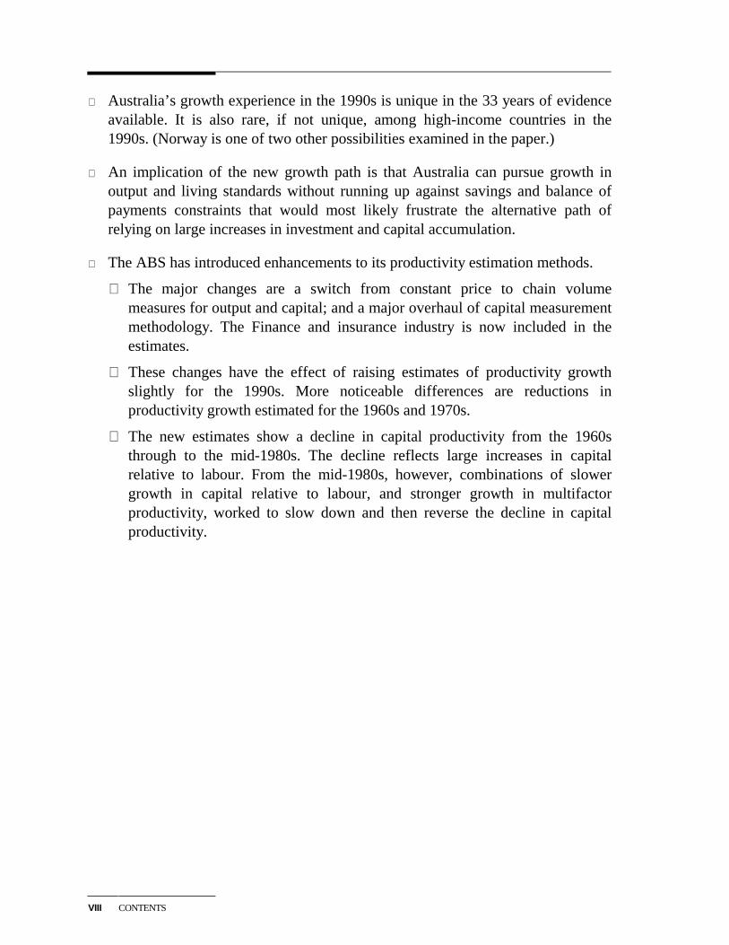
� Australia’s growth experience in the 1990s is unique in the 33 years of evidenceavailable. It is also rare, if not unique, among high-income countries in the1990s. (Norway is one of two other possibilities examined in the paper.)

� An implication of the new growth path is that Australia can pursue growth inoutput and living standards without running up against savings and balance ofpayments constraints that would most likely frustrate the alternative path ofrelying on large increases in investment and capital accumulation.

� The ABS has introduced enhancements to its productivity estimation methods.

� The major changes are a switch from constant price to chain volumemeasures for output and capital; and a major overhaul of capital measurementmethodology. The Finance and insurance industry is now included in theestimates.

� These changes have the effect of raising estimates of productivity growthslightly for the 1990s. More noticeable differences are reductions inproductivity growth estimated for the 1960s and 1970s.

� The new estimates show a decline in capital productivity from the 1960sthrough to the mid-1980s. The decline reflects large increases in capitalrelative to labour. From the mid-1980s, however, combinations of slowergrowth in capital relative to labour, and stronger growth in multifactorproductivity, worked to slow down and then reverse the decline in capitalproductivity.

INTRODUCTION 1

1 Introduction

Australians have enjoyed relatively high living standards this century, built in largepart on an abundance of natural resources. However, Australia’s productivitygrowth — a major contributor to growth in living standards — has been low byinternational standards over the long term (IC 1997).

By the 1980s, pessimism about the outlook for Australian commodity exports, theemergence of strong competition in manufactures from Asia and concern about ourslippage in the international league tables of per capita incomes focused theattention of policymakers on the need for policy reform.

It was realised that the Australian economy needed to show better productivityperformance if Australians were to enjoy the ongoing improvements in livingstandards that they value.

Australian governments embarked on major policy reforms from the mid-1980s.Both macro and micro approaches were adopted. An emphasis on microeconomicreforms was designed in large part — but not exclusively — to improve Australia’sproductivity performance.

1.1 Talk of ‘the new economy’

There is now a growing perception that the Australian economy is performing in adifferent way than it has in the past. A number of commentators have taken a leadfrom official statements.

In its recent Semi-Annual Statement on Monetary Policy, the Reserve Bankobserved that the combination of strong growth and exceptionally low inflationobserved over recent years is quite unlike the experience of the preceding 30 years.It went on to say, ‘That such a performance has been maintained, almost two yearsafter the Asian crisis first broke in Thailand, is indicative of the extent to which theAustralian economy’s underlying strength and resilience have been improved overtime.’ (RBA 1999, p. 1).

In the Budget Papers, the Commonwealth Treasury attributed the currentcombination of favourable economic indicators to a sound macroeconomic policy

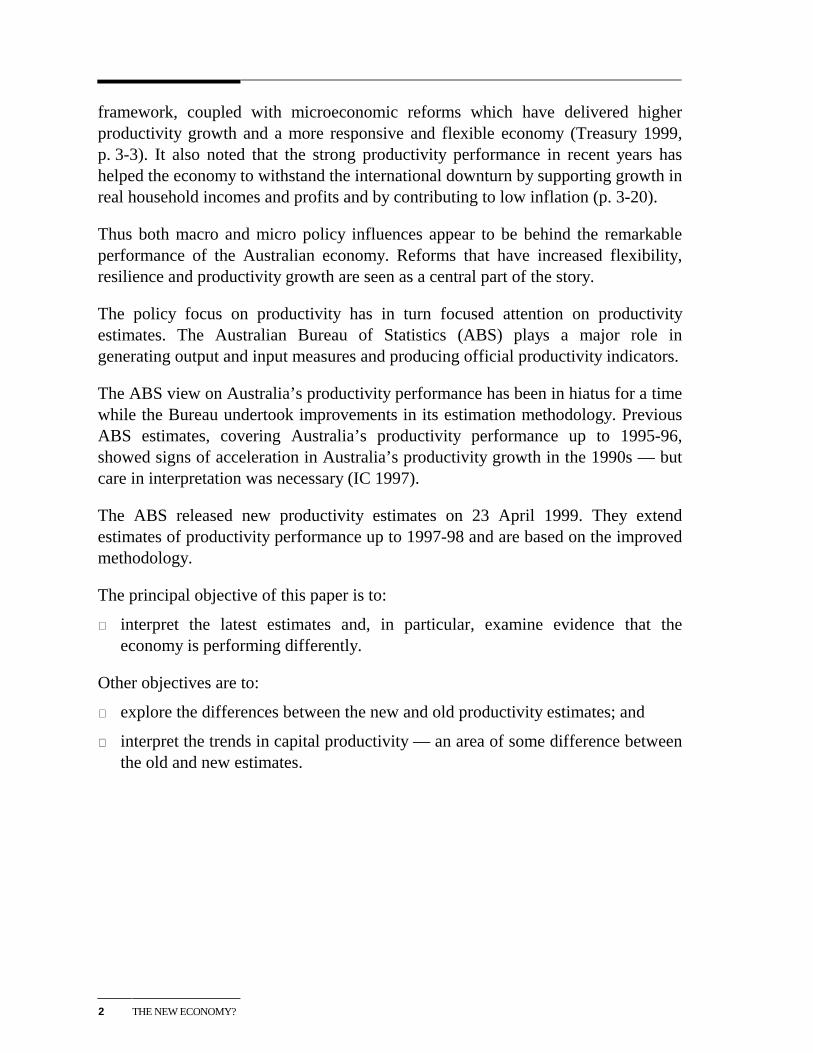
2 THE NEW ECONOMY?

framework, coupled with microeconomic reforms which have delivered higherproductivity growth and a more responsive and flexible economy (Treasury 1999,p. 3-3). It also noted that the strong productivity performance in recent years hashelped the economy to withstand the international downturn by supporting growth inreal household incomes and profits and by contributing to low inflation (p. 3-20).

Thus both macro and micro policy influences appear to be behind the remarkableperformance of the Australian economy. Reforms that have increased flexibility,resilience and productivity growth are seen as a central part of the story.

The policy focus on productivity has in turn focused attention on productivityestimates. The Australian Bureau of Statistics (ABS) plays a major role ingenerating output and input measures and producing official productivity indicators.

The ABS view on Australia’s productivity performance has been in hiatus for a timewhile the Bureau undertook improvements in its estimation methodology. PreviousABS estimates, covering Australia’s productivity performance up to 1995-96,showed signs of acceleration in Australia’s productivity growth in the 1990s — butcare in interpretation was necessary (IC 1997).

The ABS released new productivity estimates on 23 April 1999. They extendestimates of productivity performance up to 1997-98 and are based on the improvedmethodology.

The principal objective of this paper is to:

� interpret the latest estimates and, in particular, examine evidence that theeconomy is performing differently.

Other objectives are to:

� explore the differences between the new and old productivity estimates; and

� interpret the trends in capital productivity — an area of some difference betweenthe old and new estimates.

ENHANCEMENTS INTHE ABS METHODS

3

2 Enhancements in the ABSproductivity estimation methods

This chapter gives a brief overview of the changes the ABS has introduced to itsproductivity estimation methods. A full description of the changes is presented in afeature article in the National Accounts publication (ABS 5204.0: 1997-98).

2.1 Changes in estimation of MFP

The fundamentals of the ABS approach to estimating multifactor productivity(MFP) have not changed. The Bureau measures capital and labour inputs, combinesthem in a composite index, and calculates productivity as the ratio of output tocomposite inputs.

The ABS has, however, introduced some important refinements.

Chain-volume measures: The ABS now uses a chain-volume method of measuringthe value of output and capital stocks over time, rather than (fixed-weight) constant-price estimates.

Industry coverage: The new estimates now include Finance and insurance. Thisbrings the industry coverage more into line with practices adopted in many othercountries.

MFP is calculated for the market sector only and excludes sectors in which outputscannot be meaningfully measured (eg outputs in public administration are oftenmeasured in terms of expenditures). Based on 1997-98 data, the market sector nowcovers 61 per cent of GDP1. Finance and insurance adds 6.3 percentage points.

Capital input measurement: This is an area of significant change and is outlinedseparately.

1 Calculated at basic prices from ABS 5204.0.

4 THE NEW ECONOMY?

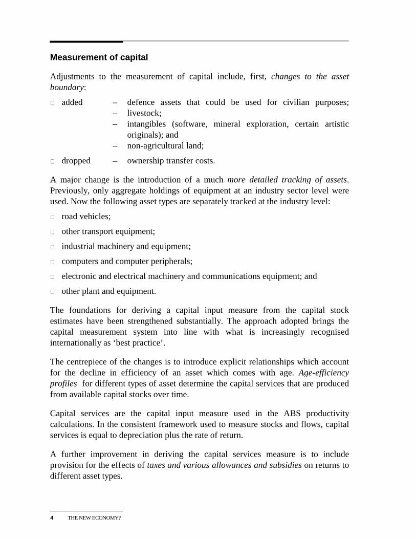
Measurement of capital

Adjustments to the measurement of capital include, first, changes to the assetboundary:

� added – defence assets that could be used for civilian purposes;– livestock;– intangibles (software, mineral exploration, certain artistic

originals); and– non-agricultural land;

� dropped – ownership transfer costs.

A major change is the introduction of a much more detailed tracking of assets.Previously, only aggregate holdings of equipment at an industry sector level wereused. Now the following asset types are separately tracked at the industry level:

� road vehicles;

� other transport equipment;

� industrial machinery and equipment;

� computers and computer peripherals;

� electronic and electrical machinery and communications equipment; and

� other plant and equipment.

The foundations for deriving a capital input measure from the capital stockestimates have been strengthened substantially. The approach adopted brings thecapital measurement system into line with what is increasingly recognisedinternationally as ‘best practice’.

The centrepiece of the changes is to introduce explicit relationships which accountfor the decline in efficiency of an asset which comes with age. Age-efficiencyprofiles for different types of asset determine the capital services that are producedfrom available capital stocks over time.

Capital services are the capital input measure used in the ABS productivitycalculations. In the consistent framework used to measure stocks and flows, capitalservices is equal to depreciation plus the rate of return.

A further improvement in deriving the capital services measure is to includeprovision for the effects of taxes and various allowances and subsidies on returns todifferent asset types.

ENHANCEMENTS INTHE ABS METHODS

5

The detailed industry and asset estimates of capital stocks and services areaggregated to form a total capital stock and a capital input measure.

The ABS considers the use of age-efficiency profiles, the detailed ‘bottom-up’construction of the capital input measure, and the use of chain-volume measurementto be major factors affecting the measurement of capital input.

2.2 Comparison of old and new estimates

There is insufficient information available to examine the difference that individualaspects of the enhancements have made to the measurement of capital andproductivity. Differences in the measured outcomes provide the only available basisof comparison.

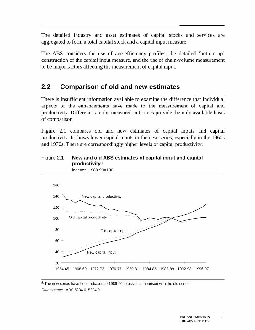
Figure 2.1 compares old and new estimates of capital inputs and capitalproductivity. It shows lower capital inputs in the new series, especially in the 1960sand 1970s. There are correspondingly higher levels of capital productivity.

Figure 2.1 New and old ABS estimates of capital input and capitalproductivitya

indexes, 1989-90=100

20

40

60

80

100

120

140

160

1964-65 1968-69 1972-73 1976-77 1980-81 1984-85 1988-89 1992-93 1996-97

New capital productivity

Old capital productivity

Old capital input

New capital input

a The new series have been rebased to 1989-90 to assist comparison with the old series.

Data source: ABS 5234.0, 5204.0.

6 THE NEW ECONOMY?

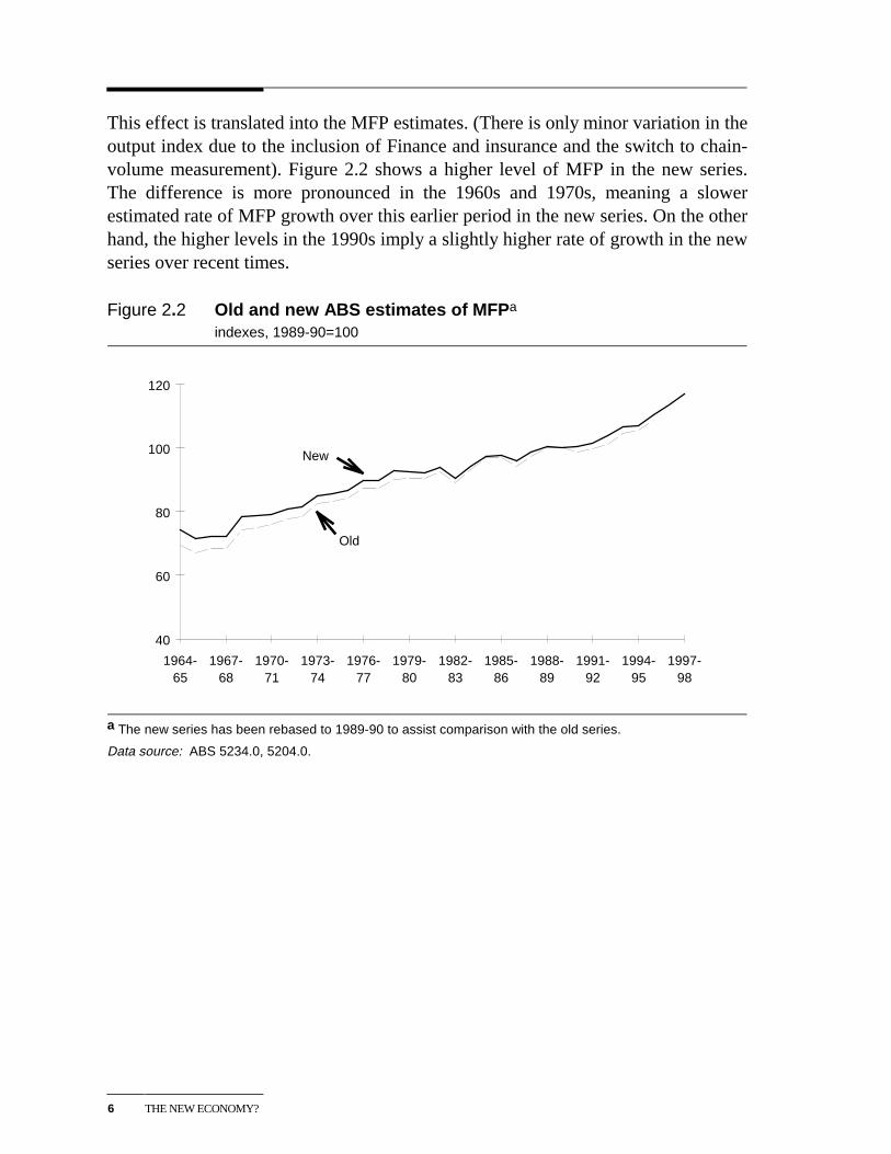
This effect is translated into the MFP estimates. (There is only minor variation in theoutput index due to the inclusion of Finance and insurance and the switch to chain-volume measurement). Figure 2.2 shows a higher level of MFP in the new series.The difference is more pronounced in the 1960s and 1970s, meaning a slowerestimated rate of MFP growth over this earlier period in the new series. On the otherhand, the higher levels in the 1990s imply a slightly higher rate of growth in the newseries over recent times.

Figure 2.2 Old and new ABS estimates of MFPa

indexes, 1989-90=100

40

60

80

100

120

1964-65

1967-68

1970-71

1973-74

1976-77

1979-80

1982-83

1985-86

1988-89

1991-92

1994-95

1997-98

New

Old

a The new series has been rebased to 1989-90 to assist comparison with the old series.

Data source: ABS 5234.0, 5204.0.

AN ASSESSMENT OFPRODUCTIVITYTRENDS

7

3 An assessment of productivity trends

The presentation of productivity results concentrates on the 1990s experience. Thelong-term picture is first sketched as background.

3.1 The major trends

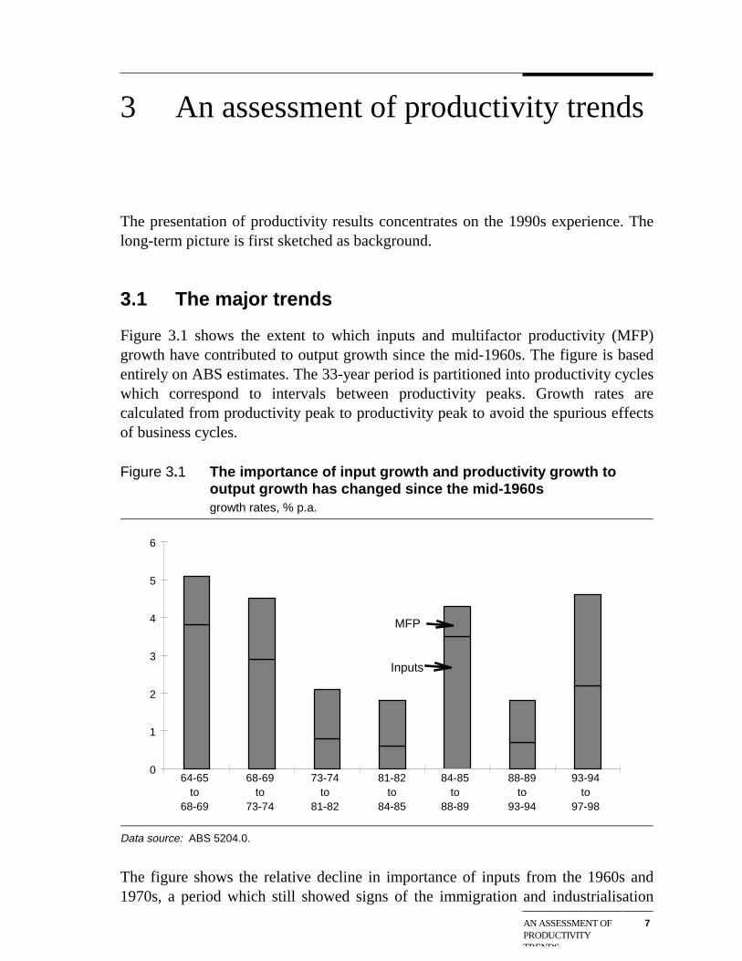
Figure 3.1 shows the extent to which inputs and multifactor productivity (MFP)growth have contributed to output growth since the mid-1960s. The figure is basedentirely on ABS estimates. The 33-year period is partitioned into productivity cycleswhich correspond to intervals between productivity peaks. Growth rates arecalculated from productivity peak to productivity peak to avoid the spurious effectsof business cycles.

Figure 3.1 The importance of input growth and productivity growth tooutput growth has changed since the mid-1960sgrowth rates, % p.a.

0

1

2

3

4

5

6

MFP

Inputs

64-65 to

68-69

68-69 to

73-74

73-74 to

81-82

81-82 to

84-85

84-85 to

88-89

88-89 to

93-94

93-94 to

97-98

Data source: ABS 5204.0.

The figure shows the relative decline in importance of inputs from the 1960s and1970s, a period which still showed signs of the immigration and industrialisation

8 THE NEW ECONOMY?

path to further development that Australia followed after the second World War.This decline in the relative importance of inputs fits with the broad pattern ofdevelopment of countries as they mature (see box 4.2 in the next chapter). As ageneral rule, developed economies become less reliant on input growth and morereliant on productivity growth as a source of output growth.

The late 1980s stands out as an aberration, with strong input growth arising fromstrong expansion in labour (associated with a decline in real wages) and anexpansion in capital (particularly in property). Productivity growth in that periodwas low.

The latest productivity cycle, from 1993-94 to 1997-98, also stands out in showingstrong growth in both inputs and productivity. Growth in inputs and productivity arenot necessarily independent events, as improved productivity can create conditionsfavourable to additional investment and employment. The latest cycle is examinedfurther below.

Figure 3.2 shows the year-to-year movements in the different productivity measures.A general upward trend in labour productivity and MFP is evident. Capitalproductivity, on the other hand, shows a secular decline until the 1980s. Capitalproductivity trends are interpreted in chapter 5.

MFP is the preferable indicator of overall production efficiency. Labourproductivity and capital productivity are partial indicators and, as such, can bedifficult to interpret from an efficiency point of view. For example, an increase incapital (per unit of labour) or a reduction in labour (to an extent that createdproduction bottlenecks) would both produce an increase in labour productivitywithout indicating the effect on overall efficiency.

Figure 3.3 focuses on MFP growth and shows that there has been a substantialacceleration in productivity growth over the latest cycle — 1993-94 to 1997-98.Productivity growth in this latest cycle has been 2.4 per cent a year, whereasprevious cycles have shown average growth in the range of 0.8 to 1.6 per cent ayear. Annual average growth since 1964-65 has been 1.4 per cent.


9

Figure 3.2 Labour productivity and MFP have trended upward, but capitalproductivity declined until the 1980sindexes, 1996-97=100

40

60

80

100

120

140

160

1964-65 1968-69 1972-73 1976-77 1980-81 1984-85 1988-89 1992-93 1996-97

Capital productivity

Multifactor productivity

Labour productivity


Figure 3.3 MFP growth has accelerated to an all-time high in the latestproductivity cycle% p.a.

0

0.5

1

1.5

2

2.5

64-65 to

68-69

68-69 to

73-74

73-74 to

81-82

81-82 to

84-85

84-85 to

88-89

88-89 to

93-94

93-94 to

97-98

1.3

1.6

1.31.2

0.8

1.1

2.4

Period average = 1.4(64-65 to 97-98)


10 THE NEW ECONOMY?

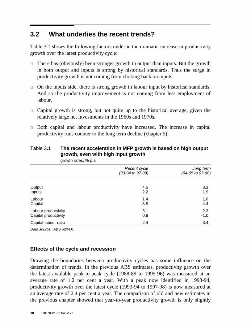
3.2 What underlies the recent trends?

Table 3.1 shows the following factors underlie the dramatic increase in productivitygrowth over the latest productivity cycle:

� There has (obviously) been stronger growth in output than inputs. But the growthin both output and inputs is strong by historical standards. Thus the surge inproductivity growth is not coming from choking back on inputs.

� On the inputs side, there is strong growth in labour input by historical standards.And so the productivity improvement is not coming from less employment oflabour.

� Capital growth is strong, but not quite up to the historical average, given therelatively large net investments in the 1960s and 1970s.

� Both capital and labour productivity have increased. The increase in capitalproductivity runs counter to the long term decline (chapter 5).

Table 3.1 The recent acceleration in MFP growth is based on high outputgrowth, even with high input growthgrowth rates, % p.a

Recent cycle(93-94 to 97-98)

Long term(64-65 to 97-98)

Output 4.6 3.3Inputs 2.2 1.9

Labour 1.4 1.0Capital 3.8 4.4

Labour productivity 3.1 2.3Capital productivity 0.8 -1.0

Capital-labour ratio 2.4 3.4


Effects of the cycle and recession

Drawing the boundaries between productivity cycles has some influence on thedetermination of trends. In the previous ABS estimates, productivity growth overthe latest available peak-to-peak cycle (1988-89 to 1995-96) was measured at anaverage rate of 1.2 per cent a year. With a peak now identified in 1993-94,productivity growth over the latest cycle (1993-94 to 1997-98) is now measured atan average rate of 2.4 per cent a year. The comparison of old and new estimates inthe previous chapter showed that year-to-year productivity growth is only slightly


11

higher over the 1990s (and has continued at a high rate for another two years) in thenew estimates. Even allowing for this, the redrawing of the productivity cycleboundary has clearly had an influence.

The determination of productivity peaks, however, is not arbitrary. Peak points inthe productivity cycle are determined by the ABS, using consistent application of astatistical technique. The ABS calculates a trend series (using a Henderson 11-period moving average) and productivity peaks are determined as years in which thegap between the actual and trend productivity series turns from increasing todecreasing.

The 1990s recession would also have affected productivity results. Productivitygrowth commonly rises rapidly coming out of a recession as capacity utilisationsteps up from unusually low rates. It is quite possible that productivity growth in theearly part of the latest cycle still reflects some effects of the recession. (There is ahint of this in one of the industry sectors examined below).

An examination of the ABS trend series is a way to get a picture of underlyingproductivity trends without the intrusion of the boundary issue from the peak-to-peak technique. It also reduces the influence of business cycles.

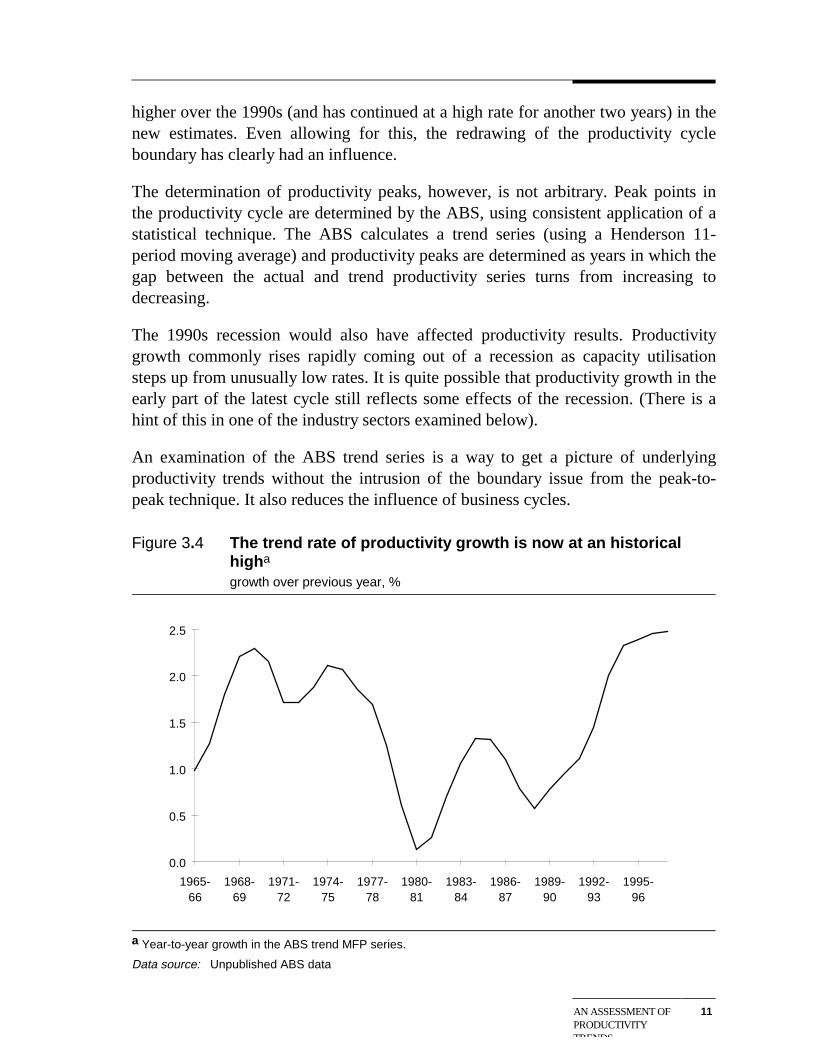
Figure 3.4 The trend rate of productivity growth is now at an historicalhigha

growth over previous year, %

0.0

0.5

1.0

1.5

2.0

2.5

1965-66

1968-69

1971-72

1974-75

1977-78

1980-81

1983-84

1986-87

1989-90

1992-93

1995-96

a Year-to-year growth in the ABS trend MFP series.

Data source: Unpublished ABS data

12 THE NEW ECONOMY?

Figure 3.4 shows the year-to-year growth in the ABS trend MFP series. It revealsthe underlying trend in productivity growth to have been at or above 2 per cent ayear since 1993-94. The growth in trend productivity only broke through 2 per centa year briefly back in the late 1960s and briefly again in the mid-1970s.

The use of the trend series reduces the influence of the recession. But, even so, it isworth noting that the highest growth in trend productivity has come outside of theperiod subject to influence from recovery from the recession. While there may besome question about recovery from recession still exerting some influence on theactual 1993-94 result, further influence beyond that time becomes increasinglyunlikely. From 1995-96, trend productivity has been growing at the historically highrate of 2.5 per cent a year.

It is also very clear from figure 3.4 that trend productivity growth in the 1990saccelerated well beyond the recovery shown after the 1980s recession.

Sectoral origins

It is also of interest to look at the sectoral origins of the productivity acceleration.Labour productivity growth estimates have to be used, because the Bureau does notyet publish sectoral MFP estimates.

From an efficiency point of view, the use of labour productivity estimates does notprovide the ideal guide to the sectoral origins of productivity growth. As statedbefore, changes in labour productivity can reflect relative expansion of capital orreduction of labour, without necessarily indicating whether (multifactor) efficiencyhas been improved.

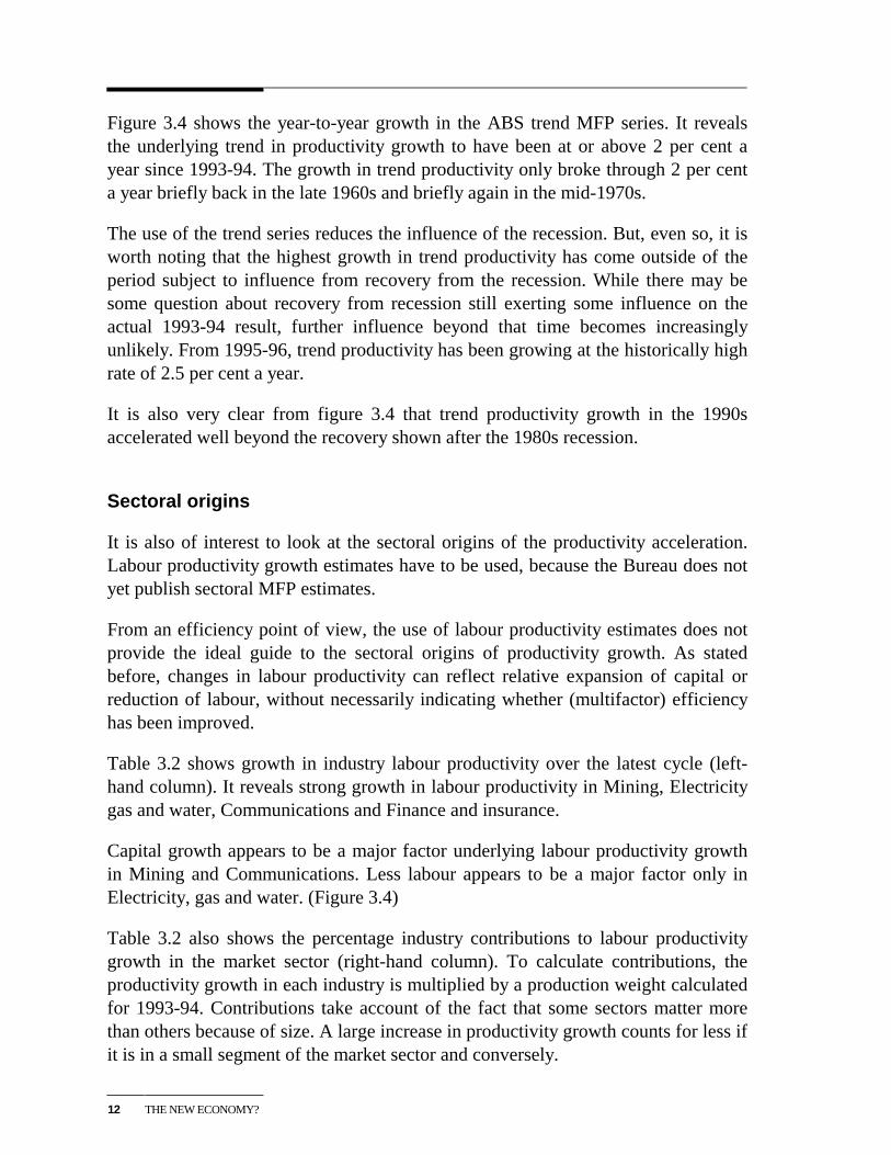
Table 3.2 shows growth in industry labour productivity over the latest cycle (left-hand column). It reveals strong growth in labour productivity in Mining, Electricitygas and water, Communications and Finance and insurance.

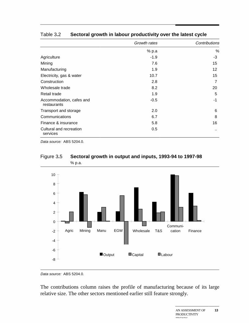
Capital growth appears to be a major factor underlying labour productivity growthin Mining and Communications. Less labour appears to be a major factor only inElectricity, gas and water. (Figure 3.4)

Table 3.2 also shows the percentage industry contributions to labour productivitygrowth in the market sector (right-hand column). To calculate contributions, theproductivity growth in each industry is multiplied by a production weight calculatedfor 1993-94. Contributions take account of the fact that some sectors matter morethan others because of size. A large increase in productivity growth counts for less ifit is in a small segment of the market sector and conversely.


13

Table 3.2 Sectoral growth in labour productivity over the latest cycle

Growth rates Contributions

% p.a %

Agriculture -1.9 -3

Mining 7.6 15

Manufacturing 1.9 12

Electricity, gas & water 10.7 15

Construction 2.8 7

Wholesale trade 8.2 20

Retail trade 1.9 5

Accommodation, cafes and restaurants

-0.5 -1

Transport and storage 2.0 6

Communications 6.7 8

Finance & insurance 5.8 16

Cultural and recreation services

0.5 ..


Figure 3.5 Sectoral growth in output and inputs, 1993-94 to 1997-98% p.a.

-8

-6

-4

-2

0

2

4

6

8

10

Output Capital Labour

Agric Mining Manu EGW Wholesale T&SCommuni-

cation Finance


The contributions column raises the profile of manufacturing because of its largerelative size. The other sectors mentioned earlier still feature strongly.

14 THE NEW ECONOMY?

Some further examination of Wholesale trade shows it was knocked around by theearly 1990s recession; and its strong growth in labour productivity is likely to reflectsome delay in its recovery from that recession. Agriculture, which shows solidproductivity growth over the long term (IC 1997), is subject to the vagaries ofclimate.

This picture of the sectoral origins can only be taken as broadly indicative. A clearerpicture would require sectoral MFP estimates and a longer time series to examineand allow for the different cycles of different industries.

3.3 Some implications

The main difference between the new and old estimates is a reduction inproductivity growth estimated for the 1960s and 1970s. Productivity growth stillremains strong for this period, as a glance at the underlying trend series (figure 3.4)reveals. The period remains as something of a ‘Golden Age’, but not quite to theextent previously thought. This is perhaps more in line with the work of AngusMaddison and others, which has shown that there was a major period of ‘catch-up’from the 1950s up until the mid-1970s in Europe associated with post-warreconstruction. Australia, however, in part because of its isolation, did not knock onthe door of the ‘Convergence Club’. (Maddison 1995,1997)

If the 1960s and 1970s were the ‘Golden Age’ of growth in output and productivity,it seems we might need to reach for an even more superlative term for the 1990s.The acceleration in productivity growth in the 1990s is outstripping any earlierresults.

There would be a combination of factors underlying this acceleration. In the earlypart of the 1990s there is likely to be some effects from recovery from the recession.But underlying productivity growth has still accelerated outside of the recession-affected period. There is also likely to be some — and possibly a major — dividendfrom reform. And there may be other factors, particularly underlying technologicaladvance, although too much should not be made of that, given that embodiedtechnological change is captured in the input measure (chapter 5). There could bedisembodied advances such as organisational and management improvements(which could be related in parts to reform and to advances in informationtechnology).

As a dividend from reform, we could expect to see greater input growth (eg due togreater returns on investment), better allocation of resources (to more productiveuses) and better technical efficiency in input use (eliminating inefficient processesand practices and spurring the search for even better ways of doing things).


15

It is not just wishful thinking to suggest that microeconomic reform may be playinga very important role. The Commission is undertaking research into the linksbetween reform and productivity. A forthcoming study (PC 1999) adds to the weightof evidence that the economy is operating differently in an environment with muchclearer allocation signals and much clearer incentives to raise productivityperformance.

EVIDENCE ON THENEW ECONOMY ANDSOME IMPLICATIONS

17

4 Evidence on the new economy andsome implications

This chapter uses published ABS data and a new methodology to examine evidenceof a shift in the way the Australian economy operates.

4.1 A break with the pastEconomic growth is to be analysed in a way that warrants at least brief explanation.The essence of the technique is to examine the evolution of input-outputrelationships in an economy over time.

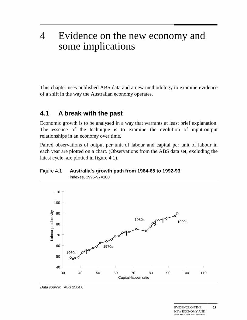
Paired observations of output per unit of labour and capital per unit of labour ineach year are plotted on a chart. (Observations from the ABS data set, excluding thelatest cycle, are plotted in figure 4.1).

Figure 4.1 Australia’s growth path from 1964-65 to 1992-93indexes, 1996-97=100

40

50

60

70

80

90

100

110

30 40 50 60 70 80 90 100 110

I

I

I

1960s

1970s

1980s1990s

Capital-labour ratio

Labo

ur p

rodu

ctiv

ity

Data source: ABS 2504.0

18 THE NEW ECONOMY?

These observations can be thought of as depicting points on an aggregate (per unitlabour) production function. Shifts from one observation to another representcombinations of shifts around the aggregate production function (based on increasesin the capital-labour ratio) and shifts of the production function (due to productivityimprovement). The derivation in box 4.1 provides a formal demonstration.

Because the capital-labour ratio increases over time, the observations generally lineup in chronological order from left to right. Joining the points in chronological ordermaps out what may be termed the ‘growth path’ of an economy’s output per labourinput — or labour productivity. It shows how an economy progresses from a lowerlevel of labour productivity to a higher level. The Australian case, based on outputper hour worked, is shown in figure 4.1.

Next it can be observed that growth in labour productivity is often used as a proxyindicator of growth in average living standards. With plausible assumptions, growthin labour productivity bears a reasonable approximation to growth in averageincome per head.1

Thus, the growth path can also be interpreted as a pathway to better living standards.

International comparisons are included in box 4.2 and appendix A to helpinterpretation of growth paths. Some countries, for example Japan, have pursued agrowth trajectory based heavily on investment and capital accumulation. Hence itsgrowth path appears relatively drawn out, reflecting large increases in the capital-labour ratio. Some countries have pursued trajectories based on productivity growth(for at least some periods). Their growth paths are steeper or have steep sections.Hong Kong is a prime example.

1 Since income and output are very closely related, growth in labour productivity will be a close

approximation to growth in income per head if there have been no major shifts in thepopulation/workforce dependency ratio, participation rates, or average hours worked.


19

Box 4.1 The relationship between labour productivity, capitaldeepening and multifactor productivity

To assist the interpretation of the factors underlying the growth path analysis used inthis chapter, take a simple Cobb-Douglas production function (with constant returns toscale). Actual observations on growth paths do not require or necessarily conformprecisely to a particular specification of the production function. It just helps to use aspecification which provides a simplified view of the relationships involved.

Output (Y) can be expressed as a function of labour (L), capital (K) and multifactorproductivity (M):

Y = M.KαL1-α

Y/L = M.(Y/L)α (4.1)

Taking differential logs:

y = α.k + m (4.2)

where

y = growth in labour productivity

k = growth in the capital-labour ratio

m = growth in multifactor productivity.

The parameter α is the marginal product of capital, which equals the capital share oftotal income if factors are paid their marginal products (normally assumed as aproperty of competitive markets).

Equations (4.1) and (4.2) show that labour productivity is a positive function of capitaldeepening and multifactor productivity, both in the levels and in terms of rates ofgrowth.

Figure 4.2 shows a curve fitted from the Australian observations up until 1992-93,the year before the commencement of the latest productivity cycle.2 The curve isone way of capturing the history of Australia’s growth path and projecting beyond1992-93, based on that history. The curve shows literally the average returnAustralia has derived in terms of additional output per hour worked from increasesin capital per hour worked. On a broader interpretation, it shows how effectivecapital deepening has been in improving our living standards.

2 A non-linear function was used, reflecting the general decline in productivity growth from the

1960s and early 1970s through to the 1990s (chapter 3).

20 THE NEW ECONOMY?

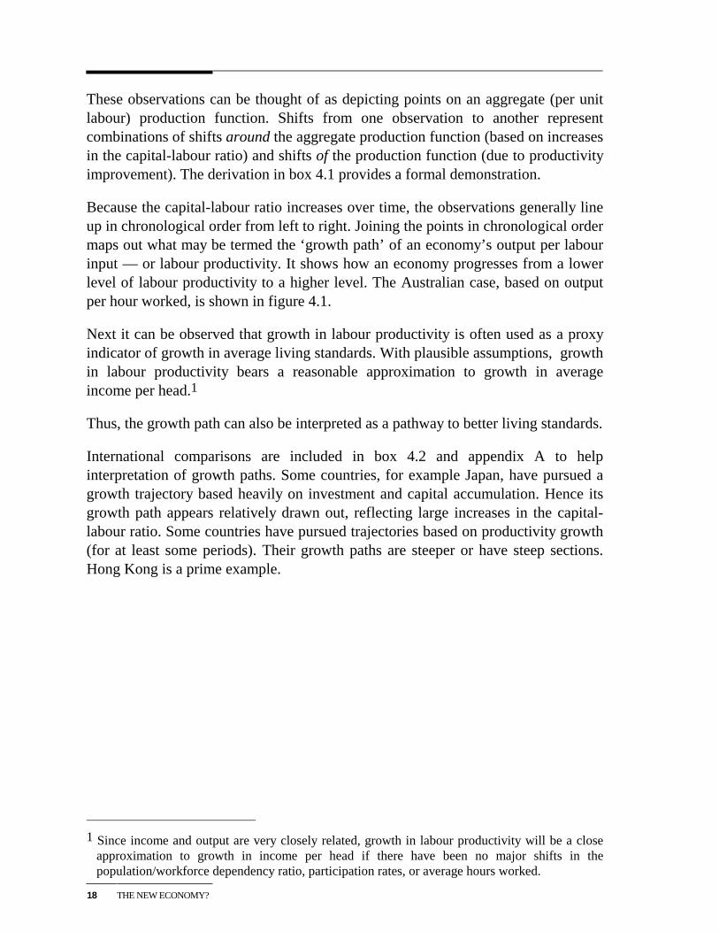
Box 4.2 Growth paths for different countries

The different strategies used by countries to pursue development and better livingstandards are revealed in their growth paths.

The comparisons in this box are drawn from data contained in the Summers andHeston (1991) Penn World Tables (PWT). It needs to be noted that the quality of thedata inputs is generally not up to the standard of the ABS data, upon which figure 4.2is based. Labour input is measured in terms of number of employees (PWT) ratherthan hours of work (ABS). Capital is measured in terms of capital stock (PWT), ratherthan flow of capital services (ABS). The PWT data refer to the economy as a whole,whereas the ABS data are confined to the market sector. And data collectionstandards vary between countries.

The growth paths for each country are based on indexes set at 100 for 1985.Consequently, the comparisons give no indication of the vast differences in levels oflabour productivity and capital-labour ratios that exist between countries at differentstages of development. The same scales are used in all charts to facilitatecomparisons between countries.

20

40

60

80

100

120

140

160

0 20 40 60 80 100 120 140 160

Labo

ur p

rodu

ctiv

ity

Capital labour ratio

1965

1990

AustraliaThe Australian growth path isreproduced from the PWT forcomparison.

20

40

60

80

100

120

140

160

0 20 40 60 80 100 120 140 160

Labo

ur p

rodu

ctiv

ity


1990

1965

United StatesThe US shows relatively slowproductivity growth. This is to beexpected of a country which hasalready, in general, reached theproductivity ‘frontier’.

Continued on next page


21

Box 4.3 (continued)

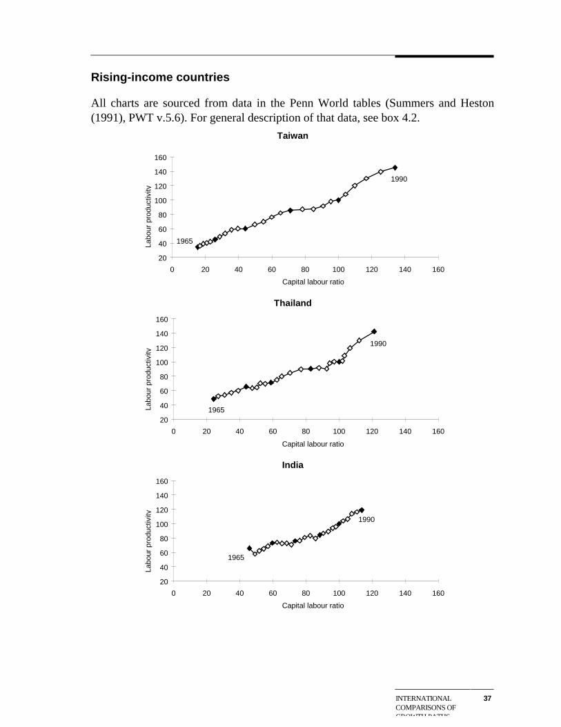
A common view of development is that countries initially focus on investing in physicaland human capital to develop their economic and social infrastructure. This, amongstother things, then provides a platform for rapid growth ‘catch up’ to more developedcountries. Once developed, countries typically become more reliant on productivitygrowth than input accumulation to underpin further growth in output and livingstandards. Consequently, as a broad generalisation, one expects to see:

� high income countries with relatively flat growth paths confined to a relatively narrowspan of capital-labour ratios;

� rising income countries with a broad span of capital-labour ratios (capitalaccumulation) and/or a steep gradient in their growth path reflecting ‘catch up’productivity growth; and

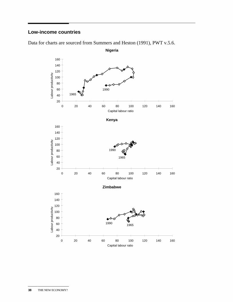
� low income countries with little evidence of sustained increases in either capitalaccumulation or productivity growth.

Growth paths for a more diverse range of countries, which illustrate these patterns, areincluded in appendix A.

20

40

60

80

100

120

140

160

0 20 40 60 80 100 120 140 160

Labo

ur p

rodu

ctiv

ity


1965

1990

JapanJapan shows growth based onproductivity growth in the 1960s,combined with high investmentfrom the 1970s. (See appendix Afor a more up-to-date picture).

20

40

60

80

100

120

140

160

0 20 40 60 80 100 120 140 160

Labo

ur p

rodu

ctiv

ity


1965

1990

1965

1990

Hong Kong

Korea

Korea and especially Hong Kongshow periods of extensive growthbased heavily on MFP growth.

22 THE NEW ECONOMY?

Figure 4.2 Australia takes a different growth path in the 1990sa

Indexes, 1996-97=100

R2 = 0.99

40

50

60

70

80

90

100

110

30 40 50 60 70 80 90 100 110

I

I

I

1960s

1970s

1980s1990s

Capital-labour ratio

Labo

ur p

rodu

ctiv

ity

(90-91)

(82-83)

a The fitted curve uses data for years up to 1992-93. The curve is of the form (Y/L) = 40.66 In (K/L) -98.39.


The observations describe a remarkably stable pattern (R2 = 0.99 for the fittedcurve). It suggests that any productivity growth up until the 1990s has served tokeep the Australian economy on a steady growth path. The 1980s recession is theonly period off the path up until the 1990s.

The observations for the latest productivity cycle (from 1993-94) are included infigure 4.2 as squares. They show the emergence of a very different growth path.Here, productivity growth is putting the economy on a new growth trajectory.

As a result of the new growth path:

� output per hour worked in the market sector was 15 per cent higher in 1997-98than it would have been if the economy had stuck to the old historical growthpath; and

� taking 1991-92 as a departure point, output per hour worked grew over the nextsix years to a level that would have taken over 13 years to achieve, had theeconomy remained on the old growth path.3

3 The estimate of 13 years is based on the assumption that the capital-labour ratio would increase

at the historical average rate of 3.4 per cent a year on the old growth path.


23

Figure 4.2 also illustrates an important difference between the recessions of the1980s and 1990s. In the 1980s recession, reduction in labour shifted the capital-labour ratio to the right, but output declined even more than labour, so the economy‘fell off’ the underlying growth path. There was a subsequent recovery back ontothe growth path. In the 1990s, the capital-labour ratio shifted to the right again, butproduction remained ‘on track’. This would be due to increased MFP. Acontinuation of productivity growth thereafter also meant that the economy ‘tookoff’ on a different growth path coming out of the recession, rather than justrecovered to the historical path.

Another possible explanation for why the economy remained on track in the 1990srecession is that cuts in labour could have been more severe in the 1990s recessionthan in the 1980s recession (which would have preserved the growth path output-labour relationship in the 1990s). However, the rightward shift in the capital-labourratio appears no more severe in the 1990s recession than in the 1980s recession. TheReserve Bank has demonstrated that the reduction in employment was no moresevere in the 1990s recession than in the 1980s recession, but that the recovery inemployment from the 1990s recession was delayed (RBA 1998).

From visual inspection, it seems that the structural break had its origins around thesame time as the recession of the early 1990s. Indeed, the fact that the economyremained on track during the recession suggests that productivity growth was higherfrom at least 1990-91.

There is nothing in the 33-year Australian history examined here of similarmagnitude or direction. From a brief examination of other high-income countries’experience (albeit on poorer quality data) it also does not appear to have occurredelsewhere in the 1990s. Norway is the only other possibility among countriesexamined4 (appendix A).

4.2 Some implications

The shift in Australia’s growth path suggests Australia has opened up new frontiersof growth possibilities and more rapid payoffs in terms of contributions to averageliving standards. Provided nothing happens to undo the productivity gains that havebeen achieved, those contributions to improvements in living standards are lockedin. Pursuing further opportunities for productivity growth will deliver opportunitiesfor further relatively rapid improvements in living standards.

4 Ireland is another possible candidate, but 1990s data are not readily available for this country.

24 THE NEW ECONOMY?

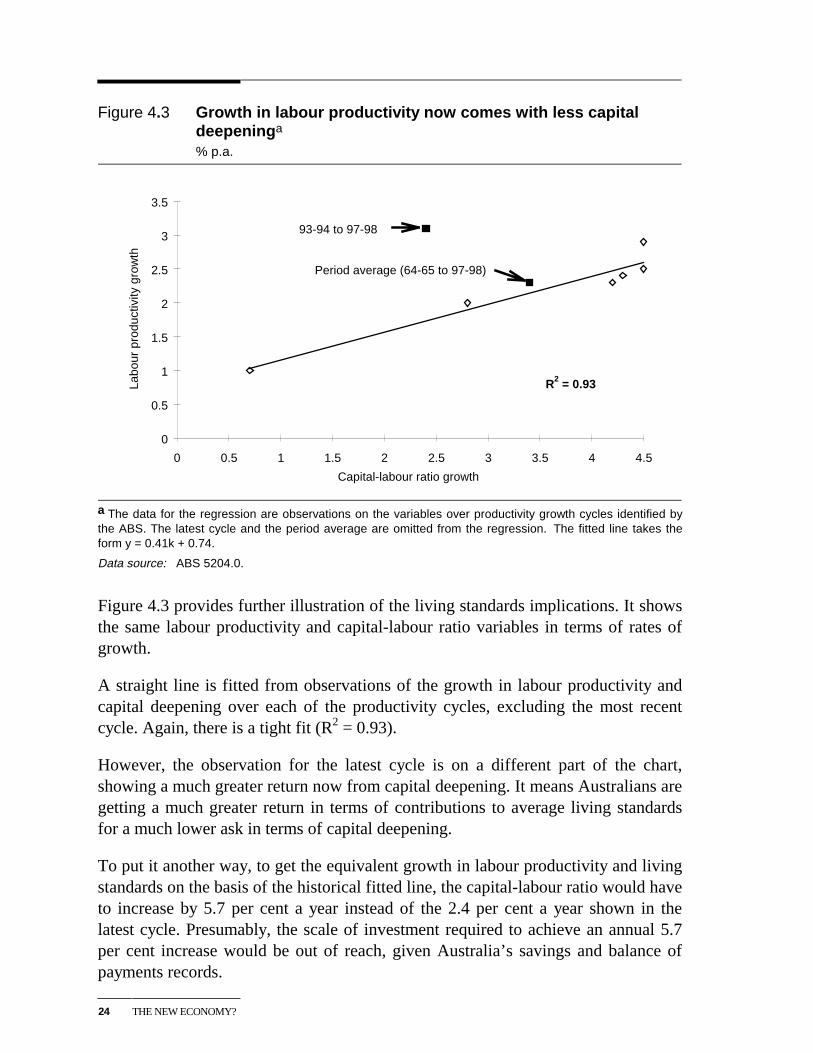
Figure 4.3 Growth in labour productivity now comes with less capitaldeepeninga

% p.a.

R2 = 0.93

0

0.5

1

1.5

2

2.5

3

3.5

0 0.5 1 1.5 2 2.5 3 3.5 4 4.5

Capital-labour ratio growth

Labo

ur p

rodu

ctiv

ity g

row

th

93-94 to 97-98

Period average (64-65 to 97-98)

a The data for the regression are observations on the variables over productivity growth cycles identified bythe ABS. The latest cycle and the period average are omitted from the regression. The fitted line takes theform y = 0.41k + 0.74.


Figure 4.3 provides further illustration of the living standards implications. It showsthe same labour productivity and capital-labour ratio variables in terms of rates ofgrowth.

A straight line is fitted from observations of the growth in labour productivity andcapital deepening over each of the productivity cycles, excluding the most recentcycle. Again, there is a tight fit (R2 = 0.93).

However, the observation for the latest cycle is on a different part of the chart,showing a much greater return now from capital deepening. It means Australians aregetting a much greater return in terms of contributions to average living standardsfor a much lower ask in terms of capital deepening.

To put it another way, to get the equivalent growth in labour productivity and livingstandards on the basis of the historical fitted line, the capital-labour ratio would haveto increase by 5.7 per cent a year instead of the 2.4 per cent a year shown in thelatest cycle. Presumably, the scale of investment required to achieve an annual 5.7per cent increase would be out of reach, given Australia’s savings and balance ofpayments records.


25

Analysis of the effects on the distribution of income would also be needed tocomplete an assessment of the living standards effects. And it should also beremembered that growth in employment and reduction in unemployment are alsopaths to increased living standards.

INTERPRETING THETRENDS IN CAPITALPRODUCTIVITY

27

5 Interpreting the trends in capitalproductivity

The ABS’s new estimates of capital productivity show a more pronounced seculardecline through to the 1980s recession, compared with the previous estimates(chapter 2). This has surprised some. For example, at the ABS seminar on CapitalStock and Multifactor Productivity in May 1999, some participants expected to seelittle long-term movement in Australia’s capital productivity.

Economic theory leads us to look for two opposing forces that affect capitalproductivity:

� the law of diminishing returns; and

� technological change.

In neo-classical steady-state growth models, these forces are assumed to be exactlyoffsetting, implying a flat capital productivity profile over time. But, in practice,these steady state conditions may not apply.

Diminishing returns are likely to be a major influence underlying the ABS estimates.As observed several times in this paper, the capital-labour ratio has generally beenincreasing over time. This means that, on average, a unit of capital increasingly hasless labour to work with. This would produce a decline in capital productivity overtime.

This observation is the mirror image of the well-known fact that increases in thecapital-labour ratio raise labour productivity. With capital deepening, each unit oflabour has, on average, more capital to work with and so more output can beproduced per unit of labour input. The opposite is true on the capital side.

So, if diminishing returns produce a decline in capital productivity, what about theoffsetting effects of technological change?

Whilst the theory is based solely on there being technological change that has theoffsetting effect, the practice is different. First, in practice, a major part oftechnological change is embodied in purchases of new plant and equipment. TheABS procedures, in allowing for quality improvements in price deflators,incorporate most of these embodied technological changes in the capital input

28 THE NEW ECONOMY?

measure used in the productivity calculations. They are not part of the unexplainedproductivity residual.

Consequently, embodied technology does not have as dramatic or immediateoffsetting effect on capital productivity. It can still have some effect throughlearning-by-doing efficiencies and so on — but it is unlikely to be sufficient to fullyoffset diminishing returns.

This leaves disembodied technological change as a potential offsetting factor. Thesecond practical issue is that there may be other disembodied efficiencyimprovements, apart from those of ‘technological’ origins — eg betterorganisational, management and work practices, including reductions in any so-called X-inefficiencies. All these factors show up in the MFP component of theABS calculations.

Thus, in practice, the capital productivity outcome will depend on the relativestrength of the (negative) effects of growth in the capital-labour ratio and the(positive) effects of growth in MFP.

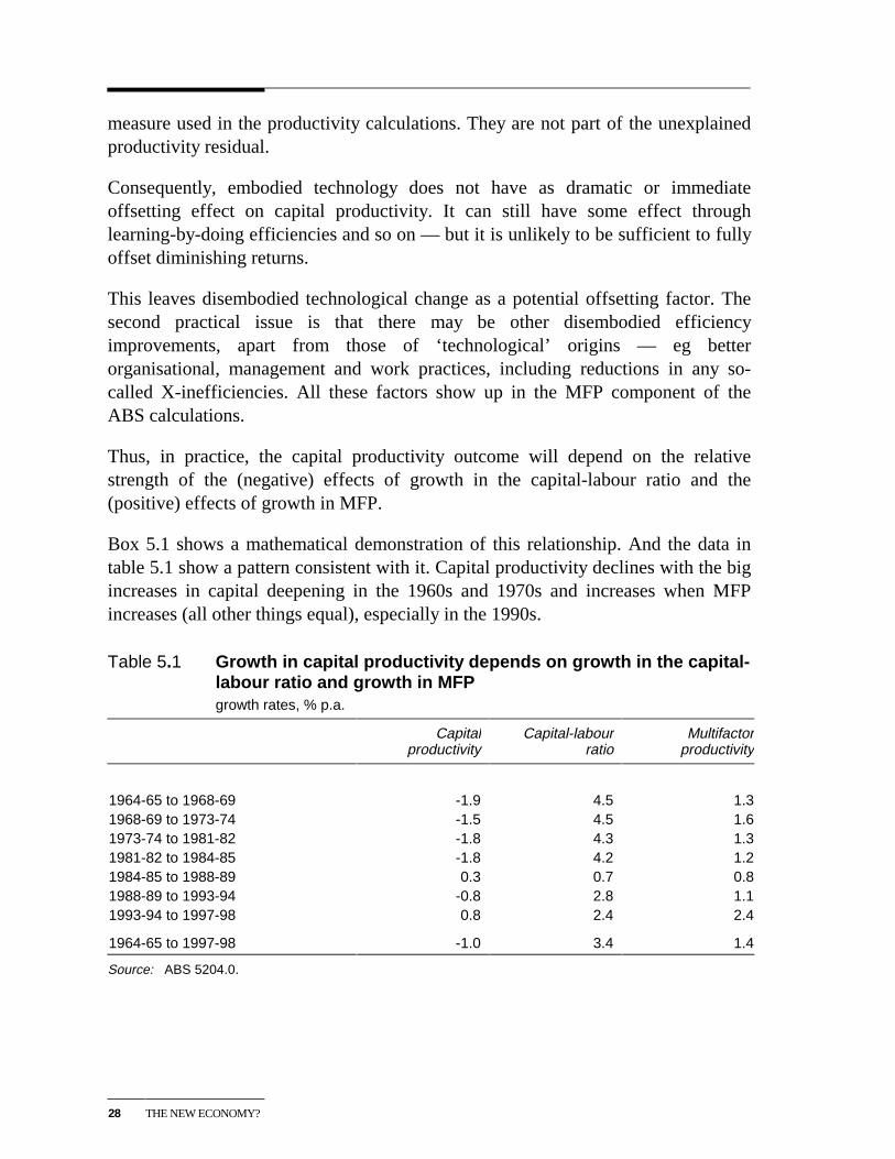
Box 5.1 shows a mathematical demonstration of this relationship. And the data intable 5.1 show a pattern consistent with it. Capital productivity declines with the bigincreases in capital deepening in the 1960s and 1970s and increases when MFPincreases (all other things equal), especially in the 1990s.

Table 5.1 Growth in capital productivity depends on growth in the capital-labour ratio and growth in MFPgrowth rates, % p.a.

Capitalproductivity

Capital-labourratio

Multifactorproductivity

1964-65 to 1968-69 -1.9 4.5 1.31968-69 to 1973-74 -1.5 4.5 1.61973-74 to 1981-82 -1.8 4.3 1.31981-82 to 1984-85 -1.8 4.2 1.21984-85 to 1988-89 0.3 0.7 0.81988-89 to 1993-94 -0.8 2.8 1.11993-94 to 1997-98 0.8 2.4 2.4

1964-65 to 1997-98 -1.0 3.4 1.4

Source: ABS 5204.0.


29

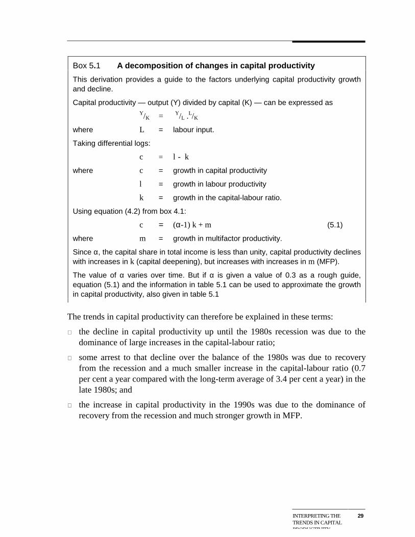
Box 5.1 A decomposition of changes in capital productivity

This derivation provides a guide to the factors underlying capital productivity growthand decline.

Capital productivity — output (Y) divided by capital (K) — can be expressed asY/K = Y/L .L/K

where L = labour input.

Taking differential logs:

c = l - k

where c = growth in capital productivity

l = growth in labour productivity

k = growth in the capital-labour ratio.

Using equation (4.2) from box 4.1:

c = (α-1) k + m (5.1)

where m = growth in multifactor productivity.

Since α, the capital share in total income is less than unity, capital productivity declineswith increases in k (capital deepening), but increases with increases in m (MFP).

The value of α varies over time. But if α is given a value of 0.3 as a rough guide,equation (5.1) and the information in table 5.1 can be used to approximate the growthin capital productivity, also given in table 5.1

The trends in capital productivity can therefore be explained in these terms:

� the decline in capital productivity up until the 1980s recession was due to thedominance of large increases in the capital-labour ratio;

� some arrest to that decline over the balance of the 1980s was due to recoveryfrom the recession and a much smaller increase in the capital-labour ratio (0.7per cent a year compared with the long-term average of 3.4 per cent a year) in thelate 1980s; and

� the increase in capital productivity in the 1990s was due to the dominance ofrecovery from the recession and much stronger growth in MFP.

30 THE NEW ECONOMY?

Underlying these broad outcomes, there could be several factors (apart from the sizeof labour input) that would show up in the capital productivity ‘residual’:

� greater workforce skill and flexibility over time would increase capitalproductivity;

� more stringent environmental requirements would reduce it;

� poor allocation of capital and inefficient use would reduce capital productivity;and

� compositional changes — both industry and asset type — could have eitherpositive or negative effect.

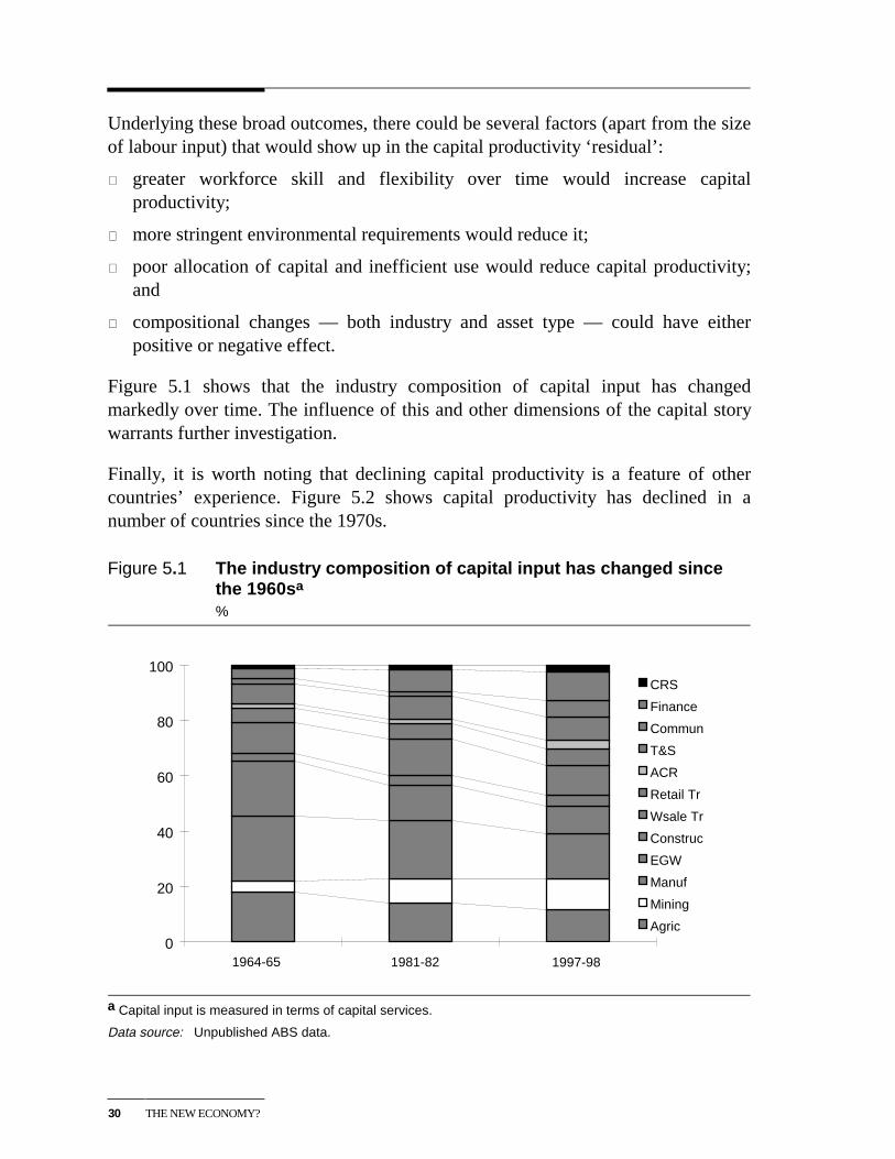
Figure 5.1 shows that the industry composition of capital input has changedmarkedly over time. The influence of this and other dimensions of the capital storywarrants further investigation.

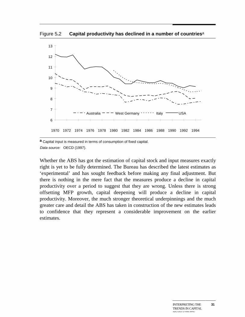
Finally, it is worth noting that declining capital productivity is a feature of othercountries’ experience. Figure 5.2 shows capital productivity has declined in anumber of countries since the 1970s.

Figure 5.1 The industry composition of capital input has changed sincethe 1960sa

%

0

20

40

60

80

100CRS

Finance

Commun

T&S

ACR

Retail Tr

Wsale Tr

Construc

EGW

Manuf

Mining

Agric

1964-65 1981-82 1997-98

a Capital input is measured in terms of capital services.

Data source: Unpublished ABS data.


31

Figure 5.2 Capital productivity has declined in a number of countriesa

6

7

8

9

10

11

12

13

1970

1972

1974

1976

1978

1980

1982

1984

1986

1988

1990

1992

1994

Australia West Germany Italy USA

a Capital input is measured in terms of consumption of fixed capital.

Data source: OECD (1997).

Whether the ABS has got the estimation of capital stock and input measures exactlyright is yet to be fully determined. The Bureau has described the latest estimates as‘experimental’ and has sought feedback before making any final adjustment. Butthere is nothing in the mere fact that the measures produce a decline in capitalproductivity over a period to suggest that they are wrong. Unless there is strongoffsetting MFP growth, capital deepening will produce a decline in capitalproductivity. Moreover, the much stronger theoretical underpinnings and the muchgreater care and detail the ABS has taken in construction of the new estimates leadsto confidence that they represent a considerable improvement on the earlierestimates.

INTERNATIONALCOMPARISONS OFGROWTH PATHS

33

A International comparisons of growthpaths

Chapter 4 introduced the notion of growth paths and box 4.2 gave someinternational examples.

This appendix presents a range of further examples and a representation of somecountries’ growth paths based on other data sources. For most of the high-incomecountries, OECD sources are used because data are available into the 1990s. For theUnited States, Bureau of Labour Statistics data are used.

The examples are grouped under headings of high-income countries, rising-incomecountries and low-income countries. Expectations about the form of growth pathsfor these country groupings were outlined in box 4.2.

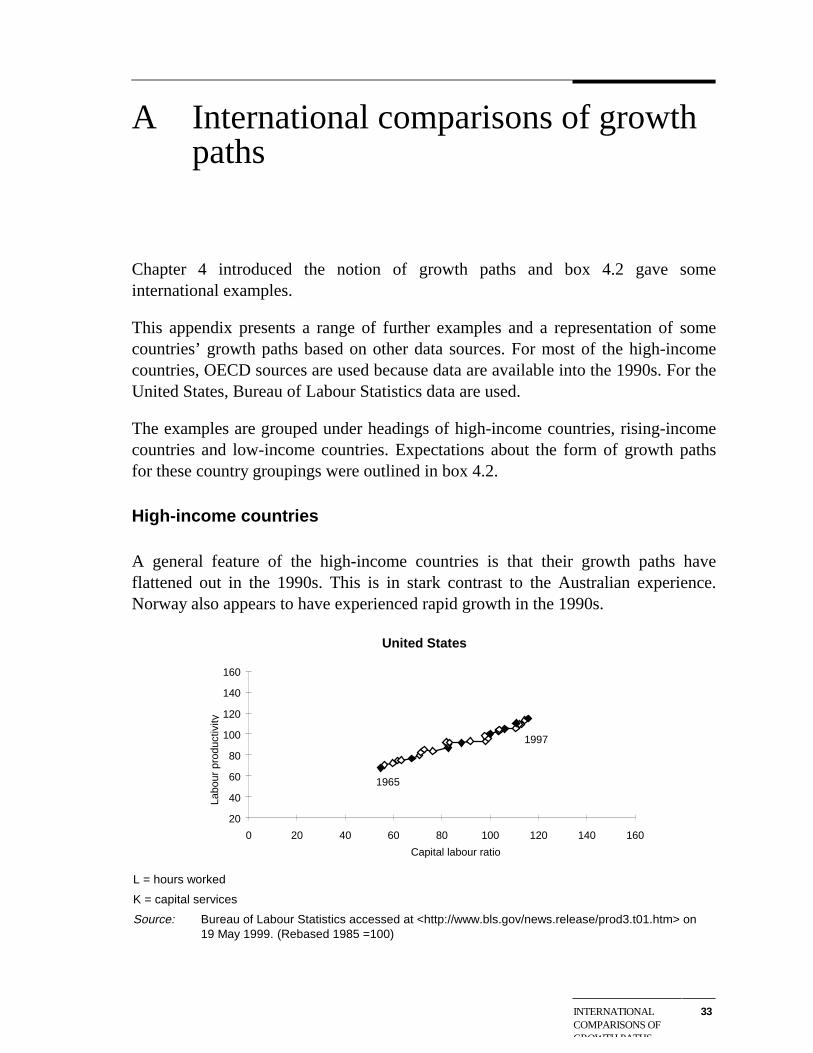
High-income countries

A general feature of the high-income countries is that their growth paths haveflattened out in the 1990s. This is in stark contrast to the Australian experience.Norway also appears to have experienced rapid growth in the 1990s.

United States

20

40

60

80

100

120

140

160

0 20 40 60 80 100 120 140 160

Labo

ur p

rodu

ctiv

ity


1965

1997

L = hours worked

K = capital services

Source: Bureau of Labour Statistics accessed at <http://www.bls.gov/news.release/prod3.t01.htm> on19 May 1999. (Rebased 1985 =100)

34 THE NEW ECONOMY?

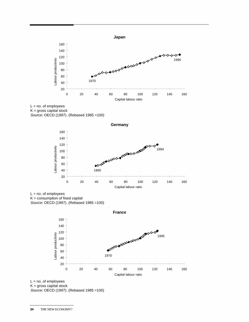
Japan

20

40

60

80

100

120

140

160

0 20 40 60 80 100 120 140 160

Labo

ur p

rodu

ctiv

ity


1970

1995

L = no. of employeesK = gross capital stockSource: OECD (1997). (Rebased 1985 =100)

Germany

20

40

60

80

100

120

140

160

0 20 40 60 80 100 120 140 160

Labo

ur p

rodu

ctiv

ity


1965

1994

L = no. of employeesK = consumption of fixed capitalSource: OECD (1997). (Rebased 1985 =100)

France

20

40

60

80

100

120

140

160

0 20 40 60 80 100 120 140 160

Labo

ur p

rodu

ctiv

ity


1970

1995



35

United Kingdom

20

40

60

80

100

120

140

160

0 20 40 60 80 100 120 140 160

Labo

ur p

rodu

ctiv

ity


1970

1992


Canada

20

40

60

80

100

120

140

160

0 20 40 60 80 100 120 140 160

Labo

ur p

rodu

ctiv

ity


1970

1995

L = no. of employeesK = consumption of fixed capitalSource: OECD (1997). (Rebased 1985 =100)

Sweden

20

40

60

80

100

120

140

160

0 20 40 60 80 100 120 140 160

Labo

ur p

rodu

ctiv

ity


1970

1994


36 THE NEW ECONOMY?

Norway

20

40

60

80

100

120

140

160

0 20 40 60 80 100 120 140 160

Labo

ur p

rodu

ctiv

ity


1970

1996

L=No. of employeesK=Gross capital stockSource: OECD 1997. (Rebased 1985 =100)Note: Employment numbers were extended from 1992 to 1996 using data from OECD Economic Outlook,No. 62, December 1997.

New Zealand

20

40

60

80

100

120

140

160

0 20 40 60 80 100 120 140 160

Labo

ur p

rodu

ctiv

ity


19651990

L = no. of employeesK = gross capital stockSource: Summers and Heston (1991), PWT v.5.6.


37

Rising-income countries

All charts are sourced from data in the Penn World tables (Summers and Heston(1991), PWT v.5.6). For general description of that data, see box 4.2.

Taiwan

20

40

60

80

100

120

140

160

0 20 40 60 80 100 120 140 160

Labo

ur p

rodu

ctiv

ity


1965

1990

Thailand

20

40

60

80

100

120

140

160

0 20 40 60 80 100 120 140 160

Labo

ur p

rodu

ctiv

ity


1965

1990

India

20

40

60

80

100

120

140

160

0 20 40 60 80 100 120 140 160

Labo

ur p

rodu

ctiv

ity


1965

1990

38 THE NEW ECONOMY?

Low-income countries

Data for charts are sourced from Summers and Heston (1991), PWT v.5.6.

Nigeria

20

40

60

80

100

120

140

160

0 20 40 60 80 100 120 140 160

Labo

ur p

rodu

ctiv

ity


1965

1990

Kenya

20

40

60

80

100

120

140

160

0 20 40 60 80 100 120 140 160

Labo

ur p

rodu

ctiv

ity


1965

1990

Zimbabwe

20

40

60

80

100

120

140

160

0 20 40 60 80 100 120 140 160

Labo

ur p

rodu

ctiv

ity


19651990

REFERENCES 39

References

Barnes, P., Johnson, R., Kulys, A. and Hook, S. 1999, Productivity and theStructure of Employment, Productivity Commmission Staff Research Paper(forthcoming).

Gretton, P. and Fisher, B. 1997, Productivity Growth and Australian ManufacturingIndustry, Industry Commission Staff Research Paper, AGPS, Canberra

Industry Commission (IC) 1997, Assessing Australia’s Productivity Performance,Research Paper, AGPS, Canberra, September.

Maddison, A. 1995, Monitoring the World Economy 1820-1992, OECD, Paris.

—— 1997, ‘Causal Influences on Productivity Performance 1820-1992: A GlobalPerspective’, Journal of Productivity Analysis, v.8, pp.325-359.

OECD 1997, International Sectoral Data Base, Statistics Directorate, OECD, Paris(Version 97).

Productivity Commission (PC) 1999, Microeconomic Reform and AustralianProductivity: Exploring the Links, (forthcoming).

Reserve Bank of Australia (RBA) 1999, Semi-Annual Statement on MonetaryPolicy, RBA, Sydney, May.

—— 1998, ‘The Economy and Financial Markets’, Reserve Bank of AustraliaBulletin, August, pp.1-33.

Summers, R. and Heston, A. 1991, ‘The Penn World Table (Mark 5): An ExpandedSet of International Comparisons, 1950-1988’, Quarterly Journal of Economics,May, pp.327-368.

Treasury (Commonwealth) 1999, ‘Economic Policy Reform and Australia’s RecentEconomic Performance’, Statement 3, 1998-99 Budget Paper No.1.

The New Economy? A New Look at Australia's Productivity Performance

Documents

Transcript of The New Economy? A New Look at Australia's Productivity Performance