1

A new look at the problem of gauge invariance in quantum field theory

by

Dan Solomon

Rauland-Borg Corporation3450 W. Oakton Street

Skokie, IL 60076USA

Phone: 1-847-324-8337Email: dan.Solomon@rauland.com

PACS 11.10.-z

(June 19, 2007)

2

Abstract

Quantum field theory is assumed to be gauge invariant. However it is well known that

when certain quantities are calculated using perturbation theory the results are not gauge

invariant. The non-gauge invariant terms have to be removed in order to obtain a

physically correct result. In this paper we will examine this problem and determine why

a theory that is supposed to be gauge invariant produces non-gauge invariant results.

3

1. Introduction

It is well know that quantum field theory contains anomalies. An anomaly occurs

when the result of a calculation does not agree with some underlying symmetry of the

theory. Such is the case with gauge invariance.

Quantum field theory is assumed to be gauge invariant [1][2]. A change in the

gauge is a change in the electromagnetic potential that does not produce a change in the

electromagnetic field. The electromagnetic field is given by,

0A

E A ; B At

(1.1)

where E

is the electric field, B

is the magnetic field, and 0A , A

is the electromagnetic

potential. A change in the electromagnetic potential that does not produce a change the

electromagnetic field is given by,

0 0 0A A A , A A At

(1.2)

where x, t

is an arbitrary real valued function. Using relativistic notation this can

also be written as,

A A A (1.3)

In order for quantum field theory to be gauge invariant a change in the gauge

cannot produce a change in any physical observable such as the current and charge

expectation values. However it is well known that when certain quantities are calculated

using standard perturbation theory the results are not gauge invariant. The non-gauge

4

invariant terms that appear in the results have to be removed to make the answer

physically correct.

For example, the first order change in the vacuum current, due to an applied

electromagnetic field, can be shown to be given by,

4vacJ x x x A x d x

(1.4)

where is called the polarization tensor and where, in the above expression,

summation over repeated indices is assumed. The above equation is normally written in

terms of the Fourier transformed quantities as,

vacJ k k A k (1.5)

where k is the 4-momentum of the electromagnetic field. In this case a gauge

transformation takes the following form,

A k A k A k ik k (1.6)

The change in the vacuum current, g vacJ k , due to a gauge transformation can be

obtained by using (1.6) in (1.5) to yield,

g vac vJ k ik k k (1.7)

Now if quantum theory is gauge invariant then an observable quantity, such as the

vacuum current, must not be affected by a gauge transformation. Therefore g vacJ k

must be zero. For this to be true we must have that,

vk k 0 (1.8)

However, when the polarization tensor is calculated it is found that the above relationship

does not hold.

5

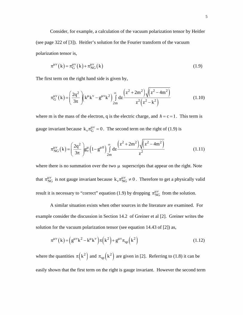
Consider, for example, a calculation of the vacuum polarization tensor by Heitler

(see page 322 of [3]). Heitler’s solution for the Fourier transform of the vacuum

polarization tensor is,

G NGk k k (1.9)

The first term on the right hand side is given by,

2 2 2 22

2G 2 2 2

2m

z 2m z 4m2qk k k g k dz

3 z z k

(1.10)

where m is the mass of the electron, q is the electric charge, and c 1 . This term is

gauge invariant because Gk 0 . The second term on the right of (1.9) is

2 2 2 22

0NG 2

2m

z 2m z 4m2qk g 1 g dz

3 z

(1.11)

where there is no summation over the two superscripts that appear on the right. Note

that NG is not gauge invariant because NGk 0

. Therefore to get a physically valid

result it is necessary to “correct” equation (1.9) by dropping NG from the solution.

A similar situation exists when other sources in the literature are examined. For

example consider the discussion in Section 14.2 of Greiner et al [2]. Greiner writes the

solution for the vacuum polarization tensor (see equation 14.43 of [2]) as,

2 2 2spk g k k k k g k (1.12)

where the quantities 2k and 2sp k are given in [2]. Referring to (1.8) it can be

easily shown that the first term on the right is gauge invariant. However the second term

6

is not gauge invariant unless 2sp k equals zero. Greiner shows that this is not the

case. Therefore this term must be dropped form the result in order to obtain a physically

valid solution.

For another example of this refer to section 6-4 of Nishijima [4]. In this

reference is it shown that the vacuum polarization tensor includes a non-gauge invariant

term which must be removed. For other examples refer to equation 7.79 of Peskin and

Schroeder [5] and Section 5.2 of Greiner and Reinhardt [6]. In all cases a direct

calculation of the vacuum polarization tensor using perturbation theory produces a result

which includes non-gauge invariant terms. In all cases the non-gauge invariant terms

must be removed to obtain the “correct” gauge invariant result.

There are two general approaches to removing these non-gauge invariant terms.

The first approach is simply to recognize that the term cannot be physically valid and

drop it from the solution. This is the approach taken by Heitler [3], Nishijima [4], and

Greiner et al [2]. The other approach is to come up with mathematical techniques which

automatically eliminate the offending terms. This is called “regularization”. One type

of regularization is called Pauli-Villars regularization [7] . In this case additional

functions are introduced that have the correct behavior so that the non-gauge invariant

terms are cancelled. An example of the use Pauli-Villars regularization is given by

Greiner and Reinhardt [6]. Another type of regularization is called dimensional

regularization. An example of this is given by Peskin and Schroeder [5].

The problem with regularization is that there is no physical explanation for why it

is required. It is an ad hoc mathematical device required to remove the unwanted terms.

Also regularization does not guarantee a unique answer. For example consider the result

7

from [2] given by equation (1.12). As discussed above the second term on the right must

be removed. In reference [2] the authors simply removed the term 2spg k by hand

without resorting to formal regularization schemes. Suppose someone invented a

mathematical procedure that subtracted the term 2 2 2spg k g k k k f k

from (1.12) where 2f k is some arbitrary function. The final “corrected” result would

be 2 2 2g k k k k f k . Since this is gauge invariant it would certainly be a

physically acceptable solution, however it is not unique because 2f k is arbitrary. That

is, there is no theoretical way to distinguish between a mathematical regularization

procedure for which 2f k 0 and one for which 2f k is non-zero. Both yield

physically valid results.

The obvious question that should be asked is why do non-gauge invariant terms

appear in a theory that is supposed to be gauge invariant? This question is briefly

addressed by Greiner et al (page 398 of [2]) who writes “… this latter [non-gauge

invariant] term violates the gauge invariance of the theory. This is a very sever

contradiction to the experimentally confirmed gauge independence of QED. [This

problem indicates] that perturbative QED is not a complete theory. As one counter

example or inconsistency suffices to prove a theory wrong, we should, in principle, spend

the rest of this book searching for an improved theory. However, there is little active

work on this today because: (1) there is a common belief that some artifact of the exact

mathematics is the source of the problem; (2) this problem may disappear when the

8

properly generalized theory, including in its framework all charged Dirac particles, is

achieved.”

It is my impression that the above paragraph pretty much expresses the current

state of thinking on this problem, i.e. , the problem is probably due to an artifact of the

mathematics and will, hopefully, go away when a complete theory is revealed. However

recent work comparing Dirac’s hole theory (HT) to quantum field theory (QFT) suggests

that we consider the problem from a different perspective.

Consider a “simple” quantum theory consisting of non-interacting electrons in a

background classical electromagnetic field. For such a situation Dirac’s hole theory and

quantum field theory are generally assumed to be equivalent. Hole theory was introduced

by Dirac to resolve the problem caused by the fact that solutions of the Dirac equation

include both positive and negative energy solutions. Dirac proposed that all the negative

energy states are occupied by a single electron and then evoked the Pauli exclusion

principle to prevent the decay of a positive energy electron into negative energy states.

The electrons in the negative energy states, the so called Dirac sea, are assumed to be

unobservable. What we observe are variations from the unperturbed vacuum state.

Recently several papers have appeared in the literature pointing out that there are

differences between Dirac’s hole theory (HT) and quantum field theory (QFT)

[8][9][10][11][12][13]. The problem was originally examined by Coutinho et al[8][9].

They calculated the second order change in the energy of the vacuum state due to a time

independent perturbation. They found that HT and QFT produce different results. They

concluded that the difference between HT and QFT was related to the validity of

Feynman’s belief that the Pauli Exclusion Principle can be disregarded for intermediate

9

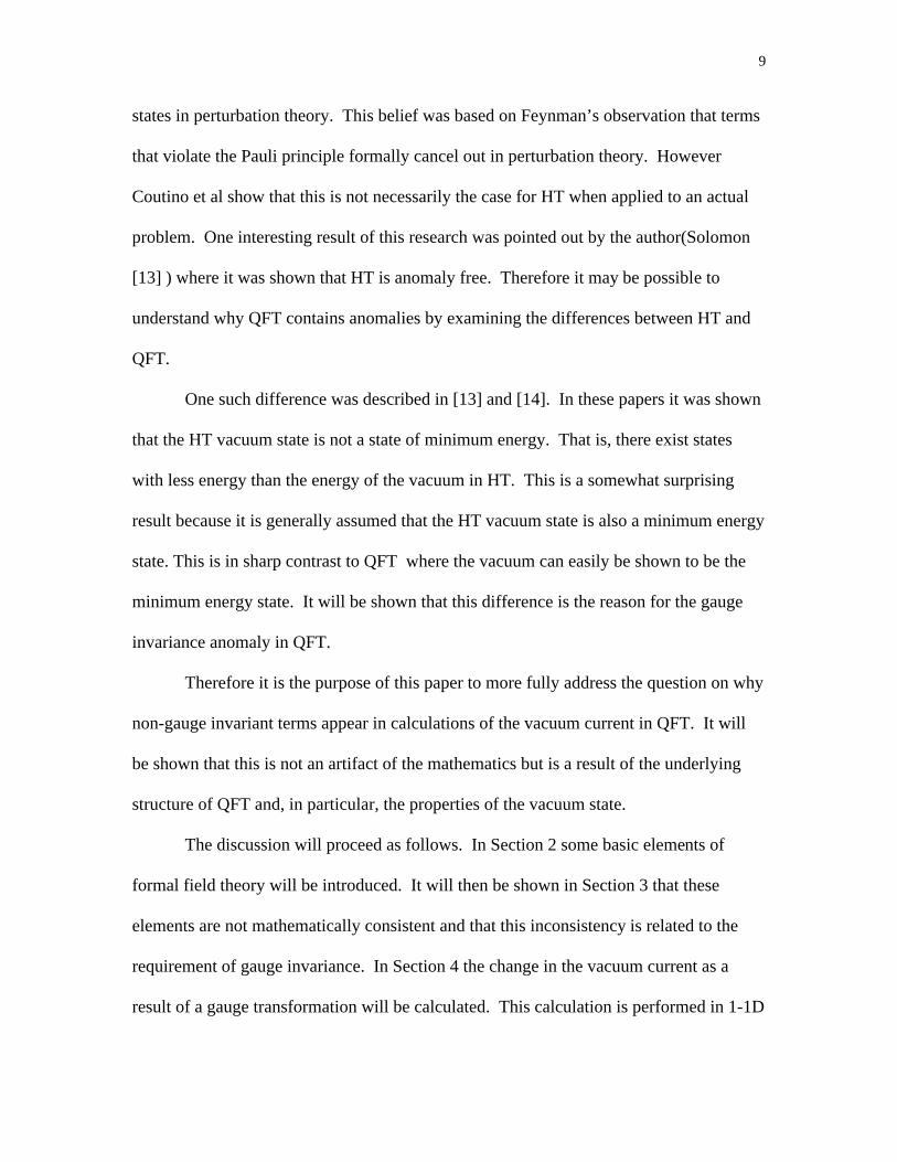
states in perturbation theory. This belief was based on Feynman’s observation that terms

that violate the Pauli principle formally cancel out in perturbation theory. However

Coutino et al show that this is not necessarily the case for HT when applied to an actual

problem. One interesting result of this research was pointed out by the author(Solomon

[13] ) where it was shown that HT is anomaly free. Therefore it may be possible to

understand why QFT contains anomalies by examining the differences between HT and

QFT.

One such difference was described in [13] and [14]. In these papers it was shown

that the HT vacuum state is not a state of minimum energy. That is, there exist states

with less energy than the energy of the vacuum in HT. This is a somewhat surprising

result because it is generally assumed that the HT vacuum state is also a minimum energy

state. This is in sharp contrast to QFT where the vacuum can easily be shown to be the

minimum energy state. It will be shown that this difference is the reason for the gauge

invariance anomaly in QFT.

Therefore it is the purpose of this paper to more fully address the question on why

non-gauge invariant terms appear in calculations of the vacuum current in QFT. It will

be shown that this is not an artifact of the mathematics but is a result of the underlying

structure of QFT and, in particular, the properties of the vacuum state.

The discussion will proceed as follows. In Section 2 some basic elements of

formal field theory will be introduced. It will then be shown in Section 3 that these

elements are not mathematically consistent and that this inconsistency is related to the

requirement of gauge invariance. In Section 4 the change in the vacuum current as a

result of a gauge transformation will be calculated. This calculation is performed in 1-1D

10

space-time. The advantage of this is that all integrals are finite and well defined.

Therefore there is no need to regularize divergent integrals. It is shown that the results

are not gauge invariant.

2. Quantum Field theory.

In this section the basic elements of quantum field theory in the Schrödinger

representation will be introduced. Natural unit will be used so that c 1 . We shall

consider a “simple” field theory consisting of non-interacting fermions acted on by a

classical electromagnetic field. In the Schrödinger representation of QFT the time

evolution of the state vector t and its dual t are given by,

t tˆ ˆiH t t , i t H tt t

(2.1)

where H t is the Hamiltonian operator which is given by,

0 0ˆˆ ˆ ˆH t H J x A x, t dx x A x, t dx

(2.2)

In the above expression the quantities 0A x, t , A x, t

are the electromagnetic

potential which are assumed to be unquantized, real valued functions. The quantity 0H is

the free field Hamiltonian, that is, the Hamiltonian when the electromagnetic potential is

zero, and J x

and ˆ x

are the current and charge operators, respectively. Note that

0H , along with the current and charge operators, are time independent which is

consistent with the Schrödinger picture approach. Throughout this discussion it is

assumed that t is normalized, i.e., t t 1 . Note that Eq. (2.1) ensures

that the normalization of t is constant in time.

11

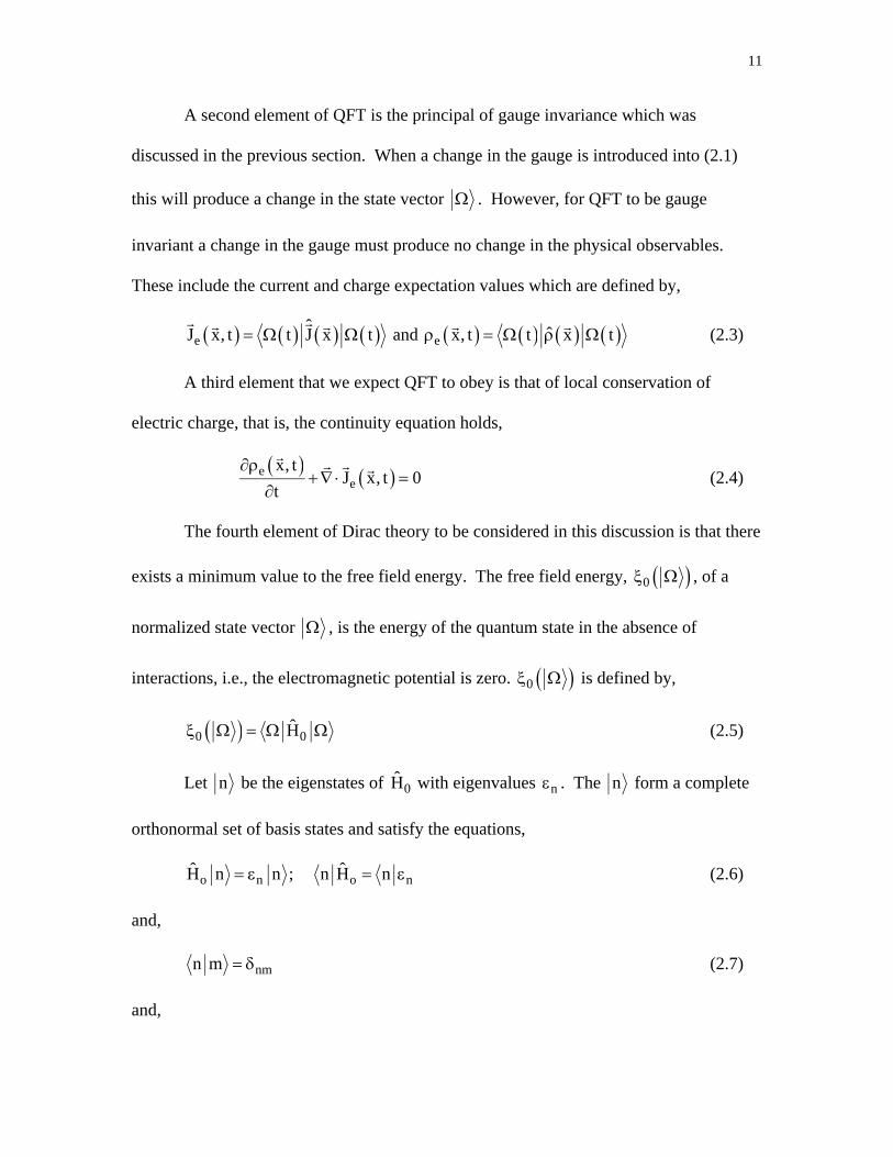
A second element of QFT is the principal of gauge invariance which was

discussed in the previous section. When a change in the gauge is introduced into (2.1)

this will produce a change in the state vector . However, for QFT to be gauge

invariant a change in the gauge must produce no change in the physical observables.

These include the current and charge expectation values which are defined by,

eˆJ x, t t J x t

and e ˆx, t t x t

(2.3)

A third element that we expect QFT to obey is that of local conservation of

electric charge, that is, the continuity equation holds,

ee

x, tJ x, t 0

t

(2.4)

The fourth element of Dirac theory to be considered in this discussion is that there

exists a minimum value to the free field energy. The free field energy, 0 , of a

normalized state vector , is the energy of the quantum state in the absence of

interactions, i.e., the electromagnetic potential is zero. 0 is defined by,

0 0H (2.5)

Let n be the eigenstates of 0H with eigenvalues n . The n form a complete

orthonormal set of basis states and satisfy the equations,

o n o nˆ ˆH n n ; n H n (2.6)

and,

nmn m (2.7)

and,

12

n

ˆn n 1 (2.8)

Any arbitrary state can be expanded in terms of the eigenstates n so that we can

write,

nn

c n (2.9)

where nc are the expansion coefficients.

The vacuum state 0 is generally assumed to be the eigenvector of 0H with the

smallest eigenvalue o 0 . For all other eigenvalues,

n o =0 for n 0 (2.10)

Using this fact along with (2.5)-(2.9) we can easily show that,

0 0 0 =0 for all 0 (2.11)

Therefore the vacuum state is the quantum state with the minimum value of the free field

energy.

3. A mathematical inconsistency.

The four elements of QFT field theory that were introduced in the last section

were (1)the Schrodinger equation, (2)the principle of gauge invariance, (3)the continuity

equation, and (4)the idea that the vacuum state 0 is the state with minimum free field

energy. The question that we will address in this section is whether or not these four

elements of Dirac field theory are mathematically consistent. From the equations of

Section 2 we will derive a number of additional relationships. First, consider the time

derivative of the current expectation value. From (2.3) and (2.1) we obtain,

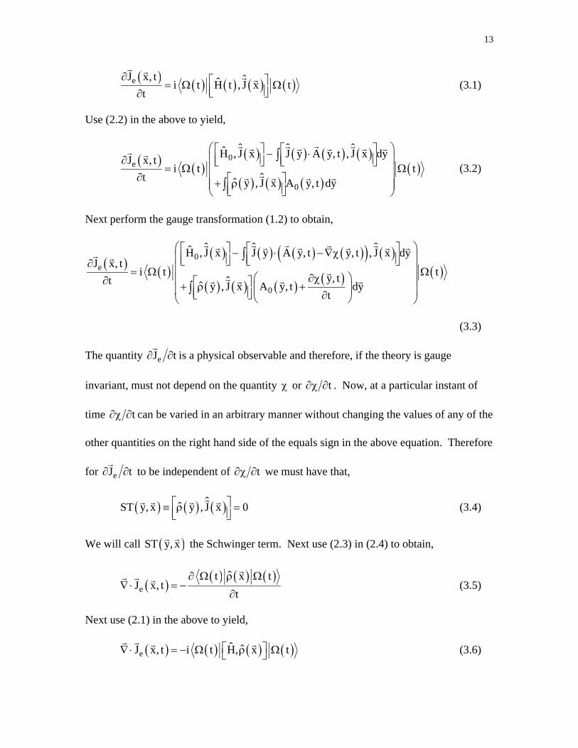
13

eJ x, t ˆˆi t H t , J x tt

(3.1)

Use (2.2) in the above to yield,

0e

0

ˆ ˆ ˆH , J x J y A y, t , J x dyJ x, t

i t tt ˆˆ y , J x A y, t dy

(3.2)

Next perform the gauge transformation (1.2) to obtain,

0

e

0

ˆ ˆ ˆH , J x J y A y, t y, t , J x dyJ x, t

i t ty, tt ˆˆ y , J x A y, t dyt

(3.3)

The quantity eJ t

is a physical observable and therefore, if the theory is gauge

invariant, must not depend on the quantity or t . Now, at a particular instant of

time t can be varied in an arbitrary manner without changing the values of any of the

other quantities on the right hand side of the equals sign in the above equation. Therefore

for eJ t

to be independent of t we must have that,

ˆˆST y, x y , J x 0

(3.4)

We will call ST y, x

the Schwinger term. Next use (2.3) in (2.4) to obtain,

e

ˆt x tJ x, t

t

(3.5)

Next use (2.1) in the above to yield,

eˆ ˆJ x, t i t H, x t

(3.6)

14

Use (2.2) in the above to yield,

0

e

0

ˆˆ ˆ ˆH , x J y , x A y, t dyJ x, t i t t

ˆ ˆy , x A y, t dy

(3.7)

Use (3.4) in the above to obtain,

e 0 0ˆ ˆ ˆ ˆJ x, t i t H , x y , x A y, t dy t

(3.8)

We can then apply a gauge transformation to obtain,

0

e 0

A y, tˆ ˆ ˆ ˆJ x, t i t H , x y , x dy ty, t

t

(3.9)

The quantity eJ x, t

is an observable and must be independent of t . Therefore,

ˆ ˆy , x 0

(3.10)

so that,

e 0ˆ ˆ ˆJ x, t t J x t i t H , x t

(3.11)

In order for the above equation to be true for arbitrary values of the state vector t

we must have,

0ˆˆ ˆi H , x J x

(3.12)

Now consider relationships (3.4) and (3.12). They following directly from the

first three of the four elements of Dirac field theory that we have introduced in Section 1.

However Schwinger [15] has shown that they are not compatible with the fourth element,

that is, the assumption that the vacuum state is the state with the lowest free field energy.

This will be demonstrated below.

15

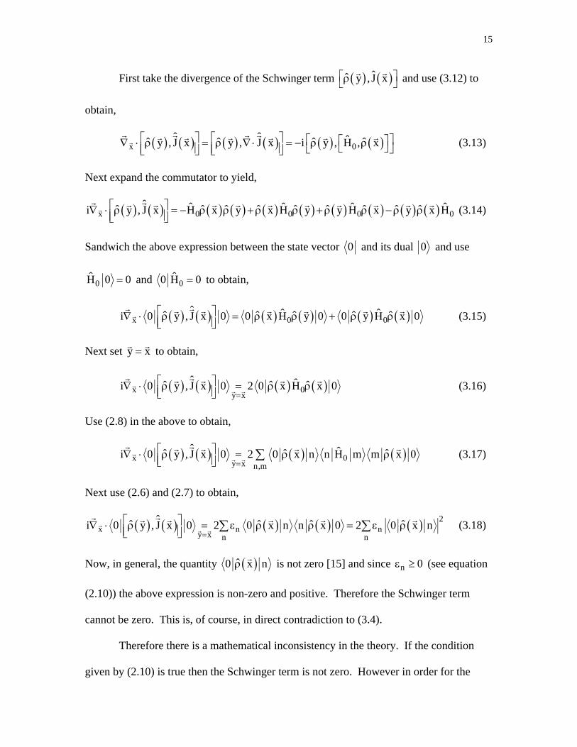
First take the divergence of the Schwinger term ˆˆ y , J x

and use (3.12) to

obtain,

x 0ˆ ˆ ˆˆ ˆ ˆ ˆy , J x y , J x i y , H , x

(3.13)

Next expand the commutator to yield,

x 0 0 0 0ˆ ˆ ˆ ˆ ˆˆ ˆ ˆ ˆ ˆ ˆ ˆ ˆ ˆi y , J x H x y x H y y H x y x H

(3.14)

Sandwich the above expression between the state vector 0 and its dual 0 and use

0H 0 0 and 0ˆ0 H 0 to obtain,

x 0 0ˆ ˆ ˆˆ ˆ ˆ ˆ ˆi 0 y , J x 0 0 x H y 0 0 y H x 0

(3.15)

Next set y x

to obtain,

x 0y x

ˆ ˆˆ ˆ ˆi 0 y , J x 0 2 0 x H x 0

(3.16)

Use (2.8) in the above to obtain,

x 0y x n,m

ˆ ˆˆ ˆ ˆi 0 y , J x 0 2 0 x n n H m m x 0

(3.17)

Next use (2.6) and (2.7) to obtain,

2x n n

y x n n

ˆˆ ˆ ˆ ˆi 0 y , J x 0 2 0 x n n x 0 2 0 x n

(3.18)

Now, in general, the quantity ˆ0 x n

is not zero [15] and since n 0 (see equation

(2.10)) the above expression is non-zero and positive. Therefore the Schwinger term

cannot be zero. This is, of course, in direct contradiction to (3.4).

Therefore there is a mathematical inconsistency in the theory. If the condition

given by (2.10) is true then the Schwinger term is not zero. However in order for the

16

theory to be gauge invariant the Schwinger term must be zero. This can be seen from

examining (3.3). If the Schwinger term is not zero then the observable eJ t

is

dependent on the gauge transformation. The result of all this is that if (2.10) is true then

the theory is not, in fact, gauge invariant. This will be shown in the next section where a

calculation of the vacuum current will be shown to be non-gauge invariant.

4. A calculation of the vacuum current.

In the previous section we showed that QFT is not gauge invariant because the

Schwinger term is not zero. In this section we will confirm the results of the previous

section by calculating the change in vacuum current due to a change in the

electromagnetic potential and showing that the result is not gauge invariant. We will

work in 1-1D space-time. This will simplify the problem and avoid mathematical

difficulties that appear when the calculations are done in normal 3-1D space-time. The

main problem that we will avoid is the problem of divergent integrals. This greatly

simplifies the discussion and makes the calculations straightforward. There is no

problem trying to interpret and regularize divergent integrals. For the problem at hand

we assume that the space dimension is in the z-direction.

In 1-1D space-time there is no magnetic field and the electric field is given in

terms of the electromagnetic potential zA and 0A by,

0z AAE

t z

(4.1)

The field operators are given by,

† † † † †r 1,r r 1,r r r1,r 1,r

r r

ˆ ˆ ˆ ˆˆ ˆz b z d z ; z b z d z

(4.2)

17

where rb ( †rb ) are the electron destruction(creation) operators and the rd ( †

rd ) are the

positron destruction (creation) operators. These operators satisfy the usual anti-

commutator relations,

† †r s s r rs

ˆ ˆ ˆ ˆb b b b ; † †r s s r rs

ˆ ˆ ˆ ˆd d d d (4.3)

with all other anti-commutators equal to zero.

The quantities ,r z satisfy,

0 ,r ,r ,rH z z (4.4)

where,

rip z,r ,rz u e (4.5)

and where,

0 x zH i mz

(4.6)

In the above expressions x and z are the usual Pauli matrices, ‘r’ is an integer, 1

is the sign of the energy, rp 2 r L , and,

r,r pE ; r

2 2p rE p m ;

r

r,r ,r

p

1

pu NE m

; r

r

p,r

p

E mN

2L E

(4.7)

and L is the 1-dimensional integration volume.

The ,r z form an orthonormal basis set and satisfy,

L 2

†,s rs,r

L 2

z z dz

(4.8)

The Hamiltonian operator is given by,

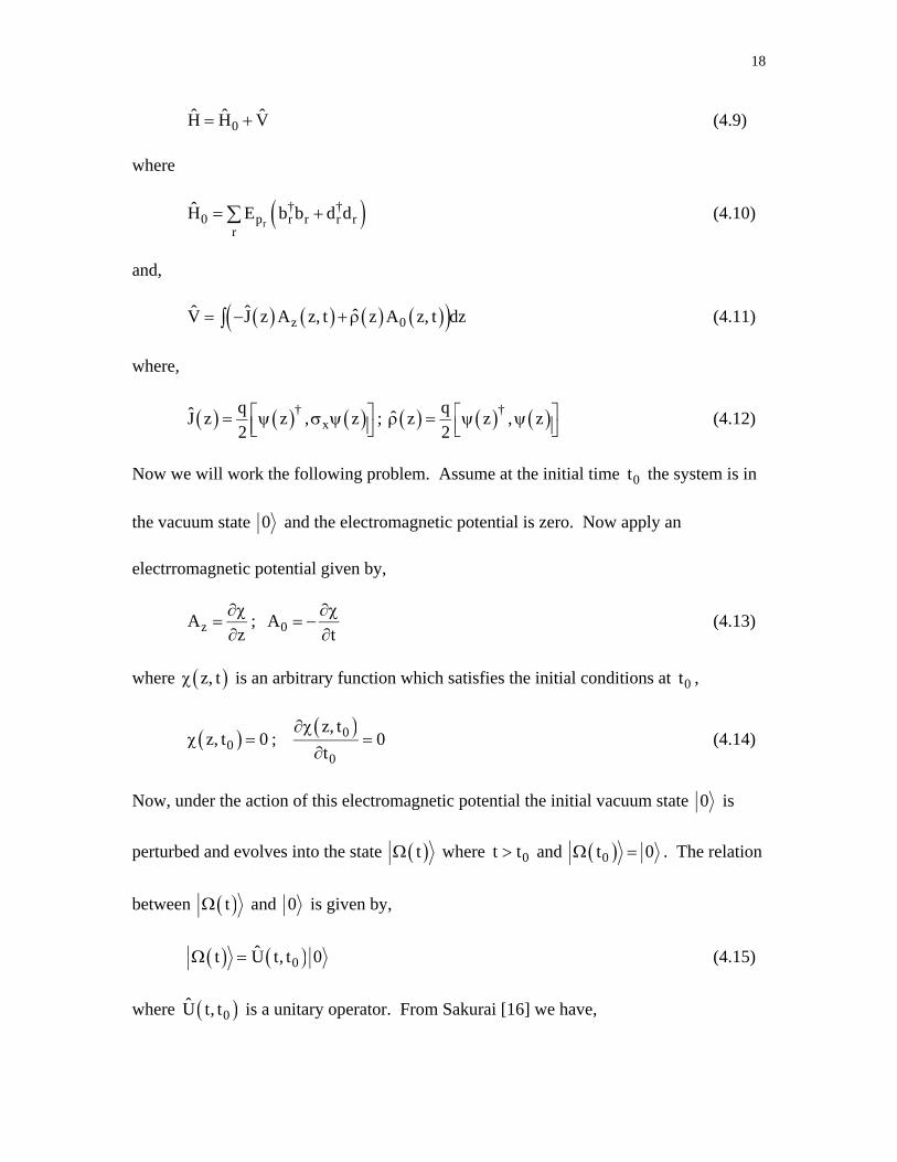
18

0ˆ ˆ ˆH H V (4.9)

where

r

† †0 p r r r r

rH E b b d d (4.10)

and,

z 0ˆ ˆ ˆV J z A z, t z A z, t dz (4.11)

where,

†x

qJ z z , z

2

; †qˆ z z , z

2

(4.12)

Now we will work the following problem. Assume at the initial time 0t the system is in

the vacuum state 0 and the electromagnetic potential is zero. Now apply an

electrromagnetic potential given by,

zAz

; 0At

(4.13)

where z, t is an arbitrary function which satisfies the initial conditions at 0t ,

0z, t 0 ; 0

0

z, t0

t

(4.14)

Now, under the action of this electromagnetic potential the initial vacuum state 0 is

perturbed and evolves into the state t where 0t t and 0t 0 . The relation

between t and 0 is given by,

0ˆt U t, t 0 (4.15)

where 0U t, t is a unitary operator. From Sakurai [16] we have,

19

0 0 0

0

tˆ ˆiH t iH t20 I

t

ˆ ˆU t, t e 1 i V t dt O q e

(4.16)

where 2O q means terms to the order 2q or higher and,

0 0ˆ ˆiH t iH t

I I 1 I 0ˆ ˆ ˆ ˆV t e V t e J z, t A z z, t A z dz (4.17)

where IJ z, t and Iˆ z, t are the current and charge operators in the interaction

representation and are given by,

0 0ˆ ˆiH t iH t

Iˆ ˆJ z, t e J z e ; 0 0

ˆ ˆiH t iH tIˆ ˆz, t e z e (4.18)

Now we want to calculate the current expectation value of the state t at

some time ft . It will be convenient to let ft 0 . Obviously, then, 0t 0 . Use (4.15)

and (4.16) along with 0H 0 0 and ˆ0 J z 0 0 to obtain for the first order change

in the current,

0

0

vac It

ˆ ˆ ˆJ z 0 J z 0 i 0 J z , V t dt 0

(4.19)

Now before proceeding with this calculation what can we conclude about vacJ z based

on physical requirements of the theory? If we substitute (4.13) into (4.1) we see that the

electric field E 0 . Therefore the electromagnetic potential (4.13) is simply a gauge

transformation from zero electric field. Therefore, if the theory is gauge invariant, then

vacJ z should be zero. Now let us proceed with the calculation and see if this is the

case.

Use (4.13) and (4.17) to obtain,

20

0 0

0 0

I I It t

z , t z , tˆ ˆ ˆV t dt dt J z , t z , t dzz t

(4.20)

Integrate by parts and rearrange terms to obtain,

0 0

0 0

I It t

ˆˆ ˆV t dt dt z , t S z , t z , t z , t dzt

(4.21)

where,

I Iˆ ˆJ z, t z, t

S z, tz t

(4.22)

Note that S z, t 0 is the continuity equation in 1-1D space-time in the interaction

representation. It can easily be shown that this condition is satisfied. Therefore, use this

along with the initial condition (4.14) in (4.21) to obtain,

0

0

It

ˆ ˆV t dt z ,0 z dz (4.23)

Use this result in (4.19) to obtain,

vacˆ ˆJ z i z ,0 0 J z , z 0 dz (4.24)

In order for vacJ z to be zero for arbitrary z ,0 the quantity ˆ ˆ0 J z , z 0

must be zero. However, based on our discussion of the Schwinger term it is evident that

this quantity cannot be zero. This calculation is done in the Appendix and the result is

s r

r s

2i p p z zsr

2r,s p p

ppqˆ ˆ0 J z , z 0 e E EL

(4.25)

Now, in the above expressions, replace the summations by integration by taking the limit

L and substituting L

dp2

to obtain,

21

2i p p z z

2p p

q p pˆ ˆ0 J z , z 0 dp dp eE E4

(4.26)

Use this result in (4.24) to obtain,

2

i p p z zvac 2

p p

iq p pJ z z ,0 dp dp e dz

E E4

(4.27)

Let k be the Fourier transform of z ,0 . Therefore we can write,

2

i p p z zikzvac 2

p p

iq p pJ z k e dk dp dp e dz

E E4

(4.28)

Integrate with respect to z to obtain,

2

i p p zvac

p p

iq p pJ z k dk dp dp p p k e

2 E E

(4.29)

Next integrate with respect to p to obtain,

ikzvac

iqJ z k e dk I p, k dp

2

(4.30)

where,

p p k

p p kI p,k

E E

(4.31)

Now let us examine the integrand I p, k as p . Use,

2 2

p 2 2 4p

m m 1E p 1 p 1 O

p 2p p

(4.32)

Also,

22

2 2

p k 2 2 4p

m m 1E p k 1 p k 1 O

p k 2 p k p k

(4.33)

Use this in (4.30) to obtain.

2 2

2p p

km 1 1 mI p, k

2 p p k 2 p

(4.34)

Therefore the integration of I p, k with respect to p is finite and well defined. It is

readily evaluated as follows,

RR

p p kR Rp p kR R

p p kI p, k dp dp E E

E E

(4.35)

Use the fact that p pE E along with (4.33) to obtain,

R R k R R k R k R kR R

I p, k dp E E E E E E 2k

(4.36)

Substitute this result in (4.30) to obtain,

2 2 2ikz ikz

vacz,02iq q q

J z k k e dk k e dk2 z z

(4.37)

From result we see that vacJ z is obviously non-zero. A gauge invariant theory would

require that this result is zero. Therefore the formal theory is not gauge invariant.

5. Conclusion.

At this point we can respond to W. Greiner’s comment that “there is a common

belief that some artifact of the exact mathematics is the source of the problem”. We have

shown that this belief is not correct. The reason non-gauge invariant terms appear in the

theory is because the formal theory is not, in fact, gauge invariant. Therefore then when

calculations are performed in perturbation theory it should be expected that non-gauge

23

invariant terms should appear in the results. These terms are not due to “some artifact of

the exact mathematics” but are the result of a correct mathematical calculation. This is

shown in Section 4 where we calculated the change in the vacuum current due to a gauge

transformation in 1-1D space-time. In 1-1D space-time we avoid the problem with

divergent integrals that that would appear in normal 3-1D space-time. Therefore there is

no problem with interpreting the results which where shown to not be gauge invariant.

As we have shown in order for the theory to be gauge invariant the Schwinger

term must be zero. However Schwinger has shown that this term cannot be zero. The

reason that this term is not zero is due to the fact that the vacuum state 0 is the state

with the minimum free field energy. In contrast Dirac hole theory, where it has been

shown that the vacuum is not a minimum energy state[13][14], has been shown to be

gauge invariant [13]. This suggests that for a theory to be gauge invariant requires a

proper definition of the vacuum state which allows for the existence of quantum states

with less energy than the vacuum state. This aspect of the problem is discussed in greater

detail in [17].

How then does quantum physics ultimately produce the correct physical result

which much be gauge invariant? Since the formal theory is not gauge invariant this

requires the introduction of an additional step. As has been discussed in Section 1 the

results of perturbation theory must be “corrected” by removing the non-gauge invariant

terms. This can be done by a number of methods as discussed in Section 1.

Appendix

Use (4.12) and (4.2) to obtain,

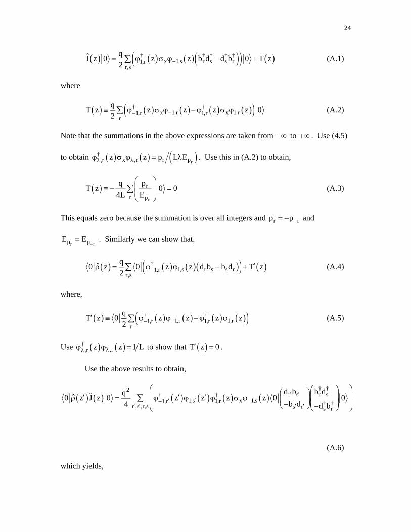
24

† † † † †x 1,s r s s r1,r

r,s

qJ z 0 z z b d d b 0 T z

2 (A.1)

where

† †x 1,r x 1,r1,r 1,r

r

qT z z z z z 0

2 (A.2)

Note that the summations in the above expressions are taken from to . Use (4.5)

to obtain r

†x ,r r p,r z z p L E . Use this in (A.2) to obtain,

r

r

r p

pqT z 0 0

4L E

(A.3)

This equals zero because the summation is over all integers and r rp p and

r rp pE E

. Similarly we can show that,

†1,s r s s r1,r

r,s

qˆ0 z 0 z z d b b d T z

2 (A.4)

where,

† †1,r 1,r1,r 1,r

r

qT z 0 z z z z

2 (A.5)

Use †,r,r z z 1 L to show that T z 0 .

Use the above results to obtain,

† †2

r s r s† †1,s x 1,s1,r1,r † †r ,s ,r,s s r s r

d b b dqˆˆ0 z J z 0 z z z z 0 0b d4 d b

(A.6)

which yields,

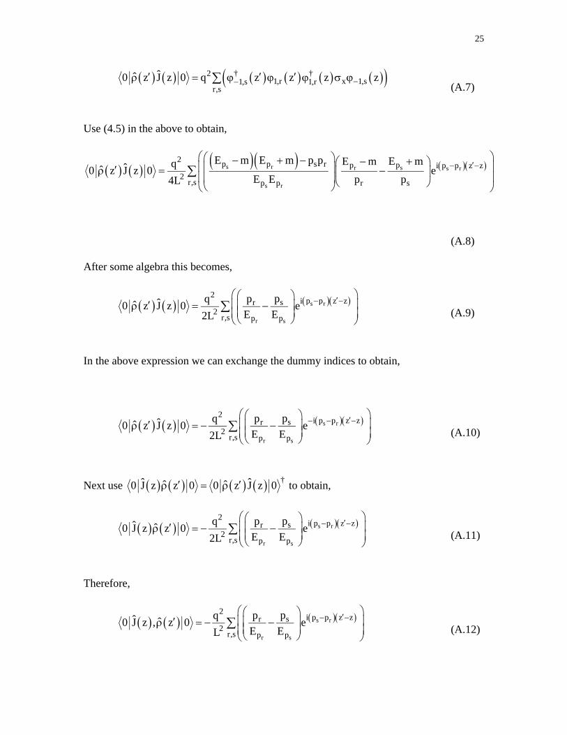
25

2 † †1,r x 1,s1,s 1,r

r,s

ˆˆ0 z J z 0 q z z z z

(A.7)

Use (4.5) in the above to obtain,

s r sr s r

s r

2 p p s r pp i p p z z2

r,s p p r s

E m E m p p E mE mqˆˆ0 z J z 0 eE E p p4L

(A.8)

After some algebra this becomes,

s r

r s

2i p p z zsr

2r,s p p

ppqˆˆ0 z J z 0 eE E2L

(A.9)

In the above expression we can exchange the dummy indices to obtain,

s r

r s

2i p p z zsr

2r,s p p

ppqˆˆ0 z J z 0 eE E2L

(A.10)

Next use †ˆ ˆˆ ˆ0 J z z 0 0 z J z 0 to obtain,

s r

r s

2i p p z zsr

2r,s p p

ppqˆ ˆ0 J z z 0 e E E2L

(A.11)

Therefore,

s r

r s

2i p p z zsr

2r,s p p

ppqˆ ˆ0 J z , z 0 e E EL

(A.12)

26

References

1. J. Schwinger, Phys. Rev. 81, 664 (1951).

2. W. Greiner, B. Muller, and J. Rafelski, “Quantum Electrodynamics of Strong

Fields”, Springer-Verlag, Berlin (1985).

3. W. Heitler. The quantum theory of radiation. Dover Publications, Inc., New

York (1954).

4. K. Nishijima. “Fields and Particles: Field theory and Dispersion Relations.” W.A.

Benjamin, New York, (1969).

5. Peskin and Schroeder. An Introduction to quantum field theory, Addison-Wesley

Publishing Company, Reading, Mass. 1995.

6. W. Greiner and J. Reinhardt. Quantum Electrodynamics. Springer-Verlag, Berlin,

1992.

7. W. Pauli and F. Villers, Rev. Mod. Phys. 21, 434 (1949).

8. F.A.B. Coutinho, D. Kaing, Y. Nogami, and L. Tomio, Can. J. of Phys., 80, 837

(2002). (see also quant-ph/0010039).

9. F.A.B. Coutinho, Y. Nagami, and L. Tomio, Phy. Rev. A, 59, 2624 (1999).

10. R. M. Cavalcanti, quant-ph/9908088.

11. D. Solomon. Can. J. Phys., 81, 1165, (2003).

12. Dan Solomon, “The difference between Dirac’s hole theory and quantum field

theory”. Chapter in “Frontiers in Quantum Physics Research”, Nova Science

Publishers (2004). F. Columbus and V. Krasnoholovets, ed. See also hep-

th/0401208.

13. D. Solomon. Can. J. Phys., 83, 257, (2005).

27

14. D. Solomon. Phys. Scr., 74, 117 (2006).

15. J. Schwinger, Phys. Rev. Lett., 3, 296 (1959).

16. J.J. Sakurai, “Advanced Quantum Mechanics”, Addison-Wesley Publishing

Company, Inc., Redwood City, California, (1967).

17. D. Solomon, Can. J. Phys. 76, 111 (1998). (see also quant-ph/9905021).