arX

iv:a

stro

-ph/

0312

362v

2 2

4 Ju

l 200

4TO APPEAR INThe Astrophysical JournalPreprint typeset using LATEX style emulateapj v. 6/22/04

THE MOUSE THAT SOARED: HIGH RESOLUTION X-RAY IMAGING OF THEPULSAR-POWERED BOW SHOCK G359.23–0.82

B. M. GAENSLER,1,2,3 E. VAN DER SWALUW,4 F. CAMILO ,5 V. M. K ASPI,6,7,8

F. K. BAGANOFF,7 F. YUSEF-ZADEH9 AND R. N. MANCHESTER10

To appear inThe Astrophysical Journal

ABSTRACTWe present an observation with theChandra X-ray Observatoryof the unusual radio source G359.23–0.82

(“the Mouse”), along with updated radio timing data from theParkes radio telescope on the coincident youngpulsar J1747–2958. We find that G359.23–0.82 is a very luminous X-ray source (LX [0.5− 8.0 keV] = 5×1034 ergs s−1 for a distance of 5 kpc), whose morphology consists of a bright head coincident with PSR J1747–2958, plus a 45′′-long narrow tail whose power-law spectrum steepens with distance from the pulsar. Wethus confirm that G359.23–0.82 is a bow-shock pulsar wind nebula powered by PSR J1747–2958; the nebularstand-off distance implies that the pulsar is moving with a Mach number of∼ 60, suggesting a space velocity≈ 600 km s−1 through gas of density≈ 0.3 cm−3. We combine the theory of ion-dominated pulsar windswith hydrodynamic simulations of pulsar bow shocks to show that a bright elongated X-ray and radio featureextending 10′′ behind the pulsar represents the surface of the wind termination shock. The X-ray and radio“trails” seen in other pulsar bow shocks may similarly represent the surface of the termination shock, ratherthan particles in the postshock flow as is usually argued. Thetail of the Mouse contains two components: arelatively broad region seen only at radio wavelengths, anda narrow region seen in both radio and X-rays. Wepropose that the former represents material flowing from thewind shock ahead of the pulsar’s motion, while thelatter corresponds to more weakly magnetized material streaming from the backward termination shock. Thisstudy represents the first consistent attempt to apply our understanding of “Crab-like” nebulae to the growinggroup of bow shocks around high-velocity pulsars.Subject headings:ISM: individual: (G359.23–0.82) — pulsars: individual (J1747–2958) — stars: neutron —

stars: winds, outflows

1. INTRODUCTION

Many isolated pulsars are observed to generate relativisticwinds. The consequent interaction with surrounding materialcan generate a variety of complex, luminous, evolving struc-tures, collectively referred to as pulsar wind nebulae (PWNe).For several decades the Crab Nebula was regarded as thearchetypal PWN, but in the last few years the realization hasgrown that PWNe can fall into a variety of classes, dependingon the properties and evolutionary state of the pulsar and ofits surroundings (Gaensler 2004).

Arguably the most spectacular such sources are pulsarbow shocks, which are PWNe confined by ram pressureowing to the pulsar’s highly supersonic motion throughsurrounding material. Less than ten years ago, just a handfulof such sources were known, predominantly seen through

1 Harvard-Smithsonian Center for Astrophysics, 60 Garden Street MS-6,Cambridge, MA 02138; bgaensler@cfa.harvard.edu

2 School of Physics, University of Melbourne, Parkville, VIC3010, Aus-tralia

3 Sir Thomas Lyle Fellow4 FOM-Institute for Plasma Physics, Postbus 1207, NL-3430 BE

Nieuwegein, The Netherlands5 Columbia Astrophysics Laboratory, Columbia University, 550 West

120th Street, New York, NY100276 Physics Department, McGill University, 3600 University Street, Mon-

treal, QC Canada H3A 2T87 Center for Space Research, Massachusetts Institute of Technology, Cam-

bridge, MA 021388 Department of Physics, Massachusetts Institute of Technology, Cam-

bridge, MA 021389 Department of Physics and Astronomy, Northwestern University, 2145

Sheridan Road, Evanston, IL 6020810 Australia Telescope National Facility, CSIRO, PO Box 76, Epping,

NSW 1710, Australia

Hα emission produced where the interstellar medium (ISM)was shocked by the pulsar’s motion (Cordes 1996). How-ever, recent efforts at optical, radio and X-ray wavelengthshave identified many new such PWNe and their pulsars(e.g., Frail et al. 1996; van Kerkwijk & Kulkarni 2001;Olbert et al. 2001; Jones et al. 2002; Gaensler et al. 2002b);see Chatterjee & Cordes (2002) and Gaensler et al. (2004) forrecent reviews. These results have consequently motivatedrenewed theoretical efforts to model these systems, throughwhich one can infer the properties of pulsar winds andof the surrounding medium (e.g., Bucciantini & Bandiera2001; Bucciantini 2002; van der Swaluw et al. 2003;Chatterjee & Cordes 2004). Pulsar bow shocks are a partic-ularly promising tool in this regard, because they correspondto pulsars more representative of the general population thanyoung pulsars like the Crab, and are unbiased,in situ, tracersof the undisturbed ISM.

X-ray emitting electrons are a powerful probe because theirshort synchrotron lifetimes allow us to trace the current be-havior of the central pulsar, in contrast to the integrated spin-down probed by radio-emitting particles. It is thus not sur-prising that significant advances in understanding “Crab-like”PWNe have been made since the launch of theChandra X-ray Observatory. This mission’s high spatial resolution in theX-ray band has allowed us to make detailed studies of mag-netic fields and particles in pulsar winds (e.g., Gaensler etal.2002a; Pavlov et al. 2003). WhileChandrahas successfullyalso identified X-ray emission from a few pulsar bow shocks(Kaspi et al. 2001; Olbert et al. 2001; Stappers et al. 2003),these sources have generally been very faint, so that littlequantitative analysis has been possible.

2 GAENSLER ET AL

1.1. G359.23–0.82: The Mouse

Here we consider the most recently established instance of apulsar bow shock, G359.23–0.82, also known as “the Mouse”.G359.23–0.82 was discovered in a radio survey of the Galac-tic Center region (Yusef-Zadeh & Bally 1987), one of severalunusual sources identified at that time in this part of the sky.

A radio image of the system is shown in Figure 1. Clearlya “Mouse” is indeed an appropriate description: a compact“snout”, a bulbous “body” and a remarkable long, narrow, tailare all apparent. The tail fades into the background∼ 12′

west of the peak position of radio flux. Further to the westcan be seen part of the rim of the supernova remnant (SNR)G359.1–0.5. The bright head and orientation of the tail sug-gested that the Mouse is powered by an energetic source pos-sibly ejected at high velocity from the supernova explosionwhich formed SNR G359.1–0.5. However, HI absorption ob-servations showed that G359.23–0.82 is at a maximum dis-tance of∼ 5.5 kpc, while SNR G359.1–0.5 is an unrelatedbackground object (Uchida et al. 1992).

The Mouse remained largely an enigma untilPredehl & Kulkarni (1995) used theROSAT PSPC toshow that the bright eastern end of this object was a sourceof X-rays. These archivalROSATdata are shown as contoursin Figure 1. Two bright sources are seen to the immedi-ate southeast of the Mouse, SLX 1744–299 (upper) andSLX 1744–300 (lower), both thought to be X-ray binariesnear the Galactic Center (Skinner et al. 1987; Sidoli et al.2001). Much fainter emission can be seen coincidentwith the head of the Mouse. Although the detection ofPredehl & Kulkarni (1995) lacked the resolution and sen-sitivity to carry out any detailed calculations, they arguedthat the radio and X-ray properties of G359.23–0.82 made itlikely that this source was a bow-shock PWN, powered bya pulsar of spin-down luminosityE ∼ 2× 1036 ergs s−1 andspace velocityV ∼ 400 km s−1. Subsequent deeper X-rayobservations confirmed the power-law spectrum of X-rayemission from G359.23–0.82, supporting this hypothesis(Sidoli et al. 1999).

Motivated by these results, we recently carried out a searchfor a radio pulsar associated with G359.23–0.82, using the 64-m Parkes radio telescope. We successfully identified a 98-mspulsar, PSR J1747–2958, with a characteristic ageτ = 25 kyrand a spin-down luminosityE = 2.5× 1036 ergs s−1, coinci-dent with the Mouse’s head (Camilo et al. 2002). The po-sition of the pulsar as determined through pulsar timing byCamilo et al. (2002) is denoted by the small ellipse coinci-dent with the bright radio and X-ray emission at the Mouse’seastern tip. The high spin-down luminosity of the pulsar, itssmall characteristic age, and its spatial coincidence withthehead of the Mouse, all argue that the pulsar is associated withand is powering the nebular emission.

The Mouse thus is no longer a mystery, but rather presentsitself as a spectacular example of an energetic, high veloc-ity, pulsar interacting with the surrounding medium. Wehere present aChandra observation of G359.23–0.82, aswell as updated radio timing parameters which confirm thatPSR J1747–2958 is physically associated with this system.The high X-ray luminosity of the Mouse enables the first de-tailed study of a pulsar bow shock at high energies, and letsus begin building a link between the hydrodynamic behaviorof ISM bow shocks and the relativistic properties of pulsarwinds. We present our observations and data analysis in §2,and our results in §3. In §4 we carry out a detailed discussion

of the structure and energetics of the X-ray bow shock drivenby PSR J1747–2958, and compare these data with hydrody-namic simulations. We constrain properties of the ambientmedium, of the shock structure around the pulsar, and of thenebular magnetic field, and consider what this bright PWNimplies for the interpretation of other pulsar bow shocks seenin X-rays.

2. OBSERVATIONS AND ANALYSIS

2.1. X-ray Observations

G359.23–0.82 and PSR J1747–2958 were observed withChandraon 2002 Oct 23/24, using the back-illuminated S3chip of the ACIS detector (Burke et al. 1997). The detectorwas operated in standard timed exposure mode, for which theframe time is 3.0 seconds. Data were subjected to standardprocessing by theChandra X-ray Center (version number6.9.2), and were then analyzed usingCIAO v3.0.1 and cal-ibration setCALDB v2.23 . No periods of high backgroundor flaring were identified in the observation; the total usableexposure time after standard processing was 36 293 seconds.

The ACIS detector suffers from charge transfer inefficiency(CTI), induced by radiation damage. However, the effects ofCTI for the back-illuminated chips are relatively minor, andhave not been corrected for here.

Energies below 0.5 keV and above 8.0 keV are dominatedby counts from particles and from diffuse X-ray backgroundemission. Unless otherwise noted, all further discussion onlyconsiders events in the energy range 0.5–8.0 keV.

2.2. Radio Timing Observations

PSR J1747–2958 was initially detected on 2002 Feb 1 us-ing the Parkes radio telescope, as reported by Camilo et al.(2002). We have continued to monitor this source at Parkes,and summarize here the timing observations through 2003Oct 6.

The pulsar is observed approximately once a month, for∼ 3 hr on each day, at a central frequency of 1374 MHz us-ing the central beam of a 13-beam receiver system. Total-power signals from 96 frequency channels spanning a bandof 288 MHz for each of two polarizations are sampled at 1-ms intervals, 1-bit digitized, and recorded to magnetic tapefor off-line analysis. Time samples from different frequencychannels are added after being appropriately delayed to cor-rect for dispersive interstellar propagation according tothedispersion measure of the pulsar (DM = 101.5 cm−3 pc). Thetime series is then folded at the predicted topocentric period(P≈ 98.8 ms) to form a pulse profile. Each of these profiles iscross-correlated with a high signal-to-noise ratio profilecre-ated by the addition of many observations; together with theprecisely known starting time of the observation, we obtainatime-of-arrival (TOA), and uncertainty, for a fiducial point (ineffect, the peak of emission) of the pulse profile.

PSR J1747–2958 is intrinsically very faint at radio wave-lengths, and the observed flux density fluctuates somewhat,likely owing to interstellar scintillation. The net resultis thata handful of observations do not yield adequate pulse profilesand these are removed from subsequent analysis. We have re-tained a total of 26 TOAs, obtained from 82.6 hr of observingtime, that we use to obtain a timing solution.

3. RESULTS

3.1. X-ray Imaging

X-RAY IMAGING OF THE PULSAR BOW SHOCK G359.23–0.82 3

The resulting X-ray image is shown in Figure 2. Apartfrom the Mouse (to be discussed below), the following othersources are apparent:

(a) In the south-east corner of the field, the very brightX-ray binary SLX 1744–299, whose position in ourChandradata is (J2000) RA 17h47m25.s90, Decl.−30◦00′02.′′0. Theimage of SLX 1744–299 shows broad wings, resultingfrom both the point spread function (PSF) of the telescopeand from dust scattering. The linear feature seen runningapproximately east-west through SLX 1744–299 is a read-outstreak, produced by photons from this source hitting the CCDwhile charges are being shuffled across the detector. The coreof the image of SLX 1744–299 suffers from severe pile up,resulting from two or more nearly contemporaneous photonsbeing detected as a single event. No signal at all is detectedin the central few pixels, because the total photon energy perframe exceeds the on-board rejection threshold of 15 keV.

(b) 21 other unresolved sources, detected using theWAVDETECTalgorithm (Freeman et al. 2002). Themost prominent of these is at coordinates (J2000) RA17h47m13.s59, Decl. −29◦59′16.′′9. This source contains1895± 44 counts in the energy range 0.5–8.0 keV, andlies 0.′′35 from the position of the USNO-A2.0 star 0600-28725346 (Monet et al. 1998). We assume that this X-raysource is associated with this star, and that the offset betweenthe X-ray and optical coordinates is an estimate of the uncer-tainty in positions determined from theseChandradata. (Theerror associated with the X-ray centroiding is negligibly smallby comparison.) The corresponding positional uncertaintyineach coordinate is therefore≈ 0.′′25.

X-ray emission from the Mouse itself is also clearly de-tected, containing∼ 13000 counts in the 0.5–8.0 keV band,after applying a small correction for background. In Fig-ure 3(a) we show an X-ray image of the Mouse alone. Thisimage has not had an exposure correction applied to it; overthe entire extent of the Mouse the exposure varies by lessthan 1%. This image shows that the source overall has anaxisymmetric “head-tail” morphology, with the main axisaligned east-west. To within the uncertainties of the radiotiming position as listed by Camilo et al. (2002), the loca-tion of PSR J1747–2958 is coincident with the peak of theX-ray emission seen from the Mouse. (In §3.5 below, we willpresent an improved position, with an uncertainty reduced bya factor of∼50 in each coordinate.)

The brightness profile along the symmetry axis is shown inFigure 4. This demonstrates that to the east of the brightestemission, the vertically-averaged count-rate decreases veryrapidly, dropping by a factor of 100 in just 3.′′5. Figure 3(a)shows that this sharp fall-off in brightness forms a clearparabolic arc around the eastern edge of the source. Alongthe symmetry axis of this source, we estimate the separationbetween the peak emission and this sharp leading edge by re-binning the data using 0.′′12×0.′′12-pixels, and in the result-ing image determining the distance east of the peak by whichthe X-ray surface brightness falls bye−2 = 0.14. Using thiscriterion, we find the separation between peak and edge to be1.′′0±0.′′2.

Further east of this sharp cut-off in brightness, the X-rayemission is much fainter, but is still significantly above thebackground out to an extent 7′′ − 8′′ east of the peak. Fig-ure 3(a) shows that this faint emission surrounds the eastern

perimeter of the source; this component can also be seen atlower resolution in Figure 2. In future discussion we refer tothis region of low surface brightness as the “halo”.

To the west of the peak, the source is considerably moreelongated. Figure 4 suggests that there are three regimes tothe brightness profile: out to 4.′′5 west of the peak, a relativelysharp fall-off (although not as fast as to the east) is seen, overwhich the mean surface brightness decreases by a factor of10. Consideration of Figure 3(a) shows that this correspondsto a discrete bright core surrounding the peak emission, withapproximate dimensions 5′′× 6′′. We refer to this region asthe “head”.

In the interval between 5′′ and 10′′ west of the peak, thebrightness falls off more slowly with position, fading by afactor of∼ 2 from east to west. Examination of Figure 3(a)shows this region to be coincident with an elongated regionsitting west of the “head”, with a well-defined boundary. As-suming this region to be an ellipse and that part of this ellipselies underneath the “head”, the dimensions of this region areapproximately 12′′×5′′. We refer to this region in future dis-cussion as the “tongue”.

The western edge of the “tongue” is marked by another dropin brightness by a factor of 2–3. Beyond this, the mean count-rate falls off still more slowly, showing no sharp edge, butrather eventually blending into the background& 45′′ west ofthe peak. Figure 3(a) shows that this region corresponds to aneven more elongated, even fainter region trailing out behindthe “head” and the “tongue”. We refer to this region as the“tail”. The tail has a relatively uniform width in the north-south direction of∼ 12′′, as shown by an X-ray brightnessprofile across the tail, indicated by the solid line in Figure5.The tail shows no significant broadening or narrowing at anyposition.

3.2. Comparison with Radio Imaging Data

In Figure 3(b) we show a high-resolution radio image ofG359.23–0.82, made from archival 4.8 GHz observationswith the Very Large Array (VLA). This image has the samecoordinates as the X-ray image in Figure 3(a) (similar datawere first presented by Yusef-Zadeh & Bally 1989; an evenhigher resolution image is presented in Fig. 2 of Camilo et al.2002). The radio image shares the clear axisymmetry andcometary morphology of the X-ray data. The “head” regionwhich we have identified in X-rays is clearly seen also in theradio image, in both cases showing a sudden drop-off in emis-sion to the east of the peak, with a slight elongation towardsthe west. The radio image shows a possible counterpart ofthe X-ray “tongue”, in that it also shows a distinct, elongated,bright feature immediately to the west of the “head”. How-ever, this region is less elongated and somewhat broader thanthat seen in X-rays. In the radio, the “tail” region appears tohave two components, as indicated by the two contour lev-els drawn in Figure 3(b), and by the dashed line in Figure 5.Close to the symmetry axis, the radio tail has a bright compo-nent which has almost an identical morphology to the X-raytail. Far from the axis, the radio tail is fainter, and broadensrapidly with increasing distance from the head. This compo-nent does not appear to fade significantly along its extent. Thefull extent of the radio tail can be seen in Figure 1, where itcan be traced a further 12′ to the west before fading into thebackground, along most of this extent having the appearanceof a narrow, collimated tube (see also Yusef-Zadeh & Bally1987, 1989). No counterpart to the X-ray “halo” is seen inthese radio data.

4 GAENSLER ET AL

3.3. X-ray Spectroscopy

Spectra for G359.23–0.82 were extracted in six regions.The first five regions are defined by the annular regions ly-ing between five smoothed contour levels, as shown in Fig-ure 6. Regions 1 and 2 represent inner and outer regions ofthe “head”, respectively; region 3 encompasses the “tongue”;regions 4 and 5 respectively correspond to the inner and outerparts of the X-ray “tail”. In all five cases, only data en-closed by these contours which is to the west of RA (J2000)17h47m15.′′94 are considered, so as to avoid contamination bythe spectrum of emission from the halo. Region 6 (not shownin Fig. 6) corresponds to the halo, and consists of data fallingin an annular region centered on the X-ray peak, and lyingbetween radii of 4.′′8 and 14.′′1. Only data in this annulus ly-ing east of RA (J2000) 17h47m15.′′79 were considered, so asto avoid contamination by the spectrum of the head and otherbright regions.

For each of the regions under consideration, we computedthe appropriate response matrix (RMF) and effective area file(ARF) using theCIAO scriptacisspec , which weights theRMFs and ARFs for well-calibrated 32×32-pixel sub-regionsof the CCD by the flux of the source at that position, and thencombines these to produce a single RMF and ARF for theregion of interest. Once spectra were extracted, they wererebinned so that each new bin contained at least 30 counts.Spectra were subsequently analyzed usingXSPECv11.2.0.

As can be seen in Figure 2, the CCD background in this ob-servation is dominated by the PSF wings and dust-scatteredemission from SLX 1744–299. The background thus showsa significant spatial gradient across the field, determined bythe distance from SLX 1744–299. To provide a good estimateof the background at the position of G359.23–0.82, we thusextract background counts within the annular region shownin Figure 2, corresponding to data lying between 2.′6 and 3.′9from SLX 1744–299, but excluding regions enclosing USNO-A2.0 0600-28725346, the read-out streak from SLX 1744–299, and G359.23–0.82 itself. This region contains 8754±94counts within the energy range 0.5–10.0 keV, at an approxi-mate surface brightness of 0.2 counts arcsec−2. The spectrumin this region was subtracted from those in the six extractionregions of G359.23–0.82 in all future discussion.

The data in regions 2–5 are all fit well by power-law spectramodified by photoelectric absorption: individual fits to eachof these four regions result in spectra with foreground hydro-gen column densitiesNH ∼ (2− 3)× 1022 cm−2 and photonindicesΓ∼ 2. When one fits region 1 to a power law, one ob-tains a comparable absorbing column (NH ≈ 2.8×1022 cm−2)but a somewhat harder spectrum (Γ ≈ 1.6). However, the fitis not particularly good (χ2

ν/ν = 222/172 = 1.29), mainly be-

cause of a hard excess seen in data at energies 7–10 keV. Thisexcess is not seen in fits to regions 2–5. Although the spec-trum of the background increases at these energies, region 1is much smaller and contains many more counts than regions2–5. It is thus unlikely that we are seeing the effects of back-ground in region 1 but not in regions 2–5.

Rather, it seems likely that the X-ray emission in region 1 isof sufficient surface brightness to be suffering from pile-up, inwhich multiple low energy photons are misconstrued as a sin-gle higher-energy event (Davis 2001). Pile-up not only affectsthe spectrum of a source, but also produces an effect knownas “grade migration”, in which the charge patterns producedby adjacent photons are combined and reinterpreted as a sin-gle pattern, potentially different from the pattern produced by

either incident photon. Generally, grade migration increasesthe possibility that a photon (or combination of multiple pho-tons) will be mistakenly identified as a particle backgroundevent. Thus an additional test for pile-up is to compare thenumber of “level-2” events (i.e., events with grades appropri-ate for X-ray photons) with the number of “level-1” events(i.e., all events telemetered by the spacecraft, regardless ofgrade). Sources which have surface brightnesses well abovethe background but which are free of pile-up will generallyshow a consistent ratio of count-rates in level-2 to level-1events. However, sources suffering from pile-up will show areduced level-2/level-1 ratio, because of grade migration. Wehave computed this ratio for the Mouse, and find that in re-gions 2–5, the ratio of level-2 to level-1 events is 0.97±0.01(where the error quoted is the standard error in the mean).However, at the center of region 1 this ratio markedly dropsto 0.88± 0.01. This thus appears to be an additional signa-ture of pile-up at the peak of the X-rays from G359.23–0.82,confirming the inference made from the spectrum of region 1.

We have tried to account for the effects of pile-up on thespectrum by incorporating the pile-up model of Davis (2001),the free parameters in this model being the “grade morphingparameter” and the PSF fraction (see Davis 2001, for details).Including this extra component in the spectral fit successfullyaccounts for the hard excess seen in the spectrum of region 1,and provides a good fit to a power law with best-fit parametersNH = (3.0±0.3)×1022cm−2 andΓ = 2.0±0.3. This spectrumis noticeably softer than the fit inferred without accounting forpile-up, as expected.

To sensibly compare the spectra from all of regions 1–5, weassume that there is minimal spatial variation in the integratedhydrogen column density across the. 1′ extent of the Mouse.We consequently have carried out a joint fit to the spectra ofthese five regions, requiring all five fits to have the same valueof NH , but otherwise leavingNH as a free parameter. Thephoton index of each region was allowed to vary freely. Thecorresponding spectral parameters are listed in Table 1; thespectra and model are plotted in Figure 7. We find that thismodel is a good fit to the data, resulting in an absorbing col-umnNH = (2.7±0.1)×1022 cm−2 and photon indices in therange 1.8≤ Γ ≤ 2.5. Most notably, there is a clear trend ofan increasingly softer spectrum as one moves away from the“head”, the outer region of the “tail” being steeper than the“head” by a factor∆Γ = 0.7±0.1 at 90% confidence.

We caution that pile-up in region 1 has two additional ef-fects on the data. First, the incident count-rate is significantlyhigher than that detected, simply because the piled-up eventlist contains multiple events incorrectly interpreted as singleevents. Using the spectral parameters for region 1 listed inTable 1, we infer that in the absence of pile-up, the count-rate for region 1 would be 0.28 counts s−1 in the energy range0.5–8.0 keV, 40% higher than that observed. This is in goodagreement with the effects on count-rate due to pile-up es-timated in Figure 21 of Townsley et al. (2002). Second, evenwhen we account for pile-up using the model of Davis (2001),the inferred flux is still an underestimate. This is becausethe spectral fit does not incorporate those events incorrectlytagged as non-standard as a result of grade migration. Theflux listed for region 1 in Table 1 is thus only a lower limit;without carrying out detailed modeling of the effects of grademigration, it is difficult to estimate by how much the flux hasbeen underestimated.

We did not include region 6 (the halo) in the joint fitshown in Figure 7, as it contains substantially less counts than

X-RAY IMAGING OF THE PULSAR BOW SHOCK G359.23–0.82 5

the other regions, and possibly has a more complex spectralshape. In the second half of Table 1, we list the parametersresulting from spectral fits to region 6 using both non-thermal(power law) and thermal (Raymond-Smith) models. (Consid-erably more sophisticated thermal models are available, butwere not considered warranted given the low count-rate.) Thebest-fit thermal and non-thermal models are both good fitsto the data, but result in estimates of the absorbing columnwhich are inconsistent with those inferred from regions 1–5.We have also fit these models to region 6 with the absorptionfixed atNH = 2.7×1022 cm−2. However, for both power-lawand Raymond-Smith spectra, the corresponding fits are notgood matches to the data.

3.4. Spatial Modeling

TheChandraimage of the Mouse reveals that most of theX-ray flux from this source is contained in the bright “head”region, a close-up of which is shown in the left panel of Fig-ure 8. Of particular interest for interpreting this emission isto characterize what fraction, if any, of the “head” is in anunresolved source. In principle, one can answer this questionby developing a spatial model for this region, and then de-convolving it by the PSF to determine the underlying spatialstructure.

Unfortunately, the pile-up which is present in the “head”(see discussion in §3.3 above) not only alters the spectrum inthis region, but also distorts the shape of the PSF. Specifically,the effective count-rate in the core of the PSF is reduced as aresult of pile-up, while that in the wings is mostly unaffected.Because of this effect, an image of an unresolved source willappears broader than the standardChandraPSF. Since fromTable 1 we know the incident spectrum of the piled-up emis-sion, we can account for this by simulating the expected piled-up PSF and fitting this to our image. However, as shown be-low, it is likely that the “head” region consists of a compact,piled-up, source sitting on top of a more extended componentsuffering from minimal pile-up. In this case, proper spatialmodeling of this emission requires us to simultaneously de-convolve the compact component by the piled-up PSF, andthe diffuse component by a PSF without pile-up. The shapeof each PSF further depends on the incident spectrum, whichlikely is different for the compact and extended components.The required analysis would be extremely challenging, andis beyond the scope of this paper. To properly determine thespatial structure of this region, we plan future observationswith the High Resolution Camera (HRC) aboardChandra,which has slightly better spatial resolution than ACIS, andwhich does not suffer from pile-up. (The HRC also providessufficient time-resolution to simultaneously search for X-raypulsations from PSR J1747–2958.)

In the meantime, we here provide an illustrative exampleof a potential spatial decomposition of emission in the “head”region. Here we fit our model directly to the image, not tak-ing into account the effects of the PSF. We are thus unableto determine the true spatial extent of the underlying modelcomponents.

We have carried out our analysis using theSHERPAfittingprogram withinCIAO. Specifically, we extracted a 5′′ × 5′′

image centered on the “head”, with 0.25 ACIS pixels = 0.′′123sampling. This region is completely contained within region 1as defined in Figure 6. UsingSHERPA, we then created amodel consisting of two gaussians plus a level offset. Thecenter, amplitude, FWHM, eccentricity and position angle ofeach gaussian are all left as free parameters, as is the ampli-

tude of the offset.This model was fit to the data using the Levenberg-

Marquardt optimization method withinSHERPA. The origi-nal image and best-fitting model are shown in the two left-most panels of Figure 8. The model matches the data well,as is demonstrated by the image in the center right panel ofFigure 8, which shows that the residuals are of low amplitudeand display no systematic structure. In the rightmost panelof Figure 8 we show the best-fit model at four times higherresolution, where the two gaussian components can better bedistinguished. The parameters for this model and their uncer-tainties are listed in Table 2.

To determine the expected extent of an unresolved source inthe absence of pile-up, we have simulated the expected PSFusing theChandraRay Tracer (CHaRT)11, for a source at theposition of the peak of X-ray emission from G359.23–0.82,and having the incident spectrum listed for region 1 in Table1.Because this PSF is not piled-up, it is not directly comparableto our data, but it serves as a likely lower limit to the extentofany unresolved source. UsingSHERPAto fit a gaussian to thisPSF, we find that an unresolved, pile-up free source shouldhave a FWHM of 0.′′95± 0.′′01 (with uncertainty quoted at90% confidence).

The good fit of the data to the simple model shown in Fig-ure 8 makes it clear that the spatial structure of the “head”consists of at least two components at the resolution ofChan-dra. In our fit, one of these components is clearly extended,but is almost circular. The more compact component hasa slightly larger extent than that expected for an unresolvedsource in the absence of pile-up, and shows a significant de-viation from circular symmetry. The orientation of the majoraxis of this component does not coincide with the east-westsymmetry axis of the overall nebula shown in Figure 3(a).Because of the complicated ways in which pile-up affects theshape of the PSF, we are unable to conclude from this anal-ysis whether this compact companion is slightly extended, orrepresents an unresolved source. As discussed above, futureobservations withChandraHRC can resolve this issue.

We can estimate the fluxes in the two gaussian compo-nents as follows. The total count-rates (0.5–8.0 keV) of thefirst (compact) and second (extended) gaussians are 0.037 and0.137 counts s−1, respectively. We assume that both regionshave the same spectrum as determined for all of region 1, i.e.,a power law with absorbing columnNH = 2.7×1022 cm−2 andphoton indexΓ = 1.8. Using the response matrix and effec-tive area determined for region 1, we estimate that the unab-sorbed flux densities (0.5–8.0 keV) needed to reproduce thesecomponents arefx = 1.5× 10−12 ergs cm−2 s−1 for the com-pact gaussian, andfx = 5.6×10−12 ergs cm−2 s−1 for the moreextended component. Both these estimates probably underes-timate the true flux in these regions, because of the effects ofpile-up on count-rate and on grade migration as discussed in§3.3 above.

As a final note, we comment that the sub-pixel imagingtechnique used to improve the spatial resolution of someACIS observations (e.g., Li et al. 2003) cannot be appliedhere. That method uses events which are split over severalpixels to better localize the incident photon. However, in ourcase many multi-pixel events in the “head” are rather dueto piled-up multiple photons, rather than split-pixel eventsfrom single photons. Sub-pixel imaging applied to this sourcewould thus almost certainly produce misleading results.

11 Seehttp://cxc.harvard.edu/chart/ .

6 GAENSLER ET AL

3.5. Radio Timing

Having obtained TOAs for PSR J1747–2958 as described in§2.2, we have used theTEMPO12 timing software to derive thepulsar ephemeris.TEMPOtransforms the topocentric TOAs tothe solar system barycenter and minimizes in a least-squaressense the difference between observed TOAs and those com-puted according to a Taylor series expansion of pulsar rota-tional phase. This fitting procedure returns updated modelparameters (pulsar spin parameters and celestial coordinates)along with uncertainties and their respective covariances, aswell as the post-fit timing residuals.

Often in pulsar timing, especially for observations withpoor signal-to-noise ratio, we find that the TOA uncertaintiesare significantly underestimated. This is reflected in a largenominalχ2

ν/ν for the fit, and is the case for our data. A com-

mon remedy employed in order to ultimately obtain realisticparameter uncertainties is to multiply the nominal TOA un-certainties by an error factor so as to ensureχ2

ν/ν = 1. We

determined this factor using a segment of the data that is shortenough in span so that no other unmodeled effects are visible(cf. below), and hereafter use TOA uncertainties increasedbya factor of 3.4.

Fitting the TOAs for PSR J1747–2958 in a straightforwardmanner with a pulsar model consisting of the usual minimalset of parameters (RA, Decl., rotation frequencyν = 1/P, andfrequency derivative) yields residuals that are not featureless.These residuals appear to be due to rotational “timing noise”,a common occurrence in youthful pulsars such as PSR J1747–2958. In the presence of timing noise, the parameters as esti-mated in this manner are biased, and we follow instead an al-ternative prescription for such cases (e.g., Arzoumanian et al.1994). First, we fit for RA, Decl., pulse frequency, and asmany of its derivatives as are required to absorb the unmod-eled noise and “whiten” the residuals. In our case this requirestwo derivatives. The resulting celestial coordinates and re-spective uncertainties represent our best unbiased estimates ofthese parameters, and are presented in Table 3. We then fix thepulsar position at the values thus obtained, and perform onefitfor frequency and its two first derivatives. The resulting val-ues and uncertainties, given in Table 3, minimize the rms tim-ing residuals for this pulsar over the time span of the observa-tions. The values ofν andν thus obtained are biased slightlywhen compared to their “deterministic” values (obtained byfixing ν at zero) but the resulting ephemeris has better pre-dictive value near the present epoch. The value for the fre-quency second-derivative is unlikely to be deterministic,butrather gives information about the magnitude of timing noise:ν measured for PSR J1747–2958 is consistent with a level oftiming noise comparable to that experienced by pulsars hav-ing similarly largeν (see compilation by Arzoumanian et al.1994).

Having followed the above procedure, we are confident thatthe celestial coordinates are free from significant systematicerrors. The position of the pulsar thus obtained is consistentwith that reported by Camilo et al. (2002), based on a subsetof the data we use here, but has much higher precision. Notethat the uncertainty in Decl. in Table 3 is seven times largerthan in RA, due to the low ecliptic latitude of the pulsar.

Using the covariance matrix of the fit and the formal stan-dard errors returned byTEMPOfor individual parameters, wecan obtain for a given confidence level the joint confidence

12 Seehttp://pulsar.princeton.edu/tempo .

region for RA and Decl. . The ellipse plotted in the first andfourth panels of Figure 8 displays this region for a confidencelevel of 99.73% (i.e., 3σ). Once one factors in the uncertaintyof≈ 0.′′25 in each coordinate between the radio and X-ray ref-erence frames (see discussion in §3.1), there is clearly goodagreement between our updated position for the radio pulsarand the peak of the most compact region of X-ray emission.

4. DISCUSSION

On the basis of a faint X-ray detection using theROSATPSPC, Predehl & Kulkarni (1995) argued that the Mouse wasa pulsar-powered bow shock. From this interpretation onecould make two clear predictions: that higher resolutionX-ray imaging would show a non-thermal cometary nebula(most likely of smaller extent than that seen at radio wave-lengths), and that an energetic radio pulsar would be foundcoincident with the head of the radio/X-ray nebula.

The detection of PSR J1747–2958 by Camilo et al. (2002)identified the likely central engine. OurChandraimage, com-bined with our updated radio timing data, confirms both thatG359.23–0.82 has the expected X-ray morphology, and thatPSR J1747–2958 is almost perfectly positionally coincidentwith the Mouse’s bright head. We therefore conclude thatG359.23–0.82 is indeed a PWN associated with PSR J1747–2958, the pulsar’s supersonic motion from west to east gener-ating a bow-shock morphology.

Other than PSR J1747–2958 and G359.23–0.82 we identifyfive other instances in which X-ray emission from a pulsarbow shock has been confirmed, as listed in Table 4. However,in the observation presented here, we detect at least an orderof magnitude more X-ray photons from this source than seenso far from most of these other sources.13 This system thuspresents our best opportunity yet to study the X-ray emissionproduced by the interaction between a supersonic pulsar andits surroundings.

Before considering the detailed structure of this source, wemake one comment on its X-ray spectrum compared to otheryoung pulsars and their PWNe. Recently, Gotthelf (2003) hasargued that for many such systems, the photon index of thepower-law X-ray spectrum seen for both pulsar and PWN arecorrelated with the pulsar’s spin-down luminosity. Specifi-cally, pulsars of progressively lower values ofE appear tohave progressively flatter photon indices. The least ener-getic pulsar presented by Gotthelf (2003) is PSR J1811–1925,which has a spin-down luminosityE = 6.1× 1036 ergs s−1

(Gavriil et al. 2004), with photon indices for the pulsar andPWN of Γ = 0.6 andΓ = 1.3, respectively (Gotthelf 2003).Clearly the Mouse does not follow the trend described byGotthelf (2003): despite PSR J1747–2958 having a value ofE a factor of> 2 lower than for PSR J1811–1925, the pho-ton indices listed in Table 1 are much steeper for this systemthan for PSR J1811–1925. This is consistent with the con-clusion made by Gotthelf (2004), namely that the relationshipdescribed by Gotthelf (2003) does not extend to pulsars withE . 3.5×1036 ergs s−1, or to PWNe with bow-shock, ratherthan “Crab-like” morphologies.

4.1. Distance to the Mouse

13 The exception is PSR B1951+32, for which∼60 000 counts were de-tected in theChandraobservation of Moon et al. (2004). However, this sys-tem reflects a complicated interaction with the associated SNR CTB 80, andso is difficult to interpret.

X-RAY IMAGING OF THE PULSAR BOW SHOCK G359.23–0.82 7

The distance to G359.23–0.82 and to PSR J1747–2958 issomething we reconsider here. The lack of HI absorptionfrom G359.23–0.82 seen against the 3-kpc spiral arm arguesthat the distance to this source is< 5.5 kpc (Uchida et al.1992). The dispersion measure towards the pulsar is DM =101.5 cm−3 pc (Camilo et al. 2002), which implies a dis-tance of 2 kpc when using the Galactic electron densitymodel of Cordes & Lazio (2002). (The earlier model ofTaylor & Cordes 1993 yields a distance≈ 2.5 kpc.)

Using the X-ray spectrum of G359.23–0.82, we have heremeasured an absorbing column to this system ofNH ≈ 2.7×1022 cm−2 (see Table 1). Assuming that G359.23–0.82 andPSR J1747–2958 are associated (which seems virtually cer-tain given their almost exact spatial coincidence), this impliesa ratio of neutral hydrogen atoms to free electrons along theline of sightNH/DM = 85. This is a value higher than thatseen for all other X-ray detected pulsars, for which typicallywe observeNH/DM ≈ 5− 10 (Dib & Kaspi 2004). We pro-pose that this high ratio of neutral atoms to electrons canbe explained if the Mouse lies behind significant amounts ofdense molecular material. Indeed the only other pulsars withcomparable ratios ofNH/DM are PSR B1853+01, for whichNH/DM ≈ 30− 70 (Wolszczan et al. 1991; Rho et al. 1994;Harrus et al. 1997) and PSR B1757–24, which hasNH/DM ≈40 (Manchester et al. 1991; Kaspi et al. 2001). It has longbeen established that PSR B1853+01 and its SNR are embed-ded in a molecular cloud complex (Seta et al. 2004, and ref-erences therein), while PSR B1757–24 lies behind the well-known molecular ring at Galactocentric radius∼ 3− 5 kpc(e.g., Clemens et al. 1988). The Mouse lies just six degrees onthe sky from PSR B1757–24, and is similarly aligned in pro-jection with the molecular ring. However, the molecular ringis more distant from the Sun than the distance to the Mouse of2 kpc adopted by Camilo et al. (2002). To reconcile the highvalue ofNH seen here, we suggest that the Mouse is at a largerdistance than 2 kpc, lying in or behind the molecular ring.

To quantify this suggestion, we have integrated along theline of sight the equivalent hydrogen column density due tomolecular clouds, using the radial profile of molecular sur-face density in the Galaxy given in Figure 1 of Dame (1993).We assume that the molecular layer has a FWHM of 120 pc(Bronfman et al. 1988)14; because the Mouse is atb= −0.◦8, atsuccessively greater distances from Earth its sight line inter-sects molecular material increasingly further from the Galac-tic plane, and thus passes through material of relatively lowerdensity.

When we perform this calculation, we find that if the dis-tance to the source is 2 kpc as suggested by the pulsar’sDM, the equivalent column due to molecular gas is onlyNH ≈ 4×1021 cm−2. Unless the pulsar fortuitously lies behinda local molecular cloud, it is difficult to reconcile a distanceof 2 kpc with our observed value ofNH .

However, if the distance to the source is 4–5 kpc, signifi-cant amounts of dense material from the molecular ring lie inthe foreground to this source, and the estimated column dueto molecular gas increases toNH ≈ (1.0− 1.3)× 1022 cm−2.Assuming that approximately half of neutral gas by mass isin atomic rather than molecular form (Dame 1993), we there-fore propose that the distance to the Mouse is approximately5 kpc. This is consistent with both the observed total columnNH = 2.7× 1022 cm−2, as well as with the upper limit to the

14 We have scaled the results of Bronfman et al. (1988) to a Galactocentricradius of 8.5 kpc.

distance inferred from HI absorption by Uchida et al. (1992).While this distance is in disagreement with that implied by thepulsar’s DM, it is reasonable to expect large uncertaintiesinthe Galactic electron density model of Cordes & Lazio (2002)in this direction, as there are few known pulsars towards theGalactic Center to calibrate the distribution. At a distance of5 kpc, the pulsar’s DM implies a mean free electron densityalong the line of sightne = 0.020 cm−3, a not atypical valuetowards the inner Galaxy (e.g., Johnston et al. 2001). In fu-ture discussion, we therefore assume a distanced = 5d5 kpc,arguing from the above discussion thatd5 ≈ 1.

We note that even at this increased distance, an associationof the Mouse with SNR G359.1–0.5, from which it appearsto be emerging in projection, is still unlikely. HI absorp-tion against G359.1–0.5 clearly shows it to be at a distanceof 8–10 kpc (Uchida et al. 1992), still significantly more dis-tant than the Mouse. This is further supported by X-ray ob-servations of G359.1–0.5, which imply an absorbing columnNH ≈ 6×1022 cm−2 to this source (Bamba et al. 2000), morethan double that seen here towards G359.23–0.82.

The revised distance to G359.23–0.82 immediately setsthe size and luminosity of the system. The full radio ex-tent of the Mouse seen in Figure 1 is an incredible 17d5 pc,while the X-ray tail has length∼ 1.1d5 pc. The total unab-sorbed isotropic X-ray luminosity in the range 0.5–8.0 keV isLX = 5d2

5 × 1034 ergs s−1. This is 2d25% of the pulsar’s total

spin-down luminosity, a conversion efficiency exceeded onlyby a few other pulsars (Possenti et al. 2002), and much morethan the low values ofLX/E seen for other X-ray pulsar bowshocks, as listed in Table 4. Even if one adopts a nearer dis-tanced5 ≈ 0.4 as argued by Camilo et al. (2002), the X-rayefficiency of the Mouse is still significantly above these othersystems.

It has previously been noted by several authors that bow-shock PWNe are particularly inefficient at converting theirspin-down luminosity into X-ray emission; possible expla-nations include minimal synchrotron cooling in the emittingregions (Chevalier 2000), particle acceleration in only a lo-calized area (Kaspi et al. 2001), or weakening of the termi-nation shock because of the significant mass-loading presentin ram-pressure confined winds (Lyutikov 2003). However,the Mouse demonstrates, as is also the case for “Crab-like”PWNe, that the X-ray efficiencies of bow shock PWNe canspan a wide range, even for pulsars of similar age andE. Clearly environment, evolutionary history, magnetic fieldstrength and possibly orientation of the system with respect tothe line of sight all play an important role.

4.2. Compact Emission Near the Pulsar

We have shown in §3.4 and Figure 8 that the bright X-rayemission in region 1 can be well-modeled by two gaussiancomponents, of FWHMs 1.′′1 and 2.′′4 respectively. While theformer is slightly larger than that expected for an unresolvedsource, we have noted in §3.4 that this apparent extension maybe entirely due to pile-up in this source. While future obser-vations can properly address this issue, for now we assumethat the more compact gaussian represents an unresolved butpiled-up source.

In this case, given this source’s location near the apex ofthe PWN, plus the good match of this location to the radiotiming position of PSR J1747–2958, the most likely explana-tion is that this compact component represents X-ray emis-sion from the pulsar itself. The flux density which we in-ferred for the first gaussian component in §3.4 implies an

8 GAENSLER ET AL

isotropic X-ray luminosity (0.5–8.0 keV) for the pulsar ofLX > 4.5d2

5 × 1033 ergs s−1.15 This represents& 10% of thetotal X-ray emission produced by this system, a value typicalof other young pulsars and their PWNe.

In Table 1 we have only listed the fit to this spectrumfrom a power-law model. Fits of poorer quality can be madeto blackbody models, but the inferred fit parameters (NH ≈1.7×1022 cm−2, kT ≈ 1 keV andRBB ≈ 200 m, whereRBB isthe equivalent radius of an isotropic spherical emitter) are notconsistent with the column density of this source seen for re-gions 2–5, or with the expected properties of thermal emissionfrom the surface of young neutron stars. We thus think it mostlikely that the emission from this source is non-thermal, andthat it represents emission from the pulsar magnetosphere,which should be strongly modulated at the neutron star ro-tation period of 98 ms. Future X-ray observations of highertime resolution can confirm this prediction.

Figure 8 demonstrates that in addition to the compact com-ponent which we have associated with PSR J1747–2958, the“head” also can be decomposed into a second extended gaus-sian, close to circular and 2.4′′ in extent. This component isby far the single most luminous discrete X-ray feature seenwithin the Mouse, with an X-ray luminosity (0.5–8.0 keV)of LX = 1.7d2

5 × 1034 ergs s−1, more than 30% of the totalX-ray flux from this system. As we will argue in §4.5 be-low, this region is contained entirely within the terminationshock of the pulsar wind, in the region where the wind iscold and generally not generating any observable emission.However, for PWNe associated with both the Crab pulsarand with PSR B1509–58, observations withChandrahaverevealed compact X-ray knots at comparable distances fromthe pulsar, located within the wind termination shock andwith spectra harder than for the rest of the PWN, just asseen here (Weisskopf et al. 2000; Gaensler et al. 2002a). Theorigin of these knots is not known, but they may representquasi-stationary shocks in the free-flowing wind (Lou 1998;Gaensler et al. 2002a). Although lack of spatial resolutionprevents us from saying anything definitive here, we speculatethat the bright extended region of X-rays seen here immedi-ately adjacent to PSR J1747–2958 may represent such knotstructures produced close to the pulsar. Certainly G359.23–0.82 would then be unusual in having such structures repre-sent such a large fraction of the total X-ray luminosity. Sig-nificant Doppler boosting in this highly relativistic flow maybe a possible explanation for this.

4.3. Bow Shock Structure and Contact Discontinuity

To interpret the other structures we see in the emission fromG359.23–0.82, we have carried out a hydrodynamic simula-tion to which we can compare our data. In subsequent discus-sion we will show that the input parameters chosen for thissimulation are a reasonable match to those likely to be appli-cable to the Mouse. We note that several previous simulationsof pulsar bow shocks exist in the literature; those carried outby Bucciantini (2002) and van der Swaluw et al. (2003) aremost relevant to the data considered here. However, the sim-ulation of Bucciantini (2002) does not incorporate regionsfarbehind the apex of the bow shock, while van der Swaluw et al.(2003) did simulate regions significantly far downstream, butonly considered pulsars with low Mach numbers through theISM. Our new simulation incorporates shocked material far

15 As emphasized earlier, this value is only a lower limit because of theeffects of pile-up.

from the apex and considers high Mach numbers, both ofwhich are likely to be relevant for understanding the Mouse(see further discussion below).

We proceed in the same manner as described byvan der Swaluw et al. (2003) in their bow shock simula-tions. We simulate a pulsar moving at a velocity of600 km s−1 through a uniform medium of mass densityρ =7× 10−25 g cm−3. For cosmic abundances we can writeρ = 1.37n0mH , wheremH is the mass of a hydrogen atomandn0 is the number density of the ambient ISM; the densityadopted thus corresponds to a number densityn0 = 0.3 cm−3.We used the Versatile Advection Code (VAC)16 (Tóth 1996)to solve the equations of gas dynamics with axial symmetry,using a cylindrical coordinate system in the rest frame of thepulsar. A non-uniform grid was adopted, centered around thepulsar so that the pulsar wind could be resolved. The to-tal number of grid cells was 150× 150. We used a shock-capturing, Total-Variation-DiminishingLax-Friedrich schemeto solve the equations of gas dynamics over the total grid. Thisscheme yields a thickness for both shocks and contact discon-tinuities of typically∼ 4 grid cells.

Apart from the differences in the Mach Number,M, andthe wind luminosity,E, of the pulsar, the simulation is initial-ized in the same way as described by van der Swaluw et al.(2003): the pulsar wind is simulated by depositing energy ata rateE = 2.5×1036 ergs s−1 (as is observed for PSR J1747–2958) and mass at a rateM = 5.56×1017 g s−1 continuously ina few grid cells concentrated around the position of the pul-sar. The terminal velocity of the pulsar wind is determinedfrom these two parameters, i.e.,V∞ = (2E/M)1/2 = 0.1c, andhas a value much larger than all the other velocities of interestin the simulation. The pulsar wind velocity converges towardthe terminal velocity; the associated Mach number has a max-imum value of∼ 20.

This initialization of the pulsar wind results in a roughlyspherically symmetric pulsar wind distribution before it is ter-minated by the surrounding medium. The current version ofthe VAC code does not include relativistic hydrodynamics,therefore for simplicity and for accuracy in the non-relativisticpart of the flow, we adopt an adiabatic index for both rela-tivistic and non-relativistic fluidγ = 5/3; we defer a full rel-ativistic simulation to a future study.17 It is expected that asimulation which would treat the pulsar wind material as rela-tivistic and the ISM material as non-relativistic would slightlychange the stand-off distance of the pulsar wind, but wouldnot qualitatively change the results of the current simulation.We adopt a Mach numberM = 60, which we show in §4.4 be-low likely describes the situation for the Mouse. This is muchlarger than the valueM = 7/

√5 ≈ 3.1, which was adopted

by van der Swaluw et al. (2003) for the case of a pulsar prop-agating through a supernova remnant rather than through theambient ISM.

We perform the simulation using the abovementioned pa-rameters until the system is steady. We then multiply thelength scales in the final output by a factor 10−1/2, because theterminal velocity used in the simulation (V∞ = 0.1c) yields astand-off distance 101/2 larger then for a more physical ter-

16 Seehttp://www.phys.uu.nl/˜toth/ .17 We note that Bucciantini (2002) has carried out a bow shock simula-

tion in which he distinguished between relativistic and non-relativistic ma-terial by adoptingγ = 4/3 andγ = 5/3 for these two components, respec-tively. However this approach produced similar results to those obtained byvan der Swaluw et al. (2003) using a uniform indexγ = 5/3.

X-RAY IMAGING OF THE PULSAR BOW SHOCK G359.23–0.82 9

minal velocity ofV∞ = c (see Equation [2] below).18 The re-sulting bow shock morphology is depicted in Figure 9, whichshows a logarithmic gray-scale representation of the densitydistribution. The scale of features in the simulation should bedirectly comparable to the data.

This simulation clearly reveals the multiple zones and in-terfaces seen in previous simulations both of pulsar bowshocks (Bucciantini 2002; van der Swaluw et al. 2003) andof other supersonic systems (e.g., Mac Low et al. 1991;Comerón & Kaper 1998; Linde et al. 1998). Moving out-wards from the pulsar, these regions are as follows:

A. Pulsar Wind Cavity: Immediately surrounding the pulsaris a region in which the relativistic wind flows freelyoutwards. Particles in this wind are assumed to havezero pitch angle and to not produce significant emis-sion. This unshocked wind zone is yet to be observed inany bow shock, but in X-ray images of the Crab Nebulaand other Crab-like PWNe, this region is clearly visibleas an underluminous zone immediately surrounding thepulsar (e.g., Weisskopf et al. 2000; Lu et al. 2002). Atthe point where the energy density of the pulsar windis balanced by external pressure, a termination shock(TS) is formed where particles are thermalized and ac-celerated. In the Crab Nebula and other related sources,this interface is seen as a bright ring or arc surroundingthe underluminous zone. Figure 9 shows that for a bowshock, the TS is highly elongated, having a significantlylarger separation from the pulsar at the rear than in thedirection of motion.

B. Shocked Pulsar Wind Material: Beyond the TS, parti-cles gyrate in the ambient magnetic field and gener-ate synchrotron emission seen in radio and in X-rays.There are two distinct regions of emission in this zone.The flow near the head of the bow shock advects thesynchrotron emitting particles back along the directionof motion of the pulsar, yielding a broad cometary mor-phology marked as region B1 in Figure 9. Directly be-hind the pulsar, material shocked at the TS flows in acylinder directed opposite the pulsar’s velocity vector;this region is labeled B2 in Figure 9. Material in regionB1 generally moves supersonically, while that in regionB2 is subsonic (Bucciantini 2002); there thus may besignificant shear at the interface between these two re-gions. Region B is thought to have been observed in ra-dio and in X-rays around several high-velocity pulsars(Chatterjee & Cordes 2002, see also Table 4), but pre-vious observers have generally not made a distinctionbetween material in region B1 and that in region B2.

The shocked pulsar wind material is bounded by acontact discontinuity (CD). Chen et al. (1996) presentan approximate analytic solution for the shape of theCD for the two-layer case appropriate for pulsar bowshocks. Wilkin (1996) has derived an exact analytic so-lution for the one-layer case, which Bucciantini (2002)shows is still a reasonable match to the CDs seen inpulsar bow shocks.

C. Shocked ISM: Beyond the CD, the much denser shockedISM material is advected away from the pulsar, form-

18 Strictly speaking, a simple rescaling does not allow us to exactly recoverthe situation forV∞ = c. However, we expect only small differences betweena full treatment and the approach adopted here.

ing a cometary tail bounding the tail containing shockedpulsar wind material. This region is in turn bounded bya bow shock (BS), at which collisional excitation andcharge exchange takes place, generating Hα emission(e.g., Jones et al. 2002; Gaensler et al. 2002b).

These regions and interfaces are all indicated in the simula-tion shown in Figure 9. Because Figure 9 represents a purelyhydrodynamic simulation, and does not incorporate the ef-fects of a relativistic wind or of magnetic fields, we cannotexpect exact correspondences between this simulation and ourdata. Nevertheless, by comparison of our high signal-to-noiseX-ray image with this simulation, we can try to identify in ourdata all the expected components of such a system.

In particular, we expect the synchrotron emission from abow shock to be sharply bounded on its outer edge by theCD. Figure 3 clearly demonstrates that the non-thermal emis-sion from G359.23–0.82 shows such a sharp outer bound-ary in both the X-ray and radio bands, respectively. Fur-thermore, in both radio and in X-rays, this edge shows thearc-like morphology expected for the CD seen in Figure 9.We therefore identify the eastern edge of the “head” as thissystem’s CD, marking the boundary separating the shockedpulsar wind and the shocked ISM. As estimated in §3.1, thisedge lies 1.′′0±0.′′2 from the peak of emission; Camilo et al.(2002) estimated a similar value from the radio emissionfrom this region. We therefore calculate for the Mouse aprojected radius for the CD in the direction of motion ofrCD = (0.024±0.005)d5 pc.

4.4. Forward Termination Shock

We now estimaterFTS, the radius of the termination

shock forward of the pulsar. Theoretical expectationsare that (van Buren & McCray 1988; Bucciantini 2002;van der Swaluw et al. 2003):

rFTS

rCD≈ 0.75 ; (1)

a comparable ratio is seen in Figure 9. We can thus in-fer rF

TS ≈ 0.018d5 pc, corresponding to an angular separa-tion from the pulsarθF

TS ≈ 0.′′75. Unfortunately, the brightX-rays from compact emission in the “head” region (see Fig.8) prevent us from identifying any features in the image whichmight correspond to this interface.

Nevertheless, without directly identifying the forward TS,we can use our estimate of its radius from Equation (1), com-bined with the expectation of pressure balance, to estimatetheram pressure produced by the pulsar’s motion. Assuming anisotropic wind, and in the case where the pulsar’s motion iswholly in the plane of the sky, we can then write:

E

4πrFTS

2c

= ρV2, (2)

whereV is the pulsar’s space velocity in the reference frameof surrounding gas. If the pulsar’s motion is inclined tothe plane of the sky, the situation becomes more compli-cated; while the projected separation between the pulsar andthe apex of the TS will be smaller than the true separa-tion (Chatterjee & Cordes 2002), the projected separation be-tween the pulsar and theprojected outer edgeof the three-dimensional surface corresponding to the TS will be largerthan the true separation (Gaensler et al. 2002b). Thus in gen-eral rF

TS will always be an upper limit on the true separation

10 GAENSLER ET AL

between the pulsar and the forward TS, and the ram pressureinferred will be a lower limit. We defer detailed simulationsof this effect for this source, and here assume that all motionis in the plane of the sky.

Since we have estimates of bothrFTS and E for this sys-

tem, we can use Equation (2) to simply derive that theram pressure produced by the Mouse isρV2 ≈ 2.1d−2

5 ×10−9 ergs cm−3. For cosmic abundances, we can thus writeV ≈ 305n−1/2

0 d−15 km s−1.

Rather than assume an ambient density to estimate the ve-locity, we can better constrain the properties of the systemby directly calculating the Mach number,M. If the speed ofsound in the ambient medium iscs =V/M, we can then write:

ρV2 = M2ρc2s = γISMM2P, (3)

whereγISM = 5/3 is the adiabatic coefficient of the ISM andPISM is the ambient pressure. We adopt a representative ISMpressurePISM/k = 2400P0 K cm−3, where P0 is a dimen-sionless scaling parameter; typical values are in the range0.5 . P0 . 5 (Ferrière 2001; Heiles 2001). We thus find thatthe pulsar Mach number isM = 62d−1

5 P−1/20 , independent of

the value ofρ. This justifies the assumption of a high Machnumber adopted in the simulation described in §4.3 above.

We note that Yusef-Zadeh & Bally (1987) derived a muchlower Mach number,M ≈ 5, by assuming that the edges ofthe broad radio tail seen in Figure 3(b) trace the Mach coneproduced by the pulsar’s supersonic motion. However, theMach cone should manifest itself only in the outer bow shock(Bucciantini 2002), which is seen in Hα around some pulsarsbut which is not detected here.

For the three main phases of the ISM, cold, warm and hot,the sound speeds are approximately 1, 10 and 100 km s−1,respectively. If the pulsar is traveling through cold gas, theimplied velocity isV = Mcs ≈ 60d−1

5 P−1/20 km s−1 which,

for 0.5 . P0 . 5, is slower than all but a few percent of theoverall population (Arzoumanian et al. 2002). Similarly, ifthe Mouse is embedded in hot gas, the implied velocity isV ≈ 6000d−1

5 P−1/20 km s−1, which is well in excess of any

observed pulsar velocity. We are left to conclude that thepulsar is most likely propagating through the warm phaseof the ISM (with a typical densityn0 ≈ 0.3 cm−3), implyinga space velocityV ≈ 600d−1

5 P−1/20 km s−1. Such a velocity

is comparable to those for other pulsars with observed bowshocks (see e.g., Table 3 of Chatterjee & Cordes 2002), andfalls near the center of the expected pulsar velocity distribu-tion at birth (Arzoumanian et al. 2002). The implied propermotion isµ ≈ 25d−2

5 P−1/20 milliarcsec yr−1 at a position angle

(north through east) of≈ 90◦. This is probably too small toeasily detect withChandra, but can be tested by multi-epochmeasurements with the VLA.

4.5. Backward Termination Shock

The simulation in Figure 9 shows that the BS and CD areboth open at the rear of the system, but in contrast, the TS isa closed structure. Specifically, the TS is elongated along thedirection of motion, because while at the apex the pulsar windis tightly confined by the ram pressure of the pulsar’s motion,in the opposite direction confinement results from pressurein the bow shock tail, which can be significantly less. Thischaracteristic elongation of the TS is also seen in simulationsof bow shocks around other systems, such as around runaway

O stars (van Buren 1993) and in the Sun’s interaction with thelocal ISM (Zank 1999).

Directly behind the pulsar, the backward termination shockis at a distance from the pulsarrB

TS, whererBTS≫ rF

TS. Thusalthough we have argued above that we cannot observe theforward TS, the backward TS might be observable in ourdata. Considering Figure 3(a), we indeed see an elongatedstructure resembling the TS in the simulation, namely the“tongue”, beyond which the brightness suddenly drops by afactor of 2–3 (see Figs. 3[a] and 4). Because the morphol-ogy of the “tongue” is very similar to that seen in Figure 9for the cross-section of the TS, it therefore seems reasonablethat the perimeter of the “tongue” marks the TS in all direc-tions around the pulsar. However, there are several importantdifferences between the appearance of the “tongue” and thatexpected for the TS in a bow-shock PWN, which we now dis-cuss.

First, the appearance of the “tongue” differs substantiallyfrom the TS structures seen around the Crab pulsar and otheryoung and energetic systems. Most notably, the unshockedwind in the Crab Nebula corresponds to a region ofmini-malX-ray emission, reflecting the fact that the outflow in thisarea lacks both the energy and the distribution in pitch angleto radiate effectively. In contrast, here the region interior tothe “tongue” is one of thebrighter regions of the PWN. Fur-thermore, the TS in many Crab-like PWNe appears to takethe form of an inclined torus (see e.g., Ng & Romani 2004),suggesting that synchrotron emitting particles are producedonly in the equatorial plane defined by the pulsar’s spin axis.(Whether this results from an outflow focused into the equa-torial plane, or corresponds to an isotropic outflow for whichparticle acceleration is efficient only in the equator, is a mat-ter of debate.) In contrast, the “tongue” does not resemble atorus at any orientation, even one that might be elongated bythe pressure gradient between the forward and backward TS.

To account for both of these discrepancies, we propose thatthe wind pressure from PSR J1747–2958 is close to isotropic,and that particles are accelerated at the TS in all directionsaround the pulsar. In this case, the TS should take the form ofan ellipsoidal sheath, with the pulsar offset towards one end,as shown in Figure 9. No toroidal structure should be seenand, because the TS is present in all directions, the underlu-minous unshocked wind is completely hidden from view.

While isotropic emissivity for the TS is not what isseen for PWNe such as those around the Crab andVela pulsars or around PSRs B1509–58 and J1811–1925(Hester et al. 1995; Helfand et al. 2001; Gaensler et al. 2002a;Roberts et al. 2003), there are various other PWNe imagedwith Chandrawhich show a more uniform distribution ofoutflow and/or illumination: the PWNe around PSR J1124–5916 (Hughes et al. 2003) and PWNe in SNRs G21.5–0.9(Slane et al. 2000) and 3C 396 (Olbert et al. 2003), all showamorphous X-ray morphologies which lack the clear “torusplus jets” structure seen for the Crab. The collective prop-erties of optical pulsar bow shocks also argue for isotropicoutflows in those sources (Chatterjee & Cordes 2002). Thedifference between pulsars which show prominent axisym-metric termination shocks and others which are surroundedby more isotropic structures may be a result of variations inthe composition of the pulsar wind: regions of efficient parti-cle acceleration may be only those in which there are ions inthe outflow (Hoshino et al. 1992), while the strength of colli-mated jets along the spin axis may be a sensitive function ofthe wind magnetization (Komissarov & Lyubarsky 2003).

X-RAY IMAGING OF THE PULSAR BOW SHOCK G359.23–0.82 11

The angular separation between the pulsar and the rearedge of the “tongue” isθtongue≈ 10′′, so thatθtongue/θF

TS ≈13. Bucciantini (2002) and van der Swaluw et al. (2003) ar-gue that the wind pressure behind the pulsar is balanced bythe thermal pressure of the ambient ISM, and correspond-ingly provide simple expressions for the ratio of backwardand forward termination shocks, in their cases giving ratiosrBTS/rF

TS∝M. However, their formulations are only valid forthe relatively low Mach numbers used in those simulations.We have carried out simulations for a series of higher MachnumbersM ≫ 1, which show that in this regime the pres-sure downstream of the pulsar is much higher than that ofthe ISM, and that the ratio of termination shock radii tendsto an asymptotic limit,rB

TS/rFTS ≈ 5, as can be seen for the

high Mach number simulation shown in Figure 9. We con-clude that the spatial extent of the “tongue” westwards of thepulsar,rtongue, is much larger than the expected value ofrB

TS— i.e., this region is much more elongated than expected ifthe perimeter of the “tongue” demarcates the TS as proposedabove.

Also problematic is that if the “tongue” is a bright hol-low sheath, representing the point at which particles are ac-celerated at the TS, then we expect it to show significantlimb-brightening. In contrast, the X-ray emission from the“tongue” in Figure 3(a) is approximately uniform in its bright-ness in the north-south direction, showing only a fading in fluxas one moves westwards, away from the pulsar (see Fig. 4).

In the following discussion, we show how both these dis-crepancies in the “tongue”, namely its excessive elongationand lack of limb-brightening, can both be accounted forthrough two effects now observed in many other pulsar winds:the finite thickness of the TS, and Doppler beaming of thepost-shock flow.

It has been argued that gyrating ions in the TS of apulsar wind can generate magnetosonic waves, which inturn can accelerate electrons and positrons up to ultrarela-tivistic energies (Hoshino et al. 1992). The resulting shockshows significant structure, compression of electrons andpositrons at the ion turning points resulting in narrow re-gions of enhanced synchrotron emission, which may pos-sibly account for the “wisps” seen around the Crab Neb-ula and around PSR B1509–58 (Gallant & Arons 1994;Gaensler et al. 2002a). In this model, the effective width,∆r,of the emitting region at the TS is approximately half of anion gyroradius. We can therefore write:

∆r =12

γ1mic2

ZeB2, (4)

whereγ1 is the upstream Lorentz factor of the flow,mi isthe ion mass,Ze is the ion charge, andB2 is the magneticfield strength downstream of the electron TS. In the model ofGallant & Arons (1994), the upstream Lorentz factor is:

γ1 = ηZeΦopen

mic2, (5)

whereΦopen= (E/c)1/2 is the open field potential of the pulsar,andη is the fraction of this potential picked up by the ions.Combining Equations (4) and (5), we find that:

∆r =ηE1/2

2c1/2B2. (6)

If σ1 is the ratio of energy in electromagnetic fields to thatin particles in the flow immediately upstream of the electron

TS (Rees & Gunn 1974), then conservation of energy implies(Kennel & Coroniti 1984b):

E

r2TSc

= B21

(

1+ σ1

σ1

)

≈ B21

σ1, (7)

whererTS is the radius of the termination shock in a givendirection,B1 is the magnetic field just upstream of the electronTS, and where in making the final approximation we haveassumedσ1 ≪ 1 (for a review of estimates ofσ1, see Arons2002). Ifσ1 ≪ 1, thenB2 = 3B1 (Kennel & Coroniti 1984a).Combining Equations (6) and (7), we then find that:

∆rrTS

≈ η

6σ1/21

. (8)

Adopting η ≈ 1/3 (Arons & Tavani 1993; Gallant & Arons1994) andσ1 ≈ 0.003 (Arons 2002), we then find that thethickness of the emitting sheath around the TS should be∆r/rTS≈ 1.

A key point is that this prediction cannot be maintained atthe forward TS, where tight confinement of the pulsar windwill prevent ions from gyrating; electrons in this region arepresumably only accelerated at the first ion turning point.Thus ahead of the pulsar, we only expect to see emissionout to a separationrF

TS. However in other directions this the-ory should be valid, so that the outer edge of the observedsheath of emission should be at a separation from the pul-sar rTS+ ∆r ≈ 2rTS. Behind the pulsar, we thus expect amaximum angular extent to the “tongue”θtongue≈ 2θB

TS ≈10θF

TS≈ 8′′. This is satisfyingly close to the observed value,θtongue= 10′′, particularly given the approximate nature of theabove calculation.

The finite thickness of the emitting region also mitigates theeffects of limb brightening. For the purposes of the presentdiscussion, we crudely approximate the ellipsoidal morphol-ogy of the TS by a cylinder, with the thickness of the curvedwalls being equal to the radius of the interior surface. Inthe optically thin case, the factorflb by which the limbs arebrightened due to differing path lengths is then:

flb =

√

(r + ∆r)2 − r2

∆r≈√

3 . (9)

Meanwhile, there is good evidence from PWN morpholo-gies that the post-shock flow is sufficiently relativistic asto produce significant Doppler boosting (Lu et al. 2002;Ng & Romani 2004). For a downstream flow velocityv2 = βc,an inclination of the flow direction to the line of sightφ, andan emitting spectrum of photon indexΓ, the factor by whichthe flux is boosted is (e.g., Pelling et al. 1987):

fdb =

(

√

1− β2

1− β cosφ

)Γ+1

. (10)

In the caseσ1 ≪ 1, we haveβ = 1/3 (Kennel & Coroniti1984a), and we have shown in Table 1 thatΓ = 2.1 for the“tongue”. The elongated geometry of the “tongue” impliesthat along the symmetry axis of the system, the front surfaceof the ellipsoidal emitting region hasφ = 0◦, while the backsurface hasφ = 180◦; the northern and southern edges of the“tongue” haveφ = 90◦. Equation (10) then implies boostingfactors of 2.9, 0.34 and 0.83 for the approaching, recedingand transverse components of the post-shock flow, respec-tively. Combining these effects with the difference in path

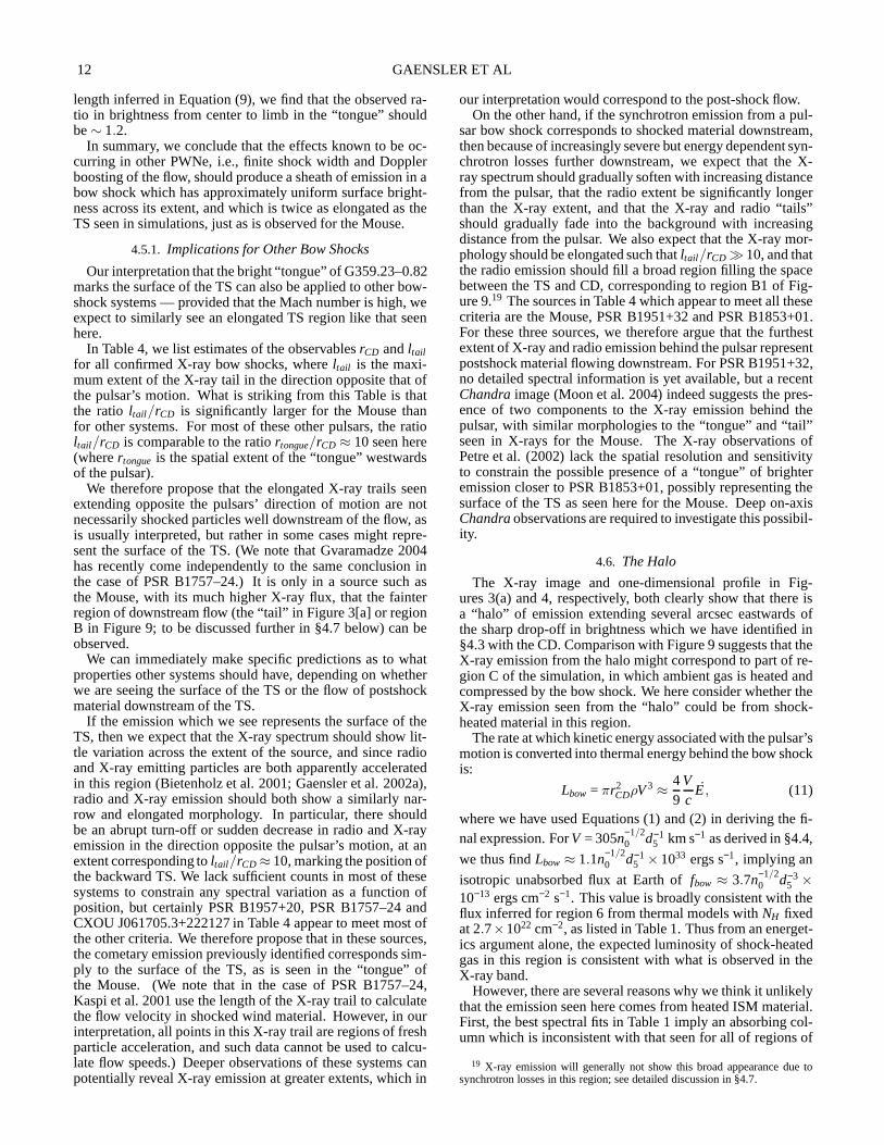
12 GAENSLER ET AL

length inferred in Equation (9), we find that the observed ra-tio in brightness from center to limb in the “tongue” shouldbe∼ 1.2.

In summary, we conclude that the effects known to be oc-curring in other PWNe, i.e., finite shock width and Dopplerboosting of the flow, should produce a sheath of emission in abow shock which has approximately uniform surface bright-ness across its extent, and which is twice as elongated as theTS seen in simulations, just as is observed for the Mouse.

4.5.1. Implications for Other Bow Shocks

Our interpretation that the bright “tongue” of G359.23–0.82marks the surface of the TS can also be applied to other bow-shock systems — provided that the Mach number is high, weexpect to similarly see an elongated TS region like that seenhere.

In Table 4, we list estimates of the observablesrCD andltailfor all confirmed X-ray bow shocks, whereltail is the maxi-mum extent of the X-ray tail in the direction opposite that ofthe pulsar’s motion. What is striking from this Table is thatthe ratio ltail/rCD is significantly larger for the Mouse thanfor other systems. For most of these other pulsars, the ratioltail/rCD is comparable to the ratiortongue/rCD ≈ 10 seen here(wherertongue is the spatial extent of the “tongue” westwardsof the pulsar).

We therefore propose that the elongated X-ray trails seenextending opposite the pulsars’ direction of motion are notnecessarily shocked particles well downstream of the flow, asis usually interpreted, but rather in some cases might repre-sent the surface of the TS. (We note that Gvaramadze 2004has recently come independently to the same conclusion inthe case of PSR B1757–24.) It is only in a source such asthe Mouse, with its much higher X-ray flux, that the fainterregion of downstream flow (the “tail” in Figure 3[a] or regionB in Figure 9; to be discussed further in §4.7 below) can beobserved.

We can immediately make specific predictions as to whatproperties other systems should have, depending on whetherwe are seeing the surface of the TS or the flow of postshockmaterial downstream of the TS.

If the emission which we see represents the surface of theTS, then we expect that the X-ray spectrum should show lit-tle variation across the extent of the source, and since radioand X-ray emitting particles are both apparently acceleratedin this region (Bietenholz et al. 2001; Gaensler et al. 2002a),radio and X-ray emission should both show a similarly nar-row and elongated morphology. In particular, there shouldbe an abrupt turn-off or sudden decrease in radio and X-rayemission in the direction opposite the pulsar’s motion, at anextent corresponding toltail/rCD ≈ 10, marking the position ofthe backward TS. We lack sufficient counts in most of thesesystems to constrain any spectral variation as a function ofposition, but certainly PSR B1957+20, PSR B1757–24 andCXOU J061705.3+222127 in Table 4 appear to meet most ofthe other criteria. We therefore propose that in these sources,the cometary emission previously identified corresponds sim-ply to the surface of the TS, as is seen in the “tongue” ofthe Mouse. (We note that in the case of PSR B1757–24,Kaspi et al. 2001 use the length of the X-ray trail to calculatethe flow velocity in shocked wind material. However, in ourinterpretation, all points in this X-ray trail are regions of freshparticle acceleration, and such data cannot be used to calcu-late flow speeds.) Deeper observations of these systems canpotentially reveal X-ray emission at greater extents, which in

our interpretation would correspond to the post-shock flow.On the other hand, if the synchrotron emission from a pul-

sar bow shock corresponds to shocked material downstream,then because of increasingly severe but energy dependent syn-chrotron losses further downstream, we expect that the X-ray spectrum should gradually soften with increasing distancefrom the pulsar, that the radio extent be significantly longerthan the X-ray extent, and that the X-ray and radio “tails”should gradually fade into the background with increasingdistance from the pulsar. We also expect that the X-ray mor-phology should be elongated such thatltail/rCD ≫ 10, and thatthe radio emission should fill a broad region filling the spacebetween the TS and CD, corresponding to region B1 of Fig-ure 9.19 The sources in Table 4 which appear to meet all thesecriteria are the Mouse, PSR B1951+32 and PSR B1853+01.For these three sources, we therefore argue that the furthestextent of X-ray and radio emission behind the pulsar representpostshock material flowing downstream. For PSR B1951+32,no detailed spectral information is yet available, but a recentChandraimage (Moon et al. 2004) indeed suggests the pres-ence of two components to the X-ray emission behind thepulsar, with similar morphologies to the “tongue” and “tail”seen in X-rays for the Mouse. The X-ray observations ofPetre et al. (2002) lack the spatial resolution and sensitivityto constrain the possible presence of a “tongue” of brighteremission closer to PSR B1853+01, possibly representing thesurface of the TS as seen here for the Mouse. Deep on-axisChandraobservations are required to investigate this possibil-ity.

4.6. The Halo

The X-ray image and one-dimensional profile in Fig-ures 3(a) and 4, respectively, both clearly show that there isa “halo” of emission extending several arcsec eastwards ofthe sharp drop-off in brightness which we have identified in§4.3 with the CD. Comparison with Figure 9 suggests that theX-ray emission from the halo might correspond to part of re-gion C of the simulation, in which ambient gas is heated andcompressed by the bow shock. We here consider whether theX-ray emission seen from the “halo” could be from shock-heated material in this region.

The rate at which kinetic energy associated with the pulsar’smotion is converted into thermal energy behind the bow shockis:

Lbow = πr2CDρV3 ≈ 4

9Vc

E, (11)

where we have used Equations (1) and (2) in deriving the fi-nal expression. ForV = 305n−1/2

0 d−15 km s−1 as derived in §4.4,

we thus findLbow ≈ 1.1n−1/20 d−1

5 ×1033 ergs s−1, implying an

isotropic unabsorbed flux at Earth offbow ≈ 3.7n−1/20 d−3

5 ×10−13 ergs cm−2 s−1. This value is broadly consistent with theflux inferred for region 6 from thermal models withNH fixedat 2.7×1022 cm−2, as listed in Table 1. Thus from an energet-ics argument alone, the expected luminosity of shock-heatedgas in this region is consistent with what is observed in theX-ray band.

However, there are several reasons why we think it unlikelythat the emission seen here comes from heated ISM material.First, the best spectral fits in Table 1 imply an absorbing col-umn which is inconsistent with that seen for all of regions of

19 X-ray emission will generally not show this broad appearance due tosynchrotron losses in this region; see detailed discussionin §4.7.

X-RAY IMAGING OF THE PULSAR BOW SHOCK G359.23–0.82 13

1–5. When one fixesNH = 2.7×1022 cm−2 to match regions1–5, the resulting spectral fits for region 6 are quite poor. Sec-ond, the expected gas temperature behind a shock of this ve-locity is kT ≈ 0.2n−1

0 d−25 keV. For n0 = 0.3 cm−3 andd5 = 1

as adopted here, we inferkT ≈ 0.6 keV, well below the valuekT & 4 keV seen in thermal fits to region 6 as listed in Table 1.Finally, even if we have overestimated the ambient densityand pulsar velocity so that the expected shock temperature isindeedkT ≈ 4 keV, the expected X-ray luminosity in shockedgas near the head isLx = Λn2

0V ≈ 4n20d3

5×1027 ergs s−1, whereΛ ≈ 10−23 ergs cm3 s−1 is the cooling function atkT ≈ 4 keV,andV ≈ πr3

CD = 4.1d35 ×1050 cm3 is the approximate volume

of shocked gas in the nose of the bow shock. The implied X-ray flux at Earth is many orders of magnitude below what isobserved in this region.

We rather propose that the emission seen in the “halo”corresponds to a combination of dust-scattering and contri-butions in this region due to the wings of the PSF. For anunresolved source with a spectrum as given for region 1 inTable 1, one expects the dust-scattered flux falling into re-gion 6 to comprise∼ 0.7% of the incident flux, if dust isdistributed homogeneously between the source and observer(R. K. Smith, 2003, private communication, using the methodof Mathis & Lee 1991). We have used the PSF generated byCHaRT(see §3.4 above) to estimate that∼ 0.9% of the inci-dent flux from a compact source with the spectrum of region 1should fall into region 6 resulting from the wings of the PSF.

Since region 1 contains 7200 counts, we thus expect∼ 120counts in region 6 due to these two effects. Although this is afactor of∼ 3 less than the count-rate actually observed in re-gion 6, the discussion in §4.1 suggests that it is highly likelythat the scattering medium is located in the molecular ringrather than is distributed evenly along the line of sight, and isthus concentrated much closer to the source than to the ob-server. Incorporating this effect would significantly increasethe estimate of the contribution of dust scattered emissioninregion 6. Furthermore, our estimate does not take into accountthat region 1 is heavily piled-up, or that there is other brightextended emission in the immediate vicinity of region 1, thephotons from which will also be scattered by dust and by theChandramirrors. We thus conclude that the 120 counts es-timated above is likely a significant underestimate, and thatthe flux in the “halo” region is indeed broadly consistent withbeing light scattered by both dust and by theChandramirrors.

We note that because the cross-section for dust scatteringdecreases with increasing energy, one expects the spectrumofdust-scattered emission to be softer than that of the source.Indeed for the power law fits to region 6 in Table 1, the ab-sorbing column is less or the photon index is steeper than forregion 1, either result indicating a softer spectrum as expected.

4.7. The Tail

The “tail” is perhaps the Mouse’s most puzzling aspect. Asseen in Figures 1 and 3(b), at radio wavelengths the tail flaresconsiderably about 10′′ west of the pulsar, then further down-stream contracts, broadens, and then contracts again into anarrow cylindrical structure, 12′ in length, which eventuallyfades into the background. Here we attempt to explain the be-havior close to the “head”, and the long thin radio tail. We donot attempt to account for the complicated radio morphologybetween these two regimes, which perhaps reflects inhomo-geneities in the surrounding medium (e.g., Jones et al. 2002).

We expect that the X-ray and radio emission from the “tail”should correspond to region B of Figure 9, where shocked

pulsar wind material emits synchrotron emission and flowsout behind the pulsar. With increasing distance from the pul-sar, we expect that the X-ray emission should fade and that itsphoton index should steepen, both as a result of synchrotronlosses. These effects are both clearly observed inChandradata. However, the properties of the “tail” differ from thoseexpected, in that the X-ray “tail” is reasonably narrow andcollimated, in contrast to the increasingly broad region ofshocked material seen in region B of Figure 9.

In the radio image shown in Figure 3(b), the outer regionsof the tail do appear to flare and broaden, showing behaviorbroadly similar to that seen in the simulation. However, aspointed out in §3.2 and shown in Figure 5, the radio tail con-sists of two components: the broad region just discussed, plusa brighter narrower component closer to the symmetry axis,and showing very good morphological correspondence withthe X-ray image.

Comparison with Figure 9 suggests that we indeed expecttwo components to the “tail”: region B1, in which shockedmaterial flows from the forward TS, and region B2, wherematerial shocked at the backward TS flows away from thepulsar in a narrower region. We propose that the outer andinner components of radio emission from the “tail” seen inFigures 3(b) and 5 correspond to regions B1 and B2 of thesimulation, respectively, and that only region B2 is seen inX-rays.

For any reasonable value of the nebular magnetic field, thesynchrotron lifetime of X-ray-emitting electrons will be sig-nificantly less than the age of the system. The X-ray extentsseen in the post-shock flow thus act as a useful diagnostic ofthe flow speed and magnetic field strength in each region.

Although our hydrodynamic simulation does not explicitlyinclude relativistic effects or magnetic fields, both of whichare likely to play an important role in moderating the proper-ties of the post-shock flow, we can use the simulation to makea rough estimate of the relative flow velocities in each of re-gions B1 and B2. We find in the simulation that material inregion B1 has an asymptotic bulk velocity∼ 4 times largerthan in region B2.

This difference in velocities can be understood by the factthat most particles feeding region B1 do not cross the termina-tion shock head-on, and are accelerated by pressure gradientsin the head of the bow shock. In contrast, particles feedingregion B2 meet the shock head on, propagate through an es-sentially uniform pressure distribution, and so are not accel-erated. Thus if the magnetic field strengths were the same inregions B1 and B2, we would expect X-ray emission to extendfar from the pulsar in a broad region corresponding to B1, andwould see a much shorter scale for the narrow component ofX-rays corresponding to B2. However, we clearly observe theopposite situation in this system: despite corresponding to aslower bulk flow speed, the spatial extent of X-rays in regionB2 is significantly larger than for B1.

A simple interpretation is that the magnetic field strengthin the post-shock flow is markedly lower in region B2 thanin region B1, which then allows X-ray-emitting electrons topropagate much further from the shock before radiating awaytheir energy. We quantify this as follows. We first estimatethe length scales of the X-ray emitting regions. We estimatethat in region B1, X-ray emitting material extends about halfway around the northern and southern sides of the “tongue”,but is not detectable further downstream. The correspondingangular distance traveled by X-ray emitting material is≈ 8′′,or a distance ofxF ≈ 0.2d5 pc. For region B2, we estimate

14 GAENSLER ET AL

from Figures 3(a) and 4 an angular extent∼ 40′′ in X-rays,corresponding to a spatial extentxB ≈ 1.0d5 pc.

If the length scale of X-rays in each region is determinedby the time traveled before synchrotron losses become signif-icant, then

xF

xB=

VF

VB

(

BFn

BBn

)−3/2

, (12)

whereV is the flow velocity,Bn is the nebular magnetic field,the superscriptsF and B correspond to situations for par-ticles flowing from the forward and backward terminationshocks respectively. From the above discussion, we have thatxF/xB ≈ 1/5 andVF/VB ≈ 4; Equation (12) then implies thatBF

n /BBn ≈ 7.

Since our simulation does not explicitly include magneticfields, we do not attempt to calculate actual values of the fieldstrength in each region. However, we note that if the degreeof magnetization of the post-shock flow is similar in the for-ward and backward directions, then an expression similar toEquation (7) implies that

BFn

BBn

=rBTS

rFTS

. (13)

Using rFTS≈ 0.018d5 pc andrB

TS≈ 0.5rtongue= 0.12d5 pc, wethen findBF

n /BBn ≈ 7, in good agreement with the estimate

made above from the X-ray morphology. While this simpletreatment provides support for the argument that the X-raymorphology of the tail is governed by differing magnetic fieldstrengths in the different parts of the tail, a full relativisticmagnetohydrodynamic treatment of this system is needed toproperly address the amplification and evolution of magneticfields in each region. Such an analysis is beyond the scope ofthis paper, but will be the subject of a future study.

If synchrotron losses indeed limit the extent of the X-ray“tail”, we expect the tail to be increasingly shorter in extent atprogressively higher energies. We have formed images of theMouse in various energy bands (0.5–0.8, 0.8–2.0, 2.0–5.0 and5.0–8.0 keV), and qualitatively can confirm that indeed the tailappears to shrink as one considers successively higher energyphotons. However, we lack sufficient counts to quantify thiseffect, as the energies where we expect the tail to be longestare those where interstellar absorption is most severe.

Synchrotron lifetimes are proportional toε−1/2, whereε isthe energy at which photons are emitted. We thus expect thelifetime of radio-emitting particles in regions B1 and B2 tobe∼ 104 times longer than their X-ray counterparts. We thus ex-pect negligible synchrotron losses in the radio band. Through-out region B1, we thus expect to see considerable emissionat radio wavelengths. Indeed this expectation is fulfilled —while there is little X-ray emission in much of region B1, thereis clearly significant radio emission in the increasingly broadcomponent of the “tail” seen far from the symmetry axis inFigure 3. Further downstream, adiabatic losses may eventu-ally become significant in the radio-emitting particles as theflow diverges, while changes in the density of the ambientmedium may have a dramatic effect on the morphology ofthis region.

To consider the properties of radio emission in region B2,we assume a post-shock velocityVB =c/6 at the backward ter-mination shock, in the reference frame of the pulsar (Lyutikov2004). Downstream of the backward termination shock, theflow velocity evolves asVB ∝ 1/A, whereA is the cross-sectional area of region B2. The morphology of radio emis-sion in Figures 1 and 3(b) suggests that the width of the radio

“tail” is a factor of ∼ 3 broader than the width of the back-ward termination shock as defined by the morphology of theX-ray “tongue”. We therefore adopt a constant flow veloc-ity VB ≈ c/6/32 ∼ 5600 km s−1 in the far downstream com-ponents of region B2, so that in an external reference framethe flow moves westwards at a speed (5600− 600d−1

5 P−1/20 ) ∼

5000 km s−1.We have not included magnetic fields in our simulation.

However, we expect that magnetic field stresses should main-tain collimation of the flow far downstream in region B2,as is seen for the Earth’s magnetotail (e.g., Bavassano et al.1974; Slavin et al. 1983) and for simulations of old neutronstars moving through the ISM (Toropina et al. 2001). Inthis case adiabatic, as well as synchrotron, losses in the ra-dio band will be negligible, and emission from the tail canthen have a considerable extent. Indeed the radio data ofYusef-Zadeh & Bally (1987) show that the tail extends for≈ 12′ west of the pulsar, corresponding to an extentxB ≈17d5 pc. At a projected velocityV ≈ 600d−1

5 P−1/20 km s−1 as

inferred in §4.4, and assuming that the pulsar’s true age isτ = 25.5 kyr, the total projected distance traveled by the pul-sar in its lifetime isL ≈ 16d−1

5 P−1/20 pc. SinceL ≈ xB, it seems

reasonable to suppose that the pulsar was born near the tail’swestern tip, with the tail representing a wake of particles leftbehind by the pulsar as it travels. Such a possibility has beensuggested previously by other authors (Predehl & Kulkarni1995; Camilo et al. 2002).

However, this suggestion is problematic for several reasons.First, the radio data in Figure 1 indicate that there is no sud-den termination of the tail at its westernmost extent. Rather,beyond this point the tail simply becomes too faint to see,particularly in the presence of emission from SNR G359.1–0.5. Second, the calculation made in the preceding para-graph neglects the backward flow velocity of emitting parti-cles, which should cause the tail to extend further westwardsof the pulsar’s birthplace as a function of time. If we adopta constant flow velocityVB ≈ 5000 km s−1 in region B2 ascalculated above, the full length of the bow shock structurecould be many times longer than its observable component, inwhich case the fact thatL ≈ xB would simply be coincidence.Third, although no associated SNR has yet been identified forPSR J1747–2958 (perhaps because the SNR expanded into alow density environment or pre-existing cavity; Kafatos etal.1980; Braun et al. 1989), the supernova blast wave shouldhave a significant impact on its environment, sweeping upsurrounding material and evacuating a large cavity around thepulsar birthplace. If the pulsar was indeed born at the tip ofthe radio tail of the Mouse, it is hard to understand how thetail extends smoothly and uninterrupted through the turbulentand highly inhomogeneous environment created by the asso-ciated SNR. Finally, forV ≈ 600 km s−1 andn0 ≈ 0.3 cm−3 asadopted in §4.4, the pulsar should have broken out of its asso-ciated SNR when the latter was still in the Sedov-Taylor phaseof evolution (see Eq. (4) of van der Swaluw et al. 2003). Inthis case, it is simple to show that the age of the pulsar whenit escapes from its SNR is:

tescape= 14E1/351 (V/1000 km s−1)−5/3n−1/3

0 kyr, (14)

whereE51 × 1051 ergs s−1 is the kinetic energy of the ex-plosion (Shull et al. 1989; van der Swaluw et al. 2003). ForV ≈ 600d−1

5 P−5/60 km s−1 andn0 ≈ 0.3 cm−3, we findtescape≈

49E1/351 d5/3

5 P−5/60 kyr. If the true age of PSR J1747–2958 is

X-RAY IMAGING OF THE PULSAR BOW SHOCK G359.23–0.82 15

τ = 25.5 kyr, then forE51 ∼ 1, d5 ≈ 1 andP0 ≈ 1, the pul-sar should still be embedded in its associated SNR, whichis not the case. A simple resolution for this discrepancy isif PSR J1747–2958 is significantly older than its character-istic age, as has also been claimed for PSRs B0833–45 andB1757–24 (Lyne et al. 1996; Gaensler & Frail 2000). Thepulsar birthplace would then be significantly further west ofthe endpoint of the radio tail.

To summarize, the radio and X-ray morphologies of the tailcan both be consistently explained by a model in which thereare two regimes of downstream flow, corresponding to mate-rial shocked at the forward and backward termination shocks.At the forward TS, a high magnetic field causes severe syn-chrotron losses, so that X-ray emitting particles in this regionlose their energy before traveling only a fraction of a parsec;radio-emitting particles form a broad cometary region, match-ing the morphology of this region seen in simulations. At thebackward TS, the flow speed is somewhat lower than at theforward TS, but the magnetic field is very weak. The result-ing synchrotron lifetime and the minimal divergence of theflow allow a collimated and significantly extended X-ray tailto form. At radio wavelengths, the flow from the backwardTS is what produces the long narrow tail for which the Mouseoriginally attracted attention. The visible endpoint of this tailprobably does not mark the pulsar birthplace; most likely thepulsar is much older than its characteristic age, and was bornwell beyond the point where radio emission from the tail be-gins.

5. CONCLUSIONS

We have here presented a detailed study of the X-ray emis-sion from G359.23–0.82 (“the Mouse”), along with an im-proved timing solution for the coincident young radio pulsarJ1747–2958. Our main findings are as follows:

1. G359.23–0.82 is a bright X-ray source with acometary morphology and a power-law spectrum, withPSR J1747–2958 embedded in its head. This conclu-sively demonstrates that the Mouse is a bow shock pow-ered by the relativistic wind of PSR J1747–2958, all ata likely distance of≈ 5 kpc. The Mouse is a highlyefficient X-ray emitter, converting 2% of its spin-downluminosity into synchrotron emission at these energies.

2. High-energy emission from the pulsar itself is likelyidentified in the form of a compact X-ray source co-incident with the pulsar position. This most probablycorresponds to pulsed emission from the pulsar magne-tosphere. A slightly extended clump of uncertain naturelies immediately adjacent to the pulsar, and produces> 30% of the total X-ray flux from this system.

3. Using the high spatial resolution ofChandradata, weidentify the contact discontinuity separating shockedwind material from shocked ISM ahead of the pulsar’smotion. Pressure balance then allows us to infer thatthe pulsar’s Mach number isM≈ 60, implying a likelyspace velocityV ∼ 600 km s−1 through warm gas withdensityn0 ≈ 0.3 cm−3.

4. We see a bright elongated region extending 10′′ behindthe pulsar, which we identify as a sheath of bright X-ray and radio emission surrounding the wind termina-tion shock of an isotropic flow. A model which incor-porates both the finite thickness of an ion-loaded windshock and Doppler beaming of the relativistic flow canaccount for both the size of this region and its lack oflimb brightening. We argue that the X-ray and radiotrails seen behind PSR B1957+20, PSR B1757–24 andCXOU J061705.3+222127 similarly represent the sur-face of the wind termination shock in these systems.

5. The tail of the Mouse contains two components: a col-limated region seen in both X-rays and in radio, and abroader component seen in radio only. We propose thatthe properties of the former are consistent with emis-sion produced by the post-shock flow beyond the back-ward termination shock behind the pulsar, where themagnetic field is low and synchrotron losses are mod-erate. The latter likely corresponds to material shockedin a high-field region ahead of the pulsar, where radia-tive losses are severe at X-ray energies. Similar behav-ior is possibly also seen in the radio/X-ray tails behindPSRs B1951+32 and B1853+01.

Taking advantage of the high X-ray count-rate seen fromthis source, we have successfully used the Mouse as a testingground for combining our understanding of the shock struc-tures seen in both Crab-like and bow-shock PWNe. How-ever, we caution that while recentChandraobservations haveshowed some satisfying similarities among PWN properties,they also reveal some puzzling differences. It is clear thattoproperly understand the pulsar bow shock phenomenon, wewill need to obtain deep observations of other such systems,which can then be compared and contrasted to the remarkableMouse.

We thank Andrew Melatos, Tom Dame, Jonathan Aronsand Patrick Slane for useful and stimulating discussions, andMaxim Lyutikov for sharing his theoretical work on pulsarbow shocks in advance of publication. We are grateful to Ran-dall Smith, Leisa Townsley and George Chartas for advice onmodeling dust scattering and pile-up, and to John Sarkissianfor help with Parkes observations. We also thank the referee,Rino Bandiera, for a very constructive series of commentswhich greatly improved this paper. The Parkes telescope ispart of the Australia Telescope which is funded by the Com-monwealth of Australia for operation as a National Facilitymanaged by CSIRO. The National Radio Astronomy Obser-vatory is a facility of the National Science Foundation op-erated under cooperative agreement by Associated Universi-ties, Inc. B.M.G. acknowledges the support of NASA throughSAO grant GO2-3075X and LTSA grant NAG5-13032, andof the University of Melbourne through the Sir Thomas LyleFellowship. F.C. acknowledges support from NSF grant AST-02-05853 and a travel grant from NRAO. V.M.K. is a CanadaResearch Chair and NSERC Steacie Fellow, and receives sup-port from NSERC, NATEQ, CIAR and NASA.

REFERENCES

Arons, J. 2002, in Neutron Stars in Supernova Remnants, ed. P. O. Slane &B. M. Gaensler (San Francisco: Astronomical Society of the Pacific), 71–80

Arons, J. & Tavani, M. 1993, ApJ, 403, 249

Arzoumanian, Z., Chernoff, D. F., & Cordes, J. M. 2002, ApJ, 568, 289Arzoumanian, Z., Nice, D. J., Taylor, J. H., & Thorsett, S. E.1994, ApJ, 422,

671Bamba, A., Yokogawa, J., Sakano, M., & Koyama, K. 2000, PASJ,52, 259

16 GAENSLER ET AL

Bałucinska-Church, M. & McCammon, D. 1992, ApJ, 400, 699Bavassano, B., Mariana, F., & Villante, U. 1974, Space Res.,14, 403Bietenholz, M. F., Frail, D. A., & Hester, J. J. 2001, ApJ, 560, 254Braje, T. M., Romani, R. W., Roberts, M. S. E., & Kawai, N. 2002, ApJ, 565,

L91Braun, R., Goss, W. M., & Lyne, A. G. 1989, ApJ, 340, 355Bronfman, L., Cohen, R. S., Alvarez, H., May, J., & Thaddeus,P. 1988, ApJ,

324, 248Bucciantini, N. 2002, A&A, 387, 1066Bucciantini, N. & Bandiera, R. 2001, A&A, 375, 1032Burke, B. E., Gregory, J., Bautz, M. W., Prigozhin, G. Y., Kissel, S. E.,

Kosicki, B. N., Loomis, A. H., & Young, D. J. 1997, IEEE Transac. Elec.Devices, 44, 1633

Camilo, F., Bell, J. F., Manchester, R. N., Lyne, A. G., Possenti, A., Kramer,M., Kaspi, V. M., Stairs, I. H., D’Amico, N., Hobbs, G., Gotthelf, E. V., &Gaensler, B. M. 2001, ApJ, 557, L51

Camilo, F., Manchester, R. N., Gaensler, B. M., & Lorimer, D.R. 2002, ApJ,579, L25

Caraveo, P. A., Bignami, G. F., DeLuca, A., Mereghetti, S., Pellizzoni, A.,Mignani, R., Tur, A., & Becker, W. 2003, Science, 301, 1345

Chatterjee, S. & Cordes, J. M. 2004, ApJ, 600, L51Chatterjee, S. & Cordes, J, M. 2002, ApJ, 575, 407Chen, Y., Bandiera, R., & Wang, Z.-R. 1996, ApJ, 469, 715Chevalier, R. A. 2000, ApJ, 539, L45Clemens, D. P., Sanders, D. B., & Scoville, N. Z. 1988, ApJ, 327, 139Comerón, F. & Kaper, L. 1998, A&A, 338, 273Cordes, J. M. 1996, in Pulsars: Problems and Progress, IAU Colloquium 160,

ed. S. Johnston, M. A. Walker, & M. Bailes (San Francisco: AstronomicalSociety of the Pacific), 393–399

Cordes, J. M. & Lazio, T. J. W. 2002, preprint (astro-ph/0207156)Dame, T. M. 1993, in Back to the Galaxy, ed. S. S. Holt & F. Verter, Vol. 278

(New York: AIP), 267–278Davis, J. E. 2001, ApJ, 562, 575Dib, R. & Kaspi, V. M. 2004, in preparationFerrière, K. M. 2001, Reviews of Modern Physics, 73, 1031Frail, D. A., Giacani, E. B., Goss, W. M., & Dubner, G. 1996, ApJ, 464, L165Freeman, P. E., Kashyap, V., Rosner, R., & Lamb, D. Q. 2002, ApJ, 138, 185Gaensler, B. M. 2004, in Young Neutron Stars and their Environments, ed.

F. Camilo & B. M. Gaensler (San Francisco: Astronomical Society of thePacific), 151–158

Gaensler, B. M., Arons, J., Kaspi, V. M., Pivovaroff, M. J., Kawai, N., &Tamura, K. 2002a, ApJ, 569, 878

Gaensler, B. M. & Frail, D. A. 2000, Nature, 406, 158Gaensler, B. M., Jones, D. H., & Stappers, B. W. 2002b, ApJ, 580, L137Gaensler, B. M., Schulz, N. S., Kaspi, V. M., Pivovaroff, M. J., & Becker,

W. E. 2003, ApJ, 588, 441Gaensler, B. M., Stappers, B., Chatterjee, S., Ghavamian, P., Jones, D. H., &

Cordes, J. 2004, in How Does the Galaxy work?, ed. E. J. Alfaro, E. Pérez,& J. Franco (Dordrecht: Kluwer), in press (astro-ph/0309740)

Gallant, Y. A. & Arons, J. 1994, ApJ, 435, 230Gavriil, F. P., Kaspi, V. M., & Roberts, M. S. E. 2004, Adv. Space Res., 33,

592Gotthelf, E. V. 2003, ApJ, 591, 361Gotthelf, E. V. 2004, in Young Neutron Stars and their Environments, ed.

F. Camilo & B. M. Gaensler (San Francisco: Astronomical Society of thePacific), 225–228

Gvaramadze, V. V. 2004, A&A, 415, 1073Harrus, I. M., Hughes, J. P., Singh, K. P., Koyama, K., & Asaoka, I. 1997,

ApJ, 488, 781Heiles, C. 2001, in Tetons 4: Galactic Structure, Stars and the Interstellar

Medium, ed. C. E. Woodward, M. D. Bicay, & J. M. Shull, Vol. 231(SanFrancisco: ASP), 294

Helfand, D. J., Gotthelf, E. V., & Halpern, J. P. 2001, ApJ, 556, 380Hester, J. J., Scowen, P. A., Sankrit, R., Burrows, C. J., Gallagher, III, J. S.,

Holtzman, J. A., Watson, A., Trauger, J. T., Ballester, G. E., Casertano,S., Clarke, J. T., Crisp, D., Evans, R. W., Griffiths, R. E., Hoessel, J. G.,Krist, J., Lynds, R., Mould, J. R., O’Neill, Jr., E. J., Stapelfeldt, K. R., &Westphal, J. A. 1995, ApJ, 448, 240

Hoshino, M., Arons, J., Gallant, Y. A., & Langdon, A. B. 1992,ApJ, 390,454

Hughes, J. P., Slane, P. O., Park, S., Roming, P. W. A., & Burrows, D. N.2003, ApJ, 591, L139

Johnston, S., Koribalski, B., Weisberg, J. M., & Wilson, W. 2001, MNRAS,322, 715

Jones, D. H., Stappers, B. W., & Gaensler, B. M. 2002, A&A, 389, L1Kafatos, M., Sofia, S., Bruhweiler, F., & Gull, S. 1980, ApJ, 242, 294Kaspi, V. M., Gotthelf, E. V., Gaensler, B. M., & Lyutikov, M.2001, ApJ,

562, L163

Kennel, C. F. & Coroniti, F. V. 1984a, ApJ, 283, 694—. 1984b, ApJ, 283, 710Komissarov, S. S. & Lyubarsky, Y. E. 2003, MNRAS, 344, L93Li, J., Kastner, J. H., Prigozhin, G. Y., & Schulz, N. S. 2003,ApJ, 590, 586Linde, T. J., Gombosi, T. I., Roe, P. L., Powell, K. G., & DeZeeuw, D. L.

1998, J. Geophys. Res., 103, 1889Lou, Y.-Q. 1998, MNRAS, 294, 443Lu, F. J., Wang, Q. D., Aschenbach, B., Durouchoux, P., & Song, L. M. 2002,

ApJ, 568, L49Lyne, A. G., Pritchard, R. S., Graham-Smith, F., & Camilo, F.1996, Nature,

381, 497Lyutikov, M. 2003, MNRAS, 339, 623—. 2004, in preparationMac Low, M.-M., van Buren, D., Wood, D. O. S., & Churchwell, E.1991,

ApJ, 369, 395Manchester, R. N., Kaspi, V. M., Johnston, S., Lyne, A. G., & D’Amico, N.

1991, MNRAS, 253, 7PMathis, J. S. & Lee, C.-W. 1991, ApJ, 376, 490Monet, D., Bird, A., Canzian, B., Dahn, C., Guetter, H., Harris, H., Henden,

A., Levine, S., Luginbuhl, C., Monet, A. K. B., Rhodes, A., Riepe, B.,Sell, S., Stone, R., Vrba, F., & R., W. 1998, USNO-A V2.0, A Catalog ofAstrometric Standards (Washington DC: US Naval Observatory)

Moon, D.-S., Lee, J.-J., Eikenberry, S. S., Koo, B.-C., Chatterjee, S., L., K. D.,Hester, J. J., Cordes, J. M., Gallant, Y. A., & Koch-Miramond, L. 2004,ApJ, 610, L33

Ng, C.-Y. & Romani, R. W. 2004, ApJ, 601, 479Olbert, C. M., Clearfield, C. R., Williams, N. E., Keohane, J.W., & Frail,

D. A. 2001, ApJ, 554, L205Olbert, C. M., Keohane, J. W., Arnaud, K. A., Dyer, K. K., Reynolds, S. P.,

& Safi-Harb, S. 2003, ApJ, 592, L45Pavlov, G. G., Teter, M. A., Kargaltsev, O., & Sanwal, D. 2003, ApJ, 591,

1157Pelling, R. M., Paciesas, W. S., Peterson, L. E., Makishima,K., Oda, M.,

Ogawara, Y., & Miyamoto, S. 1987, ApJ, 319, 416Petre, R., Kuntz, K. D., & Shelton, R. L. 2002, ApJ, 579, 404Possenti, A., Cerutti, R., Colpi, M., & Mereghetti, S. 2002,A&A, 387, 993Predehl, P. & Kulkarni, S. R. 1995, A&A, 294, L29Raymond, J. C. & Smith, B. W. 1977, ApJS, 35, 419Rees, M. J. & Gunn, J. E. 1974, MNRAS, 167, 1Rho, J., Petre, R., Schlegel, E., & Hester, J. 1994, ApJ, 430,757Roberts, M. S. E., Tam, C. R., Kaspi, V. M., Lyutikov, M., Vasisht, G.,

Pivovaroff, M., Gotthelf, E. V., & Kawai, N. 2003, ApJ, 588, 992Seta, M., Hasegawa, T., Sakomoto, S., Oka, T., Sawada, T., Inutsuka, S.,

Koyama, H., & Hayashi, M. 2004, AJ, 127, 1098Shull, J. M., Fesen, R. A., & Saken, J. M. 1989, ApJ, 346, 860Sidoli, L., Belloni, T., & Mereghetti, S. 2001, A&A, 368, 835Sidoli, L., Mereghetti, S., Israel, G. L., Chiappetti, L., Treves, A., &

Orlandini, M. 1999, ApJ, 525, 215Skinner, G. K., Willmore, A. P., Eyles, C. J., Bertram, D., & Church, M. J.

1987, Nature, 330, 544Slane, P., Chen, Y., Schulz, N. S., Seward, F. D., Hughes, J. P., & Gaensler,

B. M. 2000, ApJ, 533, L29Slavin, J. E., Tsurutani, B. T., Smith, E. J., Jones, D. E., & Sibeck, D. G.

1983, Geophys. Res. Lett., 10, 973Stappers, B. W., Gaensler, B. M., Kaspi, V. M., van der Klis, M., & Lewin,

W. H. G. 2003, Science, 299, 1372Taylor, J. H. & Cordes, J. M. 1993, ApJ, 411, 674Toropina, O. D., Romanova, M. M., Toropin, Y. M., & Lovelace,R. V. E.

2001, ApJ, 561, 964Tóth, G. 1996, Astrophys. Let. Comm., 34, 245Townsley, L. K., Broos, P. S., Chartas, G., Moskalenko, E., Nousek, J. A., &

Pavlov, G. G. 2002, Nucl. Instr. & Methods in Phys. Res. A, 486, 716Uchida, K., Morris, M., & Yusef-Zadeh, F. 1992, AJ, 104, 1533van Buren, D. 1993, in Massive stars: Their lives in the interstellar medium,

ed. J. P. Cassinelli & E. B. Churchwell (San Francisco: AstronomicalSociety of the Pacific), 315–326

van Buren, D. & McCray, R. 1988, ApJ, 329, L93van der Swaluw, E. 2004, Adv. Space Res., 33van der Swaluw, E., Achterberg, A., Gallant, Y. A., Downes, T. P., & Keppens,

R. 2003, A&A, 397, 913van der Swaluw, E., Downes, T. P., & Keegan, R. 2004, A&A, 420,937van Kerkwijk, M. H. & Kulkarni, S. R. 2001, A&A, 380, 221Wang, Q. D., Lu, F., & Lang, C. C. 2002, ApJ, 581, 1148Weisskopf, M. C., Hester, J. J., Tennant, A. F., Elsner, R. F., Schulz,

N. S., Marshall, H. L., Karovska, M., Nichols, J. S., Swartz,D. A.,Kolodziejczak, J. J., & O’Dell, S. L. 2000, ApJ, 536, L81

Wilkin, F. P. 1996, ApJ, 459, L31Wolszczan, A., Cordes, J. M., & Dewey, R. J. 1991, ApJ, 372, L99

X-RAY IMAGING OF THE PULSAR BOW SHOCK G359.23–0.82 17

Wong, D. S., Cordes, J. M., Chatterjee, S., Zweibel, E., Finley, J., Romani,R., & Ulmer, M. 2002, AAS HEAD, N17.120

Yusef-Zadeh, F. & Bally, J. 1987, Nature, 330, 455Yusef-Zadeh, F. & Bally, J. 1989, in The Center of the Galaxy (IAU Symp.

136), ed. M. Morris (Dordrecht: Kluwer), 197–204

Zank, G. P. 1999, Space Sci. Rev., 89, 413

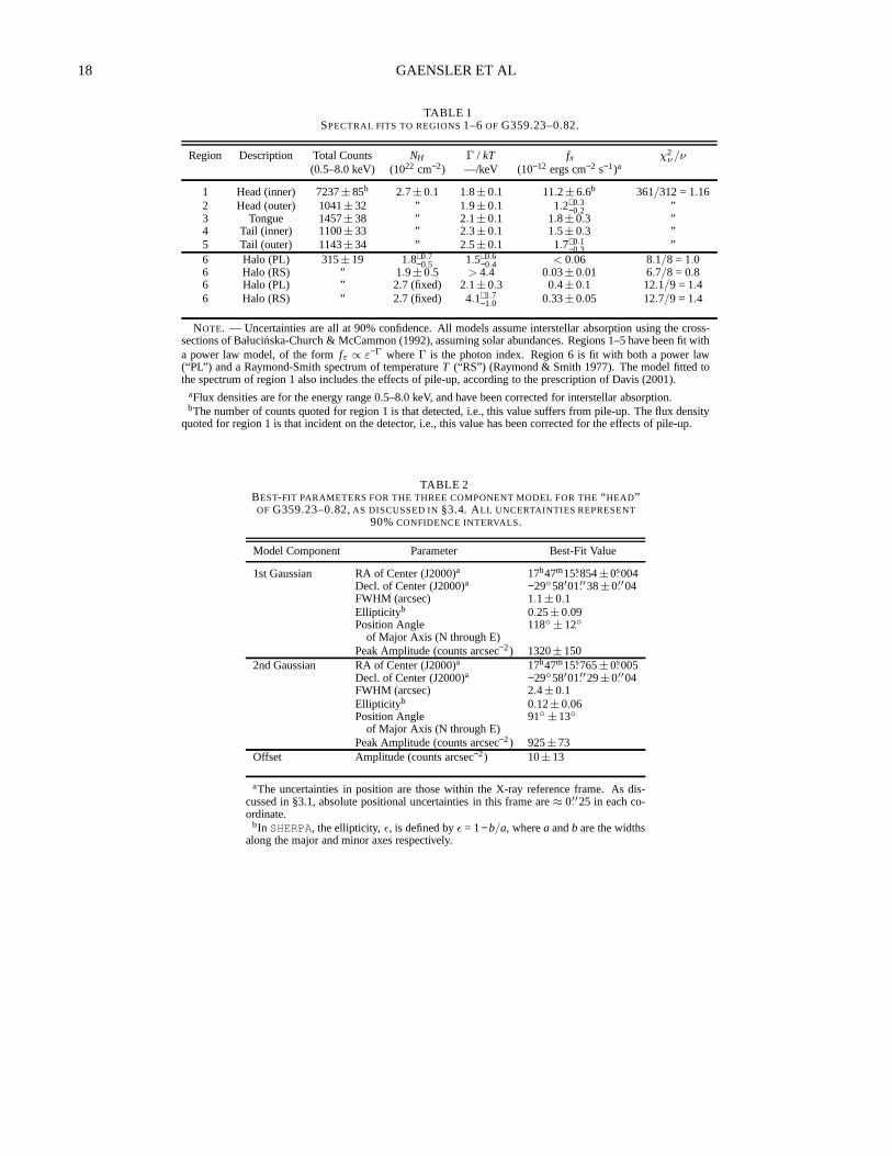
18 GAENSLER ET AL

TABLE 1SPECTRAL FITS TO REGIONS1–6OF G359.23–0.82.

Region Description Total Counts NH Γ / kT fx χ2ν/ν

(0.5–8.0 keV) (1022 cm−2) —/keV (10−12 ergs cm−2 s−1)a

1 Head (inner) 7237±85b 2.7±0.1 1.8±0.1 11.2±6.6b 361/312 = 1.162 Head (outer) 1041±32 ” 1.9±0.1 1.2+0.3

−0.2 ”3 Tongue 1457±38 ” 2.1±0.1 1.8±0.3 ”4 Tail (inner) 1100±33 ” 2.3±0.1 1.5±0.3 ”5 Tail (outer) 1143±34 ” 2.5±0.1 1.7+0.1

−0.3 ”6 Halo (PL) 315±19 1.8+0.7

−0.5 1.5+0.6−0.4 < 0.06 8.1/8 = 1.0

6 Halo (RS) ” 1.9±0.5 > 4.4 0.03±0.01 6.7/8 = 0.86 Halo (PL) ” 2.7 (fixed) 2.1±0.3 0.4±0.1 12.1/9 = 1.46 Halo (RS) ” 2.7 (fixed) 4.1+1.7

−1.0 0.33±0.05 12.7/9 = 1.4

NOTE. — Uncertainties are all at 90% confidence. All models assumeinterstellar absorption using the cross-sections of Bałucinska-Church & McCammon (1992), assuming solar abundances.Regions 1–5 have been fit witha power law model, of the formfε ∝ ε

−Γ whereΓ is the photon index. Region 6 is fit with both a power law(“PL”) and a Raymond-Smith spectrum of temperatureT (“RS”) (Raymond & Smith 1977). The model fitted tothe spectrum of region 1 also includes the effects of pile-up, according to the prescription of Davis (2001).

aFlux densities are for the energy range 0.5–8.0 keV, and havebeen corrected for interstellar absorption.bThe number of counts quoted for region 1 is that detected, i.e., this value suffers from pile-up. The flux density

quoted for region 1 is that incident on the detector, i.e., this value has been corrected for the effects of pile-up.

TABLE 2BEST-FIT PARAMETERS FOR THE THREE COMPONENT MODEL FOR THE“ HEAD”OF G359.23–0.82,AS DISCUSSED IN§3.4. ALL UNCERTAINTIES REPRESENT

90%CONFIDENCE INTERVALS.

Model Component Parameter Best-Fit Value

1st Gaussian RA of Center (J2000)a 17h47m15.s854±0.s004Decl. of Center (J2000)a −29◦58′01.′′38±0.′′04FWHM (arcsec) 1.1±0.1Ellipticityb 0.25±0.09Position Angle 118◦±12◦

of Major Axis (N through E)Peak Amplitude (counts arcsec−2) 1320±150

2nd Gaussian RA of Center (J2000)a 17h47m15.s765±0.s005Decl. of Center (J2000)a −29◦58′01.′′29±0.′′04FWHM (arcsec) 2.4±0.1Ellipticityb 0.12±0.06Position Angle 91◦±13◦

of Major Axis (N through E)Peak Amplitude (counts arcsec−2) 925±73

Offset Amplitude (counts arcsec−2) 10±13

aThe uncertainties in position are those within the X-ray reference frame. As dis-cussed in §3.1, absolute positional uncertainties in this frame are≈ 0.′′25 in each co-ordinate.

bIn SHERPA, the ellipticity, ǫ, is defined byǫ = 1−b/a, wherea andb are the widthsalong the major and minor axes respectively.

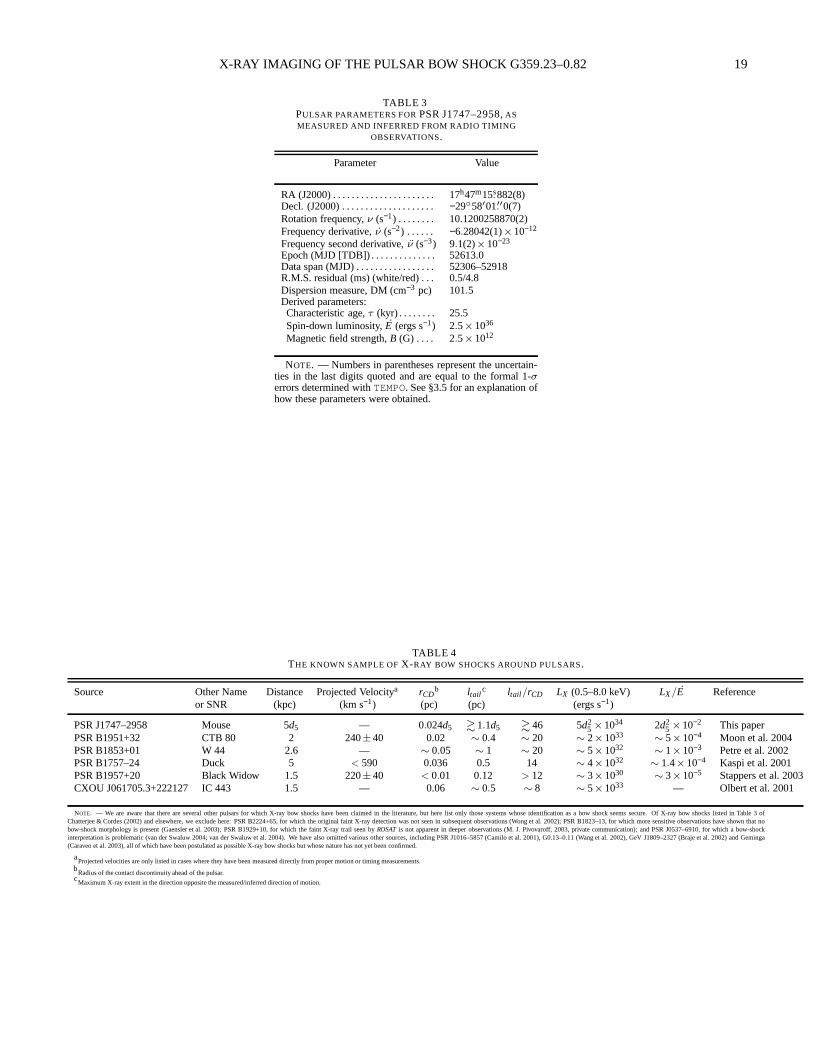
X-RAY IMAGING OF THE PULSAR BOW SHOCK G359.23–0.82 19

TABLE 3PULSAR PARAMETERS FORPSR J1747–2958,ASMEASURED AND INFERRED FROM RADIO TIMING

OBSERVATIONS.

Parameter Value

RA (J2000) . . . . . . . . . . . . . . . . . . . . . . 17h47m15.s882(8)Decl. (J2000) . . . . . . . . . . . . . . . . . . . . −29◦58′01.′′0(7)Rotation frequency,ν (s−1) . . . . . . . . 10.1200258870(2)Frequency derivative,ν (s−2) . . . . . . −6.28042(1)×10−12

Frequency second derivative,ν (s−3) 9.1(2)×10−23

Epoch (MJD [TDB]) . . . . . . . . . . . . . . 52613.0Data span (MJD) . . . . . . . . . . . . . . . . . 52306–52918R.M.S. residual (ms) (white/red) . . . 0.5/4.8Dispersion measure, DM (cm−3 pc) 101.5Derived parameters:Characteristic age,τ (kyr) . . . . . . . . 25.5Spin-down luminosity,E (ergs s−1) 2.5×1036

Magnetic field strength,B (G) . . . . 2.5×1012

NOTE. — Numbers in parentheses represent the uncertain-ties in the last digits quoted and are equal to the formal 1-σ

errors determined withTEMPO. See §3.5 for an explanation ofhow these parameters were obtained.

TABLE 4THE KNOWN SAMPLE OFX-RAY BOW SHOCKS AROUND PULSARS.

Source Other Name Distance Projected Velocitya rCDb ltail

c ltail/rCD LX (0.5–8.0 keV) LX/E Referenceor SNR (kpc) (km s−1) (pc) (pc) (ergs s−1)

PSR J1747–2958 Mouse 5d5 — 0.024d5 & 1.1d5 & 46 5d25 ×1034 2d2

5 ×10−2 This paperPSR B1951+32 CTB 80 2 240±40 0.02 ∼ 0.4 ∼ 20 ∼ 2×1033 ∼ 5×10−4 Moon et al. 2004PSR B1853+01 W 44 2.6 — ∼ 0.05 ∼ 1 ∼ 20 ∼ 5×1032

∼ 1×10−3 Petre et al. 2002PSR B1757–24 Duck 5 < 590 0.036 0.5 14 ∼ 4×1032 ∼ 1.4×10−4 Kaspi et al. 2001PSR B1957+20 Black Widow 1.5 220±40 < 0.01 0.12 > 12 ∼ 3×1030 ∼ 3×10−5 Stappers et al. 2003CXOU J061705.3+222127 IC 443 1.5 — 0.06 ∼ 0.5 ∼ 8 ∼ 5×1033 — Olbert et al. 2001

NOTE. — We are aware that there are several other pulsars for whichX-ray bow shocks have been claimed in the literature, but here list only those systems whose identification as a bow shock seems secure. Of X-ray bow shocks listed in Table 3 ofChatterjee & Cordes (2002) and elsewhere, we exclude here: PSR B2224+65, for which the original faint X-ray detection was not seen in subsequent observations (Wong et al. 2002); PSRB1823–13, for which more sensitive observations have shownthat nobow-shock morphology is present (Gaensler et al. 2003); PSRB1929+10, for which the faint X-ray trail seen byROSATis not apparent in deeper observations (M. J. Pivovaroff, 2003, private communication); and PSR J0537–6910, for which abow-shockinterpretation is problematic (van der Swaluw 2004; van derSwaluw et al. 2004). We have also omitted various other sources, including PSR J1016–5857 (Camilo et al. 2001), G0.13–0.11 (Wang et al. 2002), GeV J1809–2327 (Braje et al. 2002) and Geminga(Caraveo et al. 2003), all of which have been postulated as possible X-ray bow shocks but whose nature has not yet been confirmed.

aProjected velocities are only listed in cases where they have been measured directly from proper motion or timing measurements.b

Radius of the contact discontinuity ahead of the pulsar.cMaximum X-ray extent in the direction opposite the measured/inferred direction of motion.

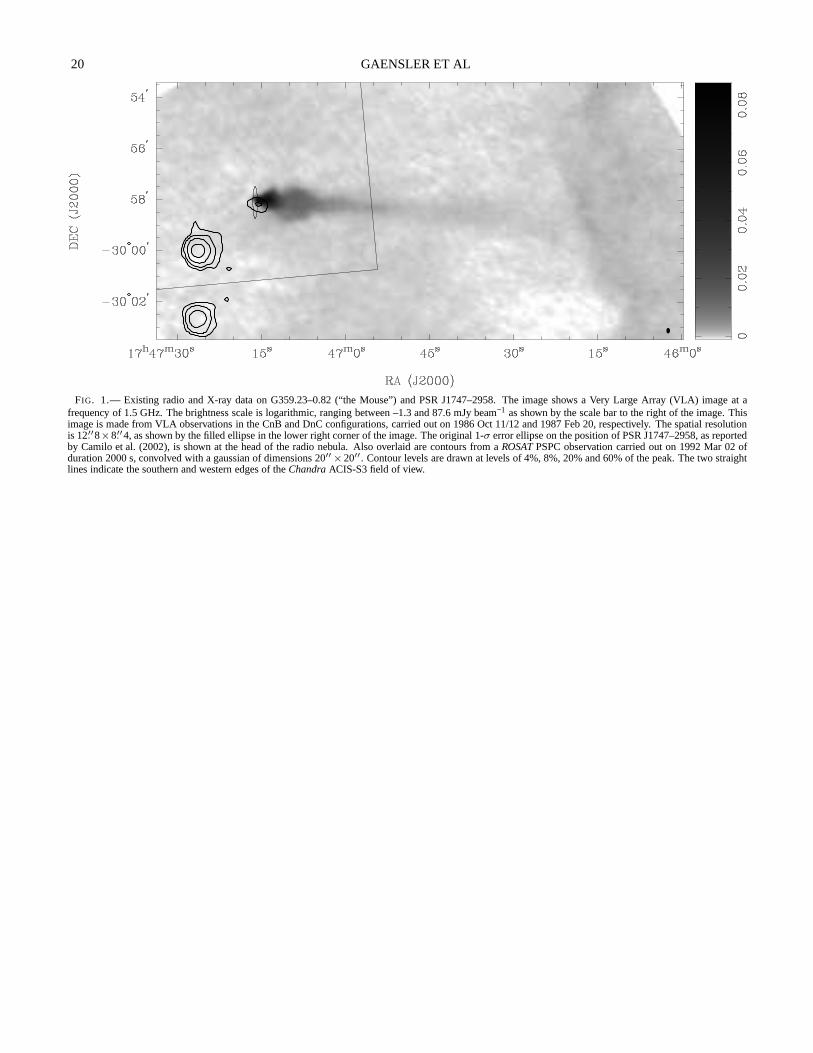
20 GAENSLER ET AL

FIG. 1.— Existing radio and X-ray data on G359.23–0.82 (“the Mouse”) and PSR J1747–2958. The image shows a Very Large Array (VLA) image at afrequency of 1.5 GHz. The brightness scale is logarithmic, ranging between –1.3 and 87.6 mJy beam−1 as shown by the scale bar to the right of the image. Thisimage is made from VLA observations in the CnB and DnC configurations, carried out on 1986 Oct 11/12 and 1987 Feb 20, respectively. The spatial resolutionis 12.′′8×8.′′4, as shown by the filled ellipse in the lower right corner of the image. The original 1-σ error ellipse on the position of PSR J1747–2958, as reportedby Camilo et al. (2002), is shown at the head of the radio nebula. Also overlaid are contours from aROSATPSPC observation carried out on 1992 Mar 02 ofduration 2000 s, convolved with a gaussian of dimensions 20′′

×20′′. Contour levels are drawn at levels of 4%, 8%, 20% and 60% of the peak. The two straightlines indicate the southern and western edges of theChandraACIS-S3 field of view.

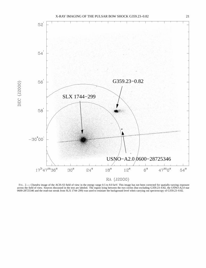
X-RAY IMAGING OF THE PULSAR BOW SHOCK G359.23–0.82 21

SLX 1744−299

USNO−A2.0 0600−28725346

G359.23−0.82

FIG. 2.— Chandraimage of the ACIS-S3 field of view in the energy range 0.5 to 8.0keV. This image has not been corrected for spatially-varying exposureacross the field of view. Sources discussed in the text are labeled. The region lying between the two circles (but excluding G359.23–0.82, the USNO-A2.0 star0600-28725346 and the read-out streak from SLX 1744–299) was used to estimate the background level when carrying out spectroscopy of G359.23–0.82.

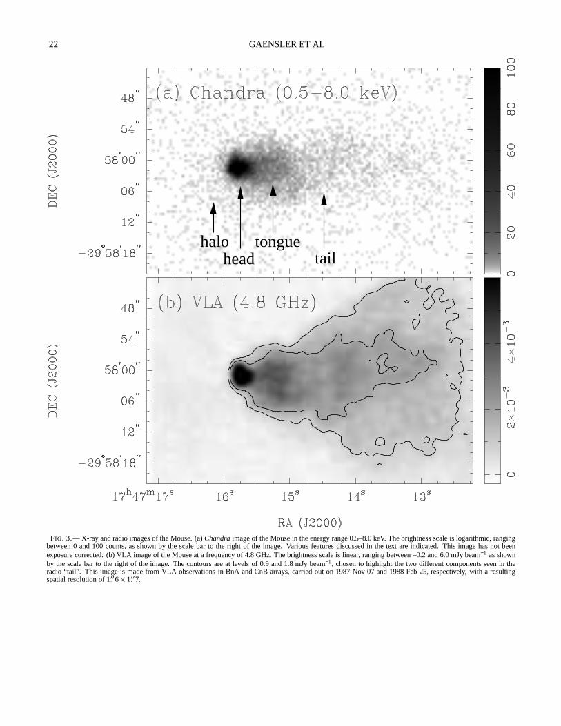
22 GAENSLER ET AL

tailhalo

headtongue

FIG. 3.— X-ray and radio images of the Mouse. (a)Chandraimage of the Mouse in the energy range 0.5–8.0 keV. The brightness scale is logarithmic, rangingbetween 0 and 100 counts, as shown by the scale bar to the rightof the image. Various features discussed in the text are indicated. This image has not beenexposure corrected. (b) VLA image of the Mouse at a frequencyof 4.8 GHz. The brightness scale is linear, ranging between –0.2 and 6.0 mJy beam−1 as shownby the scale bar to the right of the image. The contours are at levels of 0.9 and 1.8 mJy beam−1, chosen to highlight the two different components seen in theradio “tail”. This image is made from VLA observations in BnAand CnB arrays, carried out on 1987 Nov 07 and 1988 Feb 25, respectively, with a resultingspatial resolution of 1.′′6×1.′′7.

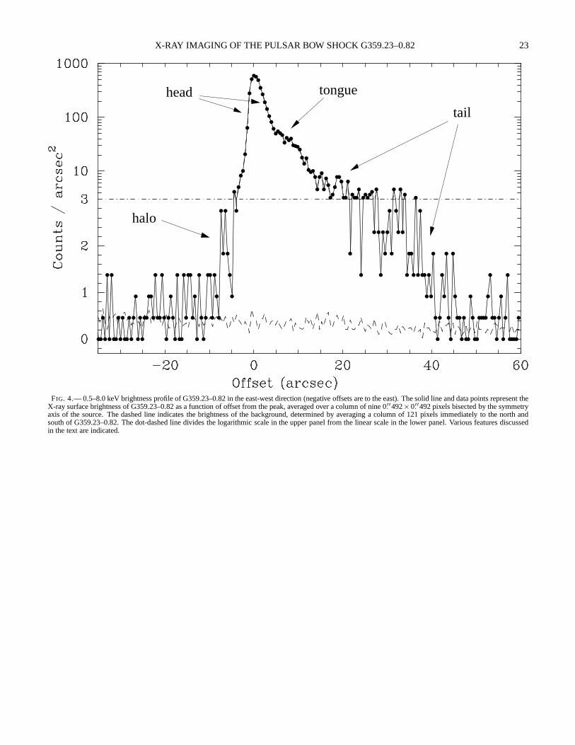
X-RAY IMAGING OF THE PULSAR BOW SHOCK G359.23–0.82 23

tongue

halo

head

tail

FIG. 4.— 0.5–8.0 keV brightness profile of G359.23–0.82 in the east-west direction (negative offsets are to the east). The solid line and data points represent theX-ray surface brightness of G359.23–0.82 as a function of offset from the peak, averaged over a column of nine 0.′′492×0.′′492 pixels bisected by the symmetryaxis of the source. The dashed line indicates the brightnessof the background, determined by averaging a column of 121 pixels immediately to the north andsouth of G359.23–0.82. The dot-dashed line divides the logarithmic scale in the upper panel from the linear scale in the lower panel. Various features discussedin the text are indicated.

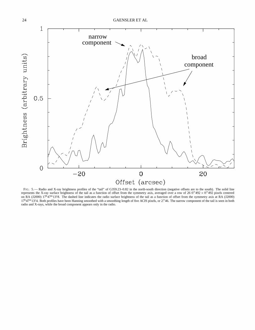
24 GAENSLER ET AL

componentnarrow

componentbroad

FIG. 5.— Radio and X-ray brightness profiles of the “tail” of G359.23–0.82 in the north-south direction (negative offsets are to the south). The solid linerepresents the X-ray surface brightness of the tail as a function of offset from the symmetry axis, averaged over a row of 26 0.′′492× 0.′′492 pixels centeredon RA (J2000) 17h47m13.s8. The dashed line indicates the radio surface brightness ofthe tail as a function of offset from the symmetry axis at RA (J2000)17h47m13.s4. Both profiles have been Hanning smoothed with a smoothing length of five ACIS pixels, or 2.′′46. The narrow component of the tail is seen in bothradio and X-rays, while the broad component appears only in the radio.

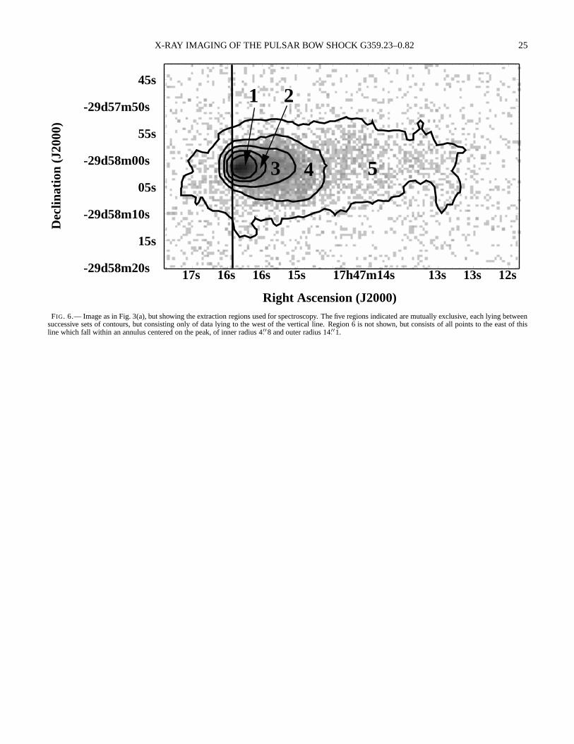
X-RAY IMAGING OF THE PULSAR BOW SHOCK G359.23–0.82 25

17h47m14s17s 16s 16s 15s 13s 13s 12s

-29d58m00s

-29d57m50s

-29d58m10s

-29d58m20s

45s

55s

05s

15s

Right Ascension (J2000)

Dec

linat

ion

(J20

00)

3 4

21

5

FIG. 6.— Image as in Fig. 3(a), but showing the extraction regions used for spectroscopy. The five regions indicated are mutually exclusive, each lying betweensuccessive sets of contours, but consisting only of data lying to the west of the vertical line. Region 6 is not shown, but consists of all points to the east of thisline which fall within an annulus centered on the peak, of inner radius 4.′′8 and outer radius 14.′′1.

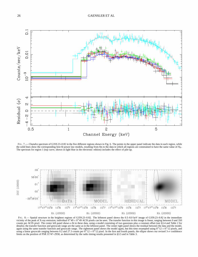
26 GAENSLER ET AL

FIG. 7.—Chandraspectrum of G359.23–0.82 in the five different regions shownin Fig. 6. The points in the upper panel indicate the data in each region, whilethe solid lines show the corresponding best fit power law models, resulting from fits to the data in which all regions are constrained to have the same value ofNH .The spectrum for region 1 (top curve, shown in light blue in the electronic edition) includes the effect of pile-up.

FIG. 8.— Spatial structure in the brightest regions of G359.23–0.82. The leftmost panel shows the 0.5–8.0 keV image of G359.23–0.82 in the immediatevicinity of the peak of X-ray emission; individual 0.′′49×0.′′49 ACIS pixels can be seen. The transfer function in this image is linear, ranging between 0 and 350counts per ACIS pixel. The center left panel shows a fit to these data, using a model consisting of two gaussians plus a constant offset (see §3.4 and Table 2 fordetails); the transfer function and greyscale range are thesame as in the leftmost panel. The center right panel shows the residual between the data and the model,again using the same transfer function and greyscale range.The rightmost panel shows the model again, but this time resampled using 0.′′12×0.′′12 pixels, andusing a linear greyscale ranging between 0.2 and 27.3 countsper 0.′′12×0.′′12 pixel. In the first and fourth panels, the ellipse shows ourrevised 3-σ confidencelimits on the position of PSR J1747–2958, as determined by the radio timing results presented in §3.5 and in Table 3.

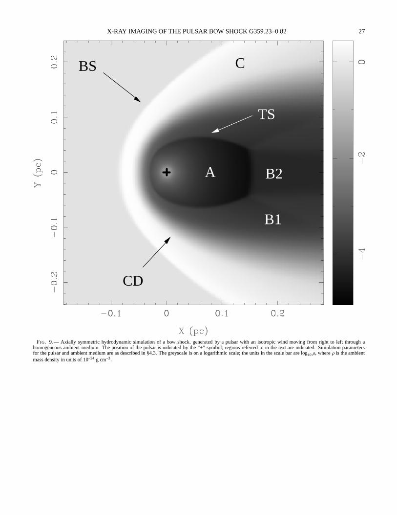
X-RAY IMAGING OF THE PULSAR BOW SHOCK G359.23–0.82 27

B1

TS

CBS

CD

A B2

FIG. 9.— Axially symmetric hydrodynamic simulation of a bow shock, generated by a pulsar with an isotropic wind moving from right to left through ahomogeneous ambient medium. The position of the pulsar is indicated by the “+” symbol; regions referred to in the text areindicated. Simulation parametersfor the pulsar and ambient medium are as described in §4.3. The greyscale is on a logarithmic scale; the units in the scale bar are log10ρ, whereρ is the ambientmass density in units of 10−24 g cm−3.