The impacts of changing transport and precipitation on pollutantdistributions in a future climate

Yuanyuan Fang,1,2 Arlene M. Fiore,2 Larry W. Horowitz,1,2 Anand Gnanadesikan,1,2,3

Isaac Held,1,2 Gang Chen,4 Gabriel Vecchi,2 and Hiram Levy2

Received 15 January 2011; revised 18 May 2011; accepted 13 June 2011; published 17 September 2011.

[1] Air pollution (ozone and particulate matter in surface air) is strongly linked tosynoptic weather and thus is likely sensitive to climate change. In order to isolate theresponses of air pollutant transport and wet removal to a warming climate, we examine asimple carbon monoxide–like (CO) tracer (COt) and a soluble version (SAt), both withthe 2001 CO emissions, in simulations with the Geophysical Fluid Dynamics Laboratorychemistry‐climate model (AM3) for present (1981–2000) and future (2081–2100)climates. In 2081–2100, projected reductions in lower‐tropospheric ventilation and wetdeposition exacerbate surface air pollution as evidenced by higher surface COt and SAtconcentrations. However, the average horizontal general circulation patterns in 2081–2100are similar to 1981–2000, so the spatial distribution of COt changes little. Precipitationis an important factor controlling soluble pollutant wet removal, but the total globalprecipitation change alone does not necessarily indicate the sign of the soluble pollutantresponse to climate change. Over certain latitudinal bands, however, the annual wetdeposition change can be explained mainly by the simulated changes in large‐scale (LS)precipitation. In regions such as North America, differences in the seasonality of LSprecipitation and tracer burdens contribute to an apparent inconsistency of changes inannual wet deposition versus annual precipitation. As a step toward an ultimate goal ofdeveloping a simple index that can be applied to infer changes in soluble pollutants directlyfrom changes in precipitation fields as projected by physical climate models, we explorehere a “Diagnosed Precipitation Impact” (DPI) index. This index captures the sign andmagnitude (within 50%) of the relative annual mean changes in the global wet deposition ofthe soluble pollutant. DPI can only be usefully applied in climate models in which LSprecipitation dominates wet deposition and horizontal transport patterns change little asclimate warms. Our findings support the need for tighter emission regulations, for bothsoluble and insoluble pollutants, to obtain a desired level of air quality as climate warms.

Citation: Fang, Y., A. M. Fiore, L. W. Horowitz, A. Gnanadesikan, I. Held, G. Chen, G. Vecchi, and H. Levy (2011), Theimpacts of changing transport and precipitation on pollutant distributions in a future climate, J. Geophys. Res., 116, D18303,doi:10.1029/2011JD015642.

1. Introduction

[2] Air quality is influenced by meteorological conditionsand thus could be sensitive to climate change [e.g., Denmanet al., 2007]. Over the next century, models project signifi-cant changes in global and regional climate [e.g.,Christensenet al., 2007; Meehl et al., 2007], including increases in tem-perature, changes in the hydrological cycle, alterations in

global and regional circulation patterns (e.g., polewardexpansion of the Hadley cell, reduced tropical convectivemass fluxes and reduced midlatitude cyclone frequency).These changes are expected to affect pollutant transportprocesses, natural pollutant precursor emissions that dependstrongly on meteorology (lightning NOx, biogenic emis-sions), and the rates of chemical reactions. Estimating theclimate change impact on air quality requires a good under-standing of each of these processes.[3] Most General Circulation Model (GCM) and Chemical

Transport Model (CTM) studies of the impact of climatechange on air pollutants focus on ozone (O3) and particulatematter (PM) because these two species are of most concernfor human health and directly affect both air quality andatmospheric radiative forcing [e.g., Jacob andWinner, 2009].Models show consistently that as a result of 21st‐centuryclimate change, background O3 in the lower troposphere(where O3 loss by reacting with water vapor is dominant) will

1Atmospheric and Oceanic Sciences Program, Princeton University,Princeton, New Jersey, USA.

2Geophysical Fluid Dynamics Laboratory, National Oceanic andAtmospheric Administration, Princeton, New Jersey, USA.

3Now at Department of Earth and Planetary Science, Johns HopkinsUniversity, Baltimore, Maryland, USA.

4Department of Earth and Atmospheric Sciences, Cornell University,Ithaca, New York, USA.

Copyright 2011 by the American Geophysical Union.0148‐0227/11/2011JD015642

JOURNAL OF GEOPHYSICAL RESEARCH, VOL. 116, D18303, doi:10.1029/2011JD015642, 2011

D18303 1 of 14

decrease while surface O3 over polluted regions at northernmidlatitudes will increase (+1–10 ppbv) [Wu et al., 2008a,2008b; Lin et al., 2008; Nolte et al., 2008; Weaver et al.,2009]. For PM, models predict significant changes (±0.1–1 mg m−3) but neither the sign nor the magnitude is consis-tent across models [Jacob and Winner, 2009]. The uncer-tainty regarding the impact of climate on particulate matterreflects the complexity of the dependence of its componentson meteorological variables, and the key role of precipitationin modulating PM sinks [Racherla and Adams, 2006;Tagaris et al., 2007; Avise et al., 2009; Pye et al., 2009;Dawson et al., 2007]. Although Racherla and Adams [2006]showed that a lower PM burden corresponds to an increase inglobal precipitation in a future climate, Pye et al. [2009]indicated that changes in precipitation are not always thegoverning factor for PM concentrations. Jacob and Winner[2009] argued that precipitation frequency is likely thedominant factor determining PM concentration changes.Such disparate results in the literature motivate our investi-gation into the impact of changing precipitation on solublepollutants in a warmer climate.[4] To isolate the roles of transport and precipitation,

processes affecting many air pollutants, idealized atmo-spheric tracers can be used to represent air pollutants in aclimate model. Previous studies have applied atmospherictracers in GCMs to study the impact of transport changesunder climate change. For example, Holzer and Boer [2001]analyzed tracers emitted from temporally constant localizedsurface sources. They find that interhemispheric exchangetimes, mixing times, and mean transit times all increaseunder global warming by about 10% from 1990 to 2000 to2090–2100, but they consider only advection and diffusionand neglect wet deposition and convection. Furthermore,their tracers have localized (rather than distributed) sources,permitting the identification of transport pathways fromspecific locations while precluding examination of the impactof spatial patterns in precipitation and ventilation changesover polluted regions. Rind et al. [2001] examined changesin the distributions of long‐lived tracers (such as CO2 andCFCs) in a doubled‐CO2 climate and found a 30% increasein troposphere‐to‐stratosphere transport and a decrease insurface tracers because of enhanced convection.Mickley et al.[2004] incorporated black carbon (BC) and CO‐like tracersof fossil fuel emissions in a GCM and found that the severityand duration of summertime regional pollution episodes inthe Midwest and northeastern United States increase signif-icantly relative to the present because of decreased frequencyof migratory cyclones. So far, the impacts of projected pre-cipitation changes on the burdens of soluble pollutants, suchas oxidized nitrogen, sulfate and nitrate aerosols, have notbeen isolated from other climate impacts (e.g., chemicalevolution, emission changes).[5] In order to investigate how pollutant distributions

respond to changing transport and precipitation in a warmerclimate, we apply idealized tracers (with insoluble and sol-uble versions) in a global chemistry‐climate coupled model(Atmospheric Model version 3, AM3, developed by theGeophysical Fluid Dynamics Laboratory (GFDL)) [Donneret al., 2011]. In section 2, we describe our model, includingthe model parameterizations most relevant to this study andthe experiments conducted. Changes in the future distribu-tions of soluble and insoluble tracers are described and

compared in section 3. Section 4 discusses the circulationchanges that are responsible for redistributing the insolubletracer in a warmer climate. Section 5 shows the impact ofprecipitation changes on soluble tracer distributions. Con-clusions are given in section 6.

2. Methods

2.1. Model Description

[6] We use the GFDL AM3 model [Donner et al., 2011]to examine the impact of climate change on tracer dis-tributions. AM3 uses a finite‐volume dynamical core similarto that used in CM2.1 [Delworth et al., 2006] but imple-ments on a cubed‐sphere grid [Putman and Lin, 2007]. TheEarth is represented as a cube with six rectangular faces andthere is no singularity associated with the north and southpoles as with the latitude‐longitude representation, avoidingthe need for polar filtering. The model horizontal resolutionis C48 (48 × 48 cells per face); the size of the grid cell variesfrom ∼163 km (at the 6 corners of the cubed sphere) to231 km (near the center of each face). The model used in oursimulations has 48 vertical levels, with the top level centeredat 1.7 Pa (∼75km).[7] Aerosols and gases are transported in the model by

advection, convection, and eddy diffusion by turbulencewith full stratospheric [Austin and Wilson, 2006] and tro-pospheric [Horowitz et al., 2003] chemistry, as described indetail by Donner et al. [2011]. Aerosol‐cloud interactionsare also included in AM3 model simulations [Donner et al.,2011]. Most pertinent to our study is the wet depositionparameterization, which we describe briefly here. Wetdeposition includes in‐cloud and below‐cloud scavenging bylarge‐scale and convective clouds. The wet deposition flux(W) is directly proportional to the local concentration (C),given byW =G ·C, where G is the wet scavenging coefficient.In‐cloud scavenging of aerosols is calculated following thework of Giorgi and Chameides [1985]. The in‐cloud scav-enging coefficient is:

Gin ¼ 1� exp �� � fð Þ; � ¼ Pkþ1rain � Pk

rain þ Pkþ1snow � Pk

snow

Dp � g�1 � xliq ;

where f is the scavenging factor, Pk is the precipitation fluxthrough the top of layer k, Pk+1 is the precipitation fluxthrough the bottom of layer k (top of layer k + 1) (thus, Pk+1 −Pk is the precipitation generated in layer k),Dp is the pressurethickness of the model layer k and g is the gravitationalacceleration. The liquid water content xliq(=

Cloud water kgð Þair mass kgð Þ ) is

calculated by the large‐scale cloud and convective para-meterizations. The fraction of aerosol incorporated in thecloud condensate, f, is prescribed. For sulfate, it is 0.2 inlarge‐scale clouds and 0.5 in convective clouds (note thatthese scavenging factors differ from those used by Donneret al. [2011]). These fractions qualitatively correspond to therelative solubility and cloud drop nucleation properties of theaerosols, but the quantitative values are selected (globally) toprovide a reasonable simulation of the global mean andregional patterns of aerosol optical depth (AOD) [Donneret al., 2011]. In the case of convective precipitation, wetdeposition is only computed within the updraft plume. In oursimulations, in‐cloud scavenging of sulfate aerosols does notdepend on the size of the droplet, the size of sulfate aerosols,

FANG ET AL.: CLIMATE CHANGE IMPACT ON AIR POLLUTANTS D18303D18303

2 of 14

or the type of precipitation (rain or snow). Below‐cloudwashout is only considered for large‐scale precipitationand is parameterized as by Li et al. [2008] for aerosols withthe below cloud scavenging coefficient (Gbc) calculated as

Gbc = 34

Prain��rainRrain��H2O þ

Psnow��snowRsnow��snow

� �, where Prain and Psnow are the

precipitation fluxes, a is the efficiency with which aerosolsare collected by raindrops and snow with arain = 0.001 andasnow = 0.001, R is the radius of precipitation droplets withRrain = 0.001 m and Rsnow = 0.001 m, r is density with rH2O =1000 kgm−3 and rsnow = 500 kgm−3.

2.2. Experiments and Tracers

[8] We conduct a pair of idealized simulations designed todetect climate change signals rather than model internalvariability. For the present‐day climate (denoted as “1981–2000”), we use a monthly 20 year mean annually invariantclimatology of observed sea surface temperature and sea icefrom the Hadley Center to drive our AM3 simulation. Forthe future climate (referred to as “2081–2100”), we add the20 year mean monthly anomalies of sea surface tempera-ture and sea ice extent (calculated from a 19 model IPCCAR4 A1B scenario ensemble mean; these models includeCSIRO‐Mk3.5 [Gordon et al., 2002], INGV‐ECHAM4[Gualdi et al., 2006] and the models in Table 1 of Vecchi andSoden [2007], except models number 10, 11, 12, 9 and 20) tothe present‐day observed climatological values. Both simu-lations are run for 21 years with the first year as spin‐up.Emissions of aerosols and trace gases in both simulations arekept at 1990 levels. Long‐lived greenhouse gas concentra-tions (CO2, N2O and CFCs) are set to the 1990 values in thepresent‐day simulation and to the 2090 A1B values in thefuture climate run. CH4 is set to the 1990 levels for tropo-spheric chemistry calculations and the present‐day radiationcalculations, but to the A1B 2090 level for the radiationcalculation in the future climate run, thus distinguishingbetween the direct radiative impact of CH4 forcing on thecirculation from its indirect chemical impacts (changingradiatively active tracers like O3). These settings allow us tostudy the effect of climate change on pollutants separatelyfrom the role of changes in anthropogenic pollutant emissions.The AM3 simulated global surface temperature increases by

2.7 K and global precipitation increases by 6% from 1981–2000 to 2081–2100, consistent with the IPCC AR4 report(2.8 K and 6% increases of surface temperature and pre-cipitation in the AR4 model ensemble mean) [Meehl et al.,2007].[9] Although our simulations include full chemistry as

described above, we introduce two sets of idealized tracersinto our simulations and focus exclusively on these tracersin this paper to clearly diagnose the impact of circulationand precipitation changes in 2081–2100 on pollutant dis-tributions. First is a passive tracer, COt, which decaysexponentially with a 25 d lifetime. The emissions of COt(Figure 1) mimic CO emissions in 2001, including anthro-pogenic emissions from the RETRO project [Schultz andRast, 2007; http://www.retro.enes.org] and biomass burn-ing emissions from GFED version2 [van der Werf et al.,2006]. Second, a soluble tracer, SAt, follows the sameemission and decays as COt, but is subjected to additionalremoval by wet deposition as for sulfate aerosols (section2.1) (note, dry deposition is not considered). The effectiveglobal atmospheric lifetime of SAt ranges from 4 to 6 ddepending on season. The application of these tracers isadapted from the diagnostic tracer experiments (TP) ofthe Task Force on Hemispheric Transport of AtmosphericPollutants (HTAP, 2007, http://www.htap.org). The totalanthropogenic and biomass burning CO emissions are about1000 Tg CO yr−1. Our paper focuses on the discussion ofthese two tracers, but we also include other tracers (COt12and SAt12, similar to COt and SAt, but with a 12 d lifetime).While we examine here tracers with 25 and 12 d lifetimes, andtheir soluble counterparts (with 4–6 and 3–4 d lifetimes,respectively), we do not exhaustively address all timescalesassociated with pollution transport.[10] The major advantages of our approach are the fol-

lowing: 1. the emissions of these tracers follow the surfaceemissions of CO, including both anthropogenic and biomassburning emissions, and their lifetimes are close to those ofreal pollutants, such as CO (COt) and sulfate aerosols (SAt);2. the application of this pair of tracers, with and withoutwet deposition, helps us to isolate the impact of precipitationin a future climate; 3. we use two 20 year simulations drivenby annually invariant sea surface temperature and sea ice tomaximize the detection of a climate change signal relative tothe internal model variability; 4. there are already a host ofHTAP TP model simulations for present‐day climate, sothis study could be repeated fairly easily by other models tobuild a multimodel ensemble.

3. The Redistribution of Insoluble and SolublePollutants in a Warmer Climate

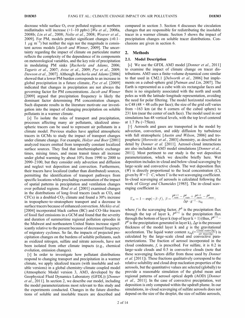
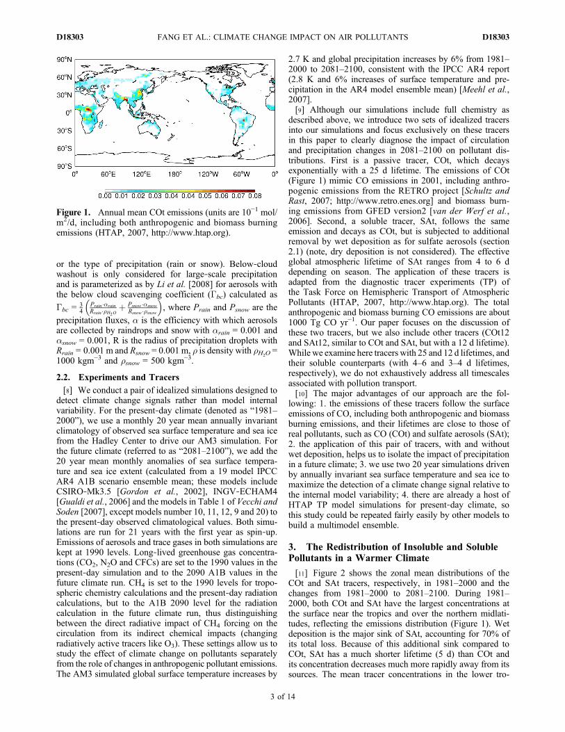
[11] Figure 2 shows the zonal mean distributions of theCOt and SAt tracers, respectively, in 1981–2000 and thechanges from 1981–2000 to 2081–2100. During 1981–2000, both COt and SAt have the largest concentrations atthe surface near the tropics and over the northern midlati-tudes, reflecting the emissions distribution (Figure 1). Wetdeposition is the major sink of SAt, accounting for 70% ofits total loss. Because of this additional sink compared toCOt, SAt has a much shorter lifetime (5 d) than COt andits concentration decreases much more rapidly away from itssources. The mean tracer concentrations in the lower tro-

Figure 1. Annual mean COt emissions (units are 10−1 mol/m2/d, including both anthropogenic and biomass burningemissions (HTAP, 2007, http://www.htap.org).

FANG ET AL.: CLIMATE CHANGE IMPACT ON AIR POLLUTANTS D18303D18303

3 of 14

posphere (below 500 hPa) and in the free troposphere(above 500 hPa) are 19 and 13 ppbv, respectively, for COt,versus 7.4 and 0.3 ppbv for SAt in 1981–2000.[12] Any redistribution of COt in the 2081–2100 simula-

tion reflects only circulation changes in a future climate. Atthe surface, COt concentrations increase by up to 6 ppbv inthe tropics and up to 1.5 ppbv at northern hemisphericmidlatitudes (with relative changes from 2 to 7%). In thefree troposphere, COt concentrations decrease with a max-imum reduction of up to 2 ppbv (−2 to −12% at 400 hPa).Near the tropopause, a large increase in the COt concen-tration (with a maximum of 2 ppbv) occurs. COt tracergenerally decreases in the southern hemisphere. Althoughcirculation changes redistribute COt, the global troposphericburden remains the same from 1981–2000 to 2081–2100because of the fixed 25 d lifetime and fixed emissions. Similarpatterns emerge for the 12 d lifetime insoluble tracer.[13] As will be shown in section 5, the future changes in

tropospheric SAt distribution differ strongly from that of COtbecause it undergoes wet deposition. SAt surface concen-tration increases both in the tropics and at the northernhemispheric midlatitudes, similar to COt, but with a greaterrelative change (above 10%). The increased surface con-centrations of SAt and COt suggest that a warmer climate willcontribute to degraded air quality in the future. In the freetroposphere and the southern hemisphere (where COt con-centration decreases), the SAt concentration increases. Thetropospheric SAt burden increases from 17 to 19 Gg (+12%)in the future, indicating a 12% increase of lifetime from1981–2000 to 2081–2100 (as emissions are identical). Sincewet deposition is the only difference between the two tra-cers, the different responses between SAt and COt result

solely from future changes in precipitation. We will discussnext the causes of the redistribution of COt (section 4) andSAt (section 5) in the future climate simulation.

4. The Impact of Changing Transporton Insoluble Pollutants

[14] To help understand the vertical redistribution of tro-pospheric COt (i.e., increases in the lower troposphere anddecreases in the free troposphere), we apply a two‐boxmodel between the lower troposphere and the free tropo-sphere. The boundary between these two boxes is defined as500 hPa level following Held and Soden [2006]. Massconservation of COt in the free troposphere box suggests abalance mF(cL − cF) = mF cF/t, in which mF is the total airmass within the free troposphere box, t is the 25 d lifetime,cL and cF are the mean COt concentrations in the lowertroposphere and the free troposphere, respectively, and mF isthe mass flux exchange between the lower troposphere andthe free troposphere. Assuming that the mass of the tropo-sphere is fixed, the balance suggests ��F

�F + � cF�cLð ÞcF�cL ≈ �cF

cF . Weuse the simulated tracer concentration in the model andcalculate the values for the second term on the left handside, the COt concentration gradient change between thefree troposphere and the lower troposphere (+10%), andthe first term on the right hand side, the relative change inthe free tropospheric COt concentration (−3%). We then

calculate ��F

�F , i.e., the relative change of the mass fluxexchange between these two boxes to be −13%. According tomodel‐diagnosed tracer tendencies in the free troposphere,most (>90%) of the transport flux change between the lowertroposphere and the free troposphere comes from the advec-

Figure 2. The 20 year average zonal mean distribution of idealized tracer (unit: ppbv) during 1981–2000(black solid contour) and the changes of that tracer from 1981–2000 to 2081–2100 (color shaded) withrespect to vertical coordinates of pressure. (a) COt tracer and (b) SAt tracer. Blue dashed and dotted linesshow the tropopause location during 1981–2000 and 2081–2100, respectively (as identified by Reichler et al.[2003], based on the World Meteorological Organization (WMO) lapse‐rate criterion); only changes sig-nificant at the 95% confidence level assessed by t test are shown.

FANG ET AL.: CLIMATE CHANGE IMPACT ON AIR POLLUTANTS D18303D18303

4 of 14

tive tendency rather than the convective tendency. Thisweaker contribution from convection is consistent with thestudy of Holzer and Boer [2001], which shows a similarvertical redistribution of their surface‐emitted tracers by onlyconsidering advection and diffusion. Applying our analysis toAM3‐simulated water vapor as by Held and Soden [2006],we get a similar 14% decrease in the lower troposphere–freetroposphere mass flux exchange. The mechanism by whichexchange between lower troposphere and upper troposphereexchange is reduced may vary regionally. For example, overthe tropics, reduced convective mass flux dominates [Heldand Soden, 2006], while over midlatitudes (such as NorthAmerica), the effect of weaker and less frequent cycloneactivity may account for less ventilation [e.g., Wu et al.,2008b]. As our focus is on the difference between solu-ble and insoluble tracers, we do not probe these regionalmechanisms more deeply here.[15] Regarding the decreasing tropospheric COt concen-

tration in the southern hemisphere in the future climate,we apply a similar two‐box model, this time representingthe troposphere in the northern and southern hemispheres. A2% decrease in the hemispheric flux exchange is derivedfrom this model. Interhemispheric transport and transportbetween the tropics and extratropics are dominated by theHadley circulation [Bowman and Carrie, 2002; Bowmanand Erukhimova, 2004; Hess, 2005]. Many previous stud-ies indicate a weakened Hadley cell [e.g., Rind et al., 2001;Holzer and Boer, 2001; Held and Soden, 2006] under globalwarming. Consistent with these results, the AM3‐simulatedHadley cell (represented by the 20 year annual mean massstream function, see Figure S1) weakens over the lower tro-posphere (by less than 5%) [Held and Soden, 2006; Vecchi

and Soden, 2007], resulting in the reduced hemispheric fluxexchange.1

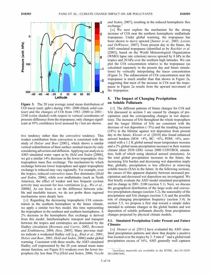
[16] We next explore the mechanism for the strongincrease of COt near the northern hemispheric midlatitudetropopause. Under global warming, the tropopause hasbeen shown to move upward [Santer et al., 2003; Lorenzand DeWeaver, 2007]. From present day to the future, theAM3‐simulated tropopause (identified as by Reichler et al.[2003], based on the World Meteorological Organization(WMO) lapse rate criterion) moves upward by 8 hPa in thetropics and 20 hPa over the northern high latitudes. We canplot the COt concentration relative to the tropopause (ascalculated separately in the present day and future simula-tions) by vertically interpolating the tracer concentration(Figure 3). The enhancement of COt concentration near thetropopause is much smaller than that shown in Figure 2a,suggesting that most of the increase in COt near the tropo-pause in Figure 2a results from the upward movement ofthe tropopause.

5. The Impact of Changing Precipitationon Soluble Pollutants

[17] The different patterns of future changes for COt andSAt discussed in section 3 are caused by changes of pre-cipitation (and the corresponding changes in wet deposi-tion). The increase of SAt throughout the whole troposphereand the longer lifetime of SAt are consistent with thedecrease of wet deposition (−5%) and the resulting increase(18%) in the lifetime against wet deposition from presentday to the future. Kloster et al. [2010] also found enhancedaerosol burdens (SO4: +4%, BC: +6%, POM: +6%, asso-ciated with a 1.2 K global annual mean temperature increaseand a 2% global mean precipitation increase) in their warmerclimate (their 2030 GHG versus 2000 CONTROL simula-tion, both of which using identical aerosol emissions). Asthe total global precipitation increases in the future, theincreasing SAt burden and decreasing wet deposition implythat, globally, precipitation is less effective at removingsoluble tracers (SAt) in the future. In the following sections,the causes of this apparent disparity between increased pre-cipitation and decreased wet deposition are investigated. Wefirst briefly evaluate the AM3 model simulated precipitationand its change in 2081–2100 (section 5.1). Next, we discussthe geographical distribution of the large‐scale and convec-tive precipitation changes (section 5.2), the seasonality of theprecipitation and SAt changes (section 5.3) and the possiblerole of changing precipitation frequency (section 5.4). Insection 5.5, we propose a first step toward a simple indexintended to estimate changes in the global burden and wetdeposition of soluble pollutants directly from precipitationchanges projected by physical climate models.

5.1. Simulated Precipitation Under Present and FutureClimates

[18] Donner et al. [2011] have evaluated the AM3 simu-lated precipitation patterns and show that despite a positivebias located over the tropics by 3–5 mm d−1 and a global totalprecipitation excess of 16%, AM3 generally well captures

Figure 3. The 20 year average zonal mean distribution ofCOt tracer (unit: ppbv) during 1981–2000 (black solid con-tour) and the changes of COt from 1981–2000 to 2081–2100 (color shaded) with respect to vertical coordinates ofpressure difference from the tropopause; only changes signif-icant at 95% confidence level assessed by t test are shown.

1Auxiliary materials are available in the HTML. doi:10.1029/2011JD015642.

FANG ET AL.: CLIMATE CHANGE IMPACT ON AIR POLLUTANTS D18303D18303

5 of 14

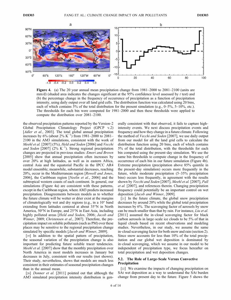
the observed precipitation patterns reported by the Version‐2Global Precipitation Climatology Project (GPCP v.2)[Adler et al., 2003]. The total global annual precipitationincreases by 6% (about 2% K−1) from 1981–2000 to 2081–2100 in the AM3 simulations, consistent with the work ofMeehl et al. [2007] (5%), Held and Soden [2006] and Vecchiand Soden [2007] (2% K−1). Strong regional precipitationchanges are projected in previous studies: Emori and Brown[2005] show that annual precipitation often increases byover 20% at high latitudes, as well as in eastern Africa,central Asia and the equatorial Pacific in the IPCC AR4model ensemble; meanwhile, substantial decreases, reaching20%, occur in the Mediterranean region [Rowell and Jones,2006], the Caribbean region [Neelin et al., 2006] and thesubtropical western coasts of each continent. In general, oursimulations (Figure 4a) are consistent with these patterns,except in the Caribbean region, where AM3 predicts increasedprecipitation. Disagreements between models as to whetherthe future climate will be wetter or drier exist at the marginsof climatologically wet and dry regions (e.g., in a 10° bandextending from latitudes centered at about 35°N in NorthAmerica, 50°N in Europe, and 25°N in East Asia, includinghighly polluted areas [Held and Soden, 2006; Jacob andWinner, 2009; Christensen et al., 2007]. Therefore, the pre-cipitation impact on soluble pollutants (such as PM) over theseplaces may be sensitive to the regional precipitation changesimulated by specific models [Jacob and Winner, 2009].[19] In addition to the spatial pattern of precipitation,

the seasonal variation of the precipitation change is alsoimportant for predicting future soluble tracer tendencies.Meehl et al. [2007] show that the monthly precipitation overNorth America in most models increases in January butdecreases in July, consistent with our results (not shown).Their study, nevertheless, shows that models are much lessconsistent in their estimates of seasonal precipitation changesthan in the annual mean.[20] Donner et al. [2011] pointed out that although the

AM3 simulated precipitation intensity distribution is gen-

erally consistent with that observed, it fails to capture high‐intensity events. We next discuss precipitation events andfrequency and how they change in a future climate. Followingthe method of Vecchi and Soden [2007], we use daily outputfrom our model for all the land grid cells to calculate thedistribution function using 20 bins, each of which contains5% of the total distribution, with the thresholds for eachbin computed using the present‐day simulation. We use thesame bin thresholds to compute change in the frequency ofoccurrence of each bin in our future simulation (Figure 4b).Extreme precipitation (precipitation above 85% quintile inthe present‐day simulation) occurs more frequently in thefuture, while moderate precipitation (5–35% precipitationbins) occurs less frequently, in agreement with the resultsshown by Vecchi and Soden [2007],Meehl et al. [2007], Pallet al. [2007], and references therein. Changing precipitationfrequency could potentially be an important control on wetdeposition [Jacob and Winner, 2009].[21] In the future climate, the global snow precipitation

decreases by around 20% while the global total precipitationincreases by 6%. The scavenging factor of aerosols by snowcan be much smaller than that by rain. For instance, Liu et al.[2011] assumed the in‐cloud scavenging factor for blackcarbon aerosols in large‐scale ice clouds to be 5% of that inliquid clouds based on recent observations and modelingstudies. Nevertheless, in our study, we assume the samein‐cloud scavenging factor for both snow and rain (section 2).Since snow accounts for less than 10% of the total precip-itation and our global wet deposition is dominated byin‐cloud scavenging, which we assume in our model to beindependent of precipitation type, we focus hereafter ontotal precipitation and wet deposition changes.

5.2. The Role of Large‐Scale Versus ConvectivePrecipitation

[22] We examine the impacts of changing precipitation onSAt wet deposition as a way to understand the SAt burdenchange from present day to the future. Figure 5 shows the

Figure 4. (a) The 20 year annual mean precipitation change from 1981–2000 to 2081–2100 (units aremm/d) (shaded area indicates the changes significant at the 95% confidence level assessed by t test) and(b) the percentage change in the frequency of occurrence of precipitation as a function of precipitationintensity, using daily output over all land grid cells. The distribution function was calculated using 20 bins,each of which contains 5% of the total distribution for the present simulation (e.g., 0–5%, 5–10%, etc.).The thresholds for each bin were computed for 1981–2000 and then these thresholds were applied tocompute the distribution over 2081–2100.

FANG ET AL.: CLIMATE CHANGE IMPACT ON AIR POLLUTANTS D18303D18303

6 of 14

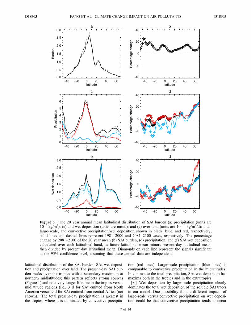
latitudinal distribution of the SAt burden, SAt wet deposi-tion and precipitation over land. The present‐day SAt bur-den peaks over the tropics with a secondary maximum atnorthern midlatitudes; this pattern reflects strong sources(Figure 1) and relatively longer lifetime in the tropics versusmidlatitude regions (i.e., 3 d for SAt emitted from NorthAmerica versus 9 d for SAt emitted from central Africa (notshown)). The total present‐day precipitation is greatest inthe tropics, where it is dominated by convective precipita-

tion (red lines). Large‐scale precipitation (blue lines) iscomparable to convective precipitation in the midlatitudes.In contrast to the total precipitation, SAt wet deposition hasmaxima both in the tropics and in the extratropics.[23] Wet deposition by large‐scale precipitation clearly

dominates the total wet deposition of the soluble SAt tracerin our model. One possibility for the different impacts oflarge‐scale versus convective precipitation on wet deposi-tion could be that convective precipitation tends to occur

Figure 5. The 20 year annual mean latitudinal distribution of SAt burden (a) precipitation (units are10−5 kg/m2); (c) and wet deposition (units are mm/d); and (e) over land (units are 10−10 kg/m2/d): total,large‐scale, and convective precipitation/wet deposition shown in black, blue, and red, respectively;solid lines and dashed lines represent 1981–2000 and 2081–2100 cases, respectively. The percentagechange by 2081–2100 of the 20 year mean (b) SAt burden, (d) precipitation, and (f) SAt wet depositioncalculated over each latitudinal band, as future latitudinal mean minors present‐day latitudinal mean,then divided by present‐day latitudinal mean. Diamonds on each line represent the signals significantat the 95% confidence level, assuming that these annual data are independent.

FANG ET AL.: CLIMATE CHANGE IMPACT ON AIR POLLUTANTS D18303D18303

7 of 14

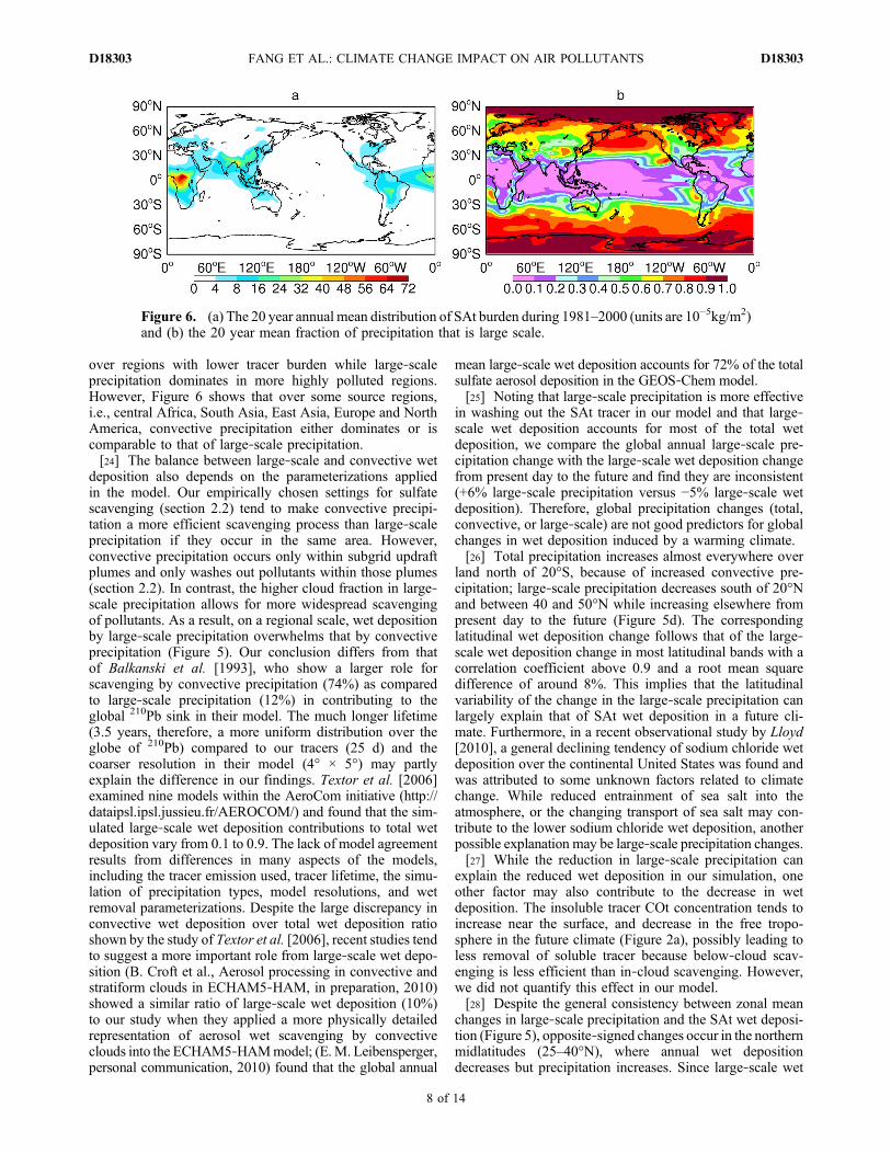
over regions with lower tracer burden while large‐scaleprecipitation dominates in more highly polluted regions.However, Figure 6 shows that over some source regions,i.e., central Africa, South Asia, East Asia, Europe and NorthAmerica, convective precipitation either dominates or iscomparable to that of large‐scale precipitation.[24] The balance between large‐scale and convective wet

deposition also depends on the parameterizations appliedin the model. Our empirically chosen settings for sulfatescavenging (section 2.2) tend to make convective precipi-tation a more efficient scavenging process than large‐scaleprecipitation if they occur in the same area. However,convective precipitation occurs only within subgrid updraftplumes and only washes out pollutants within those plumes(section 2.2). In contrast, the higher cloud fraction in large‐scale precipitation allows for more widespread scavengingof pollutants. As a result, on a regional scale, wet depositionby large‐scale precipitation overwhelms that by convectiveprecipitation (Figure 5). Our conclusion differs from thatof Balkanski et al. [1993], who show a larger role forscavenging by convective precipitation (74%) as comparedto large‐scale precipitation (12%) in contributing to theglobal 210Pb sink in their model. The much longer lifetime(3.5 years, therefore, a more uniform distribution over theglobe of 210Pb) compared to our tracers (25 d) and thecoarser resolution in their model (4° × 5°) may partlyexplain the difference in our findings. Textor et al. [2006]examined nine models within the AeroCom initiative (http://dataipsl.ipsl.jussieu.fr/AEROCOM/) and found that the sim-ulated large‐scale wet deposition contributions to total wetdeposition vary from 0.1 to 0.9. The lack of model agreementresults from differences in many aspects of the models,including the tracer emission used, tracer lifetime, the simu-lation of precipitation types, model resolutions, and wetremoval parameterizations. Despite the large discrepancy inconvective wet deposition over total wet deposition ratioshown by the study of Textor et al. [2006], recent studies tendto suggest a more important role from large‐scale wet depo-sition (B. Croft et al., Aerosol processing in convective andstratiform clouds in ECHAM5‐HAM, in preparation, 2010)showed a similar ratio of large‐scale wet deposition (10%)to our study when they applied a more physically detailedrepresentation of aerosol wet scavenging by convectiveclouds into the ECHAM5‐HAMmodel; (E.M. Leibensperger,personal communication, 2010) found that the global annual

mean large‐scale wet deposition accounts for 72% of the totalsulfate aerosol deposition in the GEOS‐Chem model.[25] Noting that large‐scale precipitation is more effective

in washing out the SAt tracer in our model and that large‐scale wet deposition accounts for most of the total wetdeposition, we compare the global annual large‐scale pre-cipitation change with the large‐scale wet deposition changefrom present day to the future and find they are inconsistent(+6% large‐scale precipitation versus −5% large‐scale wetdeposition). Therefore, global precipitation changes (total,convective, or large‐scale) are not good predictors for globalchanges in wet deposition induced by a warming climate.[26] Total precipitation increases almost everywhere over

land north of 20°S, because of increased convective pre-cipitation; large‐scale precipitation decreases south of 20°Nand between 40 and 50°N while increasing elsewhere frompresent day to the future (Figure 5d). The correspondinglatitudinal wet deposition change follows that of the large‐scale wet deposition change in most latitudinal bands with acorrelation coefficient above 0.9 and a root mean squaredifference of around 8%. This implies that the latitudinalvariability of the change in the large‐scale precipitation canlargely explain that of SAt wet deposition in a future cli-mate. Furthermore, in a recent observational study by Lloyd[2010], a general declining tendency of sodium chloride wetdeposition over the continental United States was found andwas attributed to some unknown factors related to climatechange. While reduced entrainment of sea salt into theatmosphere, or the changing transport of sea salt may con-tribute to the lower sodium chloride wet deposition, anotherpossible explanation may be large‐scale precipitation changes.[27] While the reduction in large‐scale precipitation can

explain the reduced wet deposition in our simulation, oneother factor may also contribute to the decrease in wetdeposition. The insoluble tracer COt concentration tends toincrease near the surface, and decrease in the free tropo-sphere in the future climate (Figure 2a), possibly leading toless removal of soluble tracer because below‐cloud scav-enging is less efficient than in‐cloud scavenging. However,we did not quantify this effect in our model.[28] Despite the general consistency between zonal mean

changes in large‐scale precipitation and the SAt wet deposi-tion (Figure 5), opposite‐signed changes occur in the northernmidlatitudes (25–40°N), where annual wet depositiondecreases but precipitation increases. Since large‐scale wet

Figure 6. (a) The 20 year annual mean distribution of SAt burden during 1981–2000 (units are 10−5kg/m2)and (b) the 20 year mean fraction of precipitation that is large scale.

FANG ET AL.: CLIMATE CHANGE IMPACT ON AIR POLLUTANTS D18303D18303

8 of 14

deposition accounts formore than 90% of total wet depositionat northern midlatitudes, we focus hereafter on large‐scalewet deposition.

5.3. Seasonal Changes Over North America

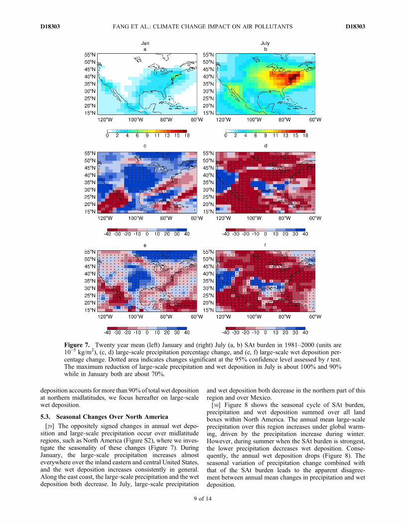
[29] The oppositely signed changes in annual wet depo-sition and large‐scale precipitation occur over midlatituderegions, such as North America (Figure S2), where we inves-tigate the seasonality of these changes (Figure 7). DuringJanuary, the large‐scale precipitation increases almosteverywhere over the inland eastern and central United States,and the wet deposition increases consistently in general.Along the east coast, the large‐scale precipitation and the wetdeposition both decrease. In July, large‐scale precipitation

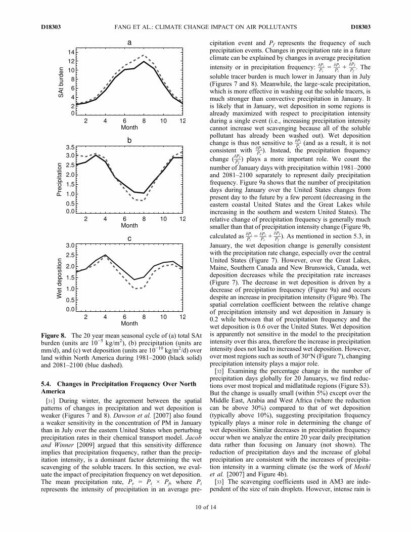
and wet deposition both decrease in the northern part of thisregion and over Mexico.[30] Figure 8 shows the seasonal cycle of SAt burden,

precipitation and wet deposition summed over all landboxes within North America. The annual mean large‐scaleprecipitation over this region increases under global warm-ing, driven by the precipitation increase during winter.However, during summer when the SAt burden is strongest,the lower precipitation decreases wet deposition. Conse-quently, the annual wet deposition drops (Figure 8). Theseasonal variation of precipitation change combined withthat of the SAt burden leads to the apparent disagree-ment between annual mean changes in precipitation and wetdeposition.

Figure 7. Twenty year mean (left) January and (right) July (a, b) SAt burden in 1981–2000 (units are10−5 kg/m2), (c, d) large‐scale precipitation percentage change, and (e, f) large‐scale wet deposition per-centage change. Dotted area indicates changes significant at the 95% confidence level assessed by t test.The maximum reduction of large‐scale precipitation and wet deposition in July is about 100% and 90%while in January both are about 70%.

FANG ET AL.: CLIMATE CHANGE IMPACT ON AIR POLLUTANTS D18303D18303

9 of 14

5.4. Changes in Precipitation Frequency Over NorthAmerica

[31] During winter, the agreement between the spatialpatterns of changes in precipitation and wet deposition isweaker (Figures 7 and 8). Dawson et al. [2007] also founda weaker sensitivity in the concentration of PM in Januarythan in July over the eastern United States when perturbingprecipitation rates in their chemical transport model. Jacoband Winner [2009] argued that this sensitivity differenceimplies that precipitation frequency, rather than the precip-itation intensity, is a dominant factor determining the wetscavenging of the soluble tracers. In this section, we eval-uate the impact of precipitation frequency on wet deposition.The mean precipitation rate, Pr = Pi × Pf, where Pi

represents the intensity of precipitation in an average pre-

cipitation event and Pf represents the frequency of suchprecipitation events. Changes in precipitation rate in a futureclimate can be explained by changes in average precipitation

intensity or in precipitation frequency: �PrPr

= �PiPi

+ �Pf

Pf. The

soluble tracer burden is much lower in January than in July(Figures 7 and 8). Meanwhile, the large‐scale precipitation,which is more effective in washing out the soluble tracers, ismuch stronger than convective precipitation in January. Itis likely that in January, wet deposition in some regions isalready maximized with respect to precipitation intensityduring a single event (i.e., increasing precipitation intensitycannot increase wet scavenging because all of the solublepollutant has already been washed out). Wet depositionchange is thus not sensitive to �Pi

Pi(and as a result, it is not

consistent with �PrPr). Instead, the precipitation frequency

change (�Pf

Pf) plays a more important role. We count the

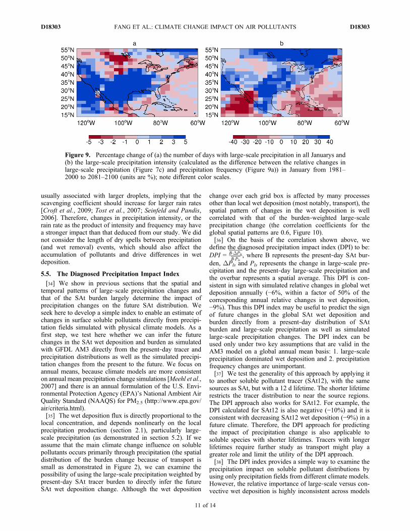
number of January days with precipitation within 1981–2000and 2081–2100 separately to represent daily precipitationfrequency. Figure 9a shows that the number of precipitationdays during January over the United States changes frompresent day to the future by a few percent (decreasing in theeastern coastal United States and the Great Lakes whileincreasing in the southern and western United States). Therelative change of precipitation frequency is generally muchsmaller than that of precipitation intensity change (Figure 9b,

calculated as �PiPi

= �PrPr

+ �Pf

Pf). As mentioned in section 5.3, in

January, the wet deposition change is generally consistentwith the precipitation rate change, especially over the centralUnited States (Figure 7). However, over the Great Lakes,Maine, Southern Canada and New Brunswick, Canada, wetdeposition decreases while the precipitation rate increases(Figure 7). The decrease in wet deposition is driven by adecrease of precipitation frequency (Figure 9a) and occursdespite an increase in precipitation intensity (Figure 9b). Thespatial correlation coefficient between the relative changeof precipitation intensity and wet deposition in January is0.2 while between that of precipitation frequency and thewet deposition is 0.6 over the United States. Wet depositionis apparently not sensitive in the model to the precipitationintensity over this area, therefore the increase in precipitationintensity does not lead to increased wet deposition. However,over most regions such as south of 30°N (Figure 7), changingprecipitation intensity plays a major role.[32] Examining the percentage change in the number of

precipitation days globally for 20 Januarys, we find reduc-tions over most tropical and midlatitude regions (Figure S3).But the change is usually small (within 5%) except over theMiddle East, Arabia and West Africa (where the reductioncan be above 30%) compared to that of wet deposition(typically above 10%), suggesting precipitation frequencytypically plays a minor role in determining the change ofwet deposition. Similar decreases in precipitation frequencyoccur when we analyze the entire 20 year daily precipitationdata rather than focusing on January (not shown). Thereduction of precipitation days and the increase of globalprecipitation are consistent with the increases of precipita-tion intensity in a warming climate (se the work of Meehlet al. [2007] and Figure 4b).[33] The scavenging coefficients used in AM3 are inde-

pendent of the size of rain droplets. However, intense rain is

Figure 8. The 20 year mean seasonal cycle of (a) total SAtburden (units are 10−5 kg/m2), (b) precipitation (units aremm/d), and (c) wet deposition (units are 10−10 kg/m2/d) overland within North America during 1981–2000 (black solid)and 2081–2100 (blue dashed).

FANG ET AL.: CLIMATE CHANGE IMPACT ON AIR POLLUTANTS D18303D18303

10 of 14

usually associated with larger droplets, implying that thescavenging coefficient should increase for larger rain rates[Croft et al., 2009; Tost et al., 2007; Seinfeld and Pandis,2006]. Therefore, changes in precipitation intensity, or therain rate as the product of intensity and frequency may havea stronger impact than that deduced from our study. We didnot consider the length of dry spells between precipitation(and wet removal) events, which should also affect theaccumulation of pollutants and drive differences in wetdeposition.

5.5. The Diagnosed Precipitation Impact Index

[34] We show in previous sections that the spatial andtemporal patterns of large‐scale precipitation changes andthat of the SAt burden largely determine the impact ofprecipitation changes on the future SAt distribution. Weseek here to develop a simple index to enable an estimate ofchanges in surface soluble pollutants directly from precipi-tation fields simulated with physical climate models. As afirst step, we test here whether we can infer the futurechanges in the SAt wet deposition and burden as simulatedwith GFDL AM3 directly from the present‐day tracer andprecipitation distributions as well as the simulated precipi-tation changes from the present to the future. We focus onannual means, because climate models are more consistenton annual mean precipitation change simulations [Meehl et al.,2007] and there is an annual formulation of the U.S. Envi-ronmental Protection Agency (EPA)’s National Ambient AirQuality Standard (NAAQS) for PM2.5 (http://www.epa.gov/air/criteria.html).[35] The wet deposition flux is directly proportional to the

local concentration, and depends nonlinearly on the localprecipitation production (section 2.1), particularly large‐scale precipitation (as demonstrated in section 5.2). If weassume that the main climate change influence on solublepollutants occurs primarily through precipitation (the spatialdistribution of the burden change because of transport issmall as demonstrated in Figure 2), we can examine thepossibility of using the large‐scale precipitation weighted bypresent‐day SAt tracer burden to directly infer the futureSAt wet deposition change. Although the wet deposition

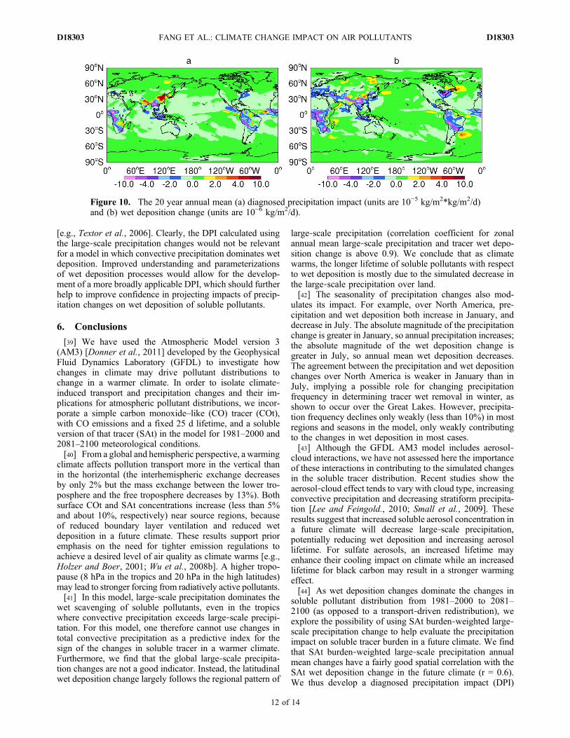
change over each grid box is affected by many processesother than local wet deposition (most notably, transport), thespatial pattern of changes in the wet deposition is wellcorrelated with that of the burden‐weighted large‐scaleprecipitation change (the correlation coefficients for theglobal spatial patterns are 0.6, Figure 10).[36] On the basis of the correlation shown above, we

define the diagnosed precipitation impact index (DPI) to be:DPI = B�DPls

B�Pls, where B represents the present‐day SAt bur-

den, DPls and Pls represents the change in large‐scale pre-cipitation and the present‐day large‐scale precipitation andthe overbar represents a spatial average. This DPI is con-sistent in sign with simulated relative changes in global wetdeposition annually (−6%, within a factor of 50% of thecorresponding annual relative changes in wet deposition,−9%). Thus this DPI index may be useful to predict the signof future changes in the global SAt wet deposition andburden directly from a present‐day distribution of SAtburden and large‐scale precipitation as well as simulatedlarge‐scale precipitation changes. The DPI index can beused only under two key assumptions that are valid in theAM3 model on a global annual mean basis: 1. large‐scaleprecipitation dominated wet deposition and 2. precipitationfrequency changes are unimportant.[37] We test the generality of this approach by applying it

to another soluble pollutant tracer (SAt12), with the samesources as SAt, but with a 12 d lifetime. The shorter lifetimerestricts the tracer distribution to near the source regions.The DPI approach also works for SAt12. For example, theDPI calculated for SAt12 is also negative (−10%) and it isconsistent with decreasing SAt12 wet deposition (−9%) in afuture climate. Therefore, the DPI approach for predictingthe impact of precipitation change is also applicable tosoluble species with shorter lifetimes. Tracers with longerlifetimes require further study as transport might play agreater role and limit the utility of the DPI approach.[38] The DPI index provides a simple way to examine the

precipitation impact on soluble pollutant distributions byusing only precipitation fields from different climate models.However, the relative importance of large‐scale versus con-vective wet deposition is highly inconsistent across models

Figure 9. Percentage change of (a) the number of days with large‐scale precipitation in all Januarys and(b) the large‐scale precipitation intensity (calculated as the difference between the relative changes inlarge‐scale precipitation (Figure 7c) and precipitation frequency (Figure 9a)) in January from 1981–2000 to 2081–2100 (units are %); note different color scales.

FANG ET AL.: CLIMATE CHANGE IMPACT ON AIR POLLUTANTS D18303D18303

11 of 14

[e.g., Textor et al., 2006]. Clearly, the DPI calculated usingthe large‐scale precipitation changes would not be relevantfor a model in which convective precipitation dominates wetdeposition. Improved understanding and parameterizationsof wet deposition processes would allow for the develop-ment of a more broadly applicable DPI, which should furtherhelp to improve confidence in projecting impacts of precip-itation changes on wet deposition of soluble pollutants.

6. Conclusions

[39] We have used the Atmospheric Model version 3(AM3) [Donner et al., 2011] developed by the GeophysicalFluid Dynamics Laboratory (GFDL) to investigate howchanges in climate may drive pollutant distributions tochange in a warmer climate. In order to isolate climate‐induced transport and precipitation changes and their im-plications for atmospheric pollutant distributions, we incor-porate a simple carbon monoxide–like (CO) tracer (COt),with CO emissions and a fixed 25 d lifetime, and a solubleversion of that tracer (SAt) in the model for 1981–2000 and2081–2100 meteorological conditions.[40] From a global and hemispheric perspective, a warming

climate affects pollution transport more in the vertical thanin the horizontal (the interhemispheric exchange decreasesby only 2% but the mass exchange between the lower tro-posphere and the free troposphere decreases by 13%). Bothsurface COt and SAt concentrations increase (less than 5%and about 10%, respectively) near source regions, becauseof reduced boundary layer ventilation and reduced wetdeposition in a future climate. These results support prioremphasis on the need for tighter emission regulations toachieve a desired level of air quality as climate warms [e.g.,Holzer and Boer, 2001; Wu et al., 2008b]. A higher tropo-pause (8 hPa in the tropics and 20 hPa in the high latitudes)may lead to stronger forcing from radiatively active pollutants.[41] In this model, large‐scale precipitation dominates the

wet scavenging of soluble pollutants, even in the tropicswhere convective precipitation exceeds large‐scale precipi-tation. For this model, one therefore cannot use changes intotal convective precipitation as a predictive index for thesign of the changes in soluble tracer in a warmer climate.Furthermore, we find that the global large‐scale precipita-tion changes are not a good indicator. Instead, the latitudinalwet deposition change largely follows the regional pattern of

large‐scale precipitation (correlation coefficient for zonalannual mean large‐scale precipitation and tracer wet depo-sition change is above 0.9). We conclude that as climatewarms, the longer lifetime of soluble pollutants with respectto wet deposition is mostly due to the simulated decrease inthe large‐scale precipitation over land.[42] The seasonality of precipitation changes also mod-

ulates its impact. For example, over North America, pre-cipitation and wet deposition both increase in January, anddecrease in July. The absolute magnitude of the precipitationchange is greater in January, so annual precipitation increases;the absolute magnitude of the wet deposition change isgreater in July, so annual mean wet deposition decreases.The agreement between the precipitation and wet depositionchanges over North America is weaker in January than inJuly, implying a possible role for changing precipitationfrequency in determining tracer wet removal in winter, asshown to occur over the Great Lakes. However, precipita-tion frequency declines only weakly (less than 10%) in mostregions and seasons in the model, only weakly contributingto the changes in wet deposition in most cases.[43] Although the GFDL AM3 model includes aerosol‐

cloud interactions, we have not assessed here the importanceof these interactions in contributing to the simulated changesin the soluble tracer distribution. Recent studies show theaerosol‐cloud effect tends to vary with cloud type, increasingconvective precipitation and decreasing stratiform precipita-tion [Lee and Feingold., 2010; Small et al., 2009]. Theseresults suggest that increased soluble aerosol concentration ina future climate will decrease large‐scale precipitation,potentially reducing wet deposition and increasing aerosollifetime. For sulfate aerosols, an increased lifetime mayenhance their cooling impact on climate while an increasedlifetime for black carbon may result in a stronger warmingeffect.[44] As wet deposition changes dominate the changes in

soluble pollutant distribution from 1981–2000 to 2081–2100 (as opposed to a transport‐driven redistribution), weexplore the possibility of using SAt burden‐weighted large‐scale precipitation change to help evaluate the precipitationimpact on soluble tracer burden in a future climate. We findthat SAt burden‐weighted large‐scale precipitation annualmean changes have a fairly good spatial correlation with theSAt wet deposition change in the future climate (r = 0.6).We thus develop a diagnosed precipitation impact (DPI)

Figure 10. The 20 year annual mean (a) diagnosed precipitation impact (units are 10−5 kg/m2*kg/m2/d)and (b) wet deposition change (units are 10−6 kg/m2/d).

FANG ET AL.: CLIMATE CHANGE IMPACT ON AIR POLLUTANTS D18303D18303

12 of 14

index (the global mean of present‐day pollutant burdenweighted large‐scale precipitation changes (future‐present)divided by the global mean of present‐day pollutant weightedlarge‐scale precipitation) to directly infer the soluble pollut-ant wet deposition responses from changes in precipitationas simulated by a climate model. This index captures thesign and magnitude (within 50%) of the relative changes inthe global wet deposition of the soluble pollutant tracer. Ifour findings that large‐scale precipitation dominates wetdeposition and that horizontal pattern transport patternschange little in a future climate are broadly applicable, theDPI could be applied to large‐scale precipitation fields inother climate models to obtain an estimate of the distributionof soluble pollutants in future scenarios.[45] The robustness of any projections of future soluble

pollutant tendencies should be evaluated with an ensemble ofmodels. Climate models, however, are notoriously inconsis-tent in their simulated seasonal and regional precipitationchanges [Christensen et al., 2007]. Applying our diagnosedprecipitation impact index to other models that have precip-itation change patterns available provides us a simple yetquantitative way to estimate the impact of precipitationchanges on soluble tracers in a warmer climate. Such anapproach, however, requires our finding that large‐scaleprecipitation dominates wet deposition to be broadly appli-cable. Given the discrepancy in large‐scale versus convec-tive precipitation simulations across climate models and theirrelative importance in determining wet deposition [Textoret al., 2006], there is a critical need for observational studiesto advance our understanding of these processes and improvetheir representation in models.

[46] Acknowledgments. The authors would like to thank the TaskForce of Hemispheric Transport of Atmospheric Pollutant, specifically MartinSchultz and Oliver Wild for putting together the HTAP TP1x emissions anddesigning the tracer experiments. The authors also want to acknowledgeLeo Donner, Junfeng Liu, and Yi Ming for helpful discussions.

ReferencesAdler, R. F., et al. (2003), The Version‐2 Global Precipitation Climatol-ogy Project (GPCP) monthly precipitation analysis (1979–present),J. Hydrometeorol., 4, 1147–1167, doi:10.1175/1525-7541(2003)004<1147:TVGPCP>2.0.CO;2.

Austin, J., and R. J. Wilson (2006), Ensemble simulations of the declineand recovery of stratospheric ozone, J. Geophys. Res., 111, D16314,doi:10.1029/2005JD006907.

Avise, J., et al. (2009), Attribution of projected changes in summertime USozone and PM2.5 concentrations to global changes, Atmos. Chem. Phys.,9, 1111–1124, doi:10.5194/acp-9-1111-2009.

Balkanski, Y. J., D. J. Jacob, G. M. Gardner, W. Graustein, and K. Turekian(1993), Transport and residence times of tropospheric aerosols inferredfrom a global three‐dimensional simulation of 210Pb, J. Geophys. Res.,98(D11), 20,573–20,586.

Bowman, K. P., and G. D. Carrie (2002), The mean‐meridional transportcirculation of the troposphere in an idealized GCM, J. Atmos. Sci., 59(9),1502–1514, doi:10.1175/1520-0469(2002)059<1502:TMMTCO>2.0.CO;2.

Bowman, K. P., and T. Erukhimova (2004), Comparison of global‐scaleLagrangian transport properties of the NCEP reanalysis and CCM3,J. Clim., 17(5), 1135–1146, doi:10.1175/1520-0442(2004)017<1135:COGLTP>2.0.CO;2.

Christensen, J. H., et al. (2007), Regional climate projections, in ClimateChange 2007: The Physical Science Basis. Contribution of WorkingGroup I to the Fourth Assessment Report of the Intergovernmental Panelon Climate Change, edited by S. Solomon et al., pp. 847–940, CambridgeUniv. Press, Cambridge, U. K.

Croft, B., U. Lohmann, R. V. Martin, P. Stier, S. Wurzler, J. Feichter,R. Posselt, and S. Ferrachat (2009), Aerosol size‐dependent below‐cloud

scavenging by rain and snow in the ECHAM5‐HAM, Atmos. Chem.Phys., 9, 4653–4675, doi:10.5194/acp-9-4653-2009.

Dawson, J. P., P.J. Adams, S.N Pandis. (2007), Sensitivity of PM2.5 toclimate in the eastern US: A modeling case study, Atmos. Chem. Phys.,7, 4295–4309.

Delworth, T. L., et al. (2006), GFDL’s CM2 global coupled climate models.Part I: Formulation and simulation characteristics, J. Clim., 19, 643–674,doi:10.1175/JCLI3629.1.

Denman, K. L., et al. (2007), Couplings between changes in the climatesystemand biogeochemistry, inClimateChange 2007: The Physical ScienceBasis. Contribution of Working Group I to the Fourth Assessment Report ofthe Intergovernmental Panel on Climate Change, edited by S. Solomonet al., pp. 499–588, Cambridge Univ. Press, Cambridge, U. K.

Donner, L., et al. (2011), The dynamical core, physical parameterizations,and basic simulation characteristics of the atmospheric component AM3of the GFDL global coupled model CM3, J. Clim., 24, 3484–3519,doi:10.1175/2011JCLI3955.1.

Emori, S., and S. J. Brown (2005), Dynamic and thermodynamic changesin mean and extreme precipitation under changed climate, Geophys. Res.Lett., 32, L17706, doi:10.1029/2005GL023272.

Giorgi, F., and W. L. Chameides (1985), The rainout parameterization in aphotochemical model, J. Geophys. Res. , 90(D5), 7872–7880,doi:10.1029/JD090iD05p07872.

Gordon, H. B., et al. (2002), The CSIRO Mk3 Climate System Model,Tech. Rep. 60, CSIRO Atmos. Res., Aspendale, Victoria, Australia.

Gualdi, S., et al. (2006), The main features of the 20th century climate assimulated with the SGX coupled GCM, Claris News, 4, 7–13.

Held, I. M., and B. J. Soden (2006), Robust response of the hydrological cycleto global warming, J. Clim., 19, 5686–5699, doi:10.1175/JCLI3990.1.

Hess, P. G. (2005), A comparison of two paradigms: The relative globalroles of moist convective versus nonconvective transport, J. Geophys.Res., 110, D20302, doi:10.1029/2004JD005456.

Holzer, M., and G. J. Boer (2001), Simulated changes in atmospheric trans-port climate, J. Clim., 14, 4398–4420, doi:10.1175/1520-0442(2001)014<4398:SCIATC>2.0.CO;2.

Horowitz, L. W., et al. (2003), A global simulation of tropospheric ozoneand related tracers: Description and evaluation of MOZART, version 2,J. Geophys. Res., 108 (D24), 4784, doi:10.1029/2002JD002853.

Jacob, D. J., and D. A. Winner (2009), Effect of climate change on air qual-ity, Atmos. Environ., 43, 51–63, doi:10.1016/j.atmosenv.2008.09.051.

Kloster, S., F. Dentener, J. Feichter, F. Raes, U. Lohmann, E. Roeckner,and I. Fischer‐Bruns (2010), A GCM study of future climate responseto aerosol pollut ion reduction, Clim. Dyn. , 34 , 1117–1194,doi:10.1007/s00382-009-0537-0.

Lee, S. S., and G. Feingold (2010), Precipitating cloud‐system response toaerosol perturbations, Geophys. Res. Lett., 37, L23806, doi:10.1029/2010GL045596.

Li, F., P. Ginoux, and V. Ramaswamy (2008), Distribution, transport, anddeposition of mineral dust in the Southern Ocean and Antarctica: Contri-bution of major sources, J. Geophys. Res., 113, D10207, doi:10.1029/2007JD009190.

Lin, J.‐T., K. O. Patten, K. Hayhoe, X.‐Z. Liang, D. J. Wuebbles (2008),Effects of future climate and biogenic emissions changes on surfaceozone over the United States and China, J. Appl. Meteorol. Climatol.,47, 1888–1909, doi:10.1175/2007JAMC1681.1.

Liu, J., S. Fan, L. W. Horowitz, and H. Levy II (2011), Evaluation of factorscontrolling long‐range transport of black carbon to the Arctic, J. Geophys.Res., 116, D04307, doi:10.1029/2010JD015145.

Lloyd, P. J. (2010), Changes in the wet precipitation of sodium and chlo-ride over the continental United States, 1984–2006, Atmos. Environ., 44,3196–3206, doi:10.1016/j.atmosenv.2010.05.016.

Lorenz, D. J., and E. T. DeWeaver (2007), Tropopause height and zonalwind response to global warming in the IPCC scenario integrations,J. Geophys. Res., 112, D10119, doi:10.1029/2006JD008087.

Meehl, G. A., et al. (2007), Global climate projections, in Climate Change2007: The Physical Science Basis. Contribution of Working Group I tothe Fourth Assessment Report of the Intergovernmental Panel on ClimateChange, edited by S. Solomon et al., pp. 747–846, Cambridge Univ.Press, Cambridge, U. K.

Mickley, L. J., et al. (2004), Effects of future climate change on regional airpollution episodes in the United States, Geophys. Res. Lett., 31, L24103,doi:10.1029/2004GL021216.

Neelin, J. D., M. Münnich, H. Su, J. E. Meyerson, and C. E. Holloway(2006), Tropical drying trends in global warming models and observa-tions, Proc. Natl. Acad. Sci. U. S. A., 103, 6110–6115, doi:10.1073/pnas.0601798103.

Nolte, C. G., A. B. Gilliland, C. Hogrefe, and L. J. Mickley (2008), Linkingglobal to regional models to assess future climate impacts on surface

FANG ET AL.: CLIMATE CHANGE IMPACT ON AIR POLLUTANTS D18303D18303

13 of 14

ozone levels in the United States, J. Geophys. Res., 113, D14307,doi:10.1029/2007JD008497.

Pall, P., M. R. Allen, and D. A. Stone (2007), Testing the Clausius‐Clapeyron constraint on changes in extreme precipitation under CO2warming, Clim. Dyn., 28, 351–363, doi:10.1007/s00382-006-0180-2.

Putman, W. M., and S.‐J. Lin (2007), Finite‐volume transport on variouscubed‐sphere grid, J. Comput. Phys., 227, 55–78, doi:10.1016/j.jcp.2007.07.022.

Pye, H. O. T., H. Liao, S. Wu, L. J. Mickley, D. J. Jacob, D. K. Henze, andJ. H. Seinfeld (2009), Effects of changes in climate and emissions onfuture sulfate‐nitrate‐ammonium aerosol levels in the United States,J. Geophys. Res., 114, D01205, doi:10.1029/2008JD010701.

Racherla, P. N., and P. J. Adams (2006), Sensitivity of global troposphericozone and fine particulate matter concentrations to climate change,J. Geophys. Res., 111, D24103, doi:10.1029/2005JD006939.

Reichler, T., M. Dameris, and R. Sausen (2003), Determining the tropopauseheight from gridded data, Geophys. Res. Lett., 30(20), 2042, doi:10.1029/2003GL018240.

Rind, D., J. Lerner, and C. McLinden (2001), Changes of tracer distributionsin the doubled CO2 climate, J. Geophys. Res., 106(D22), 28,061–28,079.

Rowell, D. P., and R. G. Jones (2006), Causes and uncertainty of futuresummer drying over Europe, Clim. Dyn., 27, 281–299, doi:10.1007/s00382-006-0125-9.q

Santer, B. D., et al. (2003), Behavior of tropopause height and atmospherictemperature in models, reanalyses, and observations: Decadal changes,J. Geophys. Res., 108(D1), 4002, doi:10.1029/2002JD002258.

Schultz, M., and S. Rast (2007), RETRO report on emission data sets andmethodologies for estimating emissions, work package 1, deliverableD1‐6, EU‐Contract EVK2‐CT‐2002‐00170, Max Planck Inst. forMeteorol., Hamburg, Germany. [Available at http://retro.enes.org/reports/D1‐6_final.pdf.]

Seinfeld, J. H., and S. N. Pandis (2006), Atmospheric Chemistry and Physics,Wiley, New York.

Small, J. D., P. Y. Chuang, G. Feingold, and H. Jiang (2009), Can aerosoldecrease cloud lifetime?, Geophys. Res. Lett., 36, L16806, doi:10.1029/2009GL038888.

Tagaris, E., K. Manomaiphiboon, K.‐J. Liao, L. R. Leung, J.‐H.Woo, S. He,P. Amar, and A. G. Russell (2007), Impacts of global climate change andemissions on regional ozone and fine particulate matter concentrations

over the United States, J. Geophys. Res., 112, D14312, doi:10.1029/2006JD008262.

Textor, C., et al. (2006), Analysis and quantification of the diversities of aero-sol life cycles within AeroCom, Atmos. Chem. Phys., 6, 1777–1813,doi:10.5194/acp-6-1777-2006.

Tost, H., P. Jöckel, A. Kerkweg, A. Pozzer, R. Sander, and J. Lelieveld(2007), Global cloud and precipitation chemistry and wet deposition:Tropospheric model simulations with ECHAM5/MESSy1, Atmos. Chem.Phys., 7, 2733–2757, doi:10.5194/acp-7-2733-2007.

van derWerf, G. R., J. T. Randerson, L. Giglio, G. J. Collatz, P. S. Kasibhatla,and A. F. Arellano Jr. (2006), Interannual variability in global biomassburning emissions from 1997 to 2004, Atmos. Chem. Phys., 6, 3423–3441,doi:10.5194/acp-6-3423-2006.

Vecchi, G. A., and B. J. Soden (2007), Global warming and the weakening ofthe tropical circulation, J. Clim., 20, 4316–4340, doi:10.1175/JCLI4258.1.

Weaver, C. P., et al. (2009), A preliminary synthesis of modeled climatechange impacts onU.S. regional ozone concentrations,Bull. Am.Meteorol.Soc., 90, 1843–1863, doi:10.1175/2009BAMS2568.1.

Wu, S., et al. (2008a), Effects of 2000–2050 changes in climate and emis-sions on global tropospheric ozone and the policy‐relevant backgroundozone in the United States, J. Geophys. Res. , 113 , D18312,doi:10.1029/2007JD009639.

Wu, S., et al. (2008b), Effects of 2000–2050 global change on ozone air qual-ity in the United States, J. Geophys. Res., 113, D06302, doi:10.1029/2007JD008917.

G. Chen, Department of Earth and Atmospheric Sciences, CornellUniversity, Ithaca, NY 14853, USA.Y. Fang, Atmospheric and Oceanic Sciences Program, Princeton

University, Princeton, NJ 08540, USA. (yfang@princeton.edu)A. M. Fiore, I. Held, L. W. Horowitz, H. Levy, and G. Vecchi,

Geophysical Fluid Dynamics Laboratory, National Oceanic andAtmospheric Administration, PO Box 308, 201 Forrestal Rd., Princeton,NJ 08542‐0308, USA.A. Gnanadesikan, Department of Earth and Planetary Science, Johns

Hopkins University, 327 Olin Hall, 3400 N. Charles St., Baltimore, MD21218, USA.

FANG ET AL.: CLIMATE CHANGE IMPACT ON AIR POLLUTANTS D18303D18303

14 of 14