1

The impact of retrofitted insulation and new heaters on health services utilisation and costs, pharmaceutical costs and mortality

Evaluation of Warm Up New Zealand: Heat Smart

Lucy Telfar Barnard, Nick Preval, Philippa Howden-Chapman He Kainga Oranga/Housing and Health Research Programme,

University of Otago, Wellington Richard Arnold, School of Mathematics,

Statistics and Operations Research Victoria University of Wellington

Chris Young, Arthur Grimes Motu, Wellington Tim Denne, Covec

October 2011

2

Author contact details Lucy Telfar-Barnard University of Otago Wellington School of Medicine and Health Science lucy.telfar-barnard@otago.ac.nz Nick Preval University of Otago Wellington School of Medicine and Health Science nicholas.preval@otago.ac.nz Phillipa Howden-Chapman University of Otago Wellington School of Medicine and Health Science phillipa.howden-chapman@otago.ac.nz Richard Arnold Victoria University of Wellington School of Mathematics, Statistics, and Operational Research richard.arnold@msor.vuw.ac.nz Chris Young Motu Economic and Public Policy Research chris.young@motu.org.nz Arthur Grimes Motu Economic and Public Policy Research; University of Waikato arthur.grimes@motu.org.nz Tim Denne Covec tim.denne@covec.co.nz

Acknowledgements We thank the Ministry of Economic Development (MED) for commissioning and funding this study, and the following agencies for considerable assistance in obtaining and interpreting the requisite data: Energy Efficiency and Conservation Authority (EECA), Quotable Value New Zealand (QVNZ), the Ministry of Health (MoH) and PHARMAC. Particular thanks go to Chris Lewis (MoH), Dr. R Scott Metcalfe (PHARMAC), Chris Peck (PHARMAC), Rachel Foster (University of Otago, Wellington), Des O’Dea (University of Otago, Wellington) and Professor Julian Crane (University of Otago, Wellington). EECA and MED also provided useful comments on earlier drafts. However the authors take sole responsibility for the analysis and views contained in the study.

3

CONTENTS

List of Tables ........................................................................................................................................................ 4

List of Figures ....................................................................................................................................................... 5

Executive Summary .............................................................................................................................................. 7

Background ........................................................................................................................................................ 10

Introduction ....................................................................................................................................................... 11

Aims .................................................................................................................................................................. 12

Methodology...................................................................................................................................................... 13

Method .......................................................................................................................................................... 13

Data description ............................................................................................................................................. 14

Data sources ............................................................................................................................................... 14

Summary of data protocol and sources......................................................................................................... 17

Dataset creation.......................................................................................................................................... 20

Data analysis ...................................................................................................................................................... 24

Key characteristics .......................................................................................................................................... 24

Model selection .................................................................................................................................................. 26

Hospitalisation: Count data.............................................................................................................................. 26

Mortality ........................................................................................................................................................ 26

Hospitalisation: Cost data ................................................................................................................................ 27

Pharmaceuticals: Cost data.............................................................................................................................. 31

Methodological limitations.................................................................................................................................. 33

Results ............................................................................................................................................................... 34

Hospitalisation: Count data.............................................................................................................................. 34

Mortality ........................................................................................................................................................ 36

Mortality: cost data......................................................................................................................................... 36

Hospitalisation: Cost data ................................................................................................................................ 40

Pharmaceuticals: Cost data.............................................................................................................................. 42

Imputed benefits: Sensitivity analysis ............................................................................................................... 43

Summary data for cost benefit analysis ............................................................................................................ 47

Conclusions ........................................................................................................................................................ 49

Appendix 1 Additional tables ............................................................................................................................... 51

Appendix 2 House typologies .............................................................................................................................. 54

QV dwelling types ........................................................................................................................................... 54

Dwelling health risk typology ........................................................................................................................... 55

Appendix 3 Annual benefit of reduced mortality ( all treatment households) ......................................................... 57

4

References ......................................................................................................................................................... 62

LIST OF TABLES

Table 1. Matching of treatment and control dwellings, by count and percentage .............................................. 14

Table 2. Weighting of QV Matching ................................................................................................................ 15

Table 3. Summary of data sources and variables ............................................................................................. 19

Table 4. Type and reasons for excluding hospitalisation data ........................................................................... 20

Table 5. ICD-10 codes included in each hospitalisation outcome group. ........................................................... 21

Table 6. Pharmaceuticals included in study by outcome measure. ................................................................... 23

Table 7. Age distribution of treatment, control and Census 2006 populations................................................... 25

Table 8. Treatment effect (RRR) for measured hospitalisation outcomes. ......................................................... 35

Table 9. Effect of treatment on mortality rates in people aged 65+ hospitalised prior to treatment month ........ 36

Table 10. Effect of treatment on mortality rates in people aged 65+ hospitalised with circulatory illness prior to

treatment month................................................................................................................................................ 36

Table 11. Effect of treatment on mortality rates in people aged 65+ hospitalised with respiratory illness prior to

treatment month................................................................................................................................................ 36

Table 12. The value of a life year for different VPFs and discount rates ($NZ June 2008) ..................................... 37

Table 13. Change in monthly hospitalisation costs per household ...................................................................... 40

Table 14. Change in monthly hospitalisation costs per household for households receiving WUNZ:HS funding as

Community Services card holders ........................................................................................................................ 41

Table 15. Change in monthly hospitalisation costs per household for households which did not qualify for the

WUNZ:HS programme as Community Services Card Holders ................................................................................. 41

Table 16. Change in monthly pharmaceutical costs per household..................................................................... 42

Table 17. Change in monthly pharmaceutical costs per household incurred by those who received WUNZ:HS

funding as Community Services Card holders ....................................................................................................... 43

Table 18. Change in monthly pharmaceutical costs per household for those households which did not qualify for

the WUNZ:HS programme as Community Services Card Holders. ........................................................................... 43

Table 19. Statistically significant health related savings documented in previous H&HRP analyses....................... 44

Table 20. Demographic profile of treatment households as at July 2009 ............................................................ 45

5

Table 21. Additional imputed yearly benefits per 1000 households assuming 3.61 occupants per household and

age structure of treatment group as at July 2009 .................................................................................................. 46

Table 22. Summary of annual health-related benefits (savings) per household ................................................... 48

Table A 1. Age-standardised hospitalisation rates for treatment, control and total populations at baseline, 1

January 2008 to 31 December 2009. .................................................................................................................... 51

Table A 2. Age-standardised treatment, control and Census populations at baseline, 1 January 2008 (treatment

and control), and 6 March 2006 (Census). ............................................................................................................ 51

Table A 3. Hospitalisation rates* per 1000 people per year, before and after treatment month, for treatment and

control groups, by hospitalisation category. ......................................................................................................... 52

Table A 4. Treatment and control hospitalisation rates before and after treatment, 1 January 2008 to 30

September 2010. ................................................................................................................................................ 53

Table A 5. QV Dwelling types . ....................................................................................................................... 54

Table A 6. Annual benefit of reduced mortality, all treatment households, 0% discount rate ............................ 57

Table A 7. Annual benefit of reduced mortality, all treatment households, 3% discount rate ............................ 58

Table A 8. Annual benefit of reduced mortality, all treatment households, 5% discount rate ............................ 59

Table A 9. Annual benefit of reduced mortality, all treatment households, 8% discount rate ............................ 60

Table A 10. Annual benefit of reduced mortality, all treatment households, 10% discount rate .......................... 61

LIST OF FIGURES

Figure 1. Data protocol (d=dwellings, n=people) .............................................................................................. 18

Figure 2. Distribution of treatment, control, and 2006 Census populations by sex, age group, ethnic group and

NZDep quintile. .................................................................................................................................................. 24

Figure 3. Distribution of treatment, control, and 2006 NHI-matched QV dwellings. ............................................ 25

Figure 4. Flow diagram of method of calculating difference between treatment and control household

hospitalisation costs ........................................................................................................................................... 28

Figure 5. Effect of removing the outliers of total hospitalisation costs ............................................................... 29

Figure 6. Flow diagram of method of calculating difference between treatment and control household

pharmaceutical costs .......................................................................................................................................... 31

Figure 7. Monthly average hospitalisation rates per day for treatment and control groups before and after

treatment (age-adjusted to total population) ....................................................................................................... 34

6

Figure 8. Treatment effect for different categories of hospitalisation ................................................................ 35

7

EXECUTIVE SUMMARY

Background

This report is an evaluation of changes in the incidence and costs of health services, pharmaceutical usage

and mortality in the first 46,655 houses retrofitted under the Warm Up New Zealand: Heat Smart

programme (WUNZ:HS), introduced in July 2009.

Previous clinical and public health research, including the results of two community trials, the Housing,

Insulation and Health Study and the Housing, Heating and Health Study have shown that both respiratory

and circulatory symptoms are affected by indoor temperature and relative humidity.

Method

We conducted a retrospective cohort study. QV matched EECA addresses for treated dwellings to addresses

in their database; 37,163 of the treatment addresses were able to be matched to a QV property listing, a

match rate of 79.7%.

The cohort was selected by matching dwellings that received insulation or heating retrofits (treatment

dwellings), by address, to up to 10 similar (control) dwellings in the same Census Area Unit (CAU); 31,423

treatment dwellings (67.4% of all treatment dwellings) were able to be matched to at least one control

address. Subsequently, via an anonymisation process, we identified records listed on the New Zealand

National Health Index (NHI) as resident at those treatment and control addresses.

Count data analysis for hospitalisations was based on exposure time measured in ‘person-days’, adjusted by

date of birth or death where relevant. We controlled for age structure and season.

Our mortality analysis used a sub-cohort of the study group, comprised of those aged 65 and over who were

hospitalised, but not deceased, prior to treatment date. We then compared mortality rates after treatment

between the treatment and control groups, and costed any change.

Our analysis of hospitalisation costs and pharmaceutical costs was based on a ‘difference in difference’

approach, i.e. we compared the difference between each treatment group household’s monthly

hospitalisation costs and the mean of its matched control group households monthly hospitalisation costs

both before and after the intervention and were thus able to control for the effect of season and region

efficiently.

Methodological limitations included imprecision in assigning NHI records to addresses, a limited measured

exposure time after treatment and the possibility that control group households may have installed

insulation or heating during the study period outside of WUNZ:HS. We were also unable to directly assess

potential benefits such as reduced GP visits, days off school/work and improved comfort, although we did

estimate these benefits based on our previous work.

Results

This study is observational, rather than experimental, and this leads to the possibility for confounding where

the self-selecting treatment group differs systematically from the matched control group. There were

statistically significant differences in the distribution of potential confounders such as ethnicity, age and

gender between both the treatment and control group and the total New Zealand population; in particular

there were more people over 60 years in the treatment group than the control group (21.3 % vs. 15.6%). At a

household level, there was a statistically significant difference in the distribution of housing types based on

8

the dwelling health risk typology that we developed. This difference also has the potential to confound

results.

Hospitalisation rates were higher in the treatment group than in the control group, both before and after

treatment.

Analysis of individual level hospitalisation count data (i.e. number of hospitalisations) using a negative

binomial model did not indicate a statistically significant change in the rate of total hospitalisations,

circulatory illness related hospitalisations, respiratory illness related hospitalisations, asthma related

hospitalisations (a subset of respiratory illness) or RSV related hospitalisations for individuals who lived in a

household that received WUNZ:HS funding as a result of treatment. .

Among those in the mortality sub-cohort who had been hospitalised with circulatory conditions (ICD-10

chapter IX), those in the treatment group had a significantly lower mortality rate than those in the control

group. These results suggest that treatment prevented about 18 deaths among those aged 65 and over who

had previously been hospitalised with circulatory illness, with a 95% confidence interval of 0 to 45 deaths

prevented.

We valued this statistically significant drop in mortality based on the demographic structure of the

treatment group as at July 2009, and estimated that there would be an annual reduction of 0.852 deaths per

1000 households each containing 3.61 individuals. The life years gained can be conservatively valued at

$439.95 per year per treated household. The benefit per year was $613.05 for households that received

treatment as Community Services Card Holders and $216.38 for those who did not, reflecting different

proportions of vulnerable occupants. We assume that these benefits are the result of improved insulation in

our cost calculations. Reduced mortality is the largest benefit of the intervention.

Among those in the mortality sub-cohort who had been hospitalised with respiratory conditions (ICD-10

chapter X), there was no significant difference in mortality rate after treatment between the treatment and

control groups.

At the household level we calculated small, but statistically significant changes in hospitalisation costs

despite no statistical change in our analysis of individual hospitalisation count data. This discrepancy is

explained by the inclusion of transfers, readmissions and severity of illness (measured by length of stay and

cost of procedures) which are included in the analysis. We found a saving of approximately $64.44 in total

hospitalisation costs per year for a household that received some combination of ceiling or floor insulation

under the WUNZ:HS programme; a $67.44 yearly saving in circulatory illness related hospitalisation costs, a

$98.88 reduction in respiratory illness related hospitalisation costs and for asthma-related hospitalisation

costs (a subset of respiratory illness) a higher saving at $107.52. The reason that the reduction in total

hospitalisation costs is lower than the sum of the reduction in respiratory illness and circulatory illness

related hospitalisation costs is likely to be variability or ‘noise’ from hospitalisation types that are unlikely to

be affected by improved insulation.

Limiting analysis to those households that received ceiling or floor insulation and who received WUNZ:HS

funding as Community Services Card (CSC) holders showed that there was a higher average cost saving per

year for all four hospitalisation cost categories, compared to those on higher incomes; an overall $109.80

yearly saving in total hospitalisations, $85.56 yearly saving in circulatory illness related hospitalisation costs,

$117.84 reduction in respiratory illness related hospitalisation costs and a $129.12 yearly saving in asthma-

related hospitalisation costs (a subset of respiratory illness).

Receiving a heating retrofit under the WUNZ:HS (as distinct from insulation) did not result in a statistically

significant change in any hospitalisation cost category as a result of the heating intervention, either with an

insulation retrofit or without one. This may reflect both a relatively small number of heater installations in

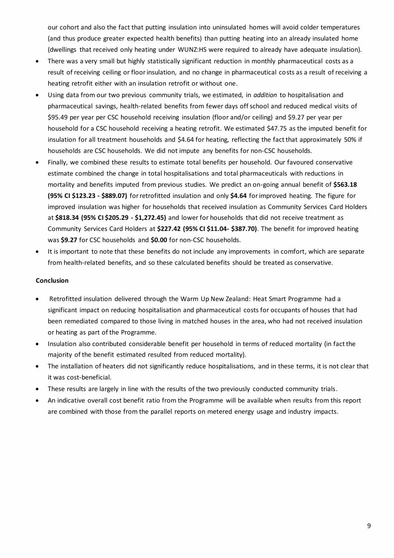
9

our cohort and also the fact that putting insulation into uninsulated homes will avoid colder temperatures

(and thus produce greater expected health benefits) than putting heating into an already insulated home

(dwellings that received only heating under WUNZ:HS were required to already have adequate insulation).

There was a very small but highly statistically significant reduction in monthly pharmaceutical costs as a

result of receiving ceiling or floor insulation, and no change in pharmaceutical costs as a result of receiving a

heating retrofit either with an insulation retrofit or without one.

Using data from our two previous community trials, we estimated, in addition to hospitalisation and

pharmaceutical savings, health-related benefits from fewer days off school and reduced medical visits of

$95.49 per year per CSC household receiving insulation (floor and/or ceiling) and $9.27 per year per

household for a CSC household receiving a heating retrofit. We estimated $47.75 as the imputed benefit for

insulation for all treatment households and $4.64 for heating, reflecting the fact that approximately 50% if

households are CSC households. We did not impute any benefits for non-CSC households.

Finally, we combined these results to estimate total benefits per household. Our favoured conservative

estimate combined the change in total hospitalisations and total pharmaceuticals with reductions in

mortality and benefits imputed from previous studies. We predict an on-going annual benefit of $563.18

(95% CI $123.23 - $889.07) for retrofitted insulation and only $4.64 for improved heating. The figure for

improved insulation was higher for households that received insulation as Community Services Card Holders

at $818.34 (95% CI $205.29 - $1,272.45) and lower for households that did not receive treatment as

Community Services Card Holders at $227.42 (95% CI $11.04- $387.70). The benefit for improved heating

was $9.27 for CSC households and $0.00 for non-CSC households.

It is important to note that these benefits do not include any improvements in comfort, which are separate

from health-related benefits, and so these calculated benefits should be treated as conservative.

Conclusion

Retrofitted insulation delivered through the Warm Up New Zealand: Heat Smart Programme had a

significant impact on reducing hospitalisation and pharmaceutical costs for occupants of houses that had

been remediated compared to those living in matched houses in the area, who had not received insulation

or heating as part of the Programme.

Insulation also contributed considerable benefit per household in terms of reduced mortality (in fact the

majority of the benefit estimated resulted from reduced mortality).

The installation of heaters did not significantly reduce hospitalisations, and in these terms, it is not clear that

it was cost-beneficial.

These results are largely in line with the results of the two previously conducted community trials.

An indicative overall cost benefit ratio from the Programme will be available when results from this report

are combined with those from the parallel reports on metered energy usage and industry impacts.

10

BACKGROUND

New Zealand housing has been widely described as “old and cold”. Around 60% of the population live in homes built

before insulation became compulsory for new dwellings in 1978. An estimated 84% of dwellings are estimated to

have inadequate insulation.1

On the 1s t of July 2009 the New Zealand Government introduced the Warm Up New Zealand: Heat Smart (WUNZ:HS)

programme, a nationwide programme designed to subsidise improved energy efficiency in residential buildings.

Subsidies were available for a range of measures for houses built before 2000:

- Retrofitted ceiling insulation and/or underfloor insulation or moisture barrier;

- A range of other measures including: draught proofing, hot water cylinder wraps, and pipe lagging;

- Funding for a clean heating device (if floor and ceiling insulation requirements met): either a heat pump, a

wood pellet burner, a modern wood burner or a flued gas heater.

WUNZS:HS was intended to improve household energy efficiency, leading to energy savings and improved comfort.

It was also expected to provide health benefits, particularly for vulnerable members of the population such as

people with respiratory illness, the young and the elderly.

The expectation that the programme would improve population health was based primarily on research by the He

Kainga Oranga/Housing and Health Research Programme (H&HRP), University of Otago, Wellington, which found

that insulating houses improved occupant health and energy use[1] with a benefit-cost ratio of almost 2 to 1 [2].

Installing effective heaters in insulated houses reduced the symptoms of children with asthma and the number of

days absent from school [3], but the benefit-cost ratio was less positive [4].

Between 1 July 2009 to 31 May 2010, 46,655 dwellings were treated under the programme. Current funding ceases

on 30 June 2013.

In 2009, the Ministry of Economic Development contracted the independent research organisation, Motu in

association with H&HRP; Victoria University, Wellington; and Covec, to assess the impact of the WUNZ:HS in the

three identified policy areas. This report covers the third of these, the impact of WUNZ:HS measures on population

health, particularly hospitalisation and pharmaceutical usage, and mortality.

1 Calculated from BRANZ 2005 dwelling condition survey figures on dwellings meeting 1996 insulation standards, QV data on the distribution of dwelling ages, and NHI/QV based data on population distribution across housing decades.

11

INTRODUCTION

Previous research has shown that the quality of housing affects the health of the population. Improvements to

housing can potentially prevent ill health, especially in sections of the population exposed to substandard housing. [5,

6] People in developed countries spend more than 90% of their time indoors, most of it in their own homes but

although research in the area is growing, we still know little about the specific health effects of the indoor

environment at a population level.[7, 8]

Inadequate warmth in the home can have health consequences for the occupants, particularly during winter.[9, 10]

Health is also linked to the efficiency of domestic energy, because money spent on energy cannot be spent on other

necessities such as food.[11, 12] Colder houses place more physiological stress on older people, babies, and sick

people, who have less robust thermoregulatory systems and are also likely to spend more time inside. [13] Houses

that are cold are also likely to be damp, and this can lead to the growth of moulds, which can cause respiratory

symptoms.[14, 15] The link between inadequate heating; damp, cold, and mouldy houses; and poor health has been

highlighted in several international reports.[15-19] Surprisingly, excess mortality in winter is more pronounced in

temperate rather than colder climates, suggesting that houses in these regions do not adequately protect occupants

from the weather.[13, 20]

In New Zealand, excess winter hospitalisation is higher in pre-war dwellings than in post-war bungalows [21], which

also indicates housing design can play a part in protecting occupants from the adverse health effects of winter.

Excess winter hospitalisation is a problem in New Zealand, with rates towards the upper end of the international

range. The cause is not clear, with recent research suggesting that a number of factors including levels of home

heating and insulation may potentially have a causal role[22].

Overall, a systematic review found that “[h]ousing improvements, especially warmth improvements, can generate

health improvements; there is little evidence of detrimental health impacts. The potential for health benefits may

depend on baseline housing conditions and careful targeting of the intervention. Investigation of socioeconomic

impacts associated with housing improvement is needed to investigate the potential for longer-term health impacts”

[23].

These conclusions were reiterated in another recent review: “Although many housing conditions are associated with

adverse health outcomes, sufficient evidence now shows that specific housing interventions can improve certain

health outcomes … investing in housing quality can yield important savings in medical care and improvements in

quality of life”.[24]

Previous research by the H&HRP on the effects of insulating dwellings found that respiratory and circulatory

hospitalisations were reduced, but as that study was not powered to discern relatively rare events, the reduction

was not statistically significant. [25] The current study provides the opportunity to measure the effects over a much

larger population sample.

Respiratory and circulatory health have each been shown to be particularly responsive to the effects of

environmental temperature. The two categories make up the bulk of excess winter mortality[26] and

hospitalisation.[27] There are multiple aetiological reasons for a relationship between cold exposure and respiratory

and circulatory health.[28] For circulatory health, “the increases in platelets, red cells, and viscosity associated with

normal thermoregulatory adjustments to mild surface cooling provide a probable explanation for rapid increases in

coronary and cerebral thrombosis in cold weather”.[29] Congestive heart disease in particular has been identified as

12

responsive to temperature exposure. [28] For respiratory health, cold exposure inhibits various respiratory defences

against infection in both the upper and lower respiratory tracts. [30-32]

AIMS

We aimed to measure the effects of WUNZ:HS installations (“treatment”) on health outcomes. We focused on health

outcomes identified as related to a cold indoor environment and/or most likely to be affected by housing

improvement. Specifically we focused on circulatory health, including congestive heart failure; and respiratory

health, including asthma and respiratory syncytial virus (RSV). We selected hospitalisations, pharmaceutical

prescriptions and mortality outcomes, and the cost of each, as our measures of health outcomes based on

availability of data. We also provided an estimate of other health related benefits that we could not address using

the data available, such as changes in the frequency of GP visits and days off work/school, based on previous work

done by our group.

13

METHODOLOGY

METHOD

We conducted a retrospective cohort study. The cohort was selected by matching dwellings that received insulation

or heating retrofits (treatment dwellings), by address, to similar (control) dwellings in the same Census Area Unit

(CAU), and subsequently, via an anonymisation process, identifying individuals listed on the New Zealand National

Health Index (NHI) as resident at those treatment and control addresses. The data are described in more detail later

in the section.

Treatment and matched control addresses were assigned a treatment date based on the month the treatment

dwelling had its WUNZ:HS measures installed. We obtained hospitalisation data for the cohort for the period 1

January 2008 to 30 September 2010 and prescription data to 31 December 2010.

Count data analysis for hospitalisations was based on exposure time measured in ‘person-days’. Individuals only

contributed person days while alive (i.e. not before birth or after death). We controlled for age structure and season.

In addition to total hospitalisations, we also measured outcomes for respiratory and circulatory illness, as well as for

asthma and respiratory syncytial virus (as specific respiratory outcomes); and congestive heart failure (as a specific

circulatory outcome).

As cause of death data was not yet available for the study period, all-cause mortality was measured separately

following respiratory and circulatory hospitalisation. Our mortality analysis used a sub-cohort of the study group,

comprised of those aged 65 and over who were hospitalised, but not deceased, prior to treatment date. We then

compared mortality rates after treatment between the treatment and control groups.

Our analysis of hospitalisation costs and pharmaceutical costs took place at the household level and was based on a

‘difference in difference’ approach, i.e. we compared the average monthly hospitalisation or pharmaceutical costs of

treatment group households with their matched controls in the periods before and after treatment occurred. Our

approach in this respect broadly parallels that taken in the sister report which addresses metered energy use

changes under the WUNZ:HS programme. We measured total hospitalisation and pharmaceutical costs, circulatory

illness related hospitalisation and pharmaceutical costs, and respiratory illness related hospitalisation and

pharmaceutical costs.

It is important to note that our analysis of hospitalisation costs was separate from the analysis of hospitalisation

count data as it took place at the household level and, as it measured changes in costs, it combines both changes in

the frequency of hospitalisation and in severity (cost per hospitalisation).

14

DATA DESCRIPTION

DATA SOURCES

EECA

EECA provided a list of 46,655 addresses for dwellings which had been treated under the WUNZ:HS programme

between the months July 2009 and May 2010 inclusive. Besides addresses of insulated dwellings, this list also

included information on what sort of treatment the dwelling had received, whether it was owner-occupier or rental

tenure, and if the retrofit was funded under the WUNZ:HS programme based on the dwelling having an occupant

eligible for a Community Services Card (labelled low-income in the dataset).

QV

QV matched EECA addresses for treated dwellings to addresses in their database. 37,163 of the treatment addresses

were able to be matched to a QV property listing, a match rate of 79.7%. QV then used the dwelling match protocol

(see “Dwelling Match Protocol” below) to identify up to 10 control addresses for each dwelling.

31,423 treatment dwellings (67.4% of all treatment dwellings) were initially able to be matched to at least one

control address; 269,110 control dwellings were selected and the distribution of matches was as follows:

Table 1. Matching of treatment and control dwellings, by count and percentage

Number of Comparables Count

% of cohort addresses

% of total treatment addresses

10 22520 71.7% 48.3%

9 962 3.1% 2.1%

8 948 3.0% 2.0%

7 1003 3.2% 2.1%

6 964 3.1% 2.1%

5 973 3.1% 2.1%

4 958 3.0% 2.1%

3 1043 3.3% 2.2%

2 985 3.1% 2.1%

1 1067 3.4% 2.3%

Total 31423 100.0% 67.4%

DWELLING MATCH PROTOCOL

QV used a scoring system to measure the accuracy of match between treatment and potential control dwellings

which was based on the results of Lucy Telfar-Barnard’s PhD thesis. [27] This score ensured that controls were

selected in order of greatest suitability.

Fields used, and the maximum score applied for each field, were as follows:

15

Table 2. Weighting of QV Matching

QV variable Definition Maximum

Points Notes

Census area unit Stats NZ defined areas – there are approx. 1860, of varying

population sizes, covering the whole of NZ. 10 Mandatory

match Category Residential/commercial/industrial etc. 10

House Type See Appendix 2 10 Levels (single/multi-story) 10

Decade Decade in which the dwelling was constructed 10

Points variable, see

below

Floor Area 10 Bedrooms Number of bedrooms 5

Main Roof Garages Number of garages included under the main roof of the house (and

therefore included in the floor area). 5 Building Wall material 10

Roof Roof material 10 Modernised 10

Matches on Census Area Unit (CAU), property category, house type and single/multi-story (levels) were all

mandatory. Dwelling construction decade was allowed to vary by up to three decades, with the score dropping by 2

points for each decade distance from the target decade. Floor area was allowed to vary by up to 50%, with the score

dropping by 1 point for each 10% difference from the target. Number of bedrooms and main roof garages were

scored with a maximum of score 5, subtracting 1 for each variance number of bedrooms and garages between the

comparable and the target. Wall materials and condition, and roof materials and condition, were given a score of 10

where both materials and condition matched, 7 where building materials matched and 0 if materials didn’t match. A

score of 10 points was assigned if the “modernised” indicator matched and 0 if it did not match

QV DATA FOR COHORT DWELLINGS

Having created our initial cohort QV then provided us with the following data for all cohort dwellings:

- Territorial Authority

- CAU

- Census mesh-block

- QV property category

- building construction decade

- house type

- number of floors/levels

- floor area

- number of bedrooms

- number of garages

- Roof and wall construction materials

- Roof and wall condition

- Dwelling quality indicator (extracted from property category)

- “Modernised” indicator

Not all fields were ultimately used in the study.

16

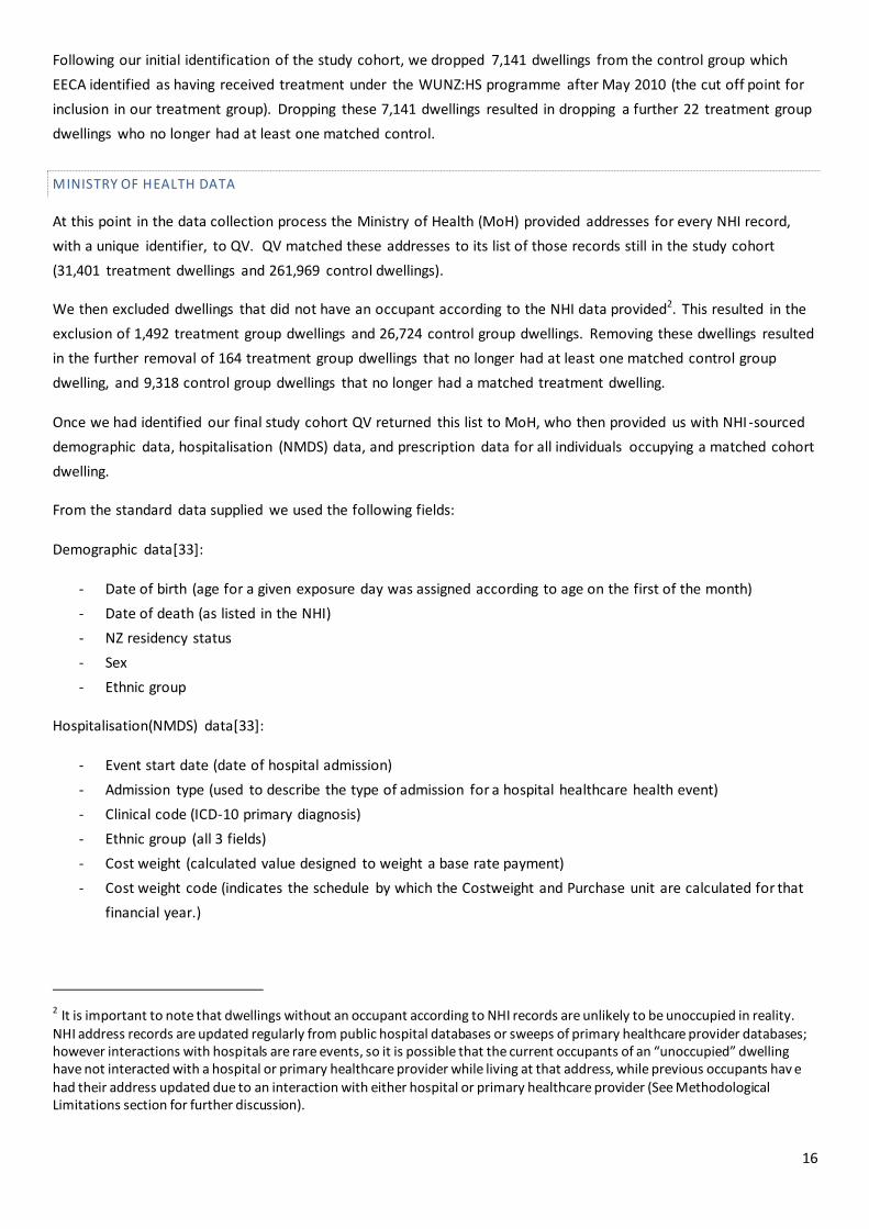
Following our initial identification of the study cohort, we dropped 7,141 dwellings from the control group which

EECA identified as having received treatment under the WUNZ:HS programme after May 2010 (the cut off point for

inclusion in our treatment group). Dropping these 7,141 dwellings resulted in dropping a further 22 treatment group

dwellings who no longer had at least one matched control.

MINISTRY OF HEALTH DATA

At this point in the data collection process the Ministry of Health (MoH) provided addresses for every NHI record,

with a unique identifier, to QV. QV matched these addresses to its list of those records still in the study cohort

(31,401 treatment dwellings and 261,969 control dwellings).

We then excluded dwellings that did not have an occupant according to the NHI data provided2. This resulted in the

exclusion of 1,492 treatment group dwellings and 26,724 control group dwellings. Removing these dwellings resulted

in the further removal of 164 treatment group dwellings that no longer had at least one matched control group

dwelling, and 9,318 control group dwellings that no longer had a matched treatment dwelling.

Once we had identified our final study cohort QV returned this list to MoH, who then provided us with NHI -sourced

demographic data, hospitalisation (NMDS) data, and prescription data for all individuals occupying a matched cohort

dwelling.

From the standard data supplied we used the following fields:

Demographic data[33]:

- Date of birth (age for a given exposure day was assigned according to age on the first of the month)

- Date of death (as listed in the NHI)

- NZ residency status

- Sex

- Ethnic group

Hospitalisation(NMDS) data[33]:

- Event start date (date of hospital admission)

- Admission type (used to describe the type of admission for a hospital healthcare health event)

- Clinical code (ICD-10 primary diagnosis)

- Ethnic group (all 3 fields)

- Cost weight (calculated value designed to weight a base rate payment)

- Cost weight code (indicates the schedule by which the Costweight and Purchase unit are calculated for that

financial year.)

2 It is important to note that dwellings without an occupant according to NHI records are unlikely to be unoccupied in reality. NHI address records are updated regularly from public hospital databases or sweeps of primary healthcare provider databases; however interactions with hospitals are rare events, so it is possible that the current occupants of an “unoccupied” dwelling have not interacted with a hospital or primary healthcare provider while living at that address, while previous occupants hav e had their address updated due to an interaction with either hospital or primary healthcare provider (See Methodological Limitations section for further discussion).

17

Prescription (PHARMS) data[34]:

- Formulation id (PHARMAC Identifier for each formulation of a drug)

- HPAC cost ex supplier excluding GST (total cost of medication in the schedule, with GST deducted)

- Retail subsidy excluding GST (total Schedule cost of medication plus mark-ups, with GST deducted).

- Dispensing fee value excluding GST (Fee paid to the claimant for dispensing the medication to the patient)

- Patient contribution excluding GST (the amount the patient has to pay for the medication, with GST

deducted)

- Reimbursement cost excluding GST (value reimbursed to the pharmacy, on this dispensing of a prescription

item, with GST deducted.)

- Price (supplier price for a specified pack associated with a formulation id)

- Subsidy (the subsidy that would be paid for a specified pack associated with a formulation id)

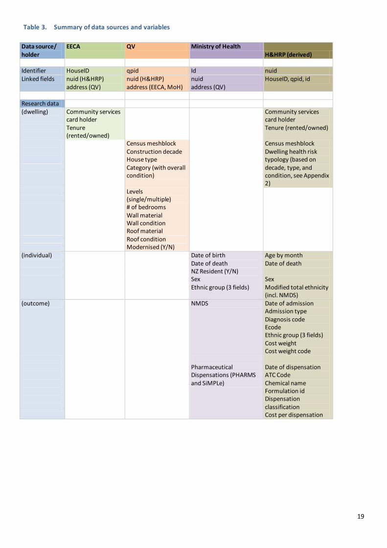
SUMMARY OF DATA PROTOCOL AND SOURCES

The data protocol and sources described above are summarised in Figure 1 and Table 3. Figure 1 sets out the data

protocol, detailing the collection of data from EECA’s initial provision of data for 46,655 dwellings to the creation of

the final cohort of 255,672 dwellings and 973,710 individuals. Table 3 summarises the data sources utilised by the

study and the variables that they provided.

18

Figure 1. Data protocol (d=dwellings, n=people)

TREATMENT DWELLINGS CONTROL DWELLINGS Excluded Remaining Remaining Excluded

EECA data

d=46,655 dwellings

H&HRP REMOVE PERSONAL

DATA AND PROVIDE TO QV

QV MATCH TO QV DATA

Unmatched d=9,492

Matched to QV data d=37,163 dwellings

QV IDENTIFY CONTROL

DWELLINGS

No control

identifiable d=5,740

Treated dwellings

d=31,423

Control dwellings

d=269,110

EECA IDENTIFY CONTROLS TREATED AFTER MAY 2010

No remaining control

d=22

Cohort treated dwellings d=31,401

Cohort control dwellings

d=261,969

Treated after May 2010 d=7,141

MOH PROVIDE UNIQUELY IDENTIFIED NHI ADDRESSES TO QV

QV MATCH TO COHORT ADDRESSES.

No identified occupants

d=1,492

Cohort treated dwellings

matched to at least one “occupant” d=29,909

n=110,918 people

Cohort control dwellings

matched to at least one “occupant” d=235,245

n=893,169 people

No identified

occupants d= 26,724

No “occupied”

controls d=164 n=558

Dwellings with “occupied”

controls d=29,745 n=110,360

“Occupied” and matched to an “occupied”

treatment d= 225,927 n= 863,350

No “occupied”

treatments d= 9,318

n= 29,819

Treatment:

d= 29,745, n= 110,360

1-3 matched “occupied” dwellings: d= 6,996,

n= 26,603

4 matched “occupied”

dwellings: d=105,076,

n= 397,927

(4+) matched “occupied” dwellings

randomly excluded from

count data

analysis d= 113,855,

n= 438,820

Cohort unique identifiers returned to MoH

d=255,672 n= 973,710

MOH provide hospitalisation and pharmaceutical data for cohort

19

Table 3. Summary of data sources and variables

Data source/ holder

EECA QV Ministry of Health H&HRP (derived)

Identifier HouseID qpid Id nuid Linked fields nuid (H&HRP)

address (QV) nuid (H&HRP) address (EECA, MoH)

nuid address (QV)

HouseID, qpid, id

Research data (dwelling) Community services

card holder Community services

card holder Tenure

(rented/owned) Tenure (rented/owned)

Census meshblock Census meshblock Construction decade Dwelling health risk

typology (based on decade, type, and condition, see Appendix 2)

House type Category (with overall

condition)

Levels (single/multiple)

# of bedrooms Wall material Wall condition Roof material Roof condition Modernised (Y/N) (individual) Date of birth Age by month Date of death Date of death NZ Resident (Y/N) Sex Sex Ethnic group (3 fields) Modified total ethnicity

(incl. NMDS) (outcome) NMDS Date of admission

Admission type Diagnosis code Ecode Ethnic group (3 fields) Cost weight Cost weight code

Pharmaceutical Dispensations (PHARMS and SiMPLe)

Date of dispensation ATC Code Chemical name Formulation id Dispensation classification Cost per dispensation

20

DATASET CREATION

EXPOSURE TIME

Exposure days were calculated by day, taking into account dates of birth and death if these occurred during the

study period; and assigned by month to “before” or “after” treatment date; exposure days during the month of

treatment were excluded because the exact date of treatment was not known, and may have been spread over

several days.

HOSPITALISATIONS

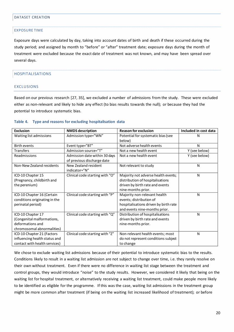
EXCLUSIONS

Based on our previous research [27, 35], we excluded a number of admissions from the study. These were excluded

either as non-relevant and likely to hide any effect (to bias results towards the null); or because they had the

potential to introduce systematic bias.

Table 4. Type and reasons for excluding hospitalisation data

Exclusion NMDS description Reason for exclusion Included in cost data Waiting list admissions Admission type=”WN” Potential for systematic bias (see

below) N

Birth events Event type=”BT” Not adverse health events N Transfers Admission source=”T” Not a new health event Y (see below) Readmissions Admission date within 30 days

of previous discharge date Not a new health event Y (see below)

Non-New Zealand residents New Zealand resident indicator=”N”

Not relevant to study N

ICD-10 Chapter 15 (Pregnancy, childbirth and the perenium)

Clinical code starting with “O” Majority not adverse health events; distribution of hospitalisations driven by birth rate and events nine-months prior.

N

ICD-10 Chapter 16 (Certain conditions originating in the perinatal period)

Clinical code starting with “P” Majority non-relevant health events; distribution of hospitalisations driven by birth rate and events nine-months prior.

N

ICD-10 Chapter 17 (Congenital malformations, deformations and chromosomal abnormalities)

Clinical code starting with “Q” Distribution of hospitalisations driven by birth rate and events nine-months prior.

N

ICD-10 Chapter 21 (Factors influencing health status and contact with health services)

Clinical code starting with “Z” Non-relevant health events; most do not represent conditions subject to change

N

We chose to exclude waiting list admissions because of their potential to introduce systematic bias to the results.

Conditions likely to result in a waiting list admission are not subject to change over time, i.e. they rarely resolve on

their own without treatment. Even if there were no difference in waiting list stage between the treatment and

control groups, they would introduce “noise” to the study results. However, we considered it likely that being on the

waiting list for hospital treatment, or alternatively receiving a waiting list treatment, could make people more likely

to be identified as eligible for the programme. If this was the case, waiting list admissions in the treatment group

might be more common after treatment (if being on the waiting list increased likelihood of treatment); or before

21

treatment (if having received treatment made people more likely to be identified). Either of these possibilities could

introduce systematic bias to the results.

We included transfers and readmissions in our analysis of cost data because, while not new health events, transfers

and readmissions represent real costs and our goal in carrying out the analysis of cost data was to be as

comprehensive as possible. However, we did continue to exclude waiting list admissions for the reasons outlined

above.

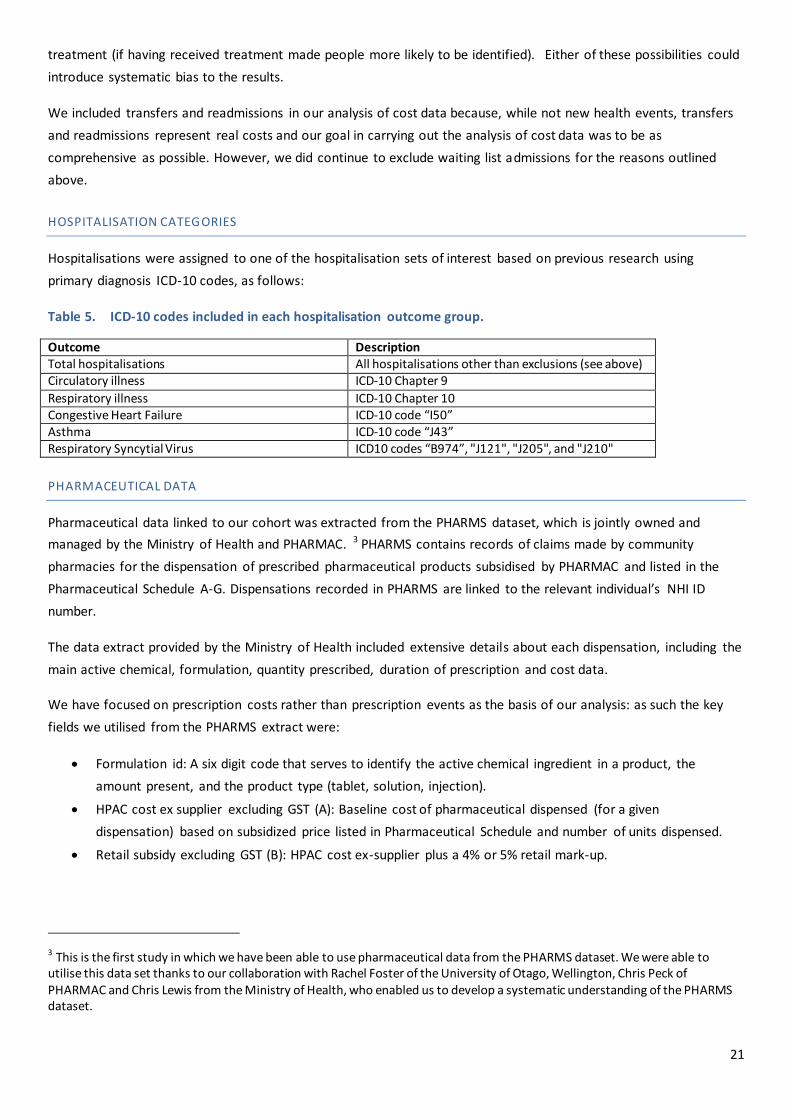
HOSPITALISATION CATEGORIES

Hospitalisations were assigned to one of the hospitalisation sets of interest based on previous research using

primary diagnosis ICD-10 codes, as follows:

Table 5. ICD-10 codes included in each hospitalisation outcome group.

Outcome Description Total hospitalisations All hospitalisations other than exclusions (see above) Circulatory illness ICD-10 Chapter 9

Respiratory illness ICD-10 Chapter 10 Congestive Heart Failure ICD-10 code “I50” Asthma ICD-10 code “J43” Respiratory Syncytial Virus ICD10 codes “B974”, "J121", "J205", and "J210"

PHARMACEUTICAL DATA

Pharmaceutical data linked to our cohort was extracted from the PHARMS dataset, which is jointly owned and

managed by the Ministry of Health and PHARMAC. 3 PHARMS contains records of claims made by community

pharmacies for the dispensation of prescribed pharmaceutical products subsidised by PHARMAC and listed in the

Pharmaceutical Schedule A-G. Dispensations recorded in PHARMS are linked to the relevant individual’s NHI ID

number.

The data extract provided by the Ministry of Health included extensive details about each dispensation, including the

main active chemical, formulation, quantity prescribed, duration of prescription and cost data.

We have focused on prescription costs rather than prescription events as the basis of our analysis: as such the key

fields we utilised from the PHARMS extract were:

Formulation id: A six digit code that serves to identify the active chemical ingredient in a product, the

amount present, and the product type (tablet, solution, injection).

HPAC cost ex supplier excluding GST (A): Baseline cost of pharmaceutical dispensed (for a given

dispensation) based on subsidized price listed in Pharmaceutical Schedule and number of units dispensed.

Retail subsidy excluding GST (B): HPAC cost ex-supplier plus a 4% or 5% retail mark-up.

3 This is the first study in which we have been able to use pharmaceutical data from the PHARMS dataset. We were able to utilise this data set thanks to our collaboration with Rachel Foster of the University of Otago, Wellington, Chris Peck of PHARMAC and Chris Lewis from the Ministry of Health, who enabled us to develop a systematic understanding of the PHARMS dataset.

22

Dispensing fee value excluding GST(C): Each dispensation incurs a dispensation fee which community

pharmacies charge the government. More complex or problematic dispensations (for example requiring

special preparation) incur a higher fee.

Patient contribution excluding GST (D): A small fee that patients may pay at time of dispensation towards the

cost of a prescription in some circumstances (typically $3 less GST). The fee does not apply to some groups

including children younger than 6, or to repeat prescriptions.

Reimbursement cost excluding GST (E): This is the total that the government pays to a community pharmacy

for a given dispensation. It is calculated in the following way:

E = B + C -D

In order to calculate the total cost of a given dispensation it is necessary to include both patient costs and

government costs. In addition to the patient contribution described above, patients must pay for any portion of a

given prescription which is not subsidised, and will typically also be charged a mark-up of 86% by the dispensing

pharmacy including GST (this is a recommended mark-up set out in the Pharmaceutical Schedule but pharmacies

may mark-up as they see fit in line with commercial imperatives – data are not collected by PHARMAC on such mark-

ups). The majority of products subsidised by PHARMAC are fully subsidised and do not require a patient contribution

of this type.

To estimate the non-subsidised portion of a given dispensation we utilised the following fields:

Price(F): This field contains a generic pack price associated with the relevant formulation id (e.g. the price of

100 tablets if the product is wholesaled in 100 tablet packs).

Subsidy (G): This field indicates the subsidy that would be paid for a generic price pack associated with a

formulation id (e.g. the subsidised price that the government would pay for 100 tablets if the product is

wholesaled in 100 tablet packs). The majority of dispensations in our data set involved products with a 100%

subsidy.

We assumed that ((F-G)/F) represented the unsubsidized proportion associated with a given formulation at the time

of dispensing and used the following formula to estimate the pre mark-up unsubsidized cost of a given dispensing:

Unsubsidised cost excluding GST (H) = ((F-G)/F)*A where A is the HPAC cost ex supplier ex GST (see definition above).

We then calculated:

Unsubsidised cost including PHARMAC suggested mark-up excluding GST (J) = H*1.86/1.125

(GST was 12.5% Jan 2008-Sept 2010, and 15% Oct 2010 onwards)

The total cost to the nation of a given dispensing excluding GST (K) = E (government) + D (patient) + J

(patient)

A final complication is that PHARMAC negotiates additional confidential rebates from pharmaceutical companies.

These rebates vary from year-to-year, do not apply equally to all products, and for reasons of commercial sensitivity

the details of these rebates are not made public. We can make an estimate of the average rebate using the

PHARMAC Annual reports which report total rebates for community pharmaceuticals. In the 2007/2008 financial

year gross expenditure was $751.71 million reduced by estimated supplier rebates of $114.89 (a 15.2% reduction).

The estimated rebate reduction for the 2008/2009 financial year was 14.3% and in 2009/2010 8%. We assumed that

23

the rebate negotiated in 2010/2011 would also be 8% as the actual figure was not available when we constructed

our dataset. We have calculated cost figures assuming that these rebates apply.

PHARMACEUTICAL CATEGORIES

The PHARMS data extract was linked to data extracted from the SiMPle database, an online database made available

by PHARMAC which contains extensive details regarding every product that has been subsidised by PHARMAC during

its operation. The key information utilized from the SiMPle database was a three level ATC (Anatomic Therapeutic

Chemical) code classification associated with each formulation id. Expert advice was sought, utilising a

comprehensive list of ATC codes from the SiMPle dataset in order to identify pharmaceuticals whose usage rates

might theoretically be altered by a change in insulation or heating. A key source of information on the potential

connections between insulation/heating and health was a report prepared for Housing New Zealand Corporation by

He Kainga Oranga/Housing and Health Research Programme University of Otago, Wellington following a workshop

on Potentially Avoidable Hospitalisations Related to Housing Conditions (He Kainga Oranga, 2008).

Table 6. Pharmaceuticals included in study by outcome measure.

Outcome Description

Total dispensations All dispensations

Circulatory illness related dispensations ACT Code Level 1: Cardiovascular System OR ATC Code Level 1: Blood and Blood Forming

Organs, Chemical name “Aspirin” OR

ATC Code Level 3: “HMG CoA Reductase Inhibitors (Statins)”

Respiratory illness related dispensations Chemical name “Prednisone” OR

ATC Code Level 3: "Inhaled Corticosteroids", "Inhaled Corticosteroids with Long-Acting Beta-Adrenoceptor Agonists", "Beta-Adrenoceptor Agonists", "Inhaled Beta-Adrenoceptor Agonists", "Inhaled

Anticholinergic agents", "Inhaled Beta-Adrenoceptor Agonists with Anticholinergic Agents", "Methylxanthines", "Other Bronchodilators" and "Cough Preparations"

24

DATA ANALYSIS

KEY CHARACTERISTICS

This study is observational, rather than experimental, and this leads to the possibility for confounding where the self-

selecting treatment group differs systematically from the matched control group. We have therefore compared the

treatment and control groups using the few demographic characteristics available to us: ethnicity, age, sex, NZDep

quintile and dwelling health risk type. The distributions across these variables are shown in Figure 2 and Figure 3.

Our initial analysis of the characteristics of the individuals within the study suggests that there were statistically

significant differences in the distribution of potential confounders such as ethnicity, age and gender between both

the treatment and control group and the total New Zealand population.

However, with sample sizes as large as these it was inevitable that Chi-square tests of differences between the

treatment group and control group would show statistically significant differences for all demographic

characteristics. These statistically significant differences might suggest we should include all such variables in our

regression analyses. However, the differences may not have any clinical significance. Moreover, we were concerned

about over-controlling for known factors while at the same time making no adjustment for unknown factors. Since

we match each treatment house to a number of controls which are similar in many key respects our study design

does mimic aspects of a randomised study. For this reason we wish to control for as few variables as necessary, and

have selected age as the only variable where the differences between treatment and control appear large enough to

warrant an explicit adjustment (Figure 2).

Figure 2. Distribution of treatment, control, and 2006 Census populations by sex, age group, ethnic group and NZDep quintile.

25

Age distribution (as at Jan 1s t 2008 for study data) is reported in Table 7 below and the distribution of other

characteristics is set out in Appendix 1. Those in the control households are more closely related to the NZ

population overall than the treatment group. The key difference from the perspective of identifying potential

confounding is the proportion of participants older than 60.

Table 7. Age distribution of treatment, control and Census 2006 populations

Treatment Control Census 2006

Age group n % n % n %

0-4 years 7,286 6.9 53,500 6.3 275,034 6.8

5-14 years 13,126 12.4 117,262 13.7 592,365 14.7

15-24 years 12,563 11.9 124,064 14.5 570,960 14.2

25-44 years 32,493 30.7 265,619 31.0 1,133,739 28.2

45-59 years 17,823 16.8 162,098 18.9 779,226 19.4

60+ years 22,523 21.3 135,916 15.6 671,718 16.7

At a household level, there was a statistically significant difference in the distribution of dwelling types, based on the

dwelling typology that we developed using the data provided by QV and Lucy Telfar-Barnard’s thesis. We developed

six categories: new low risk, new medium risk, new high risk, old medium risk and old high risk (see Appendix for

more detail of this classification system). We concluded, after an initial exploration, that most of the differences,

while statistically significant, appear too small to have clinical significance. Figure 3 demonstrates that the difference

between the distribution of dwelling types in the treatment and control groups is unlikely to bias results. The

difference between the distribution of dwelling types for the treatment and control groups and the 2006 NHI -

matched QV dwellings4 reflects the WUNZ:HS programme criteria (no post 2000 dwellings), the higher likelihood that

homeowners/landlords with an older home would choose to be involved in the WUNZ:HS programme and the way

that we selected our control group dwellings.

Figure 3. Distribution of treatment, control, and 2006 NHI-matched QV dwellings.

4 The” 2006 NHI-matched QV dwellings” comprise those dwellings matched to an NHI address in 2006. Records were matched between all NHI addresses and all QV addresses, with a match rate of approximately 63% 21. Telfar Barnard, L., Home truths and cool admissions: New Zealand housing traits and excess winter hospitalisation, PhD Thesis, , 2010, University of Otago: Wellington..

26

MODEL SELECTION

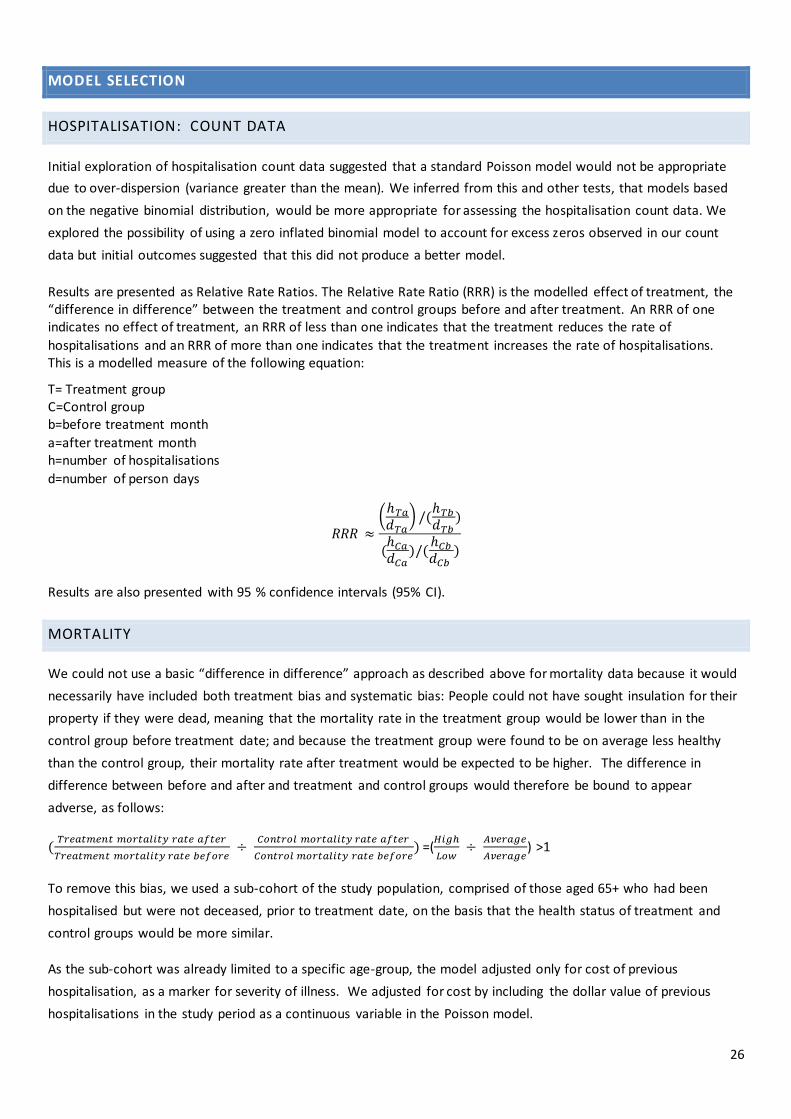
HOSPITALISATION: COUNT DATA

Initial exploration of hospitalisation count data suggested that a standard Poisson model would not be appropriate

due to over-dispersion (variance greater than the mean). We inferred from this and other tests, that models based

on the negative binomial distribution, would be more appropriate for assessing the hospitalisation count data. We

explored the possibility of using a zero inflated binomial model to account for excess zeros observed in our count

data but initial outcomes suggested that this did not produce a better model.

Results are presented as Relative Rate Ratios. The Relative Rate Ratio (RRR) is the modelled effect of treatment, the “difference in difference” between the treatment and control groups before and after treatment. An RRR of one indicates no effect of treatment, an RRR of less than one indicates that the treatment reduces the rate of

hospitalisations and an RRR of more than one indicates that the treatment increases the rate of hospitalisations. This is a modelled measure of the following equation:

T= Treatment group C=Control group b=before treatment month

a=after treatment month h=number of hospitalisations

d=number of person days

(

)

Results are also presented with 95 % confidence intervals (95% CI).

MORTALITY

We could not use a basic “difference in difference” approach as described above for mortality data because it would

necessarily have included both treatment bias and systematic bias: People could not have sought insulation for their

property if they were dead, meaning that the mortality rate in the treatment group would be lower than in the

control group before treatment date; and because the treatment group were found to be on average less healthy

than the control group, their mortality rate after treatment would be expected to be higher. The difference in

difference between before and after and treatment and control groups would therefore be bound to appear

adverse, as follows:

=(

) >1

To remove this bias, we used a sub-cohort of the study population, comprised of those aged 65+ who had been

hospitalised but were not deceased, prior to treatment date, on the basis that the health status of treatment and

control groups would be more similar.

As the sub-cohort was already limited to a specific age-group, the model adjusted only for cost of previous

hospitalisation, as a marker for severity of illness. We adjusted for cost by including the dollar value of previous

hospitalisations in the study period as a continuous variable in the Poisson model.

27

Exposure time was measured as time between treatment date and the 31 December 2010 (the end of the study

period).

We used a standard Poisson model with individual-level data to assess the difference in mortality rates between the

treatment and control groups in the sub-cohort.

Our method for costing changes in mortality is set out in the Results section.

HOSPITALISATION: COST DATA

Initial exploration of individual level hospital cost data demonstrated an extreme degree of skewedness as the vast

majority of people do not incur a hospitalisation cost in a given month, resulting in data with a high proportion of

zeros and the occasional very large value (in some cases $60,000 or more). We concluded that this continuous

dataset was not conducive to analysis at the individual level, and adopted a difference in difference approach at the

household level similar to that used in the report Warming Up New Zealand: Impacts of the New Zealand Insulation

Fund on Household Energy Use.

We compared the difference between each treatment group household’s monthly hospitalisation costs and the

mean of its matched control group household’s monthly hospitalisation costs both before and after the intervention.

This enabled us to control for the effect of season and region efficiently, while reducing the number of zeros and

producing data that is centred around zero rather than right skewed. We further cleaned the data by removing

values lower than the 1s t percentile and higher than the 99th percentile – for reasons of consistency and balance we

removed all observations associated with a household cluster (before and after) if either observation was removed

(slight variability in the number of treatment dwellings remaining after the cleaning process, for each category of

interest, reflects differences in the number of dwellings that had an extreme value for both the before and after

period) . We carried out this process separately for each hospitalisation cost outcome of interest. Figure 4 details

the data cleaning process:

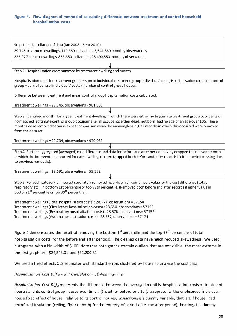
28

Figure 4. Flow diagram of method of calculating difference between treatment and control household hospitalisation costs

Figure 5 demonstrates the result of removing the bottom 1s t percentile and the top 99th percentile of total

hospitalisation costs (for the before and after periods). The cleaned data have much reduced skewedness. We used

histograms with a bin width of $100. Note that both graphs contain outliers that are not visible: the most extreme in

the first graph are -$24,543.01 and $31,200.81

We used a fixed effects OLS estimator with standard errors clustered by house to analyse the cost data:

Hospitalisation Cost Diff it = αi + β1insulationit + β2heatingit + εit

Hospitalisation Cost Diffit represents the difference between the averaged monthly hospitalisation costs of treatment

house i and its control group houses over time t (t is either before or after). αi represents the unobserved individual

house fixed effect of house i relative to its control houses, insulationi t is a dummy variable, that is 1 if house i had

retrofitted insulation (ceiling, floor or both) for the entirety of period t (i.e. the after period), heatingi t is a dummy

Step 2: Hospitalisation costs summed by treatment dwelling and month Hospitalisation costs for treatment group = sum of individual treatment group individuals’ costs, Hospitalisation costs for control group = sum of control individuals’ costs / number of control group houses. Difference between treatment and mean control group hospitalisation costs calculated. Treatment dwellings = 29,745, observations = 981,585

Step 3: Identified months for a given treatment dwelling in which there were either no legitimate treatment group occupants or no matched legitimate control group occupants i.e. all occupants either dead, not born, had no age or an age over 105. These months were removed because a cost comparison would be meaningless. 1,632 months in which this occurred were removed from the data set. Treatment dwellings = 29,734, observations = 979,953

Step 4: Further aggregated (averaged) cost difference and data for before and after period, having dropped the relevant month in which the intervention occurred for each dwelling cluster. Dropped both before and after records if either period missing due to previous removals). Treatment dwellings = 29,691, observations = 59,382

Step 5: For each category of interest separately removed records which contained a value for the cost difference (total, respiratory etc.) in bottom 1st percentile or top 99th percentile. (Removed both before and after records if either value in bottom 1st percentile or top 99th percentile). Treatment dwellings (Total hospitalisation costs) : 28,577, observations = 57154 Treatment dwellings (Circulatory hospitalisation costs) : 28,550, observations = 57100 Treatment dwellings (Respiratory hospitalisation costs) : 28,576, observations = 57152 Treatment dwellings (Asthma hospitalisation costs) : 28,587, observations = 57174

Step 1: Initial collation of data (Jan 2008 – Sept 2010).

29,745 treatment dwellings, 110,360 individuals, 3,641,880 monthly observations

225,927 control dwellings, 863,350 individuals, 28,490,550 monthly observations

29

variable that is 1 if house i had retrofitted heating for the entirety of period t: the coefficients of the insulation and

heating dummies, if statistically significant, indicate the size and direction of any change in the difference in average

monthly hospitalisation costs as a result of treatment . εit is the residual term, which is correlated between periods

within houses, but independent between houses. Note that all covariates which are constant over time for a given

household (e.g. region, deprivation, ethnicity of occupants [assuming no changes to household composition]) are

absorbed into the fixed effect αi and do not need to be explicitly included in the model. We initially considered

including an additional interaction term between insulation and heating. However exploratory analyses found that

the coefficient of this term was not significantly different from zero, so we did not include it in the final model set

out above.

Figure 5. Effect of removing the outliers of total hospitalisation costs

We began the analysis of our four categories of interest (total hospitalisation, circulatory illness related

hospitalisation, respiratory illness related hospitalisation and asthma related hospitalisation). We then carried out a

further sub-analysis looking at the results of the intervention for those households who qualified for the WUNZ:HS

programme as Community Services Card holders, and those who did not.

For each fitted model we further checked the validity of our conclusions by utilising a bootstrap calculation of the

standard errors with 500 repetitions. This was done because the residuals were highly concentrated at zero, and we

Percent

-20000 -10000 0 10000 20000 30000

Difference in hospitalisation costs $ NZ 2011 (59,382 observations)

0

10

20

30

40

Percent

-1000 0 1000 2000

Difference in hospitalisation costs $ NZ 2011 (57,154 observations)

10

0

20

30

40

30

wanted to test whether the distributional assumptions in the fitted model were affecting the standard error

estimates, and hence our conclusions.

31

PHARMACEUTICALS: COST DATA

As with the hospitalisation cost data discussed above, individual level pharmaceutical cost data was not suitable for

analysis due to extreme skewedness and a high number of zeros. We used the same difference in difference

approach set out for the hospitalisation cost data set out above. Figure 6 details the data cleaning process:

Figure 6. Flow diagram of method of calculating difference between treatment and control household pharmaceutical costs

Step 2: Pharmaceutical costs summed by treatment dwelling and month Pharmaceutical costs for treatment group = sum of individual treatment group individuals’ costs, Pharmaceutical costs for control group = sum of control individuals’ costs / number of control group houses. Difference between treatment and mean control group pharmaceutical costs calculated. Treatment dwellings = 29,745, observations = 1,070,820

Step 3: : Identified months for a given treatment dwelling in which there were either no legitimate treatment group occupants or no matched legitimate control group occupants i.e. all occupants either dead, not born, had no age or an age over 105. These months were removed because a cost comparison would be meaningless . (1,909 months in which this occurred were removed from

the data set.)

Treatment dwellings = 29,735, observations = 1,068,911

Step 4: Further aggregated (averaged) data for before and after period, having dropped the relevant month in which the intervention occurred

for each dwelling cluster. Dropped both before and after records if either period missing due to previous removals). Treatment dwellings = 29,691, observations = 59,382

Step 5: For each category of interest separately removed clusters which contained a value for the pharmaceutical cost difference (t otal, respiratory etc.) in bottom 1st percentile or top 99th percentile. (Both before and after records if either value in bottom 1

st percentile or top

99th

percentile).

Treatment dwellings (Total pharmaceutical costs) : 28,577, observations = 57,154 Treatment dwellings (Circulatory illness pharmaceutical costs) : 28,550, observations = 57,100

Treatment dwellings (Respiratory illness pharmaceutical costs) : 28,576, observations = 57,152 Treatment dwellings (Asthma reliever costs) : 28,587, observations = 57,174

As with our hospitalisation costs model we utilised a fixed effects OLS estimator with standard errors clustered by

house to analyse the cost data:

Pharmaceutical Cost Diff it = αi + β1insulationit + β2heatingit + εit

Pharmaceutical Cost Diffit represents the difference between the average monthly hospitalisation costs of treatment

housei and its control group houses over time t (t is either before or after). αi, insulationi t , heatingi t and εit are

defined as per our hospitalisation costs model. As with our hospitalisation costs model we initially considered

including an additional dummy variable insulationandheatingi t which would be 1 if house i had both retrofitted

Step 1: Initial collation of data (Jan 2008 – Dec 2010).

29,745 treatment dwellings, 110,360 individuals, 3,972,960 monthly observations

225,927 control dwellings, 863,350 individuals, 31,080,600 monthly observations

32

insulation and heating for the entirety of period t but initial explorations suggested that it did not produce any

additional explanatory power so we did not include it in the model.

We began with an analysis of the three categories of interest (total pharmaceutical costs, circulatory illness

dispensations, respiratory-illness related dispensations). We then carried out a further sub-analysis looking at the

results of the intervention for those households who qualified for the WUNZ:HS programme as community service

card holders, and those who did not.

For each fitted model we further checked the validity of our conclusions utilising a bootstrap calculation of the

standard errors with 500 repetitions.

33

METHODOLOGICAL LIMITATIONS

This study has a number of limitations which affect the interpretation of the results. The first of these is imprecision

in assigning health records to particular addresses. Addresses were matched according to individual addresses on 15

October 2010, when NZHIS provided NHI data to QV. These addresses are not necessarily accurate, as they record

only the individual’s address at last contact with a health provider, rather than their actual address on 15 October

2010. In other words, we cannot be absolutely certain that people reside where we think they do.

This introduces a slight information bias to the data, as subsidy eligibility and targeting for treatment meant that the

treatment group was a less healthy population than the control group. As they are less healthy they are likely to

have had more contact with health providers. Therefore, on average, their NHI addresses are more likely to be

accurate than the control group. In addition, a decision to install insulation or to go to the trouble of asking a

landlord to install insulation may indicate an intention to remain at that address over a longer term, making the

treatment group, on average, less mobile than the control group. Lower residential mobility also contributes to a

greater likelihood of more accurate addresses in the treatment group than the control group.

The results of the study are also inevitably biased towards the null because although we know the treatment

dwellings have received treatment, we do not know that the control dwellings have not received treatment during

the study period. As a group, the control group is expected to have less insulation and energy efficient heating than

the treatment group, but the control group will likely include dwellings insulated or with energy efficient heating

installed outside the WUNZ:HS programme. The comparison overall is not between “treated” and “untreated”

groups of dwellings, but between “all treated” and “fewer treated” groups of dwellings.

It should also be noted that hospitalisations are at the more severe end of the health outcome scale. Other health

outcomes not measured here are general well-being, school and work absences, and doctor visits, all of which have

been shown to be positively impacted by improved insulation in our previous studies.[1, 2] We briefly set out the

potential benefits that could be imputed from previous studies in the final subsection of our results section titled

“Imputed Benefits: Sensitivity Analysis”. It is not possible to assess likely benefits such as improved comfort because

methods which might be used to value them, such as willingness to pay, do not distinguish comfort from benefits

such as reduced health costs, so there would be a danger of double-counting if such measures were used and we

instead take the conservative approach of not assigning a value to comfort improvements that are separate from

health benefits.

A further limitation of the study was the limited exposure time available to be measured, particularly after treatment

date. Ideally, the study data would be updated in order to allow a longer measure of post-treatment outcomes,

which would give our study more power.

Finally, we note that changes occurring outside of the programme such as control group houses installing insulation

or heat pumps during the study period have the potential to bias results towards the null. While we cannot estimate

this effect, the increasing popularity of heat pumps during the past few years is well documented and thus this

seems particularly plausible in the case of heating. However, given that any such change is likely to bias results

towards the null this possibility contributes to the robustness of our findings.

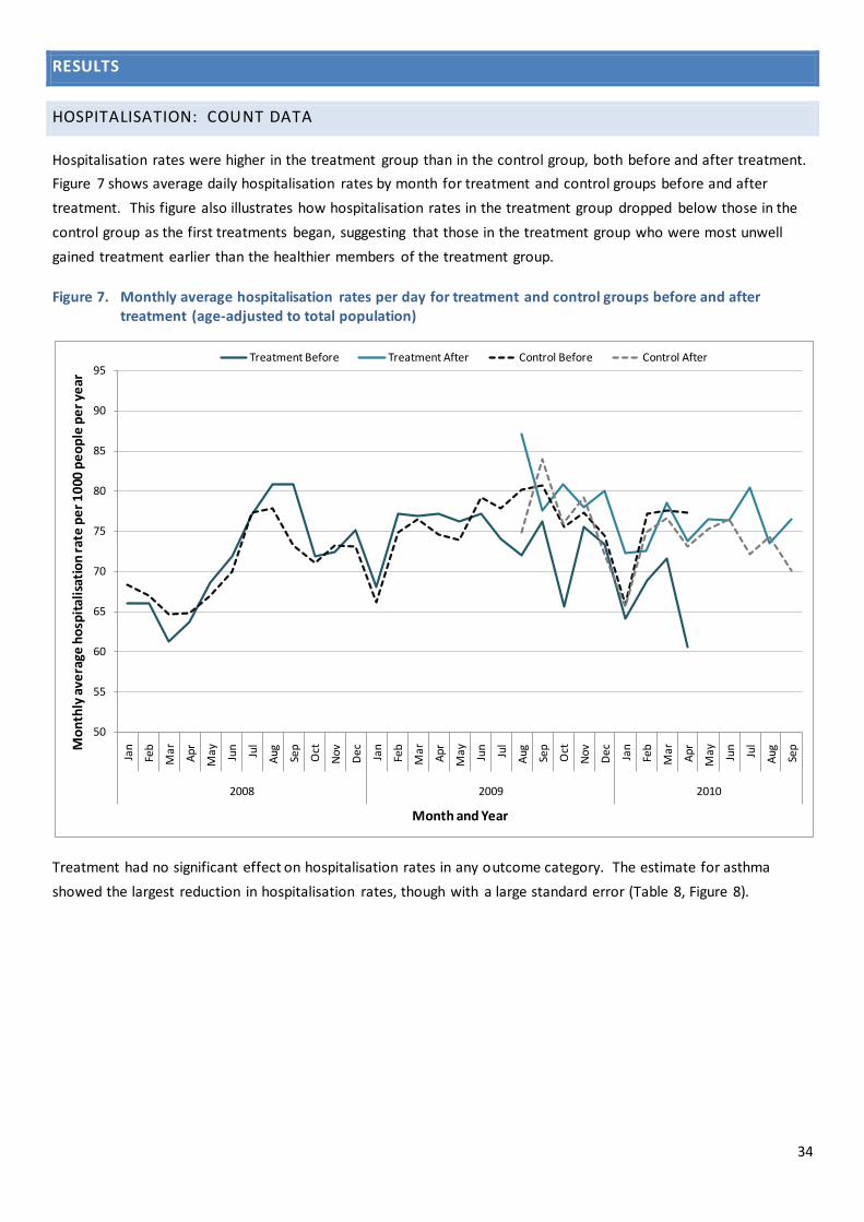
34

RESULTS

HOSPITALISATION: COUNT DATA

Hospitalisation rates were higher in the treatment group than in the control group, both before and after treatment.

Figure 7 shows average daily hospitalisation rates by month for treatment and control groups before and after

treatment. This figure also illustrates how hospitalisation rates in the treatment group dropped below those in the

control group as the first treatments began, suggesting that those in the treatment group who were most unwell

gained treatment earlier than the healthier members of the treatment group.

Figure 7. Monthly average hospitalisation rates per day for treatment and control groups before and after treatment (age-adjusted to total population)

Treatment had no significant effect on hospitalisation rates in any outcome category. The estimate for asthma

showed the largest reduction in hospitalisation rates, though with a large standard error (Table 8, Figure 8).

50

55

60

65

70

75

80

85

90

95

Jan

Feb

Ma

r

Ap

r

May Jun

Jul

Aug Se

p

Oct

No

v

Dec Jan

Feb

Ma

r

Ap

r

May Jun

Jul

Aug Se

p

Oct

No

v

Dec Jan

Feb

Ma

r

Ap

r

May Jun

Jul

Aug Se

p2008 2009 2010

Mo

nth

ly a

vera

ge h

osp

ital

isat

ion

rat

e p

er

10

00 p

eo

ple

pe

r ye

ar

Month and Year

Treatment Before Treatment After Control Before Control After

35

Table 8. Treatment effect (RRR) for measured hospitalisation outcomes.

Outcome RRR 95% CI p-value

Total hospitalisations 1.04 1.00-1.09 0.075

Circulatory illness 1.01 0.91-1.13 0.787

Congestive Heart Failure 1.00 0.76-1.31 0.974

Respiratory illness 1.01 0.91-1.12 0.898

Asthma 0.82 0.64-1.06 0.138

Respiratory Syncytial Virus* 0.83 0.43-1.59 0.573 *RSV analysis was limited to those 0-4 years, as this age range accounts for 99% of RSV hospitalisations.

Figure 8. Treatment effect for different categories of hospitalisation

36

MORTALITY

We measured mortality outcomes using a standard negative binomial model. Treatment inclined towards lowering

mortality among those aged 65 and over who had been hospitalised for any cause prior to treatment month, (RR

0.95, 95%CI 0.80-1.13, p=0.573) but the effect was not significant (Table 9).

Table 9. Effect of treatment on mortality rates in people aged 65+ hospitalised prior to treatment month

Hospitalised before treatment month

Deaths after treatment month

Mortality rate per 1000 people per year

RR (95% CI) p-value

RR after adjustment for cost difference

Treatment 3,210 185 76.8 (66.1-87.5) 0.93 (0.78-1.10) p=0.369

0.95 (0.80-1.13) p=0.573 Control 7,781 473 83.0 (75.8-90.2)

Among those in the mortality sub-cohort who had been hospitalised with circulatory conditions (ICD-10 chapter IX),

those in the treatment group had a significantly lower mortality rate than those in the control group (RR 0.73, 95%CI

0.53-1.00, p=0.048) (Table 10). These results suggest that treatment prevented about 18 deaths during the “after

treatment” study period, among those aged 65 and over who had previously been hospitalised with circulatory

illness, with a 95% confidence interval of 0 to 45 deaths prevented.

Table 10. Effect of treatment on mortality rates in people aged 65+ hospitalised with circulatory illness prior to treatment month

Hospitalised before treatment month

Deaths after treatment month

Mortality rate per 1000 people per year

RR (95% CI) p-value

RR after adjustment for cost difference

Treatment 958 51 69.8 (51.2-88.3) 0.62 (0.45-0.84) p=0.002

0.73 (0.53-1.00) p=0.048 Control 2231 184 112.7 (97.2-128.2)

Among those in the mortality sub-cohort who had been hospitalised with respiratory conditions (ICD-10 chapter X),

there was no significant difference in mortality rate after treatment between the treatment and control groups

(Table 11).

Table 11. Effect of treatment on mortality rates in people aged 65+ hospitalised with respiratory illness prior to

treatment month

Hospitalised before treatment month

Deaths after treatment month

Mortality rate per 1000 people per year

RR (95% CI) p-value

RR after adjustment for cost difference

Treatment 491 54 156.7 (98.6-165.1) 0.94 (0.68-1.30) p=0.712

1.01 (0.73-1.40) p=0.943 Control 1020 117 138.1 (114.5-161.6)

MORTALITY: COST DATA

We costed the reductions in mortality for people aged over 64 who had been hospitalised with circulatory illness

prior to treatment month reported above in the following way. Firstly we estimated the change in the number of

deaths per household in the year following treatment:

We chose a point in time, July 2009, the start of the WUNZ:HS programme, as the basis for our calculations.

We counted up the number of living individuals with valid ages (age less than 105, age not missing) in our

total treatment cohort at that time (107,421), the number of dwellings they lived in (29,704) and the

average number of individuals per dwelling (3.61).

37

We counted the number of individuals who were over 64 and who had been hospitalised for circulatory

illness in the prior 18 months within this cohort (834).

We calculated the average number of such individuals living in a treatment dwelling

=834 /29,704 = 0.028 (3 d.p.)

Assuming that, in the absence of treatment, the mortality rate for such individuals would be 112.7 deaths per 1000

individuals in the year after treatment (i.e. the estimate for the control group in Table 10), and given that there is a

27% reduction in mortality (Table 10), we estimate that in the year following the installation of insulation the

following number of deaths would be avoided:

= 0.028 (no. of individuals) * (112.7/1000) (control group mortality rate) *0.27 (27% reduction in mortality)

= 0.852 deaths avoided per 1000 households (95% CI: 0.00, 1.483 )

We then need to consider how much additional life these vulnerable individuals may gain, and how we should value

reduced mortality. A recent Technical Report produced for ACC[36] provides valuable guidance with regard to this

complex subject. In brief, the value of a preventable fatality (VPF) is typically estimated using Willingness to Pay

methods (how much people value lives). Once the VPF is established it is then possible to calculate the value of a life

year by assuming that a person dies at 40 but would have lived for 40 more years if they had not died, and then

applying a discount rate to calculate the value of each year that they lose. Table 12 presents different values for a life

year reported in O’Dea and Wren[36], based on three different VPFs, and the following discount rates 0%, 3%, and

5%.

According to O’Dea and Wren, PHARMAC currently favours a discount rate of 3.5%, however a 3% discount is

common and they adopt a value of life year figure based on this rate in their report. They favour the VPF f igure

reported in an influential 1991 report by Miller and Guria[37] of $3,352,448 ($NZ 2008) and thus utilise a value of life

year figure of $150,000 (rounded up from $145,035).

Table 12. The value of a life year for different VPFs and discount rates ($NZ June 2008)

Discount Rate Transport 1991

Based VPF Transport 1998

Based VPF Fire BERL 2007 VPF

VPF $3,352,448 $5,676,732 $2,212,616

0% $83,811 $141,918 $55,315

3% $145,035 $245,589 $95,723

5% $195,375 $330,830 $128,947

Following O’Dea and Wren we used a figure of $150,000 in our analysis, for reasons of convenience and also to

roughly approximate wage inflation in the past two years. We justify our adoption of this figure, because, as O’Dea

and Wren note, $3,352,448 is the official Transport Sector Value of Statistical Life (VoSL). Using a 3% discount rate to

establish the value of a life year is common in the United States and internationally and as PHARMAC currently

recommends a 3.5% discount rate (resulting in a higher value per life year) our choice can be seen as conservative.

38

While it could be argued that applying a standard figure such as $150,000 for the value of a life year to the

vulnerable population in our sub-cohort may appear to overstate the value of an elderly life, O’Dea and Wren note

that Willingness to Pay studies do not suggest that the elderly value their lives significantly less than others. Using a

standard figure has the benefit of equitability, making no moral judgements about the relative value of a life.

We predicted that 0.852 deaths per thousand households would be avoided in the year following treatment. We

valued the reduced mortality using a figure of $150,000 for the value of a life year. We expected that, on average, a

person that would have died would have died halfway through the year: this means in the year following treatment

the value of reduced mortality per dwelling is:

= (0.852/1000) (reduced mortality) * $150,000 (value of a life year) *0.5 (to account for half year)

=$ 63.96 (95% CI: $0.00, $111.23)

A complication is that, for the 0.852 individuals per thousand dwellings who did not die in the first year, additional

benefits will accrue for each year that they live beyond the first: the average age of our vulnerable sub-cohort is

76.63, there are slightly more females than males so we conservatively assume that the gender mix is 50:50, and if

they followed the predicted pattern for a 77 year old based on figures reported in Statistics New Zealand’s Life

Tables (www.statistics.govt.nz) we would expect that they would live to be 77 + 10.64 = approximately 87.64 on

average. For convenience we will use a figure of 87.5, i.e. an average a gain of 11 life years. Note the saving from

reduced mortality per household in year one is $63.96 because avoided mortality is assumed to happen halfway

through the year , which means that the additional savings in future years are valued at 2*$63.96=$127.92. At a

discount rate of 5% the saving per dwelling would be:

30.88)$0.00,$1,8:95%CI$1,051.78(

n)0.05)^/((1($127.92)$63.9610n

1n

We have modelled the probability of a vulnerable person avoiding mortality as a result of the intervention. The

probability of this is (112.7/1000)*0.27= 0.03 (3%). We treat avoidance of mortality by treatment in each year as

independent events. The multi-year benefit calculated above would accrue based on the life years gained as a result

of deaths avoided in year one. However, we would expect these benefits to accrue in year two for different

vulnerable individuals (aged 65 and over with a cardiovascular related hospitalisation in previous 18 months), and for

different individuals again in every subsequent year that the treatment continues to have an effect, i.e. an on-going

stream of benefits of $1,050.74 per year. This assumes a constant proportion of people aged 65+ who have recently

been hospitalised with circulatory problems. In reality, as people die or move and their homes have new occupants,

we cannot expect that the demographic structure will remain constant; however, given that New Zealand has an

aging population, the potential benefits of this intervention may increase with time.

Estimating benefit is further complicated by the fact that we cannot predict with certainty that a person from a

vulnerable population (aged over 64 and hospitalised recently for a circulatory condition) will live as long as the

average person of their age. If we estimate that a person who does not die as a result of receiving treatment lives for

half as long as they would otherwise (conservatively 5 years) then we will end up with the following on-going annual

saving per dwelling (discounted at 5%):

39

.99)$0.00,$900:%CI$517.59(95

n)0.05)^/((1($127.92)$63.964n

1n

We favour this latter approach, although we acknowledge that it may be slightly inflated as a measure of on-going

annual benefit, with the possibility of double counting difficult to avoid (i.e. if somebody avoided death due to the

treatment in year two who also avoided death due to treatment in year one we would count their benefit twice in a

cost benefit model). A final corrective for this problem is to estimate that in a given year 15%5 of the people who

avoided death as a result of treatment had also avoided death due to treatment in a previous year, so their life years

gained should not be counted to avoid double counting. This figure is likely to overstate the danger of over-counting

as it assumes that a person who avoids mortality due to treatment in a given year remains in the vulnerable cohort

i.e. does not move and has a cardiovascular hospitalisation at least once per 18 months for the rest of their life.

If we reduce the value of our figures accordingly we produce a figure that is obviously too low for the first four years

post-treatment but which avoids double counting when utilised in a cost benefit analysis:

=$517.59*0.85

=$439.95 (95% CI: $0.00, $765.84)

Finally, we note that, unsurprisingly, the proportion of vulnerable individuals was different depending on whether or

not they lived in a dwelling that received treatment under the programme as a Community Services Card holder. In

our treatment cohort as at July 2009 there were 60,544 CSC individuals, and 655 were in the vulnerable group. There

were 46,877 non-CSC individuals and of them 179 were in the vulnerable group. This means that, assuming a

household with 3.61 occupants and carrying out the calculations described above, we would expect the following

on-going annual savings given our favoured assumptions:

CSC dwelling = $ 613.05 (95% CI: $0.00, $1,067.16)

Non CSC dwelling = $216.38 (95% CI: $0.00, $376.66)

While each aspect of our model is defensible, it is clear that different assumptions have the potential to have a

marked impact on the outcome of the cost benefit analysis. We set out a fuller set of results in Appendix 3 which

make clear the impact of different assumptions.

The most extreme on-going annual benefits (looking at all treatment households) range from $23.59 (95% CI $0.00 -

$41.06) estimated using the Fire BERL 2007 VPF value per life year of $55,315 and only a single year of benefit, to

$1,925.66 per year (95% CI $0.00 - $3352.07) estimated using the Transport 1998 Based VPF value per life year of

$330,830, 11 years total benefit and discounted at 0%. Our preferred estimate of benefits, at $439.95, is towards the

lower end of this range.

5 The 15% figure is based on the likelihood that a given individual who avoided mortality due to the treatment will avoid death due to the treatment at least once more time during the additional four years of life we predict they will gain: Chance of vulnerable person avoiding mortality due to treatment in a given year= (112.7/1000)*0.27= 0.03 Chance a person who avoided mortality due to treatment will avoid it at least once more in following four year period assumin g that they continue to be a part of the vulnerable cohort= 0.03(1+0.97+0.97^2+0.97^3) = 11.5% We conservatively raise this figure to 15%.

40

HOSPITALISATION: COST DATA

We estimated each of our hospitalisation cost models using a fixed-effect OLS estimator with standard errors

clustered by house. Table 13 presents the results of our primary analysis of hospitalisation costs. Our conclusions

were tested using a bootstrap estimation of standard errors involving 500 repetitions. Bootstrapping produced

similar standard errors and p-values, confirming the validity of the model.

The results presented in Table 13 indicate a statistically significant saving of approximately $5.37 in total

hospitalisation costs per month for a household that received some combination of ceiling or floor insulation under

the WUNZ:HS. Analyses by hospitalisation type show a $5.62 monthly saving in circulatory illness related

hospitalisation costs and an $8.24 reduction in respiratory illness related hospitalisation costs. Asthma-related

hospitalisation costs (a subset of respiratory illness) are higher still at $8.96. The estimates in Table 13 come from

separate models fitted to different subsets of the data, and for this reason may seem inconsistent. For example, the

sum of circulatory and respiratory illness savings per month is approximately $13.86, greater than the $5.37 figure

for total hospitalisation costs. This difference is most likely to be caused by variability or ‘noise’ from hospitalisation

types unlikely to be affected by improved insulation. A conservative approach is to adopt the total hospitalisation

costs figure, although this seems likely to underestimate the true benefit of insulation.

Table 13. Change in monthly hospitalisation costs per household

Total

hospitalisation

Circulatory

illness

Respiratory

illness Asthma

Insulation -$5.37** -$5.62*** -$8.24*** -$8.96***

Robust standard errors (2.126) (1.887) (1.872) (1.875)

95% confidence interval (-9.54, -1.21) (-9.32, -1.92) (-11.91, -4.57) (-12.63, -5.28)

Heating -$1.37 $0.67 -$0.32 $0.25

Robust standard errors (4.431) (3.953) (3.907) (3.922)

95% confidence interval (-10.05, 7.32) (-7.07, 8.42) (-7.98, 7.34) (-7.44, 7.94)

Observations 57,154 57,100 57,152 57,174

Number of households 28,577 28,550 28,576 28,587

R-Squared (within) 0.000271 0.000334 0.000763 0.000880

R-Squared (adjusted) 0.000236 0.000299 0.000728 0.000846

*** p<0.01, ** p<0.05,* p<0.1

The results show that receiving a heating retrofit under the WUNZ:HS (as distinct from insulation) did not result in a

statistically significant change in any hospitalisation cost category. This result may in part reflect the smaller

proportion of households that received a heating retrofit in our sample, but is also consistent with the fact that for

households to receive a heating retrofit under the WUNZ:HS programme they needed to meet a minimum insulation

standard. This means that heating retrofits in some cases took place in houses that were already insulated in the

“before” period. The potential health benefits of a retrofit in such a scenario are likely to be less than those resulting

from the installation of insulation in an under-insulated home because the health benefits of going (for example)

from an average indoor temperature of 15°C to 16°C are greater than those gained by going from 16°C to 17°C.

Table 14 presents a sub-analysis of the data presented above, limiting analysis to those households who received

WUNZ:HS funding as Community Service card holders (identified as “low income” in the EECA dataset).

The results reported in Table 14 are largely consistent with those reported in Table 13, although they do

demonstrate a higher average cost saving per month for all four hospitalisation cost categories. We would expect

41

these results because dwellings which received WUNZ:HS funding as Community Services Card holders are likely to

have occupants that are, on average, sicker than the occupants of dwellings that received WUNZ:HS funding who did

not qualify as Community Services Card holders: sicker people (for example asthmatics, or elderly people with

Chronic Obstructive Pulmonary Disease (COPD)) are more likely to derive a health benefit from improved insulation

than less sick people. This effect is likely to have been compounded by the work done by Community Based Trusts

who acted as Service Providers under the WUNZ:HS in identifying sick members of their communities, and

organising, encouraging and funding their involvement in the programme, meaning that the Community Services

Card households in the treatment group may have been more likely than a typical Community Services Card

household to benefit from the intervention (for example including a higher proportion of COPD sufferers).

Table 14. Change in monthly hospitalisation costs per household for households receiving WUNZ:HS funding as

Community Services card holders

Total hospitalisation

Circulatory illness

Respiratory illness

Asthma

Insulation -$9.15*** -$7.13** -$9.82*** -$10.76***

Robust standard errors (3.174) (2.852) (2.834) (2.839)

95% Confidence Interval (-15.37, -2.93) (-12.72, -1.53) (-15.38, -4.27) (-16.33, -5.20)

Heating $1.38 $3.54 $3.88 $5.13

Robust standard errors (6.527) (5.949) (5.890) (5.944)

95% Confidence Interval (-11.42, 14.17) (-8.12, 15.20) (-7.66, 15.43) (-6.52, 16.78 )

Observations 31,662 31,606 31,620 31,688

Number of households 15,831 15,803 15,810 15,844

R-Squared (within) 0.000570 0.000402 0.000784 0.000924

R-Squared (adjusted) 0.000507 0.000338 0.000721 0.000861

*** p<0.01, ** p<0.05, * p<0.1

The results for those households which did not qualify for the WUNZ:HS programme as Community Services Card

Holders are presented in Table 15.

Table 15. Change in monthly hospitalisation costs per household for households which did not qualify for the WUNZ:HS programme as Community Services Card Holders

Total hospitalisation

Circulatory illness Respiratory illness Asthma

Insulation -$0.73 -$3.83 -$6.38*** -$6.83***

Robust standard errors (2.692) (2.330) (2.308) (2.302)

95% Confidence Interval (-6.00, 4.55) (-8.39, 0.74) (-10.91, -1.86 ) (-11.34, -2.32)

Heating -$4.37 -$2.74 -$5.40 -$5.66

Robust standard errors (5.770) (4.908) (4.839) (4.799)

95% Confidence Interval (-15.68, 6.94) (-12.37, 6.88) (-14.88, 4.09 ) (-15.07, 3.75)

Observations 25,492 25,494 25,532 25,486 Number of households 12,746 12,747 12,766 12,743 R-Squared (within) 6.70e-05 0.000302 0.000912 0.00105

R-Squared (adjusted) -1.15e-05 0.000224 0.000834 0.000968 *** p<0.01, ** p<0.05, * p<0.1

The results in Table 15 appear to corroborate the discussion above, with no statistically significant change in total

hospitalisation costs or circulatory illness costs as a result of insulation, although respiratory illness and asthma do

demonstrate a smaller but still highly statistically significant improvement in costs.

42

PHARMACEUTICALS: COST DATA

We estimated each of our pharmaceutical cost models using a fixed-effect OLS estimator with standard errors

clustered by house. Table 16 presents the results of our primary analysis of pharmaceutical costs. Results were

corroborated using a bootstrap estimation of standard errors involving 500 repetitions. Bootstrapping produced

similar standard errors and probability estimates, confirming the validity of the model.

Table 16. Change in monthly pharmaceutical costs per household

Total Pharmaceutical Dispensations

Circulatory Illness Related Dispensations

Respiratory Illness Related Dispensations

Insulation -$0.92*** -$0.29*** $0.13***

Robust standard errors (0.333) (0.0701) (0.0448)

95% Confidence Interval (-1.57, - 0.27) (-0.43, -0.16) (0.04, 0.21) Heating -$0.68 -$0.12 -$0.04 Robust standard errors (0.688) (0.146) (0.0884)

95% Confidence Interval (-2.03, 0.66) (-0.41, 0.16 ) (-0.21, 0.14)

Observations 57,618 57,724 57,732 Number of households 28,809 28,862 28,866 R-Squared (within) 0.000397 0.000783 0.000284 R-Squared (adjusted) 0.000362 0.000749 0.000250 *** p<0.01, ** p<0.05, * p<0.1

The results presented in Table 16 demonstrate a very small but highly statistically significant reduction in monthly

pharmaceutical costs as a result of receiving ceiling or floor insulation, and no change in pharmaceutical costs as a

result of receiving a heating retrofit. The pattern demonstrated by these results seems largely consistent with those

reported for hospitalisation costs, however, unlike the hospitalisation cost results, a small but highly statistical

increase in respiratory illness related dispensations is predicted as a result of improved insulation. We do not have a

clear sense of what may explain this increase and it seems inconsistent with the hospitalisation results reported

above. One possible explanation is a selection effect: those people who are suffering from a new or worsening

respiratory problem may simultaneously apply for insulation and also seek additional or more expensive medication.

As with hospitalisation costs, we further analysed pharmaceutical costs by limiting analysis to those households who

received WUNZ:HS funding as Community Services Card holders (identified as “low income” in the EECA dataset).

The results are presented in Table 17.

Table 17 follows the pattern demonstrated by the hospitalisation costs above, in that the difference in circulatory

illness related dispensations and respiratory illness dispensations are larger for the Community Services Card

subgroup than for the entire group (however, there is no difference in total pharmaceutical dispensation costs).

Table 18 presents the results for those households which did not qualify for the WUNZ:HS programme as Community

Services Card Holders.

Table 18 appears to confirm the importance of a household’s Community Services Card status in explaining our

findings, with no statistically significant change in circulatory or respiratory illness related dispensations, however

the change in total pharmaceutical dispensations is not meaningfully different from that reported for Community

Services Card holders (and is more statistically significant), suggesting that a variety of other process are influencing

the outcome of this analysis.

43

Table 17. Change in monthly pharmaceutical costs per household incurred by those who received WUNZ:HS funding as Community Services Card holders

Total Pharmaceutical Dispensations

Circulatory Illness Related Dispensations

Respiratory Illness Related Dispensations

Insulation -$0.91* -$0.47*** $0.25*** Robust standard errors (0.478) (0.106) (0.0662) 95% Confidence Interval (-1.85, 0.02) (-0.68, -0.27) (0.12, 0.38) Heating -$0.70 -$0.19 -$0.078 Robust standard errors (0.981) (0.221) (0.128)

95% Confidence Interval (-2.62, 1.23) (-0.62, 0.25) (-0.33, 0.17) Observations 32,112 31,960 31,950 Number of households 16,056 15,980 15,975 R-Squared (within) 0.000353 0.00162 0.000959 R-Squared (adjusted) 0.000291 0.00156 0.000897 *** p<0.01, ** p<0.05, * p<0.1

Table 18. Change in monthly pharmaceutical costs per household for those households which did not qualify for the WUNZ:HS programme as Community Services Card Holders.

Total Pharmaceutical Dispensations

Circulatory Illness Related Dispensations

Respiratory Illness Related Dispensations

Insulation -$0.92** -$0.07 -$0.03 Robust standard errors (0.451) (0.0864) (0.0577) 95% Confidence Interval (-1.81, -0.04) (-0.24, 0.10) (-0.14, 0.08) Heating -$0.67 -$0.03 $0.00 Robust standard errors (0.944) (0.178) (0.118) 95% Confidence Interval (-2.52, 1.18) (-0.37, 0.32) (-0.23, 0.23)

Observations 25,506 25,764 25,782 Number of households 12,753 12,882 12,891 R-Squared (within) 0.000473 6.00e-05 2.59e-05 R-Squared (adjusted) 0.000395 -1.76e-05 -5.17e-05 *** p<0.01, ** p<0.05, * p<0.1

IMPUTED BENEFITS: SENSITIVITY ANALYSIS

It was not possible for the present study to address a number of key potential benefits of improved insulation,

heating and health that have been found in previous research carried out by the Housing and Health Research

programme.[1, 38] These include reduced frequency of GP visits, reduced days off work and reduced days off school.

Statistically significant benefits found in our previous studies are set out in Table 19. The benefits were calculated for

the winter period (June –August) for the Housing, Insulation and Health Study[1], and (June – Sept) for the Housing,

Heating and Health Study[38] but then extrapolated to capture an entire year.

The Housing, Insulation and Health Study was not powered to find a statistically significant reduction in respiratory

hospitalisation admissions, but it did find a non-statistically significant reduction in respiratory hospitalisation

admissions (p = 0.16 adjusted). The Housing, Heating and Health Study was similarly not powered to find statistically

significant results for respiratory hospitalisation outcomes. Comparison of the respiratory hospitalisation admission

results for the Housing Insulation and Health Study with the non-statistically significant reduction in asthma

hospitalisations and RSV observed in the present Study suggests some basis for extrapolation in the case of

insulation.

44

Table 19. Statistically significant health related savings documented in previous H&HRP analyses

Feature Housing, Insulation and Health Study Cost benefit analysis results reported in

Chapman et al. 2009[2]

Housing, Heating and Health Study Cost benefit analysis results reported in Preval et al. 2010[39]

Study Description

A cluster randomised controlled trial comparing health and energy use outcomes for treatment and control group individuals/ households following a standardised insulation retrofit.

A cluster randomised controlled trial comparing health and energy use outcomes for treatment and control group individuals/ households following a standardised heating retrofit (replacement of an inefficient heater with either a heatpump, flued gas heater or pellet burner). Treatment and control group homes were insulated before baseline measures were taken.

Participant characteristics

Each participant household included at least one occupant who had symptoms of respiratory disease; households were in predominantly low-income communities.

Each participant household included at least one asthmatic child aged 6-12; households were located in the South Island or Lower North Island.

Reductions in GP visits

An increase(negative result) of 48 GP visits per 1000 occupants per winter (0.05 visits per occupant) based on GP records. Valued at -$3.60 ($2001) per occupant per year when extrapolated to include the entire year. [Note: a statistically significant reduction in self-reported GP visits was observed but preference was given to GP records]

A reduction of 0.37 self-reported visits to the GP per winter for each asthmatic child, valued at $22.73 per child ($2006) when extrapolated to include the entire year. No other statistically significant reductions in GP self-reported GP visits.

Reductions in days off work

Adults aged 19-64: a reduction of 102 days off work per 1000 adults per winter (0.10 days per adult) Savings valued at $16.84 ($2001)per adult per year based on 80% (to adjust for co-workers “picking up the slack”) of the 2001 average wage and extrapolated to include the entire year.

None found.

Reduction in days off school

Children aged 6-11: a reduction of 512 days off school per 1000 children over winter (0.51 days per child). Saving valued at $11.51 ($2001) per child per year when extrapolated to include the entire year, valued based on 1/3 of the youth minimum wage and 7 hours lost. Teenagers 12-18: a reduction of 1316 days off school/work per 1000 teenagers per winter (1.32 per teen) Savings valued at $59.21($2001) per teenager per year when extrapolated to include the entire year, valued based on 2/3 of the youth minimum wage and 7 hours lost.

A reduction of 1.8 days off over winter terms per asthmatic child (aged 6-12), valued at $41.50 ($2006) when extrapolated to include the entire year, valued based on 1/3 of the gross daily minimum wage. Further benefit of reduced caregiver time were valued at $124.50 per asthmatic child per year ($2006) No statistically significant changes for children without asthma.

45

Table 20 reports the demographic profile of the treatment households which we have occupant information for as at

July 2009 (the start of the WUNZ:HS programme), excluding occupants with no age or an implausible age (>105) or

who have died. We also report the proportion of child occupants aged 6-11 that we predict will have asthma

(15.1%)[40] as this is relevant for the estimation of heating related benefits.

Table 20. Demographic profile of treatment households as at July 2009

Demographic measure n

Number of dwellings 29,704 Number of occupants 107,421 Average number of occupants 3.61 Children aged 0-5 9,115 (8.49%) Children aged 6-11 estimated asthmatic 1,168 (1.09%)

Children aged 6-11 estimated non-asthmatic

6,567 (6.11%)

Teenagers aged 12 -18 9,347 (8.7%) Adults age 19-64 63,121 (58.76%) Older people (65+) 18,103 (16.85%)

It is possible to apply the data produced by previous studies to the demographic profile set out above. In order to do

so we need to update the figures used in our previous cost benefit analyses to 2011 prices and resolve any

inconsistencies between the two approaches. The key inconsistency is the valuing of childcare for sick children,

which was costed by the Housing, Heating and Health Study but not the Housing, Insulation and Health Study. We

present our results with childcare costed separately, but in general we favour the inclusion of reduced childcare

costs and consider our valuing of such costs at 6 hours at minimum wage ($13) to be reasonably conservative. We

assume that lost time from school should be valued at 2/3 of 6 hours at the minimum hourly wage ($13) for

teenagers and 1/3 for children aged 6-11, the youth minimum wage no longer applying. Adult time off work is valued

at 80% of an 8 hour day at an average hourly wage of $25.96 ($2011).

Table 21 presents a summary of the additional benefits imputed per year per 1000 dwellings receiving either an

insulation retrofit (floor and or ceiling) or a heating retrofit based on our previous analyses and assuming the

demographic distribution set out in Table 20 (there was an average of 3.61 people per dwelling, so when looking at

1000 households we estimated benefits for 3,610 occupants).

Note that for reasons of convenience we conservatively assume that the reduction in days off school reported in the

Heating, Housing and Health Study for asthmatic children only apply to ages 6-11 rather than 6-12.

Table 21. Additional imputed yearly benefits per 1000 households assuming 3.61 occupants per household and age structure of treatment g roup as at July 2009

Age group

Number of

occupants per 1000 households

Potential benefit Value per occurrence ($2011)

Change in number of occurrences per winter

Change in number of occurrences per year (adjusting for cold days in non-winter

period)*

Insulation: Predicted benefit per 1000 households per

year*

Heating: Predicted

benefit per 1000 households per year

0-5 306.489 Reduced medical visits

$54.34 -0.05 -0.0835 -$1,390.70 $0.00

6-11 (asthma)

39.349

Reduced medical visits

$54.34 -0.05 (insulation) & 0.369 (heating)

-0.0835 (insulation) + 0.461 (heating)

-$178.55 $986.29

Reduced days off

school $26.00

0.51 (insulation) & 1.8

(heating)

0.765 (insulation) +

2.025 (heating) $782.65 $2,071.72

Associated reductions in caregiver costs

$78.00 0.51 (insulation) & 1.8 (heating)

0.765 (insulation) + 2.025 (heating)

$2,347.95 $6,215.17

6-11 (without asthma)

220.571

Reduced medical visits

$54.34 -0.05 -0.0835 -$1,000.85 $0.00

Reduced days off

school $26.00 0.51 0.765 $4,387.16 $0.00

Associated reductions in caregiver costs

$78.00 0.51 0.765 $13,161.47 $0.00

12-18 314.07

Reductions in medical visits

$54.34 -0.05 -0.0835 -$1,425.10 $0.00

Reduced days off

school/work $52.00 1.32 1.98 $32,336.65 $0.00

19-64

2121.236

Reductions in medical visits

$54.34 -0.05 -0.0835 -$9,625.16 $0.00

Reduced days off work

$166.14 0.1 0.167 $58,855.92 $0.00

65+ 608.285 Reductions in medical

visits $54.34 -0.05 -0.0835 -$2,760.11 $0.00

Net benefit of insulation retrofit per 1000 households per year (Sum of Predicted Benefits for each age group)

$95,491.33

Net benefit of insulation retrofit per 1000 households excluding childcare savings per year (Sum of Predicted Benefits for each age group)

$79,981.90

Net benefit of heating retrofit per 1000 households per year (Sum of Predicted Benefits for each age group)

$9,273.19

Net benefit of heating retrofit per 1000 households excluding childcare savings per year (Sum of Predicted Benefits for each age group)

$3,058.01

*Note: negative values indicate an increase in frequency or cost

47

The figures presented in Table 21 suggest that, including childcare costs for sick children, we can impute additional

health related benefits of $95,491.33 ÷ 1000 =$95.49 per household per year for a household receiving insulation

(floor and or ceiling) and $9,273.19 ÷ 1000 = $9.27 per household per year for a household receiving a heating

retrofit given the demographic structure presented in Table 22. It is important to be cautious about these results

given the characteristics of the households included in the Housing, Insulation and Health Study (at least one

occupant with respiratory illness and located in predominantly low-income communities) and the Housing, Heating

and Health Study (South Island and Lower North Island locations only and an asthmatic child aged 6-12). We suggest

that given these complications it might be reasonable to place more confidence in these predictions for those

households identified as low income households in the present study. For this reason, when estimating the imputed

benefits of insulation for all treatment households we predict $95.49/2 = $47.75 annual benefit, reflecting

approximately 50% CSC households. We include the full $95.49 for our sub-analysis of CSC households but do not

include any imputed benefits for non-CSC households. Likewise we predict an annual benefit of $9.27/2 = $4.64

imputed benefit for improved heating for all treatment households, $9.27 for CSC households and no benefit for

non-CSC households.

We also note that in our previous cost benefit analyses insulation is predicted to have a useful life of 30 years, while

12 years seems a reasonable estimate for the life-span of a heat pump or other clean heater.

SUMMARY DATA FOR COST BENEFIT ANALYSIS

Here we combine the results of our panel data based estimates of the average monthly change in hospitalisation

costs and pharmaceutical costs (which we annualise i.e. multiply by 12) and annual reductions in mortality with

imputed benefits based on our previous cost benefit analyses which assessed changes in GP visits, days off school

and work. We present the combined results for total hospitalisations and total pharmaceutical dispensations

(conservative) and we also present the results for adding circulatory and respiratory outcomes only. We favour the

more conservative approach of focussing on the change in total hospitalisations and total pharmaceutical

dispensations, but include both for reasons of completeness. We have only included results that were statistically

significant at a (p <0.05) level in our final analysis.

Although reductions in mortality were calculated based on receiving any treatment (i.e. did not distinguish between

heating and insulation), we suggest that given the relatively low number of heating retrofits and the absence of any

change in hospitalisation costs as a result of a heating retrofit, that we should limit the mortality benefits of the

intervention to insulation at this time.

We include confidence intervals for our results based on the confidence intervals estimated for our mortality results

only. This reflects the fact that reduced mortality related benefits dominate the uncertainty and that overall benefit

is dominated by the uncertainty in mortality.

Table 22. Summary of annual health-related benefits (savings) per household Analysis based on change in total hospitalisation and total pharmaceutical use

Household type Benefits Insulation Heating

All households

Hospitalisation and pharmaceutical use related benefits calculated in present Study

$64.44 (total hospitalisations) + $11.04 (total pharmaceuticals) = $75.48

$0.00

Additional benefits imputed from previous Studies $47.75 $4.64

Value of reduced mortality $439.95 (95% CI $0.00 – $765.84) $0.00

SUM OF HEALTH BENEFITS $563.18 (95%CI $123.23 - $889.07) $4.64

Households that participated in WUNZ:HS programme as

Community Services Card holders

Hospitalisation and pharmaceutical use related

benefits calculated in present Study $109.80 (total hospitalisations) $0.00

Additional benefits imputed from previous Studies $95.49 $9.27

Value of reduced mortality $613.05 (95% CI $0.00 - $1,067.16) $0.00

SUM OF HEALTH BENEFITS $818.34 (95% CI $205.29, $1,272.45) $9.27

Households that participated in

WUNZ:HS programme as non-Community Services Card holders

Hospitalisation and pharmaceutical use related benefits calculated in present Study

$11.04 (total pharmaceuticals ) $0.00

Additional benefits imputed from previous Studies $0.00 $0.00

Value of reduced mortality $216.38 (95%CI $0.00 - $376.66) $0.00

SUM OF HEALTH BENEFITS $227.42 (95% CI $11.04 - $387.70) $0.00

Analysis based on change in circulatory and respiratory hospitalisations and pharmaceuticals only

All households

Hospitalisation and pharmaceutical use related

benefits calculated in present Study

$67.44 (circulatory hospitalisations) + $98.88 (resp. hospitalisations) +$3.48 (circulatory pharms) - $1.56

(respiratory pharms) = $168.24

$0.00

Additional benefits imputed from previous Studies $47.75 $4.64

Value of reduced mortality $439.95 (95% CI $0.00 – $765.84) $0.00

SUM OF HEALTH BENEFITS $655.94 (95% CI $215.99 - $981.83) $4.64

Households that participated in WUNZ:HS programme as Community Services Card holders

Hospitalisation and pharmaceutical use related benefits calculated in present Study

$85.56(circulatory hospitalisations) +$117.84 (resp. hospitalisations) + $5.64(circulatory pharms) - $3.00(respiratory pharms) = $206.04

$0.00

Additional benefits imputed from previous Studies $95.49 $9.27

Value of reduced mortality $613.05 (95% CI $0.00 - $1,067.16) $0.00

SUM OF HEALTH BENEFITS $914.58 (95%CI $301.53 - $1,368.69) $9.27

Households that participated in WUNZ:HS programme as Non-

Community Services Card holders

Hospitalisation and pharmaceutical use related benefits calculated in present Study

$76.56 (respiratory hospitalisations) $0.00

Additional benefits imputed from previous Studies $0.00 $0.00

Value of reduced mortality $216.38 (95%CI $0.00 - $376.66) $0.00

SUM OF HEALTH BENEFITS $292.94 (95% CI $76.56- $453.22) $0.00 *

49

CONCLUSIONS

We conducted a retrospective cohort study using Quotable Value records, that matched dwellings that received

insulation or heating retrofits by address to similar control dwellings in the same Census area unit. Subsequently,

using an anonymising process, the hospitalisation records of residents at both the treatment and control addresses

were identified through linkage with the New Zealand National Health Index.

Unlike the Housing, Insulation and Health Study and the Housing, Heating and Health Study, which were randomised

community trials, this evaluation study was observational, rather than experimental. Observational studies carry the

possibility of confounding, where the self-selecting treatment group differs systematically from the matched control

group. Indeed, those in the control households were closer to the shape of the NZ population than to the treatment

group. The key difference from the perspective of identifying potential confounding was that the proportion of

participants older than 60, who are at higher risk of being hospitalised, was higher in the treatment group (21.3% vs.

15.6%). This meant that those in the treatment group were more likely to, and did have, a higher rate of

hospitalisation than the control group pre-treatment. In other words, the treatment group was a less healthy

population than the control group.

We carried out three types of analysis: 1) a count data analysis of hospitalisations based on exposure time to an

insulated/uninsulated house or new effective heater/old heater; 2) a count data analysis comparing mortality rates

between treatment and control groups for those aged 65 and over who had been hospitalised before

insulation/heating installation month; and 3) analyses of hospitalisation and pharmaceutical costs based on a

‘difference in difference’ approach at a household level, where we compared the average monthly hospitalisations

or pharmaceutical costs of treatment, including both admissions, readmissions and transfers. This latter approach

broadly parallels the approach taken to analyse metered energy use changes.

Methodological limitations included imprecision in assigning NHI records to addresses, a limited measured exposure

time after treatment and the possibility that control group households may have installed insulation or heating

during the study period outside of WUNZ:HS. We were also unable to directly assess potential benefits such as

reduced GP visits, days off school/work and improved comfort, although we did estimate these benefits based on

our previous work.

Our analysis of hospitalisation count data did not demonstrate a statistically significant change in any hospitalisation

category after treatment (note that we did not distinguish insulation and heating in our analysis of count data).

However, our analysis of changes in mortality for those aged 65 and over demonstrated a statistically significant

drop of 27% in all causes mortality for those who had had a circulatory hospitalisation in the study period prior to

treatment but no statistically significant change for those who had a respiratory hospitalisation in the study period

prior to treatment.

When we costed this statistically significant drop in mortality, having taken account of the demographic structure of

the treatment group as at July 2009, we estimated that there would be an annual reduction of 0.852 deaths per

1000 households of 3.61 individuals. The life years gained can be conservatively valued at $439.95 per year. The

benefit per year was $613.05 for households that received treatment as Community Services Card Holders and

$216.38 for those who did not, reflecting different proportions of vulnerable occupants.

50

We analysed hospitalisation costs at a household level using a fixed effects model, and unlike our count data,

included readmissions and transfers. Because this analysis was based on costs it took into account severity of illness

through length of stay and cost of procedures, and despite the absence of a statistically significant change in the

individual level count data we found small but significant monthly differences between those in the treatment and

control groups in total hospitalisations (-$5.37), circulatory illnesses (-$5.62), respiratory illnesses (-$8.24) and

asthma (-$8.96) as a result of improved insulation, although no statistically significant change as a result of improved

heating. The reason that the reduction in total hospitalisation costs is lower than the sum of the reduction in

respiratory illness and circulatory illness related hospitalisation costs is likely to be variability or ‘noise’ from

hospitalisation types unlikely to be affected by improved insulation.

The effects for those who received insulation under the WUNZ:HS programme as Community Services Card holders

are higher and more significant than for those who did not participate in the programme as Community Service Card

holders (-$9.15 vs. - $0.73; -$7.13 vs. ,-$3.83; -$9.82 vs. -$6.38; -$10.76 vs. -$6.83) for total, circulatory, respiratory

and asthma related hospitalisations respectively).

The pharmaceutical cost data showed a similar significant pattern, but a smaller effect, but did not display quite as

marked a difference between Community Services Card holders and those who did not participate in the programme

as Community Services Card holders; there were small, but significant monthly savings for overall pharmaceutical

dispensations (-$0.92), circulatory-related dispensations (-$0.29) but a small increase in respiratory illness related

dispensations ($0.13) for households that received insulation, and no statistically significant change for heating.

Based on our previous analyses we estimated, given the demographic make-up of the treatment group as at July

2009, that a treated household would gain a combined benefit of $47.74 per year from changes in GP visits and days

off work and school as a result of receiving retrofitted insulation, and $4.64 per year from receiving a heating

retrofit. We predict that a household which received insulation as a Community Services Card holder would gain

greater imputed benefits of $95.49 from improved insulation and $9.27 from improved heating. We do not predict

any benefit for non-CSC households from improved heating or insulation based on our previous analyses.

Finally, we combined these results to estimate total benefits per household. Our favoured conservative estimate

based on the change in total hospitalisations and total pharmaceutical predicts an on-going annual benefit of

$563.18 for retrofitted insulation and only $4.64 for improved heating. The figures were higher for households that

received insulation as Community Services Card Holders at $818.34 and $9.27 for heating. The benefit of improved

insulation was lower for households that did not receive treatment as Community Services Card Holders at $227.42.

The benefit for improved heating for non-CSC households was estimated at $0.00.

51

APPENDIX 1 ADDITIONAL TABLES

Table A 1. Age-standardised hospitalisation rates for treatment, control and total populations at baseline, 1 January 2008 to 31 December 2009.

Variable Treatment rate Control rate Total population rate

Age group*

0-4 years 125.0 (4.9 - 115.4) 120.3 (0.2 - 119.9) 134.8 (14.9 - 105.4)

5-14 years 37.9 (2.5 - 33) 39.4 (2.9 - 33.7) 44.0 (3.1 - 37.9)

15-29 years 46.1 (1.7 - 42.7) 50.1 (1.6 - 46.9) 61.8 (3.2 - 55.6)

30-44 years 41.4 (1.5 - 38.4) 45.0 (1.9 - 41.4) 60.0 (1.9 - 56.1)

45-64 years 75.8 (8.5 - 58.9) 71.0 (6.9 - 57.3) 89.5 (8.4 - 72.8)

65+ years 312.5 (306.8 - 318.3) 186.6 (16.8 - 153.3) 387.6 (358.7-416.6)

Sex

Male 77.2 (75.6 - 78.8) 75.9 (75.1 - 76.8) 102.1 (101.8 - 102.4)

Female 74.0 (72.4 - 75.6) 74.7 (73.9 - 75.5) 91.3 (91.0 - 91.6)

Ethnic Group

Non-MPA(Euro/Other) 65.6 (64.8 - 66.4) 64.8 (64.3 - 65.2) 87.1 (86.9 - 87.4)

Total Maori 147.0 (141.8 - 152.1) 139.1 (136.5 - 141.7) 154.7 (153.6 - 155.8)

Total Pacific 105.3 (99.4 - 111.3) 105.2 (102.4 - 108.1) 157.3 (155.7 - 158.9)

Total Asian 63.5 (59.6 - 67.5) 58.8 (56.7 - 60.9) 72.8 (71.9 - 73.8)

NZDep quintile

1-2 58.3 (55.9 - 60.6) 57.9 (56.6 - 59.1) 65.9 (65.5 - 66.3)

3-4 63.1 (60.8 - 65.4) 64.9 (63.6 - 66.1) 71.8 (71.4 - 72.2)

5-6 70.3 (67.9 - 72.6) 72.8 (71.6 - 74.1) 93.0 (92.5 - 93.4)

7-8 84.2 (81.6 - 86.8) 81.4 (80.1 - 82.8) 117.9 (117.4 - 118.5)

9-10 98.6 (95.7 - 101.5) 95.4 (93.9 - 96.9) 138.2 (137.6 - 138.8)

*Age group is age group at start of study period (1 January 2008). People not yet born were not included.

52

Table A 2. Age-standardised treatment, control and Census populations at baseline, 1 January 2008 (treatment and control), and 6 March 2006 (Census).

Population Treatment Control Census

n % N % n %

Sex

Male 51,291 48.48 204,918 49.99 1,963,581 48.81

Female 54,514 51.52 205,003 50.01 2,059,461 51.19

Age group

0-4 years 7,186 6.79 24,885 6.07 275,034 6.84

5-14 years 13,111 12.39 56,056 13.67 592,365 14.72

15-24 years 12,541 11.85 59,548 14.53 570,960 14.19

25-44 years 32,483 30.70 126,653 30.90 1,133,739 28.18

45-59 years 17,810 16.83 78,041 19.04 779,226 19.37

60+ years 22,674 21.43 64,738 15.79 671,718 16.70

Ethnic group

NZ Euro/ Other 81,260 76.80 302,137 73.71 2,891,004 71.86

Māori 11,577 10.94 54,812 13.37 565,125 14.05

Pacific 5,750 5.43 28,027 6.84 265,929 6.61

Asian 8,384 7.92 29,598 7.22 354,474 8.81

NZDep quintile

NZDep 1-2 17,836 16.87 69,419 16.94 825,606 20.52

NZDep 3-4 21,022 19.88 79,277 19.35 810,843 20.15

NZDep 5-6 22,892 21.65 85,919 20.97 797,037 19.81

NZDep 7-8 23,556 22.28 91,259 22.27 791,394 19.67

NZDep 9-10 20,443 19.33 83,907 20.48 798,162 19.84

Dwellings 29,745 105,076 1,471,749*

Total 105,805 409,921 4,023,042

*Occupied private dwellings

Table A 3. Hospitalisation rates** per 1000 people per year, before and after treatment month, for treatment and control groups, by hospitalisation category.

Outcome Study period Treatment group Control group

Total hospitalisations Before treatment 73.4 (72.2 - 74.6) 71.1 (70.5 - 71.7)

After treatment 76.2 (74.3 - 78.1) 71.6 (70.7 - 72.5)

Circulatory illness Before treatment 8.3 (7.9 - 8.7) 7.5 (7.3 - 7.7)

After treatment 8.3 (7.8 - 8.9) 7.6 (7.3 - 7.9)

Congestive Heart Failure Before treatment 1.0 (0.8 - 1.1) 0.9 (0.8 - 1)

After treatment 1.1 (0.9 - 1.3) 1.0 (0.9 - 1.1)

Respiratory illness Before treatment 10.5 (10.0 – 11.0) 9.1 (8.9 - 9.3)

After treatment 11.4 (10.6 - 12.2) 10 (9.6 - 10.4)

Asthma Before treatment 1.8 (1.6 - 2.0) 1.4 (1.3 - 1.5)

After treatment 1.8 (1.4 - 2.1) 1.7 (1.5 - 1.8)

Respiratory Syncytial Virus Before treatment 0.2 (0.2 - 0.3) 0.2 (0.2 - 0.2)

After treatment 0.3 (0.2 - 0.5) 0.3 (0.2 - 0.4)

** Rates are standardised to the 2006 NZ Census population distribution by 10-year age-group to 90+, sex, total

(modified) ethnicity and NZDep quintile

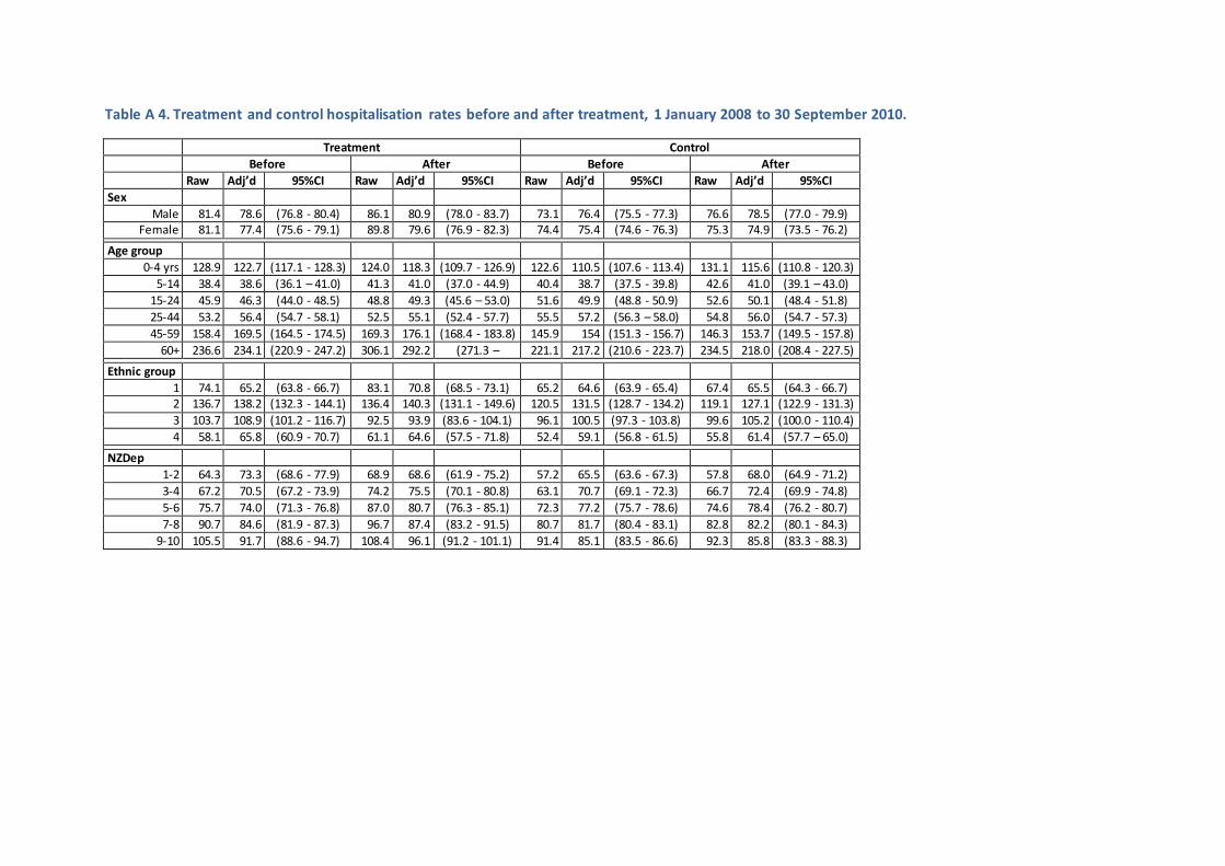
Table A 4. Treatment and control hospitalisation rates before and after treatment, 1 January 2008 to 30 September 2010.

Treatment Control

Before After Before After

Raw Adj’d 95%CI Raw Adj’d 95%CI Raw Adj’d 95%CI Raw Adj’d 95%CI

Sex

Male 81.4 78.6 (76.8 - 80.4) 86.1 80.9 (78.0 - 83.7) 73.1 76.4 (75.5 - 77.3) 76.6 78.5 (77.0 - 79.9) Female 81.1 77.4 (75.6 - 79.1) 89.8 79.6 (76.9 - 82.3) 74.4 75.4 (74.6 - 76.3) 75.3 74.9 (73.5 - 76.2)

Age group

0-4 yrs 128.9 122.7 (117.1 - 128.3) 124.0 118.3 (109.7 - 126.9) 122.6 110.5 (107.6 - 113.4) 131.1 115.6 (110.8 - 120.3)

5-14 38.4 38.6 (36.1 – 41.0) 41.3 41.0 (37.0 - 44.9) 40.4 38.7 (37.5 - 39.8) 42.6 41.0 (39.1 – 43.0)

15-24 45.9 46.3 (44.0 - 48.5) 48.8 49.3 (45.6 – 53.0) 51.6 49.9 (48.8 - 50.9) 52.6 50.1 (48.4 - 51.8)

25-44 53.2 56.4 (54.7 - 58.1) 52.5 55.1 (52.4 - 57.7) 55.5 57.2 (56.3 – 58.0) 54.8 56.0 (54.7 - 57.3)

45-59 158.4 169.5 (164.5 - 174.5) 169.3 176.1 (168.4 - 183.8) 145.9 154 (151.3 - 156.7) 146.3 153.7 (149.5 - 157.8)

60+ 236.6 234.1 (220.9 - 247.2) 306.1 292.2 (271.3 – 313.0)

221.1 217.2 (210.6 - 223.7) 234.5 218.0 (208.4 - 227.5)

Ethnic group

1 74.1 65.2 (63.8 - 66.7) 83.1 70.8 (68.5 - 73.1) 65.2 64.6 (63.9 - 65.4) 67.4 65.5 (64.3 - 66.7) 2 136.7 138.2 (132.3 - 144.1) 136.4 140.3 (131.1 - 149.6) 120.5 131.5 (128.7 - 134.2) 119.1 127.1 (122.9 - 131.3)

3 103.7 108.9 (101.2 - 116.7) 92.5 93.9 (83.6 - 104.1) 96.1 100.5 (97.3 - 103.8) 99.6 105.2 (100.0 - 110.4)

4 58.1 65.8 (60.9 - 70.7) 61.1 64.6 (57.5 - 71.8) 52.4 59.1 (56.8 - 61.5) 55.8 61.4 (57.7 – 65.0)

NZDep quintile

1-2 64.3 73.3 (68.6 - 77.9) 68.9 68.6 (61.9 - 75.2) 57.2 65.5 (63.6 - 67.3) 57.8 68.0 (64.9 - 71.2)

3-4 67.2 70.5 (67.2 - 73.9) 74.2 75.5 (70.1 - 80.8) 63.1 70.7 (69.1 - 72.3) 66.7 72.4 (69.9 - 74.8)

5-6 75.7 74.0 (71.3 - 76.8) 87.0 80.7 (76.3 - 85.1) 72.3 77.2 (75.7 - 78.6) 74.6 78.4 (76.2 - 80.7)

7-8 90.7 84.6 (81.9 - 87.3) 96.7 87.4 (83.2 - 91.5) 80.7 81.7 (80.4 - 83.1) 82.8 82.2 (80.1 - 84.3)

9-10 105.5 91.7 (88.6 - 94.7) 108.4 96.1 (91.2 - 101.1) 91.4 85.1 (83.5 - 86.6) 92.3 85.8 (83.3 - 88.3)

54

APPENDIX 2 HOUSE TYPOLOGIES

QV DWELLING TYPES

These dwelling type descriptions have been provided by Property IQ, a subsidiary of QV.

Dwelling Types, referred to by QV as “House types”, are used by Valuers as a general way of

characterising a house. They are not strictly defined nor mutually exclusive and there can be

overlaps between different house types. House type is chosen by the first Registered Valuer to

inspect and value a property.

Table A 5. QV Dwelling types .

Dwelling Type Description

Apartment generally built 1920s onwards - common entrance way, purpose built from the 1960s onwards, multi-storey blocks often with several apartments per floor. 5+ apartments per block. Apartments are normally joined on 2 walls.

Bach any age - basic design, materials, layout, often small floor size, two bedrooms, and open plan, frequently extended in different styles and materials. Also called a crib in Southland.

Contemporary

generally built 1970s onwards - modern, contemporary design, many roof breaks and pitches, high studs, grand entrance halls, often different angles walls, not uniform design. Often stucco, plaster walls. Building features are often

associated with weather-tightness issues.

Cottage generally built 1890-1900 door facing street, gable roof, veranda along front, single storey, weather clad, iron roof with two sloping slides

Pre-war bungalow

generally built 1920-1940s - House faces street - greater utility and less ostentatious, narrow weatherboard, iron roof, lower stud and gable, bay and boxed windows, verandas part of main roof. Timber joinery inside. Timber

shingles

Bungalow -

post war

generally built 1950s onwards - 'standard' dwelling using average quality materials and design. Can have gable, Dutch gable or Hip roof lines. Often

located for sunshine, not necessarily facing the street. Normally single storey, but sometime appears a dual storey if built over garage on sloping sections

Quality

Bungalow

generally built 1950s onwards - high quality materials, design, grand designs

often with swimming pools, tennis courts etc., can often be two storeys, larger sections.

Quality Old

generally built 1920-1940s - Tudor and Georgian influences, English styles, large

and grand, good quality materials, fixtures and fittings, usually 2 storey, weatherboards, stucco, brick and shingles, often in combination. Timber joinery. Sometimes referred to as "Arts and Crafts".

Spanish Bungalow

generally built 1930-1950 - Art Deco and Spanish styles, predominantly 30s and 40s built, horizontal lines feature in design, often curved walls, low pitched roofs, always stucco clad, and parapets around roof line.

State Rental generally built late 1930s onwards - purpose build by the government for social housing, often simple materials and basic design but constructed well, often multiunit, weatherboard cladding, clay or concrete tile roofs

55

Townhouse

generally built 1970s onwards - high site coverage, low maintenance sections, better quality than a Unit, can be detached or semi reattached, often separated

by a garage. Normally two storey. Stucco plaster wall coverings; can be prone to weather tightness issues. Often crossleased.

Unit generally built 1950s onwards - attached and semi-detached, 1-3 bedrooms,

small <100m2, basic design, open plan. Often cross leased.

Terraced

Apartment

generally built 1990s onwards - medium to high quality fixtures and fittings, often 2-3 levels, 3-5 units in the complex, party walls between the apartments. These

are NOT necessarily "flats". Often own entrance and garage with dwelling space above.

Villa

generally built 1900 - 1920s - door faces street, weatherboard, high stud, can be

one or two storey, iron roof with four sides and single point, eaves, brackets, finial, fretwork common

DWELLING HEALTH RISK TYPOLOGY

The authors developed a six-category dwelling health risk typology for this study. This classification

was based upon previous research and unpublished analysis of health outcomes by dwelling type,

and is based upon QV data for dwelling construction decade; dwelling type; roof and wall condition;

and the overall dwelling condition indicator included in the “category” field.

The dwelling health risk typology has two components: a binary construction type indicator (new,

old), and a ternary condition indicator (high, average, low).

Dwellings were assigned to the “old” construction category if they were built before 1950; or

belonged to QV house type categories "Pre-war Bungalow", "Spanish Bungalow", or "Quality Old".

Otherwise, they were assigned to the “new” construction category, as were pre-1950 dwellings with

the QV house type “Contemporary”.

For the condition indicator, dwellings were initially assigned to the “average” category. Second, any

dwellings with a QV overall condition category of “Superior” were reassigned to the “low risk”

category. Next, dwellings were reassigned to the “high risk” category if:

- the QV dwelling quality indicator was “Poor”;

- the Wall condition was “Poor”;

- the Roof condition was “Poor”;

- the dwelling was built in the 1930s or 1940s; the dwelling type was not “Quality Old” ,

“Quality Bungalow” or “Contemporary”; and the overall condition was not “Superior”; or

- the dwelling was a “Post-war Bungalow” built in the 2000s and its overall condition was not

“Superior”.

Finally, dwellings were reassigned to the “low risk” category if the QV dwelling type was “Quality

Old”, “Quality Bungalow” or “Contemporary” and the dwelling had not previously been assigned to

the “high risk” category

56

The construction type and condition categories were then combined to create the six categories

“Old high risk”, “Old average risk”, “Old low risk”, “New high risk”, “New average risk”, and “New

low risk”.

57

APPENDIX 3 ANNUAL BENEFIT OF REDUCED MORTALITY ( ALL TREATMENT HOUSEHOLDS)

Note: each result has been adjusted to avoid “double counting” as described on pg. 38. We reduced figures based on two additional life years gained

beyond the first by 10%, four additional life years by 15%, eight additional life years by 25% and ten additional life years 35%.

Table A 6. Annual benefit of reduced mortality, all treatment households, 0% discount rate

Life years beyond first gained

0 2 4 8 10

Value life year 95% CI 95% CI 95% CI 95% CI 95% CI

Transport 1991 Based VPF

$83,811 (0% ) $35.74 $0.00 - $62.21

$160.83 $0.00 - $279.96 $273.40 $0.00 - $475.92 $455.67 $0.00 - $793.21 $487.84 $0.00 - $849.2

$150,000 (3% ) $63.96 $0.00 - $111.34

$287.84 $0.00 - $501.05 $489.32 $0.00 - $851.78 $815.54 $0.00 - $1419.64

$873.10 $0.00 - $1519.85

$195,375 (5% ) $83.31 $0.00 -

$145.03 $374.91 $0.00 - $652.62 $637.34

$0.00 -

$1109.45 $1,062.24

$0.00 -

$1849.08 $1,137.22

$0.00 -

$1979.6

Transport 1998 based VPF

$141,918 (0% ) $60.52 $0.00 - $105.34

$272.33 $0.00 - $474.05 $462.96 $0.00 - $805.89 $771.60 $0.00 - $1343.15

$826.06 $0.00 - $1437.96

$245,589 (3%) $104.73 $0.00 - $182.3

$471.26 $0.00 - $820.35 $801.15 $0.00 - $1394.59

$1,335.24 $0.00 - $2324.31

$1,429.50 $0.00 - $2488.38

$330,830 (5%) $141.07 $0.00 - $245.57

$634.83 $0.00 - $1105.08

$1,079.22 $0.00 - $1878.63

$1,798.69 $0.00 - $3131.06

$1,925.66 $0.00 - $3352.07

Fire BERL 2007 VPF $55,315 (0%) $23.59 $0.00 - $41.06

$106.14 $0.00 - $184.77 $180.45 $0.00 - $314.11 $300.74 $0.00 - $523.51 $321.97 $0.00 - $560.47

$95,723 (3%) $40.82 $0.00 -

$71.05 $183.68 $0.00 - $319.75 $312.26 $0.00 - $543.57 $520.44 $0.00 - $905.95 $557.17

$0.00 -

$969.9

$128,947 (5%) $54.99 $0.00 - $95.72

$247.44 $0.00 - $430.72 $420.64 $0.00 - $732.23 $701.07 $0.00 - $1220.39

$750.56 $0.00 - $1306.53

58

Table A 7. Annual benefit of reduced mortality, all treatment households, 3% discount rate

Life years beyond first

gained 0 2 4 8 10

Value life year 95% CI 95% CI 95% CI 95% CI 95% CI

Transport 1991 Based VPF

$83,811 (0% ) $35.74 $0.00 - $62.21 $155.26 $0.00 - $270.27 $256.22 $0.00 - $446 $403.12 $0.00 - $701.73 $419.55 $0.00 - $730.33

$150,000 (3% ) $63.96 $0.00 - $111.34

$277.87 $0.00 - $483.71 $458.56 $0.00 - $798.23 $721.48 $0.00 - $1255.91

$750.89 $0.00 - $1307.1

$195,375 (5% ) $83.31 $0.00 - $145.03

$361.93 $0.00 - $630.03 $597.27 $0.00 - $1039.7 $939.73 $0.00 - $1635.82

$978.03 $0.00 - $1702.49

Transport 1998 based

VPF $141,918 (0% ) $60.52

$0.00 -

$105.34 $262.90 $0.00 - $457.64 $433.85 $0.00 - $755.22 $682.61

$0.00 -

$1188.24 $710.43

$0.00 -

$1236.67

$245,589 (3%) $104.73 $0.00 - $182.3 $454.95 $0.00 - $791.95 $750.78 $0.00 - $1306.92

$1,181.25 $0.00 - $2056.25

$1,229.40 $0.00 - $2140.06

$330,830 (5%) $141.07 $0.00 - $245.57

$612.86 $0.00 - $1066.83

$1,011.37 $0.00 - $1760.53

$1,591.25 $0.00 - $2769.95

$1,656.10 $0.00 - $2882.85

Fire BERL 2007 VPF $55,315 (0%) $23.59 $0.00 - $41.06 $102.47 $0.00 - $178.37 $169.10 $0.00 - $294.36 $266.06 $0.00 - $463.14 $276.90 $0.00 -

$482.01

$95,723 (3%) $40.82 $0.00 - $71.05 $177.33 $0.00 - $308.68 $292.63 $0.00 - $509.4 $460.41 $0.00 - $801.46 $479.18 $0.00 - $834.13

$128,947 (5%) $54.99 $0.00 - $95.72 $238.87 $0.00 - $415.82 $394.20 $0.00 - $686.2 $620.22 $0.00 -

$1079.64 $645.50

$0.00 -

$1123.64

59

Table A 8. Annual benefit of reduced mortality, all treatment households, 5% discount rate

Life years beyond first

gained 0 2 4 8 10

Value life year 95% CI 95% CI 95% CI 95% CI 95% CI

Transport 1991 Based VPF

$83,811 (0% ) $35.74 $0.00 - $62.21 $151.78 $0.00 - $264.21 $245.82 $0.00 - $427.9 $373.29 $0.00 - $649.8 $381.99 $0.00 - $664.94

$150,000 (3% ) $63.96 $0.00 - $111.34

$271.65 $0.00 - $472.87 $439.956 $0.00 - $765.84 $668.09

$0.00 - $1162.97

$683.66 $0.00 - $1190.07

$195,375 (5% ) $83.31 $0.00 -

$145.03 $353.82 $0.00 - $615.92 $573.03 $0.00 - $997.5 $870.19

$0.00 -

$1514.77 $890.47 $0.00 - $1550.07

Transport 1998 based VPF

$141,918 (0% ) $60.52 $0.00 - $105.34

$257.01 $0.00 - $447.39 $416.24 $0.00 - $724.57 $632.09 $0.00 - $1100.31

$646.82 $0.00 - $1125.95

$245,589 (3%) $104.73 $0.00 - $182.3 $444.76 $0.00 - $774.21 $720.31 $0.00 -

$1253.87 $1,093.83

$0.00 -

$1904.08 $1,119.33 $0.00 - $1948.46

$330,830 (5%) $141.07 $0.00 - $245.57

$599.13 $0.00 - $1042.93

$970.32 $0.00 - $1689.08

$1,473.49 $0.00 - $2564.97

$1,507.83 $0.00 - $2624.75

Fire BERL 2007 VPF $55,315 (0%) $23.59 $0.00 - $41.06 $100.18 $0.00 - $174.38 $162.24 $0.00 - $282.42 $246.37 $0.00 - $428.86 $252.11 $0.00 - $438.86

$95,723 (3%) $40.82 $0.00 - $71.05 $173.35 $0.00 - $301.76 $280.76 $0.00 - $488.72 $426.34 $0.00 - $742.15 $436.28 $0.00 - $759.45

$128,947 (5%) $54.99 $0.00 - $95.72 $233.52 $0.00 - $406.5 $378.20 $0.00 - $658.35 $574.32 $0.00 - $999.74 $587.71 $0.00 - $1023.04

6 This is our preferred estimate.

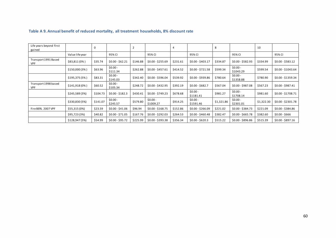
60

Table A 9. Annual benefit of reduced mortality, all treatment households, 8% discount rate

Life years beyond first

gained 0 2 4 8 10

Value life year 95% CI 95% CI 95% CI 95% CI 95% CI

Transport 1991 Based VPF

$83,811 (0% ) $35.74 $0.00 - $62.21 $146.88 $0.00 - $255.69 $231.61 $0.00 - $403.17 $334.87 $0.00 - $582.93 $334.99 $0.00 - $583.12

$150,000 (3% ) $63.96 $0.00 - $111.34

$262.88 $0.00 - $457.61 $414.52 $0.00 - $721.58 $599.34 $0.00 - $1043.29

$599.54 $0.00 - $1043.64

$195,375 (5% ) $83.31 $0.00 -

$145.03 $342.40 $0.00 - $596.04 $539.92 $0.00 - $939.86 $780.64

$0.00 -

$1358.88 $780.90 $0.00 - $1359.34

Transport 1998 based VPF

$141,918 (0% ) $60.52 $0.00 - $105.34

$248.72 $0.00 - $432.95 $392.19 $0.00 - $682.7 $567.04 $0.00 - $987.08 $567.23 $0.00 - $987.41

$245,589 (3%) $104.73 $0.00 - $182.3 $430.41 $0.00 - $749.23 $678.68 $0.00 -

$1181.41 $981.27

$0.00 -

$1708.14 $981.60 $0.00 - $1708.71

$330,830 (5%) $141.07 $0.00 - $245.57

$579.80 $0.00 - $1009.27

$914.25 $0.00 - $1591.46

$1,321.86 $0.00 - $2301.01

$1,322.30 $0.00 - $2301.78

Fire BERL 2007 VPF $55,315 (0%) $23.59 $0.00 - $41.06 $96.94 $0.00 - $168.75 $152.86 $0.00 - $266.09 $221.02 $0.00 - $384.73 $221.09 $0.00 - $384.86

$95,723 (3%) $40.82 $0.00 - $71.05 $167.76 $0.00 - $292.03 $264.53 $0.00 - $460.48 $382.47 $0.00 - $665.78 $382.60 $0.00 - $666

$128,947 (5%) $54.99 $0.00 - $95.72 $225.99 $0.00 - $393.38 $356.34 $0.00 - $620.3 $515.22 $0.00 - $896.86 $515.39 $0.00 - $897.16

61

Table A 10. Annual benefit of reduced mortality, all treatment households, 10% discount rate

Life years beyond first

gained 0 2 4 8 10

Value life year 95% CI 95% CI 95% CI 95% CI 95% CI

Transport 1991 Based VPF

$83,811 (0% ) $35.74 $0.00 - $62.21 $143.81 $0.00 - $250.34 $222.97 $0.00 - $388.13 $312.80 $0.00 - $544.51 $308.71 $0.00 - $537.39

$150,000 (3% ) $63.96 $0.00 - $111.34

$257.39 $0.00 - $448.04 $399.05 $0.00 - $694.65 $559.83 $0.00 - $974.53 $552.51 $0.00 - $961.78

$195,375 (5% ) $83.31 $0.00 - $145.03

$335.25 $0.00 - $583.58 $519.77 $0.00 - $904.78 $729.18 $0.00 - $1269.32

$719.65 $0.00 - $1252.72

Transport 1998 based VPF

$141,918 (0% ) $60.52 $0.00 - $105.34

$243.52 $0.00 - $423.9 $377.55 $0.00 - $657.22 $529.67 $0.00 - $922.02 $522.74 $0.00 - $909.96

$245,589 (3%) $104.73 $0.00 - $182.3 $421.41 $0.00 - $733.57 $653.36 $0.00 -

$1137.32 $916.59

$0.00 -

$1595.55 $904.61 $0.00 - $1574.69

$330,830 (5%) $141.07 $0.00 - $245.57

$567.68 $0.00 - $988.18 $880.13 $0.00 - $1532.07

$1,234.73 $0.00 - $2149.35

$1,218.59 $0.00 - $2121.24

Fire BERL 2007 VPF $55,315 (0%) $23.59 $0.00 - $41.06 $94.92 $0.00 - $165.22 $147.16 $0.00 - $256.16 $206.45 $0.00 - $359.37 $203.75 $0.00 - $354.67

$95,723 (3%) $40.82 $0.00 - $71.05 $164.25 $0.00 - $285.92 $254.66 $0.00 - $443.29 $357.26 $0.00 - $621.9 $352.59 $0.00 - $613.77

$128,947 (5%) $54.99 $0.00 - $95.72 $221.26 $0.00 - $385.16 $343.05 $0.00 - $597.15 $481.26 $0.00 - $837.75 $474.97 $0.00 - $826.79

62

REFERENCES

1. Howden-Chapman, P., et al., Effect of insulating existing houses on health inequality: cluster randomised study in the community. British Medical Journal, 2007(334): p. 460.

2. Chapman, R., et al., Retrofitting housing with insulation: a cost-benefit analysis of a randomised community trial. Journal of Epidemiology and Community Health, 2009. 63: p. 271– 277

3. Howden-Chapman, P., et al., Effects of improved home heating on asthma in community

dwelling children: randomised community study. British Medical Journal, 2008. 337: p. 852-855.

4. Preval, N., et al., Evaluating energy, health and carbon co-benefits from improved domestic space heating: A randomised community trial. Energy Policy, 2010. 38(9): p. 3965-3972.

5. Rose, G., The strategy of preventive medicine1992, Oxford: Oxford University Press.

6. Krieger, J. and D. Higgins, Housing and health: time again for public health action. American Journal of Public Health, 2002(92): p. 758-68.

7. Howden-Chapman, P., Housing standards: a glossary of housing and health. Journal of Epidemiology and Community Health, 2004(58): p. 162-8.

8. Sundell, J., On the history of indoor air quality and health. Indoor Air, 2004(14): p. 51-8.

9. Wilkinson, P., et al., Cold comfort: the social and environmental determinants of excess winter deaths in England, 1986-96 2001, London: The Policy Press.

10. Boardman, B., Fuel poverty: from cold homes to affordable warmth1991, London: Belhaven Press.

11. Heyman, B., et al., Keeping warm and staying well. Does home energy efficiency mediate the relationship between socio-economic status and the risk of poorer health? Housing Studies, 2005. 20(4): p. 649-664.

12. Healy, J.D., Housing, fuel poverty and health: a pan-European analysis2004, Aldershot: Ashgate Publishing Ltd.

13. Curwen, M., Excess winter mortality: a British phenomenon? Health Trends, 1991. 4: p. 169-175.

14. Tobin, R., et al., The significance of fungi in indoor air. Canadian Journal of Public Health. Revue Canadienne de Sante Publique, 1987(78): p. S1-14.

15. Institute of Medicine of the National Academies, Damp indoor spaces and health2004, Washington, D.C.: National Academies Press.

16. Bonnefoy, X.R., et al., Housing and health in Europe: preliminary results of a pan-European study. American Journal of Public Health, 2003. 93(9): p. 1559-1563.

17. Acheson, D., Independent inquiry into inequalities in health report1998, London: Stationery Office.

63

18. Howden-Chapman, P. and M. Tobias, eds. Social inequalities in health: New Zealand 1999. 2000, Ministry of Health: Wellington.

19. Department of Health, Our healthier nation: a contract for health, 1998, Stationery Office: London.

20. The Eurowinter Group, Cold exposure and winter mortality from ischaemic heart disease, cerebrovascular disease, respiratory disease, and all causes in warm and cold regions of

Europe. The Lancet, 1997. 349: p. 1341-1346.

21. Telfar Barnard, L., Home truths and cool admissions: New Zealand housing traits and excess winter hospitalisation, PhD Thesis,, 2010, University of Otago: Wellington.

22. Davie, G., et al., Trends and determinants of excess winter mortality in New Zealand: 1980 to 2000. BMC Public Health, 2007. 7(1): p. 263.

23. Thomson, H., et al., The health impacts of housing improvement: a systematic review of intervention studies from 1887 to 2007. American Journal of Public Health, 2009. 99(Supplement 3): p. S681-S692.

24. Jacobs, D.E., et al., A Systematic Review of Housing Interventions and Health: Introduction, Methods, and Summary Findings, . Journal of Public Health Management & Practice, 2010. 16(5): p. S5-S10.

25. Howden-Chapman, P., et al., Retrofitting houses with insulation to reduce health inequalities: results of a clustered, randomised trial in a community setting. British Medical Journal, 2007.

334: p. 460-464.

26. Davie, G.S., et al., Trends and determinants of excess winter mortality in New Zealand: 1980 to 2000. BMC Public Health, 2007. 7(263).

27. Telfar Barnard, L., Home truths and cool admissions: New Zealand housing attributes and excess winter hospitalisation, in Public Health2010, University of Otago: Wellington.

28. Wilson, J.S., et al., A Systematic Review of the Biological and Health Effects of Exposure to Cold Temperature in Healthy and Diseased Adults Including the Elderly, D.o. Health, Editor

2001, Birmingham Health Technology Assessment Group, University of Birmingham. p. 140.

29. Keatinge, W.R., et al., Increases in platelet and red cell counts, blood viscosity, and arterial pressure during mild surface cooling: factors in mortality from coronary and cerebral thrombosis in winter. British Medical Journal Clinical Research Ed, 1984. 289(6456): p. 1405-

8.

30. Hajat, S., W. Bird, and A. Haines, Cold Weather and GP consultations for respiratory conditions by elderly people in 16 locations in the UK. European Journal of Epidemiology,

2004. 19(10): p. 959-968.

31. Mäkinen, T.M., et al., Cold temperature and low humidity are associated with increased occurrence of respiratory tract infections. Respiratory Medicine, 2009. 103(3): p. 456-462.

32. Eccles, R., An explanation for the seasonality of acute upper respiratory tract viral infections. Acta Oto-laryngologica, 2002. 122(2): p. 183-191.

33. National Health Board Business Unit, National Minimum Dataset (Hospital Events) Data dictionary, 2010, Ministry of Health: Wellington.

64

34. New Zealand Health Information Service, Pharmaceutical claims datamart (PHARMS) data dictionary, 2006, Ministry of Health: Wellington.

35. Baker, M., et al., Close-contact infectious diseases in New Zealand: Trends and ethnic inequalities in hospitalisations 1989 to 2008, 2010, Housing and Health Research Programme, University of Otago: Wellington.

36. O'Dea, D. and J. Wren, New Zealand estimates of the total social and economic cost of "all injuries" and the six priority areas respectively, at June 2008 prices: technical report prepared for NZIPS evaluation., 2010: Wellington, New Zealand.

37. Miller, T.R. and J. Guria, The Value of Statistical Life in New Zealand: Market Research on Road Safety, 1991: Wellington, New Zealand.

38. Howden-Chapman, P., et al., Effects of improved home heating on asthma in community dwelling children: randomised controlled trial. BMJ, 2008. 337: p. a1411.

39. Preval, N., et al., Evaluating energy, health and carbon co-benefits from improved domestic space heating: A randomised community trial. Energy Policy, 2010. 38(8): p. 3965-3972.

40. Masoli, M., et al., The global burden of asthma: executive summary of the GINA Dissemination Committee Report. Allergy, 2004. 59(5): p. 469-478.