Improved Modelling of Induction and Transduction Heaters
131
Improved Modelling of Induction and Transduction Heaters Lisiate Takau A thesis presented for the degree of Doctor of Philosophy in Electrical and Computer Engineering at the University of Canterbury, Christchurch, New Zealand. 2015
-
Upload
khangminh22 -
Category
Documents
-
view
1 -
download
0
Transcript of Improved Modelling of Induction and Transduction Heaters
Improved Modelling of Induction and
Transduction Heaters
Lisiate Takau
A thesis presented for the degree of
Doctor of Philosophy
in
Electrical and Computer Engineering
at the
University of Canterbury,
Christchurch, New Zealand.
2015


ABSTRACT
This thesis starts by describing research on the design of low frequency induction heaters using
a series equivalent circuit model. Limitations associated with this design method are explained.
An alternative called the transformer equivalent circuit (TEC) model is then presented. This
models the induction heater as a single turn secondary transformer. Its advantage is that the
currents and voltages associated with components of the induction heater are what you would
expect to measure on components of an actual induction heater. Finite element analysis (FEA)
is also used to predict the performance of induction heaters. The performances of these models
are compared, with experimental verification on a small induction heater unit.
The research is then extended to transduction heaters, a combination of transformer and in-
duction heaters, which include a secondary winding to boost performance. The transformer
equivalent circuit method is used to predict the performance of transduction heaters as they
cannot be modelled using the series equivalent circuit model. The performances of the trans-
former equivalent circuit and finite element analysis models are compared with results from a
set of experimental transduction heaters.
Modifications are then made to the components of the TEC model to improve its performance
predictions. The accuracy of TEC modelling is confirmed with a second design and verified
with experimental results. This forms the basis for the final design and implementation of an
industrial unit.
The improved TEC model is then used to predict the performance of a 40kW transduction fluid
heater that was designed, built and tested. Comparisons are made between the TEC and FEA
models calculated results and test results. The TEC calculated results yielded much closer values
to those measured.


ACKNOWLEDGEMENTS
First of all, I would like to express my sincere gratitude to my supervisor, Professor Pat Bodger
and my co-supervisor Associate Professor Paul Gaynor for all the encouragement and support
that they have provided throughout the course of this study. I would like to thank Pat for
guidance and advice even after he retired from the University. The benefit of his experience has
contributed significantly to all stages of this work.
I would like to express my gratitude to my postgraduate comrades, Dr Bhaba Das, Dr Michael
Huang, Dr Senthuran Sivasubramaniam, Ming Zhong, Yanosh Irani, and Diwakar Bhujel for
the never-ending discussions on research we shared together. I would also like to mention my
colleagues at UL, Vinesh Chand, Christopher Bennetts, Neil Mallare, and Michael Passe, for all
our whiteboard-discussions about transformer equivalent circuits. The quote that summed up
these discussions was: “It’s all about the magnetizing reactance”.
I would like to acknowledge the technical staff at the Electrical and Computer Engineering
Department, Ken Smart in the Electrical Machines Lab, Edsel Villa in the Power Electronics
Lab, Florin Predan in the Computer Lab, David Healey in the Mechanical Workshop, and Paul
Agger in the High Voltage Lab for their support over the past years.
Finally, I would like to express my most sincere appreciation to my family for their love, patience,
and support.

CONTENTS
ABSTRACT iii
ACKNOWLEDGEMENTS v
LIST OF FIGURES xii
LIST OF TABLES xiv
GLOSSARY xv
CHAPTER 1 INTRODUCTION 1
1.1 General Overview 1
1.2 Thesis Objectives 2
1.3 Thesis Contribution 2
1.4 Thesis Outline 3
CHAPTER 2 HISTORICAL DEVELOPMENT 5
2.1 Introduction 5
2.2 Background 5
2.3 Induction Heating 6
2.3.1 Electromagnetic Induction 7
2.3.2 Basic Induction Heating 8
2.4 SEC Model of Induction Heater 11
2.4.1 SEC Performance 15
2.4.2 Equivalent Circuit Performance for an Experimental Induc-
tion Heater 16
2.4.3 Material Properties 17
2.5 Calculated Performance Using SEC Model 17
2.6 Summary 18
CHAPTER 3 TRANSFORMER MODEL OF INDUCTION HEATER 21
3.1 Introduction 21
3.2 Transformer Fundamentals 21
3.2.1 Ideal Transformers 21
3.2.2 Non-Ideal Transformers 24
3.3 Transformer Equivalent Circuit of Induction Heater 26

viii CONTENTS
3.4 Calculation of Equivalent Circuit Parameters 27
3.4.1 Coil Resistance 28
3.4.2 Workpiece Magnetizing Reactance 30
3.4.3 Coil/Workpiece Leakage Reactance 33
3.4.4 Workpiece Eddy Current Resistance 35
3.5 Equivalent Circuit Performance 36
3.5.1 Equivalent Circuit Performance for an Experimental Induc-
tion Heater 36
3.5.2 Equivalent Circuit Parameters 36
3.5.3 TEC Calculated Performance 37
3.6 Summary 39
CHAPTER 4 FINITE ELEMENT ANALYSIS AND MEASURED
PERFORMANCE OF EXPERIMETAL INDUCTION
HEATER 41
4.1 Introduction 41
4.2 Finite Element Method 41
4.2.1 FEA Study of the Experimental Induction Heater 42
4.2.2 Flux Plot of the Experimental Induction Heater 44
4.2.3 FEA Performance Calculation 45
4.3 Measured Performance of Experimental Induction Heater 46
4.3.1 Analysis 48
4.4 Summary 49
CHAPTER 5 TRANSFORMER AND TRANSDUCTION HEATING 51
5.1 Introduction 51
5.2 Transformer Heater 51
5.3 Equivalent Circuit of Transformer Heater 52
5.3.1 Winding Resistances 53
5.3.2 Magnetizing Reactance 54
5.3.3 Leakage Reactance 55
5.4 Transduction Heating 55
5.4.1 Basic Heating Concepts 55
5.5 Transduction Heater 57
5.6 Measured Performance of Experimental Transduction Heater 59
5.7 Equivalent Circuit of Transduction Heater 60
5.7.1 Winding Resistance 62
5.7.2 Magnetizing Reactance 63
5.7.3 Core Tube Eddy Current Resistance 63
5.7.4 Leakage Reactance 63
5.8 Equivalent Circuit Performance 64
5.9 FEA Performance Calculation 65
5.10 Design of a 6kW Transduction Heater 68
5.11 Summary 70

CONTENTS ix
CHAPTER 6 DESIGN OF AN INDUSTRIAL TRANSDUCTION FLUID
HEATER 73
6.1 Introduction 73
6.2 Transformers 73
6.3 Induction Heaters 74
6.4 Transduction Heater Design 74
6.5 Design Description 75
6.5.1 Design Consideration 75
6.6 Construction Details 76
6.6.1 Core Tube 77
6.6.2 Secondary Tube 77
6.6.3 Thermal Insulation 79
6.6.4 Primary Winding 80
6.6.5 Inter-Layer Insulation 80
6.6.6 Baffle 81
6.6.7 Transduction Heater Cooling 82
6.6.8 Transduction Heater Housing 83
6.7 Equivalent Circuit 84
6.7.1 Equivalent Circuit Performance 84
6.7.2 Calculated Performance 84
6.8 FEA Results 86
6.9 Summary 88
CHAPTER 7 EXPERIMENTAL RESULTS 89
7.1 Introduction 89
7.2 Experimental Setup 89
7.2.1 Test Equipment 89
7.2.2 Taking Measurements 90
7.3 Transduction Heater Performance 91
7.3.1 Winding Resistance and Insulation Resistance Tests 91
7.3.2 Power Input Test 92
7.3.3 Heating Test 92
7.4 Other Experimental Results 96
7.4.1 AC Withstand Voltage Test 96
7.4.2 Glow-wire Test 97
7.5 Comparison with TEC and FEA Models 98
7.5.1 Winding Resistance Test Results 98
7.5.2 Electrical Performance 99
7.6 Summary 99
CHAPTER 8 CONCLUSIONS AND FUTURE WORK 101
8.1 Conclusions 101
8.2 Future Work 103
8.2.1 Heater Design 103
8.2.2 Improve Performance 104

x CONTENTS
REFERENCES 107
APPENDIX A GLOW-WIRE FLAMMABILITY TEST RESULTS 113
APPENDIX B LIST OF PUBLICATIONS 115
B.1 Conference Papers 115
B.2 Journal Papers 115

LIST OF FIGURES
2.1 Induction heating. 7
2.2 Magnetic flux plot of steel bar workpiece. 8
2.3 Induction heating coil around a billet. 9
2.4 Series equivalent circuit of induction heater. 11
2.5 Short coil equivalent circuit which includes an external reactance. 14
3.1 An ideal full-core transformer. 22
3.2 Equivalent circuit of a non-ideal transformer. 24
3.3 Transformer equivalent circuit of an induction heater. 27
3.4 Cross-section of a multi-layer coil induction heater with a tube workpiece. 28
3.5 Flux distribution for induction heaters with different winding thicknesses. 29
3.6 Axial view of the flux flow from a cylindrical workpiece. 31
3.7 Magnetic circuit of induction heater. 32
3.8 Dimensions for representing the leakage flux for an induction heater. 34
4.1 Cross-section of workpiece 1. 43
4.2 Finite element mesh of experimental induction heater of workpiece 1. 44
4.3 Flux plot of experimental induction heater of workpiece 1. 46
5.1 Transformer heater physical arrangement. 52
5.2 Coupled circuit representation. 52
5.3 Transformer heater equivalent circuit. 53
5.4 Cross-section of a multi-layer winding transformer heater with a full core. 54
5.5 Conceptual arrangement of induction fluid heater. 56
5.6 Conceptual arrangement of transformer fluid heater. 56
5.7 Conceptual arrangement of combined transformer heater and induction fluid heater. 57
5.8 Conceptual arrangement of transduction fluid heater. 58
xii LIST OF FIGURES
5.9 Cut-away image of transduction fluid heater. 59
5.10 Transduction heater with combination of tubes (2+5). 61
5.11 Equivalent circuit of transduction heater. 62
5.12 Flux plot of workpiece combination (1+4). 66
5.13 Flux plot of workpiece combination (2+5). 67
5.14 6kW transduction fluid heater. 69
6.1 Cross-section details of transduction fluid heater. 76
6.2 The core and secondary tubes over the workpiece. 78
6.3 Thermal insulation composite tube. 79
6.4 Inter-layer insulation. 81
6.5 Winding layout of 40kW transduction heater. 81
6.6 Assembled winding without outside insulation baffle. 82
6.7 Transduction heater housing. 83
6.8 Equivalent circuit of transduction heater. 84
6.9 Flux plot of designed heater. 87
7.1 Test setup (front view). 90
7.2 Test setup (rear view). 91
7.3 Temperatures over time during heating test. 94
7.4 Temperatures over time during heating test. 96
7.5 Glow-wire test setup. 98
8.1 Transduction heater with baffle. 104
8.2 Non-metallic cover piece with four slots. 105

LIST OF TABLES
2.1 Coil dimensions 16
2.2 Workpiece dimensions 17
2.3 Physical properties of copper and mild steel 17
2.4 Component values for the SEC long coil model 18
2.5 Calculated performance of experimental heater using SEC long coil model 18
3.1 Component values for the TEC model 36
3.2 Calculated performance using TEC model 37
3.3 Calculated performance using TEC model below the saturation point 40
4.1 Physical properties of copper and mild steel 45
4.2 Calculated performance using FEA model 45
4.3 Measured performance of experimental induction heater 47
4.4 Ratio of coil and workpiece loss 48
5.1 Coil dimensions 60
5.2 Workpiece and secondary tube dimensions 60
5.3 Measured performance at 100V supply 61
5.4 Physical properties 64
5.5 Calculated performance using TEC model for a 100V supply 64
5.6 Calculated performance using TEC model at 100V supply with scale factor applied 65
5.7 Calculated performance using FEA at a 100V supply 67
5.8 Coil dimensions 68
5.9 Workpiece dimensions 68
5.10 Component values for the TEC model 69
5.11 Calculated and measured results of the designed transduction heater 69
5.12 TEC calculated performance 70

xiv LIST OF TABLES
6.1 Core tube dimensions 77
6.2 Secondary tube dimensions 78
6.3 Thermal insulation dimensions 79
6.4 Primary winding dimensions 80
6.5 Stainless steel baffle dimensions 82
6.6 Equivalent circuit parameters 85
6.7 Equivalent circuit performance 85
6.8 TEC calculated performance 86
6.9 FEA transduction heater performance 87
7.1 Measured winding resistance 92
7.2 Insulation resistance test 92
7.3 Measured power input at rated voltage(horizontal mounting) 93
7.4 Measured power input at rated voltage(vertical mounting) 93
7.5 Heating test 94
7.6 Heating test 95
7.7 AC Withstand voltage test 97
7.8 Measured winding resistance results 98
7.9 Measured and calculated performance 99
GLOSSARY
NOMENCLATURE
δc Skin depth of coil in meters
δw Skin depth of workpiece in meters
η Efficiency
µ Magnetic permeability in henries per meter
µ0 Magnetic permeability of free space equal to (4π × 10−7)
µr Relative permeability
ω Angular frequency in radians per second
φ Magnetic flux in webers
σ Conductivity in siemens per meter
a Nominal turns ratio
Ag Cross-section air-gap area in square meters
Aw Cross-section area of workpiece in square meters
B Magnetic field density in tesla
Dw Diameter of workpiece in meters
e, Ec Induced emf of coil in volts
f Frequency in hertz
Ic Coil current in amperes
J Current density in ampere per square meter
k Hysteresis loss constant
Kr Dimensionless workpiece correction factor
kr Dimensionless coil space correction factor

xvi LIST OF TABLES
N , Nc Number of coil turns
p Dimensionless flux factor
Pc Coil power loss in watts
pc Inside perimeter of coil in meters
Pw Total power input to workpiece in watts
Pe Eddy current loss in watts
Ph Hysteresis loss in watts
q Dimensionless flux factor
Rc Coil resistance in ohms
Re Reluctance of external flux path in centimeter-gram-second units
Rw Workpiece resistance in ohms
Vc Applied coil voltage in volts
Wc Diameter of coil wire in meters
x Steinmetz factor
Xc Coil reactance in ohms
Xe End-effect reactance in ohms
Xg Air gap reactance in ohms
Xmc Core tube magnetising reactance in ohms
Xmw Workpiece magnetising reactance in ohms
Xw Workpiece reactance in ohms
Z Total impedance in ohms
ABBREVIATIONS
ac Alternating current
emf Electromotive force
FEA Finite element analysis
mmf Magnetomotive force
RMS Root mean squared
SEC Series equivalent circuit
TEC Transformer equivalent circuit
Chapter 1
INTRODUCTION
1.1 GENERAL OVERVIEW
New high efficiency technology in the heating industry is prompting a demand for safe, effi-
cient, and less energy consuming products. Induction heating has been widely used for differ-
ent applications such as heating of metals to heating of dairy fluids [Jang et al. 2003], [Egan
and Furlani 1991], [Tham et al. 2009], because of its preciseness of application which satisfy
these consumer demands. Electric water heaters have been the focus of several previous studies
because of their pervasiveness in power systems and their consequential potential importance
when considering conservation of energy through more efficient design and operation [Laurent
and Malhame 1994].
A transformer heater can be combined with an induction heater to improve performance. The
concept was initially developed as a new technology [Bodger et al. 1996] and is further developed
in this thesis under the term transduction heater. Transduction heating is normally used for
fluid heating. The typical arrangement is to have a primary winding that does not produce much
heat, a core tube that produces some heat, and a shorted secondary winding that produces most
of the heat. By making the secondary conductor hollow, or by adding a fluid channel outside
the conductor, the real power losses in the secondary tube can be transferred by convection to
the fluid, thus heating it up. A transduction heater converts electrical energy into hot fluids as
a continuous process.
The concept of transduction heating is new compared to induction heating. The existing models
used to calculate the performance of induction heaters cannot be used to model the performance
of transduction heaters. Therefore a new design method is needed that will accurately model
the performance of transduction heaters.
This thesis starts by introducing a transformer equivalent circuit (TEC) model as an alternative
to the existing series equivalent circuit (SEC) model and finite element analysis (FEA) for
designing induction heaters. These three models are used to model the performance of a set of
2 CHAPTER 1 INTRODUCTION
experimental units. The performance testing of the real heaters is then used to ascertain which
model gives the best prediction of real performance.
The research is then extended to transduction heating. The TEC model is then modified to
calculate their performance as they cannot be modelled using a SEC model. The modified TEC
model is then used to predict the performances of a set of transduction heating experiments.
The calculated results from the TEC and FEA models are compared with the measured results
and the TEC model is then improved by applying an empirical correction factor to three of its
circuit parameters.
This model has been used to design a 40kW transduction fluid heater. The calculated results
from the TEC and FEA models are compared with those measured from the actual heater.
1.2 THESIS OBJECTIVES
The main objectives of this thesis are:
• to improve the modelling of transduction heaters using finite element analysis.
• to develop and improve the transformer equivalent circuit to model the performance of
transduction heaters more accurately.
• to verify the performance prediction of the TEC model on a 40kW transduction heater.
The thesis entails both developing a computer model for modelling transduction heater perfor-
mance as well as the design and production of physical models.
1.3 THESIS CONTRIBUTION
The work in this thesis has led to development of a computer model that will be used to model
the performance of transduction heaters more accurately. This has been achieved through four
significant steps:
• The development of TEC model to calculate the performance of induction heaters at mains
frequency. The validity of this model was compared with the calculated results obtained
from the SEC model and FEA and also experimental results.
• The TEC model was improved to model the performance of transduction heaters and
verified on a 6kW design.

1.4 THESIS OUTLINE 3
• The proof of the design through the construction and testing of 40kW transduction fluid
heater. The validity of the modelling was tested through comparisons to measured data.
• The thermal properties of the winding and oil were validated through extensive testing of
the 40kW prototype.
1.4 THESIS OUTLINE
To achieve the objectives above, the thesis is structured into eight chapters. The chapters are
organized functionally from the modelling, design, simulation, construction and testing process
through to conclusions and future work.
Chapter 2 gives an introduction to induction heating and electromagnetic induction. The basic
theory of induction heating is covered. This is followed with an existing modelling technique
which models the performance of induction heaters. This is called the series equivalent circuit
model. This modelling technique is applied to a set of induction heaters.
Chapter 3 details the development of a transformer model of an induction heater. This is an
alternative to the SEC model presented in Chapter 2. The equivalent circuits for ideal and non-
ideal transformers are presented. These are transformed into a circuit to model the performance
of an induction heater. The parameters of the equivalent circuit are calculated using the reverse
design method. The TEC model is applied to the set of induction heaters presented in Chapter
2. The calculated results from the TEC model are compared with those from the SEC model.
Chapter 4 describes the work on finite element analysis and experimental induction heaters.
A 2D model of the set of experimental induction heaters was created and used for FEA. The
calculated results from the FEA are compared to those from TEC and SEC models. The
calculated results from the three models are compared with the measured experimental results.
Chapter 5 extends the research on induction heating to transduction heating, an induction heater
which includes a secondary winding to boost performance. The TEC model is used to model
the performance of transduction heating experiments. The validation of the model is applied
to a set of experimental transduction heaters. The calculated results from the TEC model are
compared with the measured experimental results. Modifications are made to the parameters
of the TEC model to improve its performance predictions. The improved TEC model is then
validated on a 6kW transduction heater.
Chapter 6 discusses the design and construction of a 40kW transduction fluid heater using the
improved TEC model. The details of the construction of the transduction fluid heater are given
including the insulation design, cooling system and construction materials.

4 CHAPTER 1 INTRODUCTION
Chapter 7 presents the performance tests of the 40kW transduction fluid heater. The test results
are compared to the calculated results from the TEC and FEA models.
Chapter 8 contains the conclusions and future work.

Chapter 2
HISTORICAL DEVELOPMENT
2.1 INTRODUCTION
Induction heating is a process where a varying magnetic field is used to heat a conductor or
workpiece. When a piece of metal or conductor is placed near a magnetic field created by
energising a coil of wire, the magnetic field transfers energy into the conductor, thus heating
it up. This chapter presents the theory of induction heating and its applications. It includes
a method for modelling induction heaters at mains frequency. This model is known as the
series equivalent circuit (SEC) model. The performance of this model is applied for a set of
demonstration induction heaters. The calculated results from the SEC model are discussed.
2.2 BACKGROUND
The discovery of electromagnetic induction by Michael Faraday in 1831 led to the understanding
of the principles involved in induction heating. Faraday’s experiments with two coils wound onto
an iron ring showed that the induced electromotive force (emf) in any closed circuit is equal to
the time rate of change of the magnetic flux through the circuit,
|e| =∣∣∣∣dφdt
∣∣∣∣ (2.1)
where e is the magnitude of the induced emf in volts and φ is the magnetic flux in webers. This
principle was used in motors, generators, transformers, and radio communications for almost a
decade [Zinn and Semiatin 1988].
The first major application of induction heating was melting of metals in the 19th century [Zinn
and Semiatin 1988]. Initially, this was done using metal or electrically conducting crucibles.
Later, Ferranti, Colby, and Kjellin [Zinn and Semiatin 1988] developed induction melting fur-

6 CHAPTER 2 HISTORICAL DEVELOPMENT
naces using non-conducting crucibles. In these designs, electric currents were induced directly
into the charge or the workpiece, at simple line frequency, or 60Hz.
Ring melting furnaces were all superseded in the early 1900s by the work of Northrup, who
designed and built equipment consisting of a cylindrical crucible and a high-frequency spark-gap
power supply [Zinn and Semiatin 1988]. This equipment was first used by Baker and Company
to melt platinum and by the American Brass Company to melt other non ferrous alloys [Zinn
and Semiatin 1988].
Other applications were developed following the acceptance of induction heating for melting
metal. These included induction surface hardening of steels introduced by Midvale Steel and
the Ohio Crankshaft Company [Zinn and Semiatin 1988].
A great use of induction heating technology was during the World War II, particularly in heat
treating of ordnance components such as armour-piercing projectiles and shot [Zinn and Semi-
atin 1988].
The application of induction heating and melting in recent years has increased to a point where
most engineers in the metalworking industries are familiar with existing applications and have
some ideas for potential uses. Induction heating is unique, as compared to other conventional
heating process. It is a non-contact method of quickly heating metal by inducing current in the
part to be heated. It does not rely on a heating element to touch the part to conduct heat.
2.3 INDUCTION HEATING
Induction heating is the heating of electrical conducting parts in a varying magnetic field. It
involves electromagnetic induction, skin effect and heat transfer.
An induction heating system consists of a source of alternating current ac, an induction coil,
and the workpiece to be heated [Zinn and Semiatin 1988]. The role of the power supply is taken
into account only in terms of the frequency and magnitude of the ac voltage that it supplies to
the coil.
Induction heating relies on two mechanisms of energy dissipation for the purpose of heating [Zinn
and Semiatin 1988]. These are energy losses due to Joule heating and energy losses associated
with magnetic hysteresis.
The first of these is the sole mechanism of heat generation in non-magnetic materials (e.g.
aluminium, copper, stainless steel and carbon steels above the Curie temperature) and the
primary mechanism in ferromagnetic materials (carbon steel below the Curie temperature) [Zinn
and Semiatin 1988].
2.3 INDUCTION HEATING 7
The second mechanism of heat generation by induction for ferromagnetic materials is hysteresis
losses. This is where the magnetic dipoles turn around with each reversal of the magnetic field
applied to the material. The losses are due to the rotational friction between the molecules.
This loss is often ignored in design studies.
2.3.1 Electromagnetic Induction
Electromagnetic induction describes the generation of a voltage in a conductor. It can happen
in two entirely different ways; motional induction, where a conductor moves in a magnetic
field, or transformer induction, where the circuit is stationary and the field varies with time
[Edwards 2004]. Faraday’s law of electromagnetic induction, which relates the generated voltage
to the rate of change of flux, can take account of both effects.
If a conductor is supplied with an alternating current, then a magnetic field is set up in the
region surrounding the conductor [Barber 1983]. If a second electrical circuit is placed in this
magnetic field, an electromotive force (emf) or voltage is induced in the circuit. If the circuit is
closed, a current will flow in the circuit. The magnitude of this secondary current will depend
on the strength of the magnetic field, the electrical impedance of the secondary circuit and the
geometrical configuration of the two sets of conductors.
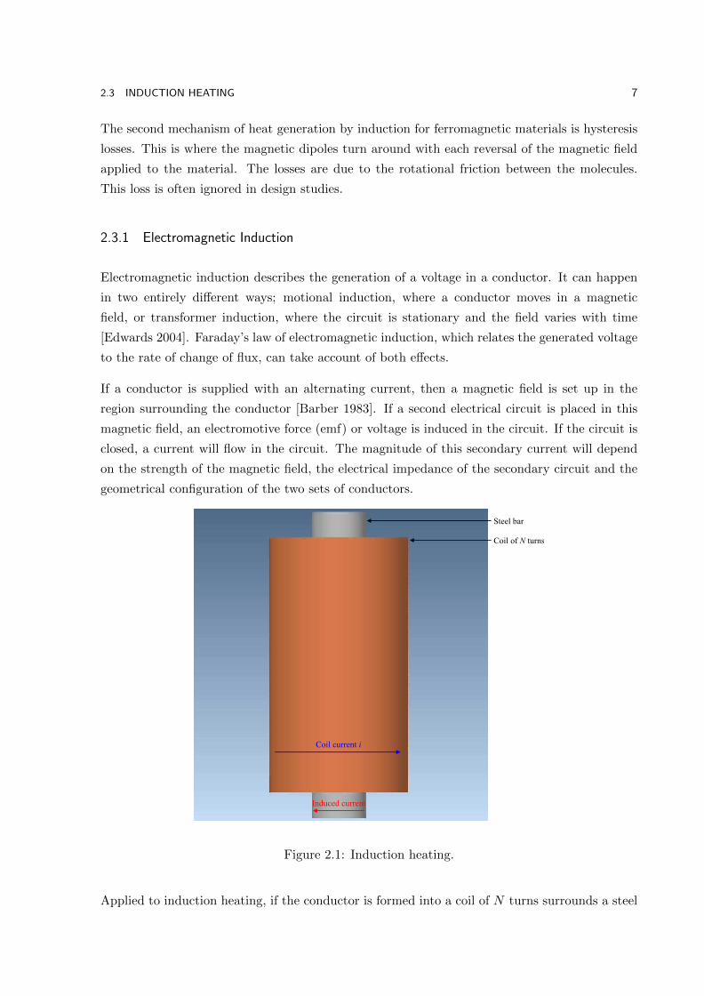
Coil of N turns
Coil current i
Induced current
Steel bar
Figure 2.1: Induction heating.
Applied to induction heating, if the conductor is formed into a coil of N turns surrounds a steel

8 CHAPTER 2 HISTORICAL DEVELOPMENT
bar, as shown in Figure 2.1, the magnetic field will be normal to the direction of the coil current
i. The flux will flow inside the coil in the longitudinal axis direction, as shown in Figure 2.2.
Figure 2.2: Magnetic flux plot of steel bar workpiece.
The direction of the current induced in the steel bar workpiece to be heated is also normal to the
magnetic field [Stansel 1949]. Because of Lenz’s law, it opposes the current in the coil but in the
same circumferential direction. The shape of the workpiece or billet does not affect the principle
involved [Stansel 1949]. Thus a workpiece of any shape can be heated by eddy currents.
2.3.2 Basic Induction Heating
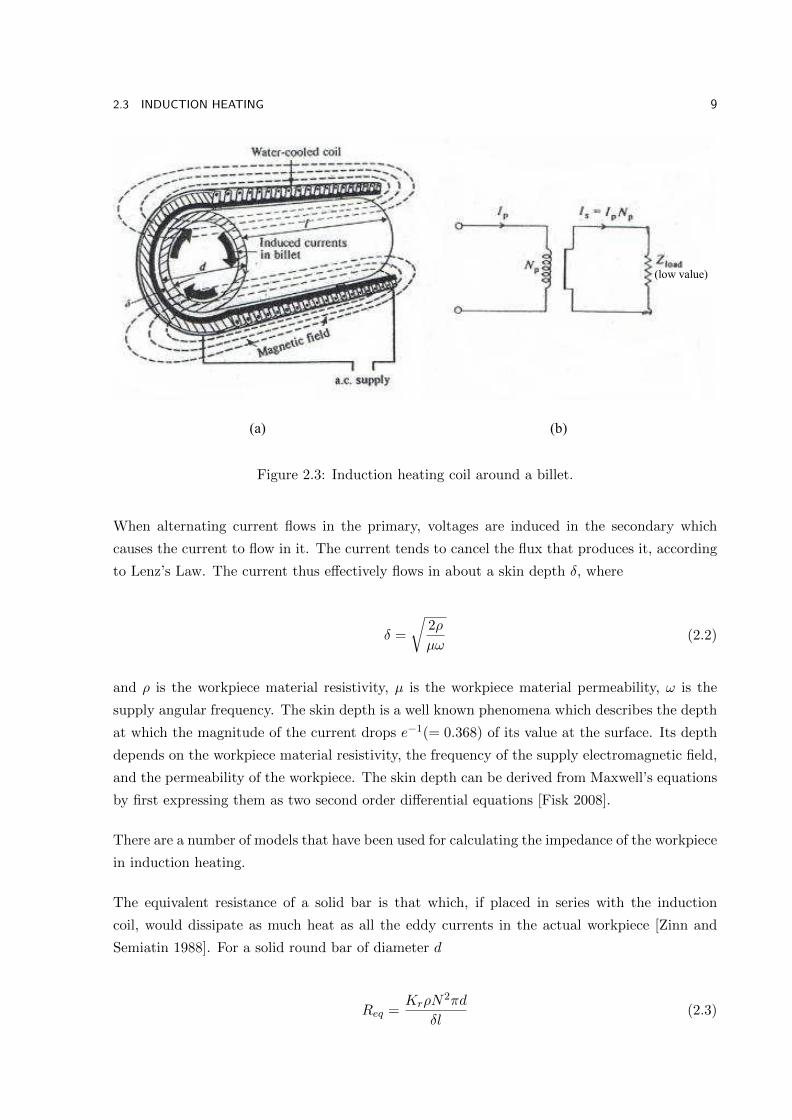
In induction heating, a metal workpiece is heated by a passage of currents through a material
which are induced from a separate source, as shown in Figure 2.3(a) [Davies and Simpson 1979].
The real power dissipated is equal to the current squared times the effective resistance of the
workpiece. The metal workpiece heats due to the resistance to the flow of this current.
The metal to be heated, known as a billet in induction heating terminology, can also be regarded
as the secondary winding of a transformer, as shown in Figure 2.3(b) [Davies and Simpson 1979].
In its normal cylindrical form, the transformer is a multi-turn, single layer primary winding and
a single-turn short-circuited secondary winding, separated by a small air gap.
2.3 INDUCTION HEATING 9
(low value)
(a) (b)
Figure 2.3: Induction heating coil around a billet.
When alternating current flows in the primary, voltages are induced in the secondary which
causes the current to flow in it. The current tends to cancel the flux that produces it, according
to Lenz’s Law. The current thus effectively flows in about a skin depth δ, where
δ =
√2ρ
µω(2.2)
and ρ is the workpiece material resistivity, µ is the workpiece material permeability, ω is the
supply angular frequency. The skin depth is a well known phenomena which describes the depth
at which the magnitude of the current drops e−1(= 0.368) of its value at the surface. Its depth
depends on the workpiece material resistivity, the frequency of the supply electromagnetic field,
and the permeability of the workpiece. The skin depth can be derived from Maxwell’s equations
by first expressing them as two second order differential equations [Fisk 2008].
There are a number of models that have been used for calculating the impedance of the workpiece
in induction heating.
The equivalent resistance of a solid bar is that which, if placed in series with the induction
coil, would dissipate as much heat as all the eddy currents in the actual workpiece [Zinn and
Semiatin 1988]. For a solid round bar of diameter d
Req =KrρN
2πd
δl(2.3)

10 CHAPTER 2 HISTORICAL DEVELOPMENT
where Kr is a workpiece correction factor, N is the number of turns in the coil, and l is the
length of the workpiece.
Kr accounts for the variation of the electrical path between the internal and external diameters of
the equivalent sleeve. It has a non-linear dependence on the ratio of dδ [Zinn and Semiatin 1988].
An analytical approximation for solid round bars is
Kr = 0.15dδ for 0 <d
δ< 5
= 0.015dδ for 5 <d
δ< 15
= 0.95 ford
δ> 15
For a round hollow tube, the value of Kr changes dramatically when the tube thickness t becomes
less than the skin depth. Under these conditions a uniform flux density is assumed and the
equivalent resistance becomes
Req =ρN2πd
tl(2.4)
For rectangular workpieces of width w and thickness t, the equivalent resistance is
Req =KrρN
22w
tl(2.5)
The factor Kr can be approximated to
Kr = 0.4 tδ for 0 <t
δ< 2.5
= 1.0 fort
δ> 2.5
For short, stubby round bars, a second multiplication correction factor Kr is used to account for
the fringing of the magnetic field at the bar ends [Zinn and Semiatin 1988]. This is dependent
on both the ratio of the workpiece diameter to the inside diameter of the coil, db1
, and the ratio
of the latter to the coil length, b1l . It is a highly non-linear relationship as shown in [Zinn and
Semiatin 1988].

2.4 SEC MODEL OF INDUCTION HEATER 11
2.4 SEC MODEL OF INDUCTION HEATER
Modelling an induction heater involves developing mathematical relationships of the physical
process of electromagnetic induction. There are a number of models [Dodd and Deeds 1968],
[Dodd et al. 1974], [Namjoshi et al. 2001], [Namjoshi and Biringer 1993], [Hussein and Biringer 1992]
which are considered valid at high frequencies only. However, at mains frequency, the SEC model
[Baker 1957], [Davies and Simpson 1979] is often used.
The SEC model looks at the parallel flow of magnetic flux through the coil, airgap and work-
piece of an induction heater and converts these into an equivalent electrical circuit, where all
components are in series. The circuit components are the coil and workpiece resistance, and
the coil, airgap and workpiece reactances, which cannot be interpreted as being actual values
that can be measured. It is their combined series impedance that yields appropriate terminal
current, power and power factor for a given applied voltage.
This model of an induction heater is based on the series equivalent circuit depicted in Figure 2.4
[Baker 1957], [Davies and Simpson 1979]. This equivalent circuit has the resistance of the coil
and workpiece (Rc, Rw) and the reactances of the workpiece, air gap and coil (Xw, Xg,andXc)
all in series.
Figure 2.4: Series equivalent circuit of induction heater.
The SEC method requires the coil to be designed by obtaining the values of the resistances and
reactances of the coil, workpiece and the air gap between them, and then solving the circuit.
The series impedance is
Z = (Rw +Rc) + j(Xg +Xw +Xc) (2.6)
12 CHAPTER 2 HISTORICAL DEVELOPMENT
where the components are
workpiece resistance
Rw = K(µrpAw) (2.7)
coil resistance
Rc = K
(krπdcδc
2
)(2.8)
air gap reactance
Xg = K(Ag) (2.9)
workpiece reactance
Xw = K(µrqAw) (2.10)
coil reactance
Xc = K
(krπdcδc
2
)= Rc (2.11)
and
K =
(2πfµ0N
2c
lc
)(2.12)
In these equations, µr is the relative permeability of the workpiece, Aw is the cross-section of
the workpiece, dc is the coil inner diameter, δc is the skin depth of the coil, Ag is the air gap
between the coil and the workpiece, µ0 is the magnetic permeability of free space (4π × 10−7),
Nc is the coil turns, and lc is the coil length.
In the equation for the coil resistance and reactance, kr is a correction factor, allowing for the
spacing between the turns (kr lies between 1 and 1.5, with 1.15 being a typical value). The
expression (2.8) for the coil resistance is dependent on relative permeability and does not appear
dimensionally correct. However, this is an expression of the model that allows terminal conditions
2.4 SEC MODEL OF INDUCTION HEATER 13
to be calculated. The individual component value calculated should not be interpreted as what
you would measure in practice.
The p and q factors in the equation for the workpiece resistance and reactance can be estimated
from graphs or calculated from analytical expressions [Davies and Simpson 1979]. The dimen-
sionless flux factors p and q depend on geometry, frequency, resistivity, and also the permeability
of the material.
In the equation for the workpiece resistance and reactance, the effective cross-sectional area of
the current flow in the workpiece should be used. This is dependent on the skin depth.
For dwδw
ratios greater than 8, then [Davies 1990]
p =2(
1.23 + dwδw
) (2.13)
q =2(dwδw
) (2.14)
Alternatively, for dwtw≥ 10 and tw
δw≤ 0.2, the p and q factors can be calculated from analytical
expressions.
p =γ
(1 + γ2)(2.15)
q =1
(1 + γ2)(2.16)
where
γ =dwtw(2γ2)
(2.17)
If the thickness ratios lie outside the limit, then p and q can be estimated from the graph of
p and q versus 2bδw
for a slap of thickness 2b, or dwδw
for a solid cylinder of diameter dw. These
graphs have been derived from complex expressions involving hyperbolic and Bessel functions
respectively [Davies 1990].
This set of equations is most relevant for long coils [Baker 1957]. However, for short coils, a
modification is suggested [Baker 1957] whereby an external reluctance Xe is placed in parallel
with the series combination of Rw, Xw, Xg, and Xc. This is to accommodate the likely significant

14 CHAPTER 2 HISTORICAL DEVELOPMENT
leakage and distortion of flux flow about the end regions if the length to diameter ratio of the
workpiece and coil is small (i.e. approaching unity). It is suggested that to accommodate this
distortion, the equivalent circuit is modified, as shown in Figure 2.5.
IcRc Rw Iw
XgXwXc
Xe
Ie
X1
Ec
Figure 2.5: Short coil equivalent circuit which includes an external reactance.
This reactance represents the impedance of the end effects of the external flux path. It can be
calculated from
Xe = K
(lcRe
)(2.18)
where Re is the external reluctance given in [Baker 1957] as
Re = kc1.80
pc(2.19)
and kc is an empirical factor which is assumed to be 1, and pc is the coil perimeter.
On the basis of the change in inductance of a cylindrical solenoid with length, it is possible to
show that its external reluctance is practically independent of the length and equal approximately
to 0.57dc
where dc is the coil diameter [Baker 1957].
For an unknown reason, the addition of the short coil external reactance has since been regarded
as an “ill-defined quantity”and “manifestly wrong”[Davies and Simpson 1979]. Hence, the long
coil model is used in this thesis. The addition of the short coil reactance would increase the
current drawn from the supply and decrease the power factor.

2.4 SEC MODEL OF INDUCTION HEATER 15
2.4.1 SEC Performance
The component values of the SEC model in Figure 2.4 can be used to calculate the major coil
properties such as efficiency, coil power factor, the number of volts per turn and the number of
ampere-turns.
The applied coil voltage Vc which is equal to the emf Ec is
Vc = IcZ (2.20)
where Ic is the coil current.
The total impedance is
Z = R+ jX (2.21)
and
Z2 = (Rw +Rc)2 + (Xg +Xw +Xc)
2 (2.22)
The electrical performance of the induction heater can now be calculated. The coil efficiency η
is the ratio of workpiece resistance Rw to the total resistance.
η =Rw
Rc +Rw(2.23)
It can be seen from (2.23) that to obtain high efficiencies, the coil resistance value Rc is required
to be significantly less than Rw. This is usually obtained by choosing copper or aluminium as
the coil material because they have the lowest resistivities of the commonly used metals.
The ratio of the total resistance to impedance Z is the coil power factor
cos θ =Rw +Rc|Z|
(2.24)
The coil power is
Pc =Pwη
(2.25)

16 CHAPTER 2 HISTORICAL DEVELOPMENT
where Pw is the total work power input to workpiece.
The coil volt-amperes
|S| = P
cos θ= I2c |Z| (2.26)
The coil volts/turn
=EcNc
(2.27)
The coil ampere-turns
= IcNc (2.28)
where Ic and Ec from Equation 2.27 are RMS quantities.
2.4.2 Equivalent Circuit Performance for an Experimental Induction Heater
A coil of a small induction heater was constructed with the parameter dimensions shown in
Table 2.1.
Table 2.1: Coil dimensions
Material Copper Units
Resistivity 1.72×10⁻⁸ ΩmLength 208 mmOutside diameter 114 mmInside diameter 83 mmWire diameter 1.7 mmWire area 2.27 mm2
Number of layers 9 -Turns per layer 111 -Number of turns 999 -Length of wire 309 mCalculated resistance 2.34 ΩMeasured resistance (50Hz) 2.15 Ω
A number of mild steel tubes of various diameters and thicknesses were cut to provide workpieces
that fitted inside the coil former. The dimensions of the workpieces are listed in Table 2.2.
2.5 CALCULATED PERFORMANCE USING SEC MODEL 17
Table 2.2: Workpiece dimensions
Workpiece Material Length Diameter Thickness(mm) (mm) (mm)
1 Mild steel 250 44.3 solid2 Mild steel 250 44.5 12.63 Mild steel 250 44.2 6.34 Mild steel 250 48.3 3.35 Mild steel 250 54.0 2.66 Mild steel 250 70.0 2.07 Mild steel 250 73.0 solid
2.4.3 Material Properties
For the sake of calculation, the physical characteristics of the copper coil and mild steel work-
pieces were taken as given in Table 2.3. These are generic values as the actual values were
unknown. There may be differences due to the metallurgy of their manufacture.
Table 2.3: Physical properties of copper and mild steel
Material Copper Mild steel
Resistivity (Ωm × 10−8) 1.72 16Relative permeability 1 750Skin depth at 50Hz (mm) 9.3 1.0
Having obtained all the parameters of the equivalent circuits from the material characteristics
and dimensions, the performance of the heater could be calculated by solving the equivalent
circuit equations and determining the current, power and power factor for a given applied voltage.
In addition, efficiencies, voltage gradients, voltages per turn and current densities could be
calculated.
2.5 CALCULATED PERFORMANCE USING SEC MODEL
To check the performance of the induction heaters, a program was written in MATLAB [Reck-
tenwald 2000] for the SEC long coil model to perform all the above calculations. The various
components of the SEC model are given in Table 2.4.
The value of the coil resistance should not be taken too literally. Indeed, for the actual as-
build induction heater of the dimensions listed in Table 2.1, the coil resistance was measured
to be 2.15Ω. Rather, it is the total circuit that gives rise to terminal conditions that is of
importance. The calculated value from the SEC model is significantly lower than that measured.
The workpiece resistance and reactance are significantly higher than the coil resistance and
reactance. The airgap reactance is about 10 times more than the coil resistance and reactance.

18 CHAPTER 2 HISTORICAL DEVELOPMENT
Table 2.4: Component values for the SEC long coil model
Circuit component Value (Ω)
Rc 0.241Rw 9.346Xc 0.241Xw 9.510Xg 2.321
For the SEC model, the short coil reactance, as suggested by Baker [Baker 1957], was calculated
to be 57.4Ω. This is much higher than any of the other components and therefore had little
effect on the results, increasing the current by about 0.1A and insignificantly changing the power
factor.
Having calculated the component values of the SEC model, the performance of the induction
heater is obtained by solving the equivalent circuit equations. Table 2.5 shows the performances
of the induction heaters for a 100V supply.
Table 2.5: Calculated performance of experimental heater using SEC long coil model
Workpiece Voltage Current Flux Coil Workpiece Apparent Power(V) (A) density loss loss power factor
(T) (W) (W) (VA)
1 100 6.9 3.2 7.6 438.6 692.1 0.62 100 6.9 3.2 7.6 438.3 691.7 0.63 100 6.9 3.2 7.6 438.8 692.3 0.64 100 6.9 2.9 7.9 431.7 685.1 0.65 100 6.8 2.6 8.5 422.2 675.8 0.66 100 6.5 2.0 9.9 397.6 652.7 0.67 100 6.5 1.9 10.2 393.3 648.7 0.6
The calculated performances from the SEC model show a maximum current of close to 7A and
a flux density of 3.2T which is likely to be more than the saturation point for all the workpieces.
The calculated flux density decreases to 1.9T as the diameter of the workpiece increases. In
addition, the calculated coil losses increase from 7.6W to 10.2W as the diameter of the workpiece
increases. The coil losses are all significantly lower compared to the workpiece losses. Both the
workpiece losses and apparent power have decreased as the workpiece diameter increased. The
power factors for the different workpieces are all the same.
2.6 SUMMARY
The theory of induction heating has been presented. Firstly, the background and applications
of induction heating were introduced. This chapter also introduced electromagnetic induction

2.6 SUMMARY 19
as a basis to understand the principle of operation of induction heating.
The conventional approach to induction heater design which has been widely used in research
is the SEC model. It has been presented in this chapter. The SEC model was used to calculate
the performance of a demonstration induction heater using a set of different workpieces. The
calculated results from the SEC model were also discussed in terms of the coil losses, workpiece
losses and power factors.

Chapter 3
TRANSFORMER MODEL OF INDUCTION HEATER
3.1 INTRODUCTION
An induction heater can be regarded as a special type of transformer with a single shorted
turn secondary winding. The coil is the equivalent of a multiple turn primary winding, and
the workpiece is the single turn secondary winding. The workpiece also performs the function
of being the core, which the magnetic field generated by the coil passes through. Hence, a
transformer equivalent circuit model can be used to calculate the performance of the induction
heater.
In this chapter, the equivalent circuits model of ideal and non-ideal transformers are presented.
These are then transformed into a circuit to model an induction heater. The performance
calculations from this circuit are compared to the more conventional SEC model of Chapter 2.
3.2 TRANSFORMER FUNDAMENTALS
The basic concept of induction heating can be shown to be similar to the well known transformer
theory. In order to develop the circuit to model the induction heater, it is useful to look at the
operation of an ideal transformer, and also the deviations from the ideal.
3.2.1 Ideal Transformers
In an ideal transformer, it is assumed that the input power to the transformer is equal to the
output power. Figure 3.1 [Lapthorn 2013] shows a schematic representation of a single phase
transformer with two coils wound on a magnetic core. The magnetic coupling is assumed to be
perfect, that is the same flux φ passes through each turn of each coil.
In Figure 3.1, V1 is the primary voltage, V2 is the secondary voltage, i1 is the primary current,
i2 is the secondary current, N1 is the number of turns on the primary, N2 is the number of turns

22 CHAPTER 3 TRANSFORMER MODEL OF INDUCTION HEATER
Figure 3.1: An ideal full-core transformer.
on the secondary, e1 is the induced emf in the primary, e2 is the induced emf in the secondary,
and φ is the magnetic flux in the core.
Faraday’s law of electromagnetic induction states that a changing magnetic flux φ induces elec-
tromotive forces (emf’s) in the circuit, thus emf’s e1 and e2 are induced in N1 and N2 owing to
a finite rate of change of flux φ such that
e1 = N1dφ
dt(3.1)
and
e2 = N2dφ
dt(3.2)
With the transformer being ideal, e1 = V1 and e2 = V2. The direction of e1 is such that it
produces a current which opposes the flux change, according to Lenz’s law. Using the dot
convention, from Equations 3.1 and 3.2,
3.2 TRANSFORMER FUNDAMENTALS 23
e1e2
=N1
N2(3.3)
If E1 and E2 are the RMS values of e1 and e2 respectively, then
E1
E2=N1
N2= a (3.4)
where a is the turns ratio.
Since e1 = V1 and e2 = V2 for an ideal transformer, the flux and voltage are related by
φ =1
N1
∫V1dt =
1
N2
∫V2dt (3.5)
In general terms, if the flux varies sinusoidally such that
φ = φm sinωt (3.6)
then the corresponding induced voltage e linking an N -turn winding is given by Faraday’s law
as
e = ωNφm cosωt (3.7)
From Equation 3.7, the RMS value of the induced voltage is thus
V =ωNφm√
2= 4.44fNφm (3.8)
where ω = 2πf (f is the frequency in Hertz). This is usually referred to the transformer equation.
For an ideal transformer, the magnetomotive force (mmf) required to produce the working flux
is negligibly small. This mmf is the resultant of the mmf due to the primary current and that
due to the secondary current such that
N1i1 = N2i2 (3.9)
Therefore

24 CHAPTER 3 TRANSFORMER MODEL OF INDUCTION HEATER
i1i2
=N2
N1=
1
a(3.10)
Multiplying Equations 3.3 and 3.10
e1i1 = e2i2 (3.11)
Thus, the apparent powers through both the primary and secondary windings are equal. The
primary absorbs power from the sources, whereas the secondary delivers power. In the ideal
transformer, no power is lost internally due to the windings and core so that the two quantities
are equal.
3.2.2 Non-Ideal Transformers
In a practical transformer, the winding resistances and the core reluctance are not zero, and the
magnetic coupling is not perfect. In addition, power will be lost in the core because the eddy
currents and hysteresis in the magnetic material. All of these effects can be represented by the
equivalent circuit shown in Figure 3.2 [Lapthorn et al. 2013a]. The equivalent circuit shows an
ideal transformer coupled with other components to model the various non-ideal characteristics.
This equivalent circuit is relevant for low frequency modeling of power transformers.
Figure 3.2: Equivalent circuit of a non-ideal transformer.
The most obvious loss is created by the current in the primary winding, even when the sec-
ondary winding is open circuited. This current has two components. The first component is the
magnetizing current, which is generated by having a core of finite permeability. A significant
magnetizing force is required to produce an operating flux. This is modeled as a magnetizing

3.2 TRANSFORMER FUNDAMENTALS 25
reactance which is represented as a shunt reactance path (designated by Xm) on the primary
side.
The second component represents two losses inside the transformer’s core, which are the hys-
teresis and eddy current losses, such that some real power is absorbed even at no-load. These
losses can be modeled by the addition of a shunt resistance (designated by Rc) on the primary
side [Liew 2001].
The hysteresis real power losses Ph depend on the rotation of the domains in the ferromagnetic
material. They are proportional to fBx [Slemon and Straughen 1980] where x is the Steinmetz
factor of core material, empirically derived (1.5−2.5).
However, from the transformer equation (3.8)
V =ωNφm√
2= 4.44fNφm
Or V is proportional to fφ or fB, where φ = BA, and A is the cross-sectional area of the core.
Hence, Ph is proportional to Vfx−1 . Ph thus depends on the voltage and frequency. It is constant
if both voltage and frequency are constant.
Since B can be calculated, the hysteresis losses are usually calculated from
Ph = kfBxWT (3.12)
where k is constant depending on the material, B is the maximum flux density, and WT is the
weight of the core material. For induction heaters, the hysteresis losses are usually ignored, as
they contribute a much smaller amount as compared to the eddy current losses.
The eddy current real power losses due to the induced currents flowing in the core material, Pe
are proportional to f2 B2 or V 2. Thus the eddy current losses also depend on the voltage [Slemon
and Straughen 1980]. The expression for eddy current losses also depends on the dimensions of
the core material and whether the core is laminated. For induction heating, the eddy current
losses are those heating up the workpiece. The combined hysteresis and eddy current losses are
Pc = Ph + Pe (3.13)
The losses can be represented by a current ic passing through a resistance Rc. The power losses
are
26 CHAPTER 3 TRANSFORMER MODEL OF INDUCTION HEATER
Pc = i2cRc =V 2
Rc(3.14)
The real power losses of both windings are the other significant components modelled to account
for the performance of a real transformer. These can be modelled as a series resistance for each
winding (R1 and R2 respectively). When current flows through the primary and secondary side
of the transformer, some leakage flux passes through the air surrounding each winding instead of
going through the core. The leakage flux links with the turns in each winding, and sets up emf’s
that oppose the flow of the current through each winding. Thus, the leakage flux produces the
same effect as an unwanted inductance in series with each winding. The unwanted inductance
is also termed the leakage inductance, which is represented by a reactance X1 and X2 in the
primary and secondary windings respectively [Liew 2001].
3.3 TRANSFORMER EQUIVALENT CIRCUIT OF INDUCTION HEATER
If an induction heater can be considered as a special type of transformer, then a transformer
equivalent circuit can be used to calculate the performance of the induction heater. The trans-
former equivalent circuit (TEC) method determines the parameters of the TEC using the reverse
design method [Liew and Bodger 2001], [Bodger and Liew 2002]. It also calculates the perfor-
mance of the induction heater. The performance of the induction heater depends on the effective
eddy current resistance of the workpiece. This will depend on the material and their dimen-
sions. For example, the length and diameter of the workpiece must be selected to optimize the
performance of the heater.
An induction heater is essentially a transformer with a single shorted turn secondary winding.
The transformer equivalent circuit is shown in Figure 3.3. This circuit is based on an ideal
transformer, with additional circuit elements to represent the practical deviations from the
ideal. It can be seen from Figure 3.3, that the ideal transformer has been eliminated and the
transformer can be represented exclusively by an RL circuit referred to the primary. The TEC
circuit in Figure 3.3 is relevant for low frequency modelling of induction heaters.
In this model, Rw represents the eddy current losses in the workpiece, which would normally
be accounted for in the core of a transformer, Rc is the resistance of the coil, which is now
the primary winding using transformer terminology (not to be confused with its former use to
represent the core losses in Figure 3.2), and Xmw is the magnetising reactance which accounts
for the current required to magnetise the core. Moreover, hysteresis losses, also normally a
component of core losses in a transformer, are insignificant in induction heating. Hence the
losses in the workpiece become resistance losses of the secondary winding.
The leakage reactance for each winding can be split between the coil and the workpiece as Xc

3.4 CALCULATION OF EQUIVALENT CIRCUIT PARAMETERS 27
Figure 3.3: Transformer equivalent circuit of an induction heater.
and Xw. The leakage reactances account for the imperfect magnetic field coupling between the
coil and the workpiece.
3.4 CALCULATION OF EQUIVALENT CIRCUIT PARAMETERS
The parameters of the equivalent circuit in Figure 3.3 are calculated using the basic dimen-
sions and physical characteristics of materials used, as per the reverse design method [Liew and
Bodger 2001], [Bodger and Liew 2002]. These are entered as known data and then the individual
circuit components are calculated using magnetic and electric circuit component models.
Figure 3.4 shows a cross-sectional profile of a multi-layer coil induction heater with a tube
workpiece. All the symbols represent dimensions of the materials used in the construction of
the heater, including the workpiece, insulation and the coil, where LW is the length of the
workpiece, DW is the diameter of the workpiece, TW is the thickness of the workpiece, IWC
is the workpiece/coil insulation thickness, WC is the diameter of the coil wire, WIC is the coil
interlayer insulation, and DOC is the outside diameter of the coil.
The equivalent circuit components in Figure 3.3 need to be modified as the flux path is open
and not entirely constrained to be inside the core. With respect to the equivalent circuit of
Figure 3.3, the winding resistance models Rc and Rw are maintained as they are not affected by
the partial core configuration. Thus modifications to the calculation of reactance Xmw and the
leakage reactance Xcw (the sum of Xc and Xw) are required as the core is no longer a closed
loop, which affects the magnetic field characteristics of the transformer.
This is demonstrated in Figure 3.5 which shows two different open core induction heaters with
28 CHAPTER 3 TRANSFORMER MODEL OF INDUCTION HEATER
Figure 3.4: Cross-section of a multi-layer coil induction heater with a tube workpiece.
the same core length but significantly different core thicknesses. The resultant magnetic field
paths are very different. These give rise to different reluctances in the air path requiring new
equivalent circuit component models.
3.4.1 Coil Resistance
If lc is the length of the coil wire and Ac is its cross-sectional area, then the primary winding or
coil resistance is given by
Rc =ρclcAc
(3.15)
where ρc is the resistivity of the coil material. The value of the resistivity depends on the coil
temperature as

3.4 CALCULATION OF EQUIVALENT CIRCUIT PARAMETERS 29
(a) Winding thickness τ1
(b) Winding thickness τ2
Figure 3.5: Flux distribution for induction heaters with different winding thicknesses.
ρc = (1 + (∆ρ(Tc − 20)))ρ20C (3.16)
where ρ20C is the resistivity at 20C, Tc is the coil temperature, and ∆ρ is the thermal resistivity
coefficient. The resistivity of all metals is considered to vary linearly with temperature. The
calculation of the winding resistanceRc also takes into account the coil skin depth and its effective
cross-sectional area. For the coil, the eddy current skin depth gives its effective thickness
δc =
√2ρc
µ0µrcω(3.17)

30 CHAPTER 3 TRANSFORMER MODEL OF INDUCTION HEATER
where µrc is the relative permeability of the coil, and ω is the angular frequency(2πf). The
coil effective cross-sectional area is calculated using the diameter of the coil and its effective
thickness.
If the skin depth is greater than the radius of the coil conductor then a uniform current density
can be assumed. This is set by
δc =Wc
2(3.18)
where Wc is the diameter of coil wire from Figure 3.4.
The coil effective cross-sectional area is
Aec = π(Wc − δc)δc (3.19)
The length of the conductor used in forming the coil, lec, is calculated from consideration of the
average length per turn, multiplied by the number of turns, Nc. This needs to take into account
the diameter of the workpiece, the thickness of the conductor in the radial direction, plus its
insulation, and the coil inter-layer and coil/workpiece insulation thickness.
Hence, the coil resistance becomes
Rc =ρclecAec
(3.20)
3.4.2 Workpiece Magnetizing Reactance
The magnetizing reactance Xmw for an open core induction heater is formulated in [Liew and
Bodger 2002] as
Xmw =ωN2
c µ0µreAwlw
(3.21)
where ω is the angular frequency, Nc is the number of turns on the coil, µ0 is the permeability
of free space (4π × 10−7), and µre is the effective permeability of the magnetic flux path which
includes the series combination of the workpiece and the return path, usually through air. Aw
is the effective cross-sectional area of the workpiece, calculated using the skin depth δw, and lw
is the length of the workpiece.

3.4 CALCULATION OF EQUIVALENT CIRCUIT PARAMETERS 31
This formulation and calculation is a modification of the theory developed for partial core trans-
formers [Liew and Bodger 2001]. A summary is given here for induction heaters. The magne-
tizing reactance of a partial core is different to that of a full core transformer, since the flux of
a partial core transformer not only goes through the core, but also flows in the air around the
core. This is shown in Figure 3.6.
Figure 3.6: Axial view of the flux flow from a cylindrical workpiece.
The magnetic flux generated by the energised coil flows through the workpiece within a skin
depth and returns via the air back to the workpiece. Hence, the reluctance of the magnetic flux
path is significantly greater than if the flux was constrained to flow inside a closed core. This
implies that the overall relative permeability of the induction heater should be much lower than
that of the workpiece material, where it is generally of the order of 2000−10000. Therefore, a
new overall relative permeability, which takes into account the magnetic flux in the air, has to
be determined.
A full derivation for the calculation of air reluctance for partial core transformers is given in
[Liew and Bodger 2001]. This has been adopted for the induction heater calculations without
proof, as the method involves empirical factors obtained from a range of transformers actually
built. The usefulness of the calculation is ultimately supported by how well the model predicts
the performance of actual built devices. Empirical factors based on a number of different as-built
32 CHAPTER 3 TRANSFORMER MODEL OF INDUCTION HEATER
induction heaters should better inform the calculation of the empirical factors.
The method assumes that the reluctance of the air is only in the regions at the ends of the core.
The reluctance of the air at one end of the partial core is
Rair = 1.694× 10⁵(
1
Aw
)0.35( 1
lw
)0.31
(3.22)
Since the workpiece flux cross-sectional area may only be a ring of skin depth thickness, a
modification for the formula uses the effective radius of the ring.
Rair = 1.141× 10⁵(
1
rw
)0.69( 1
lw
)0.31
(3.23)
The equivalent magnetic circuit of the induction heater, that includes both the workpiece reluc-
tance and the air reluctances, is given in Figure 3.7.
Figure 3.7: Magnetic circuit of induction heater.
The overall reluctance of the transformer is
RT = Rw + 2Rair (3.24)
This is equivalent to a flux path through a homogeneous medium of relative permeability µrT ,
hence

3.4 CALCULATION OF EQUIVALENT CIRCUIT PARAMETERS 33
RT =lT
µ0µrTAT(3.25)
where lT is the overall flux path length = lw + 2lair ≈ lw as lair lw, and AT is the overall
effective cross-sectional area of the workpiece = Aw
Thus
µrT =lw
µ0RTAw(3.26)
The magnetizing reactance of the induction heater is thus
Xmw =ωN2
c µ0µrTAwlw
(3.27)
3.4.3 Coil/Workpiece Leakage Reactance
The series equivalent circuit and the concept of leakage reactance for a full-core transformer
stem from the difficulty in analysing the behaviour of very tightly-coupled coils in terms of self
and mutual inductances. The leakage-based approach is well-suited to conventional transformers
where the closed magnetic circuit leads to coupling coefficients very close to 1. This conventional
approach is maintained, but modified, for the induction heater, because a closely packed multi-
layered coil will act as a guide that channels the flux up the middle and around the outside, such
that the almost perfect coupling between the coil and the workpiece still exists. The dimensions
used in calculating the leakage flux for an induction heater are presented in Figure 3.8.
The coil and workpiece leakage reactances are calculated from the total leakage reactance which
embodies the effects of both the coil and workpiece together. The total induction heater leakage
reactance is [Connelly 1965]
Xcw =ωN2
c µ0πτcwlw
(3.28)
where
τcw =
((wcdc + wwdw
3
)+ wcw∆d
)(3.29)
is the coil/workpiece thickness factor

34 CHAPTER 3 TRANSFORMER MODEL OF INDUCTION HEATER
Figure 3.8: Dimensions for representing the leakage flux for an induction heater.
and
wc =
(wic + woc
2
)(3.30)
is the mean diameter of the coil
and
ww =
(wiw + wow
2
)(3.31)

3.4 CALCULATION OF EQUIVALENT CIRCUIT PARAMETERS 35
is the mean diameter of the workpiece
and
wcw =
(wic + wow
2
)(3.32)
is the mean diameter of the space between the coil and workpiece.
The calculation of Xcw does not separate the values of the coil and workpiece leakage reactances
and they are usually assumed to be the same. Each of them is half of the total leakage reactance.
Hence
Xc = Xw =Xcw
2(3.33)
3.4.4 Workpiece Eddy Current Resistance
The workpiece eddy current resistance referred to the coil is calculated using
Rw =ρwlweAwe
N2c (3.34)
where ρw is the resistivity of the workpiece, lwe is the effective length of the eddy current flowing
around the circumference of the workpiece, Awe is the effective cross-sectional area of the eddy
current path, and Nc is the number of coil turns.
The effective length and cross-sectional area of the eddy current path takes into account the skin
depth in the workpiece
δw =
√2ρw
µ0µreω(3.35)
Thus
lwe = π(Dw − δw) (3.36)
and
Awe = lwδw (3.37)

36 CHAPTER 3 TRANSFORMER MODEL OF INDUCTION HEATER
The losses in the workpiece consist of two major components; the hysterisis loss and the eddy
current loss. The hysterisis loss is insignificant with respect to the eddy current loss and is not
included in the model.
3.5 EQUIVALENT CIRCUIT PERFORMANCE
The transformer equivalent circuit in Figure 3.3 is more complicated than the series equivalent
circuit presented in Chapter 2. The parallel impedance of the workpiece resistance and leakage
reactance with the magnetizing reactance is
Zw =jXmw × (Rw + jXw)
(Rw + j(Xw +Xmw))(3.38)
and the total impedance is the complex value
Z = (Rc + jXc) + Zw (3.39)
The performance of the induction heater is then obtained by applying a voltage to the coil
and calculating the current, apparent power, real power and power factor. In addition, voltage
gradients, voltages per turn, current densities and the efficiency can be calculated.
3.5.1 Equivalent Circuit Performance for an Experimental Induction Heater
The TEC model is applied for the same set of induction heaters presented in Chapter 2. The
dimensions of the induction heater coil and workpieces are also identical.
3.5.2 Equivalent Circuit Parameters
The calculated equivalent circuit parameters referred to the primary winding are listed in Table
3.1. These values correspond to workpiece 7.
Table 3.1: Component values for the TEC model
Circuit component Value (Ω)
Rc 2.372Rw 47.753Xc 2.513Xw 2.513Xmw 31.873

3.5 EQUIVALENT CIRCUIT PERFORMANCE 37
The component values of the TEC model are very different from those of the SEC model pre-
sented in Chapter 2. This is because the TEC model is very different.
The coil resistance is about 10 times that previously calculated. It is a better indication of what
was measured using a resistance meter applied to the coil conductor.
The workpiece resistance (referred to the coil) is also much larger (5 times) than that calculated
from the SEC model. The actual resistance is very low, 4.8µΩ. Again the value should be a
reasonable indication of what you could measure. The workpiece resistance is much larger than
the coil resistance and hence the efficiency should be high.
For this example, the leakage reactances are relatively small, which indicates that there is
good coupling between the coil and the workpiece. A relatively long coil length and small
coil/workpiece interspace ensures this. Thus the TEC model gives a useful measure of this fea-
ture. The value is about the same as the air gap reactance used in the series equivalent circuit
model, although here the value is used twice, for both the coil and the workpiece, as only the
combined effect can be calculated. The TEC model is less dominated by the leakage (air gap)
reactance.
The workpiece magnetizing reactance is much larger than the workpiece reactance used before.
There is no direct correlation between this and the workpiece reactance calculated from the SEC
model.
3.5.3 TEC Calculated Performance
Having calculated the parameters of the equivalent circuit, the performance of the induction
heater is obtained by applying the nominal voltage to the equivalent circuit. Table 3.2 shows
the calculated performances of the induction heaters at a 100V supply.
Table 3.2: Calculated performance using TEC model
Workpiece Voltage Current Flux Coil Workpiece Apparent Power(V) (A) density loss loss power factor
(T) (W) (W) (VA)
1 100 3.9 3.2 26.7 100.9 397.2 0.32 100 3.9 3.2 26.6 100.5 396.3 0.33 100 3.9 3.2 26.7 101.2 397.7 0.34 100 3.8 2.9 25.8 92.2 380.2 0.35 100 3.6 2.6 24.8 81.9 359.7 0.36 100 3.2 2.0 23.1 62.3 317.0 0.37 100 3.1 1.9 22.9 59.6 310.7 0.3
The calculated performances from the TEC model are significantly lower than the SEC model
of Chapter 2 in terms of current, apparent power and workpiece loss. The same is not true for

38 CHAPTER 3 TRANSFORMER MODEL OF INDUCTION HEATER
the coil loss. The power factors from the TEC model are half those calculated from the SEC
model. Both models yield the same flux density, but in all cases this is calculated to be a value
significantly above that of the likely saturation value for mild steel. The calculated coil and
workpiece losses decrease as the diameter of the workpiece increases. This is due to the longer
eddy current path length and hence resistance in the workpiece. This pattern is not showed in
the coil and workpiece losses calculated from the SEC model.
As a modification to the TEC model, the permeability of the workpiece is reduced until the
flux density is below the saturation point. This means that the skin depth increases. The
magnetizing reactance and the workpiece eddy current resistance are adjusted to account for
this.
If the flux penetrates beyond the thickness of the workpiece, then part of the flux flows inside
the workpiece. The parallel combination of this reluctance and that of the workpiece must be
taken into account in calculating the workpiece magnetization reactance. This can be modeled
as a parallel reluctance with components both in the workpiece and inside.
The workpiece reluctance is
Rw =lw
µ0µrwAw(3.40)
where Aw is the cross-sectional area of the workpiece tube, and µrw is the relative permeability
of the workpiece.
The inside tube reluctance is
Ri =lwµ0Ai
(3.41)
where Ai is the cross-sectional area of the inside of the workpiece tube.
The reluctance of the parallel combination is
Rp =Ri ×RwRi +Rw
(3.42)
Assuming that the flux density is within the saturation level of the material, then the effective
radius of the workpiece is
re =
√Aeπ
(3.43)

3.6 SUMMARY 39
where Ae is the effective area of the flux as if it was flowing inside a solid cylinder workpiece.
Ae = π(Dw − δw)δw (3.44)
The air path reluctance at one end of the workpiece is given in (3.23) as
Rair = 1.141× 10⁵(
1
rw
)0.69( 1
lw
)0.31
Thus the total reluctance for the complete flux path is
RT = Rp + 2Rair (3.45)
The equivalent relative permeability of the series combination of the air and the workpiece/inside
tube flux path is
µre =lw
µ0AwRT(3.46)
The workpiece magnetizing reactance (referred to the coil) is
Xmw =ωN2
c
RT(3.47)
The equivalent relative permeability calculated using the above method for workpiece 7 is 93.5
which is much lower than the nominal workpiece value of 750. At 93.5, the flux density in the
workpiece is 1.7T, and the skin depth in the workpiece has now increased from 1.1 to 2.9mm.
Table 3.3 shows the calculated performance of the induction heater for operation at the saturation
point set at a realistic 1.7T. The workpiece losses are higher than those given in Table 3.2 but
still significantly lower than those calculated using the SEC model. The power factors have, in
general, increased.
3.6 SUMMARY
In this chapter, the equivalent circuits model of ideal and non-ideal transformer were presented.
These were transformed into a circuit to model an induction heater.
The low frequency modelling of induction heaters using the TEC model has been presented.
The performances of the induction heaters from this model are compared to the SEC model

40 CHAPTER 3 TRANSFORMER MODEL OF INDUCTION HEATER
Table 3.3: Calculated performance using TEC model below the saturation point
Workpiece Voltage Current Flux Coil Workpiece Apparent Power(V) (A) density loss loss power factor
(T) (W) (W) (VA)
1 100 4.3 1.7 30.8 190.9 427.1 0.52 100 4.3 1.7 30.6 189.2 425.1 0.53 100 4.3 1.7 30.9 191.9 428.1 0.54 100 3.9 1.7 27.6 159.5 393.5 0.55 100 3.6 1.7 24.9 126.5 360.3 0.46 100 3.1 1.7 22.3 73.6 311.7 0.37 100 3.1 1.7 22.3 67.4 306.3 0.3
calculated performances of an experimental heater for a variety of sizes of mild steel workpieces
presented in Chapter 2.
The calculated performances of the TEC model shows significantly lower values in terms of the
current and workpiece losses compared to the SEC model. The power factors calculated from
the TEC model are higher than those calculated from the SEC model.

Chapter 4
FINITE ELEMENT ANALYSIS AND MEASURED PERFORMANCEOF EXPERIMETAL INDUCTION HEATER
4.1 INTRODUCTION
The finite element method is a numerical technique which gives an approximate solution to a
complicated problem. Finite element analysis offers the best approach to determine the flux
pattern inside the heater. This chapter presents the computational results obtained using finite
element analysis (FEA) for a two dimensional model of the experimental induction heater. These
results correspond to a 100V supply to the coil. At this supply voltage, solutions are computed
and performances of the heater are calculated.
Also in this chapter, the measured performances of the experimental heater are assessed. The
experimental set-up and method of measurements performed are discussed. Measurement results
include current, real power, apparent power and power factor. In addition, eddy current losses
and winding losses of the mild steel workpiece are calculated from the measurements. These
measured results are compared to the results obtained using FEA, and the SEC, and TEC
models.
4.2 FINITE ELEMENT METHOD
The finite element method has proved to be the most powerful tool in the CAD design of
electrical machines. It can allow accurate calculation of the flux distribution, flux density,
winding inductance, EMF forces and torques, even under conditions of iron saturation. The
method can also be applied to the structural and thermal analysis of a machine design.
The finite element method is well documented in the literature [Lowther and Silvester 1986],
[Hamdi 1994]. In this method, the field problem is subdivided into a number of finite elements
or a mesh. The magnetic potential distribution of the field within each element is approximated
by a polynomial with unknown coefficients. A numerical solution to the field problem is then

42CHAPTER 4 FINITE ELEMENT ANALYSIS ANDMEASURED PERFORMANCE OF EXPERIMETAL INDUCTION HEATER
obtained with respect to some optimal criterion [Hamdi 1994]. The finite element analysis is
the solution of the set of equations for the unknown coefficients. Principal element types in
two-dimensional analysis are triangle or quadrilateral, while tetrahedron elements are used in
three-dimensional analysis. Element types are defined in terms of the element shape and the
order of the polynomial interpolation. An element contains a number of nodes, where the number
is related to the type of the element.
In 2D, the problem is subdivided into triangles defined by three vertices (nodes), taking care
that the sides of the triangles coincide with material boundaries. The accuracy of the solution
depends upon the nature of the field and the size of the mesh elements. In regions where the
direction or magnitude of the field is changing rapidly, high accuracy requires small elements or
high polynomial orders (or a combination of both). After the solution has been obtained, the flux
density can be extracted, and eddy current losses in the workpiece and winding are calculated.
The Maxwell stress method is used in this analysis. The magnetic field analysis in this thesis
has been performed using the commercial MagNet software package [MagNet7.4 2014].
To reduce computational time, a two dimensional (2D) model of the heater was created instead
of a three dimensional (3D) model.
4.2.1 FEA Study of the Experimental Induction Heater
The FEA study was applied for the set of induction heaters presented in Chapter 2. The design
of the heaters has been modelled with triangular elements. Figures 4.1 and 4.2 show a half-model
of the cross-section of workpiece 1, and the finite element mesh of the heater of workpiece 1.
The mesh is refined in the region where the flux-density is expected to be high; where there is
rapid spatial variation of the field. In this model, the area of most importance is the workpiece,
and as such, it is important that meshing refinements be made in this to ensure that there are
enough small elements to model the skin depth properly.
In this model, the mesh also extends outside the workpiece, to include any fringing fields that leak
outside when the workpiece is heavily saturated. The coil is represented by a simple geometrical
rectangular shape, that represents the exact cross-section of the coil. The total flux-linkage is
the sum of the flux-linkages of all the individual loops of wire.
Each coil was modelled as a block of solid copper that covers all turns of that coil. The insulation
between the coil and the workpiece was modelled as air.
The mild steel workpiece was modelled as a single block of isotropic linear material with a relative
permeability of 750 and a resistivity of 16 Ωm × 10−8. These values were used in Chapters 2
and 3.

4.2 FINITE ELEMENT METHOD 43
(a) General view (b) Enlarged view
Figure 4.1: Cross-section of workpiece 1.
A MagNet model was made from the geometry to which the materials, boundary conditions and
excitations were assigned. The B-H curve data of the core material to be used was created in
MagNet for this analysis using the material data sheet. The first task in creating a model is
to draw the geometry of the designed heater. After this, the components of the heater can be
made from the geometry and the material properties (including magnetic permeability, electric
conductivity and mass density) created from the material information. The coil is created and
then its properties are assigned. These properties include the number of turns, supply voltage
and type of coil used, solid or stranded coils. The next step is to add a boundary condition that
surrounds the model to take into account the fringing fields. This is followed by customisation of
the mesh elements. The model is then solved by choosing the solver and adaption options. The
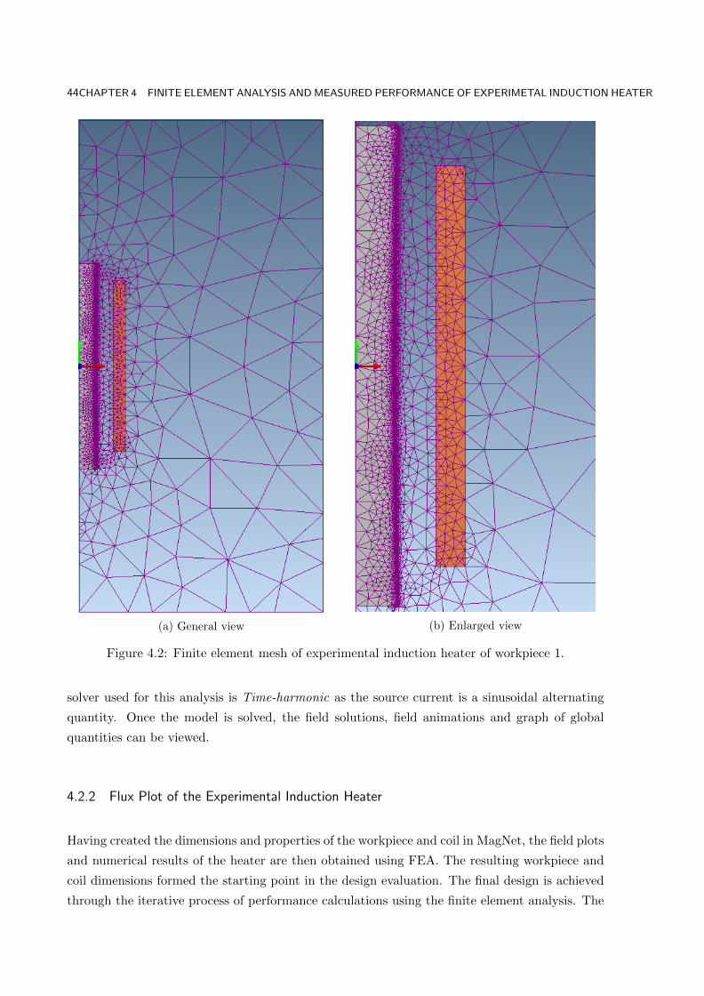
44CHAPTER 4 FINITE ELEMENT ANALYSIS ANDMEASURED PERFORMANCE OF EXPERIMETAL INDUCTION HEATER
(a) General view (b) Enlarged view
Figure 4.2: Finite element mesh of experimental induction heater of workpiece 1.
solver used for this analysis is Time-harmonic as the source current is a sinusoidal alternating
quantity. Once the model is solved, the field solutions, field animations and graph of global
quantities can be viewed.
4.2.2 Flux Plot of the Experimental Induction Heater
Having created the dimensions and properties of the workpiece and coil in MagNet, the field plots
and numerical results of the heater are then obtained using FEA. The resulting workpiece and
coil dimensions formed the starting point in the design evaluation. The final design is achieved
through the iterative process of performance calculations using the finite element analysis. The

4.2 FINITE ELEMENT METHOD 45
material properties of the mild steel workpiece used for the experimental heater depicted in
Chapter 2 are repeated here in Table 4.1. The dimensions of the workpieces are given in Chapter
2. They all have the same lengths, but different diameters and thicknesses. These experimental
workpieces were used with the same induction coil presented in Chapter 2.
Table 4.1: Physical properties of copper and mild steel
Material Copper Mild steel
Resistivity (Ωm × 10−8) 1.72 16Relative permeability 1 750Skin depth at 50Hz (mm) 9.3 1.0
A half-model of the flux plot of the heater of experiment 1 is shown in Figure 4.3. The coil
is energized with 100V supply. The maximum flux density in the workpiece is 1.7T. A small
amount of fringing can be seen at both ends of the workpiece. Most of the flux lines pass through
about 1mm at the surface of the workpiece, i.e., the skin depth for mild steel is about 1mm.
Saturation is mainly in the skin depth of the workpiece.
4.2.3 FEA Performance Calculation
Table 4.2 shows the performance of the experimental heater at 100V supply, calculated using
FEA. All the maximum flux densities are at the assumed knee point of the B-H curve. The
coil current and coil losses are, in general lower than those calculated using the SEC and TEC
models in Chapters 2 and 3 respectively. The workpiece losses and power factors are also lower
than those calculated from the SEC and TEC models. The calculated coil losses and workpiece
losses decrease as the diameter of the workpiece increases. This pattern shows up in the TEC
model calculations, but not so with the coil and workpiece losses in the SEC model.
Table 4.2: Calculated performance using FEA model
Workpiece Voltage Current Flux Coil Workpiece Apparent Power(V) (A) density loss loss power factor
(T) (W) (W) (VA)
1 100 2.3 1.7 8.6 55.5 230 0.32 100 2.3 1.7 8.4 55.4 230 0.33 100 2.3 1.7 8.6 55.9 230 0.34 100 2.1 1.7 7.1 49.4 210 0.35 100 1.9 1.7 6.1 42.0 190 0.36 100 1.5 1.7 3.9 28.0 150 0.37 100 1.5 1.7 3.5 26.2 150 0.3
The FEA has been used to determine the workpiece losses, and winding losses and can, therefore,
be used to predict the performance of the experimental heater more precisely. The FEA has
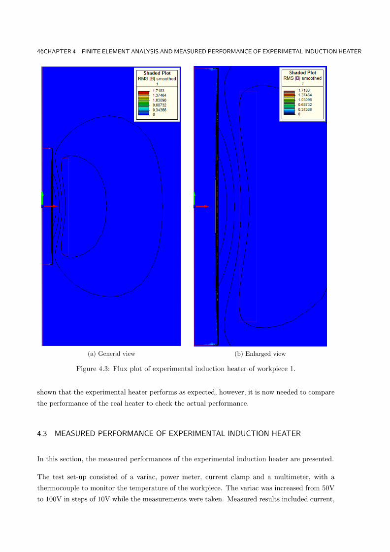
46CHAPTER 4 FINITE ELEMENT ANALYSIS ANDMEASURED PERFORMANCE OF EXPERIMETAL INDUCTION HEATER
(a) General view (b) Enlarged view
Figure 4.3: Flux plot of experimental induction heater of workpiece 1.
shown that the experimental heater performs as expected, however, it is now needed to compare
the performance of the real heater to check the actual performance.
4.3 MEASURED PERFORMANCE OF EXPERIMENTAL INDUCTION HEATER
In this section, the measured performances of the experimental induction heater are presented.
The test set-up consisted of a variac, power meter, current clamp and a multimeter, with a
thermocouple to monitor the temperature of the workpiece. The variac was increased from 50V
to 100V in steps of 10V while the measurements were taken. Measured results included current,
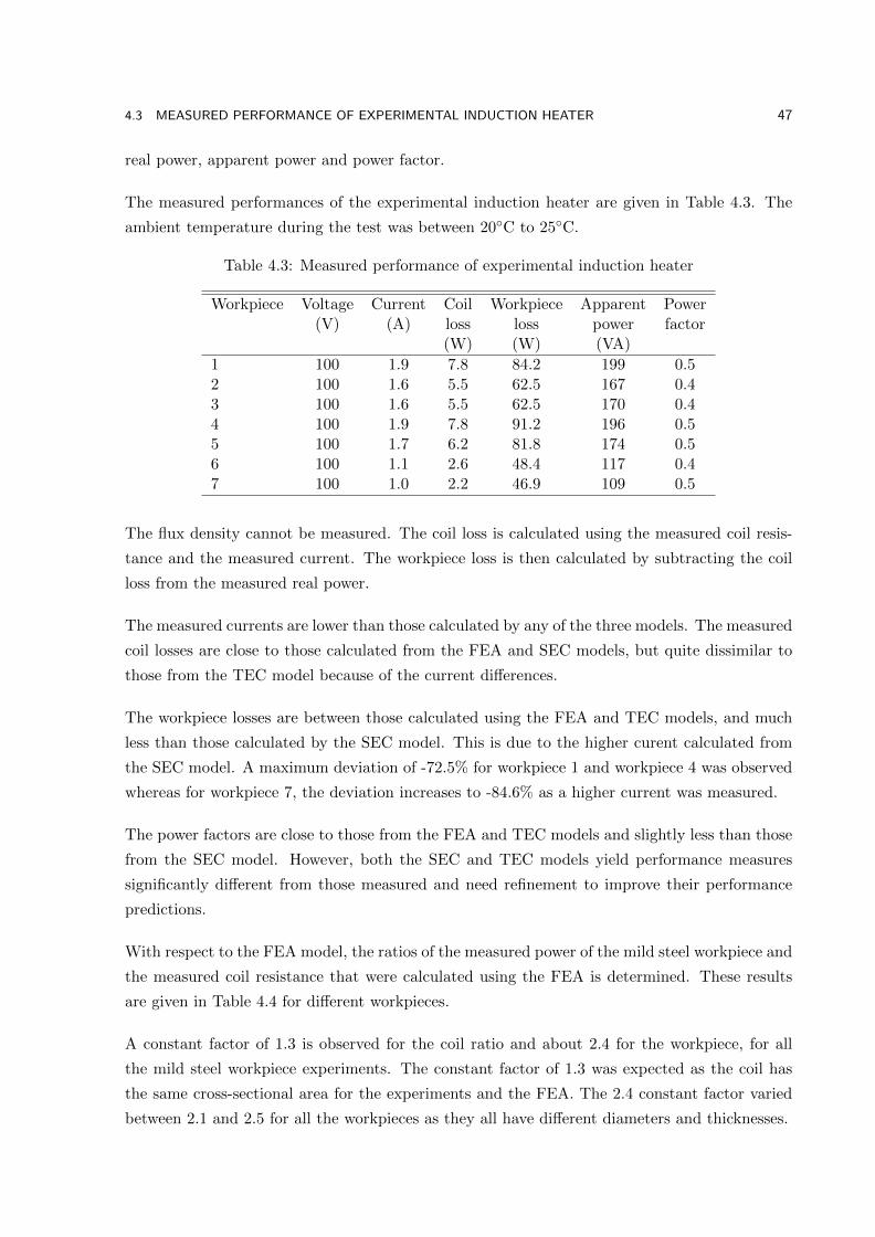
4.3 MEASURED PERFORMANCE OF EXPERIMENTAL INDUCTION HEATER 47
real power, apparent power and power factor.
The measured performances of the experimental induction heater are given in Table 4.3. The
ambient temperature during the test was between 20C to 25C.
Table 4.3: Measured performance of experimental induction heater
Workpiece Voltage Current Coil Workpiece Apparent Power(V) (A) loss loss power factor
(W) (W) (VA)
1 100 1.9 7.8 84.2 199 0.52 100 1.6 5.5 62.5 167 0.43 100 1.6 5.5 62.5 170 0.44 100 1.9 7.8 91.2 196 0.55 100 1.7 6.2 81.8 174 0.56 100 1.1 2.6 48.4 117 0.47 100 1.0 2.2 46.9 109 0.5
The flux density cannot be measured. The coil loss is calculated using the measured coil resis-
tance and the measured current. The workpiece loss is then calculated by subtracting the coil
loss from the measured real power.
The measured currents are lower than those calculated by any of the three models. The measured
coil losses are close to those calculated from the FEA and SEC models, but quite dissimilar to
those from the TEC model because of the current differences.
The workpiece losses are between those calculated using the FEA and TEC models, and much
less than those calculated by the SEC model. This is due to the higher curent calculated from
the SEC model. A maximum deviation of -72.5% for workpiece 1 and workpiece 4 was observed
whereas for workpiece 7, the deviation increases to -84.6% as a higher current was measured.
The power factors are close to those from the FEA and TEC models and slightly less than those
from the SEC model. However, both the SEC and TEC models yield performance measures
significantly different from those measured and need refinement to improve their performance
predictions.
With respect to the FEA model, the ratios of the measured power of the mild steel workpiece and
the measured coil resistance that were calculated using the FEA is determined. These results
are given in Table 4.4 for different workpieces.
A constant factor of 1.3 is observed for the coil ratio and about 2.4 for the workpiece, for all
the mild steel workpiece experiments. The constant factor of 1.3 was expected as the coil has
the same cross-sectional area for the experiments and the FEA. The 2.4 constant factor varied
between 2.1 and 2.5 for all the workpieces as they all have different diameters and thicknesses.
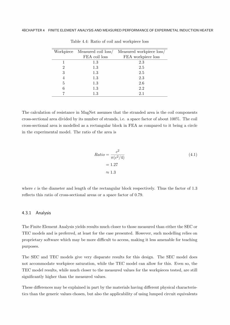
48CHAPTER 4 FINITE ELEMENT ANALYSIS ANDMEASURED PERFORMANCE OF EXPERIMETAL INDUCTION HEATER
Table 4.4: Ratio of coil and workpiece loss
Workpiece Measured coil loss/ Measured workpiece loss/FEA coil loss FEA workpiece loss
1 1.3 2.32 1.3 2.53 1.3 2.54 1.3 2.35 1.3 2.66 1.3 2.27 1.3 2.1
The calculation of resistance in MagNet assumes that the stranded area is the coil components
cross-sectional area divided by its number of strands, i.e. a space factor of about 100%. The coil
cross-sectional area is modelled as a rectangular block in FEA as compared to it being a circle
in the experimental model. The ratio of the area is
Ratio =c2
π(c2/4)(4.1)
= 1.27
≈ 1.3
where c is the diameter and length of the rectangular block respectively. Thus the factor of 1.3
reflects this ratio of cross-sectional areas or a space factor of 0.79.
4.3.1 Analysis
The Finite Element Analysis yields results much closer to those measured than either the SEC or
TEC models and is preferred, at least for the case presented. However, such modelling relies on
proprietary software which may be more difficult to access, making it less amenable for teaching
purposes.
The SEC and TEC models give very disparate results for this design. The SEC model does
not accommodate workpiece saturation, while the TEC model can allow for this. Even so, the
TEC model results, while much closer to the measured values for the workpieces tested, are still
significantly higher than the measured values.
These differences may be explained in part by the materials having different physical characteris-
tics than the generic values chosen, but also the applicability of using lumped circuit equivalents

4.4 SUMMARY 49
of open core devices.
The SEC and TEC models are seen to be useful closed form analytical expressions which can
easily be programmed using readily available advanced calculators or spreadsheet software. How-
ever, their accuracies are such that they yield design guides only, rather than definitive perfor-
mance results. The TEC model is refined in Chapter 5 to improve its performance predictions.
4.4 SUMMARY
This chapter discussed the FEA of a 2D model of the experimental induction heater. The FEA
has been used to determine the flux pattern, workpiece losses, and winding losses and can,
therefore, be used to predict the performance of the experimental heater more precisely. A
maximum flux density of 1.7T in the workpiece is saturating the core.
The measured performances for seven experimental induction heater workpieces are also dis-
cussed. The measured performances were used to validate the results obtained from the FEA,
SEC and TEC models. The measured performances correlated well with the FEA only after
using correction factors 1.3 and 2.4 for coil and workpiece losses respectively. Using a corrected
FEA model, the design FEA model would give values close to the experimental results.


Chapter 5
TRANSFORMER AND TRANSDUCTION HEATING
5.1 INTRODUCTION
In Chapter 3, an induction heater was modelled as a special type of transformer, where the coil
surrounded the workpiece to be heated. The workpiece acted as the core of the transformer and
got hot because of the eddy currents flowing through it. In this chapter, an equivalent circuit to
model the performance of a transformer heater is presented. It is then converted to an equivalent
circuit to model the performance of transduction heaters, a combination of transformer and
induction heaters. Transduction heaters have not been (and cannot be) modelled using the SEC
approach.
Finite element analysis was also used in conjunction with the TEC model to simulate a set of
transduction heating experiments and the results are compared. Analysis of the TEC calculated
results suggested modification of three parameters: the secondary resistance, the core tube eddy
current resistance and the core tube magnetizing reactance. The improved TEC model was then
used to design, build and test a 6kW transduction heater. The measured results are compared
with calculated results from the TEC and FEA models.
5.2 TRANSFORMER HEATER
It is possible to design a transformer directly as a heater. This is often used to provide hot
fluids. The typical arrangement is to have a primary winding that does not produce much
heat, a laminated core that also does not produce much heat, but a shorted secondary winding
that produces most of the heat. The arrangement is shown in Figure 5.1, where the secondary
winding is outside the primary. This allows for ease of access to the fluid.
By making the secondary conductor hollow, or by adding a fluid channel to the back of its
conductor as is done to cool induction heater coils, the real power losses in the secondary can be
transferred by convection to the fluid, thus heating it up. The secondary tube requires fluid inlet
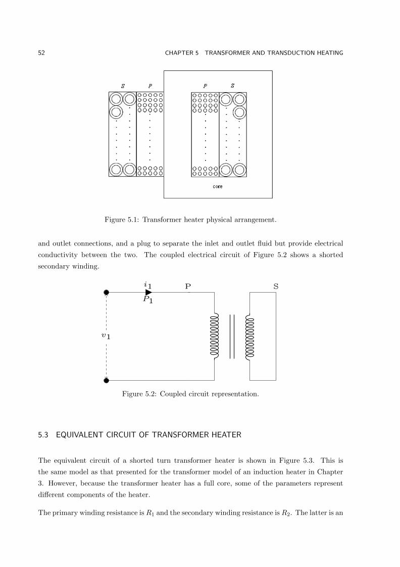
52 CHAPTER 5 TRANSFORMER AND TRANSDUCTION HEATING
Figure 5.1: Transformer heater physical arrangement.
and outlet connections, and a plug to separate the inlet and outlet fluid but provide electrical
conductivity between the two. The coupled electrical circuit of Figure 5.2 shows a shorted
secondary winding.
P1
i1 P S
v1
Figure 5.2: Coupled circuit representation.
5.3 EQUIVALENT CIRCUIT OF TRANSFORMER HEATER
The equivalent circuit of a shorted turn transformer heater is shown in Figure 5.3. This is
the same model as that presented for the transformer model of an induction heater in Chapter
3. However, because the transformer heater has a full core, some of the parameters represent
different components of the heater.
The primary winding resistance is R1 and the secondary winding resistance is R2. The latter is an

5.3 EQUIVALENT CIRCUIT OF TRANSFORMER HEATER 53
P1
i1R1 X1 X2
R2Xmv1
Figure 5.3: Transformer heater equivalent circuit.
average value as the tube temperature will vary, linearly, along its length as the fluid temperature
increases from inlet to outlet. Xm represents the magnetizing reactance. The leakage reactance,
representing the leakage flux of each winding, can be split between the primary and secondary
as X1 and X2.
With respect to the core, the eddy current and hysteresis losses would normally be accounted
for in a transformer within a resistance Rc across Xm. However, for a transformer heater, where
the secondary losses dominate, these losses can be considered insignificant and may be ignored
unless more accurate modeling is considered necessary. Hence the core loss resistance Rc is not
explicitly included in the model.
The parameters making up the model can be calculated using the basic dimensions and charac-
teristics of the materials used, as per the reverse design method. These are entered as know data
and then the individual components calculated using magnetic and electric circuit component
models.
A cross-sectional profile of a multi-layer winding transformer with a full core is shown in Figure
5.4. All the symbols represent dimensions of the materials used in the construction of the
transformer heater, including the core, insulation and the windings.
5.3.1 Winding Resistances
The primary winding resistance is
R1 =ρ1wl1wA1w
(5.1)
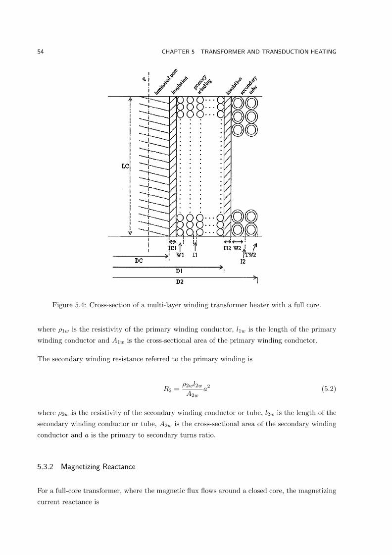
54 CHAPTER 5 TRANSFORMER AND TRANSDUCTION HEATING
Figure 5.4: Cross-section of a multi-layer winding transformer heater with a full core.
where ρ1w is the resistivity of the primary winding conductor, l1w is the length of the primary
winding conductor and A1w is the cross-sectional area of the primary winding conductor.
The secondary winding resistance referred to the primary winding is
R2 =ρ2wl2wA2w
a2 (5.2)
where ρ2w is the resistivity of the secondary winding conductor or tube, l2w is the length of the
secondary winding conductor or tube, A2w is the cross-sectional area of the secondary winding
conductor and a is the primary to secondary turns ratio.
5.3.2 Magnetizing Reactance
For a full-core transformer, where the magnetic flux flows around a closed core, the magnetizing
current reactance is

5.4 TRANSDUCTION HEATING 55
Xm =ωN2
1µ0µrcAclc
(5.3)
where ω is the angular frequency, N1 is the number of turns on the primary coil, µ0 is the
permeability of free space, and µrc is the coil permeability of the magnetic flux path. Ac is the
effective cross-sectional area of the coil, calculated using the skin depth δc, and lc is the coil
length.
5.3.3 Leakage Reactance
The primary and secondary winding leakage reactances of a transformer are calculated from
the total leakage reactance which embodies the effects of both windings together. The leakage
reactances X1 and X2 are calculated from
X1 = X2 =ωµ0N
21πτ12
2lc(5.4)
where τ12 is the winding thickness factor, as described in Chapter 3: Transformer Model of
Induction Heater, with subscripts 1 and 2 substituted for c and w.
Having obtained the component values, the equivalent circuit can be solved to calculate the
performance of the device.
5.4 TRANSDUCTION HEATING
Transformer heater can be combined with an induction heater to form a transduction heater. In
this section, the development of transduction heating concepts from the basic induction heating
and transformer heating concepts is presented. The performance of the transduction heater is
modeled using the improved TEC model. A 6kW transduction heater is designed and verified
using the improved TEC and FEA models is also presented in this section.
5.4.1 Basic Heating Concepts
Heating fluid using induction heating can be achieved by passing the fluid through a hollow
ferromagnetic workpiece as shown in Figure 5.5.
The removal of the centre of a workpiece in Figure 5.5 has little effect on the magnetics and
hence the current drawn from the supply, as long as the thickness of the tube is greater than
the skin depth of the magnetic field and hence the steel is not in saturation.

56 CHAPTER 5 TRANSFORMER AND TRANSDUCTION HEATING
Figure 5.5: Conceptual arrangement of induction fluid heater.
Alternatively, the heating can be achieved by passing the fluid over the workpiece, on the outside,
or between two tubes of different diameters such that they form a jacket through which the fluid
flows.
An alternative to induction heating of fluids is transformer heating, as shown in Figure 5.6. The
fluid gains heat as it passes through the hollow tube of the shorted secondary, or through a
cooling channel adhered to the back of a solid conductor.
Figure 5.6: Conceptual arrangement of transformer fluid heater.
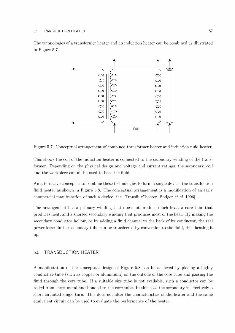
5.5 TRANSDUCTION HEATER 57
The technologies of a transformer heater and an induction heater can be combined as illustrated
in Figure 5.7.
Figure 5.7: Conceptual arrangement of combined transformer heater and induction fluid heater.
This shows the coil of the induction heater is connected to the secondary winding of the trans-
former. Depending on the physical design and voltage and current ratings, the secondary, coil
and the workpiece can all be used to heat the fluid.
An alternative concept is to combine these technologies to form a single device, the transduction
fluid heater as shown in Figure 5.8. The conceptual arrangement is a modification of an early
commercial manifestation of such a device, the “Transflux”heater [Bodger et al. 1996].
The arrangement has a primary winding that does not produce much heat, a core tube that
produces heat, and a shorted secondary winding that produces most of the heat. By making the
secondary conductor hollow, or by adding a fluid channel to the back of its conductor, the real
power losses in the secondary tube can be transferred by convection to the fluid, thus heating it
up.
5.5 TRANSDUCTION HEATER
A manifestation of the conceptual design of Figure 5.8 can be achieved by placing a highly
conductive tube (such as copper or aluminium) on the outside of the core tube and passing the
fluid through the core tube. If a suitable size tube is not available, such a conductor can be
rolled from sheet metal and bonded to the core tube. In this case the secondary is effectively a
short circuited single turn. This does not alter the characteristics of the heater and the same
equivalent circuit can be used to evaluate the performance of the heater.

58 CHAPTER 5 TRANSFORMER AND TRANSDUCTION HEATING
Figure 5.8: Conceptual arrangement of transduction fluid heater.
One option is for the fluid to make a single pass up through the centre of the workpiece. Thus
the heat from the secondary and the workpiece tubes conducts radially inwards to the fluid.
However, since the primary winding is electrically and hence thermally insulated from the core
and the secondary tubes, not much of the heat generated in the primary winding is captured by
the fluid. Most of this heat is radiated and convected outwards to ambient surroundings.
Alternatively, the fluid can be passed between the core and secondary tubes, and the primary
winding former. This helps capture some of the primary winding heat. However, again some
heat goes to the ambient surroundings. Thus the transduction fluid heater is less than 100%
efficient. While the natural cooling of the primary winding by the ambient surroundings may
be sufficient for continuous operation, some form of forced cooling may be required if higher
temperatures are involved.
A cut-away image of the transduction heater, where the fluid passes between the bonded sec-
ondary and core tubes and the primary winding former, is shown in Figure 5.9.
Stainless steel liners inside the primary winding former and outside (or instead of) the secondary
winding, allow heating of corrosive fluids, or fluids where non-contamination is critical, without
significantly affecting the electrical to thermal performance of the device. This is because the
relative permeability of stainless steel is effectively unity and the depth of penetration of the
magnetic field is large allowing the magnetic fields essentially to pass straight through and into
the ferromagnetic workpiece.

5.6 MEASURED PERFORMANCE OF EXPERIMENTAL TRANSDUCTION HEATER 59
Figure 5.9: Cut-away image of transduction fluid heater.
Because of the strength of the materials involved and the robustness of the manufacture, with
this technology, relatively high fluid pressures and temperatures can be achieved.
Laminated steel placed inside the core tube improves the power factor of this device if the core
tube steel is in saturation. This can also help counter the decreased power factor due to the
increased spacing between the primary and the secondary windings, because of the stainless steel
insertions and the fluid channel.
5.6 MEASURED PERFORMANCE OF EXPERIMENTAL TRANSDUCTION HEATER
A coil of a small transduction heater was constructed with the following parameter dimensions
as shown in Table 5.1. This is the same coil that was used for the induction heating experiments
in Chapters 2, 3 and 4 respectively.
A number of mild steel, stainless steel, aluminium, and copper tubes of various diameters and
thicknesses were cut to provide workpieces and secondary tubes that fitted inside the coil. The

60 CHAPTER 5 TRANSFORMER AND TRANSDUCTION HEATING
Table 5.1: Coil dimensions
Material Copper Units
Resistivity 1.72×10⁻⁸ ΩmLength 208 mmOutside diameter 114 mmInside diameter 83 mmWire diameter 1.7 mmWire area 2.27 mm2
Number of layers 9 -Turns per layer 111 -Number of turns 999 -Length of wire 309 mCalculated resistance 2.34 ΩMeasured resistance (50Hz) 2.15 Ω
dimensions of these are listed in Table 5.2.
Table 5.2: Workpiece and secondary tube dimensions
Workpiece Material Length Diameter Thickness(mm) (mm) (mm)
1 Mild steel 250 44.3 solid2 Mild steel 250 44.5 12.63 Mild steel 250 44.2 6.34 Stainless steel 250 50.8 1.25 Aluminium 250 50.8 1.36 Copper 250 62.0 0.87 Mild steel 250 70.0 2.08 Mild steel 250 73.0 solid9 Aluminium 250 76.0 1.25
Various combinations of the tubes were assembled inside the coil. Figure 5.10 shows a photograph
of the transduction heater with a combination of tubes (2+5) inside the coil.
The test set-up and measurement method is the same as presented for the induction heating
experiments in Chapter 4. By applying a 100V supply to the coil, the performances of different
tube combinations are given in Table 5.3. These values were used as a benchmark to compare
calculated performance values against.
5.7 EQUIVALENT CIRCUIT OF TRANSDUCTION HEATER
The transduction heater can be modelled as a transformer with a single shorted turn secondary
winding, and the core tube as a partial core of a transformer [Liew and Bodger 2001]. The core
tube has the function of acting like the core of a transformer, but it is incomplete in that the

5.7 EQUIVALENT CIRCUIT OF TRANSDUCTION HEATER 61
Figure 5.10: Transduction heater with combination of tubes (2+5).
Table 5.3: Measured performance at 100V supply
Workpiece Voltage Current Real power Apparent power Powerlabel (V) (A) (W) (VA) factor
1 +4 100 2.4 110 239 0.462 + 5 100 5.1 370 470 0.783 + 6 100 5.2 410 490 0.823 + 9 100 4.0 320 380 0.837 + 9 100 3.8 320 370 0.878 + 9 100 3.8 320 370 0.88
return path of the magnetic flux is through the ambient medium. The equivalent circuit that is
used to model the transduction heater is shown in Figure 5.11.
where R1, R2 are the primary and secondary resistances, Xmc, is the core tube magnetizing
reactance, Rce is the core tube eddy current resistance, andX1, X2 are the primary and secondary
leakage reactances. Hysteresis losses, usually the dominant part of core losses in a transformer,
are ignored in this model as they are insignificant compared to the eddy current losses.
The parameters of the equivalent circuit in Figure 5.11 are calculated using the basic dimen-
sions and physical characteristics of materials used, as per the reverse design method [Liew and
Bodger 2001], [Bodger and Liew 2002]. These are entered as known data and then the individual
circuit components are calculated using magnetic and electric circuit component models.

62 CHAPTER 5 TRANSFORMER AND TRANSDUCTION HEATING
R1 X1 X2 R2
Xmc Rce
Figure 5.11: Equivalent circuit of transduction heater.
5.7.1 Winding Resistance
The primary winding resistance is given by
R1 =ρ1wl1wA1w
(5.5)
where ρ1w is the resistivity of the primary winding conductor, l1w is the length and A1w is the
cross-sectional area of the primary winding conductor.
The secondary winding resistance referred to the primary winding is
R2 =ρ2wl2wA2w
a2 (5.6)
where ρ2w is the resistivity of the secondary winding conductor or tube, l2w is the length of the
secondary tube, A2w is the cross-sectional area of the secondary winding conductor and a is the
primary to secondary turns ratio.
The variation of resistivity with temperature of the conductor materials are accounted for. In
general, the operating resistivity of a material is
ρc = (1 + (∆ρ(Tc − 20)))ρ20C (5.7)
where ρ20C is the resistivity at 20C, Tc is the material temperature, and ∆ρ is the thermal
resistivity coefficient.

5.7 EQUIVALENT CIRCUIT OF TRANSDUCTION HEATER 63
5.7.2 Magnetizing Reactance
The magnetizing current reactance is
Xmc =ωN2
1µ0µrceAclc
(5.8)
where, N1 is the number of turns on the primary coil, Ac is the effective cross-sectional area
of the core tube, calculated using the depth of penetration, δc, and lc is the flux path length.
Also, µrce is the effective value based on the composite air/iron magnetic flux path, as for the
transformer model of an induction heater [Takau and Bodger 2013].
If the magnetic flux density in the core tube exceeds the saturation value, the relative permeabil-
ity reduces, forcing the flux skin depth to increase and the density to reduce. If the calculated
skin depth is greater than the thickness of the core tube, then the flux flows through both the
core tube metal and inside fluid space. This is also modelled as for the transformer model of an
induction heater [Takau and Bodger 2013].
5.7.3 Core Tube Eddy Current Resistance
In this model the eddy current losses in the core tube are accounted for by the resistance Rce
across Xmc. Thus Rce is calculated from
Rce =N2
1ρclceAce
(5.9)
where ρc is the core tube resistivity, lce is the length of the eddy current path around the core
tube, and Ace is the cross-sectional area of the eddy current path, the product of lc and δc.
Again, the variation of resistivity with temperature of the conductor material is accounted for.
5.7.4 Leakage Reactance
The primary and secondary leakage reactances of a transformer are calculated from the total
leakage reactance which embodies the effects of both windings together. The leakage reactances
X1 and X2 are calculated from
X1 = X2 =ωµ0N
21πτ12
2lc(5.10)

64 CHAPTER 5 TRANSFORMER AND TRANSDUCTION HEATING
where τ12 is the winding thickness factor, related to the thickness of the primary winding and
the secondary tube [Takau and Bodger 2013].
5.8 EQUIVALENT CIRCUIT PERFORMANCE
The equivalent circuit of the transduction heater can be solved to calculate the performance of
the device. The physical characteristics of the copper, stainless steel, aluminium and mild steel
tubes were taken as given in Table 5.4.
Table 5.4: Physical properties
Material Copper Mild steel Stainless steel Aluminium
Resistivity (Ωm × 10−8) 1.72 16 70 2.65Relative permeability 1 750 1 1Skin depth at 50Hz(mm) 9.3 2.5 60 11.6Density (kg/m3) 8960 7870 8000 2700
The same combinations of tubes as assembled for the measurements were used and the param-
eters of the equivalent circuits calculated from their material characteristics and dimensions.
The performance of the heater was calculated by solving the equivalent circuit equations and
determining the current, power and power factor for a given applied voltage. The equivalent
circuit also allowed separation of the real power losses into individual component values. In
addition, as required, efficiencies, voltage gradients, voltages per turn and current densities can
be calculated. The calculated results are given in Table 5.5.
Table 5.5: Calculated performance using TEC model for a 100V supply
Workpiece Voltage Current Primary Secondary Core Real Apparent Power(V) (A) loss loss loss power power factor
(W) (W) (W) (W) (VA)
1 + 4 100 3.9 36.7 18.1 165.3 220.1 398.0 0.552 + 5 100 7.6 135.2 313.1 109.2 557.5 765.0 0.733 + 6 100 7.2 118.8 308.9 133.8 561.5 717.0 0.783 + 9 100 6.9 111.1 310.3 157.3 578.7 693.0 0.837 + 9 100 5.8 77.4 337.9 64.2 479.5 579.0 0.838 + 9 100 5.7 75.8 339.4 59.1 474.3 573.0 0.83
In general, the calculated real powers are significantly higher than those measured. This is
reflected in the higher current values and apparent power. This suggested that the overall
calculated impedance was low compared to the measured value. However, the power factors
were similar.
Within the detail of the calculated results, one specific anomaly is that the losses in the core tube
are significantly higher than those in the secondary tube for the (1+4) combination. However
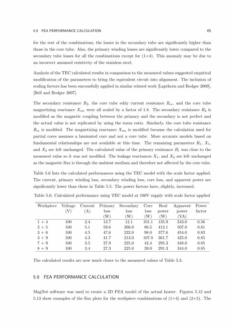
5.9 FEA PERFORMANCE CALCULATION 65
for the rest of the combinations, the losses in the secondary tube are significantly higher than
those in the core tube. Also, the primary winding losses are significantly lower compared to the
secondary tube losses for all the combinations except for (1+4). This anomaly may be due to
an incorrect assumed resistivity of the stainless steel.
Analysis of the TEC calculated results in comparison to the measured values suggested empirical
modification of the parameters to bring the equivalent circuit into alignment. The inclusion of
scaling factors has been successfully applied in similar related work [Lapthorn and Bodger 2009],
[Bell and Bodger 2007].
The secondary resistance R2, the core tube eddy current resistance Rce, and the core tube
magnetizing reactance Xmc were all scaled by a factor of 1.8. The secondary resistance R2 is
modified as the magnetic coupling between the primary and the secondary is not perfect and
the actual value is not replicated by using the turns ratio. Similarly, the core tube resistance
Rce is modified. The magnetizing reactance Xmc is modified because the calculation used for
partial cores assumes a laminated core and not a core tube. More accurate models based on
fundamental relationships are not available at this time. The remaining parameters R1, X1,
and X2 are left unchanged. The calculated value of the primary resistance R1 was close to the
measured value so it was not modified. The leakage reactances X1, and X2 are left unchanged
as the magnetic flux is through the ambient medium and therefore not affected by the core tube.
Table 5.6 lists the calculated performances using the TEC model with the scale factor applied.
The current, primary winding loss, secondary winding loss, core loss, and apparent power are
significantly lower than those in Table 5.5. The power factors have, slightly, increased.
Table 5.6: Calculated performance using TEC model at 100V supply with scale factor applied
Workpiece Voltage Current Primary Secondary Core Real Apparent Power(V) (A) loss loss loss power power factor
(W) (W) (W) (W) (VA)
1 + 4 100 2.4 13.7 12.1 101.1 135.9 243.0 0.562 + 5 100 5.1 59.6 266.0 86.5 412.1 507.0 0.813 + 6 100 4.5 47.6 232.0 98.0 377.6 454.0 0.833 + 9 100 4.3 41.7 213.0 107.0 361.7 425.0 0.857 + 9 100 3.5 27.9 225.0 42.4 295.3 348.0 0.858 + 9 100 3.4 27.3 225.0 39.0 291.3 344.0 0.85
The calculated results are now much closer to the measured values of Table 5.3.
5.9 FEA PERFORMANCE CALCULATION
MagNet software was used to create a 2D FEA model of the actual heater. Figures 5.12 and
5.13 show examples of the flux plots for the workpiece combinations of (1+4) and (2+5). The

66 CHAPTER 5 TRANSFORMER AND TRANSDUCTION HEATING
coil is energised with a 100V supply. The maximum flux density in the workpiece is 1.7T. A
small amount of fringing can be seen at both ends of the workpiece for the combination of (2+5).
Most of the flux is confined to the region near the surface of the mild steel workpiece. There is
very little field in the interior of the workpiece as the radius is several times greater than the
skin depth of the workpiece.
(a) General view (b) Enlarged view
Figure 5.12: Flux plot of workpiece combination (1+4).
Table 5.7 shows the performance of the experimental heater at a 100V supply voltage, calculated
using FEA. All the workpiece maximum flux densities are at the assumed knee point of the B-H
curve. The primary losses are, in general, lower than those given in Table 5.6 except for the
(3+6) combination. The coil current and power factors are close to those given in Table 5.6.
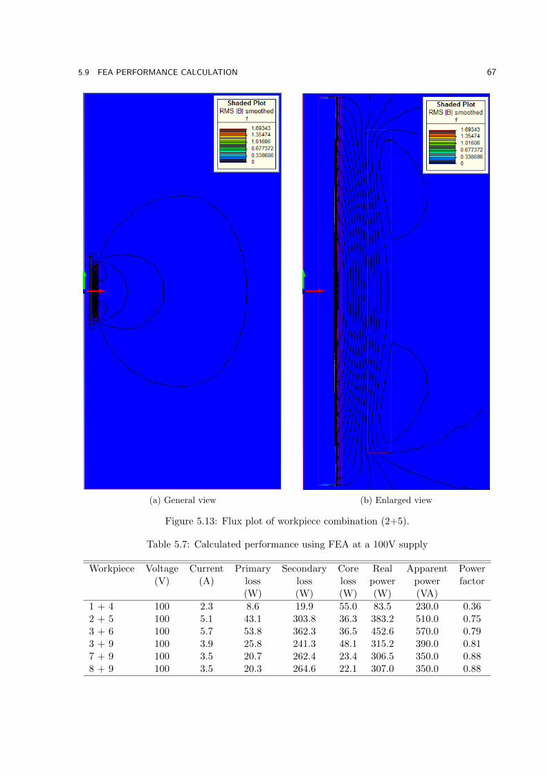
5.9 FEA PERFORMANCE CALCULATION 67
(a) General view (b) Enlarged view
Figure 5.13: Flux plot of workpiece combination (2+5).
Table 5.7: Calculated performance using FEA at a 100V supply
Workpiece Voltage Current Primary Secondary Core Real Apparent Power(V) (A) loss loss loss power power factor
(W) (W) (W) (W) (VA)
1 + 4 100 2.3 8.6 19.9 55.0 83.5 230.0 0.362 + 5 100 5.1 43.1 303.8 36.3 383.2 510.0 0.753 + 6 100 5.7 53.8 362.3 36.5 452.6 570.0 0.793 + 9 100 3.9 25.8 241.3 48.1 315.2 390.0 0.817 + 9 100 3.5 20.7 262.4 23.4 306.5 350.0 0.888 + 9 100 3.5 20.3 264.6 22.1 307.0 350.0 0.88

68 CHAPTER 5 TRANSFORMER AND TRANSDUCTION HEATING
The FEA model yields results significantly higher than those measured for workpiece combi-
nations of (2+5) and (3+6) and lower for the rest of the combinations in terms of the power
losses. The TEC model yields results significantly higher than those measured for the workpiece
combinations of (1+4), (2+5) and (3+9). However, the rest of the combinations are close to the
measured values.
5.10 DESIGN OF A 6KW TRANSDUCTION HEATER
The improved performance prediction of the TEC model was used to design a 6kW transduction
heater. The calculated performance of the designed heater was compared with FEA calculations
and experimental results. The coil and workpiece dimensions of the designed heater are given
in Tables 5.8 and 5.9. The measured resistance of the coil is very close to the calculated value
from the TEC model as shown in Table 5.8.
Table 5.8: Coil dimensions
Material Copper Units
Resistivity 1.72×10⁻⁸ ΩmLength 420 mmOutside diameter 114 mmInside diameter 83 mmWire diameter 3.4 mmWire area 9.08 mm2
Number of layers 7 -Turns per layer 140 -Number of turns 980 -Length of wire 289 mCalculated resistance 0.55 ΩMeasured resistance (50Hz) 0.54 Ω
Table 5.9: Workpiece dimensions
Workpiece Length Diameter Thickness(mm) (mm) (mm)
Mild steel core tube 500 60.0 4.6Secondary copper tube 500 62.6 1.3
Figure 5.14 shows the designed heater with the mild steel and secondary copper tubes inside the
coil. The physical properties of the mild steel and copper tubes are given in Table 5.9.
The various components of the TEC circuit are given in Table 5.10. The equivalent circuit
parameters show that the primary winding resistance is lower compared to the secondary resis-
tance, and there are lower leakage reactances, since the primary winding and secondary tube
thickness is smaller.

5.10 DESIGN OF A 6KW TRANSDUCTION HEATER 69
Figure 5.14: 6kW transduction fluid heater.
Table 5.10: Component values for the TEC model
Circuit component Value (Ω)
R1 0.55R2 8.74X1 1.24X2 1.24Xmc 35.8Rce 27.8
The calculated results of the transduction heater using the TEC and FEA models are given in
Table 5.11, along with the measured performance.
Table 5.11: Calculated and measured results of the designed transduction heater
TEC FEA Measured
Voltage (V) 230 230 230Current (A) 30.9 43.9 31.0Apparent power (kVA) 7.13 10.1 7.13Real power (kW) 6.5 8.4 6.3Power factor 0.91 0.83 0.91
The calculated results from the TEC match the measured results well, reinforcing the usefulness
of the TEC model to predict the performance of transduction heaters. The calculated results
from the FEA model show significantly higher values in terms of the current, apparent power,
70 CHAPTER 5 TRANSFORMER AND TRANSDUCTION HEATING
and real power compared to the results from the TEC. However, the power factor is significantly
lower than the TEC and measured results. Because of the higher current calculated from FEA,
the rest of the measured parameters are all affected as well. This may be due to how FEA
calculates the resistance from the geometry of the coil and inductance from Maxwell’s equations
and also the material properties created in MagNet for the calculation.
Other performance measures can be determined by calculation from the TEC program but
cannot be measured on an actual transduction heater. These are given in Table 5.12.
Table 5.12: TEC calculated performance
Parameter Value
VT1-primary voltage/turn 0.23VV2-secondary eddy voltage 0.20VVA-primary/secondary voltage ratio 1123.7VE-core tube eddy voltage 0.20VA1-primary winding current area 9.08×10⁻⁶m2
J1-primary winding current density 3.41A/mm2
I2-secondary tube current 22.3kAA2-secondary tube current area 6.5×10⁻⁴m2
J2-secondary tube current density 34.3A/mm2
ICE-core tube eddy current 7.1kAACE-core tube eddy current area 1.75×10⁻³m2
The voltage per turn on the primary is very low and no extra insulation is required. The
currents in the secondary and core tubes are very large in comparison to the primary current,
but they can be directly cooled by the water or the liquid that is going to be heated, so their
current densities are acceptable. The primary current density is 3.41A/mm2 which is at a level
that natural cooling of the coil (primary winding) would be sufficient. The tolerable current
density J1 in a conductor depends mainly on its cooling. For no forced or artificial cooling, J1
= 1−4A/mm2, varying from large to small conductors respectively.
5.11 SUMMARY
This chapter presented the modelling of transduction heaters using TEC and FEA models. The
performances of the transduction heaters from these models were compared to the measured
performances of an experimental heater for a variety of sizes of mild steel, copper, aluminium
and stainless steel tubes. The calculated performances of the TEC model showed significantly
lower values in terms of the current and workpiece losses compared to the FEA model. The TEC
model was improved by applying an empirically derived scale factor to selected components to
give much closer values to those measured.
The improved TEC model was then used to design a new transduction heater. The calculated

5.11 SUMMARY 71
and measured performances were very close. The TEC model gave a better prediction than the
FEA model, suggesting that the TEC model can be a useful tool to design transduction heaters.
The research will now move to the design of an industrially useful device, which will be presented
in Chapter 6.


Chapter 6
DESIGN OF AN INDUSTRIAL TRANSDUCTION FLUID HEATER
6.1 INTRODUCTION
This chapter presents the design and construction of a three phase 40kW transduction fluid
heater. The three phase heater is obtained by connecting three single phase units in an appro-
priate star configuration, with the fluid tubes connected in series.
A generic definition of transduction heating is explained, as derived from the co-joining of trans-
former and induction heating. The transduction heater design description and considerations
such as winding dimensions and layout are then discussed. Details of the construction of the
transduction fluid heater are also given. This includes discussion of the core tube and secondary
tube design, thermal insulation, inter-layer insulation, the primary winding construction, and
also the cooling method used.
The chapter concludes with details of the physical specifications used in the design program and
the equivalent circuit parameters given as an output of the TEC program. The magnetic field
patterns of the designed transduction fluid heater are determined using FEA. The calculated
results obtained from these two models are discussed and compared.
6.2 TRANSFORMERS
A single phase power transformer is a device which has a primary and a secondary winding
wound about a core. When a voltage is applied to the primary winding of a transformer, a
magnetic field is generated in the core. This couples to and produces an emf in the secondary
winding. Power, and hence energy, is transferred from an ac system of one voltage connected to
the primary winding, to an ac voltage of another system connected to the secondary winding.
The power transformer is normally designed for high efficiency (of the order of 98−99%). The
windings are usually made of copper, an inexpensive, low resistivity material, to give low power

74 CHAPTER 6 DESIGN OF AN INDUSTRIAL TRANSDUCTION FLUID HEATER
losses, although other materials are used. The power losses are approximately equal in the
primary and secondary windings. A ferromagnetic core is used, again achieving low losses.
The core material is usually laminated into high resistance paths to reduce eddy current power
losses and to provide a uniform flux density. The material is chosen to have little hysteresis
heating. Its high permeability implies very little magnetization current.
6.3 INDUCTION HEATERS
An induction heater can be viewed as a special type of transformer where the primary winding
is placed about the material to be heated. The power losses, and hence heating, due to eddy
currents induced in the material, are encouraged. The core material, referred to as the workpiece
or billet, is usually solid. The efficiency of an induction heater is usually not as high as that for
a transformer heater.
The extent of the heating is determined by the material resistivity, its magnetic permeability and
the frequency of the excitation source. These factors are combined into a depth of penetration or
skin depth of the flux and current in the material. Significant heating in the billet or workpiece is
usually found in the first 1.5−2 skin depths. For copper at 50Hz, the skin depth is approximately
10mm. For mild steel it is about 2.5mm. Material inside the skin depth relies on conduction
heat flow from this region.
6.4 TRANSDUCTION HEATER DESIGN
Transduction heating is a combination of transformer and induction heating. It is an induction
heater that includes a secondary winding to boost performance. Both induction and transformer
heaters use the fundamental principles of magnetic fields as the power transfer medium from
the supply to the material to be heated. Thus, there is an electric-magnetic-electric-heat series
of energy conversion.
The easiest way to design the transduction fluid heater is by the selection of the sizes and shapes
of the components that can be procured and which start with the core tube and work outwards.
The material characteristics are thus estimated and dimensions measured, and entered as known
data. Individual circuit components are then calculated using magnetic circuit and electric cir-
cuit component models and assembled into an equivalent circuit. The performance of the heater
is calculated from this equivalent circuit and is therefore a result of the design. This is called the
reverse design method [Liew and Bodger 2001], [Bodger and Liew 2002]. This design method
takes into account the physical characteristics, such as material resistivities, permeabilities, and

6.5 DESIGN DESCRIPTION 75
the dimensions of the windings and the core as specifications. By altering these specifications,
the performance of the device can be optimized and a suitable design obtained.
6.5 DESIGN DESCRIPTION
The TEC model accurately predicted the performance of the 6kW transduction heater designed
in [Takau and Bodger 2014]. The research is now moved to the design of an industrially useful
device, that is, the design of a nominal 40kW transduction fluid heater that can be used to heat
fluids (water or food). For example, in the pasteurization of milk, the milk has to be heated
up to 85C from 4C and then is cooled to 4C again. The response rate of the heater must
be very fast in order to ensure proper treatment of the milk. In the case of long life milk, it is
necessary to heat the milk to a temperature of 140C and then cool it again [MilkFacts 2014],
[ScientificAmerican 2014]. The heater of this thesis has been designed with such requirements
in mind.
6.5.1 Design Consideration
The performance of the 6kW transduction heater designed in [Takau and Bodger 2014] was
predicted well using both the TEC model and the FEA software. The new design includes some
of the design materials used in this original heater. These include the composite tubes for the
core tube and the secondary tube. The new materials that are added include grooved fiberglass
sheets for insulation between the layers of the primary winding, vegetable oil for cooling the
primary winding, a stainless steel baffle outside the primary winding, to allow heat from the
winding to flow to a heat exchanger outside the baffle with flowing water, and a stainless steel
tube for the housing. The size and length of the primary winding conductor was also changed
for the new design.
A detailed cross-section of the new transduction fluid heater is shown in Figure 6.1. To measure
the thermal performance of the heater, thermocouples are placed at different locations to monitor
the temperature rise of the primary winding, the oil, and the cooling water and fluid inlets and
outlets. The new design can be used as a water heater or as a fluid heater for other than water,
depending on the applications.
To use the device as a water heater, the water outlet can be connected to the product inlet
using a pipe or a hose. In this variation, the heat generated in the primary, core tube and the
secondary tube could all be used to heat the water. Hence, a higher efficiency is expected in
this design. For other than water, the efficiency is less than 100%, as the heat generated in the
primary will be lost to the cooling water. However, by careful design, these winding losses can
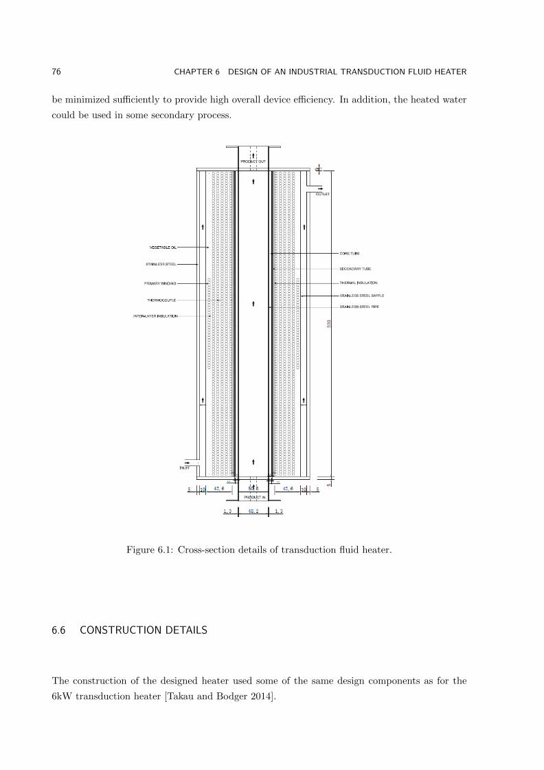
76 CHAPTER 6 DESIGN OF AN INDUSTRIAL TRANSDUCTION FLUID HEATER
be minimized sufficiently to provide high overall device efficiency. In addition, the heated water
could be used in some secondary process.
Figure 6.1: Cross-section details of transduction fluid heater.
6.6 CONSTRUCTION DETAILS
The construction of the designed heater used some of the same design components as for the
6kW transduction heater [Takau and Bodger 2014].

6.6 CONSTRUCTION DETAILS 77
6.6.1 Core Tube
The core tube is a sleeve of ferromagnetic mild steel inside the secondary tube. The core tube
has the function of acting like the core of a transformer. However, it is incomplete in that the
return path of the magnetic flux is through the ambient medium. The core tube also acts as a
billet of an induction heater and gets hot due to eddy current flow inside it.
The fluid which is desired to be heated passes inside a stainless steel tube that is inside the core
tube. This stainless steel tube is essentially the workpiece in induction heating terminology,
however, there are no eddy currents induced in this stainless steel tube as the magnetic flux
does not penetrate into it. Thus, it is not part of the transduction heater, but rather a material
to be heated indirectly by heat transfer from the transduction heater.
The stainless steel tube pipe selected such that there is a good physical contact between the
workpiece and the core tube, so that heat generated in the transduction heater is conducted to
the workpiece. Any fluid flowing in the stainless steel tube will make surface contact so that the
heat generated is transferred by convection into the fluid.
The length and diameter of the workpiece are selected as what is required. For the core tube,
the length is generally set to the same length as the workpiece to give uniform heat transfer to
the workpiece. The thickness of the core tube is selected so that it is about 2 skin depths. Thus
there is no significant magnetic field penetration inside this tube and hence into the workpiece.
The dimensions of the core tube are listed in Table 6.1. The thickness of the core tube was that
readily available from a manufacturer.
Table 6.1: Core tube dimensions
Parameter Dimension Units
Core length 500 mmOutside diameter 60 mmThickness 4.6 mmResistivity 1.72 ×10⁻⁸ ΩmRelative permeability 750 -Skin depth at 50Hz 1.0 mmMaterial density 7870 kg/m3
6.6.2 Secondary Tube
On the outside of the core tube is the secondary tube. This is selected (or machined) to fit neatly
over the core tube so that they are also in physical contact. Significant heat is generated in the
secondary tube. This heat is conducted through the core tube and transferred to the workpiece.
The thickness of the secondary tube is much less than the depth of penetration of the magnetic

78 CHAPTER 6 DESIGN OF AN INDUSTRIAL TRANSDUCTION FLUID HEATER
field in the material at mains frequency. Thus a uniform current density in the secondary tube
can be assumed. Also most of the magnetic field penetrates through to the core tube.
The length of the secondary tube is again most likely to be equal to the length of the core
tube, for uniform heat transfer to the core tube. The designer specifies the length, thickness,
permeability and resistivity of the secondary tube.
The secondary tube is constructed from a non-ferromagnetic copper tube. The dimensions of
the secondary tube are listed in Table 6.2. Figure 6.2 shows a photograph of the core tube and
secondary tube outside the stainless steel pipe.
Table 6.2: Secondary tube dimensions
Parameter Dimension Units
Secondary tube length 500 mmOutside diameter 62.6 mmThickness 1.3 mmResistivity 1.72×10⁻⁸ ΩmRelative permeability 1 -Skin depth at 50Hz 9.3 mmMaterial density 8960 kg/m3
Figure 6.2: The core and secondary tubes over the workpiece.

6.6 CONSTRUCTION DETAILS 79
6.6.3 Thermal Insulation
To restrict the heat going outwards, it is necessary to thermally insulate the composite of the
secondary and core tubes. The quality and thickness of the thermal insulation (or former) be-
tween the secondary tube and the primary winding is selected based on thermal considerations.
This space has neither electric nor magnetic field effects but the thickness does affect the cou-
pling and hence the leakage flux, and the calculation of parameters associated with the metallic
components of the device.
The thermal insulation composite tube in this project is made with 50/50 cross weave fiberglass.
It is recommended that the thermal insulation can withstand the glow-wire and needle flame
tests of IEC 60695-2-11. The glow-wire test is not carried out on parts of thermal insulation
classified as having a flammability index of 850C. The thermal insulation also acts as reinforced
insulation between the primary winding and the secondary tube. The dimensions of the thermal
insulation are given in Table 6.3 and a photograph is shown in Figure 6.3.
Table 6.3: Thermal insulation dimensions
Parameter Dimension Units
Length 500 mmOutside diameter 72.9 mmThickness 4.6 mmMaterial density 1181 kg/m3
Figure 6.3: Thermal insulation composite tube.
80 CHAPTER 6 DESIGN OF AN INDUSTRIAL TRANSDUCTION FLUID HEATER
6.6.4 Primary Winding
For the primary winding, its length is typically the same length as the secondary and the core
tube. A conductor diameter, its insulation, and the number of layers are selected. The material
will have relative permeability and resistivity properties.
A primary winding was constructed with the parameters and dimensions shown in Table 6.4. The
5.3 layers were wound over the former (or thermal insulation) with the last half layer wound on
the center as shown in Figure 6.1. This ensured symmetrical flux distribution along the heater.
Relative to the 6kW transduction heater, the number of turns in the primary winding has
changed, and the wire length is slightly greater as the former for the winding is a larger diameter
than the core tube on which it was previously wound.
Table 6.4: Primary winding dimensions
Material Copper Units
Length 500 mmOutside diameter 152.1 mmInside diameter 72.9 mmWire diameter 4.0 mmWire area 12.6 mm2
Number of layers 5.3 -Turns per layer 121 -Number of turns 641 -Length of wire 216.6 mResistivity 1.72× 10⁻⁸ ΩmCalculated resistance 0.297 Ω
6.6.5 Inter-Layer Insulation
To ensure that the heat is dissipated evenly between the layers of windings, an alternative
insulation introduced in [Lapthorn et al. 2013b] was used. Figure 6.4 shows a photograph of the
interlayer insulation design. The insulation consists of 3mm thick, g10 fibreglass. The fibreglass
sheets have 3mm wide vertical slots machined into the material every 3mm using a computer
aided manufacturing machine. This allows the oil to flow freely between the windings of each
layer. The depth of the cuts was 2mm leaving 1mm of the fibresheet. In addition to this, 85mm
long slots were cut into the vertical channels with slots on adjacent channels offset, as shown
in Figure 6.4. The first layer of winding is wound directly onto the former (thermal insulation)
as shown in Figure 6.5(a). Then the second layer of winding is wound on top of the inter-layer
insulation and so forth as shown in Figure 6.5(b).
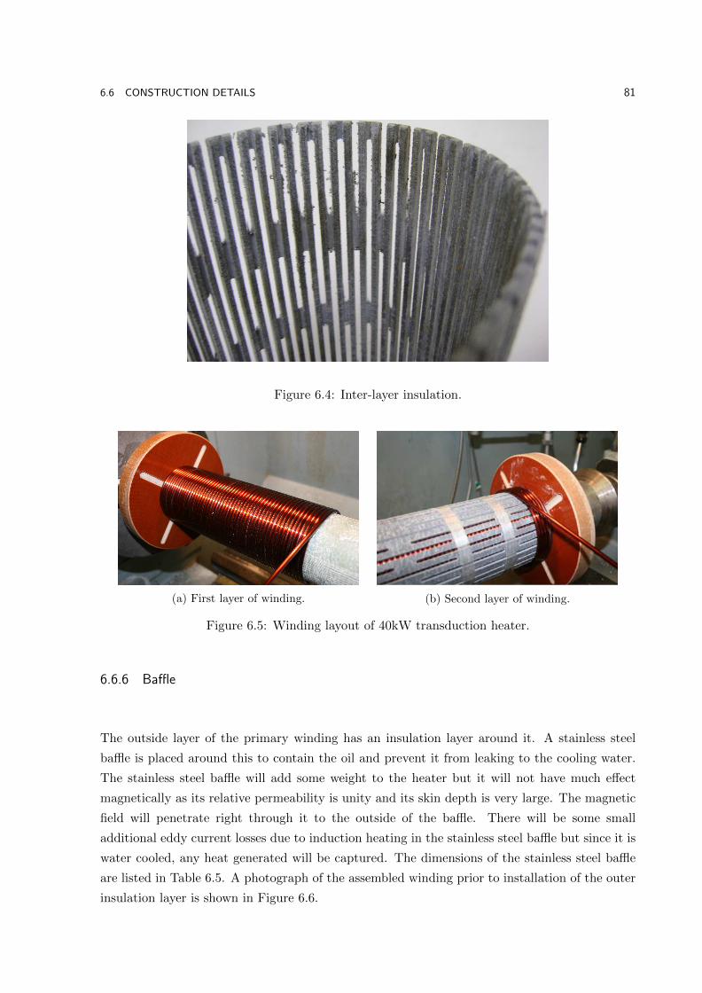
6.6 CONSTRUCTION DETAILS 81
Figure 6.4: Inter-layer insulation.
(a) First layer of winding. (b) Second layer of winding.
Figure 6.5: Winding layout of 40kW transduction heater.
6.6.6 Baffle
The outside layer of the primary winding has an insulation layer around it. A stainless steel
baffle is placed around this to contain the oil and prevent it from leaking to the cooling water.
The stainless steel baffle will add some weight to the heater but it will not have much effect
magnetically as its relative permeability is unity and its skin depth is very large. The magnetic
field will penetrate right through it to the outside of the baffle. There will be some small
additional eddy current losses due to induction heating in the stainless steel baffle but since it is
water cooled, any heat generated will be captured. The dimensions of the stainless steel baffle
are listed in Table 6.5. A photograph of the assembled winding prior to installation of the outer
insulation layer is shown in Figure 6.6.
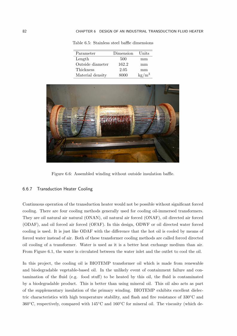
82 CHAPTER 6 DESIGN OF AN INDUSTRIAL TRANSDUCTION FLUID HEATER
Table 6.5: Stainless steel baffle dimensions
Parameter Dimension Units
Length 500 mmOutside diameter 162.2 mmThickness 2.05 mmMaterial density 8000 kg/m3
Figure 6.6: Assembled winding without outside insulation baffle.
6.6.7 Transduction Heater Cooling
Continuous operation of the transduction heater would not be possible without significant forced
cooling. There are four cooling methods generally used for cooling oil-immersed transformers.
They are oil natural air natural (ONAN), oil natural air forced (ONAF), oil directed air forced
(ODAF), and oil forced air forced (OFAF). In this design, ODWF or oil directed water forced
cooling is used. It is just like ODAF with the difference that the hot oil is cooled by means of
forced water instead of air. Both of these transformer cooling methods are called forced directed
oil cooling of a transformer. Water is used as it is a better heat exchange medium than air.
From Figure 6.1, the water is circulated between the water inlet and the outlet to cool the oil.
In this project, the cooling oil is BIOTEMP transformer oil which is made from renewable
and biodegradable vegetable-based oil. In the unlikely event of containment failure and con-
tamination of the fluid (e.g. food stuff) to be heated by this oil, the fluid is contaminated
by a biodegradable product. This is better than using mineral oil. This oil also acts as part
of the supplementary insulation of the primary winding. BIOTEMP exhibits excellent dielec-
tric characteristics with high temperature stability, and flash and fire resistance of 330C and
360C, respectively, compared with 145C and 160C for mineral oil. The viscosity (which de-

6.6 CONSTRUCTION DETAILS 83
scribes the oils resistance to flow) for BIOTEMP transformer oil is 10 at 100C and 40 at 45C
[Biotemp 2014].
6.6.8 Transduction Heater Housing
The transduction heater housing is constructed from a stainless steel tube with thickness of
2.05mm. Inside the internal tube of the water jacket is the stainless steel baffle that prevents
the oil from leaking into the cooling water. The cooling water is contained between the internal
and external walls of the water jacket. This external stainless steel tube will also add some
weight but it will not have much effect magnetically as its relative permeability is unity and
its skin depth is very large. Again, the magnetic field will penetrate right through it to the
outside of the tube. There will be some additional eddy current losses due to induction heating
in the stainless steel tube but since it is water cooled, any heat generated will be captured. A
non-metallic enclosure could also be used and would not give any losses, however, a stainless
steel enclosure is preferable in food areas.
A photograph of the water jacket used for the housing is shown in Figure 6.7(a). The oil and
water inlets can be seen on the left. The fully assembled coil is then inserted inside the water
jacket as shown in Figure 6.7(b).
(a) Water jacket. (b) Assembled winding inside water jacket.
Figure 6.7: Transduction heater housing.

84 CHAPTER 6 DESIGN OF AN INDUSTRIAL TRANSDUCTION FLUID HEATER
6.7 EQUIVALENT CIRCUIT
The equivalent circuit that is used to model the transduction fluid heater is shown in Figure 6.8.
R1 X1 X2 R2
Xmc Rce
Figure 6.8: Equivalent circuit of transduction heater.
where R1, R2 are the primary winding and secondary tube resistances, Xmc, is the core tube
magnetizing reactance, Rce is the core tube eddy current resistance, and X1, X2 are the primary
and secondary leakage reactances. Hysteresis losses, usually the dominant part of core losses in
a transformer, are ignored in this model as they are insignificant compared to the eddy current
losses. The variation of resistivity with temperature of all metal materials should be accounted
for, as this may be a high temperature device.
All the equivalent circuit components are calculated using the same formulae as presented in
Chapter 5. Also for this design, the fluid is constrained to flow inside the centre of the core tube.
6.7.1 Equivalent Circuit Performance
The physical dimensions and materials used in the design of the heater are given in Tables 6.1,
6.2, 6.3, 6.4. The parameters from these tables were entered into a computer program written
using the modeling methods in [Liew and Bodger 2001], [Bodger and Liew 2002]. The program
was able to determine the equivalent circuit parameters and performance for the designed heater.
6.7.2 Calculated Performance
The equivalent circuit parameters are listed in Table 6.6. The higher temperatures of the sec-
ondary and core tube components in particular have significantly increased the resistances of
these components. The magnetizing component has a larger value due to the higher equivalent
relative permeability. A mild steel core tube with low relative permeability aids in reducing the

6.7 EQUIVALENT CIRCUIT 85
magnetizing reactance and improving the power factor. The leakage reactances are both lower
due to the smaller primary winding and secondary tube thickness.
Table 6.6: Equivalent circuit parameters
Circuit component Value (Ω)
R1 0.297R2 3.772X1 0.949X2 0.949Xmc 10.622Rce 8.963
Having calculated the parameters of the equivalent circuit, the performance of the transduction
fluid heater is obtained by applying the nominal voltage to the equivalent circuit. The calculated
values of the TEC model are given in Table 6.7.
Table 6.7: Equivalent circuit performance
Parameter Value
V-voltage 230VI-current 70.1AS-volt-amperes 16.1kVAP-real power 12.9kWPF-power factor 0.80EFF-efficiency 88.7
The proportion of real power dissipated in the secondary and core tubes is much higher than
real power dissipated in the primary and hence the efficiency is high. The real power in the
primary winding is about 1.5kW. This is dissipated into the oil and then to the cooling water.
The net amount of real power for this design has comes from the secondary tube and the core
tube together. Most of the apparent power is real which gives a reasonable power factor of 0.84,
much better than that for an induction water heater.
For comparison, without the copper secondary tube, the device is an induction heater. This is
essentially an open circuit of the device. At 230V, the supply current was about 27.6A and the
power factor was about 0.74.
Without the core tube, the device is a coreless transformer. In this case the magnetizing reac-
tance and the power factor would be very low.
The primary current was 70.1A which gave a current density of 5.6A/mm2, which was marginal
for a multi-layer winding with forced water cooling. These figures would decrease as the tem-
peratures and hence the resistances of the tubes increase.
Other performance measures can be determined by calculation from the TEC program but

86 CHAPTER 6 DESIGN OF AN INDUSTRIAL TRANSDUCTION FLUID HEATER
cannot be measured on an actual transduction fluid heater. These are given in Table 6.8.
Table 6.8: TEC calculated performance
Parameter Value
VT1-primary voltage turn 0.36VV2-secondary eddy voltage 0.28AVA-primary/secondary voltage ratio 827.45A1-primary winding current area 1.26×10⁻⁵ m2
J1-primary winding current density 5.58A/mm2
I2-secondary tube current 29.39kAA2-secondary tube current area 6.50×10⁻⁴m2
J2-secondary tube current density 45.74A/mm2
ICE-core tube eddy current 12.79kAACE-core tube eddy current area 2.3×10⁻³m2
JCE-core tube eddy current density 5.54A/mm2
The currents in the secondary and core tubes are very large in comparison to the primary current,
but they are directly cooled by the water, so their current densities are acceptable. This will
heat the workpiece as required.
Three of these units would give a total power of 39kW.
6.8 FEA RESULTS
The dimensions in Tables 6.1 and 6.2 have been used to draw the transduction heater in MagNet
to create its geometry. The coils are also created and its properties assigned. A boundary
condition was added to surround the model to take into account the fringing fields. This is
followed by customization of the mesh elements. The model is then solved using the time
harmonic solver and the field solutions and performance can then be viewed. Figure 6.9(a)
shows a half model of the coil and the workpiece of the designed heater. An enlarged view of
the computer generated flux plot, together with the shaded plot of the flux density magnitude,
is shown in Figure 6.9(b). The values are represented by colours ranging from blue for minimum
to red for maximum.
The computer results in Figure 6.9(b) show that the flux density varies from 1.2T in the middle
of the mild steel core tube to 1.9T on the surface of the core tube. A flux density of 1.9T on
the surface of core tube of the heater is saturating the core material. The flux plot also shows
that the magnetic field does penetrate through the secondary tube to the core tube as expected.
The performance of the heater from FEA is listed in Table 6.9.
The calculated results from FEA model show significantly higher values in terms of the current,
apparent power, and real power compared to the results from the TEC model shown in Table
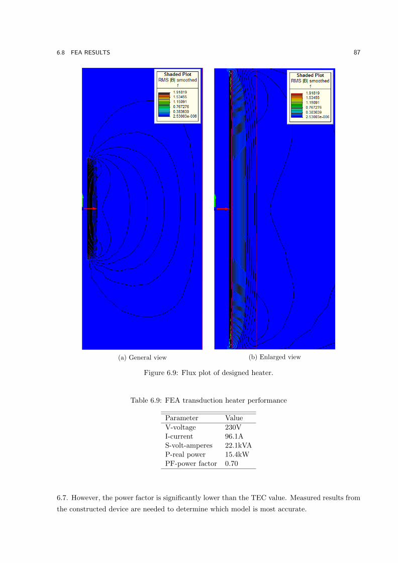
6.8 FEA RESULTS 87
(a) General view (b) Enlarged view
Figure 6.9: Flux plot of designed heater.
Table 6.9: FEA transduction heater performance
Parameter Value
V-voltage 230VI-current 96.1AS-volt-amperes 22.1kVAP-real power 15.4kWPF-power factor 0.70
6.7. However, the power factor is significantly lower than the TEC value. Measured results from
the constructed device are needed to determine which model is most accurate.

88 CHAPTER 6 DESIGN OF AN INDUSTRIAL TRANSDUCTION FLUID HEATER
6.9 SUMMARY
In this chapter, the design of a nominal 40kW transduction fluid heater has been presented.
The transduction fluid heater was designed using a computer program written in MATLAB
and is based on the reverse design method described in [Liew and Bodger 2001], [Bodger and
Liew 2002].
The design of the transduction fluid heater used aspects of the 6kW prototype [Takau and
Bodger 2014]. The new design used the same material dimensions for the core tube and the
secondary tube. Other aspects of the design that were added to the original design were inter-
layer insulation, cooling for the primary winding, and the length of the primary winding was
adjusted to be the same as the secondary and core tubes. Construction materials and dimensions
of the designed heater were also given. This included the primary winding, thermal insulation,
secondary tube, core tube, inter-layer insulation, and also the cooling system for the winding.
The TEC model used the reverse design method to determine the circuit parameters and then
calculate the performance of the heater.
An alternative to the TEC model, the FEA model, was also used to predict the performance
of the heater. A two dimensional finite element analysis of the heater was used to show the
magnetic field distribution of the heater.
The calculated results of the TEC model shows significantly lower values in terms of the current,
apparent power, and real power compared to those calculated from the FEA. The power factor
was greater. The calculated results from the FEA model were slightly different due to the higher
current. Again, the same differences were obtained from the 6kW design presented in Chapter
5.

Chapter 7
EXPERIMENTAL RESULTS
7.1 INTRODUCTION
This chapter presents the performance tests on the three phase 40kW transduction fluid heater
designed and constructed in Chapter 6. These tests include winding resistance, insulation resis-
tance, power input, heating, ac withstand voltage, and glow-wire flammability. Where applica-
ble, the tests were undertaken according to the International Standards, IEC 60335-1:2010 and
IEC 60335-2-35:2012.
The chapter begins with an overview of the experimental setup used throughout the testing,
with a discussion of the equipment used during the testing. Also the methods used in taking
electrical measurements are examined. The results of the testing are presented and the test
results are then compared with the modeling from Chapter 6.
7.2 EXPERIMENTAL SETUP
The testing of the 40kW transduction fluid heater was conducted in the High Voltage Laboratory.
This facility has a controllable three phase supply capable of delivering up to 600A at 400V. In
addition, the laboratory is fitted with water mains that can be used to supply the heater.
7.2.1 Test Equipment
The test set-up for the 40kW transduction heater is shown in Figures 7.1 and 7.2. The ar-
rangement of the three phase units were in-line rather than in parallel. This is to allow a single
fluid tube that can be easily cleaned, rather than having a more complicated manifold. The
arrangement can be oriented either horizontally and vertically during the tests. The test set-up
consists of a variable 70A variac, 50Hz, ac supply connected in series with the heater and the
controller. The power meters are connected to monitor the voltage, current, power factor and
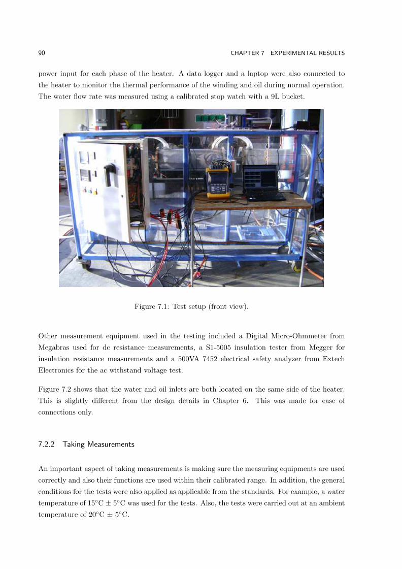
90 CHAPTER 7 EXPERIMENTAL RESULTS
power input for each phase of the heater. A data logger and a laptop were also connected to
the heater to monitor the thermal performance of the winding and oil during normal operation.
The water flow rate was measured using a calibrated stop watch with a 9L bucket.
Figure 7.1: Test setup (front view).
Other measurement equipment used in the testing included a Digital Micro-Ohmmeter from
Megabras used for dc resistance measurements, a S1-5005 insulation tester from Megger for
insulation resistance measurements and a 500VA 7452 electrical safety analyzer from Extech
Electronics for the ac withstand voltage test.
Figure 7.2 shows that the water and oil inlets are both located on the same side of the heater.
This is slightly different from the design details in Chapter 6. This was made for ease of
connections only.
7.2.2 Taking Measurements
An important aspect of taking measurements is making sure the measuring equipments are used
correctly and also their functions are used within their calibrated range. In addition, the general
conditions for the tests were also applied as applicable from the standards. For example, a water
temperature of 15C ± 5C was used for the tests. Also, the tests were carried out at an ambient
temperature of 20C ± 5C.

7.3 TRANSDUCTION HEATER PERFORMANCE 91
Water inlet Oil inlet
Figure 7.2: Test setup (rear view).
7.3 TRANSDUCTION HEATER PERFORMANCE
The main performance indicator for a transduction heater is the efficiency of the power transfer
or the distribution of the losses. The tests for instantaneous water heater are outlined in the
IEC 60335-1 and IEC 60335-2-35 standards. These standards were used as a guide in conducting
the relevant tests as the designed heater was for industrial purposes.
This section presents the tests and measurements undertaken to determine the performance of
the heater. These measurements are examined and used to validate the calculated results from
the TEC and FEA models.
The tests were arranged and performed from ensuring the device was electrically safe to energise,
to some of the tests, such as the AC withstand voltage test, being performed later as they were
considered potentially damaging to the heater. The glow-wire flammability test was performed
on a separate sample of the non-metallic part of the heater.
7.3.1 Winding Resistance and Insulation Resistance Tests
The dc resistance test was performed before the final connection of the heater was completed.
This was measured using a MPK254 Digital Micro-Ohmmeter from Megabras. The test results
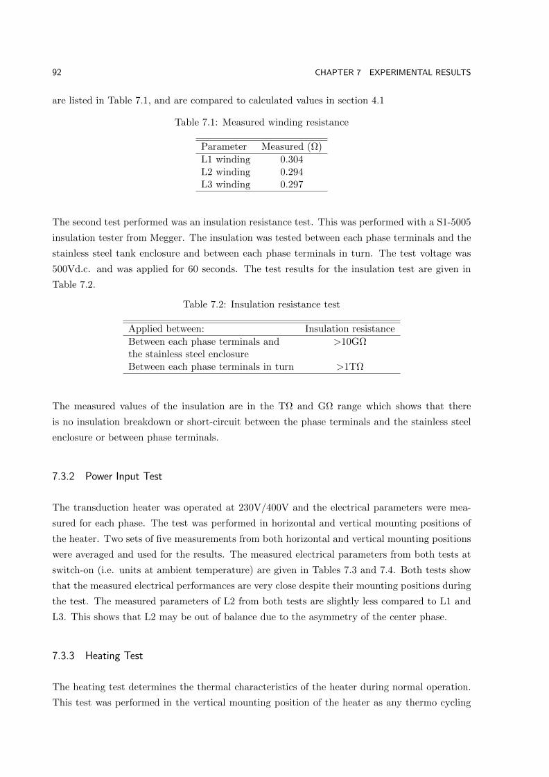
92 CHAPTER 7 EXPERIMENTAL RESULTS
are listed in Table 7.1, and are compared to calculated values in section 4.1
Table 7.1: Measured winding resistance
Parameter Measured (Ω)
L1 winding 0.304L2 winding 0.294L3 winding 0.297
The second test performed was an insulation resistance test. This was performed with a S1-5005
insulation tester from Megger. The insulation was tested between each phase terminals and the
stainless steel tank enclosure and between each phase terminals in turn. The test voltage was
500Vd.c. and was applied for 60 seconds. The test results for the insulation test are given in
Table 7.2.
Table 7.2: Insulation resistance test
Applied between: Insulation resistance
Between each phase terminals and >10GΩthe stainless steel enclosureBetween each phase terminals in turn >1TΩ
The measured values of the insulation are in the TΩ and GΩ range which shows that there
is no insulation breakdown or short-circuit between the phase terminals and the stainless steel
enclosure or between phase terminals.
7.3.2 Power Input Test
The transduction heater was operated at 230V/400V and the electrical parameters were mea-
sured for each phase. The test was performed in horizontal and vertical mounting positions of
the heater. Two sets of five measurements from both horizontal and vertical mounting positions
were averaged and used for the results. The measured electrical parameters from both tests at
switch-on (i.e. units at ambient temperature) are given in Tables 7.3 and 7.4. Both tests show
that the measured electrical performances are very close despite their mounting positions during
the test. The measured parameters of L2 from both tests are slightly less compared to L1 and
L3. This shows that L2 may be out of balance due to the asymmetry of the center phase.
7.3.3 Heating Test
The heating test determines the thermal characteristics of the heater during normal operation.
This test was performed in the vertical mounting position of the heater as any thermo cycling
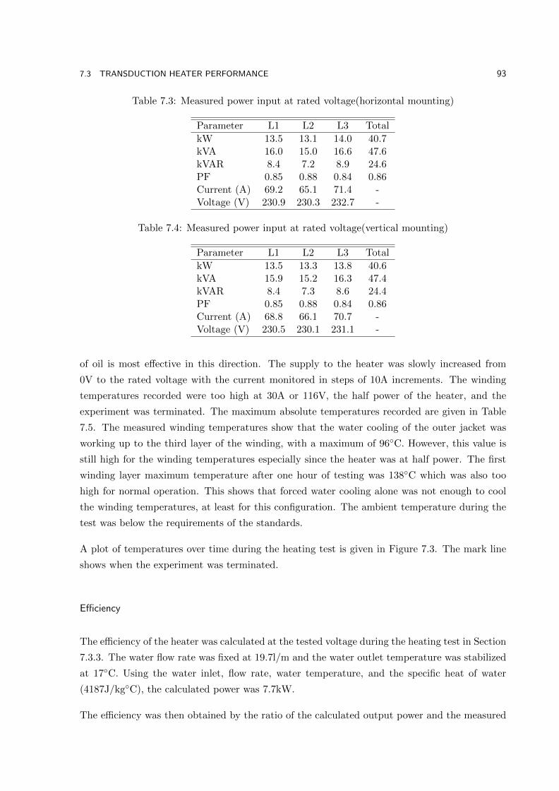
7.3 TRANSDUCTION HEATER PERFORMANCE 93
Table 7.3: Measured power input at rated voltage(horizontal mounting)
Parameter L1 L2 L3 Total
kW 13.5 13.1 14.0 40.7kVA 16.0 15.0 16.6 47.6kVAR 8.4 7.2 8.9 24.6PF 0.85 0.88 0.84 0.86Current (A) 69.2 65.1 71.4 -Voltage (V) 230.9 230.3 232.7 -
Table 7.4: Measured power input at rated voltage(vertical mounting)
Parameter L1 L2 L3 Total
kW 13.5 13.3 13.8 40.6kVA 15.9 15.2 16.3 47.4kVAR 8.4 7.3 8.6 24.4PF 0.85 0.88 0.84 0.86Current (A) 68.8 66.1 70.7 -Voltage (V) 230.5 230.1 231.1 -
of oil is most effective in this direction. The supply to the heater was slowly increased from
0V to the rated voltage with the current monitored in steps of 10A increments. The winding
temperatures recorded were too high at 30A or 116V, the half power of the heater, and the
experiment was terminated. The maximum absolute temperatures recorded are given in Table
7.5. The measured winding temperatures show that the water cooling of the outer jacket was
working up to the third layer of the winding, with a maximum of 96C. However, this value is
still high for the winding temperatures especially since the heater was at half power. The first
winding layer maximum temperature after one hour of testing was 138C which was also too
high for normal operation. This shows that forced water cooling alone was not enough to cool
the winding temperatures, at least for this configuration. The ambient temperature during the
test was below the requirements of the standards.
A plot of temperatures over time during the heating test is given in Figure 7.3. The mark line
shows when the experiment was terminated.
Efficiency
The efficiency of the heater was calculated at the tested voltage during the heating test in Section
7.3.3. The water flow rate was fixed at 19.7l/m and the water outlet temperature was stabilized
at 17C. Using the water inlet, flow rate, water temperature, and the specific heat of water
(4187J/kgC), the calculated power was 7.7kW.
The efficiency was then obtained by the ratio of the calculated output power and the measured

94 CHAPTER 7 EXPERIMENTAL RESULTS
Table 7.5: Heating test
Measured part Measured temperature (C)
Initial ambient temperature 5.8Final ambient temperature 8.3Water inlet 11.4Water outlet 17.0L1 oil temperature (top) 116.2L1 oil temperature (bottom) 30.9L2 oil temperature (top) 102.8L2 oil temperature (bottom) 31.7L3 oil temperature (bottom) 22.6L1 winding (third layer) 97.8L2 winding (third layer) 85.4L3 winding (third layer) 98.5L2 winding (first layer) 137.6L3 winding (first layer) 132.5Test power input 7.8(kW)Test voltage 116(V)
Figure 7.3: Temperatures over time during heating test.
input power during the heating test from Table 7.5. The efficiency of the heater at half power
was calculated to be 98.7%. The 1.3% loss was due to the heat dissipated at both ends of the
secondary and mild steel tubes.

7.3 TRANSDUCTION HEATER PERFORMANCE 95
To operate the heater at steady state, the winding temperatures must be less than 100C at full
load during normal operation. This applies for winding with insulation classes A(105), (E)120,
and (B)130. The forced oil cooling method was another option to apply in addition to the forced
water cooling. However, the current design has too much restriction on the oil circulation and
therefore this cooling method was not applied.
Another configuration for the current design was to remove the water inlet that was used to
cool the oil and link it directly with the oil in the winding compartment. This creates a barrier
between the windings and the cooling jacket and increases the volume of oil to better cycle and
cool the winding. In this configuration, the forced water cooling is removed and the device relies
on natural air convection to cool the oil. The water inlet in this configuration was now straight
through the product in, product out tube according to the design details of Figure 6.1. This
configuration was only applied to coil L2 the white phase (center phase). The other two phases
were connected as the first configuration for comparison. The heater was then operated by slowly
increasing the supply from 0V and with the current monitored in steps of 10A increments. The
maximum absolute temperatures recorded from this configuration are given in Table 7.6.
Table 7.6: Heating test
Measured part Measured temperature (C)
Initial ambient temperature 20.9Final ambient temperature 21.8L1 oil temperature (top) 93.9L1 oil temperature (bottom) 26.7L2 oil temperature (top) 118.8L2 oil temperature (bottom) 56.1L3 oil temperature (bottom) 21.9L1 winding (third layer) 83.3L2 winding (third layer) 91.1L3 winding (third layer) 90.2L2 winding (first layer) 105.1L3 winding (first layer) 120.2L3 water jacket enclosure 16.6L2 water jacket enclosure 70.0L1 water jacket enclosure 17.8Test power input 6.6(kW)Test voltage 98.6(V)
The measured results show the winding temperature for the first layer of the center phase (L2)
was 15C lower than that for L3 phase. At lower voltages the margin of difference was small,
but this increased as the voltage was increased. The measured oil temperature was 118.8C
and the enclosure was measured at 70.0C. By comparison, the measured temperatures for the
blue and red phase enclosures were 17.8C and 16.6C respectively. These are low compared to
the center phase due to the forced water cooling. The measured results from this configuration

96 CHAPTER 7 EXPERIMENTAL RESULTS
have shown some improvement in terms of L2 winding temperature and certainly a pointer in
the right direction to improve the cooling of the windings. Other recommendations to solve the
cooling are given in the next Chapter under future work. The efficiency of this configuration
dropped to 86% due to more losses dissipated in the oil and to ambient air. The measured flow
rate in this test was 27l/m with a 3C change of temperature.
A plot of temperatures over time for this configuration is given in Figure 7.4. The first and
second mark lines show when the current was increased in steps of 10A increments whereas the
last mark line shows when the experiment was stopped.
Figure 7.4: Temperatures over time during heating test.
7.4 OTHER EXPERIMENTAL RESULTS
The following tests were conducted on the 40kW transduction heater in addition to those men-
tioned in Section 7.3.
7.4.1 AC Withstand Voltage Test
This test was performed in accordance with IEC 60335.1. The equipment used the 500VA, 7452
electrical safety analyzer from Extech Electronics and was capable of supplying short circuit cur-
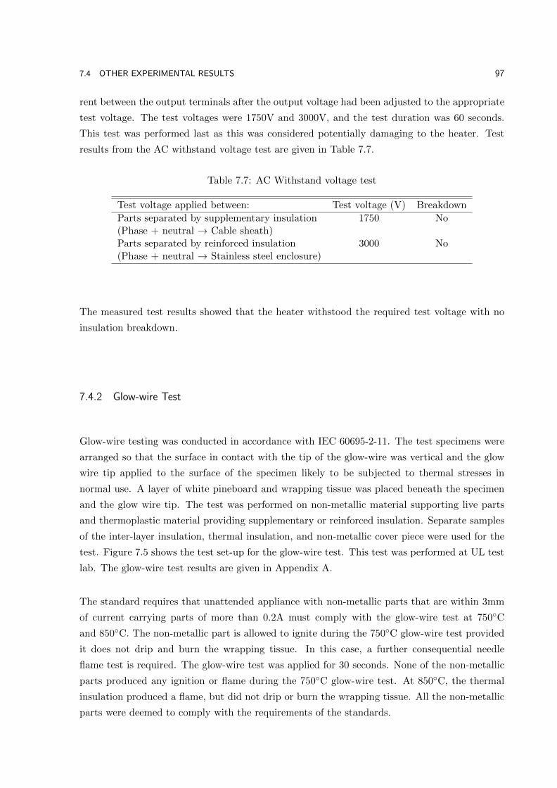
7.4 OTHER EXPERIMENTAL RESULTS 97
rent between the output terminals after the output voltage had been adjusted to the appropriate
test voltage. The test voltages were 1750V and 3000V, and the test duration was 60 seconds.
This test was performed last as this was considered potentially damaging to the heater. Test
results from the AC withstand voltage test are given in Table 7.7.
Table 7.7: AC Withstand voltage test
Test voltage applied between: Test voltage (V) Breakdown
Parts separated by supplementary insulation 1750 No(Phase + neutral → Cable sheath)Parts separated by reinforced insulation 3000 No(Phase + neutral → Stainless steel enclosure)
The measured test results showed that the heater withstood the required test voltage with no
insulation breakdown.
7.4.2 Glow-wire Test
Glow-wire testing was conducted in accordance with IEC 60695-2-11. The test specimens were
arranged so that the surface in contact with the tip of the glow-wire was vertical and the glow
wire tip applied to the surface of the specimen likely to be subjected to thermal stresses in
normal use. A layer of white pineboard and wrapping tissue was placed beneath the specimen
and the glow wire tip. The test was performed on non-metallic material supporting live parts
and thermoplastic material providing supplementary or reinforced insulation. Separate samples
of the inter-layer insulation, thermal insulation, and non-metallic cover piece were used for the
test. Figure 7.5 shows the test set-up for the glow-wire test. This test was performed at UL test
lab. The glow-wire test results are given in Appendix A.
The standard requires that unattended appliance with non-metallic parts that are within 3mm
of current carrying parts of more than 0.2A must comply with the glow-wire test at 750C
and 850C. The non-metallic part is allowed to ignite during the 750C glow-wire test provided
it does not drip and burn the wrapping tissue. In this case, a further consequential needle
flame test is required. The glow-wire test was applied for 30 seconds. None of the non-metallic
parts produced any ignition or flame during the 750C glow-wire test. At 850C, the thermal
insulation produced a flame, but did not drip or burn the wrapping tissue. All the non-metallic
parts were deemed to comply with the requirements of the standards.

98 CHAPTER 7 EXPERIMENTAL RESULTS
Figure 7.5: Glow-wire test setup.
7.5 COMPARISON WITH TEC AND FEA MODELS
The measured performance test results were compared to the TEC and FEA modeling given
in Chapter 6. Only calculated results that can be measured were used for comparisons. These
comparisons are presented in Tables 7.8 and 7.9.
7.5.1 Winding Resistance Test Results
The measured and calculated winding resistances from the TEC and FEA models are given in
Table 7.8. The measured resistances show good agreement with those calculated from the TEC
model compared to the FEA model. The calculated resistance from FEA is significantly lower
than the measured and TEC values. The winding resistance in FEA was calculated using the
coil loss and the coil current.
Table 7.8: Measured winding resistance results
Parameter Measured TEC FEA
L1 winding (Ω) 0.304 0.297 0.127L2 winding (Ω) 0.294 0.297 0.127L3 winding (Ω) 0.297 0.297 0.127
The measured winding resistances are expected to be the same for the three coils, however the
measured winding resistance for L1 may be slightly different compared to L2 and L3 due to
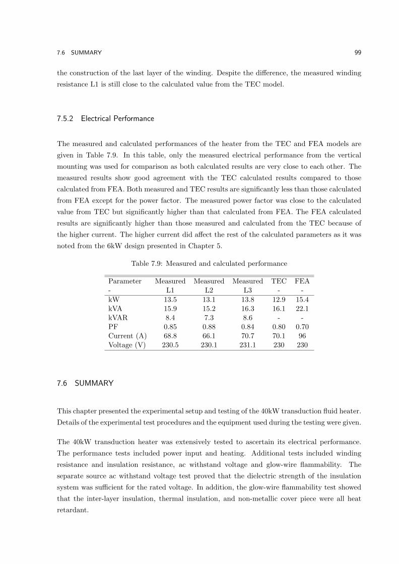
7.6 SUMMARY 99
the construction of the last layer of the winding. Despite the difference, the measured winding
resistance L1 is still close to the calculated value from the TEC model.
7.5.2 Electrical Performance
The measured and calculated performances of the heater from the TEC and FEA models are
given in Table 7.9. In this table, only the measured electrical performance from the vertical
mounting was used for comparison as both calculated results are very close to each other. The
measured results show good agreement with the TEC calculated results compared to those
calculated from FEA. Both measured and TEC results are significantly less than those calculated
from FEA except for the power factor. The measured power factor was close to the calculated
value from TEC but significantly higher than that calculated from FEA. The FEA calculated
results are significantly higher than those measured and calculated from the TEC because of
the higher current. The higher current did affect the rest of the calculated parameters as it was
noted from the 6kW design presented in Chapter 5.
Table 7.9: Measured and calculated performance
Parameter Measured Measured Measured TEC FEA- L1 L2 L3 - -
kW 13.5 13.1 13.8 12.9 15.4kVA 15.9 15.2 16.3 16.1 22.1kVAR 8.4 7.3 8.6 - -PF 0.85 0.88 0.84 0.80 0.70Current (A) 68.8 66.1 70.7 70.1 96Voltage (V) 230.5 230.1 231.1 230 230
7.6 SUMMARY
This chapter presented the experimental setup and testing of the 40kW transduction fluid heater.
Details of the experimental test procedures and the equipment used during the testing were given.
The 40kW transduction heater was extensively tested to ascertain its electrical performance.
The performance tests included power input and heating. Additional tests included winding
resistance and insulation resistance, ac withstand voltage and glow-wire flammability. The
separate source ac withstand voltage test proved that the dielectric strength of the insulation
system was sufficient for the rated voltage. In addition, the glow-wire flammability test showed
that the inter-layer insulation, thermal insulation, and non-metallic cover piece were all heat
retardant.

100 CHAPTER 7 EXPERIMENTAL RESULTS
The measured results were compared to the modelling from Chapter 6. There was good agree-
ment between measured and calculated electrical performance results from the TEC model
compared to the FEA model. The various components of the modelling results were discussed
with reference to the measured electrical performance, and limitation of the current design was
examined in terms of cooling.

Chapter 8
CONCLUSIONS AND FUTURE WORK
8.1 CONCLUSIONS
This thesis started by introducing the basic principle of induction heating. Applications of
induction heating from the 19th century were discussed. The conventional approach to model
the performance of induction heaters known as the series equivalent circuit (SEC) model was
presented. This was used to calculate the performance of a set of experimental induction heaters.
An alternative approach to the SEC model was then developed. This was known as the trans-
former equivalent circuit (TEC) model. This modelled the induction heater as a shorted sec-
ondary transformer. Equivalent circuits, which are often used in modelling ideal and non-ideal
transformers, have been presented. These include the core loss components, the primary winding
components and the secondary winding components. These equivalent circuits were transformed
into a circuit to model the performance of induction heaters. A simulation program was written
using a reverse design approach to calculate the circuit components of the TEC model. The TEC
model was then used to calculate the performance of a set of experimental induction heaters.
Finite element analysis (FEA) was also presented. This was used to calculate the performance
of the set of experimental induction heaters used for the SEC and TEC models. The set of
experimental induction heaters were constructed and tested. The measured results were used
to compare with calculated results from the FEA, TEC and SEC models. The FEA calculated
results correlated well with the measured results followed by the TEC and then the SEC model.
The coil losses and workpiece losses decreased as the diameter of the workpiece increased. This
pattern showed up in the TEC and FEA models but not so with the coil and workpiece losses
in the SEC model. The calculated results from the TEC model showed the usefulness of the
transformer model to predict the performance of induction heaters.
The research was then extended to transduction heating, an induction heater with a secondary
winding to boost performance. The TEC and FEA models only were used to calculate the
performance of a set of transduction heating experiments. There is no equivalent SEC model
102 CHAPTER 8 CONCLUSIONS AND FUTURE WORK
for such heaters. The measured results from the transduction heating experiments showed mod-
ifications were required to the equivalent circuit parameters of the TEC model to improve its
performance prediction. The circuit components that were modified included the magnetizing
reactance and the leakage reactances. The modified TEC model was verified with a 6kW exper-
imental transduction heater design. The measured results showed good agreement with those
calculated from the TEC model compared to FEA.
A new simulation program was written that used the developed model to calculate the perfor-
mance of transduction heaters. The program was then used to design a 40kW transduction
heater. The new design had several aspects in common with the 6kW heater. The 40kW design
used a new version of the inter-layer insulation for cooling purposes.
The 40kW heater was then built and a series of electrical tests were performed to determine its
performance characteristics. The tests were based, where applicable, on international instan-
taneous water heater standards. The measured electrical performance showed good agreement
with the TEC calculated results. The measured power factor was greater than that predicted by
the TEC but still close compared to the calculated value from FEA. The design heater was found
to be 98.7% efficient at half power. At half power, the winding temperatures were over 100C.
The initial design with forced water cooling did not seem to cool the winding up to the first layer
of winding. An investigation into the winding temperature overheating led to the conclusion
that insufficient cooling in terms of the thermo cycling of oil was the main contributing factor.
An alternative configuration for cooling was then tested together with the forced water cooling.
This alternative configuration was applied for the center phase or L2 only. Some improvement
in terms of the winding temperature was measured. The measured winding temperature for L2
was 15C lower than that for the Red phase (L3). The margin of difference was small at lower
voltages but increased as the supply voltage was increased. The measured results pointed in the
direction of the need for a baffle between the winding and the water jacket, with more volume
of circulating oil to cool the oil.
An additional test included a separate source ac withstand voltage test, which proved the dielec-
tric strength of the insulation material was sufficient for the rated voltage. The measured test
results showed that the heater was able to withstand the short circuit forces without damaging
the windings. A final test included a glow-wire flammability test which showed that all the
non-metallic parts were resistant to heat and fire.
The research contained in this thesis demonstrates that the performance of transduction heaters
can be successfully modeled using a TEC model. It enables the design of transduction heaters
based on available materials and using dimensions as design parameters rather than determining
these from voltages and power ratings as used in traditional transformer design methods.
Transduction fluid heaters have the potential to become widespread as benefits of high efficiency,

8.2 FUTURE WORK 103
reduced size, simplified construction and even heating will see them become a more cost effective
solution over traditional water heater designs. From the measured performance test results, there
is only one factor that is currently preventing the commercial viability of the transduction fluid
heaters, and that is the cooling of the primary winding.
8.2 FUTURE WORK
The test results of the designed 40kW transduction heater presented one major limitation while
it was being tested and evaluated, as presented in Chapter 7. This section presents the future
work that can be performed to improve the thermal design and performance of transduction
heaters.
8.2.1 Heater Design
The design of transduction heaters has to be a compromise between electrical and thermal
aspects. The major limitation of the current design is the inability to cool the first layer of
the primary winding. The measured test results from the different L2 configuration have shown
some improvement in terms of reducing the L2 winding temperature. It is suggested that a
baffle is required to promote better circulation of the oil with a water jacket outside the baffle
to cool the oil. Figure 8.1 shows a half sketch of the transduction heater with the baffle. A more
rigorous exercise to model the thermal characteristics of the heater should lead to a practical
solution to the winding heating problem.
The following recommendations are considered minor that can be incorporated into the design
to encourage better oil circulation.
Thermal insulation
The thermal insulation can be re-designed so that the oil can access the inner side of the first
layer of the winding. The thickness of the thermal insulation used in the current design was
4.6mm. It is recommended that a series of 1mm grooves be machined into the outside surface
of the thermal insulation. These grooves should be aligned with the slots in the non-metallic
cover-piece, to allow oil to flow in the grooves.
Non-metallic cover piece
The non-metallic cover piece that encloses the winding from both ends may need to be re-
designed as well. The current design has four slots as shown in Figure 8.2. It is suggested that

104 CHAPTER 8 CONCLUSIONS AND FUTURE WORK
Figure 8.1: Transduction heater with baffle.
more slots are required or be re-designed to align with the grooves in the thermal insulation.
This will promote better circulation.
Inlet and outlet
For future prototypes, the inlet and outlet for the oil must be located at the bottom and top of
the heater. This will allow oil circulation if forced oil cooling is required. The current design
had both oil inlet and oil outlet on the same side of the heater. This restricts the flow of oil
when forced oil cooling was required to apply for comparisons.
8.2.2 Improve Performance
There were some aspects of the measured performance presented in Chapter 6 that could be
improved upon. This includes the power factor. To improve the performance of the heater,
the power factor can be improved further by reducing the thickness of the inter-layer insulation
from 3mm to 2mm. This will reduce the leakage flux between the winding and the secondary
tube and hence increase the power factor and the performance of the heater. The 40kW heater

8.2 FUTURE WORK 105
Figure 8.2: Non-metallic cover piece with four slots.
was originally designed with a 2mm inter-layer insulation but only 3mm was available from the
manufacturer.
The other circuit parameter that will be affected when the inter-layer insulation is reduced to
2mm thickness is the resistance of the winding. The outside diameter of the winding will decrease
as a results of reducing the thickness. This will reduce the length of the wire and hence the
resistance. The efficiency of the heater will increase as the resistance of the winding becomes
smaller compared to the resistance of the secondary tubes.
The thickness of the thermal insulation (or the former) can be reduced from 4.6mm to 3.2mm.
This will minimise the coupling between the primary and the secondary and hence the leakage
flux. The 40kW heater was designed with a 3.2mm thickness but only 4.6mm was available.
In addition, the three phase units can be arranged in an equilateral triangular configuration.
In this arrangement, the magnetic flux from each unit would return through the remaining two
core tubes reducing the magnetic reluctance. This arrangement will give improved performance
but can complicate cleaning the secondary tubes.


REFERENCES
Baker, R.M. (1957), ‘Design and calculation of induction-heating coils’, American Institute
of Electrical Engineers, Part II: Applications and Industry, Transactions of the, Vol. 76,
No. 1, March, pp. 31–40.
Bara, N.P. (2013), ‘Finite element analysis of induction furnace for optimum heat transfer’, In-
ternational Journal of Innovative Research in Science, Engineering and Technology, Vol. 2,
No. 5, pp. 1313–1319.
Barber, H. (1983), Electroheat, Granada Publishing, Great Britain.
Bell, S.C. (2004), ‘An investigation into the magnetic performance of a three-phase partial-core
transformer’, Third Professional Year Project, University of Canterbury, Christchurch.
Bell, S.C. (2008), High-voltage partial-core resonant transformers, PhD thesis, University of
Canterbury, Christchurch, New Zealand.
Bell, S.C. and Bodger, P.S. (2007), ‘Power transformer design using magnetic circuit theory
and finite element analysis - a comparison of techniques’, In Power Engineering Conference,
2007. AUPEC 2007. Australasian Universities, Dec, pp. 607–612.
Biotemp (2014), ‘Biodegradable dielectric insulating fluid’, Website.
http://www.nttworldwide.com/docs/BIOTEMP-ABB.
Bodger, P.S. and Liew, M.C. (2002), ‘Reverse as-built transformer design method’, Int. J.
Elect. Enging. Educ, Vol. 39, No. 1, pp. 42–53.
Bodger, P.S., Walker, R.J.H. and McInnes, I. (1996), ‘Significant technology improve-
ments in fluid heating’, BNCE/UIE XIII Congress on Eletricity Applications, June.
Burca, A., Trip, N.D. and Leuca, T. (2014), ‘Considerations on the design of a low power
induction heating system’, In Fundamentals of Electrical Engineering (ISFEE), 2014 In-
ternational Symposium on, Nov, pp. 1–4.
Chuwan, S. (2012), ‘Partial core eco power transformer’, Third Professional Year Project,
University of Canterbury, Christchurch.

108 REFERENCES
Clain, S., Rappaz, J., Swierkosz, M. and Touzani, R. (1993), ‘Numerical modeling of
induction heating for two-dimensional geometries’, Mathematical Models and Methods in
Applied Sciences, Vol. 03, No. 06, pp. 805–822.
Connelly, F.C. (1965), Transformers: Their Principles and Design for Light Electrical Engi-
neers, Sir Isaac Pitman and Sons Ltd, London.
Davies, E.J. (1990), Conduction and Induction Heating, IEE power engineering series, P. Pere-
grinus Limited.
Davies, J. and Simpson, P. (1979), Induction Heating Handbook, McGraw-Hill Book Com-
pany(UK) Ltd, 1st ed.
Dodd, C.V. and Deeds, W.E. (1968), ‘Analytical solutions to eddy-current probe-coil prob-
lems’, Journal of Applied Physics, Vol. 39, No. 6, May, pp. 2829–2838.
Dodd, C.V., Cheng, C.C. and Deeds, W.E. (1974), ‘Induction coils coaxial with an arbitrary
number of cylindrical conductors’, Journal of Applied Physics, Vol. 45, No. 2, Feb, pp. 638–
647.
Edwards, J.D. (2004), ‘Course in electromechanics’, Infolytica Corporation, Montreal, Septem-
ber.
Egan, L.R. and Furlani, E.P. (1991), ‘A computer simulation of an induction heating sys-
tem’, Magnetics, IEEE Transactions on, Vol. 27, No. 5, Sep, pp. 4343–4354.
Erickson, C.J. (1995), Handbook of Electrical Heating for Industry, IEEE Press, New York.
Fisk, M. (2008), Simulation of Induction Heating in Manufacturing, PhD thesis, Lulea Univer-
sity of Technology.
Hamdi, E.S. (1994), Design of Small Electrical Machines, John Wiley and Sons Inc., New York,
USA.
Herman, S.L. (2011), Electrical Transformers and Rotating Machines, Delmar, Cengage Learn-
ing.
Huo, X.T. (2009), New Model of Eddy Current Loss Calculation and Application for Partial
Core Transformers, Master’s thesis, University of Canterbury, Christchurch, New Zealand.
Hurley, W. and Kassakian, J.G. (1979), ‘Induction heating of circular ferromagnetic plates’,
Magnetics, IEEE Transactions on, Vol. 15, No. 4, Jul, pp. 1174–1181.
Hussein, A.M. and Biringer, P.P. (1992), ‘Closed-form solution for the induction heating
problem with rotational symmetry’, Journal of Applied Physics, Vol. 72, No. 1, Jul, pp. 265–
269.

REFERENCES 109
IEC60335-1: (2010), ‘Household and similar electrical appliances - safety - part 1: General
requirements’.
IEC60335-2-35: (2012), ‘Household and similar electrical appliances - safety - part 2-35: Par-
ticular requirements for instantaneous water heaters’.
IEC60695-2-11: (2014), ‘Fire hazard testing - part 2-11: Glowing/hot-wire based test methods
- glow-wire flammability test method for end-products (gwept)’.
Jang, S.M., Cho, S.K., Lee, S.H., Cho, H.W. and Park, H.C. (2003), ‘Thermal analysis
of induction heating roll with heat pipes’, Magnetics, IEEE Transactions on, Vol. 39, No. 5,
Sept, pp. 3244–3246.
Labridis, D. and Dokopoulos, P. (1989), ‘Calculation of eddy current losses in nonlinear
ferromagnetic materials’, Magnetics, IEEE Transactions on, Vol. 25, No. 3, May, pp. 2665–
2669.
Lapthorn, A. (2013), High Temperature Superconducting Partial Core Transformers, PhD
thesis, University of Canterbury, Christchurch, New Zealand.
Lapthorn, A. and Bodger, P. (2009), ‘A comparison between the circuit theory model
and finite element model reactive components’, In Power Engineering Conference, 2009.
AUPEC 2009. Australasian Universities, Sept, pp. 1–6.
Lapthorn, A., Bodger, P. and Enright, W. (2013a), ‘A 15-kva high-temperature super-
conducting partial-core transformer 2014;part i: Transformer modeling’, Power Delivery,
IEEE Transactions on, Vol. 28, No. 1, Jan, pp. 245–252.
Lapthorn, A., Bodger, P. and Enright, W. (2013b), ‘A 15-kva high-temperature super-
conducting partial-core transformer 2014;part ii: Construction details and experimental
testing’, Power Delivery, IEEE Transactions on, Vol. 28, No. 1, Jan, pp. 253–260.
Laurent, J.C. and Malhame, R.P. (1994), ‘A physically-based computer model of aggregate
electric water heating loads’, Power Systems, IEEE Transactions on, Vol. 9, No. 3, Aug,
pp. 1209–1217.
Liew, M.C. (2001), Reverse Design Transformer Modeling Technique with Particular Applica-
tion to Partial Core Transformers, PhD thesis, University of Canterbury, Christchurch,
New Zealand.
Liew, M.C. and Bodger, P.S. (2001), ‘Partial-core transformer design using reverse modelling
techniques’, IEE Proceedings - Electric Power Applications, Vol. 148(6), pp. 513–519.
Liew, M.C. and Bodger, P.S. (2002), ‘Applying a reverse design modelling technique to
partial core transformers’, J. Electrical and Electronics Engineering, Australia, Vol. 22,
No. 1, pp. 85–92.

110 REFERENCES
Lowther, D.A. and Silvester, P.P. (1986), Computer-Aided Design in Magnetics, Springer-
Verlag, Berlin.
Lucia, O., Maussion, P., Dede, E. and Burdio, J. (2014), ‘Induction heating technol-
ogy and its applications: Past developments, current technology, and future challenges’,
Industrial Electronics, IEEE Transactions on, Vol. 61, No. 5, May, pp. 2509–2520.
MagNet7.4 (2014), MagNet 7.4 finite-element package for electromagnetic analysis, Infolytica
Corporation, Montreal.
Metaxas, A.C. (1996), Foundations of Electroheat: A Unified Approach, John Wiley and Sons
Inc., 605 Third Avenue, New York, NY-10158-0012, USA.
MilkFacts (2014), ‘Milk facts info’, Website. http://www.milkfacts.info/milk/processing
/heat/treatments/.
Mok, J. (2012), ‘Transduction heater’, Third Professional Year Project, University of Canter-
bury, Christchurch.
Namjoshi, K.V. and Biringer, P.P. (1993), ‘Current distribution in exciting coil conductors
in cross-field heating systems’, Magnetics, IEEE Transactions on, Vol. 29, No. 2, Mar,
pp. 1570–1573.
Namjoshi, K.V., Lavers, J.D. and Jain, P.K. (2001), ‘Vector potential due to a circular
loop in a toroidal cavity in a high-permeability core’, Magnetics, IEEE Transactions on,
Vol. 37, No. 6, Nov, pp. 3900–3906.
Perry, M.P. (1985), Low Frequency Electromagnetic Design, Electrical and Computer Engi-
neering, Marcel Dekker, Inc., 270 Madison Avenue, New York.
Qianzhe, Z., Yibing, L., Yanping, L. and Weisong, Z. (2010), ‘Numerical simulations for
the induction heating process of non-linear ferromagnetic billets’, In Advanced Technology
of Design and Manufacture (ATDM 2010), International Conference on, Nov, pp. 99–103.
Recktenwald, G.W. (2000), Numerical Methods with MATLAB : Implementations and Ap-
plications, Prentice Hall, Upper Saddle River, New Jersey 07458.
ScientificAmerican (2014), ‘Scientific american’, Website.
http://www.scientificamerican.com/article/experts-organic-milk-lasts-longer.
Simpson, P.G. (1960), Induction Heating: Coil and System Design, McGraw-Hill Book Com-
pany, Inc., United States.
Slemon, G.R. and Straughen, A. (1980), Electric machines, Addison-Wesley Pub. Co.
Stansel, N.R. (1949), Induction Heating, McGraw-Hill Book Co., 1221 Avenue of the Americas,
New York, NY 10020, United States.

REFERENCES 111
Takau, L. and Bodger, P. (2013), ‘Low frequency modelling of induction heaters using series
equivalent circuit, transformer equivalent circuit and finite element analysis’, In Power
Engineering Conference (AUPEC), 2013 Australasian Universities, Sept, pp. 3244–3246.
Takau, L. and Bodger, P. (2014), ‘Modelling of transduction heaters using transformer
equivalent circuit and finite element analysis’, Journal of Energy and Power Engineering,
June, pp. 1085–1092.
Tham, H.J., Chen, X., Young, B.R. and Duffy, G.G. (2009), ‘Ohmic heating of dairy
fluids-effects of local electric field on temperature distribution’, Asia-pacific Journal of
Chemical Engineering, Vol. 4, pp. 751–758.
Tudbury, C.A. (1959), ‘Electric and magnetic conditions inside an induction-heated work-
piece’, American Institute of Electrical Engineers, Part II: Applications and Industry,
Transactions of the, Vol. 78, No. 2, May, pp. 79–83.
Tudbury, C.A. (1960), Basics of Induction Heating, A Rider publication, J. F. Rider Publisher,
Inc., New York.
Yafei, S., Jing, S. and Dongjie, N. (2009), ‘Numerical simulation of induction heating of
steel bar with nonlinear material properties’, In Automation and Logistics, 2009. ICAL
’09. IEEE International Conference on, Aug, pp. 450–454.
Zhong, M. (2012), Partial Core Power Transformer, Master’s thesis, University of Canterbury,
Christchurch, New Zealand.
Zinn, S. and Semiatin, S.L. (1988), Elements of Induction Heating, ASM International, Metals
Park, Ohio, United States.


Appendix A
GLOW-WIRE FLAMMABILITY TEST RESULTS
SPECIMEN NUMBER 1 2 3 4
SPECIMEN DESCRIPTION Inter-layer
insulation
Inter-layer
insulation
Inter-layer
insulation
Inter-layer
insulation
Material Fibreglass Fibreglass Fibreglass Fibreglass
Colour Grey Grey Red Red
Test specimen SC SC SC SC
Glow wire tip temperature (°C) 750 850 750 850
Duration of glow wire application (ta) (s) 30 30 30 30
OBSERVATIONS
Duration from beginning of glow-wire tip
application to ignition of specimen or
layer (ti) (s)
NI NI NI NI
Duration from beginning of glow-wire tip
application to when flames extinguish
(te) (s)
NI NI NI NI
Maximum height of flames after initial 1s
(to nearest 5 mm) (mm)
NA NA NA NA
Flame impingement on other parts NA NA NA NA
Degree of tip penetration WPNI WPNI WPNI WPNI
Degree of specimen distortion SMD SMD SMD SMD
Scorching of pinewood board NO NO NO NO
EVALUATION CRITERIA
Visible flame or sustained glowing NO NO NO NO
Duration of flaming or glowing after tip
removal (max. allowable 30 s) (s)
NA NA NA NA
Surrounding parts burned away
completely (not permitted)
NA NA NA NA
Ignition of wrapping tissue layer
(not permitted)
NO NO NO NO
RESULTS PASS PASS PASS PASS
LEGEND: CE Complete Equipment SA Sub Assembly SE Self Extinguished
EBD Emitted Burning Droplets SBD Specimen Burned and Distorted SMD Specimen Melted and Distorted
ME Manually Extinguished SC Separate Component SS Specimen Scorched
NA Not Applicable SCC Specimen Completely Consumed WPNI Wall Penetrated but no Ignition
NI No Ignition X Flame Appeared for an Instant

114 APPENDIX A GLOW-WIRE FLAMMABILITY TEST RESULTS
SPECIMEN NUMBER 5 6 7 8
SPECIMEN DESCRIPTION Thermal
insulation
Thermal
insulation
Non-metallic
cover piece
Non-metallic
cover piece
Material Fibreglass Fibreglass Tufnol Tufnol
Colour Green Green Brown Brown
Test specimen SC SC SC SC
Glow wire tip temperature (°C) 750 850 750 850
Duration of glow wire application (ta) (s) 30 30 30 30
OBSERVATIONS
Duration from beginning of glow-wire tip
application to ignition of specimen or
layer (ti) (s)
NI 1 NI NI
Duration from beginning of glow-wire tip
application to when flames extinguish (te)
(s)
NI 34 NI NI
Maximum height of flames after initial 1s
(to nearest 5 mm) (mm)
NA 20 NA NA
Flame impingement on other parts NA NO NA NA
Degree of tip penetration WPNI SE WPNI WPNI
Degree of specimen distortion SMD SE SMD SMD
Scorching of pinewood board NO NO NO NO
EVALUATION CRITERIA
Visible flame or sustained glowing NO YES NO NO
Duration of flaming or glowing after tip
removal (max. allowable 30 s) (s)
NA 4 NA NA
Surrounding parts burned away
completely (not permitted)
NA NO NA NA
Ignition of wrapping tissue layer
(not permitted)
NO NO NO NO
RESULTS PASS PASS PASS PASS
LEGEND: CE Complete Equipment SA Sub Assembly SE Self Extinguished
EBD Emitted Burning Droplets SBD Specimen Burned and Distorted SMD Specimen Melted and Distorted
ME Manually Extinguished SC Separate Component SS Specimen Scorched
NA Not Applicable SCC Specimen Completely Consumed WPNI Wall Penetrated but no Ignition
NI No Ignition X Flame Appeared for an Instant
Appendix B
LIST OF PUBLICATIONS
B.1 CONFERENCE PAPERS
TAKAU, L. AND BODGER, P. (2013), ’Low Frequency Modelling of Induction Heaters Using
Series Equivalent Circuit, Transformer Equivalent Circuit and Finite Element Analysis’, In Aus-
tralasian Universities Power Engineering Conference (AUPEC), Hobart, Tasmania, Australia,
September, pp. 3244-3246.
B.2 JOURNAL PAPERS
TAKAU, L. AND BODGER, P. (2014), ’Modelling of Transduction Heaters Using Transformer
Equivalent Circuit and Finite Element Analysis’, Journal of Energy and Power Engineering,
June, pp.1085-1092.
TAKAU, L. AND BODGER, P. (2015), ’A 40kW Transduction Fluid Heater - Part I: Design and
Construction’, IET Electric Power Applications, To be submitted.
TAKAU, L. AND BODGER, P. (2015), ’A 40kW Transduction Fluid Heater - Part II: Experimental
Results’, IET Electric Power Applications, To be submitted.