The Impact of Globalisation

with Rigid Labour Markets

Inauguraldissertation

zur Erlangung des Grades

Doctor oeconomiae publicae (Dr. oec. publ.)

an der Ludwig-Maximilians-Universität München

2006

vorgelegt von

Tobias Seidel

Referent: Prof. Dr. Dr. h.c. Hans-Werner Sinn

Korreferent: Prof. Dr. Peter Egger

Promotions-

abschlussberatung: 07. Februar 2007

Acknowledgements

First and foremost, I would like to thank my supervisor Hans-Werner Sinn for his advice

and encouragement during my Ph.D. studies. He provided me with the opportunity to

work in a very inspiring environment. I am also very much indebted to Peter Egger for

uncountable fruitful discussions and comments on all parts of this thesis. His support

and availability improved my research to a substantial extent. Of course, I should not

forget to thank my colleagues at the Center for Economic Studies (CES) and also at

the Ifo Institute for Economic Research whose numerous comments and discussions at

internal seminars, but also during lunch and coffee breaks, contributed to this work.

Many have also supported me in proof reading preliminary versions. In addition, I am

grateful to numerous CES visitors who have stimulated my work as well, both through

comments and ideas for further research. Representatively, I mention Ray Riezman

who motivated me writing Chapter 6. Among my colleagues from the department of

economics, I am especially grateful to Simone Kohnz for her critical and very helpful

comments. In the summer 2006, I greatly benefitted from the invitation of the Bank

of Finland. During my research visit there, I found the perfect environment to finish

my dissertation.

Of course, I also thank my parents for supporting me along the entire way. Last,

but certainly not least, I am grateful to Alexandra Golem for all her patience and

refreshing non-economic conversations.

Tobias Seidel

.

Contents

1 Introduction 1

2 Globalisation from a historical perspective and recent trends 9

2.1 Trade . . . . . . . . . . . . . . . . . . . . . . . . . . . . . . . . . . . . 11

2.1.1 Obstacles to commodity market integration . . . . . . . . . . . 11

2.1.2 Trade flows from a historical perspective . . . . . . . . . . . . . 14

2.1.3 Germany’s situation in the face of EU’s Eastern Enlargement . . 17

2.2 Capital markets and financial integration . . . . . . . . . . . . . . . . . 20

2.2.1 Capital controls . . . . . . . . . . . . . . . . . . . . . . . . . . . 20

2.2.2 Capital flows from a historical perspective . . . . . . . . . . . . 21

2.2.3 Eastern Europe and Germany’s share in FDI . . . . . . . . . . . 24

2.3 Migration - the integration of labour markets . . . . . . . . . . . . . . . 27

2.3.1 Migration policies . . . . . . . . . . . . . . . . . . . . . . . . . . 27

2.3.2 Migration flows from a historical perspective . . . . . . . . . . . 28

2.3.3 Migration potential from Eastern Europe . . . . . . . . . . . . . 32

2.3.4 Immigration and labour markets . . . . . . . . . . . . . . . . . . 34

2.4 Conclusions . . . . . . . . . . . . . . . . . . . . . . . . . . . . . . . . . 36

ii CONTENTS

3 Labour markets - institutions and performance 37

3.1 Labour market institutions . . . . . . . . . . . . . . . . . . . . . . . . . 38

3.1.1 Trade unions and employers’ organisations . . . . . . . . . . . . 38

3.1.2 Bargaining systems . . . . . . . . . . . . . . . . . . . . . . . . . 41

3.1.3 Minimum wages and implicit wage floors . . . . . . . . . . . . . 44

3.1.4 Employment protection legislation (EPL) . . . . . . . . . . . . . 52

3.1.5 Regulation of holidays and working time . . . . . . . . . . . . . 57

3.1.6 Overall evaluation of labour market flexibility . . . . . . . . . . 57

3.2 Labour market reforms in selected countries . . . . . . . . . . . . . . . 60

3.3 Labour market performance . . . . . . . . . . . . . . . . . . . . . . . . 66

3.3.1 Labour costs . . . . . . . . . . . . . . . . . . . . . . . . . . . . . 66

3.3.2 Unemployment and employment trends . . . . . . . . . . . . . . 68

3.3.3 Hours worked, paid leave and strikes . . . . . . . . . . . . . . . 72

3.4 Conclusions . . . . . . . . . . . . . . . . . . . . . . . . . . . . . . . . . 73

4 Factor mobility with rigid wages - a simple model 75

4.1 The model . . . . . . . . . . . . . . . . . . . . . . . . . . . . . . . . . . 78

4.2 Autarky . . . . . . . . . . . . . . . . . . . . . . . . . . . . . . . . . . . 81

4.3 Integration with flexible wages . . . . . . . . . . . . . . . . . . . . . . . 82

4.3.1 Capital mobility . . . . . . . . . . . . . . . . . . . . . . . . . . . 82

4.3.2 Labour mobility . . . . . . . . . . . . . . . . . . . . . . . . . . . 85

4.4 Integration with rigid wages . . . . . . . . . . . . . . . . . . . . . . . . 87

4.4.1 Endowments, wages and unemployment . . . . . . . . . . . . . . 88

4.4.2 Capital mobility . . . . . . . . . . . . . . . . . . . . . . . . . . . 90

CONTENTS iii

4.4.3 Labour mobility . . . . . . . . . . . . . . . . . . . . . . . . . . . 96

4.4.4 Capital and labour mobility . . . . . . . . . . . . . . . . . . . . 100

4.5 Conclusions and policy implications . . . . . . . . . . . . . . . . . . . . 101

Appendix . . . . . . . . . . . . . . . . . . . . . . . . . . . . . . . . . . . . . 103

5 The Heckscher-Ohlin model with rigid wages 105

5.1 Factor mobility in a two-sector economy . . . . . . . . . . . . . . . . . 107

5.2 The pathological trade boom . . . . . . . . . . . . . . . . . . . . . . . . 111

5.2.1 Rigid wages in the Heckscher-Ohlin model . . . . . . . . . . . . 111

5.2.2 The large open economy . . . . . . . . . . . . . . . . . . . . . . 114

5.2.3 The small open economy . . . . . . . . . . . . . . . . . . . . . . 118

5.3 A remedy for the pathology . . . . . . . . . . . . . . . . . . . . . . . . 123

6 The short- and medium-run effects of trade with rigid wages 125

6.1 The minimum wage . . . . . . . . . . . . . . . . . . . . . . . . . . . . . 127

6.2 The model . . . . . . . . . . . . . . . . . . . . . . . . . . . . . . . . . . 129

6.2.1 The short run . . . . . . . . . . . . . . . . . . . . . . . . . . . . 129

6.2.2 The medium run . . . . . . . . . . . . . . . . . . . . . . . . . . 137

6.3 Transition to the long run . . . . . . . . . . . . . . . . . . . . . . . . . 145

6.4 Conclusions . . . . . . . . . . . . . . . . . . . . . . . . . . . . . . . . . 146

Appendix . . . . . . . . . . . . . . . . . . . . . . . . . . . . . . . . . . . . . 148

7 Agglomeration and imperfect labour markets 151

7.1 The model . . . . . . . . . . . . . . . . . . . . . . . . . . . . . . . . . . 153

7.1.1 An analytically tractable core-periphery model . . . . . . . . . . 153

iv CONTENTS

7.1.2 The fair wage constraint . . . . . . . . . . . . . . . . . . . . . . 156

7.2 Short-run equilibrium . . . . . . . . . . . . . . . . . . . . . . . . . . . . 158

7.3 Long-run equilibrium . . . . . . . . . . . . . . . . . . . . . . . . . . . . 159

7.4 Conclusions . . . . . . . . . . . . . . . . . . . . . . . . . . . . . . . . . 167

Appendix . . . . . . . . . . . . . . . . . . . . . . . . . . . . . . . . . . . . . 168

8 Conclusions and policy implications 177

Bibliography 189

Chapter 1

Introduction

The public debate reveals that people are unsettled about the impact of the current

globalisation wave. News about job losses fuel this unrest regularly. It is a matter

of fact that firms relocate their production activity to low-wage countries in Eastern

Europe and the Far East, or specialise in more capital intensive fabrication in order

to withstand international competition and to maximise profits. Although firms have

always been investing abroad and globalisation is not at all a new phenomenon, the fall

of the Iron Curtain and the rise of China and other East Asian economies have created

new investment and trade opportunities, and have thereby accelerated the process of

global market integration. Due to their proximity to the new markets in the East,

Western European countries seem to be especially affected. Low-wage competition

literally takes place in their backyard.

Economic theory basically stresses the advantage of market integration. Since the

times of Adam Smith and David Ricardo, trade has been viewed as welfare increasing,

as all participating countries can extend their consumption possibilities. In the early

20th century, Eli Heckscher and Bertil Ohlin introduced a new theory that also allowed

the analysis of the distributive effects of trade. While the existing result of welfare gains

for all participating countries remained, the theory claimed that there are winners and

losers of the process in each country. The factor that used to be relatively scarce in

autarky and becomes less so in a global world, must accept a lower remuneration and

2 INTRODUCTION

vice versa. This implies that (low-skilled) workers in capital abundant countries must

expect lower wages, whereas capital owners benefit from more profitable investment

opportunities around the world. Although the winners win more than the losers lose,

there still remains a fundamental social problem that societies have to solve. Income

dispersion, the gap between the rich and the poor, tends to widen.

To protect citizens against economic uncertainties, industrialised countries have

installed welfare systems that are partly designed in a very generous way. It is not

uncommon for the state to regulate employment conditions such as hiring and firing,

minimum wages, temporary contracts or working time and holidays. Furthermore, the

social insurance systems provide replacement income for unemployed workers. On the

one hand, the tax and benefit system in fact compresses the wage distribution, but on

the other hand simultaneously distorts economic decisions. For instance, unemploy-

ment benefits define the reservation wage for low-wage workers and thereby inhibit

wage flexibility in the lower part of the distribution. Of course, minimum wages ex-

hibit the same effect. As the Heckscher-Ohlin model predicts a decline in real wages

for low-skilled labour, rigid wages cause unemployment and thereby exert detrimental

effects on employees. What was originally intended to protect workers and contribute

to higher welfare through more security, turns out to retard structural change and

disfavours large parts of the work force in the presence of globalisation forces. In

fact, many European states have experienced a rising trend in unemployment since the

1970s.

Furthermore, the mentioned results of the classic and neoclassic trade models only

hold true if wages adjust perfectly to exogenous shocks and full employment is main-

tained. This ensures that the necessary structural change, which is the root for welfare

gains, can take place. The labour market is central as it has to absorb the adjustment

pressure caused by international competition. Workers have to be transferred from

shrinking to booming sectors. While the literature on trade and factor mobility with

flexible labour markets discusses every imaginable effect, the scientific output consid-

ering rigid labour markets appears comparably less. Nevertheless, there are seminal

INTRODUCTION 3

papers that provide basic insights into the mechanisms with imperfect labour markets.

Richard Brecher (1974) has shown that rigid wages may even cause net welfare losses

for such an economy if it opens up for trade - a result that stands in sharp contrast

to the traditional trade literature. More recently, papers by Paul Krugman (1995) and

Donald Davis (1998) have brought this issue back on the economic research agenda.

It is this book’s task to contribute further insights into this strand of the litera-

ture, and to specifically discuss the implications for developed countries. While we

take a look at the most important industrialised economies, the German situation is

stressed in various contexts. Therefore, it is helpful to relate the German situation

to other countries’ performances. While Germany benefitted from market integration

after World War II, as per capita output and wages for industrial workers caught up

with richer countries, Eastern European states and China entered the global stage in

the meantime and are now catching up with the leading nations in terms of per capita

income. This implies that high growth rates can now only be found in these ’catching

up’-economies, whereas Germany and other rich countries have to cope with this new

competition. Just consider that the emerging markets in Eastern Europe and the Far

East represent billions of people. This massive number underlines that we are not

talking about a marginal field in economics. It is the issue of our times. This work

tries to provide answers to questions evolving from this situation. We discuss both the

fundamental economic connections as well as policy implications.

In several chapters, we study the impact of economic integration when labour mar-

kets are imperfect, that is when wages do not adjust to assure market clearing. How-

ever, to motivate the subject of this analysis, we start out with two survey chapters

- one on globalisation and the other on labour market institutions and labour market

performance in several countries. Chapter 2 provides an overview of globalisation from

a historical perspective and stresses new features and recent developments. We struc-

ture that chapter by the main three channels via which market integration takes place:

trade, capital mobility and labour migration. Over the last 150 years, there have been

two major waves of globalisation. The first ended with the outbreak of World War I

4 INTRODUCTION

and ebbed away in a protectionistic interwar period. It was only after 1945, that the

international community started to strike a liberalisation path again. This commit-

ment was mirrored specifically in the trade arena, for instance with the foundation of

the General Agreement on Tariffs and Trade (GATT) in 1947, and a rising number of

regional agreements thereafter. As a consequence, trade flows recovered and reached

unprecedented levels at the beginning of the 21st century. The new feature in this

field is the high share of intra-industry trade. While in 1914, the majority of com-

modity trade took part between developing and developed countries, trade between

industrialised economies makes up a much larger share today. With respect to capital

mobility, global markets were already well developed before World War I. However, the

importance of short-term capital and cross-border mergers and acquisitions (M&A) is

unrivalled. With respect to migration, labour mobility became subject to strict regu-

lations after World War I. Nevertheless, immigration peaked in many countries in the

1990s in absolute terms. Relative to prevailing population levels though, migration in

the 19th century is unequalled. Despite the low relative migration numbers today, the

impact on national labour markets is pronounced in certain sectors. As immigrants

are mostly low-skilled or carry out low-skilled jobs, the impact of labour mobility can

specifically be expected for low-skilled workers.

As this book relaxes the traditional assumption of flexible labour markets, it is

worthwhile to take a closer look at labour market regulations in various developed

countries. We do so in Chapter 3. It turns out that there are substantial differences

across nations. The rough picture shows that the US and the UK, for instance, regulate

less than many continental European states. Especially for Germany, Italy and France,

the assumption of rigid labour markets is justified. Surprisingly, smaller countries like

Denmark or the Netherlands managed to implement fundamental labour market re-

forms to reduce their unemployment rates. Chapter 3 compares trade unions’ and

employers’ organisations, bargaining systems, minimum pay regulations and employ-

ment protection, and comes up with an overall evaluation of labour market flexibility.

In addition, the chapter provides a survey of major labour market reforms in selected

European countries as well as an overview of labour market performance.

INTRODUCTION 5

Chapter 4 provides the starting point for the theoretical analysis. In a constant

returns to scale framework, we start with a ’one-good model’ with two countries to

study the effects of capital and labour mobility when wages must not fall. It becomes

clear that the rigid wage country unambiguously loses relative to both a flexible wage

scenario and even autarky. Ironically, the welfare losses have to be borne by workers

alone. Hence, the minimum wage does not protect workers from low-wage competition.

Furthermore, capital flows are artificially inflated as wages remain on their high autarky

level. Thus, rigid wages imply excessive capital flight. A similar story holds true with

labour mobility. Chapter 4 also analyses the implications of distorting taxes. It turns

out that even more capital leaves the country if employees refuse to accept a part of

the tax burden. This speaks in favour of non-distorting tax regimes if labour markets

are imperfect.

After having read the fourth chapter, one might not be convinced that the results

also hold in a more general setting. Therefore, Chapter 5 extends the analysis by

introducing a two-good economy. This allows us to study both the effects of trade and

factor mobility. It turns out that the Heckscher-Ohlin setup, which can be regarded

as the workhorse model in international trade, confirms the outcome of the previous

chapter. Specifically, capital exports and labour immigration would be identical to

the one sector model. The excessive factor flows unambiguously bring about a welfare

loss for the rigid wage country. With regard to trade, we show that trade flows -

that are perfect substitutes for factor mobility - are pathologically too high instead.

Thereby, we arrive at the same equilibrium as with factor mobility alone, as long as

both countries are of about equal size. With a small country assumption, however,

the capital abundant region is driven into complete specialisation that prevents factor

price equalisation. It is not clear whether trade flows are higher or lower compared

to a flexible wage scenario. Due to unemployment, though, welfare clearly declines.

However, adding factor mobility brings about the same catastrophic result as in the

case of factor mobility alone.

The Heckscher-Ohlin model builds on the assumption that factors are perfectly

6 INTRODUCTION

mobile between national industries. However, this might only be a good description

of reality in the long run. In the short run, one might well assume that factors of

production are specific to their industries, and might only be reemployed in other

branches with turnover costs. Therefore, Chapter 6 looks at the effects of downwardly

rigid wages when either both capital and labour are sector specific or labour can be

transferred to other industries more quickly. This setup is well known as the ’specific

factors model’ and was revitalised in the early 1970s by Paul Samuelson (1971) and

Ronald Jones (1971a). Nevertheless, there has been no attempt to implement rigid

wages in such a setup. The insights are twofold. Firstly, we can study how results

change in the specific factors model if wages are fixed at a certain level. Secondly,

the separation between different degrees of interindustry factor mobility allows us to

analyse the transition from the short run with no interindustry factor mobility to the

long run as in the Heckscher-Ohlin case. Mussa (1974, 1978) and Neary (1978) have

introduced the specific factors model as the short run interpretation of the Heckscher-

Ohlin model. We do the same here, but with rigid wages.

Chapter 7 leaves the ground of constant returns to scale, and implements a mo-

nopolistic competition sector that exists next to an agricultural branch producing at

constant returns to scale. In a core-periphery agglomeration model, we depict im-

perfect labour markets by means of a fair wage constraint in the fashion of Akerlof

and Yellen (1990). Thereby, we can describe different degrees of wage compression

and study the impact on unemployment and relative factor remuneration, as well as

the impact on the pattern of capital agglomeration in the long run. We show that a

higher fair wage parameter, that is, a higher wage relative to the return to capital,

leads to more unemployment if regions are symmetric. Capital will agglomerate in

one region already at a higher level of trade costs that favour dispersion forces more

when wages are flexible. Interestingly, when both countries possess asymmetric fair

wage constraints, that is, one labour market is more rigid than the other, capital is

gradually driven to the less constrained region. Although there are levels of trade costs

that could theoretically ensure full agglomeration in the more constrained country, this

equilibrium will never be reached if one assumes a decreasing trend of trade costs over

INTRODUCTION 7

time. As the agglomerated region benefits from higher real income, the economy with

the more constrained labour market is disfavoured by the higher fair wage.

The overarching result in all theoretical chapters is that rigid wages turn out to be

detrimental for output and welfare. It would even be advantageous not to open borders

for trade and factor flows. Chapter 8 summarises the main findings and discusses policy

implications. Policy measures should be designed to enable an efficient outcome and

let everybody benefit from the aggregate welfare gains. What may sound like a miracle

can be achieved by wage subsidy schemes for low-wage workers - as in the fashion

of the US Earned Income Tax Credit. Thereby, wages are allowed to settle on the

market clearing level to achieve a first-best allocation, while reductions in income are

compensated by public wage supplements. The analysis in this book underlines that

there is no other promising way to become a winner of globalisation. There is just no

way to withstand global market forces by defending national wages.

Chapter 2

Globalisation from a historical

perspective and recent trends

Globalisation is not a new phenomenon. There have already been times of deep inte-

gration of factor and goods markets about 100 years ago. Capital mobility for instance,

was not more restricted than it is today, and long-term capital flows resembled actual

numbers. To understand the current globalisation discussion, it is worthwhile to take

a closer look at the development of trade, capital and migration flows. Comparing

the current situation with historical experiences allows us to put the extent of market

integration and thus, international competition, into perspective.

In recent years, several factors have led to an increase in the pace at which market

integration takes place. Apart from the fact that China introduced a more market

oriented economic system and began to open up for international trade in 1978, the

breakdown of the Communist Bloc in 1989 delivered another major external shock to

the world economy. As a consequence, an additional 1.5 billion people1 - which is about

one fourth of the entire world population - now participate in the global economy in

addition. Moreover, the reduction in transport and information costs now makes goods

from remote areas attractive for consumers at the other end of the world. This trend

was joined - at least after the Second World War - by a political commitment to cut

1United Nations (2005).

10 GLOBALISATION

back tariffs and quotas.

The outline of this chapter is composed of the three basic mechanisms through

which globalisation takes place: trade, capital mobility and labour migration. The

relevant time period we want to observe embraces the last 150 years. It turns out that

there have been two waves of globalisation, the first from about 1850 to 1914, and

the other spanning the second half of the 20th century. These two eras were sharply

divided by a relapse into protectionist policy that artificially created huge barriers to

the mobility of goods and factors. World War I sharply marked the beginning of this

period. It was not before the end of the Second World War that policy makers slowly

and modestly shifted back to a more liberal path.

The levels of market integration in 1914 and the present day resemble each other

in many respects. Furthermore, regulation of commodity and factor flows had reached

very low levels. However, there are also fundamental differences. Information and

transport costs continuously declined since and no longer impose substantial obsta-

cles to international trade. Hence, trade levels have caught up with pre-World War

I levels and clearly exceed them by now. Another difference to the end of the first

wave of globalisation is that intra-industry trade between developed countries is dom-

inant today, whereas trade between industrialised and developing countries was more

important in the past. With regard to capital market integration, it is unambiguous

that the share of short-term capital flows has reached all-time highs and that foreign

direct investments have never played such an important role as they do today, includ-

ing cross-border mergers and acquisitions. With respect to labour mobility, one must

admit that current migration flows by no means reach 19th century levels in relative

terms. Although, in absolute figures, the 1990s saw an unprecedented wave of migra-

tion. On a disaggregated level, some countries that were never subject to immigration

have just recently experienced high inflows of foreign workers. The migration pattern

has clearly changed over time.

GLOBALISATION 11

2.1 Trade

2.1.1 Obstacles to commodity market integration

Two basic obstacles prevent commodity markets from becoming integrated: technical

and political trade barriers. Crucial inventions set off a decline in transport costs.

Examples include the steamboat that replaced the sailing-ship, or the railway. Harley

(1980, 1988, 1989) and North (1958) present evidence that shipping costs declined on

a very large scale between 1850 and 1914. The British index of ocean freight rates,

for instance, fell by about 70 percent from 1870 up to the time of World War I.2 The

development of the North American railway system reduced the wheat price spread

between New York and Iowa from 69 percent in 1870 to 19 percent in 1913 — a very

clear indication of high market integration.3 Freight costs for transporting a quarter

of wheat from Chicago to New York shrunk from about six shillings in 1868 to about

one shilling at the turn of the century.4

In the course of the 20th century, transportation costs continued to decline, however

at a slower rate. For the second half of the last century, Hummels (1999) found that

ocean freight rates even increased, whereas the prices for air transport receded. This

change in relative prices caused a shift in the pattern of transport modes. While in

1965, nearly 70 percent of the imports reached the US via ocean shipping, the share

crumbled to about one half 30 years later. As air fares declined most in relative terms,

the share of trade by air freight gained importance. Table 2.1 presents an overview

of the development of shares of transport mode in US trade since 1965. A similar

pattern evolved for Europe. In terms of tonne-kilometres, road freight tripled since

1970, whereas inland waterways and railways remained on their 1970 level.5

Another feature that promoted trade growth was the sharp decline of communica-

tion or information costs. The price of a 3-minute-phone call from New York to London

2Harley (1988).3Williamson (1974), p. 254.4Findlay and O’Rourke (2003), p. 36. See same article for more evidence and Bairoch (1989).5European Conference of Ministers of Transport (2002), p. 23.

12 GLOBALISATION

Table 2.1: Share of US trade by transport mode (percent of value)

Imports Exports

year Ocean Air Land Ocean Air Land1965 69.9 6.2 23.9 61.6 8.3 30.11970 62.0 8.6 29.4 57.0 13.8 29.21975 65.5 9.2 25.3 58.9 14.1 27.01980 68.6 11.6 19.8 54.8 20.9 24.31985 60.4 14.9 24.8 43.0 24.5 32.41990 57.2 18.4 24.4 38.4 28.1 33.51995 51.2 21.6 27.3 34.7 29.3 39.0

Source: Hummels (1999).

cost about 250 US$ in 1930, 50 US$ in 1960 whereas it costs only a few cents today.6

In addition, the invention and broad diffusion of the World Wide Web fell into the era

of the second wave of globalisation.

Political trade barriers prohibited the exchange of commodities to a large extent in

the 19th century. However, politicians continuously reduced tariffs and quotas since.

The UK was at the forefront in this respect. Not only was trade within the Colo-

nial Empire entirely liberalised, but also external trade barriers had been abolished

completely since the 1870s. As the term “Empire” suggests, the United Kingdom

belonged to the most prosperous countries on the planet. Free trade and its gains

surely contributed to that prosperity. Continental Europe and other countries like the

US imitated the British way. The creation of a customs union can be seen as a first

step on the integration ladder. In Germany, for example, Prussia and several other

smaller states launched the “German Customs Union” in 1834. More states joined

the agreement at a later date. For the time being, relatively high tariffs for external

trade remained in place.7 However, they were reduced substantially by World War

I. The inter-war period was characterised by a backslide into protectionist thinking.

As the zeitgeist was to blame liberalised markets for the Great Depression, politicians

reacted to that by introducing higher protection of national markets. After World War

II trade was promoted by the General Agreement on Tariffs and Trade (GATT). It was

6Baldwin and Martin (1999), p. 24.7See Bairoch (1989) for an overview.

GLOBALISATION 13

signed in 1947 and served as the forerunner of the World Trade Organization (WTO),

which was established in the Uruguay Round negotiations (1988-94), and subsequently

came into power on January 1, 1995. The political willingness to liberalise commodity

markets is reflected in a substantial drop in tariffs. On average, tariffs were cut in half

between 1988 and 2003. While developing countries reduced their tariffs from 26 to

13.5 percent, the level in high-income OECD countries receded from 7.1 to 3 percent.8

Figure 2.1 illustrates the development for the US since 1867.

Figure 2.1: US tariffs, 1867-1988 (3-year-averages)

0%

10%

20%

30%

40%

50%

1867 1891 1908 1914 1923 1931 1935 1944 1968 1978 1988Source: Bairoch (1993).

A special feature of the 1990s was the creation of Regional Trade Agreements (RTA).

While in the period from 1958 to 1989 only 29 agreements were created, the number

rose to 94 in the 90s. This is an indication that regional integration of commodity

markets has been even more intense than trade liberalisation efforts on the world level.

The European Union is a very prominent example where the Internal Market was

finally established on December 31, 1992. From this date on, all internal tariffs were

eventually abolished. Other examples of RTAs include the North American Free Trade

8WTO, figures for 2003 estimated.

14 GLOBALISATION

Agreement (NAFTA) or the Asia-Pacific Economic Cooperation (APEC). The intra-

bloc trade shares of these three RTAs amount to 55.7 percent, 62.1 percent and 73.2

percent respectively. But it is widely discussed whether RTAs have promoted trade

more than the GATT or WTO otherwise would have done.9

2.1.2 Trade flows from a historical perspective

Compared to present levels, international goods markets were already highly integrated

before 1914. Nevertheless, actual numbers are unprecedented. Findlay and O’Rourke

(2003) provide evidence that world merchandise exports as a share of GDP accounted

for 7.9 percent in 1913, fell to 5.5 percent in 1950 and increased to 17.2 percent in

1998. This development is not very surprising in the light of shrinking transport and

information costs, as well as lower tariffs. In the second half of the 20th century, growth

rates in trade outweighed growth rates of production in every single decade. Figure

2.2 draws a very clear picture.

Figure 2.2: Growth rates of trade and production

0%

1%

2%

3%

4%

5%

6%

7%

8%

9%

1950-63 1963-73 1973-90 1990-04

Trade ProductionSource: WTO (2005) - International Trade Statistics.

9WTO (2003), World Trade Report 2003.

GLOBALISATION 15

Not surprisingly, both trade and production growth reached comparably high num-

bers by 1973 because developed economies had to begin again from a very low level

after 1945. This was due to the destruction during World War II and the protection-

istic trade policies in the interwar period. As trade growth has always outperformed

production growth, trade-to-GDP-ratios have risen steadily over time. On the aggre-

gated world level, this figure increased from 25 percent in 1960 to 58 percent in 2001.10

This result was mainly driven by developed countries that created the institutional

conditions for the reduction of political trade barriers in the late 1940s. Accordingly,

France and Italy both increased their share from about 26 percent (1960) to about

54 percent (2001). The UK had relatively integrated goods markets already: their

trade-to-GDP-ratio grew from 41.8 percent to 56.4 percent in the same period. Due

to their size, the United States traditionally possess a lower share. However, the jump

from 9.6 percent to over 26 percent in 2001 is more than distinct. Germany has shown

a steep increase since the early 1990s. During the last decade none of the mentioned

economies was characterised by such a development. Figure 2.3 visualises these trends.

Additionally, the South-East Asian Tiger States and China joined the global com-

petition game. The most populated economy became a member of the World Trade

Organization on December 11, 2001. Its trade-to-GDP-ratio had increased from only

3.7 percent in 1970 to an incredible 49.2 percent in 2001.11 The rise of China as a

leading export nation can be underlined by another figure. Relative to Germany’s

commodity exports, the world’s leading nation in this respect, China’s exports rose

from 14.7 percent in 1990 to 78.5 percent in 2005. This translates into an increase in

the world market share from 1.8 to 7.3 percent.12 India, just to mention the second

largest populated economy, increased its trade-to-GDP ratio from 8.1 percent to 29.1

percent in the same period.

Even though the ratios reflect an unambiguous trend, they still underestimate the

true development. Lindbeck (1973) has argued that the absorption of the state is

10Trade is the sum of exports and imports of goods and services measured as a share of GDP.11World Bank, World Development Indicators 2003, CD-ROM.12Calculations according to WTO Statistics Database (2006).

16 GLOBALISATION

Figure 2.3: Trade as a share of GDP, selected countries and world, 1960-2001

0

10

20

30

40

50

60

70

1960

1962

1964

1966

1968

1970

1972

1974

1976

1978

1980

1982

1984

1986

1988

1990

1992

1994

1996

1998

2000

Perc

enta

ge

UK Germany

WorldFrance

US

Source: World Bank - World Development Indicators 2003, CD-ROM.

much higher than it was 150 years ago. Back then, GDP was made up by private

activity to an overwhelmingly high extent. In the second half of the 20th century

however, governments’ expenditure accounts for between 30 and more than 50 percent

of GDP. If one relates trade to the private activity only, then the ratios would clearly

be much higher. On the other hand, trade to GDP ratios depend on the country size.

As the second half of the 20th century has seen many declarations of independence

and splitting up of countries, this trend automatically leads to higher ratios without

an intensification of trade flows. With regard to Figure 2.3, however, this argument

can only be applied to the aggregated world level. There is no doubt that for most

countries, trade-to-GDP ratios rose markedly.

These stylised facts clearly show that we can talk about a world commodity market.

It is true that industrialised countries still protect national markets against agricultural

imports, but for the majority of goods, namely industrial goods, trade barriers have

nearly completely vanished over time. A national producer has to compete with prod-

ucts from companies anywhere on the planet.

GLOBALISATION 17

2.1.3 Germany’s situation in the face of EU’s Eastern En-

largement

In the second half of the last century, Germany’s export sector has always been a

central pillar of economic development. While in 1950, trade values amounted to 10

billion euros, the figure increased to 1.4 trillion euros in 2005 in nominal terms. This

is equivalent to 20 percent and 62.9 percent respectively, relative to nominal GDP.13

Despite the new competitors in the Far East, Germany’s market share in global goods

trade resembles the level from 1960. 8.4 percent of global imports were demanded

by Germany in 1960, 9.8 percent in 1990 and 8.2 percent in 2003. The same pattern

applies to exports. Here, the share was 10 percent in 1960, peaking in 1990 with 11.9

percent. In 2003, Germany contributed 10.1 percent of world exports. It is remarkable

that German trade shares even rose in recent years.14 In 2000, export shares amounted

to 8.6 percent while imports made up 7.8 percent of the global aggregate.

Contrary to the aggregated number, the trade pattern with Eastern European

economies has defied the trend. The share of German imports and exports of the

total trade value of the 10 new EU members increased from 29 percent to 32 percent

between 1994 and 2002.15 Nearly one third of the entire foreign commodity transac-

tions is undertaken with Germany. Figure 2.4 illustrates the development of German

trade value with the eight new Eastern European EU members.

Both exports and imports were nearly five times higher in 2005 compared to 1993.16

The Eastern European trading partners have gained a higher weight for German foreign

transactions. But the trade value still does not make up more than one tenth of

Germany’s entire trade value. The dependency is much larger the other way around.

About 40 percent of Czech, Hungarian and Polish exports go to Germany. The import

13GDP in current prices were 50.4 bn € (1950) and 2,244 bn € (2005) respectively. Data accordingto Statistisches Bundesamt.

14Institut der Deutschen Wirtschaft Köln (2005), p. 137.15EUROSTAT (2003), own calculations. The ten new EU members acceding in 2004 are Poland,

Hungary, Czech Republic, Slovakia, Slovenia, Lithuania, Estonia, Latvia, Malta and Cyprus.16According to Statistisches Bundesamt. Data provided on request (2006).

18 GLOBALISATION

Figure 2.4: German trade with eight new Eastern European EU-members, 1993-2005

0

10 000

20 000

30 000

40 000

50 000

60 000

70 000

1993 1994 1995 1996 1997 1998 1999 2000 2001 2002 2003 2004 2005

Exports Imports

in m

illio

n eu

ros

Source: Statistisches Bundesamt (2006), on request.

share amounts to 33 percent, 25 percent and 25 percent respectively.17 In 2003, exports

to EU-15 countries amounted to 30.7 percent and to 5.2 percent with respect to the

US. To put these numbers into proportion, the share of German imports and exports

with EU-15 countries has stayed around 53 percent over the last 20 years. The United

States have even fallen behind the Eastern European accession countries with “only”

8.5 percent in 2003. Japan has lost importance over time and only accrues for 2.6

percent of German trade volume — less than China with 3.6 percent in 2003.

For Germany, as well as for other countries, this development necessarily implies

a reduction in the vertical integration of production, also known as international out-

sourcing. Sinn (2005a and 2005b) has called this effect the bazaar effect. Using this

image as a caricature of reality, Sinn describes the fact that an increasing share of

export value has been imported as intermediate products from foreign producers. The

value added per unit in national industry is thus declining. This in itself is a normal

development that reflects a higher degree of international division of labour and - un-

17Statistisches Bundesamt (2006), on request, calculations by the author.

GLOBALISATION 19

der the condition of full employment - indicates gains from trade. Structural change is

necessary to realise these gains. However, as will be discussed in later sections of this

book, the evaluation of this phenomenon changes with rigid labour markets. For the

time being, we just want to stress that Germany has experienced a period of relative

deindustrialisation, that is the share of total value added in manufacturing declines

relative to other sectors of the economy, especially the service sector. Compared to

other industrialised countries, Germany is hit severely. Figure 2.5 shows that the share

of gross value added in the manufacturing sector relative to its output value has fallen

from 38.3 percent in 1991 to 34 percent in 2003. Although starting from a lower level,

France and Italy faced a similarly sharp downward trend in the same period, while

the UK was able to limit the decrease to less than two percentage points. The US

constitutes a counterexample as its value added share rose from 35.4 to 36.6 percent.

Figure 2.5: Gross value added share of total output value in the manufacturing sector

28

30

32

34

36

38

40

1991 1992 1993 1994 1995 1996 1997 1998 1999 2000 2001 2002 2003

Source: Calculations of the ifo Institute (2006) based on OECD Stan Database.

Germany

US

UK

Italy

France

20 GLOBALISATION

2.2 Capital markets and financial integration

2.2.1 Capital controls

As information belongs to one of the crucial ingredients in capital market transactions,

the reduction in telecommunication costs stimulated a deeper market integration. To-

day, information is instantaneously available via the internet and thus eases asset trade.

In addition to this trend, political barriers have also been removed over the last number

of decades. Mussa and Goldstein (1993) provide a detailed overview about reforms in

selected industrialised countries. Capital and exchange controls have been dismantled

and domestic financial sectors liberalised. The fall of the Iron Curtain and the rise

of Asian economies such as China brought formerly excluded regions onto the stage,

as emerging markets reduced barriers to attract foreign capital. The Eastern Enlarge-

ment of the EU assured that the new members adjusted their legal systems to the EU

standard, thus ensuring lower uncertainty and risks for foreign investors.

However, Mussa and Goldstein (1993) point out that there is no such thing as a

global capital market. Even between the most advanced financial centres, cross-border

capital movements are still restricted by differences in language and cultural habits. In

addition, a home bias towards domestic products prevents international financial assets

from being perfect substitutes. Moreover, uncertainty about exchange rate movements

still imposes an additional uncertainty on expected returns. The higher the volatility

of exchange rates, the less capital mobility there will be. Nevertheless, home biases

and cultural barriers exist for all kinds of economic transactions. One can certainly

conclude, that the integration of capital markets has progressed quite far and that

financial transactions around the globe are easier than ever.

This is especially true if one disaggregates to certain regions. The European Union,

for example, has removed the last obstacles to capital mobility since the start of the

economic monetary union (EMU) in 1990. A further step was the introduction of

the common currency in 1999 that repealed all remaining exchange rate uncertainty.

Despite the cultural differences between the member states, the euro certainly created

GLOBALISATION 21

a common European capital market between the monetary union member states. The

clearest indication for this is the convergence of interest rates of the euro member states

since the early 1990s.18

2.2.2 Capital flows from a historical perspective

The two waves of globalisation within the last 150 years are also reflected in the de-

velopment of capital markets. Not surprisingly, different eras were coined by different

monetary systems. Obstfeld and Taylor (2003) identify four periods between 1870 and

today. The first lasted until 1914, with its main feature being the Gold Standard. An

increasing number of countries participated in the fixed exchange rate regime where

every currency could be pegged to the gold reserves. This was a great innovation as

it guaranteed more stability by reducing exchange rate risk. Indeed, capital mobility

leaped up until 1914. If we take the average values of current accounts relative to GDP

for several countries (see Table 2.2), one can see that the levels of capital movements

were only reached in the 1990s again. In the meantime, capital mobility was at a much

lower level for most countries. We can use current account data because its balance

reflects the counterpart of the capital account balance. Both accounts have to equate

each other by definition.

Table 2.2: Capital flows since 1870, absolute average value of current account deficit

UK US Argentina Canada France Germany Italy Japan

1870-1889 4.6 0.7 18.7 7.0 2.4 1.7 1.2 0.61890-1913 4.6 1.0 6.2 7.0 1.3 1.5 1.8 2.11919-1926 2.7 1.7 4.9 2.5 2.8 2.4 4.2 2.11927-1931 1.9 0.7 3.7 2.7 1.4 2.0 1.5 0.61932-1939 1.1 0.4 1.6 2.6 1.0 0.6 0.7 1.01947-1959 1.2 0.6 2.3 2.3 1.5 2.0 1.4 1.31960-1973 0.8 0.5 1.0 1.2 0.6 1.0 2.1 1.01974-1989 1.5 1.4 1.9 1.7 0.8 2.1 1.3 1.81990-1996 2.6 1.2 2.0 4.0 0.7 2.7 1.6 2.1

Source: Taylor (1996), as quoted in Baldwin and Martin (1999).

18See Sinn (2004), p. 94.

22 GLOBALISATION

World War I brought an end to the first wave of financial market integration.

National policies focused on financing war expenses by imposing capital controls. Until

1945 - the second era in Obstfeld and Taylor’s classification - capital flows fell in

most countries. Especially after the Great Depression, countries further restricted the

free movement of capital as it was common belief that too much (financial) market

liberalisation had caused the greatest economic crisis. Even though the creation of the

Bretton Woods institutions IMF and The World Bank was intended to stabilise the

world financial system by returning to fixed exchange rates, capital flows reached their

all time low in the 1950s and 1960s. However, this third period until 1971 brought a

slow recovery. Only thereafter capital mobility increased again and reached pre-World

War I levels in the 1990s.19 These stylised facts are confirmed in several econometric

studies.20 Mussa and Goldstein (1993) conclude that "the international component of

financial market activity has grown faster than either the domestic compenent or the

value of world trade."21

The new feature: foreign direct investment

Equivalently to outsourcing of production to other companies, firms can also relo-

cate parts of their production facilities abroad. This activity is called offshoring and

aims at either better market access (horizontal FDI) or cost reduction through lower

factor prices in the target country (vertical FDI). In fact, the recent trend in capital

markets is the unprecedented growth in foreign direct investment. In 1996, FDI out-

flows were six times higher than in 1980, whereas domestic savings only doubled in

absolute terms.22 As Figure 2.6 illustrates, FDI inflows peaked in 2000 with an aggre-

gated value of nearly 1.4 trillion dollars, equivalent to 20.8 percent of gross fixed capital

formation. This underlines the growing importance of foreign capital for economic de-

velopment. With regard to distribution, investments mainly flow between developed

countries. Of the remaining small share, 90 percent of FDI to developing countries go

19There is a discussion in the literature whether pre-WWI levels have been reached in the early1990s. While Sachs and Warner (1995) support this view, Zevin (1992) opposes it.

20See Taylor (1996) and Obstfeld and Taylor (1996) for a more thorough discussion.21Mussa and Goldstein (1993), p. 7.22UNCTAD (1997), p. 10.

GLOBALISATION 23

to middle-income countries.23

Figure 2.6: Global FDI inflows and share in gross fixed capital formation, 1970-2004

0

200

400

600

800

1,000

1,200

1,400

1970

1972

1974

1976

1978

1980

1982

1984

1986

1988

1990

1992

1994

1996

1998

2000

2002

2004

0

5

10

15

20

25

FDI Inflows Percentage of GFCF

Bill

ions

of d

olla

rs

Source: UNCTAD (2005), FDI Database.

Perc

enta

ge

Capital flows are pretty volatile and sensitive to business cycles and economic

growth prospects. Since 1970 there have been four major downturns in the growth

rate of FDI inflows. In 1976, foreign direct investments decreased by 21 percent, in

1982-83 by 14 percent a year on average, in 1991 by 24 percent and recently in 2001 and

2002 by 31 percent a year on average. But the booms following the busts have always

compensated the decrease. However, the future prospects are unclear as the latest

decline in FDI inflows has been continuing for three years. This has never happened

before and represents the strongest downturn within the last 30 years. Nevertheless,

the recent downturn has not changed the importance of foreign capital for domestic

productivity and output. We have just seen an adjustment to ”normal” levels. After

three years of reduction FDI-inflows increased again in 2004.

The driving force behind this FDI development are mergers and acquisitions (M&A).

In fact, M&A attribute for the major part of international capital movements. Dur-23World Bank (2001), table 2.4.

24 GLOBALISATION

ing the boom of the world economy in 2000, the market value of cross-border M&As

exceeded one trillion dollars — about five times more than in the early 1990s.24 As

a consequence, the foreign share in national capital stocks increased tremendously in

recent decades. In 2002, world FDI stock had risen to 7.1 trillion dollars, more than

ten times higher than in 1980. The importance of the global FDI stock is underlined

by the fact that foreign capital yielded an estimated value added of 3.4 trillion dol-

lars in 2002 which is about ten percent of world GDP and twice as much as in 1982.

“The world stock of FDI generated sales by foreign affiliates of an estimated 18 tril-

lion dollars, compared with world exports of eight trillion dollars.”25 This comparison

nicely illustrates the role that FDI plays in the global economy. Investors clearly have

a global perspective when thinking about where to employ their capital. It is a new

feature of globalisation that ownership of national capital stocks is more intertwined

internationally than in earlier decades.

2.2.3 Eastern Europe and Germany’s share in FDI

The growth rates of FDI inflows in Eastern Europe are not following the recent world

trend. While the global downswing was huge in 2001 and 2002, FDI inflows to the

ten new EU member states reached all time highs in 2002. This can be seen from

Figure 2.7. Moreover, the rising share in gross fixed capital formation underlines the

importance of foreign capital for the catching-up process that is at work since the fall

of the Iron Curtain. The anticipated EU enlargement reduced risks for investors before

the actual accession date on May 1, 2004 and created even more legal security since

then.

According to UNCTAD (2003), FDI inflows into Eastern Europe were driven by a

catching-up process. In 1995, inward FDI stock as a percentage of GDP only amounted

to 5.3 percent in the CEECs whereas Western Europe reached a level of 13.4 percent,

and the entire world 10.3 percent. In 2001, the ratio had climbed to 20.9 percent for

24For a recent summary of M&A development, see EEAG (2006).25See UNCTAD (2003), p. 23.

GLOBALISATION 25

Figure 2.7: FDI inflows and share in gross fixed capital formation, 10 new EU-members

0

5,000

10,000

15,000

20,000

25,000

1988 1989 1990 1991 1992 1993 1994 1995 1996 1997 1998 1999 2000 2001 2002 2003 20040

5

10

15

20

25

30

FDI inflows Percentage of GFCFSource: UNCTAD (2005) - FDI Database.

Mill

ions

of d

olla

rs

Perc

enta

ge

Eastern European countries, to 22.5 percent for the world and 31.5 percent for Europe.

Thus, FDI inward stock as a percentage of GDP increased from about 40 percent of

the Western European level to about two thirds within six years. Some countries like

Estonia or the Czech Republic even jumped from 14 to 65 percent within this time

span and have exceeded levels of many industrialised economies.

The trend in FDI inflows to Eastern Europe was mainly driven by German activity.

In 1999, 18 percent of the inward stock in the group of CEECs26 had their origin in

Germany. The United States accounted for 16 percent, the Netherlands for 12 percent,

UK and France for 6 percent each.27 If one just takes the eight new EU members from

this region, Germany’s dominance was even more pronounced, with 25.2 percent of the

total FDI inward stock accruing to German investors. However, the dominant position

has deteriorated to about 20 percent in 2002, although German investment in Eastern

26The Central Eastern European Countries (CEEC) comprise Albania, Belarus, Bosnia-Herzegovina, Bulgaria, Czech Republic, Estonia, Hungary, Latvia, Lithuania, Republic of Moldavia,Poland, Romania, Russian Federation, Serbia and Montenegro, Slovakia, Macedonia, Ukraine, (andpredecessor states).

27UNCTAD (2000), World Investment Report 2000.

26 GLOBALISATION

Europe is still growing from year to year in absolute terms. Figure 2.8 reveals that,

for the year 1999, German investors were particularly strongly represented in Slovakia,

Hungary and the Czech Republic.

Figure 2.8: German share of total FDI inward stock, Eastern European EU-members,1999

34.6%

31.6% 31.4%

25.2%

21.7%

12.5%

7.4%

2.8%1.4%

0%

5%

10%

15%

20%

25%

30%

35%

Slovakia Hungary Czech Rep. total Poland Slovenia Latvia Lithuania Estonia

Source: UNCTAD FDI Database and Deutsche Bundesbank (2004), own calculations.

According to a survey undertaken by the German Chambers of Trade and Com-

merce (DIHK) among 10,000 German firms for the period 2000 to 2002, 18 percent of

companies in the industry sector had shifted parts of their production sites abroad. This

figure was even higher in previous years: about 25 percent between 1990 and 1995 and

19 percent thereafter.28 Among the main motives, 45 percent mentioned lower labour

costs in the target region, while 38 percent named taxes and social security contribu-

tions that could be saved outside Germany. Concerning employment creation abroad,

656,000 people were working for a German parent company in Eastern European EU

member countries in 2003.29 Another study by the Institute for the German Economy

(2002) found that nearly 60 percent of German companies that employ between 1,000

28DIHK (2003), p. 5.29Deutsche Bundesbank (2005).

GLOBALISATION 27

and 5,000 workers have already invested abroad. For larger companies, the share even

exceeds 80 percent. These impressive numbers leave no doubt that foreign direct in-

vestment is a key element of economic integration. Obviously, Germany plays a major

role in this game.

2.3 Migration - the integration of labour markets

2.3.1 Migration policies

Regulation of migration flows is a recent phenomenon in human history. The first

immigration control was initiated in England in 1793, although little was regulated

compared to modern migration laws. The United States implemented the first regu-

lation in 1875 to exclude prostitutes and convicts from legal immigration. Generally

speaking, however, the free flow of people was possible because many workers were

needed in the course of the industrialisation era. Stalker (1994) divides the last 150

years into four periods. The first period, from 1860-1914, was characterised by low

regulation and mass migration from Europe to the US, Canada and Australia, just to

mention the most important host countries. Between 1914 and 1945, security reasons

provoked many European states to impose stricter controls for foreigners. However,

economic depression and ethnic reasons were also put forward as reasons for stricter

controls. After World War II, migration rules remained in place, but were applied more

liberally. Developed countries had a high demand for workers and pursued an active

immigration policy. In the 1960s and early 1970s, Germany permitted the immigration

of Turks who were needed in the coal and steel industry at the Ruhr. After 1974 -

which marks the beginning of the fourth era in Stalker’s classification - labour mar-

kets experienced sharply increasing unemployment rates. Thus, politicians kept away

foreign workers from national markets in order to avoid further pressure. However,

the demand for skilled workers needed to be satisfied by foreigners in some countries.

Hence, modern immigration laws account for these needs and clearly regulate who is

welcome and who is not.

28 GLOBALISATION

With the Treaty of Rome in 1957, the six founding countries of the European

Community - Germany, Italy, France, Belgium, Luxembourg and the Netherlands -

institutionalised the free movement of goods, services, capital and people between

them. However, free labour flows were generally not possible before 1968. But also

thereafter, many crucial details imposed restrictions on migrants within Europe. For

instance, the imperfect harmonisation of the educational system de facto reduces job

opportunities in other member states.30 Furthermore, language barriers still seem to

be a major obstacle for a high degree of labour mobility.

Following the Eastern enlargement of the EU in 2004, free migration of workers from

the new EU member countries to the old members can be restricted up until 2011. Ac-

cess to the labour market depends on national law and bilateral agreements. After

two years, EU-15 countries are required to announce whether they intend to continue

with national legislation for another three years. It is intended that these transitional

agreements should end five years after accession. However, pre-2004 member states

can apply for an extension of another two years if the national labour market “expe-

riences serious disturbances (or a threat thereof).”31 An extension possibility will not

be allowed after 2011. Hence, there will be no legal restriction to a European labour

market.

2.3.2 Migration flows from a historical perspective

To quote Adam Smith: “Man is of all sorts the most difficult to be transported.”32 The

factor of production that has to cross borders is embodied in human beings. Migration

implies that people have to give up their social environment and bear significant un-

certainty and risk. Although wage differences are the main determinant in explaining

migration flows, people do not only react to higher wages in the target region. The

probability of receiving a job or network migration constitute other important factors.

Nevertheless, the higher pay must at least compensate for the migration costs, assimi-

30Biffl (2001).31European Commission (2003c).32Cited as in Chiswick and Hatton (2003), p. 65.

GLOBALISATION 29

lating to a different culture or new investments in social networks. Despite all barriers,

migration has taken place on a very large scale in human history. For the United

States, Figure 2.9 confirms that there have been eras of mass migration within the

last 150 years. In absolute terms, the 1990s were characterised by higher immigration

levels than the previous peak that occured at the turn to the 20th century.

Figure 2.9: Immigration to the United States since 1820

0

1000

2000

3000

4000

5000

6000

7000

8000

9000

10000

Tho

usan

ds p

er d

ecad

e

1820s 1830s 1840s 1850s 1860s 1870s 1880s 1890s 1900s 1910s 1920s 1930s 1940s 1950s 1960s 1970s 1980s 1990s

Source: U.S. Department of Commerce, Bureau of the Census.

Famine and revolution were the driving forces behind the mass migration from

Europe to the US in the 1840s and 1850s. In the following decades, a sharp decline in

migration costs due to the invention of the steam boat was responsible for increasing

migration flows.33 In line with economic recession and a period of disintegration,

migration flows fell dramatically in the inter-war period. For the US, this was due to

migration quotas restricting the inflow of foreigners. During these years, net migration

for the US even became negative as remigration to Europe exceeded immigration.

The second half of the 20th century brought about growing migration flows again.

33Not only direct costs were cut, but also opportunity costs fell since travel time was reduced fromfive weeks in the 1840s to 12 days in 1913 and 9 days in the 1960s. See Chiswick and Hatton (2003)and McDonald and Shomowitz (1990, 1991) for further details.

30 GLOBALISATION

This was due to further decreasing transport costs, namely by the shift from sea to air

transport, and lower communication costs. Both factors combined decreased migration

costs substantially. However, by that time many countries had implemented migration

laws that were still in place after World War II. A key change — compared to the

previous century — was the decline of the European continent and the rise of Latin

America and parts of Asia as sources of emigration. The inflows to the United States

originated more from these new source regions whereas Europe underwent an economic

upswing that increased the demand for labour. Although US immigration exceeded

19th century levels in absolute terms, the relative levels were unrivalled. In proportion

to the population, immigrants to the US accounted for 12 percent in the 1850s and 11

percent in the 1900s compared to only 4 percent in the 1990s.

Figure 2.10: Employment by nationalities in EU-15 (1995=100)

90

95

100

105

110

115

120

125

130

135

140

1995 1996 1997 1998 1999 2000 2001 2002 2003

Source: EUROSTAT, on request, July 2004.

EU-Foreigners

Non-EU-Foreigners

EU-Nationals

With respect to Europe, intra- and international migration always used to be rather

low. Although wage differentials are still persistent, the share of EU-foreigners in total

population has remained stable at about 1.5 percent. Only countries like Luxembourg

GLOBALISATION 31

(31 percent) and Belgium (5.5 percent) need to be mentioned as outliers.34 However,

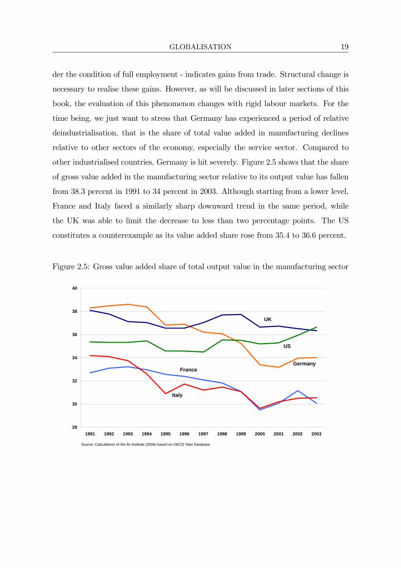
employment of EU-foreigners within Europe has increased by nearly 40 percent since

1995 whereas employment of EU15-nationals grew by only 10 percent (see Figure 2.10).

This indicates a deeper integration of labour markets in recent years. However, the

stock of foreign EU employees has remained stable at around 2-3 percent of total

employment since 1970 and only increased slightly to about 3.5 percent recently. Vis-

à-vis this number, it appears far fetched to talk about a fully integrated European

labour market.35

Figure 2.11: German migration pattern since 1965

- 400 000

- 200 000

200 000

400 000

600 000

800 000

1 000 000

1 200 000

1 400 000

1 600 000

1965

19

70

1975

19

80

1985

19

90

1995

2000

Immigration

Emigration

Source: Statistisches Bundesamt (2005): Migration Statistics 2004.

Germany’s role changed from a sending country in the 19th century to a host

country after the Second World War. Labour demand was higher than national supply,

so that the government initiated guest worker programmes in the 1960s. On average,

net immigration amounted to 240,000 people in this decade.36 By 1973, one in nine

workers was foreign-born. Between 1988 and 1992, Germany faced a second era of34Brücker, Alvarez-Plata and Siliverstovs (2003) and OECD (2004b), table 1.8.35Labour market issues are extensively discussed in chapter 3.36Brücker, Trabold, Trübswetter and Weise (2003).

32 GLOBALISATION

strong net immigration. This can partly be ascribed to skyrocketing numbers of asylum

seekers, but also to migration flows from Eastern Europe after the fall of the Iron

Curtain. From the following year on, Germany harmonised asylum laws with European

standards which led to a drastic reduction of immigration of asylum seekers. The

migration pattern since 1965 is shown in Figure 2.11.

2.3.3 Migration potential from Eastern Europe

As the most important determinant for labour migration is the wage differential be-

tween the sending and the target country, strong repercussions have been feared due

to the Eastern Enlargement of the EU in 2004. Compared to previous enlargements

to the south and the south-west, wages in the new member states relative to the old

member states are much lower than in Spain, Portugal or Greece at their time of ac-

cession. While the latter group of countries had average wages of about 50 percent of

EU member countries, Eastern European states only pay wages of one seventh of Ger-

man wages.37 Between 1950 and 1970, about 3 percent of the population of southern

European countries immigrated to western and northern European states. After 1970,

the share rose to 4 percent. Assuming an identical migration pattern, this implies

immigration to the old member states of up to 6 million people in the long run.38

Some econometric studies have estimated the migration potential under alternative

scenarios using more sophisticated arithmetical means. According to a report of the Ifo

Institute for Economic Research, 3.2 to 4 million migrants can be expected from the five

largest countries Poland, Czech Republic, Slovakia, Hungary and Romania within the

first 15 years after accession.39 If the smaller countries are added, even 4 to 5 million

people would come. Altogether, with an assumed labour mobility from the first day of

membership, 250,000 to 300,000 Eastern European citizens might emigrate per year.40

On the same grounds, the European Integration Consortium (2000) estimated a net

37Institute for the German Economy (2005), p. 141.38Stalker (1994), pp. 212-13. A similar result can be found in Layard et al. (1992).39Romania only had the status of an accession country (in 2004) whereas the other four have

already gained full membership.40Sinn et al. (2001).

GLOBALISATION 33

migration to the old member states of 930 thousand people within the first three years,

a little less than in the Ifo study. In the long run, however, the differences are much

bigger. The Consortium only expects that 1.9 million citizens will have migrated after

15 years. Bauer and Zimmermann (1999) forecast that, in the long run, 2-3 percent of

the population will move to the West. With a current population of roughly 75 million,

this would result in a total immigration of 1.5 to 2.3 million people from the eight new

Eastern European member countries.41

Brücker et al. (2000) expect initial inflows to Germany of 220,000 migrants per

year with a decreasing trend in consecutive years. They are referring to the eight

new Eastern European EU member countries plus Romania and Bulgaria, which will

accede in 2007. The population from these 10 countries that resides in the EU-15

would rise from about 550,000 today to 1.9 million in 2010, 2.4 million in 2020 and 2.5

million in 2030. Without Bulgaria and Romania, the yearly inflows would not exceed

150,000, however. In a different study, Brücker, Trabold, Trübswetter andWeise (2003)

argue that the total number of foreigners in Germany will only increase from 7.3 million

(2000) to about 8 million within the following three decades. However, the composition

will change. The share of citizens from Eastern European member countries can be

expected to be much higher in 2030.

All studies argue that the impact on the labour market will be strongest in the

first years after mobility is installed. However, a mass exodus of foreign workers to the

richer EU member states is generally denied. Concerning the distribution of migrants

across target countries in Western Europe, one can assume that Germany and Austria

can be expected to bear the heaviest burden. If the share of Eastern Europeans who

already live in the EU-15 remained constant, then two thirds of the total emigration

would have to be borne by Germany due to network migration. The second largest

country affected would be Austria with 11 percent of total migration flows.

41If Bulgaria and Romania are added and perfect labour mobility is assumed, the numbers increaseto about six million.

34 GLOBALISATION

2.3.4 Immigration and labour markets

Despite the immigration into developed countries in the 1990s, relative numbers still

reside at very low levels. Therefore, the impact on national labour markets seems to

be negligible. However, Figure 2.12 reports that the share of foreign workers in the

total labour force has increased substantially in major industrialised countries.

Figure 2.12: Stock of foreign and foreign-born labour force as a share of total labourforce

0

2

4

6

8

10

12

14

Perc

enta

ge

US Austria Germany France UK Ireland Denmark Norway Italy Spain

1992 2001Source: OECD (2004), for Germany data provided by EUROSTAT, US data for 1994 and 2001.

The US typically shows a very high ratio of foreign workers which further increased

to nearly 14 percent in 2001.42 Germany also belongs to the group of countries that is

characterised by a relatively high share of foreign workers. In 2001, more than eight

percent of the work force were either foreign or foreign-born. Starting from significantly

lower levels, Italy and Spain were affected relatively intensively by immigration in the

1990s. The share of the foreign-born labour force jumped up by 270 percent in Spain

and by 170 percent in Italy between 1992 and 2001.

42Countries like Luxembourg or Switzerland have higher shares, but are smaller and not comparableto large economies like the US, France, Germany or the UK.

GLOBALISATION 35

Table 2.3: Foreign and national population classified by level of education, 2000-01average, in percent

Lower Secondary Upper Secondary Third levelCountry Foreigners Nationals Foreigners Nationals Foreigners Nationals

Austria 41.8 21.4 43.5 64.3 14.7 14.4Belgium 54.4 39.9 24.5 32.0 21.2 28.2Denmark 21.6 20.0 51.1 53.9 27.7 26.1France 66.7 34.9 19.6 42.3 13.7 22.7Germany 48.5 15.1 36.1 60.4 15.4 24.5Greece 40.3 48.9 41.2 34.1 18.5 16.9Italy 55.0 55.8 32.1 34.4 13.9 9.8Netherlands 50.8 32.6 27.6 42.8 21.6 24.6Norway 15.7 14.4 44.1 53.2 40.2 32.4Portugal 69.5 79.6 19.8 11.0 10.7 9.4Spain 44.6 62.4 25.9 15.5 29.5 22.1Sweden 29.1 22.4 40.3 48.0 30.6 29.7Switzerland 33.6 10.5 42.6 64.4 23.8 25.1UK 30.1 18.8 29.1 53.3 40.8 27.9Czech Rep. 22.6 13.7 48.5 74.8 28.9 11.4Hungary 18.6 30.5 52.2 55.7 29.1 13.8Slovak Rep. 14.5 15.7 68.6 73.8 16.9 10.4US 30.1 9.3 24.7 33.7 45.2 57.1Canada 22.2 23.1 54.9 60.3 22.9 16.6

Source: OECD (2003a), Table 1.11, p. 45.

To trace this analysis a little further, we can take a look at the type of jobs immi-

grants get. It is evident from the data that immigrants possess a below average level

of education compared to that of nationals. In France, for instance, two thirds of the

foreign population has gained a lower secondary education, whereas only one third of

French citizens possess such an education. A similar picture evolves for Germany, Aus-

tria, Belgium, the Netherlands and the United States (see Table 2.3).43 Assuming that

education determines job opportunities, immigration has specifically increased com-

petition in low-skilled sectors. Indeed, in industries like mining, manufacturing and

energy, construction or trade, foreign workers are represented more than proportion-

ately. In Germany, 32.8 percent of all employees who work in mining, manufacturing

43OECD (2003a), p. 45.

36 GLOBALISATION

and energy, are foreigners, 26.5 percent in Austria and 18 percent in France.44

A different pattern exists in Eastern European countries. Regarding low-skilled

workers, these countries are sending rather than target regions. With respect to qual-

ified employees, though, Eastern Europe seems to be an attractive region. As Table

2.3 reports, foreigners are relatively better educated than nationals. Also, the United

Kingdom and Norway mainly attract highly educated people. The share of the foreign

population with a university degree reaches more than 40 percent in these countries.

2.4 Conclusions

This chapter has argued that globalisation of national markets had already been quite

pronounced in the past. However, the fall of the Iron Curtain and China’s rise have

created an additional stimulus. Commodity markets have never been more integrated,

and short-term capital mobility, as well as M&A activity, reached unprecedented levels

in recent years. The main reason for this trend is the continuous reduction of both

political and technological trade barriers over the last decades.

With its geo-strategical location, Germany has been particularly affected by the col-

lapse of the Communist Bloc. Apart from the high increase in trade flows with these

economies, German entrepreneurs belong to the largest investors in Eastern Europe.

Moreover, there is no doubt that Germany will host the largest fraction of Eastern

European immigration due to both geographical and cultural proximity. These devel-

opments in general exercise a substantial adjustment pressure - not only for Germany

but for all countries participating in global market exchange.

As we want to study the impact of globalisation in the presence of imperfect labour

markets, the next chapter provides an overview of labour market institutions and labour

market performance in selected countries. The analysis should serve as the motivation

for our central assumption of rigid labour markets.

44OECD (2003a), p. 63.

Chapter 3

Labour markets - institutions and

performance

The labour market belongs to one of the most important markets in an economy. In

order to absorb adjustment pressure and achieve necessary changes in the economic

structure, labour markets need to function appropriately. These adjustments take

place via bankruptcies or contraction of less efficient firms and expansion of more

efficient or entry of new firms. This necessarily implies hiring and firing of employees

and thus demands a high flexibility of labour markets with regard to employment

protection. In Germany, for instance, about 8 million people entered into and left

unemployment in 2004 alone. This makes up more than 20 percent of total employment.

Moreover, it constitutes only a lower bound because direct job changes (without the

”detour” via unemployment) are not included here.1 This impressive figure underlines

the importance of employment protection legislation for labour market flexibility.

Adjustment also takes place via changes in (relative) wages. If commodity prices of

certain products recede due to low-wage competition from abroad, wages might need

to adjust downwards in order to avoid firm bankruptcies. Hence, if labour market

institutions prevent market wages from falling below a certain floor, unemployment

emerges as a residual adjustment mechanism, and the absorbtion of exogenous shocks

1Bundesagentur für Arbeit (2006), on request.

38 LABOUR MARKETS

cannot take place in a first-best fashion.

Most economic models assume that labour markets function perfectly, that is, full

employment always prevails. However, reality tells a different story. Labour markets

are far away from being perfect markets, and even in the least regulated labour mar-

ket, adjustment needs time. In all countries, governments intervene to avoid certain

market outcomes. However, these interventions exercise a fundamental influence on

market outcome, be it the wage structure, employment and unemployment levels or

the duration of unemployment. As this book focuses on the impact of globalisation

when labour markets are rigid, it is worthwile to take a closer look at the degree of

labour market regulation in various countries.

It turns out that there are substantial differences across nations. Whereas countries

like the UK or the US choose to interfere less with market forces, many continental

European states have typically imposed generous welfare states which distort labour

supply decisions to a large extent. However, several continental European countries

have reduced their unemployment rates over the last decade by both demanding more

participation and granting generous welfare benefits at the same time.

This chapter starts with a survey of labour market institutions in OECD countries

and Eastern Europe. The second part observes major labour market reforms in selected

economies. Finally, we want to link national institutions to labour market performance.

We compare labour costs, relative earnings, unemployment and employment trends, the

pattern of unemployment and working time across countries.

3.1 Labour market institutions

3.1.1 Trade unions and employers’ organisations

A single employee might negotiate her contract with the employer directly. In many

cases, however, employees are represented by trade unions that set certain frameworks

or negotiate contracts for entire firms or industries. Similarly, a single firm might

LABOUR MARKETS 39

delegate these negotiations to the employers’ associaton. It is obvious that these or-

ganisations change the weight of participating parties in the bargaining process and

thus might lead to other market outcomes. For instance, powerful trade unions behave

as monopolists and set wages above full employment levels. Also, trade unions might

protect workers who possess a job by negotiating strict dismissal rules while excluding

the unemployed.

The picture concerning trade union membership in Western European countries is

mixed.2 France, Ireland, Italy and Norway have experienced an increase in membership

numbers between 1993 and 2003, in some cases very sharply. Many countries remained

at their 1993 level, whereas Germany, for example, faced an overall loss of about

4.4 million members between 1991 and 2003 - a reduction of 38 percent.3 In Greece

and the UK, membership receded by about 10 percent between 1993 and 2003. The

dissimilar patterns can be explained by varying developments in living standards and

unemployment rates in European countries. Additionally, a decline in traditionally

highly unionised industries and the rise of lower-unionisation services employment have

clearly enhanced this development.

With regard to Eastern European countries, the situation is fundamentally differ-

ent. Most countries of the former Soviet Bloc experienced a collapse of the old trade

union organisations. As trade union membership was compulsory during the commu-

nist era, a normalisation process began in which many former trade union members

opted out. Polish, Slovak and Bulgarian trade unions lost about 70 percent of their

members within ten years. In their 2002 report, ”Industrial Relations in Europe”,

the European Commission ascribed the steep decline in membership numbers to fac-

tors such as structural change, rising rates of unemployment, falling living standards

and the evolution of small and medium sized companies with a lower or no workers’

representation.

A glance at trade union densities in Figure 3.1 allows further insights. The ratio

describes the absolute number of members relative to total employment. In 2002,

2According to EIRO (2004a).3Deutscher Gewerkschaftsbund, by request 2005, own calculations.

40 LABOUR MARKETS

Figure 3.1: Trade union density in the EU, 2002

0

10

20

30

40

50

60

70

80

90

Denmark

Finland

Sweden

Cypru

s

Belgium

Malta

Luxembourg

Irelan

d

Slovenia

Slovakia

Austria

Italy

Greece

EU-15

Czech

Rep

ublicLatv

ia

Portugal

German

y UK

Netherl

ands

AC-10

Hungary

Lithuan

ia

Poland

Spain

Estonia

France

Source: EIRO (2003).

Perc

enta

ge

the Nordic countries Denmark, Finland and Sweden exhibited highest densities with

about 80 to 90 percent of all employees being represented by a trade union. Germany

ranks slightly below the EU-15 average with 29.7 percent. With regard to the new EU

members, Malta, Cyprus, Slovenia and Slovakia are the only countries ranking above

the EU-15 average. All others feature lower relative membership. As a reference value,

the trade union density in the US amounted to 13.2 percent in 2002 - at the lower edge

of this distribution.4

The trade unions’ counterpart in the social dialogue are the employers’ organisa-

tions. Basically, there are bodies representing employers’ interests and bodies represent-

ing business and trade interests. Several countries have installed a single organisation

for both parts, whereas some countries, like Germany, have two single organisations.

Another feature is the separation of representation by sectors such as industry, services

and agriculture.5

4EIRO (2003).5As in Finland, Greece or Portugal. For further details, see EIRO (2002).

LABOUR MARKETS 41

In contrast to the long tradition of company representation in Western Europe,

the new EU member states had to start this process from the beginning because the

communist regime only allowed state-owned enterprises. As everything was decided

by government authorities, there was no need for own representative bodies. The

transition crises substantially hampered the development of employers’ organisations.

As big companies went bankrupt and were replaced by many smaller firms, coordination

became much more difficult. The European Commission (2003a) estimates that 30 to

40 percent of industrial enterprises are represented by an organisation, but only 2

to 5 percent of all firms. Due to history and tradition, these young organisations

lack a strong influence in the social dialogue. Although trade unions and employers’

organisations intend to discuss labour market issues within their spheres autonomously

in the future, the governments currently still play a central role in negotiations.6

3.1.2 Bargaining systems

The size of trade unions and employers’ organisations provides a first impression of

the distribution of power in the bargaining process. Yet, how this process is organised

is another story. The degree of centralisation and the extent to which collective bar-

gaining results apply to firms and employees - the so-called coverage rate - are crucial

ingredients. Both a large coverage and a high degree of centralisation might be detri-

mental for labour market flexibility. Negotiating wages on the national level makes it

more difficult to account for differences between regions or firms. Consequently, wages

might be too high for low productivity firms and cause bankruptcy.

Figure 3.2 shows collective bargaining coverage in percent of total employment for

OECD- and new EU-member countries. Not surprisingly, the United Kingdom and

the United States can be found at the lower end of the scale with 36 and 14 percent,

respectively, whereas continental European countries are earmarked by comparably

high coverage rates.7 The Nordic countries Sweden and Finland, as well as Belgium,

6Funk and Lesch (2004).7The coverage rate has been decreasing in Germany over the last years and is much higher in

Western Germany, IAB (2002). See also Ochel (2001) for cross-country time series.

42 LABOUR MARKETS

Figure 3.2: Collective bargaining coverage, 2000

0%

10%

20%

30%

40%

50%

60%

70%

80%

90%

100%

Sloven

ia

Belgium

France

Austria

Sweden

Finlan

dSpa

in

Netherl

ands

German

y

Cyprus

Portug

al

Denmark

Irelan

d

Luxem

bourg

Norway

*

Slovak

ia

Poland UK

Hunga

ry

Czech R

epub

lic

Canad

a

Estonia

Switzerl

and*

Austral

ia**

Japan

*

New Zeal

and

Latvia

Lithua

niaUSA*

Source: European Commission (2003a) for EU countries; EEAG (2004) for non-EU countries. *1996-98, **2001

France and Austria, exhibit highest coverage above 80 percent of total employment.

Germany also ranks in the upper part of the distribution with 79 percent. The new

Eastern European member states are instead more comparable to the Anglo-American

pattern. Only Slovenia is the exception as the leader of the ranking.

The degree of centralisation differs markedly between countries. Bargaining takes

place on the national level in Belgium, Finland and Ireland. For most EU countries,

however, the sector is the dominant level. In the UK and in the US, negotiations even

take place on the company level. The recent trend in many EUmember states indicates

a tendency towards a more decentralised wage formation. Italy and Denmark serve as

good examples.8 However, decentralisation of wage bargaining as in the United King-

dom does still not seem to be in reach for continental Europe. The situation in Eastern

Europe again looks similar to the UK and the US. Here, wages are also negotiated on

the enterprise level in most cases. Slovenia and Slovakia are the exceptions with pay

setting at the sectoral level. Tables 3.1 and 3.2 provide a detailed overview.

8European Commission (2003), p. 77.

LABOUR MARKETS 43

Table 3.1: Summary characteristics of national wage formation systems in EU-15

Trade union Collective bargaining Duration of Bargaining leveldensity, 2000 coverage, 2000 agreements (dominant form)

Austria 30 % 92 % 1 year sectoralBelgium 69 % 96 % 2 years nationalDenmark 88 % 69 % 4 years national/ sectoralFinland 79 % 83 % 2 years nationalFrance 9 % 95 % 1 year companyGermany 30 % 79 % 2 years sectoralGreece 33 % n.a. 2 years sectoralIreland 45 % 66 % 2 years nationalItaly 35 % n.a. varying sectoralLuxemb. 50 % 60 % varying sectoral/ companyNetherl. 27 % 82 % varying sectoralPortugal 40 % 70 % 1 year sectoralSpain 15 % 83 % 3 years sectoralSweden 79 % 92 % 3 years sectoralUK 29 % 39 % varying company

Source: European Commission (2003a), Table 27. Trade union density for Portugalrefers to 1998, for Germany and Italy to 1999; collective bargaining coverage forIreland and Luxembourg based on estimates from national experts.

Table 3.2: Summary characteristics of national wage formation systems in new EUmember countries

Trade union Coll. bargaining Bargaining leveldensity, 2000 coverage, 2000 (dominant form)

Cyprus 70 % 65-70 % sectoralCzech Republic 30 % 25-30 % companyEstonia 15 % 29 % companyHungary 20 % 34 % companyLatvia 30 % <20 % companyLithuania 15 % 10-15 % companyMalta 65 % n.a. companyPoland 15 % 40 % companySlovakia 40 % 48 % sectoralSlovenia 41 % 100 % sectoral

Source: European Commission (2003a), Table 27.

44 LABOUR MARKETS

The evaluation of the new EU member states’ pay setting systems is not unam-

biguous in the literature. The European Economic Advisory Group (2004) finds a high

conformity with the less regulated Anglo-Saxon system. Kohl and Platzer (2003) sug-

gest a unique Central Eastern European industrial relations model, whereas Belke and

Hebler (2002) instead group the CEECs to continental Western European countries

like Germany and France. However, Belke and Hebler also incorporate unemployment

benefits and dismissal rules which have already converged towards the high European

regulation level.9

3.1.3 Minimum wages and implicit wage floors

The outcome of wage negotiations can be restricted by wage floors. The majority of EU

countries has installed statutory minimum wages. The US serves as another prominent

example. Concerning the theoretical implications, it depends on the market structure

whether minimum wages reduce or increase employment. With monopsonistic markets,

a minimum wage above the prevailing market level might well increase unemployment

and reduce the surplus of the monopson. Thereby, welfare rises. A prominent repre-

sentative of this view is Alan Manning (2003a and 2003b). The main argument states

that the division of labour has become so specialised that many firms within their

segments in fact behave as monopsonists. However, an economy is made up of many

sectors that are characterised by different productivities and hence, different wages.

Therefore, a minimum wage that might have positive effects in one sector could be too

high for a low-productivity branch and exercabates detrimental effects. Another argu-

ment against this view says that minimum wages are only relevant for the low-skilled

workers in the lowest part of the wage distribution. As specialised skills do not play a

role here, one can assume that labour markets can rather be described by the perfect

competition model. Then, the market clearing wage implies a Pareto optimum and

setting a statutory minimum above this level unavoidably creates unemployment and

welfare losses.

9For a summary, see Funk and Lesch (2004).

LABOUR MARKETS 45

Apart from minimum wages, benefit payments can cause similar effects. Social

security payments define workers’ reservation wages and thereby create an implicit wage

floor. Assuming perfect labour markets for low-wage workers, policy makers generally

face a fundamental trade-off when setting rules in this field. A more generous benefit

system or a higher minimum wage are intended to compress the income distribution,

that is more equality, but pari passu might reduce incentives to either employ workers

or for workers themselves to supply labour, that is less efficiency. While minimum

wages refer to the demand side, social benefits have an impact on the supply of labour.

Both aspects will be discussed in the following section.

Minimum wages

Within the enlarged European Union, 18 out of 25 countries have introduced a

statutory minimum wage — nearly all of the new members (except for Cyprus) and

nine of the old member states.10 Also the United States, usually not recognised as

having regulation in place, have protected the low-skilled by a statutory wage rate set

on the federal level. With regard to levels, Luxembourg, for instance, guraranteed the

highest minimum wage (1,237 €) whereas Lithuania established the lowest (281 €) in

2004. The statutory minimum wage in the US amounted to 727 € and in the UK to

1,083 €. France, the Netherlands and Belgium are ranked just below Luxembourg.

However, if one corrects for purchasing power, the gap between the highest and the

lowest minimum wages shrinks significantly.11

As all these economies are characterised by different average wages, the absolute

numbers do not provide an insight into whether statutory minimum wages can poten-

tially be binding for a large fraction of the work force. Figure 3.3 reports minimum

wages as a percentage of average monthly gross earnings in industry and services. It

is evident that the guaranteed minimum pay is relatively low in Eastern European

countries, the UK and the United States (30-40 percent), while it is 49 percent in the

10Among the nine old EU member states are Belgium, Greece, Spain, France, Ireland, Luxembourg,Netherlands, Portugal and the UK. In other countries like Germany, minimum pay is negotiated amongsocial partners and is not accounted for in this context. An overview is given in EUROSTAT (1998).

11EUROSTAT (2004), figures for this calculation refer to January 2004.

46 LABOUR MARKETS

Figure 3.3: Minimum wages relative to average wages, 2002

32% 33% 34% 34% 34% 35%37% 38%

42% 43%45%

49% 49% 50%

54%

0%

10%

20%

30%

40%

50%

60%

Slovak

ia

Poland

Czech R

ep.

UK USLatv

iaSpa

in

Lithua

nia

Hunga

ry

Portug

al

Sloven

ia

Luxem

bourg

Netherl

ands

Irelan

dMalt

a

Source: EUROSTAT (2004).

Netherlands and 50 percent in Ireland. From a historical perspective, real minimum

wages relative to average wages in manufacturing have decreased in a wide range of

countries, for instance in the US, the Netherlands, Belgium, Greece, Portugal, Spain

and the Czech Republic. However, Luxembourg, France and Poland even increased

their statutory minimum pay whereas in Hungary and Japan, the level remained the

same.12

As a consequence, the share of full-time workers earning the minimum wage differs

markedly between countries. The US, the UK and Ireland are characterised by small

fractions of 1.5, 1.9 and 2.1 percent, respectively. Ireland’s high relative minimum wage

does currently not impose a restriction on wage flexibility because the economic boom

of recent years has boosted market wages for most workers above the minimum level.

Hungary, France, Luxembourg and Latvia are ranked at the upper end of the scale with

shares of 11.4, 14, 15.1 and 15.4 percent, respectively.13 Hence, it seems obvious that

12OECD (1998), p. 41. Time series for Poland, Hungary and the Czech Republic refer to the 1990s,for other OECD members to the period 1970 to 1996.

13EUROSTAT (2004), see also European Commission (2003a), pp. 79-80. Other studies like OECD

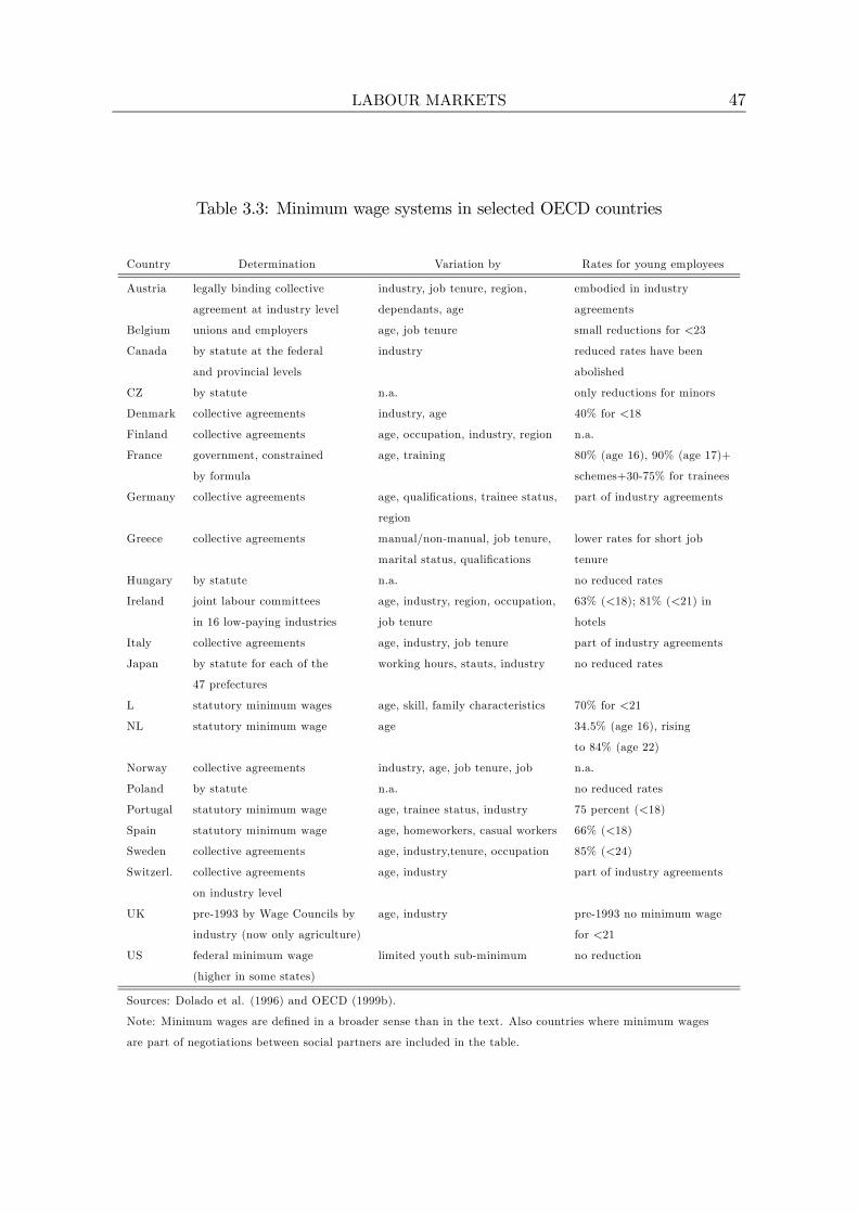
LABOUR MARKETS 47

Table 3.3: Minimum wage systems in selected OECD countries

Country Determination Variation by Rates for young employees

Austria legally binding collective industry, job tenure, region, embodied in industry

agreement at industry level dependants, age agreements

Belgium unions and employers age, job tenure small reductions for <23

Canada by statute at the federal industry reduced rates have been

and provincial levels abolished

CZ by statute n.a. only reductions for minors

Denmark collective agreements industry, age 40% for <18

Finland collective agreements age, occupation, industry, region n.a.

France government, constrained age, training 80% (age 16), 90% (age 17)+

by formula schemes+30-75% for trainees

Germany collective agreements age, qualifications, trainee status, part of industry agreements

region

Greece collective agreements manual/non-manual, job tenure, lower rates for short job

marital status, qualifications tenure

Hungary by statute n.a. no reduced rates

Ireland joint labour committees age, industry, region, occupation, 63% (<18); 81% (<21) in

in 16 low-paying industries job tenure hotels

Italy collective agreements age, industry, job tenure part of industry agreements

Japan by statute for each of the working hours, stauts, industry no reduced rates

47 prefectures

L statutory minimum wages age, skill, family characteristics 70% for <21

NL statutory minimum wage age 34.5% (age 16), rising

to 84% (age 22)

Norway collective agreements industry, age, job tenure, job n.a.

Poland by statute n.a. no reduced rates

Portugal statutory minimum wage age, trainee status, industry 75 percent (<18)

Spain statutory minimum wage age, homeworkers, casual workers 66% (<18)

Sweden collective agreements age, industry,tenure, occupation 85% (<24)

Switzerl. collective agreements age, industry part of industry agreements

on industry level

UK pre-1993 by Wage Councils by age, industry pre-1993 no minimum wage

industry (now only agriculture) for <21

US federal minimum wage limited youth sub-minimum no reduction

(higher in some states)

Sources: Dolado et al. (1996) and OECD (1999b).

Note: Minimum wages are defined in a broader sense than in the text. Also countries where minimum wages

are part of negotiations between social partners are included in the table.

48 LABOUR MARKETS

minimum wages in English speaking countries as well as in some Eastern European

states do not restrict labour market flexibility to a significant extent. In France, just

to mention a counter-example, flexibility of low wages is restricted for a substantially

larger share of the workforce.

Employment effects of minimum wages are both widely and controversially dis-

cussed in the literature. While Dolado et al. (1996) do not regard minimum wages

as a more serious constraint on the labour market than in the 1960s, Nickell and Bell

(1995) and Card and Krueger (1995) explain the rise in unemployment rates by trends

against the less-skilled in connection with imperfect wage adjustments. However, Card

and Krueger (1995) do not find large employment effects of the federal minimum wage

in the US. The overall effect on employment seems to be rather small. What is clear,

though, is the negative impact on the employment of young workers.14 Therefore, many

European countries account for that by means of lower minimum wages for the young.

The variability in this respect is higher in Europe than it is in the United States.15

Table 3.3 provides a detailed overview about minimum wage systems in selected OECD

countries.

Unemployment benefits

While the empirical evidence of minimum wages’ employment effect is not clearcut,

there is considerable support for the theory that the generosity of the benefit system

has a negative impact on employment.16 As replacement payments determine work-

ers’ reservation wages, higher benefits reduce the incentive to become re-employed and

accept low-paid jobs. Moreover, the unemployment spell continues with higher re-

placement payments, as unemployed workers can afford to wait for a better job offer or

take higher risks when negotiating wages.17 Basically, the impact of benefit systems is

similar to that of minimum wages, only that they work via the supply side of labour.

(1999b) have different figures as other references are used. However, the ranking basically remainsidentical.

14See Brown et al. (1982) and Brown (1999) .15Dolado et al. (1996), p. 357.16OECD (1994b), chapter 8. See also Nickell (1997).17See Layard (1988) and Johnson and Layard (1986).

LABOUR MARKETS 49

The institutional design of unemployment insurance varies substantially across

countries. While Finland, Ireland, Poland and the UK pay fixed amounts (calculated

as a percentage of average production workers’ income), most governments determine

replacement rates as a fraction of previous gross earnings. In a few cases like Austria,

the Czech Republic and Germany, unemployment benefits guarantee a certain amount

of previous net income. In Denmark, social security contributions must be deducted.

Table 3.4: Average of net replacement rates (NRR) over last 60 months, 2002

No children Two childrenOverall Single One-earner Lone One-earner

Country average person married couple parent married couple

Italy 5 5 5 6 6US 6 6 6 5 5Korea 6 6 6 7 6Czech Rep. 9 4 4 13 13Japan 13 7 7 27 10Canada 20 11 12 27 28Luxembourg 25 17 17 33 33Poland 26 21 21 31 29Greece 26 22 23 29 29Spain 30 29 28 32 31Switzerland 31 30 30 33 33Sweden 32 17 17 50 42UK 33 34 34 32 32Hungary 36 32 32 40 39Slovak Rep. 37 28 33 42 45Portugal 48 44 46 51 51Ireland 49 35 53 47 61Norway 54 39 40 80 57Austria 62 52 55 70 73Netherlands 65 60 67 64 70Germany 67 57 54 81 76Denmark 67 58 64 75 73France 68 62 64 74 74Finland 69 60 64 77 73Belgium 69 66 67 74 69

Source: OECD (2004d): Table 3.3b.

Due to the very complex and country-specific designs it is impossible to generate a

ranking by benefit generosity in an easy way. In order to get a better understanding of

50 LABOUR MARKETS

the unemployment benefit system’s generosity, the OECD (2004) has calculated average

net replacement rates (NRR) over 5 years of unemployment. Table 3.4 reports these

NRRs for four different family types. Italy leads the ranking with a net replacement

rate of only 5 percent. Apart from this outlier, European countries generally feature

high in replacement levels. Austria, the Netherlands, Germany, Denmark, France,

Finland and Belgium all provide income replacements above 60 percent of previous

net earnings. On the other hand, unemployment protection is rather low in the US (6

percent) or Japan (13 percent). Eastern European countries like the Czech Republic,

Poland or Hungary rank in the less generous part of the distribution with 9, 26 and

36 percent respectively. The overall picture does not change substantially with family

types.

Social assistance

People who do not qualify for unemployment benefits, and who lack resources to

make their living, fall back on governments’ social assistance. Concerning the impact

of social assistance on labour supply, the same reasoning applies as in the previous

section. The more generous these welfare payments are designed, the less attractive

it is to accept a low-paid job. Across OECD countries, the picture is very mixed and

benefits differ immensely with family types. Table 3.5 provides information on the

determination of social assistance and the maximum amounts with respect to different

family types. As benefits differ substantially across regions, the second column clarifies

how this variation is accounted for in this classification. ”National rates” means that

benefits are identical across regions within a country, whereas ”national guidelines” are

taken if these recommendations are enforced in different ways. When social benefits

vary across regions, ”national averages” are taken, if known. Otherwise the figures

refer to a representative jurisdiction.18 While lack of resources is the main criterion

for eligibility, some countries impose further conditions. A US citizen can only receive

social assistance if he or she is actively looking for work, or participates in employment,

training or workfare.

18See OECD (2004d), p. 28.

LABOUR MARKETS 51

Table 3.5: Social assistance benefits, 2002

Maximum amounts (% of APW)Head of Spouse/

Country Determination household partner Per child

Austria national average 19 12 6Belgium national rates 23 8 4-10Canada regionally 16 12 4-5Czech Rep. national rates 24 17 13-17Denmark national rates 31 31 10Finland national average 16 11 9-12France national rates 20 9 0-9Germany national rates 11 9 5-10Hungary national guidelines 16 n.a. n.a.Iceland regionally 31 25 n.a.Ireland national guidelines 24 16 3Italy regionally 16 9 7-8Japan regionally 24 13 6-7Korea national rates 16 10 9-10Luxembourg national rates 36 18 3Netherlands national rates 30 13 n.a.Norway regionally adjusted 30 7 4-16

national ratesPoland social worker discretion 21 n.a. n.a.Portugal national rates 20 20 10Slovak Rep. national rates 27 12 8Spain regionally 27 3 3Sweden national guidelines 16 11 7-12Switzerland national guidelines 22 12 6; 12UK national rates 11 8 10US national rates 5 4 4

Source: OECD (2004d): Table 1.4.Note: APW=average production worker

With regard to maximum benefits, the distribution ranges from five percent of

an average production worker’s salary in the US to 36 percent in Luxembourg. If

households earn additional income, benefits are reduced by 50 percent (Portugal),

75 percent (Canada) or 100 percent in most countries. However, some states like

Denmark, the UK or Germany have implemented disregards. Only if these amounts

are exceeded, benefits are reduced by the prevailing rates. In addition, the maximum

amount a household can receive depends on the size and the structure of the family.

52 LABOUR MARKETS

A second adult in the household may only get 11 percent in addition of the head of

household (Spain) or up to 100 percent like in Denmark or Portugal. If just one child

is present, total benefits do not rise at all in France whereas social assistance increases

by more than 70 percent in the US, the UK and Germany.

Despite the detailed information, an overall evaluation of the system’s generosity

remains difficult because interactions with other benefit schemes must be taken into

account. Furthermore, some countries grant extra payments on top for rent or clothing

which are not reflected in Table 3.5. Nevertheless, an impression the reader might get

is that the United States and the United Kingdom feature with a rather low generosity

while contintental European states are characterised by higher welfare payments.

3.1.4 Employment protection legislation (EPL)

Another important field of labour market regulation comprises rules for the hiring

and firing of workers. Once established to enhance employment conditions, EPL also

imposes additional costs on firms for hiring employees. Theoretically, two effects stand

vis-à-vis. On the one hand, EPL reduces inflows into unemployment and thus protects

job owners, whereas on the other hand, it makes reentry into the job market more

difficult for outsiders. A priori, the net effect is ambiguous and subject to empirical

investigation. According to OECD (2004c), EPL has benefited workers with some years

of work experience while young people and prime-age women are discriminated by such

policies. From a welfare perspective, there must be an optimal degree of EPL if higher

job security increases employees’ efforts and co-operation. Thus, EPL may enhance

economic efficiency as long as labour market flexibility is not restricted too much.

The relation between EPL and employment has gained attention after Lazear’s

seminal paper in 1990. For 22 developed countries over the years 1956 to 1984, he finds

that a regime shift from no severance pay to obligatory three months salary compen-

sation would reduce the employment-population-ratio by one percent. In France, for

instance, 59 percent of unemployment can be explained by changes in severance pay

requirements. In order to capture the degree of EPL, the OECD (1999a, 2004c) has

LABOUR MARKETS 53

developed an index that allows a ranking of countries. For that purpose, three areas

are distinguished, namely regular employment, temporary employment and additional

rules for collective dismissals. Out of these sub-indices, the OECD has derived an

overall EPL index between zero and six with six being the highest protection level.

Regular employment and collective dismissals

Although temporary forms of employment have increased in OECD countries in

recent years, regular employment is still by far the most dominant form.19 Therefore,

protection for regular contracts takes up the main part of the EPL index. According

to OECD (1999a), three broad sub-areas can be identified in this context: Procedural

requirements that an employer must meet to terminate the contract, regulation of

notice and severance pay, and penalties for unfair dismissals. From these categories

the OECD develops a sub-indicator revealing the protection of regular employment.

With regard to procedural requirements, the ranking takes into consideration whether

a written statement mentioning reasons for dismissal is required, whether a third party

must be consulted or whether a third party even has to approve the company’s decision.

The Netherlands have implemented the strictest rules, whereas Canada and the United

States can be found at the other end of the scale. The picture is basically the same

for notice and severance pay requirements. All OECD countries have set formal rules

for length of notice, but only two thirds prescribe severance payments. Here, Southern

European countries dictate the strictest rules. In Italy and Portugal, companies have

to pay a severance of 18 to 20 monthly salaries to their employees if they have worked

for the company for 20 years. Canada and the US have not regulated that issue at

all. Concerning the last category, unfair dismissals, many countries have laws that

make dismissals illegal for specific reasons such as gender or race. The least restrictive

legislation to dismiss employees for any reason can be found in the US, followed by

the UK and Switzerland. Germany ranks 23rd out of 28 OECD countries, Hungary

and Poland rank 11th and 12th, respectively. The Czech and Slovak Republic have

similar regulation as Germany. This sub-indicator is shown in column 4 in Table

19OECD (2002b), chapter 3.

54 LABOUR MARKETS

3.6 for all countries. Again, the English speaking economies are characterised by the

least restrictive regulation whereas continental European states have protected their

employees the most.

When it comes to collective dismissals, all countries have introduced additonal,

generally stricter rules on top of individual dismissal regulation. Surprisingly, also the

US, Canada and the UK reach relatively high index values of 2.9. Sweden and Italy

constitute the end with indices of 4.5 and 4.9, respectively. This ranking can be found

in the last column of Table 3.6.

Temporary employment

One method to make the labour market more flexible without touching the dismissal

legislation is to allow for temporary work. Thereby, employers take a lower risk because

they do not have to pay severance packages or consider length of notice periods. Short-

time work, fixed-term contracts and the recognition of temporary work agencies (TWA)

are possible ways to go. In fact, all countries allow fixed-term contracts. Many however,

restrict them to so-called objective reasons such as time-limited projects, seasonal work

or replacement of employees who are temporarily absent.20 The US, Canada and the

UK literally do not regulate, whereas Germany for instance, has specified by law how

many consecutive fixed-term contracts an employee can be given until he must receive a

permanent one. The ranking in this category shows a huge gap between the group of less

regulated countries and Southern European countries such as Greece, Italy, Portugal

and Spain. In between, one can find Central and Western European states, whereas

France compares more to Southern Europe and Nordic countries. Eastern European

EU members like Poland, the Czech Republic and Hungary have similar regulations

to the US. The Czech and Slovak Republic have installed a very lax regulation. They

reach an index of 0.5 and 0.3, respectively. Hungary follows with a value of 1.1. Table

3.6 also reveals the complete ranking of this sub-index.

20OECD (1999a), p. 59.

LABOUR MARKETS 55

Table 3.6: Summary indicators of the strictness of employment protection legislation(EPL), 2003

Regular Temporary CollectiveRank Country Overall EPL employment employment dismissal

1 US 0.2 0.2 (1) 0.3 (1) 2.9 (10)2 UK 0.7 1.1 (2) 0.4 (3) 2.9 (10)3 Canada 0.8 1.3 (4) 0.3 (1) 2.9 (10)4 Ireland 1.1 1.6 (7) 0.6 (6) 2.4 (6)

Switzerland 1.1 1.2 (3) 1.1 (8) 3.9 (23)6 Australia 1.2 1.5 (5) 0.9 (7) 2.9 (10)7 Denmark 1.4 1.5 (5) 1.4 (14) 3.9 (23)8 Hungary 1.5 1.9 (11) 1.1 (8) 2.9 (10)

New Zealand 1.5 1.7 (8) 1.3 (11) 0.4 (1)10 Poland 1.7 2.2 (12) 1.3 (11) 4.1 (25)11 Japan 1.8 2.4 (16) 1.3 (11) 1.5 (2)12 Austria 1.9 2.4 (16) 1.5 (15) 3.3 (18)

Czech Rep. 1.9 3.3 (26) 0.5 (5) 2.1 (4)Italy 1.9 1.8 (10) 2.1 (20) 4.9 (28)Slovak Rep. 1.9 3.5 (27) 0.4 (3) 2.5 (8)

16 Finland 2.0 2.2 (12) 1.9 (19) 2.6 (9)Korea 2.0 2.4 (16) 1.7 (17) 1.9 (3)

18 Netherlands 2.1 3.1 (25) 1.2 (10) 3.0 (16)19 Belgium 2.2 1.7 (8) 2.6 (21) 4.1 (25)

Germany 2.2 2.7 (23) 1.8 (18) 3.8 (21)Sweden 2.2 2.9 (24) 1.6 (16) 4.5 (27)

22 Norway 2.6 2.3 (14) 2.9 (23) 2.9 (10)23 Greece 2.8 2.4 (16) 3.3 (24) 3.3 (18)24 France 3.0 2.5 (20) 3.6 (26) 2.1 (4)25 Mexico 3.1 2.3 (14) 4.0 (27) 3.8 (21)

Spain 3.1 2.6 (21) 3.5 (25) 3.1 (17)27 Portugal 3.5 4.3 (28) 2.8 (22) 3.6 (20)28 Turkey 3.7 2.6 (21) 4.9 (28) 2.4 (6)

Source: OECD (2004c), Table 2.A2.4, p. 117.

56 LABOUR MARKETS

Summary indicators of strictness of employment protection legislation

In order to construct on overall cardinal index, the OECD proceeds in four steps.

First of all, the entire set of information items - which have been gathered in sub-indices

as described above - has to be translated into the scale between zero (no regulation)

and six (maximum regulation). On the consecutive stage, weighted averages are con-

structed to generate aggregated information, out of which the sub-indices (stage 3) are

formed as unweighted averages. The three areas described above are finally merged to

the overall EPL index as reported in Table 3.6.21 The weights used should reflect repet-

itive information already covered in other items or an economically stronger impact of

certain institutional features on the strictness of regulation.

The overall situation of strictness in employment protection legislation closely re-

sembles the ranking by sub-indices. The US, the UK, Canada, Ireland and Switzerland

offer the least restrictive legislation. Denmark leads other major European countries

with an overall index of 1.4. Germany ranks 19th, whereas Eastern European members

such as Hungary or the Czech Republic can be found in the midfield with values of 1.5

and 1.9, respectively. The strictest regulation has been implemented in France, Spain

and Portugal. In these countries, both high protection against individual dismissal and

strict rules for temporary employment are at work.

Recent figures also allow an evaluation of changes in EPL strictness over time.

Over the last number of decades, a convergence process could be observed without

having changed the relative position of most countries. Only France and Italy form

exceptions in this regard. While Italy has substantially deregulated its labour market

since the 1980s and now ranks in the middle of the spectrum, France has drifted in the

opposite direction. The US and the UK have provided and still provide the least strict

labour market regulation. High EPL states relaxed their rules, thus converging to the

leaders of the ranking. While Portugal and Spain undertook comprehensive reforms

with regard to both regular and temporary employment, most other countries reformed

partially and specifically targeted temporary work regulations.22

21For details, refer to OECD (1999a), chapter 2, Annex 2.B.22OECD (1999a).

LABOUR MARKETS 57

3.1.5 Regulation of holidays and working time

Working time and holiday regulation - issues that are not covered in OECD’s EPL

indexation - are negotiated between social partners. In some countries, the government

is involved as a third party as well (tripartite bargaining). The outcome however, must

meet certain standards which are generally set by government authorities alone. The

statutory maximum working day must not be longer than 13 hours in Ireland, the UK,

Greece, Italy, Cyprus and Denmark. In some countries like Austria and France, the

maximum amounts to ten hours, whereas Germany has even set its maximum to eight

hours.23 This figure simply says that workers must not be forced to work longer than

average. With regard to the statutory maximum working week, the normal limit is 48

hours. However, several countries like Austria, Spain and several Eastern European

countries have set 40 hours as the maximum. Annual paid leave is also regulated by

governments. The statutory annual paid leave is 20 days in most countries, only a few

like France or Austria allow 25. Of course, these standards do not reflect how many

hours are being worked and how many days workers can take off. This will be discussed

in section 3.3 below.

3.1.6 Overall evaluation of labour market flexibility

In institutional comparisons, it is quite hard to come up with a clear and transparent

figure by which countries can be unambiguously ranked. So far, we have discussed

labour market institutions in several respects in order to get an impression of labour

market flexibility. The index for strictness in employment protection legislation cal-

culated by the OECD was an exception as it provided a cardinal measure. From the

facts we concluded that Anglo-Saxon countries seem to possess a rather flexible labour

market compared to Western European economies. In the latter, employment protec-

tion is stricter, unions have a stronger influence in the wage-setting process and benefit

schemes are more generous.24 However, this description by itself does not provide ev-

23EIRO (2004b).24See also Blau and Kahn (1999), p. 1448.

58 LABOUR MARKETS

idence that labour markets have more difficulties in absorbing external shocks like an

increase in low-wage competition from former communist countries or other emerging

markets. Therefore, it is worthwhile to survey some empirical work.

Nickell (1997) identifies labour market institutions as a main determinant of unem-

ployment, whereas other rigidities have no observable impact on unemployment. To

the former group of features, Nickell counts generous unemployment benefits that are

paid without time limits and desist from pressure on the unemployed to find a new job

or strong influence of unions combined with collective bargaining on a central level.

Siebert (1997) also draws a clear connection between labour market institutions and

unemployment. He makes the expansion of the welfare state responsible for persis-

tent unemployment in many countries, especially Germany, as adjustments to adverse

shocks could not be compensated in the same way as in the United States. These

shocks comprise the two oil crises, implications from international competition with

newly industrialised economies as well as technological progress.

According to the IMD World Competitiveness Yearbook (2005) labour market reg-

ulations have been assessed by executives that represent a cross-section of the business

community in each country. With regard to regulations such as hiring and firing prac-

tices and minimum wage constraints, Germany reaches only 1.88 out of 10 points and

ranks last out of 60 participating countries.25 This means that business activity is hin-

dered most in this country. Surprisingly, Denmark heads the list with a score of 7.79.

The US comes 10th, the UK 26th. Most continental European countries appear in the

lower half of the ranking. When it comes to incentives to look for new employment,

Germany also performs badly. Only Argentina shows a more generous unemployment

scheme. The pattern is pretty similar to the previous ranking. Continental European

states gather at the end of the list. Surprisingly, the US only reaches place 45 out of

60 in this category.26

The OECD (1994b) has calculated two elasticities that describe the degree of labour

market rigidity: one is the response of labour demand on changes in real wages, the

25Contrary to the EPL index, a low value indicates poor performance.26International Institute for Management Development IMD (2004), Tables 2.4.16 and 2.4.17.

LABOUR MARKETS 59

Table 3.7: Long-term employment elasticity and long-term real wage response

Long-term Long-termemployment Median lag real wage Median lagelasticity (years) response (years)

US -1.0 1.0 US -1.0 1.0Canada -0.9 1.0 UK -1.0 1.0France -1.0 2.0 France -3.5 1.5Germany -1.0 2.0 Finland -6.0 2.0Finland -1.0 3.0 Italy -3.5 2.0Japan -0.8 3.0 Sweden -10.0 2.5UK -1.0 4.0 Japan -5.0 3.0Italy -0.5 5.0 Canada -2.0 3.5Sweden -0.9 7.0 Germany -3.0 4.0

Source: OECD (1994b), pp. 1-5.

other figure reflects the response of wages on changes in labour demand (extent of

unemployment). According to Table 3.7 that reports these figures for selected OECD

countries, a one percent increase in the real wage reduces labour demand by one percent

in the long run and vice versa. The big difference across countries however, can be

found in the adjustment speed. While half of the adjustment is completed after only

one year in the US and Canada, the same process takes twice as long in Germany and

France. Surprisingly, the UK needs four years for half of the adjustment. In Italy

and Sweden the adjustment takes even longer. The long-term real wage response to

a one percent change in unemployment, as reported in the right part of the table, is

extraordinarily high in Sweden and is also at a relatively high level in Finland and

Japan. What is more important however, is once again the adjustment speed. In

that respect, the United States rank at the top of the list next to the United Kingdom.

Germany shows the poorest performance with a median lag of four years. These results

provide further evidence for what we had suspected before: wages tend to adjust faster

in the US and the UK thus indicating a higher flexibility of the labour market.

With regard to the new Eastern European EU member states - for which similar

indicators do not exist (yet) - unionisation is lower than in Western Europe and collec-

tive bargaining mainly takes place at the company level. Concerning the generosity of

60 LABOUR MARKETS

the unemployment benefit system, data are only available for Poland, Czech Republic,

Slovakia and Hungary. Hungary has the most generous system of the four, but still

rather ungenerous relative to the old members of the European Union. As decentralised

bargaining and ungenerous benefit systems are major determinants of labour market

flexibility27, one can assume that Eastern Europe shows a higher flexibility than other

European countries, although the low regulation of Anglo-Saxon countries might not

be reached.

3.2 Labour market reforms in selected countries

To complement the discussion of institutional labour market features, this section pro-

vides a brief overview of major labour market reforms in selected European economies.

It turns out that the political response to increasing unemployment trends since the

oil crises in the 1970s has differed across countries both in timing and direction.

Denmark

In 1994, a comprehensive labour market reform initiated by the Social Democratic

Prime Minister Rasmussen, came into force. What is known as the flexicurity approach

combines flexibility (high job mobility due to low employment protection), social se-

curity (due to a generous welfare system) and active labour market programmes.28

Dismissal rules were reduced to a minimum so that employees can literally be fired

without delay. In addition, the insured unemployed have become subject to a two-

period system with a strong emphasis on activation in the second period. Unemploy-

ment benefits were initially only granted for up to 4 years (previously 9 years) in the

first period. If someone is still unemployed after the first period, he or she directly

switches to the second stage where authorities offer compulsory job training. Refusal

to participate in these programmes causes significant cuts in benefits. Whereas the first

stage was reduced to one year by 1999 and for young employees below 25 years even

27Nickell (1997).28OECD (2004c), pp. 97-98.

LABOUR MARKETS 61

to six months, the second period still spans three years. The recent 2003 reform More

people into employment entirely abolished the two-period scheme. Active job seeking

may be requested from the first day of unemployment while the maximum duration of

benefit payments still amounts to 4 years.

Another aspect of recent labour market reforms has been the shift from a rule based

to an individual action plan systemwhere individual needs of the unemployed are better

taken into consideration. This programme is specifically designed to fight long-term

unemployment.29 Overall, the Danish approach has often been seen as a third way

between low labour market regulation of Anglo-Saxon economies and stricter EPL and

more generous welfare schemes in other continental European states.

Netherlands

In 1982, government authorities and social partners agreed to give up wage indexa-

tion, to moderate wage claims, to remove obstacles to temporary work and to introduce

full social-security coverage for part-time workers. In addition, working time was re-

duced, provided that this did not lead to an increase in labour costs or a reduction in

firms’ operating hours. This consensus became popular as the Wassenaar Agreement.

Since then, the Dutch consensus model — that is, lack of industrial strife and wage

developments in line with productivity improvements — has often been cited as a key

factor for improved employment performance.30

In 1986-87, the unemployment insurance system was significantly curtailed. The

duration of benefits was reduced from thirty to six months for younger workers and

the replacement rate was lowered from 80 to 70 percent. As benefits are linked to

the minimum wage, lowering the minimum wage also reduced the minimum benefit.

By 1998, the minimum benefit had been pared to 60 percent of the average wage, a

decline of 9 percentage points since the early 1980s. In addition, in 1995 the government

tightened the eligibility standards for benefits, requiring a longer period of employment.

Recipients are now also expected to accept any “suitable” job offer. Those who refuse to

29Madsen (1999).30See Tille and Yi (2001).

62 LABOUR MARKETS

do so receive reduced benefits. Finally, what constitutes a suitable offer is interpreted

more liberally for recipients who have had relatively long unemployment spells - a

change in the rules that is designed to induce the unemployed to intensify their job

search as time passes. In the 1990s, active labour market policies to fight long-term

unemployment and new early retirement regulations complemented the reforms of the

1980s.

Sweden

In 1991 wage bargaining under public supervision became more decentralised. In

the same year, the government curtailed pre-tax unemployment benefits from 90 to 75

percent of previous gross earnings (later increased again to 80 percent). In 2001 and

2002, ceilings on unemployment benefits were raised in two steps. Since 1996, benefit

sanctions can be extended from 20 to 60 days if someone declines a job or training offer.

Social assistance recipients can now be required to undertake education or training as

well. Beneficiaries of welfare payments are required to participate in activation pro-

grammes after 27 months of unemployment. This regulation also comprises part-time

employment since 2001. With respect to employment protection legislation, fixed-term

contracts for up to 12 months were introduced in 1997, without restriction concerning

the nature of the work.

Sweden is renowned for its extensive active labour market policies (ALMP) which

were further strengthened during the last years. In 1995, the government implemented

subsidies for social security contributions if a firm hired an unemployed person. Long-

term unemployment was combatted by individual programmes for persons at risk.

In 1998, special activation for people under 24 became compulsory after 100 days of

unemployment. Concerning the targeting of ALMPs a 50 percent wage subsidiy for

firms hiring long-term unemployed over 60 and intensified effort for training of low-

skilled, long-term unemployed over 55 was supposed to increase employment prospects

for these groups.31

31Brandt, Burniaux and Duval (2005).

LABOUR MARKETS 63

United Kingdom

British Prime Minster Margaret Thatcher fundamentally reformed labour market

institutions in the 1980s. In several Employment Acts the ”Iron Lady” forcefully

broke up trade unions’ power. Moreover, work incentives were increased through a

modification of welfare payments. Unemployment benefits dropped or were even en-

tirely abolished for young people. Unemployed workers had to be interviewed every six

months about their progress in job seeking. Another direction of the Thatcher reforms

aimed at a lower weight of the government in the market economy. Many state-owned

enterprises were privatised, government employment reduced and tax rates lowered.32

More recently, notification requirements for collective dismissals have been relaxed

and maximum duration of fixed-term contracts were reduced to 4 years (before unlim-

ited) in 2000. Since 1999, unemployment benefits are granted only for a period up to

6 months (previously 12 months) if spouses are working. In 1998, the British govern-

ment initiated the New Deal for Young People which conditioned the entitlement of

unemployment benefits on the participation in activation programmes 6 months after

dismissal. This regulation was later extended to employees older than 25 years, long-

term unemployed and disabled people. Active labour market programmes targeted at

more and better training, subsidised work with the voluntary sector, design of a job

search plan and compulsory interviews every two weeks. To account for high unem-

ployment rates among the young, reduced minimum wage rates for 18-21 year-old work

force members were introduced in 1999.33

Germany

Germany’s welfare state expanded tremendously in the 1970s and became even more

generous thereafter. The evident labour market problems that especially emerged after

German Unification were comprehensively adressed in Chancellor Schröder’s speech

on March 14, 2003, where he proposed the Agenda 2010. Apart from other reform

proposals, the concept focused on the liberalisiation of the labour market. The so-

32Blanchflower and Freeman (1993).33Brandt, Burniaux and Duval (2005).

64 LABOUR MARKETS

called Hartz-reform makes up the core of this package. Hartz I and II which came

into force on January 1, 2003, introduced Ich-AGs (unemployed can apply for public

financial support if they plan self-employment), Minijobs (firms neither pay taxes nor

social security contributions up to a monthly salary of 400 euro per employee) and

Personnel-Service-Agencies within the Public Employment Service (PES) to improve

job placement of unemployed workers. Hartz III (in place since January 1, 2004)

aims at the restructuring of the German Public Employment Service in the fashion

of more decentralisation and more service orientation. The final goal was to place

unemployed workers on free positions more efficiently at lower costs. Hartz IV was

the most hotly debated regulation and caused country-wide demonstrations. From

January 1, 2005, unemployment and social assistance were merged bringing about a

level of social assistance that was in fact lower than the previous one. Unemployment

insurance which guarantees about two thirds of previous net earnings is only granted

up to 12 months (previously 24 months) since. Exceptions exist for older persons above

55 who are entitled to receive unemployment insurance benefits for up to 18 months.

Thereafter, the unemployed are only entitled to the lower benefits.

After a relaxation and retightening of dismissal rules in 1996 and 1999, dismissal

protection was only active in companies that employed more than 10 people. Restric-

tions on fixed-term contracts were reduced in the sense that longer periods and more

renewals were possible. Private temporary work agencies received more freedom for

job placement in several steps till 2004. In 2002 and 2005 sanctions for job offer denials

became tighter. Since 2002, a special programme for unemployed over the age of 50 -

the so-called Job-AQTIV regulation - is supposed to reduce high unemployment rates

in this age group. Individual profiling, job rotation, intensified training and better

access to temporary work are the key instruments to achieve this goal.

Italy

In Italy, employment protection legislation was eased in several steps since 1997.

Fixed-term contracts are no longer automatically transformed into contracts with indef-

inite duration and low-skilled workers can now be hired more easily. Private temporary

LABOUR MARKETS 65

work agencies were allowed in 1998, although restrictions on job placements were en-

tirely abolished as recently as 2003. In addition, administrative obligations for hiring

employees were relieved in 2002.

With regard to unemployment benefits, replacement rates have been increased to 60

percent of average gross earnings of the previous three months. Although the maximum

duration has been extended from six to twelve months in 2003, it is still relatively short

from a European perspective. In addition, replacement ratios automatically decline to

40 and 30 percent respectively in the last two quarters of entitlement. Another new

regulation allots benefits conditional on participation in training.34

France

Labour market reforms in France have rather tightened regulation. In 2002, sev-

erance entitlements were raised, conditions for lay-offs generally tightened - but tem-

porarily suspended again afterwards. Furthermore, firms now must pay higher premia

to employees if a temporary contract is not transformed into a permanent one. In

addition, the steady decrease of unemployment benefits over the coverage period was

slowed down and entirely abolished in 2001. The maximum duration of unemployment

entitlements shrank from 30 to 23 months in 2003.

In 2000, weekly working hours were reduced from 39 to 35 and more money was

allocated towards active labour market programmes. Recent demonstrations in France

against the Contrat Première Embauche have underlined the difficulty in undertak-

ing substantial reforms that might break the crusted structure. Thousands of French

protested against the government’s intention to introduce a probation period of two

years for young employees below 25. Thereby, dismissal rules would have effectively

been abolished for this age group. The protesters succeeded when President Chirac

withdrew the law and proposed more active labour market policies instead.

34Brandt, Burniaux and Duval (2005).

66 LABOUR MARKETS

3.3 Labour market performance

After having discussed labour market institutions, this section provides an overview

of labour market performance and trends in recent years. We take a look at labour

costs and unemployment rates in international perspective and discuss the pattern of

unemployment in selected economies. It turns out that countries with laxer labour

market regulations exhibit lower unemployment rates or decreasing trends.

3.3.1 Labour costs

Although it is still not common in public debate, economists do not question the

negative relationship between labour costs and labour demand. Nickell and Symons

(1990) and Newell and Symons (1989) are just two examples from the vast literature

on this issue. In a more recent study, the OECD (2004c) discusses in detail the labour

market developments since the 1970s and arrives at the same conclusion.

Nevertheless, international wage differentials reflect differences in the marginal value

product of labour. Hence, a higher wage in country A relative to country B may well

be compatible with full employment. Whether wage rates have developed in line with

the marginal value product of labour can only be seen from the development of the

natural unemployment rate. Therefore, this section abstains from an evaluation and

simply reports the level of labour costs. The whole picture emerges in the following

section.

In international comparison, Germany possesses the third largest labour costs of

manufacturing workers. In 2004, employees in this sector earned 26.32 euro per hour

on average.35 This level is only outweighed by Denmark (28.14 euro) and Norway

(27.31 euro). The other two Scandinavian countries Finland (24.88 euro) and Sweden

(23.32 euro) also belong to the upper end of the wage distribution in the EU-15. From

the set of more developed economies, France (20.74 euro) and the UK (19.89 euro)

instead pay moderate wages. Italy lags behind with 17.24 euro per hour. Of course,

35Data according to the Institute of the German Economy (2006), p. 142.

LABOUR MARKETS 67

the less developed Greece (10.42 euro) and Portugal (7.21 euro) can be found on the

final two ranks. As reference numbers, manufacturing workers in the US and Japan

earn 18.76 and 17.95 euro per hour, respectively. However, with regard to German

labour costs, one has to mention that - since 2000 - the increase fell short of other

developed economies. While the labour cost index climbed by 15 percent until 2005,

other EU-15 countries like Denmark (18.4 percent), Sweden (22.1 percent) or the UK

(22.5 percent) exhibited higher growth rates.36

Within the enlarged European Union a sharp contrast exists between the old and the

new member countries when it comes to manufacturing wages. In the Czech Republic,

workers receive 4.30 euro per hour on average, 4.04 euro in Hungary and 3.22 euro

in Poland. This is about one seventh of the German wage level. Of course, labour

productivity is much lower in the eastern part of the EU, but the figures impressively

illustrate that there is a strong incentive for specialisation and wage competition. This

aspect will be focused on in more detail in subsequent chapters.

A very important aspect concerning wages is the earnings dispersion across skill

groups. Exogenous shocks such as technological progress or globalisation are likely to

favour high-skilled employees relative to low-skilled workers. Thus, relative wages of the

high-skilled can be expected to rise over time. Figure 3.4 illustrates the development

of relative wages for four countries since 1980. Here, relative wages are defined as the

ratio of workers’ earnings in the 90th percentile of the distribution relative to the 10th

percentile.37 For the four countries depicted in Figure 3.4, we can only observe an

upwards trend in relative earnings for the US and the UK. France and Germany at

best keep their relative earnings constant. A closer look at the numbers even reveals

that the earnings distribution has become slightly more compressed over time. A

plausible explanation is that minimumwages and implicit wage floors like social benefits

prevented an adjustment of relative wages in the latter countries.38

Assuming that these four countries were hit by the two shocks to a similar extent,

36EUROSTAT (2006), on request.37OECD (1994b), p. 4.38OECD (1996), p. 63 and Wood (1994), p. 253.

68 LABOUR MARKETS

Figure 3.4: Trends in earnings dispersion, 1980-2001

2.5

3.0

3.5

4.0

4.5

5.0

1980-84 1985-89 1990-94 1995-99 2000-01

Source: OECD Employment Outlook 2004, Table 3.2, p. 141. 90-10 ratios of gross earnings for full-time employees.

US

UK

France

Germany

we can expect an increasing trend in unemployment rates in Germany and France.

This will be discussed in the following section below. Yet there is another aspect that

can be learned from Figure 3.4. Although both the UK and the US exhibit an upwards

trend, relative earnings are still lower in the UK. The German and French levels even

fall short of them. As labour market institutions restrict wage flexibility rather in the

lower part of the wage distribution, a higher compression might hint towards higher

unemployment rates of the low-skilled.

3.3.2 Unemployment and employment trends

As we might have expected after the discussion of labour market institutions, unem-

ployment rates in deed differ substantially across countries. As Figure 3.5 illustrates,

the US traditionally maintained low unemployment rates around 5 percent whereas the

UK brought down its figure from two-digit-levels to about 5 percent as well in recent

years. In contrast to these countries - that are characterised by a rather low degree of

LABOUR MARKETS 69

labour market regulation - most continental European states perform worse. France

and Germany reached 9.5 percent in 2005 while France converged to that figure from

above.39 At least for the German case, there is evidence that the implementation of

more generous welfare entitlements explain a large fraction of high unemployment.40

In addition, the clear upwards trend since 1970, when only 150,000 Germans were un-

employed, delivers another argument that the nature of German unemployment must

be mostly structural.

Figure 3.5: Harmonised unemployment rates

4

5

6

7

8

9

10

11

12

1994 1995 1996 1997 1998 1999 2000 2001 2002 2003 2004 2005Source: EUROSTAT (2006), on request.

USUK

Germany France

Italy

Italy successfully brought down its unemployment rate to 7.7 percent in 2005 from

more than 11 percent in the late 1990s. There are other success stories. After thorough

labour market reforms, Austria (5.2 percent), Denmark (4.8 percent) and the Nether-

lands (4.7 percent) have established low US unemployment levels for many years now.

Other countries with previously high unemployment rates have brought down their

figures significantly within the last ten years: Spain from 19.5 percent in 1994 to 9.2

39Data according to EUROSTAT (2006), on request.40See for example Nickell (1997), Franz (1999) and Franz and Koenig (1986).

70 LABOUR MARKETS

percent in 2005, Finland from 16.6 to 8.4 percent and Ireland from 14.3 to 4.3 percent

within the same time span.

Eastern European countries have mostly reduced their unemployment figures to

Western European levels after they have overcome their transition crises. The only

exceptions are Poland with 17 percent and Slovakia with 15.9 percent in January

2006.41 Latvia (8.2 percent), the Czech Republic (7.7 percent), Hungary (7.6 percent)

and Lithuania (6.9 percent) have clearly lower unemployment rates than Germany

or France. Slovenia and Estonia perform best among the new EU members with an

unemployment rate of 6.3 percent. Bulgaria (9.9 percent) and Romania (7.7 percent)

show decreasing trends and one-digit figures.

With regard to employment, all EU-15 countries were able to increase employment

between 1993 and 2004 - except for Germany where employment levels decreased by

one percentage point.42 Austria (2.7 percent), Sweden (6.1 percent) and Portugal (8.4

percent) experienced rather moderate increases. Spain (46.8 percent) and Ireland (60.7

percent) constitute the outliers with an EU-15 average of 11.3 percent.

As we have argued in the first part of this chapter, strict employment protection

legislation (EPL) exhibits a positive impact on long-term unemployment. Furthermore,

minimum wages prevent low-paid jobs from evolving or welfare benefits make low-paid

jobs unattractive. As a consequence, the duration of unemployment tends to rise. We

now relate the institutional part of this chapter to the real outcome of labour markets

in this respect. Expectedly, long-term unemployment43 makes up a small fraction of

total unemployment in countries with low EPL and vice versa. In the US, for instance,

only 11.8 percent of all unemployed were looking for a new job for at least 12 months

in 2003.44 In Denmark, the share amounts to 19.9, in the UK and Austria to 23 and

24.5 percent, respectively. While the OECD average reaches 30.1 percent, Germany

is located at the upper end of the ranking with 50 percent. Only Italy (56.5 percent)

and Greece (58.2 percent) show larger shares. Long-term unemployment represents a

41Data according to EUROSTAT, seasonally adjusted.42EUROSTAT (2006), on request.4312 months of unemployment or more.44OECD (2004c), Statistical Appendix.

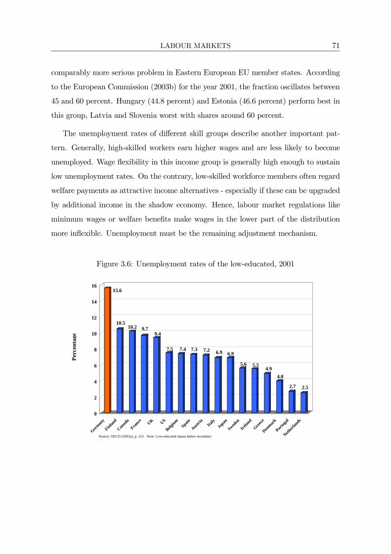
LABOUR MARKETS 71

comparably more serious problem in Eastern European EU member states. According

to the European Commission (2003b) for the year 2001, the fraction oscillates between

45 and 60 percent. Hungary (44.8 percent) and Estonia (46.6 percent) perform best in

this group, Latvia and Slovenia worst with shares around 60 percent.

The unemployment rates of different skill groups describe another important pat-

tern. Generally, high-skilled workers earn higher wages and are less likely to become

unemployed. Wage flexibility in this income group is generally high enough to sustain

low unemployment rates. On the contrary, low-skilled workforce members often regard

welfare payments as attractive income alternatives - especially if these can be upgraded

by additional income in the shadow economy. Hence, labour market regulations like

minimum wages or welfare benefits make wages in the lower part of the distribution

more inflexible. Unemployment must be the remaining adjustment mechanism.

Figure 3.6: Unemployment rates of the low-educated, 2001

15.6

10.510.2 9.7

9.4

7.5 7.4 7.3 7.2 6.9 6.9

5.6 5.54.9

4.0

2.7 2.5

0

2

4

6

8

10

12

14

16

German

y

Finland

Canad

a

France UK US

Belgium

Spain

Austria

Italy

Japan

Sweden

Irelan

d

Greece

Denmar

k

Portuga

l

Netherl

ands

Perc

enta

ge

Source: OECD (2003a), p. 151. Note: Low-educated means below secondary d ti

72 LABOUR MARKETS

In fact, there are fundamental differences in the unemployment rates of low-skilled

workers across countries. Figure 3.6 proxies the group of low-skilled by all workers who

possess less than a secondary education. It turns out that Germany has an exception-

ally high unemployment rate of this skill group in international comparison. While 15.6

percent of the low-educated were unemployed in Germany in 2001, the second worst

performer was Finland with 10.5 percent. France and the UK reached 9.7 and 9.4

percent respectively. Portugal (2.7 percent) and the Netherlands (2.5 percent) literally

have no problem in this regard. What is not shown in the figure, unemployment rates

of workers with a secondary education or higher, do not show such a clear difference

across countries.45

Germany seems to have an extraordinarily large low-skilled unemployment problem.

The rising trend of total unemployment over the last 35 years is clearly mirrored in

the development of low-skilled unemployment. In 1983, the total unemployment rate

was announced at 7.6 percent, the same figure as in 1988 and in 2000.46 However, the

unemployment rate of the low-educated was 13.3, 16.4 and 19.4 percent respectively.

3.3.3 Hours worked, paid leave and strikes

In 2003, the range of hours worked per year varied from 1,938 hours in Greece to

1,337 hours in Norway.47 This means, that on average, a Greek employee worked 45

percent more than his Norwegian colleague. Spain, Canada, the US and the UK range

between 1,800 and 1,673 hours per year. Denmark (1,475 hours), France (1,453 hours),

Germany (1,446 hours) and the Netherlands (1,354 hours) constitute the group with

the lowest annualy working time.48

The Dutch employees also belong to the privileged with regard to paid leave. Their

employers pay 31.3 days on average per year. Only the Swedes can take more days

45OECD (2003a), p. 151.46According to the definition of the Bundesagentur für Arbeit.47OECD (2004a).48OECD (2004a). See also EIRO (2004b). Althoutgh the figures are different, the ranking basically

remains the same.

LABOUR MARKETS 73

off, namely 33 per year. Germany follows with 29.1 days and Italy with 28. On the

contrary, people in Eastern European countries mostly do not get more than 20 days

per year.49

A clear trend that has evolved over the years is that negotiations of social partners

have become more constructive. Compromises were found more often than in earlier

years, thus reducing working time that fell victim to strikes. In Italy, more than 1,500

days per 1,000 workers were lost due to strikes between 1970 and 1979 whereas this

number shrank to 158 in the 1990s. Spain had the highest loss in the last decade with

276 days. Germany traditionally faced little serious conflicts between employers and

employees. In the 1970s, 52 days were lost whereas only 11 days per 1,000 workers in

the 1990s.50

3.4 Conclusions

Despite the complicacy of institutional comparisons and especially the construction of

rankings, this chapter has provided a clear-cut impression about labour market regu-

lation in various countries. It turned out that strict employment protection legislation

exercises a positive impact on unemployment spells and that generous (unconditional)

welfare benefits and binding minimum wages tend to cause higher unemployment rates,

especially of the low-skilled. It has also become apparent that all governments inter-

vene in the functioning of labour markets - although to different extents. The general

pattern that evolved from the preceding analysis classifies Anglo-Saxon countries as

low-regulated, whereas some continental European economies, typically the larger ones

like Germany or France, have installed extensive and rather strict regulations.

As a consequence, the pattern of labour market outcome differs accordingly. While

the UK and the US experienced a rising trend in earnings inequality, their unem-

ployment rates either remained on a lower level or started to decline. On the other

hand, France and Germany did not exhibit higher inequality of relative earnings (due

49EIRO (2004b).50Institute for the German Economy (2005), p. 143.

74 LABOUR MARKETS

to stronger trade union power and generous welfare entitlements), but show substan-

tially higher unemployment rates. In the case of Germany, unemployment has been

increasing from literally zero in 1970 to about five million in 2006.

However, there is a third pattern combining generous welfare payments with decent

labour market performance. In Denmark, for instance, dismissal rules have literally

been abolished and (rather generous) unemployment benefits are only granted under

the condition of active job seeking and training. Otherwise, recipients’ benefits can be

curtailed. As a result, Denmark reduced its unemployment rate substantially from the

mid-1990s to date. The Netherlands or Sweden constitute other examples.

Although only little data is available for Eastern Europe and institutions have been

subject to fundamental changes in recent years, labour market regulations rather fit

into the Anglo-Saxon category. Except for Poland and Slovakia, that still exhibit

unemployment rates above 15 percent, all Eastern European EU member states have

brought down unemployment to one digit figures.

The two previous chapters have provided evidence twofold: Firstly, globalisation

forces have gathered strength in recent years. And secondly, labour markets in some

countries, especially in larger contintal European ones, do not seem to be flexible

enough to absorb the emerging adjustment pressure. This delivers a sound foundation

to study the implications of globalisation when labour markets are rigid. The next

chapter marks the beginning of the theoretical analysis.

Chapter 4

Factor mobility with rigid wages -

a simple model

This chapter delivers a first theoretical step to approach this book’s topic. We set up

a simple MacDougall-Kemp model to gain insights into the mechanism of market inte-

gration with imperfect labour markets. Apart from trade, factor mobility is one of the

fundamental channels through which market integration takes place. Theoretical mod-

els suggest that free movement of production factors exhibits factor price equalisation

in a constant returns to scale framework as capital-labour ratios converge. Concerning

the evaluation of this process, most studies point out that market integration promises

welfare gains because integrated factor markets ensure a more efficient allocation.1

However, this result only holds under the condition of perfect factor markets. With

regard to labour marktes, though, this might not be true.

Although some would object that factor price equalisation is no more than a theo-

retical construct and turned out to be inconsistent with empirical observations, there

is substantial evidence that convergence is a real world phenomenon. It is no surprise

that factor price equalisation cannot be observed because transport or migration costs

prevent this, even in theory. What matters here, is that convergence takes place. Ac-

cording to Barro and Sala-i-Martin (1991, 1992), not only per-capita income, but also

1See, for instance, Obstfeld (1998).

76 FACTOR MOBILITY WITH RIGID WAGES

capital-labour ratios have been converging over time - although at a very slow pace.

For 16 OECD countries, Wolff (1991) also finds evidence for an assimilation of capital

intensities in the long run. Furthermore, the monetary integration of Europe provides

a good recent example for the convergence of interest rates. Of course, a large fraction

of this development must be attributed to the decline in exchange rate uncertainty

and risk-premia, but capital allocation certainly improved as a consequence. Due to

higher returns, labour intensive countries in the euro area received relatively more in-

vestment than capital intensive economies. Thereby, the common currency enhanced

the convergence of capital-labour ratios.

Becker et al. (2004) provide evidence for labour market implications of capital

mobility. Using the FDI database of the German Bundesbank, they find that German

and Eastern European manufacturing workers are substitutes, and that a wage increase

in Germany has a positive effect on the creation of jobs in Eastern European countries,

and vice versa.

While capital mobility is very pronounced, migration flows do not compare. The

empirical literature on the impact of immigration on national wages generally only finds

small effects. LaLonde and Topel (1991) and Borjas (1994) conclude that there is little

evidence for strong adverse effects on national labour markets. According to Friedberg

and Hunt (1995), most studies reason that a 10 percent increase in the fraction of

immigrants in the population reduces wages by only one percent. Even migration

shocks like the exodus of 125,000 Cubans between April and September 1980 to Miami

(Card 1990), or the return of 900,000 French after Algerian independence in 1962 (Hunt

1992), did not affect labour market outcome markedly.

Despite the small effects, the empirical literature has detected winners and losers

of immigration. When disaggregating the workforce into different skill-levels, Borjas

et al. (1997) show that lower educated workers are affected most. In his study for

the US labour market, Jaeger (1996) finds that the high-skilled benefit from immigra-

tion, whereas the low-skilled have to accept a decline in wages. The work of DeNew

and Zimmermann (1994), who show positive income effects for white collar workers

FACTOR MOBILITY WITH RIGID WAGES 77

and the opposite effect for blue collar workers, heads in the same direction. Akbari

and DeVoretz (1992) find similar results for labour-intensive industries in Canada. It

generally turns out that the data confirms complementarity of labour and capital, or

between different skill-levels, whereas immigrants and (low-skilled) workers seem to be

substitutes. Although most studies attribute only little impact of migration on the

convergence of wages, Borjas (1994) points out that econometric studies are afflicted

with many problems. Hence, the results should be interpreted cautiously.

The model we employ describes two countries producing one good under constant

returns to scale with the inputs capital and labour. We assume both jurisdictions to be

of equal size (in terms of workforce), but one country possesses more capital than the

other and downwardly rigid wages. Apart from this, other factor and especially goods

markets are perfectly competitive. The reason for rigid wages might either be due to

a statutory minimum or to welfare payments that determine a reservation wage. For

simplicity reasons, we stick to the former motivation to avoid explicit modeling of the

welfare state. In addition, we assume that both countries’ labour markets are cleared

in autarky. Despite the simplicity of the approach, later chapters prove that the results

also hold in more complex settings.

We show that unemployment emerges as a residual adjustment mechanism and

national output declines if wages are prevented from downward adjustment in the

capital abundant country. Capital movements are pathologically higher than with

flexible wages, implying an inefficient capital allocation. It also turns out that the

welfare loss is borne by workers in the rigid wage country alone. This is ironic, as the

minimum wage was installed to protect this group from low-wage competition in the

first place. It would thus be preferable for this economy to allow less factor mobility.

Workers in the foreign economy, however, benefit by excessive capital imports that

boost their labour productivity. If in addition to rigid wages a distorting capital tax

is implemented in the rigid wage country, unemployment increases further and so do

welfare losses. Identical results can be achieved by labour migration. Then, excessive

migration from the labour-abundant (low-wage) country to the high-wage region takes

78 FACTOR MOBILITY WITH RIGID WAGES

place. Equilibrium unemployment and wage rates are identical to the first scenario.

However, a tax on domestic labour only leads to distributive effects because workers

have no incentive to avoid the tax by emigrating as long as the net wage is higher

than abroad. The bottom line of this chapter is that it is not advisable to work

against market forces. Wage rigidities should be abolished to achieve a first-best market

outcome. For distributive reasons, other policies like a wage subsidy system can better

ensure lower earnings dispersion.

The outline of the chapter is as follows. The next section introduces the model.

Then, the basic autarky situation is presented, as well as the results of factor mobility

with flexible wages. This scenario should serve as the reference for later extensions

with rigid wages. Section 4.4 introduces minimum wages and studies their impact in

the presence of capital and labour mobility. Furthermore, the effects of basic tax in-

struments are analysed. Section 4.5 concludes and briefly discusses policy implications.

4.1 The model

The model depicts two economies, home (H) and foreign (F ), that produce one homo-

geneous good with the inputs capital (K) and labour (L). A one good model allows us

to suppress relative price changes and focus on the impact of factor mobility on factor

prices only. Thus, we set the commodity price to unity in both jurisdictions. A devi-

ation from this price is prevented by means of potential arbitrage. The two countries

differ in terms of their relative factor endowments ki = Ki/Li with i ∈ {H,F}. We

assume home to be relatively more abundantly endowed with capital, so kH > kF . As a

first step, both regions are supposed to be symmetric with regard to their labour force.

The implications of relaxing this assumption will be discussed later in this chapter.

Capital can be interpreted as both real and human capital. Both countries possess

the same constant returns to scale technology that can be described by a neoclassi-

cal production function with the usual properties. Output in country i is denoted by

f i (Ki, Li) = Y i. Marginal products are positive, but rise with diminishing rates, so

FACTOR MOBILITY WITH RIGID WAGES 79

fK > 0, fL > 0 and fKK < 0, fLL < 0. As it turns out, the crucial property in this

setup is the complementary relationship between capital and labour which is formally

depicted by fKL > 0 and fLK > 0. In addition, firms act under perfect competition,

thus making zero profits and paying factors their marginal product. Constant returns

to scale technology enables us to express factor prices as functions of capital-labour

ratios alone:

wi = λ(ki) with λ0 > 0 (4.1)

ri = μ¡ki¢

with μ0 < 0. (4.2)

Eqs. (4.1) and (4.2) show that a higher capital-labour ratio makes workers more

productive and enables firms to pay higher wages. The opposite is true for capital.

From the relative endowments in the respective countries we can then derive factor

prices directly. As kH > kF , we know that wH > wF and rH < rF .

The relationship between endowments and factor prices can be nicely illustrated

by means of the Lerner diagram in Figure 4.1. With capital and labour on the axes,

pf i (Ki, Li) = 1 describes the unit value isoquant, that is the geometrical location

where the value of output equals unity for different capital-labour ratios. As we have

normalised the commodity price to unity, the unit value isoquant describes all combi-

nations of capital and labour that produce one unit of output. In order to determine

factor prices, we need to introduce the unit cost line. Each firm has the following unit

cost function

C = wL+ rK = 1.

Solving for K yields

K =1

r− w

rL.

If costs for one unit (value) of output are unity firms make zero profits. Hence, the

tangency point between the unit value isoquant and the unit cost function determines

the equilibrium. In Figure 4.1, E marks the endowment point and thereby the capital-

labour ratio. This ratio is constant along the ray SA. The unit cost line that is tangent

80 FACTOR MOBILITY WITH RIGID WAGES

to the unit value isoquant is denoted by CA. There must be unique values of w and r

to ensure zero profits. They can be read from the intersections with the axes as the

inverse. The slope expresses the factor price ratio w/r.

Figure 4.1: Endowments and factor prices

Br1

Ar1

Bw1

Aw1

1),( =LKpf

B

BS

AS

O

KE

LEBC

AC

L

K

E

A

How does a change in endowments impact factor prices? As long as endowments

change without altering the ratio, factor prices do not change. This would be indicated

by a movement from E along the ray SA. If, however, either the labour force or the

capital stock change, zero profits are no longer ensured at given factor prices. Figure

4.1 depicts two examples, an increase in the labour force and a reduction in the capital

stock, indicated by EEL and EEK , respectively. The unit value isoquant and the

original unit cost line are no longer tangent because revenues exceed costs. With

commodity prices normalised to unity, factor prices have to change in order to ensure

zero profits. The unit cost line rotates anti-clockwise to CB until revenues and costs

are equated. In the Lerner diagram, this is ensured in point B. Clearly, the wage rate

has fallen whereas the capital return has increased. As both EL and EK are located

on the same ray SB, labour migration and capital mobility can both bring about the

FACTOR MOBILITY WITH RIGID WAGES 81

same result. Factor prices are identical in EL and EK .

4.2 Autarky

The MacDougall-Kemp model that is graphically displayed in Figure 4.2 permits the

analysis of efficiency and income distribution with respect to both countries. The width

of the box represents the world capital endowment whereof HK is the capital stock of

home, and KF the foreign counterpart. The downward sloping curves represent the

marginal productivity of capital for a given labour input, fHK (LH) for home and fFK(L

F)

for foreign. They are identical and homogeneous of degree zero. As kH > kF we know

that the marginal productivity of capital must be lower in home than in foreign. Thus,

there is an interest rate differential between the two jurisdictions, rH0 < rF0 , indicating

an inefficient allocation.

Figure 4.2: Autarky

)(HH

K Lf

K FK HK F

Fr0

Hr0 )(

FFK Lf

E

C

H

B

FrA

Hr

Home’s GDP can be described by the integral of fHK (LH) between the boundaries H

and K. This is the value of output for given Ki and Li. According to Euler’s Theorem

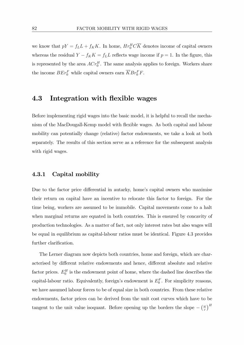
82 FACTOR MOBILITY WITH RIGID WAGES

we know that pY = fLL+ fKK. In home, HrH0 CK denotes income of capital owners

whereas the residual Y − fKK = fLL reflects wage income if p = 1. In the figure, this

is represented by the area ACrH0 . The same analysis applies to foreign. Workers share

the income BErF0 while capital owners earn KBrF0 F .

4.3 Integration with flexible wages

Before implementing rigid wages into the basic model, it is helpful to recall the mecha-

nism of the MacDougall-Kemp model with flexible wages. As both capital and labour

mobility can potentially change (relative) factor endowments, we take a look at both

separately. The results of this section serve as a reference for the subsequent analysis

with rigid wages.

4.3.1 Capital mobility

Due to the factor price differential in autarky, home’s capital owners who maximise

their return on capital have an incentive to relocate this factor to foreign. For the

time being, workers are assumed to be immobile. Capital movements come to a halt

when marginal returns are equated in both countries. This is ensured by concavity of

production technologies. As a matter of fact, not only interest rates but also wages will

be equal in equilibrium as capital-labour ratios must be identical. Figure 4.3 provides

further clarification.

The Lerner diagram now depicts both countries, home and foreign, which are char-

acterised by different relative endowments and hence, different absolute and relative

factor prices. EH0 is the endowment point of home, where the dashed line describes the

capital-labour ratio. Equivalently, foreign’s endowment is EF0 . For simplicity reasons,

we have assumed labour forces to be of equal size in both countries. From these relative

endowments, factor prices can be derived from the unit cost curves which have to be

tangent to the unit value isoquant. Before opening up the borders the slope −¡wr

¢H

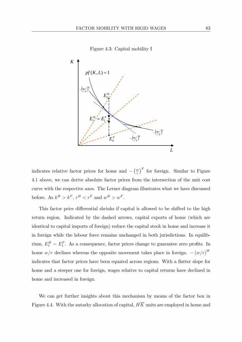
FACTOR MOBILITY WITH RIGID WAGES 83

Figure 4.3: Capital mobility I

1),( =LKpf

FH EE 11 =

FE0( )Wrw−

( )Hrw−

L

K

( )Frw−

HE0

indicates relative factor prices for home and −¡wr

¢Ffor foreign. Similar to Figure

4.1 above, we can derive absolute factor prices from the intersection of the unit cost

curve with the respective axes. The Lerner diagram illustrates what we have discussed

before. As kH > kF , rH < rF and wH > wF .

This factor price differential shrinks if capital is allowed to be shifted to the high

return region. Indicated by the dashed arrows, capital exports of home (which are

identical to capital imports of foreign) reduce the capital stock in home and increase it

in foreign while the labour force remains unchanged in both jurisdictions. In equilib-

rium, EH1 = EF

1 . As a consequence, factor prices change to guarantee zero profits. In

home w/r declines whereas the opposite movement takes place in foreign. − (w/r)W

indicates that factor prices have been equated across regions. With a flatter slope for

home and a steeper one for foreign, wages relative to capital returns have declined in

home and increased in foreign.

We can get further insights about this mechanism by means of the factor box in

Figure 4.4. With the autarky allocation of capital, HK units are employed in home and

84 FACTOR MOBILITY WITH RIGID WAGES

Figure 4.4: Capital mobility II

GHr1 Fr1

'K

D

)(HH

K Lf

K FK HK F

Fr0

Hr0 )(

FFK Lf

E

C

H

B

FrA

Hr

KF units in foreign. Due to the interest rate differential K0K units of capital change

their country of employment, namely from home to foreign. Thereby, capital returns

converge to the common level rH1 = rF1 . What impact does this have on efficiency

and distribution? Output clearly reaches a maximum if marginal productivities are

equated across regions. Both countries are better off if we take aggregated national

output as a measure. In home, output increases from ACKH to ADGKH, whereof

ADrH1 is labour income and rH1 GKH capital income. The increase of DGC entirely

accrues to capital owners who in addition also benefit from a redistribution of factor

returns from labour to capital, namely rH1 DCrH0 . With both capital and labour being

fully employed, wage rates must have fallen.

The same reasoning applies to foreign. Without capital imports, national income

was represented by the area BEFK. The increase in the capital stock makes workers

more productive and boosts national output to DEFKG. Contrary to the capital

exporting country, labour income increases, specifically from BErF0 to DErF1 . Capital

owners, however, lose their exclusive position and face competition from home’s capital.

FACTOR MOBILITY WITH RIGID WAGES 85

Due to less scarcity, capital income shrinks from BrF0 FK to GrF1 FK. The remaining

part DGKK0falls onto capital owners in home who have employed their capital in

foreign now.

The essence of this simple analysis reveals the core implications of globalisation

forces working in the direction of factor price equalisation. With flexible labour mar-

kets, both countries benefit from more efficient factor allocation and thus, higher in-

come. However, there are winners and losers within countries. In home, capital owners

gain as they can employ capital in labour-abundant regions with a higher return.

As this decreases the capital intensity, labour productivity and hence, wages decline.

Workers clearly lose from this process. Nevertheless, the net effect is positive and the

winners can theoretically compensate the losers. The same mechanism takes place in

foreign, just with opposite signs. Here, workers benefit while capital owners lose. There

is also a net output gain in foreign.

4.3.2 Labour mobility

These results can also be achieved in scenario with mobile workers and immobile capital.

Again, we start from a situation where the capital-labour ratio in home is higher than

in foreign, that is rH0 < rF0 and wH0 > wF

0 . Accordingly, home’s endowment point

EH0 is located on the steeper ray relative to EF

0 in Figure 4.5. As a consequence,

foreign workers have an incentive to migrate to the relative capital abundant country

that pays higher wages. This movement is represented by the two dashed arrows in

the diagram. If labour migrates from foreign to home, the labour force declines in

foreign (movement from EHo to EH

1 ) and rises in home (movement from EFo to EF

1 )

simultaneously. Although the absolute amount of capital is higher in home, the relative

factor endowments are equated after migration has taken place. Both endowments are

located on the same dashed ray. The migration incentive of diverging wages has fully

vanished because factor prices are identical in both countries.

With regard to efficiency and distribution, Figure 4.6 facilitates the analysis. As

we focus on labour mobility, it makes sense to picture labour rather than capital on

86 FACTOR MOBILITY WITH RIGID WAGES

Figure 4.5: Labour mobility I

FE1

1),( =LKpf

HE1

FE0( )Wrw−

( )Hrw−

L

K

( )Frw−

HE0

the horizontal axis. Hence, the partial derivatives of the production function are taken

with respect to labour instead of capital. Home is endowed with the amount HL while

there are LF foreign workers. In autarky, wH0 denotes wages in the capital abundant

region while wF0 describes the lower wage level in foreign. GDP in home is made up of

labour income wH0 BLH and capital income ABwH

0 . Equivalently for foreign, workers

receive CwF0 FL whereas capital owners get the residual CEw

F0 .

Allowing for labour mobility sets off migration from foreign to home. Diminishing

returns guarantee a stable equilibrium D with equal wages and equal interest rates

in both regions. According to Figure 4.6, LL0workers cross borders to work in the

capital abundant country. Migration costs are not considered. Migration comes to a

halt when wages are equated, that is if kH1 = kF1 . As a consequence, wages in home are

depressed and workers in foreign are left better off as wages rise. As in the previous

case with capital mobility, both countries benefit on an aggregated level. While output

in home rises to ADL0H, labour income of national workers has declined by wH

0 BGwH1

to wH1 GLH. Immigrant workers earn GDL

0L. Capital owners in home benefit because

their income increases by wH0 BDwH

1 . Foreign workers gain CGwF1 w

F0 while capital

FACTOR MOBILITY WITH RIGID WAGES 87

owners lose CDwF1 w

F0 . Thus, there is a global output gain shown by BDC. The losses

of the losers are smaller than the gains of the winners. Nevertheless, it remains true

that workers in the originally capital abundant country face a deterioration of wages.

Figure 4.6: Labour mobility II

L

G Hw1 Fw1

'L

D

)(HH

L Kf

FL HL F

Fw0

Hw0

)(FF

L Kf

E

C

H

B

FwA

Hw

The result of this section is identical to the previous case with mobile capital and

immobile labour. The relatively scarce factor in each country has to bear the losses

that are outweighed by the gains of the relatively abundant factor. Globalisation has

the potential to increase output in a Kaldor-Hicksian sense. Although there are winners

and losers in each jurisdiction, the winners can potentially compensate the losers and

are still better off. The inherent problem to be solved is how to compensate the losers.

4.4 Integration with rigid wages

One way to protect workers in developed economies from low-wage competition is

to enforce minimum wages. Thereby, the decrease of wages in home, as suggested

by the previous analysis, must not take place. For simplicity reasons, we assume

88 FACTOR MOBILITY WITH RIGID WAGES

that autarky wage levels are identical to this statutory minimum and that, initially,

full employment prevails in both jurisdictions.2 Relaxing these assumptions does not

change the results qualitatively. Only in terms of quantity does more wage flexibility

cause less unemployment, of course.

To make minimum wages and potential equilibrium unemployment plausible, we

assume that the unemployed receive welfare payments in a non-distorting lump-sum

fashion. Thereby, we can abstain from explicit modeling of the welfare state to keep

things as simple as possible.

4.4.1 Endowments, wages and unemployment

The underlying mechanism of this model with rigid wages is the following. Due to con-

stant returns to scale, factor prices can be expressed as a function of the capital-labour

ratio k alone. If home wants to maintain its high wage then the capital-labour ratio

kH must not change. However, as capital exports or labour immigration take place to

benefit from factor price differentials, capital-labour ratios converge. As a consequence,

k can only be kept constant if parts of the labour force become unemployed as long as

capital is always fully employed. Say, if 10 percent of the capital stock relocates, 10

percent of the labour force has to become unemployed to keep kH constant. Figure 4.7

illustrates this relationship for home.3

The left part of the diagram shows the link between the wage rate w and the relative

factor endowment k. The higher the capital intensity (capital per worker) the higher

marginal labour productivity and, due to perfect competition, the higher the wage rate.

Thus, the slope of λ(k) must be negative. The right part illustrates the relationship

between relative endowments and unemployment in home. As we have assumed, home

exhibits full employment of both capital and labour in autarky. Hence, the relative

endowment kH translates into the autarky wage rate wH with zero unemployment. As

foreign is endowed with relatively more labour, home’s capital-labour ratio must decline

2In this setup, the minimum wage is defined in both nominal and real terms as the price isnormalised to unity.

3The idea for this graphical illustration is taken from Davis (1998).

FACTOR MOBILITY WITH RIGID WAGES 89

Figure 4.7: Relation between wages, endowments, and unemployment

flexwHw HU HU w

),,( WWH KLkβ

k

Hk

flexk

)(kλ

in the integration equilibrium if full employment should prevail. This mechanism is

depicted in the left part of the figure. If kH declines to kflex then wages unavoidably

must fall towflex as well. In this case, unemployment would clearly be zero. If, however,

wH is the minimum wage, then the capital-labour ratio aggregated across both regions

must be identical to kH rather than kflex. Only then, home’s firms can still pay wH .

This, however, can only be achieved by unemployment in home.

A numerical example might further illustrate this: Let home be endowed with 1200

units of capital and 1000 units of labour. Foreign possesses 720 units of capital and

also 1000 units of labour. Hence, kH = 1.2, kF = 0.72, and kflex = 0.96. Each of

these endowments imply different wage rates, wH > wflex > wF . If home’s wage rate

should be kept constant, relative (employed) world endowments kW have to be equated

to kH = 1.2 in both countries. Again, this implies that factor prices are equated as

well, but to home’s autarky level.

kW =KH +KF

LH + LF − UH= kH = kF = 1.2

kW =1200 + 720

1000 + 1000− UH= kH = kF = 1.2

90 FACTOR MOBILITY WITH RIGID WAGES

Solving for UH yields

UH = 400.

In this example, 40 percent of the labour force in home has to become unemployed

in order to equate both countries’ relative endowments to the autarky level in the rigid

wage country.

Finally, we take a closer look at the function UH = β(kH , LW , KW ). It states that

unemployment depends on home’s capital-labour ratio, the aggregated global labour

force and the aggregated global capital stock. The more unequal the capital-labour

ratios and the more unequal the factor endowments in absolute terms between both

countries, the higher must be unemployment in home to keep the relative endowment

and the minimum wage rate constant. Thus, β(·) is steep if both differences are rather

small whereas the function must be plotted flatter if home is small and the rest of

the world possesses a substantially lower relative capital endowment. Hence, for small

economies that decide to open their borders for factor flows and that want to defend

their high wages at the same time, the outcome will be catastrophic. A small capital

abundant economy could never defend its wages. In other words, home could never

ensure that kW will be equal to kH as its labour force is simply not large enough.

This underlines the immense pressure on national labour markets with rigid wages and

low-wage competition from abroad.

4.4.2 Capital mobility

The implications of capital mobility with downwards rigid wages for the volume of

capital flows, factor prices and output can be analysed by means of Figure 4.8. Starting

from C and B, which reflect the autarky equilibria in home and foreign, capital shifts

to foreign. This is indicated by the movement from K to the left on the horizontal

axis. In order to keep wages constant, kH must stay the same and hence, marginal

productivity of capital. As capital owners cannot be forced to employ their capital in

home, 1/kH workers become unemployed for every unit of capital exports in order to

FACTOR MOBILITY WITH RIGID WAGES 91

keep kH constant. Unemployment can be read off from the diagram indirectly. The

marginal productivity curves of capital are plotted for constant labour input. This,

however, cannot be maintained and thus, leads to a downwards shift of fHK . For every

unit of capital less labour is employed, thereby reducing the marginal productivity of

capital. fHK shifts in until there is an intersection of both marginal productivity curves

at rH0 . D0 rather than D denotes the new equilibrium.

Figure 4.8: Capital mobility with rigid wages

G ''D

'A

Fr2 'D

''K

)( HHHK ULf −

)(FF

K Lf

Hr1 Fr1

'K

D

)(HH

K Lf

K FK HK F

Fr0

Hr0

E

C

H

B

FrA Hr

As the diagram reveals, capital returns have been equated to a global level rH0 = rF2 .

From this fact we know that kH = kF and hence, wH = wF . Despite unemployment

in home, there is still factor price equalisation. However, unemployment increases the

equilibrium wage rate and decreases the equilibrium capital return. Figure 4.8 also

reveals that capital flows are higher than in the reference situation with flexible wages.

Unemployment in home prevents the marginal productivity of capital from increasing

and thus, drives more capital out of the country. This must be true as for the allocation

K0a positive capital return differential remains between both jurisdictions. Hence, the

convergence process is extended artificially. Result 4.1 summarises the main insights.

92 FACTOR MOBILITY WITH RIGID WAGES

Result 4.1 The volume of capital exports to the labour abundant country will be

higher with rigid wages relative to a flexible wage scenario in order to achieve a global

capital-labour ratio that is equal to home’s relative autarky endowment. This ensures

factor price equalisation at home’s autarky level.

With regard to output, there are no longer gains for both countries. Compared to

the flexible wage equilibrium, world GDP is lower by ADD0A0. Home gets A0D0CKH

whereof A0D0rH0 accrues to workers who have not lost their job. Capital owners earn

rH0 CKH - composed of rH0 D0K

00H in home and D0CKK

00in foreign. Foreign’s income

can be described by the area D0EFKC. Workers receive D0ErF2 while capital owners

get CrF2 FK. Taking the integrated equilibrium with flexible wages as a benchmark,

efficiency has clearly deteriorated due to the market imperfection in home. Compared

to autarky, though, the picture seems to be ambiguous from this depiction. BCD could

be gained whereas ADD0A0 is lost. However, we know that the rigid wage country

marginally loses with every unit of capital being relocated. Recall that unemployment

makes sure that factor prices remain constant. Hence, home’s income also declines with

regard to autarky. Thus, a closed economy guarantees higher income than a scenario

with international capital mobility and rigid wages.

Workers in foreign are the only group that benefits from home’s wage rigidity. Other

groups either lose or do not gain. Intuitively, pathologically too high capital imports

boost labour productivity and thus allow firms to pay higher wages. Foreign capital

owners, though, face a deterioration of their capital return because more capital is

employed in the economy. In home, capital owners are equally well off as in autarky,

but worse off than with flexible wages. Now, they only receive the autarky return

rH0 rather than rH1 . The main losers of the process - and this is the ironic part of

the story - are workers in home who were supposed to be protected against the forces

of globalisation as they bear the entire output loss themselves. Compared to flexible

wages, home’s output loss (AD0GCD0A0) is even higher than the aggregated output

loss (ADD0A0) because foreign benefits from the other country’s wage rigidity on a net

basis (D0DC 0C). Result 4.2 summarises.

FACTOR MOBILITY WITH RIGID WAGES 93

Result 4.2 Capital mobility produces output losses if wages are rigid. This happens

via an increase in unemployment. For the capital abundant country, autarky implies a

higher output level than capital market integration. Foreign benefits from home’s wage

rigidity in terms of higher income. Compared to autarky, workers in home who should

be protected from the forces of globalisation by downwards rigid wages bear the entire

output loss themselves through unemployment.

Tax instruments

While lump-sum taxation is always an unproblematic instrument, as it does not

distort efficiency, it is also very unrealistic. In fact, distorting taxes play a more

important role in reality. Therefore, we study the impact of both a distorting capital

and labour tax in the presence of rigid wages and capital mobility.

Capital tax The government decides to implement a capital tax τ . For simplicity

reasons, let us start in the integration equilibrium D0. The unit tax is represented by

the distance TT 0 in Figure 4.9 and drives a wedge between the interest rate and the

marginal return of capital. Thus, there is an unavoidable output loss if elasticities are

larger than zero. Capital now has to earn the interest rate plus the tax rate. The new

equilibrium condition is fHK − τ = fFK . As the net return in foreign is initially higher

than in home, capital will relocate from home to foreign until the net marginal returns

are identical in both regions again. This is indicated by the movement from K00to

K000. The market interest rate has fallen to rH2 in both jurisdictions. r

H2 + τ represents

the gross interest rate in home. The question arises, however, whether this is a stable

equilibrium. With flexible wages relative toD0, this would certainly be the case. T 0D0T

would describe the additional output loss and the relocation implies a shift of the tax

burden onto labour. The capital-labour ratio falls and so do wages. The latter, however,

cannot take place if wages must not fall below their statutory minimum. In order to

prevent the marginal productivity of labour - and thus wages - from falling, (more)

unemployment emerges. The marginal productivity curve of capital shifts in further.

Hence, the increase in unemployment as a reaction to capital exports prevents marginal

94 FACTOR MOBILITY WITH RIGID WAGES

productivity of capital from increasing - just as in the transition from autarky to free

capital mobility. The incentive for capital to flee the country that has introduced a tax

is kept upright until the last unit of capital has left the region. Equilibrium is depicted

by the corner solution D000.

Figure 4.9: Capital tax with capital mobility and rigid wages

'''D

'''K

τ+Hr2

Hr2

Hr0

'T

T

'A

Fr2'D

''K

)( HHHK ULf −

)(FF

K Lf

FK HK F

E

H

FrHr

As a result, home’s income has receded to zero whereas foreign’s labour force ben-

efits from the excessive inflow of capital boosting its productivity. In the new equilib-

rium, the world interest rate (which is equal to the national interest rate in foreign) has

settled down to the level D000. Hence, capital income is earned in foreign only. Foreign

workers benefit further due to even more capital imports.

Proposition 4.1 If real wages are downwards rigid, a distorting capital tax drives

the entire capital stock out of the country. Unemployment in home reaches 100 percent

and income collapses to zero.

Proof. See Appendix 4.A.

Of course, this corner solution is far from being a true picture of reality. How-

FACTOR MOBILITY WITH RIGID WAGES 95

ever, it impressively illustrates the detrimental impact of rigid wages if distorting tax

instruments are in place.

Labour tax What are the implications if the government imposes a tax on wages?

The key is whether the net or the gross wage are subject to the minimum. If the gross

wage should be kept constant and workers bear the tax burden through lower disposable

incomes, there will be no further effect on marginal productivities. The capital-labour

ratio remains constant, that is the capital return does not change either. However, the

entire burden is carried by workers who earn a lower net income. There will be no

(further) unemployment because wages can be regarded as ”flexible”.

However, if the minimum wage fixes disposable income (or trade unions want the

gross wage to increase by τ), the story is different. Marginal productivity of labour

has to rise as the tax has to be earned additionally. Therefore, a higher capital-labour

ratio must be achieved. As foreign capital does not have an incentive to relocate to

home (because of equal marginal returns in both regions), some workers have to be

pushed out of employment in the rigid wage country. The increase in marginal labour

productivity, however, goes along with a decrease in marginal capital productivity

because additional unemployment generates a downwards pressure on the interest rate

in home. This creates an incentive for capital to move from home to foreign to maximise

capital income. The same vicious circle as in the previous section has been set-off now

if the higher gross wage rate is defended in home. The entire labour force is obliged

to become unemployed. In this case, capital is driven out of the country indirectly,

but also entirely. The tax on labour now yields unemployment as a first step which

then leads to lower marginal returns of capital and hence, capital exports. The indirect

channel is due to the immobility of labour.

Proposition 4.2 With capital mobility and a unit tax on wages, unemployment

only arises if net wages are downwards rigid. In this case, the same equilibrium arises

as with a distorting capital tax. If only gross wages matter, then workers face a dete-

rioration of their disposable income, but no (additional) unemployment occurs.

96 FACTOR MOBILITY WITH RIGID WAGES

Proof. See Appendix 4.B.

Intuitively, a distorting tax, whether on labour or on capital, forces workers to bear

at least a part of the burden. This burden implies lower (net) wages. Thus, if labour

refuses to bear this burden, unemployment evolves and leads to a corner solution. The

bottom line is that workers have no choice but to bear the burden: either through a

decline of wages or through unemployment. Also a welfare state cannot cushion this

effect if only distorting taxes are available.

4.4.3 Labour mobility

Now we turn to the impact of downwards rigid wages if labour is the only mobile

factor. Again, we employ the graphical illustration of the MacDougall-Kemp model

as shown in Figure 4.10. Contrary to the previous section, the aggregated labour

endowment rather than the aggregated capital stock is depicted on the horizontal axis.

The downward sloping curves illustrate the marginal productivity of labour in both

home and foreign. In equilibrium, this must be equal to the wage rate which can be

read off the vertical axes. Again, the initial capital-labour ratio in home exceeds the

equivalent ratio in foreign. Consequently, wH > wF provides an incentive for workers

in foreign to migrate to the high wage region. For simplicity reasons, migration costs

are not considered as they only reduce the volume of migration, but do not change the

basic results qualitatively.

Recall that, in autarky, L describes the allocation of labour, that is HL workers are

employed in home and LF workers in foreign. At a given capital stock in the respective

country, wages reach the level wH0 in home and wF

0 in foreign. LL0workers would

immigrate into home if wages were flexible. Apart from redistribution of factor income,

this would yield an output gain of BDC. With rigid wages, the capital-labour ratio

must be identical in both home’s autarky and the integration equilibrium. However,

immigration creates a downwards pressure on kH and an upwards pressure on kF

with the discussed implications for factor prices. Hence, for every immigrant in home,

one worker needs to become unemployed if we assume that immigrants get a job and

FACTOR MOBILITY WITH RIGID WAGES 97

citizens of home are entitled to receive some kind of compensation benefits.4 Moreover,

excessive migration results because factor prices are equated to home’s autarky level.

Thereby, the migration incentive is kept upright for more foreign workers as wages

do not decline in the target region. This, however, can only be achieved through

unemployment.

Figure 4.10: Labour migration with rigid wages

Fw2'D

''LL

G Hw1 Fw1

'L

D

)(HH

L Kf

FL HL F

Fw0

Hw0

)(FF

L Kf

E

C

H

B

FwA

Hw

These results can also be retraced from Figure 4.10. The foreign wage level only

rises to wH0 = wF

2 , if LL00workers emigrate - this is an excessive migration of L

0L00.

Foreign would move along fFL (KF) from C to D0. Integration equilibrium is denoted

by B and D0 respectively. LL00workers are unemployed which exactly matches the

number of migrants. With regard to welfare relative to the flexible wage integration

equilibrium, world GDP is lower by the area BDD0L00L, which under the model as-

sumption resembles the welfare loss. Now, also the diagram unambiguously reveals that

aggregated GDP is lower than in autarky, namely by CD0L00L. GDP remains the same

in home, but with a higher labour force after immigration. This implies a lower output

4See Sinn (2004) for a similar analysis.

98 FACTOR MOBILITY WITH RIGID WAGES

per capita. If we assume that all migrants find a job in the target region, per capita

income for foreigners has increased as they earn higher wages. This increase clearly

outweighs the reduction in capital returns.5 For citizens in home, income declines if

people are crowded out of the labour market. The following result summarises the

main findings of this part.

Result 4.3 With labour mobility, rigid wages in the capital abundant country yield

excessive migration. It is pathological because per capita output is lower than in both

autarky and the integrated equilibrium with flexible wages. If we assume migrants to

certainly find a job in home, the output loss only has to be borne by workers in home.

It is not surprising that the result resembles the one with capital mobility because

both mechanisms work in the direction of factor price equalisation. If national wages

are defended, the same amount of unemployment and the same output loss occur.

Tax instruments

Similar to the previous section, we also study the implications of distorting tax

instruments when labour is the only mobile factor and wages in home must not fall.

Both a capital and a labour tax are considered successively.

Capital tax A unit tax on capital reduces its net return by the tax rate τ . How-

ever, as capital is assumed to be immobile in this scenario, the tax burden cannot be

shifted onto labour. Hence, capital-labour ratios remain constant and so do marginal

productivities and wages. Therefore, a capital tax does not further derogate efficiency.

Income can be redistributed from capital owners to unemployed workers. As the wage

differential is unaffected, the same immigration can be expected as without a tax.

5This fact is unambiguously clear from the analysis in the previous section.

FACTOR MOBILITY WITH RIGID WAGES 99

Labour tax If the tax is levied on workers and if gross wages in home should remain

constant, the migration incentive decreases as the net wage shrinks by τ . Hence, the

tax works as an instrument to reduce excess migration. In the extreme case of a tax

that resembles the wage differential, τ = wH0 − wF

0 , no migration will take place and

net wages are equated in both economies. Unemployment benefits that are financed

by employees can persist. However, the average disposable income per capita is clearly

lower than with flexible labour markets and migration.

Figure 4.11: Labour tax with labour mobility and rigid wages

T

'T

'''L

τ+Hw0

Fw2'D

''LL

G Hw1 Fw1

'L

D

)(HH

L Kf

FL HL F

Fw0

Hw0

)(FF

L Kf

E

C

H

B

FwA

Hw

If lobby groups want the wage to increase by τ to keep net wages constant, the

capital-labour ratio has to increase to boost marginal productivity of labour. This

situation is depicted in Figure 4.11. As capital is immobile, an increase in the employed

relative factor endowment can only be reached through additional unemployment in

home. Here, it would amount to L000L. This reduces the marginal productivity of

capital that has to bear the entire tax burden. If the gross wage increases by less

than the tax rate, then both capital and labour have to bear a part of the burden.

An additional burden arises through unemployment. This loss of income clearly falls

100 FACTOR MOBILITY WITH RIGID WAGES

onto workers. With ∆wH0 = τ , the migration incentive remains as high as without a

labour tax since the net wage is equal to the gross wage before. Then, unemployment

adds up to LL00, which is the unemployment generated through immigration, plus the

additional unemployment L000L generated by the tax. In this case, tax revenues amount

to¡wH0 + τ

¢TT 0wH

0 . However, there is no corner solution as in the previous case with

capital mobility and capital taxes. Result 4.4 summarises this section’s major findings.

Result 4.4 Capital immobility allows the government to tax this factor and gen-

erate revenues as capital cannot flee the country. With a tax on labour, workers can

even fully shift the tax burden onto capital if wages rise by the tax rate. However, this

comes at the cost of additional unemployment.

4.4.4 Capital and labour mobility

How do the results change if both capital and labour are allowed to be mobile at the

same time? The previous analysis has demonstrated that both capital and labour mo-

bility by itself lead to identical results if distorting taxes are absent. Factor prices, the

rate of unemployment and output losses are exactly the same in both cases. There-

fore, nothing changes if both channels are at work simultaneously. Only under the

assumption that the convergence process consumes a certain amount of time, we can

expect the new integration equilibrium to be achieved faster. This might be bad news

for politicians who rather need more than less time to carry out economic reforms to

adjust to exogenous globalisation shocks.

With regard to the two distorting tax instruments discussed above, what can be

concluded if both capital and labour are mobile simultaneously? With capital mobility,

a tax on this factor would clearly yield a corner solution with the entire world capital

stock being employed in foreign. This, of course, would not change if we additionally

allowed for migration. Labour taxes alone are also capable of generating a corner

solution, but only if gross wages were explicitly increased - at least by an epsilon -

to compensate for the loss in disposable income. With fixed gross wages, though, an

FACTOR MOBILITY WITH RIGID WAGES 101

interior solution would prevail. Allowing for labour migration in addition would not

change the outcome as factor prices are already equated.

4.5 Conclusions and policy implications

The bottom line of this chapter is that a capital abundant country cannot defend its

high wages against low-wage competition without substantial output losses. Lower

wages might be necessary for full employment because capital exports or immigration

reduce the marginal productivity of labour. On the other side, the low-wage economy

benefits from the rigid wages in the other region through higher income. It also turned

out that the output loss of the capital abundant country outweighs the additional

output gain of the labour abundant economy. Ironically, workers who should have

been protected from low-wage competition by a statutory minimum must bear these

losses themselves by means of unemployment. Distorting taxes even make the situation

worse by generating further income reductions.

Of course, the simple model partly exhibits extreme results that cannot be regarded

as a true picture of reality. For instance, several obstacles to factor mobility like

technological, political or also cultural barriers prevent full equalisation of factor prices.

Hence, corner solutions that claim relocation of the entire capital stock will never

be observed in the real world. Nevertheless, this model allowed basic insights which

cannot be argued away by the preceding points. Although factor prices do not equate,

globalisation of national markets improve factor allocation and must, as a consequence,

lead to a convergence of factor prices - at least to some extent. However, if rigid

labour markets prevent wages from adjusting to the market clearing level, that is if

market integration causes unemployment, the rigid wage economy loses also on the

margin. This country would clearly be better off without international transactions.

Every factor unit that crosses the border implies a net loss for the rigid wage country.

Obstacles to factor mobility just reduce the overall output loss.

Yet, another critique may point to the fact that minimumwages are binding only for

102 FACTOR MOBILITY WITH RIGID WAGES

a small fraction of the labour force (the low-skilled) while workers with more skills earn

market wages well above the statutory minimum. Then, the results only change quan-

titatively. The higher wage flexibility or the fewer workers affected by the minimum,

the lower unemployment and output losses in equilibrium. Nevertheless, it remains

true that a country can only defend its high wage level at the cost of becoming a net

loser from market integration. The costs are higher with increasing dissimilarity be-

tween the integrating countries in terms of relative factor endowments and size. In the

absence of frictions to factor mobility, a small country can by no means defend its high

wages because its workforce is not large enough to equate relative world endowments

to relative autarky endowments. This nicely illustrates the pressure of global market

forces.

What policy recommendations can we infer from these results? There are basically

two directions. As factor mobility reduces output in the presence of rigid wages, pro-

tection of national markets at least reduces output losses and can potentially ensure

full employement. However, potential gains from an improved allocation of production

factors would be foregone. A second direction addresses the root of the problem - the

labour market rigidity. In order to gain from globalisation, it is unavoidable to let

market forces install an efficient allocation. However, this necessarily implies a more

unequal income distribution as especially (low-skilled) workers in developed countries

face wage cuts. Only distributive policies that do not distort the efficient allocation

can be regarded as a promising way out of this trade-off. The dilemma could be solved

in two steps which must be implemented at the same time. Firstly, statutory minimum

wages and unconditional replacement incomes by the welfare state must be abolished.

This ensures an efficient market outcome and gains for all participating countries. Sec-

ondly, in order to avoid social tension due to a more unequal income distribution, a

wage subsidy scheme should prevent impoverishment of large parts of the labour force

by paying wage supplements up to a certain income. Many concepts have been devel-

oped that are all based on this idea. A more detailed discussion is relegated to the

final chapter.

FACTOR MOBILITY WITH RIGID WAGES 103

Appendix

4.A Proof of Proposition 4.1

λ¡kH¢= fHL = wH with λ0

¡kH¢> 0 and μ

¡kH¢= fHK = rH with μ0

¡kH¢< 0

After imposing the tax τ , μ¡kH¢< r + τ = μ (ktax)

Assume that Ltax > 0, then ktax = Ktax

Ltax= KH

LHand hence, μ (ktax) = μ

¡kH¢= r < r+τ

Thus, Ltax = Ktax = 0 in equilibrium.

4.B Proof of Proposition 4.2

After imposing the tax τ , λ¡kH¢< λ (ktax) = wnet = wgross − τ

Assume that Ltax > 0, then ktax =Ktax

Ltax= KH

LHand hence,

λ (ktax) = λ¡kH¢= wnet < wnet + τ

Thus, μ (ktax) < μ¡kF¢implying capital exports and a lower kH .

Hence, Ltax = Ktax = 0 in equilibrium.

Chapter 5

The Heckscher-Ohlin model with

rigid wages∗

A central criticism of the previous chapter’s approach might be that an economy cannot

be properly described by a one-sector model. Therefore, we extend our analysis by a

second sector to study the impact of relative price changes when wages are rigid.

The workhorse model in this area is well known as the Heckscher-Ohlin model. We

study the implications of both trade and factor mobility with respect to efficiency and

distribution.

Although the Heckcher-Ohlin model has played, and is still playing a major role in

the international trade literature, surprisingly little has been written on the impact of

rigid wages in this setup. Nevertheless, Richard Brecher (1974a) already derived basic

insights into the mechanism of the model more than 30 years ago. He showed that

a capital abundant economy would lose from opening up for international trade if a

binding minimum wage was installed. The country would not only lose relative to a

flexible wage scenario with free commodity trade, but also relative to autarky. More

recently, Davis (1998) used these insights to show that European unemployment props

up American wages as both countries are linked via commodity trade. An exogenous

shock caused by the integration of a third region with a lower capital-labour ratio gener-

∗This chapter is based on Sinn and Seidel (2006).

106 THE HECKSCHER-OHLIN MODEL WITH RIGID WAGES

ates downwards pressure on both American and European low-skilled wages. However,

unemployment in Europe keeps world market wages on the previous level. Thereby,

American workers reap the benefits of higher wages, while unemployment only emerges

in Europe. Furthermore, wages can only be kept on their high level in both America

and Europe if unemployment is twice as high as without a trade link to America (given

that both regions are equally large). Oslington (2002) extends the existing analyses for

the empirically important case where factor price equalisation does not hold. Thereby,

he can incorporate the diverging wage and unemployment experiences in Europe and

the US, respectively, in one model. However, the results of Brecher (1974) and Davis

(1998) are only modified quantitatively. Krugman (1995) distinguishes between a Eu-

ropean model where downwardly rigid wages produce unemployment and an American

model where relative wages increase while full employment is sustained. His results re-

semble the ones by Brecher. In discussing Krugman’s (1995) article, Srinivasan (1995)

pointed out that trade flows are higher in a minimum wage-constrained trade equilib-

rium with unemployment. Landmann and Pflüger (1998) mention this outcome of the

model as well.

However, the latter results are derived without discussing their policy implications.

Especially with respect to the German situation, it is worthwhile to put this topic back

on the economic policy agenda. Despite the sluggish economic growth over the last

decade, many participants in the public policy debate point out that the extraordinary

export performance proves Germany’s international competitiveness and its gains from

trade. This chapter’s model puts forward a different perspective. If trade causes

unemployment due to imperfect labour markets, every additional unit of export implies

a welfare loss to the economy instead of a welfare gain!

We also go beyond the current results of the literature by looking at the small

open economy case. This has neither been considered by Srinivasan nor Landmann

and Pflüger. In this respect, we show that there is not necessarily a larger volume of

trade compared to the flexible wage scenario without unemployment. The elasticities

on both the demand and the supply side play a crucial role for the result.

THE HECKSCHER-OHLIN MODEL WITH RIGID WAGES 107

Before getting into the pure theory of international trade, though, we extend the

previous chapter’s model with factor mobility by a second industry. We point out that

a rigid wage economy that is relatively abundantly endowed with capital will export

more of this factor than with flexible labour markets. Alternatively, excess immigration

results if labour mobility is the only linkage between both countries. Consequently, the

rigid wage economy loses from open borders. These results are exactly the ones we

derived in Chapter 4.

The chapter is organised as follows. Next, we extend the analysis of the previous

chapter by studying the implications of factor mobility in a two-sector economy when

wages are downwardly rigid. Section 5.2 then focuses on trade as a substitute to

achieve factor price equalisation. After setting out the basic mechanism, we distinguish

explicitly between a large and a small open economy. Finally, Section 5.3 concludes

and discusses policy measures to meet both efficiency and distribution goals.

5.1 Factor mobility in a two-sector economy

The model resembles our setup in Chapter 4 - the only difference being an additional

sector. Still, both goods are homogeneous and produced under constant returns to scale

with the inputs capital (K) and labour (L). Note that good x is more capital-intensive

than good y, which means that relatively more capital is needed at given factor prices.

Contrary to the previous chapter, relative prices play a central role here. We call p

the relative price of good x in units of good y. One country, home (H), is assumed

to possess relatively more capital than the second country, foreign (F ). However, the

labour force should be of equal size to map two large countries. Formally, this reads

kH > kF with ki = Ki/Li and i ∈ {H,F}. Again, both regions are characterised

by identical preferences and technology. The latter can be described by a neoclassical

production function with the usual properties. Marginal products are positive, but rise

with diminishing rates, so fK > 0, fL > 0 and fKK < 0, fLL < 0. Due to constant

returns to scale, factor prices are determined by relative factor inputs. As kH > kF ,

108 THE HECKSCHER-OHLIN MODEL WITH RIGID WAGES

we know that wH > wF and rH < rF . As in the previous chapter, we abstain from

costs of factor mobility.

In a first step, let us assume labour markets to be flexible. As capital yields a higher

return abroad, domestic capital will be exported. Thereby, capital-labour ratios and

thus, both capital and labour remuneration converge in both countries. The conver-

gence in relative endowments also leads to an equalisation of relative commodity prices.

This comes about as home’s opportunity costs of producing the capital intensive good

increase. The opposite is true for foreign. Hence, px rises whereas py falls in home

and vice versa in foreign until³pxpy

´H=³pxpy

´F. An efficient allocation of factors, that

yields the maximum achievable output level, is reached when marginal returns in both

sectors are equated. This is achieved by means of capital exports.

What happens if domestic wage rates are downwardly rigid?1 As in the previous

chapter, relative factor endowments must not change in order to prevent a modifica-

tion of the wage rate and the capital return in home. Accordingly, relative prices that

are determined via marginal productivities stay the same. Hence, it does not make

a difference how the wage floor is defined — either in nominal terms or in real terms

as in units of the labour intensive good y or the capital intensive good x. Figure 5.1

depicts the situation of the capital abundant country. In autarky, we start from a

pareto-efficient general equilibrium where the marginal rate of substitution equals the

marginal rate of transformation, denoted by B. Capital exports to the labour abun-

dant region shifts in the production possibilities frontier. With full employment, the

capital-labour ratio declines so that the economy is able to produce relatively more of

the labour intensive commodity compared to autarky. In other words, the production

possibilities frontier shifts in more with respect to good x than with respect to good

y. With rigid wages, however, one unit of capital being exported forces 1/kH units of

labour to become unemployed in order to keep the capital-labour ratio constant. Oth-

erwise, wages would decline. The same numerical example as in the previous chapter

applies here. Recall that home was endowed with 1200 units of capital and 1000 units

1See also Brecher (1971).

THE HECKSCHER-OHLIN MODEL WITH RIGID WAGES 109

of labour. Foreign possessed 720 units of capital and also 1000 units of labour. Hence,

kH = 1.2, kF = 0.72, and kflex = 0.96. In order to keep home’s wages constant, relative

(employed) world endowments kW had to be equated to kH = 1.2 in both countries.

Unemployment amounted to 400 workers to reach a stable equilibrium. Graphically,

this translates into an inwards shifting of the production possibilities frontier as indi-

cated in Figure 5.1. It shifts in proportionately with regard to both goods. The new

equilibrium is described by C on the new production possibilities frontier which has

to be located on the ray from the origin that fixes the share and thereby the relative

price of both goods.

Figure 5.1: Factor mobility with rigid wages in a two sector model

)( autpϕ

paut

paut

B

E’

A’

H

C

E x

A

y

Assuming labour to be the only mobile factor, opening up the borders would not

change the equilibrium point A in home. However, the higher wage for workers in

the capital abundant economy attracts foreign workers and causes immigration. In

order to keep relative factor endowments constant, one domestic worker has to become

unemployed for every immigrant. The new open economy equilibrium settles when

relative factor endowments are equated - either by means of capital mobility or labour

110 THE HECKSCHER-OHLIN MODEL WITH RIGID WAGES

migration. Accordingly, relative goods and factor prices must be identical as well.

Contrary to the flexible wage scenario world market prices for goods and factors are

now equated on home’s autarky level. This implies that wages in foreign have increased

to a higher level than they would have with flexible wages in home. The only reason

why this could be achieved is by means of higher capital imports in order to increase

the capital endowment per worker to home’s autarky level. Concerning output, the

story resembles again the previous one in Chapter 4. Unemployment must emerge as

the remaining adjustment mechanism in order to keep wages at their high level. With

less factors of production being employed at the same costs, total output must have

fallen by the number of unemployed times the wage rate. From a welfare perspective,

this is clearly inferior to both autarky and the open economy equilibrium with rigid

wages.

Result 5.1: In a model with two goods, factor mobility exhibits the same outcome

as in a model with only one good. The levels of unemployment, output and factor

movements do not alter.

Finally, let us relax the assumption that both countries are of equal size. Only

in that case, the capital abundant economy is capable of equalising the relative world

factor endowment to its autarky level. A small open economy simply does not have

enough workers that could become unemployed. Even with 100 percent unemployment,

the relative world capital-labour ratio is lower than home’s autarky ratio. We can

conclude that the results of the simple model in Chapter 3 also hold in a two sector

setting. There is unemployment to maintain high domestic wages, the same amount

of excessive capital flight and an output loss relative to both a flexible wage scenario

and autarky.

THE HECKSCHER-OHLIN MODEL WITH RIGID WAGES 111

5.2 The pathological trade boom

Let us now switch to the pure theory of international trade. The standard Heckscher-

Ohlin model predicts that a capital abundant country will experience a decline in

real wages and a rise in real capital returns if it starts trade relations with a labour

abundant economy. This is due to a decrease in the relative price of the labour intensive

commodity. The link between factor and goods prices is well-known as the Stolper-

Samuelson theorem. This is the key to understand the mechanism of the model when

rigid wages are introduced. Then, any change in relative prices necessarily implies a

change in the remuneration of factors. As global trade can only decrease the relative

price of the labour intensive good in home, this price change must be avoided in the

first place. In other words, relative prices must be fixed to avoid the Stolper-Samuelson

effect. This, in turn, can only be achieved by unemployment in home. Thereby, relative

supply adjusts in the way that is in line with relative commodity prices in home in

autarky. This makes clear that the specification of the minimum wage exercises no

influence on the result. As neither prices nor factor remuneration changes, we can

either fix the nominal or the real wage.

As mentioned before, Richard Brecher (1974a) was the first to lay out this mecha-

nism. The aspect of excessive trade flows was first mentioned in a comment on Paul

Krugman’s (1995) paper by Srinivasan. Landmann and Pflüger (1998) also derive that

result among others in their work. Later, Sinn (2005a, 2005b) brought the issue back

into the German policy debate. The next part picks up on these insights, lays out

the basic mechanism again and studies the impact for both a large and a small open

economy. The latter has not been examined before.

5.2.1 Rigid wages in the Heckscher-Ohlin model

As a first step, we show how rigid wages work in a Heckscher-Ohlin framework. Figure

5.2 which is borrowed from Davis (1998) nicely illustrates the relationship between

rigid wages and the level of unemployment.

112 THE HECKSCHER-OHLIN MODEL WITH RIGID WAGES

Figure 5.2: Unemployment in the Heckscher-Ohlin model

pflex

kw wflex w waut

paut

p

k kaut

U

U

)( pψ )(kφ

);;( wwaut LKkβ

The upper left quadrant reveals the Stolper-Samuelson theorem, that is wages w are

a function of relative prices with ψ0 (p) < 0. p reflects the relative price of the capital

intensive good in units of the labour intensive one. If p rises, say from paut to pflex

due to international trade, the domestic wage rate will decline from its autarky level

waut to wflex. This is the effect if wages are flexible. The upper right quadrant depicts

the relationship between relative prices and the capital-labour ratio k. The Heckscher-

Ohlin theorem ensures that a country with a relatively high relative endowment can

produce the capital intensive good x relatively cheaper. Thus, φ0 (k) < 0. kaut denotes

home’s capital labour ratio in autarky whereas kw is the aggregated ratio of both

countries. Since we have assumed that kH > kF , kw < kaut. Finally, the lower right

section of Figure 5.2 illustrates the relation between the level of unemployment and

both the relative and the absolute endowment levels, which we explain in more detail

below.

THE HECKSCHER-OHLIN MODEL WITH RIGID WAGES 113

The mechanism works as follows. In the case of flexible wages, aggregated world

endowments are fully employed. Thus kw implies relative goods prices pflex which are

higher than for home in autarky, that is the labour intensive good will be cheaper. The

higher goods price determines the wage wflex which is lower than in autarky due to the

Stolper-Samuelson effect. In the absence of transport costs, factor price equalisation

guarantees that wflex denotes the common global wage level. However, if wages are

downwardly rigid in home relative prices must not change. This can only be realised if

the aggregated relative supply of x and y is identical in autarky and in the free trade

equilibrium. As the upper right quadrant shows, relative supply and thus relative

prices are a function of relative endowments. Hence, only unemployment in home can

keep the aggregated (employed) relative world endowment on the same level as the

capital-labour ratio in autarky under full employment. Now it becomes clear how the

level of unemployment depends on the relative endowment kaut, the absolute size of the

aggregated labour force and the aggregated capital stock, as shown in the lower right

quadrant. Unemployment is higher the more different the two countries are in terms

of relative and absolute endowments. The same numerical example from above applies

again. As trade and factor mobility are perfect substitutes in constant returns to scale

trade models, it is not surprising that the same equilibrium with the same amount of

unemployment emerges in both cases. With factor mobility, relative price changes are

caused by the change in relative endowments whereas the import and export of goods

causes relative prices to change when trade is the only linkage between two countries.

As we have laid out the basic mechanism, we can now study the implications for

both a large and a small open economy, respectively. The focus should be on the

impact of rigid wages on structural change and trade flows compared to a flexible wage

scenario.

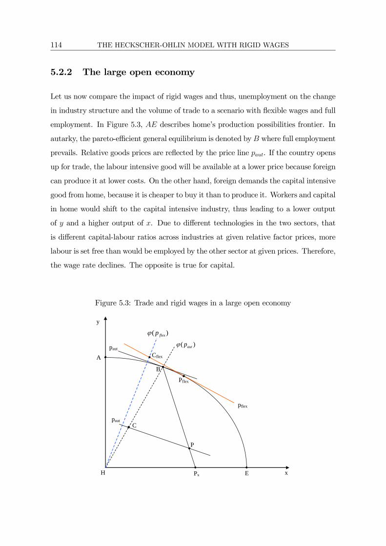
114 THE HECKSCHER-OHLIN MODEL WITH RIGID WAGES

5.2.2 The large open economy

Let us now compare the impact of rigid wages and thus, unemployment on the change

in industry structure and the volume of trade to a scenario with flexible wages and full

employment. In Figure 5.3, AE describes home’s production possibilities frontier. In

autarky, the pareto-efficient general equilibrium is denoted byB where full employment

prevails. Relative goods prices are reflected by the price line paut. If the country opens

up for trade, the labour intensive good will be available at a lower price because foreign

can produce it at lower costs. On the other hand, foreign demands the capital intensive

good from home, because it is cheaper to buy it than to produce it. Workers and capital

in home would shift to the capital intensive industry, thus leading to a lower output

of y and a higher output of x. Due to different technologies in the two sectors, that

is different capital-labour ratios across industries at given relative factor prices, more

labour is set free than would be employed by the other sector at given prices. Therefore,

the wage rate declines. The opposite is true for capital.

Figure 5.3: Trade and rigid wages in a large open economy

pflex

paut

paut

H

Cflex

C

Px E x

Pflex

B

)( autpϕ

A

y

P

)( flexpϕ

THE HECKSCHER-OHLIN MODEL WITH RIGID WAGES 115

If wages cannot fall, one part of the workers in this sector becomes unemployed while

another part moves to the expanding sector. This means that output of sector y shrinks

while output of sector x increases. Contrary to the flexible wage case, though, this shift

is now driven by unemployment and thus a change in relative (employed) endowments

in home rather than via a change in relative prices. Due to unemployment, home’s

production possibilities frontier is no longer described by AE, but turns to ABPxE

where BPx describes the Rybczynski line. This line is the locus of all efficient equilibria

given the minimum wage. Unemployment reduces home’s labour force that can be

used in the production process and hence, shifts in the initial production possibilities

frontier. BPx characterises all tangency points of the price line paut with the respective

production possibilities frontier for different levels of employment. While in B full

employment prevails, unemployment rises along the Rybczynski line until Px. Then

the economy would completely specialise in producing the capital intensive good. This

case will be considered in detail in the next section. In our example, home is driven

down the Rybczynski line to the production locus P as the large country assumption

ensures that neither country completely specialises. Due to homothetic preferences,

consumers are willing to consume the two commodities in the same ratio independently

of their level of income. This is reflected by the dashed line ϕ (paut). With C being

the consumption point, the economy’s trade vector is PC. This means that the capital

intensive commodity is exported while the labour intensive one is imported. Autarky

prices paut become world market prices.

Volume of trade

How does the trade volume with unemployment compare to the trade volume with

full employment? With regard to Figure 5.3, we need to compare PC with PflexCflex.

This, however, is a difficult task. Fortunately, the problem solves easily if we look at

both trade equilibria from a different angle — the other country (foreign). The im-

pact of rigid wages in home on foreign is shown in Figure 5.4 below. Due to a lower

capital-labour ratio, general equilibrium in autarky is characterised by a relatively

higher output - and thus a lower price - of the labour intensive commodity y. This

116 THE HECKSCHER-OHLIN MODEL WITH RIGID WAGES

is reflected in the steeper relative price line in autarky pFaut. AFEF denotes foreign’s

production possibilities frontier with BF reflecting the pareto-efficient general equilib-

rium in autarky. Opening up for trade changes relative prices. This is shown by the

shift of the relative price line pFaut to pflex and pHaut, respectively. With flexible wages in

home, world commodity prices are pflex. This yields PFflex as foreign’s efficient produc-

tion locus and CFflex as foreign’s consumption bundle. Again, the dashed line indicates

homothetic preferences.

Figure 5.4: The volume of trade with rigid wages

)( flexpϕ

)( autHpϕ

pFaut

pflex

PF

BF CF

pHaut

F

CFflex

EF xF

PFflex

AF

yF

If home maintains its high wage rate by defending its relative prices, then terms of

trade would improve even more for foreign. If the world price of the labour intensive

good remains on the high autarky level prevailing in home, then foreign will produce

more of it than it would have for lower prices, of course. Thus, the relative price line for

foreign rotates more than in the flexible wage scenario. In Figure 5.4, this is indicated

by the line paut. Now we can easily see that the trade vector PFCF must be larger

than PFflexC

Fflex. While the terms of trade effect for home was entirely absorbed by

means of domestic unemployment, the change in relative prices turns out to be larger

THE HECKSCHER-OHLIN MODEL WITH RIGID WAGES 117

for foreign. Home’s relative goods prices in autarky have become world market prices.

As we have identified a new trade equilibrium, exports of home have to be identical

to imports of foreign and vice versa. As foreign demands more of the capital intensive

commodity from home, we know that home must export more than with flexible wages.

Home pathologically exports too much if unemployment arises.

Structural change

From this analysis we can equivalently infer the change in industry structure.

Home’s wage rigidity induces a larger structural change in both home and foreign. With

flexible wages, the production locus would have only shifted from BF to PFflex abroad.

With rigid wages in home, though, even more of the labour intensive commodity will

be produced and less of the capital intensive one. Analogously, home “over-specialises”

in the capital intensive good. The adjustment of relative prices that sets in if wages

are flexible does not work as a braking force. Therefore, structural change through

unemployment is pathologically stronger than the healthy process induced by a change

in relative prices.

Welfare

As Brecher (1974a) has already shown, welfare gains from trade do not arise if wages

are downwards rigid and trade equilibrium is characterised by incomplete specialisation

of both economies. “No trade” is superior to “trade”. If this mechanism is at work,

structural change and hence, trade volumes are pathologically too high. From a high

trade volume and a strong decline of the labour intensive industry, we can no longer

infer that the economy is benefiting from global markets. On the contrary, in this

setting it clearly loses. If a country performs well in international trade, there are only

welfare gains if no (further) unemployment emerges. Hence, rising exports are not by

itself a sign of welfare gains. If trade causes unemployment, rising export figures should

ring the alarm.

118 THE HECKSCHER-OHLIN MODEL WITH RIGID WAGES

Result 5.2 A large open economy that is relatively abundantly endowed with capital

will face unemployment when it opens up for international trade and prevents wages

from adjusting downwardly. While output and welfare decline, specialisation in the

capital intensive industry becomes more pronounced than with flexible labour markets.

Hence, also trade flows reach higher levels than without unemployment.

5.2.3 The small open economy

We now turn to the small country. Contrary to many questions in international trade,

the small open economy case turns out to be more complicated if wages are rigid. This

is due to the fact that a small country has no influence on world market prices and

maintaining domestic wage levels unavoidably leads to complete specialisation. This

modification of relative prices has to be considered as an additional effect. Conse-

quently, it matters a great deal how the minimum wage is specified — either in nominal

terms or in real values as in units of good x or good y. To compare trade flows with

rigid and flexible wages, it is crucial to identify the production structure of home. It

will turn out that this depends on the definition of the minimum wage.

Figure 5.5 shows the same transformation curve of home as Figure 5.3 in the pre-

vious section. The only difference is that in this case, the rigid wage economy cannot

defend its autarky prices on the world market. Rather relative prices in the rest of

the world will become the relevant terms of trade in the small open economy. In other

words, relative goods prices pflex are exogenously given. Again, B denotes production

and consumption in autarky with ABPxE representing the transformation curve given

the minimum wage. While the previous section discussed an interior solution where

home ended up somewhere on the Rybczynski line, the economy is now driven to

complete specialisation of the capital-intensive commodity. Production of the labour

intensive good collapses entirely. Output of x now depends on the definition of the

wage floor. If defined in terms of good x, Px will be the production point. Unem-

ployment remains on its maximum level. One can imagine that the economy is driven

down the Rybczynski line at given autarky prices paut. With complete specialisation,

THE HECKSCHER-OHLIN MODEL WITH RIGID WAGES 119

Figure 5.5: Trade and rigid wages in a small open economy

pflex

pflex

)( flexpϕ

Cx

H Px Py D E x

pflex

Pflex

B

)( autpϕ

A paut

y

)( flexpϕ

Cflex

however, home can no longer defend the high price of the labour intensive commodity

and hence, the relative price of x rises. In order to keep real wages constant in terms

of good x, nominal wages have to increase by the same percentage as px. As x is the

only good being produced in the economy using the entire capital stock, the capital

return also rises by the relative increase of px. Marginal productivity of capital is un-

affected because in Px, the same capital-labour ratio is employed as both in autarky

and along the Rybczynski line. But the marginal revenue product, which determines

factor rewards, rises due to the price increase.

If one defines the real wage in terms of the labour intensive good y, firms could

pay lower nominal wages and thus employ more workers. As the value of their output

increases, the minimum wage constraint is thereby relaxed. The magnitude of new

employment (relative to Px) depends on the elasticity along the marginal revenue curve

of labour. In Figure 5.5, Py denotes output of x in this scenario. Py must lie to the right

of Px, but to the left of D. This must be true because D belongs to the Rybczynski line

starting from Pflex at world market prices. With flexible wages, we know that along

120 THE HECKSCHER-OHLIN MODEL WITH RIGID WAGES

PflexD real wages have declined in terms of both goods due to the Stolper-Samuelson

effect.

Finally, the minimum wage could be indexed to the inflation rate. With homothetic

preferences, the price index would be pindex = αpx + (1− α) py where α denotes the

constant income share spent on commodity x while (1− α) is the expenditure share

for good y. Therefore, the wage floor would be w/pindex. Depending on α, the economy

would produce x in the range of Px and Py. The higher α the less employment will be

generated and vice versa. With flexible wages, of course, the change of relative prices

from paut to pflex would drive the economy along the transformation curve AE to Pflex.

The change in industry structure depends on the elasticity along the transformation

curve.

We now turn to consumption. As consumer prices change for households in home,

the consumption mix in the new equilibrium will be different from autarky. The extent

of consumption change depends on the price elasticity of demand. Due to homothetic

preferences, consumption ratios can be expressed along a ray from the origin as long as

relative prices do not change: x/y = ϕ (p), where ϕ0 < 0. With regard to the diagram,

the question is how much will the ray describing the function ϕ (p) change when p

changes. Thus, we get Cflex as the consumption point with flexible wages and Cx with

rigid wages where the minimum wage is defined in terms of the capital intensive good

here.

This enables us to compare trade vectors with flexible and inflexible labour markets.

It will turn out that both a lower and a higher volume of trade is possible relative to the

flexible wage case. The volume of trade with flexible wages is described by the vector

PflexCflex. Shifting the dashed line to the right until it crosses Pflex, it becomes clear

that — for the situation depicted in Figure 5.5 — in equilibrium, the small open economy

trades more than it would with flexible wages. The trade vector with unemployment

is represented by PxCx, which is clearly larger than PflexCflex. If the wage floor was

defined in terms of a consumption basket or in terms of the labour intensive good, there

would also be a pathological trade boom. However, the result is not unique. One can

THE HECKSCHER-OHLIN MODEL WITH RIGID WAGES 121

easily imagine a combination of elasticities that generates a smaller trade flow than in

a flexible wage world. Say, the elasticity of demand is higher than depicted in Figure

5.5. Then ϕ (pflex) would be steeper thus cutting the horizontal axis further to the

right. If the elasticity is sufficiently higher, PxCx would be smaller than PflexCflex. As

a second possibility, one can imagine that the difference in relative endowments and

thus in relative prices is larger between the small open economy and the rest of the

world. Then, pflex would be steeper, thus driving the economy further down the flexible

wage transformation curve AE. Depending on how the minimum wage is fixed, it is

possible that home would export fewer goods in the presence of unemployment. Hence,

for a small open economy, it is not clear that rigid wages imply excessive trade flows.

Nevertheless, the production of the capital intensive commodity always outweighs the

output level with incomplete specialisation.

At least we can identify parameters that determine the volume of trade: On the

supply side the elasticity along the flexible wage transformation curve and the elasticity

along the marginal revenue curve of labour if the wage is either defined in terms of a

basket or in terms of the labour intensive commodity. On the demand side, the price

elasticity of demand turns out to be the crucial parameter. The higher the elasticity

along the flexible wage transformation curve AE, the less likely is a pathological vol-

ume of trade ceteris paribus. Also, as stated before, the larger the difference between

autarky and world market prices, the less likely are excessive trade flows. A high elas-

ticity of the marginal revenue curve of labour in sector x, however, makes it more likely

that the small rigid wage country’s volume of trade is larger than with labour market

clearance. On the demand side, a high price elasticity of demand ceteris paribus makes

excessive trade flows less likely. Contrary to the large open economy, the volume of

trade does not provide a measure of welfare loss if unemployment emerges simultane-

ously. Rather, starting from Px more trade improves welfare because unemployment

can be reduced and thereby production increased. Nevertheless, welfare is lower than

in autarky given that a whole industry vanishes.

The ambiguity in the results vanishes, however, if we add factor mobility in addition

122 THE HECKSCHER-OHLIN MODEL WITH RIGID WAGES

to trade. We have seen that complete specialisation does not equate factor prices

across both countries which leaves an incentive for factors to relocate. The domestic

wage rate exceeds the foreign labour remuneration, whereas the capital return is lower

than abroad. The differences in factor prices can only be maintained if trade is the

only linkage between both regions. With either capital or labour mobility, however,

these differentials cannot be sustainable as there is an incentive for domestic capital

to shift abroad and foreign labour to migrate to home, respectively. This enhances

convergence of factor prices and generates further unemployment in home. Due to our

small country assumption, however, home cannot equate relative factor endowments of

the entire world to its autarky level. Hence, 100 percent of the domestic labour force

will become unemployment again. Either foreign workers are employed jointly with

domestic capital in home or the entire capital stock is driven out of the rigid wage

region.

Although this is too harsh a result to be taken literally for policy debate, it impres-

sively demonstrates the catastrophic effects of defending national wages against the

forces of globalisation for a small open economy.

Result 5.3 Rigid wages drive the small open economy into full specialisation of

the capital intensive good. However, trade does not unambiguously generate excessive

trade flows. The elasticities on both the demand and the supply side crucially influence

the outcome. Contrary to a model with pure factor mobility, a small open economy that

is only linked via commodity trade to the rest of the world, can theoretically prevent

extinction by complete specialisation. The difference in factor prices vis-à-vis the rest of

the world can only be sustained without factor mobility. Otherwise, the entire domestic

labour force would be driven into unemployment again.

THE HECKSCHER-OHLIN MODEL WITH RIGID WAGES 123

5.3 A remedy for the pathology

This chapter has clearly stated that neither more complex models with more than

one sector, nor the existence of trade or factor mobility change the result. The only

difference turns out between a large and a small open economy. While the large open

economy can equate relative global factor endowments to its autarky level, the small

open economy’s factor endowments will either be made extinct from employment, or it

is driven into complete specialisation, as long as trade remains the only international

linkage between two regions.

Therefore, we must conclude that distributional goals that try to be achieved by

means of implementing labour market rigidities, come at very high cost - that is unem-

ployment, and a decrease in both output and welfare. This delivers a strong argument

for an alternative way. Certainly, protectionism would reduce the detrimental effects

of rigid wages. However, potential gains from globalisation could not be realised, of

course. Richard Brecher (1974b) analysed alternative policy measures in a second-best

fashion. He found that wage subsidies would be able to reach the same equilibrium

as without any distortions. This must be the starting point for any policy maker in

a globally linked market economy when thinking about distributional policies. Pay-

ing wage subsidies rather than minimum wages would avoid unemployment as wages

could adjust to their market clearing level. The subsidy can then be regarded as a

supplement to lower real wages.

With regard to Germany, it is the design of the welfare state rather than explicit

minimum wages that generates the distortion in the labour market. Paying wage re-

placement incomes that are only paid under the condition that someone is not working,

create a reservation wage that might not be compatible with full employment. There-

fore, policy makers should pick up on Brecher’s (1974b) result that a wage subsidy can

improve the situation. In fact, the US has installed the Earned Income Tax Credit,

that builds upon this idea, already since 1975. For Germany, there are a few policy

proposals on the table. Chapter 8 will come back to them in more detail.

Chapter 6

The short- and medium-run effects

of trade with rigid wages

One of the central assumptions of the Heckscher-Ohlin model claims that factors of

production can freely move between national industries. Thereby, firms are able to

react to relative price changes by adjusting their factor employment and thus, output.

However, this scenario might only be true in the long run as capital, for instance,

causes changeover costs or workers need new training until they can be employed

in other production processes. Hence, assuming (partial) immobilities of production

factors seems plausible to describe the impact of trade in the short and medium run.

The textbook model for this analysis is called the specific factors model. This chapter

studies the implications of rigid wages in this setup and relates them to previously

derived results.

The specific factors model has been revitalised by Jones (1971a) and Samuelson

(1971). Mayer (1974), Neary (1978) and Mussa (1978) later integrated it as the short-

run interpretation of the Heckscher-Ohlin model. However, not much focus has been

laid upon the impact of downwardly rigid wages in such a framework. One example

is Haberler (1950) who discusses different cases of factor immobilities in connection

with labour market distortions such as wage differentials and minimum wages. He

shows that trade can have detrimental effects on national welfare if factor markets

126 SHORT- AND MEDIUM-RUN EFFECTS OF TRADE

are inflexible. In most cases, however, wage differentials rather than minimum wages

have been studied. Examples include Jones (1971b), Magee (1971), Bhagwati and

Srinivasan (1971) or Matusz (1994). As in the previous chapters, this part follows the

simplest possible approach in which workers are paid a minimum wage.1 For the long-

run perspective, Brecher (1974a) and more recently Davis (1998), Oslington (2002),

Kreickemeier (2005) and Sinn (2005c) have followed this approach as well.2

This chapter distinguishes between the short and medium run by assuming different

degrees of mobility. The short run is the period of time where both capital and labour

are immobile between sectors, whereas the medium run builds on the classical specific

factors model with intersectorally mobile labour and immobile real capital. Using

Jones’ (1971a) seminal ”hat calculus” approach, we study the impact of minimumwages

on welfare, unemployment, structural change, factor returns and trade flows in both

scenarios. There are two countries, home and foreign, that produce two goods, x and

y, with the inputs capital (K) and labour (L) under perfect competition and constant

returns to scale. Sector x is capital intensive while sector y uses relatively more labour.

Home is assumed to be relatively abundantly endowed with capital. Furthermore,

both countries are of similar size in order to guarantee an interior solution, that is,

both countries always produce both goods. The definition of the minimum wage is

crucial because it can substantially influence the results. Here, the real wage is fixed in

terms of both goods via a price index. Unemployed workers receive benefits that are

financed in a lump-sum fashion. Thereby, we avoid explicit modelling of the welfare

state.

One can think of two strands of contribution of this chapter. Firstly, it extends

the specific factors literature by implementing downwardly rigid wages. Secondly, it

complements the long-run Heckscher-Ohlin model results as it relates the market out-

come in the short and medium run to the long-run effects. This provides a better

understanding of the ”adjustment process” caused by the opening up for trade and the

1Other ways to model unemployment include the search theoretic approach applied by Davidsonet al. (1999) or Weiß (2001). Fair wages are used by Brecher (1992), Matusz (1994), Kreickemeier andNelson (2006) and Kreickemeier and Schoenwald (2002).

2Sinn (2005d) interprets the minimum wage as replacement incomes paid by the welfare state.

SHORT- AND MEDIUM-RUN EFFECTS OF TRADE 127

change in relative prices.

We find that the detrimental long-run effects of the Heckscher-Ohlin framework

with rigid wages turn out to be less severe in the presence of factor immobility. Unem-

ployment and welfare losses are always lower in the specific factors model. Preferences

determine the rate of unemployment. The more of their income consumers spend on

the commodity, whose price rises, the more weight this price increase gains in the in-

dex. Thus, nominal wages have to rise more, or are not allowed to decrease as much,

in order to keep real wages constant. In the short run, unemployment emerges only in

the sector in which the price falls. Due to better allocation of labour in the medium

run, unemployment will decline. However, the impact on welfare and the volume of

trade is ambiguous both in the short and medium run. The positive terms of trade

effect is counteracted by the negative unemployment effect.

The next section explains the specification of the minimum wage. Based on this,

the following part studies the impact of rigid wages for both the short and the medium

run. Section 6.3 links the results to the outcomes in the long run (see Chapter 5). The

final part concludes and discusses policy implications.

6.1 The minimum wage

The definition of the minimum wage is crucial in the specific factors model. Contrary

to the long-run Heckscher-Ohlin framework, results change substantially with different

specifications. Recall that wages decline in terms of both goods if both captial and

labour can migrate between sectors and the relative price of the capital intensive com-

modity rises. Hence, fixing the wage in nominal terms or in terms of either commodity

does not change the result. Unemployment and welfare will reach the same level in

every case. In the specific factors model, however, wages increase in terms of one good

and fall in terms of the other depending on the direction of the relative price change.

For a capital abundant economy, which we focus on in this analysis, workers would lose

in terms of the capital intensive good and gain in terms of the labour intensive one.

128 SHORT- AND MEDIUM-RUN EFFECTS OF TRADE

Hence, fixing the real wage in terms of the latter would not yield any unemployment.

The market clearing wage would always be equal to the minimum wage level. On the

other hand, defining the wage floor in terms of the capital intensive commodity would

clearly generate unemployment because nominal wages would have to increase more

than market forces require.

As this appears rather arbitrary, we follow a different approach by defining the

minimum wage in terms of a consumption basket. With homothetic preferences, we

can use the income shares spent on each commodity as weights in the price index. The

minimum wage is then defined as

wreal ≤wi

αpx + (1− α) pyi = x, y. (6.1)

wi denotes the nominal wage in sector x or y. px and py are the prices of the

respective commodities. These prices are weighted by α which is the income share

spent on good x and (1− α) for good y, respectively. Due to homothetic preferences,

these shares remain constant independent of goods price or income changes. Eq. (6.1)

implies that the nominal wage which firms have to pay must at least rise by the same

percentage as the price index to prevent a decrease of real wages. This can be seen by

totally differentating eq. (6.1) to get

dwi

wi= bwi ≥ bpindex = αdpx + (1− α) dpy

αpx + (1− α) py. (6.2)

It also becomes clear that the nominal wage has to increase more, the higher is the

value of α, if px goes up. This, however, will be the case for a capital abundant country.3

As long as α = ]0; 1[ and home is relatively capital abundant, bpx > bpindex > bpy. Theimplications of this wage floor in the short and medium run are examined in the

following chapter.

3The proof is relegated to Appendix 6.A.

SHORT- AND MEDIUM-RUN EFFECTS OF TRADE 129

6.2 The model

The model describes two equally large countries, home and foreign, that produce two

goods (x and y) with the inputs capital (K) and labour (L) under perfect competition.

Home is assumed to be capital abundant whereas foreign possesses relatively more

labour. x is the capital intensive good whereas y needs relatively more labour in the

production process. We assume that factors differ in their mobility between sectors. In

the short run, both capital and labour are specific to their industries whereas labour is

allowed to be mobile in the medium run. International factor mobility is not considered.

This approach follows the short-run interpretation of the Heckscher-Ohlin framework

by Mayer (1974), Neary (1978) or Mussa (1978). Thereby, we get an idea about the

development of unemployment, welfare, structural change and volume of trade over

time without considering a dynamic model. The outcome with full intersectoral factor

mobility is taken from the Heckscher-Ohlin literature.4

It is enough to explicitly study the equations for the capital intensive economy

(home) alone. Foreign is only necessary to explain the direction and magnitude of

change in relative prices. The more diverse both countries are in terms of both relative

and absolute factor endowments, the more pronounced the change in relative prices

has to be. The approach builds on the ”hat calculus” model introduced by Jones

(1971a). For simplicity reasons, we start from a long-run pareto-efficient equilibrium

in autarky. This implies that factor prices are equal in both sectors and all factors are

fully employed. Opening up for trade with the labour intensive country increases the

relative price of the capital intensive good x, thereby creating an exogenous shock.

6.2.1 The short run

In the short run, both labour and capital are specific to their industries. However,

they are not specific to the firms they are employed at. This assumption is necessary

to ensure unique factor prices within sectors. With regard to capital, this assumption

4See Brecher (1974a) or Davis (1998) and Chapter 5 of this book.

130 SHORT- AND MEDIUM-RUN EFFECTS OF TRADE

is justifiable as machines require time for changeover to be productive in the other

industry, but not within industries. With regard to workers, a similar mechanism can

be assumed, for instance that workers need to acquire different skills to work in the

other industry. However, we abstain from modelling this transformation explicitly.

Sector specificity of both factors allows us to analyse the two sectors separately. With

the same technological know-how in both jurisdictions, home produces the capital

intensive commodity x relatively cheaper as it is relatively abundantly endowed with

capital. Hence, integrating goods markets leads to an increase in px and a decline in

py in home. Preferences are identical and homothetic. In a first step, we take a look

at the capital intensive sector x.

The x-sector

The sector can be described by means of the following equations

aLxwx + aKxrx = px (6.3)

aLxx+ U = Lx (6.4)

aKxx = Kx (6.5)

where aLx =Lxxand aKx =

Kx

xare the unit inputs of labour L and capital K, respec-

tively. x denotes output of the capital intensive commodity. Eq. (6.3) represents the

zero profit condition where unit costs are equated to unit revenues. Eqs. (6.4) and

(6.5) reflect the resource constraints in this sector where U describes unemployment in

absolute terms. Clearly, with flexible factor markets, U = 0. With a binding minimum

wage, however, U can take positive values. Totally differentiating eqs. (6.3) to (6.5)

and expressing in terms of relative change yields5

5For derivation see Appendix 6.B.

SHORT- AND MEDIUM-RUN EFFECTS OF TRADE 131

θLx bwx + θKxbrx = bpx − (θLxbaLx + θKxbaKx) (6.6)

bUx = bLx − bx− baLx (6.7)

bx = bKx − baKx. (6.8)

The ”b” over a variable illustrates relative changes, for example br = drr. The θs are

factor income shares of capital and labour respectively, for example θLx =aLxw

px. Hence,

θLx + θKx = 1. Now bUx shows the unemployment rate in sector x, that is the number

of workers relative to the labour force attached to the capital intensive industry, Lx. In

order to determine baLx and baKx we need two additional equations. They can be taken

from the firms’ unit cost minimisation

minwx,rx

aLxwx + aKxrx (6.9)

and from the definition of the elasticity of factor substitution, which is defined in the

following way so as to be positive

σx =baKx − baLxbwx − brx . (6.10)

By total differentiation of (6.9) we get

θLxbaLx + θKxbaKx = 0. (6.11)

Solving and substituting in (6.10) yields

baKx = θLxσx (bwx − brx) (6.12)

baLx = −θKxσx ( bwx − brx) . (6.13)

With flexible wages, only w and r adjust to changes in the goods price. As can be

seen from eq. (6.6) jointly with eq. (6.11), a one percent increase in px leads to a one

132 SHORT- AND MEDIUM-RUN EFFECTS OF TRADE

percent increase in both w and r. Wages, however, are not fully flexible, but bounded

to the floor. By implementing eqs. (6.11), (6.12) and (6.13) into eqs. (6.6) to (6.8) we

get three equations in three endogenous variables. Solving for bUx yields

bUx =σxθKx

(bpindex − bpx) . (6.14)

As we know from the previous section bpx > bpindex. Hence, bUx would be negative. How-

ever, unemployment can only be larger than or equal to zero by definition. Therefore,

in this case bUx = 0, while bx, brx, and bwx are endogenously determined.

Result 6.1 In a capital abundant country, the capital intensive sector is not af-

fected by the downwardly rigid real wage if both factors are sector specific. Hence,

unemployment in this sector is zero.

The intuition for this result is the following. From the analysis above we know

that market wages rise by the same percentage as the price of the capital intensive

commodity. This would be more than the rise in the price index and hence, implies an

increase in real wages. Hence, the minimum wage constraint is not binding in sector

x. Therefore, bwx = brx = bpx, while bUx, bx, baLx, baKx are zero.

The y-sector

We can employ the same set of equations to analyse the impact on sector y. The

only difference to the previous section is that the commodity price py declines. The

equations of change are

θLy bwy + θKybry = bpy (6.15)

bUy = bLy − by − baLy (6.16)

by = bKy − baKy . (6.17)

SHORT- AND MEDIUM-RUN EFFECTS OF TRADE 133

Solving eqs. (6.15) to (6.17) by using eqs. (6.10) and (6.11) for sector y, we get

bUy =σyθKy

(bpindex − bpy) . (6.18)

As bpy < bpindex, the minimum wage constraint becomes binding and unemployment

emerges in this sector. Only if the minimum wage was defined in terms of the labour

intensive good, that is bpindex = bpy, this term would be zero and hence, full employmentwould be maintained. Maximum unemployment would arise, if the minimum wage was

defined in terms of the capital intensive commodity x. Thus, from eqs. (6.2) and (6.18)

we can infer that α has a positive influence on the unemployment rate.

Proposition 6.1 In the short run, unemployment emerges in the labour intensive

sector. It increases in α.

Proof. ∂Uy∂α= σy

θKy

∂pindex∂α

> 0, because ∂pindex∂α

> 0. See Appendix 6.A for details.

Intuitively, the higher the preference for the capital intensive good, the higher

the weight of the price change in the price index and thus, the higher the difference

between bpindex and bpy. The term σyθKy

reflects the elasticity of the marginal product

curve of labour.6 The higher this elasticity, the more unemployment will be generated

given the difference in price changes and given α.

The impact of the binding minimum wage on bry can be seen from eq. (6.15)

directly. As bwy decreases by less than market forces require for market clearance, bryhas to decrease more than the price of y to fulfill this condition. Writing eq. (6.15)

differently brings bry = 1

θKy

bpy − θLyθKy

bpindex < bpy. (6.19)

Result 6.2 With rigid wages, the return to capital in sector y decreases more than

with flexible wages.6The marginal physical product of labour is given by wy/py. This increases as aLx/aKx , the input

of labour relative to the fixed factor capital, declines. The elasticity of the marginal product curve is¡baKy − baLy¢ / ( bwy − bpy). From eq. (6.15), bwy − bpy is equivalent to θKy ( bwy − bry). See Jones (1971a),footnote 5.

134 SHORT- AND MEDIUM-RUN EFFECTS OF TRADE

Intuitively, capital must bear a higher burden because there is a relative input

effect in addition to the regular price effect. The latter effect would reduce ry by the

same percentage as the price decrease. Unemployment, however, increases the capital-

labour ratio in this sector and hence, reduces the marginal productivity of capital.

The combination of these two effects yields a lower return than in the flexible wage

scenario. The same argument works in the opposite direction for labour. This second

effect increases marginal productivity of labour thus allowing firms to pay wages above

the market clearing level.

Finally, the effect on the third endogenous variable, output y, is revealed in the

following equation by = −θLy σyθKy

(bpindex − bpy) < 0. (6.20)

Of course, output recedes due to unemployment in sector y. Interestingly, the

change in unemployment is higher than the change in output of y in absolute terms.

This becomes clear from eqs. (6.18) and (6.20) because θLy < 1.

Welfare, trade and structural change

In order to close the model, we introduce the demand side. As both countries have

homothetic preferences, relative demand is a function of relative prices only

x

y= ρ

µpxpy

¶(6.21)

with ρ0 < 0. Totally differentiating eq. (6.21) brings

bx− by = −σD (bpx − bpy) (6.22)

where σD represents the price elasticity of demand.7 As ρ is a monotonically decreasing

7See Appendix 6.C for details of this calculation.

SHORT- AND MEDIUM-RUN EFFECTS OF TRADE 135

function, the inverse exists and we can rewrite eq. (6.22) as

bpx − bpy = − 1

σD(bx− by) . (6.23)

With identical preferences in both jurisdictions and from the fact that xy= γ

¡KL

¢with γ0 > 0, we know that xH

yH> xF

yFand hence,

³pxpy

´H<³pxpy

´Fby eq. (6.21).

Equivalently, pHx < pFx and pHy > pFy . From home’s perspective, bx−by is negative because

foreign offers more y relative to x. By eq. (6.23), bpx−bpy must therefore be positive. Asrelative supply is a function of relative endowments given preferences, we can infer that

relative prices change more the more different relative endowments are in both countries

and the larger the other country is in terms of absolute endowments. Thus, eq. (6.23)

reflects the positive terms of trade effect which increases national welfare. Although

production possibilities do not increase in the short run, consumption possibilities are

extended as long as full employment prevails.

However, from the previous section it is known that a reduction in py generates

unemployment in this sector. Thus, byH < 0. With full employment in foreign andbxF = byF = 0, the right side of eq. (6.23) becomes smaller and thus, relative prices

change less. The output effect generated by unemployment in home counteracts the

first order terms of trade effect and exercises a negative impact on welfare. As the

second order effect cannot outweigh the first order effect, the terms of trade effect still

remains positive. But there is an additional negative effect: unemployment reduces

national income through less production in sector y and consumption possibilities are

reduced. The overall effect of trade with rigid wages on home’s welfare is therefore

ambiguous. However, it is clearly lower than with full employment and free trade.

Figure 6.1 illustrates these effects.

A denotes home’s long-run autarky equilibrium. This means that factor prices are

equated across sectors and the marginal rate of substitution resembles the marginal

rate of transformation (MRS=MRT). p0 indicates relative prices and u0 social welfare

in home. Trade changes relative prices according to the previous analysis and makes

136 SHORT- AND MEDIUM-RUN EFFECTS OF TRADE

Figure 6.1: Equilibrium in the short run

p2

p0

p1

u2

u1

u0

B

A’

A B’

y0

x0

y

x

the relative price line rotate in A. Without unemployment, the economy still produces

the same quantities, but international trade increases consumption possibilities along

p1. In this scenario, there are welfare gains from trade. However, gains from special-

isation can only accrue in the medium and long run due to an efficient allocation of

factors. The trade vector is represented by AA0 implying that home exports the capital

intensive commodity and imports the labour intensive one. With binding minimum

wages output of sector y is reduced according to α and the differences in relative and

absolute endowments. Figure 6.1 depicts a case where y is reduced by AB. While the

economy produces in B, it consumes in B0. Relative to A both the second order terms

of trade as well as the unemployment effect decrease home’s welfare. The scenario in

the figure depicts a negative net effect.

Finally, how does unemployment affect structural change and trade flows compared

to free trade with flexible factor markets? As the minimum wage generates unemploy-

SHORT- AND MEDIUM-RUN EFFECTS OF TRADE 137

ment, sector y declines while output of sector x remains constant. With flexible labour

markets, there would not be any change in the output structure in the short run. We

have seen that the change in relative output worsens the terms of trade for home.

Hence, the rigid wage country will consume less y for two reasons. Firstly, home’s

income shrinks and secondly, the price of good y becomes relatively more expensive.

Vice versa, foreign benefits from improved terms of trade. Their export good, y, has

become more valuable relative to the capital intensive commodity. Thus, they can im-

port more for one unit of exports. The relative price change unambiguously increases

the demand for commodity x, which has to be matched by export supply of home.

Result 6.3 Unemployment in home artificially improves the terms of trade for

foreign. This yields excessive import demand. While welfare has clearly declined relative

to a flexible wage free trade equilibrium, it is ambiguous whether the net terms of trade

effect outweighs the negative unemployment effect in home.

6.2.2 The medium run

Now, we turn to the medium run and allow workers to be mobile between sectors. Con-

trary to the short run, a common labour market with a common wage rate emerges.

Capital, however, can only be shifted to the other sector in the long run due to

changeover costs. Home’s economy is described by means of the following equations.

ci (w, ri) = aLiw + aKir = pi (6.24)

aLi = ciw (w, ri) (6.25)

aKi = cir (w, ri) (6.26)

aLxx+ aLyy + U = L (6.27)

aKxx = Kx (6.28)

aKyy = Ky (6.29)

138 SHORT- AND MEDIUM-RUN EFFECTS OF TRADE

Eq. (6.24) describes the zero profit conditions for both sectors i, where i ∈ {x, y}.

ci (·) are the unit cost functions which have to be equal to the commodity price. Eqs.

(6.25) and (6.26) represent the minimum cost inputs for L and K in each sector, where

aLx = Lx/x. From Shepard’s lemma we know that the cost minimising inputs per unit

of output can be derived by differentiating the unit cost function with respect to the

relevant input price. Eqs. (6.27), (6.28) and (6.29) reveal the resource constraints. As

we allow for unemployment U , the labour market constraint, eq. (6.27), is extended

by this variable. On the other hand, capital markets are always cleared. Totally

differentiating this set of equations and expressing in rates of change yields

θLi bw + θKibri = bpi (6.30)

baLi = −θKiσi (bw − bri) (6.31)

baKi = θLiσi (bw − bri) (6.32)

λLxbx+ λLyby = bL− bU − (λLxbaLx + λLybaLy) (6.33)

bx = bKx − baKx (6.34)

by = bKy − baKy (6.35)

Again, the θs denote factor income shares. The λs describe the share of the labour

force and the capital stock, respectively, which are absorbed in either sector. σi de-

scribes the elasticity of factor substitution in sector x and y, respectively. aKi and aLi

represent factor inputs per unit of output. There are nine equations in nine endogenous

variables: ri, x, y, aLi, aKiand either w or U , depending on whether the minimum

wage constraint is binding.

SHORT- AND MEDIUM-RUN EFFECTS OF TRADE 139

Unemployment

Solving for bU yields

bU = λLyσyθKy

(bpindex − bpy) + λLxσxθKx

(bpindex − bpx) . (6.36)

As we have argued in the previous section, px rises and py falls so that bpx > bpindex >bpy. Therefore, the first term on the right hand side is positive whereas the second termis clearly negative. The unemployment rate, however, can only take positive numbers,

of course. Negative values imply that the minimum wage constraint is not binding

and market wages settle above the minimum level. α plays a crucial role because the

income share spent on the capital intensive good x determines how the price index

reacts to price changes. As a thought experiment, take α = 1; then bpindex = bpx.8The second term in eq. (6.36) would cancel and the first, positive one remains. The

difference between bpindex = bpx and bpy is the maximum difference that is achievable

in this setting. Hence, unemployment reaches a maximum if the minimum wage was

defined in terms of the capital intensive good. On the other hand, with α = 0, that is

the minimum wage is defined in terms of the labour intensive commodity, bpindex = bpyand the first term would cancel. The second term remains. It is negative as bpy isnegative and bpx positive. As we have argued before, bU cannot take negative values andhence, full employment is sustained. Hence, as bpindex is monotonically increasing in α,there must be an α∗ for which eq. (6.36) becomes zero. Consequently, for all α ≤ α∗

unemployment is zero.

Proposition 6.2 If α ≤ α∗, no unemployment arises in the medium run. For

any α > 0 unemployment will decline relative to the short run if intersectoral labour

mobility is introduced.

Proof. ∂U∂α=³λLy

σyθKy

+ λLxσxθKx

´∂pindex∂α

> 0 as ∂pindex∂α

> 0. See Appendix 6.A for

details.

8This should just exemplify the case where the minimum wage is defined in terms of the capitalintensive good. Taken literally, however, α = 1 would imply that only the capital intensive commoditywould be produced.

140 SHORT- AND MEDIUM-RUN EFFECTS OF TRADE

This result differs from the short run, where any α > 0 generates unemployment in

the y-sector. In any case, unemployment declines because labour migration from sector

y to sector x allows for an efficient allocation given the minimum wage constraint. As

the market wage in sector x used to be above the wage floor in the short run, this

sector can absorb more employment. As long as the minimum wage remains binding,

however, employment in sector y does not change. The additional employment in the

capital intensive industry is taken from the pool of unemployed. Equilibrium settles if

wages are equated.

Magnification effect

In the specific factors model, the magnification effect9 is preserved with respect to

the fixed factors, but not with respect to the mobile factor if wages are flexible:

brx > bpx > bw > bpy > bry.If unemployment emerges in the medium run, this magnification effect is modified

quantitatively, however staying in place qualitatively. The minimum wage influences

the demand for labour in both sectors thus yielding different capital-labour ratios and

different marginal productivities. Less people will be employed both in the x- and the

y-sector relative to a flexible wage scenario. Therefore, the return to capital falls less

in the capital intensive industry and declines more in the labour intensive one. Solving

the model for brx and bry we getbrx =

1

∆

½µλLx

σxθKx

+ λLyσyθKy

1

θKx

¶ bpx − θLxθKx

λLyσyθKy

bpy¾+1

∆

½θLxθKx

³bL− bU − λLx bKx − λLy bKy

´¾(6.37)

9The terminology goes back to Jones (1965). It states that factor prices change more than goodsprices such as br > bpx > bpy > bw. In the Heckscher-Ohlin framework, the capital return increases interms of both goods whereas wages decline in terms of both goods if x is the capital intensive good.

SHORT- AND MEDIUM-RUN EFFECTS OF TRADE 141

and

bry =1

∆

½µλLy

σyθKy

+ λLxσxθKx

1

θKy

¶ bpy − θLyθKy

λLxσxθKx

bpx¾+1

∆

½θLyθKy

³bL− bU − λLx bKx − λLy bKy

´¾, (6.38)

where ∆ = λLxσxθKx

+ λLyσyθKy, a weighted average of the elasticities of the marginal

product curves of labour. Eqs. (6.37) and (6.38) show that in addition to the regular

influence of prices on capital returns (which is shown in the first curly bracket), the

last term also exercises an influence on the interest rates as bU > 0. With regard to brxunemployment reduces the relative change in the return to capital in sector x. In the

other sector, capital has to bear a part of the burden generated by the minimum wage.

− θLiθKi

bU is negative and further reduces the capital return in sector y, while it prevents

a higher return to capital in sector x. Comparing both equations, it becomes obvious

that unemployment has a stronger influence on bry than on brx because θLxθKx

<θLyθKy

due

to different input intensities.

Result 6.4 Unemployment modifies the magnification effect quantitatively: brflexx >brrigidx , brflexy < brrigidy as bw > bwflex. However, its qualitative statement remains valid.

Intuitively, a wage rate above the market clearing level implies a lower demand

for labour in both sectors. Hence, with capital being immobile in the medium run,

the capital-labour ratio is lower in both the capital and the labour intensive industry.

Therefore, marginal value products of capital must be lower relative to a flexible wage

scenario.

Figure 6.2 illustrates some of the previous results. The labour force of home is

denoted on the horizontal axis, where labour input in sector x is plotted from the left

and labour input in sector y from the right hand side. Thereby, the width of the box

represents the size of home’s labour force. The wage rate, which has to be equal to

the marginal value product of labour, can be read from the vertical axes. pxfLx and

gLy show the marginal product curves of labour where px denotes the relative price of

142 SHORT- AND MEDIUM-RUN EFFECTS OF TRADE

commodity x in terms of commodity y, whose price is set to unity for this purpose.

Autarky is described by the intersection of both curves in A with LxL0 units of labour

being employed in sector x and LyL0 in sector y. Assume that minimum wages are

equal to market clearing wages and full employment prevails. Trade changes relative

prices so that px increases, say by 10 percent. Hence, pxfLx shifts up by 10 percent to

p0xfLx.

Figure 6.2: Equilibrium in the medium run

wy

px’fLx

pxfLx

gLy

B C’ C

A’

L2 L* L1 L0 Ly Lx

A

wflex

wxSR

wx

UMR

wmin

Without labour mobility (short run) factor prices would also rise by 10 percent in

sector x to fulfill zero profit conditions. This would yield a market wage in sector x

of wSRx . In the short run, equilibrium would be A0 and A indicating different mar-

ginal value products and hence, different wages. This scenario implies flexible wages.

However, a constant real wage matches the nominal wage level wmin. As this level has

to be equal to gLy unemployment emerges in the amount L0L2. The wage differential

between the two sectors is thereby reduced, but remains positive in this case.

If labour mobility is introduced (medium run), workers in sector y are poached by

firms in the capital intensive industry. Thereby, the prevailing wage rate in this sector

SHORT- AND MEDIUM-RUN EFFECTS OF TRADE 143

declines to the wage floor as the capital-labour ratio falls. Due to a more efficient allo-

cation of labour, unemployment is reduced by L0L1. Wages converge to wmin. Relative

inputs are kept on the same level in sector y as emigrating workers are substituted by

unemployed workers one by one. Alternatively, the additional employment in sector x

is recruited from the pool of unemployed. In any case, unemployment is lower in the

medium run.

Structural change

Figure 6.2 also illustrates, how the structure of the economy is influenced through

wage rigidity. As described in the previous section, the binding minimum wage pre-

vents a higher demand for labour. Only by employing less workers can their marginal

productivity be kept on a high level. Thus, the capital intensive industry will expand

by a lower percentage, whereas the labour intensive industry will decline by a higher

percentage relative to full employment. This can be seen by solving for the change in

output bx = θLxσx (brx − bw) > 0 (6.39)

and by = θLyσy (bry − bw) < 0. (6.40)

Nothing differs with respect to the direction of change. However, from the modifi-

cation of the magnification effect we know that brx is now lower and bw higher leading

to a lower, although still positive value of bx. By the same argument, by declines morebecause bry becomes more negative and a higher value of bw is subtracted from it.

Proposition 6.3 A binding minimum wage constraint brakes the expansion of the

capital intensive industry and leads to a larger decline of the labour intensive sector in

the medium run.

Proof. bxflex > bxrigid, as brflexx > brrigidx and bwmin > bwflex and¯̄byflex¯̄ < ¯̄byrigid¯̄, as¯̄brflexy

¯̄<¯̄brrigidy

¯̄and bwmin > bwflex.

144 SHORT- AND MEDIUM-RUN EFFECTS OF TRADE

Terms of trade, volume of trade and welfare

In order to be able to say something about terms of trade and trade flows, the change

in relative supply is crucial. Subtracting eq. (6.40) from eq. (6.39) and substituting

for brx, bry and bw yieldsbx− by = λLxθLy + λLyθLx

∆

σxθKx

σyθKy

(bpx − bpy)− 1

∆

µθLx

σxθKx

− θLyσyθKy

¶ bU, (6.41)

where bKx, bKy and bLy are set to zero. The coefficient of (bpx − bpy) denotes the elasticityof substitution of the production possibilities frontier indicating the change in relative

supply to a change in relative prices. This would be the only effect with flexible

factor markets and no international factor movements. With a binding minimum wage,

though, an additional unemployment effect sets in. bU can be handled in the same wayas emigration, that is, a reduction of the labour stock available for the domestic market.

Whether unemployment generates a positive or negative effect on relative supply, is

ambiguous depending on elasticities. Ignoring the first effect in eq. (6.41), which is

always positive for home, relative supply of x will decrease if θLxσxθKx

> θLyσyθKy. The θs

denote the labour income shares in the two sectors with θLx < θLy . The elasticity of

the marginal product curve of labour, however, is unknown. With a sufficiently highσxθKx, more labour needs to leave sector x relative to sector y in order to keep marginal

revenue values and thus, the wage rate constant. Hence, output of x will decline more

than output of y relative to a flexible wage world.

Returning to the demand side the impact of unemployment on relative supply

influences relative prices and thus generates a second order terms of trade effect. As eq.

(6.41) reflects, this terms of trade effect is ambiguous. Therefore, the first order terms

of trade effect can be further increased or reduced. The unemployment effect, however,

is always clearly negative and reduces both production possibilities and welfare. As

the terms of trade effect is ambiguous, the change in trade flows relative to a flexible

wage scenario is uncertain as well. If the terms of trade improve, home exports less x

and imports more y and vice versa.

SHORT- AND MEDIUM-RUN EFFECTS OF TRADE 145

Result 6.4 A pathological export boom, which occurs in the long-run Heckscher-

Ohlin framework, will not necessarily occur in the medium run. Home only exports too

much from a welfare perspective if the elasticity of the marginal product curve of labour

is sufficiently low in sector x and relative supply of the capital intensive commodity is

reduced via unemployment.

With regard to welfare, there are two counteracting effects again: the terms of trade

effect, which influences welfare in a positive way, and the negative unemployment

effect. Again, nothing can be said about which one dominates. Thus, it is unclear

whether autarky would be preferable from a welfare perspective. Trivially, though,

unemployment decreases welfare relative to free trade with flexible wages.

6.3 Transition to the long run

Finally, we relate this chapter’s results to the long-run outcome as is well known from

Brecher (1974a), Davis (1998) and Sinn (2005a, 2005b, 2006). As a first step, we

compare the short-run results to the case with perfect intersectoral factor mobility.

From the short run to the long run

Recall that wx > wy and rx > ry. Consequently, both labour and capital will

move to the high return sector. The wage differential prevails as long as α > 0.

Unemployment only drives an additional wedge between the capital returns. The

incentive for capital owners to shift this factor to the x-sector will therefore be increased

and more factors will pathologically be employed in the capital intensive industry.10

In the long run, unemployment ensures that world prices will be equal to autarky

prices in home. Thus, there is no beneficial terms of trade effect, but a negative

unemployment effect only. Starting from short-run equilibrium, both capital and labour

will move to sector x. However, due to different factor intensities capital demand

rises, whereas labour demand falls. The Stolper-Samuelson effect sets in and can10This terminology goes back to Sinn (2005).

146 SHORT- AND MEDIUM-RUN EFFECTS OF TRADE

only be prevented by bringing relative goods prices back to the autarky level through

unemployment. Hence, unemployment must unambiguously be higher than in the short

run. There is clearly a welfare loss and trade flows will be excessive because foreign’s

terms of trade improve further. While unemployment depends on the income share

spent on the capital intensive commodity in the short run, the long-run outcome is

independent of how the price index changes.

From the medium run to the long run

A similar line of argumentation holds for the transition from the medium to the long

run. With or without unemployment in the medium run, capital employed in sector

y has an incentive to shift to the high return capital intensive sector. Again, due to

different factor intensities the Stolper-Samuelson effect would be unavoidable if relative

goods prices were not brought back to the autarky level. Hence, more unemployment

must arise to eliminate the previously positive terms of trade effect and thus, increasing

the negative unemployment effect. This causes the transformation curve to shift in.

Result 6.6 In the long run, unemployment is higher and welfare lower than both

in the short and medium run. Thus, capital immobility cushions pressure from global

competition when wages are downwardly rigid.

6.4 Conclusions

This chapter has examined the impact of trade on employment, factor returns, struc-

tural change, trade flows and welfare in the presence of rigid wages and (partial) factor

immobility. We have distinguished between the short run, where both factors of pro-

duction, capital and labour, are immobile intersectorally and the medium run, where

only labour can move between sectors. The main lesson from this analysis is that factor

immobility in a pure trade model cushions the pressure from international competition

on national labour markets. The unambiguously detrimental effects of trade with rigid

wages that occur in the long run will be less severe in the short and medium run.

SHORT- AND MEDIUM-RUN EFFECTS OF TRADE 147

We have seen that, in the short run, unemployment only arises in the sector where

the commodity price falls. In order to pay higher wages, capital has to bear a part of

the burden through lower returns. As real wages are fixed via a price index, preferences

determine the rate of unemployment. The higher the income share spent on the cap-

ital intensive good, the higher unemployment. A lower level of employment increases

relative world supply of the capital intensive good and thereby worsens home’s terms

of trade. This yields excessive exports. In the medium run, labour mobility guarantees

a more efficient allocation of labour and hence, higher marginal productivities. This

allows firms to employ more workers and to reduce the national unemployment rate.

The change in trade flows in the presence of unemployment crucially depends on the

elasticities of the marginal product curves of labour. The terms of trade effect can

either be improved or worsened. Hence, no clear statement can be made about the

volume of trade. In both the short and the medium run, the impact on welfare is am-

biguous as a positive terms of trade effect (which is zero in the long run) is counteracted

by a welfare decreasing unemployment effect.

With regard to policy implications, a politically induced slow down of capital mobil-

ity could reduce the detrimental long-run effects. However, both intersectoral and in-

ternational capital flows must be included to retard structural change and still, welfare

would be lower than with flexible labour markets. Therefore, labour market reforms

to increase wage flexibility should be implemented to reap the benefits of globalisa-

tion. Rather than just cutting down or abolishing the minimum wage, smarter reforms

could avoid a reduction of real income. Wage supplement schemes have already been

mentioned in preceding chapters. Thereby, an efficient labour market outcome can be

combined with a socially acceptable net income of workers.11 As a consequence, the

economy as a whole would clearly benefit from global markets.

11A more detailed discussion is relegated to Chapter 8.

148 SHORT- AND MEDIUM-RUN EFFECTS OF TRADE

Appendix

6.A The impact of α on the price index

∂bpindex∂α

=(dpx − dpy) (αpx + (1− α) py)− (αdpx + (1− α) dpy) (px − py)

(αpx + (1− α) py)2

This expression is larger than zero if

(dpx − dpy) (αpx + (1− α) py) > (αdpx + (1− α) dpy) (px − py)

⇔ αpxdpx − αpxdpy + (1− α) pydpx − (1− α) pydpy > αpxdpx − αpxdpy

+(1− α) pxdpy − (1− α) pydpy

⇔ pydpx > pxdpy

⇔ dpxpx

>dpypy

This condition is fulfilled by assuming that home possesses relatively more capital.

Therefore, px will rise and py will fall in this economy.

6.B Derivation of equations of change

Totally differentiating the zero profit condition for sector x, eq. (6.1), yields

wxdaLx + aLxdwx + rxdaKx + aKxdrx = dpx

baLx aLxwx

px+ bwx

aLxwx

px+ baKx

aKxrxpx

+ brxaKxrxpx

= bpxθLx bwx + θKxbrx = bpx − (θLxbaLx + θKxbaKx)

SHORT- AND MEDIUM-RUN EFFECTS OF TRADE 149

Total differentiation of the labour market constraint, eq. (6.2), brings

xdaLx + aLxdx+ dU = dLx

baLx aLxxLx+ bxaLxx

Lx+ bUx = bLx

bUx = bLx − bx− baLxas aLxx

Lx= 1.

With respect to the capital market constraint, eq. (6.3), we get

xdaKx + aKxdx = dKx

baLx aKxx

Kx+ bxaKxx

Kx= bKx

bx = bKx − baLx,as aKxx

Kx= 1. The same procedure yields the analogous results for sector y and also

the equations of change for the medium run.

6.C Derivation of elasticity of substitution

Total differentiation of eq. (6.21) brings

x

y(bx− by) = ρ0

pxpy(bpx − bpy) .

Using the definition of the elasticity of substitution between x and y on the demand

side

σD = −d(x/y)x/y

d(px/py)px/py

= ρ0y

x

pxpy

yields bx− by = −σD (bpx − bpy) .

Chapter 7

Agglomeration and imperfect

labour markets∗

This chapter leaves the grounds of pure constant returns to scale framworks and intro-

duces a monopolistic competition sector. Although constant returns to scale models

provide answers to a large set of economic questions, they cannot describe the geo-

graphical distribution of economic activity. With constant returns to scale, one should

observe an equal geographic distribution. This, however, is not the case. The economy

rather looks like a ”lumpy place”.1 For instance, agglomeration is mirrored in the ex-

istence of large metropolitan areas, while the periphery shows less economic activity.

As a consequence of this observation, the seminal papers by Krugman (1991), Krug-

man and Venables (1995), and Venables (1996) have started off a sizable literature on

the “new economic geography”,determining the agglomeration forces in general equi-

librium with trade and international factor mobility. One major interest in this line of

research is the analysis of the role of transport costs for the agglomeration of economic

activity in the presence of firm-level economies of scale. The conceptual framework

for this is also referred to as the core-periphery model (CPM). Forslid (1999) has de-

veloped an analytically solvable CPM that has been applied later by Andersson and

Forslid (1999), Baldwin and Krugman (2000), and others. Pflüger (2004) provides a

∗This chapter is based on Egger and Seidel (2006).1Baldwin et al. (2003), p. 9.

152 AGGLOMERATION AND IMPERFECT LABOUR MARKETS

further simplified variant of this model that is based on the assumption of quasi-linear

consumer preferences with Dixit and Stiglitz (1977) type differentiated manufactures

and a homogeneous agricultural good.

This chapter implements the assumption of rigid labour markets into a core-periphery

agglomeration model. The purpose is to study the implications of unemployment for

the location decision of firms and thus, the agglomeration pattern in the long run.

We model labour market imperfection by means of a fair wage contraint following the

seminal paper by Akerlof and Yellen (1990). This approach has gained popularity in

the recent trade literature as in Kreickemeier (2004), Kreickemeier and Nelson (2006)

and Egger and Kreickemeier (2006) to mention a few examples. By fair wages we mean

that workers have preferences for being fairly paid, that is income dispersion should not

increase too much. More specifically, workers attribute some weight to the capital own-

ers’ remuneration which we assume to be always higher.2 The reason for this approach

is its simplicity. It allows us to determine factor prices and the level of unemployment

endogenously in equilibrium without considering a more complex bargaining model.

Despite this justification, we can also find evidence for fair wages. This evidence

is based on surveys among managers and workers, on firm-level studies analysing the

nexus between wages and employment spell lengths, and on experimental evidence

(see Howitt, 2002, and Bewley, 2005, for reviews of the literature). Beyond that, con-

tinental European labour markets are characterised by a much more stable dispersion

of earnings than the US or the UK over the last 25 years (see OECD, 2004c).3 The

reason for this may be seen in a preference in continental Europe to limit the gap in

the wages of high-skilled and low-skilled workers, which comes at the expense of higher

unemployment there. The fair wage constraint can also be interpreted in a different

way. Alternatively, one might think about the government influencing wage compres-

sion by fixing minimum wages relative to capital earnings. One could then talk about

fair minimum wages that yield the same outcome if the wage floor is determined in the

2Capital may be interpreted either as physical or human capital (skilled labour).3The level of the US and the UK earnings dispersion was already higher than in continental Europe

25 years ago, and it even increased since then.

AGGLOMERATION AND IMPERFECT LABOUR MARKETS 153

same way. However, this chapter sticks to the former interpretation.

Fair wage preferences affect relative capital rentals and unemployment rates in

the short run, and the agglomeration pattern in the long run. In a first step, we

only consider initially symmetric countries. Capital mobility, however, might lead

to asymmetries in the long run, of course. We show that a symmetric increase in

the fair wage constraint unambiguously decreases both domestic and foreign capital

returns. This works via unemployment that reduces demand for both domestic and

foreign manufactures. In the long run with two symmetric countries, a full dispersion

equilibrium becomes unstable already at a higher level of trade costs than with perfect

labour markets. With asymmetric fair wage constraints, workers in one region possess

a higher preference for equal remuneration than workers in the other. Then, capital

tends to flee the more constrained labour market at intermediate trade costs.

In the next section, we present the model and the fair wage constraint. Section 7.3

describes the short-run equilibrium where both capital and labour are assumed to be

internationally immobile. In Section 7.4, we treat capital as mobile and analyse the

long-run equilibrium. Section 7.5 concludes with a summary of the most important

findings and a brief policy discussion.

7.1 The model

7.1.1 An analytically tractable core-periphery model

The model builds on a variant of the core-periphery agglomeration model. Household

utility is characterised by a quasi-linear upper-tier utility function as in Pflüger (2004).

There are two sectors, a homogeneous agricultural and a differentiated industrial sec-

tor. Consumers are characterised by a love of variety as in Dixit and Stiglitz (1977).

Furthermore, there are two countries i and j where two factors are supplied, labour

L and capital K, respectively. L is used in the production of both homogeneous and

differentiated goods and immobile across borders. K is only used for firm set-up (see

154 AGGLOMERATION AND IMPERFECT LABOUR MARKETS

Flam and Helpman, 1987; Pflüger, 2004) and mobile across borders in the long run.

L’s supply is bound by a fair wage constraint.

There are Li+Ki households in country i. Labour (capital) owners supply one unit

of labour (capital) each. Household preferences in country i are determined by

Oi = α lnCXi + CY i, CXi =

ÃniXi=1

xσ−1σ

ii +

njXj=1

xσ−1σ

ji

! σσ−1

, α > 0, σ > 1, (7.1)

where CY is aggregate demand for the agricultural good and CX is aggregate demand

for industrial goods. xii is demand for a single variety that is locally supplied and xji

denotes demand for a single foreign manufacture. There are ni (nj) firms operating in

the industrial sector in country i (j). Each firm supplies a single variety. The varieties

are substitutable at a constant elasticity σ. Iceberg trade costs impede cross-border

transactions of differentiated goods. In particular, producers have to send τ units so

that one unit arrives. In equilibrium, the mill price is identical for differentiated goods

that are supplied locally and ones that are exported. Accordingly, the consumer price

differs between locally sold varieties (the corresponding consumer price in j is pj) and

exported varieties (the price of the same variety for consumers in country i is pjτ).

To simplify the notation, we account already for the fact that all firms producing and

supplying at the same market set identical mill prices in equilibrium due to their access

to identical technologies and the assumption of symmetric utility (hence, the mill price

pi is identical across all firms producing in i).

Income in country i is determined by

Ei = PiCXi + CY i, Pi =£nip

1−σi + njφp

1−σj

¤ 11−σ , 0 ≤ φ ≡ τ 1−σ ≤ 1, (7.2)

where Pi reflects the CES price index for consumers in country i. Utility maximisation

AGGLOMERATION AND IMPERFECT LABOUR MARKETS 155

determines demand and indirect utility, Vi:

CXi =α

Pi, CY i = Ei − α,

xii = αp−σi P σ−1i , xij = α(τpi)

−σP σ−1j (7.3)

Vi = −α lnPi +Ei + α(lnα− 1). (7.4)

We adopt the common assumptions that there is perfect competition in sector Y and

trade of Y is not subject to any barriers. Production of one unit of the agricultural

good requires a single unit of labour such that Yi = LY i. Choosing the price of the

agricultural good as the numéraire then guarantees that wages are wi = wj = 1 as long

as diversification prevails. Market clearing for domestic varieties of the manufacture

implies that aggregate supply at the firm level Xi equals aggregate demand of a single

variety: Xi.

The production of one unit of the manufacturing good requires c units of labour such

that Xi = LXi/c, with c > 0. Accordingly, parameter c reflects the marginal costs of

producing one unit of manufactures. The production of manufactures is characterised

by economies of scale. By assumption, each firm operating in the X-sector of country

i has to incur fixed costs ri associated with the use of a single unit of capital K in firm

set-up. Profits of firms are then determined by

πi = (pi − c)Xi − ri. (7.5)

In equilibrium, mill prices are set so that their relation to variable costs corresponds

to a fixed mark-up

pi = cσ

σ − 1 . (7.6)

Equilibrium profits are zero due to free entry which yields equilibrium firm size as4

πi =c

σ − 1Xi − ri = 0 ⇒ Xi = riσ − 1c. (7.7)

4By applying the zero-profit condition, we neglect the integer problem and treat firm numbers ascontinuous (see Baldwin, 1988).

156 AGGLOMERATION AND IMPERFECT LABOUR MARKETS

7.1.2 The fair wage constraint

In contrast to previous research, supply of labour is elastic in this framework. As

indicated before, workers’ remuneration is bound by a fair wage constraint. By fair

wage we mean that workers attribute some weight to capital’s remuneration. Since we

focus on the case where the capital rental is higher than the wage rate,5 the perceived

fair wage always exceeds its market clearing counterpart. If employees in country i

are paid less than their fair wage, they reduce effort according to the following effort

function

ei = min

µwi

w∗i, 1

¶,

where wi is the market wage in country i and w∗i denotes the fair wage. Normal

effort is set to unity. The functional form implies that workers reduce their effort

proportionately if the market wage falls short of the fair wage. Hence, effective labour

costs cannot be influenced by firms. Firms choose to pay the fair wage if doing so does

not diminish their profits. w∗i is determined by

w∗i = βri + (1− β) (1− Ui)wi. (7.8)

The preference for an equal income distribution rises with β, a preference parame-

ter workers attribute to the return to capital.6 The second component, (1− Ui)wi,

describes the expected wage of workers outside their firm (where Ui denotes the un-

employment rate) and is weighted by 1 − β. It is straightforward to show that in

equilibrium, the fair wage exceeds the market clearing wage, thus producing unem-

ployment as long as β > 0. A similar relationship as eq. (7.8) exists for capital owners.

However, as their market income always exceeds market clearing wages by assumption,

the fair capital return will always be lower than its market clearing counterpart and

thus be non-binding. Consequently, capital is always fully employed.7 Using the equi-

5Recall that capital may be associated with skilled labour.6For now, we assume that domestic and foreign workers are identical with respect to their fair

wage preferences. This condition will be relaxed in an extension of the model, below.7Again, associating capital with skilled labour, this is consistent with the stylised fact that the

risk of becoming unemployed is predominantly important for unskilled labour.

AGGLOMERATION AND IMPERFECT LABOUR MARKETS 157

librium outcome and the assumption that workers are always paid their fair wage, we

can derive the fair wage constraint as

wi

ri=

β

β + (1− β)Ui. (7.9)

As long as β > 0, unemployment arises in equilibrium and exerts a dampening effect

on the relative wage-capital-return ratio wi/ri. Under diversification, wi = 1 so that

the unemployment rate in country i is determined by

Ui =β

1− β(ri − 1)

which implies ri ∈ [1, β−1].

According to our assumptions, the factor constraints in country i are

Ki = ni

Li = UiLi + (1− Ui)Li

= UiLi + aXinixi| {z }LXi

+ Yi|{z}LY i

,

where aXi describes the labour input coefficient for the manufacturing good, that is

cL/xi. For the employed workers, we then obtain8

(1− Ui)Li =1− βri1− β

Li. (7.10)

In the sequel, we assume countries to be symmetric not only with respect to β, but

also with respect to Li = Lj ≡ L. We focus on differences in the allocation of capital

(Ki, Kj) across economies.

8As there is no unemployment benefit in the model, aggregate demand for a single variety isdetermined by Xi = ((1− Ui)Li +Ki)xii + ((1− Uj)Lj +Kj)τxij .

158 AGGLOMERATION AND IMPERFECT LABOUR MARKETS

7.2 Short-run equilibrium

In the short run, both capital and labour are immobile across borders, but goods can

be traded internationally. By using eqs. (7.2), (7.3), (7.5), (7.6) and the condition for

employed workers (7.10), zero profits imply that the capital return in country i reads

ri =κi

σκi + αeβL⎛⎝α

³L1−β +Ki

´κi

+φα³

L1−β (1− βrj) +Kj

´κj

⎞⎠ ,

where eβ = β/(1− β), κi = Ki+φKj and κj = Kj +φKi. If the fair wage parameter β

equals zero, the zero profit condition for the short run boils down to the one in Pflüger

(2004) who assumes labour markets to be perfectly flexible.

In the short run, we are interested in the impact of the fair wage constraint on

the equilibrium capital rental for a given allocation of capital among countries. We

summarise the corresponding findings in the following proposition.

Proposition 7.1 An increase in β exhibits an unambiguously negative impact on

the capital return ri. There is both a negative direct effect on ri from an increase in

the domestic fair wage parameter and a negative indirect effect from a simultaneous

increase abroad.

Proof. See Appendix 7.A.

The intuition is the following. A higher β attributes a higher weight of the capital

return to the determination of the fair wage. As the firms always pay the fair wage and

we set this wage to unity, a higher fair wage necessarily implies a lower capital return.

The reduction in ri can be inferred from the zero profit condition in eq. (7.5). With

w = 1, prices are constant and hence, the reduction in ri causes a decline in demand,

partly triggered by unemployment — that is, partly due to fewer workers that are able to

purchase varieties of the differentiated good. As firms are faced with both domestic and

foreign demand for their product, the decline in demand of one country’s households

reduces both the domestic and the foreign capital return. The following proposition

AGGLOMERATION AND IMPERFECT LABOUR MARKETS 159

states the impact of the fair wage parameter on the domestic unemployment rate and

thus sheds further light on this mechanism.

Proposition 7.2 An increase in β raises world-wide unemployment. While the

direct effect of an increase in the domestic fair wage constraint unambiguously increases

Ui, the indirect effect lowers domestic unemployment.

Proof. See Appendix 7.B.

The latter effect stems from the fact that a reduction of foreign demand for national

varieties can be compensated by more national demand through higher employment.

However, the direct impact of an increase in β on domestic unemployment can be

eventually overturned by the indirect one from rising fair wage preferences abroad.

The direct effect is more likely overturned, the more the foreign capital rental exceeds

the domestic one. If Ki = Kj, the direct effect always dominates, that is, an increase in

β necessarily leads to higher unemployment in two symmetric countries (see Appendix

7.B for further details). However, what matters here is that the effect on world-wide

unemployment is positive so that the demand for varieties declines in β as stated before.

So far, capital was assumed to be immobile across borders. In the following long-

run perspective, this will be relaxed and our focus is then on the impact of a marginal

increase in the fair wage parameter on the pattern of agglomeration.

7.3 Long-run equilibrium

In the long run, we consider a given allocation of capital as being unstable if capital

owners would be better off after relocating their firm to the other country. We assume

that they will prefer to do so as long as their indirect utility would be higher abroad.

Notice that a necessary condition for a long-run equilibrium is that the difference

between the indirect utility for capital owners residing in i and the ones in j is zero:

VKi − VKj = α ln(Pj/Pi) + (ri − rj) = 0.

160 AGGLOMERATION AND IMPERFECT LABOUR MARKETS

Furthermore, we may rewrite the price indices for countries i and j

Pi =

µcσ

σ − 1

¶(Ki + φKj)

11−σ ;

Pj

Pi=

µφKi +Kj

Ki + φKj

¶ 11−σ

.

Using the definition λ ≡ Ki/(Ki +Kj), we determine

α ln(Pj/Pi) =α

1− σln

µφλ+ 1− λ

λ+ φ(1− λ)

¶

and define ρ ≡ L/(Ki +Kj) to obtain

VKi − VKj =α

1− σln

µφλ+ 1− λ

λ+ φ(1− λ)

¶(7.11)

+ασ(1− φ)

hρ1−β [(1− 2λ) (1− φ)] + φ (2λ− 1)

inσ[λ+ φ(1− λ)] + αeβρonσ[φλ+ (1− λ)] + αeβρo− α2φ2eβ2ρ2

+α

¡1− φ2

¢αeβρ (2λ− 1)n

σ[λ+ φ(1− λ)] + αeβρonσ[φλ+ (1− λ)] + αeβρo− α2φ2eβ2ρ2 .The CPM contains two agglomeration forces and one dispersion force which appear in

this setup as well. The first term in eq. (7.11) captures the price index effect (or cost-

of-living effect), which always works in favour of agglomeration. There, an increase in

λ is associated with a higher share of firms being active in market i. This lowers the

price index because fewer varieties have to be imported. This by itself increases the

real capital return, generating a capital inflow and hence, an influx of firms. This price

index effect represents the first of the two agglomeration forces in the model.

The second term in eq. (7.11), namely ri − rj, captures the impact of a change in

the allocation of firms λ on the nominal capital return differential. This term is the

sum of two effects: the market access effect as the second agglomerative force, and

the market crowding effect as the dispersion force. The market access effect suggests

that firms earn higher profits in the larger market. Therefore, a deviation from the

symmetric equilibrium with λ = 0.5 stimulates a further capital outflow to the larger

region. The market crowding effect indicates that the agglomeration of firms in one

AGGLOMERATION AND IMPERFECT LABOUR MARKETS 161

region implies tougher competition and thus lower capital rentals there. Accordingly,

the net effect of the two is ambiguously related to λ, depending on the level of φ.

Figure 7.1: Indirect utility differentials for different trade costs, βi = βj = 0.1

We need to determine under which circumstances a symmetric equilibrium at

λ = 0.5 (also referred to as full dispersion) is stable. Stability of such an equilib-

rium is achieved if the VKi− VKj-locus intersects with the abscissa and it is negatively

sloped at λ = 0.5. Then, capital owners in country i do not have an incentive to move

one further firm abroad, because they would encounter lower real capital rentals there.

However, foreign capital owners would not want to locate one further unit of capital

in market i either, because they would then face lower real capital rentals abroad.

The stability of the dispersion equilibrium depends on the level of trade costs. This

is illustrated in Figure 7.1, where we use similar parameter values as Pflüger (2004),

namely α = 0.3 and σ = 6. However, we have to employ a sufficiently high share of

labour relative to capital (ρ = 11) to ensure that ri, rj ≥ 1. Otherwise, the fair wage

constraint would not be binding. Countries are identical in all respects except λ.

162 AGGLOMERATION AND IMPERFECT LABOUR MARKETS

According to Figure 7.1, full dispersion is a stable equilibrium at a sufficiently

high level of τ , for example, at τ = 1.0402. If trade costs are sufficiently low, the

agglomeration forces outweigh the dispersion force and equilibria at λ 6= 0.5 become

stable in the long run. A deviation from the symmetric allocation renders capital

owners in the target country better off, thus generating incentives for other firms to

follow the initial mover. At very low trade costs full agglomeration becomes stable (at

λ = 0 and λ = 1). At intermediate trade costs, there are two interior stable equilibria

(referred to as partial agglomeration).

By using the condition ∂ (VKi − VKj) /∂λ = 0, it is possible to determine analyti-

cally the highest possible level of trade costs (that is the lowest possible φ) which is

consistent with a long-run equilibrium λ = 0.5:

φ∗ =2 (σ − 1)

³ρ(σ−αβ)1−β

´− σ2 − 4αeβρ³σ + αeβρ´

2 (σ − 1)³σ + ρ(σ+αβ)

1−β

´+ σ2 − 4α2eβ2ρ2 . (7.12)

If we increase φ (lower trade costs) any further when starting at φ∗, the full dispersion

equilibrium is not tenable any more in the long run. Although the determination of

φ∗ is crucial to know whether and where full dispersion is possible in the long run,

we do not know yet whether the fair-wage-constrained CPM is still characterised by

a supercritical pitchfork bifurcation (hence, whether λ = 0.5 is a unique long-run

equilibrium at φ∗). The following proposition provides an answer on this question.

Proposition 7.3 A supercritical pitchfork bifurcation requires that

∂2 (VKi − VKj) /∂λ2¯̄φ=φ∗,λ=0.5

= 0 and ∂3 (VKi − VKj) /∂λ3¯̄φ=φ∗,λ=0.5

< 0. Whereas

∂2 (VKi − VKj) /∂λ2¯̄φ=φ∗,λ=0.5

= 0 is generally fulfilled in the fair-wage-constrained

CPM, ∂3 (VKi − VKj) /∂λ3¯̄φ=φ∗,λ=0.5

< 0 is not. Only the unconstrained model (where

β = 0) is necessarily of the supercritical pitchfork bifurcation type. Such a bifurca-

tion arises in the constrained model only if σ2 (σ − 1)¡1− φ2

¢(1 + φ)2

³σ + 2aβρ

1−β

´<

σ2 (σ − 1) (1− φ)4³σ + 2ρσ

1−β

´+ 4 (1− φ)2

∙nσ2(1 + φ) + αeβρo2 − α2φ2eβ2ρ2¸2.

Proof. See Appendix 7.C.

AGGLOMERATION AND IMPERFECT LABOUR MARKETS 163

Most importantly, we are interested in how the fair wage preference parameter β

influences φ∗. Hence, we need to determine whether a marginal increase in β fosters

agglomeration versus dispersion. We have seen that the corresponding effect on the

capital rental in the short run is unambiguously negative. The following proposition

sheds light on the relationship between β and φ∗.

Proposition 7.4 The break-point for the full dispersion equilibrium (φ∗) is ambigu-

ously related to β in general. However, a marginal increase in the fair wage parameter

in an unconstrained initial equilibrium with β = 0 leads to an unambiguous decline in

φ∗. Then, a marginal increase in β renders full dispersion at the original level of φ∗

untenable. In turn, a full dispersion equilibrium can then only be maintained at higher

trade costs in the long run.

Proof. See Appendix 7.D.

Figure 7.2: Bifurcation diagram for β = 0 (dashed) and β = 0.1 (solid)

164 AGGLOMERATION AND IMPERFECT LABOUR MARKETS

By extending the exercise of Figure 7.1 in order to cover the entire range of trade

costs, one arrives at the bifurcation diagram which depicts all stable long-run equilibria

in relation to τ . Figure 7.2 shows simulation results for the identical set of parameters

as above whereas the constrained scenario with β = 0.1 — described by the solid line

— is compared to the unconstrained case — described by the dashed line. The diagram

clearly illustrates the pitchfork bifurcation for these parameters and shows that the

break point shifts towards a higher level of τ as β increases.

The intuition behind this result is the following. Recall that the price index effect

works in favour of agglomeration as λ rises. However, an increase in β at β = 0 will

increase ri−rj and lead to a reduction of the sensitivity of the capital rental differential

with respect to λ. Therefore, the agglomeration forces will dominate the dispersion

forces already at higher trade costs. Figure 7.3 sheds further light on their interaction.

Figure 7.3: Agglomeration and dispersion forces in relation to freeness of trade

0φβφ

Magnitude of forces

Freeness of trade

Price index effect

Market crowding effect – Market access effect

*0φ

*βφ

AGGLOMERATION AND IMPERFECT LABOUR MARKETS 165

Both agglomeration and dispersion forces decline in φ. While the dispersion force

generally dominates at a low freeness of trade, there is one well-defined φ at which

agglomeration forces outweigh the market crowding effect. According to this model,

Figure 7.3 illustrates the price index effect (as one agglomeration force) and the sum of

market crowding and market access effects (henceforth referred to as the net dispersion

force) as two separate loci. With perfect labour markets, φ∗0 reflects the break point

at which full dispersion is no longer a stable equilibrium. There, the net dispersion

force exactly offsets the price index effect. For all φ < φ∗0, λ = 0.5 is stable. The net

dispersion force becomes zero at φ0. There, market crowding and market access effects

offset each other and the corresponding locus in Figure 7.3 crosses the abscissa. At

φ = 1 the magnitude of all forces becomes zero because trade costs do not impede trade

any longer. Then, the location of production has no influence on real capital rentals.

Let us now introduce a symmetric fair wage constraint — captured by β > 0 —

starting from an initial equilibrium with β = 0. This rotates the net dispersion force

locus counter-clockwise with its origin remaining at φ = 1. While the price effect does

not depend on β, the market crowding effect loses strength relative to the market access

effect. This is caused by the compression of capital rentals. Such a marginal increase

in β leads to φ∗β < φ∗0 where the agglomeration forces exactly offset the dispersion force,

and it also leads to φβ < φ0 (see Appendix 7.E for a proof of the latter result).

As a further exercise it is interesting to look at the asymmetric case where one region

possesses a stricter fair wage constraint than the other. Although the non-linearities

in the model prevent an analytical discussion in this case, we can provide tentative

insights by means of numerical simulations. For the above parameters and βi = 0.1,

βj = 0, Figure 7.4 presents the results. Comparing the asymmetric fair wage scenario

- again described by the solid lines - to the unconstrained one with βi = βj = 0, we

find that the fair wage constraint tends to drive capital to the unconstrained country

at intermediate trade costs.

166 AGGLOMERATION AND IMPERFECT LABOUR MARKETS

Figure 7.4: Bifurcation diagram for βi = βj = 0 (dashed) and βi = 0.1 and βj = 0(solid)

The intuition behind this outcome is the following. Note that ri < rj at βi > βj = 0,

because a higher fair wage constraint generates more unemployment in this country.

This by itself generates an incentive for capital owners to reside in the unconstrained

country j. Lower trade costs and, hence, more integrated commodity markets lead

to an increasing share of firms locating in country j. Then, only partial or even

full agglomeration in j is stable in the long run. The direction of capital mobility

is then unambiguous at moderate trade costs and the bifurcation breaks down. Full

agglomeration prevails at an even higher level of trade costs than in the symmetric

case. Only at extremely low trade costs may full agglomeration prevail even in the fair-

wage-constrained country. There, it is not very important where to locate production

as trade impediments are negligible. Both agglomerative and dispersive forces settle

on a lower level and, thus, the disadvantage of having a fair-wage-constrained labour

market loses its severeness.

AGGLOMERATION AND IMPERFECT LABOUR MARKETS 167

7.4 Conclusions

This chapter has demonstrated that labour market imperfection as modelled by a

fair wage constraint depresses relative capital returns by generating unemployment.

With respect to the long-run agglomeration pattern, the depression of capital rentals

fosters agglomeration forces. For symmetric countries with equally constrained labour

markets, the full dispersion equilibrium becomes unstable already at a higher level

of unemployment. More interestingly, if one country has a more constrained labour

market, capital will unambiguously be driven towards the less constrained region. This

must hold true as a stricter constraint implies lower capital returns due to higher

unemployment. Therefore, it is no longer indeterminate where firms agglomerate in

the long run.

How can we evaluate these results? What do new economic geography models tell

us about the implications of rigid labour markets when globalisation forces operate?

For symmetrically endowed countries that possess equally constrained labour markets,

the results only change quantitatively (relative to flexible wages). Apart from the fact

that the breakpoint will be shifted towards a higher level of trade costs, the pattern

of agglomeration does not change. The only difference is that higher unemployment

increases relative wages. When it comes to asymmetries with regard to the labour

market constraint, though, the picture is less promising. The ambiguity of where firms

locate in the long run vanishes. The country with the more constrained labour market

will by no means form the core. Hence, it has to pay higher prices for manufacturing

goods as they have to be imported from abroad and clearly experiences a deterioration

of income. Comparing this result to the message of constant returns to scale models

in previous chapters, it turns out that there is no fundamental difference. In both

frameworks, a more rigid labour market causes (more) capital to flee the country,

thereby causing a deterioration in real income.

168 AGGLOMERATION AND IMPERFECT LABOUR MARKETS

Appendix

7.A Proof of Proposition 7.1

Appendix 7.A lays out the proof of Proposition 7.1.

∂ri∂β

=

³αLσκj + α2eβL2´ ¡1− φ2

¢1−ri(1−β)2 + φαLσκi

1−rj(1−β)2³

σκi + αeβL´³σκj + αeβL´− φ2α2eβ2L2 < 0

∂ri/∂β is unambiguously negative as both ri and rj must be larger than one by assump-

tion. This result stems from the fact that both the direct domestic and the indirect

foreign effect point in the same direction:

∂ri∂βi

=1− ri

(1− βi)2

αLσκj + α2eβjL2 ¡1− φ2¢³

σκi + αeβiL´³σκj + αeβjL´− φ2α2eβieβjL2 < 0and

∂ri∂βj

=1− rj¡1− βj

¢2 φαLσκi³σκi + αeβiL´³σκj + αeβjL´− φ2α2eβieβjL2 ≤ 0.

The indirect effect from an increase in the foreign fair wage parameter only exhibits a

negative impact on ri if trade costs are not prohibitively high, that is φ > 0.¥

7.B Proof of Proposition 7.2

In Appendix 7.B, we determine the impact of fair wage preferences on the unem-

ployment rate Ui.

∂Ui

∂β=

³σ2κiκj + αeβLσκi´ ri−1

(1−β)2 − φαeβLσκi rj−1(1−β)2³

σκi + αeβL´³σκj + αeβL´− φ2α2eβ2L2 Q 0

The impact of a simultaneous rise in both βi and βj on home’s unemployment rate is

AGGLOMERATION AND IMPERFECT LABOUR MARKETS 169

positive iff ³σ2κiκj + αeβLσκi´ (ri − 1)− φαeβLσκi (rj − 1) > 0,

that is if the positive direct effect

∂Ui

∂βi=

ri − 1(1− βi)

2+ eβi ∂ri∂βi

=ri − 1(1− βi)

2

σ2κiκj + αeβjLσκi³σκi + αeβiL´³σκj + αeβjL´− φ2α2eβieβjL2 > 0

outweighs the indirect effect

∂Ui

∂βj= eβi ∂ri∂βj

= − rj − 1¡1− βj

¢2 φαeβiLσκi³σκi + αeβiL´³σκj + αeβjL´− φ2α2eβieβjL2 ≤ 0.

¥

7.C Proof of Proposition 7.3

In Appendix 7.C, we derive the second and third derivatives of the country i-

based capital owners’ indirect utility differential with respect to λ. For the subsequent

derivations, it will be useful to define

170 AGGLOMERATION AND IMPERFECT LABOUR MARKETS

T1i ≡ α ln(Pj/Pi) =α

1− σln

µφλ+ 1− λ

λ+ φ(1− λ)

¶T2i ≡

αnσ[λ+ φ(1− λ)] + αeβρonσ[φλ+ 1− λ] + αeβρo− α2φ2eβ2ρ2

T3i ≡µ

ρ

1− β+ λ

¶³σ [φλ+ 1− λ] +

¡1− φ2

¢αeβρ´

+

µρ

1− β+ 1− λ

¶φσ [λ+ φ(1− λ)]

T3j ≡µ

ρ

1− β+ 1− λ

¶³σ [λ+ φ(1− λ)] +

¡1− φ2

¢αeβρ´

+

µρ

1− β+ λ

¶φσ [φλ+ (1− λ)]

Note that

∂2 (VKi − VKj)

∂λ2=

∂2T1i

∂λ2+

∂2T2i

∂λ2(T3i − T3j) + 2

∂T2i∂λ

∂ (T3i − T3j)

∂λ+ T2i

∂2 (T3i − T3j)

∂λ2

Furthermore, we have

∂2T1i

∂λ2= − α

1− σ

(1− φ)4 (1− 2λ){[λ+ φ (1− λ)] [φλ+ 1− λ]}2

=⇒

∂2T1i

∂λ2

¯̄̄̄λ=0.5

> 0

T3i|λ=0.5 = T3j|λ=0.5 =⇒∂2T2i

∂λ2(T3i − T3j)

¯̄̄̄λ=0.5

= 0

∂T2i∂λ

∂ (T3i − T3j)

∂λ= −

ασ2 (1− φ)2 [1− 2λ]h¡1− φ2

¢ hσ + 2αeβρi− (1− φ)2

³2ρσ1−β + σ

´ihn

σ[λ+ φ(1− λ)] + αeβρonσ[φλ+ 1− λ] + αeβρo− α2φ2eβ2ρ2i2=⇒ 2

∂T2i∂λ

∂ (T3i − T3j)

∂λ

¯̄̄̄λ=0.5

= 0

T2i∂2 (T3i − T3j)

∂λ2= 0

Hence, ∂2 (VKi − VKj) /∂λ2¯̄λ=0.5

= 0.

AGGLOMERATION AND IMPERFECT LABOUR MARKETS 171

Analogously, we can determine

∂3 (VKi − VKj)

∂λ3

¯̄̄̄λ=0.5

=α

1− σ

8 (1− φ)4

(1 + φ)2

+2ασ2 (1− φ)2

h¡1− φ2

¢ ³σ + 2αeβρ´− (1− φ)2

³2ρσ1−β + σ

´i∙n

σ2(1 + φ) + αeβρo2 − α2φ2eβ2ρ2¸2

∂3 (VKi − VKj)

∂λ3

¯̄̄̄λ=0.5

< 0⇐⇒

σ2 (σ − 1)¡1− φ2

¢ ³σ + 2aβρ

1−β

´∙n

σ2(1 + φ) + αeβρo2 − α2φ2eβ2ρ2¸2 <

σ2 (σ − 1) (1− φ)2³σ + 2ρσ

1−β

´∙n

σ2(1 + φ) + αeβρo2 − α2φ2eβ2ρ2¸2

+4 (1− φ)2

(1 + φ)2

σ2 (σ − 1)¡1− φ2

¢(1 + φ)2

µσ +

2aβρ

1− β

¶< σ2 (σ − 1) (1− φ)4

µσ +

2ρσ

1− β

¶+4 (1− φ)2

∙nσ2(1 + φ) + αeβρo2 − α2φ2eβ2ρ2¸2

For β = 0, we obtain

∂3 (VKi − VKj)

∂λ3

¯̄̄̄λ=0.5,β=0

=1

1− σ

8 (1− φ)4

(1 + φ)2

+8σ2 (1− φ)2

£¡1− φ2

¢σ − (1− φ)2 σ (2ρ+ 1)

¤σ2 (1 + φ)4

There, ∂3 (VKi − VKj) /∂λ3 < 0 requires

σ (σ − 1) (1 + φ) < (1− φ)σ (σ − 1) (2ρ+ 1) + (1− φ) (1 + φ)2

=⇒ −2σ (σ − 1) [φ (1 + ρ)− ρ] < (1− φ) (1 + φ)2

172 AGGLOMERATION AND IMPERFECT LABOUR MARKETS

Inserting φ∗ at β = 0, we derive

− σ (2ρ+ 1)

2 (σ − 1) (1 + ρ) + σ< (1− φ) (1 + φ)2

which is generally fulfilled. Hence, the unconstrained CPM is characterised by a su-

percritical pitchfork bifurcation, but the fair-wage-constrained one is not in general.

Hence, the fair wage constrained CPM exhibits a supercritical pitchfork bifurcation

pattern only in the neighbourhood of β = 0. At high levels of β both full dispersion

and full agglomeration may be an equilibrium at a given level of φ∗ (hence, there may

be three stable equilibria at this and higher levels of trade costs).¥

7.D Proof of Proposition 7.4

In Appendix 7.D, we derive the sign of ∂φ∗/∂β:

∂φ∗

∂β=

2(σ−1)ρ(σ−α)−4σαρ−8α2βρ2(1−β)2

h2 (σ − 1)

³σ + ρ(σ+αβ)

1−β

´+ σ2 − 4α2eβ2ρ2ih

2 (σ − 1)³σ + ρ(σ+αβ)

1−β

´+ σ2 − 4α2eβ2ρ2i2 −

2(σ−1)ρ(σ+α)−8α2βρ2(1−β)2

h2 (σ − 1)

³ρ(σ−αβ)1−β

´− σ2 − 4αeβρ³σ + αeβρ´ih

2 (σ − 1)³σ + ρ(σ+αβ)

1−β

´+ σ2 − 4α2eβ2ρ2i2

In general, ∂φ∗/∂β is ambiguous. However, it is useful to evaluate ∂φ∗/∂β at β = 0 to

derive

∂φ∗

∂β

¯̄̄̄β=0

=[2 (σ − 1)σ (ρ+ 1) + σ2] [2 (σ − 1) ρ (σ − α)− 4ασρ]

[2 (σ − 1)σ (ρ+ 1) + σ2]2

− [2 (σ − 1)σρ− σ2] [2 (σ − 1) ρ (σ + α)]

[2 (σ − 1)σ (ρ+ 1) + σ2]2.

Still, the sign of ∂φ∗/∂β|β=0 is not obvious. However, it can be determined after taking

into account the following three conditions.

AGGLOMERATION AND IMPERFECT LABOUR MARKETS 173

First, diversification of production in equilibrium requires

ρ

(σ − 1) > r =α (2ρ+ 1)

σ=⇒

α <ρσ

(σ − 1) (2ρ+ 1) .

Second, r must be at least as high as unity for the fair wage approach to be meaningful:

r =α (2ρ+ 1)

σ> 1 =⇒

α >σ

2ρ+ 1.

Hence, for α we know that

σ

2ρ+ 1< α <

ρσ

(σ − 1) (2ρ+ 1) .

Whereas φ∗ ≤ 1 is an unbinding constraint, a third condition emerges from 0 ≤ φ∗,

which yields

ρ ≥ σ

2 (σ − 1) .

Note that ∂φ∗/∂β|β=0 < 0 requires

[2 (σ − 1) (ρ+ 1) + σ] [(σ − 1) (σ − α)− 2ασ] < [2 (σ − 1) ρ− σ] [(σ − 1) (σ + α)] .

Subtracting 2 (σ − 1) ρ (σ − 1)σ from both sides yields

2 (σ − 1)2 σ − 2 (σ − 1)2 (ρ+ 1)α

+σ (σ − 1) (σ − α)− 4ασ (σ − 1) (ρ+ 1)− 2ασ2

< 2 (σ − 1)2 αρ− σ (σ − 1) (σ + α) .

By rearranging and collecting all α-terms, we derive

2 (σ − 1)2 σ + 2 (σ − 1)σ2

< α£2 (σ − 1)2 (ρ+ 1) + 4σ (σ − 1) (ρ+ 1) + 2σ2 + 2 (σ − 1)2 ρ

¤.

174 AGGLOMERATION AND IMPERFECT LABOUR MARKETS

Hence,

α >(σ − 1)2 σ + (σ − 1)σ2

(σ − 1)2 (ρ+ 1) + 2σ (σ − 1) (ρ+ 1) + σ2 + (σ − 1)2 ρ.

The second condition (r > 1) must hold, so that it is sufficient to show that

(σ − 1)2 σ + (σ − 1)σ2

(σ − 1)2 (ρ+ 1) + 2σ (σ − 1) (ρ+ 1) + σ2 + (σ − 1)2 ρ<

σ

2ρ+ 1

which holds if

£(σ − 1)2 + (σ − 1)σ

¤(2ρ+ 1)

< (σ − 1)2 (2ρ+ 1) + 2σ (σ − 1) (ρ+ 1) + σ2

⇔ (σ − 1)σ (2ρ+ 1)− 2σ (σ − 1) (ρ+ 1)− σ2 < 0

⇔−σ (σ − 1)− σ2 < 0.

Hence, a marginal increase of β in an initial equilibrium with β = 0 generally shifts

the break-point towards higher levels of trade costs, that is ∂φ∗/∂β|β=0 < 0.¥

7.E Proof of ∂φ/∂β < 0

In Appendix 7.E, we derive φ (the value of φ where the market crowding effect

exactly offsets the market access effect in ri − rj) and the sign of ∂φ/∂β. Note that

∂ (ri − rj)

∂λ= α

¡1− φ2

¢ ³σ + 2αeβρ´− ³ 2ρ

1−β + 1´σ (1− φ)2h

σ2(1 + φ) + αeβρi2 − α2φ2eβ2ρ2 = 0

at

φ = ρσ − αβ

σ (1− β + ρ) + αβρ

AGGLOMERATION AND IMPERFECT LABOUR MARKETS 175

Then,

∂φ

∂β= −ρα [σ (1− β + ρ) + αβρ] + (σ − αβ) (αρ− σ)

[σ (1− β + ρ) + αβρ]2

= −ρσ (2ρ+ 1)α− σ

[σ (1− β + ρ) + αβρ]2.

Note that ∂φ/∂β < 0 requires that α > σ/ (2ρ+ 1) which holds generally whenever

ri, rj > 1 at β = 0.¥

Chapter 8

Conclusions and policy implications

The preceding analysis has generated one overarching result: rigid labour markets do

not only prevent efficiency gains from globalisation, but they also deteriorate a coun-

try’s performance relative to autarky. The reason is that structural change, which is

required by global market forces, does not take place efficiently if the labour market

cannot absorb this shock, that is, if the wage pattern cannot adjust to maintain cur-

rent employment levels. Instead, unemployment emerges as the residual adjustment

mechanism. Only a functioning labour market can assure gains from globalisation be-

cause workers have to be shifted to the internationally more competitive sector. For

a capital abundant economy, for instance, this would be the capital intensive export

industry. If, however, rigidities prevent such an efficient re-allocation, the economic

pattern of the economy becomes distorted and welfare gains cannot be realised. An

efficient structural change ensuring full employment all the time, constitutes the root

for these gains. Following this logic, it is not surprising that a rigid wage country

cannot benefit if this root is cut.

It turned out that this basic result holds in various theoretical frameworks. With

respect to constant returns to scale models, both trade and factor mobility generally

exhibit factor price convergence in a frictionless world. As long as a rigid wage economy

is not too small relative to the rest of the world, factor prices still equate. Then,

however, wages and interest rates are equated at the autarky price level of the rigid

178 CONCLUSIONS AND POLICY IMPLICATIONS

wage economy. Of course, this can only be ensured by sufficiently high unemployment

levels.

By means of a simple one sector model with factor mobility, Chapter 4 has shown

that both capital and labour movements become pathologically too high if wages are

prevented from adjustment. Either too much capital is driven out of the rigid wage

country compared to a flexible wage scenario, or the incentive for immigration is kept

upright due to a higher domestic real wage, thus generating excess immigration. One

must call these excessive factor flows pathological because the emerging unemployment

leads to a marginal reduction in output. Ironically, workers who should be protected

by the rigid wage legislation have to bear this loss themselves. To make the picture

even darker, distorting taxes might drive the entire capital out of this country if labour

refuses to bear a part of the tax burden through lower disposable income. It is alarming

that simple models which are widely used to argue in favour of globalisation’s beneficial

effects, produce such extreme results.

These pronounced findings hold in more complex setups as well. Chapter 5 extended

the analysis to a two sector model that allowed the analysis of both factor mobility and

trade. It turned out that factor mobility yields exactly the same outcome as in Chapter

4 with just one sector. With regard to commodity trade, we illustrated that trade flows

are inflated artifically by rigid wages as long as factor price equalisation prevails. This

outcome may not be too surprising as trade and factor mobility can be regarded as

perfect substitutes. However, the rigid wage country must be large enough to avoid full

specialisation despite high unemployment rates. For small open economies, defending

high wages unambiguously leads to full specialisation and a significantly lower output

level relative to large countries. Then, however, factor prices would diverge between

countries exerting some protection. Nevertheless, this protection vanishes if one allows

for factor mobility in addition. The end of the story resembles the one with factor

mobility alone. The entire domestic labour force will be driven into unemployment.

That implies that either the entire capital stock is driven out of the country or foreign

workers have crowded out domestic ones to be employed jointly with home’s capital

CONCLUSIONS AND POLICY IMPLICATIONS 179

stock. Of course, we do not claim that these results serve as an appropriate description

of reality. Nevertheless, the simple models nicely show the detrimental impact of rigid

wages in an open economy.

A central criticism of the Heckscher-Ohlin model states that inter-industry factor

mobility within countries might only be fulfilled in the long run. In the short run,

however, factors might be mobile to different degrees. In other words, factors might

be sector-specific in the short or medium run. To get an idea about the effects of rigid

wages in the shorter time perspective, Chapter 6 implemented minimum wages into

a specific factors model. By assuming capital to be less mobile than labour between

sectors in the medium run, it turned out that the detrimental long-run outcomes are

less severe.

Chapter 7 left the ground of a pure, constant returns to scale framework by study-

ing the effect of imperfect labour markets in a new economic geography setup. These

models usually describe a perfectly competitive agricultural next to a monopolistic

competition manufacturing sector with increasing returns to scale. The labour market

imperfection was modelled by means of a fair wage constraint. This means that workers

have a preference for being paid a fair wage that is determined relative to the remuner-

ation of capital. The higher their preference for fair wages, the higher the relative wage

will be. Of course, this comes at the cost of unemployment. Concerning symmetric fair

wage constraints and identical countries, the model revealed that agglomerative forces

become dominant already at a higher level of trade costs. In other words, rigid labour

markets foster capital agglomeration. With asymmetric labour market imperfections,

simulations have shown that capital is driven out of the more constrained region al-

ready at intermediate transport costs. Hence, the country with the more constrained

labour market unambiguously loses its capital stock and thus, large parts of its income.

Although the mechanism differs from the previous approach with constant returns to

scale, the qualitative argument remains valid. A more constrained labour market un-

ambiguously drives capital out of the country and leads to a deterioration of national

income.

180 CONCLUSIONS AND POLICY IMPLICATIONS

The overarching result of all chapters states that every attempt to defend high

domestic wages against the forces of globalisation exhibits detrimental effects. It would

even be better not to open borders for international transactions given the labour

market rigidity. The ironic part of the story says that workers who should have been

protected by rigid wages must bear the burden themselves. Interfering with the free

play of market forces only causes unemployment and makes the situation worse rather

than better.

Therefore, the crucial task is to find more promising alternatives than simply fixing

prevailing wage levels. The key is to protect (low-skilled) wage income without causing

the described detrimental effects. What would such a policy look like? The preceding

chapters have indicated that a wage supplement system promises a solution. Here,

we want to go into more detail as to how such a system could be designed. The idea

comprises two steps. Firstly, labour market rigidities need to be abolished to deter-

mine market clearing wages and achieve an efficient outcome. Secondly, the resulting

divergence in relative earnings (as low-skilled wages are forced down by international

competition) could be attenuated by wage supplements that are only granted under

the condition that someone is working. It is crucial not to distort the labour supply

decision in the sense that it pays off not to work and live on welfare payments instead.

This basic trade-off between efficiency and distribution on the labour market is

not a new phenomenon. Several countries have already installed such welfare-to-work

programmes. The EEAG Report on the European Economy 2002 provides a good

overview of various programmes. Rather than re-inventing the wheel, we want to study

existing programmes and concepts more closely. The US is a precursor in this respect

as it implemented the so-called Earned Income Tax Credit (EITC) already 30 years

ago. It turned out that this policy functioned as a role model for other welfare-to-work

programmes. Hence, we describe in detail how the EITC is designed and what effect

it had on the US labour market. Thereafter, we shift to the German policy debate

and present two major concepts, the Aktivierende Sozialhilfe and the Magdeburger

Alternative.

CONCLUSIONS AND POLICY IMPLICATIONS 181

The Earned Income Tax Credit (EITC)

The US is one of the first countries that set up a welfare-to-work programme tar-

geted to the working poor. Enacted by Congress in 1975, the Earned Income Tax

Credit was expanded in 1986, 1990 and 1993 and has emerged to become the largest

federal aid programme designed for low income workers. In 2003, about 22 million

households were entitled to $39.1 billion - that is an average of $1,782 per household

or $2,100 for a family with children.1

Figure 8.1: The Earned Income Tax Credit for unmarried singles, 2006

0

1,000

2,000

3,000

4,000

5,000

0 5,000 10,000 15,000 20,000 25,000 30,000 35,000 40,000

Source: Nagle and Johnson (2006), p. 3.

Tax

cred

it in

dol

lars

Single with two children

Single with one child

Single with no children

Annual gross income in dollars

The EITC provides a refundable tax credit granted to people with low income, but

especially to families with children. It is conceded indefinitely while its amount depends

on gross earnings. The idea is to offset the EITC against the tax liability. Refundability

implies that a person receives public money if the credit outweighs the tax liability.

This means that for low income the EITC functions like a wage supplement. Figure

8.1 illustrates the three intervals for unmarried singles. A single mother with two or

more children, for instance, receives a tax credit of 40 cents per dollar earned in the1Furman (2006).

182 CONCLUSIONS AND POLICY IMPLICATIONS

range of $1 to $11,300 in tax year 2006 (see Nagle and Johnson 2006). Up to an income

of $14,760 the absolute amount of the credit remains constant, whereas thereafter it is

reduced by 21.06 cents for every marginal dollar up to $36,222. This makes a maximum

tax credit of $4,520. A single with one child is only eligible for a maximum amount of

$2,737, that means 34 cents for every dollar up to a threshold of $8,050. This grant

remains constant up to $14,760 whereas it shrinks by about 21 cents with every dollar

thereafter. Singles without children only receive comparably tiny tax credits for income

below $12,080. The maximum in 2006 did not exceed $411. For married couples filing

jointly, the second and third range increase by $2,000 while the phase-out rates remain

constant.

A numerical example might further illustrate the effect of the US welfare-to-work

programme. A family with one child where one adult works full time for the minimum

wage would receive $9,881 as after-tax income - that is $2,949 below the poverty line.2

The Earned Income Tax Credit lifts the family’s income to $13,362.

There is a remarkable amount of research on employment effects of the EITC.

Meyer and Rosenbaum (2000 and 2001) find that the EITC expansions in the 1980s

and 1990s were responsible for about 50 percent in the increase in employment of

single mothers. Meyer (2002) argues that tax incentives played an important role

for employment decisions. For instance, the employment of single mothers without a

high-school degree rose by 60 percent between 1986 and 1990, while the increase was

lower for women with a better education. On the other hand, single mothers without

children showed constant or even declining employment rates for different education

levels. Dickert, Hauser and Scholz (1995) estimate that half a million families moved

from welfare to work due to expansions of the EITC between 1993 and 1996. Eissa

and Liebman (1996), Ellwood (2000), Grogger (2003) and Hotz et al. (2005) provide

further evidence for positive employment effects of the EITC.

Another aspect comprises the amount of poverty reduction. In 2003, the EITC lifted

4.4 million people above the poverty line, thereof 2.4 million children.3 In fact, about

2Figures for 2005. See Nagle and Johnson (2006).3Greenstein (2005).

CONCLUSIONS AND POLICY IMPLICATIONS 183

one fourth out of 12.6 million children considered poor was brought above the poverty

line. Furthermore, the Earned Income Tax Credit makes it possible for a minimum

wage earner to provide his or her family a sufficient income above the subsistence level.

Aktivierende Sozialhilfe

In 2002, the German Ifo Institute for Economic Research presented a concept that

is based on the American Earned Income Tax Credit.4 The goal is to allow for a less

compressed earnings dispersion to reduce high German unemployment levels, while

compensating employees in the lower part of the wage distribution by supplement

payments. Thereby, low-wage workers can only improve their net income through

work, as low market wages plus wage supplements might add up to a more attractive

income. This, however, is not guaranteed. In that case, workers have the option to

take jobs provided by the public sector, which ensure the previous welfare payment. In

other words, the implicit wage floor generated by welfare payments vanishes and wage

flexibility rises. The new feature to the old system is that higher welfare payments

are conditioned on employment. The proposal stands on three pillars that have to be

implemented simultaneously:

• Currently prevailing welfare benefits should be cut down to increase the incentive

even to accept low-paid jobs

• Up to a certain income level, the government grants wage supplements

• The public sector must provide jobs for everyone who does not find a job in the

first labour market. Thereby, the currently prevailing welfare payments can be

earned.

In concrete figures, the concept proposes that basic welfare benefits are cut from

currently 624 € to only 293 € for singles. However, as this would clearly be below

the subsistence level, the state must provide a safe opportunity for everyone to obtain

the previous welfare benefit level. This should be ensured by the third point: publicly

4Sinn et al. (2002).

184 CONCLUSIONS AND POLICY IMPLICATIONS

managed employment service centers that are able to find an appropriate employment

for every unemployed individual. At any time, though, the incentive to enter the first

labour market should dominate. This is ensured by the design of the wage supplements

scheme that makes up the core of the concept. It is important to avoid high phase-out

rates that make more employment at certain thresholds unattractive. In other words,

a higher gross income should always translate into higher net earnings.

Comparable to the US Earned Income Tax Credit, the Aktivierende Sozialhilfe sug-

gests three ranges. On the first level up to a monthly income of 200 €, the employee

receives a tax credit of 20 cents for each euro earned. Also, employees’ social security

contributions are paid by the state. Employers, however, have to pay their contribu-

tions themselves. According to Sinn et al. (2002), the marginal tax of value added

amounts to 14.3 percent in this range if one includes value added taxes. The second

range leaves the absolute amount of the tax credit untouched, that means the phase-out

rate is zero. However, between 200 € and 400 € full social security contributions must

be paid. This implies that marginal value added is taxed at 43 percent including all so-

cial security contributions plus value added tax. Phasing-out of the wage supplements

starts from the 401st €. With every additional euro the tax credit shrinks by 50 cents

thus taxing marginal gross income with 70 percent. Marginal value added is even taxed

at 80 percent if employers’ contributions and value added taxes are incorporated. With

two or more employable persons living in one household, the phase-in and phase-out

rates do not change. Only the income thresholds for the respective ranges rise by 80

percent. Thus, monthly household income up to 360 € is effectively subsidised with

20 percent. The tax credit remains unaffected between 360 € and 720 € while phasing

out starts at monthly earnings above this level.

Another important aspect to be considered is the entitlement of child benefits. The

prevailing social system allows higher benefits with every additional child living in

the household. Hence, more children unavoidably increase the household’s reservation

wage and make employment unattractive as phase-out rates are roughly 100 percent.

Therefore, child benefits should be granted independently of income in order not to

CONCLUSIONS AND POLICY IMPLICATIONS 185

distort participation in the labour market. However, maximum benefits cannot be the

reference as they would be granted to all households, thus implying huge fiscal costs.

Leaving room for higher payments, the proposal suggests basic child benefits of 154 €

as are currently paid. However, children in households entitled to social aid should not

increase welfare benefit entitlements.

The common critique when it comes to wage subsidies are windfall gains through

wage dumping and high fiscal costs. Concerning the latter point, it should be possible

to design the system in such a way to limit additional costs. There are basically

two counteracting effects: On the one hand, wage supplements cause additional fiscal

costs, but on the other hand, unemployed individuals to a large extent find new jobs

in the first labour market, thus relieving public budgets. It is a calculation exercise,

which crucially depends on the level of basic welfare benefits, the amount of subsidising

and the corresponding income thresholds as well as a reliable number on how many

unemployed can be placed.

The first argument also pops up commonly, but reveals a clear misunderstanding of

the causes of unemployment and promising remedies. It is the intent of theAktivierende

Sozialhilfe to set off a wage dumping process and not a side effect that must be avoided.

This is exactly how a market economy functions. Only if wage costs decrease, labour

demand rises and new job opportunities emerge to cure the severe unemployment

problem. Hence, not only must wages fall for unemployed workers in the low-wage

sector, but for all employed workers in that sector, too. The Ifo Institute estimates

that more than 4 million employees would be affected by wage cuts and could be

entitled to tax credits. Wages are expected to decrease by one third and 2.3 million

new jobs should durably emerge in the long run.

Yet another critique has a political-economic flavour. The argument states that

wage cuts of one third - especially in the low wage sector - are impossible to achieve for

political economy reasons. Nevertheless, if the unemployment disease should be cured,

wage cuts are unavoidable. This is the stage where welfare-to-work programmes step in

by increasing household income despite the reduction of market wages. They generally

186 CONCLUSIONS AND POLICY IMPLICATIONS

provide an economically promising way to combine efficiency with distributional issues.

The next proposal we want to briefly discuss starts from the political-economic

critique.

Magdeburger Alternative

Ronnie Schöb and JoachimWeimann, two German professors from the University of

Magdeburg, basically agree with the diagnosis of the German unemployment problem,

but doubt that theAktivierende Sozialhilfe is politically implementable. The experience

of the US since 1975 has taught that it takes many years for market wages to fall and

hence, that new jobs emerge. Also, a flexible labour market is necessary, so that wages

are not prevented from downward adjustment. This, however, could be the case if

trade unions oppose this policy. While this condition is fulfilled in the US, the authors

doubt this for Germany.

Therefore, the Magdeburger Alternative suggests not to pay wage subsidies to em-

ployees, but rather subsidise non-wage labour costs.5 Thereby, labour costs instantly

fall by the amount of the subsidy and labour demand rises. Basically, Schöb and

Weimann suggest a four point programme:

• The government subsidises firms who create new jobs in the lowest wage group

by exempting the new positions from all social security contributions. Thereby,

labour costs decline by 35 percent.

• In order to prevent windfall gains, subsidies are only paid for additional low

wage jobs in a specific company. However, new companies benefit entirely from

this new legislation because subsidies are granted for all employees. In order to

prevent artifical closures of companies and new formations with the same task to

maximise subsidies, existing firms are entitled to additional subsidies. For every

new position that is created, the firm receives additional subsidies for one existing

job in the lowest wage group.

5See Schöb and Weimann (2003 and 2004).

CONCLUSIONS AND POLICY IMPLICATIONS 187

• Those who refuse to accept offered jobs, but are basically able to work, lose their

entitlement for welfare payments. This step ensures that unemployed workers

are motivated to accept new jobs if offered by firms due to lower labour costs.

• Finally, subsidies have to be granted indefinitely as the problem on the labour

market is not a temporary phenomenon.

The authors expect that about 1.8 million new jobs in the lowest wage group emerge

over time and that the public sector is even relieved by 4 billion euros. The latter effect

is due to more employment and thus, less welfare payments. It is a trade-off between

more subsidies and less welfare payments that can well lead to a net relief of public

expenditure.

The advantage of this concept is without doubt the higher probability of implemen-

tation. The opposition can be expected to be lower than with a transparent wage cut

of up to one third. Moreover, the reduction in labour costs takes place from the first

day of implementation. Nevertheless, there are arguments against the Magdeburger

Alternative. Sinn et al. (2006) put forward that all low-wage jobs must be subject to

the subsidy - independent of the entire income situation of the household. In addition,

booming sectors benefit more from the subsidy as more employment emerges in any

case and is further subsidised whereas declining sectors face a relative disadvantage.

Efficient allocation affords adjustment of market prices which does not take place here.

A third criticism points out that social partners also play a crucial role in this frame-

work. The existence of a subsidy system creates incentives to negotiate higher wages

for which the government has to pay a large burden - the social security contributions.

A final note

Of course, one can discuss extensively about the pros and cons of these exemplary

concepts. What is clear, though, and the basis in all suggestions: only the reduction of

labour costs can increase the demand for low-skilled labour. Although the preceding

discussion has solely focussed on wage inflexibility, other labour market rigidities can

be incorporated in this line of argumentation, too. In fact, dismissal rules impose

188 CONCLUSIONS AND POLICY IMPLICATIONS

additional costs on employers and hence, a reduction thereof can decrease effective

labour costs as well. The crucial essence of the analysis is that market integration can

only boost output if the necessary structural change functions appropriately. Therefore,

it must be possible to set up new firms quickly, redirect employment into booming

sectors of the economy and pay market clearing wages.

However, protection of workers and the existence of the welfare state may generally

exhibit welfare gains as well. More job security increases workers’ motivation and effort

for training and thus, productivity. By the end of the day, it remains a political decision

how large the welfare state should be. However, as the previous reform proposals

have demonstrated, it is not only a matter of money, but also a matter of design.

Guaranteeing a social safety net with the least distortion of work incentives turns out

to be the appealing solution. Politicians who think about defending high domestic

wages against international competitors are certainly on the wrong track.

Bibliography

[1] Akbari, A.H. and D.J. Devoretz (1992): The Substitutability of Foreign-Born

Labour in Canadian Production: Circa 1980, Canadian Journal of Economics,

25 (3), 604-14.

[2] Akerlof, G.A. and J.L. Yellen (1990): The Fair-Wage Effort Hypothesis and

Unemployment, Quarterly Journal of Economics, 105 (2), 255-83.

[3] Andersson, F. and R. Forslid (1999): Tax Competition and Economic Geography,

CEPR Discussion Paper 2220.

[4] Bairoch, P. (1989): European Trade Policy, 1815-1914, in: P. Mathias and S. Pol-

lard (eds.): The Cambridge Economic History of Europe, Vol. VIII, Cambridge:

Cambridge University Press.

[5] Bairoch, P. (1993): Economics and World History: Myths and Paradoxes. New

York: Harvester.

[6] Baldwin, R.E. (1988), Hysteresis in Import Prices: The Beachead Effect, Amer-

ican Economic Review 78, 773-85.

[7] Baldwin, R.E. (2000): Agglomeration and Endogenous Capital, European Eco-

nomic Review, 43, 253-80.

[8] Baldwin, R.E., R. Forslid, P. Martin, G. Ottaviano and F. Robert-Nicoud (2003):

Economic Geography and Public Policy, Princeton University Press: Princeton

and Oxford.

190 BIBLIOGRAPHY

[9] Baldwin, R.E. and P. Krugman (2000): Agglomeration, Integration and Tax

Harmonization, CEPR Discussion Paper 2630.

[10] Baldwin, R.E. and P. Martin (1999): Two Waves of Globalization, in: H. Siebert

(ed.): Globalization and Labor, Mohr-Siebeck: Tübingen, 3-58.

[11] Barro, R.J. and X. Sala-i-Martin (1991): Convergence Across States and Regions,

Brookings Papers on Economic Activity, 1991 (1), 107-82.

[12] Barro, R.J. and X. Sala-i-Martin (1992): Convergence, Journal of Political Econ-

omy, 100 (2), 223-51.

[13] Bauer, T. and K. Zimmermann (1999): Assessment of Possible Migration Pres-

sure and its Labour Market Impact following EU Enlargement to Central and

Eastern Europe, IZA Research Report No. 3, Bonn.

[14] Becker, S.O., K. Ekholm, R. Jäckle and M.-A. Muendler (2004): Location Choice

and Employment Decisions: A Comparison of German and Swedish Multination-

als, CESifo Working Paper No. 1374.

[15] Belke, A. and M. Hebler (2002): EU-Osterweiterung, Euro und Arbeitsmärkte,

Oldenbourg: Wien, München.

[16] Bewley, T. (2005): Fairness, Reciprocity, and Wage Rigidity, in Gintis, H.,

Bowles, S., Boyd, R., Fehr, E. (eds.): Moral Sentiments and Material Interests:

The Foundations of Cooperation in Economic Life, MIT Press: Cambridge/MA,

303-38.

[17] Bhagwati, J. and T. N. Srinivasan (1971): The Theory of Wage Differentials:

Production Response and Factor Price Equalization, Journal of International

Economics, 1, 19-35.

[18] Biffl, G. (2001): Migration Policy and Western Europe and EU-Enlargement, in:

OECD (2001): Migration Policies and EU-Enlargement. The Case of Central and

Eastern Europe, Paris, 155-72.

BIBLIOGRAPHY 191

[19] Blanchflower, D.G. and R.B. Freeman (1993): Did the Thatcher Reforms Change

British Labour Market Performance?, CEP Discussion Paper No. 168.

[20] Blau, F.D. and L.M. Kahn (1999): Institutions and Laws in the Labor Market,

in: Ashenfelter, O. and D. Card (eds.): Handbook of Labor Economics, Volume

3A, 1399-1461.

[21] Borjas, G.J. (1994): The Economics of Immigration, Journal of Economic Liter-

ature, 32 (4), 1667-1717.

[22] Borjas, G.J., R. Freeman and L.F. Katz (1992): On the Labor Market Effects

of Immigration and Trade, in: Borjas, G.J. and R. Freeman (eds.): Immigration

and the Workfare, Chicago: University of Chicago Press.

[23] Borjas, G.J., R. Freeman and L.F. Katz (1997): How Much Do Trade and Immi-

gration Affect Labor Market Outcomes?, Brookings Papers on Economic Activity,

1997 (1), 1-90.

[24] Brandt, N., J.-M. Burniaux and R. Duval (2005): Assing the OECD Jobs Strat-

egy: Past Developments and Reforms, OECD Economics Department Working

Papers No. 429.

[25] Brecher, R.A. (1971): Minimum Wages and the Pure Theory of International

Trade, Cambridge, MA.

[26] Brecher, R.A. (1974a): Minimum Wage Rates and the Pure Theory of Interna-

tional Trade, Quarterly Journal of Economics, 88 (1), 98-116.

[27] Brecher, R.A. (1974b): Optimal Commercial Policy for a Minimum Wage Econ-

omy, Journal of International Economics, 4 (2), 139-49.

[28] Brecher, R.A. (1992): An Efficiency Wage Model with Explicit Monitoring: Un-

employment and Welfare in an Open Economy, Journal of International Eco-

nomics, 32, 179-91.

192 BIBLIOGRAPHY

[29] Brown, C., C. Gilroy and A. Kohen (1982): The Effect of the MinimumWage on

Employment and Unemployment, Journal of Economic Literature, 20, 487-528.

[30] Brown, C. (1999): Minimum Wages, Employment, and the Distribution of In-

come, in: Ashenfelter, O. and D. Card (eds.): Handbook of Labor Economics,

Volume 3B, Elsevier: Amsterdam.

[31] Brown, W., S. Deakin, D. Nash and S. Oxenbridge (2000): The Employment

Contract: From Collective Procedures to Individual Rights, British Journal of

Industrial Relations, 38,4, 611-29.

[32] Brücker, H., P. Trübswetter and C. Weise (2000): EU-Osterweiterung: Keine

massive Zuwanderung zu erwarten, Wochenbericht des DIW Berlin 21/00.

[33] Brücker, H., P. Alvarez-Plata and B. Siliverstovs (2003): Potential Migration

from Central and Eastern Europe into the EU15 — An Update, Report on be-

half of the Directorate General Employment and Social Affairs of the European

Commission, Berlin, 2003.

[34] Brücker, H, H. Trabold, P. Trübswetter and C. Weise (2003): Migration: Poten-

tial und Effekte für den deutschen Arbeitsmarkt, Nomos: Baden-Baden.

[35] Card, D. (1990): The Impact of the Mariel Boatlift on the Miami Labor Market,

Inustrial and Labor Relations Review, 43, 245-57.

[36] Card, D. and A.B. Krueger (1995): Myth and Measurement. The New Economics

of the Minimum Wage, Princeton University Press: Princeton.

[37] Chiswick, B.R. and T.J. Hatton (2003): International Migration and the Integra-

tion of Labour Markets, in: M.D. Bordo, A.M. Taylor and J.G. Williamson (eds.):

Globalization in Historical Perspective, University of Chicago Press/NBER.

[38] Davidson, C., L. Martin and S. Matusz (1999): Trade and Search Generated

Unemployment, Journal of International Economics, 48, 271-99.

BIBLIOGRAPHY 193

[39] Davis, J. (1992): Cross-Country Patterns of Change in Relative Wages, NBER

Working Paper No. 4085.

[40] Davis, D.R. (1998): Does European Unemployment Prop Up American Wages?

National Labor Markets and Global Trade, American Economic Review, 88 (3),

478-94.

[41] De New, J.P. and K.F. Zimmermann (1994): Native Wage Impacts of Foreign

Labor: A Random Effects Panel Analysis, Journal of Population Economics, 7,

177-92.

[42] Deutsche Bundesbank (2005): Kapitalverflechtungen mit dem Ausland, April

2005, Statistische Sonderveröffentlichung 10, Frankfurt/ Main.

[43] Deutscher Gewerkschaftsbund (2004):

[44] Deutscher Industrie- und Handelskammertag DIHK (2003): Produktionsver-

lagerung als Element der Globalisierungsstrategie von Unternehmen. Ergebnisse

einer Unternehmensbefragung, Mai 2003, Berlin.

[45] Deutscher Industrie- und Handelskammertag DIHK (2006): Investitionen im

Ausland, Ergebnisse einer DIHK-Umfrage bei den Industrie- und Handelskam-

mern, Mai 2006, Berlin.

[46] Dickert, S., S. Hauser and J.K. Scholz (1995): The Earned Income Tax Credit

and Transfer Programs: A Study of Labor Market and Program Participation, in:

Poterba, J.M. (ed.): Tax Policy and the Economy, Vol. 9, MIT Press: Cambridge,

1-50.

[47] Dixit, A.K. and J.E. Stiglitz (1977): Monopolistic Competition and Optimal

Product Diversity, American Economic Review, 67 (3), 297-308.

[48] Dolado, J., F. Kramarz, S. Machin, A. Manning, D. Margolis and C. Teulings

(1996): The Economic Impact of Minimum Wages in Europe, Economic Policy,

23, 319-72.

194 BIBLIOGRAPHY

[49] Ebbinghaus, B. and J. Visser (2000): The Societies of Europe. Trade Unions in

Western Europe since 1945, Macmillan: London.

[50] EEAG (2002): Report on the European Economy 2002, European Economic

Advisory Group at CESifo, Munich.

[51] EEAG (2004): Report on the European Economy 2004, European Economic

Advisory Group at CESifo, Munich.

[52] EEAG (2006): Report on the European Economy 2006, European Economic

Advisory Group at CESifo, Munich.

[53] Egger, H. and U. Kreickemeier (2006): Firm Heterogeneity and the Labour Mar-

ket Effects of Trade Liberalisation, mimeo, University of Zurich.

[54] Egger, P. and T. Seidel (2006): Agglomeration and Fair Wages, mimeo, Univer-

sity of Munich.

[55] EIRO (2002): Industrial Relations in the EU Member States and Can-

didate Countries, European Industrial Relations Observatory on-line, Euro-

pean Foundation for the Improvement of Living and Working Conditions,

http://www.eiro.eurofound.eu.int/2002/07/feature/tn0207104f.html.

[56] EIRO (2003): Arbeitsbeziehungen in den Mitgliedstaaten der

Europäischen Union und den beitrittswilligen Ländern, Euro-

pean Industrial Relations Observatory on-line, European Foun-

dation for the Improvement of Living and Working Conditions,

http://www.eiro.eurofound.eu.int/2002/07/feature/tn0207107f.html.

[57] EIRO (2004a): Trade Union Membership 1993-2003, Euro-

pean Industrial Relations Observatory on-line, European Foun-

dation for the Improvement of Living and Working Conditions,

http://www.eiro.eurofound.eu.int/2004/03/update/tn0403105u.html.

BIBLIOGRAPHY 195

[58] EIRO (2004b): Working Time Developments — 2003, Euro-

pean Industrial Relations Observatory on-line, European Foun-

dation for the Improvement of Living and Working Conditions,

http://www.eiro.eurofound.eu.int/2004/03/update/tn0403104u.html.

[59] Eissa, N. and J.B. Liebman (1996): Labour Supply Response to the Earned

Income Tax Credit, Quarterly Journal of Economics, 111 (2), 605-637.

[60] Ellwood, D.T. (2000): The Impact of the Earned Income Tax Credit and So-

cial Policy Reforms on Work, Marriage, and Living Arrangements, National Tax

Journal, 53 (4), 1063-1105.

[61] European Commission (2002): Industrial Relations in Europe, Brussels.

[62] European Commission (2003a): Employment in Europe - Recent Trends and

Prospects, Brussels.

[63] European Commission (2003b): Employment and Labour Market in Central Eu-

ropean Countries, Brussels.

[64] European Commission (2003c): Free Movement of Workers To and

From the New Member States — How Will It Work in Practice?;

http://europa.eu.int/comm/employment_social/free_movement/en2-pr-

pdf.pdf.

[65] European Conference of Ministers of Transport (2002): Trends in the Transport

Sector, 1970-2000, Paris.

[66] European Integration Consortium: DIW, CEPR, FIEF, IAS, IGIER (2000): The

Impact of Eastern Enlargement on Employment and Labour Markets in the EU

Member States, Report on behalf of the Employment and Social Affairs Direc-

torate General of the European Commission, Berlin and Milano.

[67] European Trade Union Confederation (2002): Third Annual Report on the Co-

ordination of Collective Bargaining in Europe, Brussels.

196 BIBLIOGRAPHY

[68] EUROSTAT (1998): Minimum Wages 1997 - A Comparative Study, Luxem-

bourg.

[69] EUROSTAT (2003): Außen- und Intrahandel der Europäischen Union, Statistis-

ches Jahrbuch, Daten 1958-2002, Luxembourg.

[70] EUROSTAT (2004): MinimumWages - EUMember States, Candidate Countries

and the US 2004, Statistics in Focus, 10/ 2004.

[71] Feenstra, R. and G. Hanson (1996): Globalization, Outsourcing, and Wage In-

equality, American Economic Review, 86 (2), 240-45.

[72] Findlay, R. and K.H. O’Rourke (2003): Commodity Market Integration, 1500-

2000, in: M.D. Bordo, A.M. Taylor and J.G. Williamson (eds.): Globalization in

Historical Perspective, University of Chicago Press/NBER.

[73] Flam, H. and E. Helpman (1987): Industrial Policy under Monopolistic Compe-

tition, Journal of International Economics, 22, 79-102.

[74] Forslid, R. (1999): Agglomeration with Human and Physical Capital: An Ana-

lytically Solvable Case, CEPR Discussion Paper 2102.

[75] Forslid, R. and G.I.P. Ottaviano (2003): An Analytically Solvable Core-Periphery

Model, Journal of Economic Geography, 3, 229-40.

[76] Foster, D. and P. Scott (eds.) (2003): Trade Unions in Europe - Meeting the

Challenge, Lang: Brussels.

[77] Franz, W. (1999): Arbeitslosigkeit in Deutschland und Möglichkeiten ihrer Über-

windung: Eine Bestandsaufnahme und Analyse aus der Sicht der wirtschaftspoli-

tischen Beratung, Empirica, 26, 151-67.

[78] Franz, W. and H. Koenig (1986): The Nature and Causes of Unemployment in

the Federal Republic of Germany since the 1970s: An Empirical Investigation,

Economica, 53, 219-44.

BIBLIOGRAPHY 197

[79] Friedberg, R.M. and J. Hunt (1995): The Impact of Immigrants on Host Coun-

try’s Wages, Employment and Growth, Journal of Economic Perspectives, 9 (2),

23-44.

[80] Funk, L. and H. Lesch (2004): Arbeitsbeziehungen in Mittel- und Osteuropa,

iw-Trends 1/2004, Institut der deutschen Wirtschaft, Cologne.

[81] Furman, J. (2006): Tax Reform and Poverty, Center on Budget and Policy Pri-

orities, Washington D.C.

[82] Greenstein, R. (2005): The Earned Income Tax Credit: Boosting Employment,

Aiding the Working Poor, Center on Budget and Policy Priorities, Washington

D.C.

[83] Grogger, J. (2003): The Effects of Time Limits, the EITC, and other Policy

Changes on Welfare Use, Work, and Income among Female-Headed Families,

Review of Economics and Statistics, 85 (2), 394-408.

[84] Guild, E. (2001): Immigration Law in the European Community, Kluwer Law

International: The Hague.

[85] Haberler, G. (1950): Some Problems in the Pure Theory of International Trade,

Economic Journal, 60, 223-40.

[86] Harley, C.K. (1980): Transportation, the World Wheat Trade, and the Kuznets

Cycle, 1850-1913, Explorations in Economic History, 17, 218-50.

[87] Harley, C.K. (1988): Ocean Freight Rates and Productivity, 1740-1913: The

Primacy of Mechanical Invention Reaffirmed, Journal of Economic History, 48,

851-76.

[88] Harley, C.K. (1989): Coal Exports and British Shipping, 1850-1913, Explorations

in Economic History, 26, 311-38.

[89] Holzner, Ch. (2006): Hartz IV fördert Minijobs und krankt an der ungenügenden

Durchsetzbarkeit der Zumutbarkeitsregeln, ifo Dresden berichtet 13 (02), 5-9.

198 BIBLIOGRAPHY

[90] Hotz, V.J., C.H. Mullin and J.K. Scholz (2005): The Earned Income Tax Credit

and the Labor Market Participation of Families on Welfare, mimeo, University

of California, Los Angeles.

[91] Howitt, P. (2002): Looking Inside the Labor Market: A Review Article, Journal

of Economic Literature, 40, 125-138.

[92] Hummels, D. (1999): Have International Transportation Costs Declined?,mimeo,

Chicago.

[93] Hunt, J. (1992): The Impact of the 1962 Repatriates from Algeria on the French

Labor Market, Industrial and Labor Relations Review, 45, 556-72.

[94] International Institute for Management Development IMD (2005): IMD World

Competitiveness Yearbook 2005, Lausanne.

[95] Institut für Arbeitsmarkt- und Berufsforschung (2002): Die Entwicklung der

Flächentarifbindung 1995-2001, http://doku.iab.de.

[96] Institute for the German Economy (2002): Wettbewerbsfähigkeit und Interna-

tionalisierungsstrategien, IW-Trends, Dokumentation 4-2002, Cologne.

[97] Institute for the German Economy (2006): Deutschland in Zahlen, Ausgabe 2005,

Cologne.

[98] Jaeger, D.A. (1996): Skill Differences and the Effect of Immigrants on the Wages

of Natives, US Bureau of Labor Statistics Working Paper No. 273.

[99] Johnson, H.G. (1965): Optimal Trade Intervention in the Presence of Domestic

Distortions, in: R.E. Baldwin et al. (eds.): Trade, Growth, and the Balance of

Payments: Essays in Honor of Gottfried Haberler, Amsterdam: North-Holland.

[100] Johnson, G. and R. Layard (1986): The Natural Rate of Unemployment: Expla-

nation and Policy, in: Ashenfelter, O. and R. Layard (eds.): Handbook of Labor

Economics, North-Holland: Amsterdam.

BIBLIOGRAPHY 199

[101] Jones, R.W. (1965): The Structure of Simple General Equilibrium, Journal of

Political Economy, 73, 557-72.

[102] Jones, R.W. (1971a): A Three-Factor Model in Theory, Trade, and History, in:

Bhagwati, J. et al. (eds.): Trade, Balance of Payments, and Growth: Essays in

Honor of C.P. Kindleberger, Amsterdam: North-Holland.

[103] Jones, R.W. (1971b): Distortions in Factor Markets and the General Equilibrium

Model of Production, Journal of Political Economy, 79 (3), 437-59.

[104] Katz, L.M and K.M. Murphy (1992): Changes in Relative Wages, 1963-87: Sup-

ply and Demand Factors, Quarterly Journal of Economics, 107 (1), 35-78.

[105] Kemp, M.C. (1969): The Pure Theory of International Trade and Investment,

Englewood Cliffs: Prentice-Hall.

[106] Kohl, H. and W. Platzer (2003): Arbeitsbeziehungen in Mittelosteuropa. Trans-

formation und Integration — Die acht EU-Beitrittsländer im Vergleich, Nomos:

Baden-Baden.

[107] Kreikemeier, U. and S. Schoenwald (2002): A General Model of Fair Wages in

an Open Economy, Research Paper 34/2002, University of Nottingham.

[108] Kreickemeier, U. (2004): Fair Wages and Human Capital Accumulation in a

Global Economy, GEP Research Paper 2004/09.

[109] Kreikemeier, U. (2005): Unemployment and the Welfare Effects of Trade Policy,

Canadian Journal of Economics, 38 (1), 194-210.

[110] Kreikemeier, U. and D. Nelson (2006): Fair Wages, Unemployment and Techno-

logical Change in a Global Economy, Journal of International Economics, forth-

coming.

[111] Krugman, P. (1991): Increasing Returns and Economic Geography, Journal of

Political Economy, 99, 483-99.

200 BIBLIOGRAPHY

[112] Krugman, P. (1995): Growing World Trade - Causes and Consequences, Brook-

ings Papers on Economic Activity, 1995 (1), 327-77.

[113] Krugman, P. and R.Z. Lawrence (1994): Trade, Jobs andWages, Scientific Amer-

ican, 270 (4), 44-9.

[114] Krugman, P. and A.J. Venables (1995): Globalization and the Inequality of Na-

tions, Quarterly Journal of Economics, 60, 857-80.

[115] LaLonde, R.J. and R.H. Topel (1991): Immigrants in the American Labor Market

- Quality, Assimilation, and Distributional Effects, American Economic Review,

81 (2), Papers and Proceedings of the Hundred and Third Annual Meeting of the

American Economic Association, 297-302.

[116] Layard, R. (1988): ‘Discussion’, following M. Burda: Unemployment, Economic

Policy, 7, 416-19.

[117] Layard, R., O. Blanchard, R. Dornbusch and P. Krugman (1992): East-West

Migration: The Alternatives. Cambridge (MA), London: MIT Press.

[118] Lazear, E.P. (1990): Job Security Provisions and Employment, Quarterly Journal

of Economics, 105 (3), 699-726.

[119] Leamer, E. (1994): Trade, Wages and Revolving Door Ideas, NBER Working

Paper No. 4716.

[120] Leamer, E. (1998): In Search of Stolper-Samuelson Linkages between Interna-

tional Trade and Lower Wages, in: S. Collins (ed.): Imports, Exports and the

American Worker, 141-202.

[121] Lindbeck, A. (1973): The National State in an Internationalized World Economy,

IIES Seminar Paper No. 26, Stockholm.

[122] MacDougall, G.D.A. (1960): The Benefits and Costs of Private Investment from

Abroad, Economic Record, 22 (3), 189-211.

BIBLIOGRAPHY 201

[123] Madsen, P.K. (1999): Denmark: Flexibility, Security and LabourMarket Success,

Employment and Training Papers No. 53, International Labour Office Geneva.

[124] Magee, S.P. (1971): Factor Market Distortions, Production, Distribution, and

the Pure Theory of International Trade, Quarterly Journal of Economics, 85 (4),

624-43.

[125] Manning, A. (2003a): The Real Thin Theory: Monopsony in Modern Labour

Markets, Labour Economics, 10 (2), 105-31.

[126] Manning, A. (2003b): Monopsony in Motion: Imperfect Competition in Labour

Markets, Princeton University Press: Princeton and Oxford.

[127] Matusz, S. (1994): International Trade Policy in a Model of Unemployment and

Wage Differentials, Candian Journal of Economics, 27, 939-49.

[128] Mayer, W. (1974): Short-Run and Long-Run Equilibrium for a Small Open Econ-

omy, Journal of Political Economy, 82 (5), 955-67.

[129] McDonald, J. and R. Shlomowitz (1990): Mortality on Immigrant Voyages to

Australia, Explorations in Economic History, 27 (1), 84-113.

[130] McDonald, J. and R. Shlomowitz (1991): Passenger Fares on Sailing Vessels to

Australia in the Nineteenth Century, Explorations in Economic History, 28 (2),

192-208.

[131] Meyer, B.D. (2002): Labor Supply at the Extensive and Intensive Margins: The

EITC, Welfare, and Hours Worked, American Economic Review, 92 (5), 373-379.

[132] Meyer, B.D. and D.T. Rosenbaum (2000): Making Single Mothers Work: Recent

Changes in Tax and Welfare Policy and Their Effects, National Tax Journal, 53

(4), 1027-62.

[133] Meyer, B.D. and D.T. Rosenbaum (2001): Welfare, the Earned Income Tax

Credit, and the Labor Supply of Single Mothers, Quarterly Journal of Economics,

116 (3), 1063-1114.

202 BIBLIOGRAPHY

[134] Mussa, M. (1978): Dynamic Adjustment in the Heckscher-Ohlin-Samuelson

Model, Journal of Political Economy, 86 (5), 775-91.

[135] Mussa, M. and M. Goldstein (1993): The Integration of World Capital Markets,

IMF Working Paper WP/93/95, Washington D.C.

[136] Nagle, A. and N. Johnson (2006): How State Earned Income Tax Credits Help

Families Escape Poverty in 2006, Center on Budget and Policy Priorities, Wash-

ington D.C.

[137] Neary, P. (1978): Short-Run Capital Specificity and the Pure Theory of Interna-

tional Trade, Economic Journal, 88, 488-510.

[138] Newell, A. and J. Symons (1989): Stylised Facts and the Labour Demand Curve,

Labor, 3, 3-21.

[139] Nickell, S. and B. Bell (1995): The Collapse in the Demand for the Unskilled and

Unemployment across the OECD, Oxford Review of Economic Policy, 11, 40-62.

[140] Nickell, S. (1997): Unemployment and Labour Market Rigidities: Europe versus

North America, Journal of Economic Perspectives, 11 (3), 55-74.

[141] Nickell, S. and R. Layard (1999): Labor Market Institutions and Economic Per-

formance, in: Ashenfelter, O. and D. Card (eds.): Handbook of Labor Economics,

North-Holland: Amsterdam.

[142] Nickell, S. and J. Symons (1990): The Real Wage-Employment Relationship in

the United States, Journal of Labor Economics, 8, 1-15.

[143] North, D.C. (1958): Ocean Freight Rates and Economic Development 1750-1913,

Journal of Economic History, 18, 538-55.

[144] Obstfeld, M. (1994): International Capital Mobility in the 1990s, International

Finance Discussion Papers No. 472, Board of Governors of the Federal Reserve

System, Washington, D.C.

BIBLIOGRAPHY 203

[145] Obstfeld, M, (1998): The Global Capital Market - Benefactor of Menace?, Jour-

nal of Economic Perspectives, 12 (4), 9-30.

[146] Obstfeld, M. and A.M. Taylor (1996): International Capital Market Integration

in the Long Run: The Great Depression as a Watershed, University of California

at Berkeley.

[147] Obstfeld, M. and A.M. Taylor (2003): Globalization and Capital Markets, in:

M.D. Bordo, A.M. Taylor and J.G. Williamson (eds.): Globalization in Historical

Perspective, University of Chicago Press/ NBER.

[148] Ochel, W. (2000): Mittel- und osteuropäische Einwohner in Westeuropa, ifo

Schnelldienst, 19-20/2000.

[149] Ochel, W. (2001): Collective Bargaining Coverage in the OECD from the 1960s

to the 1990s, CESifo Forum 4/2001, 62-5.

[150] OECD (1994a): The OECD Jobs Study. Evidence and Explanations. Part I —

Labour Market Trends and Underlying Forces of Change, Paris.

[151] OECD (1994b): The OECD Jobs Study. Evidence and Explanations. Part II —

The Adjustment Potential of the Labour Market, Paris.

[152] OECD (1996): Employment Outlook 1996, Paris.

[153] OECD (1998): Employment Outlook 1998, Paris.

[154] OECD (1999a): Employment Outlook. Protection and Employment Perfor-

mance, Paris.

[155] OECD (1999b): Benefit Systems and Work Incentives, Paris.

[156] OECD (2001a): Employment Outlook 2001, Paris.

[157] OECD (2001b): Migration Policies and EU Enlargement - The Case of Central

and Eastern Europe, Paris.

204 BIBLIOGRAPHY

[158] OECD (2002a): Benefits and Wages. OECD Indicators, Paris.

[159] OECD (2002b): Employment Outlook, Paris.

[160] OECD (2003a): Education at a Glance. OECD Indicators, Paris.

[161] OECD (2003b): Trends in International Migration, SOPEMI 2002, Paris.

[162] OECD (2004a): Main Economic Indicators, July 2004, Paris.

[163] OECD (2004b): Trends in International Migration, SOPEMI 2003, Paris.

[164] OECD (2004c): Employment Outlook, Paris.

[165] OECD (2004d): Benefits and Wages. OECD Indicators, Paris.

[166] Oslington, P. (2002): Factor Market Linkages in a Global Economy, Economics

Letters, 76, 85-93.

[167] Pflüger, M. (2004): A Simple, Analytically Solvable, Chamberlinian Agglomera-

tion Model, Journal of Regional Science and Urban Economics, 34, 565-73.

[168] Riboud, M., C. Sánchez-Páramo and C. Silva-Jáuregui (2002): Does Eurosclerosis

Matter? Institutional Reform and Labor Market Performance in Central and

Eastern European Countries in the 1990s, Social Protection Discussion Paper

Series No. 202, World Bank.

[169] Sachs, J. and A. Warner (1995): Economic Reform and the Process of Global

Integration, Brookings Papers on Economic Activity, 1995 (1), 1-118.

[170] Samuelson, P.A. (1971): Ohlin was Right, Swedish Journal of Economics, 73 (4),

365-84.

[171] Schöb, R. and J. Weimann (2003): Kombilohn - Die Magdeburger Alternative,

Perspektiven der Wirtschaftspolitik, 4 (1), 1-16.

[172] Schöb, R. and J. Weimann (2004): Arbeit ist machbar - Die neue Beschäftigungs-

formel, Janos Stekovics: Dössel.w

BIBLIOGRAPHY 205

[173] Seidel, T. (2005): Welfare Effects of Capital Mobility with Rigid Wages, Applied

Economics Quarterly, 56, 61-75.

[174] Siebert, H. (1997): Labor Market Rigidities: At the Root of European Unem-

ployment, Journal of Economic Perspectives, 11 (3), 37-54.

[175] Sinn, H.-W., G. Flaig, M. Werding, S. Munz, N. Düll and H. Hofmann (2001):

EU-Erweiterung und Arbeitskräftemigration. Wege zu einer schrittweisen An-

näherung der Arbeitsmärkte, ifo Beiträge zur Wirtschaftsforschung, München.

[176] Sinn, H.-W., Ch. Holzner, W. Meister, W. Ochel, M. Werding (2002): Ak-

tivierende Sozialhilfe - Ein Weg zu mehr Beschäftigung und Wachstum, ifo-

Schnelldienst 9/2002.

[177] Sinn, H.-W. (2004): Ist Deutschland noch zu retten?, Econ: Berlin.

[178] Sinn, H.-W. (2005a): Die Basar-Ökonomie. Deutschland: Exportweltmeister oder

Schlusslicht?, Econ: Berlin.

[179] Sinn, H.-W. (2005b): Basarökonomie Deutschland: Exportweltmeister oder

Schlusslicht?, Special issue ifo Schnelldienst 6/2005.

[180] Sinn, H.-W. (2005c): Migration and Social Replacement Incomes. How to Pro-

tect Low-income Workers in the Industrialized Countries against the Forces of

Globalization and Market Integration, International Tax and Public Finance, 12,

375-93.

[181] Sinn, H.-W. (2006): The Pathological Export Boom and the Bazaar Effect. How

to Solve the German Puzzle, CESifo Working Paper No. 1708, Munich.

[182] Sinn, H.-W., Ch. Holzner, W. Meister, W. Ochel, M. Werding (2006): Ak-

tivierende Sozialhilfe 2006 - Das Kombilohnmodell des ifo Instituts, ifo-

Schnelldienst 2/2006.

[183] Sinn, H.-W. and. T. Seidel (2006): The Pathological Trade Boom, mimeo, Uni-

versity of Munich.

206 BIBLIOGRAPHY

[184] Stalker, P. (1994): The Work of Strangers: A Survey of International Labour

Migration, ILO, Geneva.

[185] Statistisches Bundesamt (2002): Deutschlands Handelspartner in Mittel- und

Osteuropa. Ein Beitrag der deutschen Außenhandelsstatistik, Wiesbaden.

[186] Svejnar, J. (1999): Labor Markets in the Transnational Central and Eastern

European Economies, in: Ashenfelter, O. and D. Card (eds.): Handbook of

Labor Economics, Volume 3B, Elsevier: Amsterdam, 2809-57.

[187] Svejnar, J. (2002): Labor Market Flexibility in Central and Eastern Europe,

William Davidson Institute Working Paper 496.

[188] Taylor, A. (1996): International Capital Mobility in History. The Savings-

Investment Relationship, NBER Working Paper 5743.

[189] Tille, C. and K.-M. Yi (2001): Curbing Unemployment in Europe: Are there

Lessons from Ireland and the Netherlands?, Federal Reserve Bank of New York,

Current Issues in Economics and Finance, 7 (5), 1-6.

[190] UNCTAD (1997): World Investment Report 1997, Geneva.

[191] UNCTAD (2000): World Investment Report 2000, Geneva.

[192] UNCTAD (2003): World Investment Report 2003, Geneva.

[193] United Nations (1996a): Trends in Total Migrant Stock, Revision 4, Database

maintained by the Population Division, Department of Economic and Social Af-

fairs, POP/IB/DB/96/1/Rev.4.

[194] United Nations (1996): World Population Prospects - The 1996 Revision, New

York.

[195] United Nations (2005): World Population Prospects - The 2004 Revision, New

York.

BIBLIOGRAPHY 207

[196] Vecerník, J. (1995): Changing Earnings Distribution in the Czech Republic:

Survey Evidence from 1988-1994, Economics in Transition, 3, 355-71.

[197] Venables, A.J. (1996): Equilibrium Location of Vertically Linked Industries, In-

ternational Economic Review, 37, 341-59.

[198] Weiß, P. (2001): Unemployment in Open Economies: A Search Theoretic Analy-

sis, Heidelberg: Springer.

[199] Williamson, J.G. (1974): Late Nineteenth Century American Development: A

General Equilibrium History, Cambridge University Press: Cambridge.

[200] Winter-Ebmer, R. and K.F. Zimmermann (1998): East-West Trade and Migra-

tion - The Austro-German Case, IZA Discussion Paper No. 2.

[201] Wolf, E.N. (1991): Capital Formation and Productivity Convergence over the

Long Run, American Economic Review, 81 (3), 565-79.

[202] Wood, A. (1994): North-South Trade, Employment and Inequality. Changing

Fortunes in a Skill-Driven World, Claredon Press: Oxford.

[203] Wood, A. (1995): How Trade Hurt Unskilled Workers, Journal of Economic

Perspectives, 9 (3), 57-80.

[204] World Bank (2000): Global Development Finance 2000, Washington D.C.

[205] World Bank (2001): Global Development Finance 2001, Washington D.C.

[206] WTO (2003): World Trade Report 2003, Geneva.

[207] WTO (2005): International Trade Statistics 2005, Geneva.

[208] Zevin, R. (1992): Are World Financial Markets More Open?, in: T. Banuri and

J. Schor (eds.): Financial Openness and National Autonomy, Oxford: Oxford

University Press.

[209] Zlotnik, H. (1999): Trends of International Migration since 1965: What Existing

Data Reveal, International Migration, 37, 21-37.

Eidesstattliche Versicherung

Ich versichere hiermit eidesstattlich, dass ich die vorliegende Arbeit selbständig und

ohne fremde Hilfe verfasst habe. Die aus fremden Quellen direkt oder indirekt über-

nommenenGedanken sowie mir gegebenen Anregungen sind als solche kenntlich gemacht.

Die Arbeit wurde bisher keiner anderen Prüfungsbehörde vorgelegt und auch noch nicht

veröffentlicht.

München, 21. September 2006

Tobias Seidel