The gravitational field of topographic-isostatic masses and the hypothesis of mass condensation

THE G R A V I T A T I O N A L FIELD OF T O P O G R A P H I C - I S O S T A T I C

M A S S E S AND THE H Y P O T H E S I S OF M A S S C O N D E N S A T I O N

E. W. G R A F A R E N D and J. E N G E L S

Department of Geodetic Science, The University of Stuttgart, Keplerstr. 11, 7000 Stuttgart 1, Germany

(Received 15 September, 1992)

Abstract. The topographic masses (TM) load the interfaces within the earth; namely TMs are compensated by an isostatic adjustment which might depend on time. Here we focus on the loading gravitational potential to which we refer as the topographic potential. We aim at a rigorous integral representation for the topographic potential of gravity which results in corollary one and two.

In addition, a rigorous computation of the gravitational potential of a massive non-spherical shell is achieved which is limited by shape functions which represent the earth's topography ('heights') and the "negative topography" ('depths') which substitutes the internal surface of isostatic compensation. Finally by the third corollary the "single layer" potential is given of those masses which are condensed onto a reference sphere, the basis for the standard loading potential. The hypothesis of mass condensation is confronted with the exact representation, namely in the external distant zone, the near zone and the internal distant zone.

0. Introduction

For the determination of the equipotential surfaces of the terrestrial gravity field inside the earth, in particular the geoid, the topographic masses and their isostatic adjustment play a central role. There has been considerable discussion about the accurate representation of the topographic potential because of the irregularities of the terrestrial surface, e . g . R . Rummel et al. (1988). Here we present the gravitational potential of topographic masses by a new technique in an exact form. We slice the topography into infinitesimal spherical shells with no global, but with interrupted support. We arrive at a representation with six integrals where the first integral is classical, but the other five are original and can only numerically be evaluated. In a second step we condense the topographic masses by a "single layer" onto a reference sphere and compute their "single layer" gravitational potential which is used as the loading potential for the deformation of other interfaces inside the earth, namely for the formulation of isostatic compensation according to D. Wolf (1991), for instance. Finally we compute the gravitational potential of a massive shell which is limited by the shape functions which represent the earth's topography ("heights") and the "negative topography" ("depths") which substitutes the internal surface of isostatic compensation.

The results are presented in two paragraphs. Paragraph 1 collects two corollaries by which we represent the gravitational field of topographic masses and their isostatic compensation. We take advantage of generalized functions of Dirac and Heaviside type according to W. Walter (1974), for instance. Paragraph 2 is devoted

Surveys in Geophysics 140: 495-524, 1993. © 1993 Kluwer Academic Publishers. Printed in the Netherlands.

496 E . W . G R A F A R E N D A N D J. E N G E L S

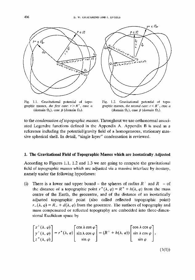
Fig. 1.1. Gravitational potential of topo- Fig. 1.2. Gravitational potential of topographic masses, the first case: r > R +, case a graphic masses, the second case: r < R +, case a

(domain fll), case/3 (domain f~2). (domain 1)1), case 13 (domain 1)2).

to the condensa t ion o f t opograph ic masses . Throughout we use orthonormal associated Legendre functions defined in the Appendix A. Appendix B is used as a reference including the potential/gravity field of a homogeneous, stationary massive spherical shell. In detail, "single layer" condensation is reviewed.

1. The Gravitational Field of Topographic Masses which are Isostatically Adjusted

According to Figures 1.1, 1.2 and 1.3 we are going to compute the gravitational field of t opograph ic masses which are adjusted via a massive interface by isostasy,

namely under the following hypotheses:

(i) There is a lower and upper bound - the spheres of radius R ÷ and R_ - of the distance of a topographic point r+(A, ~) = R + + h(A, ~) from the mass centre of the Earth, the geocentre, and of the distance of an isostatically adjusted topographic point (also called reflected topographic point) r_ (A, q~) = R_ + d(A, q~) from the geocentre. The surfaces of topography and mass compensated or reflected topography are embedded into three-dimensional Euclidean space by

[cos,cos 1 Fcos co l y+(A,~) =r +(A,~)|sin~cos~|--(R ++h(A,~))|sinAcos~|, z +(A,~) iL s in~ /d iL s in~ id

(1(1))

n+ + h(a,~,)

/i

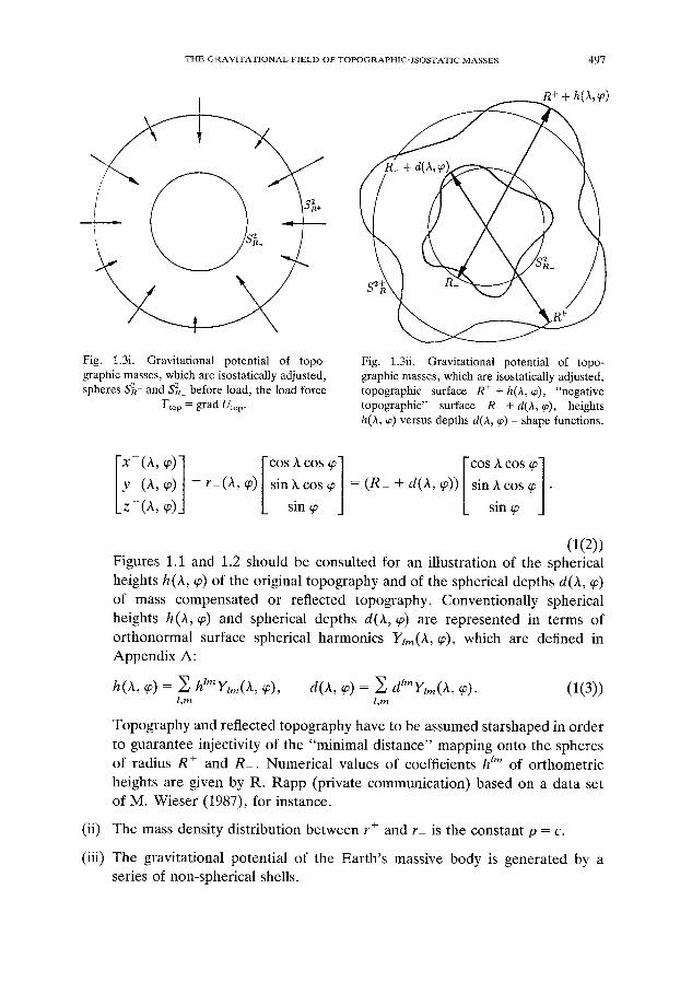
Fig. 1.3i. Gravitational potential of topographic masses, which are isostatically adjusted, spheres S 2+ and S 2_ before load, the load force

Ftop = grad Utop.

T H E G R A V I T A T I O N A L F I E L D O F T O P O G R A P H I C - I S O S T A T I C M A S S E S 497

Fig. 1.3ii. Gravitational potential of topographic masses, which are isostatically adjusted, topographic surface R ÷ + h(•, q~), "negative topographic" surface R_ + d(a, q~), heights h()t, q~) versus depths d(2t, p) - shape functions.

co cos: l cos cos:l y - ( A , ~ ) = r (a, q)) ] sin k cos = ( R _ + d ( a , ~ ) ) / s i n a c o s .

_z- (a ,~) k sinq~ k sinq~

(1(2)) Figures 1.1 and 1.2 should be consulted for an illustration of the spherical heights h(a, q~) of the original topography and of the spherical depths d(a, ~) of mass compensated or reflected topography. Conventionally spherical heights h(& q~) and spherical depths d(a, ~) are represented in terms of orthonormal surface spherical harmonics Y~m(a, ~), which are defined in Appendix A:

h(a, q~) = E h'my, m(2t, q~), d(a, ~) = • dZmy~m(a, q~). (1(3)) l ,m 1,m

Topography and reflected topography have to be assumed starshaped in order to guarantee injectivity of the "minimal distance" mapping onto the spheres of radius R + and R_. Numerical values of coefficients h ~m of orthometric heights are given by R. Rapp (private communication) based on a data set of M. Wieser (1987), for instance.

(ii) The mass density distribution between r + and r_ is the constant p = c.

(iii) The gravitational potential of the Earth's massive body is generated by a series of non-spherical shells.

498 E.W. GRAFAREND AND J. ENGELS

The non-spherical shell between r + (topography) and r_ (isostatically adjusted interface) is just the uppermost shell; the other shells, in particular their mass density distribution, may be taken from a standard Earth model, e.g. the P R E M model of A. Dziewonski and D. Anderson (1981). Corres- pondingly the gravitational field of topographic masses which are isostatically adjusted may be represented by the potential

U(A, p, r) = Utop(A, ~, r) + Ustat(a, @, r) =

f 2 ~ f + ~ / 2 f ~ + + h(A', ~ ')

= gp ] dA' | dq~' cos ~D' JR J 0 J - - ~ / 2 +

r , 2 dr' +

~/r 2 + r '2 - 2rr ' cos

2~" +-rr/2 R +

+ g P f o d A ' f dq~' cos q~' fR J --rr/2 - + d ( A ' , ~o')

r ,2 dr'

~ / r 2 + r '2 - - 2 r r ' c o s ~ -

r ,2

~ / r 2 + r '2 - 2 r r ' cos~"

f 2 ~ r (- + 7r/2 f R + + h ( X ' , ~ ' )

= g P l da'l cos dr' d O d - - ~ 1 2 3R_+d(A',q~')

(1(4))

(iv) The simple hypothesis of isostasy states a linear relation of heights and depths (topographic-isostatically adjusted interface) according to

h lm = - Co d im ; 1(5i)

the more advanced hypothesis

him(t ) = - ~ @q( t )dPq( t ) 1(5ii) P , q

relates linearly the time-varying height components hU' ( t ) to time-varying depth components dPq(t) by the time-dependent structure coefficients

l m C p q ( t ) . The indices l; p run 0, 1 , . . . , ~, but the associated indices m; q run - l , - l + 1 , . . . , l - 1, l; - p , - p + 1 . . . . . p - 1,p, respectively.

At first we are going to compute the topographic potential Utop( /~ , ~D, r) generated by the topographic masses between R + and R + + h(A, p), before secondly we compute the isostasy potential U~tat(A, p, r) being generated by the shell masses between R + and R_ + d(A, q~), the isostatically adjusted interface.

1 . 1 . T H E T O P O G R A P H I C P O T E N T I A L

The topographic potential U, op will be represented (i) for the case r t> R ÷ and (ii) for the case r ~< R + due to convergency regions of a series expansion of the Newton kernel (r e + #2 _ 2rr' cos 'It) -1/2.

T H E G R A V I T A T I O N A L F I E L D OF T O P O G R A P H I C - I S O S T A T I C MASSES 499

The first case: r i> R +.

Consider a computation point r > R + on top o f the reference sphere R +. Due to the distribution of topographic masses we separate two domains ~ and ~2 such that ~ , U ~'~2 = $ 2

(~) a , : = { a ' , ~ ' l r > / + + h ( a ' , ~ ' ) } ~ S 2,

(ffi) ~~2 := { at, @' [ r < g + + h(A', ~')} E S 2

hold. Accordingly we represent the topographic potential by

Utop(A, ~, r/> R +) := g P f a dA' d~' cos ~' x 1

I R + + h ( X ' , p ' )

× dr' JR +

r ,2

~/r 2 + r '2 - 2rr' cos

+ gP f a dA' dq£ cos q£ × 2

I R+ +h(X',~ ' )

× dr' J R +

r,2

X/r 2 + r '2 -- 2rr' cos

(1(6))

Because of r ' < r within the f irst term Utopl the N e w t o n kernel can be developed into uni formly convergent series such that

fo. (R++h(X''~') r 'l+2 1 Utop, (a, q~, r) = go da' dqY cos qY dr' ~ /+1

1 JR + l,m 2l + 1

x Ylm(A, ~)Ylm (a t, ~ , ) =

= g p f da' d~' cos ~ ' H { r - (R + + h(A', ~'))} x Js 2

× ~; (R + + h (a ' , ~ ')) '+~ - R +'+~ +' ~, Y,~(a, ~ ) h ~ ( a ' , ~ ' )

,=o (1 + 3)(2l + 1)r '+* m=-,

(1(7))

holds. Alternatively within the second t e r m Utop2 the N e w t o n kernel has to be decomposed according to r' < r or r' > r, respectively, into

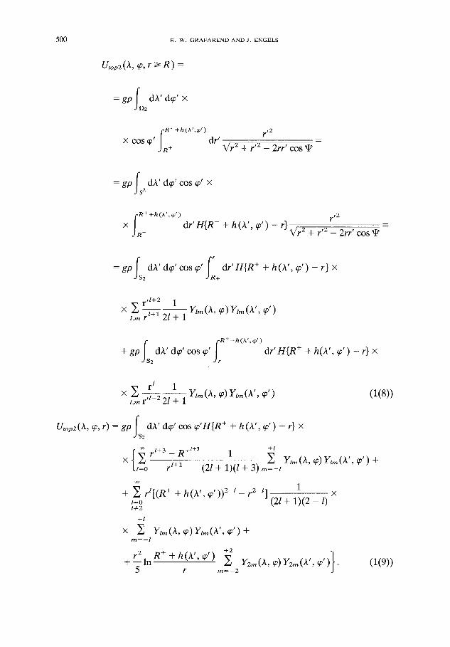
500 E. W. GRAFAREND AND J. ENGELS

Utop2 ( h, ~, r >! R ) =

= gP f n dA' dp ' × 2

i R++h (A',qo

x cos ~p' dr' J R +

r , 2

~ / r 2 + r '2 - 2rr' cos xt r

f = gp JS 2 dh' dq~' cos q~' x

j -R +h (h', q' ) r,2

x d r ' H { R + + h(A', q~') - r}~/r 2 + r' 2 _ 2rr' cosXI r R +

L L = g p dA' d~D' cos q~' d r ' H { R + + h(A', ~D') - r } × 2 +

x ~ r"+2rl+l - - 1 Ylm(l~ ' ~ )Y lm(A , ' ~t) 1,m 2l + 1

fS I R + + h (A" q#) + gp dA' dq~' cos ~' dr' H { R + + h(A', p' ) - r} × 2 Jr

r l 1 x ~ r,,_2 2 ~ - Y/re(a, qo)Y/m(A', q~')

1,m + 1

Utop2(l~, ~, r) = gP fs dA' dq~' cos ~ ' H { R + + h(A', q~') - r} × 2

+l

x r T+7 (2/71- 1)(/ 71- 3) m=--,

+ ~ r ' [ (R + + h(A', q~,))2-, _ r2 -q /=0 l¢2

+l

x ~ Y , m ( A , ~ ) Y , m ( A ' , ~ ' ) +

+2 r 2 R + + h ( A ' , q ~ ' )

+ - - In 5 r m=--2

( 2 l + 1)(2 - l) X

Y:m(A, )Y2m(a',

(1(8))

(1(9))

THE GRAVITATIONAL FIELD OF TOPOGRAPHIC-ISOSTATIC MASSES 501

In summarizing, in the first case we generate the topographic potential

Utop(A, 9, r i> R +) = Utop~ (A, 9, r; a l ) + Utop2(A, 9, r; Ft2) =

= gPfs dA' d9' cos 9'{H[r - (R + + h(A', 9'))] × 2

x ~ [R+ + h (A', 9' )],+3 _ R +'+3

l=0 r l+1 ×

+l

1 2 Ylm()t , 9 ) Y l m ( ) t ' , 9 ' ) + (21 + 1)(l + 3) m=--,

r ~ rl+3 _ R +l+3 1 + H[R + + h(a', 9') - rl 1 2

/ l = 0 (2l + 1)(l+3) ×

÷l × 2

m ~ m l g l m ( 1~, 9 ) Y l m ( a ' , 9 ' ) +

+ 2 {r'[R + + h(a ' , 9 ' ) 1 2 l __ r2-l} . 1 ,=o (2l + 1)(2 -- l) l:~2

× +l

Y/m(/~, 9 ) g / m (/~,, 9 ' ) + m = - - l

Here we apply

2 r 2 R + + h(A', 9') --Y, Y2m(A, 9)Y2.,(A', 9 ' ) ] l + - - In (1(10)) JJ 5 r m = - 2

H{r - [R + + h (A, 9)1} + H{ R+ + h (A, 9) - r} = 1,

H { r - [R + + h(A, 9)]} = 1 - H{R + + h(A, 9) - r}, (1(11))

in order to arrive at the final form 1(12) of the topographic potential, first case (r t> R ÷ ). In addition, Figure 1.4 collects details of the logical tree of decompositions for the series expansion of the first part of the topographic potential.

Otop(/~, 9 , r ~ R +) =

+l

x m=-, ~ Y,m(a, 9)V,m(a', 9')} +

(2I + 1)(l + 3) )<


domain ~1 ] domain ~2

ifR +~<r'~<R ++h(,V,q~') if R + < r ' < r , if r < r ' < R ++h(a' ,p ' ) , then r' < r then r' < r then r < r'

Uropl Utop2

Fig. 1.4.

I Height series expansion of topographic ]

kernel functions, first case, r > R + I Topographic potential, logical tree of decompositions for series expansions, zone A: r t> R ÷

(first case).

m R + + h(h ' , ~')) - r}[ ~ r'+3 - [R+ + h(h ' , ~')1/+3 1 at=0 r l+1 (2l + 1)(l + 3)

+ l

X E Ylm(A, ¢P)Ylm(h', ~P') 4- m= --l

×

4- cc + l

~] rl{[R + + h(h ' , ~o')] 2 - ' - r 2-t} ~] Ylm(l~ ' ~O)Ylm(1V, ~t) q_ ,=o (2l + 1)(2 - I) m = - - l H:2

r 2 R + + h ( A , , ~,) 2 ] ] + - - I n ~ Y2m(A, ~)Y2m(A', q~') • (1(12)) ]J 5 r r n = - 2

Conventional ly the topographic kernel functions within the topographic potential 1(12), first case r/> R +, are developed into height series according to

h " l+3 (R + + h) '+3 = R +'+' 1 + ~-7] ] =

[ R27 1 h 2 -- R +~+3 1 + (l + 3) + 2 (l + 3)(I + 2) R+2-- + (1(13))

1 h3 (h4)l + - (l + 3)(l + 2 ) ( / + 1) - - + 0,+3

6 R +3 ~ '

(R + + h ) 2 _ 1 = R+2-~(1 + ~_7) = h " 2-I

[ h2 = R +2-' 1 + ( 2 - I ) ~ + ( 2 - l ) ( 1 - I ) (1(14))

R + R +2


(2 - I ) (1 - l)l ~-- 7 + 02-- 1 ~ ,

ln(R+ +h)=lnR+(l + ~ ) = l n R + +ln(l + ~ ) =

h l h 2 l h 3 (h~4) l nR + + R+ 2 R +2 3 R +3 (1(15))

which lead to the following topographic kernel functions

(R + + h)/+3 - R +'+3 1

r t+~ (l + 3)(2 /+ 1) =

1 R +I+2 1 l + 2 R +z+l - - h + h2+

- 2 1 + 1 r 1+1 2 2 l + 1 r l+*

1 (l + 2)(• + 2) R +'

6 21+ 1 r l+1

(1(16))

h 3 + Ol(h 4)

r2 R++h r2 R+ rZFihL 1 h 2 1 h 3 J] l n - - - l n - - + - - R+ - - + - - - + o a ( h 4) . (1(17))

5 r 5 r 5 2 R +2 3 R +3

We have to notice that for large values of the exponent l within (R + + h) t+3 or (R + + 1) 2-I the effect of nonlinearity is central: E. H. Knickmeyer (1984, p. 23) has shown that in this case the linear approximation is too poor. Finally we represent the topographic potential, first case r/> R +, in terms of topographic kernel functions which have been expanded into series.

zone A: r >/R +,

Utop (A, ~, r I> R + ) = I , (h) + / 2 (H) + / 3 (/-/) + 14 ( / ~ +

+ Is(h, H) + I6(h, H),

I , ( h ) : = E E gp l=o m=--l 3 2l + 1

dA' d~p' cos ~' x

X h(A', ~ ' ) x [1 + l+2h(A', qY) R + L 2 R +

(1(18i))

X Ylm()t, ~)Ylm()[', ~0'),

(l + 2)(l + 1) h2(A ', q~') + 03 ] x t-

6 R += /

X +l 4 ~ . R + ~ R +, 3

12(H) := - ~] ~] gpr,+a , = 0 m = - - , 3 (2l + 1)(I + 3)

(1(18ii))

504 E, W, GRAFAREND AND J. ENGELS

fs R+t+3 - - rl+3 1 ~, x ~ 2 da ' dq~' cos x H { R + + h ( A ' , q ~ ' ) - r } R+,+ 3 x

I3(a9 := -

x Yzm(A, ¢)Ylm(~', ~ot),

~ ~+l 4~rR+3 rl 3 t=o ,,,=-~ 3 gP R t+---S (2l + 1)(2 - l) 14=2

X

~ fS R + t - 2 - rl-2 1 ~, x x dA' dq~' cos x H{R + + h(A', ~D') -- r} rt_2 2

(1(18iii))

X Ylm(~, ~)YIm(A', ~ ' ) , ( 1 ( 1 8 i v ) )

+ 2

I4(H) := ~ 41rR+3 r 2 1. R + 1 f s q~' m=--2 3 gp~-~-~51n 7 ~ dA' d~p' cos ×

2

X H{R + + h(A' , q~') - r} Y2m(A, (p) Y2m(A', q~')

o~ +l 4~rR+3 R +' 3 I5(h, H) := - ~, £

l=o m=-l 3 gP r l+1 2l + 1 m X

(1(18v))

~L ~'H{R+ +h(A ' '~ ' ) r} x dA' dq~' cos 2

x h(a" ~') [ R + 1 + l + 2 h(A' , q ~ ' ) _ _ 2 + R - - +

+ (I + 2 ) ( / + 1) h2(A ', ~ ' ) 6 R +2

-F 032] Ylm(A, q~)Y/m(A', q)'),

= +l 47rR+3 rl 3 I6(h, H) := ~] £ gpR+,.~

l=om=-t 3 21+ 1 i X

(1(18vi))

1 L h(a', ~') x ~ d a ' d ~ ' c o s ~ ' g { R + +h(a',~')-r}x R------v---x 2

x [1 + 1 - lh(A', ~') (1 - l)lh2(A ', ~') L 2 R + 6 R +2

+ 033] x (1(18vii))

x Y,,,,(a, ~)Y,m(a', ~').

The following comments on the various topography integrals I1 . . . . . 16 can be made. The first integral Is (h) refers to a vo lume potent ial decreasing by r -~ - I and represents in s tandard form - see, for instance R. R u m m e l et al. (1988) - the

THE GRAVITATIONAL FIELD OF TOPOGRAPH1C-ISOSTATIC MASSES 505

influence of topographic heights in a series expansion. All the other integrals depend on the Heavis ide func t ion H { R + + h(h, ~ ) - r} reflecting the slices of infinitesimal massive shells. I2, /3 and /4 are independent of topographic heights and vary proportional to r -l-~, r t and r2/5 In R+/r . I5 and 16 vary according to r -l-1 and r ~ respectively and depend on topographic heights in a series expansion. Since the integrals I2 . . . . ,/6 have no global suppor t due to the kernel Heaviside function, they can only be evaluated numerically. In terms of topographic heights the series of kernel functions are written in such a way that they make the limit h --, 0, but ph obviously f ini te , a result which we later need for the condensat ion

o f topographic masses.

The second case: r ~ R +

Consider a computation point r < R ÷ under the reference sphere R ÷. Due to the distribution of topographic masses we separate two domains f~l and ~2 such that 121 U 122 = S 2

(a) 121 := {h', q/I r > R + + h (h', q~')} E $2;

(/3) 122 := {,v, ~ ' [ r < R + + h (h ' , q~' )} ~ S 2,

hold. Accordingly we represent the topographic potential by

~ , r < ~ R + ) ' = g p ~ d h ' d q ; c o s ( x U t o p ( / ~ , J a 1

j -R +h (h ' , ~ ' ) r r2

X dr' + R + ~/r 2 + r '2 - 2rr' cos

+ gP f a dh' d~' cos q~' × 2

I -R +h (A', ~' ) r t2

x dr' R + X/r e + r '2 - - 2rr' cos ~ " (1(19))

Within the f i rs t t e r m g t o p 3 the N e w t o n kernel has to be decomposed according to r' < r or r' > r, respectively, into

g t o p 3 (A, ~ , f ~ R + ) =

= gp dh' de ' cos q~' dr' ~ ~ × 1 I-J r l ,m r

X - - 1

2 l + 1 Y l m ( ~ , ~ ) Y l m ( ~ ' , ~ ' ) ~- dr' _ ×

+


X - - 1

2 l + 1 Ylm()t' {D) Ylm(l~" ~)')1 =

= g P f s da' d~' cos 9 ' H { r - [R + + h(a', ~')]} × 2

X £ [R + + h(Z, ~')]'+3 _ r'+' x 1 1,m r '+ t ( l + 3)(2• + 1)

X Ylm()t, 9) Ylm(tV, ~') + gl f S da' d~' cos ~p' x 2

+l

×,,{r- [ , ,+ + Z m = - - l

l=1=2

(r 2-1 -- R +2 *)r l x

1 X Ylm(}[, ~O) Ylm(,~' , (Or) "{-

(2l + 1)(2 - / ) +2

r25 r 1 + - - I n 7 m__~ - ~) Y2~ (A' ~ ' 2 Y 2 m ( ~t , , ) • (1(20))

Alternatively the second t e r m Utop4 is decomposed similarly

U t o p 4 ( } t , ~ , r ~ R +) =

fs IR++h(X"~') rl l = gp dh' dq~' cos ~' dr' ~ r,l_ ~ 2 J R + 1,m 2l + 1

m X

x r,m(a, ~)r,m(a', ~')

= g P ; s dA' d~' cos 9 ' H { R + + h(A', ~') - r} x 2

o o +l

X ~ ~ rl{[R + + h(A', ~p,)]2-t_ R +2-'} X 1=0 m = --I l=#2

(21+ 1)(2-1) r2 L Yl,,, (k, q~) Yz,,, (k', ¢p' ) + g P - 5 dA' de' cos ~' x

2

x H { R + + h(X', ~') - r}ln R + + h(a', ¢')

R + +2

X ~ Y2m (1~, ~ / ) ) Y 2 m ( / V , {Dr). m = - - 2 (1(21))

In summarizing, in the second case we generate the topographic potential


g t o p ( / ~ , @, r < R +) = Utop3(A, q~; f~l) + gtop4(~, @; ~-~2) =

= gp fs 2 dA' dq~' cos ~'H{r - [R + + h(A', qY)]} x

x ~, 1 ~,)1,+3 r,+3} ,,m r -77+' x { [R + + h (a ' ,

(2l + 1)(l + 3)

x Y,m(A, q~)Y,m(A', qY) +

+ gp fs 2 dA' dqY cos p'H{r - [R + + h(k ' , ~')]} x

oo + l

x • ~ r'(r 2 - ' - R +2-') 1 1 = 0 m = - - I (2l + 1)(2 - / ) 14=2

X

x Ylm(A, ~)Ylm(A', qY) +go fs 2 da ' dqY cos q~' x

r 2 _ _ r x H{r - [R + + h (a ' , p')]} • 5 In R + x

+ 2

m ~ --2 Y2m(h, q~)Y2m(A', qY) + gp fS 2 dA' d~' COS q~' X

xH{R + + h ( A ' , q y ) - r } x ~ ~ r'{[R ++h(A',~')]2-' l = 0 m = - - I l=~2

_ R +~- ' } (2l + 1)(2 - / )

x Y,m(a, ~)hm(a ' , ~') +

+ gp fs 2 dA' dqY cos ~'H{R + + h(A', q~') - r} x

r 2 R + + h(A', ~') x - - In

5 R + X

+ 2

X ~ Y2m()t, (4 ) )Y2m(/~ t , ~ o ' ) . ( 1 ( 2 2 ) ) m = --2

By applying 1(11) we arrive at the final form 1(23) of the topographic potential ,


i f r < r ' ~ < R ++h(A ' ,~ ' ) then r' < r

N

domainC21 11 domainS2 [

i fR ÷ < r ' < r , i fR ÷~<r'~<R ÷ + h ( h ' , q ' ) , then r < r' then r < r'

/ Utop3 Utop4

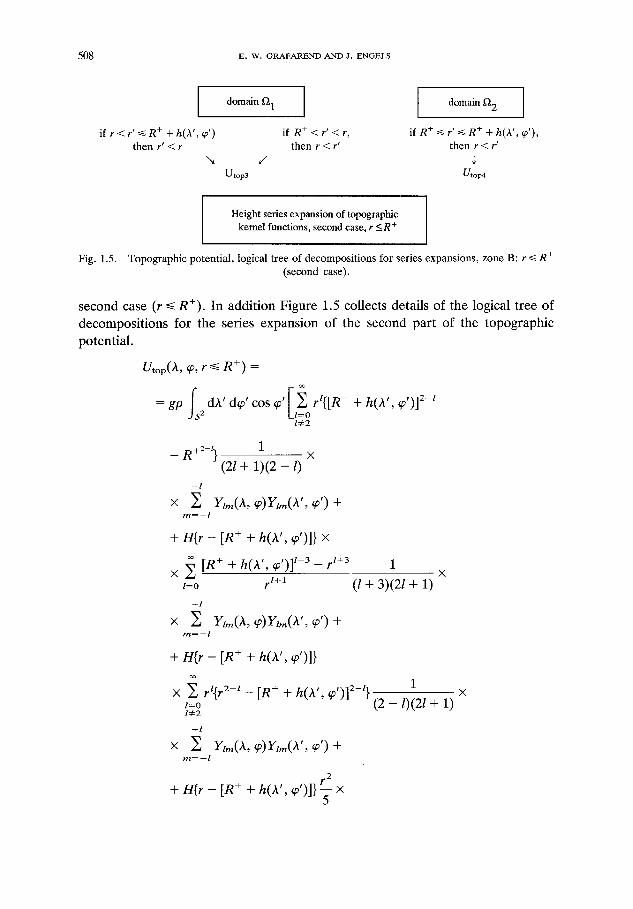
Fig. 1.5.

Height series expansion of topographic kemel functions, second case, r _< R +

Topographic potential, logical tree of decompositions for series expansions, zone B: r ~< R ÷ (second case).

second case (r ~< R+). In addition Figure 1.5 collects details of the logical tree of decompositions for the series expansion of the second part of the topographic potential .

Utop(/~,

= g p

q~,r~< n ,t~+) co

f S2 da' dq~' cos qY [l~o rl{[R+ + h(h ' (19t)] 2 - I

14=2

+2--I 1 X

- R }(21+ 1 ) (2 - 0 +l

x ~ Y,~(A, ~)Y,m(h', ~'1 + m = - - l

+ H { r - [R + + h(h' , ~')1} x

x ~ [R+ + h(h', ~,)]t+3 _ r,+3 X

l = 0 r l+1

+ l

X E Ylm(h, ~)Ylm(h', ~o') + m=--l

+ H { r - [R + + h(h ' , (p')]}

X ~ rl{r 2 - t - [R + + h(h', ~,)12-l} l=O l ¢ 2

+ l

x ~ Y,,,,(A, ~O)Ylm(IV , ~ot) + m=--I

r 2 + / - / { r - [R ÷ + h(A' , ~')1} 5 x

( l + 3 ) ( 2 l + 1 )

(2 - l)(2l + 1) X

THE GRAVITATIONAL FIELD OF TOPOGRAPHIC-ISOSTATIC MASSES 5 0 9

+2

x In r ~ Y2,,(A, P)Y2m(A', q~') + R + + h(A', q~') m = - - 2

+2 r 2 R + + h(A' , g~') £ Y2m(A, g0Y2m(A', q0')l + -- In R +

m=--2 (1(23))

Again we expand the topographic kernel functions within the topographic potential 1(23), second case r ~< R ÷, into height series according to 1(13), 1(14), 1(15) which leads us to the following topographic kernel functions

r'{[R + + h(A', q~,)]2-, _ R+2-,} 1 (2l + 1)(2 - / ' )

_ 1 rlR+Z-,~h_ + 1 h 2 1 h 3 -21+---~ LR + 2(1- / )~ -6(1- l ) l - -+ R +3

+ o2-z -- In (1(24)) 5 r

We draw attention to our former statement about the nonlinearity of the series expansion of topographic kernel functions with respect to height. Finally we represent the topographic potential, second case r ~< R ÷, in terms of topographic kernel functions which have been expanded into series.

zone B: r ~< R + ,

gtop(A, ~, r ~ R +) = J l ( h ) + J2(H) + J3(H) +

+ J4(H) + Js(h, H) + J6(h, H), ÷l

Jl (h) : = ~] ~] 4~rR+3 r ' 3 1 fs ~' /=0 m = - - l 3 gP R +~+~ 2l + 1 4~r 2 dA' de ' cos x

(1(250)

h(a ' , q/) [ 1 - lh (a ' , ~') (1 - l)lh2(a ', ~') R + L 1 + R ~ 2 6 R +2

+ 03] x

x Y,.,(a, (1(25ii))

+t R +l 3 1 ( Jz(H) := - ~ ~ 4rrR+BgPrt+~ Js dA' dq~' cos q~' ×

~=0m=-, 3 (2l + 1)(l + 3) 4~r 2

r l+3 _ R +1+3

× H{r - [R + + h(A', q~')]} R+,+3 Ytm(a, ~)Y~m(A', ~ ' ) ,

(1(25iii)


J~(H) := - 2~ 4,~R+~ / 3 1 ~, l=Om=--I 3 gpR+,+l(2l+ l ) ( 2 _ l ) 4 ~ r 2dA'd~ 'cos x 14=0

r 1-2 _ e + / - 2

x H{r - [R + + h(A', q/)]] rl_2 Y,m(A, ~)Ylm( )t', ~') ,

(1(25iv))

+2 47r +3 P 1 In R+ 1 I dA' d(#' cos q~' x J 4 ( H ) : = - m= ~ - 2 3 R g P ~ 5 5 - 7 4--~ 3S 2

x H{r - [R + + h(A', q/)]} Y2m(l~, (p)Y2rn(/~', (p'),

+t 41rR+3 R+l 3 1 Js(h, t-1) := ~] ~ X

l=Om=--I 3 gP f l+121+14rr

(1(25v))

x fs2 dA' dq~' cos q/H{r - [R + + h(A', q/)]} h(A',R +q/) x

[1 + l + 2 h ( A ' , q/)F(I+2)(I+ 1) h2(A ', ¢')+ o~]x X

L 2 R + 6 R +2 J

X Y l m ( } t , ~ ) Y l m ( l ~ ' , ~O'),

+l l ~, 47r +3 r 3 1 x

J6(h,H) := - ~=Om~_,3R gP-~Zr~-+ 147r

(1(25vi))

x f s = dX' dq/cos q/H{r - [R + + h(X', q/)]} h(k',R +q/)

1-1 + 1 - l h(h', ~') (1 - / ) l hZ(h ', ~') X L 2 R + 6 R +2

x Y,m('~, e)r,m(,V, ~').

m X

(l(25vii))

+ 4 ] x

The following comments on the various topography integrals J 1 , . . . , J6 can be made. The first integral Jl(h) refers to a volume potential increasing by r l and represents in standard form the influence of topographic heights in a series expansion. All the other integrals depend on the Heaviside function H{r - [R + + h(h', ~0')]} reflecting the slices of infinitesimal massive shells. J2, J3 and J4 are independent of topographic heights and vary proportional to r -~-1, r ~ and l/5r21n R+lr. J5 and J6 vary according to r -t-1 and r t, respectively, and depend on topographic heights in a series expansion. Since the integrals J2, •. •, J6 have no global support due to the kernel Heaviside function, they can only be evaluated numerically. In terms of topographic heights the series of kernel functions are written in such a way that they make the limit h --+ 0, but ph obviously

THE GRAVITATIONAL FIELD OF TOPOGRAPI-IIC-ISOSTATIC MASSES 511

finite, a result which we later need for the condensation o f topographic masses. Comparing Equations 1(18) and 1(25) it can be seen that formally J1 + J6 = 16 and Js = /1 + 15.12, 13, 14 differ with respect to J2, J3, J4 only by the Heaviside functions. or r = R + the integrals I2, 13, 14 and J2, -/3, J4 vanish.

Finally we take advantage of the global representation 1(3) of the shape functions h(A, ~) = hlmylm. Here we apply the summation convention over repeated indices: The first index runs 0, 1 . . . . , % but the second index - l , - l + 1 . . . . , - 1 , 0, +1 . . . . . l - 1, l. In addition we apply the scalar product re-

lation (Yllml I Yl212) = ~ll12~mlm2 of orthonormal associated Legendre functions and the Gaunt -Wigner coefficients G within the product-sum relation - we refer to H. W. Mikolaiski and P. Braun (1988) -

Yllml Ylzm2 lm = Glll~mlmzYlm, Ill - lz] <~ l <~ ll + 12, m = - I m l + m2l, (1(26i))

= Glll213mlm2m3Ylm, ( 1 ( 2 6 i i ) ) Yllml Yl2m2 Yl3rrt 3 lm

For the topographic potential, zone A: r ~< R +, as well as zone B: r/> R ÷, we obtain accordingly the topography integrals, e.g., Ii(h) and Jl(h), respectively,

l R+Z 3 h llml el(h) = 47rR+3gP3 ~=o ~ m= ~- I r t+l 2 ~ - + 1 Ylm(A, q~) R ~ ×

| [3ld6mlm q- l + 2 h 12m2 Zm × L 2 R + Glll2mlm2 q-

+ (l + 2)(• + 1) hl2m2h 12m3 lm ] 6 R +2 Gl'1213m'm2m3 + 03, , (1(27))

4'/T +3 oo l rl hllml

J l ( h ) = T R gp l~o= m E ,=-- R -~'+1 2l ~3+1 glrn('~' q)) R - - - ~

L ~6lll6rnlm "Jr- 1 -- l h tzm2 lm N 2 R + Glll2mlm2-

×

(1 - l)l ht2mzh t3m3 l,~ ] 6 R+2 Glll213mlm2m3 + 0 3 , (1(28))

Briefly we collect the results for the representation of the topographic potential by

Corollary 1. (topographic potential, series expansion): For a topographic surface which extends by r >i R + or r <~ R +, respectively, R + being the radius o f the topographic reference sphere, the potential can be represented by


Utop(/~, ~9, r ) ~-- Vtop(/~ , ~p, r ~ R +)H(r - R +) + Vtop(,~ , ~, r <<- R +)H(R + - r), (1(29))

where Utop(h, ~, r I> R+), Utop(h, ~o, r <~ R +) are given by 1(12), 1(22), respectively. I f we expand the topographic kernel functions in series with respect to spherical height h(h, q~) according to 1(13), 1(14), 1(15), 1(24) we are led to the representation 1(18), 1(25) of the topographic potential

6 6

Vtop(]~, ~D, r) = ~ I iH(r - R +) + ~, J]H(R + - r). (1(30)) i= l j = l

In the case that we neglect the terrain topographic effects, namely by using a global representation 1(3) of the shape functions h(A, ~), we obtain the topographic potential 1(30) in terms o f shape coefficients h .1ml, hllmlh 12m2, hllmlhl2m2h 13m3 etc., e.g. by 1(27), 1(28).

I f the radial coordinator r = R + + & = R+(1 + &IR +) is expanded, then in linear approximation 6rlR + the integrals 12 + 13 + 14 = O, I5 + 16 = 0 as well as • /2 + J3 + J4 = 0, ./s + ./6 = 0 disappear leaving Utop(a, q~, r) only in terms o f 11 and J1, respectively.

In order to prove

1 2 + 1 3 + 1 4 = 0 , J 2 + J 3 + J 4 = O ,

/5 q- I6 = 0 , J5 q- J6 = 0

it is sufficient to implement the linear approximations for small l

rZ+l R+ 1 - ( l + l ) ,

r l 1 ( 6 r ) R T l + l - R + 1 + l ~ - 7 ,

3r Rl-Zr 2-l -- 1 + (2 -- l) - - R +

(R+)- l -3r ~+3 -- 1 + (l + 3) ;_jr+

R + 1 3r r 2 In "--

r R + R +

For very large l these approximations do not hold, of course.

1.2. T H E POTENTIAL OF TOPOGRAPHIC MASSES WHICH ARE ISOSTATICALLY ADJUSTED

The gravitational field of topographic masses which are isostatically adjusted has been represented according to 1(4) by

THE GRAVITATIONAL FIELD OF TOPOGRAPH1C-ISOSTATIC MASSES 513

f•-rr ~ + r r / 2

Ustat(/~, ~, r) = gp dA' dq~' cos q~' d -- ~r/2

f~+ r t2 dr' -+d(,~',~') ~/r 2 + r '2 -- 2rr' cos

(1(31))

We start with the case r 1> R +, namely a position of the evaluation point outside the sphere of radius R +. Series expansion of the Newton kernel and radial integra- tion leads us to

gstat(/~, q), r >i R +) =

fs ~ R +'+3 ~, ' ) ] /+3 = gp dA' dq< cos ~' - [R_ + d(A', 2 1= 0 r l + 1

×

+1 1

X X ~ Ylm(t~, ~l~)Ylm(IV , ~9'), ( 1 ( 3 2 ) ) (2l + 1)(l + 3) m = - - I

The depth series expansion of the kernel function which is of type 1(13), namely

+ 3

(R_ + d) '+3 = R ~ 3 ( 1 + - - =

_ _ + ( l + 3 ) ( I + 2 ) ( l + 1 ) d 3 x

6 R 3_ = R Z - + 3 F l + ( l + 3 ) d ( l + 3 ) ( l + 2 ) d e

/ R _ 2 R 2 _

x 0,+3 , (1(33))

allows the potential representation in terms of 'negative topography integrals' K1 and Kz(d).

Ustat(A, ~, r/> R +) = K1 + Kz(d), (1(34i))

K1 := 4~rR +3 R +3 _ R3 - 1 (1(34ii)) 3 go R+3 r '

+~ 4rrR3 R l_ 3 ~'rr fs dA' dq~'cosq~'d(A"q<) x K2(d) : = - - ,=o £ , u f f - , 3 -gPr-77-+121+ 1 2 R_

x [ l + l + 2 d ( A ' , p ' ) + ( l + 2 ) ( l + l ) d 2 ( A ' , p ' ) ( d~_)] 6 - + o ×

X Ylm(l~, ~)Ylm(A t , ~ ') , ( 1 ( 3 4 i i i ) )

We only notice that by a global representation 1(3) of the shape functions d(A, q~) =

514 E. w. GRAFAREND AND J. ENGELS

dtmytm ( s u m m a t i o n ove r r epea t ed indices), we could der ive a r ep resen ta t ion of

the 'negative topography integrals' similar to 1(27), 1(28). Wi th an expans ion of R +3 - R 3_ according to R + = R_ + h +_ we are able to c o m p a r e Ustat(Z, q~, r >I R +) and U(r >I R_ + h +) with a mass ive spherical shell of the r e fe rence example given

in A p p e n d i x B.

R + 3 _ R 3_ = 3RZ_h + + 3R_h +z + h +3,

KI= R 3_ 3 _ + 3 ~ + R L ] r "

(1(35))

(1(36))

For the case r < R + we separa te the integral 1(31) into

Ustat(/~, ~, r < R +) =

fi2~ ~ ~,2 f~+dr, vr2+r,22rr, cosO r ~ = gp dh ' dq~' cos q~' + d -- , r r /2 - --

~ ~-rr/2

+ go dh ' d~p' cos q~' x d -- ~r/2

fR - r '2

x d r ' - + d ~ / / r 2 + r ' 2 - - 2rr' cos ~O

(1(37))

Using R ÷ = R_ + h +_, the first integral can be calculated according to B(1). The

second integral has to be eva lua ted with the same p rocedure we fo l lowed in

p a r a g r a p h 1. W e distinguish the cases r < R_ and R_ < r < R + and obtain:

U~tat(h, q~,r < R_) = 4~rgpR_h + _ 1 + + L~(d) + L2(H) + L3(H) + 2

+ L 4 ( H ) + Ls(d, H) + L6(d, H]. (1(38i))

H e r e the fo rmal ident i ty

Li = -Yl , i = 1 , 2 , . . . , 6 (1(38ii))

holds. W e only have to replace h by d and R + by R_ in the fo rmula 1(25).

Ustat(/~, @ , R _ ~ r < R +) = 2"rrgp{R2-(1 + 2 + h+~ } h _ + _

R_ ~2-_ J - ~ r~

4~r R3_gpl- + M(d ) , 3 r

(1(38iii))

with the fo rma l ident i ty

THE GRAVITATIONAL FIELD OF TOPOGRAPHIC-ISOSTATIC MASSES 5 1 5

M ' = - - I 1 . (1(38iv))

Here we have to replace h by d and R + by R_ in 11 as given by formula 1(18ii). Finally we summarize all results in

Corollary 2. (potential of topographic masses which are isostatically adjusted): The gravitational potential of topographic masses which are isostatically adjusted is given by 1(4) and can be represented by

U(A, 9, r) =

= Utop(h, 9, r >i R +)H(r - R +) + []top(A, q~, r <~ R +)H(R + - r) +

+Usta t (h ,q~ ,r>~R+)g(r -R+)+Usta t (h ,~ , r<R+) , (1(39))

where Utop(A, g,, r I> R+), Utop(A, q~, r ~ R+), Ustat(A, 9, r >i R+), are given by 1(21), 1(22), 1(32), respectively. I f we expand the "topographic kernel functions" as well as the "negative topographic kernel functions" in series with respect to height h(A, ~,) and depth d(A, q~) according to 1(13), 1(14),1(15), 1(24), 1(33) we are led to the representation 1(18), 1(25), 1(34) of the gravitational potential of topographic masses which are isostatically "adjusted"

6 6 2

U(A, q~, r) = E I i H ( r - R+) + E JiH(R + - r) + E K k H ( r - R+) + i = 1 j = l k = l

+ 2~rgp R 2 _ 1 + 2 + - r 2 R_ 3

47rR3-3 gplr + M ] H ( R _ - r).

+

(1(40))

2. Mass Condensation of Topographic Masses

The condensation of topographic masses onto a sphere R + of reference leads to a gravitational potential U.(x)2(2) which is generated by a "single layer" density /x(x +) identified as the product of volume mass density p and the topographic height function h(x+), x ÷ ~ S~+ is an element of the two-dimensional sphere S~+ of radius R +, namely of type 1(1). The result 2(3) can be derived by 1(18) Utop(A, ~p, r ~> R +) and 1(25) Utop(A, q~, r ~< R +) by the limit procedure p -+ ~, h-->0, but ph finite. In particular Iffh), Jx(h) are given by 2(3) since Ii(H), Jj(H) - i = 2, 3 , . . . , 5, 6; j = 2, 3 , . . . 5, 6-approach zero due to

516 E . W . G R A F A R E N D A N D J. E N G E L S

lim H{R + + h - r} = 0, lim H{r - (R + + h)} = 0. (2(1)) h--~O h -+O

R+ ~ r R+ ~ r

Once we compare the potential 1(18), 1(25) of topographic masses and their mass condensation 2(2), 2(3) in Corollary 3 we are led to the following interpretation: In the external distant zone r >> R ÷ the potential 1(18), 1(27) of topographic masses and their single layer condensation 2(2), 2(3i) nearly coincide. They differ with respect to the higher order height terms within Ii(h) 1(27) as well as with respect to the i n t e g r a l s / 2 , . . . , / 6 1(18). In the near zone r/> R_, r ~< R ÷ both potentials differ more dramatically because of higher order height terms within I~(h) 1(27), Jl(h) 1(28) as well as with respect to the integrals / 2 , . . . , / 6 1(18), J 2 , . . . , J6 1(25). In the internal distant zone 0 <r <~ R + the potential 1(25), 1(26) of topographic masses and their single layer condensation 2(2), 2(3ii)) nearly coincide. They disagree due to the higher order height terms within Ja(h) 1(28) as well as with respect to the integrals J2, • • •, J6 1(25).

Conventionally the idea of mass condensation of topographic masses is attri- buted to F. R. Helmert (1903).

Corollary 3. (mass condensation of topographic masses) When the mass density of topography is condensed (in the distributional sense) to "a single layer" /x(x +) = ph(x+), its potential is continuous and can be represented by

fs df~----#(x+) V.(x)=g IIx-x +11' x + E S ~ + , (2(2))

in particular

U,(A, q~, r) =

[ ~ ~ R +l 1 i gphlmY"~(h' q~) /=0 m=-i 4~rR +2 r l+1 2l +

/ ~ ~ +z r ' 1 lgph,~Y,m(h, q~) t.t=o m=_z 47rR R+t+121 +

where

i &lm = ph b~

denotes the "spectral single layer density".

if r>-R +

i f r~<R +

(2(3))

(2(4))


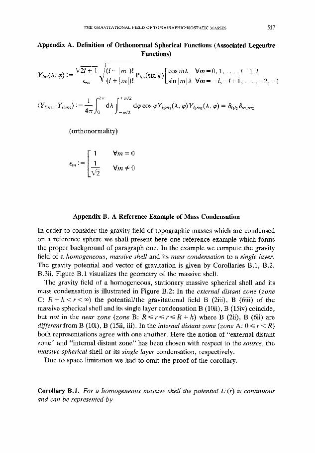
Appendix A. Definition of Orthonormal Spherical Functions (Associated Legendre Functions)

- V m = 0 , 1 , . . 1-1 ,1 Y l m ( A , ~ o ) . - ~ (l Iml)!Pzm(sin~)[-c°smA/.. " ' E m (l + [m[)! ksin ImlA V m = - l , - l + l , . . . , - 2 , - 1

1 ~27r ( + ~ / 2

(Y~lmllYz2m2) := 4---~)0 dAJ-=/2 d~cos q~Y~lml(A, P)Y~2m2(A, ~) = 6Zlt~3mlm2

(orthonormality)

E m : ~

1 V m = O

1 Vm :/: 0

Appendix B. A Reference Example of Mass Condensation

In order to consider the gravity field of topographic masses which are condensed on a reference sphere we shall present here one reference example which forms the proper background of paragraph one. In the example we compute the gravity field of a homogeneous, massive shell and its mass condensation to a single layer. The gravity potential and vector of gravitation is given by Corollaries B.1, B.2, B.3ii. Figure B.1 visualizes the geometry of the massive shell.

The gravity field of a homogeneous, stationary massive spherical shell and its mass condensation is illustrated in Figure B.2: In the external distant zone (zone C: R + h < r < ~) the potential/the gravitational field B (2iii), B (6iii) of the massive spherical shell and its single layer condensation B (10ii), B (15iv) coincide, but not in the near zone (zone B: R ~< r ~< r ~< R + h) where B (2ii), B (6ii) are different from B (10i), B (15ii, iii). In the internal distant zone (zone A: 0 ~< r < R) both representations agree with one another. Here the notion of "external distant zone" and "internal distant zone" has been chosen with respect to the source, the massive spherical shell or its single layer condensation, respectively.

Due to space limitation we had to omit the proof of the corollary.

Corollary B.1. For a homogeneous massive shell the potential U (r) is continuous and can be represented by

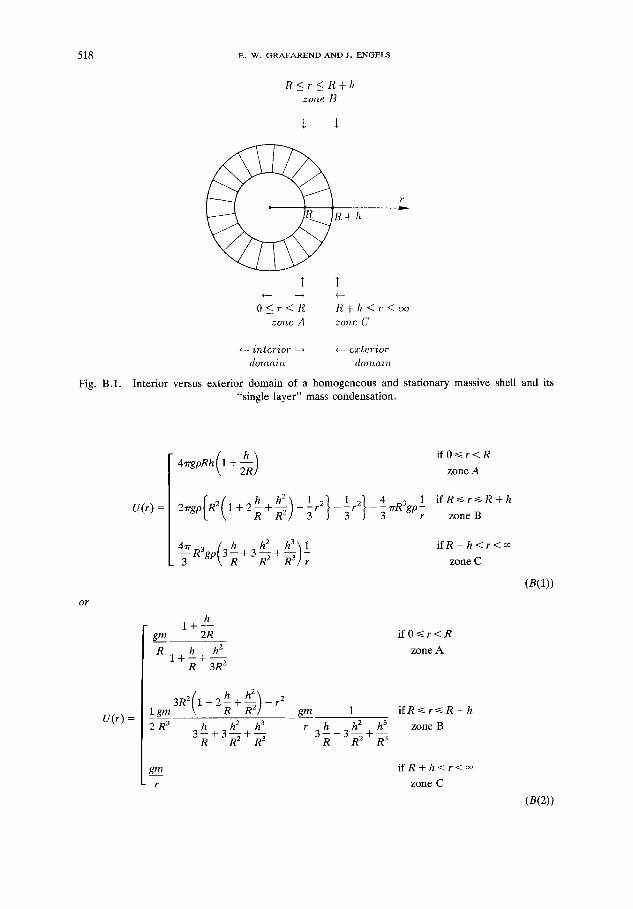
R < r < R + h ZOTle [~

Fig. B.1.

l l

I~. + h

518 E . W . G R A F A R E N D A N D J . E N G E L S

I"

T l 4-- ---+ +--

O _ < r < R R + h , < r < e , z zone A zonc C

~-- interior ---+ +-- cxtcrior domain domain.

Interior versus exterior domain of a homogeneous and stationary massive shell and its "single layer" mass condensation.

o r

U(r) = 2 z r g p f R 2 ( l + 2 h + h 2 ~ _ l r 2 ~ l r 2 ~ 4 3 1 R R2/ 3 j - 3 j - 3 ~ R g P ;

R3gp 3 h + 3 ~ 2 + R ~ r-

i f 0 ~ < r < R

zone A

i f R < ~ r ~ R + h zone B

i f R + h < r < o ~ zone C

u ( r ) =

h l + - -

gm 2R h 2 R 1 + h__+_-

R 3R 2

lgm3RZ( l+2h+hz~-rzR R2/ gm 1 2 R 3 3 h + 3 h 2 + h 3 r 3 h + 3 h : + h 3

R R 2 R 3 R R ~

gm

r

i f O ~ r < R

zone A

i fR<~r<~R+h zone B

i f R + h < r < o o zone C

(B(1))

(B(2))

T H E G R A V I T A T I O N A L F I E L D O F T O P O G R A P H I C - I S O S T A T I C M A S S E S

.0 2.0 4.0 6.0 8.0 i.i

1 . 0

.9

.8

.7

,6

.5

.4

.3

,2

. I

.0

- . i 0

\ \

2.0 4.0 6.0 8.0

a) potential [B(2)] of a homogeneous massive shell (with h = 0.2, R = 1, gm = 1)

.0 2.0 4.0 6.0 8,0

i.I

1.0

.9

.8

.7

.6

.5

.4

.3

.2

.i

.0

-.I ,0

\ L

2.0 4.0 6.0

c) gravity [B(6)] of a homogeneous massive shell (with h = 0.2, R = 1, gm = 1)

8 ,0

Fig. B.2.

i0.0

I.I

1.0

.9

.8

.7

.6

.5

.4

.3

.2

,I

.0

-.i i 0 , 0

I0,0

l.i

].0

.9

.8

.7

.6

.5

.4

.3

.2

.0

-,i i 0 . 0

2.0 4.0 6.0 8.0

\

.0 I , I

1,0

9

,8

.7

.6

,5

,4

.3

.2

. i

,0

- , i .0 2.0 4.0

b) potential [B(8)] of a homogeneous single layer (with R = 1, gm = 1)

--.,--.. ,_.,....

6,0 8.0

519

10 .0

1,1

1 .0

.9

.8

.7

,5

.5

,4

,3

.2

.1

.0

- , 1 I 0 ,0

.0 2,0 4.0 6.0 8.0 i 0 .0 1.1 1.1

1.0 1.0

.9 .9

,8 .8

.7 .7

.6 1 .6 .5 .5

.4 .4

.3 ,3

.2 ~ .2

. I ' ~ ,1

.0 .0

- . 1 - , 1 • 0 2.0 4.0 6.0 8.0 I0 ,0

d) gravity [B(15)] of a homogeneous single layer (with R = 1, gm = 1)

The gravity field of a homogeneous spherical shell and its mass condensation.

U(r)= H(R- r)4~rgpRh(l + ~ ) +

+ H(R + h - r )H(r - R)

× [ 2 r r g p { R e ( l + 2 h + h 2 ~ lr2 ~ 4wn3 1] R -'~]-'3 J--~-l"; gPr] +

520 Z. W. G R A F A R E N D A N D J, E N G E L S

h + 3 ~ h-~3 ] 1 : + H [ r - ( R + h ) ] ~ R 3 g p ( 3 R +R3]r

h 1 + - - 2R

= H ( R - r ) ~ h h 2 + I + - - + - -

R 3R 2

+ H(R + h - r ) H ( r - R) x

[ l gm3R2( l + 2 h + h 2 ] - r 2 X R R 2 ]

L2R -y 3 h + 3 h 2 + h 3 r 3 h + 3 h : + _ _ + R R z

+ H[r - (R + h)] gm t"

(B(3))

where

m = ~ [ ( R + h) 3 - R3]p = ~ (3R2h + 3Rh 2 + h3)p (B(4))

denotes its total mass.

Corollary B.2. For a homogeneous, stationary massive shell the vector F ( x ) =

grad U(x) of gravitation is continuous and can be represented by

F(x) = grad U(x) = ex 1 1

O;~ U + % - O ~ U + erOrU = r cos ~ r

- - e r

0

4~r 4vr ~3 1 ~ - g p r - ~ - t ~ g o t

h 2 h 3 1

i f 0 ~ < r < R

zone A

i f R ~ r < _ R + h

zone B

i fR + h < r < o ~

zone C

(B(5))

or


1 1 F(x) = grad U(x) = eA Ox U + eq~ - O,p U + erOr U =

r COS q~ r

m e t

0

gm 1 gm 1 F -

R 3 h + h 2 h 3 r 2 h + h 2 h 3 3 3 4 - - 3 3 - - R3 R - ~ R 3 R R 2 + - -

gm r 2

i f 0 ~ < r < R

zone A

i f R ~ r < ~ R + h

zone B

i f R + h < r < o ~

zone C

o r

r(r) = - e r H ( R - r ) . 0 -

4¢r - erH(R + h - r ) H ( r - R)[---~-gpr 4~r~3 - - ~ - K g p ~ ] -

g 0 3 + 3 + - - = R P

= - erH(R - r)0 -

- e r H ( R + h - r)H(r - R ) x

_ _ h2 h3 r r2 3 h h 2 h 3 - 3 h + 3 + - - + 3 + - -

R ~ R s R ~ R s

(B(7))

g m - erH[r - (R + h)] ~ - .

r ~

Corollary B.3i. When the mass density p = 1~6(R, r) o f a homogeneous, stationary

shell is condensed (in the distributional sense: h---> O, p---> % ) to "a single layer",

its potential is continuous and can be represented by

[ 4~Rgtz if 0 ~< r ~< R

U~(r) = zone A U zone B, (B(8))

[ -1 r if R ~ < r < ° ° 4 zrR2 glz zone B U zone C,

in particular

522 E. W. G R A F A R E N D A N D J. E N G E L S

U~(R) := lim U~(r) = 47rRgtz = lim U~(r) =: U + (R) r--->R r-->R r < R r > R

(B(9))

o r

U . ( r ) =

[ ~ if O<<-r<~R

zone A U zone B,

L gm if R ~ < r < ° °

zone B U zone C,

(B(10))

in particular

UZ (R ) := iim U . ( R ) = gin = lira U~,(R) =: U+ (R) r.-->R R r----*R r < R r > R

(B( l l ) )

o r

U.( r ) = H ( R - r)47rRgtz + H(r - R)47rR2gtx 1- = r

= H(R - r) ~ + H(r - R) gmr (B(12))

where

m = 47rR2/z (B(13))

denotes its total mass.

Corollary B.3il. When the mass density p = tz6(R, r) of a homogeneous, stationary shell is condensed (in the distributional sense) to a "single layer", the vector F(x) = grad U (x) of gravitation is discontinuous and can be represented by

1 1 r ~ (x) = grad U~ (x) = e~ c~A U~ + e~ - O~ U~ + e, Or U~

r c o s q~ r


o r

FAr) = --er

r . ( r ) : er

0 if O < - r < R

z o n e A

0 if

4"n'g/~ if

41rRZ g l~

0

r - + R

r < R

z o n e B -

r---~ R

r > R

z o n e B +

if R < r < o o

z o n e C

i f O < ~ r < R

z o n e A

if r -+ R

r < R

z o n e B -

g m if r--+ R

R 2 r > R

z o n e B ÷

g m if R < r <

r 2 z o n e C

F , ( r ) = e ~ H ( R - r) . 0 - e , H ( r - R ) 4 ~ R 2 g l . t

g m = e r H ( R - r ) . 0 - e r H ( r - R ) ----g-,

r ~

in p a r t i c u l a r

r ; ( R ) : = lim r (r) = 0 , r---> R r < R

F~ (R):= r---~Rlim F.(r) = -e,4wglx = --er~. r*<R

(B(14) )

(B(15) )

(B(16) )

(B(17) )

(B(18) )

524 ~. w. ORAVAREND AND S. ENGZLS

The difference between the inner and outer surface normal component of the vector I '(x) = grad U(x) of gravitation ("jump-relation") amounts to

( e r l r ; ( R ) - F ; ( R ) ) = 4~'g/x = -~-~. (B(19)) K -

References

Dziewonski, A. and Anderson, D. L.: 1981, 'Preliminary Reference Earth Model', Phys. Earth Planet. lnterior 25, 297-256.

Engels, J.: 1991, 'Eine approximative Lrsung der fixen gravimetrischen Rand wertaufgabe im Innen- und AuBenraum der Erde', Deutsche Geod~itische Kommission, Bayerische Akademie der Wissen- schaften, Reihe C 379, Miinchen 1991.

Helmert, F. R.: 1903, 'Ober die Reduktion der auf der physichen Erdoberfl~iche beobachteten Schwere- beschleunigungen auf ein gemeinsames Niveau (Zweite Mitteilung) Sitzungsberichte der Preussischen Akademie der Wissenschaften, Seite 650-667, Berlin.

Kreyszig, E.: 1983, 'Advanced Engineering Mathematics', Fifth Edition, J. Wiley Publ., New York. Knickmeyer, E. H.: 1984, 'Eine Approximative Lrsung der allgemeinen linearen Geod~itischen

Randwertaufgabe durch Reihenentwicklungen nach Kugelfunktionen', Deutsche Geod~itische Kommission, Bayerische Akademie der Wissenschaften, Miinchen, Reihe C 304.

Martinec, Z.: 1991, 'On the Accuracy of the Method of Condensation of the Earth's Topography', Manuscripta Geodaetica 16.

Mikolaiski, H. W. and Braun, P.: 1988, 'Dokumentation der Programme zur Multiplikation nach Kugelfunktionen entwickelter Felder', Institute of Geodesy, University of Stuttgart, Report 10, Stuttgart.

Mitrovica, J. X. and Peltier, W. R.: 1991, 'A Complete Formalism for the Inversion of Post-Glacial Rebound Data: Resolving Power Analysis', Geophys. J. Int. 104, 267-288.

Rummel, R., Rapp, R., Sankel, H. and Tscherning, C. C.: 1988, 'Comparisons of Global Topographic/ Isostatic Models to the Earth's Observed Gravity Field', Report 388, Department of Geodetic Science and Surveying, The Ohio State University, Columbus~Ohio~USA.

Waiter, W.: 1974, Einftihrung in die Theorie der Distributionen', Bibiliographisches Institut, Mannheim - Wien - Ziirich.

Wieser, M.: 1987, 'The Global Digital Terrain Model TUG 87', Inst. Math. Geodesy, Technical University of Graz, Graz.

Wolf, D.: 1991, 'Viscoelastodynamics of a Stratified, Compressible Planet; Incremental Field Equations and Short- and Long-Time Asymptotes', Geophys. J. Int. 104, 37-48.

The gravitational field of topographic-isostatic masses and the hypothesis of mass condensation

Documents

Transcript of The gravitational field of topographic-isostatic masses and the hypothesis of mass condensation