1

Permeability of Volatile Organics Vapors through plastics Packaging

Materials by the Quasi- Isostatic & Isostatic Test Procedure

By

Kirtiraj Kundlik Gaikwad

MS: Packaging

School of Packaging

Michigan State University, East Lansing USA

2

Permeability of Volatile Organics Vapors through plastics Packaging

Materials by the Quasi- Isostatic & Isostatic Test Procedure

Kirtiraj K. Gaikwad, Maria Rubino

School of Packaging, Michigan State University, East Lansing 48825 MI, USA.

ABSTRACT

In present study Polypropylene and Low density Polyethylene films were used to determine

Permeability P, Diffusion Coefficient D and solubility S. For PP film Isostastics and for LDPE film

quasi-isostastic method is used to determine P, D, and S. at 220C. Limonene and ethylene acetate

used as permeant in PP and LDPE film respectively. Thickness of PP, LDPE is 1.5 and 2 mil

respectively. Permeability P, Diffusion D, Solubility S of PP were found 3.16E-16 g*m/

(sec*Pa*m^2), 2.79E-15 m^2/s, 0.1135 g/ (m^3*Pa) respectively. And for LDPE 1.1E-15

kg*m/m2*sec*pa, 2.50E-13 m2/sec, 4.54E-03 kg/m3pa respectively. Consistency test were

performed to make sure there were no any abnormal condition during resulted error is in the

acceptable limit and found that the consistency test is does not meet.

Keywords: Organic vapor, Quasi- Isostatic, Isostatic, Permeation, Consistency test.

3

1. Introduction

There are significant applications of mass transfer in the packaging industry where

containers are designed to prevent the diffusion of moisture, gas or organic compounds In this way,

the contained product is protected from deterioration due to the interaction with gases or vapor

permeating from the outside to the inside of the package, or due to the loss of volatile components

from the product and scalping by the package material (Y.Qin et. al. 2007).

By performing permeation experiments through polymeric films, it is possible to obtain

not only the permeability coefficient of the permeant through the film, but also the diffusion and

solubility coefficients of the permeant in the polymer (Crank, 1975). Several methods have been

used for measuring solubility and diffusion coefficients of polymer films, resins and thermoformed

films or containers including isostatic permeation and quasi-isostatic permeability and thermal

stripping/thermal desorption (TS/TD) FTIR-ATR spectrophotometry and gravimetric techniques.

(Y.Qin et. al. 2007).

Although there are different methods to perform a permeation experiment, two are

commonly reported in the literature, namely the isostatic or continuous flow, method and the quasi

isostatic method. The experimental design and equipment needed for both methods are very similar.

Both use a permeation cell with two chambers separated by the film being tested. In one chamber,

the high concentration chamber, an atmosphere enriched in the permeant is generated. The

permeant molecules start to adsorb and diffuse through the polymer until they reach the surface

which is in contact with the second chamber or low concentration Chamber. The difference

between the methods arises in the experimental conditions of this second chamber. Permeant

molecules entering the lower conc. chamber may be purged out of the chamber by an inert gas

stream, maintaining the permeant concentration at zero (Iso method), or permeant molecules may

be allowed to accumulate in the low concentration chamber. (Qiso method) (Rafael Gavara et al

1996)

Application of consistency test will provide information on the applicability of the Henry’s

law of solubility and the invariability and uniqueness of the diffusion coefficient and may lead to

a better understanding of the diffusion and solubility mechanisms that are controlling the

permeation system. (Rafael Gavara & Ruben J. Hernandez 1993). Consistency test is necessary

to make sure there were no any abnormal condition during resulted error is in the acceptable limit.

4

The objective of this study is to get familiar with the concept of quasi-isostatic and isostatic

test and procedure. Learn to process the data from both procedures to calculate P, D, and S and

analyze the consistency of the flow F over time in the isostatic procedure to validate the calculation

of P, D, and S.

2. Materials and Methods

2.1 Materials

Limonene, ethyl acetate, oriented PP film (1.5 mil), LDPE film (2 mil), Gas Chromatograph (HP

5830A), Detector, He gas (as carrier gas).

2.2. Methods

2.2.1. Qua-Isostatics Method

Permeation, diffusion and solubility of PP film were performed by using Qua-isostastics method.

A permeation cell with two chambers separated by the film being tested. In one chamber, the high

concentration chamber, an atmosphere enriched in the permeant is generated. The permeant

molecules start to adsorb and diffuse through the polymer until they reach the surface which is in

contact with the second chamber or low concentration Chamber. permeant molecules may be

allowed to accumulate in the low concentration chamber.Data generated through this method

are permeated masses as a function of time. Following procedure was used to analyze data.

Calibration curve by plotting quantity verses area response

Calibration data of concentration and response is obtained from the experiment. Then data were

converted from concentration (ppm) to the mass (g), to establish the linear relationship between

quantity and area response by using below equation,

Quantity = Concentration (ppm) × Injection Volume (µl) × Conversion Factor (1)

With the help of calculated data calibration curve was plotted. Calibration factor (CF) was obtained

from the slop of graph in g/AU unit.

Determination of Concentration of permeant (limonene) in the gas mixture injected into GC

The concentration of limonene is calculated by following equation,

5

Ct=AreaRespone×CF

Injection Volume (𝑉𝑖) (2)

Where, 𝐶𝑡 is concentration of limonene (g/L), CF is Calibration factor (g/AU) and Injection

Volume (=500µl)

Determination of Quantity of permeant (limonene) in the lower-partial pressure chamber at the

time (t)

The concentration of limonene in lower pressure chamber were calculated from below equation

𝑞𝑡 = 𝐶𝑡 × 𝑉𝑐 = 𝐶𝑡 × 𝐶ℎ𝑎𝑚𝑏𝑒𝑟 𝑉𝑜𝑙𝑢𝑚𝑒 (3)

Where, qt- is quantity of limonene (g), Ct is concentration of limonene (g/l) VC is volume of either

cell chamber (=50 cc)

After calculating the quantity of limonene qt, graph is plotted for qt vs time t. The steady state is

obtained from the slope equation obtained from graph

Determination of “P”

P is determined by following equation,

P=𝑞𝐿

𝑚2𝑡𝑃𝑎=

Slope (g

min)×1.5 mil

0.0177 𝑚2×1.7 𝑚𝑚𝐻𝑔 (4)

After getting P it is convert into SI unit by taking in mind, 1 Min=60s 1 mmHg=133.322 Pa 1

mil= 2.54 E-5 m

6

Determination of the lag time Ǿ from graph and calculation for D

Lag time is nothing but time requires to reach up to steady state. From graph lag time was calculated

and diffusion “D” and Solubility “S” is calculated from below equation

D=𝑙2

6𝜃 (5)

S = P

D (6)

2.2.2. Isostatics Method

Permiation, diffusion and solubility of LDPE film were performed by Isostastic method.In this

method, permeant flow values as a function of time are recorded during the experiment.

Initially, permeant flow is zero. After some time, permeant flow starts to increase during a

transition state until it reaches a constant value. At this time, the system is in a stationary state

and the experiment can be stopped.

Conversion of Detector response (pamps) to the flow rate (q/t) at time t by given CF

The flow rate (Ft) is calculated from below equation

Flow rate (Ft) =Response ×CF (7)

After calculating the flow rate the graph for q/t versus time graph plotted and Ft/Fss is calculated.

Consistency Test

First the t 1/4, t ½ , and t ¾ is calculated by interpolation method by using below equation

X= X1-𝑌1−𝑌

𝑌1−𝑌2 (𝑋1 − 𝑋2) (8)

After calculating ratio, calculated values were compared criteria: 0.42 ≤ K1 ≤ 0.46 and 0.65 ≤ K1

≤ 0.69 and checked whether consistency test meet or not.

7

Determination of P, D and S

P, D and S were determined by using following equations.

P=(𝑞/𝑡)𝑠𝑠∗𝑙

𝐴∗ ∆𝑝 (9)

D=𝑙2

7.2∗𝑡1/2 (10)

S=𝑃

𝐷 (11)

Where, (q/t)ss or Fss is steady state, l is thickness of film, A is area, ∆𝑝 is a partial pressure

3. Results and Data Analysis

3.1 Qua-isostatics Method

Test Condition is as follow:

Organic Vapor: limonene

Test Film: PP (1.5ml)

Temperature: 220C

Film Surface area: 0.0077 m2

Permeante conc. on upper chamber: 1.7mmHg

Volume of chamber: 50cc

8

3.1.1. Calibration curve by plotting quantity verses area response.

Table1. Calibration data

Concentration

(ppm)

Area response

(AU)

0 0

43 25348

67 39926

134 84320

269 155960

672 455920

Now converting the concentration (ppm) to the mass (g), to establish the linear relationship between

quantity and area response. By using below equation we are going to convert concentration (ppm) to

the mass (g)

Quantity = concentration (ppm) × Injection Volume (µl) × conversion factor

Conversion Calculation step for 43 (ppm) is as follow,

Quantity = 43×10-9 g/µl × 1µl = 43×10-9g

By following above calculation we can calculate quantity in gram for each value.

Concentration

(ppm)

Quantity

(g)

Area response

(AU)

0 0

0

43 4.3E-08

25348

67 6.7E-08

39926

134 1.34E-07

84320

269 2.69E-07

155960

672 6.72E-07

455920

9

Fig: Calibration curve, quantity (g) verses area (AU)

There for, CF= slope = 1E-12 g/AU

Table 2: Limonene data for Quasi-isostatic method

Time (min) Area Response (AU)

0 0

74 0

469 0

827 2050

1446 18430

1607 24066

1774 39527

1990 62409

2158 85951

2949 215638

3233 261971

y = 1E-12x + 1E-08

0

0.0000001

0.0000002

0.0000003

0.0000004

0.0000005

0.0000006

0.0000007

0.0000008

0 100000 200000 300000 400000 500000

Qt

of

lim

on

ene

(g)

Area Unit (AU)

Quantity VS Area Unit

10

3.1.2. Concentration of permeant in the gas mixture injected into GC.

We have following equation,

Ct=

AreaRespone × CF

Injection Volume (𝑉𝑖)

Where,

𝐶𝑡 : The concentration of limonene (g/L),

CF: Calibration factor (g/AU)

𝑉𝑖 : Injection Volume (=500µl)

Calculation for 2050 Area Response

Ct=

2050 AU × 1E − 12 g/AU

500 × 10−6𝑙= 4.10 − 6 g/L

From above calculation steps, we can calculate concentration of limonene for all area response value

we get following table

Time

(min)

Area Response

(AU)

Concentration of

Limonene (g/L)

0 0 0

74 0 0

469 0 0

827 2050 4.10E-06

1446 18430 3.69E-05

1607 24066 4.81E-05

1774 39527 7.91E-05

1990 62409 1.25E-04

11

2158 85951 1.72E-04

2949 215638 4.31E-04

3233 261971 5.24E-04

3.1.3. Quantity of permeant in the lower-partial pressure chamber at the time (t)

We have below formula for Ct,

𝑞𝑡 = 𝐶𝑡 × 𝑉𝑐 = 𝐶𝑡 × 𝐶ℎ𝑎𝑚𝑏𝑒𝑟 𝑉𝑜𝑙𝑢𝑚𝑒

Where,

qt- Quantity of limonene (g)

Ct- Concentration of limonene (g/l)

Vc-Volume of either cell chamber (=50 cc)

Calculation for first value,

Quantity = Ct × Vc

qt= 4.10E-06 (g/l)*50 (cc)*〖 10〗 ^(-3) (l)

q t = 2.05E-07 (g)

Applying above equation for all values so we get below table

Time

(min)

Area Response

(AU)

Concentration of

Limonene (g/L)

Quantity

(g)

0 0 0 0

74 0 0 0

469 0 0 0

827 2050 4.10E-06

2.05E-07

1446 18430 3.69E-05

1.84E-07

1607 24066 4.81E-05

2.40E-07

12

1774 39527 7.91E-05

3.95E-07

1990 62409 1.25E-04

6.24E-07

2158 85951 1.72E-04

8.59E-07

2949 215638 4.31E-04

2.15E-06

3233 261971 5.24E-04

2.61E-06

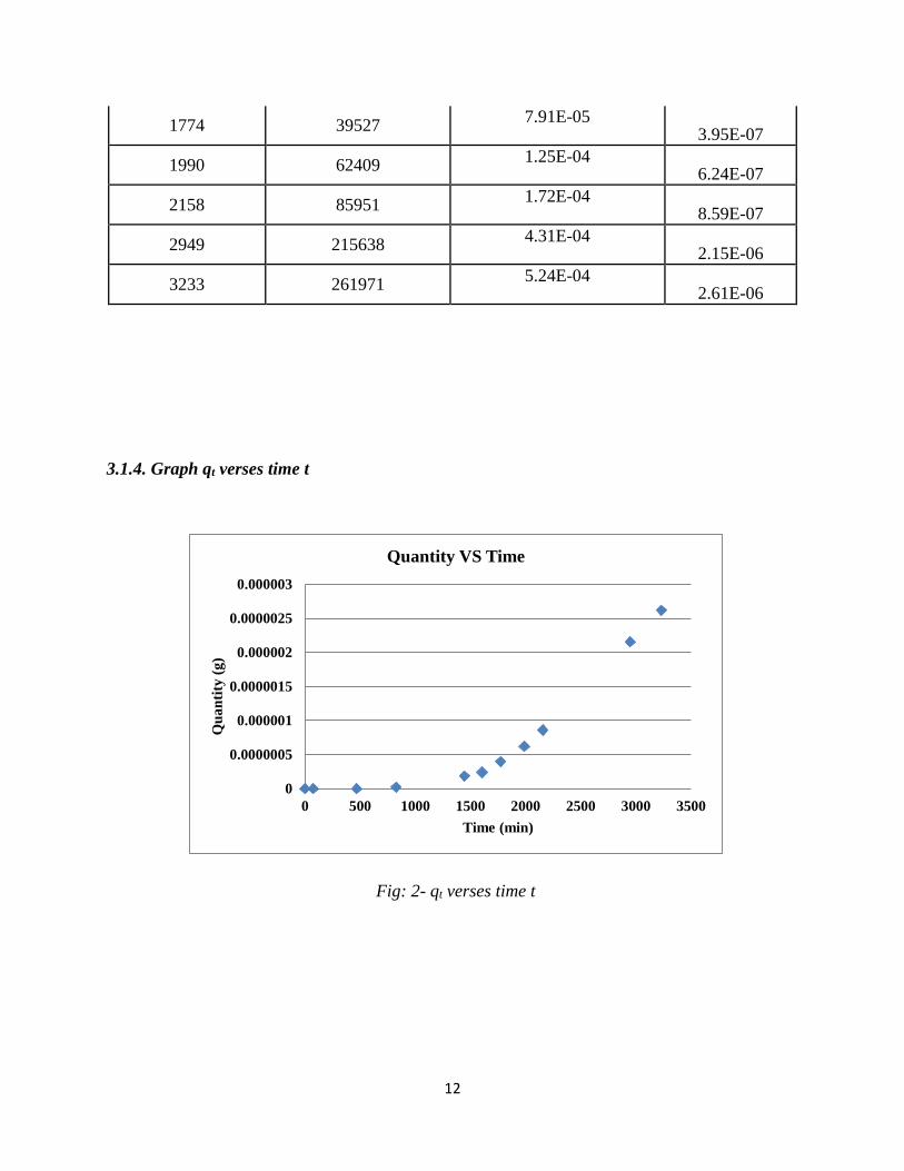
3.1.4. Graph qt verses time t

Fig: 2- qt verses time t

0

0.0000005

0.000001

0.0000015

0.000002

0.0000025

0.000003

0 500 1000 1500 2000 2500 3000 3500

Qu

an

tity

(g

)

Time (min)

Quantity VS Time

13

3.1.5. Slope of the line at steady state.

Equation of steady state line y = 2E-09x - 2E-05 and the slope I 2E-9 g/min

3.1.5 Calculation for P

We have equation for P

P=𝑞𝐿

𝑚2𝑡𝑃𝑎=

Slope (g

min)×1.5 mil

0.0177 𝑚2×1.7 𝑚𝑚𝐻𝑔

P=𝑞∗𝐿

𝑚2𝑡𝑃𝑎=

2E−9 g/min∗1.5 mil

0.0177 𝑚2∗1.7 𝑚𝑚𝐻𝑔

=99.7E-9 g*mil/ (min*mmHg*m2)

In SI unit “P” is as follow

As we know,

1 Min=60s

1 mmHg=133.322 Pa

y = 2E-09x - 2E-06

0

0.0000005

0.000001

0.0000015

0.000002

0.0000025

0.000003

0 500 1000 1500 2000 2500 3000 3500

Qu

an

tity

Qt

(g)

Time (min)

Quantity VS Time

14

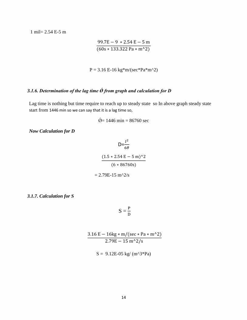
1 mil= 2.54 E-5 m

99.7E − 9 ∗ 2.54 E − 5 m

(60s ∗ 133.322 Pa ∗ m^2)

P = 3.16 E-16 kg*m/(sec*Pa*m^2)

3.1.6. Determination of the lag time Ǿ from graph and calculation for D

Lag time is nothing but time require to reach up to steady state so In above graph steady state

start from 1446 min so we can say that it is a lag time so,

Ǿ= 1446 min = 86760 sec

Now Calculation for D

D=𝑙2

6𝜃

(1.5 ∗ 2.54 E − 5 m)^2

(6 ∗ 86760s)

= 2.79E-15 m^2/s

3.1.7. Calculation for S

S = P

D

3.16 E − 16kg ∗ m/(sec ∗ Pa ∗ m^2)

2.79E − 15 m^2/s

S = 9.12E-05 kg/ (m^3*Pa)

15

3.2. Iso-Statics Method

Test Condition is as follow:

Organic Vapor: ethyl acetate

Test Film: LDPE (2ml)

Temperature: 220C

Film Surface area: 0.0081 m2

Table 3. Ethyl Acetate Data for Iso-statistics method

Time (sec) Pamps (Detector response)

0.000 0.000

302.600 0.020

665.500 26.590

907.400 106.060

1279.500 242.540

1641.800 342.400

2134.400 427.750

2616.700 477.620

3109.300 506.700

3591.800 522.540

4577.900 542.940

5060.500 549.960

5674.100 555.730

6156.800 560.960

6770.500 563.170

7373.600 566.900

7976.600 568.850

3.2.1. Conversion of Detector response (pamps) to the flow rate (q/t) at time t by given CF

Calibration Factor (CF) = 389.664 pico.g/ (pamps. sec)

Flow rate (Ft) =Response ×CF

So for 302.600 Flow rate,

= 0.020 (pamps) × 389.664 pico.g/ (pamps. sec)

16

= 7.793

By following above steps for all time we get below table 4

Time (sec) Pamps (Detector Response) Flow rate (Ft)

0.000 0.000 0.000

302.600 0.020 7.79

665.500 26.590 10361.1

907.400 106.060 41327.7

1279.500 242.540 94509.1

1641.800 342.400 133420.9

2134.400 427.750 166678.7

2616.700 477.620 186111.3

3109.300 506.700 197442.7

3591.800 522.540 203615.0

4577.900 542.940 211564.1

5060.500 549.960 214299.6

5674.100 555.730 216547.9

6156.800 560.960 218585.9

6770.500 563.170 219447.0

7373.600 566.900 220900.5

7976.600 568.850 221660.3

17

3.2.2. q/t versus time Graph

Fig: 3- qt verses time t

3.2.3. Ft/Fss Versus time

From above table no 4 value of Ft we can say that Fss is 221660.366. Now table for Ft/Fss is given

below.

Table No: 5

Time (sec) Flow rate Ft/Fss

0.000 0.000 0

302.600 7.793 3.5E-05

665.500 10361.1 0.046743

907.400 41327.7 0.186446

1279.500 94509.1 0.426368

1641.800 133420.9 0.601916

2134.400 166678.7 0.751955

2616.700 186111.3 0.839623

3109.300 197442.7 0.890744

3591.800 203615.02 0.918590

4577.900 211564.1 0.954451

0.000

50000.000

100000.000

150000.000

200000.000

250000.000

Flu

x (

Ft)

(p

icog/s

ec)

Time (sec)

Flow rate VS time

18

5060.500 214299.6 0.966792

5674.100 216547.9 0.976935

6156.800 218585.9 0.986129

6770.500 219447.0 0.990014

7373.600 220900.5 0.996572

7976.600 221660.3 1.000000

3.2.4. Obtain t 1/4, t ½ , and t 3/4 by interpolation method

We have following equation to find out t 1/4, t ½ , and t ¾ values

X= X1-𝑌1−𝑌

𝑌1−𝑌2 (𝑋1 − 𝑋2)

Now calculation for t1/4:

= 907.4 - 0.186−0.25

0.186−0.426(907.4 − 1279.5)

= 907.4- (0.266) × (-372.1)

=1006.6 sec

For t1/2

= 1279.5- 0.426−0.5

0.426−0.601(1279.5 − 1641.8)

=1279.5- (0.422) × (-362.3)

= 1432.3 sec

For t ¾

= 1641.8- 0.6019−0.75

0.6019−0.75195(1641.5 − 2134.4)

=1641.8- (0.9897) × (-492.6)

=2129.4 sec

Now we can calculate the ratios:

19

Their for, K1 = (t1/4) / (t ¾ ) = 1006.6 /2129.4 = 0.47

K2= (t1/4)/ (t1/2) = 1006.6/ 1432.3 = 0.70

We can compare now this with our criteria: 0.42 ≤ K1 ≤ 0.46 and 0.65 ≤ K1 ≤ 0.69 and we find that

the consistency test is does not meet.

Consistency does not met but we can calculate Permeability P, Diffusion coefficient D and Solubility

S

3.2.5. Determination of “P”

We Have equation

P=𝐹𝑠𝑠∗𝑙

𝐴×∆𝑝

P= 221660.3664 𝑝𝑖𝑐𝑜.

𝑔

𝑠𝑒𝑐×2𝑚𝑖𝑙

0.0081 𝑚^2×𝑜.𝑜1224𝑝𝑎

P= 1.13E-15 kg*m/m2*sec*pa

3. 2.6. Determination of “D”

We Have equation

D=𝑙2

7.2∗𝑡1/2

= 2𝑚𝑖𝑙2×(2.54∗10−5)^2

7.2×(1432 𝑠𝑒𝑐)∗𝑚𝑖𝑙^2

D= 2.50E-13 m2/sec

3. 2.7. Determination of “S”

We Have equation

S = P

D

= 1.13576E−15 kg∗m/m2∗sec∗pa

2.50295𝐸−13𝑚2/𝑠𝑒𝑐

S = 4.54E-03 kg/m3pa

20

Discussion

Organic vapor exists in food and diverse daily chemicals such as flavor snack food.

Different from inorganic gas and water vapor, most organic vapors are emitted by products

themselves as well as the key quality and main function of those products (even the sole function).

As to those products, the existence of organic vapor is very important. Dissipating or adding of

organic vapor will affect the quality and marketing of food products directly. So, kinds of organic

vapor and maintaining of their concentration are important indexes of food products quality

measurement. As for flavor snack food, it is sometimes they are key factors in selling slight

permeance of peculiar odors may affect the smells inside packages, selling as well as usage of

products. So we must select packaging materials with good barrier properties of organic vapor for

those particular products so as to avoid emitting of organic vapor inside and permeance of peculiar

odor outside. (Labthink)

Limonene is a major compound in oil extracted from citrus and it is present in orange and

fruit juices. Limonene is also used in cleaning products as a solvent or as a water-dilatable product.

Limonene is a very versatile chemical and can therefore be used in a wide variety of applications.

Scalping of limonene from citrus juices can lead to loss of citrus flavor. Ethyl acetate is a solvent

and acceptable for food applications. It is used in the packaging industry because it provides high

printing resolution on plastics and metals. Assessing permeability of ethyl acetate and-limonene

through polymer plastic material will provide an indication of its aroma barrier properties and its

potential for food packaging applications. (Hernandez, R.J et al 1996)

Organic vapors are usually freely absorbed by polymers and the absorbed molecules

diffuse by a random exchange of places with polymer segments. The vapors, once sorbed by the

polymer matrix, may act as a plasticizer, affecting the micro-Brownian motion of the polymer

chains. The micro-Brownian motion of polymer chain segments is very slow compared with that

of the sorbed molecules. The absorption of organic vapors may cause the polymer to swell,

inducing changes in the configuration of the polymer molecules. These configurationally changes

are not instantaneous but rather are controlled by the relaxation times of the polymer chains. If

these are long, as is characteristic of glassy polymers, stresses may be set up which relax only very

slowly. In rubbery polymers, relaxation times are shorter, but stresses may still take a long time

to relax.

21

In this study, we considered some assumptions for determination of Permeability P,

Diffusion Coefficient D and solubility S. these assumptions are , In isostatic procedure during the

permeation process the polymeric structure, permeant concentration on both side of tested film

and temperature always not changing. In the quasi-isostatic, we assume the pressure of low

concentration chamber is equal to zero, which is actually not zero, temperature during the

experiment is not changed.

Error analysis

1) Chances of error if temperature is not constant.

2) While taking reading, need precautions, there is chance of wrong answer.

3) If apparatus using in experiment is not working properly

4) If detector is not working properly so all data will be wrong.

5) Error due to influence of relaxation time of organic vapor

6) Thickness of film is not same.

4. Conclusion

From this study we can conclude that, The Quasi-isostatics and Isostastics is good method

for determination of Permeability P, Diffusion Coefficient D and solubility S. In isostatic method

some assumption are to be consider for calculation of P, D and S like, Polymeric structure, permeant

concentration on both side. But these assumption not work always so we need to perform

Consistency test, we can make sure there were no any abnormal condition during resulted error is in

the acceptable limit.

References: Y. Qin, M. Rubinoa, R. Aurasa, L.-T. Limb, Use of a magnetic suspension microbalance to

measure organic vapor sorption for evaluating the impact of polymer converting process. Polymer

Testing Volume 26, Issue 8, December 2007, Pages 1082–1089

22

Rafael Gavarat, Ramon Catala, Pilar M. Hernandez-Mufioz and Ruben J. Hernandez. (1996)

Evaluation of permeability through permeation experiments: isostatic and quasiisostatic

methods compared. Packaging technology and science vol 9 215-224 (1996)

Crank, J. 1975. The Mathematics of Diffusion, Second Edition. Oxford: Oxford University

Press.

Rafael GavaraRuben J. HernandezJournal , consistency test for continuous flow permeability

experimental data Plastic Film and Sheeting April 1993 vol. 9 no. 2 126-138.

Labthink, A hand book of Organic Vapor Permeability Lab, China

Hernandez, R.J, Ciacin, J.R. and Baner, A.L. (1986) ‘The evaluation of the aroma barrier

properties of polymer films’ in Plastic. Film Sheeting 2, 187-21144