The globalization of naval provisioning: ancient DNA and stable isotope analyses of stored cod from...

rsos.royalsocietypublishing.org

ResearchCite this article: Hutchinson WF, Culling M,Orton DC, Hänfling B, Lawson Handley L,Hamilton-Dyer S, O’Connell TC, Richards MP,Barrett JH. 2015 The globalization of navalprovisioning: ancient DNA and stable isotopeanalyses of stored cod from the wreck of theMary Rose, AD 1545. R. Soc. open sci. 2: 150199.http://dx.doi.org/10.1098/rsos.150199

Received: 11 May 2015Accepted: 14 August 2015

Subject Category:Genetics

Subject Areas:environmental science

Keywords:historical ecology, single-nucleotidepolymorphisms, stable isotope analysis, cod,fish trade, Mary Rose

Author for correspondence:James H. Barrette-mail: [email protected]

Electronic supplementary material is availableat http://dx.doi.org/10.1098/rsos.150199 or viahttp://rsos.royalsocietypublishing.org.

The globalization of navalprovisioning: ancient DNAand stable isotope analysesof stored cod from the wreckof the Mary Rose, AD 1545William F. Hutchinson1, Mark Culling1, David C. Orton2,

Bernd Hänfling1, Lori Lawson Handley1,

Sheila Hamilton-Dyer3, Tamsin C. O’Connell4,

Michael P. Richards5,6 and James H. Barrett4

1Evolutionary Biology Group, Department of Biological Sciences, University of Hull,Hull HU6 7RX, UK2BioArCh, Department of Archaeology, University of York, York YO10 5DD, UK3SH-D ArchaeoZoology, 5 Suffolk Avenue, Shirley, Southampton SO15 5EF, UK4McDonald Institute for Archaeological Research, Department of Archaeology andAnthropology, University of Cambridge, Cambridge CB2 3ER, UK5Department of Anthropology, University of British Columbia, Vancouver Campus,6303 NWMarine Drive, Vancouver, British Columbia, Canada V6T 1Z16Department of Human Evolution, Max Planck Institute for EvolutionaryAnthropology, Deutscher Platz 6, 04103 Leipzig, Germany

DCO, 0000-0003-4069-8004; JHB, 0000-0002-6683-9891

A comparison of ancient DNA (single-nucleotide poly-morphisms) and carbon and nitrogen stable isotope evidencesuggests that stored cod provisions recovered from the wreckof the Tudor warship Mary Rose, which sank in the Solent,southern England, in 1545, had been caught in northern andtransatlantic waters such as the northern North Sea and thefishing grounds of Iceland and Newfoundland. This discovery,underpinned by control data from archaeological samples ofcod bones from potential source regions, illuminates the roleof naval provisioning in the early development of extensive seafisheries, with their long-term economic and ecological impacts.

1. IntroductionHistorical ecology has become an essential step in understandingthe long-term human exploitation of aquatic ecosystems [1,2].

2015 The Authors. Published by the Royal Society under the terms of the Creative CommonsAttribution License http://creativecommons.org/licenses/by/4.0/, which permits unrestricteduse, provided the original author and source are credited.

on September 10, 2015http://rsos.royalsocietypublishing.org/Downloaded from

http://crossmark.crossref.org/dialog/?doi=10.1098/rsos.150199&domain=pdf&date_stamp=2015-09-09

mailto:[email protected]

http://orcid.org/0000-0003-4069-8004

http://orcid.org/0000-0002-6683-9891

http://rsos.royalsocietypublishing.org/

2

rsos.royalsocietypublishing.orgR.Soc.opensci.2:150199

................................................In one important example, the growth of long-range trade in high-bulk staple products in medievaland post-medieval Europe underpinned the development of urbanized market economies, colonialism,empires and concomitant environmental impacts [3–5]. Concurrent with conquest and deforestation forincreased cash-crop production, these periods saw the expansion of extensive sea fishing. Historicalresearch, zooarchaeological evidence and stable isotopic analysis of archaeological fish bones all suggestthat preserved Arctic Norwegian and North Atlantic cod were increasingly transported to consumersaround the North Sea—particularly expanding urban populations—between the eleventh and sixteenthcenturies [6–9]. An open question in this context is whether the requirements of naval provisioningmay also have played a role in the development of extensive sea fisheries and, concurrently, whetherthe availability of preserved fish from distant seas helped sustain Europe’s first standing navies. Thisquestion is especially pertinent for the sixteenth century, which saw both the naissance of Europeantransatlantic colonialism and the growing importance of sea power as a tool in increasingly globalconflicts [10].

An unparalleled opportunity to investigate the role of fish in early naval provisioning is provided bythe wreck of the Tudor warship Mary Rose, which sank in the Solent, southern England, in 1545 whilesailing to military action with a full complement of crew and a full store of provisions [11]. Among theexcavated remains of its supplies were thousands of cod bones, some associated with casks and baskets.The find context and absence of cranial bones strongly suggest that they were from dried or salted cod,staples of the Tudor naval diet, but where had they been caught? New stable isotopic methods providea promising way to detect non-local imports of cod [7,12,13] and genetic markers have proved usefulfor investigating population differentiation in marine fishes. Single-nucleotide polymorphisms (SNPs)are especially well suited for identifying source populations using DNA from archaeological samples,because they combine the power to detect even weak structuring on a small geographical scale [14–16]with their utility for genotyping highly degraded ancient DNA samples (less than 100 bp). Becausethe stable isotope data employed (δ13C and δ15N of bone protein) reflect diet and local environmentalconditions [17], whereas genetic markers reflect genetic drift, gene flow and selection [18], the methodsare independent. Thus, together they can provide complementary information on the potential source oftraded fish.

Prior to the use of ice or refrigeration for shipping fresh foods, fish such as cod, Gadus morhua,an important commercial species since the Middle Ages, were typically (although not exclusively)decapitated before drying and/or salting for long-distance transport [19,20]. Consequently, stable isotopeand DNA signatures recovered from archaeological cranial bones of cod can be used to provide a baselineset of control data to which potentially transported post-cranial target bones of this species can beassigned. In this way, the development of long-distance trade, and/or long-range fishing trips, can beinvestigated.

The undocumented suppliers to the Mary Rose could have drawn on preserved cod from a diverse,but probably finite, number of regions. England’s salt cod fisheries were well developed by the sixteenthcentury, involving both relatively local inshore catches (particularly around the southwest coast andin the North Sea) and long-distance fisheries conducted off southern and western Ireland, Iceland and(from ca 1502) northeastern North America, particularly Newfoundland [21–23]. Additional possibilitiesinclude dried and salted cod from northern Scotland [20,24] and Norway [25]. Lastly, stockfish (cod driedwithout salt, especially from Norway and Iceland), which had dominated earlier medieval trade, wasalso still available [21,22]. Were cod provisions on the Mary Rose caught locally or sourced from someof these distant waters? If the latter, from which population or populations? This paper aims to answerthese questions by analysing SNP genotypes and stable isotope signatures using a set of control samples(n = 168 and 239, respectively) from potential source locations and comparing these with 11 cod bonesfrom the Mary Rose. The results contribute to our understanding of globalization during the transitionfrom the European Middle Ages to the era of transatlantic expansion. In particular, they address the roleof distant food sources in the provisioning of a standing navy.

2. Material and methods2.1. Control samplesBoth aDNA and stable isotope analyses require baseline data for cod bones from potential sourcepopulations (controls) in order to attribute the Mary Rose samples (targets) to possible regions of catch.Natural and anthropogenically induced temporal changes in the baseline signatures are known to occur,particularly with recent variations in genetic selective pressures (e.g. due to fluctuating sea temperatures



3


................................................and the development of industrial fishing) and increasing isotopic pollution due to farming (with itschemical runoff) and industrialization [26–30]. Thus, pre-modern samples were required. On the basisthat most cod were decapitated prior to drying, we used cranial bones from archaeological sites as proxiesfor relatively local catches within a series of potential source regions. Contemporaneity with the MaryRose across regions was not an achievable objective given the vagaries of the archaeological record, andthe control data were gathered as part of a wider study to include earlier centuries, but in all cases thechronology of the control samples predates industrial fishing, farming and manufacturing in the regionin question. Earlier natural variation, owing to climate change for example [29], and localized spatialshifts in cod distribution due to varying water temperatures [31], may reduce the discriminating powerof our methods, but is unlikely to invalidate them (see below).

We collected a geographically wide-ranging set of archaeological control samples of cod bone (table 1).In some cases, we were able to use samples from the same location (or even the same individual bones)for both aDNA and stable isotope analyses (electronic supplementary material, table S1). For aDNA,19 collections of control skull bones (totalling 168 specimens with successful results) were obtained fromarchaeological excavations sited around the shores of the Barents Sea; the northern, western and southernNorwegian coast; the waters surrounding Britain and Ireland; the Baltic Sea; Iceland; and Newfoundland(figure 1a). Where multiple bones were sampled from the same archaeological context, these were eitherof the same anatomical element and side or clearly different in size, to eliminate the possibility ofreplicating results from individual fish. The genetic control samples range in date from the twelfth–thirteenth centuries to the eighteenth–nineteenth centuries (table 1). The use of comparatively recenteighteenth–nineteeth century control samples from Newfoundland was justified, as an SNP analysis ofmodern samples from across the cod’s distribution (using the 28 loci described in this study) showed that50 cod from Newfoundland (collected in 2011 at 48.16 latitude, −53.72 longitude) were highly divergentfrom populations in the east [32] where the rest of the control specimens were sourced (ARLEQUIN v. 3.1,θFST = 0.279–0.774, p ≤ 0.00001).

For stable carbon and nitrogen isotope analysis, 33 collections of control bones (totally 239 specimenswith successful results) have been used (table 1). Data from Barrett et al. [7] are augmented by the additionof 55 new specimens from previously covered regions and 29 specimens from the formerly unsampledcoasts of Ireland and southwestern Britain (figure 2). The latter regions developed commercial salt codindustries starting in the late fourteenth century based on historical evidence [23] and are potentiala priori candidates for the source of fish provisions on a vessel sailing from Portsmouth. The stableisotope control data are all from cod with estimated total lengths (TL) of 500–1000 mm (based on bonemeasurements and/or comparison with reference specimens of known size, the former using establishedregression formulae [33] and the latter using 1 : 1 scanned images to avoid contamination) to minimizepossible trophic-level effects on the isotope values [7]. The samples range in date from the late eighth tothe early nineteenth centuries. The δ13C and δ15N values of marine fish are known to be influenced bywater temperature, salinity, nutrient loading and the structure of the food web, all of which vary throughtime [12]. Nevertheless, when subdivided by region and date the only statistically significant differencebetween time periods in any of our pre-modern δ13C or δ15N datasets occurs in eastern Baltic δ13C(electronic supplementary material, table S2 and figures S1–S2). Moreover, this spatial group remainsisotopically distinct from others regardless of the change through time (see below). Thus, based onpresent evidence, chronological fluctuations in environmental variables are most likely to be expressed asheterogeneity within the stable isotope data of each region, with concomitant limits on their resolution.

2.2. Target samplesA collection of 11 target samples of potentially traded cod cleithra were obtained from the excavationof the Mary Rose. Subsamples of the same specimens were used for both aDNA and stable isotopeanalyses. They were selected from 4384 identified fish bones (almost all of cod) originally recoveredduring excavation and the subsequent sieving of sediment samples. Only appendicular skeletal elements(such as the cleithrum which supports the pectoral fin behind the head) and vertebrae were present.There were no cranial elements. This anatomical pattern, combined with distinctive cut marks and thefind contexts (e.g. associated with casks and baskets), strongly suggests that the bones were from storedcod, dried with or without salt [34]. Four of the target specimens analysed here (nos. 1, 3, 10 and 11) werefrom the stern of the ship in the hold, one of which (no. 3) was associated with a wicker basket. Six (nos.4, 5, 6, 7, 8 and 9) were from the orlop deck above, two of which (nos. 5 and 6) were associated with astaved container or cask. One target specimen (no. 2) does not have a specific location recorded, but wasnevertheless sealed within the wreck.



4


................................................Table 1. The genetic and stable isotope control and target samples used in the study (further information is provided in the electronicsupplementary material, table S1).

aDNA stable isotopes

settlement no. date no. date latitude longitude location key to maps. . . . . . . . . . . . . . . . . . . . . . . . . . . . . . . . . . . . . . . . . . . . . . . . . . . . . . . . . . . . . . . . . . . . . . . . . . . . . . . . . . . . . . . . . . . . . . . . . . . . . . . . . . . . . . . . . . . . . . . . . . . . . . . . . . . . . . . . . . . . . . . . . . . . . . . . . . . . . . . . . . . . . . . . . . . . . . . . . . . . . . . . . . . . . . . . . . . . . . . . . . . . . . . . . . . . . . . . .

Skonsvika 4 13th–14th 4 13th–14th 70.87 29.00 Arctic Norway 1. . . . . . . . . . . . . . . . . . . . . . . . . . . . . . . . . . . . . . . . . . . . . . . . . . . . . . . . . . . . . . . . . . . . . . . . . . . . . . . . . . . . . . . . . . . . . . . . . . . . . . . . . . . . . . . . . . . . . . . . . . . . . . . . . . . . . . . . . . . . . . . . . . . . . . . . . . . . . . . . . . . . . . . . . . . . . . . . . . . . . . . . . . . . . . . . . . . . . . . . . . . . . . . . . . . . . . . . .

Kongshavn 6 14th 6 14th 70.85 29.21 Arctic Norway 1. . . . . . . . . . . . . . . . . . . . . . . . . . . . . . . . . . . . . . . . . . . . . . . . . . . . . . . . . . . . . . . . . . . . . . . . . . . . . . . . . . . . . . . . . . . . . . . . . . . . . . . . . . . . . . . . . . . . . . . . . . . . . . . . . . . . . . . . . . . . . . . . . . . . . . . . . . . . . . . . . . . . . . . . . . . . . . . . . . . . . . . . . . . . . . . . . . . . . . . . . . . . . . . . . . . . . . . . .

Storvågan 8 12th–15th 5 12th–15th 68.20 14.45 Arctic Norway 2. . . . . . . . . . . . . . . . . . . . . . . . . . . . . . . . . . . . . . . . . . . . . . . . . . . . . . . . . . . . . . . . . . . . . . . . . . . . . . . . . . . . . . . . . . . . . . . . . . . . . . . . . . . . . . . . . . . . . . . . . . . . . . . . . . . . . . . . . . . . . . . . . . . . . . . . . . . . . . . . . . . . . . . . . . . . . . . . . . . . . . . . . . . . . . . . . . . . . . . . . . . . . . . . . . . . . . . . .

Bergen 5 14th — — 60.40 5.32 western Norway 3. . . . . . . . . . . . . . . . . . . . . . . . . . . . . . . . . . . . . . . . . . . . . . . . . . . . . . . . . . . . . . . . . . . . . . . . . . . . . . . . . . . . . . . . . . . . . . . . . . . . . . . . . . . . . . . . . . . . . . . . . . . . . . . . . . . . . . . . . . . . . . . . . . . . . . . . . . . . . . . . . . . . . . . . . . . . . . . . . . . . . . . . . . . . . . . . . . . . . . . . . . . . . . . . . . . . . . . . .

Oslo 11 12th–14th — — 59.92 10.73 southeast Norway 4. . . . . . . . . . . . . . . . . . . . . . . . . . . . . . . . . . . . . . . . . . . . . . . . . . . . . . . . . . . . . . . . . . . . . . . . . . . . . . . . . . . . . . . . . . . . . . . . . . . . . . . . . . . . . . . . . . . . . . . . . . . . . . . . . . . . . . . . . . . . . . . . . . . . . . . . . . . . . . . . . . . . . . . . . . . . . . . . . . . . . . . . . . . . . . . . . . . . . . . . . . . . . . . . . . . . . . . . .

Skriðuklaustur 12 15th–16th 14 15th–16th 65.10 −14.82 Iceland 5. . . . . . . . . . . . . . . . . . . . . . . . . . . . . . . . . . . . . . . . . . . . . . . . . . . . . . . . . . . . . . . . . . . . . . . . . . . . . . . . . . . . . . . . . . . . . . . . . . . . . . . . . . . . . . . . . . . . . . . . . . . . . . . . . . . . . . . . . . . . . . . . . . . . . . . . . . . . . . . . . . . . . . . . . . . . . . . . . . . . . . . . . . . . . . . . . . . . . . . . . . . . . . . . . . . . . . . . .

Sandwick 5 13th–14th 10 12th–14th 60.70 −0.87 northern Scotland 6. . . . . . . . . . . . . . . . . . . . . . . . . . . . . . . . . . . . . . . . . . . . . . . . . . . . . . . . . . . . . . . . . . . . . . . . . . . . . . . . . . . . . . . . . . . . . . . . . . . . . . . . . . . . . . . . . . . . . . . . . . . . . . . . . . . . . . . . . . . . . . . . . . . . . . . . . . . . . . . . . . . . . . . . . . . . . . . . . . . . . . . . . . . . . . . . . . . . . . . . . . . . . . . . . . . . . . . . .

Robert’s Haven 6 13th/14th 1 13th–14th 58.65 −3.05 northern Scotland 7. . . . . . . . . . . . . . . . . . . . . . . . . . . . . . . . . . . . . . . . . . . . . . . . . . . . . . . . . . . . . . . . . . . . . . . . . . . . . . . . . . . . . . . . . . . . . . . . . . . . . . . . . . . . . . . . . . . . . . . . . . . . . . . . . . . . . . . . . . . . . . . . . . . . . . . . . . . . . . . . . . . . . . . . . . . . . . . . . . . . . . . . . . . . . . . . . . . . . . . . . . . . . . . . . . . . . . . . .

Bornais 9 12th–13th 10 12th–13th 57.25 −7.43 northern Scotland 8. . . . . . . . . . . . . . . . . . . . . . . . . . . . . . . . . . . . . . . . . . . . . . . . . . . . . . . . . . . . . . . . . . . . . . . . . . . . . . . . . . . . . . . . . . . . . . . . . . . . . . . . . . . . . . . . . . . . . . . . . . . . . . . . . . . . . . . . . . . . . . . . . . . . . . . . . . . . . . . . . . . . . . . . . . . . . . . . . . . . . . . . . . . . . . . . . . . . . . . . . . . . . . . . . . . . . . . . .

Aberdeen 10 ca 13th–14th 4 ca 13th–14th 57.15 −2.10 northern Scotland 9. . . . . . . . . . . . . . . . . . . . . . . . . . . . . . . . . . . . . . . . . . . . . . . . . . . . . . . . . . . . . . . . . . . . . . . . . . . . . . . . . . . . . . . . . . . . . . . . . . . . . . . . . . . . . . . . . . . . . . . . . . . . . . . . . . . . . . . . . . . . . . . . . . . . . . . . . . . . . . . . . . . . . . . . . . . . . . . . . . . . . . . . . . . . . . . . . . . . . . . . . . . . . . . . . . . . . . . . .

Uppsala 7 13th–14th 12 13th–15th 59.86 17.64 eastern Sweden 10. . . . . . . . . . . . . . . . . . . . . . . . . . . . . . . . . . . . . . . . . . . . . . . . . . . . . . . . . . . . . . . . . . . . . . . . . . . . . . . . . . . . . . . . . . . . . . . . . . . . . . . . . . . . . . . . . . . . . . . . . . . . . . . . . . . . . . . . . . . . . . . . . . . . . . . . . . . . . . . . . . . . . . . . . . . . . . . . . . . . . . . . . . . . . . . . . . . . . . . . . . . . . . . . . . . . . . . . .

Gdañsk 7 13th–14th 11 13th–16th 54.36 18.66 northern Poland 11. . . . . . . . . . . . . . . . . . . . . . . . . . . . . . . . . . . . . . . . . . . . . . . . . . . . . . . . . . . . . . . . . . . . . . . . . . . . . . . . . . . . . . . . . . . . . . . . . . . . . . . . . . . . . . . . . . . . . . . . . . . . . . . . . . . . . . . . . . . . . . . . . . . . . . . . . . . . . . . . . . . . . . . . . . . . . . . . . . . . . . . . . . . . . . . . . . . . . . . . . . . . . . . . . . . . . . . . .

York 13 13th–14th 3 10th–13th 53.96 −1.08 eastern England 12. . . . . . . . . . . . . . . . . . . . . . . . . . . . . . . . . . . . . . . . . . . . . . . . . . . . . . . . . . . . . . . . . . . . . . . . . . . . . . . . . . . . . . . . . . . . . . . . . . . . . . . . . . . . . . . . . . . . . . . . . . . . . . . . . . . . . . . . . . . . . . . . . . . . . . . . . . . . . . . . . . . . . . . . . . . . . . . . . . . . . . . . . . . . . . . . . . . . . . . . . . . . . . . . . . . . . . . . .

London 10 13th–14th 16 8th–17th 51.51 −0.10 southeast England 13. . . . . . . . . . . . . . . . . . . . . . . . . . . . . . . . . . . . . . . . . . . . . . . . . . . . . . . . . . . . . . . . . . . . . . . . . . . . . . . . . . . . . . . . . . . . . . . . . . . . . . . . . . . . . . . . . . . . . . . . . . . . . . . . . . . . . . . . . . . . . . . . . . . . . . . . . . . . . . . . . . . . . . . . . . . . . . . . . . . . . . . . . . . . . . . . . . . . . . . . . . . . . . . . . . . . . . . . .

Bristol 14 13th–14th 5 12th–14th 51.45 −2.59 western England 14. . . . . . . . . . . . . . . . . . . . . . . . . . . . . . . . . . . . . . . . . . . . . . . . . . . . . . . . . . . . . . . . . . . . . . . . . . . . . . . . . . . . . . . . . . . . . . . . . . . . . . . . . . . . . . . . . . . . . . . . . . . . . . . . . . . . . . . . . . . . . . . . . . . . . . . . . . . . . . . . . . . . . . . . . . . . . . . . . . . . . . . . . . . . . . . . . . . . . . . . . . . . . . . . . . . . . . . . .

Galway 13 13th–14th 4 13th–14th 53.27 −9.05 western Ireland 15. . . . . . . . . . . . . . . . . . . . . . . . . . . . . . . . . . . . . . . . . . . . . . . . . . . . . . . . . . . . . . . . . . . . . . . . . . . . . . . . . . . . . . . . . . . . . . . . . . . . . . . . . . . . . . . . . . . . . . . . . . . . . . . . . . . . . . . . . . . . . . . . . . . . . . . . . . . . . . . . . . . . . . . . . . . . . . . . . . . . . . . . . . . . . . . . . . . . . . . . . . . . . . . . . . . . . . . . .

Cork 10 medieval 3 medieval 51.90 −8.48 southern Ireland 16. . . . . . . . . . . . . . . . . . . . . . . . . . . . . . . . . . . . . . . . . . . . . . . . . . . . . . . . . . . . . . . . . . . . . . . . . . . . . . . . . . . . . . . . . . . . . . . . . . . . . . . . . . . . . . . . . . . . . . . . . . . . . . . . . . . . . . . . . . . . . . . . . . . . . . . . . . . . . . . . . . . . . . . . . . . . . . . . . . . . . . . . . . . . . . . . . . . . . . . . . . . . . . . . . . . . . . . . .

Dos de Cheval 13 18th–19th 5 18th–19th 50.91 −55.87 Newfoundland 17. . . . . . . . . . . . . . . . . . . . . . . . . . . . . . . . . . . . . . . . . . . . . . . . . . . . . . . . . . . . . . . . . . . . . . . . . . . . . . . . . . . . . . . . . . . . . . . . . . . . . . . . . . . . . . . . . . . . . . . . . . . . . . . . . . . . . . . . . . . . . . . . . . . . . . . . . . . . . . . . . . . . . . . . . . . . . . . . . . . . . . . . . . . . . . . . . . . . . . . . . . . . . . . . . . . . . . . . .

Launceston 5 13th–14th — — 50.37 −4.36 southwest England 18. . . . . . . . . . . . . . . . . . . . . . . . . . . . . . . . . . . . . . . . . . . . . . . . . . . . . . . . . . . . . . . . . . . . . . . . . . . . . . . . . . . . . . . . . . . . . . . . . . . . . . . . . . . . . . . . . . . . . . . . . . . . . . . . . . . . . . . . . . . . . . . . . . . . . . . . . . . . . . . . . . . . . . . . . . . . . . . . . . . . . . . . . . . . . . . . . . . . . . . . . . . . . . . . . . . . . . . . .

Måsøy — — 10 17th–19th 70.98 24.63 Arctic Norway 19. . . . . . . . . . . . . . . . . . . . . . . . . . . . . . . . . . . . . . . . . . . . . . . . . . . . . . . . . . . . . . . . . . . . . . . . . . . . . . . . . . . . . . . . . . . . . . . . . . . . . . . . . . . . . . . . . . . . . . . . . . . . . . . . . . . . . . . . . . . . . . . . . . . . . . . . . . . . . . . . . . . . . . . . . . . . . . . . . . . . . . . . . . . . . . . . . . . . . . . . . . . . . . . . . . . . . . . . .

Helgøygården — — 6 14th 70.11 19.35 Arctic Norway 20. . . . . . . . . . . . . . . . . . . . . . . . . . . . . . . . . . . . . . . . . . . . . . . . . . . . . . . . . . . . . . . . . . . . . . . . . . . . . . . . . . . . . . . . . . . . . . . . . . . . . . . . . . . . . . . . . . . . . . . . . . . . . . . . . . . . . . . . . . . . . . . . . . . . . . . . . . . . . . . . . . . . . . . . . . . . . . . . . . . . . . . . . . . . . . . . . . . . . . . . . . . . . . . . . . . . . . . . .

Vannareid — — 12 17th–19th 70.20 19.60 Arctic Norway 20. . . . . . . . . . . . . . . . . . . . . . . . . . . . . . . . . . . . . . . . . . . . . . . . . . . . . . . . . . . . . . . . . . . . . . . . . . . . . . . . . . . . . . . . . . . . . . . . . . . . . . . . . . . . . . . . . . . . . . . . . . . . . . . . . . . . . . . . . . . . . . . . . . . . . . . . . . . . . . . . . . . . . . . . . . . . . . . . . . . . . . . . . . . . . . . . . . . . . . . . . . . . . . . . . . . . . . . . .

Quoygrew — — 34 11th–15th 59.34 −2.98 northern Scotland 21. . . . . . . . . . . . . . . . . . . . . . . . . . . . . . . . . . . . . . . . . . . . . . . . . . . . . . . . . . . . . . . . . . . . . . . . . . . . . . . . . . . . . . . . . . . . . . . . . . . . . . . . . . . . . . . . . . . . . . . . . . . . . . . . . . . . . . . . . . . . . . . . . . . . . . . . . . . . . . . . . . . . . . . . . . . . . . . . . . . . . . . . . . . . . . . . . . . . . . . . . . . . . . . . . . . . . . . . .

Knowe of Skea — — 3 12th–16th 59.26 −2.98 northern Scotland 21. . . . . . . . . . . . . . . . . . . . . . . . . . . . . . . . . . . . . . . . . . . . . . . . . . . . . . . . . . . . . . . . . . . . . . . . . . . . . . . . . . . . . . . . . . . . . . . . . . . . . . . . . . . . . . . . . . . . . . . . . . . . . . . . . . . . . . . . . . . . . . . . . . . . . . . . . . . . . . . . . . . . . . . . . . . . . . . . . . . . . . . . . . . . . . . . . . . . . . . . . . . . . . . . . . . . . . . . .

Carrickfergus — — 4 ca 16th–17th 54.72 −5.81 Northern Ireland 22. . . . . . . . . . . . . . . . . . . . . . . . . . . . . . . . . . . . . . . . . . . . . . . . . . . . . . . . . . . . . . . . . . . . . . . . . . . . . . . . . . . . . . . . . . . . . . . . . . . . . . . . . . . . . . . . . . . . . . . . . . . . . . . . . . . . . . . . . . . . . . . . . . . . . . . . . . . . . . . . . . . . . . . . . . . . . . . . . . . . . . . . . . . . . . . . . . . . . . . . . . . . . . . . . . . . . . . . .

Dublin — — 9 medieval 53.34 −6.27 eastern Ireland 23. . . . . . . . . . . . . . . . . . . . . . . . . . . . . . . . . . . . . . . . . . . . . . . . . . . . . . . . . . . . . . . . . . . . . . . . . . . . . . . . . . . . . . . . . . . . . . . . . . . . . . . . . . . . . . . . . . . . . . . . . . . . . . . . . . . . . . . . . . . . . . . . . . . . . . . . . . . . . . . . . . . . . . . . . . . . . . . . . . . . . . . . . . . . . . . . . . . . . . . . . . . . . . . . . . . . . . . . .

Waterford — — 2 medieval 52.26 −7.11 southern Ireland 24. . . . . . . . . . . . . . . . . . . . . . . . . . . . . . . . . . . . . . . . . . . . . . . . . . . . . . . . . . . . . . . . . . . . . . . . . . . . . . . . . . . . . . . . . . . . . . . . . . . . . . . . . . . . . . . . . . . . . . . . . . . . . . . . . . . . . . . . . . . . . . . . . . . . . . . . . . . . . . . . . . . . . . . . . . . . . . . . . . . . . . . . . . . . . . . . . . . . . . . . . . . . . . . . . . . . . . . . .

Wharram Percy — — 2 13th–14th 54.07 −0.69 eastern England 12. . . . . . . . . . . . . . . . . . . . . . . . . . . . . . . . . . . . . . . . . . . . . . . . . . . . . . . . . . . . . . . . . . . . . . . . . . . . . . . . . . . . . . . . . . . . . . . . . . . . . . . . . . . . . . . . . . . . . . . . . . . . . . . . . . . . . . . . . . . . . . . . . . . . . . . . . . . . . . . . . . . . . . . . . . . . . . . . . . . . . . . . . . . . . . . . . . . . . . . . . . . . . . . . . . . . . . . . .

Norwich — — 6 11th–18th 52.63 1.30 eastern England 25. . . . . . . . . . . . . . . . . . . . . . . . . . . . . . . . . . . . . . . . . . . . . . . . . . . . . . . . . . . . . . . . . . . . . . . . . . . . . . . . . . . . . . . . . . . . . . . . . . . . . . . . . . . . . . . . . . . . . . . . . . . . . . . . . . . . . . . . . . . . . . . . . . . . . . . . . . . . . . . . . . . . . . . . . . . . . . . . . . . . . . . . . . . . . . . . . . . . . . . . . . . . . . . . . . . . . . . . .

Cambridge — — 1 14th 52.21 0.12 eastern England 26. . . . . . . . . . . . . . . . . . . . . . . . . . . . . . . . . . . . . . . . . . . . . . . . . . . . . . . . . . . . . . . . . . . . . . . . . . . . . . . . . . . . . . . . . . . . . . . . . . . . . . . . . . . . . . . . . . . . . . . . . . . . . . . . . . . . . . . . . . . . . . . . . . . . . . . . . . . . . . . . . . . . . . . . . . . . . . . . . . . . . . . . . . . . . . . . . . . . . . . . . . . . . . . . . . . . . . . . .

Southampton — — 9 9th–14th 50.90 −1.40 southern England 27. . . . . . . . . . . . . . . . . . . . . . . . . . . . . . . . . . . . . . . . . . . . . . . . . . . . . . . . . . . . . . . . . . . . . . . . . . . . . . . . . . . . . . . . . . . . . . . . . . . . . . . . . . . . . . . . . . . . . . . . . . . . . . . . . . . . . . . . . . . . . . . . . . . . . . . . . . . . . . . . . . . . . . . . . . . . . . . . . . . . . . . . . . . . . . . . . . . . . . . . . . . . . . . . . . . . . . . . .

Exeter — — 2 11th–15th 50.72 −3.53 southwest England 28. . . . . . . . . . . . . . . . . . . . . . . . . . . . . . . . . . . . . . . . . . . . . . . . . . . . . . . . . . . . . . . . . . . . . . . . . . . . . . . . . . . . . . . . . . . . . . . . . . . . . . . . . . . . . . . . . . . . . . . . . . . . . . . . . . . . . . . . . . . . . . . . . . . . . . . . . . . . . . . . . . . . . . . . . . . . . . . . . . . . . . . . . . . . . . . . . . . . . . . . . . . . . . . . . . . . . . . . .

Norden — — 1 13th–14th 53.60 7.20 northwest Germany 29. . . . . . . . . . . . . . . . . . . . . . . . . . . . . . . . . . . . . . . . . . . . . . . . . . . . . . . . . . . . . . . . . . . . . . . . . . . . . . . . . . . . . . . . . . . . . . . . . . . . . . . . . . . . . . . . . . . . . . . . . . . . . . . . . . . . . . . . . . . . . . . . . . . . . . . . . . . . . . . . . . . . . . . . . . . . . . . . . . . . . . . . . . . . . . . . . . . . . . . . . . . . . . . . . . . . . . . . .

Mała Nieszawka — — 7 14th–15th 52.99 18.55 Poland 30. . . . . . . . . . . . . . . . . . . . . . . . . . . . . . . . . . . . . . . . . . . . . . . . . . . . . . . . . . . . . . . . . . . . . . . . . . . . . . . . . . . . . . . . . . . . . . . . . . . . . . . . . . . . . . . . . . . . . . . . . . . . . . . . . . . . . . . . . . . . . . . . . . . . . . . . . . . . . . . . . . . . . . . . . . . . . . . . . . . . . . . . . . . . . . . . . . . . . . . . . . . . . . . . . . . . . . . . .

Raversijde — — 2 15th 51.20 2.85 Belgium 31. . . . . . . . . . . . . . . . . . . . . . . . . . . . . . . . . . . . . . . . . . . . . . . . . . . . . . . . . . . . . . . . . . . . . . . . . . . . . . . . . . . . . . . . . . . . . . . . . . . . . . . . . . . . . . . . . . . . . . . . . . . . . . . . . . . . . . . . . . . . . . . . . . . . . . . . . . . . . . . . . . . . . . . . . . . . . . . . . . . . . . . . . . . . . . . . . . . . . . . . . . . . . . . . . . . . . . . . .

Mechelen — — 1 16th 51.03 4.48 Belgium 32. . . . . . . . . . . . . . . . . . . . . . . . . . . . . . . . . . . . . . . . . . . . . . . . . . . . . . . . . . . . . . . . . . . . . . . . . . . . . . . . . . . . . . . . . . . . . . . . . . . . . . . . . . . . . . . . . . . . . . . . . . . . . . . . . . . . . . . . . . . . . . . . . . . . . . . . . . . . . . . . . . . . . . . . . . . . . . . . . . . . . . . . . . . . . . . . . . . . . . . . . . . . . . . . . . . . . . . . .

St John’s — — 15 18th 47.56 −52.71 Newfoundland 33. . . . . . . . . . . . . . . . . . . . . . . . . . . . . . . . . . . . . . . . . . . . . . . . . . . . . . . . . . . . . . . . . . . . . . . . . . . . . . . . . . . . . . . . . . . . . . . . . . . . . . . . . . . . . . . . . . . . . . . . . . . . . . . . . . . . . . . . . . . . . . . . . . . . . . . . . . . . . . . . . . . . . . . . . . . . . . . . . . . . . . . . . . . . . . . . . . . . . . . . . . . . . . . . . . . . . . . . .



5


................................................

cluster 1

cluster 2

cluster 3

cluster 4

cluster 5

cluster 6

cluster 7

cluster 8

0 5 10 15

Mary Rose

Portsmouth

5

6 34 10

2

1

11

7

98

12

1314

15

16

1817

(a) (b)

(c)

Figure 1. Genetic samples: (a) locations of control samples (the squares and triangles indicate clusters to which the target samples wereassigned; see table 1 for key to site numbers); (b) UPGMA dendrogram of Kullback–Leibler divergence showing relationship between theeight genetic clusters of control data; (c) the proportion of Mary Rose targets assigned to each genetic control cluster by BAPS.

Arctic NorwayAtlantic Europeeastern BalticIrish Sea/southern North SeaNewfoundland

–18

10

12

14

16

–16 –14d13C

d15N

–12

Mary Rose DNA assignmentsnorthern North Sea (cluster 1)Newfoundland (cluster 6)Barents Sea and Iceland (cluster 7)

5

21

6

7

98

15

2414

11

87

4 6

2 5

1 10

3

10

30

28

1617

33

2212

2

2019 1

11

9

252613

27 3132

2923

Arctic NorwayAtlantic Europeeastern BalticIrish Sea/southern North SeaNewfoundland

control source regions

(a) (b)

Figure 2. Stable isotope samples: (a) locations of control samples (see table 1 for key to site numbers); (b) scatterplot of stable isotopedata for the five control macro-groups and the Mary Rose target samples (the Mary Rose sample symbols indicate the genetic clusterassignments; with the shaded examples indicating fish of greater than 1000 mm total length).

2.3. Genetic analysisTo determine the optimal loci for assigning the target samples, SNP data for 102 loci from a geneticanalysis of contemporary samples [32], which replicated the potential geographical distribution of thearchaeological control samples, were analysed to identify diagnostic loci for detecting spatial geneticstructuring and assigning individuals to their source population. A total of 28 SNP loci were identifiedas the most informative for identifying population structuring and individual assignment, based on theirhigh genetic divergence (θFST) between the geographically distributed samples. These 28 loci were usedin the subsequent ancient DNA analyses.

All ancient DNA laboratory work was carried out in a dedicated aDNA facility at the Universityof Hull with restricted access, and negative controls were used throughout the extraction and DNA



6


................................................amplification process. Each specimen was first cleaned of any soil particles with double-distilled waterand subdivided in a disposable polythene chamber using a sterile fixed-blade scalpel. Approximately 1 gof bone was then decontaminated for genetic analysis according to Yang et al.’s [35] method. Briefly, thesamples were immersed in 10% (w/v) bleach for 20 min, rinsed thoroughly in double-distilled waterthree times to remove the bleach, quickly immersed in 1 M hydrochloric acid and then 1 M sodiumhydroxide to neutralize the acid, and finally rinsed a further three times in double-distilled water. Thecleaned sample was then UV irradiated on each side for 20 min.

The dry bone was subsequently ground into a fine powder using a liquid nitrogen freezer mill,and 0.5 g of bone digested overnight in 9 ml of lysis buffer at 56◦C [35]. The resulting solution wascentrifuged for 5 min at 9500g to pellet the undigested material, and 8 ml of supernatant was treatedwith an inhibitEX tablet (Qiagen) to remove potential polymerase chain reaction (PCR) inhibitors, priorto a further centrifugation for 5 min at 9500g. In total, 2 ml of the supernatant was transferred to twoVivacon 2 micro-concentrators (30 kDa MWCO, Sartorius Stedim Biotech) and centrifuged at 2500g toconcentrate the DNA, intermittently topping up the columns until 625 µl of supernatant remained ineach. The two supernatants were subsequently combined and cleaned by passing through a QIAquickcolumn (Qiagen), with 100 µl of DNA being eluted off the columns [35]. The solutions and columnswere maintained at 56◦C throughout the latter two stages to facilitate faster filtration. The aDNA wassubsequently PCR-amplified using the selection of 28 informative SNP loci in four multiplex reactions,with each reaction containing seven different pairs of SNP primers (electronic supplementary material,table S3). The 50 µl PCRs contained 1× Qiagen Multiplex Mix, 0.2 µM of each primer, 0.1 mg ml−1 bovineserum albumin, RNase-free water, and 1 µl DNA extraction. A two-stage amplification, 36-cycle, Touch-Down PCR protocol was used to amplify the DNA, where the annealing temperature was reduced by1◦C in each cycle during the first stage of amplifications: 1. Initial denaturation at 95◦C for 15 min. 2. Firstamplification using 10 cycles of 94◦C for 20 s, 60 → 50◦C for 90 s, 72◦C for 45 s. 3. Second amplificationusing 26 cycles of 94◦C for 20 s, 50◦C for 90 s, 72◦C for 45 s. 4. Final extension of 72◦C for 30 min.

The strength of the resulting PCR products was assessed by agarose gel electrophoresis, prior toSNP genotyping using KBiosciences’s KASPar assay. KASPar is a fluorescence-based competitive allele-specific PCR genotyping system (for a description of the technique, see http://www.lgcgenomics.com/genotyping/kasp-genotyping-chemistry). Ten per cent of the samples were re-amplified and re-genotyped to test for reproducibility.

2.4. Stable isotope analysisCollagen was extracted and analysed for the stable carbon and nitrogen isotope ratios following theprocedures reported by Barrett et al. [7]. A complete cross section (ca 100–200 mg) of each specimenwas processed. Samples were demineralized in 0.5 M hydrochloric acid at 4◦C for 2–5 days and thengelatinized in a solution of acidic (pH 3) water at 70◦C for 48 h, with the resulting solution filteredthrough a 5–8 µm Ezee’ filter (Elkay). The gelatinized solution was then ultrafiltered through a 30 kDafilter, and the greater than 30 kDa fraction lyophilized for 48 h. The resultant ‘collagen’ was analysedin duplicate or triplicate by continuous-flow isotope-ratio-monitoring mass spectrometry. A ThermoFinnigan Flash EA coupled to a Thermo Finnigan Delta Plus XP mass spectrometer was used atthe Department of Human Evolution, Max Planck Institute for Evolutionary Anthropology, Leipzig,Germany, and a Costech EA coupled to a Thermo Finnigan Delta V Plus mass spectrometer at theGodwin Laboratory, Department of Earth Sciences, University of Cambridge. Electronic supplementarymaterial, table S1, provides the results and indicates where the sample preparation and massspectrometry were done (in Leipzig or Cambridge). Following convention, the carbon and nitrogenisotopic data are reported on the δ-scale in units of parts per thousand or ‘permil’ (�), with δ13Cvalues reported relative to V-PDB, and δ15N values relative to AIR [36,37]. Repeated measurements oninternational and in-house standards showed that the analytical error was less than 0.2� for both theδ13C and δ15N measurements. All reported samples produced acceptable atomic C : N ratios, defined asbetween 2.9 and 3.6 [38,39], indicating that the results are likely to reflect in vivo values. Nine of the targetsamples were from cod of the same size (TL) range as the control specimens. Two narrowly exceeded thissize, but nevertheless had δ13C and δ15N values within the range of the other target specimens.

2.5. Statistical analysis of genetic dataGeographical structuring among control samples was investigated using a Bayesian maximum-likelihood approach as implemented in BAPS v. 5 [40]. The option ‘population based clustering’ was


http://www.lgcgenomics.com/genotyping/kasp-genotyping-chemistry

http://www.lgcgenomics.com/genotyping/kasp-genotyping-chemistry


7


................................................used to explore the separation of control samples into a range of genetic clusters, and to identify the mostlikely number of clusters (K) in the dataset. Support for the identified clusters was further tested usingan analysis of molecular variance (AMOVA) in ARLEQUIN v. 3.1 [41] to quantify the amount of variationpartitioned within and between the clusters. An UPGMA dendrogram of Kullback–Leibler divergenceestimates was plotted showing the genetic relationship between the identified clusters in BAPS v. 5.

The genetic clusters (i.e. groups of control samples) identified under the most suitable K were usedas assignment units for individual target samples. A Bayesian maximum-likelihood based ‘Trained’clustering technique (BAPS v. 5) was used to estimate the likelihood of each target sample being assignedto each of the identified clusters.

2.6. Statistical analysis of isotopic dataThe control data were initially assigned to nine source regions based on geographical proximity andhistorically known fishing grounds: eastern Baltic Sea, Arctic Norway, northeast North Atlantic (Icelandand northern Scotland), Irish Sea, Irish west coast, Celtic Sea, eastern English Channel, southern NorthSea and northwest Atlantic (Newfoundland). Where these regions proved indistinguishable based uponthe observed carbon and nitrogen isotopic ratios (using linear discriminant analysis (LDA); see below)they were combined into broader groups that appear to reflect differences between open ocean and moreenclosed waters around the British Isles: northeast North Atlantic, Irish west coast and Celtic Sea weremerged into ‘Atlantic Europe’, while Irish Sea, (eastern) English Channel and southern North Sea became‘Irish/southern North Seas’. This is a conservative approach, trading off reduced geographical resolutionfor increased confidence in our source predictions, while maintaining the geographical/hydrologicalcoherence of our control groups so far as is possible.

A single extreme outlier was removed from the dataset: specimen 1554 from Carrickfergus producedδ13C and δ15N values of −12.5 and 12.7, respectively, giving p-values of less than 0.000001 based onmembership both of the original Irish Sea source region and of the combined Irish/southern North Seasgroup (based on Mahalanobis distance from group centroids—D2 = 46.21 and 28.29, respectively). Thisspecimen is very likely to represent either an individual from the Atlantic rather than the Irish Sea ormeasurement error. All other specimens were included in the final analysis.

For each of the Mary Rose target specimens, probabilities of membership of each of the five resultingcontrol groups were calculated using LDA. This was performed in R 3.1.3 using the ‘lda’ and ‘predict.lda’functions (MASS package v. 7.3-39) [42], with prior group membership probabilities (‘prior’) set touniform and using leave-one-out cross-validation (‘CV = TRUE’) to evaluate the model, but otherwisedefault arguments.

3. Results3.1. Genotyping of samplesOf the ancient samples that were extracted and genotyped at the 28 loci, 77% of the 168 × 28 control PCRsand 90% of the 11 × 28 target PCRs yielded informative genotypes, with no correlation between the ageand the genotyping success rates (see the electronic supplementary material, table S4, for full genotypedata). It was evident that the samples recovered from the Mary Rose excavation yielded substantiallybetter DNA with a greater PCR success rate, which was likely due to the anoxic marine silt from whichthey were recovered being a more optimal preservation medium [34]. There was no clear sample-specificor geographical bias to the failed PCRs, and since multiple loci were used in this analysis, any biasintroduced by individual weakly amplifying loci is likely to have a very marginal impact on estimates ofpopulation structuring.

Repeated genotyping of the samples identified the presence of allelic dropout (i.e. only one allele isamplified in heterozygotes) during PCR amplification in 14% of the control genotypes (66 PCRs), whilethe target samples showed consistently repeatable results. However, the loss of alleles was random,and since the genetic assignment methods used were based upon allele frequency rather than estimatedheterozygosity, the only impact was to make the assignment of the target samples more conservative.

3.2. Cluster analysis of genetic baseline control dataThe Bayesian maximum-likelihood analysis grouped the 19 sample groups into eight genetic clusters(table 2). A complementary AMOVA within and between these eight clusters indicated that there was no



8


................................................Table 2. Assignment of the 19 control populations into eight clusters with BAPS. Values are the change in log (marginal likelihood) if asample is moved from its most likely cluster (logML= 0) to a different cluster.

clusterarchaeological

cluster name source 1 2 3 4 5 6 7 8

northern NorthSea

Aberdeen 0 −27.2 −43.2 −43.8 −80.6 −140.5 −119.8 −89.3

. . . . . . . . . . . . . . . . . . . . . . . . . . . . . . . . . . . . . . . . . . . . . . . . . . . . . . . . . . . . . . . . . . . . . . . . . . . . . . . . . . . . . . . . . . . . . . . . . . . . . . . . . . . . . . . . . . . . . . . . . . . . . . . . . . . . . . . . . . . . . . . . . . . . . . . . . . . . . . . . . . . . . . . . . . . . . .

Sandwick,Shetland

0 −33.4 −39.6 −43.6 −59.3 −112.4 −73.9 −47.4

. . . . . . . . . . . . . . . . . . . . . . . . . . . . . . . . . . . . . . . . . . . . . . . . . . . . . . . . . . . . . . . . . . . . . . . . . . . . . . . . . . . . . . . . . . . . . . . . . . . . . . . . . . . . . . . . . . . . . . . . . . . . . . . . . . . . . . . . . . . . . . . . . . . . . . . . . . . . . . . . . . . . . . . . . . . . . .

Oslo 0 −9.7 −16.9 −35.7 −115.7 −116.8 −78.3 −59.6. . . . . . . . . . . . . . . . . . . . . . . . . . . . . . . . . . . . . . . . . . . . . . . . . . . . . . . . . . . . . . . . . . . . . . . . . . . . . . . . . . . . . . . . . . . . . . . . . . . . . . . . . . . . . . . . . . . . . . . . . . . . . . . . . . . . . . . . . . . . . . . . . . . . . . . . . . . . . . . . . . . . . . . . . . . . . . . . . . . . . . . . . . . . . . . . . . . . . . . . . . . . . . . . . . . . . . . . .

Lofoten andBergen

Storvågan,Lofoten

−7.7 0 −6.2 −36.3 −119.0 −66.0 −52.2 −35.6

. . . . . . . . . . . . . . . . . . . . . . . . . . . . . . . . . . . . . . . . . . . . . . . . . . . . . . . . . . . . . . . . . . . . . . . . . . . . . . . . . . . . . . . . . . . . . . . . . . . . . . . . . . . . . . . . . . . . . . . . . . . . . . . . . . . . . . . . . . . . . . . . . . . . . . . . . . . . . . . . . . . . . . . . . . . . . .

Bergen −13.7 0 −8.5 −9.9 −29.8 −63.1 −56.9 −41.8. . . . . . . . . . . . . . . . . . . . . . . . . . . . . . . . . . . . . . . . . . . . . . . . . . . . . . . . . . . . . . . . . . . . . . . . . . . . . . . . . . . . . . . . . . . . . . . . . . . . . . . . . . . . . . . . . . . . . . . . . . . . . . . . . . . . . . . . . . . . . . . . . . . . . . . . . . . . . . . . . . . . . . . . . . . . . . . . . . . . . . . . . . . . . . . . . . . . . . . . . . . . . . . . . . . . . . . . .

southern andcentral N Sea

London −29.4 −10.1 0 −1.7 −59.3 −106.7 −101.9 −72.3

. . . . . . . . . . . . . . . . . . . . . . . . . . . . . . . . . . . . . . . . . . . . . . . . . . . . . . . . . . . . . . . . . . . . . . . . . . . . . . . . . . . . . . . . . . . . . . . . . . . . . . . . . . . . . . . . . . . . . . . . . . . . . . . . . . . . . . . . . . . . . . . . . . . . . . . . . . . . . . . . . . . . . . . . . . . . . .

York −28.9 −11.5 0 −15.8 −111.5 −144.5 −125.4 −71.8. . . . . . . . . . . . . . . . . . . . . . . . . . . . . . . . . . . . . . . . . . . . . . . . . . . . . . . . . . . . . . . . . . . . . . . . . . . . . . . . . . . . . . . . . . . . . . . . . . . . . . . . . . . . . . . . . . . . . . . . . . . . . . . . . . . . . . . . . . . . . . . . . . . . . . . . . . . . . . . . . . . . . . . . . . . . . . . . . . . . . . . . . . . . . . . . . . . . . . . . . . . . . . . . . . . . . . . . .

Celtic Sea Bristol −41.8 −41.2 −8.9 0 −30.4 −217.3 −224.9 −116.3. . . . . . . . . . . . . . . . . . . . . . . . . . . . . . . . . . . . . . . . . . . . . . . . . . . . . . . . . . . . . . . . . . . . . . . . . . . . . . . . . . . . . . . . . . . . . . . . . . . . . . . . . . . . . . . . . . . . . . . . . . . . . . . . . . . . . . . . . . . . . . . . . . . . . . . . . . . . . . . . . . . . . . . . . . . . . .

Cork −38.7 −35.9 −16.3 0 −24.9 −212.4 −215.9 −120.8. . . . . . . . . . . . . . . . . . . . . . . . . . . . . . . . . . . . . . . . . . . . . . . . . . . . . . . . . . . . . . . . . . . . . . . . . . . . . . . . . . . . . . . . . . . . . . . . . . . . . . . . . . . . . . . . . . . . . . . . . . . . . . . . . . . . . . . . . . . . . . . . . . . . . . . . . . . . . . . . . . . . . . . . . . . . . . . . . . . . . . . . . . . . . . . . . . . . . . . . . . . . . . . . . . . . . . . . .

western UK andIreland

Launceston,Cornwall

−53.5 −77.0 −48.4 −16.5 0 −221.9 −206.2 −124.9

. . . . . . . . . . . . . . . . . . . . . . . . . . . . . . . . . . . . . . . . . . . . . . . . . . . . . . . . . . . . . . . . . . . . . . . . . . . . . . . . . . . . . . . . . . . . . . . . . . . . . . . . . . . . . . . . . . . . . . . . . . . . . . . . . . . . . . . . . . . . . . . . . . . . . . . . . . . . . . . . . . . . . . . . . . . . . .

Galway −80.7 −99.5 −86.2 −21.1 0 −320.8 −346.1 −198.0. . . . . . . . . . . . . . . . . . . . . . . . . . . . . . . . . . . . . . . . . . . . . . . . . . . . . . . . . . . . . . . . . . . . . . . . . . . . . . . . . . . . . . . . . . . . . . . . . . . . . . . . . . . . . . . . . . . . . . . . . . . . . . . . . . . . . . . . . . . . . . . . . . . . . . . . . . . . . . . . . . . . . . . . . . . . . .

Bornais, OuterHebrides

−82.0 −105.8 −93.5 −38.1 0 −308.8 −313.2 −200.2

. . . . . . . . . . . . . . . . . . . . . . . . . . . . . . . . . . . . . . . . . . . . . . . . . . . . . . . . . . . . . . . . . . . . . . . . . . . . . . . . . . . . . . . . . . . . . . . . . . . . . . . . . . . . . . . . . . . . . . . . . . . . . . . . . . . . . . . . . . . . . . . . . . . . . . . . . . . . . . . . . . . . . . . . . . . . . .

Robert’s Haven,Caithness

−53.9 −83.0 −69.0 −27.9 0 −245.7 −237.3 −150.4

. . . . . . . . . . . . . . . . . . . . . . . . . . . . . . . . . . . . . . . . . . . . . . . . . . . . . . . . . . . . . . . . . . . . . . . . . . . . . . . . . . . . . . . . . . . . . . . . . . . . . . . . . . . . . . . . . . . . . . . . . . . . . . . . . . . . . . . . . . . . . . . . . . . . . . . . . . . . . . . . . . . . . . . . . . . . . . . . . . . . . . . . . . . . . . . . . . . . . . . . . . . . . . . . . . . . . . . . .

Newfoundland Dos de Cheval,Newfoundland

−171.5 −88.7 −172.7 −281.0 −498.4 0 −28.9 −74.6

. . . . . . . . . . . . . . . . . . . . . . . . . . . . . . . . . . . . . . . . . . . . . . . . . . . . . . . . . . . . . . . . . . . . . . . . . . . . . . . . . . . . . . . . . . . . . . . . . . . . . . . . . . . . . . . . . . . . . . . . . . . . . . . . . . . . . . . . . . . . . . . . . . . . . . . . . . . . . . . . . . . . . . . . . . . . . . . . . . . . . . . . . . . . . . . . . . . . . . . . . . . . . . . . . . . . . . . . .

Barents Sea andIceland

Skonsvika,Finnmark

−82.4 −56.2 −104.7 −163.9 −270.5 −7.3 0 −32.7

. . . . . . . . . . . . . . . . . . . . . . . . . . . . . . . . . . . . . . . . . . . . . . . . . . . . . . . . . . . . . . . . . . . . . . . . . . . . . . . . . . . . . . . . . . . . . . . . . . . . . . . . . . . . . . . . . . . . . . . . . . . . . . . . . . . . . . . . . . . . . . . . . . . . . . . . . . . . . . . . . . . . . . . . . . . . . .

Kongshavn,Finnmark

−48.1 −52.1 −85.2 −139.7 −232.6 −39.7 0 −36.6

. . . . . . . . . . . . . . . . . . . . . . . . . . . . . . . . . . . . . . . . . . . . . . . . . . . . . . . . . . . . . . . . . . . . . . . . . . . . . . . . . . . . . . . . . . . . . . . . . . . . . . . . . . . . . . . . . . . . . . . . . . . . . . . . . . . . . . . . . . . . . . . . . . . . . . . . . . . . . . . . . . . . . . . . . . . . . .

Skriðuklaustur,Iceland

−121.8 −83.0 −151.2 −258.3 −457.5 −49.1 0 −56.7

. . . . . . . . . . . . . . . . . . . . . . . . . . . . . . . . . . . . . . . . . . . . . . . . . . . . . . . . . . . . . . . . . . . . . . . . . . . . . . . . . . . . . . . . . . . . . . . . . . . . . . . . . . . . . . . . . . . . . . . . . . . . . . . . . . . . . . . . . . . . . . . . . . . . . . . . . . . . . . . . . . . . . . . . . . . . . . . . . . . . . . . . . . . . . . . . . . . . . . . . . . . . . . . . . . . . . . . . .

eastern Baltic Sea Gdańsk −89.2 −57.3 −95.2 −136.3 −259.3 −57.0 −52.3 0. . . . . . . . . . . . . . . . . . . . . . . . . . . . . . . . . . . . . . . . . . . . . . . . . . . . . . . . . . . . . . . . . . . . . . . . . . . . . . . . . . . . . . . . . . . . . . . . . . . . . . . . . . . . . . . . . . . . . . . . . . . . . . . . . . . . . . . . . . . . . . . . . . . . . . . . . . . . . . . . . . . . . . . . . . . . . .

Uppsala −37.3 −40.4 −59.4 −91.7 −177.7 −61.7 −37.7 0. . . . . . . . . . . . . . . . . . . . . . . . . . . . . . . . . . . . . . . . . . . . . . . . . . . . . . . . . . . . . . . . . . . . . . . . . . . . . . . . . . . . . . . . . . . . . . . . . . . . . . . . . . . . . . . . . . . . . . . . . . . . . . . . . . . . . . . . . . . . . . . . . . . . . . . . . . . . . . . . . . . . . . . . . . . . . . . . . . . . . . . . . . . . . . . . . . . . . . . . . . . . . . . . . . . . . . . . .

significant variation among populations within clusters (table 3). The relative genetic distance betweenthe eight clusters is illustrated by the UPGMA dendrogram of the Kullback–Leibler divergence estimates(figure 1b).

The samples generally group well spatially, yielding clusters or groups of clusters containinggeographically close populations. The Caithness samples from northeast Scotland fall within the westernUK/Irish cluster, differing significantly from the more proximate northern North Sea samples, indicatingthat there is a marked break in genetic population structure in northern Scotland which separates thewestern UK and Ireland from the North Sea. Interestingly, the Iceland samples fall within the samecluster as the Barents Sea samples using the selected SNPs, despite the relatively large geographicaldistance between the two. Furthermore, the Baltic samples appear to have the strongest genetic affiliationto Barents Sea/Iceland and Newfoundland, rather than to the North Sea group as might be expected fromtheir geographical distribution and the genetic analysis of contemporary populations using purportedlyneutral microsatellite genetic markers [43–45]. This indicates either a change in population structureover time or more likely the influence of selection on our set of SNP markers. The observed patternsof structuring reflect the levels of genetic drift and gene flow among populations, but also potentially



9


................................................Table 3. AMOVA within and between the eight clusters of populations identified with BAPS.

variance

source of variation d.f. sum of squares components percentage of variation. . . . . . . . . . . . . . . . . . . . . . . . . . . . . . . . . . . . . . . . . . . . . . . . . . . . . . . . . . . . . . . . . . . . . . . . . . . . . . . . . . . . . . . . . . . . . . . . . . . . . . . . . . . . . . . . . . . . . . . . . . . . . . . . . . . . . . . . . . . . . . . . . . . . . . . . . . . . . . . . . . . . . . . . . . . . . . . . . . . . . . . . . . . . . . . . . . . . . . . . . . . . . . . . . . . . . . . . .

among clusters 7 376.17 1.26 (Va) 35.5 (p≤ 0.000001). . . . . . . . . . . . . . . . . . . . . . . . . . . . . . . . . . . . . . . . . . . . . . . . . . . . . . . . . . . . . . . . . . . . . . . . . . . . . . . . . . . . . . . . . . . . . . . . . . . . . . . . . . . . . . . . . . . . . . . . . . . . . . . . . . . . . . . . . . . . . . . . . . . . . . . . . . . . . . . . . . . . . . . . . . . . . . . . . . . . . . . . . . . . . . . . . . . . . . . . . . . . . . . . . . . . . . . . .

among populations within clusters 11 20.31 −0.03 (Vb) −0.81 (p≤ 0.000001). . . . . . . . . . . . . . . . . . . . . . . . . . . . . . . . . . . . . . . . . . . . . . . . . . . . . . . . . . . . . . . . . . . . . . . . . . . . . . . . . . . . . . . . . . . . . . . . . . . . . . . . . . . . . . . . . . . . . . . . . . . . . . . . . . . . . . . . . . . . . . . . . . . . . . . . . . . . . . . . . . . . . . . . . . . . . . . . . . . . . . . . . . . . . . . . . . . . . . . . . . . . . . . . . . . . . . . . .

within populations 317 732.41 2.31 (Vc) 65.3 (p≤ 0.000001). . . . . . . . . . . . . . . . . . . . . . . . . . . . . . . . . . . . . . . . . . . . . . . . . . . . . . . . . . . . . . . . . . . . . . . . . . . . . . . . . . . . . . . . . . . . . . . . . . . . . . . . . . . . . . . . . . . . . . . . . . . . . . . . . . . . . . . . . . . . . . . . . . . . . . . . . . . . . . . . . . . . . . . . . . . . . . . . . . . . . . . . . . . . . . . . . . . . . . . . . . . . . . . . . . . . . . . . .

total 335 1128.89 3.54. . . . . . . . . . . . . . . . . . . . . . . . . . . . . . . . . . . . . . . . . . . . . . . . . . . . . . . . . . . . . . . . . . . . . . . . . . . . . . . . . . . . . . . . . . . . . . . . . . . . . . . . . . . . . . . . . . . . . . . . . . . . . . . . . . . . . . . . . . . . . . . . . . . . . . . . . . . . . . . . . . . . . . . . . . . . . . . . . . . . . . . . . . . . . . . . . . . . . . . . . . . . . . . . . . . . . . . . .

Table 4. Assignment of the Mary Rose target bones to the eight clusters using Trained Clustering in BAPS. Values are the change in log(marginal likelihood) if a sample is moved from its most likely cluster (logML= 0) to a different cluster.

southern and western UK northern eastern Lofoten Barents Sea

specimen Celtic Sea central North Sea and Ireland North Sea Baltic Sea and Bergen Newfoundland and Iceland. . . . . . . . . . . . . . . . . . . . . . . . . . . . . . . . . . . . . . . . . . . . . . . . . . . . . . . . . . . . . . . . . . . . . . . . . . . . . . . . . . . . . . . . . . . . . . . . . . . . . . . . . . . . . . . . . . . . . . . . . . . . . . . . . . . . . . . . . . . . . . . . . . . . . . . . . . . . . . . . . . . . . . . . . . . . . . . . . . . . . . . . . . . . . . . . . . . . . . . . . . . . . . . . . . . . . . . . .

1 −30.2 −15.1 −43.9 −2.7 −10.5 −9.1 −19.8 0. . . . . . . . . . . . . . . . . . . . . . . . . . . . . . . . . . . . . . . . . . . . . . . . . . . . . . . . . . . . . . . . . . . . . . . . . . . . . . . . . . . . . . . . . . . . . . . . . . . . . . . . . . . . . . . . . . . . . . . . . . . . . . . . . . . . . . . . . . . . . . . . . . . . . . . . . . . . . . . . . . . . . . . . . . . . . . . . . . . . . . . . . . . . . . . . . . . . . . . . . . . . . . . . . . . . . . . . .

2 −18.7 −11.6 −13.0 0 −32.0 −11.5 −48.4 −22.6. . . . . . . . . . . . . . . . . . . . . . . . . . . . . . . . . . . . . . . . . . . . . . . . . . . . . . . . . . . . . . . . . . . . . . . . . . . . . . . . . . . . . . . . . . . . . . . . . . . . . . . . . . . . . . . . . . . . . . . . . . . . . . . . . . . . . . . . . . . . . . . . . . . . . . . . . . . . . . . . . . . . . . . . . . . . . . . . . . . . . . . . . . . . . . . . . . . . . . . . . . . . . . . . . . . . . . . . .

3 −51.9 −36.9 −78.7 −25.5 −14.8 −23.2 0 −5.5. . . . . . . . . . . . . . . . . . . . . . . . . . . . . . . . . . . . . . . . . . . . . . . . . . . . . . . . . . . . . . . . . . . . . . . . . . . . . . . . . . . . . . . . . . . . . . . . . . . . . . . . . . . . . . . . . . . . . . . . . . . . . . . . . . . . . . . . . . . . . . . . . . . . . . . . . . . . . . . . . . . . . . . . . . . . . . . . . . . . . . . . . . . . . . . . . . . . . . . . . . . . . . . . . . . . . . . . .

4 −30.5 −23.8 −55.2 −11.1 −3.8 −14.7 −5.4 0. . . . . . . . . . . . . . . . . . . . . . . . . . . . . . . . . . . . . . . . . . . . . . . . . . . . . . . . . . . . . . . . . . . . . . . . . . . . . . . . . . . . . . . . . . . . . . . . . . . . . . . . . . . . . . . . . . . . . . . . . . . . . . . . . . . . . . . . . . . . . . . . . . . . . . . . . . . . . . . . . . . . . . . . . . . . . . . . . . . . . . . . . . . . . . . . . . . . . . . . . . . . . . . . . . . . . . . . .

5 −43.2 −31.1 −70.1 −19.5 −0.3 −20.5 −9.3 0. . . . . . . . . . . . . . . . . . . . . . . . . . . . . . . . . . . . . . . . . . . . . . . . . . . . . . . . . . . . . . . . . . . . . . . . . . . . . . . . . . . . . . . . . . . . . . . . . . . . . . . . . . . . . . . . . . . . . . . . . . . . . . . . . . . . . . . . . . . . . . . . . . . . . . . . . . . . . . . . . . . . . . . . . . . . . . . . . . . . . . . . . . . . . . . . . . . . . . . . . . . . . . . . . . . . . . . . .

6 −22.4 −11.5 −29.1 0 −12.3 −10.6 −21.5 −3.6. . . . . . . . . . . . . . . . . . . . . . . . . . . . . . . . . . . . . . . . . . . . . . . . . . . . . . . . . . . . . . . . . . . . . . . . . . . . . . . . . . . . . . . . . . . . . . . . . . . . . . . . . . . . . . . . . . . . . . . . . . . . . . . . . . . . . . . . . . . . . . . . . . . . . . . . . . . . . . . . . . . . . . . . . . . . . . . . . . . . . . . . . . . . . . . . . . . . . . . . . . . . . . . . . . . . . . . . .

7 −52.2 −31.7 −84.6 −26.3 −5.1 −25.1 −4.7 0. . . . . . . . . . . . . . . . . . . . . . . . . . . . . . . . . . . . . . . . . . . . . . . . . . . . . . . . . . . . . . . . . . . . . . . . . . . . . . . . . . . . . . . . . . . . . . . . . . . . . . . . . . . . . . . . . . . . . . . . . . . . . . . . . . . . . . . . . . . . . . . . . . . . . . . . . . . . . . . . . . . . . . . . . . . . . . . . . . . . . . . . . . . . . . . . . . . . . . . . . . . . . . . . . . . . . . . . .

8 −33.9 −23.7 −60.3 −16.5 −2.0 −12.0 −10.0 0. . . . . . . . . . . . . . . . . . . . . . . . . . . . . . . . . . . . . . . . . . . . . . . . . . . . . . . . . . . . . . . . . . . . . . . . . . . . . . . . . . . . . . . . . . . . . . . . . . . . . . . . . . . . . . . . . . . . . . . . . . . . . . . . . . . . . . . . . . . . . . . . . . . . . . . . . . . . . . . . . . . . . . . . . . . . . . . . . . . . . . . . . . . . . . . . . . . . . . . . . . . . . . . . . . . . . . . . .

9 −63.9 −43.5 −92.6 −27.9 −11.0 −25.2 −6.8 0. . . . . . . . . . . . . . . . . . . . . . . . . . . . . . . . . . . . . . . . . . . . . . . . . . . . . . . . . . . . . . . . . . . . . . . . . . . . . . . . . . . . . . . . . . . . . . . . . . . . . . . . . . . . . . . . . . . . . . . . . . . . . . . . . . . . . . . . . . . . . . . . . . . . . . . . . . . . . . . . . . . . . . . . . . . . . . . . . . . . . . . . . . . . . . . . . . . . . . . . . . . . . . . . . . . . . . . . .

10 −20.1 −16.3 −30.6 0 −12.9 −8.4 −22.3 −5.2. . . . . . . . . . . . . . . . . . . . . . . . . . . . . . . . . . . . . . . . . . . . . . . . . . . . . . . . . . . . . . . . . . . . . . . . . . . . . . . . . . . . . . . . . . . . . . . . . . . . . . . . . . . . . . . . . . . . . . . . . . . . . . . . . . . . . . . . . . . . . . . . . . . . . . . . . . . . . . . . . . . . . . . . . . . . . . . . . . . . . . . . . . . . . . . . . . . . . . . . . . . . . . . . . . . . . . . . .

11 −28.5 −16.8 −40.5 −3.0 −10.2 −10.9 −10.4 0. . . . . . . . . . . . . . . . . . . . . . . . . . . . . . . . . . . . . . . . . . . . . . . . . . . . . . . . . . . . . . . . . . . . . . . . . . . . . . . . . . . . . . . . . . . . . . . . . . . . . . . . . . . . . . . . . . . . . . . . . . . . . . . . . . . . . . . . . . . . . . . . . . . . . . . . . . . . . . . . . . . . . . . . . . . . . . . . . . . . . . . . . . . . . . . . . . . . . . . . . . . . . . . . . . . . . . . . .

divergent selection imposed by environmental gradients given that both neutral and selected SNPmarkers had been chosen for their power to discriminate between populations. Further analysis willbe required to disentangle the fundamental evolutionary mechanisms that have created the observedpattern, but importantly these clusters are a robust framework for the purpose of assigning targetsamples to geographical populations.

3.3. Linear discriminant analysis of the isotopic baseline control dataAs described above, the 33 location-based sets of isotopic control data were combined into fivemacro-groups that reflected historical cod fishing regions while maximizing successful reclassification.Evaluation of the final model using leave-one-out cross-validation gave reclassification success ratesvarying from 58.1 to 93.3%. The success rates for the Irish and southern North Sea (including the easternEnglish Channel) (75.5%), the eastern Baltic Sea (93.3%) and the very general region we define as AtlanticEurope (82.6%) are all high, whereas the discrimination of Newfoundland (60.0%) and Arctic Norway(58.1%) is less secure.

3.4. Genetic assignment of Mary Rose target samples to control populationsOf the 11 target samples from the Mary Rose ship, three were assigned to the northern North Sea, sevento the Barents Sea/Icelandic cluster and one to Newfoundland, indicating that all were fished in distantwaters rather than being caught locally (figure 1c and table 4).

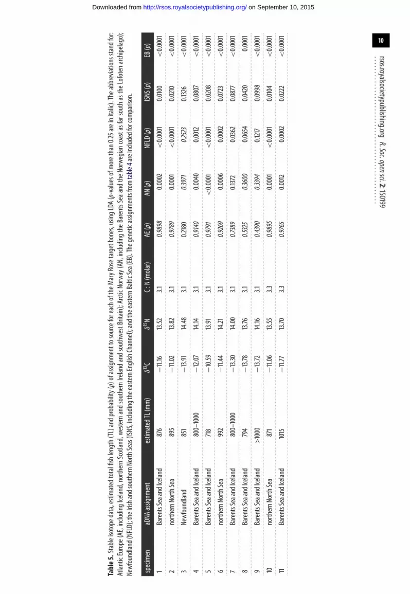
3.5. Isotopic assignment of Mary Rose target samples to control populationsThe δ13C and δ15N data for each specimen are presented in table 5, along with the probabilities ofassignment to each region by LDA. The control and target stable isotope data are also plotted in figure 2b,



10


................................................

Table5.Stableisotopedata,estimatedtotalfishlength(TL)andprobability(p)ofassignmenttosource

foreachoftheMaryRosetargetbones,usingLDA

(p-valuesofmorethan0.25areinitalic).Theabbreviationsstandfor:

AtlanticEurope(AE,including

Iceland,northernScotland,westernandsouthernIrelandandsouthwestBritain);ArcticNorway(AN,includingtheBarentsSeaand

theN

orwegiancoastasfarsouthastheLofotenarchipelago);

Newfoundland(NFLD);theIrishandsouthernNorth

Seas(ISNS,includingtheeasternEnglishChannel);andtheeasternBalticSea(EB).Thegeneticassignm

entsfromtable

4areincludedforcom

parison.

specimen

aDNA

assignm

ent

estim

atedTL(mm)

δ13C

δ15N

C:N(molar)

AE(p)

AN(p)

NFLD(p)

ISNS(p)

EB(p)

.............................................................................................................................................................................................................................................................................................................................................................................

1BarentsSeaandIceland

876

−11.16

13.52

3.10.9898

0.0002

<0.0001

0.0100

<0.0001

.............................................................................................................................................................................................................................................................................................................................................................................

2northernN

orthSea

895

−11.02

13.82

3.10.9789

0.0001

<0.0001

0.0210

<0.0001

.............................................................................................................................................................................................................................................................................................................................................................................

3Newfoundland

851

−13.91

14.48

3.10.2180

0.3971

0.2523

0.1326

<0.0001

.............................................................................................................................................................................................................................................................................................................................................................................


800–1000

−12.07

14.14

3.10.9140

0.0040

0.0012

0.0807

<0.0001

.............................................................................................................................................................................................................................................................................................................................................................................


718

−10.59

13.91

3.10.9791

<0.0001

<0.0001

0.0208

<0.0001

.............................................................................................................................................................................................................................................................................................................................................................................

6northernN

orthSea

992

−11.44

14.21

3.10.9269

0.0006

0.0002

0.0723

<0.0001

.............................................................................................................................................................................................................................................................................................................................................................................


800–1000

−13.30

14.00

3.10.7389

0.1372

0.0362

0.0877

<0.0001

.............................................................................................................................................................................................................................................................................................................................................................................


794

−13.78

13.76

3.10.5325

0.3600

0.0654

0.0420

0.0001

.............................................................................................................................................................................................................................................................................................................................................................................


>1000

−13.72

14.16

3.10.4390

0.3394

0.1217

0.0998

<0.0001

.............................................................................................................................................................................................................................................................................................................................................................................

10northernN

orthSea

871

−11.06

13.55

3.30.9895

0.0001

<0.0001

0.0104

<0.0001

.............................................................................................................................................................................................................................................................................................................................................................................


1015

−11.77

13.70

3.30.9765

0.0012

0.0002

0.0222

<0.0001

.............................................................................................................................................................................................................................................................................................................................................................................



11


................................................allowing for visual comparison. Although outside the size range of the control data, the specimens fromcod of more than 1000 mm TL do not plot separately from the other samples. On present evidence, themajority of the specimens are most consistent with origins in Atlantic Europe (a category that includesIceland, northern Scotland and the Atlantic coasts of Ireland and southwest England) or Arctic Norway,with a single specimen (no. 3) more likely to be from Arctic Norway or Newfoundland. Regardless oftheir specific origin, none of the specimens have stable isotope values consistent with control data fromthe central and southern North Sea, the Irish Sea or the (eastern) English Channel. Moreover, previouslypublished sulfur isotope data regarding the same Mary Rose samples are consistent with an offshorerather than inshore source [46]. All are likely to have derived from long-range trade or distant waterfishing, though fisheries in the Celtic Sea or the western entrance to the English Channel remain apossibility based on the isotopic results alone.

4. DiscussionBoth the aDNA and stable isotope results suggest that the Mary Rose samples are of non-localprovenance. Moreover, because each method uses different geographical groupings the genetic andisotopic evidences are complementary. The aDNA results exclude an Irish or southwest Englishsource, which remained a possibility based on isotopic attributions to Atlantic Europe. Conversely, theassignment of seven samples to Iceland or Arctic Norway by the genetic evidence can be tentativelyrefined to Iceland in at least four cases (nos. 1, 4, 5 and 11), based on attribution of these samples toAtlantic Europe by stable isotopes. In three cases (nos. 7, 8 and 9, which cluster in figure 2b) eithersource remains possible; in these instances, the LDA results are split between Atlantic Europe (mostprobable) and Arctic Norway (second most probable). In other instances, the methods are broadly inagreement, corroborating the results. The attribution of sample numbers 2, 6 and 10 to the northernNorth Sea by aDNA is consistent with their assignment to Atlantic Europe by stable isotopes. Thegenetic attribution of sample number 3 to Newfoundland is also broadly consistent with isotopicLDA probabilities that are split between Arctic Norway (40%), Newfoundland (25%) and AtlanticEurope (22%).

Setting these results in historical context, both Iceland and the waters of northern Scotland wereknown sources of dried cod (with and without salting) in the sixteenth century [20,22]. Arctic Norwayhad ceased to be a major supplier of the English market by this date, but remained an importantsource on the Continent, opening the possibility of supply by middlemen, and occasionally Englishfishermen themselves may have worked in northern Norwegian waters [47]. Our genetic data furtherindicate that one sample was probably sourced from even more distant fishing grounds off the NorthAmerican coast. Unfortunately, the isotope data could not provide the resolution to confirm or refutethis hypothesis. Nevertheless, the English Newfoundland fishery had begun in 1502, in the wake of JohnCabot’s exploratory voyage of 1497 [21], making this entirely plausible.

Regardless of the origin of this last intriguing specimen, all of the aDNA and stable isotope evidenceis consistent with the interpretation that the preserved cod used to provision the Mary Rose wereultimately sourced in the north or from across the North Atlantic, far from Portsmouth from whichshe sailed, and that the fish were drawn from diverse sources. Given that dried fish were served as themain naval ration for three of every seven days at this time [48], it is reasonable to infer that militaryneeds contributed to the demand for cod from distant waters. In comparative context, the requirementsof warfare influenced the growth of domestic fisheries in sixteenth century Scandinavia [49]. In thereign of Henry VIII (AD 1509–1547), English demand may still have been quantitatively modest; theAnthony Roll records that the royal fleet totalled only ca 58 vessels in the 1540s [50]. Nevertheless,a navy had become a royal priority, and during the reign of Elizabeth I (AD 1558–1603) it provedessential in competition with increasingly global powers such as Spain [10]. A link between the Englishfishery and navy was made explicit during Elizabeth’s reign by the introduction of weekly ‘fish days’to encourage domestic consumption and thus a commercial fleet [51]. This legislation aimed to ensurea supply of trained mariners, but must concurrently have promoted a secure source of provisions.The importance of victualling the navy continued to grow in the seventeenth century, most famouslyduring the Restoration when its administration was systematized under Samuel Pepys [52]. Militarysea power was a prerequisite for the concurrent (and subsequent) development of England’s sea-bornecolonialism, with its well-known consequences for terrestrial ecosystems globally [4]. Yet by sourcingthe cod bones from the Mary Rose, we see that the navy itself was first sustained, in part, by fishermenworking distant northern and potentially transatlantic waters. Thus, the commercial exploitation of



12


................................................aquatic ecosystems and the growth of sea power were mutually reinforcing aspects of globalization inRenaissance Europe.

Data accessibility. The supplementary material includes: table S1 Control samples of cod bone used in the study andstable isotope data; table S2 Kruskall–Wallis test results for temporal differences in δ13C and δ15N values within thearchaeological reference dataset, by geographical macro-group and two-century block; table S3 PCR primers used inthe four multiplex reactions; table S4 SNP genotypes for the control and target samples.Authors’ contributions. W.F.H. co-designed the research, jointly coordinated the study, led the genetic analysis and co-wrote the manuscript; M.C. carried out the genetics laboratory work; D.C.O. sourced archaeological control sampleswith associated contextual data, carried out the statistical analysis of the stable isotope data and contributed to thewriting of the text; B.H. and L.L.H. participated in the genetic data analysis and interpretation; S.H.D. provided thezooarchaeological data regarding the Mary Rose finds; T.C.O’C. and M.P.R. supervised the preparation and analysisof stable isotope samples; J.H.B. co-designed the study, jointly coordinated the research, led the stable isotope analysis,jointly interpreted the overall results and co-wrote the manuscript. All authors gave final approval for publication.Competing interests. We declare we have no competing interests.Funding. This research was primarily funded by grants from the Leverhulme Trust: F/00 181/R (W.F.H. and J.H.B.) andF/00 224/S (J.H.B., C. Roberts, W. Van Neer and M.P.R.). Supplementary funding was provided by the Fishmongers’Company (J.H.B.), the McDonald Institute for Archaeological Research (J.H.B. and D.C.O.) and the Max Planck Society(M.P.R.). Analysis of the stable isotope control data was funded in part by a grant from the Fishmongers’ Company,one of London’s medieval Livery Companies, which retains responsibility for quality control at London’s Billingsgatefish market. Contemporary genetic SNP data were partly sourced from a research project supported by the NaturalEnvironment Research Council’s Sustainable Marine Bioresources Programme (grant no. NE/F001967/1), ScottishGovernment Marine Scotland Science (project MF0760), and Department for Environment Food and Rural Affairs(projects MF0154 and MF1102).Acknowledgements. The Mary Rose samples were selected by Sheila Hamilton-Dyer with the permission of the MaryRose Trust, Portsmouth, and the assistance of Andrew Elkerton, collections manager. Archaeological control samplesand associated information were kindly provided by: Gerald Bigelow (Bates College); John Bryant (Bristol andRegion Archaeological Services); Bob Jones (Bristol City Council); Kate Iles (Bristol Museum); Philip Armitage(Brixham Heritage Museum); Jacqui Mulville and Niall Sharples (Cardiff University); Margaret McCarthy (Cork);Sarah Cobain (Cotswold Archaeology); Dominic Delany (Dominic Delany and Associates); Alison Locker (Escaldes-Engordany, Andorra); Charlotte Coles (Exeter Archaeology); Anton Ervynck (Flanders Heritage Agency); Leif Jonsson(Gothenburg Museum of Natural History); Polydora Baker, Pam Braddock, and Vanessa Straker (Historic England);James Rackham (James Rackham Environmental Consultancy); Hans Christian Küchelmann (Knochenarbeit);Stéphane Noël (Laval University); Francis Grew, Cath Maloney, and Dan Nesbitt (London Archaeological Archiveand Research Centre); Peter Pope (Memorial University of Newfoundland); James Morris and Natasha Powers(Museum of London Archaeology); Daniel Makowiecki (Nicolaus Copernicus University); Hannah Russ (NorthernArchaeological Associates); Rebecca Nicholson (Oxford Archaeology); Kevin Reilly (Pre-Construct Archaeology);Eileen Murphy (Queen’s University Belfast); Wim Van Neer (Royal Belgian Institute of Natural Sciences); AnneKarin Hufthammer and Colin Amundsen (University of Bergen); Jennifer Harland (University of the Highlandsand Islands); Lee Broderick (University of York); Rachel Cubitt and Christine McDonnell (York ArchaeologicalTrust). The National Museum of Ireland provided export/modification licences for all samples from the Republicof Ireland. Additional contemporary samples were kindly supplied by Carl André (University of Gothenburg)and Marije Booman (Fisheries and Oceans Canada), with origins of the rest described by Hutchinson et al. [43],Case et al. [14] and Heath et al. [32]. Thanks to Louise Butterworth, Catherine Kneale, James Rolfe and HannahZuckswert for assistance with isotopic analysis at the University of Cambridge. Thanks to Stefanie Boesel andAnnette Weiske for assistance with isotopic analysis at the Max Planck Institute for Evolutionary Anthropology,Leipzig.

References1. Jackson JBC et al. 2001 Historical overfishing and the

recent collapse of coastal ecosystems. Science 293,629–638. (doi:10.1126/science.1059199)

2. Schwerdtner Máñez K, Holm P, Blight L, Coll M,MacDiarmid A, Ojaveer H, Poulsen B, Tull M. 2014The future of the oceans past: towards a globalmarine historical research initiative. PLoS ONE 9,e101466. (doi:10.1371/journal.pone.0101466)

3. Barbier EB. 2011 Scarcity and frontiers: howeconomies have developed through natural resourceexploitation. Cambridge, UK: Cambridge UniversityPress.

4. Beinart W, Hughes L. 2009 Environment and empire.Oxford, UK: Oxford University Press.

5. Hoffmann RC. 2014 An environmental history ofmedieval Europe. Cambridge, UK: CambridgeUniversity Press.

6. Barrett JH, Locker AM, Roberts CM. 2004 The originof intensive marine fishing in medieval Europe:the English evidence. Proc. R. Soc. Lond. B271, 2417–2421. (doi:10.1098/rspb.2004.2885)

7. Barrett JH et al. 2011 Interpreting the expansionof sea fishing in medieval Europe using stableisotope analysis of archaeological cod bones.

J. Archaeol. Sci. 38, 1516–1524. (doi:10.1016/j.jas.2011.02.017)

8. Orton DC, Morris J, Locker A, Barrett JH. 2014 Fish forthe city: meta-analysis of archaeological codremains and the growth of London’s northern trade.Antiquity 88, 516–530. (doi:10.1017/S0003598X00101152)

9. Starkey DJ, Thor JTh, Heidbrink I (eds). 2009 Ahistory of the North Atlantic fisheries volume 1: fromearly times to the mid-nineteenth century. Bremen,Germany: H. M. Hauschild GmbH.

10. Quinn DB, Ryan AN. 1983 England’s sea empire,1550–1642. Winchester, MA: Allen & Unwin.


http://dx.doi.org/doi:10.1126/science.1059199

http://dx.doi.org/doi:10.1371/journal.pone.0101466

http://dx.doi.org/doi:10.1371/journal.pone.0101466

http://dx.doi.org/doi:10.1098/rspb.2004.2885

http://dx.doi.org/doi:10.1098/rspb.2004.2885

http://dx.doi.org/doi:10.1016/j.jas.2011.02.017


http://dx.doi.org/doi:10.1017/S0003598X00101152



13


................................................11. Gardiner J, Allen MJ (eds). 2005 Before the mast: life

and death aboard the Mary Rose. Oxford, UK: MaryRose Trust/Oxbow Books.

12. Barrett J et al. 2008 Detecting the medieval codtrade: a newmethod and first results. J. Archaeol.Sci. 35, 850–861. (doi:10.1016/j.jas.2007.06.004)

13. Kim H, Suresh Kumar K, Shin K-H. 2015 Applicabilityof stable C and N isotope analysis in inferring thegeographical origin and authentication ofcommercial fish (Mackerel, Yellow Croaker andPollock). Food Chem. 172, 523–527.(doi:10.1016/j.foodchem.2014.09.058)

14. Case RA, Hutchison WF, Hauser L, Van Oosterhout C,Carvalho GR. 2005 Macro- and micro-geographicvariation in pantophysin (PanI) allele frequencies inNE Atlantic cod Gadus morhua.Mar. Ecol. Progr. Ser.301, 267–278. (doi:10.3354/meps301267)

15. Milano I et al. 2014 Outlier SNP markers revealfine-scale genetic structuring across European hakepopulations (Merluccius merluccius).Mol. Ecol. 23,118–135. (doi:10.1111/mec.12568)

16. Sarvas TH, Fevolden SE. 2005 Pantophysin (Pan I)locus divergence between inshore v. offshore andnorthern v. southern populations of Atlantic cod inthe north-east Atlantic. J. Fish Biol. 67, 444–469.(doi:10.1111/j.0022-1112.2005.00738.x)

17. Layman CA et al. 2012 Applying stable isotopes toexamine food-web structure: an overview ofanalytical tools. Biol. Rev. 87, 545–562.(doi:10.1111/j.1469-185X.2011.00208.x)

18. Hemmer-Hansen J, Therkildsen NO, Meldrup D,Nielsen EE. 2014 Conserving marine biodiversity:insights from life-history trait candidate genes inAtlantic cod (Gadus morhua). Conserv. Genet. 15,213–228. (doi:10.1007/s10592-013-0532-5)

19. Barrett JH. 1997 Fish trade in Norse Orkney andCaithness: a zooarchaeological approach. Antiquity71, 616–638. (doi:10.1017/S0003598X00085367)

20. Bennema FP, Rijnsdorp AD. 2015 Fish abundance,fisheries, fish trade and consumption insixteenth-century Netherlands as described byAdriaen Coenen. Fish. Res. 161, 384–399.(doi:10.1016/j.fishres.2014.09.001)

21. Candow JE. 2009 Migrants and residents: theinterplay between European and domestic fisheriesin northeast North America, 1502–1854. In A historyof the North Atlantic fisheries volume 1: from earlytimes to the mid-nineteenth century (eds DJ Starkey,JTh Thór, I Heidbrink), pp. 416–452. Bremen,Germany: H. M. Hauschild GmbH.

22. Jones E. 2000 England’s Icelandic fishery in the earlymodern period. In England’s sea fisheries: thecommercial sea fisheries of England andWales since1300 (eds DJ Starkey, C Reid, N Ashcroft),pp. 105–110. London, UK: Chatham.

23. Kowaleski M. 2003 The commercialization of the seafisheries in medieval England andWales. Int. J.Maritime Hist. 15, 177–231.(doi:10.1177/084387140301500212)

24. Hamilton-Dyer S. 2005 Source of fish. In Before themast: life and death aboard the Mary Rose (eds J

Gardiner, MJ Allen), pp. 612. Oxford, UK: Mary RoseTrust/Oxbow Books.

25. Nielssen AR. 2009 Norwegian fisheries c.1100–1850.In A history of the North Atlantic fisheries volume 1:from early times to the mid-nineteenth century (edsDJ Starkey, JTh Thór, I Heidbrink), pp. 83–109.Bremen, Germany: H. M. Hauschild GmbH.

26. Christensen JT, Richardson K. 2008 Stable isotopeevidence of long-term changes in the North Seafood web structure.Mar. Ecol. Progr. Ser. 368, 1–8.(doi:10.3354/meps07635)

27. Doney SC. 2010 The growing human footprint oncoastal and open-ocean biogeochemistry. Science328, 1512–1516. (doi:10.1126/science.1185198)

28. Hutchinson WF. 2008 The dangers of ignoring stockcomplexity in fishery management: the case of theNorth Sea cod. Biol. Lett. 4, 693–695.(doi:10.1098/rsbl.2008.0443)

29. Ólafsdóttir GÁ, Westfall KM, Edvardsson R, PálssonS. 2014 Historical DNA reveals the demographichistory of Atlantic cod (Gadus morhua) in medievaland early modern Iceland. Proc. R. Soc. B 281,20132976. (doi:10.1098/rspb.2013.2976)

30. Struck U, Emeis K-C, Voss M, Christiansen C,Kunzendorf H. 2000 Records of southern and centralBaltic Sea eutrophication in δ13C and δ15N ofsedimentary organic matter.Mar. Geol. 164,157–171. (doi:10.1016/S0025-3227(99)00135-8)

31. Therkildsen NO et al. 2013 Spatiotemporal SNPanalysis reveals pronounced biocomplexity at thenorthern range margin of Atlantic cod Gadusmorhua. Evol. Appl. 6, 690–705.(doi:10.1111/eva.12055)

32. Heath MR et al. 2013 Combination of genetics andspatial modelling highlights the sensitivity of cod(Gadus morhua) population diversity in the NorthSea to distributions of fishing. ICES J. Mar. Sci. 71,794–807. (doi:10.1093/icesjms/fst185)

33. Jones AKG. 1991 The fish remains from excavationsat Freswick Links, Caithness. DPhil, University ofYork, UK.

34. Coy J, Hamilton-Dyer S. 2005 Meat and fish: thebone evidence. In Before the mast: life and deathaboard the Mary Rose (eds J Gardiner, MJ Allen),pp. 564–588. Oxford, UK: Mary Rose Trust/OxbowBooks.

35. Yang DY, Cannon A, Saunders SR. 2004 DNA speciesidentification of archaeological salmon bone fromthe Pacific Northwest Coast of North America. J.Archaeol. Sci. 31, 619–631.(doi:10.1016/j.jas.2003.10.008)

36. Craig H. 1957 Isotopic standards for carbon andoxygen and correction factors for mass-spectromicanalysis of carbon dioxide. Geochim. Cosmochim.Acta 12, 133–149.(doi:10.1016/0016-7037(57)90024-8)

37. Mariotti A. 1983 Atmospheric nitrogen is a reliablestandard for natural N-15 abundancemeasurements. Nature 303, 685–687.(doi:10.1038/303685a0)

38. DeNiro MJ. 1985 Post-mortem preservation andalteration of in vivo bone collagen isotope ratios in

relation to paleodietary reconstruction. Nature 317,806–809. (doi:10.1038/317806a0)

39. Szpak P. 2011 Fish bone chemistry andultrastructure: implications for taphonomy andstable isotope analysis. J. Archaeol. Sci. 38,3358–3372. (doi:10.1016/j.jas.2011.07.022)

40. Corander J, Waldmann P, Sillanpää MJ. 2003Bayesian analysis of genetic differentiationbetween populations. Genetics 163,367–374.

41. Excoffier L, Laval G, Schneider S. 2005 Arlequin ver.3.0: an integrated software package for populationgenetics data analysis. Evol. Bioinform. Online 1,47–50.

42. Venables WN, Ripley BD. 2002Modern appliedstatistics with S, 4th edn. New York, NY: Springer.

43. Hutchinson WF, Carvalho GR, Rogers SI. 2001Marked genetic structuring in localised spawningpopulations of cod Gadus morhua in the North Seaand adjoining waters, as revealed bymicrosatellites.Mar. Ecol. Progr. Ser. 233, 251–260.(doi:10.3354/meps223251)

44. Knutsen H, Jorde PE, André C, Stenseth NC. 2003Fine-scaled geographical population structuring ina highly mobile marine species: the Atlantic cod.Mol. Ecol. 12, 385–394.(doi:10.1046/j.1365-294X.2003.01750.x)

45. Skarstein TH, Westgaard J-I, Fevolden S-E. 2007Comparing microsatellite variation in north-eastAtlantic cod (Gadus morhua L.) to geneticstructuring as revealed by the pantophysin (Pan I)locus. J. Fish Biol. 70, 271–290.(doi:10.1111/j.1095-8649.2007.01456.x)

46. Nehlich O, Barrett JH, Richards MP. 2013 Spatialvariability in sulphur isotope values ofarchaeological and modern cod (Gadus morhua).Rapid Commun. Mass Spectrometry 27, 2255–2262.(doi:10.1002/rcm.6682)

47. Childs WR. 1997 The commercial shipping ofsouth-western England in the later fifteenthcentury.Mariner’s Mirror 83, 272–292.(doi:10.1080/00253359.1997.10656647)

48. Coy J, Hamilton-Dyer S. 2005 ‘Flesh, fish biscuit andbeer’: victuals for the ship. In Before the mast: lifeand death aboard the Mary Rose (eds J Gardiner,MJ Allen), pp. 602–609. Oxford, UK: Mary RoseTrust/Oxbow Books.

49. Holm P. 1998 Fiskeriets økonomiske betydning iDanmark 1350–1650. Sjæk’len. Årbog for Fiskeri- ogSøfartsmuseet 1998, 8–42.

50. Knighton CS, Loades DM (eds). 2000 The AnthonyRoll of Henry VIII’s navy: Pepys Library 2991 andBritish Library Additional MS 22047 with relateddocuments. Aldershot, UK: Ashgate.

51. Jackson G. 2000 State concern for the fisheries,1485–1815. In England’s sea fisheries: the commercialsea fisheries of England andWales since 1300 (eds DJStarkey, C Reid, N Ashcroft), pp. 46–53. London, UK:Chatham.

52. Bryant A. 1938 Samuel Pepys: the saviour of thenavy. Cambridge, UK: Cambridge UniversityPress.




http://dx.doi.org/doi:10.1016/j.foodchem.2014.09.058

http://dx.doi.org/doi:10.3354/meps301267

http://dx.doi.org/doi:10.1111/mec.12568

http://dx.doi.org/doi:10.1111/j.0022-1112.2005.00738.x

http://dx.doi.org/doi:10.1111/j.1469-185X.2011.00208.x

http://dx.doi.org/doi:10.1007/s10592-013-0532-5


http://dx.doi.org/doi:10.1016/j.fishres.2014.09.001

http://dx.doi.org/doi:10.1177/084387140301500212


http://dx.doi.org/doi:10.1126/science.1185198

http://dx.doi.org/doi:10.1098/rsbl.2008.0443

http://dx.doi.org/doi:10.1016/S0025-3227(99)00135-8

http://dx.doi.org/doi:10.1111/eva.12055

http://dx.doi.org/doi:10.1093/icesjms/fst185


http://dx.doi.org/doi:10.1016/0016-7037(57)90024-8

http://dx.doi.org/doi:10.1038/303685a0

http://dx.doi.org/doi:10.1038/317806a0



http://dx.doi.org/doi:10.1046/j.1365-294X.2003.01750.x

http://dx.doi.org/doi:10.1111/j.1095-8649.2007.01456.x

http://dx.doi.org/doi:10.1002/rcm.6682

http://dx.doi.org/doi:10.1080/00253359.1997.10656647


The globalization of naval provisioning: ancient DNA and stable isotope analyses of stored cod from...

Documents

Transcript of The globalization of naval provisioning: ancient DNA and stable isotope analyses of stored cod from...