1

Robust Dynamic CPU Resource Provisioning inVirtualized Servers

Evagoras Makridis, Kyriakos Deliparaschos, Evangelia Kalyvianaki,Argyrios Zolotas, Senior Member, IEEE , and Themistoklis Charalambous, Member, IEEE

Abstract—We present robust dynamic resource allocation mechanisms to allocate application resources meeting Service LevelObjectives (SLOs) agreed between cloud providers and customers. In fact, two filter-based robust controllers, i.e. H∞ filter andMaximum Correntropy Criterion Kalman filter (MCC-KF), are proposed. The controllers are self-adaptive, with process noise variancesand covariances calculated using previous measurements within a time window. In the allocation process, a bounded client meanresponse time (mRT) is maintained. Both controllers are deployed and evaluated on an experimental testbed hosting the RUBiS (RiceUniversity Bidding System) auction benchmark web site. The proposed controllers offer improved performance under abrupt workloadchanges, shown via rigorous comparison with current state-of-the-art. On our experimental setup, the Single-Input-Single-Output(SISO) controllers can operate on the same server where the resource allocation is performed; while Multi-Input-Multi-Output (MIMO)controllers are on a separate server where all the data are collected for decision making. SISO controllers take decisions notdependent to other system states (servers), albeit MIMO controllers are characterized by increased communication overhead andpotential delays. While SISO controllers offer improved performance over MIMO ones, the latter enable a more informed decisionmaking framework for resource allocation problem of multi-tier applications.

Index Terms—Resource provisioning, virtualized servers, CPU allocation, CPU usage, RUBiS, Robust prediction, H∞ filter, MCC-KF,Kalman filter.

F

1 INTRODUCTION

C LOUD computing has revolutionized the way applica-tions are delivered over the Internet. A typical Cloud

offers resources on demand, such as CPU cycles, memoryand storage space to applications typically using a pay-as-you-go model. Clouds often employ multiple data centersgeographically distributed to allow application deploymentin various locations around the world for reduced responsetimes. A data center contains tens of thousands of servermachines located in a single warehouse to reduce opera-tional and capital costs. Within a single data center modernapplications are typically deployed over multiple servers tocope with their resource requirements. The task of allocatingresources to applications is referred to as resource manage-ment. In particular, resource management aims at allocatingcloud resources in a way to align with application per-formance requirements and to reduce the operational costof the hosted data center. However, as applications oftenexhibit highly variable and unpredicted workload demands,resource management remains a challenge; see, for example,a comprehensive review on resource management in [1].

A common practice to resource management has been

• E. Makridis and T. Charalambous are with the Department of ElectricalEngineering and Automation, Aalto University.E-mail: name.surname@aalto.fi

• K. Deliparaschos is with the Department of Electrical Engineering, Com-puter Engineering and Informatics, Cyprus University of Technology.E-mail: k.deliparaschos@cut.ac.cy

• E. Kalyvianaki is with the Department of Computer Science and Technol-ogy, University of Cambridge, United Kingdom.E-mail: ek264@cam.ac.uk

• A. Zolotas is with the School of Engineering, University of Lincoln,United Kingdom.E-mail: azolotas@lincoln.ac.uk

to over-provision applications with resources to cope evenwith their most demanding but rare workloads. Althoughsimple, this practice has led to substantial under-utilizationof data centers (see, e.g., [2]) since practitioners are devotingdisjoint groups of server machines to a single application.At the same time, the advent of virtualization enables ahighly configurable environment for application deploy-ment. A server machine can be partitioned into mutlipleVirtual Machines (VMs) each providing an isolated serverenvironment capable of hosting a single application orparts of it in a secure and resource assured manner. Theallocation of resources to VM can be changed at runtimeto dynamically match the virtualized application workloaddemands. Virtualization enables server consolidation where asingle physical server can run multiple VMs while sharingits resources and running different applications within theVMs. In addition, studies have shown that reducing thefrequency of VM migrations and server switches can be verybeneficial for energy saving [3]. Ultimately, server consol-idation increases data center utilization and thus reducesenergy consumption and operational costs.

The main challenge of server consolidation is how todynamically adjust the allocation of VM resources so as tomatch the virtualized application demands, meet their Ser-vice Level Objectives (SLOs) and achieve increased serverutilization. Towards this end, different autonomic resourcemanagement methods have been proposed to dynamicallyallocate resources across virtualized applications with di-verse workload and highly fluctuating workload demands.Autonomic resource management in a virtualized environ-ment using control-based techniques has recently gainedsignificant attention; see [4], [5] and [6] for a survey. One

arX

iv:1

811.

0553

3v1

[cs

.SY

] 1

3 N

ov 2

018

2

of the most common approaches to control the applicationperformance is by controlling its CPU utilization within theVM; see, e.g., [7] and references therein.

1.1 ContributionsCloud service providers encounter abrupt varying loadsthat deteriorate cloud elasticity on handling peak demandsand potential unpredictable system faults and failures [8].For this reason, we formulate the problem of CPU resourceprovisioning using robust control techniques, where thecontrollers aim at anticipating abrupt workload changes inorder to maintain a certain headroom of the allocation abovethe utilization so that a certain SLO is satisfied. In particular,we use robust filters to predict the random CPU utilizationsof a two-tier virtualized server application and, therefore,provide the CPU allocations needed dynamically to satisfya certain upper bound on the mRT.

The contributions of this paper are as follows:• An adaptive H∞ filter (SISO and MIMO) which mini-

mizes the worst-case estimation error hence improvingrobustness in the state estimation problem.H∞ tracks theCPU resource utilization and adapts the state estimationbased on previous observations and noises. TheH∞ filteris designed and evaluated using our experimental setup.

• An adaptive MCC-KF (SISO and MIMO), i.e., an ex-tended version of the Kalman filter, that utilizes higher-order statistics to predict state(s) and track the CPU re-source utilization. MCC-KF is designed to adapt the stateestimation based on previous observations and noisessimilar to that of aH∞ filter. Its performance is evaluatedvia our experimental setup using real-data CPU resourcedemands.

• A generic algorithm for dynamic CPU allocation is pre-sented in order to illustrate how control theoretic ap-proaches can address the aspect of resource provisioningin virtualized servers.

1.2 OrganizationThe rest of the paper is organized as follows. Section 2presents the notation used throughout the paper. In Sec-tion 3, we introduce the client mean request response timesand the performance metric used to evaluate the perfor-mance of the system. Section 4 discusses the model adoptedfor capturing the dynamics of the CPU utilization. Section 5presents the robust controllers developed, while the experi-mental setup is described in Section 6. The performance ofthe proposed controllers is evaluated and compared withother state-of-the-art solutions in Section 7. Related work, tothe topic presented here, is discussed in Section 8. Finally,Section 9 presents conclusions and discusses directions offuture research.

2 NOTATION

Note that R and R+ represent the real and the nonnegativereal numbers, respectively. Vectors, matrices and sets, aredenoted by lowercase, uppercase and calligraphic uppercaseletters, respectively. AT and A−1 denote the transpose andinverse of matrix A, respectively. The identity matrix isrepresented by I . Also, xk|k−1 and xk|k denote the a priori

and a posteriori estimates of random value/vector xk fortime instant k. Pk denotes the matrix P at time instant k.E{·} represents the expectation of its argument. Given anyvector norm ‖ · ‖, a weighted vector norm can be written as‖x‖Q , ‖Qx‖, where Q is an arbitrary nonsingular matrix.

3 PERFORMANCE METRIC

One of the most widely used metrics for measuring serverperformance is the client mean request response times (mRT).It is difficult to predict the values of the mRT of serverapplications across operating regions, and different applica-tions and workloads. However, it is known to have certaincharacteristics [9]. In particular, its values can be dividedinto three regions:

(a) when the application has abundant resources and,therefore, all requests are served as they arrive andthe response times are kept low;

(b) when the utilization approaches 100% (e.g. around70-80% on average) the mRT increases above thelow values from the previous region, due to the factthat there are instances in which the requests increaseabruptly, approaching 90-100%;

(c) when resources are scarce and very close to 100%,since requests compete for limited resources, theywait in the input queues for long and, as a result,their response times increase dramatically to rela-tively high values.

In this work, the response time of every type of requestwas captured calculating the time difference between therequest and its response, as Fig. 1 shows. All requests wereissued to our RUBiS cluster and specifically to the WebServer, through the Client Emulator that was deployed ona separate physical machine. When all requests were com-pleted, a mean value of the response times of the requestswithin a time interval of 1s was calculated in order to havean estimate of the mRT over time. Note that in the resultsfor the experiments presented in Section 7, the mRT issmoothed over the sampling/control interval.

Fig. 1: Request-to-response path.

To maintain a good server performance, the operatorstry to keep the CPU utilization below 100% of the machinecapacity by a certain value, which is usually called headroom.Headroom values are chosen such that they form the bound-ary between the second and the third mRT regions. At suchvalues the server is well provisioned and response timesare kept low. If the utilization exceeds the boundary due toincreased workload demands, operators should increase theserver resources.

Firstly, we measure the server’s performance when 100%of resources is provisioned, without any controller adjustingthe allocation of resources, in order to extract what is the re-quired headroom. In this work, we consider a Browsing Mix

3

workload type, in order to specify the server’s performancewhile the number of clients varies. Fig. 2 shows the meanresponse times (mRT) with number of clients increasing insteps of 100 until mRT crosses the 0.5s level. Clearly, themRT increases rapidly when the number of clients exceeds1350 and the SLO is violated.

1 2 3 4 5 6 7 8 9 10 11 12 13 14 15NumberofClients (x100)

0.0

0.2

0.4

0.6

0.8

1.0

1.2

1.4

mRT (s)

Fig. 2: Mean Response Times (mRT) for different workloads

Initially, with increasing number of clients the mRT stayslow, albeit when the number of clients exceeds 1200 themRT increases above the low values. Note that, the QoSthreshold of 0.5s is exceeded when the number of clients,simultaneously issuing requests to the server, is approxi-mately 1350.

1 2 3 4 5 6 7 8 9 10 11 12 13 14 15NumberofClients (x100)

0

10

20

30

40

50

60

70

80

90

100

AverageCPUusage

(%)

WebserverUsage

DatabaseUsage

Fig. 3: Average CPU usages per component for differentworkloads.

Fig. 3 shows the average CPU usage per componentwhile the number of clients increases. As shown in thisfigure, the database server demand is lower than the webserver’s one with the same number of clients. The errorbars in Fig. 3 show one standard deviation above and belowthe mean CPU usage. When, the number of clients exceeds1350, the web server’s CPU usage becomes the bottleneckand even though the database server does not use 100%of its resources, it remains (almost) constant. Hence, it isimportant to establish the required resources for all theinvolved components comprising the requests.

4 SYSTEM MODEL

4.1 SISO system

The time-varying CPU utilization per component is mod-eled as a random walk given by the following linear stochas-tic difference equation as introduced in [7], [10]–[12]:

xk+1 = xk + wk, (1)

where xk ∈ [0, 1] is the CPU utilization, i.e., the percent-age of the total CPU capacity actually used by the appli-cation component during time-interval k. The independentrandom process wk is the process noise which models theutilization between successive intervals caused by workloadchanges, e.g., requests being added to or removed from theserver; it is often assumed to be normally distributed [7],[10], but it can also be a distribution of finite support [11].The total CPU utilization of a VM which is actually observedby the Xen Hypervisor, yk ∈ [0, 1], is given by

yk = xk + vk, (2)

where the independent random variable vk is the utilizationmeasurement noise which models the utilization differencebetween the measured and the actual utilization; vk, asit is the case with wk, is often assumed to be normallydistributed [7], [10], but it can also be a distribution of finitesupport [11]. Note that yk models the observed utilizationin addition to any usage noise coming from other sources,such as the operating system, to support the application.

4.2 MIMO system

For the MIMO system, the dynamics of all the components(VMs) can be written compactly as

xk+1 = Axk + wk, (3a)yk = Cxk + vk, (3b)

where xk ∈ [0, 1]nx is the system’s state vector represent-ing the actual total CPU capacity precentages used by theapplication components during time-interval k. The processand measurement noise vectors, wk ∈ Rnx and vk ∈ Rny , arestochastic disturbances with zero mean and finite second-order matrices Wk and Vk, respectively. The observed statexk of the system by the Xen Hypervisor is yk ∈ Rny . MatrixA shows the interdependencies between different VMs andmatrix C captures what is actually the Xen Hypervisorobserving. In the case where the CPU utilizations at the VMsare independent, matrices A and C are given by

A =

[1 00 1

], C =

[1 00 1

]. (4)

4.3 CPU allocation

By ak ∈ R+ we denote the CPU capacity of a physicalmachine allocated to the VM, i.e., the maximum amountof resources a VM can use. The purpose of a designedcontroller is to control the allocation of the VM running aserver application while observing its utilization in the VM,maintaining good server performance in the presence ofworkload changes. This is achieved by adjusting the alloca-tion to values above the utilization. For each time-interval k,

4

the desired relationship between the two quantities is givenby:

ak = max {amin,min{(1 + h)xk, amax}} , (5)

where h ∈ (0, 1) represents the headroom (i.e., how muchextra resources are provided above the actual CPU utiliza-tion), amin is the minimum CPU allocated at any given time(if allocation goes very small, then even small usage maylead to high mRT), and amax is the maximum CPU thatcan be allocated. To maintain good server performance, theallocation ak should adapt to the utilization xk.

Let Yk represent the set of all observations up to timek. Let the a posteriori and a priori state estimates be denotedby xk|k = E {xk|Yk} and xk+1|k = E {xk+1|Yk}, respec-tively; hence, xk+1|k is the predicted CPU utilization fortime-interval k + 1. In order to approach the desired CPUallocation, as given in (5), the CPU allocation mechanismuses the prediction of the usage and is thus given by

ak+1 = max{amin,min{(1 + h)xk+1|k, amax}

}. (6)

4.4 Computation of variances/covariances

To estimate the variance of the process noise at time step k,Wk, using real-data for each component, we use a slidingwindow approach in which the variance of the data belong-ing in a sliding window of size T steps at each time step kis computed. Initially, the variance is chosen based on someprior information. T steps after the process is initiated, andT CPU usages have been stored, the variance is estimated.

While the mean of a random-walk-without-a-drift is stillzero, the covariance is non-stationary. For example, for theSISO case,

var{xk} = var{wk−1 + wk−2 + ...}= var{wk−1}+ var{wk−2}+ . . .+ var{w0}=Wk−1 +Wk−2 + . . .W0.

By taking the difference between two observations, i.e., zk ,yk − yk−1, we get:

zk = xk − xk−1 + vk − vk−1= wk−1 + vk − vk−1.

The variance of the difference between observations is thus

var{zk} = var{wk−1 + vk − vk−1}=Wk−1 + Vk − Vk−1.

While the experiment is running, the last T CPU usages isstored and used for updating the variance at each step k.Computing the variance based on the difference betweenobservations, we get:

var{zk−T+1 + . . .+ zk} = var{zk−T+1}+ . . .+ var{zk}=Wk−T + Vk−T+1 − Vk−T + . . .+Wk−1 + Vk − Vk−1.

The measurement noise variance Vk was set to a small valuebecause we observed that since the CPU usage is capturedevery 1s, and therefore, the measurement is relatively accu-rate. In other words, our measurements of the CPU usageare relatively very close to the real ones. This fact let uspin the measurement noise variance to a fixed value (herein

Vk = 1). As a result, the variance of the difference breaksdown to

var{zk−T+1 + . . .+ zk} =Wk−T + . . .+Wk−1. (7)

Hence, using (7) and assuming that the variance does notchange (much) over a time horizon T , the estimate of thevariance at time k, denoted by W SISO

k , is given by:

W SISOk =

1

Tvar{zk−T+1 + . . .+ zk}

=1

T

∑kt=k−T+1 z

2t

T−(∑k

t=k−T+1 zt

T

)2 . (8)

The process noise covariance of the components is cal-culated using a similar methodology mutatis mutandis as thevariances. At this point, we have to capture each compo-nent’s CPU usage somewhere centrally (e.g., on the MIMOcontroller node) in order to compute the covariances usingthe approach of sliding window, as before. The estimateof the covariance WMIMO

k for the two components of oursystem is given by:

WMIMOk

(a)= cov{z1,t, . . . , z1,k , z2,t, . . . , z2,k}

=

(∑kt=k−T+1 (z1,t − µz1) (z2,t − µz2)

T

), (9)

where µz1 and µz2 denote the mean CPU usages for the WebServer and Database Server components, respectively, for awindow of size T , and are given by

µz1 =

(∑kt=k−T+1 z1,t

T

)and µz2 =

(∑kt=k−T+1 z2,t

T

),

while z1,t and z2,t denote the differences between observedCPU utilizations at time instant t and t − 1 of the first andthe second component of the application, respectively.Remark 1. Note that the size of the sliding window, T , is

chosen to be large enough so that it captures the varianceof the random variable, but also it is small enough so thatit can also track the change in variance due to changesin the dynamics of the requests. Numerical investigationhelps in choosing the sliding window T ; see Section 7.

Note that each VM can be controlled either locally or viaa remote physical machine. Using the locally controlled VMas a SISO system, the estimate of the VM’s variance can beobtained, but the noise covariances with respect to other ap-plications cannot be obtained. Using a remotely controlledVM to host the MIMO controller, the noise covariances ofthe whole system can be estimated via (9).

5 CONTROLLER DESIGN

This work emphasizes robust dynamic resource provision-ing that accounts for model uncertainties and non-Gaussiannoise. Two robust controllers are proposed in order topredict and hence allocate the CPU resources in a realisticscenario for each VM that constitutes the RUBiS application.More specifically:

• H∞ filter: This controller minimizes the worst-caseestimation error of the CPU allocation and provides

5

robust state estimation. It can be modeled either as aSISO filter to control a single VM or as MIMO filterto control all VMs of a multi-tier application.

• MCC-KF: This controller is an enhanced Kalmanfilter version that utilizes the Maximum CorrentropyCriterion for the state estimation of the CPU re-sources. Note the MCC-KF measures the similarityof two random variables using information of high-order signal statistics, essentially handling cases ofnon-Gaussian noises (which are not directly handledby the standard Kalman filter. As in the H∞ filtercase, this controller can be also modeled as a SISOsystem (controlling a single VM of a multi-tier appli-cation), or as a MIMO system (controlling all VMs).

5.1 H∞ Filter

H∞ filters, called minimax filters, minimize the worst-caseestimation error hence facilitates better robustness for thestate estimation problem. In this work, we adopt a gametheoretic approach to H∞ filters proposed in [13] and thor-oughly described in [14, Chapter 11].

The cost function for our problem formulation is givenby:

J =

∑N−1k=0 ‖xk − xk|k‖22

‖x0 − x0|0‖2P−10|0

+∑N−1k=0

(‖wk‖2W−1

k

+ ‖vk‖2V −1k

)(10)

where P0|0 ∈ RN×N , Wk ∈ RN×N and Vk ∈ RN×N

are symmetric, positive definite matrices defined by theproblem specifications, i.e., P0|0 is the initial error covari-ance matrix, Wk and Vk are the process and measurementcovariance matrices for time interval k, respectively; xk|k isthe estimate of the CPU allocation. The direct minimizationof J in (10) is not tractable and, therefore, a performancebound is chosen, i.e., J < 1/θ, θ > 0, and attempt tofind an estimation strategy (controller, in this case) thatsatisfies the bound. In our problem, the target is to keepthe mRT below a certain threshold (e.g., less than 0.5s).Therefore, θ is tuned such that the desired mRT is less thana certain user-specified threshold, i.e., so that the designedcontroller satisfies the desired target. The choice of θ will beinvestigated in Section 7. Considering (10), the steady-stateH∞ filter bounds the following cost function:

J = limN→∞

∑N−1k=0 ‖xk − xk|k‖22∑N−1

k=0

(‖wk‖2W−1

k

+ ‖vk‖2V −1k

) . (11)

Let Gxe be the system that has e = [w v]T as its inputand x as its output. Since the H∞ filter makes cost (11)less than 1/θ for all wk and vk, then according to [14,Equation (11.109)]:

‖Gxe‖2∞ = supζ

‖x− x‖22‖w‖2W−1 + ‖v‖2V −1

≤ 1

θ, (12)

where ζ is the phase of ‖w‖2W−1 + ‖v‖2V −1 comprised bythe sampling time of the system and the frequency of thesignals. Since we want the mRT to be less than a certainvalue (usually around 1 second), we have to keep the CPU

usage to less than a threshold set by our mRT model.Therefore, using (12) we want:

supζ

‖D‖22‖w‖2W−1 + ‖v‖2V −1

≤ 1

θ, (13)

which is equivalent to:

θ ≤ infζ

‖w‖2W−1 + ‖v‖2V −1

‖D‖22. (14)

where D is a diagonal matrix with the allowable error foreach component along the diagonal.

Let the a posteriori (updated) and a priori (predicted) errorcovariances be given by

Pk|k = E{(xk − xk|k)(xk − xk|k)T |Yk

},

Pk+1|k = E{(xk − xk+1|k)(xk − xk+1|k)

T |Yk}.

The necessary condition to ensure that Pk|k remains positivedefinite and the system retains stability for the H∞ filter isthat:

I − θPk|k−1 + CTV −1k CPk|k−1 � 0. (15)

To design the controller we consider inequalities (14)and (15).

The equations for the H∞ filter are summarized below[14]. For the prediction phase:

xk|k−1 = Axk−1|k−1, (16a)

Pk|k−1 = APk−1|k−1AT +Wk. (16b)

For the cost function (10), the update phase of theH∞ filter isgiven by:

Kk = Pk|k−1[I − θPk|k−1 + CTV −1k CPk|k−1]−1CTV −1k

(16c)xk|k = xk|k−1 +Kk(yk − Cxk|k−1) (16d)

Pk|k = Pk|k−1[I − θPk|k−1 + CTV −1k CPk|k−1]−1 (16e)

where Kk is the gain matrix.When using a SISO controller for our SISO model given

by (1)-(2), then the prediction phase is given by

xk|k−1 = xk−1|k−1, (17a)Pk|k−1 = Pk−1|k−1 +Wk, (17b)

and the update phase is given by

Kk =Pk|k−1

Vk(1− θPk|k−1 + Pk|k−1V

−1k

) , (17c)

xk|k = xk|k−1 +Kk

(yk − xk|k−1

), (17d)

Pk|k =Pk|k−1

1− θPk|k−1 + Pk|k−1V−1k

. (17e)

The Kalman filter gain is less than the H∞ filter gainfor θ > 0, meaning that the H∞ filter relies more on themeasurement and less on the system model. As θ → 0, theH∞ filter gain and Kalman filter gain coincide [14]. For acomparison between Kalman and H∞ filters see [15].

6

5.2 Maximum Correntropy Criterion Kalman FilterIn this section, a new Kalman filter approach is deployedthat uses the Maximum Correntropy Criterion (MCC) forstate estimation, referred in literature as MCC Kalman filter(MCC-KF) in [16] and [17]. The correntropy criterion mea-sures the similarity of two random variables using infor-mation from high-order signal statistics [18]–[21]. Since theKalman filter uses only second-order signal information isnot optimal if the process and measurement noises are non-Gaussian noise disturbances, such as shot noise or mixtureof Gaussian noise.The equations for the MCC-KF are summarized below [17].For the prediction phase:

xk|k−1 = Axk−1|k−1, (18a)

Pk|k−1 = APk−1|k−1AT +Wk, (18b)

and for the update phase:

Lk =Gσ(‖ yk − Cxk|k−1‖V −1

k

)Gσ(‖ xk|k−1 −Axk−1|k−1‖P−1

k|k−1

) , (18c)

Kk = (P−1k|k−1 + LkCTV −1k C)−1LkC

TV −1k , (18d)

xk|k = xk|k−1 +Kk(yk − Cxk|k−1), (18e)

Pk|k = (I −KkC)Pk|k−1(I −KkC)T +KkVkK

Tk , (18f)

where Gσ is the Gaussian kernel, i.e.,

Gσ(‖ xi − yi ‖) = exp

(−‖ xi − yi ‖

2

2σ2

)with kernel size σ1. Note that Lk is called the minimizedcorrentropy estimation cost function andKk is the Kalman gain(as in the H∞ filter).

When using a SISO controller in our model, given by(1) and (2), the original MCC-KF equations (18a)-(18f) aresimplified to:

xk|k−1 = xk−1|k−1, (19a)Pk|k−1 = Pk−1|k−1 +Wk, (19b)

Lk =Gσ(‖ yk − xk|k−1‖V −1

k

)Gσ(‖ xk|k−1 − xk−1|k−1‖P−1

k|k−1

) , (19c)

Kk =Lk

(P−1k|k−1 + LkV−1k )Vk

, (19d)

xk|k = xk|k−1 +Kk(yk − xk|k−1), (19e)

Pk|k = (1−Kk)2Pk|k−1 +Kk

2Vk, (19f)

As it can be observed in (19a)-(19f), MCC-KF has the samestructure as the Kalman filter, but in addition, it uses high-order statistics to improve state estimation.

5.3 Resource Provisioning AlgorithmIrrespective of which filter is being used, a generic algorithmfor allocating the CPU is given in Algorithm 1. A thoroughdiscussion on possible filtering approaches is presented inSection 8.

1. The kernel bandwidth σ serves as a parameter weighting thesecond- and higher-order moments; for a very large σ (compared tothe dynamic range of the data), the correntropy will be dominated bythe second-order moment [16].

Algorithm 1 Dynamic Resource Provisioning.

1: Input: amin, amax, h, T , θ (for the H∞ filter), σ (for theMCC-KF),

2: Initialization: W0, V0 (Vk = 1 ∀k), P0|03: for each time step k do4: Data: yk5: variances/covariances6: Compute Wk for SISO and MIMO controllers ac-

cording to (8) and (9), respectively7: filter8: Update phase:9: Compute Lk (for the MCC-KF), Kk, xk|k, Pk|k

10: Prediction phase:11: Compute xk+1|k, Pk+1|k12: CPU allocation:13: Compute ak+1 using (6)14: end for15: Output: CPU allocation ak+1.

The Algorithm 1 describes the steps of our approach fordynamically provisioning the CPU resources of any cloudapplication which is hosted on virtualized servers and byusing any estimation technique proposed herein.• Step 1 (Input): Firstly, the minimum (amin) and max-

imum (amax) allocations for application’s components,the sliding window width T for the computation of thevariances and covariances as well as the tunable parame-ters θ and σ for the H∞ and MCC-K filters, respectively,are needed as inputs to the system.

• Step 2 (Initialization): Initial values for the process andmeasurement noise matrices and for the initial errorcovariance matrix must be declared in advance.

• At each time step k, the observed utilization, using theXen Hypervisor, is set as the control input signal.• Step 3 (Variance/Covariance Computation:) At this

step, the algorithm calculates the variances and/orthe covariances of T passed utilizations using theapproach in Section 4.4 in order to estimate the processcovariance error Wk at each time instance k.

• Step 4 (Filtering): Using the statistics from the previ-ous step, the filter updates the state while it computesthe Lk, Kk, xk|k and Pk|k for each time instance k.Right after, the filter predicts the next state of thesystem with computing the xk+1|k, Pk+1|k. With thisprocess, the ak+1 is computed and it can be exportedas the new allocation for the next step k + 1.

• Step 5 (Output): The new predicted allocation ak+1 isadapted in the appropriate VM using the Xen sched-uler.

6 EXPERIMENTAL SETUP

The main target is to continuously provision each virtual-ized application with enough CPU resources to adequatelyserve its incoming requests from a variable workload. Thepurpose of the Dom0 component is to monitor the CPUusage by the percentage of CPU cycles of each VM runningon the Hypervisor. The controller utilizes the CPU measure-ments in order to predict the CPU usage for the next time

7

interval and hence determine the CPU allocation, which isthen fed back to to the Hypervisor to set the new allocation.

Fig. 4: Resource allocation manager architecture.

6.1 Experimental Setup BaseOur experimental setup is divided in two different infras-tructure installations. One for the SISO controller modeland one for the MIMO controller model. To evaluate theperformance of each control system, we set up a small-scaledata center in order to host the RUBiS auction site as thecloud application. The data center consists of two physicalblade servers with Intel Xeon 5140 and 1.0GB of RAM,running Debian 8 Jessie Linux distribution with 3.16.0-4-amd64 kernel and Xen 4.4.1 Virtualization technology. Notethat Xen Hypervisor was also has been widely used forexperimental evaluations in the literature; for example, [10],[22] and [23]. These physical machines are used for hostingthe VMs of the two-tier RUBiS benchmark application. Eachphysical machine, namely PM1 and PM2, hosts a VM run-ning on Debian Jessie 8 Linux with Apache 2.4.10 web serverand MySQL 5.5.55 database respectively. Note that, thisinfrastructure does not reflect the performance of modernservers, but it adequately serves our purpose of studying theperformance of the controllers over RUBiS workload. Foreach physical machine we created a couple of configurationson the Xen Credit Scheduler overriding the default time-slice and rate-limit values. The default values for the CreditScheduler are 30ms for the time-slice and 1ms for the rate-limit. We set rate-limit unchanged at it’s default value andtime-slice at 10ms, since we determined experimentally thatreducing the time-slice value increased the performance ofthe RUBiS application.

6.2 Benchmark Application - RUBiSRice University Bidding System (RUBiS), an auction sitebenchmark, implements the core functionality of an auc-tion site, i.e., selling, browsing and bidding. It is modeledafter ebay.com and involves a client-browser emulator, aweb server, an application server and a database. It wasoriginally used to evaluate application design patterns andapplication servers performance scalability. In our work,RUBiS is hosted on a two-tier application model (webserver, database), while the Client Emulator generates theworkload for the RUBiS application. Several RUBiS imple-mentations exist using Java Servlets, PHP, and Enterprise

Java Bean (EJB) technologies. It has provisions for selling,browsing and bidding items, allowing for different sessionsfor different type of users in the form of visitor, buyerand seller to be implemented. RUBiS auction site defines26 type of actions that can be performed through client’sWeb browser. In our work, the clients were modeled us-ing the Client Emulator which is mentioned below. TheMySQL database contains 7 tables which stores: bids, buynow, categories, comments, items, regions and users. Withcloud computing increasingly attracting the attention ofresearchers, RUBiS became the classic real-data benchmarkfor resource management problems [10], [23]–[26].

6.3 Client Emulator

The Client Emulator is hosted on a third physical machine(PM3) which is dedicated for generating the RUBiS auctionsite workload. A Java code is responsible for generating theworkload and creating user sessions to send HTTP requeststo the RUBiS auction site for the purpose of emulating theclient’s behavior. The original version of Client Emulatorprovides visual statistics for throughput, response timesand other information for the sessions. However, in ourexperiments we modified the original Client Emulator’ssource code in order to capture the response time of eachcompleted request and as a next step to calculate the mRTeach second or time interval. For more information aboutthe workload generation see [27].

6.4 Resource Allocation Control

All controllers presented in this work were added on thebase project code called ViResA2, first developed for thesynthetic data generation and the performance evaluation ofthe controllers in [12] and later for the real-data performanceevaluation of the H∞ and MCC-KF SISO controllers in [23].The performance of the dynamic CPU allocation is evalu-ated using the mRT, which is measured at the Client-side ofour prototype RUBiS server application, as the performancemetric. The goal of the control system is to adapt the CPUresource allocations of a single VM or group of VMs inexchange for saving resources for other applications thatare hosted on the same physical machine. The resourceallocation can be managed using the SISO or the MIMOmodel of ViResA application respectively.

There are two parameters by which a server’s perfor-mance can be affected: (i) the number of clients that sendrequests simultaneously to the server and (ii) the workloadtype. The workload scheme used in our work will be dis-cussed further in the next section.

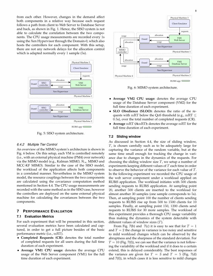
6.4.1 Single Tier ControlAn overview of the SISO system’s architecture is shown inFig. 5 below. The web server component and the databaseserver component communicate with each other via HTTPrequests, as shown in Fig. 1 Each VM of this setup iscontrolled in parallel via the SISO model (e.g., Kalman SISO,H∞ SISO and MCC-KF SISO) while keeping them isolated

2. ViResA (Virtualized [server] Resource Allocation) is a base projectcode hosted in Atlassian Bitbucket (https://bitbucket.org) as a privateGit repository. For download requests, please contact authors.

8

from each other. However, changes in the demand affectboth components in a relative way because each requestfollows a path from client to Web Server to Database Serverand back, as shown in Fig. 1. Hence, the SISO system is notable to calculate the correlation between the two compo-nents. The CPU usage measurements are recorded every 1susing the Xen Hypervisor through the Domain-0, which alsohosts the controllers for each component. With this setup,there are not any network delays for the allocation controlwhich is adapted normally every 1 sample (5s).

Fig. 5: SISO system architecture.

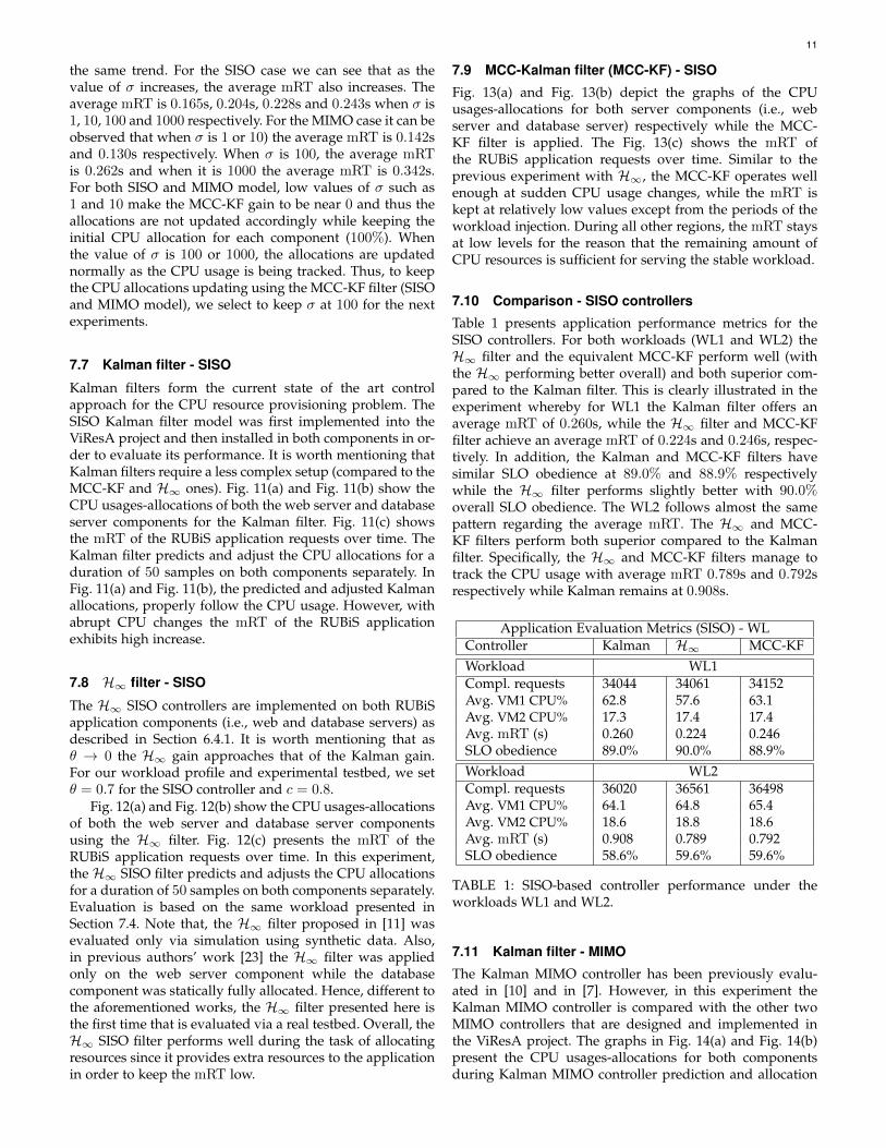
6.4.2 Multiple Tier ControlAn overview of the MIMO system’s architecture is shown inFig. 6 below. On this setup, each VM is controlled remotely(i.e., with an external physical machine (PM4) over network)via the MIMO model (e.g., Kalman MIMO, H∞ MIMO andMCC-KF MIMO). Similar to the case of the SISO model,the workload of the application affects both componentsin a correlated manner. Nevertheless in the MIMO systemmodel, the resource couplings between the two componentsare calculated using the covariance computation methodmentioned in Section 4.4. The CPU usage measurements arerecorded with the same method as in the SISO case, howeverthe controllers are deployed on the same external physicalmachine for calculating the covariances between the twocomponents.

7 PERFORMANCE EVALUATION

7.1 Evaluation MetricsFor each experiment that will be presented in this section,several evaluation metrics have been calculated and cap-tured, in order to get a full picture besides of the basicperformance metric (i.e., mRT).• Completed Requests (CR): denotes the total number

of completed requests for all users during the full timeduration of each experiment.

• Average VM1 CPU usage: denotes the average CPUusage of the Web Server component (VM1) for the fulltime duration of each experiment.

Fig. 6: MIMO system architecture.

• Average VM2 CPU usage: denotes the average CPUusage of the Database Server component (VM2) for thefull time duration of each experiment.

• SLO Obedience (SLOO): denotes the ratio of the re-quests with mRT below the QoS threshold (e.g., mRT ≤0.5s), over the total number of completed requests (CR).

• Average mRT (AmRT): denotes the average mRT for thefull time duration of each experiment.

7.2 Sliding windowAs discussed in Section 4.4, the size of sliding window,T , is chosen carefully such as to be adequately large forcapturing the variance of the random variable, but at thesame time small enough for tracking the change in vari-ance due to changes in the dynamics of the requests. Forchoosing the sliding window size T , we setup a number ofexperiments keeping different values of T each time in orderto observe the behavior of the variance for each value of T .In the following experiment we recorded the CPU usage ofthe web server component under a workload applied onRUBiS application. The workload initiates with 500 clientssending requests to RUBiS application. At sampling point20, another 500 clients are inserted to the workload foralmost another 30 samples (one sample corresponds to 5s).Then, at sampling point 100 the number of clients sendingrequests to RUBiS rise up from 500 to 1500 clients for 10samples. Finally, at sampling point 150, 1200 clients sendrequests to RUBiS for 30 more samples. The workload ofthis experiment provides a thorough CPU usage variabilitythus making the dynamics of the system detectable withdifferent values of window sizes (T ).

From Fig. 7(b) and 7(c) it is easy to see that for T = 1and T = 2 the change in variance is too noisy and sensitiveto mild workload changes which can be observed by theabruptness and the sharpness of the standard deviation. ForT = 10 (Fig. 7(f)), we can see that the variance is not follow-ing the variability of the workload and if it does to a certainextend, this is delayed considerably. The best responses ofthe variance are given for T = 3 and T = 5 (Fig. 7(d)and 7(f)), in which cases it is less sensitive to mild changes

9

0 50 100 150 200sample point

0

5

10

15

20

25

30

σ

T=1

T=2

T=3

T=5

T=10

usage

0

20

40

60

80

100

usage(%)

(a)

0 50 100 150 200sample point

0

5

10

15

20

25

30

σ

T=1

usage

0

20

40

60

80

100

usage(%)

(b)

0 50 100 150 200sample point

0

5

10

15

20

25

30

σ

T=2

usage

0

20

40

60

80

100

usage(%)

(c)

0 50 100 150 200sample point

0

5

10

15

20

25

30

σ

T=3

usage

0

20

40

60

80

100

usage(%)

(d)

0 50 100 150 200sample point

0

5

10

15

20

25

30

σ

T=5

usage

0

20

40

60

80

100

usage(%)

(e)

0 50 100 150 200sample point

0

5

10

15

20

25

30

σ

T=10

usage

0

20

40

60

80

100

usage(%)

(f)

Fig. 7: Standard deviation (σ) of the CPU usage signal for different window sizes (T) for the same workload scheme.Fig. 7(a): Standard deviation (σ) of the CPU usage all different values of window sizes (T ). Fig. 7(b)-7(f): Standard deviation(σ) of the CPU usage using window size T = 1, T = 2, T = 3, T = 5 and T = 10 sampling points respectively.

and it captures large and abrupt variabilities. Comparing

0 50 100 150 200sample point

0

5

10

15

20

25

30

σ

T=3

T=5

usage

0

20

40

60

80

100

usage(%)

Fig. 8: Standard deviation (σ) of the CPU usage signal forT = 3 and T = 5 sampling point window size.

the 2 sliding windows (T = 3 and T = 5) in Fig. 8, weconclude that there is little difference (maybe the variancefor T = 5 there is some more delay and less variability thanthat for T = 3) and any of them should work more or lessfine for our experiments. To reduce the communication andcomputational overhead, for the experiments in this workwe choose the window size to be 5 sampling points (T = 5)as it is large enough to capture the variance of the randomvariable and small enough to track the change in variancedue to the changes in the dynamics of the requests.

7.3 HeadroomLet parameter c denote the desired CPU utilization to CPUallocation ratio, i.e., c = 1/(1+ h), where h is the headroomas used in and defined right after (5). The mRT with respectto parameter c for Kalman filter - SISO,H∞ - SISO filter andMCC-KF - SISO, is shown in the Fig. 9(a) and for Kalmanfilter - MIMOH∞ - MIMO filter and MCC-KF - MIMO in the

lower Fig. 9(b) while the control action is applied every 5s.In this evaluation, we set a stable workload of 1000 clientssending requests simultaneously to the RUBiS auction site.Each measurement is derived from experiments where chas values of 0.7, 0.8, 0.9 and 0.95 which are enough topresent the behavior of mRT as parameter c grows. Whilec approaches 1, more resources are saved for other appli-cations to run, but the mRT of requests is increasing andthus the performance of the RUBiS benchmark is decreasing.This happens because the headroom approaches 0 whichmeans that there are few resources left for RUBiS to use.As it can be observed in Fig. 9(a) and Fig. 9(b), both SISOand MIMO controllers can allocate resources without a bigincrease of mRT when the parameter c is less than 0.8.However, when the c parameter increases above 0.8, themRT starts to grow exponentially. Note that the currentexperiment was conducted with a static number of clientsand thus the mRT values are relatively low. Nevertheless, alarger static number of clients sending requests to the RUBiSdoes not always lead to a higher mRT value than a dynamicsmaller number of clients. Workloads with relatively smoothdynamics can use a larger c parameter without an effectiveinfluence on the mRT. However, abrupt workloads withhigh frequency dynamics should use smaller c parameterin order to let the system to adapt on abrupt CPU usagechanges.

Using these results, we select parameter c to be 0.8for the future experiments as the workload will be moredynamic and aggressive. With the selection of such a largevalue of parameter c, enough resources would be saved forother applications to run on the same physical machine.

7.4 WorkloadThe conducted experiments run in total for 250s, an intervaladequate enough to evaluate the system’s performance.Specifically, two different workload patterns are generated

10

0.7 0.8 0.9 0.95c parameter

0.0

0.1

0.2

mRT (s)

0.052 0.055

0.109

0.159

0.051 0.053

0.099

0.155

0.053 0.061

0.095

0.159

Kalman (SISO)

H∞ (SISO)

MCC−KF (SISO)

(a)

0.7 0.8 0.9 0.95c parameter

0.0

0.1

0.2

mRT (s)

0.058 0.054

0.105

0.170

0.0450.061

0.088

0.153

0.0470.061

0.104

0.157

Kalman (MIMO)

H∞ (MIMO)

MCC−KF (MIMO)

(b)

Fig. 9: mRT with respect to c parameter - (a) SISO con-trollers, (b) MIMO controllers applied with control intervalat 5s. (Note mRT increases as c tends to unity)

for the experiments, namely Workload 1 (WL1) and Work-load 2 (WL2). Both workloads are initiated with 700 clientssending requests to the RUBiS application. At samplingpoints 10 and 30 another 500 clients are inserted to eachworkload for about 15 samples. The RUBiS Client Emula-tor deployed on PM3, sends HTTP requests to the RUBiSapplication during the entire time of the experiments. Theworkload type for RUBiS application is set to Browsing Mix(BR), where each client waits for a think time 3 following anegative exponential distribution with a mean of 7 seconds(WL1) or a custom think time (WL2) which is included inthe default RUBiS workload files, in order to send the nextrequest.

7.5 Experiment configurationEach experiment that follows (see Fig. 11- 16) was conductedfor a total duration of 250s and with c parameter set to0.8. All CPU measurements for the utilization and theallocations are exported from each component through theXen Hypervisor. The CPU usage measurements are recordedevery 1s and after the completion of one sample (i.e., 5s),the mean value of the previous interval is forwarded to thecontrollers to take action. Using this sampling approach, thecontrol action is applied every 5s in such a way that thehigh frequency variations of the workload are smoothed andbetter responses to workload increases are achieved [29]. Forthe control schemes, the initial value of the error covariancematrix, P0, the variance of the process noise, W , and thevariance of the measurement noise, V are set to 10, 4, and1 respectively. The values of the process and measurementnoises are updated on-line whenever the interval k usesthe sliding window approach, mentioned in Section 4.4.The sliding window width T is set to 5 samples, whichcorrespond to 25s.

3. Time between two sequential requests of an emulated client. Thor-ough discussion and experiments are presented in [28]

0.1 0.3 0.5 0.7theta (θ)

0.0

0.1

0.2

0.3

0.4

mRT (s)

0.258 0.245 0.249 0.2450.2460.281

0.258 0.270

SISO

MIMO

(a)

1 10 100 1000sigma (σ)

0.0

0.1

0.2

0.3

0.4

mRT (s)

0.1650.204

0.228 0.243

0.171 0.155

0.2560.283

SISO

MIMO

(b)

Fig. 10: mRT with respect to theta (θ) and sigma (σ) forH∞(Fig 10(a)) and MCC-KF (Fig. 10(b)) respectively.

7.6 Parameter tuning

Apart from Kalman filter, H∞ and MCC-KF need tuningparameters θ and σ, respectively. In order to take a decisionfor the values of these parameters, we setup experimentswith the workload WL1 described in Section 7.4. Note thatthe experiments have run for both SISO and MIMO models.Fig. 10 present the average mRT for the total duration ofeach experiment with respect to θ and σ value for H∞ andMCC-kF (SISO and MIMO models) respectively.

Fig. 10(a) illustrates the different average mRT valueswhile the H∞ controller is applied to track the CPU utiliza-tion of each component. For the SISO case, there is a smalldifference on the mRT with different values of θ, howeverfor small values (i.e., 0.1, 0.3) the controller fails to trackthe CPU utilization accurately because of the over/underestimated values of the controller gain. When θ is 0.5 or0.7 the CPU utilization tracking is better and thus we selectθ to be 0.7 whereupon the H∞ SISO controller performsbetter. For the MIMO case it is clear that when θ is at lowvalues (e.g., 0.1 and 0.3) the average mRT is relatively high(0.278s and 0.275s respectively). When θ is 0.5 or 0.7, theaverage mRT stays at lower values and specifically 0.223sand 0.239s respectively. However, the gain increases whenθ also increases which makes the CPU usage tracking moreaggressive and thus the allocations are kept for many sam-ples at the component’s CPU usage upper bound (100%).At this situation there are many CPU resources unutilizedand this is the reason for the low mRT values. To keep theCPU usage tracking using the H∞ filter non-aggressive, wechoose for the experiments, θ to be 0.1.

As in the H∞ case, MCC-KF needs a parameter tuningin order to accurately predict the CPU allocations based onthe past utilizations. For this reason, we setup experimentswith the same context as the H∞. Fig. 10(b) presents theaverage mRT for the total duration of each experiment withrespect to σ value for both SISO and MIMO. As we cansee, both SISO and MIMO models, perform with almost

11

the same trend. For the SISO case we can see that as thevalue of σ increases, the average mRT also increases. Theaverage mRT is 0.165s, 0.204s, 0.228s and 0.243s when σ is1, 10, 100 and 1000 respectively. For the MIMO case it can beobserved that when σ is 1 or 10) the average mRT is 0.142sand 0.130s respectively. When σ is 100, the average mRTis 0.262s and when it is 1000 the average mRT is 0.342s.For both SISO and MIMO model, low values of σ such as1 and 10 make the MCC-KF gain to be near 0 and thus theallocations are not updated accordingly while keeping theinitial CPU allocation for each component (100%). Whenthe value of σ is 100 or 1000, the allocations are updatednormally as the CPU usage is being tracked. Thus, to keepthe CPU allocations updating using the MCC-KF filter (SISOand MIMO model), we select to keep σ at 100 for the nextexperiments.

7.7 Kalman filter - SISO

Kalman filters form the current state of the art controlapproach for the CPU resource provisioning problem. TheSISO Kalman filter model was first implemented into theViResA project and then installed in both components in or-der to evaluate its performance. It is worth mentioning thatKalman filters require a less complex setup (compared to theMCC-KF and H∞ ones). Fig. 11(a) and Fig. 11(b) show theCPU usages-allocations of both the web server and databaseserver components for the Kalman filter. Fig. 11(c) showsthe mRT of the RUBiS application requests over time. TheKalman filter predicts and adjust the CPU allocations for aduration of 50 samples on both components separately. InFig. 11(a) and Fig. 11(b), the predicted and adjusted Kalmanallocations, properly follow the CPU usage. However, withabrupt CPU changes the mRT of the RUBiS applicationexhibits high increase.

7.8 H∞ filter - SISO

The H∞ SISO controllers are implemented on both RUBiSapplication components (i.e., web and database servers) asdescribed in Section 6.4.1. It is worth mentioning that asθ → 0 the H∞ gain approaches that of the Kalman gain.For our workload profile and experimental testbed, we setθ = 0.7 for the SISO controller and c = 0.8.

Fig. 12(a) and Fig. 12(b) show the CPU usages-allocationsof both the web server and database server componentsusing the H∞ filter. Fig. 12(c) presents the mRT of theRUBiS application requests over time. In this experiment,the H∞ SISO filter predicts and adjusts the CPU allocationsfor a duration of 50 samples on both components separately.Evaluation is based on the same workload presented inSection 7.4. Note that, the H∞ filter proposed in [11] wasevaluated only via simulation using synthetic data. Also,in previous authors’ work [23] the H∞ filter was appliedonly on the web server component while the databasecomponent was statically fully allocated. Hence, different tothe aforementioned works, the H∞ filter presented here isthe first time that is evaluated via a real testbed. Overall, theH∞ SISO filter performs well during the task of allocatingresources since it provides extra resources to the applicationin order to keep the mRT low.

7.9 MCC-Kalman filter (MCC-KF) - SISO

Fig. 13(a) and Fig. 13(b) depict the graphs of the CPUusages-allocations for both server components (i.e., webserver and database server) respectively while the MCC-KF filter is applied. The Fig. 13(c) shows the mRT ofthe RUBiS application requests over time. Similar to theprevious experiment with H∞, the MCC-KF operates wellenough at sudden CPU usage changes, while the mRT iskept at relatively low values except from the periods of theworkload injection. During all other regions, the mRT staysat low levels for the reason that the remaining amount ofCPU resources is sufficient for serving the stable workload.

7.10 Comparison - SISO controllers

Table 1 presents application performance metrics for theSISO controllers. For both workloads (WL1 and WL2) theH∞ filter and the equivalent MCC-KF perform well (withthe H∞ performing better overall) and both superior com-pared to the Kalman filter. This is clearly illustrated in theexperiment whereby for WL1 the Kalman filter offers anaverage mRT of 0.260s, while the H∞ filter and MCC-KFfilter achieve an average mRT of 0.224s and 0.246s, respec-tively. In addition, the Kalman and MCC-KF filters havesimilar SLO obedience at 89.0% and 88.9% respectivelywhile the H∞ filter performs slightly better with 90.0%overall SLO obedience. The WL2 follows almost the samepattern regarding the average mRT. The H∞ and MCC-KF filters perform both superior compared to the Kalmanfilter. Specifically, the H∞ and MCC-KF filters manage totrack the CPU usage with average mRT 0.789s and 0.792srespectively while Kalman remains at 0.908s.

Application Evaluation Metrics (SISO) - WLController Kalman H∞ MCC-KFWorkload WL1Compl. requests 34044 34061 34152Avg. VM1 CPU% 62.8 57.6 63.1Avg. VM2 CPU% 17.3 17.4 17.4Avg. mRT (s) 0.260 0.224 0.246SLO obedience 89.0% 90.0% 88.9%Workload WL2Compl. requests 36020 36561 36498Avg. VM1 CPU% 64.1 64.8 65.4Avg. VM2 CPU% 18.6 18.8 18.6Avg. mRT (s) 0.908 0.789 0.792SLO obedience 58.6% 59.6% 59.6%

TABLE 1: SISO-based controller performance under theworkloads WL1 and WL2.

7.11 Kalman filter - MIMO

The Kalman MIMO controller has been previously evalu-ated in [10] and in [7]. However, in this experiment theKalman MIMO controller is compared with the other twoMIMO controllers that are designed and implemented inthe ViResA project. The graphs in Fig. 14(a) and Fig. 14(b)present the CPU usages-allocations for both componentsduring Kalman MIMO controller prediction and allocation

12

0 5 10 15 20 25 30 35 40 45 50sample point

0

10

20

30

40

50

60

70

80

90

100

CPU

(%

)

allocation

usage

(a)

0 5 10 15 20 25 30 35 40 45 50sample point

0

10

20

30

40

50

60

70

80

90

100

CPU

(%

)

allocation

usage

(b)

0 5 10 15 20 25 30 35 40 45 50sample point

0.0

0.5

1.0

1.5

2.0

2.5

3.0

mRT (s)

Kalman (SISO)

(c)

Fig. 11: Kalman - SISO filter. Fig. 11(a): CPU usage and allocation of the web server component. Fig. 11(b): CPU usage andallocation of the database server component. Fig. 11(c): mRT with respect to time for RUBiS application.

0 5 10 15 20 25 30 35 40 45 50sample point

0

10

20

30

40

50

60

70

80

90

100

CPU

(%

)

allocation

usage

(a)

0 5 10 15 20 25 30 35 40 45 50sample point

0

10

20

30

40

50

60

70

80

90

100

CPU

(%

)

allocation

usage

(b)

0 5 10 15 20 25 30 35 40 45 50sample point

0.0

0.5

1.0

1.5

2.0

2.5

3.0

mRT (s)

H∞ (SISO)

(c)

Fig. 12: H∞- SISO filter. Fig. 12(a): CPU usage and allocation of the web server component. Fig. 12(b): CPU usage andallocation of the database server component. Fig. 12(c): mRT with respect to time for RUBiS application.

0 5 10 15 20 25 30 35 40 45 50sample point

0

10

20

30

40

50

60

70

80

90

100

CPU

(%

)

allocation

usage

(a)

0 5 10 15 20 25 30 35 40 45 50sample point

0

10

20

30

40

50

60

70

80

90

100

CPU

(%

)

allocation

usage

(b)

0 5 10 15 20 25 30 35 40 45 50sample point

0.0

0.5

1.0

1.5

2.0

2.5

3.0

mRT (s)

MCC−KF (SISO)

(c)

Fig. 13: MCC-KF - SISO filter. Fig. 13(a): CPU usage and allocation of the web server component. Fig. 13(b): CPU usage andallocation of the database server component. Fig. 13(c): mRT with respect to time for RUBiS application.

of CPU resources. Fig. 14(c) shows the mRT of the RUBiSapplication over time after the allocations that the Kalmanfilter adapts. As can be seen in Fig. 14(a) and Fig. 14(b) atsample point 10, the Web Server utilizations affects directlythe Database utilizations which show the correlation andthe inter-component resource couplings between the VMs.An abrupt Web Server utilization change causes a directDatabase utilization change and thus the mRT is affected.During the stable workload regions, the Kalman manages tooptimally allocate resources leaving the mRT unaffected.

7.12 H∞ filter - MIMO

Fig. 15(a) and Fig. 15(b) present the graphs of the CPUusages-allocations for both components during H∞ MIMOcontroller prediction and allocation of CPU resources. TheH∞ MIMO was installed on a remote physical machine inorder to predict and control the states of the system for bothcomponents as shown in Fig. 6. Fig. 15(c) shows the mRT ofthe RUBiS application over time.

7.13 MCC-Kalman filter (MCC-KF) - MIMOExperimental results for the MCC-KF MIMO controller areshown on Fig. 16(a), Fig. 16(b) and Fig. 16(c). The MCC-KF computed and adjusted allocations with respect to theCPU usages of both components are evident in Fig. 16(a)and Fig. 16(b) for the Web Server and Database Servercomponents respectively. Kernel size σ of the correntropycriterion is set to 100 to provide sufficient weight in thesecond and higher-order statistics of the MCC-KF. As in theH∞ MIMO controller, the MCC-KF MIMO controller is alsoinstalled on a remote physical machine in order to estimatethe states and control the allocation of the system for bothcomponents (see Fig. 6). The mRT of the RUBiS applicationover time during MCC-KF MIMO control resource alloca-tion is presented in Fig. 16(c).

7.14 Comparison - MIMO controllersTable 2 presents the performance results for MIMO con-trollers under the workload WL1 and WL2. Clearly a similartrend, as in the SISO cases, follows. In this context, for both

13

0 5 10 15 20 25 30 35 40 45 50sample point

0

10

20

30

40

50

60

70

80

90

100CPU

(%

)

allocation

usage

(a)

0 5 10 15 20 25 30 35 40 45 50sample point

0

10

20

30

40

50

60

70

80

90

100

CPU

(%

)

allocation

usage

(b)

0 5 10 15 20 25 30 35 40 45 50sample point

0.0

0.5

1.0

1.5

2.0

2.5

3.0

mRT (s)

Kalman (MIMO)

(c)

Fig. 14: Kalman - MIMO filter. Fig. 14(a): CPU usage and allocation of the web server component. Fig. 14(b): CPU usageand allocation of the database server component. Fig. 14(c): mRT with respect to time for RUBiS application.

0 5 10 15 20 25 30 35 40 45 50sample point

0

10

20

30

40

50

60

70

80

90

100

CPU

(%

)

allocation

usage

(a)

0 5 10 15 20 25 30 35 40 45 50sample point

0

10

20

30

40

50

60

70

80

90

100

CPU

(%

)

allocation

usage

(b)

0 5 10 15 20 25 30 35 40 45 50sample point

0.0

0.5

1.0

1.5

2.0

2.5

3.0

mRT (s)

H∞ (MIMO)

(c)

Fig. 15: H∞- MIMO filter. Fig. 15(a): CPU usage and allocation of the web server component. Fig. 15(b): CPU usage andallocation of the database server component. Fig. 15(c): mRT with respect to time for RUBiS application.

0 5 10 15 20 25 30 35 40 45 50sample point

0

10

20

30

40

50

60

70

80

90

100

CPU

(%

)

allocation

usage

(a)

0 5 10 15 20 25 30 35 40 45 50sample point

0

10

20

30

40

50

60

70

80

90

100

CPU

(%

)

allocation

usage

(b)

0 5 10 15 20 25 30 35 40 45 50sample point

0.0

0.5

1.0

1.5

2.0

2.5

3.0

mRT (s)

MCC−KF (MIMO)

(c)

Fig. 16: MCC-KF - MIMO filter. Fig. 16(a): CPU usage and allocation of the web server component. Fig. 16(b): CPU usageand allocation of the database server component. Fig. 16(c): mRT with respect to time for RUBiS application.

workloads, the MCC-KF and equivalent H∞ filters offerbetter performance (with the H∞ slightly better overall)compared to the Kalman filter. It is worth mentioning thatthe Kalman filter is not able to predict the next state ofthe system in abrupt workload changes and thus its SLOobedience is the lowest and its average mRT is the highestfor both workloads. The H∞ has the lower average mRTwith 0.270s and 0.834s under the WL1 and WL2. Slightlyhigher values of average mRT has the MCC-KF filter with0.290s and 0.835s while using Kalman filter the averagemRT is at 0.309s and 0.896s under workload WL1 and WL2respectively.

Application Evaluation Metrics (MIMO) - WLController Kalman H∞ MCC-KFWorkload WL1Cmpl. requests 34053 34402 34332Avg. VM1 CPU% 58.4 61.3 61.1Avg. VM2 CPU% 17.6 18.0 17.8Avg. mRT (s) 0.309 0.270 0.290SLO obedience 87.2% 88.1% 88.1%Workload WL2Compl. requests 36140 36523 36441Avg. VM1 CPU% 64.1 59.9 62.0Avg. VM2 CPU% 18.4 18.5 18.8Avg. mRT (s) 0.896 0.834 0.835SLO obedience 59.2% 61.7% 61.0%

TABLE 2: MIMO-based controller performance under work-loads WL1 and WL2.

Fig. 17 shows the performance evaluation of both SISO

14

Kalman H∞ MCC−KFController

0.0

0.1

0.2

0.3

0.4

mRT (s)

0.2600.224

0.246

0.3090.270 0.290

SISO

MIMO

(a)

Kalman H∞ MCC−KFController

0

20

40

60

80

100

SLOobedience

(%

)

89.0 90.0 88.987.2 88.1 88.1

SISO

MIMO

(b)

Fig. 17: Controller comparison and evaluation. Fig. 17(a):mRT for each controller SISO and MIMO. Fig. 17(b): SLOobedience for each controller SISO and MIMO.

and MIMO models. Overall, SISO controllers have loweraverage mRT and higher SLO obedience than MIMO con-trollers. However, the MIMO model offers central controlof the CPU resources for cloud applications, while the SISOmodel can only be applied on individual virtualized servers.SISO controllers do not consider the correlation between theapplication’s components, while MIMO controllers do con-sider such correlation via the covariance calculations. MIMOcontrollers are installed on a remote physical machine whichmay adds extra delays in the control signals thus affectingmRT accordingly.

The H∞ controller offers the best performance amongthe SISO and MIMO models as it achieves the lower averagemRT and the higher SLO obedience. MCC-KF controllerfollows with a slightly higher average mRT in both SISOand MIMO models thanH∞. Lastly, the Kalman filter offersthe lower performance with the highest values of averagemRT and the lowest values of the total SLO obedience.

7.15 Remarks

The following remarks are highlighted for the SISO andMIMO approaches:

Remark 2. SISO controllers do not consider inter-componentresource couplings due to their independent action oneach physical machine (installed on the Domain-0 ofeach physical machine) of a cloud application. Sincethey do not need to exchange any messages with otherphysical machines, SISO controllers do not experienceany delays.

Remark 3. Another benefit of having SISO controllers isthat each component of a cloud application can host adifferent SISO controller depending on the dynamics ofworkload variation (e.g., Kalman filter can be used forsmoother CPU usage components, while H∞ or MCC-KF for abrupt ones).

Remark 4. MIMO controllers encompass inter-componentresource couplings (cross-coupling) via the covariancecalculation process.

Remark 5. MIMO controllers are installed on remote serverswhich may experience network delays resulting in possi-ble application performance degradation. Nevertheless,as modern cloud applications are hosted on multi-tierapplications, a centralized MIMO controller is preferredover SISO controllers in order to centrally estimateneeded the allocations of each component, while takinginto account the resource couplings.

8 RELATED WORK

In [30] and [31], the authors directly control applicationresponse times through runtime resource CPU allocation us-ing an offline system identification approach with which theytried to model the relationship between the response timesand the CPU allocations in regions where it is measuredto be linear. However, as this relationship is application-specific and relies on offline identification performancemodels, it cannot be applied when multiple applications arerunning concurrently and it is not possible/easy to adjustto new conditions. This triggered the need for searching forother approaches.

The authors in [31] and [32] were among the firstto connect the control of the application CPU utilizationwithin the VM with the response times. The use of control-based techniques has emerged as a natural approach forresource provisioning in a virtualized environment. Control-based approaches have designed controllers to continuouslyupdate the maximum CPU allocated to each VM basedon CPU utilization measurements. For example, Padala etal. [25] present a two-layer non-linear controller to regulatethe utilization of the virtualized components of multi-tierapplications.

Multi-Input-Multi-Output (MIMO) feedback controllershave also been considered; see, for example, [24] and [10].These controllers make global decisions by coupling theresource usage of all components of multi-tier server appli-cations. In addition, the resource allocation problem acrossconsolidated virtualized applications under conditions ofcontention have been considered in [25], [26]: when someapplications demand more resources than physically avail-able, then the controllers share the resources among them,while respecting the user-given priorities. Kalyvianaki etal. [7], [10] were the first to formulate the CPU allocationproblem as a state prediction one and propose adaptiveKalman-based controllers to predict the CPU utilization andmaintain the CPU allocation to a user-defined threshold.Even though the standard Kalman filter provides an optimalestimate when the noise is Gaussian, it may perform poorlyif the noise characteristics are non-Gaussian.

To account for uncertainties in the system model andnoise statistics, in this work we propose the use of twocontrollers for the state estimation of the CPU resources:(a) an H∞ filter in order to minimize the maximum errorcaused by the uncertainties in the model and (b) the Maxi-mum Correntropy Criterion Kalman Filter which measuresthe similarity of two random variables using information of

15

high-order signal statistics. This type of controllers showedimproved performance in saturation periods and suddenworkload changes. The system model in this paper is repre-sented in the form of a random walk (first-order autoregres-sive model), while a higher-order autoregressive model canbe adopted if increased modeling complexity is required.For such a linear system, robust state estimation techniqueshave been proposed. Other advanced filtering techniques,such as mixed Kalman/H∞ filtering [33] and Robust Stu-dent’s t-Based Kalman Filter [34] can also be used. More-over, due to the lower and upper bounds on the values ofthe states, one can consider filtering for nonlinear systems.Nonlinear filtering based on the Kalman filter, includesthe extended and unscented Kalman filters. Additionally,particle filtering (or sequential Monte Carlo methods) is aset of genetic-type particle Monte Carlo methodologies thatprovide a very general solution to the nonlinear filteringproblem [14]. Overall, there is room for developing andtesting advanced estimation techniques for this problem andthis paper provides a springboard for researchers to makeenhanced contributions towards this direction.

Researchers have also used neuro-fuzzy control for con-trolling CPU utilization decisions of virtual machines levelcontrollers. For example, Sithu et al. [35] present CPU loadprofiles to train the neuro-fuzzy controller to predict usagewith 100% allocation but not considering CPU allocation inthe training. Deliparaschos et al. [12], on the other hand, pre-sented the training of neuro-fuzzy controller via extensiveuse of data from established controllers, such as, [7].

9 CONCLUSIONS AND FUTURE DIRECTIONS

9.1 Conclusions

In this paper, we propose and present a rigorous studyof SISO and MIMO models comprising adaptive robustcontrollers (i.e., H∞ filter, MCC-K filter) for the CPU re-source allocation problem of VMs, while satisfying certainquality of service requirements. The aim of the controllersis to adjust the CPU resources based on observations ofprevious CPU utilizations. For comparison purposes, testswere performed on an experimental setup implementing atwo-tier cloud application. Both proposed robust controllersoffer improved performance under abrupt and randomworkload changes in comparison to the current state-of-the-art. Our experimental evaluation results show that (a)SISO controllers perform better than the MIMO ones; (b)H∞ and MCC-KF have improved performance than theKalman filter for abrupt workloads; (c) H∞ and MCC-KFhave approximately equal performance for both SISO andMIMO models. In particular, the proposed robust controllersmanage to reduce the average mRT while keeping the SLOviolations low.

9.2 Future Directions

The system considered in this paper addresses only CPUcapacity, and resource needs are coupled across multiple di-mensions (i.e., compute, storage, and network bandwidth).Therefore, workload consolidation should be performedwhile catering for resource coupling in multi-tier virtualizedapplications in order to provide timely allocations during

abrupt workload changes. In this context, part of ongoingresearch considers use of system identification/learning toextract coupling information between resource needs forworkload consolidation while meeting the SLOs.

The heterogeneity of cloud workloads could be challeng-ing for choosing a suitable headroom online for minimizingthe resources provided while meeting the SLO. Thus, itis important to evaluate the system performance underdifferent types of workload as assessed in [36]. Therefore,while CPU usage headroom varies with different workloadpatterns and frequencies, adapting the headroom could bebeneficial in terms of CPU resource savings while meetingthe SLOs.

Data centers distributed in different geo-location canwork collaboratively, and these are normally connected viahigh-speed Internet or dedicated high-bandwidth commu-nication links. VMs can be migrated, if necessary, within adata center or even across data centers [37]. The combinationof dynamically changing VMs sizes and their migration isvery challenging and an open problem. Current clouds (e.g.,Google Compute Engine, Microsoft Azure) provide limitedsupport for real-time (RT) performance to VMs; in otherwords, they cannot guarantee a SLO on low-latency [38].However, cloud services benefit from RT applications sincethey can host computation-intensive RT tasks (e.g., gam-ing consoles). An RT cloud, ensures latency guarantee fortasks running in VMs, provides RT performance isolationbetween VMs, and allows resource sharing between RT andnon-RT VMs.

Moreover, we are investigating the possibility of accel-erating workload optimization through rapid adaptationto changing throughput and latency requirements via pro-grammable logic technology (i.e., FPGA) over CPU; andGPU-based alternatives for high performance virtualizedapplications. Even though FPGAs run on lower speedsrelative to CPUs, their inherent parallelism allows processmulti-tasking resulting to dramatic speed enhancement andenabling hardware consolidation due to the ability of a sin-gle FPGA simultaneously performing the tasks of multipleservers.

ACKNOWLEDGEMENTS

The authors would like to thank Ms. Kika Christou, fromthe Information Systems & Technology Service of CyprusUniversity of Technology, for her continued support on thecomputing and networking infrastructure aspects.

REFERENCES

[1] S. Mustafa, B. Nazir, A. Hayat, A. ur Rehman Khan, and S. A.Madani, “Resource management in cloud computing: Taxonomy,prospects, and challenges,” Computers & Electrical Engineering,vol. 47, pp. 186–203, 2015.

[2] E. R. Masanet, R. E. Brown, A. Shehabi, J. G. Koomey, andB. Nordman, “Estimating the Energy Use and Efficiency Potentialof U.S. Data Centers,” Proc. of the IEEE, vol. 99, no. 8, pp. 1440–1453, Aug 2011.

[3] T. H. Nguyen, M. Di Francesco, and A. Yla-Jaaski, “Virtual ma-chine consolidation with multiple usage prediction for energy-efficient cloud data centers,” IEEE Trans. on Services Computing,2017.

[4] J. Zhang, H. Huang, and X. Wang, “Resource provision algorithmsin cloud computing: A survey,” Journal of Network and ComputerApplications, vol. 64, pp. 23–42, 2016.

16

[5] A. Ullah, J. Li, Y. Shen, and A. Hussain, “A control theoreticalview of cloud elasticity: taxonomy, survey and challenges,” ClusterComputing, May 2018.

[6] Y. Al-Dhuraibi, F. Paraiso, N. Djarallah, and P. Merle, “Elasticity incloud computing: state of the art and research challenges,” IEEETrans. on Services Computing, vol. 11, no. 2, pp. 430–447, 2018.

[7] E. Kalyvianaki, T. Charalambous, and S. Hand, “Adaptive re-source provisioning for virtualized servers using Kalman filters,”ACM Transaction on Autonomous and Adaptive Systems, vol. 9, no. 2,pp. 10:1–10:35, July 2014.

[8] D. C. Marinescu, Cloud Computing: Theory and Practice, 1st ed. SanFrancisco, CA, USA: Morgan Kaufmann Publishers Inc., 2013.

[9] L. Kleinrock, Queueing Systems, Volume 1, Theory. Wiley-Interscience, 1975.

[10] E. Kalyvianaki, T. Charalambous, and S. Hand, “Self-Adaptiveand Self-Configured CPU Resource Provisioning for VirtualizedServers using Kalman Filters,” in Proc. of the 6th Int. Conf. onAutonomic Computing (ICAC). New York, NY, USA: ACM, 2009,pp. 117–126.

[11] T. Charalambous and E. Kalyviannaki, “A min-max frameworkfor CPU resource provisioning in virtualized servers using H∞Filters,” in IEEE Conf. on Decision and Control (CDC), Dec. 2010, pp.3778–3783.

[12] K. M. Deliparaschos, T. Charalambous, E. Kalyvianaki, andC. Makarounas, “On the use of fuzzy logic controllers to complywith virtualized application demands in the cloud,” in EuropeanControl Conf. (ECC), June 2016, pp. 649–654.

[13] R. N. Banavar, “A game theoretic approach to linear dynamicestimation,” Ph.D. dissertation, Texas Univ., Austin, July 1992.

[14] D. Simon, Optimal State Estimation: Kalman, H-infinity, and Nonlin-ear Approaches. John Wiley & Sons, 2006.

[15] H. Poveda, E. Grivef, G. Ferré, and N. Christov, “Kalman vs H∞filter in terms of convergence and accuracy: Application to carrierfrequency offset estimation,” in Proc. of the 20th European SignalProcessing Conf. (EUSIPCO), Aug 2012, pp. 121–125.

[16] B. Chen, X. Liu, H. Zhao, and J. C. Principe, “Maximum corren-tropy Kalman filter,” Automatica, vol. 76, pp. 70–77, 2017.

[17] R. Izanloo, S. A. Fakoorian, H. S. Yazdi, and D. Simon, “Kalmanfiltering based on the maximum correntropy criterion in the pres-ence of non-Gaussian noise,” in Annual Conf. on Information Scienceand Systems (CISS), Mar. 2016, pp. 500–505.

[18] W. Liu, P. P. Pokharel, and J. C. Principe, “Correntropy: A localizedsimilarity measure,” in Neural Networks, 2006. IJCNN’06. Interna-tional Joint Conference on. IEEE, 2006, pp. 4919–4924.

[19] W. Liu, P. P. Pokharel, and J. C. Príncipe, “Correntropy: Propertiesand Applications in Non-Gaussian Signal Processing,” IEEE Trans.on Signal Processing, vol. 55, no. 11, Nov 2007.

[20] R. He, W. S. Zheng, and B. G. Hu, “Maximum CorrentropyCriterion for Robust Face Recognition,” IEEE Trans. on PatternAnalysis and Machine Intelligence, vol. 33, no. 8, pp. 1561–1576, Aug.2011.

[21] A. Singh and J. C. Principe, “Using Correntropy As a Cost Func-tion in Linear Adaptive Filters,” in Proc. of the 2009 Int. Joint Conf.on Neural Networks, ser. IJCNN’09. Piscataway, NJ, USA: IEEEPress, 2009, pp. 1699–1704.

[22] Q. Zhu and G. Agrawal, “Resource provisioning with budget con-straints for adaptive applications in cloud environments,” IEEETrans. on Services Computing, vol. 4, no. 5, pp. 497–511, 2012.

[23] E. Makridis, K. Deliparaschos, E. Kalyvianaki, and T. Charalam-bous, “Dynamic CPU Resource Provisioning in Virtualized Serversusing Maximum Correntropy Criterion Kalman Filters,” in IEEEInt. Conf. on Emerging Technologies and Factory Automation (ETFA),Sept. 2017.

[24] E. Kalyvianaki, T. Charalambous, and S. Hand, “Resource Provi-sioning for Multi-Tier Virtualized Server Applications,” ComputerMeasurement Group (CMG) Journal, vol. 126, pp. 6–17, 2010.

[25] P. Padala, K. Shin, X. Zhu, M. Uysal, Z. Wang, S. Singhal, A. Mer-chant, and K. Salem, “Adaptive Control of Virtualized Resourcesin Utility Computing Environments,” in Proc. of the European Conf.on Computer Systems (EuroSys), 2007, pp. 289–302.

[26] P. Padala, K.-Y. Hou, K. G. Shin, X. Zhu, M. Uysal, Z. Wang,S. Singhal, and A. Merchant, “Automated Control of MultipleVirtualized Resources,” in Proc. of the 4th ACM European Conf. onComputer Systems (EuroSys ’09). New York, NY, USA: ACM, 2009,pp. 13–26.

[27] C. Amza, A. Chandra, A. L. Cox, S. Elnikety, R. Gil, K. Rajamani,W. Zwaenepoel, E. Cecchet, and J. Marguerite, “Specification and

Implementation of Dynamic Web Site Benchmarks,” in Proc. of the5th Annual IEEE Int. Workshop on Workload Characterization (WWC-5), 2002, pp. 3–13.

[28] A. Bahga and V. K. Madisetti, “Synthetic workload generation forcloud computing applications,” Journal of Software Engineering andApplications, vol. 4, no. 07, p. 396, 2011.

[29] E. Kalyvianaki, “Resource provisioning for virtualized server ap-plications,” University of Cambridge, Computer Laboratory, Tech.Rep., 2009.

[30] Z. Wang, X. Zhu, and S. Singhal, “Utilization and SLO-BasedControl for Dynamic Sizing of Resource Partitions,” in Proc. ofthe IFIP/IEEE Int. Workshop on Distributed Systems: Operations andManagement (DSOM), October 2005, pp. 133–144.

[31] X. Zhu, Z. Wang, and S. Singhal, “Utility-Driven Workload Man-agement using Nested Control Design,” in Proc. of the AmericanControl Conf. (ACC), 2006, pp. 6033–6038.

[32] Z. Wang, X. Liu, A. Zhang, C. Stewart, X. Zhu, T. Kelly, andS. Singhal, “AutoParam: Automated Control of Application-LevelPerformance in Virtualized Server Environments,” in Proc. of theIEEE Int. Workshop on Feedback Control Implementation and Design inComputing Systems and Networks (FeBID), 2007.

[33] P. P. Khargonekar, M. A. Rotea, and E. Baeyens, “Mixed H2/H∞filtering,” Int. Journal of Robust and Nonlinear Control, vol. 6, no. 4,pp. 313–330, 1996.

[34] Y. Huang, Y. Zhang, N. Li, Z. Wu, and J. A. Chambers, “A novelrobust student’s t-based kalman filter,” IEEE Trans. on Aerospaceand Electronic Systems, vol. 53, no. 3, pp. 1545–1554, June 2017.

[35] M. Sithu and N. L. Thein, “A resource provisioning model forvirtual machine controller based on neuro-fuzzy system,” in 2011The 2nd Int. Conf. on Next Generation Information Technology (ICNIT),Jun. 2011, pp. 109–114.

[36] D. Ardagna, M. Ciavotta, and M. Passacantando, “Generalizednash equilibria for the service provisioning problem in multi-cloudsystems,” IEEE Trans. on Services Computing, vol. 10, no. 3, pp. 381–395, 2017.

[37] P. T. Endo, A. V. de Almeida Palhares, N. N. Pereira, G. E.Goncalves, D. Sadok, J. Kelner, B. Melander, and J. E. Mangs,“Resource allocation for distributed cloud: concepts and researchchallenges,” IEEE Network, vol. 25, no. 4, pp. 42–46, July 2011.

[38] S. Xi, C. Li, C. Lu, C. D. Gill, M. Xu, L. T. Phan, I. Lee, andO. Sokolsky, “RT-Open Stack: CPU Resource Management forReal-Time Cloud Computing,” in IEEE Int. Conf. on Cloud Com-puting (CLOUD). IEEE, 2015, pp. 179–186.