INVESTIGATING GALVANIC CORROSION IN LOW-ALKALINITY WATER: THE EFFECTS OF PH, HIGH DOSE CORROSION INHIBITORS, AND DISSOLVED

INORGANIC CARBON

by

Amy Meredith McClintock

Submitted in partial fulfilment of the requirements for the degree of Master of Applied Science

at

Dalhousie University Halifax, Nova Scotia

July 2013

© Copyright by Amy Meredith McClintock, 2013

ii

TABLE OF CONTENTS

LIST OF TABLES ........................................................................................................... vi

LIST OF FIGURES ........................................................................................................ vii

ABSTRACT ....................................................................................................................... x

LIST OF SYMBOLS AND ABBREVIATIONS USED ............................................... xi

ACKNOWLEDGEMENTS .......................................................................................... xiii

CHAPTER 1 INTRODUCTION ..................................................................................... 1 1.1 Project Rationale ................................................................................................. 1 1.2 Research objectives .............................................................................................. 4 1.3 Organization of Thesis ........................................................................................ 4

CHAPTER 2 LITERATURE REVIEW ......................................................................... 6 2.1 Characteristics of Premise Plumbing ................................................................. 6 2.2 Principles of Galvanic Corrosion between Lead and Copper ......................... 7

2.2.1 Reactions at the Anode and Cathode ................................................................. 8 2.2.2 Accelerated Corrosion due to Galvanic Couple............................................... 10

2.3 Other Forms of Corrosion ................................................................................ 11 2.3.1 Concentration Cell Corrosion and Tuberculation ............................................ 11 2.3.2 Microbial Corrosion in Premise Plumbing ...................................................... 11

2.4 Impacts of Water Quality on Galvanic Corrosion.......................................... 13 2.4.1 Conductivity ..................................................................................................... 13 2.4.2 Chloride to Sulfate Mass Ratio (CSMR) ......................................................... 13 2.4.3 Oxidation Reduction Potential and the Role of Oxidants ................................ 14 2.4.4 The Effect of Oxygen and Chlorine on Lead Release ..................................... 14

2.5 Buffering Capacity and Water Stability .......................................................... 16 2.6 Corrosion Control Strategies ............................................................................ 17

2.6.1 pH and Alkalinity Adjustment ......................................................................... 17 2.6.2 Orthophosphate Corrosion Inhibitors .............................................................. 18

2.6.2.1 Orthophosphate and Zinc Orthophosphate ............................................... 18 2.6.2.2 Corrosion Inhibitor Dose .......................................................................... 19

2.7 Corrosion By-Products ...................................................................................... 20 2.8 Spectroscopic Ellipsometry ............................................................................... 21

2.8.1 Basic Principles of Ellipsometry ...................................................................... 22 2.8.2 Transparent and Absorbing Films .................................................................... 23

iii

CHAPTER 3 MATERIALS AND METHODS ............................................................ 25 3.1 Pockwock Lake Source Water .......................................................................... 25 3.2 Electrochemical Experimental Set-up and Design ......................................... 26

3.2.1 Lead and Copper Galvanic Cell Set-Up........................................................... 26 3.2.2 Electrochemical Experimental Designs ........................................................... 27

3.2.2.1 Effects of ZOP, pH, and Chlorine on Metals Release at Low DIC .......... 28 3.2.2.2 Effects of OP, pH and DIC on Metals Release ......................................... 29

3.3 Stock Solution Preparation ............................................................................... 33 3.3.1 Phosphate Stock Solutions ............................................................................... 33 3.3.2 Chlorine Stock Solution ................................................................................... 34 3.3.3 Sodium Bicarbonate Stock Solution ................................................................ 34 3.3.4 pH Adjustment ................................................................................................. 34

3.4 Ellipsometry Set-Up and Design....................................................................... 34 3.4.1 In-Situ Flow Cell Set-Up ................................................................................. 34 3.4.2 Sample Preparation .......................................................................................... 35 3.4.3 Protein Solution Preparation And Dosing........................................................ 36 3.4.4 In-Situ Adsorption Measurements ................................................................... 36

3.5 Analytical Procedures ....................................................................................... 37 3.5.1 General Water Quality Parameters .................................................................. 37 3.5.2 Current ............................................................................................................. 37 3.5.3 Organic and Inorganic Carbon ......................................................................... 37 3.5.4 Anions .............................................................................................................. 38 3.5.5 Metals ............................................................................................................... 38 3.5.6 Electrode Corrosion Scale Surface Analysis ................................................... 39

3.6 Data Analysis for Electrochemical Experiments ............................................ 40

CHAPTER 4 RESULTS AND DISCUSSION .............................................................. 41 4.1 Water Condition Notation ................................................................................ 41 4.2 Relationship Between Turbidity and Particulate Lead .................................. 41 4.3 Metals Release Over Time ................................................................................ 43 4.4 Influent Water Quality of the 26 Water Conditions....................................... 45

4.4.1 Fill Water CSMR ............................................................................................. 45 4.4.2 Fill Water Current ............................................................................................ 47 4.4.3 Fill Water Conductivity ................................................................................... 49

4.5 Lead Release During the Acclimation Stage ................................................... 50 4.5.1 No Corrosion Inhibitor ..................................................................................... 50 4.5.2 Zinc Orthophosphate Corrosion Inhibitor (DIC 3 mg/L) ................................ 51 4.5.3 Orthophosphate Corrosion Inhibitor ................................................................ 51

4.6 Effect of Stagnation Time on Lead Concentration During Steady State ..... 52

iv

4.7 The Effect of pH, Cl2, and ZOP on Lead Release at Low DIC (3 mg CaCO3/L) ..................................................................................................................... 53

4.7.1 Lead Release After 1- and 2-Day Stagnation .................................................. 54 4.7.2 Effect of High pH on Disinfection Potential.................................................... 57 4.7.3 Decrease in pH with Stagnation Time ............................................................. 57 4.7.4 Effect of Cl2 on Lead Release .......................................................................... 60

4.8 Effect of pH, Orthophosphate, and DIC on Lead Release During Steady State ............................................................................................................................. 61

4.8.1 Average Lead Release...................................................................................... 61 4.8.2 Factorial Analysis ............................................................................................ 63

4.8.2.1 Effect of OP on Dissolved and Particulate Lead ...................................... 65 4.8.3 Effect of pH...................................................................................................... 66

4.9 Effect of DIC on Lead Release Without Corrosion Inhibitor ........................ 68 4.10 Comparing High-Dose Corrosion Inhibitors ZOP and OP ......................... 69

4.10.1 Relationship Between Current and Lead Concentration ................................ 72 4.11 Copper Release ................................................................................................ 74

4.11.1 Copper Release during Acclimation .............................................................. 74 4.11.2 Effect of pH, ZOP, and Cl2 on Copper Release ............................................. 74 4.11.3 Effect of pH, OP, and DIC on Copper Release.............................................. 76

4.11.3.1 Average Copper Release ......................................................................... 76 4.11.3.2 Factorial Analysis ................................................................................... 77

4.11.4 Relationship Between Lead and Copper Release .......................................... 78 4.12 Elemental Analysis of Lead Coupons ............................................................ 80

4.12.1 Without Corrosion Inhibitor .......................................................................... 80 4.12.2 Orthophosphate Corrosion Inhibitor .............................................................. 83

4.13 The Impact of High-Dose Corrosion Inhibitor on Lead Release ................ 87 4.14 Copper Coupons Scale Analysis ..................................................................... 90

4.14.1 The Role of Zinc in Copper Corrosion Mitigation ........................................ 90 4.14.2 Downstream Impacts of High-Dose Corrosion Inhibitor............................... 91

4.15 Ellipsometry: An Optical Tool for Analysis of Drinking Water Films ...... 93 4.15.1 Ex-situ Ellipsometric Measurements on Lead Sputtered Plates .................... 93 4.15.2 Protein Adsorption on Copper Coupon.......................................................... 94 4.15.3 In-situ Ellipsometry Methodology ................................................................. 95

4.15.3.1 Recommendations ................................................................................... 99

CHAPTER 5 CONCLUSION AND RECOMMENDATIONS ................................ 100 5.1 Summary of Objectives and Main Findings .................................................. 100 5.2 Concluding Remarks ....................................................................................... 103 5.3 Recommendations ............................................................................................ 104

v

5.3.1 Galvanic Studies at the Bench-Scale ............................................................. 104 5.3.2 Galvanic Corrosion Studies at the Pilot-Scale ............................................... 105

BIBLIOGRAPHY ......................................................................................................... 107

Appendix A – Supplementary Data............................................................................. 114

vi

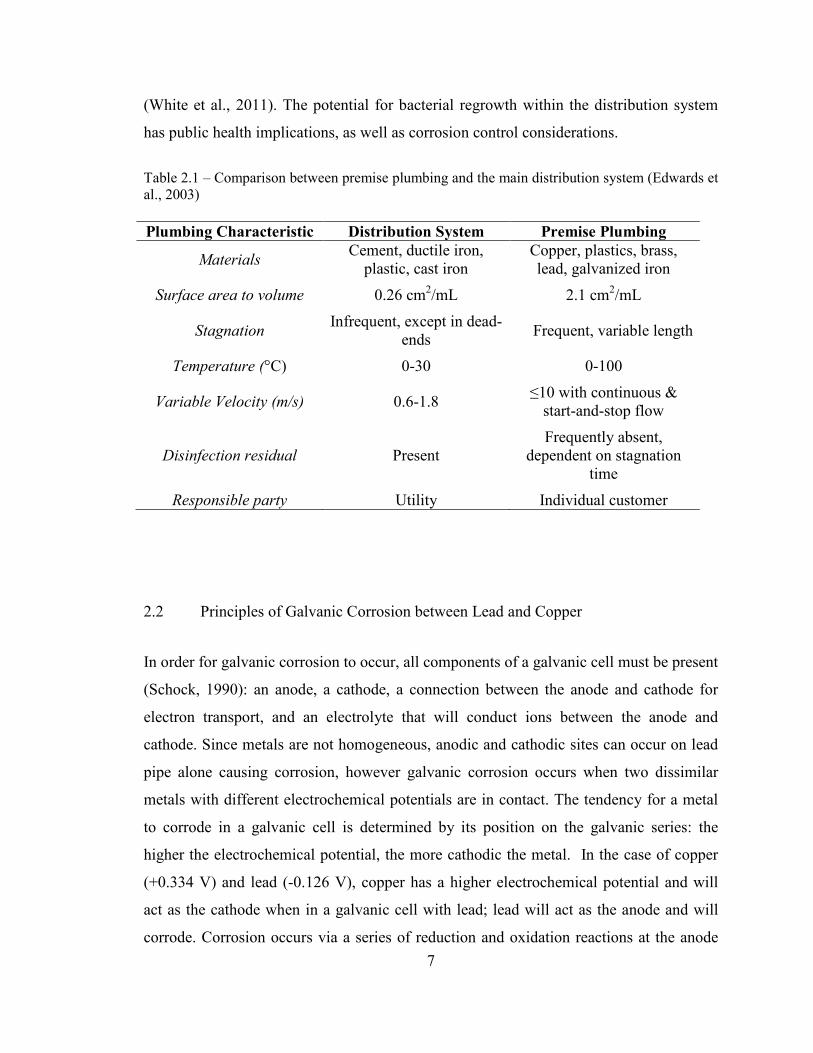
LIST OF TABLES Table 2.1 – Comparison between premise plumbing and the main distribution

system (Edwards et al., 2003) ____________________________________ 7

Table 3.1 – Summary of filtered water characteristics __________________________ 26

Table 3.2 – Low- and high- parameter levels for the electrochemical experimental design testing ZOP dose, Cl2 dose and initial pH. ____________________ 29

Table 3.3 – Low, medium, and high parameter levels for the electrochemical experimental design testing OP dose, initial pH, and DIC concentration. __ 30

Table 4.1 – Influent water quality during steady state of the 26 water conditions tested in the study _____________________________________________ 46

Table 4.2 – Decrease in bulk water pH due to atmospheric CO2 after 1, 2, and 4-day stagnation times. Value after ± represents the range of duplicate data. ____ 60

Table 4.3 – Concentration factors of all water conditions dosing corrosion inhibitors ___________________________________________________ 71

Table 4.4 – Crystalline phases identified on lead coupons exposed to OP, pH adjustment, and DIC adjustment _________________________________ 86

Table 5.1 – Summary of results __________________________________________ 101

Table A.1 – Average bulk water turbidity for all water conditions tested ___________114

Table A.2 – Average lead and copper release after 1, 2, and 4-day stagnation for all water conditions tested in this study______________________________115

vii

LIST OF FIGURES Figure 2.1 – The galvanic cell between a lead (anode) coupon and copper (cathode)

coupon. Lead oxidation and oxygen reduction occur at the anode and cathode, respectively. ___________________________________________ 9

Figure 2.2 – Schematic of an oxygen concentration cell that can occur due to biofilm adhesion to a metal surface. ______________________________ 12

Figure 2.3 – EH-pH (Pourbaix) diagram for the Pb-H2O-CO3 system. ______________ 16

Figure 2.4 – Polarization state of light reflecting off of a sample during an ellipsometric measurement (Woollam, 2013). _______________________ 23

Figure 3.1 – Summary map of the various water conditions tested according to corrosion inhibitor type, dose, pH, and chlorine dose. ________________ 31

Figure 3.2 – The flow-cell used to perform in-situ ellipsometry measurements. ______ 35

Figure 4.1 – Plot of the residual from the average over time for two representative water conditions. _____________________________________________ 44

Figure 4.2 – Pb concentration and current over the experimental duration for water type OP(10)/pH7.4/DIC(7). _____________________________________ 48

Figure 4.3 – Steady state average lead release in bulk water by stagnation time for all water conditions in with DIC(3). ______________________________ 53

Figure 4.4 – A) ZOP and pH main effects plot for 4-Day stagnation data. B) Plot of interaction between ZOP and pH where effect of one variable is dependent on the level of the other variable. ________________________ 55

Figure 4.5 – Actual pH decrease after 1, 2, and 4 day stagnation and lead release after 1-day in DIC(3) water conditions. ____________________________ 59

Figure 4.6 – Average alkalinity and DIC of the 8 water conditions. _______________ 59

Figure 4.7 – Average lead concentration of 18 water conditions dosing OP at 0, 10, or 20 mg PO4/L. ______________________________________________ 62

Figure 4.8 – Average dissolved, total, and NAD lead release of the 18 water conditions with OP dose of 0, 10, or 20 mg PO4/L and DIC either 7 or 17 mg CaCO3/L. ______________________________________________ 62

Figure 4.9 – Main effects plot displaying the effect of DIC concentration and OP dose on average lead concentration. ______________________________ 64

viii

Figure 4.10 – Interaction plot displaying the effects of OP dose on lead concentration at either DIC(7) or DIC(17). _________________________ 64

Figure 4.11 – pH after 1-, 2-, and 4-day stagnation times in water conditions without OP dosing, and representative of pH changes in water conditions at both OP doses. ____________________________________ 67

Figure 4.12 – Average steady state lead release versus influent DIC concentration of the eight water conditions without corrosion inhibitor. ______________ 70

Figure 4.13 – Average steady state lead release in the 14 water conditions dosing corrosion inhibitor, either ZOP dose of 20 mg PO4/L or OP dose of 10 or 20 mg PO4/L. ______________________________________________ 70

Figure 4.14 – Relationship between predicted lead release (calculated using initial current) versus actual lead release for two water conditions. ___________ 73

Figure 4.15 – Average copper in bulk water after 1-, 2-, and 4-day stagnation times in low alkalinity water with or without ZOP addition. ________________ 75

Figure 4.16 – Average copper concentration in 18 water conditions with OP dose of 0, 10 or 20 mg PO4/L. _________________________________________ 77

Figure 4.17 – Interaction plot demonstrating the effects of pH and OP dose on copper concentration. __________________________________________ 78

Figure 4.18 – Main effects plots of lead and copper versus ZOP dose (after 1-day stagnation). __________________________________________________ 79

Figure 4.19 – Main effects plots of lead and copper versus OP dose (all stagnation times combined). _____________________________________________ 79

Figure 4.20 – Typical copper (left) and lead (right) coupons prior to exposure to water conditions. _____________________________________________ 81

Figure 4.21 – Post-experiment copper (left) and lead (right) coupons from water condition pH9.2/DIC(3). _______________________________________ 81

Figure 4.22 – Corrosion film on lead coupon without corrosion inhibitor in water condition pH8.3/DIC(7). _______________________________________ 82

Figure 4.23 – Dendritic structure on lead coupon from water condition pH8.3/DIC(17). ______________________________________________ 82

Figure 4.24 – Higher magnification of the dendritic structure on lead coupon from water condition pH8.3/DIC(17). _________________________________ 83

ix

Figure 4.25 – Post-experiment lead and copper coupons from water condition OP(10)/pH7.4/DIC(7). _________________________________________ 85

Figure 4.26 – Post-experiment copper and lead coupons from water condition OP(20)/pH7.3/DIC(7). _________________________________________ 85

Figure 4.27 – Conductivity in water conditions with either 10 or 20 mg PO4/L. ______ 88

Figure 4.28 – EDS elemental map of copper coupon from ZOP(20)/pH7.4/DIC(3) water condition. ______________________________________________ 92

Figure 4.29 – Image of lead coupon from ZOP(20)/pH7.4/DIC(3) water condition. ___ 92

Figure 4.30 – Optical models used for (a) fitting refractive indices for the metallic Cu film in PBS, and (b) determining the thickness of adsorbed protein layer before and after rinse cycles. ________________________________ 96

Figure 4.31 – In-situ ellipsometry procedure for determining the effect of chlorine dose on protein film thickness. __________________________________ 96

Figure 4.32 – Protein film thickness (Lf, in nm) before and after the second rinse with 0.2 mg Cl2/L. ____________________________________________ 98

Figure 4.33 – Average film thickness after 2nd rinse divided by initial film thickness, Lf,f/Lf,0, over length of the copper coupon. _________________ 98

x

ABSTRACT Galvanically connected lead and copper materials in premise plumbing has shown to accelerate lead corrosion compared to lead pipe alone and can be a persistent lead release mechanism in a drinking water distribution system. pH and alkalinity adjustment and/or corrosion inhibitors are commonly used for controlling lead and copper release. The objective of this study was to evaluate galvanic corrosion potential under various pH and corrosion control conditions, and under varying buffering capacity through alkalinity addition. Bench-scale dump-and-fill beaker experiments evaluated galvanic corrosion from a lead and copper couple under stagnant conditions. Two corrosion inhibitors, orthophosphate (OP) and zinc orthophosphate (ZOP), were dosed at 10 or 20 mg PO4/L against variable pH, chlorine doses, and dissolved inorganic carbon (DIC) concentrations. As well, a new in-situ ellipsometry method was evaluated for its ability to measure nanoscale drinking water films for corrosion control applications.

Key findings from this study were that pH plays a larger role in corrosion control when alkalinity is low (DIC<3 mg CaCO3/L), and under certain conditions, high-dose corrosion inhibitor can exacerbate lead release. In particular, after 1-day stagnation, increasing pH from 7.4 to 9.2 in low alkalinity water reduced average lead release by 430 μg/L compared to 210 μg/L with ZOP addition. However, when DIC was increased to either 7 or 17 mg CaCO3/L, higher pH did not significantly reduce lead release. The combination of ZOP dose of 20 mg PO4/L and pH 9.2 resulted in the lowest lead release compared to no-corrosion inhibitor or pH adjustment alone, whereas an OP dose of 20 mg PO4/L exacerbated lead release compared to no corrosion inhibitor in some cases. On the other hand, an OP dose of 10 mg PO4/L mitigated lead release compared to no corrosion inhibitor. High lead release with 20 mg PO4/L as orthophosphate may be attributed to microbial corrosion. In-situ ellipsometry was used to evaluate lead oxide films on lead plates as well as the effects of chlorine on protein adhesion to a copper coupon to simulate bacteria adhesion to copper pipe. Analysis showed that lead films are slightly absorbing and require extensive analysis to determine film thickness and protein thickness on copper was found to be independent of chlorine dose. At this stage, ellipsometry for water treatment applications requires more troubleshooting.

This study demonstrated that lead and copper release due to galvanic couples in drinking water systems could be exacerbated with certain high-dose corrosion control strategies. The potential for exacerbating lead release with high-doses of corrosion inhibitor emphasizes the need for testing and optimizing site-specific corrosion control strategies. Additional microbial tests should be conducted when evaluating galvanic corrosion to help elucidate the role of bacteria in lead and copper corrosion, and techniques such as ellipsometry may be beneficial in understanding scale and biofilm adhesion to copper and lead materials.

xi

LIST OF SYMBOLS AND ABBREVIATIONS USED Al Aluminum

(CaOH)2 Lime

ANOVA Analysis of variance

C Carbon

Ca Calcium

CaCO3 Calcium carbonate

CFPb Lead concentration factor

Cl- Chloride

Cl2 Chlorine

CO32- Carbonate

CSMR Chloride to sulfate mass ratio

Cu Copper

DIC Dissolved inorganic carbon

DOC Dissolved organic carbon

e- Electron

EDS Electron dispersive spectroscopy

EH-pH Pourbaix

EMA Effective medium approximation

EMF Electromotive force

H2O Water

HCO3- Bicarbonate

HOCl Hypochlorous acid

ICP-ms Inductively coupled plasma mass spectrometry

ID Inner diameter

JDKWSP J.D. Kline Water Supply Plant

KH2PO4 Potassium phosphate monobasic

KMnO4 Potassium permanganate

Lf Biofilm thickness, nm

LSL Lead service line

xii

MAC Maximum allowable concentration

MSE Mean square error

NAD Nitric acid digestion

NaHCO3 Sodium bicarbonate

NaOH Sodium hydroxide/soda ash

O Oxygen

OH- Hydroxyl

ORP Oxidation reduction potential

P Phosphorus

Pb(OH)2 Lead(II) hydroxide

Pb Lead

Pb3(PO4)2 Lead(II) phosphate

Pb5(PO4)3Cl Chloropyromorphite

PbCO3 Lead(II) carbonate

PbO2 Pb(IV) oxide

PBS Phosphate buffered solution

PbSO4 Pb(II) sulfate

PO43- Phosphate

SEM Scanning electron microscope

SO42- Sulfate

THM Trihalomethane

TOC Total organic carbon

wt% Weight percent

XRD X-ray diffraction

ZOP Zinc orthophosphate

Δ Optical constant delta

Ψ Optical constant psi

xiii

ACKNOWLEDGEMENTS

I would like to acknowledge my supervisor, Dr. Graham Gagnon, who let me find my

way and who has supported my research and personal goals over the last 3 years. I am

very thankful for the opportunities you have provided me at Dal and in St. John’s that

have and will continue to play a major role in my professional development.

To Sarah Jane Payne, my lab partner and friend, your support and advice both

academically and personally have been invaluable to me. Rock on, Cowboy!

I would like to thank Heather Daurie for her guidance in the lab and for always answering

my questions with a smile on her face. I would also like to acknowledge my laboratory

assistants, Margaret Grierson and Matthew King, for their hard work and enthusiasm. It

was a pleasure working with you all.

To my committee members, Dr. Liu and Dr. Dahn, thank you for your time and

participation in my thesis development. As well, I would like to thank Dr. Dahn for

allowing me to conduct experiments in his lab, and to Mark McArthur, for patiently

showing an engineer the ellipsometry ropes and willingly lending a helping hand.

I would like to thank Tarra Chartrand for keeping paperwork and deadlines in check. The

‘small things’ made the biggest difference on stressful days, so, thank you!

To my family, who have showed ceaseless support and encouragement over the last 3

years: I finally did it! Thanks for always standing by me.

And last but certainly not least, I would like to acknowledge my labmates and friends:

You are a constant reminder that engineering is fun, and friendship will get you through

the longest of lab days.

1

CHAPTER 1 INTRODUCTION

1.1 Project Rationale

Corrosion control is a major operational challenge and cost for drinking water utilities.

Corrosion within the distribution system can lead to a loss of hydraulic capacity and

component replacements (Koch et al., 2001) as well as contribute to elevated levels of

metals, such as lead and copper, in drinking water (Cartier et al., 2012a). Although lead is

rarely naturally present in source waters, it can enter the distribution system through the

corrosion of lead bearing materials such as lead service lines (LSL), lead pipe fittings,

flux, brass, and solder.

Prior to 1975, lead was commonly used for service lines and plumbing materials because

it was soft and inexpensive, and was believed to resist corrosion by readily forming a

protective scale on the interior of pipes (Craig and Anderson, 1995). However, lead was

banned for use in plumbing material in Canada in 1975 and in solder in 1986 due to the

detrimental health effects related to the leaching of lead into drinking water. Current

regulations require that plumbing materials be ‘lead free’, however, ‘lead free’ pipes and

pipe fittings may contain up to 8% lead (SDWA, 1996). In 2011, the United States

enacted the “Reduction of Lead in Drinking Water Act” that redefines ‘lead free’ as not

containing more than 0.2% lead by weight and will come into effect January of 2014.

However, no such law has been passed in Canada and 8% by weight lead in plumbing

materials is generally accepted. Although older buildings are most likely to contain lead

bearing materials, new buildings constructed with ‘lead free’ plumbing may also

contribute to lead in drinking water (Elfland et al., 2010).

Research has shown that service lines and premise plumbing contribute a greater

proportion of dissolved and particulate lead in drinking water than does distribution

system infrastructure (Johnson et al., 1993). Service lines branching off of distribution

mains and premise plumbing are fundamentally different from the main distribution

system in terms of pipe materials, higher temperature ranges, longer stagnation times, and

higher pipe surface area to water volume ratio which all contribute to increased corrosion

2

of metals in plumbing (NRC, 2006). The connection of dissimilar metals, mainly copper

and lead that are commonly found in service lines and premise plumbing, allow for

galvanic corrosion. This commonly occurs in service lines, where the public portion

(from the distribution main to the property line) is replaced with copper and connected to

the existing lead service line on the property owner’s side. This galvanic connection has

shown to increase lead corrosion compared to undisturbed lead service lines

(Triantafyllidou and Edwards, 2011; Wang et al., 2012). For example, Cartier et al.

(2012a) found that replacing upstream lead pipe with copper pipe did not reduce the lead

concentration in water compared to lead pipe alone due to galvanic and deposition

corrosion.

To minimize the effects of corrosion on distribution and premise plumbing, two corrosion

control strategies are commonly used: (1) pH adjustment, and/or (2) passivation. Raising

water pH to above 8 typically promotes a calcium based protective scale to form on the

interior of most metal pipes (Schock, 1990). However, this approach is limited to source

waters with high buffering capacities to maintain a stable pH. In many source waters,

such as those found in the Atlantic regions, the alkalinity is low and this approach is not

feasible.

The second strategy, passivation, is facilitated using chemical corrosion inhibitors.

Phosphate passivation is effective in mitigating corrosion by creating a metal-phosphate

barrier between the copper or lead surface and the bulk water. A 2001 survey of medium

and large U.S. water utilities identified that the majority of all surface water utilities

surveyed dosed phosphate inhibitors (as opposed to pH adjustment alone) for corrosion

control (McNeill and Edwards, 2002). Orthophosphates with and without zinc are among

the most common corrosion inhibitors used in the water industry (Hill and Gianni, 2011),

however, the role of zinc in lead and copper corrosion control is not well understood.

Recent work has found that zinc orthophosphate can reduce pitting corrosion tendencies

of copper (Lattyak, 2007), however, Schneider et al. (2007) found that zinc did not play a

significant role in lead corrosion control. The type of corrosion inhibitor in conjunction

with the water chemistry and quality make corrosion control a utility–specific issue.

3

In practice, the majority of medium and large U.S. utilities surveyed dosed corrosion

inhibitors between 1 and 2 mg PO4/L (MacNeill and Edwards, 2002). Often, low dosages

are selected based on phosphorus costs that are increasing as phosphorus reserves are

depleting in quantity and quality (Smil, 2000) and to reduce the potential of phosphorus

loads on wastewater treatment processes and the receiving water bodies. Recent studies,

however, have found that high doses of orthophosphate (7 and 75 mg PO4/L) mitigated

copper corrosion (Goh et al., 2008; Lewandowski et al., 2010). These studies did not

investigate the effects of high-dose phosphate on galvanic corrosion, which is most

commonly found in premise plumbing. Although corrosion inhibitors are dosed at low

concentrations in practice, it is not known whether high doses of phosphate may be

beneficial in mitigating lead release when a galvanic connection exists.

Understanding film passivation is critical to improving corrosion control. Film thickness,

uniformity, and porosity are important characteristics in passivation effectiveness to

reduce corrosion (Hill and Cantor, 2011). Lewandowski et al. (2010) observed that

metals surfaces undergo considerable nanoscale changes in surface composition and

morphology due to corrosion within a few hours of exposure to water. Passivation scale

analysis typically occurs post experiment and no method has been developed to

characterize passivation in real-time. In-situ ellipsometry is a novel optical tool that can

measure transparent and absorbing film properties and thicknesses in real-time within a

liquid environment. Ellipsometry could provide novel information with respect to the

properties, thickness, and stability of films formed on metals which could contribute

towards our understanding of film passivation and therefore corrosion control.

4

1.2 Research objectives

The main objective of this study was to compare galvanic corrosion potential under

various pH conditions, corrosion control conditions, and under varying buffering

capacities through alkalinity addition. To achieve this, a series of bench-scale studies

were designed to address the following:

Objective 1. Compare the effects of pH adjustment, high-dose corrosion

inhibitor, and buffering capacity on galvanic corrosion:

i) Compare lead and copper release over the short- and long-term

for various corrosion control strategies.

ii) Characterize corrosion by-products formed under various

corrosion control strategies to better understand film passivation.

Objective 2. Develop an in-situ ellipsometry method for quantifying passivation

film formation at the nanometer scale in real-time to better understand passivation

corrosion control.

1.3 Organization of Thesis

A summary of each chapter is described below.

Chapter 2 presents a literature review of galvanic corrosion, premise plumbing

conditions, water quality impacts on galvanic corrosion, corrosion control strategies, and

background on the optical tool ellipsometry.

Chapter 3 describes the materials and methods used in 3 experimental designs in

Chapter 4. Electrochemical cell and ellipsometry set-ups are described, experimental

designs are presented, as well as influent water preparation, analytical sampling

techniques, and statistical methods are described in this chapter.

5

Chapter 4 presents the results of three experimental designs described in Chapter 3.

Results are discussed, including a comparison between corrosion control strategies used

in the two experimental designs.

Chapter 5 summarizes the research objectives and provides a summary of findings from

Chapter 4. Conclusions are presented followed by recommendations for future pilot- and

full-scale galvanic corrosion studies.

6

CHAPTER 2 LITERATURE REVIEW

2.1 Characteristics of Premise Plumbing

The series of pipework within a distribution system consists of service lines that

distribute water from the distribution mains to premise plumbing in the property being

served. Premise plumbing constitutes the portion of the distribution system that is

located within the building on the end-users property and differs from the distribution

system in many ways. These main differences are summarized in Table 2.1.

Unlike the distribution system, premise plumbing uses unique materials such as copper,

plastics, brass, lead, and galvanized iron with dissimilar metals often in contact. Premise

plumbing uses smaller inner diameter (ID) piping and has more surface area to unit

length than the other portions of the distribution system. As a result, higher

concentrations of metals can occur in premise plumbing than elsewhere in the system. As

well, water age varies in consumer plumbing as water can sit stagnant in pipework for

extended periods if the building is irregularly occupied. It is not uncommon for sections

of plumbing within a building to have varying water ages and temperatures if certain

sections are infrequently used. A generally accepted rule of thumb is that corrosion rates

will double for every 10°C increase in water temperature (Droste, 1997).

Water velocity and disinfection residual are different compared to the remainder of the

system. Water velocity is typically faster in premise plumbing than in the distribution

system and consists of intermittent start-and-stop flow patterns. The high velocity start-

and-stop flow can disturb corrosion scales. Cartier et al. (2012a) found that particulate

lead scales are more likely to be released at moderate to high flow rates (8-32 L/min) but

not low flow (1.3 L/min) in 1.3 cm inner diameter pipes. As well, disinfection residual is

typically below the objective disinfectant residual of the utility because of extended

stagnation times, warmer temperatures, and plumbing materials (such as copper) that

react with chlorine. Edwards et al. (2005) observed a three-log increase in bacteria during

stagnation in premise plumbing due to bacterial regrowth. As well, biofilms have shown

to be present and active even in water types with consistently high levels of chlorine

7

(White et al., 2011). The potential for bacterial regrowth within the distribution system

has public health implications, as well as corrosion control considerations.

Table 2.1 – Comparison between premise plumbing and the main distribution system (Edwards et al., 2003)

Plumbing Characteristic Distribution System Premise Plumbing

Materials Cement, ductile iron, plastic, cast iron

Copper, plastics, brass, lead, galvanized iron

Surface area to volume 0.26 cm2/mL 2.1 cm2/mL

Stagnation Infrequent, except in dead-ends Frequent, variable length

Temperature (°C) 0-30 0-100

Variable Velocity (m/s) 0.6-1.8 ≤10 with continuous & start-and-stop flow

Disinfection residual Present Frequently absent,

dependent on stagnation time

Responsible party Utility Individual customer

2.2 Principles of Galvanic Corrosion between Lead and Copper

In order for galvanic corrosion to occur, all components of a galvanic cell must be present

(Schock, 1990): an anode, a cathode, a connection between the anode and cathode for

electron transport, and an electrolyte that will conduct ions between the anode and

cathode. Since metals are not homogeneous, anodic and cathodic sites can occur on lead

pipe alone causing corrosion, however galvanic corrosion occurs when two dissimilar

metals with different electrochemical potentials are in contact. The tendency for a metal

to corrode in a galvanic cell is determined by its position on the galvanic series: the

higher the electrochemical potential, the more cathodic the metal. In the case of copper

(+0.334 V) and lead (-0.126 V), copper has a higher electrochemical potential and will

act as the cathode when in a galvanic cell with lead; lead will act as the anode and will

corrode. Corrosion occurs via a series of reduction and oxidation reactions at the anode

8

and cathode, respectively. Each reaction at the anode and cathode are called ‘half-cell’

reactions. For every oxidation reaction at the anode and dissolution of the metal,

electrons migrate towards the cathode where they are consumed in reduction reactions at

the cathode. Within the electrolyte, cations will migrate towards the anode and anions

will migrate towards the cathode to maintain an electrically neutral solution

(electroneutrality). The reactions that take place at the lead anode and copper cathode are

described below and shown in Figure 2.1.

2.2.1 Reactions at the Anode and Cathode

For every pair of electrons removed from lead by the electromotive force (EMF) of

copper, one lead molecule can be corroded (forming pits) and potentially released to

water. The half-cell reaction at the anode is shown in Equation 1.

Pb0 2e- +Pb2+ Equation 1

The Pb2+ can then diffuse into the water or participate in secondary reactions with other

ions in the electrolyte to produce lead(II) hydroxides and lead(II) carbonates. For

example, OH- typically combines with the oxidized lead ions to form surface deposits,

such as Pb(OH)2. These secondary reactions are shown in Equations 2, 3, and 4, below.

Pb2+ + CO32− ⟶ PbCO3(s) Equation 2

Pb2+ + 2OH− → Pb(OH)2(s) Equation 3

2Pb2+ + 12

O2 + 4OH− ⟶ 2PbOOH(s) + H2O Equation 4

9

Figure 2.1 – The galvanic cell between a lead (anode) coupon and copper (cathode) coupon. Lead oxidation and oxygen reduction occur at the anode and cathode, respectively.

Many possible cathodic reactions may occur at the cathode, however, due to the

abundance of oxygen in natural waters, oxygen reduction is the most likely reaction. The

half-cell reaction at the cathode is shown in Equation 5, whereby oxygen and water are

reduced to form hydroxyl (OH-) ions.

O2 +2H2O +4e-4OH- Equation 5

10

The reaction shown in Equation 5 causes an increase in pH at the cathode, and promotes

the conversion of bicarbonate to carbonate and calcium carbonate to precipitate

(Equations 6 and 7):

OH− + HCO3− → CO3

2− + H2O Equation 6

Ca2+ + CO32− ⇌ CaCO3(s) Equation 7

2.2.2 Accelerated Corrosion due to Galvanic Couple

Uniform corrosion of a single metal can occur due to impurities or differences in the

metal crystal structure that cause potential difference within the metal (Schock, 1990).

Concentration of oxidants and reductants within the solution can also cause differences in

potential over the metal surface. Anodic and cathodic sites can occur uniformly over the

metal resulting in uniform rather than localized corrosion. In this instance, oxidation and

reduction reactions occur relatively closely on the pure lead pipe surface (Dudi, 2004).

Lead ions released at the anodic site can form a number of complexes, but unlike in a

galvanic cell, all complexation reactions either increase or do no not affect pH (Dudi,

2004). However, when lead and copper pipe are connected, anodic and cathodic reactions

occur separately, and the reaction of lead with water produces H+ ions that will decrease

pH whereas reactions at the cathode will increase pH. Therefore, unlike the case for lead

pipe alone, the reactions that occur at the anode in a lead and copper galvanic cell

decrease pH and further perpetuate lead release. Edwards and Triantafyllidou (2007)

observed that pH at the anode decreased from initial pH of 7.7 to as low as 3.7 and 4.4 in

water dosed with either orthophosphate or zinc orthophosphate, respectively. A pH

decrease of 2 units can occur after as little as 1-hour stagnation (Nguyen et al., 2010). For

this reason, an increase in lead release has been observed when a galvanic connection

existed compared to lead pipe alone (Triantafyllidou and Edwards, 2011; Wang et al.,

2012). As well, low alkalinity water is particularly vulnerable to galvanic corrosion

11

because the low buffering capacity in low alkalinity water can exacerbate the pH drop at

the anode and increase corrosion (Nguyen et al., 2010).

2.3 Other Forms of Corrosion

2.3.1 Concentration Cell Corrosion and Tuberculation

Concentration cell corrosion alongside galvanic and uniform corrosion can contribute

towards lead and copper release in premise plumbing. Varying concentrations of

corrosion reaction species along a metal, such as dissolved oxygen and hydrogen ions,

can affect the potential difference between the sites (Schock, 1990). Since oxygen

participates in reduction reactions at the cathode, the metal surface with higher oxygen

concentration will be the cathode and the area with lower oxygen will be the anode. For

example, oxygen concentration cells can occur when scales or biofilm adhere to the metal

surface and oxygen is depleted below these deposits. Concentration cell corrosion

typically causes localized pitting corrosion below the deposited scale or film and

turbucles (nodule-like scale growths) accumulate above the pit (Schock, 1990).

2.3.2 Microbial Corrosion in Premise Plumbing

Aside from the public health risks associated with bacterial regrowth, bacterial corrosion

may also contribute to copper and lead concentrations in premise plumbing.

Microorganisms can promote corrosion in one of two ways (Schock, 1990): (1) By

creating oxygen concentration cells on the metal when biofilm adhere to the pipe surface,

and (2) catalyzing corrosion reactions, though these reactions are not well understood.

Aerobic and/or anaerobic microbial corrosion processes can occur within the distribution

system, though the latter is typical in polluted environments and when oxygen is limited

(Gu, 2009). Under aerobic conditions, microorganisms utilize the electron acceptor

oxygen for growth; once a biofilm establishes on a metal surface, oxygen is depleted

below the biofilm and an oxygen concentration cell is created (Figure 2.2). The initial

12

biofilm adhesion mechanism is still not well understood, and presents a challenge for

controlling biofilm and microbial corrosion (Gu, 2009).

Another challenge is that bacteria have shown to be resistant to premise plumbing metals,

such as copper and lead. For example, Escherichia coli possess genes which are resistant

to copper (Grass and Rending, 2001) and biofilm isolated from a distribution system LSL

identified a group of bacteria that have previously been found to exist in heavy metal

environments including lead (White et al., 2011).

Studies have shown that biofilms can contribute to the release of copper by-products and

have shown to increase pitting corrosion of copper (Reyes et al., 2008). Biofilms have

also been characterized on the surface of corroded lead drinking water surface lines

(White et al., 2011). Other studies have shown that bacterial members in cast iron pipe

tubercles were the same as the community in stagnant water (Chen et al., 2013). Though

the presence of biofilm on lead and copper plumbing materials has been found, it is much

more difficult to definitively attribute lead and copper release in a distribution system to

microbial corrosion as water quality plays a major role in corrosion control. Therefore,

the role of biofilm in drinking water lead and copper corrosion is still not well

understood.

Figure 2.2 – Schematic of an oxygen concentration cell that can occur due to biofilm adhesion to a metal surface. Oxygen concentration is low below the biofilm (anode) and electrons migrate towards the oxygenated cathodic site whereby oxygen reduction occurs (Gu, 2009).

13

2.4 Impacts of Water Quality on Galvanic Corrosion

2.4.1 Conductivity

Conductivity (μS/cm) represents the ability of water to conduct a current. In a galvanic

cell, the release of Pb2+ at the anode induces a positive net charge in the solution near the

anode and the flow of electrons towards the cathode induces a negative charge at the

copper cathode surface. Therefore, the charge carried by the electrons from the anode to

the cathode must be accompanied by a transport of ions between the two cells to maintain

electroneutrality. Without electroneutrality, galvanic corrosion would no longer proceed.

The main ions that contribute to conductivity in natural waters are chloride, sulfate,

bicarbonate, hydroxide, and phosphate (Nguyen et al., 2011a). A concentration gradient

of chloride, phosphate, and sulfate occurs between the anode and cathode with

concentrations of negative ions higher at the anode and positive ions (i.e., sodium) higher

at the cathode (Nguyen et al., 2010).

Although all ions contribute towards electrolyte conductivity, the transport and presence

of ions at the lead anode, particularly sulfate, carbonate/bicarbonate, and phosphate, is

also important for lead passivation. Although bicarbonate is generally believed to protect

lead by forming lead carbonate complexes as well as increase the buffering capacity of

the water, Nguyen et al. (2011a) found that increasing bicarbonate concentration, and

therefore conductivity, can exacerbate lead release when initial conductivity is low.

Therefore, conductivity can contribute towards lead release, even anions that typically

form lead passivation scales.

2.4.2 Chloride to Sulfate Mass Ratio (CSMR)

Chloride and sulfate anions both migrate towards the lead anode and form complexes

with Pb2+. Even in acidic conditions, chloride typically forms PbCl+, a soluble lead

complex, whereas sulfate forms PbSO4(s) that can passivate lead pipe (Nguyen et al.,

2011a; Revie and Uhlig, 2008). Studies have shown that corrosion rate increases when

CSMR is high (Edwards and Triantafallydou, 2007; Nguyen et al., 2011b). Nguyen et al.

14

(2011a) have developed a critical CSMR value of 0.77; when CSMR is 0.77, chloride and

sulfate are transported at equal rates to the lead anode. Water is considered more

corrosive when CSMR exceeds 0.77 as more chloride than sulfate is reaching the anode

surface and likely forming soluble lead complexes. Other authors have found that despite

having similar CSMR values (0.5), test conditions with higher concentrations of chloride

and sulfate released significantly more lead than conditions with lower concentration of

chloride and sulfate (Willison and Boyer, 2012). A shift in CSMR was found to have

greater impact on lead release when CSMR was low and increasing CSMR above 1 may

not necessarily increase adverse effects on lead, though the water is still corrosive

(Edwards and Triantafyllidou, 2007; Nguyen et al., 2011b).

2.4.3 Oxidation Reduction Potential and the Role of Oxidants

Oxidation reduction potential (ORP) is a measure of the relative oxidizing and reducing

power of a solution. A solution with high ORP is a solution with a high content of

oxidizing species that readily gain electrons from other species through reduction

reactions. ORP governs the metal speciation and mineral formation in water. An EH-pH

(Pourbaix) diagram for the lead-water-carbonate system is shown in Figure 2.3. EH-pH

diagrams demonstrate the relationship between EH (ORP) and pH and metal speciation

and mineral formation (Hill and Gianni, 2011). Although EH-pH diagrams cannot predict

water corrosiveness, they can be used to identify the thermodynamically stable metal

complexes that are most likely to be present under given ORP and pH conditions.

2.4.4 The Effect of Oxygen and Chlorine on Lead Release

The oxidation half-cell reactions that occur at the anode are coupled with the reduction of

an oxidizing agent at the cathode. Common oxidants in drinking water are dissolved

oxygen and chlorine species. Since oxygen reduction is the most common cathodic

reaction in the galvanic cell, corrosion rate is typically limited by the rate at which

oxidants, such as dissolved oxygen, are transported to the cathode surface (Snoeyink and

Wagner, 1996). Higher water temperature (such as temperatures in premise plumbing)

15

will increase the diffusion coefficient of oxygen and decrease viscosity, both of which

increase the rate at which oxygen is transported to the cathode surface (Snoeyink and

Wagner, 1996). As well, lead concentrations have been observed to increase in pipes

containing higher water flow rates (1.9 m/s) compared to low flows (0.07 m/s) (Cartier et

al., 2012a). The explanation for this phenomenon has been increased dissolved oxygen

content reaching the cathode with higher flow rates (Cartier et al., 2012a) and shearing of

particulate-based lead with accelerated flow (Zidou, 2009).

Chlorine can also participate in half-cell reactions at the cathode. As shown in Equation

8, hypochlorous acid can be reduced to form chloride and water and can be a significant

half-cell reaction in drinking water (Schock, 1990).

HOCl + H+ + 2 e− ⇆ Cl− + H2O Equation 8

Despite having the potential to participate in half-cell reactions, chlorine addition has

shown to mitigate lead release (Cantor et al., 2003; Xie and Giammar, 2011). The

addition of chlorine increases ORP (Vasquez et al., 2006), and when ORP increases to

approximately 1 V in the pH range of natural water (as shown in Figure 2.3), the

formation of Pb(IV) oxides is promoted over the more soluble Pb(II) oxides (Hill and

Gianni, 2011). Studies have shown that chlorine in sufficient dosages will oxidize Pb(II)

scales to Pb(IV) scales such as PbO2 (Liu et al., 2008; Nadagouda et al., 2011). Cantor et

al. (2003) found that a dose as low as 0.2 mg/L free chlorine reduced lead corrosion but

caused increased corrosion of copper and iron.

16

Figure 2.3 – EH-pH (Pourbaix) diagram for the Pb-H2O-CO3 system. Dissolved lead species activities = 0.05 mg/L, DIC=40 mg CaCO3/L (4x10-4 mol/L) (Schock et al., 1996)

2.5 Buffering Capacity and Water Stability

Buffering capacity in water refers to a solution’s ability to resist pH changes as acids or

bases are added to or formed within the system (Sawyer et al., 2003). Alkalinity is the

measure of buffering capacity of all salts of weak acids. Carbon dioxide and its related

species (bicarbonate, carbonate, and hydroxide) are the most significant source of

alkalinity in natural waters (shown in Equation 9), however, when bases other than

carbonates are present in significant quantities, they can also consume protons and will

contribute towards alkalinity (Schock, 1990)

Total Alkalinity = [HCO32−] + 2[CO3

2−] + [OH−] − [H+]+[Bases] Equation 9

Water stability is governed by pH, alkalinity, carbon dioxide (CO2) and ionic strength,

among other parameters (Schock, 1990). Though CaCO3 deposition is used to determine

water stability and is a passivation approach for corrosion control, Snoeyink and Wagner

(1996) state that CaCO3 scales are not a reliable passivation film and should not be used

17

for corrosion control. Therefore, alternative corrosion control strategies are often required

for sufficient corrosion control in distribution systems.

2.6 Corrosion Control Strategies

2.6.1 pH and Alkalinity Adjustment

The role of pH in corrosion control is the following (Schock et al., 1990):

(1) At low pH, there is a higher concentration of H+ that can readily accept

electrons given up by a metal when it corrodes.

(2) Film formation and solubility is greatly affected by water pH.

(3) Pipe materials are more soluble when pH is lower.

Most chemicals added to water to increase pH will simultaneously increase alkalinity. In

practice, the typical chemicals added for pH adjustment are lime (CaOH)2, caustic soda

(NaOH), and sodium bicarbonate (NaHCO3) and can increase alkalinity between 0.6 and

1.3 mg CaCO3/L for every 1 mg/L dose (Schock et al., 1996).

When no corrosion inhibitor is dosed, research has shown that average lead

concentrations are significantly higher when alkalinity is less than 30 mg CaCO3/L

compared to when alkalinity was between 30 and 74 mg CaCO3/L (Dodrill and Edwards,

1995). Utility experience has shown that increasing pH to above 8 had the most

significant impact on corrosion in drinking water (Douglas et al., 2004). North American

utilities have found pH adjustment to pH>8.5 with alkalinity adjustment >30 mg

CaCO3/L without corrosion inhibitor to be effective in controlling copper and lead

corrosion (Douglas et al., 2004; Karalekas et al., 1983).

18

2.6.2 Orthophosphate Corrosion Inhibitors

2.6.2.1 Orthophosphate and Zinc Orthophosphate

Corrosion by-products are formed when metals ions released at the anode form

compounds with ions, such as phosphate, in the water. When a corrosion by-product

compound exceeds its saturation concentration in water, excess compound precipitates on

the pipe wall and forms a protective solid film. Effective corrosion control occurs when

the solubility of the lead-phosphate film is low, preventing it from reverting to its soluble

form that requires continuous corrosion inhibitor dosing (Hill and Gianni, 2011). Based

on solubility models, the optimal pH for orthophosphate film formation is between 6.5

and 7.5 for copper surfaces (Schock et al., 1995) and between 7 and 8 on lead surfaces

(Schock, 1989).

Many studies have found that the addition of orthophosphate decreases lead release

(Edwards and McNeill, 2002; Cartier et al., 2012b). In some cases, orthophosphate

dosing can result in greater than 70% reduction in lead release (Edwards and McNeill,

2002). Orthophosphate has shown to be more effective than pH adjustment to 8.4 in

reducing lead release (Cartier et al. 2012b), and 20-90% less lead was released for

utilities using phosphate inhibitors when alkalinity was less than 30 mg CaCO3/L

compared to utilities not dosing corrosion inhibitors (Dodrill and Edwards, 1995).

Orthophosphate has the largest impact on reducing dissolved lead, however is less

effective in reducing particulate lead release (Xie and Giammer, 2011). Edwards and

McNeill (2002) found soluble lead concentrations were always lower in the presence of

orthophosphate than in an equivalent system without corrosion inhibitor. In another

study, particulate lead constituted less than 10% of the total lead in water conditions

without phosphate, whereas particulate lead accounted for 49% of the total lead in water

with phosphate (Xie and Giammar, 2011).

Theoretically, when zinc is dosed with orthophosphate, zinc forms complexes with

carbonates and passivates cathodic sites (Hill and Gianni, 2011). Churchill et al. (2000)

found that zinc orthophosphate (dosed at 3 mg PO4/L) was more effective at reducing

19

lead and copper to below the control levels in standing water samples compared to pH-

alkalinity treatment. Pinto et al. (1997) found that orthophosphate performed better than

zinc orthophosphate with respect to mitigating lead release, and other studies have shown

no statistical difference in lead release between orthophosphate corrosion inhibitors with

and without zinc (Schneider et al., 2007). Though zinc orthophosphate may not be as

effective as orthophosphate in reducing lead release, the addition of zinc may have

benefits with respect to copper release. The addition of zinc may improve the phosphate

deposition on copper and reduce the copper pitting corrosion and inhibit nonuniform

corrosion (Lattyak, 2007; Scheffer, 2006). In contrast, phosphate corrosion inhibitors

have shown to adversely affect copper release in water with high pH (>8.4) and alkalinity

less than 30 mg CaCO3/L (Dodrill and Edwards, 1995).

2.6.2.2 Corrosion Inhibitor Dose

A 2001 survey of U.S. utilities and their corrosion inhibitor practices identified that the

majority of utilities dosing phosphate inhibitor dose between 1 and 2 mg PO4/L (McNeill

and Edwards, 2002). Recent research has tested the effects of high-dose corrosion

inhibitor on copper corrosion (Nguyen et al., 2011a; Goh et al., 2008). The benefits of

high-dose phosphate have been demonstrated with respect to copper corrosion: Goh et al.

(2008) tested various PO4 concentrations and found that the optimal dose of

orthophosphate to reduce copper corrosion was 76 mg PO4/L. Copper corrosion rate was

also impeded when orthophosphate was dosed at 7 mg PO4/L (Lewandowski et al., 2010).

Neither of these studies evaluated the effects of high-dose phosphate on galvanic

corrosion between lead and copper, however.

Few studies exist whereby the effects of high-dose corrosion inhibitor on lead release

were measured. Orthophosphate concentrations as high as 3 mg PO4/L (Churchill et al.,

2000; Xie and Giammer, 2011), and 9.3 mg PO4/L (Nguyen et al., 2011a) have been

published in the literature. Zinc orthophosphate doses of 3 mg PO4/L was effective in

reducing lead and copper concentrations to below regulatory levels (Churchill et al.,

2000) whereas at higher doses, Nguyen et al. (2011a) found that a dose of 9.3 mg PO4/L

20

had a tendency to increase lead concentration in bulk water when sulfate concentration

was low (<10 mg SO4/L). The authors attribute the negative effects of high

orthophosphate dose to the increase in conductivity that occurred when high-doses of PO4

were added. The limited research on high-dose inhibitor on lead corrosion but the

demonstrated benefits of high-dose corrosion inhibitor on copper corrosion merit more

investigation in low-alkalinity water.

2.7 Corrosion By-Products

Lead pipe scales can be complex and may contain up to four different layers (Nadagouda

et al., 2011). Corrosion scales can also accumulate other elements such as arsenic,

vanadium, tin, copper, and chromium (Kim and Herrera, 2010). In general, lead

compounds identified on lead pipes are lead(II) oxides and lead(II) carbonates (Wang et

al., 2012). Lead(IV) oxides can also be present when a sufficient dose of chlorine is

added: Chlorine concentrations as low as 3.5 mg/L (Xie and Giammar, 2011) and 2 mg/L

(Liu et al., 2008) resulted in oxidation of lead(II) (hydrocerussite and cerussite) to

lead(IV), whereas Wang et al. (2012) did not identify any lead(IV) oxides in water with

pH 9.5 and low free chlorine concentration of 0.4 mg/L. As well, dosing orthophosphate

has shown to inhibit the formation of lead(IV) oxides (Lytle et al., 2009). Reddish colour

scales have been identified as characteristic of lead(IV) oxides (Lytle et al., 2009; Xie

and Giammar, 2011) whereas lead(II) carbonates, such as hydrocerussite, are a white

solid (Xie and Giammar, 2011).

Water pH and alkalinity can affect the structure of films on lead pipe surfaces. Kim and

Herrera (2010) found that lead(II) carbonates dominate in high alkalinity water whereas

more hydroxide rich solids would form in water with high pH and low alkalinity. At

lower pH (i.e. 6-7, with DIC=100 mg/L as C) the formation of different shapes, such as

nanorods, microrods, and dendritic structures, were favoured with and without

orthophosphate inhibitor whereas increasing pH to 8 and above with orthophosphate

21

inhibitor started the formation of spheres and a uniform layer of phosphate/PbCO3

coating (Nadagouda et al., 2008).

2.8 Spectroscopic Ellipsometry

The properties, thickness, and stability of anodic passivation films formed on lead are

important to better understand galvanic corrosion and improving corrosion control.

Generally, passivation film analysis consists of elemental and/or compositional analysis

such as electron dispersive spectroscopy (EDS) and X-ray diffraction (XRD), though

other techniques such as atomic force microscopy do allow for surface structure analysis.

The disadvantage of these techniques is that they require direct analysis of a sample; once

the sample has been analyzed, it has either been disturbed (such as scales removed for

direct analysis) or been exposed to air and cannot be re-tested.

Spectroscopic ellipsometry is an optical tool that is commonly used in the semi conductor

industry to measure the optical constants and thickness of dielectric and semiconductor

films. Spectroscopic ellipsometry can also be used to measure the thickness and optical

constants of thin absorbing metals, such as metals (Hilfiker et al., 2008). The potential for

ellipsometry as a new research tool to understand corrosion film growth and formation in

the drinking water distribution system has never been evaluated.

Spectroscopic ellipsometry has advantages over the other surface analysis techniques

previously mentioned: 1. Ability to make in-situ (in a liquid environment) film thickness

measurements non-invasively, without intervention between adsorption and measuring

steps, 2. A relatively fast data acquisition rate (in the order of 10 s per point), and 3.

Ability to measure film thickness in the order of Angstrons (10-10 m). Therefore, in-situ

ellipsometric measurements could be a useful tool to provide insight into the film growth

of anodic oxide films.

22

2.8.1 Basic Principles of Ellipsometry

The ellipsometer does not directly measure layer thickness or optical properties of a film

but measures changes in the polarization state of a beam of light once it interacts with a

surface. The polarization state of a light beam refers to the path its Electric field traces as

it propagates through space and time. Upon contact with a sample, the polarization of

light is affected by the physical sample parameters.

The general method of spectroscopic ellipsometry can be described as follows (shown in

Figure 2.4): linearly polarized light at a range of wavelengths (300-1000 nm) is emitted

by a source and reflects off a sample. Contact with the sample changes the light from

linearly polarized to elliptically polarized light. Subtle changes in the reflected light’s

electric and magnetic fields are detected by a photodetector. Each measurement records

two values, the amplitude ratio (Ψ) and the phase difference (Δ) that are related to the

reflectance ratio of p- and s- polarized light in the following way (Equation 10):

ρ=tan(Ψ)eiΔ = 𝑅𝑝𝑅𝑠

= Reflectance ratio Equation 10

where ρ is the ratio of Fresnel reflection coefficients for the s- and p-polarizations of light

(Rp and Rs, respectively). The polarization state is used to determine three sample

properties including index of refraction (n), extinction coefficient (k), and film thickness.

The index of refraction, n, is the ratio of the speed of light in a vacuum to the speed of

light through the medium, and k represents how far a light beam of given wavelength will

transmit into a film prior to becoming fully absorbed. Once the polarization state has

been measured, regression analysis using CompleteEASE® software is conducted to

determine the unknown sample properties n, k, and thickness, that best generate a

theoretical response to match the experimental data (Hilfiker et al., 2008). This procedure

is called ‘fitting’ the data. When data fitting, the mean square error (MSE) is a parameter

that represents the difference between a model and the experimental data; generally, a

lower MSE suggests the model fits the experimental data well.

23

Figure 2.4 – Polarization state of light reflecting off of a sample during an ellipsometric measurement (Woollam, 2013).

2.8.2 Transparent and Absorbing Films

At every wavelength, Ψ and Δ are measured, however, potentially three film properties

are unknown (n, k, and thickness). In general, transparent films are less complicated to

model because the extinction coefficient, k, of a transparent film is equal to zero and does

not need to be determined by regression analysis. A common transparent film modeled in

literature is protein (Byrne et al., 2009; McArthur et al., 2010). Recently, in-situ

ellipsometry has been used to quantify adsorbed protein onto metal surfaces such as

copper and aluminum (McArthur et al., 2010). Metals, on the other hand, absorb at all

wavelengths (Hilfiker et al., 2008). Absorbing films are more complex films to model

than transparent films since k is also unknown at each wavelength. While Ψ and Δ are

measured at every wavelength (2λ), three sample unknowns exist for an absorbing film:

n, k, and film thickness (2λ + 1).

Certain strategies have been proposed to improve modeling of absorbing films. For

example, measuring Ψ and Δ at multiple angles can increase the number of measured

values per wavelength, however this strategy will only be beneficial if new information is

generated at the additional angle (Hilfiker et al., 2008). Often with absorbing films,

despite measuring sufficient ellipsometry data points, the solution is not unique, meaning

multiple film thicknesses result in a similar quality fit (low MSE). Since absorbing films

24

are more complex to model, there are strategies to simplify the analysis. For example,

depositing a film so thick it is opaque will prevent light from penetrating the layer and

film thickness is no longer an unknown. In addition, films can be absorbing and

transparent at different wavelengths; one approach is to measure film thickness in the

transparent region where only one other unknown, n, must also be determined (Hilfiker et

al. 2008). Then, with known thickness, n(λ) and k(λ) can be determined in the absorbing

region.

Anodic oxide film thickness measurements have not been performed on lead or copper in

the literature, and most anodic oxide film studies were conducted over 10 years ago.

Ohtsuka et al. (1985) studied the anodic oxide film thickness of titanium in phosphate

solution, whereas other studies have measured anodic oxide films on iron (Sato et al.,

1971), and aluminum (De Laet et al., 1992) for example. One challenge is that metal

films are absorbing at all wavelengths and to the author’s knowledge, spectroscopic

ellipsometry has never been applied in drinking water applications.

25

CHAPTER 3 MATERIALS AND METHODS

3.1 Pockwock Lake Source Water

Water used for all experiments was from the J. D. Kline Water Supply Plant (JDWSP) in

Halifax, Nova Scotia, which draws surface water from Pockwock Lake. Pockwock Lake

raw water is generally described as low pH, low in turbidity, low in alkalinity, and low in

organic content.

JDKWSP is a direct filtration plant consisting of pre-screening, oxidation of iron and

manganese with potassium permanganate (KMnO4), pre-chlorination, coagulation with

aluminum sulfate, flocculation, direct filtration through dual-media sand and anthracite

filters, and chlorination. The pH and alkalinity of raw water are changed twice during the

treatment process with either lime or CO2 addition. Firstly, lime is added prior to the

oxidation phase to increase pH to between 9.6 and 10 to optimize the oxidation of iron

and manganese. The addition of lime also increases the water alkalinity from less than 1

mg CaCO3/L to between 18 and 20 mg CaCO3/L. After oxidation but prior to

coagulation, CO2 is dosed to decrease pH to 5.5 - 6. The following finishing chemicals

are added post direct filtration but prior to distribution:

1) Chlorine for disinfection at a dose that will achieve a residual of 1.0 mg/L in the distribution system,

2) Sodium hydroxide to increase pH to 7.4, and

3) Zinc/ortho polyphosphate is dosed at 0.5 mg PO4/L for corrosion control.

The water used for all experiments was collected post filtration but prior to chemical

addition and will herein be referred to as filtered water. A summary of filtered water

quality characteristics can be found in Table 3.1. Filtered water pH was below 6 and

alkalinity was always less than 3 mg CaCO3/L. Filtered water CSMR was 0.84 and is

considered corrosive as it exceeds the threshold value of 0.77 proposed by Nguyen et al.

(2011a).

26

Table 3.1 – Summary of filtered water characteristics

Analyte Range Average

pH 5.92-6.7 6.2 Alkalinity (mg CaCO3/L) 1.8-2.9 2.5 Turbidity (NTU) N.A.* 0.06 TOC (mg/L) N.A. 1.9 Cl- (mg/L) 6.2-8.1 7.4 SO4

2- (mg/L) 7.2-9.7 8.6 PO4 (mg/L) 0.2-0.4 0.3 CSMR 0.83-0.86 0.84 Conductivity (μS/cm) N.A. 89 Pb (μg/L) 0.002-0.035 0.04 Cu (μg/L) 2.9-3.0 3.0 *N.A.=Not available

3.2 Electrochemical Experimental Set-up and Design

3.2.1 Lead and Copper Galvanic Cell Set-Up

Experiments were designed to simulate a lead and copper galvanic cell in premise

plumbing. Identical 250 mL Erlenmeyer flasks (Fisher Scientific) were filled with 200

mL of filtered test water (measured with a volumetric flask). Each flask housed a copper

coupon (76.2 mm x 12.7 mm x 1.68 mm) and lead coupon (38.1 mm x 12.7 mm x 1.74

mm) made of sheet metal (Ames Metal Products Co., IL, USA). The metal coupons were

connected with copper alligator clips on each coupon with copper primary wire running

between the two alligator clips (Certified® 14 AWG/CAF). No metals other than lead and

copper were introduced into the system. The copper alligator clips were fastened to the

Erlenmeyer flask opening such that approximately 50% of the electrode surface area was

submerged in the test water.

Water stagnated within the flasks for either 1, 2, or 4 days. Water was changed using a

static dump-and-fill procedure three times per week (every Tuesday, Wednesday, and

27

Friday). The longest stagnation time of 4 days was chosen to simulate a worst-case

scenario of stagnant water in premise plumbing over a holiday or long weekend; this is

consistent with other researchers who have conducted dump-and fill experiments to

simulate premise plumbing conditions (Edwards and Triantafyllidou, 2007; Nguyen et

al., 2011a).

Flasks were rinsed with deionized water prior to re-filling after each ‘dump’ to prevent

metal carry-over from the previous ‘fill’ cycle. A water quality analysis was conducted

on dump-and-fill water samples. Water quality parameters measured included:

1) Current (μA) (measured in-flask upon filling and prior to dumping);

2) Phosphate, chloride, and sulfate concentrations (mg/L);

3) pH;

4) Copper and lead concentrations (μg/L);

5) Conductivity (μS/cm);

6) Turbidity (NTU).

3.2.2 Electrochemical Experimental Designs

Electrochemical flask experiments were factorial experimental designs. Factorial designs

determine which experimental factors (independent variables) produce a significant

effect, and provide an estimation of the magnitude of that effect (Berthouex and Brown,

2002). Factorial designs estimate the main effects of each experimental factor, but also

the interactions between factors (Berthouex and Brown, 2002). In addition, a large

number of variables can be tested in comparatively few experimental runs.

Two experimental designs were conducted in this study. The factors evaluated were (1)

fill water pH, (2) chlorine dose, (3) corrosion inhibitor type and dose, and (4) dissolved

28

inorganic carbon concentration. Parameter levels tested were chosen to mimic corrosion

control conditions at the JDKWSP with a few exceptions. Although 0.5 mg PO4/L of an

ortho/polyphosphate blend is dosed at JDKWSP, higher doses of the corrosion inhibitors

orthophosphate (OP) or zinc orthophosphate (ZOP) were chosen for this study to

determine the effects of high-dose corrosion inhibitor on metals release. A chlorine

concentration of 1 mg/L was dosed since this is the target chlorine residual in the

distribution system at the JDKWSP. A low pH level of 7.4 was chosen because JDKWSP

adjusts finished water to pH 7.4 prior to distribution and a high pH level of 9.2 was

chosen as increasing pH to above 9 in low alkalinity water increases water stability.

Both experimental designs are described in the sections below. A total of 26 water

conditions were tested between the two experiments and a diagram indicating the various

DIC, pH, and corrosion inhibitor types and doses tested is shown in Figure 3.1. A

summary table of all the water conditions is shown in Table 3.4

3.2.2.1 Effects of ZOP, pH, and Chlorine on Metals Release at Low DIC

The corrosion and passivation of copper and lead surfaces as influenced by ZOP, initial

pH, and chlorine (Cl2) were investigated with a factorial design. A three factor two-level

(low and high levels) factorial experiment was conducted. A total of eight experimental

conditions resulted from the combination of the three parameters and levels:

(1) ZOP dose of 0 and 20 mg PO4/L;

(2) Initial pH of 7.4 or 9.2;

(3) Cl2 dose of 0 or 1 mg/L.

The experimental water conditions are summarized in Table 3.2. DIC of all water

conditions was not manipulated and all water conditions had DIC concentrations below

3.5 mg CaCO3/L. These water conditions will be referred to as DIC(3) and had

comparatively lower DIC than all water conditions described in Section 3.2.2.2.

29

The experimental design ran for 16 weeks and each condition was tested in duplicate.

After the dump-and-fill experimentation, a surface analysis was conducted on lead and

copper coupons to identify corrosion products that formed. Surface analysis techniques

included scanning electron microscope (SEM) and electron dispersive spectroscopy

(EDS).

Table 3.2 – Low- and high- parameter levels for the electrochemical experimental design testing ZOP dose, Cl2 dose and initial pH.

Low High

ZOP (mg PO4/L) 0 20

Cl2 (mg/L) 0 1

Initial pH 7.4 9.2

3.2.2.2 Effects of OP, pH and DIC on Metals Release

The corrosion and passivation of copper and lead surfaces as influenced by

orthophosphate, initial pH, and dissolved inorganic carbon levels were investigated with

a factorial design analysis. DIC was chosen as a factor for this test for the following

reasons: (1) Increasing DIC concentration could increase pH stability, and (2) increased

concentrations of DIC was found to prevent the initiation of localized corrosion (Lytle

and Schock, 2008). OP dose and pH were evaluated at three levels, and DIC was

evaluated at 2 levels. Eighteen experimental conditions resulted with the following

factors and levels:

(1) OP dose of 0, 10, or 20 mg PO4/L;

(2) Initial pH of 7.4, pH 8.3, or pH 9.2; and

(3) Average initial DIC equal to 7 or 17 mg CaCO3/L.

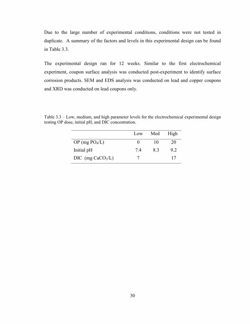
30

Due to the large number of experimental conditions, conditions were not tested in

duplicate. A summary of the factors and levels in this experimental design can be found

in Table 3.3.

The experimental design ran for 12 weeks. Similar to the first electrochemical

experiment, coupon surface analysis was conducted post-experiment to identify surface

corrosion products. SEM and EDS analysis was conducted on lead and copper coupons

and XRD was conducted on lead coupons only.

Table 3.3 – Low, medium, and high parameter levels for the electrochemical experimental design testing OP dose, initial pH, and DIC concentration.

Low Med High

OP (mg PO4/L) 0 10 20 Initial pH 7.4 8.3 9.2 DIC (mg CaCO3/L) 7 17

Figure 3.1 – Summary map of the various water conditions tested according to corrosion inhibitor type, dose, pH, and chlorine dose. Note that the 3 DIC levels tested in this study are not indicated on this map. OP was tested at 10 or 20 mg PO4/L whereas ZOP was only tested at 20 mg PO4/L.

No Corrosion Inhibitor

0 mg PO4/L

pH 7.4

+/- Cl2

pH 8.3 pH 9.2

+/- Cl2

Orthophosphate

10 OR 20 mg PO4/L

pH 7.4 pH 8.3 pH 9.2

Zinc Orthophosphate

20 mg PO4/L

pH 7.4

+/- Cl2

pH 9.2

+/- Cl2

Corrosion Inhibitor

Type:

Dose:

pH:

Chlorine: 31

32

Table 3.4 – Summary table of the 26 water conditions according to corrosion inhibitor type, dose, DIC, Cl2 dose, and pH. Each ‘x’ in the table represents a water condition that was tested in the study.

No Corrosion Inhibitor x x x x x x x x x x

Orthophosphate (10 mg PO4/L)

x x x x x x

Orthophosphate (20 mg PO4/L)

x x x x x x

Zinc Orthophosphate (20 mg PO4/L)

x x x x

DIC (mg/L) 3 7 17 3 7 17 3 7 17 3 7 17 3 7 17 3 7 17

Cl2 (mg/L) 0 1 0 1 0 1

pH 7.4 8.3 9.2

33

3.3 Stock Solution Preparation

Influent ‘fill’ water was prepared by adding chemical stock solutions to JDKWSP filtered

water. Since phosphate and alkalinity addition affected bulk water pH, chemical addition

occurred in the following order: (1) phosphate (either ZOP or OP), (2) sodium

bicarbonate for DIC adjustment, if applicable, (3) sodium hydroxide (NaOH) for pH

adjustment, and (4) chlorine. The maximum chlorine dose of 1 mg/L did not significantly

affect pH and could be added post pH adjustment with NaOH. All chemicals used for

stock solutions were laboratory grade, and all stock solutions were made with deionized

water obtained from a Milli-Q Academic water purification system (Millipore, MA,

USA).

3.3.1 Phosphate Stock Solutions

Zinc Orthophosphate (ZOP): A stock solution of ZOP was prepared by adding ZOP

(Carus 3180, Carus Chemical Company, IL, USA) to deionized water. Ingredients in the

ZOP product included proprietary concentrations of zinc chloride, zinc phosphate,

phosphoric acid, and other non-hazardous ingredients. ZOP stock solutions were prepared

once a week and 3 mL of ZOP was added to 1 L of deionized water, stored in large amber

jugs and kept at 4°C. Flasks were dosed with 20 mg PO4/L and zinc concentration was

approximate 26 mg/L (Zinc:PO4 ratio of 1:1.3). Batches of ZOP were made each day

flasks were filled, and consisted of diluting ZOP stock solution into JDKWSP filtered

water.

Orthophosphate (OP): A stock solution of OP was prepared by diluting 1.0 g of

potassium phosphate monobasic (KH2PO4) (Fischer Scientific, MA, USA) into 1.0 L of

deionized water. Batches of 10 and 20 mg/L OP were prepared by diluting the

orthophosphate stock solution into JDKWSP filtered water. 10 and 20 mg/L OP batches

were prepared once a week, stored in 1 L amber jugs and kept at 4°C.

34

3.3.2 Chlorine Stock Solution

A chlorine stock solution was prepared by adding sodium hypochlorite (NaClO) (Fischer

Scientific, MA, USA) to deionized water. Chlorine stock was prepared once a week and

the stock concentration was confirmed prior to use. Chlorine stock solution was dosed to

achieve a Cl2 concentration of 1 mg/L in the designated flasks.

3.3.3 Sodium Bicarbonate Stock Solution

A 0.1 eq/L sodium bicarbonate (NaHCO3) stock solution was prepared by dissolving 8.4

g of NaHCO3 (Fisher Scientific, M.A., USA) into 1.0 L of deionized water. Stock

solution was stored in a plastic bottle and kept at 4°C.

3.3.4 pH Adjustment

Various molarities of NaOH were added to water conditions that required increasing pH

to reach the target initial pH of 7.4, 8.3, or 9.2. However, addition of sodium bicarbonate

often increased pH to above the target pH and acidification was required. To lower pH,

H2SO4 was added which resulted in a decrease in CSMR. This may have had beneficial

effects on corrosion control. As such, CSMR was monitored over the course of the

experiment.

3.4 Ellipsometry Set-Up and Design

3.4.1 In-Situ Flow Cell Set-Up

A custom-made flow cell was used to make in-situ ellipsometric measurements along a

sample (shown in Figure 3.2). The flow cell was made of 147 mm long fused quartz tube

(8 mm ID) (Technical Glass Products Inc., OH, USA), which sat in a groove in a

machined block of aluminum (25.4 mm x 108.0 mm x 12.7 mm). The quartz tube was

35

secured to the aluminum block with metal tie-downs. A recessed aluminum insert was

machined to fit within the quartz tube and to hold an 89 mm long glass sample (described

in the following paragraph). Once the sample was inserted, two stainless-steel spring

clamps held down the sample to the aluminum insert. As well, stainless steel tube fittings

(Swagelok, Co., OH, USA) provided an air-tight connection between the quartz tube and

the influent and effluent water lines. The cell was mounted onto a custom-machined

aluminum ellipsometer mounting stage that is capable of moving in the x, y, and z

directions. Measurements were taken along the sample’s centerline to ensure equal

incident and reflected beam path lengths.

Figure 3.2 – The flow-cell used to perform in-situ ellipsometry measurements.

3.4.2 Sample Preparation

Copper and lead films were deposited onto 89 mm x 6.4 mm glass substrates by

magnetron sputtering with a VT-3 system (Corona Vacuum Coaters, B.C., Canada).

Firstly, glass substrates were cleaned (ultrasonic cleaning in acetone, ethanol, and nano-

pure water for 15 minutes each), and a thin chromium tie-layer was sputtered onto the

36

glass substrate to improve the adhesion of the metallic films to the glass during

submersion in solution. Samples were stored in airtight containers prior to use.

3.4.3 Protein Solution Preparation And Dosing

The plasma protein albumin (bovine serum albumin, Sigma, USA) was used to simulate

the proteins involved in microbial attachment to metals. A 1.0 mg/mL albumin solution

was prepared in phosphate buffered saline (PBS) at pH 7.4. Protein solution as well as

PBS alone and distilled water for rinsing were pumped through the flow cell at 2.5

mL/min using Series I diaphragm pump (Lab Alliance, PA, USA). A diaphragm pump

was chosen to reduce shearing that could potentially damage the protein in solution.

3.4.4 In-Situ Adsorption Measurements

Adsorption measurements were performed using a M-2000 Spectrocopic Ellipsometer

with an automated motion stage (J.A. Woollam, Co., NE, USA). Ellipsometric

measurements were performed with focusing optics (beam spot diameter approximately

150 μm) at incidence angles of 65, 70, and 75° over a wavelength range of 200-1000 nm

in steps of 2 nm at each point. Supplied software, CompleteEASE® (J.A. Woollam, Co.,

NE, USA), was used to align the sample for maximum signal intensity, create sample

scan patterns, and measure the ellipsometric parameters psi (Ψ) and delta (Δ) along the

designed scan pattern.

First, the optical constants of the plate prior to exposure to water were determined by

measuring Ψ and Δ in a baseline scan and fitting with a B-spline. This was to best model

the optical constants of the metal surface prior to film growth. These optical constants

were then used in the model to fit data post exposure. Measurements were taken at 20

points along the length of the sputtered plate.

37

3.5 Analytical Procedures

3.5.1 General Water Quality Parameters

Conductivity, temperature, pH, and ORP were measured using an Accumet Excel XL60

dual channel probe (Fisher Scientific, MA, USA.) according to the manufacturer’s

instructions. Probes were calibrated daily using standard buffer solutions from Fisher

Scientific. Turbidity was measured using a HACH 2100N laboratory turbidimeter

(HACH, CO, USA.) Samples were inverted at least three times before measuring. Free

chlorine was measured using a DR 4000 UV-Spectrophotometer (HACH, CO, USA.)

according to method DPD 8021. Alkalinity was measured using a titration method

according to Method 2320B (APHA, 1995)

3.5.2 Current

The galvanic current between the copper and lead coupons within the electrochemical

flasks was measured using a True RM Industrial Multimeter EX530 (Extech Instruments

Corporation, MA, USA.)

3.5.3 Organic and Inorganic Carbon

Total organic carbon (TOC), dissolved organic carbon (DOC), and dissolved inorganic

carbon (DIC) was analyzed using a Shimadzu TOC-VCSH TOC Analyzer (Shimadzu

Corporation, Kyoto, Japan) with a minimum detection limit of 0.6 mg/L. Samples were

poured into a 50 mL head-space free glass vial. DOC samples were first filtered through a

0.45 μm polysulphone filter paper (GE Water & Process Technologies, PA, USA.) that

had been pre-rinsed with 500 mL of deionized water. Concentrated phosphoric acid was

added to TOC and DOC samples to decrease pH to below 2, however no acid was added

to DIC samples. Sample vials were capped and stored at 4°C until analysis.

38

3.5.4 Anions

Chloride (Cl-), phosphate (PO42-), and sulfate (SO4

3- ) were measured using a 761

Compact Ion Chromatogram with 788 filtration sample processor (Metrohm, Herisau,

Switzerland) according to USEPA method 300.1. Standards of 2, 5, 10, 20, and 30 mg/L

Cl-, PO42-, and SO4

3- were prepared and measured on the instrument once a week. The

method detection limit for Cl-, PO42-, and SO4

3- were, 0.6 mg/L, 0.7 mg/L, and 0.5 mg/L,

respectively.

3.5.5 Metals

Influent and bulk water samples were analyzed for metals using inductively coupled

plasma mass spectrometry (ICP-ms) (Thermo Fisher X-Series 2 ICP-ms, MA, USA.).

The limit of detection was 0.7 μg/L and 0.4 μg/L for copper and lead, respectively.

Metals samples were analyzed according to Standard Methods 3030 (APHA, 2012)

which states that samples with turbidity greater than 1 NTU should undergo nitric acid

digestion (NAD) prior to analysis by ICP-ms. According to the method, all metals

samples are acidified to pH less than 2 to dissolve all particulate metals such that they can

be measured by ICP-ms. Water samples with high turbidity have been associated with

high particulate metals concentrations and NAD is a technique used to break down large

particulates into dissolved form such that they can be measured by ICP-ms (APHA,

2012).

Up to three metals concentrations were measured for each water sample: dissolved, total,

and NAD lead and copper concentrations. Dissolved metals refer to the concentration of

metals after passing the sample through a 0.45 μm filter, whereas total metals refers to the

concentration of metals without filtration and represents the dissolved as well as

particulate metals. NAD metals refers to metal concentration after NAD digestion and

includes the dissolved and particulate portion of metals, and may increase metals

concentration compared to total metals.

39

Dissolved metals samples were filtered through a 0.45 μm cellulose nitrate membrane

filter (Whatman, Dassel, Germany), acidified with nitric acid to below pH 2 and stored at

4 °C until analysis by ICP-ms. To determine total metals concentrations, bulk water

samples were acidified with nitric acid to below pH 2 and stored at 4° C until analysis by

ICP-ms (direct analysis). NAD metals concentrations were determined via the following

procedure:

1) 10 mL of sample was poured into a disposable digestion sample tube and 0.5

mL of nitric acid was added,

2) Samples were heated to 105° C for 2 hours and water was allowed to

evaporate,

(3) Samples were removed from the batch heater and allowed to cool slightly.

Deionized water was poured into the sample to return the total sample volume

to 10 mL (replenish the evaporated water volume), and

(4) Samples were stored at 4° C until analysis by ICP-ms.

As a general rule, metals concentration after NAD should be equivalent or higher than the

metals concentration without NAD (total metals), and total metals concentration will be

equivalent or higher than dissolved metals concentration (i.e. Dissolved metals ≤ Total

metals ≤ NAD metals).

3.5.6 Electrode Corrosion Scale Surface Analysis

Virgin as well as corroded lead and copper coupons from each treatment condition were

analyzed for corrosion products. SEM with EDS anlayisis using a Hitachi S-4700 FEG

SEM determined the morphology and elemental composition of the corrosion products.

The elemental percent composition was determined by averaging percent composition of

at least 3 spots on each electrode, or an area scan was performed. XRD analysis was

conducted to identify crystalline and solid phases present in the lead corrosion scales of

some lead coupons. A D500 Diffractometer x-ray system was used (Siemens, USA) and

40

was equipped with diffracted beam Soller Slits and a graphite monochrometer. The beam

path was configured with 0.3° divergence and anti-scatter slits and a 0.15° receiving

slit. Copper K-alpha radiation was used for these measurements. Samples were scanned

in step mode with a 0.05° step size and a 6 second integration time. MATCH! software

and a powder diffraction files database was used for pattern analysis. Search/match

criteria were restricted to the elements already identified in the EDS analysis. Sample

sizes were not large enough to estimate the relative proportions of each compound in a

sample. As a result, XRD analysis was used to identify the presence of particular

corrosion products.

3.6 Data Analysis for Electrochemical Experiments

Minitab® software (Minitab® 2010, 16.2.2, PA, USA) was used to conduct all statistical

analysis. The statistical tests conducted included one-way analysis of variance

(ANOVA), paired t-tests, and factorial design analysis. One-way ANOVA tests were

conducted in conjunction with Tukey’s Method - one-way ANOVA was conducted to

identify in any of the population means differed, and Tukey’s method compared each pair

of means to form groups whose means were not significantly different (using a family

error rate to control the rate of type 1 error). Paired observations, such as lead

concentration before and after NAD, were analyzed with one-tailed paired t-tests. Lastly,

the factorial design analysis function in Minitab® was used to identify significant factors

from the factorial design experiments. Responses for factorial design analysis were (1)

lead concentration and (2) copper concentration. Only data collected during steady state

was used for factorial analysis, and metals data was categorized according to stagnation

time. Since metals release had stabilized during steady state, lead and copper

concentration in each bulk water sample after a stagnation time was considered a

replicate. All statistical tests were conducted at the 95% confidence level (α=0.05).

41

CHAPTER 4 RESULTS AND DISCUSSION

4.1 Water Condition Notation

Five parameters were tested at various levels and combinations and included the

following:

1. Phosphate type: ZOP or OP

2. Phosphate dose (0, 10, or 20 mg PO4/L),

3. Initial water pH (7.4, 8.3, or 9.2),

4. DIC (3, 7, 17 mg/L), and

5. Cl2 dose (0 or 1 mg/L).

The following notation will be used to identify each water condition: corrosion inhibitor

type (corrosion inhibitor dose in mg PO4/L)/initial pH/DIC in mg CaCO3 per L/Cl2. For

example, ZOP(10)/pH(7.4)/DIC(3)/Cl2 denotes the water condition with a ZOP dose of

10 mg PO4/L, initial pH 7.4, 3 mg/L DIC, and 1 mg/L Cl2, whereas pH(9.2)/DIC(3)

represents the water condition without corrosion inhibitor, initial pH 9.2, DIC of 3 mg

CaCO3/L and no chlorine addition.

4.2 Relationship Between Turbidity and Particulate Lead

Standard Method 3030 (APHA, 2012) states that drinking water samples with turbidity

greater than 1 NTU should undergo heated NAD prior to analysis by ICP-ms whereas

samples with turbidity less than 1 NTU may be analyzed directly. Regardless of turbidity,

a minimum of 13 bulk water samples from each of the 26 water conditions were analyzed

for lead by both methods: (1) direct analysis without NAD, and (2) NAD prior to analysis

by ICP-ms.

Average bulk water turbidity ranged from 0.12 to 10.9 NTU (data shown in Table A.1 in

Appendix A). Bulk water turbidity was above 1 NTU in 11 water types and below 1

42

NTU in 15 water types. Turbidity was always less than 1 NTU in water conditions that

did not dose corrosion inhibitor (10 water conditions). Average bulk water turbidity was

occasionally below 1 NTU when OP was dosed at 10 or 20 mg PO4/L and ranged from

0.62 to 3.41 NTU. The highest bulk water turbidity occurred in the 4 water conditions

that dosed ZOP at 20 mg PO4/L; average turbidity ranged from 4.9 to 10.9 NTU.

One-sided paired t-tests (‘NAD lead concentration’ minus ‘Direct analysis lead

concentration’) were conducted to identify if a significant increase in lead concentration

occurred after NAD. Twenty of the 26 water conditions exhibited a significant increase in

lead concentration after NAD (α=0.05). Of these 20 water conditions, 12 had average

sample turbidity below 1 NTU. Water types with turbidity less than 1 NTU that exhibited

significant increases in lead concentration is likely because lead particulates settled in the

turbidity sample bottle during analysis and did not contribute towards measured turbidity

as was observed by other authors (Triantafyllidou et al., 2007). Only three water

conditions with average bulk water turbidity below 1 NTU did not result in increased lead

concentration after NAD; these water conditions all contained OP. Of the 11 water

conditions with average turbidity above 1 NTU, eight observed significant increases in

lead concentration with NAD (α=0.05). Lead concentration significantly increased in all

water conditions with ZOP addition (sample turbidity>1 NTU) after NAD indicating that

particulate lead was not completely dissolved without NAD in all ZOP water conditions.

In water conditions where lead significantly increased with NAD, the amount by which

lead increased after NAD varied by water type. The 95% lower bound of the average

difference between NAD and direct analysis samples represents the minimum increase in

lead concentration after NAD with 95% confidence. The 95% lower bound of the average

difference ranged from 2 to 60 μg/L; in other words, NAD increased lead concentration

by a minimum of 2 to 60 μg/L (α=0.05). The highest 95% lower bound increase in lead

concentration with NAD was in water condition pH7.4/DIC(3). As well, NAD increased

lead concentration by at least 10 μg/L in 12 of the 20 water conditions that exhibited

significant lead increases (α=0.05). These results demonstrate the potential for NAD to

significantly increase lead concentration by as much as 10 μg/L, the maximum allowable

43

concentration (MAC) for lead in drinking, even in water conditions with corrosion

inhibitor (Health Canada, 2012).

Other authors have conducted similar analyses on water samples. Deshommes et al.

(2010) tested 76 water samples from homes with lead service lines with turbidity>1

NTU. The authors found no significant difference between lead concentrations with and

without NAD (p>1). The current study, however, indicates that significant particulate

lead can be present when turbidity is greater or less than 1 NTU. This study likely had

significant particulate lead in the majority of water samples because galvanic corrosion

has shown to increase particulate lead (Wang et al., 2012) and the metal materials used in

this study were new and passivation scale was likely not as resilient as those in lead

service lines from older homes. Therefore, it is valuable to characterize lead

concentrations by both direct analysis and NAD to identify if significant portions of

particulate lead exist, regardless of turbidity.

The results from this analysis show that it is not exclusively samples with turbidity above

1 NTU that exhibit increased lead concentrations after NAD. These findings suggest that

the recommendation by Standard Methods 3030 to only require NAD for samples with

turbidity above 1 NTU may not adequately measure particulate lead concentrations in

some water samples. By digesting only the samples with turbidity above 1 NTU, the

particulate portion of lead in samples with turbidity less than 1 NTU may not be

represented, and potential parameter exceedences could be missed. Based on this study,

NAD lead concentrations were used in all analysis for all water conditions, regardless of

bulk water turbidity.

4.3 Metals Release Over Time

Other authors conducting dump-and-fill experiments with aged lead pipes acclimated the

pipes for 8 weeks (Wang et al., 2012) and 8 months (Cartier et al., 2013; Xie and

Giammar, 2011). Residuals from the average represent the difference between the

observed Pb concentration on a given day and the average Pb release over the

44

experimental duration for a single water type. When the residual is 0, the observed Pb

concentration is equal to the overall average Pb concentration. A plot of residuals over

time for two representative water types is shown in Figure 4.1. Vertical deviations from 0

are highest at the beginning of the experiment and residuals from the average were

sometimes greater than 7000 in the first 7 days of experimentation. According to Figure

4.1, steady state metals release was achieved after approximately 7 days, however a

conservative acclimation period of 30 days was used to ensure steady-state lead release

had occurred. In comparison to other studies, a shorter acclimation period was required in

the current study due to the difference in lead materials and the smaller lead surface area

exposed to water in the current experiment.

Figure 4.1 – Plot of the residual from the average over time for two representative water conditions. High lead release events towards experimental day 100 were identified as outliers and removed from the data set prior to data analysis.

-2000

-1000

0

1000

2000

3000

4000

5000

6000

7000

8000

9000

0 20 40 60 80 100

Experimental Duration (d)

pH7.4/Low DIC

ZOP(20)/9.2/Low DIC

Acclimation Steady State

pH7.4/DIC(3) ZOP(20)/pH9.2/DIC(3)

Res

idua

ls fr

om A

vera

ge

45

Two distinct phases of metals release were identified for data analysis (Figure 4.1):

Acclimation (30 days, short term): For all water conditions, the highest lead levels were

observed during the first 30 days of experimentation. Higher lead release during this

period coincides with higher current measurements (discussed in Section 4.4.2). Higher

current and therefore lead concentration is likely due to lead release prior to the

development of a passivation film, leading to sloughing of metal complexes into the bulk

water.

Steady State (49-68 days long-term): Systems had stabilized and consistent metals release

was observed. High lead concentration events were observed in some bulk water

samples, mainly in initial pH 7.4 conditions without corrosion inhibitor. These spikes can

be attributed to lead particles sloughing off the coupon surface during the dump-and-fill

procedure. Triantafyllidou and Edwards (2011) categorized lead release due to galvanic

corrosion as independent of other lead release mechanisms including normal dissolution,

deposition corrosion, and particle detachment (sloughing). In the current data set, metals

release events that were 1.5 times the interquartile ranges were considered due to particle

detachment rather than galvanic corrosion and were removed from the data set for

factorial analysis. Outlier events in particular water types will be addressed, however.

4.4 Influent Water Quality of the 26 Water Conditions

Influent water quality of the 26 water conditions is shown in Table 4.1.

4.4.1 Fill Water CSMR

Influent water CSMR varied between experimental conditions. Water types with

ZOP(20) had the highest average CSMR values and ranged from 4.12-4.35. Average

CSMR for water conditions with OP(10) and OP(20) ranged from 0.70 to 0.97. Without

corrosion inhibitor at all DIC levels, average CSMR values ranged from 0.55 to 1.95, and

46

Table 4.1 – Influent water quality during steady state of the 26 water conditions tested in the study

Water Condition CSMR Conductivity (μS/cm)

Current (μA)

DIC (mg CaCO3/L)

Alkalinity (mg

CaCO3/L) pH7.4/DIC(3) 1.16 71.3 6.4 2.12 8.1 pH7.4/DIC(3)/Cl2 1.95 71.3 12.4 2.12 15.2 ZOP(20)/pH7.4/DIC(3) 4.12 180.1 11.8 1.25 13.7 ZOP(20)/pH7.4/DIC(3)/Cl2 4.35 180.1 13.6 1.25 13.7 pH9.2/DIC(3) 1.16 94.0 6.0 2.74 14.0 pH9.2/DIC(3)/Cl2 1.46 94.0 11.6 2.74 12.6 ZOP(20)/pH9.2/DIC(3) 4.23 188.7 8.7 2.26 25.8 ZOP(20)/pH9.2/DIC(3)/Cl2 4.32 188.7 8.2 2.08 25.8 pH7.4/DIC(7) 0.79 125.3 9.5 7.2 31.3 pH7.4/DIC(17) 0.55 223.2 8.2 19.0 73.9 pH8.3/DIC(7) 0.78 140.0 8.9 8.3 36.0 pH8.3/DIC(17) 0.87 252.7 17.0 21.7 87.8 pH9.2/DIC(7) 0.87 132.9 7.2 8.3 34.6 pH9.2/DIC(17) 0.96 247.8 16.7 21.4 91.1 OP(10)/pH7.4/DIC(7) 0.95 133.6 10.4 7.0 30.9 OP(10)/pH7.4/DIC(17) 0.70 249.4 7.8 17.6 74.5 OP(10)/pH8.3/DIC(7) 0.79 178.6 11.6 6.7 30.5 OP(10)/pH8.3/DIC(17) 0.97 250.7 8.7 18.7 82.4 OP(10)/pH9.2/DIC(7) 0.80 140.7 10.1 6.0 27.3 OP(10)/pH9.2/DIC(17) 0.92 226.0 12.2 18.5 79.4 OP(20)/pH7.4/DIC(7) 0.96 147.5 15.4 5.3 25.3 OP(20)/pH7.4/DIC(17) 0.77 266.0 14.5 19.1 82.4 OP(20)/pH8.3/DIC(7) 0.91 154.5 13.5 6.2 31.8 OP(20)/pH8.3/DIC(17) 0.88 277.2 14.7 18.6 84.1 OP(20)/pH9.2/DIC(7) 0.71 156.8 13.7 5.9 31.1 OP(20)/pH9.2/DIC(17) 0.94 241.8 16.1 18.7 82.4

47

CSMR was always higher in water conditions with either DIC of either 7 or 17 mg

CaCO3/L.

This is likely because of H2SO4 addition in higher DIC water conditions to reduce pH

after bicarbonate addition increase the sulfate concentration and decreased CSMR. In all

but three water conditions, average CSMR was greater than the threshold value of 0.77

and were considered corrosive (Nguyen et al., 2011a). Though CSMR ranged from 0.55-

4.35, CSMR was not correlated to lead release. Other research has shown that further

increasing CSMR above 1 does not necessarily increase adverse effects on lead release

(Nguyen et al., 2011b).

4.4.2 Fill Water Current

Large galvanic currents were measured when the copper and lead coupons were initially

connected during acclimation followed by a decrease in current upon filling the flasks

during steady state. Generally, current was highest in water conditions with either 7 or 17

mg CaCO3/L and lowest currents were observed in water conditions with DIC of 3 mg

CaCO3/L. Maximum current ranged from 37 μA to 109 μA in water condition conditions

with either 7 or 17 mg CaCO3/L. During steady state, average current ranged from 7 to 17

μA in these water conditions (Table 4.1). In contrast, in water conditions with DIC(3),

maximum current over the experimental duration did not exceed 32 μA. Current was

highest in the two water conditions with ZOP(20) addition at pH 7.4, and average current

during steady state was always less than 14 μA.

In addition, elevated current upon filing the flasks at the beginning of the experiment

coincides with higher lead release (shown in Figure 4.2). In general, current decreased

between filling and dumping the bulk water (after 1, 2, and 4 days stagnation). The

greatest decreases in current over stagnation time were observed prior to reaching steady

state: in one water condition, current decreased by as much as 54 μA over a 2-day

stagnation time. Within one week, galvanic currents decreased by a factor of 4 to 26

times. Other studies have shown that galvanic current decreased on average by 29% when

lead pipe was upstream of copper pipe over the 214 day experiment, with galvanic

48

Figure 4.2 – Pb concentration and current over the experimental duration for water type OP(10)/pH7.4/DIC(7). Higher initial current corresponds with higher lead release.

currents of 18 μA at the end of the experiment in water conditions with ZOP addition

(Cartier et al., 2012a).

The lowest and highest average fill currents were in water conditions without corrosion

inhibitor, with DIC(3) and DIC(17), respectively. The five lowest average currents upon

filling the flasks were in water conditions without corrosion inhibitor and low DIC(3) but

different initial pH conditions, and the water conditions with the two highest average fill

currents were also water conditions without corrosion inhibitor but at high DIC (fill

currents were significantly different between these two groups). This suggests that DIC

concentration played a major role in sustaining galvanic current, particularly in water

conditions without corrosion inhibitor. As well, adding 1 mg/L Cl2 to water conditions

with 3 mg/L DIC increased average fill current. Average fill current significantly

increased between 3.1 and 5.2 μA when chlorine was dosed (α=0.05) except in water

0

10

20

30

40

50

60

0

500

1000

1500

2000

2500

3000

0 20 40 60 80 100Elapsed Time (days)

Pb Concentration

CurrentPb

Con

cent

ratio

n (μ

g/L

)

‘Fill

’ Cur

rent

(μA

)

49

condition ZOP(20)/pH(9.2)/DIC(3) where average fill current did not significantly

increase with addition of 1 mg/L Cl2.

All water conditions with DIC(3) observed significant decreases in current with

stagnation time (p<0.002) and dump current was always at least 0.9 μA lower than fill

current (α=0.05). When DIC was 7 or 17 mg CaCO3/L, current did have a tendency to

decrease with stagnation though a smaller difference between initial and dump current

was observed and current decrease over time was only significant in 5 of the 18 water

types. This could be because higher DIC concentration increased the water conductivity

and was able to sustain galvanic current even after longer stagnations times compared to

low DIC concentrations.

4.4.3 Fill Water Conductivity

Average fill conductivity ranged from 69 to 335 μS/cm in the 26 water conditions. Water

conductivity was most heavily influenced by DIC whereas phosphate addition did not

significantly impact conductivity. For example, water conditions without corrosion

inhibitor with DIC of 17 mg/L had higher conductivity than water conditions with ZOP

and OP with DIC of 3 or 7 mg/L, respectively. As well, increasing OP dose from 10 to 20

mg PO4/L did not significantly increase bulk water conductivity in water conditions with

DIC of 7 mg/L or 17 mg CaCO3/L. As well, all water conditions with DIC(7) had

significantly lower bulk water conductivity than water conditions with DIC(17).

Therefore, increasing bicarbonate dose had the largest influence on increasing water

conductivity in this study.

Water conditions in order of lowest conductivity to highest conductivity are shown

below. Bulk water pH did not significantly impact conductivity, but rather, conductivity

was governed by DIC concentration. The addition of corrosion inhibitors also increased

conductivity.

DIC(3) < DIC(7) < OP(10)/DIC(7) < ZOP(20)/DIC(3) < DIC(17) < OP(20)/DIC(17)

50

4.5 Lead Release During the Acclimation Stage

4.5.1 No Corrosion Inhibitor

The highest lead concentrations were observed during the acclimation phase in water

conditions without corrosion inhibitor. The highest average lead concentrations occurred

in water conditions with initial pH 7.4 and low DIC (either 3 or 7 mg CaCO3/L). When

DIC was increased to 17 mg CaCO3/L, average lead release during acclimation

decreased. When DIC was below 3 mg CaCO3/L, low pH of 7.4 resulted in the highest

lead release event and highest average lead release during the acclimation stage.

Condition pH7.4/DIC(3) also had the largest standard deviation and coefficient of

variation indicating frequent sloughing events.

The combination of higher DIC and higher pH had the largest impact on reducing

average lead release and fewer outlier lead release events occurred when initial pH was

increased from 7.4 to either 8.3 or 9.2. When DIC was 3 mg/L or less and pH was 7.4,

lead concentrations ranged from 790 μg/L to 9339 μg/L (average 2078 μg/L), whereas

lead concentrations ranged from 259 to 2665 μg/L in water conditions when pH was

increased to 9.2. When DIC was increased to 7 mg/L, lead concentration ranged from 160

to 3358 μg/L during acclimation (6000 μg/L lower than the maximum lead release event

when DIC was 3 mg/L), and when DIC was further increased to 17 mg CaCO3/L,

maximum lead concentration ranged from 86 to 1294 μg/L and had the lowest outlier

lead event of any DIC group. At all three DIC concentrations, the highest average lead

release was in water conditions with initial pH 7.4 whereas the combination of high DIC

and high initial pH had the greatest impact on mitigating lead release during acclimation;

in water condition pH9.2/DIC(17), lead concentration never exceeded 320 μg/L during

acclimation. Therefore, without corrosion inhibitor, higher DIC and higher pH reduced

average lead release during the acclimation period, and prevented high lead release

events. In all cases, however, lead concentration exceeded the Health Canada guideline of

10 μg/L during acclimation, demonstrating the potential for public health risks when

copper and lead are initially connected.

51

4.5.2 Zinc Orthophosphate Corrosion Inhibitor (DIC 3 mg/L)

ZOP was dosed at 20 mg PO4/L and was only tested with DIC of 3 mg CaCO3/L. At

initial pH 7.4, the addition of ZOP reduced average lead release. However, due to the

large amount of variation during this stage, average lead release was not significantly

different between any water condition with and without ZOP at 3 mg/L DIC. Though the

range of lead concentrations observed during acclimation was similar between initial pH

7.4 and pH 9.2 and ranged between 170 μg/L and 5800 μg/L, the low pH condition,

ZOP(20)/pH7.4/DIC(3), had higher average lead concentration than the corresponding

water condition with pH 9.2.

All water conditions with ZOP experienced at least one event where lead concentration in

bulk water exceeded 1000 μg/L. The highest measured lead concentration in bulk water

with ZOP addition was 5892 μg/L in water condition ZOP(20)/pH9.2/DIC(3)/Cl2 and was

more than 3000 μg/L less than the maximum lead concentration observed without

corrosion inhibitor. Overall, the addition of ZOP reduced outlier lead release events

compared to no corrosion inhibitor at 3 mg/L DIC, though no water condition succeeded

in reducing lead release to below the Health Canada guideline of 10 μg/L during the

acclimation stage.

4.5.3 Orthophosphate Corrosion Inhibitor

OP corrosion inhibitor was dosed at either 10 or 20 mg PO4/L and DIC was either 7 or 17

mg CaCO3/L. The lowest average lead concentration during acclimation was observed in

pH 9.2 and high DIC water condition, OP(10)/pH9.2/DIC(17). The highest lead

concentration event occurred in the corresponding water condition but with lower DIC,

OP(10)/pH9.2/DIC(7), and was 13,200 μg/L. This was the highest lead concentration

observed in any water type during the acclimation phase. All but two water conditions

with OP observed at least one lead release event above 1000 μg/L during the acclimation

stage; Lead concentration in water conditions OP(20)/pH8.3/DIC(17) and

OP(20)/pH9.2/DIC(17) never exceeded 530 μg/L during the acclimation phase. Overall,

all water conditions at lower DIC (3 or 7 mg/L) with corrosion inhibitor addition (either

52

ZOP or OP) observed at least one event with lead concentration at least 1000 μg/L,

whereas only water conditions with high DIC and high initial pH and corrosion inhibitor

never exceeded 530 μg/L. Therefore, the addition of corrosion inhibitor in high DIC(17)

and high pH (either 8.3 or 9.2) was the most effective strategy to reduce outlier lead

events, though no water conditions reduced lead release to below the health Canada

guideline.

4.6 Effect of Stagnation Time on Lead Concentration During Steady State

ANOVA tests with Tukey’s Statistical Method were performed to identify if average lead

concentration in bulk water significantly increased with longer stagnation time during the

steady state phase. In general, average lead concentration increased with longer

stagnation time, however in most cases, lead concentration was not significantly different

between stagnation times.

Average lead release was not significantly different between 1- and 2-day stagnation time

in any water condition, and average lead released was higher after 4-day stagnation time

only in water conditions without corrosion inhibitor at 3 mg/L DIC. In contrast, mean

lead concentrations in bulk water conditions without corrosion inhibitor and medium (7

mg CaCO3/L) and high (17 mg CaCO3/L) DIC were not statistically different after 1, 2,

and 4-day stagnation time (α=0.05). As well, the addition of both corrosion inhibitors

resulted in insignificant differences in lead release with longer stagnation times at all DIC

levels. Therefore, increasing DIC without corrosion inhibitor as well as dosing both ZOP

and OP addition had beneficial impacts on mitigating lead release as stagnation time

increased.

53

4.7 The Effect of pH, Cl2, and ZOP on Lead Release at Low DIC (3 mg CaCO3/L)

The current section describes the results from the factorial design described in Table 3.2:

initial pH either 7.4 or 9.2, ZOP dose either 0 or 20 mg PO4/L, and Cl2 dose of either 0 or

1 mg/L. All water conditions had DIC less than 3 mg CaCO3/L. Average lead release

according to water condition and stagnation time is shown in Figure 4.3. As mentioned in

Section 4.6, lead release significantly increased after 4-day stagnation for some water

types, therefore factorial analysis was conducted for each stagnation time independently,

though results were similar between 1- and 2-day stagnation times. Average lead and

copper release data can be found in Table A-2 of Appendix A.

Figure 4.3 – Steady state average lead release in bulk water by stagnation time for all water conditions in with DIC(3). Average lead release decreases when pH is increased from 7.4 to 9.2 and with the addition of ZOP at both pH values. Error bars represent 95% confidence intervals.

0

500

1000

1500

2000

2500

3000

1 Day

2 Day

4 Day

pH 7.4 pH 9.2

Lead

Con

cent

rati

on (μ

g/L)

54

4.7.1 Lead Release After 1- and 2-Day Stagnation

In general, low pH without corrosion inhibitor resulted in the highest average lead

release. After 1- and 2-day stagnation, water condition pH7.4/DIC(3)/Cl2 had the highest

average lead concentration (1359 μg/L) whereas water condition

ZOP(20)/pH9.2/DIC(3)/Cl2 generated the lowest average lead concentration (325 μg/L)

(Figure 4.3). Note that lead release was not significantly different between water

conditions ZOP(20)/pH9.2/DIC(3) with and without Cl2.

At both pH conditions, addition of ZOP reduced lead release. ZOP at pH 9.2 performed

better than ZOP at pH 7.4: The two ZOP(20)/pH9.2/DIC(3) water conditions with and

without chlorine resulted in statistically less average lead release than any of the pH 7.4

conditions (with and without ZOP). In addition, ZOP(20) at pH 7.4 performed similarly

to water conditions without ZOP at pH 9.2.

Factorial analysis revealed that after 1- and 2-day stagnation times, lead release was

significantly impacted by initial pH and ZOP dose but was not impacted by chlorine

dose. Despite up to 5 μA increase in fill current with chlorine addition, factorial analysis

showed that increases of 3 to 5 μA in current due to chlorine addition did not impact lead

release in these water conditions. Increasing pH and ZOP from their low to high levels

reduced lead concentration in bulk water (Figure 4.4(a)). Increasing initial pH from 7.4 to

9.2 mitigated more lead release than increasing ZOP from 0 to 20 mg PO4/L. After 1-day

stagnation, average lead reductions of 428.5 (p=0.001) and 211.5 μg/L (p=0) were

observed when pH and ZOP dose were increased from the low to high levels,

respectively. After 2-day stagnation, higher average reductions of 635 and 318 μg/L (both

p=0) for pH and ZOP, respectively, were observed.

55

A)

B)

Figure 4.4 – A) ZOP and pH main effects plot for 4-Day stagnation data. Increasing PO4 and initial pH from the low- to high-level results in less average lead release. B) Plot of interaction between ZOP and pH where effect of one variable is dependent on the level of the other variable.

9.27.4

2000

1750

1500

1250

1000

750

500

Initial pH

Ave

rage

Lea

d R

elea

se (

ug/L

) 020

(mg/L)PO4

Interaction Plot for 4-Day StagnationData Means

200

1500

1250

1000

750

500

9.27.4

PO4 (mg/L)

Ave

rage

Lea

d R

elea

se (

ug/L

)

Initial pH

Main Effects Plot for 4-Day StagnationData Means

56

4-Day Stagnation. After 4-day stagnation, ZOP dose (p=0), pH (p=0), and the

interaction between ZOP dose and pH (p=0.004) significantly impacted lead release.

Contrary to shorter stagnation times, ZOP had the greatest impact on lead release after 4-

day stagnation, and dosing ZOP(20) resulted in an average reduction of 952 μg/L,

compared to an average reduction of 605 μg/L when initial pH was increased from 7.4 to

9.2. ZOP rather than pH likely achieved better lead mitigation after 4-day stagnation

beacuase of the natural decrease in pH with increased stagnation time. This will be

discussed in the following section.

Increasing pH from 7.4 to 9.2 and increasing ZOP dose from 0 to 20 mg PO4/L both

reduced lead concentration, however a significant interaction between parameters means

that the effect of ZOP on lead release depended on the initial pH and vice versa. This

relationship is shown in Figure 4.4 (a) and (b). The addition of ZOP at pH 7.4 decreased

average lead concentration from 2094 to 592 μg/L whereas the addition of ZOP at pH 9.2

only decreased average lead release from 890 to 356 μg/L. Lead concentration was

reduced by 1204 and 178 μg/L at pH 7.4 and 9.2, respectively. This indicates that ZOP

mitigates more lead at pH 7.4 compared to pH 9.2. This interaction between ZOP dose

and initial pH also occurred after 1- and 2-day stagnation times, though the interaction

was not significant. This is consistent with other studies that have found ZOP is most

effective in the pH range 7.4-7.8 (Hill and Gianni, 2011). The same authors also do not

suggest dosing ZOP when pH is greater than 8 because zinc can prematurely precipitate,

though this was not observed in the current study. Despite ZOP being more effective at

mitigating lead release at pH 7.4, overall, the water condition with ZOP at high pH,

ZOP(20)/pH9.2/DIC(3), released the least amount of lead compared to the other water

conditions in this factorial design.

In summary, after all stagnation times, increasing pH from 7.4 to 9.2 when ZOP was

dosed reduced lead release into bulk water. Though increasing pH decreased the

effectiveness of ZOP, increasing pH had a greater impact on lead mitigation and the

benefits of increasing pH from 7.4 to 9.2 outweighed the decreased effectiveness of ZOP

at higher pH.

57

4.7.2 Effect of High pH on Disinfection Potential

As stated in Section 4.7.1, raising pH improved lead mitigation compared to dosing

ZOP(20) when DIC was less than 3 mg CaCO3/L. However, raising pH may have other

impacts on the distribution system. For example, increasing pH may result in (1) reduced

disinfection potential, and (2) an increase in trihalomethane formation (THM) (Liang and

Singer, 2003). At higher pH, there is a lower concentration of the strong oxidant,

hypochlorous acid (HOCl), at pH 9.2 compared to 7.4. Despite the potential reduction in

disinfection power at higher pH, this study did not observe significant differences

between heterotrophic plate counts between water conditions at pH 7.4 and pH 9.2 (data

not shown). As well, increasing pH from 6 to 8 has shown to increase THM formation

but decreased other disinfection by-products, such as trihaloacetic acid formation (Liang

and Singer, 2003). Though THM formation potential was not evaluated in this study, it is

an important parameter to consider at the pilot- or full-scale if pH is increased for

corrosion control.

4.7.3 Decrease in pH with Stagnation Time

A drawback of the current experimental set-up was that the flask-coupon systems were

open to the atmosphere. Attempts were made to seal the opening, but an airtight seal was

problematic and caused unnecessary coupon aggravation resulting in metals sloughing.

However, in an open system, carbon dioxide can partition between the gas and aqueous

phases and impact water pH (Sawyer et al., 2003).

When hydroxide is added to water, bicarbonate is converted to carbonate causing

carbonic acid to convert to bicarbonate. The net effect is a rise in pH (Equations 11 and

12).

HCO3− + OH− → CO3

2− Equation 11

H2CO3 + OH− ⟶ HCO3− + H2O Equation 12

58

After hydroxide addition, the water becomes deficient in H2CO3 and CO2 is absorbed to

reestablish equilibrium with air, and an overall decrease in pH occurs (Equation 13).

CO2 + H2O ⟶ H2CO3 → HCO3− + H+ Equation 13

NaOH was added to increase pH to 7.4 and 9.2 (raw water pH < 6), however, pH

decreased with stagnation due to the mechanism described in Equations 11-13. A

decrease in pH at the anode is expected when lead is released due to galvanic corrosion

(Dudi, 2004; Edwards and Triantafyllidou, 2007), however it was confirmed that even

without coupons in the water and therefore no lead release, a decrease in pH was still

observed in all water conditions. Average bulk water pH and lead concentrations are

plotted for each water condition after 1, 2, and 4 day stagnation in Figure 4.5. Despite

the largest decreases in pH when initial pH was 9.2, lead release was less than all water

conditions with initial pH 7.4 indicating that lead release is not driving pH drop in bulk

water.

The largest pH decreases occurred within the first 24 hours. The smallest pH decreases

occurred in water types with ZOP; this is likely because phosphate in sufficient

concentrations can act as a buffer against pH change (Droste, 1997). Average bulk water

alkalinity and DIC is shown for the eight water conditions in Figure 4.6. As expected,

alkalinity increased when ZOP(20) was dosed. NaOH addition for pH adjustment also

increased alkalinity such that alkalinity between ZOP(20) at pH 7.4 and no corrosion

inhibitor at pH 9.2 was not different (average 13.5 mg CaCO3/L). When ZOP(20) was

dosed and pH was adjusted to 9.2, the highest alkalinity (21 mg CaCO3/L) was observed.

As shown in Table 4.2, after 1-day stagnation, pH decreased by as much as 0.4 in water

conditions with initial pH 7.4 and by as much as 1.8 in initial pH 9.2 water conditions.

Despite pH drop, pH of water conditions with initial pH 9.2 remained significantly higher

than initial pH 7.4 water conditions after 1- and 2-day stagnation, however final pH is

very similar between low- and high-pH conditions after 4-day stagnation, particularly

between ZOP(20)/pH7.4 and pH 9.2 conditions. This could explain why ZOP rather than

59

Figure 4.5 – Actual pH decrease after 1, 2, and 4 day stagnation and lead release after 1-day in DIC(3) water conditions. Greater pH decrease occurred in water conditions with low lead release indicating that atmospheric CO2 rather than lead release is driving pH drop.

Figure 4.6 – Average alkalinity and DIC of the 8 water conditions. Data based on duplicate samples.

0

200

400

600

800

1000

1200

5

5.5

6

6.5

7

7.5

8

8.5

9

9.5

pH

t=0

1-day

2-day

4-day

Pb @ 1-day

0.00.51.01.52.02.53.03.54.0

0.00

5.00

10.00

15.00

20.00

25.00

Alkalinity (mg/L CaCO3) DIC (mg/L CaCO3)

pH 7.4 pH 9.2

Pb C

once

ntra

tion

(μg/

L)

Alka

linit

y (m

g Ca

CO3/

L)

DIC

(mg

CaCO

3/L)

60

pH had the largest impact on mitigating lead release after 4-day stagnation. Both

ZOP(20) and all pH 9.2 conditions had the least amount of pH drop. The consistently

higher pH in water conditions with ZOP addition and therefore higher buffering capacity

could explain why the water condition ZOP(20)/pH9.2/±Cl2 achieved the least amount of

lead release after all stagnation times.

Table 4.2 – Decrease in bulk water pH due to atmospheric CO2 after 1, 2, and 4-day stagnation times. Value after ± represents the range of duplicate data.

Bulk water pH

Initial pH Treatment 1 Day 2 Day 4 Day

7.4

pH 7.4 7.03±0.01 6.98±0 6.78±0

pH 7.4/Cl2 7.0±0.02 6.96±0.05 6.9±0.08

ZOP(20)/pH 7.4 7.15±0.04 7.15±0 7.07±0

ZOP(20)/pH 7.4/Cl2 7.07±0 7.15±0 7.05±0.02

9.2

pH 9.2 7.59±0.15 7.38±0.05 7.03±0.01

pH 9.2/Cl2 7.37±0.10 7.2±0.04 6.95±0.01

ZOP(20)/pH 9.2 7.82±0.05 7.81±0.11 7.5±0.01

ZOP(20)/pH 9.2/Cl2 7.77±0.05 7.75±0.07 7.41±0.07

4.7.4 Effect of Cl2 on Lead Release

Chlorine residual was measured in bulk water and was non-detectable after 1-day

stagnation. This is typical to what is observed in premise plumbing where long

stagnations, higher temperatures, and reactive materials typically result in no chlorine

residual in premise plumbing. As previously mentioned, Cl2 dose did not have a

significant effect on lead release and average lead release was either equivalent or greater

in water conditions with chlorine compared to the same condition but without chlorine,

though this was not significant in any water condition. Though chlorine has been shown

to decease corrosion by oxidizing Pb(II) to the less soluble scale Pb(IV) (Switzer et al.,

2006), the combination of low dose of 1.0 mg/L Cl2 with prolonged stagnation time

61

removing the chlorine residual resulted in insufficient chlorine to oxidize Pb(II) scales

and therefore had little impact on lead corrosion in this study. There was insufficient lead

scale remaining on the lead electrodes post-experiment to analyze for Pb(II) and Pb(IV)

compounds by XRD analysis.

4.8 Effect of pH, Orthophosphate, and DIC on Lead Release During Steady State

The following sections present the results from the factorial design presented in Table 3.3

where pH and OP dose were tested at 3 levels, and DIC concentration was increased from

3 mg CaCO3/L to either 7 or 17 mg CaCO3/L. ANOVA analysis with Tukey’s method

identified that mean lead concentration was not significantly different after 1-, 2-, and 4-

day stagnation times for any water condition (α=0.05). As such, data and factorial

analysis was conducted for all stagnation times combined.

4.8.1 Average Lead Release

A graph of average lead release for all 18 water conditions is shown in Figure 4.7. As

well, average lead and copper release data can be found in Table A-2 of Appendix A.

Average lead release ranged from 24 to 613 μg/L during steady-state. Lowest average

lead release was in water conditions OP(20)/pH9.2/DIC(17) and highest was in

OP(20)/pH7.4/DIC(7).

Overall, the highest lead concentration events occurred in water conditions dosing 20

mg/L OP as PO4 apart from water condition OP(20)/pH9.2/DIC(17), whereas the lowest

average lead concentrations were observed in water conditions dosing 10 mg/L OP as

PO4 (average lead release less than 87 μg/L). In some cases, average lead release was

higher in water conditions with OP(20) addition compared to without corrosion inhibitor,

and OP(20) water types exhibited the highest variation in lead concentration compared to

other OP doses.

62

Figure 4.7 – Average lead concentration of 18 water conditions dosing OP at 0, 10, or 20 mg PO4/L. Error bars represent the 95% confidence interval of the mean.

Figure 4.8 – Average dissolved, total, and NAD lead release of the 18 water conditions with OP dose of 0, 10, or 20 mg PO4/L and DIC either 7 or 17 mg CaCO3/L. The concentration of dissolved lead decreases when OP is dosed at either 10 or 20 mg PO4/L.

0

200

400

600

800

1000

1200

7 mg/L DIC 17 mg/L DIC pH 7.4 pH 8.3 pH 9.2

0 mg PO4/L 10 mg PO4/L 20 mg PO4/L Pb

Con

cent

rati

on (μ

g/L)

0 mg PO4/L 10 mg PO4/L 20 mg PO4/L

Pb C

once

ntra

tion

(μg/

L)

63

Despite higher lead release in other OP(20) water conditions, lead release after 1, 2, or 4-

day stagnation in water condition OP(20)/pH9.2/DIC(17) never exceeded 49 μg/L during

steady state and average lead release was the lowest of any water condition (24 μg/L).

Also, during the acclimation stage, this water condition OP(20)/pH9.2/DIC(17) never

exceeded 530 μg/L. The next lowest average lead concentrations were in the two water

conditions OP(10)/pH7.4 at both 7 and 17 mg/L DIC and average lead release was as low

as 39 and 43 μg/L. The lowest lead release event occurred in water condition

OP(10)/pH7.4/DIC(7) and released 8.8 μg/L lead whereas the highest lead release event

occurred in water condition OP(20)/pH7.4/DIC(7) and was 7332 μg/L. Lead release

events releasing greater than 1000 μg/L lead occurred in a number of water conditions,

though the majority were when OP was dosed at 20 mg PO4/L: five of the six water

conditions dosing 20 mg PO4/L observed the highest lead concentration events. The

effect of high-dose OP will be discussed further in Section 4.13.

4.8.2 Factorial Analysis

Factorial analysis determined that DIC concentration (p=0), OP dose (p=0), and the

interaction between these two parameters (p=0.049) had a significant effect on lead

release whereas pH did not have a significant effect. In general, increasing DIC from 7

mg/L to 17 mg/L decreased lead concentration in bulk water. Increasing OP

concentration from 0 to 10 mg PO4/L decreased lead concentration, whereas increasing

OP from 10 to 20 mg PO4/L caused average lead concentration to increase. These

relationships are shown in Figure 4.9. As well, the magnitude by which lead

concentration increases when OP dose is increased to 20 mg/L depends on DIC

concentration (as shown in Figure 4.10).

Increasing DIC from 7 to 17 mg CaCO3/L achieved similar lead reductions when OP

dose was either 0 or 10 mg PO4/L: lead concentration was reduced by an average of 120

μg/L when DIC was increased from 7 to 17 mg CaCO3/L. Whereas when OP dose was 20

mg PO4/L, increasing DIC from 7 to 17 mg CaCO3/L decreased average lead

64

Figure 4.9 – Main effects plot displaying the effect of DIC concentration and OP dose on average lead concentration. As DIC is increased from 7 to 17 mg CaCO3/L, lead release decreases, whereas lead concentration either decreases or increases depending on the OP dose.

Figure 4.10 – Interaction plot displaying the effects of OP dose on lead concentration at either DIC(7) or DIC(17). Increasing DIC from 7 to 17 mg CaCO3/L mitigated a higher concentration of lead when OP dose was 20 mg/L compared to 0 or 10 mg/L.

65

concentration by 400 μg/L, indicating that DIC(17) mitigates more lead when OP

dose is 20 mg/L compared to 0 or 10 mg/L. For example, only the water condition with

OP(20) but high by pH and DIC(17), OP(20)/pH9.2/DIC(17), did not exacerbate lead

release compared to no corrosion inhibitor, and achieved the lowest overall average lead

concentration. Even during acclimation, lead release never exceeded 530 μg/L suggesting

that high DIC and pH is an effective strategy for forming a protective passivation film

that protected the lead coupon against exacerbated lead release when OP dose was 20 mg

PO4/L. Though five of the six OP(20) water conditions observed increased lead release

compared to OP(10) and most OP(0) conditions, increasing DIC to 17 mg CaCO3/L and

increasing pH to 9.2 was the most effective corrosion control strategy to reduce lead

release.

4.8.2.1 Effect of OP on Dissolved and Particulate Lead

The dissolved lead, total lead, and NAD lead fractions were measured in bulk water

samples. As shown in Figure 4.8, OP dosing had the largest impact on the dissolved lead

fraction: the concentration of dissolved lead significantly decreases when OP is dosed at

either 10 or 20 mg PO4/L. When OP was dosed, average dissolved lead was always less

than 28 μg/L whereas dissolved lead ranged from 86-287 μg/L when OP was not dosed.

Other authors have found that increasing phosphate concentration decreased dissolved

lead concentration (Xie and Giammar, 2011). In the current study, average dissolved

lead concentration was not different between water conditions with an OP dose of 10 or

20 mg PO4/L (α=0.05). This suggests that 10 mg PO4/L is a sufficient OP dose to control

dissolved lead in the tested water types.

Doubling OP concentration from 10 to 20 mg PO4/L maintained equivalent dissolved

lead concentrations compared to 10 mg PO4/L, however, caused particulate lead

concentration to significantly increase in 5 of the 6 water conditions. Dosing OP

increased particulate lead by 60 to 800 % compared to no corrosion inhibitor. Other

studies have also found that dosing OP can increase particulate lead concentration from

10 to 49% of total lead in water (Xie and Giammar, 2011). Significant increases in

66

particulate lead with increased OP dosage can be a significant public health threat:

Triantafyllidou et al. (2007) simulated the dissolution of lead particles in the stomach as

if they were ingested and found that Pb(IV) particulates dissolved in the simulated

stomach dissolution scenario after 3 hours, suggesting a large fraction of particulate lead

in drinking water could be bioavailable. The exacerbating effects of high dose OP on

particulate lead stresses the importance of accurately measuring the dissolved and

particulate portion of lead in drinking water samples.

4.8.3 Effect of pH

In all cases, increasing pH when no corrosion inhibitor was dosed resulted in lead

mitigation. When corrosion inhibitors were dosed, however, the effect of pH on lead

release depended on the corrosion inhibitor that was dosed. When ZOP(20) was dosed,

increasing pH from 7.4 to 9.2 achieved overall the lowest lead concentration, whereas

increasing pH with OP addition had a tendency to increase lead release. As shown in

Figure 4.7, increasing initial pH from 7.4, to 8.3, and to 9.2 without OP reduces lead

release, though lead had a tendency to increase with increasing pH when OP was dosed at

10 and 20 mg PO4/L. This is consistent with other authors that found that OP film

formation on lead is optimized at a pH between 7 and 8 (Schock, 1989).

Similar to the previous factorial design testing ZOP, pH did not remain constant with

stagnation time due to the open-air nature of the experimental set-up. Actual average pH

in bulk water of six water conditions without corrosion inhibitor after 1, 2, and 4 day

stagnation times is shown in Figure 4.11. pH trends in Figure 4.11 are representative of

water conditions with OP dosing as well. A combination of sodium bicarbonate,

phosphate, and NaOH addition to reach DIC, phosphate, and pH targets resulted in either

an overall increase or an overall decrease in pH. pH increased by as much as 0.9 is some

cases.

When a water system open to the atmosphere becomes overloaded with bicarbonate with

respect to a normal bicarbonate concentration in equilibrium with air, bicarbonate

converts to carbonic acid by binding with a proton, and pH will rise as CO2 is released to

67

the atmosphere. This reaction is shown in Equation 14. The overall effect of bicarbonate

addition is a rise in alkalinity and a rise in pH.

HCO3− + H+ ⇌ H2CO3 ⇌ CO2 + H2O Equation 14

In general, bicarbonate addition initially decreased pH after 1 day stagnation but then

increased pH with longer stagnation times. As the system strived to achieve a new

equilibrium post bicarbonate addition, pH as well as DIC concentration was slightly

changed. However, the low- and high-DIC levels remained significantly different despite

DIC changes with stagnation: DIC(7) water conditions never exceeded 8.4 mg CaCO3L

and DIC was never below 13.9 mg CaCO3/L in DIC(17) water conditions. It is theorized

that the addition of bicarbonate and its effect on increasing pH with exposure to the

atmosphere is likely why pH was not found to be significant in these experiments.

Figure 4.11 – pH after 1-, 2-, and 4-day stagnation times in water conditions without OP dosing, and representative of pH changes in water conditions at both OP doses. pH either increased or decreased with stagnation time depending on bicarbonate addition.

68

4.9 Effect of DIC on Lead Release Without Corrosion Inhibitor

Average DIC ranged from 2.2 to 20.1 in water conditions without corrosion inhibitor. A

graph of average lead release and corresponding influent DIC concentration for the 8

water conditions tested without corrosion inhibitor is shown in Figure 4.12. Average lead

release was greatest in pH 7.4 and DIC of 2.1 mg CaCO3/L and was significantly higher

than all other water conditions without corrosion inhibitor (α=0.05). However, when

water DIC remained low (2.7 mg/L) but initial pH was increased to 9.2, lead release was

significantly higher than the three water conditions at DIC above 17 mg/L but was not

different than water conditions with DIC ranging between 6.8-7.2 mg/L. The highest lead

concentration events occurred in low DIC (<3 mg CaCO3/L) water conditions whereas

maximum lead release events were much smaller when DIC was high (>17 mg/L).

Overall, a significant difference in lead release was observed between water conditions

with DIC(3) compared to DIC(7) or DIC(17), whereas lead release was not significantly

different between water conditions with DIC 7 and 17 mg/L. When no corrosion inhibitor

is dosed, calcium carbonate precipitation on metals governs corrosion control. Increasing

pH from 7.2 to pH 9.2 at DIC(3) also had a significant impact on decreasing lead release

but at higher DIC concentrations, increasing pH did not have as large an effect on

mitigating lead release. Therefore, increasing pH when alkalinity is below 3 mg/L has a

greater impact on lead reduction than increasing pH when alkalinity is higher.

The results of this study demonstrate the potential for pH-alkalinity adjustment as a

method of corrosion control, though no pH-alkalinity treatment achieved lower lead

release in bulk water than water conditions with corrosion inhibitor. The lowest average

lead release obtained with pH-alkalinity adjustment was 75 μg/L in water conditions

pH8.3/DIC(17) (Table A.2). In contrast, recent studies have found that increasing

alkalinity without corrosion inhibitor can exacerbate lead release. Tam and Elefsiniotis

(2009) measured lead release from brass fittings and found that at pH 7 or 7.5, increasing

alkalinity from 20 to greater than 100 mg CaCO3/L resulted in a substantial increase in

lead release. Detrimental impacts on lead release were also observed at much lower

alkalinity: Nguyen et al. (2011a) found that increasing alkalinity from 8 to 20 mg

CaCO3/L increased lead release from galvanic solder by six times in low conductivity

69

water (CSMR=4) without corrosion inhibitor. It is suggested that the addition of

bicarbonate alkalinity increased water conductivity that overpowered the benefits of

carbonate alkalinity in passivation film formation. In this study, dosing bicarbonate to

increase alkalinity from less than 3 to either 7 or 17 mg CaCO3/L did not exacerbate lead

release. This discussion highlights the importance of utility-specific studies, as corrosion

control techniques can have different outcomes on lead release depending on source

water.

4.10 Comparing High-Dose Corrosion Inhibitors ZOP and OP

Average lead release and the corresponding influent DIC concentration for all water types

with corrosion inhibitor is shown in Figure 4.13. ZOP was tested at a dose of 20 mg

PO4/L whereas OP was dosed at either 10 or 20 mg PO4/L. Lead release in water

conditions dosing ZOP with and without chlorine were not significantly different,

therefore only the two water conditions without chlorine addition were included in this

analysis. As well, data from all stagnation times is averaged since it was previously

shown that lead release was not different with longer stagnation time when ZOP and OP

were dosed.

The highest average lead concentration was observed in the two water conditions dosing

ZOP(20) and low DIC(3). ZOP(20)/pH7.4/DIC(3) released significantly higher lead than

any water condition dosing corrosion inhibitor (α=0.05) whereas in the same water

condition but initial water pH 9.2, average lead release was not different than two water

conditions dosing OP at 20 mg PO4/L. ZOP(20) and OP(20) water conditions had wider

confidence intervals for the mean than OP(10) conditions. Overall, OP dose of 10 mg

PO4/L and DIC of 17 mg CaCO3/L at all initial pH conditions performed better than all

other corrosion inhibitor conditions other than OP(20)/pH9.2/DIC(17).

70

Figure 4.12 – Average steady state lead release versus influent DIC concentration of the eight water conditions without corrosion inhibitor. Lead concentration decreases as DIC and pH increase. Error bars represent the 95% confidence interval of the mean.

Figure 4.13 – Average steady state lead release in the 14 water conditions dosing corrosion inhibitor, either ZOP dose of 20 mg PO4/L or OP dose of 10 or 20 mg PO4/L. Error bars represent the 95% confidence interval of the mean.

0

500

1000

1500

2000

0 5 10 15 20 25

pH 7.4 pH 8.3 pH 9.2

10

100

1000

10000

0 5 10 15

ZOP(20) OP(10) OP(20)

Pb C

once

ntra

tion

(μg/

L)

DIC (mg CaCO3/L)

pH 7.4

pH 8.3

pH 9.2

Pb C

once

ntra

tion

(μg/

L)

DIC (mg CaCO3/L)

71

Though ZOP corrosion inhibitor resulted in the highest lead concentrations compared to

both OP doses, DIC was not consistent between corrosion inhibitor trials. Therefore, a

lead concentration factor (CFPb) was calculated to compare lead mitigation with corrosion

inhibitor compared to its corresponding water condition without corrosion inhibitor

(CFPb=Pb concentration with corrosion inhibitor divided by Pb concentration without

corrosion inhibitor). A CFPb less than 1 indicates lead was mitigated compared to no

corrosion inhibitor at the same pH and DIC.

Table 4.3 – Concentration factors of all water conditions dosing corrosion inhibitors

Water Condition CFPb

ZOP(20)/pH7.4 1.1±0.15

ZOP(20)/pH9.2 1.3±0.2

OP(10)/pH7.4/DIC(7) 0.1±0.05

OP(10)/pH8.3/DIC(7) 1.2±0.6

OP(10)/pH9.2/DIC(7) 0.7±0.4

OP(10)/pH7.4/DIC(17) 0.2±0.1

OP(10)/pH8.3/DIC(17) 0.7±0.6

OP(10)/pH9.2/DIC(17) 0.5±0.4

OP(20)/pH7.4/DIC(7) 1.0±0.6

OP(20)/pH8.3/DIC(7) 2.8±1

OP(20)/pH9.2/DIC(7) 2.7±1.6

OP(20)/pH7.4/DIC(17) 0.9±0.5

OP(20)/pH8.3/DIC(17) 3.2±2.0

OP(20)/pH9.2/DIC(17) 0.15±0.05

Average CFPb are shown in Table 4.3. Average CFPb were all below 1 when OP was

dosed at 10 mg PO4/L except for 1 water condition when pH was 7.4:

OP(10)/pH7.4/DIC(17). In comparison, average CFPb when ZOP was dosed was 1.1 and

1.3 for pH 7.4 and 9.2, respectively. Three of the six water conditions with OP dosed at

20 mg PO4/L increased lead release by a factor of 2.8 to 3.2 compared to the comparable

72

water type without OP. Therefore, despite overall less lead release by OP(20) compared

to ZOP(20), compared to their respective water condition without corrosion inhibitor, the

consequences of high dose OP on lead release is greater than for ZOP.

4.10.1 Relationship Between Current and Lead Concentration

For every pair of electrons removed from lead by galvanic current, one lead molecule can

be corroded and potentially released to water. Other authors have predicted lead released

by galvanic action using Equation 15 below (Dudi, 2004):

𝑀𝑎𝑥𝑖𝑚𝑢𝑚 𝐿𝑒𝑎𝑑 𝐿𝑒𝑎𝑐ℎ𝑖𝑛𝑔 (𝑔) = 𝐼�𝐶𝑜𝑢𝑙𝑜𝑚𝑏

𝑠𝑒𝑐 �×𝑇(𝑠𝑒𝑐)×207.2� 𝑔 𝑜𝑓 𝑃𝑏𝑚𝑜𝑙𝑒 𝑜𝑓 𝑃𝑏�

1.6×10−19�𝐶𝑜𝑢𝑙𝑜𝑚𝑏𝑒 �×6.023×1023×� 𝑃𝑏

𝑚𝑜𝑙𝑒 𝑜𝑓 𝑃𝑏�×2� 𝑒𝑃𝑏�

Equation 15

Actual lead leached was calculated as a concentration, in μg/L. To calculate mass of lead

leached, the lead concentration in bulk water was multiplied by 190 mL, the volume of

water in each flask.

Maximum predicted lead leaching (based on measured current) versus actual lead

concentrations in bulk water were plotted and two plots from representative water

conditions are shown in Figure 4.14. All water conditions had significantly higher

predicted lead than actual lead release (p<0.008). Maximum predicted lead overestimated

actual lead release by as little as 578 μg and as much as 2129 μg (α=0.05). Other

researchers have found similar trends: Dudi (2004) found that lead leaching was equal to

or less than predicted lead when brass devices were connected to copper piping.

The presence of passivation scales could be responsible for the discrepancy between

predicted and observed lead release. The galvanic current measurement is indicative of

electrons flowing from the lead to the copper coupon, but since lead concentration in

water is less than expected, lead molecules that are corroded must be retained on the

surface of the electrode and not released to the bulk water. Nguyen et al. (2010) found

lead release to water was four times less than the predicted value, and the majority of

73

‘missing’ lead was contained in the anodic scale or elsewhere in the apparatus

(determined by mass balance). As well, galvanic current is used to measure corrosion

from a galvanic connection only, whereas normal lead dissolution and deposition

corrosion are not accounted for. As such, galvanic current is a direct measure of lead

oxidation but not necessarily of lead release. Oxidized lead can remain on the lead

coupon as a deposit or part of a corrosion film and does not necessarily release into bulk

water. This study along with others, demonstrates that galvanic current measurements

do not act as an accurate predictor of lead concentration in water. From a practical

standpoint, relying on galvanic current between lead and copper materials may grossly

overestimate the lead released to water.

Figure 4.14 – Relationship between predicted lead release (calculated using initial current) versus actual lead release for two water conditions. Predicted lead was always higher than measured lead in bulk water.

0

500

1000

1500

0 1000 2000 3000 4000 5000 6000 7000

pH7.4/DIC(17)

ZOP(20)/pH7.4/DIC(3)

1:1 Relationship

Actu

al M

easu

red

Pb (μ

g)

Maximum Predicted Pb (μg)

74

4.11 Copper Release

4.11.1 Copper Release during Acclimation

Unlike lead release, there were no spikes in copper release during the acclimation phase.

In fact, average copper concentration was often higher during steady state than during the

acclimation phase. When DIC was 3 mg CaCO3/L, either without corrosion inhibitor or

with addition of ZOP(20), average copper release was less during the steady state phase

than during acclimation phase in all cases. When DIC was 7 or 17 mg/L (either without

corrosion inhibitor or OP), all but 3 water conditions exhibited higher copper release

during steady state than during acclimation. Copper concentration was between 1.1 and

3.1 times greater during steady state than acclimation in these water types.

The highest concentration of copper in bulk water during acclimation was 316 μg/L in

water condition OP(10)/pH7.4/DIC(7) and the lowest was 2 μg/L in water condition

ZOP(20)/pH9.2/DIC(3). Average copper concentration during acclimation was typically

within the range of 11-45 μg/L, but average concentration in water condition

OP(10)/pH7.4/DIC(17) was 73 μg/L and was significantly higher than all other water

conditions during acclimation except for pH7.4/DIC(3)/Cl2.

4.11.2 Effect of pH, ZOP, and Cl2 on Copper Release

A graph of copper concentration in bulk water as a function of stagnation time and the 8

water conditions during steady state is shown in Figure 4.15 and average copper release

after 1, 2, and 4 day stagnation is shown in Table A.2 of Appendix A. No copper release

event exceeded the copper aesthetic objective of 1 mg/L (Health Canada, 2012). Average

copper concentrations without corrosion inhibitor were in the range of 11-19 μg/L

whereas average copper concentrations in water conditions with ZOP(20) were in the

range of 2.8 to 4.8 μg/L. The maximum observed copper concentration was 30 μg/L and

occurred after 2-day stagnation in a water condition without ZOP. When ZOP was dosed,

no bulk water concentration exceeded 9 μg/L at any stagnation time. Water condition

ZOP(20)/pH9.2/Cl2 released the least amount of copper and released less than 3 μg/L

75

after all three stagnation times. This was also the water condition that released the lowest

average lead release.

In 6 of the 8 water types, average copper concentration was not different as stagnation

time increased (α=0.05). In water type pH9.2/DIC(3), mean concentration after 1-day

stagnation was significantly less than after 2- and 4-days, and in water type

pH9.2/DIC(3)/Cl2, mean copper concentration after 2-days was significantly higher than

after 1- and 4-days, though 1- and 4-day were not different from one another. Since only

1 stagnation time was different than the other 2 stagnation times in both of these water

types, factorial analysis was conducted with all three stagnation times combined.

Figure 4.15 – Average copper in bulk water after 1-, 2-, and 4-day stagnation times in low alkalinity water with or without ZOP addition. Error bars represent the 95% confidence interval of the mean. ZOP addition reduced copper concentration in bulk water to below 5 μg/L at both pH conditions.

0

5

10

15

20

25

30

1-Day

2-Day

4-Day

pH 7.4 pH 9.2

Cu C

once

ntra

tion

(μg/

L)

76

Factorial analysis identified that only ZOP dose had a significant impact on copper

concentration in bulk water and pH and chlorine did not significantly impact copper

concentration. Increasing ZOP from 0 to 20 mg PO4/L decreased average copper

concentration by 10.6 μg/L (p=0). Mean copper concentration was not different between

all conditions dosing ZOP, and similarly, copper concentration was not different between

all conditions not dosing ZOP after 1- and 4-day stagnation times. As well, ZOP was

equally as effective at reducing copper release at pH 7.4 and 9.2, unlike the significant

interaction effect between ZOP and pH whereby ZOP was more effective at mitigating

lead release when pH was 7.4 compared to 9.2

4.11.3 Effect of pH, OP, and DIC on Copper Release

4.11.3.1 Average Copper Release

Average copper concentration for all water conditions is shown in Figure 4.16 and

average copper release after 1, 2, and 4 day stagnation is shown in Table A.2 of

Appendix A. Average copper concentration ranged from 22 to 56 μg/L during steady

state and was well below the aesthetic objective of 1 mg/L (Health Canada, 2012) in all

water conditions. Average copper release in water conditions with or without OP at

DIC(7) or DIC(17) was always above 20 μg/L. In comparison, in water conditions with

DIC(3) with or without ZOP, average copper release never exceeded 20 μg/L.

The majority of copper release was in the dissolved form: dissolved copper comprised 58

to 87% of copper in bulk water. The lowest copper release event during steady state was

11.3 μg/L, in a water condition dosing OP(20). The maximum copper concentration event

was 202.3 μg/L in water condition pH7.4/DIC(7) and three other water conditions, either

with or without OP(20), had copper concentration events in the range of 100-200 μg/L.

The three lowest average copper concentration was in water conditions pH8.3/DIC(7),

OP(20)/pH8.3/DIC(7), and OP(20)/pH9.2/DIC(17) (averages between 22 and 27 μg/L)

and were the only three water conditions with average copper release significantly lower

77

than the two water conditions that released the highest copper concentrations,

OP(10)/pH8.3/DIC(17) and pH9.2/DIC(17) with average copper between 53 and 56 μg/L.

Figure 4.16 – Average copper concentration in 18 water conditions with OP dose of 0, 10 or 20 mg PO4/L. Error bars represent the 95% confidence interval of the mean.

4.11.3.2 Factorial Analysis

Copper concentration in bulk water was not statistically different after 1, 2, or 4 day

stagnation in all water conditions except for one water condition: In water condition

OP(10)/pH9.2/DIC(7), mean copper concentration after 4-day stagnation was greater than

mean copper concentration after 1-day stagnation (α=0.05). Therefore, factorial analysis

was conducted by combining all data from the three stagnation times. Initial pH

(p=0.009), orthophosphate dose (p=0.003), and the interaction between pH and

orthophosphate dose (p=0.004) had a significant effect on copper concentration.

The effect of increasing pH and OP dose on copper concentration was dependent on the

level of the alternate parameter. As shown in Figure 4.17, at both initial pH 7.4 and 8.3,

increasing OP dose from 0 to 10 mg PO4/L resulted in an increase in average copper

0

10

20

30

40

50

60

70

80

90

0 mg PO4 /L 10 mg PO4 /L 20 mg PO4 /L

DIC(7) DIC(17) pH 7.4 pH 8.3 pH 9.2

Cu C

once

ntra

tion

(μg/

L)

78

concentration, but increasing OP dose to 20 mg PO4/L decreased average copper

concentration. When initial pH was 9.2, however, increasing OP dose always decreased

average copper concentration.

Figure 4.17 – Interaction plot demonstrating the effects of pH and OP dose on copper concentration. At pH 7.4 and 8.3, increasing OP dose from 0 to 10 to 20 mg PO4/L increases and then decreases copper concentration, respectively. When pH is 9.2, increasing OP dose always decreases copper concentration.

4.11.4 Relationship Between Lead and Copper Release

The impacts of corrosion inhibitor dose on lead and copper release was different between

OP and ZOP.

Figure 4.18 shows the effect of ZOP dose on lead and copper release. When ZOP dose

was increased from 0 to 20 mg PO4/L, both lead and copper concentrations decreased.

The relationship between lead and copper and OP dose is shown in Figure 4.19. Figure

4.19 shows that when OP dose was increased from 0 to 10 mg PO4/L lead release

decreased, whereas increasing the dose from 10 to 20 mg PO4/L increased lead release.

The opposite relationship existed for copper release: increasing OP dose from 0 to 10 mg

PO4/L increased copper release whereas increasing the dose from 10 to 20 mg PO4/L.

79

Figure 4.18 – Main effects plots of lead and copper versus ZOP dose (after 1-day stagnation). When ZOP dose was increased from 0 to 20 mg PO4/L, both lead and copper concentration in bulk water decreased.

Figure 4.19 – Main effects plots of lead and copper versus OP dose (all stagnation times combined). When OP dose increases from 0 to 10 mg PO4/L, lead release decreases and copper release increases, but when OP dose was increased from 10 to 20 mg PO4/L, lead release increases and copper release decreases.

80

4.12 Elemental Analysis of Lead Coupons

Pipe scales were scraped from lead coupons and analyzed by EDS and XRD. Only the 18

lead coupons from the factorial design analyzing OP doses of 0, 10 or 20 mg PO4/L were

analyzed by XRD. Insufficient scale existed on lead coupons from water conditions

testing ZOP and therefore XRD analysis was not possible. As well, XRD analysis was

unable to measure the relative proportions of compounds due to the small sample size.

4.12.1 Without Corrosion Inhibitor

Coupons submerged in water conditions without corrosion inhibitor had dark films

covering the portion of the coupon that was submerged in water. Many had white films at

the water line, and three coupons with pH 8.3 and 9.2 had orange islands close to the

bottom of the coupon. An image of the lead and copper coupon from water condition

pH9.2/DIC(7) is shown in Figure 4.21 and can be compared to coupons prior to exposure

to water in Figure 4.20. All water conditions identified the presence of PbCO3 (Table

4.4). When corrosion inhibitor was not dosed, only two other compounds were identified

in corrosion scales: Two Pb(II) oxides, PbO and Pb5O8. Only pH7.4/DIC(7) and

pH7.4/DIC(17) did not contain PbO or Pb5O8 in pipe scales, respectively. In descending

weight percent (wt%), EDS analysis identified lead, oxygen, carbon, and aluminum as

present on lead coupons without corrosion inhibitor. Calcium was occasionally present

but weight percent never exceeded 4.7 wt% (only DIC<3.5 mg/L water conditions). In

general, EDS analysis confirmed that a lead carbonate scale dominated corrosion control

when no corrosion inhibitor was dosed as the carbon wt% on lead coupons decreased

when corrosion inhibitor was dosed.

SEM imaging identified a similar corrosion film on the surface of all lead plates without

corrosion inhibitor (Figure 4.22). As DIC increased from 3 to 7 or 17 mg CaCO3/L,

dendritic corrosion products about 1 nm wide were present, particularly at pH 8.3 and 9.2

(Figure 4.23). A closer image of the dendritic structure shows geometrical shapes, rather

than rod-like species (Figure 4.24).

81

Figure 4.20 – Typical copper (left) and lead (right) coupons prior to exposure to water conditions.

Figure 4.21 – Post-experiment copper (left) and lead (right) coupons from water condition pH9.2/DIC(3). Without corrosion inhibitor, portion of Pb coupon submerged in water was covered with a dark film that is likely lead carbonate scale.

82

Figure 4.22 – Corrosion film on lead coupon without corrosion inhibitor in water condition pH8.3/DIC(7).

Figure 4.23 – Dendritic structure on lead coupon from water condition pH8.3/DIC(17).

83

Figure 4.24 – Higher magnification of the dendritic structure on lead coupon from water condition pH8.3/DIC(17). Geometrical shapes, rather than rod-like structures were present.

4.12.2 Orthophosphate Corrosion Inhibitor

When OP was dosed at either 10 of 20 mg PO4/L, lead coupons in water conditions

typically had dark films similar to films observed when no corrosion inhibitor was dosed,

however, white corrosion products overlaid the dark film and covered a portion or the

entire area submerged in water. Some coupons had localized white and orange speckles.

An example of a typical lead and copper plate in a water condition dosing OP(10) is

shown in Figure 4.25. Lead coupons in water conditions with OP dosed at 20 mg PO4/L

looked similar to coupons exposed to OP doses of 10 mg PO4/L, however the white film

typically covered the entire submerged area, and larger white corrosion products, or

tubercles, extended typically from the bottom of the coupon. These large white tubercles

were not securely attached and likely contributed to the outlier lead concentration events

observed in water conditions with OP at 20 mg PO4/L. Figure 4.26 shows a lead and

copper coupon from a DIC(7) and initial pH 7.4 water condition with OP dose of 20 mg

PO4/L.

Surface scales when dosing OP consisted of lead carbonates, lead oxides, and lead

phosphates (shown in Table 4.4). All 12 water conditions with OP addition produced a

84

lead carbonate film on the lead surface whereas all but three water conditions contained

the Pb(II) oxide, PbO, and half of the water conditions produced a Pb5O8 scale (also a

Pb(II) species) on the lead coupon. The presence of PbO2, a Pb(IV) compound, was

detected on 3 of the 12 coupons that dosed OP at either 10 or 20 mg PO4/L. According to

the Pourbaix diagram for the Pb-H2O-CO3 system (shown in Figure 2.3), when pH is

between 7.4 and 9.2, lead(II) carbonates form readily between -0.5 and 1 V. When

potential is increased to above 1 within the pH range of natural waters, the Pb(IV)

compound PbO2 is preferentially formed. The production of Pb(IV) compounds can occur

when Pb(II) compounds are oxidized, and a strong oxidant, such as oxygen or chlorine, is

often necessary for oxidation of Pb(II) to occur. Though the chlorine concentration was

below detection in these water types and it has also been found that the presence of

orthophosphate can inhibit the formation of Pb(IV) oxides (Lytle et al., 2009), the open-

air experimental set-up may have created a sufficiently oxidizing system within these

water conditions to promote the oxidation of Pb(II) to Pb(IV) scales.

Lead phosphates played a role in film passivation when OP was dosed. Two lead

phosphates, either Pb5(PO4)3Cl (chloropyromorphite), or Pb3(PO4)2, or both species, were

present on all lead coupons when OP was dosed. EDS analysis identified that the main

elements on lead surfaces with OP addition were lead, oxygen (O), carbon (C), aluminum

(Al), phosphorus (P), and calcium (Ca). In general, carbon wt% decreased when OP was

dosed compared to no inhibitor; the same trend occurred with the addition of ZOP. A

decrease in carbon wt% and an increase in phosphorus wt% suggests that lead phosphates

are present and contribute towards passivation on lead coupons. Phosphorus wt% ranged

from 2.9 to 9.1 % on coupons that dosed ZOP and ranged from 5.6 to 8.1 % on coupons

that dosed OP at either 10 or 20 mg PO4/L.

As shown in Table 4.4, lead scales of all six coupons in water conditions that dosed

OP(20) contained the mineral chloropyromorphite whereas only 3 of the 6 lead coupons

in water conditions that dosed OP(10) contained scales with the mineral

chloropyromorphite. Coupons in water conditions with OP(10) all either contained

chloropyromorphite or Pb3(PO4)2, and both were present in water condition

OP(10)/pH7.4/DIC(17). An interesting finding was that Pb3(PO4)2 was only present on

85

Figure 4.25 – Post-experiment lead and copper coupons from water condition OP(10)/pH7.4/DIC(7). Dark lead carbonate scale is present beneath a white lead oxide layer and lead phosphate layer.

Figure 4.26 – Post-experiment copper and lead coupons from water condition OP(20)/pH7.3/DIC(7). White corrosion tubercles are extending from the lead surface.

86

Table 4.4 – Crystalline phases identified on lead coupons exposed to OP, pH adjustment, and DIC adjustment

Crystalline Phase

Water Condition PbCO3

ϕ PbO PbO2 Pb5O8 Pb5(PO4)3Cl§ Pb3(PO4)2

Pb(II) Pb(II) Pb(IV) Pb(II) Pb(II) Pb(II) pH7.4/DIC(7) X X

pH7.4/DIC(17) X X

pH8.3/DIC(7) X X X

pH8.3/DIC(17) X X X

pH9.2/DIC(7) X X X

pH9.2/DIC(17) X X X

OP(10)/pH7.4/DIC(7) X X X

OP(10)/pH7.4/DIC(17) X X X X X

OP(10)/pH8.3/DIC(7) X X X X

OP(10)/pH8.3/DIC(17) X X X

OP(10)/pH9.2/DIC(7) X X X

OP(10)/pH9.2/DIC(17) X X

OP(20)/pH7.4/DIC(7) X X X

OP(20)/pH7.4/DIC(17) X X X

OP(20)/pH8.3/DIC(7) X X X X

OP(20)/pH8.3/DIC(17) X X X X X

OP(20)/pH9.2/DIC(7) X X X X

OP(20)/pH9.2/DIC(17) X X X X ϕCerrusite §chloropyromorphite

87

coupons with OP(10) and was identified on four of the six coupons, whereas Pb3(PO4)2

was not identified on any coupon dosing OP(20). Increases in lead release were observed

when OP dosed was increased from 10 to 20 mg/L, and the physical and crystalline

differences in lead scale may allude to why lead release was different between these

water conditions.

Other studies have shown the formation of Pb3(PO4)2 on lead pipe (Lytle et al., 2009)

however it is less thermodynamically stable than other lead minerals.

Chloropyromorphite is the most stable lead mineral under normal environmental

conditions and other lead solids tend to transform to chloropyromorphite via a

dissolution-re-precipitation mechanism with sufficient OP and chloride concentration

(Nriuagu, 1974). Therefore, the presence of Pb3(PO4)2 on coupons that dosed OP(10)

could suggest that chloride concentration was limiting, and the formation of Pb5(PO4)3Cl

could not occur. However, influent chloride concentration (mg/L) was not significantly

different between any of the water conditions (with or without OP) (α=0.05). It is not

well understood why chloropyromorphite formation was preferred over Pb3(PO4)2 when

OP dose was 20 mg PO4/L. This will be discussed further in section 4.13.

4.13 The Impact of High-Dose Corrosion Inhibitor on Lead Release

The effect of high-dose corrosion inhibitor was dependent on corrosion inhibitor type and

dose. When ZOP was dosed in water with low DIC (<3 mg/L), 20 mg PO4/L reduced

lead concentration in bulk water in all cases, and copper release significantly decreased as

well. In comparison, OP dosed at 10 mg/L significantly decreased lead release whereas

OP dose of 20 mg/L significantly increased lead release compared to no corrosion

inhibitor in some water conditions. Previous research has suggested that high doses of OP

corrosion inhibitor (9.3 mg PO4/L) can increase water conductivity to such an extent that

lead release is increased (Nguyen et al., 2011a). As mentioned in Section 4.4.3,

increasing DIC from 7 to 17 mg/L significantly increased conductivity, but increasing

PO4 concentration from 10 to 20 mg/L did not significantly increase conductivity. As

88

shown in Figure 4.27, conductivity of water conditions with similar DIC levels at either

10 or 20 mg PO4/L are not significantly different. Therefore, conductivity was not higher

in all OP(20) compared to OP(10) water conditions and can not be attributed to the

exacerbated lead release compared to no corrosion inhibitor observed in five of the six

OP(20) water conditions.

Physical observations of the lead plates and XRD analysis suggest that differences in lead

passivation exist between the two OP doses. For example, higher variation in lead release

resulting from sloughing events over the experimental duration support the theory that

tubercles were more readily formed when OP was dosed at 20 mg PO4/L. As well,

increasing OP dose from 10 to 20 mg PO4/L increased particulate lead but not dissolved

lead, which is characteristic of tubercle sloughing.

The reason for increased tubercle formation could be related to microbial growth. As

mentioned in section 3.1, water used for experimentation was filtered water from

JDKWSP. Since no chlorine was dosed in this experimental design, influent water may

have contained native bacteria. The relationship between tubercles and bacteria has been

reported in the literature: Chen et al. (2013) identified bacterial communities within cast

Figure 4.27 – Conductivity in water conditions with either 10 or 20 mg PO4/L. Conductivity of bulk water with DIC(7) were always lower than conductivity in bulk water with DIC(17).

0

50

100

150

200

250

300

350

pH 7.4 pH 8.3 pH 9.2 pH 7.4 pH 8.3 pH 9.2

10 mg PO4/L 20 mg PO4/L

DIC(7) DIC(17)

Con

duct

ivity

(μS/

cm)

89

iron pipe tubercles and these communities were the same as bacterial members in the

bulk water. Anaerobic, sulfate-reducing bacteria have been identified within acidic

tubercle interiors and were easily removed from the pipe wall when water velocity was

high (Tuovinen et al., 1980).

Differences in microbial concentrations could be related to the concentration of

phosphorus in the bulk water. Research has shown that phosphorus can contribute to

bacterial regrowth in the distribution system (Chen et al., 2013; Lehtola et al., 2002) and

that microbial growth in drinking water can be limited by phosphorus concentration

(Fang et al., 2009; Lehtola et al., 2001). It is theorized that increasing OP concentration

from 10 to 20 mg PO4/L increased the microbial population in the bulk water and

increased tuberculation and therefore sloughing of metals into the bulk water.

Though biological activity was not monitored during the study with OP addition, a

potential indication of increased biological activity in OP(20) water conditions is the

presence of chloropyromorphite scale on OP(20) lead coupons. Phosphate has been used

to immobilize lead in soil for soil remediation by forming insoluble lead phosphate

complexes such as pyromorphite, and while this reaction was believed to consist of

purely chemical reactions, Rhee et al. (2012) recently found that microbial activities may

also contribute to pyromorphite formation in soils. Therefore, the presence of

chloropyromorphite on all lead plates from OP(20) water conditions may be indicative of

increased microbial activity in these water types.

Despite higher lead release in most OP(20) water conditions, the water condition

OP(20)/pH9.2/DIC(17) had the lowest average lead release of any water condition (with

or without corrosion inhibitor). Tuberculation was visibly less on the lead coupon

compared to other OP(20) water conditions. Factorial analysis indicated that increasing

DIC had a significant impact on reducing lead release, and increasing DIC from 7 to 17

mg CaCO3/L had the largest impact on reducing lead release when OP was 20 mg/L

(Figure 4.10). Therefore, it is suspected that high DIC of 17 mg CaCO3/L and high pH

9.2 were sufficient in preventing tuberculation and decreasing the potential for microbial

90

habitat and therefore microbial corrosion.

4.14 Copper Coupons Scale Analysis

When no corrosion inhibitor was dosed, C, O, Cu, and Pb were the dominant elements

identified on copper coupons. Trace amounts of Al were also identified on some plates.

Pb wt% on copper coupons decreased as DIC increased: Pb wt% was between 16 and 59

when DIC was less than 3 mg/L whereas it did not exceed 4 wt% when DIC was either 7

or 17 mg/L. This data suggests that increasing DIC as well as dosing OP may control

deposition corrosion better than low DIC water and ZOP corrosion inhibitor.

EDS analysis did not identify any compositional differences in copper coupons between

conditions with and without OP. Similar to when no corrosion inhibitor was dosed, C, O,

Cu and occasionally Pb were the only elements identified on copper coupons with OP

addition. In contrast, there were distinct differences between elemental analysis of copper

coupons with and without ZOP addition in DIC(3) water conditions. In general, C, O, Cu,

Pb, Zn, and P were identified on copper coupons with ZOP addition. Ca and Al were also

present on most coupons in trace amounts. A decrease in C wt% and an increase in O

wt% occurred when ZOP was dosed compared to no ZOP suggesting that oxide scales

played a role in copper coupon passivation when ZOP was dosed. As well, P wt% was

between 7.9 and 13.6 on copper coupons with ZOP addition. In comparison, P was not

detected on copper coupons without corrosion inhibitor or with OP addition.

4.14.1 The Role of Zinc in Copper Corrosion Mitigation

As was previously mentioned, ZOP addition was the only corrosion control strategy that

significantly reduced copper concentration, whereas OP was found to significantly

increase copper concentration in some cases. Phosphorus deposition onto copper coupons

only in the presence of zinc suggests that zinc promoted P deposition onto copper

coupons and protected the copper cathode from corrosion. Other authors have also found

91

that more phosphate deposited on the pipe when zinc was present that potentially

inhibited nonuniform copper corrosion (Lattyak, 2007; Scheffer, 2006).

Zn wt% ranged from 13 to 30 % on copper electrodes. EDS analysis identified higher Zn

wt% than P wt% on copper coupons. A higher Zn:P wt% ratio could indicate higher zinc

concentration on the surface that protects the cathode copper. Elemental coloured maps

were created with EDS data to show the deposition of elements on copper and lead

coupons. Elemental maps for copper and lead coupons of the water condition

ZOP(20)/pH7.4/DIC(3) are shown in Figure 4.28 and Figure 4.29, respectively. On the

copper coupon, zinc and phosphorus are evenly distributed over the entire plate. On the

lead coupon, however, phosphorus and lead deposition cover the plate, suggesting even

lead-phosphate passivation, whereas zinc deposition is localized (green in Figure 4.29).

The presence of zinc and phosphate on the copper surface is breaking the connection

between the copper coupon and the electrolyte and potentially reducing copper release in

water conditions with ZOP addition. The localized deposition of zinc on the lead anode

suggests that zinc plays a minimal role in lead corrosion control at the anode.

4.14.1 Downstream Impacts of High-Dose Corrosion Inhibitor

Within the Health Canada Guidelines for Drinking Water Quality (Health Canada, 2012)

zinc is regulated as an aesthetic objective (5 mg/L) and no objective has been identified

for phosphate in drinking water. In spite of the benefits of high-dose ZOP for control of

copper corrosion, and the demonstrated benefits of a ZOP dose of 10 mg PO4/L on

reducing lead release, the downstream impacts of high zinc and/or phosphate doses must

be considered. Research has shown that phosphorus loads may exacerbate bacterial

growth in the distribution system (Lehtola et al., 2001; Miettinen et al., 1997) and the

impacts of microbially induced corrosion should be considered. High zinc and

phosphorus concentrations could also have implications on the water quality of receiving

water bodies if wastewater is discharged without treatment. Studies have shown that zinc

is toxic to fish (Burton et al., 1972; Skidmore, 1964) and zinc can reduce reproduction in

92

Figure 4.28 – EDS elemental map of copper coupon from ZOP(20)/pH7.4/DIC(3) water condition. Green represents phosphorus, blue is zinc, and red is lead. Zinc and phosphorus are distributed evenly over the copper surface.

Figure 4.29 – Image of lead coupon from ZOP(20)/pH7.4/DIC(3) water condition. Blue represents lead, red is phosphorus, and green is zinc deposition. Phosphorus (in red) covers the lead plate evenly, whereas zinc deposition is more localized.

93

certain fish species (De Schamphelaere et al., 2004). As well, though phosphorus is non-

toxic to aquatic organisms, phosphorus inputs increase the risk of eutrophication and

oxygen depletion of receiving waters (Schindler et al., 2008). Therefore, to prevent the

downstream effects of zinc and phosphorus loads, wastewater treatment will be impacted.

4.15 Ellipsometry: An Optical Tool for Analysis of Drinking Water Films

4.15.1 Ex-situ Ellipsometric Measurements on Lead Sputtered Plates

The potential for measuring corrosion film thickness using ex-situ ellipsometry was

attempted using lead sputtered plates. The optical constants of a dry lead sputtered plate

in air were measured, and then the lead sputtered plate was soaked in JDKWSP tap water

overnight, allowed to air dry, and the optical constants were re-measured 24 hours later to

determine a change in lead film properties and thickness.

It was assumed that the lead sputtered plate was opaque, and a B-spline model was used

to determine the optical properties of the film based. However, an analysis of the pseudo

n parameters identified that the film was not opaque and it is speculated that the light

beam penetrated through the sputtered lead film and was “seeing” the glass underneath

the sputtered lead.

The benefit of an opaque film is that all light is reflected off the film, and therefore the

thickness of the opaque film does not need to be considered; this reduces the number of

unknown sample properties (Hilfiker et al., 2008). A potential solution was to sputter a

thicker lead film to create an opaque substrate, however, a lead sputtered film between 20

and 50 nm was not reflective enough and there was insufficient reflected light off the

surface to perform ellipsometric measurements.

Another issue with the lead sputtered plate was that the lead film was partially absorbing

94

at the surface. As such, depositing a thicker opaque lead sputtered film would not entirely

resolve the issue as the film was also partially absorbing at the surface. In a transparent

substrate, the extinction coefficient, k, is equal to zero and does not need to be

determined by the model. However, with absorbing films, there are more unknown

sample properties than measured values. The B-Spline model cannot simultaneously fit

for n, k, and film thickness of a partially absorbing film. As such, the lead films cannot be

adequately modeled with the B-Spline model, and other models were considered to

determine the optical constants and therefore thickness of the passivation film on lead.

An effective medium approximation (EMA) could potentially work for this system as

EMA model determines thickness of a film but not independently of n and k. Since metal

films typical have a large amount of variation across the surface, determining n and k at

each sample point may be the most effective method for film thickness determination.

This analysis was not conducted on the sample, however. This study demonstrated the

complexity that exists in measuring film thickness of thin absorbing metallic films and

that the EMA model should be considered in future ellipsometric metal oxide film

analysis.

4.15.2 Protein Adsorption on Copper Coupon

The role of bacteria in lead and copper corrosion is not well understood in the literature

and the current study suggests that bacterial corrosion may have exacerbated lead release

in water conditions with OP(20). A methodology for quantifying bacteria at the metal-

water interface would provide insight of the role of bacteria on lead and copper corrosion.

In literature, a method for quantifying adsorbed protein layers at the protein/metal

interface using an in-situ spectroscopic ellipsometry technique has been described by

other authors (Byrne et al., 2009; McArthur et al., 2010). These studies are relevant to

drinking water as the attachment of biofilm onto metallic surfaces is similar to the

concept of adsorbed protein onto metal surfaces; biofilm initially attach to surfaces,

including metallic distribution system piping, using exopolysaccharides and proteins (Gu,

95

2009). A nanoscale evaluation of protein attachment onto metallic surfaces in chlorinated

drinking water could provide insight into the effect of chlorine on biofilm attachment.

Therefore, in-situ ellipsometry was applied to assess the effect of chlorine concentration

on protein (simulating biofilm) attachment to copper surfaces.

Copper sputtered plates were used in place of lead, and fibrinogen protein was used to

simulate the proteins involved with biofilm attachment as this protein has been used in

previous studies with success (McArthur et al., 2010). Fibrinogen protein is transparent,

and can be modeled by the Cauchy model, as shown in Figure 4.30(b).

4.15.3 In-situ Ellipsometry Methodology

Firstly, a copper sputtered plate was loaded into the flow cell and the cell was filled with

PBS. The plate was allowed to sit for 2 hours prior to ellipsometric measurements to

stabilize the metal surface in PBS as PBS solution was found to modify the metallic

film’s surface properties (data not shown). Next, the parameters Ψ and Δ were measured

in duplicate at 39 pts along the centerline of the copper plate. This data was used to

determine the n and k values of copper in PBS solution prior to the addition of protein or

chlorine (optical model shown in Figure 4.30(a)). The n and k values of PBS and

fibrinogen are consistent with values used by other researchers (McArthur et al., 2010).

A 1 mg/mL fibrinogen in PBS solution was pumped through the cell (2.5 mL/min,

laminar) for 10 minutes. Flow was stopped and Ψ and Δ were measured at the 39 points

along the plate in duplicate. The optical model used for generating protein thickness is

shown in Figure 4.30(b). This stage represents the determination of the initial protein film

thickness. Next, PBS with either 0, 0.2 or 1 mg Cl2/L was pumped for 10 mins, and

ellipsometric measurements were once again measured and fit for film thickness followed

by a second identical rinse and measurement cycle. A summary of the in-situ procedure is

shown in Figure 4.31.

Protein thickness ranged from 1.5 to 2.3 nm between the three runs. As can be seen in

Figure 4.32, protein film thickness decreases along the entire length of the plate after

96

rinsing with 0.2 mg Cl2/L except for an increase in film thickness after the rinsing stage

at the 27th position from the leading edge. Increases in protein thickness may have

occurred as protein were dislodged from the plate surface and then reattached

downstream. A similar trend of decreasing protein thickness after rinsing was observed

after every rinse type; protein thickness always decreased after rinsing and was

independent of chlorine dose.

a) b)

Figure 4.30 – Optical models used for (a) fitting refractive indices for the metallic Cu film in PBS, and (b) determining the thickness of adsorbed protein layer before and after rinse cycles.

Figure 4.31 – In-situ ellipsometry procedure for determining the effect of chlorine dose on protein film thickness.

97

In Figure 4.33, the ratio of protein thickness after the 2nd rinse (Lf,f) divided by the initial

protein thickness (Lf,f/Lf,0) is plotted. An Lf,f/Lf,0 ratio smaller than 1 indicates final film

thickness is less than initial film thickness. The Lf,f/Lf,0 ratio was less than 1 for all three

Cl2 rinse conditions indicating that final protein thickness was less than initial film

thickness. As well, there was no significant difference in Lf,f/Lf,0 between rinsing with 0,

0.2, or 1 mg Cl2/L in PBS solution.

Overall, the data does not provide substantial insight into the effects of chlorine on

protein thickness for various reasons. Firstly, limited data was generated from this set-up

because the method of protein adsorption onto copper surfaces was not easily

reproducible. There were consistent issues with the copper plates including discoloration

when in contact with water and air (which was speculated to be copper oxide formation

on the plate), and the model often returned a protein thickness of -1. The return of -1 nm

thickness raised questions as to whether the protein was being completely removed from

the plate. Secondly, protein thickness decreased after every wash type, including PBS

without chlorine. It is unknown whether the initial protein thickness measurement

represents adsorbed protein or simply protein which had settled out of solution onto the

copper plate. Overall, these results cannot determine whether the effect of chlorine on

protein attachment is more significant than the effect of flow (abrasion) on protein

attachment.

98

Figure 4.32 – Protein film thickness (Lf, in nm) before and after the second rinse with 0.2 mg Cl2/L. Along the length of the plate, film thickness decreased after rinsing with 0.2 mg Cl2/L.

Figure 4.33 – Average film thickness after 2nd rinse divided by initial film thickness, Lf,f/Lf,0, over length of the copper coupon. Error bars represent the 95% confidence interval. Lf,f/Lf,0 was not significantly different between rinse types.

0

1

2

3

4

0 5 10 15 20 25 30 35Position from Leading Edge

Initial Protein Adsorption 2nd Rinse with 0.2 mg/L Cl2

L f , (n

m)

0

0.1

0.2

0.3

0.4

0.5

0.6

0.7

0.8

L f,f/L

f,0

0 mg/L Cl2 0.2 mg/L Cl2 1 mg/L Cl2

99

4.15.3.1 Recommendations

Recommendation for future development of this method include:

1. Allow plate to sit with protein solution for longer period

2. Conduct a trial with alternating rinse and measurement cycles and

determine if at any point continual rinsing no longer decreases

protein thickness.

3. Use lead sputtered plates instead of copper to avoid discolouration

of plates.

4. Conduct experiment using the simpler ex-situ methodology rather

than in-situ.

5. Develop a methodology to adequately model absorbing lead or

copper films prior to evaluating the effects of protein and chlorine

on lead and copper surfaces.

100

CHAPTER 5 CONCLUSION AND RECOMMENDATIONS

5.1 Summary of Objectives and Main Findings

Galvanic corrosion between lead and copper in drinking water distribution systems has

shown to be a major contributor to lead and copper levels in drinking water. Galvanic

corrosion can increase lead concentrations to above what would occur for lead pipe alone,

and galvanic currents can be sustained for long periods of time causing a significant

public health threat. Understanding the water quality parameters that encourage galvanic

corrosion in low alkalinity water (DIC<20 mg CaCO3/L) will be beneficial for improving

corrosion control. Corrosion control has shown to be a site-specific issue and the role of

high-dose corrosion inhibitors has not been studied in depth for lead corrosion in low

alkalinity water. This bench-scale study examined the effects of pH conditions, high-dose

ZOP and OP corrosion inhibitors, and buffering capacity through alkalinity adjustment on

galvanic corrosion between lead and copper and sought to answer the following

questions:

1. How does the high-dose corrosion inhibitor strategy compare to pH and/or

alkalinity adjustment strategies with respect to lead and copper release?

2. What are the main corrosion products formed by each strategy?

3. Can in-situ ellipsometry be a useful tool for quantifying passivation film

formation?

Table 5.1 below presents a summary of the main findings from this study.

101

Table 5.1 – Summary of results

Research Focus Finding

Particulate Lead • Samples with turbidity less than 1 NTU can also contain significant portions of particulate lead.

Acclimation Stage • Highest copper concentrations occurred during acclimation when either no corrosion inhibitor or ZOP was dosed. When OP was dosed, however, copper concentration was 1.1 to 3.1 times greater during steady state than during acclimation.

• Without corrosion inhibitor, higher DIC and higher pH reduced average lead release during the acclimation period and prevented high lead release events likely caused by sloughing.

• In water conditions with corrosion inhibitor (either ZOP or OP), lead concentration in bulk water exceeded 1000 μg/L at least once, whereas lead release never exceeded 530 μg/L in water conditions with corrosion inhibitor and high DIC and initial pH 9.2.

Steady-State: ZOP addition versus pH adjustment in low DIC water

• In DIC(3) water conditions, increasing pH had the most significant impact on reducing lead release.

• ZOP(20) also significantly reduced lead release, and mitigated a higher concentration of lead when pH was 7.4 compared to 9.2.

• The combination of high pH and ZOP addition resulted in the lowest concentration of lead in bulk water.

Steady-state: OP addition versus pH-alkalinity adjustment

• OP addition significantly reduced dissolved lead compared to no corrosion inhibitor and dissolved lead was always less than 28 μg/L.

• Increasing OP dose from 10 to 20 mg PO4/L did not significantly reduce dissolved lead concentration but significantly increased particulate lead in 5/6 water conditions.

• Lead release was best mitigated by OP(10) and DIC(17) mg CaCO3/L. Most OP(20) conditions exacerbated lead release compared to no corrosion inhibitor

102

Steady-state: OP addition versus pH-alkalinity adjustment (cont.)

• Tubercles were observed on lead plates when OP(20) was dosed and it is theorized that a higher dose of OP increased bacterial corrosion and tuberculation and therefore lead release in OP(20) conditions.

Elemental Scale Analysis

• XRD analysis of lead coupons in DIC 7 or 17 mg CaCO3/L water conditions showed that lead carbonates and lead oxides were present on all coupons with or without corrosion inhibitor.

• Lead phosphates, including chloropyromorphite and Pb3(PO4)2 were present on coupons exposed to OP.

• Dominant presence of chloropyromorphite on OP(20) lead coupons may be indicative of microbial activity.

Steady State Copper release

• Copper concentration was only significantly reduced with addition of ZOP(20) at both pH conditions and decreased copper by an average of 10 μg/L. Average copper release was always below 5 μg/L when ZOP was dosed.

• Zinc is believed to promote phosphate deposition on copper and mitigate copper corrosion.

• Average Copper concentration was between 22 and 56 μg/L when OP was dosed

• Copper increased with OP(10) and decreased with OP(20) addition, whereas the opposite effect occurred for lead release.

Ellipsometry • Lead sputtered onto a glass plate was a partially absorbing film that may require an EMA model to determine film thickness.

• Data was inconclusive as to whether chlorine concentration affects protein adsorption onto copper.

103

5.2 Concluding Remarks

The impact of pH, buffering capacity, and corrosion inhibitors on lead release was

compared in this study. When no corrosion inhibitor was dosed, increasing DIC from 3

mg CaCO3/L to 7 or 17 mg CaCO3/L had the greatest impact on reducing lead release. As

well, increasing pH when DIC was 3 mg CaCO3/L had a greater impact on reducing lead

release than when DIC was higher. Compared to ZOP, pH had the greatest impact on

reducing lead release when DIC was below 3 mg CaCO3/L, however the combination of

increased pH and ZOP corrosion inhibitor was the best corrosion control strategy overall.

When DIC was increased and OP was dosed, OP dose most significantly impacted lead

release. Though 20 mg PO4/L often had detrimental effects on lead release, a high-dose

of 10 mg PO4/L overall mitigated the most lead release. It is eluded that increasing OP

dose to 20 mg PO4/L increased microbial activity in the bulk water and exacerbated lead

release.

Lead carbonates and lead oxides were present on all lead coupons, and the dominance of

lead phosphates occurred when OP was dosed (no analysis conducted on ZOP lead

coupons). Chloropyromorphite was on OP(20) lead coupons but not OP(10) coupons

which may also elude to an increase in microbial corrosion in OP(20) water conditions.

The presence of zinc improved phosphate deposition onto copper coupons and played a

role in mitigating copper release whereas copper release was occasionally increased in

the presence of OP without zinc.

Metal passivation and biofilm attachment mechanisms are not well understood at the

nanometer-scale though they are known to play a major role in corrosion in drinking

water. This study attempted to use an optical tool, ellipsometry, to measure anodic oxide

films and to measure the effects of chlorine on protein attachment. Many challenges

existed with the technique, including modeling the metal substrate as an absorbing film.

As such, troubleshooting with respect to modeling metal absorbing films is necessary

before ellipsometry can be an effective tool within the water industry.

104

5.3 Recommendations

5.3.1 Galvanic Studies at the Bench-Scale

When analyzing metals samples, it is recommended that a cohort of samples be analyzed

with both direct and NAD methods regardless of sample turbidity to identify water

conditions that exhibit significant portions of particulate lead. As well, this study

identified changes in dissolved lead portions with addition of OP, and it would have been

beneficial to have measured dissolved lead fractions in water conditions dosing ZOP.

Therefore, due to the effects of corrosion inhibitor on lead and copper particulate and

dissolved fractions, a complete analysis of metals during galvanic studies is

recommended.

Dump-and-fill experiments are a common methodology used for bench-scale studies of

lead and copper galvanic corrosion. This study identified the role of CO2 on pH when the

system is open to the atmosphere. It is recommended that bench-scale dump-and-fill

studies be conducted in closed-systems to better mimic distribution system conditions

and to reduce pH changes due to atmospheric CO2. As well, this study found that there

was no statistical difference in lead concentration between 1- and 2-day stagnation times;

one short (1-day) and long (4-day) stagnation time would have been sufficient and

reduced the water analysis workload on a weekly basis.

Current was measured over the course of the experiment and demonstrated that current is

not directly correlated to lead release in the bulk water. Therefore, current should not be a

used as a determinant of high metals concentrations in a galvanic cell. However, actual

lead and copper concentrations in the bulk water compared to the measured current

potential can speak to the effectiveness of passivation films on the metal surfaces.

This study eluded that microbial corrosion may have played a role in increasing corrosion

in water conditions with high doses of OP (20 mg PO4/L). The role of microbial

corrosion within a copper and lead galvanic cell is difficult to determine, however

monitoring additional water quality parameters would have been beneficial to help

105

elucidate the role of microbial corrosion. For example, dissolved oxygen, ORP, and

analysis of bacterial activity (i.e. heterotrophic plate counts, adenosine triphosphate, and

assimilable organic carbon) would have provided additional information with respect to

oxygen concentration cells, lead passivation potential, and bacterial communities,

respectively. It would also be beneficial to determine whether phosphate is the limiting

factor for bacterial growth in JDKWSP filtered water. Fang et al. (2009) conducted a

similar analysis using annular reactors and would be a good reference for conducting this

analysis.

While this study used copper and lead sheet metal submerged in test water, the next step

would be to evaluate the effects of high-dose corrosion inhibitors and pH-alkalinity

adjustment with lead and copper pipe sections harvested from the distribution system.

The advantage of using new sheet metal is that the metal has not been pre-exposed to one

water type whereby passivation scale formation has already occurred on the metal,

however distribution pipe materials and geometry are different than the current sheet

metal set-up. Though premise plumbing pipe sections would require longer acclimation

periods, they would represent premise plumbing materials better that the bench-scale

sheet metal set-up of the current study.

5.3.2 Galvanic Corrosion Studies at the Pilot-Scale

The results found in the current bench-scale study are limited due to the controlled nature

of the experimental set-up and simplification of the premise plumbing scenario. It is

recommended that pilot-scale experiments, such as pipe sections or a larger pipe-loop

configuration, be conducted to confirm the bench-scale findings.

This study identified that increasing alkalinity and pH can reduce lead corrosion

particularly in water conditions without corrosion inhibitor, though neither an optimal

alkalinity concentration nor pH was identified. This study also identified that high doses

of orthophosphate corrosion inhibitor can have detrimental effects on lead release, though

this only occurred with OP addition. As well, ZOP was the only parameter tested that was

106

effective in reducing copper release. Therefore, the following recommendations are

suggested for future pilot-scale studies:

1. Conduct trials with a range of phosphate doses (including low- and high-doses) to

determine optimal dose of corrosion inhibitor.

2. Conduct high-dose corrosion inhibitor tests with ZOP and OP at constant

alkalinity.

3. Consider zinc addition in systems where copper corrosion is a concern.

4. Investigate increasing pH in smaller increments to determine if slight increases in

pH can be beneficial.

5. Determine if increasing pH for corrosion control has an effect on THM formation.

6. Consider cost effects of increasing pH and alkalinity versus corrosion inhibitor.

107

BIBLIOGRAPHY APHA (American Public Health Association). (1995). American Water Works Association and Water Environment Federation. Standard methods for the examination of water and wastewater (19th ed.). American Public Health Association, Washington, DC.

APHA (American Public Health Association). (2012). American Water Works Association and Water Environment Federation. Standard methods for the examination of water and wastewater (22nd ed.). American Public Health Association, Washington, DC.

Arnold, R.B. Jr. and Edwards, M. (2012). Potential reversal and the effects of flow pattern on galvanic corrosion of lead. Environmental Science and Technology, 46(20): 10941-10947.

Berthouex, P.M. and Brown, L.C. (2002). Statistics for environmental engineers (2nd ed.). Lewis Publishers, Boca Raton, FL, USA.

Burton, D. T., Jones, A. H., and J. Cairns. (1972a). Acute zinc toxicity to rainbow trout (Salmo gairdneri): Confirmation of the hypothesis that death is related to tissue hypoxia. Journal of the Fisheries Research Board of Canada, 29:1463-1466.

Byrne, T.M., Lohstreter, L., Filiaggi, M.J., Bai, Z., and Dahn, J.R. (2009). Quantifying protein adsorption on combinatorially sputtered Al-, Nb-, Ta- and Ti-containing film with electron microprobe and spectroscopic ellipsometry. Surface Science, 603: 992-1001.

Cantor, A.F., Park, J.K., and Vaiyavatjamai, P. (2003). Effect of chlorine on corrosion in drinking water systems. Journal of the American Water Works Association, 95(5): 112-123.

Cartier, C., Arnold Jr., R. B., Triantafyllidou, S., Prévost, M., and Edwards, M. (2012a). Effect of flow rate and lead/copper pipe sequence on lead release from service lines. Water Research, 46: 4142-4152.

Cartier, C., Doré, E., Laroche, L., Nour, S., Edwards, M., and Prévost, M. (2013). Impact of treatment on Pb release from full and partially replaced harvested lead service lines (LSLs). Water Research, 47(2): 661-671.

Cartier, C., Nour, S., Richer, B., Deshommes, E., and Prévost, M. (2012b). Impact of water treatment on the contribution of faucets to dissolved and particulate lead release at the tap. Water Research, 46: 5205-5216.

Chen, L., Jia, R.-B., and Li, L. (2013). Bacterial community of iron tubercles from a drinking water distribution system and its occurrence in stagnant tap water. Environmental Science Processes & Impacts, 15(7): 1332-1340.

Churchill, D.M., Mavinic, D.S., Neden, D. G., and MacQuarrie, D.M. (2000). The effect

108

of zinc orthophosphate and pH – alkalinity adjustment on metal levels leached into drinking water. Canadian Journal of Civil Engineering, 27(6): 33-43.

Craig, B., and Anderson, D. (Eds.). (1995). Handbook of corrosion data (2nd Ed.). ASM International, OH, USA.

De Laet, J., Vanhellemon, J., Terryn, H., and Vereecken, J. (1992). Characterization of various aluminum oxide layers by means of spectroscopic ellipsometry, A 54: 72-78.

De Schamphelaere, K.A., Canli, M., Van Lierde, V., Forrez, I., Vanhaecke, F., and Janssen, C.R. (2004). Reproductive toxicity of dietary zinc to Daphnia magna. Aquatic Toxicology, 70(3): 233-244.

Deshommes, E., Laroche, L., Nour, S., Cartier, C., and Prévost, M. (2010). Source and occurrence of particulate lead in tap water. Water Research, 44: 3734-3744.

Dodrill, D.M. and Edwards, M. (1995). Corrosion control on the basis of utility experience. Journal American Water Works Association, 87(7): 74-85.

Douglas, I., Guthmann, J., Muylwyk, Q., and Snoeyink, V. (2004). Corrosion control in the City of Ottawa — Comparison of alternatives and case study for lead reduction in drinking water. In: Robertson, W. and Brooks, T. (Ed.). 11th Canadian National Drinking Water Conference and Second Policy Forum. Calgary, Alberta, Canada. April 3 - 6. Droste, R.L. (1997). Theory and practice of water and wastewater treatment (6th ed.). John Wiley & Sons, New Jersey. Dudi, A. (2004). Reconsidering lead corrosion in drinking water: Product testing, direct chloramine attack and galvanic corrosion. (Master of Science dissertation). Virginia Polytechnic Institute and State University, Blacksburg, VA, USA.

Edwards, M. and McNeill, L.S. (2002). Effect of phosphate inhibitors on lead release from pipes. Journal of the American Water Works Association, 94(1): 79-90.

Edwards, M. and Triantafyllidou, S. (2007). Chloride-to-sulfate mass ratio and lead leaching to water. Journal of the American Water Works Association, 99(7): 96-109.

Edwards, M., Bosch, D., Loganathan, G. V., and Dietrich, A.M. (2003). The future challenge of controlling distribution system water quality and protecting plumbing infrastructure: Focusing on Consumers. Proceedings of the IWA Leading Edge Con- ference in Noordwijk, Netherlands.

Edwards, M., Marshall, B., Zhang, Y., and Lee, Y. (2005). Unintended conseqences of chloramine hit home. In Proceedings of the WEF Disinfection Conference. Mesa, Arizona.

109

Elfland, C., Scardina, P., and Edwards, M. (2010). Lead-contaminated water from brass plumbing devices in new buildings. Journal American Water Works Association, 102(11): 66-76.

Fang, W., Hu, J.Y., and Ong, S.L. (2009). Influence of phosphorus on biofilm formation in model drinking water distribution systems. Journal of Applied Microbiology, 106: 1328-1335.

Goh, K.H., Lim, T.T., and Chui, P.C. (2008). Evaluation of the effect of dosage, pH and contact time on high-dose phosphate inhibition for copper corrosion control using response surface methodology (RSM). Corrosion Science, 50(4): 918-927.

Grass, G. and Rending, C. (2001). Genes involved in copper homeostasis in Escherichia coli. Journal of Bacteriology, 183(6): 2145-2147.

Gu, J.-D. (2009). Corrosion, microbial. In Schaechter, M (Eds.), Encyclopedia of Microbiology (3rd ed.), Elsevier Inc., Oxford, UK.

Health Canada (2012). Guidelines for Canadian drinking water quality – summary table. Water, Air, and Climate Change Bureau. Healthy Environments and Consumer Safety Brand, Health Canada, Ottawa, Ontario.

Hilfiker, J. N., Singh, N., Tiwald, T., Convey, D., Smith, S. M., Baker, J. H., & Tompkins, H. G. (2008). Survey of methods to characterize thin absorbing films with spectroscopic ellipsometry. Thin Solid Films, 516(22): 7979-7989.

Hill, C.P. and Gianna, R. (2011). Water quality monitoring and assessment of internal corrosion and increased metals concentrations. In Internal corrosion control in water distribution systems – Manual of water supply practices, M58. AWWA, Denver, Colorado.

Johnson, B., Yorton, R., Tran, T., and Kim, J. (1993). Evaluation of corrosion control alternatives to meet the lead and copper rule for eastern Massachusetts. Journal New England Water Works Association. 107(1): 24 – 45

Karalekas, P.C., Ryan, C.R., and Taylor, F.B. (1983). Control of lead, copper, and iron pipe corrosion in Boston. Journal of the American Water Works Association, 75(2): 92-95.

Kim, E. J. and Herrera, J. E. (2010). Characteristics of lead corrosion scales formed during drinking water distribution and their potential influence on the release of lead and other contaminants. Environmental Science and Technology, 44: 6054-6061.

Koch, G.H., Brongers, M.P.E., Thompson, N.G., Virmany, Y.P., and Payer, J.H. (2001). Corrosion Cost and Preventative Strategies in the United States.

110

Lattyak, R. (2007). Non-uniform copper corrosion in potable water: theory and practice. (Master of Science Dissertation). Virginia Polytechnic Institute and State University, Blacksburg, VA, USA.

Lehtola, M.J., Miettinen, I.T., and Martikainen, P.J. (2002). Biofilm formation in drinking water affected by low concentration of phosphorus. Canadian Journal of Microbiology, 48: 494-499.

Lehtola, M. J., Miettinen, I.T., Vartiainen, T., Myllykangas, T. and Martikainen, P.J. (2001). Microbially available organic carbon, phosphorus, and microbial growth in ozonated drinking water. Water Research, 35(7): 1635-1640.

Lewandowski, B. R., Lytle, D. A., and Garno, J.C. (2010). Nanoscale investigation of the impact of pH and orthophosphate on the corrosion of copper surfaces in water. Langmuir, 26(18): 14671-14679.

Liang, L. and Singer, P.C. (2003). Factors influencing the formation and relative distribution of haloacetic acids and trihalomethances in drinking water. Environmental Science and Technology, 37: 2920-2928.

Liu, H., Korshin, G. V., and Ferguson, J. F. (2008). Investigation of the kinetics and mechanisms of the oxidation of cerussite and hydrocerussite by chlorine. Environmental Science and Technology, 42(9): 3241– 324

Lytle, D.A. and Schock, M.R. (2005). Formation of Pb(IV) oxides in chlorinated water, Journal American Water Works Association, 97(11): 102-114. Lytle, D.A. and Schock, M.R. (2008). Pitting corrosion of copper in waters with high pH and low alkalinity. Journal of the American Water Works Association, 100(3): 115-128.

Lytle, D.A., Schock, M.R., and Scheckel, K. (2009). The inhibition of Pb(IV) oxide formation in chlorinated water by orthophosphate. Environmental Science & Technology, 43: 6624-6631. McArthur, M.A., Byrne, T.M., Sanderson, R.J., Rockwell, G.P., Lohstreter, L.B., Bai, Z., Filiaggi, M.J., and Dahn, J.R. (2010). An in situ study of protein adsorption on combinatorial Cu-Al films using spectroscopic ellipsometry. Colloids and Surfaces B:Biointerfaces, 81(1): 58-66.

McNeill, L.S. and Edwards, M. (2002). Phosphate inhibitor use at US utilities. Journal American Water Works Association, 94(7): 57-63.

Miettinen, I.T., Vartiainen, T., and Martikainen, P.J. (1997). Applied and Environmental Microbiology, 63(8): 3242-3245. Nadagouda, M.N, Schock, M., and Metz, D. (2008). Effect of phosphate inhibitors on the

111

formation of lead phosphate. carbonate nanorods, microrods, and dendrite structures. Crystal Growth & Design, 9(4): 1798-1805.

Nadagouda, M.N., White, C., and Lytle, D. (2011). Lead pipe scale analysis using broad-bean argon ion milling to elucidate drinking water corrosion. Microscopy and Microanalysis, 17: 284-291.

Nguyen, C.K., Clark, B.N., Stone, K.R., and Edwards, M.A. (2011a) Role of chloride, sulfate, and alkalinity on galvanic lead corrosion. Corrosion Science, 67(66): 065005.

Nguyen, C., Stone, K.B., Dudi, A., and Edwards, M.A. (2010). Corrosive microenvironments at lead solder surfaces arising from galvanic corrosion with copper pipe. Environmental Science & Technology, 44: 7076-7081.

Nguyen, C. K., Stone, K.B., Edwards, M. (2011b). Chloride-to-sulfate mass ratio: Practical studies in lead solder galvanic corrosion. Journal American Water Works Association. 103(1): 81-92.

NRC. (2006). Drinking water distribution systems: Assessing and reducing risks. The National Academies Press, Washington D.C.

Ohtsuka, T., Masuda, M., and Sato, N. (1985). Ellipsometric study of anodic oxide films on titanium in hydrochloric acid, sulfuric acid, and phosphate solution. Journal of Electrochemical Science and Technology, 132(4): 787-792.

Pinto, J.A., McAnally, A.S., and Flora, J.R. (1997). Evaluation of lead and copper corrosion control techniques. Journal of Environmental Science and Health, A32(1): 31-53.

Revie, R.W. and Uhlig, H.H. (2008). Corrosion and Corrosion Control: An Introduction to Corrosion Science and Engineering, Fourth Edition. John Wiley & Sons, Inc., New Jersey.

Reyes, A., Letelier, M.V., De ka Iglesia, R., González, B. and Lagos, G. (2008). Microbiologically induced corrosion of copper pipes in low-pH water. International Biodeterioration & Biodegradation, 61: 135-141.

Rhee, Y.J., Hillier, S., and Gadd, G.M. (2012). Lead transformation to pyromorphite by fungi. Current Biology, 22(3): 237-241.

Salvato, J., Nemero, N.L., and Agardy, F.J. (2003). Environmental Engineering (5th ed.). John Wiley and Sons: New Jersey.

Sato, N., Kudo, K., and Noda, T. (1971). The anodic oxide film on iron in neutral solution. Electrochimica Acta, 16(11), 1909-1921.

112

Sawyer, C.N., McCarty, P.L., and Parkin, G.F. (2003). Chemistry for Environmental Engineering and Science. McGraw-Hill, New York.

Scheffer, G. J. A. (2006). Investigation of copper pitting propensity using bench and field scale testing. (Master’s dissertation). Virginia Tech, Blacksburg.

Schindler, D.W., Hecky, R.E., Findlay, D.L., Stainton, M.P., Parker, B.R., Paterson, M.J., Beaty, K.G., Lyng, M. and Kasian, S.E.M. (2008). Eutrophication of lakes cannot be controlled by reducing nitrogen input: Results of a 37-year whole-ecosystem experiment. PNAS, 105(32): 11254-11258.

Schneider, O. D., LeChevallier, M.L., Reed, H.F., and Corson, M.J. (2007). A comparison of zinc and nonzinc orthophosphate-based corrosion control. Journal American Water Works Association, 99(11): 103–113.

Schock, M. R. (1989). Understanding Corrosion Control Strategies for Lead. Journal American Water Works Association, 81(7): 88–100.

Schock, M.R. (1990). Internal corrosion and deposition control (4th Ed). In AWWA (Eds.), Water quality and treatment (997-1111). NY, McGraw-Hill, Inc.

Schock, M.R., Lytle, D.A., and Clement, J.A. (1995). Effect of pH, DIC and orthophosphate on drinking water cuprosolvency. U. S. EPA Office of Research and Development Report, EPA/600/R-95/085.

Schock, M.R., Wagner, I., and Oliphant, R. (1996). Corrosion and solubility of lead in drinking water (2nd Ed.). In AWWARF (Eds.), Internal corrosion of water distribution systems (131-230). Denver, CO, AWWA.

SDWA (Safe Drinking Water Act). 42 USC § 300g–6 (1996).

Skidmore, J.F. (1964). Toxicity of zinc compounds to aquatic animals, with special reference to fish. The Quarterly Review of Biology, 39(3): 227-248.

Smil, V. (2000). Phosphorus in the environment: natural flows and human interferences. Annual Review of Energy and the Environment, 25: 53-88.

Snoeyink, V. and Wagner, I. (1996). Principles of corrosion of water distribution systems (2nd Ed.). In AWWARF (Eds.), Internal corrosion of water distribution systems (1-27). Denver, CO: AWWA.

Switzer, J.A., Rajasekharan, V.W., Boonsalee, S., Kulp, E.A., and Bohannan, E.W. (2006). Evidence that monochloramine disinfectant could lead to elevated Pb levels in drinking water. Environmental Science and Technology, 40(10): 3384-3387.

Tam, Y.S. and Elefsiniotis, P. (2009). Corrosion control in water supply systems: Effect

113

of pH, alkalinity, and orthophosphate on lead and copper leaching from brass plumbing. Journal of Environmental Science and Health Part A, 44: 1251-1260.

Triantafyllidou, S. and Edwards, M. (2011). Galvanic corrosion after simulated small-scale partial lead service line replacements. Journal of the American Water Works Association, 103(9): 85-99.

Triantafyllidou, S., Parks, J. and Edwards, M. (2007). Lead particles in potable water. Journal of the American Water Works Association, 99(6): 107-117.

Tuovinen, O.H., Button, K.S., Vuorinen, A., Carlson, L., Mair, D.M. and Yut, L.A. (1980). Bacterial, chemical and mineralogical characteristics of tubercle in distribution pipelines. Journal American Water Works Association, 72(11): 626-635.

Vasquez, F.A., Heaviside, R., Tang, Z., and Taylor, J.S. (2006). Effect of free chlorine and chloramines on lead release in a distribution system. Journal of the American Water Works Association, 92(2): 144-154.

Wang, Y., Jing, H., Mehta, V., Welter, G.J., and Giammar, D.E. (2012). Impact of galvanic corrosion on lead release from aged lead service lines. Water Research, 46: 5049-5060.

White, C., Tancos, M. and Lytles, D.A. (2011). Microbial community profile of a lead service line removed from a drinking water distribution system. Applied and Environmental Microbiology, 77(15): 5557-5561.

Willison, H. and Boyer, T.H. (2012). Secondary effects of anion exchange on chloride, sulfate, and lead release: Systems approach to corrosion control. Water Research, 46: 2385-2394.

Woollam, J.A. (2013). Ellipsometry measurements (Tutorial). Retrieved from: http://www.jawoollam.com/tutorial_4.html.

Xie, Y. and Giammar, D.E. (2011). Effects of flow and water chemistry on lease release rates from pipe scales. Water Research, 45: 6525-6534.

Zidouh, H. (2009). Velocity profiles and wall shear stress in turbulent transient pipe flow. International Journal of Dynamics of Fluids, 5(1): 61-83.

114

APPENDIX A – SUPPLEMENTARY DATA Table A.1 – Average bulk water turbidity for all water conditions tested

Sample Average

Turbidity (NTU)

Total Pb (μg/L)

NAD Pb (μg/L)

Average %

increase

Lower Tailed Paired T test

pH7.4/DIC(3) 0.61 1349.6 1438.4 12.5 0 pH7.4/DIC(3)/Cl2 0.37 1447.9 1510.6 5.6 0 ZOP(20)/pH7.4/DIC(3) 7.74 759 819.4 10.1 0.001 ZOP(20)/pH7.4/DIC(3)/Cl2 10.88 748.1 814.3 11.4 0.005 pH9.2/DIC(3) 0.28 702.3 763.4 10.7 0 pH9.2/DIC(3)/Cl2 0.31 747.8 814 21.6 0 ZOP(20)/pH9.2/DIC(3) 5.57 1045.7 1121.4 9.2 0.006 ZOP(20)/pH9.2/DIC(3)/Cl2 4.91 436.3 519.5 18.4 0.047 pH7.4/DIC(7) 0.39 616.5 751 16.2 0.047 pH7.4/DIC(17) 0.29 353 357 1.8 0.258 pH8.3/DIC(7) 0.16 375.3 400.5 8.3 0.003 pH8.3/DIC(17) 0.13 182.6 189.4 2.5 0.142 pH9.2/DIC(7) 0.17 341.8 317.4 2.9 0.291 pH9.2/DIC(17) 0.12 173.6 177.6 5.2 0.064 OP(10)/pH7.4/DIC(7) 1.62 350.3 378.4 5.1 0.064 OP(10)/pH7.4/DIC(17) 0.84 211.4 214 6.6 0.298 OP(10)/pH8.3/DIC(7) 2.31 581.1 504.6 27.1 0.102 OP(10)/pH8.3/DIC(17) 0.62 199.5 186.3 -8.9 0.163 OP(10)/pH9.2/DIC(7) 3.26 498 486.8 16.6 0.389 OP(10)/pH9.2/DIC(17) 0.69 293.6 222.6 22.5 0.206 OP(20)/pH7.4/DIC(7) 2.68 863.9 975.7 0.1 0.414 OP(20)/pH7.4/DIC(17) 1.51 702.8 465.1 -6 0.026 OP(20)/pH8.3/DIC(7) 1.86 611 542.4 13.1 0.127 OP(20)/pH8.3/DIC(17) 0.7 244.1 257.8 3.1 0.403 OP(20)/pH9.2/DIC(7) 1.48 784.2 668.7 -2.9 0.091 OP(20)/pH9.2/DIC(17) 0.34 113.3 103.8 6.1 0.349

115

Table A.2 – Average lead and copper release after 1, 2, and 4-day stagnation for all water conditions tested in this study.

Average Pb Release

(μg/L) Average Cu Release

(μg/L) 1-Day 2-Day 4-Day 1-Day 2-Day 4-Day pH7.4/DIC(3) 912 1234 2094 12 14 16 pH7.4/DIC(3)/Cl2 1012 1359 1803 11 13 13 ZOP(20)/pH7.4/DIC(3) 605 927 592 4 4 4 ZOP(20)/pH7.4/DIC(3)/Cl2 841 1073 762 3 5 5 pH9.2/DIC(3) 501 608 890 12 16 17 pH9.2/DIC(3)/Cl2 514 751 1155 11 19 16 ZOP(20)/pH9.2/DIC(3) 334 343 356 4 4 3 ZOP(20)/pH9.2/DIC(3)/Cl2 303 325 438 3 3 3 pH7.4/DIC(7) 346 627 456 53 40 64 pH7.4/DIC(17) 386 221 560 44 45 48 pH8.3/DIC(7) 178 277 329 25 27 29 pH8.3/DIC(17) 75 133 151 34 41 37 pH9.2/DIC(7) 155 270 209 34 50 62 pH9.2/DIC(17) 134 164 198 35 49 86 OP(10)/pH7.4/DIC(7) 41 28 50 38 53 63 OP(10)/pH7.4/DIC(17) 51 38 40 42 50 51 OP(10)/pH8.3/DIC(7) 286 209 371 43 37 47 OP(10)/pH8.3/DIC(17) 65 80 33 44 54 69 OP(10)/pH9.2/DIC(7) 211 95 104 27 39 49 OP(10)/pH9.2/DIC(17) 76 127 55 33 44 41 OP(20)/pH7.4/DIC(7) 467 398 356 36 47 64 OP(20)/pH7.4/DIC(17) 521 184 345 33 36 34 OP(20)/pH8.3/DIC(7) 388 564 897 20 26 25 OP(20)/pH8.3/DIC(17) 245 185 584 29 44 58 OP(20)/pH9.2/DIC(7) 412 602 673 31 41 50 OP(20)/pH9.2/DIC(17) 25 19 26 22 29 25