The effects of monetary policy on economic growth of Malawi

THE CATHOLIC UNIVERSITY OF MALAWI

FACULTY OF SOCIAL SCIENCE

DEPARTMENT OF ECONOMICS

THE EFFECTS OF MONETARY POLICY ON ECONOMIC GROWTH OF MALAWI

Economics Dissertation

PETER LAWRENCE DENGULE

(BsocEco 35/08/09)

SUBMITTED IN THE PARTIAL FULFILMENT OF THE REQUIRMENT FOR THE

AWARD OF A DEGREE IN BACHELOR OF SOCIAL SCIENCE IN ECONOMICS

DECEMBER, 2013

DECLARATION

I, the undersigned, hereby declare that this dissertation is

my original work and that, to the best of my knowledge, has

never been submitted for similar purposes to this or any other

university or institution of higher learning. Acknowledgements

have been duly made where other people’s work has been used. I

am solely responsible for all errors contained herein.

Student:

PETER LAWRENCE DENGULE

Date:

_________________________________________________________

ii

STATEMENT OF APPROVAL

The undersigned certify that this dissertation represents the

student’s own work and effort, and where he has used other

sources, acknowledgements have been made.

SUPERVISOR: MR NICKSON ERIC KAMANGA

(MA.Eco, Bsoc Sc.Eco)

Signature : ___________________________________________

Date : ___________________________________________

iii

DEDICATION

This work is dedicated to my parents: my father Lawrence

Maximiano Dengule who is a strong believer in education system

as a key to success. Mrs. Mercy. Dengule, I can never ask for

another mother. You are so kind. May God bless you.

It is also dedicated to my mother Maria Esnart Kufeyani who

never stops trying.

All in all, this work is dedicated to my son Brandon Dengule.

Things may have changed but life has to go on.

iv

ACKNOWLEDGEMENTS

I would like to thank God for the unconditional mercies upon

my life. He made a way where none believed there could be one.

I am forever in his debt.

Earnestly, I would like to thank my Parents and siblings. They

have been very supportive during the entire period that I was

v

in school. My family has always been the pillar to lean on

when school was very stressing. I love you all.

I wish to express my sincere gratitude to my supervisor, Mr.

Nickson Eric Kamanga, for his untiring efforts in guiding me

with valuable comments and advice in the course of writing

this paper.

I would also like to thank the entire economics department at

catholic university of Malawi for the efforts: Mr. F. M Banda,

Mr. A. G. Kachamba, and Miss L. kapesa

I would like to thank my classmates who contributed to the

success of this work: Maurice ‘ositivi’ Banda, Paul ‘Mswati-

mandingo’Malekano, Hopkins Kawaye, Limbani ‘Samalani’Msiska,

Zikhale Ngóma, sylvestre ‘Sensei’Tsokonombwe, Shadreck Sulani,

and Martin ‘madala-iva’Chinjala and all my friends, too

numerous to mention.

I would also like to thank the following people: Lisa Magwede,

Doreen Kaluma and Alfred ‘incucucu’Chilinda, Deo Muriya,

Hastings ‘Tsietso’ Saka, Dorica Katangala, Rachel Mkandawire,

Grace Ndacheledwa, Chisomo Sibale and Samuyele

‘nachimwadra’Makuti, Vinjeru Thindwa, Vivian ‘Mdyomba’Limbe,

Humphrey Longwe, Geoffrey Kumwenda, Success Sikwese, Adriano

Ndadzera, Mr. M. S Khomba and Mr. Chando of reserve Bank of

Malawi, Aubrey Ghambi, Mtendere Kachama and all the Manchester

United Funs at catholic university, you where like a family to

me.

vi

ABSTRACT

This paper was set out to investigate the effects of monetary policy on economic

growth of Malawi. It used an Autoregressive model and time series data collected

from the period 1980 to 2012 from the Reserve Bank of Malawi. Using E-views

Econometrics Package, the results suggested that there has been a significant

impact of monetary policy changes on the economic growth of the country.

Specifically, interest rates, money supply and liquidity reserve ratio displayed a

significant impact on economic growth of the country. Overall, therefore, the results

of the study indicate that there is a strong relationship between monetary policy and

economic growth of Malawi and there is need for policy makers to pay a particular

attention to money supply, interest rate and liquidity reserve ratio when deciding a

policy to implement that would lead to economic growth. This paper, in turn

highlights to policy makers areas to consider when designing monetary policies

being recommended or implemented appropriately, in order to ensure effectiveness

in fulfilling the intended objectives of growing the economy.

vii

TABLE OF CONTENTS

DECLARATION………………………………………………………………….…...i

CERTIFICATE OF APPROVAL………………………………………………..…....ii

DEDICATION……………………………………………………………………..…iv

ACKNOWLEDGEMENTS……………………………………………………….…..v

ABSTRACT...............................................vi

TABLE OF CONTENTS.....................................vii

LIST OF TABLES…………………………………………………………………….ix

LIST OF

ACRONYMS......................................................

.............................................x

CHAPTER ONE: INTRODUCTION…………………………………………….…...1

viii

1.1

Background...................................................

...................................................1

1.2 Problem

Statement....................................................

.......................................3

1.3 Objectives of the

study........................................................

.............................4

1.4 Specific

Objectives....................................................

.......................................5

1.5 Research

Questions.....................................................

.....................................5

1.6 Hypothesis of the

study........................................................

............................5

1.7 Scope of the

study........................................................

....................................5

1.8 Significance of the

study.........................................................

..........................5

1.9 Organisation of the

study.........................................................

ix

........................4

CHAPTER TWO: OVERVIEW OF MONETARY POLICY IN

MALAWI………………………………………………………………………………7

2.0

Introduction.................................................

....................................................7

2.1 Historical Background of monetary

policy.......................................................

.8

2.2 Recent Developments of Monetary Policy in

Malawi........................................

..............................................................

.........9

2.3 Monetary Policy Design in

Malawi........................................................

...........10

2.3.1 Liquidity Reserve

Requirement...................................................

..........................11

2.3.2 Base Rates (Policy

Rate).........................................................

..............................12

2.3.3 Open Market Operation

Operations....................................................

..................12

x

CHAPTER THREE: LITERATURE REVIEW………………………………………13

3.1

Introduction.................................................

....................................................13

3.2 Theoretical

Literature...................................................

...................................13

3.3 Empirical

Literature....................................................

...................................15

CHAPTER FOUR: METHODOLOGY……………………………………………...18

4.1

Introduction.................................................

...................................................18

4.2 Source of

Data.........................................................

.......................................18

4.3 Model

Spexcification...............................................

......................................18

4.4 Expected Signs of Explanatory

Variables....................................................

..19

xi

4.5 Diagnostic tests for the

study.........................................................

................19

CHAPTER FIVE: PRESENTATION AND INTERPRETATION OF

RESULTS....23

5.1

Introduction.................................................

.................................................. 23

5.2 Descriptive

Statistics...................................................

...................................23

5.3 Interpretation of Diagnostics results

...................23

5.4 Testing for serial

Autocorrelation.....................................24

5.5 Testing for the Goodness of

fit...........................................................

................25

5.6 Unit Root Test………………………………………..26

5.7 Interpretation of Regression Results

5.3.1 Interpretation of Regression Parameters

CHAPTER SIX: CONCLUSION AND POLICY RECOMMENDATION……...…29

6.1

Introduction.................................................

..................................................29

xii

6.2

Conclusion...................................................

..................................................29

6.3 Policy

recommendation...............................................

..................................29

6.4 Limitations of the Study and areas of further

research .................................30

REFERENCE………………………………………………………………………...31

APPENDIX………………………………………………………………….…….....34

xiii

LIST OF TABLES

Table 1: Summary of Expected Signs

Table 2: Descriptive Statistics

xiv

Table 3: Estimated Regression Results

Table 4: RBM’s Monetary Policies, Trends and their Outcomes

Table 5: Regression Results

Table 6: Unit Root Test

xv

LIST OF ACRONYMS

AIC: Alkaike Information Criteria

GDP: Gross Domestic Product

GoM: Government of Malawi

LRR: Liquidity Reserve Ratio

M2: Money Supply

MPC: Monetary Policy Committee

OMOs: Open Market Operations

RBM: Reserve Bank of Malawi

REPOs: Repurchased Agreement

TBs Treasury Bills

xvi

CHAPTER ONE

INTRODUCTION

1.1. Historical background

Monetary policy is a technique that is used by central banks to

bring about economic growth and development. Monetary policy

works through the money market to affect output and employment

(Dornbusch, et al, 2004). Monetary policy can be traced back in

the time of Adam Smith (1771). The role of monetary policy is to

influence macroeconomic objectives such as economic growth, price

stability and stability in balance of payments. Monetary

authorities are therefore given the responsibility of using

monetary policy to improve the economy of the given country.

In Malawi, monetary policy plays a very important role in the

management of the economy. As outlined in the Reserve Bank Malawi

(RBM) Act of 1989, the principal objectives of the central bank

is to influence money supply, credit availability, interest rates

and exchange rates in order to ultimately promote economic

growth, employment and price stability (GoM, 1989). Achieving

these objectives clearly requires an understanding of the

transitions through which monetary policy affects economic

activities. The objectives of monetary policy in Malawi are:

price and financial stability, sustainable balance of payment and

economic growth (Chuka, 2012). Table 1 in the Appendix A

Page1

summarises the trends and the outcomes of the monetary policies

in Malawi since 1964.

There is an indirect link between monetary policy and economic

growth of a given country. Theory argues that interest rate which

is a tool of monetary policy has an effect on investment which

affects the real gross domestic Product (GDP) of a given country.

The real GDP is a commonly used indicator of economic growth.

Interest rates also affect net exports which also tend to have an

effect on the GDP (Dornbusch et al, 2004).

Economic growth is the increase in the values of goods and

services produced by an economy without inflation (Mishkin,

2003). It is conventionally measured as the percentage rate of

increase in real GDP. More importantly, economic growth can also

be referred to as intensive growth or the ratio of GDP to

population also known as GDP per capita. In economics, growth or

economic growth is usually calculated in real terms that is to

say, inflation adjusted terms-to eliminate the distorting effect

of inflation on the price of goods and services produced. It is

therefore generally agreed by economists that economic growth

typically refers to growth in real GDP.

GDP is equal to the total expenditures for all final goods and

services produced within the country in a stipulated period of

time (Mankiw, 2003). According to World Bank (2012), the GDP in

Page2

Malawi was worth 4.26 billion USD in 2012. The GDP value of

Malawi represents 0.01 percent of the world economy. Malawi GDP

averaged 1.61 USD Billion from 1960 until 2012, reaching an all-

time high of 5.62 USD Billion in December of 2011 and a record

low of 0.16 USD Billion in December of 1960.

Table 1 in the Appendix A shows how monetary policy instruments

have been changing since the existence of the RBM (RBM, 2012). As

shown in the table, the real GDP growth corresponds to the change

in monetary policy. This is evidenced in the table whereby from

the years 1964 to 1986, the RBM was using the following monetary

policy tools: interest controls, preferential lending and price

controls on selected commodities. This period, was known as the

period of financial repression. The exchange rate policy that was

used during this period was the fixed exchange rate regime. The

result was that the real GDP growth was recorded at 5.0%.

The years between 1987 to 1993 were a period of financial

reforms. The monetary policy tools that were used were as

follows: deregulation of lending rates, deregulation of deposit

rates, and the abolition of preferential lending rates. The

exchange rate that was used was pegged to a basket of currencies.

During this period, the real GDP growth declined from 5.0% to

3.3%. Indirect monetary instruments were used. The period between

1994 and 2007, was the period of financial liberalisation. The

monetary policy tools that were used during this period were:

Page3

discount rate, open market operation (OMO), liquidity reserve

ratio (LRR) and new commercial banks entered the system. The

exchange rate policies that were used included: free float and

partial deregulation of exchange controls. Real GDP growth was

recorded to be 3.2 (RBM, 2012).

However, there was a change in the instruments used in the

indirect monetary policy instruments in 2008 to April 2012. This

period was referred to as liberalised financial sector. There was

a restriction on the commercial banks to enter the system (RBM,

2012). The study used defacto fixed exchange rate with

administrative controls over current account transactions. The

real GDP growth was recorded at 6.0% from 3.2%. In May 2012, the

RBM maintained the indirect monetary policy but changed the

exchange rate from the defacto fixed exchange rate with

administrative controls over current account transactions to free

float with liberalised current account transactions. The real GDP

growth declined from 6.0 % to 1.6% (RBM, 2012). In the same

period, the GDP in Malawi also declined as depicted by the graph

below.

Figure1. Trends of GDP in Malawi from 2004 to 2012

Page4

This study was therefore meant to investigate if the fall in the

GDP level and the real GDP growth is attributed to the changes in

the combination of monetary policy and the exchange rate regimes

used.

1.2 Problem statement

There is a lot of literature on the factors that affect economic

growth in Malawi. However, there is no enough information on the

relationship between monetary policy and economic growth. The

major problem that this research paper was set to address was to

find out if monetary policy contributed to the fall of economic

growth (real GDP) in 2012.

Declining economic growth has adverse impacts on economic well-

being. Theory postulates that a period of declining growth ushers

in period of rising unemployment due to shrinkage of output

production (Dornbusch et al, 2004). In Malawi, a declining GDP

Page5

growth rate is associated with several adverse effects such as:

increase in price levels as it is the case when prices rose from

6% in 2011 to 35% in May 2012; shortage of fuel due to shrinkage

of export commodities and overvaluation of currency and its

resultant shortage in the formal market (RBM, 2013).

Conversely, stability in economic growth uplifts the living

standards of the people and attracts foreign investors into a

country (Dornbusch et al, 2004). Achieving stead state economic

growth is thus one of the major objectives of any country.

Monetary policy is one of the approaches to achieving such a

growth rate. A clear understanding of the effectiveness of the

different monetary policy instrument on economic growth should be

an area of concerned effort.

Related literature to this paper was done by Ngalawa (2009) who

looked at dynamic effects of monetary policy on shocks in Malawi.

Mangani (2011) also looked at the effects of monetary policy but

he drew his emphasis on the prices in Malawi. Ngalawa (2009) was

set to investigate the process through which monetary policy

affects consumer prices and output in Malawi. Using innovation

accounting in structural vector autoregressive model, Ngalawa

(2009) established that contrary to the official position that

monetary policy in the country targets reserve money only. He

further noted that monetary authorities in Malawi also target

short term interest rate. Ngalawa also noted that effectively,

Page6

the country employs hybrid operating procedures and it is

demonstrated that the bank rate is more effective measure of

monetary policy compared to reserve money. Consequently, this

present study was aimed at finding out how the monetary policies

have contributed to economic growth in Malawi.

1.3 Objectives of the study

The main objective of this study was to investigate the effects

of monetary policy on the economic growth of Malawi.

1.4 Specific objectives

To achieve the main objective, the study had the following

specific objectives.

1. To examine if the interest rates affect economic growth

2. To investigate if reserve required ration affects economic

growth

3. To scrutinise if money supply affect economic growth

4. To examine if inflation rate has an impact on economic

growth

5. To investigate the impact of real exchange rate volatility

on economic growth

6. To examine if the lagged real GDP has an influence on

economic growth

1.5 Research questions

Based on the objectives, the study aimed to address the following

questions:

Page7

1. Do the interest rates affect economic growth?

2. Does required reserve ratio affects economic growth?

3. Does money supply affect economic growth?

4. Does inflation rate affect economic growth?

5. Does the real exchange rate volatility affect economic

growth?

6. Does lagged real GDP have an impact on the economic growth?

1.6 Hypotheses tested

With respect to the objectives, this study aimed to test the

following hypotheses

1. Interest rates does not affect economic growth

2. Reserve required ration does not affect economic growth

3. Money supply does not affect economic growth

4. Inflation rate does not affect economic growth

5. Real exchange rate does not affect economic growth

6. The lagged real GDP does not influence economic growth

1.7 Significance of the study

The essence of this study is to add new knowledge on the

relationship betwee monetary policy and economic growth. In

particular, the aim of this study was to empirically scrutinise

the monetary policy tools that directly affect economic growth in

Malawi. However, the issue of economic growth has gained more

literature. The only drawback is that the existing literature

draws much emphasis on developed countries with lesser focus on

developing countries like Malawi. Taking into consideration the

Page8

importance of economic growth in a country, it is justifiable

cause that studies be carried out to add empirical knowledge on

the determinant of economic growth. The empirical findings of

this study are expected to bring an understanding of what

measures to be put in place for an improvement in the economic

growth and sustainable development.

1.8 Scope of the study

In order to effectively test the null hypothesis and also tackle

the research question posed, the study used time series data

which was collected at Reserve Bank of Malawi under the

department of information and research and development. It has

to be noted that the data collected was on various indicators of

economic growth which included: inflation rate, unemployment,

exchange rate, per capital income, balance of payment and gross

domestic product (GDP). The period of analysis for the study

covered the years from 1980 to 2012.

1.9 Organisation of the study

The first chapter has introduced the objective of the study and

its motivation. The rest of the paper proceeds as follows,

chapter two gives the the overview of monetary policy in malawi.

Chapter three discusses the theoretical and empirical literature

of monetary policy and economic growth. A detailed description of

the methodology and the diagnostic test to be carried out that

are associated with the model employed for the present study are

Page9

given in chapter four. Chapter five gives a presentation of

results for the estimated model but also the results of the

diagnostic tests conducted for the empirical model. Finally

chapter six concludes the discussion of the dissertation by

giving a summary of outcomes for the study together with their

policy implications, limitations of the study and directions for

further research.

CHAPTER TWO

2.0 An Overview of Monetary Policy

Monetary policy has lived under much simulation over the time in

memorial. Despite the way it may perform, it normally boils down

to adjusting the supply of money in an economy to achieve a

desired level of output and to stabilise the economy. Monetary

policy got its root from the works of Irving Fisher who laid the

foundation of the Quantity Theory of Money through his Equation

of Exchange (Diamond, 2003). In his proposition money has no

effect on economic aggregates but price. However, the role of

money in an economy got further elucidation from Keynes and other

Page10

Cambridge economists who proposed that money has indirect effect

on other economic variables by influencing the interest rate

which affects investment and cash holding of economic agents

(Keynes, 1930).

Monetary policy is generally conducted by the Central Banks such

as the Reserve Bank of Malawi. Most economists agree that in the

long run output is fixed, so changes in money supply will cause

prices to change but, however, in the short run, changes in money

supply can affect the production of goods and services. This is

because prices and wages usually do not adjust immediately. As

such monetary authorities are saddled with responsibility of

using monetary policy to grow the economy.

Views differ in the weight placed on money, credit, interest

rates, and asset prices (Ngalawa, 2009). The differences have

been prevalent even in individual developed economies where the

topic has also been a subject of research for many years.

According to Kamin, et al (1998), the process is even ambiguous

for developing countries. For example, despite the distinction

given to monetary policy, the transmission process in a typical

developing country is not well understood. Monetary policy refers

to actions taken by the central bank to influence the amount of

money and credit in the economy. In doing so, the central bank

can determine the level of consumption or investment spending and

hence influence the rate at which domestic prices grow and the

Page11

level of growth in the economy. Monetary policy operates through

the financial system- mainly commercial banks which will transact

their business influenced by the signals from the Central Banks.

In controlling the amount of money (deposits, notes and coins in

circulation), or the amount of credit (amounts that banks and

other finances houses can lend), the Central Bank will influence

the level of activity within the economy (Lattie, 2000).

2.1 Historical Background of Monetary Policy in Malawi

The RBM became operational in 1965 and was established by an act

of Parliament which was passed in July 1964. During that time,

the principle objectives of the RBM were limited to issuing legal

tender in Malawi, maintaining external reserves so as to

safeguard the external value of the Malawi Kwacha and promoting

monetary stability and developing a sound financial system, In

addition to the traditional role of being a banker to the

government.

The conduct of monetary policy in Malawi since independent can be

outlined in three broadly distinct monetary policy regimes and

these are: period of financial repression (1964-1986), period of

financial reforms (1987-1994) and a period of financial

liberalisation (post-1994) (Ngalawa, 2009). During independence

in 1964, the formal banking system which the country adopted from

the colonial government was perceived to be primarily interested

in serving the needs of an expatriate community, to have little

Page12

interest in direct lending to local entrepreneurs, and to impose

unreasonably high charges on routine banking services. To get

rid of these distortions, direct controls on credit and interest

rates were imposed. The agricultural sector, in particular, was

accorded preferential lending rates and quota credit allocations

in line with government policy to promote agricultural

production. Besides these controls, government also adopted a

fixed exchange rate system and imposed price ceilings on selected

commodities. Up until 1980s, monetary policy in Malawi was

characterised by repressive procedures such as direct credit,

interest rate ceilings, and strict controls on foreign exchange

rate and capital flows (Gondwe, 2001).

In the late 1970s, a hostile external environment forced the

economy into a deep recession, which persisted through the 1980s.

Intensifications of civil war in neighbouring Mozambique, a

consequent flooding of refugees into the country and disruption

of a cost effective route to the sea ports of Beira and Nacala;

the 1979 oil crisis; and drought in 1980 were some of the factors

that triggered the recession. The failure of the economy to

adjust to these shocks revealed structural weaknesses in the

design of the country’s macroeconomic framework. Government was

forced, therefore, to implement a policy change from the mid

1980s to the 1990s, moving away from direct to indirect tools of

monetary control, among others. A phased financial liberalisation

Page13

program targeted at enhancing competition and efficiency in the

financial sector was adopted (Ngalawa, 2009).

The reforms commenced with partial deregulation of lending rates

in July 1987 and deposit rates in April 1988. The partial

deregulation allowed commercial banks to determine their own

lending and deposit rates but not to effect any adjustment

without prior consultation with the central bank. Credit ceilings

were abolished in 1988. In January 1990, the authorities

announced the abolition of preferential lending rates to the

agricultural sector. Complete deregulation of the interest rates

occurred in May 1990 (Ngalawa, 2009).

The reform program also overhauled the legal and regulatory

framework of the banking system, which involved revision of the

RBM Act of 1964 and Banking Act of 1965 in May 1989 and December

1989, respectively. While the central bank was previously

supervising commercial banks only, the revised Banking Act

extended its coverage to include non-bank financial institutions

(NBFIs), a function that was previously in the hands of the

Treasury. In addition, inspection of the financial institutions

was broadened to include adherence to prudential requirements

besides compliance to exchange control regulations (Ngalawa,

2009).

Page14

In line with the revised RBM Act, the central bank introduced two

new instruments of monetary policy, namely liquidity reserve

requirement (LRR) and discount window facility. The discount

window facility led to the introduction of the bank rate, which

has since become a very powerful indicator of monetary policy. A

change in the bank rate is usually followed by near instantaneous

corresponding changes in both lending and deposit rates. Average

yields on government securities also follow the same direction

(Kwalingana, 2007).

2.2 Recent Development of Monetary Policy in Malawi

The Malawi currency, the Kwacha, has suffered from a volatile

exchange rate. The Central Bank has attempted to intervene to

stabilise the currency but is constrained by very low foreign

exchange reserves (less than two months of import cover).

Interest rate remains very high. Base rates have been over 40% in

recent years, but were reduced to 25% in June 2004, and remain at

this rate. High real interest rates reflect the government’s

heavy domestic borrowing and also under developed and non

competitive banking sector. Such high rates have hampered private

investment a key driver of economic growth, in addition to

exacerbating the fiscal position (RBM, 2013).

2.3 Monetary Policy Design in Malawi

Page15

The Monetary Policy committee (MPC) is responsible for the

formulation of monetary policy in Malawi. The committee meets at

list once every month to review developments in the economy and

decide the appropriate course for monetary policy. This is in

line with current central banking practice in many countries

where monetary policy formulation is placed in the hands of a

committee in order to foster greater transparency, accommodate a

diversity of views, and avoid personal and political pressures on

the part of the Governor in policy decision-making. The MPC was

instituted in February 2000. It is chaired by the governor and

draws its membership from the Bank’s senior management, the

secretary to the Treasury (Minister of Finance), the secretary of

economic planning and Development and an independent member from

the academia. Policy decisions made during these are made public

through newspapers (RBM, 2013).

Operationally, the RBM seeks to influence the M2 (broad money

stock, consisting of currency outside banks plus demand and time

and savings deposits), money aggregate and domestic interest

rates to attain its macroeconomic objectives. As with many

developing countries, the design and conduct of monetary policy

in Malawi is strongly linked with International Monetary Fund’s

(IMF) monetary programming model (World Bank, 2013). Monetary

policy has largely been conducted through reserve money

programming in which the RBM sets monthly and quarterly

operational targets for reserve money, determined under the IMF’s

Page16

monetary programming. The first step in reserve programming is to

determine a target rate of growth in a broad monetary aggregate

that is consistent with the set macroeconomic objectives of

economic growth and price development. This requires that the

velocity of broad money demand can be predicted. The second step

is then to calculate the desired base money levels. The reserve

money programme can therefore be summarised as first setting an

intermediate target for broad money and second relating this to

an operational target for base money (RBM, 2013).

In terms of monetary policy operating instruments; before the era

of financial liberalisation, monetary policy in Malawi as

characterised by use of direct instruments such as direct credit,

interest rate ceilings and strict controls on foreign exchange

and capital flows. Open market operations were limited due to the

underdeveloped nature of the domestic securities market.

Similarly, the use of the liquidity reserve requirement ratio was

limited (Kwalingana, 2007).

Although these instruments were available, the effectiveness of

monetary policy was limited. This was partly due to the fact that

Malawi being a low income country, savings have been low

consequently financed deepening has remained low. As such, the

role of monetary policy in influencing macroeconomic performance

has been minimal (Kwalingana, 2007).

Page17

2.3.1 Liquidity Reserve Requirement

The tradition description of monetary policy generally emphasises

the reserve requirement constraint on banks.

Liquidity reserve requirement (LRR) refers to the proportion of

deposit liabilities that a financial institution holds (in the

form of readily acceptable means of payments) with the Central

Bank principally for the purpose of implementing monetary policy

objectives and a second for prudential purposes so as to safe

guard depositors interest (Sato, 2001).

In this case, banks are an important link in the transmission of

monetary policy because changes in bank reserves influence the

quantity of reservable deposits held by banks. Because banks

rarely hold significant excess reserves, the reserve requirement

constraint typically is considered to be binding at all times.

In Malawi, the LRR was first applied in June 1989 following the

revision of both the Banking Act and Reserve Bank of Malawi Act.

Section 38 of the banking Act (1989) and sections 30, 36 and 48

of the Reserve Bank of Malawi Act of 1989 authorise the Reserve

Bank to prescribe a minimum cash reserve balance which other

banks are required to maintain in the form of deposits with the

Reserve Bank. The LRR is justified on the need by the Bank to

provide uniform mechanism where the central bank may implement

monetary policy objectives to protect the external value of the

Page18

national currency and maintain a monetary equilibrium and also

assure adherence to prudential liquidity standards by individual

institutions (Kwalingana, 2007).

2.3.2 Base Rates (Policy Rate)

This is the rate of interest that the central bank charges

commercial banks for credit. It is mainly used as an indicator

for monetary policy stance that is whether the monetary

authorities are tightening or relaxing monetary policy

(Kwalingana, 2007). There is general agreement among economists

and policy makers that monetary policy works mainly through

interest rates. When the Central Bank policy is tightened through

a decrease in reserve provision, for instance, interest rates

rise. The rise in interest rates leads to a reduction in spending

by interest sensitive sectors of the economy, such as housing,

consumer purchases of durable goods and investment. Banks play a

part in this interest rate mechanism since a reduction in the

money supply which may consist of deposit liabilities of banks is

one of the principal factors pushing up interest rates (Amidu,

2006). A reduction in interest rates for example lowers the cost

of borrowing, which results in higher investment activity and the

purchases of consumer durables. The expectation that economic

activity will strengthen may also prompt banks to ease lending

policy which in turn enables businesses and households to boost

spending. In low interest-rate environment, shares become a more

attractive buy, raising households’ financial assets. This may

Page19

also contribute to higher consumer spending and makes companies

investment projects more attractive. Lower interest rates also

tend to cause currencies to depreciate.

2.3.3 Open Market Operations

Open market operations (OMO) are viewed as the primary tool for

monetary policy operations. In OMOs the Central Bank buys bonds

in exchange for money, thereby increasing the stock of money or

it sells bonds for money paid by the purchasers of the bonds,

thus reducing the money stock (Dornbusch, et al, 2004). Basically,

they involve the purchase and sale of securities to influence the

levels of liquidity in the economy. However, they are also

extensively used as a tool for financing a government budget

deficit.

The main instruments that are used for OMO are Treasury Bills

(TBs), auctions, RBM bills auctions and Repurchase Agreement

(REPOs) for both TBs and RBM bills. A Repurchase Agreement also

known as a REPO is the security together with an agreement for

seller to buy back the securities at a later date. The repurchase

price should be greater than the original sale price, the

difference effectively representing interest, sometimes called

the repo rate. Repo transactions are used to temporarily create

money, or reverse repos to temporarily destroy money which offset

temporary changes in the level of bank reserves conducted in the

secondary markets, and the instruments traded include TBs, RBM

Page20

bills, bankers acceptances and commercial paper. On the other

hand, TBs are also used for financing the fiscal deficit, RBM

bills are primarily a monetary policy instrument (RBM, 2013).

The TBs were introduced in 1991. They were zero coupon government

securities which originally had tenures of 30 days, 60 days and

91 days, but these were later adjusted to 91 days, 183 days, and

271 days tenors, respectively. On the other hand, the RBM bills

were introduced in August 2000 to complement TBs in monetary

operations and are offered in two tenors: 63 days and 91 days.

Auctions for both TBs and RBM bills are held weekly (Kwalingana,

2007).

CHAPTER THREE

LITERATURE REVIEW

Page21

3.0 Introduction

Achieving stable and sustainable economic growth has been a

challenge for Malawi’s economy. It has to be noted that achieving

stable and sustainable economic growth is crucial for developing

countries like Malawi whereby these countries are net importers

of goods and services with slow economic growth. This chapter

will discuss the theoretical literature review that contains the

major schools of thought on what the theory says on this topic.

Another section of this chapter will contain the empirical

literature view. This is what other authors have already written

on a similar topic.

3.1 Theoretical literature review

Theoretical literature review provides the relationship between

monetary policy and economic growth.

3.2 Major schools of thought in monetary policy

There are two schools of thoughts that talks about the

relationship between economic growth and monetary policy, these

schools of thoughts are; the Monetarist and Keynesian school of

thought. This section however will discuss the ideologies of

these two schools of thoughts on the relationship between

economic growth and monetary policy.

3.2.1 Classical School of Thought

Page22

The Classical Economists believe that Monetary Policy affects

prices, but not real Gross Domestic Product (GDP). The main

ideology under the Classical school of thought however is that

any policy tool for monetary policy will not influence economic

growth, but it will only cause inflation since the economy will

always be at full employment (Mankiw 2003). The impact of

monetary policy under the Classical School of thought can be

expressed by the equation of exchange or the quantity theory of

money given as follows;

MV= PY, where M = the quantity of money in circulation, V = the

velocity of money, P = the price level and Y = the real GDP.

Velocity is the number of times money is used to purchase the

goods and services in a given year, and the assumption is that it

is fixed and money supply is allowed to change. However the

effect of a change in money supply changes the price level (P)

while real GDP remains constant since the assumption is that the

economy is at full employment so any changes of money supply has

no effect on the real GDP. This is why under the Classical school

of thought it is argued that monetary policy only affect the

price levels in an economy (Mankiw, 2003).

3.2.2 Keynesian School of Thought

Keynesians posit that change in money stock facilitates

activities in the financial market affecting interest rate,

investment, output and employment. The main ideology of

Keynesians school of thought was that monetary policy influences

Page23

economic growth as well as the price levels. Their argument was

that the economy cannot be at full employment always, however

Keynesians school of thought believes that an increase in money

supply (expansionary monetary policy) would decrease interest

rates, increase aggregate demand, increase prices and output and

also decrease unemployment. This view however critics the view of

the monetarists which states that monetary policy will only

affect prices but not the growth in real GDP (Dornbusch, et al,

2004).

This study therefore will follow the Keynesians school of thought

that argues that monetary policy affects economic growth, with a

view of finding out the reliable tools for monetary policy that

influence economic growth in a country.

3.3 Empirical literature review

In Kenya, the study by Maturu (2007) used a structural Vector

Autoregressive model (SVAR) to argue that interest rate and

exchange rate channels are explicitly important channels of

monetary policy transmission in the country besides the

traditional money channel. On this basis, he pointed out that

there is potential for signalling monetary policy using the

repurchased agreement interest rate. This study agrees with the

study by Ngalawa in a way that they both concur to the use of

monetary policy to stabilise the economy.

Page24

A study by Ngalawa (2009) in Malawi was set out to investigate

the process through which monetary policy affects economic

activity in Malawi. The study employed monthly time series data

for the period 1988 to 2005. Using innovation accounting in a

structural vector autoregressive model, it is established that

monetary authorities in Malawi employ hybrid operating procedures

and pursue both price stability and high growth and employment

objectives. Two operating targets of monetary policy were

identified and these were: bank rate and reserve money and it is

demonstrated that the former is a more effective measure of

monetary policy than the latter. The study also illustrates that

bank lending, exchange rates and aggregate money supply contain

important additional information in the transmission process of

monetary policy shocks in Malawi. In addition, it is shown that

the floatation of the Malawi Kwacha in February 1994 had

considerable effects on the country’s monetary transmission

process. In the post-1994 period, the role of exchange rates

became more conspicuous than before weak, blurred process to a

somewhat strong, less ambiguous mechanism.

Another study in Kenya by Cheng (2006) also used a structural

Vector Autoregressive (SVAR) to examine the impact of monetary

policy shocks on output, prices and the nominal effective

exchange rate for the country during the period 1977 to 2005.

Cheng found out that an exogenous increase in the short term

interest rate is followed by a decline in prices and an

Page25

appreciation of the nominal exchange rate, but has insignificant

impact on output. He further showed that variations in short term

interest rates account for significant fluctuations in the

nominal exchange rate and prices, while accounting little for

output fluctuations.

However, a study by Mangani (2011) in Malawi looked at the

effects of monetary policy on prices in Malawi by tracing the

channels of its transmission mechanism, while recognising several

factors that characterise the economy: market imperfections,

fiscal dominance and vulnerability to external shocks. Using

vector autoregressive modelling, Granger-causality and block

exogeneity tests as well as innovation accounting analyses, the

study established the lack of unequivocal evidence in support of

a conventional channel of the monetary policy transmission

mechanism, and found that the exchange rate was the most

important variable in predicting prices. Therefore, the study

recommends that authorities should be more concerned with

imported cost-push inflation rather than demand-pull inflation.

In the short-term, pursuing a prudent exchange rate policy that

recognises the country’s precarious foreign reserve position

could be critical in deepening domestic price stability. Beyond

the short-term, price stability could be sustained through the

implementation of policies directed towards building a strong

foreign exchange reserve base, as well as developing a

Page26

sustainable approach to the country’s reliance on development

assistance.

Page27

CHAPTER FOUR

METHODOLOGY

4.0 Introduction

This chapter presents the model used to investigate the monetary

policies that affect economic growth in Malawi. The chapter

discussed the research strategy and the sources of the data that

was used that was used in this paper. In addition, this chapter

also discussed other important sections such as: the empirical

model that was estimated, the statistical package used, the

expected signs of the explanatory variables and finally the

diagnostic test employed in the study.

4.1 Research Strategy

In order to put up with the conventional methods and norms of

economic analysis, this study falls under the scope of

quantitative data analysis and makes use of economic approaches

to data analysis. More importantly, the nature of the topic and

variables being investigated renders it very necessary to employ

quantitative data analysis techniques.

4.2 Sources of Data

Page28

This study used time series data from the period of 1990 to 2013

collected from secondary sources namely: the Reserve Bank of

Malawi (RBM) and the Ministry of Finance.

4.3 Model Specification

In order to investigate the effect of monetary policy on economic

growth, an autoregressive model was employed. It is a model in

which the dependent variable depends on its lagged variable

(Gujarat, 2004). The rationale of using an Autoregressive model

in this study is based on the reason that, the current

performance of real GDP growth of a nation depends on the past

performance of the real GDP. Hence the employed model was given

as follows;

RealGDPt=α0+α1RealGDPt−1−α2∫¿t+α3RERt−α4LRt+α5Mst−α6INFLt+μt ¿ (1)

Where;

α0 represents the constant term, α0 represents the slope

coefficient or parameter for every fitted variable, GDPt denotes

the Gross Domestic Product at time t, realGDPt−1 is the lagged

variable of real GDP , ∫¿t¿ denotes the prevailing interest rate,

LRt represents the reserve required ratio, Mst is the money

supply at time t, INFLt denotes the level of inflation at the

given time and μt is the disturbance or the error term.

Page29

4.4 Description and expected signs of the explanatory variables.

The real GDP was used as the dependent variable of the study. It

was quantified by using the total national output realized by the

country’s fiscal year in its real terms.

The lagged variable of real GDP was included as the explanatory

variable of the study. The reason for including the lagged real

GDP variable was that the current economic performance of a

nation also depends on the past performance of its national

output (Gujarati, 2004). The economic assumption behind this

assertion was that the performance of national output in the

previous year will have a positive implication on the current

national GDP. Hence with this assumption the expected sign

coefficient of lagged GDP was positive.

Interest Rate has also been included as one of the explanatory

variables. Interest rate is defined as the cost of borrowing in

an economy (Dornbusch, et al, 2004). In this study interest rate

was measured as the bank rate set by the Reserve Bank of Malawi

as a tool of controlling money stock in an economy. The

assumption behind this variable was that when interest rate

increases they reduce aggregate private investment in an economy

resulting into a reduction in the total national product. This

calls for a conclusion that there is a negative relationship

Page30

between interest rates and real GDP growth, hence the expected

sign coefficient of interest rates was negative.

Exchange rate is defined as the value of one currency for the

purpose of conversion to another (Dornbusch, et al, 2004). In this

study exchange rate was also used as an explanatory variable. The

rationale of including exchange rate as an explanatory variable

was that the country’s export performance depends on the rate of

exchange. The export performance influences economic growth and

exchange rate adjustment is performed by the Central Bank, it is

justifiable to use it as an explanatory variable. The economic

assumption was based on the liquidity preference framework by

Keynes (1930), it states that an increase in exchange rate leads

to an increase in exports therefore leading to economic growth.

This calls for a conclusion that exchange rate should have a

positive expected sign.

The Reserve Required Ratio also known as the liquidity reserve

requirement was also included as another explanatory variable.

This is defined as the central bank’s regulation that sets the

minimum fraction of customer deposits and notes that each

commercial bank must hold as reserves. It is also a fraction of

deposits that commercial banks make to the central banks. This is

also used as one of the tools by the central bank in operation of

the monetary policy, when the liquidity reserve required

increases commercial banks end up having little money to lend out

in form of loans thereby reducing private investment and

Page31

aggregate consumption in an economy (Dornbusch, et al, 2004). Hence

liquidity required reserves was expected to have a negative

expected sign coefficient.

Money Supply is defined as the total stock of money circulating

in an economy (Mankiw, 2003). This has also been included as

another explanatory variable that influences economic growth. The

assumption here is that when the central back injects more money

in the economy individual will have more money to spend as such

increasing the aggregate demand. Therefore the expected sign

coefficient of money supply was positive.

Finally, Inflation was also included as an explanatory variable,

this is defined as the general increase in the level of prices

for goods and services in an economy (Mankiw, 2003). The economic

assumption of including inflation as an explanatory variable was

that, when inflation is high, goods and services become expensive

as such aggregated demand decreases. Hence the expected sign

coefficient of inflation was negative.

Page32

Table 1: Summary of Expected Signs for the monetary policies that

affect economic growth

Variable Parameter Expected signLagged GDP α1 +

Interest rate α2 -

Real exchange rate α3 +

Required Reserve

Ratio

α4 -

Money supply α5 +

Inflation rate α6 -

4.5 Econometric and Statistical Package to be used for the

Analysis

This study used E-views version 3.1 software packages to perform

diagnostic test and estimation of parameters.

4.6 Diagnostic Test to be used

This section discusses the diagnostic tests which were performed

to ensure that the empirical Autoregressive distributed-lag model

is free from some estimation problems.

4.6.1 Inclusion of irrelevant variables (model over fitting)

Model over fitting is a situation where irrelevant variables have

been included in the empirical model (Gujarati, 2004). To verify

the reliability of the point estimates, two tailed test of

significance will be picked for the study to determine the

Page33

acceptance or rejection of null hypothesis. For this purpose, 1

percent, 5 percent and 10 percent conventional level of

significance will be used. The null hypotheses to be tested here

are stated as follows:

: The value of slope coefficients for the monetary policy

that affects economic growth is zero.

: The value of slope coefficients for the monetary

policy that affects economic growth is not equal to

zero.

To test if inclusion of a particular variable is relevant to the

empirical model, the F-test statistic will be employed. We will

reject the null hypothesis when the probability value (P-value)

is less than the conventional level of significance.

4.6.2 Testing for the presence of Serial Autocorrelation

Presence of serial correlation is a situation when the error

terms in a regression model are correlated (Gujarati, 2004). To

test for the presence of serial autocorrelation in the regression

model a Durbin Watson tests (d-statistic) will be used. However

judgement will be based on the value of serial autocorrelation,

if the value of d-statistic is equal or closer to 2 then there

will be no presence of serial autocorrelation. If its value is

not closer to two or greater than 2 then the conclusion will be

that there is negative or positive serial autocorrelation.

Page34

4.6.3 Test for the Goodness of fit

This tests involves the testing if the model to be used fits the

data in the sample, it however involves the testing if the

employed model is of good functional form. If this diagnostics

will be reasonably good the conclusion will be that the chosen

model is a fair representation of reality. The judgement of this

diagnostic test will be based on the value of the calculated R-

squared, if the value of R-Square is low then the model to be

used is not of good fit (Gujarati, 2004).

4.6.4 Unit Root Test

This involves the testing of stochastic process in time series

data; however a stochastic process is said to be stationary in

time series data if its mean and variance is constant over time

and the also covariance between two periods (Gujarat, 2004). To

test for the presence of stationary Augmented Dickey-Fuller (ADF)

Unit Root test will be used. Its judgement however will be based

on a two tailed hypothesises.

Ho: The stochastic process is not stationary

H1: The stochastic process is stationary

When the calculated ADF value is greater than its critical value

or its p-value is less than the level of significance then we

will fail to accept the null hypothesis, and conclude that the

stochastic process is stationary.

Page35

4.6.5 Model selection criteria

Several tests will be conducted to find out if the chosen model

fits the data in the sample and to investigate how the fitted

model forecasts future values of the dependent given the value of

the explanatory variables. The criteria chosen for this study are

Alkaike Information Criterion (AIC) and Schwarz Information

Criterion (SIC). All these criteria which the study will employ

aim at reducing the residual sum of squares (RSS). All the

criteria impose a penalty for including an increasingly large

number of explanatory variables and as such there is a trade-off

between goodness of fit of the model and its complexity.

Page36

CHAPTER FIVE

PRESENTATION AND INTERPRETATION OF EMPIRICAL RESULTS

This chapter presents the empirical findings of the study. The

first section presents the descriptive statistics that were

undertaken, and the second section will present the diagnostic

tests and give the interpretation of the estimated regression

model.

5.1. Descriptive Statistic

Table 2 presents the descriptive statistics of the observed

variables in the study, these descriptive statistics have been

categorised into 3, mean, median, standard deviation, minimum and

maximum value.

Table 2: Descriptive Statistics

Page37

The table

indicates that the

mean Gross

National Product

(GDP) from 1980 to

2012 was MK410.5

thousand billion.

The standard

deviation of GDP

was 132.4

indicating that

there was a higher

deviation between

the mean GDP and the realised GDP in a given year. Furthermore,

the maximum GDP from 1980 to 2012 was MK784 thousand billion and

the minimum value was MK259 thousand billion Kwacha. On the other

hand average value of interest rates between the specified

periods was 27.13 percent, with a standard deviation of 13.3

indicating that there was a higher variability of interest rates

behaviour from 1980 to 2012. The highest value of interest rates

was 50.2 percent and the lowest value was 11 percent.

On average the inflation rate from 1980 to 2011 was 22.2 percent.

While the standard deviation was 17.2 percent indicating that

Page38

Variable Mean Std.

Deviati

on

Minimum Maximum

GDP 410.5 132.424

2

259.000 784.000

0INTEREST 27.125 13.338

25

11 50.2

INFLATION 22.204 17.198

31

7.4 83.5

EXCHANGE

RATE

81.901 79.0062

3

2.65000

0

334.570

0MONEY

SUPPLY

71112.

9

106028.

7

732.100 386435.

6

LRR 24.125

0

8.22674

6

11.0000 35.0000

0

there was much difference between the inflation rate in a given

year and its mean which also means that there was a higher

variability of the general price levels. The maximum inflation

rate was 83.5 percent and the minimum inflation rate was 7.4

percent. The average annual exchange rate from 1980 to 2012 was

MK81.9 per United States dollar. The descriptive statistics

further indicates that Malawi economy experienced the highest

exchange rate value of MK334.6 and the minimum value was MK2.7

per United States dollar. The standard deviation of exchange rate

was at MK79 indicating that there was a high difference between

the mean exchange rate and the exchange rate in a given year.

During the specified period, the mean value of total money supply

in the Malawi economy was MK71112.9 thousand billion. The

statistics are further indicating that the maximum value of total

money supply per year was MK386435.6 billion and the minimum

money supply was MK732.1 billion. The standard deviation however

indicates that there was a higher variability between the total

money supply in a given year and the mean of money supply.

However the mean percentage of the reserve required ratio was

24.13 percent while it’s maximum and minimum percentage values

were 35 and 11 percent respectively.

5.2. Interpretation of Diagnostic Results

5.2.1 Testing for Serial Autocorrelation

Page39

To test for the presence of serial autocorrelation the study used

the Durbin Watson (D-statistics). Referring to Appendix A the

regression output indicates that the value of the Durbin Watson

is 2.26 indicating that there was no presence of serial

autocorrelation.

5.2.2 Testing for the Goodness of Fit

To find out whether the model is of a goodness of fit the study

used the R-squared value. Based on the value of R-Squared in

Table 4 the value of R-Squared was estimated to be 0.99

indicating that 99 percent of the variation in the dependent

variable is explained by its explanatory variable. This however

calls for the conclusion that the employed model significantly

fits the data in the sample.

5.2.3 Unit root Test

Unit root test results in the appendix B indicate that all the

employed variables were stationary at one percent significance

level, except the variable of Liquidity Reserve Required Ratio.

However the remedy that was taken to make it stationary was by

using the first difference operator.

5.3. Interpretation of Regression results

Table 3: Estimated Regression

Dependent Variable Gross Domestic Product

Variable Coefficient Standar t- P-Value

Page40

d Error Statisti

c

Constant 76.21861* 36.2104

8

2.104877 0.0505

Real GDP (-1) 0.645596*** 0.12030

5

5.366311 0.0001

INTEREST RATE -1.241429** 0.48957

9

-

2.535705

0.0213

EXCHANGE RATE 0.496541**

*

0.11373

0

4.365952 0.0004

LRR -1.704590** 0.66486

8

-

2.563802

0.0201

MONEY SUPPLY 0.000293** 0.00013

0

2.244822 0.0384

INFLATION RATE -0.653925* 0.32696

1

-

2.000008

0.0617

Sample Size

R-Squared

F-Statistic

Prob(F-

Statistic)

D-Statistic

32

0.99

281.3

0.0000

2.26

**** Indicates statistical significance based on p-values at 1%, ** statistical

significance at 5% and finally * indicates statistical significance at 10%.

Page41

The results in Table 4 are based on the detailed regression

output in appendix A. The value of F-Statistic in Table 4 is

281.3 with a p-value of 0.0000, indicating that jointly the

fitted explanatory variables are statistically significance to

the performance of economic growth in Malawi.

5.3.1. Interpretation of the regression parameters

Holding all other explanatory variables constant a percentage

increase of the lagged real GDP will result into an increase of

annual real GDP level by 0.645596. Statistically the variable of

the lagged real GDP is significant at 1 percent significance

level. This therefore means that there is a positive and also

strong relationship between lagged GDP and the GDP output in a

given year in Malawi. To determine the lags to be used in the

study, Alkaike Information Criteria (AIC). This criterion imposes

a penalty to the regression model when you add more lags. As a

result, when the study introduced another lagged variable of the

real GDP, the AIC was increasing. Therefore, the study only

adopted to use one year lagged variable in the dependent

variable.

Interest rate also indicates that holding all factors constant,

one percent increase in the level of interest rates will result

into a decrease of annual real GDP by 1.2414. This variable is

also statistically significant at 10 percent significance level.

This outcome indicates that interest rates have a strong and

negative correlation with real GDP output in Malawi.

Page42

The slope coefficient of exchange rate is positive, indicating

that holding all other variables constant a percentage of

exchange rate will result into an increase of real GDP by

0.496541. Furthermore the variables of exchange rate have also

been found to be statistically significant at 1 percent level of

significance. This also means that exchange rate is one of the

strong determinant of real GDP growth in Malawi.

The Liquidity Reserve Required Ratio has also been found to be

statistically significant at 5 percent level of significance.

Economically the slope coefficient of the Liquidity Reserve

Required Ratio is negative, indicating that a percentage increase

of LRR will result in a decrease of real GDP growth by 1.704.

The slope coefficient of money supply indicates that, holding all

variables constant a percentage increase of money supply in an

economy results into an increase of annual real GDP output by

0.000293. Statistically the variable of money supply indicates

that it is significant at 5 percent level of significance. This

will however call a conclusion that money supply is a strong

economic factor influencing GDP growth in Malawi.

Finally, the slope coefficient of inflation rate also indicates

that a percentage increase in the general price levels in Malawi

will result in a decrease of real GDP level 0.653925.

Page43

Statistically the variable of inflation rate also indicates that

it was statistically significant at 10 percent level of

significance.

Page44

CHAPTER SIX

CONCLUSION AND POLICY IMPLICATION

6.1. Summary of Results

This dissertation presents results of an empirical investigation

undertaken into the effects of monetary policy on economic growth

in Malawi. To achieve its objectives the study used time series

data obtained from the 1980 to 2012. The model employed was an

Autoregressive lagged model which allows the estimation of a

regression model in terms of its lagged dependent variable.

The main variables of interest were GDP growth, lagged GDP,

interest rate, exchange rate, inflation rate, money supply and

Liquidity Reserve Ratio. EVIEWS statistical software package was

used in order to conduct the diagnostic test and estimation of

parameters.

6.2. Outcome and Findings

The empirical findings of the study suggest that all the employed

explanatory variables which include: lagged GDP, interest rate,

exchange rate, inflation rate, money supply and Liquidity Reserve

Ratio statistically affects GDP growth in Malawi.

In summary the study has found out that a percentage increase of

the lagged GDP growth in Malawi results into an increase of

Page45

economic growth by 0.645596. Contrary to that the study has also

found out that one percent increase of interest rate by the

Reserve Bank of Malawi, results into a decrease of GDP growth by

1.2414. Furthermore, inflation rate, money supply and Require

Reserve Ratio were found to have a significant effect to real GDP

growth by -0.653925, 0.000293 and -1.704 respectively.

Overall, therefore, the results of the study indicate that there

is a strong relationship between monetary policy and economic

growth of Malawi and there is need for policy makers to pay a

particular attention to money supply, interest rate and liquidity

reserve ratio when deciding a policy to implement that would lead

to economic growth. This paper, in turn highlights to policy

makers areas to consider when designing monetary policies being

recommended or implemented appropriately, in order to ensure

effectiveness in fulfilling the intended objectives of growing

the economy.

6.3. Policy Implication of Results

The study therefore suggests that there should be regulations by

the Reserve Bank of Malawi in an attempt to reduce the interest

rates. This is based on the reason that interests rates has been

found to have a negative implication on economic growth, that in

the ends reduces overall private investment in the economy. The

study also advice the Government of Malawi should continue using

the floating exchange rate regime, since it allows the forces of

the market to determine the levels of exchange rate in an

Page46

economy. This policy implication advice has been enlightened

because exchange rate has been found to have a positive

implication on economic growth. In that way influencing the

performance of exchange rate to be increasing as it will be

determined by the economic market forces.

Finally, the study also advice the Government through the Reserve

Bank of Malawi, that it should be using all the necessary means

of increasing the level of money supply in the economy. However,

this policy implication is based on the reason that money supply

as one of the major objective of the Reserve Bank of Malawi in

controlling it has been found to have a positive effect to GDP

growth. It is therefore necessary that the expansionary monetary

policy should be applied, hence increasing the levels of money

supply in the Malawi economy.

6.4. Limitations of the Study

Although, it is hoped that the study will aid in provision of

literature aimed at highlighting on the different factors

affecting economic growth and different mechanisms that policy

makers may use in improving the performance of the country in

terms of economic growth, it is important to take into

consideration a number of shortfalls associated with data used in

this study.

Page47

Firstly, the study used annual data to investigate the effects of

monetary policy on the economic growth of Malawi. However, it

should be noted that some of the effects that monetary policy

posed on the economic grow of Malawi were temporary as such it

was essential to examine these effects using monthly data.

Secondly, the constant in the regression results shows that it is

statistically significant at 10%. This means that other variables

were omitted. The study omitted some relevant variables such as

unemployment rate due to unavailability of data as such the

results may be frail.

6.5. Area of Further Study

There are many factors that affect economic growth of a country

of which some of the factors are not outlined in this study as

such; areas of further study can be to investigate if fiscal

policy is positively affects economic growth of a country.

Another area of study associated with the current study is to

find out whether monetary policy can be used independently to

achieve economic growth in a country.

Page48

REFERENCES

Cheng, K. C. (2006). A VAR Analysis of Kenya's Monetary Policy

Transmission Mechanism: How Does the Central Bank's REPO Rate

Affect the Economy? IMF Working Paper (WP/06/300), 1-26.

Kamin, S., Turner, P., & Van't dack, J. (1998). The Transmission of

Monetary Policy. BIS Policy Papers , January 1998 (3).

Diamond, R. (2003) Irving Fisher on the international

transmission of boom and depression through money standard:

Journal of Money, Credit and Banking, Vol. 35 Pp 49 online

edition

Dornbusch. R., Fisher .S. 2004. Macroeconomics. 8th ed.

Page49

Gondwe, S. (2001). The Impact of Liberalisation Policies on Commercial Bank

Behaviour and Financial Savings in Malawi. Zomba: Unpublished MA Thesis

Gujarati, D. N., (2004), Basic Econometrics, Fourth Edition, The

McGraw-Hill Companies, USA

Keynes, J. (1930) ‘Treatise on money’ London, Macmillan.

Kwalingana, S. C. (2007). A Monetary Policy Reaction Function for

Malawi.MA Thesis Zomba: Chancellor College

Lattie. C (2000). Monetary Policy Management in Jamaica. Bank Of

Jamaica. Available [Online] www.boj.org.jm

Mangani. R (2011). The Effects of Monetary Policy in Malawi.

Available [online] www.trapca.org/.../

Malawi Government. (1989). Reserve Bank of Malawi Act. Laws of Malawi ,

44 (02), 1-19

Mankiw G.2003,principles of macroeconomics. 3rd ed

Maturu, B. (2007). Channels of Monetary Policy Transmission in

Kenya. Unpublished Manuscript , 1-25.

Mishkin (2003). Economics of Money and Banking 7th Edition. New

York: Person Education Inc. Addison-wesley.

Page50

http://www.trapca.org/.../

http://www.boj.org.jm/

Ngalawa. H . (2009). Dynamic Effects of Monetary Policy Scocks in

Malawi. Availabe [online] www.africametrics.org

Sato L. J (2001). Monetary Policy Frameworks in Africa: The Case of

Malawi. September, 2001.

APPENDICES

Appendix A: RBM’S Monetary Policies Trends and their outcomes

Table 4: RBM’s Monetary Policies Trends and their Outcomes

Period Monetary Policy Exchange Rate Lending Real Inflatio

Page51

http://www.africametrics.org/

Policy F/work GDP

growt

h

n Rate

1964-1986

(Financial

Repression)

Interest rate

controls

Preferential

lending to

agricultural

sector

Price control

on selected

commodities

Fixed Exchange

Rate regime

Credit

controls

5.0 7.8

1987-1993

(Financial

Reforms)

1987-

deregulation

of lending

rates

1988-

deregulation

of deposit

rates

1989-Review of

the Banking

Act

1990-abolition

of

Pegged to a

basket of

currencies

Deregulat

ed

lending

3.3 19.0

Page52

preferential

lending rates

1994-2007

(financial

liberalizatio

n)

Indirect

Monetary

Policy

instruments:

Discount rate,

OMO, LRR

New commercial

banks entered

the system

Free float

Partial

deregulation of

exchange

controls

establishment

of foreign

exchange bureau

establishment

of FCDA

establishment

of foreign

exchange

market,

Deregulat

ed

lending

3.2 30.4

2008-April

2012:

liberalized

financial

sector)

Indirect Monetary

Policy instruments:

Discount rate, OMO,

LRR

Defacto fixed

exchange Rate

with

administrative

controls over

current account

Deregulat

ed

lending

6.0 10.4

Page53

transactions

May 2012- to

date;

(liberalized

fin. sector)

Indirect Monetary

Policy instruments:

Discount rate, OMO,

LRR

Free float with

liberalized

current account

transactions

Deregulat

ed

lending

1.6 20.1

Source: Chuka, 2012

Appendix B: Regression ResultsDependent Variable: GDPMethod: Least SquaresDate: 07/26/13 Time: 15:14

Page54

Sample(adjusted): 1989 2012Included observations: 24 after adjusting endpoints

Variable Coeffici

ent

Std.

Error

t-

Statistic

Prob.

C 76.21861 36.21048 2.104877 0.0505GDP(-1) 0.645596 0.120305 5.366311 0.0001INTEREST -

1.241429

0.489579 -2.535705 0.0213

EXCHRATE 0.496541 0.113730 4.365952 0.0004LRR 1.704590 0.664868 2.563802 0.0201MONEYSS 0.000293 0.000130 2.244822 0.0384INFLATION 0.653925 0.326961 2.000008 0.0617

R-squared 0.990030 Mean dependent

var

410.500

0Adjusted R-

squared

0.986512 S.D. dependent

var

132.424

2S.E. of

regression

15.37961 Akaike info

criterion

8.54245

4Sum squared

resid

4021.048 Schwarz

criterion

8.88605

4Log likelihood -

95.50945

F-statistic 281.364

7Durbin-Watson

stat

2.260182 Prob(F-

statistic)

0.00000

0

Appendix C: Test for Stationarity

ADF Test 4.31329 1% Critical -3.6496

Page55

Statistic 4 Value* 5% Critical

Value

-2.9558

10% Critical

Value

-2.6164

*MacKinnon critical values for rejection of

hypothesis of a unit root.

Augmented Dickey-Fuller Test EquationDependent Variable: D(GDP)Method: Least SquaresDate: 07/26/13 Time: 15:18Sample(adjusted): 1981 2012Included observations: 32 after adjusting endpoints

Variable Coeffici

ent

Std.

Error

t-

Statistic

Prob.

GDP(-1) 0.157332 0.036476 4.313294 0.0002C -

37.23965

13.40364 -2.778323 0.0093


var

17.6250

0Adjusted R-

squared


var

29.9362

2S.E. of

regression


criterion

9.24674

8Sum squared

resid

17147.48 Schwarz

criterion

9.33835

6Log likelihood -

145.9480

F-statistic 18.6045

1Durbin-Watson

stat

1.978084 Prob(F-

statistic)

0.00016

0

Page56

ADF Test

Statistic

-

4.470822

1% Critical

Value*

-3.6576

5% Critical

Value

-2.9591

10% Critical

Value

-2.6181



Augmented Dickey-Fuller Test EquationDependent Variable: D(INTEREST,2)Method: Least SquaresDate: 07/26/13 Time: 15:20Sample(adjusted): 1982 2012Included observations: 31 after adjusting endpoints

Variable Coeffici

ent

Std.

Error

t-

Statistic

Prob.

D(INTEREST(-1)) -

0.855975

0.191458 -4.470822 0.0001

C 0.469933 1.390881 0.337867 0.7379


var

0.38709

7Adjusted R-

squared


var

9.89504

1S.E. of

regression


criterion

6.99390

2Sum squared

resid

1738.851 Schwarz

criterion

7.08641

7Log likelihood -

106.4055

F-statistic 19.9882

5

Page57

Durbin-Watson

stat

1.825620 Prob(F-

statistic)

0.00011

0

ADF Test

Statistic

-

3.280633

1% Critical

Value*

-3.6496

5% Critical

Value

-2.9558

10% Critical

Value

-2.6164



Augmented Dickey-Fuller Test EquationDependent Variable: D(INFLATION)Method: Least SquaresDate: 07/26/13 Time: 15:21Sample(adjusted): 1981 2012Included observations: 32 after adjusting endpoints

Variable Coeffici

ent

Std.

Error

t-

Statistic

Prob.

INFLATION(-1) -

0.526767

0.160569 -3.280633 0.0026

C 10.83528 4.072669 2.660485 0.0124


var

0.17500

0Adjusted R-

squared


var

15.9257

3S.E. of

regression


criterion

8.16043

4

Page58

Sum squared

resid

5786.555 Schwarz

criterion

8.25204

2Log likelihood -

128.5669

F-statistic 10.7625

5Durbin-Watson

stat

1.869419 Prob(F-

statistic)

0.00262

9

ADF Test

Statistic

2.72171

1

1% Critical

Value*

-3.6496

5% Critical

Value

-2.9558

10% Critical

Value

-2.6164



Augmented Dickey-Fuller Test EquationDependent Variable: D(EXCHRATE)Method: Least SquaresDate: 07/26/13 Time: 15:23Sample(adjusted): 1981 2012Included observations: 32 after adjusting endpoints

Variable Coeffici

ent

Std.

Error

t-

Statistic

Prob.

EXCHRATE(-1) 0.209193 0.086382 2.421711 0.0217

Page59

C -

0.324400

6.702323 -0.048401 0.9617


var

10.4293

8Adjusted R-

squared


var

30.5456

5S.E. of

regression


criterion

9.59101

7Sum squared

resid

24194.39 Schwarz

criterion

9.68262

6Log likelihood -

151.4563

F-statistic 5.86468

6Durbin-Watson

stat

1.279077 Prob(F-

statistic)

0.02170

3

ADF Test

Statistic

-

6.989260

1% Critical

Value*

-3.7667

5% Critical

Value

-3.0038

10% Critical

Value

-2.6417



Augmented Dickey-Fuller Test EquationDependent Variable: D(LRR,2)Method: Least SquaresDate: 07/26/13 Time: 15:24

Page60

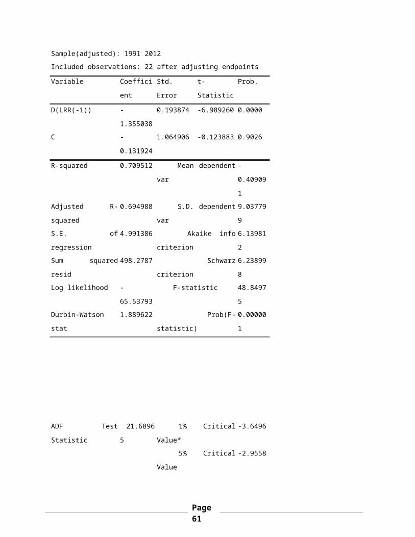
Sample(adjusted): 1991 2012Included observations: 22 after adjusting endpoints

Variable Coeffici

ent

Std.

Error

t-

Statistic

Prob.

D(LRR(-1)) -

1.355038

0.193874 -6.989260 0.0000

C -

0.131924

1.064906 -0.123883 0.9026


var

-

0.40909

1Adjusted R-

squared


var

9.03779

9S.E. of

regression


criterion

6.13981

2Sum squared

resid

498.2787 Schwarz

criterion

6.23899

8Log likelihood -

65.53793

F-statistic 48.8497

5Durbin-Watson

stat

1.889622 Prob(F-

statistic)

0.00000

1

ADF Test

Statistic

21.6896

5

1% Critical

Value*

-3.6496

5% Critical

Value

-2.9558

Page61

10% Critical

Value

-2.6164



Augmented Dickey-Fuller Test EquationDependent Variable: D(MONEYSS)Method: Least SquaresDate: 07/26/13 Time: 15:27Sample(adjusted): 1981 2012Included observations: 32 after adjusting endpoints

Variable Coeffici

ent

Std.

Error

t-

Statistic

Prob.

MONEYSS(-1) 0.279057 0.012866 21.68965 0.0000C 528.0600 1092.195 0.483485 0.6323


var

12070.5

5Adjusted R-

squared


var

21677.9

0S.E. of

regression


criterion

20.0849

3Sum squared

resid

8.73E+08 Schwarz

criterion

20.1765

4Log likelihood -

319.3589

F-statistic 470.441

1Durbin-Watson

stat

2.077399 Prob(F-

statistic)

0.00000

0

Page62

Appendix D: Unit Root Test Results

Variable Stationary

Critical level

Difference

Operator

GDP 1 percent None

Lagged GDP 1 percent None

Interest Rate 1 percent None

Exchange Rate 1 percent None

Money Supply 1 percent None

LRR 1 percent First

Inflation 1 percent None

Page63

The effects of monetary policy on economic growth of Malawi

Documents

Transcript of The effects of monetary policy on economic growth of Malawi