International Invention Journal of Arts and Social Sciences Vol. 1(3) pp. xxx-xxx, December, 2014 Available online http://internationalinventjournals.org/journals/IIJASS Copyright ©2014 International Invention Journals

Full Length Research Paper

The Effects of Export Diversification on Economic Growth in Cameroon

*Njimanted Goddfrey Forgha, PhD, Molem Christopher Sama, PhD, Ernest Musomo Atangana

Department of Economics and Management, University of Buea – Cameroon,

Abstract

This study is designed to investigate into the nature of export diversification and the relationships between export diversification and economic growth in Cameroon. Using data from 1980-2012, the Vector Autoregressive (VAR) technique of estimation is adopted to stimulate policies necessitated by the study. In reality the study establishes that export diversification had positively and significantly affected economic growth in Cameroon within the period of study. This finding is ironical since the economy of Cameroon has timidly grown over the years. Based on the VAR results, we further recommend the expansion of the export base by acquiring new production techniques, research on new products, marketing and the provision of incentives and subsidies for private sector development. Redesigning of education curriculum to train qualified man power in the export sector of the economy. Furthermore the government should properly manage the public debt and especially the external debt and the consistent negative balance of payments position which sucks away the benefits of external trade from Cameroon. Keywords: Export Diversification, Tax incentive, Development, External Debt.

INTRODUCTION The advantages of focusing on economic growth through export and export diversification are of two folds. First, the place of foreign exchange in economic transformation; that is, transactions in the international markets are carried out using hard currencies among which are the US dollar, the European Euro, the English pound, the Japanese Yen and these currencies are obtained through export exchange by the countries involved, (investopedia, 2012). Second, exports tap a ready market for the different commodities and this is because World export markets are vastly larger than domestic ones, particularly those of developing countries like Cameroon. By 2010, China became the largest of Cameroon’s exporting partners consuming 14.8% of Cameroon’s exports, Netherlands 9.5%, Spain 8.8%, India 8.4%, Portugal 7.9%, Italy 5.9%, U.S 5.3% and *Corresponding Author Email:unicalub@yahoo.com

others, (CIA World Factbook, 2012) thus providing an extended and ready market for Cameroon’s exports .

Research has shown that all of the more successful developing countries relied heavily on export and through export diversification as the primary engine of economic growth. The “newly industrialized countries” or the “Asian Tigers” epitomized this export-led growth strategy (Bradley, 1991). According to World Bank Report and statistics from econstat.com (2012), Korea, from 1980 to 2004 increased its percentage of exports of goods and services volume from 8.58% to 29.3% recording a GDP increase from 39,109.6 Won to 100,254.1 Won and thus a percentage growth rate of 61%. From 2005 to 2010 it further increased by 15% and recorded a GDP increase from 651,415.3 Won to 1,173,275 Won and thus a percentage growth of 80%. Brazil and most eastern European countries are also good examples of the export diversification drive.

In Sub-Saharan Africa, the Mauritian economy over the past thirty years has diversified from mono-crop economy depending on sugar exports in the 1970s to

one based on manufacturing of textiles and garments and tourism in the 1980s, Sanjay (2011). Global business (offshore) and Freeport activities have also been growing continuously since the mid 1990s. The country’s main export still remains textile and clothing, the services sector has surpassed the manufacturing sector to become the main contributor to the GDP which witnessed considerable growth that is $1.292 billion in 1980, $2.569 billion in 1990, $4.732 billion in the year 2000 and $11.22 billion by 2012, (World Economic Outlook, 2012). With sustained GDP per capita growth (8% on average annually), since independence, Mauritius has moved to an upper middle income country status, (Economic Watch, 2012).

Cameroon like most of the other developing countries depends on primary, few and low valued commodities as their source of export earnings. Major export commodities of Cameroon include; cocoa 9.7%, coffee 2.6%, banana 2.6%, cotton 3.2%, natural rubber 2.4%, crude oil and petroleum products 48.4%, timber and timber products 13.9%, minerals and unwrought aluminum 2.7% and others 19.5%, (Cameroon Economic, Social and Finance Report, 2011). If not all of these products, most confront a number of difficulties in the international market such as; price instability, inferior products, quotas and restrictions, tariffs, tax escalation and other trade barriers.

Agriculture was one of the main sources of growth and foreign exchanged in Cameroon until 1978 when oil production replaced it as the cornerstone of growth for the formal sector till the mid 1980s (Economic Watch, 2010). Today, due to depleting oil, agriculture is still the backbone of Cameroon’s economy, employing about 70% of its labour force, while providing about 42% of its GDP and 30% of export revenue, (Cameroon National Institute of Statistics, 2010). The most important cash crops produced are cocoa, coffee, cotton, banana, rubber, palm oil, palm kernel and peanuts each providing it own share of total exports. Small amounts of tobacco, tea and pineapple are also grown. A portion of these crops are meant for export while the rest are used locally. Main food crops are plantains, cocoyam, banana, yams, cassava and derivatives, corn, millet and sugar cane which are meant primarily for local consumption while small quantities are exported to CEMAC and other neighboring countries. From 2010 to 2012 the production of food crop stood at 15062805, 15656539 and 17028143 tonnes respectively while exports stood at 128073, 144875 and 301797 dollars respectively. (MINADER, MINEPIA Annual Reports, 2013).

In recent years, reductions in the total volume of goods exported by Cameroon became pronounced as it increased from 3.8% in 2008 to 13.3% in 2009, due to contraction of world demand. By products, the trend contrasted. While the export of some products such as fuels and lubricants (-50.4%), wooden veneer sheets

(-44.4%), aluminum (-35.2%), banana (-9.4%), timber (-5.3%), and crude oil (-4%) dropped, others witnessed expansion in their volumes such as raw cotton (52.1%), cocoa beans (8.9%) and coffee (12%), (Cameroon Economic, Social and Finance Report, 2011). In 2010 and 2011 exports increased from 1924.2 billion CFAF francs to 2171.5 billion CFA Francs respectively, up by 12.9% following increases in the export of petroleum products and lubricants (39.9%), crude oil (14.4%), raw cotton (33.9%), raw rubber (31.1%), sawn timber (10.5%), fresh banana (3.2%) and coffee (4%). Conversely, the export of cocoa beans, aluminum and log timber dropped by 19.8%, 8.1% and 62% respectively. Non-oil exports increased by 12% to stand at 1372.4 billion CFA Francs, (Cameroon Economic, Social and Financial Report, 2012).

Cameroon manufacturing sector is composed mainly of light and agro-manufacturing industries. World Bank Report (2012) shows that manufacturing export in Cameroon rose from 3.75% in 1980 to 18.28% in 1986. By 2006 industrial manufacturing contribution to total export fell to the lowest value of 3.03% and since then it has been increasing timidly. In 2009, the manufacturing production index grew by just 1.3% compared to that of 2008 which stood at 15.5%. All branches of manufacturing activity contributed positively to growth except for chemicals and petroleum industries where production contracted by 10.2%. Contrary to this, in 2011, production of agro-food was 4.2% and oil sector 10.6%, beverages 7%. The tertiary sector accounted for 45.6% of GDP by 2009, grew by 3.5% and contributed 1.6% of growth (Cameroon Economic, Social and Finance Report, 2012). This trend is explained by good performances in the telecommunication and transport with tourism sub-sectors which been increased in subsequent years.

Exports are supposed to play a major role in gross domestic product (GDP) growth. But for the recent years, in Cameroon, GDP has been 3.3 for the year 2010, 4.1 for 2011 and 4.7 for 2012 (World Economic Outlook, 2012). This poor growth can be attributed to poor export contribution to GDP. On the average between 1980 and 1990 the contributions of exports to growth in Cameroon stood at 25.6%, between 1991 and 2000 it stood at 22.6% and between 2001 and 2010 it increased to 26.7% (World Economic Outlook, 2012) which appears quite low compared to other emerging nations mentioned above. Fluctuations in export prices of major export products of Cameroon and also persistent negative current account balances which stood at -0.9796, -0.625, -0.8320 and -0.1960 billion Francs CFA in the respective recent years of 2011, 2010 , 2009 and 2008 in descending order are major causes of low contributions of export earnings to growth in Cameroon. It also resulted from long term net capital flows which became negative from 1990/91 as well as

the effects of considerable accumulation of public external debt, (Cameroon’s external debt stood at 69.1% of GDP by 2004 and 13.9% by 2011, (CIA Fact book, (2012)) relative to stagnations and declining trade surpluses. High unemployment rate and extreme poverty have both plagued the Cameroonian economy causing productivity and investments to fall leading thus to low export earnings as notice.

Theoretical conjectures mostly propagated by Cameroon politicians contend with the fact that export in Cameroon is diversified but very little scholarly works have been presented to tie these conjectures to economic growth. For example, Bamou (2002), in her study, provided only an indication of a priority order of exports by classifying them according to their world market access prospects. She used the competitive and financial capital profitability indexes to show that the 33 identified non – traditional exports of which close to three fourth are industrial, 19 (4 primary agriculture and 15 industrial) are competitive and profitable and can thus be promoted in priority within the export diversification promotion framework. This study thus, using competitive and financial capital profitability index was only able to classify the products accordingly. But it should be noted that comparative advantage plays a very important role as far as international trade is concerned and should not be minimized while making conclusions on issues of international trade. Again no product or natural resources should be allowed to rot and so even if some are not competitive but are useful, they should be exploited. And finally the study had nothing to do with the effects of export diversification on economic growth in Cameroon. Majority of empirical works on export diversification and economic growth on different countries have proven a positive result but a study on Columbia by Amin et al. (2000), produced a negative result. Based on the fact findings from different countries yield mixed conclusions, this study is designed to assess the Cameroon experience via export diversification.

Since the 1990s, Cameroon implemented a series of economic and structural reforms aimed at stabilizing the economy, restructuring internal viability, providing incentives for private sector development, fostering entrepreneurship and entrepreneurial development. In 1994, a monetary adjustment took place through the devaluation of the CFAF intending to value export earnings, adhesion to the AGOA (African Growth Opportunity Act) in the year 2002, provided export opportunities to North American markets for primary and cultural products, the Economic Partnership Agreement (EPA) with the European Union in December 2007 which gradually establish a free trade zone between ACP countries and European markets, implementation of the Poverty Reduction Strategy Paper and the Growth and Employment Strategy Paper all aimed at increasing the economic position of the country. Without minimizing the

numerous engagements with member countries of the CEMAC region from where Cameroon has to show its dominance in the export market, South American and Asian markets will be explored and negotiated against the backdrop of emerging countries in search of strategic positioning and political and diplomatic leverage. The mutual interest cooperation option advocated by countries falling under this group, (China, Brazil, India, Korea, etc.) and the high density of their population make them major trade development partner projects for Cameroon.

Given the fact that a lot have already been put in place with the expectation of increasing the rate of export contributions to growth in Cameroon to no avail, this study is thus designed to put forth answers to the following questions; what is the level of export diversification in Cameroon? What are the major determinants of economic growth and how has export diversification affected economic growth in Cameroon This study is conducted under the null hypotheses of exports in Cameroon are not significantly diversified and export diversification have no statistically significant effect on economic growth. Empirical Literature Some empirical studies have been carried out to correlate export diversification and economic growth in and out of Africa, Al Marhubi (2000). In cases where it has been done, the links are not made clear, Svedbeg (1991). Nonetheless, a high percentage of the study confirms a positive relationship. However, while these studies give a positive relationship between export diversification and economic growth, they scarcely indicate the reasons for this positive relationship.

Amin and Ferrantino (1997), affirm the modesty of export diversification as a good driver of economic growth. For a study on the Chilean economy, these authors concluded that, in the long run, export diversification might have improve Chilean growth relative to what it would have been with a concentrated export basket over the period from 1960 to 1990. Amin and Ferrantino (1997) infers that export diversification was used in Chile as a response to recessions and that before boosting economic growth, adjustment costs are made in-terms of lower export growth. The controversial idea raise by Amin and Ferrantino (1997) that export diversification should be used to reverse recessions can be misleading since the employment of export diversification is a strategy to enhance general growth and development and not only necessarily to reverse recessions. Again diversification should not only be tied to moving away from traditional products to new and manufactured products, it also comprises adding value to the traditional products.

Naude and Rosouw (2008), employed the use of time series data from 1962-2000 for South Africa to examine the causal relationship between export diversification and economic growth. They observed that export diversification granger cause growth in GDP per capita. This was confirmed by the computable general equilibrium estimate for South African economy which reveals that increase in GDP per capita and employment opportunities are as a consequence of a diversified export base.

The application of the general equilibrium model analysis by Naude and Rosouw (2008) has added value in the technique employed to estimate the effect of export diversification on economic growth using African data. This approach required full information which is not available. Their inability to examine the dynamics of this relationship also cast doubt on their recommended policies.

Hess (2006) in his part observes that, the effect of export diversification is dependent on the income level of a country. In is paper, Hess shows a positive relationship between export diversification on per capita income growth, which is non-linear. The established non-linearity in the diversified export basket is realistic for developing countries as it contributes to growth, whereas specialization is of greater benefits to developed countries. Again, for developing countries, Hess argues that, export concentration is detrimental to per capita income growth. Hess’ analysis used a panel growth model (Solow), for 91 countries for the years 1960 to 2000.

On the contrary Hess’ suggestion that income level of a country depends on export diversification is not conclusive since there are other macro economic variables that positively affect GDP growth. Again there is no limit to export diversification since technology evolve daily, therefore, export diversification and value added are continually necessary to both developed and developing countries in this dynamic world.

Using time series data from 1971-2013 and employing the vector auto regressive technique, Haseeb et al. (2014) were able to empirically prove that exports and foreign direct investment have a positive impact on economic growth in Malaysia. Using export and foreign direct investment in a model without conducting a multi-colinearity test leaves us without the knowledge of the strength of the relationship existing between the variables in the model.

Nadeem et al. (2012), in their study on investigation of the various factors influence on export, using ordinary least squares for Pakistan from 1981-2011, concluded that export volumes need to be expanded maximally in other to achieve higher levels of economic growth. Here again the work fails to conduct all the necessary pretests such as multi-colinearity test and cointegration tests, thus casting doubts on the final results obtained.

Al Marhubi (2000) further supports the conclusion that the benefits of export diversification differ from developed and developing countries. Using cross sectional data from 1961 to 1981 for 91 countries, and with use of two equations, (growth equation and the export diversification equation); the results from the equations were conventional implying a positive relationship between export diversification and economic growth. Al Marhubi coins this “the direct effect” of export diversification on growth. A possible indirect effect is tested via an investment equation. It is the direct effect that marks the difference between developing and developed countries since this effect is only present for estimations of developing countries. Hence for developing countries, a more diversified export basket leads directly to faster growth and further more increases the possibility for fruitful investment, which intend is also positively related to economic growth.

Amin et al. (2000), using time series analysis found an inverse relationship between export diversification and growth in Columbia. However, as pointed out by Herzer et al. (2006), this study suffers a lot of methodological short falls including the omission of unit root test and possible presence of structural breaks when testing for unit roots. Normality, autocorrelation and hetero-skedasticity tests were not conducted meaning that the study might have been suffering from spurious regression.

Savietti and Frenken (2008), using panel data from OECD countries, show that export diversification can have a positive effect for developed countries. They found out that both horizontal and vertical diversification have a positive impact on economic growth. This paper also presents evidence that diversifying the export basket horizontally has immediate effect on economic performance while it takes time for vertical diversification to affect economic growth positively. Vertical diversification can potentially be deterred by adjustment cost and technological barrier. Nevertheless it is good to undertake this type of diversification since, at a certain stage, the rate of horizontal diversification’s return will start to diminish, Savietti and Frenken (2008).

Sanjay (2011) observes the relationship between export diversification and economic growth for Mauritius from 1980 – 2008. Based on Vector Error Correction Modeling and the Johansen co-integration analysis, he found an inverse relationship between export concentration and economic growth. His results call for the need to promote export diversification through appropriate incentives provisions, dealing with market information and failures, promoting entrepreneurship as well as providing a competitive business environment for sustained economic growth. The work of Sanjay (2011) is a contemporary study on export diversification in a country with limited natural endowments. The necessity of export diversification through value added is

paramount to Mauritius. The use of vector error correction mechanism to test co-integration increases the reliability of the result obtained. Theoretical Literature In the field of finance, portfolio, constitute an appropriate combination or set of investments. The best of the mix of investment depends on the mix expected return and its variance (Ross et al., 2005). The higher a portfolio’s attractiveness, the higher it’s expected returns and the lower its standard deviation. It becomes therefore important to create a diversified portfolio including securities that share a negative covariance with each other as only this will lead to decrease in the portfolio’s standard deviation and hence variance. The strategy for diversification should lower earning’s variance of basically any portfolio and thus can also be applied to the export portfolio of a country, where export products represent the investments (Stanley and Bunnag, 2001).

Assumptions of the portfolio effect include; products or goods in any bundle are valued equally, there are different alternative bundle of which one is the best, the best bundle is the one with many and extended list.

Translating the theory to export diversification implies that the growth prospect of Cameroon depends on Cameroon’s export portfolio, hence the composition of its export basket. The wider the export base, the better the portfolio of a country could enhance the export earnings making it less volatile, therefore ameliorating the condition for stable growth Agosin (2009). To this theory, export concentration increases the risk of fluctuations in export earnings. Unstable export earnings make economic planning impossible, reduce import capacity, reduce chance of debt repayment resulting from total economic instability and furthermore lead to higher growth variance (Stanley and Bunnag, 2001).

Agosin (2009) refers to this portfolio effect as potential explanation for a positive relationship between export diversification and growth. By “not putting all the egg in one basket” diversification of exports will induce lower volatility of export earnings and consequently result to lower GDP variance. Export diversification is thus necessary for countries that do not have unrestricted access to world financial and commodity markets but still need to smooth consumption in times of fluctuation in export proceeds and output, Agosin (2009).

In appraisal, issues on export diversification as a means of development and growth became important in economics only in the 1950s when the world began viewing dependence on primary products as harmful for growth of developing countries due to the extreme volatile price and low elasticity of demand, Chaudhuri (2001). Today Sub- Saharan African countries are most affected since they still need to diversify out of primary

products, (Collier, 2006).

Again today, with accurate data, the “portfolio effect” theory is found to show evidences to an extent to mitigate the export instability problem. Stanley and Bunnag (2001) found out that fluctuations in export earnings do cause macroeconomic instability in developing nations. They also show that only half of the economic instability is explained by the portfolio theory and the other part is derived from other macroeconomic factors such as openness. Therefore, this theory which supports diversification into products whose price shares negative covariance with prices of existing products which is the case of manufactured goods, thus achieving stability.

According to endogenous growth theory, labour productivity and investments can affect both the level of growth and per capita output. It will be interesting at this point to use the “AK model” which works on the property of absence of diminishing returns to capital. The simplest form of the production function is given as; Y = AK

Where A is a positive constant that affects level of technology, K is capital (to include human capital). Y =AK, output per capita and the average and marginal product are constant at the level A>0.

Then f(k)/k =A in equation of transitional dynamics of Solow-Swan model which shows how an economy’s per capita income converges towards its own steady-state value and to the per capita incomes of other nations.

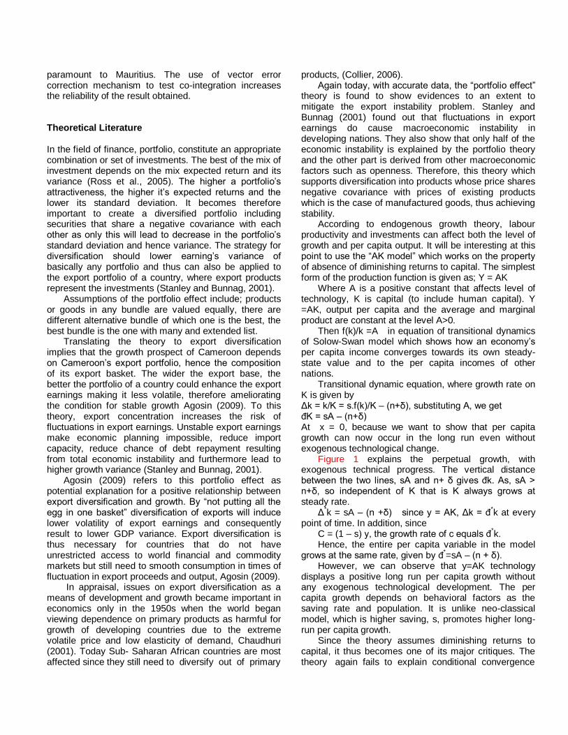
Transitional dynamic equation, where growth rate on K is given by Δk = k/K = s.f(k)/K – (n+δ), substituting A, we get đK = sA – (n+δ) At x = 0, because we want to show that per capita growth can now occur in the long run even without exogenous technological change.

Figure 1 explains the perpetual growth, with exogenous technical progress. The vertical distance between the two lines, sA and n+ δ gives đk. As, sA > n+δ, so independent of K that is K always grows at steady rate.

Δ*k = sA – (n +δ) since y = AK, Δk = đ

*k at every

point of time. In addition, since C = (1 – s) y, the growth rate of c equals đ

*k.

Hence, the entire per capita variable in the model grows at the same rate, given by đ

*=sA – (n + δ).

However, we can observe that y=AK technology displays a positive long run per capita growth without any exogenous technological development. The per capita growth depends on behavioral factors as the saving rate and population. It is unlike neo-classical model, which is higher saving, s, promotes higher long-run per capita growth.

Since the theory assumes diminishing returns to capital, it thus becomes one of its major critiques. The theory again fails to explain conditional convergence

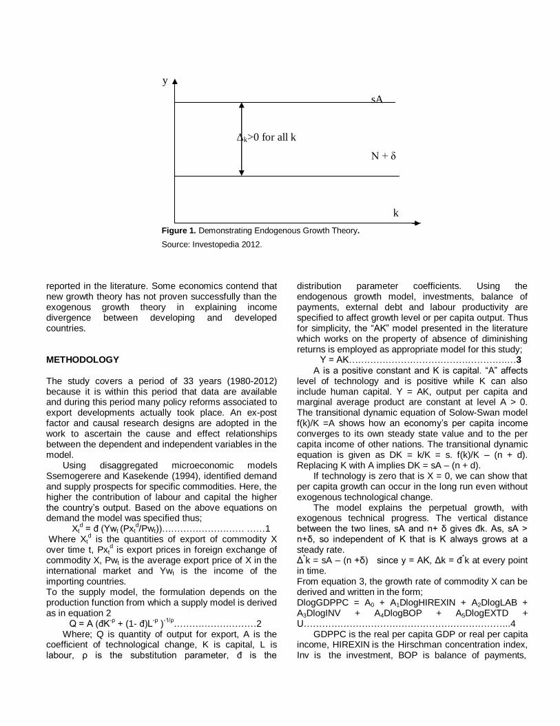
Figure 1. Demonstrating Endogenous Growth Theory.

Source: Investopedia 2012.

reported in the literature. Some economics contend that new growth theory has not proven successfully than the exogenous growth theory in explaining income divergence between developing and developed countries. METHODOLOGY The study covers a period of 33 years (1980-2012) because it is within this period that data are available and during this period many policy reforms associated to export developments actually took place. An ex-post factor and causal research designs are adopted in the work to ascertain the cause and effect relationships between the dependent and independent variables in the model.

Using disaggregated microeconomic models Ssemogerere and Kasekende (1994), identified demand and supply prospects for specific commodities. Here, the higher the contribution of labour and capital the higher the country’s output. Based on the above equations on demand the model was specified thus; Xt

d = đ (Ywt (Pxt

d/Pwt))……………………… ……1

Where Xtd is the quantities of export of commodity X

over time t, Pxtd is export prices in foreign exchange of

commodity X, Pwt is the average export price of X in the international market and Ywt is the income of the importing countries. To the supply model, the formulation depends on the production function from which a supply model is derived as in equation 2 Q = A (đK

-ρ + (1- đ)L

-ρ )

-1/ρ………………………2

Where; Q is quantity of output for export, A is the coefficient of technological change, K is capital, L is labour, ρ is the substitution parameter, đ is the

distribution parameter coefficients. Using the endogenous growth model, investments, balance of payments, external debt and labour productivity are specified to affect growth level or per capita output. Thus for simplicity, the “AK” model presented in the literature which works on the property of absence of diminishing returns is employed as appropriate model for this study; Y = AK…………………………………………….…3

A is a positive constant and K is capital. “A” affects level of technology and is positive while K can also include human capital. Y = AK, output per capita and marginal average product are constant at level A > 0. The transitional dynamic equation of Solow-Swan model f(k)/K =A shows how an economy’s per capita income converges to its own steady state value and to the per capita income of other nations. The transitional dynamic equation is given as DK = k/K = s. f(k)/K – (n + d). Replacing K with A implies DK = sA – (n + d).

If technology is zero that is X = 0, we can show that per capita growth can occur in the long run even without exogenous technological change.

The model explains the perpetual growth, with exogenous technical progress. The vertical distance between the two lines, sA and n+ δ gives đk. As, sA > n+δ, so independent of K that is K always grows at a steady rate. Δ

*k = sA – (n +δ) since y = AK, Δk = đ

*k at every point

in time. From equation 3, the growth rate of commodity X can be derived and written in the form; DlogGDPPC = A0 + A1DlogHIREXIN + A2DlogLAB + A3DlogINV + A4DlogBOP + A5DlogEXTD + U…………………………………………………………..4

GDPPC is the real per capita GDP or real per capita income, HIREXIN is the Hirschman concentration index, Inv is the investment, BOP is balance of payments,

y

sA

Δk>0 for all k

N + δ

k

Figure 2.1: Demonstrating Endogenous Growth Theory.

Source: Investopedia 2012.

EXTD is external debt, LAB is labour productivity index, U are the residual with their assumed normalities residual error variable. All variables are in logarithmic form and first difference, based on the fundamental notion that time series data are always stationary after their first difference. The logarithm applied in the model gives us the opportunity to interpret our coefficients as elasticities.

From equation 1 and 2 one can derive a set of criteria based on world market conditions and domestic supply conditions for identifying a priority of commodities for exports. These criteria will include; high income elasticity of demand, high price elasticity and supply responsiveness of the products.

Most economic models have limitations or difficulty in application for developing countries like Cameroon. Most models are not explicit enough to motivate individual exporters who produce for the world market. The higher the profits from exports, the greater will be exporter’s motivation. Competitiveness is also a factor associated to foreign trade which in turn inhibits developing country’s exporting capacity.

Following from the model expressed above, specifically the supply model, increases in capital and labour contributions, will lead to increase in output since in both developed and developing countries, what are produced are also consumed and exported. Export Concentration Index is therefore used to investigate the relationship between export diversification and economic growth. In this work, export concentration is measured using the HIREXIN and the formula is derived by Hirscmann in 1945. Written as

Hj = 𝒙𝒊

𝑿 𝟐

𝒏𝒊 ………………..…..……….5

Where; HJ is Hirschman export concentration index, xi is export of good i in j year, X is 𝑥𝑖 (sum of all export in j year). For H nearer to zero implies higher export diversification and for H nearer to one implies higher export concentration. Advantages of the HIREXIN are that it en-corporate merchandise trade and services and so it is good even to Small Island states who solely depends on services as their own principal source of foreign earnings. Also in calculating the HIREXIN, products’ export shares are used as their own weights (wi = si) and so the index takes account of all export categories.

To investigate on the causality between export diversification and economic growth for Cameroon, we employ the Vector Autoregressive (VAR) Model which has always serve as an extension of the Granger Causality test and permits the extension away from the bivariate framework of the dependent and independent variables only. From equation 4, our VAR models are presented thus; DlogGDPPCt=β +Σ

k j-1βjDlogHIREXINt-1 + Σ

k j-

1βjDlogLABt-1 + Σk j-1βjDlogINVt-1 + Σ

k j-1βjDlogBOPt-1+ Σ

k

j-1βjDlogEXTDt-1 + U1………………………………..……...6 DlogHIREXINt= β +Σ

k j-1βjDlogGDPPCt-1 + Σ

k j-

1βjDlogLABt-1 + Σk j-1βjDlogINVt-1 + Σ

k j-1βjDlogBOPt-1+ Σ

k

j-1βjDlogEXTDt-1 + U………………………………………..7 DlogLABt= β +Σ

k j-1βjDlogHIREXINt-1 + Σ

k j-

1βjDlogGDPPCt-1 + Σk j-1βjDlogINVt-1 + Σ

k j-1βjDlogBOPt-1+

Σk j-1βjDlogEXTDt-1 + U3……………………..……………..8

DlogINVt= β +Σk j-1βjDlogHIREXINt-1 + Σ

k j-1βjDlogLABt-1 +

Σk j-1βjDlogGDPPCt-1 + Σ

k j-1βjDlogBOPt-1+ Σ

k j-

1βjDlogEXTDt-1 + U4…………………………………..……9 DlogBOPt= β +Σ

k j-1βjDlogHIREXINt-1 + Σ

k j-1βjDlogLABt-1

+ Σk j-1βjDlogINVt-1 + Σ

k j-1βjDlogGDPPCt-1+ Σ

k j-

1βjDlogEXTDt-1 + U5………………………………………10 DlogEXTDt= β +Σ

k j-1βjDlogHIREXINt-1 + Σ

k j-1βjDlogLABt-

1 + Σk j-1βjDlogINVt-1 + Σ

k j-1βjDlogBOPt-1+ Σ

k j-

1βjDlogGDPPCt-1 + U6……………………………………11 It should be noted here that the differencing of the

variables will be done only when such variables is not stationary at level. It is a-priori expected that, Hirschman export concentration coefficient index and external debt should take a negative value since higher values imply lesser export diversification while investment, balance of payments and labour productivity are expected to be positive since they have expansionary effects on CPI and so their increases are expected to increase real GDP per capita.

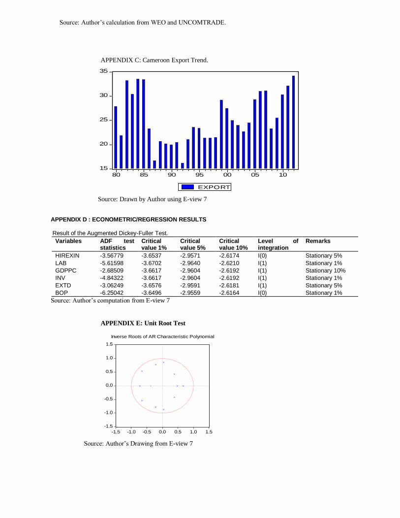
Before actual estimation, we conducted trend analyses using graphs; stationarity tests particularly the augmented Dickey-Fuller and Phillips-Perron unit root tests since no structural break has been exhibited by any of the variables as reported by the graphs. We also determine the level of integration of the variables in the series and using the unit circle tests. The Johansen-Juselius (JJ) co-integration tests were also conducted and later the normalized co-integration test to ascertain whether or not the series meets up with the a-priori expectations, the pairwise correlation test was used in testing the degree of multi-colinearity among the variables while the Langragian Multiplier (LM) test was used in testing for whether or not serial correlation are embodied in the models. The granger causality test was used to show the level of causality between the variables in the model. Normality tests such as Jacque Bera, skewness, kurtosis, standard deviation, and mean, median, minimum and maximum values were conducted (not also presented because of space). They all justify that the variables are normally distributed within our study area and period of study. PRESENTATION AND DISCUSSION OF RESULTS From the trend analyses conducted (graphs not presented here because of space) all the variables in the model exhibited no trend within the period of study. They were stochastic with drifts. Thus testing for stationarity

and order of integration of the variables reveal that some of the variables such as BOP and HIREXIN attained stationarity at level while EXTD, LAB and INV attained stationarity at their first differences. Unit circle result also showed that the residuals of the various models are all integrated at the other one 1(1). The above results affirmed the presence of co-integration; this implies that long-run equilibrium exists between the variables in the models. The normalized co-integration equation also reveals that, in the long-run further export diversification will continue to have positive effects on economic growth in Cameroon and so confirms the alternative hypothesis while rejecting the null hypothesis. These results tie with the a priori expectations. The coefficients for BOP, EXTD, LAB and INV (-0.001728, 0.035151, 0.872679 and 0.10654 respectively) also follow the a-priori expectations as any increase in labour productivity, increase in balance of payments ,investment and drop in external debt are expected to result to higher economic growth, as explained by external debt-over hanged hypothesis.

The pairwise correlation matrix (see appendix G), for BOP and DLOG(EXTD) have negative relationship with GDPPC while DLOG(LAB), DLOG(INV) and LOG(HIREXIN) have positive relationship with GDPPC but that of LOG(HIREXIN) is weak while the others are strong. The relationships between the independent variables are weak; some are weakly positive while others are weakly negative. This shows that there is no multicolinearity between the variables specified in our model. As such the variables have reported their independent effects.

Testing for auto correlation using the VAR residual serial correlation LM tests, the result shows that the calculated LM value is 63.05382 at lagged length nine with a 0.3% probability at chi-square critical value of 31.41 at five percent significant level leads us to reject the null hypothesis of serial correlation in favour of the alternative that there is no serial correlation.

From the pairwise granger causality table (see appendix H), the lagged value of labour productivity granger cause gross domestic product per capita at 5% level of significance. Since the F-statistics calculated (4.29) is greater than the critical value, with table value of 3.39 probability value of 2%, thus we rejecting the null hypothesis. Investment (lagged) granger cause gross domestic product per capita at 10% level of significance. The calculated F-statistic is 2.90 which is greater than the critical value (F-statistic table) 2.53 and with a probability value of 7%. The lagged value of External debt granger causes Hirschmann Export Concentration Coefficient Index at 5% level of significance. The calculated F-statistic is 3.74 while the critical value is 3.40 with a probability value of 4%. The other combinations of the pairwise granger causality tests, we do not reject the null hypothesis because their F-tests

statistics calculated are lower than their critical values at 1%, 5%, and 10% levels of significance.

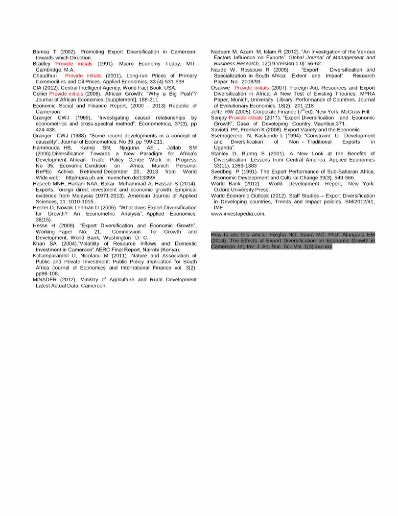
The obtained HIREXIN has the maximum value of 0.64 for the year 2006 and the minimum value of 0.33 for the year 2000. The overall mean is 0.45. The non-parametric test of year counts and expressing in-terms of percentage, reveals that exports are 72% diversified attesting to the fact that exports in Cameroon are fairly diversified since the mean value obtained was 0.45.

The Vector Auto Regression Estimate, (see appendix A), shows that GDPPC in the first and second lags adversely but significantly affects GDPPC growth, BOP only affects GDPPC negatively and significantly in the second lag. EXTD shows a negative and significant relationship with GDPPC in the second lag but significant and positive in the first lag. LAB shows a positive and very significant relationship with GDPPC implying that in the first and second lags 3.03% and 2.32% increase in GDPPC are accounted for by a% increased in labour productivity. This finding is in line with that of Amin (2002) whose findings reveal that the growing GDP in Cameroon is owed to the dynamic labour force. INV in the first lag positively and significantly affects GDPPC growth while in the second lag its negatively but significantly affects GDPPC growth. These results affirms that of Khan et al. (2004) who found out that both private and public INV combined play an important role in economic growth but the reverse is true for public INV. HIREXIN positively and significantly affect GDPPC; in the first and second lag meaning that 0.52% increase in GDPPC is accounted for by 1% increase in HIREXIN and 0.65% increase in GDPPC is accounted for by 1% change in HIREXIN respectively. Both results are significant at 1% level. This result is in line with those of Sanjay (2011) for Mauritius; in Mauritius export diversification from traditionally primary to manufacturing and services has successfully transformed Mauritius from a low income to a middle income country. The adjusted R

2 shows that 43% of the

outcome in the model is explained by the independent variables used in the model with the F-statistic of 2.77 confirming the fact that the results are about 90% reliable.

The results of the VAR model for BOP reveals that a 0.49% decrease in BOP and 0.57% decrease in BOP of the first and second lags accounted for 1% variation in current BOP. These results are both statistically significant at 10 and 1% level of significance respectively. Furthermore, it is also observed from the results that 30.78% decrease in BOP in the present year is accounted for by 1% change in EXTD of the second lag, and a 31.09% decrease in BOP of the current year is accounted for by again 1% variation in EXTD. Both results are statistically significant at 10%. These results conformed to those of Osakwe (2007) which states that most African nations have accumulated EXTD as a

consequence of persistent negative BOP. Lastly but not the least, 29.12% increase in BOP of the present year is accounted for by 1% variation in HIREXIN of the previous year although this result is statistically insignificant it is in agreement with status quo while the second lag, the increase in BOP is 60.54%, which is significant at 10% level of significance. This is in agreement with the portfolio theory which link export concentration to volatile growth via export earnings and general instability. The adjusted R

2 shows that 53% of

the outcome in the model is explained by the independent variables used in the model with the F-statistic of 3.58 confirming the fact that the results are about 95% reliable.

The VAR results for EXTD equation appear insignificant but some variables affect EXTD negatively while others positively. That is a 0.01% increase in EXTD of the present year is accounted for by 1% variation in BOP for the previous year. This result is significant at 5%. This result is still in agreement with those of Osakwe (2007), which shows that most African countries have accumulated EXTD as a consequence of persistent current account deficit.

From the VAR equation for LAB, it is observed that a 4.22% decrease in LAB for the present year is the result of 1% increased in GDPPC the previous year and this is significant at 1% while for the second lag 0.91% decrease in LAB was as a result of 1% increase in GDPPC but this result is insignificant. This explains the fact that majority of the labour force are unskilled and uneducated as such increase in their livelihood will not assist in their productivity. Again the VAR result also explains that, a decrease of 0.01% in LAB productivity current year is accounted for by 1% variation in BOP for the second lag at 1% significance level. This is in agreement with the Nurkse’s theory of disguised unemployment. The theory stipulates that given the techniques and productive resources, the marginal productivity of labour in agriculture, over a wide range, is zero in over populated underdeveloped countries. Any 1% increase in external debt in both the first and second lag, LAB increases by 0.26 percent and decrease by 0.27 percent in the current year respectively. This implies that for the second lag a 1% increase in EXTD causes 0.27% decrease in LAB but for first lag, 1% increase in EXTD in the previous year causes 0.26% increase in LAB the current year. The results of both first and second lags are significant at 5%. This can be explained by the fact that in the second lag, LAB is affected negatively by EXTD but the preceding year with increase in debts because of debt defaults, LAB will have a positive effect due to re-investments of the proceeds of labour. Furthermore for a 2.78% increase in LAB in the current year is accounted for by 1% variation in LAB for the previous year more than the increase in the second lag that is 1.97%. The result is significant at

1%. This result is in agreement with the Lewis theory of unlimited supply of labour when labour moves from the subsistence to the capitalist sector. In this sector if the minimum subsistence wage is paid to labour and surplus re-invested, marginal productivity of labour will increase leading to further increase in productivity till all labour at the subsistence sector is absorbed. Also 1.05% increased in LAB in the current year is accounted for by 1% variation in investment for the previous year and a decrease in about 0.71% the year lag. Both results are significant at five percent level of significance. This scenario can again be tied to the Lewis theory of unlimited supply of labour where in the capitalist sector increase in minimum wage causes increase in marginal productivity of labour resulting from the increase in capitalist surplus used for re-investment. A% variation in HIREXIN in the previous year is reflected by a 0.61% increase in LAB for the current year significant at 1% significance level which is greater than the 0.58% increase for the second lag. This result follows the modern growth theories which see growth as a continuous process.

The VAR estimate for INV shows that 6.05% decrease in INV for the current year is accounted for by 1% variation in GDPPC for the previous year. And in the second lag, the decrease is 3.13%. All the results are significant at 1% level of significance. Also the result follows the modern economic growth theories that regard growth as continuous process and not spontaneous, it also depicts the fact that increased GDPPC results to increase savings and subsequently increase investment. The result claims further that a 0.01% decrease in INV in the current year is accounted for by a 1% variation in the BOP position in a second lag. This result is significant at 5% level of significance. Also a 0.54% decrease in INV in the current year is accounted for by one percent variation in EXTD in the second lag but for the previous year a 0.38% increase in INV in the current year is accounted for by 1% variation in EXTD. Both results are significant at 5% level of significance. A 1% change in LAB in both first and second lags results to 3.66 and 4.33% increase in INV in the current year. These results are statistically significant at 1% level of significance. This result ties to the findings of Al-Marhubi (2000); the possible indirect effect of export diversification is tested through investment. A more diversified economy leads to faster growth and increase possibility of fruitful investment. 1.31% increase in INV in the current year is accounted for by one percent variation in INV in the previous year. The result is also statistically significant at 5% level of significance. This implies that proceed of investment when re-invested and well managed the outcome is more growth. In the same line Kollamparambil and Nicolaou (2011) using quarterly data from 1960 – 2005 to analyse the nature and relationship between public expenditure and private

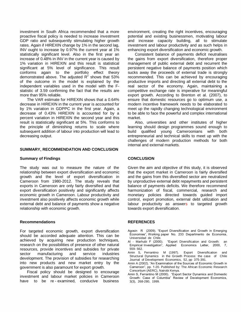
investment in South Africa recommended that a more proactive fiscal policy is needed to increase investment GDP ratio and subsequently stimulating higher growth rates. Again if HIREXIN change by 1% in the second lag, INV ought to increase by 0.97% the current year at 1% statistically significant level. Also in the first year an increase of 0.48% in INV in the current year is caused by 1% variation in HIREXIN and this result is statistical significant at 5% level of significance. This result conforms again to the portfolio effect theory demonstrated above. The adjusted R

2 shows that 53%

of the outcome in the model is explained by the independent variables used in the model with the F-statistic of 3.59 confirming the fact that the results are more than 95% reliable.

The VAR estimate for HIREXIN shows that a 0.64% decrease in HIREXIN in the current year is accounted for by 1% variation in GDPPC in the first year. Again, a decrease of 0.43% HIREXIN is accounted for by a percent variation in HIREXIN the second year and this result is statistically significant at 5%. This conforms to the principle of diminishing returns to scale where subsequent addition of labour into production will lead to decreasing output. SUMMARY, RECOMMENDATION AND CONCLUSION Summary of Findings The study was out to measure the nature of the relationship between export diversification and economic growth and the level of export diversification in Cameroon from 1980-2012. The study reveals that exports in Cameroon are only fairly diversified and that export diversification positively and significantly affects economic growth in Cameroon. Labour productivity and investment also positively affects economic growth while external debt and balance of payments show a negative relationship with economic growth. Recommendations For targeted economic growth, export diversification should be accorded adequate attention. This can be achieved by acquiring new production techniques, research on the possibilities of presence of other natural resources, provide incentives and subsides for private sector manufacturing and service industries development. The provision of subsidies for researching into new products and new market entry by the government is also paramount for export growth.

Fiscal policy should be designed to encourage investment and labour market policies in Cameroon have to be re - examined, conducive business

environment, creating the right incentives, encouraging potential and existing businessmen, motivating labour and increase capacity building, all to stimulate investment and labour productivity and as such helps in enhancing export diversification and economic growth.

Consistent balance of payments deficit neutralises the gains from export diversification, therefore proper management of public external debt and recurrent the persistent negative balance of payments position which sucks away the proceeds of external trade is strongly recommended. This can be achieved by encouraging productive imports and directing all external debt to the real sector of the economy. Again, maintaining a competitive exchange rate is imperative for meaningful export growth. According to Brenton et al. (2007), to ensure that domestic resources go to optimum use, a modern incentive framework needs to be elaborated to meet up the rapidly changing technological environment to be able to face the powerful and complex international market.

Also, universities and other institutes of higher learning should design programmes sound enough to build qualified young Cameroonians with both entrepreneurial and technical skills to meet up with the challenges of modern production methods for both internal and external markets. CONCLUSION Given the aim and objective of this study, it is observed that the export market in Cameroon is fairly diversified and the gains from this diversified sector are neutralized by unproductive external debt repayments and persistent balance of payments deficits. We therefore recommend harmonization of fiscal, commercial, research and monetary policies directed towards guided import control, export promotion, external debt utilization and labour productivity as answers to targeted growth towards export diversification. REFERENCES Agosin R (2009). “Export Diversification and Growth in Emerging

Economies”, Working paper No. 233 Departmento de Economia, Universidad de Chile.

Al - Marhubi F (2000). “Export Diversification and Growth: an Empirical Investigation”, Applied Economics Letter, 2000, 7, 559- 562.

Amin S, Ferrantino M (1997). Export Diversification and Structural Dynamics in the Growth Process: the case of Chile Journal of Development Economics, 52, pp 375-391.

Amin A (2002). “An Examination of the Sources of Economic Growth in Cameroon”, pp. 1-20. Published by: The African Economic Research Consortium (AERC), Nairobi Kenya.

Amin S, Ferrantino M (2000). “Export Sector Dynamics and Domestic Growth: Case of Columbia” Review of Development Economics, 3(3), 268-280, 1999.

Bamou T (2002). Promoting Export Diversification in Cameroon:

towards which Direction. Bradley Provide initials (1991). Macro Economy Today, MIT,

Cambridge, M.A. Chaudhuri Provide initials (2001), Long-run Prices of Primary

Commodities and Oil Prices. Applied Economics, 33 (4) 531-538

CIA (2012). Central Intelligent Agency, World Fact Book. USA. Collier Provide initials (2006). African Growth: “Why a Big Push”?

Journal of African Economies, [supplement], 188-211

Economic Social and Finance Report, (2000 - 2013) Republic of Cameroon

Granger CWJ (1969), “Investigating causal relationships by

econometrics and cross-spectral method”. Econometrica, 37(3), pp 424-438.

Granger CWJ (1988). “Some recent developments in a concept of

causality”. Journal of Econometrics, No 39, pp 199-211. Hammouda HB, Karinji SN, Njuguna AE , Jallab SM

(2006).Diversification Towards a New Paradigm for Africa’s

Development. African Trade Policy Centre Work in Progress No 35, Economic Condition on Africa. Munich Personal RePEc Achive. Retrieved December 20, 2013 from World

Wide web: http/mpra.ub.uni. muenchen.de/13359/ Haseeb MNH, Hartani NAA, Bakar Muhammad A, Hassan S (2014).

Exports, foreign direct investment and economic growth: Empirical

evidence from Malaysia (1971-2013). American Journal of Applied Sciences, 11: 1010-1015.

Herzer D, Nowak-Lehman D (2006). “What does Export Diversification

for Growth? An Econometric Analysis”, Applied Economics’ 38(15).

Hesse H (2008). “Export Diversification and Economic Growth”,

Working Paper No. 21, Commission for Growth and Development, World Bank, Washington D. C.

Khan SA (2004).”Volatility of Resource Inflows and Domestic

Investment in Cameroon” AERC Final Report, Nairobi (Kenya). Kollamparambil U, Nicolaou M (2011). Nature and Association of

Public and Private Investment: Public Policy Implication for South

Africa Journal of Economics and International Finance vol. 3(2), pp98-108.

MINADER (2012), Ministry of Agriculture and Rural Development

Latest Actual Data, Cameroon.

Nadeem M, Azam M, Islam R (2012). “An Investigation of the Various

Factors Influence on Exports” Global Journal of Management and Business Research, 12(19 Version 1.0): 56-62.

Naude W, Rossouw R (2008). “Export Diversification and Specialization in South Africa: Extent and Impact”. Research Paper No. 2008/93.

Osakwe Provide initials (2007). Foreign Aid, Resources and Export Diversification in Africa: A New Test of Existing Theories: MPRA Paper, Munich, University Library. Performance of Countries. Journal

of Evolutionary Economics, 18(2) 201-218 Jeffe RW (2005). Corporate Finance (7

thed). New York: McGraw Hill.

Sanjay Provide initials (2011). “Export Diversification and Economic

Growth”, Case of Developing Country, Mauritius.371. Saviotti PP, Frenken K (2008). Export Variety and the Economic Ssemogerere N, Kaskende L (1994). “Constraint to Development

and Diversification of Non – Traditional Exports in Uganda”.

Stanley D, Bunng S (2001). A New Look at the Benefits of

Diversification: Lessons from Central America. Applied Economics 33(11), 1369-1383

Svedbeg P (1991). The Export Performance of Sub-Saharan Africa.

Economic Development and Cultural Change 39(3), 549-566. World Bank (2012). World Development Report, New York:

Oxford University Press.

World Economic Outlook (2012). Staff Studies – Export Diversification in Developing countries, Trends and Impact policies. SM/2012/41, IMF.

www.investopedia.com.

How to cite this article: Forgha NG, Sama MC, PhD, Atangana EM (2014). The Effects of Export Diversification on Economic Growth in Cameroon. Int. Inv. J. Art. Soc. Sci. Vol. 1(3):xxx-xxx

APPENDICES APPENDIX A1: Summary of Vector Auto Regression Estimate

Variables E1Dlog(GDPPC) E2D(BOP) E3Dlog(EXTD) E4Dlog(LAB) E5Dlog(INV) E6Dlog(HIREXIN)

Dlog(GDPPC(-1)) -4.40

-4.03*

-61.95

-0.32

-0.39

-0.17

-4.22

-3.13*

-6.05

-3.82*

-0.64

-0.32

Dlog(GDPPC(-2)) -1.11

-1.81**

32.25

0.30

0.80

0.64

-0.91

-1.20

-3.13

-3.51*

-0.13

-0.12

D(BOP(-1)) 0.01

0.23

-0.57

-3.01*

0.01

1.94**

0.01

0.61

0.01

1.20

-0.01

-0.69

D(BOP(-2)) -0.02

-3.15*

-0.49

-1.58***

-0.01

-0.32

-0.01

-2.5*

-0.01

-2.42**

-0.01

-0.76

Dlog(EXTD(-1)) 0.26

2.13**

-30.78

-1.43***

0.50

2.02**

0.26

1.73***

0.38

2.14**

-0.14

-0.65

Dlog(EXTD(-2)) -0.26

-2.27**

31.09

1.50***

0.06

0.26

-0.27

-1.88**

-0.54

-3.19*

0.26

1.18

Dlog(LAB(-1)) 3.03

4.67*

48.78

0.42

-0.77

-0.58

2.78

3.47*

3.66

3.88*

0.53

0.44

Dlog(LAB(-2)) 2.32

3.43*

-78.76

-0.65

-0.12

-0.09

1.97

2.36**

4.33

4.40*

0.36

0.29

Dlog(INV(-1)) 0.92

2.34**

30.92

0.44

0.84

1.05

1.05

2.17**

1.31

2.30**

-0.04

-0.06

Dlog(INV(-2)) -0.79

-2.63*

39.58

0.74

-0.51

-0.82

-0.71

-1.90**

-0.87

1.99**

-0.05

-0.08

Dlog(HIREXIN(-1)) 0.52

3.40*

29.12

1.07

-0.09

-0.28

0.61

3.20*

0.48

2.17**

-0.43

-1.50***

Dlog(HIREXIN(-2)) 0.65

3.12*

60.54

1.64***

0.34

0.80

0.58

2.28**

0.97

3.21*

-0.24

-0.64

Constants 0.05

2.24

-0.81

-0.24

-0.01

-0.04

0.04

1.46

0.08

2.77

0.01

0.20

Adj. R2

0.43 0.53 0.02 0.22 0.53 -0.01

F-Ratio 2.77 3.58 1.06 1.66 3.59 0.99

Port. Coef. 2 2 2 2 2 2

Upper values = coefficients * Significance at 1% **Significance at 5% Lower value = t-statistics *** significance at 10% Source: Author’s computation from E-view 7

APPENDIX B: Hirschmann Export Concentration Coefficient Index for Cameroon

YEAR HIRSCHMANN EXPORT INDEX YEAR HIRSCHMANN

1980 0.3712 1997 0.3796 1981 0.4557 1998 0.3710 1982 0.3993 1999 0.4216 1983 0.4266 2000 0.3338 1984 0.4340 2001 0.5592 1985 0.4304 2002 0.5377 1986 0.4092 2003 0.5299 1987 0.3991 2004 0.5221 1988 0.4381 2005 0.5446 1989 0.4071 2006 0.6411 1990 0.3801 2007 0.6061 1991 0.4571 2008 0.3844 1992 0.4485 2009 0.4268 1993 0.4649 2010 0.5444 1994 0.4859 2011 0.3884 1995 0.4055 2012 0.5726 1996 0.3717

Source: Author’s calculation from WEO and UNCOMTRADE.

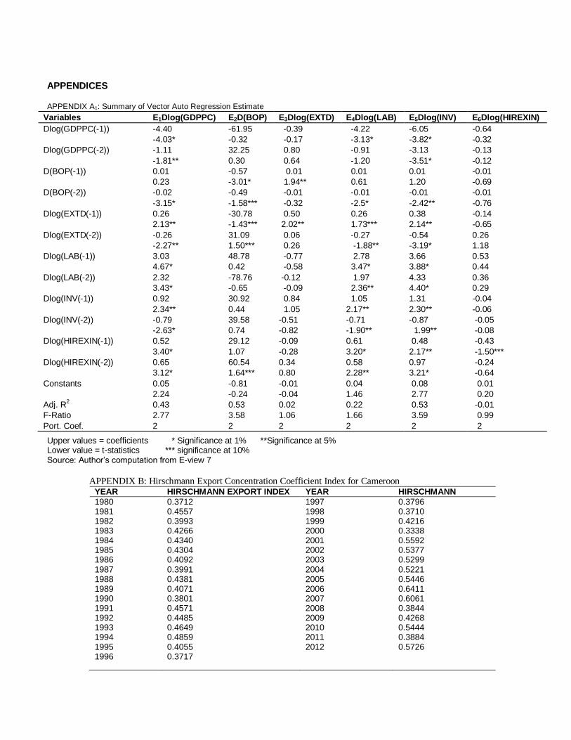
APPENDIX C: Cameroon Export Trend.

Source: Drawn by Author using E-view 7

APPENDIX D : ECONOMETRIC/REGRESSION RESULTS Result of the Augmented Dickey-Fuller Test.

Variables ADF test statistics

Critical value 1%

Critical value 5%

Critical value 10%

Level of integration

Remarks

HIREXIN -3.56779 -3.6537 -2.9571 -2.6174 I(0) Stationary 5%

LAB -5.61598 -3.6702 -2.9640 -2.6210 I(1) Stationary 1%

GDPPC -2.68509 -3.6617 -2.9604 -2.6192 I(1) Stationary 10%

INV -4.84322 -3.6617 -2.9604 -2.6192 I(1) Stationary 1%

EXTD -3.06249 -3.6576 -2.9591 -2.6181 I(1) Stationary 5%

BOP -6.25042 -3.6496 -2.9559 -2.6164 I(0) Stationary 1%

Source: Author’s computation from E-view 7

APPENDIX E: Unit Root Test

Source: Author’s Drawing from E-view 7

15

20

25

30

35

80 85 90 95 00 05 10

EXPORT

-1.5

-1.0

-0.5

0.0

0.5

1.0

1.5

-1.5 -1.0 -0.5 0.0 0.5 1.0 1.5

Inverse Roots of AR Characteristic Polynomial

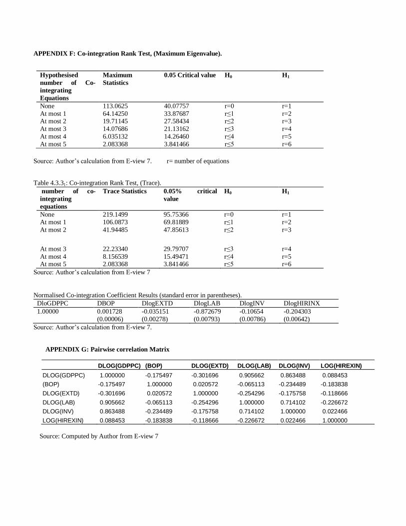
APPENDIX F: Co-integration Rank Test, (Maximum Eigenvalue).

Source: Author’s calculation from E-view 7. r= number of equations

Table 4.3.31: Co-integration Rank Test, (Trace).

number of co-

integrating

equations

Trace Statistics 0.05% critical

value

H0 H1

None 219.1499 95.75366 r=0 r=1

At most 1 106.0873 69.81889 r≤1 r=2

At most 2 41.94485 47.85613 r≤2 r=3

At most 3 22.23340 29.79707 r≤3 r=4

At most 4 8.156539 15.49471 r≤4 r=5 At most 5 2.083368 3.841466 r≤5 r=6

Source: Author’s calculation from E-view 7

Normalised Co-integration Coefficient Results (standard error in parentheses).

DloGDPPC DBOP DlogEXTD DlogLAB DlogINV DlogHIRINX

1.00000 0.001728 -0.035151 -0.872679 -0.10654 -0.204303

(0.00006) (0.00278) (0.00793) (0.00786) (0.00642)

Source: Author’s calculation from E-view 7.

APPENDIX G: Pairwise correlation Matrix

DLOG(GDPPC) (BOP) DLOG(EXTD) DLOG(LAB) DLOG(INV) LOG(HIREXIN)

DLOG(GDPPC) 1.000000 -0.175497 -0.301696 0.905662 0.863488 0.088453

(BOP) -0.175497 1.000000 0.020572 -0.065113 -0.234489 -0.183838

DLOG(EXTD) -0.301696 0.020572 1.000000 -0.254296 -0.175758 -0.118666

DLOG(LAB) 0.905662 -0.065113 -0.254296 1.000000 0.714102 -0.226672

DLOG(INV) 0.863488 -0.234489 -0.175758 0.714102 1.000000 0.022466

LOG(HIREXIN) 0.088453 -0.183838 -0.118666 -0.226672 0.022466 1.000000

Source: Computed by Author from E-view 7

Hypothesised

number of Co-

integrating

Equations

Maximum

Statistics

0.05 Critical value H0 H1

None 113.0625 40.07757 r=0 r=1

At most 1 64.14250 33.87687 r≤1 r=2 At most 2 19.71145 27.58434 r≤2 r=3

At most 3 14.07686 21.13162 r≤3 r=4

At most 4 6.035132 14.26460 r≤4 r=5

At most 5 2.083368 3.841466 r≤5 r=6

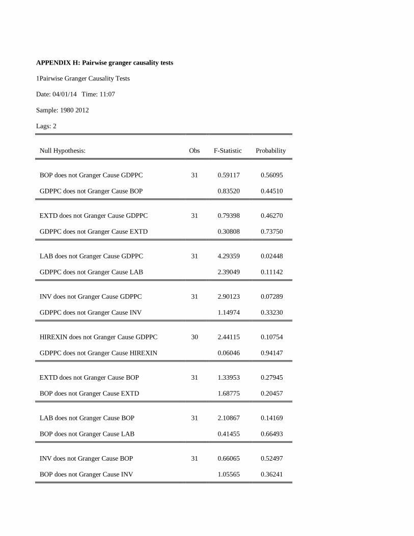
APPENDIX H: Pairwise granger causality tests

1Pairwise Granger Causality Tests

Date: 04/01/14 Time: 11:07

Sample: 1980 2012

Lags: 2

Null Hypothesis: Obs F-Statistic Probability

BOP does not Granger Cause GDPPC 31 0.59117 0.56095

GDPPC does not Granger Cause BOP 0.83520 0.44510

EXTD does not Granger Cause GDPPC 31 0.79398 0.46270

GDPPC does not Granger Cause EXTD 0.30808 0.73750

LAB does not Granger Cause GDPPC 31 4.29359 0.02448

GDPPC does not Granger Cause LAB 2.39049 0.11142

INV does not Granger Cause GDPPC 31 2.90123 0.07289

GDPPC does not Granger Cause INV 1.14974 0.33230

HIREXIN does not Granger Cause GDPPC 30 2.44115 0.10754

GDPPC does not Granger Cause HIREXIN 0.06046 0.94147

EXTD does not Granger Cause BOP 31 1.33953 0.27945

BOP does not Granger Cause EXTD 1.68775 0.20457

LAB does not Granger Cause BOP 31 2.10867 0.14169

BOP does not Granger Cause LAB 0.41455 0.66493

INV does not Granger Cause BOP 31 0.66065 0.52497

BOP does not Granger Cause INV 1.05565 0.36241

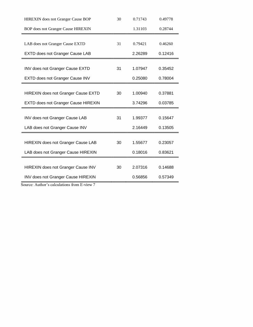
HIREXIN does not Granger Cause BOP 30 0.71743 0.49778

BOP does not Granger Cause HIREXIN 1.31103 0.28744

LAB does not Granger Cause EXTD 31 0.79421 0.46260

EXTD does not Granger Cause LAB 2.26289 0.12416

INV does not Granger Cause EXTD 31 1.07947 0.35452

EXTD does not Granger Cause INV 0.25080 0.78004

HIREXIN does not Granger Cause EXTD 30 1.00940 0.37881

EXTD does not Granger Cause HIREXIN 3.74296 0.03785

INV does not Granger Cause LAB 31 1.99377 0.15647

LAB does not Granger Cause INV 2.16449 0.13505

HIREXIN does not Granger Cause LAB 30 1.55677 0.23057

LAB does not Granger Cause HIREXIN 0.18016 0.83621

HIREXIN does not Granger Cause INV 30 2.07316 0.14688

INV does not Granger Cause HIREXIN 0.56856 0.57349

Source: Author’s calculations from E-view 7