Examining relationships between external linkages ... - CORE
Upload
khangminh22Category
view
1download
0
THE DUAL OF SU(2) IN THE ANALYSIS OF SPATIAL LINKAGES, SU(2) IN THE
SYNTHESIS OF SPHERICAL LINKAGES, AND ISOTROPIC COORDINATES IN PLANAR
LINKAGE SINGULARITY TRACE GENERATION
Dissertation
Submitted to
The School of Engineering of the
UNIVERSITY OF DAYTON
In Partial Fulfillment of the Requirements for
The Degree of
Doctor of Philosophy in Engineering
By
Saleh Mohamed Almestiri
Dayton, Ohio
May, 2018
THE DUAL OF SU(2) IN THE ANALYSIS OF SPATIAL LINKAGES, SU(2) IN THE
SYNTHESIS OF SPHERICAL LINKAGES, AND ISOTROPIC COORDINATES IN PLANAR
LINKAGE SINGULARITY TRACE GENERATION
Name: Almestiri, Saleh Mohamed
APPROVED BY:
Andrew P. Murray, Ph.D.Advisor Committee ChairmanProfessor, Department of Mechanicaland Aerospace Engineering
David H. Myszka, Ph.D.Committee MemberAssociate Professor, Department ofMechanical and Aerospace Engineering
Vinod Jain, Ph.D.Committee MemberProfessor, Department of Mechanicaland Aerospace Engineering
Muhammad Islam, Ph.D.Committee MemberProfessor, Department of Mathematics
Robert J. Wilkens, Ph.D., P.E.Associate Dean for Research and InnovationProfessorSchool of Engineering
Eddy M. Rojas, Ph.D., M.A., P.E.Dean, School of Engineering
ii

© Copyright by
Saleh Mohamed Almestiri
All rights reserved
2018

ABSTRACT
THE DUAL OF SU(2) IN THE ANALYSIS OF SPATIAL LINKAGES, SU(2) IN THE
SYNTHESIS OF SPHERICAL LINKAGES, AND ISOTROPIC COORDINATES IN PLANAR
LINKAGE SINGULARITY TRACE GENERATION
Name: Almestiri, Saleh MohamedUniversity of Dayton
Advisor: Dr. Andrew P. Murray
This research seeks to efficiently and systematically model and solve the equations associated
with the class of design problems arising in the study of planar and spatial kinematics. Part of this
work is an extension to the method to generate singularity traces for planar linkages. This extension
allows the incorporation of prismatic joints. The generation of the singularity trace is based on
equations that use isotropic coordinates to describe a planar linkage. In addition, methods to analyze
and synthesize spherical and spatial linkages are presented. The formulation of the analysis and the
synthesis problem is accomplish through the use of the special unitary matrices, SU(2). Special
unitary matrices are written in algebraic form to express the governing equations as polynomials.
These polynomials are readily solved using the tools of homotopy continuation, namely Bertini. The
analysis process presented here include determining the displacement and singular configuration for
spherical and spatial linkages. Formulations and numerical examples of the analysis problem are
presented for spherical four-bar, spherical Watt I linkages, spherical eight-bar, the RCCC, and the
RRRCC spatial linkages. Synthesis problem are formulated and solved for spherical linkages, and
with lesser extent for spatial linkages. Synthesis formulations for the spherical linkages are done in
iii
two different methods. One approach used the loop closure and the other approach is derived from
the dot product that recognizes physical constraints within the linkage. The methods are explained
and supported with Numerical examples. Specifically, the five orientation synthesis of a spherical
four-bar mechanism, the eight orientation task of the Watt I linkage, eleven orientation task of an
eight-bar linkage are solved. In addition, the synthesis problem of a 4C mechanism is solved using
the physical constraint of the linkage between two links. Finally, using SU(2) readily allows for the
use of a homotopy-continuation-based solver, in this case Bertini. The use of Bertini is motivated
by its capacity to calculate every possible solution to a system of polynomials .
iv
TABLE OF CONTENTS
ABSTRACT . . . . . . . . . . . . . . . . . . . . . . . . . . . . . . . . . . . . . . . . . . . iii
LIST OF FIGURES . . . . . . . . . . . . . . . . . . . . . . . . . . . . . . . . . . . . . . . vii
LIST OF TABLES . . . . . . . . . . . . . . . . . . . . . . . . . . . . . . . . . . . . . . . ix
CHAPTER I. INTRODUCTION . . . . . . . . . . . . . . . . . . . . . . . . . . . . . . 1
1.1 Review of Related Work . . . . . . . . . . . . . . . . . . . . . . . . . . . . . . 31.1.1 Singularity Trace . . . . . . . . . . . . . . . . . . . . . . . . . . . . . . 31.1.2 Unitary Matrices and Spatial Linkages . . . . . . . . . . . . . . . . . . 4
1.2 Contribution . . . . . . . . . . . . . . . . . . . . . . . . . . . . . . . . . . . . 71.3 Organization . . . . . . . . . . . . . . . . . . . . . . . . . . . . . . . . . . . . 9
CHAPTER II. MATHEMATICAL BACKGROUND . . . . . . . . . . . . . . . . . . . . 11
2.1 Singularity Traces and Isotropic Cordinates . . . . . . . . . . . . . . . . . . . . 112.1.1 Forward Kinematics . . . . . . . . . . . . . . . . . . . . . . . . . . . . 132.1.2 Singularity Analysis . . . . . . . . . . . . . . . . . . . . . . . . . . . . 142.1.3 Critical Points . . . . . . . . . . . . . . . . . . . . . . . . . . . . . . . 15
2.2 Special Unitary Matrices . . . . . . . . . . . . . . . . . . . . . . . . . . . . . . 152.2.1 Point and Line Transformations . . . . . . . . . . . . . . . . . . . . . . 172.2.2 Derivatives . . . . . . . . . . . . . . . . . . . . . . . . . . . . . . . . . 18
2.3 Homogeneous Transformation Review . . . . . . . . . . . . . . . . . . . . . . 19
CHAPTER III. SINGULARITY TRACES FOR LINKAGES WITHPRISMATIC AND REVOLUTE JOINTS . . . . . . . . . . . . . . . . . . . . . . . . 22
3.1 General Method . . . . . . . . . . . . . . . . . . . . . . . . . . . . . . . . . . 223.2 Offset Slider-Crank Linkage . . . . . . . . . . . . . . . . . . . . . . . . . . . . 23
3.2.1 Loop Closure . . . . . . . . . . . . . . . . . . . . . . . . . . . . . . . . 243.2.2 Forward Kinematics . . . . . . . . . . . . . . . . . . . . . . . . . . . . 243.2.3 Singularity Points . . . . . . . . . . . . . . . . . . . . . . . . . . . . . 253.2.4 Critical Points . . . . . . . . . . . . . . . . . . . . . . . . . . . . . . . 253.2.5 Motion Curve and Singularity Trace . . . . . . . . . . . . . . . . . . . 263.2.6 Validation . . . . . . . . . . . . . . . . . . . . . . . . . . . . . . . . . 27
3.3 Inverted Slider Crank Linkage . . . . . . . . . . . . . . . . . . . . . . . . . . . 283.3.1 Loop Closure . . . . . . . . . . . . . . . . . . . . . . . . . . . . . . . . 293.3.2 Forward Kinematics . . . . . . . . . . . . . . . . . . . . . . . . . . . . 293.3.3 Singularity Points . . . . . . . . . . . . . . . . . . . . . . . . . . . . . 293.3.4 Critical Points . . . . . . . . . . . . . . . . . . . . . . . . . . . . . . . 303.3.5 Motion Curve and Singularity Trace . . . . . . . . . . . . . . . . . . . 303.3.6 Validation . . . . . . . . . . . . . . . . . . . . . . . . . . . . . . . . . 32
v
3.4 Assur IV/3 with Two Prismatic Joints . . . . . . . . . . . . . . . . . . . . . . . 333.4.1 Loop Closure . . . . . . . . . . . . . . . . . . . . . . . . . . . . . . . . 353.4.2 Forward Kinematics . . . . . . . . . . . . . . . . . . . . . . . . . . . . 363.4.3 Singularity Points . . . . . . . . . . . . . . . . . . . . . . . . . . . . . 363.4.4 Critical Points . . . . . . . . . . . . . . . . . . . . . . . . . . . . . . . 373.4.5 Singularity Trace . . . . . . . . . . . . . . . . . . . . . . . . . . . . . . 373.4.6 Motion Curve . . . . . . . . . . . . . . . . . . . . . . . . . . . . . . . 38
CHAPTER IV. SPHERICAL LINKAGE ANALYSIS . . . . . . . . . . . . . . . . . . . 40
4.1 The 3-Roll Wrist on SU(2) . . . . . . . . . . . . . . . . . . . . . . . . . . . . . 404.2 Spherical Four-Bar Linkage Analysis . . . . . . . . . . . . . . . . . . . . . . . 43
4.2.1 Loop Closure and Forward Kinematics . . . . . . . . . . . . . . . . . . 444.2.2 Spherical Four-Bar Singularity Points . . . . . . . . . . . . . . . . . . . 44
4.3 Spherical Watt I Linkage Analysis . . . . . . . . . . . . . . . . . . . . . . . . . 464.3.1 Loop Closure and Forward Kinematics . . . . . . . . . . . . . . . . . . 474.3.2 Singularity Points . . . . . . . . . . . . . . . . . . . . . . . . . . . . . 48
4.4 Spherical Eight-Bar Linkage Analysis . . . . . . . . . . . . . . . . . . . . . . . 504.4.1 Loop Closure and Forward Kinematics . . . . . . . . . . . . . . . . . . 514.4.2 Singularity Points . . . . . . . . . . . . . . . . . . . . . . . . . . . . . 54
CHAPTER V. SPHERICAL LINKAGE SYNTHESIS . . . . . . . . . . . . . . . . . . . 59
5.1 Four-Bar Synthesis Using Dot Product Approach . . . . . . . . . . . . . . . . . 595.2 Watt I Synthesis Using Dot Product Approach . . . . . . . . . . . . . . . . . . 615.3 Eight-Bar Synthesis Using Dot Product Approach . . . . . . . . . . . . . . . . 675.4 Four-Bar Synthesis Using Loop Closure Approach . . . . . . . . . . . . . . . . 695.5 Watt I Synthesis Using Loop Closure . . . . . . . . . . . . . . . . . . . . . . . 715.6 Discussion . . . . . . . . . . . . . . . . . . . . . . . . . . . . . . . . . . . . . 72
CHAPTER VI. SPATIAL LINKAGE ANALYSIS AND 4C SYNTHESIS . . . . . . . . . 74
6.1 RCCC Spatial Linkage Analysis . . . . . . . . . . . . . . . . . . . . . . . . . . 746.1.1 RCCC Loop Closure and Forward Kinematics . . . . . . . . . . . . . . 756.1.2 RCCC Singularity Points and Motion Curve . . . . . . . . . . . . . . . 75
6.2 RRRCC Linkage Analysis . . . . . . . . . . . . . . . . . . . . . . . . . . . . . 776.2.1 RRRCC Loop Closure and Forward Kinematics . . . . . . . . . . . . . 776.2.2 RRRCC Singularity Points and Motion Curve . . . . . . . . . . . . . . 78
6.3 4C Spatial Linkage Synthesis . . . . . . . . . . . . . . . . . . . . . . . . . . . 80
CHAPTER VII. CONCLUSIONS AND FUTURE WORK . . . . . . . . . . . . . . . . . . 83
7.1 Conclusion . . . . . . . . . . . . . . . . . . . . . . . . . . . . . . . . . . . . . 837.2 Future Work . . . . . . . . . . . . . . . . . . . . . . . . . . . . . . . . . . . . 85
REFERENCES . . . . . . . . . . . . . . . . . . . . . . . . . . . . . . . . . . . . . . . . . 87
vi
LIST OF FIGURES
1.1 Spherical four-bar linkage is used to place an object in three consecutive positions [1]. 2
2.1 Prismatic joint on a moving line of slide. . . . . . . . . . . . . . . . . . . . . . . . 12
3.1 The position vector loop for an offset, slider-crank linkage. . . . . . . . . . . . . . 24
3.2 The slider-crank singularity trace. Red markers represent the critical points.Regions of equal GI and circuits are identified. Singularities at different valuesof a1 are indicated. Both circuits within the gray zone exhibit a fully rotatable crank. 26
3.3 Inverted slider-crank linkage position vector loop. . . . . . . . . . . . . . . . . . . 28
3.4 The inverted slider-crank singularity trace. Red markers denote the critical points.Region of equal GIs and circuits are identified. Singularities at different values ofa1 are indicated. Both circuits within the gray zones exhibit a fully rotatable crank. 31
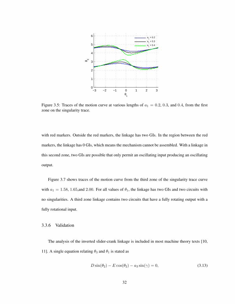
3.5 Traces of the motion curve at various lengths of a1 = 0.2, 0.3, and 0.4, from thefirst zone on the singularity trace. . . . . . . . . . . . . . . . . . . . . . . . . . . . 32
3.6 Traces of the motion curve at various lengths of a1 = 0.5, 1.0, and 1.5, from thesecond zone on the singularity trace. Singularity points are identified with red markers. 33
3.7 Traces of the motion curve at various lengths of a1 = 1.58, 1.65,and 2.00, from thethird zone on the singularity trace. . . . . . . . . . . . . . . . . . . . . . . . . . . 34
3.8 Assur IV/3 linkage position vector loop. . . . . . . . . . . . . . . . . . . . . . . . 35
3.9 The singularity trace for Assur IV/3 with respect to a1. Red markers denote thecritical points. Regions of equal GIs and circuits are identified. The zone shaded ingray contains at least one circuit with a fully rotatable crank. . . . . . . . . . . . . 38
3.10 The singularity trace for Assur IV/3 with respect to a12. Red markers denote thecritical points. The zone shaded in gray contains at least one circuit with a fullyrotatable crank . . . . . . . . . . . . . . . . . . . . . . . . . . . . . . . . . . . . 39
3.11 Motion curve for Assur IV/3 with a1 = 0.25 projected onto θ1-θ3. . . . . . . . . . 39
vii

4.1 A 3-roll wrist in a robot assembly. Adopted from[2]. . . . . . . . . . . . . . . . . 41
4.2 A spherical four-bar linkage. . . . . . . . . . . . . . . . . . . . . . . . . . . . . . 43
4.3 Motion curve for spherical Four-Bar linkage projected onto θ1 − θ4. Singularitypoints are identified with red circles. . . . . . . . . . . . . . . . . . . . . . . . . . 46
4.4 Spherical Watt I six-bar linkage. . . . . . . . . . . . . . . . . . . . . . . . . . . . 47
4.5 Motion curve for Watt I spherical linkage projected onto θ1-θ7. Singularity pointsare identified with red circles. . . . . . . . . . . . . . . . . . . . . . . . . . . . . . 50
4.6 Spherical eight-bar linkage schematic diagram. . . . . . . . . . . . . . . . . . . . 51
4.7 Spherical eight-bar linkage. . . . . . . . . . . . . . . . . . . . . . . . . . . . . . . 52
4.8 Motion curve for spherical eight-bar linkage projected onto θ1-θ5. Singularitypoints are identified with red circles. . . . . . . . . . . . . . . . . . . . . . . . . . 57
4.9 Motion curve for spherical eight-bar linkage projected onto θ1-θ6. Singularitypoints are identified with red circles. . . . . . . . . . . . . . . . . . . . . . . . . . 58
5.1 The parameters of the spherical four-bar identified for solving the synthesisproblem. All frames are located in the center of the sphere but some are shownon the sphere’s surface for clarity. . . . . . . . . . . . . . . . . . . . . . . . . . . 60
5.2 The parameters of the spherical Watt I identified for modeling the synthesisproblem. All frames are located in the center of the sphere but are shown on thesphere for clarity. . . . . . . . . . . . . . . . . . . . . . . . . . . . . . . . . . . . 62
5.3 The parameters of the spherical eight-bar linkage identified for solving the synthesisproblem. All frames are located in the center of the sphere but are shown on thesphere for clarity. . . . . . . . . . . . . . . . . . . . . . . . . . . . . . . . . . . . 67
6.1 RCCC linkage . . . . . . . . . . . . . . . . . . . . . . . . . . . . . . . . . . . . . 74
6.2 Motion curve for RCCC linkage projected onto θ1-d2. . . . . . . . . . . . . . . . . 77
6.3 RRRCC linkage . . . . . . . . . . . . . . . . . . . . . . . . . . . . . . . . . . . . 78
6.4 Motion curve for RRRCC linkage projected onto θ2-θ3. . . . . . . . . . . . . . . . 79
7.1 RSRC linkage. Adopted from [3]. . . . . . . . . . . . . . . . . . . . . . . . . . . 86
viii
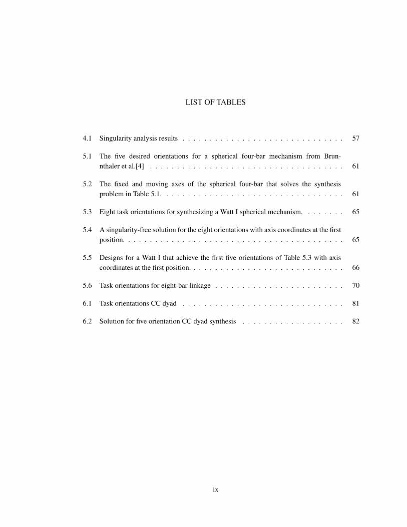
LIST OF TABLES
4.1 Singularity analysis results . . . . . . . . . . . . . . . . . . . . . . . . . . . . . . 57
5.1 The five desired orientations for a spherical four-bar mechanism from Brun-nthaler et al.[4] . . . . . . . . . . . . . . . . . . . . . . . . . . . . . . . . . . . . 61
5.2 The fixed and moving axes of the spherical four-bar that solves the synthesisproblem in Table 5.1. . . . . . . . . . . . . . . . . . . . . . . . . . . . . . . . . . 61
5.3 Eight task orientations for synthesizing a Watt I spherical mechanism. . . . . . . . 65
5.4 A singularity-free solution for the eight orientations with axis coordinates at the firstposition. . . . . . . . . . . . . . . . . . . . . . . . . . . . . . . . . . . . . . . . . 65
5.5 Designs for a Watt I that achieve the first five orientations of Table 5.3 with axiscoordinates at the first position. . . . . . . . . . . . . . . . . . . . . . . . . . . . . 66
5.6 Task orientations for eight-bar linkage . . . . . . . . . . . . . . . . . . . . . . . . 70
6.1 Task orientations CC dyad . . . . . . . . . . . . . . . . . . . . . . . . . . . . . . 81
6.2 Solution for five orientation CC dyad synthesis . . . . . . . . . . . . . . . . . . . 82
ix

CHAPTER I
INTRODUCTION
Emerging engineering problems, increasing productivity, and decreasing cost are the driving
forces toward development. Since the industrial revolution, mechanisms are considered to be the
backbone of any industrial facility. Machine designers are often required to engineer a device that
is able to move an object through a set of prescribed positions. The process is called rigid-body
guidance. Rigid-body guidance has become the essence of todays automated manufacturing and
design machinery.
Manufacturing mechanisms are categorized into open-loop and closed-loop chains. In a closed-
loop chain, each link is connected to two or more other links. Closed-loop mechanisms can be
either planar or spatial. In an open-loop chain, there is at least one link that is connected to only
one other link such as an articulated robotics arm. Both open-loop and closed-loop mechanisms can
be divided into planar mechanisms and spatial mechanisms. In planar mechanisms, all points on
the mechanism describe paths located in one plane or multiple planes that are parallel to each other.
Otherwise, a mechanism is said to be spatial.
Commercially available multi-axis robots are prepared for use and their specifications are
already defined by their manufacturer. Thus, they do not require prototype testing. However, they
are expensive and their operation and maintenance are costly [5]. In addition, for many tasks the
use of multi-axis robots is unreasonable as several of the axes remain unused. Spatial mechanisms
offer alternative solutions that can be considered competitive to the flexible open-chain robot, for
example Fig. 1.1 shows a spatial closed-loop spherical four-bar mechanism in a pick-and-place
1
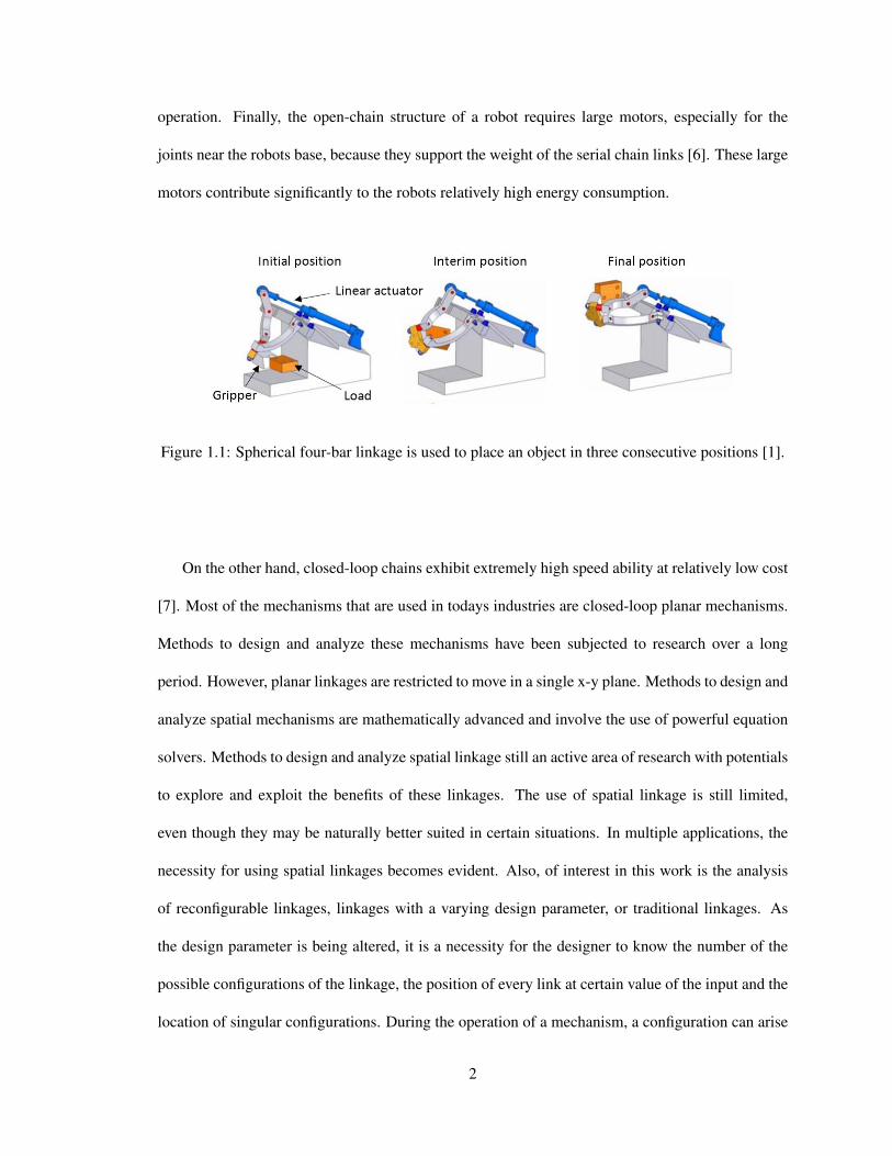
operation. Finally, the open-chain structure of a robot requires large motors, especially for the
joints near the robots base, because they support the weight of the serial chain links [6]. These large
motors contribute significantly to the robots relatively high energy consumption.
Figure 1.1: Spherical four-bar linkage is used to place an object in three consecutive positions [1].
On the other hand, closed-loop chains exhibit extremely high speed ability at relatively low cost
[7]. Most of the mechanisms that are used in todays industries are closed-loop planar mechanisms.
Methods to design and analyze these mechanisms have been subjected to research over a long
period. However, planar linkages are restricted to move in a single x-y plane. Methods to design and
analyze spatial mechanisms are mathematically advanced and involve the use of powerful equation
solvers. Methods to design and analyze spatial linkage still an active area of research with potentials
to explore and exploit the benefits of these linkages. The use of spatial linkage is still limited,
even though they may be naturally better suited in certain situations. In multiple applications, the
necessity for using spatial linkages becomes evident. Also, of interest in this work is the analysis
of reconfigurable linkages, linkages with a varying design parameter, or traditional linkages. As
the design parameter is being altered, it is a necessity for the designer to know the number of the
possible configurations of the linkage, the position of every link at certain value of the input and the
location of singular configurations. During the operation of a mechanism, a configuration can arise
2
such that the input link is no longer able to move the mechanism. The mechanism becomes locked,
and the mechanical advantage goes to zero. This stationary position of a mechanism is termed as
singular configuration and must be avoided when attempting to operate the mechanism with a fully
rotating input crank. The input-output relationships between various link variables and the possible
configuration of the mechanism indicate the mechanism ability to achieve the targeted task.
The design problem is concerned with finding dimensions for a linkage to move an object
through a set of specified orientations. Once the device’s dimensions are determined, these
dimensions are used in the analysis problem where the motion characteristics of a mechanism are
specified. The motion characteristics of interest are the number of possible assembly configuration,
the relationship between the input and the output variables, and the limits on the range of motion
which are best known as singularities.
1.1 Review of Related Work
1.1.1 Singularity Trace
A singularity trace has been introduced to classify the general motion characteristics of a single-
degree of freedom (DOF) linkage containing revolute joints [8]. For a designated input angle and
design parameter, the general motion characteristics include the singularities, circuits and critical
points, which are described below. Li et al. [9] generated the singularity trace for complex linkages,
such as Stephenson and double-butterfly linkages. Forward (direct) kinematic position analysis of
a single DOF linkage involves determining all possible joint positions at a certain position of the
input link [10]. The set of position equations defines a motion curve, which exhibits the relationship
between the joint variables. For a given position of the input link, multiple positions of the other
joints are expected since the governing loop equations are non-linear. Erdman et al. [11] refers to
each solution of the forward kinematic analysis as a geometric inversion (GI). The conventional
3
method for solving the forward kinematic problem uses tangent-half-angle substitution for the
output variables [12]. Porta et al. [13] used relaxation techniques for position analysis of multiloop
mechanisms. Alternatively, Wampler [14] presents the use of isotropic coordinates to formulate a
set polynomial equations which determine the locations of the links.
The study of parallel mechanisms called attention to the importance of determining singular
configurations during the design phase, and avoiding them while operating the mechanism [15].
At singularities the input link is no longer able to move the linkage [16]. Singularities appear on
the motion curve as turning points with respect to the input link displacement. Chase and Mirth
[17] defined the circuit of a linkage as the set of all assembly configurations achievable without
disconnecting any of the joints. The region on a circuit between two singularities is defined as a
branch. When a physical parameter of a linkage becomes a variable, the singularities form a curve
whose projection is called the singularity trace. The turning points on the singularity curve with
respect to the design parameter are called critical points, where many correspond to the transition
linkages as described by Murray et al. [18]. Linkages, where one or more physical parameter is
considered a variable, have been addressed in the literature. Larochelle et al. [19, 20] refer to
them as reconfigurable planar motion generators. Toa [21] calls them adjustable mechanisms and
Kota et al. [22] describe them as adjustable robotic mechanisms or programmable mechanisms.
1.1.2 Unitary Matrices and Spatial Linkages
The kinematic constraints imposed by articulated multi-body systems generate a set of nonlinear
simultaneous algebraic equations. Solving problems associated with closed- or open-loop systems
is challenging due to the nonlinearities that are typically expressed using trigonometric terms [23].
Formulations of such problems are considered successful when they reduce the size of the system
resulting in equations of the lowest order and avoiding trigonometric expressions. One common
4
approach for avoiding such expressions is to to write sines and cosines in terms of tangent-half-angle
formulas and converting to an algebraic formulation [24]. This approach has been successfully
used for the displacement analysis of spherical mechanisms [25, 26] and in computing the direct
kinematics of a spherical three-degree-of-freedom parallel manipulator [27]. This approach has
also been associated with the possibility of extraneous solutions and can be ill-conditioned if an
unknown angle equals π [28]. A second common approach is to write the trigonometric expression
in algebraic form using the unit circle identity to relate sine and cosine of the same angle [23]. The
formulation to find all 16 solutions to a general 6R robot using continuation methods embraced
this approach [29]. A final approach worthy of mention is the formulation of planar analysis and
synthesis problems via isotropic coordinates to reduce the degree of the nonlinear simultaneous
albegraic expressions [30]. Plecnik et al. [31] used isotropic coordinates to generate the synthesis
equations for the planar Watt I linkage generating a system of 28 equations with 28 unknowns.
This work considers only spherical mechanisms which constrain all points to move on concen-
tric spheres about a fixed point. As such, the location of any rigid-body in a spherical mechanism
is described by a rotation about this fixed point [32]. All single degree of freedom one- two- and
three-loop spherical mechanisms were analyzed using a mix of rotation matrices and quaternions
finding all geometric inversions [25]. The full set of spherical four-bar mechanisms achieve four
specific orientations was found, highlighting those that are defect free [33]. Brunnthaler et al. [4]
used kinematic mapping to design a spherical four bar mechanism for five orientations that had six
(real) dyads as solutions. Soh et al. [34] solved the five-orientation synthesis problem for defect-free
six-bar mechanisms by constraining a three degree of freedom spherical chain with two additional
links. This work has been extended into modeling tools Sonawale et al. [35, 36]. Spherical function
generators have also received consideration [37, 38].
5

Special orthogonal matrices, SO(3), are commonly used in the literature to represent rota-
tions [39]. These matrices possess a redundancy in their structure that is the result of nine matrix
elements representing only three independent parameters and encompassing six constraints [40].
Various challenges have been raised is using SO(3) including numerical computation difficul-
ties [41], the potentially unnecessary computations in formulating loop equations for spatial
linkages [42], and Gimbal lock [39]. Among several alternatives for writing rotations about a
fixed point in three-dimensional space, one is using 2 by 2 special unitary matrices, SU(2) [43].
An element of the 2 × 2 unitary group, U(2), is a matrix of complex numbers with the property
that the complex conjugate of its transpose is its inverse. Like the relationship between O(3) (the
orthogonal matrices) and SO(3), unitary matrices with determinant equal to +1 are referred to as
special unitary. Unitary matrices have been utilized in quantum mechanics, both classically [44]
and more recently [45]. One advantage of using SU(2) is its compact form and that a general
element is constructed from only two complex numbers related by one constraint. This results in
a decreased number of algebraic operations when performing multiple consecutive rotations about
different axes. The rotation axis and angle are also explicit in an element of SU(2) [42]. Finally,
SU(2) matrices are isomorphic to unit quaternions and so share many identical properties. This
paper utilizes SU(2) in the algebraic formulation of several kinematics problems.
A numerical method proving successful in solving large kinematics problems is homotopy
continuation. Homotopy continuation may be used to find every isolated solution of a square system
without sensitivity to initial guesses. Oft-cited examples from the field of kinematics instrumental in
showing the developments of numerical algebraic geometry include the bootstrap approach of Roth
and Freudenstein to synthesize path generating geared five-bar linkages [46], the complete solution
to the inverse kinematics of a general 6R manipulator by Tsai and Morgan [29], and the complete
solution to the nine-point path generation of a four-bar linkage by Wampler et al. [47]. Homotopy
6

continuation may be readily performed with the Bertini software package [48], used throughout this
work.
The screw displacement has received significant interest as a tool in the kinematic analysis
and synthesis of spatial mechanical systems [49]. Detailed introductions include 2 × 2 dual
special unitary matrices presented by Denavit [50], Yang and Freudenstein’s use of the dual-number
quaternions [51], and the dual-number rotation matrices presented by Yang [52] and by Soni and
Harrisberger [53]. Each formalism has advantages and limitations. Dual quaternions, for example,
are compact in the fact that the screw information is represented by a single dual hypercomplex
number. The dual special unitary matrix is not as concise, but has the advantage of matrix elements
being typical complex numbers. Significant detail on these formalisms can be found in Rooney [54]
and Funda [55]. For spatial operations, the screw displacement is expressed as a dual special unitary
matrix, SU(2) for short, a 4×4 matrix of complex numbers. This matrix has a significant amount of
structure in that four of the sixteen elements are identically zero, and two of its 2×2 sub-matrices are
elements of SU(2), leaving only four general complex numbers in the entire matrix. By employing
SU(2) in the formulations in this work, equations result that are readily solved using Bertini.
1.2 Contribution
The goal of this research is to formulate kinematic problems as polynomial equations that is
suited for available solvers such as Bertini and fsolve function in MATLAB. The contribution of
this dissertation include solving kinematic challenges involving a wide variety of linkages: planar,
spherical, and spatial linkages. A formulation was developed to generate singularity traces for
planar linkages to incorporate prismatic joints. Previously, singularity traces were restricted to
mechanisms composed of only rigid bodies and revolute joints. The motion characteristics identified
on the singularity plot include changes in the number of solutions to the forward kinematic position
7
analysis (geometric inversions), singularities, and changes in the number of branches. To illustrate
the adaptation of the general method to include prismatic joints, basic slider-crank and inverted
slider-crank linkages are explored. Singularity traces are then constructed for more complex Assur
IV/3 linkages containing multiple prismatic joints. These Assur linkages are of interest as they form
an architecture that is commonly used for mechanisms capable of approximating a shape change
defined by a general set of closed curves. This work is published in [56, 57]
Another, contribution is exploring the potential of the special unitary matrices, SU(2), in the
field of kinematics. Specifically, 2 × 2 special unitary matrices are written in symbolic forms
to formulate a system of polynomials that describe the behavior of spherical linkages. SU(2)
are used in the displacement analysis where the location of any link is determined at a given
location of the input link. The displacement analysis is extended to determine the location of
singular configurations. Moreover, SU(2) is used to formulate the motion synthesis of spherical
linkages, where the linkage is designed to guide an object through a set of positions. Two methods
of formulating the synthesis problem are considered. Precisely, synthesis formalism exploits the
loop closure equations and an approach derived from the dot product that recognizes physical
constraints within the linkage. Examples include the five orientation synthesis of a spherical four-
bar mechanism and the eight orientation task of the Watt I linkage. In addition, the dot product
approach is used to formulate the synthesis equations for an eight-bar linkage which is able to
achieve up to eleven positions. Using SU(2) readily allows for the use of a homotopy-continuation-
based solver, in this case Bertini. The use of Bertini is motivated by its capacity to calculate every
solution to a design problem. Methods to synthesize spherical linkages with more than four bars are
numbered with most advanced methods being able to achieve up to five positions. Part of this work
was published in [58].
8
Lastly, The formulation of the special unitary matrices is expanded to introduce the dual of the
special unitary matrices, SU2. These are used to represent a displacement and a rotation along
the axes of spatial linkages. An algebraic form of the dual special unitary matrices are used to
form the loop closure of spatial linkages. Polynomials that are extracted from the loop closure are
solved to provide solutions for the displacement analysis and the singularity analysis. In addition,
a formulation of the dot product is introduced using the dual special unitary. This is utilized to
solve the synthesis of 4C linkage. The uniqueness of this part of the research resides in its use
of the special unitary to mathematically describe spatial linkage coupled with use of the use of
homotopy continuation tool, which guarantees finding every possible solution to the problem. What
is presented on here offers a systemic and efficient approach for solving spatial linkages which has
the potential to be the backbone of a software to analyze and synthesize spatial linkages.
1.3 Organization
Each chapter of this dissertation focuses on a particular task where the formulation of the
problem is the key point. Chapter II provides a review of the mathematical background of this
work. It includes two main parts: First, an introduction to the isotropic coordinates and their use
in writing systems of equations to determine forward kinematic solutions, singularity points, and
critical points. Solutions from this analysis are exploited to generate the singularity trace of planar
linkages with prismatic joints. Second, a review of the most relevant properties of the group SU(2).
This part encompasses an algebraic formulations of a general displacement element of SU(2) that
represents rotation and translation. Moreover, point and line transformation on SU(2) are presented
as well as derivative of the rotational part and the dual part of SU(2).
Chapter III is dedicated to show examples of the extension in the general method of generating
singularity traces to incorporate prismatic joints. Three examples are provided: offset slider crank,
9
inverted slider crank, and Assur IV/3 linkage with two prismatics. For each example, the process is
detailed to find the forward kinematic solutions, singularity points, and critical points. Results are
depicted on motion curves and the singularity traces for the linkages.
Chapter IV discusses the use of 2× 2 matrices of SU(2) in analyzing spherical linkages. These
matrices are written symbolically to represent a rotation about a fixed point. Such rotations are then
used to write the loop closure of a spherical linkage. The entries of the loop closure matrices are
polynomial equations. Angular velocity matrices and screw vectors are used to write the Jacobian
from which the singularity condition is specified. Spherical four-bar, spherical Watt I, and spherical
eight-bar linkages are utilized as examples to illustrate the process.
Chapter V focus on solving the synthesis problem of spherical linkage. Two approach are used
in the synthesis process: the dot product approach and the loop closure approach. Examples are
provided for a full insight into the methods. The examples include linkages with up to eight links.
Chapter VI addresses the use of dual special unitary, SU(2), to solve analysis and synthesis
problems for spatial linkages. This chapter provides a systematic method to solve the displacement
analysis of spatial linkages. In addition, locations of any singular configurations are specified. The
results of the analysis output are shown on motion curves. This work is supported by two examples
of RRRCC and RCCC linkages. Moreover, the synthesis problem of the 4C linkage is solved using
the dot product between two lines, which represent axes of the cylindrical joint, C, on the linkage.
The final chapter, Chapter VII, provides a conclusion to the dissertation and highlights the most
important achievements.
10
CHAPTER II
MATHEMATICAL BACKGROUND
This research was initiated by using the isotropic coordinates to generate singularity traces
for planar linkage with prismatic joints. Equations for planar linkages are well-formulated to
utilize powerful, numerical algebraic geometry solution methods. Loop closure equations can
be formulated using special unitary group transformations in a fashion that parallels the planar
formulations. Both the isotropic coordinates and SU(2) use complex numbers to model a linkage.
2.1 Singularity Traces and Isotropic Cordinates
To explain the basic approach of using the isotropic coordinate to formulate the loop closure of
a planar linkage, assume a rigid link of length aj rotated by angle θj can be represented by isotropic
coordinates (ajTj , ajTj). When constructing loop closure equations, the two variables Tj and Tj
can be considered as independent variables under the condition that TjTj = 1. A unit vector in the
complex plane defined by θj can be represented in polar form by the variable and its conjugate as
Tj = eiθj , and Tj = e−iθj , (2.1)
which are called isotropic coordinates [14]. By substituting the Euler equivalents into Eq. (2.1),
Tj = cos θj + i sin θj and Tj = cos θj − i sin θj . When constructing loop closure equations,
the two variables Tj and Tj can be considered as independent variables under the condition that
TjTj = 1. When rotated in the plane by angle θj , a rigid link of length aj has isotropic coordinates
(ajTj , ajTj).
11
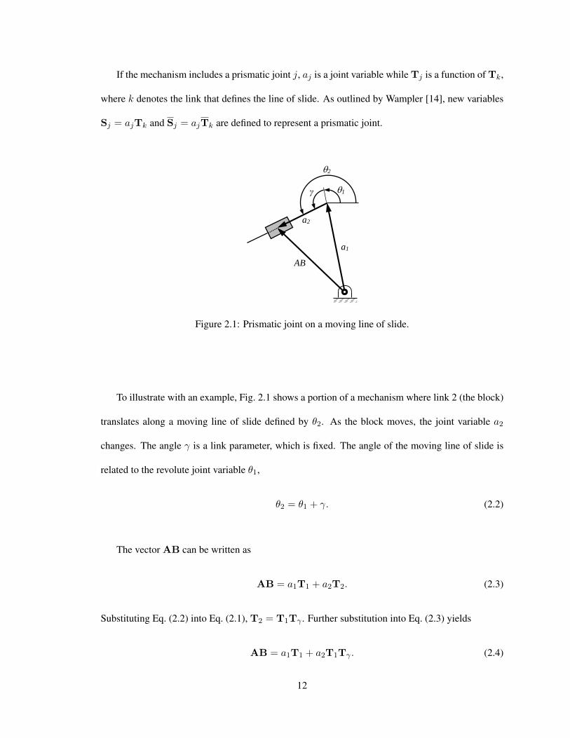
If the mechanism includes a prismatic joint j, aj is a joint variable while Tj is a function of Tk,
where k denotes the link that defines the line of slide. As outlined by Wampler [14], new variables
Sj = ajTk and Sj = ajTk are defined to represent a prismatic joint.
a2
γ 1
2
a1
AB
Figure 2.1: Prismatic joint on a moving line of slide.
To illustrate with an example, Fig. 2.1 shows a portion of a mechanism where link 2 (the block)
translates along a moving line of slide defined by θ2. As the block moves, the joint variable a2
changes. The angle γ is a link parameter, which is fixed. The angle of the moving line of slide is
related to the revolute joint variable θ1,
θ2 = θ1 + γ. (2.2)
The vector AB can be written as
AB = a1T1 + a2T2. (2.3)
Substituting Eq. (2.2) into Eq. (2.1), T2 = T1Tγ . Further substitution into Eq. (2.3) yields
AB = a1T1 + a2T1Tγ . (2.4)
12
Defining S2 = a2T1 and S2 = a2T1, then
AB = a1T1 + S2Tγ , (2.5)
and the complex conjugate,
AB = a1T1 + S2Tγ . (2.6)
An identity equation can be written as 0 = T1a2T1 −T1a2T1 = T1S2 −T1S2.
In summary, a prismatic joint j is incorporated into the general method by introducing Sj and Sj
into the loop closure equations to represent the variable aj . An identity equation is also appropriately
formulated. The method to determine singularities and critical points remains unchanged from
Ref. [8], and is reviewed in the following sections for completeness.
2.1.1 Forward Kinematics
In the general analysis methodology, the linkage input variable is designated as x ∈ C and the
design variable is p ∈ C. All the remaining passive joint variables are y ∈ CN . Loop closure
equations are formulated as
f(p, x, y) = 0, f : C× C× CN → CN . (2.7)
Considering a linkage that includes bothm revolute and n−m prismatic joints, the ` loop equations
of Eq. (2.7) convert to 2`+ n− 1 equations in isotropic coordinates as:
m∑j=1
ajTj +n∑
k=m+1
SkTγk = 0,
m∑j=1
ajTj +n∑
k=m+1
SkTγk = 0, (2.8)
TjTj =(eiθj)(
e−iθj)
= 1, j = 2, . . . ,m,
Tk−1Sk −Tk−1Sk = 0, k = m+ 1, . . . , n.
13
In its most general form, the coefficients aj ∈ C in Eq. (2.8) correspond to the line segments that
connect the joints. The complex conjugates of the link edges aj also appear. For a binary link, the
vector Tj lies along the line that connects the joints, in which case aj is real, and aj = aj . This
is done throughout the examples in this paper. Also, note that TjTj = 1, where j corresponds to
any ground link, is not included as its angle θj is known. The system in Eq. (2.8) consists of N + 1
equations in N + 2 unknowns and for a given value of x produces a set of y values that correspond
to geometric inversions of the linkage. Methods for solving the system of equations are discussed in
[48]. The solutions in this paper were produced using numerical polynomial continuation methods
using the Bertini software package [59].
2.1.2 Singularity Analysis
Finding all branches of the motion with respect to x is desirable. The branches on the motion
curve meet at a singularity point. The singularity is a mechanism configuration where the driving
link is unable to move the mechanism. For a fixed design parameter p, the tangent [∆x,∆y] to the
motion curve is given by
fx∆x+ fy∆y = 0, (2.9)
where fx = ∂f∂x ∈ CN×1 and fy = ∂f
∂y ∈ CN×N . The singularities occur when ∆y 6= 0 with
∆x = 0, which implies that
D(p, x, y) := det fy = 0. (2.10)
Combining the loop closure and singularity conditions,
F (p, x, y) =
[f(p, x, y)D(p, x, y)
]. (2.11)
This system of N + 1 equations in N + 1 unknowns is solved to find the singularities.
14
2.1.3 Critical Points
To this point in the analysis, the design parameter p is considered fixed. As the design parameter
is altered, the gross motion behavior of the linkage changes at critical points. The singularity curve
consists of the singularities as p changes. The projection of the singularity curve into the plane of
the input joint x and the design parameter p is known as the singularity trace. At certain values of p
(termed critical points) the number of singularities change. The process of determining the critical
points is analogous to the singularity problem, but replacing x by p, y by (x, y), and f by F . The
tangency condition from Eq. (2.9) becomes
∂F
∂p∆p+
∂F
∂x∆x+
∂F
∂y∆y = 0. (2.12)
Defining
Fxy =[∂F∂x
∂F∂y
]=
[∂f∂x
∂f∂y
∂D∂x
∂D∂y
]. (2.13)
Critical points occur when ∆(x, y) 6= 0 with ∆p = 0, which implies
E := detFxy = 0. (2.14)
Combining loop closure, singularity and critical point conditions generates a system of N + 2
equations f(p, x, y)D(p, x, y)E(p, x, y)
= 0 (2.15)
in N + 2 unknowns that include p, x, y. As before, the system is solved using Bertini and produces
all critical points.
2.2 Special Unitary Matrices
In the case of spatial linkages, it is known that a screw displacement is defined by a line in
space where c is a point on the line, the unit vector s = (sx, sy, sz) is the direction of the line, θ
15
is the rotation angle about the line, and d is a displacement along the line. These components are
combined into an element of SU(2) as
Q(s, θ, c, d) =
[Q 0Q0 Q
](2.16)
where 0 is the 2× 2 zero matrix,
Q(s, θ) =
[cos θ2 + isz sin θ
2 sy sin θ2 − isx sin θ
2
−sy sin θ2 − isx sin θ
2 cos θ2 − isz sin θ2
], (2.17)
and
Q0(s, θ, c, d) =
[Q0
4 + iQ03 Q0
2 − iQ01
−Q02 − iQ0
1 Q04 − iQ0
3
]. (2.18)
The components of Q0(s, θ, c, d) are
Q01 =
d
2cos
θ
2sx + sin
θ
2s0x, Q0
2 =d
2cos
θ
2sy + sin
θ
2s0y,
Q03 =
d
2cos
θ
2sz + sin
θ
2s0z, Q0
4 = −d2
sinθ
2,
(2.19)
where s0 = c × s. All components of Q are observed to be complex numbers where i =√−1.
The matrices Q and Q0 are referred to as the rotation and the dual part, respectively. Note that the
matrix Q has determinant 1 due to s being a unit vector.
As SU(2) is a group, the composition of elements is also in SU(2) following the standard rules
of matrix and complex number multiplication. The inverse of Q is readily found from the complex
conjugate transposes of the 2× 2 sub-matrices of Q,
Q−1 =
[Q∗ 0Q0∗ Q∗
]. (2.20)
Three special cases will prove useful, which represent displacements along and about the
frame’s axes z, x, and y. Given a screw displacement along the z-axis, s = (0, 0, 1), c = (0, 0, 0),
Qz(θ) =
[T 0
0 T
]and Q0
z(θ, d) =
[id2T 0
0 −id2T
]. (2.21)
16
where T = cos(θ/2) + i sin(θ/2) and the complex conjugate T = cos(θ/2)− i sin(θ/2). Observe
that TT = 1, as the determinant of Q = 1. Given a screw displacement about the x-axis, s =
(1, 0, 0), c = (0, 0, 0),
Qx(θ) =
[a −ib−ib a
]and Q0
x(θ, d) =
[−d
2b −id2a−id2a −d
2b
]. (2.22)
where a = cos(θ/2) and b = sin(θ/2). The determinant of this matrix is 1, since a2 + b2 = 1.
Similarly, for a rotation of angle θ about the y-axis, s = (0, 1, 0), c = (0, 0, 0),
Qy(θ) =
[a b−b a
]and Q0
y(θ, d) =
[−d
2bd2a
−d2a −d
2b
]. (2.23)
2.2.1 Point and Line Transformations
Given a point (x, y, z) in R3, define
p =
[iz y − ix
−y − ix −iz
], (2.24)
and a point transformation is constructed from an element of SU(2) as
P = QpQ∗. (2.25)
Note that for two points, p1 and p2, expressed as in Eq. (2.24), the dot product is
(x1, y1, z1) · (x2, y2, z2) =1
2tr(p∗1p2) (2.26)
where tr is the trace. Given a unit vector s = (sx, sy, sz), and a point c on the unit vector such that
c · s = 0, and s0 = c× s = (s0x, s0y, s
0z). The vector s0 is the moment of the line about the origin of
the reference frame. Note that s ·s0 = s · (c×s) = 0. The Plucker coordinates of a line E = (s, s0)
define
E =
[s 0s0 s
], E−1 =
[s∗ 0s0∗ s∗
]. (2.27)
17
In the matrix E, the matrices s and s0 are 2× 2 sub-matrices, representing the unit vector s and the
vector s0 as
s =
[isz sy − isx
−sy − isx −isz
], s0 =
[is0z s0y − is0x
−s0y − is0x −is0z
]. (2.28)
and a line transformation is constructed from an element of SU(2) as
E = QeQ−1. (2.29)
The dot product between two lines E1 = (s1, s01) and E2 = (s2, s
02) is obtained from E−11 E2. The
dot product consists of two parts. The real part of the dot product defines the twist angle θ between
the two line around the common normal as
cos(θ) =1
2tr(s∗1s2), (2.30)
and the dual part defines the distance v along the common normal between the two lines by
−v sin(θ) =1
2tr(s0∗1 s2 + s∗1s
02). (2.31)
2.2.2 Derivatives
The derivative of QQ−1 = I yields the property Q˙Q−1 = − ˙
QQ−1. Now consider P =
QpQ−1. Taking the derivative, P =˙QpQ−1 + Qp
˙Q−1. Substituting p = Q−1PQ,
P =˙QQ−1P + PQ
˙Q−1 =
˙QQ−1P − P ˙
QQ−1, (2.32)
The term ˙QQ−1 in Eq. (2.32) is the angular velocity matrix of a rotation Q. For the determination
of singularities, it is convenient to define
Ω(θ, d) =˙QQ−1 =
[Ω(θ) 0
Ω0(θ, d) Ω(θ)
], (2.33)
where
Ω(θ) = QQ∗ =1
2
[iuz uy − iux
−uy − iux −iuz
]θ. (2.34)
18
and
Ω0(θ, d) =1
2
[iuz uy − iux
−uy − iux −iuz
]d+
1
2
[iu0z u0y − iu0x
−u0y − iu0x −iu0z
]θ. (2.35)
The angular velocity matrix from the rotational part Ω(θ) is defined by the components of the vector
U = (ux, uy, uz). The dual part introduces three additional components u0x, u0y, u
0z which are the
components of the moment of the axis about the origin of the reference frame, U0. Six independent
components, three from the rotational part and three from the dual part can be assembled into
a six dimentional vector called a screw. For the work herein, all mechanism joint variables are
displacements along and about the z-axis. For Qz(θ), the angular velocity is found to be
Ωz(θ) = QzQ∗z =
1
2
[i 00 −i
]θ. (2.36)
and for the spatial displacement, Qz(d),
Ωz(d) =˙QzQz
−1=
1
2
0 0 0 00 0 0 0i 0 0 00 −i 0 0
d. (2.37)
Ωz(θ) =˙QzQz
−1=
1
2
i 0 0 00 −i 0 00 0 0 00 0 0 0
θ. (2.38)
2.3 Homogeneous Transformation Review
This particular representation of the spatial displacement is the most common and widely
used in various disciplines. Elements of the real 4 × 4 matrices are referred to as homogeneous
transformation. Homogeneous transformation matrices consists of two main parts. The rotational
part is represented by a 3 × 3 orthogonal matrix, A, that satisfy the condition ATA = I with a
determinant of 1. These rotation matrices form a group that is referred to as the special orthogonal
group, SO(3). The translation is represented by a vector d = (dx, dy, dz)T . Homogeneous
19
transformation matrices take the general form as
H(θ, d) =
[A d0 1
](2.39)
The inverse of H can be determined from
H−1(θ, d) =
[AT −ATd0 1
](2.40)
For a rotation and a translation along and about the frame’s axes x-axis, y-axis, and z-axis, the
following forms are used. Given a screw displacement defined as a rotation about x-axis by θ, and
translation along the x-axis by d = (dx, 0, 0),
Hx(θ, dx) =
1 0 0 dx0 cos θ − sin θ 00 sin θ cos θ 00 0 0 1
, H−1x (θ, dx) =
1 0 0 −dx0 cos θ sin θ 00 − sin θ cos θ 00 0 0 1
(2.41)
Given a screw displacement defined as a rotation about y-axis by θ, and translation along the y-axis
by d = (0, dy, 0),
Hy(θ, dy) =
cos θ 0 sin θ 0
0 1 0 dy− sin θ 0 cos θ 0
0 0 0 1
, H−1y (θ, dy) =
cos θ 0 − sin θ 0
0 1 0 −dysin θ 0 cos θ 0
0 0 0 1
(2.42)
Given a screw displacement defined as a rotation about z-axis by θ, and translation along the z-axis
by d = (0, 0, dz),
Hz(θ, dz) =
cos θ − sin θ 0 0sin θ cos θ 0 0
0 0 1 dz0 0 0 1
, H−1z (θ, dz) =
cos θ sin θ 0 0− sin θ cos θ 0 0
0 0 1 −dz0 0 0 1
(2.43)
A point p = (x, y, z) in R3 is rotated by A and translated by d as[P1
]=
[A d0 1
] [p1
](2.44)
Now consider P = Hp. Taking the derivative, P = Hp. Substituting p = H−1P to obtain
P = HH−1P . The term HH−1 is of interest when determining singularities.
Ω = HH−1 =
[AAT AATd + d
0 1
], or
[Ω Ω0
0 0
], (2.45)
20
where Ω = AAT and Ω0 = AATd + d. Ω is skew-symmetrix matrix as
Ω(θ) = AAT =
0 −uz uyuz 0 −ux−uy ux 0
θ. (2.46)
from which a screw vector can be extracted U = (ux, uy, uz).
21
CHAPTER III
SINGULARITY TRACES FOR LINKAGES WITH
PRISMATIC AND REVOLUTE JOINTS
This chapter extends the general method to construct a singularity trace for single degree-of-
freedom, closed-loop linkages to include prismatic along with revolute joints. The singularity trace
has been introduced in the literature as a plot that reveals the gross motion characteristics of a linkage
relative to a designated input joint and a design parameter. The motion characteristics identified on
the plot include a number of possible geometric inversions, circuits, and singularities at any given
value for the input link and the design parameter. When a physical parameter of a linkage becomes a
variable, the singularities form a curve whose projection is called the singularity trace. The turning
points on the singularity curve, with respect to the design parameter, are called critical points.
3.1 General Method
A rigid link of length aj rotating in the plane by angle θj can be represented by isotropic
coordinates (ajTj , ajTj ). When constructing loop closure equations, the two variables Tj and Tj
can be considered as independent variables under the condition that TjTj = 1. The vector that
corresponds to a prismatic joint k has a varying magnitude ak and an angle θk. In a single DOF
linkage, there is an angular relationship between θk, and the angle of a previous link, θj through a
fixed angle γ. This relationship allows the elimination of θk from the loop closure, and the vector of
joint k to be written in the isotropic coordinates in the form of akTjTγ , which is a function in ak
and θj . Now, introducing Sk = akTj , and its conjugate Sk = akTj leads to a linear expression in
the loop closure variables. An identity equation TjSk − TjSk = 0, is formulated based on the22
definition of Sk and Sk, and the condition on Tj and Tj . Identities are used to eliminate half of
the unknown variables from the loop closure equations, resulting in a reduced form. Considering
a linkage that includes m revolute and n − m prismatic joints, the loop equations in isotropic
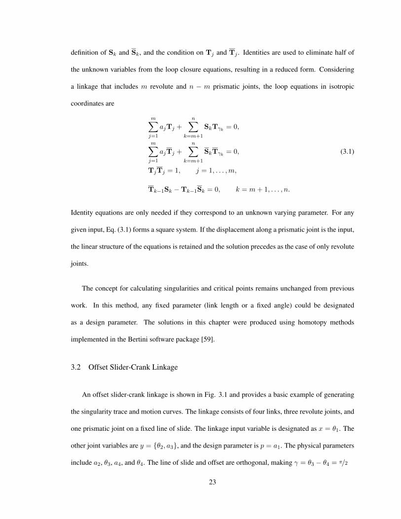
coordinates are
m∑j=1
ajTj +n∑
k=m+1
SkTγk = 0,
m∑j=1
ajTj +n∑
k=m+1
SkTγk = 0, (3.1)
TjTj = 1, j = 1, . . . ,m,
Tk−1Sk −Tk−1Sk = 0, k = m+ 1, . . . , n.
Identity equations are only needed if they correspond to an unknown varying parameter. For any
given input, Eq. (3.1) forms a square system. If the displacement along a prismatic joint is the input,
the linear structure of the equations is retained and the solution precedes as the case of only revolute
joints.
The concept for calculating singularities and critical points remains unchanged from previous
work. In this method, any fixed parameter (link length or a fixed angle) could be designated
as a design parameter. The solutions in this chapter were produced using homotopy methods
implemented in the Bertini software package [59].
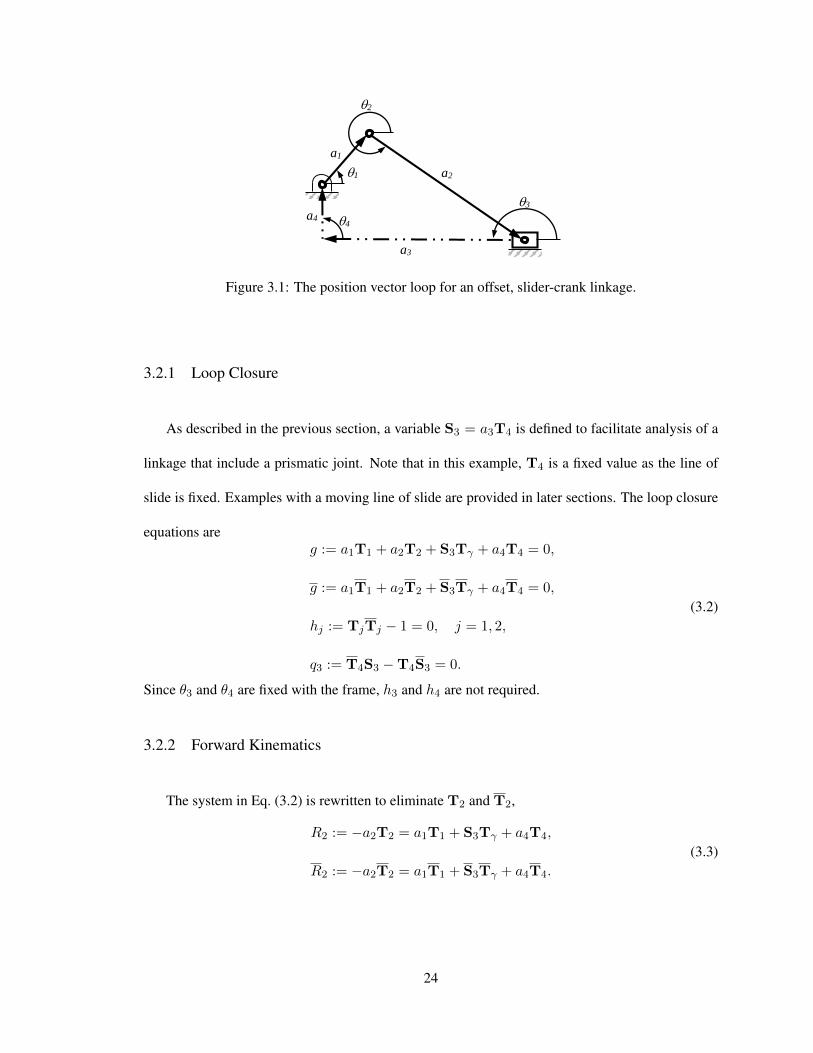
3.2 Offset Slider-Crank Linkage
An offset slider-crank linkage is shown in Fig. 3.1 and provides a basic example of generating
the singularity trace and motion curves. The linkage consists of four links, three revolute joints, and
one prismatic joint on a fixed line of slide. The linkage input variable is designated as x = θ1. The
other joint variables are y = θ2, a3, and the design parameter is p = a1. The physical parameters
include a2, θ3, a4, and θ4. The line of slide and offset are orthogonal, making γ = θ3 − θ4 = π/2
23
2
3
4
1
a3
a1
a2
a4
Figure 3.1: The position vector loop for an offset, slider-crank linkage.
3.2.1 Loop Closure
As described in the previous section, a variable S3 = a3T4 is defined to facilitate analysis of a
linkage that include a prismatic joint. Note that in this example, T4 is a fixed value as the line of
slide is fixed. Examples with a moving line of slide are provided in later sections. The loop closure
equations areg := a1T1 + a2T2 + S3Tγ + a4T4 = 0,
g := a1T1 + a2T2 + S3Tγ + a4T4 = 0,
hj := TjTj − 1 = 0, j = 1, 2,
q3 := T4S3 −T4S3 = 0.
(3.2)
Since θ3 and θ4 are fixed with the frame, h3 and h4 are not required.
3.2.2 Forward Kinematics
The system in Eq. (3.2) is rewritten to eliminate T2 and T2,
R2 := −a2T2 = a1T1 + S3Tγ + a4T4,
R2 := −a2T2 = a1T1 + S3Tγ + a4T4.
(3.3)
24
Since a2 6= 0, a22h2 = 0, which leads to R2R2 − a22 = 0. Expanding,
H2 := (a1T1 + S3Tγ + a4T4)(a1T1 + S3Tγ + a4T4)
−a22 = 0.
(3.4)
In this example, θ4 = γ = π/2, producing T4 = Tγ = i and T4 = Tγ = −i.
When solving the forward kinematic problem, the design parameter is considered fixed. The
designated input angle, θ1 is selected making T1 known. Equation (3.4) and q3 establish a system
of two equations (one linear and one quadratic), which can be readily solved for S3,S3. The joint
variables are determined by using a3 =√
S3S3 and T2 = −R2/a2. Each solution to the direct
kinematic problem corresponds with a GI.
3.2.3 Singularity Points
To find singularity points, the input angle θ1 becomes a variable and the design parameter
remains fixed. Applying the singularity condition of Eq. (2.10) to the slider-crank gives
D : = ∂H2∂a3
= a1(T1TγT4 + T1TγT4) + a4(Tγ + Tγ) + 2S3T4 = 0.
(3.5)
Equations (3.4), (3.5), h1 and q3 establish a system of four equations for T1,T1,S3,S3. Because
the isotropic coordinates are treated as independent variables, actual solutions are those where
|T1| =∣∣T1
∣∣ = 1, and S3S3 ∈ R.
3.2.4 Critical Points
To determine the critical points, the design parameter a1 is considered variable. Applying the
singularity condition of Eq. (2.14) to the offset slider-crank,
E : = det
[∂H2∂θ1
∂H2∂a3
∂D∂θ1
∂D∂a3
]= 0
= T1(TγS3 + a4T4)−T1(TγS3 − a4T4) = 0.
(3.6)
25
When solving for the critical points, Eqs. (3.4), (3.5), (3.6), h1 and q3 establish a system of five
equations for a1,T1,T1,S3,S3. As before, actual solutions are those where |T1| =∣∣T1
∣∣ = 1,
and S3S3 ∈ R.
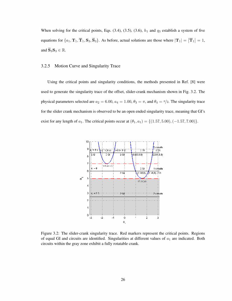
3.2.5 Motion Curve and Singularity Trace
Using the critical points and singularity conditions, the methods presented in Ref. [8] were
used to generate the singularity trace of the offset, slider-crank mechanism shown in Fig. 3.2. The
physical parameters selected are a2 = 6.00, a4 = 1.00, θ3 = π, and θ4 = π/2. The singularity trace
for the slider crank mechanism is observed to be an open ended singularity trace, meaning that GI’s
exist for any length of a1. The critical points occur at (θ1, a1) = (1.57, 5.00), (−1.57, 7.00).
Figure 3.2: The slider-crank singularity trace. Red markers represent the critical points. Regionsof equal GI and circuits are identified. Singularities at different values of a1 are indicated. Bothcircuits within the gray zone exhibit a fully rotatable crank.
26
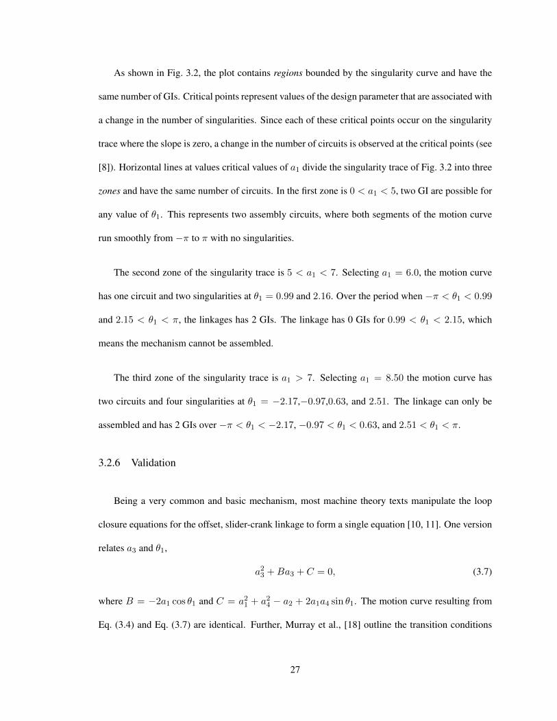
As shown in Fig. 3.2, the plot contains regions bounded by the singularity curve and have the
same number of GIs. Critical points represent values of the design parameter that are associated with
a change in the number of singularities. Since each of these critical points occur on the singularity
trace where the slope is zero, a change in the number of circuits is observed at the critical points (see
[8]). Horizontal lines at values critical values of a1 divide the singularity trace of Fig. 3.2 into three
zones and have the same number of circuits. In the first zone is 0 < a1 < 5, two GI are possible for
any value of θ1. This represents two assembly circuits, where both segments of the motion curve
run smoothly from −π to π with no singularities.
The second zone of the singularity trace is 5 < a1 < 7. Selecting a1 = 6.0, the motion curve
has one circuit and two singularities at θ1 = 0.99 and 2.16. Over the period when −π < θ1 < 0.99
and 2.15 < θ1 < π, the linkages has 2 GIs. The linkage has 0 GIs for 0.99 < θ1 < 2.15, which
means the mechanism cannot be assembled.
The third zone of the singularity trace is a1 > 7. Selecting a1 = 8.50 the motion curve has
two circuits and four singularities at θ1 = −2.17,−0.97,0.63, and 2.51. The linkage can only be
assembled and has 2 GIs over −π < θ1 < −2.17, −0.97 < θ1 < 0.63, and 2.51 < θ1 < π.
3.2.6 Validation
Being a very common and basic mechanism, most machine theory texts manipulate the loop
closure equations for the offset, slider-crank linkage to form a single equation [10, 11]. One version
relates a3 and θ1,
a23 +Ba3 + C = 0, (3.7)
where B = −2a1 cos θ1 and C = a21 + a24 − a2 + 2a1a4 sin θ1. The motion curve resulting from
Eq. (3.4) and Eq. (3.7) are identical. Further, Murray et al., [18] outline the transition conditions
27

for the offset, slider-crank as being a1 = a2 − a1 and a1 = a2 + a4. Substituting a2 = 6.00 and
a4 = 1.00 result in a1 = 5.00 and 7.00, which correspond with the critical points identified in
Fig. 3.2.
3.3 Inverted Slider Crank Linkage
An inverted slider-crank linkage is shown in Fig. 3.3. This linkage includes a prismatic joint
that translates along a moving line of slide. The linkage input variable is designated as x = θ1, the
other joint variables are y = a2, θ3, and the design parameter is p = a1. The physical parameters
include a3, γ, a4, and θ4.
a1
1
a3
γ
2
a2
a4
4
3
Figure 3.3: Inverted slider-crank linkage position vector loop.
28
3.3.1 Loop Closure
The variable S2 = a2T3 is defined to include the prismatic joint. The loop closure equations
areg := a3T3 + TγS2 − a4T4 − a1T1 = 0,
g := a3T3 + TγS2 − a4T4 − a1T1 = 0,
hj := TjTj − 1 = 0 j = 1, 3,
q2 := T3S2 −T3S2 = 0.
(3.8)
Since the frame is designated j = 4 and θ2 depends on θ3, then h2 and h4 are not required.
3.3.2 Forward Kinematics
Eliminating S2 and S2 from Eq. (3.8),
R2 := TγS2 = a1T1 + a4T4 − a3T3,
R2 := TγS2 = a1T1 + a4T4 − a3T3.
(3.9)
Using q2 with the identity TγTγ = 1, T3TγR2 −T3TγR2 = 0. Expanding,
H2 :=T3Tγ(a1T1 + a4T4 − a3T3)
−T3Tγ(a1T1 + a4T4 − a3T3) = 0.
(3.10)
When solving the forward kinematic problem, the design parameter is considered to be fixed.
With designated input angle, θ1 (ie., T1 known), Eq. (3.10) and h3 establishes a system of two
equations for T3,T3. The prismatic joint variable is determined by using a2 =√
S2S2. Each
solution to the direct kinematic problem represents a GI.
3.3.3 Singularity Points
To determine the singularity points, the input angle θ1 becomes a variable and the design
parameter remains fixed. Applying the singularity condition of Eq. (2.10) to the inverted slider-
29
crank givesD := det
[∂H2∂θ3
]=T3Tγ(a1T1 + a4T4) + T3Tγ(a1T1 + a4T4) = 0.
(3.11)
When solving for the singularity points, Eqs. (3.10), (3.11), h1 and h3 establish a system of four
equations for T1,T1,T3,T3. Because the isotropic coordinates are treated as independent
variables, actual solutions are those where |T1| =∣∣T1
∣∣ = |T3| =∣∣T3
∣∣ = 1.
3.3.4 Critical Points
To determine the critical points, the design parameter a1 is considered a variable. Applying the
critical point condition of Eq. (2.14) to the inverted slider-crank,
E := det
[∂H2∂θ1
∂H2∂θ3
∂D∂θ1
∂D∂θ3
]= T1T4 −T1T4 = 0. (3.12)
When solving for the critical points, Eqs. (3.10), (3.11), (3.12), h1 and h3 establish a system of five
equations for a1,T1,T1,T3,T3. Actual solutions are those where a1 = a1 and |T1| =∣∣T1
∣∣ =
|T3| =∣∣T3
∣∣ = 1.
3.3.5 Motion Curve and Singularity Trace
Using physical parameter values of a3 = 0.6, a4 = 1, θ4 = π, γ = 1.2, the singularity trace of
the inverted slider-crank mechanism is given in Fig. 3.4. Again, each of these critical points occur
on the singularity trace where the slope is zero. Thus, a change in the number of circuits is observed
each critical point: (θ1, a1) = (0, 0.44), (0, 1.56). Also observed is that for values of a1 < 0.44
and a1 > 1.56, the linkage has a fully rotating crank.
Regions in the singularity trace bounded by the singularity curve have the same number of GIs.
The singularity trace is further divided into three zones based on the values of a1 at the critical
points. The first zone is 0 < a1 < 0.44, the second is 0.44 < a1 < 1.56, and the third zone
30

Figure 3.4: The inverted slider-crank singularity trace. Red markers denote the critical points.Region of equal GIs and circuits are identified. Singularities at different values of a1 are indicated.Both circuits within the gray zones exhibit a fully rotatable crank.
a1 > 1.56. By generating the motion curve for the mechanism at a certain values of a1, the number
of GIs and circuits are identified for each zone and region in the the singularity trace.
Figure 3.5 shows traces of the motion curve at a1 = 0.2, 0.3, and 0.4, projected onto θ1-θ3
plane. For each value of a1, two assembly circuits exist and 2 GIs are possible for any value of
θ1. For each circuit, the linkage has a fully rotating crank as all GI branches extend from −π to π.
This zone on the singularity trace has two GIs, two circuits, and no singularities. Thus, a first zone
linkage contains two circuits that have an oscillating output with a fully rotational input.
In the second zone of the singularity trace, two singularities exist for a selected value of a1.
Figure 3.6 shows traces of the motion curve at a1 = 0.5, 1.0, and 1.5, projected onto θ1-θ3. For
each value of a1, the motion curve has one assembly circuit and two singularity points denoted
31
−3 −2 −1 0 1 2 30
1
2
3
4
5
6
θ1
θ 3
a
1 = 0.2
a1 = 0.3
a1 = 0.4
Figure 3.5: Traces of the motion curve at various lengths of a1 = 0.2, 0.3, and 0.4, from the firstzone on the singularity trace.
with red markers. Outside the red markers, the linkage has two GIs. In the region between the red
markers, the linkage has 0 GIs, which means the mechanism cannot be assembled. With a linkage in
this second zone, two GIs are possible that only permit an oscillating input producing an oscillating
output.
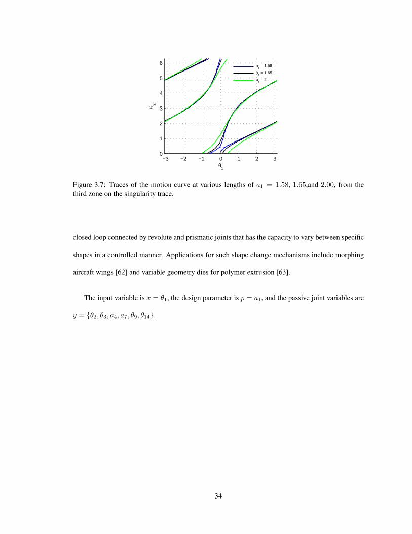
Figure 3.7 shows traces of the motion curve from the third zone of the singularity trace curve
with a1 = 1.58, 1.65,and 2.00. For all values of θ1, the linkage has two GIs and two circuits with
no singularities. A third zone linkage contains two circuits that have a fully rotating output with a
fully rotational input.
3.3.6 Validation
The analysis of the inverted slider-crank linkage is included in most machine theory texts [10,
11]. A single equation relating θ3 and θ1 is stated as
D sin(θ2)− E cos(θ2)− a3 sin(γ) = 0, (3.13)
32
−3 −2 −1 0 1 2 30
1
2
3
4
5
6
θ1
θ 3
(−0.37,3.81)
(0.37,3.16)
(−0.57,4.77)
(0.57,2.21)
(−0.21,6.03)
(0.21,0.95)
a1 = 0.5
a1 = 1
a1 = 1.5
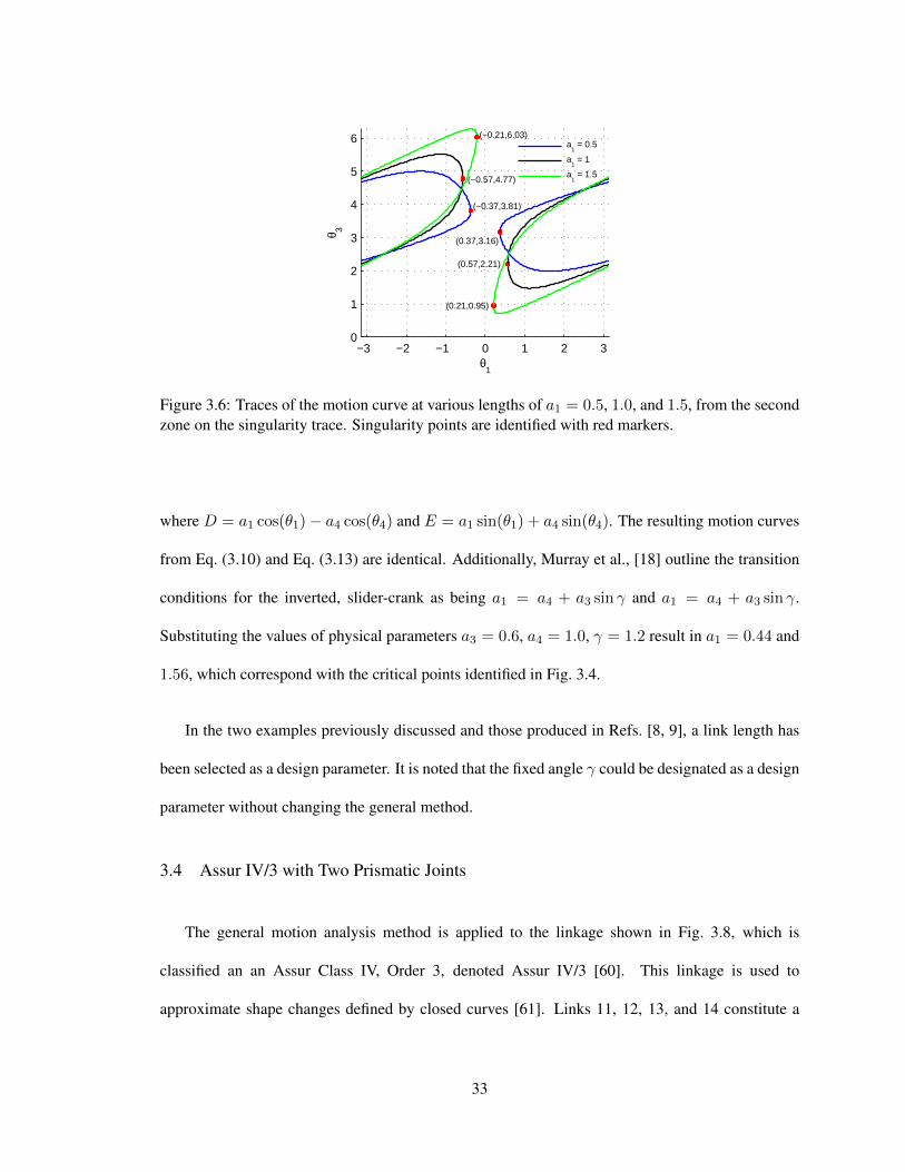
Figure 3.6: Traces of the motion curve at various lengths of a1 = 0.5, 1.0, and 1.5, from the secondzone on the singularity trace. Singularity points are identified with red markers.
where D = a1 cos(θ1)− a4 cos(θ4) and E = a1 sin(θ1) + a4 sin(θ4). The resulting motion curves
from Eq. (3.10) and Eq. (3.13) are identical. Additionally, Murray et al., [18] outline the transition
conditions for the inverted, slider-crank as being a1 = a4 + a3 sin γ and a1 = a4 + a3 sin γ.
Substituting the values of physical parameters a3 = 0.6, a4 = 1.0, γ = 1.2 result in a1 = 0.44 and
1.56, which correspond with the critical points identified in Fig. 3.4.
In the two examples previously discussed and those produced in Refs. [8, 9], a link length has
been selected as a design parameter. It is noted that the fixed angle γ could be designated as a design
parameter without changing the general method.
3.4 Assur IV/3 with Two Prismatic Joints
The general motion analysis method is applied to the linkage shown in Fig. 3.8, which is
classified an an Assur Class IV, Order 3, denoted Assur IV/3 [60]. This linkage is used to
approximate shape changes defined by closed curves [61]. Links 11, 12, 13, and 14 constitute a
33
−3 −2 −1 0 1 2 30
1
2
3
4
5
6
θ1
θ 3
a
1 = 1.58
a1 = 1.65
a1 = 2
Figure 3.7: Traces of the motion curve at various lengths of a1 = 1.58, 1.65,and 2.00, from thethird zone on the singularity trace.
closed loop connected by revolute and prismatic joints that has the capacity to vary between specific
shapes in a controlled manner. Applications for such shape change mechanisms include morphing
aircraft wings [62] and variable geometry dies for polymer extrusion [63].
The input variable is x = θ1, the design parameter is p = a1, and the passive joint variables are
y = θ2, θ3, a4, a7, θ9, θ14.
34

12
a1
a3
a13
a12
a14
6
a11
a5
a4
a8
a2
a9
a7
a10 a6
13
3
7 =14 1
4
3
2
5
6
2
1
8 11
9
10
4
5
Figure 3.8: Assur IV/3 linkage position vector loop.
3.4.1 Loop Closure
The variables S4 = a4T3 and S7 = a7T14 are defined to represent the prismatic joints that
slide along links 4 and 7, respectively. The loop closure conditions and appropriate identities are
g1 := a1T1 + a2T2 + a3T3 + Tδ3S4 + a5T5 = 0,
g2 := a1T1 + a6T6 + S7 + a8T8 + a9T9 + a10T10 = 0,
g3 := a11T11 + a12T12 + a13T13 + a14T14 + S7 = 0,
hj := TjTj − 1 = 0 j = 1, 3, 9, 12, 14,
q4 := T3S4 −T3S4 = 0,
q7 := T14S7 −T14S7 = 0.
(3.14)
35
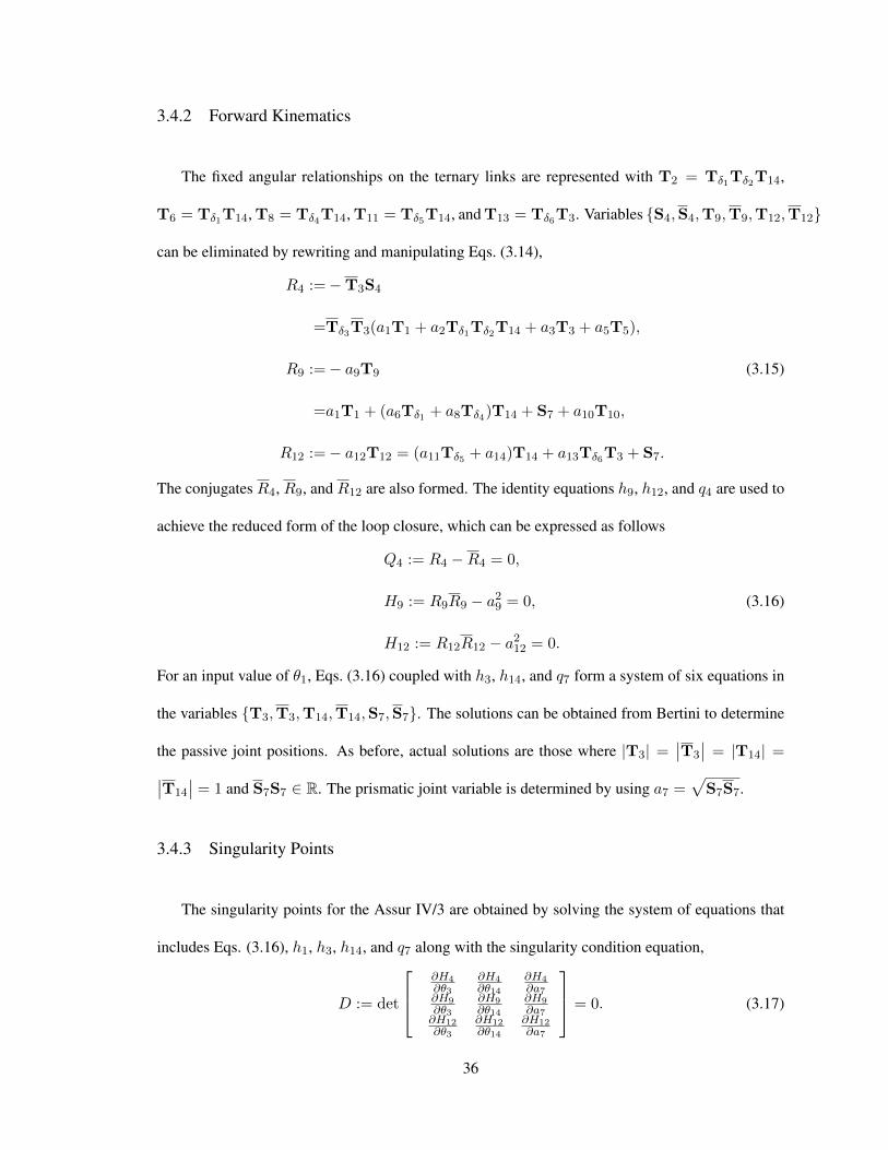
3.4.2 Forward Kinematics
The fixed angular relationships on the ternary links are represented with T2 = Tδ1Tδ2T14,
T6 = Tδ1T14, T8 = Tδ4T14, T11 = Tδ5T14, and T13 = Tδ6T3. Variables S4,S4,T9,T9,T12,T12
can be eliminated by rewriting and manipulating Eqs. (3.14),
R4 :=−T3S4
=Tδ3T3(a1T1 + a2Tδ1Tδ2T14 + a3T3 + a5T5),
R9 :=− a9T9
=a1T1 + (a6Tδ1 + a8Tδ4)T14 + S7 + a10T10,
R12 :=− a12T12 = (a11Tδ5 + a14)T14 + a13Tδ6T3 + S7.
(3.15)
The conjugates R4, R9, and R12 are also formed. The identity equations h9, h12, and q4 are used to
achieve the reduced form of the loop closure, which can be expressed as follows
Q4 := R4 −R4 = 0,
H9 := R9R9 − a29 = 0,
H12 := R12R12 − a212 = 0.
(3.16)
For an input value of θ1, Eqs. (3.16) coupled with h3, h14, and q7 form a system of six equations in
the variables T3,T3,T14,T14,S7,S7. The solutions can be obtained from Bertini to determine
the passive joint positions. As before, actual solutions are those where |T3| =∣∣T3
∣∣ = |T14| =∣∣T14
∣∣ = 1 and S7S7 ∈ R. The prismatic joint variable is determined by using a7 =√
S7S7.
3.4.3 Singularity Points
The singularity points for the Assur IV/3 are obtained by solving the system of equations that
includes Eqs. (3.16), h1, h3, h14, and q7 along with the singularity condition equation,
D := det
∂H4∂θ3
∂H4∂θ14
∂H4∂a7
∂H9∂θ3
∂H9∂θ14
∂H9∂a7
∂H12∂θ3
∂H12∂θ14
∂H12∂a7
= 0. (3.17)
36
The solution to the system of seven equations with seven unknowns can be obtained from Bertini to
determine the the input and passive joint positions that place the linkage in a singularity.
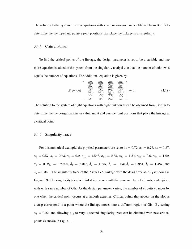
3.4.4 Critical Points
To find the critical points of the linkage, the design parameter is set to be a variable and one
more equation is added to the system from the singularity analysis, so that the number of unknowns
equals the number of equations. The additional equation is given by
E := det
∂H4∂θ1
∂H4∂θ3
∂H4∂θ14
∂H4∂a7
∂H9∂θ1
∂H9∂θ3
∂H9∂θ14
∂H9∂a7
∂H12∂θ1
∂H12∂θ3
∂H12∂θ14
∂H12∂a7
∂D∂θ1
∂D∂θ3
∂D∂θ14
∂D∂a7
= 0. (3.18)
The solution to the system of eight equations with eight unknowns can be obtained from Bertini to
determine the the design parameter value, input and passive joint positions that place the linkage at
a critical point.
3.4.5 Singularity Trace
For this numerical example, the physical parameters are set to a2 = 0.72, a3 = 0.77, a5 = 0.87,
a6 = 0.57, a8 = 0.53, a9 = 0.9, a10 = 1.546, a11 = 0.65, a12 = 1.34, a13 = 0.6, a14 = 1.09,
θ5 = 0, θ10 = −2.926, δ1 = 2.015, δ2 = 1.727, δ3 = 0.634,δ4 = 0.981, δ5 = 1.487, and
δ6 = 0.356. The singularity trace of the Assur IV/3 linkage with the design variable a1 is shown in
Figure 3.9. The singularity trace is divided into zones with the same number of circuits, and regions
with with same number of GIs. As the design parameter varies, the number of circuits changes by
one when the critical point occurs at a smooth extrema. Critical points that appear on the plot as
a cusp correspond to a point where the linkage moves into a different region of GIs. By setting
a1 = 0.22, and allowing a12 to vary, a second singularity trace can be obtained with new critical
points as shown in Fig. 3.10
37

Figure 3.9: The singularity trace for Assur IV/3 with respect to a1. Red markers denote the criticalpoints. Regions of equal GIs and circuits are identified. The zone shaded in gray contains at leastone circuit with a fully rotatable crank.
3.4.6 Motion Curve
Figure 3.11 shows a motion curve with a1 = 0.25 projected onto θ1-θ2 plane. At this driving link
length, the linkage has six circuits, five of them have continuously rotating cranks. Additionally, the
sixth circuit exhibits two singularity points, between which is a linkage that is able to rotate greater
than one full revolution. That is, the linkage upon return to the same value of the input link angle is
placed into a different GI without encountering a singularity. As observed in Ref. [8], this motion
characteristic is associated with being near a cusp on the singularity trace.
38
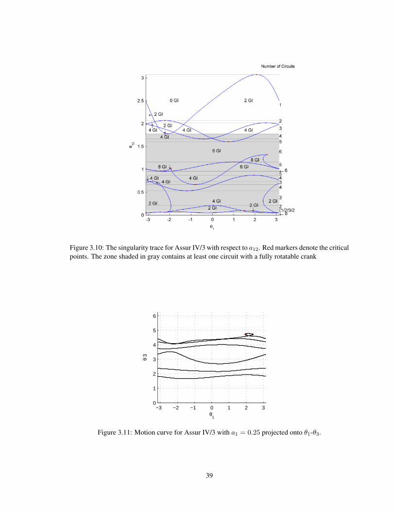
Figure 3.10: The singularity trace for Assur IV/3 with respect to a12. Red markers denote the criticalpoints. The zone shaded in gray contains at least one circuit with a fully rotatable crank
−3 −2 −1 0 1 2 30
1
2
3
4
5
6
θ1
θ 3
Figure 3.11: Motion curve for Assur IV/3 with a1 = 0.25 projected onto θ1-θ3.
39
CHAPTER IV
SPHERICAL LINKAGE ANALYSIS
In this chapter a process is developed to solve displacement and singularity analysis of spherical
linkages using 2 × 2 special unitary rotation matrices, SU(2). The process is valid for multiloop
spherical linkages. Three examples are provided to show the process in details. To facilitate the
process of equations development for analyzing spherical linkages, a straightforward example of
3-roll wrist is utilized.
4.1 The 3-Roll Wrist on SU(2)
A 3-roll wrist is often used as the final set of axes on a robot and has three perpendicular
intersecting revolute joints for the creation of arbitrary orientations as shown in Fig. 4.1. The inverse
kinematics task is to determine the joint angles in order to position the end effector in a desired
orientation Q3RW . The desired orientation is defined by an angle θ about a line s as specified in
Eq. (2.17) to create
Q3RW =
[M1 M2
−M2 M1
], (4.1)
where M j is the conjugate of Mj . For this example, let the three successive rotations be about
Z then X then Z. Thus, the forward kinematics is
Q3RW = Qz(θ1)Qx(θ2)Qz(θ3). (4.2)
Rearranging Eq. (4.2),
H := Qx(θ2)Qz(θ3)Q∗3RW = Q∗z(θ1). (4.3)
40
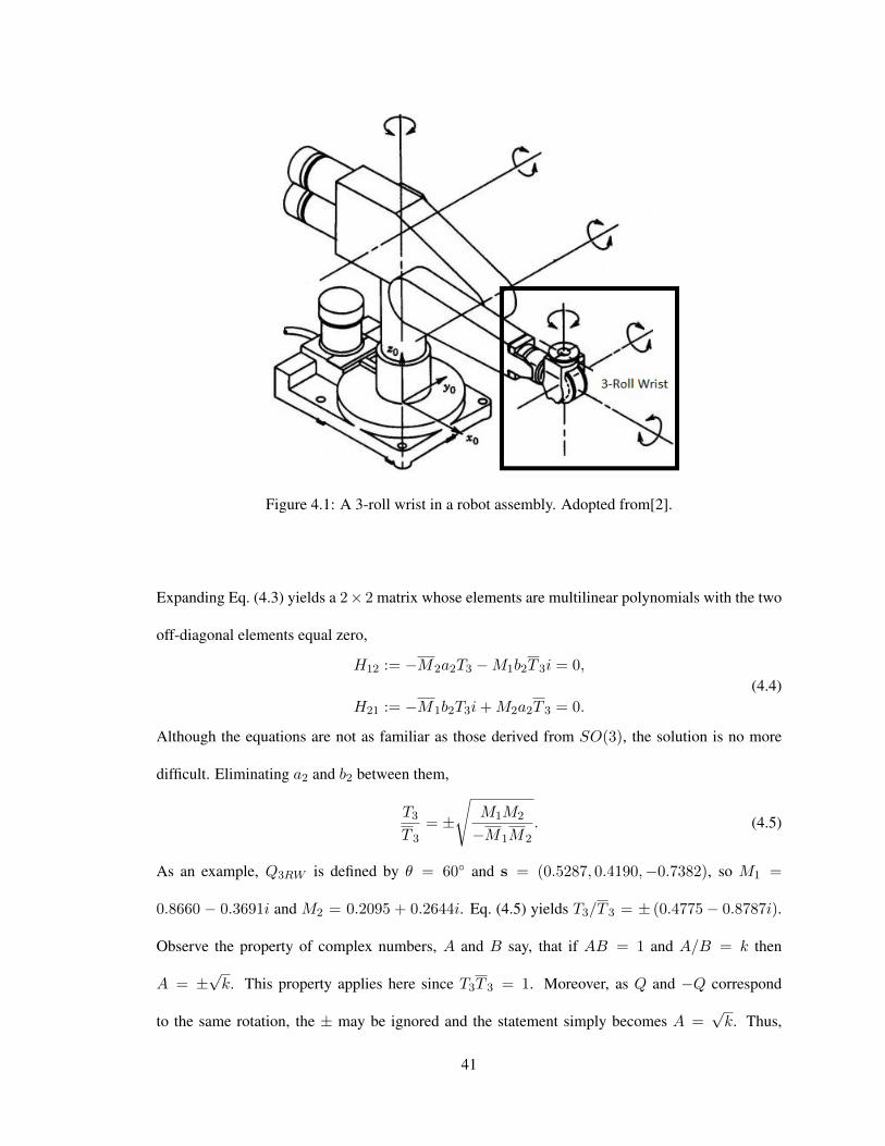
Figure 4.1: A 3-roll wrist in a robot assembly. Adopted from[2].
Expanding Eq. (4.3) yields a 2× 2 matrix whose elements are multilinear polynomials with the two
off-diagonal elements equal zero,
H12 := −M2a2T3 −M1b2T 3i = 0,
H21 := −M1b2T3i+M2a2T 3 = 0.
(4.4)
Although the equations are not as familiar as those derived from SO(3), the solution is no more
difficult. Eliminating a2 and b2 between them,
T3
T 3
= ±
√M1M2
−M1M2
. (4.5)
As an example, Q3RW is defined by θ = 60 and s = (0.5287, 0.4190,−0.7382), so M1 =
0.8660 − 0.3691i and M2 = 0.2095 + 0.2644i. Eq. (4.5) yields T3/T 3 = ± (0.4775− 0.8787i).
Observe the property of complex numbers, A and B say, that if AB = 1 and A/B = k then
A = ±√k. This property applies here since T3T 3 = 1. Moreover, as Q and −Q correspond
to the same rotation, the ± may be ignored and the statement simply becomes A =√k. Thus,
41
the first possibility is T3 =√
0.4775− 0.8787i = 0.8595 − 0.5111i corresponding to an angle of
θ3 = −61.5. The second possibilty is T3 =√−0.4775 + 0.8787i = 0.5111 + 0.8595i for an
angle of θ3 = 118.5. Eq. (4.4) now determines θ2 (from a2 and b2) and then the diagonal terms of
Eq. (4.3) define θ1.
Although using numerical algebraic geometry on such a straightforward example is unnecessary,
the Bertini tool is now used to prepare for the significantly more complicated examples to come
and to introduce some numerical issues that need to be addressed. For example, in Bertini, it is
computationally advantageous to identify groups of homogeneous variables. This is readily done
by grouping the variables associated by a joint rotation angle. Groups are identified with angle
brackets as in [31]. The variable groups are 〈a2, b2〉 and 〈T3, T 3〉 corresponding to the wrist angles
θ2 and θ3, respectively. With Eq. (4.4) homogeneous, solutions are determined as a ratio of the
values in the variable group. For example, Bertini determines a value of Tv3 for the variable T3 and
T v3 for T 3. Due to the homogeneity, either Tv3 or T v3 will equal 1. Although these values solve
the equations, it is also the case that Tv3T v3 6= 1. The desired dehomogenized values are
T3 =
√Tv3
T v3and T 3 =
√T v3Tv3
. (4.6)
For an x-axis rotation, the process of determining the desired values is slightly different. In this
case, Bertini determines a value of av2 for a2 and bv2 for b2 where either av2 or bv2 will equal 1.
The desired values are
a2 =av2√
a2v2 + b2v2and b2 =
bv2√a2v2 + b2v2
. (4.7)
Although not used here, a y-axis rotation is handled similarly to the x-axis case. For this example,
Bertini solved Eq. (4.4) tracking two paths to two solutions. For the first path tracked, Bertini
produced av2 = 1, bv2 = 0.3583, Tv3 = 1, and T v3 = 0.4775 + 0.8787i. The corresponding
values are a2 = 0.9414, b2 = 0.3373, T3 = 0.8595 − 0.5111i, and T 3 = 0.8595 + 0.5111i
42

producing the solution θ1 = 13.7, θ2 = 39.4, θ3 = −61.5. The second solution produces
θ1 = −166.3, θ2 = −39.4, θ3 = 118.5, the two solutions matching the above method.
4.2 Spherical Four-Bar Linkage Analysis
A spherical four-bar mechanism is shown in Fig. 4.2. The mechanism consists of four links, one
being fixed, connected by four revolute joints with intersecting axes. The fixed origin is placed at
the intersection of the axes. The z-axis of the fixed frame is aligned with the axis of joint 1 and the
x-z plane is aligned with the fixed link. The actuated angle is θ1, and the remaining joint variables
are θ2, θ3, and θ4. The physical parameters defining the link lengths are α12, α23, α34, and α41.
1
G1
W1
W2
G2
2
3
4
α12
α23
α34
α41
X
Z
Y
Figure 4.2: A spherical four-bar linkage.
43

4.2.1 Loop Closure and Forward Kinematics
The loop closure equations for this spherical mechanism are constructed using successive
rotations.
Qz(θ1)Qy(α12)Qz(θ2)Qy(α23)Qz(θ3)Qy(α34)Qz(θ4)Qy(α41) = I, (4.8)
where I is the identity. Isolating θ3 in Eq. (4.8),
Qy(α34)Qz(θ4)Qy(α41)Qz(θ1)Qy(α12)Qz(θ2)Qy(α23) = Q∗z(θ3). (4.9)
The off-diagonal terms in Q∗z(θ3) are zero and the polynomials from the left hand side are observed
to be homogeneous in the variable groups 〈T2, T 2〉 and 〈T4, T 4〉 representing θ2 and θ4, respectively.
For a given θ1, Bertini tracks two paths and finds (up to) two sets of usable values for 〈T2, T 2〉 and
〈T4, T 4〉. Like the previous example, these values must be dehomogenized. Usable solutions meet
the condition that the diagonal elements on the right side of Eq. (4.9) are complex conjugates and
of unit magnitude. This check is performed throughout to discard solutions that do not result in
actual loop closure. The terminology here is worth highlighting. Classically, when solving for an
unknown θ value, a complex value corresponds to a configuration at which the mechanism cannot be
assembled. Since all values are imaginary when using SU(2), that terminology is insufficient. Thus,
the check is to see if the values of T3 and T 3 calculated from Eq. (4.9) are complex conjugates and
of unit magnitude. Given the condition is met, the values for θ3 are straightforwardly determined.
Using the physical parameters α12 = 90, α23 = 90, α34 = 45, α41 = 72, the motion curve in
Fig. 4.3 is produced by varying θ1.
4.2.2 Spherical Four-Bar Singularity Points
When determining singularities the input angle is considered to be a variable. The singularity
condition is determined from the velocity expression presented in Eq. (2.34). In this analysis,
44
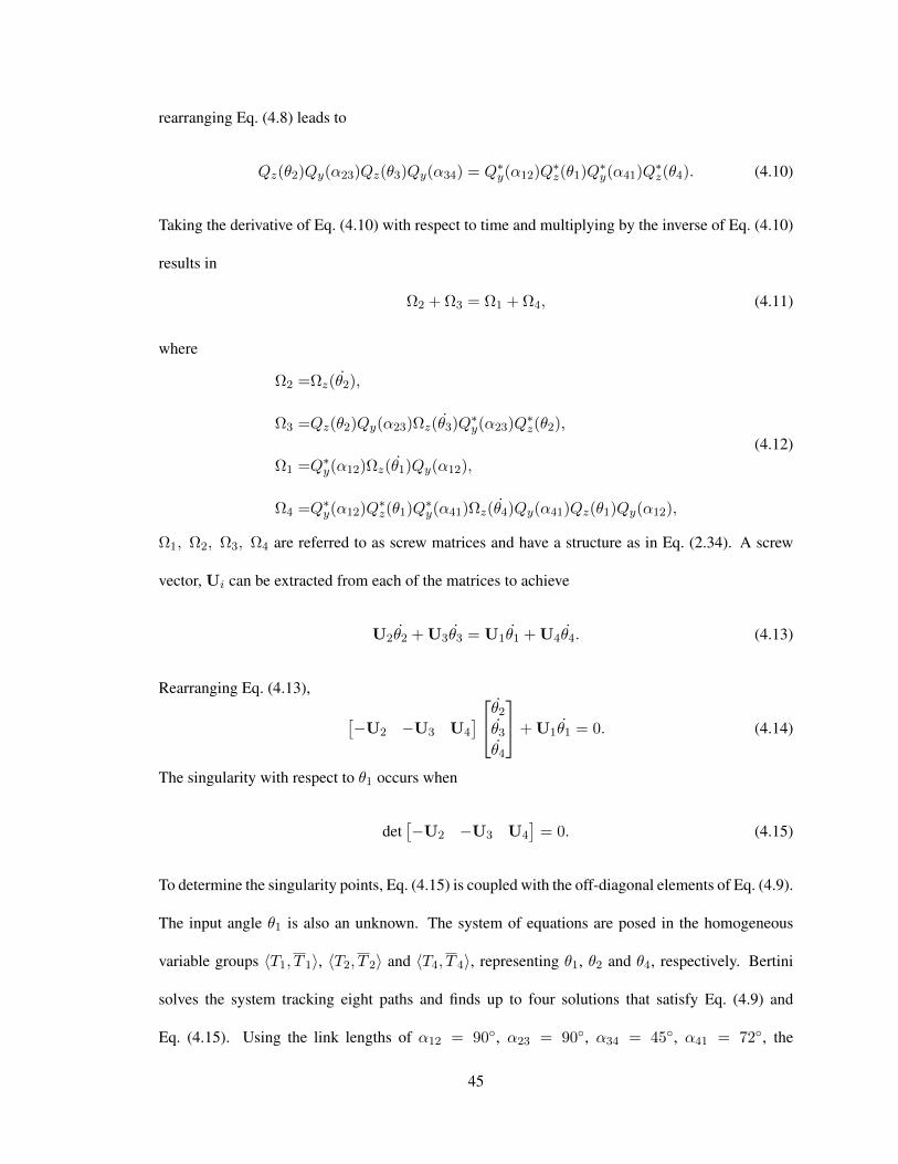
rearranging Eq. (4.8) leads to
Qz(θ2)Qy(α23)Qz(θ3)Qy(α34) = Q∗y(α12)Q∗z(θ1)Q
∗y(α41)Q
∗z(θ4). (4.10)
Taking the derivative of Eq. (4.10) with respect to time and multiplying by the inverse of Eq. (4.10)
results in
Ω2 + Ω3 = Ω1 + Ω4, (4.11)
where
Ω2 =Ωz(θ2),
Ω3 =Qz(θ2)Qy(α23)Ωz(θ3)Q∗y(α23)Q
∗z(θ2),
Ω1 =Q∗y(α12)Ωz(θ1)Qy(α12),
Ω4 =Q∗y(α12)Q∗z(θ1)Q
∗y(α41)Ωz(θ4)Qy(α41)Qz(θ1)Qy(α12),
(4.12)
Ω1, Ω2, Ω3, Ω4 are referred to as screw matrices and have a structure as in Eq. (2.34). A screw
vector, Ui can be extracted from each of the matrices to achieve
U2θ2 + U3θ3 = U1θ1 + U4θ4. (4.13)
Rearranging Eq. (4.13), [−U2 −U3 U4
] θ2θ3θ4
+ U1θ1 = 0. (4.14)
The singularity with respect to θ1 occurs when
det[−U2 −U3 U4
]= 0. (4.15)
To determine the singularity points, Eq. (4.15) is coupled with the off-diagonal elements of Eq. (4.9).
The input angle θ1 is also an unknown. The system of equations are posed in the homogeneous
variable groups 〈T1, T 1〉, 〈T2, T 2〉 and 〈T4, T 4〉, representing θ1, θ2 and θ4, respectively. Bertini
solves the system tracking eight paths and finds up to four solutions that satisfy Eq. (4.9) and
Eq. (4.15). Using the link lengths of α12 = 90, α23 = 90, α34 = 45, α41 = 72, the
45
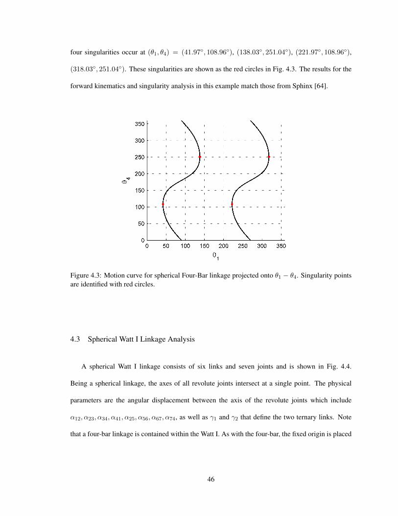
four singularities occur at (θ1, θ4) = (41.97, 108.96), (138.03, 251.04), (221.97, 108.96),
(318.03, 251.04). These singularities are shown as the red circles in Fig. 4.3. The results for the
forward kinematics and singularity analysis in this example match those from Sphinx [64].
Figure 4.3: Motion curve for spherical Four-Bar linkage projected onto θ1 − θ4. Singularity pointsare identified with red circles.
4.3 Spherical Watt I Linkage Analysis
A spherical Watt I linkage consists of six links and seven joints and is shown in Fig. 4.4.
Being a spherical linkage, the axes of all revolute joints intersect at a single point. The physical
parameters are the angular displacement between the axis of the revolute joints which include
α12, α23, α34, α41, α25, α56, α67, α74, as well as γ1 and γ2 that define the two ternary links. Note
that a four-bar linkage is contained within the Watt I. As with the four-bar, the fixed origin is placed
46
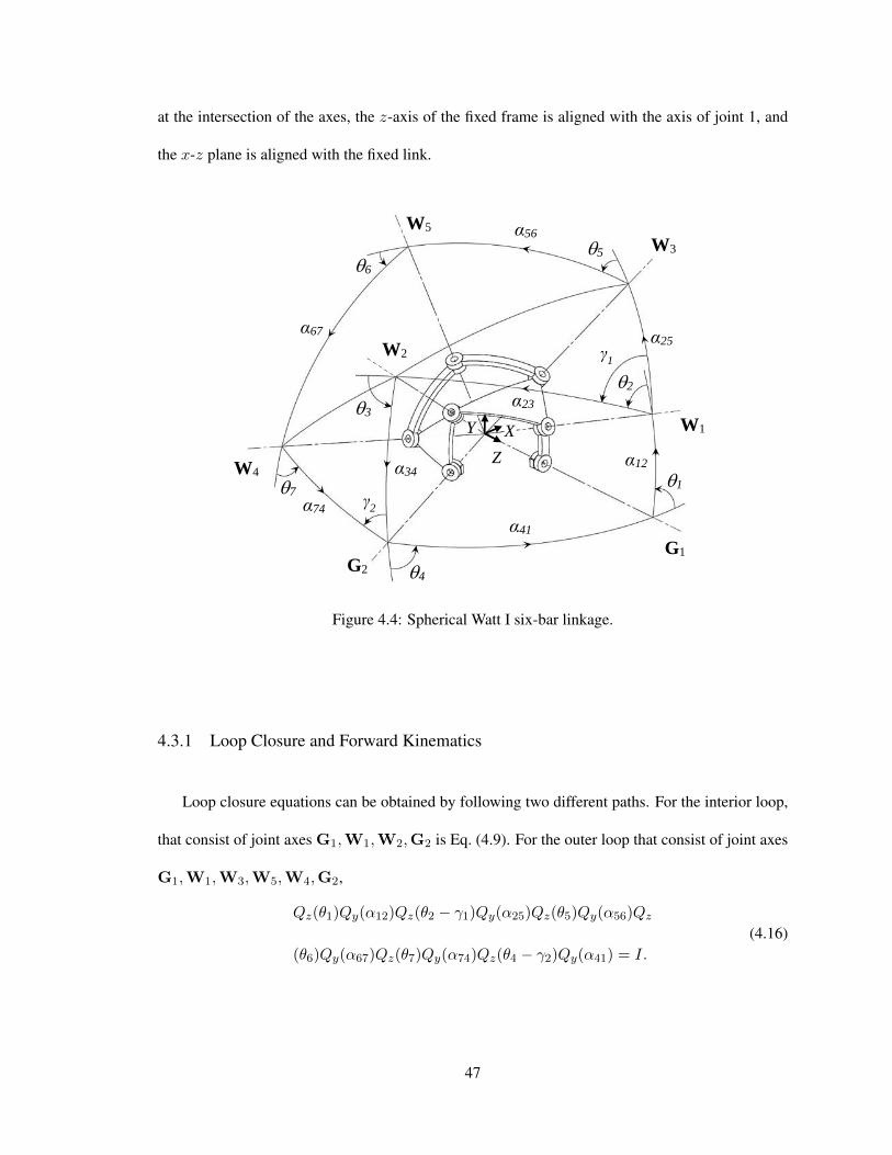
at the intersection of the axes, the z-axis of the fixed frame is aligned with the axis of joint 1, and
the x-z plane is aligned with the fixed link.
G1
W1
W3
W5
W4
G2
W2
α12
α23
α34
α41
α25
α56
α67
α74
1
2
3
4
5 6
7
γ1
γ2
X Y
Z
Figure 4.4: Spherical Watt I six-bar linkage.
4.3.1 Loop Closure and Forward Kinematics
Loop closure equations can be obtained by following two different paths. For the interior loop,
that consist of joint axes G1,W1,W2,G2 is Eq. (4.9). For the outer loop that consist of joint axes
G1,W1,W3,W5,W4,G2,
Qz(θ1)Qy(α12)Qz(θ2 − γ1)Qy(α25)Qz(θ5)Qy(α56)Qz
(θ6)Qy(α67)Qz(θ7)Qy(α74)Qz(θ4 − γ2)Qy(α41) = I.
(4.16)
47
To reduce the system, θ5 is isolated and Eq. (4.16) becomes
Qy(α56)Qz(θ6)Qy(α67)Qz(θ7)Qy(α74)Qz(θ4 − γ2)
Qy(α41)Qz(θ1)Qy(α12)Qz(θ2 − γ1)Qy(α25) = Q∗z(θ5).
(4.17)
Given θ1, the (unknown) joint variables are θj , j = 2, . . . , 7, associated with relative rotation about
z-axis. z-axes. The judicious approach is to solve Eq. (4.9) first as detailed in the previous section,
and then use each of those solutions to solve Eq. (4.16) repeatedly for each valid solution.
As a more generic modeling procedure is sought in this work, the off-diagonal elements in
Eqs. (4.9) and (4.17) are used simultaneously. Four homogeneous equations are posed in the variable
groups 〈T2, T 2〉, 〈T4, T 4〉, 〈T6, T 6〉 and 〈T7, T 7〉 representing θ2, θ4, θ6 and θ7, respectively. The
system is solved using Bertini, following four paths and finding up to four usable solutions for
each θ1. The solutions are checked by substituting them into the diagonal elements of Eqs. (4.9)
and (4.17). Passing the check, the corresponding values of θ3 and θ5 are readily determined. Using
physical parameters α12 = 25, γ1 = γ2 = α23 = 60, α34 = α25 = α56 = 40, α41 = 110,
α67 = 55, and α74 = 45, the motion curve in Fig. 4.5 is produced by varying θ1 and projecting
onto θ1-θ7.
4.3.2 Singularity Points
When determining singularities, the input angle θ1 is considered a variable. As in the four-
bar singularity analysis, the loop closure is arranged to reduced the size of the equations. The
singularity condition for the interior loop is identical to that of the four-bar spherical linkage as
given in Eq. (4.15). For the outer loop, Eq. (4.16) is written as
Qy(α74)Qz(θ4 − γ2)Qy(α41)Qz(θ1)Qy(α12)Qz(θ2 − γ1)Qy(α25) =
Q∗z(θ7)Q∗y(α67)Q
∗z(θ6)Q
∗y(α56)Q
∗z(θ5).
(4.18)
Taking the derivative of Eq. (4.18) with respect to time and multiplying by the inverse of Eq. (4.18),
Ω†4 + Ω†1 + Ω†2 = Ω7 + Ω6 + Ω5, (4.19)
48
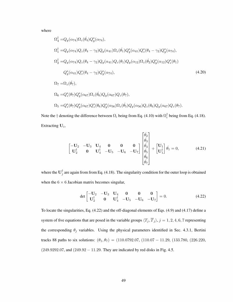
where
Ω†4 =Qy(α74)Ωz(θ4)Q∗y(α74),
Ω†1 =Qy(α74)Qz(θ4 − γ2)Qy(α41)Ωz(θ1)Q∗y(α41)Q
∗z(θ4 − γ2)Q∗y(α74),
Ω†2 =Qy(α74)Qz(θ4 − γ2)Qy(α41)Qz(θ1)Qy(α12)Ωz(θ2)Q∗y(α12)Q
∗z(θ1)
Q∗y(α41)Q∗z(θ4 − γ2)Q∗y(α74),
Ω7 =Ωz(θ7),
Ω6 =Q∗z(θ7)Q∗y(α67)Ωz(θ6)Qy(α67)Qz(θ7),
Ω5 =Q∗z(θ7)Q∗y(α67)Q
∗z(θ6)Q
∗y(α56)Ωz(θ5)Qy(α56)Qz(θ6)Qy(α67)Qz(θ7).
(4.20)
Note the † denoting the difference between Ωi being from Eq. (4.10) with Ω†i being from Eq. (4.18).
Extracting Ui,
[−U2 −U3 U4 0 0 0
U†2 0 U†4 −U5 −U6 −U7
]
θ2θ3θ4θ5θ6θ7
+
[U1
U†1
]θ1 = 0, (4.21)
where the U†j are again from from Eq. (4.18). The singularity condition for the outer loop is obtained
when the 6× 6 Jacobian matrix becomes singular,
det[−U2 −U3 U4 0 0 0
U†2 0 U†4 −U5 −U6 −U7
]= 0. (4.22)
To locate the singularities, Eq. (4.22) and the off-diagonal elements of Eqs. (4.9) and (4.17) define a
system of five equations that are posed in the variable groups 〈Tj , T j〉, j = 1, 2, 4, 6, 7 representing
the corresponding θj variables. Using the physical parameters identified in Sec. 4.3.1, Bertini
tracks 88 paths to six solutions: (θ1, θ7) = (110.0792.07, (110.07 − 11.29, (133.780, (226.220,
(249.9292.07, and (249.92− 11.29. They are indicated by red disks in Fig. 4.5.
49
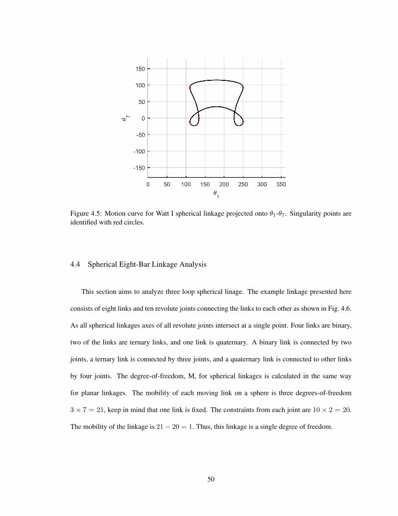
Figure 4.5: Motion curve for Watt I spherical linkage projected onto θ1-θ7. Singularity points areidentified with red circles.
4.4 Spherical Eight-Bar Linkage Analysis
This section aims to analyze three loop spherical linage. The example linkage presented here
consists of eight links and ten revolute joints connecting the links to each other as shown in Fig. 4.6.
As all spherical linkages axes of all revolute joints intersect at a single point. Four links are binary,
two of the links are ternary links, and one link is quaternary. A binary link is connected by two
joints, a ternary link is connected by three joints, and a quaternary link is connected to other links
by four joints. The degree-of-freedom, M, for spherical linkages is calculated in the same way
for planar linkages. The mobility of each moving link on a sphere is three degrees-of-freedom
3 × 7 = 21, keep in mind that one link is fixed. The constraints from each joint are 10 × 2 = 20.
The mobility of the linkage is 21− 20 = 1. Thus, this linkage is a single degree of freedom.
50
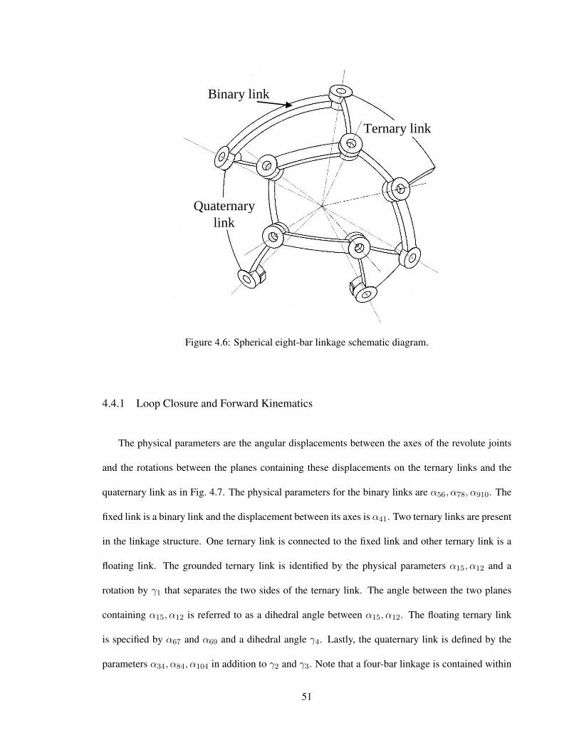
Ternary link
Quaternary
link
Binary link
Figure 4.6: Spherical eight-bar linkage schematic diagram.
4.4.1 Loop Closure and Forward Kinematics
The physical parameters are the angular displacements between the axes of the revolute joints
and the rotations between the planes containing these displacements on the ternary links and the
quaternary link as in Fig. 4.7. The physical parameters for the binary links are α56, α78, α910. The
fixed link is a binary link and the displacement between its axes is α41. Two ternary links are present
in the linkage structure. One ternary link is connected to the fixed link and other ternary link is a
floating link. The grounded ternary link is identified by the physical parameters α15, α12 and a
rotation by γ1 that separates the two sides of the ternary link. The angle between the two planes
containing α15, α12 is referred to as a dihedral angle between α15, α12. The floating ternary link
is specified by α67 and α69 and a dihedral angle γ4. Lastly, the quaternary link is defined by the
parameters α34, α84, α104 in addition to γ2 and γ3. Note that a four-bar linkage is contained within
51
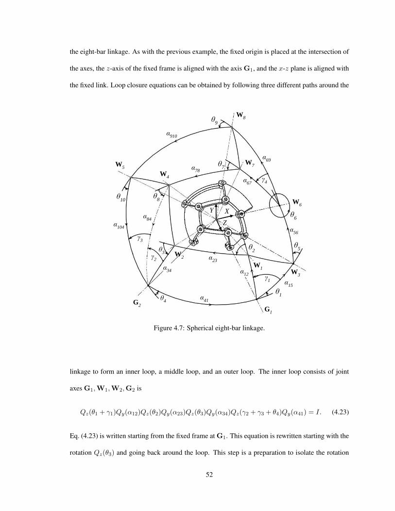
the eight-bar linkage. As with the previous example, the fixed origin is placed at the intersection of
the axes, the z-axis of the fixed frame is aligned with the axis G1, and the x-z plane is aligned with
the fixed link. Loop closure equations can be obtained by following three different paths around the
W6
W7
W8
G1
G2
W3
W1
W2
W4
W5
θ1
θ2 θ
3
θ4
α12
α23
α
34
α41
Z
Y X
γ1
γ2
γ3
γ4
θ5
θ6
θ7
θ8
α56
α67
α78
α84
α69
α910
α104
θ9
θ10
α15
Figure 4.7: Spherical eight-bar linkage.
linkage to form an inner loop, a middle loop, and an outer loop. The inner loop consists of joint
axes G1,W1,W2,G2 is
Qz(θ1 + γ1)Qy(α12)Qz(θ2)Qy(α23)Qz(θ3)Qy(α34)Qz(γ2 + γ3 + θ4)Qy(α41) = I. (4.23)
Eq. (4.23) is written starting from the fixed frame at G1. This equation is rewritten starting with the
rotation Qz(θ3) and going back around the loop. This step is a preparation to isolate the rotation
52
containing θ3 as
Qz(θ3)Qy(α34)Qz(γ2 + γ3 + θ4)Qy(α41)Qz(θ1 + γ1)Qy(α12)Qz(θ2)Qy(α23) = I. (4.24)
Multiply both sides of Eq. (4.24) by Q∗z(θ3) to isolate θ3
Qy(α34)Qz(γ2 + γ3 + θ4)Qy(α41)Qz(θ1 + γ1)Qy(α12)Qz(θ2)Qy(α23) = Q∗z(θ3). (4.25)
The middle loop consists of joint axes G1,W3,W6,W7,W4,G2. Starting from the fixed frame
at G1, the middle loop equation is
Qz(θ1)Qy(α15)Qz(θ5)Qy(α56)Qz(θ6 + γ4)Qy(α67)Qz(θ7)
Qy(α78)Qz(θ8)Qy(α84)Qz(θ4 + γ3)Qy(α41) = I.
(4.26)
With the intention of isolating, θ7. Eq.(4.26) is rewritten starting from the rotation containing θ7.
Qz(θ7)Qy(α78)Qz(θ8)Qy(α84)Qz(θ4 + γ3)Qy(α41)
Qz(θ1)Qy(α15)Qz(θ5)Qy(α56)Qz(θ6 + γ4)Qy(α67) = I.
(4.27)
Multiply both sides by Q∗z(θ7). Eq. (4.27) takes the form as
Qy(α78)Qz(θ8)Qy(α84)Qz(θ4 + γ3)Qy(α41)
Qz(θ1)Qy(α15)Qz(θ5)Qy(α56)Qz(θ6 + γ4)Qy(α67) = Q∗z(θ7).
(4.28)
The outer loop is the third loop and it consists of the axes G1,W3,W6,W8,W5,G2. The process
of constructing the loop closure equation is similar to the previous loops. Starting from the fixed
frame at G1, the outer loop equation is
Qz(θ1)Qy(α15)Qz(θ5)Qy(α56)Qz(θ6)Qy(α69)Qz(θ9)
Qy(α910)Qz(θ10)Qy(α104)Qz(θ4)Qy(α41) = I.
(4.29)
To isolate, θ9 write Eq.(4.29) starting from the rotation containing θ9.
Qz(θ9)Qy(α910)Qz(θ10)Qy(α104)Qz(θ4)Qy(α41)
Qz(θ1)Qy(α15)Qz(θ5)Qy(α56)Qz(θ6)Qy(α69) = I.
(4.30)
Multiply both sides by Q∗z(θ9). Eq. (4.30) becomes
Qy(α910)Qz(θ10)Qy(α104)Qz(θ4)Qy(α41)
Qz(θ1)Qy(α15)Qz(θ5)Qy(α56)Qz(θ6)Qy(α69) = Q∗z(θ9).
(4.31)
53
The off-diagonal elements in Eqs. (4.25), (4.28), and (4.31) are solved simultaneously when solving
the displacement analysis. Given θ1, the (unknown) joint variables are θj , j = 2, 4, 5, 6, 8, 10,
associated with relative rotation about z-axis. Note, the two off-diagonal elements from each loop
does not contain the angles θ3, θ7, and θ9. Since these angles are only present in the diagonal
elements of the loop closure equations. Six homogeneous equations are posed in the variable groups
〈T2, T 2〉, 〈T4, T 4〉, 〈T5, T 5〉, 〈T6, T 6〉, 〈T8, T 8〉 and 〈T10, T 10〉 representing θ2, θ4, θ5, θ6, θ8, and
θ10. respectively. To give a numerical example, the physical parameters are set as α12, α15 = 25,
α34 = 40, α23, α84 = 60, α69, α104 = 80, α41 = 100, α56, α67, α78, α910 = 45, and
γ1...4 = 10. The system is solved using Bertini, following sixteen paths and finding up to eight
usable solutions for each θ1. The solutions are checked by substituting them into the diagonal
elements of Eqs. (4.25), (4.28), and (4.31). The motion curve in Fig. 4.8 is produced by varying θ1
and projecting onto θ1-θ5. The motion curve in Fig. 4.8 and Fig. 4.9 is produced by varying θ1 and
projecting onto θ1-θ5,θ6.
4.4.2 Singularity Points
When determining singularities, the input angle θ1 is considered a variable. The inner loop
closure Eq. (4.23) is arranged to reduced the size of the resulting screw vector as
Qz(θ2)Qy(α23)Qz(θ3)Qy(α34) = Q∗y(α12)Q∗z(θ1 + γ1)Q
∗y(α41)Q
∗z(γ2 + γ3 + θ4). (4.32)
Multiplying the derivative of each side of this equation by the inverse of the same side to obtain
Ω2 + Ω3 = Ω†1 + Ω†4, (4.33)
54
where
Ω2 =Ωz(θ2),
Ω3 =Qz(θ2)Qy(α23)Ωz(θ3)Q∗y(α23)Q
∗z(θ2),
Ω1 =Q∗y(α12)Ωz(θ1)Qy(α12)
Ω4 =Q∗y(α12)Q∗z(θ1 + γ1)Q
∗y(α41)Ωz(θ4)Qy(α41)Qz(θ1 + γ1)Qy(α12),
(4.34)
For the middle loop, Eq. (4.26) is written as
Qz(θ5)Qy(α56)Qz(θ6 + γ4)Qy(α67)Qz(θ7)Qy(α78) =
Q∗y(α15)Q∗z(θ1)Q
∗y(α41)Q
∗z(θ4 + γ3)Q
∗y(α84)Q
∗z(θ8).
(4.35)
Taking the derivative of Eq. (4.35) with respect to time and multiplying by the inverse of Eq. (4.35),
Ω†5 + Ω†6 + Ω7 = Ω†1 + Ω†4 + Ω8, (4.36)
where
Ω†5 =Ωz(θ5),
Ω†6 =Qz(θ5)Qy(α56)Ωz(θ6)Q∗y(α56)Q
∗z(θ5),
Ω7 =Qz(θ5)Qy(α56)Qz(θ6 + γ4)Qy(α67)Ωz(θ7)
Q∗y(α67)Q∗z(θ6 + γ4)Q
∗y(α56)Q
∗z(θ5),
Ω†1 =Q∗y(α15)Ωz(θ1)Qy(α15),
Ω†4 =Q∗y(α15)Q∗z(θ1)Q
∗y(α41)Ωz(θ4)Qy(α41)Qz(θ1)Qy(α15),
Ω8 =Q∗y(α15)Q∗z(θ1)Q
∗y(α41)Q
∗z(θ4 + γ3)Q
∗y(α84)Ωz(θ8)
Qy(α84)Qz(θ4 + γ3)Qy(α41)Qz(θ1)Qy(α15).
(4.37)
For the outer loop, Eq. (4.29) is written as
Qz(θ5)Qy(α56)Qz(θ6)Qy(α69)Qz(θ9)Qy(α910) =
Q∗y(α15)Q∗z(θ1)Q
∗y(α41)Q
∗z(θ4)Q
∗y(α104)Q
∗z(θ10).
(4.38)
Taking the derivative of Eq. (4.38) with respect to time and multiplying by the inverse of Eq. (4.38),
Ω‡5 + Ω‡6 + Ω9 = Ω‡1 + Ω‡4 + Ω10, (4.39)
55
where
Ω‡5 =Ωz(θ5),
Ω‡6 =Qz(θ5)Qy(α56)Ωz(θ6)Q∗y(α56)Q
∗z(θ5),
Ω9 =Qz(θ5)Qy(α56)Qz(θ6)Qy(α69)Ωz(θ9)Q∗y(α69)Q
∗z(θ6)Q
∗y(α56)Q
∗z(θ5),
Ω‡1 =Q∗y(α15)Ωz(θ1)Qy(α15),
Ω‡4 =Q∗y(α15)Q∗z(θ1)Q
∗y(α41)Ωz(θ4)Qy(α41)Qz(θ1)Qy(α15),
Ω10 =Q∗y(α15)Q∗z(θ1)Q
∗y(α41)Q
∗z(θ4)Q
∗y(α104)
Ωz( ˙θ10)Qy(α104)Qz(θ4)Qy(α41)Qz(θ1)Qy(α15).
(4.40)
Screw matrices that appear in more than one loop are distinguished with † and ‡. Ω†i being from the
middle loop, and Ω‡ is from the outer loop. Extracting Ui,
−U2 −U3 U4 0 0 0 0 0 0
0 0 U†4 −U†5 −U†6 −U7 U8 0 0
0 0 U‡4 −U‡5 −U†6 0 0 −U9 U10
θ2θ3θ4θ5θ6θ7θ8θ9˙θ10
+
U1
U†1U‡1
θ1 = 0, (4.41)
The singularity condition for the outer loop is obtained when the 9 × 9 Jacobian matrix becomes
singular,
det
−U2 −U3 U4 0 0 0 0 0 0
0 0 U†4 −U†5 −U†6 −U7 U8 0 0
0 0 U‡4 −U‡5 −U†6 0 0 −U9 U10
= 0. (4.42)
To locate the singularities, Eq. (4.42) and the off-diagonal elements of Eqs. (4.25), Eqs. (4.28)
and (4.31) define a system of seven equations that are posed in the variable groups 〈Tj , T j〉,
j = 1, 2, 4, 5, 6, 8, 10 representing the corresponding θj variables. Using the physical parameters
identified in Sec. 4.4.1, Bertini tracks 512 paths to find the singularities shown in Table 4.1.
Singularities are indicated by red disks in Fig. 4.8 and 4.9.
56
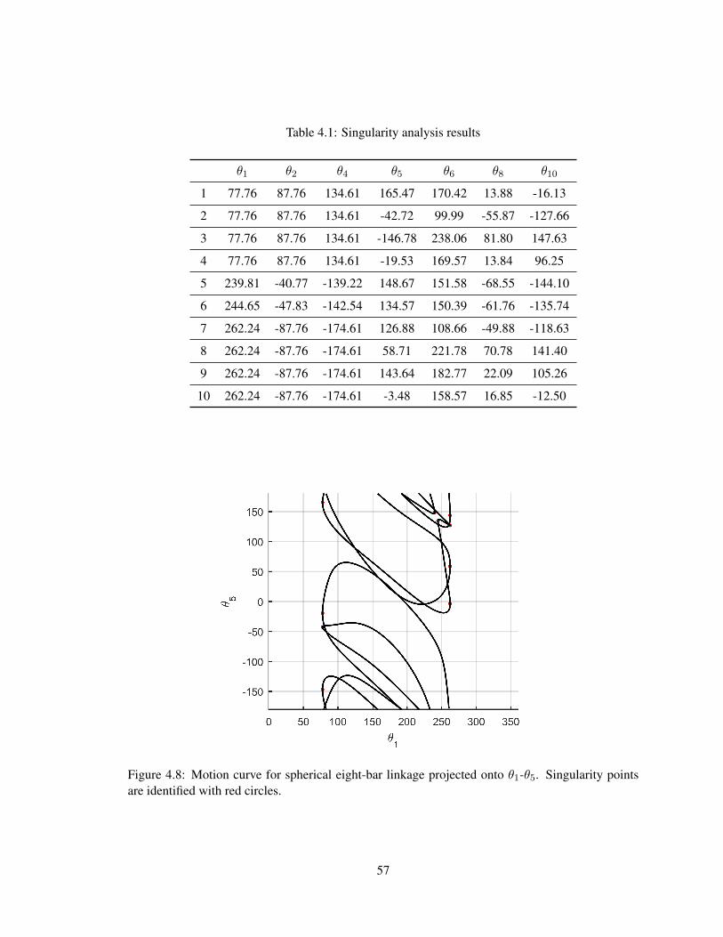
Table 4.1: Singularity analysis results
θ1 θ2 θ4 θ5 θ6 θ8 θ10
1 77.76 87.76 134.61 165.47 170.42 13.88 -16.13
2 77.76 87.76 134.61 -42.72 99.99 -55.87 -127.66
3 77.76 87.76 134.61 -146.78 238.06 81.80 147.63
4 77.76 87.76 134.61 -19.53 169.57 13.84 96.25
5 239.81 -40.77 -139.22 148.67 151.58 -68.55 -144.10
6 244.65 -47.83 -142.54 134.57 150.39 -61.76 -135.74
7 262.24 -87.76 -174.61 126.88 108.66 -49.88 -118.63
8 262.24 -87.76 -174.61 58.71 221.78 70.78 141.40
9 262.24 -87.76 -174.61 143.64 182.77 22.09 105.26
10 262.24 -87.76 -174.61 -3.48 158.57 16.85 -12.50
Figure 4.8: Motion curve for spherical eight-bar linkage projected onto θ1-θ5. Singularity pointsare identified with red circles.
57
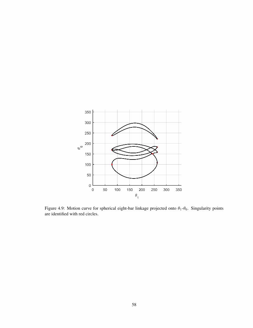
Figure 4.9: Motion curve for spherical eight-bar linkage projected onto θ1-θ6. Singularity pointsare identified with red circles.
58
CHAPTER V
SPHERICAL LINKAGE SYNTHESIS
Elements of SU(2) are now used to formulate and solve spherical linkage synthesis problems.
In motion guidance, a form of kinematic synthesis, the goal is to determine the physical parameters
of a linkage that is able to guide a task frame through a set of specified positions. In this chapter,
two formulations of the motion guidance synthesis equations are considered. The first approach
utilizes the idea that the angle between revolute joint axes connected by a link remains constant
as the mechanism moves between positions. This constraint is readily expressed using the dot
product. The dot product using SU(2) is employed in this chapter to solve the synthesis problem
for the spherical four-bar, spherical Watt I linkage, and an eight-bar spherical linkage. The second
approach utilizes the full loop closure equations. Although unnecessary when synthesizing four-
bars, the approach is presented due to its required use when generalizing to spatial mechanisms.
5.1 Four-Bar Synthesis Using Dot Product Approach
The two revolute joints on the input and output links of a spherical four-bar include one that
is fixed and one that moves. As shown in Fig. 5.1, the unit vector along the fixed joint axis is
G = (Gx, Gy, Gz) when specified in the fixed frame. The unit vector along the moving joint axis
is w = (wx, wy, wz) when specified relative to the moving frame attached to the floating link.
The desired locations of the floating link are specified with j orientations Qj ∈ SU(2). As
such, the coordinates of the moving axis are known relative to the fixed frame from W = QjwQ∗j
as in Eq. (2.25) for some position j of the motion of the floating link. With both axis vectors known
59

θ1
θ2
θ4
θ3
θa
αa
G1
W1
, w1
G2
W2
, w2
α12
αc
θc
θd
αd
α34
θb α
b
X
Y
Z
Figure 5.1: The parameters of the spherical four-bar identified for solving the synthesis problem.All frames are located in the center of the sphere but some are shown on the sphere’s surface forclarity.
in the fixed frame, a constant angle α is identified between them. Typically, using the dot product,
G ·Wj = |G||Wj |cos(α). As G and W are unit vectors, the right side of this expression is equal
at all orientations of the floating link and G ·Wj = G ·Wk for any two positions j and k. Recalling
Eq. (2.26)
1
2tr(QjwQ∗jG
∗)− 1
2tr(Q1wQ
∗1G∗) = 0 j = 2 . . . , 5 (5.1)
where w and G are stated as in Eq. (2.24). Four equations result that are homogeneous in the
variable groups 〈Gx, Gy, Gz〉 and 〈wx, wy, wz〉. This method was applied to the synthesis problem
in Table 5.1 originally solved in Brunnthaler et al. [4]. Bertini tracks six paths to the solutions shown
in Table 5.2.
60
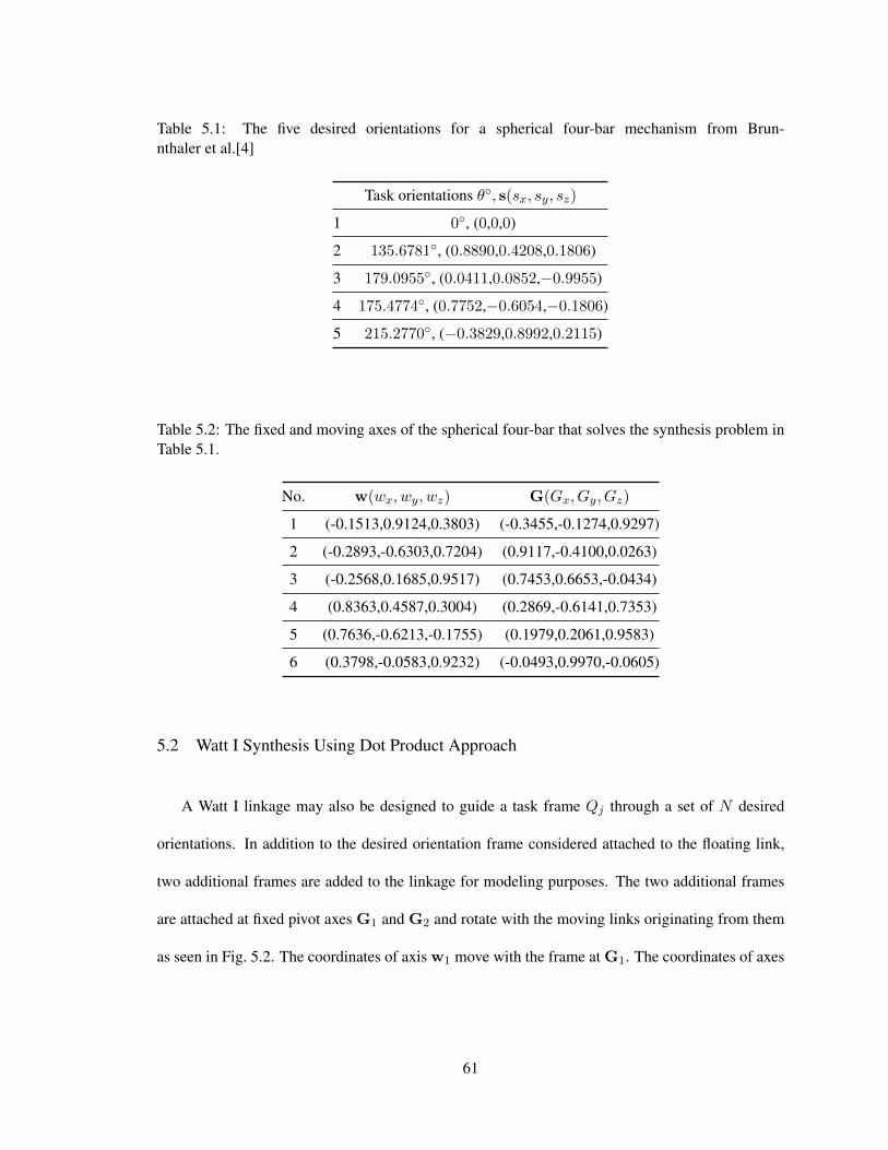
Table 5.1: The five desired orientations for a spherical four-bar mechanism from Brun-nthaler et al.[4]
Task orientations θ, s(sx, sy, sz)
1 0, (0,0,0)
2 135.6781, (0.8890,0.4208,0.1806)
3 179.0955, (0.0411,0.0852,−0.9955)
4 175.4774, (0.7752,−0.6054,−0.1806)
5 215.2770, (−0.3829,0.8992,0.2115)
Table 5.2: The fixed and moving axes of the spherical four-bar that solves the synthesis problem inTable 5.1.
No. w(wx, wy, wz) G(Gx, Gy, Gz)
1 (-0.1513,0.9124,0.3803) (-0.3455,-0.1274,0.9297)
2 (-0.2893,-0.6303,0.7204) (0.9117,-0.4100,0.0263)
3 (-0.2568,0.1685,0.9517) (0.7453,0.6653,-0.0434)
4 (0.8363,0.4587,0.3004) (0.2869,-0.6141,0.7353)
5 (0.7636,-0.6213,-0.1755) (0.1979,0.2061,0.9583)
6 (0.3798,-0.0583,0.9232) (-0.0493,0.9970,-0.0605)
5.2 Watt I Synthesis Using Dot Product Approach
A Watt I linkage may also be designed to guide a task frame Qj through a set of N desired
orientations. In addition to the desired orientation frame considered attached to the floating link,
two additional frames are added to the linkage for modeling purposes. The two additional frames
are attached at fixed pivot axes G1 and G2 and rotate with the moving links originating from them
as seen in Fig. 5.2. The coordinates of axis w1 move with the frame at G1. The coordinates of axes
61
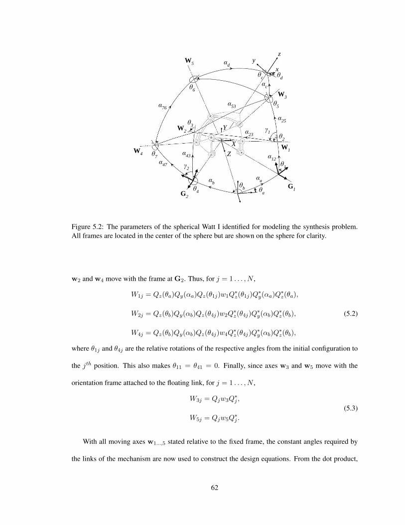
X
Y
Z W
1
G1
G2
W2
W4
W3
W5
θ1
θa
θb
αa α
b
θ4
α43
α
47
α12
γ1
θ2
θ5
αc
αd
θc θ
d
x y
z
θ6
α76
α23
θ
3
θ7
α25
γ2
α53
Figure 5.2: The parameters of the spherical Watt I identified for modeling the synthesis problem.All frames are located in the center of the sphere but are shown on the sphere for clarity.
w2 and w4 move with the frame at G2. Thus, for j = 1 . . . , N ,
W1j = Qz(θa)Qy(αa)Qz(θ1j)w1Q∗z(θ1j)Q
∗y(αa)Q
∗z(θa),
W2j = Qz(θb)Qy(αb)Qz(θ4j)w2Q∗z(θ4j)Q
∗y(αb)Q
∗z(θb),
W4j = Qz(θb)Qy(αb)Qz(θ4j)w4Q∗z(θ4j)Q
∗y(αb)Q
∗z(θb),
(5.2)
where θ1j and θ4j are the relative rotations of the respective angles from the initial configuration to
the jth position. This also makes θ11 = θ41 = 0. Finally, since axes w3 and w5 move with the
orientation frame attached to the floating link, for j = 1 . . . , N ,
W3j = Qjw3Q∗j ,
W5j = Qjw5Q∗j .
(5.3)
With all moving axes w1...,5 stated relative to the fixed frame, the constant angles required by
the links of the mechanism are now used to construct the design equations. From the dot product,
62
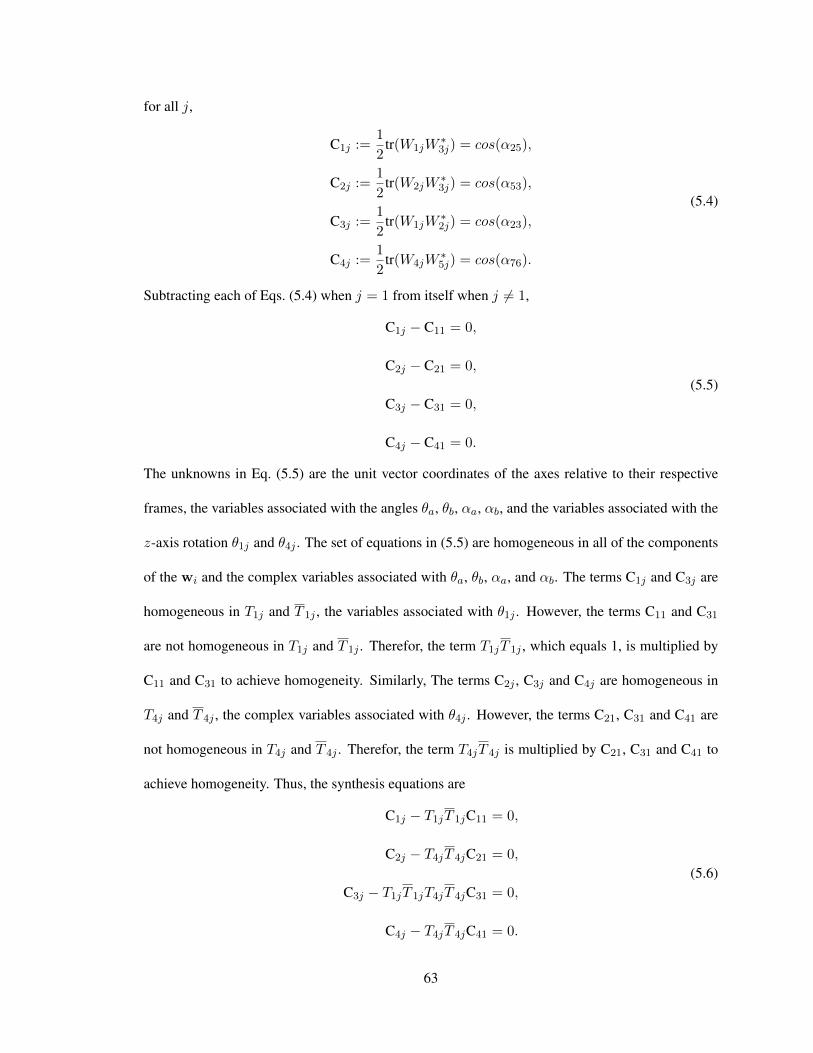
for all j,
C1j :=1
2tr(W1jW
∗3j) = cos(α25),
C2j :=1
2tr(W2jW
∗3j) = cos(α53),
C3j :=1
2tr(W1jW
∗2j) = cos(α23),
C4j :=1
2tr(W4jW
∗5j) = cos(α76).
(5.4)
Subtracting each of Eqs. (5.4) when j = 1 from itself when j 6= 1,
C1j − C11 = 0,
C2j − C21 = 0,
C3j − C31 = 0,
C4j − C41 = 0.
(5.5)
The unknowns in Eq. (5.5) are the unit vector coordinates of the axes relative to their respective
frames, the variables associated with the angles θa, θb, αa, αb, and the variables associated with the
z-axis rotation θ1j and θ4j . The set of equations in (5.5) are homogeneous in all of the components
of the wi and the complex variables associated with θa, θb, αa, and αb. The terms C1j and C3j are
homogeneous in T1j and T 1j , the variables associated with θ1j . However, the terms C11 and C31
are not homogeneous in T1j and T 1j . Therefor, the term T1jT 1j , which equals 1, is multiplied by
C11 and C31 to achieve homogeneity. Similarly, The terms C2j , C3j and C4j are homogeneous in
T4j and T 4j , the complex variables associated with θ4j . However, the terms C21, C31 and C41 are
not homogeneous in T4j and T 4j . Therefor, the term T4jT 4j is multiplied by C21, C31 and C41 to
achieve homogeneity. Thus, the synthesis equations are
C1j − T1jT 1jC11 = 0,
C2j − T4jT 4jC21 = 0,
C3j − T1jT 1jT4jT 4jC31 = 0,
C4j − T4jT 4jC41 = 0.
(5.6)
63
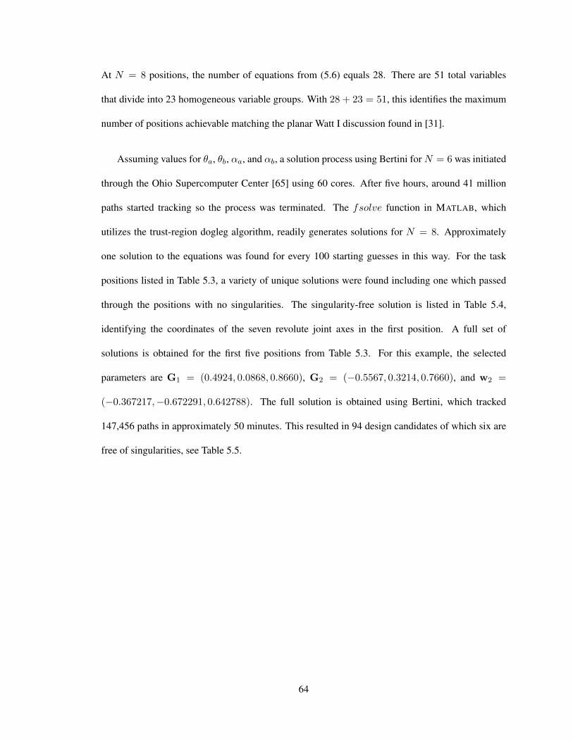
At N = 8 positions, the number of equations from (5.6) equals 28. There are 51 total variables
that divide into 23 homogeneous variable groups. With 28 + 23 = 51, this identifies the maximum
number of positions achievable matching the planar Watt I discussion found in [31].
Assuming values for θa, θb, αa, and αb, a solution process using Bertini forN = 6 was initiated
through the Ohio Supercomputer Center [65] using 60 cores. After five hours, around 41 million
paths started tracking so the process was terminated. The fsolve function in MATLAB, which
utilizes the trust-region dogleg algorithm, readily generates solutions for N = 8. Approximately
one solution to the equations was found for every 100 starting guesses in this way. For the task
positions listed in Table 5.3, a variety of unique solutions were found including one which passed
through the positions with no singularities. The singularity-free solution is listed in Table 5.4,
identifying the coordinates of the seven revolute joint axes in the first position. A full set of
solutions is obtained for the first five positions from Table 5.3. For this example, the selected
parameters are G1 = (0.4924, 0.0868, 0.8660), G2 = (−0.5567, 0.3214, 0.7660), and w2 =
(−0.367217,−0.672291, 0.642788). The full solution is obtained using Bertini, which tracked
147,456 paths in approximately 50 minutes. This resulted in 94 design candidates of which six are
free of singularities, see Table 5.5.
64

Table 5.3: Eight task orientations for synthesizing a Watt I spherical mechanism.
Task orientations θ, s(sx, sy, sz)
1 80.6372, (−0.8884,0.4463,−0.1079)
2 84.5098, (−0.9375,0.3475,−0.0165)
3 82.7674, (−0.9496 ,0.3124,−0.0241)
4 80.8227, (−0.9531 ,0.2992,−0.0457)
5 76.4885, (−0.9494 ,0.2934,−0.1123)
6 65.4334, (−0.7797 ,0.4604,−0.4244)
7 68.1438, (−0.7291 ,0.5768,−0.3684)
8 70.9738, (−0.7664 ,0.5638,−0.3080)
Table 5.4: A singularity-free solution for the eight orientations with axis coordinates at the firstposition.
Axis Solution
G1 (0.4924,0.0868,0.8660)
G2 (-0.5567,0.3214,0.7660)
W1 (0.7185,0.1812,0.6715)
W2 (0.2219,0.6482,0.7284)
W3 (0.5887,0.5797,0.5634)
W4 (-0.4412,0.7478,0.4962)
W5 (0.0379,0.9964,0.0760)
65
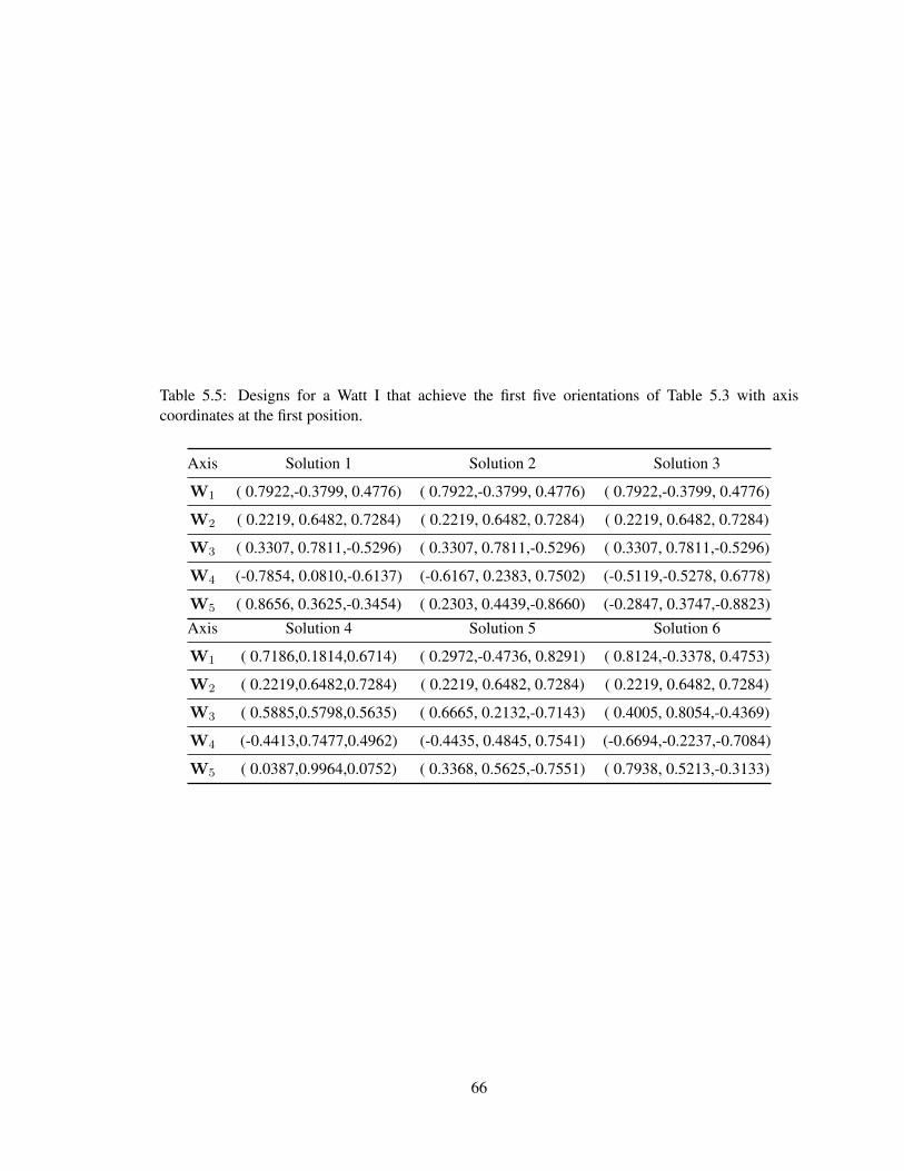
Table 5.5: Designs for a Watt I that achieve the first five orientations of Table 5.3 with axiscoordinates at the first position.
Axis Solution 1 Solution 2 Solution 3
W1 ( 0.7922,-0.3799, 0.4776) ( 0.7922,-0.3799, 0.4776) ( 0.7922,-0.3799, 0.4776)
W2 ( 0.2219, 0.6482, 0.7284) ( 0.2219, 0.6482, 0.7284) ( 0.2219, 0.6482, 0.7284)
W3 ( 0.3307, 0.7811,-0.5296) ( 0.3307, 0.7811,-0.5296) ( 0.3307, 0.7811,-0.5296)
W4 (-0.7854, 0.0810,-0.6137) (-0.6167, 0.2383, 0.7502) (-0.5119,-0.5278, 0.6778)
W5 ( 0.8656, 0.3625,-0.3454) ( 0.2303, 0.4439,-0.8660) (-0.2847, 0.3747,-0.8823)Axis Solution 4 Solution 5 Solution 6
W1 ( 0.7186,0.1814,0.6714) ( 0.2972,-0.4736, 0.8291) ( 0.8124,-0.3378, 0.4753)
W2 ( 0.2219,0.6482,0.7284) ( 0.2219, 0.6482, 0.7284) ( 0.2219, 0.6482, 0.7284)
W3 ( 0.5885,0.5798,0.5635) ( 0.6665, 0.2132,-0.7143) ( 0.4005, 0.8054,-0.4369)
W4 (-0.4413,0.7477,0.4962) (-0.4435, 0.4845, 0.7541) (-0.6694,-0.2237,-0.7084)
W5 ( 0.0387,0.9964,0.0752) ( 0.3368, 0.5625,-0.7551) ( 0.7938, 0.5213,-0.3133)
66
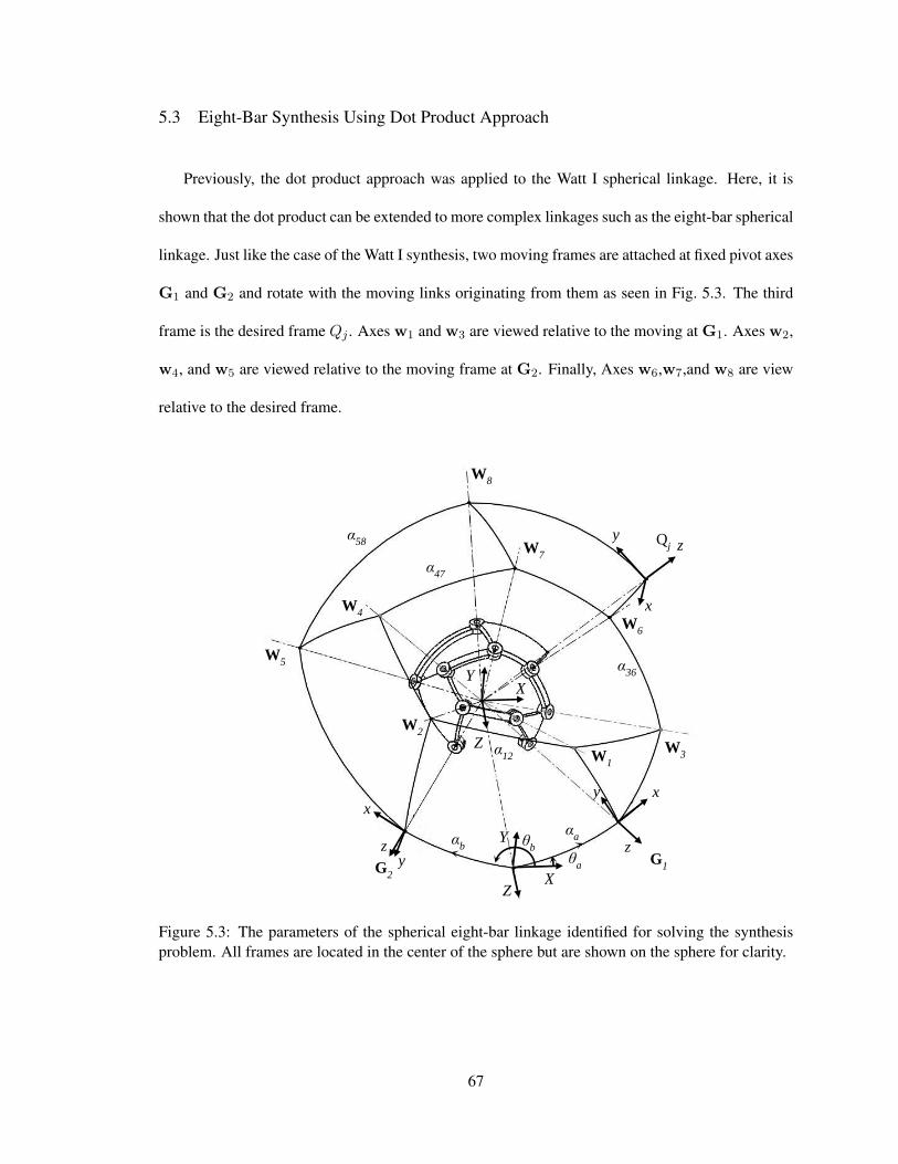
5.3 Eight-Bar Synthesis Using Dot Product Approach
Previously, the dot product approach was applied to the Watt I spherical linkage. Here, it is
shown that the dot product can be extended to more complex linkages such as the eight-bar spherical
linkage. Just like the case of the Watt I synthesis, two moving frames are attached at fixed pivot axes
G1 and G2 and rotate with the moving links originating from them as seen in Fig. 5.3. The third
frame is the desired frame Qj . Axes w1 and w3 are viewed relative to the moving at G1. Axes w2,
w4, and w5 are viewed relative to the moving frame at G2. Finally, Axes w6,w7,and w8 are view
relative to the desired frame.
G1
G2
W3 W
1
W2
W6
W7
W8
W4
W5
X Y
Z
X
Y
Z
Qj
x
y z
x
z
y x
z y
αa
αb
θa
θb
α36
α12
α47
α58
Figure 5.3: The parameters of the spherical eight-bar linkage identified for solving the synthesisproblem. All frames are located in the center of the sphere but are shown on the sphere for clarity.
67
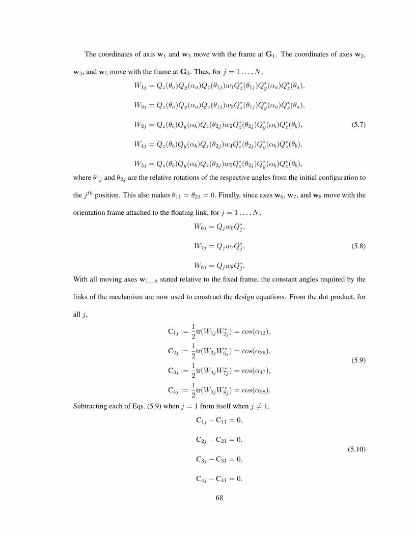
The coordinates of axis w1 and w3 move with the frame at G1. The coordinates of axes w2,
w4, and w5 move with the frame at G2. Thus, for j = 1 . . . , N ,
W1j = Qz(θa)Qy(αa)Qz(θ1j)w1Q∗z(θ1j)Q
∗y(αa)Q
∗z(θa),
W3j = Qz(θa)Qy(αa)Qz(θ1j)w3Q∗z(θ1j)Q
∗y(αa)Q
∗z(θa),
W2j = Qz(θb)Qy(αb)Qz(θ2j)w2Q∗z(θ2j)Q
∗y(αb)Q
∗z(θb),
W4j = Qz(θb)Qy(αb)Qz(θ2j)w4Q∗z(θ2j)Q
∗y(αb)Q
∗z(θb),
W5j = Qz(θb)Qy(αb)Qz(θ2j)w5Q∗z(θ2j)Q
∗y(αb)Q
∗z(θb),
(5.7)
where θ1j and θ2j are the relative rotations of the respective angles from the initial configuration to
the jth position. This also makes θ11 = θ21 = 0. Finally, since axes w6, w7, and w8 move with the
orientation frame attached to the floating link, for j = 1 . . . , N ,
W6j = Qjw6Q∗j ,
W7j = Qjw7Q∗j ,
W8j = Qjw8Q∗j .
(5.8)
With all moving axes w1...,8 stated relative to the fixed frame, the constant angles required by the
links of the mechanism are now used to construct the design equations. From the dot product, for
all j,
C1j :=1
2tr(W1jW
∗2j) = cos(α12),
C2j :=1
2tr(W3jW
∗6j) = cos(α36),
C3j :=1
2tr(W4jW
∗7j) = cos(α47),
C4j :=1
2tr(W5jW
∗8j) = cos(α58).
(5.9)
Subtracting each of Eqs. (5.9) when j = 1 from itself when j 6= 1,
C1j − C11 = 0,
C2j − C21 = 0,
C3j − C31 = 0,
C4j − C41 = 0.
(5.10)
68
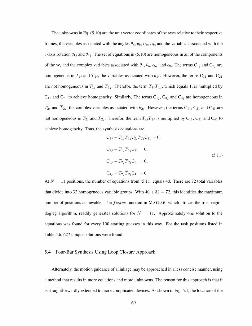
The unknowns in Eq. (5.10) are the unit vector coordinates of the axes relative to their respective
frames, the variables associated with the angles θa, θb, αa, αb, and the variables associated with the
z-axis rotation θ1j and θ2j . The set of equations in (5.10) are homogeneous in all of the components
of the wi and the complex variables associated with θa, θb, αa, and αb. The terms C1j and C2j are
homogeneous in T1j and T 1j , the variables associated with θ1j . However, the terms C11 and C21
are not homogeneous in T1j and T 1j . Therefor, the term T1jT 1j , which equals 1, is multiplied by
C11 and C21 to achieve homogeneity. Similarly, The terms C1j , C3j and C4j are homogeneous in
T2j and T 2j , the complex variables associated with θ2j . However, the terms C11, C31 and C41 are
not homogeneous in T2j and T 2j . Therefor, the term T2jT 2j is multiplied by C11, C31 and C41 to
achieve homogeneity. Thus, the synthesis equations are
C1j − T1jT 1jT2jT 2jC11 = 0,
C2j − T1jT 1jC21 = 0,
C3j − T2jT 2jC31 = 0,
C4j − T2jT 2jC41 = 0.
(5.11)
At N = 11 positions, the number of equations from (5.11) equals 40. There are 72 total variables
that divide into 32 homogeneous variable groups. With 40 + 32 = 72, this identifies the maximum
number of positions achievable. The fsolve function in MATLAB, which utilizes the trust-region
dogleg algorithm, readily generates solutions for N = 11. Approximately one solution to the
equations was found for every 100 starting guesses in this way. For the task positions listed in
Table 5.6, 627 unique solutions were found.
5.4 Four-Bar Synthesis Using Loop Closure Approach
Alternately, the motion guidance of a linkage may be approached in a less concise manner, using
a method that results in more equations and more unknowns. The reason for this approach is that it
is straightforwardly extended to more complicated devices. As shown in Fig. 5.1, the location of the
69
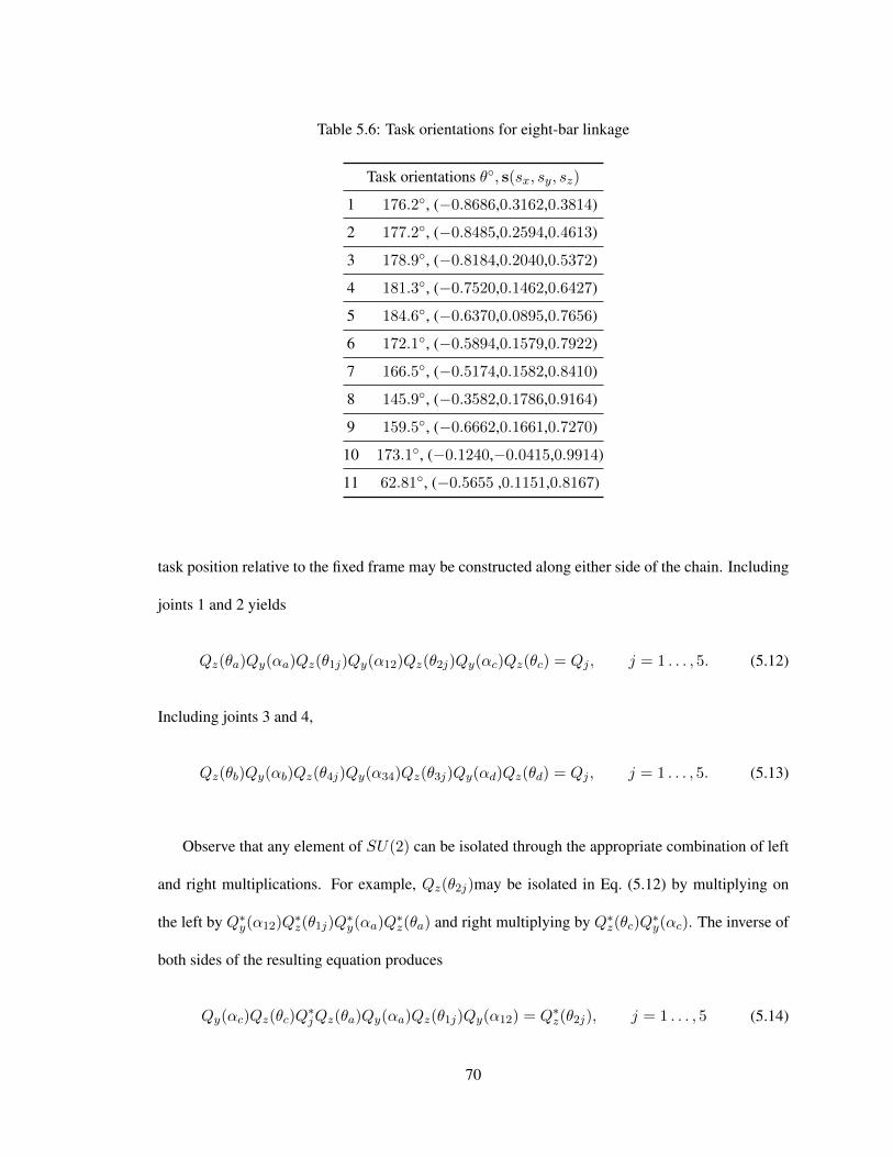
Table 5.6: Task orientations for eight-bar linkage
Task orientations θ, s(sx, sy, sz)
1 176.2, (−0.8686,0.3162,0.3814)
2 177.2, (−0.8485,0.2594,0.4613)
3 178.9, (−0.8184,0.2040,0.5372)
4 181.3, (−0.7520,0.1462,0.6427)
5 184.6, (−0.6370,0.0895,0.7656)
6 172.1, (−0.5894,0.1579,0.7922)
7 166.5, (−0.5174,0.1582,0.8410)
8 145.9, (−0.3582,0.1786,0.9164)
9 159.5, (−0.6662,0.1661,0.7270)
10 173.1, (−0.1240,−0.0415,0.9914)
11 62.81, (−0.5655 ,0.1151,0.8167)
task position relative to the fixed frame may be constructed along either side of the chain. Including
joints 1 and 2 yields
Qz(θa)Qy(αa)Qz(θ1j)Qy(α12)Qz(θ2j)Qy(αc)Qz(θc) = Qj , j = 1 . . . , 5. (5.12)
Including joints 3 and 4,
Qz(θb)Qy(αb)Qz(θ4j)Qy(α34)Qz(θ3j)Qy(αd)Qz(θd) = Qj , j = 1 . . . , 5. (5.13)
Observe that any element of SU(2) can be isolated through the appropriate combination of left
and right multiplications. For example, Qz(θ2j)may be isolated in Eq. (5.12) by multiplying on
the left by Q∗y(α12)Q∗z(θ1j)Q
∗y(αa)Q
∗z(θa) and right multiplying by Q∗z(θc)Q
∗y(αc). The inverse of
both sides of the resulting equation produces
Qy(αc)Qz(θc)Q∗jQz(θa)Qy(αa)Qz(θ1j)Qy(α12) = Q∗z(θ2j), j = 1 . . . , 5 (5.14)
70
The two off-diagonal terms in Eq. (5.14) are equations independent of the variables associated with
θ2j as those terms in Qz(θ2j) are both 0. Recall that an unknown angle has two variables associated
with it, the T and T like in Eq. (2.21). The matrixQz(θ3j) may be isolated similarly from Eq. (5.13)
and two more equations found independent of the variables associated with θ3j . Thus, for each
specified orientation Qj of the floating link, 4 equations are determined. A total of 20 equations
result for 5 given task orientations. All equations are homogeneous in the remaining unknowns.
Although it is now possible to attempt to solve this system as one set of equations, the symmetry
in Eqs. (5.12) and (5.13) is noted. Like the previous approach using the dot product, the set
of equations for one side of the mechanism will generate all solutions. Via this approach, the
values in table 5.2 are determined for the problem in table 5.1. Bertini tracked 3840 paths solving
the problem, a noted increase in paths versus the previous approach. Again, the redundancy of
formulating both sides of the kinematic loop was presented in order to move to identify a stepping
stone toward the more complicated mechanism in the following section.
5.5 Watt I Synthesis Using Loop Closure
As shown in Fig. 5.2, the Watt I linkage is used to guide a task frame Qj through a set of
orientations. The 16 physical parameters sought to solve the design problem include the fixed joint
locations in the fixed frame, θa, θb, αa, αb, the location of the outermost revolute joints connected
to the moving frame, θc, θd, αc, αd, and the angular link lengths of the other members of the
mechanism, α12, α23, α25, α43, α47, α76, γ1, γ2. Similar to the four-bar, potential synthesis
equations are generated by determining the location of the task position relative to the fixed frame
along either side of the chain. For the side that include joint axes G1, W1, and W3,
Qz(θa)Qy(αa)Qz(θ1j)Qy(α12)Qz(θ2j − γ1)Qy(α25)Qz(θ5j)
Qy(αc)Qz(θc) = Qj , j = 1 . . . , N.
(5.15)
71

For the side that includes joint axes G2, W4, and W6,
Qz(θb)Qy(αb)Qz(θ4j + γ2)Qy(α47)Qz(θ7j)Qy(α76)Qz(θ6j)
Qy(αd)Qz(θd) = Qj , j = 1 . . . , N.
(5.16)
From the inner loop,
Qz(θb)Qy(αb)Qz(θ4j)Qy(α43)Qz(θ3j) = Qz(θa)Qy(αa)
Qz(θ1j)Qy(α12)Qz(θ2j)Qy(α23), j = 1 . . . , N.
(5.17)
From each loop one angle may be isolated and eliminated as in the process in Eqs. (5.12) and (5.14).
The joint angles that appear in only one loop are eliminated: θ3, θ5, and θ6. This reduces the joint
variables present in the synthesis equations to θ1, θ2, θ4, and θ7. As noted previously, the elimination
process results in two homogeneous equations, per loop, per position. Since there are three loop
equations, the total number of equations is six per single orientation. The system becomes square at
8 positions, matching other Watt I synthesis discussions in the literature namely what is presented
in [31]. Again using the Ohio Supercomputer Center, a solution process for N = 8 was initiated
using 240 cores. No count of the paths was generated in 95 hours and the process was terminated.
Like the previous method, the fsolve function in MATLAB readily generates solutions for N = 8
at approximately the same likelihood, 1 in 100, for starting guesses.
5.6 Discussion
As an initial exploration of using SU(2) in a variety of kinematic challenges, several
observations can be made. For modeling, SU(2) provides a formalism for rotations that is efficient
and compact. Rotation are expressed using only two complex numbers in a matrix with only four
entries. With so few entries to consider, the equation selection tends to be obvious. Although
it is not necessarily difficult on SO(3) where there are more relationships to select from, there
are essentially no decisions to be made when using SU(2) as there are so few relationships.
Moreover, the resulting equations, whether being used for analysis or design, are homogeneous.
72

With all parameters and variables being complex numbers, these equations readily import into the
tools of numerical algebraic geometry, though formatting other approaches for this does not prove
cumbersome. Although no strict comparisons to SO(3) are made in this work, some problems were
solved to compare to this work in SU(2). Many problems were formulated such that the number of
solutions (the m-homogeneous Bezout number) was the same for two approaches. In a few specific
problems, the equations on SO(3) would solve faster when using fsolve, but in many problems
when Bertini is used the systems would solve in approximately the same amount of time.
73
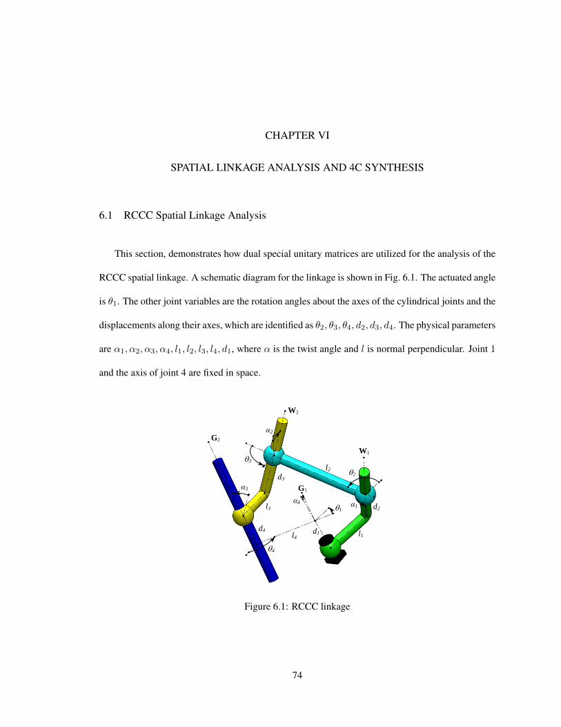
CHAPTER VI
SPATIAL LINKAGE ANALYSIS AND 4C SYNTHESIS
6.1 RCCC Spatial Linkage Analysis
This section, demonstrates how dual special unitary matrices are utilized for the analysis of the
RCCC spatial linkage. A schematic diagram for the linkage is shown in Fig. 6.1. The actuated angle
is θ1. The other joint variables are the rotation angles about the axes of the cylindrical joints and the
displacements along their axes, which are identified as θ2, θ3, θ4, d2, d3, d4. The physical parameters
are α1, α2, α3, α4, l1, l2, l3, l4, d1, where α is the twist angle and l is normal perpendicular. Joint 1
and the axis of joint 4 are fixed in space.
1
G1
d1 l1
l2
l3
l4
α1
α2
α3
α4
W1
W2
G2
d2
d3
d4
2
3
4
Figure 6.1: RCCC linkage
74
6.1.1 RCCC Loop Closure and Forward Kinematics
In a process similar to that of analyzing the spherical linkage, The loop closure equations for this
mechanism are constructed using rotations, describing the loop closure. To facilitate the variables
elimination, the loop is written starting at W2,
Qz(θ3, d3)Qx(α3, l3)Qz(θ4, d4)Qx(α4, l4)Qz(θ1, d1)Qx(α1, l1)Qz(θ2, d2)Qx(α2, l2) = I, (6.1)
To reduce the system, θ3, and d3 are eliminated by pre-multiplying Eq. (6.1) by Q−1z (θ3, d3),
Qx(α3, l3)Qz(θ4, d4)Qx(α4, l4)Qz(θ1, d1)Qx(α1, l1)Qz(θ2, d2)Qx(α2, l2) = Q−1z (θ3, d3), (6.2)
and observing that the off-diagonal terms from the rotation and the dual part in Q−1z (θ3, d3) are zero.
The off-diagonal zero elements of Eq. (6.2) are homogeneous polynomials in the variable groups
〈T2, T 2〉 and 〈T4, T 4〉, representing θ2 and θ4, respectively. In addition to 〈d2〉, 〈d4〉 variable groups.
With θ1 actuated, its value is known. Using the Bertini, two solutions are obtained for each value of
the input link. Solutions are substituted in Eq. (6.2) and those that correspond to a mechanism meet
the condition that the diagonal elements on the right side of Eq. (6.2) are complex conjugate.
6.1.2 RCCC Singularity Points and Motion Curve
The RCCC linkage has a spherical image where the twist angle of the RCCC equal the link
lengths of the spherical linkage. In this example, The links of the spherical linkage presented in
Chapter. IV are the twist angle of the RCCC. The Numerical values are α1 = 90o, α2 = 90o, α3 =
45o, α4 = 72o, l1 = 5, l2 = 2.3, l3 = 4, l4 = 4.37, d1 = −3. When determining singularities the
input angle is considered to be a variable. The singularity condition is determined from the velocity
expression presented in Eq. (2.34). In this analysis, rearranging Eq. (6.1) leads to
Qz(θ2, d2)Qx(α2, l2)Qz(θ3, d3)Qx(α3, l3) = Q−1x (α1, l1)Q−1z (θ1, d1)Q
−1x (α4, l4)Q
−1z (θ4, d4),
(6.3)
75
The jacobian from which the singularity condition is determined is found via the use of the screw
method. As it was done in the previous sections, the following screw matrices are obtained.
Ωθ2 =Ωz(θ2),
Ωd2 =Ωz(d2),
Ωθ3 =Qz(θ2, d2)Qx(α2, l2)Ωz(θ3)Q
−1x (α2, l2)Q
−1z (θ2, d2),
Ωd3 =Qz(θ2, d2)Qx(α2, l2)Ωz(d3)Q
−1x (α2, l2)Q
−1z (θ2, d2),
Ω1 =Q−1x (α1, l1)Ωz(θ1)Qx(α1, l1),
Ωθ4 =Q−1x (α1, l1)Q
−1z (θ1, d1)Q
−1x (α4, l4)Ωz(θ4)Qx(α4, l4)Qz(θ1, d1)Qx(α1, l1),
Ωd4 =Q−1x (α1, l1)Q
−1z (θ1, d1)Q
−1x (α4, l4)Ωz(d4)Qx(α4, l4)Qz(θ1, d1)Qx(α1, l1).
(6.4)
A set of screw vectors Ω1, Ωθ2, Ωd
2, Ωθ3, Ωd
3, Ωθ4, Ωd
4 is extracted from the screw matrices.
Each of the screw vectors is 6 × 1, three elements of this vector are extracted from the rotational
part and another three are extracted from the dual part. The resulting jacobian is a 6× 6 in the form
J =
[D1 0D3 D4
], (6.5)
Where D1 and D4 are 3 × 3 identical matrices that are equal to the jocobian of the spherical
image. Considering the structure of the jacobian, it is noticed that the determinant of such matrix
equals zero if the determinant of D1 or D4 equals zero. Based on the previous fact, it can
be said that the singularity condition is independent of the displacements along the cylindrical
joints axes. The singularity of the RCCC occurs at the same value of the spherical image at
(θ1, θ4) = (41.97, 108.96), (138.03, 251.04), (221.97, 108.96), (318.03, 251.04). The motion
curve that relates the input angle to the output angle is identical to that of the spherical image.
The cylindrical joint displacement can go to infinity at singular configuration as shown in Fig. 6.2.
76
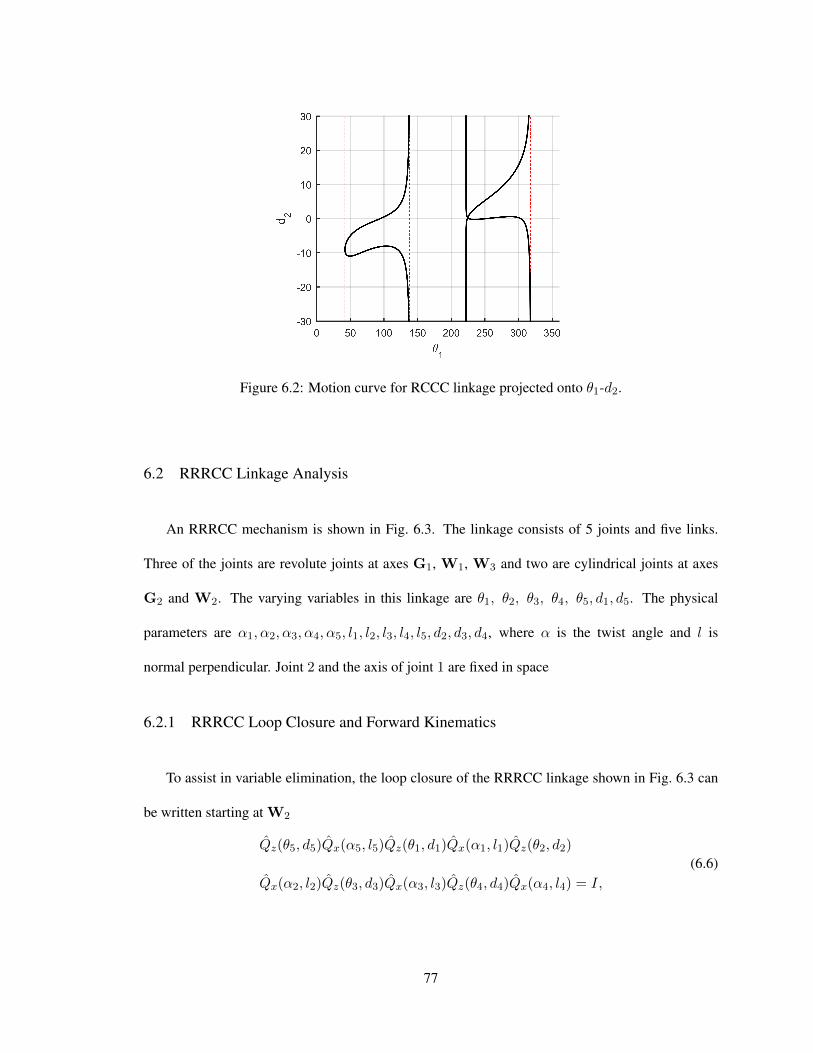
Figure 6.2: Motion curve for RCCC linkage projected onto θ1-d2.
6.2 RRRCC Linkage Analysis
An RRRCC mechanism is shown in Fig. 6.3. The linkage consists of 5 joints and five links.
Three of the joints are revolute joints at axes G1, W1, W3 and two are cylindrical joints at axes
G2 and W2. The varying variables in this linkage are θ1, θ2, θ3, θ4, θ5, d1, d5. The physical
parameters are α1, α2, α3, α4, α5, l1, l2, l3, l4, l5, d2, d3, d4, where α is the twist angle and l is
normal perpendicular. Joint 2 and the axis of joint 1 are fixed in space
6.2.1 RRRCC Loop Closure and Forward Kinematics
To assist in variable elimination, the loop closure of the RRRCC linkage shown in Fig. 6.3 can
be written starting at W2
Qz(θ5, d5)Qx(α5, l5)Qz(θ1, d1)Qx(α1, l1)Qz(θ2, d2)
Qx(α2, l2)Qz(θ3, d3)Qx(α3, l3)Qz(θ4, d4)Qx(α4, l4) = I,
(6.6)
77
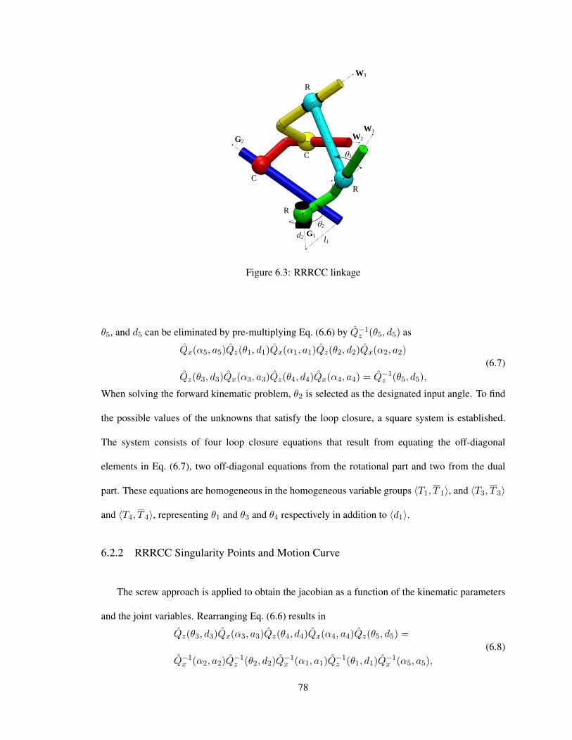
1
2
3
l1 d1
d2
R
R
R
C
C
G2
G1
W1
W3
W2
Figure 6.3: RRRCC linkage
θ5, and d5 can be eliminated by pre-multiplying Eq. (6.6) by Q−1z (θ5, d5) as
Qx(α5, a5)Qz(θ1, d1)Qx(α1, a1)Qz(θ2, d2)Qx(α2, a2)
Qz(θ3, d3)Qx(α3, a3)Qz(θ4, d4)Qx(α4, a4) = Q−1z (θ5, d5),
(6.7)
When solving the forward kinematic problem, θ2 is selected as the designated input angle. To find
the possible values of the unknowns that satisfy the loop closure, a square system is established.
The system consists of four loop closure equations that result from equating the off-diagonal
elements in Eq. (6.7), two off-diagonal equations from the rotational part and two from the dual
part. These equations are homogeneous in the homogeneous variable groups 〈T1, T 1〉, and 〈T3, T 3〉
and 〈T4, T 4〉, representing θ1 and θ3 and θ4 respectively in addition to 〈d1〉.
6.2.2 RRRCC Singularity Points and Motion Curve
The screw approach is applied to obtain the jacobian as a function of the kinematic parameters
and the joint variables. Rearranging Eq. (6.6) results in
Qz(θ3, d3)Qx(α3, a3)Qz(θ4, d4)Qx(α4, a4)Qz(θ5, d5) =
Q−1x (α2, a2)Q−1z (θ2, d2)Q
−1x (α1, a1)Q
−1z (θ1, d1)Q
−1x (α5, a5),
(6.8)
78
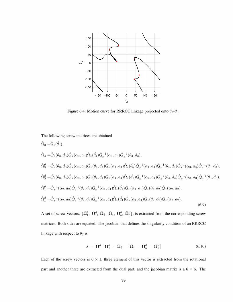
Figure 6.4: Motion curve for RRRCC linkage projected onto θ2-θ3.
The following screw matrices are obtained
Ω3 =Ωz(θ3),
Ω4 =Qz(θ3, d3)Qx(α3, a3)Ωz(θ4)Q−1x (α3, a3)Q
−1z (θ3, d3),
Ωθ5 =Qz(θ3, d3)Qx(α3, a3)Qz(θ4, d4)Qx(α4, a4)Ωz(θ5)Q
−1x (α4, a4)Q
−1z (θ4, d4)Q
−1x (α3, a3)Q
−1z (θ3, d3),
Ωd5 =Qz(θ3, d3)Qx(α3, a3)Qz(θ4, d4)Qx(α4, a4)Ωz(d5)Q
−1x (α4, a4)Q
−1z (θ4, d4)Q
−1x (α3, a3)Q
−1z (θ3, d3),
Ωθ1 =Q−1x (α2, a2)Q
−1z (θ2, d2)Q
−1x (α1, a1)Ωz(θ1)Qx(α1, a1)Qz(θ2, d2)Qx(α2, a2),
Ωd1 =Q−1x (α2, a2)Q
−1z (θ2, d2)Q
−1x (α1, a1)Ωz(d1)Qx(α1, a1)Qz(θ2, d2)Qx(α2, a2).
(6.9)
A set of screw vectors, Ωθ1, Ωd
1, Ω3, Ω4, Ωθ5, Ωd
5, is extracted from the corresponding screw
matrices. Both sides are equated. The jacobian that defines the singularity condition of an RRRCC
linkage with respect to θ2 is
J =[Ωθ
1 Ωd1 −Ω3 −Ω4 −Ωθ
5 −Ωd5
](6.10)
Each of the screw vectors is 6 × 1, three element of this vector is extracted from the rotational
part and another three are extracted from the dual part, and the jacobian matrix is a 6 × 6. The
79
determinant is added to the system from the forward kinematic along with a variable group 〈T2, T 2〉
that represents the input angle. The dimension for this example are α1 = 80o, l1 = 4, d2 = 0,
α2 = 30o, l2 = 2, d3 = 0, α3 = 15o, l3 = 5, d4 = 3, α4 = 40o, l4 = 3, α5 = 70o, and l5 = 5.
As shown on the motion curve Fig. 6.4, at these numerical values, singularities are encountered
at (θ2, θ3) = (−88.65, 79.06), (−50.62, 6.79),(−40.5, 104.8), (42.6, 24.82), (43.15,−100.57),
(68.48,−74.74). The motion curve of the RRRCC matches what is presented in [3].
6.3 4C Spatial Linkage Synthesis
In this section, SU(2) is used to solve the synthesis problem for the 4C linkage. The 4C linkage
is a closed loop with two degrees of freedom that is created by joining two CC chains. The spatial
CC chain consists of two C-joints linked together such that one of them moves on a fixed axis and
other moves on a moving axis. The end effector is attached to the joint on the moving axis. The
distance along the common normal and the twist angle between the two axes are constrained by the
geometry of the connecting link. Mathematically, this means that the dot product, between the two
axes remains constant as the linkage moves between positions as shown in Eq. (2.30) and Eq. (2.31).
The fixed axis of the CC chain is G = (G,G0) when specified in the fixed frame. The axis along
the moving joint is w = (w,w0) when specified relative to the moving frame. G0 = B ×G and
w0 = p × w. The point B is a a reference point on the fixed axis and p is the reference point
on the moving axis. The solution of the CC chain synthesis are the coordinates of the line along
G and w, represented by (Gx, Gy, Gz, G0x, G
0y, G
0z) and (wx, wy, wz, w
0x, w
0y, w
0z) respectively. As
the mechanism moves, the displacement of the end effector may be specified with given rotations
Q ∈ SU(2). As such, the coordinates of the moving axis are known in the fixed frame from
Wj = QjwQ−1j as in Eq. (2.29) for some position j of the end effector. With both axes known in
80
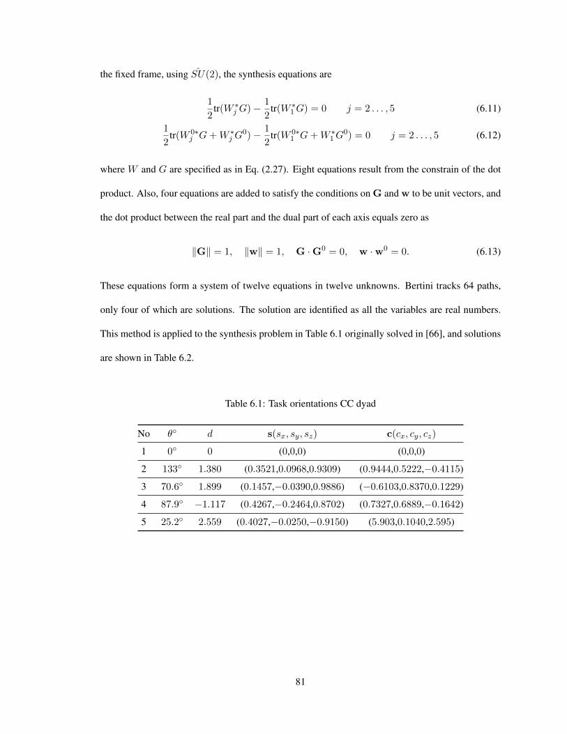
the fixed frame, using SU(2), the synthesis equations are
1
2tr(W ∗j G)− 1
2tr(W ∗1G) = 0 j = 2 . . . , 5 (6.11)
1
2tr(W 0∗
j G+W ∗j G0)− 1
2tr(W 0∗
1 G+W ∗1G0) = 0 j = 2 . . . , 5 (6.12)
where W and G are specified as in Eq. (2.27). Eight equations result from the constrain of the dot
product. Also, four equations are added to satisfy the conditions on G and w to be unit vectors, and
the dot product between the real part and the dual part of each axis equals zero as
‖G‖ = 1, ‖w‖ = 1, G ·G0 = 0, w ·w0 = 0. (6.13)
These equations form a system of twelve equations in twelve unknowns. Bertini tracks 64 paths,
only four of which are solutions. The solution are identified as all the variables are real numbers.
This method is applied to the synthesis problem in Table 6.1 originally solved in [66], and solutions
are shown in Table 6.2.
Table 6.1: Task orientations CC dyad
No θ d s(sx, sy, sz) c(cx, cy, cz)
1 0 0 (0,0,0) (0,0,0)
2 133 1.380 (0.3521,0.0968,0.9309) (0.9444,0.5222,−0.4115)
3 70.6 1.899 (0.1457,−0.0390,0.9886) (−0.6103,0.8370,0.1229)
4 87.9 −1.117 (0.4267,−0.2464,0.8702) (0.7327,0.6889,−0.1642)
5 25.2 2.559 (0.4027,−0.0250,−0.9150) (5.903,0.1040,2.595)
81
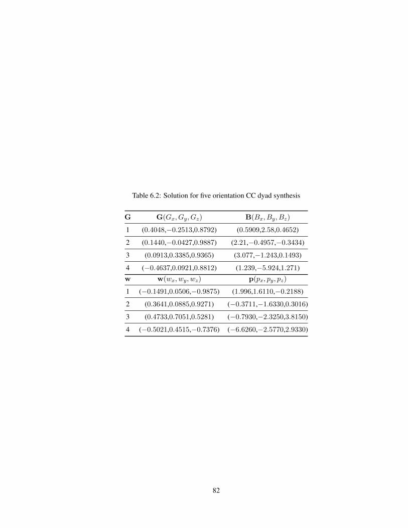
Table 6.2: Solution for five orientation CC dyad synthesis
G G(Gx, Gy, Gz) B(Bx, By, Bz)
1 (0.4048,−0.2513,0.8792) (0.5909,2.58,0.4652)
2 (0.1440,−0.0427,0.9887) (2.21,−0.4957,−0.3434)
3 (0.0913,0.3385,0.9365) (3.077,−1.243,0.1493)
4 (−0.4637,0.0921,0.8812) (1.239,−5.924,1.271)w w(wx, wy, wz) p(px, py, pz)
1 (−0.1491,0.0506,−0.9875) (1.996,1.6110,−0.2188)
2 (0.3641,0.0885,0.9271) (−0.3711,−1.6330,0.3016)
3 (0.4733,0.7051,0.5281) (−0.7930,−2.3250,3.8150)
4 (−0.5021,0.4515,−0.7376) (−6.6260,−2.5770,2.9330)
82

CHAPTER VII
CONCLUSIONS AND FUTURE WORK
7.1 Conclusion
This research presented a general method to construct a singularity trace for single DOF closed-
loop linkages. This method provides the ability to include prismatic along with revolute joints. The
singularity trace provides a convenient figure for observing the number of possible GIs, circuits,
and singularities for a given linkage as a design parameter is varied. As part of the process, the
forward kinematics, singularity points, critical points and motion curves were developed. Numerical
examples are provided to show the formulation applied to an inverted slider-crank and an Assur IV/3
mechanism.
The rotational part of a general displacement element of SU(2) is used to formulate equations
to solve analysis and synthesis problems for spherical linkages. Using the special unitary matrices
for the description of spatial displacement about a fixed point is efficient and compact. The rotation
matrix consists of only four entries, when expressed algebraically, the variable from a single rotation
are related by one constraint. The loop closure equations are linear homogeneous polynomials,
which are readily solved using Bertini. Since all the variable are homogeneous, there is no need to
include the constraint equations, these variables are declared as homogeneous variables in Bertini.
The use of this feature offers computational advantage. This formulation requires solving the two
off-diagonal equation from the loop matrix. Results viewed here can be extended to other spherical
linkages.
83
The synthesis of the spherical linkages presented in chapter V, of the dissertation, presented two
approach to formulate the synthesis questions. The first approach utilizes the loop closure equations
and the second approach employ the dot product as geometric constraints between two moving
links. For the spherical Watt I, as an example, the loop closure approach requires the use of four
joint angles from each position with six equations, while the dot product approach requires only two
joint angles from each position with four equations. Equations from the loop closure approach are
linear and homogeneous. Equations from the dot product approach are quadratic, and can be made
homogeneous. Both formulations of the synthesis equations are verified by finding solutions for the
system using fsolve function in MATLAB. On Bertini, the dot product has less joint variables and
equations, thus, it requires less number of paths to be tracked. Both formulations are flexible and it
allows the user to vary design parameters to achieve up to eight positions for the Watt linkage and
five for the four-bar. A full set of solutions using Bertini is obtained for the synthesis of the five
positions of Watt I linkage, where 147,456 paths are tracked in a bout 50 minutes using 60 cores
computer. Finally, the dot product approach is applied to an eight-bar linkage, which is able to pass
through eleven positions. Formulating the synthesis problem of the eight-bar spherical linkage is
very similar to that of the Watt I. Each position introduce four equations and two joint variables.
The eight-bar example is also verified by finding large set of solutions for the full system of eleven
position using fsolve function in MATLAB.
A general displacement element of SU(2) is used to analyze and synthesize spatial linages that
contains revolute joints and cylindrical joints such as RCCC and RRRCC linkages. Like the case of
spherical linkages, the analysis process including solving the off-diagonal terms of the loop closure
equations. The two off-diagonal polynomial from the rotational part and dual part are needed.
These equations are homogeneous and linear in the joint angles parameters, but not in terms of
displacement along the axis of rotation. Bertini, allows the combination of homogeneous variable,
84
non-homogeneous variable groups in the same input file. Also, Loop closure equations along with
another equation that is derived from the determinant of the Jocobian are used to calculate singular
configurations. In addition, it was shown that the dot product of SU(2) can be utilized to solve
synthesis of 4C linkage.
7.2 Future Work
Work developed here can find some applications in manufacturing to possibly tackle a real world
problem. One application could be incorporating methods presented in this work to build a software
to analyze and synthesis spatial linkages. Building such software will help design engineers to
visualize the motion of the linkage without the need to build a prototype. The lack of tools to design
spatial linkage pushes the design engineers to find solutions to design problems through the use
of planar linkages or open-chain robots. The design software could have the governing equation
for a specified linkage presented to a solver, and then results from the solver are drawn on a solid
modeler. This allows designers to synthesize or analyze spatial linkages in a timely manner and
obtain a full insight of the devices behavior while still in a computer modeled form. These tools
open up the possibilities for spatial linkages to be incorporated into many products. The ultimate
goal is to provide alternative solutions that are more efficient, more reliable and cost less.
Developing methods to further reduce the size and the order of the synthesis problem of
spherical linkages to generate a full solution set to the eight positions synthesis. As the polynomial
solvers continue to improve, the possibility of solving such problems still exist. Generating a full
solution set provides many possible design candidate linkages, which increase the chance of finiding
a single solution that pass through all position in the desired orders with no singularities. Large
number of theses linkages will suffer from branch defect, order defect, singularities.
85
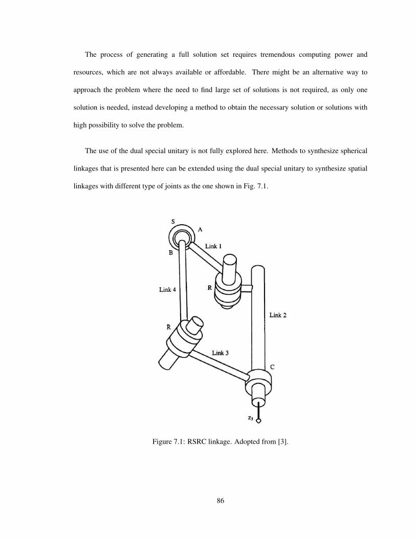
The process of generating a full solution set requires tremendous computing power and
resources, which are not always available or affordable. There might be an alternative way to
approach the problem where the need to find large set of solutions is not required, as only one
solution is needed, instead developing a method to obtain the necessary solution or solutions with
high possibility to solve the problem.
The use of the dual special unitary is not fully explored here. Methods to synthesize spherical
linkages that is presented here can be extended using the dual special unitary to synthesize spatial
linkages with different type of joints as the one shown in Fig. 7.1.
Figure 7.1: RSRC linkage. Adopted from [3].
86
REFERENCES
[1] A. P. Murray and F. Pierrot, “Design of a high-speed spherical four-bar mechanism for use ina motion common in assembly processes,” in ASME 2007 International Design EngineeringTechnical Conferences and Computers and Information in Engineering Conference. Ameri-can Society of Mechanical Engineers, 2007, pp. 511–518.
[2] M. W. Spong and M. Vidyasagar, Robot dynamics and control. John Wiley & Sons, 2008.
[3] D. E. Foster and R. J. Cipra, “Assembly configurations of spatial single-loop single-dofmechanisms,” Journal of Mechanical Design, vol. 131, no. 10, p. 101002, 2009.
[4] K. Brunnthaler, H.-P. Schrocker, and M. Husty, “Synthesis of spherical four-bar mechanismsusing spherical kinematic mapping,” in Advances in Robot Kinematics. Springer,Netherlands, 2006, pp. 377–384.
[5] V. Venkataramanujam and P. Larochelle, “Analysis of planar reconfigurable motion genera-tors,” in ASME 2014 International Design Engineering Technical Conferences and Computersand Information in Engineering Conference. American Society of Mechanical Engineers,2014.
[6] M. T. Das and L. C. Dulger, “Mathematical modelling, simulation and experimentalverification of a scara robot,” Simulation Modelling Practice and Theory, vol. 13, no. 3, pp.257–271, 2005.
[7] P. Larochelle and V. Venkataramanujam, “A new concept for reconfigurable planar motiongenerators,” in ASME 2013 International mechanical engineering congress and exposition.American Society of Mechanical Engineers, 2013.
[8] D. H. Myszka, A. P. Murray, and C. W. Wampler, “Computing the branches, singularity trace,and critical points of single degree-of-freedom, closed-loop linkages,” Journal of Mechanismsand Robotics, vol. 6, no. 7, p. 011006, 2014.
[9] L. Li, D. H. Myszka, A. P. Murray, and C. W. Wampler, “Using the singularity trace tounderstand linkage motion characteristics,” in Proceedings of IDETC/CIE 2013, Portland,Oregon, USA, August 2013, p. 13244.
[10] R. L. Norton, Design of Machinery: An Introduction to the Synthesis and Analysis ofMechanisms and Machines, 2nd ed. New York: McGraw-Hill, 1999.
87
[11] A. G. Erdman, G. N. Sandor, and S. Kota, Mechanism Design: Analysis and Synthesis, 4th ed.New Jersey: Prentice Hall, 2001, vol. 1.
[12] P. Kovacs and G. Hommel, “On the tangent-half-angle substitution,” in ComputationalKinematics, J. Angeles, Ed. Norwell, MA: Kluwer Academic Publishers, 1993, pp. 27–39.
[13] J. M. Porta, L. Ros, T. Creemers, and F. Thomas, “Box approximations of planar linkageconfiguration spaces,” Journal of Mechanical Design, vol. 129, no. 4, pp. 397–405, 2007.
[14] C. W. Wampler, “Solving the kinematics of planar mechanisms,” Journal of MechanicalDesign, vol. 121, no. 3, pp. 387–391, 1999.
[15] R. D. Gregorio, “A novel geometric and analytic technique for the singularity analysis of one-dof planar mechanisms,” Mechanism and Machine Theory, vol. 42, pp. 1462–1483, February2007.
[16] C. Gosselin and J. Angeles, “Singularity analysis of closed-loop kinematic chains,” IEEETransactions on Robotics and Automation, vol. 6, no. 3, pp. 281–290, 1990.
[17] T. R. Chase and J. A. Mirth, “Circuits and branches of single-degree-of-freedom planarlinkages,” Journal of Mechanical Design, vol. 115, no. 2, pp. 223–230, 1993.
[18] A. P. Murray, M. L. Turner, and D. T. Martin, “Synthesizing single dof linkages via transitionlinkage identification,” Journal of Mechanical Design, vol. 130, p. 022301, February 2008.
[19] P. Larochelle and V. Venkataramanujam, “A new concept for reconfigurable planar motiongenerators,” in Proceedings of IMECE2013, San Diego,California, USA, November 2013, p.62571.
[20] P. Larochelle and V. Venkatesh, “Analysis of planar reconfigurable motion generators,” inProceedings of IDETC/CIE 2014, Buffalo,New York, USA, August 2014.
[21] D. C. Tao, Applied Linkage Synthesis. MA.: Addison-Wesley,Reading, 1964.
[22] T. Chuenchom and S. Kota, “Synthesis of programmable mechanisms using adjustable dyads,”Journal of Mechanical Design, vol. 119, no. 2, pp. 232–237, 2007.
[23] J. J. Uicker, B. Ravani, and P. N. Sheth, Matrix methods in the design analysis of mechanismsand multibody systems. Cambridge University Press, 2013.
[24] J. Angeles, G. Hommel, and P. Kovacs, Computational kinematics, ser. Solid mechanics andits applications. Dordrecht: Kluwer Academic Publishers, 1993, vol. 28.
[25] W. C. Wampler, “Displacement analysis of spherical mechanisms having three or fewer loops,”Journal of Mechanical Design, vol. 126, pp. 93–100, 2004.
[26] A. Dhingra, A. Almadi, and D. Kohli, “Closed-form displacement analysis of 8, 9 and 10-link mechanisms: Part i: 8-link 1-dof mechanisms,” Mechanism and Machine Theory, vol. 35,no. 6, pp. 821–850, 2000.
88
[27] C. Gosselin, J. Sefrioui, and M. J. Richard, “On the direct kinematics of spherical three-degree-of-freedom parallel manipulators of general architecture,” Journal of Mechanical Design, vol.116, no. 2, pp. 594–598, 1994.
[28] S. Bai, M. R. Hansen, and J. Angeles, “A robust forward-displacement analysis of sphericalparallel robots,” Mechanism and Machine Theory, vol. 44, no. 12, pp. 2204–2216, 2009.
[29] L.-W. Tsai and A. P. Morgan, “Solving the kinematics of the most general six- and five-degree-of-freedom manipulators by continuation methods,” J. Mech., Trans., and Automation, vol.107, no. 2, pp. 189–200, 1985.
[30] C. W. Wampler, “Isotropic coordinates, circularity, and bezout numbers: Planar kinematicsfrom a new prespective,” in ASME Design Technical Conference, no. 96-DETC/MECH-1210,Portland, Oregon, USA, August 1996, pp. 1–11.
[31] M. Plecnik, J. M. McCarthy, and C. W. Wampler, “Kinematic synthesis of a watt i six-barlinkage for body guidance,” in Advances in Robot Kinematics. Springer, 2014, pp. 317–325.
[32] J. M. McCarthy and G. S. Soh, Geometric design of linkages. Springer Science & BusinessMedia, 2010, vol. 11.
[33] D. A. Ruth and J. M. McCarthy, “The design of spherical 4r linkages for four specifiedorientations,” Mechanism and Machine Theory, vol. 34, no. 5, pp. 677–692, 1999.
[34] G. S. Soh and J. M. McCarthy, “Five position synthesis of spherical (6, 7) linkages,” inASME 2008 International Design Engineering Technical Conferences and Computers andInformation in Engineering Conference. American Society of Mechanical Engineers, 2008,pp. 689–696.
[35] K. H. Sonawale, A. Arredondo, and J. M. McCarthy, “Computer aided design of usefulspherical watt i six-bar linkages,” in ASME 2013 International Design Engineering TechnicalConferences and Computers and Information in Engineering Conference. American Societyof Mechanical Engineers, 2013, pp. V06AT07A064–V06AT07A064.
[36] K. H. Sonawale and J. M. McCarthy, “A design system for six-bar linkages integrated with asolid modeler,” Journal of Computing and Information Science in Engineering, vol. 15, no. 4,p. 041002, 2015.
[37] C. Gosselin and J. Angeles, “Optimization of planar and spherical function generators asminimum-defect linkages,” Mechanism and Machine Theory, vol. 24, no. 4, pp. 293–307,1989.
[38] Z. Liu and J. Angeles, “Optimization of planar, spherical and spatial function generators usinginput-output curve planning,” Journal of Mechanical Design, vol. 116, no. 3, pp. 915–919,1994.
[39] M. D. Shuster, “A survey of attitude representations,” Navigation, vol. 8, no. 9, pp. 439–517,1993.
89
[40] K. W. Spring, “Euler parameters and the use of quaternion algebra in the manipulation of finiterotations: a review,” Mechanism and machine theory, vol. 21, no. 5, pp. 365–373, 1986.
[41] H. Goldstein, C. Poole, and J. Safko, Classical Mechanics, 3rd ed. San Francisco: AddisonWesley, 2002.
[42] J. Rooney, “A survey of representations of spatial rotation about a fixed point,” Environmentand Planning B: Planning and Design, vol. 4, no. 2, pp. 185–210, 1977.
[43] S. L. Altmann, Rotations, quaternions, and double groups. Dover Publications, 2005.
[44] E. P. Wigner, Group theory: and its application to the quantum mechanics of atomic spectra,expanded and improved ed., ser. Pure and Applied Physics. New York: Academic Press,1959, vol. 5, translated from the German by J. J. Griffin.
[45] V. Heine, Group theory in quantum mechanics: an introduction to its present usage. Mineola,N.Y.: Dover Publications, 2007.
[46] B. Roth and F. Freudenstein, “Synthesis of path-generating mechanisms by numericalmethods,” Journal of Engineering for Industry, vol. 85, no. 3, pp. 298–304, 1963.
[47] C. W. Wampler, A. P. Morgan, and A. J. Sommese, “Complete solution of the nine-point pathsynthesis problem for four-bar linkages,” Journal of Mechanical Design, vol. 114, no. 1, pp.153–159, 1992.
[48] D. J. Bates, J. D. Hauenstein, A. J. Sommese, and C. W. Wampler, Numerically SolvingPolynomial Systems with Bertini. Philadelphia: Society for Industrial and AppliedMathematics, 2013.
[49] J. S. Dai, “An historical review of the theoretical development of rigid body displacementsfrom rodrigues parameters to the finite twist,” Mechanism and Machine Theory, vol. 41, no. 1,pp. 41–52, 2006.
[50] J. Denavit, “Displacement analysis of mechanisms based on (2 x 2) matrices of dual numbers,”VDI-Berichte, vol. 29, pp. 81–89, 1958.
[51] A. T. Yang and F. Freudenstein, “Application of dual-number quaternion algebra to the analysisof spatial mechanisms,” Journal of Applied Mechanics, vol. 31, no. 2, pp. 300–308, 1964.
[52] A. Yang, “Displacement analysis of spatial five-link mechanisms using (3× 3) matrices withdual-number elements,” Journal of Engineering for Industry, vol. 91, no. 1, pp. 152–156, 1969.
[53] A. Soni and L. Harrisberger, “Application of 3x3 screw matrix to kinematic and dynamicanalysis of mechanisms,” VDI-Berichte, 1968.
[54] J. Rooney, “A comparison of representations of general spatial screw displacement,”Environment and Planning B: Planning and Design, vol. 5, no. 1, pp. 45–88, 1978.
90
[55] J. Funda, “A computational analysis of line-oriented screw transformations in robotics,”Technical Reports (CIS), p. 665, 1988.
[56] S. M. Almestiri, A. P. Murray, D. H. Myszka, and C. W. Wampler, “Singularity traces ofsingle degree-of-freedom planar linkages that include prismatic and revolute joints,” Journalof Mechanisms and Robotics, vol. 8, no. 5, p. 051003, 2016.
[57] S. M. Almestiri, D. H. Myszka, A. P. Murray, and C. W. Wampler, “Singularity tracesof planar linkages that include prismatic and revolute joints,” in ASME 2015 InternationalDesign Engineering Technical Conferences and Computers and Information in EngineeringConference. American Society of Mechanical Engineers, 2015.
[58] S. M. Almestiri, A. P. Murray, and D. H. Myszka, “Spherical linkages analysis and synthesisby special unitary matrices for solution via numerical algebraic geometry,” in ASME 2017International Design Engineering Technical Conferences and Computers and Information inEngineering Conference. American Society of Mechanical Engineers, 2017.
[59] D. J. Bates, J. D. Hauenstein, A. J. Sommese, and C. W. Wampler, “Bertini: Soft-ware for numerical algebraic geometry,” Available at bertini.nd.edu with permanent doi:dx.doi.org/10.7274/R0H41PB5.
[60] C. U. Galletti, “A note on modular approaches to planar linkage kinematic analysis,”Mechanism and Machine Theory, vol. 21, no. 52, pp. 385–391, 1986.
[61] J. A. Persinger, J. P. Schmiedeler, and A. P. Murray, “Synthesis of planar rigid-bodymechanisms approximating shape changes defined by closed curves,” Journal of MechanicalDesign, vol. 131, no. 7, p. 071006, 2009.
[62] K. Zhao, J. P. Schmiedeler, and A. P. Murray, “Design of planar, shape-changing rigid-bodymechanisms for morphing aircraft wings,” Journal of Mechanisms and Robotics, vol. 4, no. 4,p. 041007, 2012.
[63] K. Giaier, D. H. Myszka, W. P. Kramer, and A. P. Murray, “Variable geometry dies for polymerextrusion,” in Proceedings of IMECE2014, Montreal, Quebec, Canada, November 2014, p.38409.
[64] P. Larochelle, J. Dooley, A. Murray, and J. McCarthy, “Sphinx: Software for synthesizingspherical 4r mechanisms,” in NSF Design and Manufacturing Systems Conference, vol. 1,1993, pp. 607–611.
[65] O. S. Center, “Ohio supercomputer center,” http://osc.edu/ark:/19495/f5s1ph73, 1987.
[66] A. P. Murray and J. M. McCarthy, “Burmester lines of spatial five position synthesis from theanalysis of a 3-cpc platform,” Journal of Mechanical Design, vol. 121, no. 1, pp. 45–49, 1999.
91
Copyright © 2022 FDOKUMEN