Linkages, Impact & Feedback in Light of Linear Similarity

Linkages, Impact & Feedback in Light of Linear Similarity

Nikolaos K. Adamou, Ph.D.1

In memory of Carlton Lemke & Romesh Diwan2

In honor of Mária Augusztinovics & Carl Carlucci3

Abstract: This paper uses the linear similarity between production & allocation activities in order to explore linkages & impact between final demand & value added. Augusztinovics’ notion of final structure matrix (FSM) as the functional form that links final demand to value added via interrelations of production & allocation is extended by an introduction of two-dimensional distributions. Produc-tion and allocation based Final Structure Matrices emerging from two-dimensional causal distribu-tions are the same, an expected outcome, since production and allocation are presented by similar ma-trices. The link between production and allocation Final Structure Matrices provide either a Markov or symmetric feedback matrices. The sectoral view transmitting the impact from final demand to value added and vice versa is provided by final demand – value added multipliers.

A critical view to traditional multiplier and linkage analyses reveals that Power & Sensitivity of Dispersion coefficients deliver the same information as to that of a row and column summation of the Leontief inverse. In contrast to inconclusive implications of the traditional multipliers, it is shown that total gross output weighted multiplier of the Leontief model is the same as the analogously constructed multiplier derived from Ghosh’s model. Although, as will be shown the decomposition of the value added driven multiplier differentiates from the decomposition of the final demand driven multiplier.

Japanese input-output tables from 1995 and 2000 are utilized in order to provide empirical vali-dation to the proposed developments.

Key Words: Input-Output, Linkages, Impact, Similarity, Markov, 2-D Distributions, Feedback

JEL Classification: C67, D57, R15

1 Department of Business Management, Borough of Manhattan Community College / The City University of New York,

199 Chambers Street, New York City, NY 1007-1097, office S657, phone +1 212 220 8220, fax +1 212 2201281, [email protected], [email protected] A reassign time awarded to the author by the President of BMCC made this work possible.

2 Carlton Lemke was my Professor of Mathematics, and Romesh Diwan was my Professor of Economics & Econometrics at Rensselaer Polytechnic Institute. They were also my mentors. I was using mathematics before I met Carlton, but he taught me how to think using matrices. Romesh taught me that all tools we use in analysis are as powerful as knives, and if we use them carelessly we injure ourselves. Both departed from this world recently. Let their memory be eternal.

3 Mária Augustinovics inspired most of my work in input-output economics. Carl Carlucci, as the secretary of the Ways & Means Committee of the New York State Assembly, questioned the practical validity of the traditional multipliers and en-couraged me to look at this issue before the Ways & Means Committee of the New York State initiated any specific policies based on implications of the traditional multipliers.

2 16th International Input-Output Conference, Istanbul 2007 Nikolaos Adamou

1 Linkages & Impact in light of linear similarity

Ghosh (1958) presented an interindustry model as an alternative to Leontief’s model that may be used in allocation decisions for planned economies. Yamada (1961) discussed similar-ity, although not in strictly linear algebra formation. In Yamada’s work the allocation model was not an alternative to that of Leontief’s, but a parallel one. Yamada discussed production and allocation processes as two sides of the same activity. Yamada’s work did not have any signifi-cant impact on the subject in western literature. On the contrary, Augusztinovics’ work, pre-sented in 1968 and published in 1970, was referenced in almost every single presented and pub-lished work about the “supply driven I-O models.” Augusztinovics provided a clear and sound methodology linking final demand & value added through the production and allocation proc-esses. Augusztinovics’ work was not taken into serious consideration in the debate with respect to relevance, meaning or implausibility of the “supply” model despite the fact that she was al-ways referenced. She was the first scholar that related explicitly the final demand items (that she appropriately called final use4) to the items of value added, and used Ghosh’s model not as an alternative but in association with Leontief’s model. The contribution she provided is signifi-cant, and her theoretical analysis was supported by empirical evidence.

Adamou & Gowdy (1990) provided clarifications and extensions to Augusztinovics’ work. In this work, Augusztinovics’ complex coefficients, the matrices that are post and pre multiplied to Leontief inverse and its similar matrix were characterized as “inner” structures because they provide two different aspects of the esoteric information of the interdependencies of the system, and were clarified either as weighted multipliers or distribution matrices. Inner structures define in essence correctly the backward and forward linkages for both production and allocation proc-esses. These Augusztinovics’ final structure matrices relate final use and value added and vice versa, and were combined to define feedback structure matrices distributing final use and value added to each other.

Gowdy, (1991) in an empirical examination interpreted as a multiplier the inner structure what is indeed a Markov distribution. This point was noted in the literature.5 Adamou (1995) clarified various fallacies about the “supply” driven models and discussed structural aspects of similarity and symmetry relating the “supply” & “demand” driven models. Although similarity was men-tioned as a relationship between the two models by Miller & Blair (1985), similarity it is not taken into analytical consideration. Adamou & Şenesen (2001) show similarity’s application in sectoral productivity studies, where one may identify where productivity is generated and where the benefits from the generated productivity are paid off.

As was noted by Dietzenbacher6 (2002) “there is not a relationship between multipliers and linkages to mathematical similarity” of the Leontief Inverse L and its similar matrix G.7

1ˆˆ −= xBxA1ˆˆ −= xGxL

4 This is so because “demand” is a term that relates prices to quantities, while “use” is a term that indicates the usage of items that have given value.

5 Iris Claus, 2002, Inter industry linkages in New Zealand, NEW ZEALAND TREASURY, WORKING PA-PER 02/09, JUNE/2002

6 “As one of the referees remarked, the matrices A and B and the inverses L and G are mathematically similar, i.e.

and . Unfortunately, this relationship does not in general induce a simple relationship between multipliers or linkages. To my knowledge, the only exception is when the dominant eigenvalue of A (respectively B) is used as a weighted

Linkages, Impact & Feedback in Light of Linear Similarity 3

Oosterhaven (1988 & 1989) and Miller (1989) wrote on the implausi-bility of the similarity to the Leontief model. The literature on this subject did not take linear similarity into con-sideration. On the contrary, this paper is based on the use of mathematical similarity.

While economists focused on the dominant eigenvalue, similarity indi-cates that all eigenvalues of similar matrices are the same – not only the dominant eigenvalue. An appropriate treatment of the similar matrices Z and

points out that, the weighted gross output multiplier identified by both similar matrices is exactly the same. Following Augusztinovics’ (1997) views on circularity, similarity allows one to view Leontief and Ghosh ap-proaches as complementary and not contradicting, or as alternatives to each other (Schema 1).

Z~

Schema 1 Views of the circular flows in input – output accounting

as the basis of linear similarity

XY

HX YH

x

x x

x

Production based on a Allocation based on a Final Demand Driven Model Value Added Driven Model

Final demand generates the total production (gross output in value terms) that is in balance with the total sectoral demand. This process is becom-ing feasible due to the interrelationship of the processing sectors. Value added generates the value of total sectoral demand that is in balance with the value of total production, (gross output). This is workable via the interrelationship of the allocation process among industrial sectors.

Causes for the generation of output are both final demand and value added. Production will cease if there is no demand for it, or if there is not income to pay for it.

The consequence of the dual causal relationship is the production and allocation of output. As output is produced, its value is compared (ratios) to both final demand and value added. These ratios are the structural outcome of the process. For every ¥ value of production they provide its proportion to the associated final demand and value added.

The matrix of interindustry transactions X f or any given industrial sector presents: diagonally the sales of the industry to itself, column wise purchases from other industries, and value added requirements H, and row wises sales to other industries and to final demand Y. The relation-ship of matrix X to vector x provides the analytical base for the two simi-lar models.

The production based – final demand driven model has the final demand matrix Y to interact to interrelated production sectors as the base for the multiplier and the value added in association with the interrelated production, which provides a Markov distribution matrix. In an analo-gous way, value added in its association with interrelated allocation sec-tors, provides the basis for a multiplier matrix, while final demand and interrelated allocation yields another Markov distribution.

One of the reasons for the misconcep-tions about using the supply driven model is that the interindustry model is taken to be somewhat different than what it really is, an accounting model of circular flow. Accounting models are given in three steps: (a) an ac-counting identity8, (b) an analytical assumption9, and (c) the resulted model derived from the identity incor-

average of the backward (respectively forward) linkages, measured as the column (respectively row) sums of A (respec‐tively B). Due to the similarity of A and B, the average backward linkages are equal to the average forward linkages. In‐cluding indirect effects and taking the column sums of L and the row sums of G yields the same result for their weighted averages (see also DIETZENBACHER, 1992).” Endnote 3 on page 135 Erik Dietzenbacher “Interregional Multipliers: Looking Backward, Looking Forward” Regional Studies, Vol. 36.2, pp 125–136, 2002

7 The notation used for the Leontief inverse in this paper is Z and not L, and instead of G, as for Ghoshian in-verse, the adapted here notation is Z~ taken from linear algebra to indicate that a matrix is similar to Z.

8 Augusztinovics assumption about homogeneity (1995, p. 272) refers to the construction of the table, while the assumption of linearity refers to the construction of the simple static model.

9 The assumption needed is the linear relationship between gross sectoral output and the input requirements or similarly the sales made by each sector.


porating the assumption. The interindustry model is based on the accounting identity. This identity provides gross output either from column addition10 of the interindustry transactions (X) to the value added (H), ( TTT xHiXi =+ ), or as row addition of the interindustry transactions and final demand (Y), and provide the same gross output (x), ( xYiXi =+ ).

These two different aspects of identity are the source of similarity. The accounting identity evolves into the Leontief model, where primary input are implicitly given in the

model, while final demand plays the role of the exogenous causal building block of the model. Gross output is generated due to final demand and the linear interdependency of processing sec-tors with a given the assumption of proportional direct requirement of each sector to its gross product. The accounting identity

xYiXi =+

TTT xHiXi =+ serves as the basis of what is known as the Ghosh model. Primary inputs operate as the exogenous causal building block of the model. Fi-nal demand is implicitly given as the difference of the gross output to interindustry output. Total final demand equals in value total primary input. The Ghoshian model uses the proportional di-rect allocation of each sector to gross output as its analytical assumption.

The data for the model are given either in purchasing or producer prices, constant or current val-ues, but always in value terms.11 There is no distinction between quantities and prices, and not an implicit or explicit assumption about any type of elasticity. Any price interpretation at-tempted so far has used additional assumptions along with the assumption of linearity. Pub-lished papers still present analyses based on interpretations of the “supply” & “demand” driven models without conclusive results due to the fact that linear similarity is not taken into account.12 Linear similarity is the basis for the relationship between the allocation (supply13 model) and the traditional production based interindustry model.

The only assumption needed is the linear relationship of gross output to interindustry transac-tions. The matrix of direct input requirement coefficients A or its similar matrix of direct sales allocation coefficients (known in the literature as output coefficients and usually noted as B) are defined as &

A~

( )[ ] 1−= xXA diag ( )[ ] 1 XxA~ −= diag . This indicates that both are similar ma-trices in a linear algebra sense and both are described based on the same data (X, the value of interindustry transactions, and x, the value of the gross sectoral output) and the same assumption of proportional relationship of gross output to interindustry transactions.14

The essence of similarity15 transformation is the change of a basis of a matrix. One representa-tion is that of production, and the other, the allocation activity. Production and allocation are the 10 i indicates a vector of 1’s 11 Japanese data are provided either in purchase or producer prices, but other statistical agencies provide data in

basic prices, and others in current and constant prices. 12 Dietzenbacher, Erik & Gülay Günlük Şenesen (2003) 13 The term “supply” implies a relationship between prices and quantities in providing commodities, a relation-

ship that is not presented or examined in inter-industry models. ( )[ ] ( )[ ]AxxAX ~diagdiag == 14

15 Linear similarity between A and A~ implies similarity for matrices [ ]AI − & [ ]AI ~−

[ ] 1−− AI as well as

& [ ]~ 1−− AI . Matrices A and [ ]AI − read column wise since the denominator of their

fraction (sectoral gross output) is different from a column to a column. Matrices [ ]A~ and AI ~− read row


two side vies of the same motion. Similar matrices have identical traces, determinants and char-acteristic values.

i. The same trace, ( ) ( )AIAI ~−=− trtr , net purchases and sales of an industry to itself

matching each other. ii. The same determinant, ( ) ( )AIAI ~detdet −=− , the relation function that combines all in-

formation given by a matrix into one single number, the determinant, indicates that simi-lar matrices cover the same area, although located differently. The determinant of pro-duction or allocation provides the same portion of the net relative to gross production.

iii. Finally, the same characteristic values16 provide exactly the same signals, as purchases or sales.

As is noted, similar matrices provide the same information from different points of view, pur-chases and sales. Matrix A indicates what is purchased by an industry from all industries as a percentage of its gross output, and matrix what is sold by an industry to all industries as a percentage of its gross output. It is obvious that the selling pattern is not identical to the pur-chasing pattern in any industry. It is also apparent that an industry, in order to be able to pur-chase from other industries, the value of sales provides the means allowing purchases to be paid. This is the logic relating these two similar matrices.

A~

[ ]~

wise for the same reason. Matrices [ ] 1−− AI and 1−− AIAI −

have the same denominator, the

det [ ] = det [ ]AI ~−

AI − [ ] 1−− AI

and read column wise as well as row wise. The characteristic values of these matrices and the coefficients of the associated characteristic polynomials have linear relationships. Matrices A, [ ] and have the same set of characteristic vectors. While similar matrices have the same characteristic values, their characteristic vectors are not the same but related, as the similarity transfor-mation implies, Needham (2001) p. 171

16 Adamou (1996) There is a variation of opinions about the interpretation of the characteristic values. One interpretation of the dominant characteristic value is as if this represents a systemic growth factor. Another interpretation of all eigenvalues is that they play the role of a multiplier. • If the dominant characteristic-value provides the systemic growth factor, then which matrix provides this factor, A, [I-A] or its inverse Z? Why does the actual data growth rate that is observable of any economy de-viate so much from the appropriate evaluation of such dominant eigenvalues? • If all characteristic values are multipliers, then to which sector are they associated, and by which causal change are they generated? A multiplier identifies the impact of a given exogenous variation (government consumption of the final products of various sectors has such a structure) to the over all outcome (what would be the value of the total domestic sectoral production). How does a given characteristic value not find asso-ciation to a particular sector, like services or manufacturing? Strang (1988), in his classical linear algebra text, explains characteristic values as a measurement of oscilla-tion (p. 248-9), and suggests that they are the most important features of any dynamic system. He gives a bridge and stock-market example with respect to a marching army and a stock-broker’s portfolio. In the first case, the marching unit does not want to have eigenvalues close to the structure of the bridge, while, in the second example, the stock-broker wants his portfolio to have eigenvalues as close to the market’s as possible. We do not want the bridge to collapse, and we want our portfolios to behave like the market, in order to achieve successful investment outcomes. These cases do not look like multipliers or growth factors, but ra-ther behavioral aspects. The notion of a multiplier may be accepted as the diagonal matrix of eigenvalues when multiplied to the ma-trix of eigenvectors in matrix decomposition. Then the task is to provide an interpretation of the decomposi-tion.


The analysis comparing the row and column summation of the non-weighted Leontief and Ghosh inverse matrices, & [ ]~[ ] 1−−= AIZ ~ 1−

~

~

−= AIZ , understandably provides inconclu-sive results. This is because the pattern of sales does not match the pattern of purchases in any industry. Matrices Z & provide the total interrelationship among all processing sectors in purchasing and selling. The only common element is the intersectoral transactions, recorded in the main diagonal.

Z

Row and the column summations of the element of the Z & inverses were interpreted as dif-ferent types of multipliers. The row summation of Z is interpreted as the outcome due to a de-mand equal to one ¥ in all sectors, while the column summation of Z is interpreted as the out-come due to a demand of one ¥ in a sector and zero to all other sectors. An analogous interpreta-tion is given to multipliers based on the inverse matrix with respect to value added. Any comparison of these four different multiplier concepts yields rightfully inconclusive results and different policy conclusions. The issue at the present moment is not the significant variation of the findings and their possible meaning, but the validity of the logical process that produces those results. Before this issue is addressed, it is meaningful to examine the row and column summations of the Z matrix to interrelationship measurements provided by Rasmussen (1956).

Z~

Z

Figure 1

Japanese Input-Output 2000 ( Producer Prices ) Leontief Inverse

0.0 0.5 1.0 1.5 2.0 2.5 3.0 3.5 4.0 4.5

Agriculture ,fo res try and fis hery

Mining

Manufac turing

Co ns truc tio n

Elec tric po wer,gas and water s upply

Co mmerce

Finance and ins urance

Real es ta te

Trans po rt

Co mmunica tio n and bro adcas ting

P ublic adminis tra tio n

Services

Activities no t e ls ewhere c las s ified

Total Column Total Row

Japanese Input-Output 2000 ( Producer Prices ) Leontief Inverse

0.0 0.5 1.0 1.5 2.0 2.5

Agriculture ,fo res try and fis hery

Mining

Manufac turing

Co ns truc tio n

Elec tric po wer,gas and water s upply

Co mmerce

Finance and ins urance

Real es ta te

Trans po rt

Co mmunica tio n and bro adcas ting

P ublic adminis tra tio n

Services

Activities no t e ls ewhere c las s ified

Pow er of Dispersion Sensibility of Dispersion

A careful observer may easily identify that the patterns of both graphs are exactly the same

The Power of Dispersion and the Sensitivity of Dispersion indices are assumed to indicate some-thing different in essence than the row and column multipliers. A careful graphical examination of these two indices in comparison with row and column summation of the elements in the Leon-tief and Ghosh inverses indicates that the Power of Dispersion and the Sensitivity of Dispersion provide the same pattern in different scales as the row and column summations of the Leontief inverse (Figure 1). A standardized average of a vector’s elements (which are these indices) pro-vides comparable information with the summation of a vector’s elements (which are the previ-ously discussed multipliers). A change of scale though, does not alter the essence of the two concepts, which are analogously the same.

A further test of one to one correlation indicates that the column sum of the Leontief inverse and the power of dispersion coefficients are proportionately related, and the exact same proportion is the result of the relationship between the row sum of the Leontief inverse and the sensitivity of


dispersion coefficients. Japanese input-output data published for 200017 illustrate that the pro-portionality factor is 58.58% (Figure 2). This means that power, as well as sensitivity of disper-sion coefficients are not different in essence from the row and column summations of the Leon-tief inverse, but simply the same information on a different scale. Power of dispersion coeffi-cients provide the same order as the (1, 0, …, 0) type multiplier and the sensitivity of dispersion coefficients indicate the equivalent relationship to (1, 1, …, 1) type multiplier. The meaning of power and sensitivity of dispersion are NOT what we were trained to accept, but a transformation of the row and column summation of the Leontief inverse matrix to another scale.

Figure 2

Relationship between Total Column Sum & Power of Dispersion

y = 0.5858x + 3E-07R2 = 1

0.5

1.0

1.5

2.0

2.5

1.0 1.5 2.0 2.5

Total of Column Coefficients of the Leontief Inverse

Pow

er o

f Dis

pers

ion

Relationship betw eenTotal Row Sum & Sensitivity of Dispersion

y = 0.5858x + 2E-07R2 = 1

0.0

0.5

1.0

1.5

2.0

2.5

1.0 2.0 3.0 4.0

Total of Row Coeff icients of the Leontief Inverse

Sens

itivity

of D

ispe

rsio

n

Although it is obvious that power and sensitivity of dispersion coefficients show the same infor-mation as the row and column summations of the two similar inverse matrices under investiga-tion, the question of the nature of the sectoral economic multiplier still remains with inconclu-sive intriguing findings from the appropriate summations.

What is known to economists as a Leontief inverse matrix is known to all other scientists and engineers as a Minkowski inverse. We do have experi-ences and examples using Minkowski matrices that are helpful to draw comparisons. None of the other disciplines have used row and columns summations of the Minkowski inverse the way it is used in economics. Similar inverses Z and provide two different types of information as are pre-multiplied or post-multiplied by appropriate matrices or vectors. Matrix ZY allocates gross output to final demand, and matrix H Z distributes gross output to value added. Given that final demand and value added are the two causal elements generating output, final demand affects the rows of the Leontief inverse (NOT its

Z

Minkowski

~

~

17 Thirteen sector aggregation data are used here.


columns), and value added is engaged to the columns to its similar inverse (NOT its rows). These two inverses do not have double entry causal links as the known backward and forward linkages imply (meaning one for sectors and another for the entire economy). Matrices HZ and Y are NOT multiplier matrices at all. A multiplier transmits impact from a cause, demand, to a proc-ess, sectoral interdependency of production, yielding an outcome, a given value of production. A multiplier matrix Z, post-multiplied by final demand Y, yields the value sectoral output, x. The demand is not the same in any sector or any type of final demand, and the value of produced output is not the same for all sectors.

Z~

~

Matrices Z and have two-way links, as Augusztinovics showed, but their meaning of the con-nection via their rows and the affiliation via their columns is different. Leontief inverse Z is connected to value added through its columns, comparable to the way that its similar inverse is related to final demand via its rows. The matrix presentation of final demand Y, and value added H, provides information for the entire economy as well as a specific sector as it is posi-tioned in the economy.

Z~

Z

A unit of sectoral gross output is distributed column wise, either to interindustry transactions and

value added in the compound matrix , or, row wise to interindustry transactions and final

demand,

⎥⎦

⎤⎢⎣

⎡

xHA

[ ]xYA~ .18 These are Markov matrices; the summation of their columns and rows re-spectively is a unit (1). These linkages of the direct relations lead to equivalent linkages of the total interrelations of the industrial sectors, HxZ and YZ~

~ ~~

~

H

x respectively, which are also Markov matrices. Although matrices Z and are multiplier matrices, and matrices HZ xZ and YZ x are outcomes of matrix multiplication to a multiplier matrices, HxZ and YZ x are not multipliers but Markov distributions. Matrices Hx and Yx are parts of Markov matrices, and they do not indicate any causal effect. The sectoral outcome of the HxZ and YZ x multiplication is the same, a unit, since the above multiplications indicate how a unit of sectoral output is produced and allocated given the interrelations of the production and allocation processes.

Linkages are defined by a matrix multiplication. Different matrices identify the nature of the distinct linkages. Y & are column-wise and row-wise Markov matricesm m

19 underlying the reason for the economic activity of production. They show the distribution of a unit of each spe-cific aspect of final demand and value added. Thus, these matrices indicate equality among the various aspects of final demand and value added.

ZH x & xYZ~ are Markov matrices that characterize the total distributional outcome of produc-tion and allocation.

18

j

ijij x

XA = ( )[ ] 1−= Tdiag xHH x , &

i

ijij x

XA =~ [ ( )] YxYx

1−= Tdiag

[19 ( )] [ ( )] HiH 1−= diagmH 1−= YiYY Tm diag &


Row summation reveals causal relation from the right hand side of the Leontief inverse. Column summation discloses causal relation of the similar Leontief inverse from the left hand side. Le-ontief inverse has its causal linkage to final demand through its rows from its left, and its similar inverse has its causal linkage to value added though its columns from its right.

mZY is the weighted Leontief inverse Augusztinovics multiplier matrix. The row elements of the Leontief inverse are multiplied by the appropriate percentage of every type of final demand. Thus a unit of each final demand type distributed to various sectors has impact on associated

processing sectors producing output. This is a much more acceptable case as a working hypothesis for an impact analysis. It has to be noted however, that not all types of final demand are equal to each other as the Markov matrix Ym implies. Usually, private consumption dominates the field; public spending varies in significance from one economy to another, exports counterbalance imports when there is stable trade.

An alternative to Augusztinovics Markov distribu-tion of final demand is the two dimensional distri-bution of one unit of final demand each different category of final demand and processing sectors,

.dYZY

Y

Y ZY

20 The weighted Leontief inverse multiplier matrix proposed is . This weighted inverse relates every row element of Z to the percentage of the total final demand. Matrix distribution cap-tures the variations in the composition of final de-mand.

d

d

These two weighted multipliers capture different aspects of the same structure of final demand and may be used appropriately. Whenever one wishes to observe the impact of an equal amount that may

be allocated for example to either private or public consumption or any other category of final demand, matrix ZY is utilized. If one wants to distinguish the impact of a unit of final demand with a particular distribution, may use .

m

d d

Schema 2 Final Structure Matrices

Yx

Hm

ZYm

Hx

Z~Yd

Hd

Augusztinovics

mx YZH xYZH ~m

Adamou

dx YZH = xYZH ~d

Production Allocation

Final Demand Driven Value Added Driven

Sectoral unit of output distributed to: columns of production rows of allocation

ZH x xYZ~ Multiplier Matrices

Demand driven Production Value added driven Allocation

mZY ZH ~m

dZY ZH ~d

If instead of treating final demand & value added as matrices, one looks at the impact of the total final demand and value added, treating them as vectors, then one can see how this simplified case is based on the marginal distributions of the Yd and Hd matrices. The unit distribution of the total final demand and total value added occurs. We know that gross output is given either as a post multiplication of a Leontief inverse to total final demand or as a pre-multiplication of a

[ ] 1−= YiiYY T

d 20


( ) ==TT xZhZyGhoshian inverse to total value added, ~ . In a comparable way, the distribution

of a final demand unit post-multiplied to the Leontief inverse provides the same multiplier to the pre-multiplication of its similar inverse, ( )T

mZhZymT~= .21 Similarity between Z & Z implies

that weighed output multipliers provided by both inverses are identical.

~

The column summation of the Leontief inverse multiplier indicates demand exists only by a unit in one sector while there is no demand to any other sectors. The row summation of the Leontief

inverse multiplier assumes that the demand is identical to a unit in all sectors. Both approaches recall to memory the Hellenic myth about Theseus and Procrustes.22 The Procrustean action to stretch the ex-ogenous impact of all sectors to a unit or to eliminate the impact of all sectors except one to zero and then stress the remaining to a unit does not provide any pragmatic approach to reality, and its results seem ir-relevant.

Aristotle taught the young Alexander that assumptions should not be used except whenever there is an absolute necessity, since assumptions distort reality, and each real case has its own vir-tues that one should explore. Final demand and value added do not exist in any such pattern and fashion dictated by assumptions utilized in the traditional mul-tiplier exercises. Final demand affects processing sectors in a particular distri-butional form. This distribution is important whenever we would like to evalu-ate the impact on gross output. We need to liberate our thinking process from our procrustean training if we wish to virtually and safely travel from a Doric, Spartan dominated Peloponnesus, to a completely different aesthetical, cultural and intellectual environment of Athens.

The multipliers we learned in our education are based on the procrustean recipe “one size fits all”. Fortunately, currently provided data do not give just a final demand and value added vector

21

∑+++

nnn

y

yzyzyz

1

1212111 L =

∑+++

nnn

h

zhzhzh

1

1212111~ ~ ~L

22 «The most interesting of Theseus's challenges came in the form of an evildoer called Procrustes, whose name means "he who stretches." This Procrustes kept a house by the side of the road where he offered forcefully his hospitality to passing strangers. They were invited in for a pleasant meal and a night's rest in his very special bed. If the guest asked what was so special about it, Procrustes replied, "Why, it has the amazing property that its length exactly matches whom so ever lies upon it." What Procrustes didn't volunteer was the method by which this "one-size-fits-all" was achieved, namely as soon as the guest lay down Procrustes went to work upon him, stretching him on the rack if he was too short for the bed and chopping off his legs and head if he was too long. Theseus lived up to his do-unto-others credo, fatally adjusting Procrustes to fit his own bed».

in http://www.mythweb.com/heroes/theseus/theseus07.html & http://www.sikyon.com/Athens/Theseus/theseus_eg01.html

http://www.mythweb.com/heroes/theseus/theseus07.html

http://www.sikyon.com/Athens/Theseus/theseus_eg01.html


but complete and detail matrices. The details of these matrices have very important information for policy makers. Those who are concerned about analyses applicable to policy decisions need to bring to their attention particular specifics. Otherwise, “academic” exercises will exist with-out considerable practical applicability. Final demand and value added matrices have more than just their total magnitude as a macroeconomic scalar. The relationship of the processing sectors to final demand and value added are given in a matrix form and we have to utilize them with full respect to all information these matrices provide, without any procrustean action.

Given the proportional relationship of primary inputs to gross output, , matrix is a Markov distribution matrix of a unit of sectoral output to production requirement. This matrix involves the columns of the Leontief inverse. The incorporation of both column and rows of the Leontief inverse provides Augusztinovics’ final structure matrix as , also a Markov dis-tribution matrix. This matrix provides the way that a unit of each type of final demand affects the value added relationship to output via the total interrelationship of the production process. An alternative final structure matrix of the production approach proposed in this paper is a two-dimensional distribution matrix .

xH ZHx

mxZYH

ZYH

YH

H

dx

An analogous structural presentation of the allocation approach provides: (a) The sectoral distri-bution of gross output to final demand, , that is a portion of a Markov matrix; (b) the distri-bution of a unit of each type of primary input, , a Markov matrix; and (c) the distribution of a primary input unit to industrial sectors and all components of value added, , a two dimen-sional distribution matrix. The interrelationship of allocation presented by the Leontief similar inverse are engaging their columns in the weighted multiplier matrices

x

m

d

ZH ~m and ZH ~

d as well

as their rows in the Markov matrix xYZ~ . Thus, two final structure matrices of the allocation approach are defined, Augusztinovics’ Markov distribution matrix, xYZH ~

m , and the two-way

distribution matrix xYZH ~d suggested in this paper.

It is noticeable that final structure matrices identifying the impact of a final demand and value added unit for production and allocation inverse matrices are equal, xYZH ~

d = , as one may observe in Table 5. This is because similarity exhibits not only the same gross output mul-tiplier, but also the same linkages between the two aspects of the net production (demand and income).

dZYHx

In the Leontief model, , and in its alternative, [ ] YiAIx 1−−= [ ] iHAIx TT 1~ −−= , the causal relationship is indicated by two different aspects of the accounting formulation. Inverse matrices

and play the role of inter-connectors of the production and allocation processes. Matrix captures only backward causal connection of the final demand, and matrix indicates only forward causal linkages from the primary input. Matrix transmits forward outcome to value added, and matrix allocates forward the required produced output to final demand. A com-plete picture requires looking at both sides of the same coin.

Z Z~~

Z~

ZZ

Z


In light of the above presentation, linkage analysis is much more than the widely used but falla-cious backward and forward linkages. Linkages should follow the positional relationship of the building blocks given by the data and the circular behaviour of the economy. Thus, linkages based on the interrelationships of production (Leontief inverse) have final demand as a causal block and value added is generated in the process of producing output. The causal element is linked to the rows, and the outcome of the process is associated with the columns of the Leontief inverse. The direction of the movement is counter-clock-wise. Allocation activity is presented with a clock-wise movement and is based on the similar Leontief inverse. Value added is the causal element linked to the columns of the Ghosh inverse. The relationship of final demand to allocated sectoral output is the outcome of the process, linked to the rows of the Ghosh inverse.

Production and allocation are inherently different faces of the same activity. Final demand and primary input ratios to sectoral gross output may be viewed as the outcome of the process. Thus final structure matrices relate the causal building block to the inter-relational structural building block to the end outcome. In the production presentation of the final structure, the causal linkage starts from the final demand and finishes at the primary inputs. The allocation presentation of the final structure starts with primary inputs and ends with final demand.

2 Final demand & value added feedback & multiplier matrices

The production/final demand driven model [ ] 1− YiAIx −= and the allo-cation/value added driven (similar) model

Schema 3 Final Demand Feedback Structures

Decision Process ProcessTerminator

Summing Junction

Hx Hx

YmZ

Hm

YxZ~

YdZ

Hd

YxZ~

xx YZHHZY ~

mTTT

m xx YZHHZY

[ ] iHAIx TT 1~ −−= provide the basis that define the final structure matrices. Final structure matrices in-dicate complete linkages for the pro-duction and allocation processes, one seen separate from the other. How-ever, production is not a separate proc-ess from allocation and vice versa, the two processes coexist. This coexis-tence of production and allocation is given by the multiplication of produc-tion based on the allocation based final structure matrix. The result is a feed-back matrix. These square matrices are feedback because they indicate a route finishing at the starting point. They are final demand and a value added feedback matrices.

~dd

TTT

Final demand feedback structures (Schema 3) show the manner in which a final demand distri-bution affects final demand’s relationship to gross output. In a parallel way, value added feed-


back structures (Schema 4) uncover value added distributional affect on value added portion to gross output.

Since the Leontief & Ghosh models provide the same gross output solution, they define the equation [[ ] ] iHAIiYAI −=− TT 11 ~ −− that links final demand and value added directly. This equation yields either a matrix relating the production matrix to a transposed allocation in-verse, or the transposed allocation matrix to a Leontief inverse. The product of these two matri-ces is itself a different weighted multiplier that transmits effects from value added to final de-mand as well as from final demand to value added.

2.1 Final demand feedback Structure

The final demand feedback structure is a square matrix that takes into account explicitly both production and allocation processes. The starting point of the route that this matrix identifies is the distribution of final demand. The top portion in Scheme 4 identifies all matrix multiplica-tions involved. Both distributions of final demand, Ym and Yd, that may be used to identify pol-icy and de facto decisions made, are the causal elements of the process. These decisions affect the process as the weighted multiplier matrices ZYm and ZYd depict. The result is transmitted by the Markov matrices to the finishing element of the process, the value added. Then, the share of value added to gross output is reflected in the value added distributions. The HxHm and HxHd are reflection matrices from the production to the allocation process. Matrices ZHZH ~

mx or

ZHZH ~dx are connector matrices. These matrices link the causal to the terminating aspects of

interindustry accounting in final demand. In the same way that occurs in the final demand feed-back matrix, the value added feedback structure is de-

fined. In this case, since the process starts with decisions made in value added, the allocation final structure matrix is the first building block. The first process is the alloca-tion and the summing junction that reflects the route that is on final de-mand. The reflection works through the pro-duction process and fin-ishes at the terminal point of the value added share to the value of gross out-put.

This value added feed-back matrix is also a square matrix. The dimension of value added feedback matrix is smaller

2.2 Value added feedback structure

Schema 4 Value Added Feedback Structures

Decision Process ProcessTerminator

Summing Junction

Hm Hd

Yx Z

Hx

YmZ~ Yx Z

Hx

YdZ~

TTTmm xx HZYYZH ~ TTT

dd xx HZYYZH ~


than the dimension of the final demand feedback matrix. Although there is a difference in their size, these two matrices provide the same quality of information, as having the same set of ei-genvalues. Feedback matrices are not similar; xx YZHHZY ~

mmTTT TTT & mm xx HZYYZH ~ are Mar-

kov, while xx YZHHZY ~dd

TTT TTT and dd xx HZYYZH ~ are two dimensional symmetric matrices. The reason of their symmetry is that two dimensional final structure matrices of production & allocation activities are equal to each other.

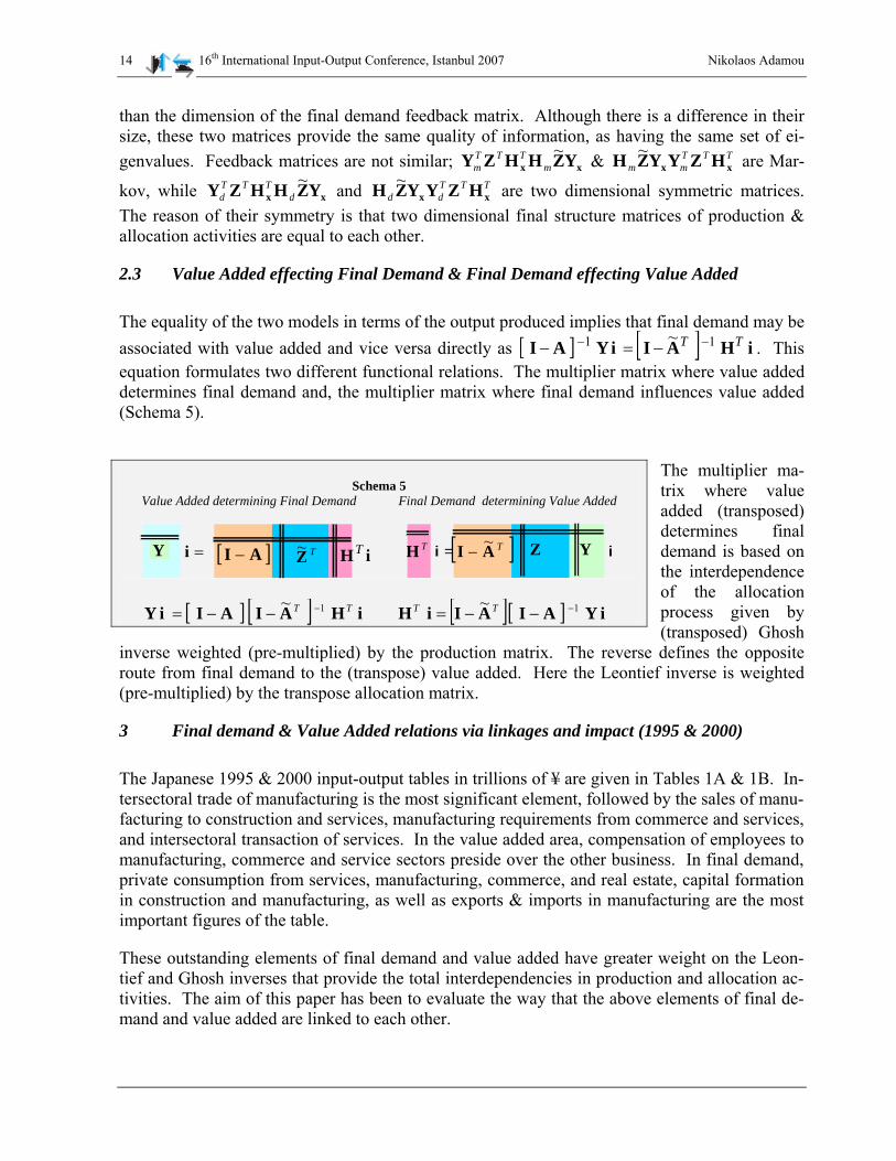
2.3 Value Added effecting Final Demand & Final Demand effecting Value Added

The equality of the two models in terms of the output produced implies that final demand may be associated with value added and vice versa directly as [ ] [ ] iHAIiYAI TT 11 ~ −− −=− . This equation formulates two different functional relations. The multiplier matrix where value added determines final demand and, the multiplier matrix where final demand influences value added (Schema 5).

The multiplier ma-trix where value added (transposed) determines final demand is based on the interdependence of the allocation process given by (transposed) Ghosh

inverse weighted (pre-multiplied) by the production matrix. The reverse defines the opposite route from final demand to the (transpose) value added. Here the Leontief inverse is weighted (pre-multiplied) by the transpose allocation matrix.

Schema 5 Value Added determining Final Demand Final Demand determining Value Added

Y [ ]AI − TZ~ iHT=i

i = iZ[ ]TAI ~−TH Y

3 Final demand & Value Added relations via linkages and impact (1995 & 2000)

The Japanese 1995 & 2000 input-output tables in trillions of ¥ are given in Tables 1A & 1B. In-tersectoral trade of manufacturing is the most significant element, followed by the sales of manu-facturing to construction and services, manufacturing requirements from commerce and services, and intersectoral transaction of services. In the value added area, compensation of employees to manufacturing, commerce and service sectors preside over the other business. In final demand, private consumption from services, manufacturing, commerce, and real estate, capital formation in construction and manufacturing, as well as exports & imports in manufacturing are the most important figures of the table.

These outstanding elements of final demand and value added have greater weight on the Leon-tief and Ghosh inverses that provide the total interdependencies in production and allocation ac-tivities. The aim of this paper has been to evaluate the way that the above elements of final de-mand and value added are linked to each other.

[ ] [ ] [ ]iHAIAIiY −−= TT 1~ − [ ] 1~ −TT iYAIAIiH −−=


Table 1 A 1995 1 2 3 4 5 6 7 8 9 10 11 12 13

In Trillions of Yen

Agr

icul

ture

Min

ing

Man

ufac

turin

g

Con

stru

ctio

n

Elec

tric

pow

er

Com

mer

ce

Fina

nce

Rea

l est

ate

Tran

spor

t

Com

mun

icat

ion

Publ

ic A

dmin

.

Serv

ices

Act

. not

els

e cl

assi

fied

Inte

rmed

iate

Out

put

1 Agriculture, forestry and fishery 1.9 0.0 9.9 0.2 0.0 0.0 0.0 0.0 0.0 0.0 0.0 1.2 0.0 13.3

2 Mining 0.0 0.0 5.3 0.8 1.3 0.0 0.0 0.0 0.0 0.0 0.0 0.0 0.0 7.43 Manufacturing 2.5 0.1 124.7 25.9 1.4 3.8 1.3 0.2 5.4 0.4 2.7 26.8 0.5 195.84 Construction 0.1 0.0 1.4 0.2 1.2 0.6 0.1 2.3 0.5 0.2 0.5 1.2 0.0 8.15 Electric power, Gas and water

supply 0.1 0.0 5.9 0.6 2.5 1.2 0.2 0.2 0.9 0.2 0.9 4.6 0.1 17.36 Commerce 0.7 0.0 17.2 6.2 0.3 1.1 0.2 0.1 1.8 0.1 0.5 7.8 0.1 36.17 Finance and insurance 0.5 0.1 4.3 1.0 0.7 5.9 3.5 3.3 3.1 0.2 0.1 5.4 0.9 29.08 Real estate 0.0 0.0 1.1 0.3 0.3 3.8 0.7 0.5 0.8 0.2 0.0 2.8 0.1 10.69 Transport 0.7 0.4 9.3 4.7 0.7 5.3 0.7 0.2 5.3 0.4 0.8 3.9 0.1 32.6

10 Communication and broadcasting 0.0 0.0 0.9 0.5 0.1 1.9 0.7 0.0 0.3 0.9 0.4 3.7 0.0 9.5

11 Public administration 0.0 0.0 0.0 0.0 0.0 0.0 0.0 0.0 0.0 0.0 0.0 0.0 0.5 0.512 Services 0.2 0.1 20.7 7.0 2.4 5.3 3.8 1.0 6.6 2.0 1.9 14.3 0.3 65.613 Activities not elsewhere

classified 0.2 0.0 2.3 0.2 0.2 0.6 0.1 0.5 0.2 0.1 0.4 1.2 0.0 6.0

Intermediate Input 6.8 0.8 203.2 47.5 11.1 29.6 11.4 8.3 24.9 4.7 8.1 72.8 2.6 431.9

1 Consumption expenditure outside households (row) 0.1 0.1 6.4 1.7 0.6 2.7 1.3 0.3 1.1 0.2 0.5 4.4 0.0 19.4

2 Compensation of employees 1.5 0.3 54.3 29.3 4.6 49.9 14.0 2.5 16.7 4.9 16.8 78.3 0.2 273.23 Operating surplus 5.2 0.2 20.1 3.1 3.6 11.3 6.0 28.4 2.8 1.5 0.0 15.2 2.3 99.74 Depreciation of fixed capital 1.8 0.2 16.8 4.5 5.4 5.0 3.7 20.8 3.3 2.8 0.8 15.5 0.3 80.85 Indirect taxes * 0.6 0.1 14.3 2.2 1.5 4.0 1.6 4.1 1.6 0.6 0.1 5.8 0.0 36.56 (less) Current subsidies -0.2 0.0 -0.4 -0.2 -0.2 -0.2 -1.5 -0.2 -0.3 0.0 0.0 -1.1 0.0 -4.3

Value Added 9.0 0.9 111.4 40.6 15.3 72.7 24.9 55.9 25.2 10.1 18.1 118.2 2.9 505.2

Domestic production (gross inputs) 15.8 1.7 314.6 88.1 26.5 102.3 36.3 64.2 50.1 14.8 26.2 191.0 5.5 937.1

1 2 3 4 5 6 7

In Trillions of Yen

Con

sum

ptio

n. O

ut

Hou

seho

lds

Con

sum

ptio

n (P

rivat

e)

Con

sum

ptio

n G

over

nmen

t

Cap

ital F

orm

atio

n

Incr

ease

in S

tock

s

Expo

rts

Impo

rts

Tota

l Fin

al

Dem

and

Tota

l Dem

and

- G

ross

Out

put

1 fishery 0.1 4.1 0.0 0.2 0.5 0.0 -2.4 2.5 15.82 Mining 0.0 0.0 0.0 0.0 0.0 0.0 -5.8 -5.8 1.73 Manufacturing 2.8 63.8 0.7 39.1 1.2 37.9 -26.7 118.8 314.64 Construction 0.0 0.0 0.0 80.0 0.0 0.0 0.0 80.0 88.15 supply 0.0 7.5 1.6 0.0 0.0 0.0 0.0 9.1 26.56 Commerce 2.2 50.5 0.0 10.4 0.2 3.1 -0.2 66.2 102.37 Finance and insurance 0.0 7.8 0.0 0.0 0.0 0.6 -1.0 7.4 36.38 Real estate 0.0 53.5 0.0 0.0 0.0 0.0 0.0 53.5 64.29 Transport 0.7 14.7 -0.1 0.8 0.2 3.7 -2.5 17.5 50.1

10 broadcasting 0.1 5.2 0.0 0.0 0.0 0.0 -0.1 5.3 14.811 Public administration 0.0 0.8 25.0 0.0 0.0 0.0 0.0 25.8 26.212 Services 13.5 64.0 41.9 9.2 0.0 1.3 -4.4 125.4 191.013 classified 0.0 0.0 0.0 0.0 0.0 0.0 -0.6 -0.5 5.5

Total 19.4 271.8 69.2 139.7 2.1 46.8 -43.7 505.2 937.1


Table 1 B 2000 1 2 3 4 5 6 7 8 9 10 11 12 13

In Trillions of Yen

Agr

icul

ture

Min

ing

Man

ufac

turin

g

Con

stru

ctio

n

Elec

tric

pow

er

Com

mer

ce

Fina

nce

Rea

l est

ate

Tran

spor

t

Com

mun

icat

ion

Publ

ic A

dmin

.

Serv

ices

Act

. not

els

e cl

assi

fied

Inte

rmed

iate

O

utpu

t

1 Agriculture, forestry and fishery 1.6 0.0 8.4 0.2 0.0 0.0 0.0 0.0 0.0 0.0 0.0 1.3 0.0 11.5

2 Mining 0.0 0.0 7.4 0.7 2.0 0.0 0.0 0.0 0.0 0.0 0.0 0.0 0.0 10.13 Manufacturing 2.5 0.1 122.9 21.6 1.7 3.2 1.3 0.2 6.1 0.5 2.9 28.2 0.4 191.44 Construction 0.1 0.0 1.3 0.2 1.3 0.5 0.2 2.8 0.5 0.2 0.6 1.4 0.0 9.05 Electric power, Gas and water

supply 0.1 0.0 6.3 0.5 1.6 1.2 0.2 0.2 0.9 0.3 1.0 5.5 0.1 18.16 Commerce 0.7 0.0 16.3 4.9 0.4 1.4 0.2 0.1 1.6 0.1 0.5 8.3 0.1 34.67 Finance and insurance 0.5 0.1 4.0 0.9 0.8 4.9 2.9 3.3 2.9 0.5 0.1 5.8 1.0 27.68 Real estate 0.0 0.0 0.9 0.3 0.2 2.9 0.6 0.4 0.7 0.4 0.0 2.7 0.0 9.19 Transport 0.6 0.4 8.2 4.0 0.7 4.6 0.7 0.1 5.0 0.5 1.1 4.2 0.2 30.5

10 Communication and broadcasting 0.0 0.0 1.1 0.9 0.1 2.5 0.8 0.1 0.4 2.7 0.5 4.9 0.1 14.2

11 Public administration 0.0 0.0 0.0 0.0 0.0 0.0 0.0 0.0 0.0 0.0 0.0 0.0 0.7 0.712 Services 0.2 0.1 23.1 6.4 2.8 6.3 5.0 1.7 6.7 3.6 2.8 19.3 0.3 78.213 Activities not elsewhere

classified 0.1 0.0 1.7 0.3 0.1 0.6 0.3 0.3 0.2 0.1 0.0 0.7 0.0 4.4

Intermediate Input 6.3 0.7 201.5 40.9 11.7 28.3 12.1 9.2 25.0 8.8 9.5 82.3 2.9 439.4

1 Consumption expenditure outside households (row) 0.1 0.1 5.6 1.3 0.5 2.3 1.3 0.2 1.0 1.4 0.6 4.7 0.1 19.2

2 Compensation of employees 1.3 0.2 53.1 26.8 4.7 47.3 12.5 2.4 14.8 5.9 16.6 89.8 0.3 275.63 Operating surplus 4.7 0.2 16.9 1.4 3.5 10.0 9.0 29.6 2.6 1.5 0.0 16.7 0.4 96.54 Depreciation of fixed capital 1.5 0.1 16.7 4.1 5.0 4.8 3.4 20.7 3.0 3.8 9.5 20.3 0.4 93.45 Indirect taxes * 0.7 0.1 15.0 3.3 1.7 4.5 1.5 4.0 1.6 0.7 0.1 6.9 0.1 40.06 (less) Current subsidies -0.2 0.0 -0.6 -0.3 -0.3 -0.2 -1.6 -0.2 -0.2 0.0 0.0 -1.5 0.0 -5.2

Total Value Added 8.1 0.7 106.6 36.5 15.3 68.6 26.0 56.6 22.9 13.3 26.7 136.9 1.3 519.5

Domestic production (gross inputs) 14.4 1.4 308.2 77.3 27.0 96.9 38.1 65.9 47.9 22.1 36.2 219.2 4.2 958.9

1 2 3 4 5 6 7

In Trillions of Yen

C. O

ut H

ouse

hold

s

Con

sum

ptio

n (P

rivat

e)

Con

sum

ptio

n G

over

nmen

t

Cap

ital F

orm

atio

n

Incr

ease

in S

tock

s

Expo

rts

Impo

rts

Tota

l Fin

al D

eman

d

Tota

l Dem

and

- G

ross

Out

put

1 Agriculture, forestry and fishery 0.1 3.9 0.0 0.2 0.8 0.1 -2.1 2.9 14.4

2 Mining 0.0 0.0 0.0 0.0 0.0 0.0 -8.7 -8.7 1.43 Manufacturing 3.3 61.6 0.5 39.7 -0.6 46.6 -34.3 116.8 308.24 Construction 0.0 0.0 0.0 68.3 0.0 0.0 0.0 68.3 77.35 Electric power, Gas and water

supply 0.0 8.1 0.8 0.0 0.0 0.0 0.0 8.9 27.06 Commerce 1.9 45.9 0.0 10.7 0.1 4.5 -0.7 62.4 96.97 Finance and insurance 0.0 10.5 0.0 0.0 0.0 0.4 -0.4 10.5 38.18 Real estate 0.0 56.7 0.0 0.0 0.0 0.0 0.0 56.7 65.99 Transport 0.5 14.7 0.0 0.7 0.0 4.3 -2.9 17.4 47.9

10 Communication and broadcasting 0.2 7.8 0.0 0.0 0.0 0.1 -0.1 7.9 22.1

11 Public administration 0.0 0.7 34.8 0.0 0.0 0.0 0.0 35.5 36.212 Services 13.1 71.1 49.7 10.4 0.0 1.6 -4.8 141.0 219.213 Activities not elsewhere

classified 0.0 0.0 0.0 0.0 0.0 0.0 -0.2 -0.2 4.2

Total 19.2 281.0 85.7 130.0 0.3 57.5 -54.2 519.5 958.9

* (except custom duties and commodity taxes on imported goods)


Table 2 provides the distributions of total final demand, value added and gross output, as well as the output multiplier. This aggregate output multiplier of both the production/demand side,

( ) ∑+++ nn yyzyzyz1

1212111 Ln

, is the same to its equivalent ( ) ∑+++ n hzhzhzh1

212111~~~ L

n

multiplier of the allocation/value added side. The logic behind this multiplier is that each ele-ment of the Leontief inverse row is weighed with the appropriate sectoral demand that exists for this sector. The same occurs with the Ghosh inverse. Each element of the appropriate column is multiplied by the associated percentage of the value added distribution. As is previously ex-plained, the equality of the aggregate output multiplier is based on the same gross output that the two similar models yield, x = ( )TZhZy ~= . This multiplier is in agreement with available eco-nomic data. Large multiplier values exist in manufacturing and services followed by commerce and real estate. These are the sectors that provide the significant portion of output, comprise the largest amount of final demand and generate most of value added.

Table 2

1995 2000 1995 2000 1995 2000 1995 2000Agriculture, forestry and fishery 0.5% 0.6% 1.8% 1.6% 1.7% 1.5% 0.028 0.031Mining -1.1% -1.7% 0.2% 0.1% 0.2% 0.1% 0.003 0.003Manufacturing 23.5% 22.5% 22.0% 20.5% 33.6% 32.1% 0.593 0.623Construction 15.8% 13.2% 8.0% 7.0% 9.4% 8.1% 0.149 0.174Electric power, Gas and water supply 1.8% 1.7% 3.0% 2.9% 2.8% 2.8% 0.052 0.052Commerce 13.1% 12.0% 14.4% 13.2% 10.9% 10.1% 0.187 0.203Finance and insurance 1.5% 2.0% 4.9% 5.0% 3.9% 4.0% 0.073 0.072Real estate 10.6% 10.9% 11.1% 10.9% 6.8% 6.9% 0.127 0.127Transport 3.5% 3.3% 5.0% 4.4% 5.3% 5.0% 0.092 0.099Communication and broadcasting 1.0% 1.5% 2.0% 2.6% 1.6% 2.3% 0.043 0.029Public administration 5.1% 6.8% 3.6% 5.1% 2.8% 3.8% 0.070 0.052Services 24.8% 27.1% 23.4% 26.4% 20.4% 22.9% 0.422 0.378Activities not elsewhere classified -0.1% 0.0% 0.6% 0.2% 0.6% 0.4% 0.008 0.011Total 100% 100% 100% 100% 100% 100%

Distributions of total final demand, value added, gross output & its multiplier

MultiplierDemand Added Gross OutputOutput Total Final Total Value

Figure 3, presents the traditional row and column summations of the Leontief and Ghosh in-verses and shows that there is a sizeable variability. The row summation of Ghosh inverse provides very large multiplier values of mining for both input-output tables, and the column summation of the Ghosh inverse for manufacturing. These numerical values, ranging from 12.6 to 17.3, are not acceptable as multipliers; therefore the Ghosh’s inverse was declared im-plausible.

The reason for this implausibility, as it was mentioned in the methodological part of the paper is the fact that we apply Procrustian logic. Not all sectors are equivalent, as Table 2 shows. While construction is significant in its final demand proportion, it follows behind while one observes its contribution to value added or gross output. There is NO base for the assumption that we should evaluate the impact of a unit of final demand or value added in one sector, assuming all others have zero value demand or value added. Neither, we have any evidence that all sectors are equivalent. Thus, the reality shown in Table 2 should lead us towards our impact (multiplier) evaluations. The last two columns of Table 2 indicate not only that Leontief and Ghosh models


Figure 3

Traditional Output Multipliers

0

5

10

15

20

Leo ntief Inv199 5

Ghosh Inv.19 95

Leont ief Inv.20 00

Ghosh Inv.2 00 0

Leont ief Inv.199 5

Ghosh Inv.19 95

Leont ief Inv.20 00

Gho sh Inv2 00 0

Row Summatio ns Co lumn Summations

Agriculture , fo res try and fis hery MiningManufac turing Co ns truc tio nElec tric po wer, Gas and wa te r s upply Co mmerceFinance and ins urance Real e s ta teTrans po rt Co mmunica tio n and bro adcas tingP ublic adminis tra tio n ServicesActivities no t e ls ewhere c las s ified

Table 4 (distribution of a unit of each type of final demand) & (distribution of a unit of final demand) mY Yd

1995 2000 1995 2000 1995 2000 1995 2000 1995 2000 1995 2000 1995 2000 1995 2000

Agriculture 0.01 0.00 0.02 0.01 0.00 0.00 0.00 0.00 0.23 2.80 0.00 0.00 0.05 0.04 0.01 0.01Mining 0.00 0.00 0.00 0.00 0.00 0.00 0.00 0.00 0.02 -0.04 0.00 0.00 0.13 0.16 -0.01 -0.02Manufacturing 0.15 0.17 0.23 0.22 0.01 0.01 0.28 0.31 0.58 -2.30 0.81 0.81 0.61 0.63 0.24 0.22Construction 0.00 0.00 0.00 0.00 0.00 0.00 0.57 0.53 0.00 0.00 0.00 0.00 0.00 0.00 0.16 0.13Electric power 0.00 0.00 0.03 0.03 0.02 0.01 0.00 0.00 0.00 0.00 0.00 0.00 0.00 0.00 0.02 0.02Commerce 0.11 0.10 0.19 0.16 0.00 0.00 0.07 0.08 0.09 0.42 0.07 0.08 0.00 0.01 0.13 0.12Finance 0.00 0.00 0.03 0.04 0.00 0.00 0.00 0.00 0.00 0.00 0.01 0.01 0.02 0.01 0.01 0.02Real estate 0.00 0.00 0.20 0.20 0.00 0.00 0.00 0.00 0.00 0.00 0.00 0.00 0.00 0.00 0.11 0.11Transport 0.04 0.03 0.05 0.05 0.00 0.00 0.01 0.01 0.08 0.12 0.08 0.07 0.06 0.05 0.03 0.03Communication 0.01 0.01 0.02 0.03 0.00 0.00 0.00 0.00 0.00 0.00 0.00 0.00 0.00 0.00 0.01 0.02Public administ. 0.00 0.00 0.00 0.00 0.36 0.41 0.00 0.00 0.00 0.00 0.00 0.00 0.00 0.00 0.05 0.07Services 0.69 0.68 0.24 0.25 0.61 0.58 0.07 0.08 0.00 0.00 0.03 0.03 0.10 0.09 0.25 0.27Other Activities 0.00 0.00 0.00 0.00 0.00 0.00 0.00 0.00 0.00 0.00 0.00 0.00 0.01 0.00 0.00 0.00

Total 1 1 1 1 1 1 1 1 1 1 1 1 1 1 1

Agriculture 0.00 0.00 0.01 0.01 0.00 0.00 0.00 0.00 0.00 0.00 0.00 0.00 0.00 0.00 0.01 0.01Mining 0.00 0.00 0.00 0.00 0.00 0.00 0.00 0.00 0.00 0.00 0.00 0.00 -0.01 -0.02 -0.01 -0.02Manufacturing 0.01 0.01 0.13 0.12 0.00 0.00 0.08 0.08 0.00 0.00 0.07 0.09 -0.05 -0.07 0.24 0.22Construction 0.00 0.00 0.00 0.00 0.00 0.00 0.16 0.13 0.00 0.00 0.00 0.00 0.00 0.00 0.16 0.13Electric power 0.00 0.00 0.01 0.02 0.00 0.00 0.00 0.00 0.00 0.00 0.00 0.00 0.00 0.00 0.02 0.02Commerce 0.00 0.00 0.10 0.09 0.00 0.00 0.02 0.02 0.00 0.00 0.01 0.01 0.00 0.00 0.13 0.12Finance 0.00 0.00 0.02 0.02 0.00 0.00 0.00 0.00 0.00 0.00 0.00 0.00 0.00 0.00 0.01 0.02Real estate 0.00 0.00 0.11 0.11 0.00 0.00 0.00 0.00 0.00 0.00 0.00 0.00 0.00 0.00 0.11 0.11Transport 0.00 0.00 0.03 0.03 0.00 0.00 0.00 0.00 0.00 0.00 0.01 0.01 0.00 -0.01 0.03 0.03Communication 0.00 0.00 0.01 0.02 0.00 0.00 0.00 0.00 0.00 0.00 0.00 0.00 0.00 0.00 0.01 0.02Public administ. 0.00 0.00 0.00 0.00 0.05 0.07 0.00 0.00 0.00 0.00 0.00 0.00 0.00 0.00 0.05 0.07Services 0.03 0.03 0.13 0.14 0.08 0.10 0.02 0.02 0.00 0.00 0.00 0.00 -0.01 -0.01 0.25 0.27Other Activities 0.00 0.00 0.00 0.00 0.00 0.00 0.00 0.00 0.00 0.00 0.00 0.00 0.00 0.00 0.00 0.00

Total 0.038 0.037 0.538 0.541 0.137 0.165 0.277 0.250 0.004 0.001 0.093 0.111 -0.087 -0.104 1 1

Distribution of each type of final demand

Distribution of a total final demand unit

Increase in Stocks Exports Imports

Total Final Demand

Consum. Out HH.

Consumption (Private)

Consumption Government

Capital Formation

1

yield the same gross output multiplier, but this multiplier is not implausible and it is realistic.


Thus, the important driving forces are the distributions of final demand (Table 3) and value added (Table 4). Not all aspects of final demand are equivalent as the matrix indicates. Matrix is useful whenever one is interested in examining the impact of a ¥ allocated to any type of final demand equivalently.

mYYm

The sectoral breakdown of these figures is more important because it indicates to which sectors these specific components of demand are channeled. Most (83%) of the Private consumption expenditure is channeled to four sectors. The service sector absorbs 25.3%, Manufacturing 21.9% Real estate 20.2% and Commerce 16.3% of a unit of private consumption expenditure for 2000. Construction absorbs more than half of the gross domestic fixed capital formation, that is 13.2% of final demand, and almost the half of this value is channeled to manufacturing. Manufacturing is the dominant player for exporting (81%) as well as importing (63%) activity, while mining sector (16%) is noticeable in the import column.

Private consumption expenditure concentrates 54% of final demand, exports are more or less equal to imports with 11% and 10% respectively, with gross domestic fixed capital formation absorbing one forth of the final demand and the consumption expenditure of the general gov-ernment being the 16.5% of final demand. These specific characteristics given in the Yd ma-trix are those that provide the tone and purpose for the analysis, and these characteristics are captured when the weighted inverse is evaluated.

It is noticeable that this is not a positive column, since imports in the mining sector are greater than domestic production. The service sector dominates the economy with 27.1% of final de-mand, mainly allocated to private (13.7%) and general government (9.6%) of the consumption expenditures. The manufacturing sector follows with 22.5% of final demand, indicating that there is a strong industrial base in the economy, and the demand of the manufacturing sector is driven by private consumption expenditures (11.9%), exports (9%), fixed capital formation (7.6%) and imports (6.6%). Construction (13.2%) is allocated only to fixed capital formation; Commerce (12%) and real estate are mainly affected by private consumption (8.8% & 10.9%) respectively.

Table 4 provides comparable information for the value added distributions & . The compensation of employees is just a percentage point lower than the share of private consump-tion to the net output and it is distributed mainly to services, manufacturing and commerce. Operating surplus and depreciation of fixed capital have almost the same share. While operat-ing surplus is mainly concentrated into real estate, depreciation of fixed capital has similar al-location to real estate and service.

mH dH

Looking at the sectoral distribution of the value added, services (26.4%) has less than a per-centage point difference from final demand distribution; manufacturing and real estate have the same weight in value added as in final demand (20.5% and 10.9%) respectively, and commerce with 13.2% has a little more weight in value added than its final demand (12%).

Seventy one percent of the value added allocation to construction comes from employee com-pensation, while for services the equivalent assessment is 65% and for manufacturing 49%.


Most of the real estate value added is allocated to operating surplus and to depreciation of fixed capital.

Table 4 (distribution of a unit of each type of value added) & (distribution of a unit of value added)

mH H d

1995 2000 1995 2000 1995 2000 1995 2000 1995 2000 1995 2000 1995 2000

Agriculture 0.01 0.01 0.01 0.00 0.05 0.05 0.02 0.02 0.02 0.02 0.05 0.03 0.02 0.02Mining 0.00 0.00 0.00 0.00 0.00 0.00 0.00 0.00 0.00 0.00 0.00 0.00 0.00 0.00Manufacturing 0.33 0.29 0.20 0.19 0.20 0.17 0.21 0.18 0.39 0.37 0.10 0.12 0.22 0.21Construction 0.09 0.07 0.11 0.10 0.03 0.01 0.06 0.04 0.06 0.08 0.04 0.07 0.08 0.07Electric P. 0.03 0.03 0.02 0.02 0.04 0.04 0.07 0.05 0.04 0.04 0.05 0.05 0.03 0.03Commerce 0.14 0.12 0.18 0.17 0.11 0.10 0.06 0.05 0.11 0.11 0.04 0.04 0.14 0.13Finance 0.07 0.07 0.05 0.05 0.06 0.09 0.05 0.04 0.04 0.04 0.35 0.32 0.05 0.05Real Estate 0.01 0.01 0.01 0.01 0.28 0.31 0.26 0.22 0.11 0.10 0.04 0.04 0.11 0.11Transport 0.06 0.05 0.06 0.05 0.03 0.03 0.04 0.03 0.04 0.04 0.08 0.04 0.05 0.04Communic. 0.01 0.07 0.02 0.02 0.02 0.02 0.04 0.04 0.02 0.02 0.00 0.00 0.02 0.03Public administ. 0.03 0.03 0.06 0.06 0.00 0.00 0.01 0.10 0.00 0.00 0.00 0.00 0.04 0.05Services 0.23 0.24 0.29 0.33 0.15 0.17 0.19 0.22 0.16 0.17 0.25 0.29 0.23 0.26Other Activities 0.00 0.00 0.00 0.00 0.02 0.00 0.00 0.00 0.00 0.00 0.00 0.00 0.01 0.00

Total 1 1 1 1 1 1 1 1 1 1 1 1 1 1

Agriculture 0.00 0.00 0.00 0.00 0.01 0.01 0.00 0.00 0.00 0.00 0.00 0.00 0.02 0.02Mining 0.00 0.00 0.00 0.00 0.00 0.00 0.00 0.00 0.00 0.00 0.00 0.00 0.00 0.00Manufacturing 0.01 0.01 0.11 0.10 0.04 0.03 0.03 0.03 0.03 0.03 0.00 0.00 0.22 0.21Construction 0.00 0.00 0.06 0.05 0.01 0.00 0.01 0.01 0.00 0.01 0.00 0.00 0.08 0.07Electric P. 0.00 0.00 0.01 0.01 0.01 0.01 0.01 0.01 0.00 0.00 0.00 0.00 0.03 0.03Commerce 0.01 0.00 0.10 0.09 0.02 0.02 0.01 0.01 0.01 0.01 0.00 0.00 0.14 0.13Finance 0.00 0.00 0.03 0.02 0.01 0.02 0.01 0.01 0.00 0.00 0.00 0.00 0.05 0.05Real Estate 0.00 0.00 0.00 0.00 0.06 0.06 0.04 0.04 0.01 0.01 0.00 0.00 0.11 0.11Transport 0.00 0.00 0.03 0.03 0.01 0.00 0.01 0.01 0.00 0.00 0.00 0.00 0.05 0.04Communic. 0.00 0.00 0.01 0.01 0.00 0.00 0.01 0.01 0.00 0.00 0.00 0.00 0.02 0.03Public administ. 0.00 0.00 0.03 0.03 0.00 0.00 0.00 0.02 0.00 0.00 0.00 0.00 0.04 0.05Services 0.01 0.01 0.15 0.17 0.03 0.03 0.03 0.04 0.01 0.01 0.00 0.00 0.23 0.26Other Activities 0.00 0.00 0.00 0.00 0.00 0.00 0.00 0.00 0.00 0.00 0.00 0.00 0.01 0.00

Total 0.038 0.037 0.541 0.531 0.197 0.186 0.160 0.180 0.072 0.077 -0.009 -0.010 1 1

Consumption out. HH

Compensation of employees Added

Distribution of each type of value added

Distribution of a totalvalue added unit

Operating surplusDepreciation of

fixed capital Indirect taxes *(less) Current

subsidiesTotal Value

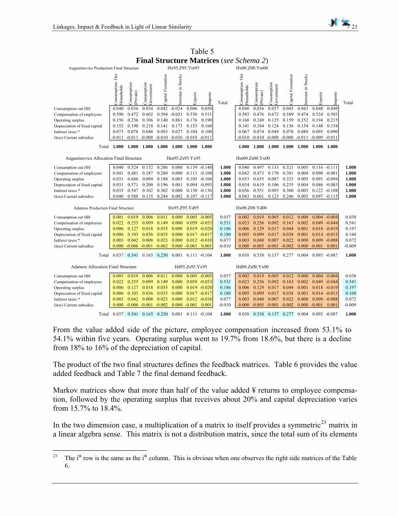
Given the total interdependencies provided by the appropriate inverses, and their appropriate backward and forward linkages, production and allocation based final structure matrices are calculated. Augustinovics’ final structure matrices are Markov matrices and the production based final structure matrix is different from the allocation based final structure matrix, as one may observe in Table 5. In the contrary, production and allocation based final structure matri-ces driven by a two-dimension distribution are exactly the same. This is because as we already mentioned production and allocation are the two sides of the same activity, and one ¥ of value added has the same overall impact as one ¥ of final demand. Private consumption dominates the field, with a slide decline from 54.1% to 53.8% from 1995 to 2000. During the same time period, capital formation increased 2.7%, and government consumption declined from 16.5% to 13.7%.


Table 5 Final Structure Matrices (see Schema 2)

Hx00.Z00.Ym00Hx95.Z95.Ym95Augustinovics Production Final Structure

Con

sum

ptio

n. O

ut

Hou

seho

lds

Con

sum

ptio

n (P

rivat

e)

Con

sum

ptio

n G

over

nmen

t

Cap

ital F

orm

atio

n

Incr

ease

in S

tock

s

Expo

rts

Impo

rts

Total Con

sum

ptio

n. O

ut

Hou

seho

lds

Con

sum

ptio

n (P

rivat

e)

Con

sum

ptio

n G

over

nmen

t

Cap

ital F

orm

atio

n

Incr

ease

in S

tock

s

Expo

rts

Impo

rts

TotalConsumption out HH 0.040 0.036 0.034 0.042 -0.024 0.046 0.050 0.040 0.036 0.037 0.045 0.043 0.048 0.049Compensation of employees 0.590 0.472 0.602 0.594 -0.021 0.530 0.511 0.593 0.476 0.672 0.589 0.474 0.524 0.503Operating surplus 0.156 0.236 0.106 0.140 0.881 0.176 0.190 0.168 0.240 0.125 0.159 0.252 0.194 0.215Depreciation of fixed capital 0.152 0.190 0.218 0.141 0.173 0.153 0.160 0.141 0.184 0.124 0.136 0.154 0.148 0.154Indirect taxes * 0.073 0.078 0.048 0.093 0.027 0.104 0.100 0.067 0.074 0.049 0.078 0.089 0.095 0.090(less) Current subsidies -0.011 -0.011 -0.008 -0.010 -0.036 -0.010 -0.011 -0.010 -0.010 -0.008 -0.008 -0.011 -0.009 -0.011

Total 1.000 1.000 1.000 1.000 1.000 1.000 1.000 1.000 1.000 1.000 1.000 1.000 1.000 1.000

Hm00.Zs00.Yx00

Consumption out HH 0.040 0.524 0.152 0.286 0.000 0.139 -0.140 1.000 0.040 0.497 0.133 0.321 0.005 0.116 -0.111 1.000Compensation of employees 0.041 0.481 0.187 0.280 0.000 0.111 -0.100 1.000 0.042 0.473 0.170 0.301 0.004 0.090 -0.081 1.000Operating surplus 0.031 0.686 0.094 0.188 0.003 0.105 -0.106 1.000 0.033 0.655 0.087 0.223 0.005 0.091 -0.094 1.000Depreciation of fixed capital 0.031 0.571 0.200 0.196 0.001 0.094 -0.093 1.000 0.034 0.619 0.106 0.235 0.004 0.086 -0.083 1.000Indirect taxes * 0.035 0.547 0.102 0.302 0.000 0.150 -0.136 1.000 0.036 0.551 0.093 0.300 0.005 0.122 -0.108 1.000(less) Current subsidies 0.040 0.588 0.135 0.244 0.002 0.107 -0.117 1.000 0.043 0.601 0.123 0.246 0.005 0.097 -0.115 1.000

Hx00.Z00.Yd00

Consumption out HH 0.001 0.019 0.006 0.011 0.000 0.005 -0.005 0.037 0.002 0.019 0.005 0.012 0.000 0.004 -0.004 0.038Compensation of employees 0.022 0.255 0.099 0.149 0.000 0.059 -0.053 0.531 0.023 0.256 0.092 0.163 0.002 0.049 -0.044 0.541Operating surplus 0.006 0.127 0.018 0.035 0.000 0.019 -0.020 0.186 0.006 0.129 0.017 0.044 0.001 0.018 -0.019 0.197Depreciation of fixed capital 0.006 0.103 0.036 0.035 0.000 0.017 -0.017 0.180 0.005 0.099 0.017 0.038 0.001 0.014 -0.013 0.160Indirect taxes * 0.003 0.042 0.008 0.023 0.000 0.012 -0.010 0.077 0.003 0.040 0.007 0.022 0.000 0.009 -0.008 0.072(less) Current subsidies 0.000 -0.006 -0.001 -0.002 0.000 -0.001 0.001 -0.010 0.000 -0.005 -0.001 -0.002 0.000 -0.001 0.001 -0.009

Total 0.037 0.541 0.165 0.250 0.001 0.111 -0.104 1.000 0.038 0.538 0.137 0.277 0.004 0.093 -0.087 1.000

Hd00.Zs00.Yx00

Consumption out HH 0.001 0.019 0.006 0.011 0.000 0.005 -0.005 0.037 0.002 0.019 0.005 0.012 0.000 0.004 -0.004 0.038Compensation of employees 0.022 0.255 0.099 0.149 0.000 0.059 -0.053 0.531 0.023 0.256 0.092 0.163 0.002 0.049 -0.044 0.541Operating surplus 0.006 0.127 0.018 0.035 0.000 0.019 -0.020 0.186 0.006 0.129 0.017 0.044 0.001 0.018 -0.019 0.197Depreciation of fixed capital 0.006 0.103 0.036 0.035 0.000 0.017 -0.017 0.180 0.005 0.099 0.017 0.038 0.001 0.014 -0.013 0.160Indirect taxes * 0.003 0.042 0.008 0.023 0.000 0.012 -0.010 0.077 0.003 0.040 0.007 0.022 0.000 0.009 -0.008 0.072(less) Current subsidies 0.000 -0.006 -0.001 -0.002 0.000 -0.001 0.001 -0.010 0.000 -0.005 -0.001 -0.002 0.000 -0.001 0.001 -0.009

Total 0.037 0.541 0.165 0.250 0.001 0.111 -0.104 1.000 0.038 0.538 0.137 0.277 0.004 0.093 -0.087 1.000

Hx95.Z95.Yd95

Hd95.Zs95.Yx95

Adamou Production Final Structure

Adamou Allocation Final Structure

Hm95.Zs95.Yx95Augustinovics Allocation Final Structure

From the value added side of the picture, employee compensation increased from 53.1% to 54.1% within five years. Operating surplus went to 19.7% from 18.6%, but there is a decline from 18% to 16% of the depreciation of capital.

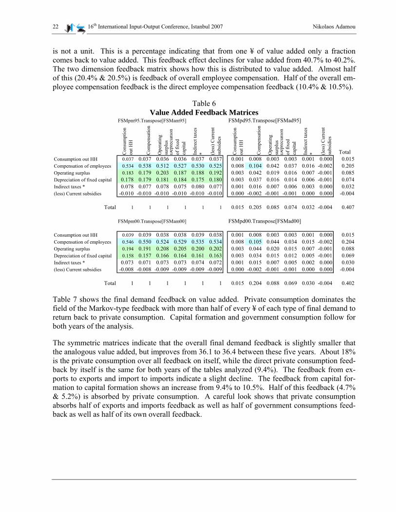
The product of the two final structures defines the feedback matrices. Table 6 provides the value added feedback and Table 7 the final demand feedback.

Markov matrices show that more than half of the value added ¥ returns to employee compensa-tion, followed by the operating surplus that receives about 20% and capital depreciation varies from 15.7% to 18.4%.

In the two dimension case, a multiplication of a matrix to itself provides a symmetric23 matrix in a linear algebra sense. This matrix is not a distribution matrix, since the total sum of its elements

23 The ith row is the same as the ith column. This is obvious when one observes the right side matrices of the Table

6.


is not a unit. This is a percentage indicating that from one ¥ of value added only a fraction comes back to value added. This feedback effect declines for value added from 40.7% to 40.2%. The two dimension feedback matrix shows how this is distributed to value added. Almost half of this (20.4% & 20.5%) is feedback of overall employee compensation. Half of the overall em-ployee compensation feedback is the direct employee compensation feedback (10.4% & 10.5%).

Table 6 Value Added Feedback Matrices

FSMpm95.Transpose[FSMam95] FSMpd95.Transpose[FSMad95]C

onsu

mpt

ion

out H

H

Com

pens

atio

n

Ope

ratin

g su

rplu

sD

epre

ciat

ion

of fi

xed

capi

tal

Indi

rect

taxe

s * (le

ss) C

urre

nt

subs

idie

s

Con

sum

ptio

n ou

t HH

Com

pens

atio

n

Ope

ratin

g su

rplu

sD

epre

ciat

ion

of fi

xed

capi

tal

Indi

rect

taxe

s * (le

ss) C

urre

nt

subs

idie

s

TotalConsumption out HH 0.037 0.037 0.036 0.036 0.037 0.037 0.001 0.008 0.003 0.003 0.001 0.000 0.015Compensation of employees 0.534 0.538 0.512 0.527 0.530 0.525 0.008 0.104 0.042 0.037 0.016 -0.002 0.205Operating surplus 0.183 0.179 0.203 0.187 0.188 0.192 0.003 0.042 0.019 0.016 0.007 -0.001 0.085Depreciation of fixed capital 0.178 0.179 0.181 0.184 0.175 0.180 0.003 0.037 0.016 0.014 0.006 -0.001 0.074Indirect taxes * 0.078 0.077 0.078 0.075 0.080 0.077 0.001 0.016 0.007 0.006 0.003 0.000 0.032(less) Current subsidies -0.010 -0.010 -0.010 -0.010 -0.010 -0.010 0.000 -0.002 -0.001 -0.001 0.000 0.000 -0.004

Total 1 1 1 1 1 1 0.015 0.205 0.085 0.074 0.032 -0.004 0.407

FSMpm00.Transpose[FSMam00] FSMpd00.Transpose[FSMad00]

Consumption out HH 0.039 0.039 0.038 0.038 0.039 0.038 0.001 0.008 0.003 0.003 0.001 0.000 0.015Compensation of employees 0.546 0.550 0.524 0.529 0.535 0.534 0.008 0.105 0.044 0.034 0.015 -0.002 0.204Operating surplus 0.194 0.191 0.208 0.205 0.200 0.202 0.003 0.044 0.020 0.015 0.007 -0.001 0.088Depreciation of fixed capital 0.158 0.157 0.166 0.164 0.161 0.163 0.003 0.034 0.015 0.012 0.005 -0.001 0.069Indirect taxes * 0.073 0.071 0.073 0.073 0.074 0.072 0.001 0.015 0.007 0.005 0.002 0.000 0.030(less) Current subsidies -0.008 -0.008 -0.009 -0.009 -0.009 -0.009 0.000 -0.002 -0.001 -0.001 0.000 0.000 -0.004

Total 1 1 1 1 1 1 0.015 0.204 0.088 0.069 0.030 -0.004 0.402

Table 7 shows the final demand feedback on value added. Private consumption dominates the field of the Markov-type feedback with more than half of every ¥ of each type of final demand to return back to private consumption. Capital formation and government consumption follow for both years of the analysis.

The symmetric matrices indicate that the overall final demand feedback is slightly smaller that the analogous value added, but improves from 36.1 to 36.4 between these five years. About 18% is the private consumption over all feedback on itself, while the direct private consumption feed-back by itself is the same for both years of the tables analyzed (9.4%). The feedback from ex-ports to exports and import to imports indicate a slight decline. The feedback from capital for-mation to capital formation shows an increase from 9.4% to 10.5%. Half of this feedback (4.7% & 5.2%) is absorbed by private consumption. A careful look shows that private consumption absorbs half of exports and imports feedback as well as half of government consumptions feed-back as well as half of its own overall feedback.


Table 7 Final Demand Feedback on Value Added Matrices

Transpose[FSMam95].FSMpm95 Transpose[FSMam00].FSMpm00

Con

sum

ptio

n.

Out

HH

Con

sum

ptio

n (P

rivat

e)

Con

sum

ptio

n G

over

nmen

t

Cap

ital

Form

atio

n

Incr

ease

in

Stoc

ks

Expo

rts

Impo

rts

Total Con

sum

ptio

n.

Out

HH

Con

sum

ptio

n (P

rivat

e)

Con

sum

ptio

n G

over

nmen

t

Cap

ital

Form

atio

n

Incr

ease

in

Stoc

ks

Expo

rts

Impo

rts

TotalConsumption. Out HH 0.037 0.036 0.038 0.038 0.030 0.037 0.037 0.039 0.038 0.040 0.039 0.038 0.038 0.038Consumption (Private) 0.532 0.552 0.526 0.529 0.674 0.539 0.542 0.529 0.549 0.518 0.528 0.548 0.538 0.542Consumption Government 0.168 0.161 0.175 0.167 0.108 0.163 0.162 0.141 0.132 0.147 0.141 0.131 0.136 0.134Capital Formation 0.255 0.245 0.254 0.258 0.186 0.254 0.252 0.280 0.272 0.285 0.281 0.273 0.278 0.276Increase in Stocks 0.000 0.001 0.000 0.000 0.002 0.000 0.001 0.004 0.004 0.004 0.004 0.004 0.004 0.004Exports 0.111 0.110 0.109 0.112 0.103 0.112 0.112 0.093 0.093 0.092 0.093 0.093 0.094 0.094Imports -0.104 -0.104 -0.102 -0.105 -0.104 -0.106 -0.106 -0.086 -0.087 -0.085 -0.086 -0.088 -0.087 -0.087

Total 1.000 1.000 1.000 1.000 1.000 1.000 1.000 1.000 1.000 1.000 1.000 1.000 1.000 1.000

Transpose[FSMad95].FSMpd95 Transpose[FSMad00].FSMpd00

Consumption. Out HH 0.001 0.007 0.002 0.004 0.001 0.002 -0.001 0.015 0.001 0.007 0.002 0.004 0.000 0.001 -0.001 0.015Consumption (Private) 0.007 0.094 0.032 0.047 0.000 0.020 -0.018 0.182 0.007 0.094 0.028 0.052 0.001 0.017 -0.015 0.183Consumption Government 0.002 0.032 0.012 0.017 0.000 0.007 -0.006 0.063 0.002 0.028 0.009 0.017 0.000 0.005 -0.005 0.057Capital Formation 0.004 0.047 0.017 0.025 0.000 0.010 -0.010 0.094 0.004 0.052 0.017 0.031 0.000 0.009 -0.009 0.105Increase in Stocks 0.001 0.000 0.000 0.000 0.003 0.000 0.000 0.004 0.000 0.001 0.000 0.000 0.000 0.000 0.000 0.001Exports 0.002 0.020 0.007 0.010 0.000 0.004 -0.004 0.039 0.001 0.017 0.005 0.009 0.000 0.003 -0.003 0.033Imports -0.001 -0.018 -0.006 -0.010 0.000 -0.004 0.004 -0.036 -0.001 -0.015 -0.005 -0.009 0.000 -0.003 0.002 -0.030

Total 0.015 0.182 0.063 0.094 0.004 0.039 -0.036 0.361 0.015 0.183 0.057 0.105 0.001 0.033 -0.030 0.364

Final structure and feedback matrices indicate linkages between final demand and value added. The final demand value added multipliers are based on the identity [ ] =− iYAI −1

[ ] iHAI − TT 1~ − and explained in Schema 5. The final demand/value added multipliers allow one to pinpoint a particular sector and its role in this process. The formation in Schema 5 shows how via the allocation matrix and the Leontief inverse, or the production matrix and the Ghosh inverse final demand is translated into value added and vice versa. Table 8 presents multipliers that show the impact of value added into final demand as Markov and two dimensional distribu-tions.

One ¥ of total value added feedback given in Table 8 , is not that different either, although it is not exactly the same as the analogous of that indicated in feedback matrices. For example a value added ¥ according to Table 8, is distributed 51.8% to compensation, 19.9% to operating surplus and 18% to depreciation of fixed capital, while according to Table 5 the same distribu-tion indicates 53.1%, 19.9% & 18%. For all practical purposes, these differences are normal while vast numerical calculations are preformed, and they do not alter the validity of the analy-sis.

The production matrix post-multiplied to the transposed Ghosh inverse play the role of a multi-plier matrix that absorbs row wise causal effects from the transposed value added and generates the matrix that the summation of row elements yields total final demand. Thus, one may exam-ine the impact of either the Markov or the two dimensional distribution of value added on final demand. This is what Table 8 indicates. In the top part the impact of a Markov distribution is given, and in the bottom part the effect of the two dimensional value added distribution to final demand is provided. Both presentations allow the role of processing sectors to be identified. Although there is not a one to one correlation between these sectoral multipliers, the correlation


coefficient among them is significant, indicating that they provide the same information without noticeable variability.

Table 8 Multipliers indicating the sectoral impact of value added to final demand

Pr95.Transpose[Zs95].Transpose[Hm95] Pr00.Transpose[Zs00].Transpose[Hm00]

Con

sum

ptio

n ou

t H

H

Com

pens

atio

n

Ope

ratin

g su

rplu

s

Dep

reci

atio

n of

fix

ed c

apita

l

Indi

rect

taxe

s *

(less

) Cur

rent

su

bsid

ies

Total Con

sum

ptio

n ou

t H

H

Com

pens

atio

n

Ope

ratin

g su

rplu

s

Dep

reci

atio

n of

fix

ed c

apita

l

Indi

rect

taxe

s *

(less

) Cur

rent

su

bsid

ies

TotalAgriculture -0.008 -0.005 0.040 0.007 0.003 0.029 0.065 -0.011 -0.006 0.040 0.009 -0.002 0.044 0.074Mining -0.019 -0.016 -0.016 -0.017 -0.024 -0.016 -0.108 -0.012 -0.011 -0.011 -0.013 -0.016 -0.009 -0.071Manufacturing 0.323 0.197 0.237 0.199 0.394 0.175 1.525 0.338 0.193 0.263 0.236 0.409 0.184 1.623Construction 0.149 0.165 0.064 0.089 0.158 0.133 0.757 0.185 0.189 0.100 0.121 0.155 0.129 0.879Electric power 0.017 0.004 0.028 0.042 0.030 0.044 0.165 0.017 0.003 0.026 0.056 0.027 0.042 0.170Commerce 0.108 0.153 0.108 0.049 0.085 0.068 0.571 0.115 0.163 0.115 0.064 0.084 0.082 0.623Finance 0.037 0.018 0.056 0.008 0.006 0.287 0.412 0.033 0.019 0.018 0.010 0.008 0.316 0.404Real estate 0.013 0.008 0.310 0.222 0.099 0.061 0.713 0.011 0.003 0.283 0.255 0.108 0.058 0.717Transport 0.041 0.041 0.023 0.025 0.028 0.050 0.207 0.039 0.044 0.017 0.031 0.027 0.089 0.247Communication 0.060 0.009 0.008 0.033 0.009 -0.010 0.110 0.001 0.007 0.008 0.028 0.008 -0.012 0.040Public administ. 0.052 0.078 0.015 0.117 0.021 0.018 0.300 0.045 0.077 0.014 0.025 0.018 0.017 0.196Services 0.256 0.327 0.196 0.227 0.186 0.309 1.502 0.240 0.291 0.184 0.217 0.180 0.281 1.394Other Activities 0.002 -0.002 0.001 0.003 -0.004 0.002 0.003 -0.005 -0.005 0.016 -0.003 -0.007 0.001 -0.004

Pr95.Transpose[Zs95].Transpose[Hd95] Pr00.Transpose[Zs00].Transpose[Hd00]

Agriculture 0.000 -0.003 0.007 0.001 0.000 0.000 0.006 0.000 -0.003 0.008 0.001 0.000 0.000 0.005Mining -0.001 -0.008 -0.003 -0.003 -0.002 0.000 -0.017 0.000 -0.006 -0.002 -0.002 -0.001 0.000 -0.011Manufacturing 0.012 0.105 0.044 0.036 0.030 -0.002 0.225 0.013 0.105 0.052 0.038 0.030 -0.002 0.235Construction 0.005 0.087 0.012 0.016 0.012 -0.001 0.132 0.007 0.102 0.020 0.019 0.011 -0.001 0.158Electric power 0.001 0.002 0.005 0.008 0.002 0.000 0.017 0.001 0.002 0.005 0.009 0.002 0.000 0.018Commerce 0.004 0.081 0.020 0.009 0.007 -0.001 0.120 0.004 0.088 0.023 0.010 0.006 -0.001 0.131Finance 0.001 0.009 0.010 0.001 0.000 -0.003 0.020 0.001 0.010 0.003 0.002 0.001 -0.003 0.015Real estate 0.000 0.004 0.058 0.040 0.008 -0.001 0.109 0.000 0.002 0.056 0.041 0.008 0.000 0.106Transport 0.002 0.022 0.004 0.004 0.002 -0.001 0.033 0.001 0.024 0.003 0.005 0.002 -0.001 0.035Communication 0.002 0.005 0.002 0.006 0.001 0.000 0.015 0.000 0.004 0.002 0.005 0.001 0.000 0.010Public administ. 0.002 0.041 0.003 0.021 0.002 0.000 0.068 0.002 0.041 0.003 0.004 0.001 0.000 0.051Services 0.009 0.173 0.036 0.041 0.014 -0.003 0.271 0.009 0.157 0.036 0.035 0.013 -0.002 0.248Other Activities 0.000 -0.001 0.000 0.001 0.000 0.000 0.000 0.000 -0.003 0.003 -0.001 0.000 0.000 -0.001

Total 0.038 0.518 0.199 0.180 0.076 -0.011 1.000 0.038 0.522 0.212 0.166 0.072 -0.010 1.000

Table 9 is comparable to the previous one. In this table, the multiplier matrix is the product of transposed allocation to the Leontief inverse. The causal effect from final demand is captured either as Markov (top) or two dimensional distributions (bottom). Again, there is no consider-able variation between this table and the previously presented final demand feedback structures.


Table 9 Multipliers indicating the sectoral impact of final demand to value added

Transpose[Al95].Z95.Ym95 Transpose[Al00].Z00.Ym00

Con

sum

ptio

n.

Out

Hou

seho

lds

Con

sum

ptio

n (P

rivat

e)

Con

sum

ptio

n G

over

nmen

t

Cap

ital

Form

atio

n

Incr

ease

in

Stoc

ks

Expo

rts

Impo

rts

Total Con

sum

ptio

n.

Out

Hou

seho

lds

Con

sum

ptio

n (P

rivat

e)

Con

sum

ptio

n G

over

nmen

t

Cap

ital

Form

atio

n

Incr

ease

in

Stoc

ks

Expo

rts

Impo

rts

TotalAgriculture 0.016 0.021 0.007 0.017 2.733 0.026 0.060 2.880 0.018 0.025 0.009 0.020 0.257 0.031 0.078 0.437Mining 0.014 0.016 0.009 0.027 -0.114 0.037 0.191 0.179 0.009 0.011 0.007 0.020 0.040 0.025 0.153 0.264Manufacturing 0.063 0.071 -0.021 0.250 -3.032 0.545 -0.451 -2.576 0.082 0.128 0.009 0.320 0.258 0.654 0.035 1.486Construction -0.076 -0.064 -0.038 0.434 0.200 -0.142 -0.199 0.116 -0.087 -0.077 -0.050 0.471 -0.140 -0.157 -0.197 -0.237Electric power -0.002 0.018 0.020 -0.028 0.139 -0.029 -0.254 -0.137 0.010 0.031 0.041 -0.004 -0.012 0.004 -0.100 -0.031Commerce 0.112 0.155 0.010 0.135 0.414 0.122 0.048 0.996 0.123 0.174 0.013 0.132 0.124 0.105 0.032 0.702Finance 0.024 0.072 0.014 0.032 0.103 0.044 0.048 0.337 0.030 0.068 0.020 0.034 0.045 0.052 0.066 0.315Real estate 0.007 0.205 0.004 -0.012 0.000 0.006 0.005 0.214 0.012 0.205 0.007 -0.005 0.008 0.008 0.005 0.240Transport 0.031 0.058 0.009 0.045 0.204 0.097 0.115 0.559 0.036 0.061 0.006 0.050 0.117 0.105 0.108 0.484Communication 0.022 0.036 0.012 0.013 0.006 0.010 0.010 0.109 0.019 0.027 0.013 0.009 0.007 0.008 0.008 0.092Public administ. -0.020 -0.014 0.391 -0.019 0.024 -0.022 -0.019 0.323 -0.017 -0.011 0.348 -0.016 -0.016 -0.020 -0.018 0.249Services 0.664 0.230 0.600 0.093 -0.190 -0.003 0.068 1.462 0.672 0.203 0.615 0.078 -0.046 -0.008 0.072 1.587Other Activities 0.004 0.004 -0.005 0.007 0.004 0.008 0.013 0.033 0.007 0.007 0.005 0.008 0.011 0.011 0.023 0.071

Transpose[Al95].Z95.Yd95 Transpose[Al00].Z00.Yd00

Agriculture 0.001 0.012 0.001 0.004 0.000 0.003 -0.006 0.014 0.001 0.013 0.001 0.005 0.001 0.003 -0.007 0.018Mining 0.001 0.008 0.001 0.007 0.000 0.004 -0.020 0.001 0.000 0.006 0.001 0.005 0.000 0.002 -0.013 0.002Manufacturing 0.002 0.038 -0.004 0.063 0.000 0.060 0.047 0.207 0.003 0.069 0.001 0.089 0.001 0.061 -0.003 0.220Construction -0.003 -0.034 -0.006 0.108 0.000 -0.016 0.021 0.070 -0.003 -0.042 -0.007 0.130 -0.001 -0.015 0.017 0.080Electric power 0.000 0.010 0.003 -0.007 0.000 -0.003 0.027 0.029 0.000 0.017 0.006 -0.001 0.000 0.000 0.009 0.030Commerce 0.004 0.084 0.002 0.034 0.000 0.013 -0.005 0.132 0.005 0.093 0.002 0.037 0.001 0.010 -0.003 0.144Finance 0.001 0.039 0.002 0.008 0.000 0.005 -0.005 0.050 0.001 0.037 0.003 0.010 0.000 0.005 -0.006 0.049Real estate 0.000 0.111 0.001 -0.003 -0.001 0.001 -0.001 0.108 0.000 0.110 0.001 -0.001 0.000 0.001 0.000 0.111Transport 0.001 0.031 0.001 0.011 0.000 0.011 -0.012 0.044 0.001 0.033 0.001 0.014 0.000 0.010 -0.009 0.050Communication 0.001 0.020 0.002 0.003 0.001 0.001 -0.001 0.027 0.001 0.015 0.002 0.002 0.000 0.001 -0.001 0.020Public administ. -0.001 -0.007 0.065 -0.005 0.000 -0.002 0.002 0.051 -0.001 -0.006 0.048 -0.005 0.000 -0.002 0.002 0.036Services 0.024 0.124 0.099 0.023 0.000 0.000 -0.007 0.264 0.026 0.109 0.084 0.022 0.000 -0.001 -0.006 0.234Other Activities 0.000 0.002 -0.001 0.002 0.000 0.001 -0.001 0.003 0.000 0.004 0.001 0.002 0.000 0.001 -0.002 0.006

Total 0.032 0.437 0.167 0.249 0.000 0.077 0.038 1.000 0.035 0.458 0.143 0.309 0.003 0.076 -0.023 1.000

Table 10 Final Demand – Value Added Multiplier

Hd YdHd Yd

1995 2000 1995 2000 00-95 00-95Agriculture 0.006 0.005 0.014 0.018 -0.001 0.004Mining -0.017 -0.011 0.001 0.002 0.005 0.000Manufacturing 0.225 0.235 0.207 0.220 0.010 0.014Construction 0.132 0.158 0.070 0.080 0.027 0.010Electric power 0.017 0.018 0.029 0.030 0.001 0.001Commerce 0.120 0.131 0.132 0.144 0.011 0.012Finance 0.020 0.015 0.050 0.049 -0.006 -0.001Real estate 0.109 0.106 0.108 0.111 -0.003 0.003Transport 0.033 0.035 0.044 0.050 0.001 0.006Communication 0.015 0.010 0.027 0.020 -0.005 -0.007Public administ. 0.068 0.051 0.051 0.036 -0.017 -0.016Services 0.271 0.248 0.264 0.234 -0.023 -0.030Other Activities 0.000 -0.001 0.003 0.006 -0.001 0.003

Table 10 summarises the previous two tables providing the sectoral overall multipliers that come from the two dimensional distributions in value added, Hd, and final demand, Yd. It is shown that services, manufacturing and contraction value added affect final demand. Although this


happens since final demand influence value added mainly through services, manufacturing and commerce.

Figure 4

Final Demand - Value Added Multiplier

-0.1

0.0

0.1

0.2

0.3

1995 2000 1995 2000

Hd YdCause of impact

AgricultureMiningManufacturingCo ns truc tio nElec tric po werCo mmerceFinanceReal e s ta teTrans po rtCo mmunica tio nP ublic adminis t.ServicesOther Activities

Figure 4 shows the outcome of Table 10. As one may observe, the role of services, although dominant, illustrates some decline, while on the contrary the role of manufacturing displays some strength. Likewise, the role of public administration as well as finance and insurance sec-tors diminishes in the final demand value added linkages.

4 Conclusion

This paper showed both theoretically and empirically, that linkage is an essential and important aspect of interindustry analysis. Technically, linkages are defined by a matrix multiplication. The columns and rows in the interindustry system are defined by the processing sectors as well as various types or final demand and value added. Each element of a matrix identifies how a column is related to a row. The interindustry transaction matrix depicts the relationship of pur-chases and sales among the processing sectors, the final demand matrix presents the sales of in-dustrial sectors to the different types of final demand, and the value added matrix shows the non processing sectoral payments.

Having a complete set of input output data; the summation of the row elements gives the sectoral gross output and total value added, while the summation of the column elements provides the same sectoral output and the various aspects of final demand. From this we derive the Produc-

tion – Value Added Direct Markov Distribution (column wise) and its equivalent Alloca-

tion – Final Demand Direct

⎥⎦

⎤⎢⎣

⎡

xHA

Markov Distribution [ ]xYA~ (row wise). These matrices show how a unit or sectoral product is distributed, either as purchases or sales. This is the basis for linear similarity that is utilized in this paper.

Linear similarity implies that two matrices, A and , may look different, but they possess the same structural properties if they A=diag(x) diag(x)

A~

A~~

-1 exists. Precisely, this is the case here, since A=X diag(x)-1 and = diag(x)A -1X.


Hence output multipliers are defined when we take into account total sectoral interdependences, as they are given by the Leontief inverse for production activity, and its similar (Ghosh) inverse for allocation activity. Multiplier ←mZY

←ZY provides the impact of a yen in each final demand

category, the impact of a yen in final demand. The first multiplier assumes, for exam-ple, that private and public consumption is treated equivalently, while the second takes into ac-count their difference in magnitude. These two multipliers relate final demand distributions to the

d

rows of Leontief inverse. In the same manner, multipliers a ZH ~m and a ZH ~

d relate value added distributions to the columns of the Ghosh inverse. These multipliers provide the impact of value added to gross sectoral output through the total interrelation of allocation. These multipliers may be decomposed based on the Taylor decomposition as (I+A+A2+A3+…)Ym & (I+A+A2+A3+…)Yd as well as Hm(I+ + + +…) & HA~ 2~ 3~ ~ 2~ 3~A A d(I+ + + +…). A A A

The columns of the Leontief inverse and the rows of the Ghosh inverse provide meaningful link-age interactions with value added and final demand ratios to sectoral output, Hx and Yx respect-fully. These are the Production – Value Added Total Markov Distribution and Alloca-

tion– Final Demand Total

ZH← x

Markov Distribution xYZ~→ of a sectoral output unit. These rela-

tionships provide the total aspect, in an analogous way that and ⎥⎦

⎤⎢⎣

⎡

xHA [ ]xYA~ indicate the di-

rect aspect of the distribution of a unit of sectoral output. As a result, they can be decomposed as Hx(I+A+A2+A3+A4 …) and as (I+ + + + +…)YA~ 2~ 3~ 4~

←ZYZH

A A A x.

The above paragraphs indicate clearly that columns of rows of the Leontief and its similar in-verses cannot be treated in the same way. The processes of capturing and transmitting in linear algebra are based on the distinction of a multiplication as pro- and post- multiplication from and to the appropriate matrices. Thus, Leontief inverse captures impact from final demand, and this affects its rows, , while it transmits results to the relationship of value added to gross output, and this affects its columns,

d

x← . The Ghosh inverse captures impact from the value

added, and this affects its columns, a ZH ~d , and transmits results to the relationship of final

demand to gross output, and this affects its rows, xYZ~→ .

Final Structure Matrices are distributions depicting a complete movement, from the origin (fi-nal demand or value added) to the destination (relationship of value added or final demand to gross output). As a result there is a Production Final Structure Matrix defined by Augusztino-vics, , which is a Markov distribution, and the two dimensional distribution defined

in this paper, . The Augusztinovics Allocation Final Structure Matrix is

←mxZYH

←dxZYH xm YZH ~→

and its two dimensional alternative, xd YZH ~→ .

Feedback structures identify the linkage between the causality of an origin point (distribution) of the process to the result (its relationship to the value of output). Since we have two different points of origin, final demand and value added, we have two feedback structures. The final de-mand feedback structures are xx YZHHZY ~

mmTTT , & xx YZHHZY ~

ddTTT and the value added feed-


TTTmm xx HZYYZH ~ & TTT

dd xx HZYYZHback structures are ~ . These are square matrices. Final de-mand feedback structures have the dimensions of final demand, while the value added feedback structures have the dimensions of value added. A noticeable fact is that xx YZHHZY ~

ddTTT

TTT

has

the same eigenvalues as matrix dd xx HZYYZH ~ . Matrices & are summing junc-tions, connectors for the production and allocation processes. The decision is when the distribu-tion of final demand or value added is specified, and the termination when final demand or value added is contrasted to the realized value of gross sectoral output.

T TdYYx dHHx

The relationship between final demand and value added in the sectoral aspect is given with the multipliers that final demand determines value added ( )T YiiH f= , and value added determines final demand ( )iHYi f= T . These matrices are: the allocation weighted Leontief inverse [ ][ ] 1~ −T −− AIAI , and the production weighted Ghosh inverse [ ][ ] 1~ −T−− AIAI .

Table 11 Linkages as Multipliers

Sectoral Multipliers Capturing impact Determining outcome ←mZY

A yen in all types of final demand distributed appropriately to the in-dustrial sectors

Value of sectoral gross output

←dZY A yen of final demand distributed appropriately to the industrial sec-tors & types of final demand


a ZH ~m

A yen in all types of value added distributed appropriately to the in-dustrial sectors


a ZH ~d

A yen of value added distributed appropriately to the industrial sec-tors and types of value added


( )YiiH fT =

[ ][ ] 1~ −−−= AIAI Tf Final demand, or a distribution of final demand

Value added, or a distribution of value added

( )iHYi Tf= Value added, or a distribution of value added

Final demand, or a distribution of final demand [ ][ ] 1~ −−−= Tf AIAI

What is being revealed is that the aggregate output multiplier is the same in both approaches. The proposed weighted multiplier is a correction to the traditional output multiplier. The Ras-mussen indices are rejected as linkage measurement since they are simply linear transformations of the row and column summations of the appropriate Leontief and Ghosh inverses. Linkage is something that links. In genetics it is in the DNA, in mechanics it is in cams and levers. Link-


ages are multiplier matrices in interindustry analysis. As matrices, linkages link an action to its outcome. The Leontief and its similar inverse are the two basic linkage matrices. Since there are similar matrices, they have the same structural characteristics. These linkage measurements are appropriately weighted as Tables 11 &12 summarize.

Table 12 Linkages as Distributions

Column Row Two dimensional

ZH x← Total distribution of a unit of output to value added categories

xYZ~→ Total distribution of a unit of output to final demand categories

xm YZH ~→ Distribution of a unit in each value added category to final demand categories

xd YZH ~→ = ←dxZYH Distribution of a final demand (value added) unit to the categories of value added (final demand)

←mxZYH Distribution of a unit in each final demand category to value added categories

xx YZHHZY ~d

TTTd

TTTmm xx HZYYZH ~ xx YZHHZY ~

mTTT

m TTTdd xx HZYYZH ~

Feedback of a unit in each value added category to the value added relationship to output

Feedback of a unit in each final demand category to the final de-mand relationship to output

Feedback of a final demand (value added) unit to final demand (value added) relationship to output

(same eigenvalues)

Distributions do not transmit an action providing outcome. They provide decompositions of a unit of final demand or value added or their categorical types. In that sense, they do indicate an-other aspect of a linkage.

Significant work has been recently published dealing with the linkage issue within the input-output framework. This paper did not deal with this discussion due to the enormity of associated information. Definitely, for a complete presentation of such a literature review, an analysis is required so that the topic can be comprehensively examined.


Bibliography

Adamou N., & J. M. Gowdy (1990) “Inner, final, and feedback structures in an extended input–output system” Environment and Planning A, Vol. 22, pp. 1621-1636

Adamou, N. (1996) “Determinants and Eigensystems in Similar Input-Output Matrices: ‘Supply’ & ‘De-mand’ Driven I-O Structures of the Irish Economy”, unpublished manuscript

Adamou, N. & M. Ciaschini, (1998) “Singular & Characteristic Structures of Similar Multisectoral Sys-tems” 12th International Conference of Input-Output Techniques, New York University, May 18 - 22

Adamou N., Mavridis D. & K. Mattas, (2000), “Stability in Multisectoral Linear Similar Systems: In-tertemporal & International Testing” XIII International Conference on Input-Output Tech-niques, August 21-25, 2000, Macerata, Italy

Adamou, N. & Gülay Günlük-Şenesen (2001) “Labor Productivity Decomposition”, Szigma: Matemati-kai-közgazdasági folyóirat, Vol. 3-4, pp. 81-90

Augustinovics, Mária (1970) “Methods of international and intertemporal comparison of structure” In Carter & Bródy, (ed.) Contributions to Input-Output Analysis, North Holland, Vol. I, Chapter 13, pp. 249-269.

Augustinovics, Mária (1995) What Input-Output is About. Structural Change and Economic Dynamics, No.6. 1995

Augustinovics, Mária (1997) Accounting for Duality and Circularity. In: Prices, Growth and Cycles, Es-says in Honour of András Bródy. Simonovits, A. - Steenge, J. (eds.) Macmillan Press Ltd., London; St.Martin's Press, INC., New York

Claus Iris, (2002) Inter industry linkages in New Zealand, New Zealand Treasury, Working Paper 02/09, June

Dietzenbacher, Erik (1992) “The measurement of interindustry linkages: key sectors in the Netherlands”, Economic Modelling 9, pp. 419–37.

Dietzenbacher, Erik (2002) Interregional Multipliers: Looking Backward, Looking Forward, Regional Studies, Vol. 36.2, pp. 125–136, 2002

Dietzenbacher, Erik & Gülay Günlük Şenesen (2003) Demand-pull and cost push effects on labor income in Turkey, 1973-90, Environment and Planning A, Vol. 35, pp. 1785-1807

Ghosh, A. (1958) “Input-Output Approach in an Allocation System.” Economica 25, pp. 58-64. Gowdy J. (1991) “Structural Change in the USA and Japan: an extended input-output analysis.” Eco-

nomic System Research, 3, pp. 413-423 Miller & Blair (1985) Input-Output Analysis: Foundations and Extensions, Prentice Hall Miller, Ron. E. (1989) “Stability of Supply coefficients and consistency of supply-driven and demand-

driven input-output models: a comment.” Environment and Planning A, 21, pp. 1113-1120 Needham Tristan (2001) Visual Complex Analysis, Clarendon – Oxford University Press Oosterhaven, Jan (1988) On the plausibility of the supply-driven input–output model. Journal of Regional

Science, 28, pp. 203–217 Oosterhaven, Jan (1989) The supply-driven input–output model: a new interpretation but still implausi-

ble, Journal of Regional Science, 29, pp. 459–465 Rasmussen, P. N. (1956) Studies in Intersectoral Relations, Amsterdam, North-Holland Strang, Gilbert (1988) Linear Algebra and its Applications, 3rd edition, Saunders/HBJ Yamada I. (1961) Theory and Applications of Interindustry Analysis, Kinokunika Bookstore, Tokyo, Ja-

pan


Mathematical Appendix

Weighed Multipliers

Production – weighted by the Distribution Final Demand multipliers←mZY Augusztinovics type (1A)

⎥⎥⎥⎥⎥⎥⎥

⎦

⎤

⎢⎢⎢⎢⎢⎢⎢

⎣

⎡

+++++++++

+++++++++

∑∑∑

∑∑∑

mmzmzmz

ggzgzgz

cczczcz

mmzmzmz

ggzgzgz

cczczcz

nnnnnnnnnnnnnnn

nnnnnn

LL

LLMOMM

LL

LL

221122112211

121211112121111212111

←dZY Adamou type (1B)

⎥⎥⎥⎥⎥⎥⎥

⎦

⎤

⎢⎢⎢⎢⎢⎢⎢

⎣

⎡

+++++++++

+++++++++

∑∑∑

∑∑∑

ymzmzmz

ygzgzgz

yczczcz

ymzmzmz

ygzgzgz

yczczcz

nnnnnnnnnnnnnnn

nnnnnn

LL

LLMOMM

LL

LL

221122112211

121211112121111212111

Allocation– weighted by the Distribution Value Added multipliersa ZH ~

m Augusztinovics type (1C)

( ) ( )

( ) ( )⎥⎥⎥⎥⎥

⎦

⎤

⎢⎢⎢⎢⎢

⎣

⎡

++++++

++++++

∑∑

∑∑

vzvzvzv

vzvzvzv

wzwzwzw

wzwzwzw

nnnnnnn

nnnnnnn

~~~~~~

~~~~~~

22111212111

22111212111

LL

LMOM

LL

L

a ZH ~d Adamou type (1D)

( ) ( )

( ) ( )⎥⎥⎥⎥⎥

⎦

⎤

⎢⎢⎢⎢⎢

⎣

⎡

++++++

++++++

∑∑

∑∑

hzvzvzv

hzvzvzv

hzwzwzw

hzwzwzw

nnnnnnn

nnnnnnn

~~~~~~

~~~~~~

22111212111

22111212111

LL

LMOM

LL

L


Production – Value Added Total Markov Distribution (2A) ZH x←

⎥⎥⎥⎥⎥⎥

⎦

⎤

⎢⎢⎢⎢⎢⎢

⎣

⎡

⎟⎟⎠

⎞⎜⎜⎝

⎛++⎟⎟

⎠

⎞⎜⎜⎝

⎛+⎟⎟

⎠

⎞⎜⎜⎝

⎛⎟⎟⎠

⎞⎜⎜⎝

⎛++⎟⎟

⎠

⎞⎜⎜⎝

⎛+⎟⎟

⎠

⎞⎜⎜⎝

⎛

⎟⎟⎠

⎞⎜⎜⎝

⎛++⎟⎟

⎠

⎞⎜⎜⎝

⎛+⎟⎟

⎠

⎞⎜⎜⎝

⎛⎟⎟⎠

⎞⎜⎜⎝

⎛++⎟⎟

⎠

⎞⎜⎜⎝

⎛+⎟⎟

⎠

⎞⎜⎜⎝

⎛

nnn

nnnn

n

n

nnn

nnnn

n

n

zxv

zxv

zxv

zxv

zxv

zxv

zxw

zxw

zxw

zxw

zxw

zxw

LLL

MOM

LLL

22

21

1

1121

2

211

1

1

22

21

1

1121

2

211

1

1

Analogous to Production – Value Added Direct Markov Distribution (2A1) ⎥⎦

⎤⎢⎣

⎡

xHA

Allocation– Final Demand Total Markov Distribution xYZ~→ (2B)

⎥⎥⎥⎥⎥⎥

⎦

⎤

⎢⎢⎢⎢⎢⎢

⎣

⎡

⎟⎟⎠

⎞⎜⎜⎝

⎛++⎟⎟

⎠

⎞⎜⎜⎝

⎛+⎟⎟⎠

⎞⎜⎜⎝

⎛⎟⎟⎠

⎞⎜⎜⎝

⎛++⎟⎟

⎠

⎞⎜⎜⎝

⎛+⎟⎟⎠

⎞⎜⎜⎝

⎛

⎟⎟⎠

⎞⎜⎜⎝

⎛++⎟⎟

⎠

⎞⎜⎜⎝

⎛+⎟⎟⎠

⎞⎜⎜⎝

⎛⎟⎟⎠

⎞⎜⎜⎝

⎛++⎟⎟

⎠

⎞⎜⎜⎝

⎛+⎟⎟⎠

⎞⎜⎜⎝

⎛

n

Mnnn

Mn

Mn

n

Cnnn

Cn

Cn

n

Mnn

MM

n

Cnn

CC

xy

zx

yz

xy

zxy

zx

yz

xy

z

xy

zx

yz

xy

zxy

zx

yz

xy

z

~~~~~~

~~~~~~

1

22

1

11

1

22

1

11

11

212

1

1111

1

212

1

111

LLL

MOM

LLL

[ ]xYA~ (2B1) Analogous to Allocation – Final Demand Direct Markov Distribution

Final Structure Matrices (3)

Production Final Structure Matrix Augusztinovics type ←mxZYH (3A)

Markov Distribution

Z Ym

Hx

⎥⎥⎥⎥⎥⎥⎥⎥

⎦

⎤

⎢⎢⎢⎢⎢⎢⎢⎢

⎣

⎡

++++

++++++

++

++++

++++++

++

++++

++++++

++

∑∑∑∑

∑∑∑∑

∑∑∑∑

M

MnnnMn

n

n

M

MnnM

C

CnnnCn

n

n

C

CnnC

M

MnnnMn

n

n

M

MnnM

C

CnnnCn

n

n

C

CnnC

M

MnnnMn

n

n

M

MnnM

C

CnnnCn

n

n

C

CnnC

yyzyz

xv

yyzyz

xv

yyzyz

xv

yyzyz

xv

yyzyz

xt

yyzyz

xt

yyzyz

xt

yyzyz

xt

yyzyz

xw

yyzyz

xw

yyzyz

xw

yyzyz

xw

LL

LL

LL

LMOM

LL

LL

LL

L

LL

LL

LL

L

111111

1

1111111

1

1

111111

1

1111111

1

1

111111

1

1111111

1

1


(3B) Production Final Structure Matrix, Adamou type ←dxZYH

Z Yd

Hx

Two – Dimensional Distribution

⎥⎥⎥⎥⎥⎥⎥⎥

⎦

⎤

⎢⎢⎢⎢⎢⎢⎢⎢

⎣

⎡

++++

++++++

++

++++

++++++

++

++++

++++++

++

∑∑∑∑

∑∑∑∑

∑∑∑∑

yyzyz

xv

yyzyz

xv

yyzyz

xv

yyzyz

xv

yyzyz

xt

yyzyz

xt

yyzyz

xt

yyzyz

xt

yyzyz

xw

yyzyz

xw

yyzyz

xw

yyzyz

xw

MnnnMn

n

nMnnMCnnnCn

n

nCnnC

MnnnMn

n

nMnnMCnnnCn

n

nCnnC

MnnnMn

n

nMnnMCnnnCn

n

nCnnC

LL

LL

LL

LMOM

LL

LL

LL

L

LL

LL

LL

L

111111

1

1111111

1

1

111111

1

1111111

1

1

111111

1

1111111

1

1

xm YZH ~→Allocation Final Structure Matrix Augusztinovics type (3C) Yx

Hm

Z~Markov Distribution

∑∑∑∑

∑∑∑∑

∑∑∑∑

++++

++++++

++

++++

++++++

++

++++

++++++

++

vzvzv

xy

vzvzv

xy

vzvzv

xy

vzvzv

xy

tztzt

xy

tztzt

xy

tztzt

xy

tztzt

xy

wzwzw

xy

wzwzw

xy

wzwzw

xy

wzwzw

xy

nnnn

n

MnnnMnnnn

n

CnnnC

nnnn

n

MnnnMnnnn

n

CnnnC

nnnn

n

MnnnMnnnn

n

CnnnC

~~~~~~~~

~~~~~~~~

~~~~~~~~

111111

1

1111111

1

1

111111

1

1111111

1

1

111111

1

1111111

1

1

LL

LL

LL

LMOM

LL

LL

LL

L

LL

LL

LL

L

xd YZH ~→Allocation Final Structure Matrix Adamou type (3D)

Yx

Hd

Z~Two – Dimensional Distribution

∑∑∑∑

∑∑∑∑

∑∑∑∑

++++

++++++

++

++++

++++++

++

++++

++++++

++

hzvzv

xy

hzvzv

xy

hzvzv

xy

hzvzv

xy

hztzt

xy

hztzt

xy

hztzt

xy

hztzt

xy

hzwzw

xy

hzwzw

xy

hzwzw

xy

hzwzw

xy

nnnn

n

MnnnMnnnn

n

CnnnC

nnnn

n

MnnnMnnnn

n

CnnnC

nnnn

n

MnnnMnnnn

n

CnnnC

~~~~~~~~

~~~~~~~~

~~~~~~~~

111111

1

1111111

1

1

111111

1

1111111

1

1

111111

1

1111111

1

1

LL

LL

LL

LMOM

LL

LL

LL

L

LL

LL

LL

L

Linkages, Impact & Feedback in Light of Linear Similarity

Documents

Transcript of Linkages, Impact & Feedback in Light of Linear Similarity