The Di�erential Infectivity and Staged ProgressionModels for the Transmission of HIV �yJames M. HymanTheoretical Division, MS-B284Center for Nonlinear StudiesLos Alamos National LaboratoryLos Alamos, NM 87545Jia LiDepartment of Mathematical SciencesUniversity of Alabama in HuntsvilleHuntsville, AL 35899E. Ann StanleyTheoretical Division, MS-B284Los Alamos National LaboratoryLos Alamos, NM 87545November 5, 1998AbstractRecent studies of HIV RNA in infected individuals show that viral levelsvary widely between individuals and within the same individual over time. In-dividuals with higher viral loads during the chronic phase tend to develop AIDSmore rapidly. If RNA levels are correlated with infectiousness, these variationsexplain puzzling results from HIV transmission studies and suggest that a smallsubset of infected people may be responsible for a disproportionate number ofinfections. We use two simple models to study the impact of variations in in-fectiousness. In the �rst model, we account for di�erent levels of virus between�This research was supported by the Department of Energy under contracts W-7405-ENG-36 andthe Applied Mathematical Sciences Program KC-07-01-01.yThe authors thank John Jacquez and an anonymous referee for their valuable comments.1

individuals during the chronic phase of infection, and the increase in the averagetime from infection to AIDS that goes along with a decreased viral load. Thesecond model follows the more standard hypothesis that infected individualsprogress through a series of infection stages, with the infectiousness of a persondepending upon his current disease stage. We derive and compare thresholdconditions for the two models and �nd explicit formulas of their endemic equi-libria. We show that formulas for both models can be put into a standard form,which allows for a clear interpretation. We de�ne the relative impact of eachgroup as the fraction of infections being caused by that group. We use theseformulas and numerical simulations to examine the relative importance of dif-ferent stages of infection and di�erent chronic levels of virus to the spreading ofthe disease. The acute stage and the most infectious group both appear to havea disproportionate e�ect, especially on the early epidemic. Contact tracing toidentify superspreaders and alertness to the symptoms of acute HIV infectionmay both be needed to contain this epidemic.Keywords: Di�erential infectivity, staged progression, reproductive number, endemicequilibrium, stability, sensitivity1 IntroductionNewly developed techniques for measuring HIV RNA levels are allowing researchers todevelop a picture of HIV infection patterns. HIV-1 RNA levels in plasma and serumbecome extremely high during the 1-2 weeks of acute primary infection, before thereis a detectable immune response [1, 2]. These levels are higher than at any other timeduring infection. Acute primary infection is followed by a chronic phase. During thechronic phase, HIV RNA levels drop several orders of magnitude and remain \nearlyconstant" for years [3, 4, 5], where \nearly constant" includes uctuations that areless than an order of magnitude up and down for about 90% of the cohort and lessthan a factor of 100 for the remaining [4]. Fluctuations may be caused by transientillnesses and vaccinations. Successful therapy causes a drop in the viral load to a newlevel that is maintained until viral resistance develops [6]. Viral levels di�er by manyorders of magnitude between individuals. Those people with high viral loads in thechronic phase tend to progress rapidly to AIDS, whereas those with very low loadstend to be slow or nonprogressors [4, 5, 7, 8]. During late chronic infection, there isa small increase in HIV-1 RNA levels, at most tenfold, in many individuals [3].2

Common sense says that viral levels in serum and plasma are correlated with infec-tiousness. If this is the case, then these results on HIV-1 RNA levels can explain muchof the data on HIV transmission in couples. Couples studies have found that someindividuals transfer the infection to their sexual partners after only a few contacts,but other couples have had thousands of unprotected contacts without transferringinfection [9, 10, 11, 12]. A few epidemiological studies for small cohorts have foundthat either a partner transferred the virus early in the course of infection, or it wasnot transferred at all [13]. Some researchers have found evidence for increased trans-mission late in infection [14, 15] although others have not [11, 13]. Sometimes late-stage transmission does not occur because of the increased use of protective methodsamong couples; however, late-stage transmission occurred infrequently in one studyeven when the use of protective methods was controlled for in the data analysis [11].These couples studies show that there must be either great variability in theinfectiousness among infected individuals or great variability in the susceptibility oftheir partners, or both. The HIV-1 RNA data support the idea of variations ininfectiousness and suggest that there are di�erences of many orders of magnitude inviral shedding rates both over time and between individuals. In this paper, we focuson those possibilities, and neglect variations in susceptibility. This not only allows usto focus in on the impact of variations in transmissibility, and keeps the mathematicsmore tractable, but it is also easy to see that variations in susceptibility will not a�ectthe dynamics of an epidemic until depletion of the most susceptible groups occurs.However, note that the CCR5 results [16, 17] indicate that some individuals are notsusceptible to infection: since they are a small fraction of the actual population, fewcontacts will be with them and these individuals can be accounted for with our modelsby simply assuming they don't belong to the susceptible population.Variations in infectiousness over time can be explained as part of a Markov chain,or staged-progression (SP), model in which infected individuals sequentially passthrough a series of stages, being highly infectious in the �rst few weeks after their owninfection, then having low infectivity for many years, and �nally becoming graduallymore infectious as their immune system breaks down and they progress to AIDS. This3

Markov chain model also provides an explanation for the very low progression rates toAIDS in the �rst few years after infection and allows for a good �t to the data for thedistribution of the time from infection to AIDS [18]. Many modelers and statisticianshave studied the SP hypothesis (see [18, 19, 20, 21, 22, 23, 24, 25]), �rst proposedbecause of early studies indicating that viral load in the bloodstream increases latein infection, as individuals begin to show signs of impaired immunity [26, 27] andindications of virus in the bloodstream before there is an antibody response [28, 29].In this paper we study this SP hypothesis further, using a simple model. However,the HIV-1 RNA data show that the SP hypothesis is incomplete. Infected individualshave di�erent levels of virus after the acute phase, and those with high levels progressto AIDS more rapidly than those with low levels. We separate the issues by proposinga new model that only accounts for di�erences between infected people, and we referit to as a di�erential infectivity (DI) model. In our simple DI model, individualsenter a speci�c group when they become infected and stay in that group until theyare no longer involved in transmission. Their infectivity and progression rates toAIDS depend upon which group they are in. In a future paper, we will examine whathappens when the two processes are combined into a DISP model in which individualsboth go through stages and have intrinsic di�erences in viral loads and progressionrates.We derive explicit formulas for the reproductive numbers and the endemic steadystates for the DI and SP models, including the fraction of infections being causedby each group at equilibrium. By properly de�ning the mean duration of infectionand the mean transmissibility of infected individuals, we express all of our formulasfor the reproductive number and endemic states in the same and easily interpretedform for both models. We determine a baseline set of parameters for both modelsand use these formulas and numerical simulations of the transient dynamics to studywhich groups in each model are causing the bulk of the infections at di�erent pointsin time. For the SP model, this provides further insight into the results in [21, 30].Their numerical simulations showed that when partner acquisition rates are high,the bulk of the infections early in the epidemic are caused by those in the acute4

infectious stage. Our results indicate that this is also the case at fairly moderatepartner acquisition rates and that as the epidemic progresses, the late-stage becomesmore important to disease transmission than the early acute stage. We also showthat a small number of individuals who are highly infectious during the chronic stagecan have a disproportionate impact on the epidemic, even if they have a short lifeexpectancy.Note that di�erential infectiousness was studied in [31] for diseases transmittedby casual contact, which have a di�erent mathematical structure than sexually trans-mitted disease models. That study also considered the impact of superspreaders, butfrom a di�erent perspective.2 The DI Model2.1 The Model FormulationIn order to examine only one question at a time, we assume that the susceptiblepopulation is homogeneous and we neglect variations in susceptibility, risk behavior,and many other factors associated with the dynamics of HIV spread. We also assumethat the population we are studying is a small, high-risk subset of a larger population.The larger embedding population is relatively free of HIV and provides a constantsource of uninfected individuals entering the high-risk population we are studying.For example, we might apply this model to the homosexual population of a majorAmerican city or to a group of highly active heterosexuals. When no virus is presentin the population, the population of susceptible individuals, S, has a constant steadystate, S0. This equilibrium is thus assumed to be maintained by a constant in owand out ow during which time each individual remains in the population an averageof ��1 years; where � is the removal rate due to natural death in the absence of HIVinfection, migration, and changes in sexual behavior. Individuals are infected by HIVat a per capita rate �(t).The infected population is subdivided into n subgroups, I1; I2; � � � ; In. Upon infec-tion, an individual enters subgroup i with probability pi and stays in this group until5

becoming inactive in transmission, where nPi=1 pi = 1. We assume that the infectionsubgroup is not a transmissible property of the HIV virus because there is no evidenceto the contrary. In fact, one study has shown that some characteristics of the virus(resistance to AZT) can change between infector and infectee [1]. By treating thesusceptible population as a homogeneous group, we also neglect, for simplicity, anysigni�cant links between susceptibility and infectiousness or progression rates thatmay occur due to human genetics such as CCR5.The rate, �i, of leaving the high-risk population because of behavior changes thatare induced by either HIV-related illnesses or a positive HIV test, and subsequentlythe desire not to transmit infection, may depend on the subgroup, since there maybe a link between the amount of virus being shed by an infected individual an howquickly an individual gets sick. Let A denote this subgroup of removed people. Peoplein A are assumed to die at a rate � � �. These assumptions de�ne the DI model:dSdt = �(S0 � S)� �S;dIidt = pi�S � (�+ �i)Ii; i = 1; � � � ; n;dAdt = nXj=1 �jIj � �A: (2.1)The rate of infection, �, depends upon the transmission probability per partner,�i, of individuals in subgroup i, the proportion of individuals in the subgroup, Ii=N ,and the number of partners of an individual per unit time, r. Simple random mixingleads to �(t) = nXi=1 �i(t);�i(t) = r�i Ii(t)N(t) ; (2.2)where N = S + nPj=1 Ij.Since we wish to examine the relative importance of each infection group in main-taining the chain of transmission, we will be concerned with the relative fraction of6

individuals being infected by each group, which we call the relative impact of thegroup. This fraction is �i(t) = �i(t)�(t) = �iIinPj=1 �jIj : (2.3)2.2 Mathematical Analysis of the ModelBecause transmission by individuals in group A has been neglected under our as-sumptions, the transmission dynamics of (2.1) are determined by the transmissiondynamics of the �rst two equations in system (2.1) and equation (2.2).2.2.1 The Reproductive NumberThe infected subgroups are linked in such a way that one infected subgroup cannotgo to zero unless all of the infected subgroups go to zero. Therefore, system (2.1)has only two kinds of equilibria: the infection-free equilibrium given by (S = S0; Ii =0) and the endemic equilibrium given by (S = S� > 0; Ii = I�i > 0). Analyzingthe stability of the infection-free equilibrium gives the epidemic threshold condition,which speci�es the conditions under which the number of HIV-infected individuals willincrease when there are a small number of them or will decrease to zero otherwise.A simple stability analysis of (2.1), done by linearizing around the infection-freeequilibrium and determining when the largest real part of the eigenvalues crosseszero, gives the threshold condition, characterized by the reproductive numberR0 = r nXi=1 pi�i�+ �i : (2.4)If R0 < 1, the infection-free equilibrium is locally asymptotically stable. If R0 > 1,the infection-free equilibrium is unstable, and an initial infection will spread. Theproof is given in Appendix A.We can rewrite the reproductive number in a more intuitive and useful way as theproduct of the mean duration of infection, the average number of partners per unittime, and the mean probability of transmission per partner. This form for R0 holds for7

all of the models studied here and allows to it be reinterpreted as the average numberof individuals that a single infected individual will infect in a naive population.For the DI model, the mean duration of infectiousness of an infected individual ingroup i is 1=(�+ �i). Because pi of the infected individuals enter group i, the meanduration of infectiousness for all infected individuals in this model is��D = nXi=1 pi�+ �i : (2.5)There are several ways that we could de�ne the mean probability of transmissionfrom an infected individual in the population. We de�ne it so that the averagenumber of partners per unit time, r, times the mean probability of transmission givesthe average number of individuals an infected individual will infect throughout thecourse of infection, given that none of his partners are infected before he has contactwith them. Thus, the probability of transmission is weighted by the duration ofinfection, ��D = 1��D nXi=1 pi�i�+ �i : (2.6)These de�nitions give RD0 = r ��D��D:2.2.2 Endemic EquilibriumTo de�ne an explicit formula for the endemic equilibrium, (S�; I�), when R0 > 1 weset the right-hand sides of (2.1) equal to zero. Then,�(S0 � S�) = �S� = (�+ �i)I�i =pi; (2.7)which gives I�i = �(S0 � S�) pi(�+ �i) ; (2.8)8

and then at the endemic equilibrium, the rate of infection is�� = r nXi=1 �i I�jN� = r nXi=1 �i�(S0 � S�)pi(�+ �i)N� = �(S0 � S�)R0N� : (2.9)Also, it follows from (2.7) that�� = �(S0 � S�)S� : (2.10)As both (2.10) and (2.9) hold, N� = R0S�.Denote the total number of infected individuals by I tot�. Then, I tot� = S�(R0�1).Using (2.5), we also have I tot� = nXi=1 I�i = �(S0 � S�)��D;and hence S� + �(S0 � S�)��D = R0S�: (2.11)Solving (2.11) for S�, we arrive atS� = ���DS0���D +R0 � 1 : (2.12)Combining (2.8) and (2.12), we haveI�i = �S0(R0 � 1)pi(���D +R0 � 1) (�+ �i) = pi(R0 � 1)S���D(�+ �i) : (2.13)From (2.10) and the expression for S�,�� = �S� �S0 � ���DS0���D +R0 � 1� = �S0(R0 � 1)S�(���D +R0 � 1) = R0 � 1��D : (2.14)It follows from (2.11) that we can rewrite the susceptible population asS� = �S0�+ �� :All components are positive at the endemic equilibrium if and only if the reproduc-tive number R0 is greater than 1. Moreover, the endemic equilibrium is always locallyasymptotically stable whenever it exists, i. e., when it lies in physical space with allpositive components. (The detailed proof is given in Appendix B.) In summary, wehave the following theorem: 9

Theorem 2.1. There exists a nonzero equilibrium given by (2.12) and (2.13) if andonly if the reproductive number R0 is greater than 1. If this endemic equilibriumexists, it is always locally asymptotically stable.Substituting the equilibrium formula for Ii into the formula for the relative impact,we get ��i = pi�i(�+ �i) nPj=1 pj�j=(�+ �j)= rpi�i(�+ �i)R0 = pi�i(�+ �i) ���� : (2.15)Note that at equilibrium, the fraction of infecteds in each group is independentof the per partner contact rate, but numerical studies [32] show that this is not trueearly in the epidemic. The larger the contact rate, the more important the mostinfectious group is to the early epidemic.3 The SP ModelAs in the DI model above, we assume that the susceptible population is homogeneousand is maintained by the same type of in ow and out ow. Assume that the popula-tion of infected individuals are subdivided into subgroups I1; I2; � � � ; In with di�erentinfection stages such that infected susceptible individuals enter the �rst subgroup I1and then gradually progress from subgroup I1 �nally to subgroup In. Let i be theaverage rate of progression from subgroup i to subgroup i + 1, for i = 1; � � � ; n � 1,and let n be the rate at which infected individuals in subgroup In become sexu-ally inactive or uninfectious due to end-stage disease or behavior changes. Then the10

dynamics of the transmission are governed by the following SP model:dSdt = �(S0 � S)� �S;dI1dt = �S � ( 1 + �)I1;dIidt = i�1Ii�1 � ( i + �)Ii; 2 � i � n;dAdt = nIn � �A; (3.1)where the infection rate � is given by� = nXi=1 �i�i = r�i IiN : (3.2)Here, r is the average number of partners per individual per unit of time, �i is thetransmission probability per partner with an infected individual in subgroup i, � � �,and N = S + nPi=1 Ii. Notice that the transmission by the A group is neglected justas it was in the DI model. We also de�ne the relative impact of the group as thefraction of individuals being infected whose infecting partner comes from group i:�i = �i� : (3.3)Like the DI model, the SP model has two equilibria: the infection-free equilibriumand the positive endemic equilibrium.By investigating the local stability of the infection-free equilibrium, a straight-forward calculation shows that the reproductive number can be de�ned byRS0 = r nXk=1 �kqk k + �; (3.4)where we de�ne qi := i�1Yj=1 j�+ j : (3.5)11

When R0 > 1, the infection-free equilibrium is unstable, and thus the numberof infected individuals will grow when a small number of individuals are infected.The epidemic will die out in the neighborhood of the infection-free equilibrium whenR0 < 1.The mean duration of infection for the SP model is��S = nXi=1 qi�+ i ; (3.6)where 1=(�+ j) is the average time period that infected individuals, who survive toinfection stage j + 1, spend in infection stage j, or the death-adjusted expected timein stage j [23]. Because 1= j is the waiting time in stage j [18] (i.e., the mean timethat an individual who progresses to stage j +1 spends in stage j), j=(�+ j) is theprobability that an infected individual with infection stage j survives to stage j + 1,and qi is the total probability that an infected individual survives to stage i.The mean probability of transmission per partner from an individual during thecourse of infection is��S = nXi=1 �i � (fraction of time spent in stage i):The fraction of time spent in stage i during the course of infection is the probabilityof reaching stage i times the mean time spent in stage i once it is reached, all dividedby the mean duration of infection. The probability of entering stage i is the probabilityof entering the previous stage, i� 1, times the probability i�1=( i�1+ �) of enteringstage i, given that the individual has entered stage i� 1. Thus, the probability thatan infected individual reaches stage i is i�1Qj=1 j j + � , or qi. Because the mean timespent in stage i is 1=( i + �), we obtain��S = 1��S nXi=1 �iqi i + �: (3.7)These de�nitions allow us to rewrite the reproductive number formula for the SPmodel in the same form as that of the DI model:RS0 = r ��S��S;12

or, in other words, it is the average number of individuals an infected individual willinfect early in the epidemic when none of his or her partners are infected by someoneelse.In Appendix C we show that the endemic equilibrium for the SP model can beexplicitly expressed by S� = ���SS0���S +RS0 � 1 ;I�i = S�(RS0 � 1)qi��S( i + �) : (3.8)It follows from (3.8) that there exists a unique endemic equilibrium if and only ifR0 > 1.Then, the total number of infected individuals isI tot� = nXi=1 I�i = S�(RS0 � 1);and �� = rN� nXi=1 �iI�i = r(RS0 � 1)RS0 ��S nXi=1 �iqi i + � = RS0 � 1��S : (3.9)Finally, we wish to know the fraction infected by each group once equilibrium isreached: ��i = r�iIi��SS�RS0 (RS0 � 1) = r�iqi(�+ i)RS0 : (3.10)Table 1 consolidates our results for both DI and SP models.Note that all of these formulas have the same form, with pi and �i from the DImodel being replaced by qi and i for the SP model formulas. However, while it couldbe argued that �i and i are both progression rates and thus play somewhat similarroles in both models, qi is quite di�erent from pi. Not only is qi a derivative quantity,but q1 = 1, so that the sum of the qi is larger than one, whereas the pi sum to one.Thus we should not let the similarity of form fool us into thinking the two models arethe same. 13

Table 1: Formulas for the Two ModelsName DI Model SP Model Name DI Model SP ModelR0 r�� �� r�� �� S� �S0�+ �� �S0�+ ���� nXi=1 pi�+ �i nXi=1 qi�+ i I�i piS����+ �i qiS����+ i�� nXi=1 pi�i�� (�+ �i) nXi=1 qi�i�� (�+ i) I tot� S�(R0 � 1) S�(R0 � 1)�� RD0 � 1��D RS0 � 1��S ��i pi�i(�+ �i) ���� qi�i(�+ i) ����4 Model Simulations4.1 Parameter EstimationHere we review studies and data on the parameters for both the DI and SP modelsand obtain estimates for the numerical simulations in the next section. Many of theseparameters have wide ranges of uncertainty. We choose a baseline set of parametersthat lies in the center of this range. In this paper we examine the sensitivity of themodels to one of our parameters, the probability of transmission per contact: in [32]we will present sensitivity studies for the other parameters.4.1.1 Parameters Common to Both ModelsNatural Death Rate We split up the removal rate, �, into the natural death rate,d, and the rate, �, at which individuals leave the high-risk population due to migrationand changes in sexual behavior. Thus � = d+ �. We assume that individuals in ourpopulation are young adults and can expect to live an average of 50 more years. Thusd = 0:02 yrs�1.Mean Time in the High-Risk Group The number of years that people engagein high-risk behavior is unknown and probably varies greatly between populations.14

We take a baseline of 20 years. In [32] we will study how changing ��1 from 5 to50 years a�ects our model results. Note that increasing � decreases the mean timethat an individual spends in the sexually active population in di�erent ways for eachmodel. Thus it implies that the two models will have di�erent reproductive numbersas soon as � 6= 0 unless we modify other parameters to hold �� constant.Mean Duration of Infection One of the best statistical analyses of progression toAIDS is that in [18], where the authors used a staged-progression model and found amean time from infection to AIDS of 8.6 years. However, this study was done in 1989and thus did not have access to data on long-term progressors, since the epidemichad not been around long enough, and could not take into account the impact oftreatments that have been developed since 1989. A careful statistical analysis of theduration of infection is outside of the scope of this paper, but we look at data fromtwo recent papers [4, 33] and make rough estimates of their progression rates. Allof our estimates came out longer than 8.6 years, since they included data on longer-term progressors than any people included in [18]. This increase is consistent withpast trends: statistical estimates for the mean duration of infection have tended toincrease as data has accumulated on long-term survivors, and new treatments haveincreased life expectancies.In a recently published study on HIV-RNA levels [4], the authors present Kaplan-Meier curves for times from infection to AIDS for each of their four groups. By readingnumbers o� of their curves and weighting them by the fraction of the population ineach group, we obtained a crude estimate of 19 years from infection to AIDS. Thisestimate is so much longer than that in [18] that we didn't use it. However, we diduse the relative progression rates for each group in [4] for the DI model (see below).In a more recent study [33], the population was divided according to HIV RNAplasma levels. Most participants were already infected at entry, and the start pointused in their analysis was either 1 or 1.5 years after entry (the time when the �rstreliable plasma sample was taken). The authors provided a table of the fractionof participants with AIDS at 3, 6, and 9 years after the start date. This study15

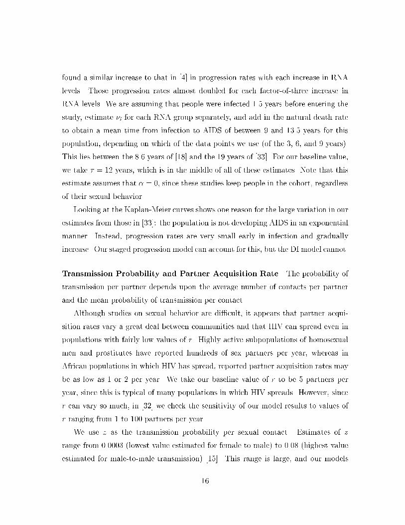
found a similar increase to that in [4] in progression rates with each increase in RNAlevels. Those progression rates almost doubled for each factor-of-three increase inRNA levels. We are assuming that people were infected 1.5 years before entering thestudy, estimate �i for each RNA group separately, and add in the natural death rateto obtain a mean time from infection to AIDS of between 9 and 13.5 years for thispopulation, depending on which of the data points we use (of the 3, 6, and 9 years).This lies between the 8.6 years of [18] and the 19 years of [33]. For our baseline value,we take �� = 12 years, which is in the middle of all of these estimates. Note that thisestimate assumes that � = 0, since these studies keep people in the cohort, regardlessof their sexual behavior.Looking at the Kaplan-Meier curves shows one reason for the large variation in ourestimates from those in [33]: the population is not developing AIDS in an exponentialmanner. Instead, progression rates are very small early in infection and graduallyincrease. Our staged progression model can account for this, but the DI model cannot.Transmission Probability and Partner Acquisition Rate The probability oftransmission per partner depends upon the average number of contacts per partnerand the mean probability of transmission per contact.Although studies on sexual behavior are di�cult, it appears that partner acqui-sition rates vary a great deal between communities and that HIV can spread even inpopulations with fairly low values of r. Highly active subpopulations of homosexualmen and prostitutes have reported hundreds of sex partners per year, whereas inAfrican populations in which HIV has spread, reported partner acquisition rates maybe as low as 1 or 2 per year. We take our baseline value of r to be 5 partners peryear, since this is typical of many populations in which HIV spreads. However, sincer can vary so much, in [32] we check the sensitivity of our model results to values ofr ranging from 1 to 100 partners per year.We use z as the transmission probability per sexual contact. Estimates of zrange from 0.0003 (lowest value estimated for female to male) to 0.08 (highest valueestimated for male-to-male transmission) [15]. This range is large, and our models16

are very sensitive to this parameter. We take z = 0:003 as our baseline value, partlybecause it is close to the value found in a number of couples studies, partly becauseit lies on the low side of the possible range for z, and partly because the reproductivenumber ends up near 2, given all of our other baseline choices.If n is the number of contacts with a partner, then the average probability oftransmission per partner is �� = 1� (1� z)n. There is no known relationship betweenthe average number of contacts per partner and the number of partners per year. Ingeneral, the number of contacts per partner will decrease as the partner acquisitionrate, r, increases. We choose a simple function with this property to be n = 104=r+1.Then �� = 1� (1� z)104=r+1. We are assuming that people with few partners have 2contacts per week and people with many partners have slightly more than one contactper partner. At the baseline value of r, this gives a mean of 21:8 contacts per partner,and �� = 0:063.Since z is in the interval (0:0003; 0:08), in a population with 30 partners per year,�� lies in the range 0.0013 to 0.31, and the reproductive number for both models rangesfrom 0.48 to 112 when �� = 12 years. In a population with 3 partners per year, ��lies between 0.011 and 0.95, giving a reproductive number of 0.38 to 51. Notice howthe variability in estimates for the probability of transmission leads to such a largeuncertainty in the reproductive number and, thus, in the dynamics of the epidemic,while the dependence of �� on r prevents r having such a large e�ect on the epidemic,especially at lower values of z. If we make a di�erent assumption about how thenumber of contacts per partner varies with r, then, of course, we would get more orless sensitivity of our results to r. In fact, in [32] we show that if n drops more rapidlyas r increases, the reproductive number can be nonmonotonic.In both scenarios, if the transmission probability is actually at its lowest estimatedvalue, then the epidemic will not spread, whereas at its highest value, the epidemicwill spread very rapidly and be very di�cult to stop. This is one reason why condomusage, which can reduce the probability of transmission per contact by 90% or more,can have such a dramatic e�ect on the spreading of the epidemic.17

Infectivity of the Subgroups Our models, and the theoretical results we derivedfrom them, are not dependent on the assumption that RNA viral levels in serum andtransmissibility of the virus are correlated. However, we now make this assumptionin order to derive relative values for the subgroups in each model to use in ournumerical studies. Although it seems highly plausible that viral levels in serum andplasma are correlated with infectiousness, it is important to keep in mind that such acorrelation does not necessarily exist. Assuming that it does assumes that serum levelsare correlated with membrane and secretion levels, and that those in turn somehowdetermine transmissibility itself. Newly developed lab techniques allow researchersto begin to measure HIV levels in semen, membranes, and cervical and vaginal uidsand to examine whether or not these levels correlate with plasma and serum levels.As pointed out by Royce et al. [15] in their review of sexual transmission, results onthis correlation to date are inconsistent: some studies, such as those in [34, 35, 36],have found a correlation; others, such as those in [37], have not.There is other evidence that HIV serum and plasma levels or individual varia-tions a�ect transmission, but it is less direct. Maternal HIV-1 RNA levels a�ect theprobability of transmission to the fetus [38]. Occasional reports of superspreaders (in-dividuals who have infected large numbers of partners) (see [9, 39], and the discussionin [10]) or the odd case of a dentist apparently infecting several patients [40] provideadditional support for the hypothesis that some individuals are highly infectious overlong periods of time. It seems reasonable to assume that genetic factors can partiallydetermine an infected individual's infectiousness, especially since they are known topartly determine susceptibility. Other factors, such as viral strain, age (which a�ectsprogression rates [4, 41]), the presence of other sexually transmitted diseases [42],smoking [43], general health, individual chemistry, and pregnancy [44], may a�ect anindividual's ability to transmit HIV.4.1.2 Parameters Speci�c to the DI ModelThe remaining parameters for the DI model are obtained from the HIV progressionstudy reported in [4], where the authors measured HIV RNA levels in a long-term18

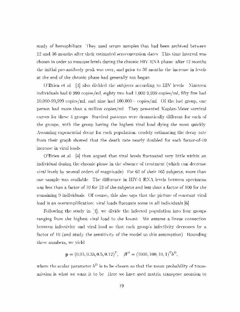
study of hemophiliacs. They used serum samples that had been archived between12 and 36 months after their estimated seroconversion dates. This time interval waschosen in order to measure levels during the chronic HIV RNA phase: after 12 monthsthe initial pre-antibody peak was over, and prior to 36 months the increase in levelsat the end of the chronic phase had generally not begun.O'Brien et al. [4] also divided the subjects according to HIV levels. Nineteenindividuals had 0-999 copies/ml, eighty-two had 1,000-9,999 copies/ml, �fty-�ve had10,000-99,999 copies/ml, and nine had 100,000+ copies/ml. Of the last group, oneperson had more than a million copies/ml. They presented Kaplan-Meier survivalcurves for these 4 groups. Survival patterns were dramatically di�erent for each ofthe groups, with the group having the highest viral load dying the most quickly.Assuming exponential decay for each population, crudely estimating the decay ratefrom their graph showed that the death rate nearly doubled for each factor-of-10increase in viral loads.O'Brien et al. [4] then argued that viral levels uctuated very little within anindividual during the chronic phase in the absence of treatment (which can decreaseviral levels by several orders of magnitude). For 62 of their 165 subjects, more thanone sample was available. The di�erence in HIV-1 RNA levels between specimenswas less than a factor of 10 for 53 of the subjects and less than a factor of 100 for theremaining 9 individuals. Of course, this also says that the picture of constant viralload is an oversimpli�cation: viral loads uctuate some in all individuals [6].Following the study in [4], we divide the infected population into four groupsranging from the highest viral load to the lowest. We assume a linear connectionbetween infectivity and viral load so that each group's infectivity decreases by afactor of 10 (and study the sensitivity of the model to this assumption). Roundingthese numbers, we yieldp = (0:05; 0:33; 0:5; 0:12)T ; �D = (1000; 100; 10; 1)TbD;where the scalar parameter bD is to be chosen so that the mean probability of trans-mission is what we want it to be. Here we have used matrix transpose notation to19

give the numbers.When we used the Kaplan-Meier curves from [4] to estimate progression rates foreach of their four groups, we obtain � = (0:1; 0:05; 0:03; 015)T yrs�1: This gives amean duration of infection of 18.6 years. To modify this to give the mean of 12 yearsthat we have assumed, we increase each �i by a factor of 1.92 so that� = (0:19; 0:096; 0:058; 0:028)T yrs�1when these baseline parameters are substituted into equation 2.5 with � = 0. Notethat as soon as � > 0, ��D is less than 12 years. Substituting all of the above parameterchoices into equation 2.6 gives a baseline mean probability of transmission per partner(with � = 0:05 yrs�1) of �� = 59:0bD:Specifying �� then allows us to calculate the appropriate value for bD.4.1.3 Parameters Speci�c to the SP ModelFor the SP model, we assume that the population goes through 4 stages: an early,highly infectious pre-antibody phase, two chronic stages at low infectiousness, and a�nal stage at higher infectiousness. According to [2, 6, 21], the peak in viral loadsoccurs 2 to 6 weeks after infection in the majority of patients, after which viral levelsdecline rapidly over the next 1 to 2 weeks. Viral loads at their peak may be ashigh as 106 or 107 copies/ml. From the data presented above, we know that afterthis early phase viral loads are rarely this large. In fact, the majority of infectedindividuals have between 103 and 104 copies/ml. Late in infection, viral loads mayrise but usually by less than tenfold. Therapy tends to reduce viral levels, but oftenonly temporarily.We need to choose our parameters so that the mean duration of infection is 12years when � = 0. If we take 4 weeks as the duration of the initial stage, 3 years asthe mean duration of the �nal and more infectious stage, and assume the middle twostages to have an equal duration, with a rate of moving on to the next stage denoted20

by m, then 1 = 13 yrs�1; 2 = 3 = m; 4 = 0:333 yrs�1:Substituting these values into (3.5) for qi, setting �� = 12 yrs, and then solving (3.6)gives m = 0:177 yrs�1:Thus each of the middle stages lasts an average of 5:7 years.Given the data on viral loads, we assume for the SP model that�S = (100; 1; 1; 10)TbS ;where bS is a scalar parameter that determines the mean probability of transmission.Using the i obtained above, we get �� = 3:345bS.4.1.4 SummaryWe have chosen the baseline parameters for each model to represent our best estimatefor �tting the model to the current HIV epidemic in the United States. These param-eters, de�ned in Table 2, are selected based on the analysis of epidemiological datapresented in Sections 4.1.1{4.1.3. For both the DI and SP models, the mean durationof infection is �� = 12 yrs, which is obtained by setting � = 0. However, the meantime an infected person stays in the active population (� = 0:05) is shorter in the DImodel (�̂D = 7:3 yrs ) than in the SP (�̂S = 8:26 yrs). Therefore, the reproductivenumber for the DI model is smaller than for the SP model.4.2 Numerical SimulationsOur goal in these examples is to investigate the relative impact of the infected sub-groups in the DI and SP models on the epidemic. Although the two models werederived using very di�erent assumptions about the biology of infected individuals, ifthe mean duration of infection and the mean infectivity are the same for the two mod-els, then their reproductive numbers and the numbers of total infected individuals atthe endemic equilibrium will be the same. This implies that, without direct evidence21

Table 2: Baseline ParametersInitial population size N = S(0) + Itot(0) 1.0Initial infected population Itot(0) 0.01Natural death rate d 0.02 yrs�1Sexually active removal rate � 0.05 yrs�1Total removal rate � = d+ � 0.07 yrs�1Mean duration of infection (� = 0) �� 12 yearsPartner acquisition rate r 5 partners/yearMean probability of transmission per contact z 0.003Mean probability of transmission per partner �� 0.063DI parametersDistribution by group upon infection pi (0.05, 0.33, 0.5, 0.12)Progression rates by group �i (0.19, 0.096, 0.058, 0.028)Relative infection rates �i (103; 102; 10; 1)bDMean duration of infectivity �̂D 7.3 yrsReproductive number R0 2.3bD = ��=59:0 0.00107SP parametersProgression rates by group i (13:0; 0:177; 0:177; 0:333)Relative infection rates �i (100; 1; 1; 10)bSMean duration of infectivity �̂S 8.26 yrsReproductive number R0 2.6bS = ��=3:3 0.01922

of the manner in which infectivity varies between individuals, it is not possible touse these two quantities to tell which hypothesis is valid. However, even when thereproductive numbers and endemic equilibrium are the same, the transient behaviorand internal dynamics of the models can be very di�erent.An added complication in any model with infected subgroups is the sensitivity ofthe model to the distribution of the initial infected population between the di�erentsubgroups. Di�erent distributions of even a small infected population can hasten ordelay the onset of an epidemic by several years. We approximate the natural initialconditions for an epidemic by introducing a very small infected group (0:01%) intothe population and allowing the epidemic to progress until 1% of the population isinfected. At this time, we re-normalize the population while maintaining the samerelative distribution of the infected population and call this time t = 0. With thisapproach, we �nd the model to be insensitive to the distribution of the initial 0:01%infected population. We explore this issue in more detail in [32].In all the examples, unless we explicitly state otherwise, we use the baseline pa-rameters in Table 2.4.2.1 Relative Impact of the Infected Groups on the EpidemicWhen there are multiple infected subgroups, each infected subgroup has a di�erentimpact on the spread of the disease. In this example, we compare the relative impactof the infected groups on the epidemic and observe how quickly these rates converge totheir asymptotic values. This example identi�es which infected groups are driving theepidemic. The hope is that this information may eventually help guide interventionstrategies to slow the epidemic. In particular, the analysis can be used to compare thesensitivity of the epidemic by targeting intervention strategies focused on identifyingpeople in the most infectious group in the DI model and the group in the SP modelwith the acute infectious period.We use the relative impact of each infected group, �i(t) = �i(t)=�(t), to study howfraction of the infections attributed to each infected group is directly related to theassumptions about the length of time spent in each group and the infectivity. In the23

numerical simulations, we monitor �i(t) directly and study how quickly these ratiosconverge to their asymptotic values given by (2.15) and (3.10).DI Model: The numerical simulation for the DI model in Figure 1 demonstrateshow the epidemic converges to the endemic equilibrium. The plot of the functions �i(t)shows that in the early spreading of the epidemic, the very small but highly infectiousgroup I1 causes the bulk of the infections. However, as the epidemic progresses, theseindividuals develop AIDS more rapidly than the individuals in the other groups andthey have less impact than the larger (but less infectious) group I2 . Interestinglyenough, even though group I3 is the largest group and stays in the population muchlonger than the �rst two groups, the assumption that they are tenfold less infectiousprevents this group from ever having a major impact on the epidemic. The moderatesize and small infectiousness of group I4 results in this long-lived group playing almostno role in the epidemic at any time.SP Model: The solution for the SP model in Figure 2 con�rms the observationmade by Jacquez et al. [21, 30] that in the early epidemic almost all infections forthe SP model are due to individuals in the �rst infection stage. Later on, this stagebecomes less important until eventually the infections transmitted from people in thelong lived last stage of the epidemic (Stage I4) dominate. Stages I2 and I3 play lessof a role throughout the epidemic.Comparison: Although the macro dynamics of the total infected populations forthe DI and SP are similar, the internal dynamics of the transmission process, asmeasured by the relative importance of the infected groups, are very di�erent. Thesedi�erences have signi�cant implications if the models are used to gain insight intoplanning intervention strategies. For example, suppose that the most infectious groupcould be identi�ed, perhaps through contact tracing, and convinced to change theirbehavior. In the DI model this would have an immediate and signi�cant impact onthe epidemic. In the early epidemic for the SP model, the most infectious group is24

0 10 20 30 40 50 600

0.1

0.2

0.3

0.4

0.5

0.6

0.7

0.8

0.9

1

Pop

ulat

ion

Time (years)

Baseline DI case

S(t)

I(t)

I1(t)

I2(t)

I3(t)

I4(t)

0 10 20 30 40 50 600

0.1

0.2

0.3

0.4

0.5

0.6

0.7

Time(years)

Fra

ctio

n in

fect

ed b

y gr

oup

i

Baseline DI case

ρ1

ρ2

ρ3

ρ4Figure 1: The solution and relative infection rates of the DI model for the baselineparameters (Table 2) show how quickly they converge to the equilibrium values (shownby the dashed lines). Note that the initial relative impact of the infected groups canbe di�erent from its asymptotic value. In fact, in this example the �rst infected groupcauses the largest number of infections early in the epidemic, and after about 25 yearsthe second infected group becomes the most important in terms of transmission.25

0 10 20 30 40 50 600

0.1

0.2

0.3

0.4

0.5

0.6

0.7

0.8

0.9

1

Pop

ulat

ion

Time (years)

Baseline SP case

S(t)

I(t)

I1(t)

I2(t)

I3(t)

I4(t)

0 10 20 30 40 50 600

0.1

0.2

0.3

0.4

0.5

0.6

0.7

0.8

Time(years)

Fra

ctio

n in

fect

ed b

y gr

oup

i

Baseline SP case

ρ1

ρ2

ρ3

ρ4

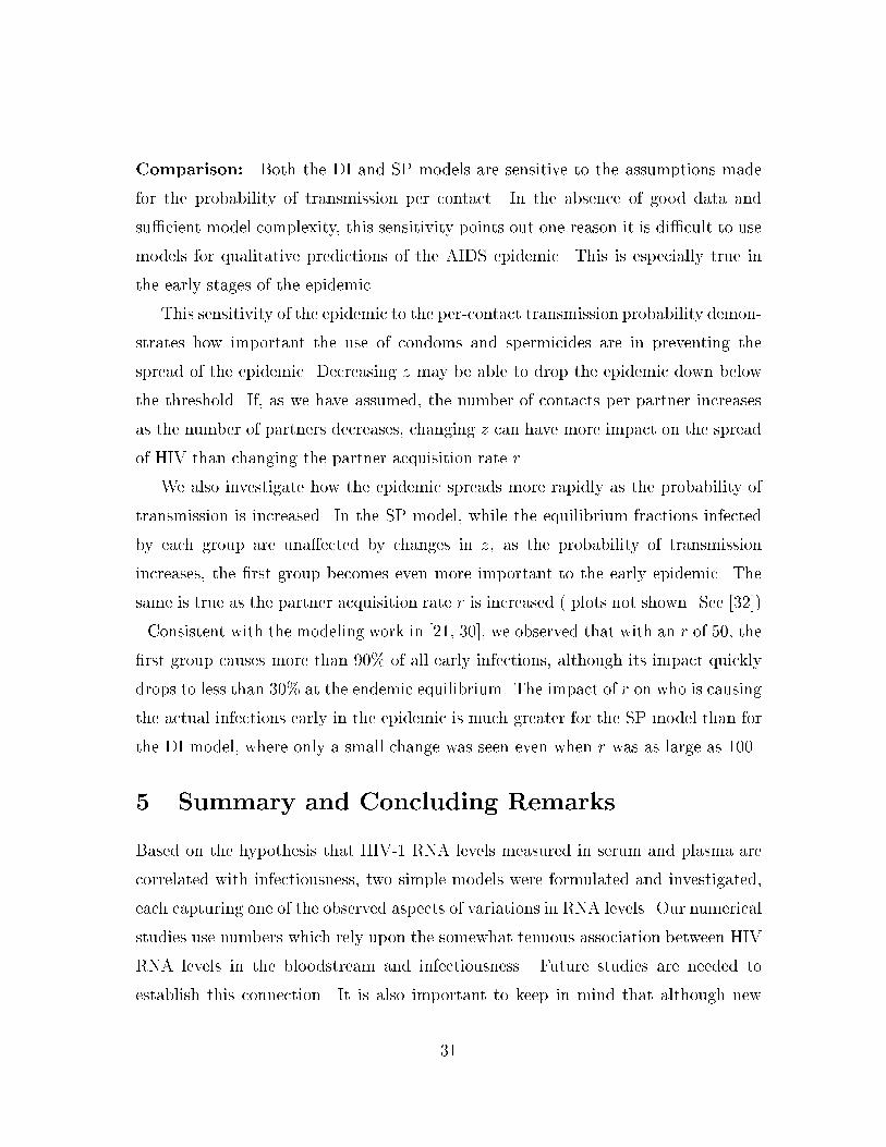
Figure 2: The solution and relative impacts of the SP model for the baseline caseparameters given in Table 2. The plot of the populations shows the initial rise andsubsequent convergence to the equilibrium values. Note that the initial relative impactof an infected group can be signi�cantly di�erent from its asymptotic value. In fact,in this example the relative impact of the �rst and fourth infected groups in the SPmodel switch places, in that early in the epidemic the I1 group causes most of theinfections, and later on the I4 group becomes the most signi�cant. Even though theother two groups are the largest, they transmit a small fraction of the infections.26

the one in the �rst infection stage which is continually being replenished and theimpact would be signi�cantly less. On the other hand, if an approach could be usedto identify more people in the very early stages of the infection, then this wouldhave only a proportional e�ect on the DI model, but could have a large impact oninfections caused by those in the �rst stage of the SP model. The insight gained byusing a model to understand the impact of drug therapy to extend the life expectancyof infected individuals is also sensitive to which model is being used.4.2.2 Sensitivity to the Probability of Transmission Per ContactWhen de�ning the baseline parameters, we made the assumption that the mean prob-ability of transmission per partner is �� = 1 � (1 � z)(104=r+1), where z is the meanprobability of transmission per contact. Under this assumption, the reproductivenumber increases rapidly with z when it is small, and gradually levels o�. As pointedout above, z is not well known. Not only are the ranges of z from any study fairlylarge, but it also appears that it may vary greatly between populations. In thisexample, we demonstrate the sensitivity of both models to small changes in z.DI Model: Figure 3 illustrates the extreme sensitivity of R0 for the DI model asa function of z. At the minimum estimate for z, R0 is below 1, and there is noepidemic. At the highest estimate of z = 0:08, R0 is 31, and the epidemic is rapidand devastating. R0 crosses 1 when z = 0:00127. When R0 is near 1, there is avery small, slow epidemic, but as it increases, there is at �rst a rapid change in thebehavior of the epidemic, which spreads more quickly and extensively.The sensitivity can be further seen by the wide variations in the progression ofthe epidemic in Figure 4, where we compare (z = 0:002; R0 = 1:56), (z = 0:003; R0 =2:31) and (z = 0:004; R0 = 3:06). Once R0 is greater than four or �ve, the epidemicsall progress similarly by rapidly infecting and depleting the susceptible population.Even though z has no impact on the equilibrium fractions of infections attributableto each group, as z increases, group I1 becomes relatively more important to theearly epidemic than the other groups. Group I1 contributes less and less as the27

0 0.01 0.02 0.03 0.04 0.05 0.06 0.07 0.08 0.09 0.10

5

10

15

20

25

30

35

Infectivity per contact

Rep

rodu

ctiv

e N

umbe

r

Figure 3: The reproductive number for the DI model is a sensitive function of themean probability of transmission per contact z. All the other parameters are thebaseline values given in Table 2.epidemic reaches its peak. For these parameters, most of the infections at all timesare attributable to groups I1 and I2. Although groups I3 and I4 make up the bulk ofinfected individuals, they have relatively little to do with spreading the epidemicSP Model: Both the endemic states and the transient dynamics of the SP epidemicare sensitive to z. The susceptible population shown in Figure 5 at time t = 20 di�ersby a factor of four when the probability of transmission per contact is changed by afactor of two.As in the DI model, the asymptotic fraction of the population infected by eachgroup is independent of z, although the transient dynamics are sensitive to the part-nership acquisition rates. When z is large, the �rst (highly infectious) group I1 pro-gresses extremely rapidly and initially drives the epidemic. When z is small, the earlyepidemic progresses much slower, and the last infected group I4 is more important.28

0 10 20 30 40 50 600

0.1

0.2

0.3

0.4

0.5

0.6

0.7

0.8

0.9

1

Time

Pop

ulat

ion

S(z=0.003)

S(z=0.002)

S(z=0.004)

I(z=0.002)

I(z=0.004)

0 10 20 30 40 50 600

0.1

0.2

0.3

0.4

0.5

0.6

0.7

Time

Infe

ctio

n R

ate

ρ1

ρ2

ρ3

ρ4Figure 4: The solution of the DI model is extremely sensitive to the mean probabilityof transmission per contact. The baseline epidemic z = 0:003 (solid line) progressesmore rapidly as z increases and all parameters (except bD) are held �xed as seen whenz = 0:002, bD = 7:23 10�4 (dashed line), and when z = 0:004, bD = 1:42 10�3 (dottedline). The plot of the fractions infected shows the relative impact of the infectedgroups for the z = 0:002 (dashed line) and z = 0:004 (dotted line) cases29

0 10 20 30 40 50 600

0.1

0.2

0.3

0.4

0.5

0.6

0.7

0.8

0.9

1

Time

Pop

ulat

ion

S(z=0.003)

S(z=0.002)

S(z=0.004)

I(z=0.002)

I(z=0.004)

0 10 20 30 40 50 600

0.1

0.2

0.3

0.4

0.5

0.6

0.7

0.8

0.9

Time

Infe

ctio

n R

ate

ρ1

ρ2

ρ3

ρ4

Figure 5: The SP model is also sensitive to the partnership acquisition rate z, evenwhen the total number of contacts is �xed. In the population plot, the solid curvesare the S and I populations for the baseline case of z = 0:003. The populationsare also shown for the cases when z = 0:002 ,bS = 0:013, R0 = 1:8, (dashed line),and z = 0:004 ,bS = 0:025, R0 = 3:4 (dotted line). All of the other parametersare at the baseline values given in Table 1. In the infection rate plot note thatthe asymptotic fraction of population being infected by each group is independentof z. The relative importance of the di�erent groups changes drastically during theepidemic when z = 0:002 (dashed line) and when z = 0:004 (dotted line), respectively.30

Comparison: Both the DI and SP models are sensitive to the assumptions madefor the probability of transmission per contact. In the absence of good data andsu�cient model complexity, this sensitivity points out one reason it is di�cult to usemodels for qualitative predictions of the AIDS epidemic. This is especially true inthe early stages of the epidemic.This sensitivity of the epidemic to the per-contact transmission probability demon-strates how important the use of condoms and spermicides are in preventing thespread of the epidemic. Decreasing z may be able to drop the epidemic down belowthe threshold. If, as we have assumed, the number of contacts per partner increasesas the number of partners decreases, changing z can have more impact on the spreadof HIV than changing the partner acquisition rate r.We also investigate how the epidemic spreads more rapidly as the probability oftransmission is increased. In the SP model, while the equilibrium fractions infectedby each group are una�ected by changes in z, as the probability of transmissionincreases, the �rst group becomes even more important to the early epidemic. Thesame is true as the partner acquisition rate r is increased ( plots not shown. See [32]). Consistent with the modeling work in [21, 30], we observed that with an r of 50, the�rst group causes more than 90% of all early infections, although its impact quicklydrops to less than 30% at the endemic equilibrium. The impact of r on who is causingthe actual infections early in the epidemic is much greater for the SP model than forthe DI model, where only a small change was seen even when r was as large as 100.5 Summary and Concluding RemarksBased on the hypothesis that HIV-1 RNA levels measured in serum and plasma arecorrelated with infectiousness, two simple models were formulated and investigated,each capturing one of the observed aspects of variations in RNA levels. Our numericalstudies use numbers which rely upon the somewhat tenuous association between HIVRNA levels in the bloodstream and infectiousness. Future studies are needed toestablish this connection. It is also important to keep in mind that although new31

RNA lab techniques are more reliable than older techniques, there remain questionsabout their accuracy [45].The di�erential infectivity model, which has never been previously studied, ac-counts for di�erences between individuals, and the staged-progression model, whichis similar to models previously studied, accounts for di�erences within the same in-dividual over the course of infection. Although, undoubtedly, individuals vary in in-fectiousness both temporally and individually, and the most complete model shouldinclude a combination of these two hypotheses, it is insightful (and more mathemat-ically tractable) to �rst consider them separately.For both models, we derived explicit formulas for their reproductive numbers andendemic equilibria. These formulas were expressed in a similar and easily interpretedform for both models. For example, the reproductive number is R0 = r ���� for bothmodels. We showed that if the reproductive number is less than one, the infection-free equilibrium is the only equilibrium which is locally asymptotically stable. Ifthe reproductive number is greater than one, the infection-free equilibrium becomesunstable, the epidemic spreads, and a unique endemic equilibrium appears. For theDI model we showed that this endemic equilibrium is locally asymptotically stable.We de�ned a new quantity, the relative impact of the group, as the fraction ofnew infections being caused by that group. Then, using mid range parameters andestimates from cohort studies, we examined the transmission dynamics of these twomodels and the relative impact of each group. Despite very moderate choices for thepartner acquisition rate and the transmission probability, both models had reproduc-tive numbers greater than 2. We also showed that the reproductive number and manydetails of the epidemic are very sensitive to the transmission probability per contact.For the DI model, and our parameter choices, the two most infectious groupsare responsible for almost all of the transmissions, despite the fact that their life-expectancy is shorter than the other two groups. The most infectious group, enteredby only 5% upon infection, is responsible for over 40% of all transmissions. Forthe SP model, those in the acute infectious phase transmit a very large fraction ofthe infections despite the very short duration of this phase. Most of the remaining32

infections are transmitted by those in the late chronic stage. These conclusions aboutwho transmits infection are robust to changes in the probability of transmission percontact, despite the fact that the overall epidemic is very sensitive to z.In the absence of a vaccine, epidemiologists must rely upon e�ecting behaviorchanges and providing condoms in order to control the spread of HIV. If infectiousindividuals could be identi�ed and convinced to change their behavior, then perhapsthe spread of HIV could be slowed or halted. If viral levels indicate infectiousness,then treatment of these individuals could also slow spreading by lowering their viralloads even when they are unwilling to change their behavior. Ideally, all infectedindividuals should be identi�ed and provided with treatments. However, screeningeveryone is not possible, and HIV is an infection which remains asymptomatic formany years, so that most infected people do not know they are infected. Our studyindicates that it is more urgent to identify some infected individuals than others.The DI and SP models capture two di�erent aspects of the HIV epidemic. Moresigni�cantly, we believe that the two mechanisms imply di�erent things about the bestway to control the epidemic in the absence of a vaccine. In particular, contact tracingcould be very e�ective at catching the most infectious individuals if a small group isresponsible for most of the infections and if that group of individuals is very infectiousthroughout the chronic stage. Such superspreaders would have infected a number ofpartners, one of whom is likely to identify the superspreader in an interview, thushopefully allowing the superspreader to be contacted and counseled and no longerspreading the virus to others. On the other hand, if every individual is infectiousfor only a short period of time at the beginning of the infection, then, by the time aperson is named by someone who has been infected, that person will already be in theuninfectious chronic stage. In that case, awareness of the symptoms of early acuteinfection might be the best way to identify people before they infect others. Likewise,alertness to symptoms may be a fairly e�ective way, perhaps combined with generalscreening programs, to identify individuals before they enter a more infectious stagelate in their infection.There has not been space to present further examples. In a future paper [32] we33

will do extensive sensitivity studies of both models to all of the parameters and, inparticular, to the migration rate and the relative infectivities of the di�erent groups.We will also carefully address the neglected question of initial conditions for thesetypes of models, showing that model results can be extremely sensitive to initialconditions. We will develop a \natural initialization procedure," that will be robustand will work for many population dynamics models.It is important to explore and understand the DI and SP models separately beforegoing to a model that has more complexity. However, the HIV RNA data indicate thata combined model might be necessary to capture some very important characteristicsof the epidemic. This is indeed the case if we wish to settle the question of who causesmost of the infections and, thus, whether or not contact tracing is a cost-e�ective wayof controlling the HIV epidemic. In a future paper, we plan to explore a DISP modelin which the infected population is divided into n�m groups, where n is the number ofdi�erent stages of infection and m is the number of inherently di�erent groups. Notethat we have also neglected many other important features of the AIDS epidemic,such as variations in sexual behavior, age, and inherent susceptibility.Although in this paper we have not explored the possibility that individuals varyinherently in their susceptibility, there is growing evidence to support this inherentvariation. Some individuals appear to be genetically immune to infection [17], andothers seem to be more susceptible [46]. Circumcision appears to decrease suscepti-bility in men [47], and the presence of other sexually transmitted diseases seems toincrease susceptibility [14, 47]. Variations in susceptibility should not a�ect epidemicdynamics much until an epidemic is far advanced and the more susceptible individualshave been depleted from the population, unless susceptibility and infectiousness arelinked.It is clear from our preliminary explorations of these two models that most HIVinfected individuals are not spreading the infection. If the subgroups that are trans-mitting infection could somehow be identi�ed and convinced to refrain from riskybehaviors, at least while they are infectious, the epidemic could perhaps be con-tained. Unfortunately, if the SP model results are to be believed, a lot of the spread34

occurs during the �rst few weeks to two months after infection. While a large numberof infecteds have acute primary infection symptoms, many do not. Further study witha combined model will tell us whether this group is truly important or whether thesuperspreaders of the DI model are more important.References[1] Pratt, R. D., J. F. Shapiro, N. McKinney, S. Kwok, and S. A. Spector, Virologiccharacterization of primary HIV-1 infection in a health care worker followingneedlestick injury, J Infect. Dis, 172 (1995), 851{854.[2] Quinn, T. C., Acute primary HIV infection, JAMA, 278 (1997), 58{62.[3] Henrard, D. R., J. F. Phillips, L. R. Muenz, W. A. Blattner, D. Weisner, M.E. Eyster, and J. J. Goedert, Natural history of HIV-1 cell-free viremia, JAMA,274 (1995), 554{558.[4] O'Brien, T. R., W. A. Blattner, D. Waters, M. E. Eyster, M. W. Hilgartner,A. R. Coher, N. Luban, A. Hatzakis, L. M. Aledort, P. S. Rosenberg, W. J.Milet, B. L. Kroner, and J. J. Goedert, Serum HIV-1 RNA levels and time todevelopment of AIDS in the multicenter hemophilia cohort study, JAMA, 276(1996), 105{110.[5] Wong, M. T., M. J. Dolan, E. Kozlow, R. Doe, G. P. Melcher, D. S. Burke, R.N. Boswell, and M. Vahey, Patterns of virus burder and T cell phenotype areestablished early and are correlated with the rate of disease progression in HIVtype 1 infected persons, J. Infect. Dis., 173 (1996), 877{887.[6] Piatak, M., M. S. Saag, L. C. Yang, S. J. Clark, J. C. Kappes, K. C. Luk, B. H.Hahn, G. M. Shaw, and J. D. Lifson, High levels of HIV-1 in plasma during allstages of Infection determined by competitive PCR, Science, 259 (1993), 1749{1754.[7] Baltimore, D., Lessons from people with nonprogressive HIV infection, New Eng-land Journal of Medicine, 332 (1995), 259{260.[8] Cao, Y., L. Qin, L. Zhang, J. Safrit, D. D. Ho, Virologic and immunologiccharacterization of long-term survivors of HIV type 1 infection, N. Engl. J. Med.,332 (1995), 201{208.[9] Clumeck, N., H. Taelman, P. Hermans, P. Piot, M. Schoumacher, and S. Dewit,A cluster of HIV infection among heterosexual people without apparent risk-factors, N. Engl. J. Med., 321 (1989), 1460-1462.[10] Holmberg, S. D., C. R. Horsburgh, J. W. Ward, and H. W. Ja�e, Biologic factorsin the sexual transmission of human immunode�ciency virus, J. Infect. Dis., 160(1989), 116{122. 35

[11] Palenicek, J., R. Fox, J. Margolick, H. Farzadegan, D. Hoover, N. Odaka, S.Rubb, H. Armenian, J. Harris, and A. J. Saah, Longitudinal study of homosexualcouples discordant for HIV-1 antibodies in the baltimore MACS study, J. AIDS,5 (1992), 1204{1211.[12] Peterman, T. A., R. L. Stonebrunner, J. R. Allen, H. W. Ja�e, and J. W. Curran,Risk of human immunode�ciency virus transmission from heterosexual adultswith transfusion-associated infections, JAMA. 256 (1988), 55{58.[13] Ragni, M. V., L. A. Kingsley, P. Nimorwicz, P. Gupta, and C. R. Rinaldo, HIVheterosexual transmission in hemophilia couples: Lack of relation to T4 number,clinical diagnosis, or duration of HIV exposure, J. AIDS, 2 (1989), 557{563.[14] Lazzarin, A., A. Saracco, M. Musicco, and A. Nicolosi, Man-to-woman sex-ual transmission of the human immunode�ciency virus, Arch. Intern. Med., 151(1991), 2411{2416.[15] Royce, R. A., A. Sena, W. Cates, and M. S. Cohen, Sexual transmission of HIVN. Eng. J. Med., 336 (1997), 1072{1078.[16] Biti, R., R. French, J. Young, J. Bennets, G. Stewart, T. Liang, HIV-1 infectionin an individual homozygous for the CCR5 deletion allele, Nat. Med., 3 (1997),252.[17] Huang, Yaoxing, et al., The role of a mutant CCR5 allele in HIV-1 transmissionand disease progression, Nature Medicine, 2 (1996), 1240{1243.[18] Longini, I. M., W. S. Clark, M. Haber, and R. Horsburgh, The stages of HIVinfection: Waiting times and infection transmission probabilities, In: Mathe-matical Approaches to AIDS Epidemiology (Castillo-Chavez, Levin, and Shoe-maker, Eds.), Lecture Notes in Biomathematics Vol. 83, Springer-Verlag, NewYork (1989), 111{137.[19] Anderson, R. M., R. M. May, G. F. Medley, and A. Johnson, A preliminary studyof the transmission dynamics of the human immunode�ciency virus (HIV), thecausative agent of AIDS, IMA, J. Math. Med. Biol., 3 (1986), 229{263.[20] Jacquez, J. A., C. P. Simon, J. Koopman, L. Sattenspiel, and T. Perry, Modellingand analyzing HIV transmission: The e�ect of contact patterns, Math. Biosc.,92 (1988), 119{199.[21] Jacquez, J. A., J. S. Koopman, C. P. Simon, and I. M. Longini, Role of theprimary infection in epidemics of HIV infection in gay cohorts, J. AIDS, 7 (1994),1169{1184.[22] Lin, Xiaodong, Qualitative analysis of an HIV transmission model,Math. Biosc.,104 (1991), 111-134.[23] Lin, Xiaodong, H. W. Hethcote, and P. Van den Driessche, An epidemiologicalmodel for HIV/AIDS with proportional recruitment, Math. Biosc., 118 (1993),181-195. 36

[24] Thieme, H. R. and C. Castillo-Chavez, How may infection-age dependent in-fectivity a�ect the dynamics of HIV/AIDS?, SIAM J. Appl. Math., 53 (1993),1449{1479.[25] Wiley, J. A., S. J. Herschkorn, and N. S. Padian, Heterogeneity in the probabilityof HIV transmission per sexual contact: the case of male-to-female transmissionin penile-vaginal intercourse, Stat. in Med., 8 (1989), 93{102.[26] Ho, D. D., M. Tarsem, and A. Masud, Quantitation of human immunode�ciencyvirus type 1 in the blood of infected persons, N. Engl. J. Med., 321 (1989),1621{1625.[27] Pedersen, C., C. M. Nielsen, B. F. Vestergaard, J. Gerstoft, K. Krogsgaard, andJ. O. Nielsen, Temporal relation of antigenaemia and loss of antibodies to coreantigens to development of clinical disease in HIV infection, Br. Med. J., 295(1987), 567{569.[28] Allian, J. P., Y. Laurian, D. A. Paul, and D. Senn, Serological markers in earlystages of immunode�ciency virus infection in haemophiliacs, Lancet, 2 (1986),1233-1236.[29] Sydow, M., H. Gaines, A. Sonnerborg, M. Forsgren, P. O. Pehrson, and O. Stran-negard, Antigen detection in primary HIV infection, Br. Med. J., 296 (1989),238{240.[30] Jacquez, J. A., C. P. Simon, and J. Koopman, Core groups and the R0s forsubgroups in heterogeneous SIS and SI models, In: Epidemic Models: TheirStructure and Relation to Data (Mollison, Ed.), Cambridge Univ. Press, Cam-bridge (1995), 279{301.[31] Kemper, J. T., On the identi�cation of superspreaders for infectious disease,Math. Biosci., 48 (1980), 111{127.[32] Hyman, J. M., Jia Li, and A. E. Stanley, Sensitivity Studies of the Di�eren-tiated Infectivity and Staged Progression Models for the Transmission of HIV,In preparation, available from http://math.lanl.gov/ mac/papers/papers.html inlate 1998.[33] Mellors, J. W., A. Munoz, J. V. Giorgi, J. B. margolick, C. J. Tassoni, P. Gupta,L. A. Kingsley, J. A. Todd, A. J. Saah, R. Detels, J. P. Phair, and C. R. Ri-naldo, Plasma viral load and CD4+ lymphocytes as prognostic markers of HIV-1infection, Ann. Intern. Med., 126 (1997), 946{954.[34] Gupta, P., J. Mellors, L. Kingsley, S. Riddler, M. Singh, S. Schreiber, M. Cronin,and C. Rinaldo, High viral load in semen of HIV-1 infected men at all stages ofdisease and its reduction by antiretroviral therapy, 4th Conf. Retro. and Oppor-tun. Infect., abstract no. 726 (1997).[35] Hart, C., M. Palmore, T. Wright, J. Lennox, T. Evans-Strickfaden, T. BushC. Schnell, L. Conlet, and T. V. Ellerbrock, Correlation of cell-free and cell-associated HIV RNA levels in plasma and vaginal sectretions, 4th Conf. Retro.and Opportun. Infect., abstract no. 25 (1997).37

[36] Speck, C. E., R. Coombs, L. Koutsky, J. Zeh, L. Corey, T. Hooton, S. Ross, andJ. Krieger, Rates and determinants of HIV shedding in semen, Int. Conf. AIDS,abstract no. We. C.334 (1996).[37] Jurrianns, S., P. L. Vernazza, J. Goudsmit, J. Boogaard, B. Van Gemen, HIV-1viral load in semen versus blood plasma, Int. Conf. AIDS, abstract no. Th.A.4036(1996).[38] Dickover, R. E., E. M. Garratty, S. A. Herman, M. S. Sim, S. Plaeger, P. J.Boyer, M. Keller, A. Deveikis, E. R. Stiehm, and Y. J. Bryson, Identi�cationof levels of maternal HIV-1 RNA associated with risk of perinatal transmission,JAMA, 275 (1996), 599{605.[39] Padian, N., L. Marquis, D. P. Francis, R. E. Anderson, G. W. Rutherford, P. M.O'Malley, and W. Winkelstein, Male-to-female transmission of human immun-ode�ciency virus, JAMA, 258 (1987), 788{790.[40] MMWR, Update: transmission of HIV infection during and invasive dental pro-cedure { Florida, 40 (1991), 21{27.[41] Pezzotti, P., A. N. Phillips, M. Dorrucci, A. C. Lepri, N. Galai, D. Vlahov, andG. Rezza, Category of exposure to HIV and age in the progression to AIDS, Br.Med. J., 313 (1996), 583{586.[42] Latif, A. S., D. A. Katzenstein, M. T. Basset, S. Houston, J. C. Emmanuel, andE. Marowa, Genital ulcers and transmission of HIV among couples in Zimbabwe,J. AIDS, 3 (1989), 519{523.[43] Royce, R. A., W. Winkelstein, and P. Bachetti, Cigarette smoking and inci-dence of AIDS, Abstracts of the Sixth International Conference on AIDS, SanFrancisco, CA (1990), Abstract Th.C.39.[44] Henin, Y., L. Mandelbrot, R. Henrion, R. Pradinaud, J. P. Couland, and L.Montagnier, Virus excretion in the cervicovaginal secretions of pregnant andnonpregnant HIV-infected women, J. AIDS, 6 (1993), 72{75.[45] Landesman, S. H. and D. Burns, Quantifying HIV, JAMA, 275 (1996), 640{641.[46] Garred, P., Susceptibility to HIV infection and progression of AIDS in relationto variant alleles of Mannose-Binding lectin, Lancet, 349 (1997), 236{240.[47] Greenblatt, R. M., S. A. Lukehart, F. A. Plummer, T. C. Quinn, C. W. Critchlow,R. L. Ashley, L. J. D'Costa, J. O. Ndinya-Achola, L. Corey, A. R. Ronald, andK. K. Holmes, Genital ulceration as a risk factor for HIV infection, J. AIDS, 2(1988), 47{50.38

AppendixesA The Reproductive Number for the DI ModelThe asymptotic dynamics of the infection-free equilibrium are determined by thefollowing submatrix in the Jacobian matrix of (2.1) at the infection-free equilibriumJ := 0BBB@p1r�1 � (�+ �1) p1r�2 : : : p1r�np2r�1 p2r�2 � (�+ �2) : : : p2r�n... ... . . . ...pnr�1 pnr�2 : : : pnr�n � (�+ �n)1CCCA :Since all o�-diagonal elements are positive, we now consider matrix �J . Using thepositive vector V := � p1(�+ �1) � � � pn(�+ �n)�T , we have�J � V = 1� r nXj=1 pj�j(�+ �j)!E;where E = (p1; p2; � � � ; pn)T . Then it follows from M-matrix theory that each eigen-value of J has a negative real part ifR0 = r nXj=1 pj�j(�+ �j) < 1;which implies the infection-free equilibrium is locally asymptotically stable.On the other hand, by mathematical induction, it can be shown that the deter-minant of J equals (�1)n+1 nYi=1 �+ �i�i (R0 � 1) :Then, if R0 > 1, J has eigenvalues with positive real parts, which implies the insta-bility of the infection-free equilibrium.B Stability of the Endemic Equilibrium for the DIModelFor the DI model, we establish the local stability of the endemic equilibrium byshowing that all eigenvalues of the Jacobian matrix at the endemic equilibrium have39

negative real parts.The Jacobian matrix at the endemic equilibrium has the formJ = 0BBBBB@��� � �1� SN � �h1 �h2 : : : �hnp1� �1� SN � �(�+ �1) + p1h1 p1h2 : : : p1hnp2� �1� SN � p2h1 �(�+ �2) + p2h2 : : : p2hn... ... ... . . . ...pn� �1� SN � pnh1 pnh2 : : : �(� + �n) + pnhn1CCCCCA ;

where hi := SN (r�i � �).By the similarity matrixM := 0BBBBB@ 1 0 0 : : : 0p1 1 0 : : : 0p2 0 1 : : : 0... ... ... . . . ...pn 0 0 : : : 11CCCCCA ;J is transformed into the following matrix:B := 0BBBBBB@��� �+ rR0 Pi pi�i �h1 �h2 : : : �hnp1�1 �(� + �1) 0 : : : 0p2�2 0 �(�+ �2) : : : 0... ... ... . . . ...pn�n 0 0 : : : �(�+ �n)

1CCCCCCA :Hence, matrix J has all eigenvalues with negative real parts if and only if B has alleigenvalues with negative real parts.Let � be an eigenvalue ofB with the corresponding eigenvectorX = (x0; x1; � � � ; xn)T .Then pj�jx0 = (�+ �j + �) xj; j = 1; � � � ; n: (B.1)Solving (B.1) for xj, j = 1; � � � ; n, in terms of x0 and then substituting them into the�rst row of BX = �X, we arrive at��� �+ rR0 nXj=1 pj�j � 1R0 nXj=1 pj�j (r�j � �)(�+ �j + �) = �:40

Let � = u+ iv. Then u and v satisfy the following equations:u+ �+ �� rR0 nXj=1 pj�j + 1R0 nXj=1 pj�j (r�j � �) (u+ �+ �j)(u+ �+ �j)2 + v2 = 0; (B.2a)1� 1R0 nXj=1 pj�j (r�j � �)(u+ �+ �j)2 + v2 = 0: (B.2b)Now we have the following two lemmas.Lemma B.1. Any eigenvalue of B with a nonnegative real part must be a real num-ber.Proof. Assume u � 0 and v > 0. Then it follows from (B.2b) thatR0 + � nXj=1 pj�j(u+ �+ �j)2 + v2 =r nXj=1 pj�j�j(u+ �+ �j)2 + v2< r nXj=1 pj(�+ �j)�j(u+ �+ �j)2 � r nXj=1 pj(�+ �j)�j(�+ �j)2 = R0;which is impossible. Hence, if u � 0, v must be nonpositive. However, since u� iv isalso an eigenvalue of B, v cannot be negative. Hence, v must be zero, and � must bea real number.Lemma B.2. Matrix B has no nonnegative real eigenvalue.Proof. Matrix B has a positive real eigenvalue � = u if and only if (B.2a) has apositive solution u while v = 0.De�ne F (u) := u+ �+ �� rR0 nXj=1 pj�j + 1R0 nXj=1 pj�j (r�j � �)u+ �+ �j :Then F (0) = �+ �� rR0 nXj=1 pj�j + 1R0 nXj=1 pj�j (r�j � �)�+ �j � ��1� 1R0� > 0;41

if R0 > 1.On the other hand,F 0(u) =1� 1R0 nXj=1 pj�j (r�j � �)(u+ �+ �j)2 � 1� rR0 nXj=1 pj�j�j(u+ �+ �j)2� 1� rR0 nXj=1 pj(�+ �j)�j(u+ �+ �j)2 � 1� rR0 nXj=1 pj�j�+ �j = 0;for all u � 0. Hence, F (u) > 0 for all u � 0. That is, matrix B has no nonnegativereal eigenvalue.Based on Lemmas B.1 and B.2, all eigenvalues of B must have negative real parts.Then the local asymptotic stability of the endemic equilibrium of (2:1) follows.C The Endemic Equilibrium for the SP ModelDe�ning �i = i + �, it follows from the equations for Ii, i = 2; � � � ; n, in (3.1) thatIi�1 = �i i�1 Ii:De�ne �i := nQj=i+1�jn�1Qj=i j :Then Ii = �iIn; i = 1; � � � ; n� 1: (C.1)Since �S = �1I1, Sr nPk=1�kIk = S�1I1 + �1I1 nPk=1 Ik. Then Sr nPk=1�k�k = S�1�1 +�1�1 nPk=1�kIn, and henceS = �1�1 nPk=1�kr nPk=1�k�k � �1�1 In = nPk=1�kr�1�1 nPk=1�k�k � 1In:42

It can be shown that RS0 = r nPk=1�k�k�1�1 :Then, S = nPk=1�kRS0 � 1In; (C.2)which is positive if and only if RS0 > 1.On the other hand, from �(S0 � S) = �1I1 = �1�1In, it follows that�S0 = 0BB@� nPk=1�kRS0 � 1 + �1�11CCA In:Thus In = �S0� nPk=1�kRS0 � 1 + �1�1 : (C.3)Substituting (C.3) into (C.2) and (C.1), respectively, we can solve for the endemicequilibrium explicitly as in (3.8).

43