INTERNATIONAL ASSOCIATION IA FOR ENERGY ECONOMICS EE President Hoesung Lee President-Elect Peter A. Davies Immediate Past President Charles Spierer Past President Dennis J. O’Brien Treasurer Jean-Thomas Bernard Vice President for Development & International Affairs Peter C. Fusaro Vice President for Publications Hossein Razavi Vice President and Secretary Arild N. Nystad Vice President for Conferences Michelle Michot Foss Elected Council Member Michael C. Lynch Elected Council Member Hans Larsen Appointed Council Member Robert Bartels Appointed Council Member David Knapp Appointed Council Member Anthony Owen Appointed Council Member Paul J. Stevens

The Energv Journal is a publication of the Energy Economics Education Foundation, Inc., 28790

Chagrin Blvd., Suite 350, Cleveland, OH, 44122-4630, USA, anon-protit organization, in association with the Intemational Association for Energy Economics.

Membership dues for the IAEE include subscriptions to The Energy Journal and the IAEE

Newsletter. Subscriber & Membership matters should be sent to IAEE, 28790 Chagrin Blvd., Suite 350, Cleveland, OH, 44122, USA; phone (216) 464-5365, fax 464-2737. Non-member subscriptions to The Energy Journal are $175 for institutions, libraries, and individuals. Postage and handling are

paid by the publisher. Outside the United States and Canada, non-member subscriptions are $200. Articles appearing in The Energv Journal are listed in both Environmental Periodicals

Bibliography and The Journal of Economic Literafure and are indexed in SciSearch, Research Alert,

COMPENDEX*PLUS, Energy Abstracis, Ei Page One, PAIS Bulletin, Trade and Industty, DOE

Energv, Energvline, Enviroline, and Wilsonline.

Authorization to photocopy articles published in The Energy Journal for interna1 or personal use,

or the interna1 or personal use of specific clients, is granted by IAEE provided that you register with the Copyright Clearance Center, 222 Rosewood Drive, Danvers, MA 01923. CCC’s phone number is (978) 750-8400. The Energy Journal is available in referente systems (e.g. microfilm, CD-ROM,

full text etc.) produced by the Information Access Company (IAC), University Microfilms Inc. (UMI), and the H.W. Wilson Company’s Business Periodicals Index. For further information please

contact IAC at (415)-378-5000, UMI at (313)-761-4700, or H.W. Wilson Co., at (718)-588+X400.

AUTHORS: Please see back pages for information on the proper style of submissions. ADVERTISING INFORMATION: For a complete media kit, contact Marketing Department, IAEE

Headquarters, 28790 Chagrin Blvd., Ste. 350, Cleveland, OH, 44122-4630. Phone: 216-464-5365, fax: 216-464-2737. E-mail: iaee@iaee.org. Homepage: http://www.iaee.org.

Copyright 0 1999 by the International Association for Energy Economics. All rights reserved.

The editors and publisher assume no responsibility for the views expressed by the authors of articles printed in The Energv Journal.

International Standard Serial Number: 0195-6574. Printed in the U.S.A.

Editors, Adonis Yatchew, Campbell Watkins Founding Editor, Helmut J. Frank

European Editor, Yves Smeers Associate Editor, Geoffrey Pearce

Book Review Editor, Richard L. Gordon

Board of Editors

Alexander A. Arbatov Institute for Systems

Studies. Moscow

Lars Bergman Stockllolm scllool

of Economics

Fadhil J. Chalabi Centre for Global Energy

Studies, London

Caro1 Dahl Colorado School of

Mines

Dnvid Dorenfeld Exxon Ventures CIS

Joy C. Dunkerley Washington, DC.

A. Denny Ellerman MIT Center for Energy & Enviromnental Research

Michelle Michot Foss CBA Energy Institute,

University of Houston

Lawrence J. Goldstein Petroleum Industry Research Foundation, Inc.

Richard L. Gordon Pennsylvania State

University

James M. Griffin Texas A & M University

William W. Hogan Harvard University

David Huettner University of Oklahoma

Mark K.Jaccard Simon Fraser University British Columbia

Willirm A. Johnson JECOR, Saudi Arabia

J. Daniel Khazzoom San Jose State University

Jean Masseron Institut Francais du Petrole

Kenichi Matsui Institute of Energy Economics, Tokyo

Mohan Munasinghe The World Bank

Washington, DC

Peter R. Odell Erasmus Universiteit

R.K. Pachauri TATA Energy Research Institute, New Delhi

Frrncisco R. Parra F.R. Parra Inc.

Peter Pearson Imperial College of Science, Technology and

Medicine, London

Stephen Peck EPRI, Palo Alto, CA

André Plourde University of Alberta

Hossein Razavi The World Bank Washington, DC

Ali Reza Oakland California

Dieter Schmitt Universität Essen Germany

Margaret Slade University of British Columbia

James L. Smith Southern Methodist University, Dallas

Thomas Sterner Göteborg University

John Surrey University of Sussex United Kingdom

Leonard Waverman London Business School

John P. Weyant Stanford University

Franz Wirl Otto-von-Guericke

University of Magdeburg

Chi-Keung Woo Energy and Environmental

Economics. 111~.

ii

THE COSTS OF THE KYOTO PROTOCOL A MULTI-MODEL EVALUATION

A Special Issue of The Energy Journal

GUEST EDITOR

JOHN P. WEYANT Director, Energy Modeling Forum Stanford University

Assisted by

Henry Jacoby Massachusetts Institute of Technology James Edmonds Batelle Pacijk Northwest National Laboratory Richard Richels Electric Power Research Institute

Publication of this special issue was made possible by generous financia1 support from the U 3. DEPARTMENT OF ENERGY, THE U.S. ENVIRONMENTAL PROTECTION AGENCY, AND THE ELECTRIC POWER RIBEARCH INSTITUTE. The studies of the Energy Modeiing Forum are sponsored by the U.S DOE, U.S. EPA, EPRI, Mitsubishi Corporation, the New Energy and Industrial Technology Development Organization of Japan, and about 20 corporate afftliates.

. . . III

THE ENERGY JOURNAL

SPECIAL ISSUE

THE COSTS OF THE KYOTO PROTOCOL: A MULTI-MODEL EVALUATION

Table of Contents

Preface Campbell Watkins vi

Introduction and Overview John P. Weyant and Jennifer N. Hill vii

The Kyoto Protocol: A Cost-Effective Strategy for Meeting Environmental Objectives? Alan S. Manne and Richard Richels 1

The Economics of the Kyoto Protocol Christopher N. MacCracken, James A. Edmonds,

Son H, Kim, and Ronald D. Sands 25

Adjustment Time, Capital Malleability and Policy Cost Henry D. Jacoby and lan Sue Wing 73

Requiem for Kyoto: An Economic Analysis of the Kyoto Protocol William D. Nordhaus and Joseph G. Boyer 93

Kyoto, Effkiency, and Cost-Effectiveness: Applications of FUND Richard S.J. Tol 13 1

Analysis of Carbon Emission Stabilization Targets and Adaptation by Integrated Assessment Model Atsushi Kurosawa, Hiroshi Yagita, Zhou Weisheng

Koji Tokimatsu, and Yukio Yanagisawa 157

Clubs, Ceilings and CDM: Macroeconomics of Compliance with the Kyoto Protocol Johannes Bollen, Arjen Gielen, and Hans Timmer 177

iv

Analysis of Post-Kyoto Scenarios: The Asian-Pacific Integrated Model Mikiko Kainuma, Yuzuru Matsuoka, Tsuneyeki Morita 207

Effects of Restrictions on International Permit Trading: The MS-MRT Model Paul M. Bernstein, W. David Montgomery, Thomas F. Rutherford and Gui-Fang Yang 221

The Kyoto Protocol: An Economic Analysis Using GTEM Vivek Tulpulé, Stephen Brown, Jaekyu Lim,

Cain Polidano. Hom Pant and Brian S. Fisher 257

Emissions Trading, Capital Flows and the Kyoto Protocol Warwick McKibbin, Martin Ross, Robert Shackleton and Peter Wilcoxen 287

The Economic Implications of Reducing Carbon Emissions: A Cross-Country Quantitative Investigation using the Oxford Global Macroeconomic and Energy Model Adrian Cooper, Scott Livermore, Vanessa Rossi,

Alan Wilson and John Walker 335

CO, Emissions Control Agreements: Incentives for Regional Participation Stephen C. Peck and Thomas J. Teisberg 367

About the Authors

Short biographies of the contributing authors 391

Preface

The Kyoto Protocol dealing with climate change was adopted in December, 1997. Over a year later 84 countries have signed, but only eight had ratified it. Getting agreement among Protocol participants is one thing; achieving ratification is quite another.

The main culprit targeted is carbon dioxide emissions from fossil fuels. A five percent reduction from 1990 emission levels to be reached about a decade from now seems modest. Not so. Given actual economic growth since 1990 and anticipated growth, the ‘Kyoto Gap’ could be as much as 30 percent from base line emissions expected by 2010.

Implementing the Protocol will require prodigious efforts. Hence the importance of attempts to measure the magnitude, severity and incidence of meeting the Kyoto targets. This special issue of i%e Energy Journal, edited by John Weyant of Stanford University with assistance from Henry Jacoby of MIT, Jae Edmonds of Batelle and Richard Richels of EPRI, provides international simulations of implementing the Kyoto agreement using several different models. The canvas is wide. The modeling tapestry is rich. The results provide both focus and perspective.

I think I am right in saying that this volume is the longest E,yergy Journal Special Issue to date. It could not have been produced wi.thout substantial financial support from the Electric Power Research Institute, the US Department of Energy and the US Environmental Protection Agency. We are in their debt.

G. Campbell Wtztkins Joint Bditor

The Energy Journal

vi

INTRODUCTION AND OVERVIEW

John P. Weyant and Jennifer N. Hill*

This Special Issue of 27ze Energy Journal represents the first comprehensive report on a comparative set of analyses of the economic and energy sector impacts of the Kyoto Protocol on Climate Change. Organized by the Stanford Energy Modeling Forum (EMF), the objectives of this study were the same as for previous EMF studies: (1) identifying policy-relevant insights and analyses that are robust across wide ranges of models, (2) providing explanations for differences in results from different models, and (3) identifying high priority areas for future research. This study has produced a particularly rich set of results in all three areas, which is a tribute to the active participation of the modeling teams and the care each team took in preparing a paper for this volume.

The volume consists of a paper prepared by each modeling team on what it did and what it concluded from the model runs that were undertaken, proceeded by this introduction and summary paper. This summary focuses on the motivation for the study, the design of the study scenarios, and the interpretation of results for the four core scenarios, which all the teams ran. Each succeeding chapter contains ideas and insights drawn by the modeling teams from applying their models to issues they were able to address selected from a small set of important areas on which the group had mutually agreed to focus.

Ihe Energy Journal, Kyoto Special Issue. Copyright Q 1999 by the IAEE. All rights reserved.

* Department of Engineering-Economic Systems and Operations Research, Stanford University,

Stanford, CA 94305-4023. E-mail: weyant@leland.Stanford.edu.

The studies of the Energy Modeling Forum are sponsored by the U.S. Department of Energy, the

U.S. Environmental Protection Agency, the Electric Power Research Institute, Mitsubishi

Corporation, the New Energy and Industrial Technology Development Organization of Japan, and

about 20 corporate affiliates. Besides the authors of the other papers in this volume, we would

especially like to thank Campbell Watkins for his enthusiasm about the idea of doing this specia.1

issue and his insightful advice at each step in the production process. In addition, we would like to

thank Geoff Pearce of the Energy Journal and Dave Williams of the IAEE for going above and

beyond the call of duty in making this special issue a reality.

vii

viii / The Energy Journal

The reader is cautioned not to view the wide range of model results presented here as an expression of hapless ignorance on the part of the analysts, but as a manifestation of the uncertainties inherent in projecting how the future will unfold with and without climate change policies. The uncertainties highlighted here are endemic in the operation of our world or the result of limitations in our understanding it. The models do not produce lthese uncertainties. They make them more transparent and help assess their magnitudes. This is important in the analyses of climate policies because of the complexities and interdependencies involved.

The climate change debate is often posed as an all or nothing choice about whether or not we are serious about a problem that could have disastrous consequences. However, we know that the problem may turn out to be more or less serious than currently envisioned and that we can change our course of action in subsequent years as more is learned about the nature of the problem and its potential solutions. It is also often asserted that the models do not provide useful information because they sometimes produce different results. No thing could be further from the truth; by comparing results from alternative modeling systems we gain additional information about the relationships between assumptions and outputs that are not available when results from a single model or a single expert are considered.

This introduction starts with a brief discussion of the UN Framework Convention on Climate Change (UNFCCC); the Conference of Parties process set out in the UNFCCC, the Kyoto Protocol, and the Buenos Aires agenda. Next the scenarios designed by the group to address some of the key uncertainties about how the Protocol might be implemented are described, followed by brief overviews of mitigation economics and a structural comparison of the models included in the comparison. A summary of key common results and interpretations of model differences that were developed this from a review of results for the core scenarios follows. Finally, an overview of the papers by the participating modeling teams, stressing issues focused on and insights obtained, completes the process of setting the stage for the papers prepared by the modeling teams which follow.

A BRIEF HISTORY OF THE FCCC AND THE KYOTO PROTOCOL

The United Nations Framework Convention on Climate Change was adopted on May 9, 1992, and was opened for signature at the UN Conference on Environment and Development in June 1992. The Convention entered into force on March 21, 1994, 90 days after receipt of the 50th ratification. Currently, 176 countries have ratified it. One of the key elements of the UNFCCC was a set of voluntary commitments to stabilize carbon emissions at 1990 levels by 2000 by the developed countries listed in Annex I of the Convention document (dominantly the OECD countries, the countries in Eastern

Introduction / ,k

Europe and the states of the former Soviet Union-e.g., the Russian Federation, the Ukraine, Belarus, etc.-which, thus, became known as the “Annex I” countries).

The first meeting of the Conference of the Parties to the FCCC (COP- 1) took place in Berlin from March 28 - April 7, 1995. In addition to addressing a number of important issues related to the future of the Convention, delegates reached agreement on what many believed to be the central issue before COP- 1 -adequacy of commitments, the “Berlin Mandate” to establish binding emission limitations for Annex I countries beyond the year 2000. At that point, an open-ended Ad Hoc Group on the Berlin Mandate (AGBM) was established to begin a process toward appropriate action for the period beyond 2000, including the strengthening of the commitments of Annex I Parties through th.e adoption of a protocol or other legal instrument. COP-I also requested th.e Secretariat to make arrangements for sessions of a Subsidiary Body on Scienc:e and Technological Advice (SBSTA) and a Subsidiary Body on Implementation (SBI). SBSTA would serve as the link between scientific, technical and technological assessments, the information provided by competent international bodies, and the policy-oriented needs of the COP. During the AGBM process, SBSTA addressed several issues, including the treatment of the Intergovernmental Panel on Climate Change’s (IPCC’s) Second Assessment Report (SAR). SBI was created to develop recommendations to assist the COP in the review and assessment of the implementation of the Convention and in the preparation and implementation of its decisions.

The AGBM met eight times between August 1995 and December 1997. During the first three sessions, delegates focused on analyzing and assessing possible policies and measures to strengthen the commitments of AMeX I Parties, how Annex I countries might distribute or share new commitments and whether commitments should take the form of an amendment or Protocol. AGBM4, which coincided with COP-2 in Geneva in July 1996, completed its in-depth analysis of the likely elements of a Protocol and the participating States appeared ready to prepare a negotiating text. At AGBM-5, which met in December 1996, delegates recognized the need to decide whether or not to allow mechanisms that would provide Annex I Parties with flexibility in meeting quantified emission limitation and reduction objectives (QELROs).

As a Protocol on climate change was drafted during the sixth and seventh sessions of the AGBM, in March and August of 1997, respectively, delegates created a negotiating text by merging or eliminating some overlapping provisions within the myriad of proposals. Much of the discussion centered on a proposal from the European Union (EU) for a 15% cut in a “basket” of three greenhouse gases by the year 2010 relative to 1990 levels. In October 1997, as AGBM-8 began, U.S. President Bill Clinton made a call for “meaningful participation” by developing countries in the negotiating position he announced

x / The Energy Journal

in Washington. This statement rekindled some of the major debates that had preceded the tentative agreement reached agreement in 1995; G-77/Chins* involvement was once again linked to the level of commitment acceptable to the US. In response, the G-77/Chins distanced itself from anything that could be interpreted as new commitments.

The Third Conference of the Parties (COP-3) to the FCCC was held from December l-l 1, 1997 in Kyoto, Japan. Over 10,000 participants, including representatives from governments, intergovernmental organizations, Non- Government Organizations (NGOs) and the press, attended the Conference, which included a high-level segment featuring statements from over 125 ministers. Following a week and a half of intense formal and infalrmal negotiations, Parties to the FCCC adopted the Kyoto Protocol on December 11, 1997; it was opened for signature on March 16, 1998 at United Nations Headquarters, New York.

The Protocol is subject to ratification, acceptance, approval or acce:ssion by Parties to the Convention. It enters into force on the ninetieth day after the date on which not less than 55 Parties to the Convention, incorporating Annex I Parties which accounted in total for at least 55 percent of the total carbon dioxide emissions for 1990 from that group, have deposited their instruments of ratification, acceptance, approval or accession. As of March 15, 1999, 84 countries had signed the Kyoto Protocol, but only the Maldives, Antigua and Barbuda, El Salvador, Panama, Fiji, Tulvalu, and Trinidad and Tobago had ratified it.

The subsidiary bodies of the FCCC met from June 2-12, 1998 in BOM, Germany. These were the first formal FCCC meetings since the adoption of the Kyoto Protocol. SBSTA-8 agreed to draft conclusions on cooperation with relevant international organizations, methodological issues, and education and training. SBI-8 reached conclusions on, national communications, the financial mechanism and the second review of adequacy of Annex I Party commitments. After joint SBVSBSTA consideration and extensive contact group debates on the flexibility mechanisms, delegates could only agree to a compilation docu.ment containing proposals from the G- 77/Chins, the EU and the US on the issues for discussion and frameworks for implementation.

The Fourth Conference of the Parties to the UNFCCC (COP-4) met in Buenos Aires from November 2-13, 1998 concluding in the early hours of Saturday morning of November 141h with the adoption a ‘Buenos Aires Action Plan’ establishing deadlines for finalizing work on the Kyoto Mechanisms (joint implementation, emissions trading and the clean development mechanism), compliance issues and policies and measures.

1. The G-77 was originally a group of 77 developing countries, but now refers to a coalition of

virtually all non-Annex I countries except China which joins it in supporting positions OEI many

matters.

Introduction / xi

KEY FEATURES OF THE KYOTO PROTOCOL’

The most prominent feature of the Kyoto Protocol is the quantified emissions limitations and reduction commitments. Thirty-nine parties accepted quantified emissions limitations or reduction commitments, which would result in emissions of greenhouse gases from Annex 1 countries in 2008-2012 being about 5 percent below their 1990 level.3 We can summarize the obligations as follows.

Western European nations accepted an 8 percent reduction relative to 1990 emissions, with the exception of Iceland and Norway which were allowed 110 and 101 percent of 1990 emissions respectively.

Eastern European nations generally had the same obligation as Western European nations with some exceptions-Croatia was 95 percent, and Hungary and Poland were 94 percent of base year emissions. Note that the base year for the countries in this region need not be 1990, but could be a later date like 1995.

The Russian Federation and Ukraine were allowed 1990 emissions levels, while Latvia, Estonia and Lithuania agreed to 8 percent reductions.

Japan and Canada agreed to a 6 percent reduction from 1990 emissions levels.

The United States of America agreed to reduce emissions 7 percent below 1990 levels. And,

Australia was allowed to increase emissions 8 percent above 1990 levels and New Zealand was allowed to emit up to 1990 levels.

2. This section was provided by the group that authored MacCracken. et al. in this volume.

3. The Kyoto Protocol actually prescribes emissions limitations for countries listed in Annex 13

to the Protocol. These countries are: Australia, Austria, Belgium, Bulgaria, Canada, Croatia, Czech

Republic, Denmark, Estonia, Finland, France, Germany, Greece, Hungary, Iceland, Ireland, Italy,

Japan, Latvia, Liechtenstein, Lithuania, Luxembourg, Monaco, Netherlands, New Zealand, Norway,

Poland, Portugal, Romania, Russian Federation, Slovakia, Slovenia, Spain, Sweden, Switzerland,

Ukraine, United Kingdom, and the United States. This list varies somewhat from the countries

contained in Annex I to the 1992 Framework Convention (FCCC). Several countries such as

Slovakia, Slovenia, Liechtenstein, and Monaco have been added, while Belarus and Turkey are listed

in Annex I of the FCCC but not Annex B of the Kyoto Protocol. In this volume we generally refer

only to Annex I. This yields results that are approximately the same as for Annex B in the

aggregate.

xii / The Energy Journal

In the Protocol, emissions are defined in terms of a basket of six gases: carbon dioxide (CO?), methane (CH,), nitrous oxide (N,O), hydrofluorocarbons (HFCs), perfluorocarbons (PFCs), and sulfur hexaflouride (SF,). Gases are compared to each other using global warming potential (GWP) coefficients as developed by the IPCC. The use of GWPs allows for the aggregation of the six greenhouse gases specified in the Protocol into a single value based on the carbon equivalent of each gas. Carbon dioxide emissions lead to well over half of the increase in radiative forcing that is taking place today and that share is likely to increase in the future. Thus, although reductions in several of these gases could be significant in meeting the objectives of the Kyoto Protocol, reductions in CO, emissions will be the most significant.

Another feature of the Kyoto Protocol is the treatment of emissions of greenhouse gases from land-use change. A very complicated set of rules was developed which addresses both political and scientific concerns. They describe how nations compute their base year emissions, against which all future mitigation is measured.

The principle of international emissions trading was established in the Kyoto Protocol. However, several important issues were left unresolved. Emissions trading could occur within or between Annex I parties. Within a nation, domestic permit trading could take place among firms or other groups to which permits are allocated. Similarly, permit trading could take place among firms or governments of different nations in an international permit market. Specific arrangements under which trade would occur, however, are left to be worked out in the future. The Protocol also established the principle that, “trading shall be supplemental to domestic actions for the purpose of meeting quantified emission limitation and reduction.” Therefore, limits may be established in the use of emissions trading to satisfy a commitment.

The Protocol also established a Clean Development Mechanism (CDM). The CDM was created “to assist Parties not included in Annex I in achieving sustainable development and in contributing to the ultimate objective of the Convention, and to assist Parties included in Annex I in achieving compliance with their quantified emission limitation and reduction commitments under Article 3.” It allows emissions mitigation credits to be developed by non-Annex I parties beginning in the year 2000, as long as these activities are supplemental to activities that would have been undertaken in the normal course of events. It also identified a certification authority to insure that emissions mitigation activities were in fact real and supplemental. As with emissions trading, the rules are left to be developed in subsequent deliberations. Further, the degree to which this mechanism can capture emissions mitigation potential outside Annex I remains unclear. Unlike the Montreal Protocol, which established sanctions for non-compliance, the Kyoto Protocol establishes no such penalties.

Introduction / xiii

EMF 16 SCENARIOS

The 13 modeling teams were asked to run three types of scenarios with respect to variations in different dimensions of the implementation of the Kyo to Protocol. The second and third types are sometimes referred to as “where” and “when flexibility” scenarios, respectively.

(1) First, each team was asked to run a “modelers reference” scenario, with modeler chosen GDP, population, energy prices, etc. This scenario was to assume no new policies other than those currently in effect (e.g., nothing new from Kyoto).

(2) Second, the modeling teams were asked to run a number of stylized Kyoto scenarios varying on three dimensions: (i) The amount of international emissions trading assumed, (ii) The availability of sinks and “other greenhouse gas” emission reductions to satisfy the Protocol’s requirements, and (iii) The required emission reduction beyond 2010.

(3) Third, two cost minimizing scenarios were specified for models that can do the optimization: (1) Following the Kyoto Protocol targets through 2010 and then minimizing the cost of limiting the concentration of CO2 in the atmosphere to no more than 550 parts per million by volume (ppmv); and (2) Minimizing the cost of limiting the concentration of CO2 in the atmosphere to 550 ppmv without observing the targets proposed in the Kyoto Protocol.

Since it was not feasible for each modeling team to run all combinations of variations in the key dimensions of the Kyoto Protocol, one-by-one sensitivities on the key dimensions were specified. This strategy enabled us to sketch out results for a broad range of possible outcomes, providing us with a feel for the importance of variations on each dimension. Modeling teams were encouraged to explore the implications of other sets of assumptions as their interests dictated. Fifteen scenarios are specified (see Table l), with the fit% four designated as highest priority “core” scenarios; much more detailed output was requested for these core scenarios than for the other eleven scenarios. Results from them are used to analyze differences in how the models represent the response of the energy sector to carbon emissions limitations.

The regional disaggregation used for reporting the results is shown in Table 2.

xiv / The Energy Journal

Table 1. EMF 16 Kyoto Scenarios

Scenario Emissions Trading

Clean Contribution of Development Sinks and

Post-2010

Mechanism “Other Gases” Objectives

1. Modelers Reference’

2. No Emissions Trading’

3. Full Annex I Trading’

4. Full Global Trading’

5. The Double Bubble

6. Annex I Trading - Limit on Purchases

7. Annex I Trading - Limit on Sales

8. Annex 1 Trading- Limit on Purchases and Sales

9. Annex I Monopoly

10. Annex I + China & India

11. CDM (Clean Development Mechanism)

12. Supply Curves for Sinks and ‘Other GWZS.”

13. Kyoto + 550 ppm

14. Kyoto + Full Annex I Min. Cost 550 ppm Trading

15. Min. Cost Full Annex I Trading

Reference case using your preferred set of population, economic, trade flow, and energy inputs assuming the Kyoto Protocol is never implemented.

None None None Kyoto Forever

Kyoto Forever

Kyoto Forever

Kyoto Forever

Annex I Only

Global

Separate EU and Rest of Annex-I Emissions Trading Bubbles Purchases Limited to 10% of Target Sales Limited to 10% of Target Both Purchases and Sales Limited to 10% of Target Sellers Use Monopoly Power India and China Added to Annex I Trading Regime Full Annex I Trading

Full Annex I Trading

550 ppm Limit

None

None

None

None

None

None

None

None

Non Annex I countries can sell 15% of full global trading sales None

None

None

None

None

None

None

None

None

None

None

None

None

5 %tage point increase in emissions allocations None

None

Kyoto Forever

Kyoto Forever

Kyoto Forever

Kyoto Forever

Kyoto Forever

Kyoto Forever

Kyoto For,ever

Kyoto. then limit CO, ‘10 550 ppmv by any feasible program Kyoto.then min. cost of 550 ppmv Min. cost of 550 ppmv

*Core Scenarios

Introduction / xv

Table 2. EMF 16 Regional Reporting Scheme

Annex 1 Non-Annex I -

US China

OECD-Europe India

Japan Mexico & OPEC

CAN2 (Canada/Australia/New Zealand) ROW (Rest of World)

Japan Non-Annex I Total

OECD Total Non-OECD Total

EEFSU (East Europe and Former Soviet Union) (=Non-Annex I + non-OECD Annex I)

Non-OECD Annex I

Annex I Total

Global Total

INTRODUCTION TO GREENHOUSE GAS MITIGATION ECONOMICS

We can use simple supply and demand economics to introduce some of the key concepts embedded in the models used to compute mitigation costs. Figure 1 shows the supply and demand for energy. For simplicity here we assume a single energy aggregate transacted at a single point in time and space. The supply and demand curves can be the result of either a statistical analysis, an engineering process model, or a combination of the two. If we also assume a uniform carbon content of each unit of energy, this picture also represents the supply and demand for carbon in the form of energy.4

If a tax is imposed on carbon, this creates a gap between the supply and demand price and a reduction in carbon emissions. We can plot the tax/carbon reduction relationship as a marginal cost curve for carbon emission reductions as shown in Figure 2. Note that at this point, unlike the simple fixed coefficients approach used in Figure 1, we could (and will) aggregate across fuels using the more realistic multi-fuel/multi-carbon emission factor formulation actually embedded in the model to generate the aggregate supply curve shown in Figure 2. Among other refinements, this would allow fuel switching from more to less carbon intensive fuels to be considered along side other emission reduction options.

4. Note here we can use the same price/cost axis for carbon as for energy but a linealr

transformation is required.

xvi / The Energy Journal

Figure 1. Supply and Demand for Energy/Carbon

Marginal Cost/Price

($/Gj or ton)

Pe or Pc

Qe or Qc

Figure 2. Marginal Cost Curve for Carbon Emission Reductions

Carbon TaX

Won)

Tax

, Emission Reduction

Reduction In Carbon Emissions (tons)

Introduction / xvii

The carbon tax resulting from any particular policy is an imperfect measure of the welfare costs (or even the total economic costs) of a particular policy. By integrating under the marginal cost curve we can compute a total resource cost estimate that includes the loss of surplus by consumers who are no longer willing to buy the carbon intensive goods at the new price and producers who no longer find it profitable to produce them. To this we would need to add payments for carbon emission rights or receipts from the sale of them to form a simple cost measure that can be easily understood and compared acrclss models. However, this simple cost measure will generally be different from. a more comprehensive measure such as the change in welfare derived fmm changes in consumers’ utility. Divergence between these two cost measures can be attributed to changes in other components that are explicitly included in sorne models, but not in others, yet contribute to overall changes in economic welfare. Examples of such components include changes in the world price of crude oil, the effect of pre-existing energy taxes, and the manner in which carbon tax revenues are recycled. In addition, some representation of consumers’ utilities of consumption and leisure would need to be added to get a consistent and meaningful welfare measure. The size of the carbon tax required is, howeve:r, a good indicator of the size of the economic adjustments required to satisfy the requirements of the Protocol under the alternative international emissions trading regimes.

The benefits from international emissions trading result from differences in the marginal cost of reducing emissions between countries. If the marginal cost in any country participating in the trading regime is higher than in any other participating country, it is advantageous to both countries for the higher cost country to buy emissions rights from the lower cost country at a price that is between the two marginal costs.’ The resulting equilibrium for a simple two country example is shown in Figure 3. Country “a” initially has an emission reduction obligation of % and country “b” an emissions reduction obligation of R,. Without trading, the carbon tax required to meet the obligations would be T, in country a and Tb in country b, and the total cost of the emissions reductions would be A, + AZ in country a, and B, in country b. Since the tax required to meet country b’s obligation is lower than that for country a, if trading is allowed it will be possible for country b to sell emission rights 1.0 country b at a price of Tb,f = T,,,, making both countries better off than without trading. The total amount of emissions reductions must be the same with and without trading, so R,, + R,,, = R, + Rt,. Country a’s marginal cost curve -is now capped at T,,,, and country b receives Tb,l x (Rb,t - R,,) for emission reductions that cost it (Tb,t - T&/2 x (Rb,, - R,,) = B,. So the global cost of reducing emissions is reduced from A, + A2 + B, to A, + B, + B2 for a reduction of A2 - BZ.

5. This is just another example of the gains fmm trade (c.f., Bhagwatti and Scrinivasan, 1983),

albeit for a good that is not now traded.

xviii / The Energy Journal

Figure 3. Two Country Example of International Emissions

Emission

Price TT:,,

Rights

R ..I R. Em ission Reductions Rb R b.l

If we aggregate all regions participating in the trading system together, we can compute similar supply and demand schedules for emissions rights, and corresponding equilibrium emission rights price, P,, as shown in Figure 4. Besides the unconstrained equilibrium, ER, and P,, three other cases are shown in Figure 4. If the supply of emissions rights is restricted to ER,,, a higher price, P,, results. Restrictions on the demand for emission rights, ER,, leads to a lower price, P,,. Finally, if there is a single seller of emission rights or a unified block of sellers, a monopoly price, P, and quantity of emissions rights traded, ER, would result.6

Figure 4. Impact of Restrictions on Emissions Trading and Exercise of Monopoly Power by Sellers

Price of Emission Rights

($/ton)

Prs

Pm

Pu

Prd

ERrd ERrs ERm ERu Emissions Rights Traded (tons)

S=MC

6. For a more in-depth discussion of the monopoly case see Bernstein, et al. in this volume.

Introduction / xix

THE MODELS

Thirteen modeling teams participated in this exercise, with half of them based in the U.S. and half outside of it. Each team made a special effort to run the five scenarios discussed here, and selected additional scenarios to run in accordance with their interests and model capabilities. The models are identified in Table 3. For a list of principal model architects, see the individual papers in the balance of this volume.

Although each model has characteristics that are unique to it and have proven to be extremely valuable for studying certain types of issues, the structures of the models can be put into the five basic categories shown in Table 4, with many of the models now employing combinations of traditional modeling paradigms.

One category of models focuses on carbon as one key input to the economy. These models consider the cost of reducing carbon emissions from an unconstrained baseline via an aggregate cost function in each country/region which takes into account the time lags in the reduction in carbon intensity in response to increases in the price of carbon via a simple vintaging structure. In these models, all industries are aggregated together, and GDP is determined by an aggregate production function with capital, labor, and carbon inputs. These models generally omit inter-industry interactions, include trade in carbon and carbon emissions rights, but not in other goods and services, and assume full employment of capital and labor. The RICE and FUND models are examples of this category of models.

Another closely related category of models focuses heavily on the energy sector of the economy. These models consider the consumption and supplies of fossil fuels, renewable energy sources, and electric power generaticln technologies, as well as energy prices, and transitions to future energy technologies. In general, they explicitly represent capital stock turnover and new technology introduction rate constraints in the energy industries, but take a more aggregated approach in representing the rest of the economy. In these models, all industries are aggregated together, and GDP is determined by an aggregate production function with capital, labor, and energy inputs. These models generally omit inter-industry interactions and assume full employment of capital and labor. The MERGE3, CETA, and GRAPE models are examples of this category of models. MERGE3 and CETA have the same basic structure, but nine and up to four regions respectively. GRAPE includes a somewhat broader set of technology options, including especially carbon sequestration technologies.

xx / The Energy Journal

Table 3. Models Analyzing Post-Kyoto EMF Scenarios - -

Model Acronym

(Full Model Name)

ABARE-GTEM (Global Trade and Environment Model)

-

Home Institution(s)

- Australian Bureau of Agriculture and

Resource Economics

(ABARE, Australia)

AIM National Institute for Environmental -

(Asian-Pacific Integrated Model) Studies (NIES-Japan)

Kyoto University -

CETA Electric Power Research Institute

(Carbon Emissions Trajectory Assessment) Teisberg Associates -

(Climate Framework for Uncertainty,

Negotiation, and Distribution)

G-Cubed

(Global General Equilibrium Growth Model)

Vrije Universiteit Amsterdam

(Netherlands)

- Australian National University

University of Texas

U.S. Environmental Protection Agency

GRAPE Institute for Applied Energy (Japan) -

(Global Relationship Assessment to Protect the Research Institute of Innovative

Environment) Technology for Earth (Japan)

University of Tokyo -

MERGE 3.0 (Model for Evaluating Regional and Global

Stanford University

Effects of GHG Reductions Policies) Electric Power Research Institute

- MIT-EPPA

(EPPA - Emissions Projection and Policy Massachusetts Institute of Technology

Analysis Model) (MIT)

-

MSMHT Charles River Associates

(Multi-Sector - Multi-Region Trade Model) University of Colorado -

Oxford Model (Oxford Economic Forecasting)

Oxford Economic Forecasting

-

RICE

(Regional Integrated Climate and Economy Yale University

Model) -

SGM Batelle Pacific Northwest National

(Second Generation Model) Laboratory -

WorldScan Central Planning Bureau/

Rijksinstituut voor Volksgezondheid en

Milieuhygiene (RIVM) (Netherlands) -

Introduction / yxi

Table 4. Model Types

ENERGY/CARBON MODEL -

Fuel Supplies & Energy

Demands Technology Carbon

by Sector Detail Coefficients

ECONOMY

MODEL

Aggregate CETA

Production/Cost MERGE3

Function GRAPE

Multisector

General

Equilibrium

MIT-EPPA

WorldScan

G-Cubed

ABARE-GTEM

AIM

MS-MRT

SGM

Multisector

Macroeconometric

FUND

RICE

Oxford

A third category of models are those that include multiple economic sectors within a general equilibrium framework, focusing on the interactions of the firms and consumers in various sectors and industries, allowing for inter- industry interactions and international trade in non-energy goods. In these models, adjustments in energy use result from changes in the prices of energy fuels produced by the energy industries included in the inter-industry structure of the model (e.g., coal, oil, gas, electricity), and explicit energy sector capital stock dynamics are generally omitted. These multi-sector general equilibrium models tend to ignore unemployment and financial market effects. The MIT- EPPA, and WorldScan models are examples of this type of model. G-Cubed does consider some unemployment and financial effects and is, therefore, a hybrid general equilibrium/macro-econometric model, G-Cubed, MIT-EPPA, and WorldScan all include trade in non-energy goods.

A fourth basic class of models are those that combine elements of the first two categories. That is, they are multi-sector, multi-region economic models with explicit energy sector detail on capital stock turnover, energy efficiency, and fuel switching possibilities. Examples of this type of hybrid model are the AIM, ABARE-GTEM, SGM and MS-MRT models. These models include trade in non-energy goods, with AIM including energy end-use detail, GTEM and MS-MRT including some energy supply detail, and the SGM considering five separate supply sub-sectors to the electric power industry.

xvii / The Energy Journal

By including unemployment, financial markets, international capital flows, and monetary policy, the Oxford model is the only model included here that is fundamentally macro-economic in orientation. However, as shown in Table 4, the G-Cubed model does consider some unemployment and financial effects, as well as international capital flows.

Given space limitations, it is not possible to give a complete report on what was learned from the model comparisons, but we can give the reader a good feel for the kinds of insights that were developed by focusing on one issue (international emissions trading), and a small number of economic and environment variables (carbon emissions, GDP, total primary energy and carbon taxes/incremental value of carbon emissions). With this background we can also describe what happens when one looks beyond these scenarios/measures in more detail.

BASELINE EMISSION PROJECTIONS

The Kyoto Protocol constrains emissions in certain countries (the developed or Annex I countries) to specified rates in the first budget period (2008-2012). One of the major determinants of the cost of satisfying the constraint in each region is the level of emissions projected to occur in that region in the absence of the constraint during the budget period. Other things being equal, the higher the baseline emissions, the higher the cost of satisfying the constraint. In the EMF 16 study we asked each modeling team to prepare its own reference case (or baseline) projection of carbon emissions in each world region.

Reference case carbon emission projection results for Annex I (approximately the same as Annex B) in the aggregate are shown here in Figure 5. The corresponding Reference case carbon emission projection results for the four OECD regions-the United States, the European Union, Japan, and CANZ (Canada, Australia and New Zealand) are shown in Figure 6. A wide range of projected carbon emissions reveals itself by the latter part of the next century, but even by the time of the first (and only) budget period covered by the Kyoto Protocol (2008-2012), significant differences are observed.

These differences are the result of different assumptions about economic growth, fuel costs, capital stock turn over, etc. Figure 7 shows how reference case GDP, Total Primary Energy, and carbon emissions are projected to change between 1990 and 2010 in each model. These differences are analyzed more fully in EMF 16 Working Group (1999), but here simply help set the stage for the carbon tax comparison results.

Introduction / xxiii

H 5 0

xxiv / The Energy Journal

Introduction / xxv

I t 1 Y .

I \\ I , l �

(Suol qJPw UOllllW)

xxvi / The Energy Journal

l m

!i \\ ;* \\ , .’

Introduction 1 xxvii

. . f

(suoa WM u!) patmauag uoq433

xxviii / The Energy Journal

Figure 7. Comparison of Characteristics of Reference Case Projections

(a) United States

Model 2

(c)Japan

% ‘0 0

Model

Introduction / xxix

Figure 7. Comparison of Characteristics of Reference Case Projections (Continued)

M&el

(d) Canada-Australia-New Zealand

120 I

xxx / The Energy Journal

COMPARISONS OF ALTERNATIVE EMISSION TRADING REGIMES

Although the Kyoto Protocol does explicitly mention the possibility of international trading of carbon emission rights, the negotiators have yet to agree on the extent of participation in any trading regime and whether there will be constraints on how many emissions rights can be bought or sold by individual participants. In our scenario design we started with some relatively simple implementations of the trading provisions in the Protocol in order to get a rough idea for what is at stake in the determination of the rules governing the trading regime. Here we look at carbon tax results for four alternative scenarios: (1) No Trading of international emission rights, (2) full Annex 1 (or Annex B) Trading of emissions rights, (3) the Double Bubble, which considers separate EU and rest of Annex 1 emissions trading blocks, and (4) Full Global Trading of emissions rights, with the non-Annex 1 countries constrained to their reference case emissions.

Several conclusions emerged from running these scenarios. First, virtually all of the modeling teams were uncomfortable running the Full Global Trading scenario as a realistic outcome of the current negotiating process; there is simply not enough time between now and the first budget period to agree on and design a trading regime involving all the participants in the United Nat-ions Framework Convention on Climate Change. Thus, this scenario was run only as a benchmark for what ultimately might be achieved only. Second, in many of the models carbon taxes in the No Trade scenario rise to levels that make the modeling teams question whether the macro-economic constraints left out of most of the models (except the Oxford model, and parts of G-Cubed) might liead to economic impacts that are on the order of the equilibrium impacts that are considered. Despite these limitations a number of general conclusions can be drawn from the model results.

Figure 8 shows carbon tax results for the U.S., EU, Japan, and CANZ for four alternative trading regimes (here we add results for the Double Bubble scenario to those for the three “core” trading scenarios). The potential advantages of expanding the scope of the trading regime are evident in the figures. Moving from the No Trade to the Annex 1 Trading case lowers the carbon tax required in the four regions by a factor of two as a result of equalizing the marginal abatement cost across regions. This effect is particularly significant in this case because almost all models project a significant amount of “hot air” will be available from Russia. This represents reductions in Russia’s Reference Case carbon emissions by 2010 relative to its 1990 level baseline allocation. Figure 9 shows projected GDP loss results for the U.S., EU, Japan, and CANZ for the four alternative trading regimes. The GDP losses are generally adjusted for payments for the purchase of carbon emission rights (a deduction) or receipts for the sale of carbon emission rights (an addition). The pattern of these results is similar to that for the carbon tax comparisons.

Zntroduction / mxi

Figure 8. Year 2010 Carbon Tax Comparisons

(a) United States

50

0

2 Model H No Trading n Annex I Trading 0 Double Bubble q Global Trading

(4 Japan

q No Trading n Annex I Trading 0 Double Bubble q Global Trading

mii / The Energy Journal

Figure 8. Year 2010 Carbon Tax Comparisons (Continued)

(b) Euopean Union

1200 I

q No Trading n Annex I Trading 0 Double Bubble •l Global Trading

(d) Canada-Au&alla-New Zealand

2 Model

q No Trading n Annex I Trading 0 Double Bubble 0 Global Trading

Introduction / xxxi.ii

Figure 9. Comparison of Year 2010 GDP Losses

(a) United States

200

180 3 2 180

2 140

e 80 p .Z 40 g

20

WNo Trading n Annex I Trading q Double Bubble q Global Trading

(c) Japan

90 G k 80 = B 70

3: 80

Model n NO Trading Wtnnex I Trading q Double Bubble q Global Trading

xrxiv / The Energy Journal

Figure 9. Comparison of Year 2010 GDP Losses (Continued)

(b) European Union

Model

WNo Trading WAnnex I Trading 0 Double Bubble q Global Trading

(d) Canada-Australia-New Zealand

Model n No Trading Wumex I Trading q Double BubMe q Global Trading

introduction / xxxv

The advantages of Global Trading relative to Annex I Trading are also significant. They result primarily from the fact that non-Annex I countries can reduce emissions more inexpensively relative to their unconstrained allocation of emissions rights than can the Annex I countries relative to their much more tightly constrained Kyoto allocation. For example, most of the models project about a 30 percent increase in the amount of carbon emissions in the U.S. in 2010 relative to 1990. By contrast the Protocol calls for a 7 percent decline from 1990 levels, while reference case emissions in China are projected to increas,e by 100 percent or more over that time period.

Finally, it turns out that the Double Bubble, which assumes separate EU and rest of Annex I trading blocks, increases the cost of implementing the Protocol for the EEC countries and decreases it for the non-Annex 1 countries. This result occurs because Russia and the United States have lower cost emission reduction options than the EEC.

UNDERSTANDING MODEL DIFFERENCES

Although all the models show a similar pattern of results for the relative costs of the alternative trading regimes, there are significant differences in the models’ projections of the magnitude of the economic dislocations projected for each regime. Part of the explanation for these differences is the differences in reference case carbon emissions. In general, other things being equal, the higher the reference case emissions, the higher the costs of implementing the Protoco.l. However, this observation provides only an incomplete explanation of the relative cost estimates from the models.

The other reason for the observed differences is the degree of difficulty in adjusting energy demands embedded in the input assumptions and structure of each model. Important dimensions of the adjustments dynamics are the rate at which energy demands and energy inputs into production respond to pric.e changes, the rate at which the energy producing and consuming capital stock can be turned over, the rate at which new technologies can be introduced, the rate at which natural gas production can be increased, etc. We cannot discuss all these differences individually here, but we can use model results to give us an aggregate picture of how they work together in each model.

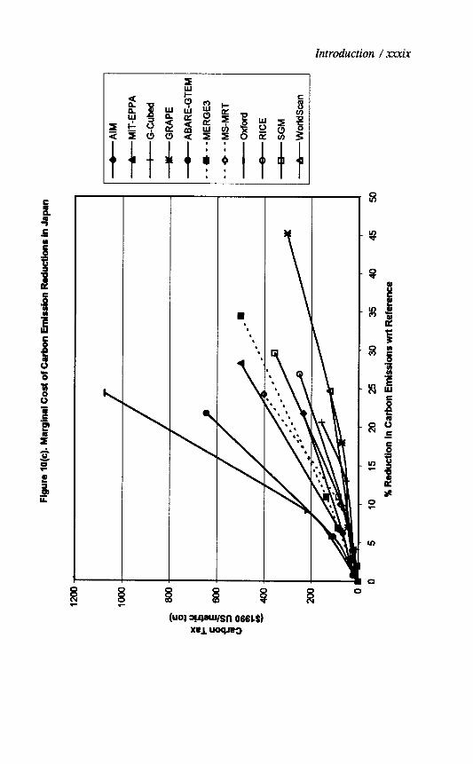
By plotting the projected carbon tax versus percentage reduction in carbon emissions for each of the trading regimes considered, we can construct an approximate marginal cost of carbon emission reductions curve for each model for each region in each year. Marginal cost curves for the four OECD regions in 2010 are shown in Figure 10. A steeper marginal cost curve for a model implies that it requires a larger price incentive to reduce carbon emissions by a given amount through energy conservation and fuel switching. That is, the steeper the marginal cost curve, the larger the carbon tax required to achieve a

mvi / The Energy Journal

given percentage reduction in reference case emissions. The steepness of .these curves depends on the reference case emissions projected by the model, the magnitude of the substitution and demand elasticities embedded in it, and the way capital stock turnover/energy demand adjustments are represented. All ithree factors work together, so one observes that models with higher baseline emissions to lead to higher adjustment costs. If the elasticities are high and the adjustment dynamics rapid, that can lead to lower adjustment costs. In addition, a relatively high adjustment cost can result from either relatively low long-run elasticities and relatively rapid adjustment dynamics, or relatively high long run elasticities and relatively slow adjustment dynamics, or both.

As in past EMF studies, it has proven difficult to anticipate differefnces in the price responsiveness of the models from published parameter values. The definitions, points of measurement, and level of aggregation of the parameters differ greatly from mode1 to model, greatly complicating the task of formulating a price sensitivity estimate analytically. Thus, the information embedded in Figure 10 is an extremely valuable starting point in the process of understanding model differences. Besides the difference in the magnitude of the response and different baseline shown in Figure 10, we also observe that some of the models exhibit a nearly linear dependence of the carbon tax on the percentage reduction in carbon emissions, while others exhibit a quadratic or even more steeply rising relationship. These differences among models in the relative contribution of energy intensity reductions and carbon intensity reductions in achieving carbon emission reductions and the implied differences in fuel share adjustments; are discussed more fully in EMF 16 Working Group, 1999.

OVERVIEW OF SPECIAL ISSUE

Since each modeling team ran and reported results for the four core scenarios, each of the thirteen papers that follow contains some discussion o-f the comparison of the different pure trading options with more depth, but basically reaches the same bottom line as that reported here. In addition to that comparison, each modeling team focused on sensitivities, additional results, and sets of scenarios (many drawn from Table 1) that seemed particularly interesting to them and that the structures of their models allowed them to address. For example, several modeling teams focused on the impact of restrictions on the amount of emissions trading that would be allowed in the Annex I Trading case (which assumes no restrictions) and the potential for a limited number of selllers to exercise monopoly power in that trading regime (i.e., no explicit restrictions, but self imposed restrictions by sellers designed to increase the price they receive and their revenues). The MS-MRT (Bernstein, et al.), SGM (MacCracken, et al.), and MERGE3 (Marme and Richels) papers deal with these issues in some depth and conclude that restrictions on Annex 1 trading could double the cost of meeting the objectives of the Protocol under unrestricted Annex I trading without the exercise of market power.

Introduction / x.xmii

.,

\

\

0 . . .

.

.

q

\

xxviii / The Energy Journnl,

Introduction 1 xxxi.x

Q 8 R O (UOJ wwsn 066LS)

ml uoqrw

xl / l%e Energy Journal

\

\

\

I

\

0

\

‘. l ,

Introduction 1 xl’i

Another group of models dealt with comparing the results of the Kyoto Protocol with those obtained for other longer-run objectives for climate policy. The RICE model (Nordhaus and Boyer), MERGE3 (Manne and Richels), FUND (Tol), and CETA (Peck and Teisberg) analyses considered a number of potential longer term objectives for climate policy-for example, stabilization of the concentration of CO? in the atmosphere, limitations on the rise in global mean temperature, match the marginal benefits of greenhouse gas reductions in each region with its marginal costs of mitigation. These studies generally show that the emissions trajectory prescribed in the Protocol is lower and the cost of emissions mitigation higher than that required to meet the long run objectives that were considered.

Other groups focused their analysis on key sensitivities that could potentially affect results for both the core and other types of scenarios. One example is the careful and insightful analysis done with the MIT-EPPA model (Jacoby and Wing) on the sensitivity of results from a multi-sector general equilibrium model to variations in the parameters represented the sectoral malleability of capital, that is the rate at which the capital stock in each sector is assumed to turn over or to have its input mix adjusted. This analysis shows both the sensitivity of the cost of meeting the Protocol to variations in these parameters, and also the extent to which the cost of meeting the emission reductions obligation specified in the Protocol for 2008-2012 increases with each year there is a delay in initiating action (this point is also made by To1 in the FUND analysis).

Another group of important sensitivities concerns the use of sinks and the “other” greenhouse gases covered by the Protocol to satisfy its emission reduction requirements. Although the core scenarios did not consider sinks and “other gases” a number of the modeling teams did. The analysis with FUND by To1 considers the potential of methane reductions to reduce the costs of satisfying the Protocol’s requirements, while the SGM analysis (MacCracken, et al.) considers the potential of both sinks and all the other gases. It is important to understand that broadening the scope to all six gases covered in the Protocol brings with it both new mitigation options and new obligations, so the key issue becomes the relative costs of reducing a unit of global radiative forcing attributable to each of the gases. That is, the other gases are not simply low cost alternatives to carbon emission reductions. They also generate additional emission reduction requirements. Nonetheless, preliminary estimates seem to show that the inclusion of sinks and other gases have the potential to reduce the total cost of meeting the obligation specified in the Protocol.

A number of teams focused on the role of technologies and technology trends in influencing the costs and energy sector impacts of satisfying the requirements of the Protocol. Although many of the models have some technology detail, the GRAPE model (Kurosawa, et al.) considered .a

xiii / The Energy Journal

particularly rich set of energy supply technologies, including carbon separation and isolation technologies. The AIM model (Kainuma, et al.) is the only model included here that represents energy demand at the end-use level. The availability of new technologies can have a significant effect on the costs of satisfying the requirements of the Protocol, although the first budget period (2008-2012) is soon enough at this point that most of the benefits of the: new technologies are felt after 2012.

Another area that is well covered in this volume and one that is sure to attract additional policy and research attention in the years ahead is the impact of any emissions reductions agreement that work through the international trade system. In early global emissions reduction modeling systems, trade in energy fuels and carbon were the only international trade possibilities considered. A number of models now represent trade in non-energy goods within a general equilibrium representation of economic activity. These analyses have generally focused on the impact of international trade considerations on the cost of the Protocol to both Annex I and non-Annex I countries (the latter commonly referred to as “spill over” effects), as well as the increase in carbon emissions from non-Annex I countries that might result from AMeX I actions to limit carbon emissions (the so called “carbon leakage” effect). The ABARE-GTEM (Tulpule, et al.), MS-MRT (Bernstein, et al.), WorldScan (Bollen, et al.), G- Cubed (McKibbin, et al), MIT-EPPA (Jacoby and Wing), and AIM (Kainuma, et al.) analyses consider international trade of non-energy goods, with the first four including detailed descriptions of trade results in this volume. In general, the models show that there can be significant positive economic impacts of Annex I action on non-AMeX I economies with the sign and magnitude depending on who the country trades with and what they trade (see Bernstein, et al.), the magnitude of international capital flows (see McKibbin, et al.), and the magnitude of the trade and substitution elasticities embedded in the models (see especially McKibbin, et al., Bernstein, et al., and Bollen, et al.). The carbon leakage projections produced by the models span a wide range and depend on many of the same factors that determine the spill over effects, with the import substitution elasticity parameter values likely the most impclrtant assumptions.

Some of the papers deal with very important issues not addressed anywhere else in the volume. For example, the Oxford model considers m.acro- economic adjustment costs (e.g., induced unemployment, inflation, and exch.ange rate adjustments) that are generally not, with the exception of the treatment in G-Cubed, included in the other analyses included in this volume. Results from this model confirm the suspicions of the other groups that these additional adjustment costs depend on assumptions about baseline monetary and fiscal policy assumptions and the assumed policy responses to the introduction of the Protocol, but can be quite significant, especially in the cases with very lirnited amounts of international emissions trading available. The G-Cubed ana:lysis

Introduction / xliii

(McKibbin, et al.) also looks in considerable depth at the impact that adjustments in capital flows could have on the costs of the Protocol to participants in the Protocol (both those that have first budget period obligations and those that do not) under alternative trading regimes. Interesting results concerning the impact of global trading on the cost of the Protocol to the non- Annex I countries emerge.

The CETA model looks at a very simple two party (Annex I and Non- Annex I) formulation of the climate policy debate, focusing on the bargaining set between the two parties (that is, the set of allocations that leads both parties to be better off (in terms of benefits less costs). This analysis is performed for the optimal emissions trajectory and then compared with the allocation suggested by the Kyoto program.

A final highlight of the analyses presented in this volume is the discussion of appropriate cost measures to use in assessing the economic impact of the Protocol. This issue is addressed explicitly or implicitly in every paper, with illuminating comparisons and analysis of results for alternative measures included in MacCracken, et al. using results from the SGM and especially in Bernstein, et al. using results from the MS-MRT. The alternative o:r complementary cost/welfare measures included in the volume include carbon taxes, total resource costs, GDP, GNP, aggregate economic consumption, discounted aggregate consumption, and intertemporal equivalent variation. Bernstein, et al. conducted a standardized comparison of projections for a number of the different measures across scenarios for the MS-MRT model. (See also MacCracken, et al., and EMF 16 Working Group, 1999) for more on this issue.

This volume contains a wide range of estimates of the cost of the Kyoto Protocol. This range of estimates reflects differing assumptions about how the Protocol will get implemented and differences in the structures of the models used to make the cost projections. The key uncertainties about how the Protocol will be implemented include the scope for carbon emission rights trading that will be permitted; the extent to which reductions in emissions of the othe:r greenhouse gases besides carbon and the development of carbon sinks will be permitted, and how the accounting will be done; and the type of post-201:! commitments that will be undertaken. The principal model differences that impact the magnitude of the cost estimates are the level of baseline emissions during the first budget period (2008-2012), the value of the substitution and demand elasticities embedded in the models, and the rate at which it is assumed that the stock of energy using equipment can be adjusted over time. However, there are also other categories of costs that are largely omitted from the models that participated in this study that could be quite significant. First, there are macro-economic adjustment costs that come through induced unemployment and financial markets that are omitted in all but the Oxford and parts of the G-Cubed

xliv / The Energy Journal

model and that could be significant, especially in the more tightly constrained scenarios. Second there are regulatory imperfections that could lead policy makers to implement much less efficient and more costly instruments than the carbon taxes that are assumed to be the instrument of preference here. Finally, there could be less or more efficient recycling of the carbon tax revenues than the lump sum recycling that is assumed in virtually all of the simulations reported here.

Despite these considerable uncertainties, a number of common results and insights emerge from the set of model results considered here. First, meeting the requirements of the Kyoto Protocol will not stop economic g:rowth anywhere in the world, but it will not be free either. In most Annex I countries, significant adjustments will need to be undertaken and costs will need to be paid. Second, unless care is taken to prevent it, the sellers of international emissions rights (dominantly the Russian Federation in the case of Annex I trading, and China and India in the case of global trading) may be able to exercise market power raising the cost of the Protocol to the other Annex I countries. Third, meaningful global trading probably requires that the non-Annex I countries take on emissions targets; without them accounting and monitoring (even Annex I monitoring and enforcement may be quite difficult) becomes almost impossible. Finally, it appears that the emissions trajectory prescribed in the Kyoto Protocol is neither optimal in balancing the costs and benefits of climate change mitigation, nor cost effective in leading to stabilization of the concentration of carbon dioxide at any level above about 500 ppmv.

With this introduction, the stage has been set for the set of papers that follows. We hope you find them as interesting and insightful as we did. That the study has produced such a rich set of results owes everything to the active participation of the modeling teams and the care each team took in preparing a paper for this volume.

REFERENCES

Bhagwatti, Jagdish N.. and T.N. Scrinivasan (1983). Lectures on International Trade. Cambridge,

MA: MIT Press.

EMF 16 Working Group (1999). ‘Economic and Energy System Impacts of the Kyoto Protocol;

Results from the Energy Modeling Forum Study,” the EMF 16 Working Group, Stanford Energy

Modeling Forum, Stanford University, Stanford, CA, July 1999.

The Kyoto Protocol: A Cost-Effective Strategy for Meeting Environmental Objectives?

Alan S. Manne* and Richard G. Richels**

This paper has three purposes: 1) to identify the near-term costs to the United States of ratifying the Kyoto Protocol; 2) to assess the significance of the Protocol ‘s ‘Iflexibility provisions “; and, 3) to evaluate the Kyoto targets in the context of the long-term goal of the Framework Convention. We find that the short-term U.S. abatement costs of implementing this Protocol are likely to be substantial. These costs can be reduced through international trade in emission rights. The magnitude of the costs will be determined by the number of countries participating in the trading market, the shape of each country’s marginal abatement cost curve, and the extent to which buyers can sari@ their obligation through the purchase of emission rights. Finally and perhaps most important: unless the ultimate concentration target is well below 550ppmv, the Protocol seems to be inconsistent with a long-term strategy for stabilizing global concentrations.

INTRODUCTION

The Kyoto Protocol represents a milestone in climate policy.’ For the first time, negotiators have attempted to lay out emission reduction targets for the early part of the 21”’ century. The goal is for Annex 1 (developed countries plus economies in transition) to reduce their aggregate anthropogenic carbon dioxide equivalent emissions by at least 5 percent below 1990 levels in the commitment period 2008 to 2012. The Protocol, however, has yet to enter into force. To do so will require ratification by 55 countries representing 55 percent of total Annex 1 CO, emissions in 1990.

?71a Energy Jolrmal, Kyoto Special Issue. Copyright Q 1999 by the IAEE. All rights reserved.

* Professor Emeritus, Engineering-Economic Systems and Operations Research, Stanford University, Terman Engineering Center, Stanford, CA 943054023 USA.

** Electric Power Research Institute, Environment Division, 3412 Hillview Avenue, P.O. Box 10412, Palo Alto, CA 94303. E-mail: rrichelsQepri.com

1. Conference of the Parties (1997). “Kyoto Protocol to the United Nations Framework Convention on Climate Change,” Third Session Kyoto. l-10 December.

1

2 / The Energy Journal

As each country considers ratification, important questions will arise. High up on the U.S. list is the issue of economic costs. The Senate, for example, has stated that “any Protocol should be accompanied by a detailed financial analysis of impacts on the economy .“* Not surprisingly, U.S. negotiators had hardly returned from Kyoto before the first hearings were scheduled on Capitol Hill. Although the issue of costs is but one of many important considerations, policy makers are keenly interested in the economic implications of ratification.

This paper is intended to help clarify our understanding of compliance costs. The focus is on three questions, which we believe to be of particular relevance: What are the near-term costs of implementation? How significant are the so-called “flexibility provisions ?” And, perhaps most importantly, is the Protocol cost-effective in the context of the long-term goals of the Framework Convention?3

Unfortunately, the answers to these questions will not come easily. It has always been difficult to calculate the economic costs of implementing climate policy. Kyoto has done little to simplify matters. Indeed, it raises at least as many questions as it resolves. These questions fall into two categories: those related to the near-term implementation of the Protocol and those related to the evolution of climate policy over the longer term.

The Protocol is unclear on a number of topics. These include the rules governing emission trading, joint implementation (JI), the Clean Development Mechanism (CDM), and the treatment of carbon sinks. In addition, there is a weak knowledge base regarding the costs of sink enhancement and of controlling several of the relevant trace gases. Until these issues are clarified, analyses will be highly speculative.

Calculating the costs of Kyoto is also complicated by the issue of “what happens next?” Energy sector investments are typically long-lived. Today’s investment decisions are not only influenced by what happens during the next decade, but also by what happens thereafter. In order to estimate the costs of implementing emission cuts in the first commitment period, assumptions are required concerning the longer-term requirements. Unfortunately, the international negotiation process offers little guidance on this issue. This further complicates the process of analysis.

We do not wish to suggest that economic analysis is premature at the present time. Uncertainty is rarely an excuse for paralysis. It does mean, however, that we must be careful to highlight the tentative nature of the projections and focus, to the extent possible, on the insights for decision making.

2. 105th Congress, 1st Session (1997), S. Res. 98. 3. Intergovernmental Negotiating Committee for A Framework Convention on Climate Change

(1992). Fifth Session, Second Part, New York, 30 April-9 May.

Kyoto Protocol: A Cost-Effective Strategy / 3

Here, sensitivity analysts can be particularly useful. For example, in the case of several of the flexibility provisions (emission trading, joint implementation and the Clean Development Mechanism), we explore a variety of scenarios regarding constraints on the purchase of carbon emission rights. While the exact magnitude of the benefits will continue to be debated, the insights, nevertheless, appear to be quite robust.

We also examine the Protocol in the context of the longer-term goal of the Framework Convention, i.e., the stabilization of greenhouse gas concentrations in the earth’s atmosphere. A particular concentration goal can be reached through a variety of emission pathways. Considerable effort has been devoted to trying to understand the characteristics of cost-effective pathways (IPCC, 1997). It is interesting to examine Kyoto in the context of this work. The price tag for moving forward may be formidable. Consistent with the Framework Convention, it is essential that “policies and measures to deal with climate change should be cost-effective so as to ensure global benefits at the lowest possible costs. ‘14

2. THE MODEL

This analysis is based on MERGE (a _model for evaluating the regional and global effects of greenhouse gas reduction policies).5 MERGE is an intertemporal market equilibrium model, It combines a bottom-up representation of the energy supply sector together with a top-down perspective on the remainder of the economy. Savings and investment decisions are modeled as though each of the regions maximizes the discounted utility of its consumption subject to an intertemporal wealth constraint. Each region’s wealth includes not only capital, labor and exhaustible resources, but also its negotiated international share in carbon emission rights.

For the present version of the model, known as MERGE 3.0, we have adopted IO-year time intervals through 2050 and 25-year intervals through 2100. Geographically, the world is divided into nine geopolitical regions: 1) the USA, 2) OECDE (Western Europe), 3) Japan, 4) CANZ (Canada, Australia and New Zealand), 5) EEFSU (Eastern Europe and the Former Soviet Union), 6) China, 7) India, 8) MOPEC (Mexico and OPEC) and, 9) ROW (the rest of world). Note that the OECD (regions 1 through 4) together with EEFSU constitute Annex 1 of the Framework Convention.

Particularly relevant for the present analyses, MERGE provides a general equilibrium formulation of the global economy. We model the possibility

4. Intergovernmental Negotiating Committee for A Framework Convention on Clirmate Change (1992).

5. See Manne, Mendelsohn and Richels (1995); and Manne and Richels (1995).

4 / The Energy Journal

of international trade in carbon emission rights. This is sometimes known as “where” flexibility. It would allow regions with high marginal abatement costs to purchase emission rights from regions with low marginal abatement costs. In addition, MERGE can be used to examine the related issue of “when” flexibility -intertemporal transfers of carbon emission rights.

We also model international trade in oil, natural gas, and energy- intensive basic materials. We are therefore able to examine issues related to “carbon leakage. ” Such leakage can occur through a variety of pathways. For example, AMeX 1 emission reductions will result in lower oil demand, which in turn will lead to a decline in the international price of oil. As a result, non- Annex 1 countries may increase their oil imports and emit more than they would otherwise.

The present version of the model includes the notion of endogenous technical diffusion. Specifically, in the electric sector, the near-term adoption of high-cost carbon-free technologies leads to accelerated future introduction of lower cost versions. The model also includes both price-induced and non-price conservation. For most regions and time periods, the AEEI (autonomous energy efficiency improvement) rate is taken to be 40 percent of the rate of GDP growth. By 2100, this leads to regional energy-GDP ratios that are much closer to each other than they were in 1990.

In calibrating MERGE for the present analysis, several supply- and demand-side parameters were adjusted so that the global emissions baseline would approximate the Intergovernmental Panel on Climate Change (IPCC) central case “no policy” scenario (IS92a) (IPCC, 1994). Figure 1 shows carbon emissions for each region in the reference case scenario. For more on the model and its key assumptions, see our website:

http://www.stanford.edulgrouplMERGE/

3. TREATMENT OF SINKS AND NON-CO, GREENHOUSE GASES

Few issues have engendered as much confusion as that of carbon sinks. Key questions include their definition, the extent to which they are included in the Protocol, the amount currently being sequestered, their time profile, and the costs of sink enhancement.

The Protocol states that Annex 1 commitments can be met by “the net changes in greenhouse gas emissions from sources and removal by sinks resulting from direct human-induced land use change and forestry activities limited to afforestation, reforestation, and deforestation since 1990, measured

Kyoto Protocol: A Cost-Effective Strategy / 5

as verifiable changes in,stocks in each commitment period.“6 The confusion results from alternative interpretations regarding the treatment of soil carbon, an issue flagged for further study in the Protocol. Their inclusion may result in large increases in the international legal definition of sink potential.

Figure 1. Regional Carbon Emissions - Reference Case

25

@I ROW

ll---l

0 MOPEC

. NDtA

a-l q CHNA

0

1990 2000 2010 2020 2030 2040 2050 2060 2070 2060 2090 2100

The quality of the data is uneven. The supply curves for sink enhancement are particularly questionable. The degree of confidence concerning current and predicted future levels of carbon sequestration varies enormously across regions of the globe. Not surprisingly, information is most reliable (albeit still poor) for Annex 1 countries. Comparatively little effort has been made to collect such data elsewhere.

As placeholders, we have adopted the values shown in Table 1. To provide some perspective, in order for the US to reduce industrial carbon emissions by 7 percent below 1990 levels in 2010, it would have to reduce emissions by approximately 550 million tons below its reference trajectory. Sink enhancement would satisfy 9 percent of this obligation. For purposes of the present analysis, we assume that this sink enhancement is costless.

6. Conference of the Parties (1997). “Kyoto Protocol to the United Nations Framework Convention on Climate Change.”

6 / The Energy Journal

Table 1. Sink Enhancement (million metric tons of carbon annually)

CO, is by far the most important of the greenhouse gases. In addition, the Protocol includes five other trace gases (methane, nitrous oxide, hydrofluorocarbons, perfluorocarbons, and sulphur hexafluoride). Given the scarcity of reliable emissions and cost data, the treatment of the non-CO? greenhouse gases is also problematic. For purposes of the present analysis, we assume that each gas is reduced proportionately. With this proportionality assumption, the inclusion of the non-CO, greenhouse gases does not affect the requirements for CO, reductions.

As with our treatment of sinks, we do not include the costs of abating the non-CO1 greenhouse gases in our estimates of the costs of complying with the Protocol. Clearly, an important next step would be to develop supply curves for the cost of abating non-CO, greenhouse gases and for sink enhancement. Neither of these costs is included in the present version of MERGE.

4 . “KYOTO FOREVER”

We begin with an examination of a “Kyoto Forever” scenario. This is a case in which the Kyoto constraints on Annex 1 countries are maintained throughout the 21”’ century. With regard to non-Annex 1 emissions, we assume they will continue to be bounded by their business-as-usual baseline (Figure 1). The latter constraint is imposed in order to prevent carbon leakage. Later on, we will explore the impact of relaxing this constraint.

Numerous studies have shown that global mitigation costs can be reduced substantially by allowing emission reductions to take place wherever it is cheapest to do so-regardless of geographical location (Richels et al. 1996). The Kyoto Protocol includes several provisions allowing for a limited amount of “where” flexibility. These include emission trading and joint implementation among Annex 1 countries. They also include provisions for a Clean Development Mechanism (CDM) that is intended to facilitate joint implementation between Annex 1 and non-Annex 1 countries.

As with the definition of sinks, the Protocol leaves many critical details unresolved. For example, it remains unclear whether there will be limits on the extent to which a country can rely upon the purchase of emission rights to satisfy its obligations. The Protocol states that “the Conference of the Parties

Kyoto Protocol: A Cost-Effective Strategy / 7

shall define the relevant principles, modalities, rules and guidelines . ..“’ Similar ambiguity surrounds the Clean Development Mechanism. Again, the elaboration of “modalities and procedures” is left to a future meeting of the Conference of the Parties .*

In this section, we explore three scenarios: 1) no trading, 2) Annex 1 trading plus CDM, and 3) full global trading. These three options are representative of alternative implementations of the Kyoto Protocol. Each has its own advocates and opponents, but we do not consider them equally likely. In our opinion, there is little likelihood of enticing all major countries to participate in a global market in emission rights during the initial commitment period (2008-2012).

The full global trading scenario represents an upper bound on the CDM’s potential to reduce GDP losses. In calculating the potential size of the contribution from a CDM, we therefore calculate this upper bound on the export of emission rights from non-Annex 1 regions. Because of the difficulties in implementation of the CDM, however, we assume that only 15 percent of the potential would be available for purchase through this mechanism. This is a highly subjective estimate. Given the complexities of the CDM, however, we are not inclined to assign a higher value

Figure 2 reports the incremental value of carbon emission rights to the US in 2010 and 2020. We focus first on 2010. In the most constrained scenario, the US must satisfy its emission reduction requirements within its own geographical boundaries. In this case, the value of emission rights approaches $240 per ton. With Annex 1 trading plus CDM, the value drops to slightly less than $100 per ton. As might be expected, the value of emission rights is lowest with full global trading. Here, it falls below $70 per ton.

For the two scenarios in which trading is permitted, the value of emission rights increases in 2020. This is because EEFSU’s projected emissions lie below its negotiated constraint for 2010. It has been allocated more emission rights than it needs to satisfy its internal obligations. By 2020, however, EEFSU’s economic growth is expected to be such that it no longer enjoys an excess of emission rights. As a result, there is more competition for emission rights in the international marketplace, and there is an increase in their price.

7. Conference of the Parties (1997). “Kyoto Protocol to the United Nations Framework Convention on Climate Change.”

8. Conference of the Parties (1997). “Kyoto Protocol to the United Nations Framework Convention on Climate Change.”

8 / The Energy Journal

Figure 2. Incremental Value of Carbon Emission Rights in U.S. Under Kyoto Forever

250-

200 -

j ‘50-

B

5

a loo- *

50 -

No Trading

n 2010 I c32020

‘.‘.‘.‘.‘.‘.’ ‘.‘.‘.‘.‘.‘.~ ‘.‘.‘_‘.~_‘.’

:. ::::. ::::::. _‘.‘_‘.‘.‘.‘.

‘.‘.‘.‘_‘.‘. ‘.‘...’

.:.I.: .,.,.,.

‘.‘,~.~.‘_‘.’

Annex 1 Trading Plus CDM Full Global Trading

Another way to view the costs of abatement is to show the GDP losses. Figure 3 contains those for the United States. Losses are highest in the absence of trade. Here, they exceed $80 billion in 2010. This is approximately one percent of U.S. GDP. To the extent that trade is introduced, losses decline. In the most optimistic scenario (full global trade), losses are approximately $20 billion or one-quarter of one percent of GDP in 2010.

Of the three scenarios, “Annex 1 trading plus the CDM” is most consistent with the Protocol as it currently stands. However, the U.S. Senate has stated that the U.S. should not be a signatory to the Protocol if it does not mandate specific commitments for developing countries.g If this were to result in full global emission trading, we move in the direction of the right-most bar of Figure 3.

There is, however, strong sentiment among many parties to the Framework Convention to substantially limit the extent to which Annex 1 countries can meet their obligation through the purchase of emission rights. Several influential developing countries have expressed strong opposition to the concept altogether. Figure 3 shows the costs of the no trading scenario. We now turn to the case where trading is permitted, but with limitations on the purchase of emission rights.

9. 10Yh Congress, 1” Session (1997), S. Res. 98.

Kyoto Protocol: A Cost-Effective Strategy / 9

Figure 3. Annual U.S. GDP Losses Under Kyoto Forever ($ billions)

120

1 100

20

0 !

n 2010 cl El2020

No Trading Amex 1 Trading Plus CDM Full Global Trading

5. LIMITS ON THE PURCHASE OF CARBON EMISSION RIGHTS

Figure 4 shows our estimates of the percentage of the U.S. emission reduction obligation that would be satisfied through the purchase of emission rights under base case assumptions. With full global trading (the least-cost of our three scenarios), trading is used to satisfy more than 50 percent of the U.S. obligation. But suppose that limits are placed on the purchase of emission rights? For example, suppose that international negotiators agree that Annex 1 buyers can satisfy only one-third of their obligation through this means. What would be the impact on GDP losses?

Figure 5 compares three cases. All assume full global participation in an international market for carbon emission rights, but only the first assumes no limits on the amount a country can buy. The second and third case are based upon the one-third limitation. We further make the distinction between a buyers’ market and a sellers’ market. With the former, sellers of emission rights are price takers. Buyers exert sufficient market power to hold the international price to the marginal cost of abatement in the selling countries. However, since a country is only able to satisfy one-third of its obligation through the purchase of emission rights, it must eventually rely on its own domestic marginal abatement capabilities to meet its obligations. Hence, there is an important distinction between the international price and the domestic price. Conversely, with a sellers’ market, buyers face but one price. Here, the rents accrue to the sellers.

10 / The Energy Journal

Figure 4. Percent of U.S. Obligation Satisfied Through the Purchase of Emission Rights

n 2010 cl El2020

-l

No Trading Annex 1 Trading Plus CDM Full Global Tradmg

Figure 5. Incremental Value of Carbon Emission Rights With and Without Limits on the Purchase of Emission Rights - Kyoto Forever

220

170

s c 120

s

B

5

t 70 *

20

-30

_ I

(

40 limitation

in emission

trading

.. .‘.’

‘.‘.‘. ‘,‘.‘.

‘.‘.‘. ‘.‘.‘. ‘.‘.‘.

i-

::: ::: :::

::: ::: ;::

‘. :

Buyers’ Market --

purchases limited to

one-third of obligation

Sellers’ Market -

purchases limited to

one-third of obligation

lnlernational Price

US Price Annex 1 Buyers Price

Kyoto Protocol: A Cost-Effective Strategy / 11

Figure 6 shows the GDP losses associated with the three scenarios. Note that losses in 2010 are two and’bne-half to three times higher with the constraint on the purchase of carbon emission rights. That is, the benefits from “where” flexibility are greatly diminished. The message is clear. Developing country participation in the market for carbon emission rights is a necessary, but by no means a sufficient condition for reaping the full benefits of “where” flexibility. To achieve a cost-effective solution, buyers must also be unconstrained in the manner in which they fulfill their obligation.

Also note that the distribution of the rents makes a difference to GDP losses. U.S. losses are 25 percent higher in 2020 when market power resides with the sellers. The analysis provides an additional message for Annex 1 buyers. If at a given point in time, low-cost sellers are concentrated among a few countries (e.g., EEFSU), they may have considerable potential for extracting monopoly rents.

Figure 6. Annual U.S. GDP Losses with Full Trading - Annex 1 May Satisfy Only One-third of Obligation Through the Purchase of Emission Rights - Kyoto Forever

Full Trading

12 / The Energy Journal

6. THE ISSUE OF CARBON LEAKhGE

The Kyoto Protocol refers specifically to the period centered about 2010. During this period, the onus for emission reductions falls on Annex 1. No specific obligations are imposed on countries outside Annex 1, and there is the possibility of “leakage.” That is, the reductions in Annex 1 might be partially offset by increased emissions from China, India, Brazil and other countries that do not belong to Annex 1.

In this section, we examine the potential for leakage through international fuel markets and through the migration of energy-intensive industries. We therefore drop the assumption that non-Annex I countries are constrained to their reference case emissions. Two variants on the reference scenario are reported. In the first, the only trade impact of the Protocol consists of limiting the ability of the Annex 1 countries to import oil and gas. There is a lower international price of these goods, and there is a modest increase in price-induced demands by non-Annex 1 countries. However, there is no international trade in carbon emission rights, and there is no international migration of production within the energy-intensive sectors (EIS).

The second alternative is the same as the first, except that we now permit EIS trade. For a description of how the model has been modified to account for international trade in the energy-intensive sectors, see Appendix A. Figure 7 summarizes the overall results. According to this figure, neither of the two trade alternatives leads to a dramatic increase in carbon emissions outside Annex 1. Apparently there is an international leakage problem, but it appears to be of manageable dimensions.

Figure 8 suggests a somewhat different interpretation. Here we report the EIS trade scenario, and we compare the impact upon production- consumption ratios in each region. Under the reference case, these ratios are close to unity (the horizontal line) in most regions. The bars in Figure 8 show that the Protocol could lead to serious competitive problems for EIS producers in the USA, Japan and OECD Europe. The Protocol would lead to significant reductions in their output and employment, and there would be offsetting increases in regions with low energy costs. One can easily anticipate calls for protection against “unfair competition. n In its present form, the Protocol could lead to acrimonious conflicts between those who advocate free international trade and those who advocate a low-carbon global environment.

Kyoto Protocol: A Cost-Effective Strategy / 13

Figure 7. Carbon Emissions Outside Annex 1 - Alternative Leakage Scenarios

6

5

2

1990 2ooo 2010 2020 m30

Figure 8. Ratios of Domestic EIS Supplies to Demands - Kyoto with Leakage

14

1.2

1

0.6

06

0.4

02

0 I

USA

i

El2010 I-I 0 2020

OECDE JAPAN CAN2 EEFSU CHINA INDIA MOPEC ROW

14 / The Energy Journal

7. EVALUATING KYOTO IN THE CONTEXT OF THE LONGER-TERM GOAL

The objective of the Framework Convention is “the stabilization of greenhouse gas concentrations at a level that would prevent dangerous anthropogenic interference with the climate system.“” The drafters of the Protocol focused exclusively on the initial steps to be taken by Annex 1 countries. Little attention was paid to the ultimate goal. We now examine the Protocol in the context of a long-term stabilization objective.

From Figure 1 it is clear that the “Kyoto Forever” scenario will fail to stabilize global emissions and concentrations. A particular concentration target can be achieved through a variety of emission pathways. In this section, we explore three pathways for stabilizing concentrations at 550 ppmv (twice preindustrial levels) by 2100. We stress, however, that the issue of what constitutes “dangerous interference” has yet to be determined. Indeed, it is likely to be the subject of intense scientific and political debate for decades to come. Hence, our choice of a target is meant to be purely illustrative.

Our three pathways are intended to illustrate the benefits of “when” flexibility. They are titled: 1) “Kyoto followed by arbitrary reductions,” 2) “Kyoto followed by least-cost,” and, 3) “least-cost.” As their names imply, the first two are designed to be consistent with the Protocol during the first commitment period. The third assumes a clean slate in the choice of emissions pathway throughout the 2 1” century.

For the first scenario, we assume that Annex 1 countries reduce emissions through 2030 at the same rate as the OECD during the first decade of the 21”’ century (2 percent per year). During this period, non Annex-l countries are permitted to emit up to their reference case levels. By 2020, emissions in the developing nations are larger than those in Annex I. We then choose a pathway to stabilization which represents a relatively smooth transition to the target. As for the post-2030 burden-sharing scheme, we assume that between 2030 and 2050 all regions move to equal per capita emission rights (based on their 1990 population). Equal per capita emission rights have been proposed as one approach to international fairness, but there are others that might also serve to separate the issue of equity from that of economic efficiency.

With “Kyoto followed by least-cost,” the Protocol is adopted for the initial commitment period. Thereafter, the most cost-effective pathway is followed for stabilizing concentrations at 550 ppmv. With “least-cost,” the most cost-effective pathway for stabilizing concentrations at 550 ppmv is followed

10. Intergovernmental Negotiating Committee for A Framework Convention on Climate Change (1992).

Kyoto Protocol: A Cost-Effective Strategy / 15

from the outset. The latter two scenarios adopt the same proportionate burden- sharing scheme as the first.

All three scenarios assume Annex 1 trading plus the CDM. However, they differ as to the timing of developing country involvement in the international market for carbon emission rights. By definition, least-cost assumes that emission reductions will be made where it is cheapest to do so, regardless of the geographical location. Hence, in the least-cost scenario, we assume global emission trading from the outset. In the case of “ Kyoto followed by least-cost, ” we assume that global emission trading is delayed until after the first commitment period. With “Kyoto followed by arbitrary reductions,” global emission trading does not begin until 2030, the year that developing countries agree to lower their emissions below business-as-usual.

Global Carbon Emissions

Figure 9 shows global carbon emissions for the reference case and the three stabilization scenarios. Following a least-cost strategy from the outset results in an emissions pathway that tracks the reference path through 2010 and then departs at an increasing rate thereafter. There are several reasons why a gradual transition to a less carbon-intensive economy is preferable to one involving sharper near-term reductions.

Figure 9. Global Carbon Emissions - Reference Case and Three Alternative Emission Pathways for Stabilizing Concentrations of 550 ppmv

--reference + leastcost - Kyoto followed by least-cast -A- Kyoto followed by arbitrary redudions

04

zoo0 2010 2020 2030 2040 2050 2060 2070 2080 2090 2100

16 / The Energy Journal

Concentrations at a given point in time are determined more by cumulative, rather than year-by-year, emissions. Indeed, a concentration target defines an approximate carbon budget, i.e., an amount of carbon that can be emitted between now and the date at which the target is to be reached. At issue is the optimal allocation of the budget. Reasons for relying more heavily on the budget in the early years include: 1) providing more time for the economic turnover of existing plant and equipment, 2) providing more time to develop low-cost substitutes to carbon-intensive technologies, 3) providing more time to remove carbon from the atmosphere via the carbon cycle, and 4) the effect of time discounting on mitigation costs (Wigley, Richels and Edmonds, 1996).

We next turn to the two scenarios where we adopt the Protocol for the first commitment period. Notice that the two emission pathways behave quite differently post-2010. “Kyoto followed by least-cost” follows the least-cost pathway once the Protocol’s constraints are relaxed. “Kyoto followed by arbitrary reductions, ” on the other hand, bears no resemblance to the least-cost pathway. What is striking about Figure 9 is that with a 550 ppmv target, the Protocol is inconsistent with the most cost-effective mitigation pathway, i.e., “least-cost,” Indeed, it appears that the ultimate target would have to be considerably lower than 550 ppmv for the Protocol to be justified in terms of cost-effectiveness.

Near-Term Losses

It is instructive to look at the incremental value of emission rights for the three stabilization scenarios (Figure 10). With the least-cost path, the value is relatively low in the early years ($11 per ton of carbon in 2010), and it rises gradually over time. With “Kyoto followed by least-cost,” the value is $130 per ton in 2010 and then tracks the least-cost path thereafter. In the case labeled “Kyoto followed by arbitrary reductions,” the incremental value of emission rights starts at about $160 per ton and it remains high.

Figure 11 shows U.S. GDP losses in 2010 and 2020 under the three stabilization scenarios. Notice that GDP losses in 2010 differ for the two scenarios involving the initial adoption of the Protocol. Because of the long-lived nature of energy investments, investors are concerned both with what happens in the initial commitment period and what happens thereafter. In the case of the more rapid transition away from the baseline (“Kyoto followed by arbitrary reductions”), investors will be forced to invest more heavily in high-cost substitutes in the early years. With “Kyoto followed by least-cost,” they will have more flexibility.

Figure 10.

Kyoto Protocol: A Cost-Effective Strategy / 17

Incremental Value of Carbon Emission Rights Under Three Alternative Emission Pathways for Stabilizing Concentrations at 550 ppmv - Global Trading

t Kyoto followed by arbitrary redudions t Kyoto followed by leastcost + leastcost

350

1

2010 2020 2030 2040 2050

Figure 11. U.S. GDP Losses Under Alternative 550 ppmv Stabilization Scenarios

n 2010 cl cl 2020

Kyoto followed by arbitrary reductions

Kyota followed by leastcost leaslcost

18 / The Energy Journal

It is striking by how much GDP losses can be lowered under the “least- cost” scenario. This strategy involves a more gradual transition away from the baseline in the early years. It relieves much of the pressure for premature retirement of existing plant and equipment and for dependence on high-cost substitutes (both on the supply- and demand-sides of the energy sector). Relative to the reference case, the U.S. also receives some benefits as an oil importer. Recall that a carbon constraint decreases the overall demand for oil and lowers its price on the international market.

Global Losses

Finally, it is instructive to examine losses from a global perspective (Figure 12). For purposes of the present comparison, we focus on the present value of consumption losses over the 21”’ century discounted to 1990 at 5 percent. The relative magnitude of the cumulative losses for the three stabilization scenarios comes as no surprise given the previous discussion. “Kyoto followed by arbitrary reductions” is by far the most expensive of the three paths. “Kyoto followed by least-cost” is a considerable improvement, but is still 40 percent more expensive than embarking on the most cost-effective mitigation pathway from the outset.

Figure 12. Global Consumption Losses Through 2100 Discounted to 1990 at 5% - Kyoto Forever vs. Three Scenarios for Stabilizing Concentrations at 550 ppmv

2500

2GQo

E d 8 1500

$ e

ii

e lcoo p

I

500

0 I Kyoto forever leastcost Kyoto followed by Kyoto followed by

arbitrary reductions leastCost

Kyoto Protocol: A Cost-Effective Strategy / 19

What is surprising is that “Kyoto Forever” turns out to be more expensive than “Kyoto followed by least cost” or “least cost.” “Kyoto Forever” results in sharper global emission reductions during the early decades of the 2 1”’ century. It does not, however, succeed in stabilizing emissions, much less concentrations. By contrast, the other scenarios all lead to stabilization at 550 ppmv. In other words, “Kyoto Forever” ends up costing more, and it buys less long-term protection.

8. FURTHER COMMENTS

Some suggest that models such as MERGE tend to overestimate the costs of mitigation. They argue that, when prospects for technical progress are incorporated, the costs of a carbon constraint, even a sharp near-term constraint, will be minimal. We, too, are optimistic about the outlook for technical innovation. Indeed, such innovation is embedded both in our reference case and in the policy scenarios. The disagreement is over the rate at which such progress will occur. We do not believe that economically competitive substitutes will become available at such a rate as to trivialize the costs of a Kyoto-like Protocol.

A more valid concern may be that we are underestimating the costs of a carbon constraint. There are several reasons why this may be the case. To begin with, optimization models assume that decision makers have perfect foresight. That is, they assume that investors are fully informed about the nature of future constraints, and act accordingly. Given the present state of uncertainty, this is highly unlikely. Models such as MERGE also tend to ignore short-term macro shocks. For example, the higher delivered energy prices brought about by a carbon constraint are likely to be inflationary. If this leads to higher interest rates, investment may be dampened. The result would be a slowdown in economic growth.

In addition, we assume that policies will be efficient. That is, market mechanisms will be chosen over “command and control” approaches to accomplishing environmental objectives. Whereas, in recent years, there has been an increasing trend toward market mechanisms, the approach to be taken with climate policy is by no means assured. Moreover, even if such a commitment were made, we have no assurances that the requisite international institutions will be available when needed.

Although it is easy to quibble over the numbers, the real value of analyses lies more in insights than in numerical values. And, indeed we believe that the current exercise has yielded several insights that may be of value to those charged with interpreting the current proposal. Here, we summarize what we have learned:

20 / The Energy Journal

First, it is extremely unlikely that a “Kyoto Forever” scenario will stabilize emissions -- much less concentrations. Non-Annex 1 emissions are quickly overtaking those of the OECD and the economies in transition. Hence, meeting the stabilization goal of the Framework Convention will eventually require the participation of developing countries.

International cooperation through trade in emission rights is essential if we are to reduce mitigation costs. The magnitude of the savings will depend on several factors. These include the number of countries participating in the trading market, the shape of each country’s marginal abatement cost curve, and the extent to which buyers can satisfy their obligation through the purchase of emission rights.

With regard to the latter, limitations on the purchase of emission rights may be especially costly. In the example explored here, limiting purchases to one-third of a country’s obligation increased GDP losses by a factor of at least two and one-half in the year 2010. If proponents of such limitations are successful, they may seriously reduce the benefits from “where” flexibility.

The issue of monopoly power in markets for emission rights may turn out to be important. This is most likely to occur if trading is limited to Annex 1 and the majority of inexpensive emission rights are concentrated in a small number of countries. If these countries were successful in organizing a sellers’ cartel, they might be able to extract sizable rents.

The near-term costs of the Protocol will depend on expectations regarding the future. Energy investments are typically long-lived. Today’s investment decisions are not only influenced by what happens during the next decade, but also by what happens thereafter. Hence, analyses which focus solely on 2010 may be underestimating the costs of Kyoto.

Finally, and perhaps most importantly, unless the concentration target for CO* is well below 550 ppmv, the Protocol appears to be inconsistent with a cost-effective long-term strategy for stabilizing CO, concentrations. Rather than requiring sharp near-term reductions, it appears that a more sensible strategy would be to make the transition at the point of capital stock turnover. This would eliminate the need for premature retirement of existing plant and equipment and would provide the time that is needed to develop low-cost, low-carbon substitutes.

Kyoto Protocol: A Cost-Effective Strategy / 21

APPENDIX

Modeling International Trade in the Energy-intensive Sectors

MERGE 3.0 has recently been modified to include the possibility of trade in EIS (energy-intensive sectors). EIS is an aggregate including ferrous and non-ferrous metals, chemicals, nonmetallic minerals, paper, pulp and print. This aggregate does not include the energy-intensive industry of petroleum refining. The model may be run either with or without EIS trade.

The new feature is introduced in a way that preserves the basic simplifying characteristics of the ETA-MACRO submodel. That is, energy, capital and labor are substitutes that enter into an aggregate production function. They produce a numeraire good which may be used for consumption, investment and interindustry payments for energy costs.

It is assumed that trade will continue to represent a relatively small amount of each region’s total internal demand for EIS. The GTAP (General Trade Analysis Program, 1992) data base is employed to estimate each region’s EIS demands. In all other respects, the model is the same as MERGE 3.0.

For projecting the impact of the Kyoto protocol, each region is taken to be self-sufficient at base year energy prices. Changes in the location of production are attributed primarily to changes in the cost of energy. At base year prices in the USA, 85 percent of the cost of EIS consisted of non-energy inputs (labor, shipping, capital, iron ore, etc.), and 15 percent of the cost consisted of energy inputs (half electric and half non-electric). Under these conditions, a doubling of energy prices would imply only a 15 percent increase in the cost of EIS. This is why it is assumed that the demand for EIS is inelastic with respect to the price of energy. For projecting future demands, the income elasticity is taken to be 0.5.

For modeling purposes, we have supposed that the marginal supplies of EIS in all regions are determined by the same international technology that prevails in the USA. Each region has the same energy-EIS production ratio. For non-energy inputs, each supply curve is linear. Its positive slope serves the same purpose as an Armington elasticity describing substitution between foreign and domestic goods. This is the way in which we avoid penny-switching as a characteristic solution mode.

The slope of the non-energy supply curve is described as a Heckscher- Ohlin fraction. If this fraction is unity, EIS is viewed as a perfectly homogeneous commodity. Small changes in energy costs will then lead to large changes in the international location of production. If this fraction is less than unity, the supply function is less elastic, and the changes in location will be less dramatic. (See Figure A.l.)

22 / The Energy Journal

Figure Al. EIS Supply Curves - Marginal Cost of Non-Energy Inputs to EIS

1.5 - Heckscher-Ohlin

fractions:

0 ,

Cl

I

0.5 1

Fraction of region’s demand supplied domestically

1

1.5

ACKNOWLEDGMENTS

This research results from our participation in Stanford University’s Energy Modeling Forum 16 Study. The authors are indebted to James Deaker and Robert Parkin for their research assistance. We have benefited from discussions with Jae Edmonds, Henry Jacoby, David Montgomery, William Nordhaus, Stephen Peck, Thomas Rutherford, and John Weyant. Funding was provided by EPRI. The results presented here are solely those of the individual authors.

REFERENCES

Conference of the Parties (1997). “Kyoto Protocol to the United Nations Framework Convention on Climate Change,” Report of the Conference of the Parties, Third Session Kyoto, l-10 December. FCCClCPll997/L.7/Add.l. http://www.unfccc.de

Intergovernmental Negotiating Committee for A Framework Convention on Climate Change (1992). Fifth Session, Second Part. New York, 30 April - 9 May.

IPCC (1997). Intergovernmental Panel on Climate Change. “Stabilization of Atmospheric Greenhouse Gases: Physical, Biological and Socio-Economic Implications,” Technical Paper III.

Kyoto Protocol: A Cost-Effective Strategy 123

Manne, A., R. Mendelsohn, and R. Richels (1995). “MERGE: a model for evaluating regional and global effects of GHG reduction policies.” Energy Policy 3( 1).

Manne, A. and R. Richels (1995). “The Greenhouse Debate: economic efficiency, burden sharing and hedging strategies.” I7zhe Energy Journal 16(4).

Richels, R.. J. Edmonds. H. Gruenspecht, and T. Wigley (1996). “The Berlin Mandate: The Design of Cost Effective Mitigation Strategies.” EMF-14, Working Paper 3, Stanford University, Stanford, CA.

U.S. Congress (1997). 105th Congress, 1st Session, 1997, S. Res. 98. Washington, DC: U.S. Government Printing Office.

Wigley, T., R. Richels and J. Edmonds (1996). “Economic and Environmental Choices in the Stabilization of Atmospheric CO, Concentrations.” Nufure 379 (January 18).

The Economics of the Kyoto Protocol

Christopher N. MacCracken, James A. Edmonds, Son H. Kim and Ronald D. Sands*

In this paper we use the Second Generation Model to develop an assessment of the energy and economic implications of achieving the goals of the Kyoto Protocol. We find that many of the details of the Protocol that remain to be worked out introduce critical uncertainties affecting the cost of compliance. Our analysis shows that the cost of implementing the Protocol in the United States can vary by more than an order of magnitude. The marginal cost in 2010 could be as low as $26 per tonne of carbon if a global system of emissions mitigation could be quickly and effectively implemented. But it could also exceed $250per tonne of carbon ifthe United States must meet its emissions limitations entirely through domestic actions, and if mitigation obligations are not adequately anticipated by decision-makers.

INTRODUCTION

The Kyoto Protocol was completed on the morning of December 11, 1997, following more than two years of negotiations. The product of these deliberations is a complex and incomplete document knitting together the diversity of interests and perspectives represented by the more than 150 delegations. Because the document is complex, its implications are not immediately obvious. If it enters into force, the Kyoto Protocol could have far-

The Energy Journal, Kyoto Special Issue. Copyright o 1999 by the IAEE. All rights reserved.

* Pacific Northwest National Laboratory, Battelle Washington Operations, 901 D Street, S. W.,

Suite 900, Washington, DC 20024-2115. E-mail: c.maccracken@pnl.gov; jae@pnl.gov; skim@pnl.gov; ronald.sands@pnl.gov.

The Pacific Northwest National Laboratory is operated for the U.S. Department of Energy by Battelle Memorial Institute under contmct DE-AC06-76RL0 1830. The views and opinions of the authors expressed herein do not necessarily state or reflect those of the United States Government

or any agency thereof.

25

26 / The Energy Journal

reaching implications for both Annex I’ and non-Annex I member states. National energy systems, and the world’s energy system, could be forever changed.

In this paper we assess the energy and economic implications of achieving the goals of the Kyoto Protocol. We find that many of the details of the Protocol that remain to be worked out introduce critical uncertainties affecting the cost of compliance. There are also a variety of uncertainties that further complicate the analysis. These include future non-CO, greenhouse gas emissions and the cost of their mitigation. Other uncertainties include the resolution of negotiations to establish rules for determining and allocating land- use emissions rights, mechanisms for Annex I trading, and participation by non- Annex I members in the Clean Development Mechanism. In addition, there are economic uncertainties, such as the behavior of Eastern Europe and the former Soviet Union in supplying emissions credits under Annex I trading.

We begin by describing our general approach to modeling the Kyoto Protocol and the variety of policy issues remaining to be resolved. We then review some of the necessary assumptions for this exercise, as well as the structure and calibration of the Second Generation Model (SGM). The SGM was used to simulate the impact of mitigation policies on the economies participating in the Kyoto Protocol. Finally, we discuss the results of our analysis in several areas, including the impacts of several degrees of emissions permit trading, the Clean Development Mechanism, the inclusion of the six greenhouse gases, and land-use emissions. We focus on the impacts on regional energy systems and measures of compliance cost.

During 1998, two sets of analyses were prepared using the global SGM to address the cost implications of the Kyoto Protocol. The analyses differ on the treatment of the non-CO, greenhouse gases. Results presented at the Energy Modeling Forum meeting in August 1998 did not include any abatement opportunities for the non-CO, greenhouse gases. The analysis reported in this paper, however, incorporates a stylized representation of abatement opportunities for the non-CO, greenhouse gases. Assumptions concerning the non-CO,

1. The Kyoto Protocol actually prescribes emissions limitations for countries listed in Annex B

to the Protocol. These countries are: Australia, Austria, Belgium, Bulgaria, Canada, Croatia, Czech

Republic, Denmark, Estonia, European Community, Finland, France. Germany. Greece, Hungary, Iceland, Ireland, Italy, Japan, Latvia. Liechtenstein, Lithuania, Luxembourg, Monaco, Netherlands,

New Zealand, Norway, Poland, Portugal, Romania, Russian Federation, Slovakia, Slovenia, Spain, Sweden, Switzerland, Ukraine, United Kingdom of Great Britain and Northern Ireland, and the

United States of America. This list varies somewhat from the countries contained in Annex I to the FCCC. Several countries such as Slovakia, Slovenia, Liechtenstein, and Monaco have been added,

while Belarus and Turkey are listed in Annex I of the FCCC but not Annex B of the Kyoto Protocol. In this analysis we refer only to Annex I, with Annex B obligations allocated appropriately as specified in Appendix A of this report.

The Economics of the Kyoto Protocol / 27

greenhouse gases are described in greater detail in the Compliance section of this paper.’

APPROACH

We examine the economic consequences of implementing the Kyoto agreement using the SGM. The SGM is a computable general equilibrium economic model that projects economic activity, energy consumption, and carbon emissions for twelve world regions. It is designed specifically to address issues associated with global change with special emphasis given toward performing the following types of analysis:

1. Provide estimates of future time paths of environmentally important emissions associated with economic activity.

2. Provide estimates of the economic cost of actions to reduce greenhouse gas emissions.

Sectors

The SGM has nine producing sectors and twelve inputs to production. The inputs are land, labor, capital, and the nine produced goods. Economic detail is maintained in the energy supply and transformation sectors that are important for greenhouse gas emissions projections, but aggregated elsewhere into one large “everything else” sector.

Five different fuels are used for producing electricity, resulting in at least five subsectors for the electric generating sector. A separate economic production function, of the constant elasticity of substitution (CES) functional form, is used for each sector or subsector. Capital investment decisions depend on an assumed lifetime of capital for each sector or subsector. Capital lifetimes range from 15 years in the oil, gas, and coal production sectors to 70 years for hydroelectric power. The relative size of each production sector and subsector for the United States is shown in Table 1.

2. Including abatement opportunities from non-CO2 greenhouse gases tends to reduce the carbon price required for any abatement scenario. In the Energy Modeling Forum ‘No Trading’ case, for

example, the carbon price for the United States is $188 measured in 1990 dollars or $201 measured in 1992 dollars. The carbon price in the ‘No Trading’ case in this paper, including abatement of the

non-CO, greenhouse gases, is $168 (1992 dollars).

28 / The Energy Journal

Table 1. Producing Sectors in the SGM

Producing Sector Gross Output in 1985

(millions of 1985 $)

Agriculture 468,618 Everything Else 5,086,486 Oil Production 64,171 Gas Production 45,804 Coal Production 20,006 Uranium Processing 2.195 Electricity Generation 165.800

a. oil 10,959 b. gas 34.152 c. coal 85.930 d. nuclear 21.370 e. hydro 13,389

Petroleum Refining 145,015 Gas Transmission and Distribution 105,330

Market Clearing

In the SGM, markets are said to clear when the model solves for the set of prices for all markets (or sectors) in the modeled economy so that demands and supplies of each market are in equilibrium. The set of prices in which the equilibrium holds is called the market-clearing price set. In an equilibrium model like the SGM, markets are linked to other markets through the market-clearing process. For example, a change in the demand for coal will have an effect not just on the price of coal, but also the prices of oil, gas, and, at least indirectly, the prices of all markets in the economy.

Carbon permit prices are also solved for by the SGM as part of the market equilibrium. Specifically, the SGM finds the carbon price such that the amount of carbon emitted is just equal to the carbon constraint of the region or group of regions under a carbon emissions limitation constraint. The 12 SGM regions are listed in Table 2.3

Carbon Permit Fees and Revenue Recycling

The SGM uses a carbon permit fee within each region to provide an economic incentive for the economy to substitute away from carbon. We model this as a carbon tax placed on fossil fuels. The government collects the tax just as it would collect revenues from allocating the emissions permits. These

3. The Rest of World (ROW) includes Latin America, Africa, and other Asian countries.

The Economics of the Kyoto Protocol / 29

revenues can be very large, and how the revenues are recycled, or redistributed to the economy, makes a difference in the final economic cost. For this exercise, we assume that all carbon fee revenues are recycled back to consumers through a lump-sum transfer.

For the cases where emissions rights are traded between countries, each SGM region is allocated an initial number of carbon emissions permits based on its commitments as defined in the Kyoto Protocol. Carbon permits can then be traded between countries at a price that clears the international market in these permits.

Table 2. Regions in the SGM

Annex I

United States

Canada Western Europe

Japan Australia

former Soviet Union Eastern Europe

Non-Annex I

China

India Mexico

South Korea Rest of World

Modes of Operation

All of the SGM regions were initially developed as single-region models with a base year of 1985. Each regional model operates in five-year time steps and has been run with forecast horizons ranging up to the year 2100. Most of the single-region models were developed in collaboration with experts from that country. It is possible to run all of the regions individually or simultaneously in a global model with international trade. The three modes of operation for the SGM are:

1. Single Region 2. Global with Partial Market Clearing 3. Global with Full Market Clearing

Single-region Operation

For each SGM region, all produced goods are classified as being tradable, non-tradable, or traded at a fixed quantity. When SGM regions are operated independently, a fixed world price is assumed for certain tradable goods; regions may import or export as much of that good as desired at that fixed world price, subject to an overall balance of payments constraint. For all non-tradable goods,

30 / The Energy Journal

the quantity of trade is fixed in advance. The following assignments are used when a regional model is operated independently:

1. Numeraire Sector: 2. Fixed World Price: 3. Fixed Trade Quantities:

4. Nontradables:

Everything else (price always equals 1) Crude oil Agriculture, coal, nuclear fuel, refined petroleum, electricity Distributed gas, land, labor

For each region, the large ‘everything else’ sector is the numeraire, with its price fixed at 1 for all time periods. The prices of the other sectors in the economy are reported relative to this fixed value. The ‘everything else’ good is a tradable good for all regions. An exogenous balance-of-payments constraint is specified in advance for each region. Most regions are assumed to move linearly from a historical trade balance in 1985 to balanced trade by 2005.

Given a trial set of prices, the SGM computes supply and demand for all producing sectors and primary factors of production. Markets for the non- tradable goods and goods traded at fixed quantities are brought into equilibrium by searching for a set of prices that equate supply and demand. Prices are adjusted until supply and demand are within 0.01 percent of each other.

Global Model with Partial Market Clearing

The global version of the SGM is used when there is at least one market that must clear globally. For the scenarios described in this paper, the market is the tradable carbon emission permit market. The model searches for a global permit price that clears the market for permits.

Each region is initially allocated a number of carbon permits and may trade those permits at the world permit price. Some regions will be sellers of permits and some will be buyers. After trading permits, all regions must hold permits equal to the domestic level of carbon emissions.

All regions are still subject to a period-by-period balance of payments constraint. The model does not allow borrowing to pay for carbon emissions permits. Imports of permits must be paid for with exports of some other good.

Global Model with Full Market Clearing

Under this mode of operation, there are no longer any markets with a fixed world price. A set of world prices is found that clears all world markets. Also, world markets can be created for goods that were traded in fixed quantities in the single-region model.

All of the scenarios described in this paper were run in the second mode, global with partial market clearing. This mode was chosen for two

The Economics of the Kyoto Protocol / 31

reasons. The first is that we chose to adopt a fixed time path of world oil prices for SGM model runs that were completed for the United States Government during the spring of 1997. This meant that the world oil market would not be allowed to clear in the model. The second reason is that model results are often easier to interpret when some variables in the model remain predetermined over time.

Data Requirements

Three types of data are used to construct and calibrate each region of the SGM:

1. Economic and Demographic Data 2. Energy Balances 3. Technology Descriptions

Economic data include input-output tables and supplemental information from the national income accounts. Population projections were obtained from the World Bank. Energy balance tables were obtained either from the International Energy Agency or from government agencies within a region.

Input-output tables describe, in value terms, the flow of goods between industries and consumers in an economy. However, a model concerned with quantities of carbon emissions must also be concerned with quantities of energy. An input-output table alone is not sufficient to determine the quantities of oil, gas, coal, electricity, and refined petroleum that are produced and consumed. Supplemental information on energy quantities is required to map currency units from an input-output table to energy units needed to calculate levels of carbon emissions. We combine economic input-output tables with energy balance tables to create a hybrid input-output table with units of joules for energy products and real dollars for all other products. Miller and Blair (1985) provide a general description of, and the motivation for using, hybrid input-output tables.

Individual energy technologies are characterized by the annualized cost of providing an energy service. Data needed to determine the annualized cost include capital cost, equipment lifetime, annual fuel requirements, the interest rate, and other annual maintenance and operating costs.

Measuring and Reporting Mitigation Costs

We use two measures of cost in this analysis. The first measure, which we call the direct cosf, can be thought of as either a deadweight loss or the integral under the marginal cost curve for carbon. Direct cost is approximately equal to one-half of the carbon tax (or permit price) times the reduction in carbon emissions. For the permit trading cases we use a second measure, direct

32 / The Energy Journal

costs net of the value of transfer payments required to purchase or sell permits. We use these measures because they are simple to construct and are comparable across models. We discuss the measurement of costs in more detail later in the paper.

REFERENCE CASE AND CALIBRATION

The cost of reducing greenhouse gas emissions is dependent on the reference case. The higher the growth rates of emissions in the reference case the greater the cost of meeting the Kyoto commitments. Therefore, much effort is expended to create an acceptable reference case before running any of the mitigation scenarios.

Results for this study are reported for the years 1990 through 2020. The United States reference case was closely calibrated to the Annual Energy Outlook 1998 (AE098). For the other global regions, economic and energy consumption growth rates were roughly calibrated to regional projections from the World Energy Outlook 1996 (WE096) or the International Energy Outlook 1998 (IE098). Population projections for all regions with the exception of the United States were set exogenously based on the World Population Projections 1994-1995, published by the World Bank. The United States population projection was set according to AE098 projections. The international crude oil price trajectory was also taken from the AE098. Prices for all other fuels and goods in the model were determined endogenously. Projections of carbon emissions, population, gross domestic product (GDP), energy consumption, and electricity generation for the Annex I regions are described below.

The general calibration procedure was to first match GDP growth by adjusting parameters that control total factor productivity in the ‘everything else’ sector. Then energy consumption by fuel was calibrated by adjusting input- specific technical change parameters. Carbon emissions are an output of the model derived directly from primary energy consumption by applying fuel- specific emission factors.

Gross Domestic Product

Table 3 shows average annual growth rates for the seven Annex I regions for GDP, CO, emissions, carbon equivalent emissions, and primary energy consumption. The negative growth rates shown for the former Soviet Union and Eastern Europe reflect the economic downturn that occurred in those regions between 1990 and 1995.

The Economics of the Kyoto Protocol / 33

Table 3. Projected Average Annual Growth in GDP, CO, Emissions, Carbon Equivalent Emissions and Primary Energy Consumption from 1990 to 2010 in the SGM Reference Case

Region GDP

Canada 2.6%

former Soviet Union -1.1%

Japan 1.9%

United States 2.2%

Western Europe 2.3%

Australia 2.8%

Eastern Europe 2.3%

co, Emissions

1.8%

-1.2% 1.5%

1.5% 0.8%

1.8% -0.2%

Carbon

Equivalent Emissions

1.8%

-1.1% 1.7%

1.4% 0.4%

1.6% -0.3%

Primary Energy Consumption

1.4%

-0.9% 1.5%

1.5% 1.2%

1.7% -0.2%

Carbon Equivalent Emissions

For the purpose of this analysis, we generated non-CO2 greenhouse gas emissions trajectories for each Annex I region based on values provided by the Working Group on Public Health and Fossil Fuel Combustion (1997). We used these trajectories, measured in million metric tons (tonnes) of carbon equivalent, in conjunction with our carbon dioxide emissions trajectories, to adequately represent the basket of six gases called for in the Protocol. As a result, the baseline trajectories and required commitments in this analysis are expressed in terms of carbon equivalent rather than carbon or carbon dioxide.

Figure 1 shows emissions paths for the reference case in million metric tonnes of carbon equivalent (MMTCe) by region.4 The reference case assumes that no emissions mitigation policies are undertaken to control emissions of greenhouse gases to the atmosphere. In 1990, total carbon equivalent emissions in the Annex I regions were 4,913 MMTCe. Model results show that total Annex I emissions actually drop from 1990 to 1995 as the decline in Eastern Europe and the former Soviet Union overwhelms emissions growth in the other Annex I regions. After 1995, Annex I emissions rise as those two regions begin their recovery and as fossil fuel consumption increases in all regions. By 2010, Annex I emissions reach 5,479 million tonnes, or a 12 percent increase in total emissions over the 1990 level at an average emissions growth rate of 0.55 percent per year.

4. We use the following regional abbreviations in several figures: “CAN” for Canada, “FSU” for former Soviet Union, “JPN” for Japan, “US” for United States, “WEU” for Western Europe,

“AUS” for Australia, and “EEUR” for Eastern Europe.

34 / The Energy Journal

Figure 1. Baseline Carbon Equivalent Emissions for Annex I 7000

1 .._._.............._.... .._..................... . . . . . ..- ._ . . . .._ . . ..__.............. . _ ._.....

5ooo

4ooo

3ooo

2ooo

1000

0

-- w EEUR

~DAUS

0 WEU

;WUS

SIJPN

,BFSU

W CAN ~___

1990 1995 2000 2005 2010 2015 2020

Eastern Europe and former Soviet Union Permit Allocations

While carbon equivalent emissions in most regions are anticipated to continually increase beyond commitment levels over time, this is not the case for the Eastern Europe and former Soviet Union regions. Emissions in these regions have declined since 1990. Their reference case emissions trajectories reflect this decline from 1990 to 1995 and then increase slowly from 1995 onward. Economic growth and the nature of restructuring will play an important role in determining the potential supply of emissions permits originating from these two regions. Because the Russian Federation and Ukraine are allocated emissions rights equal to their 1990 emissions levels, they have potentially greater emissions rights in excess of their quantified emissions limitation than Eastern European nations as a group.

As noted earlier, Eastern European parties to the Kyoto Protocol have different quantified emissions limitations than the Russian Federation and Ukraine, Table 4. We allocate the former Soviet Union region rights to emit up to its 1990 emissions levels as the Russian Federation and Ukraine represent over three-quarters of the region’s 1990 emissions. Given the national limitations, Eastern Europe as a region must reduce emissions 7 percent below base year levels. Article 4, paragraph 6, of the Framework Convention on Climate Change, however, allows for “a certain degree of flexibility” for countries undergoing the transition to a market economy. Under this provision, four countries in Eastern Europe (Bulgaria, Hungary, Poland, and Romania) have been permitted to select base years other than 1990 for the determination

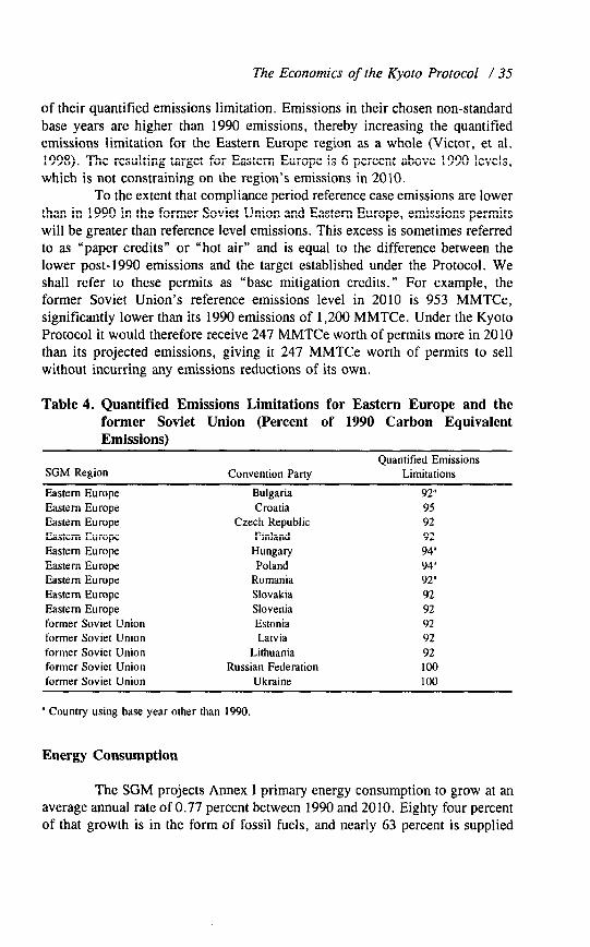
l%e Economics of the Kyoto Protocol / 35

of their quantified emissions limitation. Emissions in their chosen non-standard base years are higher than 1990 emissions, thereby increasing the quantified emissions limitation for the Eastern Europe region as a whole (Victor, et al. 1998). The resulting target for Eastern Europe is 6 percent above 1990 levels, which is not constraining on the region’s emissions in 2010.

To the extent that compliance period reference case emissions are lower than in 1990 in the former Soviet Union and Eastern Europe, emissions permits will be greater than reference level emissions. This excess is sometimes referred to as “paper credits” or “hot air” and is equal to the difference between the lower post-1990 emissions and the target established under the Protocol. We shall refer to these permits as “base mitigation credits.” For example, the former Soviet Union’s reference emissions level in 2010 is 953 MMTCe, significantly lower than its 1990 emissions of 1,200 MMTCe. Under the Kyoto Protocol it would therefore receive 247 MMTCe worth of permits more in 2010 than its projected emissions, giving it 247 MMTCe worth of permits to sell without incurring any emissions reductions of its own.

Table 4. Quantified Emissions Limitations for Eastern Europe and the former Soviet Union (Percent of 1990 Carbon Equivalent Emissions)

Quantified Emissions SGM Region Convention Party Limitations

Eastern Europe Bulgaria 92”

Eastern Europe Eastern Europe

Eastern Europe Eastern Europe

Eastern Europe Eastern Europe

Eastern Europe Eastern Europe

former Soviet Union former Soviet Union

former Soviet Union former Soviet Union

former Soviet Union

Croatia 95 Czech Republic 92

Finland 92

Hungary 94

Poland 94 Romania 92’

Slovakia 92 Slovenia 92

Estonia 92 Latvia 92

Lithuania 92 Russian Federation 100

Ukraine 100

’ Country using base year other than 1990.

Energy Consumption

The SGM projects Annex I primary energy consumption to grow at an average annual rate of 0.77 percent between 1990 and 2010. Eighty four percent of that growth is in the form of fossil fuels, and nearly 63 percent is supplied

36 / The Energy Journal

by natural gas alone. Figure 2 shows the percentage of total primary energy consumption supplied by fossil fuels by region in 2010. The total percentage and the composition of that fossil fuel consumption have a significant impact on the costs of mitigating carbon equivalent emissions.

Petroleum remains the major source of energy through 2010, but its share of total consumption declines over time, giving way to natural gas and, to a lesser extent, renewable energy sources. Coal is the third largest source of energy, and its consumption remains steady at slightly more than 20 percent of total consumption. Nuclear energy’s contribution to energy consumption also remains steady with declines in the United States roughly matched by increases in Western Europe.

Figure 2. Percentage of Total Primary Energy Consumption Supplied by Fossil Fuels in 2010

100%

90%

80%

70%

60% n coal

50% 0 Gas

n Oil 40%

30%

20%

10%

0%

El ectricity Generation

CAN FSU JPN US WEU AUS EEUR

Figure 3 shows electricity generation by fuel in 2010 for the Annex I regions. The composition varies greatly from region to region. The United States, Australia, and Eastern Europe, for example, rely heavily on coal while Canada generates almost 60 percent of its electricity from hydroelectric sources. Eastern Europe has the most balanced composition with no one fuel supplying more than one-third of the total generation.

The Economics of the Kyoto Protocol / 37

Figure 3. Total Electricity Generation by Fuel in 2010

4

2-

0 r

CAN FSU JPN US WEU AUS EEUR

Gas n Coal 0 Nuclear n Hydro n Renewables

COMPLIANCE

In the following sections, we systematically address the question of compliance cost for the Kyoto Protocol. In each mitigation scenario, allowable emissions are reduced linearly from the reference level in 2000 to the emissions target in 2010. Because the SGM operates with 5-year time steps, we treat the year 2010 as a typical year within the 2008 to 2012 budget period and assume that average cost experienced in the budget years before and after are on average the same as for the year 2010. We address five different issues:

1. The impacts of no permit trading,

2. The impacts of joint compliance with Annex I trading,

3. The impacts of joint compliance with Annex I trading with an

operational Clean Development Mechanism,

4. The effect of non-CO, greenhouse gases on compliance costs, and

5. The effect of carbon sinks on compliance costs.

38 / The Energy Journal

No Permit Trading

In the no trading case, each Annex 1 region must individually meet its quantified emissions limitations without any trading of permits across regions. A time series of carbon taxes is determined for each region to reduce emissions to be equal to its allocated emissions rights. In our examination of the no trading scenario, we assume that non-CO? greenhouse gases grow at exogenously specified rates in the reference case. Because we are ignorant about the mitigation cost functions for these other gases, we assume that their aggregate mitigation cost functions are similar to fossil fuel carbon. Thus, we compute non-CO? greenhouse gas mitigation cost as a proportion of fossil fuel carbon mitigation cost. In other words, the same percentage of total non-CO> emissions is abated for a given tax as the percentage of carbon dioxide emissions abated for that same tax. In a later portion of this paper we will investigate the implications of relaxing this assumption. Similarly, we apply ad hoc assumptions regarding land-use emissions mitigation. Although most of the Annex I regions had net sequestration in 1990, we assume for this analysis that regions receive no credits for this sequestration in the compliance period.’ As with the mitigation cost assumptions, this assumption about credits for emissions sequestration will be relaxed in analysis discussed later in the paper.

Several issues arise in the analysis of a no trading scenario. Successful compliance will change the regional and world energy systems. The individual energy circumstances of each region will shape the nature and cost of compliance. For example, the electric power sector plays an important role in shaping the cost of compliance. In the United States the substitution of natural gas for coal plays an important role whereas in Western Europe the role of nuclear power is increased substantially.

Some technology options have significant lead times to their deployment. For example, it takes time to build the gas pipeline infrastructure needed to re-power coal fired electricity generating facilities, to build and deploy gas turbines, and to build and license new nuclear power plants. Sub-optimal investment decisions may result from uncertainty regarding whether or not and under what conditions the Protocol will ever enter into force as well as national implementation policies.

5. The exception to this is Australia. Because Australia was a net land-use emitter in 1990, its

land-use emissions are included in its Kyoto target. Australia is also projected to be a net emitter in the compliance period in this analysis and these emissions are added to the carbon equivalent

emissions to generate its emissions in 2010.

The Economics of the Kyoto Protocol / 39

Costs of No Permit Trading

We first compute the permit fees required to bring each region into compliance independently on the assumption that compliance is fully anticipated by all public and private sector investment decisions taken after the year 2000. These results are shown in Table 5. Values are included for 2020 to show what the potential compliance costs would be if the requirements of the Kyoto Protocol were to be extended beyond the 2008 to 2012 budget period.

Table 5. Emissions Mitigation Relative to Reference and Emissions Taxes Required to Meet Kyoto Quantified Emissions Limitations and Reduction Commitments (MMTCelyear & 1992 US$ per tonne of carbon equivalent)

Emissions Mitigation Relative to Carbon Permit Price or

Reference to Meet Kyoto Quantified Tax Needed to Achieve

Emissions Limitations and Compliance Without

Reduction Commitments Trading (MMTCelyr.) (1992 US $/tonne Ce)

Region 2010 2020 2010 2020

Canada 12 86 350 3x7 former Soviet Union - 247 - 65 -_ __

Japan 137 150 458 430

United States 634 805 168 199

Western Europe 176 314 130” 208 ” 144” 241”

Australia 34 44 117 141

Eastern Europe - 42 22 __ 41

’ Allows new nuclear power capacity to be built. ’ No new nuclear power capacity allowed.

Permit fees of this magnitude change domestic and international energy systems. The changes in national energy systems vary greatly from region to region. Different growth rates in the Annex 1 regions result in varying amounts of mitigation required to comply with the Kyoto Annex I emissions limitations. Figure 4 shows the percent reduction in emissions from 2010 required by each region to meet its emissions goal. As mentioned earlier in the discussion of the construction of the regional reference cases, emissions growth rates, by affecting the emissions projection in 2010, significantly affect the cost of mitigation. Within the OECD regions, permit prices under the no trading case are lowest in Australia, where it requires $117 per tonne of carbon equivalent to comply with the Protocol in 2010, and highest in Japan, where the price rises to $458 per tonne.

40 / The Energy Journal

Figure 4. Percentage Reduction in Carbon Equivalent Emissions Required to Meet Kyoto Constraint

0

w

E

4s

35% ~-

30% -~

25% ~-

20% --

15% -.-

10% --

5% ~-

0% r -I-

CAN JPN us WEU AUS

Energy Sector Adjustments in the United States

In the absence of emissions trading, the Kyoto quantified emissions limitations and reduction commitments anchor a nation’s energy system to 1990. There are a limited number of ways to meet this target. Nations can either

. Capture and sequester carbon-in the time frame of the first commitment period this is limited to afforestation and reforestation;

. Undertake Fuel Switching-either expanding the production of non- carbon emitting energy sources such as hydro, nuclear, and solar power or biomass, or shifting from fuels with high carbon-to-energy ratios (such as coal) to fossil fuels with low carbon-to-energy ratios (such as natural gas);

. Conserve Energy-increasing the amount of services provided by a fixed energy input, or a reduction in the provision of energy services.

One of the notable responses in the United States is the substitution of natural gas for coal in the production of electric power. Fuel switching from coal to natural gas and renewable fuels in the United States electricity generation sector accounts for roughly 40 percent of the reduction in total emissions.

The Economics of the Kyoto Protocol / 41

Energy conservation makes up the remaining 60 percent of the reduction in 2010.

The domestic carbon tax of $168 in 2010 in the no trading case results in a reduction of total energy consumption by 20 percent relative to the reference case. Consumption of coal drops by three-quarters while consumption of petroleum drops by 13 percent. Consumption of natural gas, however, increases by 3 percent due to fuel switching. Figure 5 shows the change in energy consumption by fuel in the year 2010 under the no trading regime relative to the 2010 baseline value.6 Although we do not account for carbon capture and sequestration in this analysis, the figure does show indications of fuel switching and conservation. In the United States, the carbon tax leads to a slight increase in total gas consumption and a significant amount of conservation. Meeting the commitment in Western Europe leads to significantly less conservation but a much greater degree of fuel switching from fossil fuels to nuclear power. Note that even though emissions are drawn below 1990 levels, the scale of the total energy system remains above 1990 levels for all regions but Japan and Canada. The fuel switching mentioned above allows the emissions targets to be met without reducing total consumption by the same percentage as the required reduction in emissions.

Figure 5. Change in 2010 Energy Consumption from Baseline by Region and Fuel - No Permit Trading

20

10 B -2 ‘3 0 x

* -10

-20

CAN JPN US WEU AUS

Gas H Coal 0 Nuclear n Hvdro n Conservation ~

6. Eastern Europe and the former Soviet Union are not included because their 2010 emissions are not constrained by the quantified emissions limitation.

42 / The Energy Journal

Total electricity generation in the United States drops by 24 percent as a result of the emissions constraint. The permit fee results in the share of electricity generated from coal dropping from 51 percent in the reference case to 11 percent in the no trading case. The reduction in electricity generation from coal is partially compensated for by fuel switching to natural gas. The share of electricity generation from natural gas more than doubles from 21 percent in the reference case to 48 percent in the no trading case. Even so, conservation accounts for 70 percent of the drop in total generation from reference levels. Figure 6 shows how the utility sector in the United States switches from coal- fired to gas-fired electricity generation technologies given a range of permit fees.

Figure 6. The Relationship between Carbon Taxes and Coal Utilization in the SGM

$0 $25 $50 $75 $100 $125 $150 $175

Tax P2$)

The imposition of permit fees has a depressing effect on the price of coal. Gas prices under the no trading regime increase nearly 20 percent in response to increased demand from the utilities sector. But interestingly, it has relatively little effect on the overall consumption of natural gas. The increased demand for gas to replace coal in power generation is roughly offset by a

The Economics of the Kyoto Protocol / 43

decrease in the demand for natural gas for end-use applications resulting from the higher price, leaving total consumption relatively stable.’

Certain caveats apply to the discussion above concerning the substitution of natural gas-fired electricity generation capacity for existing coal-fired capacity. The analysis requires that the emissions targets be in place indefinitely. If the targets are believed to be only temporary, the optimal degree of substitution is diminished and the permit fee required for Protocol compliance raised. The permit fees required for mitigation also depend on the cost of altering the existing infrastructure necessary to supply natural gas to potential new users. Extending pipelines to particular areas, for example, might increase the cost of gas enough so as to discourage switching from coal-fired plants in those areas.

Energy Sector Adjustments in Australia

The energy system in Australia reflects a relative abundance of coal and scarcity of domestic natural gas supply. It has the lowest cost of compliance without permit trading among OECD regions primarily because it has the highest allowable percentage emissions growth relative to 1990, eight percent. Compliance with the Kyoto Protocol is accomplished primarily by reducing coal usage and secondarily with reductions in oil consumption.

Energy Sector Adjustments in Western Europe

The energy system in Western Europe is very different from that of the United States. Whereas relatively low energy tax rates and high dependence on coal for electric power generation characterize the United States, Western Europe is characterized by relatively high energy-tax rates and only modest use of coal for power generation. As Figure 5 shows, the model responds to a constraint on carbon emissions by shifting to non-carbon power generating technologies-in particular, nuclear power. This is a case that may be either politically or technically impossible to realize. Outside of France few nations would allow a significant expansion of nuclear power. Furthermore, given the lead time required to build and deploy a new nuclear facility, even in France, this option will be available for only a brief period if it is to impact emissions by the beginning of the budget period. If it takes ten years to bring a new

7. Other models have shown substitution of gas into the non-utility end-use sectors (e.g. Manne and Richels, 1998). This increase in demand could drive up gas prices even further, possibly limiting

the extent to which utilities would increase their consumption as a substitute for coal. Such a result could increase the permit fee necessary for the economy to comply with the required emissions

reductions.

44 / The Energy Journal

facility on line, that process must commence in 1998 to have an influence on the first compliance year, 2008.

When no new nuclear power generation capacity is allowed, the cost of compliance rises from $130 per tonne of carbon equivalent in 2010 to $144. Without a nuclear option more of the Western European mitigation must come from conservation.

The model shows relatively little energy conservation in Western Europe relative to the other Annex I regions. This reflects the fact that existing energy prices are already high, and whereas a $100 per tonne carbon equivalent tax raises the price of end-use fuels by between 20 and 25 percent in the United States, this is not the case in Western Europe. As a consequence of the relatively smaller price signal in Western Europe than in the United States, there is a relatively smaller conservation response.

Energy Sector Adjustments in Canada and Japan

The energy systems in Canada and Japan are quite different from each other. The Canadian energy system obtains a high fraction of electric power from hydroelectric facilities, while oil and gas dominate the Japanese system. Canada is a nation with low population density, with a transportation system reflecting a greater need to transport people greater distances. In contrast Japan has relatively high population density and a transportation sector geared appropriately. However, these two systems are similar in that both systems have relatively little coal use and have high percentage emissions mitigation requirements-more than 30%-relative to the reference case emissions in the year 2010. The minimal domestic coal consumption available for replacement by alternative fuels leaves these nations with the two highest marginal costs of compliance in our analysis.

Imperfect Energy Transitions

In the preceding analysis we have assumed that investment decisions begin to be altered starting in the year 2000. This assumption implies a smooth compliance transition, which need not be the case. We have run excursions to explore the implication of a less than perfect transition under a no trading scenario in the United States in the year 2010. In one exercise, we systematically reduced the mitigation potential available outside the electric utility sector. As the ability of the non-utility sectors to reduce emissions is diminished, the burden borne by the electric power sector increases-implying higher marginal abatement costs. The relationship between the burden borne by the utility sector and marginal abatement cost is shown in Figure 7.

At a marginal cost of approximately $100 per tonne carbon equivalent utilities provide approximately 45 percent of the mitigation in the year 2010 by

The Economics of the Kyoto Protocol / 45

substituting gas plants for coal plants. But the marginal cost must reach $255 per tonne carbon equivalent before the mitigation reaches 70 percent of the 2010 requirement. If the non-utility sectors have difficulty in reducing emissions, either because technical options are unavailable or because emissions mitigation requirements were not anticipated in investment planning during the decade prior to the first compliance year, 2008, then the marginal cost could exceed $250 per tonne of carbon equivalent emission.

Figure 7. The Relationship between Utility Emissions Mitigation and Marginal Cost in the United States in the Year 2010

~1 80% w .$ .g : 70%

E” 60% ,do” Y 50%

E 3 40% 2pc: % 8

.; 30%

$ .jf 20%

b 52 10%

0%

$0 $100 $200

Tax ( 1992$)

Relaxing the assumption that utilities begin anticipating implementation of the Kyoto Protocol in investment decisions from the year 2000 onward has a similar effect on the marginal cost of mitigation. In the case of perfect foresight, utilities replace existing coal-fired capacity with gas turbines. This implies building new gas transmission and distribution lines as well as the turbines. When no anticipatory actions are undertaken, utilities are left with the option of either paying for the carbon emissions and continuing to operate the plant or shutting down. Utilities that are forced to shut down lose the value of the capital stock and cease to generate power but reduce emissions by the full amount of the plant’s capacity.

46 / The Energy Journal

Sensitivity of Results to Economic Growth in the United States

The reference case shows United States GDP growing at an average rate of 2.1 percent per year from 2000 to 2010. Because the future rate of economic growth is uncertain, we performed two additional analyses to determine the sensitivity of marginal costs to the United States to changes in its GDP growth rate. To conduct this experiment we adjusted the total factor productivity in the ‘everything else’ sector to increase or decrease the average rate of growth by 1 percent per year relative to the 2.1 percent reference level while holding the carbon equivalent-to-GDP ratio at reference case levels in 2010.

Changes in the expected rate of economic growth in the United States could have significant impacts on the costs of compliance with the Protocol. A decrease in the average annual rate of GDP growth from the reference level of 2.1 percent to 1.1 percent per year results in a marginal cost of mitigation for the no trading case of $85 in 2010, just over half of the $168 per tonne cost required under reference case growth assumptions. The high growth case of 3.1 percent per year, or 1.0 percent above reference level growth rates, results in a cost of $301 per tonne, nearly 80 percent higher than under reference assumptions.

Annex I Trading

In an AMeX I trading regime, regions may only emit more carbon than their allocated emissions rights allow if another Annex 1 region is willing to sell a corresponding number of its permits, thereby forcing the seller region to reduce its domestic emissions beyond the required target. This is modeled as if a common carbon tax were applied to all AMeX I regions to meet the overall Annex I emissions target. Since the overall Annex 1 target is met with equality, excess emissions in permit buying regions are exactly matched by emissions credits in permit selling regions. The permit price is inferred to be the common Annex I tax rate and is used to compute the value of sales and purchases.

Allowing trade among AMfX I parties raises a number of additional, important issues. These include:

1. Reference emissions in Annex I nations: Of particular interest is the degree and nature of recovery of Eastern Europe and the former Soviet Union. These countries are the largest block of potential suppliers of emissions credits to the market. The number of credits available will have an important influence on the international price of credits, and the incentive to mitigate domestically.

The Economics of the Kyoto Protocol / 47

2. Trade behavior: Since the number of sellers could be small, there is potential for monopolistic behavior. Thus a smaller number of permits could be placed on the market than are potentially available. The monopolistic selling position of a few nations could imply a floor on the price of mitigation credits.

3. Trade Rules: Rules may be written which restrict trade.

4. Incomplete markets: Market formation may be incomplete. Trade may occur among a subset of regions. For example, the European Union could form one trading regime and the other Annex I nations could form another. This is sometimes referred to as the “double bubble.”

“Base Mitigation Credits” in Eastern Europe and the former Soviet Union

It has been argued that the excess permits granted to the former Soviet Union and Eastern Europe should not be tradable because they would lead to lower environmental benefits than if the emissions could not be traded. The argument is that if each region meets its commitments independently, then total Annex I emissions will be lower than the quantitative emissions limitation. If trade is allowed, then Annex I emissions will be exactly equal to the quantified emissions limitation. The difference is the amount of extra emissions that go into the atmosphere due to trade in the budget period. The problem with this argument is that it is static. It presumes that there is only one budget period. But if there is only one budget period and no subsequent mitigation commitment, then it is hard to see why any party would ever undertake a Kyoto commitment.

But, if there were multiple budget periods, and no trade, the excess permits would be banked by the former Soviet Union and Eastern European parties for use in subsequent periods when national emissions exceeded the quantified emissions limitation. These parties’ emissions would therefore simply be moved into the future. Over time, cumulative Annex I emissions would therefore be the same whether or not trade in “base mitigation credits” is allowed. And to the extent that there is any difference to the environment, the long-term, year 2050, concentration is somewhat lower if emissions are released earlier in the century rather than later. The carbon cycle has a bit longer in that case to remove carbon from the atmosphere.

The Cost of Compliance with Annex I Trading

Trading regimes are inherently more complicated than non-trading regimes, particularly when the rules for trade have not been established. But even if the rules were known, the circumstance could exist in which the number of buyers

48 / The Energy Journal

and/or sellers is small, raising the issue of market power. We examine four cases: 1) Competitive permit supply; 2) Monopolistic permit supply; 3) Trade limitation; and 4) The “Double Bubble.”

Competitive Permit Supply

Under a competitive permit supply model, suppliers of permits are numerous and no single permit vender can affect the price received by withholding permits from the market. This situation would be the case if all permits were distributed within nations to numerous private parties. The competitive prices of Annex I permits in comparison to prices under the no trading case are shown in Table 6.

Permit prices are lower with Annex I trading than in the no trading case, Table 6. In the no trading case, greenhouse gas emitters in the United States may undertake emissions mitigation options available only within the United States. In the Annex I joint case, however, regions are included that have mitigation options with significantly lower costs, thereby lowering the marginal cost to the emissions permit market of meeting the desired emissions targets. This flexibility in meeting emissions targets has a significant impact on permit prices and costs, especially in the case in which “base mitigation credits” are available on the market at no cost to the supplier.

Table 6. Emissions Taxes/Permit Prices Required to Meet Policy Goal (1992 US$ per tonne of carbon equivalent)

No Permit Trading Annex I Trading

Region

Canada former Soviet Union

Japan United States Western Europe Australia

Eastern Europe

2010 2020 2010 2020

350 387 __ _-

458 430 168 199 73 118 130 208 117 141

-- 41

A fixed emissions level and an increasing reference case emissions level imply both a rising percentage emissions reduction and a rising price of meeting the fixed emissions target over time. Increasing population in the United States, and the economic growth that accompanies it, put upward pressure on emissions that in turn forces larger shifts away from coal toward natural gas and renewable energy sources.

As the permit prices decrease across trading regimes, the United States purchases increasing quantities of permits from abroad, thereby enabling it to

The Economics of the Kyoto Protocol / 49

emit more than its allocated permits alone would allow. Figure 8 shows total emissions in 2010 for each region disaggregated into emissions allowable under the Kyoto commitment, or the level allowed under the no trading case, and additional emissions granted by the purchase of permits. Under the no trading case, the United States is limited to emitting only what it is allocated under the Kyoto Protocol. With AMeX I trading, however, the United States purchases 248 MMTCe worth of permits in 2010 from two sellers, the former Soviet Union and Eastern Europe.

Figure 8. Annex I Emissions by Region - Kyoto Protocol

2500 . . .._....,.,_.____._.~~.~....,.~~~.~.~.~~....~.~~~..~~..... _,_...____.__ __ ._.. _.._ ..-.......- ._._......_. . .

* Net Emissions

1500 a2

g loo0

3

500

0

-500

CAN FSU JPN US WEU AUS EEUR

Cost calculations for the emissions trading cases are different than in the no trading case. Costs for the trading case must take into account the value of permits traded. For a buyer of permits, such as the United States, net cost therefore includes the direct cost of domestic mitigation plus expenditures on carbon permits. A breakdown of these two cost components is shown for the Annex I trading case with competitive permit supply in Figure 9. The direct costs of domestic mitigation range from 15 to 55 percent of the net cost for Annex I regions. The remaining cost, the difference between the ‘direct cost’ and ‘net cost’ lines in Figure 9, is the value of emissions permits that would be purchased from other Annex I countries.

50 / The Energy Journal

Figure 9. Breakdown of Costs by Region - Kyoto Protocol

-2.0%

B3 Permit Transfer

_ m Direct Cost

1

-2.5 % _--

CAN FSU JPN US WEU AUS EEUR

Increased growth in the regional energy systems is allowed by the purchase of permits. Figure 10 shows the percent change in primary energy consumption in 20 10 relative to 1990 baseline consumption for permit buyers for three cases: the baseline, no permit trading, and Annex I permit trading. Annex I permit trading restores a portion of the growth in the regional energy systems lost under the no trading case. The impacts of permit trading are especially evident in Japan and Canada. Trading under an Annex I permit trading regime allows Japanese and Canadian energy consumption to expand to approximately two-thirds of reference case emissions growth.

The former Soviet Union and Eastern Europe regions, the permit sellers under Annex I trading, face no reductions in energy growth under the no trading case but undertake large reductions in a permit trading regime to generate more marketable permits. The heavy dependence on coal in Eastern Europe and the multiplicity of conservation opportunities in the former Soviet Union provide inexpensive mitigation credits. These reductions are predicated on a competitive model of economic behavior. The conditions necessary for such a model may be unrealized, however. We further note that we assume no problems with measurement or verification of emissions mitigation. Such real-world problems could limit market performance,

The Economics of the Kyoto Protocol / 51

Figure 10. Percentage Change in Energy Consumption to 2010 from 1990 Baseline - Three Permit Trading Scenarios

50% ---- r

-- .- --- --___ n Baseline H Global Trading

n Annex I Tradin

CAN JPN us WEU AUS

Sensitivity of Results to Mitigation Supply

In the following two sections, we discuss the impacts on Annex I permit prices of the former Soviet Union and Eastern Europe limiting, either by choice or as required by the final treaty, sales of permits to other Annex I regions. In both cases, the available quantity of “base mitigation credits” in the two regions plays a significant role in determining the supply of permits to the market. Because the quantities of “base mitigation credits” available to the former Soviet Union and Eastern Europe are highly uncertain, we first examine the sensitivity of the Annex I permit price to the supply of these permits.

Several factors might contribute to a change in the amount of “base mitigation credits” available for sale to the Annex I permit market relative to the reference case. These factors could include, among other things, changes in the economic growth rate of the former Soviet Union and Eastern Europe, choices in the fuel mix as these economies recover, and methods of accounting for land- use change under the final Protocol. For the purpose of this analysis, we do not specify which of the many possible contributing factors or combinations of factors might lead to a change in the number of these permits.

Table 7 shows the impact on Annex I permit prices of altering the number of “base mitigation credits” that the former Soviet Union and Eastern Europe have available to sell in the permit market. We vary the availability of

52 / The Energy Journal

these credits from 0 percent of reference level permits, or no “base mitigation credits” at all, to double the reference level supply. With no “base mitigation credits” available to the Annex I market, permit prices to the Annex I regions rise by nearly 5.5 percent. If an Annex I permit trading regime is to develop, therefore, future developments in the former Soviet Union and Eastern Europe are likely to impact compliance costs both domestically and throughout Annex I.

Table 7. Sensitivity of Annex I Permit Prices in 2010 to Mitigation Supply (1992 US$ per tonne of carbon equivalent)

Percentage of Reference Case Annex I Permit Price

“base mitigation credits” (1992 US$)

0% $113

50% $92 100% (Reference) $73 150% $56 200% $41

Monopolistic Permit Supply

If the Russian Federation and Ukraine were the dominant sellers of emissions mitigation credits, these governments could control the supply of permits centrally. From a national perspective, it is never optimal to sell permits beyond the point at which total revenues begin to fall. Since from the perspective of a monopolist adding permits to the market always lowers the price, the trick is to never add permits beyond the point at which the price declines faster than permits are being added to the market. If revenues can be maximized without exhausting the supply of “base mitigation credits,” then supply cost is zero and no more sophisticated model is required for a single period analysis. Of course, adding multiple periods or non-zero costs of permit creation to the problem creates situations in which still fewer permits might be introduced for sale in the first budget period.

If a seller of a base mitigation credit anticipates that the price of a permit will rise faster than the rate of interest, then it pays to hold the permit for sale in a later period. If, on the other hand, the seller anticipates that the permit price will rise less rapidly than the rate of interest, it pays to cash the permit and invest the proceeds. Note that the price of permits rose at a rate less than three percent per year in the competitive case.

For the purpose of this analysis, we combine the former Soviet Union and Eastern Europe regions and treat them as a single monopolist. The monopolist maximizes its profits, or the difference between its revenues from permit trading and its costs of domestic mitigation, in each time period without

The Economics of the Kyoto Protocol / 53

respect to the potential value of the permits in later periods. The potential supply of permits available to the permit buying regions includes any excess in emissions rights above reference emissions, “base mitigation credits” which might exist in both regions, and any permits created by domestic mitigation undertaken within the seller regions. The monopolist controls the supply of permits and sells the permits at the resulting market price.

In the year 2010 a revenue-maximizing monopolist would withhold permits to the point at which the price rose to $105 per tonne of carbon equivaIent.8 This market price is 44 percent higher than the competitive market price. The sellers restrict the supply of permits to 62 percent of the permits available in the competitive case. As a result, the combined sellers generate 10 percent more profits under a monopolistic supply regime than under the competitive supply regime. Note, however, that even the monopolistic permit price under the Annex I permit trading regime is less than the permit prices faced by the regions under the no permit trading scenario.

As one might expect given the level of the permit price, monopolistic permit pricing restricts the regional energy systems by more than competitive Annex I trading but by less than the no trading regime. Energy consumption in Japan, for example, increases by 16 percent from 1990 to 2010 under monopolistic pricing, near to the 20 percent achieved under competitive pricing and well above the drastic reductions undertaken in a no trading regime. Growth in the United States is reduced from 17 percent in the competitive case to 12 percent in the monopolistic case.

Limited Trading

Limits may be placed on the fraction of a party’s quantified emissions limitation and reduction commitment that may be satisfied with allowances originating outside of that party’s boundaries. Such limits may be non-binding. That is, they may be set at levels at which regions’ behavior would not be constrained. If they are set at binding levels, then the marginal cost of mitigation for a party is simply that cost of the final mitigation action necessary to satisfy the domestic requirement. In a competitive permit supply market the marginal cost of international permits would be set by the interplay of supply and demand among parties for whom the constraint is non-binding.

8. We also ran a case in which the former Soviet Union acted as a monopolist without collaboration by Eastern Europe. The resulting permit fee for Annex I permit trading, including the sale of some permits by Eastern Europe, is $99 per tonne of carbon equivalent. Total profits for the former Soviet Union arc 3 percent lower than in the case in which the monopoly includes

Eastern Europe.

54 / The Energy Journal

At the June meeting of the Framework Convention on Climate Change’s subsidiary bodies in Bonn, Germany, two proposals were presented regarding Annex I permit trading and limits on that trading. The United States and seven other industrialized nations, including the Russian Federation and Japan, proposed that Annex I trading of all six greenhouse gases considered under the Kyoto Protocol be permitted without limiting the number of permits bought and sold by a particular region. This proposal describes the trading system that we have used thus far in this analysis. Less than a week later, however, the European Union, Switzerland, and seven Eastern European nations proposed an as yet unspecified ceiling on the number of permits a nation could purchase from the international market. Their proposal also required that Annex I permit sales be limited so that net permit transfers from a country could not exceed the amount of emissions mitigated domestically. This condition would effectively limit the portion of “base mitigation credits” that the former Soviet Union and Eastern Europe could sell to the amount of domestic reductions that each region undertakes. Such a rule would ensure that the total Annex I reductions under a permit trading regime would be at least as great as the total reductions required in a case without permit trading. Such proposals are difficult to implement. The degree of realized mitigation is impossible to calculate. There is only one history that will ever be recorded, and therefore no unambiguous reference case will ever exist against which to compare the realized historical emission.

This is not a problem from the perspective of a model, however. We consider here a ceiling on permit purchases from the international market set at 10 percent of each region’s allowable emissions under the no trading case as defined in the Kyoto Protocol. For example, because the United States has an emissions cap of 1,542 MMTCe in 2010, it would be limited to purchasing a maximum of 154 MMTCe in permits from the international market to meet its obligation. As suggested in the European proposal discussed above, we also limit sales of “base mitigation credits” permits from the former Soviet Union and Eastern Europe to the number of tonnes of carbon equivalent mitigated domestically. For the former Soviet Union to sell all 247 MMTCe of permits, therefore, it would need to undertake at least 247 MMTCe of domestic mitigation.

A ceiling on permit purchases implies that each region will face a distinct marginal cost for its domestic mitigation activities and another cost for the permits it purchases from the international permit market. The domestic price, as in the no trading case discussed above, will be a function of each particular region’s marginal cost curve and the ceiling placed on permit trading. The marginal cost for each region is reported in Table 8.

The entire market for permits under this regime can be satisfied with sellers providing permits to the market at price of $64 per tonne of carbon equivalent in Eastern Europe and the former Soviet Union, But there is no unique market clearing price under this particular set of rules. The domestic

The Economics of the Kyoto Protocol / 55

price of mitigation within potentially buying regions and the cost of mitigation supply in potentially selling regions bound the range of prices.

Table 8. Permit Prices in 2010 Under Limited Permit Trading Case (1992 US$ per tonne of carbon equivalent)

Permit Price (1992 US$)

Domestic Marginal Domestic Marginal Cost in

Region Cost in Buying Regions Supplying Regions

Canada 197

former Soviet Union 64

Japan 304 United States 100

Western Europe 47 Australia 60

Eastern Europe 64

The “Double Bubble”

As mentioned earlier, permit trading may occur among only a subset of the Annex I regions. In the “Double Bubble” case, the Western Europe region is removed from the Annex I trading bloc, leaving it to meet its obligations independently. For Western Europe, the necessary carbon taxes and energy impacts are the same as under its no trading case. But for the remaining regions in the permit market, the departure of Western Europe results in a 20 10 permit price that is lower than in full Annex I competitive trading-$64 per tonne as compared to $73 under full Annex I trading.

The Clean Development Mechanism

The Clean Development Mechanism (CDM) was created as a vehicle which would allow non-Annex I nations to continue to pursue economic growth while at the same time have access to additional resources for the purpose of reducing greenhouse gas emissions. In the words of the Protocol:

The purpose of the clean development mechanism shall be to assist Parties not included in Annex I in achieving sustainable development and in contributing to the ultimate objective of the Convention, and to assist Parties included in Annex I in achieving compliance with their quantified emission limitation and reduction commitments under Article 3.

56 / The Energy Journal

The CDM provides a mechanism in which certified emission reductions can be created on a project by project basis. Annex I parties can use these certified emission reductions to contribute to compliance with part of their quantified emission limitation. The CDM is to be subject to the authority of the Conference of the Parties and will be supervised by an executive board. Participation in the CDM is voluntary.

Certified emission reduction credits can be created by projects as long as these projects:

1. Lead to real, measurable, and long-term benefits related to the mitigation of climate change, and

2. Undertake reductions in emissions that are in addition to any that would occur in the absence of the certified project activity.

Interestingly, the CDM can create certified emission reduction credits beginning in the year 2000, and these credits can be applied to the budget period.

At the writing of this paper the rules for creating certified emission reduction credits have not been written. Therefore, we can not directly simulate the impact of the CDM on permit prices and costs of mitigation. However, full global trading of emissions rights provides a lower bound on permit prices and mitigation costs. The CDM should provide a cost of mitigation that lies between the cost of Annex I trading and full global trading.

Full Global Permit Trading

In the global trading case, emissions rights are allocated to Annex I regions at the same levels as in the Annex I trading case. Under global trading, however, the Annex I regions are allowed to purchase permits from each other as well as from non-Annex I regions so long as the global emissions constraint is met. The global constraint in each period is composed of the Annex I constraint and the sum of the non-Annex I regions’ reference level emissions in that period. The SGM is used to determine a global permit price just large enough to meet the global emissions target.

Non-Annex I regions are not required to constrain their emissions in the global trading scenario. Under this hypothesized global trading regime, non- Annex I regions participate in the market for emissions permits only when it is to their economic benefit to do so. These regions are allocated permits equal to their projected reference emissions, so they only reduce their emissions by an amount equal to the number of permits they wish to sell.

Expanding the supply of emissions mitigation through global permit trading results in significantly lower permit prices than those achieved under the

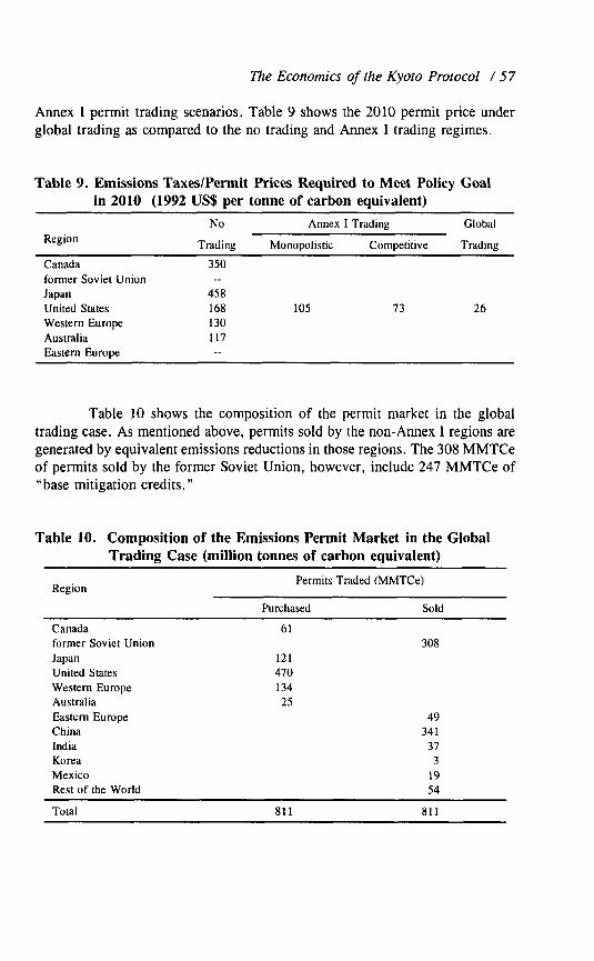
The Economics of the Kyoto Protocol / 57

Annex I permit trading scenarios. Table 9 shows the 2010 permit price under global trading as compared to the no trading and Annex I trading regimes.

Table 9. Emissions Taxes/Permit Prices Required to Meet Policy Goal in 2010 (1992 US$ Per tonne of carbon eauivalent)

Region

Canada

former Soviet Union Japan United States Western Europe

Australia Eastern Eurooe

No

Trading

350 __

458 168

130

117 __

Annex I Trading Global

Monopolistic Competitive Trading

105 13 26

Table 10 shows the composition of the permit market in the global trading case. As mentioned above, permits sold by the non-Annex I regions are generated by equivalent emissions reductions in those regions. The 308 MMTCe of permits sold by the former Soviet Union, however, include 247 MMTCe of “base mitigation credits.”

Table 10. Composition of the Emissions Permit Market in the Global Trading Case (million tonnes of carbon equivalent)

Region Permits Traded (MMTCe)

Purchased Sold

Canada 61 former Soviet Union 308

Japan 121 United States 470

Western Europe 134 Australia 25

Eastern Europe 49 China 341 India 37 Korea 3 Mexico 19 Rest of the World 54

Total 811 811

58 / The Energy Journal

The additional permits supplied by China account for most of the difference in permit prices between the Annex I permit trading and global trading cases. To sell such a large number of permits, China reduces its energy consumption by nearly 24 percent in 2010 relative to the baseline consumption, with over 85 percent of that reduction coming from reduced coal consumption. The mitigation activities in China and the other non-Annex I regions are undertaken at significantly less cost than in the Annex I regions, however, thereby allowing the permit buying regions to emit more than in the Annex I trading or no trading cases for less cost. And although the non-Annex I permit sellers achieve mitigation primarily through conservation, their energy consumption and carbon equivalent emissions continue to grow.

Costs as a percentage of GDP are consequently the lowest for the Annex I regions under the global trading case, although Eastern Europe and the former Soviet Union lose some of their gains from trade to the non-Annex I permit sellers. Figure 11 shows the total costs as a percent of GDP to all regions separated into the direct cost and net permit trading revenue components for the global trading case.

Figure 11. Cost by Component and Region in 2010 in Percentage of GDP - Global Trading

0.8% 7_ _......._.......... ._ _....._ . . .._.. -- .._........-..._I _....__ . . ~ B3 Permit Transfer

0.6% ~~~ ~-~ -~~-~~~ -- - Direct Cost

a 0.4% +- ~ * Net Cost

-0.6%

-0.8% --- py-----2

The lower permit price induces only minor changes in the Annex I regions’ energy systems relative to the reference case. Energy consumption in the United States in 2010 increases by 26 percent over 1990 levels, as compared to an increase of only 17 percent under Annex I competitive permit trading, as

The Economics of the Kyoto Protocol / 59

shown in Figure 10. The remaining Annex I permit buyers experience similar impacts, with energy growth under global trading falling about halfway between that in Annex I trading and the baseline case.

SUMMARY OF PARTICIPATION AND BEHAVIOR ANALYSIS

Where and under what circumstances emissions mitigation can be undertaken has a significant impact on the potential costs or benefits of participation in the Kyoto Protocol. Figure 12 shows the range of permit prices that the United States could face depending on which of the above permit trading frameworks is accepted as part of the final Protocol. Note that the other Annex I regions face the same range of permit prices as those shown in the figure except that the no trading case values differ from region to region. Note also that in the case of Annex I Trading with EU Limits, the permit value is indeterminate. We therefore present a range; while the lower end of the range is determined by the conditions in the permit supplying regions, the upper end of the range is always region specific.

Figure 12. Range of Permit Prices for U.S.

No Trading, No Trading Annex I Annex I Annex I Global

70% Utility Trade, EU Trade, Trade, Trading,

Mitigation Limits EE/FSU Competitive Perfect

Monopoly SUPPlY Competition

60 / The Energy Journal

NON-CO, GREENHOUSE GASES

The complexity of the Kyoto Protocol is not limited to issues concerning the characteristics of the permit trading mechanism. The protocol is also framed in terms of a suite of six gases and contains provisions for the inclusion of credits for terrestrial carbon sinks. This section will discuss the role of non-CO, greenhouse gases in determining costs and the following section will address the importance of land-use change emissions.

The contribution of non-CO? greenhouse gases to total carbon equivalent emissions in 1990 ranges from 10 percent in Japan to over 24 percent in Australia and Eastern Europe among the Annex I regions. Figure 13 shows the composition of total carbon equivalent emissions in 1990 and 2010 for the Annex I regions. The figure also shows the emissions target by region as specified in the Kyoto Protocol (see Appendix A). The former Soviet Union and Eastern Europe face targets that are above their 2010 baseline emissions levels, resulting in the “base mitigation credits” discussed in previous sections. Australia is allocated an 8 percent increase in emissions from 1990 to 2010, so its target as shown in Figure 13 is greater than the sum of its 1990 greenhouse gas emissions.

Figure 13. Breakdown of Kyoto Target by CO, and Non-CO, Emissions

2500 __.-_-------- ~- -----

Non-CO2 Emissiom& Us I

2ooo m CO2 Emissions

-o- Kvoto Target r-l

EEUR

The Economics of the Kyoto Protocol / 61

The results until now have assumed that the mitigation costs of the non- CO? greenhouse gases are proportionate to the cost of mitigating emissions of fossil fuel carbon. We refer to this case as the “Proportional Cost” case. In an attempt to bound the compliance costs with respect to these other gases, we modeled two additional mitigation cost cases. In the first case, the “$0 Cost” case, we assume that all of the non-CO, greenhouse gases can be mitigated in 2010 at zero marginal cost, thereby reducing the total commitment level by the 2010 emissions of these gases. In the second case, the “Infinite Cost” case, we assume exactly the opposite-that the non-CO, gases are impossible to mitigate at any cost. The “Infinite Cost” case therefore assumes that the Kyoto commitment must be met using reductions in carbon dioxide only. All of these scenarios share the same assumptions about land-use emissions as the previous cases.

Figure 14 shows the impacts on the marginal cost of compliance without permit trading for the Annex I regions of the two non-CO, greenhouse gas mitigation cost cases and the original “Proportional Cost” case. Total Annex I emissions fall under the target in the “$0 Cost” case because of the reduced mitigation requirements in each country and the additional “base mitigation credits” available to the former Soviet Union and Eastern Europe from their non-CO, gas credits. The permit price in a competitive Annex I market with no constraint is zero. On the other hand, the Annex I competitive permit price under the “Infinite Cost” case increases from $73 under the “Proportional Cost” case to $93, causing total costs to increase as well.

Figure 14. Permit Prices in 2010 Under Three Non-CO, Gas Mitigation Cost Options - No Permit Trading

CAN

n $0 cost

0 Proportional Cost

q Infinite Cost t

-

AUS

1

62 / The Energy Journal

LAND-USE EMISSIONS

In the preceding analysis we have ignored the potential of terrestrial carbon sinks on net carbon emissions under the Protocol. But the Protocol makes provision for land-use change emissions and sinks and, while net land-use emissions are small relative to fossil fuel carbon emissions, their treatment can have a major impact on the initial cost of achieving any emissions mitigation objective. Land-use emissions are presently treated as a flow in determining the base year (1990) emission rate. Most Annex I nations are in the process of reforesting, and therefore have net accumulation of carbon. This accumulation reduces net anthropogenic emissions.

Although this approach is appropriate for a global accounting of carbon flux, it may not be desirable as a methodology for setting 1990 base year emissions. The implication of this treatment is that if a nation were reforesting in 1990 and were committed to maintaining 1990 emissions rates under the Protocol, it could not reduce the rate of reforestation without lowering fossil fuel carbon emissions to below 1990 levels. Thus, reforesting is not enough. The rate must be maintained. For nations that were deforesting, this method would create a base year emission target that is the sum of deforestation plus fossil fuel emissions which would in turn implicitly grant those nations a perpetual right to deforest. If the deforestation rate is ever reduced, for example as a consequence of destroying all forested areas, then fossil fuel emissions could be higher than 1990 levels by the 1990 rate of deforestation.

The delegates at Kyoto agreed that if a country in the base year had net land-use accumulation of carbon-negative land-use change emissions-the base year emissions for determining emissions limits would be determined by industrial emissions only. This method was termed the “gross” approach to accounting, a term which is anything but self-explanatory. The idea is that the country would note its stock of terrestrial carbon, not the change in stock. In other words, land-use emissions are ignored in computing the base emissions rate.

On the other hand, if a country had net land-use carbon release, then it could count both industrial and land-use change emissions in determining its base year emission inventory. This accounting method became known as the “net” approach.

In the budget period, 2008 to 2012, all countries include both industrial and net land-use emissions in their emissions inventory. For those countries with net emissions from land-use change in the base year, the accounting method was then the “net-net” approach in that net emissions flows are used in both the base year and the budget year. If a country has a net accumulation, however, it counts as negative emissions only those accumulations of carbon that are the result of actions taken since 1990 in the areas of afforestation and reforestation.

The Economics of the Kyoto Protocol / 63

This method has come to be known as the “gross-net” approach in that net emissions are ignored in the base year but counted in the budget period.

Many issues remain to be worked out. The protocol stipulates that

The net changes in greenhouse gas emissions from sources and removals by sinks resulting from direct human-induced land- use change and forestry activities, limited to afforestation, reforestation, and deforestation since 1990, measured as verifiable changes in stocks in each commitment period shall be used to meet the commitments in this Article of each Party included in Annex I.

This presents an interesting problem in what to count. Do soils beneath the forests count? Can normal anthropogenic forest management be counted? Given the nature of forest growth, the rate of carbon uptake in 2008 would be small for a program that began in 1998 due to the carbon absorption cycle by forests. Therefore, to the extent that net carbon uptake by sinks, or stores of carbon, is credited in the first budget period, it will largely be determined by an interaction between the rules and actions that were taken earlier. Unless interpreted very broadly, the language of the Protocol limits the potential impact of new initiatives.

For this analysis, we assume that the “gross-net” approach applies for all Annex I regions except Australia, for which we used the “net-net” approach. Because of the uncertainty surrounding the actual quantity of credits to be given for net land-use change emissions in the first budget period, we defined three levels of credits for each Annex I region, as shown in Table 11: no sinks credits, “half” sinks credits, and “full” sinks credits.’ This quantity is specified exogenously in the budget period and is not priced in our analysis. For the analysis presented thus far, we have used the “no sinks” assumptions.

Varying the land-use change credit assumptions has significant impacts on the permit prices required for compliance without permit trading for some regions and on the price under Annex I joint compliance. Figure 15 shows the permit prices for the Annex I regions for the three sinks options under the no trading case. The application of “full sinks” credits in the Canadian case more than covers Canadian mitigation requirements in 2010 thereby bringing its permit price in the no trading case to zero. The “half” and “full sinks” cases offer the former Soviet Union and Eastern Europe even more “base mitigation credits” than in previous cases, increasing their potential benefit from permit trading. The increased “base mitigation credits” also reduces the 2010 permit

9. Australia values from Working Group on Public Health and Fossil Fuel Combustion, 1997. Other values from personal communication with Joe Aldy, Council of Economic Advisers.

64 / The Energy Journal

price of competitive Annex I joint compliance from $73 per tonne in the “no sinks” case to $46 and $23 per tonne in the half and full sinks cases, respectively.

Table 11. Land-Use Change Emissions Assumptions for the First Budget Period (million tonnes of carbon equivalent)

Region Land-Use Change Emissions Credits (MMTCe)

No Sinks Half Sinks Full Sinks

Canada 0 40 80 former Soviet Union 0 103 20.5

Japan 0 13 25 United States 0 52 104

Western Europe 0 30 60 Australia -36 -36 -36

Eastern Europe 0 4 8

Figure 15. Permit Prices in 2010 Under Three Sink Options - No Permit Trading

$500

$400

$300

$200

$100

$0

CAN JPN us WEU AUS

The economic implications of alternative treatments of land-use change emissions are large and their treatment was one of the most hotly debated issues in the Kyoto negotiations. As discussed above, the size of regional carbon stores has a substantial impact on regional costs in the budget period. However, this is a short-term consideration. In the long term, land-use emissions mitigation

The Economics of the Kyoto Protocol / 65

potential is limited. Eventually all forestry programs approach steady-state carbon-to-land ratios. If a given plot of land is to continue to provide carbon uptake services, the existing biomass must be removed. Since the biomass resources can be used as a zero-cost energy form to replace fossil fuels, forestry programs ultimately mature into biomass energy programs.

DISCUSSION

In this section, we consider some of the lessons learned from this analysis and present further discussion of issues relevant to this type of analysis. First, the method used to measure costs can significantly vary the representation of the potential burden placed on an economy by a particular policy. Second, economic costs depend a great deal on our assumptions about future carbon emissions. Third, the distribution of costs among countries in a system of global permit trading is sensitive to assumptions on exchange rates as well as the initial allocation of permits. Fourth, any system of global trade in carbon permits implies potentially large transfers of wealth from one region to another. Finally, we discuss how some of our assumptions affect the results on costs.

Measurement and Reporting of Costs

As mentioned earlier in the paper, our cost measure is a direct cost net of international transfer payments due to permit sales between countries. Direct cost is defined here to be the area under the marginal abatement curve for carbon, which can be approximated as one-half of the marginal price of carbon multiplied by the amount of carbon abatement. This approximation is the same as that for deadweight loss. To provide a sense of scale to the rest of the economy, we often express cost as a percentage of GDP.

Of ultimate interest, however, is the impact on some broader measure of economic activity such as GDP or real consumption. There are many reasons why a change in GDP may differ from direct cost. In addition to direct cost, other cost components include the effects of pre-existing taxes, changes in terms of trade, and how tax revenues are recycled. Also, measurement of GDP or real consumption depends on the choice of index and base year used to construct that index. This reflects real-world problems in constructing a quantity index when relative prices are changing.

Determining the size of the indirect cost components has proven difficult, and is a topic of study for modeling groups participating in Stanford University’s Energy Modeling Forum. Some modeling groups, including the SGM group, have chosen to report only direct costs net of sales of emissions rights. Other groups have reported overall changes in economic welfare, but without an indication of the relative sizes of the other cost components.

66 / The Energy Journal

If the overall economic cost differs from direct cost, or if the market price of carbon does not reflect all costs to a nation, there are cases where nations will not gain from participating in a carbon emissions trading program. If social costs are much greater than private costs, sellers of emissions permits may be made worse off by selling permits and would not participate in emissions trading. More specifically, if the average social cost of permits sold exceeds the world permit price (marginal private cost), sellers of permits are worse off than if they had not sold any permits. That is, trade may make some nations (in this case nations selling carbon emissions rights) worse off rather than better off, even though the individual trading parties (in this case companies or persons) were all made better off. The implications of a substantial divergence between public and private interests, in the absence of apparent market imperfections, is important and goes to the heart of the motivation for free and open trade.

If we are to create mitigation scenarios where emissions trading is assumed, then we should verify that our cost measure is consistent with gains from emissions trade in all regions. The simple measure of direct cost net of permit sales does indeed report gains from trade in all regions. Beyond this, it would be informative to calculate as many indirect costs components as practical, and then determine whether any of these components could affect a nation’s choice to participate in emissions trading.

For example, one of the indirect cost components is the additional deadweight loss due to pre-existing energy taxes. For a seller of permits, the additional loss is approximately equal to the reduction in tax revenue of the pre- existing tax, as a carbon tax is imposed to reduce carbon emissions below that country’s emissions allocation. This cost component could be large enough to offset other gains from emissions trade. This suggests a bottom-up approach to measuring costs, beginning with direct cost net of permit sales, and then accounting for indirect cost components one at a time.

Role of Reference Emissions in Shaping Marginal Mitigation Costs

All of the results in this study depend on assumptions used to create a reference emissions scenario from the present to 2020. The amount of regional emissions mitigation required to satisfy the Kyoto emissions limitation depends directly on reference case emissions. In the Annex I trading cases, carbon permit prices are particularly sensitive to reference scenarios for potential sellers of permits, especially Eastern Europe and the former Soviet Union.

Among the Annex I countries, projecting future carbon emissions is especially uncertain for Eastern Europe and the former Soviet Union. Of particular importance is when emissions in these regions will once again reach 1990 levels. If this point is reached before 2010, then we model Eastern Europe and the former Soviet Union just as any other Annex I country. If this point is

The Economics of the Kyoto Protocol / 67

reached after 2010, then emissions restrictions are not binding in those regions until that point in time.

Foreign Exchange Rates

Permit prices for the global permit trading cases are very sensitive to assumptions about exchange rates. And while the United States follows a largely free market approach to exchange rates, most developing nations do not. Therefore, while it may be perfectly reasonable to assume that over the long- term the United States exchange rate with other free market trading partners would tend toward the purchasing power parity rate, this assumption is questionable with other partners. This is particularly true for developing countries where market exchange rates, in local currency per U.S. dollar, can be three to five times the corresponding exchange rate based on purchasing power parity. A global permit price of $100 per tonne translates, at market exchange rates, into a much higher relative price in the developing countries than in the United States.

Exchange rates based on purchasing power parity are usually used to compare income levels between countries, but market exchange rates must be used for goods actually traded between countries. This creates a potential problem for developing countries considering participation in a global permit trading program; carbon permits would be traded at market exchange rates, while GDP losses are better measured using purchasing power parity. For developing countries, losses in GDP could be greater than the value of carbon permits sold.

International Transfer Payments

We have modeled an international system of carbon permit trading that implies potentially large wealth transfers from buyers to sellers of permits. These transfers also change the pattern of other goods traded internationally. For a buyer of permits, this annual transfer of wealth is equal to the annual quantity of permits purchased times the world market price of the permits. The size of these transfers depends directly on the initial allocation of permits between countries. The initial allocation determines not only the number of permits traded by each country, but also whether a country is a buyer or seller of permits.

Each region in the SGM is assigned a period-by-period balance of payments constraint. Buyers of carbon permits must, therefore, export more of other traded goods than otherwise to pay for the purchased permits. Conversely, sellers of permits use the permit revenues to increase imports of other goods.

68 / The Energy Journal

Sensitivity of Costs to Model Assumptions

Economic costs reported by the SGM for the Annex I nations are sensitive to model inputs, such as the choice of exchange rate and the modeling of revenue recycling.

If purchasing power parity exchange rates were used instead of market exchange rates for the developing countries, then any given world permit price would translate into a lower carbon tax in that country’s local currency. For global trading cases, this would increase the global permit price needed to meet a global emissions limit, and the SGM would report higher costs for the United States.

In this study, we assume that all revenues from permit fees are recycled as a lump sum to consumers. If the government collects the fees for the emissions permits, another option is to use the revenues to offset other taxes. This has the potential to reduce overall costs, since revenues from permit fees would displace other distortionary taxes.

SOME FINAL OBSERVATIONS

Economic costs are reduced with a permit-trading program that equalizes the marginal cost of carbon between countries. The least expensive emissions reductions are taken first, regardless of where they occur. The permit prices shown in Figure 12 provide a good example of the importance of maximizing the degree of participation in the Protocol. Compliance costs are low only if participation is broad, including both Annex I and non-Annex I, and essentially competitive. Failure of major energy using regions to participate in the Protocol or the failure of markets to effectively access low-cost emissions mitigation potential raises compliance costs.

Limits on permit trading or monopolistic behavior on the part of the permit sellers, ‘Eastern Europe and the former Soviet Union, affect the permit prices and resulting costs to the regions of participating in an international market. The number of participants in the market and the addition of regions with a large number of permits, such as China, will also impact the market price. The ability of these permit selling regions, whomever they may be, to price discriminate across regions will largely determine where in each region’s range of permit prices the final price for permits will fall.

The incorporation of the non-CO, gases into the Protocol, the cost of mitigating those gases, and the credits granted for land-use change emissions will directly affect the type and amount of mitigation required by each nation.

The compliance costs to the regions will depend heavily on their current energy systems and the degree to which carbon capture and sequestration, energy conservation, and fuel switching are possible within those systems.

The Economics of the Kyoto Protocol / 69

The range of possible costs for complying with the terms of the Kyoto Protocol varies by more than an order of magnitude, depending on how the Protocol is interpreted and implemented. Under the most favorable circumstances, costs could be zero for several regions as a direct consequence of the treatment of land-use emissions. The nature and degree of international participation has a similarly large influence on the cost of compliance. For the United States, permit prices could be as low as $26 per tonne of carbon equivalent emissions if all nations were engaged in an effectively competitive carbon market. On the other hand marginal compliance costs could be more than an order of magnitude higher if compliance is limited to domestic measures and mitigation opportunities are limited.

ACKNOWLEDGMENTS

The authors would like to express their appreciation to the United States Department of Energy and to EPRI for support in this endeavor. We would also like to thank David Victor, Richard Richels, Joe Aldy, Richard Benedick, Elizabeth Malone, Marshall Wise, David Montgomery and Daniel Klein for their valuable suggestions and comments that have greatly improved the quality of this manuscript. While we are indebted to them for their many insights, responsibility for any remaining errors or misinterpretations remains with the authors.

70 / The Energy Journal

APPENDIX A

ANNEX B TO THE KYOTO PROTOCOL Listed by SGM Region

1 2 3 4 5 6 7 8 9 10 11 12 13 14 15 16 17 18 19 20 21 22 23 24 25 26 27 28 29 30 31 32 33 34 35 36 37 38 39

Romania 92 Slovakia 92 Slovenia 92 Estonia 92 Latvia 92 Lithuania 92 Russian Federation 100

Austria 92 Belgium 92 Denmark 92 European Community 92 France 92 Germany 92 Greece 92

Ireland 92 Italy 92 Liechtenstein 92 Luxembourg 92 Monaco 92

Portugal 92 Spain 92 Sweden 92 Switzerland 92 United Kingdom of Great Britain and Northern 92 Ireland

The Economics of the Kyoto Protocol / 71

REFERENCES

Edmonds. J.A.. H.M. Pitcher, D. Barns. R. Baron, and M.A. Wise (1995). “Modeling Future

Greenhouse Gas Emissions: The Second Generation Model Description.” In L.R. Klein and Fu- Chen Lo, eds., Modelling Global Change. Tokyo, Japan: United Nations University Press. pp.

295-340.

Edmonds, J.A.. S.H. Kim, C.N. MacCracken, R.D. Sands, and M.A. Wise (1997). Rerun1 to 1990: The Cost of Mifigating United States Carbon Emissions in the Post-2000 Period. PNNL-118 19. Pacific Northwest National Laboratory, Washington, DC.

Fisher-Vanden, K.A., R. Baron, J.A. Edmonds, H.M. Pitcher, R.D. Sands and M.A. Wise (1993). Calibration of the Second Generation Model. Draft Report. Pacific Northwest National

Laboratory, Washington, D.C. Fisher-Vanden, K.A., P.R. Shukla, J.A. Edmonds, S.H. Kim, and H.M. Pitcher (1997). “Carbon

Taxes and India.” Energy Economics 19:289-325.

Hibiki, A., and R.D. Sands (1996). “Estimating the Impact of a Carbon Tax Using the Second Generation Model of Greenhouse Gas Emissions for Japan.” In A. Amano, ed., Global Warming, Carbon Limitation, and Economic Development. Tsukuba, Japan: Center for Global

Environmental Research, National Institute for Environmental Studies. Interagency Analytical Team (1997). Economic Effects of Global Climate Change Policies: Results

of the Research Efforts of Ihe Interagency Analytical Team. Draft Report. Washington, D.C.

International Energy Agency (1996). World Energy Outlook: 1996 Edition. Paris, France: Organization for Economic Cooperation and Development.

International Energy Agency (1997). Energy Balances for OECD and Non-OECD Countries (data

provided on floppy disk). Paris, France: Organization for Economic Cooperation and

Development. Manne, A.S. and R.G. Richels (1998). The Kyoro Protocol: A Cost-Efecrive Strategy for Meeting

Environmenral Objectives? Draft Report. Miller, R.E., and P.D. Blair(1985). Input-Output Analysis: FoundationsandExtensions. Englewood

Cliffs, New Jersey: Prentice-Hall, Inc.

United Nations (1992). Fmmework Convenrion on Climate Change. New York: United Nations. United Nations (1997). Kyoto Protocol To The United Nations Framework Convention On Climate

Change. New York: United Nations.

United States Department of Energy, Energy Information Administration (1996). Annual Energy Outlook 1997: with Projections lo 2015. Washington, D.C.: DOE/EIA-0383(97).

United States Department of Energy, Energy Information Administration (1997). Annual Energy Outlook 1998: with Projections to 2020. Washington, D.C.: DOEIEIA-0383(98).

United States Department of Energy, Energy Information Administration (1997). Inrernational Energy Outlook 1998: with Projections to 2020. Washington, D.C.: DOEIEIA-0484(98).

Victor, D.G., N. Nakicenovic, and N. Victor (1998). The Kyoto Prorocol carbon bubble: Implications for Russia, Ukraine and emissions trading. Draft Report.

Working Group on Public Health and Fossil Fuel Combustion (1997). “Short-term improvements in public health and global-climate policies on fossil fuel combustion: an interim report.” The

Loncet. 350(9088).

Adjustment Time, Capital Malleability and Policy Cost

Henry D. Jacoby and Ian Sue Wing*

The cost of meeting Kyoto-style emissions reductions is heavily dependent on the malleability of an economy’s stock of capital and the number of years available for adjustment. Each year of delay introduces more emission- producing activities that must be squeezed out of the system and shortens the time horizon for change, raising the carbon price required toproduce the needed changes in capital structure. The MIT Emissions Prediction and Policy Assessment model is used to explore the effects of uncertainty in the degree of capital malleability in the short run, and to analyze how implied carbon prices vary depending on the time of credible commitment to emissions targets.

INTRODUCTION

Emissions reductions of the magnitude foreseen in the Kyoto Protocol would require large changes in the structure of production and consumption in Annex I countries, a challenging task even if attempted over a period of decades. With each succeeding year of dispute, deliberation and negotiation, the window to achievement of these proposed targets progressively closes. The shorter the time period over which the control task would be undertaken the higher the expected short-run cost, until at some point the targets lose credibility even with strong political commitment. One key influence on the level of difficulty is the rate at which the capital stock can be either replaced or retrofit, in order to sustain economic activity with a less carbon-intensive input mix.

For analysis of greenhouse gases, especially CO,, our focus naturally is on energy as an input to economic activity, and in particular on the various forms of fossil energy. Energy is not used by itself, of course, but in the form of energy services supplied with the aid of some capital device. To some degree these two inputs can be substituted for one another in providing these services (e.g., a more costly but more efficient air conditioner). Further substitution is possible among the various sources of primary energy (oil, gas, coal, nuclear,

i’k Energy Journal, Kyoto Special Issue. Copyright 0 1999 by the IAEE. All rights reserved.

* Joint Program on the Science and Policy of Global Change, Massachusetts Institute of Technology, 77 Massachusetts Avenue, Building E40-271, Cambridge, MA 02139-4307. E-mail: globalchange@mit.edu

73

74 1 The Energy Journal

etc.) and between energy and capital and other inputs such as labor and non- energy materials. The cost of reducing emissions from fossil fuel use depends importantly on the ease of substitution among these various inputs to production. For purposes of our analysis we frame this issue of economic adjustment in terms of the “malleability” of an economy’s capital stock, defined in terms of the relative ease or difficulty of changing the proportions of these factors as they are combined in productive processes.

Market economies, like those that make up most of Annex I, will seek a least-cost mix of these input factors. Historically, CO, emissions have been priced at zero, so we inherit a capital structure whose technology and design were selected without regard to this byproduct of energy use. Moreover, most nations appear set to continue for some years applying energy- and emissions- intensive production techniques, further developing their economies along a zero-carbon-price trajectory despite their participation in the Climate Convention. We are already at the brink of the millenium, however. If and when actions are taken to meet the 2008-2012 Kyoto targets, the window for structural change will be short relative to the normal time of capital stock turnover in many sectors.

Of course, it is not necessary to wait-out the “normal” life of capital assets (i.e., an adjustment period consistent with stable long-run energy prices). We can speed-up the process through the retrofit of existing capital assets, and by under-utilizing the worst of the existing facilities or abandoning them before the end of their useful life. To the degree that change by this route is limited, however, reductions must come through ever higher expenditure on emissions- reducing features of facilities and equipment installed in new investment, and through reductions in the consumption of energy services (a process with its own rigidities in the short run). The more rapidly the emissions reduction is attempted the higher the actual (or implicit) carbon price must rise to bring about the required adjustments.

Here we consider these issues of economic adjustment with a focus on two determinants of the difficulty of the task, both yet to be determined: how soon nations will commit to the implied emissions controls, and whether emissions permit trading will play a significant role in Protocol implementation.

THE CHALLENGE OF MODELING SHORT-TERM ADJUSTMENT

The process of capital adjustment under policy pressure is not well understood. Although much effort has gone into analysis of the productivity effects of the energy price shocks of the 1970s (Bemdt and Wood, 1987), studies of the potential effects of carbon policies imposed over periods as short as a few years have begun only recently. For example, several of the models discussed in this volume were designed to assess alternative patterns of

Adjustment Time, Capital Malleability / 75

emissions controls spanning several decades, or to study the stabilization of atmospheric COP concentration over periods of 150 years or more (Jacoby, Reiner and Schmalensee, 1997; Jacoby, Schmalensee and Sue Wing, 1998; Manne and Richels, 1992, 1997). The Emissions Prediction and Policy Assessment (EPPA) model which we use below is a descendent of the General Equilibrium Environment (GREEN) model (Bumiaux, 1992) which was applied by the OECD to analyses covering the period 1985 to 2050. Among other changes in its adoption at MIT the model was extended to 2100, for computation of greenhouse gas scenarios applied in integrated studies of economic and climatic effects (Prinn et al., 1998). Other models which have a similar multi- region, multi-sector representation of the world economy are applied on EPPA’s century horizon (e.g., Edmonds et al., 1995), or over even longer periods (e.g., Manne, Mendelsohn, and Richels, 1995).

As negotiations proceed under the Climate Convention, and particularly with the specification of the emissions targets in the Kyoto Protocol, the interest of both policymakers and the public is shifting from longer-term climate issues to the consequences of emissions controls in the near term. This shift in emphasis imposes new and difficult demands on these economic modeling efforts. Naturally, no model can do everything well, and different analysis groups have pursued diverse objectives when formulating the models currently used in climate change policy analysis.

Three characteristics of these models are important in application to analysis on the time horizon of the Kyoto targets. The first and most obvious is the time-step on which a model solves. Several models use a ten-year time step which limits their ability to analyze phenomena occurring within a decade, such as the consequences of accepting a 2008-2012 Kyoto target only some time after the year 2000. The results of such models may thus obscure important short-run dynamics of adjustment.

The second attribute is the level of detail in modeling the capital stock and the production structure, which affects how models represent the sources of rigidity in the production sectors of the economy. Models that assume a fully malleable capital stock (in which inputs are fully fungible, a so-called putty-putty specification) are less able to capture the difficulties of short-term adjustment of the energy economy than those with an engineering-process representation of the energy technologies (e.g., Manne and Richels. 1992). Models in the former category based on the constant-elasticity-of-substitution (CES) or other aggregate production functions frequently rely on elasticities of substitution that gradually increase over the modeling horizon to distinguish between short- and long-term adjustment. Through this contrivance factor substitution is made more difficult in the short run, thereby approximating the effects of both the short-term aggregate rigidity. of capital, and the long-run increase in substitution possibilities due to technical progress.

76 / The Energy Journal

The third characteristic is the specification of economic behavior as forward-looking or myopic. Intertemporal models assume that agents with perfect foresight solve for the path of emissions reductions that minimizes discounted cost over the entire modeling horizon, choosing the timing and stringency of control measures so ‘as to optimally smooth the costs of adjustment. By contrast, myopic models assume that economic agents seek to minimize the costs of policy on a period-by period basis, and take little or no action in advance of the onset of carbon constraints. For a given level of rigidity in the economy, the latter behavior thus creates the possibility of a bunching of investment in measures to control emissions, leading to higher short-run costs.’

Here we use the MIT EPPA model (Yang et al., 1996) to study these issues of short-run adjustment to policy pressure.* This model keeps track of capital by vintage, with capital retaining some substitutability of inputs post investment (which may be thought of as retrofit). This feature provides a capacity to investigate the ease of adjustment to policy restriction and issues of timing. The model experiments are intended to serve two purposes. First of all, we seek insight into climate policy issues, particularly the influence of the timing of ratification and start of serious policy action on the climate issue. But we also explore general issues that arise in using computable general equilibrium (CGE) models to study the pace of adjustment in response to policy change.

The start of serious carbon-saving action and the path of subsequent reductions will be determined by expectations as to when nations will commit to the proposed targets, and the credibility of these commitments once declared. Because EPPA is a myopic model, the analysis of expectations, credibility and response must be conducted outside the model and imposed via a set of simple scenarios. Our procedure is suggested by the structure of the Kyoto Protocol, whose provisions go into effect only when countries representing 55 percent of 1990 Annex I emissions have ratified the agreement. We treat this date as the point of credible commitment, when carbon restrictions are applied, and refer to it as the time of “ratification.” Further, we assume that greenhouse gas controls imposed before this time, in expectation of ratification, will not be so large as to invalidate the insights gained here and so can be ignored.

1. Other studies with a short-term focus use an econometric approach, or a hybrid of

econometric and other methods. Examples include a study by the Energy Information Administration (1998a) using the National Energy Modeling System (Energy Information Administration, 1998b),

and work by the Wharton Econometric Forecasting Associates (1997) employing a model based on Klein et al. (1995).

2. The EPPA model has been developed with the support of a government-industry partnership that includes the U.S. Department of Energy (901214-HAR; DE-FGO2-94ER61937; DE-FGOZ- 93ER61713), U.S. National Science Foundation (9523616-ATM), U.S. National Oceanic and Atmospheric Administration (NA56GP0376). and U.S. Environmental Protection Agency (CR-

820662-02). and a group of corporate sponsors from the United States and other countries,

Adjustment Time, Capital Malleability 1 77

This last assumption is a crude approximation. It gives insufficient credit to actions already being taken in some counties, even in advance of ratification, and to efforts to organize programs of credit for early action.3 Given the 55 percent requirement, however, the Protocol cannot enter into force without ratification by the United States. Considering the great uncertainty introduced by the U.S. Constitutional provision which puts ratification in the hands of a Senate independent of the Administration, it seems a reasonable assumption that, in the U.S. at least, the expected magnitude of future policy constraints on greenhouse gases will be low in advance of actual Senate approval. Moreover, it is likely that issues of national competitiveness will limit activity by other nations in advance of substantive actions by the U.S.

After a description of the EPPA model, with a particular focus on its representation of the capital stock, we turn to its application to analysis of the influence of capital malleability on. required carbon prices and the effect of the length of wait before commitment to the 2008-2012 targets.

CAPITAL RIGIDITY IN A CES FRAMEWORK

Structure of the EPPA Model

EPPA is a recursive-dynamic CGE model solved on a five-year time step. In the model the world is divided into 12 regional economies, as shown in Table 1. Each region is represented by eight production sectors and four consumption sectors, listed in Table 2, with savings and consumption choices made by a representative agent. Regions are linked by bilateral trade in energy and non-energy producer goods, with the representative agents maximizing regional utility subject to the constraint that supply equal demand in all markets, and that productive factors be fully employed. The model is calibrated to a 1985 benchmark data set and then solved recursively for a sequence of static equilibria. Factor endowments are updated at each step, according to assumed exogenous trends in rates of population growth, increases in labor productivity, autonomous energy efficiency improvement (AEEI), and availability of natural resources (Yang et al., 1996).

For the purposes of the present study, each economy is modeled as having two forms of capital in any period. One portion of the aggregate capital stock is old capital that is fixed in its input proportions, the other is malleable in that its mix of inputs can be altered in response to changing relative prices. Associated with each type of capital is a sub-model that represents the

3. EPA’s voluntary climate change programs are an example of early action. For an assessment

of their performance, see General Accounting Office (1997).

78 / The Energy Journal

Table 1. EPPA Regions

Annex I

USA

JPN

EEC

OOE

EET

FSU

United States

Japan

European Union: Belgium, Denmark, France, Germany, Greece, Ireland, Italy,

Luxembourg, Netherlands, Portugal, Spain, UK

Other OECD nations: Australia, Canada, New Zealand, the European Free-

Trade Area (excluding Switzerland and Iceland), and Turkey

Eastern European economies in transition: Bulgaria, Czechoslovakia, Hungary,

Poland, Romania, and Croatia/Slovenia

Former Soviet Union: Russia and Ukraine

Non-Annex I

EEX

CHN

IND

BRA

DAE

ROW

Energy-exporting developing countries: OPEC states as well as other nations

exporting oil, gas, and coal

China

India

Brazil

Dynamic Asian Economies: Hong Kong, Philippines, Singapore, South Korea,

Taiwan, and Thailand

Rest of World

Table 2. EPPA Sectors

Production I Constnnption

AGRIC Agriculture I

FOODBEV Food and beverages

COAL

OIL

GAS

REFOIL

ELEC

ENERINT

OTHERIND

Coal

Crude oil

Natural gas

Refined oil

Electric Power I

Energy-intensive industries

Other industries

ENERGY

TRNSCOMM

OTHER

Final demand for energy

Transport and communications

Non-essential

commodities

Adjustment Time, Capital Malleability / 79

Figure 1. EPPA Production Structure for Malleable and Fixed Capital

DU Domestic Output (Malleable Capital)

,!Fl-JF$, L EKF

USA JPN EEC OOE EET FSU EEX . . . L /

Regions

DF Domestic Outpot (Rigid Capital)

I I I I I AWC AePCrhl A-M L

K F E1ec coal Oil

Gas Refoil

/...\ / . ..\ /.,,\

transformation of primary factors (labor, capital, and resources) and intermediate inputs (including energy) into outputs of the production sectors shown in Table 2. (These goods are then combined into the consumer goods in the table.) The two formulations are shown in Figure 1. In the upper part of the figure is the sub-model (DM) which represents the malleable part of the production structure. Output is modeled by a set of nested CES production functions. With exception of oil and gas, which are treated as perfect substitutes across regions, each of the intermediate goods is an Armington bundle of domestic and imported components (A). Intermediate goods are then combined with capital (K), labor (L), resources (F), and energy (E), nested as shown in the figure. The substitution elasticities in this part of the production structure are

80 / The Energy Journal

fixed at levels appropriate for long-term adjustment to the prevailing factor prices (Yang et al., 1996).4

The second part of the structure (DF) is shown in the lower part of Figure 1. It is represented by a series of Leontief production functions, capturing the “rigid” (fixed input proportions) component of the capital stock. The larger the share of sectoral output that originates in the rigid portion of the production structure, the less substitutable are other inputs for fossil fuels at the level of the various sectors and the aggregate economy, and the greater is the inertia of the energy-carbon system. The distribution of aggregate capital between the DM and DF structures therefore strongly affects EPPA’s short-run response to pressures on fossil fuel use resulting from emissions reduction quotas.

Vintage Structure and Capital Malleability

The dynamic updating of the capital stock in each region and sector is determined within the capital “vintaging” procedure whereby in each period a fraction of the malleable capital is “frozen” to become part of the rigid Leontief portion.’ Letting K”’ represent the malleable portion of capital and R the rigid portion, the procedure can be described as follows. New capital installed at the beginning of each period starts out in a malleable form (DM in Figure 1). By the end of the period a portion 4 of this capital becomes fixed with the prevailing techniques of production (DF in Figure l), thereby losing its capacity to be substituted for other inputs. As the model steps forward in time it preserves v vintages of such rigid capital, each retaining the (fixed) coefficients of factor demand that prevailed in the malleable portion of the capital stock when it was frozen in place v periods ago. (Currently, v = 1,. . .,4.) As rigid capital gets older its value of v increases, which determines the amount of this capital remaining each period after depreciation.

The evolution of capital over time is implemented in a set of dynamic equations. The total capital stock in period t+ 1 is the sum of new investment (unproductive in period t), old capital that remains malleable, and v vintages of old (fixed) capital,

4. Among the substitution elasticities, policy cost is most sensitive to ~~~ and nEKF. In the calculations below these values are 1 .O and 0.7 respectively, and equal across regions.

5. OIL and GAS are omitted from the vintaging procedure for reasons of computational efficiency. They are treated as Heckscher-Ohlin goods (i.e., perfect substitutes across regions), implying that the model would have to be solved for a unique international price to clear the market in every vintage of these two sectors simultaneously across all 12 regions, a time-consuming procedure. The omission does not substantively alter the character of the results.

Adjustment Time, Capital Malleability / 81

K,,, =I,+(1 -+I(1 -w,++~u -vq+,-, Y

The rigid capital is calculated as the partially-depreciated components of malleable capital frozen in previous periods:

K,:, =d(l -6)K,m+4(l -S)2K,“, +d(l -S)3K,“, +. . .

= 4x (1 - VKY, -y (2)

”

Here vintage v = 1 is comprised of capital frozen in the previous period (t), which is a proportion t#~ of the depreciated value of the malleable capital in that period. Older vintages (v = 2, 3, 4) simply depreciate over time, frozen in the Leontief structure of their vintage year. Depreciation rates (a), which are calculated from the base data set, differ across regions. For the Annex I regions of interest here, the annual rates of depreciation vary from 4% for the EEC to 7% for the FSU.

Malleable capital in period I + 1 then consists of the new investment, I,, plus a share (1 - 6) of the last period’s malleable capital, whose input proportions can still be changed:

zc,:, =z, +(l -4)(1 -6)K,“. (3)

The fraction (1 - 6) can be thought of as that proportion of previously-installed malleable capital which is able to be retrofit to adjust its input proportions to current input prices, and take advantage of intervening technical developments.6 Examples of retrofit activity, in the face of generally rising carbon and energy prices, include the re-powering of electric generating facilities (say, converting from coal to natural gas), insulation of existing buildings, improvement of the instrumentation of existing equipment, and general improvement of maintenance and management practices. This simple formulation ignores the fact that retrofit itself requires resources, and that the costs of retrofitting are likely to rise the more drastic the adjustment of the capital stock attempted. Thus we implicitly assume that this cost is small compared to the overall bundle of inputs to production, and so can be ignored. In addition, the opportunities for altering

6. In this process once investment takes place, malleable capital in one sector cannot be shifted

to another. That is, for each sector and region K ,:, 2 (1 -b)(l -6)K,“‘. Inter-sectoral capital mobility

is likely to be severely limited in practice.

82 / The Energy Journal

existing capital also are likely to differ across regions, and especially across sectors. However, for the sake of simplicity and to facilitate comparison we assume uniformity of this parameter in both dimensions.

This retrofit or renewal aspect of capital dynamics appears to be neither systematically investigated nor well understood, which is problematic because it represe’nts a large (and as we shall see, potentially important) uncertainty in the analysis of emissions control policy. It significance is raised by the fact that carbon-induced increases in energy prices are likely to be manifest over a decade or less. This is a short time in relation to the normal turnover in energy-using capital stock, but long in terms of the potential for modification of existing capital.

Reference Emissions Forecasts

There are many sources of uncertainty in future emissions (Webster, 1997). Here we focus on the influence of 6, the proportion of the capital stock that becomes frozen in each period.’ This malleability parameter has two opposing effects on emissions growth. On the one hand, the Leontief technology characterizing the rigid portion of the production structure prevents adjustment in the mix of inputs per unit of output in response to changing relative input prices. Technical progress (through the AEEI) thus continually increases the energy efficiency of the malleable part of the capital stock by reducing its unit energy demand, but the rigid part remains unchanged in this characteristic. If surviving capital is completely malleable (9 = 0) emissions per unit output are at their lowest, because the energy economy as a whole both adjusts completely to changing prices and fully adopts state-of-the-art technology in every period. The higher the value of 9 the less complete the adjustment, and the higher the emissions per unit of output.

On the other hand, the reduction in the energy demand of malleable capital through action of the AEEI enables an increasing share of the energy endowment of each representative agent to be re-allocated to alternative productive uses within the economy, which facilitates more rapid growth of output. Thus the more malleable the economy the greater the quantity of energy inputs that will be freed up by increased efficiency, and the higher the growth of output, saving, and capital accumulation. By contrast, the larger the

7. The EPPA model was originally formulated to analyze long-run effects of policy, and

previous studies (e.g., Jacoby et al., 1997) initialized # in the base period, after which it declined linearly to zero over a number of periods. In simulations to 2100 this procedure enabled EPPA to

reflect the increasing malleability of aggregate capital with time while retaining fixed elasticities of substitution. The results shown here differ somewhat from those derived from earlier versions of the model.

Adjustment Time, Capital Malleability / 83

proportion of capital that remains frozen at the factor proportions appropriate to input prices in previous periods the smaller the faction of productive capacity at the best-practice energy-efficiency frontier, and the slower the rate of economic growth.

Because the time path of emissions depends on the relative magnitudes of these two opposing influences, the algebraic sign of the combined effect of greater capital rigidity on emissions cannot be determined a priori. The reference forecasts that result from varying levels of capital malleability are shown in Figure 2. They indicate that, in the EPPA model, the attenuating effect of the more rigid capital stock on economic growth outweighs its amplifying effect on the emissions intensity of production, leading to higher emissions the more malleable the capital stock.

Figure 2. Influence of Capital Malleability on USA Reference Emissions

j 1800

$j 1700

5 1600

1500

1400

2200

2100

2000

1900

12001 I I I b I ! I I I

1985 1995 2005 2015 2025

Year

-Malleable

- - 0=0.1

-0 =0.3 - - _ _ ‘0 =0.5 -. -0 =0.7

Formulation of Policy Experiments

Policy scenarios for study of the Kyoto Protocol are formulated as follows. Under the agreement each Annex I region r undertakes an emissions reduction commitment of CY(T) times its 1990 reference level of greenhouse gas emissions Cref(r, 1990), where for example (Y = 0.93 for the USA. How fast a region’s emissions are cut to its Kyoto commitment level is governed by the length of time between the date at which it begins to reduce emissions (i.e.,

84 / l%e Energy Journal

“ratification”) and the Kyoto commitment period. Here we approximate the 2008-2012 commitment period by the emissions and costs of the middle year, 2010. Denoting T as the date of such initial actions, we assume that over the period T < t < 2010 cuts in emissions are undertaken as a linearly increasing fraction /3(T, t) of the widening gap between each region’s business-as-usual emissions in period t, @(r, I), and its eventual commitment level. During this interim period, Annex I carbon quotas, C*(r, C, T), for various values of T are calculated as

C*(r, t, r) = C”r<r, t) - /3(T, t) [ Cr6(r, t) - cx(r)C’d(r, 1990) ] , (4)

where I 2 p(T, t) > 0. Figure 3 illustrates the general idea. The results presented below explore the implications of different values of the start-date T, and alternative levels of the malleability parameter ranging from I#J = 0.1 to 4 = 0.7.

Figure 3. Carbon Reduction Profiles for Alternative Dates of Ratification

Emissions Reference

T 2008-2012 ‘Ratitieation Time’- Commitment Period

EFFECTS OF MALLEABILITY ON POLICY COST

To explore the implications of the Kyoto Protocol we make two simplifying assumptions. First, we assume that the Kyoto emissions targets are maintained unchanged throughout the analysis period to 2030, and that no additional nations join Annex I and undertake similar commitments. Second, we consider fossil CO* only. As shown by Reilly et al., (1999), ignoring the possible influence of carbon sinks and the non-CO, greenhouse gases leads to

Adjustment Time, Capital Malleability 185

an overstatement of the required 2010 carbon price for the USA by a little over one-quarter, so their inclusion would not change the insights sought here.

In the next section we consider the effects of a credible commitment to meet the Kyoto target coming at different times, but at this point we assume that the action is taken beginning in the year 2000. The resulting carbon prices for the USA are shown in Figure 4 for alternative values of the capital rigidity parameter, $. A tightening carbon constraint reduces the total permissible carbon content of the aggregate fuel supply, prompting first inter-fuel substitution toward low-carbon fossil energy sources (e.g., natural gas) and then actual reductions in the aggregate energy supply from fossil fuels. If the fuel and energy demand coefficients of the aggregate capital stock could be adjusted completely in each period to such a constraint, then the short-run cost of adapting to the carbon policy would be minimized. In 2010 the required price is around $103 per ton of carbon ($/tC) for 4 = 0, whereas at the other end of the range of 4 values considered here the carbon price rises to as high as $245/tC. All carbon prices are shown in 1990 U.S. dollars.

Figure 4. USA Carbon Price: Graduated Kyoto Constraint Beginning in 2000

300

250

2005 2015

Year

2025 2030

-=-Malleable

-a-0=0.1

-0 =0.3

-0-O =0.5

*0 =0.7

The process underlying these changes can be seen in Figure 5. The Reference and Kyoto cases are presented, and the bars show the split of emissions between activities related to malleable capital and those tied to fixed

86 / The Energy Journal

capital. At the far left is the putty-putty case where there is no fixed capital. In part the Kyoto target is met by adjustments in the input proportions of the capital stock. At larger values of 4 (i.e., less opportunity for retrofit) larger and larger quantities of emissions are coming from activities tied to the rigid portion of the capital stock, which necessitates ever more strenuous (and expensive) cuts in emissions from production activities in the malleable portion.

Figure 5. USA Emissions by Type of Capital in 2010: Restrictions Beginning in 2000

1600 ,

Malleable t$= 0.1 $ = 0.3 4= 0.5 $=0.7

Note also in Figure 4 that when capital is highly malleable (4 = 0) the required carbon price rises monotonically over time, as the fixed constraint binds more tightly on the more rapidly growing USA economy. If capital is more rigid, however, the pattern is very different. The carbon price is at its highest in 2010, and then falls for some period of time. Such “overshooting” behavior comes about because the aggregate production structure can only undergo limited adjustment in the near-term, requiring a higher implicit carbon price to clear the market for emissions reductions and achieve the necessary changes in the input demand coefficients of the malleable portion of the capital stock. With more time, however, the older and least energy-efficient vintages of capital depreciate completely, and the input demand characteristics of aggregate capital gradually shift to factor proportions more appropriate to the new conditions. With the carbon constraint remaining at the Kyoto level the carbon price declines for a few periods, until economic growth ultimately forces it to resume an upward trend. By such time, however, the carbon price in the

Adjustment Time, Capital Malleability / 87

more rigid economy has been outstripped by that in the more malleable economy, due to the latter’s faster growth of output and emissions.

In the analysis to follow, we adopt a reference value for the capital rigidity parameter of 4 = 0.3. This level is not intended as a “best” estimate, which awaits more analysis of the phenomenon, but is chosen to facilitate comparison with the results of other MIT studies of the Kyoto Protocol. Figure 4 shows that this assumption would lead to a carbon price in 2010 of around $193/tC. Assuming a single value of 4 simplifies the presentation of results, so the fundamental insight can be drawn from the analysis.’ However, it is worth re-emphasizing that the uncertainty surrounding the actual value of this parameter remains considerable, awaiting research on the process of capital turnover and empirical investigation of the influence of retrofit.

EFFECT OF THE TIME OF RATIFICATION

We have specified the point of credible commitment and start of emissions control action as the time when the Protocol goes into force. It seems plausible to assume that action by the U.S. Senate will be the key determinant of that date. The question is, when might this moment come? In October 1997, President Clinton laid out the timing of U.S. policy development on this issue. He initiated a Climate Change Technology Initiative (CCTI) which was intended to support increased R&D and to subsidize the introduction of low-emission technologies that are now available. A cap-and-trading system that could actually lower national emissions substantially was to be taken up after “a decade of experience, a decade of data, a decade of technical innovation” (The White House, 1997). The timing of subsequent steps could change, of course, in response to political events, such as a substantial revision of public attitudes about the climate issue. For the present, however, it appears unlikely that political conditions will be favorable to submission of the Protocol to the U.S. Senate for ratification until at least some time after the year 2000, if at all. If this happens, the prospects for actual ratification are even harder to forecast, although a Senate resolution stating necessary conditions for approval (U.S. Senate, 1997) and the tone of subsequent Senate hearings on this issue do not bode well for early ratification. Additionally, efforts by the Congress to block what some members have viewed as Administration efforts at “implementation without ratification” further dampens the expectation that, beyond the CCTI, there will be much activity in the United States until the ratification barrier is surmounted.

8. The EPPA-derived carbon prices shown in the introductory chapter to this volume assume

that reductions are initiated in the year 2000 and that 4 = 0.3.

88 / The Energy Journal

To illustrate the implications of different degrees of lead time, we consider three different times of ratification. Our main focus is on analysis of the price of carbon for each period in the modeling horizon, which we take as indicative of the degree of short-term dislocation that the economy is likely to suffer and thus the feasibility of achieving the reductions required by Kyoto. Also, we examine the timing of ratification as it influences the net present value of a Kyoto achievement, viewed from 1990.

As shown in Figure 3, action to shift the emissions trajectory from the reference to the policy path begins at some ratification time T, which in this analysis is 5, 10, and 15 years ahead of the 2010 target date. Figure 4 showed the resulting carbon prices for T = 2000 and a range of values of 4. The required $193 carbon price under this condition and the carbon price for 4 = 0.3 is repeated in Figure 6, along with results for the other start times. Although it is now too late, it is interesting to compute how much easier the task would have been had a commitment to controls been agreed five years earlier. Just this small shift backward in time lowers the estimated 2010 carbon price from $193 to around $164/tC. What seems more likely, however, is that the time of ratification will come, if at all, not before 2005. The carbon price rises to $24 l/tC in this event.

Figure 6. USA Carbon Price: Effect of Abatement Start Date (+ = 0.3)

1995 2000 2005 2010 2015 2020 2025 2030

Year

Adjustment Time, Capital Malleability / 89

Present value analysis of the welfare cost of the Kyoto commitment indicates that, for the United States, only for discount rates above 8% real is it better to wait until 2005 to initiate action. On the other hand, it is only for discount rates as low as 1% that a 1995 start would have been preferable, rather than waiting until 2000. These results are valid only for the assumed paths of reductions leading to the Kyoto target. In line with our focus, we did not determine the optimal pattern of policy restraint. The choice of different reduction paths may therefore shift these break points.

It should be noted that the shorter the time period (2010 - r) the less dependable is the estimate from a CES model like EPPA. The present analysis cannot model the influence of barriers that would affect the costs of adjustment in periods as short as five years, such as regulatory lags, design and equipment order times, and capacity constraints in supplier industries. In effect, if action does not come until only a few years before the budget period, then price shocks and related disruptions are implied that are outside the domain of CGE-type models, leading to an underestimate of the likely economic disruption. With this caveat in mind, however, an important message can still be drawn from the results shown in Figure 6. The longer the delay in initiating action the higher the carbon price needed to bring about the desired reduction as the time-frame grows shorter, until at some point in the span of years shown the Annex I commitments under the Kyoto Protocol are no longer credible, even as notional targets.

Savings from Emissions Trading in Annex I

The required carbon price could be reduced if carbon emissions trading among Annex I countries were arranged in time to influence the distribution of emissions reductions in 2010. The results in Table 3 show the substantial reduction in price of emissions permits that would be possible if the full gains of a system of Annex I trading could be realized. For $ = 0.3 and ratification in 2000, for example, the carbon price would fall from $193 to $76/tC for the United States. For Japan and Europe, where EPPA estimates 2010 carbon prices (with no trading) to be substantially higher than the United States, the gain would be greater. Note that nations comprising the Former Soviet Union are below their Kyoto target in 2010, the gap representing some 330 MtC of “hot air” in these calculations.g

9. The carbon prices in the trading case are lower than results from earlier versions of the EPPA model (e.g.. Jacoby, et al., 1997: Ellerman, Jacoby and Decaux, 1998). The difference arises from

larger amounts of “hot air” in FSU, which of course is a highly uncertain quantity. The increased hot air results from updated assumptions about post-transition economic recovery and the rate of

phase-out of fuel subsidies (particularly for coal) m FSU and EET.

Table 3. Carbon Prices in 2010, with and without Annex I Emissions Trading. O’ for Alternative Times of Policy Initiation, +=0.3, (1990 US$/tC)

Date of Ratification/Action

1995 2000 2005

No With No trade With No trade With trade trade trade trade

90 / The Energy Journal

EEC 1 240 1

6

The issue of timing of action should be stressed again with regard to a trading regime. Many years would be required to establish a full trading system, even after agreement was reached on its form under the Climate Convention. Thus the later the time of ratification T the less likely that any substantial portion of the savings shown in Table 3 would actually be realized during the 2008-20 12 commitment period.“’

CONCLUSIONS

The prices of carbon and associated energy services that would be required to achieve the Kyoto emissions targets are highly uncertain. Part of this uncertainty results from our limited knowledge of how easily the economy can respond to policy restraint over a period as short as five to ten years, and part originates in current doubt as to when action might actually be initiated.

The calculations above explore a key aspect of the likely response of the first component of this uncertainty, which is the speed with which the capital

IO. The pattern of cost savings on the assumption that trading spreads gradually over time is explored by Ellerman, Jacoby and Decaux (1998) for a global trading case.

Adjustment Time, Capital Malleability / 91

stock can be modified given the pace of depreciation and replacement, and the scope of opportunities for retrofit. Over periods of adjustment as short as the years between 1999 and the start of the first Kyoto commitment period, the required carbon price turns out to be very sensitive to this issue of malleability. We have concentrated on results for the USA, but the same pattern emerges for other AMeX I regions. The processes of capital adjustment that are involved are poorly understood, which makes them an important topic for future research. Unfortunately, it does not appear that these uncertainties can be resolved in time to be relevant to policy choice regarding the Kyoto target. As a result, fulfilling the Kyoto commitment will require Annex I countries to take actions that involve a wide range of possible costs, which are not well represented either by the point estimates of single-scenario analyses or by the narrow sensitivity bands of this study. Domestic carbon policies will therefore have to be formulated in a world where it is impossible to know ex ante what commitment to a particular fixed target will cost.

Trading in emission allowances could lower the costs substantially, particularly for Europe and Japan. It is highly uncertain, however, how many years it might take to set up such a system, even after global agreement on its rules, or how much of the potential advantage might be gained as soon as the 2008-2012 period. Put another way, at present we cannot now tell whether the emissions reductions induced by a particular intended carbon price (perhaps to be achieved under a cap and trading system) will over- or undershoot the Kyoto target.

With regard to the second component of current uncertainty our results are more definitive. With each passing year the difficulty of meeting any fixed quantitative target increases progressively. Moreover, plausible estimates of when the Protocol would go into effect leave such a small window of time before the first commitment period that achievement of the Kyoto targets will eventually pass out of reach. Sooner or later, it seems to us, the Kyoto targets will need to be reconsidered. On the assumption that the targets-and-timetables approach to negotiations will prove a permanent feature of the Climate Convention (Jacoby, Schmalensee and Sue Wing, 1998), it will be important for any revision of Kyoto to consider how subsequent Protocols might be better constructed, given the uncertainties highlighted here.

REFERENCES

Bemdt, E. R. and D.O. Wood (1987). “Energy Price Shocks and Productivity Growth,” in R.L. Gordon, H.D. Jacoby, and M.B. Zimmerman (eds.), Energy: Markers and Regulation.

Cambridge, MA: MIT Press. Bumiaux. J.. G. Nicoletti, and J. Oliveira-Martins (1992). “GREEN: A Global Model for

Quantifying the Cost of Policies to Curb CO, Emissions. ” OECD Economic Studies 19: 123-140.

92 / The Energy Journal

Edmonds, I. et al. (1995). “Modeling Future Greenhouse Gas Emissions: the Second-Generation

Model Description, ” in L. R. Kline (ed.), Modeling Global Change. Tokyo: United Nations University Press.

Ellerman. A. D., H.D. Jacoby, and A. Decaux (1998). “The Effects on Developing Countries of the Kyoto Protocol and CO, Emissions Trading,” MIT Joint Program on the Science and Policy

of Global Change, Report No. 41, Cambridge, MA. Energy Information Administration (1998a). “Impacts of the Kyoto Protocol on U.S. Energy

Markets and Economic Activity,” SR/OIAF/98-03, Washington D.C. Energy Information Administration (1998b). “The National Energy Modeling System: An Overview

(1998),” DOEIEIA-O581(98), Washington D.C. General Accounting Oftice (1997). “Global Warming: Information on the Results of Four of EPA’s

Voluntary Climate Change Programs,” Report to Congressional Committees, GAOIRCED-97-

163.

Jacoby, H.D. et al. (1997). “CO, Emissions Limits: Economic Adjustments and the Distribution of

Burdens.” The Energy Journal 18(3): 31-57. Jacohy, H.D., D.M. Reiner and R. Schmalensee (1997). “What Does Stabilizing Greenhouse Gas

Concentrations Mean?“, B.P. Flannery, K.R. Kolhase and D.G. Levine (eds.), Critical Issues in the Economics of Climate Change. London, UK: IPIECA.

Jacoby, H.D., R. Schmalensee and I. Sue Wing (1998). “Toward and Useful Architecture for

Climate Change Negotiations.” Report of OECD Workshop on Economic Modeling of Climate

Change, Paris, 17-18 September.

Klein, L. R. and J. Y. Park (1995). “The University of Pennsylvania Model for High-Frequency Economic Forecasting.” Economic und Financial Modeling 2(3): 95-146.

Manne. A.S. and R.G. Richels (1997). “On Stabilizing CO, Concentrations: Cost Effective

Emissions Reduction Strategies.” Environmental Modeling and Assessment 2: 25 l-265.

Manne, A.S., R. Mendelsohn and R.G. Richels (1995). “MERGE: A Model for Evaluating Regional and Global Effects of GHG Reduction Policies.” Energy Policy 23(l): 17-34.

Prinn. R. et al. (1998). “Integrated Global System Model for Climate Policy Analysis: Feedbacks and Sensitivity Studies.” Climatic Change, forthcoming.

Reilly, J. et al. (1999). ‘Integrated Assessment of the Kyoto Climate Change Protocol.” MIT Joint Program on the Science and Policy of Global Change, Report No. 45, Cambridge, MA.

U.S. Senate (1997). Report No. 105-54 on SRes. 98. June 12. Webster, M.D. (1997). “Uncertainty in FutureCarbon Emissions: A Preliminary Exploration,” MIT

Joint Program on the Science and Policy of Global Change, Report No. 30, Cambridge, MA.

Wharton Econometric Forecasting Associates (1998). ‘Global Warming: The High Cost of the

Kyoto Protocol, National and State Impacts.” Eddystone, PA. The White House (1997). Remarks by the President on Global Climate Change. Address to the

National Geographic Society, Office of the Press Secretary. October 22.

Yang, Z. et al. (1996). ‘The MIT Emissions Prediction and Policy Assessment (EPPA) Model.” MIT Joint Program on the Science and Policy of Global Change, Report No. 6, Cambridge, MA.

Requiem for Kyoto: An Economic Analysis of the Kyoto Protocol

William D. Nordhaus* and Joseph G. Bayer**

This paper uses the newly developed RICE-98 model to analyze the economics of the Kyoto Protocol. It analyzes versions of the Kyoto Protocol that have different approaches to trading emissions rights and compares these with e#icient approaches. The major conclusions are: (a) the net global cost of the Kyoto Protocol is $716 billion in present value, (b) the United States bears almost two-thirds of the global cost; and (c) the benefit-cost ratio of the Kyoto Protocol is l/7. Additionally, the emissions strategy is highly cost-ineffective, with the global temperature reduction achieved at a cost almost 8 times the cost of a strategy which is cost-effective in terms of “where” and “when” eflciency. These conclusions assume that trading in carbon permits is allowed among the Annex I countries.

1. CLIMATE-CHANGE POLICY AND THE KYOTO PROTOCOL

Governments have struggled to find policies that can at the same time satisfy the demands of electoral politics and meet the needs for responsible stewardship of the globe. The initial response of nations to the threat of global warming was the Framework Convention on Climate Change (FCCC), which issued from the Rio Summit of 1992. Under the FCCC, Annex I countries (high-income nations plus the former Soviet Union and Eastern European countries) committed on a voluntary basis to limit their concentrations of greenhouse gases (GHGs) to 1990 levels. This commitment left open almost all the important questions, such as the environmental, economic, and political components of such a commitment .I

The Energy Journal, Kyoto Special Issue. Copyright o 1999 by the IAEE. All rights reserved.

* A. Whitney Griswold Professor of Economics, Yale University, Department of Economics,

Box 208268, Yale Station, Hew Haven, CT 06520-8268. E-mail: nordhaus@econ.yale.edu

** Research Associate, Yale University, Department of Economics, Box 208268, Yale Station, New Haven, CT 065204268. E-mail: joseph.boyer@yale.edu

1. A full discussion of the FCCC can be found at the website http:// www.unfccc.de/. The text

and discussion of the Kyoto Protocol can also be found at this site.

93

94 / The Energy Journal

It soon became apparent that the voluntary approach under the FCCC was producing next to nothing in actual policy measures. Moreover, some countries, particularly the U.S., were experiencing rapid growth in CO, emissions. This led the advocates of strong policy measures to pursue binding commitments, which led to the Kyoto Protocol of December 1997. The key provision of the Kyoto Protocol is Article 3, which states: “The Parties included in Annex I shall, individually or jointly, ensure that their aggregate anthropogenic carbon dioxide equivalent emissions of the greenhouse gases . . . do not exceed their assigned amounts, . . . with a view to reducing their overall emissions of such gases by at least 5 percent below 1990 levels in the commitment period 2008 to 2012.” In other words, Annex I countries will on average reduce their emissions of greenhouse gases by 5 percent relative to 1990 levels by the budget period 2008-2012.

Both economic theory and the broad array of economic experience has shown that allowing economic agents to trade-in this case, trade national emissions-reduction permits-can substantially reduce the cost of meeting an aggregate quantitative reduction target. The U.S. therefore proposed international emissions trading. The trading provision is contained in Article 6, which reads: “For the purpose of meeting its commitments under Article 3, any Party included in Annex I may transfer to, or acquire from, any other such Party emission reduction units . . . provided that: . . . [t]he acquisition of emission reduction units shall be supplemental to domestic actions for the purposes of meeting commitments under Article 3.” This provision gives Annex I nations the right to trade emissions units. However, it is haunted by the vague and troubling provision that the acquired permits shall be supplemental to domestic actions. In other words, nations can buy only part of their emissions reductions- although the allowable amounts are unspecified.

An additional provision introduces the possibility of offsets from developing countries. Article 12 defines a clean development mechanism, under which “(a) Parties not included in Annex I will benefit from project activities resulting in certified emission reductions; and (b) Parties included in Annex I may use the certified emission reductions accruing from such project activities to contribute to compliance with part of their quantified emission limitation and reduction commitments.. . Emission reductions resulting from each project activity shall be certified . . . on the basis of . ..real. measurable, and long-term benefits related to the mitigation of climate change [and] reductions in emissions that are additional to any that would occur in the absence of the certified project activity. “’ Some have interpreted this as a green light to include trading with

2. All citations to the Protocol have omitted provisions that are not relevant to the present

analysis, such as the need for consent and the monitoring by international bodies.

Requiem for Kyoto / 95

developing countries3 but the need to ensure additionality and to certify each transaction probably means it will lead to only a small fraction of potential trades.

A further complication involves GHG emissions other than those from energy use. The Kyoto Protocol has provision for five other gases as well as for the potential for enhancing sinks. Specialists are working to understand the potential offsets that might come from these additional actions, and we incorporate current assumptions used in the Energy Modeling Forum’s runs of July 1998.

II. ECONOMIC ANALYSIS OF THE KYOTO PROTOCOL

A. The RICE-98 model

This analysis uses a newly developed integrated-assessment model of the global economy and global warming. 4 The present model, the RICE-98 model, is a revised and updated version of earlier work by the author and collaborators. Earlier versions of the DICE and RICE models (these being acronyms for the Dynamic Integrated Model of Climate and the Economy and a Regional Integrated Model of Climate and the Economy) have been widely applied in climate-change studies. ’ We begin with a description of the RICE-98 model, with a fuller account to be available shortly on the Internet.

The approach taken in the RICE model views climate change in the framework of optimal economic growth theory. This approach was developed by Frank Ramsey in the 1920s (see Ramsey, 1928) and made rigorous by Tjalling Koopmans and others in the 1960s (see especially Koopmans, 1967). In

this framework, society invests in reproducible and human capital, along with investments to slow harmful climate change, in order to increase consumption in the future. Emissions reductions in the extended model are analogous to investment in the mainstream model. Society must take steps today, reducing consumption by devoting resources to reducing greenhouse-gas emissions, in order to prevent economically harmful climate change and thereby increasing consumption possibilities in the future.

In the RICE model, the world is divided into thirteen regions-both large sovereign countries (such as the U.S. and India) and large regions (such as the European Union or Africa). The regional definition is provided in the

3. A substantial but unspecified use of the clean development initiative is assumed in the administration’s economic analysis of the Kyoto Protocol. See section II1.E below.

4. The discussion here presents the results of RICE-98.09. 5. The earlier models are the DICE model (see especially Nordhaus, 1992, 1993, 1994) and the

RICE model (see Nordhaus and Yang, 1996).

96 ! The Energy Journal

appendix B. Each country is assumed to have a well-defined set of preferences by which it chooses its path for consumption over time. The preferences are increasing in per capita consumption, with diminishing marginal utility of consumption. The welfare of different generations is combined using a time- separable function that applies a pure rate of time preference to different generations. Each nation is assumed to maximize its social welfare function subject to a number of economic and geophysical constraints. The key decisions faced by each country or region are the levels in each period of consumption, investment in tangible capital, and carbon-energy use. The carbon-energy use produces CO? emissions which lead to future climate change.

The model contains both a traditional economic sector and a novel climate sector designed for climate-change modeling. In the economic sector, each country or region is assumed to produce a single commodity which can be used for either consumption or investment. In the baseline model, there is no trade in goods or capital, but countries sometimes trade rights for carbon emissions and receive consumption goods in return. Each country is endowed with an initial stock of capital and labor and an initial and different level of technology. Population growth and technological change are exogenous in the baseline model, while capital accumulation is determined by optimizing the flow of consumption over time.

In the revised RICE-98 model, energy is treated by defining a new input into production called “carbon-energy.” Carbon-energy is the carbon equivalent of energy consumption and is measured in carbon units. Output is produced with a Cobb-Douglas production function in capital, labor, and carbon- energy inputs. CO, emissions and output are therefore a joint product of using inputs of carbon-energy. Technological change takes two forms: economy-wide technological change and energy-saving technological change. Economy-wide technological change is Hicks neutral, while energy-saving technological change is modeled as reducing the output-carbon elasticity (or the amount of carbon emissions per unit output at given input prices). There is also a non-carbon backstop technology that is available at $500 per ton of carbon-energy (approximately $700 per ton of coal or $120 per barrel of oil).

On the supply side, a long-run carbon supply curve is introduced. The supply curve allows for limited (albeit huge) long-run supplies of carbon-energy at rising costs. The shape of the cost curve is drawn from estimates of the long- run cost curve for coal because the preponderance of recoverable fossil fuels are coal-based. In the optimal-growth framework, fossil fuels are efficiently allocated over time, which implies that low-cost resources have scarcity (Hotelling) rents and that carbon-energy prices rise over time. There is a world market for carbon-energy, and the wholesale price of carbon-energy is equalized in all regions. The retail price in each region is the sum of the world wholesale price and a region-specific markup. Each country is assumed to supply its carbon-energy domestically, so there is no trade in carbon-energy.

Requiem for Kyoto / 97

We calibrate the production function and the markups using existing cross-country evidence on energy use, energy prices, and energy-use price elasticities.

The environmental sector of the model contains a number of geophysical relationships that link together the different factors affecting climate change. This part contains a carbon cycle, a climate-change equation, and a climate-damage relationship. In the earlier RICE model, endogenous emissions included all GHG emissions, although CO2 was quantitatively the most important. In RICE-98, endogenous emissions are limited to industrial CO?. A major change in environmental policy over the last decade is that the chlorofluorocarbons (CFCs) are now strictly controlled outside the framework of the climate-change agreements under different protocols. It is not generally appreciated that control of CFCs has had a significant impact on projected global warming. CFCs are fairly potent greenhouse gases, with loo-year GWPs (global warming potential-a measure of the climatic effect of a greenhouse gas over a given time period) thousands of times that of carbon dioxide. Industrial emissions are, as noted above, treated as a joint product of carbon-energy in the new models. Other contributions to global warming are taken as exogenous. These include CO, emissions from land-use changes as well as the non-CO, greenhouse gases.

The original DICE and RICE models used an empirical approach to estimating the carbon flows, deriving the parameters of the emissions- concentrations equation from data on emissions and concentrations. RICE-98 replaces the earlier treatment with a structural approach that uses a three- reservoir model calibrated to existing carbon-cycle models. Climate change is represented by global mean surface temperature, and the relationship uses the consensus of climate modelers and a lag suggested by coupled ocean-atmospheric models.

Understanding the economic impacts of climate change continues to be the thorniest issue in climate-change economics. The present study follows first- generation approaches by analyzing impacts on a sectoral basis. There are three major differences from many earlier studies. First, the approach here is focused on developing estimates for all major countries and regions rather than for the U.S. This focus is obviously necessary both because global warming is a global problem and because the impacts are likely to be larger in poorer countries. Second, this study focuses more heavily on the non-market aspects of climate change with particular importance given to the potential for catastrophic risk; this approach is taken because of the finding of the first-generation studies that the “best-guess” impacts on market sectors are likely to be relatively limited. Third, we estimate that impacts are likely to differ sharply by region-Russia and other high-latitude countries (principally Canada) are likely to benefit slightly from a 3 degree C benchmark warming. At the other extreme, low-

98 / The Energy Journal

income regions-particularly Africa and India-and Europe appear to be quite vulnerable to climate change. The United States appears to be relatively less vulnerable to climate change than many countries.

A final important revision in the RICE-98 model is different treatment of the discount rate. Two important changes have been made. First, the new model allows for different discount rates in different regions. The pure rate of social time preference appears to be higher in low-income countries than in high- income countries. Based on the observed relationship between measured capital stock and GDP, we take the initial pure rate of time preference to be 3 percent per year in high-income countries and up to 6 percent per year in low-income countries. The second difference builds in a decline in the pure rate of social time preference in the coming decades. This can either be interpreted as reflecting a likely decline in the discount rate or as reflecting uncertainty in underlying factors which would lead to a decline in the certainty-equivalent discount rate even if the underlying discount rate were unchanged. (For more explanation, see Nordhaus 1998b.) In the modeling results presented here, the pure rate of social time preference rate in high-income countries declines to 2.3 percent per year by 2100 and about 1.4 percent per year by 2300. The major effect of the changing treatment of the discount rate is to lower current optimal carbon taxes and control rates and to raise long-run optimal carbon taxes and control rates.

The equations of the RICE-98 model are provided in appendix A. A more thorough discussion of the model can be found in Nordhaus (1998b). The version of the model described in that source has been updated since the writing of this paper.

B. Assumptions for the Analysis of the Kyoto Protocol

In the current analysis, we analyze a number of different runs to determine the effect of different climate-change policies on the global and regional economies as well as on the major environmental variables related to climate change. Table 1 shows the major runs analyzed in the present paper. Most of them require no discussion, but a few details need elaboration.

The reference case (Run 1) assumes that the energy and economic systems evolve with no carbon-emissions constraints or carbon taxes. In the “optimal” case (run 2), carbon abatement is optimized over space and time-the optimization balances the costs of substituting other inputs for carbon energy with the benefits of reduced climate change. It will be useful to provide a word of interpretation of the optimal case. This is not presented in the belief that an environmental pope will suddenly appear to provide the infallible canons of policy that should and will be scrupulously followed by all. Rather, the optimal policy is provided as a benchmark for policies to determine how efficient or inefficient alternative approaches may be.

Requiem for Kyoto 199

Table 1. Runs for Analysis of the Kyoto Protocol

1. Reference: no controls

2. Optitnd sets emissions by region and period to minimize the net benefits of emissions

reductions 3. Kyoto emissions limitations:

a. No trade: no trade among six major Annex I blocs b. OECD trade: emissions trading limited to OECD countries

c. Annex I trade: emissions trading limited to Armex I countries d. Global trade: emissions trade among all regions

4. Cost eflectiveness benchmarks: a. Limit atmospheric concentrations to those resulting from the Kyoto Protocol case 3c

(for the period after 2050)

b. Limit global mean temperature to that resulting from the Kyoto Protocol case 3c (for the period after 2100)

Note: This list shows the runs examined in the present analysis of the Kyoto Protocol

The cases denoted “Kyoto emissions limitations” take the emissions limitations agreed upon in the Kyoto Protocol and extend them indefinitely for Annex I countries-this might be called “Kyoto forever.” There are four variants of the Kyoto Protocol analyzed here. Under the “no-trade” run 3a, no trading of emissions permits is allowed among the six major blocs of Annex I countries and there are no offsets with the non-Annex I countries. Under the “OECD-trade” runs (run 3b), emissions trading is allowed only among the OECD regions.6 The “Annex I-trade” case (shown as run 3c) allows full trading among all Annex I regions. The global trading case (3d) extends the umbrella of trading to all countries. In this case, the non-Annex I regions receive emissions permits equal to their no-control emissions in run 1, but regions are then allowed to sell any emissions rights that exceed their actual emissions. Each of these runs has serious implementation issues, but these are ignored in this analysis.

It should be emphasized that global trading in case 3d is actually a radical extension of the Kyoto Protocol and contains crucial and questionable assumptions about the behavior of non-Annex I countries. In principle, each region will be better off by agreeing to this limit-and-trade procedure-it can do no worse than simply consuming its permits and can do better by reducing its low marginal-cost sources and selling the permits at the world price. This assumption is highly questionable in practice, however, because of the difficulty of estimating and assigning the appropriate baseline emissions, because of the need to ensure compliance among countries with weak governance structures,

6. Strictly speaking, the “OECD” here includes the OECD less Mexico and South Korea and

includes Hong Kong. It is essentially all the high-income countries.

100 / The Energy Journal

and because of the potential for countries repudiating their commitments in the future.’

In addition to the Kyoto runs, we present two alternative cases which are useful for assessing the efficiency of different approaches. The emissions objectives of the Kyoto Protocol are not based on any ultimate environmental objective-they are instead simple and easily understood guidelines of holding emissions constant. We can translate the emissions objectives into more meaningful environmental objectives by examining the consequences of the Kyoto Protocol for CO, concentrations and for global temperature. Run 4a determines a program that minimizes the cost of meeting the concentrations target implicit in the Kyoto emissions limitations; in this policy, concentrations are constrained to be at the same level implied by the Kyoto Protocol after 2050. Run 4b takes the same approach for global temperature, finding the path that minimizes the cost of attaining the temperature trajectory implicit in the Kyoto Protocol after 2100. (These dates are selected to take account of the lags between emissions and the two other objectives.) The idea behind runs 4a and 4b is that we can ask how cost-effective the different approaches are in attaining the environmental objectives embodied in the Kyoto Protocol.

This point can be put in a different way. It is desirable to design policies that are economically efficient so that the environmental objectives can be attained in a least cost manner. There are four kinds of standards that we can examine: how-efficiency, where-efficiency, when-efficiency, and why-efficiency. How-efJicienq denotes the use of efficient ways of achieving the actual emissions in a given year and country; in the current study, we assume that countries attain how-efficiency by either using uniform carbon taxes or by auctioning off emissions permits. Where-efJicienq denotes allocating emissions reductions across countries to minimize the costs of attaining the global emissions target for a given year. As we move from the no-trade to the global- trade case, we are assured to attain where-efficiency. When-efJiciency refers to efficient allocation of emissions over time. There is no reason to believe the Kyoto Protocol satisfies the criterion of when-efficiency because the emissions targets were arbitrarily chosen. Cases 4a and 4b examine the efficient pattern of emissions reductions to achieve when efficiency when the targets are the concentrations and global temperature associated with the Kyoto Protocol. Finally, why-efficiency refers to the question of the ultimate goal of the environmental program and denotes a plan which balances costs of abatement and benefits of damage reduction. Again, the Kyoto Protocol is unlikely to satisfy the criterion of why-efficiency because the emissions targets were arbitrarily chosen; moreover, one of the major findings of the present study is

7. Some of the issues raised by a quantitative approach to climate-change policy are discussed in the companion paper to this one Nordhaus (1998a).

Requiem for Kyoto / 101

that the Kyoto Protocol is extremely far from a why-efficiency policy. The optimal program in run 2 satisfies why-efficiency (given the parameters of the RICE model) and can therefore be used as a benchmark for why-efficiency comparisons with other proposals.

III. MAJOR RESULTS

In this section we present the major results of the current set of runs. It should be emphasized that these projections from the RICE-98 model are subject to major uncertainties and are constantly being revised as new data and models are developed. The sections review in order the results for the climate variables, the economic variables, the costs and damages, the comparisons among the different runs, and finally compares these results with other studies.

A. Environmental Variables

The first set of results pertains to the major environmental variables- emissions, concentrations. and global temperature increases. Figure 1 and Table 2 show the level of global industrial CO* emissions for the major cases, while Figure 2 shows the difference in cumulative emissions reductions from the uncontrolled base. The RICE-98 model foresees a strong continuation of the growth of CO* emissions, primarily because of the projection of significant economic growth over the coming decades. In the reference (uncontrolled) run, emissions rise from 5.9 GtC per year (gigatons or billions of metric tons of carbon) in the 1990-99 period to about 23 GtC tons per year around 2100.

Table 2. Global Carbon Emissions (GtC per year) for Different Policies

Policy 2010 2050 2100

Reference 8.1 15.7 22.9

Optimal 8.0 14.9 20.0

Global trade 7.5 13.5 19.8

Annex I trade 7.5 13.5 19.8

OECD trade 7.4 13.5 19.8

No trade 7.4 13.5 19.8

102 / The Energy Journal

Requiem for Kyoto / IO3

104 / The Energy Journal

The controlled runs show an interesting feature. One important result is that the global emissions in the Kyoto Protocol are close to our estimate of the optimal emissions over the next century. Indeed, cumulative emissions reductions are virtually identical over the period until 2100. The different Kyoto cases have similar reductions.

The buildup of CO, concentrations projected in the RICE-98 model is shown in Figure 3. The buildup is slightly less rapid than in standard scenarios. In the uncontrolled run of RICE-98, CO, concentrations in 2100 are about 642 ppm (1357 GtC) as compared to 710 ppm (1500 GtC) in the IPCC IS92a scenario.s The lower buildup of concentrations is due to both lower emissions and a slightly lower fraction of CO, concentrations retained in the atmosphere than in standard calculations.

The impact on globally averaged temperature is shown in Figure 4 and Table 3. The trend in the reference RICE-98 run is close to the conventional IPCC scenarios. The baseline temperature increase is 0.43” C in 1995 and rises to 2.3“ C by 2 100, for an increase of 1.9 degrees. This increase compares with a baseline warming used in IPCC (1996a) of 2.0° C in 2100 relative to 1990 for the baseline with a climate sensitivity of 2.5O C.

Table 3. Global Temperature Increase for Different Policies (increase from 1800, globally averaged, degrees C)

Policy 2010 2050 2100

Reference 0.49 I.18 2.30

Optimal 0.49 I.18 2.25

Global trade 0.49 I.15 2.17

OECD trade 0.49 I.15 2.17

Annex I trade 0.49 1.15 2.17

Figure 5 shows the difference in temperature from the reference for different scenarios. These impacts mirror the numbers on cumulative emissions with a lag. Note that the impact of the Kyoto Protocol on global temperature is quite modest, especially for the first century. The reduction in global mean temperature in the Annex I case relative to the reference in 2 100 is 0.13 O C; this compares with a difference of 0.17’ C from the Kyoto Protocol calculated by Wigley (1998). The temperature reduction in the optimal run is essentially the same as the Kyoto runs by the 22” century.

8. The IPCC 92a scenario is shown in IPCC (1996a). p. 23.

Requiem for Kyoto / 105

t

106 / The Energy Journal

0

Requiem for Kyoto / 107

108 / The Energy Journal

Requiem for Kyoto / 109

Ii . i 1

110 / The Energy Journal

The key results here are the following:

. Emissions trends in this analysis are close to the standard estimates considered in climate-change policies.

. The Kyoto Protocol will have a modest impact on global warming. Because the Kyoto Protocol policy does not succeed in capping the emissions of non-Annex I countries, the long-run impact of the Kyoto Protocol on carbon emissions and global temperature is extremely small.

. In the short run, the emissions, concentrations, and warming under the Kyoto Protocol are more stringent than the optimal policy; by the 22” century the optimal and Kyoto policies have essentially the ,same environmental impacts.

B. Economic variables

1. Carbon Prices

One of the most useful measures of the stringency of climate-change policy is the level of carbon prices that would be generated by the policies. “Carbon prices” are the prices of rights to emit CO,. In a tradable-emissions regime, they would be the prices of emissions permits; in a fiscal regime, they would be carbon taxes or emissions fees. Table 4 and Figures 6 and 7 show the carbon prices for the major cases. The optimal and global-trading cases have relatively modest carbon prices. The carbon tax in the global-trading case is $17 per ton in 2010, then rises to $46 per ton in 2100. (All these are in 1990 prices per ton of carbon; 1998 prices would be about 20 percent higher using the U.S. GDP deflator.)

Policies which restrict trade would have extremely large and potentially damaging carbon prices. The Annex I-trading case has sharply rising carbon prices in the Annex I region, starting at $57 per ton in 2010 and rising to around $300 per ton in the second half of the next century. (These are for Annex I countries; carbon prices in non-Annex I countries are by assumption zero.)

Russia and Eastern Europe play a crucial role in the base Kyoto Protocol case. The existence of large baseline emissions in these countries represents an enormous pool of reducible emissions that keeps the carbon prices in the OECD region down in the Annex I case. As shown in Figures 6 and 7, the prices for the no-trade or OECD-only trading versions of the Kyoto Protocol are significantly higher than the Annex I case. For example, the U.S. 2010 prices are $144 and $127 per ton for the OECD and no-trading cases. In the U.S. carbon prices are estimated to rise to $350 to $314 per ton carbon by the

Requiem for Kyoto / 111

middle of the next century. These numbers are so large that they cast a fairy-tale (or perhaps horror-story) quality to the analysis. For example, by the middle of the next century, annual U.S. carbon tax revenues are between $70 and $400 billion depending upon the version of the Kyoto Protocol. In the Annex I case, the U.S. is transferring $10 to $70 billion annually to other countries through carbon emissions permits in the next century. It seems unlikely that our models can adequately represent the impacts on the overall economy, on trade flows, or on the political response of such enormous changes.

Table 4. Carbon Prices for Different Policies (Price of emissions permits in dollars per ton carbon)

1990 Prices

Policy 1995 2010 2050 2100

Reference 0 0 0 0 Optimal 2 3 12 43 Global trade 0 17 36 46 Annex 1 trade 0 57 222 300

OECD trade 0 144 350 406 No trade 0 127 314 442

1998 Prices”

Reference 0 0 0 0

Optimal 2 4 15 52 Global trade 0 21 43 56

Annex I trade 0 69 270 365 OECD trade 0 175 425 494

No trade 0 154 382 538

Note: Prices are the market-clearing prices of carbon emission permits. For global trading and

optimal cases, prices are equalized in all regions. For other cases, carbon prices are zero in regions with no controls and differ across controlled regions in “no trade” case.

1 1990 prices are converted into 1998 prices using the U.S. GDP deflator, which is 21.6 percent

higher in 1998 than 1990.

2. Overall Abatement Costs

The next set of issues concerns the economic impact of alternative policies. The present value of total abatement costs is shown in Table 5 and Figure 8. The present value of abatement (which excludes damages) ranges from a low of $173 billion in the global-trading case; to $828 billion in the Annex I- trading case; to a high of $1,488 billion in the no-trade case. Clearly, there are enormous stakes involved in global warming.

112 / The Energy Journal

Table 5. Discounted Abatement Costs in Different Strategies

Strategy Discounted Costs

(billions of 1990 dollars)

Reference (no controls)

Optimum

Kyoto Protocol:

Global trade Annex I trade

OECD trade No trade

Limit to Kyoto concentrations Limit to Kyoto temperature

0

49

173 828

1,463 1,488

171 109

Note: Table shows the discounted global costs of different targets and control strategies. The

estimates are calculated as the difference between the discounted value of consumption in the case considered relative to the reference case. The figures are in 1990 U.S. dollars and exclude damages

from climate change.

It is interesting to compare the costs of different regimes with the minimum global cost of meeting the Kyoto temperature trajectory. We estimate that the trajectory can be attained at a minimum cost of $109 billion. The global trading scenario is relatively efficient, with costs only 1.6 times the minimum cost. The other scenarios have a cost of between 8 and 14 times the minimum cost. Note that there is relatively little gain from trading within the OECD countries alone; most of the gain from Annex I trade arises from the inclusion of Russia and other Eastern European countries under the trading bubble.

Figure 9 shows the impact of different strategies on the time path of world output, while Table 6 and Figures 10 and 11 show the impact on different regions. The measures here are the gross domestic outputs including net permit sales of different countries aggregated at market prices and market exchange rates. The major and not surprising result is that the economic burden of the Kyoto Protocol lies completely on Annex I countries. The countries whose outputs are most seriously affected are Russia and Eastern Europe. Their outputs are reduced because of the need to reduce energy use to sell permits; their levels of income as opposed to output are actually higher.

Requiem for Kyoto / 1 I3

8 v

‘suo!ll!q) ‘uogdumsuoa 40 anleA pqunoma

114 / The Energy Journal

t B .CI k

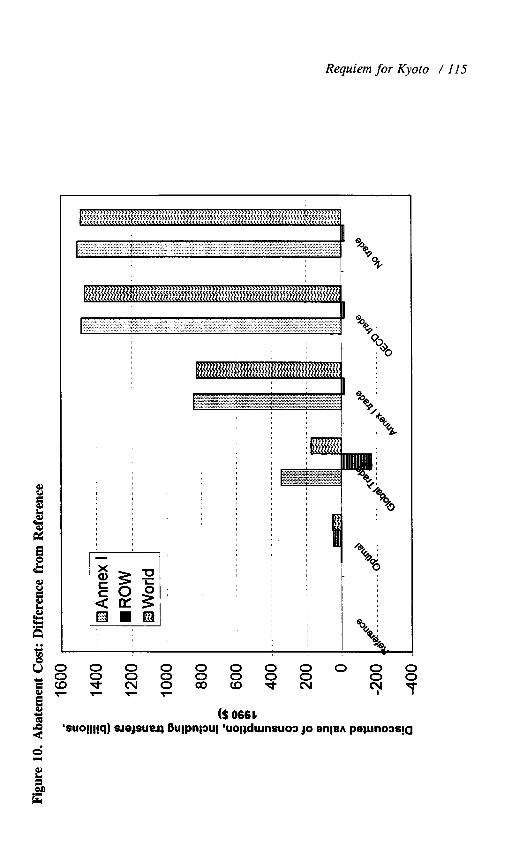
Requiem for Kyoto / 115

‘suo!l(!q) ~J~JSUEJJ Bu!pnpu! ‘uo!8dumsuo:, JO enleA peaunoss!a

116 / The Energy Journal

(a3uaJa~a~ 01 aygelaJ apeJt I xauuy) da9 u! aSueq3

Requiem for Kyoto / 117

Table 6A. Economic Impact of Different Policies: Excluding Climate Damages (difference from no-control base; billions of 1990 US$)

With transfers Annex I ROW World Total

Reference 0 0 0

Optimal -3 -46 -49

Global Trade -344 171 -173

Annex I trade -846 18 -828

OECD trade -1483 19 -1463

No trade -1507 20 -1488

Limit to Kyoto Concentrations 49 -122 -171

Limit to Kyoto Temperature -14 -95 -109

Note: Cost is equal to the discounted value of consumption for 30 decades, discounted at the

consumption discount rate. Transfers are calculated as the present value of the permit purchases

(sales being negative) valued at the U.S. discount rate. Runs exclude climate damage.

Table 6B. Economic Impact of Different Policies: Including Climate Damages (difference from no-control base; billions of 1990 US$)

With transfers Annex I ROW World Total

Reference 0 0 0

Optimal 23 -13 10

Global Trade -291 232 -59

Annex I trade -790 74 -716

OECD trade -1406 77 -1329

No trade -1454 77 -1377

Limit to Kyoto Concentrations 2 -60 -58

Limit to Kyoto Temperature 9 -24 -15

Note: Cost is equal to the discounted value of consumption for 30 decades, discounted at the

consumption discount rate. Transfers are calculated as the present value of the permit purchases

(sales being negative) valued at the U.S. discount rate. Runs include climate damage.

3. Costs by Region

It is important to understand the distribution of costs by region. The following table shows the impact on discounted consumption (including net sales of permits):

118 / The Energy Journal

Total Increase in Production Costs for Annex I Case

(billions of dollars, present value to 1990 in 1990 U.S. prices, difference from no controls, excluding damages but inclusive of permit purchases)

Japan 166 USA 517 Europe 325 Rest of World -180

World 828

This table gives some idea of why the U.S. might be unhappy about the Kyoto Protocol: it bears two-thirds of the burden.

4. Trading and Transfers

Figure 12 shows the impact of the Kyoto Protocol-assuming Annex I trading-on incomes of different countries. In these figures, “gross domestic income” equals gross domestic product plus the net revenues from sale of emissions permits. Both the United States and Europe are losers, although the time paths are different. Russia is a winner.

Figure 13 and Table 7 show the permit trading in the Annex I-trade version of the Kyoto Protocol. The Annex I case shows the near-term advantage gained by Russia and Eastern Europe and the major losses suffered by the U.S. The U.S. increases its permit purchase from about $40 billion annually in 2050 to $73 billion at the end of the next century. Sales of permits would probably be Russia’s major export.

The results on flows of permit revenues reveal two major flaws in the design of the Kyoto Protocol. First, the Protocol caps the emissions of one group of countries at historical levels but does not do so for the non-Annex I countries. Bringing non-Annex I countries in under the additionality criterion assigns reference emissions to non-Annex I countries, thus giving them substantially different treatment from Annex I countries. A second and related major design flaw is assigning historical emissions. This gives a major windfall to those countries which had inefficient energy systems (particularly Russia, Eastern Europe, and Germany after its purchase of East Germany). A better procedure would be a rolling emissions base, which would remove the advantages of inefficiency and also remove the difference of treatment of non- Annex I and Annex I countries.

Requiem for Kyoto / 119

The Energy Journal

-i- s

-

(~eeA ml $066~ JO suo!ll!q) sqes ~yumd 40 enleA

Requiem for Kyoto / 121

Table 7. Permit Purchases with Annex I Trade: Billions of 1990 US$ per year, sales are (+) and purchases are (-)

2010 2050 2100

JAPAN -4 -18 36

USA -10 -40 -73

EUROPE -7 -29 -61

OH1 -3 -15 -25

HI0 0 0 0

MI 0 0 0

RUSSIA 13 70 100

EE 10 33 23

LI 0 0 0

CHINA 0 0 0 INDIA 0 0 0

AFRICA 0 0 0

Note: Transfers are the sales (+) or purchases (-) of carbon emissions permits under the Kyoto Protocol with trading only among Annex I countries.

5. Summary of Economic Impacts

The overall impacts of the Kyoto Protocol and variants are complex, but the major points to emphasize are the following:

. There are big impacts of virtually all variants of the Kyoto Protocol on Annex I countries. The discounted value of production costs (exclusive of transfers and climate damages) for Annex I countries range from a low of $50 billion in the global-trading case to a high of $1,507 billion in the no-trading case.

. However, these number are impacts on output. Even though the global cost in the global trading case is significantly reduced by emissions trading, the impacts on national income continue to be extremely large in all cases. If transfers are included, the overall cost to Annex I nations of the Kyoto Protocol ranges from $344 to $1,507 billion.

. Non-Annex I countries, Russia, and Eastern Europe are the major beneficiaries of the Kyoto Protocol, even if damages are excluded. The benefits for non-Annex I countries are around $20 billion in lower production costs, exclusive of lower damages.

. Trading significantly reduces the aggregate cost of abatement- particularly trading with Russia and low-income countries like China. But the cost of these efficiency gains are large transfers-particularly from the United States.

122 / The Energy Journal

C. Costs and Damages

The comparisons up to now exclude the damages from global warming. It is always important to keep in mind that the point of reducing emissions is to reduce future damages. The impact of different policies on both costs and damages is shown in Figure 14. The first set of bars shows the discounted value of damages. Our estimates indicate that there are likely to be substantial costs of global warming in any of the cases examined here; the costs total approximately $1.8 trillion in present value in the reference case.9

As shown in Figure 14, the different policies reduce damages by only a modest amount. Indeed, one of the surprises is how little the policies affect the damages from global warming. The reasons are that, because there is so much inertia in the climate system and because the Protocol does not limit the emissions of developing countries, the Kyoto Protocol reduces the global temperature increase by only a fraction of a degree over the next century. The other point that is shown in Figure 14 is that inefficient policies, such as OECD trading or no trading, raise the costs of abatement substantially with little or no improvement in benefits. For example, moving from no controls to the Kyoto Protocol plan with Annex I trading incurs discounted abatement cost of $0.83 trillion; however, the discounted value of damages decreases only from $1.83 to 1.72 trillion. The benefit cost ratio of moving to the optimal plan is 1.2. By contrast, the benefit-cost ratios are 0.14 for Annex I trading and 0.07 for no trading. All these ratios make the optimistic assumption that the policies are efficiently implemented in each region.

Finally, Figure 15 shows the distribution of net impacts (including transfers and climate damages) of the two major policies considered here.

The main conclusions that come from an examination of damages are that there are likely to be substantial damages from climate change, but that the Kyoto Protocol captures essentially the same damage reduction as the optimal program at a substantial increase in costs.

D. The Gains from Trade

Much has been made about the gains from trade. Table 8 shows the improvements in cost-effectiveness under different trading options. In this comparison, we have taken the temperature path associated with meeting the Kyoto Protocol (policy 4b) as the standard of a cost-effective policy; the “no- trading” plan has zero cost-effectiveness. We then calculate the costs of attaining the Kyoto temperature trajectory under different trading plans.

9. The damage function in the version of the RICE-98 model used for this analysis is undergoing

revision and will change in the final version.

Requiem for Kyoto 1123

124 / The Energy Journal

a w s

377 066L 40 =Jo!ll!q ‘Ad) kwd UKq su!e3

Requiem for Kyoto / 125

Table 8. Cost-effectiveness of Different Policies

Policy Cost-effectiveness (percent)

Temperature target 100.0

Concentrations target 95.5

Global trade 95.4

Annex I trade 47.8

OECD trade 1.8

No trade 0.0

Note: “Cost-effectiveness” is defined as the fraction of the total gains from trading, different timing,

or different targets that is achieved by a given policy. The standard is relative to the “temperature target,” which is the trajectory of global mean temperature after 2100 that is implicit in the Kyoto

Protocol.

One major surprise is that trading within the OECD only attains relatively little-2 percent-of the potential gains from trade. This low fraction comes because the energy efficiencies are relatively similar within the large OECD blocs. The other surprise is how much of the gains are obtained by global trading-95 percent. Moreover, targeting concentrations rather than temperature gets about 96 percent of the way to a cost-effective strategy.

IV. FINDINGS AND CONCLUSIONS

The present paper examines the implications of the Kyoto Protocol and variants of that policy in a new integrated-assessment model of climate change and the world economy. Before moving to the major conclusions, it must be emphasized that these results should be taken with suitable reservations reflecting the difficulties inherent in the subject and the fact that this is but one of many models that can be used to estimate the impacts of the Kyoto Protocol.

First, it appears that the strategy behind the Kyoto Protocol has no grounding in economics or environmental policy. The approach of freezing emissions at a given level for a group of countries is not related to a particular goal for concentrations, temperature, or damages. Nor does it bear any relation to an economically oriented strategy that would balance the costs and benefits of greenhouse-gas reductions. The best way of comparing runs is probably the stringency of policy as indicated by the carbon prices. The emissions and concentrations implicit in the Kyoto Protocol are close to those in the optimal policy over the next century. However, because the emissions reductions are targeted to Annex I countries, the costs of achieving these emission reductions are 8 to 14 times more costly (these being the full Annex I-trading and the no- trading variants).

126 / The Energy Journal

Second, while the environmental damages from climate change do not differ markedly among the different Kyoto Protocol variants, the costs of implementation vary enormously. The cost of the no-trade variant of the Kyoto Protocol is about 9 times the cost of the global-trade variant. Most of the gains from trade come from including non-OECD countries such as Russia, China, and India. The costs of an efficiently designed Kyoto Protocol range between $0.8 to $1.5 trillion in discounted costs, while the benefits of the emissions reduction from the Kyoto Protocol are around $0.12 trillion. This emphasizes the point that efficient design of the policy should be the major concern of policymakers.

Third, carbon prices in the realistic versions of the Kyoto Protocol are projected to be extremely high and to grow rapidly in the coming decades. The model suggests that prices exceeding $250 per ton of carbon in the controlled regions are likely to occur if the Protocol is effectively enforced through the middle of next century. The implications of such high prices for fiscal, macroeconomic, and trade policy are daunting.

Fourth, the Kyoto Protocol has significant distributional consequences, Annex I countries pay the costs of Protocol. These costs will come either through abatement activities or through purchase of permits. The lion’s share of these costs are borne by the United States- the U.S. pays almost two-thirds of the global cost in the central Annex I case.

APPENDIX

A. Equations of RICE-98

Market equilibrium

(1) max c #JJ WJ c,O) J

Utility function for region J

(2) wJ = c UJ[cJ(t),L,(t)l(l+pJ(t))-' = c L,(t)(log[cJ(t)l)(l +pJ(t))-'

t t

*Production function for region J (3) Q’(t) = Sa,(t)A,(t)K,(t)Y L,(t)‘7-8J(‘)EC,(t)J(t)

*Output plus income from permit sales equals investment and consumption plus energy costs: (4) Q'(t) + 7'(f)tEC'(f) -n,(t)] = c,(t) + I'(t) + pEJ(t> EC,(t) + p"(t>B,(t)

Per capita consumption (3 c,(t) = CJ(tYL,(t)

Requiem for Kyoto / 127

Capital accumulation

(6) K,(t) = (l-&)K,(t-1) + IJ(t-1)

*Retail price of carbon-energy (7) pEJ(t)= q(t) + markupE,(t) + T,(t)

*Cumulative world extraction of carbon-energy (8) CumC(t) =CumC(t-1) + EC(t)

*Energy supply (94 q(t) = [, + t2[CumC(t)/CumC*lE3 (9b) E,(t) = EC,(t) + B,(t)

*Carbon cycle WW MwW = Wt-1) + Cl- w,p,Lo) M&l) + 01Lo.w Mm@-1)

(lob) ML&) = aup,Lo M&l) + (1- (~t,o,up) M&t-l) WC) W-r(t) = aAT Mu&)

Radiative forcings (11) F(t) = rl{log[MAr(t>~MAT(o)l/logo) + o(t)

Climate equations Wa) TUP(t) = TUP(f-1) +a,{F(t) - XT,,(t-1) - 41Up(t-1) -T,,(t-l)]} (12b) J-Lo(t) = TLo(f - 1) + uJTup(t- 1) -TLoO- 1 )I

*Damage equation (13) DJ(t>/QJ(t) = 81.1 We2 + 03. J T(t)‘4

Damage parameter (14) n,(t) = 1 -DJ(t>/QJ(t)

Note: Equations with asterisks (*) are for equations that are substantially revised since the original DICE and RICE models.

B. Variable Definitions in RICE-98

A,(t) = total factor productivity of region J

B,(t) = backstop energy supplied in region J

cJtt) = per capita consumption of region J

CumC(t) = cumulative world extraction of carbon energy CumC* = total recoverable world resources of carbon-energy

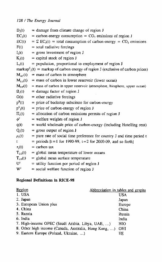
128 / The Energy Journal

D’(t) = damage from climate change of region J

EC,(t) = carbon-energy consumption = CO, emissions of region J

EC(t) = C EC,(t) = total consumption of carbon-energy = CO, emissions

F(t) = total radiative forcings

IJtt) = gross investment of region J

K,(t) = capital stock of region J

LJ(t) = population, proportional to employment of region J markupEJ(t) = markup of carbon energy of region J (exclusive of carbon prices) MAT(t) = mass of carbon in atmosphere MLO(t) = mass of carbon in lower reservoir (lower ocean) MuP(t) = mass of carbon in upper reservoir (atmosphere, biosphere, upper ocean)

nJ(t) = damage factor of region J

00) = other radiative forcings

pB(t> = price of backstop substitute for carbon-energy

pEJ(t) = price of carbon-energy of region J

nJ(t> = allocation of carbon emissions permits of region J

4’ = welfare weights of region J

s(t) = world wholesale price of carbon-energy (including Hotelling rent)

Q’(t) = gross output of region J

pJtt) = pure rate of social time preference for country J and time period t t = periods [t = 1 for 1990-99, t =2 for 2000-09, and so forth]

rJ(t) = carbon tax

TLoW = global mean temperature of lower oceans

TwO) = global mean surface temperature UJ = utility function per period of region J WJ = social welfare function of region J

Regional Definitions in RICE-98

Region Abbreviation in tables and graphs 1. USA USA 2. Japan Japan 3. European Union plus Europe 4. China China 5. Russia Russia 6. India India 7. High-income OPEC (Saudi Arabia, Libya, UAE, . ..) HI0 8. Other high income (Canada, Australia, Hong Kong, . . .) OH1 9. Eastern Europe (Poland, Ukraine, . . .) EE

Requiem for Kyoto / 129

10. Middle income (Brazil, Korea, Taiwan, . . .) MI 11. Lower middle income (Mexico, Turkey, Iran, . ..) LMI 12. Low income (Indonesia, Pakistan, . ..) LI 13. Sub-Saharan Africa (Nigeria, Zaire, . . .) Africa

REFERENCES

Eizenstat, Stuart (1998). Sfuremenf, testimony before Subcommittee on Energy and Power, House

Commerce Committee, March 4.

IPCC (1996a). Intergovernmental Panel on Climate Change, Clirnafe Change 199.5: The Science of Climare Change. The Conrribution of Working Group I to (he Second Assessmetrr Report oj’the Intergovernmentul Paj~el on Climate Change, J.P. Houghton, L.G. Meira Filho, B.A. Callendar,

A. Kattenberg, and K. MaskelI, eds., Cambridge, UK: Cambridge University Press.

IPCC (1996b). Intergovernmental Panel on Climate Change, Climate Chunge 1995: Itnpocrs,

Adoptdon. and Mitigation of Climate Change: Scientific-Technical Analysis. The Conmribu~ion of Working Group II to the Second Assesstnenr Report of the Intergovernmental Panel on Climate Change, R.T. Watson, M.C. Zinyowera, R.H. Moss, eds.. Cambridge. UK: Cambridge University Press.

IPCC (1996~). Intergovernmental Panel on Climate Change Climate Change 1995: Economic and Cross-Cuning Issues. The Conmribution of Working Group III to the Second Assessmenr Repot? of rhe Inrergovernmentul Panel on Climate Chunge, J.P. Bruce, H. Lee, and E.F. Haites, eds..

Cambridge, UK: Cambridge University Press. Koopmans. Tjalling (1967). “Objectives, Constraints, and Outcomes in Optimal Growth Models,

Economerrica 35: l-15.

Nakicenovic, Nebojsa, W.D. Nordhaus, R. Richels, and F.L. Toth, eds. (1994). Inregrufive Assessmenr of Mitigation, Impacts, und Adaptation to Clitnate Change, IIASA, CP-94-9, May

1994.

Nakicenovic, Nebojsa, W. Nordhaus, R. Richels, and F. Toth, eds. (1996). Clitnare Chunge: Integrating Science, Economics, and Policy, , IIASA, CP-96-1, 1996.

National Academy of Sciences (1983). Changing Climate, Washington, D. C.: National Academy

Press. Nordhaus, William D. (1979). The Eficienr Use of Energy Resources. New Haven, Conn: Yale

University Press. (1991). “To Slow or Not to Slow: The Economics of the Greenhouse Effect.” The

Economic Journal (July) 101: 920-937. (1992). “in Optimal Transition Path for Controlling Greenhouse Gases.” Science

(November 20): 258: 1315-1319. (1993). “Rolling the ‘DICE’: An Optimal Transition Path for Controlling Greenhouse

Gases.” Resource and Energy Economics 15: 21-50.

(1994). Managing the Global Cotnmons: The Econotnics of Clitnale Change. Cambridge, MA: MIT Press. IIASA, CP-96-1, 1996, pp. 3-45.

(I998a). “Is the Kyoto Protocol a Dead Duck? Are There Any Live Ducks Around’? Comparison of Alternative Global Tradable Emissions Regimes,” paper prepared for the

Yale/NBER Workshop on Alternative Approaches to Global Environmental Change, August, 13- 14, 1998

(I998b). Roll the DICE Again: The Economics of Global Wartning. Mimeo, Yale

University Department of Economics: Dee 15, 1998. and Zili Yang (1996). “A Regional Dynamic General-Equilibrium Model of

Alternative Climate-Change Strategies.” American Econotnic Review 86(4) (September): 741-765.

130 / The Energy Journal

Ramsey, Frank P. (1928). “A Mathematical Theory of Saving.” The Economic Jourtrd (December):

543-559.

Wigley, T.M.L. (1998). “The Kyoto Protocol: CO!, CH,, and climate implications.” Geuph,ysicul Research Letters. 1998, in press.

Yellen, Janet (1998). Testimony before Subcommittee on Energy and Power, House Commerce

Committee, March 4.

Kyoto, Efficiency, and Cost-Effectiveness: Applications of FUiVD

Richard S. J. Tel*

In this paper various emission reduction scenarios are evaluated with FUND-the Climate Framework for Uncertainty, Negotiation, and Distribution model. The aim is to help international negotiators improve upon the Kyoto Protocol. International cooperation in greenhouse gas emission reduction C;s important, and the more of it the better. The emission reduction targets as agreed in the Kyoto Protocol are irreconcilable with economic rational@. If the targets nevertheless need to be met, it is better to start emission reduction sooner than later in order to minimise costs. Methane emission reduction may be an important instrument to reduce costs.

INTRODUCTION

The Kyoto Protocol signifies the first serious attempt of th.e international community to take concrete action on greenhouse gas emission reduction. Time will tell whether the attempt will be a successful one. Th:is paper looks at some of the economic implications of the agreement, and sheds some light on the issues unresolved in the Kyoto Protocol. It thus hopes to inform the negotiations on extending and refining the Kyoto Protocol. The first opportunity for this was in Buenos Aires, at the end of 1998, but little progress was made there.

The analyses in this paper are based on the Climate Framework for Uncertainty, Negotiation, and Distribution (FUND), an integrated assessment model of climate change (Tol, 1997, 1998). Section 2 presents the model. Weyant et al. (1996) classify FUND as a policy-optimization model, that is, a model which selects the best policy strategy given certain constraints. In this paper, however, the constraints (inspired by the Kyoto Protocol) are so strict that there is often little room for (assumed) preferences to play a substantial

The Energy Journal, Kyoto Special Issue. Copyright o 1999 by the IAEE. All rights reserved.

* Institute for Environmental Studies, Vrije Universiteit Amsterdam, De Boelelaan 1115, 1081

HV Amsterdam, The Netherlands. E-mail: richard.tolQivml.vu.nl; and Center for Integrated

Study of the Human Dimensions of Global Change, Carnegie Mellon University, Pittsburg’h,

PA. USA.

131

132 / 7’he Energy Journal

role. Compared to other policy-optimisation integrated assessment models of climate change (CETA, Peck and Teisberg, 1991, 1996; MERGE, Mamre et al., 1995, Manne and Richels, 1998; MiniCAM, Edmonds et al., 1994, Edmonds and Wise, 1998; RICE, Nordhaus and Yang, 1996), the representation of the economy and the energy sector in FUND is simple. International trade (EA~PA, Jacoby and Yang, 1994, Jacoby et al., 1997) and the monetary sector (G- CUBED, McKibbin and Wilcoxen, 1992) are not included. FUND’s impact module, however, is more elaborate than other models’ (To1 and Fankhauser, 1998), but this part of the model is hardly used here.

Section 3 looks at the importance of international cooperation in greenhouse gas emission reduction. It shows that the option to reduce greenhouse gas emissions elsewhere than domestically greatly lowers the costs of meeting strict emission targets. This conclusion is well-known, in potential, from first principles in economics (Barrett, 1994; Carraro and Siniscalco, 1992; Hoel, 1994) and, in magnitude, from other numerical studies (Manne and Richels, 1998; Peck and Teisberg, 1996; Tol, 1998a).

The agreements in the Kyoto Protocol are the outcome of a political negotiation process. Section 4 compares the Kyoto targets to the results of more objective analyses. It turns out that the Kyoto Protocol (if implemented) does not minimise economic costs (presuming an ultimate objective of 550 ppm) nor maximise welfare. Again, this only reconfirms well-known conclusions in the literature (Kolstad, 1994; Maddison, 1995; Manne et al., 1995; Nordhaus, 1991, 1993; Nordhaus and Yang, 1996; Peck and Teisberg, 1994, 1996; Richels and Edmonds, 1995; Schneider and Goulder, 1997a,b; Tol, 1997, 1998b; Wigley et al., 1996).

Section 5 shows that the costs of delaying the implementation of the Kyoto Protocol can be substantial, even though FUND ignores many of the short-term rigidities in the economy that can only increase costs further. This reinforces an earlier conclusion (Tol, 1997) that, once a target has been ag:reed on, it is always better to start working towards it sooner than later.

Based on a very preliminary analysis, Section 6 shows that reducing methane emissions instead of carbon dioxide emissions could substantially lower costs. This is already hinted at by Hogan (1993) and Van Ham et al. (1994), but this paper is the first to demonstrate this in a full-blown cost-effectiveness analysis. Section 7 concludes the paper.

2. THE MODEL

The model used is version 1.6 of the Climate Framework for Uncertainty, Negotiation and Distribution (FUND). ’ Version 1.6 differs :in a

1. The source code of the model is available upon request. The model is implemented in

TurboPascal 7.0 and operates under DOS and Windows.

Kyoto, Eflciency, and Cost-Effectiveness / 133

number of ways from version 1.5, which is described in To1 (1997). The main differences between this and the previous versions are (i) the representations of atmosphere and climate, (ii) the costs of emission reduction, particularly in non- OECD regions, and (iii) the decision-making structure.

Essentially, FUND consists of a set of exogenous scenarios and endogenous perturbations. The model is specified for nine major world-regions: OECD-America (excl. Mexico); OECD-Europe; OECD-Pacific (excl. South Korea); Central and Eastern Europe and the former Soviet Union; Middle East; Latin America; South and Southeast Asia; Centrally Planned Asia; and Africa. The model runs from 1950 to 2200, in time steps of a year. Some overlap witlh

the observational record provides an opportunity for model validation. The prime reason for starting in 1950, however, is the necessity to initialise the climate change impact module. In FUND, climate impacts are assumed to depend on the impact of the year before, to reflect the process of adjustment to climate change. Thus, climate impacts (both physical and monetized) ar,e misrepresented in the first decades. This would bias optimal control if the first decades of the simulation coincided with the first decades of emission abatement. Similarly, the period 2100-2200 is there to provide the forward-looking agents in the 21”’ century with a proper time horizon. The calculated emission reductions in 2100-2200 have little meaning in and of themselves.

The IMAGE database (Batjes and Goldewijk, 1994) is the basis for the calibration of the model to the period 1950- 1990. Scenarios for the period 20 lo- 2100 are based on the EMF14 Standardised Scenario. Note that the original EMF14 Standardised Scenario had to be adjusted to fit FUND’s nine regions and yearly time-step. The period 1990-2010 is a linear interpolation between observations and the EMF14 Standardised Scenario. The period 2100-2200 is an extrapolation of the EMF14 Standardised Scenario.

The scenarios concern the rate of population growth, urbanisation, economic growth, autonomous energy efficiency improvements, the rate of decarbonization of the energy use (autonomous carbon efficiency improvements), and emissions of carbon dioxide from land use change, methane and nitrou:s oxide.

The scenarios of economic and population growth are perturbed by the impact of climate change. Population falls with climate change deaths, resulting from changes in heat stress, cold stress, malaria, and tropical cyclones. Heat and cold stress are assumed to affect only the elderly, non-reproductive population. The other sources of mortality do affect the number of births. Heat stress only affects urban population. The share of urban in total population is, up to 2025, based on the World Resources Databases; after 2025, urban population slowly converges to 95% of total population (comparable to present day Belgium or Kuwait). Population also changes with climate-induced migration between the

134 / lXe Energy Journal

regions. Immigrants are assumed to assimilate immediately and completely with the host population.

The tangible impacts of climate change are dead-weight losses to the economy. Consumption and investment are reduced, without changing the savings rate. Climate change thus reduces long-term economic growth, although at the short term consumption takes a deeper cut. Economic growth is also reduced by carbon dioxide emission abatement.

The energy intensity of the economy and the carbon intensity of the energy supply autonomously decrease over time. This process can be sped up by abatement policies.

The endogenous parts of FUND consist of the atmospheric concentrations of carbon dioxide, methane and nitrous oxide, the global lmean temperature, the impact of carbon dioxide emission reductions on economy and emissions, and the impact of the damages of climate change on the economy and the population.

Methane and nitrous oxide are taken up in the atmosphere, and then geometrically depleted:

C, = C,-, + aEt - PC Cl-, - C,,J

where C denotes concentration, E emissions, I year, and pre pre-industrial. Table 1 displays the parameters for both gases.

Table 1. Parameters of Equation (1)

Gas a” Bh pre-industrial

concentration

methane (CH,) 0.3597 118.6 790 ppb

nitrous oxide (NZO) 0.2079 11120 285 nob

“The parameter 01 translates emissions (in million metric tonnes of CH, or N1O) into

concentrations (in parts per billion by volume).

hThe parameter /3 determines how fast concentrations return to their pre-industrial (and assumedly

equilibrium) concentrations; 118 is the atmospheric life time (in years) of the gases.

Source: After Schimel et al. (1996).

The atmospheric concentration of carbon dioxide follows from a five- box model:’

2. Note that the boxes do not represent identifiable subsystems of the carbon cycle; instea.d, the

boxes are mathematical abstractions, as the model is a reduced-form version of a more complex

carbon cycle model.

Kyoto, Eficiency, and Cost-Effectiveness / 135

Box,,, = piBoxi , + 0.000471 a;E, GO

with

c, = k lYiBOXj I i-l

where c+ denotes the fraction of emissions E (in million metric tonnes of carbon) that is allocated to box i (0.13, 0.20, 0.32, 0.25 and 0.10, respectively) and 13; the decay-rate of the boxes (pi = exp[-l/lifetime]), with lifetimes infinity, 363, 74, 17 and 2 years, respectively). Thus, 13 % of total emissions remains forever in the atmosphere, while 10% is-on average-removed in two years (after Hammitt et al., 1992). Carbon dioxide concentrations are measured in parts per million by volume.

Radiative forcing for carbon dioxide, methane and nitrous oxide are based on Shine et al. (1990). The global mean temperature T is governed by a geometric build-up to its equilibrium (determined by radiative forcing RF), with a half-time of 50 years. In the base case, global mean temperature rises in equilibrium by 2.5”C for a doubling of carbon dioxide equivalents, so:

T,-, + -!- - 2*5 RF, 50 6.3ln(2)

(3)

Global mean sea level is also geometric, with its equilibrium level determined by the temperature and a lifetime of 50 years. Temperature and se:a level are calibrated to the best guess temperature and sea level for the IS92.a scenario of Kattenberg et al. (1996). The climate impact module is based on To1 (1996). A limited number of categories of the impact of climate change is con- sidered: agriculture, sea level rise, heat and cold stress, malaria, tropical and extratropical storm, river floods, and unmanaged ecosystems. The damage module has two units of measurement: people and money.

People can die (heat stress, malaria, tropical cyclones), not die (cold stress), or migrate. These effects, like all impacts, are monetized. The value of a statistical life is set at $250,000 plus 175 times the per capita income. The value of emigration is set at 3 times the per capita income, the value of immigration at 40% of the per capita income in the host region.

Other impact categories are directly expressed in money, without an intermediate layer of impacts measured in their ‘natural’ units.

Damage can be due to either the rate of change (benchmarked at 0.04”Uyr) or the level of change (benchmarked at 2.5”C). Benchmark estimates are displayed in Table 2. Damage in the rate of temperature change slowly fades

136 / The Energy Journal

at a speed indicated in Table 3. Damage is calculated through a second-order polynomial in climatic change. Thus, damage D, in year t is either

D,=a,W,+&W:

or

D, = ci,AW, + /3,AW,’ + pDt-,

with W the appropriate climate variable (temperature, sea level, hurricane activity, etc.) and CY, @ and p parameters.

Table 2. Monetized Estimates of the Impact of Global Warming (in billion US$ per year)

Region species life agric. Sea extreme

levels (temperature: +2.X; sea level: +50cm; hurricane activity: +25%;

winter precipitation: + 10%; extratropical storm intensity: + 10%)

total

OECD-A 0.0 -1.0 -5.3 0.9 2.5 -2.9

OECD-E 0.0 -1.1 -6.0 0.3 0.3 -6.5

OECD-P 0.0 -0.5 -6.1 1.5 5.5 0.3

CEE&fSU 0.0 3.7 -23.2 0.1 0.2 -19.1

ME 0.0 3.5 3.1 0.1 0.0 6.6

LA 0.0 67.0 7.3 0.2 0.0 74.5

S&SEA 0.0 81.4 15.8 0.2 0.6 98.8

CPA 0.0 58.4 -22.2 0.0 0.1 36.3

AFR 0.0 22.5 5.4 0.1 0.0 28.0

rate (temperature: O.OC’C/year; other variables follow)

OECD-A 0.3 0.2 0.3 0.2 0.2 1.2 OECD-E 0.3 0.2 0.0 0.2 0.0 0.7

OECD-P 0.2 0.1 0.0 0.3 0.4 1.0

CEE&fSU 0.1 0.1 0.0 0.0 0.0 0.2

ME 0.0 0.0 0.1 0.0 0.0 0.2

LA 0.0 0.4 0.1 0.0 0.0 0.6

S&SEA 0.0 0.3 0.1 0.0 0.0 0.6

CPA 0.0 0.2 0.3 0.0 0.0 0.5

AFR 0.0 0.0 0.1 0.0 0.0 0.2

Source: Tol (1996)

Kyoto, EfJiciency, and Cost-Effectiveness / 1317

Table 3. Duration of Damage Memory per Category”

category years category years

species loss

agriculture

coastal protection

life loss

tropical cyclones

100 immigration 5

IO emigration 5

50 wetland (tangible) 10

I5 wetland (intangible) 50

5 dryland 50

“Damage is assumed to decline geometrically at a rate of l-l/lifetime.

Source: Tol (1996)

Damage is distinguished between tangible (market) and intangible (non- market) effects. Tangible damages affect investment and consumption; through investment, economic growth is affected; through consumption, welfare is affected. Intangible damages affect welfare.

Relative vulnerability to climate change-a and /3 in (4)-is a function of economic development in many ways. The importance of agriculture falls with economic growth. The share of agriculture in total output changes with per capita income with an elasticity of -0.3 1, which corresponds to the per capita income elasticity across FUND’s nine regions in 1990. Malaria incidence and the inclination to migrate fall logistically with increases in per capita income. Heat stress increases linearly with urbanisation. The valuation of intangible impacts increases logistically with per capita income.

Emission abatement is restricted to industrial sources of carbon dioxide. The costs of carbon dioxide emission reduction are calibrated to the survey results of Hourcade et al. (1996) supplemented with results of Rose and Stevens (1993) for developing countries. Regional and global average cost estimates, and their standard deviations result. Regional relative costs are shrunk to the global average, that is, the weighted average of the regional and global average is taken, with the inverse variances as weights. This reduces the influence of a single study. It particularly influences the developing regions, for which much less information on emission abatement costs is available. Costs are represented by a quadratic function. Table 4 presents the parameters. Roughly, a 1% cut in emissions costs 0.02% of GDP; a 10% cut costs 2%.

In FUND, each region has its own decision maker. FUND1.6 also distinguishes generations of decision makers (rather than a single one as in previous versions and other models). Each decision maker has control over a ten-year period only, but does optimise the net present welfare of her region (in the non-co-operative cases) from the start of the control period up to 2200. In the case of global co-operation, the unweighted sum of the net present regional welfares is maximised. Each decision maker knows the emission reduction efforts of all decision makers in all regions at all times. The equilibrium is found

138 / The Energy Journal

iteratively; without co-operation between regions, convergence is rapid (i.e., 4 or 5 iterations); with global co-operation, convergence is much slower (i.e., over 10 iterations). The distinction between generations of decision make:rs has two implications. Firstly, in a cost-benefit analysis, a decision-maker not only has to match her decisions with those of other regions, but also with the decisions of other generations. Secondly, the definition of intertemporal cost- effectiveness vanishes, as there is no decision-maker controlling the entire time- period. Explicitly distinguishing generations of decision makers recognises the sovereignty of each generation. In a cost-benefit analysis, this implies that emission reductions are individually rational at all times. Collective decision- making over generations and targeted capital transfers between generations are impossible in the model as in reality. Cost-effectiveness also implicitly assumes that targeted intergenerational capital transfers are possible (such transfers are needed to make an actual Pareto improvement of a potential one). In addition, cost-effectiveness analysis usually places undue weight on the preferences in the first periods (unless the pure rate of time preference is zero).

Table 4. Parameters of the CO, Emission Reduction Cost Function”

OECD-A 2.0789 CEE&fSU 2.0488 S&SEA 2.1268

OECD-E 2.3153 ME 2.1041 CPA I .9544

OECD-P 2.2171 LA 2.1253 AFR 2.0931

The proportional loss of GDP C in year r of proportional emission reduction R in year r follows:

C, = 0rR:. The costs to GDP are modelled as a dead-weight loss to the economy.

Emission reduction is brought about by a permanent shift in energy- and carbon-intensity.

Source: After Hourcade et al. (1996) and Rose and Stevens (1993).

3. THE GAINS FROM SPATIAL FLEXIBILITY

Annex I countries agreed to greenhouse gas emission reduction in the Kyoto protocol. For the regions of FUND, the agreed reductions are -7X for OECD-A, -8% for OECD-E, -6% for OECD-P, and 0% for CEE&fSlJ, all relative to the 1990 emissions (as modelled). These targets are to be met in the year 2010, and maintained thereafter. The other regions are restricted to their business-as-usual emissions. Note that, at the short term, there is little to no leakage in FUND.3 These emission reductions can be achieved at various levels of international cooperation. At the one extreme, all regions should meet their regional target. At the other extreme, the emissions target is a global one, and

3. Recall that the only link between the regions is climate.

Kyoto, Efficiency, and Cost-Effectiveness / 139

emissions are reduced there where it is cheapest to do SO.~ Figure 1 displays the costs of these extremes, and those of three intermediate cases. Costs are defined as the loss of consumption in the period 1990-2100, discounted to 1990 at a 5% discount rate.’ The intermediate cases are as follows: (1) the Annex I regions, except OECD-Europe, cooperate; (2) the Annex I regions cooperate; and (3) the Annex I and Asian regions cooperate. Figure 1 makes clear that the greater the coalition, the lower the costs.

Figure 2 looks differently at the gains of international cooperation. At the two extremes are no cooperation, and full Annex I cooperation. The intermediate cases place restrictions on the amount of emission reductions that can be achieved outside the own region.6 In the first case, regions may emit at most 110% of their allotment, provided that the target for Annex I as a whole is met. This restricts the amount of emissions reduction ‘bought’ from abroad. In the second case, regions must emit more than 90% of their allotment. This restricts the amount ‘sold.’ In the third case, both restrictions apply. The case with both restrictions is (slightly) cheaper than the case in which only purchases are limited. This can happen because the optimal allocation of emission reduction effort between Annex I regions is determined per decade, and not over the whole period. The reason is that in the first 20 years, the sales of emission reductions by Central and Eastern Europe and the former Soviet Union are restricted by the limits on purchases, and after that by the limits on sales. The former are stricter than the latter. In the case that both restrictions apply there is thus more hot air available in the long run, reducing the emission reduction costs to the OECD. This story is probably specific to FUND.

Figure 3 conducts a sensitivity analysis on the amount of ‘hot air. ’ The scenarios assume full cooperation between AMeX I regions. The amount of hot air in Central and Eastern Europe and the former Soviet Union is varied between 30 and 430 million metric tonnes of carbon.’ The central case of 230 MMTC is used for all other analyses. The net present consumption loss of meeting Kyoto forever to the OECD varies between $1.8 and 2.4 trillion, with a central estimate of $2.0 trillion. 200 MMTC extra hot air decreases costs b} 10%. 200 MMTC less hot air increases costs by 25 % . The path-dependencies in FUND mean that less abatement in the near future (because of more hot air)

4. Note that FUND does not have trade in emission permits. Instead, regions cooperate in a

game-theore6c sense, that is, the sum of the welfares of the regions in the coalition is maximised.

5. Note that reducing emissions slows climate change, diminishing the negative impacts of

climate change on non-Annex regions. This is the explanation of the negative costs of non-Annex

regions if they are outside the coalition.

6. At the time of negotiating the Kyoto Protocol, the European Union insisted on limits to trade

in emission reduction. However, the EU Environment Commissioner, Ritt Bjerregaard, recentl)

announced that all trade is allowable on the condition that it is strictly policed (JIQ, 1998).

7. This is achieved by changing the assumed economic growth rates in the region.

140 / The Energy Journal

t

sl .I k

2 m

x c-4

2 d

r: ;

SJellOP sfl “O!ll!‘J

Kyoto, EfJicienq, and Cost-Effectiveness / 141

SJWP sn “O!ll!‘l

142 / The Energy Journal

x N n

i

SJW’P Sfl “O!ll!‘t

Kyoto, Efscienq, and Cost-Effectiveness / 143

implies more abatement (and costs) in the far future. This dampens the sensitivity of the costs to changes in the amount of hot air available. It also explains the asymmetric reaction of the costs.

4. KYOTO, COST-EFFECTIVENESS, AND EFFICIENCY

The emission reduction targets of the Kyoto Protocol resulted from a political negotiation process. Figure 4 compares these targets to the results of cost-minimising and welfare-maximising exercises. The targets of the Kyoto Protocol deviate from the economic analysis. This may be because the economic analysis is not comprehensive enough. It may also be because the negotiators of the Kyoto Protocol preferred short-term political success over a treaty that would minimise the burden of emission reduction to their economies.

In 2010, the Kyoto targets lie below cost-effective path towards 550 ppm and below the non-cooperative optimal solution, particularly if the hot air of the former Soviet Union is not accounted for. The Kyoto targets lie above the fully cooperative solution.’ Note that full cooperation can only be maintained by substantial capital transfers from the poorer to the richer regions (Tol, 1997), a less than realistic prospect. At the long-term, the relative positions of the 550 ppm trajectory and the cooperative welfare maximisation are reversed. The Kyoto forever trajectories, however, stay somewhere between the cooperative and non-cooperative optimal solutions.

Cost-effectiveness is hard to define in an intergenerational context. A standard choice is to minimise the net present value of the costs of emission reduction. As is the case for all welfare criteria which aggregate over actors, the cost-effective solution is only potentially Pareto superior. Transfers are needed to ensure actual Pareto superiority. Transfers are hard to imagine in an intergenerational context. Therefore, the ‘cost-effective’ solution in FUND minimises net present costs, subject to the constraint that the relative burden of emission reduction is smoothly spread over generations of decision makers.

Intergenerational issues are less complicated in the context of cost- benefit analysis. Here, each generation of decision makers maximise their net present welfare, knowing what all other decision makers have done, are doing or will be doing. Thus, emission reduction strategies are always compatible with the (assumed) incentives of the decision makers. In one case, each decision maker maximises the welfare of his/her regions. In a second case, decision makers in one period co-operate to maximise global welfare.

8. This is not so in the case of global trading. Recall that ‘global trading’ is in fact ‘maximise

global welfare subject to an emission constraint.’ The difference between the ‘Kyoto forever with

global trading’ scenario and the ‘global cost-benefit analysis’ is that, in the former case, the decision

makers are backward looking whereas, in the latter case, they are both forward and backward

looking.

144 / The Energy Journal

‘.:,:,:::::,:::::‘:: .:j:... .v: : i i(

;Iggg~lesPes”

.9 k

“Oqm p “““0, qIwu “of,,,U

Kyoto, E’ciency, and Cost-Effectiveness / 145

146 / The Energy Journal

Kyoto, Eflciency, and Cost-Effectiveness / 147

fi a

148 / The Energy Journal

Kyoto. Efficiency, and Cost-Effectiveness / 149

Figure 5 further illustrates the importance of economic considerations. Displayed at the extreme left are the ‘minimum’ costs of keeping concentrations below 550 ppm. To the right of this are the costs of first implementing the Kyoto Protocol (both with and without international cooperation), and then embarking on the cost-effective track. The Kyoto Protocol would cost a discounted 0.5-l .5 trillion US dollars, without gaining any additional benefit (cf. Tol, 1998). Also shown are three other scenarios in the spirit of Kyoto. In one,, denoted as ‘non-envy,’ future emission reduction efforts (measured in fraction reduction from baseline) are kept at the level of the Kyoto Protocol (with fidl international cooperation). This would keep concentrations below 565 ppm. This would cost about $2 trillion more than following the cost:effective trajectory. In another scenario, Annex I countries meet their Kyoto targets and reduce emissions by 2% a year afterwards. Other countries embark on the same trajectory once their per capita income exceeds $5,000 per year. This would keep concentrations below 547 ppm. It is a very costly strategy though. This is largely due to the fact that no cooperation is allowed. If it is, costs fall to about a discounted $4 trillion, still $1.5 trillion more expensive than the cost-effective solution.

5. TIMING

Many of the models used for analyses of the Kyoto Protocol (e.g.., CETA, EPPA, MERGE, RICE) share one deficiency: They operate in time-steps of five to ten years. These models are therefore not really suited to look at issues of when-flexibility before 2012. FUND, on the other hand, operates in time steps of one year. Note that FUND has all the characteristics of a growth model: short-term rigidities or cycles in the economy are not included.

In the analyses above, emission reduction efforts are uniformly spread over the years within one decade, as similar models with time-steps of a decade implicitly assume. Figure 6 compares this set-up to one in which the intradecadal distribution is ‘optimal’ for the USA and Canada. Optimal here means that the marginal, direct, undiscounted costs of emission reductions are equated across the years. If one is not misled by the scale, Figure 6 shows that the difference is minimal.

Figure 7 compares the costs. Here also, the difference is minimal.. Figure 7 also reports the results of another analysis. On the extreme left, the OECD has ten years to meet its Kyoto commitments (without international trade). Moving to the right, the time available for implementing the Kyoto protocol decreases from ten to two years. (The model does not solve for a one year implementation time.) The costs increase dramatically. Arguably, if short- term dynamics would have been part of the model, the increase would have been much more dramatic.

150 / The Energy JournaL

6002

8002

LOOZ

9002

9ooz t5 tit

POOZ

OD Fi fJ 0 8 dddddddd

6

su!laseq IJJOJJ uo!pnpaJ uoymj

Kyoto, Efficiency, and Cost-Effectiveness ! 15,1

In

co

152 / The Energy Journal

Kyoto, Eficienq, and Cost-Effectiveness / 15.3

In contrast to secular when-flexibility, an analysis of decadal timing suggests that it is better to act sooner than later. Letting time pass without reducing emissions only increases costs. The Kyoto Protocol, if enforced, is a substantial shift away from current trends. Starting later means that the change is more drastic, that costs are consequently higher, and that public oppositio:n may increase.

6. THE IMPORTANCE OF METHANE

The analyses above are confined to CO, emissions from fossil fuel combustion. The Kyoto Protocol, on the other hand, explicitly includes other sources and sinks of CO, and other greenhouse gases. It is hard to include these in an economic analysis for want of data on costs of emission reduction. For methane, however, cost estimates now begin to emerge (De Jager and Blok, 1993; Kruger et al., 1998). To1 et al. (1998) use these estimates in a preliminary investigation of the role methane emission reduction could play in climate policy.

In order to get an idea of the importance of methane, cost estimates of De Jager and Blok (1993) are used. They derive a supply curve of methane emission reduction in The Netherlands in the 1990s. Expressed as costs relative to total income due to emission reductions relative to baseline emissions, this cost curve is applied in all regions and all time periods. Figure 8 displays the results. Compared are the situations with and without full international cooperation for carbon dioxide, and with and without methane emissio:n reduction with international cooperation. Including methane emission reductio:n in climate policy has about the same effect on costs as international cooperation. To1 et al. (1998) show that this result is robust to alternative specifications of the costs. However speculative this analysis may be, it definitely warrants further exploration of methane emission reduction as a tool for climate policy.

7. CONCLUSIONS

What should a climate change policy maker make of the above? Where- flexibility greatly reduces the costs of greenhouse gas emission reduction. Where-flexibility, however, requires setting up an international market for emission permits. This will be hard, particularly with regard to enforcement (e.g., Cooper, 1997). Even the European Union-one of strongest international organisations-cannot always enforce its agreements on its member states. Priority should therefore be given to setting up a regime for international trade in greenhouse gas emission permits.

A second finding is that the agreements of the Kyoto Protocol are not readily reconciled with economic rationality. Imposing unnecessary or

154 / The Energy Journal

unnecessarily high burdens on society does not help mustering support for greenhouse gas emission reduction. A conclusion could be that policy makers should try hard to sell the Kyoto Protocol to the public. An alternative conclusion could be that the near-term emission reduction target should be softened.

A further finding is that once a target is agreed upon, one should start acting on it.g Any delay in implementing the Kyoto Protocol only increases the costs, and reduces the chance that it will be met. Implementation is currently delayed, as countries wait for other countries, particularly the USA, to ratify the Kyoto Protocol. Not meeting the commitments of the Kyoto Protocol would be a poor precedent for future climate treaties, particularly since the Rio commitments were not met either.

Methane emission reduction may be a promising option. Substantial research is needed, however, on measuring emissions, estimating emission reduction costs, designing policy instruments, and evaluating the effects on the climate system.

Finally, with so many open questions, some of which call for a research programme of years, one may wonder whether the great haste with which policy makers agree to international treaties is a sensible strategy.

REFERENCES

Barrett, S. (1994). “Self-Enforcing International Environmental Agreements.” Oxford Economic

Papers, 46: 878-894. Batjes, J.J. and C.G.M. Goldewijk (1994). ?71e IMAGE 2 Hundred Year (X890-1990) Database of

fhe Global Environment (HYDE), 41OlOCQ82, Bilthoven: RIVM.

Carraro, C. and D. Siniscalco (1992). “The International Dimension of Environmental Policy.”

European Economic Review 36: 379-387. Cooper, R.N. (1997). “A Treaty on Global Climate Change: Problems and Prospects,” in B.P.

Flannery, K.R. Kohlhase and D.G. Levine, eds., Critical Issues in the Economics of Climate Change. London: IPIECA, pp. 291-304.

De Jager, D. and K. Blok (1993). “Cost-Effectiveness of Emission Reducing Measures for M:ethane

in the Netherlands.” Ecofys Research and Consultancy. Utrecht: The Netherlands.

Edmonds. J.A., M. Wise and C. MacCracken (1994). “Advanced Energy Technologies and Climate

Change: An Analysis Using the Global Change Assessment Model (GCAM),” in C.V. Mathai and

G. Stensland, eds., Global Climate Change--Science, Policy. and Mitigation Strategies. Boston,

MA: Air & Waste Management Association.

Edmonds, J.A. and M.A. Wise (1998). “Building Backstop Technologies and Policies to Implement

the Framework Convention on Climate Change.” Energy & Environment 9(4): 383-398. Hammitt, J.K., R.J. Lempert and M.E. Schlesinger (1992). “A Sequential-Decision Strategy for

Abating Climate Change.” Nature 357: 315-318.

Hoel, M. (1994). “Efficient Climate Policy in me Presence of Free Riders.” Journal of Environmental Economics and Management 27: 259-274.

9. In fact, one should start acting once there is a positive chance of an effective constraint

(Manne and Richels, 1992).

Kyoto, Eflciency, and Cost-Eflectiveness / 153

Hogan, K. B., ed. (1993). “Opportunities to Reduce Anthropogenic Methane Emissions in th:

United States, EPA 430-R-93-012. U.S. Environmental Protection Agency, Washington, DC.

Hourcade. J.-C., K. Halsneas, M. Jaccani, W.D. Montgomery, R.G. Richels, J. Robinson, P.R.

Shukla and P. Sturm (1996). “A Review of Mitigation Cost Studies,” in J.P. Bruce, H. Lee and

E.F. Haites, eds., Climate Change 1995: Economic and Social Dimensions--Contribution of Working Group 111 to the Second Assessment Report of the Intergovernmental Panel on Climat,r Change. Cambridge: Cambridge University Press, pp. 297-366.

Jacoby. H.D. and Z. Yang (1994). “Integrating Scientific, Economic, and Ecological Aspects of

Global Change,” in C.V. Mathai and G. Stensland, eds., Global Climate Change--Science, Policy, und Mitigation Strategies. Boston, MA: Air & Waste Management Association.

Jacoby. H.D., R.S. Eckaus. A.D. Ellerman, R.G. Prinn. D.M. Reiner and Z. Yang (1997). “CO?

Emission Limits: Economic Adjustments and the Distribution of Burdens.” The Energy Journal 18 (3): 31-58.

JIQ (1998). “EU Environment Commissioner: Rules Instead of Ceilings.” Joint Implementution Quarterly 4 (3): 3-3.

Kattenberg, A., F. Giorgi, H. Grass], G.A. Meehl. J.F.B. Mitchell, R.J. Stouffer, T. Tokioka, A.J.

Weaver and T.M.L. Wigley (1996). “Climate Models - Projections of Future Climate,” in J.T.

Houghton, L.G. Meiro Filho, B.A. Callander. N. Harris, A. Kattenberg and K. Maskell, eds.,

Climate Change 1995: The Science of Climate Change -- Contribution of Working Group I to the Second Assessment Report of the Intergovernmental Panel on Climate Change. Cambridge:

Cambridge University Press, pp. 285-357.

Kolstad. C.D. (1994). “George Bush versus Al Gore - Irreversibilities in Greenhouse Gas

Accumulation and Emission Control Investment.” Energy Policy 22(9): 772-778. Kruger, D., M. Dastin-Van Rijn and R. Harvey Gibbs, M.J., ed. (1998). “Costs of Reducing

Methane Emissions in the United States.” Environmental Policy Agency, Washington, DC.

Leggett. J.. W.J. Pepper and R.J. Swat? (1992). “Emissions Scenarios for the IPCC: An Update,”

in J.T. Houghton, B.A. Callander and S.K. Varney, eds., Climate Change 1992 - Th.r Supplementary Reportto theIPCCScient$cAssessment. Cambridge: Cambridge University Press.

pp. 71-95.

Maddison, D.J. (1995). “A Cost-Benefit Analysis of Slowing Climate Change.” Energy Policy 2.3 (415): 337-346.

Manne, A.S. and R.G. Richels (1992). Buying Greenhouse Insurance - The Economic Costs of Co’,

Emission Limits. Cambridge, MA: The MIT Press.

Manne. A.S., R.O. Mendelsohn and R.G. Richels (1995). “MERGE - A Model for Evaluating

Regional and Global Effects of GHG Reduction Policies.” Energy Policy 23(l): 17-34.

Manne. A.S. and R.G. Richels (1998). “On Stabilizing CO1 Concentrations -- Cost-Effect&

Emission Reduction Strategies.” Environmental Modeling and Assessment 2: 25 l-265.

McKibbin, W.J. and P.J. Wilcoxen (1992). The Global Costs of Policies to Reduce Greenhouse Gus Emissions 97. Washington, D.C.: Brookings Institution.

Michealis. P. (1992). “Global Warming: Efficient Policies in the Case of Multiple Pollutants.”

Environmental and Resource Economics 2: 61-77. Nordhaus, W.D. (1991). “To Slow or Not to Slow: The Economics of the Greenhouse Effect.”

Economic Journal 101: 920-937.

Nordhaus, W.D. (1993). “Rolling the ‘DICE’: An Optimal Transition Path for Controlling

Greenhouse Gases.” Resource and Energy Economics 15: 27-50.

Nordhaus, W.D. and Z. Yang (1996). “RICE: A Regional Dynamic General Equilibrium Model of

Optimal Climate-Change Policy.” American Economic Review 86 (4): 741-765.

Peck. S.C. and T.J. Teisberg (1991). “CETA: A Model for Carbon Emissions Trajectory

Assessment.” The Energy Journal 13(l): 55-77.

Peck, S.C. and T.J. Teisberg (1994). “Optimal Carbon Emissions Trajectories When Damages

Depend on the Rate or Level of Global Warming.” Climatic Change 28: 289-314.

156 / The Energy Journal

Peck, S.C. and T.J. Teisberg (1996). “International CO, Emissions Targets and Timetables: An

Analysis of the AOSIS Proposal.” Environmental Modeling and Assessment l(4): 219-221.

Richels, R.G. and J.A. Edmonds (1995). “The Economics of Stabilizing Atmospheric CO,

Concentrations.” Energy Policy 23(4/5): 373-378. Schimel, D.. D. Alves, I. Enting, M. Heimann, F. Joos, M. Raynaud, R. Derwent. D. Ehhalt, P.

Fraser, E. Sanhueza. X. Zhou, P. Jonas, R. Charlson, H. Rodhe, S. Sadasivan, K.P. Shine, Y.

Fouquart, V. Ramaswany, S. Solomon, J. Srinivasan, D. Albritton, 1. Isaksen, M. Lal and D.

Wuebbles (1996). “Radiative Forcing of Climate Change, ” in J.T. Houghton, L.C. Meiro Filho,

B.A. Callander, N. Harris, A. Kattenberg and K. Maskell, eds., Climate Change 199:i: The Science of Climate Change-Contribution of Working Group I to the Second Assessment Report ofthe Intergovernmentul Punel on Climate Change. Cambridge: Cambridge University Press, pp.

65-131.

Schneider, S.H. and L.H. Goulder (1997a). “Achieving Low-Cost Emissions Targets.” Nuture 389: 13-14.

Schneider, S.H. and L.H. Goulder (1997b). “Achieving Carbon Dioxide Targets Cost-Effectively:

What Needs To Be Done Now?” Nature, (in press).

Shine, K.P., R.G. Derwent, D.J. Wuebbles and J.-J. Morcrette (1990). “Radiative Forcing of

Climate,” in J.T. Houghton, G.J. Jenkins and J.J. Ephraums, eds., Climate Change - The IPCC Scientific Assessment. Cambridge: Cambridge University Press, pp. 41-68.

Tol, R.S.J. (1996). “International Capital Transfers and Human Security: A Case in Global

Warming.” in M.T.J. Kok, ed., Environmental Security and Sustainable Development. Bilthoven:

Dutch National Research Programme on Global Air Pollution and Climate Change, pp. 173-179.

Tol, R.S.J. (1996). “The Damage Costs of Climate Change Towards a Dynamic Representation.”

Ecological Economics 19: 67-90. Tol, R.S.J. (1997). “On the Optimal Control of Carbon Dioxide Emissions: An Application of

FUND.” Environmental Modeling and Assessment 2: 151-163.

Tol, R.S.J. and S. Fankhauser (1998). On the Representation of Impact in Integrated Assessment

Models of Climate Change.” Environmental Modeling and Assessment 3: 63-74. Tol, R.S.J. (1998). The Optimal Timing of Greenhouse Gus Emission Abatement, Inuividuul

Rationality and Intergenerational Equity. 3.98. Milan: Fondazione Eni Enrico Mattei.

Van Ham, J., L.H.J.M. Janssen, and R.J. Swart, eds. (1994). Non-CO, Greenhause Gases: Why und How to Control? --Proceedings ofun International Symposiutn. Maastricht, The Netherlands,

13-15 December, 1993. Dordrecht: Kluwer Academic Publishers.

Weyant, J.P. 0. Davidson, H. Dowlatabadi, J.A. Edmonds, M.J. Grubb, E.A. Parson, R.G.

Richels, J. Rotmans, P.R. Shukla, R.S.J. Tol. W.R. Cline, and S. Fankhauser(l996). “1nt~:grated

Assessment of Climate Change: An Overview and Comparison of Approaches and Resudts,” in

J.P. Bruce, H. Lee, and E.F. Haites, eds., Climate Change 1995: Economic and Sociul Dimensions--Contribution of Working Group III to the Second Assessment Report of the Intergovernmental Panel on Climate Chunge. Cambridge: Cambrige University Press, pp. 367-

396.

Wigley, T.M.L. R.G. Richels and J.A. Edmonds (1996). “Economic and Environmental Choices

in the Stabilization of Atmospheric CO, Concentrations.” Nature 379: 240-243.

Analysis of Carbon Emission Stabilization Targets and Adaptation by Integrated Assessment Model

Atsushi Kurosawa*, Hiroshi Yagita, Weisheng Thou, Koji Tokimatsu** and Yukio Yanagisawa * * *

This paper proposes a new framework for integrated assessment mode/s of global environmental issues, including energy, climate, land use, macroeconomics, and environmental impacts. We conducted simulations on carbon emission stabilization in regions specified at the Third Conference of the Parties to the United Nations Framework Conventions on Climate Change (UNFCCC/COP3). Adaptation strategies including technology choice, conservation and carbon emission certificate trade are evaluated. We find that carbon certificate trade is potentially effective in averaging relative impact i&n macroeconomic activity.

INTRODUCTION

It is difficult to find a fundamental solution for global climate change issues, although experts in environmental science and policy-making discuss international agreements. Integrated assessment studies for evaluating comprehensive strategies are conducted by combining interdisciplinary knowledge such as climate change, energy, land use, etc. (IPCC, 1996). Integrated assessment can be summarized by three key terms, namely, “interdisciplinary characteristics, ” “uncertainties” and “long-term aspects.” Mitigation and adaptation of climate change impacts are interdisciplinary by nature. If we take a simple example, global circulation of the atmosphere and

The Energy Journal, Kyoto Special Issue. Copyright c 1999 by the IAEE. All rights reserved.

* Research and Development Division, The Institute of Applied Energy (IAE), 1-14-2 Nishishinbashi, Minato Tokyo, 105-0003, Japan. E-mail: KurosawaQiae.or.jp

** System Analysis for Global Environment Lab (SAGE), Research Institute of Innovative Technology for the Earth (RITE). 9-2 Kizugawadai. Kizu, Soraku, Kyoto, 619-0292, Japan. E-mail: yagita@rite.or.jp; zhouQrite.or.jp; toki@rite.or.jp

*** Department of Chemical System Engineering, Global Environmental Engineering Program, University of Tokyo, 7-3-l Hongo, Bunkyo, Tokyo, 113 Japan. E-mail: yukio@chemsys.t.u-tokyo.ac.jp

The views expressed in this paper are solely those of the individual authors and do not represent organizational views of the Institute of Applied Energy and the Research Institute of Innovative Technology for the Earth.

157

158 / The Energy Journal

oceans (e.g., natural science), and technologies and/or economic measures (e.g., engineering and/or economic) should be assessed in one integrated framework. There exist considerable uncertainties in the climate change mechanis.m. It remains an unsettled question how greenhouse gas emissions, which might cause physical and/or economic impacts, should be reduced. Taking this into account, the authors propose an integrated assessment model GRAPE (Global Relationship Assessment to Protect Environment).

2. MODEL FRAMEWORK

The current version of GRAPE consists of five modules dealing with issues on energy, climate, land use, macroeconomics and environmental impacts (Figure 1). Global disaggregation covers ten regions. They are North America (NAMR), Western Europe (EEC), Japan (JAPAN), Oceania (OCEA), Central Planned Economy Asia (CPAS), Southeastern Asia and other Asia (SEAS), Middle East and North Africa (MENA), Sub-Sahara Africa (SSAF), Latin America (LAMR), and Former Soviet Union and Eastern Europe (EEFSU). To include long-term climate change dynamics, the base year and time horizon of the model are 1990 and 2100, respectively. The model depends on a non-linear dynamic intertemporal optimization methodology. Shared variables among modules include energy cost, energy trade, carbon emission certificate ,trade, biomass energy potential, land use cost, food trade, carbon balance change from fossil fuel & deforestation/reforestation, and climate temperature. New Earth 2 1 and MARIA have been influential models in GRAPE model development (Fujii, 1992; and Mori, 1997). The model is written in GAMS (General Algebraic Modeling System).

Figure 1. Framework of the GRAPE Model

Analysis of Carbon Emission Stabilization / l:i9

2.1 Macroeconomic Module

The macroeconomic module consists of the following equations including a utility objective function.

K RG. YR+ I = x ‘K RGYR + To ‘I RG.YR (1)

Y RG. YR = DR,, ’ F(K,L,E,N,F) - EC,,,, - LcRG,YR (3

C RG.YR - - yRG,YR - IRGYR + TmRG,YR (3)

uTzL = cRGJ’R~wRG ’ [(’ + P)-‘yR ml ’ LR, YR ’ l”g(cR,,‘R / LR,, )} (4)

where

A: production function parameter determined by share and shift parameter, AEEI: autonomous energy efficiency improvement factor, 13: parameter determined in same procedure as A, C: consumption, D: climate change damage, E: electric energy, EC: energy system cost, F: fixed factor (land), F(K, L, E, N, F): production function, I: investment, K: capital stock, L: labor (population), LC: land use related cost, N: non-electric energy, RG: region, TFP: total factor productivity, TRD: net import of numeraire goods, To: length of one period (10 years), UT.IL: utility, Y: gross domestic product (GDP), IX: period, elvs: electric energy value share, kpvs: capital value share, 1~: regional averaged unit price of land use, w: negishi weight, 6K: depreciation rate of capital stock per period, p: utility discount rate.

Mori has already succeeded in developing a macroeconomic model by employing Negishi weights to generate the international trade prices (Mori, 1997). We follow this methodology to diminish the deadweight loss in global trade. The parameters of the regional production functions are calibrated using base year statistics, initial capital stock from GTAP data (McDougall, 1997), power generation efficiency from the energy system module, and Global 2100 model elasticities (Manne, 1992). In the reference case described in the section below, we fix the regional population and energy demand based on the IPCC IS92a scenario. The utility discount rate adopted is 2% per year. The total factor productivity of each region is calibrated to satisfy equation (2) by substituting reference GDP and production factors, energy cost and land use related cost, after energy and land use submodel solutions are obtained,

I60 / The Energy Journal

2.2 Energy System Module

The energy module structure is basically a simplified modification of the New Earth 21 model (Fujii, 1992). The schematic design of energy flow is shown in Figure 2. Resources included in the analysis are natural gas, oil, coal, nuclear, biomass, hydropower and geothermal, solar (photovoltaics) and wind. Supply curves of exhaustible resources are formulated with costs represented as increasing functions of cumulative resource extraction. Biomass resource unit price is constant and its resource potential is determined by land use allocation competition. Biomass is not treated as a backstop energy in this sense. Unit price parameters are determined by an iterative relaxation procedure.

Figure 2. Energy Flow

- ii ‘II -

There are two types of nuclear power generation. Uranium fueled light water reactors (LWRs) with once-through fuel cycle is available by current technology. In addition, we assume that commercial scale fast breeder reactors (FBRs) with closed fuel cycle are available after 2050. The variable cost factors of LWR power generation include front end related ones (e.g., from ore

Analysis of Carbon Emission Stabilization / I61

purchase to fuel fabrication) and operation & maintenance etc. According to the OECD/NEA, variable cost is approximately 1520% of total generation cost (OECD/NEA, 1994). Since ore purchases are a relatively small fraction of variable cost, it is tentatively assumed that the ore purchase price increases by 20% per decade, and that remaining variable unit cost is held constant. Fast breeder reactors have initial fuel loading requirements; that is, LWRs are a prerequisite to FBRs for fuel recycling. Therefore, the model includes an initial penetration constraint that LWR exists for fuel reprocessing.

Final energy demand is disaggregated into three categories: electricity, transportation and other demand. This classification is different from most existing energy statistics; it is designed to provide a clear representation of fuel options without an enormous increase in model size.

Although it takes considerable time to change the transportaticln infrastructure, GRAPE has several fuel options other than oil in the transportation sector for the future. Natural gas and biomass alcohol transportation are realized in some regions, and there remains the possibility of methanol from coal conversion if we consider the long-term resource exhaustion. In the energy system module, we assume that fuel options other than oil are available from 2010 on.

Carbon capture from coal and several isolation options are included in the module. The carbon capture ratio from Integrated Gasification Combined- Cycle (IGCC) generation before combustion and from coal gasification methanol conversion are set to 90% and 30% respectively based on engineering information. Enhanced oil recovery, depleted gas wells, aquifers and oceans are treated as potential carbon sinks.

2.3 Climate Change Module

The climate change module is based on the MARIA model framework (Mori, 1997). It adopted the five time constants model by Wigley et al. and applied parameters by Enting. Greenhouse gases other than COZ have already been included exogenously in the module. Even this simple climate module may provide reasonable approximations to the climate changes that could occur under the proposed carbon emission profiles. Depending on this framework, regional fossil fuel carbon emissions and carbon from land use change from ten regions are aggregated into one to represent carbon accumulation, concentration and temperature rise.

2.4 Land Use Module

Global total land area is finite and it is necessary to utilize this limited resource under a long-term sustainable strategy. Land use is classified into fiv,e

162 / The Energy Journal

categories; these are cropland, grassland, forest, urban area and other areas. Other areas include rural areas which cannot be classified in the categories adopted and unutilized areas such as desert. Initial allocation follows Food and Agriculture Organization (FAO) statistics except the urban area estimates (MAFF, 1996). Regional urban area is a function of three parameters: urban residents rate, regional population and its density. The urban residents rate is expressed as function of per capita GDP. The urban area is calculate:d by multiplying the three parameters.

In addition to land use allocation, food supply and demand including trade are evaluated simultaneously. Regional food demand is represented by a function of per capita GDP. Four kinds of human-being nutrition intake (total calorie, total protein, animal calorie and animal protein) in approximately 100 global regions were obtained from statistics (MAFF, 1995; and FAO, 1991, 1994). A cross-section analysis was done to calibrate the parameters of the food demand function (Yagita, 1997). Cereal and meat production can be endogenously assessed and other nutritional intakes such as seafood, oil, eggs are set to constants in base year numbers. Two subcategories of meat include grass-fed animal (e.g., beef & mutton), and crop-fed animal (e.g., chicken & pork). Initial efficiency parameters, such as crop yield, grass-fed animal production per unit grassland, and crop-fed animal production per unit crop intake are determined by base year data. In the preliminary analysis (Yagita, 1997), agricultural productivity in cereal and meat production was confirmed as one of the most influential factors to dominate the long-term assumptions. We assume that these efficiencies are improved up to ceiling values, but the annual improvement rate gradually goes down to zero in the long term.

Biomass energy potential and carbon balance are evaluated in the: land use module and link to other modules. Some experts argue that biomass energy has large potential in quantity, but it may be safely assumed that biomass energy only from crop residue is available, considering deforestation and relative long- term recycle of forest lifetime. Crop residue energy potential is linked to crop production and the potential usage rate. The usage rate parameter is based on the assessment of Yamamoto et al. (1998). The regional carbon balance from land use change is formulated by proportional relationship between foresl: area change and emission & absorption. Unit land use cost of each category is a non- linear parameter, considering the land resource scarcity. Regional land-related cost linked to the economic module is calculated as the sum of land use cost, food production cost other than land use, and food import penalty.

2.5 Climate Impact Module

Assessment of impacts, when irreversible climate change on a global scale is actualized, is accompanied by great uncertainty in the physical mechanisms involved (e.g., changes in eco-system function or in various

Analysis of Carbon Emission Stabilization / 163

measures of bio-diversity) and in their valuation. Thus we take a relatively simple approach by assessing macroeconomic impact using a damage function in the following way:

(6)

where 8 RG : impact parameter, T YR: atmospheric temperature (deg C), T 1990 : atmospheric temperature in base year (deg C), T * b * atmospheric temperature rise assumed in reference damage assessment

(3.0 deg C).

It is an open question how climate change impacts should be assessed qualitatively and quantitatively. As preliminary assumptions, impact parameters for developing regions are larger than those of OECD regions, which are in turn higher than in high latitude EEFSU where some sectors may benefit from increases in temperature. The parameters 19~~ are set to 1.4 % in OECD regions, 1 .O % in EEFSU and 2 % in other developed regions. The above formulation and parameters are tentative and they may be modified according to the impact- related research progress.

3. SIMULATION RESULTS

3.1 Test Cases

In the following analysis, it should first be mentioned that we temporally set regional impact parameters OR, to zero to observe the economic impact of carbon emission stabilization on Annex I regions without climate change damage, and that the four kinds of carbon isolation options from th,e energy sector are not included. Some basic issues on carbon isolation, land us’e change and climate change damage have been discussed in the previous assessments (Kurosawa, 1997; and Yagita, 1997).

We assumed the four test cases below to focus on economic impacts of carbon certificate trade under the constraints in the Kyoto Protocol adopted in the Third Conference of the Parties to the United Nations Framework Conventions on Climate Change (UNFCCC/COP3).

164 / The Energy Journal

l No carbon emissions abatement policies (Business as Usual - BAU) l COP3 constraints with no carbon certificate trade (No Trade - NT) l COP3 constraints with ANNEX I certificate trade (Annex I Trade - AT) l COP3 constraints with global certificate trade (Global Trade - GT)

According to the Kyoto Protocol, Annex I regions ceilings on carbon emissions from fossil fuels are set after 2010. The permitted net carbon emissions, as a percentage of 1990 emissions, for NAMR, EEC, JAPAN, OCEA and EEFSU are 93 %, 92%) 94%) 108% and 100%) respectively. Flexibility in net emission reduction, including sinks (e.g., forest and/or engineering isolation) and greenhouse gases other than CO, shall be considered. There are, however, large uncertainties in the measurement and assessment methodology to be used to convert emissions of the other greenhouse gases to CO, equivalents and in how the contribution of sinks should be measured. Therefore we limit the analysis of carbon emissions from anthropogenic fossil fuels at this point.

Importers shall pay transaction costs proportional to the imported certificates. The unit transaction cost is set to US$lO (1990$) per ton-C throughout the simulation periods. The carbon trade price is determined endogenously by balancing the regional abatement marginal cost and trade price.

We need not elaborate on this point, although land use change is quite important in global-scale climate change, since the above formulation and case settings make land use patterns almost the same in the four cases.

3.2. Technology Choice in the Energy Sector

3.2.1 BAU Case

The share of coal in the world energy supply increases in the BAU case, as it is a relatively cheap and abundant fuel option (Figure 3). Oil currently plays a current major role in the transportation sector, but resource exhaustion cannot catch up with transportation demand growth, particularly in developing regions. Natural gas, biomass and methanol from coal conversion are regarded as the candidates of alternative fuels in the transportation sector. Penetration of transportation methanol in the latter half of next century in non- Annex I regions is simulated. Annex I energy demand in the IPCC IS92a scenario is saturated after 2030 and in general the relative share of fuel mix is not changed drastically (Figure 4).

Analysis of Carbon Emission Stabilization / 165

Figure 3. World Energy Supply (BAU)

GTOE

Figure 4. Annex 1 Energy Supply (BAU)

.GTOE

Yr I

NEAR

lmo allLl 2030 MS0 i3l70 al90 WEAR

166 / The Energy Journal

3.2.2 Carbon Constraints Cases

The Kyoto protocol affects Annex I energy supply and demand strategies. The share of natural gas, nuclear, wind and photovoltaics in Annex I are larger in the NT case (Figure 5). It is observed that coal and oil use decline in Annex I regions, while there is no significant change in non-Annex I regions. The world carbon emissions cap is set to the NT carbon emission value in the AT and GT cases. In the GT case, nuclear power expansion trends can be seen in non-Annex I regions, while the relative share of nuclear power becomes small in Annex I regions (Figure 6). As for Annex I regions, qualitative increasing trends in nuclear and natural gas are the same as the NT case although the rate of growth is moderated. The general trends of AT and NT are quite similar in the long run, but there are some differences in early and smooth adaptation actions in fossil fuel choices (Figure 7). The main reason for differences in the rate of coal and nuclear switching in Annex I and non-Annex I regions is the differences in coal-fired power generation efficiencies.

Figure 5. Annex 1 Energy Supply (No Trade)

GTOE

lml am am M5l a370 Zcfm h .,‘EAR

Analysis of Carbon Emission Stabilization / 167

Figure 6. Annex 1 Energy Supply (Global Trade)

GTOE

I#¶ ano am am am aHJ

Figure 7. Annex 1 Energy Supply (Annex 1 Trade)

LTOE

Mm 2llllo 2030 2050 2070 2wll WEAR

168 / The Energy Journal

3.3 Carbon Certificate Trade

In the two carbon certificate trade cases, carbon emission certificates are traded after 2010 via the market. In the carbon trade cases, the upper bound of net carbon emissions from fossil fuels is set to the Kyoto Protocol constraints for Annex I regions. For GT including non-Annex I regions, the bound is set to NT emissions with some carbon leakage compared to BAU. Figure 8 shows the AT case net import of carbon until 2030. EEFSU is the only exporter and other Annex I regions are importers. On the contrary in the GT case, since EEFSU becomes an importer, all Annex I regions are importers after :!030 (Figure 9). The trade price is shown in Figure 10. The GT price is lower than the AT price, reflecting very reduced opportunities. Marginal carbon abatement cost of EEFSU in the NT case is lower than the GT price in 2010, in between the GT and AT cases in 2020, and higher than the AT price in 2030.

Figure 8. Net Import of Carbon Certificates (Annex 1 Trade)

H EEFSU

HOCEA

E4 JAPAN

0 EEC

n NAIIK ___-

(year

Analysis of Carbon Emission Stabilization / 169

Figure 9. Net Import of Carbon Certificates (Global Trade)

2010 2020

Figure 10. Carbon Trade Price

2lJ30

I EEFS Ll

IBLAIR

ISSAF

IH ENA

n SEAS

HCPAS

HOCEA

q JAPAN

q EEC

n NAHR

J (year

170 / The Energy Journal

3.4. Comparing Emissions Trading Regimes Using Macro Indices

In the following analysis, we compare the NT, GT and AT cases with BAU by observing the ratios of macro indices.

3.4.1 Carbon and Carbon Zntensity in the Energy Sector

Figures 11 and 12 illustrate the case comparisons for gross carbon emissions (e.g., before trade) ratios. The Annex I line in NTlBAU reflect:s the Kyoto Protocol constraints. It is obvious that the AT/BAU figure is almost the same as the NT/BAU one, since hneX I and non-Annex I regions tota:l net emissions are almost the same as in the NT case. If we compare the NT and BAU cases, since the BAU case follows a fossil fuel dependent trend, approximately 35 % carbon reductions are required in 2010, and the reductions reach 45% in the latter half of the next century. In the GT/BAU comparison, the ratios for both Annex I and nOn-AMeX I are close to converging at a 15% reduction in carbon emissions in the long run. In addition, carbon/energy indicators converge by 2070 in the global trade case (Figure 13) before diverging again in the latter part of the next century.

Figure 11. Carbon Emissions Ratio (No Trade vs. BAU)

13

10

03

08

07

Ob

+ANa1 [.I -IIlKNANEXI *VKHD

Analysis of Carbon Emission Stabilization / 171

Figure 12. Carbon Emission Ratio (Global Trade vs. BAU)

LO

Ofl

06

07

Ob

05

OY

llmanamzo5oaJ7uaJ¶

Figure 13. Carbon/Energy Ratio (Global Trade vs. BAU)

08

0.7

+NONANVD(I

WEAR

llm znla am a!ilJ m 2090

172 / The Energy Journal

3.4.2 Gross Domestic Product

Carbon reduction requirements affect macroeconomic indicators, although there are complex root relationships. If we assume drastic carbon reductions from the energy sector and consider only the energy-economy linkage, the reduction affects energy demand level, fossil fuel supply price, energy and energy-intensive industry activities, and energy trade. As for energy capital investment in the social infrastructure scale, adaptation requires that fossil fuel related investment shall be replaced by low- or non-carbon technologies in spite of relatively long-term turnover periods (e.g., 30 years or more). In the analysis, carbon reduction will occur through conservation, fuel switching and carbon certificate trade. Impacts on regional energy-related cost and macroeconomic indicators by carbon reduction are positive or negative, depending on the regional characteristics and reduction policy.

Relative GDP impacts are summarized in Figures 14 to 16. Energy conservation in Annex I regions in 2000 causes new energy capital stock suppression, and a downshift of fossil fuel prices. This energy system cost reduction is the main reason for positive GDP impacts. The impacts vary by scenario after 2010. Non-Annex I relative impact is small or the same level throughout the simulation periods compared to Annex I. It is observed that partial trade and global trade are potentially effective in averaging relative impacts on macroeconomic activity. The number of market players and market size are influential factors that determine the degree of Annex I impact mitigation.

Figure 14. GDP Impacts (No Trade vs. BAU)

1.01

Analysis of Carbon Emission Stabilization / I73

Figure 15. GDP Impacts (Global Trade vs. BAU)

1.01

l.CO

a!B

as8

-+ANWI !---I -c)-NIINANEXI *VUXD

Figure 16. GDP Impacts (Annex 1 Trade vs. BAU)

l.CO

0.93

+-NCNAMD(I

I74 / The Energy Journal

4. DISCUSSION

Global energy and other resources are considered to be finite. In addition, land area limitation constrains food production and population capacity. Environmental constraints, as well as energy and food limitations, are gradually becoming much-debated global issues, while the existence of population and economic growth are intrinsic human wants. These finite requirements are basic factors in long-term sustainability and strategy as several experts have pointed out.

Energy sector adaptation includes supply side technologies and demand side conservation, under some constraints on carbon emissions. Coal and nu.clear power have advantages as attractive options from a resource exhaustion viewpoint. Conventional coal use involves relatively large quantities of carbon emission per energy generation, therefore the proper carbon reduction technologies are necessary if we depend on it under some carbon emission constraints. Although nuclear fuel with fuel breeding would potentially enhance long-term resource utilization efficiency, we cannot assume a short-term drastic increase in nuclear power usage because of public acceptance problems, etc. Energy conservation in final demand and conversion efficiency depend.s on lifestyle changes and technology penetration.

There is a room for further investigation on international and intergenerational equity. The UNFCCCXOP3 Kyoto protocol is only the beginning for international negotiations, although the first target year has been determined to be 2010.

5. CONCLUSIONS

The following conclusions are obtained from the analysis:

(1) Under carbon emission constraints, the existence of a carbon trade sys,tem, the trade schemes, the number of market players and market size have impacts concerning energy system adaptation strategy.

(2) Carbon emission certificate trade is potentially effective in avera.ging relative impact in macroeconomic activity and carbon reduction for the trade participants.

ACKNOWLEDGMENTS

Our special thanks are due to Professor S. Mori from Science University of Tokyo, Japan, for providing the MARIA model (version June 1996), and to Professor Y. Fujii from Yokohama National University, Japan for providing the NEW EARTH 21 model (version Dec. 1992). This research was partly supported by Central Research Institute of Electric Power Industry (CRIEPI), Japan.

Analysis of Carbon Emission Stabilization / 175

REFERENCES

FAO (1992, 1995). FAO Yearbook. Production Vols. 45 & 48. Rome: Food and Argiculture Organisation of the United Nations.

Fujii, Y. (1992). “CO2 problem assessment in energy system” (in Japanese). Doctoral Thesis, University of Tokyo, Japan.

IPCC (1996). Climate Change 1995 - Economic and Social Dimensions of Climate Change, Contribution of Working Group III to the Second Assessment Report of the Intergovernmetual Panel on Climate Change. IPCC. Cambridge: Cambridge University Press, pp. 367-396.

Kurosawa, A. et al. (1997). “Integrated Assessment Model GRAPE - Framework and Tentative Results.” IPCC Workshop on the Economic Impacts of Annex I Actions on All Countries. Oslo, Norway.

MAFF (1996). International Statistics of Agriculture, Forestry and Fisheries 1995 (in Japanese). Statistics and Information Department. Ministry of Agriculture, Forestry and Fisheries, Japan.

Manne. AS., and R. Richels. (1992). Buying GreenhouseInsurance: The Economic Costs of Carbon Dioxide Emission Rights. Cambridge, MA: MIT Press.

McDougall, R.A., ed. (1997). Global Trade, Assistance, and Protection: The GTAP3 Data Base. Center for Global Trade Analysis, Purdue University, USA.

Mori. S. et al. (1997). An Integrated Assessment Model for the Evaluating of New Energy Technologies and Food production - An Extension of Multiregional Approach for Resource and Industry Allocation Model. IPCC Asia-Pacific Workshop on Integrated Assessment Models, United Nations University, Tokyo, Japan.

OECDINEA (1994). The Economics of the Nuclear Fuel Cycle. Paris: OECD. Yagita, H. et al. (1997). Long-term Simulation by Integrated Model - Land Use Change and Food

Demand & Supply (in Japanese). Proceedings of 13th energy system and economy conference, Japanese Society of Energy and Resources.

Yamamoto, H. et al. (1998). Bioenergy in Global Energy Systems in the Future - Considering Land Use Competition and Energy Resource Constraints. The 21st International Conference of the International Association for Energy Economics, Quebec City, Canada, May 13-16.

Clubs, Ceilings and CDM: Macroeconomics of Compliance with the Kyoto Protocol

Johannes Bollen*, Arjen Gielen**, and Hans Timmer***

The Kyoto Protocol suggests that imposing restrictions on emission trat;!e among Annex I countries may force domestic action in each country. The Protocol also mentions the Clean Development Mechanism (CDM) as an instrument to extend trade to countries outside Annex I. We analyze borh restrictions on and extensions of permit trade among Annex I countries. We use the applied general equilibrium model WorldScan in this analysis. We show that, compared to unrestricted trade, the USA tends to gain from restrictions on emission trade while other OECD countries are likely to be harmed. We further show that restrictions probably do not prevent so-called hot air in the former Soviet Union from being used. On the contrary, restrictions tend to increase global emissions. Finally, we conclude that CDM can be an efJicient option to reduce abatement costs, but certain conditions should be fulfilled to avoid severe carbon leakage.

INTRODUCTION

The Kyoto Protocol was adopted during the third Conference of Parties to the Framework Convention on Climate Change (FCCC) in December 199’7. The Protocol defines commitments for Annex I Parties (OECD countries and Economies in Transition) to reduce their overall greenhouse gas emissions by on average 5.2% below their 1990 levels in the five years after 2008. The commitments differ among the Annex I Parties-each party has a different level of so-called ‘Assigned Amounts’ (AA’s) of greenhouse gas emissions. The EU committed to 8 % , the USA to 7 % and Japan to 6 % , while Australia, Norway and Iceland committed to levels about 1990 emissions and New Zealand

The Energy Journal, Kyoto Special Issue. Copyright c 1999 by the IAEE. All rights reserved

* Researcher, Dutch National Institute for Public Health and the Environment (RIVM), P.O.

Box I, 3720 BABilthoven, The Netherlands. E-mail: JC.Bollen@rivm.nl; J.C.Bollen@cpb.nl ** Economist, Ministry of Economic Affairs, Postbus 20101, 2500 EC Den Haag, Tl,re

Netherlands.

*** Economist, Netherlands Bureau for Economic Policy Analysis (CPB), P.O. Box 80510, 2508

GM, Den Haag, The Netherlands.

177

178 / The Energy Journal

stabilizes emissions. Of the Central European countries listed in Annex I, most share the EU reduction target, except for Poland (6%), Hungary (6%) and Croatia (5 %). Russia and the Ukraine have only committed to a stabilization at 1990 levels.

The Parties to the FCCC have introduced three new instruments under the Protocol, allowing Parties (or entities) with emission limits to achieve emission reductions outside their national borders. There are three mechanisms for transferring the emissions internationally under the protocol: Joint Implementation (JI), International Emission Trading (IET) and Clean Development Mechanism (CDM).

. Joint Implementation (JI) concerns project-level credits, labeled Emission Reduction Units (ERU’s) as defined in Article 6, transferrable among Annex I Parties.

. International Emission Trading (IET), as defined in Article 17 of the Protocol, concerns transfer of the AA’s among Annex I Parties, which are applicable in the first budget period, running from 2008 till 2.012. The AA’s are corrected for Certified Emission Reductions (CER) obtained from CDM projects.

. Clean Development Mechanism (CDM) concerns CER’s, as defined in Article 12, transferrable from non Annex I Parties to AMeX I Parties.

The first two instruments can reduce the total costs of emission reductions within the Annex I region, because they create the option to realize reductions in those countries where marginal abatement costs are lowest. From an Annex I perspective, the third instrument can be seen as an extension of this flexibility to the global level. Since costs of emission reduction are relatively low outside the Annex I area, this global flexibility should further reduce costs for Annex I Parties.

The basic argument in favor of flexible instruments such as IET and Jr-their efficiency gains as compared to a situation in which each country has to achieve its own reduction target domestically-are well-known and widely accepted (see IPCC, 1996, for a review). The difference between unrestricted IET and JI is that in the former case one uniform price of emissions will exist, while in the latter for each project a separate price might be negotiated. The uniform price in case of unrestricted IET will equal the marginal cost of reducing emissions in the Annex I region. The prices in case of JI will equal the marginal cost of reducing emissions in the individual projects, which are generally lower than the marginal costs of the whole Annex I region. In this paper we will not focus on the potential difference between IET and JI. Instead, we will take both mechanisms as parts of the same system with one uniform

Clubs, Ceilings and CDM / 17!?

emission price. This comes down to assuming that permits resulting from JI projects are traded internationally, so that the price for these and AA’s are uniform.

The Protocol states that the contribution of IET and JI should be “supplemental” to domestic action. Such an additional policy goal implies that restrictions might be imposed on the international trade in emissions in order to stimulate-or better, to force-domestic action. Indeed, the European Union’ mentions ‘concrete ceilings’ on the flexible instruments. Although concrete can be interpreted in different ways, many interpret it as absolute ceilings on the amount of emissions that can be traded.

Another type of limitation is reflected by the possible emergence of sub-groups of countries, restricting emission trade between members within one of these sub-groups. An example may be the Umbrella Group, consisting of Japan, the United States, Canada, and New Zealand and the Russian Federation.

Our focus in this paper will be the analysis of restrictions on trade in emission permits among Annex I regions and of extensions of trade to countries outside Annex I. In the analysis of restrictions both ceilings and trade within restricted clubs will be discussed. We will focus on the impact of restrictions on

burden sharing among Annex I countries. In the discussion of extensions of trade, the certification of reductions resulting from CDM projects is a central issue, because non-Annex I countries do not have overall emission targets. Therefore, in that analysis we focus on carbon leakage and global emissions. Wle use the applied general equilibrium model WorldScan to analyze the quantitative effects of the different cases.

The rest of this paper is organized as follows. Section 2 provides .a general analysis of clubs, ceilings and CDM. Section 3 contains information on

how we used WorldScan. Section 4 presents the results of the model simulations. Section 5 draws the main conclusions from the outcomes.

1. The Environmental Council of the European Community concluded in its October 6 meeting

that “flexible instruments [...I are supplemental to domestic action, which should provide the main

means for meeting the commitments.” Furthermore, the Council also recalls that “a concrete ceiling

on the use of flexible mechanisms is needed, which should be defined in both qualitative and

quantitative terms, based on equitable criteria.”

180 / The Energy Journal

2. RESTRICTIONS AND AN EXTENSION ON EMISSIONS TRADING

In an Annex I trading system,2 marginal abatement costs are equalized in all Annex I countries.3 Within these countries there are no options left to reduce emissions at lower costs than the uniform price. This implies thalt total abatement costs for the Annex I region are minimized. When emission trade is restricted, the marginal abatement costs will not be equalized across borders and the resulting emission reduction is less efficient than with the Annex I Trading case, and hence total abatement costs will be higher. The increase in abatement costs will not be equally distributed among the Annex I countries. Some countries may even gain from restrictions, while other countries lose.4 This distributional effect is crucial in the coming international negotiations on instruments that can be used to comply with Kyoto Protocol. It will be shown that these instruments may affect the burden sharing, even when the Kyoto targets are maintained. In the first part of this section we will analyze in qualitative terms the distributional effects of restrictions on trade. We will discuss two forms of restrictions. In the first case trade is only allowed within certain clubs and not between the clubs. In the second case ceilings are imposed on the volume of imports or exports of trade in emission permits. In sea:ion 4 we will present the empirical analysis, based on simulations with WorldScan.

The Kyoto Protocol also opens the possibility to extend emission trade to countries not belonging to Annex I through the CDM. Clearly, allowing emissions to be reduced via the CDM will lead to lower costs in Annex I a;s well as a change in the distribution of the burden, see Bollen and Gielen (1997) for the macro-economic consequences of extending the where-flexibility to non- Annex I countries. As the non-Annex I countries have no emission reduction targets, it poses some additional challenges related to industry relocation and carbon leakage. In the second part of this section we will focus on these

2. This is unrestricted IET. In Box I, first it is explained how World&an models region-r,pecific

carbon taxes that meet the requirement of reaching a target emission level. Secondly, Box 1 explains

how emission trading is modelled in WorldScan.

3. See IPCC (1996) for a concise overview of the basic analysis of permit trade cases, and the

relevant literature.

4. Besides (restrictions on) emission trade, also other factors determine the level of the burden

for individual countries. First of all the burden depends on the reduction target. A more ambitious

target means a higher burden. Secondly, the burden depends on the business-as-usual baseline. The

reduction targets in Kyoto are defined relative to a base year. The economic burden depends on the

target in deviation from a business-as-usual baseline without climate policies. Therefore, the expected

economic burden is higher if countries are expected to grow fast from the base-year onwards.

Thirdly, the economic burden depends on average abatement costs instead of marginal aba.tement

costs. Even with equal marginal abatement costs and an equal reduction target, burdens may differ

between countries because average abatement costs differ.

Clubs, Ceilings and CDM / 181

challenges in qualitative terms. Again, in section 4 the empirical analysis ins presented.

Two Emission Trading Clubs

To illustrate the impact of clubs and to mimic an influential stance in the current international negotiations, we assume that there will be two clubs. We assume a competitive market within both clubs, so that there is no pric.e discrimination within the clubs. This leads to two carbon prices: one price for each club. The existence of two prices implies an efficiency loss compared to trade among all Parties. There will be a club with high marginal costs-the high price club, and one with lower marginal costs-the low-price club.

In the high-price club, the exporters of permits gain compared to a full trade case. They benefit from the fact that other exporters with lower marginal abatement costs are excluded from trade. That means that the exporters in the club can export more at a higher price. The net importers in the high-price club suffer a loss compared to full trade, because their imports become more expensive. The reverse story goes for the low-price club. In that club importers will import more at a lower price compared to unrestricted trade.

It is possible that importers in the full-trade case become exporters if they join the high-price club.’ In that case the impact on the burden 11s ambiguous. The exports in the club are profitable, but those countries have to achieve their own target completely domestically and lose the opportunity to achieve the target through cheap imports. Similarly, exporters in the full-trade case may become importers if they join the low-price club. Also in that case the impact on the burden is ambiguous. These countries gain cheap options to achieve their target, but they lose profitable export opportunities.

Clearly, as compared to a no-trade case, the clubs are a step forward towards higher efficiency: the overall costs are lower compared to a case in which each country has to achieve its own target. In other words, clubs are Pareto-optimal compared to a no-trade case. However, clubs may also give ris,e to some serious problems. The change of relative burdens may lead to problems with the compliance and enforcement of the agreement. It may even lead to the desire to re-negotiate the targets. If burdens become more unequal, even if all burdens are lower compared to the no-trade case, this may lead to undesirable distortions in competitiveness of countries.

5. In the literature on custom unions this shift in the direction of trade tlows is called trade

diversion. We can see a club as a custom union, stimulating trade within the union and deterring

trade with countries outside the union.

182 / The Energy Journal

Setting Ceilings

The condition that IET should be supplemental to domestic action has provoked proposals to put limits on permit trade. The possible existence of hot air in the Former Soviet Union is often used as an argument to insist on domestic reduction of emissions in every Annex I region. Hot air exists if the emission target (AA) of a country exceeds the emissions in a Business-As-Usual (BAU) scenario, i.e., a scenario without additional environmental policies. Without ceilings on trade, the hot air will be supplied on the permit market. Importing countries will increase their emissions, while exporting countries-with BAU emissions levels below the AA-will not reduce their emissions but, instead, supply the “hot air permits.” In this reasoning the gains from applying flexible instruments will be undermined by the potential increase of the global emission level. However, we will argue that ceilings on trade: may even lead to increased global emissions.

We will analyze restrictions on imports and restrictions on exports. In all cases we assume that the price of internationally traded permits equals the marginal abatement costs of the unrestricted countries. For example, in ca.se of import restrictions the permit price will equal the marginal abatement costs in exporting countries. We implicitly assume that competition between many individual exporters keeps the price at marginal costs.6 The exporters of permits will export less-because total demand is lower-thus reducing their domestic abatement efforts which leads to lower marginal abatement costs. In a competitive market for permits, these lower abatement costs are passed through in the price for traded permits. Therefore, these exporters suffer a terms of trade loss (lower export price, lower exports). The net importers experience a terms of trade gain because of the lower import price, but, due to the ceiling also higher domestic costs. Domestic emission prices in restricted importing countries are higher than the permit price since these countries have to reduce domestic emissions more than in case of unrestricted trade. The domestic prices will differ among the restricted countries, depending on the domestic cost curves. The mechanisms at play in the case of import restrictions are illustrated in Box 2 of the Appendix by a simple theoretical two region example.

On the other end, in case of export restrictions the permit price will equal the marginal cost of importing regions. These marginal costs will be

6. Manne & Richels (1998) refer to this case as a buyers’ market in which buyers ha,we the

market power to push the price down to the marginal costs of sellers. We prefer the emphasis on

competition between suppliers in stead of market power of demand. Importing countries do not

cooperate, they experience different domestic prices and the restrictions are not the result of

monopsonistic optimizing behavior. The term buyers’ market can also be confusing, since in

disequilibrium economics this term is used in case sellers are restricted in volume terms because the

fixed price exceeds the equilibrium price.

Clubs, Ceilings and CDM / 18.3

higher than in the unrestricted case because importing countries increasing1.y have to reduce emissions within their own borders. In other words, the restriction on exports pushes up the permit price, as for example, in the oil market reduced supply leads to higher oil prices. All importing regions will have the same emission price, while emission prices in restricted exporting countries will be lower and differentiated. Compared to unrestricted trade importin, countries suffer a terms of trade loss. They import less at a higher price.

Ceilings will generally be inefficient and will have an asymmetric impact on the burden sharing. Clearly, when countries are rationed in their demand for emission permits, they will have to revert to domestic abatement options which have a higher marginal cost. Given that the abatement cost curves differ across countries, the marginal abatement costs will diverge again.

While on average importing countries will face higher costs as a resu1.t of restrictions on trade, individual importing countries may actually gain compared to the unrestricted case. This is clear when a country is not affecteNd by the restriction because it imports only a limited amount. The lower price for traded permits implies lower import costs. It even means that this unrestricte’d importing country can now import more than with fully competitive trade. This leads to less domestic abatement (so that ceilings have a perverse impact) and a decrease in the burden. Even when a country is slightly restricted, ceilings may lower its burden because of the lower import costs. At the same time, more restricted countries will experience a serious increase in the burden. These examples show how ceilings may have a asymmetric impact on the burden o’f countries.

Ceilings are inefficient and they increase inequality, but do they prevent hot air from being used? Can they reduce global emissions? The answer to those questions is: probably not, they rather tend to increase global emissions. The reason is that ceilings will likely increase carbon leakage to the country with hot air and to countries outside the Annex I area.

Let us first consider the country with hot air. In such a country emissions remain below the target, even without additional environmental policies. However, the emissions depend not only on domestic environmental policies, but also on foreign policies. Environmental policies abroad will increase the price of foreign energy intensive products. That gives the country without additional environmental policies a comparative advantage in those markets. As a result, that country will increase energy intensive production and use some of its hot air. As we have seen above, the restrictions on permit trade will increase domestic emission prices in most importing countries. The resulting price increases of energy intensive products will induce more emissions in the country with hot air. So, hot air is used not directly through permit trade, but indirectly through trade in energy intensive products.

184 / The Energy Journal

This so-called carbon leakage is even stronger to countries outside the Annex I area. Higher costs as a result of inefficiencies induced by ceilings reduces competitiveness of most Annex I countries on energy intensive markets. Since countries that do not belong to Annex I are not restricted by formal targets, this carbon leakage will increase global emissions.

The Clean Development Mechanism (CDM)

CDM investments are very similar to JI projects.’ The aim of the investments is to reduce emissions in countries with low abatement costs. The investments are paid by countries with high abatement costs. In return, the funding country can add all certified reductions to its domestic emission target. Like JI and IET, CDM is an instrument to reduce global emissions in a cost- efficient way, i.e., to reduce emissions at locations where abatement costs are lowest. The main difference between CDM, as defined in the Kyoto protocol, and JI is that in case of CDM projects, the host country has no emission targets, while in case of JI the host country entered into the Annex-I agreement. That difference makes the implementation of CDM more difficult and the impact more uncertain. Box 3 of the Appendix expands on the modelling details of CDM in WorldScan.

The first problem with CDM is that it is difficult to assess a busmess- as-usual world without CDM subsidies. In a CDM project a technology may be subsidized that would be applied even without subsidy. In this case the subsidy will be a mere income transfer, instead of a tool to reduce emissions. That problem cannot occur with JI, because then the host country is forced to reduce its domestic emissions, since emission reductions contributed to JI are subtracted from the host country’s assigned amount.

A second problem with CDM is that, instead of lowering emissions, it may even increase emissions in the host country. Due to the subsidy, unit production costs of energy intensive production could decrease, so that the host country’s output of energy-intensive industries can be expanded at the cost of other countries’ market share. In that case lower energy intensity in the host country goes hand in hand with higher total energy use.

CDM has also some advantages, compared to JI. First of all, the most efficient options for emission reduction can be found outside the Annex-I region. Secondly, CDM may show countries outside the Annex-I region the benefits of entering into a climate agreement, because CDM projects are profitable for the host countries. CDM could be an attractive first step towards a more global

7. A difference with JI is that CDM is explicitly aimed at stimulating sustainable development,

capacity building, technology transfer and financing adaptation.

Clubs, Ceilings and CDM / 185

agreement on reduction of emissions. Given these advantages, it is worthwhile to explore the options for CDM projects, while minimizing the disadvantages.

To avoid, or at least limit, the carbon leakage effects of CDM projects, the projects should probably be focused on the replacement of existing capital by cleaner production technologies with the same production capacity. Such a replacement does not change total capacity in the receiving country and it does not change the costs of new capacity. Therefore, the probability of serious leakage is low. Also the business-as-usual scenario is rather straightforward, at least as long as the existing capacity was not about to be scrapped because of economic or technical reasons.

In WorldScan, we therefore analyze CDM projects only in the form of investments that replace existing capita1 or change input intensities of existing capacity. Such investments are assumed not to affect the overall production capacity. For the investor, the incentives for such CDM investments are derived from the marginal abatement costs in alternative locations, and its marginal investment costs. As long as the marginal cost of CDM investment is lower than the marginal cost in alternative locations, it will be profitable for the investor to continue expanding its CDM activities in the host country. The investor earns credits which it can add to its current assigned amounts.* The incentives for the host country are determined by the revenues of the project. If the total costs of the project are paid by the investor, the host country will fully take advantage of the decrease in production costs. Production costs are reduced because the investments make the existing capita1 stock less energy-intensive.

Although carbon leakage is reduced by focusing on existing capital, it cannot be completely excluded. For example, the replacement could increase future capacity if the life expectancy of the new capacity is longer than of the old one. Leakage can also occur if there are costless technology spill-overs due to such investments to other investments in the host country. A third source of leakage is related to possible regional differences in energy prices. If part of the Annex-I target is reached outside the Annex-I area, non-Annex-I energy demand is reduced, while Annex-I energy demand is increased. The energy demand reduction in non-Annex-I countries affects the regional energy markets. If energy markets are not entirely globalized (due to transportation costs, e.g., for coal) the lower domestic energy demand leads to lower domestic energy prices.

8. As with all recursive dynamic models with an explicit distinction between existing and new

capacity, the emission reductions during a certain period will have effects after the end of the

relevant period. Thus. when we analyze the Annex I Trading case in Kyoto’s first budget period we

should be aware of the effects that such permit trade has on the capital stock. Even after the end of

the budget period, emissions will be lower than in the baseline because the capital stock has become

less energy-intensive. By making the same assumption for CDM/JI projects, the policy cases are

comparable.

186 ! The Energy Journal

These will lead to leakage (more energy use) within the non-Annex-I region. Investments outside the CDM projects will then become more energy intensive.

3. MODEL, BASELINE, AND POLICY ASSUMPTIONS

In this section, we discuss some features of the world economic model WorldScan and the assumptions of the baseline and the policy cases.

Model Specification

WorldScan is a scenario and policy simulation model. It is based on general equilibrium theory. This implies that economic sectors-and the agents in those sectors-interact in the macro economy. The macroeconomic feedbacks through prices affect production, employment, and value added in all sectors of the economy. In WorldScan, these macroeconomic feedbacks also cover international trade in commodities, financial capital, and emission permits. It has a dynamic structure in which investment in physical capital stock is made every year with a one-year planning horizon. Trade is modeled assuming that sectoral commodities are differentiated according to the region of origin. This implies that there is international bilateral trade in the commodities of each sector. Furthermore, the model distinguishes between newly installed capita-to be used in the next and following periods-and the existing capital stock. The latter can be changed to a limited extent in order to reduce input costs-modeled as retrofit investments-while the former is more easily adjustable. We refer to Geurts et al. (1997) for an extended discussion of WorldScan. There are six different Annex I regions and six non Annex I regions. These do not perfectly match the Annex groups, but make a fair approximation. Figure 1 shows the world map with the WorldScan regions.

Baseline Projections

As reduction targets were set with 1990 as a reference year, the regional impacts in 2010 depend on growth in a no-policy or Business-As-Usual (BAU) projection, which is shown in Figure 2.

The increase of emissions between 1990-2010 is the largest in the Rest- of-the-OECD region (ROECD), which is projected to experience a more than 70% increase. The reason is that Mexico is included in this region, which expands its economy and CO, emissions rapidly. Emissions in Western Europe (EU) are assumed to grow at a slightly higher rate than the USA emissions. The emissions in the Former Soviet Union (FSU) are only slightly above their 1990 levels, which results from assuming a fast recovery of the producing sectors after the decline in the 1990-1998 period. The recession in Central and Eastern Europe (EE) was somewhat less severe than in the FSU and started before 1990.

Clubs, Ceilings and CDM / 187

Figure 1. World Regions and Annex 1 Regions in World&an

Notes:

(I) United States, (2) Japan, (3) Western Europe. (4) Rest OECD, (5) Central Europe, (6) FSU, (7)

Middle-East and Northern Africa, (8) Rest of Africa, (9) Latin America, (10) China, (11) Dynamic

Asian Economies (12) Rest Asia. The Kyoto agreement contains emission reduction targets for tht

regions 1 to 6 (the “Annex 1 countries” in white)

Hence economic growth prevails for a longer time within the 1990-2010 period. The Annex I target of a 5% cut compared to 1990 levels amounts to a 22% cut compared to emissions in 2010. On the one hand, the OECD regions in our baseline scenario are expected to experience strong economic and emissions growth. This implies that OECD regions will have to make a strong emission reduction effort to comply with the targets of the Kyoto Protocol. On the other end, our baseline assumes rather low economic growth for EE and FSU, which implies that their emission reduction efforts are lower than for the OECD. For the FSU, the target under the Protocol could even not be binding.

The main characteristics of this scenario are in line with the assumptions made for the High Growth Scenario in OECD (1997). In order to check for the robustness of our conclusions, we performed a sensitivity analysis

188 / The Energy Journal

by redoing the calculations of all the policy cases within the context of another baseline scenario. The major findings from these analyses will be presented in the result section if they diverge from the conclusions from analyses based on the baseline as presented in Figure 2. One example of a qualitative difference between the original and the alternative baseline concerns the so-called hot air. In the original baseline, emissions in the Eastern Europe and the Former Soviet Union in 2010 are not below their targets (AA’s) and hence that baseline does not include hot air. In the alternative baseline, hot air exists for the FSLJ.

Policy Cases

The policy cases as implemented in the WorldScan model are presented in Table 1. The No Trading case (NTR) without permit trade is the extreme one in which all the reductions have to be realized domestically. The other ex.treme is the Annex I Trading case (AIT) . That case is the most flexible and efficient one, which ensures uniform marginal abatement costs throughout the Annex I group. All the other cases lie between these two extremes, and should be considered as a restriction compared to Annex I Trading.

Table 1. Policv Cases

Case Abbreviation Description

No Trading NTR

Annex I Trading m

Clubs CLUB

Restricted Trading

Restricted Trading

Clean Development

Mechanism

Mx

xx

CDMOS

Kyoto targets, to be reached within Annex 1 by each model

region separately.

Kyoto targets, to be reached within Annex 1 with one emissions

price and transfers based on Kyoto quotas.

Kyoto targets, to be reached within Annex 1 with two trading

clubs (EUICE and the rest of Annex I). with transfers within

clubs but not between clubs.

Kyoto targets, to be reached within Annex I with an import

constraint, i.e., each region may import permits up to x% of the

quota.

Kyoto targets, to be reached within Annex 1 with an export

constraint, i.e., each region may export permits up to x% of the

quota.

95% of the Kyoto targets to be reached within Annex 1, without

trade among Annex 1 and with investment subsidies from Annex

1 to non-Annex 1 equal to investment needed to reduce emissions.

Clubs, Ceilings and CDM / 18!)

Figure 2. Growth of Baseline Emissions in the 1990-2010 Period

80

60

-3-j A- I I I

USA EU JAP ROECD EE FSU

The Club case is included in this analysis, because of the possible emergence of sub-groups of countries within Annex I-the so-called Umbrella Group, consisting of Japan, the United States, Canada, and New Zealand and the Russian Federation. The other group consists of Western and Eastern Europe. The Club case assumes two separate, but full trade permit markets.’ Two carbon prices will emerge, and the divergence between the two prices point at the restriction compared to Annex I Trading.

In the Ceiling cases, the restrictions on trade are formulated in term,s of the 2010 targets. As argued before, these restrictions will have different impacts on carbon abating countries. Both uniform import (M in Table 1) and export (X in Table 1) restrictions are imposed. Each region may only import or

9. A slightly different interpretation could be that this is a case on extensive use of Joint

Implementation projects. Several conditions have to be met. First, it should be assumed that JI will

occur without any restrictions and that the announced projects compete in a full competitive setting.

Second, the EU focusses its attention solely on potential projects in EE, and the other OECD

countries focus only on the FSU. Other conditions should also be met, but are beyond the scope of

this paper and do not apply to the WorldScan model. But if these conditions apply then prices of the

Emission Reduction Units will equal the carbon prices, and which will be presented in the result

section.

190 / The Energy Journal

export permits as long as they do not exceed a certain percentage of its AA.” We have analyzed import and export restrictions equal to 15, 20 and 25 pe:rcent of the AA’s. For the Annex I group as a whole, the relaxation of restrictions from 10 to 25 percent is just a gradual movement from the No Trading to the Annex I Trading. For individual countries, however, further relaxation may imply a qualitative difference between binding and non-binding restrictions. We will choose in the next section some of the Ceiling cases to illustrate this point.

Finally, we also investigated the potential effects from extending flexibility beyond the Annex I region to the global level. This case is labeled as the CDM case, and is somewhat different from the other cases. It restricts trade up to 5% of Annex I AA’s, and trade concerns Annex I Emission Reduction Units with non-Annex I countries. The CDM case leads to unilateral actions for all Annex I countries, and hence to different regional marginal costs.” 13ut it will also lead to a uniform carbon price level in Non Annex I.

4. SIMULATION RESULTS

Free Trade versus No Trading

Now we turn to the main results of the cases as simulated with WorldScan. We discuss the impact on realized emissions and the marginal cost of carbon abatement. Macroeconomic and sectoral changes are not explicitly shown, but they do, of course, determine the distribution of emissions and the level of carbon prices. Consider first the two extreme cases: No Trading (NTR) and Annex I Trading (AIT). Figure 3 provides some key information about emission reductions in those two cases. The lower part of the figure shows the domestic emission reductions in the No Trading case as percentage of the emission level in the business-as-usual scenario. The upper part of the figure

10. In the U.S. example this means an upper limit equal to 10% of 1.4 GtC, which isO. GtC.

For the EU this would be equal to 0.11 GtC. Alternatively, they could have been formulated as a

percentage of the difference between the region’s BAU emission level and it’s 2010 AA. If a 37%

restriction on trade were to be imposed on the US, their upper limit on trade would be equal ~to 0.14

GtC ( = 37% * [ 2010 BAU level - AA] ). this would be qua1 to 0.099 GtC for the EU. It can be

seen that uniform trade restrictions yield different results for the allowed trade in volume terms. The

latter case will surely yield constraints which will have less asymmetric impacts than the former.

However. if uniform constraints will be imposed on trade, then its easier to negotiate and formulate

them in terms of agreed targets, which are known in advance, whereas the latter option needs the

information of a future 2010 baseline emission level.

11. Alternatively, we could have chosen to analyse CDM, in addition to Annex I permit trade.

but then it would no longer be a restrictive trade case compared to Annex 1 Trading. However, the

major conclusions we will draw will not be subject to the assumption of trade or no trade to the 90%

of Annex I’s AA’s,

Clubs, Ceilings and CDM / 191

shows the imported emission permits as percentage of the reductions realized in the No Trading case.

Figure 3. Upper Part: Imported Permits in 2010 in AIT as % Reductions in NTR. Lower Part: Emission Reductions in 2010 in NTR as % BAU Emissions

80

60

ANNEX I Ty ADING

-60 + USA EU JAP ROECD

In the Annex I Trading case all OECD countries appear to be importers of carbon permits. The USA imports 45% of their reduction target, and the other OECD countries between 75 and 80%. This means that the US will reduce 55% and the other OECD countries 20-25% within their own borders. Hence, even in a full trade system the OECD will make a significant effort to reduce their carbon emissions. The domestic reduction effort in the USA is relatively large, because their abatement costs are lower compared to the other OECD regions. This holds for 1990 (see IPCC, 1996) and even more so in future years. As can be seen from Figure 2, the USA emissions increase at a lower rate in the BAU scenario, and therefore reductions compared to the BAU are lower. This implies for the longer term that the regional differences of marginal costs of reduction will diverge more strongly compared to 1990. Not shown in Figure 3 is that both the EE and the FSU export permits to the OECD regions.

Figure 4 presents for the USA and the EU the unilateral marginal costs of reduction, and if applicable, the uniform carbon price in 1992 dollar prices per ton of Carbon (US$/tC) in 2010. The comparison of No Trading with the Annex I Trading shows the efficiency of permit trade. The uniform carbon price equals 20 US$/tC which is much lower than the unilateral prices in No Trading (82 US$/tC and 44 US$/tC for the EU and USA, respectively). The Annex I

192 / The Energy Journal

Trading case leads to increased burden sharing through the side payments. See Gielen and Koopmans (1998), and Gielen and Bollen (1997) for a discussion on these topics.

Restricting Trade: the emergence of clubs

Figure 4 also presents the results of the club case. The group of the EU and EE is the high-price club, the USA and other Annex I countries belong to the low price group. Figure 5 presents for all cases the emissions in deviation from the BAU-scenario. These deviations are measured in MtC. The figure shows e.g., that in the club case EE’s exports rise with 60 MtC compared to Annex I Trading. The higher demand for EE permits drives up the price. In that club, the EU suffers a loss compared to Annex I Trading, because the permit price is higher. Therefore the EU reduces more domestically than in the Annex I Trading case. The marginal costs of this domestic reduction equals the price of imported permits and is thus also higher than in case of unrestricted trade (Figure 4). Consequently, it is harmful for the EU to belong to the high price club and to be excluded from trade with members of the low price club. At the same time, the EE countries gain from the higher carbon price.

Figure 4. Carbon Prices in 2010 for All Cases (in real US$/tC)

100 1

80

20

0

cl TRADE USA WEU

Clubs, Ceilings and CDM / 193

Figure 5. Change in Emissions Compared to Baseline in 2010 (MtC),

-400

-500

-600

NTR, X15, MU, CDMOS, M25, CLUB, and AIT

USAWEU WEE q FSU

Clearly, the low-price club also has winners and losers compared to1 Annex I Trading. The net importers (USA, ROECD and JAP) gain because the: price at which they can import permits is lower than in Annex I Trading, also’ implying a lower domestic marginal cost and thus lower total costs. At the same: time the FSU loses from the Club option, since there is no longer the demand for permits by the EU. The total demand for permits will decline in the: Umbrella group and reduce the price of permits, and the FSU will experience a terms of trade loss.

Ceilings on International Emission Trading

Ceilings impose a constraint on the exports or imports of permits. Figure 6 presents the emission reductions in terms of the 2010 permit levels for several cases. For example, the Xl5 case assumes that exports are restricted to 15% of the emission target. This reduces overall trade in permits by 590 MtC” (equal to 71% of permit trade in the Annex I Trading case). The restriction is binding on the supply side for all exporting regions as Figure 6 shows. The

12. See Figure 5, and compare the EE + FSU reduction of exports in the Annex I Trading case

compared to X15. The export reduction in volume terms equals [(44+ 161) - (94+613)] / (94+613:1

= -71%

194 / The Energy Journal

demand for traded emission permits will decrease because permit prices increase. The permit price will rise till it becomes equal to the m,arginal abatement costs in the importing countries. Importers will compete for permits and EE and FSU exhibit market power in their supply of permits. Because of the higher price, EE and FSU will experience a terms of trade gain, but they will export less in value terms,13 a 28% reduction compared to the Annex I Trading case. The importers in the Annex I Trading case which remain importers in the Xl5 case (the ROECD, JAP and the EU) will experience a loss. Their marginal costs will more than double (see Figure 4), and they will make a greater domestic effort to reduce domestic emissions (see Figure 5). The USA with its relatively low abatement costs, compared to the other OECD regions, now becomes a non-rationed exporter of emission permits. The reason is that their permits can be sold at a higher permit price at the international market. Because of these exports, their domestic reduction effort will increase (550 MtC against 250 MtC emission reduction in the Annex I Trading case).

20

IO -e 0 0

-10

-20

-30

-40

-50

Figure 6. Net Permit Imports as Share of Assigned Amount in 2010 (exports negative)

70 I

-60 I--- -- -70 -4

Xl5 Ml5 M25 CLUB AIT -

n USA 0 EU JAP q ROECD

13. This is equal to the change of permit trade flows of the Xl5 and the AIT cases, but now

weightedagainst the real permitprices, i.e. [(44+161)*50-(613+94)*20]/ [(613+94)*20]:=-28%.

Clubs, Ceilings and CDM / 195

Now we turn to the import restrictions (see Ml5 and M25). In this case, the OECD regions will be restricted in their imports. They relatively gain in market power, because the suppliers are not constrained and remain fully competitive with each other. As stated before, regional marginal costs of the constrained players will differ, and the carbon price of the imported permits will equal the marginal costs of the unconstrained exporters. This is also illustrated in Figure 4. Hence the permit price drops significantly compared to the Annex I Trading case.

In most cases all the OECD importers are constrained (Figure 6) and make a larger domestic reduction effort (see Figure 5). An exception is the USA in the M25 case. That restriction is not binding for the USA and their domestic reduction effort declines. Because the price of traded permits declines, the USA increases their imports, allowing for less reduction effort. That case shows that a restriction can be-beneficial for the USA.

Restriction will always harm the EU, because they will drastically increase their domestic marginal costs. That increase outweighs the advantage of lower prices of imported permits. The exporting countries will suffer from the import restrictions. They will export less against a lower price and thus suffer from a terms of trade loss.

Summarizing, import restrictions will have different impacts on the importing countries, they turn out to be relatively beneficial for the USA and a disadvantage for the EU. On the other end the exporters EE and FSU will suffer from a terms of trade loss.

The Clean Development Mechanism

We have analyzed the CDM assuming that there is no trading within Annex I. Looking at Figure 4, we see that the CDM projects offer opportunities to earn certified reductions that increase the domestic emission allowances. Because the marginal abatement costs are lower outside the Annex-l, this implies that even EE and FSU now import permits. Carbon prices in the No Trading case are higher than in the CDM case. This is due to the realization of targets through CDM investments outside the Annex-l. The prices decline for all regions, because of the less stringent domestic targets.

Figure 7 presents the carbon emissions compared the No Trading case, and it can be seen that CDM increases the global emissions. This carbon leakage is surprising and of a somewhat different in nature than in other cases. In other cases carbon leakage is be fueled by lower global energy demand and higher prices of energy intensive products in the Annex I region. Therefore, the use of efficient instruments like unrestricted trade reduces carbon leakage because it reduces the price of energy intensive products in Annex I. However, also in the: CDM case the price of energy intensive products is lower, because the Annex

196 / The Energy Journal

I regions can impose lower carbon taxes. So, there must be another reason for leakage in this case.

Figure 7. Emissions in 2010 Compared to NTR - Selected Regions

300 -

200 ~- -- ----~------ --~ ~--.-.-~-

u ,** ..--.-.----~~~ -.--. .~~ -. .--

E

0

-200 t -

AIT CDMOS

63 :,;;;;::l CHI A-l q NA-I GLOBAL

That reason is the existence of local energy markets. Because of CDM energy demand increases in the Annex I region and decreases outside the ‘4nnex I region, mainly in China that hosts the bulk of the CDM projects. Cl.early, emission reduction in China is now substantial. But the input factors allocated to the energy supply sectors in China will not easily move away from these sectors. This results in a downward pressure on local energy prices. Transport costs and other impediments to trade prevent energy prices from equallizing across borders. As a result, China and other hosting countries experience lower energy prices even when global energy use increases, and energy-intensive sectors in those countries will increase their energy demand.

Sensitivity analysis and the Issue of Hot Air

In order to check for the robustness of our results and conclusions we conducted a sensitivity analysis. Alternative assumptions have been made with regards to the BAU emission profile of the EU, EE and FSU. The alternative baseline leads to a 21% increase of COr emissions in the EU compared to’ 28% in the original BAU-scenario. and a decrease for EE and FSU by 7 % and 18 %

Clubs, Ceilings and CDM / 197

respectively, instead of the increases presented in Figure 2.14 Figure 8 presems the carbon prices in the different policy cases simulated on basis of the alternative baseline. The carbon prices in the EU in the unilateral case will go down compared to the previous baseline, and also the USA unilateral carbon price declines. The latter decline comes from the lower price distortion of the EU policy, which implies less reallocation of energy intensive industries to the competitors, and hence other OECD regions. This implies that the carbon policy in the USA can also be relaxed, resulting in a lower US carbon price. The prices of the FSU are zero, their emissions remain below the Kyoto target and thus so-called hot air exists in this case.

Figure 8. Carbon Prices in 2010 for All Cases in BAU2 (real USWtC)

120

-.

NTR M20 M25 AIT

cl TRADE USA n EU

The import restrictions show a similar pattern as before but at lower price levels, and still higher unilateral prices for the constrained permit importing OECD regions compared to the permit prices. But also here the volume of demand for permits is constrained compared to the Annex I trading case, and hence a lower trade price will emerge. However, if the import constraints are relaxed, now for the EU the constraints will cease to be binding. And as can be seen from Figure 8, the EU region will now gain compared to the Annex 1 trading case. The USA now experiences slightly higher domestic

14. The assumptions of the previous baseline hold, except for the technology. Technological

growth of all sectors is lowered by a region specific fixed fraction.

198 / The Energy Journal

marginal costs compared to AIT, but lower marginal costs of the imported permits, The USA is also here expected to gain from restrictions on trade. This does not hold for JAP and the ROECD, they will loose from the (relaxed) constraint.

Figure 9 presents the change of emissions in 2010 compared to the alternative baseline. It shows that emissions in EE and FSU increase by 75; MtC in the No Trading case, due to carbon leakage of the OECD carbon policy. The striking result is that despite the existence of hot air in EEFSU, unrestricted Annex I Trading yields lower global emissions than the No Trading case (100 Mt C). The explanation of this result is that the reduction of marginal costs, from Annex I Trading is higher in the alternative BAU, because the supply of “hot air” permits reduces the carbon price. Therefor, the price distortion in the Annex-region in the alternative BAU is lower. This implies less reallocation of energy-intensive industries to the Non Annex I region and hence less carbon leakage to Non Annex I. Secondly, it should also be kept in mind that in the No Trading case there is now the possibility of carbon leakage from the OECD to EEFSU. These results suggest that the main reason for imposing ceilings on trade, i.e., to avoid abuse of “hot air,” does not hold.

Figure 9. Emissions in 2010 Compared to BAU2

400 I

200

-1000

-1200 ’ MI-P AIT

I OECD q EEFSU n NA-I •j GLOBAL

Clubs, Ceilings and CDM / 199

5. CONCLUSIONS

Given the projections for emissions in the baseline and the policy variants as simulated with the WorldScan model, the Kyoto targets do not reflect an efficient distribution of emission reductions. Marginal abatement costs diffe:r strongly across regions affecting the competitive position of the regions, and leading to high abatement costs. Emission trade based on the Kyoto targets can reduce the costs for the Annex I group as a whole and is beneficial for al.1 regions. In a fully competitive market, regions with either relatively high or relatively low cost of abatement will gain the most.

The requirement that 15% of the emission targets (agreed assigned amounts) may be imported from abroad is restrictive for all OECD regions compared to the full trade case. Limiting trade will lead to diverging marginal costs across regions and the total Annex-l abatement costs will be higher than in a fully competitive trade case. All Annex I regions will be harmed by such a restriction, although each to a different degree. Exporters can export less permits at a lower prices compared to unrestricted trade. Importers have to realize more domestic reductions at higher costs compared to unrestricted trade. The advantage of importers of lower prices of imported permits does not outweigh the higher domestic costs in this case. If the restriction is relaxed, e.g., to 25%, the USA will gain compared to full trade, because the advantage of lower prices of traded permits gets the upper hand. The 25 % restriction is not binding for the USA, but still their domestic reductions are smaller than in the full trade case. Both the costs of imports, and the costs of domestics reductions are lower for the USA. For other OECD regions a 25% restriction of imports is more costly.

Export restrictions are always harmful to importing countries, because higher domestic costs are combined with higher import prices. Whethe:r exporters gain from the restrictions, resulting in less exports against higher prices, depends on their domestic cost curves.

When compared to full emission trade, two separate clubs of emission trading will be costly to the Annex I as a whole. Like in the case of ceilings imposed on imports or exports, the marginal abatement costs will diverge. Again, the USA is likely to gain from restrictions on trade. In this case their advantage is mainly that they are in the so-called low-price club. They can profit from low abatement costs in the Former Soviet Union, while Western Europe is excluded as a competitor for imports. Western Europe can only import from Central and Eastern European countries with abatement costs that exceed those in the FSU. Therefore, compared to unrestricted trade, clubs are inefficient and tend to change the burdens in an undesirable way. However, compared with a case without emission trade, clubs could provide a profitable step in the right direction.

200 / The Energy Journal

The analysis on clubs and ceilings shows that, although the quotas have been agreed in Kyoto, the burden sharing is still highly dependent upon the rules and guidelines. Unequal burdens will affect competitiveness and international trade patterns, which are becoming important issues in the debate. When restrictions imply marginal abatement costs diverging across regions, the pressure from industry on the negotiations will become more severe: because the competitive position of industry in the rationed region will be negatively affected compared to the non-rationed region. This relates to one of the major benefits of unrestricted trade. The equality of marginal abatement costs across regions will not only lead to an efficient emission reduction. Perhaps more importantly, unrestricted trade is fair from a competitive point of view. It will even remove existing distortions, e.g., in the form of carbon taxes already implemented by some regions.

Sensitivity analysis shows that most of the conclusions regarding ceilings on trade remain valid. This alternative baseline scenario assumes lower economic growth in the EU, but also the existence of “Hot Air” permits in the EEFSU region. The sensitivity analysis shows that the EU gains from restrictions on trade, whereas previously this was only the case for the IJSA.

But more important, this alternative baseline suggests that there is no reason for ceilings. One of the arguments for ceilings is that it reduces the potential abuse of supply of “Hot Air” permits. This argument may turn out to be wrong. First, if there is no trading, there will be carbon leakage I:O the EEFSU, which will partly offset the emission reduction by the OECD countries. Second, the carbon price in the Annex I trading case will be very low because of the supply of “Hot air” permits. And this will lead to lower carbon leakages to Non Annex I countries. Generally, the WorldScan calculations show that global emissions rise with increasing restrictions on Annex I Trading.

The major difficulty with the Clean Development Mechanism (CDM) is the absence of national targets in countries that host the CDM-projects. This absence implies the possibility of carbon leakage to those countries. CDM-related carbon leakage can be reduced by focusing the CDM primarily on replacement investments, and on sectors which are sheltered from international competition. Such a focus inhibits a directly increased competition from the host countries on world markets for energy intensive products. However that condition is not sufficient to prevent carbon leakage. A major additional danger remains. That danger has to do with the functioning of regional energy markets. If the energy market in the host country is sheltered from international trade because of high transport costs or trade policies and if regional energy supply is price inelastic, then it will be difficult to reduce energy consumption in the host country. That implies that credits given to Annex I regions because of CDM investments tend to increase global emissions, because they fail to ac:hieve sufficient reduction of energy use outside Annex I. Since the majority of CDM projects will take place in China the coal market in China is a good example of

Clubs, Ceilings and CDM / 201

the type of regional energy markets that matter. Only if that problem is solved, carbon leakage can be prevented. In that case CDM may even lower global emissions because it reduces the carbon price in Annex I and thereby reduces distortions on global markets for energy intensive products.

ACKNOWLEDGMENTS

Thanks to Casper van Ewijk, George Gelauff and Paul Tang at CPB, Bert Metz and Marcel Berk at RIVM, Ruud Lubbers and Michiel de Nooij #at Tilburg University, Henk Merkus at the Ministry of Environment, and participants of Energy Modelling Forum workshops in Stanford, Venice, and Snowmass for useful comments. The views expressed in this paper are those of the authors and do not reflect those of the RIVM, the Ministry of Economic Affairs or the CPB.

APPENDIX

Box 1. International Emission Trading in WorldScan

The WS model calculates the equilibrium carbon shadow price P* using an iterative process, in

which the value of P* is calculated from that in the previous step - P - increased by the difference

between the targeted emission TAR and the resulting emission EM. As long as the emissions are not

equal to their target level, P* will not be equal to P. The equilibrium value of P* = P is obtained

when EM = TAR. Thus,

CTAX’ = CTAX + (EM -TAR) /TAR

with the following identities

EM = E,(EM,) TAR = E,(TAR,)

EM, = E,(EM,,)

EM, = EQN * Es (Qt..) P”, = PS, + TAX, + CCT,

CCT, = EQNr * CTAX’

TRA, = CTAX * (EM, -TAR,)

r = countries in the abatement coalition (from 1 to K!)

r = countries in the abatement coalition (from 1 to l:!)

f = coal, oil/gas

s = energy demand sectors

CTAX = the uniform carbon tax in US$ / tC

EM, = CO2 - emissions in tC of region r in the abatement coalition

TAR, = CO2 - permits in tC of region r in the abatement coalition

EM,, = CO2 - emissions due to fuel fin region r in tC

EQN, = CO, - emission factor of combusting fuel f in tC I GJ

QDrx = demand for for fuel f by sector s in GJ

PDr = user price of oil/gas and coal ($ I GJ)

PSf = supply price of oil/gas and coal ($ I GJ)

TAX, = domestic taxes on oil/gas and coal ($ / GJ)

202 / The Energy Journal

With ET, the net transfers via the current account are determined by the difference between targets

and realised emissions, and the carbon shadow price, as in

TRANSFER, = (TAR, - EM,) * CTAX

with

TRANSFER, = the net transfers via the current account due to ET.

This value is negative for net importers and positive for net exporters. Note that in case of ET, the

sum of the transfers within the trading block is zero (it is pure reallocation of income and

emissions).

Box 2. The Effects from Limits on Trade: A Simple Theoretical Example

Let us assume two small open economies, denoted by country 1 and country 2. In both countries,

the marginal costs P(i) is a function f(.) of emission reduction ER(i). ER(i) is the percentage

reduction of emissions compared to 1990. Take the simple linear function where the marginal costs

depend only on the reduction percentage:

P(1) = 2ER(l) and P(2) =ER(2) Now assume that allowances are tradeable, and that they are traded at a uniform trade price,

P=P(l)=P(2)=20 The upper part of Figure A shows that the costs are the same for both countries and repres.ents a

“feasible” set of targets - being the outcome of the negotiation process. The resulting emis:rion

reductions ER(i) will be equal to

ER(1) =20/2 = lOER(2)=20/1=20

Figurc A

Clubs, Ceilings and CDM / 203

I IER 22.5 13 45 50

Now let us assume that emission imports are restricted of two countries. An illustration is given in

Figure B. Both countries are also assumed to be small players on the permit market, implying that

the permit price will not be affected by any restriction. If 75% of the reduction target must be

realised domestically,

204 / The Energy Journal

we find

ER(1) = 0.75 * ERT(1) = 33.8, P(1) = 2ER(l) = 67.5 ER(2) = 0.75 * ERT(2) = 37.5, P(2) = ER(2) = 37.5

The costs compared to the full trade case - denoted by the two areas below the margina. costs

functions - are not equally distributed among the two countries.

If 50% of the reduction target must be realised domestically, or

ER(1) = 0.5 * ERT(l) = 22.5, P(1) = 2ER(l) = 45 ER(2) = 0.5 * ERT(2) = 25.0, P(2) = ER(2) = 25

The costs are now almost zero to country 2, as can be seen in Figure C.

In principal we can calculate a cut-off point, being equal to the level at which country 2 is indlfferent

compared to free trade. The restriction percentage on trade equals the percentage at which country

2 will trade as much as in the case of free trade (50 minus 20). Country 2’s burden must be equal

to the free-trade case, while the burden for country I can be calculated. At the cut-off point country

I is rationed in its demand for permits at the going international price, while country 2 is not. Any

restriction percentage below 56% will impose costs on both countries with generally higher costs

for country I.

When the countries are not small, the price for emission permits will be affected by the changes in

demand. As compared to the full trade case, demand restrictions will, upon impact, lead to at most

the same level of demand, where lower demand can lead to a lower permit price, indicated by the

dashed lines in Figures B and C. The cut-off point will be larger compared to the previous cases.

Box 3. The Clean Development Mechanism in WorldScan

Retrofitting investments change input intensities, but do not alter the size of output capacity.

Substitution possibilities of retrofitting investments are specified as a CES function with a

substitution elasticity of 0.5. This leads to the following isoquant.

ffhR E= I-- [ 1 E,, RZO TK,, + R

where E energy input after retrofitting e, R retrofitting investments K,

energy input before retrofitting

capital stock before retrofitting

In each region and each sector cost

minimization, under restriction of the

isoquant, determines the optimal amount of

retrofitting investments. In formulas:

min! C = p. E + pI R

where P. = energy price,

PI = capital cost

= 0 + @P, P&

= price of investment goods

This results in R*, which minimizes the

costs of retrofitting investments

“~P,E ’ R*=:[O [ t-

~P,K 1’ ) -I U<K

with

L

= real interest rate

= rate of depreciation

Clubs, Ceilings and CDM / 205

The purpose of CDM is to reduce CO, emissions by financing retrofitting investments. 0ptim:al

retrofitting investments from this perspective are derived from minimization of a different cost

function:

min! C = p< q E + pr R

where

PC (shadow) price of carbon emission

q emission coefficient

This results in R’,equal to the optimal CDM investments

The actual retrofitting investments equal

R = max {r* , R’)

A necessary condition for CDM-investments is that those investments would otherwise not be made.

Actual CDM-investments are therefore defined as additional investments. R” = R _ R* with R” = E R”

Transfers to the host country are the ye’arl6 capital costs to finance the CDM-investments

T = E , @&, R ” where T transfers to compensate for CDM-investments

Emission rights that are earned because of CDM are computed as the additional emission reduction.,

compared to the situation with only normal retrofitting investments.

Z = 9 [E ( R” ) - E ( R* )] with Z emission rights, earned because of CDM

Transfers from the donor countriesequal the regional share of GDP times the total transfers to NA-1:

r, = Y, IE, U,, * C,,T, with a the subset of A-l countries and q the NA-1 countries.

REFERENCES

Bollen, J.C. and A.M. Gielen (1998). “Multilateral Emission Reduction.” Fondazione Eni Enrico

Mattei, Nota di Lavoro 20.98. Milan: Italy.

COP (1997). “Conference of the Parites to the Framework Convention of Climate Change.” Thl:

Kyoto protocol text is published at http://www.unfccc.de/fccc/docs/cop.htm

Geurts B.M.E. A.M. Gielen, R. Nahuis, P.J.G. Tang, and H.R. Timmer (1997). “WorldScan,

project report to the National Research Program on Global Air Pollution and Climate Change,”

Report No. 410200008 (1997). Bilthoven: The Netherlands.

Gielen A.M. and J.C. Bollen (1998). “Internationally Cost-effective Emission Reduction,” Report

to the Dutch Ministry of Environment, CPB Netherlands Bureau for Economic Policy Analysis.

Den Haag: The Netherlands.

Gielen A.M. and C.K. Koopmans (1998). “The Economic Consequences of Kyoto,” CPB Report

98/l, CPB Netherlands Bureau for Economic Policy Analysis, April 1998. Den Haag: The

Netherlands.

IPCC (1996). Climate Change 1995, Economic and Social Dimensions of Climate Change. New York: Cambridge University Press.

206 1 The Energy Journal

Manne AS. and R.G. Richels (1998). “The Kyoto Protocol: A Cost-Effective Strategy for Meeting

Environmental Objectives’?” paper in OECD workshop report on Economic modelling of Climate

Change, OECD. Paris: France.

OECD (1997). The world in 20.20. Towards a new global age. OECD. Paris: France.

Analysis of Post-Kyoto Scenarios: The Asian-Pacific Integrated Model

Mikiko Kainuma*, Yuzuru Matsuoka** and Tsuneyuki Morita*

The AIM/top-down model is a recursive general equilibrium model used to analyze the post-Kyoto scenarios presented by EMF16. Differences among scenarios mainly arise from the setting of emission trading. Japan’s marginal cost is the highest among the Annex I countries except New Zealand, where a relatively high emission reduction is necessary, while the highest GDP loss is observed in the USA in 2010 in the no trading case. The marginal costs are much less in the global trading case. The countries of the former Soviet Union sell emission rights and the USA buys the largest amount of them. Emission reductions by trading will account for a Large part of the total emission reductions if there is no restriction on trading. The GDP gain of the former Soviet Union is the largest in 2010 in the trading cases. The GDP change in Middle East Asia is negative, and reaches the highest level in the no trading case. Carbon leakage is particularly observed in the no trading case.

INTRODUCTION

The Asian-Pacific Integrated Model (AIM) estimates the emission and absorption of greenhouse gases in the Asia-Pacific region and judges their impact on the natural environment and socio-economy. It aims to contribute to policymaking with respect to global warming and its evaluation.

The AIM model consists of a greenhouse gas emissions model (AIM/emission) that forecasts the amount of anthropogenic greenhouse gas emissions, a warming phenomenon model (AIM/climate) that forecasts the concentration of greenhouse gases in the atmosphere and estimates the temperature increase, and a warming impact model (AIM/impact) that estimates the influence that climate change has on the natural environment and socio- economy of the Asia-Pacific region (Matsuoka et al. 1995).

ZXe Energy Journal, Kyoto Special Issue. Copyright Q 1999 by the IAEE. All rights reserved.

* Global Environment Division, National Institute for Environmental Studies (NIES), 16-2 Onogawa, Tsukuba. 305-0053 Japan. E-mail: mikiko@nies.go.jp; t-morita@nies.go.jp

** Professor, Faculty of Engineering, Kyoto University, Yoshida-Honmachi, Sakyo-ku, Kyoto, 606-8501, Japan.

207

208 / The Energy Journal

The AIM/emission model is made up of models of social and economic activities that become the origin of greenhouse gas emissions through energy consumption, changing land use, and agricultural and industrial production. At its heart lies the energy model, comprising a world model as well as country- specific models for the Asia-Pacific region. The world model is a top-down model that uses economic indices based on prices and elasticities to express the connection between energy consumption and production. The country-specific model is a bottom-up, end-use model that focuses on the activities of the people who deal with industrial production and the consumption of energy as well as changes in the technologies used in these countries, and forecasts from these detailed descriptions the total energy consumption and production. These two models are linked to each other. Future energy efficiencies are calculated based on the end-use model and international trade effects are estimated based on the top-down model.

The AIM/top-down model was used to analyze the economic impacts of post-Kyoto scenarios presented by EMF16. It was found that Japan’s marginal cost of COz reduction is the highest among the USA, the EU, and Japan in ;!OlO in the no trading case. The highest GDP loss is observed in the USA. The marginal cost is much less in the global trading case. The countries of the former Soviet Union sell emission rights and the USA buys the largest amount of them. Emission reductions by trading will account for a large part of the total emission reductions if there is no restriction on trading. The GDP gain of the former Soviet Union is the largest in 2010 in the trading cases. The GDP change in China is negative while that in India is positive, although the values are small. The GDP change in Middle East Asia is negative, and reaches the highest level in the no trading case. Carbon leakage is particularly observed in the no trading case.

2. THE AIM MODEL STRUCTURE

The AIM model is a recursive dynamic equilibrium model of the world economy used to analyze the effects of post-Kyoto scenarios. The model divides the world into 21 geopolitical regions. To analyze the impacts of post-Kyoto scenarios, Annex I is divided into the following regions: Japan, Australia, New Zealand (NZL), the United States of America (USA), Canada, the European Union (EU), and Eastern Europe and the former Soviet Union (EEFSU). The AIM model focuses on the Asia-Pacific region, which is divided into 10 regions: Taiwan, the Republic of Korea, Hong Kong, Singapore, China, India, Indonlesia, Malaysia, the Philippines, and Thailand. Other regions are Latin America (L- America), Middle East Asia and North Africa (ME-Asia), Sub-Saharan Africa (SS-Africa), and Rest of World (ROW).

Analysis of Post-Kyoto Scenarios / 209

Goods are aggregated into seven energy goods and four non-energy goods. Energy goods are coal, crude oil, petroleum and coal products, natural gas, nuclear energy, renewable energy, and electricity. Non-energy goods are aggregated into four categories. The first is energy-intensive products; the second is agriculture, other manufactures and services; the third is transport industries; and the last is savings.

Figure 1 shows the structure of the AIM/top-down model. The model has three sectors-the production, household, and government sectors-in each region. CO2 and other greenhouse gases are emitted by each of these sectors.

Figure 1. AIM/Top-Down Model Stucture

rnput

input

Non-energy

goods *t 1 Production Sectors I I

Household 1

The production of electricity and of non-energy goods uses fossil fuels in the production sector, and the use of automobiles and other direct uses of fossil fuels emit CO, in the household and government sectors. It is assumed that the household sector has carbon emission rights and distributes them to the other sectors and within the household sector itself. Fossil fuels cannot be use’d without carbon rights. The price of carbon rights depends on several factors such as emission targets and the method of emission trading. The householld sector also supplies primary factors to the production and government sectors. An agent in the household sector determines consumption and saving. The

210 / The Energy Journal

marginal propensity to save is a calibrated function of a weighted aggregate of regional and global rates of return on fixed capital. A regional investment is calculated with the GDP growth rate, regional and global rates of return. Investment is balanced with saving on a global scale. The model allows for trade in intermediate goods. AIM assumes identical preferences in all countries for foreign versus domestic goods; i.e., the elasticity of substitution is the same: for all regions. Domestic and export goods are not perfect substitutes.

Figure 2 shows the nesting of the production structure in AIM. All industries have a similar production structure. Output is calculated by primary factors, intermediate goods, and energy. Energy is nested into fossil fuels and electricity, and fossil fuels are in turn nested into fuel goods and carbon emission rights. We assume elasticity between fuel goods and carbon rights equals zero. Therefore, carbon rights become a constraint on production functions.

Figure 2. Nesting of Production Structure in AIM

output

- Intermediate

Fossil Fuels

Fuel Carbon Goods Rights

Labor Capital

Elasticity of Substitution: Energy/Primary/Intermediates = 0.3 (EIS), 0.2-0.5 (Others) Electricity/Fossil Fuels = 0.3, Fuel/Fuel = I Labor/Capital = 1, Fuels/Carbon = 0

3. POST-KYOTO SIMULATION

AIM was run under six scenarios: reference, no trading, Annex I trading, full global trading, double bubble, and no trading with 5% offset. Tlhese were analyzed for implementation of the Kyoto Protocol agreements. Each region must achieve the following reductions from 1990 levels by 2010: Australia, -8% (i.e., an increase in emissions is allowed); New Zealand 10% ; Japan 6%; USA, 7%; EEFSU, 0%; and EU, 8%. It is assumed that carbon

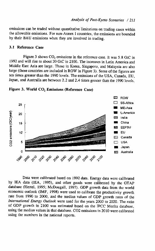
Analysis of Post-Kyoto Scenarios / 211

emissions can be traded without quantitative limitations on trading cases within the allowable emissions. For non-Annex I countries, the emissions are bounded by their BAU emissions when they are involved in trading.

3.1 Reference Case

Figure 3 shows CO* emissions in the reference case. It was 5.8 GtC in 1992 and will rise to about 20 GtC in 2100. The increases in Latin America and Middle East Asia are large. Those in Korea, Singapore, and Malaysia are als,o large (these countries are included in ROW in Figure 3). Some of the figures are ten times greater than the 1990 levels. The emissions of the USA, Canada, EU , Japan, and Australia are between 2.2 and 2.4 times greater than the 1990 levels,.

Figure 3. World CO, Emissions (Reference Case)

@Zl ROW

0 %-Africa

m ME-Asia

I L-America

m India

I China

i%I EEFSU

I EU

13 Canada

0 USA

0 Japan

Australia

Data were calibrated based on 1992 data. Energy data were calibrated by IEA data (IEA, 1995), and other goods were calibrated by the GTAP database (Hertel, 1995; McDougall, 1997). GDP growth data from the world economic outlook (IMF, 1998) were used to calibrate the productivity growth rate from 1990 to 2000, and the median values of GDP growth rates of the International Energy Outlook were used for the years 2000 to 2020. The ratio of GDP growth in 2100 was estimated based on the IPCC Morita database, using the median values in that database. CO2 emissions in 20 10 were calibrated using the numbers in the national reports.

212 / The Energy Journal

3.2 Changes of CO, Emissions Under the Kyoto Agreement

How much will the marginal cost be in order to permanently achieve the Kyoto targets in each case? Figure 4 shows the CO, emissions and marginal costs in the no trading case in 2010. The bar graph shows CO1 emissions. The left-hand bar for each region shows the 1990 emission level, the second bar shows the target emission level, the third bar shows the BAU emission level, and the right-hand bar shows the emission level in the no trading case. The 13AU emission of EEFSU is less than the target, reflecting the economic deterioration of that region. The emission of EEFSU in the no trading case is higher than the BAU emission by about 1% ; that is, CO, leakage is observed.

Figure 4. CO, Emissions and Marginal Costs in 2010 (No Trading Case)

1800 1600 1400 1200 1000

800 600 400 200

0

Marginal Cost usr(l99q/tc

r' . . . . . . . . . . . . . . . . . . . . . . . . . . . . . . . . . . . . . . . . . . . . . . . . . . . . . . . . . . . . . . . . . . . . . . . . . . . . . . . '21 e-$jJ

250

200

150

100

50

0

tq 1990

m Target L! q BaU

m No Trading

The line graph in Figure 4 shows the marginal costs to achieve the emission targets. The emission of EEFSU is below the 1990 level until 2030 in the BAU case, so no policy intervention is necessary in 2010. On the other hand, CO, emission in NZL in the reference case is 11 MtC in 2010, and its emissions must be reduced to 7 MtC. As NZL has to reduce about 50% of its emissions, the marginal cost becomes exceptionally high. Apart from NZL,, the marginal cost of Japan is the highest at 234 US$/tC (1992$). The ranking of other regions is EU, Canada, USA, and Australia, in that order. Although the target for Australia is +8%, the emission in the BAU case is larger than the target and an intervention policy is required to reduce emissions. However, the cost is the lowest except for EEFSU.

Analysis of Post-Kyoto Scenarios / 213

Figure 5 plots changes in emission right prices in AMeX I countries in the no trading case from 1990 to 2050. Except for EEFSU, emission right prices rise sharply in 2010 compared to 2000, while that of EEFSU rises slowly from 2030. When a heavy reduction policy is adopted, Annex I countries must

struggle to achieve it. They will try to invest in energy-related industries for the development of new energy sources and/or to decrease energy demand. The first step is usually difficult when the burden is severe.

Figure 5. Emission Right Prices (No Trading Case)

*Australia +-Japan * USA

* Canada *EU +-EEFSU

1990 2010 2030 2050

How much will the emission right prices be in the trading cases? Figure 6 compares emission right prices in the trading scenario. The emission right in the global trading case is priced lower than those in other cases. It is about 38 US$ in 2010, compared to the emission right price in the Annex I case

of 65 US$ in 2010. It is much less than that in the no trading case. The emissio.n right price in the EU in the double bubble case is almost the same as that in the no trading case, and the emission right price curve also follows the same pattern.

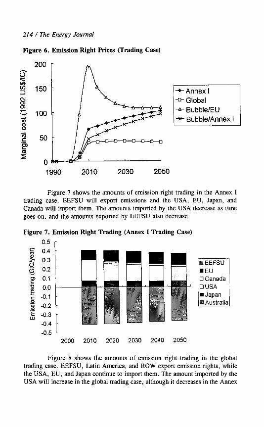
214 / The Energy Journal

Figure 6. Emission Right Prices (Trading Case)

* Annex I -i)- Global * Bubble/EU * Bubble/Annex I

1990 2010 2030 2050

Figure 7 shows the amounts of emission right trading in the Annex I trading case. EEFSU will export emissions and the USA, EU, Japan, and Canada will import them. The amounts imported by the USA decrease as time goes on, and the amounts exported by EEFSU also decrease.

Figure 7. Emission Right Trading (Annex I Trading Case)

0.5

g 0.4

g 0.3 L! (g 0.2

G 6

0.1

; -0.1 0.0

‘9 -0.2

$ -0.3

-0.4

-0.5 L 2000 2010 2020 2030 2040 2050

Figure 8 shows the amounts of emission right trading in the global trading case. EEFSU, Latin America, and ROW export emission rights, while the USA, EU, and Japan continue to import them. The amount imported by the USA will increase in the global trading case, although it decreases in the Annex

Analysis of Post-Kyoto Scenarios / 215

I trading case. One reason is that as the economic impact in the Annex I trading case is much larger than that in the global trading case and emission rights can only be imported from EEFSU, investments are shifted to energy industries a:nd more renewable energy will become available in the future. On the contrary, as Annex I countries can import emissions much more cheaply in the global trading case than in the Annex I trading case, they rely on emission trading and reductions in their own countries are not promoted.

Figure 8. Emission Right Trading (Global Trading Case)

1.5

c I

1.0

s 05 g '

F 0.0 5

s" -0.5 5 'Z .u, -1 .o

IFi -1.5

2000 2010 2020 2030 2040 2050

Figure 9 compares CO, emission changes relative to the BAU case in Annex I countries in 2010. In the no trading case, the USA has to reduc:e emissions by about 25 % and Japan has to reduce them by about 22 % . Carbon leakage is observed in EEFSU. The emission level of EEFSU is 1% larger compared to the BAU emission. In the Annex I and global trading cases, EEFSU will reduce emissions by 32% and 23 %, respectively in order to sell emission rights. In the global trading case, the USA will reduce emissions by 7% compared to the BAU case, which is significantly less compared to the no trading case.

Figure 10 shows CO2 emission changes in non-Annex I countries in 2010 under the same three scenarios. Carbon leakage is observed in man,y countries in the no trading case. For example, in 2010 the emission level of Singapore is 4.5 % higher compared to the BaU case and that in Korea is 2.6% higher. Carbon leakage in China is less than that in other countries.

216 / The Energy Journal 216 / The E ‘nergy Journal

Figure 9. C Figure 9. CO, Emission Changes in Annex I Countries :O, Emission Changes in Annex I Countries

-30

-35 No trading No trading Annex I Annex I Global Global

Figure 10. CO, Emission Changes in Non-Annex I Countries in 2010

in 2010

(B EEFSU

5

4

3

2

1

0

-1

-2

-3

-4

.................. ...... .........

..............

......... ....... ..... ... .......... .........

-5 L I

No trading Annex I Global

3.3 Impacts on GDP

How much will the GDP losses be? Figure 11 shows a comparison of GDP losses in Annex I countries under different scenarios in 2010. The GDP loss is 0.45% in the no trading case, higher than for the other cases, in the USA. The GDP loss in the double bubble case is highest in the EU, at albout 0.35%. The impacts on GDP in the global trading case are the lowest in Z!OlO except for EEFSU. The GDP loss in EEFSU in the no trading case is 0.21%.

Analysis of Post-Kyoto Scenarios / 21’7

Since Figure 4 shows zero marginal cost of emissions reductions in EEFSU :m the no trading case in 2010, the loss in EEFSU is a spill-over effect. EEFSU experiences GDP gains in the trading cases, because the countries of that region sell emission rights. The GDP gain in the Annex I trading case is the largest for EEFSU, at about 3.5%. The GDP gain for EEFSU in the global trading case is about 1.6%, which is less than in other trading cases. The GDP losses in the no trading with 5% offset case are between those in Annex I trading and in no trading. Annex I trading has a much greater effect on GDP than in the no trading with 5% offset case.

Figure il. Comparison of GDP Losses in Annex I Countries in 2010 Under Different Scenarios

0

-1

-2

-3

-4

Figure 12 shows GDP losses in non-Annex I countries. The GDP changes in China and Middle East Asia are negative, while those in Korea and India are positive (i.e., a negative loss). The loss in Middle East Asia is the highest among these regions, and reaches its maximum level in the no trading case.

218 / The Energy Journal

Figure 12. Comparison of GDP Losses in Non-Annex I Countries in 2010 Under Different Scenarios

4. MAJOR FINDINGS

Several interesting findings are obtained from this simulation.

(1) The marginal cost ranking from highest to lowest is NZL, Japan, EU, and USA. The marginal costs of the USA, EU, Japan, and NZL in the no trading case in 2010 are 153$, 198$, 234$, and 274$, respectively. CO? emission in NZL in the reference case is 11 MtC in 2010, and emissions must be reduced to 7 MtC. As NZL has to reduce about 50% of its emissions, the marginal cost becomes exceptionally high. Except for NZL, the marginal cost of Japan is the highest, followed by that of the EU. The highest GDP loss is observed in the USA. The percent GDP losses of the USA, EU, and Japan in 2010 in the no trading case are 0.45 %, 0.3 1 %, and 0.25 % , respectively, while their percent en.ergy reductions in 20 10 are 22.5 % , 14.8 % , and 14.7 % . The percent en.ergy reduction of the USA in 2010 is larger than that of the EU and Japan. The GDP loss in the USA is higher even though the carbon tax is lower than in other countries because more carbon is used in the baseline projection. That is, the price of carbon is lower, but the quantity is higher in the USA.

Analysis of Post-Kyoto Scenarios / 219

(2) Who earns by emission trading? Global trading has a great impact on GDP, with a much lower marginal cost compared to other trading cases. The marginal cost in the global trading case is less than 40 US$ (1992)/tC, which is significantly less than that in the no trading case. EEFSU sells emission rights, while the USA buys the largest amount of emission rights (207 MtC/year). This is 17% of the target and 53% of the total emission reduction in 2010. Japan will buy 57 MtC in 2010, representing 20% of the target emission and 71% of the emission reduction. Emission reductions by trading will account for a large part of emission reductions if there is no limitation on trading. The GDP gain of EEFSU in 2010 is the largest among the regions in trading cases.

(3) The GDP loss of the EU in the double bubble case is larger than that in the no trading case. This is because the EU has access to relatively low cost emission rights from EEFSU in the Annex I trading case, but loses access to that “hot air” in the double bubble case. Therefore, the double bubble scenario has no merit for the EU.

(4) The GDP changes in China are negative in all cases while those in India and Korea are positive, although the numbers are small at 1e:ss than 0.4 %. Non-Annex I countries are directly or indirectly affected by the reduction strategies of Annex I countries. The GDP loss in Middle East Asia is 1.5% in the no trading case. The GDP changes in Middle East Asia are negative in all cases.

Emission trading is effective in reducing CO2 emissions in the sense that it has less GDP impact. Emission reductions by trading will account for a large part of the total emission reductions if there is no restriction on trading. The Kyoto protocol states that the acquisition of emission reduction units shall be supplemental to domestic actions which expresses anxiety that emission trading reduces incentive of Annex I countries to introduce a substantial policy of greenhouse gas emission reduction. It is essential to improve energy efficiency, to develop renewable energy, and to change the socioeconomic structure, so that fossil fuels will be less used.

ACKNOWLEDGMENTS

This research was funded by the Global Environmental Researc.h Program of the Japan Environment Agency. The authors acknowledge their thanks to Dr. T. Masui and Mr. K. Takahashi of the National Institute for Environmental Studies for their extensive support.

220 / The Energy Journal

REFERENCES

Hertel. T.W. (1995). Globul Trude Analysis: Modeling and ~~pplicafions. Cambridge University Press.

IEA/OECD (1995). Energy statistics and balances of non-OECD countries 1992-1993. International Energy Agency, Paris: OECD.

IEAlOECD (1995). Energy statistics of OECD countries 1992-1993. International Energy Agency, Paris: OECD.

IMF (1997, 1998). World Economic Outlook. Washington, D.C.: International Monetary Fu~nd. Matuoka, Y., M. Kainuma and T. Morita (1995). “Scenario analysis of global warming using the

Asian Pacific Integrated Model (AIM).” Energy Policy 23(4/5): 357-371. McDougall, R. A. (1997). Global Trade Assistance, and Protection : The GTAP 3 Dufo Bose,

Center for Global Trade Analysis, Purdue University.

Effects of Restrictions on International Permit Trading: The MS-MRT Model

Paul M. Bernstein*, W. David Montgomery*, Thomas F. Rutherford** and Gui-Fang Yang*

Thispaper assesses the economic impacts of carbon abatementprograms proposed under the Kyoto protocol: the distribution of economic burden across countries and regions, the implications for international competitiveness, and the consequences of international permit trading. Our analysis is based on a dynamic global trade model which accounts for systematic differences in the energy eficiency of production in industrial and developing countries. Emission limits adversely affect the welfare of industrial ana’ some developing countries, including all of the oil-exporting countries. Imports from Annex-B countricr become more costly while demand for most developing country exports is reduced. Oil prices simultaneously fall, so the net impact on oil-importing developing countries is ambiguous. Energy-intensive industries have a strong economic incentive to relocate production to tow-energy cost developing countries. Global trading in emission rights provides the lowest cost path to Kyoto, but it is unclear whether there are incentives for all non-Annex 13 countries to participate.

INTRODUCTION

The Kyoto Protocol, signed in December 1997 but not yet ratified by a majority of countries including the United States, defined the next steps to be taken to reduce global greenhouse gas emissions. It also left unsolved a wide range of questions about the future course of climate change policy. The Protocol calls for the majority of industrialized countries to limit their emissiom of greenhouse gases by the first decade of the next century, and includes several “flexibility mechanisms” that could significantly reduce costs for some countries. Developing Countries undertook no commitments to limit their

The Energy Journal, Kyoto Special Issue. Copyright o 1999 by the IAEE. All rights reserved

* Charles River Associates Inc., 600 13th Street N.W., Suite 700, Washington, DC 20004- 3094. E-mail: pmb@crai.com Web site: www.crai.com

** Associate Professor, University of Colorado, Department of Economics, Boulder, CO 80309- 0256. E-mail: rutherford@colorado.edu

221

222 / The Energy Journal

emissions, and insisted that proposed procedures under which such commitments could be made be deleted from the Protocol. Flexibility mechanisms included coverage of six greenhouse gases, provisions for international emissions tra.ding, credits for reforestation and other actions that remove greenhouse gases from the atmosphere (“sinks”), and a “Clean Development Mechanism” under which industrial countries could finance and gain credit for emissions reductions in developing countries. Virtually all of the details concerning the flexibility mechanisms were left open for further negotiation. These include such issues as the role of developing countries in the overall emissions reduction effort and the scope and design of an international emissions trading system.

In the aftermath of the Kyoto negotiations, countries have argued extensively over the equitable structuring of an international permit trading protocol. Unrestricted, comprehensive, and properly designed, an international emissions trading system would significantly reduce the global costs of limiting greenhouse gas emissions. Nevertheless, parties to the ongoing negotiations have taken mutually incompatible positions on how emissions trading shou1.d be implemented. The United States has advocated unrestricted -emissions tra’ding, extended as rapidly as possible to include key non-Annex I countries. The European Union and a number of developing countries have proposed tight restrictions on emissions trading and oppose any efforts to include non-Annex I countries. Russia has made it clear that its participation in the Kyoto Protocol is contingent on its unrestricted ability to sell permits to other Annex I countries. Furthermore, all sides debate the meaning of language in the Protocol that emissions trading must be “supplementary” to domestic abatement efforts.

Restrictions on emissions trading could eradicate most of such a system’s potential benefits. Curtailing Russia’s ability to sell permits or, conversely, efforts by Russia to restrict sales in order to raise prices could have a major negative impact. Imposing a ceiling on purchases by the U.S. or other countries to enforce a restrictive notion of “supplementarity” would probably have a similar effect. Ultimately, such restrictions would lead to higher permit prices in the United States, lower purchases of permits on international markets, and losses in GDP and exports that would approximate levels to be expected in a no-trade regime.

Currently, the outcome of the Kyoto Protocol remains highly uncertain; thus, the final form of emissions trading is unclear. Because of the great uncertainties involved; this paper analyzes three possible emissions trading regimes under a number of different trading restrictions. To assess the possible impacts on world regions from this diverse set of possible outcomes. we employed our Multi-Sector, Multi-Region Trade (MS-MRT) model. Since this model is a fully dynamic, general equilibrium model of trade, it accounts well for the interactions among industries and regions that result from international policies.

Effects of Restrictions / 2;?3

In the next section, we describe the MS-MRT model, providing an overview of the model structure and key elements. We then report the results from three basic emissions trading regimes that we denote as our benchma:rk cases: no trading among countries in emissions permits, unrestricted trading among Annex I countries, and unrestricted trading among all regions. After presenting results from these scenarios, the paper analyzes a number of different restricted trading scenarios. First, it describes the modeling methodology for these scenarios, then presents results and discusses how restrictions on trading affect the level and distribution of costs of compliance with the Kyoto Protocol.

DESCRIPTION OF THE MS-MRT MODEL

The Multi-Sector Multi-Region Trade (MS-MRT) Model is a dynamic, multi-region general equilibrium model that is designed to study the effects of carbon restrictions on trade and economic welfare in different regions of the world. The model includes a disaggregated representation of industries, based on the GTAP4 dataset, so that differences in energy intensities across countries and differences in the composition of industry can be taken into account. It can represent a wide variety of international emissions trading regimes, define trading blocs composed of any grouping of regions, and place any set of constraints on both purchases and sales of emissions permits. The model computes changes in welfare (calculated as the infinite horizon equivalent variation), national income and its components, terms of trade, output, imports and exports by commodity, carbon emissions, and capital flows. It is fully dynamic, with saving and investment decisions based on full intertemporal optimization.

Conceptually, the MS-MRT model is an Arrow-Debreu model with

complete markets and no money. There is a representative agent in each region, and goods are indexed by region and time. The budget constraint in the Arrow- Debreu model implies that there can be no change in any region’s net foreign indebtedness over the time horizon of the model. Even though there is no money in the model, changes in the prices of internationally traded goods produce changes in the real terms of trade between regions. All markets cle,ar simultaneously, so that agents correctly anticipate all future changes in terms of trade and take them into account in saving and investment decisions. The MS- MRT model is calibrated to the benchmark year 1995, and solves in five-ye.ar intervals spanning the horizon from 2000 to 2030.

In order to capture some of the short-run costs of adjustment, elasticities of substitution between different fuels and between energy and other goods vary with time. The model is benchmarked to assumed baseline rates of economic growth and a common rate of return on capital in all countries. The rate of growth in the effective labor force (population growth plus factor-

224 / The Energy Journal

augmenting technical progress) and the consumption discount rate are computed to be consistent both with the assumed rates of growth and return on capital, and with zero capital flows between regions on the balanced growth path.

In the form used for the EMF study, the MS-MRT model divides the world into ten geopolitical regions (see Table 1).

Table 1. Regions in the MS-MRT Model

Code Region Member of

OECD Annex I

USA

JPN EUR

OOE FSU

CHI SEA

OAS MPC

ROW

United States

Japan Europe Union of 15

Other OECD Eastern Europe and Former Soviet Union

China and India Korea, Singapore, Taiwan, Thailand, and Malaysia

Other Asia Mexico and OPEC

Rest of world

Yes

Yes

YtS Yes No

No No

No No

No

Yes

Yes Yes

Yes Yes

NO No

No No

No

Six industries are represented in the MS-MRT model structure:

. Four energy forms: oil, coal, natural gas, and electricity; and

. Two non-energy goods: Energy-Intensive Sectors (EIS), and All Other Goods (AOG).

The MS-MRT model uses an Armington structure in its representation of international trade in all goods except crude oil, and places no constraints on capital flows. Crude oil is treated as a homogeneous good perfectly substitutable across regions. For all other goods, we assume that domestically produced gosods and imports from every other region are differentiated products. Domestic goods and imports are combined into Armington aggregates, which then function as inputs into production or consumption.

The model includes the markets for the three fossil fuels. Electricity is produced using these fuels, capital, labor, and materials as inputs. Crude oil trades internationally under a single world price. Natural gas and coal are represented as Armington goods, to approximate the effects of infrastructure requirements and high transportation costs between some regions. Depletion is assumed to lead to rising fossil fuel prices under constant demand, but the relation between depletion effects on the supply of oil, gas, and coal and the actual supply of these fuels is ignored. That is, the model does not keep a record of the current stock of each fuel in each time period. World supply and demand

Effects of Restrictions / 22.5

determine the world price of fossil fuels. Current energy taxes and subsidies are included in each country’s energy prices. The carbon-free backstop, represente’d as a carbon sequestration activity that requires inputs of non-energy goods, establishes an upper bound on world fossil fuel prices.

NON-TECHNICAL DISCUSSION OF THE MS-MRT MODEL STRUCTURE

This section offers a non-technical discussion of the important elements of the MS-MRT model: production, household behavior/consumer choice, international trade, savings and investment, and carbon restrictions. It relies largely on diagrams to illustrate the nesting structures used in the utility and production functions and the definitions of markets.’

Production of the Non-Energy Goods

The MS-MRT model represents non-energy production in two sectors using a constant elasticity of substitution (CES) function for each. In producing non-energy goods, the model accounts for regional differences in factor intensities, degrees of factor substitutability, and the price elasticities of output demand in order to trace back the structural change in industrial production that is induced by carbon abatement policies.

All non-energy industries have a similar production structure (see Figure 1). Materials (outputs of the two industries used as inputs in other industries) enter the production function in fixed proportion with a value-added aggregate and an energy aggregate. The value-added aggregate comprises capital and labor. When the energy value share of an industry is small, the elasticity of substitution between the value-added aggregate and the composite energy good (uVA+) is equal to the own-price elasticity of demand for energy. This elasticity determines how difficult or easy it is for a region to adjust its production processes in response to changes in energy prices. Higher values of the energy substitution elasticity imply that a region can more easily substitute value-added for energy as the price of energy increases. This elasticity is time varying to reflect capital stock turnover and the ease of deploying new technology. For OECD countries, this elasticity begins at a value of 0.35 in the year 2000 and rises linearly to 0.6 by 2030; in non-OECD countries, it starts at 0.3 and rises linearly to 0.5 over the 30-year time horizon.

1. For a mathematical description of the model, see Bernstein, Montgomery and Rutherford.

“Trade Impacts of Climate Policy: The MS-MRT Model,” in review, Energy and Resource Economics, 1998.

226 / The Energy Journal

Figure 1. Production Structure for AOG, EIS, and Electricity

i f energy good

Oil Gas

Capital and labor are nested as Cobb-Douglas (a,,= 1). They may be substituted directly for each other through activities such as the automation of labor-intensive tasks. Therefore, the higher the wage rate, the more attractive it becomes to adopt automation. Labor inputs in this model are measured in efficiency units, so that one unit of labor supply is the same as ten billion dollars of base-year wages.

Labor supply is inelastic. Growth rates in the labor force are exogenously specified, so that the effective labor endowment for each region increases over time with labor force efficiency and population growth along the region’s baseline growth assumptions. Labor is regionally immobile, and the labor force is fully employed at all times.

Capital stocks evolve through geometric depreciation of existing capital stocks and new investment of sector-specific capital (within countries). The rates of return on capital are determined in an international market by endogenous

Effects of Restrictions / 227

levels of lending and borrowing. We assume perfectly competitive capital markets in which the rate of return adjusts so that supply equals demand. The model is calibrated to an equalized net rate of return equal to 5 percent in all regions.

Armington composites enter the material nest, so that intermediate inputs from domestic industry j are imperfect substitutes for imports of good j. Material inputs are complements among each other; all other inputs are substitutes.

Production of Fossil Fuels

The production of fossil fuels requires inputs of the aggregate non- energy good and a fuel-specific factor of production that can be thought of as a sector-specific resource. In the baseline solve, this resource is used to match the baseline level of fossil fuel production to the U.S. Department of Energy’,s projections for fossil fuel production (EIA, International Energy, Outlook 1998) through 2020 and to the IPCC IS92a scenario from 2020 to 2030. This matching is achieved by requiring that this resource be used in fixed proportions (ulf =: 0) with the aggregate good (see Figure 2). Then, defining the level of available fixed resource for each fuel determines the level of each region’s oil, gas, and coal production. After we solve the baseline scenario, we solve the fossil fuel production equations for the non-zero value of ufl required to arrive at the same fuel prices and fuel production levels. This value for the fuel supply elasticity is used when we solve the model under the carbon abatement scenario. Therefore, the level of production is allowed to vary in the scenario solve.

Household Behavior, Consumer Choice, and the Representative Agent

For each region, there is one infinitely-lived “representative” agent who chooses to allocate its region’s entire lifetime income across consumption in different time periods in order to maximize welfare. In each period, the consumer faces the choice between current consumption and future consumption that is purchased via savings. The pure rate of time preference between current and future consumption determines the intertemporal allocation of consumption. In equilibrium, the agent is indifferent between consuming one unit of consumption today or consuming the value of one unit of consumption that is adjusted for time preference tomorrow. We employ an intertemporal separable utility function where the intra-period utility from consumption is based on a nested CES function over imported and domestic commodities. The representative agent maximizes utility subject to an intertemporal budget constraint.

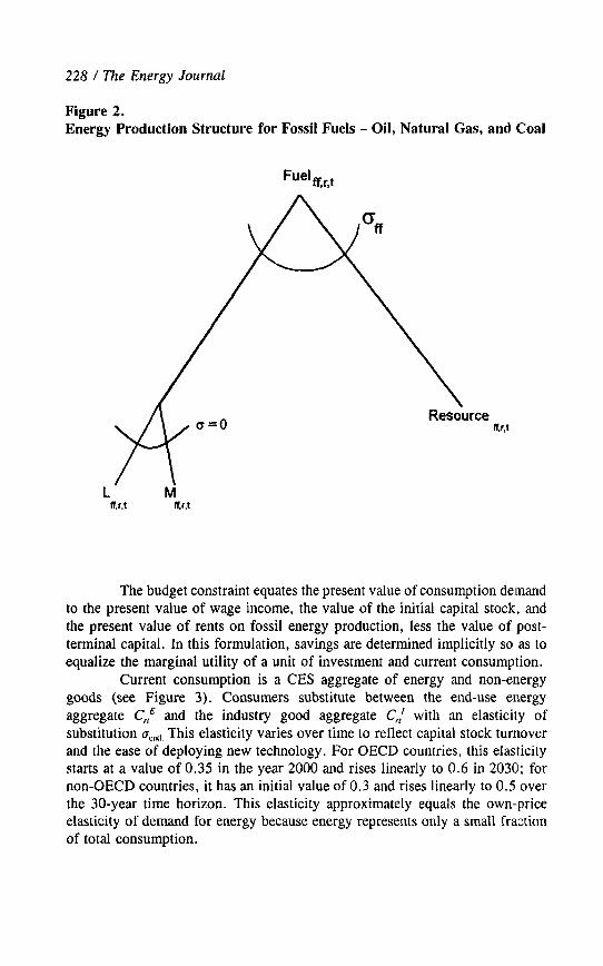
228 / The Energy Journal

Figure 2. Energy Production Structure for Fossil Fuels - Oil, Natural Gas, and Coal

M ff.r.t

The budget constraint equates the present value of consumption demand to the present value of wage income, the value of the initial capital stock, and the present value of rents on fossil energy production, less the value of post- terminal capital. In this formulation, savings are determined implicitly so as to equalize the marginal utility of a unit of investment and current consumption.

Current consumption is a CES aggregate of energy and non-energy goods (see Figure 3). Consumers substitute between the end-use energy aggregate C,” and the industry good aggregate C,’ with an elasticity of substitution a,,, This elasticity varies over time to reflect capital stock turnover and the ease of deploying new technology. For OECD countries, this elasticity starts at a value of 0.35 in the year 2000 and rises linearly to 0.6 in 2030; for non-OECD countries, it has an initial value of 0.3 and rises linearly to 0.5 over the 30-year time horizon. This elasticity approximately equals the own-price elasticity of demand for energy because energy represents only a small fraction of total consumption.

Effects of Restrictions / 229

Aggregate end-use energy is composed of the fossil fuel aggregate. Th.e aggregate comprises oil, gas, and coal; these fuels substitute against each other with an interfuel elasticity of substitution equal to ufUel. Electricity is nested together with the non-energy goods. Each non-energy good in the fuel nest is an Armington composite, in which domestic and imported goods are combined in the manner described below. Purchase of the goods is financed from the value of the household’s endowments of labor, capital, energy-specific resources, and revenue from any carbon permit sales.

Figure 3. Consumption Nest

Consumption r t 9

c.7 end

Oil Gas Coal Y EIS ELE

International Trade

Trade takes place in the fossil fuels and in the composite non-energ:y goods. All bilateral trade flows for the non-energy goods are represented in the MS-MRT model.

On the import side, consumers and industries choose between these domestically produced goods and imports. Demands for imports stem from cost- minimizing producer behavior and utility-maximizing household behavior. For the non-energy goods, an Armington trade structure is used so that the model differentiates between domestic and foreign goods. Therefore, domestically

230 / The Energy Journal

produced goods and imports are imperfect substitutes. Small cost differences across regions for a good do not lead to a total shift in demand from one region to another, and small changes in costs lead to small movements away from existing trade patterns. In addition, the Armington structure accommodates both imports and exports of the same commodity across regions (cross-hauling).

To create the Armington aggregate, imports of each non-energy good from each region substitute against each other with an elasticity of substitution equal to the Armington elasticity, uMM, and the aggregate import good substitutes against the comparable domestic good with an elasticity of substitution (uDM) equal to half of uMM. The Armington elasticity +,,,, is set at 4 for this model with two non-energy goods because those composite goods are not likely to be identical across countries.

This elasticity measures how easily imports can substitute for domestically produced goods. The Armington elasticity affects the potential gains in non-Annex 1 export sales that will occur when lower energy costs give these non-participating countries a competitive advantage. Figure 4 displays this structure. Armington,,,,, represents either consumer or industry demand for the non-energy good i in region r in time period t. Industries and consumers consume an Armington aggregate of domestically produced goods (D,,,.,,) and goods imported (M,,,,,) from regions s # r.

Figure 4. Armington Nest Trade Structure for Consumption and Production

Armington i,r,t

Import GOOt&t (M,s,t)

Effects of Restrictions / 23.1

The models incorporate international markets for all goods. For these goods, we have a global market-clearing condition for the MS-MRT model:

cx;=p4,‘; v t , j E { energy goods , non -energy goods ) r r

The model is closed with respect to international trade through the intertemporal budget constraint. The intertemporal budget constraint for the representative agent in each region requires that the net present value of international borrowing or lending remain equal to the baseline level over the model’s time horizon. This implies that any change in capital flows must net to zero (in present value terms) over the time horizon. Since the current account surplus or deficit (equal to the value of net exports) equals net international lending or borrowing, this also implies that the net present value of the change in the current account must be zero over the time horizon. The imposition of an intertemporally balanced trade account is linked to an implicit exchange rate that reconciles the present value of each region’s domestic import demands with the present value of its exports.

This budget constraint allows changes in capital flows to play a part in determining the trade impacts of carbon limits. In contrast, the EPPA model assumes a period-by-period balance-of-payments constraint so that the current account deficit or surplus must equal baseline levels in each year. The GCUBED model imposes a constraint on capital flows, so that a region’s net foreign indebtedness can change over the model time horizon. GCUBED accounts for the effects of changes in indebtedness by calculating GNP, in which interest payments on foreign debt are deducted from gross domestic output (GDP).

Savings and Investment (Dynamics)

Since MS-MRT is a fully dynamic general equilibrium trade model, its model structure incorporates forward-looking investment and savings behavior, so that businesses, individuals, and governments anticipate the effects of announced policies that are to take effect in the future. The level of savings and investment in a given period is endogenously determined by entrepreneurs and households that maximize the firm’s value and the representative agent’s lifetime consumption. Entrepreneurs choose investment levels to maximize the net present value of profits, and savings behavior is determined by intertemporal utility maximization. Therefore, investment dollars are placed in the area where they will receive the highest return.

Physical capital stocks depreciate at a constant geometric rate, and the] are incremented by investment from domestic output. The finite horizon poses

232 / The Energy Journal

some problems with respect to capital accumulation. In the absence of any terminal adjustment, agents would consume all capital stock in the terminal period and thus let the value of the capital stock decline to zero after 2030. This would have significant repercussions for rates of investment in the periods leading up to the end of the model horizon. To correct for these effect:;, we apply an auxiliary equation dealing with the terminal capital stock.

It should be emphasized that we apply this side constraint along with the other economic equilibrium conditions (zero profit, market clearance, and income balance), but the application of this constraint has no implications for investment and consumption activities because these impacts do not enter into the zero-profit conditions for these activities. Instead, we close the model by including a terminal capital stock variable; the quantity of which is determined so that the rate of growth of terminal investment is balanced. That is, the shadow price of the above auxiliary constraint is the price of the terminal capital stock.

Carbon Restrictions

To comply with the Kyoto Protocol, the model places a carbon emissions limit on the participating countries. The model endows these countries with emissions permits that allow them to emit carbon up to the level to which they agreed. In the MS-MRT model, it is assumed that, under the no-trade scenario, the emissions permits are tradable within each Annex I region but not across regions. Under the trading scenarios, emissions permits can be traded among the different blocs: for the Annex I trading scenario, only Annex I countries face carbon limits, and the permits are tradable across all Amrex I countries; for the global trading scenario, all countries face carbon limits, and the permits are tradable throughout the world.2

BENCHMARKING AND CALIBRATION3

This section describes how the MS-MRT model was benchmarked and calibrated. As is customary in applied general equilibrium analysis, the MS- MRT model is benchmarked to economic transactions in a particular year (1995). Benchmark data determine the parameters and coefficients (value shares) of the CES production, demand, and utility functions. Base-year finance

2. In the MPWGE framework in which MRT-MS is written, creating a market for carbon permits and imposing a cap on carbon emissions for each country is straightforward. See the web site, www.gams.com, for a description of the MPS/GE modeling language.

3. For further technical details on how the MS-MRT is benchmarked, see Bernstein, Montgomery, and Rutherford (1998).

Effects of Restrictions / 233

statistics indicate the value of payments to capital across sectors and the gross, value of capital formation. For calibration, we needed to determine a reference: level of emissions growth, GDP growth, energy production, energy, and non- energy trade. This entailed assigning values to key elasticities, such as end-use: demand, Armington, oil supply, and the Autonomous Energy Efficiency Improvement (AEEI).

To develop a consistent database for energy and non-energy trade and input-output data, we merged non-energy trade data, input-output data, and input-output coefficients for energy from the GTAP database with data from the International Energy Agency (IEA). See Babiker and Rutherford (1996) for details.

For carbon emissions forecasts, the model was calibrated to the projections of both DOE and the International Panel on Climate Control. The. reference or business-as-usual (BAU) level growth path for world emissions is taken to be the IPCC’s reference scenario IS92A. The IS92A scenario’ corresponds to the IPCC’s baseline (medium growth) scenario, which calls for worldwide carbon dioxide emissions to grow from 6.0 billion tonnes in 1990 to 10.7 billion tonnes by the year 2025. The reference level emissions growth determines the amount of emissions reduction required to meet the carbon limits called for by any carbon abatement policy.

The energy production and consumption forecasts as well as regional emissions were obtained from the Department of Energy’s International Energy Outlook, 1998. These forecasts were then calibrated to current EIA data and the IS92A scenario so that energy consumption was consistent with carbon emissions. The business-as-usual GDP growth rates were taken from MERGE (a Model for Evaluating the Regional and Global Effects of greenhouse gas reduction policies), which was developed by Alan Manne and Richard Richels.

Selecting Elasticity Values and Backstop Prices

Selecting elasticity values affects the dynamics of the model and how the model responds under a carbon abatement policy. The choice of values has no effect on the baseline level of energy production and consumption, which is benchmarked through choice of other free parameters so that the chosen baseline is replicated as a market equilibrium. There are several key elasticities that need to be chosen for an MS-MRT simulation, including the oil supply price elasticity, Armington elasticity, end-use demand elasticity, interfuel elasticity of substitution, and the cost of the carbon-free backstop technology.

234 / The Energy Journal

BENCHMARK CASES

For a point of reference, the MS-MRT model was run under three different emissions trading scenarios: No trading, trading only among Annex I countries (Annex I trading), and full global trading (Global trading). These three trading regimes provide a basis for understanding the opportunity Icost of restrictions on emissions, so we refer to them as the benchmark cases. The first two scenarios are possible outcomes of the Kyoto Protocol, unlike the third, which is impossible given the Protocol’s current wording. Under Annex I and global trading, no restrictions on sales or purchases of emissions permits were applied. Each Annex I region was assigned emissions limits for 2010 and beyond consistent with its obligation under the Protocol (see Table 2). Under the global trading scenario, non-Annex I countries assume an emissions target equal to their emissions under the no trading scenario.

Table 2. Kyoto Protocol’s Emissions Targets for Annex I Regions

Region 2010 Target

(% Change from 1990)

U.S. -1%

Japan -6%

Canada -6%

European Union of 15 -8%

Other OECD +l.l%

Eastern Europe/Former Soviet Union -2%

Results for Benchmark Cases

In the benchmark cases, the MS-MRT model consistently finds that emissions limits on industrial countries with no international emissions trading lead to negative impacts on the welfare of industrial and oil-producing countries, and both positive and negative welfare effects on energy-importing non-Annex I countries (see Table 3). Annex I trading improves the situation for all regions, except China and India, but only changes the sign for EE/FSU. All regions benefit under global trading as compared to no trading; only EE/FSU is worse off under global trading than under Annex I trading.

Effects of Restrictions / 23!i

Table 3. Welfare under the Three Benchmark Trading Cases (Percentage Change from Baseline)

Trading Scenarios

Regions No Trading Annex I Global -

USA -0.56% -0.36% -0.14%

JPN -0.64 -0.23 -0.03

EUR -0.45 -0.25 -0.05

OOE -0.92 -0.76 -0.30

SEA -0.18 -0.04 0.25

OAS -0.10 -0.01 0.19

CHI 0.34 0.22 0.34

FSU -0.42 4.44 0.48

MPC -1.39 -1.15 -0.36

ROW -0.10 -0.08 0.03

Carbon permit prices differ across regions when international permit trading is not allowed (Table 4). Annex 1 trading lowers permit prices for all. Annex 1 regions except the FSU, which is the sole seller of permits. Global trading further lowers prices for Annex 1 regions, but raises permit and energy prices for non-Annex 1 regions.

Table 4. Carbon Permit Price under Three Benchmark Scenarios (1995 U.S. Dollars per Metric Ton)

Scenario Region 1 2010 2020 2030

No Trading

Annex I Trading Global Trading

USA $275 $314 $356

JPN 468 523 526 EUR 209 309 430

OOE 249 363 505 FSU 0 10 49

Annex I 90 151 225 World 31 36 32

Terms of trade generally move against developing countries and in favor of industrial countries when developing countries do not participate in international emissions trading. This is because industrial countries’ costs increase, driving up the price of their exports, and their incomes and import demand fall, driving down the price of their imports. This is the reason for the negative welfare impacts on developing countries noted above. Some developing countries (e.g., China) can offset these terms-of-trade losses with industrial countries because of their gains in terms of trade with OPEC and ability to shift to production of energy-intensive goods where they have increased comparative advantage over the industrial countries. (see Table 5).

236 / The Energy Journal

Table 5. Terms of Trade under the Three Benchmark Cases (Percentage Change from Baseline)

No Trading Annex I Global No Trading Annex I

Region 2010 2010 2010 2020 2020 Global 2,020

USA 0.04% -0.14% -0.08% -0.03% -0.14% -0.10% JPN 0.11 -0.05 -0.05 0.44 -0.01 -0.05

EUR 0.02 0.04 -0.05 0.07 0.07 -0.06

OOE 0.00 -0.08 -0.08 0.15 -0.09 -0.12

SEA -0.27 -0.10 0.08 -0.29 -0.15 0.11

OAS -0.14 0.04 0.09 -0.21 -0.02 0.09

CHI -0.19 -0.04 0.44 -0.28 -0.14 0.57

FSU -0.44 1.71 0.27 -0.76 1.99 0.23

MPC -0.60 -0.44 0.10 -0.89 -0.69 0.05

ROW 0.28 0.22 0.13 0.13 0.18 0.08

The shift of energy-intensive industries out of Annex I countries into non-Annex I countries when non-Annex I countries do not participate in emissions trading is significant. Annex I emissions trading moderates the shift of industry by reducing production costs in most Annex I countries. Interestingly, the U.S. and EE/FSU, the lowest-cost providers of permits, suffer the greatest losses in their energy-intensive industries under Annex I trading. With global trading, production from non-Annex I energy-intensive industries declines from the levels it reaches under no trading and Annex I trading. For a subset of these countries and in certain time periods, some EIS production relocates to Annex I countries as reported by the negative percentage changes in Table 6. This occurs because the GTAP data show that many of the Non- OECD countries have the least energy-efficient industries and, therefore, are the most vulnerable to a uniform, global increase in energy costs (see Table 6).

Table 6. Output from Energy-Intensive Industries in 2010 and 2020 (Percentage Change from Baseline)

Region

No Trading Annex 1

2010 2010

Global

2010

No Trading

2020

USA -7.87% -2.43% -0.59% -7.66%

JPN -1.06 0.10 0.18 -1.82 EUR -0.17 0.50 0.44 -1.56

OOE -2.69 -0.32 0.35 -5.98 SEA 4.69 2.01 0.07 4.21

OAS 2.51 0.56 0.07 2.26 CHI 1.94 0.89 -0.57 2.01 FSU 5.87 -10.22 -2.98 6.42 MPC 4.67 2.51 -0.15 5.65 ROW 1.32 0.52 -0.04 1.53

Annex 1 Global

2020 2ozo

-3.62% -0.51 %

-0.15 0.15 0.33 0.45

-1.04 0.50 2.55 -0.06

0.87 0.12 1.32 -0.85

-13.93 -2.'78 4.10 0.04

0.89 0.03

Effects of Restrictions / 237

Carbon leakage is also significant. It is connected with relocation of energy-intensive industries, reduced energy efficiency, and fuel substitution due to lower fuel prices in developing countries (see Table 7). Leakage is affected very little by Annex I trading, because it arises mostly from differences in energy prices between Annex 1 and non-Annex 1 countries. With Annex 1 trading, global emissions also increase because of hot air sales by EE/FSU, decreasing apparent leakage to developing countries in percentage terms. Global trading, by definition, eliminates leakage because all regions face emissions caps.

Table 7. Carbon Leakage under No Trading and Annex I Trading, Regimes (Change in Non-Annex I Emissions Divided by Change in Annex I Emissions)

2010 2015 2020 2025 2030

No Trading 18 19 20 21 21

Annex I Trading 16 18 19 21 22

MEASURES OF WELFARE

There are a number of alternative measures of economic impacts that appear in different studies: change in consumers’ surplus measured by the: equivalent variation, the discounted present value of consumption (DPVC), GDP, and direct cost. In general, for each model there is one theoretically consistent measure, which is based on the value of the objective function maximized in the model. In our model, this measure is the intertemporal equivalent variation.4 If we had implemented this model with an infinite horizon (difficult computationally), changes in welfare could be taken directly from the: value of the intertemporal utility function. Since we terminate the model in 2030, we must add to the utility experienced during the period an adjustment that represents the change in the value of the terminal capital stock that is left for future generations. This adjustment makes our calculation of the infinite: horizon welfare approximate, because to value the terminal capital stock we: need to employ some assumptions about how close the temporary equilibrium. in 2030 is to one on a balanced growth path.

4. For a discussion of how this welfare measure is computed in the MRT-MS, see Thomas F. Rutherford, “Constant Elasticity of Substitution Functions: Some Hints and Useful Formulae.” Note:,

prepared for CAMS General Equilibrium Workshop, held December 1995, in Boulder, Colorado: available from http:/lwww.gams.com/solvers/n~psge/cesfun.htm. For a general discussion of this

welfare measure, see Hal Varian, Microeconomic Analysis, Third Edition, New York, 1992. pp. 160-171.

238 / The Energy Journal

The same issue about terminal capital stock applies to calculating the discounted present value of consumption as a welfare measure. These considerations about the terminal capital stock are important, because emi:ssions limits produce large drops in investment (as high as 2.5 percent under no trading in the U.S.), which imply very different capital stocks in 2030 in the baseline and the policy cases. Agents buffer consumption during the shock period by reducing investment, and the effects of this reduced investment on their future welfare need to be taken into account.

GDP, the other common measure, has classic index number probllems, that in our model, appear in sensitivity of the results to choice of numeraire. GDP includes both consumption and investment, so that over short periods of time GDP may increase due to a stimulus to investment even though consumption falls. In addition, GDP is a measure of gross, not net, income, in the sense that it does not account for depreciation of capital. When policies lead to large reductions in investment for a sustained period of time, they lead to lower levels of capital stock and to reduced capital consumption allowances (CCA). As a result, GDP falls because of both contemporaneous reductions in investment and lower CCA. This effectively double-counts the reduction in investment and produces a larger percentage reduction in GDP than in net national income. GDP also fails to account for net interest payments on foreign debt, so that if a policy causes a significant change in foreign debt, GDP will inaccurately measure the change in real income for residents of a country.’

Finally, it is possible to produce an approximate measure of the direct cost of a policy using the standard Harberger triangle. Some models (e.g., the SGM) use this measure. It equals one-half the carbon tax times the reduction in emissions plus the net receipts or payments for international permits6

The values of these different measures are provided in Table 8. GDP and “direct cost” are all annual measures, while EV and discounted present value of consumption are present value measures. Thus, we present GDP and “direct cost” for different years (2010 and 2020) and welfare and DPVC as a single number. For welfare, DPVC, and GDP, the numbers report the percentage change from baseline numbers whereas direct cost reports the cost in units of billions of 1995 U.S. dollars.’

5. William Nordhaus deserves the credit for this observation.

6. This measure is reported by the SGM and in the Administration’s economic analysis of the Kyoto Protocol. See “The Kyoto Protocol and the President’s Policies to Address Climate Change,”

Administrdtion Economic Analysis, July 1998: and J.A. Edmonds, et al., “Return to 1990: The Cost of Mitigating United States Carbon Emissions in the Post-2000 Period,” October 1997.

7. Costs are reported as negative numbers.

Effects of Restrictions / 239

Table 8. Comparison of All Four Welfare Measures for Selected Regions

Welfare DPVC Direct Cost GDP

2010 2020 2010 2020

No Trading CR) (%) (Billions of U.S. $) (%) (%)

USA -0.56% -0.41% -$45.20 -$43.55 -1.88% -2.33%

SEA -0.18 -0.03 n.a. n.a. 0.51 0.01

CHI 0.34 0.59 n.a. n.a. 0.64 0.21

MPC -1.39 -1.65 n.a. n.a. -0.99 -1.60

ROW -0.10 0.10 ma. n.a. 0.71 0.17

Annex 1

USA -0.36 -0.31 -36.39 -57.53 -0.91 -1.27

SEA -0.04 0.04 ma. n.a. 0.47 0.50

CHI 0.22 0.33 n.a. n.a. 0.53 0.60

MPC -1.15 -1.45 n.a. n.a. -0.64 -0.91

ROW -0.08 0.01 n.a. n.a. 0.60 0.60

Global

USA -0.14 -0. I4 -15.41 -21.91 -0.29 -0.33

SEA 0.25 0.36 1.33 2.63 0.06 0.02

CHI 0.34 0.52 4.55 13.58 -0.17 -0.07

MPC -0.36 -0.42 1.40 3.02 -0.45 -0.48

ROW 0.03 0.08 2.42 5.02 0.06 0.04

Comparing these measures illuminates three critical issues. First, one measure can imply a country benefits under a specific scenario while another measure implies a loss. Second, the measures can produce different policy rankings for a specific region. Third, the magnitudes of these measures are incomparable unless all of them are in the same units (see Table 9).

Table 8 points out the problems of reporting welfare measures that are not directly connected to the model’s objective function. As mentioned, for our model, equivalent variation of welfare is the only self-consistent welfare measure. In general, DPVC closely approximates welfare, but the sign differs for ROW in the no trading and Annex I trading scenarios and for SEA under the Annex I trading scenario. This inconsistency arises because of the difference between the implicit discount rate (intertemporal rate of substitution) in the welfare function and the specified discount rate for DPVC.

For Annex I countries, the direct cost is consistent with equivalent variation (welfare) both within and across emissions trading scenarios. But this measure reveals little about the welfare of non-Annex I countries because it leaves out the terms-of-trade effects that are responsible for spillover effects. Furthermore, under global trading, direct cost reports a gain for MPC, but MPC experiences a loss in welfare due to the fall in world oil prices.

Comparing GDP results among countries or across scenarios may not present a clear picture of whether one country does better compared to another,

240 / The Energy Journal

or whether a particular scenario is beneficial for a country because the change in GDP may be positive in one period but negative in the next. Also, to compute GDP, one needs a numeraire; there is no theoretically correct choice for this. Therefore, depending on the choice of numeraire, one arrives at different results for GDP. This leads to some of the inconsistencies when comparing impacts on CHI across scenarios. Using GDP as the welfare measure, CHI is better off under no trading and Annex I trading than under global trading, whereas EV (welfare) implies the opposite conclusion. This problem arises when comparing results for many of the non-Annex I, non-energy exporting regions and is due to the large changes in investment that increase GDP in some countries for a period of time at the expense of consumption.

Table 9. Comparison of Four Welfare Measures for the U.S. (Percentage Change from Baseline - Cumulative and Discounted to 2000)

Scenario Welfare DPVC Direct Cost GDP

No Trading -0.56% -0.41% -0.19% -1.31% Annex I Trading -0.36 -0.31 -0.07 -0.75

Global Trading -0.14 -0.11 -0.01 -0.18

The magnitudes of the welfare measures as reported in Table 8 a.re not directly comparable. GDP and direct cost are annual measures, whereas EV welfare and DPVC measure the discounted present value of impact over a horizon. Furthermore, the units of direct cost are dollars. To eliminate these differences, we computed the discounted PV of the direct cost and GDP for the scenarios over the full time horizon. Then, to compute the percentage change from baseline, these are divided by the DPV of the baseline GDP (see Table 9). The EV Welfare still differs from the other measures since it approximates the impacts over the infinite horizon rather than the model’s 30-year horizon.

The GDP measure shows the largest impacts, partly because of the double counting of investment impacts noted above. Direct cost shows the smallest impacts since it leaves out effects on investment, terms of trade, and other general equilibrium effects, and also because it is not based on the compensated demand curve required theoretically to approximate consumer surplus. Welfare and DPVC are close, with slight differences caused by discrepancies between the discount rate assumed in calculating the DPVC and the internal discount rate used in the welfare calculation. The EV welfare measure could be closer to GDP if its denominator were limited to welfare during the model horizon, rather than the infinite horizon.

Effects of Restrictions / 241

RESTRICTED TRADING CASES

The Kyoto Protocol did not reconcile the positions of the U.S. and other Annex I nations on emissions permit trading. Three unresolved issues are especially important: 1) the extent to which a country may satisfy its obligation through permit purchases, 2) the amount of paper tons or permits for “hot air”’ EE/FSU countries will be allotted, and 3) how market power will be exercised. Two other questions also arise: What will be the economic impacts of restricting the sales of emissions permits, and what will be the potential benefits to the Annex I countries of instituting the CDM?

To address the first three issues, we consider several different Annex I trading regimes. First, we consider three regimes in which Annex I regions are limited in how many permits they can purchase. Proponents of restricted emissions trading cite the Kyoto Protocol language that trading should be “supplementary” to domestic efforts in support of these limits. The EU and several of its member countries have proposed that a “concrete ceiling” be imposed on the percentage of a country’s emissions obligation that may be satisfied through the purchase of emissions permits. These countries have suggested a limit of 50 percent or less. In addition, some have advocated a system of buyer liability that would so burden buyers of permits with potential liabilities that only the most attractive trades would have any likelihood of being accomplished.

In our scenarios, the limits are set at 10 percent, 30 percent, and 50 percent of each country’s obligation. Since the limits are placed only on the demand side, countries can sell as many permits as they like but are restricted by how much of their commitment they can satisfy through the purchase of permits. We also consider a case in which a 50 percent limit exists under a global trading system, since it is under global trading that our benchmark results suggest that the U.S. would want to purchase more permits than this limit would allow.

Second, we consider the impacts of prohibiting the EE/FSU region from selling its “hot air.” Russia, and possibly some of the former Soviet Republics and other Eastern European countries, will clearly be the least-cost suppliers of permits in an Annex I trading system in 2010. Because its economic collapse has reduced current emissions to levels well below its 1990 baseline,

8. This positive difference between the EEIFSU’s Kyoto emissions targets and its actual

forecasted emissions is referred to as “hot air” or “paper tons.” Because the EE/FSU’s economy has been in a decline since 1990, its carbon emissions are forecasted to be below its 1990 emissions

level until somewhere in the 2020 to 2025 time period.

242 / The Energy Journal

Russia’s emissions in 2010 are projected to be about 20 percent below its Kyoto target.’

Most of the members of the EU, and many developing countries, are opposed to a system that allows Russia to sell its hot air, arguing correctly that hot air sales would raise total world emissions above the levels they would. reach without such sales. Table 10 helps illustrate the concept of hot air. The line titled “Baseline” shows that, until 2020, EE/FSU’s emissions are below its Kyoto target of 1990 emissions levels (“Kyoto Target” line). This gap between the region’s Baseline emissions and its target is referred to as “hot air.” In 2010, the EE/FSU is forecasted to have about 220 million metric paper tons. In the No Hot Air case, EE/FSU is restricted from selling its paper tons of carbon. Under this case, EE/FSU’s emissions target is denoted by the “No Hot Air” line, which equals the smaller of EE/FSU’s business-as-usual emissions or its Kyoto target of the 1990 emissions level. Therefore, under the Annex I trading regime, the emissions cap for the entire Annex I bloc is lower under the No Hot Air case than under the other cases.

Table 10. EEIFSU’s Carbon Emissions Targets (Millions of Metric Tons)

2000 2005 2010 2015 2020 2025 Z!O30

Baseline 870 Kyoto Target n.a.

Hot Air n.a. No Hot Air n.a

940 1,023 1,094 1,174 1,267 1,371

n.a. 1,240 1,240 1,240 1,240 1,240

ma. 217 146 66 0 0

n.a. 1,023 1,094 1.174 1,240 1,240

Third, we address the issue of market power. As the only net seller of permits under a trading system limited to Annex I countries, Russia would be in a position to restrict output and charge monopoly prices for its em&ions permits. We consider one scenario in which EE/FSU is able to exercise some market power. We also describe a method for estimating the output restriction that would maximize benefits to EE/FSU and the resulting prices. This case is intended to provide an illustration of how monopoly power could be exercised.

Fourth, we consider other restrictions on sales. We analyze a case where countries are allowed to sell only 30 percent of the permits that they would sell under unrestricted Annex I trading. This case is designed to examine whether proposed restrictions on sales would achieve the same result as exercise of monopoly power, and whether restrictions on sales could produce ‘worse outcomes than unilateral exercise of monopoly power.

Finally, we examine how closely the CDM approximates the benefits of full global trading. The CDM is designed to support projects to reduce emissions from developing countries, with funding from industrial countries that

9. U.S. Department of Energy, Inrernational Energy Outlook, 1998.

Effects of Restrictions / 243

would receive emission credits. We limit permit sales from each of the non- Annex I regions to 15 percent of its total sales under unrestricted global trading. This differs from full global trading because it leaves most of the price differentials between Annex I and non-Annex I countries in place.

Modeling of Restricted Trading Cases

To model restricted trading in the Arrow-Debreu framework, one needs to create markets for import and export quota coupons in addition to markets for permits. The permit is a normal traded good, subject to a nontradable quota. These coupons must be used when either importing or exporting emissions permits. In the case of unrestricted permit trading, every region is endowed with an excess of quota coupons so that the price of coupons is zero. In the restricted trading cases, however, each region that is a member of the trading bloc is endowed with a fixed number of quota coupons equal to the limit of its restriction. For example, if the final version of the Protocol were to limit each Annex I country’s permit purchases to 30 percent of its obligation, then each country would be given quota coupons equal to 30 percent of its obligation. Restricting permit sales works the same way except, now, sellers must use quota coupons to vend permits.

Under the CDM case, the non-Annex I countries are allowed to sell 15 percent of their permits that they would have sold under the unrestricted global trading case. This is a modeling convenience and could not be implemented in reality. But this case serves to estimate the effect of implementing the CDM in a way that would allow non-Annex I countries to participate in the process of reducing global emissions, but with costs and restrictions that render 85 percent of the trades possible under global trade no longer economic. To model this proxy for the CDM, the non-Annex I countries are endowed with quota coupons equal to 15 percent of their emissions permit sales under unrestricted global trading. There are no restrictions on permit trading among Annex I regions.

By treating limits on purchases and sales of emissions permits as, respectively, import and export quotas, the international price of permits is set by the holder of the quota coupons. Therefore, when purchases are restricted, the international price is determined by the market supply curve for permits (line “S” in Figure 5), but when the sales are limited, the international price is determined by the market demand curve for permits (line “D” in Figure 5).

Figure 5 illustrates that international permit prices differ under the restricted purchases (P,) and restricted sales (P,) cases. When purchases are restricted, permit sales decrease from CP,, to CP, and the international price of permits declines to Pr,,. The price of permits is P,, because the regions that impose import quotas on themselves will be able to capture all the rents from these quotas. If not, they could remove the self-imposed quotas and, assuming

244 / The Energy Journal

that the sellers do not have market power, the equilibrium would return to (P,,CP,), (see Markusen and Melvin, 1984). On the other hand, if under restricted sales, permit sales decline from CPU to CP,,, then the international price of permits increases to P,.

Figure 5. Equilibrium Permit Price

Permit Price

(Won)

c& bPu Permits (tons)

Modeling Russian Exercise of Monopoly Power

Because EE/FSU is the sole seller under Annex I trading, the potential arises for this group of countries to exercise market power. To estimate the possible effects of this event, we allow the EE/FSU to maximize its welfare by selling permits above competitive price levels. In the MS-MRT model, a markup is added to the EE/FSU’s domestic price of permits, much like an export tariff. Other Annex I regions pay the EE/FSU this marked-up price. The markup drives a wedge between the price received by sellers of permits in Russia and the price received by Russia on the international market. The markup thus reduces the EE/FSU’s incentive to sell permits and (consistent with standard trade theory) has the same effect as a quota on the sales of permits (see Figure 6).

Effects of Restrictions / 245

Figure 6. Optimal Permit Price Markup in 2010 for EE/FSU (Percentage Increase from EE/FSU’s Domestic Price)

4.4oJ 0% 50% 100% 150% 200%

Carbon Permit Price Mark Up in 2010 250% 300%

To analyze whether the EE/FSU could benefit from acting as a monopolist, we imposed different markups on the price of permits offered fol sale by the EE/FSU. This treatment is similar to letting a country charge a tariff where the country captures all the revenues from the levy. In order to determine the optimal tariff (the one that maximizes EE/FSU’s welfare), we investigated! several markup formulas. Intuitively, the optimal tariff should decline over time as the EE/FSU’s baseline emissions increase relative to its target and the: difference between the OECD’s marginal cost of abatement and that of the EE/FSU decreases. From the tariffs tried, the following markup schedule: yielded the greatest welfare gains for EE/FSU:

Table 11. Mark Up in the Price of International Permits (Percentage Increase over EE/FSU’s Domestic Permit Price)

2010 2015 2020 - - 2025 - 2030

Mark Up (%) 180 90 45 23 18

246 / The Energy Journal

Modeling of No Hot Air

In this scenario, EE/FSU is prohibited from selling permits that are the result of hot air. Equivalently, EE/FSU’s emissions target becomes the lesser of its baseline emissions and its Kyoto target. For the period 2010 to 2020, EE/FSU’s new emissions target equals its baseline emissions. After 2020, its target reverts back to its assigned target under the Kyoto Protocol-its 1990 emissions level (see Line titled “No Hot Air” in Table 10).

Results for Restricted Trading Cases

This section reports results for three different sets of restrictions. First, restrictions on Annex I trading are compared to the case of unrestricted .4nnex I trading. Second, the effect of EE/FSU exercising market power and restricting permit sales is examined. Third, the impacts of imposing trade restrictions under the global trading regime are studied.

Restricted Annex Z Trading Scenarios

This section presents the results from the five Annex I restricted trading scenarios. These results are compared to the unrestricted Annex I trading scenario. Trading is restricted in three different ways: purchases, sales, and allowable permits. Three scenarios that limit purchases are considered. The limits are set at 10 percent, 30 percent, and 50 percent of each country’s obligation. These scenarios are named, respectively, Annex I-lOB, Annex I-30B, and Annex I-50B. One scenario (Annex 1-30s) considers limits on sales where Annex I countries are allowed to sell only 30 percent of the permits that are assigned to them. This equals 30 percent of their Kyoto targets. Finally, in the policy “ No Hot Air, ” we consider the impacts of prohibiting the EE/FSU region from selling its “hot air.”

Table 12. EV Welfare for all Regions under Different Annex I Trading Regimes (Percentage Change from Baseline)

Annex I Annex I-1OB Annex I-30B Annex I-50B Annex 1-30s uo

Hoc Air

USA -0.36% -0.43% -0.34% -0.35% -0.43 % -0.39% JPN -0.23 -0.52 -0.31 -0.24 -0.30 -0.24 EUR -0.25 -0.33 -0.25 -0.24 -0.30 -0.25 OOE -0.76 -0.78 -0.71 -0.75 -0.80 -0.82 SEA a.04 -0.13 -0.07 -0.05 -0.08 -0.02 OAS -0.01 -0.08 -0.05 -0.02 -0.05 0.03 CHI 0.22 0.31 0.25 0.22 0.23 0.26 FSU 4.44 0.05 2.18 4.18 4.57 4.27 MPC -1.15 -1.26 -1.17 -1.15 -1.13 -1.23 ROW -0.08 -0.08 -0.08 -0.08 -0.08 -0.06

Effects of Restrictions / 247

Table 12 displays the range in welfare impacts under the different trading regimes. For the OECD countries, unrestricted Annex I trading is better than either the Annex I-IOB, Annex I-3OS, or No Hot Air scenarios. Depending on the region’s marginal cost of abatement, its welfare under Anne I-30B (USA, OOE) or Annex I-50B (EUR) exceeds that in the unrestricted Annex I scenario. While limited trading is better for the United States than no trading, a system of unrestricted trading is not necessarily the best regime for the U.S. In fact, the optimum policy for the U.S. would be one that limits the purchase of emissions permits by countries with higher marginal costs of abatement than the U.S. without restricting U.S. purchases of permits. Other countries, that more urgently need permits, would not be allowed to bid up their price, while the U.S. would gain more from lower prices on the permits it buys than it loses on restricting emissions. Out of the Annex I trading regimes considered, Annex 1.. 30B best matches this requirement. Obviously, this result is very sensitive to assumptions about baselines and a variety of elasticities and other parameters., and therefore should not be taken as a strong guide to policy.

Table 13. U.S. GDP under Different Annex I Trading Regimes (Percentage Change from Baseline)

Scenario 2000 2010 2020 2030

Annex I -0.1% -0.8% -1.1% -1.4% Annex I-50B -0.1 -0.9 -1.1 -1.4 Annex I-30B -0.1 -1.2 -1.2 -1.2

Annex I-10B -0.1 -1.6 -1.7 -1.6 Annex 1-30s -0.1 -1.1 -1.4 -1.6

No Hot Air -0.1 -1.1 -1.2 -1.4

Table 13 helps explain the relationship of U.S. GDP losses under the unrestricted, 10 percent limit, 30 percent limit, and 50 percent limit cases. The 10 percent limit case is the worst for the United States because, under unrestricted trade, the U.S. always wants to satisfy more than 10 percent of its obligation through permit purchases (55 percent in 2010 declining to 22 percent in 2030). Thus, a 10 percent limit restricts U.S. permit purchases and leads to GDP losses close to those in the no-trade case.

At the other end, in the unrestricted case, the United States only satisfies more than 50 percent of its obligation through permit purchases in 2010; therefore, a 50 percent limit places little restriction on the U.S. and only limits the purchase of permits by other Annex I regions. As a result, the demand for permits declines and the price drops relative to the regime of unrestricted Annex I trading. Therefore, the permit price to the U.S. under the 50 percent case is always less than or equal to the price under the unrestricted case (see Table 14).

248 / The Energy Journal

Table 14. International and U.S. Domestic Price of Carbon Permits (1995 U.S. Dollars per Metric Ton)

International Permit Price U.S. Domestic Permit Price

Scenario ($ per Metric Ton) ($ per Metric Ton)

Annex I Annex I-50B

Annex I-30B

Annex I-1OB Annex 1-30s No Hot Air

2010 2020 2030 2010 2020 2030

$90 $151 $225 $90 $151 9,225 72 150 225 104 150 225

27 95 201 159 178 201

0 33 89 230 263 293 123 193 275 123 193 275 130 164 227 130 164 227

Applying this analysis to the 30 percent case explains why, after 2015, the minimum weighted-average permit price” for the United States occurs under the 30 percent limit case. After 2015, this case places no restrictions on the U.S.‘s purchase of permits. But it does limit Europe and the OECD regions from purchasing as many permits as they would like; hence, they do not bid up the price of permits as high as in the 50 percent case. In the 30 percent case, the EE/FSU sells fewer permits and, hence, their marginal cost of abatement is lower than in the 50 percent case. Consequently, after 2015 the U.S. pays the least for emissions permits under the 30 percent limit case-less even than under the 50 percent case, because the demand for permits by other Annex 1 countries is restricted while the U.S. demand is unaffected. This translates directly into less GDP loss after 2015 for the United States under the 30 percent case than under any of the other Annex I trading cases.

Currently, the U.S. government is advocating unrestricted emissions trading while many European countries are calling for at least 50 percent of emissions reductions to be achieved through domestic actions. Interestingly, the above results show that the United States and the EU would stand to benefit most from what the other wants: the U.S. would experience smaller GDP losses with limited trading, while the EU would benefit more from unrestricted trading.

Restricting the EE/FSU’s sale of hot air reduces the pool of emissions permits in the years 2010 to 2020. Therefore, the price of permits under this case is higher during that period than under the unrestricted case. After 2020, the EE/FSU has no more hot air, and the pool of emissions permits is identical under the no hot air and unrestricted cases. This leads to nearly identical carbon permit prices and GDP losses under the two cases.

10. The Annex B weighted average permit price equals the price of international permits times the number of international permits purchased plus the price of domestic permits times the number

of domestic permits purchased all divided by the total number of permits purchased.

Efsects of Restrictions / 249

Sensitivity Analysis of Results to Assumptions about Elasticity Values

To determine the robustness of the results about the benefits of unrestricted trading over restricted trading, we varied the values of the Armington (Arm) elasticities and the elasticity between energy and value-added (Esub) in the production and consumption nests. Table 15 presents the differenoe in the percentage change in welfare between the unrestricted Annex I trading scenario and the 10 percent permit purchase restricted Annex I trading scenario under different elasticity assumptions.

Under the Low Arm-High Esub case, the U.S. is actually better off if permit purchases are restricted to 10 percent of a country’s obligation rather than being unrestricted. These results occur because of the shape of the U.S.‘s marginal cost curve relative to that of the OECD’s aggregate marginal cost curve and the EE/FSU’s supply curve for permits. Under the other elasticity assumptions, the expected result that restricted trading hurts the U.S. appears. This sensitivity analysis emphasizes the importance of particular elasticity values in evaluating restricted trading regimes.

Table 15. Welfare Differences under Different Elasticity Assumptions (Percent Change in Welfare in the Annex I Case Less That in Annex I-1OB Case)

Reeion

High Arm- High Arm-

Low Esub Med. Esub

Low Arm- Hinh-Esub

USA 0.092% 0.068% -0.025 %

JPN 0.291 0.287 0,236

EUR 0.072 0.083 0.053

OOE 0.003 0.024 0.048

SEA 0.095 0.082 0.070

OAS 0.080 0.066 0.029 CHI -0.104 -0.091 -0.066

FSU 4.890 4.389 4.265

MPC 0.081 0.118 0.266

ROW -0.019 0.000 0.030

Russian Exercise of Monopoly Power

To analyze Russia’s ability to exercise monopoly power under Annex I trading, we run the model repeatedly with different markups and then choose the markup under which Russia’s welfare is maximized. Table 16 reports this markup and the carbon prices under this markup schedule. For comparison, Table 16 also states the international carbon price in the competitive Annex I trading scenario. The size of the markup (or export tariff) determines the

250 ! The Energy Journal

restriction on Russian sales. As the markup decreases over time, EE/FSIJ sells more permits (see Figure 7 and Table 16).

Table 16. Permit Price under Monopolistic and Competitive Annex I Trading

International Permit Price -

Monopoly ($/tonne)

EE/FSU Domestic Permit Price

($/tonne)

International Carbon Price -

Competitive Market ($/tonne)

Mark-up (%)

2010 2015 2020 2025 2030

129 150 172 195 239

46 79 119 160 202

90 119 151 182 225

180 90 45 23 18

In 2010, the optimal markup is about 180 percent (see Figure 6), implying that it could be in Russia’s interest to restrict sales by as much as 150 million metric tons (see Figure 7) and raise prices by $39 per metric ton above competitive levels (rising from $90 to $129 per tonne). Permit prices in Russia would be driven down to $46 per tonne (see Table 16). Given the assumptions underlying the MS-MRT model, the demand curve for permits is relatively flat at this point, so that EE/FSU must restrict output considerably in order to raise prices.

In this calculation, Russia is a very sophisticated monopolist, taking into account not only the normal calculation of a price that maximizes revenue given demand elasticities, but the effects of higher permit prices on economic performance of Russia’s trading partners and the resulting feedback effects on Russia. This is the same sophistication that analysts speculated that Saudi Arabia showed during the 1970s in moderating oil price increases.

We also carried out a partial equilibrium analysis by using repeated model runs to construct a supply curve for permits from Russia and a demand curve for permits in the rest of the Annex I. The monopoly solution is where marginal revenue curve crosses the supply curve. Figure 8 shows that this partial equilibrium analysis predicts higher prices in both the competitive and monopoly cases for Annex I trading than does the general equilibrium analysis, but the output restriction and price increase are about the same.

Effects of Restrictions / 251

Figure 7. EE/FSU Permit Sales under Monopoly and Competitive Market Scenarios

Figure 8. Partial Equilibrium Model of Permit Price under Monopoly and Competitive Market Cases

900

0

Csrbon Pwmits (BYlions of M&k Tons)

252 / The Energy Journal

In both the monopoly and competitive cases, EE/FSU would sell considerably more permits than its endowment of “hot air.” Its high ratio of energy consumption per dollar of output makes EElFSU the lowest-cost supplier of permits until it has achieved a significant reduction in emissions below baseline levels.

Comparison of Annex I Restricted Sales Scenarios: Monopoly vs. Annex .I-30s

Under the 30 percent restricted sales case, the international permit price is higher after 2010 than in the monopoly case (see Tables 14 and Table 16, respectively). But the EE/FSU region sells fewer permits and receives less revenue than if its sales are unrestricted and it can exercise market pow,er: Under the monopoly case, the EElFSU chooses the permit selling price so as to maximize its welfare, which is basically the same as maximizing its revenues from the sale of permits.

The higher permit price harms the OECD countries’ economies. This negative income effect on Annex I countries spills over to non-Annex 1 countries and causes their welfare to be lower under the 30 percent case than the monopoly case. Compared to the case where EE/FSU exercises monopoly power, welfare for all countries is lower under the 30 percent restricted sales case.

Compatison of Global Trading Scenarios

This section compares the difference in welfare impacts, domestic carbon permit prices, and U.S. GDP for the following three global trade scenarios: Unrestricted global trading (global), permit purchase-restricted global trade (global-SOB), and global trade under a CDM (global-CDM). Under the global-50B case, all regions are prohibited from satisfying more than 50 percent of their obligation through permit purchases. Under the CDM case, the non- Annex I countries are allowed to sell 15 percent of their permits that they would have sold under the unrestricted global trading case. There are no restrictions on permit trade among Annex I regions.

Since, under unrestricted global trading, the U.S. would be purch.asing over 80 percent of its 2010 obhgation on the international permit market in all years, the 50 percent purchase limit is binding on the U.S. as well as ,other Annex 1 regions under global trading. This is seen in the regional permit prices shown in Table 17. U.S. GDP losses are much larger in the 50 percent limit case than in the unrestricted global trading case. These results show that EU proposals for limiting purchases of permits would negate many of the benefits of U.S. efforts to bring developing countries into the trading system.

Effects of Restrictions / 25.3

Table 17. Domestic Permit Price under the Different Global Trading Regimes (1995 U.S. Dollars Per Tonne)

Region

Unrestricted Global 50% Purchase Limit CDM-15 % Sales Limit

2010 2030 2010 2030 2010 2030

USA $31 $32 $102 $112 $79 $181

JPN 31 32 117 224 79 181 EUR 31 32 85 134 79 181

OOE 31 32 90 132 19 181 SEA 31 32 13 19 0 2 OAS 31 32 13 19 0 3 CHI 31 32 13 19 3 5

FSU 31 32 13 26 79 181 MPC 31 32 13 19 1 5

ROW 31 32 13 19 0 5

All OECD countries are better off under global and global-50B than global-CDM because more permits are available, the international price of permits is lower, and the domestic permit prices are lower after 2010 (see Tables 17 and 18). The global-50B scenario essentially limits the non-Annex f countries’ permit sales by 50 percent; whereas, the global-CDM limits their sales by 85 percent. These limits on non-Annex I sales affect the EE/FSU’s welfare in the opposite direction as that of the OECD countries. EE/FSU benefits more under scenarios that limit the sale of low-cost permits from othe:r parties. Consequently, EE/FSU experiences the largest welfare gains under Annex I trading (100 percent limit on non-Annex I sales) since all non-Annex I regions are excluded from selling permits. Therefore, the EE/FSU countries and the OECD countries desire vastly different trading regimes. This will furthe] impede the U.S. efforts to expand emissions trading to non-Annex I countries.

Table 18. Welfare for the Three Global Trading Scenarios (Percentage Change from Baseline)

Region Global Global-SOB Global-CDM

U.S. -0.14 -0.13 -0.32 Japan -0.03 -0.1 1 -0.18 EU 15 -0.05 -0.09 -0.20 0-OECD -0.30 -0.35 -0.67

S.E. Asia 0.25 0.09 0.06 O-Asia 0.19 0.08 0.09

CHN & ID1 0.34 0.21 0.55 EE/FSU 0.48 -0.04 3.47 M-OPEC -0.36 -0.62 -0.92 ROW 0.03 -0.02 0.01

Annex I

. -0.36% -0.23 -0.25 -0.76

-0.04 -0.01

0.22 4.44

-1.15 -0.08

254 / The Energy Journal

Table 19. Percentage Change in U.S. GDP

Scenario 2000 2010 2020 2030

Ghbal -0.1% -0.3% -0.3% -0.3%

Global-SOB -0.2 -0.8 -1.0 -1.0

Global-CDM -0.2 -0.8 -1.1 -1.3

Annex I -0.2 -0.9 -1.3 -1.5

The CDM does little to improve the welfare of Annex I regions above the level they reach under unrestricted Annex I trading because the CDM greatly restricts permit trade. Under unrestricted global trading, non-Annex I regions account for 59 and 99 percent of permit sales in 2010 and 2030, respectively; however, under the global-CDM scenario, non-Annex I regions account for only 12 and 32 percent of permit sales in 2010 and 2030, respectively. This equates to loss in permits of 380 million and 1,230 billion metric tons in 2010 and 2030, respectively.

For most regions, the change in welfare under the Global-CDM scenario is close to that in the unrestricted Annex I trading scenario (see Table 18). Furthermore for the U.S., its GDP is only one-tenth to two-tenths of a percentage point better under the CDM scenario (see Table 19).

Although the EMF scenario is only an example of how the limited possibilities of the CDM could work out, it captures some real problems, with the CDM. Many layers of approval are likely to be required for any project. These could include the host country government, the sponsoring caluntry government, the private party in the host country, the private party planning the investment in the sponsoring country, and the CDM bureaucracy. A requirement contained in the language of the Kyoto Protocol that appears to encourage spreading investment across all non-Annex I countries could make it impossible to allocate investment where it would achieve the largest or most cost-effective emissions reductions. Project content restrictions (such as discouragement of nuclear power or encouragement of unrelated social objectives) are possible given the sentiments expressed on these topics throughout both the Kyoto negotiating process and the earlier IPCC process. Language suggesting that projects approved under the CDM should supplement baseline activities may lead to large administrative costs to justify the difference a project will make; it may also cause adjustment of credits for reductions included in the baseline. A tax on projects for administrative costs and the adaptation fund will be collected by the CDM, creating the equivalent of a tax wedge between the selling price and buying price of permits.

The CDM is seen by some as providing a form of partial global emissions trading, so that its adoption might lead to an outcome between Annex I and full global trading. Given its restrictions, extensive bureaucracy, and other potential pitfalls, however, the CDM in its current manifestation differs greatly

Effects of Restrictions / 23

from agreements to abide by emissions caps and unrestricted participation in international emissions trading.

CONCLUSION

Several broad observations about effects of restrictions on trading emerge from our analysis. The first is that emissions trading has significant potential to improve welfare for all parties, and the broader and less restricted trading is, the greater is that potential.

The second is that developing countries will not escape costs, even :if they do not participate in emissions trading because changes in the terms of trade shift some of the cost of Annex l-only emissions reductions onto developing countries. In general, less restricted trading has the potential to benefit developing countries. In our results, developing countries are potentially better off under global trading than under no trading and in general they are better off under Annex I trading than under no trading. Achieving this potential will require delicate negotiations about the initial allocation of permits - the cap assigned to developing countries.

In general, restricting emissions trade reduces global welfare, but within that global total some countries gain and some lose from restrictions. In many cases, the countries advocating restrictions are those most harmed by them. The distribution of impacts depends strongly on assumptions about baselines and elasticities, suggesting that distributional issues are likely to remain contentious.

Exercise of market power is clearly possible under policies like Annex I trading that create markets with a single seller, but our estimates suggest that it is easy to choose policies that are worse than monopoly pricing. For example, prohibiting sales of hot air would restrict sales and raise permit prices higher than it would ever be in the interest of Russia acting as a monopolist. Choosing not to interfere with the possibility of market power may be better for the world than imposing caps on the sales of permits.

In terms of restrictions on trading that include developing countries, CDM would provide small benefits relative to global trading if its operations are subject to constraints now under discussion. Limits on purchases of permits by Annex 1 countries would largely eliminate benefits that the U.S. could achieve by extending permit trading to developing countries.

Finally, Annex 1 trading does not significantly reduce leakage. Full global trading is required to prevent increases in emissions in non-participating countries.

256 / The Energy Journal

ACKNOWLEDGMENTS

The authors are grateful for comments and suggestions from the participants in the EMF

16 workshops in Washington, DC, and at Stanford University and Snowmass during 1998, as well as to Edward Balistreri of CRA for his contributions to developing both consistent measures of

welfare and an approach to treatment of international trade issues. We gratefully acknowledge financial support from the Business Roundtable, the Electric Power Research Institute, and the

American Petroleum Institute. All statements and findings are the sole responsibility of the authors.

REFERENCES

Armington, Paul (1969). “A Theory of Demand for Products Distinguished by Place of Production.”

IMF Staff Papers 16 (1969): 159-178. Babiker, Mustafa H., and Thomas F. Rutherford (1998). “GTAPinGAMS: Tools for Energy-

Economy Modeling,” Working Paper, University of Colorado, Department of Economics. Babiker, Mustafa H., Keith E. Maskus, and Thomas F. Rutherford (1997). “Carbon Taxes and the

Global Trading System,” Working Paper, University of Colorado, Department of Economics. Bernstein, Paul M., W. David Montgomery, and Thomas F. Rutherford (1998). “Trade Impacts of

Climate Policy: The MS-MRT Model,” in review, Energy and Resuurce Ecunotnics. Edmonds, J.A., H.M. Pitcher, D. Barns, R. Baron, and M.A. Wise (1992). “Modelling future

greenhouse gas emissions: the second generation model description,” in Marfelling Global

Change, Lawrence R. Klein and Fu-Chen Lo, eds., Tokyo, Japan: United Nations University

Press, pp. 295-340. Edmonds. J.A., S.H. Kim, C.N. MacCracken. R.D. Sands, and M.A. Wise (1997). “Return to

1990: The Cost of Mitigating United States Carbon Emissions in the Post-2000 Period.” PNNL-

11819. Pacific Northwest National Laboratory: Washington. D.C., October.

Hertel, Thomas W., ed., (1997). Global Trade Analysis: Modeling and Applications. Camb’ridge.

UK: Cambridge University Press. Manne, Alan S. and Richard Richels (1990). Buying Greenhouse Insurance: The Economic Cc~sts

uf CO, Emission Litnits. Cambridge, MA: MIT Press. Manne. Alan S., and Thomas F. Rutherford (1994). “International Trade, Capital Flows, and

Sectoral Analysis: A Formulation and Solution of Intertemporal Equilibrium Models,” in New

Direcrions in Compudonal Econotnics, William W. Cooper and Andrew B. Whinston, eds.,

Dordrecht, Boston: Kluwer Academic Publishers, pp. 191-205.

Markusen, J.R., and J.R. Melvin (1984). “The Theory of International Trade and Its Caliadian Applications” Butterworths.

McKibbin, Warwick J. and Peter J. Wilcoxen (1995). “The Theoretical and Empirical Struc:ure of

the G-Cubed Model,” Working Paper, The Brookings Institution. Pepper, William, Jane Leggett, Rob Swart, John Watson, Jae Edmonds, and Irving Mintzer (1992).

“Emission Scenarios for the IPCC: An Update -- Assumptions, Methodology, and Results,”

prepared for the Intergovernmental Panel on Climate Change Working Group, May. President’s Council of Economic Advisors (1998). “The Kyoto Protocol and the President’s Policies

to Address Climate Change: Administration Economic Analysis,” Washington, D.C., July. Rutherford, Thomas F. (1998). “GTAPinGAMS: The Dataset and Static Model,” Working Paper,

University of Colorado, Department of Economics. Rutherford, Thomas F., Morten Lau, and Andreas Pahlke (1998). “A Primer in Dynamic General

Equilibrium Analysis,” Working Paper, IJniversity of Colorado, Department of Economics. U.S. Department of Energy (1997). Energy Information Administration, Annual Energy O~ctlook,

lYY8, DOE/EIA-O383(98), Washington, D.C.: Government Printing Office.

Varian, Hal R. (1992). Microeconomic Analysis, Third Edition, New York: Norton, pp. 160-171.

The Kyoto Protocol: An Economic Analysis Using GTEM

Vivek Tulpule, Stephen Brown, Jaekyu Lim, Cain Polidano, Horn Pant and Brian S. Fisher*

In this paper ABARE’s Global Trade and Environment Model (GTEM) is used to analyse thepotential of international emissions trading as a mechanism for helping to achieve the abatement commitments agreed to in the Kyoto Protocol. The prospect of two emission trading blocs, one consisting of the European Union and eastern Europe and the other consisting of many of the remaining Annex I regions, is also considered. The analysis shows that the carbon penalty varies significantly across regions when no emissions trading is allowed. In aggregate, the cost of abatement to Annex I regions falls with emissions trading. Under the assumption of the two trading blocs, the carbon penalty in the European bloc is higher than with full Annex I trading. The paper also considers the impact on developing countries and the role of carbon leakage in determining the economic impacts on Annex I regions.

INTRODUCTION

Negotiations for the Kyoto Protocol to the UN Framework Convention on Climate Change concluded on 11 December 1997. Parties listed in Annex I to the protocol agreed to reduce their aggregate greenhouse gas emissions to at least 5.2 percent below 1990 levels over the commitment period 2008-12:. Significantly, the use of so-called ‘flexibility mechanisms’ that could reduce the economic costs of achieving emission reduction targets was agreed to in the protocol. These mechanisms include: joint implementation (Article 6), the clean development mechanism (Article 12) and international emissions trading (Article 17). While the Kyoto Protocol provides a legal basis for the introduction of such mechanisms, negotiations are now underway to determine the principles and guidelines that could govern their implementation.

Zhe Energy Journal, Kyoto Special Issue. Copyright o 1999 by the IAEE. All rights reserved.

The authors are grateful to John Weyant, Kate Woffenden and Jennifer Noel Hill for helpful comments and suggestions.

* Australian Bureau of Agricultural and Resource Economics, GPO Box 1563, Canberra, ACT 2601, Australia. Web site: httpllwww.abare.gov.au. E-mail: sbrown@abare.gov.au

257

258 / The Energy Journal

Two distinct negotiating blocs have formed among the Annex I’ countries-the “umbrella group, ” consisting of Australia, Canada, Japan, Iceland, New Zealand, Norway, the Russian Federation, the Ukraine and the United States; and a group that includes most other Annex I countries, led by the European Union. The umbrella group has expressed support for an international emissions trading system with characteristics similar to those observed in markets for other financial instruments. The European Union has been more muted in its support of emissions trading.

The purpose in this paper is to provide estimates of the global economic impacts associated with reducing carbon dioxide emissions from fossil fuel combustion. Estimates of the impacts of emission abatement policies in this paper are based on simulation results from the Global Trade and Environment Model (GTEM). An important limitation of the analysis presented here is its focus on emissions of carbon dioxide from fossil fuel combustion. At this point data constraints prevent adequate analysis of the comprehensive approach to greenhouse gas reduction embodied in the Kyoto Protocol. This means that results in this paper are only indicative of the economic impacts that may occur when all gases and sinks are modeled. ABARE has now extended GTEM to include methane and nitrous oxide and is in the process of adding the remaining GHGs and sinks to enable a more comprehensive assessment of the Kyoto Protocol.

Three different policy scenarios have been analysed, each based on alternative negotiating outcomes in a post-Kyoto setting. They are as follows: no trading, where Annex I countries act independently to meet their Kyoto commitment in terms of emissions of carbon dioxide from fossil fuel combtrstion to levels specified in Table 1; Annex I trading, where Annex I countries engage in emissions trading (initial allocations of emissions quotas are at levels specified in Table 1); and a double bubble, where two emissions trading bubbles are formed, one consisting of members of the umbrella group and another consisting of the European Union and eastern Europe. In this case countries within each bubble trade in emissions quotas, but there is no quota trade between bubbles. Again, initial allocations of emissions quota are at levels specified in Table 1.

I. Throughout the EMF model comparison exercise, the set of developed countries undertaking emission reductions have been referred to as Annex I countries. Annex I countries are those with

specific developed country commitments under the UNFCCC. Annex B countries are those with specific emission targets under the Kyoto Protocol. Both groups are generally developed countries and the former Soviet Union and eastern Europe, with some differences in inclusion. For example, Belarus and Turkey are Annex I countries that did not agree to emissions limitations at Kyoto. To

avoid confusion this paper will follow the EMF convention and refer to those countries undertaking quantitative emission limitations under the Kyoto Protocol as Annex I countries. Howevet:, it is important to note the slight inconsistency.

The Kyoto Protocol / 259

Table 1. Kyoto Protocol Target Commitments for Annex I Countries

Party Target Party Target

(percentage of base year) (percentage of base year)

Australia I08 Austria 92

Belgium 92 Bulgaria 92

Canada 94 Croatia 95

Czech Republic 92 Denmark 92 Estonia 92 European Community 92

Finland 92 France 92

Germany 94 Greece 110

Hungary 92 Iceland 92 Italy 94

Japan 92

Latvia 92 Liechtenstein 92

Lithuania Luxembourg

Monaco

Netherlands

New Zealand Norway

Poland Portugal

Romania Russian Federation Slovakia

Slovenia

Spain Sweden

Switzerland Ukraine

United Kingdom of Great

Britain and Northern Ireland

United States of America

92 92

92 92

100 101

94

92

92 100 92

92 92

92

92 100

92

93

Source: United Nations (1998)

The comparative assessment in this paper focuses on the effects of emission reduction policies on marginal emission abatement costs, real GNP and GDP, real consumption, trade and changes in emissions in developing countries resulting from carbon leakage.

THE GLOBAL TRADE AND ENVIRONMENT MODEL

GTEM is a dynamic general equilibrium model of the world economy developed at ABARE to address global change issues including those related to climate change policy. It is derived from the GTAP model (Hertel, 1997) and the MEGABARE model (ABARE, 1996). The starting point for the GTER4 database is the GTAP 3 database (McDougall, 1997). A detailed description of the model, together with some working papers that illustrate further model developments, can be found on ABARE’s web site at www.abare.gov.au.

In the version of GTEM used in this paper the world is divided into 18 regions where 16 tradable goods are produced. Each tradable good is produced by a single industry (Table 2). Of the 16 goods, GTEM identifies three-coal, gas, and petroleum and coal products-that are responsible for producing carbon

260 / The Energy Journal

dioxide when converted into working energy form. Projections of carbon dioxide emissions are obtained by applying emission coefficients to projections of use of the three fossil fuels.

Table 2. Regional and Commodity Coverage

Region Commodity

1 Australia 1 Coal 2 New Zealand 2 Oil 3 United States 3 Natural Gas 4 Canada 4 Other minerals 5 Japan 5 Petroleum products 6 European Union (15)” 6 Chemicals, plastics

7 South Korea 7 Nonmetallic minerals 8 China 8 Iron and steel 9 Chinese Taipei 9 Nonferrous metals 10 Indonesia 10 Fabricated metal products 11 Other ASEAN 11 Electricity 12 India 12 Primary agriculture

13 Mexico 13 Processed agriculture 14 Brazil 14 Resources processing 15 Rest of America 15 Manufacturing 16 Former Soviet Union 16 Services

17 Eastern Europeh 18 Rest of world

“Comprises Austria, Belgium, Denmark, Finland, France, Germany, Greece, Ireland, Italy,

Luxembourg, the Netherlands, Portugal. Spain, Sweden, and the United Kingdom. “Comprises Bulgaria, Czech Republic, Hungary, Poland, Romania, Slovakia and Slovenia.

Capital, land and labor are the three primary factors of production. The capital stock in each region accumulates by net investment in each period. Capital can move between industries within regions and also between regions through international investment flows. Land is used only in agriculture and is region specific and therefore does not move between regions. Labor can move between industries within regions and migration leads to movements of labor between regions.

The labor supply for each region is determined endogenously over time. GTEM contains an elaborate description of population dynamics, which captures the idea that as countries move along the economic development path, with increasing per person incomes, changes in fertility and mortality rates foll.ow a well defined pattern discussed in ABARE (1996). The model uses estimates of the dependence of fertility and mortality rates on income and an exogermusly imposed migratory pattern to predict age and gender specific population changes.

In GTEM, electricity and iron and steel production are modeled using

The Kyoto Protocol / 261

a ‘technology bundle’ approach. With this approach, different production techniques are used to generate a homogeneous output from each industry. Electricity can be generated from coal, petroleum, gas, nuclear, hydro or renewable based technologies, while iron and steel can be produced using blast furnace or electric arc technologies. Each production technique is represented by a Leontief production function. To achieve a given level of industry output, outputs from each of the production techniques are chosen to minimise the CRESH (constant ratios of elasticities of substitution, homothetic, first introduced by Hanoch, 1971) aggregate of the respective cost functions of the techniques. By modeling energy intensive industries in this way GTEM rules out technically infeasible combinations of inputs being chosen as model solutions while allowing for input substitution within each industry in response to price changes arising from emission constraints.

A key assumption made when modeling emission abatement scenarios is that the amounts of electricity generated by hydro and nuclear power in OECD (Annex I excluding the former Soviet Union and eastern Europe) countries remain at reference case levels over the simulation period. For hydroelectricity, the assumption reflects the increasing difficulty of locating sites for hydroelectric projects in OECD countries and the political opposition to such projects (IEA, 1996). For nuclear power, the assumption reflects the political barriers to installing additional nuclear capacity in OECD countries.

The industries other than electricity and iron and steel combine primary factors and intermediate inputs to produce a single good each. They minimise input costs by choosing least cost combinations of inputs in a nested sequence. At the bottom of the nest, a nontechnology bundle industry obtains a CE:S (constant elasticity of substitution) least cost combination of the four energy commodities (coal, gas, petroleum and coal products, and electricity) and a CE:S least cost combination of the three primary factors to obtain an energy composite and a primary factor composite; at the next level of the production nest, the industry forms a CES least cost combination of these two composites to obtan an energy factor composite. Allowing for interfuel substitution and substitution between fuel and primary factors in this way means that industries can alter their carbon intensity of production in response to emissions constraints by substituting between energy and primary factors or by changing energy mix.

At the top of the production nest, the energy factor composite is used in fixed proportion with the remaining commodities to produce the industry’s output. The industry’s intermediate demand for each commodity is disaggregated into demands for goods from domestic and imported sources via the Armington (1969a, b) process to minimise the cost of production.

In GTEM, a single ‘superhousehold’ in each region owns all factors of production, receives all payments made to the factors, all tax revenues and all net interregional income transfers. In the standard model closure, it takes prices

262 / The Energy Journal

as given. The superhousehold allocates its net income to private and public consumption and savings. In a given period, total savings equal the sum of the age specific savings of the population in that period. Savings for a particular age group are derived by maximising the lifetime utility of a representative individual from that age group subject to a financial wealth constraint.

In a given period, consumption expenditure of the superhousehold is calculated as the difference between current household income and savings. Taking this expenditure level as given, the superhousehold maximises its current period utility function by choosing consumption levels for the 16 goods (specified in Table 2) from domestic and imported sources.

Changes in regional savings over time are determined by changes in income and via changes in the age composition of regional population. In aggregate, these changes determine changes in the global supply of savings over time.

Investment flows from the pool of global savings to regions are determined by the divergence of the risk neutralised regional expected rates of return from the expected global rate of return and by changes in regional real GDP. Effectively, investment flows are greater to regions with higher GDP growth rates and higher rates of return to capital. A change in the global rate of return clears the global saving investment market in each period. Any excess of investment over domestic savings for a given region causes an increase in net debt for the region. This is serviced at the global rate of return out of current regional household income.

A key feature of GTEM is that it takes account of and models the impacts of policies on trade flows between regions. In equilibrium, the exports of a given good from one region to the rest of the world are equal toI the demand for the good produced in that region from the remaining 17 regions. Goods are transported between regions by an international transport industry. This industry takes prices as given and minimises the cost of obtaining transport services from each region subject to a Cobb-Douglas function. The cost of international transport is added to the cost of imports to each country.

For each good and primary factor, taxes on production, sales, exports and imports are accounted for separately. As a result, for a given good, the supply price, market price, domestic user prices and export price (including export taxes) of a commodity in the producing region and the import price (including international freight), duty paid market price and user prices in the importing region of a given commodity are clearly distinguished.

In the standard model closure used in this paper, prices adjust fully to equate the supplies of and demands for all factors and goods from each region in each period. Among other things, this implies that any unemploy.ment generated as a result of policy changes is eliminated instantaneously through adjustments in the real wage. All prices in the model are determined relative to the price of savings - the numeraire price.

The Kyoto Protocol / 263

MODELING EMISSION ABATEMENT POLICIES

In the policy simulations presented in this paper, countries are assumed to reduce national emissions gradually until they reach their Kyoto target in the year 2010. The model specification requires that a particular year be defined as the time at which the Kyoto targets are met. In practice, countries must only meet their emissions target over an average of the years 2008-12.

In GTEM, modeling independent emission abatement involves imposing a per unit tax on carbon dioxide emissions or a ‘carbon emission penalty’ in each period for which emission restrictions apply. The carbon emission penalty will be sufficiently large to achieve the assumed emission target and it will differ from country to country. Revenue from the carbon emission penalty is assumed to be returned to the economy in a lump sum fashion, thereby having a neutral effect on the economy. In practice, however, changing the way in which revenue is returned to the economy can alter estimates of the economic impacts of emission abatement.

In this study, modeling an international emissions trading scheme requires the application of a shock to the aggregate emissions of participating regions that is consistent with the emission reduction commitment under the Kyoto Protocol. The model determines a uniform carbon emission penalty acro;ss participating regions sufficient to meet the aggregate emission target. The individual Kyoto commitments represent an initial allocation of ‘rights to emit’ or emission quotas, among the participating countries. These can be traded between countries. The uniform carbon emission penalty can therefore be interpreted as the price of the international emission quota. Income (payments) from the sale (purchase) of emissions permits are accounted for as foreign income transfers that add to (subtract from) gross national product (GNP).

Under competitive market conditions the allocation of quotas with-in economies should not affect the cost effectiveness of international emissions trading. In this paper it is assumed that the entire quota for a region is allocated to the superhousehold, which uses proceeds from quota sales to fund consumption, savings and expenditure on government services. In practice, such an allocation process could lead to substantial income transfers to the superhousehold, depending on the number of quotas transferred to it and the price at which quotas trade. Following Montgomery (1972), to simplify the analysis it is assumed that no trader is able to exercise market power, that there are no transaction costs and that there is perfect compliance with the scheme.

THE REFERENCE CASE

The reference case carbon dioxide emission projections for Annex I and non-Annex I countries are shown in Tables 3 and 4. The reference case does not

264 / The Energy Journal

include the impacts of energy policies that are currently being either implemented or negotiated in response to climate change. The projection serves as a base against which to determine the magnitude of constraint implied by the Kyoto targets for emissions growth in Annex I regions using a base year of 1990.

Table 3. Projected Annual Average Growth in Emissions, Population, and Output, 1990-2010: Annex I Regions, Reference Case

Australia New Zealand United States

Canada Japan

European Union Former Soviet Union

Eastern Europe

Annex I average

Emissions Population Output (GDP1

% % %

1.79 1.15 3.43 1.83 0.74 2.96 1.26 0.71 2.66

1.57 0.93 2.70 0.92 0.23 3.17 1.05 0.21 2.84

-0.08 0.42 0.80 0.99 0.33 2.51

0.85 0.41 2.76

Table 4. Projected Annual Average Growth in Emissions, Population, and Output, 1990-2010: Non-Annex I Regions, Reference Case

South Korea

China

Chinese Taipei Indonesia

Other ASEAN India Mexico

Brazil Rest of America Rest of world

Non-Annex I average

Emissions Population Output (GDP)

% % %

5.54 0.68 5.01 5.92 1.08 7.62 4.64 0.53 5.39 6.45 1.46 5.15 7.29 1.42 6.23 5.63 1.52 5.24 3.97 1.69 6.16 4.02 1.39 3.85 4.14 1.43 7.17 5.03 1.63 5.46

5.36 1.40 5.79

In the absence of abatement measures, global anthropogenic emissions of carbon dioxide from fossil fuel combustion are projected to grow by approximately 69 percent between 1990 and 2010. This is equivalent to an increase of around 15 billion tonnes of carbon dioxide. Emissions from developing countries are projected to increase more rapidly than emissions from

The Kyoto Protocol / 265

Annex I countries over the projection period in the reference case. Emissions from Annex I countries are projected to rise by around 25 percent over the period 1990-2010, compared with around 116 percent for developing countrie:s. Accordingly, the Annex I share of world emissions is projected to fall from 70 percent in 1990 to 49 percent in 2010.

Key drivers of emissions growth in the different regions are changes in GDP, population and the carbon intensity of output. In turn, the carbon intensity of output, measured by the ratio of aggregate emissions to aggregate output, depends critically on the shares of different fuels in electricity generation. Projected GDP and population growth rates are shown in Tables 3 and 4. These GDP assumptions take account of the impacts on growth of the recent Asian financial crisis that started in 1997. Fuel shares in electricity generation have been calibrated with projections based on information from individual countries and the International Energy Agency (IEA, 1996) (Table 5). The shares in electricity generation of oil, nuclear energy and hydro power are projected to decline for most Annex I regions by 2010. In comparison, gas use for electricity generation is projected to increase considerably in most regions under the reference case due to technological improvements in the design, operation and efficiency of combined cycle gas turbines (IEA, 1996).

IMPACTS OF ABATEMENT POLICIES ON ANNEX I COUNTRIES

An extensive theoretical and qualitative literature has developed on the topic of emissions trading and comparisons with other policies. For example, Fisher et al. (1996) contains an extensive bibliography on the literature cln emissions trading before 1996. Mullins and Baron (1997) provide a nontechnical discussion of the various types of emissions trading schemes. Rose (199’7) reviews the use of tradable quota schemes for natural resource management problems. Hinchy et al. (1998) consider a number of design and implementaticln issues that are critical to achieving a least cost outcome in an emissions trading scheme. Ensuring that the market for tradable permits is competitive and that transaction costs are minimised are central to these key design features.

There have been a number of modeling studies examining the use of global emissions trading and independent abatement as mechanisms for achieving an emission abatement target (Manne and Richels, 1991, 1995; Edmonds et al. 1995; Richels et al. 1996; Jacoby et al. 1997). Each of these studies found th,at the use of a global emissions trading scheme could reduce the economic costs of emission abatement.

266 / The Energy Journal

The Kyoto Protocol I 267

Measuring Impacts

A range of macroeconomic variables has been used in recent literature to measure the impact of climate change policies on national economic welfare. These include GDP (Marine and Richels, 1998), GNP (McKibbin and Pearce, 1996; Kennedy et al. 1998), GNE (Brown et al. 1997), direct net cost measures (Jacoby et al. 1998), real consumption and equivalent variation (Montgomery et al. 1997).

In this paper, percentage changes in gross national product (GNP) from reference case levels are used to measure the aggregate economic impact of emission abatement policies. GNP is equal to gross domestic product (GDP) plus foreign income transfers, and therefore provides a complete measure of the flow of income available to an economy for consumption, saving and depreciation. In the context of international emissions trading, for example, changes in GNP from reference case levels account for both the income transfers associated with quota purchases and sales and changes in GDP resulting from increases in the cost of emitting carbon.

Changes in GNP can be decomposed (to a first order approximation) into impacts from a range of sources-the direct impact on an Annex I country of an increase in the cost of emitting carbon within that country; a foreign income transfer impact arising from international quota purchases and sales (if any); and a trade impact.

The trade impact arises because actions to limit emissions in Annex I countries will affect the relative prices of products traded on world markets. For example, reduced world demand for fossil fuels resulting from emission abatement in Annex I countries will reduce returns to fossil fuel producers. This will have negative trade related impacts on net exporters of fossil fuels such as Australia. Such trade impacts will affect output and also net returns from foreign held assets in Annex I countries and non-Annex I countries. Such trade impacts could be large for individual countries, depending on the composition and direction of their trade and extent of net foreign asset holdings (McKibbin and Pearce, 1996; Brown et al. 1997).

Changes in real consumption resulting from the imposition of policies are used to measure changes in instantaneous national welfare. At each point in time, national income (as measured by GNP) is divided by final consume:rs (private and government) into consumption and savings. The consumption component of this contributes to consumer welfare at that point in time. Savings are accumulated to fund future consumption and therefore contribute to welfare in future years. Under particular assumptions, for a given period, changes in real consumption are a first order approximation of changes in national welfare resulting from a policy change (Varian, 1984; p. 276).

268 / The Energy Journal

Carbon Emission Penalties and Emission Reductions

Estimated carbon emission penalties at 2010 and associated emission reductions under the various scenarios are shown in Table 6. With independent emission reduction, carbon emission penalties vary substantially from country to country. The estimated carbon emission penalty is related to the magnitude of emission reduction required in a country, the ease of substitution between fuel sources with different carbon dioxide intensity, and the responsiveness of energy demand, more generally, to changes in energy costs.

No Trading

When acting independently, countries are assumed to utilise the least costly methods of reducing emissions first. Consequently, as the size of the emission abatement task is increased, the carbon emission penalty will tend to increase, as lower cost abatement possibilities become increasingly scarce. Canada has the largest projected emission abatement task (when considering carbon dioxide emissions from fossil fuel use) and this contributes to the relatively high marginal cost of abatement under the Kyoto Protocol, without emissions trading.

The imposition of a carbon emission penalty will result in consumers and producers attempting to substitute into less emission intensive fuel sources. This fuel switching is particularly important in the electricity sector. Substitution possibilities can be limited if a region already uses technologies in the electricity sector that are not emission intensive. This implies a need to reduce emissions in the transport and industrial sectors, where substitution possibilities tend to be more limited and where higher carbon penalties are required to encourage emission abatement. The contributions of the electricity sector to total carlbon dioxide emissions for Annex I countries are shown in Figure 1. For example, Canada relies heavily on hydroelectricity (and to a lesser extent nuclear power) and therefore has less scope for low cost emission reductions in the electricity sector than countries that are less reliant on hydroelectricity.

The relatively low carbon emission penalty for eastern Europe and the zero penalty for the former Soviet Union indicate the existence of opportunities for emission reduction at a lower cost than in other Annex I countries. For the former Soviet Union, because projected emissions do not rise above 1990 levels by 2010, that region has already undertaken abatement (contraction) sufficient to meet its commitment set out in Table 1. Emissions in the former Soviet Union are above reference case levels in this scenario as production costs rise in Annex I countries where emission constraints are binding, leading to some shift in carbon intensive industries from other Annex I countries to the former Soviet Union.

The Kyoto Protocol / 269

270 / The Energy Journal

Figure 1. Carbon Dioxide Emissions from Electricity Generation as a Proportion of Total Carbon Dioxide Emissions from Fossil Fuel Combustion in 1992

Annex I Trading

With Annex I emissions trading, carbon emission penalties in participating countries are equabsed at the Annex I emission quota price. Because trading allows more emission abatement to take place in regions where pre-trade marginal emission abatement costs are low, carbon emission penalties for all Annex I regions except the former Soviet Union and eastern Europe are reduced relative to independent abatement. Emission reductions rise significantly relative to the case without trading in these regions as they take advantage elf the low cost abatement opportunities and sell emission rights to the other Annex I countries. To compensate the former Soviet Union and eastern Europe for mking on additional abatement, income is transferred to them from all other Annex I regions in the form of payment for emission quota. These transfers are discussed in greater detail in the following section.

The lower carbon emission penalty under emissions trading is consistent with other analyses of the Kyoto Protocol with Annex I trading. Edmonds et al. (1998), Kainuma et al. (1998) and Manne and Richels (1998) all show a considerable reduction in the carbon emission penalty for Annex I regions, excluding Russia, under an Annex I emissions trading scheme. However, the magnitude of the carbon emission penalty projected under Annex I emissions trading varies considerably across these models (including GTEM). Differences in the estimated carbon emission penalties between models depend to a large extent on model structure, particularly the energy substitution possibilities

The Kyoto Protocol / 27’1

assumed in each model. For example, the greater the fuel switching possibilities in a particular model the lower the carbon emission penalty is likely to be. Another important determinant of the size of the carbon emission penalty is th.e reference case emissions growth. Generally, the higher the emissions growth th.e higher the marginal cost of abatement. The marginal cost of abatement is affected by output and population growth and, in a number of models, assumptions about autonomous energy efficiency. Some of the key factors determining the carbon emission penalty in the GTEM model are examined in the sensitivity analysis in the appendix.

Double Bubble

Under the double bubble, the carbon emission penalty in the European bubble is substantially higher than the emission penalty under full Annex I trading. This is because the European Union no longer has access to low co,st emission abatement opportunities in the former Soviet Union. Instead it must purchase more expensive emission quotas from eastern Europe where pre-trade carbon emission penalties (marginal abatement costs) are higher than for the former Soviet Union. The change in carbon emission penalty for the umbrella group is relatively small because the removal of the European Union’s demand for quotas (which would tend to reduce quota prices) is offset to some extent bly the removal of a similar quantity of quota supply by eastern Europe (Figure 2). The net effect is a small decrease in quota price for the umbrella group relative to full Annex I trading.

Figure 2. Proportion of Total Emission Quotas Bought by the European Union and Sold by Eastern Europe under the Kyoto Protocol with Annex I Emissions Trading

20 E -

European Union

Eastern Europe

272 / The Energy Journal

Key Macroeconomic Impacts and National Economic Welfare

The GDP, GNP and consumption changes resulting from the various emission abatement policies are shown in Table 7. The increased costs to industry associated with the carbon emission penalties shown above tend to dampen economic activity as measured by real GDP. The resulting decline in demand for labor and capital reduces real returns to labor and capital (defined as the gains in output associated with adding an extra unit of labor and capital, respectively, to the economy), in turn, leading to reduced income (GNP) and consumption. These latter measures are indicators of national economic welfare.

In terms of GNP and consumption, emissions trading provides substantial benefits to the former Soviet Union and eastern Europe as they receive transfers associated with quota sales. The monetary transfers as a proportion of GNP resulting from emission quota trades are shown in Figure 3. At the same time, gains to purchasing countries (all in the OECD), measured in terms of GNP and consumption, are generally reduced to some extent by having to transfer income to the former Soviet Union and eastern Europe. On balance, all countries experience gains associated with trading compared with independent abatement.

Figure 3. Income Transfers as a Percentage of GNP at 2010 under the Kyoto Protocol with Annex I Emissions Trading

-1 Australia New United

Zealand States Canada Japan European FSU Eastern

Union Europe

The Kyoto Protocol / 27.3

274 1 The Energy Journal

Under the double bubble arrangement, all quota purchasing countries in the umbrella group are better off than under full Annex 1 trading. This result is directly related to the reduction in quota price described in the previous section. On the other hand, the European Union is worse off under the bubble arrangement due to its assumed inability to access low cost emission abatement opportunities in the former Soviet Union through trading. The increased quota price in the European bubble relative to full Annex 1 trading works to the benefit of eastern Europe as its quota income is increased, increasing GNP and consumption.

An important feature of the results presented here is that the economic impacts (on GDP, GNP and consumption) are only partly correlated with the size of the carbon emission penalty projected under the Kyoto Protocol, with or without emissions trading. For example, without emissions trading the ca.rbon penalties projected for Japan and the European Union are higher than those projected for Australia and the United States (Table 1). However, the projected economic impacts (GDP, GNP and consumption) on Australia and the United States are higher than for Japan and the European Union. This is because, although the size of the carbon penalty is important in determining the economic impacts of emission abatement, the extent to which a particular country relies on fossil fuels in the production structure of its economy is also important. The greater a region’s emission intensity of output, the more widespread. the economic impacts of a carbon penalty on the use of fossil fuels are likely to be. This implies that a more accurate indicator of the impacts of a carbon penalty on GDP is the size of the carbon penalty for the economy as a whole (carbon penalty multiplied by emissions) as a percentage of GNP (Figure 4). This measure captures the combined effects of the carbon emission penalty and emissions intensity of output.

The availability of relatively inexpensive fossil fuels in Australia and the United States has led to high fossil fuel intensity in these economies. In particular, in Australia, there is a heavy reliance on coal fired electricity generation (Table 5). Consequently, the imposition of a carbon penalty will result in relatively large increases in electricity prices. This will have widespread impacts throughout these economies, leading to greater economic costs in terms of GDP, GNP and consumption. On the other hand, Japan is relatively less emission intensive because of significant advances in energy efficiency made in recent decades and the emission intensity of the European Union is declining due to a projected strong growth in gas fired electricity (Table 3). These types of factors now limit the availability of further low cost emission reductions, and this is reflected in higher carbon emission penalties (Table 6). However, the high carbon penalty associated with reducing fossil fuel use is offset to an extent by the low fossil fuel dependence of these economies and therefore the penalty has more limited flow on effects on competitiveness and output in Japan and the European Union than in Australia and the United States, for example.

The Kyoto Protocol / 271;

Figure 4. Total Carbon Penalty for Annex I Regions as a Percentage of GNP under the Kyoto Protocol without Emissions Trading

I e mAI

10 -

8

6

Zealand States Union Europe -

IMPACTS ON DEVELOPING COUNTRIES

Emission abatement undertaken in Annex I regions affects non-Annex I regions primarily through trade impacts. First, non-Annex I fossil fuel exporters, such as Indonesia and Mexico, experience a decline in demand and prices for their fossil fuel exports, which contributes negatively to total output (GDP), and has adverse implications for income (GNP) and consumption (Table 8). At the same time, non-Annex I fossil fuel importers, such as South Korea and Chinese Taipei, will benefit from the fall in the world price of fossil fuels. Second, the increased costs of production in Annex I regions are passed on to consumers of Annex I products in non-Annex I regions, reducing the international purchasing power of non-Annex I regions. Third, exporters in non- Annex I regions face an overall decline in export demand as income growth in Annex I regions declines.

On the positive side, non-Annex I regions, particularly China, will benefit from increased export earnings from carbon leakage. Carbon leakage i.s the partial offsetting of emission reductions in abating regions by increases in emissions from nonabating regions. Leakage occurs because emission abatement increases the cost of fossil fuels in AMeX I regions, thereby increasing the price of fossil fuel intensive products, such as iron and steel. As a result, non-Annex I producers of fossil fuel intensive products gain a competitive advantage over producers in Annex I regions. In response, there is a partial shift in emission intensive industries from Annex I to non-Annex I regions. In effect, this response will intensify the trend toward service dominated economies in Annex I regions.

276 / The Energy Journal

o-oo~oo~qq ddddQdddO0

0. -. 0. 0. T 0, 0, -. 0. 0. 0000Q00000

9 0

9 0

4

9 0

9 0

c 0

0 0

c c

c c

.

.

The Kyoto Protocol / 277

Without emissions trading, non-Annex I carbon dioxide emissions from fossil fuel combustion are projected to increase by 3.5 percent from the reference case level at 2010. This implies a carbon leakage rate of 18 percent; that is, for every one million tonnes reduction in carbon dioxide emissions in Annex I regions, carbon dioxide emissions in non-Annex I regions are projected to rise by 180 000 tonnes. With an emissions trading scheme, non-Annex I emissions are projected to be 1.2 percent above reference case levels at 2010. Therefore, the carbon leakage rate is lower with trading (6 percent) as Annex I regions face, on average, a lower carbon emission penalty.

Under the double bubble scenario, non-Annex I emissions are projected to be 1.4 percent higher than reference case levels at 2010. The carbon leakage rate under the double bubble arrangement (8 percent) is lower than leakage when there is no trading. However, carbon leakage is still slightly higher under thle double bubble than under Annex I trading as increased abatement costs in the European Union and eastern Europe lead to more leakage from countries tha.t compete with these regions in the production of emission intensive products.

A number of multiregion models have previously been used to estimate carbon leakage rates (Martin et al. 1992; Pezzey 1992; Oliveira-Martins, Bumiaux and Martin, 1992; Manne and Oliveira-Martins, 1994; Edmonds, Wise and Barns, 1995; Golombek, Hagen and Hoel, 1995; Jacoby et al. 1997). Estimated carbon leakage rates range from close to zero (Martin et al. 1992 using the GREEN model) to 70 percent (Pezzey, 1992 using the Whalley-Wigle model). GTEM estimates lie at the lower end of this range. However, differences in regional and sectoral detail make intermodel comparisons of carbon leakage rates problematic.

Carbon Leakage and Annex I Competitiveness

Emission abatement policies that allow non-Annex I countries to increase emissions, while Annex I countries reduce emissions, cause a decline in the international competitiveness of Annex I emission intensive industries, leading to carbon leakage. It could therefore be argued that such leakage leads to reduced national income in Annex I countries. To test this hypothesis, a simulation was undertaken with independent emission abatement for each Annex I country (as in the first scenario) but with emissions growth in each non-Annex I region restricted to reference case growth rates. This implies zero carbon leakage.

A key result is that eliminating carbon leakage is estimated to have a negligible effect on the GNP impacts for Annex I economies (Table 9). This IIS because developing countries, faced with a zero carbon leakage requirement, can keep their emissions at reference case levels at relatively low marginal cost by taking advantage of low cost domestic emission reduction opportunities in

278 / The Energy Journal

nontraded energy intensive industries while increasing emissions and produ.ction in energy intensive export sectors. For example, Table 10 shows that imposing zero carbon leakage leads to only small reductions in the change in iron and steel output in large non-Annex I country producers. Indeed, iron and steel output in Chinese Taipei is projected to increase slightly as this region is projected to gain a competitive advantage over other developing country producers such as South Korea.

This result implies that the loss in competitiveness of Annex I emission intensive industries remains an issue even if emissions in non-Annex I countries are constrained to reference case levels.

Table 9. Projected Change in Annex I Real GNP under the Kyoto Protocol at 2010, Relative to the Reference Case with and without Carbon Leakage

With carbon leakage Without carbon leakage

% %

Australia -1.37 -1.40

New Zealand -2.11 -2.12

United States -2.00 -2.01

Canada -2.24 -2.26

Japan -0.80 -0.79

European Union (15) -0.88 -0.88

Former Soviet Union 0.47 0.53

Eastern Europe 0.36 0.43

Table 10. Projected Change in Iron and Steel Output under the Kyoto Protocol at

2010, Relative to the Reference Case: Selected Regions

With carbon leakage

%

Without carbon leaka;:e

%

Australia -13.5 -10.7

United States -9.3 -8.2

Japan -12.5 -11.6

Korea -23.0 17.1

China 15.1 14.3

Chinese Taipei 15.5 15.7

The Kyoto Protocol / 279

CONCLUSION

There is still significant uncertainty surrounding the Kyoto Protocol for a number of reasons. First, much of the detail in the protocol remains to be negotiated. For example, the details of emissions trading and the way in which the clean development mechanism will work are yet to be formulated. Much also remains to be done in terms of defining the way in which sinks will be used in assisting countries to meet their targets. Second, uncertainty still remains about the timing of the entry into force of the protocol and the implications that may have for the size of the adjustment costs associated with meeting the target for the first commitment period.

Despite the uncertainty, the decisions taken at Kyoto have changed the growth path for the world economy forever. Governments have already moved to implement policies to reduce emissions and industries have already responded. But a great deal remains to be done in designing the policies that minimise the economic costs of achieving the targets already agreed. Emissions trading, and the other flexibility mechanisms allowed for in the protocol, provide one way of minimising the costs and at the same time increase the environmental effectiveness of the protocol through the reduction in carbon leakage. The acceptance of the so-called flexibility mechanisms as legitimate instruments is one of the primary keys to the successful implementation of the Kyoto Protocol.

Such policy development needs to be complemented with detailed analysis of alternative policy options that accounts for the key impacts and uncertainties associated with future policy outcomes. One important feature of the modeling results is that the structure of emissions trading arrangements will have a major impact on abatement costs. For example, under the double bubble arrangement, the loss of access to relatively inexpensive emission reduction opportunities in the former Soviet Union is estimated to impose substantial costs on the European Union. Further analysis on the nature of trading arrangements and the degree of involvement of Annex I countries would add considerabl,e information to the debate concerning emissions trading.

Second, the results presented in this paper highlight the importance of trade effects and assumptions concerning restrictions on the growth of hydro and nuclear power on estimates of the costs associated with climate change response policies. In particular, developing country responses to Annex I emission reductions and the feedback effects of those responses on Annex I competitiveness are areas of research that require further detailed examination.

280 / The Energy Journal

APPENDIX: SENSITIVITY ANALYSIS

Sensitivity of the Carbon Emission Penalty to Model Assumptions :about Restrictions on Electricity Technologies

In GTEM, estimates of marginal emission abatement costs are particularly sensitive to assumptions about restrictions on the expansion of hydroelectricity and nuclear power for electricity generation. Estimates of marginal emission abatement costs under Annex I emission trading with relaxed restrictions regarding possible growth in hydro and nuclear power are presented in Figure 5.

Figure 5. Carbon Emission Penalty at 2010 under the Kyoto Protocol with Annex I Emissions Trading

e 120

100

80

60

40

20

USS1992 Annex I Standard

constrained assumptions Nuclear

unconstrained Annex I

unconstmined

The standard assumption made in GTEM when modeling emission abatement scenarios is that the amounts of electricity generated by hydro and nuclear power in OECD (Annex I excluding the former Soviet Union and eastern Europe) countries remain at reference case levels over the simulation period. The reference case levels of hydro and nuclear power are determined by growth in electricity generation and the assumptions concerning the proportion of electricity generated by each technology presented in Table 5.

Under the ‘all Annex I constrained’ simulation, hydro and nuclear power are not permitted to grow above reference case levels for the former Soviet Union and eastern Europe. The ‘nuclear unconstrained’ result is based on the assumption that electricity production using nuclear power in the OECD is allowed to increase above reference case levels under the policy simulations but that hydroelectricity remains constrained as in the standard assumptions. The Annex I unconstrained case assumes no restriction on growth above reference

The Kyoto Protocol / 281

case levels on the quantity of either hydroelectricity or nuclear power in OECD regions.

The carbon emission penalty is projected to be around 28 percent lower under the Annex I unconstrained case than under the standard assumptions. Making additional hydro and nuclear capacity available for Annex I regions increases the potential for emission abatement to be undertaken by fuel switching. Ignoring the absolute physical constraints on the expansion of hydro power and the political constraints, Annex I regions are able to substitute ‘fossil fuel free’ electricity generation technologies for fossil fuel based technologies at a lower cost than was possible under the standard assumptions. This, in turn, lowers the carbon emission penalty needed to meet given targets.

The results indicate that removing the assumed nuclear constraint on. OECD regions decreases the carbon emission penalty by 23 percent compared with standard assumptions. The relaxation of the hydro constraint as well is projected to reduce the carbon emission penalty by a further 7 percent. The importance of the nuclear constraint in determining carbon emission penalties is due to relatively high costs associated with substantial expansion of hydro power in a number of large OECD countries such as the United States, Japan and the European Union.

By including constraints on hydro and nuclear power in the formei Soviet Union and eastern Europe, the carbon emission penalty under trading is projected to increase by 13 percent. This is because of a reduction in the availability of low cost emission reduction opportunities in these regions and a subsequent increase in the price that would need to be paid to them to reduce emissions.

The unconstrained case mimics the features of the approach used to model energy substitution in the energy sector in many general equilibrium models used to analyse climate change issues. In this case, capital and labor use in electricity production are permitted to expand without bound. Brown et al. (1996) have shown that such an approach leads to technologically infeasible electricity mixes. Also, significant increases in capital and labor usage could imply expansion in renewable power forms including hydro and nuclear that may not be feasible from a physical or political perspective.

At the regional level, imposing constraints on hydro and nuclear power is projected to increase the carbon emission penalty. The carbon Emission penalty under independent emission abatement given various assumptions about technology constraints on the United States is shown in Figure 6. The results show that the carbon emission penalty falls when the restrictions are removed. The.most significant constraint in terms of raising the abatement cost is that placed on nuclear power. If it is removed the carbon emission penalty falls by 40 percent. Removing the constraint on hydroelectricity reduces the carbon emission penalty by a further 10 percent.

282 / The Energy Journal

Figure 6. Carbon Emission Penalty in the United States at 2010 under the Kyoto Protocol without Emissions Trading

US$1992 Standard Nuclear Annex I

assumptions unconstramed unconstrained

Sensitivity of the Carbon Emission Penalty to Model Assumptions ,about

Former Soviet Union Emissions Growth

Reference case emissions growth is an important determinant of the marginal cost of abatement in a given region. Considerable uncertainty surrounds reference case emissions growth in the former Soviet Union because of the uncertainty about economic growth and energy efficiency trends in that region. As the former Soviet Union is projected to be the main supplier of emission quotas under the Annex I trading scenario, changes in the reference case emissions growth in the former Soviet Union are likely to have consid’erable impacts on the Annex I carbon emission penalty under an emissions trading scheme.

For example, with lower growth in emissions, the quantity of emissions quota available for sale by the former Soviet Union will increase. This increase in supply will tend to reduce the international price of emission quotas and, therefore, lower the Annex I carbon emission penalty under an emissions trading scheme.

The projected emissions growth in the standard GTEM reference case declines at an average annual rate of 0.08 percent between 1990-2010 (Table 3). A second reference case has been undertaken using emission projections from the IEA (1998) that decline at an average annual rate of 1.35 percent. This is significantly lower than the emissions growth projected under standard GTEM assumptions and reflects the uncertainty surrounding future developments in the former Soviet Union.

The Kyoto Protocol / 28.3

The projected carbon emission penalties under the Kyoto Protocol with emissions trading with standard reference case assumptions and lower emissions growth in the former Soviet Union are presented in Table 11. With lower emissions growth the carbon emission penalty is reduced and the former Soviet Union can sell more quota to other Annex I regions. This lowers the international quota price.

Table 11. Carbon Emission Penalty and Change in Carbon Dioxide Emissions at 2010 under the Kyoto Protocol (standard assumptions, and lower former Soviet Union growth)

Emission penalty Change in CO, emissions oer tonne of carbon (relative to the reference case)

Standard reference case

Former Soviet Union

low growth case’

Standard reference case

Former Soviet Union

low growth casti

Australia 114.3 96.6 -6.4 -5.5

New Zealand 114.3 96.6 -14.4 -12.6

United States 114.3 96.6 -10.3 -8.R

Canada 114.3 96.6 -9.0 -7.9

Japan 114.3 96.6 -5.8 -5.0

European Union 114.3 96.6 -6.3 -5.5

Former Soviet Union 114.3 96.6 -40.8 -30.6 Eastern Europe 114.3 96.6 -46.2 -43.1

Annex I average

US$ 1992 US$ 1992 %

114.3 96.6 -19.7

%

-16.1

a Lower emissions growth in the former Soviet Union compared with the standard reference case

REFERENCES

ABARE (1996). The MEGABARE Model: Interim Documenfufion. Canberra: Australian Bureau of Agricultural and Resource Economics, Canberra.

Armington, P.S. (1969a). “A theory of demand for products distinguished by place of production.” IMF Strrfffupers 16(2): 159-78.

- (1969b). “The geographic pattern of trade and the effects of price changes.” IMF .SruflPupers I 6(2): I 79-20 1.

Brown, S., D. Donovan, B. Fisher, K. Hanslow, M. Hinchy, M. Matthewson, C. Polidano, V.

Tulpul& and S. Wear. (1997). The Economic impact of lnternrrfional Climate Change Policy. ABARE Research Report 97.4. Canberra: ABARE.

Edmonds, J., S. Kim, C. MacCracken, R. Sands, and M. Wise (1998). “Return to 1990: The cost of mitigating United States carbon emissions in the post-2000.” Paper presented at the Energy Modeling Forum Meeting, Snowmass, Colorado, August I O-l I

284 / The Energy Journal

-, Pitcher, H.M., D. Barns, R. Baron, and M.A. Wise (199s). “Modeling future greenhol.lse gas

emissions: the second generation model description,” in Modeling Globcrl Chunge. Tokyo: United

Nations University Press. -, Wise, M. snd D.W. Barns (1995) “Carbon coalitions: the cost effectiveness of energy

agreements to alter trajectories of atmospheric carbon dioxide emissions.” Energy Policy 23(4): 309-35.

Fisher, I)., S. Barrett, P. Bohm, M. Kuroda, J. Mubazi, A. Shah, and R. Stavins (1996). “An

ecmiomic assessment of policy instruments for combatting climate change”. in IPCC, #Second Assessmenf Report, Working Group Ill. Cambridge, Massachusetts: Cambridge Universiv Press.

Golombek, R., C. Hagen. and M. Hoel (1995). “Efficient incomplete international climate

agreements.” Resource und Energy Economics l7( 1): 25-46. Hanoch, G. (197 I). “CRESH production functions.” Econometrica 20 August: 71-91.

Hinchy. M., K. Hanslow, B.S. Fisher, B. and Graham (1998). Infernational Truding in Greenhouse Gus Emissions: Some Fundamenful Principles. ABARE Research Report 98.3, Canberra: ABARE.

Hertel, T. (ed.) (1997). Globul Trade Anufysis: Modeling ond Applicutions. Massachusetts: Cambridge University Press.

IEA (International Energy Agency)( 1996). World Energy Outlook 1996 Edifion. Paris: OECD.

- (1998). /nferna/ionul Energy Outlook 1998. Washington DC: OECD Jacoby, H., R. Schmalenese. and IS. Wing (1998). “Toward a useful architecture for climate change

negotiations.” Paper presented at the Energy Modeling Forum Meeting, Snowmass, Colorado. August IO-I I.

-, Eckhaus, R.. A.D Ellerman, R. Print, D. Reiner, and Z. Yang (1997). “CO, emission limits: economic adjustments and the distribution of burdens.” The Energy Journal lS(3): 31-58.

Kainuma. M., Y. Matsuoka, T. Mortia, and T. Masui (1998). “Preliminary analysis of post-Kyoto EMF scenarios.” Paper presented at the Energy Modeling Forum Meeting, Snowmass, Colorado.

August IO-1 I. Kennedy, D., C. Polidano, J. Lim, and B.S. Fisher (1998). “Climate change policy and the economic

impact ofthe Kyoto Protocol.” ABARE paper presented at the South Australian Office of Energy Policy Conference, “Opportunities Out of Kyoto”, Adelaide, I September.

McDougall, R. (ed.) (1997). Globul Trade, Assistunce, und Protection: The GTAP 3 D&u Buse. Center for Global Trade Analysis, Purdue University.

McKibbin, W. and D. Pearce (1996). “Global carbon taxes: an Australian perspective”, in Bouma,

W.S., Pearman. G.I. and Manning, M.R., eds, Greenhouse: Coping with Climute Chunge. Melbourne: CSIRO.

Manne, A., and 1. Oliveira-Martins (1994). “Comparison of model structure and policy scenarios: GREEN and 12RT.” OECD Economics Department Working Paper. 146. Paris: OECD

Manne, A. and R. Richels (1998). “The Kyoto Protocol: A cost-effective strategy for meeting environmental objectives?’ Paper presented at the Energy Modeling Forum Meeting, Snolvmass.

Colorado, August I O-l I,

- (1995). “The greenhouse debate: economic efticiency, burden sharing and hedging strategies.” The Energy Journal 16(4): l-37.

~ (1991). “International trade in carbon emission rights: a decomposition procedure.” American Economic Revrew: Pupers and Proceedings 8 l(2): 136-9.

Martin. J., J-M. Burniaux, G. Nicoletti, and J. Oliveira-Martins (1992). “The cost of international

agreements to reduce CO, emissions: evidence from GREEN.” OECD Economic Undies 19(Winter): 92-121.

Montgomery. D. (1972). “Markets in licences and efficient pollution control programs.” Jownul o/ Economic Theory 5:101-l I5

Montgomery, W.D. (1997). “Impacts of Annex I actions on non-Annex I countries.” Presentation

at the IPCC Workshop, Oslo, I8 August.

The Kyoto Protocol / 285

Mullins, F. and R. Baron (1997). lnternutionul GHG Emission Truding. Policies und Meuswesjbt Common Acfion. Working Paper 9, Annex I Expert Group on the UN Framework Convention or, Climate Change.

Oliveira-Martins, 1.. J-M. Burniaux, and J. Martin (1992). “Trade and the effectiveness of unilateral

CO, -abatement policies: evidence from GREEN.” OECD Economic Studies /9(Winter). Pezzey, J. (1992). “Analysis of unilateral CO, control in the European Community and the OECD.”

The Energy Journal I3(3): I 59-7 I Richels, R., J. Edmonds, J.. H. Gruenspecht, and T. Wigley (1996). “The Berlin Mandate: The desiglr

of cost-effective strategies.” Paper presented at the Stanford Energy Modeling Forum, 3 February

Rose, R. (1997). “Tradable quotas for efficient natural resource use”, in On/look 97, Proceedings 01

the National Agriculture and Resources Outlook Conference, Canberra 4-6 February, vol. I,

Commodiry Murkets und Resource Munugement, ABARE, Canberra, pp. 107-I IS.

United Nations (I 998). Kyofo Prorocol to the United Nations Frumework Convenlion on Climu/e Chunge. http://www.unfccc.de/

Varian, H. (I 984). Microeconomic Analysis, 2nd edn. New York: Norton and Coy.

Emissions Trading, Capital Flows and the Kyoto Protocol

Warwick J. McKibbin*, Martin T. Ross**, Robert Shackleton** and Peter J. Wilcoxen ***

We use an econometrically estimated multi-region, multi-sector general equilibrium model of the world economy to examine the effects of the tradable emissions permit system proposed in the 1997 Kyoto Protocol, under various assumptions about the extent of international permit trading. We focus, in particular, on the effects of the system on international trade and capitaljlows. Our results suggest that consideration of these jlows significantly affects estimates of the domestic effects of the emissions mitigation policy, compared with analyses that ignore international capital jlows.

INTRODUCTION

As part of an effort to reduce global emissions of greenhouse gases (GHGs) that are expected to contribute to a significant warming of the earth’s climate, the Kyoto Protocol to the United Nations Framework Convention on Climate Change, signed in Kyoto in December 1997, includes binding GHG emissions targets for the world’s industrial economies (“Annex I” countries) foI the period 2008-2012. The Protocol also provides for international trading of emission allowances among the countries that accept binding targets, in. recognition of the theoretical efficiency benefits of allowing emission reductions,

The Energy Journal, Kyoto Special Issue. Copyright GJ 1999 by the IAEE. All rights reserved.

* Economics Division, Research School of Pacific and Asian Studies, The Australian National.

University. Canberra ACT 0200, Australia. E-mail: Warwick.McKibbin@anu.edu.au; and1

The Brookings Institution, Washington, DC.

** United States Environmental Protection Agency, Mail Code 2126, 401 M Street S.W.,

Washington, DC 20460. E-mail: shackleton.robert@epa.gov

**** University of Texas at Austin, Department of Economics, Campus Mail Code C3100, Austin, TX 78712. E-mail: wilcoxenQeco.utexas.edu; and The Brookings Institution, Washington

The views expressed in this paper are those of the authors and should not be interpreted as reflecting the views of the organizations with which they are affiliated.

287

288 / The Energy Journal

to be obtained at least cost. In addition, the Protocol provides for a Clean Development Mechanism (CDM), under which agents from industrial countries can earn emission credits for certified reductions from investments in “clean development” projects in developing countries that have not taken on binding targets.

In this paper we present estimates of the potential economic effects of the Kyoto Protocol, using the G-Cubed multi-region, multi-sector intertemporal general equilibrium model of the world economy.’ We examine and compare four potential implementations of the Protocol involving varying degrees of international permit trading, focusing particularly on short-term dynamics and on the effects of the policies on output, exchange rates and international flows of goods and financial capital. We present calculations of some of the gains from allowing international permit trading, and examine the sensitivity of the results to changes in the most important assumptions.

2. MODEL STRUCTURE

In this section we give a necessarily brief overview of the key features of the model underlying this study that are important in understanding the results. For a more complete coverage of the model, please see McKibbin and Wilcoxen ( 1999).2

At the most abstract level, the G-Cubed model consists of a set of eight regional general equilibrium models linked by consistent international flows of goods and assets. We assume that each region consists of a representative household, a government sector, a financial sector, twelve industries, and two sectors producing capital goods for the producing industries and households, respectively. The regions and sectors are listed in Table 1. The regions are similar in structure (that is, they consist of similar agents solving similar problems), but they differ in endowments, behavioral parameters and government policy variables.3 In the remainder of this section we present the key features of the regional models.4

1. G-Cubed stands for “Global General Equilibrium Growth Model.” An earlier draft of this paper used version 31 of the model. This draft uses version 39, which includes significant data

updates and has emission coefficients on gas and oil separately rather than on the crude oil a.nd gas extraction sector.

2. This and other papers describing the model are available at http:\www.msgpl.com.au. 3. This is enough to allow the regions to be quite different from one another. For example, even

though all of the regions consist of the 12 industries in Table 1 we do not impose any requirement that the output of a particular industry in one country be identical to that of another country. The

industries are themselves aggregates of smaller sectors and the aggregation weights can be very different across countries: the output of the durable goods sector in Japan will not be identical to that

of the U.S. The fact that these goods are not identical is reflected in the assumption (discussed further below) that foreign and domestic goods are generally imperfect substitutes.

4. A more complete description of the model is contained in McKibbin and Wilcoxen (1999)

Emission Trading, Capital Flows / 289

Table 1. Regions and Sectors in G-Cubed

Regions

1. United States

2. Japan

3. Australia

4. Other OECD countries

5. China

6. Former Soviet Bloc

7. Oil exporting developing countries

8. Other developing countries

Sectors

1. Electric utilities

2. Gas utilities

3. Petroleum refining

4. Coal mining

5. Crude oil and gas extraction

6. Other mining

7. Agriculture

8. Forestry and wood products

9. Durable goods

10. Nondurables

11, Transportation

2.1 Producer Behavior

Within a region, each producing sector is represented by a single firm which chooses its inputs and investment in order to maximize its stock market value subject to a multiple-input production function and a vector of prices iI takes to be exogenous. We assume that output can be represented by a constant elasticity of substitution (CES) function of inputs of capital, labor, energy and materials:

(1)

where Qi is output, X0 is industry i’s use of inputj (i.e., K,L,E and M), andAio, 6,, and a,, are parameters. Energy and materials, in turn, are CES aggregates of inputs of intermediate goods: energy is composed of the first five goods in Table 1 and materials is composed of the remaining seven:

01E Xi, =A, 6 8;aiEX~-1)‘a” (olE-1)

j=l l-

(2)

(3)

290 / The Energy Journal

Intermediate goods are, in turn, functions of domestically produced and imported goods.

We use a nested system of CES equations rather than a more flexible functional form because data limitations make even the CES model a challenge to estimate. In principle, to estimate a more flexible specification we would need time-series price and quantity data for 14 inputs (12 goods plus capital and labor) in each of 96 industries (12 industries in 8 regions). Unfortunately, no country collects annual data on intermediate inputs, and most devel.oping countries collect almost no industry data at all.

The scarcity of input-output data requires us to restrict the model further by imposing the assumption that each industry has the same energy, materials and KLEM substitution elasticities no matter where it is located (although the elasticities differ across industries).5 However, even though the substitution elasticities are identical across countries, the overall production models differ because the CES input weights are taken from the latest available input-output data for each country or region. 6 Thus, the durable goods sectors in the United States and Japan, for example, have identical substitution elasticities but different sets of input weights. The consequence of this is that the cost shares of inputs to a given industry are based on data for the country in which the industry operates, but the industry’s response to a given percentage increase in an input price is identical across countries. Taken together, these assumptions are equivalent to assuming that all regions share production methods that differ in first-order properties but have identical second-order characteristics. This approach is intermediate between one extreme of assuming that the regions share common technologies and the other extreme of allowing the technologies to differ across regions in arbitrary ways.

The regions also differ in their endowments of primary factors, their government policies, and patterns of final demands, so although they share some common parameters they are not simple replicas of one another.

To estimate the elasticities we have constructed time-series data on prices, industry inputs, outputs and value-added for the country for which we were able to obtain the longest series of input-output tables: the United States. The following is a sketch of the approach; complete details are contained in McKibbin and Wilcoxen (1999).

We began with the benchmark input-output transactions tables produced by the Bureau of Economic Analysis (BEA) for years 1958, 1963, 1967, 1972,

5. This assumption is consistent with the available econometric evidence (see for example Kim

and Lau, 1994). 6. Input-output tables were not available for the regions in the model larger than individual

countries. The input weights for those regions were based on data for the United States.

Emission Trading, Capital Flows / 291

1977 and 1982.’ The conventions used by the BEA have changed over time, so the raw tables are not completely comparable. We transformed the tables to make them consistent and aggregated them to twelve sectors. We then shifted consumer durables out of final consumption and into fixed investment.* We also increased the capital services element of final consumption to account for imputed service flows from durables and owner-occupied housing. Finally, we used a data set constructed by Dale Jorgenson and his colleagues to decompose the value added rows of the tables,’ and a data set produced by the Office of Employment Projections at the Bureau of Labor Statistics to provide product prices.

Table 2 presents estimates of the substitution elasticities for each industry; standard errors are shown in parentheses.” The elasticity of substitution between capital, labor, energy and materials (KLEM) for each sector, parameter uiO in (l), is shown in the column labeled “Output”; the columns labeled “Energy” and “Materials” give the elasticities of substitution within the energy and materials node, a, and a,. Standard errors are shown in parentheses.

Table 2. Production Elasticities Sec1or Energy

Estimated Imposed

Materials output

Estimated Imposed

Electricity 0.200 l.ooo 0.763 ( 0.076) 0.200 Natural Gas 0.933 ( 0.347) 0.200 0.200 0.810( 0.039) 0.200 Petroleum

Refining 0.200 0.200 0.543 ( 0.039) 0.200 Coal Mining 0.159( 0.121) 0.529 ( 0.018) I.703 ( 0.038) 0.200 Crude Oil &

Gas 0.137 ( 0.034) 0.200 0.493 ( 0.031) Other Mining 1.147( 0.136) 0.500 2.765 ( 0.028) I.001 (0.315) Agriculture 0.628 ( 0.051) I.732 ( 0.105) 1.283 ( 0.047) Forestry &

Wood 0.938( 0.138) 0.400 0.176 ( 0.000) 0.935 ( 0.080) Durables 0.804 ( 0.058) 0.500 0.200 0.410( 0.019) Nondurables l.ooo 0.400 0.057 ( 0.000) I .004 ( 0.012) 0.410 Transportation 0.200 0.200 0.537 ( 0.070) Services 0.321 ( 0.045) 3.006 ( 0.073) 0.256( 0.027)

7. A benchmark table also exists for 1947 but it has inadequate final demand detail for out

purposes. Subsequent to our estimation work a 1987 table has become available. 8. The National Income and Product Accounts (and the benchmark input-output tables as well:1

treat purchases of consumer durables as consumption rather than investment. 9. This data set is the work of several people over many years. In addition to Dale Jorgenson.

some of the contributors were Lau Christiansen, Barbara Fraumeni, Mun Sing Ho and Dae Keun Park. The original source of data is the Fourteen Components of Income Tape produced by the Bureau of Economic Analysis. See Ho (1989) for more information.

10. The parameters were estimated using systems of factor demand equations derived from the KLEM portion of the production function and the dual versions of the energy and materials tiers

292 / The Energy Journal

A number of the estimates had the wrong sign or could not be estimated (the estimation procedure failed to converge). In such cases we examined the data and imposed elasticities that seemed appropriate; these values are shown in the table without standard errors. I’ For most of the imposed parameters, the data suggest complementarities among inputs, which is incompatible with the CES specification. If more data were available, it would be worthwhile to use a more flexible functional form.

Finally, in order to improve the model’s ability to match physical flows of energy we have imposed lower energy and output elasticities in a few sectors. These are shown in the columns labeled “Imposed.” For example, the estimated KLEM elasticity in the electric sector was 0.763 but we have imposed an elasticity of 0.2 in order to help the model more accurately track the physical quantities of energy inputs and outputs to the sector.

Maximizing the firm’s short-run profit subject to its capital stock and the production functions above gives the firm’s factor demand equations. At this point we add two further levels of detail: we assume that domestic and imported inputs of a given commodity are imperfect substitutes, and that imported products from different countries are imperfect substitutes for each other. Given the model’s level of aggregation these are more a simple acknowledgment of reality than an assumption. I2 Thus, the final decision the firm must make: is the fraction of each of its inputs to buy from each region, including the firm’s, home country. Due to data constraints we impose a unitary elasticity of substitution between domestic and foreign goods. The significance of this is examined in Section 5, which presents results for several alternative elasticities. In addition, we assume that all agents in the economy have identical preferences over foreign and domestic varieties of each particular commodity.‘3 We parameterize this decision using trade shares based on aggregations of the United Nations international trade data for 1987.14 The result is a system of demand equations for domestic output and imports from each other region.

In addition to buying inputs and producing output, each sector must also choose its level of investment. We assume that capital is specific to each sector, it depreciates geometrically at rate 6, and that firms choose their investment paths in order to maximize their market value. Following the cost-of-adjustment models of Lucas (1967), Treadway (1969) and Uzawa (1969) we assume that the

1 I. For this study we also imposed lower KLEM substitution elasticities on a few of the energy

industries where it seemed that the estimated elasticities might overstate the true ability of the industry to shift factors of production.

12. This approach is based on the work of Armington (1969). 13. Anything else would require time-series data on imports of products from each country of

origin to each industry, which is not only unavailable but difficult to imagine collecting. 14. Specifically, we aggregate up from data at the 4-digit level of the Standard Interrnational

Trade Classification.

Emission Trading, Capital Flows / 29.3

investment process is subject to rising marginal costs of installation. To formalize this we adopt Uzawa’s approach by assuming that in order to install J units of capital the firm must buy a larger quantity, Z, that depends on its rate of investment (J/K) as follows:

I= 1+2!1 J I 1 2K (4)

where 4 is a non-negative parameter and the factor of two is included purely for algebraic convenience. The difference between J and I may be interpreted many ways; we will view it as installation services provided by the capital vendor.

Setting up and solving the firm’s investment problem yields the following expression for investment in terms of parameters, the current capital stock, and marginal q (the ratio of the marginal value of a unit of capital to it,s purchase price):

I=$(q2-l)K

Following Hayashi (1979), and building on a large body of empirical evidence suggesting that a nested investment function fits the data much better than a pure q-theory model, we extend (5) by writing I as a function not only of q, but also of the firm’s current profit, a, adjusted by the investment tax credit, 74:

z=cY ,~~q2 - 1)K + (1 - a21 (1 -:4)zJl

This improves the empirical behavior of the specification and is consistent with the existence of firms that are unable to borrow and therefore invest purely out of retained earnings. The parameter CY* was taken to be 0.3 based on a range of empirical estimates reported by McKibbin and Sachs (199 1).

In addition to the twelve industries discussed above, the model also includes a special sector that produces capital goods. This sector supplies the new investment goods demanded by other industries. Like other industries, the investment sector demands labor and capital services as well as intermediate inputs. We represent its behavior using a nested CES production function with the same structure as that used for the other sectors, and we estimate the parameters using price and quantity data for the final demand column for investment. As before, we use U.S. data to estimate the substitution elasticities and country or region data to determine the share parameters.

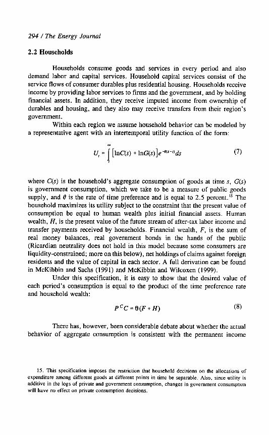
294 1 The Energy Journal

2.2 Households

Households consume goods and services in every period and also demand labor and capital services. Household capital services consist of the service flows of consumer durables plus residential housing. Households receive income by providing labor services to firms and the government, and by holding financial assets. In addition, they receive imputed income from ownership of durables and housing, and they also may receive transfers from their region’s government.

Within each region we assume household behavior can be modeled by a representative agent with an intertemporal utility function of the form:

U, = i [lnC(s) + lnC(s)]e48’“-od.s I

where C(s) is the household’s aggregate consumption of goods at time s, G(s) is government consumption, which we take to be a measure of public goods supply, and 8 is the rate of time preference and is equal to 2.5 percent. ” The household maximizes its utility subject to the constraint that the present value of consumption be equal to human wealth plus initial financial assets. Human wealth, H, is the present value of the future stream of after-tax labor income and transfer payments received by households. Financial wealth, F, is the sum of real money balances, real government bonds in the hands of the public (Ricardian neutrality does not hold in this model because some consumers are liquidity-constrained; more on this below), net holdings of claims against foreign residents and the value of capital in each sector. A full derivation can be found in McKibbin and Sachs (1991) and McKibbin and Wilcoxen (1999).

Under this specification, it is easy to show that the desired value of each period’s consumption is equal to the product of the time preference rate and household wealth:

PcC = O(F + H) 63)

There has, however, been considerable debate about whether the actual behavior of aggregate consumption is consistent with the permanent income

15. This specification imposes the restriction that household decisions on the allocations of expenditure among different goods at different points in time be separable. Also, since utility is additive in the logs of private and government consumption, changes in government consumption will have no effect on private consumption decisions.

Emission Trading, Capital Flows / 293

model.” Based on a wide range of empirical evidence in the macroeconomics literature (see Campbell and Mankiw, 1990), we impose that only a fraction /3 of all consumers choose their consumption to satisfy (8) and that the remainder consume based entirely on current after-tax income. It is important to emphasize that this is not a capricious or arbitrary assumption. Rather, we have deliberately chosen to depart from the theoretical elegance of (8) because we are evaluating real-world policy and it is absolutely clear from empirical data that (8) alone i:s not a satisfactory model of aggregate consumption. This is an important difference between our approach and many of the other models used to study climate change policy, where theoretical elegance has often been given greater importance than realism. Whenever we have had to choose between theoretical elegance and empirical relevance, we have chosen the latter.”

The empirical finding that pure permanent income models such as (8) are rejected by the data while nested functions that include a large weight on current income fit much better could be interpreted in various ways, including the presence of liquidity-constrained households or households with myopic expectations. For the purposes of this paper we will not adopt any particular explanation but simply take @ to be an exogenous constant.‘s This produces the final consumption function shown below:

PCC=@(F+H) +(I -P)-yZA’C (9)

where y is the marginal propensity to consume for the households consuming out of current income. Following McKibbin and Sachs (1991) we take /3 to be 0.3 in all regions.”

Within each period, the household allocates expenditure among goods and services in order to maximize C(s), its intratemporal utility index. In this version of the model we assume that C(s) may be represented by a nested CES function. At the top tier, consumption is composed of inputs of capital services, labor, energy and materials. Energy and materials, in turn, are CES aggregates

16. Some of the key papers in this debate are Hall (1978). Flavin (1981). Hayashi (1982), and Campbell and Mankiw (1990).

17. One complication of introducing a nested specification for consumption is that traditional welfare evaluations are difficult. However, we view it as far more important to take empirical facts

into account than for it to be easy to calculate equivalent variations. 18. One side effect of this specification is that it will prevent us from using equivalent variation

or other welfare measures derived from the expenditure function. Since the behavior of some of the

households is implicitly inconsistent with the previous equation, either because the households art: at corner solutions or for some other reason, aggregate behavior is inconsistent with the expenditure function derived from our utility function.

19. Our value is somewhat lower than Campbell and Mankiw’s estimate of 0.5.

296 / The Energy Journal

of inputs of individual goods. *’ The elasticities of substitution at the energy and materials tiers were estimated to be 0.8 and 1 .O, respectively. In this version of the model the top tier elasticity has been imposed to be unity.

Finally, the supply of household capital services is determined by consumers themselves who invest in household capital. We assume households choose the level of investment to maximize the present value of future service flows (taken to be proportional to the household capital stock), and that investment in household capital is subject to adjustment costs. In other words, the household investment decision is symmetrical with that of the firms.

2.3 Labor Market Equilibrium

We assume that labor is perfectly mobile among sectors within each region but is immobile between regions. Thus, within each region wages will be equal across sectors. The nominal wage is assumed to adjust slowly according to an overlapping contracts model (adjusted for different labor market institutional structures in different economies) where nominal wages are set based on current and expected inflation and on economy-wide labor demand relative to labor supply. In the long run labor supply, which is specified in terms of labor efficiency units, is given by the exogenous rate of population growth, but in the short run the hours worked can fluctuate depending on the demand for labor. For a given nominal wage, the demand for labor will determine short-run unemployment.

Relative to other general equilibrium models, this specification is unusual in allowing for involuntary unemployment. We adopt this approach because we are particularly interested in the transition dynamics of the world economy. As in the case of consumption behavior, we are deliberately choosing to make the model less theoretically elegant in order to better represent reality. The alternative of assuming that all economies are always at full employment, which might be fine for a long-run model, is clearly inappropriate during the first few years after a shock. Unemployment is very likely to be an important part of the adjustment of the global economy in the short to medium teml, and it is hard to justify assuming it away simply because it is inconvenient for theory. This is by no means a new idea, but despite its long and empirically robust standing in mainstream macroeconomics it is rarely implemented in a general equilibrium model.

20. This specification has the undesirable effect of imposing unitary income and price elasticities. There is abundant empirical evidence against this assumption and we intend to generalize it in future work.

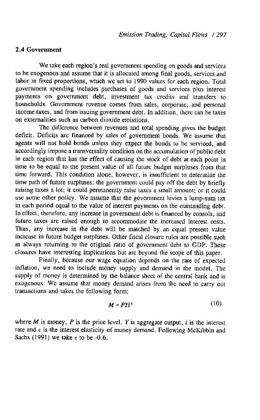
Emission Trading, Capital Flows / 297

2.4 Government

We take each region’s real government spending on goods and services to be exogenous and assume that it is allocated among final goods, services and labor in fixed proportions, which we set to 1990 values for each region. Total government spending includes purchases of goods and services plus interest payments on government debt, investment tax credits and transfers to households. Government revenue comes from sales, corporate, and personal income taxes, and from issuing government debt. In addition, there can be taxes on externalities such as carbon dioxide emissions.

The difference between revenues and total spending gives the budget deficit. Deficits are financed by sales of government bonds. We assume that agents will not hold bonds unless they expect the bonds to be serviced, and accordingly impose a transversality condition on the accumulation of public debt in each region that has the effect of causing the stock of debt at each point in time to be equal to the present value of all future budget surpluses from that time forward. This condition alone, however, is insufficient to determine the time path of future surpluses: the government could pay off the debt by briefly raising taxes a lot; it could permanently raise taxes a small amount; or it could use some other policy. We assume that the government levies a lump-sum tax in each period equal to the value of interest payments on the outstanding debt. In effect, therefore, any increase in government debt is financed by consols, and future taxes are raised enough to accommodate the increased interest costs. Thus, any increase in the debt will be matched by an equal present value increase in future budget surpluses. Other fiscal closure rules are possible such as always returning to the original ratio of government debt to GDP. These closures have interesting implications but are beyond the scope of this paper.

Finally, because our wage equation depends on the rate of expected inflation, we need to include money supply and demand in the model. The supply of money is determined by the balance sheet of the central bank and is exogenous. We assume that money demand arises from the need to carry out transactions and takes the following form:

M=PYi’ (10)

where M is money, P is the price level, Y is aggregate output, i is the interest rate and E is the interest elasticity of money demand. Following McKibbin and Sachs (1991) we take E to be -0.6.

298 / The Energy Journal

2.5 International Trade and Capital Asset Flows

The eight regions in the model are linked by flows of goods and assets. Each region may import each of the 12 goods from potentially all of the other seven regions. In terms of the way international trade data is often expressed, our model endogenously generates a set of twelve 8x8 bilateral trade matrices, one for each good. The values in these matrices are determined by the import demands generated within each region.

The trade balance in each economy is the result of intertemporal saving and investment decisions of households, firms and governments. Trade imbalances are financed by flows of assets between countries: countries with current account deficits have offsetting inflows of financial capital; countries with surpluses have matching capital outflows. Global net flows are constrained to be zero. We assume that asset markets are perfectly integrated and that financial capital is freely mobile. 2’ Under this assumption, expected returns on loans denominated in the currencies of the various regions must be equalized period to period according to a set of interest arbitrage relations of the following form:

(11)

where i, and ii are the interest rates in countries k and j, pk and ,pj are exogenous risk premiums demanded by investors (possibly zero), and El is the exchange rate between the two currencies. The risk premiums are calculated in the c:ourse of generating the model’s baseline and are generally held constant in simulations. Thus, if, in the base year, capital tended not to flow into a region with relatively high interest rates, it will not do so during the simulation. Finally, we also assume that OPEC chooses its foreign lending in order to maintain a desired ratio of income to wealth subject to a fixed exchange rate with the U.S. dollar.

Although financial capital is perfectly mobile, it is important to remember that physical capital is specific to sectors and regions and is hence immobile. The consequence of having mobile financial capital and immobile physical capital is that there can be windfall gains and losses to owners of physical capital. For example, if a shock adversely affects profits in a particular industry, the physical capital stock in that sector will initially be unaffected. Its value, however, will immediately drop by enough to bring the rate of return in

21. The mobility of international capital is a subject of considerable debate; see Gordon and

Bovenberg (1994) or Feldstein and Horioka (1980).

Emission Trading, Capital Flows / 299

that sector back into equilibrium with that in the rest of the economy. Because physical capital is subject to adjustment costs, the portion of any inflow of financial capital that is invested in physical capital will also be costly to shift once it is in place.22

2.6 Constructing the Base Case

To solve the model, we first normalize all quantity variables by the economy’s endowment of effective labor units. This means that in the steady state all real variables are constant in these units although the actual levels of the variables will be growing at the underlying rate of growth of population p1u.s productivity. Next, we must make base-case assumptions about the future path of the model’s exogenous variables in each region. In all regions we assume that the long-run real interest rate is 5 percent, tax rates are held at their 1990 levels and that fiscal spending is allocated according to 1990 shares. Population growth rates vary across regions as shown in Table 3.

Table 3. Population Growth Rates Region Population Growth Rate

United States 0.5

Japan 0.0 Australia 0.8

Other OECD 0.7 China 1.5

Former Soviet Union 0.5 Other developing countries 1.0

A crucial group of exogenous variables are productivity growth rates by sector and country. The baseline assumption in G-Cubed is that the pattern of technical change at the sector level is similar to the historical record for the United States (where data is available). In regions other than the United States,, however, the sector-level rates of technical change are scaled up or down in order to match the region’s observed rate of aggregate productivity growth. This approach attempts to capture the fact that the rate of technical change varies considerably across industries while reconciling it with regional differences in overall growth. 23 This is clearly a rough approximation; if appropriate data were

22. Financial inflows are not necessarily invested entirely in physical capital. Because of adjustment costs, part of any given inflow goes toward bidding up the stock market value of existing

assets. 23. For a more detailed discussion of the importance of accounting for heterogeneity in sector-

level productivity growth rates see Bagnoli, McKibbin and Wilcoxen (1996).

300 / The Energy Journal

available it would be better to estimate productivity growth for each sector in each region.

Given these assumptions, we solve for the model’s perfect-foresight equilibrium growth path over the period 1990-2050. This is a formidable task: the endogenous variables in each of the sixty periods number over 6,000 and include, among other things: the equilibrium prices and quantities of each good in each region, intermediate demands for each commodity by each industry in each region, asset prices by region and sector, regional interest rates, bilateral exchange rates, incomes, investment rates and capital stocks by industry and region, international flows of goods and assets, labor demanded in each industry in each region, wage rates, current and capital account balances, final demands by consumers in all regions, and government deftcits.24 At the solution, the budget constraints for all agents are satisfied, including both intratemporal and intertemporal constraints.

3. THE EFFECTS OF THE KYOTO PROTOCOL

We now explore the effects of the Kyoto Protocol in five different scenarios. In the first, the United States meets its commitment under the Protocol but no other regions take action. This scenario is presented not as a practical proposition but as a benchmark against which multilateral scenarios can be compared. In the remaining four scenarios we examine the effects of the Protocol when all regions meet their commitments but the extent of international emissions permit trading varies.

The model only accounts for emissions of carbon dioxide from fossil fuel combustion, while the Protocol specifies targets for all greenhouse gases in carbon equivalent units. 25 Accordingly, we make the simplifying assumption that reductions in fossil-related carbon dioxide emissions will be made in proportion to the reductions required in total GHGs, and set the carbon target accordingly. For instance, the Protocol specifies a 2008-2012 average annual target for the United States of 93 % of 1990 GHG emissions, which were approximately 1,600 million metric tons of carbon equivalents (MMTCe). The overall U.S.

24. Since the model is solved for a perfect-foresight equilibrium over a 60 year period, the

numerical complexity of the problem is on the order of 60 times what the single-period set of variables would suggest. We use software developed by McKibbin (1992) for solving large models

with rational expectations on a personal computer. 25. The carbon equivalent units are specified in terms of the lOO-year global warming potentials

(GWPs) of carbon: e.g. a ton of methane emissions are counted as the equivalent of 21 tons of carbon (or 21 times 3.67 tons of carbon dioxide), since a ton of methane contributes roughly the

same amount of radiative forcing over a century as 21 tons of carbon in the form of carbon dioxide. The permits are sold and used annually; we do not allow for banking or borrowing of emissions

between years within the 2008-2012 budget period although this is permitted under the Protocol.

Emission Trading, Capital Flows / 301

greenhouse gas target is therefore roughly 1,490 MMTCe. However, the share of fossil-related carbon dioxide in this target will depend on the marginal cost schedules for all of the gases, not just CO?. To simplify, we assume that the fossil CO, target will be 93% of 1990 fossil CO, emissions, or approximately 1247 MMTC. This approach ignores the likelihood that relatively inexpensive GHG reductions will be available from non-energy and non-carbon sources, but provides a useful (if conservative) first approximation of the costs of achieving the Kyoto targets.

In each scenario, Annex I regions hold annual auctions of the specified quantity of carbon emissions permits in each of the years from 2008 to 2020.26 The permits are required for the use of fossil fuels (coal, refined oil and natural gas) in proportion to the average carbon content per physical unit of each fuel. Revenues from the permit sales are assumed to be returned to households via a deficit-neutral lump-sum rebate. *’ The policy is announced in 2000 so that agents have nearly a decade to anticipate the policy and adapt to it.

Because G-Cubed represents each region as a competitive market economy in dynamic equilibrium with other regions, its representation of the former Soviet Bloc does not capture the shock associated with the institutional collapse of the formerly planned economy, the consequent dramatic decrease in emissions, or the fact that the region’s emissions are likely to be well below the limit mandated by the Kyoto Protocol a decade from now. However, except for the reunification of Germany and the extensive development of parts of Eastern Europe, and the fact that crude oil and gas exports have continued, much of the region has remained substantially independent of the global economy since 1990; and it seems unlikely that international trade and capital flows between thi,s region and the rest of the world will be large enough over the next decade to be a first-order concern. Since the region has relatively little interaction with the rest of the world in the model (as a consequence of the calibration that rendem it in equilibrium in the base year), we treat the former Soviet Bloc exogenously in this analysis. (However, we account for income flows from the international sale of permits.) Taking these observations into account, in each of these scenarios, emission reductions in the former Soviet Bloc (encompassing the former Soviet Union and Eastern Europe) are specified exogenously, drawing on mitigation supply curves constructed mainly from the results of the Pacific

26. Beyond 2020 the supply of permits is allowed to increase at such a rate as to leave the real

permit price at its 2020 value. 27. The rebate is chosen to leave the deficit unchanged. It is not necessarily equal to the revenue

raised by permit sales because other changes in the economy may raise or lower tax revenue. This formulation is not equivalent to free distribution of permits ( “grandfathering”) - that would be

represented in a similar fashion in the model but the rebate would be set to the gross revenue raised by permit sales. Other uses of the revenue, such as cutting income taxes or reducing the fiscal

deficit, would change some of the results substantially.

302 / The Energy Journal

Northwest National Laboratory’s Second Generation Model (SGM). Furthermore, since former Soviet Bloc GHG emissions are expected to remain well below the targets mandated by the Kyoto Protocol, our exogenously specified supply curve for this region includes mitigation of greenhouse gases other than carbon. Thus the analysis assumes a former Soviet Bloc mitigation supply curve with roughly 300 MMTC of “paper tons” (emission allowances that would otherwise remain unused) available in 2010, declining to about 220 MMTC in 2015 and 140 MMTC in 2020, and roughly an additional 220 MMTC available at a cost of less than $SO/MTC ($95).28

Taken together, the G-Cubed baseline and additional simplifying assumptions lead to reduction requirements in 2010 of 526 million metric tons of carbon (MMTC) for the United States, 67 MMTC for Japan, 48 MMTC for Australia, and 461 MMTC for the Other OECD countries; with approximately 27% of those reductions potentially offset by paper tons from the former !joviet Bloc.

We first present a scenario with unilateral U.S. commitment to meeting its Kyoto target, with no action undertaken by other regions. The remaining four scenarios involve the attainment of Annex I targets specified in the Protocol with:

1. no international permit trading between regions;

2. international permit trading permitted among all Annex I countries;

3. international permit trading permitted within the Other OECD region, and among the other Annex I regions (the U.S., Japan, Australia, and the former Soviet Bloc), but prohibited between the Other OECD region and the rest of the AMeX I countries - the so-called “double umbrella” or “double bubble;” and

4. global permit trading; that is, the developing regions accept an emissions allocation consistent with their modeled baselines, and allow sales from their permit allocations to Annex I countries.

Figures 1-16 at the back of the paper contain graphs illustrating the most important impacts of the Protocol under different assumptions about the extent of international permit trading. The variables illustrated include regional emission permit prices; emission reductions; international permit sales and

28. The SGM numbers, in turn, are based partly on the results of a joint project between the OECD. the World Bank and the Office of Policy Development at US EPA (see OECD document

OECD/GD(97)154 “Environmental Implications of Energy and Transport Subsidies” or Chapter 6 of OECD publication “Reforming Energy and Transport Subsidies.” Our estimates ignore a

projected - 140 MMTCe of other GHG upaper tons” available in 2010.

Emission Trading, Capital Flows / 303

purchases; impacts on OPEC oil prices, sales and revenues; changes i.n international investment and exchange rates; and changes in regions’ exports, gross domestic products and gross national products.

Since neither the model’s behavioral parameters nor the future values of tax rates, productivity, or other exogenous variables can be known with complete certainty, these numbers should be regarded as point estimates within a range of possible outcomes. They do, however, give a clear indication of the mechanisms that determine how the economy responds to climate change policy. Section 5 will examine the sensitivity of the results to key parameters.

3.1 Unilateral Emissions Stabilization by the United States

Key macroeconomic results for the United States in the case of unilateral action by the United States are shown in Table 4. The figures shown are either percent deviations from a “business as usual” baseline or as changes from the baseline in units of 1995 dollars. Results are presented for a selection of years, although the model itself is annual.

Table 4. Aggregate Effects of Unilateral U.S. Action 2005 2010 2015 2020

Permit price ($95) __ $80 $85 $94 Carbon emissions 0.6% -29.6% -35.7% -41.5% Coal consumption 0.1% -48.0% -56.2% -64.5% Oil consumption 1.0% -18.8% -22.9% -26.7% Gas consumption 0.6% -13.9% -19.2% -23.0%

GDP 0.2% -0.7% -0.8% -0.7% Consumption 0.7% -0.4% -0.2% 0.1%

Investment 1.0% -1.1% -0.7% -0.5%

Exchange rate 3.5% 3.5% 4.6% 5.4%

Exports -2.8% -3.3% -4.5% -5.4% Imports -0.7% -3.7% -4.2% -4.7%

Net foreign assets (Bil. $95) $77 -$I24 $73 -$21 GNP 0.1% -0.7% -0.8% -0.7%

In order to achieve the Kyoto target, emissions in the United States would need to drop by about 30 percent relative to the baseline in 2010 and by 42 percent in 2020.29 The resulting price of carbon emissions permits would be

29. Some of the emissions eliminated within the United States - roughly 10% in 2010 - are offset by increases in emissions elsewhere. Initially, over half of this “leakage” is due to the fact

that other countries buy and burn the oil that the U.S. stops importing. This effect diminishes over time: by 2020 about two-thirds of the leakage is due to higher energy demand resulting from greater

economic activity.

304 / The Energy Journal

$80 per metric ton ($95) in 2010 rising to $94 per ton in 2020.M Most of the drop in emissions comes about through a decline in coal consumption as total energy use drops and the fuel mix shifts toward natural gas, the least carbon- intensive fuel. This is reflected in the industry-level results shown in Table 5: the after-tax price of coal rises by more than 235 % relative to its baseline level, while coal output declines by 40% in 2010 and by 56% in 2020. Output of petroleum products falls by 16% in 2010 and 24% in 2020; while natural1 gas output falls by 14% in 2010 and 23 % in 2020. The crude oil and gas sector is somewhat less affected, suggesting that declines in demand fall disproportionately on imports: and domestic output declines by 10% to 20% over the period.

Table 5. Industry Effects of Unilateral U.S. Action 2005 2010 2020

Price QV Price Qty Price Qty Energy Industries

Electric utilities -0.1% 0.4% 7.2% -6.2% 12.6% -9.5 %

Gas utilities -0.2% 0.4% 14.3% -13.6% 26.0% -22.7 %

Petroleum refining -0.5% 0.4% 19.6% -16.2% 27.6% -24.4%

Coal mining 0.1% -0.1% 235.4% -40.3% 375.6% -56.0%

Oil and gas extraction -0.2% 0.0% -8.1% -10.4% -7.0% -1!>.7%

Other Sectors Other mining -0.4% -0.3% 0.7% -2.6% 0.7% -3.3%

Agriculture -0.3% 0.2% -0.2% -1.2% -0.7% -0.8%

Forestry and wood -0.4% 0.1% -0.4% -1.2% -0.9% -1.0% Durable goods -0.6% -0.2% -0.6% -1.4% -1.2% -L.4%

Nondurables -0.3% 0.3% -0.5% -1.0% -0.9% -0.6% Transportation -0.2% 0.3% -0.1% -1.6% -0.6% -1.3%

Services -0.2% 0.4% -0.9% -0.2% -1.4% 0.5%

Outside the energy industries, prices and output are affected very little. The only noteworthy result is that investment rises by about one percent during the period before the policy is implemented (2000-2007). This stems fro:m the fact that the demand for services increases slightly when households and firms substitute away from energy. As a result, investment by the service industry increases as well, in anticipation of the increase in demand. The increase in investment is financed by an inflow of foreign capital, as aggregate national savings decline slightly. The capital inflow causes the exchange rate to appreciate by about 3.5% over that period. The exchange rate appreciation

30. Throughout the paper, carbon will be measured in metric tons (tonnes) and prices will be

in 1995 U.S. dollars.

Emission Trading, Capital Flows / 305

reduces exports, primarily of durable goods, and enables the capital inflow 1.0 be reflected in a worsening of the current account.

The international effects of the U.S. policy vary across regions. Mo:st Annex I countries experience mild decreases in GDP on the order of -0.1% , mild exchange rate depreciation, and increases in their net investment positions. China’s exports rise by 4-6 % in the early years of the policy. Other developing countries receive minor capital inflows after 2010, experience very slight exchange rate appreciation and end up with slightly higher GDP, but also have lower production and exports of durable goods due to the change in exchange rates.

3.2 Annex I Targets Met Without International Permit Trading

In the second scenario, all Annex I regions meet their commitments under the Protocol. Each region is restricted to use of their allocated emissions,; the permits can be traded within regions but not from one region to another.“’ This simulation allows us to measure the heterogeneity of the Annex I regions. Differences in baseline emissions growth, endowments of fossil fuels, reliance on fossil fuels for energy generation and initial fossil fuel prices mean that the regions face substantially different costs of achieving stabilization. This will b’e reflected in the pattern of permit prices (which will indicate the cost of stabilization at the margin) and GDP losses across regions.

The results for the Annex I policy without international permit trading are shown in Table 6. Key results are presented for 2005, 2010 and 2020 for the four OECD regions in the model (United States, Japan, Australia and other OECD, hereafter referred to as ROECD), as well as China and the less developed countries (LDCs).

The effects of the policy differ substantially across the regions: in 2010, permit prices per metric ton of carbon range from a low of $87 in the US to a high of $261 in the ROECD region. These results show that both marginal and average costs of abating carbon emissions differ substantially across countries. Since, by assumption, all regions have access to the same technologies, the differences in permit prices reflect differences in mitigation opportunities: regions which have relatively low baseline carbon emissions per unit of output, and are thus relatively sparing in their use of fossil fuels, have relatively fewer options for reducing emissions further. The differences among regions stem in part from differences in the fuel mix but also depend on the availability of alternative fuels and the extent to which baseline emissions rise above the

3 1. Even though there is no trading between regions, trading is implicitly allowed between the:

countries within a region. In particular, the “Other OECD” region lumps together the Europearl Union, Canada and New Zealand, so trading is implicitly allowed between these countries.

304 / The Energy Journal

Table 6. Annex I Commitments Without International Permit Trading

United States Japan Australia

Other OECD China LDC’S

2w5

Permit price ($95)

Carbon emissions

Coal consumption

Oil consumption

Gas consumption

GDP

Investment

Exports

Exchange rate

Net foreign assets (Bil. $95)

GNP

2010

Permit price ($95)

Carbon emissions

Coal consumption

Oil consumption

Gas consumption

GDP

Investment

Exports

Exchange rate

Net foreign assets (Bil. $95)

GNP

2020

Permit price ($95)

Carbon emissions

Coal consumption

Oil consumption

Gas consumption

GDP

Investment

Exports

Exchange rate

Net foreign assets (Bil. $95)

GNP

__ _- -_ -_ 1.9% -2.4% 4.1% -1.8%

0.7% -0.8% 0.0% -0.6% 3.1% -3.3% -0.1% -2.4%

1.9% -0.7% 0.0% -1.5%

0.4% -0.3% 0.1% -0.2%

2.9% -0.5% .6% -2.0%

-8.6% 3.4% -0.3% 7.6%

10.8% -6.5% 0.7% -12.9%

$244 -$49 $16 $184

0.3% -0.3% 0.1% 0.0%

$87 $112

-29.6% -20.6%

-51.9% 43.6%

-15.6% -14.2%

-12.6% -4.6%

-0.4% -0.6%

0.8% -1.3%

-10.7% 1.2%

10.5% -5.8%

-$451 -$55

-0.6% -0.5%

$181 $261

-31.5% -32.7%

-55.1% 49.6%

-18.4% -29.5 %

-19.4% -18.2%

-1.8% -1.5%

0.2% -3.8%

4.5% 5.8%

2.1% -13.5%

329 $370

-1.6% -1.3%

$101 $162

-35.7% -27.6%

-59.7% -56.5%

-19.8% -19.6%

-17.9% -6.7%

-0.5% -0.7%

0.9% -1.4%

-12.2% 1.3%

11.0% --7 .o %

-$489 -5104

-0.7% -0.7%

$230 $315

44.1% -39.1%

-64.7% -58.4%

-21.2% -35.1%

-23.9% -24.0%

1.8% -1.6%

0.3% -3.5%

-6.7% 4.1%

5.0% -13.0%

$48 $490

-1.5% -1.3%

- _- -0.9% 1.7%

-0.8% am.295

-1 .O% 2.6%

-1.5% 1.8%

-0.3% 0.3%

-1 .O% 2.7%

17.2% -21.5%

-4.7% 15’.4%

$20 $78

-0.2% (1.5%

__ __

-0.7% 3.3%

-0.8% 0.3%

-0.4% 5 ,I %

-1.2% 3.4%

-0.2% 0.4%

-0.4% >!.9%

.I% -25.1%

-4.7% l!i.9%

$34 $141

-0.1% 0.7%

-- --

-0.7% 3.1%

-0.7% 0.2%

-0.4% 4.8 %

-1.1% 3.4%

-0.2% 0.4%

-0.7% 2.5%

4.7% -20.7%

-5.0% 15.7%

$43 $184

-0.1% 0.7%

Emission Trading, Capital Flows / 307

stabilization target. Thus Australia, which has relatively few substitution possibilities and a high baseline emission trajectory (due to fairly high population growth and strong productivity growth) finds it costly to reach the 1990 stabilization target. The United States, with low energy prices, a high reliance on coal and abundant natural gas, finds it relatively cheap to change thie composition of energy inputs.

Table 6 shows results for both GDP and GNP. The GDP results indicate the extent of international shifts in production but are a poor measure of national welfare. The GNP figures are a better (although far from perfect) welfare measure because GNP reflects the total income of the residents of a country and includes net income transfers to and from factors of production located abroad. Savers in countries with high costs of abatement shift some of their financial capital overseas, maintaining rates of return that otherwise would be much lower. The ordering of countries by GNP loss is the same as that by GDP loss’but the dispersion of GNP losses is smaller because of the ability of agents to shift capital into higher return activities abroad.

The effect on GDP follows a pattern similar to that of mitigation costs: GDP in 2010 falls slightly in the U.S. and Japan while in Australia and ROECD it falls by 1.8% and lS%, respectively. Comparing this simulation with the previous one shows that the United States is better off under the Annex I policy than it is when it reduces emissions on its own: in 2010, U.S. GDP is 0.4% below its baseline value while under the unilateral policy it would have fallen by 0.7%. One reason for the lower costs is that U.S. exports are more competitive relative to those from other OECD economies when more countries impose carbon constraints. Another reason for the reduction in GDP loss lies in the fact that the United States has substantially lower marginal costs of abating carbon emissions than other OECD economies. Stabilizing emissions require:s a smaller price increase in the U.S. than it does in other countries. Also the policy directly reduces rates of return in each economy, and relatively more so in sectors that are relative carbon intensive. Lower abatement costs in the U.S. mean that rates of return to capital in the U.S. fall less than in other OECD countries. This shift in rates of return induces investors to shift their portfolios toward U.S. assets, leading to an increase in U.S. investment. Thus, production tends to fall less in the U.S. than it does in other OECD economies. The effect is particularly apparent in the years immediately before the policy takes effect: U.S. investment is three percent above baseline in 2005. In addition, the U.S. also benefits from lower world oil prices as Annex I oil demand falls. The boost in investment and lower oil prices both tend to raise energy demand and cause permit prices to rise relative to the unilateral stabilization scenario - from $80 to $87 in 2010 and from $94 to $101 in 2020. U.S. income, as measured by GNP, rises slightly in the period before the policy takes effect and then falls by 050.6% in 2010-2020.

308 / i%e Energy Journal

Examining the effects of the policy on different regions raises a number of interesting results that tend to be ignored in popular discussion of the impacts of emission permit trading. Those regions that have the largest rel.ative abatement costs, such as Australia and ROECD, have large capital outfIows because of the fall in the rate of return to capital in high abatement cost countries. ROECD, which faces the greatest cost of stabilizing emissions’, has a large capital outflow, accumulating to roughly $490 billion ($95) by :!020. Most of this capital outflow goes to the United States, and also to some developing countries, which are not controlling emissions at all. Capital flows to developing countries are limited by adjustment costs, however: it is expensive for a region with a relatively small capital stock to absorb a large flow of new capital. x It is relatively cheap for a large country such as the United States to absorb capital for the same reason: the costs of a given absolute change in a particular capital stock decrease with the size of the stock. Thus, relatively small capital inflows can exhaust arbitrage opportunities in developing economies. This is an important insight because it contradicts the popular perception. that greenhouse abatement policies will lead to wholesale migration of industries from developed countries to non-abating developing countries. Our results show this is quite unlikely; moreover, most of the financial capital reallocation is between OECD economies.

Capital flows cause the exchange rates of countries receiving financial capital, such as the United States and developing countries, to appreciate and cause the Japanese and ROECD currencies to depreciate. The dollar appreciates by 25 % relative to the ROECD currencies, but depreciates by 5 % relative to the currency of developing countries. The ROECD currency depreciates by 30% relative to the developing countries. These changes lead directly to changes in export patterns. By 2010, ROECD exports of durable goods increase by about 6% over baseline while U.S. exports of durables fall by 11% . At the same time, capital flows cause Australian and ROECD GNP to fall by slightly less than GDP, since these countries’ increased foreign investments offset some of the lost income from domestic production.

Overall, the effect of achieving the Kyoto targets is to reduce GDP in countries with high abatement costs, cause an outflow of capital, depreciate their exchange rates and stimulate exports. The effect on low-cost countries is the opposite: capital inflows tend to raise GDP by reducing real interest rates and stimulating domestic demand in the short run, and by raising the capital stock

32. In apparent contradiction to this statement, the results in Table 6 show an apparent net capital ourflow from the LDCs rather than a capital inflow. The improvement in the LDCs’ net

foreign asset position is due to the fact that their real exchange rate appreciation leads to a decrease

in the dollar value of their outstanding debt. The decrease in the value of outstanding debt outweighs the policy-induced capital inflow, leading to an apparent capital outflow.

Emission Trading, Capital Flows / 309

in the medium to long run. Capital flows also appreciate the exchange rate and diminish exports.

The effect of the Protocol on developing countries is particularly interesting. In the case of the LDCs, the exchange rate appreciation has multiple costs and benefits. Exports become less competitive but imports become cheaper and the dollar value of LDC international debt falls dramatically, leading to a net improvement in the LDCs’ net international investment position in spite of significant capital inflows, as mentioned above. LDC gross domestic produ.ct rises by 3.0% in 2010, and gross national product rises by 0.7%. Clearly, the absence of commitments under the Kyoto Protocol confers significant benefits to LDCs through international policy transmission.

In addition, the decline in Annex I oil demand leads to a 10% decline in OPEC oil exports and a 17% decline in world oil prices. The decline in oil prices benefits the LDCs, whose increased oil consumption causes an increase in LDC carbon emissions equivalent to approximately 6% of Annex I emission reductions. This 6% “leakage effect, ” however, does not translate into increased LDC exports of carbon-intensive durable goods, which are significantly dampened by the impact of capital inflows on LDC exchange rates. Instead it is the region most adversely affected by mitigation policy - ROECD - which experiences an increase in exports. It may seem surprising that expolrt performance should improve in the country most hurt by climate change policy but it is simply the result of consistent international accounting: countries which experience capital outflows must experience trade surpluses, while countries which experience capital inflows must experience trade deficits.

3.3 Annex I International Permit Trading

The third scenario is identical to the second except that we allow international trading in emissions permits among Annex I countries. The effect of allowing trading is twofold. First, arbitrage will cause the price of a permit to be equal in all Annex I countries. This will ensure that marginal costs of carbon abatement will be equal across countries and that AMcX I emission reductions will be achieved at minimum cost. Countries with relatively low abatement costs will sell permits and abate more than in the previous scenario; countries with high costs will buy permits and undertake less domestic abatement.

In addition, trading makes possible a relaxation of the overall constraint during the 2008-2012 period because the emissions of one Annex I region, the former Soviet Bloc, are likely to be below the limit specified under the Protocol. The relaxation of the constraint means that actual emission reductions under the Protocol will be considerably lower - perhaps as much as 40% lower - with international permit trading than without it, at least during the first budget

310 / The Energy Journal

period. The particular circumstances of the former Soviet Bloc thus make it difficult to determine the pure gains from permit trading, independent of the relaxation of the constraint.33

Results for this scenario are shown in Table 7. In contrast to independent mitigation, international permit trading leads to a uniform permit price throughout the Annex I that rises from about $61 per ton in 2010 to !§109 per ton in 2020. These prices, lower than any OECD region’s marginal mitigation cost in the absence of international permit trading, lead to lower increases in fossil fuel prices and considerably lower domestic reductions than in the previous case since reductions can be avoided by purchasing allowances from the former Soviet Bloc. At the 2010 permit price of $61 per ton, the former Soviet Bloc sells not only its excess allowances, 293 MMTC, but also reduces emissions to sell an additional 253 MMTC of allowances. Thus the OECD countries purchase nearly 550 MMTC of emission allowances from the former Soviet Bloc rather than undertake domestic reductions, thereby dramatically reducing the cost of meeting their commitments. These purchases particularly benefit ROECD, which uses internationally purchased allowances to meet 72 % of its obligations and thus achieves a 77 % reduction in its marginal abatement costs. The United States and Australia use internationally purchased allowances to meet 29% and 65% of their respective obligations, and benefit from 30% and 66% reductions in marginal abatement costs. International purchases of former Soviet Bloc’s allowance amount to nearly $33 billion ($95) in 2010 and rise to nearly $54 billion by 2020.

Interestingly, as the regional economies continue to grow after 2,010, the demand for emission allowances increases while the former Soviet Bloc’s willingness to supply them declines. As a consequence, international permit prices rise continuously after 2010, and by 2020, prices rise to $109 per ton. At this price, the United States becomes a net permit seller, supplying about 83 MMTC of allowances to Japan, Australia and ROECD at a total cost of nearly $9 billion, and undertaking an equivalent quantity of domestic emission reductions in excess of its international commitment.

The economic impacts of the Protocol are generally significantly reduced by both the equalization of marginal mitigation costs and permit prices under an international permit trading regime, as well as by the reduction in overall mitigation due to the sale of the former Soviet Bloc’s excess allowances. Japanese GDP costs in 2010 are cut from 0.6% to 0.4%, Australia’s from 1.8% to 0.7%, and ROECD’s from 1.5% to 0.6%. Permit trading has little effect on non-participants: results for China and the developing countries are very similar to the no-trading case.

33. Previous analysis using the G-Cubed model indicates that the pure gains from trade are on the order of 20 to 25 percent in the case OECD international permit trading. See McKibbin,

Shackleton and Wilcoxen (1998).

Emission Trading, Capital Flows / 3,!1

Table 7. Annex I Commitments With International Permit Trading

United States Japan Australia

Other OECD China LDC’s

2w5

Permit price ($95)

Annual permit sales (Bil $95)

Carbon emissions

Coal consumption

Oil consumption

Gas consumption

GDP

Investment

Exports

Exchange rate

Net foreign assets (Bil. $95)

GNP

2010

Permit price ($95)

Annual permit sales (Bil $95)

Carbon emissions

Coal consumption

Oil consumption

Gas consumption

GDP

Investment

Exports

Exchange rate

Net foreign assets (Bil. $95)

GNP

2020

Permit price ($95)

Annual permit sales (Bil $95)

Carbon emissions

Coal consumption

Oil consumption

Gas consumption

GDP

Investment

Exports

Exchange rate

Net foreign assets (Bil. $95)

GNP

--

1.4% -2.7%

0.6% -I .O%

2.3% -3.7%

1.5% -0.7%

0.3% -0.2%

2.3% -0.6%

-6.9% 3.6%

8.9% -7.1%

-$I39 -$28

0.2% -0.2%

$61

-$9.4

-20.9%

-36.0%

-11.8%

-8.8%

-0.2%

0.8%

-7.6%

8.5%

-5304

-0.5%

$61

-$1.5

-13.0%

-24.2%

-10.4%

-2.9%

-0.4%

-1.0%

2.5%

-6.7%

-$12

-0.4%

$109

$9.0

-33.3%

-54.5%

-19.9%

-16.6%

-0.5%

0.5%

-9.1%

9.1%

-$390

-0.7%

$109

-$4.4

-18.6%

-35.4%

-14.3%

4.5%

-0.5%

-1.1%

2.2%

-7.1%

-$22

-0.5%

__ __

-0.3%

0.3%

-0.7%

-0.8%

0.0%

-0.3%

-1.1%

-0.6%

$22 0.0%

$61

-$1.9

-13.0%

-18.7%

-6.7%

-6.8%

-0.7%

0.3%

-0.8%

-0.4%

$36 -0.8%

$109

-54.6

-18.4%

-26.8%

-9.2%

-10.0%

-0.9%

-0.2%

-1.9%

0.5%

$47 -1.1%

-- --

-2.1%

-0.6%

-2.9%

-1.7%

-0.2%

-2.2%

8.9%

-14.4%

$242

0.1%

$61

$20.3

-9.1%

-12.1%

-9.0%

-5.6%

-0.6%

-2.4%

8.0%

-14.7%

$476

-0.6%

$109

-53.7

-13.0%

-17.8%

-12.3%

-8.3%

-0.7%

-2.4%

7.3%

-15.0%

$614

-0.7%

-_ -- __ --

-0.6% 1.8%

-0.6% 0.2%

-0.8% 2.7%

-1.2% 1.9%

-0.2% 0.3%

-0.6% 3.0%

11.5% -22.8%

-2.4% 16.6%

$16 $67

-0.2% 0.5%

-_

-- -_

-0.5% 2.6%

-0.5% 0.4%

-0.4% 4.0%

-0.7% 2.9%

-0.1% 0.4%

4.3% 2.8%

5.7% -23.7%

-2.1% 17.5%

S29 $121

-0.1% 0.7%

__ -_

-- __

-0.4% 2.7%

-0.4% 0.4%

-0.3% 4.2%

-0.6% 3.1%

-0.1% 0.5%

-0.4% 2.7%

2.7% -20.2%

-2.1% 17.9%

$40 $165

0.0% 0.7%

312 / The Energy Journal

Exchange rate changes are similar in sign but generally larger in magnitude than under the no-trading scenario. The Japanese and ROECD currencies, in particular, depreciate somewhat more, while the currency of the developing region has a larger appreciation. This happens because the countries buying permits must ultimately pay for them with additional exports, either immediately or in the future. Thus, the purchasing country’s current account must eventually move toward surplus by an amount corresponding to the value of the permits.” The changes in real exchange rates are necessary to accommodate the changes in trade balances.

Permit trading reduces the OECD’s overall GNP costs of meeting their commitments under the Kyoto Protocol by about 63% in 2010, from $272 billion to $128 billion, or by $143 billion. 3s On the basis of previous analysis using G-Cubed of OECD permit trading without former Soviet Bloc participation, we estimate that roughly 60% of these benefits are due to relaxation of the constraint, while the other 40% constitute true gains from trade. If we also take into account the spillover effects on China and the LDCs, the world GNP costs of meeting Kyoto commitments are cut by 52 % from $24 1 billion to $115 billion, or by $125 billion. These 2010 GNP gains are very unequally dispersed, however: the U.S.36 gains only $14 billion, and Australia and Japan only $5 billion each; while the ROECD region gains $102 billion. Chinese and LDC GNPs are almost completely unaffected.

3.3 The “Double Umbrella”

The fourth scenario, in which the ROECD countries engage in exclusive permit trading and the rest of the Annex I countries engage in permit trading independently of the ROECD countries, is contained in Table 8. The key difference between this scenario and full Annex I trading is that ROECD no longer buys 327 million tonnes worth of permits from the former Soviet 1310~. As a result, the effects on ROECD look much like the no-trading case and abatement costs in the rest of Annex I fall substantially. Permit prices fall to $32 in 2010 and $71 in 2020. The U.S. benefits in two ways: from lower permit prices and also from relatively large capital flows from ROECD to the U.S. (because high energy prices reduce returns to capital in ROECD). As a result, U.S. GDP remains at its baseline level in 2010 and falls by only 0.2% in 2020.

34. This shifting of resources between economies due to changes in property rights, known in international economics as the “transfer problem, n is the subject of a large literature.

35. We do not provide estimates of GNP effects for the former Soviet Bloc because of the difficulties mentioned previously.

36. The U.S. experiences a small GDP loss from trading in 2010 due to business cycle ,effects stemming from our assumption that wages adjust slowly: the sharp increase in U.S. energy prices under the trading scenario temporarily reduces labor demand relative to the no-trading case.

Emission Trading, Capital Flows / 313

Table 8. Annex I Commitments With “Double Umbrella”

United States

- Other

Japan Australia OECD China LDC’s

2005

Permit price ($95)

Annual permit sales (Bil $95)

Carbon emissions

Coal consumption

Oil consumption

Gas consumption

GDP

Investment

Exports

Exchange rate

Net foreign assets (Bil. $95)

GNP

2010 Permit price ($95)

Annual permit sales (Bil $95)

Carbon emissions

Coal consumption

Oil consumption

Gas consumption

GDP

Investment

Exports

Exchange rate

Net foreign assets (Bil. $95)

GNP

2020

Permit price ($95)

Annual permit sales (Bil $95)

Carbon emissions

Coal consumption

Oil consumption

Gas consumption

GDP

Investment

Exports

Exchange rate

Net foreign assets (Bil. $95) GNP

__ __ --

1.2% -2.0%

0.5% -0.7%

1.9% -2.9%

1.2% -0.6%

0.3% -0.2%

1.8% -0.5%

-5.4% 3.2%

6.9% -5.7%

-$137 -$18

0.2% -0.2%

$32

-$11.4

-9.2%

-18.2%

-3.3%

-3.1%

-0.0%

1.3%

-6.9%

6.6%

-$281

-0.2%

$71 -$19.8

-18.6%

-32.3%

-9.6%

-8.5%

-0.2%

0.7%

-7.7%

6.2%

-8363

-0.5%

_-

$32

-$1.6

-5.7%

-11.9%

4.1%

-1.5%

4.3%

-0.6%

1.9%

-5.4%

-$l -0.2%

$71

-.$5.7

-10.4%

-21.3%

-7.3%

-2.6%

-0.3%

-0.8%

1.7%

-6.0%

-$15

-0.3%

--

-0.3%

0.0%

-0.7%

-0.4%

-0.1%

-0.5%

1.1%

-1.3%

$20 0.0%

$32

-$1.3

-6.7%

-9.6%

-3.2%

-3.6%

-0.4%

-0.2%

-0.5%

-1.3%

$32 -0.5%

$71 -$3.9

-11.0%

-16.1%

-5.3%

-6.1%

-0.6%

-0.3%

-1.2%

-1.3%

$41

__ __

-1.3%

-0.5%

-1.8%

-1.1%

-0.1%

-1.4%

5.3%

-9.1%

$139

0.0%

$263 __

-32.7%

49.8%

-29.5 %

-18.1%

-1.4%

-3.4%

4.3%

-9.3%

$298

-1.3%

$318 __

-39.9%

-60.0%

-35.7%

-24.2%

-1.5%

-3.1%

2.4%

-8.4%

$440 -0.7% -1.3%

-_ -- __

-0.5% 1.1%

-0.5% 0.1%

-0.6% 1.8%

-0.9% 1.3%

-0.2% 0.2%

-0.6% 1.9%

10.5% -14.8%

-2.7% 10.5%

$13 $53 -0.1% 0.3%

__ --

__ --

-0.4% 2.2%

-0.4% 0.3%

-0.3% 3.4%

-0.7% 2.2%

-0.1% 0.3%

-0.2% 2.0%

5.3% -16.7%

-2.5% 11.0%

$23 $103

-0.1% 0.5%

__ --

__ __

-0.3% 2.2%

-0.4% 0.3%

-0.2% 3.5%

-0.4% 2.4%

-0.1% 0.3%

-0.3% 1.8%

2.7% -14.5%

-2.8% 10.7%

$29 $141

0.0% 0.5%

314 / The Energy Journal

It is interesting to note that the ROECD region is slightly better off in the initial years of the double umbrella simulation than under Annex I trading. In 2005, GDP and GNP are slightly higher (that is, they fall slightly less), fuel consumption and investment are both higher, and capital outflows are smaller. The reason for this is somewhat subtle. When the ROECD region adopts carbon controls under either simulation, one effect is to shift some investment to other regions, especially the United States. Under Annex I trading, other countries are also subject to relatively tight carbon controls and are attempting to do the same thing. This causes the U.S. dollar to appreciate substantially, rising by 23% relative to the ROECD currency in 2005. Under the double umbrella, however, carbon controls are much looser in regions other than the ROECD so there is less competition to shift capital into the United States. There is less appreciation of the dollar, which rises by only 16% relative to the ROECD currency. This makes it less expensive for ROECD investors to convert part of their portfsolios to U.S. investments.

This is entirely a short run effect, however. Once the policy is actually in force, the ROECD is hurt more by high abatement costs under the double umbrella than it gains from changes in the terms of trade. By 2010, RO:ECD GDP and GNP are about 0.8% below what they would have been under AMeX

I trading.

3.4 Global Trading

In the final scenario, we assume that the non-Annex I developing countries agree to distribute annual quantities of domestic emission permits consistent with their baseline emissions, and to allow these permits to be traded on international markets.37 These results are contained in Table 9. The consequence of bringing developing countries into the trading regime is that Annex I countries can purchase emission allowances from owners in developing countries. These owners, in turn, would be willing to sell allowances to Annex I buyers only if the allowance price exceeded the marginal cost to the owners of undertaking emission reductions within the developing countries. The market process would thus lead to least-cost reductions on a global scale: emission reductions would be taken wherever they are cheapest, but Annex I countries would pay for them.

37. As with the Annex I regions, we assume that developing regions sell a fixed number of

permits at auction on an annual basis, and return the revenues to households as a lump-sum payment.

Emission Trading, Capital Flows / 315

Table 9. Annex I Commitments With Global Permit Trading

United States

Other Japan Australia OECD China LDC’s

- 2005

Permit price ($95)

Annual permit sales (Bil $95)

Carbon emissions

Coal consumption

Oil consumption

Gas consumption

GDP

Investment

Exports

Exchange rate

Net foreign assets (Bil. $95)

GNP

2010

Permit price ($9.5)

Annual permit sales (Bil $95)

Carbon emissions

Coal consumption

Oil consumption

Gas consumption

GDP

Investment

Exports

Exchange rate

Net foreign assets (Bil. $95)

GNP

2020

Permit price ($95)

Annual permit sales (Bil $95)

Carbon emissions

Coal consumption

Oil consumption

Gas consumption

GDP

Investment

Exports

Exchange rate

Net foreign assets (Bil. $95) GNP

-_ __ __ _-

0.6% -1.2%

0.2% -0.3%

1.0% -1.7%

0.7% -0.3%

0.1% -0.1%

1.0% -0.2%

-2.9% 1.5%

3.7% -3.1%

-$54 48 0.1% -0.1%

$23

-$8.9

-7.4%

-13.3%

-3.6%

-3.0%

-0.1%

0.4%

-3.4%

3.6%

-$115

-0.2%

$23

-$1.2

-4.2%

-8.9%

-2.8%

-1.0%

-0.1%

-0.3%

0.8%

-2.8%

-$2 -0.1%

$37 -$21.1

-11.4%

-19.2%

-6.2%

-5.5%

-0.1%

0.3%

-3.9%

3.6%

-$155

-0.3%

537 -$3.9

-6.1%

-12.8%

-4.2%

-1.5%

-0.2%

-0.4%

0.7%

-3.4%

-$13

-0.2%

__ _-

-0.1%

0.0%

-0.4%

-0.4%

0.0%

-0.3%

1.0%

-0.6%

$12 0.0%

$23 -$l .o

-4.9%

-7.0%

-2.4%

-2.9%

-0.3%

-0.2%

-0.3%

-0.6%

$20

-0.4%

$37

-$2.5

-6.5%

-9.7%

-3.1%

-3.5%

-0.3%

-0.1%

-0.7%

-0.4%

$25 -0.4%

__ _- -_ __

-0.9% 0.9%

-0.3% 0.9%

-1.3% 1.2%

-0.8% 1.8%

-0.1% 0.4%

-I .O% 2.4%

4.1% -27.2%

-7.0% 12.4%

$106 -$38

0.0% 0.3%

$23 $23

-$9.3 $7.0

-3.4% -19.1%

4.5% -22.0%

-3.3% -3.3%

-2.2% -10.4%

-0.3% -0.6%

-1.0% 0.6%

3.6% -22.6%

-7.2% 10.9%

$208 -$71

-0.2% -0.4%

$37 $37 ~$25.2 $24.3

-4.6% -24.9%

-6.3% -28.7%

-4.4% -4.9%

-3.0% -13.5%

-0.3% -0.7%

-1.0% 0.3%

3.3% -20.0%

-7.5% 15.0%

$263 -$66

-0.3% -0.1%

-- __

0.8%

0.4%

1.1%

0.7%

0.1%

1.1%

-8.7%

6.1%

$25 0.2%

$23

$4.5

-7.99:

-13.3%

-5.6%

-2.09;

-0.29;

0.1%

-9.7%

6.596

$51 0.09;

$37

$17.1

.11.14;

-17.84;

-8.2%

-3.6 4;

-0.3 4;

0.0%

-9.04;

7.0%

$78

0.0% -

316 / The Energy Journal

Full global trading cuts the permit cost to $23 per metric ton of carbon (MTC) in 2010 and $37 per MTC in 2020, and has only small effects on. the Annex I economies. In 2010, the OECD regions achieve 7590% of their targets through international purchases of emission allowances. Moreover, since wider availability of emission allowances reduces permit prices, OECD regions are able to purchase international permits at a lower overall cost than in the preceding scenarios: in 2010, international permit sales total $20 billion in. the global trading case, about 60% of the $33 billion value of former Soviet 1310~ international permit sales in the Annex I trading case. China provides about 300 MMTC of these allowances, and the other LDCs provide about 195 MMTC:; the former Soviet Bloc provides another 410 MMTC. Nearly all of the reductions in China and the LDCs are achieved through reductions in coal use. Thus, one of the crucial effects of expanding from an Annex I trading regime to global trading is to transfer mitigation from oil-related emissions to coal. As a result, oil-exporting countries experience only very modest losses in exports and revenues. Finally, global trading eliminates the possibility of carbon leakage.

The reduction in mitigation costs and the equalization of mitigation costs across regions greatly reduces the international macroeconomic effects of the Kyoto Protocol, compared with the previous scenarios. Except for Australia, OECD regions experience GDP and GNP impacts of at most 0.4%. Capital flows, exchange rate impacts and trade effects are all considerably lower. Relative to the no-trading case, aggregate OECD GNP costs in 2010 are cut by 78% from $233 billion to $51 billion; and relative to the Annex I trading case, costs are cut by 59%. All OECD regions benefit from cost reductions.

Relative to scenarios in which they do not participate in controlling emissions, the developing countries are significantly worse off because they no longer experience significant capital inflows, exchange rate appreciations, reductions in the value of their debt burdens, or lower oil prices. GDP in the LDC region falls by 0.2% relative to baseline in 2010 instead of rising as it does under the other simulations. Similarly, China’s GDP is also lower under global trading than under the other regimes. In terms of GNP, participating in global trading costs the LDCs $26 billion in 2010 relative to both the Annex I no- trading and Annex I trading cases. These results suggest that the Annex I countries may have to use part of their savings ($73 billion in 2010 from moving from Annex I trading to global trading) simply to induce the developing countries to participate in helping them meet their commitments under the Protocol.

4. ALTERNATIVE REVENUE RECYCLING MECHANISMS

The preceding results are all based on the assumption that countries undertake commitments to auction emission permits and return the revenues to households in lump-sum payments. We have used the G-Cubed model to

Emission Trading, Capital Flows / 317

perform additional scenarios, using alternative assumptions about the distribution of permits and/or recycling of revenues. 38 While we do not present those results in detail here, we note that the results suggest that alternative revenue recycling mechanisms that serve to increase national savings and/or investment do not have any substantial impact on the marginal costs of meeting targets (under any given set of rules about international permit trading), but can have substantially different international macroeconomic effects. For example, when permit revenues are used to reduce fiscal deficits or increase fiscal surpluses, regions’ national savings increase and the global cost of capital falls. Changes in the cost of capital lead to different net international capital flows, exchange rate impacts, and GDP/GNP effects. Extending this insight, we note that the distribution of costs and benefits may be substantially affected if regions pursue differing policies; for example if some regions pursue revenue recycling policies that encourage saving and investment and other regions pursue policies that encourage current consumption. We intend to explore these issues further in continued work with the model.

5. SENSITIVITY ANALYSIS

The results discussed in the preceding sections are conditional on a range of assumptions built into the model. For a model like G-Cubed, which focuses on trade and capital flows, two particularly important sets of parameters are those governing the responsiveness of trade to changes in the prices of traded goods (the “Armington” elasticities) and those governing the ease with which investment can increase industries’ stocks of physical capital (capital stock adjustment cost parameters). In this section we examine how changes in these parameters affect both the baseline case and policy scenario results. To keep the discussion manageable, we focus only on the case which the Annex I regions achieve their targets without international permit trading. Because it involves the largest international responses to carbon targets, this no-trade case provides the greatest illumination of the sensitivity of the results to parameter assumptions.

There are two sets of Armington trade elasticities in the model, one specifying the elasticity of substitution between domestic and foreign goods, and the other specifying substitutability between alternative sources of foreign goods. In our standard model, we set both of these elasticities to unity. For comparison, we have conducted two groups of sensitivity analyses: one group which we set both elasticities at values of 1.5, 2.0 and 2.5, and another in which we set one of the elasticities at 1 .O and the other at 2.0. The first group of analyses reveals the importance of the overall responsiveness of trade to policy shocks while the

38. See McKibbin and Wilcoxen (1995b) for results on recycling assumptions using an earlier

version of the model.

318 / The Energy Journal

second reveals relative importance of the two tiers in determining that responsiveness.

Like the trade elasticities, the capital stock adjustment cost parameters can strongly influence the results. In our standard model, we specify an adjustment cost parameter 6 of 0.4. In our sensitivity analysis, we reduce the parameter to 0.2. For an economy with net investment equal to 10% of the capital stock, this sensitivity implies reducing adjustment costs from 20% to 10% of net investment. With these lower adjustment costs it is cheaper to expand a sector’s capital stock, all else being equal. Furthermore, for regions with relatively small initial capital stocks, this can imply a dramatic reduction in the costs of rapidly expanding the capital stock through foreign investment inflows.

The results for the no-trade scenarios are contained in Table 10 and Table 11, which show, respectively, the effects of varying the parameters on baseline case variables and policy case results. First, higher Armington elasticities permit large baseline capital outflows from developed regions (with relatively modest investment opportunities) to developing regions with greater prospects for productivity growth. This has concomitant effects on the regions’ gross domestic and national products, trade, and carbon emissions. Second, this result is influenced by both trade elasticities, although the “top-tier” elasticity of substitution between domestic and foreign goods plays a somewhat greater role in easing baseline capital flows than that between imports from different regions.

Third, note that lower capital stock adjustment costs make it easier for a region to expand its own domestic capital stock. Although intuition suggests that lower adjustment costs might make it easier to invest in developing countries with small capital stocks, and thus further encourage capital flows to developing regions, the opposite appears to be the case: lower adjustment costs reduce baseline international capital flows and, consequently, growth pros;pects in developing regions.

Finally, note that Japanese carbon emissions are significantly higher in baselines with higher trade elasticities. In all the baselines, Japan’s real exchange rate depreciates over the next two decades as large quantities of capital flow out of Japan in favor of higher returns in developing countries. With low l:rade elasticities, the real exchange rate depreciation makes fossil fuels more expensive and tends to moderate energy and carbon emissions. With higher trade elasticities, capital outflows do not have as large an effect on the exchange rate. Since the exchange rate depreciates less, fossil fuel imports are relatively cheaper, which leads to higher Japanese baseline carbon emissions. Higher carbon emissions, finally, require a higher permit price to achieve the Japanese target specified by the Kyoto Protocol.

Emission Trading, Capital Flows / 319

320 / L%e Energy Journal

Emission Trading, Capital Flows / 321

322 / The Energy Journal

The policy case sensitivities in Table 11 reveal a number of interesting insights. Perhaps most importantly, larger trade elasticities dramatically reduce the exchange rate adjustment required to generate a capital movement of given magnitude. This is not surprising, since the exchange rate change acts on both imports and exports. As a result, the effect of doubling the Armington elasticity is to cut the exchange rate adjustment required to transfer a given quantity of financial capital by roughly a factor of four. Greater trade responsiveness also reduces the need to relocate physical capital stocks. As a result, the higher the trade elasticities are, the smaller the net foreign asset flows out of regions with high control costs to regions with low or no control costs.

Because higher trade elasticities moderate both capital flows and exchange rate responses to a given set of carbon emission mitigation policies, they have rather dramatic effects on the distribution of costs across regions. With higher trade elasticities, neither the United States nor the developing countries benefit as much from capital inflows and the resulting improvements in their terms of trade. Consequently, developing countries’ GDP and GNP gains from mitigation policies in the Annex I region are dramatically reduced, and U.S. losses are significantly greater. The ROECD region experiences significantly lower declines, and China, which is harmed by Annex I policy when trade elasticities are low, experiences no harm when they are relatively high.

Interestingly, (although we omit the results from the tables to save space) we note that with higher trade elasticities, it is no longer the case that the ROECD region benefits (in the sense of having smaller exchange rate effects and consumption losses) from having the rest of the Annex 1 form a trading bloc that excludes it. With higher elasticities, and the resulting moderation in exchange rate and capital flow effects, consumption losses are moderated in both the no- trade and double umbrella scenarios, and are almost indistinguishable in the two.

Finally, lower capital stock adjustment costs have the opposite effect of higher trade elasticities. As described above, lower adjustment costs make it easier for a region to expand its own domestic capital stock, and therefore tend to reduce foreign investment in the baseline. However, lowering the adjustment cost parameter has a more profound effect on the investment prospects of developing countries with small capital stocks than it does on the prospects of large developed countries. As a result, all else being equal, lower adjustment costs lead to larger capital flows from the Annex I regions to the developing regions, with concomitantly larger exchange rate effects and GDP and GNP effects.

It thus appears that the key insights of the G-Cubed model still obtain under the sensitivities considered here. It is clear, however, that trade price elasticities and capital stock adjustment costs are important determinants of the magnitudes of capital flows and exchange rate responses to a permit trading regime.

Emission Trading, Capital Flows / 323

6. CONCLUSION

The theoretical appeal of an international permits program is strongesi if participating countries have very different marginal costs of abating carbon. emissions - in that situation, the potential gains from trade are largest. Our results show that within the Annex I and globally, abatement costs are indeed. quite heterogeneous. The marginal cost of meeting Kyoto targets in the “Rest of the OECD” region is triple that of United States; and large quantities of relatively inexpensive emission reductions are available from the former Soviet Bloc and non-Annex I developing regions. These differences in abatement costs are caused by a range of factors including different carbon intensities of energy use, different substitution possibilities and different baseline projections of future carbon emissions. Because of these differences, international trading offers large potential benefits to parties with relatively high mitigation costs.

Our results also highlight the potentially important role of international trade and capital flows in global responses to the Kyoto Protocol, a role not adequately captured in any other modeling system of which we are aware. The results suggest that regions that do not participate in permit trading systems, or that can reduce carbon emissions at relatively low cost, will benefit from significant inflows of international financial capital under any Annex I policy, with or without trading. It appears that the United States is likely to experience capital inflows, exchange rate appreciation and decreased exports. In contrast, the ROECD region, as the highest cost region, will see capital outflows, exchange rate depreciation, increased exports of durables and greater GDP losses. Total flows of capital could accumulate to roughly a half a trillion dollar,s over the period between 2000 and 2020. 3g Global participation in a permit trading system would substantially offset these international impacts, but is likely to require additional payments to developing countries to induce them to forgo the benefits that accrue to them if they do not participate.

Because the model is calibrated to a year in which the former Soviet Bloc and China did not participate extensively in global trade, the model effectively assumes that these regions never experience extensive capital inflows or outflows. If these regions become fully participating members of the international trade and finance system by 2010, then the international trade and capital effects in our scenarios would have to be revised. In particular, the capital that flows to the U.S. and LDCs in these scenarios might be spread to the former Soviet Bloc and China too, with more modest exchange rate and trade balance effects in any given region.

39. Compare these magnitudes to the more than trillion dollar decline just in the U.S. net international investment position in the past fifteen years. See the U.S. Government’s Survey of

Currenr Business (July 1998).

324 / The Energy Journal

The model’s results are also sensitive to assumptions that determine the mitigation cost differences among regions. Different results would be obtained if U.S. domestic mitigation costs were significantly higher but the other regions’ permit prices were on the same order of magnitude as in these scenarios (this is the case, for example, in the SGM model from which we derive mitigation cost curves for the former Soviet Bloc). With a smaller relative control cost differential between the U.S. and other countries in the OECD, the magnitude of capital flows to the U.S., and the costs and benefits of those flows, would all be smaller.

Finally, it must be remembered that there are inescapable uncertainties in the values of the model’s behavioral parameters and the future values of exogenous variables. As shown by our sensitivity analysis, our results should be interpreted as point estimates in a range of possible outcomes. It is clear, however, that in an increasingly interconnected world in which international financial flows play a crucial role, the impact of greenhouse abatement policy cannot be determined without paying attention to the impact of these policies on the return to capital in different economies. Focusing only on domestic effects would miss a crucial part of the economy’s response to climate change policy. To understand the full adjustment process to international greenhouse abatement policy it is essential to model international capital flows explicitly.

Figure 1. 2010 Permit Prices ($95/MTC)

Annex I. No Trading Annex I Trading Double Umbrella Full Global Trading

Emission Trading, Capital Flows / 325

Figure 2. 2010 Emission Reductions (MMTC)

-100

Annex 1. No Trading Annex I Trading DO uble Umbrella Full Global Trading I

Figure 3. 2010 Emission Purchases ($95 Billion)

s2s.o

$15.0

ss.0

S(S.0)

S(15.0)

S(25.0)

S(35.0)

Annex I Trading Double Umbrella Full Global Trading

326 / The Energy Journal

Figure 4. 2010 OPEC Oil

0.0%

-5.0%

9 $ E e -10.0% u.

B z ; -15.0%

I B P

Annex I. No Trading Annex I Trading Double Umbrella Full Global Trading

Figure 5. 2010 Net International Investment Position

Australia Other OECD China LDCs

Emission Trading, Capital Flows / 327

Figure 6. 2010 Real Exchange Rates

& 5

0.0% 0 e -5.0% 8 ; o -10.0%

0 Double Umbrella

Japan Australia

0 Full Global Trading

Other OECD China LDCS

Figure 7. 2010 Gross Domestic Product

1.0%

0.5% Annex I Trading

Double Umbrella

0

$ 0.0%

s Ii

g 0.5%

2 0

z B -1.0% 8 0

-1.5%

Australia Other OECD China

328 / The Energy Journal

Figure 8. 2010 Gross National Product

Annex I, No Trading

n Annex I Trading

13 Double Umbrella

I Australia other OECO China LDCS

Figure 9. 2010 Exports

5.0%

IH 0.0% E 4 5.0%

$ 6 -10.0% E ii! t -15.0%

-20.0%

-25.0%

Japirn Japirn AUSbillk AUSbillk Other OECD Other OECD China China LDCS LDCS

Emission Trading, Capital Flows / 329

Figure 10. 2010 Permit Prices (!$95/MTC)

$300 q liigher Trade Elastlcttles (1.5)

$250 q Hl6her Trade Elastlcill~s (2)

United States Japan Australia Other OECD

Figure 11. 2010 Baseline International Investment Position

$8,000 ,

(u,0661

(t6,666)

($6,000)

OHlgher Trade Elrstlcltlas (1.5)

0 Hloher Trade Elastlcltlcs (2)

n Higher Trade Elrstlcltlas (2.6)

q High DomestlclForelgn Elastlclty

n High ForelgnlDomestlc Elastlclly

GLOW Adlustmant Costs ~s10.000)

I

Unlted States Jilpl Australia Other OECD China LOCS

330 I The Energy Journal

Figure 12. 2010 Net International Investment Position

$600 ,

J $200

z

I

i so

E $ JZOO

::

i * $400

3600

$600 ’ I

Unlted States Japan Australia Other OECD China LDCS

Figure 13. 2010 Real Exchange Rates

25.0%

20.0%

? 15.0%

a

I 10.0% k

g 5.0%

: 0 E 0.0%

8

B 5.0%

-10.0%

-20.0%

Unlted States Japan Australia Other OECD Chlna LDCs

Emission Trading, Capital Flows / 331

Figure 14. 2010 Gross Domestic Product

0.0%

B I; -a.IY*

E r 0 -1.0% E

f a

-1.5% aHIgher Trade Elastlcltles (1.5) 1

-2.0%

aHIgher Trade Elrsticlties (2)

n Higher Trade Elrstlcltles (2.5)

iia Low Adiustment Costs

aHIgh Domestic/Foreign Elasticity

m Hlgh ForeignlDomesllc Elastlclty

,

I -2.5X

United States Japan Australia Other OECD Chlnr LDCs

Figure 15. 2010 Gross National Product

1.5%

l.OY9

$9 0.5%

a

s ; 0.0%

P :

: 4.5x 3 5

o -1.0%

-1.5Yo

-2.0%

Higher Trade Elastlcltles

Hlgher Trade Elastlcltlcs (2)

Higher Trade Elastlcltles (2.5)

High DomertlclForelgn Elastlclty

High ForelgnlDomestlc Elastlclty

Unlted States Japan Australlr Other OECD China

332 / The Energy Journal

Figure 16. 2010 Exports

16.0%

United Strter Japan Australia Other OECD China

REFERENCES

Armington (1969). “A Theory of Demand for Products Distinguished by Place of Production,” International Monetary Fund Stafl Papers 16: 159-76.

Bagnoli, Philip, Warwick J. McKibbin, and Peter J. Wilcoxen (1996). “Future Projections and

Structural Change,” in N. Nakicenovic, W. D. Nordhaus, R. Richels and F. L. Toth (eds.),

Climate Change: Integrating Science, Economics, and Poky, Laxenburg, Austria: International

Institute for Applied Systems Analysis, pp. 181-206.

Campbell J. and N. G. Mankiw (1990). “Permanent Income, Current Income and Consumption.”

Journal of Business and Economic Statistics 8(2): 265-79. Feldstein. Martin and Charles Horioka (1980). “Domestic Savings and International Capital Flows.”

The Economic Journal 90: 314-29. Flavin, M. A. (1981). “The Adjustment of Consumption to Changing Expectations about Future

Income.” Journal of Political Economy 89: 974-1009.

Gordon, Roger H. and A. Lans Bovenberg (1994). “Why is Capital so Immobile Internationally? Possible Explanations and Implications for Capital Taxation.” mimeo, July.

Goulder, Lawrence H. (1991). “Effects of CarbonTaxes in an Economy with Prior Tax Distortions: An Intertemporal General Equilibrium Analysis for the U.S.” mimeo, June.

Goulder, Lawrence H. and B. Eichengreen (1989). “Savings Promotion, Investment Promoti’on, and

International Competitiveness.” in Rob Feenstra (ed.), Trade Policies for international Comperitiveness. Chicago: University of Chicago Press.

Gurvich, E., A. Golub, A. Mukhin, M. Uzyakov and M. Ksenofontov (1997). “Greenhouse Gas

Impacts of Russian Energy Subsidies,” in Reforming Energy and Transport Subsidies: Environmental and Economic Implications. Paris: Organization for Economic Co-operation and

Development.

Emission Trading, Capital Flows / 333

Hall, Robert E. (1978). “Stochastic Implications of the Life-Cycle Hypothesis: Theory and

Evidence.” Journal of Political Economy 86: 971-987.

Hayashi, F. (1979). “Tobin’s Marginal q and Average q: A Neoclassical Interpretation.”

Econometrica 50: 2 13-224.

Hayashi, F. (1982). “The Permanent Income Hypothesis: Estimation and Testing by Instrumental

Variables. Journal of Political Economy 90(4): 895-916. Ho, Mun Sing (1989). “The Effects of External Linkages on U.S. Economic Growth: A Dynamic

General Equilibrium Analysis. ” Ph.D. Dissertation, Harvard University.

Hoel, Michael (1991). “Global Environment Problems: The Effects of Unilateral Actions Taken by

One Country.” Journal of Environmental Economics and Management 20( 1): 55-70.

Jorgenson, Dale W. and Peter J. Wilcoxen (1991a). “Reducing U.S. Carbon Dioxide Emissions: The Cost of Different Goals,” in John R. Moroney, ed., Energy, Growth and the Environment. Greenwich, Connecticut: JAI Press, pp. 125-158.

Kalt, J. P. (1985). “The Impact of Domestic Environmental Regulatory Policies on U.S.

International Competitiveness.” Discussion Paper E-85-02. Kennedy School of Government, Harvard University.

Kim J. and L. Lau (1994). “The Role of Human Capital in the Economic Growth of the East Asian Newly Industrialized Countries.” Paper presented at the Asia-Pacific Economic Modelling

Conference, Sydney, August.

Lucas, R. E. (1967). “Optimal Investment Policy and the Flexible Accelerator.” International Economic Review 8(l): 78-85.

Manne, Alan S., and Richard G. Richels (1990). “CO, Emission Limits: An Economic Analysis for the USA.” The Energy Journal ll(2): 51-74.

Manne, Alan S., and Richard G. Richels (1992). Buying Greenhouse Insurance - The Economic Costs of CO, Emission Limits. Cambridge, MA: MIT Press.

McKibbin Warwick J. and Jeffrey Sachs (1991). Global Linkages: Macroeconomic interdependence and Cooperation in the World Economy. Washington, DC: The Brookings Institution, June.

McKibbin, W. I. and P. J. Wilcoxen (1995a). “Environmental Policy and International Trade.”

Brookings Discussion Paper in International Economics #117. Washington, DC: The Brooking!; Institution.

McKibbin. Warwick J. and Peter J. Wilcoxen (1995b). “The theoretical and empirical structure of the G-Cubed model.” Brookings Discussion Paper in International Economics #118. Washington,

DC: The Brookings Institution.

McKibbin, Warwick J. and Peter J. Wilcoxen (1999). “The theoretical and empirical structure of

the G-Cubed model.” Economic Modelling 16: 123-148. McKibbin, Warwick J., Robert Shackleton and Peter J. Wilcoxen (1998). “International Trade and

Financial Flows in a Carbon-Constrained World.” mimeo.

Peck, Stephen and Thomas Teisberg (1990). A Framework for Exploring Cost Eflective Carbon Dioxide Control Paths. Palo Alto, CA: Electric Power Research Institute, October.

Treadway, A. (1969). “On Rational Entrepreneurial Behavior and the Demand for Investment.”

Review of Economic Studies 3(2): 227-39. Uzawa, H. (1969). “Time Preference and the Penrose Effect in a Two Class Model of Economic

Growth.” Journal of Political Economy 77: 628-652.

The Economic Implications of Reducing Carbon Emissions

A Cross-Country Quantitative Investigation using the Oxford Global Macroeconomic and Energy Model

Adrian Cooper, Scott Livermore, Vanessa Rossi, Alan Wilson and John Walker*

This paper presents the results of a series of simulations analysing the implications of measures to reduce carbon emissions in Annex I countries, conducted using the Oxford Global Macroeconomic and Energy Model. It shows that the GDP costs of reducing carbon emissions vary significantly across countries and that the cost depends on a number of critical factors including energy intensity, the rise in emissions in the base case and the amount of coal used especially in electricity generation. Moreover, it illustrates that a combination of macroeconomic rigidities andmonetarypolicy responses to higher energy prices means that the output losses are likely to be substantial in the years immediately following the introduction of a carbon tax or similar emissions abatement policy.

INTRODUCTION

This paper reports the results of a series of simulations analysing the implications of measures to reduce carbon emissions in Annex 1 countries, conducted using the Oxford Global Macroeconomic and Energy Model. It is organised as follows. In section I we define some of the key economic concepts in the global warming debate and outline the theory behind abatement costs. We also describe how these economic concepts are embedded in the Oxford Model, and illustrate their importance by means of numerical simulations. In Section I1 we present quantitative analysis of the GDP costs of meeting the emissions, reduction targets agreed under the Kyoto Protocol, under a variety of policy options:

7’7~ Energy Journal, Kyoto Special Issue. Copyright 0 1999 by the IAEE. All rights reserved.

* Oxford Economic Forecasting, Ltd., Abbey House, 121 St Aldates, Oxford OX1 1HB. United1 Kingdom. E-mail: acooper@oef.co.uk Web site: www.oef.com

335

336 / The Energy Journal

l Carbon taxes imposed on a country-by-country basis.

l Trade in ‘pollution permits’ between the Annex I countries.

l The so-called ‘Double Bubble’ in which the EU is assumed not to enter into international permit trading (preferring to implement its own internal burden-sharing agreement), while permit trading occurs among other Annex I members.

Conclusions and areas for further analysis are presented in Section III.

I. THE ECONOMICS OF EMISSIONS ABATEMENT

(i) Some Theory - The Costs of Emissions Abatement

Greenhouse gas emissions impose external costs on the global environment. That is to say, individual emitters-whether firms or countries-do not take the full costs of environmental degradation into account when planning their production/consumption, since their marginal contribution to it tends to be small, the damage is borne in large part by others, and there is no guarantee that a commitment to make allowance for environmental effects will be matched by competitors.

This divergence of private from social costs motivates the establishment of binding international agreements to cut emissions to agreed levels. At the Rio ‘Earth Summit’ of 1992, much of the industrialised world agreed to reduce carbon emissions to 1990 levels (an arbitrary target) by the end of the century, but very few nations have complied with the commitment since.

The Kyoto summit of 1997 has attempted to revive the process, but action to curb emissions remains controversial for a number of reasons:

Science has yet to provide a dejinitive estimate of the extent of global warming in the next century under ‘current policies ‘. Until recently, there was no consensus that global warming is actually taking place or that, if it is, it is primarily the result of the stock of greenhouse gases in the atmosphere. The consensus appears now to be shifting further towards the man-made warming view, and most policy makers believe that early prudential action taken by risk-averse governments makes a lot of sense a priori.

The implication is that we are unsure about the environmental cost of changes in the scale and composition of economic activity, either for the

The Economic Implications / 337

world as a whole or for individual countries (represented technically by the so-called ‘marginal damage function’).

l Just as important, the cost of reducing emissions differs dramatically from country to country (represented by the ‘marginal abatement costs function’). In short, complying with a given stabilisation target will cost some countries much more than others. These are the costs which this report identifies and quantities.

Why do abatement costs vary so much between countries? Among the most important reasons are:

The existing and prospective level of emissions per capita. Countries with high per capita emissions, which have seen high growth in those emissions in the last 10 years, or are expecting them to grow substantially in the next 20 years, face relatively high costs of emissions abatement. This can mean that even countries with relatively low marginal costs of abatement may face high total costs to meet particular targets.

The size of the country. Geography (land mass) and population (growth) make a big difference, with larger countries (in both senses) tending to use more energy and create more emissions. They also find it relatively difficult to reduce emissions.

The carbon-intensity of energy consumption andproduction. For reasons 01 history or comparative advantage, some countries use more coal than others. This tends to reduce their marginal abatement costs compared with countries which are less coal-dependent because it offers opportunities to switch to other, less carbon-intensive, fuels (e.g., gas) relatively cheaply. Clearly, though, the less the scope for substitution from coal to other fuels, the higher marginal abatement costs tend to be.

The level of technology. Some countries operate less fuel-efficient plant and machinery than others-this is particularly important in electricity generation. (as measured by primary fuel use per kWh generated). Consequently, the: scope for emissions reduction through technological improvement exists-although it is probably most relevant to developing countries and the: transition economies. This last point is particularly important in the permit. trading scenarios involving Russia.

338 / The Energy Journal

(ii) The Oxford World Macroeconomic and Energy Model

The numerical analysis presented in this Report has been conducted using Oxford’s Global Macroeconomic and Energy Model. This Model is used by nearly 200 organisations throughout the USA, Europe and the Middle East for forecasting and policy analysis. It captures the interactions (operating in both directions) between the macroeconomic environment and the demand, supply and price of energy. It disaggregates energy into six fuel types (oil, coal, gas, electricity, nuclear, and other primary) and, for the G7 economies, identifies energy demand on a sectoral basis-residential, industrial, transportation and electricity generation.

A variety of models are currently being used to analyse the economic impact of reducing carbon emissions. The Oxford Model has a number of advantages that make it particularly useful in this context:

It is a global model, covering 22 economies in detail, with analysis of the key macro variables for a further 50. The nature of the model reflects Oxford’s view that single country models which treat world trade, world prices and exchange rates as exogenous are not well suited to a world that is becoming increasingly integrated due to rising trade and capital flows between countries.

It has clear theoretical foundations. Generally these theoretical foundations are of the same form as those adopted in the Computable General Equilibrium (CGE) models which have also been used to analyse the issues addressed in this report. In some respects, however, the Oxford Mcldel is more realistic than the CGE systems as it allows for firms operating in an environment of imperfect competition, whereas many of the CGE models are based on the assumption of perfect competition.

Moreover, unlike CGE models, the Oxford Model has been subject to statistical verification and so is capable of explaining accurate1.y the historical data. The Oxford Model is also better placed to analyse the dynamic responses of the economy over time.

The Oxford Model includes a large number of variables of importance to policy-makers including GDP, inflation, the trade balance, employment and unemployment, exchange rates, etc.

In particular, unlike CGE models, the Oxford Model includes a careful treatment of the likely monetary policy reactions to economic shocks. S,o, for example, the Federal Reserve is assumed to set US interest rates to limit the

The Economic Implications / 339

inflationary consequences of measures to tackle carbon emissions, taking into account the impact on growth, unemployment etc. CGE models, in contrast, typically include only a crude analysis of monetary policy.

l The above advantages are underscored by the ability to modify key parameters in the Oxford Model. The implications of alternative views of the impact of changes in energy prices on demand for fuels, technical innovation etc. can therefore be readily considered.

The Appendix describes the Oxford Model in more detail.

(iii) Abatement Costs in the Oxford Model

Higher real energy prices lead to a reduction in GDP in the Oxford Model for three main reasons:

They reduce the profitability of production at a given price of output, reducing firms ’ incentive to supply goods and services and prompting them to scrap capital that is no longer economically viable. Consequently, higher energy prices lead to a reduction in the economy’s productive potential.

They are likely to trigger an inflationary spiral, as workers seek compensation for the reduction in the real value of their earnings. But while central banks might be prepared to accommodate the direct effects of an energy price increase on the CPI, they are likely to resist the second-round consequences of higher wages back on to firms’ costs and hence on to prices. The resulting tightening of monetary policy will then have adverse consequences for demand and output.

if some countries see bigger increases in energy costs than others, they are likely to suffer a loss of competitiveness in energy intensive sectors, which in turn will hit demand for their output. In addition, some companies might be encouraged to relocate production from the high energy cost country to one with lower energy costs. This is likely to be an important issue for countries which have a particularly energy-intensive industrial base (e.g., Canada). But it is a wider issue in the context of the current negotiations about abatement policy, since the emphasis has been on measures to reduce emissions in Annex 1 countries (principally, the industrialised nations). If similar measures are not introduced in other countries as well, the Annex 1 nations as a bloc could become significantly less competitive vis-a-vis LDCs.

340 / The Energy Journal

Table 1. Key Abatement Cost Parameters in the Model

Annual Emissions per Coal demand

Emissions in emissions capita, 1990 as % primary

1990 growth, 1990- Population (metric energy use.

cnimt*) 2010. % (millions) tonnes) 1994

US 1346 1.5 265 5.0 23

Canada 119 1.7 30 4.0 11

Japan 214 1.1 125 2.5 16

Germany 267 0.1 82 3.2 28

France 107 0.8 58 1.8 6

Italy 116 0.6 57 2.0 :3

UK 161 0.6 56 2.9 22

EU total 868 0.8 373 2.3

Russia 624

* Millions of metric tonnes

-0.9 I48 4.2 20

We have already noted that the output loss associated with emissions reduction will differ from country to country for technological and structural reasons. Table 1 illustrates the key factors behind the differences in abatement costs across countries in the Oxford Model simulations. Much of this variance can be explained by the base level of emissions and projections for emissions growth over the future:

l Countries facing high emissions growth over the next 10 to 15 years in the ‘current policies’ scenario include the US, Canada and Japan. Of these, however, the US appears to have the greater scope for substituting away from ‘carbon-intensive’ fuels, partly because its coal use is higher.

. European emissions are generally expected to grow less rapidly, although the range of variation across countries is large-from Germany’s negligible growth to France’s near 1% per annum. Low emissions growth coupled with still high coal intensity suggest that Germany would require a relatively low carbon tax to stabilise emissions, while the reverse applies to France and, to a lesser extent, Italy. This pattern is also reflected in the EU’s burden sharing proposals-the bulk of the 8% cut in EU emissions agreed at Kyoto centres on Germany and the UK (with Denmark, Austria and Luxembourg also required to reduce emissions sharply), while France is required to make no reduction in emissions from 1990 levels and some countries (e.g., Spain, Portugal and Greece) actually allowed higher emissions.

l%e Economic Implications / 341

. Emissions in Russia are expected to be below 1990 levels in 2010 even on the basis of current policies.

Figure 1. Carbon Emissions

Mm

1900

1600

1300

1000

700

400

100

1998 2002 2006 2010

Figure 2. Carbon Emissions

tmm MMT

2m- 62%)

260. ‘260

24’ ‘240

220 - .220

200- ‘200

180’ --- ‘180

“. I-- . . . -.

. _ I . . . . .,*

MO--‘-” - -. . 4 - ‘160

1400’ France

'140

UO’... . r= ?.*.:b! ~ wwa-.-v- c..

.-C---- --ml24

1001 . :--. . . . * . , r1m

1990 1994 1998 2002 2006 2010 sourcc:OEF

342 / The Energy Journal

The variation in abatement costs in the policy analysis presented here also reflects:

. The amount of coal used as a proportion of total primary energy. Since an effective way of reducing carbon emissions is to switch from coal into gas/oil, countries with high coal use find it easier to reach any given percentage reduction target. Coal use in the US and UK is about Z!O% of total primary energy demand, while in France and Italy it is well under 10% (Figures 3 and 4).

Figure 3. Coal as a Percentage of Total Primary Energy

K K 26. Fomat -26

24’

22’

20-c’, /’

E-, .- /’

-..- ‘Lh -20

.,

18’ * - 18 . .

16’ -...la.- - ..*_

--.. JW ----..m._I_ - 16 - -. . . .

14 - - 14

13 - ,.. ... , chada - 12 L I .“- ~

- _” . . . . - . ,... - - _ _ .C -- . . .

1oi . . . * . Y-. . . . . . . . . . , . * r1lJ

1990 lW2 1994 1996 1998 2000 2002 2004 2006 2006 2010

souw:OEF

Figure 4. Coal as a Percentage of Total Primary Energy

K % 400- -40

Fomcmt -35

The Economic Implications / 343

l The base level of energy taxes and hence prices. If a country already has ,a high tax on a particular fuel, the absolute rise in price to achieve a given percentage price change has to be greater. For example, tax rates on energly are typically much higher in Europe than in the US and Canada. Other things being equal, European countries would therefore need to raise taxes by a relatively large amount to stimulate any given percentage decline in emissions. (Figures 5 and 6 compare tax rates on gasoline across countries).

Figure 5. The Rate of Taxation on Gasoline

w

360- TU~Hdpr-hrprl~d~~ , . . ..*

,’ 310 * ,

i 260’ /’

I” 210 -

+lwr.. Yi C- -

160’ i’

110’ .-

60-- . _ C. “”

us lo*-;-; . . . . . . ' r . . . . '

1980 1982 1984 1986 19138 1990 1992 1994 1996

E3olww OEF

Figure 6. The Rate of Taxation on Gasoline

K K soo- ‘so0 450. Tur%ofprc-tupriaofgasdii

.J -’ ’ 450 /

40000’ i ,‘400

344 / The Energy Journal

l i%e degree of energy-intensity of the economy. The US and Canada a.re both major energy consumers (Figures 7 and 8). Other things equal, any given change in energy prices is therefore likely to hit profitability and competitiveness relatively hard in these countries.

Figure 7. Total Primary Energy Relative to GDP

035 - - 035

03 . . . -ci--x .

. . _ - -. '03 -. *

035 - -. - 0.25 *.

0.2 - -----..,“__” -03

- ---. 0.15 - ,--a* -..-*... ..“._““._. -a^-* ‘015

0.1* . . . . . . . . . . . , , co.1

1982 1984 1986 1968 1990 1992 1994 1996 sauce: OEF

Figure 8. Total Primary Energy Relative to GDP

l The macroeconomic policies followed. Countries which historically have been determined to keep inflation low, such as Germany, tend to run tighter monetary policies in the face of a rise in energy prices than other countries, and hence face larger output losses in the short to medium term.

The Economic Implications / 34.5

. Trade linkages. In the results presented here, it is assumed that all Annex 1 countries implement carbon reduction policies. Since this reduces output in all these countries, it also tends to reduce imports. This in turn tends to amplify the output losses, with a larger impact on countries whose trade is predominantly with other Annex 1 partners (e.g., Canada, France and Italy) than for countries having significant trade with LDCs (e.g., US and Japan). This effect will tend to be offset, however, by the impact of losses in competitiveness vis-a-vis LDCs-the most obvious beneficiaries of the change in Annex 1 competitiveness, trade and investment trends.

Two ‘stylised’ simulations illustrate the importance of some of these factors to the estimates of abatement costs across countries.

First, Table 2 shows how much GDP and carbon emissions fall in the major countries when all fuel prices are raised by 50% and the tax revenues are recycled to consumers (a standard assumption on all the simulations). The numbers reported refer to the effect on variables ten years after prices were first raised (e.g., in 2010 for price changes implemented in 2000). This is akin to measuring the slope of the marginal abatement cost function.

Table 2. The Effects of a 50 Percent Rise in all Fuel Prices (percent changes from base projection unless otherwise stated)

Potential Output after Actual GDP Industrial energy Change in

10 years after 10 years costs CO, emissions

us -1.0 -1.0 50 -11

Canada -1.1 -1.0 50 -11

Japan -1.0 -0.9 50 -11

Germany -0.7 -1.0 50 -11

France -0.8 -1.0 50 -8

Italy -0.6 -0.9 50 -9

UK -0.9 -0.9 50 -9

EU total -0.7 -0.9 50 -11

China 0.3 0.4 -2 1

Russia -0.6 -0.5 50 10

. Note that the effect on potential output (and GDP after ten years) of the rise in energy prices is reasonably similar across countries - the role of energy in the production technologies of the major economies does not differ greatly.

346 / The Energy Journal

l However, the short run effects on GDP vary more, which demonstrates that the macroeconomic policy response to a shock of this size has important effects. Most important among these is the response of monetary policy. In Europe, for example, a relatively aggressive monetary policy generates long-lasting cycles, as the Central Bank tries to squeeze inflation out of the system.

Comparing the GDP cost of reducing emissions across countries:

l Overall, the US, Europe and Japan appear to have similar marginal abatement costs. But there is some variation within Europe. In particular, France uses relatively little coal thanks to its large nuclear programme. If, as in this simulation, electricity prices nevertheless rise by 50 % , it faces the highest marginal abatement costs of all with no easy switches from coal to oil/gas available. Virtually all the adjustment must be made within the transport sector and from lower GDP.

. Russia, in contrast, has relatively low marginal abatement costs. This reflects the country’s large pool of very inefficient generating plants and generally poor technological state. This means that it would be relatively straightforward to reduce emissions by closing the dirtiest plants, concentrating electricity generation (and production generally) in more efficient plants and introducing new technologies that are already available in the West.

Table 3 shows percentage falls in GDP for the same countries when a carbon tax equivalent to $100 per million metric tonnes (mmt) is imposed (at 1997 prices, held constant in real terms). Here the GDP effects differ partly because the base level of fuel prices differs substantially across countries. That is, a $100 tax translates into different percentage price rises for different fuels across different countries.

For example, a ‘flat rate’ carbon tax leads to a relatively large percentage increase in fuel prices in the US because energy is currently cheap by international standards (e.g., US gasoline prices are only some 25% of Japanese levels and 30% of typical levels in Europe, while the price of coal purchased by electricity generators is around 25% of German and 55% of UK levels). This creates a particularly strong incentive to switch to more energy- efficient technologies, which are typically already being used in countries -facing higher fuel costs.

The Economic Implications / 347

Table 3. The Effects of a $lOO/tonne Carbon Tax (percent change from base projection unless otherwise stated)

Potential

output after 10

years

-

Actual GDP Industrial Carbon tax after 10 energy costs

Change in CO, emissions

(1997 $ peir

years after 10 years tonne)

US -0.7 -0.6 30 -15 100 Canada -0.7 -0.6 29 -10 100

Japan -0.2 -0.2 17 -5 100

Germany -0.3 -0.3 25 -7 100 France -0.2 -0.1 21 -3 100 Italy -0.3 -0.2 27 -3 100 UK -0.5 -0.4 32 -10 100 EU total -0.3 -0.3 26 -8 100

China 0.3 0.8 -1 +1 0 Russia -0.7 -0.2 50 -16 100

II. QUANTITATIVE POLICY ANALYSIS

(i) The Cost of Cutting Carbon Emissions

We now move on to the quantification of the costs associated with specific abatement policies:

A pure carbon tax, implemented on a country-by-country basis, in order to meet commitments under the Kyoto protocol in each of the participating countries. The revenues raised are assumed to be recycled by lump sum payments to households. We concentrate on GDP costs as a summary measure, but also report effects on industrial energy costs as an indicator of the impact on competitiveness.

A system of internationally tradable emissions permits amongst Annex I countries. We report the same statistics as above, but also detail how many permits each country sells and the value of these international transfers.

The so-called ‘Double Bubble’ in which the EU is assumed not to enter into international permit trading @referring to implement its own internal burden sharing agreement), while permit trading occurs among other Annex .I members.

348 / The Energy Journal

(ii) Carbon Taxes

Winners and Losers Among the G7

Table 4 details the carbon tax required to meet the Kyoto emissions targets as well as the GDP cost, competitiveness loss and the percentage reduction in emissions in 2010. A number of features stand out:

Canada, France and Italy have to impose carbon taxes of around $1200 per tonne (in 1997 dollars) in order to reduce emissions to Kyoto target levels by 2010, while lower taxes are sufficient elsewhere.

The reasons for the high taxes vary. In Canada’s case it reflects the fact that the reduction from baseline levels required is larger than anywhere else, and the relatively ‘clean’ technology in use. Canada’s problems are exacerbated in the longer run because its per capita emissions are high while its per KM? emissions are low. In France, it reflects the difficulty of reducing emissions when there is little coal still in use in electricity generation.

In the US, although emissions grow strongly to 2010 in the baseline, and therefore a relatively large reduction in emissions is required, the scope for carbon substitution is still high because of its relatively high dependence on coal. So the US carbon tax is only around $400 per tonne in 1997 prices in 2010, because the coal share of final fuel demand falls sharply as producers, consumers and generators substitute towards gas, oil. and backstop technologies.

Within Europe, the burden-sharing in the Kyoto targets tends to equalise the GDP losses involved: although very different emission targets relative to 1990 levels are involved, the reductions relative to our baseline forecasts for 2010 are much closer.

Competitiveness gains and losses are additional reasons for the cross- country variation in GDP outcomes. These issues are discussed in more detail below.

Russia’s emissions in 2010 are expected to be well below 1990 levels in the base projection, thanks to widespread closure of dirty plant during transition. World energy prices fall as a result of carbon taxes imposed elsewhere reducing demand, resulting in increased demand for energy in Russia. But emissions remain slightly below 1990 levels in 2010. Therefore it has no need to impose a carbon tax.

The Economic Implications / 349

Table 4. Kyoto Emissions Targets, Carbon Tax, No Trading (percent changes from base projection unless otherwise stated)

Potential

output

in 2010

Industrial energy

costs in 2010

Change in Carbon tax

co, (1997 $ per emissions tonne)

Carbon tax (current $ per

tonne)

US -2.5 155 -30 407 619

Canada -3.9 385 -35 1261 1917

Japan -1.8 171 -24 1067 1622

Germany -2.2 218 -26 873 1327

France -2.2 277 -20 1261 1917

Italy -2.3 344 -20 1222 1858

UK -1.9 208 -22 485 737

EU total -2.2 257 -22 951 1446

China Russia

+1.6 -25 +7 +0.9 -33 +16

0 0

0 0

Dynamic Effects

Table 4 focuses on impacts in 2010. However, there are a number of important dynamic effects caused by the introduction of carbon taxes, illustrated in Figures 9-12:

l The impact of meeting the Kyoto emissions targets by 20 10 and then holding emissions at those levels thereafter means that the resulting loss of potential output increases gradually over time-for example, for the US from 2.5% in 2010 to 4.2% by 2020. There are two reasons for the increase in the cos,t of holding down emissions in the long run:

1) First, the baseline projection shows emissions rising continually to 2020. So, holding emissions at a given level implies an ever increasing reduction in emissions relative to the baseline projection, and therefore an increasing carbon tax and increase in real energy prices.

2) Second, the Oxford Model implies that the cost of reducing emissions is non-linear. Having cut emissions by around 30% below base by 2010, it is then substantially more costly to reduce them by a further 5% relative to base by 2020-because, for example, coal use has already been substantially reduced and it is difficult for there to be further switching to other fuels.

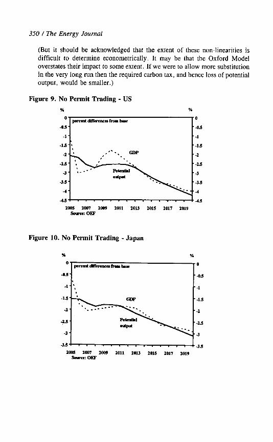
350 / The Energy Journal

(But it should be acknowledged that the extent of these non-linearities is difficult to determine econometrically. It may be that the Oxford Model overstates their impact to some extent. If we were to allow more substitution in the very long run then the required carbon tax, and hence loss of potential output, would be smaller.)

Figure 9. No Permit Trading - US

K %

O pemmt dimemlccr from ba¶e -0

-0.5’ ‘-0.5

-1 * - -1

-1.5” - -1.5 8

- -2

'-2.s

-4’

-lJ, , . rn . . . . . . . . . . . r43

2005 2OO7 2009 2011 2013 2015 2017 2019

saurce: OEF

Figure 10. No Permit Trading - Japan

- -15

-3’ ‘-3

35‘1 . . . . . . . . . , . , , , -33

2005 2007 2009 2011 2013 2015 2017 2019 Sarer: OEF

The Economic Implications / 351

Figure 11. No Permit Trading - Germany

Yi Y.

0- percent dimerencea from Imu

-0

-0.5’ ‘-0.5

4-f . . . . . . . . . . . . . . r-4

2005 2007 2009 2011 2013 2015 2017 2019

SoIwcc: OEF

Figure 12. No Permit Trading - France

-0.5’

,

-1. ‘. I

-15' ‘* ‘, GDP

-2 - ‘,

- -0.5

- -1

- -1s

- -2

-35i . , , . . . . . . . . . . . r-3.s

2005 2007 2009 2011 2013 2015 2017 2019

salrcc: OEF

l The fall in actual GDP is larger than potential in the short term, reflecting adjustment cost effects. For example, following the introduction of the carbon tax, companies find themselves no longer with the optimal mix of energy-efficient capital or the optimal capital-labour ratio. However, they are not able to switch to more energy-efficient forms of capital immediatehy (e.g., because of ordering lags, or because it is not economic to make the change given the sunk costs of the existing capital stock). A disproportionate amount of the adjustment cost is therefore likely to have to be offset initially by shedding labour (especially since real wages are likely to be slow to adjust), with multiplier effects on to demand and output in the short run.

352 / The Energy Journal

Similarly, monetary policy is assumed to tighten to prevent the increase in energy costs generating a wage-price spiral, which again depresses actual GDP relative to potential. There are some offsetting lags in the respo:nse of demand components to a supply shock, but those are insufficient to outweigh the effects outlined for more than a very short period.

l Actual GDP then tends to cycle around potential GDP, before th’e two converge in the long term.

Trade, Competitiveness and Other Issues

Competitiveness losses/gains represent an important mechanism by which gains and losses are transmitted internationally and a variable of concern to policy makers in its own right.

Unsurprisingly, those imposing the highest carbon taxes tend to suffer the largest competitiveness losses and trade account deterioration as industry costs and prices rise. These structural effects will, however, be modified by short- to medium-run movements in exchange rates, which appreciate in those countries which adopt tight monetary policies to curb price rises (e.g., Europe).

The imposition of a carbon tax has much the same effect as an unexpected fall in productivity or potential output. In the short run, countries experiencing the sharpest squeeze (Canada) borrow temporarily from those that are less affected (UK) in order to minimise the impact on domestic consumption, and they run trade deficits as a consequence.

In the long run, however, trade deficits will start to move back towards balance and countries experiencing the largest carbon tax increases will end up with lower potential output, lower levels of productivity, a lower real exchange rate, but trade back in balance. There are at least two reasons why the real exchange rate ought to end up lower in countries facing the biggest carbon tax increases:

1. Having borrowed during the initial squeeze, France and Canada soon build up external debt, on which they now have to permanently pay interest abroad. Assume for a moment that these countries started in current account balance and have to return there in the long run (to stabilise debt stocks). Then, given that the IPD (Interest, profits and dividends) account is now permanently in deficit, these countries will ultimately have to run a trade surplus to finance it. The way this is achieved is by allowing the real exchange rate to fall in the new equilibrium.

2. These countries end up with lower productivity than others, and th’ere is plenty of empirical evidence which associates high traded-sector productivity with high real exchange rates. This is known in the literature as the

The Economic Implications / 353

‘Balassa-Samuelson’ effect, and it arises because countries with higher productivity in tradables relative to non-tradables tend to have higher price levels. High carbon taxes tend to reduce tradables productivity more than non-tradables, so the relative price of tradables falls, as does the real exchange rate.

All this is complicated in the medium run by monetary policy and the response of the exchange rate, as well as the fact that, even after 10 years, the economies are still some way from the long run in these simulations. Aggressive countries might raise interest rates sharply in the face of a large carbon tax increase (even though they know this only affects relative prices and not inflation in the long run), and this may cause the nominal exchange rate to appreciate initially, depending on what happens in other countries. Canada does actually see a nominal exchange rate appreciation in the short run, even thoug:h in the longer term we know the real exchange rate has to fall for the reasons outlined above.

It is possible to offset the effects of the carbon tax increase on the price level by cutting indirect taxes or VAT by an appropriate amount, which would vary across countries of course. This would eliminate the short run impact on inflation and mitigate most of these monetary policy response effects.

Trade and capital flows are also affected by changes in investment and potential output. At one extreme, LDCs such as China see a fall in the price of energy raising potential output and increasing the marginal productivity of capital. At the other extreme, Canada has large rises in energy prices leading to a fall in potential output and a fall in the marginal productivity of capital. Investment falls in Canada and rises in China essentially reflecting a movement of energy intensive industry from one to the other. At the same time, capital flows from Canada to China to help finance this investment. These capital flows and investment changes further affect trade and the exchange rate etc.

(iii) Permit Trading

We now move on to the permit trading scenarios. We assume that ‘permits to emit’ are issued to consumers who are then free to sell them to domestic and foreign industry at the international market price. Consumers are therefore fully compensated for the energy tax increase, and emissions are redistributed from areas where the marginal cost of reducing them is high to those where the marginal cost is lowest.

Table 5 reports on 2010 emissions stabilisation with permit trading between the Annex I countries, including Russia. Important results include the following:

354 / The Energy Journal

The permit price required to meet the Kyoto emissions reduction target is $222 at constant 1997 prices. This price is below the single-country carbon tax in all countries except Russia.

Consequently, at that price Russia is the only seller of permits, exporting 293 mmt of emissions by 2010. These exports generate income inflows equivalent to around 4% of GDP for Russia in 2010.

The biggest permit purchaser is the US, which buys 114 mmt of emissions permits in 2010, Canada is the largest purchaser relative to the size of its GDP, however.

Overall ‘world’ output in 2010 is higher than in the country-specific carbon tax case-a measure of the welfare gain associated with permit trading.

Table 5. Kyoto Emissions Targets, Annex I Permit Trading including Russia (percent changes from base projection unless otherwise stated)

Potential Industrial Change in Carbon tax Permits bought Output energy costs CO? (1997 $ per (+)/sold(-)

in 2010 in 2010 emissions tonne) (mmt)

US -1.4 92 -23 222 114 Canada -1.2 76 -15 222 33

Japan -0.5 41 -9 222 52

Germany -0.8 57 -12 222 37

France -0.6 48 -6 222 ‘19 Italy -0.7 61 -6 222 :I8

UK -1.0 100 -15 222 I! 1 EU total -0.7 64 -10 222 94

China +0.6 -15 +3 0 0

Russia -1.4 110 -35 222 -293

Figures 13-16 show the profile of actual GDP and potential output to 2020 under Annex I trading.

The Economic Implications / 355

Figure 13. Permit Trading - US

% % 0- pcmntMerrncrrfrabuc -0

-05‘ '-03

-2 - - -2

3.57 = . . . . . . , , . . . . . r-2J

2005 2007 2009 2011 2013 2015 2017 source: OEF

2019

Figure 14. Permit Trading - Japan

Y. Y.

O- permtdiffelmcafmmbuc -0

-0.2 . \ --03 L \

- -oA

- -0.6

-1 .

-13. . . . . . r . , . , , , . , p-13

2005 2007 2009 2011 2013 2015 2017 2019 Sam: OEF

Permit Trading: An Important Caveat

The optimality of permit trading arrangements rests on a number of assumptions-not least that international markets are competitive, that firms are price-takers, that they face uniform prices for goods and factors (when expressed in a common currency) and that transaction costs are low. Clearly thea,e conditions do not hold in practice, but studies have shown that even in a second- best world permit trading arrangements can be an improvement, and our quantification appears to bear that out.

356 / The Energy Journal

Figure 15. Permit Trading - Germany K

0

4.2

-13 -

-1.4.

-1.6'

-1.8 -

-0.4

-0.6

4.8

-1

-13

-1.4

-1.6

-1.0

-14 . . . . . . . . , , . , , . c-2 2005 2007 2009 2011 2013 2015 2017 2019

source: OEF

Figure 16. Permit Trading - France

-13 * - -13

-15+ , . , . . . . . . . . . . . r-u

2OOS 2007 2009 2011 2013 201s 2017 2019 sarce: OEF

However, real world goods and services do not cost the same in different countries, because market exchange rates deviate persistently from purchasing power parity (PPP). But all permit trades are assumed to take place at market exchange rates-it is difficult to think of any other way they could be made. Consequently, ‘cheap’ countries whose currencies are undervalued. face an extra incentive to sell permits (which are dollar-denominated), because their purchasing power in terms of American goods, services and industrial equipment is greater than the market exchange rate says they are. In extremis, Russians could shut down their domestic energy industries and live off the permit proceeds forever.

The Economic Implications / 35 7

(iv) The Double Bubble

Table 6 reports the impact of meeting the Kyoto emissions targets under the so-called ‘Double Bubble’ in which the EU is assumed not to enter into international permit trading (preferring to implement its own internal burden sharing agreement), while permit trading occurs among other Annex I members.

In this case, the EU countries have to introduce carbon taxes effectively equivalent to those in the no trading case. In contrast, non-EU countries benefit from a lower international permit price (since, with the EU out of the market, the demand for permits is lower)-$170 mmt in 2010 compared with $222 under full Annex I trading. As a result, US GDP falls by only 1.0% in 2010 under the Double Bubble, compared with 1.4% under full Annex I trading. In this case, Russia ‘exports’ 242 mmt of emissions by 2010, generating income equivalent to around 2% % of GDP.

Table 6. Kyoto Emissions Targets, Double Bubble (percent changes from base projection unless otherwise stated)

- Potential Industrial Change in Carbon tax Permits bought

output energy costs CO? (1997 $ per (+)/sold (-)

in 2010 in 2010 emissions tonne) (mmts)

-

us -1 .o 71 -20 170 156

Canada -1.0 60 -13 170 33

Japan -0.3 32 -7 170 53

Germany -2.2 197 -26 779

France -2.2 298 -20 1325

Italy -2.3 336 -20 1234

UK -1.8 206 -22 475

EU total -2.2 252 -22 932

China +0.7 -16 +4 0

Russia -1.0 85 -28 170 -242

Figures 17-20 show the profile of actual GDP and potential output to 2020 under Annex I trading.

358 / The Energy Journal

Figure 17. Double Bubble - US

$=y==-j~

4.6 , *. ,

. *. GnP t

'4.6

'4.8

- -1

'-13

. -1.4

. -1.6

2005 2007 2009 2011 2013 2015 2017 2019

- OEF

Figure 18. Double Bubble - Japan %

O- pcrcenl difftrencn from base

4.1 - .

43' '. \ .

Yi

-0

'-0.1

- -03

'43

- -0.4

45'

-0.6 -

4.74 , . , . . . . . . . . I . * r4.7

2005 2007 2009 2011 2013 201s 2017 2019 swre: OEF

Figure 19. Double Bubble - Germany

% %

O- prc&dMfmncafra~

-0

45‘ '45

-1.: '-1

-15‘ '. - -15

- -2

- -25

'-3

'-35 I

-4' . . --4 \ .

-45' a'

'. . '-15

*__ ' -5-l , , , rn , . . . . I . . . . r-s

2005 2OO7 2009 2011 2013 2015 2017 2019 source: OEF

The Economic Implications / 3S9

Figure 20. Double Bubble - France

% %

O- -0 prcen( dnTeretKn from base

45' '45 .

-1' '. - -1 \

-15 - '- - -15 1, GDP

-2' ' - -2 *

3'

45, , . . . . . . . . . . . . . r-35

200~ 2007 2009 2011 2013 201s 2017 2019 sMI:OJCF

III. CONCLUSIONS AND PROPOSALS FOR FURTHER WORK

This paper clearly shows that the GDP costs of reducing carbon emissions vary significantly across countries and that the cost depends upon a number of critical factors including energy intensity, the rise in emissions in the base case and the amount of coal used especially in electricity generation.

There are three areas where the analysis could be extended or modified.

The rises in energy prices when a carbon tax is introduced may well depend upon the mix of fuels available for a particular economy. This is especially true in electricity generation. For example, France with electricity generate:d almost entirely from nuclear could choose not to raise electricity prices wiih a carbon tax. Alternatively, it could raise prices by a significant amount to reflect the higher prices that are being charged for other fuels in France and for electricity in neighbouring economies. The results will vary significantly depending on the assumptions made.

The results so far imply that the GDP loss for any country will depend upon the way other countries attempt to cut their own emissions. As a consequence, the US, for example, will need to consider carefully the way the EU and Japan plan to achieve their targets since it will have an impact on how they should react. These ‘strategic interactions’ deserve further consideration.

360 / The Energy Journal

l Countries which have relatively large exports of energy intensive products are likely to be more affected than countries which export only a small proportion of their GDP and whose exports are mostly services or high tech goods. The model does not fully reflect these differences and we hope to modify the model to incorporate these effects at some stage.

APPENDIX

The Oxford World Macroeconomic and Energy Model

The Oxford Model has its origins in the international macro model and software system built by Oxford Economic Forecasting (OEF) during the 1980s. The model was substantially reviewed and re-estimated in the 1990s. This new generation macro-model is designed not only to fit the historic data but also to have long-run properties that are consistent with modem macro theory. A detailed energy sector has been integrated into this macro model, thus providing a unique tool for assessing the impact of policies to control carbon emissions. The model is very different to most other macro-models since it can be used for analysis of the long-term as well as the normal two to three year forecasting time scale. This is partly because there is an explicit production function properly incorporating energy, capital scrapping and a NAIRU (Non-accelerating inflation rate of unemployment).

As a consequence of the above, the model incorporates all the key features of CGE models: it has clear theoretical foundations and can incorporate forward and backward looking expectations.

An Outline of the Individual Country Models

The structure of each of the country models continues to be based on the income-expenditure accounting framework. However, the models have a fully coherent treatment of supply. In the long-run, each of the economies behaves like the textbook description of a one sector economy under Cobb- Douglas technology in equilibrium. Countries have a natural growth rate, which is ultimately beyond the power of governments to alter and is the result of population and productivity growth (although changing tax rates and government borrowing can modify growth rates in the short run). Output cycles around a deterministic trend, so at any point in time we can define the level of potential output, corresponding to which is a natural rate of unemployment. Firms are assumed to set prices given output and the capital stock, but the labour market is imperfectly competitive. Firms bargain with workers over wages, but the former set the level of employment. Countries with high real wage costs get high unemployment in the long run, and countries with rigid real wage:s get persistently high unemployment relative to the natural rate.

The Economic Implications / 361

Inflation is a monetary phenomenon in the long run. The models have vertical long-run Phillips curves, so expansionary demand policies put upward pressure on inflation. Unchecked, these pressures would cause the price level to accelerate away without bound, and in order to prevent this we have endogenised monetary policy responses. These are summarised in an inflation target for each country. Interest rates are assumed to move up whenever inflation is accelerating and/or is above the target rate and/or output is above potential. The coefficients in the interest rate reaction function, as well as the inflation target itself, reflect our perceptions of how hawkish different countries are about inflation. Consumption is a function of real incomes, real financial wealth, real interest rates and inflation. Investment equations are influenced by “q-theories” in which the investment rate is determined by its opportunity cost, after taking taxes and allowances into account. Countries are assumed to be “small” in the sense that exports are determined by demand and a country cannot ultimately dictate its own terms of trade. Consequently, exports are a function of world demand and the real exchange rate, and the world trade matrix ensures adding-up consistency across countries. Imports are determined by real domestic demand and competitiveness. Trade competitiveness elasticities are typically between 0.3 and 0.6.

The individual economic models are linked via disaggregated trade equations and exchange rates which react to interest rates and changes in competitiveness.

The Energy Equations

For the G7 countries (and China) demand for energy is broken down in the following way:

(i) Fuel types: oil, coal, gas, electricity, nuclear, other.

(ii) Sectors: residential, industrial, transport,electricitygeneration.

The main data source is the OECD energy balances. For each sector and fuel type this gives the annual volumes consumed and an associated price and tax rate. The following countries are also separately treated in detail:

Taiwan, Korea, Australia Mexico Spain, Netherlands, Belgium, Switzerland, Sweden, Austria

But for these only total demand for oil, coal and gas is identified.

362 / The Energy Journal

Schematically the model works in the following way:

(9 Demand functions are estimated for all the energy types by sector identified above, primarily as a function of economic activity and relative energy prices (and trends). The estimated price elasticities, especially in electricity generation, have been modified to take into account results produced by technology models such as IDEAS. This usually results in higher elasticities than suggested by time series econometric analysis. Typical elasticities are shown in Table Al. (It is worth noting that the long-run elasticities allow for capital stock turnover effects.)

Table Al. Typical Energy Demand Elasticities

Energy Demand

Component Elasticity** Relative Price/Technology

Substitution Effect

Transport (gasoline)

Industry

Household

Electricity generation:

(u) Coal

(b) Oil & Gas Total

of which Oil

(c) Nuclear/non fossil fuel elecrricity

s.t. 1.0 1.t. 1.0

s.t. 1.0

1.t. 1.0

s.t. I.0 1.t. I.0

s.t. 1.0

1.t. I.0

s.t. 1.0 I.t. 1.0

s.t. I.0

1.t. 1.0

s.t. 1.0

1.t. 1.0

impact effect 0 -0.25 over about 5 years

s.t. 0

1.1. -0.5

s.t. 0

1.t. -0.5

s.t. 0

1.t. -0.5*

s.t.0 I.t. -0.5*

s.t. -0.5 1.t. -1.0 (for substitution between

OIL and GAS)

s.t. 0

1.t. -0.5*

* 0.3 substitution effect between fuels which is in principle reversible and a 0.2 technological gain

which is a switch to more efficient plant that is far less likely to be reversed.

**depending on the energy equation, this may be consumer spending, industrial production or GDP.

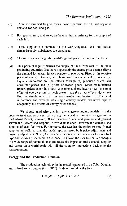
(ii)

(iii)

(iv)

(VI

(vi>

The Economic Implications / 363

These are summed to give overall world demand for oil, and regional demand for coal and gas.

For each country and zone, we have an initial estimate for the supply ‘of each fuel.

These supplies are summed to the world/regional level and initial demand/supply imbalances are calculated.

The imbalances change the world/regional price for each of the fuels.

This price change influences the supply of fuels from each of the main producing countries. But more importantly the energy price change affects the demand for energy in each country in two ways. First, as the relative price of energy changes, we obtain substitution to and from energy. Equally important are the effects through (a) producer prices, (b)

consumer prices and (c) prices of traded goods. Since manufactured import prices enter into both consumer and producer prices, the total effect of energy prices is much greater than the direct effects alone. We find in simulations that this transmission mechanism is of crucial importance and explains why single country models can never capture adequately the effects of energy price shocks.

We should emphasise that in many macro-economic models it is the norm to treat energy prices (particularly the world oil price) as exogenous. ln the Oxford Model, however, all fuel prices-oil, coal and gas-are endogenised within the system and respond to world imbalances between the demand and supplies of each fuel type. Furthermore, the user has the option to modify fuel supplies as well, so that the model approximates both price adjustment and quantity adjustment. Since, for the G7 economies, sets of tax rates for each fuel type and sector are included in the model, it allows the user to simulate changes to a wide range of potential taxes and to see the impact on fuel demand, supplies and prices on a world scale with all the complex interactions back onto the macroeconomy.

Energy and the Production Function

The production technology in the model is assumed to be Cobb-Douglas and related to net output (i.e., GDP). It therefore’takes the form:

Y = /A + (I-p)1 + TREND (L)

364 / The Energy Journal

where

Y = potential output k = capital stock 1 TREND 1

labour supply (when unemployment is at the NAIRU) total factor productivity trend

(All variables in logarithms.)

Note that since (1) relates to net output, the only factor inputs identified are capital and labour. This does not mean that energy is considered not to be a component of firms’ inputs in a general sense. Rather, energy inputs are a component of gross output, not net output. For example, an increase in energy inputs may enable a firm to produce a greater number of widgets. But this will only mean higher net output if either additional labour and capital are employed domestically to produce the extra energy, or if additional energy usage raises the technical efficiency (i.e., marginal product) of existing labour and capital inputs, which would be reflected in higher total factor productivity.

The impact of energy inputs on productive potential through their impact on the efficiency of capital and labour is incorporated in the Oxford Model in two ways. First a rise in the relative price of energy results in some premature scrapping of the capital stock. Secondly, total factor productivity is related to real energy prices:

TREND=A+Bt-Srep

where

t = time trend rep = real energy prices

An increase in the real price of energy therefore acts to shift the production function downwards, reducing the volume of output that can be produced with a given set of capital and labour inputs as the efficiency of these factors declines. Put another way, the increase in real energy prices increases the cost of producing any given level of output, and therefore reduces, the profitability of production at a given price of output. As a result, it causes the economy’s supply curve to .shift inwards. In the Oxford Model S typically takes a value of about 0.02, implying that a 10% rise in real energy prices reduces potential output by 0.2 % .

The Economic Implications / 365

The size of S in (2) can be derived using the following formula (from Marion and Svensson (1983)) for the direct substitution effects on value-added of changes in real energy prices:

S = E(Q/(l-Q)) (3

where

Q = share of energy in total costs E = elasticity of substitution between energy and an

assumed composite of capital and labour

With Q typically around 5 % for industrialised countries, a value of S of 0.02 is consistent with an elasticity of substitution between energy and other factors .in gross output of around 0.5 (i.e., within the range of 0.3 to 0.6 suggested by Lindbeck (1983) to be plausible).

As well as affecting potential output directly, as described above, changes in real energy prices will also affect the desired long run size of the economy’s capital stock in the Oxford Model. For example, with a rise in real energy prices cutting the marginal productivity of capital, firms’ desired capital stock will fall, implying lower aggregate gross investment and/or capital scrapping and lower potential output in the long run. Within total investment, however, a rise in real energy prices may encourage higher investment in energy-saving areas (and thus less elsewhere).

REFERENCES

Hogan, W.W., and D.W. Jorgenson (1991). ‘Productivity Trends and the Cost of Reducing CO2 Emissions.” The Energy Journal 12(l): 67-85.

Lindbeck, A. (1983). “The Recent Slowdown of Productivity Growth.” Economic Journal 13.

Manne. AS., and R.G. Richels (1994). ‘The Costs of Stabilising Global CO2 Emissions: A Probabilistic Analysis Based on Expert Judgements.” The Energy Journal 15(l): 31-56.

Marion, N.P.. andL.E.0. Svensson (1983). “Structural Differences andMacroeconomic Adjustment

to Oil Price Changes.” International Economic Studies Seminar Paper No. 248, Stockholm (quoted in “The Economic Effects of Lower Oil Prices” HM Treasury Working Paper No. 34).

Ogawa, Y. (1991). ‘Economic Activity and the Greenhouse Effect.” The Energy Journal 12(l): 23-

35. Proops, J.L.R., M. Faber, and G. Wagenhals (1993). Reducing CO, Emissions, A Comparatwe

Input-Output Study for Germany and the UK. Berlin: Springer.

CO2 Emissions Control Agreements: Incentives for Regional Participation

Stephen C. Peck* and Thomas J. Teisberg**

This paper explores the incentives forparticipation in international CO, control agreements using tradable emission permits. We employ a welfare analysis in a two-region model to explore these incentives. The two regions are Annex-l (A-I) and Non-Annex I (Non-A-I). A key insight underlying the analysis is that emission permit allocations must not depart too farfrom optimal emissions paths, to avoid creating future incentives to drop out of the agreement. We find a range of permit allocations that improves the welfare of both the Annex-I and the Non-Annex I. and compare them with allocations based on region’al population or GDP. In addition, we examine the implications of the Kyoto agreement in the context of this welfare analysis. We find that the Kyo,to agreement transfers wealth from A-I to the Non-A-I, while failing to realize the mciency gains to be hoped for from an agreement to control CO, emissions.

INTRODUCTION

In this paper, we use a version of the CETA model to consider the implications of alternative rules for allocating tradable emission permits between two regional aggregations of the world. The two regional aggregations are the Annex I countries (A-I) and the Non-Annex I countries (Non-A-I). Alternative rules for allocating tradable emission permits produce different distributions of the net benefits of emission control between these two regions. Of particular interest are rules that provide higher net benefits to both regions than would be achieved in the absence of an agreement to control emissions; we refer to such rules as being in the “bargaining range.” If the allocation rule of an agreement is in the bargaining range, then the agreement is more likely to be signed in the first place and more likely to be upheld over time. Conversely, if the rule is not in the bargaining range, there is no reason to expect the agreement to be signed or to expect it to last, if it is signed.

The Energy Journal, Kyoto Special Issue. Copyright 0 1999 by the IAEE. All rights reserved.

* Electric Power Research Institute, 3412 Hillview Avenue, P.O. Box 10412, Palo Alto, CA

94303. E-mail: scpeck@epri.com ** President, Teisberg Associates, 1475 Ingleside Drive, Charlottesville. VA 22901, USA.

E-mail: TJTeisberg@compuserve.com

367

368 / The Energy Journal

In this paper, we find permit allocations that are in the bargaining range, and that appear to remain in the bargaining range over time. We contrast these permit allocations with allocations resulting from arbitrary rules. The latter include permit allocations proportional to population or GDP; such rules may or may not be in the bargaining range.

We also consider the implications of the Kyoto agreement’s plan for worldwide emissions reduction. The Kyoto agreement not only specifies an allocation of permits, but it also implies a worldwide emissions path. Because the emissions path specified in the Kyoto agreement is not the optimal path, the welfares of A-I and the Non-A-I are not on the utility frontier, and therefore not in the bargaining range; furthermore, the welfare of A-I under Kyoto is below its welfare in the No Control case. These results are the same with or without emissions rights trading between A-I and the Non-A-I.

Section II begins with a description of our model and the assumptions we make about the benefits of controlling emissions. In Section III we identify permit allocation rules that define the bargaining range, and we contrast the permit allocations resulting from these rules with those resulting from rules based on population or GDP. In Section IV, we consider the implications of the Kyoto agreement. Finally, Section V provides a summary.

II. THE CETA-M MODEL

The CETA (Carbon Emissions Trajectory Assessment) Model is the foundation for CETA-M. ’ CETA represents worldwide economic growth, energy consumption, energy technology choice, global warming, and global warming costs (costs of damage from and adaptation to higher temperature). Much of the data for CETA is adopted from Manne and Richels (1992) and the base case assumptions of EMF14, the Stanford Energy Modeling Forum Global Climate Change study.’

CETA-M is similar to CETA in many respects. However, it disaggregates the world into regions, and allows for trade between these regions in multiple goods. Equilibrium is found using an approach based on Ne:gishi welfare weights. The following sections provide more detail.3

1. The CETA-M model is introduced in Peck and Teisberg (1997), where it is used to analyze

the costs of alternative proposals for CO, emission reduction.

2. Energy Modeling Forum (1995).

3. The model used for this paper is not completely comparable to the model used to generate

results for EMF16. For one thing, the EMF16 results were generated from a four-region model, and

solving such a model requires a minor re-specification of regional welfare functions. In addition, we

made some AEEI parameter adjustments to increase long run EEFSU energy efficiency in the four

region model; here, EEFSU is embedded in A-I, and no energy efficiency adjustment is made.

CO, Emissions Control Agreements / 369

A. Regions

The EMF14 study disaggregates the world into six regions: the United States (USA), the European Economic Community (EEC), other OECD countries (OOECD), Eastern Europe and the former Soviet Union (EEFSU), China, and the rest of the world. For our analysis in this paper, we divide the world into two regions: Annex-I (an aggregation of USA, EEC, OOECD, EEFSU) and the Non-Annex I. Data for these two regions are obtained by aggregating EMF14 data for the appropriate subregions comprising our two regions.

For each of our two CETA-M regions, our representations of the economy and energy use are essentially the same as those for the world as a whole in the CETA model. Thus, regional output depends on exogenous labor input, the endogenous capital stock, and energy use. CO, emissions depend on the quantity and type of energy used in each region.

B. International Trade

In CETA-M, we allow for international trade in the numeraire good (aggregate output), carbon emission permits, and two key energy goods: oil and gas (which are aggregated together as a single commodity in CETA and CETA- M) and synthetic fuels (derived from coal). This choice of energy goods abstracts from the possibility of trade in other energy goods such as coal 8r electricity, and it ignores some important differences in transportation costs for oil and natural gas. Nevertheless, we think it is a reasonable first approximation of the most important energy trade flows we would expect to observe over the next century or so.

When international trade in the numeraire good is allowed, the numeraire flows from the region with a lower market rate of interest to the region with a higher market rate of interest, until rates of return are equalized across regions. To prevent unrealistically high capital flows, we follow the approach of Marme and Richels and benchmark our regional utility discount rates (i.e., those used to calculate the present value utility of any given consumption path) so that market rates of return are approximately equal (and equal to 5 percent) for both regions.4

For each traded good and each region, model equations representing the economy and energy use are augmented by an equation requiring regional u:se of traded goods to equal regional production (or allocation, in the case of carbon permits) plus net imports. In addition, for each traded good, an equation is added to require that the sum of net imports over regions equals zero.

4. See Manne and Richels (1992) p. 126.

370 / The Energy Journal

C. Determining the Equilibrium

To determine the competitive equilibrium in CETA-M, we use an approach employing Negishi weights (Negishi, 1972). That is, we specify a problem in which the objective function is a weighted sum of utilities in the two regions; these weights are known as Negishi weights. When this problem is solved for any arbitrary set of weights, the shadow prices of the constraints requiring net imports to sum to zero are the international prices for the corresponding goods. These prices may then be used to calculate a present value trade surplus or deficit for each of the two regions for this model solution. The competitive equilibrium is then found by adjusting the Negishi weights until the present value trade surplus (or deficit) is zero.

With two regions, there is only one independent Negishi weight (the other being completely determined because the weights must sum to one). This makes it simple to adjust the Negishi weight until the present value trade surplus is zero. In fact, we find that the trade surplus is very nearly a linear function of the Negishi weight, which makes it possible to come very close to the equilibrium Negishi weights using two sets of trial weights and interpolati:ng or extrapolating using the results from these trial weights. Repeating the interpolation once or twice produces an even closer approximation to the equilibrium.

D. Regional Warming and Damages in CETA-M

The CETA-M model used for this paper contains a climate change damage representation that is different from that in earlier versions of the CETA model. We have replaced a damage function based on the globalized damage estimate of Nordhaus (1991) with regionalized damage functions derived from the damage estimates of Fankhauser (1995).

Fankhauser’s damage estimates represent “benchmark” damage from a 2.5 degree C temperature increase, i.e., the temperature increase considered most likely by IPCC (1990) for a doubled CO? concentration.5 Since Fankhauser’s estimates are presented in 1988 dollars, we have inflated them by 10 percent as a rough adjustment for inflation and growth to 1990.

Fankhauser’s damage estimates are presented in categories, which may be aggregated into two classes-market damages and non-market damages. Market damages are those for which market prices can be used directly or indirectly to measure costs; an example is agricultural losses where the plrices of crops can be used to value production losses. Non-market damages are those

5. In its subsequent 1995 report, IPCC did not change its earlier estimate of the most likely

value of the climate sensitivity.

CO, Emissions Control Agreements / 371

for which there are no market prices to help in valuing damages; an example #of non-market damages are health effects (including increased mortality) attributable to climate change.

We aggregated the following of Fankhauser’s damage categories into the non-market damage class: wetland loss (even though fisheries loss is included), ecosystem loss, human life, air pollution, migration, natural hazards (even though this is partly a market damage). The remaining categories are aggregated as market damage: coastal defense, dryland loss, agriculture, forestry, energy, and water.

Table 1 below presents the resulting damage estimates by EMF1.4 region, together with EMF14 GDP and population numbers. Overall, the market and non-market damages are of approximately equal magnitude, and together come to roughly 1.4 percent of GDP.

Table 1. Climate Change Damages, GDP, and Population

EMF14 Region

USA

EEC

OOECD

FSU

CHINA

ROW

Non-Market Market EMF14

Dam. Uh.J Dam. (D,) GDP

(billion $) (billion $) (billion $)

33.11 33.99 5520

35.64 34.32 5710

32.12 29.26 4970

8.91 11.11 1310

7.26 11.11 1330

41.03 18.59 3110

EMF14

POP

(millions)

- 250

244

259

289

1134

2976

Sources: Fankhauser (1995) and Energy Modeling Forum (1995).

Our next step is to “explain” statistically the cross sectional variation in market and non-market damages in terms of GDP and population. It is reasonable to expect that market damages would be linearly related to GDP, and indeed we find that the data are consistent with this expectation:

D,=a,+fl;GDP (1)

where:

aI = 3.573223 (SE = 0.97596)6

0, = 0.005327 (SE = 0.000237)

R” = 0.992083.

6. “SE” is the standard error of the estimated parameter. Under the usual assumptions

underlying regression analysis, there is approximately a 95 percent probability that the true

parameter is within the range defined by the estimated parameter f 2 x SE.

372 / The Energy Journul

For non-market damages, it seems reasonable to suppose that:

D, = f(y) * POP (2)

where y is income per capita, and f(y) may be interpreted as an amount per person that represents willingness to pay to avoid non-market damage. Intuitively, it is plausible that the functionf(y) might be non-linear in income per capita. However, after a little experimentation, we concluded that the following linear relationship best fits the data:

D GDP NM =a*+&-- POP POP

(3)

The regression results for the above equation were:

ff2 = 0.003705 (SE = ~302785)

p2 = 0.006017 (SE = 0.000200)

R2 = 0.995566

Multiplying both sides of equation (3) by POP, DNM is seen to be a linear function of population and GDP (with no constant term).

Equations (1) and (3) provide functional relationships between inc:ome, population, and benchmark damages. These may be used to produce regionalized (and time varying) benchmark damages from the projected future regional populations and incomes. Benchmark damages, however, only indicate the damages at a certain temperature increase, 2.5 degrees C, in this case. To get actual estimated damages, it is necessary first to have regional temperature changes and then to specify the functional relationship between temperature change and estimated damages. We next describe the procedures we use to accomplish these last steps.

In CETA-M we explicitly track global mean temperature. To go from this to regional temperature, we assume there is a regional temperature differential relative to the global mean. This differential is developed from regional temperature results presented in IPCC (1990). Specifically, Figure 6.3 (p. 140) shows climate sensitivity by latitude and month of year. Roughly speaking, the figure suggests that if latitude exceeds 45” north or south., the temperature change is significantly different. In the north high latitude, it’s warmer (than average) for roughly half the year (fall and winter); in the :jouth high latitude it’s warmer all year. However, since there is relatively little

CO, Emissions Control Agreements / 373

inhabited land south of latitude 45”, we ignore the south and focus on the north. Although the fall and winter temperature increase ranges from 4” C I:O

12” C north of latitude 45”, the more populated land areas are close to latitude 45”. Thus, we assume that north of latitude 45” is characterized as having +5” C for half the year and +3” C for half the year, or an average of +4” C for the whole year. Below latitude 45”, on the other hand, might reasonably be characterized as having +3” C throughout the year. Thus, in an obviously rough way, we assume that the temperature rise above latitude 45” is 1.33 times the temperature rise below latitude 45”.

If high latitude warming is 1.33 times low latitude warming, and global mean temperature is the average of the high and low latitude warming, then hig,h latitude warming must be 1.14 times the global mean, while low latitude warming must be 0.86 times the global mean.

Having characterized high latitude regions as having 1.33 times the warming of low latitude regions, we next need to decide which of the EMF14 legions (see Table 1 above) should be treated as high latitude regions. Again, in a rough way, we assume that the EC and EEFSU are reasonably identified as high latitude, while all other regions are low latitude. The most troubling aspect of this decision is the placement of the OOECD, consisting of Australia, Japan, Canada, and New Zealand, in the low latitude category. While Canada is unambiguously high latitude, Japan is the most important country economically and in terms of population, and it is predominantly low latitude, by our definition. Thus, we include OOECD in the low latitude group.

To summarize, then, we specify regional temperature change by assuming that warming in the EU and EEFSU is 1.14 times the global mean temperature rise, while warming in the other regions is 0.86 times the global mean temperature rise.

Finally, it is necessary to assume a relationship between regional temperature rise and regional damages, when temperature rise is something other than the 2.5 degrees C benchmark. We assume that actual damages are a quadratic function of regional temperature rise, which passes through th.e benchmark damage amount when the temperature rise is 2.5 degrees C.

III. ALLOCATION OF EMISSION PERMITS

Under a CO, emission permit system, emissions are limited by the requirement that a permit be surrendered when a unit of CO, is emitted. :[f permits are marketable, emitters with relatively low cost of control will want to reduce emissions to create surplus permits for sale, while those with relatively high cost of control will want to buy those permits to support continued emissions. As a result, the overall limit on emissions can be achieved at

374 / The Energy Journal

minimum cost. This is one of the appealing features of a tradable permit system for emission control.

Marketable CO, emission permits are likely to have considerable monetary value. Consequently, the rules for allocating permits among the parties to an agreement will have major implications for the net benefits accruing to these parties under the agreement. The net benefit accruing to each party will consist of whatever benefits it derives from reduced climate change, less its CO? emission control costs, plus any net revenues (positive or negative) from trade in emission permits. Since the latter revenues loom large in the overall picture, the rules for distribution of permits among the parties would be a critical element of any agreement to control CO? emissions.

Many rules for distributing permits have been discussed. Permits could be distributed to parties proportionate to their populations, or proportionate to their GDPs, or proportionate to their current CO, emissions. Distributing permits proportionate to populations would be favorable to the less developed countries whose populations are large relative to their current emissions. Distributing permits proportionate to GDPs would be favorable to regions like Japan and Western Europe whose output is large relative to their CO? emissions. Distributing permits proportionate to current emissions would be favorable to regions with currently high emissions; the U.S. would presumably fare best under this distribution rule.

In this paper, we seek to identify permit distribution rules with the property that each party to the agreement has positive net benefits unde:r the emission control system when the rule is used. We refer to such rules as being in the “bargaining range. ” Rules that are outside the bargaining range are unlikely to be agreed to in the first place. If such rules are agreed to (either out of ignorance or altruistic motivation), there is a good chance that there subsequently would be defections from the agreement as its true implications became apparent or the initial resolve waned to do something about CO,.

The identification of permit distribution rules in the bargaining range is complicated by the fact that the CO, emission control problem is one that extends over decades to centuries. Thus, a permit allocation in the bargaining range needs to produce positive net benefits to each party, not just looking forward from the present time, but also looking forward from any point in time over many decades. Relative populations, GDPs, and uncontrolled emission rates are likely to change substantially over such a time frame, This makes it desirable that the allocation rule be appropriately responsive to such changes to ensure that the agreement is durable over time.

The key insight underlying the present analysis is that permit allocation paths should not depart too far from optimal emissions paths under the control agreement if the agreement is to be durable. This is because allocation paths that do not track optimal emission paths will tend to produce large regional income transfers from permit trading, and this may create incentives to drop out of the

CO, Emissions Control Agreements / 375

agreement. Thus, in this paper, we will specify the bargaining range in terms of permit allocations that are defined relative to regions’ optimal emissions paths.

Our analysis here extends that of an earlier paper (Peck and Teisberg, 1998) in which we found fixed regional permit allocations which were in the bargaining range from the perspective of 1990. That is, we found fixed fractions of total available permits that were to be allocated to each region in each time period, so that the present value utilities of both regions would be higher under the agreement than in the no control situation. The risk with fixed fractions is that such allocations will become disadvantageous to one of the regions as circumstances change with the passage of time.

As in our previous paper, we here use a two-region version of th.e CETA-M model. However, the two regions used in this paper are the A-I countries and the non-A-I countries (instead of the OECD and the ROW). While two regions is a gross simplification of the real world, these regions serve as a stylized representation of the key tension between countries with large populations but relatively low GDP and emissions (i.e., Non-Annex-I) versus countries with relatively small populations but high GDP and emissions (Annex- I).

Our analysis in this section proceeds as follows. First, we show the time path of optimal emissions, broken down by region. Next, we show the Non-A-I share of optimal emissions, and contrast it with its shares of population and GDP. Then we find the bargaining range, expressed in terms of the fractions of Non-A-I’s optimal emissions represented by the permits it receives,. Also, we examine how this bargaining range may change in the future. Finally, we show the Non-A-I permit shares defining the bargaining range, relative tto its shares if its allocation were based on population or GDP, and we directl,y determine whether population or GDP based allocations are indeed in the bargaining range.

A. Optimal Emissions Paths and Emission Shares

The optimal emissions path produced by the CETA-M model depends on our assumptions, particularly the assumptions about the benefits of controlling CO, emissions and a parameter specifying the cost of a key carbon- free future energy technology. In Peck and Teisberg (1998), we performed sensitivities on a range of benefit and cost assumptions and found the concentration path that would be optimal for each set of assumptions. These optimal concentration paths ranged from one which peaked at about 1100 ppm (high costs and low benefits) to one which peaked at about 530 ppm (low costs and high benefits). Of these, we focus here on the case in which concentration peaks at about 530 ppm, not because we think it is the most likely outcome or

376 / The Energy Journal

a “base case” in any sense, but because it is the most interesting case from an analytical perspective.7 This case is analytically interesting because it implies that there is much to be gained from a successful international agreement to control emissions.

Figure 1 shows the optimal emissions paths of A-I and the Non-A-I for these cost and benefit assumptions. Total emissions rise to a peak just over 12 billion tons per year around the middle of the next century. Subsequently, emissions fall sharply as carbon-free energy technologies become available and are used in place of fossil-based energy technologies. Note also, in Figure 1, that the Non-A-I share of optimal emissions tends to rise significantly over time.

Figure 2 contrasts the Non-A-I share of optimal emissions, population, and GDP.8 Notice, first, that the Non-A-I share of optimal emissions is initially below 40 percent, but that it rises to almost 60 percent by the latter part of the next century. The Non-A-I share of GDP starts even lower, but rises rapidly to surpass the Non-A-I emissions share by 2100. Finally, notice that the Na’n-A-I share of population is mostly in the 80-90 percent range, and always abalve its shares of optimal emissions or of GDP.

Figure 2 suggests the potential difficulty in allocating emission permits in relation to population or GDP. If the Non-A-I were given permits proportional to its share of GDP, it would need to buy permits from A-I in every year except 2100, and the Non-A-I might find this unacceptable. On the other hand, if the Non-A-I were given permits proportional to its sha.re of population, the Non-A-I would be pleased, but A-I would need to buy large numbers of permits from the Non-A-I throughout the next century. This would likely be unacceptable to A-I.

Figure 2 raises this question: How far could the Non-A-I’s share of permits depart from its share of optimal emissions before the Non-A-I or A-I would no longer be willing to participate in an agreement to control emissions? To answer this question, we need to find the bargaining range, i.e., the range of emission permit allocations such that both parties are better off with the agreement than with no agreement.

B. Bargaining Range

We assume that with no international agreement to control emissions, there would be no emission control at all. In fact, a non-cooperative solution involving two regions would be characterized by more than zero emission

7. For this case, we increased the climate change damages derived from Fankhauser’s estimates

by about a factor of two, and we reduced the cost of the key non-electric backstop technology by

25 percent. See Peck and Teisberg (1998) for details.

8. Population is an input to the model: GDP and optimal emissions are endogenous in the model.

c t 0

CO, Emissions Control Agreements / 3;‘7

w

378 / The Energy Journal

CO, Emissions Control Agreements / 379

control. Of course, in reality, there would be many more than two regions involved in negotiating an international control agreement, and the non- cooperative solution for this larger number of regions might in fact be quite close to the zero control solution we posit in our analysis.

We define the bargaining range as the range of permit allocations that leaves each region’s welfare at least as high as it would be in the no control solution. To find this range, we experimentally change the number of permits allocated to the Non-A-I to various percentages of the numbers of permits required by the Non-A-I for its optimal emissions path. We then compare the welfares of the two regions under each experimental permit allocation to their respective welfares in the no control situation. We find that the Non-A-I can be allocated as much as 115 percent of its optimal emissions allocation, before A-,1 welfare drops below that in the no control situation. And the Non-A-I can be allocated as little as 70 percent of its optimal emissions allocation, before its welfare drops below that in the no control situation. Thus, 70-l 15 percent represents the bargaining range defined relative to Non-A-I’s optimal emissions path.

The asymmetry of the bargaining range around the 100 percent point is interesting, and perhaps a little surprising. One might have thought that A-I would have the most to gain from an agreement, and that this would mean thalt A-I could shift more permits to the Non-A-I (than the Non-A-I could shift to A- I) while still wanting to remain in the agreement. In fact, the opposite appears to be true. This is because, over the long run, the Non-A-I grows relative to A-I in both income and population. Thus, the Non-A-I’s warming damages increase relative to A-1’s. Since most of the damages from warming come in the future (even after discounting at 5 percent), the Non-A-I actually suffers a larger shar’e of total warming damages and derives a larger benefit from an agreement that reduces warming.’

The 70-l 15 percent bargaining range is calculated from 1990 forward in time. Any point within this range gives each region a present value utility (net of warming damages) equal to or greater than its present value utility in the absence of an agreement. For an agreement within this bargaining range to be durable over time, however, it would have to be true that a bargaining range recalculated from some future date looking forward contains this 70-I 15 percent range. To see if this is true, we calculated new bargaining ranges fifty and one hundred years into the future. For these calculations, we assumed that the world

9. Note that we here adopt a perspective in which past costs and benefits associated with CO,

emissions are not relevant in finding the range of agreements to which self-interested parties would

agree. The Non-Annex I countries have argued that the Annex I countries have benefited from past

disposal of CO2 into the global atmosphere, and therefore they have a moral obligation to contrcl

future emissions even if it is not in their self-interest to do so.

380 / The Energy Journal

was on an optimal emissions path, and that each region’s share of emission rights equaled its share of optimal emissions, for the time prior to the recalculation of bargaining ranges. We found that the bargaining range calculated at future times tends to expand. Thus in 2040, the bargaining range is 40-150 percent. By 2090, the bargaining range has expanded to the point where any distribution of permits is in the bargaining range. Figures 3 and 4 illustrate these results. Figure 3 shows the bargaining range expressed as Non-A- I rights allocations relative to Non-A-I’s optimal emissions. Figure 4 shows the bargaining range expressed in terms of the Non-A-I’s emission rights.

We believe the bargaining range, expressed as limiting percentages of optimal emissions, expands over time because optimal emissions eventually become small (see Figure 1). As optimal emissions become small, each percentage point represents fewer permits and hence a smaller income transfer between the two regions. In any case, the implication of these results is that a 1990 Non-A-I rights allocation defined relative to Non-A-I’s optimal emissions and within the 70-l 15 percent range would remain within bargaining ranges recalculated at later dates, and thus would produce a control agreement that would be durable over time.

If we apply the (interpolated) bargaining range percentages shown in Figure 3 to the Non-A-I optimal emissions share shown in Figure 2, we can show the bargaining range permit shares over time and contrast them with the permit shares based on GDP or population. This is done in Figure 5. As the figure shows, the permit share based on population lies outside the bargaining range until 2060, after which it is within but at the high end of the bargaining range. These results suggest that population based permit allocations are not likely to be in the bargaining range now (though several decades in the future, this could change). In contrast, the permit share based on GDP moves into the bargaining range very early, in 2000; this suggests that permit distributions based on GDP could be in the bargaining range now.

To determine whether a permit allocation is or is not in the bargaining range we need to directly calculate the welfares of the two regions under that permit allocation, and compare them to welfares in the no control situation. We do this and show the results in Figure 6 for permit allocations based on population or GDP. Figure 6 shows the utility frontier (the set of highest welfares attainable using efficient emission reduction), the welfares attained at the no control point, those at the ends of the bargaining range, and those resulting from population-based and GDP-based permit allocations. We see, in Figure 6, that a permit allocation based on population proportions lies outside the bargaining range (it is too favorable to the Non-A-I). Also, as was hinted in Figure 5, a permit allocation based on GDP lies inside the bargaining range, though it is relatively close to the end of the range that is most favorable to A-I.

CO, Emissions Control Agreements / 381

1

gB -II liti

I

ai d

t+

1 T

, ,

c

382 / The Energy Journal

/

\

0’

\

/

/

\

\

/

t

/

tJh="'l1!8)SWl~!~ l =UUWUON

CO, Emissions Control Agreements / 383

I

/’ \

t

.

I f

384 / The Energy Journal

b ‘S s Ii

.- ;

i 4 s .- ii 3 % n

/

CO, Emissions Control Agreements / 38.5

IV. THE KYOTO AGREEMENT

In this section, we briefly analyze the Kyoto agreement, using the welfare approach of the preceding section. The recent Kyoto agreement set,s 2010 emission targets for A-I countries, but has no emission reduction requirements for the Non-A-I countries. What happens after 2010 will be the subject of future negotiations. However, to analyze the Kyoto agreement in our 1990-2150 model time frame, we need to make assumptions about the future after 2010. Following the EMF16 approach, we assume that the Kyoto targets will continue indefinitely for the A-I countries (see Energy Modeling Forum, 1998). For the Non-A-I countries, we assume that emissions will not exceed business-as-usual (BAU) levels until 2050, and they will not exceed the 2050 BAU level thereafter.

Figure 7 illustrates the emissions rights allocations implied by the above assumptions. A comparison of Figures 1 and 7 indicates that the emissions path under Kyoto is different from the optimal path. The optimal path has higher emissions from about 2010 to 2050, and much lower emissions after 2050. Figure 8 compares the CO? concentration paths that result from the emissions paths in Figures 1 and 7. Note that the concentration path resulting from optima.1 emissions is a little higher between 2030 and 2070, and then it is significantly lower.

As noted above, the worldwide emissions path under the Kyoto agreement is not an optimal one. Thus, it makes little sense to compare the Non-. A-I permit allocation under Kyoto with the Non-A-I permit allocations defining the bargaining range, since the latter assume an optimal emissions path iI: followed for any permit distribution rule. Because the Kyoto emission path is not optimal, the Non-A-I permit allocation under Kyoto could lie within the: allocations defining the bargaining range, even though the welfare outcomes tcl both regions under Kyoto were well below the utility frontier.

Thus, we directly examine the welfare results of the Kyoto agreement for the two regions. We do this, and present the results in Figure 9. This figure is the same as Figure 6, except that we have added two points in welfare space representing the welfare results of Kyoto with and without trade between A-l and the Non-A-I. As Figure 9 indicates, both versions of the Kyoto agreement are inside the utility frontier, i.e., they are inefficient. These points are inefficient because the underlying emissions path implied by Kyoto“’ is not optimal, given the cost and benefit assumptions embedded in our model (assumptions that imply a 530 ppm maximum optimal CO? concentration).

10. Strictly speaking, this emissions path is implied by the Kyoto agreement and our assumptions

about how the agreement is extended beyond 2010.

386 1 The Energy Journal

I

‘Jhd0~ UO!ll!Q

CO, Emissions Control Agreements / 387

388 / The Energy Journal

/

t hll!M I =“W-UON

CO, Emissions Control Agreements i 389

Also, notice that the point representing Kyoto without trade is the more inefficient one. Overall, the Kyoto points are at least as far from the frontier as the No Control point.

Turning to the distributional implications of Kyoto, it is interesting to note from Figure 9 that either Kyoto solution represents a welfare improvement to the Non-A-I relative to No Control. Not surprisingly, this welfare improvement is much greater when the Non-A-I is allowed to sell permits to A-I (the Trade case). From the point of view of A-I, either Kyoto point represents a significantly lower welfare position than No Control.

Somewhat surprisingly, our results suggest that A-I welfare is about the same with and without emission rights trade between A-I and the Non-A-I. lt appears that this result is attributable to oil price effects. The Non-A-I is a large exporter of oil to A-I. When trade in emission rights is allowed, the world oil price is significantly higher relative to its level when no trade is allowed.” The A-I countries thus realize a benefit of lower oil import costs in the No Trad’e case that almost completely offsets the efficiency losses from having to meet emission targets without emissions rights trading.

V. SUTvlMARY

In this paper, we have explored some issues associated with the use of tradable permits to control CO, emissions in an international control agreement. By explicitly assuming a warming damage function, we derived a “bargaining range” defining the possible distributions of emission permits between two highly aggregated world regions, such that both regions would prefer to be in the international control agreement. A key insight underlying our derivation of a bargaining range is that permits distributed to regions must be fairly close to each region’s optimal emissions over time. If this is not true, the interregional income transfers from emission permit trade could become large enough to cause one of the regions to want to drop out of the international agreement. Thus, we have defined bargaining ranges in terms of percentages of the optimal emissions paths for each region over time. In our two-region illustration, we found that the bargaining range is defined by allocating permits to the Non-A-I equal to 70 to 115 percent of its optimal emissions, with A-I receiving the balance of the permits.

Over a time period of many decades, circumstances can change greatly, Thus, we recalculated bargaining ranges at two future dates, 2040 and 2090. These recalculated bargaining ranges were assumed to apply from each starting date (2040 or 2090) to the end of the model time horizon. We found that these

I I. In our model, there is no market power, and oil prices are set at their competitive markei

levels.

390 / l%e Energy Journal

bargaining ranges, defined as percentages of optimal emissions granted to the Non-A-I, tend to increase over time. This is presumably because optimal emissions fall sharply after 2050, so a given percentage deviation of the permit allocation from optimal emissions represents a smaller interregional income transfer from the permit trade necessitated by this deviation. The implication, however, is that a Non-A-I permit allocation in the 70 to 115 percent range would still be in the (broader) bargaining ranges of 2040 or 2090.

Finally, we considered the Kyoto agreement from an international welfare perspective. We find that the welfare outcomes for the two regions are well short of the utility frontier, i.e., they represent an inefficient point in welfare space. From a welfare perspective, the major effect of the Kyoto agreement is to produce a large wealth transfer from A-I to the Non-A-I, while realizing none of the potential benefits of CO, control. These results, of course, depend in part on the assumptions we made about what happens under Kyoto post-2010, as well as on our warming damage and control cost assumptions, which were calibrated to be consistent with an optimal maximum CO1 concentration of 530 ppm.

REFERENCES

Energy Modeling Forum (1995). “Second Round Study Design for EMF14: Integrated Assessment

of Climate Change.” Stanford University Energy Modeling Forum, Stanford CA, March 3.

Energy Modeling Forum (1998). “Post-Kyoto EMF Scenarios - Round #2.” Stanford University

Energy Modeling Forum, Stanford CA, June 11.

Fankhauser, Samuel (1995). Valuing Climate Change: The Economics ofthe Greenhouse. Earthscan

Publications Ltd., London.

Intergovernmental Panel on Climate Change (1990). Climate Change: The IPCC Scientific Assessment. Cambridge University Press, Cambridge.

Manne, Alan S. and Richard G. Richels (1992). Buying Greenhouse Insurance: The Economic Costs of CO, Emission Limits. MIT Press, Cambridge, MA.

Negishi, T. (1972). General Equilibrium Theory and International Trade. North-Holland,

Amsterdam.

Nordhaus, William D. (1991). “To Slow or Not to Slow: The Economics of the Greenhouse Effect.”

The Economic Journal 101: 920-937.

Peck, Stephen C. and Thomas J. Teisberg (1992). “CETA: A Model for Carbon Emissions

Trajectory Assessment.” The Energy Journal 13(l): 55-77.

Peck, Stephen C. and Thomas J. Teisberg (1997). “International CO2 Emissions Targets and

Timetables: An Analysis of the AOSIS Proposal.” Environmental Modeling and Assessment I(4): 219-227.

Peck, Stephen C. and Thomas J. Teisberg (1998). “CO, Concentration Limits, The Costs and

Benefits of Control, and The Potential for International Agreement.” Nofa Di Lnvoro 6.98. Fondazione Eni Enrico Mattei, Milano, Italy.

ABOUT THEAUTHORS

JOHANN&S C. BOLLEN is an environmental economist at the Dutch National Institute OF Public Health and the Environment (RIVM) in Bihhoven, the Netherlands. He has held that position since 1992. His current research interests include the economics of climate change, Previously, he worked in cooperation with the World Bank on their environmental action programme for Central and Eastern Europe (1996). He has a MS degree in econometrics from the University of Amsterdam.

JOSEPH G. BOYER is currently working as a research associate in the Department of Economics at Yale University. He has collaborated with Professor William Nordhaus on global warming research. He obtained his MA in economics from Yale University.

PAUL M. BERNSTEIN is a senior associate in Charles River Associates’ environmental practice. Over the past three years, he has been participating in studies that assess the economic impacts of carbon abatement policies on different countries and industries. He holds a PhD in operations research from Stanford University where his dissertation advisor was Professor Alan S. Manne.

STEPHEN BROWN manages the global change program within the Australian Bureau of Agricultural and Resource Economics (ABARE). Since joining ABARE he has worked extensively on developing and applying ABARE’s global trade and environment model (GTEM), with a particular focus on analysis of the economic impacts of international climate change policy. Before joining ABARE, he worked as a general equilibrium modeling specialist with the Australian Industry Commission, where he was part of the research team that developed the SALTER world trade model.

ADRIAN CARPER is Managing Director of Oxford Economic Forecasting (OEF). He is responsible for coordinating and managing OEF’s world economic forecasting activities, and overseeing its team of economists based in Oxford, Philadelphia, the United States, and Basel, Switzerland. Mr. Cooper was educated at the University of Bristol and at the London School of Economics.

JAMES A. EDMONDS is a senior staff scientist and the technical leader of economics programs at the Pacific Northwest National Laboratory (PNNL). He has been associated with PNNL since 1986 during which time he has developed programs in the area of global change and sustainable development. He heads an international global change research program at PNNL with active collaborations in more than a dozen institutions and countries. His duties include scientific and programmatic direction, communication and research. He has co-authored three books, the most recent of which won a science book of the year award at the Lawrence Livermore National Laboratory.

391

392 / The Energy Journal

BRIAN S. FISHER is Executive Director of the Australian Bureau of Agricultural and Resource Economics (ABARE). He has held this position since November 1988. During 1984-85 he was chief research economist, then deputy director, of the former Bureau of Agricultural Economics. He was appointed to the Chair in agricultural economics <at the University of Sydney in 1985, becoming Dean of the faculty of agriculture at the University in 1987. In 1993 he was appointed one of the experts completing the socioeconomic assessment of climate change for the U.N. ZPCC Second Assessment Report. More recently, he played an integral role in the international climate change negotiations as economic adviser to Australia’s negotiating team at Kyoto in 1997 and Buenos Aires in 1998. He is currently one of the experts completing the ZPCC’s Third Assessment Report. He holds a PhD in agricultural economics from the University of Sydney.

ARJEN GIELEN is a policy advisor on climate change at the Dutch Ministry of Economic Affairs. He has held that position since August, 1998. Previously, he worked ,ls an economist at the CPB-Netherlands Bureau for Economic Policy Analysis. The CPB provides independent forecasts and analysis for policy decisions of government and other organizations. He obtained his MS (doctorandus) degree in economics from Tilburg University in 1993.

HENRY D. JACOBY is the William F. Pounds Professor of Management at Massachusetts Institute of Technology. At present he is Co-director of the MIT joint program on the science and policy of global change, and environmental fellow of the American Council on Capital Formation. He has served as Director of the Harvard water program and the Harvard environmental systems program, Director of the MIT Center for Energy and Environmental Policy Research, and Associate Director of the MIT Energy Laboratory. He holds a Bachelors in mechanical engineering from the University of Texas at Austin and a PhD in economics from Harvard University.

MIKIKO KAINUMA is a member of the research staff at the National Institute fog Environmental Studies (NIES) in Japan. Since 1977, she has served with the Environment Agency of Japan as a researcher, senior researcher, and as head of the global warming response team, all at the NIES. Her fields of interest are modeling, estimation and control of environmental systems. She received her BS, MS, and PhD degrees, all in applied mathematics and physics, from Kyoto University.

SON H. KIM is a senior research scientist at the Pacific Northwest National Laboratory (PNNL) and has been associated with PNNL since 1993. His focus is on the development of energy-economic models at PNNL, and the utilization of such models to understand the global impact of technologies on the reduction of carbon emissions. He cooperates with foreign visiting scholars and international institutes to better represent all regions in the modeling effort. He has a BS in nuclear engineering from University of California, Berkeley, and a PhD in nuclear engineering from Massachusetts Institute of Technology.

About the Authors / 393

ATSUSHI KUROSAWA is a senior researcher at the Institute of Applied Energy (IAE) in Tokyo, Japan. His research interests include energy economics, technology assessment, and R&D policies. This work involves using integrated assessment models of climate change. He has held visiting positions at Stanford University and the Research Institute of Innovative Technology for the Earth (RITE). He received his MS in nuclear engineering from the Tokyo Institute of Technology.

JAEKYU LIM is a senior research officer in the trade and international policy branch at the Australian Bureau of Agricultural and Resource Economics (ABARE). His main area of research is the interaction between trade, economic growth and environment, and the application of a computable general equilibrium model. He joined ABARE in March 1998, where his research has concentrated on the development of GTEM and the analysis of issues relating to climate change policies. He holds an honors degree from the University of Sydney and a PhD in economics from the University of New South Wales.

SCO'IT LIVERMORE is an international economist with Oxford Economic Forecasting (OEF), a consulting firm founded in 1981 by a group of academics and professional forecasters. He holds a BA from St. Edmund Hall, Oxford and a MSc in economics from University College, London.

CHRISI-OPHER N. MACCRACKEN is a senior research scientist in the Washington, D.C. office of the Pacific Northwest National Laboratory (PNNL). Since joining the Laboratory in 1993, his research has focused on the development and use of the second generation model, an economic model developed at PNNL to examine the costs and energy-sector impacts of reducing greenhouse gas emissions. He has a BA in economic:s from the University of California and an MBA from Carnegie Mellon University.

ALAN S. MANNE is Professor Emeritus of Operations Research, Stanford University. He received his AB in 1943 and his PhD in economics in 1950 from Harvard University. Subsequently, he taught at Harvard and Yale, and worked at the RAND Corporation. During most of the years between 1961 and 1992, he was professor of operatiorrs research at Stanford University until his retirement in 1992. He is co-organizer of the International Energy Workshop, and the author or coauthor of seven books and 120 papers. His most recent book, coauthored with Richard Richels, is titled Buyin); Greenhouse Insurance - the Economic Costs of CO, Emission Limits. (MIT Press, 1992).

YUZIJRU biATSUOK.4 is a professor in the Department of Environmental Engineering, Graduate School of Engineering, Kyoto University. His fields of research cover environmental modeling of local air pollution and global warming problems. He was ,a research associate with the Department of Sanitary and Environmental Engineering, Kyoto University from 1976-82, and a researcher at NIES from 1982-83. He worked as an associate professor at Kyoto University during 1985-94, and as a professor in thle Department of Geotechnical and Environmental Engineering of Nagoya University from 199597. He received his BS, MS and PhD degrees, all in sanitary and environmental engineering from Kyoto University.

394 / The Energy Journal

WARWICK J. MCKIBBIN is Executive Director of the Economics Division of the Asia Pacitic School of Economics and Management and Convenor of the Economics Division in the Research School of Pacific and Asian Studies at the Australian National University. He is also a non-resident senior fellow at the Brookings Institution, and President of McKibbin Software Group Inc. He has published widely in journals and books and has been a consultant for international agencies and national governments on macroeconomic policy, international trade and finance and greenhouse policy. He is renowned for his contribution to multi-country economic modeling and research on the MSG and G-Cubed multi-country models. He obtained his PhD from Harvard University.

W. DAVID MONTGOMERY has been Vice President of Charles River Associates since 1991. He currently directs Charles River Associates’ environment practice. He previously held a number of senior positions in the U.S. Department of Energy and Congressional Budget Ofice, and was on the faculty of the California Institute of Technology. He holds a PhD from Harvard University.

TSUNEYUKI MORITA is head of the environmental economics program at the National Institute for Environmental Studies (NIES) in Japan. He is also a professor at the Graduate School of Decision Science & Technology, Tokyo Institute of Technology, and an adjunct professor at the Institute of Advanced Studies, United Nations University, both located in Tokyo. His fields of research cover environmental modeling analysis, environmental economics and environmental policy studies. He is currently working for IPCC as a coordinating lead author. He received his BS, MS, and PhD degrees from Tokyo Institute of Technology.

WILLIAM D. NORDHAUS is the A. Whitney Griswold Professor of Economics at Yale University and on the staff of the Cowles Foundation at Yale. Recently his research has focused on the economics of global warming, including the construction of integrated economic and scientific models to determine the efficient path for coping with climate change. He is the current or past editor of several journals, and the author of several books including The Eficient Use of Energy Resources, Reforming Federal Regulation, Managing the Global Commons, and (joint with Samuelson) the classic textbook Economics. He received his PhD from the Massachusetts Institute of Technology.

HOM PANT is a principal research officer in the global change program at the Australian Bureau of Agricultural and Resource Economics. Since joining ABARE he has worked on the development of ABARE’s global trade and environment model (GTEM). Previously, he was a research fellow at the Centre for Regional Economic Analysis (CREA), University of Tasmania. He contributed substantially to the development and application of different versions of FEDERAL, which is CREA’s multiregion general equilibrium model of the Australian economy. He has also worked at the Australian National University, where he contributed to the construction of computable general equilibrium models of Thailand and the Philippines. He holds a PhD in economics from the Australian National University.

About the Authors / 395

STEPHEN C. PECK has been Vice President Environment at EPRI since 1995, and has recently been appointed, in addition, Vice President for Public Sector Activities. He joined EPRI in 1976 and has served in a number of positions of increasing responsibility related to energy systems analysis and environmental studies. From 1976-82 he served with the systems program, from 1982-86 he was Director of the energy and environment integration staff, and from 1986-95 he served as Director of the environment division. Prior to joining EPRI he was a member of the economics faculty of the University of California, Berkeley. He holds a MA degree in mechanical sciences from Cambridge University (1965). a MSc from the London School of Economics (1967) a MBA from the University of Chicago (1967) and a PhD in business economics from the University of Chicago (1973). He currently serves on the editorial board of The Energy Journal.

CAIN POLIDANO is a senior research officer in the trade and international policy branch at the Australian Bureau of Agricultural and Resource Economics (ABARE). Since joining ABARE in 1997, he has undertaken economic research into the economic impacts of greenhouse emission reductions. Such research has been focused on analysing the effects of greenhouse emission abatement policy on global trade, agricultural production and employment and has been conducted using GTEM. He has an honors degree in agricultural and resource economics from the La Trobe University and a Masters degree in agricultural economics from the University of Sydney.

RICHARD RICHELS directs global climate change research at the Electric Power Research Institute (EPRI) in Palo Alto, California. Previously, he directed EPRI’s energy analysis, environmental risk, and utility planning research activities. He has served on a number of national and international advisory panels, including committees of the U.S. DOE, the EPA and the National Research Council. He has served as an expert witness at the DOE’s hearings on the national energy strategy and testified at Congressional hearing,s on priorities in global climate change research. More recently, he served as a principal lead author for the IPCC. He received his PhD from Harvard University’s division of applied sciences. He is a co-author (with Alan Manne) of Buying Greenhouse Insurance -

the Economic Costs of CO, Emission Limits.

MARTIN RCAW is an economist at the United States Environmental Protection Agency. His research interests include computable general equilibrium modeling of international trade and investment, with an emphasis on the economic effects of climate change policies. He received his PhD from the University of Colorado.

VANESA Rosa is a senior international economist with Oxford Economic Forecasting (OEF). She has 20 years experience in the construction and application of econometric and financial models in the government, university and private sectors. She gained her first degree in mathematics, economics and statistics from Birmingham University (1975) followed by a Masters degree in economics from Warwick University (1976) and postgraduate research at Princeton University.

396 / The Energy Journal

THOMAS F. RUTHERFORD is an associate professor of economics at the Univers:lty of Colorado where he has taught since 1992. He previously taught economics at the University of Western Ontario. His research interests include the formulation and analysis of large-scale economic equilibrium models. His applied work ranges from the analysis of the effects of trade and economic growth to the economic effects of carbon emissions restrictions in response to global warming. He holds a PhD in operaltions research from Stanford University where his dissertation advisor was Alan S. Manne.

RONALD D. SANDS is a senior economist in the Washington, D.C., office of P,acific Northwest National Laboratory (PNNL). Since joining the Laboratory in 19861, his research has focused on energy demand in buildings and the development of economic models to estimate the cost of reducing greenhouse gas emissions. Recently, he has used the second generation model, an energy-economy model developed at PNNL, for several studies of the cost of reducing carbon emissions. He holds a Bachelor of electrical engineering degree from the University of Minnesota, and a PhD in economics. also from the University of Minnesota.

ROBERT SHACKLETON is an economist at the United States Environmental Protection Agency in Washington, DC. His principal area of research is the economic effects of environmental and energy policy, particularly climate change policy. He received his PhD from the University of Maryland, College Park.

THOMAS TEISBERG is President of Teisberg Associates, a consulting firm which specializes in the use of computer-based optimization techniques to solve strategic and managerial problems, for a wide range of business and public clients. Formerly, he was a senior economist at Natomas Company (an international energy company), and an assistant professor of economics at the Massachusetts Institute of Technology. He holds a BA in economics from the University of Minnesota, a Masters in public policy from Harvard University, and a PhD in economics from the University of California, Berkeley.

HANS TIMMER is head of the international modelling division at the Netherlands Bureau for Economic Policy Analysis. He specializes in the construction of medium-term and long-term world models. He contributed to several scenario studies, such as The TCVorM in 2020 (OECD, 1997) and Scanning fhe Future (CPB, 1992). He represents The Netherlands in Project LINK, which establishes a formal linkage of 80 macroeconornetric country models.

KOJI TOKIMATSU is a researcher at the Research Institute of Innovative Technology for the Earth (RITE). His main research interests are long-term sustainability of energy supplies, CO, abatement technologies and policies, and equity/efficiency issues of developing/developed countries. He is currently engaged in evaluating CO, abatement technologies and economic mechanisms by use of integrated assessment models, as well as evaluating economies, energy gain, and CO, emissions of nuclear fusion reactors. He obtained a PhD in electrical engineering from the University of Tokyo in 1998.

About the Authors / 397

RICHARD S.J. TOL is an economist and statistician working as a researcher at the Institute for Environmental Studies, Vrije Universiteit, Amsterdam. He is also a visiting associate professor at the Center for Integrated Study of the Human Dimensions of Global Change, Carnegie Mellon University, Pittsburgh. His work focuses on climate change, particularly detection and attribution, impact and adaptation, integrated assessment modeling, and decision analysis. He has played an active role in international bodies such as the Stanford Energy Modeling Forum, the Intergovernmental Panel on Climate Change, and the European Forum on Integrated Environmental Assessment.

VIVEK TULPULJ? has recently taken up the position of branch head in the portfolio strategies group at Environment Australia. Previously he was a senior research economist. at the Australian Bureau of Agricultural and Resource Economics, where he led research on international trade and policy issues, participated in international conferences, and was, responsible for overseeing research on the economics of climate change policy. This, research drew extensively on ABARE’s dynamic general equilibrium model of the world1

economy, GTEM. He has published on a wide range of topics, including the benefits of scientific research, international trade and economics of climate change policy. He holds honors and MS degrees in economics from the Australian National University.

JOHN WALKER is Chairman and chief economist of Oxford Economic Forecasting, which he founded in 1981. He has headed Oxford’s move into international modelling and forecasting, and has developed strong links with economists around the globe and co. ordinated the development of the PC versions of OEF models which are widely used in the UK and the rest of the world. He holds a MA from Balliol College, Oxford where he studied chemistry and a MSc in economics from the London School of Economics.

JOHN P. WEYANT is a professor of engineering-economic systems and Director of the Energy Modeling Forum (EMF) at Stanford University. His current research focuses on analysis of global climate change policy options, and models for strategic planning. He was convening lead author of the chapter on Integrated Assessment in the IPCC’s Second Assessment Report, and is co-coordinating lead author of the Scoping chapter of the Mitigation Working Group and a lead author “Synthesis” chapter of the Impacts ancl Adaptation Working Group in the Third Assessment Report. He has a PhD in management science with minors in economics, operations research, and organization theory from University of California at Berkeley.

PETER J. WILCOXEN is an assistant professor of economics at the University of Texas at Austin and a non-resident senior fellow at the Brookings Institution. His principal area of research is the effect of environmental and energy policy on economic growth, international trade, and the performance of individual industries. He has published more than a dozen articles on the subject and has co-authored a book on the design and construction of large scale economic models. His past positions include visiting fellow at the Brookings Institution, visiting scholar at Harvard University and senior research fellow at the University of Melbourne in Australia. He has also been a consultant to the U.S. Environmental Protection Agency. He received his PhD from Harvard University.

398 / The Energy Journal

ALAN WILSON is a senior economist with Oxford Economic Forecasting. He graduated from Cambridge University in economics in 1983, and later obtained a MSc from Birkbeck College, London. Before joining OEF he spent more than 12 years in thle UK Government Economic Service working for a number of departments on a wide range of economic issues.

IAN SUE WING is a doctoral student at the Massachusetts Institute of Technology and a research assistant in the MIT Joint Program on the Science and Policy of Global Change. He is currently pursuing research in induced technical change in computable general equilibrium energy-economy models. He holds a Bachelor of engineering from Dartmouth College and a MSc in economics for development from Oxford University.

HIROSHI YAGITA is a senior researcher at the Research Institute of Innovative Technology for the Earth (RITE). He obtained a Masters degree in applied chemistry from Tokyo University in 1986, and received a Doctor of engineering in applied chemistry from Tokyo University in 1989. He was previously a researcher at the National Institute for Resources and Environment (NIRE) from 1992-1996.

YUMO YANAGISAWA is a professor at the Department of Environmental System Engineering, Graduate School ofthe Environment, University of Tokyo. He was aw,arded Doctor of engineering in chemical engineering from the University of Tokyo in 1981. Since 1984 he has been an associate and adjunct professor at Harvard School of Public Health. His research interests include system analysis of global environmental problems, technology assessment of measures to mitigate global climate change, and the relationship between air pollution and its health effects, especially indoor air pollution. His major research topic is exposure and tisk assessment for multi-chemical sensitivity.

GUI-FANG YANG is a senior associate at Charles River Associates. She conducts restearch on different topics in international trade and development economics, as well as the economic impacts of carbon abatement policies. She holds a PhD in economics fro:m the University of Colorado.

WEISHENG ZHOU is a senior researcher at the Research Institute of Innovative Technology for the Earth (RITE). Previously he has been a research fellow at the New Energy and Industrial Technology Development Organization (NEDO). and an associate professor at Dalian University of Technology. He has a Bachelors degree from Zhejiang University, a Masters in power engineering from Dalian University of Techonology , and a Doctor of engineering physics from Kyoto University in 1995.

Your university library depends upon its faculty for recommenda- tions before purchasing. Please be good enough to send this form to the acquistions or collection department officer of your library with your recommendations so that they will be included in future budgets.

PLEASE ENTERA NEW SUBSCRIPTION

Al1 subscriptions are for the calendar year only and must be prepaid. New subscriptions will start with the next available issue.

The Energy Jownal Topics regularly covered include:

Altemative Transportation Fuels Conservation of Energy Economic Energy Modeling Energy Demand Studies Electricity and Coal Energy and Economic Development Energy Management Energy Policy Issues Environmental Issues Greenhouse Effect

Hydrocarbon Issues Intemational Energy Issues Exploration and Production Markets for Crude Oil Natural Gas Nuclear Power Energy Taxation Renewable Energy OPEC Energy Issues Developing Country Issues

Subscription rate: $175 (VS & Canada) $200 (Rest of World) ISSN 01956574 1999 Vol. 20 Published 4 times a year

Name

Signature Date

1 would like to recommend The Energy Journal for acquistion. To enter a new subscription please contact:

IAEE, The Energy Journal Subscriptions Department 28790 Chagrin Boulevard, Suite 350 Cleveland, OH 44122, USA Tel: 216-464-5365 Fax: 216-464-2737 E-mail: IAEE@IAEE.org Website: www.IAEE.org

Special issue of The Energy Journal now available!

International Association IA for Energy Economics EE

THE CHANGING WORLD PETROLEUM MARKET

Edited by HELMUT J. FRANK

This special issue describes and explains the major changes that have been occur- ring in the world petroleum market and examines trends over the next decade. It is directed at noneconomists, managers, policy makers, and the investment commu- nity as well as regular readers of The Energy Journal. The issue contains eighteen papers by distinguished authors and leading energy economists with varying pro- fessional backgrounds, atflliations and geographical perspectives.

Nine Chapters cover the following topics: Petroleum Demand, Petroleum Supply, Oil Refining, Natural Gas, Industry Structure, Financia1 Requirments, and a series of Policy Issues. The common theme is the evolution of markets and their effects on the various players, ranging from producers and financia1 interests to governments and the consuming public. The authors examine reasons for the ever-widening competition in the industry, including more open access to resources, freer move- ment of capital, improvements in technology, and greater acceptance of capitalist principies worldwide. The impact of these forces on the vertical and horizontal structure of the industry is examined. Special attention is given to the growth of the natural gas industry and to its likely future impact on oil demand, supply and prices. The issue concludes with a summary perspective about the implications of these forces for the tüture. Contributors include: M.A. Adelman, S.P.A. Brown, C. Dahl, J. Dargay, M. Erdogan, D. Eklof, E. Erickson, D. Gately, J. Griffin, K. Hamm, H. Huntington, J. Jensen, A. Kemp, H. Lee, J.H. Lichtblau, J. Mitchell, K. Mork, P. Odell, M. Radetzki, J. Roeber, M. Rogers, E. Treat, L. Vielhaber, and C. Watkins.

ISSN 0195-6574

Name:

Atfiliation:

Address line 1:

Address line 2:

380 pages $65 USA & Canada, $75 Others

Send payment in US$ with check drawn on a U.S. bank to:

Special Issue of The Energy Journa/ available now!

IA DISTRIBUTED RESOURCES:

EE TOWARD A NEW PARADIGM OF THE ELECTRICITY BUSINESS

Editors: Adonis Yatchew and Yves Smeers

As electricity industries worldwide move toward restructuring, rationalization and increased competition, a variety of factors are combining to increase the prominente of distributed resource alternatives. This special issue examines issues relating to distributed resource alternatives in a world where electricity industries are undergoing restructuring.

Table of Contents:

What’s in the Cards for Distributed Generation? Distributed Electricity Generation in Competitive Energy Markets: A Case Study in Australia Defining Distributed Resource Planning Using Distributed Resources to Manage Risks Caused by Demand Uncertainty Capacity Planning Under Uncertainty: Developing Local Area Strategies for

Integrating Distributed Resources Control and Operation of Distributed Generation in a Competitive Electricity Market Integrating Local T&D Planning Using Customer Outage Costs Winners and Losers in a Competitive Electricity Industry: An Emprical Analysis Regulatory Policy Regarding Distributed Generation by Utilities: The Impact of Restructuring

Financia1 support for this special issue is generously provided by EPRI, one of America’s oldest and largest research consortia with soma 700 members.

ISSN 0195-6574 240 pagas $75 US 81 Canada, $65 All Other Countries

ORDER FORM To order send payment in USS with check drawn on a US bank

Name:

Address:

City, State, Mail Code Country

Phone: Fax:

Special Issues Sales Dept., IAEE, 28790 Chagrin Blvd., Sutie 350, Cleveland, OH 44122, USA. Phone (216) 464-5365, Fax (216) 464-2737

“Technology’s Critica1 Role in Energy and Environmental Markets” Ith Annual North Ameritan Conference USAEE/IAEE, Albuquerque, New Mexico, Oct. 18-21, 1998

Single Volume $85.00 - members $105.00 - non-members

s publication is 434 pages and includes articles on the following topics:

ompetitive Electricity Markets D2 Emissions Reductions: Country Impacts

teclear. Renewables and CO, Emissions :enarios of Technological Change: Implications

for the Energy Industry ternational Electricity: Latin America & Europe

re Natural Gas Chain and Electricity Convergence .ansportation and Environmental Quality

il and Gas Upstream Developments tergy Demand Trends and Issues

novationsin Electricity Technology

Regulatory Considerationsin Energy Restructuring Greenhouse Gas Reduction Policies

Educational Opportunities for Energy Economics

Electricity Modeling, Market Structure and Organizadon

Renewable Energy : Technology Progress & Prospects

Gas-to-Liquids: Technology and Markets Energy Policy, OPEC. and Oil Crisis

Energy and the Economy Oil Price Volatility

Electricity Modeling, Technology, Costs & Pricing

perimenting with Freer Markets: Lessons from the Last 20 Years & Prospects for the Future 21st IAEE International Conference, Quebec, Canada, May 13-16, 1998

Two Volume Set $99.95 - members $119.95 - non-members

s publication is 5.50 pages and includes articles on the following topics:

rergy and CO, Emissions

PEC: Past, Present. Future rergy Efticiency

te State in Energy Markets II Supply Issues I & II nergence of Freer Energy Markets in me Baltics eeing Electricity Markets: International Evidente

tergy Demand - Residential Issues tsessing the Consequences of Freer Energy Markets

te World After Kyoto eeing the Russian Oil Sector

Irge Energy Database and Demand Models: Current Trends

Current status of Non-traditional Energy Sources Technical Issues in Electricity Supply 1 & II Electricity Market Deregulation in North America

Energy Intensity Experimenting witb Freer Markets for Electricity & Natural Gas Greenhouse Gas Emissions: Modeling & Analysis

Do Gains in Efficiency Boost Energy Demand? Rebound Effect Electricity and the Environment Conservation and Efficiency

Energy in Asia Non-Traditional Energy Sources Energy in the TransportationSector

“International Energy Markets, Competition and Policy” 6th Annual North Ameritan Conference of the USAEEDAEE, San Francisco, CA, Sept. 7-10, 1997

Single Volume $75.00 - members $95 .OO - non-members

s publication is 686 pages and includes articles on the following topics:

odeling Competitive Electricity Markets tergy Reform in Transition Economies dicators of Energy Use and Efficiency

ectricity Markets Restructuring rategic Behavior in Electricity Markets

.onomic Analysis of Public Policy :onomic Structure and Energy Demand

(olving U.S. Natural Gas Markets rle of Technologies in U.S. Climate Change Policy

‘EC Decisions and Security :w Horizons for Electricity Markets

Petroleum Inventory Management and Policy Issues

Oil Supply Outlook: International Projections CO, Emissions Reductions in the Americas

Market Structure, Market Power Empirical Modeling for Oh and Gas

Energy Transmission and Access Fees Restructuring Electricity Markets in the Pacific Region

Modeling CO, Emissions Restrictions Regional Energy System Modeling

Elcctricity Generation and Renewables The Changing European Energy Systems

“Energy and Economic Growth: Is Sustainable Growth Possible?” 20th IABE International Conference, New Delhi, India, January 22-24, 1997

Three Volume Set $99.95 - members $119.95 - non-members

This publication is 1004 pages and includes articles on the following topics:

Emerging Development Paradigms & Rural Energy Planning Environmental and Resource Rconomies HydrocarbonEeonomics Energy Taxes and Subsidies: Efficiency, Equity and

Environmental Implications Financing Sustainable Energy Development Issues in the Power Sector Integradon of Energy Systems & Resource Planning Transportationand Energy The Energy Cycle and Environmental Effects Privatization and Institutional Restructuring

Greenhouse Gas Emissions & Global Warming: Causes Br Impar Energy Efficiency and Conservadon Rconomics of Climate Change Renewable Energy Technologies Energy Demand Forecasting and Analysis Strategies to Combat Cliate Change Energy Supply Prospecta and Changes Financing Sustainable Energy Development Trends and Developments in the Global Oil Economy Regulatory Frameworks for Energy Development Energy Markets - Overview

“@e)Regulation of Energy: Intersecting Business, Economics and Policy” 17th Annual North Ameritan Conference of the USAEEHAEE, Boston, MA, October 27-30, 1996

Singe Volume $65.00 - members $85.00 - non-members

This publication is 533 pages and includes articles on the following topics:

Regulation of Greenhouse Gases Latin Ameritan Deregulation Market Power in me Utility Sector Utility Restructuring and Sustainability The Theory of Regulation Economics of Oh Consumption Utility Deregulation Developments Regulation of Emissions European Elcctricity International Oil Issues U.S. Oil Policy U.K. Deregulation Impact of Gas Industry Deregulation Deregulation and Costs Residential Energy ConsumptionIssues

Oil and Gas Resource Development Economic Impact of Environmental Regulation Fiscal Issues in the Petroleum Industry

Send che& or internationol money order paycrble to IAEE in US$ drawn on a US bank

INTERNATIONAL ASSOCIATION FOR ENERGY ECONOMICS I Proceedings Order Department

I 28790 Chagrin Blvd., Suite350, Cleveland, OH 44122, USA.

I Phone (216) 464-5365, FAX (216) 464-2737, Email: iaee@iaee.org

1 Name I 1 Organization

Address

City

PClZip

State/Prov

Country

Send Conference Proceedings of meeting in ( ) Albuquerque, ‘98, ( ) Quebec, ‘98,

( ) San Francisco, ‘97, ( ) New Delhi, ‘97, ( ) Boston, ‘96