The correlation between locomotor performance and hindlimb kinematics during burst locomotion in the...

442

INTRODUCTIONLocomotor performance (i.e. sprint speed, endurance, acceleration,etc.) is a key intermediate between organismal morphology andfitness and ecology (e.g. Arnold, 1983; Garland and Losos, 1994;Irschick and Garland, 2001; LeGalliard et al., 2004; Husak et al.,2006; Calsbeek and Irschick, 2007). However, variation inmorphology may not directly translate to variation in performance,as the link between morphology and performance can be impactedby biomechanics and physiology (Reilly and Wainwright, 1994).Thus, a detailed understanding of function is required to quantifythe nature of evolutionary transitions in morphology–performance–fitness relationships.

Most previous studies of locomotor performance have focusedon steady-state locomotion in which the movement is uniform, suchas when an animal is moving at a constant, maximal speed (Garlandand Losos, 1994; Irschick and Garland, 2001; McElroy et al., 2008).However, in nature, animals often do not move at steady speed (seeKramer and McLaughlin, 2001), and thus selection may not directlyact on locomotor performance at a steady speed. Correlationsbetween steady-speed performance in the laboratory and fitness arepotentially spurious, and more ecologically relevant studies of

locomotor behavior are warranted. Studying non-steady-statelocomotion may provide a more realistic connection betweenlocomotor performance and organismal fitness. In particular, lizardsoften exhibit bursts of movement, with bouts of acceleration anddeceleration (Vanhooydonck et al., 2006a; Vanhooydonck et al.,2006b) being used in a variety of behavioral contexts such asforaging, social interactions and fleeing from predators (Irschickand Losos, 1998; McElroy et al., 2007).

Recent years have seen a tremendous growth in the number ofstudies examining non-steady-state locomotion, particularlyacceleration performance. These studies demonstrate the relevanceof underlying morphological, physiological and functionalparameters to acceleration performance (Delecluse, 1997;Vanhooydonck et al., 2006a; Vanhooydonck et al., 2006b; Williamset al., 2009). For example, both limb length and muscle mass arepositively correlated with high sprint speeds and accelerationcapacity (Losos, 1990; Garland and Losos, 1994; Vanhooydoncket al., 2006a; Higham et al., 2011). In addition, hip, knee and anklejoints and their associated musculature have been repeatedly shownto predict acceleration in variety of quadrupedal vertebrates, although

The Journal of Experimental Biology 215, 442-453© 2012. Published by The Company of Biologists Ltddoi:10.1242/jeb.058867

RESEARCH ARTICLE

The correlation between locomotor performance and hindlimb kinematics duringburst locomotion in the Florida scrub lizard, Sceloporus woodi

Eric J. McElroy1,*, Kristen L. Archambeau1 and Lance D. McBrayer2

1Department of Biology, College of Charleston, Charleston, SC 29401, USA and 2Department of Biology, Georgia SouthernUniversity, Statesboro, GA 30460, USA

* Author for correspondence ([email protected])

Accepted 26 September 2011

SUMMARYBurst locomotion is thought to be closely linked to an organismʼs ability to survive and reproduce. During the burst, animals startfrom a standstill and then rapidly accelerate to near-maximum running speeds. Many previous studies have described thefunctional predictors of maximum running speed; however, only recently has work emerged that describes the morphological,functional and biomechanical underpinnings of acceleration capacity. Herein we present data on the three-dimensional hindlimbkinematics during burst locomotion, and the relationship between burst locomotor kinematics and locomotor performance in asmall terrestrial lizard (Sceloporus woodi). We focus only on stance phase joint angular kinematics. Sceloporus woodi exhibitedconsiderable variation in hindlimb kinematics and performance across the first three strides of burst locomotion. Stride 1 wasdefined by larger joint angular excursions at the knee and ankle; by stride 3, the knee and ankle showed smaller joint angularexcursions. The hip swept through similar arcs across all strides, with most of the motion caused by femoral retraction androtation. Metatarsophalangeal (MTP) kinematics exhibited smaller maximum angles in stride 1 compared with strides 2 and 3. Thesignificant correlations between angular kinematics and locomotor performance were different across the first three strides. Forstride 1, MTP kinematics predicted final maximum running speed; this correlation is likely explained by a correlation between stride1 MTP kinematics and stride 2 acceleration performance. For stride 3, several aspects of joint kinematics at each joint predictedmaximum running speed. Overall, S. woodi exhibits markedly different kinematics, performance and kinematics–performancecorrelations across the first three strides. This finding suggests that future studies of burst locomotion and accelerationperformance should perform analyses on a stride-by-stride basis and avoid combining data from different strides across the burstlocomotor event. Finally, the kinematics–performance correlations observed in S. woodi were quite different from those describedfor other species, suggesting that there is not a single kinematic pattern that is optimal for high burst performance.

Supplementary material available online at http://jeb.biologists.org/cgi/content/full/215/3/442/DC1

Key words: lizard, locomotion, performance, kinematics, acceleration.

THE JOURNAL OF EXPERIMENTAL BIOLOGY

443Burst locomotor function in a lizard

the exact joints and muscles involved appear to vary across species(Williams et al., 2009; Higham et al., 2011). Thus, a generalunderstanding of acceleration performance and mechanics seems tobe emerging, but many details are still lacking.

Two central issues are crucial for understanding the relationshipbetween kinematics and performance. First, accelerationperformance is typically maximal when an animal bursts from astandstill to near-maximal speeds (e.g. Vanhooydonck et al., 2006b;McElroy and McBrayer, 2010; Higham et al., 2011). As burstlocomotion progresses, locomotor performance changes frommaximizing acceleration to maximizing speed, and thus kinematicsare likely to change. Second, if locomotor kinematics andperformance are changing from stride-to-stride during burstlocomotion, then the relationship between kinematics andperformance is also likely to change from stride-to-stride. Thesetwo important aspects have yet to be examined, despite a suite ofrecent studies on acceleration performance where data from differentstrides were combined to compute a single regression or correlation(e.g. McGowan et al., 2005; Williams et al., 2009). Combiningstrides could have a profound impact on the interpretation of thedata and the development of any general principles underlying non-steady-state locomotor performance.

The goal of this study was to examine the relationship betweenlimb kinematics and whole-animal performance during burstlocomotion. We asked three questions: (1) do joint angular kinematicschange across strides as an animal accelerates from a standstill; (2)do per-stride joint angular kinematics predict per-stride whole-animalperformance; and (3) what effect does analyzing locomotor data ona per-stride vs combined strides basis have on the interpretation ofthe kinematic factors underlying locomotor performance? To addressthese questions, we collected kinematic and performance data froma small terrestrial lizard (Sceloporus woodi) as it burst from standstillthrough the first three strides of locomotion. We examined kinematicvariables associated with angular motion of the hindlimb joints [hip,knee, ankle and metatarsophalangeal (MTP)]. In particular, wemeasured key aspects of motion for each joint: the minimum andmaximum angles, total angular excursion and the peak angularvelocity. At the hip, three-dimensional (3-D) motion was decomposedinto rotation, abduction–adduction and retraction–protraction. Theseangular variables were chosen because the angles through which thesejoints sweep can be conceptually linked to relevant aspects of musclemorphology and physiology (e.g. the angle the knee sweeps throughduring extension can be linked to mm. ambiens function) and mayguide future functional studies regarding which muscles drivelocomotor performance. Previous studies have suggested that the kneeextensors and hip retractors are the most important muscle groupsinvolved in speed and acceleration in lizards (Reilly and Delancey,1997; Nelson and Jayne, 2001; Vanhooydonck et al., 2006a).However, several other studies (Miles, 1994; Bauwens et al., 1995;Irschick and Jayne, 1999; Vanhooydonck et al., 2006a; Miles et al.,2007) have suggested that the lengths of the distal limb bones (tibia,metarsus and toes) are important predictors of maximum sprint speed.Thus, we expected that angular kinematics at the hip and knee jointswould be better predictors of acceleration and mass-specific powerthan those at the ankle and MTP, whereas angular kinematics at theankle and MTP would be better predictors of final speed than thoseat the hip and knee.

MATERIALS AND METHODSAnimals

Ten adult male Sceloporus woodi (Stejneger 1918) were capturedin the Ocala National Forest in central Florida during April and

June 2009. The lizards were individually housed in aquariacontaining loose, sandy substrate. They were fed vitamin-dustedcrickets three times per week and misted with water daily. Onlyhealthy individuals were used in the experiments. The animals werewarmed to 35°C for 1h before each trial and between trialsperformed on the same day. Lizards were rested for at least 30minbetween trials held on the same day and were ran on at least threeseparate days with 2days rest between experimental days.

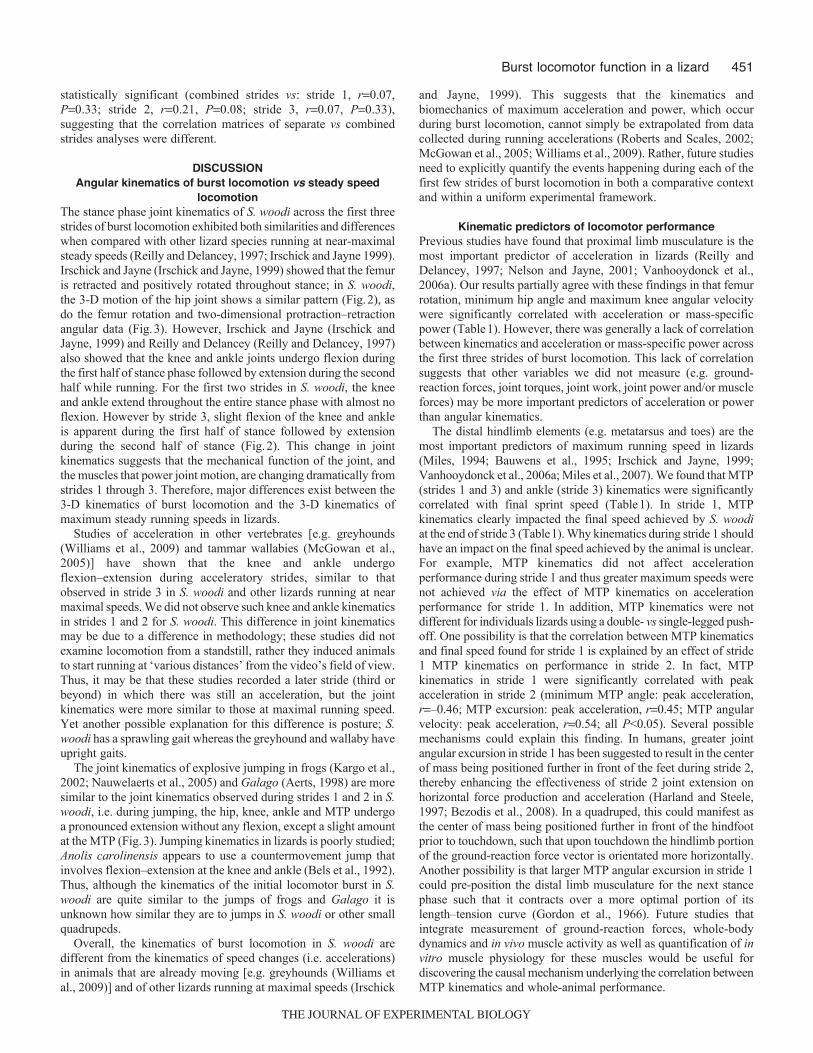
Before any trials were conducted, lizards were weighed (0.1g)and then a small spot of non-toxic white correction fluid was paintedon the six markers indicated in Fig.1. An additional dot was paintedat the base of the lizards’ head. These markers were later used asdigitization landmarks in the high-speed video records to obtain thekinematic data. These landmarks enable the straightforwardcalculation of the kinematic variables that are likely to change duringburst locomotion (i.e. high accelerative steps initially transitioningto steps that maintain high speed) (McElroy and McBrayer, 2010).The hip marker was typically placed ~1mm from the location ofthe acetabulum; very minor variation in the placement of theacetabulum marker introduced error into our kinematic computationsthat was always <5%, and more typically <3%. Because we couldnot precisely adjust the position of the hip marker for each lizard(we lacked radiographs) (see Jayne and Irschick, 1999), we choseto proceed with all analyses based on the marked position of thehip on the animal. All methods followed approved IACUC protocols(Georgia Southern: I08009; College of Charleston: 2009-009).

TrialsThe lizards ran down a horizontal racetrack towards a dark hidebox. The racetrack was 3m long and 0.35m wide, with woodensidewalls 0.4m tall. Cork bark covered the track’s surface providingtraction; we rarely observed foot slippage in the video. A CasioEXILIM EX-F1 camera (512�384pixel resolution, Casio America,Dover, NJ, USA) was suspended over the track in order to collecta vertical view of the lizard over the first 0.4m of the track. A secondCasio EXILIM EX-F1 camera was placed on a tripod next to thetrack in order to obtain a lateral view of the lizard over the first0.4m of the track. All video was recorded at 300framess–1.

Lizards were placed at the beginning of the track so that theirentire bodies could be seen in the camera. The lizards were initiallymotionless. In order to observe a rapid burst of motion from rest,the lizards were startled by hand clapping or a light tail pinch.Continuous clapping encouraged the lizard to run all the way downthe track and out of the cameras’ view. Each individual ran downthe track five to 10 times with at least 30min of rest between eachrun and with each individual being run on three or more separatedays. Trials were excluded if lizards ran at an angle, moved slowly

12

56

7

Hip

KneeAnkle

MTP

3

4

Fig.1. Lateral-view schematic of kinematic markers (1–7) and hindlimb jointangles. MTP, metatarsophalangeal. The angles depicted are three-dimensional. Dotted line represents a horizontal line connecting markers 1and 2, which was used as a reference for computing angles of femoralprotraction–retraction and abduction–adduction.


444

or stopped. This selection process resulted in a total of 20 trialsfrom 10 individuals being retained for analysis (i.e. a single trialfrom six individuals, two trials from two individuals and three trialsfrom two individuals).

Video analysisRaw video was imported and manually trimmed using AdobePremiere Elements software (Adobe Systems, San Jose, CA, USA).The vertical and horizontal videos were synchronized via a lightpulse that was visible in both cameras’ field of view. Individualtrials were trimmed to 10 frames before the lizard’s initial movementuntil the lizard was completely out of the camera’s view, yieldingvideo of the first 0.4m of locomotion from a standstill.

The video from the dorsal view was used to estimate the lizard’sposition for each frame. Using DIDGE software (Cullum, 1999),we manually digitized the white marker at the base of the back ofthe head to obtain the lizard’s position. The point on the head waschosen because the head stayed relatively straight, rather thantracking left to right with medio-lateral bending as was observed atpositions closer to the center of mass (e.g. the hips). Additionally,the front of the body rarely lifted from the substrate (only six of 60strides were bipedal, and these strides occurred without noticeablehead lifting); thus, we are confident that tracking at the head markeris a useful technique for estimating whole-animal performance inthis species [as opposed to other species that may show considerablelifting due to bipedalism (e.g. Clemente et al., 2008)]. Next, weused the program GCVSPL (Woltring, 1986) to fit a quintic splineto the position data and calculate the first and second derivativesof the spline coefficients fitted to the position data (see also McElroyand McBrayer, 2010). This procedure yielded the instantaneousvelocity and acceleration for each frame of the video. We alsocomputed instantaneous external mechanical power by multiplyinginstantaneous velocity by acceleration by the lizard’s body mass.From these data we calculated four performance variables: finalspeed (i.e. the maximum instantaneous speed obtained, alwaysduring stride 3); per-stride total acceleration [i.e. integral of theacceleration–time curve over stance phase per stride (McElroy andMcBrayer, 2010)], per-stride peak acceleration (i.e. maximumvalue of the acceleration–time curve for each stride), and per-stridebody mass-specific instantaneous peak whole-animal externalmechanical power (i.e. peak of the power–time curve divided bybody mass per stride).

Three-dimensional analysis was performed using DLTdv3software (Hedrick, 2008) in MATLAB (MathWorks, Natick, MA,USA). First, we constructed a 3-D cube using Lego blocks and usedwhite correction fluid to mark 13 points on the cube. The first frameof each video sequence from the horizontal and vertical views ofthe cube was used to calibrate the field of view using DLTcal3(Hedrick, 2008) in MATLAB. Next, we uploaded vertical andhorizontal videos for each trial and digitized all markers in eachframe from foot touchdown to foot lift-off for each stride (i.e. stancephase). We focused on 3-D limb kinematics during stance phaseonly, as this is the only part of the locomotor cycle when force, andthus acceleration, can be generated (Curtin et al., 2005; McGowanet al., 2005; Williams et al., 2009; Higham et al., 2011). The endresult of the 3-D kinematic analysis was the instantaneous xyzcoordinate data for each kinematic marker during stance phasesacross several strides.

During stance phase, we calculated the instantaneous 3-D anglesat the hip, knee, ankle and MTP joints. We transformed xyzcoordinate data into 3-D joint angles using the following procedure.The hip position was fixed in each frame by subtracting the x, y

E. J. McElroy, K. L. Archambeau and L. D. McBrayer

and z coordinates of the hip marker (marker 2) from each point(markers 1–6) in each frame. The 3-D angle of the hip joint wasfound by taking the arccosine of the dot product of two vectorswhose bases were at the hip (marker 2) and whose tips were at theknee (marker 3) and caudofemoralis origin (marker 1). To performthis matrix operation we used the following simple algebraicformula in Microsoft Excel:

This process was repeated to calculate the 3-D angle at theknee (markers 2 and 4), ankle (markers 3 and 5) and MTP(markers 4 and 6). From this we could determine the minimumangle, maximum angle and total angle swept of the hip, knee,ankle and MTP for the first several strides of burst locomotion.Additionally, a quintic spline was fitted to the data and the firstderivative, corresponding to the instantaneous angular velocity,was calculated. From this angular velocity data, we estimatedmaximum instantaneous angular velocity for each stride at eachjoint. Finally, the hip joint is a ball-and-socket joint; therefore,we also computed joint angular motion in the horizontal(protraction–retraction), vertical (abduction–adduction) planes aswell as the femoral rotation. Femoral rotation was defined as theangle between two planes: (1) a vertical plane through the femurand (2) the plane containing the hip, knee and ankle markers (i.e.the plane formed by the thigh and shank). To determine the anglebetween these planes, we computed the dot product of their normalvectors. Normal vectors were computed by taking the crossproduct of two vectors contained within the plane.

We report angles such that increasing values would correlate withconcentric contraction of the musculature responsible for producingjoint motion hypothesized to be correlated with burst locomotion[i.e. femoral retraction, knee, ankle and MTP extension(Vanhooydonck et al., 2006a)]. For example, knee angles wererelatively small when the knee was flexed near touchdown and thenincreased throughout stance as the knee extensor musculatureand/or tendons were shortening. To force the hip angles to beincreasing throughout stance phase (as the caudofemoralis musclepresumably concentrically contracts), this required calculating thedot product as mentioned above (markers 1, 2 and 3), and then takingthe resulting angles and subtract them from 180deg. Fig.1 providesa summary schematic of the kinematic markers and joint angles.Because of the positioning of the lateral view camera, all data werecollected for footfalls from the animal’s left hindlimb only. We notethat researchers with two camera systems are often constrained tocollect data in this way, making it impossible to quantify kinematicsfor every step for every trial. This resulted in steps 1, 2 and 4 beingcollected from some individuals because steps 3 and 5 wereobscured in lateral view, and steps 1, 3 and 5 being collected fromother individuals because steps 2 and 4 were obscured by the bodyin lateral view. To help ameliorate these differences and proceedwith statistical analyses, we coded all data by stride number (stride1step 1, stride 2step 2 or 3, stride 3step 4 or 5) for furtheranalysis. We provide additional analyses (see below) to explore howthis choice of grouping impacts the results.

Statistical analysisWe used JMP7 and SAS 9.2 (SAS Institute, Cary, NC, USA) andR v.2.10.1 (R Development Core Team, 2009) for all analyses. Allvariables were checked for normality and transformed, if necessary,prior to analysis.

Hipθ = arccosine (x1x2 + y1y2 + z1z2 )

x12 + y1

2 + z12 x2

2 + y22 + z2

2

⎛

⎝⎜

⎞

⎠⎟ (1).



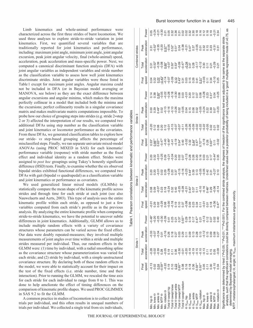
Limb kinematics and whole-animal performance werecharacterized across the first three strides of burst locomotion. Weused three analyses to explore stride-to-stride variation in jointkinematics. First, we quantified several variables that aretraditionally reported for joint kinematics and performance,including: maximum joint angle, minimum joint angle, joint angularexcursion, peak joint angular velocity, final (whole-animal) speed,acceleration, peak acceleration and mass-specific power. Next, wecomputed a canonical discriminant function analysis (DFA) withjoint angular variables as independent variables and stride numberas the classification variable to assess how well joint kinematicsdiscriminate strides. Joint angular variables were those listed inTable1 except for maximum joint angles. Angular maxima couldnot be included in DFA (or in Bayesian model averaging orMANOVA, see below) as they are the exact difference betweenangular excursions and angular minima, which makes the maximaperfectly collinear in a model that included both the minima andthe excursions; perfect collinearity results in a singular covariancematrix and makes multivariate matrix computations impossible. Toprobe how our choice of grouping steps into strides (e.g. stride 2step2 or 3) affected the interpretation of our results, we computed twoadditional DFAs using step number as the classification variableand joint kinematics or locomotor performance as the covariates.From these DFAs, we generated classification tables to explore howour stride- vs step-based grouping affects the percentage ofmisclassified steps. Finally, we ran separate univariate mixed-modelANOVAs (using PROC MIXED in SAS) for each kinematic/performance variable (response) with stride number as the fixedeffect and individual identity as a random effect. Strides wereassigned to post hoc groupings using Tukey’s honestly significantdifference (HSD) tests. Finally, to examine whether the six observedbipedal strides exhibited functional differences, we computed twoDFAs with gait (bipedal vs quadrupedal) as a classification variableand joint kinematics or performance as covariates.

We used generalized linear mixed models (GLMMs) tostatistically compare the mean shape of the kinematic profile acrossstrides and through time for each stride at each joint (see alsoNauwelaerts and Aerts, 2003). This type of analysis uses the entirekinematic profile within each stride, as opposed to just a fewvariables computed from each stride’s profile as in the previousanalysis. By analyzing the entire kinematic profile when comparingstride-to-stride kinematics, we have the potential to uncover subtledifferences in joint kinematics. Additionally, GLMM allows us toinclude multiple random effects with a variety of covariancestructures whose parameters can be varied across the fixed effect.Our data were doubly repeated-measures; they involved multiplemeasurements of joint angles over time within a stride and multiplestrides measured per individual. Thus, our random effects in theGLMM were: (1) time by individual, with a radial smoothing splineas the covariance structure whose parameterization was varied foreach stride; and (2) stride by individual, with a simple unstructuredcovariance structure. By declaring both of these random effects inthe model, we were able to statistically account for their impact onthe test of the fixed effects (i.e. stride number, time and theirinteraction). Prior to running the GLMM, we rescaled the time axisfor each stride for each individual to range from 0 to 1. This wasdone to help ameliorate the effect of timing differences on thecomparison of kinematic profile shapes. We used PROC GLIMMIXin SAS 9.2 to fit the GLMM.

A common practice in studies of locomotion is to collect multipletrials per individual, and this often results in unequal numbers oftrials per individual. We collected a single trial from six individuals,

Tab

le1

. Pea

rson

cor

rela

tions

bet

wee

n ki

nem

atic

and

per

form

ance

var

iabl

es

Str

ide

1S

trid

e 2

Str

ide

3C

ombi

ned

strid

es

Fin

al

Tot

al

Pea

k F

inal

T

otal

P

eak

Fin

al

Tot

al

Pea

k F

inal

T

otal

P

eak

spee

dac

cele

ratio

nac

cele

ratio

nP

ower

spee

dac

cele

ratio

nac

cele

ratio

nP

ower

spee

dac

cele

ratio

nac

cele

ratio

nP

ower

spee

dac

cele

ratio

nac

cele

ratio

nP

ower

Min

. hip

–0

.13

–0.2

8–0

.33

–0.4

8*–0

.01

0.08

0.20

0.20

0.53

*–0

.20

0.00

0.14

0.04

0.31

0.31

0.05

Min

. kne

e

0.02

–0.0

2–0

.07

–0.2

00.

290.

090.

200.

320.

66**

0.12

0.29

0.38

0.22

–0.5

2*–0

.52*

–0.2

4M

in. a

nkle

0.

04–0

.39

–0.3

4–0

.25

0.02

–0.0

7–0

.01

–0.0

10.

63**

0.06

0.49

*0.

60*

0.22

–0.3

9–0

.35

–0.2

1M

in. M

TP

–0

.59*

*0.

280.

01–0

.30

–0.2

90.

230.

02–0

.25

–0.4

7*0.

200.

02–0

.05

–0.4

3 *–0

.08

–0.2

0–0

.30

Min

. rot

atio

n

–0.2

2–0

.05

–0.1

6–0

.39

0.08

0.18

0.29

0.29

–0.4

00.

12–0

.13

–0.2

2–0

.14

0.60

*0.

57**

0.21

Tot

al

swep

t hip

0.

190.

190.

260.

41–0

.00

–0.2

4–0

.28

–0.2

1–0

.49*

–0.0

1–0

.16

–0.2

8–0

.07

–0.0

7–0

.05

0.05

Tot

al

swep

t kne

e0.

100.

110.

180.

25–0

.18

0.32

0.20

–0.0

4–0

.41

–0.1

5–0

.10

–0.1

8–0

.09

0.50

*0.

52*

0.32

Tot

al

swep

t ank

le

0.23

0.36

0.27

0.21

0.19

0.40

0.37

0.20

–0.1

9–0

.07

–0.2

6–0

.30

0.10

0.53

*0.

51*

0.36

Tot

al

swep

t MT

P

0.65

**–0

.30

0.03

0.37

0.10

–0.2

5–0

.15

0.02

0.54

*–0

.07

0.02

0.08

0.43

*–0

.09

0.04

0.21

Tot

al

swep

t rot

atio

n0.

38–0

.01

0.29

0.55

**0.

37–0

.28

–0.1

60.

070.

40–0

.11

–0.0

50.

030.

31–0

.47*

–0.3

80.

02

Vm

axhi

p 0.

16–0

.20

0.11

0.29

–0.0

8–0

.31

–0.2

3–0

.13

–0.0

2–0

.26

0.04

–0.0

10.

03–0

.34

–0.2

10.

02

Vm

axkn

ee

0.18

–0.1

90.

090.

190.

090.

43*

0.44

*0.

280.

32–0

.26

0.15

0.20

0.15

0.37

0.47

*0.

32

Vm

axan

kle

0.36

–0.1

90.

130.

170.

230.

370.

390.

260.

44*

–0.0

90.

060.

120.

260.

280.

370.

30

Vm

axM

TP

0.59

**–0

.15

0.28

0.47

*0.

340.

110.

130.

200.

47*

–0.0

20.

020.

070.

41–0

.17

–0.0

50.

18

Vm

axro

tatio

n0.

55**

–0.1

00.

130.

210.

11–0

.10

–0.0

50.

160.

72**

*–0

.22

–0.0

50.

080.

51*

–0.1

20.

010.

16M

ax. h

ip

0.05

–0.1

3–0

.12

–0.1

3–0

.01

–0.1

6–0

.05

0.03

–0.1

9–0

.22

–0.2

4–0

.28

–0.0

30.

300.

320.

12M

ax. k

nee

0.11

0.11

0.15

0.12

0.01

0.48

*0.

420.

210.

26–0

.05

0.22

0.23

0.11

0.11

0.15

0.18

Max

. ank

le

0.30

0.15

0.09

0.07

0.18

0.29

0.31

0.17

0.63

**0.

020.

390.

51*

0.34

0.21

0.23

0.19

Max

. MT

P

–0.1

00.

050.

080.

02–0

.36

–0.0

6–0

.27

–0.4

4*0.

110.

210.

070.

04–0

.10

–0.2

9–0

.31

–0.2

1M

ax. r

otat

ion

0.34

–0.0

90.

270.

400.

47*

–0.1

40.

100.

35–0

.02

0.02

–0.2

3–0

.25

0.25

0.21

0.31

0.34

Sig

nific

ance

was

det

erm

ined

by

t-te

st (

*P<

0.05

; **P

<0.

01; *

**P

<0.

001)

. For

the

com

bine

d st

ride

anal

ysis

, the

deg

rees

of f

reed

om o

f the

sig

nific

ance

test

wer

e ad

just

ed to

be

sam

e as

the

sepa

rate

str

ide

anal

ysis

, suc

h th

at th

e si

gnifi

cant

cor

rela

tions

cou

ld b

e di

rect

ly c

ompa

red

betw

een

mat

rices

. Und

erlin

ed v

alue

s ha

d a

post

erio

r pr

obab

ility

of b

eing

incl

uded

in a

ʻgoo

dʼ m

ultip

le r

egre

ssio

n m

ode

of >

0.75

, as

dete

rmin

ed b

y B

ayes

ian

mod

el a

vera

ging

.M

TP

, met

atar

soph

alan

geal

; , a

ngle

; V

max

, max

imum

inst

anta

neou

s an

gula

r ve

loci

ty.


446

two trials from two individuals and three trials from two individuals.This creates a statistical issue where complex linear models cannotbe fit because of unbalanced data sets (e.g. three samples from someindividuals and only two from different individuals). We addressedthis issue by using a nesting approach in which we declared therandom effect as sample number nested within individual in boththe univariate mixed models and the GLMMs. This allowed us toinclude all of the data to estimate the parameters of the mixed modelwhilst appropriately specifying denominator degrees of freedom inthe hypothesis test.

In a second set of analyses, we estimated the importance of limbkinematics as predictors of whole-animal performance. Mass wassignificantly correlated with several kinematic variables, thus wecomputed the residuals of regressions of each kinematic variableon mass for each stride and used those for subsequent analyses.Performance variables were not correlated with mass (maximumspeed: r<0.001, P0.88; peak acceleration: r<0.001, P0.86, totalacceleration: r<0.001, P0.92; mass-specific power: r<0.001,P0.88). First, we computed simple Pearson univariate correlationsbetween each kinematic and performance variable for each strideand then tested each correlation with a t-test. To account for theinherent multivariate nature of the kinematic data, we used aBayesian model averaging method to estimate the importance ofeach kinematic predictor for each performance for each stride withina multiple regression framework (Ellison, 1996). Choosing the ‘best’multiple regression model has many well-known issues; Bayesianmodel averaging accounts for the uncertainty in choosing the singlebest model by generating a posterior sample of ‘good’ models usinga leaps-and-bound algorithm. From this sample of models, themethod computes the posterior probability that a predictor variablehas a non-zero coefficient. Given the nature of kinematic data, ourpredictor variables (kinematics) were often inter-correlated, whichcan create issues when attempting to interpret simple Pearsoncorrelations (Chevan and Sutherland, 1991) and when attemptingto compute multiple regression coefficients (Quinn and Keough,2003). These inter-correlations make it difficult for one to knowwhether each simple correlation and/or regression coefficient is dueto the predictor of interest independently, or due to collinearitybetween the predictor and other predictors (Quinn and Keough,2003). Hierarchical partitioning is a statistical tool that can helpdisentangle independent correlation vs correlation that is due tocollinearity (Chevan and Sutherland, 1991; Mac Nally, 2000; MacNally, 2002). This analysis works by computing all possibleregression models and then comparing subsets of models with andwithout the predictor variable of interest. The increase in R2 becauseof the inclusion of the predictor can be averaged across allcomparisons to compute the independent contribution of thatvariable to the variance explained. The analysis also determines thejoint contribution of other variables to the variance explained bythe predictor of interests (i.e. the variance explained by collinearitywith other predictors). Positive joint contribution values show thatcollinearity has inflated with correlation whereas negative jointvalues indicate suppression of the correlation. We computedhierarchical partitions for each performance variable for each stride,using ‘important’ predictors that were defined as having: (1)significant simple correlation coefficients or (2) a posteriorprobability of a non-zero coefficient greater than 0.75 (Kass et al.,1995). Only a subset of predictors was used in the partition because:(1) including all predictors (i.e. 14) is beyond the currentcomputational abilities of ‘hier.part’ package, and (2) predictors thatwere not deemed ‘important’ by Pearson correlation or Bayesianmodel averaging were unlikely to reveal any additional information


via partitioning their variance. We used the R packages ‘hier.part’(Walsh and Mac Nally, 2008) for hierarchical partitioning and‘BMA’ for Bayesian model averaging (Raftery et al., 2005).

Preliminary video review showed that stride 1 (i.e. the firstmovement from standstill) consisted of either a single leg push-offor a simultaneous double leg push-off. We tested for differencesrelated to this behavioral variation by running two separateMANOVAs, one with the kinematic variables for stride 1 asresponses, and one with performance variables for stride 1 asresponses. In both MANOVAs, burst behavior (i.e. single- vs double-leg push-off) was the main effect.

Separate vs combined strides analysisFirst, we computed the Pearson correlation between kinematics andperformance after combining data across all strides. Next, wecomputed the Euclidean distance matrix from each of the fourcorrelation matrices (stride 1, stride 2, stride 3 and combined strides).We then compared the distance matrix for the combined strides datawith each of the distance matrices for the separate strides data usingMantel tests.

RESULTSComparison of joint angular changes across strides during

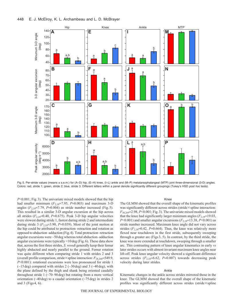
burst locomotionLizards ranged from 2.0 to 4.4g (mean: 2.9g). Trials were mostlyquadrupedal; only six of 60 strides were bipedal. Bipedal andquadrupedal strides did not differ in performance (Wilks’ 0.893,F4,551.65, P0.17) or kinematics (Wilks’ 0.641, F15,441.64,P0.10). Several of the kinematic variables showed significantchanges across the first three strides of burst locomotion (Figs2–6).

DFA found that stride number was significantly classifiedaccording to joint kinematics (Wilks’ 0.148, F24,926.13,P<0.001). DFA misclassified 10% of the observations (six of 60).All six misclassified strides were misclassified as an adjacentstride (e.g. stride 1 as stride 2). DF1 accounted for 84% of thevariance and clearly separated the data into three groups (Fig.2).

–10

–9

–8

–7

–6

–5

–4

–3

–2

–4 –3 –2 –1 0 1 2 3 4 5 6

DF2

DF1Min. hip Θ (–0.6)Total Θ swept knee (–0.6)Total Θ swept ankle (–0.5)Θ Velocity knee (–0.5)

Θ

Vel

ocity

hip

(–0.

5)M

in. a

nkle

Θ (0

.5)

Min. knee Θ (0.8)Min. ankle Θ (0.4)

Fig.2. Results of the discriminant function analysis with stride as theclassification variable. The best discriminating variables are labeled at theends of each axis with their loading in parentheses. All other variables hadloadings between –0.3 and 0.3. Stride 1, red squares; stride 2, greenpluses; stride 3, blue crosses. , angle; Velocity, Vmax.



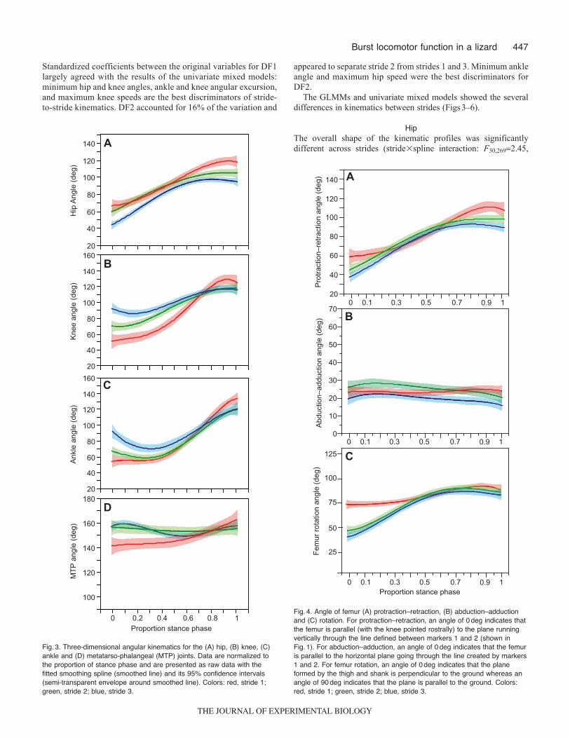
Standardized coefficients between the original variables for DF1largely agreed with the results of the univariate mixed models:minimum hip and knee angles, ankle and knee angular excursion,and maximum knee speeds are the best discriminators of stride-to-stride kinematics. DF2 accounted for 16% of the variation and

appeared to separate stride 2 from strides 1 and 3. Minimum ankleangle and maximum hip speed were the best discriminators forDF2.

The GLMMs and univariate mixed models showed the severaldifferences in kinematics between strides (Figs3–6).

HipThe overall shape of the kinematic profiles was significantlydifferent across strides (stride�spline interaction: F30,2692.45,

Proportion stance phase0 0.1 0.3 0.5 0.7 1

75

100

125 C

20

40

60B

20

40

60

80

100

120

140 A

Fem

ur ro

tatio

n an

gle

(deg

)P

rotra

ctio

n–re

tract

ion

angl

e (d

eg)

0.9

Abd

uctio

n–ad

duct

ion

angl

e (d

eg)

30

50

70

50

0

10

25

0 0.1 0.3 0.5 0.7 10.9

0 0.1 0.3 0.5 0.7 10.9

Fig.4. Angle of femur (A) protraction–retraction, (B) abduction–adductionand (C) rotation. For protraction–retraction, an angle of 0deg indicates thatthe femur is parallel (with the knee pointed rostrally) to the plane runningvertically through the line defined between markers 1 and 2 (shown inFig.1). For abduction–adduction, an angle of 0deg indicates that the femuris parallel to the horizontal plane going through the line created by markers1 and 2. For femur rotation, an angle of 0deg indicates that the planeformed by the thigh and shank is perpendicular to the ground whereas anangle of 90deg indicates that the plane is parallel to the ground. Colors:red, stride 1; green, stride 2; blue, stride 3.

100

120

140

160

180

Proportion stance phase0 0.2 0.4 0.6 0.8 1

D

20

40

60

80

100

120

140

160C

20

40

60

80

100

120

140

160B

20

40

60

80

100

120

140 A

MTP

ang

le (d

eg)

Kne

e an

gle

(deg

)A

nkle

ang

le (d

eg)

Hip

Ang

le (d

eg)

Fig.3. Three-dimensional angular kinematics for the (A) hip, (B) knee, (C)ankle and (D) metatarso-phalangeal (MTP) joints. Data are normalized tothe proportion of stance phase and are presented as raw data with thefitted smoothing spline (smoothed line) and its 95% confidence intervals(semi-transparent envelope around smoothed line). Colors: red, stride 1;green, stride 2; blue, stride 3.


448

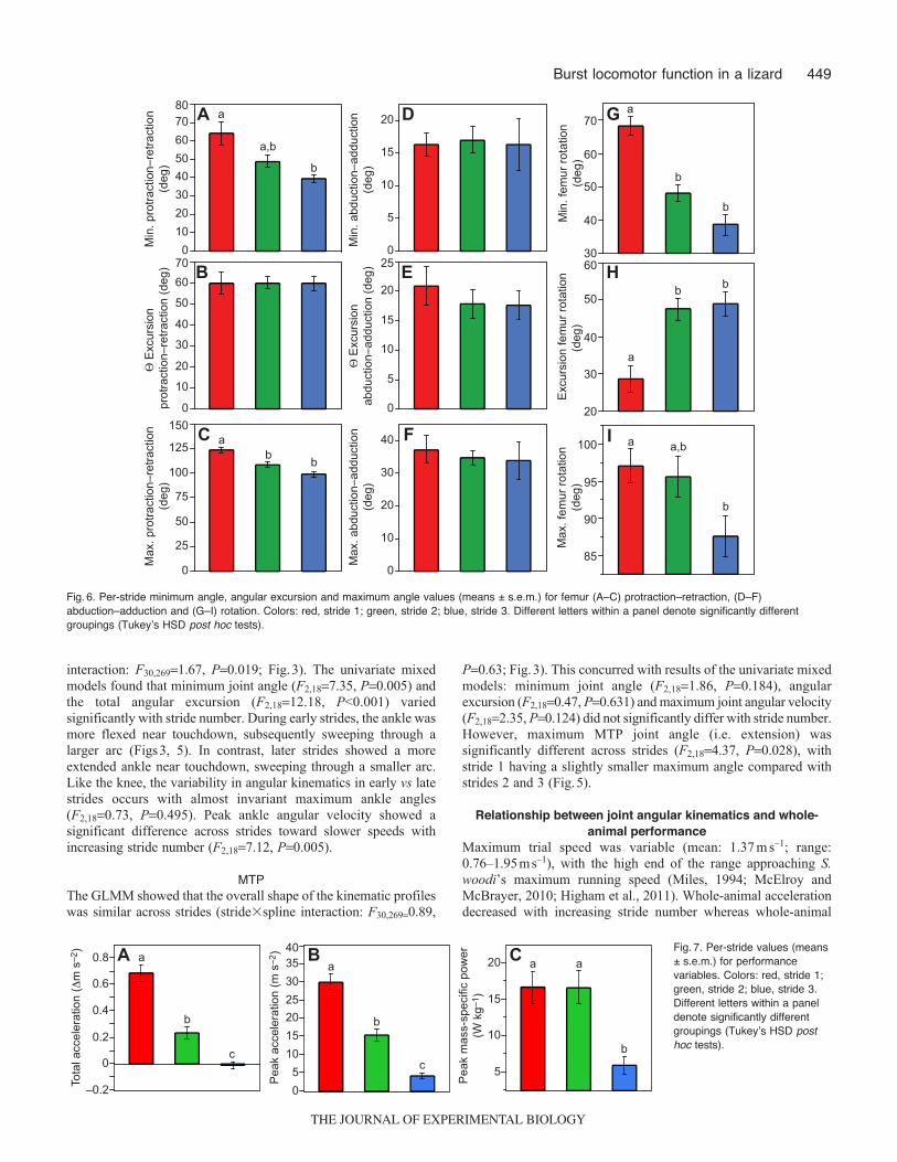
P<0.001; Fig.3). The univariate mixed models showed that the hiphad smaller minimum (F2,187.95, P0.003) and maximum 3-Dangles (F2,187.79, P0.004) as stride number increased (Fig.5).This resulted in a similar 3-D angular excursion at the hip acrossall strides (F2,180.40, P0.675). Peak 3-D hip angular velocitieswere slowest during stride 1, fastest during stride 2 and intermediateduring stride 3 (F2,183.90, P0.039). Most of the joint motion atthe hip could be attributed to protraction–retraction and rotation asopposed to abduction–adduction (Fig.4). Total protraction–retractionangular excursions were ~50deg whereas total abduction–adductionangular excursions were typically <10deg (Fig.6). These data showthat, across the first three strides, S. woodi generally keep their femurhighly abducted and nearly parallel to the ground. Femur rotationwas quite different when comparing stride 1 with strides 2 and 3(overall profile comparison, stride�spline interaction: F28,268549.9,P<0.001): rotational excursions were less pronounced for stride 1(~15deg) compared with strides 2 (~30deg) and 3 (~40deg), withthe plane defined by the thigh and shank being oriented caudallythroughout stride 1 (~70–90deg) but rotating from a more verticalorientation (~40deg) to a caudal orientation (~75deg) in strides 2and 3 (Figs4, 6).


KneeThe GLMM showed that the overall shape of the kinematic profileswas significantly different across strides (stride�spline interaction:F30,2692.98, P<0.001; Fig.3). The univariate mixed models showedthat the knee had significantly larger minimum angles (F2,1819.03,P<0.001) and smaller angular excursions (F2,1813.38, P<0.001) asstride number increased. Maximum knee angle did not vary acrossstrides (F2,180.42, P0.664). Thus, the knee was relatively moreflexed near touchdown in the first stride, subsequently sweepingthrough a greater arc (Figs3, 5). In contrast, by the third stride, theknee was more extended at touchdown, sweeping through a smallerarc. This contrasting pattern of knee angular kinematics in early vslater strides occurs with almost invariant maximum knee angles nearlift-off. Peak knee angular velocity showed a significant differenceacross strides (F2,186.62, P0.007) towards decreasing peakvelocity during later strides.

AnkleKinematic changes in the ankle across strides mirrored those in theknee. The GLMM showed that the overall shape of the kinematicprofiles was significantly different across strides (stride�spline

20304050607080

3-D

ang

ular

exc

ursi

on(d

eg)

Pea

k an

gula

r vel

ocity

(d

eg s

–1)

4000

5000

6000

2000

3000

100110120130140150160170

Max

imum

3-D

ang

le(d

eg)

40

60

80

100

120

140

Min

umum

3-D

ang

le(d

eg)

KneeHip Ankle MTP

B

C

A

D

F

G

E

H

J

K

I

L

N

O

M

P

a

a,bb

a

bc

a ab

b

a

a

aa

b

aa

bab

b

ba,b

a

b

a

a,b

a

b

a,b

Fig.5. Per-stride values (means ± s.e.m.) for (A–D) hip, (E–H) knee, (I–L) ankle and (M–P) metatarsophalangeal (MTP) joint three-dimensional (3-D) angles.Colors: red, stride 1; green, stride 2; blue, stride 3. Different letters within a panel denote significantly different groupings (Tukeyʼs HSD post hoc tests).



interaction: F30,2691.67, P0.019; Fig.3). The univariate mixedmodels found that minimum joint angle (F2,187.35, P0.005) andthe total angular excursion (F2,1812.18, P<0.001) variedsignificantly with stride number. During early strides, the ankle wasmore flexed near touchdown, subsequently sweeping through alarger arc (Figs3, 5). In contrast, later strides showed a moreextended ankle near touchdown, sweeping through a smaller arc.Like the knee, the variability in angular kinematics in early vs latestrides occurs with almost invariant maximum ankle angles(F2,180.73, P0.495). Peak ankle angular velocity showed asignificant difference across strides toward slower speeds withincreasing stride number (F2,187.12, P0.005).

MTPThe GLMM showed that the overall shape of the kinematic profileswas similar across strides (stride�spline interaction: F30,2690.89,

P0.63; Fig.3). This concurred with results of the univariate mixedmodels: minimum joint angle (F2,181.86, P0.184), angularexcursion (F2,180.47, P0.631) and maximum joint angular velocity(F2,182.35, P0.124) did not significantly differ with stride number.However, maximum MTP joint angle (i.e. extension) wassignificantly different across strides (F2,184.37, P0.028), withstride 1 having a slightly smaller maximum angle compared withstrides 2 and 3 (Fig.5).

Relationship between joint angular kinematics and whole-animal performance

Maximum trial speed was variable (mean: 1.37ms–1; range:0.76–1.95ms–1), with the high end of the range approaching S.woodi’s maximum running speed (Miles, 1994; McElroy andMcBrayer, 2010; Higham et al., 2011). Whole-animal accelerationdecreased with increasing stride number whereas whole-animal

Exc

ursi

on fe

mur

rota

tion

(deg

)

0

10

20

30

40

50

6070

Θ E

xcur

sion

pr

otra

ctio

n–re

tract

ion

(deg

)

01020304050607080

Min

. pro

tract

ion–

retra

ctio

n(d

eg)

0

5

10

15

20

Min

. abd

uctio

n–ad

duct

ion

(deg

)

D

B

A

b

a,b

0

25

50

75

100

125

150

Max

. pro

tract

ion–

retra

ctio

n(d

eg)

Cb

ab

H

a

b b

Max

. fem

ur ro

tatio

n(d

eg)

I a a,b

b

G a

b

b

Min

. fem

ur ro

tatio

n(d

eg)

0

5

10

15

20

25 E

Θ E

xcur

sion

abdu

ctio

n–ad

duct

ion

(deg

)

0

10

20

30

40 F

Max

. abd

uctio

n–ad

duct

ion

(deg

)

100

95

90

85

60

50

40

30

20

70

60

50

40

30

a

Fig.6. Per-stride minimum angle, angular excursion and maximum angle values (means ± s.e.m.) for femur (A–C) protraction–retraction, (D–F)abduction–adduction and (G–I) rotation. Colors: red, stride 1; green, stride 2; blue, stride 3. Different letters within a panel denote significantly differentgroupings (Tukeyʼs HSD post hoc tests).

–0.2

0

0.2

0.4

0.6

0.8

Tota

l acc

eler

atio

n (Δ

m s

–2)

05

10152025303540

Pea

k ac

cele

ratio

n (m

s–2

)

5

10

15

20

Pea

k m

ass-

spec

ific

pow

er(W

kg–

1 )

A B Ca

b

c

a

b

c

a a

b

Fig.7. Per-stride values (means± s.e.m.) for performancevariables. Colors: red, stride 1;green, stride 2; blue, stride 3.Different letters within a paneldenote significantly differentgroupings (Tukeyʼs HSD posthoc tests).


450

mass-specific power was large on stride 1 and 2 but smaller on stride3 (Fig.7). In general, the Pearson correlations between per-stridejoint angular kinematics and performance were weak (r<0.40) andnot significant (P>0.05, Table1). However, a few of the kinematicvariables were significantly correlated with performance (r>0.43)for some strides. For stride 1, MTP and hip angular kinematics wereimportant predictors of final speed and mass-specific power,respectively. Stride 2 had only two significant correlations, betweenmaximum MTP angle and mass-specific power and betweenmaximum knee angle and total acceleration. Stride 3 had the greatestnumber of significant correlations, with variables from each jointbeing correlated with final speed, and minimum ankle anglecorrelating with mass-specific power.

Strong correlations among kinematic variables were apparent(supplementary material TableS1), which could potentially impactthe interpretation of the simple Pearson correlations. Bayesian modelaveraging revealed a few new kinematic variables as importantpredictors of performance (Table1); however, this analysis alsoconcurred, in some cases, with the simple correlations. Hierarchicalpartitioning clearly showed that kinematic collinearity had a largeinfluence on the simple correlations between kinematics andperformance (Table2). When comparing the results of thehierarchical partitioning analysis with the simple correlations, onemust first square the simple correlation to compute the variance itexplains (e.g. for minimum MTP angle, r–0.59 and r20.35), andthen examine how r2 is partitioned into independent (e.g. 0.15) vsjoint (e.g. 0.20) contributions (Table2). Examining the breakdownof all significant simple correlations, it becomes apparent that mostof these simple correlations are due primarily to joint contributions(i.e. collinearity). Thus, collinear patterns between kinematicvariables are more important than simple individual effects inexplaining the variance in performance.

Separate MANOVAs found that single-legged push-offs exhibitedsignificantly lower locomotor performance than double-leggedpush-offs (for final speed, total and peak acceleration, and mass-


specific power, Wilks’ 0.545, F2,177.08, P0.006). Jointkinematics did not differ between single- and double-legged push-offs (Wilks’ 0.865, F4,150.59, P0.67).

Separate vs combined strides analysisThe DFA using step as a classification variable according to jointkinematics was significant (Wilks’ 0.116, F48,1722.68, P<0.001).The classification table (supplementary material TableS2) showedthat most steps were accurately classified as the correct step (22%misclassification rate) and/or the correct stride (10%misclassification rate; stride is based on our grouping of steps).Supplementary material Fig.S1 shows that step 2 is separated fromall other steps, steps 2 and 3 group together and steps 4 and 5 grouptogether.

The DFA using step as a classification variable according tolocomotor performance was also significant (Wilks’ 0.103,F16,159.511.0, P<0.001). The classification table (supplementarymaterial TableS3) showed that most steps were accurately classifiedas the correct step (25% misclassification rate) and/or the correctstride (8% misclassification rate; stride is based on our grouping).Supplementary material FigsS2 and S3 show that step 1 is separatedfrom all other steps, steps 4 and 5 group together and are almostdistinct from step 2, and step 3 is intermediate to step 2 and thestep 4/5 group.

The Pearson correlation matrix for the combined strides data setwas different from the separate stride matrices (Table1). Severalvariables that were significantly correlated with whole-animalperformance in the separate stride analysis were not significant oncestrides were combined (e.g. minimum hip, knee and ankle angles).In addition, several kinematic variables that were never significantlycorrelated with performance in the separate stride analysis hadsignificant correlations in the combined stride analysis (e.g.minimum knee angle, knee and ankle angular excursion). Manteltests comparing the combined stride matrix with each separate stridematrix found very small correlation coefficients that were not

Table2. Results of the hierarchical partitioning analysis

Stride 1 Stride 3 Combined

Peak mass-Final speed specific power Final speed Final speed Total acceleration Peak acceleration

I J I J I J I J I J I J

Min. hip – – 0.12 0.11 0.06 0.22 – – – – – –Min. knee – – – – 0.15 0.28 – – 0.11 0.17 0.10 0.17Min. ankle 0.06 –0.06 – – 0.10 0.30 0.10 –0.05 – – – –Min. MTP 0.15 0.20 – – 0.05 0.17 0.10 0.09 – – – –Min. rotation – – – – – – – – 0.14 0.22 0.15 0.17Total swept hip – – – – 0.09 0.16 – – – – – –Total swept knee – – – – – – – – 0.08 0.17 0.07 0.20Total swept ankle 0.10 –0.04 – – – – 0.04 –0.03 0.11 0.18 0.08 0.18Total swept MTP 0.14 0.28 – – 0.08 0.20 0.07 0.11 – – – –Total swept rotation – – 0.14 0.16 – – – – 0.07 0.15 – – Vmax hip – – – – – – – – 0.10 0.02 – – Vmax knee – – – – – – – – – – 0.07 0.15 Vmax ankle – – – – 0.16 0.04 – – – – – – Vmax MTP 0.10 0.24 0.13 0.09 0.04 0.18 – – – – – – Vmax rotation 0.13 0.17 – – 0.17 0.36 0.15 0.10 – – – –

Only variables with a significant simple Pearson correlation, or 0.75 posterior probability in Bayesian model averaging, were included in the partitioninganalysis. I is the variance explained by a predictor variable that is independent of the variance explained by other predictors (i.e. not influenced bycollinearity) and is always a positive number or zero. J is the variance explained by collinearity between predictors. A positive J suggests that collinearity hasinflated the simple correlation between the predictor and response, whereas a negative J suggests that collinearity has suppressed the simple correlation.The square root of the sum of I and J for each variable is the absolute value of its simple Pearson correlation.

MTP, metatarsophalangeal; , angle; Vmax, maximum instantaneous angular velocity.



statistically significant (combined strides vs: stride 1, r0.07,P0.33; stride 2, r0.21, P0.08; stride 3, r0.07, P0.33),suggesting that the correlation matrices of separate vs combinedstrides analyses were different.

DISCUSSIONAngular kinematics of burst locomotion vs steady speed

locomotionThe stance phase joint kinematics of S. woodi across the first threestrides of burst locomotion exhibited both similarities and differenceswhen compared with other lizard species running at near-maximalsteady speeds (Reilly and Delancey, 1997; Irschick and Jayne 1999).Irschick and Jayne (Irschick and Jayne, 1999) showed that the femuris retracted and positively rotated throughout stance; in S. woodi,the 3-D motion of the hip joint shows a similar pattern (Fig.2), asdo the femur rotation and two-dimensional protraction–retractionangular data (Fig.3). However, Irschick and Jayne (Irschick andJayne, 1999) and Reilly and Delancey (Reilly and Delancey, 1997)also showed that the knee and ankle joints undergo flexion duringthe first half of stance phase followed by extension during the secondhalf while running. For the first two strides in S. woodi, the kneeand ankle extend throughout the entire stance phase with almost noflexion. However by stride 3, slight flexion of the knee and ankleis apparent during the first half of stance followed by extensionduring the second half of stance (Fig.2). This change in jointkinematics suggests that the mechanical function of the joint, andthe muscles that power joint motion, are changing dramatically fromstrides 1 through 3. Therefore, major differences exist between the3-D kinematics of burst locomotion and the 3-D kinematics ofmaximum steady running speeds in lizards.

Studies of acceleration in other vertebrates [e.g. greyhounds(Williams et al., 2009) and tammar wallabies (McGowan et al.,2005)] have shown that the knee and ankle undergoflexion–extension during acceleratory strides, similar to thatobserved in stride 3 in S. woodi and other lizards running at nearmaximal speeds. We did not observe such knee and ankle kinematicsin strides 1 and 2 for S. woodi. This difference in joint kinematicsmay be due to a difference in methodology; these studies did notexamine locomotion from a standstill, rather they induced animalsto start running at ‘various distances’ from the video’s field of view.Thus, it may be that these studies recorded a later stride (third orbeyond) in which there was still an acceleration, but the jointkinematics were more similar to those at maximal running speed.Yet another possible explanation for this difference is posture; S.woodi has a sprawling gait whereas the greyhound and wallaby haveupright gaits.

The joint kinematics of explosive jumping in frogs (Kargo et al.,2002; Nauwelaerts et al., 2005) and Galago (Aerts, 1998) are moresimilar to the joint kinematics observed during strides 1 and 2 in S.woodi, i.e. during jumping, the hip, knee, ankle and MTP undergoa pronounced extension without any flexion, except a slight amountat the MTP (Fig.3). Jumping kinematics in lizards is poorly studied;Anolis carolinensis appears to use a countermovement jump thatinvolves flexion–extension at the knee and ankle (Bels et al., 1992).Thus, although the kinematics of the initial locomotor burst in S.woodi are quite similar to the jumps of frogs and Galago it isunknown how similar they are to jumps in S. woodi or other smallquadrupeds.

Overall, the kinematics of burst locomotion in S. woodi aredifferent from the kinematics of speed changes (i.e. accelerations)in animals that are already moving [e.g. greyhounds (Williams etal., 2009)] and of other lizards running at maximal speeds (Irschick

and Jayne, 1999). This suggests that the kinematics andbiomechanics of maximum acceleration and power, which occurduring burst locomotion, cannot simply be extrapolated from datacollected during running accelerations (Roberts and Scales, 2002;McGowan et al., 2005; Williams et al., 2009). Rather, future studiesneed to explicitly quantify the events happening during each of thefirst few strides of burst locomotion in both a comparative contextand within a uniform experimental framework.

Kinematic predictors of locomotor performancePrevious studies have found that proximal limb musculature is themost important predictor of acceleration in lizards (Reilly andDelancey, 1997; Nelson and Jayne, 2001; Vanhooydonck et al.,2006a). Our results partially agree with these findings in that femurrotation, minimum hip angle and maximum knee angular velocitywere significantly correlated with acceleration or mass-specificpower (Table1). However, there was generally a lack of correlationbetween kinematics and acceleration or mass-specific power acrossthe first three strides of burst locomotion. This lack of correlationsuggests that other variables we did not measure (e.g. ground-reaction forces, joint torques, joint work, joint power and/or muscleforces) may be more important predictors of acceleration or powerthan angular kinematics.

The distal hindlimb elements (e.g. metatarsus and toes) are themost important predictors of maximum running speed in lizards(Miles, 1994; Bauwens et al., 1995; Irschick and Jayne, 1999;Vanhooydonck et al., 2006a; Miles et al., 2007). We found that MTP(strides 1 and 3) and ankle (stride 3) kinematics were significantlycorrelated with final sprint speed (Table1). In stride 1, MTPkinematics clearly impacted the final speed achieved by S. woodiat the end of stride 3 (Table1). Why kinematics during stride 1 shouldhave an impact on the final speed achieved by the animal is unclear.For example, MTP kinematics did not affect accelerationperformance during stride 1 and thus greater maximum speeds werenot achieved via the effect of MTP kinematics on accelerationperformance for stride 1. In addition, MTP kinematics were notdifferent for individuals lizards using a double- vs single-legged push-off. One possibility is that the correlation between MTP kinematicsand final speed found for stride 1 is explained by an effect of stride1 MTP kinematics on performance in stride 2. In fact, MTPkinematics in stride 1 were significantly correlated with peakacceleration in stride 2 (minimum MTP angle: peak acceleration,r–0.46; MTP excursion: peak acceleration, r0.45; MTP angularvelocity: peak acceleration, r0.54; all P<0.05). Several possiblemechanisms could explain this finding. In humans, greater jointangular excursion in stride 1 has been suggested to result in the centerof mass being positioned further in front of the feet during stride 2,thereby enhancing the effectiveness of stride 2 joint extension onhorizontal force production and acceleration (Harland and Steele,1997; Bezodis et al., 2008). In a quadruped, this could manifest asthe center of mass being positioned further in front of the hindfootprior to touchdown, such that upon touchdown the hindlimb portionof the ground-reaction force vector is orientated more horizontally.Another possibility is that larger MTP angular excursion in stride 1could pre-position the distal limb musculature for the next stancephase such that it contracts over a more optimal portion of itslength–tension curve (Gordon et al., 1966). Future studies thatintegrate measurement of ground-reaction forces, whole-bodydynamics and in vivo muscle activity as well as quantification of invitro muscle physiology for these muscles would be useful fordiscovering the causal mechanism underlying the correlation betweenMTP kinematics and whole-animal performance.


452

Stride 3 had several significant correlations between kinematicsand final speed. These correlations imply that greater final sprintingspeeds are obtained with: (1) more extended hip, knee and ankle attouchdown (i.e. greater minimum angle), (2) greater MTP jointexcursion and speed, (3) smaller hip joint excursion and (4) greaterankle extension at toe-off (Table1). Coupled with the correlationsfound for stride 1, it appears that in S. woodi, the kinematics of theankle and MTP joints are the key determinants of final sprintingspeed. The fiber-type composition of the gastrocnemius muscle (anankle extensor) in S. woodi was recently shown to be correlatedwith both maximum sprinting speed and acceleration capacity(Higham et al., 2011). In addition, functional studies of Sceloporusclarki suggest that plantar flexion is an important component ofthrust generation during sub-maximal steady speed running (e.g.Reilly and Delancey, 1997). Finally, several studies ofphrynosomatine lizards have shown a correlation between distal limbmorphology, particularly metatarsus length, and maximum sprintingperformance (e.g. Miles, 1994; Irschick and Jayne, 1999). Thusamong phrynosomatine lizards, it appears that the distal bonyelements and musculature of the hindlimb are the key determinantsof maximum locomotor performance. However, additional data areneeded on the physiological properties of limb muscles (e.g.ambiens, flexor digitorum communis). Finally, when linking jointmotion and locomotor performance, one must be cautious: only acomputational musculoskeletal model coupled with inverse dynamicanalysis will definitively quantify joint moments. Only with suchdata in hand may we fully assess the differential contribution ofeach joint and its musculature to locomotion performance (e.g. Aerts,1998).

Although the distal limb appears to be the most importantpredictor of burst performance in S. woodi and perhaps thePhrynosomatidae, this may not hold true for other groups. Forexample, Vanhooydonck et al. (Vanhooydonck et al., 2006a)showed that the mass of the knee extensors was the most importantmuscular predictor of acceleration capacity and maximum speedfor a sample of 16 Anolis species. In addition, Curtin et al. (Curtinet al., 2005) showed that the power output of the entire mass of theretractors and extensors of the hindlimb are required to powermaximal accelerations in Acanthodactylus, suggesting that functionat all joints is important for achieving maximum acceleration andspeed. Finally, in mammals, the pattern is complex and speciesspecific; greyhounds rely on hip retractors and ankle extensors(Williams et al., 2009), wallabies rely on ankle extensors coupledwith power transfer from the proximal limb muscles (McGowan etal., 2005), and humans rely on the femur retractors and kneeextensors (Delecluse, 1997). What is emerging from the study ofthe functional basis of acceleration across taxa is that evolutiongenerates many different functional solutions (i.e. many-to-onemapping) to achieve greater acceleration capacity (Alfaro et al.,2004; Bock, 1959; Wainwright, 2007). Although the discovery ofbroad general principles is a central goal in science, the emergingrelationships between morphology, function and accelerationperformance indicates that different clades find different functionalsolutions to increase performance (Vanhooydonck et al., 2006a),and that maximizing acceleration capacity may be better definedby divergent functional mechanisms than by any general principle.

Separate vs combined strides analysisAn important finding from our study is that the correlation structurebetween joint angular kinematics and performance changes basedon how one analyzes a burst locomotor event. When all strides werecombined, most of the significant correlations between speed or


mass-specific power and joint kinematics disappeared and severalnew correlations between acceleration and kinematics appeared(Table1). Thus, had we pooled kinematic data across strides, ourinterpretations of the functional basis of performance would havebeen drastically altered (e.g. knee kinematics seem to be importantpredictors of acceleration in the combined analysis). In our opinion,separate stride analysis is the best method and this seems justifiedfor several reasons. First, we clearly show that limb joint kinematicsand locomotor performance are different from strides 1 through 3during the burst locomotor event (e.g. Figs2–7). Thus, by combiningthe kinematic data, one is ignoring a potentially important sourceof variation (i.e. stride to stride) that could potentially mask or evenreverse our interpretation of function (i.e. knee vs ankle or MTPkinematic correlations; Table1). This issue is even further amplifiedbecause of the collinear nature of limb kinematics (supplementarymaterial TableS1) and the correlation between limb kinematics andperformance, as shown by the hierarchical partitioning analysis(Table2). Second, from the perspective of the organism, burstlocomotion is a very different behavior than speed changes (i.e.acceleration) while running. The animal starts at a completestandstill and then suddenly engages in rhythmic cycling of thelimbs, whereas, for an animal already in motion, it simply has toalter the cyclical pattern of muscle activation and joint kinematics.Both behaviors involve acceleration, even large accelerations, butthey seem to be fundamentally different in kinematics and function.The fact that most previous studies have used a ‘combined’ stridesapproach likely stems from the history of how we have studiedsteady-speed locomotion. Most studies of steady-speed locomotionessentially ignore ‘stride number’ because once the animal ismoving at steady speed, stride-to-stride variation in kinematics andmechanics are minimal. This is why using a treadmill for steady-speed studies works well. It should be noted that even the presentstudy has a shortfall: we combined steps into strides, which wasjustified based on methodological constraints and statistical grounds(supplementary material FigsS1–S3, TablesS2, S3). Although thisseems acceptable for the study of burst locomotor in S. woodi, itmay not be in other organisms. Based on these findings, we feelthat it is important to find common methodologies by which wecan expand our functional understanding of burst locomotion,acceleration performance and acceleration biomechanics.

ACKNOWLEDGEMENTSWe thank Anna Baur, Shea Diaz, Melissa Strickland and Allyson Wilson forassistance running lizards, trimming videos for analysis and animal care. Wethank Allan Strand and Ralph Mac Nally for advice regarding Bayesian modelaveraging and hierarchical partitioning.

FUNDINGThis work was supported by start-up funds provided by the College of Charlestonto E.J.M.

REFERENCESAerts, P. (1998). Vertical jumping in Galago senegalensis: the quest for a hidden

power amplifier. Philos. Trans. R. Soc. Lond. B 353, 1607-1620.Alfaro, M. E., Bolnick, D. I. and Wainwright, P. C. (2004). Evolutionary dynamics of

complex biomechanical systems: an example using the four-bar mechanism.Evolution 85, 495-503.

Arnold, S. J. (1983). Morphology, performance and fitness. Am. Zool. 23, 347-361.Bauwens, D., Garland, T., Jr, Castilla, A. M. and Van Damme, R. (1995). Evolution

of sprint speed in lacertid lizards: morphological, physiological, and behavioralcovariation. Evolution 49, 848-863.

Bels, V. L. and Theys, J.-P., Bennett, M. R. and Legrand, L. (1992). Biomechanicalanalysis of jumping in Anolis carolinensis (Reptilia: Iguanidae). Copeia 1992, 492-504.

Bezodis, N. E., Trewartha, G. and Salo, A. I. (2008). Understanding elite sprintstarting performance through an analysis of joint kinematics. In Proceedings of theXXVI International Conference on Biomechanics in Sports (ed. Y.-H. Kwon, J. Shim,J. K. Shim and I. S. Shin), pp. 498-501. Seoul, Korea: Rainbow Books.



Bock, W. J. (1959). Preadaptation and multiple evolutionary pathways. Evolution 13,194-211.

Calsbeek, R. and Irschick, D. J. (2007). The quick and the dead: locomotorperformance and natural selection in island lizards. Evolution 61, 2493-2503.

Chevan, A. and Sutherland, M. (1991). Hierarchical partitioning. Am. Stat. 45, 90-96.Clemente, C. J., Withers, P. C., Thompson, G. and Lloyd, D. (2008). Why go

bipedal? Locomotion and morphology in Australian agamid lizards. J. Exp. Biol. 211,2058-2065.

Cullum, A. J. (1999). Didge - Image Digitizing Software. Version 2.0.Curtin, N., Woledge, R. and Aerts, P. (2005). Muscle directly meets the vast power

demands in agile lizards. Proc. R. Soc. Lond. B 272, 581-584.Delecluse, C. (1997). Influence of strength training on sprint running performance:

current findings and implications for training. Sports Med. 24, 147-156.Ellison, A. M. (1996). An introduction to Bayesian inference for ecological research

and environmental decision-making. Ecol. Appl. 6, 1036-1046.Garland, T., Jr and Losos, J. B. (1994). Ecological morphology of locomotor

performance in squamate reptiles. In Ecological Morphology: Integrative OrganismalBiology (ed. P. C. Wainwright and S. M. Reilly), pp. 240-302. Chicago, IL: Universityof Chicago Press.

Gordon, A. M., Huxley, A. F. and Julian, F. J. (1966). The variation in isometrictension with sarcomere length in vertebrate muscle fibers. J. Physiol. 184, 170-192.

Harland, M. J. and Steele, J. R. (1997). Biomechanics of the sprint start. Sports Med.23, 11-20.

Hedrick, T. L. (2008). Software techniques for two- and three-dimensional kinematicmeasurements of biological and biomimetic systems. Bioinspir. Biomim. 3, 034001.

Higham, T. E., Korchari, P. G. and McBrayer, L. D. (2011). How muscles definemaximum running performance in lizards: an analysis using swing and stance phasemuscles. J. Exp. Biol. 214, 1685-1691.

Husak, J. F., Lovern, M. B., Fox, S. F. and Van Den Bussche, R. A. (2006). Fasterlizards sire more offspring: sexual selection on whole-animal performance. Evolution60, 2122-2130.

Irschick, D. J. and Garland, T., Jr (2001). Integrating function and ecology in studiesof adaptation: investigations of locomotor capacity as a model system. Ann. Rev.Ecol. Syst. 32, 367-396.

Irschick, D. J. and Jayne, B. C. (1999). Comparative three-dimensional kinematics ofthe hindlimb for high-speed bipedal and quadrupedal locomotion of lizards. J. Exp.Biol. 202, 1047-1065.

Irschick, D. J. and Losos, J. B. (1998). A comparative analysis of the ecologicalsignificance of locomotor performance in Caribbean Anolis lizards. Evolution 52, 219-226.

Jayne, B. C. and Irschick, D. J. (1999). Effects of incline and speed on the three-dimensional hindlimb kinematics of a generalized iguanian lizard (Dipsosaurusdorsalis). J. Exp. Biol. 202, 143-159.

Kargo, W. J., Nelson, F. and Rome, L. C. (2002). Jumping in frogs: assessing thedesign of the skeletal system by anatomically realistic modeling and forward dynamicsimulation. J. Exp. Biol. 205, 1683-1702.

Kass, R. E. and Raftery, A. E. (1995). Bayes factors. J. Am. Stat. Assoc. 90, 773-795.

Kramer, D. L. and McLaughlin, R. L. (2001). The behavioural ecology of intermittentlocomotion. Am. Zool. 41, 137-153.

Le Galliard, J.-F., Clobert, J. and Ferriere, R. (2004). Physical performance andDarwinian fitness in lizards. Nature 432, 502-505.

Losos, J. B. (1990). Ecomorphology, performance capability, and scaling of WestIndian Anolis lizards: an evolutionary analysis. Ecol. Monogr. 60, 369-388.

Mac Nally, R. (2000). Regression and model-building in conservation biology,biogeography and ecology: the distinction between and reconciliation of predictiveand ʻexplanatoryʼ models. Biodivers. Conserv. 9, 655-671.

Mac Nally, R. (2002). Multiple regression and inference in ecology and conservationbiology: further comments on identifying important predictor variables. Biodivers.Conserv. 11, 1397-1401.

McElroy, E. J. and McBrayer, L. D. (2010). Getting up to speed: accelerationstrategies in the Florida scrub lizard, Sceloporus woodi. Physiol. Biochem. Zool. 83,643-653.

McElroy, E. J., Meyers, J. J., Reilly, S. M. and Irschick, D. J. (2007). Dissecting theroles of behaviour and habitat on the locomotion of a lizard, Urosaurus ornatus.Anim. Behav. 73, 359-365.

McElroy, E. J., Hickey, K. H. and Reilly, S. M. (2008). The correlated evolution ofbiomechanics, gait, and foraging mode in lizards. J. Exp. Biol. 211, 1029-1040.

McGowan, C. P., Baudinette, R. V. and Biewener, A. A. (2005). Joint work andpower associated with acceleration and deceleration in tammar wallabies (Macropuseugenii). J. Exp. Biol. 208, 41-53.

Miles, D. B. (1994). Covariation between morphology and locomotory performance insceloporine lizards. In Lizard Ecology: Historical and Experimental Perspectives (ed. L. J. Vitt and E. R. Pianka), pp. 207-236. Princeton, NJ: Princeton UniversityPress.

Miles, D. B., Losos, J. B. and Irschick, D. J. (2007). Morphology, performance, andforaging mode. In Lizard Ecology: The Evolutionary Consequences of ForagingMode (ed. S. M. Reilly, L. B. McBrayer and D. B. Miles), pp. 49-93. Cambridge:Cambridge University Press.

Nauwelaerts, S. and Aerts, P. (2003). Propulsive impulse as a covarying performancemeasure in the comparison of the kinematics of swimming and jumping in frogs. J.Exp. Biol. 206, 4341-4351.

Nauwelaerts, S., Stamhuis, E. and Aerts, P. (2005). Swimming and jumping in asemi-aquatic frog. Anim. Biol. 55, 3-15.

Nelson, F. E. and Jayne, B. C. (2001). The effects of speed on the in vivo activity andlength of a limb muscle during the locomotion of an iguanian lizard, Dipsosaurusdorsalis. J. Exp. Biol. 204, 3507-3522.

Quinn, G. P. and Keough, M. J. (2003). Experimental Design and Data Analysis forBiologists. Cambridge: Cambridge University Press.

R Development Core Team (2009). R: A language and environment for statisticalcomputing. Vienna, Austria: R Foundation for Statistical Computing, http://www.R-project.org.

Raftery, A. E., Hoeting, J. A. and Volinsky, C. T. (2005). BMA: Bayesian modelaveraging. R package version 2.3. http://CRAN.R-project.org/packageBMA

Reilly, S. M. and DeLancey, M. L. (1997). Sprawling locomotion in the lizardSceloporus clarkii: the effects of speed on gait, hindlimb kinematics, and axialbending during walking. J. Zool. Lond. 243, 417-433.

Reilly, S. M. and Wainwright, P. C. (1994). Conclusion: ecological morphology andthe power of integration. In Ecological Morphology: Integrative Organsimal Biology(ed. P. C. Wainwright and S. M. Reilly), pp. 339-354. Chicago, IL: University ofChicago Press.

Roberts, T. J. and Scales, J. A. (2002). Mechanical power output during runningaccelerations in wild turkeys. J. Exp. Biol. 205, 1485-1494.

Vanhooydonck, B., Herrel, A. and Irschick, D. J. (2006a). The quick and the fast:the evolution of acceleration capacity in Anolis lizards. Evolution 60, 2137-2147.

Vanhooydonck, B., Herrel, A. and Irschick, D. J. (2006b). Out on a limb: thedifferential effect of substrate diameter on acceleration capacity in Anolis lizards. J.Exp. Biol. 209, 4515-4523.

Wainwright, P. C. (2007). Functional versus morphological diversity in macroevolution.Annu. Rev. Ecol. Evol. Syst. 38, 381-401.

Walsh, C. and Mac Nally, R. (2008). hier.part: hierarchical partitioning. R packageversion 1.0-3. http://CRAN.R-project.org/packagehier.part

Williams, S. B., Usherwood, J. R., Jespers, K., Channon, A. J. and Wilson, A. M.(2009). Exploring the mechanical basis for acceleration: pelvic limb locomotorfunction during accelerations in racing greyhounds (Canis familiaris). J. Exp. Biol.212, 50-65.

Woltring, H. J. (1986). A Fortran package for generalized, cross-validatory splinesmoothing and differentiation. Adv. Eng. Softw. 8, 104-113.


The correlation between locomotor performance and hindlimb kinematics during burst locomotion in the...

Documents

Transcript of The correlation between locomotor performance and hindlimb kinematics during burst locomotion in the...