arX

iv:q

uant

-ph/

0504

050v

6 3

Jun

200

8

The complexity of quantum spin systems on a two-dimensional

square lattice

Roberto Oliveira ∗ Barbara M. Terhal †

June 3, 2008

Abstract

The problem 2-LOCAL HAMILTONIAN has been shown to be complete for the quantumcomputational class QMA [1]. In this paper we show that this important problem remainsQMA-complete when the interactions of the 2-local Hamiltonian are between qubits on a two-dimensional (2-D) square lattice. Our results are partially derived with novel perturbationgadgets that employ mediator qubits which allow us to manipulate k-local interactions. As a sideresult, we obtain that quantum adiabatic computation using 2-local interactions restricted to a2-D square lattice is equivalent to the circuit model of quantum computation. Our perturbationmethod also shows how any stabilizer space associated with a k-local stabilizer (for constant k)can be generated as an approximate ground-space of a 2-local Hamiltonian.

1 Introduction

The novel possibilities that quantum mechanics brings to information processing have been thesubject of intense study in recent years. In particular, much interest has been devoted to under-standing the strengths and weaknesses of quantum computing as it pertains to important problemsin computer science and physics.

An important part of this research program consists of understanding which families of quantumsystems are computationally complex. This complexity can manifest itself in two ways. On the onehand, a positive result shows that a given family of systems is “complicated enough” to efficientlyimplement universal quantum computation. On the other hand, a negative result shows thatcertain questions about such systems are unlikely to be efficiently answerable. A proof of QMA-completeness offers compelling evidence of the negative kind while also locating the given problemin the complexity hierarchy, since QMA, –the class of decision problems that can be efficientlysolved on a quantum computer with access to a quantum witness–, is analogous to the classicalcomplexity classes NP and MA. More precisely, the class QMA is defined as

Definition 1 (QMA) A promise problem L = Lyes ∪ Lno ⊆ 0, 1∗ is in QMA if there is anefficient (of poly(|x|) size) uniform quantum circuit family Vxx∈0,1∗ such that

∀x ∈ Lyes, ∃ |ψx〉 ∈ H⊗poly(|x|), Prob(Vx(|ψx〉〈ψx|) = 1) ≥ 2/3,

and

∀x ∈ Lno, ∀ |ξ〉 ∈ H⊗poly(|x|), Prob(Vx(|ξ〉〈ξ|) = 1) ≤ 1/3.

∗IBM Watson Research Center, Yorktown Heights, NY, USA 10598. riolivei@us.ibm.com

†IBM Watson Research Center, Yorktown Heights, NY, USA 10598. terhal@watson.ibm.com

1

The work on finding QMA-complete problems was jump-started by a ‘quantum Cook-LevinTheorem’ proved by Kitaev [2] (see also the survey [3]). Kitaev showed that the promise problemk-LOCAL HAMILTONIAN for k = 5 is QMA-complete. Before we state this problem, let us reviewsome definitions. A Hamiltonian is a Hermitian operator. A Hamiltonian on n qubits is k-localfor constant k if it can be written as

∑rj=1Hj where each term Hj acts non-trivially on at most

k qubits and thus r ≤ poly(n). Furthermore, we require that ||Hj|| ≤ poly(n) and the entries ofHj are specified by poly(n) bits. The smallest eigenvalue of H, sometimes called the ‘ground stateenergy’ of H, will be denoted as λ(H).

With these definitions in place one can define the promise problem k-LOCAL HAMILTONIAN as:

Definition 2 (k-LOCAL HAMILTONIAN) Given is a k-local Hamiltonian H and α, β such thatβ − α ≥ 1

poly(n) . We have a promise that either λ(H) ≤ α or λ(H) > β. The problem is to decide

whether λ(H) ≤ α. When λ(H) ≤ α we say we have a ‘YES-instance’.

Kitaev’s result was strengthened in Ref. [4], which showed that 3-LOCAL HAMILTONIAN wasQMA-complete. The subsequent [1] proved that also 2-LOCAL HAMILTONIAN is QMA-complete.

In another direction it was first shown by Aharonov et al. [5] that adiabatic quantum computationusing 3-local Hamiltonians is computationally equivalent to quantum computation in the circuitmodel. In the adiabatic computation paradigm one starts the computation in the ground-state,i.e. the eigenstate with smallest eigenvalue, of some Hamiltonian H(t = 0). The computationproceeds by slowly (at a rate at most poly(n)) changing the parameters of the Hamiltonian H(t).The adiabatic theorem (see Ref. [6] for an accessible proof thereof) states essentially that if theinstantaneous Hamiltonian H(t) has a sufficiently large spectral gap, – i.e. the difference betweenthe second smallest eigenvalue and the smallest eigenvalue is Ω(1/poly(n))–, then the state attime t during the evolution is close to the ground-state of the instantaneous Hamiltonian H(t).At the end of the computation (t = T ), one measures the qubits in the ground-state of the finalHamiltonian H(T ). Ref. [1] improved on the result by Aharonov et al. by showing that anyefficient quantum computation can be efficiently simulated by an adiabatic computation employingonly 2-local Hamiltonians.

These results on the complexity of Hamiltonians can be viewed as the first (see also Ref. [7]) ina field that is still largely unexplored as compared to the classical case. The class of Hamiltonianproblems is likely to be a very important class of problems in QMA. Hamiltonians govern thedynamics of quantum systems and as such contain all the physically important information abouta quantum system. The problem of determining properties of the spectrum, in particular theground state (energy) or the low-lying excitations, is a well-known problem for which a variety ofmethods, both numerical and analytical, (see e.g. [8, 9]) have been developed. Furthermore, findingQMA-complete problems may help us in finding new problems that are in BQP.

Let us briefly review the classical situation. In some sense the 2-LOCAL HAMILTONIAN problemis similar to the MAX-2-SAT problem [10]. But perhaps a better analogue is the set of problemsdefined with ‘classical’ Hamiltonians such as ISING SPIN GLASS:

Definition 3 (ISING SPIN GLASS) Given is an interaction graph G = (V,E) with Hamiltonian

HG =∑

i,j∈E

Jij Zi ⊗ Zj +∑

i∈V

ΓiZi. (1)

Here the couplings Jij ∈ −1, 0, 1 and Γi ∈ −1, 0, 1 and Z = |0〉〈0| − |1〉〈1| is the Pauli Zoperator. The problem is to decide whether λ(HG) ≤ α for a given α.

It is known that the problem ISING SPIN GLASS, which is a special case of the 2-local Hamiltonianproblem, is NP-complete on a planar graph. In fact, it is even NP-complete on a planar graph when

2

Jij = J = 1 and Γi = Γ = 1 [11]. In this paper we prove some results on the complexity of a quantumversion of this model, a quantum spin glass. Our results are based on two ideas. The first one isa small modification to the ‘quantum Cook-Levin’ circuit-to-5-local Hamiltonian construction thatwill prove QMA-completeness of a 5-local Hamiltonian on a ‘spatially sparse’ hypergraph (to bedefined below). Such QMA-completeness result on a spatially sparse hypergraph could also havebeen obtained from the 6-dim particle Hamiltonian on a 2D lattice that was constructed in [5].

Secondly, we introduce a set of mediator qubit gadgets∗to manipulate k-local interactions. Thesegadgets can be used to reduce any k-local interaction for constant k to a 2-local interaction. Then weuse the gadgets to reduce a 2-local Hamiltonian on a spatially sparse graph to a 2-local Hamiltonianon a planar graph, or alternatively to a 2-local Hamiltonian on a 2D lattice. The general techniqueis based on the idea of perturbation gadgets introduced in Ref. [1]. However the gadgets that weintroduce here are more general and more powerful than the one in Ref. [1].

Before we state the results, let us give a few more useful definitions. With a 2-local HamiltonianHG acting on n qubits we can associate an interaction graph G = (V,E) with |V | = n. Forevery edge in e ∈ E between vertices a and b there is a nonzero 2-local term He on qubits a andb such that He is not 1-local nor proportional to the identity operator I. We can write HG =∑

e∈E He +∑

v∈V Hv where Hv is a potential 1-local term on the vertex v. Similarly, with a k-localHamiltonian one can associate an interaction hypergraph in which the k-local terms correspond tohyper-edges in which k vertices are involved. We also use the following definition of a spatiallysparse hypergraph. A spatially sparse interaction (hyper)graph G is defined as a (hyper)graph inwhich (i) every vertex participates in O(1) hyper-edges, (ii) there is a straight-line drawing in theplane such that every hyper-edge overlaps with O(1) other hyper-edges and the surface covered byevery hyper-edge is O(1).

A Pauli edge of an interaction graph G is an edge between vertices a and b associated with anoperator αabPa ⊗ Pb where Pa, Pb are Pauli matrices X = |0〉〈1| + |1〉〈0|, Y = −i|0〉〈1| + i|1〉〈0|,Z = |0〉〈0| − |1〉〈1| and αab is some real number. For an interaction graph in which every edge isa Pauli edge, the degree of a vertex is called its Pauli degree. For such a graph, the X- (resp. Y -,resp. Z-) degree of a vertex a is the number of edges with endpoint a for which Pa = X (resp.Pa = Y , resp. Pa = Z).

We will prove the following results. First we show that

Theorem 4 2-LOCAL HAMILTONIAN on a planar graph with maximum Pauli degree equal to3 is QMA-complete.

With only a little more work, we prove that

Theorem 5 2-LOCAL HAMILTONIAN with Pauli interactions on a subgraph of the 2-D squarelattice is QMA-complete.

Lastly, we answer an open problem in Ref. [5] (see Section 5 for a more detailed statement ofthe result), namely that:

Theorem 6 Universal quantum computation can be efficiently simulated by a quantum adiabaticevolution of qubits interacting on a 2-D square lattice.

We believe that our Theorem 5 is in some sense the strongest result that one can expect forqubits, since we consider it unlikely that 2-LOCAL HAMILTONIAN restricted to a linear chain ofqubits is QMA-complete. A recent surprising result in this respect is that 2-LOCAL HAMILTONIAN

∗These gadgets are inspired by the idea of superexchange between particles with spin. Loosely speaking, superexchangeis the creation of an effective spin ‘exchange’ interaction due to a mediating particle, first calculated by H.A. Kramersin 1934 [12].

3

on a one-dimensional lattice with 12-dimensional qudits is QMA-complete [13]. With regards toTheorem 6, one should note that Aharonov et al. [5] had already proven that interactions of six-dimensional particles on a two-dimensional square lattice suffice for universal quantum adiabaticcomputation. Our improvement to qubits on a two-dimensional lattice is an application of ourperturbation gadgets to [5]’s 6-dim particle construction.

We would like to draw attention to the power of the perturbative method and in particular tothe gadgets that we develop in this paper. There are a variety of interesting states that can bedefined as the ground-states or ground-spaces of k-local Hamiltonians. Prime examples are thestabilizer states where the Hamiltonian equals H = I −∑i Si and S = Si is a set of commutingstabilizer operators. The ground-space is formed by all states with +1 eigenvalue with respect tothe stabilizer S and this space is separated by a constant gap from the rest of the spectrum. Anexample is the cluster state [14], the toric code space [15] or any stabilizer code space. Typically,the stabilizer operators Si are k-local with k > 2 which seems to preclude the generation of suchground-space as the ground-space of a natural Hamiltonian, see the arguments in Ref. [16]. Theperturbative gadgets introduced in this paper show how to generate a 2-local Hamiltonian whichhas a ground-space with is approximately a product of a trivial ancilla-qubit space times the ground-space of the desired k-local Hamiltonian. Thus the use of ancillas and the use of approximationget us past the constraints derived in [16]. If the original k-local Hamiltonian has some restrictedspatial structure, one can show that the resulting 2-local Hamiltonian can be defined on a planargraph or, if desired, on a 2-D lattice.

In the Appendix of this paper we prove a stronger perturbation theorem than what has beenshown in [1]. The results in the Appendix show that under the appropriate conditions the per-turbative method does not only reproduce the eigenvalues of the target Hamiltonian, but alsothe eigenstates, possibly restricted to the low-lying levels of the target Hamiltonian. We believethat these results may have applications beyond reductions in QMA and the adiabatic universalityresults in Section 5.

This paper is organized as follows. In Section 2 we show how to modify Kitaev’s original 5-localHamiltonian construction [2] to a 5-local Hamiltonian with interactions restricted to a spatiallysparse hypergraph. In Section 3 we introduce our perturbation gadgets and in Section 3.1 weshow how to go from a 5-local to a 2-local Hamiltonian using our basic mediator qubit gadget. InSection 3.2 we use new variants of the basic gadget to further reduce the 2-local Hamiltonian on aspatially sparse hypergraph to a 2-local Hamiltonian on a planar graph of Pauli degree at most 3,Theorem 4. With a bit more work we reduce it to a 2-local Hamiltonian on a 2-D square lattice,Theorem 5. Finally, Section 5 presents the proof that adiabatic quantum computation using 2-localHamiltonians on a 2D lattice is computationally universal (Theorem 6).

2 A Spatially Sparse 5-local Hamiltonian Problem

We start by modifying the proof that 5-LOCAL HAMILTONIAN is QMA-complete in Ref. [2] (seealso [3]). The essential insight is (1) to modify any quantum circuit to one in which any qubit isused a constant number of times and (2) make sure that the program to execute the gates in thecorrect time sequence is spatially local. We note that some of the ideas in this section are quitesimilar to those behind the adiabatic 2D-lattice Hamiltonian construction with 6-dim particles inRef. [5].

Let a quantum circuit use N qubits where n qubits are input qubits and the other N − n qubitsare ancilla qubits. We first modify this circuit such that gates are executed in R = poly(N)

4

‘rounds’ where in every round only 1 (non-trivial) gate is performed †. After a round, the N qubitsare swapped to a next row of N qubits and then the next gate in the original circuit is executed.The total number of qubits in this modified circuit is M = RN . The rows of N qubits for differentrounds R are depicted in Fig. 1. Let us specify an order in which the swap and gate operationsare executed. In the first round R = 1 we start by applying gates, I and the non-trivial gate, withthe qubit on the left in Figure 1. After this round, the swapping starts with the qubit on the right.Then again the R = 2 gate-round starts with qubits on the left etc. If we label the gates (includingI) with a time-index depending on when they are executed, then it is clear that in this model timechanges in a spatially local fashion.

We also note that in our construction, each physical qubit enters a gate at most 3 times, twicein a swap gate, and once in a I gate or a nontrivial gate.

R=1

R=2

R=3

R=4

Fig. 1. Two-dimensional spatial layout of the qubits in a quantum circuit for R = 4. Aqubit is indicated by a •. One and two-qubit gates are indicated by boxes. After the gateis executed in row R, those qubits are swapped with the qubits above them in row R + 1.The order in which the swap and gate operations are executed can be represented by a(time)cursor that snakes over the circuit as follows. We start with the qubit on the left inrow R = 1. Identity gates are applied on qubits in this row except for the one non-trivialgate. We end up at the right and then start swapping the qubits in row 1 with those inrow 2, starting with the qubit on the right. By doing this we end up at the left. Now weperform a round of gate-applications (going right) on the qubits in row R = 2. We end upat the right and go left while swapping the qubits in rows R = 2 and R = 3. We continueuntil all necessary gates are executed and the computational qubits are sitting in the lastrow.

In the class QMA the verifier Arthur uses a verifying quantum circuit Vx for an instance x. Wewill use the fact that we can always replace such verifying quantum circuit by a modified verifyingcircuit with the properties that we derived above.

Given any instance x of a promise problem L ∈ QMA and the verification circuit Vx, we willconstruct a 5-local Hamiltonian H(5) such that

• if on some input |ξ, 0〉 Vx accepts with probability more than 1 − ǫ (x is a YES-instance),then H(5) has an eigenvalue less than ǫ

p1(n) for some polynomial p1(n).

• if Vx accepts with probability less than ǫ then all eigenvalues of H(5) are larger than 1−ǫ−√ǫ

p2(n)

for some polynomial p2(n).

Thus we can map each promise problem in QMA onto a 5-local Hamiltonian problem where thespecific restricted form of Arthur’s verifying circuit will lead to restrictions on the interactions in

†One could do more gates per round, but this construction is perhaps more easily explained.

5

the 5-local Hamiltonian, that is, the interaction hypergraph will be spatially sparse. In particular,when ǫ = O(2−n) for a n qubit proof from Merlin, we obtain a Hamiltonian which obeys the promisein Definition 2. Note that Definition 1 uses ǫ = 1/3 but it has been shown, see e.g. [17], that onecan make the error ǫ = O(2−n) for a n qubit proof input.

Thus, these arguments will prove that the 5-local Hamiltonian problem on a so-called spatiallysparse hypergraph is QMA-hard. Since it is also known that 5-LOCAL HAMILTONIAN is in QMA [2],this proves the QMA-completeness of 5-LOCAL HAMILTONIAN on a spatially sparse hypergraph.

Let us now look at the details of mapping a QMA circuit onto a Hamiltonian problem. Ourconstruction is a small modification from the standard construction by Kitaev [2]. We define aset of clock-qubits. We use T = (2R − 1)N clock-qubits labeled as c1 . . . , cT . Time t will berepresented as the state |1t0T−t〉c1...cT

as in Ref. [2]. Let U1 . . . UT be the sequence of operations onthe computational qubits of the quantum circuit V , one operation for every clock-qubit c1, . . . , cT .The set of operations includes the actual gates, the I operations when only time advances and theswap gates. Let Qin be the set of n qubits that contain the input |ξ〉. Let qout be the final qubitthat is measured in the quantum circuit Vx. The 5-local Hamiltonian H(5) that we associate withthis circuit is as follows. H(5) = Hin +Hout +Hclock + 1

2

∑Tt=0Hevolv(t) where

Hin =∑

q /∈Qin

|1〉〈1|q ⊗ |100〉〈100|ctq−1,ctq ,ctq+1,

Hout = |0〉〈0|qout⊗ |1〉〈1|cT

,

Hclock =

T−1∑

t=1

|01〉〈01|ct ,ct+1. (2)

and

Hevolv(1) = |00〉〈00|c1 ,c2 + |10〉〈10|c1 ,c2 − U1 ⊗ |10〉〈00|c1 ,c2 − U †1 ⊗ |00〉〈10|c1 ,c2,

Hevolv(t) = |100〉〈100|ct−1 ,ct,ct+1+ |110〉〈110|ct−1 ,ct,ct+1

−Ut ⊗ |110〉〈100|ct−1 ,ct,ct+1− U †

t ⊗ |100〉〈110|ct−1 ,ct,ct+1, 1 < t < T

Hevolv(T ) = |10〉〈10|cT−1 ,cT+ |11〉〈11|cT−1 ,cT

− UT ⊗ |11〉〈10|cT−1 ,cT− U †

T ⊗ |10〉〈11|cT−1 ,cT.(3)

Hin is the only term that is different from the 5-local Hamiltonian considered in Ref. [2]; it usesthe definition of a set of special times tq. Before we define these times, let us look more closely at theinteractions in the Hamiltonian and how the qubits can be laid out so that each qubit only interactswith a set of qubits in its neighborhood. The precise form of this neighborhood is irrelevant, weonly require that the interaction hyper-graph of this Hamiltonian spatially sparse, as defined in theIntroduction.

Given the lay-out of the computational (non-clock) qubits in Figure 1 we can ‘drape a string’of clock qubits over the line following the sequence of computational steps. This ensures that theterms in Hevolv involve qubits that are in each other’s local neighborhood. We can also ensure thislocality property of Hout by choosing the output qubit qout to be the last qubit on the right in thefinal row. Now let us consider Hin. For every qubit in the layout in Figure 1 there is a time inwhich the running cursor which snakes over the circuit first arrives at this qubit. For the qubitsin R = 1, this is when the cursor comes from the left doing the I operations or the non-trivialgate. For the qubits in the other rows R > 1, it is when the cursor, coming from the right, startsswapping the qubit with the previous row R − 1. These cursor actions are represented in Hevolv.

6

For a qubit q we define the clock-qubit ctq as the clock-qubit whose bit is flipped in the interactionrepresenting the earliest gate (the action of the cursor) on the qubit q in Hevolv. Then it is clearthat the clock-qubit ctq is local to the qubit q and therefore Hin again represents an interactionbetween qubits that are in each other’s local neighborhood. It is also clear that the role of Hin isto make sure that the state of the qubits is set to 0 before the gates actually act on these qubits.Note that we set the state of all qubits (except those in Qin) to zero, also the ones in the later rowsthat are merely used as dummy qubits to be used in swaps. This is not absolutely necessary butmerely convenient.

These arguments show that the interaction hypergraph of the Hamiltonian is spatially sparse.Note also that given a quantum circuit with N qubits one can efficiently construct the interac-tion hypergraph of the corresponding Hamiltonian and draw this hypergraph in the plane wherehyperedges involving 5 qubits are represented as five-sided polygons.

The proof of the following Lemma is analogous to the proof of Theorem 14.3 in [2].

Lemma 1 Let |ψ〉 =√

1T+1

∑Tt=0 |ξt〉q1...qM

|1t0T−t〉c1...cTwhere |ξt〉 = Ut|ξt−1〉 for all 1 ≤ t ≤ T

and |ξ0〉 = |ξ〉|0M−n〉 for some state |ξ〉 of the input qubits. If Arthur’s verifying quantum circuitVx accepts with probability more than 1− ǫ on some input |ξ, 00 . . . 0〉 then 〈ψ|H(5)|ψ〉 < ǫ

T+1 . If Vx

accepts with probability less than ǫ on all inputs |ξ, 0〉 then all eigenvalues of H(5) are larger than

or equal to c(1−ǫ−√ǫ)

T 3 for some constant c.

Proof. Consider first 〈ψ|H(5)|ψ〉. We only need to check that 〈ψ|Hin|ψ〉 = 0 since this term isdifferent than the one in Ref. [2]. We note that Hin|ψ〉 ∝

∑

q /∈Qin|1〉〈1|q |ξtq−1, 1

tq−10T−(tq−1)〉 = 0since in |ψ〉 all computational qubits are set to 0 before they are being acted upon, i.e. qubit q is thestate 0 at all times t < tq. Thus |ψ〉 has zero eigenvalue with respect to all terms inH(5) except Hout.If Vx accepts with probability more than 1 − ǫ, this implies that 〈ψ|H(5)|ψ〉 = 〈ψ|Hout|ψ〉 < ǫ

T+1 .The second part of the proof is to show that if Vx accepts with small probability, the eigenvaluesof H are bounded from below. Again the proof is identical in structure to the proof in [2] exceptfor Hin. We first note that H(5) preserves the space of ‘legal’ clock-states S, i.e. clock-states ofthe form |1t0T−t〉 and thus we can consider the minimum eigenvalue problem of H(5) on S and S⊥

separately. On S⊥ this minimum eigenvalue is 1 since at least one of the constraints of Hclock isnot satisfied. Now we consider H(5)|S which we can express using the definition |t〉 ≡ |1t0T−t〉. Wehave Hin|S =

∑

q /∈Qin|1〉〈1|q ⊗ |tq − 1〉〈tq − 1|. As in the standard proof we perform a rotation W

to a more convenient basis where W =∑T

t=0 Ut . . . U1 ⊗ |t〉〈t|. Let

H2 ≡W †Hevolv|SW = I ⊗ E, (4)

where E is defined below Eq. (14.9) in [2]. Let

H1 ≡W †(Hin +Hout)|SW =∑

q /∈Qin

|1〉〈1|q ⊗ |tq − 1〉〈tq − 1| + U †|0〉〈0|qoutU ⊗ |T 〉〈T |, (5)

where U = UT . . . U1. Note that Hin|S is unchanged by the rotation W since there are no gatesacting on a qubit q prior to the time tq. Now we would like to use Lemma 14.4 in Ref. [2] andlower-bound the smallest eigenvalue of H1 +H2. Let L1 and L2 be the non-empty null-spaces of H1

and H2. Lemma 14.4 states that for such H1 ≥ 0 and H2 ≥ 0 we can bound H1 +H2 ≥ 2v sin2(θ/2)where v is the smallest non-zero eigenvalue of H1 and H2 and cos2 θ = maxη∈L2

〈η|PL1|η〉 where

PL1is the projector on L1. The minimum of the smallest non-zero eigenvalue of H1 and H2 is as

in Ref. [2], namely v ≥ cT−2.

7

Now we show that, as in [2], one can bound sin2 θ ≥ 1−ǫ−√ǫ

T+1 . Putting these results together

shows that the minimum eigenvalue of H(5) is at least c(1−ǫ−√ǫ)

T 3 for some constant c, as claimed.

As in Ref. [2] any state in L2 is of the form |ξ〉 ⊗ 1√T+1

∑Tt=0 |t〉 where |ξ〉 is arbitrary. We can

also write PL1=∑T

t=0 Pt ⊗ |t〉〈t| where PT = U †|1〉〈1|qoutU , and Pt = Πq /∈Qin|tq=t+1|0〉〈0|q ⊗ Ielse,t

where Ielse,t is the I operator on all computational qubits for which tq 6= t+ 1. At some times Pt

may just be I on all qubits. Here Πq /∈Qin|tq=t+1 is tensor product of |0〉〈0| for all qubits q for whichtq = t+ 1. Thus we need to bound

cos2 θ =1

T + 1max

ξ〈ξ|∑

t

Pt|ξ〉. (6)

All Pt for t < T commute and their common eigenspace is the space where all qubits q /∈ Qin areset to |00 . . . 0〉. We can write any |ξ〉 as |ξ〉 = α|00 . . . 0, ψ0〉+ |β〉 where ψ0 is a state for all qubitsin Qin and |β〉 is a state with norm 1 − |α|2 in which at least one of the k non-input qubits is notin |0〉. Thus we have

cos2 θ ≤ 1

T + 1

(

|α|2T + |α|2〈0, ψ0|PT |0, ψ0〉 + 2|α| |〈0, ψ0|PT |β〉| + (T − 1)〈β|β〉 + 〈β|PT |β〉)

. (7)

Given the acceptance probability of the circuit Vx we can bound 〈0, ψ0|PT |0, ψ0〉 < ǫ. We alsobound 〈β|PT |β〉 ≤ 〈β|β〉. This gives

cos2 θ ≤ 1

T + 1

(

T + |α|2ǫ+ 2|α|√ǫ√

1 − |α|2)

≤ 1 − 1 − ǫ−√ǫ

T + 1. (8)

2.

3 Perturbation Theory

In this section we introduce the perturbation method. Our main new idea is the use of mediatorqubits that perturbatively generate interactions. The mediator qubits are weakly coupled to theother qubits and to lowest order in the perturbation this coupling generates an interaction betweenthe other qubits, see Section 3.1. We will show as a first step how this can be used to reduce anyk-local Hamiltonian problem to a 3-local Hamiltonian problem. We can then use the perturbationgadget in [1] to reduce a 3-local to a 2-local Hamiltonian (we also sketch an alternative mediatorqubit method). To reduce a 2-local Hamiltonian to a 2-local Hamiltonian on a 2D lattice or a planargraph, we need a few other applications of our mediator qubit gadgets which will be introduced inSection 3.2.

In Ref. [1] the authors reduce the problem 3-LOCAL HAMILTONIAN to 2-LOCAL HAMILTONIAN

by introducing a perturbation gadget. The idea is to approximate λ(Htarget) of a desired (3-local)Hamiltonian Htarget by λ(H) of a 2-local Hamiltonian H where λ(H) is calculated using pertur-bation theory. One sets H = H + V where H is the ‘unperturbed’ Hamiltonian which has a largespectral gap ∆ and V is a small perturbation operator. We will choose H such that it has a de-generate ground-space associated with eigenvalue 0 and the eigenvalues of the ‘excited’ eigenstatesare at least ∆. The effect of the perturbation V is to lift the degeneracy in the ground-space andcreate the target Hamiltonian in this space.

More accurately, we have a Hilbert space L = L+⊕L− whereL− is the ground-space ofH. Let Π±be the projectors on L±. For some operator X we define X++ = Π+XΠ+,X−+ = Π−XΠ+,X+− =Π+XΠ−,X−− = Π−XΠ− and X+ ≡ X++. In order to calculate the perturbed eigenvalues, oneintroduces the self-energy operator Σ−(z) for real-valued z

Σ−(z) = H− + V−− + V−+G+(I+ − V++G+)−1V+−, (9)

8

where we can perturbatively expand

(I+ − V++G+)−1 = I+ + V++G+ + V++G+V++G+ + . . . . (10)

Here G+, called the unperturbed Green’s function (or resolvent) in the physics literature, is definedby

G−1+ = zI+ −H+. (11)

In Ref. [1] the following theorem is proved (here we state the case where the ground-space of Hhas eigenvalue 0 and H has a spectral gap ∆ above the ground-space):

Theorem 7 ([1]) Let ||V || ≤ ∆/2 where ∆ is the spectral gap of H and λ(H) = 0. Let H|<∆/2

be the restriction of H = H + V to the space of eigenstates with eigenvalues less than ∆/2. Letthere be an effective Hamiltonian Heff with Spec(Heff) ⊆ [a, b]. If the self-energy Σ−(z) for allz ∈ [a− ǫ, b+ ǫ] where a < b < ∆/2 − ǫ for some ǫ > 0, has the property that

||Σ−(z) −Heff || ≤ ǫ, (12)

then each eigenvalue λj of H|<∆/2 is ǫ-close to the jth eigenvalue of Heff . In particular

|λ(Heff) − λ(H)| ≤ ǫ. (13)

This theorem can be generalized to Theorem A.1 proved in the Appendix. Theorem A.1 showsthat under appropriate conditions, the effective Hamiltonian is approximately identical to H re-stricted to its low-lying eigenspaces. With the same technique we also prove Lemma A.1 in theAppendix which shows that the ground-space of a target Hamiltonian can be generated perturba-tively (under the assumption that the target Hamiltonian has a 1/poly(n) gap). Lemma A.1 wasalso proved in [1] in the special case that the ground-space is non-degenerate.

3.1 Mediator Qubit Gadgets

In the following explanation of the gadgets we will refer to Htarget as the desired Hamiltonian thatwe want to generate perturbatively and the effective Hamiltonian is Heff = Htarget⊗|00 . . .〉〈00 . . . |,i.e. the ancillary ‘mediator’ qubits are in their ground-state |00 . . . 0〉.

The gadgets that we introduce below to accomplish the reduction are what we call mediatorqubit gadgets and seem to be useful in general to manipulate k-local interactions. The idea isthat we replace a direct interaction between two groups of ⌈k/2⌉ qubits with indirect interactionsthrough a mediator qubit. In the ground-state of the unperturbed Hamiltonian H the mediatorqubit is in state |0〉. The perturbation V is chosen such that interaction with the other qubitscan flip the mediator qubit. The perturbative corrections to the self-energy, up to second order inthe perturbation, involve the process of flipping the mediator qubit by interaction with a group ofqubits a and flipping the mediator qubit back to |0〉 by a second interaction with a group of qubitsb. If a = b we potentially obtain some ⌈k/2⌉-local terms. For a 6= b we obtain an effective k-localinteraction involving groups a and b. This gadget could also be used with three or more groupsof qubits (or higher dimensional quantum systems); in this case interactions would be generatedbetween all groups of qubits. An example of such application is the Cross gadget, explained inSection 3.2.

Subdivision Gadget. Assume that a k-local operator associated with (hyper)edge ab is of theform A ⊗ B and let r = max(||A||, ||B||). The hyper-edge ab is part of a larger (hyper)graph and

9

a b a bw

A B A BX X

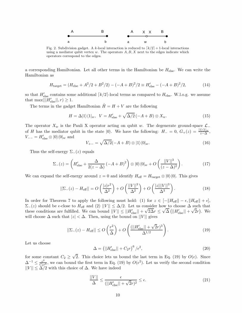
Fig. 2. Subdivision gadget. A k-local interaction is reduced to ⌈k/2⌉+1-local interactionsusing a mediator qubit vertex w. The operators A,B, X next to the edges indicate whichoperators correspond to the edges.

a corresponding Hamiltonian. Let all other terms in the Hamiltonian be Helse. We can write theHamiltonian as

Htarget = (Helse +A2/2 +B2/2) − (−A+B)2/2 ≡ H ′else − (−A+B)2/2, (14)

so that H ′else contains some additional ⌈k/2⌉-local terms as compared to Helse. W.l.o.g. we assume

that max(||H ′else||, r) ≥ 1.

The terms in the gadget Hamiltonian H = H + V are the following

H = ∆|1〉〈1|w , V = H ′else +

√

∆/2 (−A+B) ⊗Xw. (15)

The operator Xw is the Pauli X operator acting on qubit w. The degenerate ground-space L−of H has the mediator qubit in the state |0〉. We have the following: H− = 0, G+(z) = |1〉〈1|w

z−∆ ,V−− = H ′

else ⊗ |0〉〈0|w and

V+− =√

∆/2(−A+B) ⊗ |1〉〈0|w. (16)

Thus the self-energy Σ−(z) equals

Σ−(z) =

(

H ′else +

∆

2(z − ∆)(−A+B)2

)

⊗ |0〉〈0|w +O

( ||V ||3(z − ∆)2

)

. (17)

We can expand the self-energy around z = 0 and identify Heff = Htarget ⊗ |0〉〈0|. This gives

||Σ−(z) −Heff || = O

( |z|r2∆2

)

+O

( ||V ||3∆2

)

+O

( |z|||V ||3∆3

)

. (18)

In order for Theorem 7 to apply the following must hold: (1) for z ∈ [−‖Heff‖ − ǫ, ‖Heff‖ + ǫ],Σ−(z) should be ǫ-close to Heff and (2) ||V || ≤ ∆/2. Let us consider how to choose ∆ such thatthese conditions are fulfilled. We can bound ||V || ≤ ||H ′

else|| +√

2∆r ≤√

∆(

||H ′else|| +

√2r)

. Wewill choose ∆ such that |z| < ∆. Then, using the bound on ||V || gives

||Σ−(z) −Heff || ≤ O

(

r2

∆

)

+O

(

(||H ′else|| +

√2r)3

∆1/2

)

. (19)

Let us choose∆ =

(

||H ′else|| + C2r

)6/ǫ2, (20)

for some constant C2 ≥√

2. This choice lets us bound the last term in Eq. (19) by O(ǫ). Since

∆−1 ≤ ǫ2

C2r6 , we can bound the first term in Eq. (19) by O(ǫ2). Let us verify the second condition||V || ≤ ∆/2 with this choice of ∆. We have indeed

||V ||∆

≤ ǫ

(||H ′else|| +

√2r)2

≤ ǫ. (21)

10

Consider the conditions on |z|, i.e. z ∈ [−‖Heff‖ − ǫ, ‖Heff‖ + ǫ] and |z| < ∆. Since ||Heff || ≤||H ′

else||+ 2r2, we can consider the interval |z| ≤ ||H ′else||+ 2r2 + ǫ. For sufficiently small ǫ we have

(using max(||H ′else||, r) ≥ 1)

|z|∆

=ǫ2(||H ′

else|| + 2r2 + ǫ)

(||H ′else|| + C2r)6

≤ O(ǫ2) < 1. (22)

Thus for the choice of ∆ as in Eq. (19) we have Σ−(z) = Htarget ⊗ |0〉〈0|w + O(ǫ). From Theorem7 it follows that |λ(Heff) − λ(H)| = O(ǫ). When ||H ′

else||, r and 1/ǫ are polynomial in n (n is thenumber of qubits of Htarget), it is clear from Eq. (20), that the norm of the gadget HamiltonianH which uses ∆ is polynomially larger than the norm of the effective Hamiltonian. This impliesthat the gadget can only be used a constant number of times in series if norms have to remainpolynomial.

We will use this type of gadget in parallel, that is, in many places in an interaction graphat once. Let us explain how this happens in detail and argue that the local gadgets operateindependently, i.e. there are no cross-gadget contributions to 2nd order in the perturbation. LetHtarget = Helse −

∑ki=1H

itarget where H i

target = (−Ai +Bi)2/2 for some operators Ai and Bi. Helse

contains all interactions that are not generated perturbatively in addition to the compensating termsA2

i /2 etc., similar as above. We introduce k mediator qubits w1 . . . wk and choose H =∑

iHi + Vwhere Hi = ∆|1〉〈1|wi

and V = Helse +√

∆/2∑

i(−Ai +Bi) ⊗Xwi.

The degenerate ground-space L− of H has all mediator qubits w1 . . . wk in the state |0〉. Let h(x)be the Hamming weight of a bit-string x ∈ 0, 1k of the qubits w1 . . . wk. We have the following:

G+ =∑

x 6=00...0|x〉〈x|

z−h(x)∆ , V−− = Helse ⊗ |00 . . . 0〉〈00 . . . 0| and

V+− =√

∆/2∑

i

(−Ai +Bi)|00 . . . 1i . . . 0〉〈00 . . . 0|, (23)

where |00 . . . 1i . . . 0〉 has qubit wi in the state |1〉. To second order in the perturbation V , thereare no cross-gadget terms in Σ−(z). Thus the self-energy Σ−(z) to second order equals

Σ−(z) =

(

Helse +∆

2(z − ∆)

∑

i

(−Ai +Bi)2

)

⊗ |00 . . . 0〉〈00 . . . 0| +O

( ||V ||3(z − ∆)2

)

. (24)

Choosing ∆ = poly(n)/ǫ2 for some sufficiently large poly(n) gives

Σ−(z) = Htarget ⊗ |00 . . . 0〉〈00 . . . 0| +O(ǫ). (25)

We need to use the parallel application of this gadget twice in order to reduce the ground-state energy problem of our 5-local Hamiltonian to that of a 3-local Hamiltonian; one applicationresults in a 4-local Hamiltonian, another one reduces it to 3. Similarly, any k-local Hamiltonian forconstant k can be reduced to a 3-local Hamiltonian by these means. A 3-to-2-local reduction canbe carried out using the gadget in [1]. However an alternative construction exists which we nowexplain.

3-to-2-local gadget. Assume that we have a target Hamiltonian Htarget = A⊗B ⊗ C +Helse.The idea is to generate the 3-local term A⊗B⊗C by using perturbative effects up to third order. Asbefore one introduces a mediator qubit w whose ground-state is |0〉 for the unperturbed operator.And, as before, we have perturbations proportional to A ⊗ Xw and B ⊗ Xw which can flip themediator qubit. We also have a perturbation V which contains a term proportional to C ⊗ |1〉〈1|w

11

which implies that there is an interaction with C if the mediator qubit is ‘excited’. Thus, thesecond-order perturbative corrections give us terms proportional to A ⊗ B whereas third-ordercorrections gives us the desired A⊗B⊗C (and some additional 2-local terms). More precisely, letHtarget = Helse +A⊗B ⊗ C. Let r = max(||A||, ||B||, ||C||). We choose H = ∆|1〉〈1|w and

V = Helse + Vextra − ∆2/3C ⊗ |1〉〈1|w + ∆2/3(−A+B) ⊗Xw/√

2 (26)

where the additional 2-local compensating term is Vextra = ∆1/3(−A+ B)2/2 + (A2 + B2) ⊗ C/2.One can show that

Σ−(z) = [Helse +A⊗B ⊗ C] ⊗ |0〉〈0|w +O(|z|∆−2/3) +O(∆−1/3). (27)

For sufficiently large ∆ and |z| ≤ ||Helse||+O(r3) + ǫ we make Σ−(z) sufficiently close to Htarget ⊗|0〉〈0|.

The important conclusion of this section is that one can derive a 2-local Hamiltonian on aspatially sparse graph for which the ground-state energy problem is QMA-complete. The interactiongraph is restricted because the perturbation gadgets preserve the spatial restrictions of the originalhypergraph of the 5-local Hamiltonian.

3.2 More Mediator Qubit Gadgetry

For our next round of reductions we need to describe some different uses of the subdivision gadgetacting on 2-local interactions. In the following we will assume that every edge in the interactiongraph is a Pauli edge. It may thus be that the interaction graph contains other edges between thesame vertices, each edge associated with a different product of Paulis. The Pauli degree of a vertexis then the number of Pauli edges that are incident on this vertex.

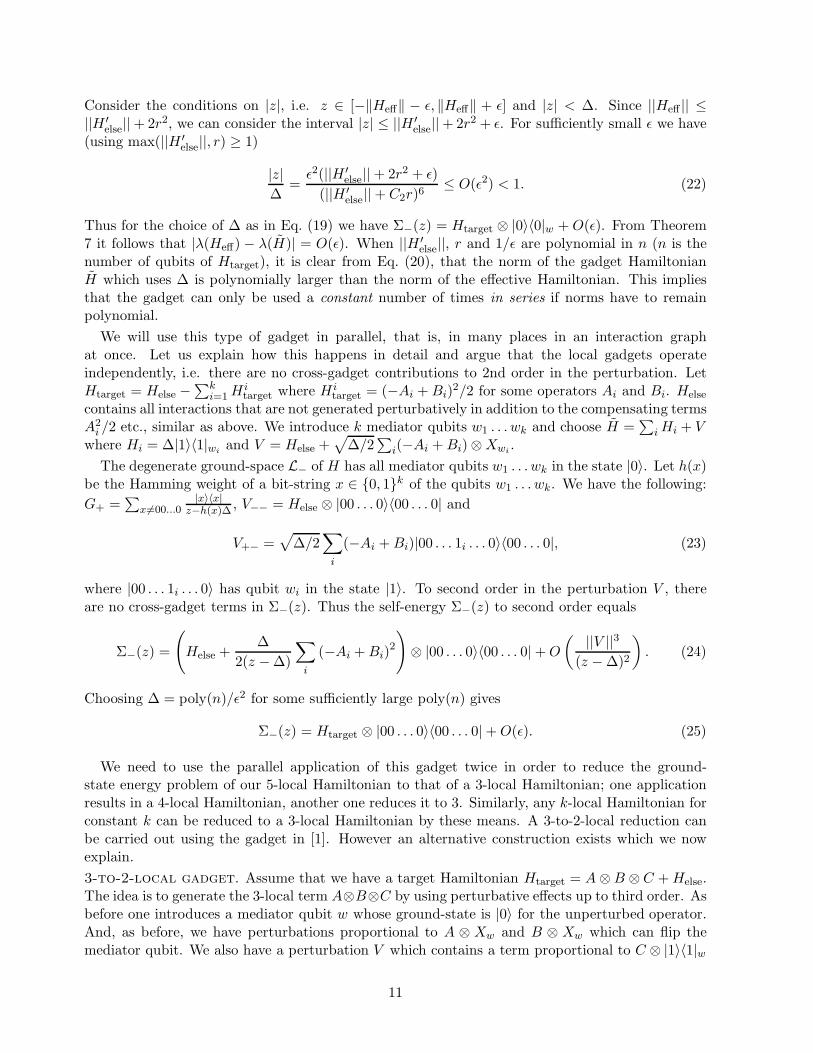
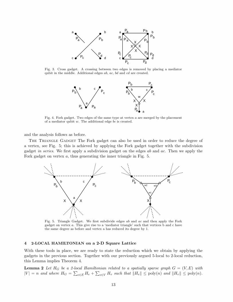
The Cross Gadget. For the Cross Gadget we assume that we have a graph G which, whenembedded in the plane, contains two crossing edges such as in Fig. 3. Assume that the operatoron edge ad is αadPa ⊗ Pd and on edge bc we have αbcPb ⊗ Pc. Our desired Hamiltonian is

Htarget = Helse − (−αadPa − αbcPb + Pc + Pd)2/2. (28)

It is clear that the last term in this Hamiltonian generates the desired crossing edges αadPa ⊗ Pd

and αbcPb ⊗Pc in addition to other operators on the edges ab, bd, cd and ac. Thus Helse is a sum ofall other operators associated with the original graph G and a set of operators on the edges aroundthe cross, see Figure 3, which are meant to cancel the extra operators generated by the last termin Htarget. As before we set H = H + V with

H = ∆|1〉〈1|w, V = Helse +√

∆/2 (−αadPa − αbcPb + Pc + Pd) ⊗Xw, (29)

and the analysis follows as for the subdivision gadget. Note that if there are no edges ab, bd, cd,or ac in Htarget, there will be such edges in H, as indicated in Fig. 3.

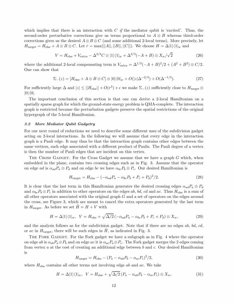
The Fork Gadget. For the Fork gadget we have a subgraph as in Fig. 4 where the operatoron edge ab is αabPa⊗Pb and on edge ac it is αacPa⊗Pc. The Fork gadget merges the 2 edges comingfrom vertex a at the cost of creating an additional edge between b and c. Our desired Hamiltonianis

Htarget = Helse − (Pa − αabPb − αacPc)2/2, (30)

where Helse contains all other terms not involving edge ab and ac. We take

H = ∆|1〉〈1|w, V = Helse +√

∆/2 (Pa − αabPb − αacPc) ⊗Xw, (31)

12

a b

c d

P P

PP

a b

cP

d

a b

c dd

Pa Pb

Pc Pd

c PcPd P

Pb

PbPa

XX

XX

Pa

Fig. 3. Cross gadget. A crossing between two edges is removed by placing a mediatorqubit in the middle. Additional edges ab, ac, bd and cd are created.

a

b c

a

b c

w

P Paa

Pb Pc

Pa

X

Pb Pc

Pb Pc

X X

Fig. 4. Fork gadget. Two edges of the same type at vertex a are merged by the placementof a mediator qubit w. The additional edge bc is created.

and the analysis follows as before.

The Triangle Gadget The Fork gadget can also be used in order to reduce the degree ofa vertex, see Fig. 5; this is achieved by applying the Fork gadget together with the subdivisiongadget in series. We first apply a subdivision gadget on the edges ab and ac. Then we apply theFork gadget on vertex a, thus generating the inner triangle in Fig. 5.

a

b c

XX

X

P Pb c

X

w1

w2 w3

Pb Pc

Fig. 5. Triangle Gadget. We first subdivide edges ab and ac and then apply the Forkgadget on vertex a. This give rise to a ‘mediator triangle’ such that vertices b and c havethe same degree as before and vertex a has reduced its degree by 1.

4 2-LOCAL HAMILTONIAN on a 2-D Square Lattice

With these tools in place, we are ready to state the reduction which we obtain by applying thegadgets in the previous section. Together with our previously argued 5-local to 2-local reduction,this Lemma implies Theorem 4.

Lemma 2 Let HG be a 2-local Hamiltonian related to a spatially sparse graph G = (V,E) with|V | = n and where HG =

∑

e∈E He +∑

v∈V Hv such that ‖He‖ ≤ poly(n) and ‖Hv‖ ≤ poly(n).

13

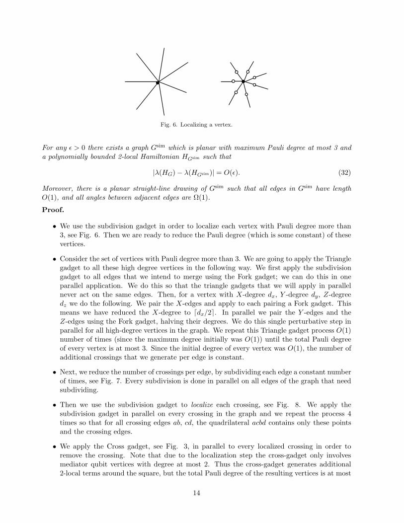
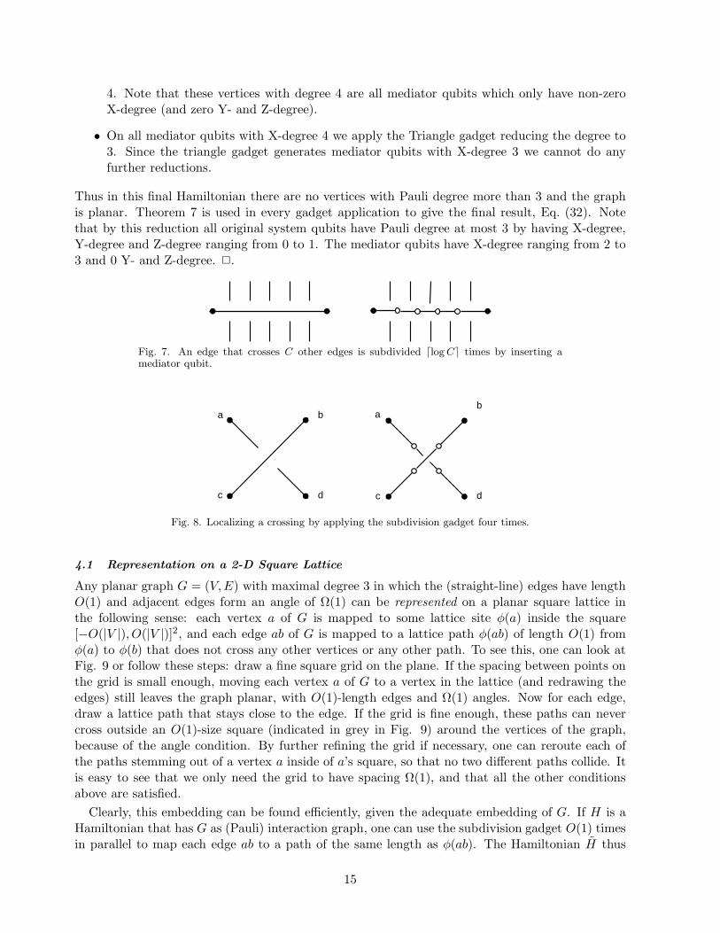
Fig. 6. Localizing a vertex.

For any ǫ > 0 there exists a graph Gsim which is planar with maximum Pauli degree at most 3 anda polynomially bounded 2-local Hamiltonian HGsim such that

|λ(HG) − λ(HGsim)| = O(ǫ). (32)

Moreover, there is a planar straight-line drawing of Gsim such that all edges in Gsim have lengthO(1), and all angles between adjacent edges are Ω(1).

Proof.

• We use the subdivision gadget in order to localize each vertex with Pauli degree more than3, see Fig. 6. Then we are ready to reduce the Pauli degree (which is some constant) of thesevertices.

• Consider the set of vertices with Pauli degree more than 3. We are going to apply the Trianglegadget to all these high degree vertices in the following way. We first apply the subdivisiongadget to all edges that we intend to merge using the Fork gadget; we can do this in oneparallel application. We do this so that the triangle gadgets that we will apply in parallelnever act on the same edges. Then, for a vertex with X-degree dx, Y -degree dy, Z-degreedz we do the following. We pair the X-edges and apply to each pairing a Fork gadget. Thismeans we have reduced the X-degree to ⌈dx/2⌉. In parallel we pair the Y -edges and theZ-edges using the Fork gadget, halving their degrees. We do this single perturbative step inparallel for all high-degree vertices in the graph. We repeat this Triangle gadget process O(1)number of times (since the maximum degree initially was O(1)) until the total Pauli degreeof every vertex is at most 3. Since the initial degree of every vertex was O(1), the number ofadditional crossings that we generate per edge is constant.

• Next, we reduce the number of crossings per edge, by subdividing each edge a constant numberof times, see Fig. 7. Every subdivision is done in parallel on all edges of the graph that needsubdividing.

• Then we use the subdivision gadget to localize each crossing, see Fig. 8. We apply thesubdivision gadget in parallel on every crossing in the graph and we repeat the process 4times so that for all crossing edges ab, cd, the quadrilateral acbd contains only these pointsand the crossing edges.

• We apply the Cross gadget, see Fig. 3, in parallel to every localized crossing in order toremove the crossing. Note that due to the localization step the cross-gadget only involvesmediator qubit vertices with degree at most 2. Thus the cross-gadget generates additional2-local terms around the square, but the total Pauli degree of the resulting vertices is at most

14

4. Note that these vertices with degree 4 are all mediator qubits which only have non-zeroX-degree (and zero Y- and Z-degree).

• On all mediator qubits with X-degree 4 we apply the Triangle gadget reducing the degree to3. Since the triangle gadget generates mediator qubits with X-degree 3 we cannot do anyfurther reductions.

Thus in this final Hamiltonian there are no vertices with Pauli degree more than 3 and the graphis planar. Theorem 7 is used in every gadget application to give the final result, Eq. (32). Notethat by this reduction all original system qubits have Pauli degree at most 3 by having X-degree,Y-degree and Z-degree ranging from 0 to 1. The mediator qubits have X-degree ranging from 2 to3 and 0 Y- and Z-degree. 2.

Fig. 7. An edge that crosses C other edges is subdivided ⌈log C⌉ times by inserting amediator qubit.

a b

c d

ab

c d

Fig. 8. Localizing a crossing by applying the subdivision gadget four times.

4.1 Representation on a 2-D Square Lattice

Any planar graph G = (V,E) with maximal degree 3 in which the (straight-line) edges have lengthO(1) and adjacent edges form an angle of Ω(1) can be represented on a planar square lattice inthe following sense: each vertex a of G is mapped to some lattice site φ(a) inside the square[−O(|V |), O(|V |)]2, and each edge ab of G is mapped to a lattice path φ(ab) of length O(1) fromφ(a) to φ(b) that does not cross any other vertices or any other path. To see this, one can look atFig. 9 or follow these steps: draw a fine square grid on the plane. If the spacing between points onthe grid is small enough, moving each vertex a of G to a vertex in the lattice (and redrawing theedges) still leaves the graph planar, with O(1)-length edges and Ω(1) angles. Now for each edge,draw a lattice path that stays close to the edge. If the grid is fine enough, these paths can nevercross outside an O(1)-size square (indicated in grey in Fig. 9) around the vertices of the graph,because of the angle condition. By further refining the grid if necessary, one can reroute each ofthe paths stemming out of a vertex a inside of a’s square, so that no two different paths collide. Itis easy to see that we only need the grid to have spacing Ω(1), and that all the other conditionsabove are satisfied.

Clearly, this embedding can be found efficiently, given the adequate embedding of G. If H is aHamiltonian that has G as (Pauli) interaction graph, one can use the subdivision gadget O(1) timesin parallel to map each edge ab to a path of the same length as φ(ab). The Hamiltonian H thus

15

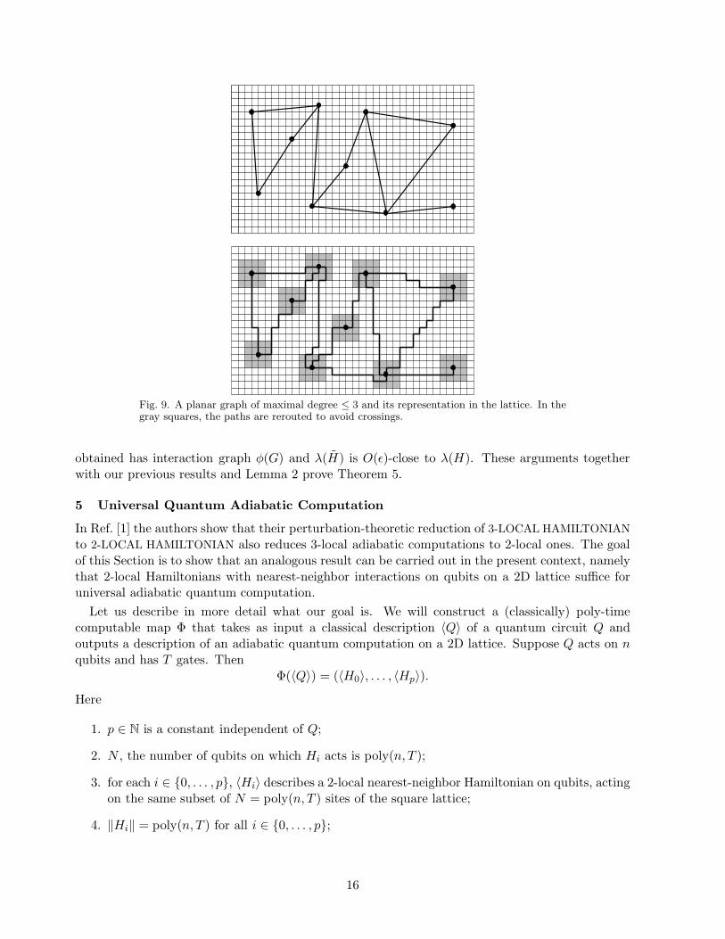
Fig. 9. A planar graph of maximal degree ≤ 3 and its representation in the lattice. In thegray squares, the paths are rerouted to avoid crossings.

obtained has interaction graph φ(G) and λ(H) is O(ǫ)-close to λ(H). These arguments togetherwith our previous results and Lemma 2 prove Theorem 5.

5 Universal Quantum Adiabatic Computation

In Ref. [1] the authors show that their perturbation-theoretic reduction of 3-LOCAL HAMILTONIAN

to 2-LOCAL HAMILTONIAN also reduces 3-local adiabatic computations to 2-local ones. The goalof this Section is to show that an analogous result can be carried out in the present context, namelythat 2-local Hamiltonians with nearest-neighbor interactions on qubits on a 2D lattice suffice foruniversal adiabatic quantum computation.

Let us describe in more detail what our goal is. We will construct a (classically) poly-timecomputable map Φ that takes as input a classical description 〈Q〉 of a quantum circuit Q andoutputs a description of an adiabatic quantum computation on a 2D lattice. Suppose Q acts on nqubits and has T gates. Then

Φ(〈Q〉) = (〈H0〉, . . . , 〈Hp〉).Here

1. p ∈ N is a constant independent of Q;

2. N , the number of qubits on which Hi acts is poly(n, T );

3. for each i ∈ 0, . . . , p, 〈Hi〉 describes a 2-local nearest-neighbor Hamiltonian on qubits, actingon the same subset of N = poly(n, T ) sites of the square lattice;

4. ‖Hi‖ = poly(n, T ) for all i ∈ 0, . . . , p;

16

5. Let

H(s) =

p∑

i=0

siHi (s ∈ [0, 1]).

The spectral gap between the ground-state and first excited state of H(s) is 1/poly(n, T ) forall s.

6. The ground-state of H(0) is |0〉⊗N and the ground-state of H(1) encodes the result of thecomputation of Q on input |0〉⊗n (a more precise description is given in [1, Section 7] or [5]).

Of course, all occurrences of poly above correspond to fixed polynomials that do not depend onQ. Notice that for any Hamiltonian satisfying the above conditions one has that

sups∈[0,1]

∥

∥

∥

∥

djH(s)

dsj

∥

∥

∥

∥

≤ poly(n, T ), for all j = 0, 1, . . .

This is sufficient to ensure that adiabatic computation implemented by H(s), starting from |0〉⊗N ,appropriately simulates the quantum circuit Q, that is, in polynomial time [6]. Note that the usualadiabatic computation, e.g. the universal adiabatic computation in [5], has p = 1.

There are several ways to map a circuit Q to a corresponding H(s). One could modify the 5-localconstruction in this paper in order to show that one can do universal quantum computation usinga quantum adiabatic computation with a 5-local Hamiltonian on a spatially sparse graph. Thenwe could apply the perturbation gadgets to derive a 2-local Hamiltonian with similar properties.However, an easier route to the desired result is the following. In [5] it was shown how to map acircuit Q to a corresponding Hamiltonian H(6)(s) on a 2D lattice. That construction satisfies allbut one of the above requirements, as it acts on 6-dimensional qudits rather than qubits. However,we can embed 6-dimensional qudits in states of 3 qubits. This implies that the 2-local interac-tions between these particles will be mapped onto 6-local interactions. Then we can apply theperturbation gadgets to ‘massage’ this Hamiltonian on a spatially sparse hypergraph to a 2-localHamiltonian as we have done in our QMA construction.

Let us first review the 6-dim particle Hamiltonian, see Sec. 4.2 in [5]. The four phases of theparticles, the unborn, the first, second and dead phase, can be described by two qubits in thestates |unborn〉 = |00〉,|first〉 = |01〉, |second〉 = |10〉 and |dead〉 = |11〉. The third qubit holdsthe actual computational degree of freedom. In the 6-dimensional representation of the unbornand dead phase the computational degree of freedom is assumed to be fixed. If we represent thosestates as 3-qubit states, we fix the third qubit to be in the state |0〉. Hence we obtain 6 states: 2‘first’ states |010〉, |011〉, two ‘second’ states |100〉, |101〉 and one unborn state |000〉 and one deadstate |110〉. With this mapping the entire Hamiltonian in Sec. 4.2 in [5] can be rewritten in termsof 6-local interaction between qubits. Since we embed the 6-dim particle Hamiltonian in a higherdimensional space, we need to make sure that states outside the embedded space (i.e. |001〉 and|111〉) are penalized in the Hamiltonian, i.e. do not contribute to the ground-space. In Table 1 in[5] a list of forbidden configurations is given. In this list we can replace every unborn state by twounborn states |unborn, 1〉 and |unborn, 0〉 and similarly for the dead states. This implies a smallmodification of H ′′

clock. As a consequence we get that the space of legal shapes S is the same forthis embedded Hamiltonian as for the original 6-dim particle Hamiltonian. It then follows that onecan apply Lemma 4.6 and 4.7 bounding the spectral gap of the Hamiltonian in the space of legalstates. We note in passing the Hamiltonian H(6)(s) has only linear terms in s (that correspond top = 1 above) and terms independent of s (corresponding to p = 0).

17

Our second step is to analyze how this desired 6-local Hamiltonian can be implemented usinga 2-local Hamiltonian on a 2D lattice. It is clear that one can apply the perturbation gadgets inSection 3 and 4 of this paper and map a 6-local Hamiltonian on a spatially sparse hypergraph onto a2-local Hamiltonian on a subgraph of the 2D lattice. To go from a 3-local to a 2-local Hamiltonianwe will use our alternative 3-to-2-local gadget described in Section 3.1. One needs to show thefollowing properties of the perturbation method in order for these reductions to work:

1. The 2-local adiabatic path Hamiltonian H(2)(s) obtained through the perturbation gadgetssimulates the 6-local adiabatic path Hamiltonian. This implies that the ground-state of the2-local Hamiltonian should be approximately the ground-state of the desired 6-local Hamil-tonian and the gap for the 2-local Hamiltonian is approximately the gap of the 6-local Hamil-tonian. This requires showing that the perturbative method that we employ does not onlyreproduce the lowest-eigenvalue but also the ground-state and the gap above the ground-state.

2. One needs to verify that H(2)(s) is of the form∑p

i=0 siHi, with p constant and maxi ‖Hi‖ ≤

poly(n, T ).

Our 2-local simulator Hamiltonian H(2)(s) is determined by applying the perturbative gadgetsin Sections 3.1 and 3.2, on the 6-local Hamiltonian H(6)(s). In [1] it was shown how to generate,not only the lowest eigenvalues, but also the ground-state with the perturbative technique. Thisimplies that both the ground-state of the target Hamiltonian as well as the gap above this ground-state can be generated perturbatively. Since the total number of applications of the perturbationtheory is constant, one can apply this argument for each step and thus show that the 6-local targetHamiltonian can be effectively generated by a simulator Hamiltonian H(2).

We now fulfill our second task, i.e. we show that H(2)(s) =∑p

i=0 siHi, with p constant and

‖Hi‖ polynomially bounded. In [1] such arguments were developed for the 3-to-2 local perturbationgadget and basically identical arguments can be given here. The original Hamiltonian H(6) is atmost linear in s. If a gadget is applied on a term which is linear in s, for example a 6-local termsuch sA⊗B = A(s)⊗B, we obtain a new Hamiltonian of which the terms are at most quadratic in

s. Similarly each application of the perturbation gadgets takes a Hamiltonian H ′(s) =∑p′

j=0 sj H ′

j

to another Hamiltonian H ′′(s) =∑p′′

i=0 siH ′′

i where p′′ ≤ 2p′. Assuming that the norm of each H ′i is

polynomial in n and T , then the norms of each H ′′j are also poly(n, T ). Thus the final Hamiltonian

H(2), obtained after a constant number of gadget applications, is indeed of the desired form.

6 Discussion and Acknowledgements

The drawback of the reductions performed by our perturbation theory method is that the 2-localHamiltonian that we construct has large variability in the norms of the 2-local terms. In otherwords, 2-local terms have constant norm whereas others can be fairly high degree polynomials inn. Such dependence on n may be undesirable from a practical point of view, e.g. if one wants toperform universal adiabatic quantum computation.

It is possible that a less stringent but still rigorous perturbation theory could be developedin which only the expectation values of local observables with respect to the ground-space areperturbatively generated. If such expectation values are reproduced with constant accuracy (notscaling as 1/poly(n)), then the perturbation theory need not be accurately reproduce the entireground-space as in Lemma 3. For adiabatic quantum computation this method would suffice sinceone can measure a single output qubit to extract the answer of the computation.

One of the reasons why finding QMA-complete problems is of interest is that it may give usa hint at what problems can be solved in BQP. One example is the unresolved status of the

18

2-local Hamiltonian problem on qubits in one dimension. Another example is to find a quantumextension of classical 2-local Hamiltonian problems which can be solved efficiently. We thank DavidDiVincenzo for an inspiring discussion about superexchange. We would like to thank Sergey Bravyifor pointing out an improvement in the proof of Lemma 2. We acknowledge support by the NSAand the ARDA through ARO contract number W911NF-04-C-0098.

Appendix A

7 General Perturbation Theorem

In order to give a more complete background in the perturbation method we will prove in TheoremA.1 that under the right conditions the entire operator H|<λ∗

is approximated by Heff , not onlyits eigenvalues. In Ref. [1] a similar result was proven, namely that the ground-state of H isapproximately the ground-state of Heff . We extend their result to the case when the ground-spaceis degenerate in Lemma A.1 of this Appendix. To a certain extent our proof-technique is similarto the one used in Ref. [1], however we will use complex z and contour integration in parts of theproofs.

Some of our notation has been given in Section 3 for the specific cases considered in this paper.Here we consider the more general setting as defined in Ref. [1].

Assume that H and V are operators acting on the Hilbert space L and H = H + V . H hasa spectral gap ∆ such that no eigenvalues lie in the interval [λ∗ − ∆/2, λ∗ + ∆/2] for some cutoffλ∗. Let L− (resp. L+) be the span of all eigenvectors of H whose eigenvalues are less than λ∗(respectively larger than λ∗). We will use the resolvent G(z) ≡ (zI − H)−1 of H with complexz ∈ C and let G(z) = (zI − H)−1 be the resolvent of H. The definition of the self-energy Σ−(z) isgiven by

Σ−(z) = zI− − G−1−−(z). (A.1)

see also Eqs. (9)-(10).

The perturbation theory result of Kempe et al. states that under suitable technical conditions,–namely if Σ−(z) is close to a fixed operator Heff for all z in some range–, all eigenvalues ofH = H + V that lie below the cutoff λ∗ are close to those of Heff . Our result shows that theentire operator H restricted to its low-lying energy levels is close to Heff under a slightly strongerassumption.

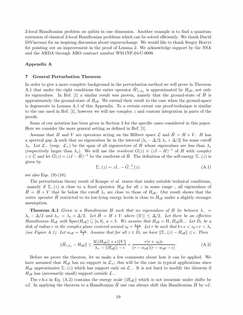
Theorem A.1 Given is a Hamiltonian H such that no eigenvalues of H lie between λ− =λ∗ − ∆/2 and λ+ = λ∗ + ∆/2. Let H = H + V where ||V || ≤ ∆/2. Let there be an effectiveHamiltonian Heff with Spec(Heff) ⊆ [a, b], a < b. We assume that Heff = Π−HeffΠ−. Let Dr be adisk of radius r in the complex plane centered around z0 = b+a

2 . Let r be such that b+ǫ < z0+r < λ∗(see Figure A.1). Let weff = b−a

2 . Assume that for all z ∈ Dr we have ‖Σ−(z) −Heff‖ ≤ ǫ. Then

‖H<λ∗−Heff‖ ≤ 3(||Heff || + ǫ)‖V ‖

λ+ − ||Heff || − ǫ+

r(r + z0)ǫ

(r − weff)(r − weff − ǫ). (A.2)

Before we prove the theorem, let us make a few comments about how it can be applied. Wehave assumed that Heff has no support in L+; this will be the case in typical applications sinceHeff approximates Σ−(z) which has support only on L−. It is not hard to modify the theorem ifHeff has (necessarily small) support outside L−.

The r.h.s in Eq. (A.2) contains the energy scale ||Heff || which is not invariant under shifts byαI. In applying the theorem to a Hamiltonian H one can always shift this Hamiltonian H by αI,

19

λ∗ + ∆/2λ∗bz0a

Spec(Heff)

3

r

Dr

i

b+ ǫ

Fig. A.1. The disk Dr in the complex plane, the spectrum of Heff and the other parametersin Theorem A.2.

without changing its eigenvalues or eigenvectors, such that Heff has a spectrum centered around 0.In that case ||Heff || = minα ||Heff + αI|| = weff , the effective width. Thus one may replace ||Heff ||by weff in the application of the Theorem.

In the construction using mediator qubits, we will choose λ− = 0 and thus λ∗ = ∆/2. L− isthe space in which the mediator qubits are in the state |00 . . . 0〉 and Heff is of the form Htarget ⊗|00 . . . 0〉〈00 . . . 0|. In order for the right-hand-side of Eq. (A.2) to be small, we need to take thespectral gap ∆ to be sufficiently large (some poly(n)). This will directly bound the first term onthe right hand side. Now consider the second term and the choice for r. In our applications Heff isderived from the perturbative expansion of Σ−(z). Since H and H on n qubits have norm poly(n),the Hamiltonian Heff (related to the target Hamiltonian) will also have norm poly(n). Hence a, band thus z0 are at most poly(n). Note that we need to take z0 + r > b + ǫ which implies thatΣ−(z) has to be approximately equal to Heff in a range of z which is larger than what is neededin Theorem 7. Secondly, it is necessary that the eigenvalues of H are bounded away from λ∗, thedifference between the largest eigenvalue below λ∗ and the smallest eigenvalue above λ∗ needs tobe at least 1/poly(n). For our mediator qubit gadgets, one could take r (for example) to scale as∆1/k for some constant k > 1 in order for these conditions to be fulfilled.

Proof. (of Theorem A.1)We start from Theorem 3 in Ref. [1] (stated as Theorem A.1 in thispaper) which shows that under the assumptions in the Theorem one has |λj(H<λ∗

)− λj(Heff)| ≤ ǫfor each 1 ≤ j ≤ dim(L−). We can draw a contour C in the complex plane, the disk Dr in FigureA.1, that encloses all the eigenvalues of H<λ∗

and none of the higher eigenvalues of H. The radiusr needs to be chosen such that b+ ǫ < z0 + r to include all the eigenvalues of H<λ∗

. At the sametime z0 + r < λ∗ such that none of the higher eigenvalues of H are included in the contour integral.Using Cauchy’s contour integral formula we can write

H<λ∗=

1

2πi

∮

Cz G(z) dz. (A.3)

The remainder of our proof proceeds in two parts. In the first part we show that H<λ∗is close

to Π−H<λ∗Π−; this is expressed in Eq. (A.8). In the second part we show that Π−H<λ∗

Π− is closeto Heff , expressed in Eq. (A.12).

20

First part. We have

‖H<λ∗− Π−H<λ∗

Π−‖ = ‖Π+H<λ∗Π+ + Π+H<λ∗

Π− + Π−H<λ∗Π+‖

≤ 2 ‖Π+H<λ∗‖ + ‖H<λ∗

Π+‖, (A.4)

using standard properties of the operator norm ||.||. Let Π<λ∗be the projector onto the space

spanned by the eigenvectors of H<λ∗with eigenvalues below λ∗. We can insert Π<λ∗

before or afterH<λ∗

and use that for projectors P1, P2, ||P1P2|| = ||P2P1||, so that

||H<λ∗− Π−H<λ∗

Π−‖ ≤ 3 ‖H<λ∗‖ ‖Π+Π<λ∗

‖ ≤ 3 (||Heff || + ǫ) ‖Π+Π<λ∗‖. (A.5)

In order to bound this, we first derive

||Π+HΠ<λ∗|| = ||Π+HΠ+Π<λ∗

|| ≥ λ+||Π+Π<λ∗||. (A.6)

On the other hand, we have

||Π+HΠ<λ∗|| ≤ ||Π+HΠ<λ∗

|| + ||V || ≤ (||Heff || + ǫ)||Π+Π<λ∗|| + ||V ||. (A.7)

Putting the last three equations together gives the final bound

‖H<λ∗− Π−H<λ∗

Π−‖ ≤ 3(||Heff || + ǫ)‖V ‖λ+ − (||Heff || + ǫ)

. (A.8)

Second part. We consider

Π−H<λ∗Π− =

1

2πi

∮

CzΠ−G(z)Π− dz, (A.9)

and recall that Π−G(z)Π− = G−−(z) = (zI−−Σ−(z))−1, Eq. (A.1). By showing that this operatoris close to Π−(zI −Heff)−1Π− = (zI−−Heff)−1, we will be able to deduce that Π−H<λ∗

Π− is closeto Heff .

For all z ∈ Dr, ‖Σ−(z)−Heff‖ ≤ ǫ by assumption. In order to bound ‖(zI−−Σ−(z))−1 − (zI−−Heff)−1‖, we will use the following

||(A−B)−1 −A−1|| = ||(I −A−1B)−1A−1 −A−1|| ≤(

(1 − ||A−1|| ||B||)−1 − 1)

||A−1||, (A.10)

when ||A−1|| ||B|| < 1. We choose A = zI− −Heff and B = Σ−(z) −Heff . For z ∈ C (i.e. on thecontour) ||A−1|| ≤ (r − weff)−1 and thus ||A−1|| ||B|| ≤ ǫ

r−weff≤ 1. It follows that

supz∈C

‖(zI− − Σ−(z))−1 − (zI− −Heff)−1‖ ≤ ǫ

(r − weff − ǫ)(r −weff).

Now we will use the following for an operator-valued function F (z) and a contour C with radiusr around a real-valued z0:

∥

∥

∥

∥

1

2πi

∮

Cz F (z) dz

∥

∥

∥

∥

≤ r(r + z0) supz∈C

||F (z)||. (A.11)

Using this bound and the resolvent for Heff , we find that

||Π−H<λ∗Π− −Heff || =

∥

∥

∥

∥

1

2πi

∮

Cz(

(zI− − Σ−(z))−1 − (zI− −Heff)−1)

∥

∥

∥

∥

≤ r(r + z0)ǫ

(r − weff)(r − weff − ǫ). (A.12)

21

where we have used that Heff = Π−HeffΠ−. Putting Eqs. (A.8) and (A.12) together gives thedesired result, Eq. (A.2). 2.

The proof technique used in this theorem can be easily adapted to prove properties of the low-lying eigenspace of H; this is the content of the following Lemma. For the resulting bound ofEq. (A.13) to be useful one needs (1) to take ∆ large enough compared to ||V || (which boundsthe first term in Eq. (A.13)) and (2) the gap ∆eff of the effective Hamiltonian Heff , defined as∆eff ≡ λ1,eff − λ0,eff , needs to be bounded away from zero. In particular in the Lemma we can take

r = ∆eff − 2ǫ and then the second term in Eq. (A.13) can be (upper)-bounded byǫλ1,eff

(∆eff−2ǫ)(∆eff−3ǫ) .

If ∆eff ≥ 1poly(n) we can thus take a polynomially small ǫ to bound the second term in Eq. (A.13)

by some other inverse polynomial.

Lemma A.1 Given is a Hamiltonian H such that no eigenvalues of H lie between λ− = λ∗ −∆/2and λ+ = λ∗ + ∆/2. Let the perturbed Hamiltonian H = H + V where V is a small perturbationwith ||V || ≤ ∆/2. We assume that Heff = Π−HeffΠ− and Spec(Heff) ⊆ [a, b]. Let 0 < ǫ < ∆ andassume that for all z ∈ Dr, a disk of radius r centered around z0 = λ0,eff with ǫ < r < ∆eff − ǫ, wehave ‖Σ−(z) −Heff‖ ≤ ǫ. Let Π0,eff be the projector onto the ground-space of Heff with degeneracyd. Let Πlow be the projector onto the d lowest-lying eigenvectors of H. Then we can bound

||Πlow − Π0,eff || ≤3‖V ‖

λ+ − (λ0,eff + ǫ)+ǫ(λ0,eff + r)

r(r − ǫ). (A.13)

Proof. As in the proof of Theorem A.1, we first prove that Π−ΠlowΠ− is close to Πlow. Then weshow that Π−ΠlowΠ− is close to the projector onto the ground state ofHeff , Π0,eff . For both parts wewill use that due to the assumptions in the Lemma, Theorem 7 implies that for all i = 0, . . . , d− 1,|λi(Heff)− λi(H)| ≤ ǫ. Let λ0,eff be the lowest (degenerate) eigenvalue of Heff . We can first bound

||Πlow − Π−ΠlowΠ−|| ≤ 3||Π+Πlow||. (A.14)

As before we bound ||Π+HΠlow|| in two different directions:

(ǫ+ λ0,eff)||Π+Πlow|| + ||V || ≥ ||Π+HΠlow|| ≥ λ+||Π+Πlow||. (A.15)

These inequalities together with the previous equation give us the first bound

||Πlow − Π−ΠlowΠ−|| ≤3‖V ‖

λ+ − (λ0,eff + ǫ)(A.16)

In order to prove the other part we draw a circular contour C of radius r centered aroundz0 = λ0,eff with ǫ < r < ∆eff − ǫ such that it encloses only the lowest d eigenvalues of H. We willchoose r such that ∆eff − r > r or z0 + r is closer to λ0,eff than to λ1,eff . We have

Π−ΠlowΠ− =1

2πi

∮

CΠ−G(z)Π−. (A.17)

We use that ||Σ−(z) −Heff || ≤ ǫ for z ∈ C and bound

supz∈C

‖(zI− − Σ−(z))−1 − (zI− −Heff)−1‖ ≤ ǫ

r(r − ǫ), (A.18)

using ||(zI− −Heff)−1|| ≤ r−1 for z ∈ C. It follows that

||Π−ΠlowΠ− − Π0,eff || ≤ ǫ(λ0,eff + r)

r(r − ǫ). (A.19)

2.

22

1. J. Kempe, A. Kitaev, and O. Regev. The Complexity of the Local Hamiltonian Problem, SIAM Journalof Computing, 35(5): 1070–1097, 2006. Earlier version in Proc. of 24th FSTTCS.

2. A. Yu. Kitaev, A.H. Shen, and M.N. Vyalyi. Classical and Quantum Computation. Vol. 47 of GraduateStudies in Mathematics., American Mathematical Society, Providence, RI, 2002.

3. D. Aharonov and T. Naveh. Quantum NP—A Survey, 2002, http://arxiv.org/abs/quant-ph/0210077.4. J. Kempe and O. Regev. 3-Local Hamiltonian is QMA-complete, Quantum Information and Computation,

3(3): 258–264, 2003, http://arxiv.org/abs/quant-ph/0302079.5. D. Aharonov, W. van Dam, Z. Landau, S. Lloyd, J. Kempe, and O. Regev. Universality of Adiabatic

Quantum Computation, SIAM Journal of Computing, 37(1):166–194, 2007. Prelim. version in Proceedingsof 45th FOCS, 2004, http://arxiv.org/abs/quant-ph/0405098.

6. A. Ambainis and O. Regev. An elementary proof of the quantum adiabatic theorem, quant-ph/0411152,2004.

7. D. Janzing, P. Wocjan, and T. Beth. Identity Check is QMA-complete, 1996,http://arxiv.org/abs/quant-ph/9610012.

8. B. Nachtergaele. Quantum Spin Systems, In J.-P. Francoise, G. Naber, and S.T. Tsou (Eds.), Encyclopediaof Mathematical Physics (Elsevier), pp. 295–301, 2006, http://arxiv.org/abs/math-ph/0409006.

9. M. Plischke and B. Bergersen. Equilibrium Statistical Physics, World Scientific, Singapore, 1994.10. C. H. Papadimitriou. Computational Complexity, Addison-Wesley, 1994.11. F. Barahona. On the computational complexity of Ising spin glass models, Jour. of Phys. A: Math. and

Gen., 15:3241–3253, 1982.12. H.A. Kramers. L’ interaction entre les atomes magnetogenes dans un cristal paramagnetique, Physica,

1:182, 1934.13. D. Aharonov, D. Gottesman, S. Irani, and J. Kempe. The power of quantum systems on a

line, In Proceedings of 48th FOCS, pp. 373–383, 2007, http://arxiv.org/abs/0705.4077 andhttp://arxiv.org/abs/0705.4067.

14. R. Raussendorf and H. Briegel. A one-way quantum computer, Phys. Rev. Lett., 86:5188–5191, 2001,http://arxiv.org/abs/quant-ph/0010033.

15. A. Kitaev. Fault-tolerant quantum computation by anyons, http://arxiv.org/abs/quant-ph/9707021.16. M.A. Nielsen. Cluster-state quantum computation, 2005, http://arxiv.org/abs/quant-ph/0504097.17. C. Marriott and J. Watrous. Quantum Arthur-Merlin games, Computational Complexity, 14(2):122–152,

2005.

23