arX

iv:c

ond-

mat

/980

1079

v2 [

cond

-mat

.sta

t-m

ech]

10

Jan

1998 The 3-State Square-Lattice Potts Antiferromagnet

at Zero Temperature

Jesus SalasDepartamento de Fısica de la Materia Condensada and

Departamento de Fısica TeoricaFacultad de Ciencias

Universidad de Zaragoza50009 Zaragoza SPAIN

JESUS@JUPITER.UNIZAR.ES

Alan D. SokalDepartment of PhysicsNew York University4 Washington Place

New York, NY 10003 USASOKAL@NYU.EDU

February 1, 2008

Abstract

We study the 3-state square-lattice Potts antiferromagnet at zero temper-ature by a Monte Carlo simulation using the Wang-Swendsen-Kotecky clusteralgorithm, on lattices up to 1024 × 1024. We confirm the critical exponentspredicted by Burton and Henley based on the height representation of thismodel.

Key Words: Antiferromagnetic Potts model, critical ground state, height represen-tation, critical exponent, Monte Carlo, Wang-Swendsen-Kotecky algorithm, clusteralgorithm.

1 Introduction

Antiferromagnetic Potts models [1, 2, 3] are much less well understood than theirferromagnetic counterparts. One reason for this is that the behavior depends stronglyon the microscopic lattice structure, in contrast to the universality typically enjoyedby ferromagnets. As a result, many basic questions have to be investigated case-by-case: Is there a phase transition at finite temperature, and if so, of what order? Whatis the nature of the low-temperature phase? If there is a critical point, what are thecritical exponents and the universality classes? Can these exponents be understood(for two-dimensional models) in terms of conformal field theory?

One thing is known rigorously [4, 5]: for q large enough (how large depends on thelattice in question), the antiferromagnetic q-state Potts model has a unique infinite-volume Gibbs measure and exponential decay of correlations at all temperatures,including zero temperature: the system is disordered as a result of the large ground-state entropy.1 However, for smaller values of q, phase transitions can and do occur.One expects that for each lattice L there will be a value qc(L) such that

(a) For q > qc(L) the model has exponential decay of correlations uniformly at alltemperatures, including zero temperature.

(b) For q = qc(L) the model has a critical point at zero temperature.

(c) For q < qc(L) any behavior is possible. Often (though not always) the modelhas a phase transition at nonzero temperature, which may be of either first orsecond order.

The problem, for each lattice, is to find qc(L) and to determine the precise behaviorfor each q ≤ qc(L).

For the common two-dimensional lattices, strong theoretical arguments2 — which,however, fall short of a rigorous proof — yield the following predictions for qc(L):

qc(L) =

(3 +√

5)/2 ≈ 2.618 . . . for the hexagonal lattice3 for the square lattice3 for the Kagome lattice4 for the triangular lattice

(1.1)

Monte Carlo simulations have confirmed numerically that the 3-state square-latticemodel has a zero-temperature critical point [6, 7], and that the 4-state square-latticemodel [6, 7] and the 3-state hexagonal-lattice model [8, 9] are non-critical uniformlydown to zero temperature.3

1 This behavior has been proven for q ≥ 4 on the hexagonal lattice, q ≥ 6 on the Kagome lattice,q ≥ 7 on the square lattice, and q ≥ 11 on the triangular lattice [5]. However, these bounds arepresumably not sharp: see equation (1.1) below.

2 Summarized in the introduction to [5].

3 The Monte Carlo simulations of the 3-state hexagonal-lattice model reported in Ref. [8] giveno evidence of any first-order phase transition as the temperature is varied from infinity to zero;

2

Two-dimensional models with zero-temperature critical points are of particularinterest, as they can in most cases be mapped onto a “height” (or “interface” or “SOS-type”) model [10, 11, 12, 13, 14, 15, 16, 17, 18, 19, 20, 21, 22, 23, 24, 25, 26, 27]. If thisheight model lies in its “rough” phase — a question that has to be investigated ona case-by-case basis — then its long-distance behavior is that of a massless Gaussianwith some (a priori unknown) “stiffness” K > 0. The critical operators can thenbe identified via the height mapping, and the corresponding critical exponents canbe predicted in terms of the single parameter K. In particular, if we know (by someother means) one of these exponents, then we can deduce the rest.

Height representations thus give a means for recovering a sort of universalityfor some (but not all) antiferromagnetic Potts models and for understanding theircritical behavior in terms of conformal field theory. All the nonuniversal details ofthe microscopic lattice structure are encoded in the height representation and in thestiffness parameter K. Given these, everything can be understood in terms of theuniversal behavior of massless Gaussian fields.

The plan of this paper is as follows: In Section 2 we present briefly the generaltheory of height representations and then work out in detail the case of the 3-statesquare-lattice Potts antiferromagnet. Our presentation is based on the work of Henleyand collaborators [19, 20, 23, 24, 26, 27], supplemented by a few minor innovations ofour own. In the remainder of the paper, our goal is to test, by Monte Carlo simulation,the critical exponents predicted by Burton and Henley [26] for the three relevantoperators in the 3-state square-lattice Potts antiferromagnet at zero temperature. InSection 3 we describe our simulations, and in Section 4 we analyze the data.

2 Height Representations

Many two-dimensional models with zero-temperature critical points can be mappedonto a “height” model: these include the triangular-lattice Ising antiferromagnet[11, 12], the triangular-lattice spin-S Ising antiferromagnet [24], the 3-state square-lattice Potts antiferromagnet [10, 13, 26], the 3-state Kagome-lattice Potts antiferro-magnet [16, 20], the 4-state triangular-lattice Potts antiferromagnet [27], the 4-statePotts antiferromagnet on the covering lattice of the square lattice [19, 20], a con-strained 4-state Potts antiferromagnet on the square lattice [26], a special 6-vertexmodel [20], and various dimer models [14, 15, 23, 25] and fully packed loop models[17, 18, 21, 22]. Here we shall explain briefly the basic principles underlying the con-struction of such mappings and their use to extract critical exponents. We shall thenwork out in detail the case of the 3-state square-lattice Potts antiferromagnet.

this behavior is consistent with the theoretical prediction that the model has exponential decayof correlations uniformly down to zero temperature. However, these authors did not measure thecorrelation length or the staggered susceptibility, so no direct test of the non-criticality at zerotemperature was made. Such a direct test is being made in Ref. [9].

3

2.1 General Theory

The first step is to define a map assigning to each zero-temperature spin configura-tion {σ(x)} a corresponding microscopic height configuration {h(x)}. This height rule

is usually defined by local increments, i.e. one prescribes the change ∆h ≡ h(y)−h(x)in going from a site x to a neighboring site y in terms of the spin variables σ(x) andσ(y). For such a rule to be well-defined, one must verify that in all cases the netincrement ∆h around any closed loop is zero.4 The height variables h(x) lie in somediscrete set H ⊂ RD (for some suitable dimension D), which we call the height lattice.

The next step is to identify the so-called ideal states : these are ground-stateconfigurations (or families of configurations) of the original spin model whose corre-sponding height configurations are macroscopically “flat” (i.e. have zero net slope)and which maximize the entropy density (in the sense of maximizing the number ofground states that can be obtained from the ideal states by local modifications of thespins). We label each ideal state by its average height h ∈ RD, and we define theideal-state lattice I ⊂ RD to be the set of all average heights of ideal states. Theequivalence lattice

E = {a ∈ RD: a + I = I} (2.1)

is the subgroup of RD summarizing the underlying periodicity of I.We now guess that, in typical configurations of the spin model, the lattice is

subdivided into reasonably large domains in which the spin configuration closelyresembles one of the ideal states. It follows that typical configurations of the heightmodel are given by domains in which the height h(x) exhibits small fluctuationsaround one of the values in the ideal-state lattice. We therefore expect that a suitablydefined coarse-grained height variable h(x) will take values in or near the ideal-statelattice I, except at boundaries between domains. The long-wavelength behavior ofthe height model is thus postulated to be controlled by an effective coarse-grainedHamiltonian of the form

H =∫

d2x

[K

2

D∑

i=1

|∇hi|2 + Vlock(h(x))

], (2.2)

where we have made explicit the components of the macroscopic height h = (h1, h2, . . . , hD).The gradient term in (2.2) takes into account the entropy of small fluctuations aroundthe ideal states; the second term is the so-called locking potential , which favors theheights to take their values in I. We then expect that there exists some constantKr such that for K < Kr (resp. K > Kr) the locking potential is irrelevant (resp.relevant) in the renormalization-group sense. Thus, if K < Kr our surface model is“rough” and its long-wavelength behavior can be described by a massless Gaussianmodel [28, 20] with D components:

⟨[hi(x) − hi(y)] [hj(x) − hj(y)]

⟩≈ δij

πKlog |x − y| (2.3)

4 In fact, this property usually holds for free boundary conditions but not for periodic boundaryconditions. We shall hereafter neglect this latter subtlety, by imagining that we are working alwaysin infinite volume.

4

for |x − y| ≫ 1; in this case, the original zero-temperature spin system is critical.If, on the other hand, K > Kr, then the surface model is in its “smooth” phase,exhibiting long-range order

〈h(x)〉 = h0 (2.4)

and bounded fluctuations around this ordered state:⟨[h(x) − h(y)]2

⟩bounded as |x − y| → ∞ ; (2.5)

correspondingly, the spin system is “locked” into small fluctuations around one of theideal states. At K = Kr the surface model undergoes a roughening transition.5

Let us note, finally, that a given ideal state can be represented by many differentaverage heights h ∈ I. More precisely, suppose that in some domain we have aparticular ideal state X and that its average height is h0 ∈ I. Now let us passthrough various other domains of the lattice, coming back finally to a domain inwhich the ideal state is again X. We will find the average height in this latter domainto lie in the set h0 +R, where R is a particular subgroup of E that we call the repeat

lattice; we will also find, conversely, that whenever we enter a domain in which theaverage height lies in h0 +R, that domain is in ideal state X. It follows that the idealstates are in one-to-one correspondence with the cosets I/R.

The coarse-grained correlation functions of local operators in the spin languagecan be understood in terms of the correlation functions of local operators of thecoarse-grained heights. The important point is that these latter operators shouldhave the periodicity of the repeat lattice R. This means that the Fourier expansionof such an operator O,

O(x) =∑

G∈R◦

OG eiG·h(x) , (2.6)

contains only wavevectors belonging to the reciprocal lattice of the repeat lattice,

R◦ ≡ {G ∈ RD: G · a ∈ 2πZ for all a ∈ R} . (2.7)

On the other hand, two wavevectors whose difference belongs to the reciprocal latticeof the equivalence lattice,

E◦ ≡ {G ∈ RD: G · a ∈ 2πZ for all a ∈ E} , (2.8)

give rise to vertex operators exp[iG · h(x)] having identical long-distance behavior.The vertex operators of the height model are thus in one-to-one correspondence withthe cosets R◦/E◦ ≃ (E/R)◦.

Now, provided that the height model is in the rough phase (K < Kr), the corre-lation functions of the vertex operators exp[iG · h(x)] are given by

⟨eiG·h(0) e−iG′·h(x)

⟩= δG,G′ exp

[−G2

2

⟨[h(0) − h(x)]2

⟩]∼ δG,G′ |x|−G2/(2πK) .

(2.9)

5 Note that the only alternatives for the spin model are criticality and long-range order. Thus, ifthere exists a height representation, the original spin model cannot be disordered at zero temperature.

5

It follows that the critical behavior of the operator O will be given by the mostrelevant vertex operator exp[iG · h(x)] appearing in its Fourier expansion with anonzero coefficient:

〈O(0)O(x)∗〉 ∼ |x|−ηO (2.10)

where

ηO = minOG 6=0

G2

2πK. (2.11)

(The scaling dimension is xO = ηO/2, and the operator is relevant in case therenormalization-group eigenvalue d − xO = 2 − xO is > 0.) This formula impliesthat we can write all the critical exponents in terms of a single parameter K. If oneexponent is known, then all of them are.

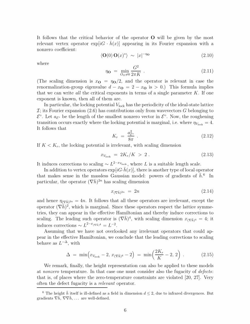
In particular, the locking potential Vlock has the periodicity of the ideal-state latticeI; its Fourier expansion (2.6) has contributions only from wavevectors G belonging toE◦. Let aE◦ be the length of the smallest nonzero vector in E◦. Now, the rougheningtransition occurs exactly where the locking potential is marginal, i.e. where ηVlock

= 4.It follows that

Kr =a2E◦

8π. (2.12)

If K < Kr, the locking potential is irrelevant, with scaling dimension

xVlock= 2Kr/K > 2 . (2.13)

It induces corrections to scaling ∼ L2−xVlock , where L is a suitable length scale.In addition to vertex operators exp[iG·h(x)], there is another type of local operator

that makes sense in the massless Gaussian model: powers of gradients of h.6 Inparticular, the operator (∇h)2n has scaling dimension

x(∇h)2n = 2n (2.14)

and hence η(∇h)2n = 4n. It follows that all these operators are irrelevant, except the

operator (∇h)2, which is marginal. Since these operators respect the lattice symme-tries, they can appear in the effective Hamiltonian and thereby induce corrections toscaling. The leading such operator is (∇h)4, with scaling dimension x(∇h)4 = 4; it

induces corrections ∼ L2−x(∇h)4 = L−2.Assuming that we have not overlooked any irrelevant operators that could ap-

pear in the effective Hamiltonian, we conclude that the leading corrections to scalingbehave as L−∆, with

∆ = min(xVlock

− 2, x(∇h)4 − 2)

= min(

2Kr

K− 2, 2

). (2.15)

We remark, finally, the height representation can also be applied to these modelsat nonzero temperature. In that case one must consider also the fugacity of defects :that is, of places where the zero-temperature constraints are violated [20, 27]. Veryoften the defect fugacity is a relevant operator.

6 The height h itself is ill-defined as a field in dimension d ≤ 2, due to infrared divergences. Butgradients ∇h, ∇∇h, . . . are well-defined.

6

2.2 Three-State Square-Lattice Potts Antiferromagnet

The height representation of the 3-state square-lattice Potts antiferromagnet atzero temperature is very simple [10, 26]. Let the Potts spins σ(x) take values in theset {0, 1, 2}. The microscopic height variables h(x) are then assigned as follows: Atthe origin we take h(0) = 0, 4, 2 (mod 6) according as σ(0) = 0, 1, 2; this ensures that

h(0) = σ(0) (mod 3) (2.16a)

h(0) = 0 (mod 2) (2.16b)

We then define the increment in height in going from a site x to a nearest neighbory by

h(x) − h(y) = σ(x) − σ(y) (mod 3) (2.17a)

h(x) − h(y) = ±1 (2.17b)

This is well-defined (in free boundary conditions) because the change ∆h around anyplaquette is zero.7 It follows from (2.16) and (2.17) that

h(x) = σ(x) (mod 3) (2.18a)

h(x) = x1 + x2 (mod 2) (2.18b)

for any site x = (x1, x2). In particular, the height h(x) is uniquely determined mod 6once we know the spin value σ(x) and the parity of x, and conversely. The heightlattice H is clearly equal to Z.

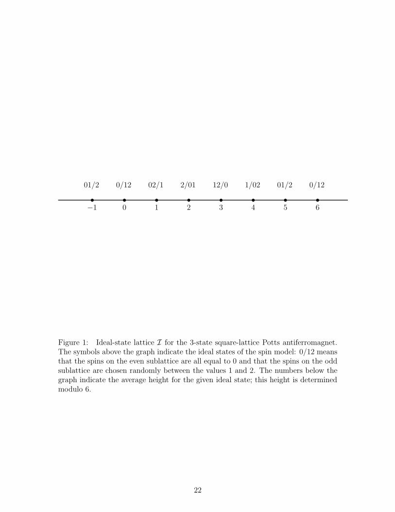
There are six ideal states, given by 0/12 (spins on the even sublattice all equal to 0,spins on the odd sublattice chosen randomly between 1 and 2) and its permutations.8

In an ideal state, the height is constant on the ordered sublattice and fluctuatesrandomly ±1 around this level on the disordered sublattice. The average height of anideal state is thus equal to its height on the ordered sublattice; it then follows from(2.18) that there is a one-to-one correspondence between ideal states and averageheights mod 6 (see Figure 1).9 The ideal-state lattice I is thus also Z, as is theequivalence lattice E , while the repeat lattice R is 6Z. The corresponding reciprocallattices are E◦ = 2πZ and R◦ = (π/3)Z.

There are three relevant operators (in the renormalization-group sense) appearingin this model (see Table 1) [10, 26]:

Mstagg(x) = (−1)x1+x2 ~σ(x) (2.19)

Mu(x) = ~σ(x) (2.20)

Pstagg(x) =1

4(−1)x1+x2

∑

y nnn of x

(2δσ(x),σ(y) − 1) (2.21)

7 If four numbers ±1 add up to 0 mod 3, they must necessarily be two +1’s and two −1’s, henceadd up to 0.

8 States like 0/1 are not ideal states because they do not have maximal entropy density.

9 This fact was proven, in a different way, by Burton and Henley [26, Appendix B.2].

7

where we have represented the Potts spin at site x = (x1, x2) by a unit vector in theplane

~σ(x) =(cos

2π

3σ(x), sin

2π

3σ(x)

). (2.22)

The first operator is the staggered magnetization; the staggering corresponds to amomentum kstagg = (π, π). The second operator is the uniform magnetization. Thethird operator is a staggered sum over diagonal next-nearest-neighbor correlations(i.e. over y with |y − x| =

√2); we call it the staggered polarization. In an ideal

state, it takes the average value +1 (resp. −1) according as it is the even (resp. odd)sublattice that is ordered.10

We can relate these observables directly to the microscopic height variables h(x)by exact identities. For the vertex operators with G = ±π/3,±2π/3,±π we have

e±i(π/3)h(x) = M(1)stagg(x) ∓ iM

(2)stagg(x) (2.23)

e±i(2π/3)h(x) = M (1)u (x) ± iM (2)

u (x) (2.24)

e±iπh(x) = (−1)x1+x2 (2.25)

Here (2.24) and (2.25) follow immediately from (2.18a) and (2.18b), respectively, while(2.23) follows by multiplying these two and taking the complex conjugate. Of course,the strictly local operator (2.25) is trivial, but we can define a nontrivial almost-localoperator with the same (G = π) long-distance behavior:

e±i(π/2)[h(x)+h(y)] = (−1)x1+x2 (2δσ(x),σ(y) − 1) (2.26)

for diagonal next-nearest-neighbor sites x, y.11 It follows that G = π corresponds tothe staggered polarization.

Remark. It is also of interest to define almost-local operators living on plaquettes.Let x be a lattice site, and let 2(x) ≡ {(x1, x2), (x1+1, x2), (x1+1, x2+1), (x1, x2+1)}be the plaquette whose lower-left corner is x. We then define the average height h(x)over that plaquette as

h(x) ≡ 1

4

∑

y∈2(x)

h(y) . (2.27)

It is easy to see that h(x) takes values in Z ∪ (Z + 12): namely, it takes an integer

(resp. half-integer) value if there are three (resp. two) distinct spin values σ(y) on the

10 Burton and Henley [26] chose a slightly different definition of this operator: Pstagg(x) =(1/4)(−1)x1+x2

∑y nnn of x

δσ(x),σ(y).

11Proof: Next-nearest-neighbor sites x, y always satisfy h(y)− h(x) = 0 or ±2: the former case

occurs when σ(x) = σ(y), and the latter when σ(x) 6= σ(y). It follows that

e±i(π/2)[h(y)−h(x)] = 2δσ(x),σ(y) − 1 .

Now multiply this by (2.25).

8

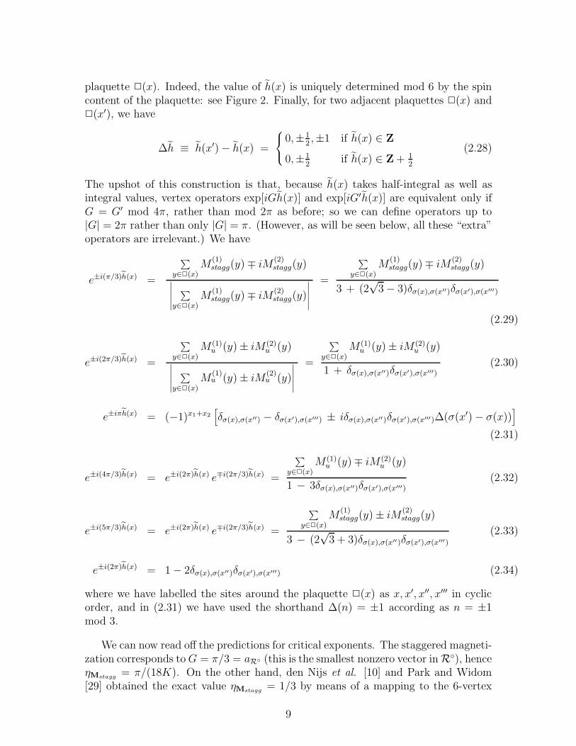
plaquette 2(x). Indeed, the value of h(x) is uniquely determined mod 6 by the spincontent of the plaquette: see Figure 2. Finally, for two adjacent plaquettes 2(x) and2(x′), we have

∆h ≡ h(x′) − h(x) =

0,±12,±1 if h(x) ∈ Z

0,±12

if h(x) ∈ Z + 12

(2.28)

The upshot of this construction is that, because h(x) takes half-integral as well asintegral values, vertex operators exp[iGh(x)] and exp[iG′h(x)] are equivalent only ifG = G′ mod 4π, rather than mod 2π as before; so we can define operators up to|G| = 2π rather than only |G| = π. (However, as will be seen below, all these “extra”operators are irrelevant.) We have

e±i(π/3)h(x) =

∑y∈2(x)

M(1)stagg(y) ∓ iM

(2)stagg(y)

∣∣∣∣∣∑

y∈2(x)M

(1)stagg(y) ∓ iM

(2)stagg(y)

∣∣∣∣∣

=

∑y∈2(x)

M(1)stagg(y) ∓ iM

(2)stagg(y)

3 + (2√

3 − 3)δσ(x),σ(x′′)δσ(x′),σ(x′′′)

(2.29)

e±i(2π/3)h(x) =

∑y∈2(x)

M (1)u (y) ± iM (2)

u (y)

∣∣∣∣∣∑

y∈2(x)M

(1)u (y) ± iM

(2)u (y)

∣∣∣∣∣

=

∑y∈2(x)

M (1)u (y) ± iM (2)

u (y)

1 + δσ(x),σ(x′′)δσ(x′),σ(x′′′)

(2.30)

e±iπh(x) = (−1)x1+x2

[δσ(x),σ(x′′) − δσ(x′),σ(x′′′) ± iδσ(x),σ(x′′)δσ(x′),σ(x′′′)∆(σ(x′) − σ(x))

]

(2.31)

e±i(4π/3)h(x) = e±i(2π)h(x) e∓i(2π/3)h(x) =

∑y∈2(x)

M (1)u (y) ∓ iM (2)

u (y)

1 − 3δσ(x),σ(x′′)δσ(x′),σ(x′′′)(2.32)

e±i(5π/3)h(x) = e±i(2π)h(x) e∓i(2π/3)h(x) =

∑y∈2(x)

M(1)stagg(y) ± iM

(2)stagg(y)

3 − (2√

3 + 3)δσ(x),σ(x′′)δσ(x′),σ(x′′′)

(2.33)

e±i(2π)h(x) = 1 − 2δσ(x),σ(x′′)δσ(x′),σ(x′′′) (2.34)

where we have labelled the sites around the plaquette 2(x) as x, x′, x′′, x′′′ in cyclicorder, and in (2.31) we have used the shorthand ∆(n) = ±1 according as n = ±1mod 3.

We can now read off the predictions for critical exponents. The staggered magneti-zation corresponds to G = π/3 = aR◦ (this is the smallest nonzero vector in R◦), henceηMstagg

= π/(18K). On the other hand, den Nijs et al. [10] and Park and Widom[29] obtained the exact value ηMstagg

= 1/3 by means of a mapping to the 6-vertex

9

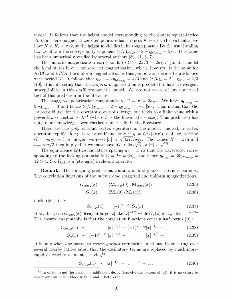
model. It follows that the height model corresponding to the 3-state square-latticePotts antiferromagnet at zero temperature has stiffness K = π/6. (In particular, wehave K < Kr = π/2, so the height model lies in its rough phase.) By the usual scalinglaw we obtain the susceptibility exponent (γ/ν)stagg = 2 − ηMstagg

= 5/3. This valuehas been numerically verified by several authors [30, 31, 6, 7].

The uniform magnetization corresponds to G = 2π/3 = 2aR◦ . (In this modelthe ideal states have a nonzero net magnetization, which, however, is the same forA/BC and BC/A; the uniform magnetization is thus periodic on the ideal-state latticewith period 3.) It follows that ηMu

= 4ηMstagg= 4/3 and (γ/ν)u = 2 − ηMu

= 2/3[10]. It is interesting that the uniform magnetization is predicted to have a divergentsusceptibility in this anti ferromagnetic model. We are not aware of any numericaltest of this prediction in the literature.

The staggered polarization corresponds to G = π = 3aR◦ . We have ηPstagg=

9ηMstagg= 3 and hence (γ/ν)Pstagg

= 2 − ηPstagg= −1 [26]. This means that the

“susceptibility” for this operator does not diverge, but tends to a finite value with apower-law correction ∼ L−1 (where L is the linear lattice size). This prediction hasnot, to our knowledge, been checked numerically in the literature.

These are the only relevant vertex operators in the model. Indeed, a vertexoperator exp[iG · h(x)] is relevant if and only if η = G2/(2πK) < 4; or, writingG = naR◦ with n integer, we need |n| <

√8πK/aR◦ . The values K = π/6 and

aR◦ = π/3 then imply that we must have |G| < 2π/√

3, or |n| <√

12.The equivalence lattice has lattice spacing aE = 1, so that the wavevector corre-

sponding to the locking potential is G = 2π = 6aR◦ and hence ηVlock= 36ηMstagg

=12 > 4. So, Vlock is a (strongly) irrelevant operator.

Remark. The foregoing predictions contain, at first glance, a serious paradox.The correlation functions of the microscopic staggered and uniform magnetizations,

Gstagg(x) = 〈Mstagg(0) · Mstagg(x)〉 (2.35)

Gu(x) = 〈Mu(0) · Mu(x)〉 (2.36)

obviously satisfyGstagg(x) = (−1)x1+x2 Gu(x) . (2.37)

How, then, can Gstagg(x) decay at large |x| like |x|−1/3 while Gu(x) decays like |x|−4/3?The answer, presumably, is that the correlation functions contain both terms [10]:

Gstagg(x) ∼ |x|−1/3 + (−1)x1+x2|x|−4/3 + . . . (2.38)

Gu(x) ∼ (−1)x1+x2|x|−1/3 + |x|−4/3 + . . . (2.39)

It is only when one passes to coarse-grained correlation functions, by smearing overseveral nearby lattice sites, that the oscillatory terms are replaced by much-more-rapidly decaying remnants, leaving12

Gstagg(x) ∼ |x|−1/3 + |x|−10/3 + . . . (2.40)

12 In order to get the maximum additional decay (namely, two powers of |x|), it is necessary tosmear over an m × n block with m and n both even.

10

Gu(x) ∼ |x|−7/3 + |x|−4/3 + . . . (2.41)

A similar cancellation of oscillatory terms occurs, of course, when one looks at thesusceptibilities.

3 Numerical Simulations

In order to test all these predictions, we have carried out a Monte Carlo simulationof the 3-state square-lattice Potts antiferromagnet at zero temperature, on periodicL × L lattices with L ranging from 4 to 1024. We made our simulation using theWang-Swendsen-Kotecky (WSK) cluster algorithm [30, 31], which is ergodic at T = 0on any bipartite graph, and in particular on a periodic square lattice whenever thelinear lattice size L is even [26, 7].13

For each lattice size, we made 106 measurements after discarding 105 iterationsfor equilibration. For L ≤ 512 we performed a single long run starting from theordered state 0/1. For L = 1024 we made two independent runs with differentinitial conditions, one starting in the ordered state 0/1 and the other starting inthe ideal state 0/12 (each individual run was of total length 6 × 105, with the first105 iterations discarded); there was no noticeable disagreement between the two setsof results. In units of the longest autocorrelation time τint,P2

stagg(see below), our

run length corresponds to ≈ 1.3 × 105τint measurements, and our discard intervalcorresponds to ≈ 1.3 × 104τint iterations. This run length is sufficient to get a high-precision determination of both static and dynamic observables: we obtain errors oforder ∼< 0.2% for the static observables and of order ∼< 2% for the dynamic ones.14

Our program was written in Fortran. The runs for L ≤ 512 were carried outon a Pentium 166 machine: each WSK iteration took approximately 5.7 L2 µsec.The runs for L = 1024 were carried out on an IBM RS-6000/370 workstation, taking8.5 L2 µsec per iteration. The total CPU time used in this project was approximately1 month on the former machine plus 4 months on the latter.

13 By contrast, the WSK algorithm for q = 3 is known to be nonergodic on periodic 3m × 3nsquare lattices whenever m and n are relatively prime [32]. Other cases are open questions.

14 Our discard interval might seem to be much larger than necessary: 102τint would usually bemore than enough. However, there is always the danger that the longest autocorrelation time inthe system is much larger than the longest autocorrelation time that one has measured , becauseone has failed to measure an observable having sufficiently strong overlap with the slowest mode.(Here is a minor example of this effect: the authors of Refs. [6, 7] reported τint ∼< 5 because theyfailed to consider our slowest observable Pstagg, which has autocorrelation time τint,P2

stagg≈ 8.) As

an undoubtedly overly conservative precaution against the possible (but unlikely) existence of sucha (vastly) slower mode, we decided to discard approximately 10% of the entire run. This discardamounts to reducing the accuracy on our final estimates by a mere 5%.

Note also that while we have here performed our simulations only at zero temperature (β = ∞),the authors of Refs. [6, 7] employed a closely-spaced set of temperatures ranging from very hightemperature (β = 2.0, ξ ≈ 5) to very low temperature (β = 6.0, ξ ≈ 20000) and found theautocorrelation times of M2

stagg and the energy to be uniformly small. This constitutes further

evidence against the existence of an undetected extremely slow mode.

11

The “zero-momentum” observables

Mstagg =∑

x

Mstagg(x) (3.1)

Mu =∑

x

Mu(x) (3.2)

Pstagg =∑

x

Pstagg(x) (3.3)

all have mean zero. We have therefore measured their squares

M2stagg =

(∑

x

Mstagg(x)

)2

=3

2

∑

a

∣∣∣∣∣∑

x

(−1)x1+x2δσx,a

∣∣∣∣∣

2

(3.4)

M2u =

(∑

x

Mu(x)

)2

=3

2

∑

a

∣∣∣∣∣∑

x

δσx,a

∣∣∣∣∣

2

− V 2

2(3.5)

P2stagg =

(∑

x

Pstagg(x)

)2

=

∣∣∣∣∣∣

∑

〈xy〉 nnn

(−1)x1+x2δσx,σy

∣∣∣∣∣∣

2

(3.6)

as well as the “smallest-nonzero-momentum” observable associated to Mstagg(x):

Fstagg =1

2

∣∣∣∣∣∑

x

e2πix1/L Mstagg(x)

∣∣∣∣∣

2

+

∣∣∣∣∣∑

x

e2πix2/L Mstagg(x)

∣∣∣∣∣

2

=3

2× 1

2

∑

a

∣∣∣∣∣∑

x

(−1)x1+x2e2πix1/Lδσx,a

∣∣∣∣∣

2

+

∣∣∣∣∣∑

x

(−1)x1+x2e2πix2/Lδσx,a

∣∣∣∣∣

2

.

(3.7)

Here V = L2 is the volume of the system, the sum∑

a is over the three possible valuesof the Potts spins, and the sum

∑〈xy〉 nnn is over all pairs of diagonal-next-nearest

neighbors x, y (each pair taken only once). The staggered and uniform susceptibilitiesare given by

χstagg =1

V〈M2

stagg〉 (3.8)

χu =1

V〈M2

u〉 (3.9)

and the “susceptibility” associated to the observable Pstagg is

χPstagg=

1

V〈P2

stagg〉 . (3.10)

Finally, the second-moment correlation length is defined by

ξ =[(χstagg/Fstagg) − 1]1/2

2 sin(π/L), (3.11)

12

where

Fstagg =1

V〈Fstagg〉 . (3.12)

The results of our simulations for the mean values of all these static observables aredisplayed in Table 2.

We have also measured the integrated autocorrelation time associated to each ofthe basic observables, using a self-consistent truncation window of width 6τint [33,Appendix C]. We find that the largest autocorrelation time (of the observables wemeasured) corresponds to P2

stagg, though all of them are roughly of the same order ofmagnitude (Table 3). None of these autocorrelation times diverges as L grows; theytend to a constant. We have fitted the autocorrelation time for each observable to aconstant (using methods to be described at the beginning of the next section). Ourbest fits are:

τint,P2stagg

= 7.552 ± 0.052 (Lmin = 128, χ2 = 5.43, 3 DF) (3.13)

τint,M2u

= 4.921 ± 0.027 (Lmin = 128, χ2 = 1.87, 3 DF) (3.14)

τint,M2stagg

= 4.528 ± 0.028 (Lmin = 256, χ2 = 0.56, 2 DF) (3.15)

τint,Fstagg= 3.804 ± 0.015 (Lmin = 32, χ2 = 4.81, 5 DF) (3.16)

We conclude that the WSK algorithm for this model at T = 0 has no critical slowing-down [6, 7]: τint ∼< 8 uniformly in L.

4 Data Analysis

We perform all fits using the standard weighted least-squares method. As a pre-caution against corrections to scaling, we impose a lower cutoff L ≥ Lmin on the datapoints admitted in the fit, and we study systematically the effects of varying Lmin onboth the estimated parameters and the χ2. In general, our preferred fit correspondsto the smallest Lmin for which the goodness of fit is reasonable (e.g., the confidencelevel15 is ∼> 10–20%) and for which subsequent increases in Lmin do not cause the χ2

to drop vastly more than one unit per degree of freedom.

4.1 Staggered Susceptibility

The theoretically expected behavior of the staggered susceptibility at criticality(i.e., at zero temperature) is

χstagg = L(γ/ν)stagg

[A + BL−∆ + . . .

](4.1)

15 “Confidence level” is the probability that χ2 would exceed the observed value, assuming thatthe underlying statistical model is correct. An unusually low confidence level (e.g., less than 5%)thus suggests that the underlying statistical model is incorrect — the most likely cause of whichwould be corrections to scaling.

13

with (γ/ν)stagg = 5/3; here ∆ is a correction-to-scaling exponent and the dots indicatehigher-order corrections to scaling. Based on the numerical results of Refs. [6, 7], wedo not expect large corrections to scaling on this observable.

We tried first to extract the leading term in (4.1) by fitting our data to a simplepower-law Ansatz χstagg = AL(γ/ν)stagg . This fit is reasonable already for Lmin = 32(χ2 = 4.34, 4 DF, level = 36%), but our preferred fit is Lmin = 128:

(γ

ν

)

stagg= 1.66621 ± 0.00035 (4.2)

with χ2 = 1.31 (2 DF, confidence level = 52%). This result is only 1.5 standarddeviations away from the expected value 5/3.

We then considered the Ansatz (4.1), imposing the leading exponent (γ/ν)stagg =5/3 and trying various values for the first correction-to-scaling exponent ∆. We areable to find reasonably good fits already for Lmin = 4, provided we take ∆ in therange 1.50 ∼< ∆ ∼< 1.76. We therefore performed a three-parameter nonlinear weightedleast-squares fit to simultaneously estimate A, B and ∆. Using Lmin = 4, we obtain

∆ = 1.624 ± 0.061 (4.3)

with χ2 = 7.30 (6 DF, level = 29%).It is interesting to note that the exponent 5/3 is included in the interval (4.3).

If this is the true behavior, it means that the leading correction to pure power-lawbehavior in the staggered susceptibility is merely an additive constant:

χstagg = 0.87696(17)L5/3 − 0.2820(30) (4.4)

with χ2 = 7.78 (7 DF, level = 35%). Such a correction can be interpreted as a merelattice artifact, not necessarily arising from any irrelevant operator of the continuumtheory.

4.2 Uniform Susceptibility

The theoretically expected behavior for the uniform susceptibility is

χu = L(γ/ν)u

[A + BL−∆ + . . .

](4.5)

with (γ/ν)u = 2/3. The simple power-law Ansatz gives a decent fit only for Lmin =256, yielding (

γ

ν

)

u= 0.6705 ± 0.0022 (4.6)

with χ2 = 0.35 (1 DF, level = 55%). This result is 1.75 standard deviations awayfrom the theoretical prediction.

The large deviations from pure power-law behavior for L < 256 can be explainedas an effect of corrections to scaling. Indeed, if we consider the Ansatz (4.5) with(γ/ν)u = 2/3 imposed and with just one correction-to-scaling term, we can obtainsensible fits even for Lmin = 4. But in this case, in contrast to the preceding one,

14

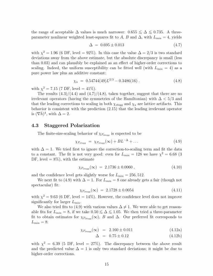
the range of acceptable ∆ values is much narrower: 0.655 ∼< ∆ ∼< 0.735. A three-parameter nonlinear weighted least-squares fit to A, B and ∆, with Lmin = 4, yields

∆ = 0.695 ± 0.013 (4.7)

with χ2 = 1.96 (6 DF, level = 92%). In this case the value ∆ = 2/3 is two standarddeviations away from the above estimate, but the absolute discrepancy is small (lessthan 0.03) and can plausibly be explained as an effect of higher-order corrections toscaling. Indeed, the uniform susceptibility can be fitted well (with Lmin = 4) as apure power law plus an additive constant:

χu = 0.54744(49)L2/3 − 0.3486(16) . (4.8)

with χ2 = 7.15 (7 DF, level = 41%).The results (4.3)/(4.4) and (4.7)/(4.8), taken together, suggest that there are no

irrelevant operators (having the symmetries of the Hamiltonian) with ∆ < 5/3 andthat the leading corrections to scaling in both χstagg and χu are lattice artifacts. Thisbehavior is consistent with the prediction (2.15) that the leading irrelevant operatoris (∇h)4, with ∆ = 2.

4.3 Staggered Polarization

The finite-size-scaling behavior of χPstaggis expected to be

χPstagg= χPstagg

(∞) + BL−∆ + . . . (4.9)

with ∆ = 1. We tried first to ignore the correction-to-scaling term and fit the datato a constant. The fit is not very good: even for Lmin = 128 we have χ2 = 6.68 (3DF, level = 8%), with the estimate

χPstagg(∞) = 2.1736 ± 0.0060 , (4.10)

and the confidence level gets slightly worse for Lmin = 256, 512.We next fit to (4.9) with ∆ = 1. For Lmin = 8 one already gets a fair (though not

spectacular) fit:χPstagg

(∞) = 2.1728 ± 0.0054 (4.11)

with χ2 = 9.63 (6 DF, level = 14%). However, the confidence level does not improvesignificantly for larger Lmin.

We also tried fits to (4.9) with various values ∆ 6= 1. We were able to get reason-able fits for Lmin = 8, if we take 0.50 ∼< ∆ ∼< 1.05. We then tried a three-parameterfit to obtain estimates for χPstagg

(∞), B and ∆. Our preferred fit corresponds toLmin = 8:

χPstagg(∞) = 2.160 ± 0.011 (4.12a)

∆ = 0.75 ± 0.12 (4.12b)

with χ2 = 6.39 (5 DF, level = 27%). The discrepancy between the above resultand the predicted value ∆ = 1 is only two standard deviations; it might be due tohigher-order corrections.

15

4.4 Correlation Length

Finally, we consider the scaling behavior of the second-moment correlation length,which is expected to be of the form

ξ = Lp[x⋆ + BL−∆ + . . .

](4.13)

with p = 1.First, we tried to estimate the power p by a simple power-law fit. This gives a

good result for Lmin = 128:

p = 0.99875 ± 0.00069 (4.14)

with χ2 = 0.48 (2 DF, level = 79%). This estimate is only 1.8 standard deviationsaway from the expected value p = 1, and the very small discrepancy (less than 0.0013)can be explained as an effect of corrections to scaling.

If we look at Table 4, we see that the ratio ξ/L increases from L = 4 to L = 8,decreases monotonically from L = 8 to L = 64, and then oscillates due to statisticalnoise for L > 64. Thus, if we want to study the L → ∞ limit of this quantitywithout including correction-to-scaling terms, we expect to get a reasonable fit onlyfor Lmin ≥ 64. Indeed, if we fit our data to a constant x⋆, the first decent fit occursfor Lmin = 64, giving

x⋆ = 0.63546 ± 0.00030 (4.15)

with χ2 = 3.77 (4 DF, level = 44%). However, our preferred fit corresponds toLmin = 512,

x⋆ = 0.63483 ± 0.00048 (4.16)

with χ2 = 0.0051 (1 DF, level = 94%).On the other hand, if we want to study corrections to scaling, we must use at least

some of the data with L ≤ 64. The non-monotonic behavior for 4 ≤ L ≤ 64 indicatesthat, to obtain a reasonable fit over this whole interval, we would need at least two

correction-to-scaling terms with amplitudes of opposite sign. An Ansatz with onlyone correction-to-scaling term could, at best, fit the data with Lmin ≥ 8, and verylikely not even that.

Indeed, if we fit the data to the Ansatz (4.13) with p = 1 and only one correction-to-scaling term ∼ L−∆, we find that reasonably good fits are obtained for 0.25 ∼< ∆ ∼<0.60 with Lmin = 8. (For Lmin = 4 we were unable to find any good fit, as expected.)We next tried a three-parameter fit to estimate x⋆, B and ∆. The first reasonablygood fit corresponds again to Lmin = 8, and the estimates are

x⋆ = 0.63359 ± 0.00132 (4.17a)

∆ = 0.42 ± 0.16 (4.17b)

with χ2 = 9.35 (5 DF, level = 10%). However, a better fit is obtained with Lmin = 16,giving

x⋆ = 0.63479 ± 0.00066 (4.18a)

∆ = 0.84 ± 0.32 (4.18b)

16

with χ2 = 5.95 (4 DF, level = 20%). For Lmin ≥ 32, we do not get any sensible result(∆ and B become very large, along with their error bars); this is due to the fact thatmost of these data correspond to the regime L ≥ 64 where the corrections to scalingare submerged under the statistical noise. Let us remark that the value of x⋆ given in(4.18a) is only 1.6 standard deviations away from the one estimated by Ferreira andSokal [7] using extrapolation techniques at nonzero temperature:

x⋆FS ≈ 0.633888 . (4.19)

If we want to fit all the data (i.e. take Lmin = 4), we should introduce at leasttwo correction-to-scaling terms. From the definition (3.11), we expect two types ofcorrections to scaling for the correlation length: one of order L−5/3 coming from thenumerator [cf. (4.4)], and another of order L−2 coming from the subleading terms inthe sine. Furthermore, we might also expect an effective constant-term “correction”of order L−1, analogously to what happened for the two susceptibilities. Thus, ournext Ansatz would be

ξ

L= x⋆ + BL−1 + CL−5/3 . (4.20)

If the coefficients B and C have different signs, the contribution of these two termscould be mimicked (in the range of monotonicity, Lmin ≥ 8) by a single correctionterm with an exponent ∆eff < 1, where ∆eff increases towards 1 as Lmin → ∞.Indeed, this scenario is in good agreement with our results (4.17b)/(4.18b). Wetherefore tried a three-parameter fit directly to the Ansatz (4.20). Our preferred fitcorresponds to Lmin = 4:

x⋆ = 0.63457± 0.00033 (4.21a)

B = 0.182 ± 0.014 (4.21b)

C = −0.521 ± 0.035 (4.21c)

with χ2 = 7.01 (6 DF, level = 32%). This result certainly does not prove that theAnsatz (4.20) is correct, since many other pairs of correction-to-scaling exponentscould give an equally good fit; but it does display a satisfying agreement.

Acknowledgments

We wish to thank Chris Henley for valuable correspondence and for making avail-able some of his unpublished notes.

J.S. gratefully acknowledges the hospitality of the Department of Physics at NewYork University, where this work was finished. The authors’ research was supportedin part by CICyT grants PB95-0797 and AEN97-1680 (J.S.) and by U.S. NationalScience Foundation grant PHY-9520978 (A.D.S. and J.S.).

17

References

[1] R.B. Potts, Proc. Camb. Philos. Soc. 48, 106 (1952).

[2] F.Y. Wu, Rev. Mod. Phys. 54, 235 (1982); 55, 315 (E) (1983).

[3] F.Y. Wu, J. Appl. Phys. 55, 2421 (1984).

[4] R. Kotecky, cited in H.-O. Georgii, Gibbs Measures and Phase Transitions (deGruyter, Berlin–New York, 1988), pp. 148–149, 457.

[5] J. Salas and A.D. Sokal, J. Stat. Phys. 86, 551 (1997).

[6] S.J. Ferreira and A.D. Sokal, Phys. Rev. B51, 6727 (1995).

[7] S.J. Ferreira and A.D. Sokal, in preparation.

[8] R. Shrock and S.–H. Tsai, J. Phys. A 34, 495 (1995).

[9] J. Salas, in preparation.

[10] M. den Nijs, M.P. Nightingale and M. Schick, Phys. Rev. B 26, 2490 (1982).

[11] H.W.J. Blote and H.J. Hilhorst, J. Phys. A 15, L631 (1982).

[12] B. Nienhuis, H.J. Hilhorst and H.W.J. Blote, J. Phys. A 17, 3559 (1984).

[13] J. Kolafa, J. Phys. A 17, L777 (1984).

[14] L.S. Levitov, Phys. Rev. Lett. 64, 92 (1990).

[15] W.P. Thurston, Amer. Math. Monthly 97, 757 (1990).

[16] D.A. Huse and A.D. Rutenberg, Phys. Rev. B 45, 7536 (1992).

[17] H.W.J. Blote and B. Nienhuis, Phys. Rev. Lett. 72, 1372 (1994).

[18] J. Kondev and C.L. Henley, Phys. Rev. Lett. 73, 2786 (1994).

[19] J. Kondev and C.L. Henley, Phys. Rev. B 52, 6628 (1995).

[20] J. Kondev and C.L. Henley, Nucl. Phys. B 464, 540 (1996).

[21] J. Kondev, J. de Gier and B. Nienhuis, J. Phys. A 29, 6489 (1996).

[22] J. Kondev, Loop models, marginally rough interfaces, and the Coulomb gas,cond-mat/9607181, to appear in the proceedings of the symposium on “ExactlySoluble Models in Statistical Mechanics” (March 1996, Northeastern University,Boston).

[23] R. Raghavan, C.L. Henley and S.L. Arouh, J. Stat. Phys. 86, 517 (1997).

18

[24] C. Zeng and C.L. Henley, Phys. Rev. B 55, 14935 (1997).

[25] C.L. Henley, J. Stat. Phys. 89, 483 (1997).

[26] J.K. Burton Jr. and C.L. Henley, A constrained Potts antiferromagnet modelwith an interface representation, cond-mat/9708171, submitted to J. Phys. A.

[27] C.L. Henley, private communications.

[28] P. Ginsparg, in Fields, Strings and Critical Phenomena, edited by E. Brezinand J. Zinn-Justin (North Holland, Amsterdam 1989).

[29] H. Park and M. Widom, Phys. Rev. Lett. 63, 1193 (1989).

[30] J.-S. Wang, R.H. Swendsen and R. Kotecky, Phys. Rev. Lett. 63, 109 (1989).

[31] J.–S. Wang, R.H. Swendsen and R. Kotecky, Phys. Rev. B 42, 2465 (1990).

[32] M. Lubin and A.D. Sokal, Phys. Rev. Lett. 71, 1778 (1993).

[33] N. Madras and A.D. Sokal, J. Stat. Phys. 50, 679 (1988).

19

Operator G η γ/ν = 2 − η Numerical Result

Mstagg ±π/3 1/3 5/3 1.66621 ± 0.00035Mu ±2π/3 4/3 2/3 0.6705 ± 0.0022Pstagg ±π 3 −1 −0.75 ± 0.12

Table 1: Critical operators for the 3-state antiferromagnetic Potts model on the squarelattice at zero temperature. The last column indicates the results from our MonteCarlo simulation (Section 4).

L χstagg χu χPstaggξ

4 8.5576 ± 0.0024 1.0443 ± 0.0010 2.4486 ± 0.0076 2.5127 ± 0.00238 27.7671 ± 0.0120 1.8614 ± 0.0028 2.3888 ± 0.0124 5.1306 ± 0.0055

16 88.8206 ± 0.0441 3.1537 ± 0.0058 2.2882 ± 0.0128 10.2497 ± 0.011032 282.8085 ± 0.1477 5.2052 ± 0.0105 2.2464 ± 0.0126 20.4422 ± 0.021964 897.3520 ± 0.4776 8.4362 ± 0.0179 2.2110 ± 0.0124 40.6662 ± 0.0433

128 2851.2642± 1.5484 13.5899 ± 0.0296 2.1826 ± 0.0120 81.4388 ± 0.0880256 9056.7475± 4.8888 21.8141 ± 0.0479 2.1852 ± 0.0122 162.8235 ± 0.1745512 28731.6260± 15.5273 34.7753 ± 0.0767 2.1480 ± 0.0116 325.0478 ± 0.3449

1024 91167.3235± 49.2042 55.2604 ± 0.1240 2.1806 ± 0.0120 650.0264 ± 0.6924

Table 2: Mean values of the static observables for the 3-state square-lattice Pottsantiferromagnet at zero temperature.

20

L τint,M2stagg

τint,M2u

τint,P2stagg

τint,Fstagg

4 2.487 ± 0.020 1.525 ± 0.010 5.038 ± 0.057 3.330 ± 0.0308 4.073 ± 0.041 3.240 ± 0.029 7.456 ± 0.101 4.032 ± 0.041

16 4.417 ± 0.046 4.154 ± 0.042 7.845 ± 0.109 3.850 ± 0.03832 4.488 ± 0.047 4.628 ± 0.049 7.765 ± 0.107 3.826 ± 0.03764 4.483 ± 0.047 4.803 ± 0.052 7.863 ± 0.110 3.803 ± 0.037

128 4.587 ± 0.049 4.903 ± 0.054 7.528 ± 0.103 3.855 ± 0.038256 4.558 ± 0.049 4.908 ± 0.054 7.686 ± 0.106 3.816 ± 0.037512 4.515 ± 0.048 4.889 ± 0.054 7.377 ± 0.100 3.752 ± 0.036

1024 4.512 ± 0.048 4.986 ± 0.056 7.638 ± 0.105 3.776 ± 0.037

Table 3: Mean values of the dynamic observables for the 3-state square-lattice Pottsantiferromagnet at zero temperature.

L ξ/L

4 0.62818 ± 0.000578 0.64133 ± 0.00069

16 0.64061 ± 0.0006932 0.63882 ± 0.0006864 0.63541 ± 0.00068

128 0.63624 ± 0.00069256 0.63603 ± 0.00068512 0.63486 ± 0.00067

1024 0.63479 ± 0.00068

Table 4: Values of the ratio ξ/L for the 3-state square-lattice Potts antiferromagnetat zero temperature.

21

• • • • • • • •−1 0 1 2 3 4 5 6

01/2 0/12 02/1 2/01 12/0 1/02 01/2 0/12

Figure 1: Ideal-state lattice I for the 3-state square-lattice Potts antiferromagnet.The symbols above the graph indicate the ideal states of the spin model: 0/12 meansthat the spins on the even sublattice are all equal to 0 and that the spins on the oddsublattice are chosen randomly between the values 1 and 2. The numbers below thegraph indicate the average height for the given ideal state; this height is determinedmodulo 6.

22

• × • × • × • × • × • × • × •−1 −1

20 1

21 3

22 5

23 7

24 9

25 11

26

01/20/2

0/120/1

02/12/1

2/012/0

12/01/0

1/021/2

01/20/2

0/12

Figure 2: The average height h(x) on a plaquette is uniquely determined modulo 6by the spin content of that plaquette: 0/12 means, for example, that the two spinsbelonging to the even sublattice are both equal to 0, while the two spins belongingto the odd sublattice are 1 and 2.

23