The Blow-Up Profile for a Fast Diffusion Equation with a Nonlinear Boundary Condition

ROCKY MOUNTAINJOURNAL OF MATHEMATICSVolume 33, Number 1, Spring 2003

THE BLOW-UP PROFILE FORA FAST DIFFUSION EQUATION WITH ANONLINEAR BOUNDARY CONDITION

RAUL FERREIRA, ARTURO DE PABLO,

FERNANDO QUIROS, JULIO D. ROSSI

ABSTRACT. We study positive solutions of a fast diffusionequation in the half-line with a nonlinear boundary condition,{

ut = (um)xx (x, t) ∈ R+ × (0, T ),

−(um)x(0, t) = up(0, t) t ∈ (0, T ),

u(x, 0) = u0(x) x ∈ R+,

where 0 < m < 1 and p > 0 are parameters. We describein terms of p and m when all solutions exist globally in time,when all solutions blow up in a finite time, and when thereare both blowing up and global solutions. For blowing upsolutions we find the blow-up rate and the blow-up set and wedescribe the asymptotic behavior close to the blow-up time Tin terms of a self-similar profile.

1. Introduction and main results. We deal with the problem

(1.1)

ut = (um)xx (x, t) ∈ R+ × (0, T ),−(um)x(0, t) = up(0, t) t ∈ (0, T ),u(x, 0) = u0(x) x ∈ R+,

where 0 < m < 1 and p > 0 are parameters. We assume that u0 isbounded, continuous and positive in R+ = (0,∞).

For every m > 0 problem (1.1) can be thought of as a model fornonlinear heat propagation. In this case u stands for the temperature

2000 AMS Mathematics Subject Classification. 35B40, 35B35, 35K65.Key words and phrases. Blow-up, asymptotic behavior, fast diffusion equation,

nonlinear boundary conditions.The first three authors were partially supported by DGICYT grant PB94-0153

(Spain). The fourth author was supported by Universidad de Buenos Aires undergrant EX046, CONICET (Argentina) and Fundacion Antorchas (Argentina).

Received by the editors on November 21, 2000, and in revised form on April 10,2001.

Copyright c©2003 Rocky Mountain Mathematics Consortium

123

124 R. FERREIRA, A. DE PABLO, F. QUIROS AND J.D. ROSSI

and −(um)x represents the heat flux. Hence the boundary conditionrepresents a nonlinear radiation law at the boundary. This kind ofboundary condition appears also in combustion problems when thereaction happens only at the boundary of the container, for examplebecause of the presence of a solid catalyzer, see [22] for a justification.

Local in time existence of positive classical solutions of this problemand comparison arguments can be easily established, see Section 2. Thetime T is the maximal existence time for the solution, which may befinite or infinite. If T < ∞, then u becomes unbounded in finite timeand we say that it blows up. If T = ∞ we say that the solution is global.

In this article we are interested in the blow-up phenomenon, asubject that has deserved a great deal of attention in recent years,see for example the book [26] and the surveys [19] and [7]. Forspecific references about blow-up in problems with nonlinear boundaryconditions see the surveys [6, 8].

As a precedent we have the work of Galaktionov and Levine [12],where they study the same problem for the range of parameters m ≥ 1.The authors show that if 0 < p ≤ p0 = (m + 1)/2, then for arbitraryinitial data the solution is global in time, while for p > (m + 1)/2there are solutions with finite time blow-up. Thus, p0 is the criticalglobal existence exponent. Moreover, they prove that pc = m + 1 is acritical exponent of Fujita type. By definition, this means that pc hasthe following properties:

(i) if p0 < p ≤ pc, then u blows up for all nontrivial u0;

(ii) if p > pc, then u is global in time for “small” u0.

Our first theorem proves that the same result holds valid for0 < m < 1.

Theorem 1.1. The critical exponents for problem (1.1) are given byp0 = (m+ 1)/2 and pc = m+ 1. More precisely:

(i) If 0 < p ≤ (m+ 1)/2 every positive solution is global in time.

(ii) If (m + 1)/2 < p ≤ m + 1 every positive solution blows up infinite time.

(iii) If p > m+1 there exist solutions that blow up in finite time andthere exist also global solutions.

BLOW-UP PROFILE FOR A FAST DIFFUSION EQUATION 125

The main difference between the cases m < 1, the so-called fast dif-fusion equation, and m > 1, the well-known porous medium equation,is the finite speed of propagation property. Solutions with compactlysupported initial data u0 stay compactly supported for 0 < t < T ifm > 1. However, if m < 1, solutions become instantaneously positiveeverywhere. That is the reason why we are restricting ourselves topositive solutions. This introduces a technical difficulty. The resultsin [12] for m > 1 are restricted to compactly supported initial data.This makes comparison with global supersolutions easier. In our casem < 1 and we have to take care of the decay of solutions at infinity.This is done thanks to the decay results for general solutions of the fastdiffusion equation of Herrero and Pierre, [14]. The linear case m = 1,also treated in [12], is similar to the fast diffusion case, as solutionsbecome instantaneously positive. However, the linearity of the equa-tion provides a representation formula. In the nonlinear case we do nothave such a tool, and the proofs have to be necessarily different.

We also remark that the critical exponents are not the same in thecases m > 1 or m < 1 if we consider problem (1.1) defined in a boundedinterval [0, L] with the boundary conditions −(um)x(0, t) = up(0, t),−(um)x(L, t) = 0, see [10]. In fact, in this situation p0 = 1 if m > 1while p0 = (m+1)/2 if 0 < m < 1; the exponent pc does not exist, sinceevery nontrivial solution blows up for p > p0. Therefore Theorem 1.1is not so evident.

Once we have characterized for which exponents the solution toproblem (1.1) can or cannot blow up, we want to study the way theblowing up solutions behave as approaching the blow-up time. Thismeans that we must investigate where the solutions blow up, the blow-up set, the speed at which they blow up, the blow-up rate, and theshape of the solutions close to the blow-up time, the blow-up profile.To this purpose we consider from now on exponents p > (m+1)/2 andu a blowing up solution with blow-up time T .

We begin with the blow-up set, which is defined in the following way,

B(u) = {x ∈ [0,∞); ∃xn → x, tn ↗ T, with u(xn, tn) → +∞}.We have single-point blow-up for every p > (m+ 1)/2.

Theorem 1.2. Let u be a blowing up solution of (1.1). ThenB(u) = {0}.


The argument that we use is valid for a bounded interval, improvingthe result in [10] as we do not require conditions on the initial data.

Our theorem is in contrast with the case m > 1, where the blow-upset is a single point if p > m, but is the whole half-line if p < m anda bounded interval if p = m. Notice that in our case in order to haveblowing up solutions we need p > (m+ 1)/2, and hence p > m.

To get the blow-up rate of blowing up solutions, we need an extramonotonicity assumption,

(H) ut > 0 for t near T .

This hypothesis holds for example for solutions with smooth compatibleinitial data such that (um

0 )′′ ≥ 0.

Theorem 1.3. Let u be a solution of (1.1) with finite blow-up timeT satisfying (H). As t approaches T we have

(1.2) ‖u(·, t)‖∞ ∼ (T − t)−1/(2p−m−1).

where f ∼ g means that there exist finite positive constants c1, c2 suchthat c1g ≤ f ≤ c2g.

The argument in the proof is local and hence applies to the case ofa bounded interval. Therefore (1.2) holds for solutions of the latterproblem, improving slightly the result of [10]. This contrasts with thecase m > p > 1, where the rate is not the same in the half-line as in abounded interval, see [10, 24].

Remark. Following [15] it is possible to obtain the blow-up ratewithout the monotonicity assumption (H). However, a restriction on theexponents arises and the rates are only valid for (m+1)/2 < p ≤ m+1.A different approach to eliminate the monotonicity assumption, basedon the study of the energy functional, has been recently proposed in[5] for the case m = 1. These authors use a concavity argument of [20]to prove a lower bound for the energy. However, it is unclear whetherthis concavity argument may be applied in the nonlinear case m �= 1.

Next we study the asymptotic behavior of blowing up solutions, whichis the main subject of this work. As is often the case in nonlinear


problems of parabolic type, the characteristic properties of an equation,in this case the blow-up behavior, are displayed by means of appropriateself-similar solutions, [3].

The linear case m = 1 is considered in [9] and [16]. The case m > 1is studied in [23] by means of a self-similar solution constructed usingresults from [13]. When m < 1 no such self-similar solution is available(the results in [13] are restricted to m > 1) and we must establish itsexistence in the present paper.

In the case of problems with finite-time blow-up, the expected self-similar solutions take the form

(1.3) U(x, t) = (T − t)−αF (ξ), ξ = x(T − t)−β.

The values of the similarity parameters α and β are automaticallydetermined from the fact that U(x, t) is a solution of (1.1); we easilyget the values

(1.4) α =1

2p−m− 1, β =

p−m2p−m− 1

.

Observe that in the blow-up range we have α, β > 0. The profileF = F (ξ) must satisfy the problem

(1.5){(Fm)′′ − βξF ′ − αF = 0 ξ ∈ (0,∞),−(Fm)′(0) = F p(0).

Theorem 1.4. There exists a unique solution of problem (1.5). Thissolution is positive, strictly decreasing and satisfies

(1.6) F (ξ) ∼ ξ−α/β as ξ → ∞.

The precise decay (1.6) is crucial. Other decays would lead eitherto a self-similar solution with global blow-up, something which isimpossible, or to a trivial asymptotic profile.

Next we show that the asymptotic behavior of the solution u(x, t)of problem (1.1) as t approaches the blow-up time T is described by


the self-similar solution (1.3). Following the standard technique, weintroduce the new rescaled function

g(ξ, τ) = (T − t)αu(x, t), ξ = x(T − t)−β,

where α and β are given by (1.4) and

τ = − log(T − t)

is the new time. Then g(ξ, τ) satisfies the following parabolic problem

gτ = (gm)ξξ − βξgξ − αg (ξ, τ) ∈ R+ × (− log T,∞),−(gm)ξ(0, τ ) = gp(0, τ ) τ ∈ (− logT,∞),g(ξ,− logT ) = Tαu0(ξT−β) ξ ∈ R+.

Therefore, the problem of the asymptotic behavior of u(x, t) near afinite blow-up time T > 0 is reduced to the problem of the stabilizationof g(ξ, τ) as τ → ∞ to a stationary solution of (1.7), i.e., a solution of(1.5). We prove the following general result.

Theorem 1.5. Let u be a solution to problem (1.1) satisfying therate (1.2). Then the rescaled orbits g(ξ, τ) tend to the stationary self-similar profile constructed in Theorem 1.4. Therefore, as t approachesT , we have single point blow-up in the precise form

(1.8) limt↗T

(T − t)α|u(x, t)− U(x, t)| = 0,

uniformly in sets of the form |x| ≤ c(T − t)β.

In particular, from (1.6) we obtain

(1.9) u(x, T ) ∼ x−α/β for x ≈ 0.

This behavior can also be proved directly, see for instance [8], even ifwe only assume u0 nonincreasing.

The self-similar solution constructed in Theorem 1.4 also gives thebehavior close to the blow-up time for solutions of problem (1.1)


in a bounded interval (0, L) with a Neumann boundary condition(um)x(L, t) = 0 at the right boundary. This completes the analysisgiven in [10].

Organization of the paper. In Section 2 we prove Theorem 1.1;Theorems 1.2 and 1.3 are proven in Section 3; Theorem 1.4 is provenin Section 4; finally we prove Theorem 1.5 in Section 5 and give theappropriate modifications needed to adapt the proof to the case of abounded interval.

2. Global existence and Fujita exponents. We start by makingsome comments on the local in time theory for problem (1.1). Toestablish the existence of a solution for some time 0 ≤ t < T , we makeuse of two auxiliary problems. For any n ∈ N, let un, Un be thesolutions of

(In)

(un)t = (umn )xx (x, t) ∈ (0, n)× (0, tn),

−(umn )x(0, t) = up

n(0, t) t ∈ (0, tn),

un(n, t) = 0 t ∈ (0, tn),

un(x, 0) = φn(x) x ∈ (0, n),

(IIn)

(Un)t = (Umn )xx (x, t) ∈ (0, n)× (0, Tn),

−(Umn )x(0, t) = Up

n(0, t) t ∈ (0, Tn),

(Umn )x(n, t) = 0 t ∈ (0, Tn),

Un(x, 0) = ψn(x) x ∈ (0, n),

where the initial functions satisfy: {φn} is a monotone increasing ap-proximation of u0, continuous and compatible with the boundary con-ditions of (In); {ψn} is a monotone decreasing sequence of decreasingfunctions, continuous and compatible with the boundary conditions of(IIn), and with ψn ≥ ‖u0‖∞.

The local in time existence for these problems for some tn and Tn,as well as comparison properties are classical for (In) and follows from[10] for (IIn).

Now it is easy to check the following properties:

• un+1 is a supersolution to problem (In);


• Un+1 is a subsolution to problem (IIn);

• Uk is a supersolution to problem (In) for every k ≥ n.This in particular implies

Tn ≤ Tn+1 ≤ tn+1 ≤ tn.

Therefore, there exists the limit u = limn→∞ un, it is a solution toproblem (1.1), and it is defined for 0 ≤ t < T for some T > 0.

As to comparison of sub and supersolutions to problem (1.1), thesame argument as in [24] shows that it holds provided that the initialvalues are also strictly ordered at x = 0. Observe that this does notimply uniqueness, as it can fail for some values of the exponents, seefor instance [24].

Finally, the positivity of u follows by comparison with the solutionsof the problem with Neumann boundary condition zero at x = 0.

We are now ready to prove Theorem 1.1. The basic idea is to comparefrom below with blowing up subsolutions or from above with global intime supersolutions.

Proof of Theorem 1.1. (i) We look for a supersolution in self-similarform

u(x, t) = eLtϕ(ξ), ξ = xeJt,

see [23]. We choose ϕ(ξ) = (K + e−Mξ)1/m, with

J =12(1−m)L, L = (K + 1)(2p−1)/m,

M = (K + 1)p/m, K > 0.

It is not hard to check that ifK is large enough, then u satisfies the firsttwo equations in problem (1.1) with the = sign replaced by ≥. Also,we have u(x, 0) ≥ u0(x) and u(0, 0) > u0(0) if we choose K ≥ ‖u0‖m

∞.Hence the comparison argument gives u(x, t) ≥ u(x, t) and we concludethat u is global.

(ii) We now construct blowing up subsolutions for p > (m + 1)/2.Consider the function

u(x, t) = (T − t)−αϕ(ξ), ξ = x(T − t)−β,


with α and β as in (1.4), and with profile ϕ(ξ) = (A+Bξ)−2/(1−m). Itis a subsolution if

B2 ≥ (1−m)2

2m(m+ 1)(2p−m− 1), A(2p−m−1)/(1−m) ≤ 1−m

2mB,

i.e., B large and A small. The condition p > (m+1)/2 comes from thesecond inequality.

We have thus proven that p0 = (m + 1)/2 is the global exis-tence exponent. To prove that every solution blows up in the range(m+1)/2 < p < m+1, we use this subsolution u and show that it canbe put from below any solution u. We follow the same argument usedin [12], comparing our solution with the explicit Barenblatt solution(see below) and then comparing this solution with the above blowingup subsolution.

We first assume, without loss of generality, that u is nonincreasingin x. If not we consider any (nonincreasing) solution w correspondingto an initial nonincreasing value w0 ≤ u0, with w0(0) < u0(0), forinstance w0 = (1− ε)u0, where u0 is the nonincreasing minorant of u0.If w blows up in finite time, so does u. On the other hand, u satisfies,for every ε > 0 and t0 > 0 fixed,

u(x, t0) ≥((Cm + ε)x2

t0

)−1/(1−m)

for x ≥M,

with

(2.1) Cm = (1−m)/(2m(m+ 1))

and some M > 0 large, see [14]. Also,

u(x, t0) ≥ u(M, t0) for 0 ≤ x ≤M.

Now consider the Barenblatt solution(2.2)E(x, t) = t−1/(m+1)G(x/t1/(m+1)), G(ξ) = (a2+Cmξ

2)−1/(1−m),

where Cm is given in (2.1) and a > 0 is a free constant. It is easy tochoose a > 0 large and 0 < τ < t0 such that u(x, t0) ≥ E(x, τ). As


∂E/∂x(0, τ ) = 0, comparison implies that u(x, t + t0) ≥ E(x, t + τ )for every t > 0. The final step is to select t∗ > 0 such thatE(x, t∗ + τ ) ≥ u(x, 0). This means

a−2/(1−m)(t∗ + τ )−1/(m+1) ≥ T−αA−2/(1−m),

((t∗ + τ )/Cm)1/(1−m) ≥ (T/B2)1/(1−m).

This is possible ifTα � T 1/(m+1)

for arbitrarily large T , i.e., if and only if p < m+ 1.

It remains to deal with the case p = m+1. We follow the stationarystate technique from [12]. Assume by contradiction that there existsa global nontrivial solution. Without loss of generality, we can assumethat u0(0) > 0. Hence, using the spatial decay given in [14], we canchoose a and b such that

u0(x) ≥ G(x+ b),

where Cm is given (2.1) and G is the Barenblatt profile given in (2.2).Now we make the following change of variables,

θ(ξ, τ) = (1 + t)1/(m+1)u(ξ(1 + t)1/(m+1), t),

where τ = log(1+t) denotes the new time. This function θ is a solutionof

θτ = (θm)ξξ +

1m+ 1

(ξθ)ξ (ξ, τ) ∈ R+ × R+,

−(θm)ξ(0, τ ) = θm+1(0, τ ) τ ∈ R+,θ(ξ, 0) = u0(ξ) ξ ∈ R+.

Let us call θ(ξ, τ) the corresponding solution with initial data G(ξ+ b).It follows that θ ≥ θ and therefore θ is also global. It can be easilychecked that θτ ≥ 0, see [12]. We will prove that for any ξ > 0,

+∞ > limτ→∞ θ(ξ, τ) = G(ξ) �≡ 0.

To see this we just observe that the limit of θ(ξ, τ) exists (finite or not)for every ξ > 0. If there exists a point ξ0 > 0 with limτ→∞ θ(ξ0, τ ) =+∞, then we have that θ(ξ, τ) → +∞ uniformly for 0 < ξ < ξ0. Hence


we can put a blowing up solution below θ, a contradiction with the factthat θ is global. Arguing as in [12] we can prove that G is a solutionof

(2.3) (Gm)ξξ +1

m+ 1(ξG)ξ = 0.

satisfying the boundary condition −(Gm)′(0) = Gm+1(0). We end theargument by recalling that every solution of (2.3) is a Barenblatt profile,and this profile does not satisfy the boundary condition, leading to acontradiction.

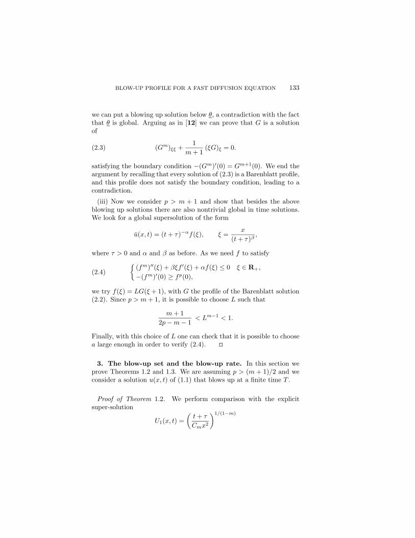
(iii) Now we consider p > m + 1 and show that besides the aboveblowing up solutions there are also nontrivial global in time solutions.We look for a global supersolution of the form

u(x, t) = (t+ τ )−αf(ξ), ξ =x

(t+ τ )β,

where τ > 0 and α and β as before. As we need f to satisfy

(2.4){(fm)′′(ξ) + βξf ′(ξ) + αf(ξ) ≤ 0 ξ ∈ R+,−(fm)′(0) ≥ fp(0),

we try f(ξ) = LG(ξ + 1), with G the profile of the Barenblatt solution(2.2). Since p > m+ 1, it is possible to choose L such that

m+ 12p−m− 1

< Lm−1 < 1.

Finally, with this choice of L one can check that it is possible to choosea large enough in order to verify (2.4).

3. The blow-up set and the blow-up rate. In this section weprove Theorems 1.2 and 1.3. We are assuming p > (m + 1)/2 and weconsider a solution u(x, t) of (1.1) that blows up at a finite time T .

Proof of Theorem 1.2. We perform comparison with the explicitsuper-solution

U1(x, t) =(t+ τCmx2

)1/(1−m)


for τ > 0 large enough and Cm as before, if u0 has the appropriatedecay at infinity. If not we use the super-solution

U2(x, t) = (t+ τ )1/(1−m)w(x),

where w is a solution of the elliptic problem (wm)′′ − 1

1−m w = 0 0 < x < R,

w(0) = w(R) = ∞,

and τ and R are large enough, see [4].

For the rest of the section we assume that u satisfies hypothesis (H).As a consequence we have that (um)xx ≥ 0 and ux ≤ 0. Therefore, thefollowing properties hold for t close to T ,

u(0, t) = maxx∈[0,∞)

u(x, t), (um)x(0, t) = minx∈[0,∞]

(um)x(x, t).

Proof of Theorem 1.3. In this proof we follow the techniques used in[16, 24] for the case m ≥ 1.

We define M(t) = u(0, t) and the function

φM (r, s) =1M(t)

u(ar, bs+ t),

where a = Mm−p, b = Mm+1−2p. Since p > (m + 1)/2 > m, we havethat a and b go to zero as t→ T .The function φM is a solution of the following problem,{

(φM )s = (φmM )rr (r, s) ∈ R+ × (−t/b, 0),

−(φmM )r(0, s) = φ

pM (0, s) s ∈ (−t/b, 0).

Moreover, using that ut ≥ 0, we get that 0 ≤ φM ≤ 1 and φM (0, 0) = 1.

We claim that there exist two positive constants c and C such that

c ≤ (φM )s(0, 0) ≤ C.


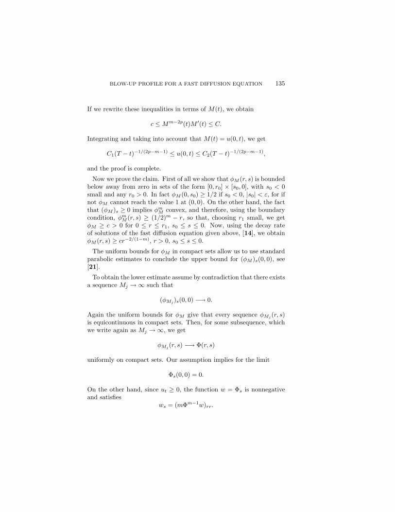
If we rewrite these inequalities in terms of M(t), we obtain

c ≤Mm−2p(t)M ′(t) ≤ C.

Integrating and taking into account that M(t) = u(0, t), we get

C1(T − t)−1/(2p−m−1) ≤ u(0, t) ≤ C2(T − t)−1/(2p−m−1),

and the proof is complete.

Now we prove the claim. First of all we show that φM (r, s) is boundedbelow away from zero in sets of the form [0, r0] × [s0, 0], with s0 < 0small and any r0 > 0. In fact φM (0, s0) ≥ 1/2 if s0 < 0, |s0| < ε, for ifnot φM cannot reach the value 1 at (0, 0). On the other hand, the factthat (φM )s ≥ 0 implies φm

M convex, and therefore, using the boundarycondition, φm

M (r, s) ≥ (1/2)m − r, so that, choosing r1 small, we getφM ≥ c > 0 for 0 ≤ r ≤ r1, s0 ≤ s ≤ 0. Now, using the decay rateof solutions of the fast diffusion equation given above, [14], we obtainφM (r, s) ≥ cr−2/(1−m), r > 0, s0 ≤ s ≤ 0.

The uniform bounds for φM in compact sets allow us to use standardparabolic estimates to conclude the upper bound for (φM )s(0, 0), see[21].

To obtain the lower estimate assume by contradiction that there existsa sequence Mj → ∞ such that

(φMj)s(0, 0) −→ 0.

Again the uniform bounds for φM give that every sequence φMj(r, s)

is equicontinuous in compact sets. Then, for some subsequence, whichwe write again as Mj → ∞, we get

φMj(r, s) −→ Φ(r, s)

uniformly on compact sets. Our assumption implies for the limit

Φs(0, 0) = 0.

On the other hand, since ut ≥ 0, the function w = Φs is nonnegativeand satisfies

ws = (mΦm−1w)rr.


Moreover, at r = 0,

−(mΦm−1w)r(0, s) = pΦp−1w(0, s).

Observe that Φ(0, 0) = 1 > 0 and that w has a minimum at (0, 0). Soby Hopf’s lemma we obtain that w ≡ 0. Then Φ is a stationary solutionof the fast diffusion equation, i.e.,

Φm = c1r + c2.

The boundary conditions imply Φm(r) = 1−r, which is a contradictionwith the fact that Φ is a nonnegative function in all R+. The claim isproved and the theorem follows.

4. The self-similar profile. In this section we construct the self-similar profile giving the asymptotic behavior. The construction isbased in the following lemma.

Lemma 4.1. Let 0 < m < 1, α, β > 0 with α/β < 2/(1 − m),V ∈ R, and consider the problem

(Fm)′′ − βξF ′ − αF = 0 ξ ∈ R+,F (0) = 1,−(Fm)′(0) = V.

There exists a unique value V = V∗ > 0 such that this problem has aclassical bounded solution. The solution is unique, strictly decreasingand satisfies the decay rate (1.6).

The existence of a unique self-similar profile for our problem with theproper decay is now immediate.

Proof of Theorem 1.4. Let F1 be the solution to problem (4.1) withV = V∗ for α and β as in (4.1). For this choice of α and β the conditionα/β < 2/(1−m) reads p > (m+ 1)/2. Then the scaled function

Fλ(ξ) = λF1(λ(1−m)/2ξ)


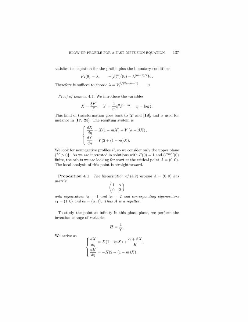
satisfies the equation for the profile plus the boundary conditions

Fλ(0) = λ, −(Fmλ )′(0) = λ(m+1)/2V∗.

Therefore it suffices to choose λ = V 2/(2p−m−1)∗ .

Proof of Lemma 4.1. We introduce the variables

X =ξF ′

F, Y =

1mξ2F 1−m, η = log ξ.

This kind of transformation goes back to [2] and [18], and is used forinstance in [17, 25]. The resulting system is

dX

dη= X(1−mX) + Y (α+ βX) ,

dY

dη= Y (2 + (1−m)X).

We look for nonnegative profiles F , so we consider only the upper plane{Y > 0}. As we are interested in solutions with F (0) = 1 and (Fm)′(0)finite, the orbits we are looking for start at the critical point A = (0, 0).The local analysis of this point is straightforward.

Proposition 4.1. The linearization of (4.2) around A = (0, 0) hasmatrix (

1 α0 2

)with eigenvalues λ1 = 1 and λ2 = 2 and corresponding eigenvectorse1 = (1, 0) and e2 = (α, 1). Thus A is a repeller.

To study the point at infinity in this phase-plane, we perform theinversion change of variables

H =1Y.

We arrive at dX

dη= X(1−mX) +

α+ βXH

,

dH

dη= −H(2 + (1−m)X).


In order to eliminate the singularity we perform the nonlinear changeof variable given implicitly by

dη

dτ= H(η).

Observe that this change preserves the direction of the flow on theupper half-plane {H > 0}, which is the same, {Y > 0}. Then X, Hsatisfy

dX

dτ= HX(1−mX) + (α+ βX) ,

dH

dτ= −H2(2 + (1−m)X).

The proper behavior in these variables corresponds to the criticalpoint B = (−α/β, 0). The local analysis around this point is againstraightforward.

Proposition 4.2. The critical point B = (−α/β, 0) is a saddle-nodeof system (4.3). The linearization of (4.3) around B = (−α/β, 0) hasmatrix (

β − αβ2

(β +mα)

0 0

)

with eigenvalues λ1 = β and λ2 = 0 and corresponding eigenvectorse1 = (1, 0) and e2 = (1, β3/(α(β+mα))). The point B is a repeller onthe half-plane {H < 0} and a saddle on the half-plane {H > 0}.

Existence of the connection. We are looking for an orbit connectingthe critical points A and B. As there is a unique orbit σ∗ arrivingat B, we just have to trace back where it comes from. In the XY -plane the critical point B corresponds to (−α/β,+∞). We observethat dY/dη > 0 for X > −2/(1 − m), Y > 0 and that dX/dη > 0for X = 0, Y > 0. Since 2/(1 − m) > α/β (this is equivalent to thecondition p > (m+ 1)/2), then the orbit σ∗ necessarily comes from A.

We now have to look more carefully at the behavior of this trajectorynear the point A. From Proposition 4.1, we have that in the secondquadrant, {X < 0, Y > 0}, all the trajectories exit the origin tangentto the horizontal axis. Moreover, it is easy to check that they do thisquadratically. In particular our trajectory exits A like Y ∼ ΛX2 for


F

1

�0

FIGURE 1. The trajectories in the XY -plane.

some Λ > 0. This gives the value V∗ = 1/√mΛ . Even more, X < 0

implies that the profile F∗ corresponding to the orbit σ∗ is strictlydecreasing.

In order to give a complete understanding of the picture in the upperplane {Y > 0}, and prove that σ∗ gives the unique profile, we considerall the trajectories starting at the origin (X,Y ) = (0, 0) and check thatother choices of V give profiles that are either unbounded or definedonly in a bounded interval.

First of all, from the equation of the profile (4.1), it is easy to see thatonce the function F satisfies F ′(ξ0) ≥ 0 for some ξ0 ≥ 0, then F ′(ξ) > 0for every ξ > ξ0. Therefore, integrating (4.1) we get the inequality

(Fm)′ ≥ c1F,which implies that F becomes unbounded for a finite value of ξ. Thiscorresponds to the trajectories in the XY -plane that exit the origin inthe first quadrant, V ≤ 0, and also those in the second quadrant thatcross the vertical axis, 0 < V < V∗.

We also observe that the trajectory σ∗ is a separatrix in the secondquadrant between those trajectories that cross the vertical axis and


�

2

1�m�

�

�0

��

Y

X

FIGURE 2. Solutions of (4.1) for different values of V .

those trajectories that cross the vertical line X = −2/(1−m). We nowprove that these last trajectories, which correspond to taking V > V∗,give profiles that vanish at a finite value of ξ, thus not being definedin the whole R+. To see this, let Y = Y (X) be a trajectory passingthrough a point (−2/(1 −m), D), D > 0, at a time η0 ∈ R. The firstequation in (4.2) gives, for η > η0,

dX

dη≤ −mX2,

since α + βX < 0, Y > 0. This implies that there exists a finite η∞such that

(4.4) limη→η∞

X(η) = −∞.

Also, since dY/dη < 0 and dX/dη < 0 for η > η0, we have that thereexists the limit

limη→η∞

Y (η) = Y∞ ≥ 0.

If Y∞ > 0 and (4.4), we get F (η∞) > 0 and F ′(η∞) = −∞, a con-tradiction with the regularity of positive solutions of (4.1). Therefore,


from the relation between η and ξ, we deduce that there exists a finiteξ∞ such that,

limξ→ξ∞

F (ξ) = 0.

This completes the proof.

5. Asymptotic behavior. In this section we prove the stabilizationresult for the rescaled problem (1.7).

Proof of Theorem 1.5. Thanks to the blow-up rate (1.2) we knowthat g is bounded. The behavior of u near t = T is translated into thebehavior of g as τ → ∞. As expected, stationary solutions will play anoutstanding role.

Using arguments similar to those in the proof of Theorem 1.3, wehave that there exists a sequence τj → ∞ such that

(5.1) limj→∞

g(ξ, τ + τj) = g∗(ξ, τ)

uniformly in compact sets of R+. We want to prove that the functiong∗ does not depend on τ and therefore it coincides with the uniquestationary solution F constructed in the previous section.

We now construct a Lyapunov function for g following the ideas of[27] and [11], taking note of the boundary condition. Putting h = gm,we get the problem{

hτ = a(h)(hξξ + b(ξ, h, hξ)), (ξ, τ) ∈ R+ × R+,−hξ(0, τ ) = hp/m(0, τ ), τ ∈ R+,

where

a(h) = mh(m−1)/m, b(ξ, h, z) = − βmξh(1−m)/m z − αh1/m.

We remark that the boundedness of h, together with 0 < m < 1, implya(h) ≥ a0 > 0.

Consider the function

Lh(τ ) =∫ ∞

0

Φ(ξ, h(ξ, τ), hξ(ξ, τ)) dξ − m

m+ ph(m+p)/m(0, τ ).


Differentiating and integrating by parts, we get

d

dτLh(τ ) = − (hp/m(0, τ ) + Φz(0, h, hξ))hτ (0, τ )−

∫ ∞

0

1aΦzz(hτ )2 dξ

+∫ ∞

0

(Φh − Φξz − Φhzhξ + bΦzz)hτ dξ.

We can eliminate the last integral by choosing appropriately the func-tion Φ using the method of characteristics. It is given by

Φ(ξ, h, z) =∫ z

0

(z − s) ρ (ξ, h, s) ds−∫ h

0

b(ξ, s, 0) ρ (ξ, s, 0) ds,

where

ρ(ξ, h, z) = exp(∫ ξ

0

bz(η) dη),

and bz is evaluated along the characteristic φ(η, ξ, h, z), solution to{φ′′ + b(η, φ, φ′) = 0 0 < η < ξ,φ(ξ) = h, φ′(ξ) = z,

see [11]. Thus

ρ(ξ, h, z) = exp(− βm

∫ ξ

0

ηφ(1−m)/m(η, ξ, h, z) dη).

Therefore, ρ is defined only on the domain spanned by characteristiclines. The calculation above allows to generate a global function ρ ifequation φ′′ = −b(η, φ, φ′) allows to pass in a homeomorphic way fromdata at η = 0 to data at η = ξ. It is then clear that whenever β ≥ 0,as in our case, we have ρ ≤ 1. A lower estimate for ρ is crucial in ourLyapunov argument. If we could assert that all solutions φ involvedin bz are bounded then the last formula would imply a lower estimatefor ρ of the form ρ ≥ exp(−Cξ2). This is in principle not the case forproblem (5.2) and we meet problems if there are blow up solutions. Thisdifficulty will be dealt with below, so we assume that ρ ≥ exp(−Cξ2).We now calculate

Φz(0, h, hξ) =∫ hξ

0

ρ(0, h, s) ds = hξ(0, τ ) = −hp/m(0, τ ).


Putting it all together we get

d

dτLh(τ ) = −

∫ ∞

0

1a(h)

ρ(ξ, h, hξ)(hτ )2 dξ.

Since b(ξ, h, z) ≤ 0 and the function h is bounded, we have that

Lh(τ ) ≥ −C.

On the other hand, if we restrict ourselves to 0 < ξ < L for any givenL, we get ρ ≥ C(L) > 0. These estimates imply

4m(m+ 1)2

∫ τ2

τ1

∫ L

0

((h(m+1)/(2m))τ )2 dξ dτ

≤ 1C(L)

∫ τ2

τ1

∫ ∞

0

1a(h)

ρ(ξ, h, hξ)(hτ )2 dξ dτ

=1C(L)

(Lh(τ1)− Lh(τ2)) ≤ C.

We conclude in a rather standard way the convergence of the orbitsto a stationary solution to the limit problem, (1.7), see for instance [1,11]. Indeed,

∥∥∥h(m+1)/(2m)(·, τj + τ )− h(m+1)/(2m)(·, τj)∥∥∥2

L2([0,L])

=∫ L

0

∣∣∣h(m+1)/(2m)(ξ, τj + τ )− h(m+1)/(2m)(ξ, τj)∣∣∣2 dξ

≤ τ∫ L

0

∫ τj+τ

τj

∣∣∣∣ ddτ h(m+1)/(2m)(ξ, s)∣∣∣∣2

ds dξ → 0

as j → ∞, uniformly for bounded τ . Therefore, the sequenceh(m+1)/2m(ξ, τj + τ ) converges in the space L∞([0, τ ] : L2([0, L])) forevery τ > 0 and every L > 0. The limit does not depend on τ and is astationary solution of (1.7). The uniqueness of the stationary solutionto that problem, cf. Theorem 1.4, implies that the limit function g∗ in(5.1) does not depend on τ . Hence (1.8).


Justification of the computation. If there exist solutions of equation(5.2) which blow up, the justification of the above process implies thestudy of the approximate problem

(5.3){hτ = a(h)(hξξ + b(ξ, h, hξ)) in R+ × R+,(hm)ξ(0, τ ) = hp/m(0, τ ),

where as before a(h) = mh(m−1)/m, and b is b corrected only for largevalues of h, h ≥ M , so that the stationary solutions φ(η; ξ, h, z) areuniformly bounded for bounded data ξ > 0, h > 0, z < 0 and dependcontinuously on the data ξ, h, z. Now, if we take a particular solutionof the original evolution problem, from Theorem 1.3 we have that thefunction h is globally bounded, h(ξ, τ) ≤ C for all ξ ∈ R+ and τ > 0.Taking a constant M ≥ C in the correction performed above, we seethat the solution under consideration is also a solution of the correctedproblem (5.3). Therefore, the use of the corrected problem is justifiedand the calculations given above hold.

The problem in a bounded interval. We define the Lyapunov func-tional as before, but now integrating in the interval (0, R(τ )), whereR(τ ) = L(T − t)−β, (recall that τ = − log(T − t)). Then we have

Lh(τ ) =∫ R(τ)

0

Φ(ξ, h(ξ, τ), hξ(ξ, τ)) dξ − m

m+ ph(m+p)/m(0, τ ).

We must show that the extra term that appears in the expression forthe derivative of Lh(τ ), namely

Φ(R(τ ), h(R(τ ), tau), hξ(R(τ ), τ )

)R′ (τ ),

is integrable. To this purpose we observe that φ(η,R(τ ), s, 0) isdecreasing for η ∈ (0, R(τ )) and that v(ξ, τ) ≤ C. Hence∫ τ2

τ1

Φ(R(τ ), h(R(τ ), τ ), hξ(R(τ ), τ )

)R′ (τ ) dτ

=∫ τ2

τ1

∫ h(R(τ),τ)

0

R′(τ )s1/m

· exp(− βm

∫ R(τ)

0

η (φ(η,R(τ ), s, 0))(1−m)/m dη

)ds dτ

≤∫ C

0

∫ τ2

τ1

R′(τ )s1/m exp(− c s(1−m)/mR(τ )2

)dτ ds ≤ C,


where the last constant is independent of τ1, τ2. Therefore, followingthe same argument given above we conclude that (1.8) holds also inthe case of a bounded interval.

Acknowledgments. This research was performed while the fourthauthor was a visitor at Universidad Autonoma de Madrid. He isgrateful to this institution for its hospitality.

REFERENCES

1. D.G. Aronson, M.G. Crandall and L.A. Peletier, Stabilization of solutions ofa degenerate nonlinear diffusion problem, Nonlinear Anal. 6 (1982), 1001 1022.

2. G.I. Barenblatt, On some unsteady motions of a liquid or a gas in a porousmedium, Prikl. Mat. Mekh. 16 (1952), 67 78. (Russian)

3. , Scaling, self-similarity and intermediate asymptotics, Cambridge Univ.Press, Cambridge, UK, 1996.

4. E. Chasseigne and J.L. Vazquez, Theory of extended solutions for fast diffusionequations in optimal classes of data. Radiation from singularities, Arch. Rat. Mech.Anal. (2002), to appear.

5. M. Chlebık and M. Fila, On the blow-up rate for the heat equation with anonlinear boundary condition, Math. Methods Appl. Sci. 23 (2000), 1323 1330.

6. , Some recent results on the blow-up on the boundary for the heatequation, Banach Center Publ., Vol. 52, Polish Academy of Science, Inst. of Math.,Warsaw, 2000, pp. 61 71.

7. K. Deng and H. Levine, The role of critical exponents in blow-up theorems:The sequel, J. Math. Anal. Appl. 243 (2000), 85 126.

8. M. Fila and J. Filo, Blow-up on the boundary: A survey, in Singularities anddifferential equations (S. Janeczko et al., eds.), Banach Center Publ., Vol. 33, PolishAcademy of Science, Inst. of Math., Warsaw, 1996, pp. 67 78.

9. M. Fila and P. Quittner, The blowup rate for the heat equation with a nonlinearboundary condition, Math. Methods Appl. Sci. 14 (1991), 197 205.

10. J. Filo, Diffusivity versus absorption through the boundary, J. DifferentialEquations 99 (1992), 281 305.

11. V.A. Galaktionov, On asymptotic self-similar behaviour for a quasilinear heatequation. Single point blow-up, SIAM J. Math. Anal. 26 (1995), 675 693.

12. V.A. Galaktionov and H.A. Levine, On critical Fujita exponents for heatequations with nonlinear flux boundary conditions on the boundary, Israel J. Math.94 (1996), 125 146.

13. B.H. Gilding and L.A. Peletier, On a class of similarity solutions of theporous media equation, J. Math. Anal. Appl. 55 (1976), 351 364.

14. M.A. Herrero and M. Pierre, The Cauchy problem for ut = ∆um when0 < m < 1, Trans. Amer. Math. Soc. 291 (1985), 145 158.


15. B. Hu, Remarks on the blowup estimate for solution of the heat equation witha nonlinear boundary condition, Differential Integral Equations 9 (1996), 891 901.

16. B. Hu and H.M. Yin, The profile near blow-up time for solutions of the heatequation with a nonlinear boundary condition, Trans. Amer. Math. Soc. 346 (1994),117 135.

17. J. Hulshof, Similarity solutions of the porous medium equation with signchanges, J. Math. Anal. Appl. 157 (1991), 75 111.

18. C.W. Jones, On reducible nonlinear differential equations occurring in me-chanics, Proc. Roy. Soc. London Ser. A 217 (1953), 327 343.

19. H.A. Levine, The role of critical exponents in blow up theorems, SIAM Rev.32 (1990), 262 288.

20. , Some nonexistence and instability theorems for solutions of formallyparabolic equations of the form Put = −Au + F (u), Arch. Rat. Mech. Anal. 51(1973), 371 386.

21. G.M. Lieberman, Second order parabolic differential equations, World Scien-tific Publ., River Edge, NJ, 1996.

22. F.J. Mancebo and J.M. Vega, A model of porous catalyst accounting forincipiently non-isothermal effects, J. Differential Equations 151 (1999), 79 110.

23. A. de Pablo, F. Quiros and J.D. Rossi, Asymptotic simplification for areaction-diffusion problem with a nonlinear boundary condition, IMA J. Appl.Math. 67 (2002), 69 98.

24. F. Quiros and J.D. Rossi, Blow-up sets and Fujita type curves for a degenerateparabolic system with nonlinear boundary conditions, Indiana Univ. Math. J. 50(2001), 629 654.

25. F. Quiros and J.L. Vazquez, Asymptotic behaviour of the porous mediaequation in an exterior domain, Ann. Scuola Norm. Sup. Pisa Cl. Sci. (4) 28 (1999),183 227.

26. A.A. Samarskii, V.A. Galaktionov, S.P. Kurdyunov and A.P. Mikhailov,Blow-up in problems for quasilinear parabolic equations, Nauka, Moscow, 1987(Russian). English transl., Walter de Gruyter, Berlin, 1995.

27. T.I. Zelenyak, Stabilization of solution of boundary value problems for asecond order parabolic equation with one space variable, Differ. Uravn. 4 (1986),34 45 (Russian). English transl., Differential Equations 4 (1986), 17 22.

Depto. de Matematicas, U. Autonoma de Madrid, 28049 Madrid, SpainE-mail address: [email protected]

Depto. de Matematicas, U. Carlos III de Madrid, 28911 Leganes, SpainE-mail address: [email protected]

Depto. de Matematicas, U. Autonoma de Madrid, 28049 Madrid, SpainE-mail address: [email protected]

Depto. de Matematica, F.C.E. y N., UBA, (1428) Buenos Aires, ArgentinaE-mail address: [email protected]

The Blow-Up Profile for a Fast Diffusion Equation with a Nonlinear Boundary Condition

Documents

Transcript of The Blow-Up Profile for a Fast Diffusion Equation with a Nonlinear Boundary Condition