Nonlinear Analysis 54 (2003) 959–976www.elsevier.com/locate/na

Global existence and stability for wave equationof Kirchho' type with memory condition

at the boundary

M.L. Santosa ;∗, J. Ferreirab, D.C. Pereirac, C.A. RaposodaDepartamento de Matematica, Universidade Federal do Para Campus Universitario do Guama,

Rua Augusto Correa 01, CEP 66075-110, Para, BrazilbDepartamento de Matematica-DMA, Universidade Estadual de Maringa-UEM, Av. Colombo,

5790-Zona 7, CEP 87020-900, Maringa-Pr., BrazilcInstituto de Estudos Superiores da Amazonia (IESAM) Av. Gov. Jose Malcher 1148,

CEP 66.055-260, Belem-Pa., BrazildDepartamento de Matematica, Universidade Federal de Sao Joao Del-Rei,

Sao Joao Del-Rei-MG, Brazil

Received 23 August 2002; accepted 27 November 2002

Abstract

We consider a nonlinear wave equation of Kirchho' type with memory condition at theboundary and we study the asymptotic behavior of the corresponding solutions. We proved thatthe energy decay with the same rate of decay of the relaxation function, that is, the energydecays exponentially when the relaxation function decay exponentially and polynomially whenthe relaxation function decay polynomially.? 2003 Elsevier Science Ltd. All rights reserved.

Keywords: Global existence; Wave equation; Galerkin method; Asymptotic behavior; Boundary valueproblem

1. Introduction

The main purpose of this work is to study the asymptotic behavior of the solutionsof a nonlinear wave equation of Kirchho' type with boundary condition of memory

∗ Corresponding author.E-mail addresses: ls@ufpa.br (M.L. Santos), jferreira@wnet.com.br (J. Ferreira), ducival@aol.com

(D.C. Pereira), raposo@funrei.br (C.A. Raposo).

0362-546X/03/$ - see front matter ? 2003 Elsevier Science Ltd. All rights reserved.doi:10.1016/S0362-546X(03)00121-4

960 M.L. Santos et al. / Nonlinear Analysis 54 (2003) 959–976

type. To formalize this problem let us take a open bounded set of Rn with smoothboundary and let us assume that can be divided into two non-null parts

= 0 ∪ 1 with C0 ∩ C1 = ∅:Let us denote by (x) the unit normal vector at x∈ outside of and let us considerthe following initial boundary value problem:

utt −M (‖∇u‖22)Du−Dut + f(u) = 0 in × (0;∞); (1.1)

u= 0 on 0 × (0;∞); (1.2)

u+∫ t

0g(t − s)

((M (‖∇u(s)‖22)

@u@

(s) +@ut

@(s)

)ds= 0 on 1 × (0;∞);

(1.3)

u(0; x) = u0(x); ut(0; x) = u1(x) in : (1.4)

Here, u is the transverse displacement, the relaxation function g is positive and non-decreasing and the function f∈C1(R) satisfy

f(s)s¿ 0 ∀s∈R:Additionally, we suppose that f is superlinear, that is

f(s)s¿ (2 + )F(s); F(z) =∫ z

0f(s) ds ∀s∈R

for some ¿ 0 with the following growth conditions:

|f(x)− f(y)|6 c(1 + |x|−1 + |y|−1)|x − y| ∀x; y∈Rfor some c¿ 0 and ¿ 1 such that (n− 2)6 n. We shall assume that the functionM ∈C1([0;∞[) satisfy

M ()¿m0 ¿ 0; M ()¿ M () ∀¿ 0; (1.5)

where M ()=∫ 0 M (s) ds. The integral equation (1.3) describe the memory e'ect which

can be caused, for example, by the interaction with another viscoelastic element. Indeed,from the physical of view, condition (1.3) means that is composed of a materialwhich is clamped in a rigid body in 0 and is clamped in a body with viscoelasticproperties in the complementary part of its boundary named 1. Also, we shall assumethat there is x0 ∈Rn such that

0 = x∈ : (x) · (x − x0)6 0;1 = x∈ : (x) · (x − x0)¿ 0:

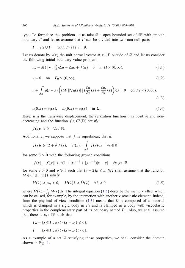
As a example of a set satisfying those properties, we shall consider the domainshown in Fig. 1.

M.L. Santos et al. / Nonlinear Analysis 54 (2003) 959–976 961

Ω Γ0

Γ1

x 0•

Fig. 1.

Let us denote by m(x) = x − x0. Note that the compactness of 1 imply that thereis a small positive constant 0 such that

0¡06m(x) · (x) ∀x∈1: (1.6)

The existence of global solutions and exponential decay to problem (1.1) and (1.2)with @=0 has been investigated by many authors (see, e.g. [1,2,5,6,9–11,16]). Thereexists a large body of literature regarding viscoelastic problems with the memory termacting in the domain or in the boundary. Among the numerous works in this direction,we can cite Rivera [7] and Santos [14]. Cavalcanti et al. [3,4] studied the existenceand uniform decay of strong solutions of wave equation (1.1) without strong dampingterm Dut with nonlinear boundary damping and memory source term when M (s) = 1,that is, semilinear case. Park et al. [12] studied the existence and uniform decay ofstrong solutions of the wave equation (1.1) with nonlinear boundary damping andmemory source term and M (s) = 1 + s. It is important to emphasize that in [12]they only obtained uniform decay of strong solutions of wave equation (1.1) withoutthe term nonlinear f. In the present paper, we obtained respectively, besides, thedecay exponential and uniform rate of polynomial decay. Moreover, Eq. (1.1) is moregeneral than the equation considered in [12], because they only consider the case inthat M (s) = 1 + s. We would like to remark that we used only the damping term Dut

to obtain the existence result because in any step it was used to obtain the results ondecays, exponential and polynomial.The main result this paper is to show that the solutions of system (1.1) – (1.4) decays

uniformly in time with the same rate of decay of the relaxation function. More precisely,denoting by k the resolvent kernel of −g′=g(0), we show that the solution decaysexponentially to zero provided k decays exponentially to zero. When the resolventkernel k decays polynomially, we show that the corresponding solution also decayspolynomially to zero. The method used here is based on the construction of a suitable

962 M.L. Santos et al. / Nonlinear Analysis 54 (2003) 959–976

Lyapunov functional L satisfying

ddt

L(t)6− c1L(t) + c2e−t orddt

L(t)6− c1L(t)1+1= +c2

(1 + t)+1

for some positive constants c1; c2; and . Note that, because of condition (1.2) thesolution of system (1.1) – (1.4) must belong to the following space:

V := v∈H 1() : v= 0 on 0:The notation used in this paper is standard and can be found in Lions’ book [8]. Inthe sequel by c (sometime c1; c2; : : :) we denote various positive constants independentof t and on the initial data. The organization of this paper is as follows. In Section 2we establish the existence and uniqueness of strong solutions for system (1.1) – (1.4).In Section 3 we prove the uniform rate exponential decay. In Section 4 we prove theuniform rate of polynomial decay. Finally in Section 5 will make a Mnal comment ontwo problems related with the problem in subject, that is, (1.1) – (1.4), that the methodexplored in this paper can be used to solve problems (5.1) and (5.2), respectively. Theauthors of this paper have already solved these.

2. Existence and regularity

In this section, we shall study the existence and regularity of solutions for system(1.1) – (1.4). First, we shall use Eq. (1.3) to estimate the term M (‖∇u(t)‖22)@u=@ +@ut=@. Denoting by

(g ∗ ’)(t) =∫ t

0g(t − s)’(s) ds;

the convolution product operator and di'erentiating Eq. (1.3) we arrive at the followingVolterra equation:

M (‖∇u(t)‖22)@u@

+@ut

@+

1g(0)

g′ ∗(M (‖∇u‖22)

@u@

+@ut

@

)=− 1

g(0)ut :

Applying the Volterra’s inverse operator, we get

M (‖∇u‖22)@u@

+@ut

@=− 1

g(0)ut + k ∗ ut

where the resolvent kernel satisfy

k +1

g(0)g′ ∗ k =− 1

g(0)g′:

Denoting by "= 1=g(0) we obtain

M (‖∇u‖22)@u@

+@ut

@=−"ut + k(0)u− k(t)u0 + k ′ ∗ u: (2.1)

M.L. Santos et al. / Nonlinear Analysis 54 (2003) 959–976 963

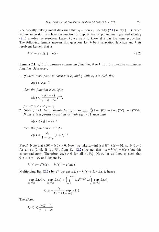
Reciprocally, taking initial data such that u0=0 on 1, identity (2.1) imply (1.3). Sincewe are interested in relaxation function of exponential or polynomial type and identity(2.1) involve the resolvent kernel k, we want to know if k has the same properties.The following lemma answers this question. Let h be a relaxation function and k itsresolvent kernel, that is

k(t)− k ∗ h(t) = h(t): (2.2)

Lemma 2.1. If h is a positive continuous function, then k also is a positive continuousfunction. Moreover,

1. If there exist positive constants c0 and with c0 ¡ such that

h(t)6 c0e−t ;

then the function k satis?es

k(t)6c0(− $)− $− c0

e−$t ;

for all 0¡$¡− c0.2. Given p¿ 1, let us denote by cp := supt∈R+

∫ t0 (1 + t)p(1 + t − s)−p(1 + s)−p ds.

If there is a positive constant c0 with c0cp ¡ 1 such that

h(t)6 c0(1 + t)−p;

then the function k satis?es

k(t)6c0

1− c0cp(1 + t)−p:

Proof. Note that k(0)=h(0)¿ 0. Now, we take t0=inft ∈R+ : k(t)=0, so k(t)¿ 0for all t ∈ [0; t0[. If t0 ∈R+, from Eq. (2.2) we get that −k ∗ h(t0) = h(t0) but thisis contradictory. Therefore, k(t)¿ 0 for all t ∈R+

0 . Now, let us Mxed $, such that0¡$¡− c0 and denote by

k$(t) := e$tk(t); h$(t) := e$th(t):

Multiplying Eq. (2.2) by e$t we get k$(t) = h$(t) + k$ ∗ h$(t), hence

sups∈[0; t]

k$(s)6 sups∈[0; t]

h$(s) +(∫ ∞

0c0e($−)s ds

)sup

s∈[0; t]k$(s)

6 c0 +c0

(− $)sup

s∈[0; t]k$(s):

Therefore,

k$(t)6c0(− $)− $− c0

;

964 M.L. Santos et al. / Nonlinear Analysis 54 (2003) 959–976

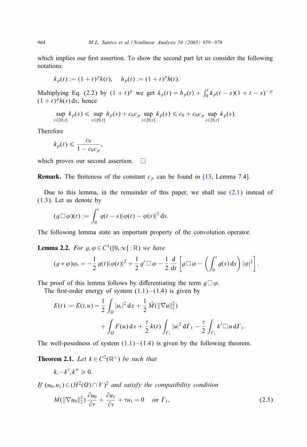
which implies our Mrst assertion. To show the second part let us consider the followingnotations:

kp(t) := (1 + t)pk(t); hp(t) := (1 + t)ph(t):

Multiplying Eq. (2.2) by (1 + t)p we get kp(t) = hp(t) +∫ t0 kp(t − s)(1 + t − s)−p

(1 + t)ph(s) ds, hence

sups∈[0; t]

kp(s)6 sups∈[0; t]

hp(s) + c0cp sups∈[0; t]

kp(s)6 c0 + c0cp sups∈[0; t]

kp(s):

Therefore

kp(t)6c0

1− c0cp;

which proves our second assertion.

Remark. The Mniteness of the constant cp can be found in [13, Lemma 7.4].

Due to this lemma, in the remainder of this paper, we shall use (2.1) instead of(1.3). Let us denote by

(g ’)(t) :=∫ t

0g(t − s)|’(t)− ’(s)|2 ds:

The following lemma state an important property of the convolution operator.

Lemma 2.2. For g; ’∈C1([0;∞[ :R) we have

(g ∗ ’)’t =−12g(t)|’(t)|2 + 1

2g′ ’− 1

2ddt

[g ’−

(∫ t

0g(s) ds

)|’|2

]:

The proof of this lemma follows by di'erentiating the term g ’.The Mrst-order energy of system (1.1) – (1.4) is given by

E(t) := E(t; u) =12

∫|ut |2 dx + 1

2M (‖∇u‖22)

+∫F(u) dx +

"2k(t)

∫1

|u|2 d1 − "2

∫1

k ′ u d1:

The well-posedness of system (1.1) – (1.4) is given by the following theorem.

Theorem 2.1. Let k ∈C2(R+) be such that

k;−k ′; k ′′¿ 0:

If (u0; u1)∈ (H 2() ∩ V )2 and satisfy the compatibility condition

M (‖∇u0‖22)@u0@

+@u1@

+ "u1 = 0 on 1; (2.3)

M.L. Santos et al. / Nonlinear Analysis 54 (2003) 959–976 965

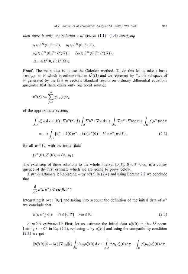
then there is only one solution u of system (1.1) – (1.4) satisfying

u∈L∞(0; T :V ); ut ∈L∞(0; T :V );

utt ∈L∞(0; T :L2()); Du∈L∞(0; T :L2());

Dut ∈L2(0; T :L2()):

Proof. The main idea is to use the Galerkin method. To do this let us take a basiswjj∈N to V which is orthonormal in L2() and we represent by Vm the subspace ofV generated by the Mrst m vectors. Standard results on ordinary di'erential equationsguarantee that there exists only one local solution

um(t) :=m∑

j=1

gj;m(t)wj;

of the approximate system,∫umtt w dx +M (‖∇um(t)‖22)

∫∇um · ∇w dx +

∫∇um

t · ∇w dx +∫f(um)w dx

=− "∫1

umt + k(0)um − k(t)um(0) + k ′ ∗ umw d1; (2.4)

for all w∈Vm with the initial data

(um(0); umt (0)) = (u0; u1):

The extension of these solutions to the whole interval [0; T ], 0¡T ¡∞, is a conse-quence of the Mrst estimate which we are going to prove below.A priori estimate I: Replacing w by um

t (t) in (2.4) and using Lemma 2.2 we concludethat

ddt

E(t; um)6 cE(0; um):

Integrating it over [0; t] and taking into account the deMnition of the initial data of um

we conclude that

E(t; um)6 c ∀t ∈ [0; T ] ∀m∈N: (2.5)

A priori estimate II: First, let us estimate the initial data umtt (0) in the L2-norm.

Letting t → 0+ in Eq. (2.4), replacing w by u′′m(0) and using the compatibility condition(2.3) we get

‖umtt (0)‖22 =M (‖∇u0‖22)

∫Du0um

tt (0) dx +∫Du1um

tt (0) dx −∫f(u0)um

tt (0) dx:

966 M.L. Santos et al. / Nonlinear Analysis 54 (2003) 959–976

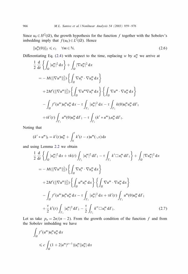
Since u0 ∈H 2(), the growth hypothesis for the function f together with the Sobolev’simbedding imply that f(u0)∈L2(). Hence

‖umtt (0)‖26 c1 ∀m∈N: (2.6)

Di'erentiating Eq. (2.4) with respect to the time, replacing w by umtt we arrive at

12

ddt

∫|um

tt |2 dx+∫|∇um

tt |2 dx

=−M (‖∇um‖22)∫

∇um

t · ∇umtt dx

+2M ′(‖∇um‖22)∫

∇um∇um

t dx∫

∇um · ∇um

tt dx

−∫f′(um)um

t umtt dx − "

∫1

|umtt |2 dx − "

∫1

k(0)umt u

mtt d1

+"k ′(t)∫1

um(0)umtt d1 − "

∫1

(k ′ ∗ um)tumtt d1:

Noting that

(k ′ ∗ um)t = k ′(t)um0 +

∫ t

0k ′(t − s)um(·; s) ds

and using Lemma 2.2 we obtain

12

ddt

∫|um

tt |2 dx + "k(t)∫1

|umt |2 d1 − "

∫1

k ′ umt d1

+∫|∇um

tt |2 dx

=−M (‖∇um‖22)∫

∇um

t · ∇umtt dx

+2M ′(‖∇um‖22)∫

umum

t dx∫

∇um · ∇um

tt dx

−∫f′(um)um

t umtt dx − "

∫1

|umtt |2 dx + "k ′(t)

∫1

um(0)umtt d1

+"2k ′(t)

∫1

|umt |2 d1 − "

2

∫1

k ′′ umt d1: (2.7)

Let us take pn = 2n=(n − 2). From the growth condition of the function f and fromthe Sobolev imbedding we have∫

f′(um)um

t umtt dx

6 c∫(1 + 2|um|−1)|um

t ‖umtt | dx

M.L. Santos et al. / Nonlinear Analysis 54 (2003) 959–976 967

6 c[∫

(1 + 2|um|−1)n dx

]1=n [∫|um

t |pn dx]1=pn

[∫|um

tt |2 dx]1=2

6 c[∫

(1 + |∇um|2) dx

](−1)=2 [∫|∇um

t |2 dx]1=2 [∫

|um

tt |2 dx]1=2

:

Taking into account the Mrst estimate (2.5) we conclude that∫f′(um)um

t umtt dx6 c

[∫|∇um

t |2 dx]1=2 [∫

|um

tt |2 dx]1=2

6 c∫

|∇um

t |2 dx +∫|um

tt |2 dx

: (2.8)

Note that Young’s inequality, the Mrst estimate and hypothesis on M give us

M (‖∇um‖22)∫

∇um

t · ∇umtt dx

6 c

∫|∇um

t |2 dx +14

∫|∇um

tt |2 dx (2.9)

and similarly

2M ′(‖∇um‖22)∫

∇um∇um

t dx∫

∇um · ∇um

tt dx

6 c∫|∇um

t |2 +14

∫|∇um

tt |2 dx: (2.10)

Substitution of inequalities (2.8) – (2.10) into (2.7) we arrive at

12

ddt

∫|um

tt |2 dx + "k(t)∫1

|umt |2 d1 − "

∫1

k ′ umt d1

+12

∫|∇um

tt |2 dx6"c2

∫1

|u0|2 d1 + c∫|∇um

t |2 dx + c∫|um

tt |2 dx:

Integrating with respect to the time and applying Gronwall’s inequality we concludethat ∫

|um

tt |2 dx +∫ t

0

∫|∇um

tt |2 dx6 c ∀m∈N ∀t ∈ [0; T ]: (2.11)

A priori estimate III: Replacing w by −Dumt in (2.4) and using the Green’s formula

yields

−∫umttDum

t dx +M (‖∇um‖22)∫DumDum

t dx +∫|Dum

t |2 dx

=∫f(um)Dum

t dx:

968 M.L. Santos et al. / Nonlinear Analysis 54 (2003) 959–976

Using similar arguments as in (2.11) we conclude

‖Dum‖22 +∫ T

0‖Dum

t (t)‖22 dt6 c ∀m∈N ∀t ∈ [0; T ]: (2.12)

Now, from estimates (2.5), (2.11) and (2.12) and of the Lions–Aubin’s compact-ness theorem we can pass to the limit in (2.4). The rest of the proof is a matter ofroutine.

3. Exponential decay

In this section, we shall study the asymptotic behavior of the solutions of system(1.1) – (1.4) when the resolvent kernel k is exponentially decreasing, that is, there existpositive constants b1, b2 such that

k(0)¿ 0; k ′(t)6− b1k(t); k ′′(t)¿− b2k ′(t): (3.1)

Note that this conditions implies that

k(t)6 k(0)e−b1t :

Our point of departure will be to establish some inequalities for the strong solution ofsystem (1.1) – (1.4).

Lemma 3.1. Any strong solution u of system (1.1) – (1.4) satisfy

ddt

E(t)6− "2

∫1

|ut |2 d1 +"2k2(t)

∫1

|u0|2 d1

+"2k ′(t)

∫1

|u|2 d1 − "2

∫1

k ′′ u d1 −∫|∇ut |2 dx:

Proof. Multiplying Eq. (1.1) by ut and integrating by parts over we get

12

ddt

∫|ut |2 + 1

2ddt

M (‖∇u‖22) +ddt

∫F1(u) dx +

∫|∇ut |2 dx

=∫1

M (‖∇u‖22)

@u@

+@ut

@

ut d1:

Substituting the boundary term by (2.1) and using Lemma 2.1 our conclusionfollows.

Let us consider the following binary operator:

(k♦’)(t) :=∫ t

0k(t − s)(’(t)− ’(s)) ds:

M.L. Santos et al. / Nonlinear Analysis 54 (2003) 959–976 969

Then applying the HRolder’s inequality for 06 -6 1 we have

|(k♦’)(t)|26[∫ t

0|k(s)|2(1−-) ds

](|k|2- ’)(t): (3.2)

Let us introduce the following functionals:

N(t) :=∫|ut |2 dx + M (‖∇u‖22) +

∫F(u) dx;

(t) =∫

m · ∇u+

(n2− /

)uut dx;

where / is a small positive constant. The following lemma plays an important role forthe construction of the Lyapunov functional.

Lemma 3.2. For any strong solution of system (1.1) – (1.4) we get

ddt

(t)6−/2N(t) + c

∫1

(|ut |2 + |k(t)u|2 + |k ′♦u|2 + |k(t)u0|2) d1

+ c$

∫|∇ut |2 dx

for some positive constants c and $.

Proof. From Eq. (1.1) we obtain

ddt

(t) =∫utm · ∇ut dx +

(n2− /

)∫|ut |2 dx

+∫m · ∇u(M (‖∇u‖22)Du+Dut − f(u)) dx

+(n2− /

)∫u(M (‖∇u‖22)Du+Dut − f(u)) dx:

Performing a integration by parts and using Young’s inequality we get

ddt

(t)612

∫1

m · |ut |2 d1 − /∫|ut |2 dx

+∫1

(M (‖∇u‖22)

@u@

+@ut

@

)m · ∇u+

(n2− /

)ud1

− (1− /)M (‖∇u‖22)∫|∇u|2 dx

+ $cM (‖∇u‖22)∫|∇u|2 dx + c$

∫|∇ut |2 dx

970 M.L. Santos et al. / Nonlinear Analysis 54 (2003) 959–976

−(n2− /

)∫f(u)u dx + n

∫F(u) dx

−12M (‖∇u‖22)

∫1

m · |∇u|2 d1;

where $ is a positive constant. Taking into account that f is superlinear we concludethat

ddt

(t)612

∫1

m · |ut |2 d1 − /∫|ut |2 dx

+∫1

(M (‖∇u‖22)

@u@

+@ut

@

)m · ∇u+

(n2− /

)ud1

− (1− /)M (‖∇u‖22)∫|∇u|2 dx

+ $cM (‖∇u‖22)∫|∇u|2 dx + c$

∫|∇ut |2 dx

−(n2− /

)(2 + )

∫F(u) dx

−12M (‖∇u‖22)

∫1

m · |∇u|2 d1:

Using PoincarSe’s inequality and taking / and $ small enough we obtain

ddt

(t)6−/N(t) +12

∫1

m · |ut |2 d1 + c$

∫|∇ut |2 dx

−12M (‖∇u‖22)

∫1

m · |∇u|2 d1

+∫1

(M (‖∇u‖22)

@u@

+@ut

@

)m · ∇u+

(n2− /

)ud1: (3.3)

Now, we analyze the boundary term of the above inequality. Applying Young’s andPoincarSe’s inequalities we have, for $1 ¿ 0∫

1

(M (‖∇u‖22)

@u@

+@ut

@

)m · ∇u+

(n2− /

)ud1

6 $1

∫1

|m · ∇u|2 +

(n2− /

)2|u|2

d1

+ c$1

∫1

∣∣∣∣(M (‖∇u‖22)

@u@

+@ut

@

)∣∣∣∣2

d1

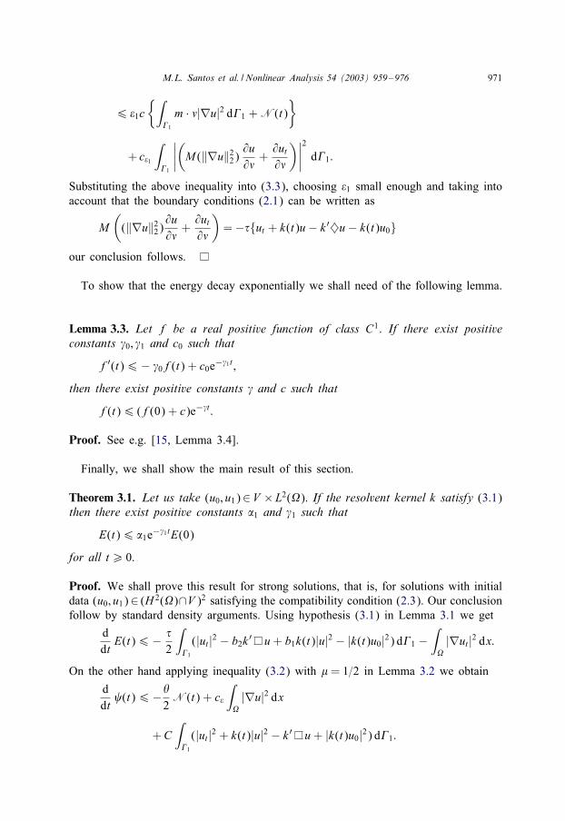
M.L. Santos et al. / Nonlinear Analysis 54 (2003) 959–976 971

6 $1c∫

1

m · |∇u|2 d1 +N(t)

+ c$1

∫1

∣∣∣∣(M (‖∇u‖22)

@u@

+@ut

@

)∣∣∣∣2

d1:

Substituting the above inequality into (3.3), choosing $1 small enough and taking intoaccount that the boundary conditions (2.1) can be written as

M((‖∇u‖22)

@u@

+@ut

@

)=−"ut + k(t)u− k ′♦u− k(t)u0

our conclusion follows.

To show that the energy decay exponentially we shall need of the following lemma.

Lemma 3.3. Let f be a real positive function of class C1. If there exist positiveconstants 0; 1 and c0 such that

f′(t)6− 0f(t) + c0e−1t ;

then there exist positive constants and c such that

f(t)6 (f(0) + c)e−t :

Proof. See e.g. [15, Lemma 3.4].

Finally, we shall show the main result of this section.

Theorem 3.1. Let us take (u0; u1)∈V × L2(). If the resolvent kernel k satisfy (3.1)then there exist positive constants 1 and 1 such that

E(t)6 1e−1tE(0)

for all t¿ 0.

Proof. We shall prove this result for strong solutions, that is, for solutions with initialdata (u0; u1)∈ (H 2()∩V )2 satisfying the compatibility condition (2.3). Our conclusionfollow by standard density arguments. Using hypothesis (3.1) in Lemma 3.1 we get

ddt

E(t)6− "2

∫1

(|ut |2 − b2k ′ u+ b1k(t)|u|2 − |k(t)u0|2) d1 −∫|∇ut |2 dx:

On the other hand applying inequality (3.2) with - = 1=2 in Lemma 3.2 we obtain

ddt

(t)6−/2N(t) + c$

∫|∇u|2 dx

+C∫1

(|ut |2 + k(t)|u|2 − k ′ u+ |k(t)u0|2) d1:

972 M.L. Santos et al. / Nonlinear Analysis 54 (2003) 959–976

Let us introduce the Lyapunov functional

L(t) := NE(t) + (t) (3.4)

with N ¿ 0. Taking N large, the previous inequalities imply thatddt

L(t)6− /2E(t) + 2Nk2(t)E(0):

Moreover, using Young’s inequality and taking N large we Mnd thatN2

E(t)6L(t)6 2NE(t): (3.5)

From this inequality, we conclude thatddt

L(t)6− /2L(t) + 2Nk2(t)E(0);

from where follows, in view of Lemma 3.3 and of the exponential decay of k, that

L(t)6 L(0) + ce−1t

for some positive constants c; . From inequality (3.5) our conclusion follows.

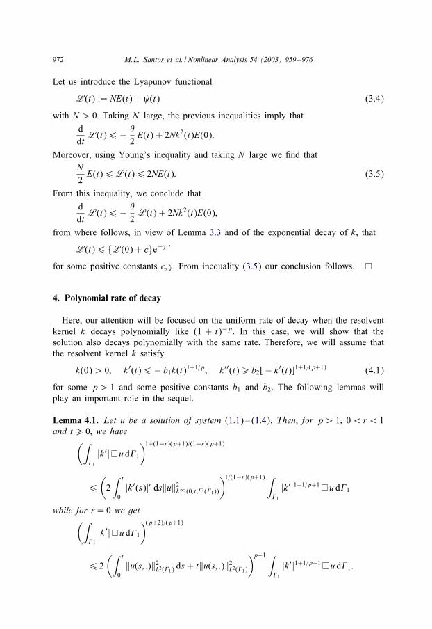
4. Polynomial rate of decay

Here, our attention will be focused on the uniform rate of decay when the resolventkernel k decays polynomially like (1 + t)−p. In this case, we will show that thesolution also decays polynomially with the same rate. Therefore, we will assume thatthe resolvent kernel k satisfy

k(0)¿ 0; k ′(t)6− b1k(t)1+1=p; k ′′(t)¿ b2[− k ′(t)]1+1=(p+1) (4.1)

for some p¿ 1 and some positive constants b1 and b2. The following lemmas willplay an important role in the sequel.

Lemma 4.1. Let u be a solution of system (1.1) – (1.4). Then, for p¿ 1, 0¡r¡ 1and t¿ 0, we have(∫

1

|k ′| u d1

)1+(1−r)(p+1)=(1−r)(p+1)

6(2∫ t

0|k ′(s)|r ds‖u‖2L∞(0; t;L2(1))

)1=(1−r)(p+1) ∫1

|k ′|1+1=p+1 u d1

while for r = 0 we get(∫1

|k ′| u d1

)(p+2)=(p+1)

6 2(∫ t

0‖u(s; :)‖2L2(1) ds+ t‖u(s; :)‖2L2(1)

)p+1 ∫1

|k ′|1+1=p+1 u d1:

M.L. Santos et al. / Nonlinear Analysis 54 (2003) 959–976 973

Proof. See e.g. [14, Lemma 4.2].

Lemma 4.2. Let f¿ 0 be a diBerentiable function satisfying

f′(t)6− c1f(0)1=

f(t)1+1= +c2

(1 + t)2f(0) for t¿ 0

for some positive constants c1; c2, and 2 such that

2¿ + 1:

Then there exists a constant c¿ 0 such that

f(t)6c

(1 + t)f(0) for t¿ 0:

Proof. See e.g. [15, Lemma 4.3].

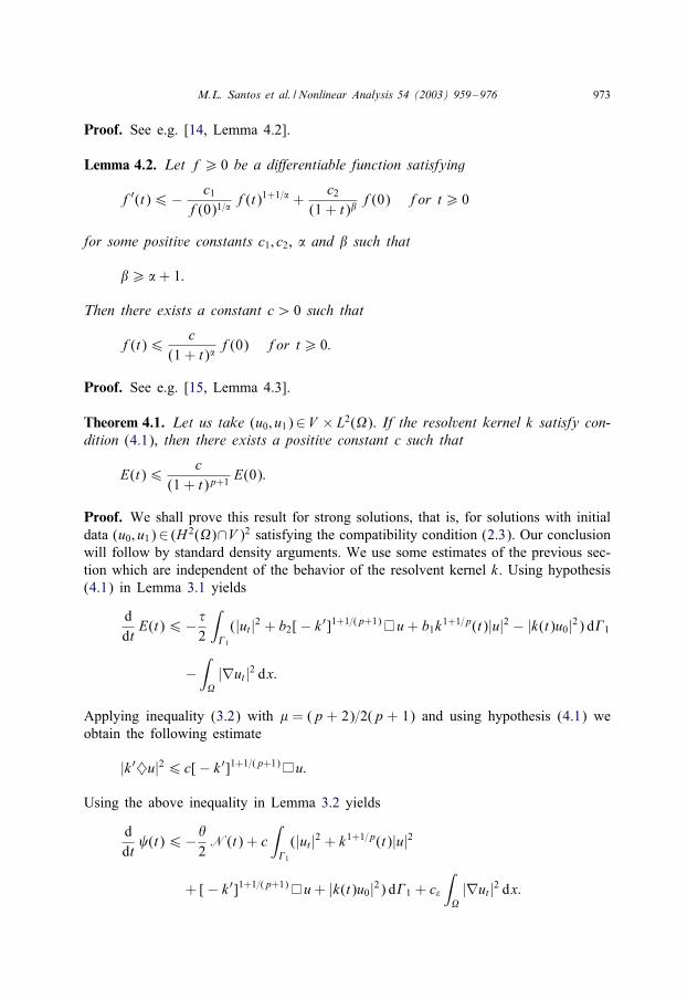
Theorem 4.1. Let us take (u0; u1)∈V × L2(). If the resolvent kernel k satisfy con-dition (4.1), then there exists a positive constant c such that

E(t)6c

(1 + t)p+1 E(0):

Proof. We shall prove this result for strong solutions, that is, for solutions with initialdata (u0; u1)∈ (H 2()∩V )2 satisfying the compatibility condition (2.3). Our conclusionwill follow by standard density arguments. We use some estimates of the previous sec-tion which are independent of the behavior of the resolvent kernel k. Using hypothesis(4.1) in Lemma 3.1 yields

ddt

E(t)6− "2

∫1

(|ut |2 + b2[− k ′]1+1=(p+1) u+ b1k1+1=p(t)|u|2 − |k(t)u0|2) d1

−∫|∇ut |2 dx:

Applying inequality (3.2) with - = (p + 2)=2(p + 1) and using hypothesis (4.1) weobtain the following estimate

|k ′♦u|26 c[− k ′]1+1=(p+1) u:

Using the above inequality in Lemma 3.2 yields

ddt

(t)6−/2N(t) + c

∫1

(|ut |2 + k1+1=p(t)|u|2

+ [− k ′]1+1=(p+1) u+ |k(t)u0|2) d1 + c$

∫|∇ut |2 dx:

974 M.L. Santos et al. / Nonlinear Analysis 54 (2003) 959–976

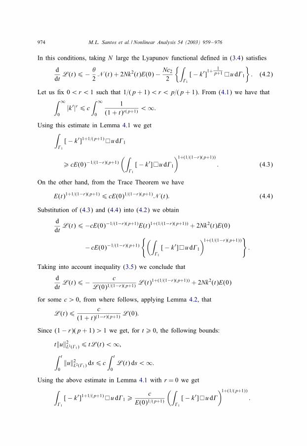
In this conditions, taking N large the Lyapunov functional deMned in (3.4) satisMes

ddt

L(t)6− /2N(t) + 2Nk2(t)E(0)− Nc2

2

∫1

[− k ′]1+1

p+1 u d1

: (4.2)

Let us Mx 0¡r¡ 1 such that 1=(p+ 1)¡r¡p=(p+ 1). From (4.1) we have that∫ ∞

0|k ′|r6 c

∫ ∞

0

1(1 + t)r(p+1) ¡∞:

Using this estimate in Lemma 4.1 we get∫1

[− k ′]1+1=(p+1) u d1

¿ cE(0)−1=(1−r)(p+1)(∫

1

[− k ′] u d1

)1+(1=(1−r)(p+1))

: (4.3)

On the other hand, from the Trace Theorem we have

E(t)1+1=(1−r)(p+1)6 cE(0)1=(1−r)(p+1)N(t): (4.4)

Substitution of (4.3) and (4.4) into (4.2) we obtain

ddt

L(t)6−cE(0)−1=(1−r)(p+1)E(t)1+(1=(1−r)(p+1)) + 2Nk2(t)E(0)

− cE(0)−1=(1−r)(p+1)

(∫1

[− k ′] u d1

)1+(1=(1−r)(p+1))

:

Taking into account inequality (3.5) we conclude that

ddt

L(t)6− cL(0)1=(1−r)(p+1) L(t)1+(1=(1−r)(p+1)) + 2Nk2(t)E(0)

for some c¿ 0, from where follows, applying Lemma 4.2, that

L(t)6c

(1 + t)(1−r)(p+1) L(0):

Since (1− r)(p+ 1)¿ 1 we get, for t¿ 0, the following bounds:

t‖u‖2L2(1)6 tL(t)¡∞;∫ t

0‖u‖2L2(1) ds6 c

∫ t

0L(t) ds¡∞:

Using the above estimate in Lemma 4.1 with r = 0 we get∫1

[− k ′]1+1=(p+1) u d1¿c

E(0)1=(p+1)

(∫1

[− k ′] u d)1+(1=(p+1))

:

M.L. Santos et al. / Nonlinear Analysis 54 (2003) 959–976 975

Using these inequality instead of (4.3) and reasoning in the same way as above weconclude that

ddt

L(t)6− cL(0)1=(p+1) L(t)1+(1=(p+1)) + 2Nk2(t)E(0):

Applying Lemma 4.2 again, we obtain

L(t)6c

(1 + t)p+1 L(0):

Finally, from (3.5) we conclude

E(t)6c

(1 + t)p+1 E(0);

which completes the present proof.

5. Final comments

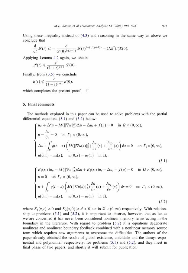
The methods explored in this paper can be used to solve problems with the partialdi'erential equations (5.1) and (5.2) below:

utt +D2u−M (‖∇u‖22)Du−Dut + f(u) = 0 in × (0;∞);

u=@u@

= 0 on 0 × (0;∞);

Du+∫ t

0g(t − s)

(M (‖∇u(s)‖22)

@u@

(s) +@ut

@(s)

)ds= 0 on 1×(0;∞);

u(0; x) = u0(x); ut(0; x) = u1(x) in ;(5.1)

K1(x; t)utt −M (‖∇u‖22)Du+ K2(x; t)ut −Dut + f(u) = 0 in × (0;∞);

u= 0 on 0 × (0;∞);

u+∫ t

0g(t − s)

(M (‖∇u(s)‖22)

@u@

(s) +@ut

@(s)

)ds= 0 on 1 × (0;∞);

u(0; x) = u0(x); ut(0; x) = u1(x) in ;(5.2)

where K1(x; t)¿ 0 and K2(x; 0)¿d¿ 0 a.e in × (0;∞) respectively. With relation-ship to problems (5.1) and (5.2), it is important to observe, however, that as far aswe are concerned it has never been considered nonlinear memory terms acting in theboundary in the literature. With regard to problem (5.2) it is equations degeneratenonlinear and nonlinear boundary feedback combined with a nonlinear memory sourceterm which requires new arguments to overcome the diTculties. The authors of thepaper already obtained the results of global existence, unicidade and the decays expo-nential and polynomial, respectively, for problems (5.1) and (5.2), and they meet inMnal phase of two papers, and shortly it will submit for publication.

976 M.L. Santos et al. / Nonlinear Analysis 54 (2003) 959–976

Now we would like to mention that problem (1.1) – (1.4) and the correspondingproblem for Eqs. (5.1) and (5.2) in a bounded domain with moving boundary areinteresting open problems.

Acknowledgements

This research was written while the second author was visiting, the Federal Uni-versity of ParSa—UFPA-Brazil, during June of 2002. He was partially supported byCNPq-BrasSilia-Brazil under grant No. 300344/92-9. The authors thank the referee ofthis paper for his valuable suggestions which improved this paper.

References

[1] P. Biler, Remark on the decay for damped string and beam equations, Nonlinear Anal. TMA 9 (1)(1984) 839–842.

[2] E.H. Brito, Nonlinear initial boundary value problems, Nonlinear Anal. TMA 11 (1) (1987) 125–137.[3] M.M. Cavalcanti, V.N. Domingos Cavalcanti, J.S. Prates, J.A. Soriano, Existence and uniform decay

rates for viscoelastic problems with nonlinear boundary damping, Di'erential Integral Equations 14 (1)(2001) 85–116.

[4] M.M. Cavalcanti, V.N. Domingos Cavalcanti, J.S. Prates, J.A. Soriano, Existence and uniform decay ofsolutions of a degenerate equation with nonlinear boundary memory source term, Nonlinear Anal. 38(1999) 281–294.

[5] R. Ikerata, On the existence of global solutions for some nonlinear hyperbolic equations with Neumannconditions, TRU Math. (1988) 1–24.

[6] R. Ikerata, A note on the global solvability of solutions to some nonlinear wave equations withdissipative terms, Di'erential Integral Equations 8 (3) (1995) 607–616.

[7] S. Jiang, J.E. Munoz Rivera, A global existence for the Dirichlet problems in nonlinear n-dimensionalviscoelasticity, Di'erential Integral Equations 9 (4) (1996) 791–810.

[8] J.L. Lions, Quelques MXethodes de resolution de problXemes aux limites non lineaires, Dunod GauthiersVillars, Paris, 1969.

[9] M.P. Matos, D.C. Pereira, On a hyperbolic equation with strong damping, Funkcial. Ekvac. 34 (1991)303–311.

[10] T. Matsuyama, R. Ikerata, On global solutions and energy decay for the wave equations of Kirchho'type with nonlinear damping terms, J. Math. Anal. Appl. 204 (1996) 729–753.

[11] K. Nishihara, Exponentially decay of solutions of some quasilinear hyperbolic equations with lineardamping, Nonlinear Anal. TMA 8 (6) (1984) 623–636.

[12] J.Y. Park, J.J. Bae, Il Hyo Jung, Uniform decay of solution for wave equation of Kirchho' type withnonlinear boundary damping and memory term, Nonlinear Anal. TMA 50 (2002) 871–884.

[13] R. Racke, Lectures on nonlinear evolution equations. Initial value problems, Aspect of MathematicsE19. Friedr. Vieweg & Sohn, Braunschweig/Wiesbaden, 1992.

[14] M.L. Santos, Asymptotic behavior of solutions to wave equations with a memory condition at theboundary, European J. Di'erential Equations 73 (2001) 1–11.

[15] M.L. Santos, Decay rates for solutions of a system of wave equations with memory, EuropeanJ. Di'erential Equations 38 (2002) 1–17.

[16] Y. Yamada, On some quasilinear wave equations with dissipative terms, Nagoya Math. J. 87 (1982)17–39.