Chapter 13

The Biogeochemistry of the Aucilla River Fauna

KATHRYN A. HOPPE1 and PAUL L. KOCH2

1 Department of Geological and Environmental Sciences, Stanford University, Stanford, CA95064, USA.2 Department of Earth Sciences, 1156 High St., University of California, Santa Cruz, SantaCruz, CA 95064, USA.

13.1 Introduction . . . . . . . . . . . . . . . . . . . . . . . . . . . . . . . . . . . . . . . . . . . . . . . . . . . . . 37913.1.1 Carbon Isotopes and Diet . . . . . . . . . . . . . . . . . . . . . . . . . . . . . . . . . . . . . 38013.1.2 Oxygen Isotopes and Environmental Variability . . . . . . . . . . . . . . . . . . . . 38113.1.3 Strontium Isotopes and Migration . . . . . . . . . . . . . . . . . . . . . . . . . . . . . . . 382

13.2 Materials and Methods . . . . . . . . . . . . . . . . . . . . . . . . . . . . . . . . . . . . . . . . . . . . . 38413.2.1 Localities . . . . . . . . . . . . . . . . . . . . . . . . . . . . . . . . . . . . . . . . . . . . . . . . . 38413.2.2 Sample Collection . . . . . . . . . . . . . . . . . . . . . . . . . . . . . . . . . . . . . . . . . . . 38513.2.3 Analytical Methods . . . . . . . . . . . . . . . . . . . . . . . . . . . . . . . . . . . . . . . . . . 385

13.3 Results . . . . . . . . . . . . . . . . . . . . . . . . . . . . . . . . . . . . . . . . . . . . . . . . . . . . . . . . . 38613.3.1 Carbon Isotopes . . . . . . . . . . . . . . . . . . . . . . . . . . . . . . . . . . . . . . . . . . . . 38613.3.2 Oxygen Isotopes . . . . . . . . . . . . . . . . . . . . . . . . . . . . . . . . . . . . . . . . . . . . 38913.3.3 Strontium Isotopes . . . . . . . . . . . . . . . . . . . . . . . . . . . . . . . . . . . . . . . . . . 390

13.4 Discussion . . . . . . . . . . . . . . . . . . . . . . . . . . . . . . . . . . . . . . . . . . . . . . . . . . . . . . 39213.4.1 Paleodiets . . . . . . . . . . . . . . . . . . . . . . . . . . . . . . . . . . . . . . . . . . . . . . . . . 39213.4.2 Oxygen Isotopes . . . . . . . . . . . . . . . . . . . . . . . . . . . . . . . . . . . . . . . . . . . . 39413.4.3 Migration Patterns . . . . . . . . . . . . . . . . . . . . . . . . . . . . . . . . . . . . . . . . . . 396

13.5 Conclusions . . . . . . . . . . . . . . . . . . . . . . . . . . . . . . . . . . . . . . . . . . . . . . . . . . . . . 39713.6 Acknowledgments . . . . . . . . . . . . . . . . . . . . . . . . . . . . . . . . . . . . . . . . . . . . . . . . 398References . . . . . . . . . . . . . . . . . . . . . . . . . . . . . . . . . . . . . . . . . . . . . . . . . . . . . . . . . . 398

13.1 Introduction

Ecosystems in the late Pleistocene differed dramatically from the ones we know today,particularly in their striking diversity and abundance of large mammals. North Americaalone supported a wide range of now globally or locally extinct taxa, including severalfamilies of proboscideans, giant ground sloths, glyptodonts, equids, camelids, and tapir,as well as surviving taxa such as deer and bison (Kurtén and Anderson, 1980).Although reconstructing fossil ecosystems is often problematic, the survival of somePleistocene species allows us to compare paleobiological reconstructions with modernobservations. We can thus assess the precision of any proxy used, which in turn allowsus to evaluate the accuracy of paleoecological reconstructions.

S. David Webb (ed.), First Floridians and Last Mastodons: The Page-Ladson Site on the Aucilla River, 379–402©2006 Springer. Printed in The Netherlands.

379

Chap13.qxd 3/13/06 4:26 PM Page 379

Accurately reconstructing the biology of extinct taxa is essential not only for assess-ing paleoecological relationships, but also for evaluating many extinction hypotheses.Historically, two opposing sets of theories have been argued to explain the Pleistoceneextinction. One set of theories blames this extinction directly on human hunters (e.g.Churcher, 1980; Martin, 1984), while the other invokes climatic and/or ecologicalchanges associated with deglaciation (e.g. Graham and Lundelius, 1984; Guthrie, 1984).More recently, it has been suggested that extinctions resulted from the combined stress ofhunting and ecological changes, some of which may have been indirectly caused by earlyhumans (Owen-Smith, 1988; Haynes, 1991; Miller et al., 1999). Researchers on all sidesof this debate frequently make complex assumptions about the biology of extinct fauna,many of which cannot be tested using traditional morphological or taphonomic methods.

The Aucilla River fauna, with its abundance of well-preserved specimens from bothlate glacial and full glacial times, provides an unprecedented opportunity to test severaltheories about the paleoecology of extinct species. We analyzed the chemistry of toothenamel from several extinct taxa, including equids, llamas, mammoths, mastodons, andtapir, as well as from deer, which have survived into the present. The stable isotoperatios of carbon (δ13C) were used to reconstruct the diets of each individual and thedegree of dietary specialization of each species. Oxygen isotope ratios (δ18O) were usedto examine climatic variability. Finally, strontium isotope ratios (87Sr/86Sr) were used toexamine the migration patterns of mammoths and mastodons.

13.1.1 Carbon Isotopes and Diet

One possible source of environmental stress for herbivores is the disruption of existingfloral communities (Graham and Lundelius, 1984; Guthrie, 1984). If extinct fauna hadrelatively restricted dietary preferences, they may have been subject to dietary stress asa result of these changes (Graham and Lundelius, 1984; King and Saunders, 1984;Miller et al., 1999). In order to evaluate this possibility, we must first reconstruct thediets of extinct animals by distinguishing between browsers (animals with diets con-sisting primarily of trees, shrubs, and/or herbs), grazers (animals with diets consistingof >90% grass), and generalized intermediate feeders. Traditionally, the diets of extinctherbivores have been reconstructed through analysis of tooth morphology and/or com-parison with modern analogs. However, such reconstructions may be misleading, espe-cially when applied to taxa that have few modern analogs, such as proboscideans orequids. For example, MacFadden et al. (1999) used δ13C values and tooth microwear toexamine the diets of several Miocene equids with high crowned teeth, which are con-ventionally associated with a grazing diet; they found that some of these equids werebrowsers or intermediate feeders. Even when analysis of tooth morphology preciselyreflects the average diet of a species, it cannot yield information about dietary differ-ences between individuals, or track short-term dietary fluctuations. We therefore usedthe δ13C values of tooth enamel to reconstruct the diets of each individual.

The δ13C value of a herbivore’s tooth enamel, which is formed of carbonatedhydroxylapatite [Ca10(PO4,CO3)6(OH,CO3)2], reflects the average δ13C value of plants

380 hoppe and koch

Chap13.qxd 3/13/06 4:26 PM Page 380

consumed during tooth formation (Ambrose and Norr, 1993). The δ13C value of eachplant in turn depends primarily on its photosynthetic pathway (O’Leary, 1981, 1988).Plants with a C3 metabolism (most trees, herbs, and cool climate grasses) have highlynegative δ13C values, which today average approximately −27 ± 3%. Plants with a C4metabolism (warm/dry climate grasses and sedges) display less negative δ13C valuesaveraging approximately −13 ± 2% (O’Leary, 1981, 1988; Koch et al., 1991). A thirdgroup of plants, which includes primarily succulents, uses CAM photosynthesis,which yields δ13C values that vary between these two extremes (Ehleringer, 1989).However, northern Florida was covered with mainly forests and prairies during theglacial (Watts et al., 1992; Watts and Hansen, 1994). Thus, only a minor percent of theflora were likely to have been CAM plants.

Since the δ13C value of tooth enamel directly reflects the average δ13C value of anherbivore’s diet, this proxy can be used to reconstruct that diet (Lee-Thorp and van derMerwe, 1987). In the wild, the δ13C values of herbivore teeth are fractionated byapproximately +13.5% relative to dietary values (Bocherens et al., 1996; Cerlinget al., 1997; Koch, 1998a). Thus, in warm/dry regions the tooth enamel of moderngrazers averages approximately 0.5%. Modern browsers typically average −13.5%,whereas mixed-feeders display intermediate values (Lee-Thorp and van der Merwe,1987, 1991; Bocherens et al., 1996; Cerling et al., 1997).

However, several additional factors must be considered when using the δ13C values ofteeth to reconstruct the detailed diet of prehistoric herbivores. For example, atmosphericδ13C values have changed with time, correlating with changes in ice volume (Marinoet al., 1992). These fluctuations result in corresponding shifts in the δ13C values of plantsand ultimately herbivores. The values of late glacial and full glacial herbivores would thusbe shifted by +0.5 to +1.1%, relative to modern animals (Koch et al., 1998).

Additionally, the δ13C values of C3 plants exhibit systematic differences among andwithin ecosystems. For example, plants from open habitats display less negative δ13Cvalues than plants from closed-canopy forests due to differences in light levels and therecycling of respired CO2 (Vogel, 1978; Medina and Minchin, 1980). The δ13C valuesof herbivores reflect these differences; van der Merwe and Medina (1991) found thatbrowsers from dense forests displayed values ~4% more negative than browsers fromopen woodlands. The δ13C values of C3 plants also vary systematically among differentlife forms (i.e. functional groups). For example, evergreen trees have δ13C values up to3% more positive than sympatric deciduous trees, which may be 2–5% more positivethan herbs growing at ground level (Medina and Minchin, 1980; Brooks et al., 1997).These differences may be reflected in the δ13C values of browsers that preferentiallyforage on different plants or at different heights in the canopy. However, such variationsare relatively small compared to the difference between C3 and C4 vegetation.

13.1.2 Oxygen Isotopes and Environmental Variability

The root causes of many ecological shifts are often thought to be changes in climaticfactors such as temperature or the evaporation/precipitation balance. The δ18O values

the biogeochemistry of the aucilla river fauna 381

Chap13.qxd 3/13/06 4:26 PM Page 381

of herbivore tooth enamel may record such climatic fluctuations; enamel δ18O valuescorrelate with the values of ingested water, which consists of drinking water and plantwater (Ayliffe et al., 1992; Bryant and Froelich, 1995). The δ18O values of thesesources often correlate with those of meteoric water. The δ18O of meteoric water, inturn, varies on both a geographic and temporal scale. In temperate and high-latituderegions, the mean δ18O value of meteoric water correlates with mean temperatures,with low δ18O values in cold regions and high values in warmer regions (Dansgaard,1964; Rozanski et al., 1993). At each location, the δ18O of meteoric water also variesseasonally, with low values in cold months and high values in warm months. Forexample, at Hatteras, NC (the best well-documented site close to Florida), the δ18O ofmodern precipitation varies by ~4.5% (Koch, 1989b).

The δ18O values of plant waters and tissues also vary regionally; plants derive theirwater from soil moisture, which tracks the δ18O values of precipitation (Förstel, 1978;DeNiro and Epstein, 1979; Saurer et al., 1997). However, plant waters may beenriched in 18O due to transpiration, with the degree of enrichment varying from ~0%,when relative humidity is high, to >20% when relative humidity is low (Förstel, 1978).Plant tissues also show a slight increase not only in δ18O values, but also in δ13C val-ues as conditions become drier (Saurer et al., 1997).

The δ18O values of tooth apatite will reflect environmental variations in the δ18Ovalues of meteoric waters and ingested plant waters. Since tooth enamel forms byaccretion without remodeling, it can record seasonal variations in the δ18O values ofwater (and the δ13C values of plants) ingested by an animal (Fricke and O’Neil, 1996;Sharp and Cerling, 1998). Isotopic variations in teeth have been used to reconstructtooth growth rates, as well as seasonal cycles in environmental δ18O values (Kochet al., 1989; Fisher and Fox, Chapter 12). Comparison of the δ18O and δ13C values ofa tooth may provide additional information; if relative humidity varied seasonally, orif an animal migrated between relatively wet and dry environments seasonally, thenδ13C values should correlate with δ18O values. Additionally, intraspecies comparisonof bulk enamel δ18O values may help identify individuals that lived under differentclimatic regimes. High variability at a site can mean either that the site is time-aver-aged (e.g. containing a mixture of glacial and interglacial individuals) or that someof the animals at the site are non-residents (Stuart-Williams et al., 1996; Koch et al.,1998).

13.1.3 Strontium Isotopes and Migration

It has been proposed that climatic changes may force animals to alter establishedmovement patterns. Changes in migratory behavior factor into many extinctionhypotheses, especially those relating to the extinction of proboscideans. For example,Churcher (1980) suggested that human hunters preyed on mammoths as they crossednatural traps during seasonal migrations of up to 2400 km one way. Additionally,Owen-Smith (1988) and Haynes (1991) proposed that climate/habitat change caused

382 hoppe and koch

Chap13.qxd 3/13/06 4:26 PM Page 382

animals to reduce their range sizes, which in turn resulted in an increased vulnerabil-ity to human hunters.

If proboscideans migrated in order to escape harsh winters and/or to exploit sea-sonally available resources (Olivier, 1982; Holman et al., 1988), then climaticchanges may have also directly contributed to their extinction. If ecological changesdisrupted migration routes, then extinction may have resulted from nutritional stresscaused by overfeeding or limited access to resources (Martin and Klein, 1984;Holman et al., 1988). Alternatively, animals may increase their range size whenstressed. For example, modern white-tailed deer usually inhabit a home range lessthan 3.2 km across, but they increase their range size to over 14 km across when envi-ronmentally stressed (Marchington and Hirth, 1984). Thus, changes in an animal’smovement patterns may correlate with environmental stresses. Reconstructing migra-tion routes and their ecological significance has been difficult because traditionaltaphonomic methods yield little information about lifetime movement patterns.However, analysis of an animal’s 87Sr/86Sr ratio may allow us to reconstruct an indi-vidual’s movements.

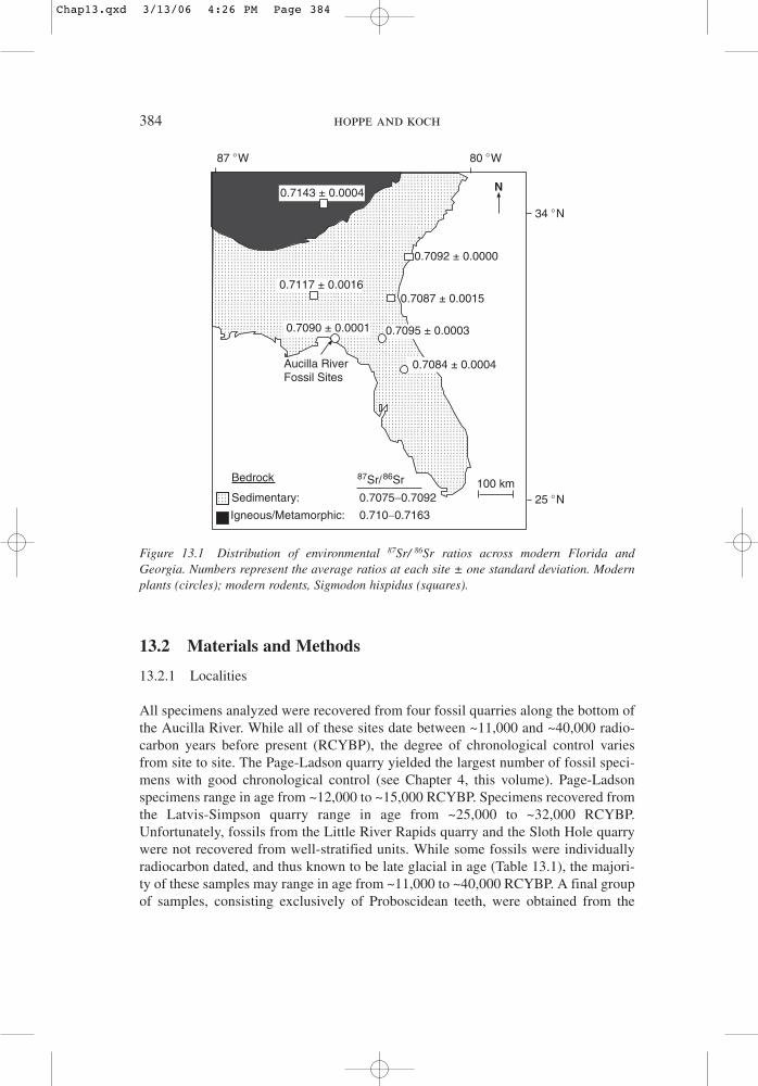
An animal’s 87Sr/86Sr ratio directly tracks the 87Sr/86Sr ratios of its environment.When environmental 87Sr/86Sr ratios vary regionally, the 87Sr/86Sr ratio of tooth enam-el may be used to reconstruct an animal’s lifetime movement patterns (Hoppe et al.,1999). The 87Sr/86Sr ratio of a local environment is a combination of the 87Sr/86Srratio of material weathered from underlying bedrock and that deposited from atmos-pheric sources (Miller et al., 1993; Chadwick et al., 1999). Florida and southernGeorgia are composed primarily of marine carbonates (Scott, 1992), which have rel-atively low 87Sr/86Sr ratios. Northern Georgia, in contrast, has bedrock composed ofigneous and metamorphic rocks, which have relatively high 87Sr/86Sr ratios.Measurements of modern plants and small rodents, both of which reflect local87Sr/86Sr ratios, reveal that environmental 87Sr/86Sr ratios in this region record pat-terns in underlying bedrock (Fig. 13.1) (Hoppe et al., 1999). Florida environmentsdisplay relatively low 87Sr/86Sr ratios of 0.7080 to 0.7095, while environments in theAppalachian Mountains, and in parts of central Georgia that are dominated by sedi-ments from the Appalachians, have higher 87Sr/86Sr ratios of 0.7110 to 0.7143(Hoppe et al., 1999). Thus, animals that migrated outside of Florida toward theAppalachian Mountains should display higher 87Sr/86Sr ratios than individuals whodid not migrate.

Additionally, comparison of microsample 87Sr/86Sr ratios and δ18O values and/orδ13O values may reveal whether an individual migrated on a consistent, seasonal basisor in a random, nomadic fashion. Since the δ18O values of tooth enamel vary season-ally, seasonal migrations should produce 87Sr/86Sr ratios that correlate strongly withδ18O values. Nomadic migrations, on the other hand, would produce no correlationbetween 87Sr/86Sr and δ18O values. Seasonal migrations might also produce a correla-tion of 87Sr/86Sr ratios with δ13C values, but such a correlation would only appear if ananimal moved between ecosystems with different plants or different plant δ13C values(Koch et al., 1995).

the biogeochemistry of the aucilla river fauna 383

Chap13.qxd 3/13/06 4:26 PM Page 383

13.2 Materials and Methods

13.2.1 Localities

All specimens analyzed were recovered from four fossil quarries along the bottom ofthe Aucilla River. While all of these sites date between ~11,000 and ~40,000 radio-carbon years before present (RCYBP), the degree of chronological control variesfrom site to site. The Page-Ladson quarry yielded the largest number of fossil speci-mens with good chronological control (see Chapter 4, this volume). Page-Ladsonspecimens range in age from ~12,000 to ~15,000 RCYBP. Specimens recovered fromthe Latvis-Simpson quarry range in age from ~25,000 to ~32,000 RCYBP.Unfortunately, fossils from the Little River Rapids quarry and the Sloth Hole quarrywere not recovered from well-stratified units. While some fossils were individuallyradiocarbon dated, and thus known to be late glacial in age (Table 13.1), the majori-ty of these samples may range in age from ~11,000 to ~40,000 RCYBP. A final groupof samples, consisting exclusively of Proboscidean teeth, were obtained from the

384 hoppe and koch

0.7087 ± 0.0015

100 kmSedimentary: 0.7075−0.7092

Aucilla RiverFossil Sites

N

Bedrock

Igneous/Metamorphic: 0.710−0.7163

87Sr/ 86Sr

0.7090 ± 0.0001

0.7084 ± 0.0004

0.7095 ± 0.0003

0.7092 ± 0.0000

0.7117 ± 0.0016

0.7143 ± 0.0004

87 �W 80 �W

25 �N

34 �N

Figure 13.1 Distribution of environmental 87Sr/ 86Sr ratios across modern Florida andGeorgia. Numbers represent the average ratios at each site ± one standard deviation. Modernplants (circles); modern rodents, Sigmodon hispidus (squares).

Chap13.qxd 3/13/06 4:26 PM Page 384

Ohmes Collection of the Florida Natural History Museum. This collection consists ofa mixture of specimens retrieved from surface deposits near the Page-Ladson andSloth Hole quarries and are believed to range in age from ~11,000 to ~40,000RCYBP.

13.2.2 Sample Collection

We analyzed bulk tooth enamel from 69 specimens collected from the Aucilla River.We sampled bulk enamel from extinct species including mammoth (Mammuthuscolumbi), mastodon (Mammut americanum), tapir (Tapirus veroensis), horse (Equussp.), and llama (Palaeolama mirifica and Hemiauchenia macrocephala), as well asfrom white-tailed deer (Odocoileus virginianus), which survive into modern times.These bulk samples reflect the average isotopic composition of each tooth (Koch et al.,1998). We also microsampled one mastodon and one mammoth molar to examine atime series of isotopic variations across approximately two years and one year ofgrowth, respectively. Microsamples were milled from petrographic thin sections usinga Lohmann Computerized Microsampler. Each mastodon microsample was collectedfrom a groove (~0.15 mm deep, ~0.12 mm wide, and ~5.0 mm long) milled parallelto growth increments, although some of these samples had to be combined to obtainenough material for analysis of carbon and oxygen isotope ratios. Mammothmicrosamples were also collected from grooves (~0.17 mm deep, ~0.06 mm wide, and~5.0–15.0 mm long) milled parallel to growth increments.

13.2.3 Analytical Methods

Carbon and oxygen samples were prepared according to the methods described inKoch et al. (1998), then analyzed on a VG Optima or a Prism gas source mass spec-trometer with an ISOCARB automated carbonate system. Dissolution of sampleswas achieved by reaction in a constantly stirred bath of 100% phosphoric acid at90°C. Reaction time for each sample was greater than 5 min. Precision for analysisof calcite standards was ≤0.2% for δ13C and δ18O. Replicate analysis of enamel sam-ples (n = 23) differed by 0.12 ± 0.10% (mean ± 1σ) for carbon and 0.14 ± 0.12% foroxygen.

Strontium samples were prepared for analysis according to methods described inHoppe et al. (1999) and measured on either a VG 354 or a VG 354-S thermal ioniza-tion mass spectrometer. All measurements are referenced to a value of 87Sr/86Sr =0.71025 for the NBS 987 Sr standard and are precise to within ±0.00005.

Data were analyzed statistically with an F-test to confirm that there were no sig-nificant differences in the variance of values for each species. We then used one-wayanalysis of variance (ANOVA) to examine significant differences among mean valuesfor each species. Finally, we used Scheffé’s test to identify the sources of significantdifference among mean values (Norman and Streiner, 1992).

the biogeochemistry of the aucilla river fauna 385

Chap13.qxd 3/13/06 4:26 PM Page 385

13.3 Results

13.3.1 Carbon Isotopes

Because temporal changes in δ13C values of the atmosphere could cause fluctuationsbetween the δ13C values of animals consuming the same diet, we focused primarily oncomparison among specimens that were known to be of approximately the same age.The largest group of fossils were late glacial, ~12,000–15,000 RCYBP (Table 13.1).The second group of fossils was full glacial in age (~25,000–32,000 RCYBP). Thefinal group of specimens, which consists almost entirely of proboscideans, ranges inage from ~11,000 to ~40,000 RCYBP.

386 hoppe and koch

Table 13.1 Isotopic ratios of bulk tooth enamel samples

Age Site1 Sample Taxon δ13C2 δ18O2 87Sr/ 86Sr3

12–15KPL 92513 Tapirus –12.0 27.2 0.7087PL 92568 Tapirus –11.3 26.3 0.7087LRR 180216 Tapirus –13.5 29.3LRR 200680 Tapirus –11.4 29.7PL 92522 Odocoileus –11.5 26.2 0.7097PL 92563 Odocoileus –13.3 28.7 0.7086PL 147359 Odocoileus –15.9 30.6 0.7092PL 147362 Odocoileus –14.1 28.7 0.7092PL 147364 Odocoileus –13.6 29.9 0.7094PL 147365 Odocoileus –14.6 29.1 0.7087PL 150249 Odocoileus –13.0 28.0 0.7087PL 150470 Odocoileus –13.8 28.6 0.7108PL 151916 Odocoileus –14.7 28.4 0.7087PL 151917 Odocoileus –14.2 32.1 0.7091PL 151941 Odocoileus –10.9 31.7 0.7093PL 151942 Odocoileus –13.8 27.8 0.7089PL 146914 Hemiauchenia –12.8 32.5PL 92512 Palaeolama –12.4 32.5PL 180214 Palaeolama –14.9 32.0PL 148670 Equus –5.6 29.5PL 14780 Mammuthus 0.5 31.1 0.7089LRR 200655 Mammuthus 0.5 33.5 0.7095PL 103505 Mammut –10.0 29.2 0.7099PL 130570 Mammut –12.2 30.2 0.7101PL 147400 Mammut –10.7 30.1PL 148668 Mammut –11.0 28.8 0.7114PL 148669 Mammut –10.3 29.8 0.7101PL 150775 Mammut –11.9 30.2 0.7101PL 192224 Mammut –9.8 30.7 0.7097PL 192226 Mammut –10.3 31.4 0.7112SH 200681 Mammut –11.6 29.1

16K 3B 14779 Mammuthus –0.2 30.6 0.709525–32K

LS 200673 Equus –4.7 31.9

Chap13.qxd 3/13/06 4:26 PM Page 386

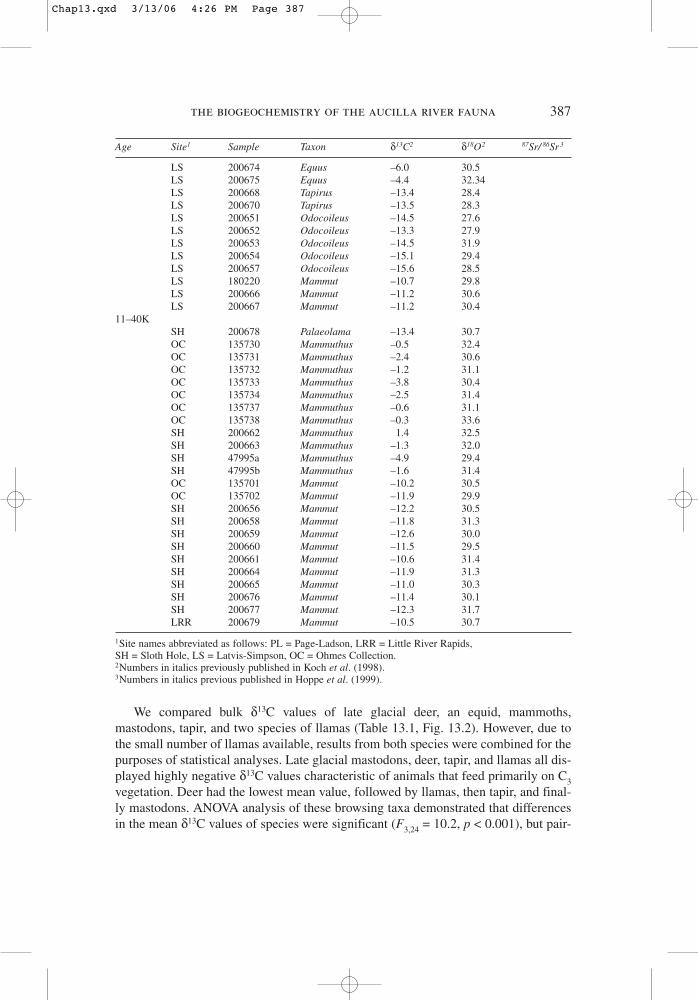
We compared bulk δ13C values of late glacial deer, an equid, mammoths,mastodons, tapir, and two species of llamas (Table 13.1, Fig. 13.2). However, due tothe small number of llamas available, results from both species were combined for thepurposes of statistical analyses. Late glacial mastodons, deer, tapir, and llamas all dis-played highly negative δ13C values characteristic of animals that feed primarily on C3vegetation. Deer had the lowest mean value, followed by llamas, then tapir, and final-ly mastodons. ANOVA analysis of these browsing taxa demonstrated that differencesin the mean δ13C values of species were significant (F3,24 = 10.2, p < 0.001), but pair-

the biogeochemistry of the aucilla river fauna 387

Age Site1 Sample Taxon δ13C2 δ18O2 87Sr/ 86Sr3

LS 200674 Equus –6.0 30.5LS 200675 Equus –4.4 32.34LS 200668 Tapirus –13.4 28.4LS 200670 Tapirus –13.5 28.3LS 200651 Odocoileus –14.5 27.6LS 200652 Odocoileus –13.3 27.9LS 200653 Odocoileus –14.5 31.9LS 200654 Odocoileus –15.1 29.4LS 200657 Odocoileus –15.6 28.5LS 180220 Mammut –10.7 29.8LS 200666 Mammut –11.2 30.6LS 200667 Mammut –11.2 30.4

11–40KSH 200678 Palaeolama –13.4 30.7OC 135730 Mammuthus –0.5 32.4OC 135731 Mammuthus –2.4 30.6OC 135732 Mammuthus –1.2 31.1OC 135733 Mammuthus –3.8 30.4OC 135734 Mammuthus –2.5 31.4OC 135737 Mammuthus –0.6 31.1OC 135738 Mammuthus –0.3 33.6SH 200662 Mammuthus 1.4 32.5SH 200663 Mammuthus –1.3 32.0SH 47995a Mammuthus –4.9 29.4SH 47995b Mammuthus –1.6 31.4OC 135701 Mammut –10.2 30.5OC 135702 Mammut –11.9 29.9SH 200656 Mammut –12.2 30.5SH 200658 Mammut –11.8 31.3SH 200659 Mammut –12.6 30.0SH 200660 Mammut –11.5 29.5SH 200661 Mammut –10.6 31.4SH 200664 Mammut –11.9 31.3SH 200665 Mammut –11.0 30.3SH 200676 Mammut –11.4 30.1SH 200677 Mammut –12.3 31.7LRR 200679 Mammut –10.5 30.7

1Site names abbreviated as follows: PL = Page-Ladson, LRR = Little River Rapids,SH = Sloth Hole, LS = Latvis-Simpson, OC = Ohmes Collection.2Numbers in italics previously published in Koch et al. (1998).3Numbers in italics previous published in Hoppe et al. (1999).

Chap13.qxd 3/13/06 4:26 PM Page 387

wise comparisons indicated that the only significant differences were betweenmastodons and deer and mastodons and llamas (Scheffé’s test, p < 0.05). Pair-wisecomparisons of the variance of δ13C values for each species revealed no significant dif-ferences (F-test, p > 0.05). Both mammoths and the equid displayed δ13C values thatwere significantly higher than the values of other animals (F5,25 = 59.4, p = 0.0001).Mammoths displayed the most positive δ13C values, which were indicative of a dietconsisting almost exclusively of C4 grasses. The equid displayed a δ13C value indica-tive of a mixed-diet consisting of both C3 and C4 vegetation.

Fewer individuals from full glacial times (~25,000–32,000 RCYBP) were avail-able for study; however, similar patterns were observed for all taxa present (Table13.1, Fig. 13.2). No significant differences in variance were found among species(F-test, p < 0.05). Once again deer had the most negative mean δ13C values, followedby tapir, mastodons, and then equids. Differences among mean values for browsingtaxa were significant (F2,7 = 26.7, p < 0.001). Mean values for mastodons were sig-nificantly different from values for both deer and tapir (Scheffé’s test, p < 0.05), butmean values for deer and tapir were not significantly different from one another(Scheffé’s test, p > 0.05). No mammoths were available for from this time period, butthe equids displayed δ13C values that were significantly different from all other taxa(F3,9 = 118.9, p = 0.0001) and are intermediate between values expected for a pure C3browser and a C4 grazer (Fig. 13.2).

388 hoppe and koch

123456 ~12−40 K

123456 Full Glacial

−15 −13 −11 −9 −7 −5 −3 −1 1

Late Glacial

123456

−15 −13 −11 −9 −7 −5 −3 −1 1

δ13C

Figure 13.2 Histograms of bulk d 13C values (PDB) of tooth enamel of species during eachtime slice: Mastodons; mammoths; deer; tapir; camelids; equids.

Chap13.qxd 3/13/06 4:26 PM Page 388

The final group of specimens, which range from full glacial to late glacial in age,consisted of proboscideans and one llama (Table 13.1, Fig. 13.2). The llama andmastodons displayed negative δ13C values indicative of animals that fed only on C3 veg-etation. The δ13C value of the llama was more negative than any values displayed bymastodons. Mammoths displayed mean δ13C values indicative of animals that fed pri-marily on C4 vegetation mixed with the consumption of some C3 vegetation (Fig. 13.2).

The patterns observed between the δ13C values of each taxon appear to remain con-sistent with time. We tested for temporal changes by comparing the δ13C values ofdeer, equids, mastodons, and tapir between full and late glacial times. None of thesetaxa displayed significant temporal differences in either mean values or variance (p >0.05). While no mammoths or llama definitively full glacial in age were available foranalysis, we compared mammoths and llama of indeterminate age with their late gla-cial counterparts. Differences in mean values were not significant (p > 0.5), but lateglacial mammoths did have significantly lower variance than the mammoths of inde-terminate age (F-test, p < 0.05). This may be an artifact of the small sample size (n =2) of late glacial mammoths or a real difference among individual mammoths.Mastodons of indeterminate age were not significantly different from either their lateglacial or full glacial counterparts (F2,20 = 0.36, p > 0.5; F-test, p > 0.5).

In addition to examining bulk samples, we also analyzed microsamples from onelate glacial mastodon and one mammoth (~15,910 ± 160 RCYBP). The δ13C values ofmicrosamples displayed less variation than the range of values for bulk samples of thecorresponding species (Table 13.1, Fig. 13.3). The mastodon microsamples were rel-atively negative, ranging from −9.8% to −11.3%, while mammoth microsamples weremore positive, ranging from −0.4% to −1.6%. Variations between high and low δ13Cvalues were not obviously cyclic in either animal.

13.3.2 Oxygen Isotopes

Since an animal’s δ18O values change as environmental conditions vary, we again con-ducted interspecies comparisons only on individuals of approximately the same age.Samples were divided into time slices as discussed above. However, statistical analy-sis revealed few significant differences among species, perhaps due to the relativelyhigh intraspecies variability (Fig. 13.4). For example, late glacial individuals displayrelatively high intraspecies variability (>2%) for all taxa except llamas (range = 0.5%).Only differences between the mean value of llamas and tapir were significant (F5,25 =5.1, p < 0.05; Scheffé’s test, p < 0.05), although the difference in the mean values ofllama and deer was almost significant (Scheffé’s test, p = 0.05). No llama specimensknown to be full glacial in age were available to test whether this pattern was robust.However, mean δ18O values for species with numerous individuals from both the fullglacial and the late glacial display remarkably little difference. Deer, tapir, andmastodons displayed less than 0.5% difference in mean values, while the late glacialequid was ~1% lower than any of its full glacial counterparts. None of these differ-ences was significant (p < 0.05).

the biogeochemistry of the aucilla river fauna 389

Chap13.qxd 3/13/06 4:26 PM Page 389

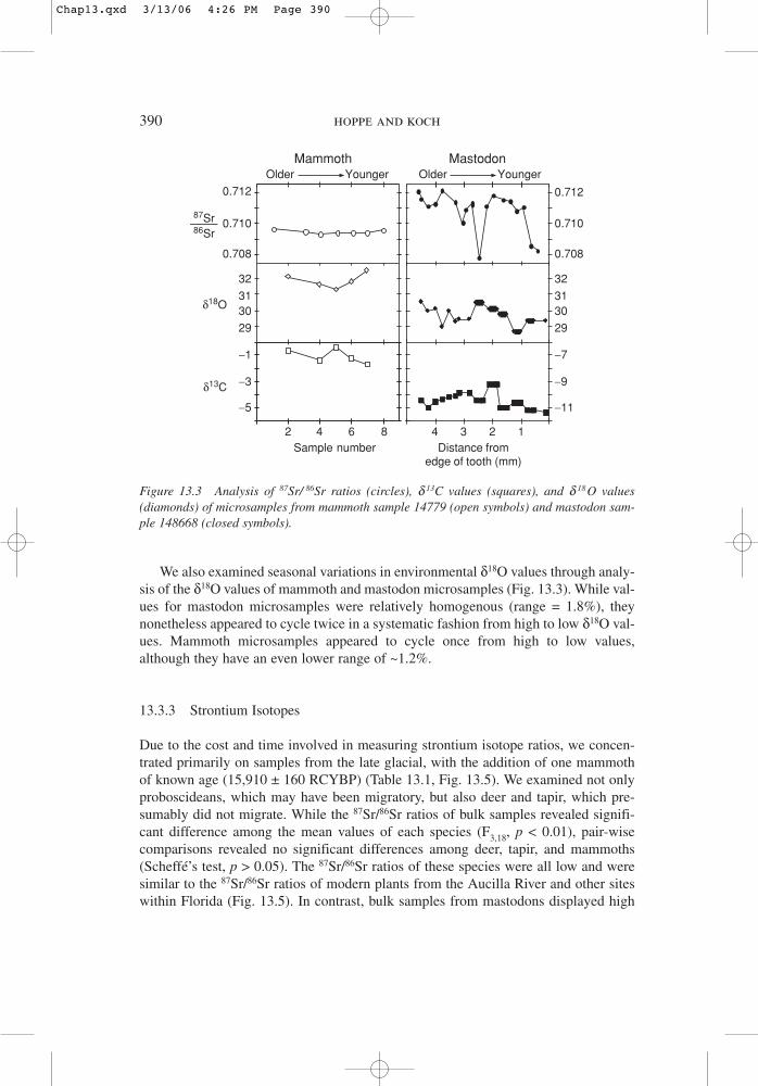
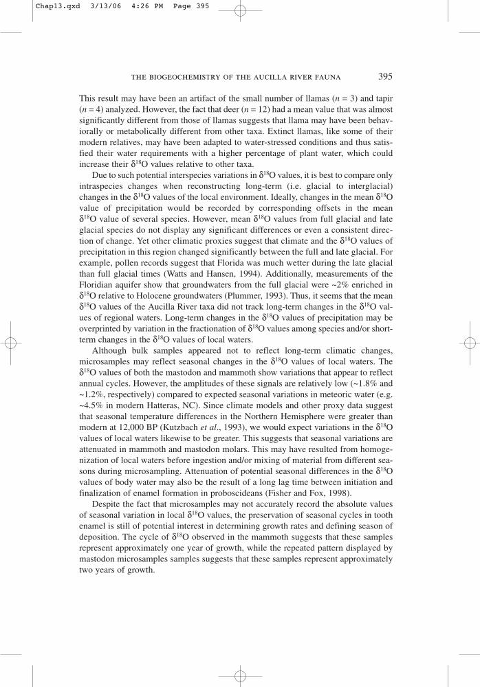
We also examined seasonal variations in environmental δ18O values through analy-sis of the δ18O values of mammoth and mastodon microsamples (Fig. 13.3). While val-ues for mastodon microsamples were relatively homogenous (range = 1.8%), theynonetheless appeared to cycle twice in a systematic fashion from high to low δ18O val-ues. Mammoth microsamples appeared to cycle once from high to low values,although they have an even lower range of ~1.2%.

13.3.3 Strontium Isotopes

Due to the cost and time involved in measuring strontium isotope ratios, we concen-trated primarily on samples from the late glacial, with the addition of one mammothof known age (15,910 ± 160 RCYBP) (Table 13.1, Fig. 13.5). We examined not onlyproboscideans, which may have been migratory, but also deer and tapir, which pre-sumably did not migrate. While the 87Sr/86Sr ratios of bulk samples revealed signifi-cant difference among the mean values of each species (F3,18, p < 0.01), pair-wisecomparisons revealed no significant differences among deer, tapir, and mammoths(Scheffé’s test, p > 0.05). The 87Sr/86Sr ratios of these species were all low and weresimilar to the 87Sr/86Sr ratios of modern plants from the Aucilla River and other siteswithin Florida (Fig. 13.5). In contrast, bulk samples from mastodons displayed high

390 hoppe and koch

Older Younger

29

3031

32

0.710

0.708

0.712

0.710

0.708

0.712

−11

−9

−7

δ18O

δ13C

29

3031

32

86Sr

87Sr

2 4 86 1234Distance from

edge of tooth (mm)

Mastodon

Sample number

Older YoungerMammoth

−5

−3

−1

Figure 13.3 Analysis of 87Sr/ 86Sr ratios (circles), d 13C values (squares), and d 18O values(diamonds) of microsamples from mammoth sample 14779 (open symbols) and mastodon sam-ple 148668 (closed symbols).

Chap13.qxd 3/13/06 4:26 PM Page 390

the biogeochemistry of the aucilla river fauna 391

26 28 30 32 34

2

4

6

8Late Glacial

~12−40 K

2

4

6

8

2

4

6

8Full Glacial

26 28 30 32 34δ18O

Figure 13.4 Histograms of bulk d 18O values (SMOW) of tooth enamel of species during eachtime slice; Mastodons; mammoths; deer; tapir; camelids; equids.

Floridaplants

0.708

0.709

0.710

0.711

0.712

87Sr86Sr

Deer Mammoth Tapir Mastodon

Figure 13.5 Average 87Sr/86Sr ratios of bulk samples from mastodons (circle), mammoths(square), deer (up-pointing triangle), and tapir (down-pointing triangle). Lines representcalculated ± 1 standard deviation from average values for each species with over threeindividuals, or the range of sample values when only two individuals were available.

Chap13.qxd 3/13/06 4:26 PM Page 391

87Sr/86Sr ratios that were significantly different from the mean values of residentspecies (Scheffé’s test, p < 0.05) and were higher than the highest value observed forFlorida plants. Mastodon microsamples displayed values (0.7078–0.7121) thatexceeded the range of values observed in all bulk samples (Fig. 13.3). Microsample87Sr/86Sr ratios varied systematically and repeatedly from high to low values. In con-trast, mammoth microsamples displayed uniformly low 87Sr/86Sr ratios with a homo-geneous distribution (0.7094–0.7096) and no obvious cycles.

13.4 Discussion

13.4.1 Paleodiets

Most of the Aucilla River mammals examined here appear to have been browsers;the highly negative δ13C values of deer, llamas, tapir, and mastodon indicate that theseanimals consumed C3 vegetation. Although a diet of C3 grasses will also produce sim-ilarly negative δ13C values, it seems unlikely that such grasses composed a significantpart of these animals’ diets. The positive δ13C values displayed by mammoths demon-strate that C4 grasses were abundant in this region, at least during late glacial times.

The accuracy of our dietary reconstruction can be easily confirmed for white-taileddeer. Modern observations show that white-tailed deer are indeed primarily browsers(Krausman and Ables, 1981). While corroborating evidence on the diets of extinct ani-mals is less direct, it nonetheless also supports our interpretations. For example, obser-vations of Tapirus indicus, which is closely related to extinct the Tapirus veroensis,have shown that modern tapir are primarily browsers (Williams and Petrides, 1980).While this analogy supports our reconstruction of the diets of Tapirus veroensis, it isbest to compare individuals from several sites when attempting to reconstruct thedietary range of a species. Comparison of our results with previous measurements oftapir from Pleistocene sites across Florida (MacFadden and Cerling, 1996; Koch et al.,1998) revealed that all individuals displayed similar, extremely negative values. Ittherefore seems likely that all Pleistocene tapir, like their modern relatives, were spe-cialized browsers.

A more unusual source provides confirmation of the diets of mastodons. Depositsof mastodon digesta from Page-Ladson also suggest that mastodons consumed prima-rily browse (Webb et al., 1992). Analysis of digesta may also reveal why the meanδ13C values of mastodons were significantly more positive (by ~1–3%) than the val-ues displayed by other browsing taxa. Such a difference could potentially result fromseveral factors; mastodons may have preferentially foraged in different habitats, con-sumed vegetation from a higher level in the canopy, and/or their diet may have con-sisted of up to 20% C4 plants (Koch et al., 1998). However, digesta deposits suggestanother explanation. They consisted primarily of C3 vegetation, and evergreen treeswere the most abundant component identified (Webb et al., 1992). If mastodons pref-erentially consumed evergreen foliage, as has been suggested by others (e.g. King and

392 hoppe and koch

Chap13.qxd 3/13/06 4:26 PM Page 392

Saunders, 1984), then their δ13C values would have been more positive than values ofsympatric browsers that consumed deciduous vegetation. Analyses of microsamplesprovide additional insight into mastodon diets. Modern elephants have been observedto switch seasonally between grazing and browsing as the nutritional content of grass-es changes (Sikes, 1971). If mastodons indeed supplemented a diet of browse withsome C4 grasses, then they would have likely done so on a seasonal basis. Such behav-ior would produce seasonal variations in the δ13C values of a tooth. However, the δ13Cvalues of mastodon microsamples revealed little variation and no apparent cycles, sug-gesting that mastodon diets did not vary in a set seasonal pattern.

Reconstructing the diets of the two Aucilla River llama species, Palaeolama andHemiauchenia, was less straightforward. Although δ13C values suggested that allAucilla River llamas consumed C3 vegetation, observations have shown that their clos-est living relatives (animals in the genus Lama) are grazers or mixed-feeders (Nowak,1991). However, analyses of premaxillary dimensions suggest that Palaeolama andHemiauchenia were browsers or intermediate feeders (Dompierre and Churcher,1996). Geochemical analyses of Hemiauchenia have been scarce. The isotopic signa-ture of one individual from Florida yielded a positive δ13C value indicative of a C4grazer in the previous study by MacFadden and Cerling (1996), in contrast to the high-ly negative value displayed by the individual analyzed in this study. A fuller range ofsamples was analyzed by Feranec and MacFadden (2000). The wider range of δ13Cvalues resulting from their study suggests that Hemiauchenia may have been a gener-alized feeder, but progressively through the Plio-Pleistocene switched from morebrowse to feeding more on grass.

Palaeolama has been more extensively studied. Not only were we able to analyzeseveral individuals, but the taxon has also been examined from sites in Bolivia(MacFadden and Cerling, 1996) and Texas (Koch, 1998). All individuals of this taxondisplay highly negative δ13C values, despite the regional abundance of C4 grasses. Thissuggests that all these Palaeolama were indeed specialized browsers as also suggest-ed by Webb and Stehli’s (1995) functional analysis of the incisors and cheek teeth.

In contrast to the majority of animals recovered from the Aucilla River, mam-moths and equids appear to have consumed a high proportion of C4 foliage.Mammoths display the most positive δ13C values; indeed, we can calculate that indi-viduals from the late glacial consumed >90% C4 vegetation (Koch et al., 1998).Calculations of the amount of C4 vegetation consumed by the other mammoths ana-lyzed are less precise because their ages are not well known and thus corrections forthe exact δ13C value of atmospheric CO2 cannot be precise (Koch et al., 1998).Nonetheless, we estimate that the majority of mammoths consumed at least ~80% C4vegetation, although one individual appears to have consumed only ~54–58% C4 veg-etation. The observed variations may reflect increased consumption of either browseor C3 grasses, which increase proportionally as climatic conditions become cooler orwetter (Teeri and Stowe, 1976). The lack of chronological control makes it difficultto distinguish between these two possibilities. However, analysis of mammothmicrosamples confirms that dietary δ13C values of an individual mammoth were rel-atively homogenous over the course of a year. Thus, the observed variations in the

the biogeochemistry of the aucilla river fauna 393

Chap13.qxd 3/13/06 4:26 PM Page 393

bulk δ13C value of mammoths do not appear to reflect seasonal shift in diets toinclude more browse. Additionally, previous analyses of mammoths from across thesouthwest suggest that mammoths were primarily grazers, as their δ13C values corre-late with shifts in the percentage of C3 versus C4 grasses (Connin et al., 1998). Ittherefore seems likely that the range of δ13C values displayed by the Aucilla Rivermammoths reflects temporal changes in the local abundance of C3 versus C4 grasses.

Although equids also display δ13C values that suggest consumption of C4 grasses,they appear to have also consumed ~40–60% C3 vegetation. While this vegetation mayhave been either C3 browse or grass, the positive δ13C values of mammoths suggestthat C4 grass composed ≥90% of the regional grass biomass during the late glacial. Ittherefore seems unlikely that diet of late glacial equids consisted of ≥40% C3 grass.Additionally, previous analyses of equids have revealed a wide range of δ13C valueseven when C4 grass was regionally abundant (Connin et al., 1998; Koch, 1998). Thissuggests that Pleistocene equids were mixed-feeders that consumed both grass and C3browse.

Overall the Aucilla River fauna appears to have contained animals that employeda variety of dietary strategies. Some species were specialists, primarily consumingeither C3 browse (i.e. deer, mastodons, tapir, and Palaeolama) or C4 grass (i.e. mam-moths). Other taxa may have been generalists (i.e. equids and Hemiauchenia). Whilesome specialized feeders may have been nutritionally stressed by change in the localflora, it seems unlikely that all members of the Aucilla River fauna would experiencedietary stress during the same floral reorganization. Additionally, the δ13C values ofbrowsers remain constant between the full and late glacial, suggesting that these taxaconsumed the same diets during both time periods. It therefore seems unlikely thatdietary stress played a significant role in the extinction of browsing species. However,additional work is needed to constrain the ages of the mammoths sampled in order todetermine whether the same trend holds true for animals that consumed a large per-centage of grass.

13.4.2 Oxygen Isotopes

The bulk δ18O values of the Aucilla River fauna yielded few distinct patterns; the vari-ation displayed within each species was generally greater than that displayed amongspecies. Although the δ18O values of animals often correlate with the values of localmeteoric waters (Ayliffe et al., 1992; Bryant and Froelich, 1995; Bryant et al., 1996),other factors likely influenced the δ18O values displayed by taxa from Aucilla River.For example, animals could display different δ18O values depending on their bodymass, their reliance on ingested plant water, and/or the type of plants in their diet(Förstel, 1978; Sternberg et al., 1984; Bryant and Froelich, 1995). Additionally, mostindividuals recovered were time-averaged over several thousand years, at least. Thus,the δ18O values of the waters ingested by each individual may have varied with cli-matic fluctuations. Given these potential sources of variation, it is perhaps surprisingthat a significant difference in mean δ18O values was found between llamas and tapir.

394 hoppe and koch

Chap13.qxd 3/13/06 4:26 PM Page 394

This result may have been an artifact of the small number of llamas (n = 3) and tapir(n = 4) analyzed. However, the fact that deer (n = 12) had a mean value that was almostsignificantly different from those of llamas suggests that llama may have been behav-iorally or metabolically different from other taxa. Extinct llamas, like some of theirmodern relatives, may have been adapted to water-stressed conditions and thus satis-fied their water requirements with a higher percentage of plant water, which couldincrease their δ18O values relative to other taxa.

Due to such potential interspecies variations in δ18O values, it is best to compare onlyintraspecies changes when reconstructing long-term (i.e. glacial to interglacial)changes in the δ18O values of the local environment. Ideally, changes in the mean δ18Ovalue of precipitation would be recorded by corresponding offsets in the meanδ18O value of several species. However, mean δ18O values from full glacial and lateglacial species do not display any significant differences or even a consistent direc-tion of change. Yet other climatic proxies suggest that climate and the δ18O values ofprecipitation in this region changed significantly between the full and late glacial. Forexample, pollen records suggest that Florida was much wetter during the late glacialthan full glacial times (Watts and Hansen, 1994). Additionally, measurements of theFloridian aquifer show that groundwaters from the full glacial were ~2% enriched inδ18O relative to Holocene groundwaters (Plummer, 1993). Thus, it seems that the meanδ18O values of the Aucilla River taxa did not track long-term changes in the δ18O val-ues of regional waters. Long-term changes in the δ18O values of precipitation may beoverprinted by variation in the fractionation of δ18O values among species and/or short-term changes in the δ18O values of local waters.

Although bulk samples appeared not to reflect long-term climatic changes,microsamples may reflect seasonal changes in the δ18O values of local waters. Theδ18O values of both the mastodon and mammoth show variations that appear to reflectannual cycles. However, the amplitudes of these signals are relatively low (~1.8% and~1.2%, respectively) compared to expected seasonal variations in meteoric water (e.g.~4.5% in modern Hatteras, NC). Since climate models and other proxy data suggestthat seasonal temperature differences in the Northern Hemisphere were greater thanmodern at 12,000 BP (Kutzbach et al., 1993), we would expect variations in the δ18Ovalues of local waters likewise to be greater. This suggests that seasonal variations areattenuated in mammoth and mastodon molars. This may have resulted from homoge-nization of local waters before ingestion and/or mixing of material from different sea-sons during microsampling. Attenuation of potential seasonal differences in the δ18Ovalues of body water may also be the result of a long lag time between initiation andfinalization of enamel formation in proboscideans (Fisher and Fox, 1998).

Despite the fact that microsamples may not accurately record the absolute valuesof seasonal variation in local δ18O values, the preservation of seasonal cycles in toothenamel is still of potential interest in determining growth rates and defining season ofdeposition. The cycle of δ18O observed in the mammoth suggests that these samplesrepresent approximately one year of growth, while the repeated pattern displayed bymastodon microsamples samples suggests that these samples represent approximatelytwo years of growth.

the biogeochemistry of the aucilla river fauna 395

Chap13.qxd 3/13/06 4:26 PM Page 395

13.4.3 Migration Patterns

Most animals restrict their lifetime movements to a limited area, or home range,although they may also disperse in a permanent one-way move to a new home range.However, some animals move repeatedly throughout life. Movements that are repeatedin the same pattern each year are defined as seasonal migrations, while movementsthat occur in a less regular fashion are defined as nomadic migrations. Bulk samplesof strontium isotopes can be used to identify animals that moved outside of a localarea, but may not distinguish between different migration patterns. Analysis ofmicrosamples allows more precise reconstruction of the timing and extent of move-ment. We presented a more detailed discussion of the implications of 87SR/86SR ratiosin animals from the Aucilla River in Hoppe et al. (1999). Here we present a summaryof that work and incorporate the results of several additional measurements.

Predictions regarding the range size of the smaller taxa can be made based ondirect observations of modern deer and tapir, both of which typically range over anarea less than 10 km in diameter (Williams, 1979; Marchington and Hirth, 1984). Wewould thus expect Pleistocene deer and tapir to range only locally, and indeed the rel-atively low 87Sr/86Sr ratios measured for deer and tapir confirm that the majority ofthese individuals did not range outside of the Florida region.

More surprisingly, mammoths also display low 87Sr/86Sr ratios, suggesting thatthey stayed within the Florida region. Because the coastal plain environments have arelatively uniform distribution of 87Sr/86Sr ratios, mammoths may have moved largedistances (250 or 500 km) without encountering high environmental 87Sr/86Sr ratios.However, microsamples from one mammoth display much less variability than isfound within local Florida environments. It thus appears that this individual, at least,did not move large distances.

In contrast, the elevated 87Sr/86Sr ratios of mastodons suggest that they did migrateoutside of Florida. They would have had to travel north ~250 km to reach environ-ments with high 87Sr/86Sr in the Appalachian Mountains. However, if mastodons trav-eled along the flood plains of rivers that drained the mountains, then they may havereached environments with higher 87Sr/86Sr ratios at distances of only ~120 km fromthe Aucilla River. The high variability of 87Sr/86Sr ratios in microsamples from thePage-Ladson mastodon confirms the mobility of this individual. The low ratios in thistooth match the ratios of marine carbonates and the high ratios match those ofAppalachian bedrocks, suggesting that this animal moved repeatedly between thecoastal plain and the Appalachian Mountains.

Modern herbivores in mountainous regions often migrate seasonally from loweraltitude winter ranges to higher altitude summer ranges, in response to changes in tem-perature and snow cover (Dingle, 1996). However, in mastodon microsamples, low87Sr/86Sr ratios correlate with high δ18O values, suggesting that this individual inhab-ited the low-lying coastal plains during at least one summer and northern regions dur-ing the winter season. Seasonally significant plant remains within mastodon digesta atPage-Ladson likewise suggest that mastodons inhabited this region of Florida duringthe summer and early fall seasons (Webb et al., 1992 and Chapter 10 by Newsom and

396 hoppe and koch

Chap13.qxd 3/13/06 4:26 PM Page 396

Mihlbachler). Thus mastodons probably moved south in response to other factorsbesides cold temperature or deep snows. They may have instead moved in response tosummer drought or other critical resource needs. Additionally, the variability of bulk87Sr/86Sr ratios demonstrates that migration patterns differed between individualmastodons. This suggests that mastodons, like modern elephants (Eltringham, 1982),were not obligate seasonal migrants, but rather moved in a more nomadic fashion.However, as the Page-Ladson site represents at least several hundred years of deposi-tion, the issue remains unresolved without further analysis of larger samples. It is quitepossible that these mastodon populations migrated regularly on a seasonal basis. Theobserved variability in 87Sr/86Sr ratios among individuals may simply reflect theresponse of the local populations to century-scale climatic fluctuations.

We attributed the surprising differences in movement patterns between mammothsand mastodons to their fundamentally different dietary preferences (Hoppe et al.,1999). During the late Pleistocene, southern Florida contained more open scrub andprairie habitat, whereas forests predominated in northern Florida and Georgia (Wattsand Hansen, 1994). Thus, it is likely that the grazing mammoths preferentially foragedin the more open southern habitats, while the browsing mastodons foraged primarilyin the forested habitats to the north.

13.5 Conclusions

This study uses several isotopic proxies to reconstruct the paleobiology of extinctspecies and test whether the taxa affected by the Pleistocene extinction shared com-mon paleobiological attributes. Overall we found that extinct taxa appear to be morenotable for their differences than their similarities. If climatically induced dietarystress contributed to the extinction of these taxa, then we would expect that extincttaxa would have more specialized diets than surviving taxa. Our results suggest thatthe reverse was true: extinct taxa include not only specialized browsers and grazers,but also generalized intermediate feeders. Additionally the δ13C value of extinct taxaremained constant over time, suggesting that these animals did not dramaticallychange their dietary habits from full to late glacial times.

The δ18O values of tooth enamel also displayed relatively little change between fulland late glacial times. However, this is likely an artifact of the large variability dis-played within each species. The fact that no consistent trend appears in the δ18O val-ues of each species suggests that samples from the Aucilla River fauna did not tracklocal variation in meteoric water.

Another proposed stress is the potential climatic disruption of migration routes.Previously it has been difficult to evaluate the effects of such stresses due to the diffi-culty in reconstructing lifetime migrations from the fossil record. The results dis-cussed in this study clearly show that 87Sr/86Sr ratios can be used to reconstructlifetime migrations. However, once again we found that extinct animals, in this casemammoths and mastodons, did not share the same movement patterns. Mammoths

the biogeochemistry of the aucilla river fauna 397

Chap13.qxd 3/13/06 4:26 PM Page 397

appear to have ranged only locally in Florida, while mastodons appear to have migrat-ed across distances of at least 120 km into granitic terrain. While mastodons may havebeen stressed by disruption of migration routes, it seems unlikely that mammoths werelikewise affected. However, since we were only able to analyze the 87Sr/86Sr ratios oflate glacial animals, it remains possible that these animals displayed movement pat-terns that had already been disrupted. Analysis of the 87Sr/86Sr ratios of animals fromthe full glacial should reveal whether the movement patterns of proboscideanschanged with time, and whether this factor was associated with their extinction.

13.6 Acknowledgments

This research was supported by National Science Foundation grants EAR-9316371and EAR-9725854. We thank S. David Webb for providing access to the Aucilla Riverspecimens and for discussing Florida faunas. Valuable comments and technical assis-tance were provided by R. Carlson, M. Hogan, P. Holden, A. Hoppe, C. Janousek, andM. Mellott.

References

Ambrose, S. H. and Norr, L., 1993, Experimental evidence for the relationship of the carbon iso-tope ratios of whole diet and dietary protein to those of bone collagen and carbonate, in:Prehistoric Human Bone: Archaeology at the Molecular Level (J. B. Lambert and G. Grupe,eds.), pp: 1–37, Springer-Verlag, New York.

Ayliffe, L. K., Lister, A. M., and Chivas, A. R., 1992, The preservation of glacial–interglacialclimatic signatures in the oxygen isotopes of elephant skeletal phosphate, Palaeogeography,Palaeoclimatology, Palaeoecology 99:179–191.

Bocherens, H., Koch, P. L., Mariotti, A., Geraads, D., and Jaeger, J. J., 1996, Isotope biogeo-chemistry (13C, 18O) of mammalian enamel from African Pleistocene homonid sites: impli-cations for the preservation of paleoclimatic signals, Palios 11:306–318.

Brooks, J. R., Flanagan, L. B., Buchmann, N., and Ehleringer, J. R., 1997, Carbon isotope com-position of boreal plants: functional grouping of life forms, Oecologia 110:310–311.

Bryant, J. D. and Froelich, P. N., 1995, A model of oxygen isotope fractionation in body waterof large mammals, Geochimica et Cosmochimica Acta 59:4523–4537.

Bryant, J. D., Koch, P. L., Froelich, P. N., and Showers, W. J., 1996, Oxygen isotope partition-ing between phosphate and carbonate in mammalian apatite, Geochimica et CosmochimicaActa 24:5145–5148.

Cerling, T. E., Harris, J. M., MacFadden, B. J., Leaksy, M. G., Quade, J., Elsenmann, V., andEhleringer, J. R., 1997, Global vegetation change through the Miocene/Pliocene boundary,Nature 389:153–158.

Chadwick, O. A., Derry, L. A., Vitousek, P. M., Huebert, B. J., and Hedin, L. O., 1999,Changing sources of nutrients during four million years of ecosystem development, Nature397:491–497.

398 hoppe and koch

Chap13.qxd 3/13/06 4:26 PM Page 398

Churcher, C. S., 1980, Did North American mammoths migrate? Canadian Journal ofAnthropology 1:103–105.

Connin, S. L., Betancourt, J., and Quade, J., 1998, Late Pleistocene C4 plant dominance andsummer rainfall in the southwestern United States from isotopic study of herbivore teeth,Quaternary Research 50:179–193.

Dansgaard, W., 1964, Stable isotopes in precipitation, Tellus 16:436–468.DeNiro, M. J. and Epstein, S., 1979, Relationship between the oxygen isotope ratios of terres-

trial plant cellulose, carbon dioxide, and water, Science 204:51–53.Dingle, H., 1996, Migration: The Biology of Life on the Move, Oxford University Press, New York.Dompierre, H. and Churcher, C. S., 1996. Premaxillary shape as an indicator of the diet of

seven extinct late Cenozoic New World camels, Journal of Vertebrate Paleontology16:141–148.

Ehleringer, J. R., 1989, Carbon isotopes ratios and physiological processes in arid land plants,in: Stable Isotopes in Ecological Research (P. W. Rundel, J. R. Ehleringer, and K. A. Nagy,eds.), pp. 41–54, Springer-Verlag, New York.

Eltringham, S. K., 1982, Elephants, Blandford Press, Poole.Feranec, R. S. and B. J. MacFadden, 2000, Evolution of the grazing niche in Pleistocene mam-

mals from Florida: evidence from stable isotopes, Palaeogeography, Palaeoclimatology,Palaeoecology 162:155–169.

Fisher, D. C. and Fox, D. L., 1998, Oxygen isotopes in mammoth teeth: sample design, miner-alization patterns, and enamel–dentin comparisons, Journal of Vertebrate Paleontology18:41A–42A.

Förstel, H., 1978, The enrichment of 18O in leaf water under natural conditions, Radiation andEnvironmental Biophysics 15:323–344.

Fricke, H. C. and O’Neil, J. R., 1996, Inter- and intra-tooth variation in the oxygen isotope com-position of mammalian tooth enamel phosphate: implications for palaeoclimatological andpalaeobiological research Palaeogeography, Palaeoclimatology, Palaeoecology 126:91–99.

Graham, R. W. and Lundelius, E. L., 1984, Coevolutionary disequilibrium and Pleistoceneextinctions, in: Quaternary Extinctions: A Prehistoric Revolution (P. S. Martin and R. G.Klein, eds.), pp. 223–249, University of Arizona Press, Tucson.

Guthrie, D. R., 1984, Mosaic, allelochemics and nutrients, in: Quaternary Extinctions: APrehistoric Revolution (P. S. Martin and R. G. Klein, eds.), pp. 259–298, University ofArizona Press, Tucson.

Haynes, G., 1991, Mammoths, Mastodonts, and Elephants: Biology, Behavior, and the FossilRecord, Cambridge University Press, Cambridge.

Holman, J. A., Abraczinskas, L. M., and Westjohn, D. B., 1988, Pleistocene proboscideans andMichigan salt deposits, National Geographic Research 4:4–5.

Hoppe, K. A., Koch, P. L., Carlson, R. W., and Webb, S. D., 1999, Tracking mammoths andmastodons: reconstruction of migratory behavior using strontium isotope ratios, Geology27:439–442.

King, J. E. and Saunders, J. J., 1984, Environmental insularity and the extinction of theAmerican mastodont, in: Quaternary Extinctions: A Prehistoric Revolution (P. S. Martinand R. G. Klein, eds.), pp. 315–339, University of Arizona Press, Tucson.

Koch, P. L., 1998, Isotopic reconstruction of past continental environments, Annual ReviewEarth and Planetary Science 26:573–613.

Koch, P. L., 1989, Paleobiology of Late Pleistocene Mastodonts and Mammoths fromSouthern Michigan and Western New York. University of Michigan. Ph.D. dissertation,p. 280.

the biogeochemistry of the aucilla river fauna 399

Chap13.qxd 3/13/06 4:26 PM Page 399

Koch, P.L., Fischer, D.C., and Dettman, D., 1989, Oxygen isotope variation in the tusks ofextinct Proboscideans: A measure of death and seasonality, Geology 17:515–519.

Koch, P. L., Behrensmeyer, A. K., and Fogel, M. L., 1991, The isotopic ecology of plants andanimals in Amboseli National Park, Kenya, Annual Report of the Director of theGeophysical Laboratory, Carnegie Institution of Washington 1989–1990:163–171.

Koch, P. L., Heisinger, J., Moss, C., Carlson, R. W., Fogel, M. L., Behrensmeyer, A. K., 1995,Isotopic tracking of change in diet and habitat use in African elephants. Science267:1340–1343.

Koch, P. L., Hoppe, K. A., and Webb, S. D., 1998, The isotope ecology of late Pleistocene mam-mals in North America part 1. Florida, Chemical Geology 152:119–138.

Krausman, P. R. and Ables, E. D., 1981, Ecology of the Carmen Mountains White-tailed Deer,U.S. Department of the Interior, Washington, DC.

Kurtén, B. and Anderson, E., 1980, Pleistocene Mammals of North America, ColumbiaUniversity Press, New York.

Kutzbach, J. E., Guetter, P. J., Behling, P. J., and Selin, R., 1993, Simulated climate change:results of the COHMAP climate-model experiments, in: Global Climates since the LastGlacial Maximum (H. E. Wright Jr., J. E. Kutzbach, T. Webb III, W. F. Ruddiman, F. A.Street-Perrott, and P. J. Bartlein, eds.), pp. 24–93, University of Minnesota Press,Minneapolis.

Lee-Thorp, J. A. and van der Merwe, N. J., 1987, Carbon isotope analysis of fossil bone apatite,South African Journal of Science 83:71–74.

Lee-Thorp, J. A. and van der Merwe, N. J., 1991, Aspects of the chemistry of modern and fossilbiological apatites, Journal of Archaeological Sciences 18:343–354.

MacFadden, B. J. and Cerling, T. E., 1996, Mammalian herbivore communities, ancient feedingecology, and carbon isotopes: a 10 million-year sequence from the Neogene of Florida,Journal of Vertebrate Paleontology 16:103–115.

MacFadden, B. J., Solounias, N., and Cerling, T. E., 1999, Ancient diets, ecology, and extinctionof 5-million-year-old horses from Florida, Science 283:824–827.

Marchinton, R. L. and Hirth, D. H., 1984, Behavior, in: White-tailed Deer: Ecology andManagement (L. K. Halls, ed.), pp. 129–168, Stackpole Books, Harrisburg.

Marino, B. D., McElray, M. B., Salawitch, R. J., and Spaulding, W. G., 1992, Glacial-to-interglacialvariations in the carbon isotopic composition of atmospheric CO2, Nature 357:461–466.

Martin, P., 1984, Prehistoric overkill: the global model, in: Quaternary Extinctions: APrehistoric Revolution (P. S. Martin and R. G. Klein, eds.), pp. 354–403, University ofArizona Press, Tucson.

Martin, P. S. and Klein, R. G. (eds.), 1984, Quaternary Extinctions: A Prehistoric Revolution,University of Arizona Press, Tucson.

Medina, E. and Minchin, P., 1980, Stratification of δ13C values of leaves in Amazonian rainforests, Oecologia 45:337–378.

Miller, E. K., Blum, J. D., and Friedland, A. J., 1993, Determination of soil exchangeable-cationloss and weathering rates using Sr isotopes, Nature 362:438–441.

Miller, G. H., Magee, J. W., Johnson, B. J., Fogel, M. L., Spooner, N. A., McCulloch, M. T.,and Ayliffe, L. K., 1999, Pleistocene extinction of Genyornis newtoni: human impact onAustralian megafauna, Science 283:205–283.

Norman, G. R. and Streiner, D. L., 1992, Biostatistics the Bare Essentials, Mosby, St. Louis.Nowak, R. M., 1991, Walker’s Mammals of the World, Volume 5, John Hopkins University

Press, Baltimore.O’Leary, M. H., 1981, Carbon isotope fractionation in plants, Phytochemistry 20:553–567.

400 hoppe and koch

Chap13.qxd 3/13/06 4:26 PM Page 400

O’Leary, M. H., 1988, Carbon isotopes in photosynthesis, BioScience 38:328–336.Olivier, R. C. D., 1982, Ecology and behavior of living elephants: bases for assumptions

concerning the extinct woolly mammoth, in: Paleoecology of Beringia (D. M. Hopkins, J. V.Mathews, C. E. Schweger, and S. B. Young, eds.), pp. 291–305, Academic Press, New York.

Owen-Smith, R. N., 1988, Mega-herbivores, Cambridge University Press, New York.Plummer, L. N., 1993, Stable isotope enrichment in paleowaters of the southeast Atlantic

coastal plain, United States, Science 262:2016–2020.Rozanski, K., Araguas-Araguas, L., and Gonfiantini, R., 1993, Isotopic patterns in modern

global precipitation, in: Climate Change in Continental Isotopic Records (P. K. Swart, K. C.Lohmann, and S. Savin, eds.), pp. 1–35, American Geophysical Union, Washington, DC.

Saurer, M., Aellen, K., and Siegwolf, R., 1997, Correlating delta 13C and delta 18O in celluloseof trees, Plant Cell and Environment 20:1543–1550.

Scott, T. M., 1992, A geological overview of Florida, State of Florida Department of NaturalResources Open File Report No. 50, p. 78.

Sharp, Z. D. and Cerling, T. E., 1998, Fossil isotope records of seasonal climate and ecology:straight from the horse’s mouth, Geology 26:219–222.

Sikes, S. K., 1971, The Natural History of the African Elephant, American Elsevier PublishingCo., Inc., New York.

Sternberg, L. O., DeNiro, M. J., and Johnson, H. B., 1984, Isotope ratios of cellulose fromplants having different photosynthetic pathways, Plant Physiology 74:557–561.

Stuart-Williams, H. L. Q., Schwarcz, H. P., White, C. D., and Spence, M. W., 1996, The isotopiccomposition and diagenesis of bone from Teotihuacan and Oaxaca, Mexico,Palaeogeography, Palaeoclimatology, Palaeoecology 126:1–14.

Teeri, J. A. and Stowe, L. G., 1976, Climatic patterns in the distribution of C-4 grasses in NorthAmerica, Oecologia 23:1–12.

van der Merwe, N. J. and Medina, E., 1991, The canopy effect, carbon isotope ratios andfoodwebs in Amazonia, Journal of Archeological Science 18:249–259.

Vogel, J. C., 1978, Recycling of carbon in a forest environment, Oecologia Plantarum13:89–94.

Watts, W. A. and Hansen, B. C. S., 1994, Pre-Holocene and Holocene pollen records of vege-tation history from the Florida peninsula and their climate implications, Palaeogeography,Palaeoclimatology, Palaeoecology 109:167–176.

Watts, W. A., Hansen, B. C. S., and Grimm, E. C., 1992, Camel Lake: A 40,000-yr record ofvegetational and forest history from northwest Florida, Ecology 73:1056–1066.

Webb, S. D and F. G. Stehli., 1995, Selenodont Artiodactyls (Camelidae and Cervidae) from theLeisey Shell Pits, Hillsborough County, Florida. Bulletin of the Florida Museum of NaturalHistory 37:621–643.

Webb, S. D., Dunbar, J., and Newsom, L., 1992, Mastodon digesta from north Florida, CurrentResearch in the Pleistocene 9:114–116.

Williams, K. D., 1979, Radio-tracking tapirs in the primary rain forest of west Malaysia, TheMalayan Nature Journal 32:253–258.

Williams, K. D. and Petrides, G. A., 1980, Browse use, feeding behavior, and management ofthe Malayan tapir, Journal of Wildlife Management 44:489–494.

the biogeochemistry of the aucilla river fauna 401

Chap13.qxd 3/13/06 4:26 PM Page 401

Chap13.qxd 3/13/06 4:26 PM Page 402