experimental and numerical investigation of cold-formed lean ...
Upload
khangminh22Category
view
1download
0
The Behaviour of Cold-Formed Steel Built-up
Structural Members
(Volume I)
By:
Francisco Javier Meza Ortiz
A thesis submitted in partial fulfilment of the requirements for the degree of
Doctor of Philosophy
The University of Sheffield
Faculty of Engineering
Department of Civil & Structural Engineering
September 2018


Abstract
i
Abstract
Cold-formed steel sections offer many benefits to construction, such as a high strength-to-
weight ratio, an ease of handling, transportation and stacking, and important sustainability
credentials. For these reasons their range of application has rapidly expanded from being mainly
used as secondary members in steel structures to an increasing use as primary members. This
trend in construction is exerting an increased demand on cold-formed steel structural members
in terms of the span length and the load carrying capacity they need to provide. A common and
practical solution to address these new demands consists of creating built-up sections by
connecting two or more individual sections together using fasteners or spot welds. However, a
lack of understanding of the way these sections behave and a gap in specific design provisions
has prevented the exploitation of the real potential which these types of sections can offer.
This research aims to develop an improved understanding of the behaviour, stability and
capacity of built-up cold-formed steel members in compression and bending, paying special
attention to the various interactions resulting from cross-sectional instabilities, buckling of the
individual components in between connector points and global buckling of the built-up member,
as well as the role played by the connector spacing in these interactions.
To this end, a series of experiments on built-up beams and columns was carried out. A total of
20 stub column tests were completed with four different built-up geometries, each constructed
from four individual components assembled with either bolts or self-drilling screws at varying
spacings. The columns were tested between fixed end conditions and were designed to exclude
global instabilities of the built-up specimens. In addition, 24 long column tests with almost
identical built-up cross-sectional geometries, assembled with the same types of connectors, were
also conducted. The columns were compressed between pin-ended boundary conditions and the
load was applied with eccentricities of L/1000 or L/1500. Each built-up geometry was tested
with three different connector spacings, and this time the columns were designed to exhibit
global buckling of the whole column in addition to cross-sectional buckling of the components
and possible buckling of the components in between connector points. A series of 12 beam tests
was also carried out for two different cross-sectional geometries, constructed from multiple
channel sections and connected with bolts at varying spacing. The built-up beams were tested in
four-point bending, with lateral restraint provided at the locations where the concentrated loads
were applied in order to avoid global instability. All tests on columns and beams showed that
the different components of the built-up geometry mutually restrained each other while
buckling, relative to their individually preferred buckled shapes, and that while the connector
spacing may significantly affect the amount of restraint they exert on each other, its effect on
the ultimate capacity is considerably less. The material properties of all tested specimens were
determined by means of coupon tests taken from the corners and flat portions of the constituent
sections, while detailed measurements of the geometric imperfections of each specimen were
carried out using a laser displacement sensor mounted on a specially designed measuring rig. In
addition, the mechanical behaviour of the connectors used to assemble the built-up specimens
was determined by means of single lap shear tests.
Detailed finite element models were created of the built-up beams and columns, which included
the material non-linearity obtained from the tensile coupons, the geometric imperfections
recorded on the actual specimens and the connector behaviour obtained from the single lap
shear tests. The models were first validated against the data gathered from the experimental
programmes and were further used in parametric studies, in which the sensitivity of the ultimate
capacity to contact between the components and to the connector spacing was investigated. The
numerical studies revealed that the effects of both contact between the components and the
connector spacing on the ultimate capacity was most pronounced when the connector spacing
was shorter than the natural local buckle half-wave length of the components. However, this
range of connector spacings may prove impractical in construction due to the large amount of
labour it requires.

Acknowledgements
ii
Acknowledgements
I would like to express my deepest gratitude to Dr. Jurgen Becque for the opportunity he gave
me to do this Ph.D under his supervision. His guidance, support and trust during the
development of this work have been key to its successful completion. I feel that what I have
learned from his values and approach to research have helped me to become a better researcher.
Thanks to the EPSRC [Grant EP/M011976/1] for making some funding available for a project
related to this research.
My thanks goes to the technicians Christopher Todd, Paul Blackbourn and Robin Markwell for
their support and insight in the preparation of the experiments, and for their patience and good
humour while introducing me to the Yorkshire dialect. Thanks also to future Dr. Seyed
Mohammad Mojtabaei for his kind and selfless help in the laboratory.
I would also like to thank my partner Maria Kelly for the immense support, care and patience
she gave me during my studies. She has also had to take much of the burden of me completing
this thesis by filling my absence in many day-to-day responsibilities. This work could not have
been possible without her. Thanks to my daughter for putting up with my long working hours,
especially during the last few months. Your smile have been a great source of encouragement to
me during the drawn-out writing up period.
Finally, I would like to take the liberty to thank my mother, Julia, my father, Fernando, and my
brother, Rodrigo in my native language (Spanish):
Gracias por el apoyo que me han dado durante mis estudios. Soy consciente del sacrificio que
han tenido que hacer durante este tiempo, teniendo que a veces callar lo que más cuesta para
asegurar que terminase mis estudios. Gracias mamá por haber venido durante estos últimos
meses a ayudarme en casa. Realmente no sé cómo hubiese podido escribir esta tesis sin tu
ayuda.

Table of Contents
iii
Table of Contents
Abstract ......................................................................................................................................... i
Acknowledgements ..................................................................................................................... ii
Table of Contents ....................................................................................................................... iii
List of Figures .............................................................................................................................. x
List of Tables ........................................................................................................................... xxv
List of Symbols ........................................................................................................................ xxx
Chapter 1 ..................................................................................................................................... 1
1.1. Background ........................................................................................................................ 1
1.2. Objectives and scope .......................................................................................................... 4
1.3. Thesis layout ...................................................................................................................... 5
1.4. Publications ........................................................................................................................ 7
Chapter 2 ..................................................................................................................................... 9
2.1. Material properties of cold-formed steel ............................................................................ 9
2.1.1 Mechanical properties .................................................................................................. 9
2.1.2 Residual stresses ........................................................................................................ 11
2.2. Geometric imperfections .................................................................................................. 13
2.3. Instabilities in thin-walled members ................................................................................ 15
2.3.1 Local buckling ........................................................................................................... 16
2.3.2 Distortional buckling ................................................................................................. 19
2.3.3 Global buckling .......................................................................................................... 20
2.3.4 Buckling interaction ................................................................................................... 21
2.4. Elastic stability analysis of thin-walled CFS members .................................................... 22
2.4.1 Finite element method (FEM) .................................................................................... 22
2.4.2 Finite strip method (FSM) .......................................................................................... 22

Table of Contents
iv
2.4.3 Compound strip method (CSM) ................................................................................. 23
2.4.4 Generalised Beam Theory (GBT) ............................................................................... 24
2.5. Design Methods ................................................................................................................ 24
2.5.1 Effective with method ................................................................................................ 24
2.5.2 Direct Strength Method (DSM) .................................................................................. 27
2.5.3 Erosion of Critical Bifurcation Load (ECBL) ............................................................ 30
2.6. Design codes ..................................................................................................................... 31
2.6.1 Eurocode 3 (EC3) ....................................................................................................... 31
2.6.2 North American Specification (NAS) ........................................................................ 32
2.7. Previous research on CFS built-up members ................................................................... 35
2.7.1 Modified slenderness ratio.......................................................................................... 35
2.7.2 Extending the DSM to the design of built-up members ............................................. 36
2.7.3 Additional research on built-up members .................................................................. 39
2.8. Numerical modelling of CFS built-up members using Abaqus ........................................ 40
2.8.1 Abaqus solvers for non-linear buckling analysis ........................................................ 40
2.8.2 Solving a non-linear problem with Abaqus/Standard General Statics solver ............. 41
2.8.3 Stabilization schemes and solution control in Abaqus/Standard ................................ 43
2.8.4 Contact interaction ...................................................................................................... 48
2.8.5 Mesh-independent fasteners ....................................................................................... 50
2.8.6 Fastener coordinate system ......................................................................................... 53
Chapter 3 .................................................................................................................................... 55
3.1. Introduction ...................................................................................................................... 55
3.2. Labelling ........................................................................................................................... 57
3.3. Material Properties ........................................................................................................... 58
3.3.1 Flat coupons ................................................................................................................ 58
3.3.2 Corner coupons ........................................................................................................... 60
3.3.3 Coupon test procedure and results .............................................................................. 62
3.4. Section design and geometry ............................................................................................ 65
3.4.1 Design of built-up column 1 ....................................................................................... 67
3.4.2 Design of built-up column 2 ....................................................................................... 68

Table of Contents
v
3.4.3 Design of built-up columns 3 and 4 ........................................................................... 69
3.5. Cross-section assembly and specimen preparation .......................................................... 70
3.6. Imperfection Measurements ............................................................................................. 76
3.6.1 Imperfection measuring rig ........................................................................................ 76
3.6.2 Measuring process ..................................................................................................... 77
3.6.3 Imperfection measurement results ............................................................................. 86
3.7. Test Set up ........................................................................................................................ 88
3.7.1 Introduction ................................................................................................................ 88
3.7.2 Instrumentation .......................................................................................................... 89
3.7.3 Test procedure ............................................................................................................ 92
3.8. Test results ....................................................................................................................... 93
3.8.1 Strain gauge readings ................................................................................................. 93
3.8.2 Deformed shape ......................................................................................................... 95
3.8.3 Critical buckling stresses ......................................................................................... 104
3.8.4 Ultimate load ............................................................................................................ 113
3.9. Summary and conclusions ............................................................................................. 117
Chapter 4 ................................................................................................................................. 121
4.1. Introduction .................................................................................................................... 121
4.2. Labelling ........................................................................................................................ 122
4.3. Material Properties ......................................................................................................... 122
4.3.1 Flat coupons ............................................................................................................. 123
4.3.2 Corner coupons ........................................................................................................ 123
4.3.3 Coupon testing and results ....................................................................................... 125
4.4. Section Design and geometry ........................................................................................ 126
4.5. Cross-section assembly and specimen preparation ........................................................ 130
4.6. Imperfection Measurements ........................................................................................... 133
4.7. Test Set up ...................................................................................................................... 139
4.7.1 Introduction .............................................................................................................. 139
4.7.2 Boundary conditions ................................................................................................ 140
4.7.3 Instrumentation ........................................................................................................ 142

Table of Contents
vi
4.7.4 Test procedure .......................................................................................................... 144
4.8. Test results ...................................................................................................................... 144
4.8.1 Deformed shape ........................................................................................................ 144
4.8.2 Critical buckling stress and shear force at the connectors ........................................ 157
4.8.3 Ultimate capacity ...................................................................................................... 162
4.9. Summary and conclusions .............................................................................................. 166
Chapter 5 .................................................................................................................................. 169
5.1. Introduction .................................................................................................................... 169
5.2. Labelling ......................................................................................................................... 171
5.3. Material Properties ......................................................................................................... 171
5.3.1 Flat coupons .............................................................................................................. 172
5.3.2 Corner coupons ......................................................................................................... 173
5.3.3 Coupon testing and results ........................................................................................ 175
5.4. Section design and geometry .......................................................................................... 177
5.4.1 Design of built-up column 1 ..................................................................................... 178
5.4.2 Design of built-up column 2 ..................................................................................... 180
5.4.3 Design of built-up columns 3 and 4 .......................................................................... 181
5.5. Cross-section assembly and specimen preparation ......................................................... 183
5.6. Imperfection Measurements ........................................................................................... 190
5.6.1 Imperfection measuring rig ...................................................................................... 190
5.6.2 Measuring process .................................................................................................... 191
5.6.3 Imperfection measurement results ............................................................................ 201
5.6.4 Measuring rig accuracy ............................................................................................ 224
5.7. Test Set up ...................................................................................................................... 233
5.7.1 Introduction .............................................................................................................. 233
5.7.2 Pin-ended supports ................................................................................................... 234
5.7.3 Instrumentation ......................................................................................................... 236
5.7.4 Test procedure .......................................................................................................... 241
5.8. Test results ...................................................................................................................... 241
5.8.1 Strain gauge readings ............................................................................................... 241

Table of Contents
vii
5.8.2 Deformed shape ....................................................................................................... 248
5.8.3 Critical buckling stresses ......................................................................................... 262
5.8.4 Ultimate load ............................................................................................................ 269
5.9. Summary and conclusions ............................................................................................. 277
5.9.1 Conclusions regarding the imperfection measurements........................................... 278
5.9.2 Conclusions regarding the column tests results ....................................................... 280
Chapter 6 ................................................................................................................................. 282
6.1. Introduction .................................................................................................................... 282
6.2. Labelling ........................................................................................................................ 283
6.3. Specimen geometry and preparation .............................................................................. 283
6.4. Material Properties ......................................................................................................... 287
6.5. Test Set-up ..................................................................................................................... 287
6.5.1 Transducers .............................................................................................................. 288
6.5.2 Digital image correlation ......................................................................................... 288
6.6. Test results ..................................................................................................................... 290
6.6.1 Ultimate capacity and failure mode ......................................................................... 290
6.6.2 Comments on the LVDT arrangement ..................................................................... 298
6.6.3 DIC accuracy ........................................................................................................... 300
6.7. Summary and conclusions ............................................................................................. 303
Chapter 7 ................................................................................................................................. 306
7.1. Introduction .................................................................................................................... 306
7.2. Details of the FE models ................................................................................................ 307
7.2.1 Boundary conditions ................................................................................................ 307
7.2.2 Geometric imperfections .......................................................................................... 308
7.2.3 Material properties ................................................................................................... 309
7.2.4 Contact interaction ................................................................................................... 313
7.2.5 Connector modelling ................................................................................................ 314
7.2.6 Type of analysis ....................................................................................................... 316
7.2.7 Overcoming convergence issues in Abaqus/Standard ............................................. 316

Table of Contents
viii
7.2.8 Mesh analysis ........................................................................................................... 324
7.3. FE model verification ..................................................................................................... 329
7.3.1 Ultimate load ............................................................................................................ 329
7.3.2 Deformed shape ........................................................................................................ 332
7.3.3 Critical buckling stresses .......................................................................................... 337
7.4. Parametric study ............................................................................................................. 338
7.4.1 Effect of fastener modelling ..................................................................................... 338
7.4.2 Connector spacing and contact interaction ............................................................... 345
7.5. Summary and conclusions .............................................................................................. 352
Chapter 8 .................................................................................................................................. 356
8.1. Introduction .................................................................................................................... 356
8.2. FE modelling details ....................................................................................................... 357
8.2.1 Boundary conditions ................................................................................................. 357
8.2.2 Geometric imperfections .......................................................................................... 361
8.2.3 Material properties .................................................................................................... 363
8.2.4 Contact interaction .................................................................................................... 364
8.2.5 Connector modelling ................................................................................................ 365
8.2.6 Type of analysis ........................................................................................................ 366
8.2.7 Stabilization study .................................................................................................... 366
8.2.8 Mesh analysis ........................................................................................................... 370
8.3. Detailed FE model: verification ..................................................................................... 374
8.3.1 Ultimate moment capacity ........................................................................................ 374
8.3.2 Deformed shape ........................................................................................................ 376
8.3.3 Critical buckling stresses .......................................................................................... 379
8.4. Simplified FE model: verification .................................................................................. 382
8.4.1 Ultimate moment capacity ........................................................................................ 382
8.4.2 Deformed shape and critical buckling stresses ......................................................... 384
8.5. Parametric study ............................................................................................................. 386
8.5.1 Effect of fastener modelling ..................................................................................... 386
8.5.2 Connector spacing and contact interaction ............................................................... 390

Table of Contents
ix
8.6. Summary and conclusions ............................................................................................. 397
Chapter 9 ................................................................................................................................. 400
9.1. Introduction .................................................................................................................... 400
9.2. Details of the FE models ................................................................................................ 401
9.2.1 Boundary conditions ................................................................................................ 401
9.2.2 Geometric imperfections .......................................................................................... 402
9.2.3 Material properties ................................................................................................... 403
9.2.4 Contact interaction ................................................................................................... 405
9.2.5 Connector modelling ................................................................................................ 406
9.2.6 Type of analysis ....................................................................................................... 406
9.2.7 Overcoming convergence issues in Abaqus/Standard ............................................. 406
9.2.8 Stabilization study .................................................................................................... 407
9.2.9 Mesh analysis ........................................................................................................... 414
9.3. FE model verification .................................................................................................... 418
9.3.1 Ultimate load ............................................................................................................ 418
9.3.2 Deformed shape ....................................................................................................... 421
9.3.3 Critical buckling stresses ......................................................................................... 429
9.4. Parametric study ............................................................................................................. 432
9.4.1 Effect of fastener modelling ..................................................................................... 432
9.4.2 Connector spacing and contact interaction .............................................................. 435
9.5. Summary and conclusions ............................................................................................. 440
Chapter 10 ............................................................................................................................... 444
10.1. Summary and conclusions ........................................................................................... 444
10.1.1 Experimental studies .............................................................................................. 444
10.1.2 Numerical studies ................................................................................................... 448
10.2. Recommendations for future work .............................................................................. 450
References ................................................................................................................................ 454

List of Figures
x
List of Figures
Figure 1.1: CFS used as secondary steelwork: a) roof purlins in a steel structure
(http://www.rki-bg.com [accessed on August 2018]); b) beams in a mezzanine floor; c) wall
cladding (http://www.bw-industries.co.uk [accessed on August 2018]) ....................................... 2
Figure 2.1: Effect of strain hardening and strain aging on the stress-strain characteristic of
structural steel .............................................................................................................................. 10
Figure 2.2: Buckling behaviour of a perfect and imperfect plate: a) Force vs. lateral deflection;
b) average stress vs. strain ........................................................................................................... 18
Figure 2.3: Effective width concept ............................................................................................ 25
Figure 2.4: Reduction factor ρ against relative plate slenderness 𝜆𝑝 .......................................... 26
Figure 2.5: The interactive buckling mode based on the ECBL theory ...................................... 30
Figure 2.6: Tensile force in the connectors of a flexural member composed of back-to-back
channels (AISI, 2016b) ................................................................................................................ 34
Figure 2.7: Iteration process in a time increment ........................................................................ 42
Figure 2.8: Mesh independent fasteners ...................................................................................... 51
Figure 2.9: Methods used to locate the fastening points with a point-based or a discrete fastener
..................................................................................................................................................... 53
Figure 2.10: Global and fastener coordinate systems .................................................................. 54
Figure 3.1:Built-up cross sections ............................................................................................... 57
Figure 3.2: a) M6 bolts, b) M5.5 self-drilling screws .................................................................. 57
Figure 3.3: Flat coupon dimensions ............................................................................................ 58
Figure 3.4: a) Flat coupons before testing, b) Flat coupon during testing ................................... 59
Figure 3.5: Corner coupon dimensions ........................................................................................ 60
Figure 3.6: Corner coupons and square block arrangement ........................................................ 61
Figure 3.7: a) Corner coupons before testing, b) Pair of corner coupons during testing ............. 61
Figure 3.8: Photograph of the cross-section of corner coupon T10412-a ................................... 62
Figure 3.9: T15414-a Flat coupon test results ............................................................................. 63
Figure 3.10: Stress-strain curve of flat and corner coupons belonging to section T12012 ......... 65
Figure 3.11: Bending deformations in corner coupons ............................................................... 65
Figure 3.12: Nomenclature used to refer to the dimensions of the component sections ............. 66
Figure 3.13: Signature curve of the components of built-up column 1 ....................................... 68
Figure 3.14: Signature curve of the components of built-up column 2 ....................................... 69
Figure 3.15: Signature curve of the components of built-up columns 3 and 4 ............................ 70
Figure 3.16: Location of connectors in a) geometry 1 and b) geometry 2 .................................. 73
Figure 3.17: Images of built-up columns 1 and 2 during and after assembly .............................. 74
Figure 3.18: Location of connectors in a) geometry 3 and b) geometry 4 .................................. 74
List of Figures
xi
Figure 3.19: Images of built-up columns 3 and 4 during and after assembly ............................. 75
Figure 3.20: a), c) and d) Mould made with modelling clay and cardboard, b) Column set in
resin ............................................................................................................................................. 76
Figure 3.21: a) and b) Traverse system for measuring imperfections, c) Trolley, d) Laser sensor
.................................................................................................................................................... 77
Figure 3.22: Location of the imperfection measurements in built-up column 1 ......................... 79
Figure 3.23: Measurement of the imperfections of built-up column 1 ....................................... 79
Figure 3.24: Location of the imperfection measurements in built-up column 2 ......................... 80
Figure 3.25: Measurement of the imperfections of built-up column 2 ....................................... 80
Figure 3.26: Location of the imperfection measurements in built-up column 3 ......................... 82
Figure 3.27: Location of the imperfection measurements in the lipped channels of built-up
column 3 ..................................................................................................................................... 82
Figure 3.28: Measurement of the imperfections of built-up column 3 ....................................... 83
Figure 3.29: Location of the imperfection measurements in built-up column 4 ......................... 84
Figure 3.30: Location of the imperfection measurements in the plain channels of built-up
column 4 ..................................................................................................................................... 84
Figure 3.31: Measurement of the imperfections of built-up column 4 ....................................... 85
Figure 3.32: Typical web imperfections of channel T15414-2 in built-up column 1 ................. 86
Figure 3.33: Typical web imperfections of channel S11012-9 in built-up column 4 ................. 87
Figure 3.34: Typical flange imperfections of channel T15414-2 in built-up column 2 .............. 87
Figure 3.35: Plaster used to correct misalignment between the platen of the machine and the
column end plate ......................................................................................................................... 89
Figure 3.36: Location of strain gauges in a) SC1, b) SC2, c) SC3 and d) column 4 .................. 89
Figure 3.37: Arrangement of LVDTs to measure axial deformation .......................................... 90
Figure 3.38: a), b), c) and d): Potentiometer frame, e) Potentiometer used to record out-of-plane
deformations, f) LVDTs used to record axial deformation of the column .................................. 91
Figure 3.39: Potentiometer arrangement for a) column 1, b) column 2 ...................................... 92
Figure 3.40: Potentiometer arrangement for a) column 3, b) column 4 ...................................... 92
Figure 3.41: Axial load vs compressive strain in column SC1-2a .............................................. 93
Figure 3.42: Axial load vs compressive strain in column SC2-2a .............................................. 94
Figure 3.43: Axial load vs compressive strain in column SC3-2a .............................................. 94
Figure 3.44: Axial load vs compressive strain in column SC4-2a .............................................. 95
Figure 3.45: Deformed shape approaching ultimate load in a) SC1-2a, b) SC1-3a, c) SC1-5a .. 97
Figure 3.46: Final deformed shape at end of test in a) SC1-2a, b) SC1-3a, c) SC1-5a .............. 97
Figure 3.47: Deformed shape approaching ultimate load in a) SC2-2a, b) SC2-4a, c) SC2-6a .. 98
Figure 3.48: Final deformed shape at end of test in a) SC2-2a, b) SC2-4a, c) SC2-6a .............. 99
Figure 3.49: Deformed shape approaching ultimate load in a) SC3-2a, b) SC3-2b, c) SC3-5a, d)
SC3-5b ...................................................................................................................................... 101

List of Figures
xii
Figure 3.50: Final deformed shape at end of test in a) SC3-2a, b) SC3-2b, c) SC3-5a, d) SC3-5b
................................................................................................................................................... 101
Figure 3.51: Deformed shape approaching ultimate load in a) SC4-2a, b) SC4-2b, c) SC4-5a, d)
SC4-5b ....................................................................................................................................... 103
Figure 3.52: Final deformed shape at end of test in a) SC4-2a, b) SC4-2b, c) SC4-5a, d) SC4-5b
................................................................................................................................................... 103
Figure 3.53: Force against lateral deflection curve for: a) a channel; b) a plate ....................... 104
Figure 3.54: Post-buckling change of stiffness in column SC1-2a recorded with strain gauges
................................................................................................................................................... 106
Figure 3.55: Axial load vs lateral displacements in SC1-2a ...................................................... 107
Figure 3.56: Axial load vs lateral displacements in SC2-2a ...................................................... 109
Figure 3.57 Axial load vs lateral displacements in SC2-4a ....................................................... 109
Figure 3.58: Axial load vs lateral displacements in SC3-5a ...................................................... 111
Figure 3.59: Axial load vs lateral displacements in SC4-5b ..................................................... 113
Figure 3.60: Axial load vs axial displacements in SC2-4a ........................................................ 114
Figure 3.61: Axial load vs. deformation curves: geometry 1 .................................................... 114
Figure 3.62: Axial load vs. deformation curves: geometry 2 .................................................... 115
Figure 3.63: Axial load vs. deformation curves: geometry 3 .................................................... 116
Figure 3.64: Axial load vs. deformation curves: geometry 4 .................................................... 117
Figure 4.1: Built-up cross-sections ............................................................................................ 122
Figure 4.2: Flat coupon during testing ....................................................................................... 123
Figure 4.3: Corner coupon dimensions ...................................................................................... 124
Figure 4.4: Pair of corner coupons during testing ..................................................................... 124
Figure 4.5: T12915 Corner coupon test results ......................................................................... 125
Figure 4.6: Nomenclature used to refer to the dimensions of the component sections ............. 127
Figure 4.7: Stress distribution within component sections for elastic stability analysis ........... 128
Figure 4.8: Signature curve of the components of geometry 1 .................................................. 129
Figure 4.9: Signature curve of the components of geometry 2 .................................................. 130
Figure 4.10: Location of connectors in geometry 1 beams ....................................................... 132
Figure 4.11: Location of connectors in geometry 2 beams ....................................................... 132
Figure 4.12: Built-up beams during and after assembly ............................................................ 133
Figure 4.13: Locations of the imperfection measurements in geometry 1 ................................ 135
Figure 4.14: Measurement of the imperfections in geometry 1 ................................................. 136
Figure 4.15: Locations of the imperfection measurements in geometry 2 ................................ 136
Figure 4.16: Measurement of the imperfections in geometry 2 ................................................. 137
Figure 4.17: Imperfections in the web of channel T12915-6 (geometry 1) ............................... 138
Figure 4.18: Imperfections of a flange of channel T10412-1 (geometry 2) .............................. 139
Figure 4.19: 4-point bending test rig ......................................................................................... 139

List of Figures
xiii
Figure 4.20: Laterally restraining assembly .............................................................................. 140
Figure 4.21: Loading devices: a) Pin support, b) Roller support .............................................. 141
Figure 4.22: Distribution of the LVDTs along the test specimen ............................................. 142
Figure 4.23: Location of the LVDTs within the cross-section .................................................. 142
Figure 4.24: Potentiometer lay-out within the cross-sections ................................................... 143
Figure 4.25: Location of the potentiometers along the test specimens ..................................... 143
Figure 4.26: Top channel in specimen B1-3b displaying buckles with different half-wave
lengths ....................................................................................................................................... 145
Figure 4.27: Deformed shape of specimen B1-0a: a) before peak load, b) after peak load ...... 146
Figure 4.28: Deformed shape of specimen B1-0b: a) before peak load, b) after peak load ...... 146
Figure 4.29: Deformed shape of specimen B1-2a: a) before peak load, b) after peak load ...... 147
Figure 4.30: Deformed shape of specimen B1-2b: a) before peak load, b) after peak load ...... 147
Figure 4.31: Deformed shape of specimen B1-3a: a) before peak load, b) after peak load ...... 148
Figure 4.32: Deformed shape of specimen B1-3b: a) before peak load, b) after peak load ...... 148
Figure 4.33: Plastic hinge in B1-2a: a) Top channel b) Channels comprising the web ............ 149
Figure 4.34: Asymmetric plastic hinge in built-up specimens a) B1-0b b) B1-2b ................... 149
Figure 4.35: Axial load vs lateral displacements (B1-2a) ......................................................... 150
Figure 4.36: Axial load vs lateral displacements (B1-3a) ......................................................... 151
Figure 4.37: Deformed shape of specimen B2-0a: a) before peak load, b) after peak load ...... 153
Figure 4.38: Deformed shape of specimen B2-0b: a) before peak load, b) after peak load ...... 153
Figure 4.39: Deformed shape of specimen B2-2a: a) before peak load, b) after peak load ...... 154
Figure 4.40: Deformed shape of specimen 2-2b: a) before peak load, b) after peak load ........ 154
Figure 4.41: Deformed shape of specimen B2-3a: a) before peak load, b) after peak load ...... 155
Figure 4.42: Deformed shape of specimen B2-3b: a) before peak load, b) after peak load ...... 155
Figure 4.43: Yield line mechanism in B2-2a: a) Top channel, b) Channels comprising the web
.................................................................................................................................................. 156
Figure 4.44: Axial load vs lateral displacements of B2-0a ....................................................... 156
Figure 4.45: Axial load vs lateral displacements of B2-3b ....................................................... 157
Figure 4.46: Distance between the centroid of the top channel and the centroid of the built-up
cross-section 1 ........................................................................................................................... 158
Figure 4.47: Slip at specimen end between the components of built-up beam 1 ...................... 161
Figure 4.48: Slip at specimen end between the components of built-up beam 2 ...................... 162
Figure 4.49: Moment vs relative deflection at mid-span (B1-2a) ............................................. 163
Figure 4.50: Moment vs relative deflection at mid-span of specimens with geometry 1 ......... 163
Figure 4.51: Ultimate capacity vs connector spacing of specimens with geometry 1 .............. 164
Figure 4.52: Moment vs relative deflection at mid-span of specimens with geometry 2 ......... 165
Figure 4.53: Ultimate capacity vs connector spacing of specimens with geometry 2 .............. 165
Figure 5.1: Built-up cross sections ............................................................................................ 170

List of Figures
xiv
Figure 5.2: a) Flat coupons before testing, b) Flat coupon during testing ................................. 172
Figure 5.3: a) Corner coupons before testing, b) Pair of corner coupons during testing ........... 174
Figure 5.4: static stress–strain curve for flat coupons T15414(l) and T15414(s) ...................... 176
Figure 5.5: Nomenclature used to refer to the dimensions of the component sections ............. 177
Figure 5.6: Signature curve of the components of built-up column 1 ....................................... 180
Figure 5.7: Signature curve of the components of built-up column 2 ....................................... 181
Figure 5.8: Signature curve of the components of built-up columns 3...................................... 182
Figure 5.9: Signature curve of the components of built-up columns 4...................................... 183
Figure 5.10: Nomenclature used to refer to the dimensions of the component sections ........... 184
Figure 5.11: Location of connectors in a) geometry 1 and b) geometry 2 ................................ 186
Figure 5.12: Built-up columns 1 and 2 during and after assembly ............................................ 187
Figure 5.13: Location of connectors in a) geometry 3 and b) geometry 4 ................................ 187
Figure 5.14: Built-up columns 3 and 4 during and after assembly ............................................ 188
Figure 5.15: a) and b) Endplate welded to the columns; c) welding process d) scribed lines on
specimen and endplate; .............................................................................................................. 189
Figure 5.16: Typical flange distortion at the end of channel T15414 in specimens: a) LC2-2b; b)
LC2-4b ....................................................................................................................................... 190
Figure 5.17: Imperfection measuring rig ................................................................................... 191
Figure 5.18: Imperfections measured in plain and lipped channels .......................................... 194
Figure 5.19: Imperfection measurements on the individual channels ....................................... 195
Figure 5.20: Location of the imperfection measurements in built-up column 1 ....................... 196
Figure 5.21: Measurement of the imperfections of built-up column 1 ...................................... 197
Figure 5.22: Location of the imperfection measurements in built-up column 2 ....................... 198
Figure 5.23: Measurement of the imperfections of built-up column 2 ...................................... 198
Figure 5.24: Location of the imperfection measurements in built-up column 3 ....................... 200
Figure 5.25: Measurement of the imperfections of built-up column 3 ...................................... 200
Figure 5.26: Location of the imperfection measurements in built-up column 4 ....................... 201
Figure 5.27: Measurement of the imperfections of built-up column 4 ...................................... 201
Figure 5.28: Imperfection components and bearing deformations along the web of channel
S11012-7 ................................................................................................................................... 203
Figure 5.29: Imperfection components and bearing deformations along the web of channel
T13014-2 ................................................................................................................................... 203
Figure 5.30: Undulating imperfection component along the left flange of channel S11012-2 . 204
Figure 5.31: Imperfection profile recorded along the left flange of specimens of each type of
channel ....................................................................................................................................... 204
Figure 5.32: Imperfection profile along the flanges of channels T13014-2 and T12012-2 ....... 205
Figure 5.33: Imperfection profile along the web, flanges and lips of channel S11012-3 .......... 206
Figure 5.34: Imperfection distribution along the web of channels T13014 after assembly ...... 208

List of Figures
xv
Figure 5.35: Imperfection profile along the web of channels T15414 after assembly .............. 209
Figure 5.36: Imperfection profile along the web of channels S11012 after assembly .............. 209
Figure 5.37: Imperfection profile along one of the flanges of channels T15414-1, T15414-5 and
T15414-9 after the assemblage ................................................................................................. 210
Figure 5.38: Average PSD of the web imperfections of channels T13014 before and after the
assemblage ................................................................................................................................ 212
Figure 5.39: Average PSD of the web imperfections of channels T15414 before and after the
assemblage ................................................................................................................................ 213
Figure 5.40: Average PSD of the web imperfections of channels T7914 before and after the
assemblage ................................................................................................................................ 213
Figure 5.41: Average PSD of the web imperfections of channels T12012 before and after the
assemblage ................................................................................................................................ 214
Figure 5.42: Average PSD of the flange imperfections of channels S11012 before the
assemblage ................................................................................................................................ 214
Figure 5.43: Average PSD of the web imperfections of channels S11012 before and after the
assemblage ................................................................................................................................ 215
Figure 5.44: Average PSD of the flange imperfections of channels T15414 before and after the
assemblage ................................................................................................................................ 215
Figure 5.45: Average PSD of the flange imperfections of channels T12012 before and after the
assemblage ................................................................................................................................ 216
Figure 5.46: Average PSD of the flange imperfections of channels S11012 before and after the
assemblage ................................................................................................................................ 216
Figure 5.47: Minor axis global imperfection of a representative specimen of each type of
channel before the assemblage .................................................................................................. 217
Figure 5.48: Minor axis global imperfections of channels T12012 before the assemblage ...... 217
Figure 5.49: Major axis global imperfections of a representative specimen of each type of
channel before the assemblage .................................................................................................. 218
Figure 5.50: Minor axis global imperfections of channels T12012 after the assemblage......... 220
Figure 5.51: Minor axis global imperfections of channels S11012 after the assemblage ......... 220
Figure 5.52: Minor axis global imperfections of channels T15414 after the assemblage......... 221
Figure 5.53: Minor axis global imperfections of channels T7914 after the assemblage........... 221
Figure 5.54: Global imperfection of channels T13014 before and after the assemblage .......... 222
Figure 5.55: Global imperfection of channels T15414 before and after the assemblage .......... 222
Figure 5.56: Global imperfection of channels T7914 before and after the assemblage ............ 222
Figure 5.57: Global imperfection of channels T12012 before and after the assemblage .......... 223
Figure 5.58: Global imperfection of channels S11012 before and after the assemblage .......... 223
Figure 5.59: Calibration of the imperfection measuring rig ..................................................... 225

List of Figures
xvi
Figure 5.60: Imperfections of the guiding system along the measuring lines of the web of
channels T12012 ........................................................................................................................ 226
Figure 5.61: Flexural and torsional deformations due to self-weight ........................................ 226
Figure 5.62: Measured channel positions to check accuracy of the measuring rig ................... 227
Figure 5.63: Imperfections of the web of channel T12012-26 measured in four different
positions ..................................................................................................................................... 228
Figure 5.64: ΔImp,L_i(x) obtained in the web of channel T12012-26 .......................................... 229
Figure 5.65: ΔImp,L_i obtained in the web of channel T12012-26 after removing the self-weight
deflections ................................................................................................................................. 230
Figure 5.66: Maximum imperfection difference obtained in the web of channel T12012-26 after
removing the self-weight deflections ........................................................................................ 231
Figure 5.67: Maximum imperfection difference obtained in the web of channel T12012-25 after
removing the self-weight deflections ........................................................................................ 232
Figure 5.68: Maximum imperfection difference obtained in the web of channel T7914-13 after
removing the self-weight deflections ........................................................................................ 232
Figure 5.69: Test set-up ............................................................................................................. 234
Figure 5.70: a) and b) components of top support; c) and d) components of bottom support ... 235
Figure 5.71: a) alignment between scribed lines; b) bottom support bolted to the specimen .... 235
Figure 5.72: Location of LVDTs G1 and G2 for: a) LC1; b) LC2; c) LC3 and d) LC4 ........... 237
Figure 5.73: Location of potentiometers W-1 and W-2 ............................................................ 238
Figure 5.74: Schematic representation of the aluminium frame holding potentiometers D1 and
D2 .............................................................................................................................................. 239
Figure 5.75: Aluminium frame attached to a specimen with geometry 4 .................................. 239
Figure 5.76: Location of strain gauges in a) LC1, b) LC2, c) LC3 and d) LC4 ........................ 240
Figure 5.77: Strain gauge lay-out for each geometry ................................................................ 240
Figure 5.78: Displacement rate achieved in specimen LC1-8a ................................................. 241
Figure 5.79: Axial load vs compressive strain in column LC1-2a ............................................ 242
Figure 5.80: Axial load vs compressive strain in column LC2-2a ............................................ 242
Figure 5.81: Axial load vs compressive strain in column LC3-2a ............................................ 243
Figure 5.82: Axial load vs compressive strain in column LC4-2a ............................................ 243
Figure 5.83: Strain gauge locations and distance between left and right channel webs ............ 244
Figure 5.84: Axial load vs initial eccentricity at mid-height for column LC4-8a ..................... 247
Figure 5.85: Deformed shape approaching ultimate load in a) LC1-2a, b) LC1-2b, c) LC1-3a, d)
LC1-3b, e) LC1-8a, f) LC1-8b .................................................................................................. 250
Figure 5.86: Final deformed shape at end of test in a) LC1-2a, b) LC1-2b, c) LC1-3a, d) LC1-
3b, e) LC1-8a, f) LC1-8b ........................................................................................................... 251
Figure 5.87: Plastic yield line mechanism in a) LC1-3a, b) LC1-3b ......................................... 251
Figure 5.88: Plastic yield line mechanism in LC2-6b ............................................................... 252

List of Figures
xvii
Figure 5.89: Deformed shape approaching ultimate load in a) LC2-2a, b) LC2-2b, c) LC2-6a, d)
LC2-6b, e) LC2-4a, f) LC2-4b .................................................................................................. 254
Figure 5.90: Final deformed shape at end of test in a) LC2-2a, b) LC2-2b, c) LC2-6a, d) LC2-
6b, e) LC2-4a, f) LC2-4b .......................................................................................................... 255
Figure 5.91: Deformed shape approaching ultimate load in a) LC3-2a, b) LC3-2b, c) LC3-3a, d)
LC3-3b, e) LC3-8a, f) LC3-8b .................................................................................................. 257
Figure 5.92: Yield line mechanism in a) LC3-2b, b) LC3-8b ................................................... 257
Figure 5.93: Final deformed shape at end of test in a) LC3-2a, b) LC3-2b, c) LC3-3a, d) LC3-
3b, e) LC3-8a, f) LC3-8b .......................................................................................................... 258
Figure 5.94: Synchronicity between the local buckling pattern of the lipped and plain channels
in a) LC3-8a, b) LC3-8b ........................................................................................................... 258
Figure 5.95: Deformed shape approaching ultimate load in a) LC4-2a, b) LC4-2b, c) LC4-3a, d)
LC4-3b, e) LC4-8a, f) LC4-8b .................................................................................................. 260
Figure 5.96: Distortional buckling in lipped channel on compression side as yield lines formed
in a) LC4-2b, b) LC4-3b ........................................................................................................... 260
Figure 5.97: Yield line mechanism in column a) LC4-2b, b) LC4-8b, c) LC4-8a ................... 261
Figure 5.98: Final deformed shape at end of test in a) LC4-2a, b) LC4-2b, c) LC4-3a, d) LC4-
3b, e) LC4-8a, f) LC4-8b .......................................................................................................... 261
Figure 5.99: Axial load vs lateral displacements of LC1-2b .................................................... 263
Figure 5.100: Axial load vs lateral displacements of LC2-2a ................................................... 265
Figure 5.101: Axial load vs lateral displacements of LC2-4b .................................................. 265
Figure 5.102: Axial load vs lateral displacements of LC3-2b .................................................. 267
Figure 5.103: Axial load vs lateral displacements of LC3-8a ................................................... 268
Figure 5.104: Axial load vs lateral displacements of LC4-2b .................................................. 269
Figure 5.105: Axial load vs axial displacements of LC3-2b ..................................................... 270
Figure 5.106: Axial load vs. axial deformation curves: geometry 1 ......................................... 272
Figure 5.107: Axial load vs. lateral deflection curves: geometry 1 .......................................... 272
Figure 5.108: Axial load vs. axial deformation curves: geometry 2 ......................................... 273
Figure 5.109: Axial load vs. lateral deflection curves: geometry 2 .......................................... 274
Figure 5.110: Axial load vs. axial deformation curves: geometry 3 ......................................... 275
Figure 5.111: Axial load vs. lateral deflection curves: geometry 3 .......................................... 275
Figure 5.112: Axial load vs. axial deformation curves: geometry 4 ......................................... 276
Figure 5.113: Axial load vs. lateral deflection curves: geometry 4 .......................................... 277
Figure 6.1: Connector specimens fabricated for each built-up geometry ................................. 284
Figure 6.2: Nominal dimensions of steel plate ......................................................................... 285
Figure 6.3: Single lap shear test set-up ..................................................................................... 287
Figure 6.4: a) BCS14-14a and b) SCS12-12b ........................................................................... 288
Figure 6.5: Camera and lamp arrangement for DIC ................................................................. 290

List of Figures
xviii
Figure 6.6: Load-elongation curve of specimens BCS24-14 ..................................................... 291
Figure 6.7: Load-elongation curve of specimens BCS15-15 ..................................................... 292
Figure 6.8: Load-elongation curve of specimens BCS14-12 ..................................................... 292
Figure 6.9: Load-elongation curve of specimens BCS15-12 ..................................................... 292
Figure 6.10: Load-elongation curve of specimens BCS14-20/SCS14-20 ................................. 293
Figure 6.11: Load-elongation curve of specimens BCS14-14/SCS14-14 ................................. 294
Figure 6.12: Load-elongation curve of specimens SCS12-12/BCS12-12 ................................. 294
Figure 6.13: Small gap between steel sheets of specimen SCS14-14 ....................................... 295
Figure 6.14: Load-elongation curve of all screwed specimens ................................................. 295
Figure 6.15: Deformed shape of a) BCS24-14b; b) BCS15-15c ............................................... 296
Figure 6.16: Deformed shape of a) BCS12-14c; b) BCS12-14a ............................................... 296
Figure 6.17: Deformed shape of a) BCS14-20b; b) SCS14-20c ............................................... 297
Figure 6.18: Deformed shape a) BCS14-14b; b) SCS14-14c .................................................... 297
Figure 6.19: Deformed shape of a) SCS12-12a; b) BCS12-12c ................................................ 297
Figure 6.20: Force vs displacement curve of specimen BCS15-12c ......................................... 299
Figure 6.21: Source of error in LVDT readings ........................................................................ 299
Figure 6.22: Load vs deformation curve obtained from LVDTs and Ncorr v1.2 for specimen
BCS15-15a ................................................................................................................................ 301
Figure 6.23: Difference between Ncorr v1.2 and average LVDT measurements ..................... 302
Figure 6.24: Difference between deformations obtained from Jones’ DIC and LVDTs ........... 302
Figure 6.25: Load vs deformation curve obtained from LVDTs and Jones’ DIC code for
specimen SCS12-12a ................................................................................................................. 303
Figure 7.1: Built-up cross-sections ............................................................................................ 307
Figure 7.2: Location of measured imperfections in stub columns ............................................. 308
Figure 7.3: Interpolated imperfections ...................................................................................... 309
Figure 7.4: FE models including amplified out-of-plane imperfections ................................... 309
Figure 7.5: Corner coupon width ............................................................................................... 311
Figure 7.6: Bilinear and actual stress-strain curve..................................................................... 311
Figure 7.7: Effect of material modelling approach on predicted column response: a) SC1-5b; b)
SC2-6a; c) SC3-5b; d) SC4-5a .................................................................................................. 312
Figure 7.8: Master and slave role in contact interaction ............................................................ 314
Figure 7.9: PLANAR connector element .................................................................................. 315
Figure 7.10: Contact stabilization in columns SC1-2b: a) Dissipated energy over total strain
energy; b) Load-axial shortening curve ..................................................................................... 320
Figure 7.11: Contact stabilization in columns SC2-2b: a) Dissipated energy over total strain
energy; b) Load-axial shortening curve ..................................................................................... 320
Figure 7.12: Contact stabilization in columns SC3-2a: a) Dissipated energy over total strain
energy; b) Load-axial shortening curve ..................................................................................... 320

List of Figures
xix
Figure 7.13: Load-lateral displacement curve of plate sections in column SC1-2b for different
scale factors ............................................................................................................................... 321
Figure 7.14: Automatic stabilization in columns SC1-2b: a) Dissipated energy over total strain
energy; b) Load-axial shortening curve .................................................................................... 323
Figure 7.15: Automatic stabilization in columns SC2-2b: a) Dissipated energy over total strain
energy; b) Load-axial shortening curve .................................................................................... 323
Figure 7.16: Automatic stabilization in columns SC3-2a: a) Dissipated energy over total strain
energy; b) Load-axial shortening curve .................................................................................... 323
Figure 7.17: Automatic stabilization in columns SC4-2a: a) Dissipated energy over total strain
energy; b) Load-axial shortening curve .................................................................................... 324
Figure 7.18: Effect of mesh size and element type on the ultimate load and total CPU time for
columns SC1 ............................................................................................................................. 328
Figure 7.19: Effect of mesh size and element type on the ultimate load and total CPU time for
columns SC2 ............................................................................................................................. 328
Figure 7.20: Effect of mesh size and element type on the ultimate load and total CPU time for
columns SC3 ............................................................................................................................. 329
Figure 7.21: Numerical and experimental load vs. axial shortening curves of columns SC1 ... 330
Figure 7.22: Numerical and experimental load vs. axial shortening curves of columns SC2 ... 331
Figure 7.23: Numerical and experimental load vs. axial shortening curves of columns SC3 ... 331
Figure 7.24: Numerical and experimental load vs. axial shortening curves of columns SC4 ... 332
Figure 7.25: Deformed shape of SC1-2a: a) before peak load; b) after peak load .................... 333
Figure 7.26: Deformed shape of SC1-5a: a) before peak load; b) after peak load .................... 333
Figure 7.27: Deformed shape of SC2-2a: a) before peak load; b) after peak load .................... 333
Figure 7.28: Deformed shape of SC2-6a: a) before peak load; b) after peak load .................... 334
Figure 7.29: Deformed shape of SC3-5a: a) before peak load; b) after peak load .................... 334
Figure 7.30: Deformed shape of SC4-5a: a) before peak load; b) after peak load .................... 334
Figure 7.31: Experimental and numerical axial load vs lateral displacement curves of SC1-3b
.................................................................................................................................................. 335
Figure 7.32: Experimental and numerical axial load vs lateral displacement curves of SC2-2a
.................................................................................................................................................. 335
Figure 7.33: Experimental and numerical axial load vs lateral displacement curves of SC3-2a
.................................................................................................................................................. 336
Figure 7.34: Experimental and numerical axial load vs lateral displacement curves of SC4-5b
.................................................................................................................................................. 336
Figure 7.35: Amplified deformed shape of one of the lipped channels of: a) SC3-2a; b) SC4-2a
.................................................................................................................................................. 337
Figure 7.36: Ultimate load comparison for different connector modelling approaches ........... 340
Figure 7.37: Maximum connector shear force .......................................................................... 341

List of Figures
xx
Figure 7.38: Maximum connector slip ...................................................................................... 341
Figure 7.39: FE models: deformed shape of SC1-2a ................................................................. 342
Figure 7.40: FE models: deformed shape of SC1-3a ................................................................. 343
Figure 7.41: FE models: deformed shape of SC1-5a ................................................................. 343
Figure 7.42: Load-lateral displacement curves from Hinge and Planar FE models of SC1-5b . 343
Figure 7.43: FE models: deformed shape of SC2-6a ................................................................. 344
Figure 7.44: Load-lateral displacement curves from Hinge and Planar FE models of SC2-6a . 344
Figure 7.45: FE models with varying number of connectors and Tie constraint for column SC3
................................................................................................................................................... 345
Figure 7.46: Load-axial deformation curve of SC1: a) with contact; b) without contact .......... 346
Figure 7.47: Load-axial deformation curve of SC2: a) with contact; b) without contact .......... 346
Figure 7.48: Load-axial deformation curve of SC3: a) with contact; b) without contact .......... 346
Figure 7.49: Load-axial deformation curve of SC4: a) with contact; b) without contact .......... 347
Figure 7.50: Ultimate load vs. connector spacing obtained from FE models: a) with contact; b)
without contact .......................................................................................................................... 348
Figure 7.51: Amplified buckled shape of columns SC1 ............................................................ 349
Figure 7.52: Amplified buckled shape of columns SC2 ............................................................ 349
Figure 7.53: Amplified buckled shape of columns SC3 ............................................................ 350
Figure 7.54: Gap formation between the web of the plain channels and the flanges of the lipped
channels in columns SC3 ........................................................................................................... 351
Figure 7.55: Amplified buckled shape of two of the components of columns SC4 .................. 351
Figure 7.56: Effect of contact interaction on the ultimate capacity ........................................... 352
Figure 8.1: Built-up cross-sections ............................................................................................ 356
Figure 8.2: Loading and support conditions in test set-up ......................................................... 358
Figure 8.3: Loading and support conditions in FE model ......................................................... 358
Figure 8.4: Modelling of the loading points of beam: a) B1; b) B2 .......................................... 359
Figure 8.5: End support modelling of beam B1 ........................................................................ 360
Figure 8.6: End support modelling of beam B2 ........................................................................ 360
Figure 8.7: Boundary conditions in simplified FE models ........................................................ 361
Figure 8.8: Location of the imperfection measurements ........................................................... 362
Figure 8.9: Interpolated imperfections ...................................................................................... 362
Figure 8.10: Beam B2 FE model incorporating out-of-plane imperfections (amplified x50) ... 362
Figure 8.11: Effect of material properties modelling approaches on beams: a) B1-3a; b) B2-3a
................................................................................................................................................... 364
Figure 8.12: Master and slave surfaces in contact interaction ................................................... 365
Figure 8.13: Dissipated viscous energy relative to total strain energy using Stabilization 3 in
beams B1 ................................................................................................................................... 368

List of Figures
xxi
Figure 8.14: Dissipated viscous energy relative to total strain energy using Stabilization 2 and
Stabilization 3 in beams B2 ...................................................................................................... 368
Figure 8.15: Dissipated viscous energy relative to total strain energy using Stabilization 1 and
Stabilization 3 in beams B2 ...................................................................................................... 369
Figure 8.16: Moment-deflection curve using Stabilization 1 and Stabilization 3 in beams B2 369
Figure 8.17: Effect of mesh size on the ultimate moment and total CPU time for beam B1 .... 372
Figure 8.18: Effect of mesh size on the ultimate moment and total CPU time for beam B2 .... 373
Figure 8.19: Mesh 3A configuration in beam B1 ..................................................................... 373
Figure 8.20: Mesh 3A configuration in beam B2 ..................................................................... 373
Figure 8.21: Mesh 3B configuration in beam B1 ...................................................................... 374
Figure 8.22: Moment vs. mid-span deflection curve obtained from tests and detailed FE models
for beams B1 ............................................................................................................................. 375
Figure 8.23: Moment vs. mid-span deflection curve obtained from tests and detailed FE models
for beams B2 ............................................................................................................................. 375
Figure 8.24: Deformed shape of B1-0b: a) before peak load (amplified); b) after peak load ... 376
Figure 8.25: Deformed shape of the web channels of B1-0b at the peak load .......................... 377
Figure 8.26: Deformed shape of B1-2b: a) before peak load (amplified); b) after peak load ... 377
Figure 8.27: Deformed shape of B1-0b: a) before peak load (amplified); b) after peak load ... 377
Figure 8.28: Deformed shape of B2-0b: a) before peak load (amplified); b) after peak load ... 378
Figure 8.29: Deformed shape of B2-2b: a) before peak load (amplified); b) after peak load ... 378
Figure 8.30: Deformed shape of B2-3b: a) before peak load (amplified); b) after peak load ... 379
Figure 8.31: Axial load vs lateral displacements curve of B1-0b obtained from the test and the
detailed FE model ..................................................................................................................... 380
Figure 8.32: Axial load vs lateral displacements curve of B1-2b obtained from the test and the
detailed FE model ..................................................................................................................... 380
Figure 8.33: Axial load vs lateral displacements curve of B2-2b obtained from the test and the
detailed FE model ..................................................................................................................... 381
Figure 8.34: Axial load vs lateral displacements curve of B2-3b obtained from the test and the
detailed FE model ..................................................................................................................... 381
Figure 8.35: Moment vs. mid-span deflection curve obtained from tests and simplified FE
models for beams B1 ................................................................................................................ 383
Figure 8.36: Moment vs. mid-span deflection curve obtained from tests and simplified FE
models for beams B2 ................................................................................................................ 383
Figure 8.37: Axial load vs lateral displacements of B1-0b obtained from the tests and the
simplified FE models ................................................................................................................ 384
Figure 8.38: Axial load vs lateral displacements of B1-2b obtained from the tests and the
simplified FE models ................................................................................................................ 385

List of Figures
xxii
Figure 8.39: Axial load vs lateral displacements of B2-2b obtained from the tests and the
simplified FE models ................................................................................................................. 385
Figure 8.40: Axial load vs lateral displacements of B2-3b obtained from the tests and the
simplified FE models ................................................................................................................. 386
Figure 8.41: Ultimate moment comparison for different connector modelling approaches ...... 387
Figure 8.42: Shear forces in the connectors: a) B1-2a; b) B2-2a .............................................. 388
Figure 8.43: Failure mode of beam B1-2a:a) PLANAR model; b) Validated model ................ 389
Figure 8.44: Failure mode of beam B2-2a:a) PLANAR model; b) Validated model ................ 389
Figure 8.45: Moment vs. mid-span deflection of B1: a) with contact; b) without contact ........ 390
Figure 8.46: Moment vs. mid-span deflection of B2: a) with contact; b) without contact ........ 391
Figure 8.47: Ultimate load vs. connector spacing for FE models: a) with contact; b) without
contact ....................................................................................................................................... 392
Figure 8.48: Deformed shape of beam B2-0: a) with contact; b) without contact .................... 393
Figure 8.49: Amplified buckling deformed shape of beams B1 ................................................ 395
Figure 8.50: Amplified buckled shape of beams B2 ................................................................. 396
Figure 8.51: Signature curve top channel in: a) B1-3; b) B2-3 ................................................. 396
Figure 8.52: Effect of contact interaction on the ultimate capacity ........................................... 397
Figure 9.1: Built-up cross-sections ............................................................................................ 401
Figure 9.2: FE model boundary conditions ............................................................................... 402
Figure 9.3: Location of measured imperfections in stub columns ............................................. 403
Figure 9.4: Interpolated imperfection ........................................................................................ 403
Figure 9.5: Effect of material properties modelling approaches on columns: a) LC1-8a; b) LC2-
6a; c) LC3-2a; d) LC4-3a .......................................................................................................... 404
Figure 9.6: Master and slave role in contact interaction ............................................................ 405
Figure 9.7: Contact stabilization in columns LC1: a) Dissipated energy over total strain energy;
b) Load-axial shortening curve .................................................................................................. 409
Figure 9.8: Contact stabilization in columns LC2: a) Dissipated energy over total strain energy;
b) Load-axial shortening curve .................................................................................................. 409
Figure 9.9: Contact stabilization in columns LC3: a) Dissipated energy over total strain energy;
b) Load-axial shortening curve .................................................................................................. 410
Figure 9.10: Contact stabilization in columns LC4: a) Dissipated energy over total strain energy;
b) Load-axial shortening curve .................................................................................................. 410
Figure 9.11: Load-lateral displacement curves of plate sections in column LC1-2a for different
scale factors ............................................................................................................................... 410
Figure 9.12: Automatic stabilization in columns LC1: a) Dissipated energy over total strain
energy; b) Load-axial shortening curve ..................................................................................... 413
Figure 9.13: Automatic stabilization in columns LC2: a) Dissipated energy over total strain
energy; b) Load-axial shortening curve ..................................................................................... 413

List of Figures
xxiii
Figure 9.14: Automatic stabilization in columns LC3: a) Dissipated energy over total strain
energy; b) Load-axial shortening curve .................................................................................... 413
Figure 9.15: Automatic stabilization in columns LC4: a) Dissipated energy over total strain
energy; b) Load-axial shortening curve .................................................................................... 414
Figure 9.16: Effect of mesh size on the ultimate load and total CPU time for columns LC1 ... 417
Figure 9.17 Effect of mesh size on the ultimate load and total CPU time for columns LC2 .... 417
Figure 9.18: Effect of mesh size on the ultimate load and total CPU time for columns LC3 ... 418
Figure 9.19: Numerical and experimental load vs. axial shortening curves of columns LC1 .. 419
Figure 9.20: Numerical and experimental load vs. axial shortening curves of columns LC2 .. 420
Figure 9.21: Numerical and experimental load vs. axial shortening curves of columns LC3 .. 420
Figure 9.22: Numerical and experimental load vs. axial shortening curves of columns LC4 .. 421
Figure 9.23: Comparison of the buckled shape: a) LC1-2a; b) LC1-3a; c) LC1-8a ................. 422
Figure 9.24: Comparison of localized plastic deformations: a) LC1-2a; b) LC1-2b ................ 423
Figure 9.25: Comparison of localized plastic deformations: a) LC1-3b; b) LC1-8b ................ 423
Figure 9.26: Comparison of the buckled shape: a) LC2-2b; b) LC2-6a; c) LC2-4a ................. 424
Figure 9.27: Comparison of localized plastic deformations: a) LC2-2b; b) LC2-6b ................ 425
Figure 9.28: Comparison of the buckled shape: a) LC3-2a; b) LC3-3b; c) LC3-8b ................. 426
Figure 9.29: Comparison of localized plastic deformations: a) LC3-2a; b) LC3-8a ................ 426
Figure 9.30: Comparison of the buckled shape: a) LC4-2a; b) LC4-3b; c) LC4-8b ................. 427
Figure 9.31: Deformed shape of lipped channel on compression side ...................................... 428
Figure 9.32: Comparison of localized plastic deformations: a) LC4-2b; b) LC4-3b; c) LC4-8b
.................................................................................................................................................. 428
Figure 9.33: Experimental and numerical axial load vs lateral displacement curves of LC1-3a
.................................................................................................................................................. 430
Figure 9.34: Experimental and numerical axial load vs lateral displacement curves of LC2-6b
.................................................................................................................................................. 430
Figure 9.35: Experimental and numerical axial load vs lateral displacement curves of LC3-3a
.................................................................................................................................................. 430
Figure 9.36: Experimental and numerical axial load vs lateral displacement curves of LC4-3b
.................................................................................................................................................. 431
Figure 9.37: Ultimate load comparison for different connector modelling approaches ........... 433
Figure 9.38: Maximum connector slip ...................................................................................... 433
Figure 9.39: Maximum connector slip ...................................................................................... 434
Figure 9.40: Failure mode in PLANAR FE model: a) LC1-8a; b) LC2-6a; c) LC3-8a; d) LC4-8a
.................................................................................................................................................. 435
Figure 9.41: Load-axial deformation LC1: a) with contact; b) without contact ....................... 436
Figure 9.42: Load-axial deformation LC2: a) with contact; b) without contact ....................... 436
Figure 9.43: Load-axial deformation LC3: a) with contact; b) without contact ....................... 436
List of Figures
xxiv
Figure 9.44: Load-axial deformation LC4: a) with contact; b) without contact ........................ 437
Figure 9.45: Ultimate load vs. connector spacing for FE models: a) with contact; b) without
contact ....................................................................................................................................... 439
Figure 9.46: Effect of contact interaction on the ultimate capacity ........................................... 440
Figure 10.1: Arrangements of two 2D laser sensors taking measurements in the vertical
direction ..................................................................................................................................... 452
Figure 10.2: Arrangements of two 2D laser sensors taking measurements in a horizontal
direction ..................................................................................................................................... 452

List of Tables
xxv
List of Tables
Table 3.1: Measured dimensions of flat coupons........................................................................ 59
Table 3.2: Measured area of corner coupons .............................................................................. 62
Table 3.3: Material properties of tensile coupons ....................................................................... 64
Table 3.4: Nominal dimensions of the component sections ....................................................... 66
Table 3.5: Predicted buckling stress of built-up column 1 .......................................................... 68
Table 3.6: Predicted buckling stress of built-up column 2 .......................................................... 69
Table 3.7: Predicted buckling stress of built-up columns 3 and 4 .............................................. 70
Table 3.8: Measured dimensions of built-up column 1 ............................................................... 71
Table 3.9: Measured dimensions of built-up column 2 ............................................................... 71
Table 3.10: Measured dimensions of built-up column 3 ............................................................. 72
Table 3.11: Measured dimensions of built-up column 4 ............................................................. 72
Table 3.12: Maximum and averaged imperfection measurement ............................................... 88
Table 3.13: Buckling stresses of the components of geometry 1 .............................................. 107
Table 3.14: Buckling stresses of the components of geometry 2 .............................................. 110
Table 3.15: Buckling stresses of the different components of geometry 3 ............................... 110
Table 3.16: Buckling stresses of the different components of geometry 4 ............................... 112
Table 3.17: Ultimate loads: geometry 1 .................................................................................... 115
Table 3.18: Ultimate loads: geometry 2 .................................................................................... 115
Table 3.19: Ultimate loads: geometry 3 .................................................................................... 116
Table 3.20: Ultimate loads: geometry 4 .................................................................................... 117
Table 4.1: Measured dimensions of flat coupons...................................................................... 123
Table 4.2: Measured area of corner coupons ............................................................................ 124
Table 4.3: Material properties of tensile coupons ..................................................................... 126
Table 4.4: Nominal dimensions of the component sections ..................................................... 127
Table 4.5: Predicted buckling stresses of the components of geometry 1 ................................ 129
Table 4.6: Predicted buckling stresses of the components of geometry 2 ................................ 130
Table 4.7: Measured dimensions of geometry 1 specimens ..................................................... 131
Table 4.8: Measured dimensions of geometry 2 specimens ..................................................... 131
Table 4.9: Maximum and averaged imperfection measurement ............................................... 137
Table 4.10: Shear force in shear span connectors of specimens with geometry 1 .................... 159
Table 4.11: Buckling stresses of the top channel of specimens with geometry 1 ..................... 160
Table 4.12: Shear force in shear span connectors of specimens with geometry 2 .................... 161
Table 4.13: Buckling stresses of the top channel of specimens with geometry 2 ..................... 161
Table 4.14: Ultimate capacity of built-up beam 1 ..................................................................... 164
Table 4.15: Ultimate capacity of built-up beam 2 ..................................................................... 166

List of Tables
xxvi
Table 5.1: Measured dimensions of flat coupons ...................................................................... 173
Table 5.2: Measured area of corner coupons ............................................................................. 174
Table 5.3: Material properties of tensile coupons ..................................................................... 175
Table 5.4: Nominal dimensions of the component sections ...................................................... 177
Table 5.5: Predicted buckling stress of built-up column 1 ........................................................ 179
Table 5.6: Predicted buckling stress of built-up column 2 ........................................................ 181
Table 5.7: Predicted buckling stress of built-up columns 3 ....................................................... 182
Table 5.8: Predicted buckling stress of built-up columns 4 ....................................................... 183
Table 5.9: Measured dimensions of built-up column 1 ............................................................. 184
Table 5.10: Measured dimensions of built-up column 2 ........................................................... 184
Table 5.11: Measured dimensions of built-up column 3 ........................................................... 184
Table 5.12: Measured dimensions of built-up column 4 ........................................................... 185
Table 5.13: Average thickness of zinc coating .......................................................................... 185
Table 5.14: Statistical values of the out-of-plane imperfection of the channels before the
assemblage ................................................................................................................................. 207
Table 5.15: Statistical values of the out-of-plane imperfections of the channels after the
assemblage ................................................................................................................................. 210
Table 5.16: Statistical values of the global imperfection of the channels before the assemblage
................................................................................................................................................... 219
Table 5.17: Statistical values of the global imperfection of the channels after the assemblage 224
Table 5.18: Imperfection difference obtained in channels measured in positions 1, 2, 3 and 4 233
Table 5.19: Global flexural imperfection difference in channels measured in positions 1, 2, 3
and 4 .......................................................................................................................................... 233
Table 5.20: Vertical location of potentiometers L1, L2, L3 and L4 ........................................... 237
Table 5.21: Stress difference between left and right channel .................................................... 245
Table 5.22: Accuracy assessment of load eccentricity .............................................................. 247
Table 5.23: Buckling stresses of the different components of geometry 1 ................................ 264
Table 5.24: Buckling stresses of the different components of geometry 2 ................................ 266
Table 5.25: Buckling stresses of the different components of geometry 3 ................................ 266
Table 5.26: Buckling stresses of the different components of geometry 4 ................................ 268
Table 5.27: Ultimate loads: geometry 1 .................................................................................... 273
Table 5.28: Ultimate loads: geometry 2 .................................................................................... 274
Table 5.29: Ultimate loads: geometry 3 .................................................................................... 275
Table 5.30: Ultimate loads: geometry 4 .................................................................................... 277
Table 6.1: Measured width and thickness of steel plates ........................................................... 286
Table 6.2: Ultimate capacity and failure mode of test specimens ............................................. 298
Table 6.3: Comparison between DIC and LVDTs .................................................................... 301
Table 7.1 Difference in ultimate load relative to FE model with actual material properties ..... 313

List of Tables
xxvii
Table 7.2: Ultimate load comparison with contact control schemes ......................................... 318
Table 7.3: Ultimate load comparison with automatic stabilization schemes ............................ 322
Table 7.4: Mesh configuration for built-up column 1 ............................................................... 325
Table 7.5: Mesh aspect ratios in built-up column 1 .................................................................. 325
Table 7.6: Mesh configuration for built-up column 2 ............................................................... 326
Table 7.7: Mesh aspect ratios in built-up column 2 .................................................................. 326
Table 7.8: Mesh configuration for built-up column 3 ............................................................... 326
Table 7.9: Mesh aspect ratios in built-up column 3 .................................................................. 326
Table 7.10: Effect of element type and mesh size on the ultimate load and total CPU time for
columns SC1 ............................................................................................................................. 327
Table 7.11: Effect of element type and mesh size on the ultimate load and total CPU time for
columns SC2 ............................................................................................................................. 327
Table 7.12: Effect of element type and mesh size on the ultimate load and total CPU time for
columns SC3 ............................................................................................................................. 327
Table 7.13: Numerical and experimental ultimate loads of columns SC1 ................................ 330
Table 7.14: Numerical and experimental ultimate loads of columns SC2 ................................ 330
Table 7.15: Numerical and experimental ultimate loads of columns SC3 ................................ 331
Table 7.16: Numerical and experimental ultimate loads of columns SC4 ................................ 331
Table 7.17: Numerical and experimental buckling stresses of the components of columns SC1
.................................................................................................................................................. 337
Table 7.18: Numerical and experimental buckling stresses of the components of columns SC2
.................................................................................................................................................. 338
Table 7.19: Numerical and experimental buckling stresses of the components of columns SC3
.................................................................................................................................................. 338
Table 7.20: Numerical and experimental buckling stresses of the components of columns SC4
.................................................................................................................................................. 338
Table 8.1: Difference in ultimate moment with respect to FE model with actual material
properties .................................................................................................................................. 364
Table 8.2: Mesh configurations for built-up beam 1................................................................. 370
Table 8.3: Mesh configurations for built-up beam 2................................................................. 370
Table 8.4: Maximum aspect ratios in built-up beams 1 and 2 .................................................. 371
Table 8.5: Effect of mesh size on the ultimate load and total CPU time for beam B1 ............. 371
Table 8.6: Effect of mesh size on the ultimate load and total CPU time for beam B2 ............. 371
Table 8.7: Ultimate moment capacity obtained from tests and detailed FE models for beams B1
.................................................................................................................................................. 374
Table 8.8: Ultimate moment capacity obtained from tests and detailed FE models for beams B2
.................................................................................................................................................. 375

List of Tables
xxviii
Table 8.9: Buckling stresses of the top channel of beams B1 obtained from the tests and the
detailed FE models .................................................................................................................... 380
Table 8.10: Buckling stresses of the top channel of beams B2 obtained from the tests and the
detailed FE models .................................................................................................................... 382
Table 8.11: Ultimate moment capacity obtained from tests and simplified FE models for beams
B1 .............................................................................................................................................. 382
Table 8.12: Ultimate moment capacity obtained from tests and simplified FE models for beams
B2 .............................................................................................................................................. 383
Table 8.13: Buckling stresses of the top channel of beams B1 obtained from the tests and the
simplified FE models ................................................................................................................. 385
Table 8.14: buckling stresses of the top channel of beams B2 obtained from the tests and the
simplified FE models ................................................................................................................. 386
Table 8.15: Failure modes beams B1 and B2 ............................................................................ 391
Table 9.1: Difference in ultimate load with respect to FE model with actual material properties
................................................................................................................................................... 405
Table 9.2: Ultimate load comparison with contact control schemes ......................................... 408
Table 9.3: Ultimate load comparison with automatic stabilization schemes ............................. 412
Table 9.4: Mesh configuration for column LC1 ........................................................................ 415
Table 9.5: Mesh aspect ratio in column LC1 ............................................................................. 415
Table 9.6: Mesh configuration for columns LC2 ...................................................................... 415
Table 9.7: : Mesh aspect ratio in columns LC2 ......................................................................... 415
Table 9.8: Mesh configuration for column LC3 ........................................................................ 415
Table 9.9: Mesh aspect ratio in columns LC3 ........................................................................... 416
Table 9.10: Effect of the mesh size on the ultimate load and total CPU time for columns LC1
................................................................................................................................................... 416
Table 9.11: Effect of the mesh size on the ultimate load and total CPU time for columns LC2
................................................................................................................................................... 416
Table 9.12: Effect of the mesh size on the ultimate load and total CPU time for columns LC3
................................................................................................................................................... 416
Table 9.13: Numerical and experimental ultimate loads of columns LC1 ................................ 419
Table 9.14: Numerical and experimental ultimate loads of columns LC2 ................................ 419
Table 9.15: Numerical and experimental ultimate loads of columns LC3 ................................ 420
Table 9.16: Numerical and experimental ultimate loads of columns LC4 ................................ 421
Table 9.17: Numerical and experimental buckling stresses of the components of columns LC1
................................................................................................................................................... 431
Table 9.18: Numerical and experimental buckling stresses of the components of columns LC2
................................................................................................................................................... 431

List of Tables
xxix
Table 9.19: Numerical and experimental buckling stresses of the components of columns LC3
.................................................................................................................................................. 431
Table 9.20: Numerical and experimental buckling stresses of the components of columns LC4
.................................................................................................................................................. 432
Table 9.21: Failure modes in columns LC1 .............................................................................. 437
Table 9.22: Failure modes in columns LC2 .............................................................................. 437
Table 9.23: Failure modes in columns LC3 .............................................................................. 438
Table 9.24: Failure modes in columns LC4 .............................................................................. 438

List of Symbols
xxx
List of Symbols
Latin letters
A: Area
Abuilt-up: Cross-sectional area of a built-up geometry
Acons: Constant imperfection component
Aeff: Effective area
Atopch: Area of the top channel in a built-up geometry
Aund: Undulating imperfection component
b: Flange width of a channel section
bc: Width of tensile coupon gauge length
c: Damping factor
ca: Displacement correction for iteration a
cd: Damping coefficient
dSG,x: Distance between centre lines of strain gauges in the x-direction
dSG,y: Distance between centre lines of strain gauges in the y-direction
dw: Distance between the web of two opposite channels in a built-up specimen
D: Flexural rigidity of the plate
e0,mid: Initial eccentricity at mid-height obtained from the nominal eccentricity applied
at the column end and the global imperfection at mid-height
e0,SG: Initial eccentricity at mid-height obtained from strain gauges
E: Young’s modulus
fx: Compressive stress in x-direction
F: Force
Fv: Stabilizing viscous forces
Fy: Squash load

List of Symbols
xxxi
g: Distance between the two rows of connectors nearest to the top and bottom
flange of a channel
h: Web width of a channel section or width of the plate sections
I: Second moment of area
Ia: Internal forces for iteration a
Ibuilt-up,xx: Second moment of area of a built-up cross-section about the horizontal axis
through its centroid
kσ: Buckling coefficient for plates
KL/r: Slenderness ratio
(KL/r)o: Global slenderness of a built-up cross-section about its minor axis
l: Lip width of a channel section
L: Specimen length
Lcr: Effective length
Lp: Buckling half-wave length of the plate sections
m: Distance from the shear centre of a channel to the mid-plane of the web
M: Bending moment
M*: Artificial mass matrix with unit density
Mcrd: Elastic distortional buckling moment
Mcrl: Elastic local buckling moment
Mnd: Ultimate moment capacity against distortional buckling
Mnl: Ultimate moment capacity against local buckling
My: Moment that causes first yielding
N: is equal to Aeff∙fy in ECBL
�̅�: is equal to 𝑁/𝑁𝑝𝑙
Ncr: Flexural buckling load
Npl: is equal to Q∙Aeff∙fy in ECBL
P: External forces
Pcrd: Elastic distortional buckling load

List of Symbols
xxxii
Pcrl: Elastic local buckling load
Pnd: Ultimate load against distortional buckling
Pnl: Ultimate load against local buckling
Ps: Factored concentrated load or reaction in a built-up beam
q: Design load on a beam for the purpose of determining the maximum connector
spacing
Q: ratio between the effective area and the gross area in ECBL
ri: Minimum radius of gyration
rint: Internal radii of a channel section
Ra: Force residual for iteration a
s: Connector spacing
sampl and sincr: Time-dependent scale factors
sconst: Constant scale factor
sgap: Gap-dependent scale factor
siter: Iteration-dependent scale factor
smax: Maximum connector spacing
sspan: Length of the shear span in beams specimens
stang: Constant scale factor for tangential stabilization
t: Plate thickness; thickness
Tconnector: Connector local coordinate system
Tconn.orientation: Connector orientation relative to fastener coordinate system
Tfastener: Fastener local coordinate system
Tr: Required tensile strength of the connection in a built-up beam
Ts: Factored strength of the connection in tension
v: Vector of nodal velocities
vrelN: Relative normal velocity between nearby points
vrelT: Relative tangential velocity between nearby points

List of Symbols
xxxiii
V: Vertical shear force
Vcon: Shear force at the connector
Vslip: Slip shear force at the connectors
w: plate deflection
y: Vertical distance of a point in a cross-section to the centroid
�̅�: Distance from the centroid of the top channel to the centroid of the built-up
cross-section
Greek letters
α: Imperfection factor
δflanges: Cross-sectional imperfection along the flanges of the channels
δflanges,L: Local imperfection along the flanges of the lipped channels
δglobal,m: Global flexural imperfection of the channel about its minor axis
δglobal,M: Global flexural imperfection of the channel about its major axis
δlips: Local imperfection along the lips of the lipped channels
δplate: Global imperfection along the plate sections
δweb: Cross-sectional imperfection along the web of the channels
δr,mid: Beam mid-span deflection measured relative to the deflections at the loading
points
ΔImp,L_i(x): Cross-sectional imperfection difference
ΔP: Incremental external forces
Δua: Incremental displacement at the nodes for iteration a
Δδglobal,m: Minor axis global imperfection difference
ε: Engineering strains
εc: Average strain on the compression side of a built-up geometry obtained from
strain gauges
εf: Elongation after fracture

List of Symbols
xxxiv
εt: Average strain on the tension side of a built-up geometry obtained from strain
gauges
εT: True strains
εTPl: True plastic strains
λ: Slenderness factor
�̅�: Non-dimensional slenderness
�̅�𝑝: Reduced plate slenderness
λd: Distortional slenderness
λl: Local slenderness
ν: Poisson’s ratio
ξ: Accuracy of imperfection measurement
ρ: Effective width reduction factor
σ: Engineering stresses
σ0.2%: 0.2 % proof strength
σcr: Elastic buckling stress for local, distortional or global buckling
σL,avg: Average stress in a cross-section obtained from the column load
σSG,avg: Average stress in a cross-section obtained from strain gauges
σSG,ch,L, σSG,ch,R: Stress in the left/right channel obtained from strain gauges
σstab: Stabilizing stress normal to the surfaces
σT: True stresses
σu: Ultimate tensile stress
τstab: Stabilizing stress tangent to the surfaces
υ: Maximum imperfection
ψ: Maximum erosion factor in ECBL

Chapter 1 Introduction
1
Chapter 1
Introduction
1.1. Background
Cold-formed steel (CFS) sections with thicknesses ranging between 0.5 mm to 6 mm have
traditionally been used as secondary steelwork in buildings. Common examples include roof
purlins and wall girts consisting of lipped channels, sigma or zed sections, as well as wall and
roof cladding made of profiled sheets with thicknesses of up to 1.5 mm (see Figure 1.1). CFS
sections have also been used in mezzanine floors and as steel framing in light industrial and
commercial buildings (Dubina et al., 2012).
Depending on the quantity, length and complexity of the sections, they can be produced by roll
forming or brake-pressing. In roll forming, a continuous strip of steel is passed through a series
of rolls which progressively deform it until the desired shape is achieved. This technique is
preferred when large quantities of a given shape have to be fabricated. In contrast, in the press-
braking procedure each bend of the cross-section is produced by folding the sheet along its full
length when it is pressed against a shaped die. This technique is used for low volume
productions and for lengths of up to 8 m. Improvements in manufacturing technology have
allowed increasing production speeds and have enabled steel strips of up to 25 mm thickness to
be roll formed, while sheets of up to 12.5 mm thickness can be brake-pressed. Also,
improvements in the application of zinc coatings to CFS sections have improved their corrosion
resistance.
These improvements, together with the advantages originating from the slender nature of these
sections have significantly widened their range of applications. Due to their shape, they can
often be nested when stored, allowing for compact packing and reducing the cost of
transportation. They are also easily handled, with single members and sub-frames easily put in
place by operators, facilitating rapid construction. In addition, CFS sections are sustainable as
they have a long service life and can be easily re-used or recycled, minimising waste generation.

Chapter 1 Introduction
2
Figure 1.1: CFS used as secondary steelwork: a) roof purlins in a steel structure (http://www.rki-
bg.com [accessed on August 2018]); b) beams in a mezzanine floor; c) wall cladding
(http://www.bw-industries.co.uk [accessed on August 2018])
The efficient use of the material in CFS sections also leads to a high strength-to-weight ratio,
offering on the one hand a reduced carbon footprint, while on the other hand providing a more
economical solution by reducing the self-weight of the structure. This issue is not just important
for reducing the total cost of a building, but can also be essential in cases where it is necessary
to add a new storey to a building, minimising the added load on the existing structure and its
foundations.
CFS sections also provide a great flexibility of cross-sectional profiles and sizes, which means
that their geometry can easily be tailored to satisfy specific demands.
The above reasons are leading to an increasing use of thin-walled structural steel, not just as
secondary members, but also as primary load-bearing members, with the CFS industry
consequently experiencing a drive towards producing sections that can provide larger spans and

Chapter 1 Introduction
3
resist higher loads. Examples of this evolution are multi-storey buildings and portal frames
constructed entirely out of CFS (Schafer, 2011; Zhang and Rasmussen, 2014).
On the other hand, the reduced wall thickness of CFS sections makes them more prone to being
affected by cross-sectional instabilities such as local and distortional buckling. These cross-
sectional instabilities originate in addition to the global instabilities which are common to the
traditionally used hot-rolled sections. The various instabilities can interact with each other,
further reducing the ultimate capacity of CFS sections. Moreover, due to the nature of the
fabrication process, the cross-sectional shapes that can be cold-formed are commonly mono-
symmetric or point-symmetric, with double symmetry difficult to obtain.
A logical solution to increase the load carrying capacity of CFS members is joining two or more
sections together by means of welding or fasteners, such as bolts, rivets or screws to form a
built-up section. A wider range of cross-sectional shapes can thus be obtained using the
currently available single shapes and be tailored to meet specific requirements. In addition,
doubly symmetric cross sections can easily be constructed by joining single sections together,
suppressing certain buckling modes which tend to occur in members with singly symmetric
cross-sections, such as flexural-torsional buckling. Double symmetry also eliminates the shift of
the effective centroid which single sections may experience when local or distortional buckling
takes place. Additionally, closed sections can be constructed with increased torsional resistance.
Since built-up sections can in principle be assembled on site, the advantages of ease of
transportation and handling largely remain.
Despite the potential benefits built-up sections offer, the current major design codes (AISI,
2016a; CEN, 2006) provide at best only limited provisions for certain specific types of built-up
sections, with Europe lagging behind in this area. Both the Eurocode (EC3) and the North
American Specification (NAS) have traditionally been based on the Effective Width Method
(EWM) to address the design of thin-walled members which are susceptible to cross-sectional
instabilities. This design approach may become iterative and time consuming. This provided an
incentive for the American code to introduce the Direct Strength Method (DSM) more than a
decade ago. The DSM has managed to reduce the tediousness of the design process and has
fuelled new research in this field. However, it is currently limited to single sections. It is the
author’s opinion that the European design guidelines need to be improved in order to provide a
timely response to new practical developments in the CFS construction industry, as well as to
mobilize the potential for future innovation, particularly with respect to built-up sections. This
can be achieved by taking advantage of new design methods such as the DSM, which can
potentially be modified or extended to apply to built-up sections. Before this stage can be
achieved, however, a more fundamental study of the stability and behaviour of built-up sections
is required, which is what this thesis aims to provide.

Chapter 1 Introduction
4
1.2. Objectives and scope
This research aims to contribute towards the understanding of the buckling behaviour and
capacity of CFS built-up members, paying special attention to the coupled instabilities resulting
from interaction between cross-sectional instabilities of the components, buckling of the
individual components between connector points and global instabilities of the entire built-up
member. The objectives of this research are to:
carry out experimental work on CFS built-up members, in particular to:
1. design and conduct 20 stub column tests with four different cross-sectional
geometries to investigate the cross-sectional compressive behaviour and
capacity. The columns are assembled with either screws or bolts at varying
spacings in order to study the influence of the connector type and spacing on
the buckling behaviour and capacity of the built-up specimens.
2. design and conduct 24 long column tests, covering the same four cross-sections,
with varying connector spacings to investigate the interaction between buckling
of the individual components in between connector points, cross-sectional
instabilities and global buckling of the built-up member, paying special
attention to the effect of the connector spacing on the nature of the buckling
interaction and the load carrying capacity.
3. design and conduct 12 four-point bending tests on beams with two different
cross-sectional geometries, assembled with varying connector spacings, to
investigate the cross-sectional bending moment capacity, paying especial
attention to the local buckling interaction between the individual components
and the role of the connector spacing in this interaction. The beams are tested
with lateral restraints at the loading points to avoid global instability.
4. conduct coupon tests to determine the material behaviour of all the components
used to assemble the built-up specimens.
5. measure the geometric imperfections of the built-up specimens prior to testing.
A state-of-the-art measuring system is developed for this purpose, satisfying the
requirements related to the length of the specimens to be measured and the
desired accuracy of the readings.
6. carry out single lap shear tests to determine the behaviour of the connectors
used in the built-up members.
conduct numerical work on CFS built-up members, in particular to:

Chapter 1 Introduction
5
1. develop detailed finite element (FE) models of the tested specimens,
incorporating the recorded geometric imperfections, the measured material
properties and the experimentally determined connector behaviour data.
2. validate the FE models against the experimental data gathered from the
laboratory tests.
3. conduct parametric studies using the validated models to investigate the effect
of various parameters on the buckling response and strength of CFS built-up
members, including the connector spacing and the presence of contact between
the components.
1.3. Thesis layout
This thesis is divided into two volumes, with the first volume constituting the main text, which
is divided into ten chapters. A brief overview of each chapter is given below:
Chapter 2 presents a review of the relevant literature in the field of cold-formed steel (CFS)
built-up members. This includes a review of the different factors which affect the buckling
behaviour of CFS members, the type of instabilities which are present in thin-walled members
and the different numerical tools which can be used to determine their critical elastic buckling
stresses. A review of the main codes currently available for the design of CFS members is also
presented, highlighting their design philosophy and limitations for the design of built-up
members. The chapter also includes a thorough review of the previous research on CFS built-up
members and concludes with a summary of the key factors to take into account when
developing finite element models to simulate the behaviour of CFS built-up members.
Chapter 3 presents an experimental programme on built-up CFS stub columns with four
different cross-sectional geometries. The built-up columns were constructed from individual
channels and plate sections, assembled with bolts or self-drilling screws at varying connector
spacings. They were tested between fixed boundary conditions, avoiding global instabilities of
the column. Test coupons were taken from the corners and flat portions of the sections in order
to determine their material properties and detailed measurements of the geometric imperfections
of each specimen were performed. The results of the compression tests are discussed in terms of
the ultimate capacity of the columns, their deformed shape and the critical buckling stresses
experimentally derived for some of their components.
Chapter 4 presents an experimental programme on built-up CFS beams with two different cross-
sectional geometries. The specimens were tested in a four-point bending configuration,
providing lateral restraints at the loading points to avoid global instability. The built-up

Chapter 1 Introduction
6
specimens were composed of plain channel sections assembled with bolts. The material
properties of the test specimens were determined by means of coupon tests and the geometric
imperfections were measured prior to testing. The results of the tests are examined in terms of
the ultimate moment capacity of the beams, their deformed shape and the critical buckling
stresses experimentally derived for some of their components.
Chapter 5 presents an experimental programme consisting of compression tests on long built-up
columns with four different cross-sectional geometries. The columns were subjected to uniaxial
compression between pin-ended boundary conditions, while applying the load with
eccentricities of L/1000 or L/1500. The built-up sections were formed from channels and plate
sections and were assembled with bolts or self-drilling screws. The connector spacing was
varied between specimens. Test coupons were taken from the corners and flat portions of the
sections in order to determine their material properties. In addition, the chapter presents the
development of a state-of-the-art measuring system, which was used to record the geometric
imperfections of the components of the long columns before and after they were assembled into
their final configuration.
Chapter 6 presents a series of single lap shear tests carried out on the connectors used to
assemble the built-up members discussed in Chapter 3, Chapter 4 and Chapter 5. The chapter
also include an assessment of the reliability of Digital Image Correlation (DIC) for the
measurements of in-plane deformations in CFS members by comparing the deformations of the
connector test specimens recorded with this method to those recorded using LVDTs.
Chapter 7 describes the development of detailed finite element (FE) models of the stub columns
presented in Chapter 3. The FE models included the initial geometric imperfections measured
on the columns, the non-linear material behaviour obtained from tensile coupons and the
connector behaviour obtained from the single lap shear tests. The models were verified against
the experimental data gathered from the stub column tests and were further used in parametric
studies.
Chapter 8 describes the development of both detailed and simplified FE models for the beams
presented in Chapter 4. The FE models included the initial geometric imperfections measured
on the beams and the non-linear material behaviour obtained from tensile coupons, as well as
the connector behaviour obtained from the single lap shear tests. The models were verified
against the experimental data gathered from the beam tests and the simplified models were
further used in parametric studies.
Chapter 9 describes the development of detailed FE models of the long columns presented in
Chapter 5. The FE models incorporated the initial geometric imperfections as measured on the
columns and the non-linear material behaviour obtained from tensile coupons. In addition, the
connector behaviour as measured in the single lap shear test was also incorporated into the FE

Chapter 1 Introduction
7
models. The models were verified against the experimental data gathered from the long column
tests and were further used in parametric studies.
Chapter 10 presents the general conclusions drawn from the research and provides
recommendations for future work.
The second volume of the thesis contains all the Appendices.
1.4. Publications
The following papers have resulted from the research presented in this thesis:
Meza, F., Becque, J. and Hajirasouliha, I. “Experimental Study of Cold-Formed Steel Built-up
Columns” Thin-Walled Structures, [Accepted for publication].
Ye, J., Meza, F., Hajirasouliha, I., Becque, J., Shepherd, P. and Pilakoutas, K. “Experimental
investigation of the cross-sectional bending capacity of cold-formed steel channels
subject to local-distortional buckling interaction.” Journal of Structural Engineering,
{Accepted for publication].
Meza, F., Becque, J. and Hajirasouliha, I. (2018) “Experimental investigation of slender cold-
formed steel built-up columns.” Eighth International Conference on Thin-Walled
Structures, Lisbon, Portugal.
Ye, J., Meza, F., Hajirasouliha, I. and Becque, J. (2018) “Experimental investigation of the
bending capacity of CFS back-to-back channel sections.” Eighth International
Conference on Thin-Walled Structures, Lisbon, Portugal.
Meza, F. and Becque, J. (2017). “Experimental and numerical investigation of cold-formed steel
built-up stub columns.” EUROSTEEL, Copenhagen, Denmark.
Meza, F., Becque, J. and Hajirasouliha, I. (2016). “Experimental investigation of cold-formed
steel built-up beams.” Proceedings of the 7th International Conference on Coupled
Instabilities in Metal Structures, Baltimore, USA.
Meza, F., Cheng, S. and Becque, J. (2016). “Experimental investigation of the cross-sectional
stability of cold-formed steel built-up columns.” The International Colloquium on
Stability and Ductility of Steel Structures, Timisoara, Romania.
Meza, F., Becque, J. and Hajirasouliha, I. (2016). “Experimental investigation of the buckling
interaction between individual components of a built-up steel beam.” The Annual
Postgraduate Research Conference, Sheffield, UK.
Meza, F., Becque, J. and Hajirasouliha, I. (2015). “Experimental investigation of the buckling
interaction between individual components of a built-up steel column.” The Annual
Postgraduate Research Conference, Sheffield, UK.
Chapter 1 Introduction
8
Meza, F., Becque, J. and Hajirasouliha, I. (2015). “Experimental investigation of cold-formed
steel built-up stub columns.” Eighth International Conference on Advances in Steel
Structures, Lisbon, Portugal.

Chapter 2 Literature Review
9
Chapter 2
Literature Review
2.1. Material properties of cold-formed steel
The production of cold-formed steel (CFS) starts with a hot-rolled steel slab, which is cold-
reduced until a steel sheet of a desired thickness is obtained. The steel sheet is subsequently
subjected to a heat treatment called annealing whereby the residual stresses induced during the
cold-rolling process are removed. The sheets are then stored onto coils, ready to be transported
to the final stage, where they can be folded into their desired shape by either roll-forming or
press-braking at room temperature. These cold-forming operations can significantly affect the
mechanical properties of cold-formed steel, while also introducing residual stresses and
geometric imperfections in the final product which can have a significant impact on its strength
and behaviour.
2.1.1 Mechanical properties
The change in the mechanical properties of cold-formed steel is characterised by an increase of
the yield stress and ultimate strength, and a reduction of the ductility. Chajes et al. (1963)
attributed this change in the stress-strain characteristic of cold-formed steel to three main
phenomena, namely: strain hardening, strain aging and the Bauschinger effect. Figure 2.1
illustrates the effect of strain hardening and strain aging on a typical hot-rolled carbon steel. The
effect of strain hardening results in an increase in the yield stress, while removing the typical
yield plateau, and a decrease in ductility. Strain aging, on the other hand, produces increases in
the yield stress and ultimate strength and a further decrease in ductility. Another aspect of strain
aging in carbon steel, observed by Chajes et al. (1963), is the recovery of the yield plateau
present in the virgin material before cold-work takes place. The Bauschinger effect is related to
imperfections in the crystalline structure of the steel. It takes place immediately after the
material is plastically deformed, resulting in an increase in the yield stress when the material is

Chapter 2 Literature Review
10
unloaded and reloaded in the same direction as the initial prestrain, and a decrease when it is
reloaded in the opposite direction.
Figure 2.1: Effect of strain hardening and strain aging on the stress-strain characteristic of
structural steel
Chajes et al. (1963) and Karren (1967) concluded that there are several factors which affect the
extent to which the mechanical properties of the virgin material are affected by the cold-forming
process. These include the chemical composition of the steel, its prior metallurgical history, its
prior history of cold-working and the type and magnitude of plastic strains caused by the cold-
working.
Since during the cold-forming process most of the strain hardening is introduced in the folded
regions of the cross-section (where the amount of plastic straining is the largest), and it is in
these regions where over time most of the strain aging take place, the mechanical properties in
these regions may significantly differ from those in the flat regions. The amount of plastic strain
introduced in the corner regions depends on the geometric characteristics of the corner. A low
ratio of the inside corner radius to the thickness induces the highest amount of cold-working and
therefore causes a larger increase in yield stress (Karren, 1967). Karren (1967) and Kenneth and
Winter (1967) found that the increment in ultimate strength in the corner regions is relatively
small compared to the increase in the yield stress. In addition, steel materials with a high
ultimate strength to yield stress ratio were found to be more susceptible to undergoing large
amounts of strain hardening and experience larger increment in the yield stress when they are
plastically deformed. Karren (1967) also noted that the corner regions showed more gradual
yielding than the flat portions of a CFS section, and that this gradual yielding was present even

Chapter 2 Literature Review
11
after strain aging took place. Karren (1967) attributed this gradual yielding behaviour in the
corner regions to the fact that, as the corner is formed, the various fibres located throughout the
thickness are subjected to varying amounts of cold work, causing the yield stress of the fibres to
also increase by different amounts and resulting in a gradual stress-strain curve.
On the other hand, Chajes et al. (1963) and Kenneth et al. (1967) also observed that the stress-
strain curve of the flat portions may either have a sharp yield transition or show more gradual
yielding, depending on the type of material used. Aging materials present stress-strain curves
with sharper transitions than non-aging materials after having been subjected to cold work.
Abdel-Rahman and Sivakumaran (1997) observed, after testing steels with nominal yield
stresses of 345 MPa and 228 MPa, that the grade of steel may also have an effect on the
sharpness of the yield transition of the material in the flat portions. Results from coupons tests
showed that, while all coupons extracted from the sections with the highest steel grade
experienced a gradual yielding behaviour, coupons cut from the sections with the lower grade
showed either very sharp yielding or moderately sharp yielding behaviour.
While the specifics of the cold-forming method used in the manufacturing process make little
difference in the enhancement of the yield stress and the ultimate strength in the corner regions
of a cross-section, they can have an important effect on the properties of the flat portions
(Kenneth et al., 1967). For example, roll-formed sections may undergo a significant
enhancement of the mechanical properties of the flat portions as a result of the pressure exerted
by the rollers. This was corroborated by Abdel-Rahman and Sivakumaran (1997), who observed
that the yield stress and the ultimate strength in areas adjacent to the corners were generally
higher than in the middle of the flat portions, producing a non-uniform enhancement of the
mechanical properties. On the other hand, Abdel-Rahman and Sivakumaran (1997) also found
that, away from the corner regions, the mechanical properties of the flat portions of the flanges
and the web were almost identical. In the case of specimens which are press-braked, where the
flat portions of the cross-section are only subject to straining due to the coiling and uncoiling
process, the enhancement of the mechanical properties in these regions can be considered
negligible. For these types of sections, Kenneth et al. (1967) suggested that the influence of the
cold-working extends less than one sheet thickness from the corner.
2.1.2 Residual stresses
As a result of the forming process, residual stresses are introduced in CFS members.
Determining the distribution and the magnitude of these residual stresses has attracted
significant research interest in the past, as they may result in early yielding of certain areas of
the cross-section and affect the way in which stresses are distributed. Many researchers have
tried to experimentally quantify the magnitude of the residual stresses in cold-formed thin-
walled members. Initially, experiments were based on strain measurements taken on the surface

Chapter 2 Literature Review
12
of strips cut from the studied member. The measured surface strains were then converted into
residual stresses using Hooke’s Law (Batista and Rodrigues, 1992; Ingvarsson, 1975; Weng and
White, 1990; Weng and Pekoz, 1990). Weng and Pekoz (1990) studied the magnitude and
distribution of residual stresses in the longitudinal direction of lipped channels that were roll-
formed or press-braked. They found that the residual stresses on opposite surfaces of the
channel had opposite signs and assumed a simplistic linear variation of the residual stresses
through the thickness. Later on, Key and Hancock (2006) experimentally demonstrated that this
distribution is indeed non-linear.
Quach et al. (2004) suggested that the non-linear distribution of the longitudinal residual
stresses through the thickness in the flat portions of CFS sections is mainly due to the coiling
and uncoiling process. During coiling, the fibres closer to the surface of the steel sheet may
undergo plastic bending while the fibres closer to central portion of the sheet undergo elastic
bending. This introduces residual stresses and a residual curvature in the steel sheet. Additional
residual stresses are reintroduced as the steel sheet is flattened due to the restraints imposed by
the folds created during the forming process. Quach et al. (2004) found that the magnitude and
distribution of these residual stresses are related to the coil diameter and found that the
maximum diameter for which these residual stresses are introduced depends only on the
material properties of the steel sheet.
Residual stresses originating from the forming process are mainly concentrated in the corner
regions. Ingvarsson (1975) showed theoretically and experimentally that these residual stresses
are not only introduced in the direction of bending, but also in the transverse direction (along
the specimen length). In common CFS members the corners become fully plastic through their
thickness when the steel sheet is bent into shape. Residual stresses are locked into the plate and
after the forming load is released, they induce an elastic recovery of the plate known as
springback. This results in a nonlinear distribution of the residual stresses through the thickness
in the direction of the bent, which in turn, due to the plain strain condition and the Poisson’s
effect, results in a nonlinear residual stress distribution in the longitudinal direction of the
member. Weng and White (1990) experimentally corroborated this non-linear distribution of the
transverse residual stresses through the thickness when studying thick plates which were
gradually cold-bent.
The specific method used in the forming process also has an effect on the magnitude of the
residual stresses. Flexural residual stresses originating from a roll-forming process are larger
than the ones originating from press-brake operations (Batista and Rodrigues, 1992; ECCS,
1978; Schafer and Pekoz, 1998). Numerous researchers have proposed different ways of
modelling the residual stresses in CFS members. The first theoretical models to predict the
magnitude and distribution of residual stresses only included the effect of the forming process
itself (Ingvarsson, 1975; Rondal, 1987). More recently, Quach et al. (2004) presented an

Chapter 2 Literature Review
13
analytical solution to predict the residual stresses originating from the coiling and uncoiling
process. These residual stresses were included in an FE model that was used to simulate the
residual stresses originating from press-brake operations (Quach et al., 2006). A set of algebraic
equations was presented by Moen et al. (2008) which can be used to predict the residual stresses
and the effective plastic strains in CFS members, taking into account each of the stages of the
manufacturing process. Quach et al. (2010) also presented an advanced numerical approach to
include the effect of residual stresses, as well as the effect of cold-working in a FE non-linear
buckling analysis. In this study, both the residual stresses originating from the coiling-uncoiling
process and the press-braking process were accounted for, and the plastic strains were predicted
by a closed-formed analytical solution. Other researchers have opted to derive the residual
stresses using FE by modelling the whole fabrication process (Pastor et al., 2013).
However, adequate incorporation of these residual stress predictions into numerical models is a
complicated and time consuming process. At the same time, it is important to consider that
residual stresses and the enhancement of the yield stress of the virgin material are consequences
of the same fabrication process and that the effect of one tends to partially compensate for the
effect of the other (Schafer et al., 2010; Schafer and Pekoz, 1998). For this reason, it has been
common practice to ignore both effects when numerically modelling the behaviour of CFS
members to predict their capacity. A more recommended approach is to include the combined
effects of residual stresses and strain hardening by using the stress-strain characteristic obtained
from tensile coupons extracted from the corners and the flat portions of the member. After the
coupons are cut from the specimen they tend to curve longitudinally as a result of the release of
longitudinal through-thickness bending residual stresses. However, after securing the coupons
between the grips of the testing machine and applying the initial stages of loading, they are
straightened to a state similar to the one before they were extracted from the specimen and the
through-thickness residual bending stresses are almost fully reintroduced into the coupon before
they are tested (Rasmussen and Hancock, 1993). This way of accounting for the combined
effects of strain hardening and residual stresses has been successfully applied to model the non-
linear buckling behaviour of CFS members by various researchers (Becque and Rasmussen,
2009a, 2008; Jiahui, 2014; Sivapathasunderam, 2009).
2.2. Geometric imperfections
Geometric imperfections are also introduced into CFS members as a result of the manufacturing
process. These geometric imperfections are normally categorized into global imperfections and
cross-sectional imperfections. Global imperfections include bowing, camber, warping and
twisting, while cross-sectional imperfections are commonly divided into local and distortional
imperfections. Zeinoddini and Schafer (2012) suggested that, while bowing imperfections are

Chapter 2 Literature Review
14
largely a result of the coiling process, the other types of imperfections are mainly introduced
during the cold-forming process.
The buckling response and the ultimate capacity of CFS members may show a considerable
sensitivity to geometric imperfections. A probabilistic examination of the effect of geometric
imperfections on the ultimate strength of members made of cold-formed steel was presented in
(Schafer et al., 1998). The effect of geometric imperfections on the ultimate capacity depends
on the type of failure mode. Thus, an element failing in distortional buckling is more likely to be
affected by geometric imperfections than an element failing in the local mode (Pastor et al.,
2014; Schafer, 2000). The effect of geometric imperfections on the ultimate capacity may also
be accentuated when interaction between buckling modes takes place. Van der Neut (1969)
demonstrated that both local and global imperfections can cause a severe reduction of the
ultimate capacity when the local buckling load and the global buckling load are of similar
magnitude.
Advanced numerical modelling has proven to be of great use to supplement experimental
research. However, the reliability of numerical models depends to a great extent on the
characterization of geometric imperfections. In order to accurately characterize the geometric
imperfections of a member, both their magnitude and distribution should be considered. It
should also be taken into account that when the critical buckling load of a member is
approached, the imperfections in the shape of this buckling mode have the most pronounced
effect on the response of the member (Rasmussen and Hancock, 1988).
It is common practice for the global geometric imperfections to be represented in the form of the
flexural buckling mode. An amplitude of 1/1500 times the length of the column was proposed
by (Bjorhovde, 1972), whereas a more conservative value of 1/1000 was suggested by the
ECCS (1978). Cross-sectional imperfections are associated with local and distortional failure
modes and their magnitude is typically defined as a function of the thickness or the width of the
cross-section. Different scaling factors have been suggested to model cross-sectional
imperfections, depending on whether the predominant type of failure is the local or the
distortional buckling mode. For instance, Walker (1975) proposed an imperfection magnitude
for local imperfections based on the thickness and the local slenderness of the cross-section,
while Schafer and Pekoz (1998) and CEN (2009) proposed imperfection magnitudes which are
proportional to the width of the web of the cross-section. Regarding the distortional
imperfection Schafer and Pekoz (1998) suggested using an imperfection magnitude proportional
to the thickness of the cross-section, while CEN (2009) recommends that the imperfection
magnitude should be proportional to the flange width.
The behaviour predicted by an FE model can vary significantly depending on the magnitude of
the geometric imperfections introduced. This was demonstrated in a study carried out on rack
sections by Pastor et al. (2014), where an FE model was created using the first eigenmode from

Chapter 2 Literature Review
15
a buckling analysis as the imperfect shape and the response of the member to different
imperfection magnitudes proposed by various researchers was compared. The study showed
differences in the predicted peak loads of up to 30%. Moreover, most of the existing geometric
imperfection data which have been used to propose imperfection magnitudes consists of
maximum imperfection measurements, typically taken at a few sparse points using straight
edges and dial gauges or calipers. Schafer and Pekoz (1998) have argued that using the
maximum imperfection values often leads to a conservative characterization of the geometrical
imperfections in a member since these imperfection values do not necessarily follow the shape
of a critical buckling mode of the member. This was proved by Dubina and Ungureanu (2002)
in a study carried out on channel columns, which showed that the ultimate loads predicted by
FE models in which the geometric imperfections were modelled using the maximum cross-
sectional imperfection value and the critical local mode shape were 12% lower than those
predicted by FE models in which the geometric imperfections were incorporated using the real
distribution as measured on the channels.
A different approach consists of using an imperfection spectrum, which accounts for the
randomness of the imperfections, as proposed by Zeinoddini and Schafer (2012). The
imperfection spectrum was created by averaging the Fourier transform of the imperfection
signal measured in 11 lipped channels by Schafer and Pekoz (1998).
Imperfection measuring techniques have also improved significantly in recent years. Becque
and Rasmussen (2009b) used laser displacement sensors mounted on a frame to measure the
geometric imperfections of lipped channels along five longitudinal lines (three lines along the
web and one line along the lipped end of each flange). A similar measuring technique was also
used by Sivapathasunderam (2009) to measure the geometric imperfections of a built-up
LiteSteel beam. More recently, a laser-based scanning platform was presented by Zhao et al.,
(2017, 2015), which was able to measure and reconstruct the full-three dimensional imperfect
geometry of a lipped zed section.
2.3. Instabilities in thin-walled members
Instabilities in thin-walled members can generally be categorized into three distinct buckling
modes: local, distortional and global. These buckling modes may appear individually or they
may interact with each other. Local and distortional buckling are referred to as cross-sectional
instabilities because the cross-sections do not undergo any global displacements out of their
original positions and the buckling stresses and resistances are independent of the member
length, whereas global buckling modes, which involve displacements of the cross-sections as
near rigid bodies out of their original positions, are referred to as member instabilities.

Chapter 2 Literature Review
16
Local buckling involves plate bending deformations of the components of the cross-section,
without translation of the corners and is characterized by a relatively short half-wavelength,
which is comparable to the cross-sectional dimensions (Àdàny, 2004). Out of the three different
types of buckling modes encountered in thin-walled members, local buckling possesses the
greatest post-buckling reserve strength.
Global buckling occurs at the longest half-wave length and is characterized by the deformation
of the member with minimal distortion of its cross-section. Depending of the type of
deformations and the type of loading, further sub-classes can be distinguished, such as: flexural
buckling, torsional buckling, flexural-torsional buckling and lateral-torsional buckling (Àdàny,
2004). As opposed to local buckling, global buckling hardly possesses any post-buckling
capacity, and therefore, collapse is imminent once the member reaches the minimum of the
lateral, torsional or lateral-torsional critical loads.
Distortional buckling occurs at half-wave lengths longer than those of local buckling, but
shorter than those associated with global buckling. Hancock et al. (1994) stipulated that this
buckling mode was characterized by a rotation of the flange at the flange/web junction or by the
displacement of an intermediate stiffener normal to the plate in which it is located. Distortional
buckling involves membrane displacements of the edge or intermediate stiffener and it may
occur when the stiffener is not adequate at preventing the out-of-plane displacement of the
element it supports. For this reason it was first referred to as ‘stiffener buckling’ by Timoshenko
and Gere (1963) and Desmond et al. (1981). The post-buckling capacity of the distortional
buckling mode is intermediate between those of local and global buckling.
2.3.1 Local buckling
Research on the stability of plates can be traced back to Saint-Venant (1883) who derived the
differential equation which describes the elastic buckling behaviour of a thin plate subject to in-
plane compressive stresses. Later on, Bryan (1891) applied the energy method to a simply
supported plate of dimensions a and b, subject to a compressive load along the side b, and
expressed that the work done by the external compressive load has to equal the elastic strain
energy accumulated in the plate due to bending:
W U (2.1)
He thereby represented the deflected shape of the simply supported plate w by a Fourier series:
sin sinmn
m nw A x y
a b
(2.2)
Considering that the work done by the compressive load has to be equal to the strain energy in
order for the plate to be in a stable equilibrium, he concluded that the plate should buckle with a

Chapter 2 Literature Review
17
single half-wave in the direction orthogonal to the direction of the applied load and that the
number of half-waves in the loading direction would depend on the length of the plate in that
direction (Bryan, 1891). The value of the critical load obtained from the energy method can be
written as:
2
2cr
k DN
b
(2.3)
Where D is the flexural rigidity of the plate and kσ is the buckling coefficient of the plate, which
depends on the a/b ratio and is equal to 4.0 for a simply supported plate.
In 1910, Timoshenko solved the problem of a compressed plate under different types of loading
and boundary conditions by integrating Saint-Venant’s equation, derived from thin plate theory
(Timoshenko and Gere, 1963):
4 4 4 2
4 2 2 4 22 0xf tw w w w
x x y y D x
(2.4)
where w is the plate deflection, t is the thickness of the plate and fx is the compressive stress
applied in the longitudinal x-direction.
In addition, he used the energy method to obtain the critical load in cases were a closed form
solution could not be achieved A list of the values of the buckling coefficient kσ for plates with
different boundary conditions, including plates reinforced with stiffeners, is presented in
Timoshenko and Gere (1963).
Lundquist et al. (1945) proposed calculating the critical load of plate assemblies based on the
general solution provided by Timoshenko for plates simply supported along the loaded edges
and with different boundary conditions along the longitudinal edges, while applying the
principle of moment redistribution to the junctions between the different plates to account for
the rotational stiffness of each plate. This resulted in an iterative process, which was deemed too
cumbersome. Therefore, (Bleich, 1952) and Bulson (1970) opted for an approximate approach
which solved the differential equations of each plate while satisfying the static and kinematic
continuity conditions at the junctions between the different plate components of the cross-
section.
The post-buckling behaviour of plates is characterized by a non-linear redistribution of the
longitudinal stresses towards the stiffened edges of the plate. This behaviour was
mathematically captured by von Karman in 1910 by modifying Saint-Venant’s equation using
large deflection theory. This resulted in the set of non-linear equations Eq. (2.5) and Eq. (2.6),
known as von Karman’s equations, which apply to elastic plates without geometric
imperfections, where the buckling behaviour is characterized by a sudden out-of-plane
deformation when the compressive force reaches the critical buckling load of the plate.

Chapter 2 Literature Review
18
24 4 4 2 2 2
4 2 2 4 2 22
F F F w w wE
x x y y x y x y
(2.5)
4 4 4 2 2 2 2 2 2
4 2 2 4 2 2 2 22 2
w w w t F w F w F w
x x y y D x y y x x y x y
(2.6)
In the above equations, F is the Airy stress function and E is the Young’s modulus.
Von Karman’s equations were modified by Marguerre (1938) to account for the presence of
geometric imperfections. In this case the buckling behaviour is characterised by a smooth
deformation process, which depends on the magnitude of the initial imperfections. Figure 2.2a
illustrates the load vs. lateral deflection behaviour of a square plate simply supported along its
four edges, with and without including geometric imperfections, and subject to a uniaxial
compressive load. Figure 2.2b shows the average stresses against the average strains for the
same plate and shows that for the case in which membrane deformations are unrestrained, once
the load exceeds the critical buckling stress, the stiffness of the plate is reduced by 60 %
(Bulson, 1970).
Figure 2.2: Buckling behaviour of a perfect and imperfect plate: a) Force vs. lateral deflection; b)
average stress vs. strain
The solution to von Karman’s equations is beyond reach, even for simple boundary conditions,
making them impractical for design applications. For this reason, the ‘effective width’ concept
was introduced by von Karman et al. (1932), in which the non-uniform post-buckling stress
distribution is replaced by an equivalent uniform stress distribution over part of the plate. The
effective width method is discussed in more detail in section 2.5.1.

Chapter 2 Literature Review
19
2.3.2 Distortional buckling
Distortional buckling is governed by the rotational stiffness at the web/flange junction in
members with edge stiffened flanges. The phenomenon of distortional buckling has been known
since the 1940’s. However, due to the complexity associated with describing it analytically, it
was often ignored. It was not until the 1980’s, with the advancement of new numerical methods
such as the finite strip method (FSM), that researchers started gaining interest in this
phenomenon (Schafer, 2000).
Making use of the finite strip method, Hancock (1985) developed a detailed design chart for
computing the critical stress of the distortional buckling mode in rack sections with rear flanges.
A few years later, a set of simplified equations were derived analytically by Lau and Hancock
(1987) to calculate the distortional buckling stresses of lipped channel sections subject to
compression. The model they used to derive the design equations considered the lipped flanges
of the cross-section in isolation. The effect of the web was represented by a lateral and a
rotational spring at the web/flange junction. Further research was also carried out on zed section
columns by Charnvarnichborikarn et al. (1992). They modified the simplified equations derived
by Lau and Hancock (1987) to calculate the elastic distortional buckling stresses of lipped zed
sections under axial load. The model they used assumed that the web only provides vertical
restraint to the lipped flanges and that the rotational and lateral restraint are negligible.
A model conceptually equivalent to the one used by Lau and Hancock (1987) was proposed by
Schafer (1997) to calculate the elastic distortional buckling load, although the method used to
represent the rotational restraint provided by the web to the lipped flange differed. A parametric
study was carried out by Schafer (2000) to assess the accuracy of the various predictive
equations for computing the distortional buckling load of zed and channel sections subject to
pure compression. The study showed that both Lau and Hancock's (1987) and Schafer's (1997)
equations predicted the distortional buckling load reasonably well, although Schafer’s equation
was slightly more accurate. The accuracy of the equations was also assessed against results
obtained with the finite strip method.
Lau and Hancock’s equation was adjusted by Hancock (1997) to compute the distortional
buckling stress of flexural members made of zed and channel sections. This modified equation
accounted for the stress gradient in the web and the different restraint the web provides to the
flange due to the different buckling deformations it undergoes under flexural stresses. Schafer
and Pekoz (1999) modified Hancock’s closed-form solution to cover members in which
distortional buckling initiates in the web.
The post-buckling capacity of the distortional buckling mode was studied in experimental tests
carried out by Hancock (1985), Lau and Hancock (1988) and Lau and Hancock (1990). In these
tests the distortional buckling stress was greater or equal to half the yield stress and the sections

Chapter 2 Literature Review
20
showed no substantial post-buckling reserve capacity. On the other hand, test carried out by
Kwon and Hancock (1992a; 1992b) and Bernard et al. (1993), in which the distortional buckling
stress was significantly lower than the yield stress, showed a significant post-buckling reserve
capacity.
2.3.3 Global buckling
The study of global instability of columns started with Leonhard Euler in 1744. He studied the
case of an ‘ideal column’, assumed to be perfectly straight and subject to a concentrically
applied compressive load. The column was fixed at the base and free at the upper end
(Timoshenko and Gere, 1963). Euler recognized that the column always buckled about its
weakest axis, and that the load at which the column buckled was inversely proportional to the
square of its height.
Timoshenko and Gere (1963) studied Euler’s equation and expanded it to the cases of columns
with different boundary conditions, leading to the general form of Euler’s equation, given as:
2
2cr
cr
EIN
L
(2.7)
In the above equation Lcr is the effective length of the column, which depends on its boundary
conditions, EI is the flexural rigidity of the column, and Ncr is the flexural buckling load or Euler
load. This is the most predominant type of global buckling in slender closed sections.
In addition to flexural buckling, thin-walled open cross-sections subject to an axial load may
also be susceptible to a torsional or a flexural-torsional buckling mode due to their low torsional
rigidity. Several researchers have investigated these types of global instabilities, including
Goodier (1941), Timoshenko (1945), Vlasov (1961) and Fang and Winter (1965). The
permissible types of global buckling depend on the type of cross-section. Doubly-symmetric
and point-symmetric open cross-sections may be subject to a torsional buckling mode, in which
the cross-section rotates about its shear centre. In the case of singly-symmetric shapes, the shear
centre does not coincide with the centroid of the cross-section, and therefore the cross-section
may buckle in a flexural-torsional mode by rotating about its shear centre and simultaneously
bending about its minor axis.
In the case of slender flexural members bent about their major axis, the only possible global
instability involves a simultaneous lateral deflection and twist. This type of instability is
referred to as lateral-torsional buckling (Galambos, 1998; Vlasov, 1961).

Chapter 2 Literature Review
21
2.3.4 Buckling interaction
The stability of thin-walled members may also be affected by interaction between any of the
basic buckling modes previously described: local, distortional and global. This interaction
typically reduces the capacity of the member below the capacities associated with the pure
modes.
Interaction between local and global buckling has been extensively studied experimentally and
theoretically since the 1950s and -60s (e.g. Fisher and Bijlaard (1953), Graves Smith (1967) and
Van der Neut (1969)). After local buckling takes place the stiffness of the member in overall
bending and torsion is significantly reduced, thereby reducing the global buckling load. Van der
Neut (1969) also demonstrated that the interaction between local and flexural buckling becomes
more pronounced when the local buckling load lies in the proximity of the flexural buckling
load. In this case the interaction between local and flexural buckling becomes very sensitive to
geometric imperfections. Additional research on local-global interaction can be found in
(Davids and Hancock, 1986; Hancock, 1981; Kalyanaraman et al., 1977; Rasmussen, 2006)
The study of local-distortional interaction has much more recent origins. The first observation
that both buckling modes can simultaneously occur in CFS sections is credited to Kwon and
Hancock (1992b), who carried out compression tests on fixed-ended high-strength CFS lipped
channel sections with and without intermediate stiffeners in the web. The authors observed
significant post-buckling strength, even when the flange buckled locally while also deforming in
the distortional mode, and initially concluded that the simultaneous presence of both modes did
not appear to adversely affect the load carrying capacity. However, it was not until more than 10
years after the first observations of the possible coexistence of local and distortional buckling
that the potentially adverse nature of their interaction was properly acknowledged by Yang and
Hancock (2004), based on evidence obtained from tests performed by the authors on high-
strength CFS lipped channels with intermediate stiffeners in the web and flanges, which were
compressed between fixed-ends. Additional research on the interaction between local and
distortional buckling in columns can be found in (Dinis and Camotim, 2015; Kwon et al., 2009;
Kwon and Hancock, 1993; Schafer, 2002; Silvestre et al., 2009; Yap and Hancock, 2008;
Young et al., 2013), while for beams it can be found in (Anbarasu, 2016; Dinis and Camotim,
2010; Martins et al., 2017). These studies revealed the ratio between the local and distortional
buckling stresses to be one of the main factors affecting the reduction in ultimate strength
produced by this interaction. Members in which the local and distortional buckling stresses of
the section differed by less than 10% (referred to as ‘true interaction’) were found to be the most
affected by local-distortional buckling interaction.

Chapter 2 Literature Review
22
Interaction between distortional and global buckling is generally considered to be of less
importance (Schafer, 2002), and significantly less research has been directed to study this
phenomenon.
2.4. Elastic stability analysis of thin-walled CFS members
Determining the critical buckling stresses of thin-walled members by means of analytical
solutions, which may be based on simplified models, may result in an unduly cumbersome task,
especially when applied to local or distortional buckling modes. These solutions may also
ignore critical mechanical features, such as inter-element equilibrium and compatibility
(Schafer, 2006). Fortunately, advancements in computers now allow an elastic stability analysis
of thin-walled members to be performed by means of numerical computational methods, such as
the finite element method (FEM), the finite strip method (FSM) or generalized beam theory
(GBT).
2.4.1 Finite element method (FEM)
Among the numerical methods, the finite element method is by far the most popular and general
one, able to handle practically any cross-sectional geometry and arbitrary loading and support
conditions. In the finite element method the member is discretized both within the cross-section
and along its length, requiring a large number of degrees of freedom in order to provide an
accurate prediction of the buckling stresses. This implies that a large number of candidate
buckling modes are generated, among which the finite element method cannot automatically
distinguish, leaving it to the user to identify the buckling modes. In addition, the finite element
method is not able to directly calculate the critical load associated with a pure (local, distortional
or global) buckling mode, limiting its applicability significantly in the stability analysis of thin-
walled members (Adany and Schafer, 2006).
2.4.2 Finite strip method (FSM)
The finite strip method was initially developed by (Cheung, 1976). This numerical method
provides the most widely used approach to examine all the possible instabilities in CFS
members subject to longitudinal stresses caused by axial loading, bending or a combination of
those two. In the finite strip method, a thin-walled member is discretized into a series of
longitudinal strips. The stiffness of each strip is governed by Kirchhoff’s thin plate theory for
the bending behaviour and a plate stress condition for the membrane behaviour. The shape
functions for the bending degrees of freedom employ a cubic polynomial in the transverse

Chapter 2 Literature Review
23
direction and a sinusoid in the longitudinal direction, while the shape functions for the
membrane degrees of freedom are linear in the transverse direction and sinusoidal in the
longitudinal direction (Cheung, 1976; Schafer, 2006).
The finite strip method was modified by Adany and Schafer (2006) in order to decompose the
buckling modes of thin-walled members into their pure global and distortional constituents. The
method has been implemented in the open source software package CUFSM and has been
further extended to provide a full modal decomposition which includes local, shear and
transverse extension modes (Ádány and Schafer, 2008). The method is referred to as the
constrained finite strip method because it employs a series of constraint equations to reduce the
general deformation field provided by the finite strip method to the global, distortional, local,
shear and transverse extension deformation fields. Initially, the applicability of the constrained
finite strip method was limited to members with single-branched, open cross-sections and
simply supported boundary conditions. However, this was later extended by Li and Schafer
(2013) to cover general end conditions, and then by Ádány and Schafer (2014a, 2014b) to apply
to members with arbitrary thin-walled cross-sectional geometries, including any flat-walled
closed or open cross-sections and cross-sections containing both open and closed parts.
Despite these remarkable advancements in the applicability of the FSM, its range of application
is still mostly limited to single sections. However, some attempts have been made to extend the
FSM towards analysing built-up members by modelling the connector points as smeared multi-
point constraints along the length of the member (Fratamico et al., 2018a, 2018b; Young and
Chen, 2008) or as longitudinal stiffeners (Zhang and Young, 2015). However, these modelling
approaches can only be considered approximations and can only provide an upper bound
solution due to the discrete nature of the connector distribution in a built-up member.
2.4.3 Compound strip method (CSM)
The compound strip method was initially developed by Puckett and Cutkowski (1986) to
incorporate the effect of the support conditions on a plate assembly using a direct stiffness
approach. It has recently been used by Abbasi et al. (2018) to carry out the stability analysis of
CFS built-up members assembled with discrete fasteners.
The CSM is an extension of the finite strip method in which the fasteners are represented by
connector elements with adjustable translational and rotational stiffnesses. The connector
elements can be placed anywhere within the strips and their end displacements and rotations are
chosen such that they are compatible with the displacements of the connected strips. The
stiffness matrix of each connector element is obtained by minimizing the strain energy with
respect to the end displacements. The stiffness matrices of all the fasteners are then added to the
total stiffness matrix in a direct stiffness approach.

Chapter 2 Literature Review
24
The CSM is able to analyse built-up members with an arbitrary cross-sectional geometry and
arbitrary fastener configuration, as well as general boundary conditions.
2.4.4 Generalised Beam Theory (GBT)
GBT is an effective method to analyse the elastic buckling behaviour of thin-walled members
due to its intrinsic modal decomposition features. In GBT the displacement field is expressed as
a linear combination of cross-section deformation modes with continuously varying amplitudes
along the member length. As the method evolved, different cross-sectional deformation modes
were added to the formulation. Schardt (1989) extended Vlasov’s classical treatment by adding
the distortional modes, Davies et al. (1994) and Davies and Leach (1994) included plate
deformation modes to describe local instabilities, while Silvestre and Camotim (2003) added
shear and transverse deformation modes. Due to the way in which the deformation field is
decomposed in GBT, the buckling stresses associated with the pure buckling modes are directly
provided.
Initially, GBT was only able to describe unbranched open cross-sections. However, Gonçalves
et al. (2010) extended the method to arbitrary polygonal cross-sections, while Camotim et al.
(2008) and Silvestre and Camotim (2003) extended it to thin-walled members with general
loading and support conditions.
2.5. Design Methods
2.5.1 Effective with method
The effective width method is based on the concept that when the different plate elements which
comprise the cross-section of a thin-walled member buckle locally, their effectiveness in
carrying the load is reduced while the stresses shift towards the adjoining edges. The concept of
an ‘effective width’ was introduced by von Karman et al. (1932) as a design tool that would
simplify the complexity of equations (2.5) and (2.6), derived by the same author (Yu and
LaBoube, 2010).
Von Karman’s simplification is based on the assumption that the non-uniform distribution of
stresses, which appears over the width of the plate as it develops its post-buckling strength can
be replaced by an equivalent uniform stress applied over a fictitious effective width. The
magnitude of the uniform stress is considered to be equal to the maximum non-uniform stress,
which develops at the supported edges of the plate. In a plate supported along both longitudinal

Chapter 2 Literature Review
25
edges the load is considered to be carried by two strips, one on each side of the plate (Karman et
al., 1932), as depicted in Figure 2.3.
Figure 2.3: Effective width concept
The effective width is determined such that the non-uniformly distributed stress applied over the
entire plate width equals the uniform stress carried by the two strips, as depicted in Figure 2.3.
Therefore, the effective width can be written as:
effb b (2.8)
Where b is the actual width of the plate and ρ is less than or equal to 1.
The critical buckling stress for a rectangular plate subject to a uniaxial compressive stress can
be written as:
2
2212 1cr
k E
b t
(2.9)
Where kσ is a buckling factor which depends on the loading and support conditions of the plate
and is equal to 4.0 for a plate simply supported along all four edges. E is the Young’s modulus,
ν is the Poisson’s ratio, b is the width of the plate and t is the thickness.
According to Karman et al. (1932) since the plate is considered to fail when the magnitude of
the uniform stress carried by its effective area equals the yield stress of the material, by
replacing σcr with fy and b with beff in Eq. (2.9) the effective width beff can be obtained as:
212 1eff
y
k Eb t
f
(2.10)
When designing a thin-walled member, the effective width method is applied to each plate
element of the cross-section and their combined capacity constitutes the capacity of the cross-
section. The effective width method thus provides a clear indication of which parts of the cross-
section are effectively carrying the load and which parts are not contributing. However, the

Chapter 2 Literature Review
26
calculation of the effective widths of the different plate elements of the cross-section does not
consider the interaction between them and assumes boundary conditions for each plate which
may not always agree with reality. In addition, the effective width method, as originally
presented by von Karman, did not account for the detrimental effect of imperfections, such as
the deviation from flatness of the plate. For this reason, Eq. (2.10) was modified to correlate
with results from experimental tests carried out by Winter and Sechler in 1946 (Yu, 2000). This
led to the well-known effective width equation which is nowadays used by the main design
codes.
1 0.221
p p
(2.11)
where �̅�𝑝 is the reduced plate slenderness and is given by:
yp
cr
f
(2.12)
Von Karman’s equation (2.10) and Winter’s equation (2.11) are depicted in Figure 2.4. It can be
seen that for reduced slenderness values smaller than 0.673 the plate does not buckle and fails in
compression with the whole cross-section yielding, whereas for greater values the plate fails by
local buckling.
Figure 2.4: Reduction factor ρ against relative plate slenderness 𝝀𝒑
The effective width method provides a meaningful way to include the detrimental effect of local
buckling of plate elements on the cross-sectional resistance and, through use of the effective
section properties in the definition of a global slenderness, also on the capacity of the whole
member to global buckling. However, the inclusion of distortional buckling is not straight-

Chapter 2 Literature Review
27
forward. In addition, determining the effective width becomes increasingly more complicated as
the number of plate elements in the cross-section increases, for instance, when internal stiffeners
are added to the cross-section or when more complex cross-sections are used, limiting the
opportunities for the optimization of cross-sections and discouraging design engineers from
looking for new types of cross-sections for specific applications.
In addition, while the effective width method is able to provide satisfactory results for stiffened
plate elements, it has been proved to provide results that are too conservative for both the
strength and stiffness of unstiffened plate elements, such as the flanges of a plain channel
section (Dubina et al., 2012). This has been attributed to the low value of the buckling factor kσ
(equal to 0.43) specified for these type of elements, which may lead to overly conservative
predictions for sections with slender unstiffened flanges, especially when subject to stress
gradients (Bambach and Rasmussen, 2002; Rasmussen, 1994; Rasmussen and Hancock, 1992).
2.5.2 Direct Strength Method (DSM)
The direct strength method is essentially an extension of the traditional approach used for the
design of columns against global buckling to the situations where local or distortional buckling
are the predominant failure modes. The method is based on proposing a relationship between
the elastic buckling stresses (i.e. local, distortional and global), in combination with the yield
stress of the member, and its ultimate capacity. This relationship is established through design
curves which account for the post-buckling capacity of the various failure modes, their possible
interaction with each other and their sensitivity to the initial geometric and material
imperfections that may be present in the member. Based on the elastic buckling stresses and the
yield stress a slenderness factor can be defined:
y
cr
f
(2.13)
where σcr is the elastic buckling stress for local, distortional or global buckling. This slenderness
factor can then be used in combination with the design curves for the different failure modes to
determine the ultimate capacity of the member in local, distortional and global buckling.
The idea of using design curves to account for buckling modes other than global buckling can
be credited to Hancock et al. (1994), who showed that there exists a relationship between the
ultimate strength of thin-walled sections failing in a distortional buckling mode and their
slenderness based on the distortional buckling stress. This conclusion was based on previous
experimental research carried out at the University of Sydney on beams and columns made of
channel, hat, rack, deck and zed sections. Hancock et al. (1994) proposed two sets of design
curves, applicable for both CFS beams and columns undergoing distortional buckling. Later, an

Chapter 2 Literature Review
28
additional strength curve was proposed by Hancock et al. (1996), this time specifically for
flexural members undergoing distortional buckling.
The term ‘The Direct Strength Method’ was first introduced in the context of the design of
beams by Schafer and Pekoz (1998). The proposed method was presented as an alternative to
the traditional effective width approach. The authors presented three design curves for beams
that were prevented from undergoing lateral-torsional buckling. The method was based on the
results of 574 tests carried out on channels, hat, zed sections and trapezoidal decks with and
without longitudinal stiffeners. The first strength curve used the same reduction factor as the
one proposed by Winter in the effective width method (Eq. (2.11)), but applied it to local
buckling of the entire cross-section. The second curve was identical to the distortional buckling
curve proposed by Hancock et al. (1996) and provided a reduction factor in case distortional
buckling is the dominant type of failure. The third strength curve was a modification of the first
curve to better correlate with the available experimental data (Schafer and Pekoz, 1998).
Eventually, the third curve proposed by Schafer and Pekoz (1998) became the Direct Strength
design curve for beams failing by local buckling, while the design curve proposed by Hancock
et al. (1996) became the Direct strength curve for beams failing by distortional buckling. For
global buckling, the already existing strength curve for global buckling was retained.
The design strength curves for local and distortional buckling, as included in the current DSM
for beams, are given by Eq. (2.14) and Eq. (2.15), respectively, for the slenderness ranges in
which failure is governed by buckling instabilities.
For
0.4 0.4
1 0.776 1 0.15 crl crlnl y
y y
M MM M
M M
(2.14)
For
0.5 0.5
0.673 1 0.22 crd crdd nd y
y y
M MM M
M M
(2.15)
In the above equations l y crlM M and d y crdM M are the local and distortional
slenderness values for flexural members, respectively. My is the moment that causes first
yielding of the cross-section, Mcrl and Mcrd are the elastic local and distortional buckling
moments, respectively, and Mnl and Mnd are the capacities in local and distortional buckling,
respectively.
A DSM for the design of columns was proposed by Schafer (2002) based on the results of 187
tests carried out on columns he collected from literature (Schafer 2002, 2000). The design curve
proposed for local buckling was the same as the one used for beams, whereas for distortional

Chapter 2 Literature Review
29
buckling the relevant design curve proposed by Hancock et al. (1994) was adopted. For global
buckling, the existing curve for columns failing by global buckling was retained.
The design curves for local and distortional buckling, as included in the current DSM for
columns, are given by Eq. (2.16) and Eq. (2.17), respectively, for the slenderness ranges in
which failure is governed by buckling instabilities.
For
0.4 0.4
1 0.776 1 0.15 crl crlnl y
y y
P PP F
F F
(2.16)
For
0.5 0.5
0.673 1 0.22 crd crdd nd y
y y
P PP F
F F
(2.17)
In the above equations l y crlF P and d y crdF P are the local and distortional
slenderness values for compression members, respectively. Fy is the squash load, Pcrl and Pcrd
are the elastic local and distortional buckling loads, respectively, and Pnl and Pnd are the
capacities in local and distortional buckling, respectively.
The Direct Strength Method also takes into account possible interaction between local and
global buckling in beams and columns by relating the elastic local buckling load (or moment) to
the inelastic global buckling load (or moment), rather than to the squash load (or the moment
which causes first yielding). The interaction between local and distortional buckling and
between distortional and global buckling, on the other hand, is generally considered weak and is
not included in the current formulation of the DSM (AISI, 2016a).
One of the main advantages of the DSM lies in its simplicity. This makes it a desirable
alternative to the effective width method, which requires cumbersome calculations for cross-
sections with more complex geometries. In addition, since the DSM does not require calculation
of the effective cross-sectional properties, optimization of cross-sections by adding intermediate
stiffeners can be achieved without implying additional complications in the design process.
Also, interaction and compatibility of the deformations between the plate elements of a cross-
section is accounted for in the DSM, since the elastic buckling stresses are obtained for the
whole cross-section and not for the individual elements, as is the case in the effective width
method.
On the other hand, it is important to point out that the DSM is a semi-empirical design method
which is mainly based on the results of experiments. Therefore, the range of cross-sections
which can reliably be designed using this method is limited to the geometries which were used
to derive the design curves. A common example of cross-sections for which the DSM may not
be suitable are those in which one part of the cross-section is noticeably more slender than the
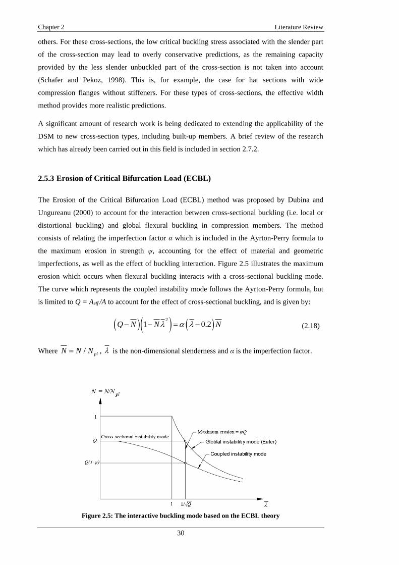
Chapter 2 Literature Review
30
others. For these cross-sections, the low critical buckling stress associated with the slender part
of the cross-section may lead to overly conservative predictions, as the remaining capacity
provided by the less slender unbuckled part of the cross-section is not taken into account
(Schafer and Pekoz, 1998). This is, for example, the case for hat sections with wide
compression flanges without stiffeners. For these types of cross-sections, the effective width
method provides more realistic predictions.
A significant amount of research work is being dedicated to extending the applicability of the
DSM to new cross-section types, including built-up members. A brief review of the research
which has already been carried out in this field is included in section 2.7.2.
2.5.3 Erosion of Critical Bifurcation Load (ECBL)
The Erosion of the Critical Bifurcation Load (ECBL) method was proposed by Dubina and
Ungureanu (2000) to account for the interaction between cross-sectional buckling (i.e. local or
distortional buckling) and global flexural buckling in compression members. The method
consists of relating the imperfection factor α which is included in the Ayrton-Perry formula to
the maximum erosion in strength ψ, accounting for the effect of material and geometric
imperfections, as well as the effect of buckling interaction. Figure 2.5 illustrates the maximum
erosion which occurs when flexural buckling interacts with a cross-sectional buckling mode.
The curve which represents the coupled instability mode follows the Ayrton-Perry formula, but
is limited to Q = Aeff /A to account for the effect of cross-sectional buckling, and is given by:
2
1 0.2Q N N N (2.18)
Where / plN N N , is the non-dimensional slenderness and α is the imperfection factor.
Figure 2.5: The interactive buckling mode based on the ECBL theory

Chapter 2 Literature Review
31
Therefore, by equating Eq. (2.18) to 1Q at 1/c Q the imperfection factor α can be
obtained as a function of the erosion factor ψ:
2
1 1 0.2
Q
Q
(2.19)
The imperfection factor calculated from Eq. (2.19) can then be introduced into the European
column design curves, commonly used for hot-rolled sections (CEN, 2005), in order to adapt
them to thin-walled CFS members accounting for the interaction between cross-sectional and
global buckling (Dubina et al., 2012).
The main difficulty in this approach is to properly evaluate the erosion of the critical load in the
‘interactive slenderness range’. The authors have suggested that the evaluation of the erosion
factor can be carried out by means of statistical analysis of compression tests on columns with
slendernesses in the interactive buckling range, as well as non-linear numerical analyses of
columns in the vicinity of the critical bifurcation point.
2.6. Design codes
2.6.1 Eurocode 3 (EC3)
The method adopted in Eurocode 3 (EC3) for the design of thin-walled CFS members
susceptible to cross-sectional instabilities is based on the effective width concept. In EC3 the
effect of local buckling is accounted for by using the provisions included in EN 1993-1-5 (CEN,
2009a) whereby the plate slenderness used in the effective width calculations is based on the
yield stress, irrespective of whether global buckling takes place before any part of the cross-
section reaches the yield stress. The interaction between local and global buckling is accounted
for by using the effective cross-sectional area in the definition of the global slenderness, as
specified in EN 1993-1-1 (CEN, 2005).
In the case of sections with edge or intermediate stiffeners, EN 1993-1-3 (CEN, 2006) provides
specific provisions to incorporate the effect of distortional buckling in the calculation of the
effective cross-sectional properties of the member. Distortional buckling results in a reduction
of the effective thickness of both the stiffener and the adjacent part of the stiffened element.
These provisions are based on the assumption that the stiffener behaves as a compression
member with a continuous partial restraint, with a spring stiffness which depends on the flexural
stiffness of the adjacent plane elements (CEN, 2006).

Chapter 2 Literature Review
32
While the effective width approach included in EC3 has the advantage of being able to combine
the effects of local and distortional buckling in the calculation of the effective cross-sectional
properties of the member, the calculation procedure for stiffened cross-sections and cross-
sections with more complex geometries becomes exceedingly complicated, especially if a more
refined solution is sought, which may require several iterations.
2.6.1.1 EC3 provisions for built-up members
The provisions included in EC3 for built-up members are mainly focused on laced or battened
built-up compression members, while for built-up compression members with chords in contact
or closely spaced, the provisions are limited to giving a maximum allowable spacing between
connectors (CEN, 2005). In addition, most of these provisions are only applicable to hot-rolled
built-up members.
For thin-walled CFS built-up members, EN 1993-1-3 does not provide any specific design rules
and only specifies the global buckling curve which should be used to determine the member
buckling resistance for a limited number of open and closed cross-sectional geometries. No
mention is made of whether those strength curves can be used for any type of open or closed
cross-section, assembled from two or more individual sections with either identical or different
cross-sectional geometries. There is also no guidance on the maximum connector spacing which
should be used to assemble the built-up member or any indication of how the connector spacing
or the type of connector may affect the ultimate capacity of the member. In addition, there is no
consideration of how the individual components may interact with each other when buckling or
how this interaction may affect the buckling response of the built-up member.
2.6.2 North American Specification (NAS)
The NAS (AISI, 2016a) has traditionally addressed the design of thin-walled CFS members
through a variation of the Effective Width approach, which differs slightly from the one used in
EC3. In the NAS, interaction between local and global buckling is treated by limiting the stress
in the effective width calculations to the maximum compressive stress in the element when
global buckling takes place. This global buckling stress is calculated using the gross section
properties. In addition, in the NAS distortional buckling is treated as a limit state separate from
local or global buckling.
In 2004, the NAS incorporated the Direct Strength Method (DSM) as an alternative design
method, which was included in Appendix 1 of the specifications. In 2016, the DSM was moved
to the main body of the specifications and is now considered an equivalent design method to the
Effective Width approach (AISI, 2016b).

Chapter 2 Literature Review
33
2.6.2.1 NAS provisions for built-up members
The provisions for built-up members included in the NAS can be used in conjunction with the
effective width approach or the DSM. These provisions are scarce and apply to a limited
number of built-up cross-sectional geometries consisting only of two identical components.
Provisions for built-up flexural members (AISI, 2016a)
The provisions for built-up flexural members included in (AISI, 2016a) only apply to I-shaped
sections assembled from channels connected through their web in a back-to-back configuration.
The provisions limit the maximum longitudinal connector spacing smax to the following value:
max
2min 6; sgT
s Lmq
(2.20)
where L is the span of the beam, g is the distance between the two rows of connectors nearest to
the top and bottom flange, (see Figure 2.6), Ts is the factored strength of the connection in
tension, m is the distance from the shear centre of one channel to the mid-plane of the web (see
Figure 2.6) and q is the design load on the beam for the purpose of determining smax. If the beam
is subject to a uniformly distributed load, q should be taken as three times the uniformly
distributed load. If the beam is subject to concentrated loads, q should be obtained by dividing
the concentrated loads or reactions by the length of bearing. If the length of bearing is smaller
than the longitudinal connector spacing, s, the required strength of the connections closest to the
load or reaction should be calculated as follows:
/ 2r sT P m g (2.21)
where Ps is the factored concentrated load or reaction and Tr is the required strength of the
connection in tension.
The first requirement in Eq. (2.20) is an empirically determined limit to prevent excessive
distortion of the top flange between connectors, while the second requirement in Eq. (2.20) is
based on the fact that the shear centre of an individual channel is not contained in the plane of
its web, and therefore, when a load is applied in the plane of the web, it produces a twisting
moment in each channel about its shear centre. This generates a pull-out force in the connectors
(AISI, 2016b).

Chapter 2 Literature Review
34
Figure 2.6: Tensile force in the connectors of a flexural member composed of back-to-back
channels (AISI, 2016b)
Provisions for built-up compression members (AISI, 2016a)
The provisions included in (AISI, 2016a) for built-up members in compression apply only to
members comprised of two sections in direct contact. The (AISI, 2016a) rules require that if
global buckling of the built-up column introduces shear forces in the connectors between the
components, the slenderness ratio KL/r, which is used in the calculation of the elastic global
buckling stress, should be replaced by the modified slenderness ratio given by:
22
m o i
KL KL a
r r r
(2.22)
In the above equation (KL/r)o is the global slenderness ratio of the entire built-up cross-section
about its minor axis, a is the intermediate fastener spacing and ri is the minimum radius of
gyration of the individual components of the built-up member.
The modified slenderness ratio accounts for the reduced shear rigidity of built-up members
connected at discrete points and applies to columns failing in flexural or flexural-torsional
buckling.
In addition, the (AISI, 2016a) provisions require the intermediate connector spacing, a, to be
limited such that a/ri ≤ 0.5(KL/r)o to prevent failure of the individual components due to flexural
buckling between connectors in the case that any one of the connectors becomes loose or
ineffective. The intermediate connectors in any cross-section along the member are also
required, as a group, to be able to transmit a force equal to 2.5 % of the ultimate capacity of the
column. Additionally, the ends of the built-up member should be connected by a weld having a
length of at least the maximum width of the member, or by connectors spaced longitudinally at
less than 4 times the diameter of the connectors over a distance of at least 1.5 times the
maximum width of the member, in order to prevent slip in the end connections.
It is worth noting that these provisions for built-up members in compression have mainly been
derived from research on hot-rolled built-up members connected with bolts or welds (AISI,

Chapter 2 Literature Review
35
2016b), and therefore, they do not necessarily reflect the behaviour of thin-walled members, in
which cross-sectional instabilities often occur before global buckling takes place, and in which
the material and geometric imperfections can differ substantially from those encountered in hot-
rolled members.
2.7. Previous research on CFS built-up members
2.7.1 Modified slenderness ratio
The modified slenderness formula, as included in the (AISI, 2016a) provisions, was developed
based on the experimental research of Zandonini (1985) on hot-rolled built-up struts consisting
of back-to-back channels, connected to each other with intermediate welded or snug-tight bolted
filler plates. In order to assess the applicability of the modified slenderness ratio to thin-walled
CFS I-shaped columns, Stone and LaBoube (2005) carried out an experimental investigation
consisting of 32 pin-ended compression tests on columns with four different cross-sectional
dimensions. The columns were assembled from two identical lipped channels connected back-
to-back with screws. The investigation showed that using the modified slenderness ratio resulted
in conservative strength predictions, especially for the columns assembled with thicker
channels. Whittle and Ramseyer (2009) also compared the predictions given by (AISI, 2016a)
using the modified slenderness ratio to the results obtained from over 150 compressive tests on
simply supported built-up box sections assembled from square lipped channels welded together
in a toe-to-toe configuration at discrete intervals, and found them to be exceedingly
conservative. It is worth pointing out, however, that the square lipped channels used to assemble
the built-up specimens tested by Whittle and Ramseyer (2009) were relatively stocky, with
width-to-thickness ratios ranging from 16 to 41, and therefore they did not exhibit local
buckling. Reyes and Guzmán (2011) carried out compression tests on 48 built-up box sections
made from two lipped channels welded together at discrete intervals, similar to those tested by
Whittle and Ramseyer (2009). However, in this case the lipped channels had more slender
cross-sections, with width-to-thickness ratios of the web which ranged from 50 to 67. The
specimens were tested between fixed or flexible support conditions. The columns were
relatively short, failing predominantly due to local buckling, and in the case of the specimen
with the largest weld spacing, also by global buckling of the individual channels between the
welds. The tests showed that, excluding the columns with the largest weld spacing, there was no
statistical reduction in the ultimate capacity due to a larger connector spacing and therefore, the
modified slenderness ratio was not applicable to these columns.
A simple design equation, which employed the modified slenderness ratio as one of the
independent variables, was proposed by Piyawat et al. (2013) to predict the ultimate capacity of

Chapter 2 Literature Review
36
doubly symmetric built-up tubular and I-shaped sections failing by distortional or global
flexural buckling. The equation was developed by carrying out a regression analysis of a three-
dimensional surface fitting the experimental and numerical data gathered in (Brueggen and
Ranrseyel, 2005; Piyawat et al., 2011; Whittle and Ramseyer, 2009). However, the authors
suggested that more compression tests on other practical built-up geometries were needed to
further validate their proposed equation.
2.7.2 Extending the DSM to the design of built-up members
The inherent characteristic of the DSM of simply combining the elastic local, distortional, and
global buckling stresses of thin-walled members in the calculation of the ultimate strength has
prompted a significant amount of research to try and extend the applicability of the DSM to the
design of built-up members. Most of the effort in extending the DSM to built-up members has
been devoted to the way in which composite action between the individual components of the
built-up geometry should be taken into account when calculating the elastic buckling stresses of
the member, considering the limitations of the FSM in accounting for the discrete distribution of
the connectors along the member.
The first attempt to incorporate composite action into the DSM equations can be attributed to
Young and Chen (2008), who compared the predictions given by the DSM to the ultimate
capacities obtained from a series of tests carried out on CFS built-up closed section columns.
The built-up specimens were assembled from channels with intermediate web stiffeners
connected at their flanges using self-tapping screws. The authors used the FSM to calculate the
elastic critical buckling stresses required by the DSM using three different assumptions, which
reflected different levels of composite behaviour. First, the individual channels were considered
in isolation assuming no interaction between them. An intermediate level of interaction was
incorporated by representing the connectors by smeared constraints along the column, while full
composite action was modelled by considering the built-up geometry as one solid cross-section.
Young and Chen (2008) showed that the ultimate capacities of the columns were intermediate
between the predictions given by the DSM when considering the built-up cross-section as fully
integral and the predictions assuming two independent profiles, suggesting that some level of
composite action was present in the tested columns.
(Georgieva et al., 2012a, 2012b, 2012c, 2011) carried out an extensive experimental and
numerical investigation to study the buckling behaviour of double-zed built-up columns and
assessed the predictions of the DSM. The built-up columns were assembled with hot-rolled
spacers bolted to the individual zed sections to restrict distortion of the cross-section at the
interconnection points, and were designed to exhibit local, distortional and global buckling. The
DSM was found to give conservative strength predictions for these members.

Chapter 2 Literature Review
37
Zhang and Young (2012) also evaluated the suitability of the DSM to predict the ultimate
capacity of built-up I-shaped compression members based on the results obtained from
experiments. The specimens considered in the study were assembled from lipped sigma-
channels connected back-to-back with self-tapping screws, and were designed to exhibit local,
distortional and global buckling, as well as interaction between these buckling modes. As in
(Young and Chen, 2008), the authors used the FSM to calculate the elastic cross-sectional
buckling loads. However, this time they considered five different cases to represent the amount
of composite behaviour which was experienced by the individual channels. In the first case, the
channels were analysed in isolation, and therefore no composite action was considered. In the
last four cases the entire built-up cross-section was considered as one solid cross-section and the
different levels of composite action were represented by setting the thicknesses of the contact
surfaces of the channels equal to 1.0, 1.2, 1.5 and 2.0 times the thickness of the individual
channels. The study showed that the best agreement between the DSM predictions and the
experimental results was achieved when assuming that the thickness of the channel webs in
contact with each other was equal to 1.2 times the thickness of the individual channels,
suggesting that some degree of composite behaviour was present in the tested specimens. Zhang
and Young (2015) carried out parametric studies of the built-up geometries tested by Zhang and
Young (2012) to assess the effect of the web and edge stiffeners on the bucking response of the
built-up specimens. They also explored additional DSM approaches to predict the ultimate
capacity, including one in which the effect of the composite action is included in the stability
analysis by considering a channel in isolation with the connectors represented by longitudinal
stiffeners.
A study similar to the one presented in (Zhang and Young, 2012), using the same five cases to
represent the level of composite action, was carried out by Zhang and Young (2018) to evaluate
the DSM predictions for built-up closed compression members with different types of web
stiffeners. Two different built-up cross-sections were studied, both of them assembled with self-
taping screws. This study showed that good DSM predictions were obtained when the
thicknesses of the contact surfaces in the built-up geometry were set equal to the thicknesses of
the individual components, but also revealed some level of composite action in the tested built-
up geometries. In this case, setting the thickness to 1.2 times the thickness of the individual
components, however, as in the geometries tested by Zhang and Young (2012), resulted in
slightly unsafe predictions.
Another experimental investigation of the structural response of CFS built-up I-sections was
reported in (Lu et al., 2017). However, the built-up members tested by Lu et al. (2017) consisted
of screw connected back-to-back lipped channels without web stiffeners. The authors concluded
that there was clear evidence of ultimate strength erosion due to local-distortional and local-
distortional-global interaction, and they subsequently proposed a novel direct strength based

Chapter 2 Literature Review
38
method to account for these interactions. In addition, by comparing the ultimate capacities
obtained for the built-up specimens with those obtained for the individual components, the
authors showed that a significant amount of composite action could be achieved when the
failure mode was governed by global buckling. They also concluded that when the failure mode
of the tested columns was predominantly local or distortional buckling, the effect of composite
action could be disregarded. Based on these observations, the authors decided to calculate the
elastic cross-sectional buckling loads, required by the proposed DSM equations, using the FSM
while considering the individual channels in isolation. However, to determine the elastic global
buckling load they considered the built-up cross-section as one solid cross-section.
Fratamico et al. (2018b) also reported an experimental investigation of the buckling and
collapse behaviour of screw connected back-to-back lipped channels. However, in this study the
columns were seated in tracks, which provided a more realistic semi-rigid support condition.
The authors assessed the effect of adding a group of connectors at each end of the column, as
prescribed by (AISI, 2016a), and confirmed the importance of these end group fasteners (EGFs)
in reducing the relative slip between the individual components and increasing the amount of
composite action when flexural buckling takes place. The experimental study revealed that the
benefit of adding the EGFs was more pronounced when global flexural buckling occurs without
much participation of local buckling. Based on the experimental results, an extension of the
DSM was proposed, in which the end support conditions were assumed to be fixed and the
elastic buckling stresses were calculated using the FSM while modelling the connectors using
the smeared constraint approach.
While most of the effort in extending the DSM to the design of built-up members has been
concentrated on compression members, some research has also been dedicated to built-up
flexural members. Wang and Young (2015) experimentally investigated the flexural behaviour
of built-up CFS members with open and closed cross-sectional geometries and with circular
web holes, with the aim of extending the DSM to the design of these types of members. The
built-up geometries studied by Wang and Young (2015) consisted of an open cross-section
formed by two lipped channels screw connected in a back-to-back configuration, and a closed
cross-section assembled from two plain channels screwed together through their flanges. The
authors explored different ways of calculating the elastic buckling stresses required by the DSM
in order to account for the effect of the connectors and the web opening. The applicability of the
DSM to the design of built-up flexural members was also assessed by Wang and Young (2016a,
2016b), who carried out an experimental and numerical investigation of flexural members with
four different built-up cross-sectional geometries failing by cross-sectional instabilities. Each
built-up geometry was assembled from two identical sections, screw connected either in a back-
to-back configuration to form an open section, or connected through their flanges to form a
closed section. The authors assumed in their analysis that the built-up geometries behaved as

Chapter 2 Literature Review
39
one solid cross-section, and found that, while for some built-up geometries the DSM provided
acceptable predictions, for other built-up geometries the predictions were either conservative or
unsafe. The authors resolved to modify the DSM equations and proposed tailored DSM
equations for each built-up geometry based on their experimental and numerical data.
A recently developed compound strip method (CSM) for the stability analysis of built-up
members (Abbasi et al., 2018) was used in (Abbasi et al., 2017) to study the effect of the
connectors spacing on the buckling behaviour of CFS built-up columns and to assess the
applicability of the DSM to built-up members, based on the experimental results obtained in
(Zhang and Young, 2012). The novelty of this study stemmed from the fact that the CSM is able
to account for the discrete character of the connector points when computing the elastic
buckling stresses of the built-up member. Using the CSM in numerical studies, the authors
found that reducing the connector spacing enhanced the elastic local and global buckling
stresses. In addition, an assessment of the DSM in which the elastic buckling stresses were
obtained from the CSM revealed that the DSM predictions were fairly accurate in predicting the
ultimate capacity of the built-up specimens tested by Zhang and Young (2012). However, the
authors stressed the need to perform further comparisons to calibrate the DSM for a wider range
of built-up sections with more complicated geometries.
2.7.3 Additional research on built-up members
Li et al. (2014) carried out a numerical and experimental investigation of built-up box section
columns composed of two lipped channels with web stiffeners connected through their flanges
with self-drilling screws. The researchers showed that local buckling of the individual
components cannot effectively be restricted in a built-up member because its half-wave length is
usually shorter than the connector spacing. They also indicated that some of the components of
a built-up member may attract more load than the others due to a small difference in length,
reducing the capacity of the member.
An experimental investigation was presented by Craveiro et al. (2016) on columns with open
and closed built-up cross-sectional geometries. The tested columns were assembled from lipped
and plain channels connected with self-drilling screws, constructing built-up geometries with up
to four individual channels. The study revealed a significant degree of composite action, with
the built-up geometries exhibiting ultimate capacities larger than those expected by simply
adding up the contributions of the individual components. Liao et al. (2017) carried out an
experimental and numerical investigation of multi-limb built-up stub columns with similar
geometries as those tested by Craveiro et al. (2016) and found that the connector spacing had
little impact on the ultimate capacity of the stub columns.

Chapter 2 Literature Review
40
A significant research effort has also been focused on developing innovative built-up
geometries. The built-up LiteSteel beam (LSB), consisting of two channels with hollow
rectangular flanges connected back-to-back, has been investigated numerically and
experimentally by (Jeyaragan and Mahendran, 2008a, 2008b). The authors found that the
detrimental effect of lateral-distortional buckling, common in the single LSB, can be mitigated
by connecting two LSB back-to-back, resulting in a moment capacity which is more than twice
the capacity of the individual LSB section. The Modular Light-Weight Cold-formed beam
(MLC beam) is another innovative built-up beam, consisting of two lipped channels with
hollow flanges and a web containing beads and openings. The channels are laser welded
together in a back-to-back configuration with reinforcing plates placed inside the flanges. The
MLC beam was designed to provide a high resistance to lateral-torsional buckling and has been
extensively investigated both numerically and experimentally (Dilorenzo et al., 2006; Landolfo
et al., 2009, 2008; Lorenzo et al., 2004; Portioli et al., 2012).
2.8. Numerical modelling of CFS built-up members using Abaqus
This section is mainly based on Abaqus manual (Dassault Systemes, 2014).
2.8.1 Abaqus solvers for non-linear buckling analysis
Abaqus provides three different techniques for solving a non-linear buckling analysis.
The Modified Riks method has been successfully used by many researchers to predict the non-
linear buckling behaviour of CFS members composed by a single section (Ashraf et al., 2006;
Gardner and Nethercot, 2004; Li et al., 2013; Yan and Young, 2004; Young and Yan, 2004).
This method can account for non-linear material properties and arbitrary boundary conditions,
and can provide solutions irrespective of whether the response of the system is stable or
unstable. However, in order for the Riks method to be applicable, the loads applied to the
system must be proportional and the equilibrium path in the load-displacement space must be
smooth and unbranched. In addition, in problems which involve contact non-linearity, such as
buckling of a built-up member, the Riks analysis is most likely to terminate before the ultimate
load of the member has been reached, since this method is not able to properly address the
discontinuities associated with this type of non-linearity. A detailed description of the Modified
Riks method can be found in (Dassault Systemes, 2014).
Another approach is to use the General Static method with the inclusion of artificial damping to
stabilize the solution. This approach has proved to be very useful in determining the non-linear
buckling response of built-up specimens in cases where the Modified Riks method has failed to
converge (Becque, 2008; Piyawat, 2011). However, this approach should be used with caution,

Chapter 2 Literature Review
41
as adding artificial damping in excess may significantly affect the solution and overestimate the
ultimate capacity of the model.
The third approach is to use the Explicit Dynamic method, which treats the quasi-static buckling
response as a dynamic problem. As this method does not attempt to converge to the exact
solution, the specified time increment has to be sufficiently small to prevent the response
predicted by this method from excessively deviating from the exact response. On the other
hand, since no iterations are required, the computational cost of each increment is considerably
lower than in the previous two methods. Also, to prevent inertial effects from affecting the
response, the specified loading rate has to be limited, which in turn increases the number of
increments needed. This typically requires several runs to find the optimum value of the loading
rate. The Explicit Dynamic method always provides a solution. However, its validity needs to
be scrutinized using the engineer’s judgement.
Out of the three methods available in Abaqus to solve non-linear buckling problems, the
General Static method is the most suitable one for problems involving contact discontinuities.
These are likely to occur between components of a built-up member when it is subject to
buckling instabilities. For this reason, the method used by the General Static solver to solve a
non-linear problem is described in more detail in the next section.
2.8.2 Solving a non-linear problem with Abaqus/Standard General Statics solver
In a non-linear problem the stiffness matrix of the system changes as it deforms. For this reason,
in order to determine the non-linear response of the system to certain loading conditions, the
loading has to be expressed as a function of time and the simulation has to be divided into a
series of time increments. In each time increment, Abaqus/Standard iteratively solves a static
system of linear equations with an updated stiffness matrix of the system. By default, the
General Static solver carries out this iterative process using the Newton-Raphson method.
Abaqus/Standard adjusts the size of each increment depending on whether or not a converged
solution is achieved after a series of iterations.
The Newton-Raphson method is represented for a single time increment in Figure 2.7, which
illustrates the non-linear displacement response of a system to a given loading. At any time
during the analysis, in order for the system to be in a static equilibrium, the total internal forces
(I) must balance the external forces acting at each node (P).

Chapter 2 Literature Review
42
Figure 2.7: Iteration process in a time increment
Therefore, in a given time increment during the non-linear analysis, a small load increment ΔP
applied at the beginning of the increment will result in the external forces P which must be
balanced by the internal forces Ia. These internal forces are calculated based on the system
configuration at ua = u0 + ca, where ca is referred to as the displacement correction for iteration
a. ca is determined using the system’s tangent stiffness K0, which is based on the system
configuration at u0, and P, as shown in Figure 2.7. In a non-linear problem Ia and P will never
completely balance each other and therefore, Abaqus/Standard defines a force residual Ra for
iteration a as:
a aR P I (2.23)
This force residual Ra is compared to a tolerance value, which by default is equal to 0.5 % of a
spatial average force computed over a number of nodes in the system, averaged over time. If Ra
is less than this force residual tolerance at all nodes, Abaqus/Standard considers P and Ia to be in
equilibrium. However, before the solution is accepted, Abaqus/Standard checks whether the
final displacement correction ca is less than 1 % of the total incremental displacement Δua = ua -
u0. If this check is not satisfied, Abaqus/Standard performs another iteration. Similarly, if Ra is
larger than the force residual tolerance value, Abaqus/Standard will try to balance the external
and internal forces by performing iteration b, in which a new stiffness matrix is computed based
on its updated configuration ua. This stiffness matrix is used in combination with ΔP to
determine the new displacement correction cb for iteration b, which in turn is used to determine
the new configuration of the system ub and the internal forces Ib. As Figure 2.7 shows, if the
solution converges within a given increment, each iteration will bring the external and internal
forces closer to each other.

Chapter 2 Literature Review
43
By default, Abaqus/Standard will continue performing iterations until either a maximum of 16
iterations are completed, or the force residual is less than the tolerance value while the
displacement correction c is less than a fraction of the increment displacement Δu. If after 16
iterations the solution has not converged, Abaqus/Standard reduces the increment size to 25 %
of its previous value and tries to find a converging solution for this smaller increment size. If the
solution still does not converge, Abaqus/Standard will continue reducing the increment size
until a converging solution is found, the minimum increment size specified is reached or a
maximum of 5 consecutive reductions of the increment size have been carried out. If the
solution still has not converged, Abaqus/Standard terminates the analysis prematurely. On the
other hand, if during two consecutive increments the solution converges in fewer than 5
iterations, Abaqus/Standard will automatically increase the size of the next increment by 50 %.
This ensures that in problems without severe convergence issues the solution can be reached in
a reasonable time.
For non-linear problems with severe convergence issues Abaqus/Standard allows the user to
change the default solution control parameters which govern the convergence criteria and the
time incrementation algorithm. In addition to this, Abaqus/Standard offers a series of
stabilization mechanisms, which can help to achieve convergence in cases where the solution
tends to diverge.
2.8.3 Stabilization schemes and solution control in Abaqus/Standard
In a non-linear buckling analysis of a built-up member there are three sources of numerical
instabilities which may prevent Abaqus/Standard from converging to the desired solution. The
first source of instability is of a geometric character and originates from the very nature of the
buckling phenomenon, which results in a local transfer of strain energy from one part of the
built-up member to the neighbouring parts. The second source of instability is related to the
material non-linearity and comes into effect after the proportionality limit of the material is
exceeded due to material softening. The third source of non-linearity originates from the contact
between the different components in the built-up member, which may lead to severe
discontinuities in the model with gaps potentially opening up or closing and suddenly being
unable/able to transfer pressures.
Abaqus/Standard includes two stabilization mechanisms which can be used with the General
Static Solver to overcome these issues. The Automatic Stabilization scheme is mainly designed
to address issues due to geometric non-linearity and material non-linearity, while the Contact
Stabilization scheme focuses on smoothening the discontinuities introduced into the model by
contact between nearby surfaces. Both stabilization mechanisms consist of adding artificial
damping to the model to help stabilize it. In addition, Abaqus/Standard also allows the user to

Chapter 2 Literature Review
44
modify some solution control parameters, which can prevent unnecessary cutbacks to the
increment size during the simulation and can help prevent the solution from diverging in
severely non-linear problems.
More details about the different options which can be used in a non-linear buckling analysis to
help Abaqus/Standard converge to the desired solution are described below.
2.8.3.1 Automatic stabilization
The automatic stabilization mechanisms in Abaqus/Standard allow for the addition of artificial
viscous forces into the global equilibrium equations solved in each increment:
0vP I F (2.24)
In the above equation P and I are the external and internal forces acting at each node in the
model and Fv are the stabilizing viscous forces which are added at each node. These viscous
forces are obtained from
*vF cM v (2.25)
Where M* is an artificial mass matrix calculated with unity density, c is a damping factor and v
is the vector of nodal velocities. Therefore, if a region of the model has a tendency to undergo
large displacements in a single increment, for instance due to sudden buckling, or a sudden loss
of material stiffness, the local velocities at the nodes in that region generate viscous forces
which dissipate part of the strain energy released. Regions in the model which are stable (i.e.
which undergo small displacements in said increment) generate low viscous forces and,
therefore, the artificial damping in those regions has little or no effect.
The damping factor c can be constant over the whole analysis step. In this case,
Abaqus/Standard allows the user to specify the damping factor directly. Alternatively,
Abaqus/Standard can calculate it automatically based on the ‘dissipated energy fraction’ which
is the ratio between the energy dissipated during a given increment and the strain energy
extrapolated based on the first increment of the step. The default value of the dissipated energy
fraction is 2.0x10⁻⁴.
Alternatively, Abaqus/Standard offers an adaptive automatic stabilization scheme, in which the
damping factor can vary spatially and with time. This is the preferable approach as it reduces
the effect the artificial forces may have on the response of the system. When this option is
selected, the amount of artificial damping introduced into the model is controlled by the
convergence history and the ratio of the energy dissipated by viscous damping to the total strain
energy. If the convergence behaviour is problematic, Abaqus/Standard automatically increases
the damping factor. Abaqus/Standard tries to limit the ratio of the energy dissipated by the

Chapter 2 Literature Review
45
artificial forces to the total strain energy by imposing an accuracy tolerance. If this tolerance is
exceeded, Abaqus/Standard adjusts the damping factor in each individual element so that the
accuracy tolerance is satisfied both at the global and the local (element) level. Abaqus/Standard
also restricts the ratio of the incremental value of the stabilization energy to the incremental
value of the strain energy in each increment to ensure that this value does not exceed the
accuracy tolerance. By default, the accuracy tolerance used with the adaptive automatic
stabilization scheme is set to 0.05. However, this value can be adjusted to the specifics of the
model.
To ensure that the artificial damping forces introduced into the model are not excessively large
and distort the solution, Abaqus recommends performing a post-analysis to ensure that the
energy dissipated by viscous damping (ALLSD) is negligible compared to the total strain
energy (ALLIE).
2.8.3.2 Contact stabilization
The contact stabilization (or contact control) scheme is also based on the addition of viscous
damping to help stabilize the model. The main difference with respect to the automatic
stabilization scheme is that, in this case, artificial viscous stresses are applied at the slave nodes
of a contact interaction to oppose the incremental relative motion between nearby surfaces.
Contact stabilization can be specified for particular surfaces where contact is likely to occur. By
default, the viscous stresses are automatically calculated for each contact constraint. However,
Abaqus/Standard also allows the user to specify the damping coefficient directly. The first
approach is a more robust solution as, in this case, the damping stresses are automatically
adjusted over the step and are increased when severe contact discontinuity is present and
reduced when contact between the surfaces is stable.
The viscous stresses determined by the contact stabilization scheme can be decomposed in to a
stress normal to the interacting surfaces (σstab) and a tangential stress (τstab). These are given by:
itstab const er ampl gap d relNs s s s c v (2.26)
it tanstab const er ampl gap g d relTs s s s s c v (2.27)
where cd is the damping coefficient which is automatically calculated by Abaqus/Standard for
each contact constraint based on the stiffness of the respective elements and the time step. vrelN
and vrelT are the relative normal and tangential velocities, respectively, between nearby points on
opposing contact surfaces. siter is a scale factor which varies across iterations, allowing for larger
viscous stresses during the early iterations of an increment and reducing them during later
iterations to minimize the effect of the contact stabilization on the desired solution. sampl and sincr
are time-dependent scale factors which reduce the effect of the contact stabilization as the

Chapter 2 Literature Review
46
analysis progresses. sgap is a scale factor which controls the magnitude of the viscous stresses
based on the distance between the slave and master nodes, with it being maximal when a zero
gap distance exists between the slave and master node and being equal to zero when this
distance is larger than a characteristic surface dimension. The two scale factors sconst and stang are
constant factors which allow the Abaqus user to adjust the computed viscous stresses. This
provides great flexibility in cases where the automatically calculated contact stabilization is not
adequate.
As Eq. (2.26) and Eq. (2.27) show, the scale factor sconst applies to both normal and tangential
stabilization, while stang only applies to tangential stabilization. This means that the viscous
contact stresses can be controlled separately in order to stabilize the relative motion of the
surface nodes in the normal and the tangential directions of the surfaces. This is important
especially when the relative tangential motion between nearby surfaces is large, as may be the
case when the component sections of a built-up member buckle. In this case tangential contact
stabilization may absorb significant energy, and therefore it may be preferable to set the
tangential viscous stresses to zero. Normal contact stabilization, on the other hand, is much less
likely to absorb significant energy and therefore tends to have less influence on the results.
Contact stabilization can be activated in Abaqus/Standard by using the *CONTACT
STABILIZATION or *CONTACT CONTROL keywords. Both options provide a similar
contact stabilization option, with the main difference between them being the default values
given to some of the scale factors used to calculate the viscous stresses.
As for the automatic stabilization scheme, care must be taken to ensure that the viscous
damping does not significantly alter the response of the system. This can be achieved by
performing a post-analysis check to ensure that the dissipated stabilization energy (ALLSD) is
significantly smaller than the total strain energy of the system (ALLIE).
2.8.3.3 Solution Control Parameters
The Solution Control Parameters can be used to modify the convergence control algorithm
Abaqus uses to solve a non-linear analysis, as well as the time incrementation scheme.
However, modification of the solution control parameters may significantly affect the accuracy
of the solution and/or the computational speed. For most analyses the solution control
parameters need not be changed. However, there are cases where the solution procedure may
not be able to converge with the default controls and it is necessary to change certain control
parameters.
Displacement correction control
As mentioned in section 2.8.2, before Abaqus/Standard accepts the solution obtained for a given
increment as a sufficiently close approximation of the exact solution, it checks whether the
Chapter 2 Literature Review
47
largest displacement correction at the nodes is a small fraction of the total displacement
increment. The limit for this ratio is given by Cnα, which by default is equal to 0.01. Some
analyses may not require such accuracy, and therefore Abaqus/Standard allows the user to
increase the value of Cnα, or even to remove this check by setting Cn
α to 1.
Time incrementation parameters
I0 and IR are the most significant time incrementation parameters, since they have a direct effect
on convergence. However, they do not affect the accuracy of the solution. In non-linear analyses
which are performed using the Newton-Raphson method the solution can be expected to
converge quadratically if the estimate of the solution is within the radius of convergence.
However, there are some problems in which quadratic convergence may not be achieved, for
example, if the Jacobian is not exact. In addition, monotonic convergence may also not be
achieved in problems in which various sources of non-linearity, such as contact, material or
geometric non-linearity, interact with each other. Abaqus/Standard carries out regular checks to
see the rate at which the residual forces are decreasing. If Abaqus/Standard detects that
quadratic convergence is not being achieved it may reduce the time increment to enforce a
quadratic convergence.
I0 specifies the number of equilibrium iterations carried out before Abaqus/Standard checks
whether the residuals are not increasing in two consecutive iterations. The default value for I0 is
4. However, it may be necessary to increase this parameter if the initial convergence is non-
monotonic. Similarly, IR specifies the number of equilibrium iterations after which
Abaqus/Standard checks whether the convergence happens at a logarithmic rate. The default
value for IR is 8. Abaqus/Standard recommends increasing the values of these two time
incrementation parameters to I0 = 8 and IR = 10 in problems with severe discontinuities, in order
to avoid premature cutbacks of the time increment.
‘Line search’ algorithm
The ‘line search’ algorithm is an option included in Abaqus/Standard to improve the robustness
of the Newton-Raphson and quasi-Newton methods. In severely non-linear problems the
Newton-Raphson algorithms may diverge during equilibrium iterations where residuals are
large. The line search algorithm detects these situations automatically and scales the correction
to the computed solution using a line search scale factor, sls, which helps to prevent divergence.
The scale factor sls is obtained through an iterative process which minimizes the component of
the residual vector in the direction of the correction vector. The accuracy of sls depends on
several control parameters, with the most important ones being Nls, which is the number of line
search iterations that are performed, and ηls, which indicates the minimum change of sls between
iterations before the line search algorithm stops. By default, when Abaqus/Standard uses the
Newton-Raphson method, Nsl is set to zero (i.e. the line search algorithm is deactivated). When

Chapter 2 Literature Review
48
using the quasi-Newton’s method Nsl is set to 5 and ηsl is set to 0.1. Nsl can be increased, for
example to 20, to allow for more line search iterations, while ηsl can be reduced, for example to
0.01, to request more accuracy in the line search factor sls. The additional computational cost the
line search algorithm requires may be compensated by a reduction in the number of non-linear
increments and a reduction in increment cutbacks.
2.8.4 Contact interaction
Abaqus/Standard offers two approaches for modelling surface-based contact interactions,
namely: the general contact implementation and the contact pair implementation. Both
approaches have very similar capabilities, with the main differences lying primarily in the user
interface, the default numerical settings and the available options for defining the contact
interaction. Abaqus/Standard provides several contact formulations that can be used in a contact
simulation. Each formulation is based on the choice of a contact discretization, a tracking
approach, and assignment of ‘master’ and ‘slave’ roles to the contact surfaces.
Two contact discretization approaches are available in Abaqus/Standard to model contact. The
first one is the node-to-surface discretization approach, in which the nodes of one of the contact
surfaces (slave surface) are constrained to not penetrate the other (master) surface. This is
achieved by creating projection points on the master surface which interact with the slave nodes.
Each contact condition involves a single slave node and a group of nearby master nodes which
are used to define the projection point. In the node-to-surface approach the nodes of the master
surface can, in principle, penetrate the slave surface. In addition, as the constraints are applied
directly to the slave nodes, the contact forces tend to concentrate at these slave nodes. The other
option is to use the surface-to-surface discretization formulation, in which the contact conditions
are enforced in an average sense over regions nearby the slave nodes rather than at the
individual slave nodes themselves. With this approach, although some small penetration may
occur at some individual nodes, large undetected penetration of master nodes into the slave
surface is not an issue. The surface-to-surface discretization approach tends to provide more
accurate stress and pressure results than the node-to-surface approach. However, since the
surface-to-surface approach generally involves a larger number of slave nodes in each contact
constraint than the node-to-surface approach, its computational cost tends to be higher.
For each type of contact discretization, Abaqus/Standard offers the finite-sliding and the small-
sliding tracking approaches to account for the relative motion of the two interacting surfaces.
The finite-sliding approach allows for any arbitrarily large relative separation, sliding and
rotation of the contact surfaces, while the small-sliding approach assumes that, although the
surfaces may undergo arbitrarily large rotations, each slave node interacts with the same local
area of the master surface throughout the analysis. With the small-sliding approach,

Chapter 2 Literature Review
49
Abaqus/Standard does not have to monitor slave nodes for possible contact along the entire
master surface, which is why this tracking approach generally leads to less computationally
expensive solutions than the finite-sliding approach.
The general contact implementation only uses the surface-to-surface formulation in combination
with the finite-sliding tracking approach. The contact pair implementation, on the other hand, by
default uses the node-to-surface contact formulation with the small-sliding tracking approach,
although it also allows the user to opt for any possible combination of the node-to-surface or
surface-to-surface formulation with the small-sliding or finite-sliding tracking approach.
Regardless of the contact algorithm selected, the first step in defining a contact interaction
between element-based deformable surfaces is to specify the surfaces which will be involved in
the contact interaction. Alternatively, the general contact implementation offers an all-inclusive
self-contact definition in which Abaqus/Standard automatically includes all exterior element
faces, with the exception of faces belonging to cohesive elements, for potential contact. This is a
simple way of defining the contact domain. However, it may result in a more computationally
demanding solution since in this case, contact between elements which are not realistically able
to be in contact with each other is also accounted for.
Once the contact surfaces have been specified, their properties have to be defined. In the case of
contact between shell elements, these include, for example, the contact thickness of the shell
and any possible offsets in the contact surface. The general contact formulation automatically
accounts for the thickness associated with shell-like surfaces, defining contact on the outer
faces. With the contact pair implementation, the shell thickness and any offsets are only
accounted for when the surface-to-surface contact formulation is selected. In addition, when
defining contact between two surfaces, the general contact formulation automatically accounts
for any possible contact between the edge of one of the surfaces and the other surface. In this
case, the surface-to-surface contact formulation is used as the primary formulation, while the
edge-to-surface formulation is used as a supplementary formulation which uses the penalty
enforcement method and only involves the displacement degrees of freedom of the edge nodes.
The contact pair implementation also allows for edge-to-surface contact interaction. However,
this type of interaction has to be defined separately.
The next step is to define the contact property model which governs the behaviour of the
surfaces when they are in contact. The default contact property model in Abaqus/Standard
assumes a ‘hard’ contact in the normal direction and a frictionless contact in the tangential
direction. However, other types contact property models can be defined such as a ‘softened’
contact relationship in the normal direction or different types of friction models in the tangential
direction. The latter include a penalty formulation which uses the Coulomb friction model or the
‘rough’ formulation, which assumes that, once the surfaces are in contact, they cannot slide.
Three constraint enforcement methods are available in Abaqus/Standard to define normal

Chapter 2 Literature Review
50
contact, namely: the direct method, the penalty method and the augmented Lagrange multiplier
method. The direct method strictly enforces a given pressure-overclosure behaviour in each
constraint and is the only method that can be used for softened pressure-overclosure
relationships. The penalty method is the default method used for hard contact when the finite-
sliding surface-to-surface formulation is selected. This method approximates hard pressure-
overclosure behaviour by allowing a limited amount of penetration and calculates the contact
pressure based on the amount of penetration. The augmented Lagrange formulation is similar to
the penalty method but uses an augmentation iteration scheme when a specified penetration
tolerance is exceeded. This reduces the amount of penetration, improving the accuracy of the
hard pressure-overclosure approximation. The augmented Lagrange method is used by default
for self-contact with the node-to-surface formulation if the hard pressure-overclosure
relationship is selected.
Finally, it is also important to specify the way in which the initial overclosures (at the beginning
of the analysis) in a contact interaction should be resolved. General contact, by default,
eliminates initial overclosures by adjusting the position of the slave nodes without generating
any stress or strain in the model. The contact pair formulation, on the other hand, by default
solves the initial overclosures during the first increment by treating them as ‘interference fits’,
in which the penetration of the slave nodes into the master surface is resolved by the generation
of stresses and strains in the model. It is important to mention that only those slave nodes which
penetrate into the master surface over a distance smaller than an overclosure tolerance
calculated by Abaqus/Standard are repositioned. The philosophy behind this is that the default
initial adjustments are intended to correct only minor mismatches associated with the generation
of the mesh. Therefore, if the overclosures are larger than the calculated tolerance, an exclusion
zone is automatically generated and the contact interaction between these surfaces is removed.
Abaqus/Standard offers alternative contact initialization methods to solve initial overclosures
between contact surfaces. For example, a more robust option to solving all the initial
overclosures in the first increment is to use the shrink-fit method to gradually resolve the
overclosures over multiple increments. This may be useful when there are large overclosures in
the model which cannot be solved in a single increment. In addition, Abaqus/Standard allows
the user to increase the search zones for strain-free or interference fit adjustment when the
default overclosure tolerance is not appropriate.
2.8.5 Mesh-independent fasteners
Mesh-independent fasteners make use of position points to define a point-to-point connection
between two or more surfaces. The fasteners can be located anywhere between the surfaces to
be connected, irrespective of the location of the nodes. The location of the fastening points is
defined by either specifying an attachment point or an attachment line. The fastening points are

Chapter 2 Literature Review
51
connected to the neighbouring nodes on each surface with distributing coupling constraints, as
illustrated in Figure 2.8. Different weighting options can be used to apply these constraints,
making use of the distances of the coupling nodes to the fastening point. By default, Abaqus
uses the uniform weighting scheme. However, this can be changed to a scheme in which the
importance of the constraints provided by the neighbouring nodes decreases with distance
following a linear, quadratic, or cubic polynomial weight distribution. Depending on the
weighting function selected, the characteristic length of the connected facets and the geometric
properties of the fastener, Abaqus/Standard defines a region of influence, which determines the
number of coupling nodes that are associated with the fastening points. For a given mesh and
weighting scheme, the region of influence can be modified manually by changing the physical
fastener radius, although it will always include a minimum of three coupling nodes.
Figure 2.8: Mesh independent fasteners
Mesh-independent fasteners can be defined using either connector elements or Beam Multi-
point Constrains (MPCs). BEAM MPCs can be used to model perfectly rigid connectors
between the fastened surfaces by eliminating all the translational and rotational degrees of
freedoms of one of the fastening points. This approach has the advantage of reducing the size of
the model. However, it does not allow any output of the connector such as forces or
deformations. Also, since the constraints are imposed by eliminating the degrees of freedom of
one of the fastening nodes, it is not possible to model more complex connector behaviour,
which can include, for example, slip between the connected surfaces or bearing deformations of
the surfaces around the connectors. To model more complex connector behaviour
Abaqus/Standard includes the option of using connector elements (CONN3D2), which use
Lagrange multipliers to enforce kinematic constraints between the fastening nodes. This allows
for a more flexible and tailored modelling of the connectors, since kinematic constraints can be
applied to specific components of relative motion between the fastening nodes. This allows, for
example, to model the effects of elasticity and plasticity in the connectors and the surrounding
surface or local friction at the connector. In addition, connector elements provide output of the

Chapter 2 Literature Review
52
different variables that are included in the definition of the connector behaviour, such as forces
or relative displacements between the fastening nodes.
2.8.5.1 Fastener types
Mesh-independent fasteners can be created using point-based fasteners, discrete fasteners or
assembled fasteners.
Point-based fasteners and assembled fasteners make use of position points to create the
fasteners. Abaqus automatically creates the fastening points by projecting the positioning point
onto the fastened surfaces. The main difference between point-based fasteners and assembled
fasteners is that the former creates individual fastener objects which can be viewed and
manipulated while working in Abaqus/CAE, while the latter are used to efficiently replicate
complex fastener-like behaviour in several places by creating a template model which is
mapped to the corresponding locations in the main model. Assembled fasteners can be produced
only by direct coding into the input file.
Discrete fasteners are similar to point-based fasteners in the sense that they also create
individual fastener objects and can be modelled using connector elements or beam MPCs.
However, discrete fasteners make use of attachment lines to create the mesh-independent
fasteners. The process of creating an attachment line is similar to the process of creating point-
based fasteners. The first point of the attachment line (or the first fastening point in a point-
based fastener) is generated by either projecting the positioning point onto the closest surface
along a normal to the surface or along a specified projection direction, as shown in Figure 2.9.
The location of the second point of the attachment line (or fastening point) is determined by
projecting the first fastening point onto the other surface along the fastener normal direction,
which generally coincides with the normal of the closest surface. The main advantage of
discrete fasteners over point-based fasteners and assembled fasteners is that when discrete
fasteners are modelled using connectors they allow for connector loads and connector boundary
conditions to be applied individually to their available components of relative motion. In
addition to that, discrete fasteners can be viewed with their connectors and couplings outside the
Visualization module.

Chapter 2 Literature Review
53
Figure 2.9: Methods used to locate the fastening points with a point-based or a discrete fastener
2.8.5.2 Coupling methods
Abaqus/Standard offers two different ways to couple the motion of the fastening point to the
motion of the neighbouring nodes on the fastened surface: the continuum coupling method and
the structural coupling method.
By default, Abaqus/Standard uses the continuum coupling method to attach the fastening points
to the connected surfaces. In the continuum method, the translational and rotational degrees of
freedom of the fastening point are coupled to the average translational degrees of freedom of the
neighbouring coupling nodes on each of the fastened surfaces. Therefore, forces and moments at
the fastening point are distributed only as coupling forces to the coupling nodes. The advantage
of the continuum coupling method is that it can be used with any type of shell element.
However, in some situations, when the fastened surfaces are close to one another, this method
may provide unrealistic contact interaction.
The structural coupling method couples the translational and rotational degrees of freedom of
the fastening point to both the average translational and rotational degrees of freedom of the
neighbouring coupling nodes on each of the fastened surfaces, rather than to the translational
degrees only. The constraint distributes forces and moments at the fastening point as coupling
node forces and moments. This coupling method is particularly suited for bending-like
applications of shells when the coupling constraint only spans a small patch of nodes. However,
in order to be applicable, all the rotational degrees of freedom at the coupling nodes must be
active and constrained. Therefore, the structural coupling method cannot be used with shell
elements which only have two rotational degrees of freedom such as S4R5 or S9R5 elements.
2.8.6 Fastener coordinate system
Fasteners are formulated in a local coordinate system which rotates with the motion of the
reference node (first fastening point). If point-based fasteners are used, Abaqus, by default
defines the local coordinate system of the fastener by projecting the global coordinate system

Chapter 2 Literature Review
54
onto the surface containing the first fastening point, so that the z-axis of the fastener local
coordinate system is normal to this surface. On the other hand, if the connectors are modelled
with discrete fasteners, the orientation of the local coordinate system of the fastener, by default,
coincides with that of the global coordinate system. A schematic representation of the fastener
coordinate system which is by default created by Abaqus when using point-based and discrete
fasteners is illustrated in Figure 2.10.
Figure 2.10: Global and fastener coordinate systems
If the fastener is defined using a connector element, it may be necessary to specify its
orientation to ensure that the components of relative motion of the connector act in the desired
directions. This is achieved by defining a local coordinate system for the connector (Tconnector),
relative to the local coordinate system for the fastener (Tfastener). Assuming that Tconnector and
Tfastener are orthogonal rotation matrices with the local x, y and z-axis corresponding to the first,
second and third rows, respectively, the orientation of the connector relative to the local
coordinate system of the fastener (Tconn.orientation) is given by:
.conn orientation connector fastenerT T T (2.28)
As an example, if two parallel surfaces have to be connected in such a way that they can only
rotate about the axis of the fastener normal to the surfaces, the fastener can be modelled using a
HINGE connector. However, since the only available component of relative motion of this
connector is a rotation about its x-axis, if the default local coordinate system is used for the
fastener (with the z-axis normal to the surfaces), the connector has to be orientated using a
Tconnector matrix in which the x-axis is set to (0., 0., 1.).

Chapter 3 Experimental Study of Cold-Formed Steel Built-up Stub Columns
55
Chapter 3
Experimental Study of Cold-Formed Steel
Built-up Stub Columns
3.1. Introduction
The experimental programme described in this chapter intended to investigate the cross-
sectional compressive behaviour and capacity of four different built-up geometries. Particular
attention was devoted to the way the individual components within the cross-section interact
with each other and affect each other’s stability. Furthermore, the experiments sought to
quantitatively study the effects of the connector type and the longitudinal connector spacing on
the cross-sectional stability and the ultimate capacity of the built-up specimens. A total of 20
stub columns were tested. The entire experimental programme was carried out in the Heavy
Structures Laboratory at The University of Sheffield.
Figure 3.1 illustrates the four cross-sectional geometries included in the tests. Cross-sectional
geometries 1 and 2 were assembled using commercially available cold-formed steel sections,
supplied by BW Industries and selected from their catalogue of standard sections. The sections
were manufactured from pre-galvanized steel plates with a guaranteed yield stress of 450 MPa
and a nominal 0.04 mm thick Z275 zinc coating. They were connected using M6 bolts,
tightened with a torque of 10 Nm. This torque did not result in any substantial clamping force
on the connected plates. Rather it is more representative of hand-tightened bolts. A wrench with
measured torque was used, however, for reasons of consistency. The bolts used to assemble
built-up geometries 1 and 2 are shown in Figure 3.2a. Built-up geometry 1 was formed by
connecting the flanges of two plain channel sections with a nominal depth of 154 mm and
thickness of 1.4 mm to flat plate sections with a nominal width of 200 mm and thickness of 2.4
mm. In built-up geometry 2 the plate sections were replaced by plain channels with a nominal
depth of 154 mm and thickness of 1.4 mm, connected to the flanges of two plain channels with
a nominal depth of 79 mm and thickness of 1.2 mm.

Chapter 3 Experimental Study of Cold-Formed Steel Built-up Stub Columns
56
Cross-sectional geometries 3 and 4 were assembled using bespoke plain and lipped channel
sections with nominal depths of 120 mm and 110 mm, respectively, and thicknesses of 1.2 mm,
brake-pressed by an external specialist fabricator. The sections were fabricated from hot-dip
zinc coated steel sheet with material characteristics adherent to the CEN (1995) standard. The
plain and lipped channels had a guaranteed yield stress of at least 260 MPa. No information
about the zinc coating could be obtained from the manufacturer. Therefore, the coating
thicknesses was determined by measuring the total thickness at each end of the plain and lipped
channels before and after removing the coating. An average coating thickness of 0.03 mm was
obtained. The plain and lipped channels used to construct both built-up geometries 3 and 4 had
identical nominal cross-sectional dimensions and were joined together using M5.5 self-drilling
sheet metal screws (Figure 3.2b). Built-up geometry 3 resembled a box section in which two
lipped channels were connected through their flanges to the webs of two plain channels. Built-
up geometry 4 could be interpreted as an I-shaped section with double webs and stiffened
flanges, as illustrated in Figure 3.1.
All columns were loaded in uniform compression between fixed supports. For cross-sectional
geometries 1 and 2 three different connector spacings were considered, while for the other two
geometries two different connector spacings were investigated. Each test was repeated in order
to account for statistical variability in the results.
Prior to testing the columns, their geometric imperfections were measured by moving a laser
sensor along different lines on each face of the built-up columns. Tensile coupons were also
extracted from the corner regions and the flat portions of each type of component in order to
determine their material properties.

Chapter 3 Experimental Study of Cold-Formed Steel Built-up Stub Columns
57
Figure 3.1:Built-up cross sections
Figure 3.2: a) M6 bolts, b) M5.5 self-drilling screws
3.2. Labelling
The cross-sectional components (i.e. the constituent channels and flat plates) were given a
specific label, as were the completed built-up test specimens. Plain channels and lipped
channels were labelled using the letter ‘T’ or ‘S’, respectively, followed by the nominal width of
their web in mm and the nominal wall thickness in mm multiplied by 10. To refer to the plate
sections, the letter ‘P’ was chosen, followed by the width of the plate and its thickness
multiplied by 10.
To refer to each built-up specimen, a label was used consisting of the letters ‘SC’ to indicate that
the specimen was a stub column, followed by a number ranging from 1 to 4 to indicate its cross-
sectional geometry (with reference to Figure 3.1). Next, following a hyphen, the number of
T15414
P20024T15414
T7912
Built-up geometry 1 Built-up geometry 2
S11012T12012T12012
S11012
Built-up geometry 3 Built-up geometry 4
(a) (b)

Chapter 3 Experimental Study of Cold-Formed Steel Built-up Stub Columns
58
rows of intermediate connectors (i.e. not counting the connectors in the end sections) in the
built-up column was provided. Finally, as each test was repeated, the letters ‘a’ and ‘b’ were
used to indicate whether the specimen was the first or the second of twin columns tested. As an
example, the label ‘SC1-2a’ referred to the first stub column tested with cross-section geometry
1, which contained two intermediate rows of connectors between the end connectors.
3.3. Material Properties
The material properties of the test specimens were obtained by carrying out a series of tensile
coupon tests. The coupons were cut from spare sections belonging to the same batch as those
used in the test and were taken in the longitudinal (rolling) direction of the specimen. Two flat
coupons were taken along the centre line of the web of each type of channel section and along
the centre line of the plate section. In addition, two corner coupons were also cut from the web-
flange junction of each type of channel section. Therefore, ten coupons were tested in total. The
dimensions of all coupons adhered to the specifications provided in (CEN, 2009b).
3.3.1 Flat coupons
All flat coupons had a nominal width of 12.5 mm. Figure 3.3 shows the nominal dimensions of
the flat coupons and Figure 3.4a shows all of the flat coupons before testing.
Figure 3.3: Flat coupon dimensions
Dimensions in mm
20
63 63
200
12.5
57
12.5

Chapter 3 Experimental Study of Cold-Formed Steel Built-up Stub Columns
59
Figure 3.4: a) Flat coupons before testing, b) Flat coupon during testing
Each coupon was instrumented with an extensometer with 50 mm gauge length and one linear 5
mm strain gauge on each side of the coupon, as depicted in Figure 3.4b. In order to effectively
attach the strain gauges to the coupons, the zinc coating of the coupons was removed using an
emery cloth. After removing the coating, the width and thickness of each coupon were measured
using a digital Vernier caliper with a precision of ±0.03 mm. The measured values are listed in
Table 3.1, where the letters ‘a’ and ‘b’ were used to differentiate between twin coupons.
Table 3.1: Measured dimensions of flat coupons
Component
section Coupon
bc
(mm)
t
(mm)
A
(mm2)
P20024 a 12.48 2.44 30.4512
P20024 b 12.48 2.34 29.2032
T15414 a 12.49 1.39 17.3611
T15414 b 12.48 1.39 17.3472
T7912 a 12.48 1.09 13.6032
T7912 b 12.48 1.09 13.6032
T12012 a 12.53 1.09 13.6299
T12012 b 12.53 1.09 13.6161
S11012 a 12.53 1.07 13.3799
S11012 b 12.52 1.07 13.4080
Readings from the extensometer were used to obtain the stress-strain curve of the coupons over
a wider strain range than the strain gauges allowed, whereas the average readings from the strain
gauges were used to obtain a more accurate measurement of the Young’s modulus.
(a) (b)

Chapter 3 Experimental Study of Cold-Formed Steel Built-up Stub Columns
60
3.3.2 Corner coupons
Corner coupons with two different dimensions were used, as illustrated in
Figure 3.5. All corner coupons had the same nominal width of 6 mm, but differed in gauge
length and grip length. The corner coupons taken from the components of built-up geometries 1
and 2 had a gauge length of 25 mm. This gauge length was found to be too short to allow for an
easy installation of the instrumentation onto the coupon, and therefore the coupons taken from
the components of built-up geometries 3 and 4 were cut with a gauge length of 50 mm.
Figure 3.5: Corner coupon dimensions
The corner coupons were tested in pairs in order to avoid the introduction of unwanted bending
resulting from flattening the gripped ends. Two coupons extracted from the same type of
channel were tested together, with a square bar in between the gripped ends of the coupons. The
square bar had two opposite corners machined in order to improve contact with the inner side of
the coupons. Figure 3.6 illustrates the arrangement. Each pair of corner coupons was
instrumented with an extensometer of either 25 mm gauge length or 50 mm gauge length,
10
40 40
120
6
32
6
195
10
65 65
6
57
6
Dimensions in mm
10
40 40
120
6
32
6
195
10
65 65
6
57
6
Dimensions in mm
(a)
(b)

Chapter 3 Experimental Study of Cold-Formed Steel Built-up Stub Columns
61
depending on the dimensions of the coupons. In addition, a 5 mm strain gauge was fitted on the
outer side of each coupon. Figure 3.7 shows the corner coupons before and during testing.
Figure 3.6: Corner coupons and square block arrangement
Figure 3.7: a) Corner coupons before testing, b) Pair of corner coupons during testing
To determine the cross-sectional area of the corner coupons, it was assumed that the sides of the
coupon were parallel along the gauge length, an assumption which agreed with observation. The
width of the coupon at the grip end and along the gauge length was measured with a micrometre
with a precision of ±0.002 mm. The end section of the coupon was then photographed using the
reverse lens technique, whereby special care was taken to place the coupon as perpendicular to
the camera as possible to avoid distortion of the cross-section. Next, the photograph was
imported into AutoCAD® software and scaled using the measurement taken at the grip end of
the coupon, as illustrated in Figure 3.8. Finally, using the width of the cross-section measured
along the gauge length of the coupon, the cross-section of the coupon was drawn on the
photograph and the area was calculated automatically by the software. The process was repeated
with pictures taken from the opposite end of the coupon and the average calculated area was
Square bar
Machined corner
Corner coupons
(a) (b)

Chapter 3 Experimental Study of Cold-Formed Steel Built-up Stub Columns
62
used. Differences of less than 1.46 %, 2.92 %, 2.86 % and 1.10 % were observed in the
calculated areas of coupons T15414, T7912, T12012 and S11012, respectively, when using
photographs from opposite ends. Table 3.2 lists the measured area obtained for each corner
coupon.
Figure 3.8: Photograph of the cross-section of corner coupon T10412-a
Table 3.2: Measured area of corner coupons
Component
section
Coupon A
(mm2)
T15414 a 10.6978
T15414 b 10.6546
T7912 a 8.7997
T7912 b 8.7777
T12012 a 7.7140
T12012 b 7.5662
S11012 a 7.6751
S11012 b 7.6263
Readings from the extensometer were used to obtain the average stress-strain curve of each pair
of coupons, whereas the readings from the strain gauges were used to calculate the Young’s
modulus.
3.3.3 Coupon test procedure and results
All coupons were tested following the specifications given in the standard (CEN, 2009b). The
tests were performed in a 300 kN Shimadzu AGS-X universal testing machine employed in
displacement control mode. A displacement rate of 2 mm/min was used for the tensile coupons
extracted from sections P20024, T15414 and T7912, while for the tensile coupons extracted
from sections T12012 and S11012 the displacement rate was reduced to 1 mm/min.
Each test was halted for 2 min at regular intervals, with the first pause imposed when yielding
was first observed in the coupon. This allowed the load to settle down to ‘static’ values and
eliminated strain rate effects. The ‘dynamic’ stress-strain curve obtained from the readings,

Chapter 3 Experimental Study of Cold-Formed Steel Built-up Stub Columns
63
together with the magnitude of the drop in stress when halting the test, were then used to
generate a static stress-strain curve, from which the material properties were derived. It is worth
noting that the stresses and strains obtained from the tests correspond to ‘engineering’ values.
Unlike the true stress and true strain values, they did not consider the reduction of the cross-
section as the coupons were strained and its effect on the stress, while strains were calculated
based on the original undeformed gauge length. Figure 3.9 shows the stress-strain curve of one
of the flat coupons taken from channel T15414. The figure also includes the static true stress-
strain curve, which was used to define the material properties in a numerical Abaqus model. The
stress-strain curves of all coupons are included in Appendix A.
Figure 3.9: T15414-a Flat coupon test results
Table 3.3 lists the engineering (static) values of the 0.2 % proof stress (σ0.2%), the ultimate
tensile strength (σu) and the elongation after fracture (εf) obtained for each coupon, as well as the
average values over twin coupons. For the corner coupons extracted from sections P20024,
T15414 and T7912 the elongation at fracture was based on a gauge length of 25 mm, while for
the rest of corner coupons and all of the flat coupons this was based on a gauge length of 50
mm.

Chapter 3 Experimental Study of Cold-Formed Steel Built-up Stub Columns
64
Table 3.3: Material properties of tensile coupons
Type Section Coupon
E
(GPa)
σ0.2%
(MPa)
σu
(MPa)
εf
(%)
Ind. Avg. Ind. Avg. Ind. Avg. Ind. Avg.
Flat P20024 a 203 197
425 428
464 465
- 17
Flat P20024 b 191 430 466 17
Flat T15414 a 213 214
617 604
656 647
11 12
Flat T15414 b 215 591 637 13
Flat T7912 a 200 198
430 411
480 483
14 15
Flat T7912 b 195 391 485 16
Flat T12012 a 190 192
244 242
319 320
30 31
Flat T12012 b 194 240 321 31
Flat S11012 a 197 198
275 277
356 357
28 28
Flat S11012 b 198 279 357 27
Corner T15414 a 214 222
- 604
- 676
- 11
Corner T15414 b 230 - - -
Corner T7912 a 192 199
- 462
- 522
- 18
Corner T7912 b 206 - - -
Corner T12012 a 237 235
309
353
16
Corner T12012 b 234
Corner S11012 a 276 258
344
384
12
Corner S11012 b 239
The table shows that for the coupons taken from sections P20024, T15414 and T7912, the grade
of steel used to fabricate the sections was at least S450, as specified by the supplier. In the case
of sections T15414, the 0.2 % proof stress was found to be considerably larger than the
minimum specified, with an average 0.2 % proof stress of over 600 MPa for the flat coupons.
For the coupons belonging to sections T12012 and S11012, it was concluded that the sections
were most likely fabricated using steel grades DX52D and DX53D, with nominal yield
strengths of 300 MPa and 260 MPa, respectively, as specified by (CEN, 1995). It is important to
note that although the values of the 0.2 % proof stresses listed in the table are in some cases
lower than the nominally specified values, the values listed in the table correspond to the static,
not the dynamic, 0.2 % proof stresses. The dynamic values (with strain rates within the limits set
by the standards) are the ones routinely used and reported in practice as the nominal values.
The results obtained from the tensile coupons also showed the effect of cold-working on the
mechanical properties of the coupons. As an example, Figure 3.10 shows the stress-strain curve
obtained from the flat and corner coupons extracted from section T12012. The figure shows that
the corner coupon displayed increases in the yield stress and the ultimate strength of 28 % and
10 %, respectively, and a reduction of the ductility by almost half with respect to the average
flat coupon. Although the reduction in ductility due to cold-working is not evident in the
coupons extracted from sections T15414 and T7912, this is only due to the fact that the gauge
length over which the strains were recorded in the corner coupons was only half of the one used
in the flat coupons. Increments in the yield stress and the ultimate strength due to cold-working
similar to those presented for coupons T12012 were also observed in all the other coupons.

Chapter 3 Experimental Study of Cold-Formed Steel Built-up Stub Columns
65
Figure 3.10: Stress-strain curve of flat and corner coupons belonging to section T12012
It is worth pointing out that the Young’s modulus obtained for the corner coupons was up to 38
% larger than the expected value of 200 GPa. This was due to some minor amount of bending
deformations experienced by the coupons (see Figure 3.11), which resulted from the offset
between the centroid of the gripped section and that of the reduced section along the gauge
length. Consequently, additional compressive bending strains were introduced into the strain
gauges attached on the outer surface of the coupons. These additional strains may have slightly
affected the 0.2 % proof strength reported.
Figure 3.11: Bending deformations in corner coupons
3.4. Section design and geometry
This paragraph serves to explain the design process which led to the development of the
geometries of the test specimens pictured in Figure 3.1. Four different built-up cross-sections
were designed. Two of them were designed with three different connector spacings, while the
other two were designed with two. Two identical columns were fabricated for each built-up
geometry and connector spacing in order to increase confidence in the results obtained from the
tests. All of the stub columns were designed to fail by cross-sectional instability, buckling of the
Strain gauges location

Chapter 3 Experimental Study of Cold-Formed Steel Built-up Stub Columns
66
individual components between connectors, or a combination of both, but without influence of
global instabilities.
Built-up geometries 1 and 2 were designed using standard sections taken from the catalogue of
BW Industries, a UK cold-formed steel manufacturer, in order to improve the immediate
practicality of the solution.
Built-up geometries 3 and 4 were both designed using T12012 and S11012 components. Both
geometries had identical nominal material properties, as well as the same connector type and
spacing, but the components were arranged in different configurations. This allowed for a more
direct comparison between the two different built-up geometries. Custom brake-pressed sections
were used. However, the cross-sectional dimensions of the components fell within the range of
geometries allowed by (CEN, 2006), in particular with respect to their width-to-thickness ratios.
The nominal cross-sectional dimensions of the components used to assemble each built-up
geometry are listed in Table 3.4. The relevant symbols are illustrated in Figure 3.12.
Figure 3.12: Nomenclature used to refer to the dimensions of the component sections
Table 3.4: Nominal dimensions of the component sections
Column section h
(mm)
b
(mm)
l
(mm)
t
(mm)
rint
(mm)
SC1 T15414 154 54 - 1.4 2.8
P20024 200 - - 2.4 -
SC2 T15414 154 54 - 1.4 2.8
T7912 79 36 - 1.2 2.4
SC3/SC4 T12012 120 40 - 1.2 2.4
S11012 110 50 10 1.2 2.4
The design process of the test specimens was facilitated by an elastic stability analysis of the
individual components which made up the cross-section. The elastic critical buckling stress of
each individual section was obtained using the CUFSM 4.05 software (Schafer, 2006), which
uses the finite strip method to calculate the critical buckling stresses at different half-wave
lengths. The lengths of the stub columns were chosen following the specifications given by the
‘Column Research Council’, which state that the length of the column should be larger than
h
b
r int
t
l
h
b
r int
h
t
t

Chapter 3 Experimental Study of Cold-Formed Steel Built-up Stub Columns
67
three times the largest dimension of the cross-section and smaller than 20 times the least radius
of gyration (Ziemian, 2010). As a result, the length chosen for columns 1, 3 and 4 was 1100 mm
and the length of column 2 was 800 mm. At these lengths, all columns were expected to buckle
with at least three half-waves along their length. This resulted in at least one buckling wave (in
the middle) where the influence of the boundary conditions was minimal.
During the preliminary design stage, some simplifying assumptions were made. In particular, it
was assumed that the individual components in the cross-section buckle independently from
each other and that no interaction occurs through contact between surfaces. Furthermore, it was
assumed that the connectors remain in their original position during buckling, without
translating or rotating.
Built-up column 1 was designed with 2, 3 and 5 equally spaced connectors, built-up column 2
was designed with 2, 4 and 6 equally spaced connectors, and built-up columns 3 and 4 were
designed with 2 and 5 equally spaced connectors.
3.4.1 Design of built-up column 1
Figure 3.13 shows the critical buckling stress vs. the buckle half-wave length (the so-called
‘signature curve’) of the components used in built-up column 1. The red curve represents local
buckling of the T15414 channels, whereas the black curve represents the stresses at which the
P20024 plate sections fail in global flexural buckling about their minor axis. Both the channel
and the plate sections are assumed to buckle with a half-wave length equal to half the distance
between connectors. For the plates, this is justified by the fact that the plates can only physically
buckle outwards due to the presence of the channel webs. For the channels, on the other hand,
local buckling at the connector points is restrained by the need for transverse bending in the
plates. The resulting half-wave lengths are indicated by the dashed lines in Figure 3.13 for the
three connector configurations.
From Figure 3.13 it can be seen that in the column with two connectors, global buckling of the
plate is expected to occur at a stress lower than the local buckling stress of the channel, whereas
in the column with five connectors local buckling of the channel occurs before the plate buckles.
The column with three connectors was designed to trigger buckling of the channel and the plate
sections at approximately the same stress level and to encourage interactive buckling effects.
The critical buckling stress of the channel is expected to be approximately the same for the
columns with two and three connectors and very close to the minimum buckling stress of 63
MPa in the signature curve. In the column with five connectors, as the spacing between
connectors (and consequently the buckle half-wave length) is reduced, the buckling stress of the
channel is expected to increase to 95 MPa.

Chapter 3 Experimental Study of Cold-Formed Steel Built-up Stub Columns
68
The critical stress of the plate is expected to increase from 38 MPa to 153 MPa as the number of
connectors is increased from two to five and the spacing between connectors is reduced. The
predicted buckling stresses of the components of built-up column 1 are summarized in Table
3.5.
Table 3.5: Predicted buckling stress of built-up column 1
Column
Predicted buckling
stress (MPa)
Channel Plate
SC1-2 63 41
SC1-3 63 73
SC1-5 95 165
Figure 3.13: Signature curve of the components of built-up column 1
3.4.2 Design of built-up column 2
Figure 3.14 shows the signature curves of the individual components that form built-up column
2. In this case, both curves represent local buckling modes. The red curve represents the stress at
which local buckling occurs in the inner channels (T7912), whereas the black curve represents
the stress at which the outer channels (T15414) buckle locally. The three dashed vertical lines
represent the buckling half-wave lengths of the individual components when they buckle
between connectors (i.e. half of the connector spacing). This assumption is again motivated by
the fact that the webs of the outer channels prevent the flanges of the inner channels from
buckling outwards.
In Figure 3.14 it is seen that local buckling of the outer channels is critical over local buckling
of the inner channels in all columns. The local buckling stress is expected to increase in both the
inner and the outer channels as the connector spacing is decreased. Table 3.6 summarizes the
predicted bucking stresses of all of the components of built-up column 2.

Chapter 3 Experimental Study of Cold-Formed Steel Built-up Stub Columns
69
Table 3.6: Predicted buckling stress of built-up column 2
Column
Predicted buckling
stress (MPa)
Int.
Channel
Ext.
Channel
SC2-2a 146 71
SC2-4a 156 112
SC2-6a 201 180
Figure 3.14: Signature curve of the components of built-up column 2
3.4.3 Design of built-up columns 3 and 4
For built-up columns 3 and 4, the signature curves of the individual components are illustrated
in Figure 3.15. The red curve represents the stresses at which the lipped channels (S11012)
buckle. For these channels, buckles with half-wave lengths up to 200 mm are mainly composed
of the local mode, while buckles with half-wave lengths of more than 250 mm are
predominantly distortional. The black curve shows the stresses at which the plain channel
(T12012) buckles in a local mode.
From the figure it can be seen that the plain channels buckle before the lipped channels. For the
columns with five connectors, still assuming that the connectors do not translate or rotate, both
the lipped channels and the plain channels buckle with a (local) buckling pattern that
accommodates one buckle (with a full wave-length) between the connectors. This buckling
pattern corresponds to a buckling stress of 82 MPa in the plain channels and 125 MPa in the
lipped channels. For the columns with two internal connectors, due to the increased spacing the
lipped channel can accommodate two buckles between connectors, while the plain channels
(possessing a longer local buckle half-wave length) still buckle with only one, as this requires
the lowest stress. The predicted local buckling stresses of each component in built-up columns 3
and 4 are listed in Table 3.7.

Chapter 3 Experimental Study of Cold-Formed Steel Built-up Stub Columns
70
It is also noted from Figure 3.15 that the individual lipped channels possess a distortional mode
with a half-wave length of approximately 370 mm and a critical stress of 187 MPa.
Table 3.7: Predicted buckling stress of built-up columns 3 and 4
Column
Predicted buckling
stress (MPa)
Lipped
Channel
Plain
Channel
SC3-2/SC4-2 125 82
SC3-5/SC4-5 125 91
Figure 3.15: Signature curve of the components of built-up columns 3 and 4
3.5. Cross-section assembly and specimen preparation
The sections used for the tests were supplied by an external fabricator, cut to the right length
with a tolerance of 2 mm and unperforated. Sections P20024, T15414 and T7912 had a zinc
coating with a total nominal thickness of 0.04 mm, while for sections T12012 and S11012 the
coating thickness was not specified by the manufacturer, but was determined to be 0.03 mm by
measuring the thickness of the sections at each end before and after removing the zinc coating
with hydrochloric acid. The preparation and assembly of the test specimens were carried out in
the Heavy Structures Laboratory at The University of Sheffield, using the process described in
this paragraph.
First, the cross-sectional dimensions of all individual sections were measured prior to assembly.
The thickness of the sections was measured using a digital micrometre with a precision of
±0.002 mm, while the rest of measurements were carried out using a digital Vernier caliper with
a precision of ±0.03 mm All measurements were of the outside dimensions, as illustrated in

Chapter 3 Experimental Study of Cold-Formed Steel Built-up Stub Columns
71
Figure 3.12. The measured cross-sectional dimensions of the specimens belonging to geometries
1, 2, 3 and 4 are listed in Table 3.8, Table 3.9, Table 3.10 and Table 3.11, respectively. Each
listed value is the average result of several measurements taken at different locations. For the
components used in built-up geometries 1 and 2 the listed values were obtained after deducting
the nominal 0.04 mm zinc coating thickness, while for the components used in built-up
geometries 3 and 4 they were obtained after deducting the 0.03 mm zinc coating, assuming that
the coating was equally distributed on each side of the cross-sections.
Table 3.8: Measured dimensions of built-up column 1
Column
Channel Plate
section h
(mm)
b
(mm)
t
(mm) section
h
(mm)
t
(mm)
SC1-2a T15414-1 153.96 53.90 1.452 P20024-1 199.83 2.476
T15414-2 154.19 53.60 1.440 P20024-2 199.73 2.466
SC1-2b T15414-3 154.09 53.83 1.444 P20024-3 199.67 2.474
T15414-4 154.09 53.43 1.435 P20024-4 199.83 2.472
SC1-3a T15414-5 154.19 53.73 1.441 P20024-5 199.53 2.493
T15414-6 154.06 53.65 1.441 P20024-6 199.27 2.486
SC1-3b T15414-7 154.13 53.41 1.429 P20024-7 199.43 2.482
T15414-8 154.06 53.73 1.445 P20024-8 200.40 2.481
SC1-5a T15414-9 154.13 53.58 1.437 P20024-9 200.10 2.478
T15414-10 154.13 53.61 1.429 P20024-10 199.47 2.477
SC1-5b T15414-11 154.09 53.35 1.417 P20024-11 198.93 2.472
T15414-12 154.19 53.60 1.425 P20024-12 198.73 2.487
Average 154.11 53.62 1.436 199.58 2.479
St. Dev. 0.067 0.166 0.010 0.465 0.008
Table 3.9: Measured dimensions of built-up column 2
Column
Channel Channel
section h
(mm)
b
(mm)
t
(mm) section
h
(mm)
b
(mm)
t
(mm)
SC2-2a T15414-1 154.03 53.43 1.426 T7912-1 78.93 36.26 1.147
T15414-2 154.06 53.28 1.416 T7912-2 78.99 36.25 1.172
SC2-2b T15414-3 153.96 53.46 1.428 T7912-3 78.83 36.40 1.142
T15414-4 153.96 53.40 1.407 T7912-4 79.13 36.30 1.176
SC2-4a T15414-5 154.03 53.58 1.43 T7912-5 79.16 36.40 1.145
T15414-6 153.96 53.26 1.438 T7912-6 79.09 36.46 1.169
SC2-4b T15414-7 154.03 53.70 1.434 T7912-7 79.06 36.50 1.128
T15414-8 154.13 53.51 1.436 T7912-8 79.13 36.46 1.166
SC2-6a T15414-9 154.03 53.51 1.422 T7912-9 79.03 36.51 1.143
T15414-10 154.29 53.35 1.417 T7912-10 79.06 36.41 1.172
SC2-6b T15414-11 154.16 53.73 1.433 T7912-11 79.03 36.16 1.141
T15414-12 154.23 53.68 1.431 T7912-12 78.99 36.30 1.171
Average 154.07 53.49 1.427 79.04 36.37 1.156
St. Dev. 0.108 0.158 0.009 0.093 0.111 0.016

Chapter 3 Experimental Study of Cold-Formed Steel Built-up Stub Columns
72
Table 3.10: Measured dimensions of built-up column 3
Channel Channel
Column section h
(mm)
b
(mm)
t
(mm) section
h
(mm)
b
(mm)
l
(mm)
t
(mm)
SC3-2a T12012-1 119.61 39.97 1.117 S11012-1 110.46 49.83 9.83 1.109
T12012-2 119.97 40.01 1.090 S11012-2 111.07 49.93 9.87 1.095
SC3-2b T12012-3 119.82 40.07 1.102 S11012-3 110.75 49.79 9.83 1.107
T12012-4 119.84 39.99 1.097 S11012-4 110.91 49.92 9.88 1.090
SC3-5a T12012-5 119.96 40.03 1.118 S11012-5 110.80 49.97 9.79 1.098
T12012-6 119.81 40.01 1.127 S11012-6 110.44 49.93 9.89 1.119
SC3-5b T12012-7 119.59 39.99 1.124 S11012-7 110.07 49.90 9.87 1.120
T12012-8 119.72 39.95 1.095 S11012-8 110.85 49.82 9.85 1.098
Average 119.79 40.00 1.109 110.67 49.88 9.85 1.104
St. Dev. 0.144 0.035 0.014 0.325 0.064 0.033 0.011
Table 3.11: Measured dimensions of built-up column 4
Channel Channel
Column section h
(mm)
b
(mm)
t
(mm) section
h
(mm)
b
(mm)
l
(mm)
t
(mm)
SC4-2a T12012-9 119.70 39.94 1.101 S11012-9 111.07 49.98 9.76 1.094
T12012-10 119.90 39.98 1.089 S11012-10 111.13 49.91 9.86 1.088
SC4-2b T12012-11 119.90 39.97 1.085 S11012-11 111.08 49.88 9.83 1.086
T12012-12 119.83 39.97 1.096 S11012-12 110.89 49.83 9.87 1.097
SC4-5a T12012-13 119.71 40.01 1.096 S11012-13 110.15 49.89 9.88 1.120
T12012-14 119.89 39.98 1.096 S11012-14 111.11 49.86 9.88 1.103
SC4-5b T12012-15 119.77 40.00 1.118 S11012-15 110.79 49.82 9.78 1.115
T12012-16 119.67 40.05 1.120 S11012-16 110.87 49.92 9.84 1.092
Average 119.80 39.99 1.100 110.89 49.89 9.84 1.099
St. Dev. 0.097 0.034 0.013 0.325 0.050 0.046 0.012
As a next step in the preparation of the specimens, the zinc coating was removed at the ends of
the specimens in order to improve the bond of the resin used to attach the endplates to the
columns. For the specimens with geometries 1 and 2, this was achieved by grinding the surface
of the sections over a length of 30 mm at both ends. However, since this process was time
consuming and due to the difficulty in removing the zinc with the grinder in certain regions,
such as the web-flange junction on the interior side of the channels, it was decided for the
specimens with geometries 3 and 4 to remove the zinc using hydrochloric acid instead.
The specimens were built up using two different types of connectors. Geometries 1 and 2 were
assembled using M6 bolts, while geometries 3 and 4 were assembled using M5.5 self-drilling
sheet metal screws. In order to assemble geometries 1 and 2, bolt holes with a diameter of 6.25
mm were drilled in the appropriate locations. In the columns of geometry 1, the holes were first
marked and drilled in the flat plate sections at the locations shown in Figure 3.16a. For the
columns of geometry 2, the holes were first marked and drilled in the outer channels at the
locations illustrated in Figure 3.16b. These sections were then used as templates to drill the
holes in the rest of the sections after positioning all sections in their built-up configurations and
securing them with clamps. With the clamps still in place, the sections were bolted together

Chapter 3 Experimental Study of Cold-Formed Steel Built-up Stub Columns
73
using a torque wrench, applying a torque of 10 Nm. This permitted an accurate assembly of the
sections, avoiding any major misalignment of the individual components at the end sections.
Finally, the clamps were removed.
A similar procedure was followed in order to assemble the specimens with geometries 3 and 4.
First, the locations of the screws were marked in one of the connecting components and small
diameter holes were drilled in order to facilitate the installation of the screws and improve
accuracy. Next, the sections were positioned in their built-up configuration and secured with
clamps. Finally, the sections were screwed together and the clamps were removed. The
locations of the screws are illustrated in Figure 3.18a and Figure 3.18b for geometries 3 and 4,
respectively.
Figure 3.17a-d show some of the specimens with geometries 1 and 2 during and after the
assembly process, while Figure 3.19a-c show the specimens with geometries 3 and 4.
Figure 3.16: Location of connectors in a) geometry 1 and b) geometry 2
333
333
333
1100
250
250
250
1100
167
1100
250
167
167
167
167
167
SC1-2 SC1-3 SC1-5
15
3020
Column 1
SC2-2 SC2-4 SC2-6
233
800233
233
800
100
100
100
800
140
140
140
140
140
100
100
100
100
15
3020
Column 2

Chapter 3 Experimental Study of Cold-Formed Steel Built-up Stub Columns
74
Figure 3.17: Images of built-up columns 1 and 2 during and after assembly
Figure 3.18: Location of connectors in a) geometry 3 and b) geometry 4
333
333
333
1100
167
1100
167
167
167
167
167
SC3-2 SC3-5
30
3020
Column 3
333
333
333
1100
167
1100
167
167
167
167
167
SC4-2 SC4-5
25
3020
Column 4
(a) (b)
(c) (d)

Chapter 3 Experimental Study of Cold-Formed Steel Built-up Stub Columns
75
Figure 3.19: Images of built-up columns 3 and 4 during and after assembly
Once the assembly process was completed, both ends of each column were manually filed to
correct the difference in length of the individual components. Much care was put into this
process to ensure that a completely flush bearing surface was obtained between the specimen
ends and the end plates.
Endplates with dimensions of 250x300 mm2 and a thickness of 20 mm were attached to both
ends of the built-up columns with geometries 1 and 2, while endplates with dimensions of
200x200 mm2 and a thickness of 20 mm were attached to the ends of the built-up columns with
geometries 3 and 4. It was decided not to weld the endplates to the columns because of the
limited wall thickness of the sections and the concern that the welding process would introduce
considerable distortions into the sections. Instead, a Sikadur 31 FC Normal 2-part thixotropic
epoxy resin was used to attach the endplates to the columns, which in addition to a double row
of connectors placed at each end of the columns and manually filing the ends, provided an extra
means to ensure a uniform introduction of the load into all components. In order to reduce the
amount of resin used for each column, a mould following the shape of the cross-section was
prepared on the surface of the endplates using modelling clay and strips of cardboard, as
depicted in Figure 3.20. The mould was then filled with the epoxy resin and the columns were
placed into the mould. The height of the epoxy layer was 20 mm. Based on the specifications
provided by the manufacturer (in particular, a bond strength of 18 MPa and an elastic modulus
of 6.6 GPa), this was sufficient to transfer a load of 350 kN in shear through the interface with
(a) (b)
(c)

Chapter 3 Experimental Study of Cold-Formed Steel Built-up Stub Columns
76
the steel column. The resin was left to set for three days while applying a load on the column of
100 N before repeating the same process at the other end of the column.
Figure 3.20: a), c) and d) Mould made with modelling clay and cardboard, b) Column set in resin
3.6. Imperfection Measurements
Imperfections may have a significant influence on the stability of thin-walled structural
members, particularly when coupled instabilities are involved. The imperfections of all test
specimens were therefore recorded before testing. The measurements were performed after the
built-up columns were assembled into their final configurations, as joining the single sections
together might somewhat modify their geometric imperfections.
3.6.1 Imperfection measuring rig
The imperfections were measured by moving a laser displacement sensor along different
longitudinal lines on each face of the built-up column. The equipment used to carry out the
measurements consisted of a steel table with a very high degree of flatness, a traverse system
powered by electric motors travelling at a pre-determined constant speed and a laser
displacement sensor.
The flat table was made of cast iron with dimensions of 1500x920 mm2 and was considered to
be grade 3 according to (BSI, 2008), meaning that it provided a flat surface with a deviation
(a) (b)
(c) (d)

Chapter 3 Experimental Study of Cold-Formed Steel Built-up Stub Columns
77
from flatness of less than 0.06 mm. A traverse system consisting of an aluminium frame with a
trolley, high-precision guiding bars and two electric motors was placed on top of the flat table as
illustrated in Figure 3.21a and Figure 3.21b. The frame had dimensions of 2400x600 mm2 and
rested on four supports, adjustable in height by tightening or loosening a screw in each support.
The two electric motors allowed movement of the laser sensor, attached to a trolley, along two
orthogonal axes. Movement in the vertical direction was controlled manually by turning a crank
handle located on the trolley (Figure 3.21c). This permitted the laser sensor to be positioned
within measuring range from the surface.
Figure 3.21: a) and b) Traverse system for measuring imperfections, c) Trolley, d) Laser sensor
The laser displacement sensor used for the measurement of the geometric imperfections was a
Keyence LK-G82 sensor with a beam spot diameter of 70 μm, a measurement range between 65
and 95 mm and an accuracy of ±0.0075 mm. This type of sensor uses triangulation, in which the
distance to the target surface is measured by projecting the laser beam onto the surface and
determining the position of the beam which is reflected back into the laser sensor. A picture of
the laser sensor is shown in Figure 3.21d.
3.6.2 Measuring process
The out-of-plane imperfection measurements were used to determine representative
imperfections of the components. For both the plain and the lipped channels, the imperfections
of interest included the out-of-plane imperfections along the web (δweb) and the out-of-plane
(a) (b)
(c) (d)

Chapter 3 Experimental Study of Cold-Formed Steel Built-up Stub Columns
78
imperfections along the flange edge (the ‘flange edge’ either indicates the free edge in the case
of a plain channel or the flange-lip junction in the case of a lipped channel). In addition, for
lipped channels the out-of-plane imperfections along the centre line of the flange (δflanges,L) were
also considered.
The imperfections of the columns with geometry 1 were measured along three longitudinal lines
on each face of the column, as illustrated in Figure 3.22. The readings along lines 2 and 5, as
well as 8 and 11 were taken along the centre lines of the plates and the webs of the channels,
respectively. The readings along lines 7, 9, 10 and 12 were taken 12 mm away from the inner
flange surface of the channels, while the readings along lines 1, 3, 4 and 6 were taken 6 mm
away from the edges of the plates. The flat plate sections in built-up column 1 were expected to
buckle in a global flexural mode between connectors and the corresponding imperfections were
captured by readings along lines 1, 2 and 3, and 4, 5 and 6. A representative magnitude of the
imperfections of each plate section of the built-up geometry was computed using Eq. (3.1) and
Eq. (3.2).
( ) _1 _ 2 _ 3 / 3plate x Line Line Line (3.1)
( ) _ 4 _ 5 _ 6 / 3plate x Line Line Line (3.2)
Local buckling of the channel sections was expected to be mainly affected by imperfections in
the web, as this constituted the most slender part of the cross-section. Readings along lines 7, 8
and 9, as well as lines 10, 11 and 12 were therefore taken to capture the local imperfections of
the two channels using Eq. (3.3) and Eq. (3.4).
( ) _ 8 ( _ 7 _ 9) / 2web x Line Line Line (3.3)
( ) _11 ( _10 _12) / 2web x Line Line Line (3.4)
The imperfections of the flanges, however, were not measured as there was not enough space
within the channels to place the laser sensor at an appropriate distance from the flanges. The
process of measuring the imperfections of the columns with geometry 1 is illustrated in Figure
3.23.

Chapter 3 Experimental Study of Cold-Formed Steel Built-up Stub Columns
79
Figure 3.22: Location of the imperfection measurements in built-up column 1
Figure 3.23: Measurement of the imperfections of built-up column 1
6 6
6 6
12
12 12
12
1 2 3
4 5 6
9
8
7
12
11
10
Dimensions in mm

Chapter 3 Experimental Study of Cold-Formed Steel Built-up Stub Columns
80
. Figure 3.24: Location of the imperfection measurements in built-up column 2
Figure 3.25: Measurement of the imperfections of built-up column 2
In the columns with geometry 2, the imperfections were measured along twenty different
longitudinal lines, as illustrated in Figure 3.24. The imperfections of the web of each channel
were measured along three lines, with lines 2, 5, 16 and 19 located at the centre of the web and
lines 1, 3, 4 and 6, as well as 15, 17, 18 and 20 located 5 mm away from the inner flange
surfaces. These readings were used to compute δweb for each component of built-up geometry 2
using Eqs. (3.5)-(3.8).
( ) _ 2 ( _1 _ 3) / 2web x Line Line Line (3.5)
5 5
5
55
6
5
5
6
6
5
6
5
1 2 3
9
1018
19
2013
14
7
815
16
1711
12
4 5 6
5 5
Dimensions in mm

Chapter 3 Experimental Study of Cold-Formed Steel Built-up Stub Columns
81
( ) _ 5 ( _ 4 _ 6) / 2web x Line Line Line (3.6)
( ) _16 ( _15 _17) / 2web x Line Line Line (3.7)
( ) _19 ( _18 _ 20) / 2web x Line Line Line (3.8)
The imperfections of the flanges of the outer channels were also measured along two lines. The
readings along lines 7, 9, 12 and 14 were located 5 mm away from the flange tips, while the
readings along lines 8, 10, 11 and 13 were located 6 mm away from the outside surface of the
web. The readings were mainly intended to capture imperfections in the shape of the local
buckling pattern, and they were used to compute δflanges in the outer channels using Eqs. (3.9)-
(3.12).
( ) _ 7 _ 8flanges x Line Line (3.9)
( ) _ 9 _10flanges x Line Line (3.10)
( ) _12 _11flanges x Line Line (3.11)
( ) _14 _13flanges x Line Line (3.12)
Readings of the flange imperfections of the inner channels were not taken because of access
restrictions for the sensor. Figure 3.25 illustrates the imperfection measurement process for
columns with geometry 2.
The imperfections in columns with geometry 3 were recorded along fourteen different
longitudinal lines after the specimens were assembled. The readings along lines 2 and 5 were
recorded along the centre lines of the plain channel webs, while the readings along lines 1, 3, 4
and 6, as well as lines 7, 9, 12 and 14 were recorded 6 mm away from the outer surfaces. The
readings along lines 8, 10, 11 and 13 were taken 5 mm away from the tips of the plain channels.
For the plain channels δweb and δflanges were calculated using Eqs. (3.13)-(3.18).
( ) _ 2 ( _1 _ 3) / 2web x Line Line Line (3.13)
( ) _ 5 ( _ 4 _ 6) / 2web x Line Line Line (3.14)
( ) _ 8 _ 7flanges x Line Line (3.15)
( ) _10 _ 9flanges x Line Line (3.16)
( ) _11 _12flanges x Line Line (3.17)
( ) _13 _14flanges x Line Line (3.18)

Chapter 3 Experimental Study of Cold-Formed Steel Built-up Stub Columns
82
Due to the closed configuration of the sections, the imperfections in the lipped channels could
not be measured after the specimens were assembled. Therefore, they were recorded prior to
assembly. Only the web imperfections of the lipped channels were considered to be important,
as the web was the most slender part of the channel, and readings were taken at the same
locations as for the plain channel webs, as illustrated in Figure 3.27. For these channels, δweb
was calculated as:
( ) _16 ( _15 _17) / 2web x Line Line Line (3.19)
Figure 3.28 illustrates the process of measuring the imperfections of columns with geometry 3.
Figure 3.26: Location of the imperfection measurements in built-up column 3
Figure 3.27: Location of the imperfection measurements in the lipped channels of built-up column 3
6 6
6 6
6
6
6
6
5
5
5
5
1 2 3
4 5 6
7
8
9
10
11
12
13
14
Dimensions in mm
6 6
Dimensions in mm
15 16 17

Chapter 3 Experimental Study of Cold-Formed Steel Built-up Stub Columns
83
Figure 3.28: Measurement of the imperfections of built-up column 3
In the columns with geometry 4 the imperfections were recorded along three different lines on
the webs and the flanges of the lipped channels, as illustrated in Figure 3.29. The readings
aimed to capture the imperfections relevant to local and distortional buckling of these channels.
Readings along lines 2 and 5, as well as 8, 11, 14 and 17 were recorded along the centre lines of
the web and the flanges of the lipped channels, respectively, while the rest of readings were
taken 6 mm away from the outer surface of the adjacent plate element. For the lipped channels,
readings along lines 1-6, were used to calculate δweb using Eq. (3.20) and Eq. (3.21), while
readings along lines 7-18 were used to calculate δflanges using Eq. (3.22)-(3.25). In addition,
readings along lines 7-18 were also used to calculate representative local imperfections in the
flanges of the lipped channels (δflanges,L) using Eqs. (3.26)-(3.29).
( ) _ 2 ( _1 _ 3) / 2web x Line Line Line (3.20)
( ) _ 5 ( _ 4 _ 6) / 2web x Line Line Line (3.21)
( ) _ 8 _ 7flanges x Line Line (3.22)
( ) _10 _ 9flanges x Line Line (3.23)
( ) _11 _12flanges x Line Line (3.24)
( ) _13 _14flanges x Line Line (3.25)
( ) _ 8 ( _ 7 _ 9) / 2web x Line Line Line (3.26)
( ) _11 ( _10 _12) / 2web x Line Line Line (3.27)
( ) _14 ( _13 _15) / 2web x Line Line Line (3.28)

Chapter 3 Experimental Study of Cold-Formed Steel Built-up Stub Columns
84
( ) _17 ( _16 _18) / 2web x Line Line Line (3.29)
The imperfections of the plain channels could again not be recorded after the specimens were
assembled and were therefore recorded before assembly. Only the web imperfections of the
plain channels were measured (Figure 3.30), as the web constituted the most slender element,
and the readings were taken at the same locations as for the lipped channels webs. For these
components, δweb was calculated as:
( ) _ 20 ( _19 _ 21) / 2web x Line Line Line (3.30)
The process of measuring the imperfections of the columns with geometry 4 is illustrated in
Figure 3.31.
Figure 3.29: Location of the imperfection measurements in built-up column 4
Figure 3.30: Location of the imperfection measurements in the plain channels of built-up column 4
6
6
6
6
6
6
6 10
11
12
13
14
15
16
17
18
Dimensions in mm
6
6 6
6 6
1 2 3
4 5 6
7
8
9
19 20 21
Dimensions in mm
6 6

Chapter 3 Experimental Study of Cold-Formed Steel Built-up Stub Columns
85
Figure 3.31: Measurement of the imperfections of built-up column 4
In order to measure the imperfections, the electric motors moved the laser sensor along
longitudinal lines at a constant speed of 5 mm/s, while readings were taken with a sampling rate
of 50 Hz for built-up columns 1 and 2, resulting in a reading every 0.1 mm. It was subsequently
concluded that taking readings at such short intervals was not strictly necessary to obtain a
representative imperfection profile of the sections. Therefore, for built-up columns 3 and 4 the
sampling rate was reduced to 5 Hz, resulting in readings every 1 mm. Readings were continued
for approximately 100 mm before and after the laser beam made contact with the surface to be
measured. When the laser beam was not in contact with the surface of the columns, its readings
indicated ‘out of range’. This made it possible to identify the end points of the column in the
output and consequently the location of each reading along the column length. Measurements of
the nominally flat table, without a test specimen present, were used to correct for the out-of-
straightness of the guiding bars along which the laser sensor was moved. Therefore, the
accuracy of the measurements was determined by the flatness of the table and of the order of
0.06 mm.
Once the imperfections were recorded, the readings over the last 20 mm at each end of the
column were discarded as these corresponded to the areas where the resin was applied. For each
measured plate element (web, flange, etc.), the recorded imperfections were adjusted so that at
the four corners of each plate element the value of the imperfection was zero. This was achieved
by presenting the imperfections relative to an ideal plane which intersected the measured plate
element at three of the corners, and forcing the imperfection at the fourth corner to be zero by
applying a slight twist to the reference plane. While this process eliminated the global twist
imperfection in each plate, this imperfection was not thought to be critical in stub columns
failing by local/distortional instability. An assumption also had to be made on how to assemble
the data measured on each plate individually into a complete 3D picture of the specimen

Chapter 3 Experimental Study of Cold-Formed Steel Built-up Stub Columns
86
imperfections. It was therefore assumed that at each end of the specimen the respective plate
elements in the built-up cross-section were perfectly orthogonal to each other.
3.6.3 Imperfection measurement results
Figures 3.32-3.34 show typical out-of-plane imperfections recorded from the components of the
test specimens (after the measurements were adjusted using the process described above). In the
figures, the coordinate along the length of the column is normalized by dividing it by the length
of the column (after deducting the 20 mm at each end of the column), while the vertical dashed
black lines indicate the location of the connectors along the columns. Figure 3.32 shows the
imperfections of the web of channel T15414-2 of specimen SC1-2a, which was connected to the
adjacent components through its flanges. Figure 3.33, on the other hand, shows the
imperfections recorded along the web of channel S11012-9 of specimen SC4-2a, which was
connected to the adjacent components directly through the web. In this channel, the location of
the connectors is clearly evidenced by the imperfection shape. Figure 3.34 also illustrates the
imperfections of one of the flanges of channel T15414-2 of specimen SC2. It is worth noting
that the imperfections measured along the corner (Line 11) are smaller than the ones measured
along the free end (Line 12), as expected. The imperfection profile in Figure 3.34 is very typical
for those observed in the flanges of all the outer channels. The reader is reminded that positive
readings indicate imperfections in the direction away from the centroid of the column. The
imperfection data of all specimens are included in Appendix B.
Figure 3.32: Typical web imperfections of channel T15414-2 in built-up column 1

Chapter 3 Experimental Study of Cold-Formed Steel Built-up Stub Columns
87
Figure 3.33: Typical web imperfections of channel S11012-9 in built-up column 4
Figure 3.34: Typical flange imperfections of channel T15414-2 in built-up column 2
Table 3.12 lists, for each built-up geometry, the maximum and the average out-of-plane
imperfections recorded on the individual components. For the imperfections recorded along the
flanges of the channels, the maximum out-of-plane deviation of the flange edge would only
coincide with the maximum δflange recorded if the web and the flanges of the channels were
perfectly orthogonal at each end of the column. Since the angles between the web and the
flanges of the channels were not measured, it was deemed most representative to report δflange
relative to the average value along the flange of the channel.
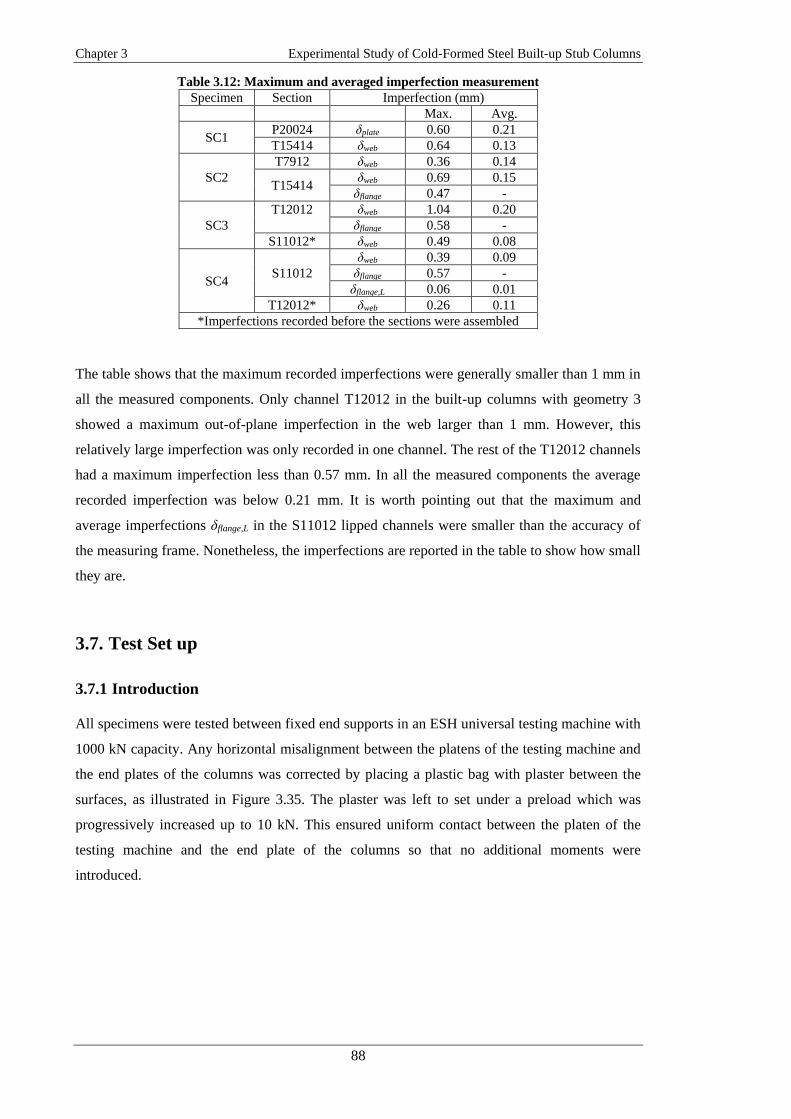
Chapter 3 Experimental Study of Cold-Formed Steel Built-up Stub Columns
88
Table 3.12: Maximum and averaged imperfection measurement
Specimen Section Imperfection (mm)
Max. Avg.
SC1 P20024 δplate 0.60 0.21
T15414 δweb 0.64 0.13
SC2
T7912 δweb 0.36 0.14
T15414 δweb 0.69 0.15
δflange 0.47 -
SC3
T12012 δweb 1.04 0.20
δflange 0.58 -
S11012* δweb 0.49 0.08
SC4 S11012
δweb 0.39 0.09
δflange 0.57 -
δflange,L 0.06 0.01
T12012* δweb 0.26 0.11
*Imperfections recorded before the sections were assembled
The table shows that the maximum recorded imperfections were generally smaller than 1 mm in
all the measured components. Only channel T12012 in the built-up columns with geometry 3
showed a maximum out-of-plane imperfection in the web larger than 1 mm. However, this
relatively large imperfection was only recorded in one channel. The rest of the T12012 channels
had a maximum imperfection less than 0.57 mm. In all the measured components the average
recorded imperfection was below 0.21 mm. It is worth pointing out that the maximum and
average imperfections δflange,L in the S11012 lipped channels were smaller than the accuracy of
the measuring frame. Nonetheless, the imperfections are reported in the table to show how small
they are.
3.7. Test Set up
3.7.1 Introduction
All specimens were tested between fixed end supports in an ESH universal testing machine with
1000 kN capacity. Any horizontal misalignment between the platens of the testing machine and
the end plates of the columns was corrected by placing a plastic bag with plaster between the
surfaces, as illustrated in Figure 3.35. The plaster was left to set under a preload which was
progressively increased up to 10 kN. This ensured uniform contact between the platen of the
testing machine and the end plate of the columns so that no additional moments were
introduced.

Chapter 3 Experimental Study of Cold-Formed Steel Built-up Stub Columns
89
Figure 3.35: Plaster used to correct misalignment between the platen of the machine and the
column end plate
3.7.2 Instrumentation
3.7.2.1 Strain gauges
To monitor whether the load was transmitted uniformly to each component of the column, four
columns –one of each geometry– were instrumented with strain gauges at mid-height. One
strain gauge was placed on each individual component of the built-up columns. In the case of
the channels, the strain gauges were installed at the centre line of the web, whereas for the flat
plate sections the strain gauges were located at mid-width, as illustrated in Figure 3.36. For each
geometry, one of the columns with the least amount of connectors was chosen to be
instrumented. This choice was made because, in case the load was not being transmitted evenly
through the endplate and the resin, these columns had fewer connectors available to transmit the
load from one component to the other and the effects of uneven participation of the various
components would have been most pronounced.
Figure 3.36: Location of strain gauges in a) SC1, b) SC2, c) SC3 and d) column 4
Strain gauges
(a)
Strain gauges
(b)
Strain gauges
(c)
Strain gauges
(d)

Chapter 3 Experimental Study of Cold-Formed Steel Built-up Stub Columns
90
3.7.2.2 Transducers
Two potentiometers, with one placed on each side of the column as illustrated in Figure 3.37,
were used to record the axial shortening of the specimens and monitor that no rotation occurred
at the top end of the specimen. The readings obtained from these two potentiometers were in
close agreement for all specimens, indicating that fixed support conditions were successfully
achieved and that no end rotation took place during the test.
Figure 3.37: Arrangement of LVDTs to measure axial deformation
In addition, for specimens with built-up geometries 1 and 2 another twelve potentiometers with
a stroke of 25 mm were divided over two cross-sections and placed at mid-distance between
connectors. They were used to measure the out-of-plane deformations of the components and
capture the onset of local buckling. Similarly, for specimens with built-up geometries 3 and 4
eight and ten potentiometers, respectively, were placed at two different heights in order to
capture the onset of cross-sectional buckling. For these columns, the potentiometers were placed
at the same relative location in all columns of a certain geometry. This resulted in columns SC3-
2 and SC4-2 having both sets of four potentiometers located between connectors, while columns
SC3-5 had one set of potentiometers located at mid-distance between connectors and the other
set of potentiometers located at a cross-section containing connectors (Figure 3.38). Columns
SC4-5 had both set of potentiometers located within a cross-section containing connectors.
The potentiometers were mounted on a frame which allowed adjustment of their position, as
illustrated in Figure 3.38. The typical layout of the potentiometers for columns SC1 and SC2 is
illustrated in Figure 3.39, while the layout for columns SC3 and SC4 is shown in Figure 3.40.
The figures also show the potentiometer serial number enclosed in a square and the component
number in a circle. At the bottom right of each figure, the vertical position of the potentiometers
along the length of the columns is also indicated. In each pair of numbers associated with one
2
1
Section A Section B
A A
B B
Section A
A A
Section A
A A
2
1 1 1
2 2

Chapter 3 Experimental Study of Cold-Formed Steel Built-up Stub Columns
91
potentiometer in plan view, the lower number corresponds to the lower cross-section along the
column height. For instance, potentiometer 6 was located in the lower part of column 1 whereas
potentiometer 12 was located at mid height (see Figure 3.40a). The layout of the potentiometers
for the other columns is included in Appendix C.
Figure 3.38: a), b), c) and d): Potentiometer frame, e) Potentiometer used to record out-of-plane
deformations, f) LVDTs used to record axial deformation of the column
(f) (e)
(a) (b) (c) (d)

Chapter 3 Experimental Study of Cold-Formed Steel Built-up Stub Columns
92
Figure 3.39: Potentiometer arrangement for a) column 1, b) column 2
Figure 3.40: Potentiometer arrangement for a) column 3, b) column 4
3.7.3 Test procedure
The specimens were tested in an ESH universal testing machine with a capacity of 1000 kN. A
consistent strain rate of 1.7x10⁻⁶ /s was applied to all the specimens. This corresponded to a
displacement rate of 0.112 mm/min for geometries 1, 3 and 4 (with a length of 1100 mm), and
0.082 mm/min for geometry 2 (with a length of 800 mm). The columns with geometries 1 and 2
were compressed up to a deformation of 10 mm while the columns with geometries 3 and 4
were deformed up to 3.5 mm. This was sufficient to observe a significant drop in the load after
the peak load. Each test was halted for 3 min when approaching the peak load in order to
determine the lower bound ‘static’ value of the load without strain rate dependent effects.
2
2 1
1
7
1
2
8
4
10
5
11
6
12
3
9
Section
Transducer
Section
Transducer
7
1
2
8
3
9
4
10
5
11
6
12
21 2
1
11 2
2
3
7
8
4
5
1
6
2
Section
Transducer
9
10
Section
Transducer
9
9
10
3
7
8
4
5
1
6
2
10
(a) (b)
(a) (b)

Chapter 3 Experimental Study of Cold-Formed Steel Built-up Stub Columns
93
The data acquisition system was controlled by a LabView script, which imposed a sampling rate
of 1 Hz.
3.8. Test results
3.8.1 Strain gauge readings
Figure 3.41, Figure 3.42, Figure 3.43 and Figure 3.44 show the readings of the strain gauges
over the course of the test for a column with geometry 1, 2, 3 and 4, respectively, with
compressive strains taken as positive.
For built-up column 1, Figure 3.41 shows that the strains in the channel sections and the flat
plate sections were in good agreement until buckling occurred at a load of 60 kN. Below this
load, the strain in the flat plate sections differed by at most 12 % from the column average,
while this number is 11 % for the channel sections. The readings also show that, typically, the
plates carried slightly less strain compared to the channels for a given load. This may be due to
the initial imperfections present in the plate sections and their relatively low flexural stiffness.
This is also evidenced by Figure 3.55, which shows that the plate sections started to undergo
small out-of-plane deformations from a very early stage (approximately at a load of 10 kN).
These out-of-plane deformations introduced additional flexural tensile strains in the strain
gauges, thus reducing the overall compressive strain.
Figure 3.41: Axial load vs compressive strain in column SC1-2a
With respect to built-up column 2, Figure 3.42 shows a very similar strain response for all
channel sections, with the slight exception of inner channel 1. This channel underwent larger
strains than the other components for a given load, suggesting that it attracted slightly more

Chapter 3 Experimental Study of Cold-Formed Steel Built-up Stub Columns
94
load. The maximum difference in strains between this channel and the other components was
approximately 12 % with respect to their average at a load of 70 kN.
Figure 3.42: Axial load vs compressive strain in column SC2-2a
For built-up column 3, Figure 3.43 shows very good agreement between the strains experienced
by the different components. At a load of 80 kN the maximum difference in strain between the
components was approximately 10 %.
Figure 3.43: Axial load vs compressive strain in column SC3-2a
An even better agreement was achieved between the strains in the components of built-up
column 4, as is seen in Figure 3.44. The maximum difference between the strains in each
component was approximately 5 % at a load of 70 kN.

Chapter 3 Experimental Study of Cold-Formed Steel Built-up Stub Columns
95
Figure 3.44: Axial load vs compressive strain in column SC4-2a
Based on these results, it was concluded that the load was being transmitted with a sufficient
degree of uniformity to all components of the built-up columns. Therefore, the rest of the
columns were tested without strain gauges.
3.8.2 Deformed shape
3.8.2.1 Built-up column 1
All columns with geometry 1 failed by interaction of global buckling of the plate sections
between connectors and local buckling of the channels. Typically, multiple buckling half-waves
were observed along the column in both the plates and the channels. An exception to this
occurred in columns SC1-2, where the plate sections buckled only in the central field in
between the inner sets of connectors and remained straight in the other fields. Every pair of twin
columns showed the same initial buckled shape, although localization of the buckling pattern
often occurred in different locations upon approaching the peak load. Eventually, yield lines
started to appear in both the plates and the channels. Figure 3.45 illustrates the deformed shapes
of the columns just before the peak load was reached. The deformed shape of the columns after
the yield lines were formed are shown in Figure 3.46.
In columns SC1-2, containing the smallest amount of connectors, the observed buckling pattern
most closely reflected the assumptions previously made in section 3.4.1 (Figure 3.45). The flat
plate sections buckled in between connector points with a half-wave length approximately equal
to half the connector spacing. However, the observation that the plate deformations were
concentrated in the central field of the column, with the adjacent fields remaining straight was
unanticipated. Seen the regularity of the buckling pattern in the adjacent channels, it is clear that
a certain amount of bolt slip necessarily occurred in order to make this possible. The channel

Chapter 3 Experimental Study of Cold-Formed Steel Built-up Stub Columns
96
components maintained deformational compatibility with the unbuckled plate sections in the
end fields by the flanges buckling inwards over the whole length of the column with a half-
wave length equal to half of the connector spacing. It is seen from Figure 3.13 that the signature
curve for (unrestrained) local buckling of the channels displays a fairly flat minimum for half-
wave lengths between 140-200 mm. The connector spacing of columns SC1-2, on the other
hand, was 333 mm. While it is expected that the fact that the channel flanges are forced to
buckle inwards slightly extended the natural half-wave length due to the extra bending
necessary in the web, it can be understood from these numbers why the channels adopted a full
wave-length in between connector points. In the post-peak range the channel deformations
localized in the central field, with the buckling pattern largely disappearing in the end fields
(Figure 3.46).
In columns SC1-3, the channel components buckled in a similar way with the flanges bending
inwards. It was clear from the observed deformation pattern, however, that the channels
preferred to adopt a half-wave length slightly beyond half the connector spacing. As shown in
Figure 3.13, the connector spacing in columns SC1-3 stood at 250 mm and, consequently, the
natural local buckle half-wave length of the channels exceeded half the connector spacing by a
noteworthy amount. This extended half-wave length was particularly evident in the two central
fields of the column and was made possible by localized deformations around the connectors.
The flat plate sections buckled outwards in two of the fields with a half wave-length
sympathetic to the one observed in the channels, while they remained largely straight in the
other two fields, prevented from buckling inwards by the presence of the channel webs. In the
latter two fields, the potentiometer readings confirmed negligible out-of-plane deformations.
Similar to columns SC1-2 the post-peak deformations localized in a field where the plates
buckled outwards.
Columns SC1-5 featured a connector spacing of 167 mm, which was approximately equal to the
natural local buckling half-wave length of the channel components. The channels in these
columns were observed to buckle in a completely different way from those in columns SC1-2
and SC1-3. They buckled with a half-wave length equal to the distance between the connectors,
with the flanges alternatingly moving inwards and outwards in successive fields, much like the
unrestrained local buckling pattern. The connector locations corresponded to the nodal lines of
the buckling pattern, implying that they did not undergo any out-of-plane translation, but did
accommodate the plate rotations. The flat plate sections buckled in a shape which completely
followed the flange tips in the fields where those moved outwards, while they remained straight
in the fields where the flange tips moved inwards, prevented from maintaining complete
uniformity by the presence of the channel webs. The readings from the potentiometers again
confirmed that the plates underwent negligible out-of-plane deformations in the regions where
they were visually observed to remain straight. This buckling pattern in the plate sections

Chapter 3 Experimental Study of Cold-Formed Steel Built-up Stub Columns
97
required some localized bending near the connectors. Post-peak localization of the buckled
shape occurred in the central field, where the plate sections initially moved outwards.
Figure 3.45: Deformed shape approaching ultimate load in a) SC1-2a, b) SC1-3a, c) SC1-5a
Figure 3.46: Final deformed shape at end of test in a) SC1-2a, b) SC1-3a, c) SC1-5a
It can be concluded from the above that the buckling pattern in these built-up columns is highly
dependent on the connector spacing.
3.8.2.2 Built-up column 2
Unlike in the columns with geometry 1, where global buckling of one of the components in
between connector points was prevalent, the relevant buckling modes of the components of
(a)
(a) (b) (c)
(c) (b)

Chapter 3 Experimental Study of Cold-Formed Steel Built-up Stub Columns
98
geometry 2 were all local. Geometry 2 aimed to study the interaction between the local buckling
patterns in the inner and outer channels as a result of the presence of the connectors and contact
between surfaces.
Multiple regular buckles were observed along the length of all columns, indicating that the
chosen length of the stub columns was appropriate. Each pair of twin columns showed an
identical buckling pattern. In the vicinity of the ultimate load, the buckling pattern started to
localize and in the post-peak range a yield line mechanism was formed. Figure 3.47 illustrates
the deformed shapes of the columns just before the peak load was reached, while the eventual
yield line patterns are shown in Figure 3.48.
Figure 3.47: Deformed shape approaching ultimate load in a) SC2-2a, b) SC2-4a, c) SC2-6a
(c)
(a) (b)

Chapter 3 Experimental Study of Cold-Formed Steel Built-up Stub Columns
99
Figure 3.48: Final deformed shape at end of test in a) SC2-2a, b) SC2-4a, c) SC2-6a
In the columns with only two rows of intermediate connectors (SC2-2) the buckling half-wave
length of the outer channels coincided with half the distance between the connectors. Due to the
presence of the inner channels, the webs of the outer channels were forced to buckle outwards
(away from the centre of the column). The buckled shape is shown in Figure 3.47a. This
deformation pattern could be expected in the outer channels, as their natural half-wave length
was calculated to be 170 mm, while the connector spacing was 233 mm.
In columns SC2-4 the outer channels buckled with a half-wave length equal to the distance
between the connectors. This buckling pattern is shown in Figure 3.47b. It can easily be
(c)
(a) (b)

Chapter 3 Experimental Study of Cold-Formed Steel Built-up Stub Columns
100
explained when considering the results of a buckling analysis of an unrestrained channel. The
critical stress associated with a half-wave length equal to the distance between connectors is 72
MPa, whereas generating buckles half that length would require a stress level of 124 MPa.
In columns SC2-6 the outer channels were observed to buckle with a varying half-wavelength
along the column. Along part of the specimen height the outer channels buckled with a half-
wave length very close to the distance between connectors. However, this pattern switched to
one in which the outer channels generated a half-wave which spanned almost two fields over an
intermediate connector. This is illustrated in Figure 3.47c. This buckling pattern of the outer
channels can be explained by the fact that neither generating buckles with a half-wave length
equal to the distance between connectors (100 mm) nor buckling with a half-wave length twice
as large resulted in the lowest buckling stresses, as shown from the signature curve of the
channel in Figure 3.14. Instead, the outer channels preferred to buckle with half-wave lengths
slightly larger than 100 mm, while for compatibility that also meant that one of the buckles had
to have a half-wave length slightly shorter than 200 mm. Figure 3.14 shows that this two half-
wave lengths require very similar buckling stresses, and that these buckling stresses are lower
than those required to generate a half-wave length of 100 mm or 200 mm.
In all specimens with geometry 2 the inner channel sections buckled with a half-wave length
equal to half the distance between the connectors. Due to the presence of the outer channel
webs, the flanges of the inner channels were forced to deform towards the inside of the
channels. This pattern occurred in all columns despite the wide range of connector spacings and,
consequently, the wide range of local buckle half-wave lengths in the inner channels, indicating
a high degree of constraint on the inner channels.
3.8.2.3 Built-up column 3
All columns with geometry 3 failed by local buckling, displaying significant interaction
between the individual components. In all cases multiple half-waves were observed along the
column height. In the post-peak range the plastic deformations localized around mid-height in
between two connector rows in all components simultaneously. The only exception to this
occurred in column SC3-2a, where the plastic deformations of one of the plain channels
localized near the bottom of the column at mid-distance between connector rows, while they
localized at mid-height in the rest of components. Figure 3.49 and Figure 3.50 show the
deformed shapes of the columns right before and well after the peak load was reached,
respectively.
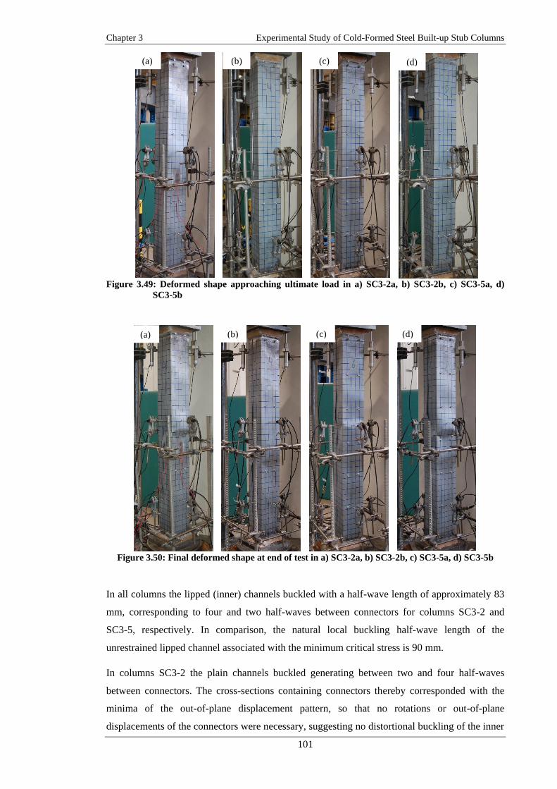
Chapter 3 Experimental Study of Cold-Formed Steel Built-up Stub Columns
101
Figure 3.49: Deformed shape approaching ultimate load in a) SC3-2a, b) SC3-2b, c) SC3-5a, d)
SC3-5b
Figure 3.50: Final deformed shape at end of test in a) SC3-2a, b) SC3-2b, c) SC3-5a, d) SC3-5b
In all columns the lipped (inner) channels buckled with a half-wave length of approximately 83
mm, corresponding to four and two half-waves between connectors for columns SC3-2 and
SC3-5, respectively. In comparison, the natural local buckling half-wave length of the
unrestrained lipped channel associated with the minimum critical stress is 90 mm.
In columns SC3-2 the plain channels buckled generating between two and four half-waves
between connectors. The cross-sections containing connectors thereby corresponded with the
minima of the out-of-plane displacement pattern, so that no rotations or out-of-plane
displacements of the connectors were necessary, suggesting no distortional buckling of the inner
(a) (b) (c) (d)
(a) (c) (b) (d)

Chapter 3 Experimental Study of Cold-Formed Steel Built-up Stub Columns
102
channels. In column SC3-2a the flanges of the outer channels were seen to follow the half-wave
length of the buckles in the web of the inner channels almost perfectly, despite the occurrence of
some irregular buckles in the web of the inner and outer channels (Figure 3.49a). In twin
specimen SC3-2b the flanges of the outer channels did not follow the half-wave length of the
web of the inner channels, causing a more pronounced gap between the inner and outer
channels, as is visible in Figure 3.49b. In this respect, it is also worth noting that the natural
local bucking half-wave length of the plain channels was 130 mm, which was associated with a
critical stress of 64 MPa. Half-wave lengths of 83 mm and 167 mm corresponded to buckling
stresses of 74 MPa and 67 MPa on the local buckling curve, respectively.
A more regular buckling pattern was observed in the plain channels of the columns with five
rows of intermediate connectors. In all columns the web of the plain channels buckled with a
half-wave length equal to half the distance between connectors (83 mm). This occurred despite
the slightly larger buckling stress associated with this wave length in comparison to a wave
length twice as long, and is illustrative of the amount of restraint received by the outer channels.
The plain and lipped channels buckled in near complete sympathy, especially in column SC3-
5b, in which virtually no gap was formed between the flanges of the plain channels and the web
of the lipped channels (Figure 3.49d). In column SC3-5a, on the other hand, the flanges of the
plain channel, being less restrained by the connectors, were displaying a half-wave length closer
to their natural half-wave length, resulting in the formation of some gaps between them and the
web of the lipped channels (Figure 3.49c).
3.8.2.4 Built-up column 4
All columns with built-up geometry 4 failed predominantly by local buckling with some minor
participation of distortional buckling of the lipped channels. Again, multiple local buckling half-
waves were observed along the specimens, indicating that the length of the stub columns was
appropriately chosen. The potentiometer readings indicated that in columns SC4-2a, SC4-2b
and SC4-5a, distortional buckling originated in one of the lipped channels just before the peak
load was reached, while for column SC4-5b distortional buckling originated in both lipped
channels simultaneously. Figure 3.51 illustrates the deformed shape of the columns shortly
before the peak load was reached, while Figure 3.52 shows the failed shapes after localization of
the buckling pattern.

Chapter 3 Experimental Study of Cold-Formed Steel Built-up Stub Columns
103
Figure 3.51: Deformed shape approaching ultimate load in a) SC4-2a, b) SC4-2b, c) SC4-5a, d)
SC4-5b
Figure 3.52: Final deformed shape at end of test in a) SC4-2a, b) SC4-2b, c) SC4-5a, d) SC4-5b
The reader is reminded that geometry 4 contains the same component sections as geometry 3,
but arranged in a different configuration.
In all columns, the lipped channels first buckled in a local mode with a half-wave length of
approximately 83 mm, corresponding to a quarter and half of the connector spacing in
specimens SC4-2 and SC4-5, respectively. As the webs of the plain channels prevented the
webs of the lipped channels from buckling towards the inside of the column, the flanges of the
lipped channels were forced to buckle inwards.
(a) (b) (c) (d)
(a) (b) (c) (d)

Chapter 3 Experimental Study of Cold-Formed Steel Built-up Stub Columns
104
Due to the geometric arrangement of the component sections, direct observation of the buckling
pattern in the plain (inner) sections was difficult. The potentiometers placed on the plain
channels still provided information, however, and their readings will be discussed as part of the
next section.
3.8.3 Critical buckling stresses
This section explains how an estimate of the critical buckling stresses of the various
components was obtained from the potentiometers readings during the test. The potentiometer
readings as a function of the load applied on the column are included in Appendix C for all
tests.
As indicated by the strain gauge readings (previously discussed in Section 3.8.1) the load can be
considered in very good approximation to be uniformly transmitted to the component sections
up to the point of first buckling. The loads at which the various channel sections buckled was
determined by assuming that the stress, when plotted against the initial post-buckling out-of-
plane displacements, follows a parabolic trend, as shown in Figure 3.53a. This has been
confirmed by a perturbation analysis in classical plate theory (Bulson, 1970). The buckling load
was thus found by determining the intersection point of this parabola and the vertical load axis
Figure 3.53: Force against lateral deflection curve for: a) a channel; b) a plate
It is worth pointing out that this parabolic post-buckling trend can be expected to occur only if
the channel is unrestrained while undergoing local buckling. In a built-up column, on the other
hand, the adjacent components of the built-up geometry may prevent the buckles of the channel
from freely developing, and therefore determination of the critical buckling stress of the channel
may become a subjective task. As an example, Figure 3.55 shows the out-of-plane deformations
obtained for column SC1-2a. The load in the column at which the channels sections buckled

Chapter 3 Experimental Study of Cold-Formed Steel Built-up Stub Columns
105
was found to be 76 kN. This value is in good agreement with the value obtained from the strain
gauge readings shown in Figure 3.41 using the strain reversal method (Venkataramaiah and
Roorda, 1982), which is 71 kN. Similar agreements were also obtained for the critical buckling
loads calculated for the channels in the rest of the columns instrumented with strain gauges.
For a plate section, the critical buckling stress due to flexural buckling can be determined using
Euler’s equation for an isolated perfectly flat plate, which is represented by a solid line in Figure
3.53b. If the plate forms part of a built-up specimen, such as in columns LC1, once the plate
buckles the unbuckled components of the cross-section are able to prevent the plate from
collapsing. Therefore, the built-up specimen is able to continue resisting increments of load,
although its axial stiffness is reduced by a certain amount after buckling of the plates. The out-
of-plane deformations of the buckled plate then gradually increase as the rest of the column
deforms axially. The dash-dotted lines in Figure 3.53b show the relationship between the total
load applied to the column and the out-of-plane deformations of the plate, both for the case
where geometric imperfections are included and for the case where they are not. As the figure
shows, the load at which the plate buckles can approximately be determined by projecting a
straight line onto the vertical load axis tangent to the portion of the load vs. lateral deformation
curve in which the rest of the column remains unbuckled. When applying this technique to
Figure 3.55 (corresponding to column SC1-2a), the critical buckling load of the plates is
estimated to be 48 kN. This result does not agree well with the prediction given by the strain
reversal method, which predicts a value of 66 kN. However, this is because the strain reversal
method overestimates the critical buckling load of the plates due to the fact that after the plates
buckle, their out-of-plane deformations are limited by the support provided by the rest of the
column. Consequently, the tensile strains on the surface of the plates due to out-of-plane
bending are relatively small. Figure 3.54 shows the strain gauges readings in column SC1-2a
against the applied load. The figure shows a change in the axial stiffness of the column
(highlighted by the dashed lines) at a load of around 47 kN, which agrees very well with the
predictions of the potentiometers. It is worth noting that the change in stiffness is more obvious
from the readings of the strain gauges attached to the channel sections than from those attached
to the plates. This is due to the introduction of out-of-plane (tensile) bending strains in the strain
gauges attached to the plates which, despite being relatively small, are opposite to the additional
compressive strains resulting from the loss of axial stiffness in the column.

Chapter 3 Experimental Study of Cold-Formed Steel Built-up Stub Columns
106
Figure 3.54: Post-buckling change of stiffness in column SC1-2a recorded with strain gauges
The overall column loads at buckling obtained from the potentiometer readings were then used
to calculate the critical buckling stresses of each component sections by adopting the
assumptions described in Sections 3.8.3.1-3.8.3.4 below for each geometry.
The experimental buckling stresses were compared to the theoretical buckling stresses
calculated based on the measured cross-sectional dimensions (averaged over the two
components in the cross-section) and using the Young’s modulus obtained from the flat tensile
coupons. The theoretical buckling stresses were obtained while considering the individual
components in isolation, without any interaction with the rest of the cross-section, and whenever
possible adopting the buckle half-wave length observed during the test, which was estimated
based on the number of half-waves counted between connectors. For the plain and lipped
channel sections, the theoretical critical buckling stresses were obtained using the CUFSM 4.05
software (Schafer, 2006), while for the plate sections in columns SC1, the critical buckling
stresses were determined using Euler’s equation:
2 2
212cr
p
Et
L
(3.31)
In the above Eq. (3.31), E is the Young’s modulus, t is the averaged measured thickness of the
two plate sections in the column and Lp is the buckle half-wave length.
3.8.3.1 Built-up column 1
In built-up columns SC1-2 and SC1-3, the plate sections buckled in a flexural mode before
buckling of the channel sections occurred, while simultaneous buckling of the channel and plate
sections was observed in columns SC1-5. The buckling stress of the plate sections was thus
obtained by dividing the column load over the total area of the built-up section. As the plates

Chapter 3 Experimental Study of Cold-Formed Steel Built-up Stub Columns
107
buckled in a global mode, it is a reasonable assumption due to the lack of post-buckling capacity
in the global flexural mode, that after buckling of the plates any increase in load would be
resisted entirely by the channels. Consequently, this allowed an estimate of the buckling stress
of the channels based on the total column load.
In Figure 3.55 the readings from the potentiometers show that, due to the effect of initial
imperfections, a gradual increase of the out-of-plane deformation occurred from the onset of
loading (as opposed to sudden bifurcation of the equilibrium path in a perfectly flat plate). The
effect of initial imperfections was generally more significant in the plate sections than in the
channel sections. This can be attributed to the low flexural rigidity of the plate sections.
Figure 3.55: Axial load vs lateral displacements in SC1-2a
Table 3.13 shows the theoretical critical buckling stresses of the channels and the plates, and
compares them to the ones obtained from the tests. An upper and a lower bound were defined
for the theoretical buckling stresses of the plate sections. The upper bound corresponds to a
half-wave length (effective length) equal to half the spacing between connectors, whereas the
lower bound corresponds to a half-wave length equal to the distance between connectors.
Table 3.13: Buckling stresses of the components of geometry 1
Column
Theoretical buckling stress
(MPa)
Buckling stress
from test (MPa)
Channel Plate
Channel Plate Lower Upper
SC1-2a 71 9 35 65 28
SC1-2b 71 9 36 72 19
SC1-3a 76 16 64 70 46
SC1-3b 75 16 64 69 45
SC1-5a 70 36 144 69 69
SC1-5b 69 36 145 67 67

Chapter 3 Experimental Study of Cold-Formed Steel Built-up Stub Columns
108
The table shows that for columns SC1-2 the plate sections buckled before the channels and their
experimental buckling stresses were intermediate between the theoretical lower and upper
bounds. This agrees with the experimentally observed buckled shape, in which the plates were
forced by the channels web to buckle outwards. The channels, on the other hand, buckled at a
stress very close to the theoretically predicted value (and which was around 4 % lower). This
suggests that the channels were not significantly affected by any restraint provided by the
buckled plates.
In columns SC1-3 the plates also buckled before the channels, which differed from the
theoretical prediction that the plates would buckle at the same time as the channels. This can be
explained by the experimental observation (Figure 3.45c) that the plates buckled with a half-
wave length larger than half the connector spacing, contrary to what was initially assumed. The
experimentally derived plate buckling stresses agreed with this observation, showing that the
plates buckled at a stress which was around 29 % below the theoretical upper bound. The
experimentally derived buckling stress of the channels was around 15 % lower than the
theoretically predicted value, which was calculated for a half-wave length equal to half the
connector spacing. This may be attributed to the fact that the channels buckled with a slightly
larger half-wave length, as described in Section 3.8.2.1.
In columns SC1-5, the channels and the plates were observed to buckle simultaneously in the
experiment. The plate sections buckled at a stress well below the theoretical upper bound value
(around 53 % lower), but almost twice as high as the theoretical lower bound. Neither
theoretical assumption bore much resemblance to the actual deformed shape, where the plates
buckled outwards with a half-wave length roughly equal to the connector spacing, but were
restrained from buckling inwards, resulting in localized bending around the connectors. The
experimentally obtained buckling stress of the channels was approximately the same as the
theoretical value, indicating that the channel sections were not significantly affected by the plate
sections while trying to buckle in the observed pattern.
3.8.3.2 Built-up column 2
All components of built-up column 2 failed by local buckling. The local mode has significant
post-buckling load-bearing capacity, however at the cost of a significantly reduced axial
stiffness. Consequently, the relative distribution of the additional load over the column
components after the first component buckles becomes a non-trivial problem. Therefore, only
the critical buckling stress of the outer channels was determined from the experimental results
(as they were the first components to buckle in all the columns) and was obtained by dividing
the column load at which buckling was observed by the total cross-sectional area of the column.

Chapter 3 Experimental Study of Cold-Formed Steel Built-up Stub Columns
109
In all but one column local buckling was observed nearly simultaneously in both outer channels.
In column SC2-2a, however, the two outer channels buckled at slightly different loads, as
shown in Figure 3.56. Both channel sections also initiated buckling in different locations along
the height: one channel buckled first between the connectors at mid-height of the column,
followed by buckling near the bottom, whereas the other channel buckled first near the bottom
of the column and then at mid-height. This might have been due to the effect of imperfections or
the effect of contact between the components. In column SC2-4a one of the outer channels was
recorded to buckle slightly before the other, as shown in Figure 3.57. For both columns, both
buckling stresses are listed in Table 3.14.
Figure 3.56: Axial load vs lateral displacements in SC2-2a
Figure 3.57 Axial load vs lateral displacements in SC2-4a
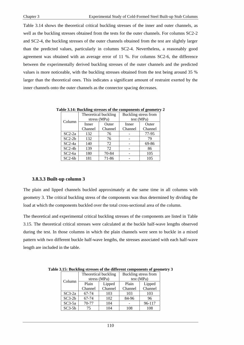
Chapter 3 Experimental Study of Cold-Formed Steel Built-up Stub Columns
110
Table 3.14 shows the theoretical critical buckling stresses of the inner and outer channels, as
well as the buckling stresses obtained from the tests for the outer channels. For columns SC2-2
and SC2-4, the buckling stresses of the outer channels obtained from the test are slightly larger
than the predicted values, particularly in columns SC2-4. Nevertheless, a reasonably good
agreement was obtained with an average error of 11 %. For columns SC2-6, the difference
between the experimentally derived buckling stresses of the outer channels and the predicted
values is more noticeable, with the buckling stresses obtained from the test being around 35 %
larger than the theoretical ones. This indicates a significant amount of restraint exerted by the
inner channels onto the outer channels as the connector spacing decreases.
Table 3.14: Buckling stresses of the components of geometry 2
Column
Theoretical buckling
stress (MPa)
Buckling stress from
test (MPa)
Inner
Channel
Outer
Channel
Inner
Channel
Outer
Channel
SC2-2a 132 76 - 77-95
SC2-2b 132 76 - 79
SC2-4a 140 72 - 69-86
SC2-4b 139 72 - 86
SC2-6a 180 70-84 - 105
SC2-6b 181 71-86 - 105
3.8.3.3 Built-up column 3
The plain and lipped channels buckled approximately at the same time in all columns with
geometry 3. The critical buckling stress of the components was thus determined by dividing the
load at which the components buckled over the total cross-sectional area of the column.
The theoretical and experimental critical buckling stresses of the components are listed in Table
3.15. The theoretical critical stresses were calculated at the buckle half-wave lengths observed
during the test. In those columns in which the plain channels were seen to buckle in a mixed
pattern with two different buckle half-wave lengths, the stresses associated with each half-wave
length are included in the table.
Table 3.15: Buckling stresses of the different components of geometry 3
Column
Theoretical buckling
stress (MPa)
Buckling stress from
test (MPa)
Plain
Channel
Lipped
Channel
Plain
Channel
Lipped
Channel
SC3-2a 67-74 103 103 103
SC3-2b 67-74 102 84-96 96
SC3-5a 70-77 104 - 96-117
SC3-5b 75 104 108 108

Chapter 3 Experimental Study of Cold-Formed Steel Built-up Stub Columns
111
In column SC3-2a the channels were observed to buckle at a stress level of approximately 103
MPa. This stress is very close to the theoretically predicted buckling stress of the lipped
channel, while it is around 39 % higher than the highest theoretical buckling stress predicted for
the plain channel. This indicates that the plain channels clearly benefited from the restraint
provided by the lipped channels. A similar conclusion can be drawn for the twin specimen SC3-
2b, although in this case one of the potentiometers placed near the bottom of the column
detected the onset of local buckling in one of the plain channels at a slightly lower stress level.
The rest of potentiometers, however, detected local buckling of the components at a stress level
of 96 MPa, which was around 30 % higher than the stress predicted for the plain channels and
6% lower than the stress predicted for the lipped channels.
In column SC3-5b local buckling occurred at a stress level very close to the predicted value for
the lipped channels, and around 44 % larger than the predicted value for the plain channels. In
column SC3-5a local buckling was first detected in the lipped channels by the potentiometers at
mid-height of the column at a stress level of 96 MPa and subsequently by the potentiometers
near the bottom at a stress level of 117 MPa (Figure 3.58). These stresses are relatively close to
the predicted buckling stress of the lipped channels. However, compared to its twin specimen an
anomaly was observed in that the plain channels (which have the lower theoretical buckling
stress) remained unbuckled up to a stress level of 117 MPa. However, as soon as the plain
channels buckled, the lipped channels were forced to adjust and reverse the initial directions of
some of their out-of-plane deformations in order to accommodate local buckling of the plain
channels (Figure 3.58).
Figure 3.58: Axial load vs lateral displacements in SC3-5a

Chapter 3 Experimental Study of Cold-Formed Steel Built-up Stub Columns
112
3.8.3.4 Built-up column 4
In columns SC4-2, the plain channels buckled before the lipped channels, while in columns
SC4-5 all the components buckled at approximately the same time. Consequently, the
experimental buckling stresses of the lipped channels of columns SC4-5, as well as the
experimental buckling stresses of the plain channels of all columns were determined by dividing
the load at which the components buckled over the total area of the cross-section.
Table 3.16 lists the theoretical and experimental buckling stresses of the different components
of the columns with geometry 4. As the buckle half-wave length of the plain channels could not
be directly observed during the tests due to the geometric arrangement, theoretical buckling
stresses associated with buckle half-wave lengths of 167 mm and 83 mm were included in the
table. These values correspond to the plain channels generating two and four half-waves
between connectors in columns SC4-2, respectively, or one and two half-waves between
connectors in columns SC4-5. These assumed values are close to the natural local buckle half-
wave length of 130 mm, and consistent with the observations in the (geometrically identical)
plain channels of columns SC3.
Table 3.16: Buckling stresses of the different components of geometry 4
Column
Theoretical buckling
stress (MPa)
Buckling stress from
test (MPa)
Plain
Channel
Lipped
Channel
Plain
Channel
Lipped
Channel
SC4-2a 66-73 100 87 -
SC4-2b 66-72 100 88 -
SC4-5a 66-73 105 73-91 91
SC4-5b 69-76 103 93-104 104
For specimens SC4-2, Table 3.16 shows that the plain channels buckled at a stress level which
is around 21 % higher than the highest predicted value for the assumed buckle half-wave
lengths. This is due to the restraint exerted by the lipped channels, which force the flanges of the
plain channels to buckle inwards.
For specimens SC4-5, the plain and lipped channels buckled, in general, at approximately the
same stress level. However, it should be noted that some potentiometers recorded buckling in
the plain channels at slightly lower stresses compared to the lipped channels, as shown in Figure
3.59 for column SC4-5b. This does not alter the overall conclusion, however, that the plain
channels buckled at stresses which were around 25 % higher than the predicted ones, while the
lipped channels buckled at stresses which were up to 13 % lower than the predicted ones. This
again illustrates that the plain channels benefited from the restraint provided by the lipped
channels, while the plain channels as a result of their buckling deformations played a role in
initiating buckling in the lipped channels.

Chapter 3 Experimental Study of Cold-Formed Steel Built-up Stub Columns
113
Figure 3.59: Axial load vs lateral displacements in SC4-5b
3.8.4 Ultimate load
Figure 3.60 shows a typical load-axial shortening curve (SC2-4a). The figure also shows (in
red) the equivalent ‘static’ curve, obtained by eliminating strain rate dependent effects. The red
curve was obtained by scaling down the load values outside the elastic range using the observed
settlement in the load after halting the test close to the ultimate load.
Figure 3.61, Figure 3.62, Figure 3.63 and Figure 3.64 plot the (static) load vs. axial
displacement curves of all columns with geometries SC1, SC2, SC3 and SC4, respectively. It is
worth pointing out the marked decrease in the stiffness of the columns SC1 after first buckling
of one of their components takes place, compared to the more gradual decrease in stiffness
observed in the columns with geometries SC2, SC3 and SC4. This decrease in stiffness
experienced by columns SC1 can be explained by the fact that the cross-sectional area of the
plate sections contributed 57 % to the total cross-sectional area of the built-up column while,
after buckling in a global flexural mode, these sections were unable to contribute in resisting a
further increase in load.
The ultimate loads obtained for all the columns with geometries SC1, SC2, SC3 and SC4 are
listed in Table 3.17, Table 3.18, Table 3.19 and Table 3.20, respectively. The tables include
both the ‘dynamic’ and the ‘static’ ultimate loads, together with the averaged values for each set
of twin columns.
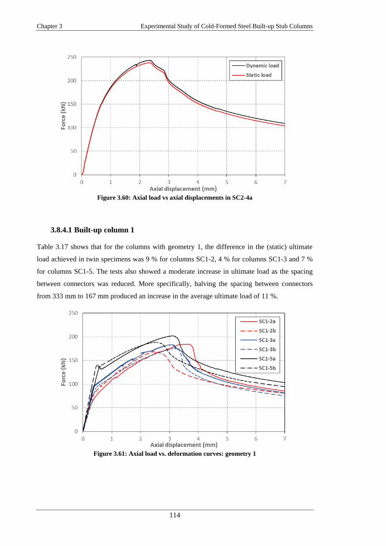
Chapter 3 Experimental Study of Cold-Formed Steel Built-up Stub Columns
114
Figure 3.60: Axial load vs axial displacements in SC2-4a
3.8.4.1 Built-up column 1
Table 3.17 shows that for the columns with geometry 1, the difference in the (static) ultimate
load achieved in twin specimens was 9 % for columns SC1-2, 4 % for columns SC1-3 and 7 %
for columns SC1-5. The tests also showed a moderate increase in ultimate load as the spacing
between connectors was reduced. More specifically, halving the spacing between connectors
from 333 mm to 167 mm produced an increase in the average ultimate load of 11 %.
Figure 3.61: Axial load vs. deformation curves: geometry 1

Chapter 3 Experimental Study of Cold-Formed Steel Built-up Stub Columns
115
Table 3.17: Ultimate loads: geometry 1
Column
Ultimate load
(kN)
Averaged Ultimate load
(kN)
Dynamic Static Dynamic Static
SC1-2a 190.47 183.97 181.56 176.07
SC1-2b 172.65 168.17
SC1-3a 193.01 183.01 189.44 179.44
SC1-3b 185.86 175.86
SC1-5a 208.60 201.72 201.94 195.11
SC1-5b 195.28 188.50
3.8.4.2 Built-up column 2
In the columns with geometry 2 good agreement was again obtained between the results of twin
specimens, as shown in Table 3.18. The difference in ultimate load was 6 % for columns SC2-2,
2 % for columns SC2-4 and 5 % for columns SC2-6. In this case the tests showed that reducing
the spacing between connectors did not necessarily result in a noticeable increase in ultimate
load. For example, the columns with a connector spacing of 140 mm (columns SC2-4) showed
marginally higher ultimate loads than columns with connectors spaced every 100 mm (columns
SC2-6). However, the largest connector spacing (233 mm) did result in an evidently lower
ultimate load, which was on average 9 % below that of the SC2-6 columns.
Figure 3.62: Axial load vs. deformation curves: geometry 2
Table 3.18: Ultimate loads: geometry 2
Column
Ultimate load
(kN)
Averaged Ultimate load
(kN)
Dynamic Static Dynamic Static
SC2-2a 227.46 213.32 220.97 206.83
SC2-2b 214.47 200.34
SC2-4a 243.00 238.00 241.20 235.70
SC2-4b 239.39 233.39
SC2-6a 226.24 220.54 232.18 226.58
SC2-6b 238.12 232.62

Chapter 3 Experimental Study of Cold-Formed Steel Built-up Stub Columns
116
3.8.4.3 Built-up column 3
Table 3.19 shows that the difference in ultimate load between twin specimens was 3 % for
columns SC3-5 and just 1 % for columns SC3-2. The results also show that halving the
connector spacing from 333 mm to 167 mm only resulted in a negligible increase in ultimate
capacity of 2 %.
Figure 3.63: Axial load vs. deformation curves: geometry 3
Table 3.19: Ultimate loads: geometry 3
Column
Ultimate load
(kN)
Averaged Ultimate load
(kN)
Dynamic Static Dynamic Static
SC3-2a 142.90 139.30 142.32 138.92
SC3-2b 141.73 138.53
SC3-5a 142.07 138.77 144.03 141.08
SC3-5b 146.00 143.40
3.8.4.4 Built-up column 4
With respect to columns SC4, Table 3.20 shows that the difference in ultimate load between
twin specimens was 3 % for columns SC4-5 and 0.7 % for columns SC4-2. In this case,
reducing the connector spacing actually resulted in a slight reduction in the ultimate capacity.
More specifically, halving the connector spacing from 333 mm to 167 mm caused a reduction in
the ultimate capacity of 6 %. The difference is quite marginal and might be due to the statistical
variation of the relevant parameters (imperfections, geometry, material properties, etc.).
Whether this is the case or not will be further investigated using detailed finite element models
in following chapters.

Chapter 3 Experimental Study of Cold-Formed Steel Built-up Stub Columns
117
Figure 3.64: Axial load vs. deformation curves: geometry 4
Table 3.20: Ultimate loads: geometry 4
Column
Ultimate load
(kN)
Averaged Ultimate load
(kN)
Dynamic Static Dynamic Static
SC4-2a 150.29 148.09 149.61 147.56
SC4-2b 148.93 147.03
SC4-5a 144.13 141.23 142.69 139.49
SC4-5b 141.24 137.74
3.9. Summary and conclusions
An experimental program was carried out consisting of 20 built-up thin-walled stub columns
with four different cross-sectional geometries. The cross-sections were assembled from flat
plate, plain channels and lipped channels with nominal thicknesses ranging from 1.2 mm to 2.4
mm. Two of the cross-sectional geometries (SC1 and SC2) were assembled using M6 bolts,
while the other two (SC3 and SC4) were assembled using M5.5 self-drilling sheet metal screws.
The connector spacing was varied among specimens of the same cross-sectional geometry.
The experimental investigation included tensile coupon tests to determine the material
properties of the flat portions and the corner regions of the different components. Accurate
measurements of the out-of-plane geometric imperfections of the specimens were also carried
out using a laser sensor.
The columns were compressed between fixed supports in a displacement controlled regime.
Strain gauge readings obtained from a select number of specimens confirmed a uniform
introduction of the load into all components of the cross-sections. This was achieved thanks to

Chapter 3 Experimental Study of Cold-Formed Steel Built-up Stub Columns
118
hand-filing the end sections, placing a double row of connectors at the specimen ends and
epoxy-gluing the end plates to the specimens.
The out-of-plane deformations of each column component were recorded during the test using
potentiometers. This allowed, in most cases, a determination of the stress at which buckling
occurred in the components. These values were compared to theoretical predictions which
considered the individual components in isolation without any interaction with the rest of the
cross-section, but used the experimentally observed wave-lengths.
The following conclusions could be drawn from the experimental investigation:
It was clear from the observations of the deformed column shapes that the buckling
patterns of the individual components within the columns were subject to considerable
restraint. This restraint manifested itself in two different ways: (1) a change in the
natural local buckle half-wave length to accommodate the presence of the connectors,
and (2) contact between adjacent surfaces forcing the buckling out-of-plane
displacements to occur in a certain direction.
Substantially different buckling patterns were generally observed in columns with the
same cross-sectional geometry, but different connector spacing.
Out of all the possible buckling patterns allowed by the constraints imposed by the
connectors and contact with the rest of the column, the components choose the one
which required the lowest buckling stresses. This resulted in some cases in a buckling
pattern with a varying half-wave length along the member, as was observed in the outer
channels of columns SC2-6, or in a buckling pattern isolated in one field, as seen in the
plate sections of columns SC1-2 and SC1-3. The latter was only possible after some slip
between the components at the connector points.
By comparing the theoretical predictions of the buckling stresses to the experimentally
measured values it was observed that the buckling stress of the most slender
components was increased by up to 44 % as a result of the restraint provided by the
remainder of the cross-section. The amount of restraint was seen to be dependent on the
connector spacing. The less slender components, on the other hand, generally showed
buckling stresses which ranged from being 30 % lower than the predicted values to
being very close to the theoretical value.
Although the buckling deformations and the buckling stresses of the component
sections showed considerable dependence on the connector spacing, the ultimate
capacity showed much less sensitivity:
o Columns SC1 exhibited a modest increase in the ultimate strength of around 11
% when halving the connector spacing. This gain was mainly a result of the

Chapter 3 Experimental Study of Cold-Formed Steel Built-up Stub Columns
119
increase in the global flexural buckling capacity of the plate sections in between
connectors.
o When the critical buckling modes of the individual components were all local,
the difference was even smaller. Only the SC2-2 columns showed 11 % less
capacity than the SC2-4 and SC2-6 columns, which had similar capacities. For
geometries 3 and 4, the effect of the connector spacing was negligible or non-
existent.
o Geometries 3 and 4, which were assembled from individual components with
identical nominal dimensions using the same connector type and spacing,
allowed a direct comparison with respect to the effect of their relative
arrangement. However, both geometries achieved similar capacities. For the
specimens with two intermediate connectors, columns SC3 showed an ultimate
capacity which was on average 6 % lower than the one achieved by columns
SC4, while for the specimens with five intermediate connectors the ultimate
capacities were within 1 % of each other.

Chapter 3 Experimental Study of Cold-Formed Steel Built-up Stub Columns
120

Chapter 4 Experimental Study of Cold-Formed Steel Built-up Beams
121
Chapter 4
Experimental Study of Cold-Formed Steel
Built-up Beams
4.1. Introduction
The experimental programme described in this chapter intended to investigate the cross-
sectional bending moment capacity of two different built-up thin-walled beams. Particular
attention was devoted to the way in which the individual components of the cross-section
interacted with each other as they underwent local buckling. The specimens were tested in a 4-
point bending configuration, with point loads applied 1600 mm apart. This length was long
enough to allow the component sections to generate several buckles along the constant moment
span. Lateral-torsional buckling was excluded as a failure mode by means of lateral supports.
All specimen preparation, assembly and testing was carried out in the Heavy Structures
Laboratory at The University of Sheffield.
The test specimens were assembled using commercially available cold-formed steel sections,
supplied by BW Industries. All sections were manufactured from pre-galvanized steel plates
with a nominal 0.04 mm Z275 zinc coating and a guaranteed yield strength of at least 450 MPa.
The two built-up cross-sectional geometries are illustrated in Figure 4.1. The first built-up
section consisted of two channels with a nominal depth of 129 mm and thickness of 1.5 mm,
which were connected back-to-back, and two extra channels with a nominal depth of 104 mm
and thickness of 1.2 mm, which were attached to the flanges of the back-to-back channels. The
second built-up geometry was assembled using three channels. Two channels with a nominal
depth of 129 mm and thickness of 1.5 mm were connected back-back and a channel with a
nominal depth of 104 mm and 1.2 mm thickness was attached to the top flanges of the back-to-
back channels with its flanges facing upward. Grade 8.8 M6 bolts were used to join the
individual sections together in both geometries. Each built-up geometry was tested with three
different connector spacings and each test was repeated, accounting for a total of 12 tests. The
geometric imperfections of all specimens were recorded prior to the test. Coupon tests were also

Chapter 4 Experimental Study of Cold-Formed Steel Built-up Beams
122
extracted from the flat portions and the corners regions of each different components in order to
determine their material properties.
Figure 4.1: Built-up cross-sections
4.2. Labelling
The labelling used to refer to the cross-sectional components is consistent with the one used for
the stub columns: the channel sections are identified using the letter ‘T’ followed by the nominal
width of their web in mm and their nominal thickness in mm multiplied by 10.
The built-up specimens are labelled using the letter ‘B’ followed by the number 1 or 2,
indicating the geometry with reference to Figure 4.1. Then, following a hyphen, the number of
intermediate rows of connectors between the loading points is indicated. Finally, since each test
was repeated, the letter ‘a’ and ‘b’ are used to differentiate between twin test specimens. As an
example, the label ‘B1-2a’ refers to the first beam tested with cross-sectional geometry 1 which
has connectors at two intermediate cross-sections along the constant moment span.
4.3. Material Properties
A series of coupon tests were carried out in order to determine the material properties of the
beams. The coupons were cut along the rolling direction (i.e. the longitudinal direction of the
beams) near the end section of one of the test specimens after testing. This location was chosen
since the material had not been subject to significant stress during the test. For each type of
channel section, two flat coupons were cut along the centre line of the web and two corner
coupons were taken from the web-flange junction. Therefore, eight coupons were tested in total.
The dimensions of all coupons follow the specifications set in CEN (2009).
Built-up section 1 Built-up section 2
T12915
T10412
T12915T10412

Chapter 4 Experimental Study of Cold-Formed Steel Built-up Beams
123
4.3.1 Flat coupons
The flat coupons had the same nominal dimensions as those used to determine the material
properties of the stub columns, and they were masured and intrumented in the same way, as
described in Section 3.3.1 of Chapter 3. Figure 4.2 shows a flat coupon during testing, while
Table 4.1 lists the measured width and thickness of the coupons. The letters ‘a’ and ‘b’ are used
to differentiate between twin coupons.
Figure 4.2: Flat coupon during testing
Table 4.1: Measured dimensions of flat coupons
Component
section Coupon
bc
(mm)
t
(mm)
A
(mm2)
T10412 a 12.484 1.141 14.2962
T10412 b 12.480 1.146 14.3325
T12915 a 12.482 1.501 18.7355
T12915 b 12.481 1.484 18.5218
4.3.2 Corner coupons
The corner coupons had a nominal width of 6 mm. The nominal dimensions of the coupons are
illustrated in Figure 4.3. They were intrumented in the same way as the corner coupons taken
from the stub columns and were tested using the same arrangement, as described in Section
3.3.2. Figure 4.4 shows the corner coupons during testing.

Chapter 4 Experimental Study of Cold-Formed Steel Built-up Beams
124
Figure 4.3: Corner coupon dimensions
Figure 4.4: Pair of corner coupons during testing
The cross-sectional area of the corner coupons along the gauge length was determined by
following the thechnique previously described in Section 3.3.2 of Chapter 3, which involves
taking a macro-photograph of the coupon cross-section from each end. The photographs taken
from each end of the coupon provided two cross-sectional areas per coupon, which were
averaged. Differences of less than 1.42 % and 1.08 % were observed between the calculated
areas obtained from each end of coupons T10412 and T12915, respectively. Table 4.2 lists the
area obtained for each corner coupon after accounting for the (nominal) thickness of the zinc
coating.
Table 4.2: Measured area of corner coupons
Component
section
Coupon
number
A
(mm2)
T10412 a 7.9821
T10412 b 7.9549
T12915 a 10.4495
T12915 b 10.4286
145
10
40 40
6
57
6
Dimensions in mm

Chapter 4 Experimental Study of Cold-Formed Steel Built-up Beams
125
As in the flat coupons, the readings from the extensometer were used to obtain the average
stress-strain curve of each pair of coupons, while the readings from the strain gauges were used
to calculate the Young’s modulus.
4.3.3 Coupon testing and results
The tensile coupons were tested in a 300 kN Shimadzu AGS-X universal testing machine
controlled in displacement mode. A displacement rate of 2 mm/min was used for all coupon
tests.
Each test was halted for 2 minutes at regular intervals in order to allow the load to settle down
to ‘static’ values and eliminate strain rate effects. The ‘dynamic’ stress-strain curve obtained
from the test was then used to generate a static stress-strain curve from which the material
properties were derived. As an example, Figure 4.5 shows the stress-strain curve of the pair of
corner coupons cut from channel T12915. The figure also includes the static true stress-strain
curve, which was used to define the material properties in a numerical Abaqus model. The
stress-strain curves of all the tested coupons are included in Appendix D.
Figure 4.5: T12915 Corner coupon test results
Table 4.3 illustrates the (static) engineering values of the material properties obtained for each
coupon, as well as the averaged values. In the table, (σ0.2%) corresponds to the 0.2% proof stress,
(σu) is the ultimate tensile strength and (εf) is the elongation after fracture measured over a gauge
length of 50 mm.

Chapter 4 Experimental Study of Cold-Formed Steel Built-up Beams
126
Table 4.3: Material properties of tensile coupons
Type Section
E
(GPa)
σ0.2%
(MPa)
σu
(MPa)
εf
(%)
Ind. Avg. Ind. Avg. Ind. Avg. Ind. Avg.
Flat T10412-a 212 208
432 426
471 466
14 14
Flat T10412-b 204 419 461 14
Flat T12915-a 201 204
544 531
628 619
13 13
Flat T12915-b 207 518 610 12
Corner T10412-a 193 198
- 460
- 479
- 3
Corner T10412-b 202 - - -
Corner T12915-a 211 218
- 585
- 645
- 5
Corner T12915-b 225 - - -
The results confirmed that the steel grade used to fabricate the channels was at least S450, as
specified by the manufacturer. Although the values of the 0.2 % proof stress listed in the table
for the flat coupons taken from sections T10412 are smaller than 450 MPa, this can be attributed
to the fact that these values correspond to the static 0.2 % proof stress, and not the dynamic 0.2
% proof stress, which is normally used to determine the grade of the steel. The dynamic values
of the 0.2 % stress obtained from all the tensile coupons were larger than 450 MPa.
It is also important to mention that the steel grade of section T12915 is considerably larger than
the minimum specified by the manufacturer, with the flat coupons extracted from these sections
showing an averaged static 0.2 % proof stress of 531 MPa.
4.4. Section Design and geometry
Two different built-up cross-sectional geometries were chosen for testing, as illustrated in
Figure 4.1. The first geometry was chosen because it resembles the traditional I-shaped cross-
section widely used for beams in construction. In addition to the traditional back-to-back
channel arrangement this built-up geometry included two additional channels to increase the
flange area and provide increased bending capacity. The second built-up geometry was selected
in consultation with cold-formed steel manufacturers/contractors, who indicated that this built-
up geometry is regularly used as a solution to bridge large openings in structural framing
systems made of cold-formed steel. The back-to-back channels thereby work as a lintel, while
the top channel is used as a track to receive the studs of the wall above the opening. Due to lack
of design guidance, however, only the capacity of the back-to-back channels is currently
counted on in practice.
In addition to the connectors placed in the cross-sections under the loading points, specimens
were designed with zero, two and three equally spaced connectors within the constant moment
span. Two identical beams were fabricated for each configuration in order to gain increased
confidence in the results. All beams were designed to fail by local buckling of the individual
components, without any influence of global instability of the beam. The shear span length was

Chapter 4 Experimental Study of Cold-Formed Steel Built-up Beams
127
chosen as 700 mm. This was determined to be long enough to avoid premature shear failure in
the webs of the built-up specimens. The component sections were bolted together in this region
with a connector spacing of 100 mm to encourage even load sharing and as an extra safety
measure against shear buckling in the webs of the built-up specimens, as shown in Figure 4.10
and Figure 4.11 for specimens with built-up geometry 1 and 2, respectively. The nominal
dimensions of the cross-sections are listed in Table 4.4. The symbols in the table refer to the
dimensions of the individual channels, as clarified in Figure 4.6.
Figure 4.6: Nomenclature used to refer to the dimensions of the component sections
Table 4.4: Nominal dimensions of the component sections
Beam Section h
(mm)
b
(mm)
t
(mm)
rint
(mm)
B1 T12915 129 48 1.5 3.0
T10412 104 42 1.2 2.4
B2 T12915 129 48 1.5 3.0
T10412 104 42 1.2 2.4
The built-up specimens were designed with the help of an elastic stability analysis using the
CUFSM 4.05 software (Schafer, 2006). Each component was analysed individually (without
interaction with the other components), but under a linear stress gradient consistent with the
assumption that the whole cross-section remained plane under pure bending (no slip in the
connectors). Figure 4.7 illustrates the stress distribution used as input in CUFSM 4.05 for each
component. In addition, the connectors were assumed not to translate or rotate while the
component sections buckled. Therefore, the individual components were only allowed to rotate
with respect to each other at the connector location about an axis aligned with the connector
axis.
h
b
r int
t

Chapter 4 Experimental Study of Cold-Formed Steel Built-up Beams
128
Figure 4.7: Stress distribution within component sections for elastic stability analysis
Figure 4.8 and Figure 4.9 show the critical buckling stress vs. the buckle half-wave length of the
components of geometries 1 and 2, respectively. The critical stresses in these diagrams represent
the maximum compressive stresses in the full cross-section, in order to allow a fairer
comparison and evaluate which component of the built-up cross-section is likely to buckle first.
Thus, in Figure 4.8, the vertical axis represents the stress in the web of the channel which forms
the top flange of geometry 1 (T10412), whereas in Figure 4.9 it is the stress at the tip of the
flanges of the top channel in geometry 2. Figure 4.8 shows that the critical local buckle half-
wave length of both types of channels in geometry 1 is 110 mm. Figure 4.9, on the other hand,
shows that in geometry 2 the critical half-wave lengths are 120 mm for the top channel and 110
mm for the web channels.
Based on the assumption that the connectors do not translate or rotate as the components buckle,
an expected buckle half-wave length can be determined depending on the number of buckles
that can geometrically fit between connectors. Of all possible solutions, the one that corresponds
to the lowest bucking stress in the signature curve is the most likely to occur. For instance, in
the beams with 3 rows of intermediate connectors (corresponding to a connector spacing of 375
mm), the lowest critical buckling stress is achieved if four half-waves with a length of 94 mm
occur between connectors. This conclusion applies equally to all component channels of
geometries 1 and 2. Similarly, in the beams with 2 rows of intermediate connectors, four half-
waves of 125 mm are expected. In the beams without intermediate connectors, 14 half-waves
are anticipated in the components of geometry 1, while in geometry 2 the top channel and the
0.364
1.000 1.000
0.364
0.9790.979
-0.979-0.979
1.000 1.000
0.5290.529
0.5130.513
-0.938-0.938
Top channel Top channel
Web channel Web channel
Built-up geometry 1 Built-up geometry 2

Chapter 4 Experimental Study of Cold-Formed Steel Built-up Beams
129
web channels are expected to display 12 and 14 half-waves between the loading points,
respectively.
The elastic stability analysis also indicated that interaction between local and global buckling of
the top channel might occur in both geometries with zero intermediate connectors provided that
the global buckling stress of the locally buckled section falls below the point at which the
ultimate capacity of the beam is reached. The critical global buckling mode thereby
corresponding to a flexural-torsional mode with a buckling half-wave length of 750 mm.
Table 4.5 and Table 4.6 show the predicted buckling stresses of the individual components of
geometries 1 and 2, respectively. It is seen that the top channel is the critical component and is
expected to buckle first in all beams, irrespective of the geometry.
Figure 4.8: Signature curve of the components of geometry 1
Table 4.5: Predicted buckling stresses of the components of geometry 1
Beam
Predicted buckling
stress (MPa)
Number of half-waves
between connectors
T12915 T10412 T12915 T10412
B1-0 173 118 14 14
B1-2 174 119 4 4
B1-3 176 120 4 4

Chapter 4 Experimental Study of Cold-Formed Steel Built-up Beams
130
Figure 4.9: Signature curve of the components of geometry 2
Table 4.6: Predicted buckling stresses of the components of geometry 2
Beam
Predicted buckling
stress (MPa)
Number of half-waves
between connectors
T12915 T10412 T12915 T10412
B2-0 340 130 14 12
B2-2 348 130 4 4
B2-3 344 136 4 4
4.5. Cross-section assembly and specimen preparation
The assembly of the built-up beams was carried out in the Heavy Structures Laboratory at The
University of Sheffield.
The cross-sectional dimensions of each component were measured at several locations along its
length before assembly. The dimensions of the web and the flanges were measured using a
digital Vernier caliper with a precision of 0.03 mm. All measurements were taken of the outside
dimensions. The thickness of the cross-section was measured with a micrometre with a
precision of ±0.002 mm. The measured cross-sectional dimensions are listed in Table 4.7 and
Table 4.8 for all the specimens belonging to geometry 1 and 2, respectively. Each listed value
represents the average of several measurements. The values reported in the tables were obtained
after accounting for the 0.04 mm nominal thickness of the zinc coating.

Chapter 4 Experimental Study of Cold-Formed Steel Built-up Beams
131
Table 4.7: Measured dimensions of geometry 1 specimens
Beam
Web channels Flange channels
section Web
(mm)
Flange
(mm)
Thickness
(mm) section
Web
(mm)
Flange
(mm)
Thickness
(mm)
B1-0a T12915-1 129.36 43.38 1.493 T10412-1 104.35 39.82 1.141
T12915-2 129.15 43.49 1.487 T10412-2 104.10 39.92 1.139
B1-0b T12915-3 129.31 43.48 1.495 T10412-3 104.24 39.95 1.136
T12915-4 129.20 43.45 1.493 T10412-4 104.05 39.72 1.137
B1-2a T12915-5 129.26 43.45 1.489 T10412-5 103.95 39.94 1.137
T12915-6 129.13 43.53 1.496 T10412-6 104.06 40.04 1.139
B1-2b T12915-7 128.95 43.78 1.501 T10412-7 104.04 39.99 1.139
T12915-8 129.02 43.66 1.496 T10412-8 104.01 39.97 1.144
B1-3a T12915-9 128.93 43.74 1.498 T10412-9 103.95 39.98 1.141
T12915-10 128.90 43.69 1.501 T10412-10 104.18 39.97 1.140
B1-3b T12915-11 128.83 43.70 1.506 T10412-11 104.22 39.86 1.147
T12915-12 128.87 43.69 1.497 T10412-12 103.96 39.93 1.146
Average 129.08 43.59 1.496 104.09 39.92 1.141
St. Dev. 0.183 0.136 0.005 0.129 0.087 0.004
Table 4.8: Measured dimensions of geometry 2 specimens
Beam
Web channels Flange channels
section Web
(mm)
Flange
(mm)
Thickness
(mm) section
Web
(mm)
Flange
(mm)
Thickness
(mm)
B2-0a T12915-1 129.28 43.42 1.486 T10412-1 104.11 39.71 1.141
T12915-2 129.25 43.45 1.487 -
B2-0b T12915-3 129.41 43.40 1.489 T10412-2 104.04 39.92 1.136
T12915-4 129.13 43.44 1.490 -
B2-2a T12915-5 129.05 43.65 1.495 T10412-3 103.99 39.71 1.137
T12915-6 129.14 43.49 1.494 -
B2-2b T12915-7 128.80 43.69 1.495 T10412-4 103.89 39.76 1.137
T12915-8 128.84 43.72 1.495 -
B2-3a T12915-9 129.02 43.69 1.507 T10412-5 103.98 39.78 1.133
T12915-10 128.85 43.62 1.504 -
B2-3b T12915-11 128.91 43.63 1.506 T10412-6 103.95 39.70 1.134
T12915-12 129.07 43.61 1.508 -
Average 129.06 43.57 1.496 103.99 39.76 1.136
St. Dev. 0.201 0.123 0.007 0.076 0.083 0.003
In order to assemble the specimens, holes with a nominal diameter of 6.25 mm were first drilled
in one of the components at the appropriate locations. Figure 4.10 and Figure 4.11 illustrate the
locations of the holes in built-up beam 1 and built-up beam 2, respectively. The components
were then positioned in their built-up configuration and secured with clamps. The first
component (containing the holes) was used as a template to drill the holes in the components
that were in contact with them. This allowed for an easy assembly, avoiding any mismatch of
the holes. Finally, the components were bolted together with M6 bolts, and the clamps were
removed. All bolts were tightened with a controlled torque of 10 Nm. This is representative of
the torque exerted by a spanner when hand-tightening the bolts and did not introduce any
significant pre-tensioning in the bolts. Figure 4.12 shows some of the specimens during and
after the assembly process.

Chapter 4 Experimental Study of Cold-Formed Steel Built-up Beams
132
Figure 4.10: Location of connectors in geometry 1 beams
Figure 4.11: Location of connectors in geometry 2 beams
200 20010010010010010010010050 501001001001001001001001500
200 20010010010010010010010050 50100100100100100100100
200 20010010010010010010010050 50100100100100100100100
500 500
375 375 375 375
25
30
500
B1-0
B1-2
B1-3
Beam 1
(All dimensions in mm)
200 20010010010010010010010050 501001001001001001001001500
200 20010010010010010010010050 50100100100100100100100
200 20010010010010010010010050 50100100100100100100100
500 500
375 375 375 375
500
25
30
Beam 2
B2-0
B2-2
B2-3
(All dimensions in mm)

Chapter 4 Experimental Study of Cold-Formed Steel Built-up Beams
133
Figure 4.12: Built-up beams during and after assembly
4.6. Imperfection Measurements
The imperfections of all test specimens were measured before testing. The measurement set-up
consisted of a nominally flat steel table and a traverse system powered by two electric motors
which allowed the movement of a laser displacement sensor in two orthogonal directions (as
previously described in Section 3.6.1 of Chapter 3). Since the specimens were expected to
buckle in a local mode in the constant moment span between the applied loads, the
imperfections were only recorded in this zone, which occupied a length of 1500 mm in the
central part of the beams. The set-up was estimated to provide readings with an accuracy of less
than 0.06 mm, as this was the guaranteed flatness of the table.

Chapter 4 Experimental Study of Cold-Formed Steel Built-up Beams
134
As the beams underwent bending in the test, only their top flange and the upper portion of the
webs were subject to compression and were at risk of buckling. For this reason, imperfections
were recorded in the webs and the top flanges of the built-up specimens only. It should be noted
that in geometry 1 the channel which formed the bottom flange of the built-up beam was also
observed to undergo local buckling of its flanges in the test, since the neutral axis of the built-up
cross-section shifted downward by a sufficient amount due to buckling in the upper part of the
cross-section. However, this did not occur until far into the post-peak range and did not have
any effect on the ultimate capacity of the built-up specimen. Therefore, the imperfections of the
bottom channel were not recorded.
The geometric imperfections of the specimens were recorded after assembling the individual
components as much as possible. Exceptions were made for the imperfections in the webs of the
built-up specimens, which were recorded before assembling the channels that form the flanges
of geometry 1, and before assembling the top channel in geometry 2. This was due to the fact
that for the specimens with geometry 1, the channels which comprise the flanges of the built-up
specimens would have interfered with the laser beam when measuring the imperfections of the
webs, while for the specimens with geometry 2, the bolts connecting the top channel to the web
channels would have partially blocked the laser beam when measuring the imperfections of the
webs along the adjacent edge. The locations where the imperfections were recorded in
geometries 1 and 2 are illustrated in Figure 4.13 and Figure 4.15, respectively.
In both geometries the imperfections were recorded along three longitudinal lines on the webs
of the channels and along two longitudinal lines on the flanges of the top channel. These
imperfection readings permitted the determination of the out-of-plane imperfections in the
channels related to local buckling of the web (δweb) and local buckling of the flanges (δflanges).
The exact angles between the web and the flanges of the channels were not measured, and it was
assumed that at each end of the constant moment span the flanges were perfectly orthogonal to
the web. The imperfections recorded on the web and the flanges of the channels were adjusted
so that the imperfection value at each corner of the plate element was zero. This imposition
inevitably resulted in the elimination of the twist imperfection in each plate. However,
eliminating this imperfection component can be expected to have little effect on the capacity of
beams failing due to cross-sectional instabilities.
For geometry 1 the readings along lines 3, 5, 8, 10, 11 and 13 were taken 6 mm away from the
flange outer surface, while the readings along lines 4, 9 and 12 were taken along the centre line
of the channels web. The readings along lines 2 and 6 were taken 6 mm away from the outer
surface of the web of the top channel and the readings along lines 1 and 7 were taken 4 mm
away from the flange tips.

Chapter 4 Experimental Study of Cold-Formed Steel Built-up Beams
135
For geometry 2 the imperfection readings along lines 3 and 5 were taken 4 mm away from the
inner surface of the flanges, while the readings along lines 8, 10, 11 and 13 were taken 6 mm
away from the outer surface of the flanges. The readings along lines 4, 9 and 12 were taken
along the centre line of the web. In the flanges of the top channel lines 2 and 6 were located 6
mm away from the outer surface of the web, while lines 1 and 7 were located 4 mm away from
the flange tips.
For both geometries, the imperfections recorded along the different lines were used to compute
δweb and δflanges using Eqs. (3.5))-(4.5). Figure 4.14 and Figure 4.16 illustrate the process of
measuring the imperfections in geometries 1 and 2, respectively.
( ) _ 4 ( _ 3 _ 5) / 2web x Line Line Line (4.1)
( ) _ 9 ( _ 8 _10) / 2web x Line Line Line (4.2)
( ) _12 ( _11 _13) / 2web x Line Line Line (4.3)
( ) _1 _ 2flange x Line Line (4.4)
( ) _ 7 _ 6flange x Line Line (4.5)
Figure 4.13: Locations of the imperfection measurements in geometry 1
66
4 4
6
6 6
6
6
Dimensions in mm
1
2
3 4 5
6
9
8
12
11
10
7
13
6

Chapter 4 Experimental Study of Cold-Formed Steel Built-up Beams
136
Figure 4.14: Measurement of the imperfections in geometry 1
Figure 4.15: Locations of the imperfection measurements in geometry 2
8
12
11
10 13
2
1
3 4 5
7
6
9
6
4 4
6
4
6
4
Dimensions in mm
6 6
6
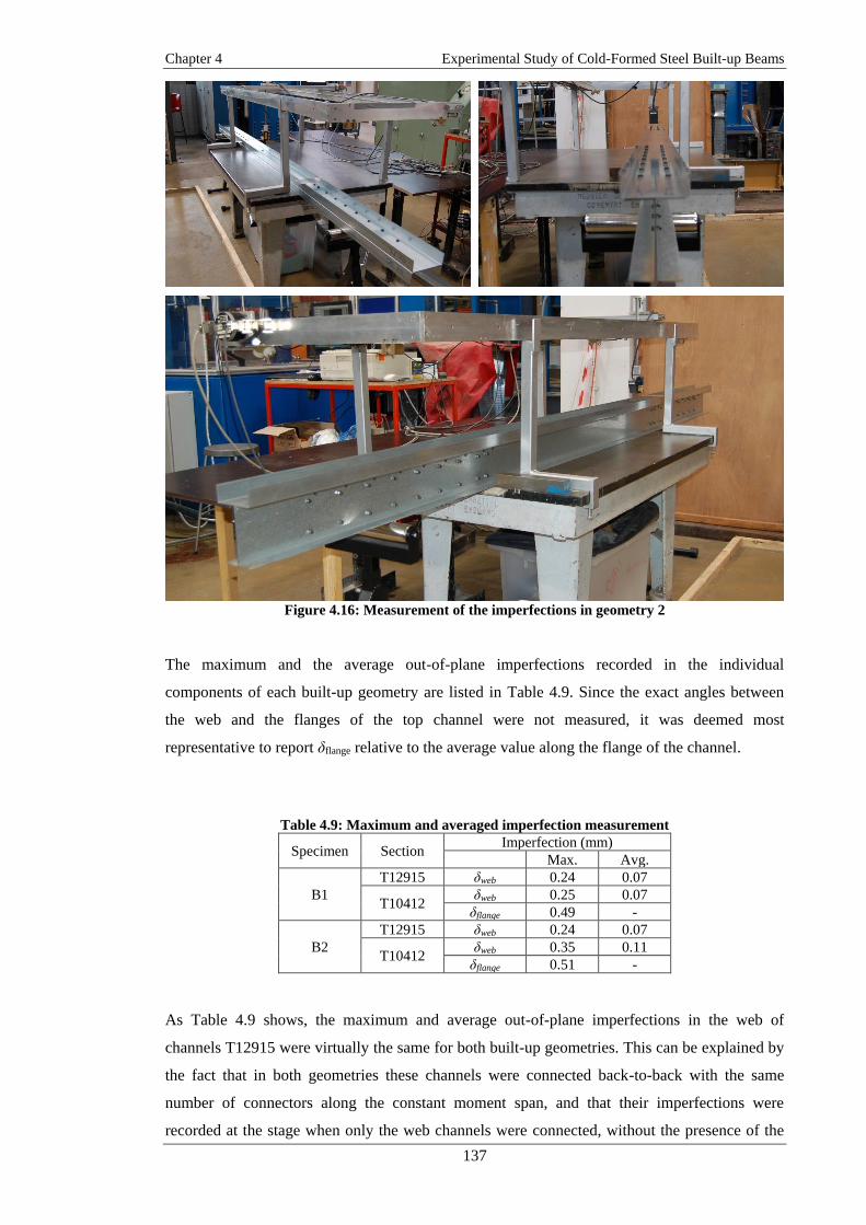
Chapter 4 Experimental Study of Cold-Formed Steel Built-up Beams
137
Figure 4.16: Measurement of the imperfections in geometry 2
The maximum and the average out-of-plane imperfections recorded in the individual
components of each built-up geometry are listed in Table 4.9. Since the exact angles between
the web and the flanges of the top channel were not measured, it was deemed most
representative to report δflange relative to the average value along the flange of the channel.
Table 4.9: Maximum and averaged imperfection measurement
Specimen Section Imperfection (mm)
Max. Avg.
B1
T12915 δweb 0.24 0.07
T10412 δweb 0.25 0.07
δflange 0.49 -
B2
T12915 δweb 0.24 0.07
T10412 δweb 0.35 0.11
δflange 0.51 -
As Table 4.9 shows, the maximum and average out-of-plane imperfections in the web of
channels T12915 were virtually the same for both built-up geometries. This can be explained by
the fact that in both geometries these channels were connected back-to-back with the same
number of connectors along the constant moment span, and that their imperfections were
recorded at the stage when only the web channels were connected, without the presence of the

Chapter 4 Experimental Study of Cold-Formed Steel Built-up Beams
138
flange channels. On the other hand, the web of channels T10412, which in geometry 1 were
assembled with the flanges facing down and in geometry 2 with the flanges facing upwards,
showed the largest differences in the maximum and average imperfections.
Providing examples of the measurements, Figure 4.17 shows the out-of-plane imperfections
recorded in the web of one of the web channels of beam B1-2a, while Figure 4.18 shows the
imperfections recorded in one of the flanges of the top channel of beam B2-0a. The vertical
dashed lines in Figure 4.17 indicate the location of the connectors (the specimen in Figure 4.18
was tested without connectors in the constant moment span). In both figures, the length
coordinate along the constant moment span is normalized with respect to the total constant
moment span length. Positive readings indicate imperfections in the direction away from the
centroid of the built-up cross-section. The imperfection data of all specimens are included in
Appendix E.
Figure 4.17: Imperfections in the web of channel T12915-6 (geometry 1)

Chapter 4 Experimental Study of Cold-Formed Steel Built-up Beams
139
Figure 4.18: Imperfections of a flange of channel T10412-1 (geometry 2)
4.7. Test Set up
4.7.1 Introduction
All specimens were tested adopting a 4-point bending configuration. The specimens were bent
about their major axis, with lateral restraint provided at the loading points. The rig used in the
tests is illustrated in Figure 4.19.
Figure 4.19: 4-point bending test rig
Spreading beam
Lateral restraintLoad cell
Actuator
Rigid frame

Chapter 4 Experimental Study of Cold-Formed Steel Built-up Beams
140
4.7.2 Boundary conditions
4.7.2.1 Roller supports
The test specimens were simply supported at their ends on rollers located 3000 mm apart. These
supports allowed rotations about the major axis and axial shortening, while preventing vertical
displacement and twist. The out-of-plane forces at the beam ends resulting from the tendency of
the beam to fail in lateral-torsional buckling were small enough to be restrained by friction
between the rollers and the bottom surface of the test specimens.
4.7.2.2 Lateral uprights
The specimens were loaded through a spreader beam, which applied concentrated loads at
points 1600 mm apart. The spreader beam was restrained near its ends against any out-of-plane
movement by the assemblies shown in Figure 4.20. These consisted of adjustable upright
supports made of 6 mm thick square hollow sections, which were bolted to the reaction frame.
Steel plates of 6 mm thickness were welded to the flanges of the spreader beam and had nylon
blocks bolted to them. The nylon blocks worked as linear bearing pads which increased contact
surface and reduced friction between the spreader beam and the uprights. The uprights were
adjusted to ensure full contact with the nylon blocks by tightening or loosening the top and
bottom threaded rods shown in Figure 4.20. Friction between the uprights and the spreader
beam was estimated to be around 50 N at the beginning of the test.
Figure 4.20: Laterally restraining assembly
Uprights
Spreading beamNylon blocks
Threaded rodsLoadng plate

Chapter 4 Experimental Study of Cold-Formed Steel Built-up Beams
141
4.7.2.3 Loading points
Special devices, which are illustrated in Figure 4.21, were built to transmit the vertical load
from the spreader beam to the test specimens. They consisted of a bottom half with a steel
cylinder which either tightly fitted in a rounded recess or was free to roll over a rectangular area,
and a matching top half. High strength steel flanges were bolted to both sides of the bottom
halves in order to prevent out-of-plane displacements of the test specimens at the loading points.
The one device emulated a pin connection, allowing only rotations in the plane of loading
between the spreader beam and the test specimen. The other one emulated a roller connection,
which allowed rotations in the plane of loading, as well as axial displacements. The top and
bottom halves of each device were bolted to the spreader beam and the test specimens,
respectively. Sufficient clearance was provided in the holes drilled in the spreader beam to
allow tight alignment between the top and bottom halves.
Figure 4.21: Loading devices: a) Pin support, b) Roller support
4.7.2.4 Wooden blocking
The end sections of the built-up specimens above the supports were packed with wooden blocks
which tightly fitted within the web and flanges. While this also prevented possible bearing
failure, the main reason was to prevent a distortion of the cross-section caused by a lateral
displacement of the compression flange combined with bending of the web about a horizontal
axis in its plane. The lateral bending of the compression flange originated from a tendency of
the beam to fail in lateral-torsional buckling in between the loading points as the built-up
specimens approached their maximum moment capacity, but after local buckling of the
component sections was observed. Neither the devices at the loading points nor the lateral
restraint assemblies were thereby able to completely eliminate rotations of the beam about the
vertical axis. This phenomenon was observed in built-up beam B1-0a, which was tested without
wooden blocks and resulted in the built-up beam being unable to reach the load attained by its
twin specimen.
(a) (b)

Chapter 4 Experimental Study of Cold-Formed Steel Built-up Beams
142
4.7.3 Instrumentation
4.7.3.1 LVDTs
Three LVDTs with a stroke of 50 mm were used to record the deflections of the beams. The
LVDTs were placed underneath the specimens, vertically aligned with the centroid of the built-
up cross-section, at the loading points and at mid-span, as illustrated in Figure 4.22. Steel plates
were bolted to the bottom flanges of the channels which formed the web of geometry 2 in order
to provide a smooth surface for the LVDTs to bear on, as illustrated in Figure 4.23.
Figure 4.22: Distribution of the LVDTs along the test specimen
Figure 4.23: Location of the LVDTs within the cross-section
4.7.3.2 Potentiometers
Eight potentiometers with a stroke of 25 mm were used to measure the buckling deformations of
the component sections. The potentiometers were mounted on two identical yokes, which were
attached to the bottom flange of the built-up cross-sections, as illustrated in Figure 4.24. As the
Spreading beam
L1 L3 L2
Built-up section 1 Built-up section 2
Steel plate

Chapter 4 Experimental Study of Cold-Formed Steel Built-up Beams
143
test specimens underwent overall bending, the bottom flange of the built-up cross-section
experienced tension and was not at risk of local buckling, while the yokes were able to move
with the cross-section as a whole. Thus, the potentiometers were able to record the out-of-plane
deformations of the web and the top flange of the built-up cross-sections due to local buckling.
Figure 4.24: Potentiometer lay-out within the cross-sections
Figure 4.25 illustrates the locations at which the yokes were placed for each test specimen of
geometry 1 and 2. For the specimens without intermediate connectors in between the loading
points, yoke Y1 was placed 200 mm to the left of the mid-span and yoke Y2 300 mm to the
right. These locations were chosen while considering the buckling half-wave length of the
different components, so that if one of the yokes happened to coincide with the inflection point
of the local buckling pattern in one of the components, the other yoke would still be able to
record its buckling deformations. For the specimens with two and three intermediate connectors,
the potentiometers were placed at mid-distance between the connectors.
Figure 4.25: Location of the potentiometers along the test specimens
Built-up geometry 2Built-up geometry 1
Y1
Y1
Y1
Y2
Y2
Y2
2 intermediate connectors
3 intermediate connectors
200 300
(All dimensions in mm)
Zero intermediate connector

Chapter 4 Experimental Study of Cold-Formed Steel Built-up Beams
144
4.7.4 Test procedure
The specimens were tested in a reaction frame using an actuator with a maximum capacity of
160 kN and a 50 kN load cell. The actuator was steered using a Cubus controller, operated in
displacement mode. The load was applied using a displacement rate of 1 mm/min and the test
was halted for 4 min slightly before the peak load was reached in order to determine the lower
bound ‘static’ value of the load. The specimens were deformed well beyond the peak load in
order to identify the location at which the plastic deformations localized.
The data was also collected using the Cubus system, using a sampling rate of 1 Hz.
4.8. Test results
4.8.1 Deformed shape
4.8.1.1 Geometry 1
All test specimens with geometry 1 failed by local buckling in the constant moment region, with
significant interaction taking place between the top channel and the channels comprising the
web of the built-up cross-section. Multiple buckling half-waves were observed along the
constant moment span. The top channel buckled before buckling was observed in the channels
comprising the webs of the built-up cross-section in all beams.
In beams B1-0 and B1-2, the top channel buckled in a pattern containing 15 or 16 half-waves
with approximately the same half-wave length along the constant moment span. These buckles
were estimated to have an average half-wave length of around 100 mm. In the case of beams
B1-2, one intermediate set of connectors coincided with an inflection point in the local buckling
pattern, where the web of the top channel neither buckled outward nor inward. Consequently,
these connectors underwent a rotation about an axis perpendicular to the plane of loading. The
other set of connectors, on the other hand, coincided with a cross-section in which the flanges of
the top channel buckled outward and the web buckled inward. Consequently, these connectors
rotated about an axis parallel to the plane of loading.
For beams B1-3, buckles with a similar half-wave length to the one reported for beams B1-0
and B1-2 were observed. However, in these beams the flanges of the top channel buckled
outward in the cross-sections containing connectors. This resulted in the top channel buckling
with 17 half-wave buckles along the constant moment span, with two of the buckles being
smaller than the others, as shown in Figure 4.26.

Chapter 4 Experimental Study of Cold-Formed Steel Built-up Beams
145
Figure 4.26: Top channel in specimen B1-3b displaying buckles with different half-wave lengths
It is important to note that the half-wave length of the buckles displayed by the top channel in
all beams was very close to its natural (calculated) local buckle half-wave length of 110 mm.
The web channels had a similar natural local buckle half-wave length of 100 mm, however the
number of buckles generated in the web channels and the associated wave length could not be
determined as the magnitude of these buckles was not large enough to allow accurate
measurements.
Despite the similarity in the initial buckling pattern observed for each pair of twin specimens,
the plastic deformations generally localized around the peak load in different locations. Figures
4.27-4.32 illustrate the deformed shape before and after the peak load for all beams with
geometry 1.
As Figure 4.27 shows, beam B1-0a was tested without packing the end sections with wooden
blocks. This caused the built-up cross-section to experience significant lateral distortion at the
end sections, accompanied by in-plane bending of the top flange and resulted in a slightly lower
ultimate load compared to the twin specimen. To avoid this in subsequent tests, the remaining
built-up specimens were tested with wooden blocking at each end.

Chapter 4 Experimental Study of Cold-Formed Steel Built-up Beams
146
Figure 4.27: Deformed shape of specimen B1-0a: a) before peak load, b) after peak load
Figure 4.28: Deformed shape of specimen B1-0b: a) before peak load, b) after peak load
(a)
(a)
(b)
(b)

Chapter 4 Experimental Study of Cold-Formed Steel Built-up Beams
147
Figure 4.29: Deformed shape of specimen B1-2a: a) before peak load, b) after peak load
Figure 4.30: Deformed shape of specimen B1-2b: a) before peak load, b) after peak load
(a)
(a)
(b)
(b)

Chapter 4 Experimental Study of Cold-Formed Steel Built-up Beams
148
Figure 4.31: Deformed shape of specimen B1-3a: a) before peak load, b) after peak load
Figure 4.32: Deformed shape of specimen B1-3b: a) before peak load, b) after peak load
For most of the test specimens, a yield line pattern developed at one specific location along the
constant moment span, resulting in a hinge-like behaviour. Yield lines simultaneously
developed in the top channel and in the web and the top flange of the channels comprising the
web of the built-up specimens. In general, the pattern in the top channel was symmetric with
respect to the plane of bending, while that in the web of the web channels was anti-symmetric,
as shown in Figure 4.33. An exception to this occurred in specimens B1-0b and B1-2b, in which
the top channel developed an asymmetric yield line pattern near mid-span. This was
(a)
(a)
(b)
(b)

Chapter 4 Experimental Study of Cold-Formed Steel Built-up Beams
149
accompanied by the top flange undergoing some out-of-plane deformations combined with
twisting of the cross-section along the constant moment span, while a second ‘hinge’ appeared
near one of the loading supports, as shown in Figure 4.34. As a result, lateral forces were
induced at the end supports which eventually underwent some lateral slip. However, the out-of-
plane displacements of the beam did not occur until after the peak load was reached and
therefore, all beams could be considered fully laterally restrained until the test specimens
reached their ultimate capacity.
Figure 4.33: Plastic hinge in B1-2a: a) Top channel b) Channels comprising the web
Figure 4.34: Asymmetric plastic hinge in built-up specimens a) B1-0b b) B1-2b
Regarding the initial buckling deformations, the potentiometers mounted on the yokes recorded
a locally buckled shape in the top channel which was symmetric about the plane of bending in
all beams with both flanges buckling either inward or outward. The web channels were recorded
to buckle in a symmetric shape with respect to the plane of bending in those specimens without
any connectors in the constant moment span (B1-0), while in the remaining specimens the
buckling pattern was anti-symmetric. The symmetric buckling pattern of the web channels in
beams B1-0 can be attributed to the fact that the channels were able to buckle largely
(a) (b)
(b) (a)

Chapter 4 Experimental Study of Cold-Formed Steel Built-up Beams
150
independently from each other, without any connectors in the constant moment span forcing
them to remain in contact. On the other hand, a connector spacing of 500 mm, as encountered in
beams B1-2, was short enough to force the web channels to buckle in a synchronous manner.
This is illustrated in Figure 4.35, which shows the out-of-plane deformations of the components
of beam B1-2a against the applied load. In the figure, the solid and dashed lines represent the
readings obtained from the sets of potentiometers placed on each of the two yokes. Positive
values indicate deformations towards the potentiometer (outward) while negative values
indicate deformations away from the potentiometers (inward).
Figure 4.35: Axial load vs lateral displacements (B1-2a)
In the specimens with two and three sets of intermediate connectors along the constant moment
span, the buckling pattern of the top channel was seen to be affected by subsequent buckling of
the web channels. More specifically, in beam B1-2a one set of potentiometers recorded the
flanges of the top channel changing the initial direction of their buckles when the web channels
started buckling, as shown in Figure 4.35, while in beam B1-2b the potentiometers only
recorded the flanges of the top channels adjusting the amplitude of their buckles. In beams B1-3
this interaction was even more pronounced. In beam B1-3a, all four potentiometers at the top
channel recorded the flanges changing the direction of their buckles when the web channels
started buckling, as illustrated in Figure 4.36. A similar behaviour was also observed in the twin
specimen (B1-3b). These observations can be interpreted as an attempt of the top channel to
accommodate the buckling deformed shape of the web channels by modifying the wavelength
of its buckles. The closer the connector spacing, the more pronounced this effect becomes.

Chapter 4 Experimental Study of Cold-Formed Steel Built-up Beams
151
Figure 4.36: Axial load vs lateral displacements (B1-3a)
4.8.1.2 Geometry 2
In general, the specimens with geometry 2 failed predominantly by local buckling, characterized
by significant interaction between the buckling patterns in the top channel and the web
channels. Figures 4.37-4.42 show the deformed shapes of all test specimens before and after the
peak load. In the beams without intermediate connectors (B2-0), global twisting of the top
channel was observed to interact with local buckling near the peak load. In the case of beam B2-
0a this occurred shortly after the local buckling deformations in the top channel localized near
mid-span, resulting in a localized twisting, as illustrated in Figure 4.37b. However, in specimen
B2-0b the interaction between local buckling and flexural-torsional buckling of the top channel
was more significant, causing the top channel to twist with a half wave-length of approximately
750 mm before the built-up specimen reached its ultimate capacity, as shown in Figure 4.38b.
In all test specimens, the top channel buckled locally before the web channels, and the
amplitude of its buckles was significantly larger. The top channel buckled while displaying 14
or 16 half-waves along the constant moment span with approximately the same half-wave
length. The number of half-waves generated in the web channels was not easily appreciated due
to their small amplitude. However, it was estimated to also be approximately 14 or 16 along the
constant moment span. This resulted in half-wave lengths in the top channel and the web
channels ranging from approximately 94 mm to 107 mm. These half-wave lengths were very
close to the natural local buckling half-wave lengths of the top channel and the web channels,
which are 120 mm and 100 mm, respectively.
In the beams without intermediate connectors (B2-0), a gap developed along the constant
moment span between the top channel and the web channels as the specimens deformed. This
gap was more pronounced around mid-span, allowing a larger amplitude of the buckles in the

Chapter 4 Experimental Study of Cold-Formed Steel Built-up Beams
152
top flange of the web channels to develop in this region. On the other hand, towards the ends of
the constant moment span, where the components were in closer contact with each other, the
amplitude of the buckles in the top flange of the web channels was considerably smaller, to the
point that it was difficult to observe them. In the B2-0 specimens, the top channels buckled
while displaying 14 or 15 half-waves along the constant moment span.
In beams B2-2, the top channel also tended to separate from the web channels, especially at
mid-span. However, the intermediate connectors opposed this separation, thereby pulling the
flanges of the web channel upward. This resulted in the connectors between the top channel and
the web channels undergoing a slight translation in the vertical direction and a rotation about an
axis parallel to the length of the beam. In addition, due to the presence of the connectors one of
the buckles in the web channels (at mid-span) had a half-wave length which was almost twice as
large as the others. This half-wave tried to divide into two half-waves as the specimens
continued to deform. In the B2-2 specimens, 15 half-waves were counted in the top channel
along the constant moment span, while between 14 and 16 half-waves were counted in the top
flange of the web channels.
In beams B2-3, no gap originated between the top channel and the web channels and the
locations of the intermediate connectors coincided with the cross-sections in which the top
channel buckled with its flanges moving inward. In these specimens the top channels displayed
four buckling half-waves between connectors resulting in 16 half-waves along the constant
moment span.
Although the buckling pattern observed for twin specimens was, in general, similar until the
ultimate capacity was reached, localization of the plastic failure often occurred at different
locations along the constant moment region. As the built-up specimens deformed beyond their
ultimate capacity, yield lines started to develop in the top channel and in the top flange of the
web channels.

Chapter 4 Experimental Study of Cold-Formed Steel Built-up Beams
153
Figure 4.37: Deformed shape of specimen B2-0a: a) before peak load, b) after peak load
Figure 4.38: Deformed shape of specimen B2-0b: a) before peak load, b) after peak load
(a)
(a)
(b)
(b)

Chapter 4 Experimental Study of Cold-Formed Steel Built-up Beams
154
Figure 4.39: Deformed shape of specimen B2-2a: a) before peak load, b) after peak load
Figure 4.40: Deformed shape of specimen 2-2b: a) before peak load, b) after peak load
(a)
(a)
(b)
(b)

Chapter 4 Experimental Study of Cold-Formed Steel Built-up Beams
155
Figure 4.41: Deformed shape of specimen B2-3a: a) before peak load, b) after peak load
Figure 4.42: Deformed shape of specimen B2-3b: a) before peak load, b) after peak load
As the yield line mechanism developed, the specimens generally experienced some twisting and
lateral displacement in the neighbourhood of the resulting hinge. These deformations gradually
spread over the whole constant moment span as the specimen continued to deflect. Figure 4.43
shows the hinge which developed in the top channel and the top flange of the web channels of a
typical specimen. The twisting and lateral deformations along the constant moment span finally
resulted in lateral slip at the end supports. These end supports were not designed to restrain
lateral displacement, except for the friction generated between their mechanical components.
(a)
(a)
(b)
(b)

Chapter 4 Experimental Study of Cold-Formed Steel Built-up Beams
156
However, this lateral displacement consistently occurred in the decreasing part of the load-
deflection curve, after the peak load was reached, and it is therefore reasonable to consider the
lateral displacement at the end supports as restrained until the test specimens reached their
ultimate capacity.
Figure 4.43: Yield line mechanism in B2-2a: a) Top channel, b) Channels comprising the web
Regarding the initial buckling deformations, the potentiometers recorded the top channels
buckling with a symmetric buckling pattern with respect to the plane of bending along the
constant moment span in all test specimens, while the web channels were recorded to buckle in
an anti-symmetric shape. As an example, Figure 4.44 shows the out-of-plane deformations of
the components of beam B2-0a. The potentiometers mounted on the yoke located 200 mm to the
left of mid-span recorded both flanges of the top channel to buckle outward (solid black line),
while the potentiometer mounted on the yoke located 300 mm to the right of mid-span recorded
the flanges of this channel to buckle inward (dashed black line). Among the potentiometers
which were used to measure the out-of-plane deformation of the web channels (red lines), in
both yokes one of the potentiometers recorded an inward deformation, while the other
potentiometer recorded an outward deformation.
Figure 4.44: Axial load vs lateral displacements of B2-0a
(a) (b)

Chapter 4 Experimental Study of Cold-Formed Steel Built-up Beams
157
In general, readings from the potentiometers did not record the buckling pattern of the top
channels to be affected by subsequent buckling of the web channels to the same degree as in the
specimens with geometry 1. Only beam B2-3b showed a noticeable interaction between the
components, as illustrated by Figure 4.45, which shows that the magnitude of the buckles in the
flanges of the top channel was altered when the web channels started to buckle.
Figure 4.45: Axial load vs lateral displacements of B2-3b
4.8.2 Critical buckling stress and shear force at the connectors
The load at which the individual cross-sectional components buckled was determined from the
readings of the potentiometers. Graphs showing the potentiometer readings against the applied
load are included in Appendix F for all beams. The load at which the top channels buckled was
determined based on the prediction by classical (perturbation) theory that, after local buckling
occurs, the initial post-buckling deformations, when plotted against the load, follow a parabolic
shape (Venkataramaiah and Roorda, 1982). This parabolic relationship between the load and the
initial post-buckling deformations can be expected to appear when the section is free to develop
its local buckles. This may not be strictly the case in a built-up member due to contact between
the components. Nonetheless, this principle is expected to give a reasonable estimation of the
load at which local buckling takes place.
An example of a typical load vs lateral deformation curves is illustrated in Figure 4.45 for beam
B2-3b. Since the top channel was the first component to buckle in all of the test specimens, its
critical buckling stress could be estimated from the recorded bending moment, assuming that no

Chapter 4 Experimental Study of Cold-Formed Steel Built-up Beams
158
slip occurred at the connectors prior to buckling, so that plane sections remained plane. Based
on these assumptions, the critical stress in the top channel was obtained from the moment:
2
spanF sM
(4.6)
where F is the critical load obtained from the load vs. lateral displacement curve, sspan is the
length of the shear span and M is the moment in the constant moment zone. The stress (σ) in the
top channel at a vertical distance y from the centroid of the built-up cross-section is then given
by:
,built up xx
M y
I
(4.7)
where Ibuilt-up,xx is the second moment of area of the built-up cross-section about the horizontal
axis through its centroid. The stress given by Eq. (4.7) provides an upper bound to the actual
stress because connector behaviour is not accounted for. Since the web channels consistently
buckled after the top channel, the critical buckling stress of these channels could not be
determined.
For each beam the experimentally derived buckling stress of the top channel was compared with
the theoretical buckling stress obtained from an elastic stability analysis carried out using
CUFSM 4.05 (Schafer, 2006), in which the buckling stresses were determined based on the
average measured cross-sectional dimensions and the Young’s modulus obtained from the flat
tensile coupons. The theoretical buckling stresses were obtained while considering the top
channel in isolation, without any interaction with the rest of the cross-section, but under a stress
gradient consistent with the plane section assumption, and using the buckle half-wave length
observed during the test.
Figure 4.46: Distance between the centroid of the top channel and the centroid of the built-up cross-
section 1
Built-up section 1
y
Built-up section 2
y

Chapter 4 Experimental Study of Cold-Formed Steel Built-up Beams
159
In order to confirm that no slip occurred prior to buckling, the shear force in the connectors
located between the top channel and the web channels along the shear span was derived at the
buckling load. This force was calculated using the same assumption previously employed to
determine the critical buckling stresses in the top channel. Thus, knowing that the vertical shear
force (V) in the shear span is constant and equal to half of the total force (F) applied to the
beam, the shear force to which each connector was subjected when the top channel buckled
(Vcon) was obtained from:
,16
topch
con span
xx built up
V A yV s
I
(4.8)
In the above equation Atopch is the area of the top channel, �̅� is the distance from the centroid of
the top channel to the centroid of the built-up cross-section, as illustrated in Figure 4.46 for both
geometries, and sspan is the length of the shear span. The resulting force was compared to the slip
force of the connectors, which was determined from single lap shear tests aimed at determining
the full shear behaviour of the connectors of the tested built-up beams. A detail description of
these tests is included in Chapter 6.
4.8.2.1 Geometry 1
Table 4.10 shows that the slip force exceeded the experimentally derived shear force in each
tested beam with geometry 1, indicating that no slip occurred in the connectors before the top
channel started buckling. This result supports the initial assumption that plane sections remained
plane at least up to the moment at which the top channel started buckling.
Table 4.10: Shear force in shear span connectors of specimens with geometry 1
Specimen Vcon
(N)
Vslip
(N)
Vslip/Vcon
(-)
B1-0a 1528 2600 1.702
B1-0b 1881 2600 1.382
B1-2a 2010 2600 1.294
B1-2b 1836 2600 1.416
B1-3a 1573 2600 1.653
B1-3b 1490 2600 1.745
Table 4.11 shows the theoretical critical buckling stress of the top channel for each test
specimen and compares this value to the one derived from the test.

Chapter 4 Experimental Study of Cold-Formed Steel Built-up Beams
160
Table 4.11: Buckling stresses of the top channel of specimens with geometry 1
Specimen Component
section
Theoretical
buckling stress
(MPa)
Buckling stress
from test
(MPa)
Buckling stress
from test
/Theoretical
buckling stress
B1-0a T10412-1 107 138 1.29
B1-0b T10412-3 111 170 1.53
B1-2a T10412-5 106 170 1.60
B1-2b T10412-7 109 154-166 1.41-1.52
B1-3a T10412-9 107 142 1.33
B1-3b T10412-11 108 126-134 1.17-1.24
The potentiometers located on the two different yokes captured the onset of local buckling in
the top channel at consistent stress levels in each specimen, with the marginal exception of
specimens B1-2b and B1-3b, for which the two slightly different readings are listed in Table
4.11. Comparing the critical buckling stresses obtained from the tests with the ones obtained
from the analysis, it is seen that the former are, on average, 40 % higher than the latter. This can
be attributed to the fact that the top channel benefited from the constraint provided by the
unbuckled web channels.
The relatively high value of the buckling stress reported in Table 4.11 for built-up beam B1-2a
was due to the fact that, in this specimen, the buckling pattern was initially localized in between
the two sets of connectors located near mid-span. As the load increased, the buckling pattern
gradually spread out over the whole constant-moment span. Consequently, the potentiometers,
which were located outside the central set of connectors, were not able to record the initial
buckling deformations. In the twin specimen (B1-2b), the buckles were observed to appear
simultaneously over the whole constant-moment span, although they were noticeably more
pronounced near mid-span.
While no slip occurred in the connectors before first buckling, once the specimens deformed
beyond their ultimate capacity, some slip was typically noticed at one end of the built-up beams.
This is illustrated in Figure 4.47, where the relative movement between the components has
been exaggerated for clarity. The observed slip measured between 1 and 2 mm at the end of the
test.

Chapter 4 Experimental Study of Cold-Formed Steel Built-up Beams
161
Figure 4.47: Slip at specimen end between the components of built-up beam 1
4.8.2.2 Geometry 2
Table 4.12 shows that in all tested beams with geometry 2, the slip force of the connectors was
more than twice the estimated shear force in the connectors located between the top channel and
the web channels in the shear span at the moment when the top channel buckled. Therefore, it is
reasonable to conclude that no slip had occurred up to that point, and that the initial assumptions
used to calculate the theoretical and experimental buckling stresses of the top channel were
valid.
Table 4.12: Shear force in shear span connectors of specimens with geometry 2
Specimen Vcon
(N)
Vslip
(N)
Vslip/Vcon
(-)
B2-0a 1044 2600 2.490
B2-0b 954 2600 2.725
B2-2a 1091 2600 2.383
B2-2b 1041 2600 2.498
B2-3a 1087 2600 2.392
B2-3b 1035 2600 2.512
Table 4.13 lists the theoretical critical buckling stress of the top channel, and compares this
value to the one obtained from the test.
Table 4.13: Buckling stresses of the top channel of specimens with geometry 2
Specimen Component
section
Theoretical
buckling stress
(MPa)
Buckling stress
from test
(MPa)
Buckling stress
from test
/Theoretical
buckling stress
B2-0a T10412-1 126 127 1.01
B2-0b T10412-2 126 120-142 0.95-1.13
B2-2a T10412-3 127 133-152 1.05-1.20
B2-2b T10412-4 127 121-136 0.95-1.07
B2-3a T10412-5 128 133 1.04
B2-3b T10412-6 128 128 1.00

Chapter 4 Experimental Study of Cold-Formed Steel Built-up Beams
162
Table 4.13 shows that, in some specimens, the two sets of potentiometers captured the onset of
local buckling in the top channel at a slightly different stress level. This was the case, for
example, in beams B2-0b and B2-2a. It is also noted that in beam B2-2b only one of the
potentiometers recorded the flange of the top channel buckling at a stress level of 121 MPa,
while all the other recorded the top channel buckling at a stress level of 136 MPa. The table also
shows that, in general, the experimentally derived buckling stresses were only marginally higher
than the theoretical ones, indicating that in the specimens with geometry 2 the top channel did
not noticeably benefit from any restraint provided by the unbuckled web channels.
While no slip between the components occurred before first buckling, after the specimens
deformed beyond the peak load some slip was typically noticed at one specimen end. However,
the exact moment at which slip occurred could not be determined. Figure 4.48 illustrates the
relative movement observed between the components of the specimens with geometry 2. As for
the beams with geometry 1, the observed slip measured between 1 and 2 mm at the end of the
test.
Figure 4.48: Slip at specimen end between the components of built-up beam 2
4.8.3 Ultimate capacity
The load-deflection behaviour of a representative test specimen (B1-2a) is illustrated in Figure
4.49. The vertical axis represents the bending moment in the constant moment zone, obtained
using Eq. (4.6), while the horizontal axis shows the deflection at mid-span measured relative to
the deflections of the beam at the loading points:
,
3 1 3 2
2r mid
L L L L
(4.9)
In the above equation δr,mid is the relative deflection at mid-span and L1, L2 and L3 are the
readings given by the LVDTs shown in Figure 4.22. The LVDT readings were considered
positive when they recorded a downward displacement of the beam.

Chapter 4 Experimental Study of Cold-Formed Steel Built-up Beams
163
The black curve in Figure 4.49 corresponds to the ‘dynamic’ (measured) moment, while the red
curve corresponds to the ‘static’ moment, which was obtained by deducting the decrease in
moment observed when halting the test for 4 min shortly before the ultimate capacity of the
specimen was reached from the dynamic moment in the inelastic range.
Figure 4.49: Moment vs relative deflection at mid-span (B1-2a)
4.8.3.1 Geometry 1
In Figure 4.50 the static moment is plotted against the relative deflection at mid-span for all
specimens with geometry 1, while the static ultimate capacities are plotted against the connector
spacing in Figure 4.51.
Figure 4.50: Moment vs relative deflection at mid-span of specimens with geometry 1

Chapter 4 Experimental Study of Cold-Formed Steel Built-up Beams
164
Figure 4.51: Ultimate capacity vs connector spacing of specimens with geometry 1
The ultimate moments obtained for all beams with geometry 1 are listed in Table 4.14. The
table includes the dynamic and static moments, as well as the average values of the ultimate
moments for each set of twin specimens.
Table 4.14: Ultimate capacity of built-up beam 1
Beam
Ultimate Moment
(kNm)
Average Ultimate Moment
(kNm)
Dynamic Static Dynamic Static
B1-0a (10.79) (10.56) 12.06 11.84
B1-0b 12.06 11.84
B1-2a 12.79 12.51 12.43 12.17
B1-2b 12.07 11.83
B1-3a 13.51 13.28 13.38 13.14
B1-3b 13.25 13.01
In general, good agreement in the ultimate capacity was achieved between each pair of twin
specimens. Only the B1-0 pair showed a relatively large discrepancy in the ultimate capacity
(11 %). This can be attributed to the fact that beam B1-0a was tested without wooden blocking
in the end sections, causing the specimen to fail with significant distortion of the end sections
accompanied by in-plane bending of the top flange. This resulted in the beam failing with a
slightly lower ultimate load and, therefore, the results of this test were discarded. For beams B1-
2 and B1-3, the twin specimens showed differences in the (static) ultimate capacity of 6 % and 2
%, respectively.
According to the test results, reducing the connector spacing in the constant moment span
resulted in a modest increase in the ultimate capacity of the built-up specimens. The beams with
two rows of connectors experienced an average increase in the (static) ultimate capacity of 3 %

Chapter 4 Experimental Study of Cold-Formed Steel Built-up Beams
165
relative to the beam without connectors, while the specimens with three rows of connectors
exhibited an average increase of 11 %.
4.8.3.2 Geometry 2
Figure 4.52 plots the (static) moment against the relative deflection at mid-span for all beams
with geometry 2, while Figure 4.53 plots the ultimate (static) moment against the connector
spacing.
Figure 4.52: Moment vs relative deflection at mid-span of specimens with geometry 2
Figure 4.53: Ultimate capacity vs connector spacing of specimens with geometry 2
Table 4.15 lists the ultimate (static and dynamic) moments for all test specimens with geometry
2, together with the average value for each set of twin specimens.

Chapter 4 Experimental Study of Cold-Formed Steel Built-up Beams
166
Table 4.15: Ultimate capacity of built-up beam 2
Beam
Ultimate Moment
(kNm)
Average Ultimate Moment
(kNm)
Dynamic Static Dynamic Static
B2-0a 9.23 9.08 8.78 8.63
B2-0b 8.33 8.19
B2-2a 10.59 10.41 10.71 10.53
B2-2b 10.82 10.64
B2-3a 11.83 11.66 11.90 11.70
B2-3b 11.97 11.74
It is seen that twin specimens B2-0 showed the maximum difference in ultimate capacity, which
was 11 %. This can be attributed to the fact that in beam B2-0b global flexural-torsional
buckling of the top channel was observed before the specimen reached its ultimate capacity,
while in beam B2-0a the top channel developed a yield line mechanism at mid-span due to local
buckling before displaying flexural-torsional buckling. In beams B2-2 and B2-3, the difference
in ultimate capacity between twin specimens was 2 % and 1 %, respectively.
Compared to geometry 1 the tests showed a more substantial increase in ultimate capacity when
the spacing between connectors was reduced. The beams with two intermediate rows of
connectors along the constant moment span experienced an average increase in ultimate
capacity of 22 % relative to the beams without intermediate connectors, while the beams with
three rows of intermediate connectors displayed an average increase of 36 %.
4.9. Summary and conclusions
A detailed experimental program including 12 built-up CFS beams with two different cross-
sectional geometries, tested in a four-point bending configuration, was carried out. Lateral
restraints were provided at the loading points in order to avoid global instability. The built-up
specimens were composed of 104 mm to 129 mm deep plain channel sections with nominal
thicknesses between 1.2 mm and 1.5 mm, which were joined together using M6 bolts. The
beams were designed to fail within the constant moment span by local buckling of the
component sections. The connector spacing within the constant moment span was varied among
specimens of the same cross-sectional geometry in order to study its effect. In one of the
geometries, strut buckling of the channel comprising the top flange in between connector points
was observed in addition to local buckling.
As part of the experimental program, the out-of-plane geometric imperfections of the test
specimens were measured using a laser sensor prior to testing. In addition, the material
properties of the constituent channels were determined by testing a series of tensile coupons
which were extracted from the flat parts and rounded corner zones of the channels.

Chapter 4 Experimental Study of Cold-Formed Steel Built-up Beams
167
The deflections of the beams were recorded during the test using three LVDTs located at mid-
span and at the loading points. In addition, potentiometers recorded the out-of-plane
deformations of each component in order to determine the onset of local buckling. The
experimentally determined buckling stresses were compared to theoretical predictions which
considered the individual components in isolation, without any interaction with the rest of the
cross-section.
The following conclusions were drawn from the experimental program:
The deformed shapes of the beams after buckling revealed an adjustment in the
buckling patterns of the component sections relative to their preferred pattern as
individual sections as a result of being part of the built-up cross-section. This
adjustment manifested itself both as a reduction in the amplitude of the buckles due to
contact between the components and an adjustment of the half-wave length of the
buckles due to the constraints provided by the connectors. However, the latter effect
was relatively minor and the individual components buckled with half-wave lengths
close to the ones associated with their minimum buckling stress. Specimens with built-
up geometry 1 showed a more significant interaction between their components than
specimens with built-up geometry 2, and this interaction was more pronounced in the
specimens with the largest number of intermediate connectors within the constant
moment span.
The connectors were observed to rotate and/or translate in order to accommodate the
buckling pattern and could not be considered as fixed points in space. No slip occurred
in the shear span connectors before buckling, but some slip was noticed in all beams at
the end of the test.
The potentiometer readings showed that the top channel was the first component to
buckle in all beams. By comparing the experimentally derived critical buckling stress of
this component with the theoretical prediction obtained from an elastic analysis, it was
concluded that in the specimens with geometry 1 the top channel significantly
benefitted from the restraint provided by the unbuckled web channels. In the specimens
with geometry 2, on the other hand, the top channel did not benefit to the same degree
from the restraint provided by the web channels.
The tests showed a relatively modest increase in the ultimate capacity when reducing
the connector spacing in the specimens with geometry 1, while the ultimate capacity of
the specimens with geometry 2 was more significantly affected by the connector
spacing. More specifically, reducing the connector spacing from 1500 mm to 375 mm
resulted in increases in the ultimate capacity of 11 % and 36 % for the specimens with
geometries 1 and 2, respectively.

Chapter 4 Experimental Study of Cold-Formed Steel Built-up Beams
168

Chapter 5 Experimental Study of Long Cold-Formed Steel Built-up Columns
169
Chapter 5
Experimental Study of Long Cold-Formed
Steel Built-up Columns
5.1. Introduction
The experimental programme described in this chapter intended to investigate the behaviour and
capacity of long built-up columns, paying special attention to the interaction between buckling
of the individual components between connector points, cross-sectional instabilities and global
buckling of the built-up member. The experiments also sought to study the effects of the
connector spacing on these buckling interactions and the ultimate capacity. A total of 24 long
column tests were completed. All the specimen preparation, assembly and testing was carried
out in the Heavy Structures Laboratory at The University of Sheffield.
Four different cross-sectional geometries, each assembled from four individual sections, were
tested, as shown in Figure 5.1. Geometries 1 and 2 were assembled with M6 bolts, tightened
with a torque of 10 Nm, representative of hand-tightened ‘snug’ conditions. These geometries
are nearly identical to those used in the stub column tests presented in Chapter 3. However, the
precise cross-sectional dimensions and the material properties of their components differed.
Built-up geometry 1 was constructed using two plain channels with a nominal depth of 130 mm
and a thickness of 1.4 mm, and two flat plate sections with a nominal width of 150 mm and a
thickness of 2.0 mm. All columns had a nominal length of 3000 mm. In built-up geometry 2 the
two inner channels had a nominal depth of 79 mm and a thickness of 1.4 mm, while the two
outer channels had a nominal depth of 154 mm and a thickness of 1.4 mm. The nominal length
of these columns ranged from 1800 mm to 2500 mm. Geometries 3 and 4 were constructed
using plain and lipped channels with identical nominal cross-sectional dimensions, but
assembled into different configurations using M5.5 self-drilling sheet metal screws. The plain
and lipped channel sections had nominal depths of 120 mm and 110 mm, respectively, a
thickness of 1.2 mm and a nominal length of 3000 mm. The cross-sectional dimensions of these

Chapter 5 Experimental Study of Long Cold-Formed Steel Built-up Columns
170
columns were nominally identical to those of the stub columns with geometries 3 and 4
presented in Chapter 3 and their components were fabricated from steel sheets belonging to the
same batch. The components of all the built-up geometries considered in this chapter were
guaranteed to have a yield stress of at least 260 MPa. However, no information about their zinc
coating could be obtained from the manufacturer.
Figure 5.1: Built-up cross sections
All columns were subjected to compression between pin-ended boundary conditions, while
applying the load with eccentricities of L/1000 or L/1500. Three different connector spacings
were investigated for each built-up geometry and eccentricity. In order to verify the eccentricity,
half of the test specimens were instrumented with strain gauges at mid-height.
It is acknowledged that relative slip between the components at the column ends may play an
important role both in the buckling behaviour and the capacity of built-up columns, especially
when global instabilities are present. This effect was deemed likely to overshadow the
potentially more modest effects of other factors involved, such as the connector spacing. In
addition, potential small differences in length between the components would have made it
difficult to determine the load attracted by each component of the built-up geometry, making it
more difficult to study and evaluate the interaction between the various instabilities in the
member. For this reason, it was decided to spot weld the different components of the built-up
geometries together at each end, while also welding endplates to the column ends. This also
facilitated positioning the columns relative to the pin supports.
Built-up geometry 1 Built-up geometry 2
T15414
P15020T15414
T7914
S11012T12012T12012
S11012
Built-up geometry 3 Built-up geometry 4

Chapter 5 Experimental Study of Long Cold-Formed Steel Built-up Columns
171
In addition, coupon tests were extracted from the flat portions and corner regions of each
different component in order to determine their material properties. Detailed measurements of
the geometric imperfections were also carried out on the components before and after they were
assembled into their final configuration to study the effect of the assembly process on the
amplitude and shape of the imperfections. An imperfection measuring rig incorporating a laser
displacement sensor and a traverse system, able to perform measurements over a length of 3000
mm, was specifically designed for this purpose. A simple and inexpensive calibration technique,
which was developed to achieve imperfection measurements with sufficient accuracy to capture
both the global and cross-sectional imperfections of the specimens, is also presented and
assessed.
5.2. Labelling
The labelling system used to refer to the cross-sectional components of the long columns is
consistent with the one used for the cross-sectional components of the stub columns in Chapter
3. Plain channels and lipped channels are identified by the letter ‘T’ or ‘S’, respectively,
followed by the nominal width of the web in mm and the nominal wall thickness in mm
multiplied by 10. The flat plate sections were identified by the letter ‘P’ followed by the width
of the plate and its thickness multiplied by 10.
The labelling used to refer to each built-up specimen consists of the letters ‘LC’, followed by a
number ranging from 1 to 4 to indicate its cross-sectional geometry (with reference to Figure
5.1), a hyphen and the number of intermediate rows of connectors (i.e. not counting the
connectors in the end sections). Since each test was repeated, the letter ‘a’ and ‘b’ are used to
differentiate between twin test specimens. As an example, the label ‘LC1-2a’ refers to the first
column tested with cross-sectional geometry 1 which contained two intermediate rows of
connectors in addition to the end connectors.
5.3. Material Properties
A total of 26 tensile coupons were tested in order to quantify the material properties of the test
specimens. The coupons were cut along the rolling direction of spare specimens belonging to
the same batch as those used in the test. For each type of channel section, two flat coupons were
taken along the centre line of the web and two corner coupons were cut from the web-flange
junction, while for the plate sections two flat coupons were cut along the centre line of the plate.

Chapter 5 Experimental Study of Long Cold-Formed Steel Built-up Columns
172
It is worth mentioning that the coupon results for sections T12012 and S11012 have already
been presented in Section 3.3 of Chapter 3 discussing the stub columns, as sections with
identical cross-sectional dimensions fabricated from steel sheet belonging to the same batch
were used to fabricate some of the stub columns. Those coupon tests results are here repeated
for completeness.
Also, channels T15414, which were used to assemble the columns with geometry 2, were
supplied in two different lengths. It was noted that the pattern of the zinc coating of the shorter
channels differed from the coating pattern of the longer ones. In addition, although all channels
labelled as T15414 had the same nominal dimensions, the measured thickness of the shorter
channels was noted to be slightly smaller than that of their longer counterparts. This is
evidenced in Table 5.10, which lists the measured dimensions of the different components of all
columns with geometry 2. It was thus suspected that channels T15414 were fabricated from two
different steel sheets and, therefore, two flat and two corner coupons were cut for each batch.
The dimensions of all the tensile coupons adhered to the specifications provided in (CEN,
2009b).
5.3.1 Flat coupons
The nominal dimensions, preparation and instrumentation of the flat coupons are described in
Section 3.3.1 of Chapter 3. Figure 5.2 shows the flat coupons before and during testing. The
averaged measured width and thickness of the coupons are listed in Table 5.1, where the letters
‘a’ and ‘b’ were used to differentiate between twin coupons, and the letters ‘l’ and ‘s’ following
the label ‘T15414’ were used to differentiate between the coupons taken from the longest
T15414 channels and the ones taken from the shortest, respectively.
Figure 5.2: a) Flat coupons before testing, b) Flat coupon during testing
(a) (b)

Chapter 5 Experimental Study of Long Cold-Formed Steel Built-up Columns
173
Table 5.1: Measured dimensions of flat coupons
Component
section Coupon
bc
(mm)
t
(mm)
A
(mm2)
P15020 a 12.525 1.935 24.235
P15020 b 12.528 1.936 24.254
T13014 a 12.532 1.368 17.143
T13014 b 12.527 1.376 17.241
T15414 (l) a 12.525 1.403 17.577
T15414 (l) b 12.525 1.401 17.548
T15414 (s) a 12.532 1.373 17.202
T15414 (s) b 12.527 1.362 17.058
T7914 a 12.533 1.376 17.245
T7914 b 12.532 1.385 17.353
T12012 a 12.531 1.088 13.630
T12012 b 12.526 1.087 13.616
S11012 a 12.528 1.068 13.380
S11012 b 12.523 1.071 13.408
5.3.2 Corner coupons
The corner coupons had a nominal width of 6 mm. The nominal dimensions of the coupons are
illustrated in
Figure 3.5b. Information about the instrumentation and the test arrangement used for the corner
coupons is included in Section 3.3.2 of Chapter 3.
10
40 40
120
6
32
6
195
10
65 65
6
57
6
Dimensions in mm

Chapter 5 Experimental Study of Long Cold-Formed Steel Built-up Columns
174
Figure 5.3: a) Corner coupons before testing, b) Pair of corner coupons during testing
The cross-sectional area along the gauge length of each corner coupon was determined by
following the same procedure described in Section 3.3.2 of Chapter 3, which involes taking a
macro-photograph of the cross-section from each end of the coupon using the reversed lens
technique. The photographs taken from each end of the coupon provided two cross-sectional
areas per coupon, which were averaged. Differences of less than 1.28 %, 1.59 %, 2.12 %, 2.21
%, 2.88 % and 1.10 % were observed between the calculated areas obtained from each end of
coupons T13014, T15414(l), T15414(s), T7914, T12012 and S11012, respectively. Table 5.2
lists the area obtained for each corner coupon after accounting for the thickness of the zinc
coating.
Table 5.2: Measured area of corner coupons
Component
section
Coupon A
(mm2)
T13014 a 9.155
T13014 b 9.307
T15414(l) a 9.745
T15414(l) b 9.771
T15414(s) a 9.235
T15414(s) b 9.096
T7914 a 9.164
T7914 b 9.224
T12012 a 7.595
T12012 b 7.447
S11012 a 7.551
S11012 b 7.503
(a) (b)

Chapter 5 Experimental Study of Long Cold-Formed Steel Built-up Columns
175
5.3.3 Coupon testing and results
All coupons were tested following the specification given in the standard (CEN, 2009b). The
tensile tests were carried out in a 300 kN Shimadzu AGS-X universal testing machine at a
displacement rate of 1 mm/min. Each test was halted for 2 min at regular intervals in order to
eliminate strain rate effects and determine the ‘static’ material properties of the coupons. The
stress-strain curves of all the tested coupons are included in Appendix G.
The (static) engineering values of the material properties, reported as individual as well as
averaged values for each set of coupons, are listed in Table 5.3. In this table (σ0.2%) corresponds
to the 0.2% proof stress, (σu) is the ultimate tensile strength and (εf) is the elongation after
fracture measured over a gauge length of 50 mm.
Table 5.3: Material properties of tensile coupons
Type Section
E
(GPa)
σ0.2%
(MPa)
σu
(MPa)
εf
(%)
Ind. Avg. Ind. Avg. Ind. Avg. Ind. Avg.
Flat P15020-a 202 206
257 260
355 357
25 26
Flat P15020-b 209 262 358 26
Flat T13014-a 199 199
280 279
340 340
35 35
Flat T13014-b 199 277 339 34
Flat T15414(l)-a 206 207
322 325
385 388
27 27
Flat T15414(l)-b 207 327 390 27
Flat T15414(s)-a 198 198
280 280
341 341
35 34
Flat T15414(s)-b 198 279 340 32
Flat T7914-a 200 203
278 281
339 339
34 35
Flat T7914-b 206 283 338 36
Flat T12012-a 190 192
244 242
319 320
30 31
Flat T12012-b 194 240 321 31
Flat S11012-a 197 198
275 277
356 357
28 28
Flat S11012-b 198 279 357 27
Corner T13014-a 221 212
- 347
- 379
- 12
Corner T13014-b 204 - - -
Corner T15414(l)-a 215 220
- 409
- 429
- (6)
Corner T15414(l)-b 226 - - -
Corner T15414(s)-a 236 231
- 361
- 395
- 12
Corner T15414(s)-b 226 - - -
Corner T7914-a 241 227
- 342
- 383
- 13
Corner T7914-b 212 - - -
Corner T12012-a 237 235
- 309
- 353
16
Corner T12012-b 234 - - -

Chapter 5 Experimental Study of Long Cold-Formed Steel Built-up Columns
176
Corner S11012-a 276 258
- 344
- 384
- 12
Corner S11012-b 239 - - -
The results obtained from the tensile coupons show that the sections used in this experimental
programme were fabricated from three different steel grades. Sections P15120 and T12012 were
most likely fabricated using steel grade DX53D, with a nominal yield strength of 260 MPa,
while sections T13014, T15414(s), T7914 and S11012 were most likely fabricated using steel
grade DX52D, with a nominal yield strength of 300 MPa, as specified by CEN (1995).
Interestingly, the flat coupons belonging to sections T15414(l) showed that these sections were
fabricated with steel grade DX51D, which, as suspected, was different from the steel grade used
to fabricate sections T15414(s). The difference can be appreciated from Figure 5.4. The average
0.2 % proof strength of 325 MPa obtained from the flat coupons extracted from sections
T15414(l) was 16 % larger than the average proof stress obtained from the coupons extracted
from sections T15414(s).
Figure 5.4: static stress–strain curve for flat coupons T15414(l) and T15414(s)
It is worth mentioning that, while all flat coupons failed at a cross-section around the middle of
the gauge length, the corner coupons tended to fail towards one end of the gauge length.
Although in nearly all of the corner coupons failure occurred at a sufficient distance from the
grips of the extensometer to allow for all the localized plastic deformations (necking) to be fully
contained within the gauge length, in the pair of corner coupons extracted form sections
T15414(l) failure occurred right next to one of the grips of the extensometer, with a large
portion of the localized plastic deformation falling outside the measured gauge length.
Therefore, the elongation after fracture obtained for this pair of corner coupons should be
disregarded.

Chapter 5 Experimental Study of Long Cold-Formed Steel Built-up Columns
177
An explanation for the relatively large Young’s modulus obtained for the corner coupons is
included in Section 3.3.3 of Chapter 3.
5.4. Section design and geometry
Four different built-up cross-sectional geometries were designed, as shown in Figure 5.1. The
specimens were designed to fail by interaction between cross-sectional instability, possible
global-type buckling of individual components between connectors and global flexural buckling
of the whole column. Each built-up geometry was designed with three different connector
spacings. Built-up columns 1 and 2 were assembled using M6 bolts, while built-up columns 3
and 4 were assembled with M5.5 self-drilling screws. Two identical columns were fabricated
for each geometry and connector spacing. However, they were tested while applying the load
with different eccentricities.
All cross-sectional dimensions of the components fell within the range of geometries allowed by
CEN (2006), in particular with respect to their width-to-thickness ratios. The nominal cross-
sectional dimensions of the components used to assemble each built-up geometry are listed in
Table 5.4. The relevant symbols are illustrated in Figure 5.5.
Figure 5.5: Nomenclature used to refer to the dimensions of the component sections
Table 5.4: Nominal dimensions of the component sections
Column section h
(mm)
b
(mm)
L
(mm)
t
(mm)
rint
(mm)
LC1 T13014 130 35 - 1.4 2.8
P15020 150 - - 2.0 -
LC2 T15414 154 54 - 1.4 2.8
T7914 79 36 - 1.4 2.8
LC3/LC4 T12012 120 40 - 1.2 2.4
S11012 110 50 10 1.2 2.4
h
b
r int
t
l
h
b
r int
h
t
t

Chapter 5 Experimental Study of Long Cold-Formed Steel Built-up Columns
178
The built-up specimens were designed with the help of the CUFSM 4.05 software (Schafer,
2006) which was used to carry out an elastic stability analysis of the individual components
which made up the cross-section, as well as of the built-up cross-section as a whole. When
analysing the individual components of the cross-section, it was assumed that they buckled
independently form one another, without experiencing any contact interaction. However, it was
also assumed that the connectors remained in their original position during buckling, without
translating or rotating, and that the individual components were only allowed to rotate at the
connector point in a plane perpendicular to the axis of the connector. This assumption was
inspired by the observation that for the geometries illustrated in Figure 5.1 local/distortional
buckling of the components in one direction (either inward or outward) is restrained by adjacent
components. Similarly, when analysing the cross-section as a whole, no contact interaction was
considered between the components. However, the discrete connector points in the built-up
cross-section were modelled by defining coupling constraints between all the available degrees
of freedom of the pair of nodes at the locations of the connectors, which were smeared along the
column length. As a rough but representative estimate, global elastic buckling of the built-up
cross-sections can be assumed to occur at a stress level about 60 % below to that given by the
signature curve of the built-up cross-section, based on the reduction in flexural stiffness
experienced by the theoretical van der Neut column after local buckling of its flanges take place
(Van der Neut, 1969).
5.4.1 Design of built-up column 1
Built-up column 1 was designed with a nominal length of 3000 mm and 2, 3 or 8 equally spaced
connectors.
Figure 5.6 shows the signature curve of the individual components used to assemble geometry
1, as well as the signature curve of the whole built-up cross-section. The black curve represents
the stresses at which the P15020 plates buckle in a global flexural mode about their minor axis,
while the red curve represents the stresses at which the T13014 channels buckle. For these
channels, buckles with half-wave lengths of up to 600 mm are mainly composed of the local
mode, while buckles with half-wave lengths exceeding 800 mm are predominantly associated
with global flexural buckling. The blue curve shows the stresses at which the built-up cross-
section buckles as a whole. Only the descending part of this curve, which represents the stresses
at which the built-up member buckles in a global flexural mode about its major axis, is of
current interest.
Based on the assumption that the connectors do not translate or rotate as the components buckle,
an expected buckle half-wave length can be determined depending on the number of buckles
that can geometrically fit between connectors. Of all possible solutions, the one that corresponds

Chapter 5 Experimental Study of Long Cold-Formed Steel Built-up Columns
179
to the lowest bucking stress in the signature curve is the most likely to occur. For instance, the
plates can only physically buckle outwards between connector points due to the presence of the
channel webs, so they are expected to buckle with a half-wave length equal to half the distance
between connectors for any connector configuration. In the case of the channels, on the other
hand, if they try to buckle in a local mode, they will be restrained at the connector points by the
need for transverse bending of the plates. Therefore, in the columns with 8 internal connectors
the lowest critical buckling stress will be achieved if the channels buckle with two half-waves
which lengths are equal to half the connector spacing, while in the columns with 3 and 2
internal connectors the channels are anticipated to buckle with six and eight half-waves between
connectors, respectively. In addition, in the columns with 2 internal connectors, minor axis
global flexural buckling of the channels between connectors is also anticipated since at a half-
wave length of 960 mm (the connector spacing) the critical buckling stress of this buckling
mode is 200 MPa, which is lower than the stress at which the whole built-up specimen is
expected to buckle in a global flexural mode, as indicated by the red dashed vertical line and the
blue dashed horizontal line in Figure 5.6. For this type of buckling mode, the half-wave length
is assumed to coincide with the connector spacing because the channels are not prevented from
rotating at the connector points in the plane orthogonal to the connector axis.
Figure 5.6 also shows that global buckling of the plates is critical over local buckling of the
channels in all the columns, and their critical buckling stress is expected to increase from 3 MPa
to 26 MPa as the number of connectors is increased from two to five and the spacing between
connectors is reduced. The critical buckling stress of the channels, on the other hand, is
expected to be approximately the same in all the columns and very close to the minimum
buckling stress of 97 MPa in the signature curve. The predicted buckling stresses of the
components of built-up column 1, as well as the predicted global flexural buckling stress of the
whole built-up cross-section reduced by 60 % to approximately account for the reduction of
flexural stiffness of the built-up column after local buckling are listed in Table 5.5.
Table 5.5: Predicted buckling stress of built-up column 1
Column
Predicted buckling stress (MPa)
Channel Plate Built-up section
Local Global Global Global
LC1-2 98 200 3 254
LC1-3 98 - 5 254
LC1-8 100 - 26 254

Chapter 5 Experimental Study of Long Cold-Formed Steel Built-up Columns
180
Figure 5.6: Signature curve of the components of built-up column 1
5.4.2 Design of built-up column 2
Built-up column 2 was designed with nominal lengths of 1800 mm and 4 equally spaced
connectors, and 2500 mm and 2 and 6 equally spaced connectors. Although, columns LC2-4
and LC2-6 have different lengths and number of internal connectors, their connector spacing
was approximately the same, 336 mm and 340 mm, respectively.
Figure 5.7 shows the signature curves of the individual components that form built-up column
2, as well as of the whole built-up cross-section. In the figure, the red and black curves represent
the stress at which the inner channels (T7912) and the outer channels (T15414) buckle, while
the blue curve shows the stresses at which the built-up cross-section buckles as a whole. The
descending part of the blue curve corresponds to the built-up cross-section buckling in a global
flexural mode about its mayor axis.
In Figure 5.7, it is seen that if the connectors are to remain in their original position, the lowest
critical stress due to local buckling in the outer channels is achieved in the columns with 4 and 6
internal connectors if these channels buckle with a half-wave length equal to half the distance
between connectors, while in the columns with 2 internal connectors this occurs if the outer
channels buckle with four half-waves between connectors. Likewise, the inner channels are
expected to buckle in a local mode generating eight half-waves between connectors in columns
LC2-2, and four half-waves in columns LC2-6 and LC2-4.
Table 5.6 summarizes the predicted bucking stresses of all of the components of built-up
column 2, as well as of the whole built-up cross-section reduced by 60 %.

Chapter 5 Experimental Study of Long Cold-Formed Steel Built-up Columns
181
Table 5.6: Predicted buckling stress of built-up column 2
Column
Predicted buckling stress (MPa)
Int.
Channel
Ext.
Channel
Built-up section
Local Local Global
LC2-2 196 64 232
LC2-6 199 63 232
LC2-4 199 63 411
Figure 5.7: Signature curve of the components of built-up column 2
5.4.3 Design of built-up columns 3 and 4
Built-up columns 3 and 4 were designed with a nominal length of 3000 mm and 2, 3 and 8
equally spaced connectors. Both built-up geometries were designed using T12012 and S11012
components, but the components were arranged in different configurations. This allowed for a
more direct comparison between the two different built-up geometries.
The signature curves of the individual components, as well as of the whole built-up cross-
section are illustrated in Figure 5.8 and Figure 5.9 for built-up column 3 and 4, respectively. In
both figures, the black and red curves show the stresses at which the plain channel (T12012) and
the lipped channels (S11012) buckle, respectively, while the blue curves represent the stresses at
which the built-up cross-sections buckle as a whole, with the descending part of these curves
corresponding to global flexural buckling of the built-up cross-sections about their mayor axis.
The black and red curves are the same in both figures, since the built-up geometries were
assembled using the same type of components. For the plain channels, the black curves show
that buckling half-waves lengths up to 300 mm are predominantly associated with the local
buckling mode. Likewise, for the lipped channels, the red curves, show that buckles with half-
wave lengths up to 200 mm are mainly composed of the local mode, while buckles with half-
wave lengths between 250 mm and 850 mm are predominantly distortional.

Chapter 5 Experimental Study of Long Cold-Formed Steel Built-up Columns
182
From the figures, it can also be seen that local buckling of the plain channels occurs before local
buckling of the lipped channels. Assuming that the connectors do not translate or rotate, the
plain channels are anticipated to buckle in a local mode generating 8, 6 and 2 half-waves
buckles between connectors in the columns with 2, 3 and 8 internal connectors, respectively,
since this requires the lowest buckling stresses. Likewise, for the columns with 2, 3 and 8
internal connectors, the lipped channels are expected to buckle in a local mode generating 12, 8
and 4 half-waves between connectors.
It is also noted form Figure 5.8 and Figure 5.9 that the lipped channels may also buckle in a
distortional mode with a half-wave length of approximately 370 mm and a critical stress of 187
MPa., since the critical buckling stress of the distortional mode in the lipped channels is very
close to the critical buckling stress that triggers global flexural buckling of the whole cross-
section in columns with geometry 3 and 4.
The predicted buckling stresses of each component, as well as of the whole built-up cross-
section are listed in Table 5.7 and Table 5.8 for built-up columns 3 and 4, respectively. In the
tables, the global flexural buckling stresses predicted by CUFSM were reduced 60 % to
approximately account for the reduction in the flexural stiffness of the columns as a result of
local buckling.
Table 5.7: Predicted buckling stress of built-up columns 3
Column
Predicted buckling stress (MPa)
Lipped
Channel
Plain
Channel
Built-up section
Local Local Global
LC3-2 125 79 164
LC3-3 125 79 164
LC3-8 125 81 164
Figure 5.8: Signature curve of the components of built-up columns 3

Chapter 5 Experimental Study of Long Cold-Formed Steel Built-up Columns
183
Table 5.8: Predicted buckling stress of built-up columns 4
Column
Predicted buckling stress (MPa)
Lipped
Channel
Plain
Channel
Built-up section
Local Local Global
LC4-2 125 79 170
LC4-3 125 79 170
LC4-8 125 81 170
Figure 5.9: Signature curve of the components of built-up columns 4
5.5. Cross-section assembly and specimen preparation
All columns were assembled and prepared for testing in the Heavy Structures Laboratory at The
University of Sheffield.
Prior to assembly, the cross-sectional dimensions of each component were measured at three
locations along its length. The widths of the web and the flanges of the channels, as well as the
width of the plate sections, were measured using a digital Vernier caliper with a precision of
±0.03 mm, while the thicknesses of the sections were measured with a digital micrometre with a
precision of ±0.002 mm. Table 5.9, Table 5.10, Table 5.11 and Table 5.12 list the averaged
measured cross-sectional dimensions of the components belonging to geometries 1, 2, 3 and 4,
respectively, using the nomenclature stablished in Figure 5.10. The values reported in the tables
were obtained after deducting the thickness of the coating from the measured dimensions. An
average coating thickness was determined for each type of channel by measuring the thickness
of each channel at both ends before and after removing the zinc coating with hydrochloric acid.
In addition, as the sections T15414 with lengths of 1800 mm and 2500 mm were fabricated
from two different types of steel sheets, the average thickness of the zinc coating was
determined for each length. The measurements are listed in Table 5.13 for each component type.

Chapter 5 Experimental Study of Long Cold-Formed Steel Built-up Columns
184
Figure 5.10: Nomenclature used to refer to the dimensions of the component sections
Table 5.9: Measured dimensions of built-up column 1
Column
Channels Plates
component h
(mm)
b
(mm)
t
(mm) component
h
(mm)
t
(mm)
LC1-2a T13014-1 129.64 35.85 1.381 P15020-1 149.91 1.962
T13014-2 129.70 35.91 1.382 P15020-2 149.87 1.929
LC1-2b T13014-3 129.87 35.79 1.375 P15020-3 150.18 1.964
T13014-4 130.11 35.81 1.368 P15020-4 149.86 1.959
LC1-3a T13014-5 129.92 35.97 1.377 P15020-5 150.01 1.957
T13014-6 129.92 35.88 1.380 P15020-6 149.82 1.962
LC1-3b T13014-7 129.87 35.89 1.373 P15020-7 150.02 1.956
T13014-8 129.96 35.86 1.370 P15020-8 149.75 1.928
LC1-8a T13014-9 129.75 35.99 1.388 P15020-9 150.02 1.963
T13014-10 129.86 35.96 1.386 P15020-10 149.85 1.955
LC1-8b T13014-11 129.93 35.89 1.373 P15020-11 149.97 1.949
T13014-12 129.84 35.94 1.382 P15020-12 149.94 1.948
Average T13014 129.87 35.90 1.378 P15020 149.93 1.953
St. Dev. T13014 0.124 0.062 0.006 P15020 0.115 0.012
Table 5.10: Measured dimensions of built-up column 2
Column
Outer channels Inner channels
component h
(mm)
b
(mm)
t
(mm) component
h
(mm)
b
(mm)
t
(mm)
LC2-2a T15414(l)-1 153.72 54.43 1.403 T7914-1 78.93 36.87 1.373
T15414(l)-2 153.86 54.37 1.386 T7914-2 79.00 36.88 1.368
LC2-2b T15414(l)-3 153.88 54.37 1.381 T7914-3 79.09 36.83 1.459
T15414(l)-4 153.67 54.43 1.404 T7914-4 79.05 36.88 1.375
LC2-6a T15414(l)-5 153.79 54.28 1.399 T7914-5 79.02 36.91 1.375
T15414(l)-6 153.71 54.34 1.399 T7914-6 78.73 36.90 1.373
LC2-6b T15414(l)-7 153.91 54.40 1.393 T7914-7 78.87 36.68 1.360
T15414(l)-8 153.86 54.41 1.378 T7914-8 78.95 36.83 1.369
LC2-4a T15414(s)-9 153.77 54.13 1.368 T7914-9 79.63 36.31 1.366
T15414(s)-10 153.84 54.09 1.377 T7914-10 79.12 36.71 1.372
LC2-4b T15414(s)-11 153.73 54.31 1.381 T7914-11 79.20 36.81 1.371
T15414(s)-12 153.73 54.21 1.383 T7914-12 79.26 36.79 1.364
Average T15414(l) 153.80 54.38 1.393
T7914 79.07 36.78 1.377 T15414(s) 153.77 54.19 1.377
St. Dev. T15414(l) 0.090 0.051 0.010
T7914 0.227 0.165 0.026 T15414(s) 0.052 0.097 0.007
Table 5.11: Measured dimensions of built-up column 3
Column
Plain channels Lipped channels
component h
(mm)
b
(mm)
t
(mm) component
h
(mm)
b
(mm)
l
(mm)
t
(mm)
LC3-2a T12012-1 119.67 39.92 1.101 S11012-1 108.98 49.50 9.62 1.100
T12012-2 119.21 39.86 1.103 S11012-2 109.21 49.50 9.62 1.096

Chapter 5 Experimental Study of Long Cold-Formed Steel Built-up Columns
185
LC3-2b T12012-3 119.39 39.91 1.107 S11012-3 109.54 49.61 9.70 1.108
T12012-4 119.57 40.05 1.109 S11012-4 108.99 49.75 9.71 1.102
LC3-3a T12012-5 119.61 40.03 1.104 S11012-5 110.14 49.71 9.73 1.093
T12012-6 119.62 40.10 1.110 S11012-6 109.27 49.76 9.75 1.103
LC3-3b T12012-7 119.65 40.06 1.107 S11012-7 109.18 49.55 9.80 1.104
T12012-8 119.62 40.04 1.112 S11012-8 109.66 49.74 9.86 1.104
LC3-8a T12012-9 119.60 40.00 1.104 S11012-9 109.32 50.04 9.96 1.102
T12012-10 119.62 40.03 1.109 S11012-10 109.71 50.06 9.98 1.100
LC3-8b T12012-11 119.23 39.83 1.112 S11012-11 109.65 49.97 10.03 1.105
T12012-12 119.19 39.73 1.115 S11012-12 109.78 49.85 9.97 1.104
Average T12012 119.50 39.96 1.108 S11012 109.45 49.75 9.81 1.102
St. Dev. T12012 0.188 0.113 0.004 S11012 0.351 0.198 0.145 0.004
Table 5.12: Measured dimensions of built-up column 4
Column
Plain channels Lipped channels
component h
(mm)
b
(mm)
t
(mm) component
h
(mm)
b
(mm)
l
(mm)
t
(mm)
LC4-2a T12012-13 119.15 39.72 1.113 S11012-13 109.89 49.85 9.97 1.097
T12012-14 119.19 39.78 1.107 S11012-14 109.37 49.84 9.88 1.107
LC4-2b T12012-15 119.29 39.73 1.102 S11012-15 109.24 49.75 9.96 1.108
T12012-16 119.29 39.75 1.103 S11012-16 110.86 49.77 9.22 1.110
LC4-3a T12012-17 119.12 39.69 1.100 S11012-17 109.47 49.80 9.80 1.108
T12012-18 119.17 39.74 1.102 S11012-18 109.17 49.77 9.82 1.107
LC4-3b T12012-19 119.17 39.80 1.110 S11012-19 109.88 49.79 9.81 1.091
T12012-20 119.24 39.69 1.108 S11012-20 109.27 49.93 9.75 1.104
LC4-8a T12012-21 119.18 39.67 1.108 S11012-21 109.66 49.82 9.82 1.096
T12012-22 119.29 39.62 1.108 S11012-22 110.21 49.71 9.70 1.097
LC4-8b T12012-23 119.29 39.60 1.102 S11012-23 109.06 49.78 9.88 1.102
T12012-24 119.11 39.71 1.110 S11012-24 108.93 49.98 9.83 1.106
Average T12012 119.21 39.71 1.106 S11012 109.58 49.82 9.79 1.103
St. Dev. T12012 0.070 0.060 0.004 S11012 0.553 0.077 0.194 0.006
Table 5.13: Average thickness of zinc coating
Section
Measured thickness
(mm)
Average Standard
Deviation
P15020 0.039 0.006
T13014 0.019 0.008
T15414(l) 0.054 0.006
T15414(s) 0.025 0.004
T7914 0.031 0.016
T12012 0.031 0.006
S11012 0.031 0.010
In order to accurately position the specimens relative to the axis of the pin supports, the location
of the major axis of the built-up cross-section was scribed onto the channel webs at each end
before the components were assembled into their final configuration. Due to the symmetry of
the built-up geometries, the scribed lines coincided with the centre line of the channel webs.
The specimens were assembled using the same types of connectors used to assemble their stub
column counterparts described in Chapter 3. In particular, geometries 1 and 2 were assembled
using M6 bolts, while geometries 3 and 4 were assembled using M5.5 sheet metal screws. The

Chapter 5 Experimental Study of Long Cold-Formed Steel Built-up Columns
186
procedure followed to assemble the columns was similar to the one used for the stub columns.
The locations of the connectors were first marked in one component of each pair to be
connected and small diameter holes were drilled. The components were then positioned in their
built-up configuration, secured with clamps and spot welded together at each end. Four spot
welds were used at each end for each contact pair. The spot welds were designed to ensure a
uniform distribution of the stresses between the different components of the built-up specimens
upon loading. Finally, bolt holes with a diameter of 6.25 mm were drilled into the specimens
with geometries 1 and 2, and the components were bolted together while applying a torque of 10
Nm, whereas the specimens with geometries 3 and 4 were screwed together using self-drilling
screws. Due to the significant overall length of the columns, the components tended to separate
when drilling or screwing the components together. In order to avoid this clamps were placed
near the connectors whenever possible and the drilling/screwing sequence was started from the
ends of the column (close to the spot welds), while moving towards the centre of the column.
The locations of the connectors, as well as the arrangement of the spot welds, are illustrated in
Figure 5.11a, Figure 5.11b, Figure 5.13a and Figure 5.13b for geometries 1, 2, 3 and 4,
respectively. Figure 5.12a-d shows some of the specimens with geometries 1 and 2 during and
after the assembly process, while Figure 5.14a-c shows specimens with geometries 3 and 4.
Figure 5.11: Location of connectors in a) geometry 1 and b) geometry 2
LC1-2 LC1-3 LC1-8
Column 1
320960 720
960
960
3000 3000320
320
320
320
320
720
720
720
3000
320
320
320
Spot welds
60
15Column 2
2500
1800
LC2-2 LC2-6 LC2-4
336
336
336
336
793
793
793
340
340
340
340
340
340
336
2500
340
Spot welds
60
15

Chapter 5 Experimental Study of Long Cold-Formed Steel Built-up Columns
187
Figure 5.12: Built-up columns 1 and 2 during and after assembly
Figure 5.13: Location of connectors in a) geometry 3 and b) geometry 4
Column 3Spot welds
LC3-2 LC3-3 LC3-8
960 720
960
60
30
960
720
720
720
320
320
320
320
320
320
320
320
320
3000 3000 3000
Column 4
3000 3000 3000
Spot welds
60
25
LC4-2 LC4-3 LC4-8
960 720
960
960
720
720
720
320
320
320
320
320
320
320
320
320
(c) (d)
(a) (b)

Chapter 5 Experimental Study of Long Cold-Formed Steel Built-up Columns
188
Figure 5.14: Built-up columns 3 and 4 during and after assembly
Endplates with dimensions of 250x300 mm2 and a thickness of 20 mm were marked with
scribed lines along the centre line of their shorter edge and were welded to each end of the built-
up specimens after aligning them with the scribed lines previously marked onto the latter, as
illustrated in Figure 5.15. The endplates had slotted holes near each corner which allowed for
around 10 mm of adjustment when bolting the endplates to the pin supports.
(a) (b)
(c)

Chapter 5 Experimental Study of Long Cold-Formed Steel Built-up Columns
189
Figure 5.15: a) and b) Endplate welded to the columns; c) welding process d) scribed lines on
specimen and endplate;
It is worth mentioning that, although the specimens with geometries 3 and 4 did not show any
local end distortion after welding on the endplates, specimens with geometries 1 and 2 did show
some local distortion. More specifically, in the specimens with geometry 1, the plate sections
showed a small out-of-plane bending deformation immediately after welding on the endplates.
This deformation was mainly noticeable in the specimens with 2 and 3 intermediate connectors
and had mostly disappeared after the welding area had cooled down. It should also be noted that
for geometry 1 the plate sections were up to 2 mm longer than the channels components, as
opposed to the less than 1mm length difference observed between the components of the other
built-up geometries. In the case of the specimens with geometry 2, the flange tips of channels
T15414 bent out at each end of the column after welding on the endplates, as shown in Figure
5.16, and although this effect diminished when the welding area cooled down, it was still
noticeable in the final state. The flange distortion was especially noticeable in specimens LC2-4,
which had a length of 1800 mm.
(a)
(d) (b) (c)

Chapter 5 Experimental Study of Long Cold-Formed Steel Built-up Columns
190
Figure 5.16: Typical flange distortion at the end of channel T15414 in specimens: a) LC2-2b; b)
LC2-4b
5.6. Imperfection Measurements
Global buckling is known to be sensitive to initial geometric imperfections. This sensitivity is
typically even more pronounced when the column fails by interaction of global and cross-
sectional buckling. For this reason the geometric imperfections of all test specimens were
measured before they were tested. The imperfections were measured before and after the
individual components were assembled into their final configuration in order to assess the effect
the assembly process may have had on their magnitude and shape.
5.6.1 Imperfection measuring rig
An imperfection measuring rig was specially designed to record the imperfections of the test
specimens. The rig consisted of a traverse system with two electric motors which moved a laser
sensor mounted on a trolley along high precision bars in two orthogonal directions. The
measuring frame had dimensions of 3390x1250 mm2 and was able to take measurements over a
length of 3000 mm. The traverse system had six adjustable supports which were bolted on top
of a rigid steel frame, as illustrated in Figure 5.17. The rigid frame, in turn, also had six
adjustable supports which ensured that the entire rig was fully resting on the floor. The
specimens to be measured were placed on two beams spanning across the rigid frame, of which
both the position along the frame and the height could be adjusted.
(b) (a)

Chapter 5 Experimental Study of Long Cold-Formed Steel Built-up Columns
191
The laser displacement sensor had an accuracy of ±0.0075 mm and a measuring range between
65 and 95 mm. A crank handle on the trolley controlled the vertical position of the laser sensor.
This permitted the laser sensor to be positioned within its measuring range relative to the
surface to be measured.
Figure 5.17: Imperfection measuring rig
5.6.2 Measuring process
The specimens were placed on the adjustable beams within the measuring rig. In order to
minimise the deflections of the specimen due to its self-weight, the beams were positioned at a
distance of 5/9L from each other, where L is the specimen length.
The imperfections were measured by moving the laser displacement sensor along different
longitudinal lines on each plate element comprising the cross-section (web, flange, etc.). A more
detailed description of the exact locations where the readings were taken for the individual
channels as well as for the built-up specimens is included in section 5.6.2.1 and section 5.6.2.2,
respectively. The laser sensor was moved at a constant speed of 20 mm/s, while readings were
taken at a sampling rate of 20 Hz, resulting in one reading every millimetre. Readings were

Chapter 5 Experimental Study of Long Cold-Formed Steel Built-up Columns
192
continued slightly before and after the laser beam made contact with the surface to be measured
and these ‘out of range’ readings permitted to identify the end points of the plate element and
therefore the location of each reading along the specimen length. After the imperfections of all
specimens were recorded, the out-of-straightness of the guiding bars along which the laser
sensor was moved was accounted for by measuring a nominally flat surface and deducting these
readings from the imperfections recorded for each specimen. Details on how the flat surface was
generated and the obtained accuracy of the measurements is included in section 5.6.4.
Vibrations generated by the motors used to move the laser sensor were removed from the
imperfection readings by post-processing the data using a Fourier filter to remove the high
frequency components. In addition, the recorded imperfections of each plate element were
adjusted so that the imperfection amplitudes at the four corners of the plate element were zero.
This was achieved by calculating the imperfections relative to an imaginary plane which
intersected the measured plate element at three of the corners, and then forcing the imperfection
at the fourth corner to be zero by applying a linearly varying twist to the reference plane.
Although this adjustment eliminated the global twist imperfection in each plate element, this
particular imperfection was not deemed to have a significant effect on the buckling behaviour of
the columns. However, this adjustment also implied that after combining the imperfections
measured on each plate element, all plate elements in the cross-section were perfectly
orthogonal to each other at each specimen end, making it easier to incorporate the geometric
imperfections into the FE models.
The imperfection data were further used to determine the magnitudes of the cross-sectional out-
of-plane imperfections, as well as the global imperfections, separately.
5.6.2.1 Individual components
The imperfections of the individual components were measured before they were assembled
into their final configuration. For each channel, the imperfections were recorded along four
equally spaced lines on the web and the flanges, while for the lipped channels the imperfections
were additionally recorded along two lines on the lips, as illustrated in Figure 5.18. The figure
also shows the sign convention used for the imperfection measurements. The process of
measuring the imperfections of the individual channels is illustrated in Figure 5.19.
The imperfections recorded on each plate element of the channels were used to determine
representative cross-sectional out-of-plane imperfections and representative global
imperfections of the channels.
For both the plain and the lipped channels cross-sectional imperfections of interest include the
out-of-plane imperfection along the web (δweb) and the out-of-plane imperfection along the
flange edge (δflanges) (the ‘flange edge’ either indicates the free edge in the case of a plain

Chapter 5 Experimental Study of Long Cold-Formed Steel Built-up Columns
193
channel, or the flange-lip junction in the case of a lipped channel). Additionally, for lipped
channels relevant cross-sectional imperfections also include the out-of-plane imperfection along
the centre line of the flanges (δflanges,L) and the out-of-plane imperfection along the free edge of
the lips (δlips).
δweb was calculated as the imperfection along the centre line of the web relative to the straight
line connecting the corner lines of the web in each cross-section. Since no readings were taken
along the centre line of the web, these imperfection values were determined using polynomial
interpolation between the imperfections recorded along the four equally spaced lines in the web.
δweb was calculated according to Eq. (5.1):
( ) _1/16 9 _ 2 /16 9 _ 3 /16 _ 4 /16 ( _1 _ 4) / 2web x Line Line Line Line Line Line (5.1)
For the plain channels, δflanges is indicative of the imperfections relevant to local buckling, while
for the lipped channels δflanges is connected to distortional buckling. For each flange δflanges was
calculated as the difference between the flange edge readings and the readings along the flange-
web junction:
( ) _ 8 _ 5flange x Line Line (5.2)
( ) _12 _ 9flange x Line Line (5.3)
For the lipped channels, δflanges,L is relevant to local buckling. However, these imperfections are
expected to be significantly smaller than δflanges, and for a typical lipped channel, their effect on
the local buckling mode is expected to be of less significance than δweb due to the relatively low
plate slenderness of the flanges compared to the web. Even so, these imperfections were
calculated for each flange of the lipped channels as follows:
, ( ) _ 5 /16 9 _ 6 /16 9 _ 7 /16 _ 8 /16 ( _ 5 _ 8) / 2flange L x Line Line Line Line Line Line (5.4)
, ( ) _ 9 /16 9 _10 /16 9 _11/16 _12 /16 ( _ 9 _12) / 2flange L x Line Line Line Line Line Line (5.5)
In addition, for the lipped channels, δlips is relevant to local buckling, and for each lip in the
channel δlips was calculated as the imperfection reading along the lip edge relative to the reading
along the lip-flange junction:
( ) _14 _13lip x Line Line (5.6)
( ) _15 _16lip x Line Line (5.7)
The global imperfections calculated for the lipped and plain channels consisted of a minor axis
flexural imperfection δglobal,m and a major axis flexural imperfection δglobal,M .
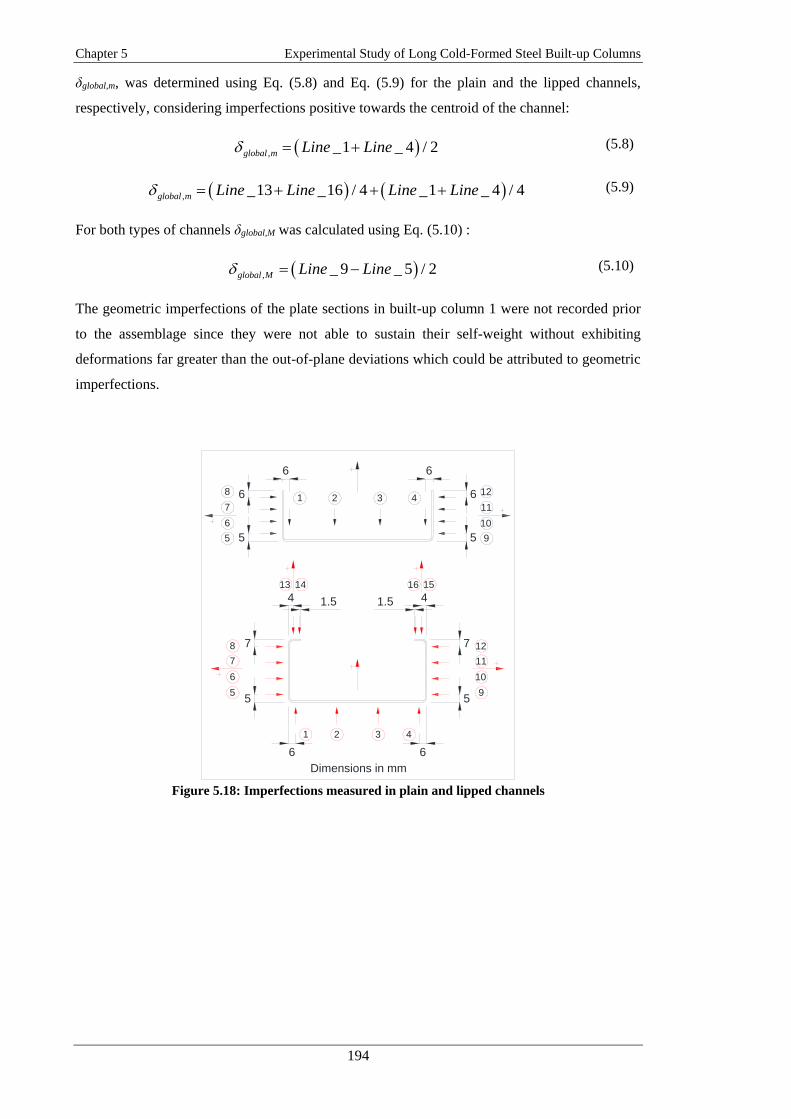
Chapter 5 Experimental Study of Long Cold-Formed Steel Built-up Columns
194
δglobal,m, was determined using Eq. (5.8) and Eq. (5.9) for the plain and the lipped channels,
respectively, considering imperfections positive towards the centroid of the channel:
, _1 _ 4 / 2global m Line Line (5.8)
, _13 _16 / 4 _1 _ 4 / 4global m Line Line Line Line (5.9)
For both types of channels δglobal,M was calculated using Eq. (5.10) :
, _ 9 _ 5 / 2global M Line Line (5.10)
The geometric imperfections of the plate sections in built-up column 1 were not recorded prior
to the assemblage since they were not able to sustain their self-weight without exhibiting
deformations far greater than the out-of-plane deviations which could be attributed to geometric
imperfections.
Figure 5.18: Imperfections measured in plain and lipped channels
6 6
5 5
6 6
66
77
55
44 1.51.5
6
7
8
9
10
11
121 2 3 4
5
Dimensions in mm
1 2 3 4
5
6
7
8
9
10
11
12
13 14 1516

Chapter 5 Experimental Study of Long Cold-Formed Steel Built-up Columns
195
Figure 5.19: Imperfection measurements on the individual channels
5.6.2.2 Built-up specimens
The geometric imperfections of the components were measured again after the different built-up
geometries were assembled. The imperfections of each component were measured along the
same lines as before the assemblage wherever the geometry permitted it.
In the specimens with built-up geometry 1, the geometric imperfections of the plates and the
web of the channels were recorded along four equally spaced lines, as shown in Figure 5.20.
The process of measuring the imperfections of the columns with geometry 1 is illustrated in
Figure 5.21.
The magnitude of the imperfections recorded in the plate sections was not expected to provide
an accurate representation of the initial state of the plate sections during the tests, since the low
flexural rigidity of the plates resulted in these imperfections being significantly reduced due to
the self-weight of the plates. The imperfections were nonetheless recorded in order to have an
approximate imperfection profile which could be used in an FE model. Moreover, the out-of-
plane imperfections of the plates were not expected to have a significant effect on the overall
behaviour of the built-up specimens.

Chapter 5 Experimental Study of Long Cold-Formed Steel Built-up Columns
196
The geometric imperfections of the channels were only recorded along the web. The
imperfections of the flanges were not recorded because after assembling the built-up geometry
there was not enough space within the channels to place the laser sensor at an appropriate
distance from the flanges. Therefore, for the channels used in built-up geometry 1 (T13014),
only the out-of-plane imperfections δweb were calculated using Eq. (5.11) and Eq. (5.12).
( ) _ 9 /16 9 _10 /16 9 _11/16 _12 /16 ( _ 9 _12) / 2web x Line Line Line Line Line Line (5.11)
( ) _13 /16 9 _14 /16 9 _15 /16 _16 /16 ( _13 _16) / 2web x Line Line Line Line Line Line (5.12)
This information was considered sufficient to quantify the imperfections of the channels related
to local buckling, since local buckling is expected to be primarily affected by the imperfections
in the most slender part of the cross-section. The imperfections recorded along the web of the
channels of built-up geometry 1 were also used to calculate δglobal,m after they were assembled
into built-up geometry 1, using Eq. (5.13) and Eq. (5.14).
, _ 9 _12 / 2global m Line Line (5.13)
, _13 _16 / 2global m Line Line (5.14)
However, for these channels δglobal,M could not be calculated after the channels were assembled
because the imperfections of the flanges could no longer be measured.
Figure 5.20: Location of the imperfection measurements in built-up column 1
8 8
8 8
6 6
6 6
1 2 3 4
5 6 7 8
9
10
11
12
13
14
15
16
Dimensions in mm

Chapter 5 Experimental Study of Long Cold-Formed Steel Built-up Columns
197
Figure 5.21: Measurement of the imperfections of built-up column 1
In the specimens with geometry 2, the geometric imperfections were measured along four
equally spaced lines on the web of the inner channels (T7914), as well as on the web and the
flanges of the outer channels (T15414), as depicted in Figure 5.22. The process of measuring
the imperfections of the columns with geometry 2 is illustrated in Figure 5.23.
The readings taken on the outer channels were used to calculate their cross-sectional out-of-
plane imperfections δweb and δflanges, using Eq. (5.15)-(5.19), which are relevant to the local
buckling mode.
( ) _1/16 9 _ 2 /16 9 _ 3 /16 _ 4 /16 ( _1 _ 4) / 2web x Line Line Line Line Line Line (5.15)
( ) _ 5 /16 9 _ 6 /16 9 _ 7 /16 _ 8 /16 ( _ 5 _ 8) / 2web x Line Line Line Line Line Line (5.16)
( ) _ 9 _12flange x Line Line (5.17)
( ) _13 _16flange x Line Line (5.19)
( ) _ 20 _17flange x Line Line (5.18)
( ) _ 24 _ 21flange x Line Line (5.19)
The global bucking imperfections δglobal,m and δglobal,M were also calculated for these channels
using Eq (5.20)-(5.23).
, _1 _ 4 / 2global m Line Line (5.20)
, _ 5 _ 8 / 2global m Line Line (5.21)
, _16 _12 / 2global M Line Line (5.22)
, _17 _ 21 / 2global M Line Line (5.23)

Chapter 5 Experimental Study of Long Cold-Formed Steel Built-up Columns
198
For the inner channels, readings of the flange imperfections were not taken because of access
restrictions for the laser sensor. However, the imperfections recorded along the web were used
to calculate δweb and δglobal,m using Eq. (5.24)-(5.27).
( ) _ 25 /16 9 _ 26 /16 9 _ 27 /16 _ 28 /16 ( _ 25 _ 28) / 2web x Line Line Line Line Line Line (5.24)
( ) _ 29 /16 9 _ 30 /16 9 _ 31/16 _ 32 /16 ( _ 29 _ 32) / 2web x Line Line Line Line Line Line (5.25)
, _ 25 _ 28 / 2global m Line Line (5.26)
, _ 29 _ 32 / 2global m Line Line (5.27)
Figure 5.22: Location of the imperfection measurements in built-up column 2
Figure 5.23: Measurement of the imperfections of built-up column 2
1 2 3 4
5 6 7 8
6 6
5
55
6
6
6
6
6
6
6
6
6 6
14
15
16
17
18
19
22
23
25 29
30
31
32
9
10
11
12
13
20 24
21
26
27
28
Dimensions in mm

Chapter 5 Experimental Study of Long Cold-Formed Steel Built-up Columns
199
After the specimens with geometry 3 were assembled, only the geometric imperfections of the
plain channels (T12012) could be measured. The imperfections of these channels were recorded
along four equally spaced lines on the web and the flanges, as shown in Figure 5.24. These
readings were used to calculate δweb, δflanges, δglobal,m and δglobal,m, using Eq. (5.28)-(5.37). Figure
5.25 illustrates the imperfection measurement process for columns with geometry 3.
( ) _1/16 9 _ 2 /16 9 _ 3 /16 _ 4 /16 ( _1 _ 4) / 2web x Line Line Line Line Line Line (5.28)
( ) _ 5 /16 9 _ 6 /16 9 _ 7 /16 _ 8 /16 ( _ 5 _ 8) / 2web x Line Line Line Line Line Line (5.29)
( ) _12 _ 9flange x Line Line (5.30)
( ) _16 _13flange x Line Line (5.31)
( ) _17 _ 20flange x Line Line (5.32)
( ) _ 21 _ 24flange x Line Line (5.33)
, _1 _ 4 / 2global m Line Line (5.34)
, _ 5 _ 8 / 2global m Line Line (5.35)
, _ 9 _13 / 2global M Line Line (5.36)
, _ 24 _ 20 / 2global M Line Line (5.37)

Chapter 5 Experimental Study of Long Cold-Formed Steel Built-up Columns
200
Figure 5.24: Location of the imperfection measurements in built-up column 3
Figure 5.25: Measurement of the imperfections of built-up column 3
In the specimens with geometry 4, the imperfections could only be recorded in the lipped
channels (S11012) due to the impossibility of accessing the plain channels with the laser sensor
after the specimens were assembled. The imperfections were recorded along four equally spaced
lines on the web and the flanges of the lipped channels, as shown in Figure 5.26. These
imperfections readings were used to determine δweb, δflanges, δglobal,m and δglobal,m, using Eq. (5.28)-
(5.37). In addition, Eq. (5.38)-(5.41) were used to calculate δflanges,L.
, ( ) _ 9 /16 9 _10 /16 9 _11/16 _12 /16 ( _ 9 _12) / 2flange L x Line Line Line Line Line Line (5.38)
, ( ) _13 /16 9 _14 /16 9 _15 /16 _16 /16 ( _13 _16) / 2flange L x Line Line Line Line Line Line (5.39)
6 6
6 6
5
5
5
5
6
6
6
6
14
15
16
13
22
23
24
21
1 2 3 4
5 6 7 8
17
18
19
20
9
10
11
12
Dimensions in mm

Chapter 5 Experimental Study of Long Cold-Formed Steel Built-up Columns
201
, ( ) _17 /16 9 _18 /16 9 _19 /16 _ 20 /16 ( _17 _ 20) / 2flange L x Line Line Line Line Line Line (5.40)
, ( ) _ 21/16 9 _ 22 /16 9 _ 23 /16 _ 24 /16 ( _ 21 _ 24) / 2flange L x Line Line Line Line Line Line (5.41)
Figure 5.27 illustrates the process of measuring the imperfections of the columns with geometry
4.
Figure 5.26: Location of the imperfection measurements in built-up column 4
Figure 5.27: Measurement of the imperfections of built-up column 4
5.6.3 Imperfection measurement results
The imperfections recorded on the individual channels and the built-up specimens were
classified into out-of-plane imperfections and global imperfections. The following sections
5
6
5
6
5
6
5
6
6 6
6 6
Dimensions in mm
9
10
11
12
17
18
19
20
14
15
16
13
22
23
24
21
1 2 3 4
5 6 7 8

Chapter 5 Experimental Study of Long Cold-Formed Steel Built-up Columns
202
discuss the main observations extracted from the experimental results, while the detailed
imperfection data of the channels, measured before and after they were assembled, are included
in Appendix H and I, respectively. In addition, Appendix J present a comparison between the
cross-sectional imperfections of the channels before and after they were assembled.
5.6.3.1 Cross-sectional imperfections
Before assembling the channels
Before the individual channels were assembled, each type of channel revealed a similar out-of-
plane imperfection profile along their web, flanges and lips, respectively. This consistency in
the imperfection shape can be attributed to the fact that each type of channel section was
presumably fabricated from the same steel coil and followed the same type of cold-forming
process and handling.
The out-of-plane imperfections recorded along the web (δweb) were very small in all channels,
with typical maximum amplitudes of 0.14 mm for the S11012 channels, 0.13 mm for the
T12012 channels, 0.16 mm for the T13014 channels, 0.31 mm for the T15414 channels and
0.06 mm for the T7914 channels. In the lipped channels (S11012), the out-of-plane imperfection
profile along the web consisted mainly of one undulating component Aund with a half-wave
length of around 600 mm and a constant component Acons of similar magnitude, while in the
plain channels the web out-of-plane imperfection consisted of several undulating components of
varying wavelength, in addition to the constant imperfection component Acons, as presented in
Figure 5.28 and Figure 5.29 for channel S11012-7 and T13014-2, respectively. Acons was
calculated as the average out-of-plane imperfection in the measured plate element, while Aund
was taken as the difference between the extremities of the imperfection profile. When
computing Acons and Aund the localised out-of-plane deformations at the support locations (which
resulted from direct bearing of the channels onto the support beams) were first removed from
the imperfection profile. A further discussion of these bearing deformations is included in
section 5.6.4.
The ratio between the constant imperfection component (Acons) and the undulating imperfection
component (Aund) varied significantly among channels of identical nominal cross-sectional
dimensions, as well as among different types of channels. This ratio was particularly large
(more than 2 on average) in channels T15414 with a length of 2500 mm. This reveals a great
deal of conservativism in the common practice to use the maximum out-of-plane imperfection
measurement to characterise the imperfections related to local or distortional buckling, given
that the constant imperfection component does not contribute to the onset of these types of
buckling modes. Moreover, using the maximum undulating imperfection component Aund is also
expected to result in a conservative characterisation of the out-of-plane imperfections since the
profile of the undulating component will not necessarily resemble the longitudinal shape of the

Chapter 5 Experimental Study of Long Cold-Formed Steel Built-up Columns
203
cross-sectional critical buckling mode of the channel. However, using the maximum undulating
imperfection component is a simple way to characterise the measured out-of-plain imperfections
and provides more meaningful information about the measured imperfections than simply
reporting the maximum value.
Figure 5.28: Imperfection components and bearing deformations along the web of channel S11012-
7
Figure 5.29: Imperfection components and bearing deformations along the web of channel T13014-
2
Regarding the imperfections recorded along the edge of the channel flanges (δflange), it was
observed that these out-of-plane imperfections were mainly dominated by one undulating
component Aund, as illustrated in Figure 5.30 for a sample channel S11012-2. It is important to
note that, since the imperfections δflange were measured with respect to only one reference line

Chapter 5 Experimental Study of Long Cold-Formed Steel Built-up Columns
204
(the web-flange junction), and since the angles between the flanges and the web of the channels
were not measured in this study, it was not possible to determine the constant imperfection
component of the flange imperfection δflange However, as mentioned before, this constant
component is not expected to have a significant effect on the buckling behaviour.
Figure 5.30: Undulating imperfection component along the left flange of channel S11012-2
All the measured channels displayed a similar imperfection profile along their flanges, with a
half-wave length of the undulating component Aund ranging from 600 mm to 800 mm. Figure
5.31 shows the out-of-plane imperfections δflange recorded along the left flange of one channel of
each type and length.
Figure 5.31: Imperfection profile recorded along the left flange of specimens of each type of channel

Chapter 5 Experimental Study of Long Cold-Formed Steel Built-up Columns
205
The out-of-plane imperfections recorded along the flange tips of channels T12012 had an almost
symmetric profile, while in channels T13014, T15414, T7914 and S11012 this symmetry was
not as evident. However, in the less symmetric imperfection profiles, it was noticed that the
imperfection shape on one flange was nearly the mirror image (with respect to mid-length) of
the shape on the other flange, as illustrated in Figure 5.32. The figure also shows, a symmetric
imperfection profile obtained for the flanges of a representative channel belonging to series
T13014. These observations clearly suggest that the flange imperfection profile is largely a result
of the ‘imprint’ left by the brake-press and the need to turn the specimen over 180o about mid-
length in order to press the second flange. This is in agreement with observations by Schafer
(1997), who suggested that these imperfections are largely determined by the manufacturing
process and not by the slenderness of the element.
Figure 5.32: Imperfection profile along the flanges of channels T13014-2 and T12012-2
In the lipped channels (S11012), the out-of-plane imperfections recorded along the web, the
flange edges and the free edges of the lips approximately followed the same profile, as shown in
Figure 5.33 for channel S11012-3. It is noted that, in this figure, the imperfection profile along
the web of the channel is inverted with respect to the ones along the flanges and lips due to the
sign convention used when recording the imperfections. The imperfections in the web were
considered to be positive towards the interior of the channel, while the opposite convention was
adopted for the imperfections in the flanges and the lips.

Chapter 5 Experimental Study of Long Cold-Formed Steel Built-up Columns
206
Figure 5.33: Imperfection profile along the web, flanges and lips of channel S11012-3
The out-of-plane imperfections recorded along the centre line of the flanges of channels S11012
relative to the line connecting the edges (δflange.L) were significantly smaller than the rest of the
imperfections recorded in the lipped channels, with a maximum amplitude of the undulating and
the constant components of less than 0.1 mm and 0.03 mm, respectively.
Table 5.14 lists the 25%, 50%, 75%, 95% and 99% percentiles of the amplitudes of the constant
and undulating imperfection components, as well as the maximum imperfection, obtained for
δweb, δflanges, δflanges.L and δlips based on the measurements before the components were assembled.
The table also includes the mean and the standard deviation of the reported imperfections. Since
the exact angles between the web and the flanges of the channels were not measured, a
representative maximum value of δflanges was computed as the maximum δflanges imperfection
measured relative to the average δflanges imperfection.
The table shows that the maximum δweb imperfections recorded in the web of the channels are,
on average, 47 % larger than the undulating imperfection components. However, they can be up
to 183 % larger than the undulating component, as shown for the T15414 channels with a length
of 2500 mm.

Chapter 5 Experimental Study of Long Cold-Formed Steel Built-up Columns
207
Table 5.14: Statistical values of the out-of-plane imperfection of the channels before the assemblage
Section Length
(mm) Imp.
Imp.
Comp
.
P(Δ<δ)
Mean St.
dev. 0.25 0.50 0.75 0.95 0.99
T13014 3000
δweb
Aund 0.07 0.08 0.08 0.10 0.10 0.08 0.012
Acons 0.02 0.10 0.16 0.17 0.17 0.10 0.062
Max. 0.09 0.15 0.20 0.22 0.23 0.16 0.058
δflanges Aund 0.55 0.57 0.58 0.62 0.64 0.57 0.029
Max. 0.34 0.35 0.37 0.39 0.34 0.35 0.025
T15414
2500
δweb
Aund 0.11 0.11 0.12 0.14 0.14 0.12 0.015
Acons 0.25 0.26 0.31 0.34 0.34 0.28 0.041
Max. 0.30 0.34 0.38 0.40 0.40 0.34 0.045
δflanges Aund 0.87 0.95 1.02 1.09 1.11 0.95 0.100
Max. 0.46 0.50 0.53 0.57 0.59 0.48 0.129
1800
δweb
Aund 0.15 0.15 0.16 0.19 0.19 0.16 0.018
Acons 0.01 0.05 0.16 0.23 0.23 0.11 0.099
Max. 0.13 0.15 0.27 0.32 0.32 0.21 0.090
δflanges Aund 1.06 1.17 1.33 1.44 1.44 1.21 0.162
Max. 0.57 0.61 0.69 0.75 0.75 0.63 0.083
T7914
2500
δweb
Aund 0.04 0.05 0.05 0.06 0.06 0.05 0.006
Acons 0.01 0.02 0.04 0.05 0.05 0.02 0.017
Max. 0.05 0.05 0.06 0.09 0.09 0.06 0.014
δflanges Aund 0.63 0.65 0.69 0.72 0.77 0.66 0.041
Max. 0.37 0.39 0.39 0.43 0.45 0.39 0.021
1800
δweb
Aund 0.04 0.05 0.05 0.05 0.05 0.05 0.005
Acons 0.01 0.02 0.02 0.03 0.03 0.02 0.009
Max. 0.05 0.05 0.05 0.06 0.06 0.05 0.005
δflanges Aund 0.84 0.87 0.88 0.92 0.92 0.87 0.038
Max. 0.42 0.45 0.47 0.50 0.50 0.41 0.161
T12012 3000
δweb
Aund 0.10 0.11 0.13 0.18 0.23 0.12 0.031
Acons 0.01 0.03 0.06 0.12 0.12 0.04 0.040
Max. 0.07 0.09 0.16 0.28 0.35 0.13 0.074
δflanges Aund 0.84 0.89 0.93 1.03 1.26 0.90 0.125
Max. 0.46 0.50 0.55 0.63 0.72 0.52 0.109
S11012 3000
δweb
Aund 0.12 0.14 0.18 0.21 0.41 0.16 0.062
Acons 0.01 0.04 0.05 0.08 0.09 0.04 0.024
Max. 0.11 0.13 0.15 0.18 0.41 0.14 0.063
δflanges.L
Aund 0.03 0.03 0.04 0.07 0.09 0.04 0.016
Acons 0.00 0.00 0.01 0.02 0.03 0.01 0.006
Max. 0.03 0.04 0.05 0.10 0.14 0.04 0.025
δflanges Aund 0.53 0.60 0.69 1.22 1.34 0.65 0.204
Max. 0.48 0.57 0.63 0.73 1.11 0.58 0.128
δlips Aund 0.14 0.14 0.17 0.21 0.23 0.15 0.027
Max. 0.11 0.11 0.12 0.14 0.17 0.12 0.015
After assembling the channels
After the individual channels were assembled into their final configuration, similarity of the out-
of-plane imperfection magnitude and shape along the web and flanges of each type of channel
was still evident in those channels with the same connector distribution along their length.
Channels T13014 and T7914 were used to assemble the specimens with built-up geometry 1
and built-up geometry 2, respectively, by connecting them through their flanges to the adjacent
components, as shown in Figure 5.1. In these channels, the magnitude of the undulating

Chapter 5 Experimental Study of Long Cold-Formed Steel Built-up Columns
208
component of the out-of-plane imperfections along the centre line of the web (δweb) had clearly
increased after the channels were assembled, with the largest amplitude of the undulations being
displayed around mid-length, as illustrated in Figure 5.34 for channels T13014. This can be
explained by the fact that, before the channels were assembled, the flanges consistently
exhibited an outward imperfection at mid-length with a large undulation, as shown in Figure
5.32 for channel T12012-2. Therefore, as contact between the different components of the built-
up specimens was enforced by the connectors, the flanges of channels T13014 and T7914 had to
rotate inward to accommodate the adjacent components, with the rotation being more
pronounced at mid-length due to the larger outward imperfection of the flanges. Due to the
continuity of the cross-section the rotation of the flanges caused an increased out-of-plane
imperfection in the web. The particularly marked out-of-plane imperfection at mid-length
shown in Figure 5.34 for the channels with three intermediate connectors is attributed to the fact
that in these specimens the connectors were sparsely distributed along the column (with a
connector spacing of 720 mm) and the cross-section at mid-length coincided with one of the
cross-sections containing connectors.
Figure 5.34: Imperfection distribution along the web of channels T13014 after assembly
On the other hand, channels T15414, T12012 and S11012, which were used to assemble
geometries 2, 3 and 4, respectively, were connected to their adjacent components through their
webs, as shown in Figure 5.1. In these channels the assembly process affected the out-of-plane
imperfection profile along the web of the channel (δweb) significantly more than in the channels
connected through their flanges. The connectors created localised out-of-plane imperfections
along the web, which resulted in an imperfection profile with repetitive ‘bumps’, as shown in
Figure 5.35 and Figure 5.36 for channels T15414 and channels S11012, respectively.

Chapter 5 Experimental Study of Long Cold-Formed Steel Built-up Columns
209
Figure 5.35: Imperfection profile along the web of channels T15414 after assembly
Figure 5.36: Imperfection profile along the web of channels S11012 after assembly
The flanges of channels T15414, T12012 and S11012 were affected by the assembly process to
a lesser degree than the webs. In most of these channels the out-of-plane imperfection profile
along the flange edges remained almost unaltered after the channel was assembled into its built-
up configuration, with only a slight increase or decrease in the magnitude of the undulating
component. However, in the case of channels T15414, which were connected to the adjacent
components of geometry 2 with connectors spaced at around 340 mm along the channel web
(i.e. channels with a length of 2500 mm and 6 intermediate connectors and channels with a
length of 1800 mm and 4 intermediate connectors), the presence of the connectors introduced an
undulating out-of-plane imperfection component in the flanges with a half-wave length equal to
the distance between connectors. This is illustrated in Figure 5.37 for the left flange of channels
T15414-1, T15414-5 and T15414-9 before and after they were assembled using 2, 6 and 4
equally spaced intermediate connectors along the length of the channel, respectively.

Chapter 5 Experimental Study of Long Cold-Formed Steel Built-up Columns
210
Figure 5.37: Imperfection profile along one of the flanges of channels T15414-1, T15414-5 and
T15414-9 after the assemblage
Table 5.15 lists the 25%, 50%, 75%, 95% and 99% percentiles, as well as the mean and the
standard deviation of the out-of-plane imperfections of each type of channel after they were
assembled into their final configuration, including their maximum values.
Table 5.15: Statistical values of the out-of-plane imperfections of the channels after the assemblage
Section Length
(mm) Imp.
Imp.
Comp.
P(Δ<δ) Mean
St.
dev. 0.25 0.50 0.75 0.95 0.99
T13014 3000 δweb
Aund 0.12 0.25 0.33 0.41 0.42 0.26 0.119
Acons 0.06 0.13 0.18 0.21 0.26 0.13 0.073
Max. 0.20 0.27 0.35 0.45 0.48 0.30 0.117
T15414
2500
δweb
Aund 0.44 0.48 0.52 0.60 0.60 0.48 0.080
Acons 0.05 0.06 0.10 0.20 0.20 0.08 0.059
Max. 0.28 0.34 0.42 0.50 0.50 0.36 0.083
δflanges Aund 1.00 1.12 1.17 1.24 1.26 1.10 0.110
Max. 0.62 0.66 0.72 0.78 0.80 0.67 0.075
1800
δweb
Aund 0.41 0.43 0.62 0.64 0.64 0.52 0.124
Acons 0.11 0.15 0.17 0.17 0.17 0.15 0.026
Max. 0.40 0.47 0.54 0.57 0.57 0.49 0.076
δflanges Aund 1.12 1.18 1.41 1.67 1.67 1.30 0.221
Max. 0.62 0.65 0.80 0.96 0.96 0.73 0.132
T7914
2500 δweb
Aund 0.13 0.15 0.18 0.25 0.25 0.17 0.047
Acons 0.00 0.01 0.02 0.04 0.04 0.02 0.014
Max. 0.09 0.11 0.16 0.59 0.59 0.23 0.222
1800 δweb
Aund 0.17 0.19 0.19 0.20 0.20 0.19 0.013
Acons 0.01 0.04 0.07 0.07 0.07 0.05 0.029
Max. 0.13 0.16 0.19 0.19 0.19 0.17 0.029
T12012 3000
δweb
Aund 0.24 0.29 0.38 0.41 0.61 0.33 0.116
Acons 0.01 0.02 0.03 0.13 0.14 0.04 0.046
Max. 0.36 0.44 0.45 0.58 0.61 0.44 0.088
δflanges Aund 0.78 0.86 0.98 1.06 1.07 0.87 0.133
Max. 0.44 0.47 0.56 0.64 0.65 0.50 0.087
S11012 3000
δweb
Aund 0.24 0.35 0.39 0.45 0.46 0.34 0.088
Acons 0.02 0.06 0.07 0.07 0.09 0.05 0.027
Max. 0.30 0.34 0.35 0.39 0.41 0.33 0.052
δflanges.L
Aund 0.03 0.04 0.05 0.09 0.12 0.05 0.021
Acons 0.00 0.01 0.01 0.03 0.07 0.01 0.015
Max. 0.03 0.04 0.04 0.07 0.15 0.04 0.026
δflanges Aund 0.45 0.60 0.69 0.96 1.13 0.61 0.195
Max. 0.46 0.64 0.84 1.05 1.12 0.67 0.232

Chapter 5 Experimental Study of Long Cold-Formed Steel Built-up Columns
211
Comparison of the out-of-plane imperfections based on Power Spectral Densities
In order to study the effect of the assembly process on the magnitude and shape of the out-of-
plane imperfections, the power spectral density (PSD) function was computed for the
imperfections recorded along the web and flanges of each channel, before and after they were
assembled. The PSD represents the spatial frequency response of the sinusoidal components
into which the imperfection signal can be decomposed. For the purpose of this study, the PSD
plotted the imperfection magnitude of each sinusoidal component against its half-wave length.
Figures 5.38-5.46 compare the PSD functions of the imperfections recorded along the web and
flanges of each type of channel, before and after they were assembled. The channels were
grouped according to the number of connectors used to assemble them. The solid lines
correspond to the PSD of the imperfections before the channels were assembled and the dashed
lines correspond to the PSD of the imperfections after the channels were assembled. The figures
also show three vertical lines which represent half of the distance between the connectors.
The PSDs reveal that, in general, before the channels were assembled the out-of-plane
imperfection profile along the web of the channels was mainly composed of imperfection
components with half-wave lengths larger than 500 mm, as illustrated in Figure 5.38, Figure
5.39, Figure 5.40, Figure 5.41 and Figure 5.46 for channels T13014, T15414, T7914, T12012
and S11012, respectively.
For the flanges of the plain channels, on the other hand, the out-of-plane imperfection profile
was mainly composed of one component with a half-wave length which ranged from around
600 mm for channels T12012 to 800 mm for channels T15414, as illustrated in Figure 5.45 and
Figure 5.44, respectively. For the lipped channels, two imperfection components of similar
magnitude were seen to dominate the out-of-plane imperfection profile along the flanges, with
half-wave lengths of around 600 mm and 1000 mm, as shown in Figure 5.46.
After the channels were assembled into their final configuration, the PSDs show the web
imperfection components were amplified over a relatively wide range of half-wave lengths.
Channels T13014 and T7914 were both connected through their flanges to the adjacent
components of the built-up geometry. For channels T13014 the half-wave-lengths of the
amplified components ranged from 250 mm to around 1100 mm, with an average maximum
amplification at a half-wave length of around 600 mm, while for channels T7914, mainly
components with half-wave lengths larger than 500 mm were amplified, as shown in Figure
5.38 and Figure 5.40, respectively. This might be indicative of the fact that the imperfections
induced by the connectors do not have an exact sinusoidal shape (but look more like the
‘bumps’ previously described), so that a range of frequencies (or half-wave lengths) is needed to
mathematically describe them.

Chapter 5 Experimental Study of Long Cold-Formed Steel Built-up Columns
212
Similar observations were made for channels T12012, S11012 and T15414, where the
connectors were located in the web of the channels. For channels T12012 and S11012 the
assembly process mainly affected components with a half-wave length larger than 100 mm, as
shown in Figure 5.41 and Figure 5.43, respectively. In the case of channels T12012 the
connectors mainly amplified components with a half-wave length close to the connector
spacing. In addition, imperfection components of around 500 mm and 1000 mm were also
amplified irrespective of the number of connectors used along the channel, with the
amplification being more pronounced in the channels with the largest number of connectors.
This may be attributed to the fact that the web of these channels was connected to the flanges of
the S11012 lipped channels, which before the assembly had undulating imperfection
components close to these half-wave lengths, as shown in Figure 5.42. For channels T15414, on
the other hand, after the channels were assembled the connectors clearly amplified the
imperfection components with a half-wave length equal to half the distance between connectors
in all channels, as shown in Figure 5.39.
It is important to note that for the channels studied, the local buckling half-wave lengths ranged
from 100 mm to 400 mm, while the distortional half-wave lengths of the lipped channels
reached up to 800 mm. This was precisely the range of half-wave lengths which were most
affected by the assembly process.
Figure 5.38: Average PSD of the web imperfections of channels T13014 before and after the
assemblage
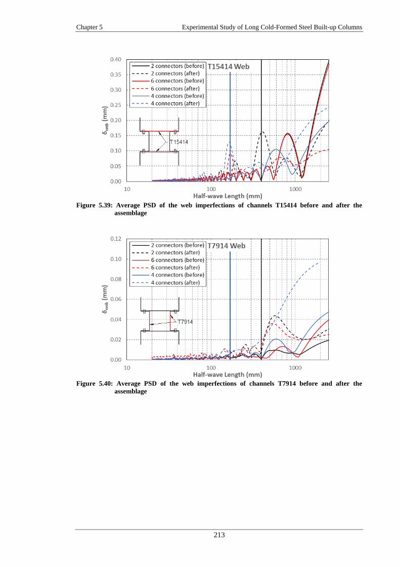
Chapter 5 Experimental Study of Long Cold-Formed Steel Built-up Columns
213
Figure 5.39: Average PSD of the web imperfections of channels T15414 before and after the
assemblage
Figure 5.40: Average PSD of the web imperfections of channels T7914 before and after the
assemblage

Chapter 5 Experimental Study of Long Cold-Formed Steel Built-up Columns
214
Figure 5.41: Average PSD of the web imperfections of channels T12012 before and after the
assemblage
Figure 5.42: Average PSD of the flange imperfections of channels S11012 before the assemblage

Chapter 5 Experimental Study of Long Cold-Formed Steel Built-up Columns
215
Figure 5.43: Average PSD of the web imperfections of channels S11012 before and after the
assemblage
Regarding the out-of-plane imperfections along the flanges of the channels, Figure 5.44, Figure
5.45 and Figure 5.46 compare the PSD functions of channels T15414, T12012 and S11012
before and after they were assembled. The figures show that in channels T12012 and S11012
the assembly process did not significantly affect the imperfection profile. However, in channels
T15414, the assembly process tended to reduce the half-wave length of the main component.
For the channels with a connector spacing of around 430 mm, it also introduced an additional
imperfection component with a half-wave length equal to half the distance between connectors,
as previously revealed in Figure 5.37.
Figure 5.44: Average PSD of the flange imperfections of channels T15414 before and after the
assemblage

Chapter 5 Experimental Study of Long Cold-Formed Steel Built-up Columns
216
Figure 5.45: Average PSD of the flange imperfections of channels T12012 before and after the
assemblage
Figure 5.46: Average PSD of the flange imperfections of channels S11012 before and after the
assemblage
5.6.3.2 Global imperfections
Before assembling the channels
All measured channels displayed a global flexural imperfection about the minor axis δglobal,m
with a profile closely resembling a ‘Bow imperfection’ (i.e. a half-sinusoidal wave equal to the
channel length) with a maximum imperfection amplitude around mid-length. Figure 5.47 shows
the average bow imperfection recorded for a representative channel of each type and length. The
direction of the Bow imperfection was consistently towards the web in all channels, irrespective
of their cross-sectional dimensions or whether they were stiffened with a lip. This bias in the
imperfection is attributed to the details of the fabrication process (Zeinoddini and Schafer,

Chapter 5 Experimental Study of Long Cold-Formed Steel Built-up Columns
217
2011), in particular whether the steel sheet used to fabricate the channels was fed into the
forming machine with a concave or convex residual curvature as a result of the coiling-
uncoiling stage.
Figure 5.47: Minor axis global imperfection of a representative specimen of each type of channel
before the assemblage
A large scatter in the magnitude of the bow imperfection was observed, even among channels
with the same nominal cross-sectional dimensions and length. As an example, Figure 5.48
shows the bow imperfections measured in all T12012 channels, with a length of 3 m. This large
variability in the magnitude of the bow imperfection may be attributed to the differences in the
radial location within the coil of the steel sheet used to fabricate the channels. As indicated by
Moen et al. (2008) and Quach et al. (2004), this position introduces longitudinal residual
stresses and strains which are locked into the member as it is cold-formed into its structural
shape.
Figure 5.48: Minor axis global imperfections of channels T12012 before the assemblage

Chapter 5 Experimental Study of Long Cold-Formed Steel Built-up Columns
218
In all channels the global flexural imperfections about the major axis (δglobal,M) were
significantly smaller than those recorded about the minor axis, and their profile could be less
accurately approximated by a ‘Camber imperfection’ (i.e. a half-sinusoidal wave equal to the
channel length). In most cases the maximum amplitude was recorded away from the mid-length
of the channel, as illustrated in Figure 5.49 for one specimen of each type of channel. Similarly
to the minor axis bow imperfections, a large scatter was observed in the magnitude of the major
axis global imperfections, even for channels with the same nominal dimensions.
Figure 5.49: Major axis global imperfections of a representative specimen of each type of channel
before the assemblage
Table 5.16 lists the 25%, 50%, 75%, 95% and 99% percentiles, as well as the mean and the
standard deviation of the minor and major axis global flexural imperfections at mid-length,
obtained for each type of channel section and length. The table also includes the statistical
results obtained when combining the measurements of all channels.
The table shows that the mean bow imperfection recorded at mid-length was L/2218, while 95%
of the bow imperfections were smaller than L/1000, which is commonly adopted in the
numerical analysis of cold-formed steel members as a conservative value. The major axis global
imperfection at mid-length, on the other hand, was found to be, on average, more than ten times
smaller than the minor axis global imperfection, with an average magnitude at mid-length of
L/24275 and a maximum value of L/5345 (which was encountered in channels T12012).
These results justify the use of a maximum out-of-straightness of L/1000 to model the bow
imperfection of single CFS channel members. However, this imperfection magnitude seems

Chapter 5 Experimental Study of Long Cold-Formed Steel Built-up Columns
219
excessively conservative when modelling the global flexural imperfection about the major axis
of CFS channels.
Table 5.16: Statistical values of the global imperfection of the channels before the assemblage
Section Length
(mm) Imp.
P(Δ<δ) Mean St. dev.
0.25 0.50 0.75 0.95 0.99
T13014 3000 δglobal,m L/1556 L/1398 L/1295 L/1249 L/1228 L/1440 L/7809
δglobal,M L/149033 L/39033 L/28525 L/22647 L/18821 L/38359 L/56765
15414
2500 δglobal,m L/6743 L/3594 L/3284 L/2711 L/2711 L/3860 L/11860
δglobal,M L/208978 L/124932 L/77356 L/42265 L/42265 L/99130 L/82258
1800 δglobal,m L/6369 L/4866 L/4818 L/4546 L/4546 L/5063 L/36046
δglobal,M L/398624 L/258842 L/59233 L/25420 L/25420 L/63904 L/49335
T7914
2500 δglobal,m L/2203 L/2099 L/2033 L/1972 L/1972 L/2197 L/12246
δglobal,M L/85251 L/43027 L/22360 L/16749 L/16749 L/34561 L/28054
1800 δglobal,m L/3023 L/2976 L/2556 L/2157 L/2157 L/2629 L/16188
δglobal,M L/91002 L/54995 L/44130 L/30280 L/30280 L/47138 L/108393
T12012 3000 δglobal,m L/3288 L/2293 L/2015 L/880 L/879 L/1935 L/3219
δglobal,M L/75442 L/28205 L/13110 L/6159 L/5345 L/18362 L/13241
S11012 3000 δglobal,m L/4166 L/2501 L/2194 L/1527 L/1498 L/2651 L/7271
δglobal,M L/27972 L/17160 L/14038 L/10016 L/9248 L/17758 L/15450
All
sections -
δglobal,m L/3431 L/2379 L/2015 L/1002 L/879 L/2218 L/4305
δglobal,M L/85251 L/30865 L/17084 L/9248 L/6159 L/24275 L/26483
After assembling the channels
The assembly process significantly affected the weak axis flexural imperfection δglobal,m of the
individual channels. In general, after the channels were assembled the shape of the minor axis
global imperfections resembled less of a sinusoidal bow imperfection. This was particularly the
case for channels T12012, which were used to assemble geometry 3, as illustrated in Figure
5.50. This can be attributed to the fact that in this built-up geometry, the relatively large flexural
rigidity of the stiffened flanges of the lipped channels, to which channels T12012 were attached,
resulted in large pulling forces at the connector locations which significantly affected the minor
axis global flexural imperfection profile of these channels.

Chapter 5 Experimental Study of Long Cold-Formed Steel Built-up Columns
220
Figure 5.50: Minor axis global imperfections of channels T12012 after the assemblage
On the other hand, for channels T15414, T7914 and S11012, the minor axis flexural
imperfection profile was still reasonably close to the initial bow imperfection present in the
channels before they were assembled, as illustrated in Figure 5.51 for channels S11012.
However, in all the channels belonging to series T15414 and T7914, which were used to
assemble geometry 2, the direction of the bow imperfection was reversed after the channels
were connected, as illustrated in Figure 5.52 and Figure 5.53 for channels T7914 and T15414,
respectively. A similar situation was observed in some of the T13014 channels, which were
connected to plate sections in geometry 1, where two channels experienced a reverse in the
direction of their bow imperfection.
Figure 5.51: Minor axis global imperfections of channels S11012 after the assemblage

Chapter 5 Experimental Study of Long Cold-Formed Steel Built-up Columns
221
Figure 5.52: Minor axis global imperfections of channels T15414 after the assemblage
Figure 5.53: Minor axis global imperfections of channels T7914 after the assemblage
Figure 5.54-1.59 compare the minor axis imperfection at mid-length for channels T13014,
T15414, T7914, T12012 and S11012, respectively, before and after they were assembled. In
addition, Figure 5.55, Figure 5.57 and Figure 5.58 also include a comparison of the major axis
imperfection at mid-length for channels T15414, T12012 and S11012, respectively.
The figures show that the assembly process affected the major axis imperfections of channels
T15414, T12012 and S11012 in different ways. In particular, after the channels T15414 were
assembled the major axis imperfections remained almost unaltered, as shown in Figure 5.55,
while for the channels T12012 and S11012, in some cases the assembly process increased the
major axis imperfections, while in other cases it reduced them or even inverted the direction of
the imperfections, as shown in Figure 5.57 and Figure 5.58, respectively.

Chapter 5 Experimental Study of Long Cold-Formed Steel Built-up Columns
222
Figure 5.54: Global imperfection of channels T13014 before and after the assemblage
Figure 5.55: Global imperfection of channels T15414 before and after the assemblage
Figure 5.56: Global imperfection of channels T7914 before and after the assemblage

Chapter 5 Experimental Study of Long Cold-Formed Steel Built-up Columns
223
Figure 5.57: Global imperfection of channels T12012 before and after the assemblage
Figure 5.58: Global imperfection of channels S11012 before and after the assemblage
The 25%, 50%, 75%, 95% and 99% percentiles of the minor and major axis global
imperfections, measured at mid-length after assembly, are listed in Table 5.17 for each type of
channel. The table also includes the mean and the standard deviation obtained for each type of
channel and length.
When comparing the results listed in Table 5.16 and Table 5.17 it can be seen that, on average,
after the channels were assembled the mean minor axis global imperfection at mid-length was
reduced by 48%, from L/2218 to L/4255, while the maximum imperfection amplitude was
reduced from L/879 to L/1326. The major axis global imperfection at mid-length, on the other
hand, was still found to be, on average, smaller than the minor axis one, with an average

Chapter 5 Experimental Study of Long Cold-Formed Steel Built-up Columns
224
amplitude at mid-length of L/10465 and a maximum amplitude of L/3710 (which occurred in
channels T12012).
Table 5.17: Statistical values of the global imperfection of the channels after the assemblage
Section Length
(mm) Imp.
P(Δ<δ) Mean St. dev.
0.25 0.50 0.75 0.95 0.99
T13014 3000 δglobal,m L/9998 L/6372 L/4414 L/3852 L/3229 L/5885 L/7182
δglobal,M - - - - - - -
15414
2500 δglobal,m L/7269 L/5956 L/4868 L/3764 L/3764 L/5568 L/19612
δglobal,M L/271243 L/71717 L/55655 L/34861 L/34861 L/75286 L/63055
1800 δglobal,m L/23564 L/16384 L/5240 L/4594 L/4594 L/7813 L/11229
δglobal,M 0 L/135950 L/135950 L/33086 L/33086 L/52853 L/41165
T7914
2500 δglobal,m L/2495 L/1983 L/1791 L/1326 L/1326 L/1887 L/7930
δglobal,M - - - - - - -
1800 δglobal,m L/3643 L/3441 L/2650 L/2048 L/2048 L/2796 L/10197
δglobal,M - - - - - - -
T12012 3000 δglobal,m L/54042 L/12546 L/5501 L/3845 L/3667 L/8191 L/9903
δglobal,M L/8588 L/5922 L/5226 L/3753 L/3710 L/6104 L/6385
S11012 3000 δglobal,m L/4930 L/3994 L/3466 L/3340 L/2966 L/4032 L/18335
δglobal,M L/45213 L/12432 L/7144 L/5630 L/5277 L/10028 L/9091
All
sections -
δglobal,m L/7124 L/4691 L/3466 L/1834 L/1541 L/4255 L/6451
δglobal,M L/54293 L/17480 L/5922 L/4206 L/3710 L/10465 L/12099
5.6.4 Measuring rig accuracy
The accuracy of the measuring rig is largely dependent on the straightness of the high precision
bars along which the laser sensor is moved. However, imperfection measurements with a higher
accuracy than the one provided by the guiding bars can be achieved by measuring the out-of-
flatness of a surface of which the tolerances are smaller than those of the guiding bars. This
way, the out-of-straightness of the guiding bars can be measured against the surface and used to
correct the imperfection measurements taken of the specimens. Obviously, the accuracy of the
measurements then depends on the deviation from flatness of the surface. However, other
sources of error, including the deformation of the specimen due to its self-weight, torsion of the
specimen due to uneven support conditions and vibrations of the laser sensor and the specimen
resulting from the propulsion mechanism will also limit the accuracy of the measurements.
In order to measure the out-of-straightness of the guiding bars, a flat surface was created by
taking advantage of the fact that a liquid at rest with a low viscosity tends to form a flat surface.
In this experimental study, the liquid chosen to generate the flat surface was milk, since its
surface was reflective to the laser sensor and its low viscosity permitted to obtain a measuring
surface which was virtually perfectly flat. In addition, milk has the advantage of being low-cost
and easily obtainable and can easily be cleaned up.
In order to generate a milk surface that could be measured by the laser sensor, a sealed container
for the milk was built and placed within the measuring rig, as illustrated in Figure 5.59. The

Chapter 5 Experimental Study of Long Cold-Formed Steel Built-up Columns
225
container was designed to be wide enough to ensure that all the measurements taken of the milk
surface were sufficiently far away from the edges of the container in order to avoid introducing
errors due to capillarity between the milk and the container. The container rested on two
portable stands, which were independent from the measuring frame in order to avoid
introducing vibrations originating from the stepper motors to the milk surface. Readings of the
milk surface were taken along the same longitudinal lines as the imperfection measurements of
the test specimens. This permitted to correct for the out-of-straightness of the longitudinal as
well as the transverse guiding bars.
Figure 5.59: Calibration of the imperfection measuring rig
Figure 5.60 shows the imperfections of the guiding bars, as detected from measuring the milk
surface along the same lines used to measure the imperfections of the web of channels T12012.
It can be seen that the deviation from straightness of the longitudinal guiding bars is around 0.6
mm over a length of 3 m.

Chapter 5 Experimental Study of Long Cold-Formed Steel Built-up Columns
226
Figure 5.60: Imperfections of the guiding system along the measuring lines of the web of channels
T12012
The measurements taken of the milk surface were then subtracted from the measurements of the
imperfections recorded on each test specimen.
Assuming that the reference surface was perfectly flat, the remaining errors in the corrected
measurements were mainly introduced by the deformations of the test specimen due to its self-
weight, and to a lesser degree by vibrations induced into the specimen during the measurements
by the movement of the laser sensor. The vibrations in the measurements had an amplitude of
around 0.05 mm. However, they were mostly removed during the data post-processing. The
self-weight deformations of the specimen can be decomposed into flexural deformations and a
torsion induced due to uneven support conditions, as illustrated in Figure 5.61. The latter is
composed of a point-symmetric component and a rigid body twist.
Figure 5.61: Flexural and torsional deformations due to self-weight

Chapter 5 Experimental Study of Long Cold-Formed Steel Built-up Columns
227
Errors due to flexural deformations of the specimen can be quantified by comparing the
geometric imperfections of the same plate element measured before and after flipping the
specimen so with each measurement the self-weight of the specimen causes it to deform in
opposite directions relative to the geometric imperfections in the plate element.
For this reason, in order to check the accuracy obtained from the imperfection measurements,
after accounting for the out-of-straightness of the guiding bars of the measuring rig, the web of
three plain channels, two of them with a length of 3000 mm and a third one with a length of
2500 mm, were measured with the channel placed in the four positions relative to the measuring
rig illustrated in Figure 5.62. The imperfections of the channels web were recorded along the
same equally spaced four lines used to record the imperfections in the rest of plain channels.
If the thickness of each channel web is assumed to be constant over the entire web, by
comparing the imperfections taken with the test specimen in positions 1 and 3, and 2 and 4,
respectively, the error introduced into the measurements due to the flexural deformation of the
specimen can be determined. It is important to note that by comparing the imperfection
measurements with the channel placed in the aforementioned positions, it is not possible to
detect errors introduced into the measurements related to the torsional deformation of the test
specimen due to uneven support conditions. This error component is, however, of little interest
for this experimental programme since the imperfection recorded from all the measured surfaces
were adjusted to zero the imperfection values at the corners of the surface by applying a small
twist to the reference surface from which the imperfections were taken, as described in section
5.6.2.
Figure 5.62: Measured channel positions to check accuracy of the measuring rig

Chapter 5 Experimental Study of Long Cold-Formed Steel Built-up Columns
228
Figure 5.63 shows the corrected imperfections readings obtained along each line measured on
the web of channel T12012-26 before the flexural deformation of the specimen due to its self-
weight was deducted, with the channel placed in the four aforementioned positions (Figure
5.62). In the figure, the solid lines show the measurements obtained with the channel placed in
positions 1 and 2, while the dashed lines shows the measurements obtained with the channel in
positions 3 and 4. The imperfections presented in the figure were obtained after processing the
data as described in section 5.6.2. The sign of the imperfection measurements was adjusted so
that positive values indicate imperfections towards the centroid of the cross-section.
Figure 5.63: Imperfections of the web of channel T12012-26 measured in four different positions
The effect of the self-weight on the measurements taken along the web of channel T12012-26 is
revealed in Figure 5.64, which shows, for each measured line, the imperfection difference
ΔImp,L_i(x), calculated using Eq. (5.42):
Imp, _ _1 _ 2 _3 _ 4( ) _ ( ) _ ( ) / 2 _ ( ) _ ( ) / 2L i position position position positionx Line i x Line i x Line i x Line i x (5.42)
, _1 , _ 2 , _3 , _ 4( ) ( ( ), ( ), ( ), ( ))Imp Imp L Imp L Imp L Imp Lx Max x x x x (5.43)
where Line_iposition_1, Line_iposition_2, Line_iposition_3 and Line_iposition_4 correspond to the
imperfection taken along each of the lines measured in the web, with the channel in position 1,
2, 3 and 4, respectively. Eq. (5.42) gives the difference between the average imperfection
obtained with the channel in positions 1 and 2, versus positions 3 and 4, while preserving the
sign of the difference.

Chapter 5 Experimental Study of Long Cold-Formed Steel Built-up Columns
229
Likewise, the maximum difference for the minor axis global flexural imperfection measured at
mid-length of the plain channel (Δδglobal,m) can be calculated using Eq. (5.44)
, , . _1 , . _ 2 , . _3 , . _ 4/ 2 / 2global m global m position global m position global m position global m position (5.44)
where δglobal,m.position_1, δglobal,m.position_2, δglobal,m.position_3 and δglobal,m.position_4 are calculated using Eq.
(5.8) with the channel in positions 1, 2, 3 and 4, respectively.
Figure 5.64: ΔImp,L_i(x) obtained in the web of channel T12012-26
It is important to note that, for each measured line, the true imperfection must lay at
approximately mid-distance between the maximum and minimum value of the recorded
imperfection. Therefore, the accuracy of the imperfection measurements (ξ) can be estimated as:
( ( )) / 2ImpMax x (5.45)
, , / 2global m global m (5.46)
Figure 5.64 shows that, for each measured line, the shape of ΔImp,L_i(x) closely follows the
expected flexural deformation of the channel due to its self-weight multiplied by two, as
represented by the red dashed line. This reveals that at this state, the accuracy of the
measurements is limited by the effect of the self-weight of the specimen to be measured. The
fact that the difference of the measurements follows twice the deformed shape of the specimens
can be expected since when the web of the channel was measured with the channel in positions
1 and 2, the deformation of the channel due to its self-weight reduced the imperfection of the
channel web, while the opposite can be said when the channel was measured in positions 3 and
4. The sharp increase of the imperfection difference, in Figure 5.64, calculated along lines 2 and

Chapter 5 Experimental Study of Long Cold-Formed Steel Built-up Columns
230
3 at x/length equal to 0.22 and 0.78 is due to the fact that when the channel was measure in
positions 1 and 2 the channel was directly rested on its web, which experienced localised
deformations at the supports location. This deformations, however, only covered a length of
around 100 mm along the channel. Therefore, it is not expected to have a significant effect on
the buckling behaviour of the built-up specimen. Similar imperfections measurements were
recorded along the web of the rest of plain channels.
In order to reduce the error in the measurements, the deformations due to the self-weight of the
channels were subtracted from the readings, assuming that, for a given cross-section along the
channel length, each point within the cross-section deflected by the same amount. In addition,
the calculation of the flexural deformations of the channel due to its self-weight was based on
the nominal cross-sectional dimensions of the channel, a Young modulus of 203 GPa, a density
of the steel of 7850 Kg/m3 and the measured distance between supports. Figure 5.65 shows
ΔImp,L_i(x) for each measured line after removing the flexural deformations of the channel due to
its self-weight, while Figure 5.66 shows the differences (in absolute value) between the
imperfections recorded with the channel in positions 1, 2, 3 and 4, after removing the self-
weight deformations of the channel. Figure 5.66 also includes the maximum and average
imperfection differences, as well as the standard deviation. The effect of the localized bearing
deformations at the support locations was not considered when calculating these statistical
parameters.
Figure 5.65: ΔImp,L_i obtained in the web of channel T12012-26 after removing the self-weight
deflections

Chapter 5 Experimental Study of Long Cold-Formed Steel Built-up Columns
231
Figure 5.66: Maximum imperfection difference obtained in the web of channel T12012-26 after
removing the self-weight deflections
Using Eq. (5.45) the accuracy of the imperfection measurements taken along the web of channel
T1212-26 was estimated to be around ±0.05 mm after the deflections of the channel were
removed from the measurements, with an average error of ±0.03 mm and a standard deviation
of ±0.01 mm. In addition, Eq. (5.46) was also used to estimate the accuracy of the global
flexural buckling imperfection calculated at mid-length of channel T12012-26. In this case, the
accuracy obtained was ±0.03 mm after removing the effect of the self-weight of the channel
from the measurements.
Similar results were also obtained when comparing the imperfection measurements taken on the
web of channels T12012-25 and T7914-13. Figure 5.67 and Figure 5.68 show the differences (in
absolute value) between the imperfections recorded when the channels were placed in positions
1, 2, 3 and 4, after removing the self-weight deformation of the channel, for channels T12012-
25 and T7914-13, respectively. A summary of the accuracy obtained from the imperfection
measurements and the global flexural imperfections carried out on the web of channels T12012-
25, T12012-26 and T7914-13 is listed in Table 5.18 and Table 5.19, respectively.

Chapter 5 Experimental Study of Long Cold-Formed Steel Built-up Columns
232
Figure 5.67: Maximum imperfection difference obtained in the web of channel T12012-25 after
removing the self-weight deflections
Figure 5.68: Maximum imperfection difference obtained in the web of channel T7914-13 after
removing the self-weight deflections
From Table 5.18 it can be seen that the maximum imperfection in the web of the channels
chosen to assess the accuracy of the measuring rig varied from 4.4 mm to 0.66 mm. The table
also shows that, on average, after removing the effect of the self-weight of the channel, the
maximum error in the imperfection measurements was reduced around 30%. Channels T12012
were also more affected by the effect of the self-weight than channel T7914. This could be
expected since channels T12012 had a larger self-weight/inertia ratio and were longer than
channel T7914. Therefore, they were expected to experience larger deformations under their
self-weight. Table 5.18 also shows that the accuracy of the imperfection measurements
obtained, after accounting for the self-weight, was virtually the same for all the channels, and
below ±0.063 mm, irrespective of the magnitude of the imperfection present in the channel.

Chapter 5 Experimental Study of Long Cold-Formed Steel Built-up Columns
233
Table 5.19, on the other hand, shows that the global flexural imperfection calculated at mid-
length of the channels had an accuracy of less than ±0.03 mm for all the channels after
accounting for the effect of the self-weight on the imperfection measurements. However, in this
case, removing the deformation of the channel due to its self-weight only resulted in an
averaged increase of the measurements accuracy of around 9 %. This can be explained by the
fact that the adjustable beams on which the channels were supported were positioned so as to
minimize the deflection of the channels due to their self-weight, which occurs when the
deflection at each end of the channel is the same as at mid-length. Therefore, since the
imperfections of the channel web are presented respect to a plane that intersect the corners of
the web, the deflection of the channel at the cross-section were the global flexural imperfection
were calculated was almost null.
Table 5.18: Imperfection difference obtained in channels measured in positions 1, 2, 3 and 4
Section
Before removing the self-weight After removing the self-weight
Max Imp
(υ)
Imperfection error (ξ) Max Imp
(υ)
Imperfection error (ξ)
Max. Avg. St. dev. Max. Avg. St. dev.
(mm) (mm) (mm) (mm) (mm) (mm) (mm) (mm)
T12012-25 4.446 ±0.104 ±0.038 ±0.023 4.446 ±0.063 ±0.018 ±0.014
T12012-26 1.838 ±0.077 ±0.033 ±0.015 1.839 ±0.049 ±0.025 ±0.009
T7914-13 0.657 ±0.057 ±0.019 ± 0.657 ±0.053 ±0.017 ±0.009
Table 5.19: Global flexural imperfection difference in channels measured in positions 1, 2, 3 and 4
Section
Before removing the self-weight After removing the self-weight
δglobal,m ξglobal,m ξ/δglobal,m δglobal,m ξglobal,m ξ/δglobal,m
(mm) (mm) (%) (mm) (mm) (%)
T12012-25 -3.311 ±0.006 ±0.18 -3.311 ±0.015 ±0.45
T12012-26 -1.718 ±0.037 ±2.15 -1.718 ±0.024 ±1.40
T7914-13 -0.596 ±0.015 ±2.52 -0.596 ±0.014 ±2.35
5.7. Test Set up
5.7.1 Introduction
All long columns were tested in a 2000 kN AMSLER universal testing machine. The columns
were subjected to compression between pin-ended boundary conditions, applying the load with
nominal eccentricities of L/1000 and L/1500. The bottom end of the column was the active end
accommodating the hydraulic actuator and a 300 kN load cell was mounted between the
actuator and the bottom support. The test set-up is illustrated in Figure 5.69.

Chapter 5 Experimental Study of Long Cold-Formed Steel Built-up Columns
234
Figure 5.69: Test set-up
5.7.2 Pin-ended supports
The pin-ended supports were designed to allow rotations about the major axis, while restraining
twisting and rotations about the minor axis. They consisted of hinge assemblies of which one
side was fixed to the cross-head or the actuator of the testing machine, while the other side was
welded to steel plates with dimensions of 250x300 mm2 and a thickness of 20 mm, and
containing slotted holes of 22 mm width, as shown in Figure 5.70. Two scribed lines were
marked on the sides of the steel plates. One of them was lined up with the axis of the pin, while
the other one was parallel to it, indicating the eccentricity to be applied. The steel plates were
bolted to the endplates of the column after aligning the centroid of the built-up specimens with
the scribed line on the bearing plates which indicated the applied eccentricity. Fine adjustment
between the specimens and the supports was achieved by means of four adjustable screws
located on the bearing plates (Figure 5.71). The distance from the centre of the pin of the top
support to the top end of the column was 75 mm, while the distance from the centre of the pin of
the bottom support to the bottom end of the column was 72 mm. Therefore, the effective length
of each specimen was calculated as:
Bottom
support
Top
support
Top support
Bottom support
Adjusting screws
Scribed line-specimen
Scribed line-Endplate
Scribed lines-Bottom
support
A
A Section A
B-1 B-2
T-1 T-2
L-2 L-4 L-3 L-1
G-1, G-2
Scribed lines-Top
support
Scribed line-Endplate
Scribed line-specimen
Adjusting screwsLoad cell
Actuator
Built-up
specimen
Adjustable
cross-head
W-2 W-2

Chapter 5 Experimental Study of Long Cold-Formed Steel Built-up Columns
235
147eL L (5.47)
where Le and L are the effective length and the actual length of the specimen in mm.
Figure 5.70: a) and b) components of top support; c) and d) components of bottom support
Figure 5.71: a) alignment between scribed lines; b) bottom support bolted to the specimen
(b) (b)
(c)
(a) (b)
(d)

Chapter 5 Experimental Study of Long Cold-Formed Steel Built-up Columns
236
5.7.3 Instrumentation
The columns were instrumented with 6 LVDTS with a maximum stroke of 50 mm and six
potentiometers with a maximum stroke of 25 mm. In addition, half of the specimens were also
instrumented with four 10 mm strain gauges.
5.7.3.1 LVDTs
Figure 5.69 shows the overall layout of the LVDTs used in the tests. The LVDTs were clamped
to the pillars of the testing machine. Four LVDTs were used to record the axial shortening of the
columns as well as their end rotations. LVDTs T1 and T2, and B1 and B2 were placed at a
horizontal distance of 110 mm away from the pin axis of the top and bottom support,
respectively.
The global flexural buckling deformations at mid-height were recorded with LVDTs G1 and
G2. The LVDTs were placed on the side of the specimen which experienced superimposed
tensile stresses due to the flexural buckling deformations and which will herein be referred to as
the ‘tension side’ of the specimen (in the appreciation that the total stress may still be
compressive). The opposite side, where flexural buckling caused additional compressive
stresses, will be referred to as the ‘compression side’. In geometries 2, 3 and 4, the LVDTs were
placed at the corners of the web of the channel component, while in the case of geometry 1, as
the plate sections were expected to buckle in a flexural mode between connectors before global
flexural buckling of the column, the LVDTs were placed at the flange corner of the channels, as
illustrated in Figure 5.72.
(a) (b)
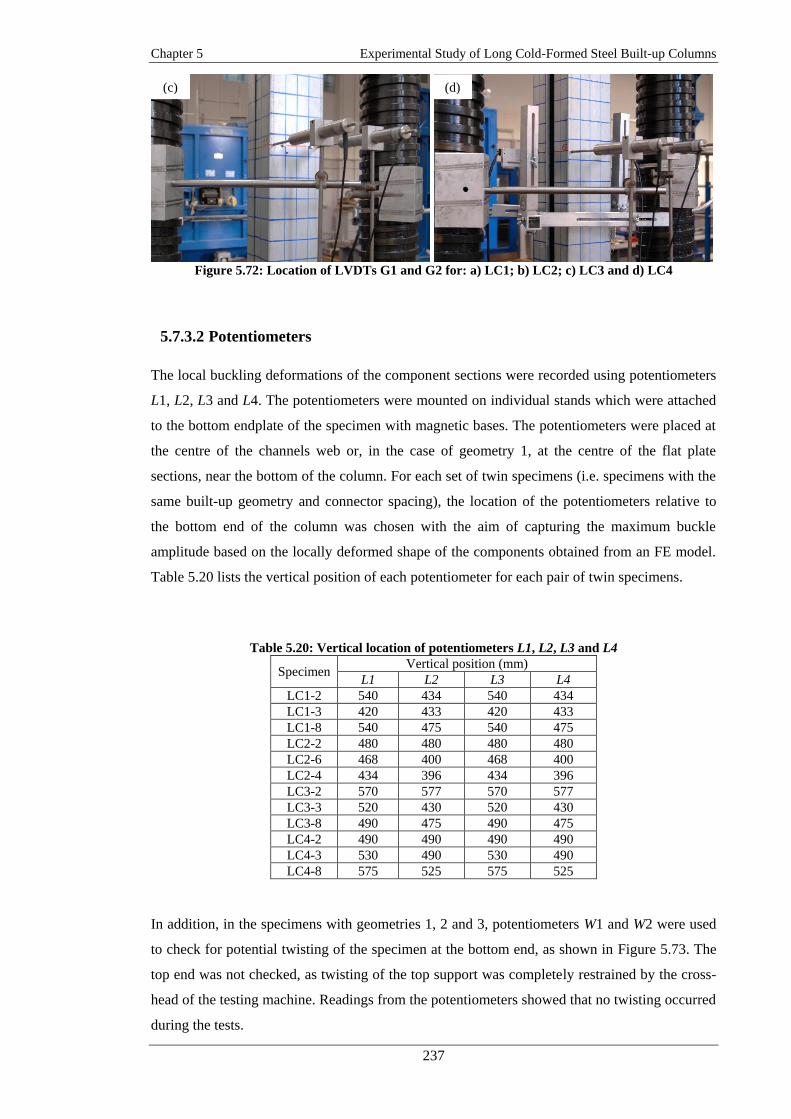
Chapter 5 Experimental Study of Long Cold-Formed Steel Built-up Columns
237
Figure 5.72: Location of LVDTs G1 and G2 for: a) LC1; b) LC2; c) LC3 and d) LC4
5.7.3.2 Potentiometers
The local buckling deformations of the component sections were recorded using potentiometers
L1, L2, L3 and L4. The potentiometers were mounted on individual stands which were attached
to the bottom endplate of the specimen with magnetic bases. The potentiometers were placed at
the centre of the channels web or, in the case of geometry 1, at the centre of the flat plate
sections, near the bottom of the column. For each set of twin specimens (i.e. specimens with the
same built-up geometry and connector spacing), the location of the potentiometers relative to
the bottom end of the column was chosen with the aim of capturing the maximum buckle
amplitude based on the locally deformed shape of the components obtained from an FE model.
Table 5.20 lists the vertical position of each potentiometer for each pair of twin specimens.
Table 5.20: Vertical location of potentiometers L1, L2, L3 and L4
Specimen Vertical position (mm)
L1 L2 L3 L4
LC1-2 540 434 540 434
LC1-3 420 433 420 433
LC1-8 540 475 540 475
LC2-2 480 480 480 480
LC2-6 468 400 468 400
LC2-4 434 396 434 396
LC3-2 570 577 570 577
LC3-3 520 430 520 430
LC3-8 490 475 490 475
LC4-2 490 490 490 490
LC4-3 530 490 530 490
LC4-8 575 525 575 525
In addition, in the specimens with geometries 1, 2 and 3, potentiometers W1 and W2 were used
to check for potential twisting of the specimen at the bottom end, as shown in Figure 5.73. The
top end was not checked, as twisting of the top support was completely restrained by the cross-
head of the testing machine. Readings from the potentiometers showed that no twisting occurred
during the tests.
(a) (c) (d)

Chapter 5 Experimental Study of Long Cold-Formed Steel Built-up Columns
238
Figure 5.73: Location of potentiometers W-1 and W-2
Results obtained from FE models showed that the specimens with geometry 4 generated
twisting forces at the supports of the same order of magnitude as the specimens with built-up
geometry 3. Therefore, twisting deformations in these specimens were not measured. In
geometry 4, the potentiometers were mounted on an aluminium frame, which was in contact
with the cross-section at its four corners and rested on three supports which were glued to the
corners of the cross-section, as illustrated in Figure 5.74. The frame was fixed to the supports by
hand-tightening a screw at one of the supports. Therefore, the frame was able to remain in place
when the specimens experienced cross-sectional deformations, while moving with the cross-
section as a whole when global buckling occurred. The potentiometers where located at mid-
height of the column. Potentiometer D1 was used to record the deformations of one of the
flanges of the lipped channel located on the tension side of the cross-section, while
potentiometer D2 was used to record the distortional buckling deformations of one of the
flanges of the lipped channel located on the compression side. Figure 5.75 shows the aluminium
frame with the potentiometers when mounted on specimen LC4-2b.

Chapter 5 Experimental Study of Long Cold-Formed Steel Built-up Columns
239
Figure 5.74: Schematic representation of the aluminium frame holding potentiometers D1 and D2
Figure 5.75: Aluminium frame attached to a specimen with geometry 4
5.7.3.3 Strain gauges
As global buckling and, in particular, the interaction of global and cross-sectional modes are
sensitive to the presence of geometric imperfections and therefore also to the initial eccentricity
of the applied load, all specimens tested with a load eccentricity of L/1000 were instrumented
with four strain gauges at mid-height in order to verify the applied eccentricity, as illustrated in
Figure 5.76. Figure 5.77 shows the strain gauge configuration used for each geometry. Strain
gauges SG1 and SG2 were placed on the tension side of the cross-section, while strain gauges
Supports
Supports
Fixing screw
D-1
D-2
A A
Section A
Built-up
specimen

Chapter 5 Experimental Study of Long Cold-Formed Steel Built-up Columns
240
SG3 and SG4 were located on the compression side. The strain gauge readings were also used to
check whether the magnitude of the minor axis bending moments resulting from possible
uneven contact along the supporting pin was small enough to be neglected.
Figure 5.76: Location of strain gauges in a) LC1, b) LC2, c) LC3 and d) LC4
Figure 5.77: Strain gauge lay-out for each geometry
(a) (b) (c) (d)

Chapter 5 Experimental Study of Long Cold-Formed Steel Built-up Columns
241
5.7.4 Test procedure
The specimens were tested while manually controlling the displacement rate at which the
columns were compressed. The data were collected in a Cubus data acquisition system using a
sampling rate of 1 Hz. The AMSLER testing machine used for the tests had a single piston
actuator which was controlled by opening or closing two valves. In order to perform the test in a
displacement controlled mode, a virtual channel was created in Cubus by differentiating the
average readings obtained from LVDTs B1 and B2 with respect to the time to obtain the rate at
which the specimen deformed axially. The valves controlling the actuator were then adjusted
during the test to keep the displacement rate as close to 0.08 mm/min as possible. This resulted
in approximate strain rates of 4.4x10⁻⁷ /s, 5.3x10⁻⁷ /s and 7.4x10⁻⁷ /s for the specimens with
lengths of 3000 mm, 2500 mm and 1800 mm, respectively. In addition, the test was halted for 4
min slightly before the peak load was reached in order to eliminate strain rate dependent effects.
After the peak load was reached, the displacement rate was increased. Figure 5.78 shows the
displacement rate achieved for a representative test specimens.
Figure 5.78: Displacement rate achieved in specimen LC1-8a
5.8. Test results
5.8.1 Strain gauge readings
Strain gauge readings obtained over the course of the test for representative columns with
geometry 1, 2, 3 and 4 are shown in Figure 5.79, Figure 5.80, Figure 5.81 and Figure 5.82,
0
0.02
0.04
0.06
0.08
0.1
0.12
0.14
0.16
0.18
0.2
0 1000 2000 3000 4000 5000 6000
Dis
pla
cem
ent
Rat
e (m
m/m
in)
Time (s)
Peak load reached
Test
paused

Chapter 5 Experimental Study of Long Cold-Formed Steel Built-up Columns
242
respectively. In these figures, compressive strains were taken as positive. All readings obtained
from columns instrumented with strain gauges are included in Appendix K.
Figure 5.79: Axial load vs compressive strain in column LC1-2a
Figure 5.80: Axial load vs compressive strain in column LC2-2a

Chapter 5 Experimental Study of Long Cold-Formed Steel Built-up Columns
243
Figure 5.81: Axial load vs compressive strain in column LC3-2a
Figure 5.82: Axial load vs compressive strain in column LC4-2a
5.8.1.1 Minor axis bending
Due to possible uneven contact between the endplates of the columns and the platens of the
testing machine, a small minor axis bending moment might have been introduced into the built-
up specimens. Steel shims were placed between the column endplates and the hinge assemblies
in order to reduce this unwanted bending moment. However, the introduction of a small bending
moment during the test was deemed unavoidable.
In order to assess the effect of the minor axis bending moment on the stresses which developed
in the components of the built-up geometry half of all columns were instrumented with strain
gauges at mid-height. The stresses at the centre line of the webs of two channels located on
opposite sides of the minor axis of the built-up geometries were calculated from the strain gauge

Chapter 5 Experimental Study of Long Cold-Formed Steel Built-up Columns
244
readings slightly before the channels started buckling in a local mode. In each built-up geometry
the stresses at the centre line of the web of the channels located to the left and to the right of the
minor axis (Figure 5.83) were determined using Eq. (5.48) and Eq. (5.49), respectively.
, ,
,2
R L w
SG ch L avg
SG x
dE
d
(5.48)
, ,
,2
R L w
SG ch R avg
SG x
dE
d
(5.49)
In the above equations E is the Young’s modulus, taken as 203000 MPa, εL, εR and εavg are given
by Eq. (5.50), Eq. (5.51) and Eq. (5.52), respectively, dSG,x is the distance between the centre
lines of the strain gauges and dw is the distance between the webs of the channels, as illustrated
in Figure 5.83 for each geometry.
1 4
2
SG SG
L
(5.50)
2 3
2
SG SG
R
(5.51)
1 2 3 4
4
SG SG SG SG
avg
(5.52)
Figure 5.83: Strain gauge locations and distance between left and right channel webs
Table 5.21 lists the load at which the stresses were calculated, the average stress in the column
obtained from the strain gauges readings (σSG,avg) and the average stress (σL,avg) obtained by
dividing the column load over the measured cross-sectional area of the built-up column. The
table also includes the stresses in the webs of the left channel (σSG,ch,L) and right channel
(σSG,ch,R), their difference (ΔσR-L), and an estimation of the importance of the minor axis bending
stresses in the web of these channels, defined as:
SG 1 SG 2
SG 4 SG 3
SG 1 SG 2
SG 4 SG 3
SG 1 SG 2
SG 4 SG 3
SG 1 SG 2
SG 4 SG 3
dSG,x
dw
x x xxx x x x
dSG,x
dSG,xdSG,x
dw dw dw
dSG,y dSG,y dSG,y dSG,y

Chapter 5 Experimental Study of Long Cold-Formed Steel Built-up Columns
245
, ,
,
100SG ch SG avg
ch
SG avg
(5.53)
Table 5.21: Stress difference between left and right channel
Specimen Load
(kN)
σL,avg
(MPa)
σSG,avg
(MPa)
σSG,ch,L
(MPa)
σSG,ch,R
(MPa)
ΔσR-L
(MPa)
ξch
(%)
LC1-2a 45 40 83 80 86 6 4
LC1-3a 45 40 75 73 77 3 2
LC1-8a 45 40 52 49 55 6 6
LC2-2a 75 67 78 72 83 11 7
LC2-6a 75 67 65 60 69 9 7
LC2-4a 75 68 69 64 74 10 7
LC3-2a 55 61 61 58 65 7 6
LC3-3a 55 61 64 60 67 8 6
LC3-8a 55 60 61 55 66 11 9
LC4-2a 55 60 60 60 59 1 0
LC4-3a 55 60 64 64 64 0 0
LC4-8a 55 60 61 60 61 1 1
Table 5.21 shows that, with the exception of columns LC1, good agreement was generally
achieved between σL,avg and σSG,avg. For columns LC2, the only exception occurred in column
LC2-2a, for which a difference of 11 MPa was obtained between σL,avg and σSG,avg. This larger
discrepancy was preceded by a loss of linearity recorded by the strain gauges at a load of around
50 kN, as illustrated in Figure 5.80. However, up to this load the values obtained for σL,avg and
σSG,avg agreed well and were 45 MPa and 44 MPa at a load of 50 kN, respectively. For columns
LC3 and LC4, an almost perfect match between σL,avg and σSG,avg was obtained, with only
columns LC3-3a and LC4-3a showing a slightly larger discrepancy. This slightly larger
difference was believed to be due to stress concentrations captured by the strain gauges due to
their close proximity to some of the connectors, which in these columns were located only a few
millimetres away from the strain gauges.
Table 5.21 also shows that the difference between σSG,ch,L and σSG,ch,R was less than 11 MPa in all
the columns instrumented with strain gauges, while the average difference between these
stresses and the average stress in the built-up cross-section was around 5 %. This shows that the
effect of the minor axis bending moment introduced into the test specimens was minor.
However, the results listed in Table 5.21 should be taken into consideration when interpreting
the readings obtained from the potentiometers, which were used to derive the critical buckling
stresses in the components of the built-up specimens.

Chapter 5 Experimental Study of Long Cold-Formed Steel Built-up Columns
246
5.8.1.2 Eccentricity
Readings from the strain gauges were also used to assess the accuracy of the load eccentricity
achieved by aligning the scribed lines on the supports and the endplates of the built-up columns,
as described in Section 5.7.3.3.
Using the initial linear portion of the strain gauges readings, the initial eccentricity at mid-height
(e0,SG) was derived by computing the moment to axial load ratio in the cross-section at mid-
height, while correcting for the lateral displacement experienced by the cross-section as loading
progressed. This resulted in Eq. (5.54), which has been used in (Becque, 2008) for a similar
purpose.
,
0,
,
2 1 2
2
built up xx c t
SG
built up SG y c t
I G Ge
A d
(5.54)
In the above equation Abuilt-up and Ibuilt-up,xx are the cross-sectional area and the second moment of
area about the major axis of the built-up geometry. dSG,y is the distance between the centrelines
of the strain gauges, as indicated in Figure 5.83. G1 and G2 are the lateral deformations of the
built-up specimen at mid-height given by LVDTs G1 and G2, and εc and εt are the average
strains given by the strain gauges attached to the compression and tension side of the built-up
geometry, calculated as:
3 4
2
SG SG
c
(5.55)
1 2
2
SG SG
t
(5.56)
In Eq. (5.54), e0,SG includes both the load eccentricity applied at the ends of the built-up column
and the initial major axis global imperfection of the built-up specimen at mid-height δglobal,M.
Therefore, a direct assessment of the accuracy of the load eccentricity can be achieved by
adding δglobal,M to the applied end eccentricity to obtain e0,mid, and comparing it with e0,SG. Figure
5.84 provides a graphical representation of this comparison for one of the specimens, while
Table 5.22 compares e0,mid, and e0,SG for all the specimens instrumented with strain gauges.
In Figure 5.84, after the specimen settles under the load, a region with a fairly constant
eccentricity can be distinguished. The average eccentricity within this region was used to
compute the values of e0,SG listed in Table 5.22.

Chapter 5 Experimental Study of Long Cold-Formed Steel Built-up Columns
247
Figure 5.84: Axial load vs initial eccentricity at mid-height for column LC4-8a
Table 5.22: Accuracy assessment of load eccentricity
Specimens δglobal,M
(mm)
e0,nom
(mm)
e0,mid
(mm)
e0,SG
(mm)
|Difference|
(mm)
LC1-2a - 3.0 - - -
LC1-3a - 3.0 - - -
LC1-8a - 3.0 - 3.13 -
LC2-2a -0.03 2.5 2.47 3.01 0.54
LC2-6a 0.01 2.5 2.51 2.73 0.22
LC2-4a -0.16 1.8 1.64 1.50 -0.14
LC3-2a -0.26 3.0 2.75 3.08 0.33
LC3-3a 0.03 3.0 3.03 (2.02) (-1.01)
LC3-8a -0.38 3.0 2.62 2.85 0.23
LC4-2a -0.07 3.0 2.93 3.01 0.08
LC4-3a -0.02 3.0 2.99 (4.76) (1.77)
LC4-8a 0.13 3.0 3.13 3.48 0.35
In Table 5.22, δglobal,M was calculated from the imperfections recorded along the top and bottom
channels after they were assembled into their final configuration, as shown in Figure 5.83. For
the specimens with built-up geometry 1, e0,mid was not calculated since the major axis global
imperfection at mid-height of this specimens was not considered to be represented by the
imperfections recorded along the plate sections due to their low flexural rigidity. Moreover, in
columns LC1-2a and LC1-3a the plate sections displayed out-of-plane displacements between
the connectors from the onset of loading.
Table 5.22 shows that in most cases a good agreement was achieved between the eccentricities
calculated from the strain gauges readings and the ones obtained from adding the major axis
global imperfection of the built-up specimen to the nominal eccentricity applied at the ends of
the column. An exception occurred in specimens LC3-3a and LC4-3a, where a relatively large
difference between e0,SG and e0,mid was obtained. As previously mentioned, the reason for these
larger differences can be attributed to stress concentrations captured by the strain gauges due to
their close proximity to a set of connectors which were also located at mid-height in these

Chapter 5 Experimental Study of Long Cold-Formed Steel Built-up Columns
248
specimens. With the exception of said specimens, the average difference between e0,SG and e0,mid
was 0.27 mm, which proves the high accuracy of the procedure followed during this
experimental programme when applying the load eccentricity to the test specimens.
5.8.2 Deformed shape
This section describes the way in which the different columns deformed during the test, with
special emphasis on the different types of buckling modes observed in the components as well
as in the built-up specimen as a whole.
In all columns, local buckling of the components was observed before the built-up specimen
failed due to global flexural buckling. In column LC1 a global-type buckling of the plates in
between connector points was also observed. As a result of the combined effects of the applied
eccentricity and the initial imperfections lateral displacements of the column took place from
the onset of loading. This introduced additional second order compressive stresses on one side
of the column and superimposed tensile stresses on the opposite side (as stated before, here
referred to as the ‘compression’ and ‘tension’ side of the built-up specimen, respectively).
Consequently, in all tested columns, the magnitude of the buckles of the component located on
the compression side of the built-up specimen was observed to be larger than the magnitude of
the buckles formed in the symmetric component located on the tension side.
5.8.2.1 Built-up geometry 1
Columns with geometry 1 failed by global flexural buckling about the major axis of the built-up
specimen which interacted with local buckling of the channels and a global-type buckling of the
plate sections between connector points, while global flexural-torsional buckling of the channels
between connectors was also observed in some columns. Columns with the same number of
connectors exhibited the same initial buckled shape. However, development of the plastic yield
line mechanism often occurred at different locations along the specimen. In all columns, yield
lines formed in the web and the flange of the channels located on the compression side of the
built-up specimen. The deformed shapes of all the columns with geometry 1, before and after
yield line formation, are illustrated in Figure 5.85 and Figure 5.86, respectively.
In columns LC1-2 and LC1-3, the relatively large connector spacing caused the plate sections to
buckle outward within each field between connectors in a global flexural mode with a half-wave
length equal to half the distance between connectors. The channels, on the other hand, buckled
in a local mode, generating 22 half-waves along the column, irrespective of the number of
connectors.

Chapter 5 Experimental Study of Long Cold-Formed Steel Built-up Columns
249
In columns LC1-2, the distance between connectors was large enough (960 mm) to cause failure
of the channels due to flexural-torsional buckling between connectors. In the lower field of the
columns the channels rotated and translated towards the interior of the built-up cross-section,
while in the central field the channels rotated and moved outwards. Flexural-torsional buckling
of the channels prompted a sudden failure of the built-up specimen due to global flexural
buckling. Upon localization of the deformation pattern the formation of yield lines symmetric
with respect to the major axis of the column was observed.
In column LC1-3b, which was tested with a load eccentricity of L/1500 and had a connector
spacing of 720 mm, the channels also failed by flexural-torsional buckling between connectors.
However, in this case, both channels rotated and moved laterally in the same direction, while
this direction alternated in successive fields. Upon failure of the channels, yield lines developed
in the channels in the field where they moved towards the interior of the column. This meant
that one of the channels developed its plastic mechanism in the field below the column mid-
height, while in the other channel the plastic mechanism was formed in the field above mid-
height. As the specimen continued deforming, a second plastic mechanism developed in each
channel in the field where they moved outward. The tendency of the channels to twist and move
laterally introduced some twisting into the already buckled plate sections, in the fields sharing
the set of connectors located at mid-height (Figure 5.85d). However, the readings obtained from
potentiometer W1 revealed no twisting of the built-up column as whole, with the specimen
instead failing by global flexural buckling about the major axis. In column LC1-3a, which was
tested with a larger load eccentricity (L/1000) than LC1-3b, but with an identical connector
spacing, the channels only experienced local buckling, without any flexural-torsional
deformations, as illustrated in Figure 5.85c. In this specimen the yield line mechanism, which
developed slightly below mid-height, was perfectly symmetric about the major axis of the
column. It is worth noting the difference in the plastic yield line mechanism which formed in
the channels when they failed by interaction between local buckling and flexural-torsional
buckling between connector points, as opposed to the one which formed when failure occurred
due to interaction between local buckling of the channels and global flexural buckling of the
built-up specimen. In the former, the plastic hinge mechanism developed mainly in the
compression flange of the channels, as illustrated in Figure 5.87b for specimen LC1-3b, while in
the latter, yield lines also spread across the web of the channels, as shown in Figure 5.87a for
specimen LC1-3a
In columns LC1-8, the channels were also observed to initially buckle in a local mode with
multiple half-wave lengths along the column. However, the precise number of buckles could not
be determined. Due to the shorter distance between connectors in these columns the plate
sections did not buckle with a half-wave length equal to half the distance between connectors.
Rather the plate sections buckled outwards in every other field along the column and remained

Chapter 5 Experimental Study of Long Cold-Formed Steel Built-up Columns
250
almost straight in the adjacent fields, as the channels web prevented them from buckling
inwards. The buckle half-wave length was longer than half the connector spacing, which
required some localized deformations to take place around the connector points. It is also
important to note that this discontinuous buckling pattern could only be possible if some slip
between the plate and the channels occurred at the connector points. Interestingly, in both
columns tested with eight intermediate connectors, the plate sections always remained straight
in the top and bottom field, and consequently in the central field of the column. This is most
likely due to a higher degree of fixity of the plates in the end fields with respect to their end
rotations as a result of the fillet weld between the column and the endplates. In both columns,
the post-peak deformations in the channels localized in fields where the plates initially buckled
outward. In the case of column LC1-8a, the plastic deformations in each channel localized in
different fields, namely in the field below the central field in one of the channels, and in the
field above it in the other channel, as shown in Figure 5.85e. In column LC1-8b, on the other
hand, a yield line mechanism symmetric with respect to the major axis of the column was
formed, with the plastic mechanism in both channels developing in the second field from the
bottom, as shown in Figure 5.85f.
Figure 5.85: Deformed shape approaching ultimate load in a) LC1-2a, b) LC1-2b, c) LC1-3a, d)
LC1-3b, e) LC1-8a, f) LC1-8b
(a) (c) (e) (b) (d) (f)

Chapter 5 Experimental Study of Long Cold-Formed Steel Built-up Columns
251
Figure 5.86: Final deformed shape at end of test in a) LC1-2a, b) LC1-2b, c) LC1-3a, d) LC1-3b, e)
LC1-8a, f) LC1-8b
Figure 5.87: Plastic yield line mechanism in a) LC1-3a, b) LC1-3b
5.8.2.2 Built-up geometry 2
All columns with geometry 2 failed by interaction between global flexural buckling about the
major axis of the built-up specimen and local buckling of the individual components. Multiple
(a) (b)
(a) (c) (e) (b) (d) (f)

Chapter 5 Experimental Study of Long Cold-Formed Steel Built-up Columns
252
regular local buckles were observed along the columns. A distortion of the outer channel flanges
at each end of the column, caused by the localized temperature gradients during welding of the
endplates (as described in Section 5.5), was noticeable before the test in all specimens of
geometry 2 (Figure 5.16). These initial out-of-plane deformations were amplified as the
specimens were loaded, even before the channels buckled locally. Also, in some columns,
buckles with slightly larger amplitude were observed in the flanges of the outer channels on one
side of the minor axis. This was attributed to the small, yet ineludible bending moments present
about the minor axis of the built-up specimen.
Figure 5.88: Plastic yield line mechanism in LC2-6b
In all columns yield lines formed in the outer channel located on the compression side of the
built-up specimen, and in the web and the most compressed flange of the inner channels. This
yield line mechanism was identical in most of the columns and is shown in Figure 5.88 for
column LC2-6b after the load was removed. The deformed shapes before and after the ultimate
capacity was reached are illustrated in Figure 5.89 and Figure 5.90, respectively, for all columns
with built-up geometry 2.
In columns LC2-2, with two rows of intermediate connectors, the outer channels were forced to
buckle mainly outwards due to the presence of the inner channels, displaying four half-waves
between the connectors in the central field. This could be expected since the natural buckle half-
wave length of the outer channels was calculated to be 170 mm, and this was close to the 200
mm resulting from fitting four half-waves between connector points. In the adjacent fields, on
the other hand, the outer channels accommodated six half-waves, with the buckle closest to the
end of the column being noticeably shorter than the others. This is attributed to the initial
distortion of the outer channel flanges. The remaining buckles in the top and bottom fields had a

Chapter 5 Experimental Study of Long Cold-Formed Steel Built-up Columns
253
buckle half-wave length somewhere between 130 mm and 200 mm, which was still close to
their natural buckle half-wave length. The inner channels in these columns did not buckle, as
illustrated in Figure 5.89a and Figure 5.89b. After the ultimate capacity was reached, column
LC2-2a formed a yield line mechanism in the vicinity of the upper set of connectors in the
central field, as illustrated in Figure 5.90a. In column LC2-2b, a yield line mechanism was first
formed in the outer channel around mid-height (Figure 5.90b) and in one of the inner channels
close to the lower set of connectors in the central field. As the column was further compressed,
a yield line mechanism also formed in the other inner channel, next to the plastic hinge
previously formed in the outer channel. This sequential formation of yield lines in the built-up
specimen was reflected in a loss of stiffness in the form of a descending step in the load-axial
deformation curve (Figure 5.108).
Columns LC2-6 and LC2-4 had different column lengths, but similar connector spacings,
namely 340 mm and 336 mm, respectively. Similarly to columns LC2-2, the inner channels
forced the outer channels to buckle outwards. However, in columns LC2-4, some minor inwards
out-of-plane displacements were recorded in the web of the outer channels by the
potentiometers which were located around 40 mm above a cross-section containing connectors.
This was attributed to a slight rotation of the flanges of the inner channels which were forced to
open slightly in order to accommodate the inward buckles of the outer channels web. Due to the
reduced connector spacing, the outer channels buckled with a half-wave length equal to half the
distance between connectors, as shown in Figure 5.89c-f, which virtually coincided with their
natural local buckle half-wave length.
In columns LC2-6, the initial distortion of the outer channel flanges resulted in the buckles in
the top and bottom field having a slightly larger amplitude than the ones in the other fields. The
amplitude of these initial imperfections was amplified from the beginning of the test. As a result
of the reduced connector spacing in these columns, the interaction between the different
components was more pronounced and triggered local buckling in the most compressed flange
of the inner channels at around the point where the column reached its ultimate capacity,
something which was not observed in the columns with larger connector spacing. The most
compressed flange of these channels was forced to buckle towards the inside of the channel due
to the presence of the outer channel webs and displayed four half-waves between connectors, as
illustrated in Figure 5.89c and Figure 5.89d. After the ultimate capacity was reached, both
columns developed a yield line mechanism around mid-height which was perfectly symmetric
with respect to the major axis of the column, as shown in Figure 5.90c and Figure 5.90d,
respectively.
In columns LC2-4, the initial distortion of the outer channel flanges was more pronounced than
in columns LC2-6. As a result of this, the flanges of the outer channels buckled displaying four
half-waves between connectors in one of the fields next to the column ends, while in all the

Chapter 5 Experimental Study of Long Cold-Formed Steel Built-up Columns
254
other fields only two half-waves were formed. In both columns, the plastic deformations
localized in the end field located on the compression side of the built-up specimen where the
four half-waves had previously formed, as shown in Figure 5.90e and Figure 5.90f. This
resulted in premature failure, especially in column LC2-4a, where some twisting of the bottom
endplate (by around 0.8°) was also recorded before the ultimate capacity of the specimen was
reached. In this specimen, the plastic mechanism formed before the most compressed flange of
the inner channels could buckle in a local mode, as illustrated in Figure 5.89e and Figure 5.90e.
In column LC2-4b, on the other hand, the most compressed flange of the inner channels buckled
just before the yield line mechanism localized at the top end of the column, as shown in Figure
5.89f and Figure 5.90f.
Figure 5.89: Deformed shape approaching ultimate load in a) LC2-2a, b) LC2-2b, c) LC2-6a, d)
LC2-6b, e) LC2-4a, f) LC2-4b
(c) (d) (e) (f) (a) (b)

Chapter 5 Experimental Study of Long Cold-Formed Steel Built-up Columns
255
Figure 5.90: Final deformed shape at end of test in a) LC2-2a, b) LC2-2b, c) LC2-6a, d) LC2-6b, e)
LC2-4a, f) LC2-4b
5.8.2.3 Built-up geometry 3
All columns with built-up geometry 3 failed by interaction between local buckling of the
individual components and global flexural buckling about the major axis of the built-up
specimen. Each component displayed multiple half-waves along the column height and for each
pair of columns with the same number of intermediate connectors, a similar initial local
buckling pattern was observed in each of the components, as illustrated in Figure 5.91. The
plain channel located on the compression side of the built-up specimen always developed
buckles of larger amplitude than the one located on the tension side. After reaching the ultimate
capacity, a plastic yield line mechanism, almost perfectly symmetric with respect to the major
axis of the specimen, was formed in each column, with yield lines appearing in the lipped
channels, the plain channel located on the compression side of the built-up specimen and the
flanges of the plain channel located on the tension side, as illustrated in Figure 5.92 for columns
LC3-2b and LC3-8b. No yield lines were observed in the web of the plain channel located on
the tension side of the built-up specimen. In most columns, the yield line mechanism was
formed around mid-height. The only exception to this occurred in column LC3-3b, where the
yield line mechanism formed near the top end of the column, as shown in Figure 5.93.
(c) (d) (e) (f) (a) (b)

Chapter 5 Experimental Study of Long Cold-Formed Steel Built-up Columns
256
In columns LC3-2, with two intermediate sets of connectors, the lipped channels buckled with
ten or twelve half-waves between connectors, with half-wave lengths ranging from 80 mm to 96
mm. The presence of the lipped channels forced the plain channels to buckle mainly outwards
between connectors, with the cross-sections containing connectors always falling inside a
concave buckle. Eight buckle half-waves were formed between connectors in the plain channels,
with a half-wave length of around 120 mm. This buckling pattern could be expected, since the
natural local buckle half-wave lengths of the lipped and plain channels were 90 mm and 130
mm, respectively.
In columns LC3-3, the connector spacing was reduced to 720 mm. In this case, the plain
channels were again forced to buckle mostly outwards, generating six half-waves between
connectors with a length of around 120 mm. The lipped channels typically buckled with eight
half-waves between connectors, with a half-wave length equal to the natural local buckle half-
wave length. However, in some regions of column LC3-3a, the lipped channels were seen to
buckle sympathetically with the plain channels, generating only six half-waves between
connectors.
In columns LC3-8, with a connector spacing of 320 mm, the plain and the lipped channels
buckled generating either two or four half-waves between connectors. As in the columns with a
larger connector spacing, the cross-sections containing connectors always fell within a concave
buckle. However, as in some fields the plain channels were forced to accommodate two buckles
between connectors, some of the concave buckles at the cross-sections containing connectors
were slightly displaced, the cross-section with connectors thereby moving towards an inflection
point in the local buckling pattern of the plain channels. Due to the different number of buckles
accommodated between connectors, the plain and lipped channels generated buckles with half-
wave lengths of either around 160 mm or around 80 mm. It is important to note that a half-wave
length of 160 mm was preferable for the plain channels, since this is associated with a critical
stress of 81 MPa, while buckles with a half-wave length of 80 mm are associated with a critical
stress of 93 MPa. For the lipped channels on the other hand, buckles with a half-wave length of
80 mm were closer to their natural local buckle half-wave length of 90 mm. Although in some
of the fields of column LC3-8a the lipped channels and plain channels buckled in sympathy, in
other parts of the column this synchronisation was lost, as shown in Figure 5.94a. A more
synchronous buckling pattern was observed in column LC3-8b, as illustrated in Figure 5.94b,
where only a very small gap formed between the flanges of the plain channels and the web of
the lipped channels as a result of local buckling of the components.

Chapter 5 Experimental Study of Long Cold-Formed Steel Built-up Columns
257
Figure 5.91: Deformed shape approaching ultimate load in a) LC3-2a, b) LC3-2b, c) LC3-3a, d)
LC3-3b, e) LC3-8a, f) LC3-8b
Figure 5.92: Yield line mechanism in a) LC3-2b, b) LC3-8b
(a) (b) (c) (d) (e) (f)
(a) (b)

Chapter 5 Experimental Study of Long Cold-Formed Steel Built-up Columns
258
Figure 5.93: Final deformed shape at end of test in a) LC3-2a, b) LC3-2b, c) LC3-3a, d) LC3-3b, e)
LC3-8a, f) LC3-8b
Figure 5.94: Synchronicity between the local buckling pattern of the lipped and plain channels in a)
LC3-8a, b) LC3-8b
5.8.2.4 Built-up geometry 4
In all columns with geometry 4 the component sections buckled in a local mode before the
column eventually failed by interaction of cross-sectional buckling and global flexural buckling
(a) (b) (c) (d) (e) (f)
(a) (b)

Chapter 5 Experimental Study of Long Cold-Formed Steel Built-up Columns
259
of the built-up specimen about the major axis. Columns with the same number of connectors
showed an identical local buckling pattern in the lipped channels. The amplitude of the local
buckling pattern was always more pronounced in the lipped channel located on the compression
side of the built-up specimen and also developed with larger amplitude towards mid-height. The
lipped channels were forced to buckle mostly outwards between connectors due to the presence
of the plain channel webs. As a result, the cross-sections containing connectors always fell
inside a concave buckle. The local buckle half-wave length in the lipped channels ranged from
80 mm to 90 mm in all columns. In columns LC4-2, this resulted in twelve half-waves between
connectors in the central field and between ten and twelve in the adjacent fields, while in
columns LC4-3 and LC4-8, the lipped channels generated eight and four half-waves between
connectors, respectively.
Some minor interaction with the distortional mode could also be appreciated in the lipped
channels of columns LC4-2 and LC4-3 before the peak load was reached. The distortional
buckling pattern was again more visible in the lipped channel located on the compression side
of the built-up specimen. Figure 5.95 shows the deformed shape of all columns with built-up
geometry 4 just before the peak load was reached. Because the plain channels prevented the web
of the lipped channels from buckling towards the inside of the column, the flanges of the lipped
channels were forced to deform inwards when buckling distortionally. As the deformations
localized and a yield line mechanism formed, the distortional buckling pattern became more
evident. This was particularly the case in columns LC4-2b and LC4-3b, which were tested with
a load eccentricity of L/1500, as illustrated in Figure 5.96a and Figure 5.96b, respectively.
Two distinctive yield line mechanisms were observed to form in the lipped channel located on
the compression side of the column. The first yield line mechanism was dominated by the
distortional mode and was spread over a much longer region along the channel, as illustrated in
Figure 5.97a for column LC4-2b. The second mechanism was dominated by local buckling and
resulted in a much more localized pattern, as shown in Figure 5.97b for columns LC4-8b. In
both cases, due to the influence of global flexural buckling in the column the lipped channel
located on the tension side of the built-up specimen did not form yield lines, while the plain
channels only formed yield lines in the web and their most compressed flange. The yield line
mechanism in one of the plain channels always formed at the same height as in the lipped
channel. In the other plain channel it generally formed at a different location along the column,
but always within a distance of less than 300 mm from the first one. In most columns the yield
line mechanism which formed in the lipped channel located on the compression side was
symmetric with respect to the major axis of the built-up specimen. The only exceptions to this
occurred in columns LC4-2b and LC4-8a, where the mechanism was initially slightly more
pronounced on one side of the column, as illustrated in Figure 5.97c for column LC4-8a.
However, as the column continued to deform the yield line mechanisms became more

Chapter 5 Experimental Study of Long Cold-Formed Steel Built-up Columns
260
symmetric. The deformed shapes of all columns after the formation of the yield lines are shown
in Figure 5.98.
Figure 5.95: Deformed shape approaching ultimate load in a) LC4-2a, b) LC4-2b, c) LC4-3a, d)
LC4-3b, e) LC4-8a, f) LC4-8b
Figure 5.96: Distortional buckling in lipped channel on compression side as yield lines formed in a)
LC4-2b, b) LC4-3b
(a) (b)
(a) (b) (c) (d) (e) (f)

Chapter 5 Experimental Study of Long Cold-Formed Steel Built-up Columns
261
Figure 5.97: Yield line mechanism in column a) LC4-2b, b) LC4-8b, c) LC4-8a
Figure 5.98: Final deformed shape at end of test in a) LC4-2a, b) LC4-2b, c) LC4-3a, d) LC4-3b, e)
LC4-8a, f) LC4-8b
(a) (b) (c) (d) (e) (f)
(b) (a) (c)
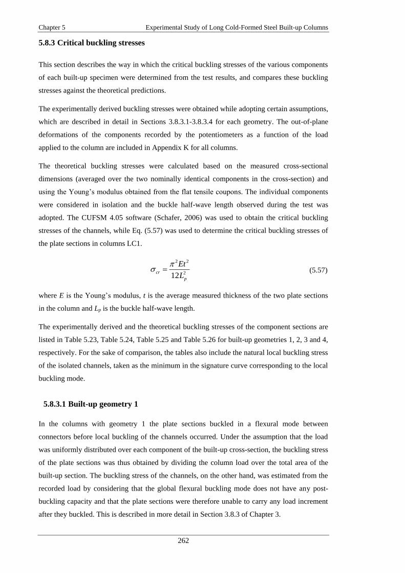
Chapter 5 Experimental Study of Long Cold-Formed Steel Built-up Columns
262
5.8.3 Critical buckling stresses
This section describes the way in which the critical buckling stresses of the various components
of each built-up specimen were determined from the test results, and compares these buckling
stresses against the theoretical predictions.
The experimentally derived buckling stresses were obtained while adopting certain assumptions,
which are described in detail in Sections 3.8.3.1-3.8.3.4 for each geometry. The out-of-plane
deformations of the components recorded by the potentiometers as a function of the load
applied to the column are included in Appendix K for all columns.
The theoretical buckling stresses were calculated based on the measured cross-sectional
dimensions (averaged over the two nominally identical components in the cross-section) and
using the Young’s modulus obtained from the flat tensile coupons. The individual components
were considered in isolation and the buckle half-wave length observed during the test was
adopted. The CUFSM 4.05 software (Schafer, 2006) was used to obtain the critical buckling
stresses of the channels, while Eq. (5.57) was used to determine the critical buckling stresses of
the plate sections in columns LC1.
2 2
212cr
p
Et
L
(5.57)
where E is the Young’s modulus, t is the average measured thickness of the two plate sections
in the column and Lp is the buckle half-wave length.
The experimentally derived and the theoretical buckling stresses of the component sections are
listed in Table 5.23, Table 5.24, Table 5.25 and Table 5.26 for built-up geometries 1, 2, 3 and 4,
respectively. For the sake of comparison, the tables also include the natural local buckling stress
of the isolated channels, taken as the minimum in the signature curve corresponding to the local
buckling mode.
5.8.3.1 Built-up geometry 1
In the columns with geometry 1 the plate sections buckled in a flexural mode between
connectors before local buckling of the channels occurred. Under the assumption that the load
was uniformly distributed over each component of the built-up cross-section, the buckling stress
of the plate sections was thus obtained by dividing the column load over the total area of the
built-up section. The buckling stress of the channels, on the other hand, was estimated from the
recorded load by considering that the global flexural buckling mode does not have any post-
buckling capacity and that the plate sections were therefore unable to carry any load increment
after they buckled. This is described in more detail in Section 3.8.3 of Chapter 3.

Chapter 5 Experimental Study of Long Cold-Formed Steel Built-up Columns
263
The potentiometers consistently recorded that the plate sections located on the compression side
of the built-up specimen buckled slightly before the plate sections located on the tension side,
while the channels in most columns were recorded to buckle at the same time, as illustrated in
Figure 5.99 for column LC1-2b. The critical buckling stress of the plate sections was taken as
the average value of both plates.
Figure 5.99: Axial load vs lateral displacements of LC1-2b
The theoretical and experimental buckling stresses of the plates and the channels are listed in
Table 5.23, together with the buckling half-wave length observed during the test. Since the
buckle half-wave length of the plate sections could not be accurately determined from the test,
an upper and lower bound was defined. The upper bound corresponded to a half-wave length
equal to half the distance between the connectors, and the lower bound corresponded to a half-
wave length equal to the connector spacing.
In columns LC1-2 and LC1-3 the plate sections were seen to buckle outwards between
connectors in each field along the column with a half-wave closer to the upper bound value. The
plates were also seen to buckle in the top field first, where no potentiometer was present to
record the out-of-plane deformations. This may explain why for these columns the
experimentally derived buckling stresses of the plates were larger than the theoretical upper
bound. In columns LC1-8, which had a connector spacing of 320 mm, the plate sections were
seen to buckle in every other field with a buckle half-wave length slightly larger than half the
distance between connectors. This was confirmed by the measured buckling stress of 23 MPa,
which corresponds to a half-wave length of 170 mm (which is indeed slightly larger than half
the distance between connectors).

Chapter 5 Experimental Study of Long Cold-Formed Steel Built-up Columns
264
The experimentally derived buckling stresses of the channels, on the other hand, were only
around 8 % larger than the theoretically predicted values for columns LC1-2 and LC1-3, which
virtually coincided with the natural local buckling stress of the channel, while for columns LC1-
8 they were 11 % larger than the natural local buckling stress.
Table 5.23: Buckling stresses of the different components of geometry 1
Column
Min.
theoretical
buckling
stress (MPa)
Half-wave length observed
during tests (mm)
Theoretical buckling stress
(MPa)
Buckling stress
from test (MPa)
Channel Channel Plate
Channel Plate
Channel Plate Lower Upper Lower Upper
LC1-2a 93 131 960 480 93 1 3 99 6
LC1-2b 91 131 960 480 91 1 3 98 5
LC1-3a 92 131 720 360 92 1 5 97 8
LC1-3b 91 131 720 360 91 1 5 101 8
LC1-8a 93 - 320 160 - 6 25 100 23
LC1-8b 92 - 320 160 - 6 25 106 23
5.8.3.2 Built-up geometry 2
In the columns with built-up geometry 2 the outer channels buckled in a local mode before the
inner channels. Since local buckling has a significant, yet not easily quantifiable, post-bucking
load-bearing capacity, only the critical buckling stress of the outer channels was determined
from the experimental results. This critical stress was obtained assuming that, prior to buckling,
the load was uniformly distributed over the built-up cross-section. Thus, the load in the column
at which buckling was observed was divided over the total cross-sectional area of the column.
In columns LC2-2 and LC2-6, with a length of 2.5 m, the outer channel located on the
compression side of the built-up specimen was seen to buckle slightly before the outer channel
located on the tension side, as shown in Figure 5.100 for column LC2-2a. Therefore, the critical
buckling stress of these channels was taken as the average value of both channels. In columns
LC2-4, with a shorter column length of 1.8 m, both outer channels buckled at approximately the
same load, as shown in Figure 5.101 for columns LC2-4b.

Chapter 5 Experimental Study of Long Cold-Formed Steel Built-up Columns
265
Figure 5.100: Axial load vs lateral displacements of LC2-2a
Figure 5.101: Axial load vs lateral displacements of LC2-4b
Table 5.24 shows the theoretical critical buckling stresses of the inner and outer channels, as
well as their half-wave lengths observed from the tests and the buckling stresses of the outer
channels obtained from the tests. The table shows that the buckling stresses of the outer
channels obtained from the tests were larger than the theoretical predictions in all columns, with
the difference being slightly affected by the connector spacing. In columns LC2-2 and LC2-6,
with a column length of 2.5 m and connector spacings of 793 mm and 340 mm, respectively, the
experimentally derived buckling stresses were around 20 % larger than the predicted values. In
columns LC2-4, on the other hand, with a column length of 1.8 m and a connector spacing of
336 mm, a more significant difference of around 34 % was obtained. Table 5.24 also shows
that, despite the fact that in most columns the outer channels buckled with a half-wave length
equal to the natural local buckle half-wave length, the stress at which the outer channels buckled
was, on average, around 26 % larger than the natural local buckling stress of the unrestrained

Chapter 5 Experimental Study of Long Cold-Formed Steel Built-up Columns
266
channel. This shows that the outer channels received a significant amount of restraint from the
inner channels against local buckling.
Table 5.24: Buckling stresses of the different components of geometry 2
Column
Min. theoretical
buckling stress (MPa)
Half-wave length
observed in tests (mm)
Theoretical buckling
stress (MPa)
Buckling stress from
test (MPa)2
Inner
Channel
Outer
Channel
Inner
Channel
Outer
Channel
Inner
Channel
Outer
Channel
Inner
Channel
Outer
Channel
LC2-2a 182 64 - 198 - 66 - 83
LC2-2b 182 64 - 198 - 66 - 77
LC2-6a 183 64 85 170 187 64 - 74
LC2-6b 181 63 85 170 185 63 - 78
LC2-4a 183 59 - 168 - 59 - 83
LC2-4b 181 60 84 168 185 60 - 76
5.8.3.3 Built-up geometry 3
In columns LC3-2 and LC3-3, the plain channels buckled before the lipped channels, while in
columns LC3-8 the components buckled at approximately the same time, as shown in Figure
5.102 and Figure 5.103 for columns LC3-2b and LC3-8a, respectively. Under the assumption
that the load was evenly distributed over the built-up cross-section before the components
buckled, the experimental buckling stresses of the lipped channels in columns LC3-8, as well as
the experimental buckling stress of the plain channels in all columns were determined by
dividing the load at which the components buckled over the total area of the cross-section.
Table 5.25 lists the theoretical and experimental critical buckling stresses of the lipped and plain
channels. The theoretical critical stresses were calculated at the buckle half-wave lengths
observed during the test, which are also included in the table. In some columns the components
were seen to buckle with two different half-wave lengths, as previously explained in Section
5.8.2.3, and the stresses associated with each half-wave length are included in the table. The
table shows that the plain channels were expected to buckle before the lipped channels in all the
columns, as their theoretical buckling stresses are almost 50 % lower than those of the lipped
channels.
Table 5.25: Buckling stresses of the different components of geometry 3
Column
Min. theoretical
buckling stress
(MPa)
Half-wave length
observed during tests
(mm)
Theoretical buckling
stress (MPa)
Buckling stress from
test (MPa)
Plain
Channel
Lipped
Channel
Plain
Channel
Lipped
Channel
Plain
Channel
Lipped
Channel
Plain
Channel
Lipped
Channel
LC3-2a 63 103 120 80-96 63 103-105 82 -
LC3-2b 64 104 120 80-96 64 104-106 84 -
LC3-3a 64 102 120 90-120 64 102-115 77 -
LC3-3b 64 104 120 90 64 104 79 -
LC3-8a 63 103 80-160 80-160 75-66 103-148 82-105 99
LC3-8b 65 103 80-160 80-160 77-67 104-148 88-109 109

Chapter 5 Experimental Study of Long Cold-Formed Steel Built-up Columns
267
In columns LC3-2 and LC3-3, the plain channels were observed to buckle at a stress level in
between the predicted values for the plain and lipped channels. In column LC3-2, with a
connector spacing of 960 mm, the measured buckling stress in the plain channels was around 31
% higher than the theoretical prediction, while in column LC3-3, with a connector spacing of
720 mm, the measured buckling stress in the plain channels was around 22 % higher than the
theoretically predicted value. This is indicative of the high level of restraint which the plain
channels received from the lipped channels in these columns, despite the relatively large
connector spacing.
Interaction between the different components was even more pronounced in columns LC3-8. In
these columns, the plain channel located on the compression side of the built-up specimen first
buckled at a stress level of around 85 MPa. However, as the load was further increased, the
lipped channels and the plain channel located on the tension side of the built-up specimen
buckled simultaneously at a stress level close to the theoretical value predicted for the lipped
channels. The plain channel located on the compression side was then forced to reverse the
initial direction of its out-of-plain deformations in order to accommodate the local buckling
pattern of the adjacent components, as illustrated in Figure 5.103 for column LC3-8a.
Figure 5.102: Axial load vs lateral displacements of LC3-2b
Table 5.25 also shows that in most cases the components buckled with a half-wave length very
close to their natural half-wave length. Only in columns LC3-8, with the shortest connector
spacing, the components showed some buckles along the column with a half-wave length which
differed from the natural local buckle half-wave length. On average, the plain channels buckled
at a stress around 34 % larger than their natural local buckling stress.

Chapter 5 Experimental Study of Long Cold-Formed Steel Built-up Columns
268
Figure 5.103: Axial load vs lateral displacements of LC3-8a
5.8.3.4 Built-up geometry 4
The plain channels buckled before the lipped channels in all columns with geometry 4.
Therefore, only the critical buckling stress of the plain channels could be experimentally
determined, under the assumption that the load was evenly distributed over the built-up cross-
section prior to buckling. Thus, the critical buckling stresses of the plain channels were obtained
by dividing the load at which the channel buckled over the total cross-sectional area of the
column.
The theoretical and experimental buckling stresses of the different components are listed in
Table 5.26, which also includes the buckle half-wave length observed in the lipped channels
during the tests. Since the geometric arrangement of the components in the columns with built-
up geometry 4 prevented direct observation of the buckle half-wave length of the plain channels
during the tests, the theoretical buckling stresses included in the table for these channels are
associated with the buckle half-wave lengths observed in the plain channels of columns LC3
(which had identical nominal dimensions).
Table 5.26: Buckling stresses of the different components of geometry 4
Column
Min. theoretical
buckling stress
(MPa)
Half-wave length
observed during tests
(mm)
Theoretical buckling
stress (MPa)
Buckling stress from
test (MPa)
Plain
Channel
Lipped
Channel
Plain
Channel
Lipped
Channel
Plain
Channel
Lipped
Channel
Plain
Channel
Lipped
Channel
LC4-2a 64 103 - 80-96 64 103-104 74 -
LC4-2b 64 103 - 80-96 64 104-105 63 -
LC4-3a 64 104 - 90 64 105 78 -
LC4-3b 64 102 - 90 65 102 73 -
LC4-8a 66 101 - 80 68-77 102 63-85 -
LC4-8b 64 104 - 80 66-76 105 67 -

Chapter 5 Experimental Study of Long Cold-Formed Steel Built-up Columns
269
The table shows that the critical buckling stresses of the plain channels measured during the
tests were on average 7 % larger than the theoretical predictions using the assumed buckle half-
wave length, while compared to the natural local buckling stress of the unrestrained channel,
they were on average around 11 % larger. However, in columns LC4 the connector spacing did
not seem to significantly affect the stress at which the plain channels buckled.
It may be worth noting that in columns LC4-2b and LC4-3b, the critical buckling stresses of the
plain channels were slightly lower than those measured in the plain channels of columns LC4-
2a and LC4-3a, respectively. This may be attributed to the fact that in columns LC4-2b and
LC4-3b, distortional bucking of the lipped channels occurred at approximately the same time as
local buckling in the plain channels, as illustrated by the black dashed curves in Figure 5.104 for
column LC4-2b. In column LC4-2a, on the other hand, the potentiometers did not record any
significant distortion of the lipped channels flanges, while in column LC4-3a distortional
buckling of the lipped channels was recorded to occur after the plain channels buckled. No
significant flange distortion was recorded in the lipped channels of columns LC4-8.
Figure 5.104: Axial load vs lateral displacements of LC4-2b
5.8.4 Ultimate load
All columns failed by interaction between cross-sectional buckling of the component sections
and global flexural buckling about the major axis of the whole column, while in columns LC1 a
global-type buckling of the components in between connector points was also observed. Figure
5.105 shows a typical load vs axial displacement curve, obtained for column LC3-2b, in which
both the ‘dynamic’ load, as well as the ‘static’ load (obtained by accounting for the decrease in

Chapter 5 Experimental Study of Long Cold-Formed Steel Built-up Columns
270
the dynamic load observed after halting the test for 4 min shortly before the peak load was
reached) are plotted. The figure reveals that there is little difference between the dynamic and
static curves. The maximum difference observed at the peak load among all columns was 1.65
kN, obtained for column LC4-8a, while the average difference at the peak load was 0.72 kN.
This small difference was due to the relatively slow targeted displacement rate of 0.08 mm/min
employed during the tests.
Figure 5.105: Axial load vs axial displacements of LC3-2b
The (static) load vs. axial displacement curves of all columns with geometries LC1, LC2, LC3
and LC4 are plotted in Figure 5.106, Figure 5.108, Figure 5.110 and Figure 5.112, respectively,
while for the same columns, Figure 5.107, Figure 5.109, Figure 5.111 and Figure 5.113 plot the
load against the average lateral deflections recorded at mid-height.
For columns LC1, three distinct areas can be distinguished in Figure 5.106, in terms of the
stiffness of the columns before the ultimate load is reached. A first transition is characterised by
a marked decrease in stiffness, which in the case of columns LC1-2 and LC1-3 occurs at a load
of less than 10 kN, due to early buckling of the plate sections in a global flexural mode between
connectors. In columns LC1-8, however, with a considerably smaller connector spacing, the
first reduction of stiffness is delayed to a load just below 30 kN due to the postponement of
global buckling of the plate sections between connectors. A second loss of stiffness in Figure
5.106 is attributed to the channels buckling in a local mode. This transition is characterised by a
more gradual decrease in stiffness, and is similar to the one observed in columns LC2, LC3 and
LC4.
In Figure 5.108 two different initial stiffness values can be distinguished for columns LC2. This
geometry was tested with two different column lengths, the stiffer curves corresponding to the
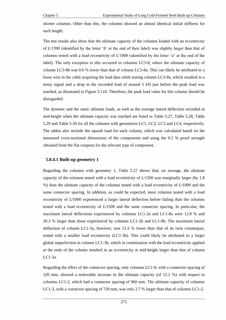
Chapter 5 Experimental Study of Long Cold-Formed Steel Built-up Columns
271
shorter columns. Other than this, the columns showed an almost identical initial stiffness for
each length.
The test results also show that the ultimate capacity of the columns loaded with an eccentricity
of L/1500 (identified by the letter ‘b’ at the end of their label) was slightly larger than that of
columns tested with a load eccentricity of L/1000 (identified by the letter ‘a’ at the end of the
label). The only exception to this occurred in columns LC3-8, where the ultimate capacity of
column LC3-8b was 0.6 % lower than that of column LC3-8a. This can likely be attributed to a
loose wire in the cable acquiring the load data while testing column LC3-8a, which resulted in a
noisy signal and a drop in the recorded load of around 5 kN just before the peak load was
reached, as illustrated in Figure 5.110. Therefore, the peak load value for this column should be
disregarded.
The dynamic and the static ultimate loads, as well as the average lateral deflection recorded at
mid-height when the ultimate capacity was reached are listed in Table 5.27, Table 5.28, Table
5.29 and Table 5.30 for all the columns with geometries LC1, LC2, LC3 and LC4, respectively.
The tables also include the squash load for each column, which was calculated based on the
measured cross-sectional dimensions of the components and using the 0.2 % proof strength
obtained from the flat coupons for the relevant type of component.
5.8.4.1 Built-up geometry 1
Regarding the columns with geometry 1, Table 5.27 shows that, on average, the ultimate
capacity of the columns tested with a load eccentricity of L/1500 was marginally larger (by 1.8
%) than the ultimate capacity of the columns tested with a load eccentricity of L/1000 and the
same connector spacing. In addition, as could be expected, most columns tested with a load
eccentricity of L/1000 experienced a larger lateral deflection before failing than the columns
tested with a load eccentricity of L/1500 and the same connector spacing. In particular, the
maximum lateral deflections experienced by columns LC1-2a and LC1-8a were 12.8 % and
20.3 % larger than those experienced by columns LC1-2b and LC1-8b. The maximum lateral
deflection of column LC1-3a, however, was 13.3 % lower than that of its twin counterpart,
tested with a smaller load eccentricity (LC1-3b). This could likely be attributed to a larger
global imperfection in column LC1-3b, which in combination with the load eccentricity applied
at the ends of the column resulted in an eccentricity at mid-height larger than that of column
LC1-3a.
Regarding the effect of the connector spacing, only columns LC1-8, with a connector spacing of
320 mm, showed a noticeable increase in the ultimate capacity (of 15.1 %) with respect to
columns LC1-2, which had a connector spacing of 960 mm. The ultimate capacity of columns
LC1-3, with a connector spacing of 720 mm, was only 2.7 % larger than that of columns LC1-2.

Chapter 5 Experimental Study of Long Cold-Formed Steel Built-up Columns
272
Table 5.27 also shows that the ultimate capacity of the columns constituted only around 27 % of
the squash load. The reason for this rather low ratio is found in the low efficiency of the plate
sections, which buckled in a global flexural mode between connectors at a very early stage
during the test, becoming ineffective in resisting any further increase of the load.
Figure 5.106: Axial load vs. axial deformation curves: geometry 1
Figure 5.107: Axial load vs. lateral deflection curves: geometry 1
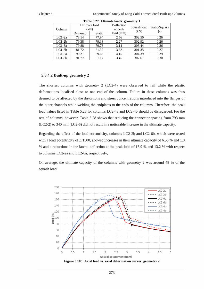
Chapter 5 Experimental Study of Long Cold-Formed Steel Built-up Columns
273
Table 5.27: Ultimate loads: geometry 1
Column
Ultimate load
(kN)
Deflection
at peak
load (mm)
Squash load
(kN)
Static/Squash
(-) Dynamic Static
LC1-2a 78.14 77.94 2.56 302.50 0.26
LC1-2b 79.38 79.18 2.27 302.92 0.26
LC1-3a 79.88 79.73 3.14 303.44 0.26
LC1-3b 81.72 81.57 3.62 301.35 0.27
LC1-8a 90.21 89.66 4.15 304.39 0.29
LC1-8b 91.77 91.17 3.45 302.61 0.30
5.8.4.2 Built-up geometry 2
The shortest columns with geometry 2 (LC2-4) were observed to fail while the plastic
deformations localised close to one end of the column. Failure in these columns was thus
deemed to be affected by the distortions and stress concentrations introduced into the flanges of
the outer channels while welding the endplates to the ends of the columns. Therefore, the peak
load values listed in Table 5.28 for columns LC2-4a and LC2-4b should be disregarded. For the
rest of columns, however, Table 5.28 shows that reducing the connector spacing from 793 mm
(LC2-2) to 340 mm (LC2-6) did not result in a noticeable increase in the ultimate capacity.
Regarding the effect of the load eccentricity, columns LC2-2b and LC2-6b, which were tested
with a load eccentricity of L/1500, showed increases in their ultimate capacity of 6.56 % and 1.0
% and a reductions in the lateral deflection at the peak load of 16.9 % and 13.2 % with respect
to columns LC2-2a and LC2-6a, respectively,
On average, the ultimate capacity of the columns with geometry 2 was around 48 % of the
squash load.
Figure 5.108: Axial load vs. axial deformation curves: geometry 2

Chapter 5 Experimental Study of Long Cold-Formed Steel Built-up Columns
274
Figure 5.109: Axial load vs. lateral deflection curves: geometry 2
Table 5.28: Ultimate loads: geometry 2
Column
Ultimate load
(kN)
Deflection
at peak
load (mm)
Squash load
(kN)
Static/Squash
(-) Dynamic Static
LC2-2a 161.90 160.90 5.13 345.89 0.47
LC2-2b 172.42 171.82 4.39 349.20 0.49
LC2-6a 166.15 165.15 7.71 346.73 0.48
LC2-6b 167.68 166.88 6.81 343.70 0.49
LC2-4a (163.61) (162.31) (3.68) 309.72 (0.52)
LC2-4b (174.27) (173.37) (4.53) 311.46 (0.56)
5.8.4.3 Built-up geometry 3
With respect to the columns with geometry 3, Table 5.29 shows that the ultimate capacity was
slightly higher in the columns with the smaller load eccentricity. For example, the ultimate
capacities of columns LC3-2b and LC3-3b, which were tested with a load eccentricity of
L/1500, were on average 3.6 % larger than the ultimate capacities of columns LC3-2a and LC3-
3a, which were tested with a load eccentricity of L/1000. In addition, columns LC3-2a and LC3-
3a showed increases in the lateral deflection at the peak load of 35.7 % and 59.2 %, relative to
the columns tested with a load eccentricity of L/1500 and the same connector spacing.
As for the effect of the connector spacing on the ultimate capacity of these columns, reducing
the connector spacing resulted in a negligible increment in their ultimate capacity. For example,
the increment in ultimate capacity obtained by reducing the connector spacing from 960 mm in
column LC3-2a to 320 mm in column LC3-8a was only 0.5 %, while the ultimate capacity of
columns LC3-3, with a connector spacing of 720 mm, was on average slightly lower than that of
columns LC3-2 (by 0.1 %). All columns failed at a load which was around half of the squash
load.

Chapter 5 Experimental Study of Long Cold-Formed Steel Built-up Columns
275
Figure 5.110: Axial load vs. axial deformation curves: geometry 3
Figure 5.111: Axial load vs. lateral deflection curves: geometry 3
Table 5.29: Ultimate loads: geometry 3
Column
Ultimate load
(kN)
Deflection at
peak load
(mm)
Squash load
(kN)
Static/Squash
(-) Dynamic Static
LC3-2a 119.94 119.04 6.62 236.50 0.50
LC3-2b 123.98 123.48 4.88 236.50 0.52
LC3-3a 119.88 118.88 5.43 238.01 0.50
LC3-3b 123.44 122.94 3.41 238.71 0.52
LC3-8a 121.22 120.22 6.60 238.78 0.50
LC3-8b (120.54) (119.54) (4.07) 239.48 (0.50)

Chapter 5 Experimental Study of Long Cold-Formed Steel Built-up Columns
276
5.8.4.4 Built-up geometry 4
Regarding the columns with geometry 4, Table 5.30 shows that columns LC4-2b, LC4-3b and
LC4-8b, which were tested with a load eccentricity of L/1500, achieved a peak load which was
1.2 %, 2.1 % and 9.7 % higher than the peak load achieved by columns LC4-2a, LC4-3a and
LC4-8a, respectively, which were tested with a load eccentricity of L/1000. The relatively large
difference in ultimate capacity obtained for the LC4-8 columns was due to the relatively low
ultimate capacity achieved in column LC4-8a. This was most likely due to the relatively large
global imperfection present in this column, which further increased the eccentricity at the
column mid-height, as shown in Table 5.22. The increases in the lateral deflection at the peak
load in the columns tested with a load eccentricity of L/1000, relative to those tested with a load
eccentricity of L/1500, were 7.64 %, 42.1 % and 14.4 % for columns LC4-2, LC4-3 and LC4-8,
respectively.
Regarding the effect of the connector spacing on the ultimate capacity, Table 5.30 shows that
this was negligible, with a mere 0.7 % increase when reducing the connector spacing from 960
mm to 320 mm, and a 0.3 % increase when reducing the connector spacing from 960 mm to 720
mm. All columns failed at a load of less than 50 % of the calculated squash load.
Figure 5.112: Axial load vs. axial deformation curves: geometry 4

Chapter 5 Experimental Study of Long Cold-Formed Steel Built-up Columns
277
Figure 5.113: Axial load vs. lateral deflection curves: geometry 4
Table 5.30: Ultimate loads: geometry 4
Column
Ultimate load
(kN)
Deflection
at peak load
(mm)
Squash load
(kN)
Static/Squash
(-) Dynamic Static
LC4-2a 117.33 116.53 6.20 238.48 0.49
LC4-2b 118.50 117.90 5.76 238.46 0.49
LC4-3a 116.84 116.19 5.30 237.81 0.49
LC4-3b 119.22 118.57 3.73 237.63 0.50
LC4-8a 110.71 109.06 5.96 238.55 0.46
LC4-8b 120.20 119.65 5.21 237.83 0.50
5.9. Summary and conclusions
A comprehensive experimental programme consisting of compression tests on 24 long built-up
columns with four different cross-sectional geometries and lengths ranging from 1800 mm to
3000 mm is presented. The cross-sections were assembled from flat plates, plain channels and
lipped channels with nominal depths ranging from 79 mm to 154 mm and thicknesses ranging
from 1.2 to 2.0 mm. Two of the cross-sectional geometries (LC1 and LC2) were assembled
using M6 bolts, while the other two (LC3 and LC4) were assembled using M5.5 self-drilling
sheet metal screws.
The columns were subjected to compression between pin-ended boundary conditions, applying
the load with eccentricities of L/1000 or L/1500, while varying the connector spacing among
specimens with the same cross-sectional geometry. The different components of the built-up
specimens were spot welded together at each end and endplates were welded to the column ends
to ensure a controlled introduction of the load to each component, as well as to facilitate
positioning the columns relative to the pin supports. In order to verify the eccentricity, half of

Chapter 5 Experimental Study of Long Cold-Formed Steel Built-up Columns
278
the test specimens were instrumented with strain gauges at mid-height. In addition, coupon tests
were taken from the flat portions and corner regions of the components in order to determine
their material properties, and detailed measurements of their geometric imperfections were
performed before and after they were assembled into their final configuration, using a specially
designed measuring rig which consisted of a laser sensor moving along high precision guiding
bars.
The out-of-plane deformations of each column component were recorded during the test using
potentiometers located near the bottom end of the column. This allowed, in most cases, a
determination of the stress at which buckling occurred in the components. These values were
compared to theoretical predictions, obtained from a finite strip analysis which considered the
individual components in isolation without any interaction with the rest of the cross-section.
The main conclusions obtained from this experimental programme are listed below. They are
divided into those related to the accuracy of the developed imperfection measuring rig and the
study of the effect of the assembly process on the amplitude and shape of the imperfections, and
those related to the results obtained from the column tests.
5.9.1 Conclusions regarding the imperfection measurements
The accuracy of the readings taken with the measuring rig was found to be limited by
the out-of-straightness of the guiding bars along which the laser sensor is moved. A
technique was proposed to achieve a higher measurement accuracy, which consisted of
using a reflective liquid, such as milk, to generate a virtually perfectly flat surface,
which can then be used to measure the out-of-straightness of the guiding bars. After
accounting for this out-of-straightness, the accuracy of the imperfection measurements
was estimated to be ± 0.06 mm over the full 3 m length of the rig.
The imperfections recorded on the components of the built-up geometries were
classified into out-of-plane imperfections and global imperfections.
A similar out-of-plane imperfection profile was recorded for each type of channel along
their respective web, flanges and lips before they were assembled into their built-up
configuration. This consistency in the imperfection shape was attributed to the fact that
each type of channel section was presumably fabricated from the same steel coil and
followed the same cold-forming process and handling. The fabrication process was also
deemed responsible for the consistency in the minor axis global flexural imperfection
recorded in all channels before they were assembled, which closely resembled a ‘Bow
imperfection’ towards the web of the channel. The global imperfection of the channels
about the major axis, on the other hand, could be less accurately approximated by a
Chapter 5 Experimental Study of Long Cold-Formed Steel Built-up Columns
279
‘Chamber imperfection’, with the maximum imperfection magnitude typically
occurring away from the mid-length of the channel.
Characterising the imperfections related to local or distortional buckling using the
maximum out-of-plane imperfection was found to yield exceedingly conservative
imperfection values. This conclusion was reached after decomposing the out-of-plane
imperfections recorded in the channels (before they were assembled) into a constant and
an undulating component along the channel length and noting that the former, which
does not contribute to the onset of these cross-sectional buckling modes, may be up to
twice as large as the latter. Moreover, using the maximum undulating imperfection
component can also be expected to result in a conservative characterisation of the out-
of-plane imperfections, since the profile of the undulating component does not
necessarily resemble the longitudinal shape of the critical cross-sectional buckling mode
of the channel.
Assembling the channels into their final configuration significantly altered the
amplitude and shape of the out-of-plane imperfections of the channels. The
imperfections along the web of the individual channels were affected (1) due to direct
contact with the adjacent components of the built-up geometry and the presence of the
connectors, or (2) due to rotational compatibility at the junction with the flanges, which
were themselves in a situation described in (1). The former resulted in a greater
modification of the out-of-plane imperfections, with the connectors creating localised
out-of-plane imperfections along the web, resulting in an imperfection profile with
repetitive ‘bumps’. The assembly process had a lesser effect on the out-of-plane
imperfections along the flanges of the channels, which in most cases resulted from
rotational compatibility with the web.
The assembly process was also found to significantly affect the minor axis global
flexural imperfection of the channels, reducing its amplitude at mid-length or even
inverting it. The shape of these imperfections was also affected, resembling less of a
sinusoidal bow imperfection. For most of the channels, the reduction in the magnitude
of their minor axis global flexural imperfection can be explained by the fact that the
major axis global flexural imperfection of all the channels was significantly smaller
than the one about the minor axis, while their flexural rigidity in that direction is
significantly higher. Therefore, the channels connected through their web were
straightened by the adjacent channels, which were positioned orthogonally to them. It is
worth pointing out that in built-up geometries assembled from two identical channels
connected to each other facing in opposite directions and with the plane of contact
parallel to their minor axis (as is the case in a back-to-back I-shaped built-up section or
a toe-to-toe built-up box section), if the individual channels are fabricated following the

Chapter 5 Experimental Study of Long Cold-Formed Steel Built-up Columns
280
same procedure, their minor axis global flexural imperfection after the assembly can be
expected to be smaller than the one prior the assembly, since the imperfections of each
channel is somehow cancelled by the imperfections of the other channel and the
enforcement of contact exerted by the fasteners.
5.9.2 Conclusions regarding the column tests results
All columns failed by interaction between cross-sectional instability of the component
sections and global flexural buckling about the major axis of the built-up column, while
a global-type buckling of the components in between connector points was also
observed in columns LC1.
The connectors were seen to affect the buckling patterns of the components by forcing
them to adjust their individually preferred buckling half-wave length to accommodate
their presence. For the channel sections, this adjustment resulted in half-wave lengths
which were still relatively close to the natural local buckle half-wave length of the
individual channels. In addition, whether the buckles were enlarged or shortened
depended on which half-wave length required the lowest critical buckling stress.
The cross-sectional buckling patterns of the individual components within the columns
were also seen to be affected by contact with the adjacent components, which often
forced the buckling out-of-plane displacements to exclusively occur in one direction.
Interaction between global buckling of the built-up specimen and cross-sectional
buckling of the components was evidenced by a slight amplification of the amplitude of
the buckles of the component located on the most compressed side of the built-up
specimen. These components were also recorded to buckle slightly before those located
on the opposite side.
A comparison between the theoretical predictions of the buckling stresses and the
experimentally derived ones showed that the buckling stress of the most slender
components was increased by up to 34 % as a result of the restraint provided by the rest
of the cross-section. In particular, in columns LC1, LC2, LC3 and LC4, the stress at
which the most slender component buckled exceeded the natural local buckling stress of
the component considered in isolation by 13 %, 26 %, 34 % and 11 %, respectively.
The tests also showed that in those columns where the individual components only
experienced cross-sectional instabilities (i.e. columns LC2, LC3 and LC4), the effect of
the connector spacing on the ultimate capacity was negligible. For instance, reducing
the connector spacing from 793 mm to 340 mm in columns LC2 resulted in a mere 0.3
% increase in the ultimate capacity, while for columns LC3 and LC4, reducing the

Chapter 5 Experimental Study of Long Cold-Formed Steel Built-up Columns
281
connector spacing from 960 mm to 320 mm resulted in an increase in the ultimate
capacity of less than 1 %. Only columns LC1 showed a noticeable increase in the
ultimate capacity of 15.1 % when reducing the connector spacing from 960 mm to 320
mm, which resulted from an increase in the global flexural buckling capacity of the
plate sections between connectors.
Chapter 6 Experimental Study of the Fastener Behaviour in Built-up Specimens
282
Chapter 6
Experimental Study of the Fastener Behaviour
in Built-up Specimens
6.1. Introduction
The buckling behaviour and capacity of CFS built-up members may be significantly affected by
the shear and bearing deformations of the connectors between the components. This is expected
to particularly be the case for long built-up columns and built-up beams, where relatively large
shear forces may be introduced into the connectors as a result of the relative displacements of
the components originating from global buckling in the former and lateral-torsional buckling
and/or bending in the latter. The result is a reduction in capacity, which may also be interpreted
as an increase in the effective global slenderness of the built-up member.
For the above reasons a series of single lap shear tests were carried out in order to study the
behaviour of the connectors used in the built-up members discussed in Chapter 3, Chapter 4 and
Chapter 5. Ten different types of connector test specimens were fabricated in order to fully
cover the various combinations of plate thicknesses and fastener types encountered in the built-
up specimens, as well as to compare the behaviour of different types of fasteners when
connecting steel plates with a given thickness and mechanical properties. The results obtained
from the single lap shear tests were then used in Chapter 7, Chapter 8 and Chapter 9 as input
data in detailed FE models used in parametric studies after validation against the experiment.
The experimental programme presented in this chapter also sought to investigate the reliability
of Digital Image Correlation (DIC) for these purposes. DIC is a relatively new non-contact
measuring technique, which has great potential in situations where conventional measuring
techniques cannot be used, such as tests under fire conditions. To this end the deformations of
the connector test specimens were recorded using both LVDTs and DIC and the results were
compared.

Chapter 6 Experimental Study of the Fastener Behaviour in Built-up Specimens
283
6.2. Labelling
The connector test specimens were labelled with the letters ‘BCS’ or ‘SCS’ to indicate that the
specimen was assembled using bolts or self-drilling screws, respectively, followed by the
thicknesses of both steel plates multiplied by 10 and separated by a hyphen. The first thickness
in the label corresponded to the plate directly underneath the head of the connector. Finally, the
letters ‘a’, ‘b’ and ‘c’ were used to differentiate between multiple connector specimens with the
same combination of plate thicknesses and fastener type. For example, the label ‘BCS24-14a’
refers to a bolted specimen assembled with steel sheets with nominal thicknesses of 2.4 mm and
1.4 mm.
The labelling used to refer to the cross-sectional components is consistent with the one used in
previous chapters. Plain channels and lipped channels were labelled using the letters ‘T’ or ‘S’,
respectively, followed by the nominal width of the web in mm and the nominal wall thickness in
mm multiplied by 10, while the plate sections were labelled using the letter ‘P’ followed by the
width of the plate and its thickness multiplied by 10.
6.3. Specimen geometry and preparation
The connector specimens consisted of single lap joints connected with the same type of bolts or
self-drilling screws used to assemble the built-up members. Since the connector behaviour was
expected to be affected not just by the type of fastener used, but also by the mechanical
properties of the fastened sections, each steel sheet in the single lap joint was cut from spare
sections of the built-up specimens, and they were paired together to cover all the combinations
of plate thicknesses and connector type encounter in the built-up beams and columns previously
tested. In order to avoid excessive tilting of the fastener and out-of-plane curling of the steel
plates prior to failure, the specimens were assembled with two fasteners in the direction of the
applied load. Figure 6.1 shows the specimens fabricated for each built-up geometry.

Chapter 6 Experimental Study of the Fastener Behaviour in Built-up Specimens
284
Figure 6.1: Connector specimens fabricated for each built-up geometry
The test programme was divided in two stages. During the first part, four different types of
bolted specimens were fabricated to study the connector behaviour in geometries 1 and 2 of the
built-up stub columns and beams (i.e. BCS24-14, BCS12-14, BCS15-15 and BCS12-15). The
connector specimens belonging to the stub columns were fabricated after seeing clear evidence
of slip between the components of geometry 1 during the stub column tests. Test specimens
were also fabricated for the fasteners contained in the beams, so that the connector behaviour
could be incorporated in FE models which did allow global instabilities of the built-up beams.
Three identical test specimens were fabricated for each combination of plate thicknesses in
order to assess the statistical variability of the results.
During the second part of the experimental programme, both bolted and screwed specimens
were fabricated in order to study the connector response in the long built-up columns (i.e.
BCS14-20, BCS14-14 and SCS12-12). It is worth noting that since the stub columns with
geometries 3 and 4 were assembled from components with nominally identical thicknesses and
material properties as those used to assemble the long columns, the test specimens fabricated to
study the behaviour of the fasteners in the long columns with geometries 3 and 4 were also
representative of the behaviour of the fasteners in the stub columns with geometries 3 and 4.
Again three test specimens were fabricated for each combination of plate thicknesses. However,
for each such combination one test specimen out of three was assembled using a different
T12012S11012
Built-up column 1
(Stub column) (Long column)
BCS24-14aBCS24-14bBCS24-14c
BCS14-20aBCS14-20bSCS14-20
BCS12-14aBCS12-14bBCS12-14c
BCS14-14aBCS14-14bSCS14-14
T12915T10412 T12915
T10412
Built-up column 3 Built-up beam 1Built-up column 4Built-up beam 2
(Beam) (Beam)
SCS12-12aSCS12-12bBCS12-12
BCS15-15aBCS15-15b
BCS15-15c
BCS12-15aBCS12-15b
BCS12-15c
Built-up column 2
S11012T12012
(Stub and long column)
(Stub column)
T15414
P20024
(Long column)
T15414
P15020 T15414
T7912
T15414
T7914

Chapter 6 Experimental Study of the Fastener Behaviour in Built-up Specimens
285
fastener type (i.e. bolts or screws). This allowed for a direct comparison regarding the effect of
the fastener type on the connection behaviour.
Figure 6.2 shows the nominal dimensions of the steel sheets used to construct the test
specimens, as well as the location of the connectors. The steel sheets had a nominal width of 70
mm, which was reduced to 50 mm at one end in order to accommodate the specimen into the
grips of the testing machine. The edge distance of the fasteners in the direction of the force and
the distance between fasteners were chosen following the recommendations given by ECCS
TC7 (2009), which ensured that the behaviour of the connector was not affected by its
proximity to the edge.
Figure 6.2: Nominal dimensions of steel plate
The thickness and the width of the steel sheets were measured prior to the assemblage. The
thickness of the sheet was measured with a digital micrometre with a precision of ±0.002 mm,
while the width of the sheet was measured with a digital Vernier caliper with a precision of
±0.03 mm. The measured dimensions of the steel sheets are listed in Table 6.1 for each
specimen. They correspond to the averages of several measurements taken along the length of
the sheet.
The bolted specimens were assembled using M6 bolts with M6 washers placed between the bolt
head/nut and the steel sheets, replicating the same type of connection used to assemble the built-
up specimens. It is worth mentioning that the bolts used during the first and second stage of the
experimental programme were supplied by different manufacturers. However, all of them were
grade 8.8. Holes with a nominal diameter of 6.25 mm were drilled into the connecting plates
and the bolts were tightened with a torque of 10 Nm, identically to what was done for the actual
built-up specimens.
The screwed specimens were assembled using the same M5.5 self-drilling sheet metal screws
used to assemble the built-up specimens. In order to ensure the screws were aligned with the
line of action of the applied force, small holes with a diameter of 3 mm were predrilled into the
35
35
30
(All dimensions in mm)
300
50
230
60

Chapter 6 Experimental Study of the Fastener Behaviour in Built-up Specimens
286
steel sheets, which served as guidance for the screws. Once the steel sheets were positioned and
secured with clamps, the screws were drilled applying the same torque as used to assemble the
built-up specimens.
Table 6.1: Measured width and thickness of steel plates
Specimen Section Width
(mm)
Thickness
(mm)
BCS24-14a P20024 69.73 2.530
T15414 70.31 1.481
BCS24-14b P20024 70.01 2.542
T15414 70.34 1.479
BCS24-14c P20024 70.40 2.546
T15414 70.33 1.470
BCS12-14a T7912 70.36 1.215
T15414 70.33 1.475
BCS12-14b T7912 63.96 1.186
T15414 70.32 1.482
BCS12-14c T10412 69.46 1.189
T15414 70.34 1.473
BCS15-15a T12915 70.40 1.528
T12915 69.12 1.529
BCS15-15b T12915 70.45 1.530
T12915 70.76 1.544
BCS15-15c T12915 70.40 1.542
T12915 70.26 1.535
BCS12-15a T10412 70.37 1.186
T12915 70.14 1.540
BCS12-15b T10412 70.41 1.197
T12915 70.41 1.537
BCS12-15c T10412 70.28 1.185
T12915 70.28 1.532
BCS14-20a T13014 69.94 1.398
P15020 70.08 1.977
BCS14-20b T13014 69.99 1.405
P15020 70.09 1.976
SCS14-20 T13014 70.10 1.401
P15020 70.12 1.973
BCS14-14a T15414 70.11 1.447
T7914 69.99 1.404
BCS14-14b T15414 70.07 1.451
T7914 70.24 1.406
SCS14-14 T15414 70.11 1.447
T7914 69.89 1.400
SCS12-12a T12012 70.11 1.137
S11012 69.97 1.115
SCS12-12b T12012 70.09 1.138
S11012 70.19 1.112
BCS12-12 T12012 69.97 1.135
S11012 70.00 1.112

Chapter 6 Experimental Study of the Fastener Behaviour in Built-up Specimens
287
6.4. Material Properties
Since the test specimens were fabricated from the flat portions of spare sections belonging to the
same batch as those used to assemble the built-up specimens, the material properties of the steel
sheets were the same as those of the sections used to assemble the built-up specimens. They can
be found in Table 3.3 of Chapter 3 for connector specimens BCS24-14, BCS12-14, BCS12-12
and SCS12-12, Table 4.3 of Chapter 4 for connector specimens BCS15-15 and BCS12-15, and
Table 5.3 of Chapter 5 for specimens BCS14-20, BCS14-14, SCS14-20 and SCS14-14.
6.5. Test Set-up
All specimens were tested in a 300 kN Shimadzu universal testing machine. The test set-up is
illustrated in Figure 6.3. The specimens were loaded until failure at a constant displacement rate
of 0.5 mm/min. Each steel sheet was packed at the end with a steel plate which had the same
thickness as the adjacent steel sheet to ensure the load was being applied along the shear plane.
Figure 6.3: Single lap shear test set-up
The specimen deformations were recorded using two LVDTs, as well as with a DIC (digital
image correlation) system. Representative bolted and screwed test specimens are shown in
Figure 6.4a and Figure 6.4b, respectively, at the onset of testing.
LVDTs
(All dimensions in mm)
Target plate
150
Packing plate
Packing plate
Target plate

Chapter 6 Experimental Study of the Fastener Behaviour in Built-up Specimens
288
Figure 6.4: a) BCS14-14a and b) SCS12-12b
6.5.1 Transducers
Two LVDTs were glued to the steel sheets and spring-loaded against target plates, which were
glued to the adjacent sheet a distance of 150 mm apart, as illustrated in Figure 6.3 and Figure
6.4. For specimens BCS12-14c, BCS12-15a, BCS15-15c and BCS24-14a, both LVDTs were
attached on the same side of the specimen in order to keep the other side clear to carry out the
DIC measurements. However, it was found that any initial curvature present in the specimens
significantly affected the LVDT readings. Consequently, the remaining specimens were
instrumented with one LVDT on each side of the specimen. This way, the effect of the initial
curvature on one LVDT was compensated by the opposite effect on the LVDT placed on the
other side of the specimen. The deformation of the specimen was then taken as the average
reading obtained from both LVDTs.
6.5.2 Digital image correlation
DIC was explored as part of a more general initiative within the Cold-Formed Steel Research
group at The University of Sheffield to develop alternative ways of measuring deformations in
CFS members. In this test programme the DIC measurements were compared with the average
measurements recorded by the LVDTs in order to assess the reliability of the DIC system.
In the DIC method a digital camera is used to take a series of pictures of the surface of an object
as the object deforms. A software algorithm then tracks the changes in the grey value pattern
between consecutive images. A grey value pattern can artificially be generated on the surface by
printing or painting a randomly distributed speckle pattern onto it. DIC has the advantage of
being a non-contact method which is able to provide full-field deformation measurements, as
(a) (b)

Chapter 6 Experimental Study of the Fastener Behaviour in Built-up Specimens
289
opposed to the relative displacement measurements between two discrete points provided by
more conventional measuring devices such as LVDTs or potentiometers.
In order to obtain the full deformation field around the fasteners a randomly distributed speckle
pattern was created on one face of the specimens by first spray painting the specimens with
Plasti-Kote Super Matt Spray White after they were assembled and then randomly generating
the speckle pattern using a black marking pen. This method provided a pattern with high
contrast and the density and size of the speckles could easily be controlled. This method can be
recommended when covering small surfaces. Figure 6.4 shows the speckle patterns obtained for
two representative connector specimens.
A direct comparison between the measurements obtained from the LVDTs and the ones
obtained with DIC was achieved by marking horizontal scribed lines onto the connector
specimen at the location where the LVDTs and the target plates were attached. The scribed lines
were used to identify the pixels in the photographs which needed to be tracked.
The photographs were taken with a Canon EOS D70 DSLR camera, which was positioned 1 m
away from the test specimens and was operated in manual focus mode with the autofocus
feature deactivated, using an aperture of f/7.1, a shutter speed of 1/100 sec and an ISO 200
setting. The camera was automatically triggered at regular intervals of 10 sec using a LabView
script. Details about the technique used to synchronize the photographs with the acquisition of
the load and the LVDTs readings are included in Section 6.6.3. Two 20 W LED floodlights
were used to ensure that the specimens received sufficient light and that no shadows were
projected onto the surface. The positioning arrangement of the camera and the lamps is
illustrated in Figure 6.5.
Two different DIC software packages were used to obtain the deformations of the test
specimens. During the first part of the experimental programme the Ncorr v1.2 software (Blaber
et al., 2015) was used, while during the second part the DIC code developed by Jones (2015)
was used. A more detailed description of the DIC process can be found in (Dai, 2017).

Chapter 6 Experimental Study of the Fastener Behaviour in Built-up Specimens
290
Figure 6.5: Camera and lamp arrangement for DIC
6.6. Test results
6.6.1 Ultimate capacity and failure mode
The load vs elongation curves are illustrated in Figures 6.6-6.12 for specimens assembled with
various combinations of plate thicknesses. The load-elongation response of the individual
fasteners was obtained by dividing the force applied to the specimen over the number of
fasteners. All connector specimens with identical nominal dimensions and type of fasteners
showed the same type of failure mode. In the bolted connector specimens the failure modes
consisted of shear failure of the bolts, excessive bearing deformations of the thinnest steel plate
and a combination of both, while all the screwed connector specimens failed by pull-out of the
fastener as a result of tilting. In all the connector specimens the contributions of the elastic
deformations of the plates to the measurements were estimated to be negligible (less than 0.1
mm at the peak load).
The load-elongation response of the bolted specimens was characterized by bolt slip of up to 1
mm at a load of around 3 kN. Although the bolts used to assemble the specimens were all grade
8.8., the bolts used during the later part of the programme (specimens BCS14-20, BCS14-14
and BCS12-12) seemed to be stronger than those used to assemble the specimens tested during
the first part of the programme (specimens BCS24-14, BCS14-12, BCS15-15 and BCS12-15).
The two sets of bolts were supplied by different manufacturers and as a result of the difference
in strength, all specimens tested during the last part of the programme failed due to bearing of
the steel plate, as opposed to those tested during the first part of the programme, which failed by
bolt shear.

Chapter 6 Experimental Study of the Fastener Behaviour in Built-up Specimens
291
It is important to note that although the material properties of the bolts affected the failure mode
of the specimens, this was not problematic since the main purpose of this experimental
programme was to obtain the initial part of the load-elongation curve. Indeed, in the tested built-
up members the relative deformation at the connector points was observed to be in all cases less
than 2 mm before failure of the member occurred. Consequently, only the early part of the load-
elongation curve was of interest. Nonetheless, a complete description of the connector
behaviour, including the ultimate capacity and failure mode of each type of connector is
included below.
With respect to the bolted specimens tested during the first part of the programme, the test
results showed that, as the thickness of the steel plates decreased, the bearing deformations in
front of the fastener became more pronounced, resulting in a more ductile type of failure. For
example, specimens BCS24-14, assembled with steel plates of 2.4 mm and 1.4 mm thickness,
failed by bolt shear with little bearing deformation of the steel plates, as shown in Figure 6.15a
for specimen BCS24-14b. These specimens showed the least ductile behaviour, experiencing
deformations of around 3 mm before failure (Figure 6.6). Similarly, specimens BCS15-15,
assembled with steel plates of 1.5 mm thickness, also failed by bolt shear. However, in these
specimens some bearing deformations developed in the steel plates before the bolts failed in
shear (Figure 6.15b), which increase the deformation at failure to around 5 mm, as shown in
Figure 6.7. In connector specimens BCS12-14 and BCS12-15, in which the thinnest steel plate
had a thickness of 1.2 mm, the maximum deformations before shear failure of one of the bolts
took place were around 6 mm (Figure 6.8) and 7 mm (Figure 6.9), respectively. In these
specimens, the thinnest steel plate exhibited significant bearing deformations and out-of-plane
curling, while the bolts exhibited a large amount of tilting, as illustrated in Figure 6.16a and
Figure 6.16b for specimens BCS12-14c and BCS12-15a, respectively.
Figure 6.6: Load-elongation curve of specimens BCS24-14

Chapter 6 Experimental Study of the Fastener Behaviour in Built-up Specimens
292
Figure 6.7: Load-elongation curve of specimens BCS15-15
Figure 6.8: Load-elongation curve of specimens BCS14-12
Figure 6.9: Load-elongation curve of specimens BCS15-12

Chapter 6 Experimental Study of the Fastener Behaviour in Built-up Specimens
293
All the bolted specimens tested in the second part of the experimental programme failed due to
bearing failure in the thinnest steel plate. However, two distinctive types of failure could be
distinguished depending on the amount of tilting of the fastener. In specimen BCS14-20b, for
example, the thickest steel plate effectively limited the amount of tilting of the bolts, and
although some tilting was noticeable (Figure 6.17a), most of the bearing in the steel plates
resulted from direct contact between the bolt shaft and the edge of the hole. This resulted in a
gradual loss of stiffness in the specimen towards the ultimate capacity, as illustrated in Figure
6.10. In specimens BCS14-14 and BCS12-12, on the other hand, the bolts experienced a larger
amount of tilting due to the lower restraint provided by the steel plates, as illustrated in Figure
6.18a and Figure 6.19b for specimens BCS14-14b and BCS12-12c, respectively. As the bolts
tilted, the load, which was initially transferred from the bolt shaft to the edge of the hole, started
to mainly be transferred through the inner surface of the washer. This resulted in an increase of
the bearing contact area and caused a slight increase in the stiffness of the specimen right before
the ultimate capacity was reached, as shown in Figure 6.11 and Figure 6.12 for specimens
BCS14-14 and BCS12-12, respectively.
Regarding the screwed specimens, all of them failed by pull-out of the screw. Consequently, the
ultimate capacity of the screwed specimens was significantly lower than that of bolted
specimens with the same combination of steel plates. Pull-out of the screw resulted in a load-
elongation curve with a fluctuating stiffness in the later stages of deformation, as illustrated in
Figure 6.10, Figure 6.11 and Figure 6.12 for specimens SCS14-20, SCS14-14 and SCS12-12,
respectively.
Figure 6.10: Load-elongation curve of specimens BCS14-20/SCS14-20

Chapter 6 Experimental Study of the Fastener Behaviour in Built-up Specimens
294
Figure 6.11: Load-elongation curve of specimens BCS14-14/SCS14-14
Figure 6.12: Load-elongation curve of specimens SCS12-12/BCS12-12
When comparing the results obtained for specimens with the same combination of plate
thicknesses but a different type of fastener (Figure 6.10, Figure 6.11 and Figure 6.12), it is clear
that the bolted specimens exhibited a stiffer response than the screwed specimens, at least until
slip took place in the bolted connections. After slip, the bolted specimens were still able to
provide an increasing bearing resistance, while the strength of the screwed specimens rapidly
degraded. The reduced stiffness of the screwed specimens is mostly due to tilting of the
fastener, which in the case of the bolted specimens is mostly prevented by the restraint provided
by the washer and the nut. It is important to note that during the assembly of the bolted
specimens the steel sheets were pressed against each other in the longitudinal direction in order
to obtain maximum slip.

Chapter 6 Experimental Study of the Fastener Behaviour in Built-up Specimens
295
It is also worth mentioning that the response of the screwed specimens is highly dependent on
how well the steel sheets are screwed together. For example, in specimen SCS14-14 the steel
sheets separated while being screwed together, leaving a small gap, as illustrated in Figure 6.13.
This resulted in a reduction in the stiffness of the connection, as shown in Figure 6.14, which
compares the load-elongation curves obtained for all screwed specimens.
Figure 6.13: Small gap between steel sheets of specimen SCS14-14
Figure 6.14: Load-elongation curve of all screwed specimens
Table 6.2 lists the ultimate load per fastener obtained for each specimen, and provides a brief
description of the type of failure observed during the test. The table also lists the load in the
fastener achieved at a deformation of 3 mm, as recommended by ECCS TC7 (2009). In general,
good agreement was obtained between the ultimate capacities of twin specimens, with a
maximum difference of less than 5 %. The only exception occurred for specimens BCS14-20,
which showed a slightly larger difference. This was due to the fact that for specimen BCS14-
20a the test was stopped before the specimen reached its ultimate capacity due to time

Chapter 6 Experimental Study of the Fastener Behaviour in Built-up Specimens
296
constraints in the lab. Therefore, the maximum load obtained for this specimen should be
disregarded.
Figure 6.15: Deformed shape of a) BCS24-14b; b) BCS15-15c
Figure 6.16: Deformed shape of a) BCS12-14c; b) BCS12-14a
(a) (b)
(b) (a)

Chapter 6 Experimental Study of the Fastener Behaviour in Built-up Specimens
297
Figure 6.17: Deformed shape of a) BCS14-20b; b) SCS14-20c
Figure 6.18: Deformed shape a) BCS14-14b; b) SCS14-14c
Figure 6.19: Deformed shape of a) SCS12-12a; b) BCS12-12c
(b) (a)
(a)
(a) (b)
(b)

Chapter 6 Experimental Study of the Fastener Behaviour in Built-up Specimens
298
Table 6.2: Ultimate capacity and failure mode of test specimens
Specimen Ultimate load (N)
Type of failure Pult PECCS
BCS24-14a 11304 11297 Shear failure of one of the bolts. Minor bearing deformations in
the thinner plate. Almost no plate curling or bolt tilting. BCS24-14b 11735 11481
BCS24-14c 11179 10639
BCS12-14a 11669 9951 Shear failure of one of the bolts with significant bearing
deformations in the thinner plate. Curling of both plates,
especially the thinner one.
BCS12-14b 11196 9558
BCS12-14c 11487 9481
BCS15-15a 12002 11118 Shear failure of the bolts. Bearing deformations equally
distributed over both plates. Almost no plate curling or bolt
tilting.
BCS15-15b 12127 10692
BCS15-15c 12391 10382
BCS12-15a 11506 10058 Shear failure of one of the bolts with significant bearing
deformations in the thinner plate and some bearing deformations
in the thicker plate. Curling of the thinner plate and slight tilting
of the bolts.
BCS12-15b 11604 9320
BCS12-15c 11419 9631
BCS14-20a (12444) 8960 Bearing failure of the thinner plate. Both plates showed
significant bearing deformations. Noticeable tilting of the bolts. BCS14-20b 13092 8895
SCS14-20 8538 6552 Pull-out failure as a result of significant tilting of the screws.
Noticeable bearing deformations, especially in the thinner plate.
BCS14-14a 11696 7898 Bearing failure in both plates with significant tilting of the bolts.
BCS14-14b 11663 7650
SCS14-14 5904 5676 Pull-out failure as a result of significant tilting of the screws.
Noticeable bearing deformations in both plates and some curling
of the plate closest to the head of the screw.
SCS12-12a 4011 3994 Pull-out failure as a result of significant tilting of the screws.
Noticeable bearing deformations in both plates. SCS12-12b 4033 4007
BCS12-12 8332 5341 Bearing failure in both plates with significant tilting of the bolts.
6.6.2 Comments on the LVDT arrangement
As a result of an initial curvature present in some of the specimens, the LVDTs located on
opposite sides of the specimen recorded different deformations, as illustrated in Figure 6.20 for
specimen BCS12-15c. This was due to the fact that the LVDTs recorded the deformations at a
distance of 20 mm away from the surface of the specimen, as illustrated in Figure 6.21. As the
specimen is loaded in tension (and tensile deformations are considered positive), the
deformations recorded by each LVDT (δLVDT_1 and δLVDT_2) are given by:
_1 1 1 2' xLVDT v x x (6.1)
_ 2 2 2 1' xLVDT v x x (6.2)
where δv is the actual elongation of the specimen over the gauge length, while x1, x2, x1’ and x2’
are deformations recorded by the transducers as a result of the flattening of the steel plates to
which the LVDTs are attached, as illustrated in Figure 6.21 for one of the LVDTs. x1, x2, x1’ and
x2’ can be determined using basic trigonometry, based on the measuring gauge length (150 mm),
the distance from where the LVDT measurements were taken to the surface of the specimen (20
mm) and the initial inclination of the transducers and target plates, θ1 and θ2, which resulted

Chapter 6 Experimental Study of the Fastener Behaviour in Built-up Specimens
299
from the initial curvature of the steel plates. It is worth noting that averaging the LVDT readings
does not completely cancel out the effect of the initial curvature, as shown by Eq. (6.3).
_1 _1 1 2' '
2 2
LVDT LVDT
v
x x
(6.3)
In fact, the average LVDT readings slightly underestimates the actual deformations by a factor
of (x1’ + x2’)/2. However, the error is relatively small. For example, an average inclination of the
LVDTs (θ1 and θ2) of 2º resulted in an error of around 0.2 mm. However, this is worth taking
into account when comparing the deformations obtained using DIC with those obtained from
the LVDTs.
Figure 6.20: Force vs displacement curve of specimen BCS15-12c
Figure 6.21: Source of error in LVDT readings

Chapter 6 Experimental Study of the Fastener Behaviour in Built-up Specimens
300
6.6.3 DIC accuracy
The accuracy of the DIC measurements was assessed by comparing the DIC results with the
average deformations obtained from the LVDTs attached to the specimens. The accuracy of the
readings given by the LVDTs was checked before and after testing the specimens and they were
found to give readings with an accuracy of at least 0.08 mm for the range of deformations
measured during the tests when verified against the stroke of a calibrated universal testing
machine.
To ensure that the deformations measured with the DIC system and the LVDTs were
synchronized in time, a computer monitor displaying the applied load and the LVDT readings
was placed next to each specimen during the tests, so that this information was contained in the
DIC pictures. This allowed for a direct comparison between the LVDT measurements and the
DIC results. Only those specimens instrumented with LVDTs on both sides were used in the
comparison. Table 6.3 lists the average and maximum differences between the deformations
obtained using DIC and those obtained by averaging the readings provided by the LVDTs. The
table also lists the average and maximum differences obtained between the deformations
recorded with each LVDT. In addition, since the maximum deformation which was recorded
varied significantly between different specimens (maximum deformations ranged from around 2
mm to 15 mm), the differences between the DIC and LVDT measurements are also presented as
a fraction of the maximum recorded deformation. The deformations used to assess the accuracy
of the DIC measurements were taken relative to a load level equal to 30 % of the ultimate
capacity. This load level was chosen to avoid the initial loading range where possible
straightening of the specimen took place.
Table 6.3 shows that the average difference between the deformations obtained with the Ncorr
DIC code and the average deformations recorded with the LVDTs was 0.034 mm (or 0.92 % of
the of the maximum displacement), which is less than the estimated error on the LVDT
readings. The deformations obtained with Ncorr v1.2 differed by less than 0.142 mm from the
average LVDT measurement in all specimens considered. It is important to note that in all of the
specimens analysed with Ncorr v1.2, except specimen BCS12-14b, the average difference
between the DIC and the LVDT measurements is less than half of the difference between the
deformations recorded with the individual LVDTs. This indicates that the DIC measurements
are situated in between the measurements recorded by each LVDT, as illustrated in Figure 6.22,
which plots the load vs deformation curve obtained from the LVDT readings and from Ncorr
v1.2 for a representative test specimen. Figure 6.23 shows the evolution of the difference
between the LVDT and the Ncorr v1.2 measurements over the deformation history for different
specimens. As the figure shows, the difference oscillates around zero without exhibiting any
clear trend.

Chapter 6 Experimental Study of the Fastener Behaviour in Built-up Specimens
301
Table 6.3: Comparison between DIC and LVDTs
DIC
Algorithm Specimen
Difference between
LVDTs
Difference between DIC and average
LVDT (mm)
Avg.
(mm)
Max.
(mm)
Avg.
(mm)
Max.
(mm)
Avg.
(% δmax)
Max.
(% δmax)
Ncorr v1.2
BCS12-14a 0.193 0.621 0.046 0.142 1.32 4.02
BCS12-14b 0.057 0.075 0.045 0.134 0.77 2.28
BCS12-15b 0.195 0.518 0.042 0.136 0.60 1.96
BCS12-15c 0.101 0.364 0.035 0.105 0.62 1.86
BCS15-15a 0.136 0.229 0.026 0.066 0.77 1.97
BCS15-15b 0.196 0.318 0.025 0.077 0.64 1.99
BCS24-14b 0.047 0.075 0.015 0.047 0.63 1.95
BCS24-14c 0.097 0.682 0.039 0.089 2.05 4.67
Jones DIC
SCS12-12a 0.135 0.290 0.178 0.299 1.66 2.80
SCS12-12b 0.214 0.340 0.156 0.282 1.42 2.57
BCS12-12 0.110 0.159 0.228 0.427 1.94 3.62
BCS14-14a 0.257 0.348 0.114 0.248 0.79 1.72
BCS14-14b 0.140 0.195 0.167 0.318 1.42 2.69
SCS14-14c 0.431 0.594 0.123 0.216 1.17 2.06
BCS14-20b 0.195 0.269 0.121 0.219 1.32 2.39
SCS14-20 0.284 0.355 0.194 0.403 1.72 3.57
Ncorr v1.2 Avg. 0.128 0.360 0.034 0.100 0.92 2.59
Max. 0.196 0.682 0.046 0.142 2.05 4.67
Jones DIC Avg. 0.221 0.319 0.160 0.302 1.43 2.68
Max. 0.431 0.594 0.228 0.427 1.94 3.62
Note: δmax is the maximum recorded displacement
Figure 6.22: Load vs deformation curve obtained from LVDTs and Ncorr v1.2 for specimen
BCS15-15a

Chapter 6 Experimental Study of the Fastener Behaviour in Built-up Specimens
302
Figure 6.23: Difference between Ncorr v1.2 and average LVDT measurements
With respect to the difference between the deformations obtained using Jones’ DIC code and the
average of the LVDTs readings, Table 6.3 shows that the average difference was 0.160 mm, or
1.43 % of the maximum deformation measured, while the maximum difference was 0.427 mm
(for specimens BCS12-12 with a maximum deformation of around 12 mm). Figure 6.24 shows
the difference obtained by deducting the DIC measurements from Jones’ algorithm from the
average LVDT readings over the deformation history for different specimens. In this case a
clear trend can be appreciated, whereby the deformations obtained with Jones’ DIC code were
consistently smaller than those recorded by the LVDTs. The difference appeared proportional to
the measured deformations and was roughly equal to 2.6 % of the recorded measurement.
Figure 6.24: Difference between deformations obtained from Jones’ DIC and LVDTs

Chapter 6 Experimental Study of the Fastener Behaviour in Built-up Specimens
303
Figure 6.25: Load vs deformation curve obtained from LVDTs and Jones’ DIC code for specimen
SCS12-12a
6.7. Summary and conclusions
A series of single lap shear tests was carried out in order to determine the behaviour and
capacity of the connectors used in the built-up members presented in Chapter 3, Chapter 4 and
Chapter 5. The specimens were fabricated with the aim of replicating conditions in the actual
built-up members as much as possible, in terms of dimensions, material properties, fabrication
and torque.
The connector behaviour was recorded using LVDTs attached to the test specimens and also
using Digital Image Correlation (DIC), an alternative, non-contact measuring technique of
which the reliability was assessed by comparing the results with those obtained from the
transducers.
The tests allowed to successfully obtain the load-deformation curves of the connectors, which
were further used in the next chapters as input data in detailed FE models.
The assessment of the two DIC algorithms suggests that both algorithms can be successfully
used to measure deformations in CFS sections, provided that the deformations are contained
within a plane. Out of the two codes assessed, Ncorr v1.2 showed a significantly higher
accuracy than Jones’ DIC code. Moreover, the accuracy of the measurements obtained from
Ncorr v1.2 was at least of the same order as the accuracy of the LVDTs. Therefore, in order to
properly assess the accuracy of this DIC algorithm, the results would have to be compared to
more precise measuring techniques. The measurements obtained from Jones’ DIC code showed
a systematic error of about 2.6 % when compared with the LVDTs readings. This shows that

Chapter 6 Experimental Study of the Fastener Behaviour in Built-up Specimens
304
DIC can be used as an alternative method to record deformations in CFS members. This might
prove particularly useful in cases where conventional measuring techniques cannot be applied,
such as in tests under fire conditions.

Chapter 6 Experimental Study of the Fastener Behaviour in Built-up Specimens
305

Chapter 7 Numerical Study of Cold-Formed Steel Built-up Stub Columns
306
Chapter 7
Numerical Study of Cold-Formed Steel Built-
up Stub Columns
7.1. Introduction
This chapter describes the development of detailed finite element (FE) models for the built-up
stub columns presented in Chapter 3 using the software package Abaqus v.6.14 (Dassault
Systemes, 2014). Figure 7.1 shows the cross-sectional geometry of the four different built-up
columns modelled. Geometries 1 and 2 were assembled using M6 bolts, which were placed in
holes with a slightly larger diameter, leading to the possibility of slip at the connector points
during the deformation of the column. Geometries 3 and 4 were assembled using M5.5 self-
drilling screws. In these columns relative deformations between the connected surfaces was
only expected to originate from localized bearing deformations in the components and tilting of
the connector.
The stub column models presented significant convergence issues which were addressed by
modifying some of the solution control parameters which Abaqus/Standard uses when solving a
non-linear problem, and by introducing artificial damping into the models. A stabilization
analysis was carried out to ensure that the ultimate capacity predicted by the models was not
significantly affected by the amount of damping introduced into the model.
The FE models were verified against the experimental data obtained from the stub column tests,
which included the ultimate capacity of the column, their buckled shape and the critical
buckling stresses obtained for some of their components. The validated models were further
used to carry out parametric studies with the aim of investigating the way in which the
connector modelling approach and connector spacing, as well as contact between the
components affects the buckling response of the built-up stub columns.

Chapter 7 Numerical Study of Cold-Formed Steel Built-up Stub Columns
307
Figure 7.1: Built-up cross-sections
7.2. Details of the FE models
Detailed finite element models were developed of the built-up stub columns presented in
Chapter 3 using the software package Abaqus v.6.14. The columns were discretized using
structural shell elements with five integration points through the thickness and using Simpson’s
rule. The models were constructed based on the measured cross-sectional dimensions of the
components. They included the initial geometric imperfections measured on the columns and
material non-linearity obtained from tensile coupons. In addition, the connectors used to
assemble the columns were modelled using mesh-independent fasteners which accounted for the
connector properties obtained from single lap shear tests. All columns were modelled with fixed
end conditions. The FE models were verified against the experimental data reported in Chapter
3, and were further used in parametric studies.
The numerical models were labelled following the same nomenclature used for the tested
columns. The letters ‘SC’ were used to indicate that the model corresponded to a stub column,
and the numbers 1 to 4 were used to indicate its cross-sectional geometry (with reference to
Figure 7.1). The number after the hyphen was used to indicate the number of intermediate rows
of connectors along the column. For example, the label ‘SC1-2’ refers to the FE model of a stub
column with cross-sectional geometry 1 and two intermediate rows of connectors.
7.2.1 Boundary conditions
The test specimens were compressed between fix-ended boundary conditions under
displacement control. The ends of the test specimens were attached to endplates using an epoxy
resin which covered the specimens over a distance of 20 mm at each end. The FE models were
developed assuming that the resin provided a mould rigid enough to prevent the enclosed ends
of the specimens from rotating and deforming laterally. In order to simplify the FE models
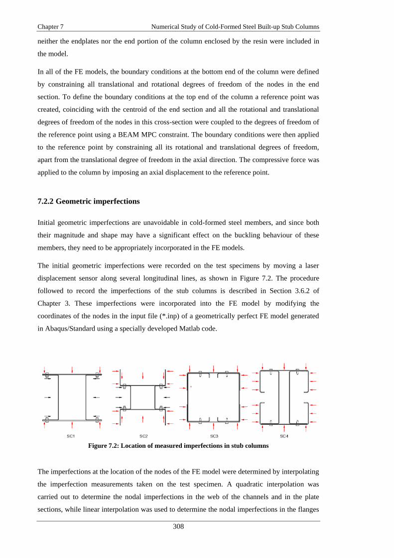
Chapter 7 Numerical Study of Cold-Formed Steel Built-up Stub Columns
308
neither the endplates nor the end portion of the column enclosed by the resin were included in
the model.
In all of the FE models, the boundary conditions at the bottom end of the column were defined
by constraining all translational and rotational degrees of freedom of the nodes in the end
section. To define the boundary conditions at the top end of the column a reference point was
created, coinciding with the centroid of the end section and all the rotational and translational
degrees of freedom of the nodes in this cross-section were coupled to the degrees of freedom of
the reference point using a BEAM MPC constraint. The boundary conditions were then applied
to the reference point by constraining all its rotational and translational degrees of freedom,
apart from the translational degree of freedom in the axial direction. The compressive force was
applied to the column by imposing an axial displacement to the reference point.
7.2.2 Geometric imperfections
Initial geometric imperfections are unavoidable in cold-formed steel members, and since both
their magnitude and shape may have a significant effect on the buckling behaviour of these
members, they need to be appropriately incorporated in the FE models.
The initial geometric imperfections were recorded on the test specimens by moving a laser
displacement sensor along several longitudinal lines, as shown in Figure 7.2. The procedure
followed to record the imperfections of the stub columns is described in Section 3.6.2 of
Chapter 3. These imperfections were incorporated into the FE model by modifying the
coordinates of the nodes in the input file (*.inp) of a geometrically perfect FE model generated
in Abaqus/Standard using a specially developed Matlab code.
Figure 7.2: Location of measured imperfections in stub columns
The imperfections at the location of the nodes of the FE model were determined by interpolating
the imperfection measurements taken on the test specimen. A quadratic interpolation was
carried out to determine the nodal imperfections in the web of the channels and in the plate
sections, while linear interpolation was used to determine the nodal imperfections in the flanges

Chapter 7 Numerical Study of Cold-Formed Steel Built-up Stub Columns
309
of the channels, as illustrated in Figure 7.3. This technique was previously successfully
employed in (Becque and Rasmussen, 2009a).
Figure 7.4 shows, as an example, FE models belonging to geometries SC1, SC2, SC3 and SC4
with amplified out-of-plane imperfections for clarity.
Figure 7.3: Interpolated imperfections
Figure 7.4: FE models including amplified out-of-plane imperfections
7.2.3 Material properties
The material properties of the components of the built-up columns were modelled as elastic-
plastic using the isotropic linear elastic material model together with the metal plasticity model
available in Abaqus/Standard. The data used in the FE models corresponded to the ‘static’
values of the material properties obtained from the flat and corner coupon tests, as described in
Section 3.3.3 of Chapter 3. The elastic behaviour was defined using a Poisson’s ratio of 0.3 and
the elastic modulus obtained from the tensile coupons, following the recommendations given by
Huang and Young (2014). The metal plasticity behaviour was defined using the standard von
SC1 SC2 SC3 SC4

Chapter 7 Numerical Study of Cold-Formed Steel Built-up Stub Columns
310
Mises yield surface with associated plastic flow and isotropic hardening. The start of the plastic
range was taken as the last point on the stress-strain curve which was used to calculate the
elastic modulus. Enough data points were taken from the stress-strain curve obtained from the
tensile coupons in order to accurately replicate the inelastic behaviour of the material. Since
Abaqus/Standard employs true stresses and true (logarithmic) plastic strains, the engineering
values obtained from the coupons were converted into true values using the following
relationship:
1T (7.1)
ln 1T (7.2)
Pl
T T T E (7.3)
where σT, εT and εTPl are the true stresses, the true strains and true plastic strains, respectively,
and σ and ε are the engineering stresses and the engineering strains.
All the flat portions of a component section were considered to have the same material
properties, regardless of the part of the section they belonged to (e.g. web, flanges or lips). This
was considered to be a valid simplification, since it has been shown by Karren (1965) that
similar cold-working effects are experienced by all the flat elements of the cross-section,
irrespective of the forming-process used. In addition, since cold-working may significantly
increase the yield stress of cold-formed steel sections, the enhancement of the mechanical
properties in the corner regions of the individual channels was also included in the FE models.
Karren, (1965) reported that the influence of cold-working may extend beyond the corner over a
distance less than the sheet thickness. However, this influence decreases with the distance from
the centre of the corner. The corner coupons tested in Chapter 3 had a width of 6 mm, as
illustrated in Figure 7.5, covering, in general, a slightly larger portion than the actual corner of
the cross-sections. However, since the values obtained from the tensile coupons corresponded to
the average value of the material properties in this region, the corner regions in the FE models
were defined based on the width of these coupons.
This approach to model the material properties in the FE models, which included an accurate
representation of the stress-strain curve and the enhancement of the mechanical properties at the
corner regions of the channels is further referred to as the ‘actual material’ modelling approach.

Chapter 7 Numerical Study of Cold-Formed Steel Built-up Stub Columns
311
Figure 7.5: Corner coupon width
7.2.3.1 Simplified approaches to model material properties
A material modelling study was carried out to investigate the degree to which the ultimate
capacity of the built-up stub columns was affected by simplifications in modelling their material
behaviour. The effects of two simplified material modelling approaches were investigated using
a representative column of each built-up geometry, by comparing the ultimate load predictions
obtained from the FE models incorporating these simplified material models with those
obtained from the FE model including the actual material properties.
The first simplified material model approximated the stress-strain curve obtained from the
tensile coupons by a bilinear curve. The elastic range was defined in the same way as in the
actual material modelling approach described in the previous sub-section, while the plastic
range was defined using the 0.2 % proof strength without any strain hardening, as shown in
Figure 7.6. The enhancement of the mechanical properties in the corner regions was still
included in this material modelling approach. The second simplified material modelling
approach was identical to the actual material modelling approach, with the only exception that
the enhancement of the mechanical properties in the corner regions was not considered.
Figure 7.6: Bilinear and actual stress-strain curve

Chapter 7 Numerical Study of Cold-Formed Steel Built-up Stub Columns
312
The load-axial deformation curves obtained using the three different material modelling
approaches are illustrated in Figure 7.7 for a representative column belonging to each built-up
geometry. As expected, the figure shows that, across all geometries, the post-buckling stiffness
predicted by the FE model in which the material properties are approximated by a bilinear
stress-strain curve remains higher (up to the peak load) than in the FE models including gradual
yielding in the material behaviour, and the peak load is achieved at a smaller axial shortening of
the column. The figure also shows that, across all geometries, the ultimate capacity obtained
using the bilinear stress-strain curve is noticeably larger than the one obtained using the actual
material modelling approach. On the other hand, ignoring the enhancement of the material
properties in the corner regions resulted in slightly lower ultimate capacities with respect to the
predictions given by the FE model including the actual material properties. Table 7.1 reports the
differences in ultimate capacity obtained using the simplified material modelling approaches
relative to the predictions obtained using the actual material properties for each geometry.
Figure 7.7: Effect of material modelling approach on predicted column response: a) SC1-5b; b)
SC2-6a; c) SC3-5b; d) SC4-5a
(a) (b)
(c) (d)

Chapter 7 Numerical Study of Cold-Formed Steel Built-up Stub Columns
313
Table 7.1 Difference in ultimate load relative to FE model with actual material properties
Column Difference in ultimate load with
respect to model with actual
material properties (%)
Bilinear Without corners
SC1-5a 5.0 -0.4
SC2-6a 4.0 -0.9
SC3-5b 4.6 -1.5
SC4-5a 4.0 -2.0
7.2.4 Contact interaction
In all numerical models contact was defined using the finite-sliding surface-to-surface contact
formulation, in which the surfaces in contact are allowed to experience an arbitrarily large
relative separation, sliding and rotation. The contact conditions are enforced in an average sense
over regions nearby the slave nodes, avoiding large undetected penetration of the master nodes
into the slave surface and improving contact pressure predictions. Since the components of the
built-up geometries were modelled based on their mid-surface, the different components were
positioned with respect to each other leaving a gap equal to their average thickness. The general
contact formulation automatically accounts for the thickness associated with shell-like surfaces,
defining contact on the outer faces. Interaction between the surfaces in contact was defined as
‘frictionless’ in the tangential direction, while a ‘hard’ pressure-overclosure relationship was
approximated in the normal direction by using ‘Augmented Lagrange’ as the constraint
enforcement method. This enforcement method reduces the amount of penetration of the slave
nodes into the master surface, improving the accuracy of the ‘hard’ pressure-overclosure
approximation.
In order to reduce the computational cost, contact was only activated between those surfaces of
components which were likely to interact with each other during the analysis, as shown in
Figure 7.8. For built-up column 1, these surfaces corresponded to the plate sections and the
flanges of the channels, while for built-up column 2, these surfaces corresponded to the web of
the outer channels and the flanges of the inner channels. For built-up column 3 contact was
defined between the web of the lipped channels and the flanges of the plain channels, and also
between the flanges of the lipped channels and the web of the plain channels. For built-up
column 4 it was decided to only define contact between the flanges of the plain channels and the
webs of the lipped channels. This contact definition for built-up column 4 implied that the edges
of the flanges of the plain channels were allowed to penetrate into the flanges of the lipped
channels. The additional edge-to-surface contact interaction resulted in significant convergence
issues and therefore it was decided not to include it. This decision was supported by the fact that
penetration of the edges of the plain channel flanges into the lipped channel flanges only
occurred after the column reached its peak load. Therefore, not including edge-to-surface

Chapter 7 Numerical Study of Cold-Formed Steel Built-up Stub Columns
314
contact between the flanges of the plain channels and those of the lipped channels was deemed
not to affect the pre-peak behaviour and ultimate capacity of these columns.
Figure 7.8: Master and slave role in contact interaction
Any possible initial overclosure between the slave and master surfaces in a contact interaction
was eliminated at the beginning of each analysis using the strain-free adjustment method, which
adjusts the positions of the penetrating slave nodes so they lie directly on their associated master
surface. Initial overclosures were likely to occur due to the introduction of the initial geometric
imperfections into the FE models. In addition, since the default strain-free adjustment available
in Abaqus/Standard was designed to remove only small initial overclosures measuring up to the
average thickness of the connected surfaces, the default search zone for the strain-free
adjustment method was increased to 2 mm. Care was taken to ensure that the ‘master’ role in a
contact interaction was assigned to a surface of which the nodes had previously been adjusted
when introducing the geometric imperfections into the FE model. This warranted that the
accurate modelling of the imperfection data was not lost due to the initial strain-free adjustment
of the penetrating slave nodes.
7.2.5 Connector modelling
One of the main objectives during the development of the FE models was to determine the best
way to model the two different types of connectors used to assemble the built-up columns,
namely the bolts and the self-drilling screws. Built-up columns with geometry 1 and geometry 2
were connected using M6 bolts with a nominal diameter of 6 mm. To ease the assembly of the
built-up specimens the holes were drilled with a nominal diameter of 6.25 mm. This resulted in
a small clearance at the connectors which allowed a certain slip between the component
sections. Built-up columns with geometry 3 and geometry 4 were assembled using M5.5 self-

Chapter 7 Numerical Study of Cold-Formed Steel Built-up Stub Columns
315
drilling sheet metal screws. These type of fasteners are drilled into the metal sheets and do not
result in any clearance.
In order to reduce the computational cost of the FE models, the body of the connectors was not
explicitly modelled, but instead a discrete approach using mesh-independent fasteners was
chosen. Mesh-independent fasteners create a point-to-point connection between two or more
surfaces using fastening points, which are independent of the location of the nodes on each
surface. The fastening point was connected to the neighbouring nodes on the surface using the
structural coupling method, which couples the translational and rotational degrees of freedom of
the fastening point to the average translational and rotational degrees of freedom of the
neighbouring coupling nodes using a uniform weighting scheme. The radius of influence, which
dictates the number of coupling nodes that are used to connect the fastening point to the surface,
was not seen to affect the behaviour of the studied stub columns and this was set by defining a
physical radius for the fastener of 5 mm in all numerical models.
The mesh-independent fasteners were modelled using discrete fasteners with PLANAR
connector elements, which were orientated so that their rotational component of relative motion
(CRM) was normal to the surfaces and the two translational CRMs were tangential to the plane
of contact, as shown in Figure 7.9.
Figure 7.9: PLANAR connector element
In order to replicate the actual behaviour of the fasteners used to assemble the built-up stub
columns, the elastic and plastic properties derived from the single lap shear tests carried out on
the bolted and screwed connections were assigned to the two translational CRMs of the
PLANAR connectors. This permitted to account in the FE model for the effect of the localized
bearing deformations, possible tilting of the connector and, in the case of the bolted built-up
columns, possible slip.

Chapter 7 Numerical Study of Cold-Formed Steel Built-up Stub Columns
316
7.2.6 Type of analysis
A geometrically and material non-linear analysis of the stub columns was carried out using the
General Static solver with the inclusion of artificial damping to stabilize the solution. This
modelling approach has proved to be suitable for modelling the response of built-up specimens
in which contact discontinuities may result in severe convergence errors. Abaqus/Standard
automatically adjusted the time increments during the simulation using the automatic
incrementation control algorithm.
7.2.7 Overcoming convergence issues in Abaqus/Standard
The numerical models of the built-up stub columns presented significant convergence issues.
These issues arose mainly at the point when initial buckling took place and also when the
columns reached their ultimate capacities. These events caused a sudden reduction in stiffness in
certain areas of the built-up column. Moreover, contact between the components of the built-up
column introduced significant discontinuities into the model, which further affected
convergence.
In order to overcome these issues, the models were stabilized using either the automatic
stabilization or the contact stabilization mechanisms available in Abaqus/Standard. Automatic
stabilization and contact stabilization make use of artificial damping forces applied at the nodes
to oppose their sudden movement. The main difference between these stabilization mechanisms
is that automatic stabilization is designed to address convergence issues mainly related to
geometric and material non-linearity. Therefore, the calculated viscous forces computed with
this stabilization mechanism are applied to all the nodes of the model and their magnitude is
proportional to the absolute velocity of each node. Contact stabilization, on the other hand, is
only meant to smoothen contact discontinuities. In this case, the viscous forces are only applied
to the slave nodes in a contact interaction and are proportional to the relative motion between
the surfaces, as described in Section 2.8.3.2 of Chapter 2. Since both stabilization schemes help
to achieve convergence by introducing artificial forces into the numerical model, it is important
to ensure that these artificial forces are small enough so that they do not distort the solution.
This can be achieved by performing a post-analysis check to ensure that the dissipated
stabilization energy (ALLSD) is significantly smaller than the total strain energy of the system
(ALLIE).
In addition to using the stabilization schemes available in Abaqus/Standard, convergence issues
were significantly mitigated by modifying some of the default solution control parameters in the
General Static solver. The solution control parameters which were modified were the
displacement correction control parameter Cαn and the time incrementation parameters I0 and IR.

Chapter 7 Numerical Study of Cold-Formed Steel Built-up Stub Columns
317
In each increment Abaqus/Standard checks whether the force residuals at each node are within
the tolerance limit (by default equal to 0.5 % of an average force in the structure, averaged over
time). Subsequently it carries out an additional check to ensure that the maximum displacement
correction cαmax at each node is less than a fraction of the total incremental displacement of the
node, as explained in Section 2.8.2 of Chapter 2. This fraction is given by Cαn, which by default
is set to 0.01. This additional check was found to create significant convergence issues in the
column models due to the relatively large and sudden displacements and rotations the nodes in
the model experience as a result of buckling, and also when the column is approaching its
ultimate capacity and a yield line mechanism start to form. The check resulted in an unnecessary
reduction of time increment sizes, despite the force residuals in the resulting equilibrium
configuration being within the tolerance limits. Abaqus/Standard allows the user to remove this
check by setting Cαn to 1. This modification was found not to have any noticeable effect on the
accuracy of the solution.
The time incrementation parameters I0 and IR are used to control the frequency with which
Abaqus/Standard checks whether the solution converges monotonically and whether
convergence is quadratic. The default values of these parameters (4 for I0 and 8 for IR) were
increased to 8 and 10, respectively, as recommended in (Dassault Systemes, 2014) for severely
discontinuous problems in order to avoid unnecessary cutbacks of the time increments. Also, the
‘line search algorithm’, which helps prevent divergence by applying a scale factor to the
computed solution, was activated, allowing up to 40 line search iterations to calculate the scale
factor and defining a tolerance for the change of the scale factor between successive iterations
of 0.001. This permitted minimizing the amount of damping required to help Abaqus/Standard
achieve convergence. It is important to note that, although these modified solution control
parameters do not alter the accuracy of the solution, they require some additional computational
time per increment. However, this additional computational cost was observed to be
compensated by the smaller number of increments required to complete the simulation.
For all models presented in this chapter the strategy followed to achieve a converging solution
consisted of running the model using the contact stabilization mechanism together with the non-
default time incrementation control parameters previously described. If the simulation
terminated before the ultimate capacity of the column was reached, an additional step was added
to the simulation, in which the contact control scheme was removed and replaced with the
automatic stabilization mechanism. Also, in this second step the maximum displacement
correction check was removed by setting Cαn to 1. The following sections describe a
stabilization study which was carried out to ensure that the artificial viscous forces introduced
through the contact stabilization and the automatic stabilization schemes were sufficiently low
not the significantly alter the solution.

Chapter 7 Numerical Study of Cold-Formed Steel Built-up Stub Columns
318
7.2.7.1 Contact stabilization
Contact stabilization was used through the *CONTACT CONTROL keyword while specifying
a constant scale factor for the magnitude of the viscous forces normal to the surfaces in contact,
which were automatically calculated by Abaqus/Standard. A suitable value for this scale factor
which does not result in a significant distortion of the solution was determined by carrying out a
series of numerical simulations for each built-up geometry, in which identical FE models were
run while varying the scale factor from zero (no artificial damping added to the model) over
2x10⁻⁴ to 8x10⁻⁴. No artificial damping was added to oppose the relative motion of the nodes in
the tangential direction to the surfaces. This was achieved by setting the ‘tangent fraction’
parameter to zero. This option was chosen because the tangential viscous stresses are likely to
absorb significant amounts of energy when there is slip between the contacting surfaces.
Table 7.2 lists the ultimate loads obtained for each built-up geometry and the corresponding
values given to the scale factor. The table shows that column SC1 was the only geometry for
which a converging solution could be achieved past the peak load by only adjusting the solution
control parameters. Columns SC2 and SC3, on the other hand, were only able to converge after
activating the contact control scheme, while for column SC4 a converging solution could not be
achieved even after activating the contact control scheme. The ratio between the energy
dissipated through artificial damping (ALLSD) and the total strain energy of the model (ALLIE)
is illustrated in Figure 7.10a, Figure 7.11a and Figure 7.12a for columns SC1, SC2 and SC3,
respectively. The vertical dashed line shows the approximate axial deformation at which the
columns reached their ultimate capacity. The load-axial shortening curves of columns SC1, SC2
and SC3 are shown in Figure 7.10b, Figure 7.11b and Figure 7.12b, respectively.
Table 7.2: Ultimate load comparison with contact control schemes
Specimen Stabilization
scheme
Contact
control
Ult. Load
(kN)
SC1-2b
No stabilization - 178.99
cc 0.0002 2x10⁻⁴ 178.34
cc 0.0005 5x10⁻⁴ 178.68
cc 0.0008 8x10⁻⁴ 177.01
SC2-2b
No stabilization - Divergence
cc 0.0002 2x10⁻⁴ 227.13
cc 0.0005 5x10⁻⁴ 226.95
cc 0.0008 8x10⁻⁴ 225.97
SC3-2a
No stabilization - Divergence
cc 0.0002 2x10⁻⁴ 133.89
cc 0.0005 5x10⁻⁴ 133.66
cc 0.0008 8x10⁻⁴ 133.77
SC4-2a
No stabilization - Divergence
cc 0.0002 2x10⁻⁴ Divergence
cc 0.0005 5x10⁻⁴ Divergence
cc 0.0008 8x10⁻⁴ Divergence

Chapter 7 Numerical Study of Cold-Formed Steel Built-up Stub Columns
319
Table 7.2 shows that the ultimate loads of columns SC1, SC2 and SC3 were not significantly
affected by the contact stabilization scheme over the range of values selected for the scale
factor. For column SC1, the difference in the ultimate load achieved with a scale factor equal to
2x10⁻⁴ was 0.36 % relative to the model in which no stabilization was used. For columns SC2
and SC3, the maximum variations in the ultimate load when varying the scale factor from 2x10⁻⁴
to 8x10⁻⁴ were only 0.51 % and 0.09 %, respectively. This small variation in the ultimate load
can be attributed to the fact that in the contact stabilization scheme the viscous forces are only
used to oppose the relative motion between the nodes involved in a contact interaction and they
are only introduced into the model when the nodes are relatively close to each other. This occurs
mainly when the components of the column start buckling, as shown in Figure 7.10a, Figure
7.11a and Figure 7.12a for columns SC1, SC2 and SC3, respectively. When the column is
reaching its ultimate capacity, on the other hand, most of the contact or separation between the
surfaces has already been established, and therefore the amount of artificial damping introduced
at this point is significantly smaller.
Although the ultimate capacity of columns SC1 was not significantly affected by the artificial
forces introduced through the contact stabilization scheme for the range of scale factors
considered, the onset of global buckling of the plate sections between connector points was
significantly delayed, as shown in Figure 7.13, which plots the load vs. lateral deformation
curves of the plate sections at the column mid-height obtained for the different values given to
the scale factor. However, once buckling of the plate sections was fully developed the load vs.
lateral deformation curves of all FE models in which the contact stabilization scheme was
activated converged to the curve obtained with the FE model in which no stabilization was used.
Based on this stabilization study it was decided not to use the contact stabilization scheme for
the FE models with geometry SC1 in order to ensure an accurate prediction of the critical
buckling stresses of the components of these columns. In addition, it was concluded that using a
constant scale factor equal to 2x10⁻⁴ resulted in a negligible change in the ultimate capacity for
the studied geometries and this value was used in all models in which the contact stabilization
scheme was activated.

Chapter 7 Numerical Study of Cold-Formed Steel Built-up Stub Columns
320
Figure 7.10: Contact stabilization in columns SC1-2b: a) Dissipated energy over total strain energy;
b) Load-axial shortening curve
Figure 7.11: Contact stabilization in columns SC2-2b: a) Dissipated energy over total strain energy;
b) Load-axial shortening curve
Figure 7.12: Contact stabilization in columns SC3-2a: a) Dissipated energy over total strain energy;
b) Load-axial shortening curve
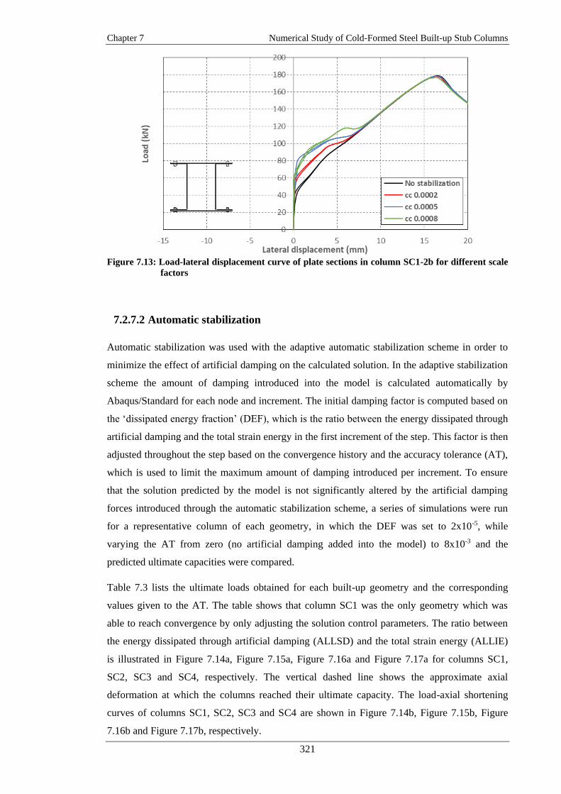
Chapter 7 Numerical Study of Cold-Formed Steel Built-up Stub Columns
321
Figure 7.13: Load-lateral displacement curve of plate sections in column SC1-2b for different scale
factors
7.2.7.2 Automatic stabilization
Automatic stabilization was used with the adaptive automatic stabilization scheme in order to
minimize the effect of artificial damping on the calculated solution. In the adaptive stabilization
scheme the amount of damping introduced into the model is calculated automatically by
Abaqus/Standard for each node and increment. The initial damping factor is computed based on
the ‘dissipated energy fraction’ (DEF), which is the ratio between the energy dissipated through
artificial damping and the total strain energy in the first increment of the step. This factor is then
adjusted throughout the step based on the convergence history and the accuracy tolerance (AT),
which is used to limit the maximum amount of damping introduced per increment. To ensure
that the solution predicted by the model is not significantly altered by the artificial damping
forces introduced through the automatic stabilization scheme, a series of simulations were run
for a representative column of each geometry, in which the DEF was set to 2x10⁻⁵, while
varying the AT from zero (no artificial damping added into the model) to 8x10⁻³ and the
predicted ultimate capacities were compared.
Table 7.3 lists the ultimate loads obtained for each built-up geometry and the corresponding
values given to the AT. The table shows that column SC1 was the only geometry which was
able to reach convergence by only adjusting the solution control parameters. The ratio between
the energy dissipated through artificial damping (ALLSD) and the total strain energy (ALLIE)
is illustrated in Figure 7.14a, Figure 7.15a, Figure 7.16a and Figure 7.17a for columns SC1,
SC2, SC3 and SC4, respectively. The vertical dashed line shows the approximate axial
deformation at which the columns reached their ultimate capacity. The load-axial shortening
curves of columns SC1, SC2, SC3 and SC4 are shown in Figure 7.14b, Figure 7.15b, Figure
7.16b and Figure 7.17b, respectively.

Chapter 7 Numerical Study of Cold-Formed Steel Built-up Stub Columns
322
From the ALLSD/ALLIE ratios for each geometry it is seen that SC3 is the only geometry for
which most of the artificial damping was introduced at the peak load. For this geometry, the
peak load predicted by the FE model increased by 1.23 % when the AT was increased from
2x10⁻³ to 8x10⁻³, while for columns SC2 and SC4 the increases in the ultimate load were only
0.20 % and 0.23 %, respectively. For columns SC1, on the other hand, the ultimate load showed
a slight decrease as the AT was increased. In these columns, most of the artificial damping was
introduced when the components started buckling.
For column SC1, the difference in the peak load predicted by the FE model in which the AT
was set to 2x10⁻³ was only 0.06 % relative to the one in which no artificial damping was added,
while the ALLSD/ALLIE ratio was around 0.1 % when the peak load was reached. Similar
ALLSD/ALLIE ratios were obtained for the other geometries when the AT was set to 2x10⁻³.
More precisely, the ALLSD/ALLIE ratios were 0.12 %, 0.20 % and 0.07 % when the peak load
was reached in the columns with geometries SC2, SC3 and SC4, respectively. Although no
convergence could be reached in these geometries without damping, it seems reasonable to
assume that the variation in the ultimate capacity in these columns as a result of the artificial
damping forces is similar to the one observed in the column with geometry SC1. This variation
in the ultimate capacity was considered to be negligible, and it was therefore decided to set the
AT equal to 2x10⁻³ in all models in which automatic stabilization was activated.
Table 7.3: Ultimate load comparison with automatic stabilization schemes
Specimen Stabilization
scheme DEF AT
Ult. Load
(kN)
SC1-2b
No stabilization - - 178.99
sc 0.002 2x10⁻⁵ 2x10⁻³ 178.88
sc 0.005 2x10⁻⁵ 5x10⁻³ 178.73
sc 0.008 2x10⁻⁵ 8x10⁻³ 177.03
SC2-2b
No stabilization - - Divergence
sc 0.002 2x10⁻⁵ 2x10⁻³ 227.85
sc 0.005 2x10⁻⁵ 5x10⁻³ 228.09
sc 0.008 2x10⁻⁵ 8x10⁻³ 228.31
SC3-2a
No stabilization - - Divergence
sc 0.002 2x10⁻⁵ 2x10⁻³ 133.08
sc 0.005 2x10⁻⁵ 5x10⁻³ 134.12
sc 0.008 2x10⁻⁵ 8x10⁻³ 134.73
SC4-2a
No stabilization - - Divergence
sc 0.002 2x10⁻⁵ 2x10⁻³ 135.18
sc 0.005 2x10⁻⁵ 5x10⁻³ 135.26
sc 0.008 2x10⁻⁵ 8x10⁻³ 135.49

Chapter 7 Numerical Study of Cold-Formed Steel Built-up Stub Columns
323
Figure 7.14: Automatic stabilization in columns SC1-2b: a) Dissipated energy over total strain
energy; b) Load-axial shortening curve
Figure 7.15: Automatic stabilization in columns SC2-2b: a) Dissipated energy over total strain
energy; b) Load-axial shortening curve
Figure 7.16: Automatic stabilization in columns SC3-2a: a) Dissipated energy over total strain
energy; b) Load-axial shortening curve

Chapter 7 Numerical Study of Cold-Formed Steel Built-up Stub Columns
324
Figure 7.17: Automatic stabilization in columns SC4-2a: a) Dissipated energy over total strain
energy; b) Load-axial shortening curve
7.2.8 Mesh analysis
A mesh analysis was carried out to establish the best suited element type to model the non-
linear behaviour of CFS built-up stub columns and determine the effect of the mesh size on the
accuracy of the model. The study was performed for representative columns of geometry SC1,
SC2 and SC3, using five intermediate connectors for specimens SC1 and SC3 and six
intermediate connectors for specimen SC2. The results obtained from the mesh analysis for
columns SC3 were considered to also be applicable to columns SC4, since columns SC4 were
assembled using component sections with the same nominal dimensions as those used to
assemble the columns with geometry SC3. The specimens were modelled using the nominal
dimensions of the component sections. The FE models included material non-linearity, which
was obtained from coupon tests, and the recorded geometric imperfections of a representative
test specimen of each geometry. The connectors were modelled using HINGE connector
elements. Both the total CPU time required to run the analysis and the peak load were taken into
account in the study.
7.2.8.1 Element type
The two element types chosen for the mesh analysis were the conventional shell elements S4
and S4R, available in Abaqus/Standard. These are general-purpose quadrilateral linear elements
that have been widely used by other researchers to model the non-linear behaviour of cold-
formed steel members (Becque and Rasmussen, 2009b; Jiahui, 2014; Li, Ádány, and Schafer,
2013; Yang and Hancock, 2006; Zhang and Young, 2015). These elements can be used to
model thick and thin shell problems. They account for the transverse shear deformations present
in thick shell elements. However, as the thickness of the shell decreases and the transverse shear
deformations in the element become negligible, the elements follow discrete Kirchoff theory,
where plain sections normal to the mid-surface of the shell remain straight and normal

Chapter 7 Numerical Study of Cold-Formed Steel Built-up Stub Columns
325
throughout the deformation of the mid-surface. The elements account for thickness changes as a
result of in-plane deformations and they are not affected by transverse shear locking. These
elements use finite membrane strain formulation, allowing for arbitrarily large deformations and
rotations. Therefore, they are suitable for non-linear geometric analysis. S4 is a fully integrated
shell element with three translational and three rotational degrees of freedom at each node. It
has four integration points and does not have hourglass modes in either the membrane or
bending response of the element. However, due to its number of integration points, this element
is computationally more expensive, especially for large problems, than its counterpart S4R
element with reduced integration points. S4R elements only use a single integration point to
formulate the element stiffness. They can provide accurate results, although they are prone to
hourglassing modes. However, in the problems under consideration hourglassing modes were
not found to be an issue.
7.2.8.2 Mesh size
Five different mesh densities were used in the analysis. The size of the elements in the flanges
and the web of the channels, as well as over the width of the plate sections, was chosen to be as
similar as possible. The aspect ratio of these elements was kept below 2 as much as possible,
following the recommendations given by Schafer (1997). The number of elements used across
the corner regions of the channels was varied from two to six. Due to the limited area of the
corners the aspect ratio of the elements in these regions was somewhat relaxed to be less than 4,
in order to avoid an overly dense mesh. At least two elements were used across the lips of the
lipped channels. Table 7.4, Table 7.6 and Table 7.8 show the number of elements and nodes
used in the mesh analyses for columns SC1, SC2 and SC3, respectively, while Table 7.5, Table
7.7 and Table 7.9 report the aspect ratios of the studied meshes.
Table 7.4: Mesh configuration for built-up column 1
Mesh
N of elements N of
nodes Channels Plates column Total
Flange Web Corner Width Length
Mesh 1 2 6 2 8 76 3344 3696
Mesh 2 4 12 2 16 76 6080 6468
Mesh 3 6 18 4 24 152 18848 19584
Mesh 4 8 24 4 32 152 24320 25092
Mesh 5 10 30 6 40 228 46512 47632
Table 7.5: Mesh aspect ratios in built-up column 1
Mesh
Aspect ratio
Channels Plates
Flange Web Corner Width
Mesh 1 0.569 0.581 4.000 0.558
Mesh 2 1.137 1.161 4.000 1.116
Mesh 3 0.853 0.871 4.000 0.837
Mesh 4 1.137 1.161 4.000 1.116
Mesh 5 0.948 0.968 4.000 0.930

Chapter 7 Numerical Study of Cold-Formed Steel Built-up Stub Columns
326
Table 7.6: Mesh configuration for built-up column 2
Mesh
N of elements N of
nodes Inner Channels Outer Channels column Total
Flange Web Corner Flange Web Corner Length
Mesh 1 1 3 2 2 6 2 54 2484 2750
Mesh 2 3 6 2 4 12 2 54 4320 4620
Mesh 3 5 10 4 7 22 4 108 15552 16132
Mesh 4 7 15 4 10 30 4 108 20520 21146
Mesh 5 9 20 6 14 42 6 163 43032 43952
Table 7.7: Mesh aspect ratios in built-up column 2
Mesh
Aspect ratio
Inner Channels Outer Channels
Flange Web Corner Flange Web Corner
Mesh 1 0.452 0.609 4.000 0.574 0.586 4.000
Mesh 2 1.355 1.218 4.000 1.147 1.172 4.000
Mesh 3 1.129 1.015 4.000 1.004 1.074 4.000
Mesh 4 1.581 1.523 4.000 1.434 1.465 4.000
Mesh 5 1.347 1.345 4.000 1.331 1.359 4.000
Table 7.8: Mesh configuration for built-up column 3
Mesh
N of elements N of
nodes Plain Channels Lipped Channels column Total
Flange Web Corner Flange Web Lip Corner Length
Mesh 1 2 4 2 2 4 2 2 74 4736 5100
Mesh 2 3 9 2 3 8 2 2 74 6660 7050
Mesh 3 4 13 4 5 12 2 4 148 21016 21754
Mesh 4 8 16 4 8 16 4 4 148 28416 29204
Mesh 5 10 20 6 10 20 6 6 220 56320 57460
Table 7.9: Mesh aspect ratios in built-up column 3
Mesh
Aspect ratio
Plain Channels Lipped Channels
Flange Web Corner Flange Web Lip Corner
Mesh 1 0.814 0.519 4.000 0.711 0.571 5.552 4.000
Mesh 2 1.221 1.168 4.000 1.066 1.142 5.552 4.000
Mesh 3 0.814 0.843 4.000 0.888 0.857 2.776 4.000
Mesh 4 1.628 1.038 4.000 1.421 1.142 5.552 4.000
Mesh 5 1.369 0.873 4.000 1.195 0.961 5.603 4.000
7.2.8.3 Mesh analysis results
Table 7.10, Table 7.11 and Table 7.12 list the ultimate load and the total CPU time required to
complete the simulations with different mesh densities and element types for columns SC1, SC2
and SC3, respectively. The tables also show the total number of increments in which the
analyses were divided and the average CPU time required to solve each increment. The CPU
times listed in brackets correspond to simulations in which, although the peak load was reached,
the analysis was not completed.

Chapter 7 Numerical Study of Cold-Formed Steel Built-up Stub Columns
327
Table 7.10: Effect of element type and mesh size on the ultimate load and total CPU time for
columns SC1
Element
type
Mesh Ultimate
Load (kN)
Total CPU
time (s)
N of
increments
CPU time per
increment (s)
S4
Mesh 1 245.48 2315 210 11
Mesh 2 231.19 2799 169 17
Mesh 3 212.92 12555 198 63
Mesh 4 215.90 10344 118 88
Mesh 5 214.90 28816 155 186
S4R
Mesh 1 254.70 2884 283 10
Mesh 2 234.77 (2472) 153 16
Mesh 3 214.33 10715 189 57
Mesh 4 216.59 10514 137 77
Mesh 5 215.34 29301 177 166
Table 7.11: Effect of element type and mesh size on the ultimate load and total CPU time for
columns SC2
Element
type
Mesh Ultimate
Load (kN)
Total CPU
time (s)
N of
increments
CPU time per
increment (s)
S4
Mesh 1 268.59 (1105) 132 8
Mesh 2 261.08 1923 156 12
Mesh 3 239.42 4741 104 46
Mesh 4 239.25 7457 135 55
Mesh 5 235.45 18012 137 131
S4R
Mesh 1 256.43 957 120 8
Mesh 2 253.97 (1341) 113 12
Mesh 3 238.94 4195 100 42
Mesh 4 238.74 6669 126 53
Mesh 5 235.35 14086 119 118
Table 7.12: Effect of element type and mesh size on the ultimate load and total CPU time for
columns SC3
Element
type
Mesh Ultimate
Load (kN)
Total CPU
time (s)
N of
increments
CPU time per
increment (s)
S4
Mesh 1 175.96 946 48 20
Mesh 2 163.48 1697 60 28
Mesh 3 159.04 13464 113 119
Mesh 4 158.20 14250 82 174
Mesh 5 156.94 34124 81 421
S4R
Mesh 1 176.00 2095 99 21
Mesh 2 162.65 2640 99 27
Mesh 3 158.68 20334 164 124
Mesh 4 157.94 16880 109 155
Mesh 5 156.93 48466 122 397
From these tables it can be seen that the number of increments required to complete the
simulations is not related to the mesh density of the model. For this reason, in order to better
compare the computational efficiency of S4 and S4R elements Figure 7.18, Figure 7.19 and
Figure 7.20 plot the ultimate load and the CPU time per increment obtained with these elements
for the different mesh densities considered in this study.

Chapter 7 Numerical Study of Cold-Formed Steel Built-up Stub Columns
328
Figure 7.18: Effect of mesh size and element type on the ultimate load and total CPU time for
columns SC1
Figure 7.19: Effect of mesh size and element type on the ultimate load and total CPU time for
columns SC2

Chapter 7 Numerical Study of Cold-Formed Steel Built-up Stub Columns
329
Figure 7.20: Effect of mesh size and element type on the ultimate load and total CPU time for
columns SC3
The figures show that for columns SC1, SC2 and SC3, the ultimate capacities predicted by the
FE models with both S4 and S4R elements converged asymptotically as the mesh size was
reduced, and that both element types converged to virtually the same prediction. The CPU time
per increment, on the other hand, increased more than linearly with the number of nodes in the
model. The FE models with S4R elements required, on average, around 7 % less computational
time per increment than the models built with S4 elements and the same mesh density across all
the geometries , while the difference in the ultimate capacity predicted with the S4 and S4R
elements was typically around 0.25 % for a given mesh density. For this reason, it was decided
to use S4R elements to develop all the models presented in this thesis.
Regarding the mesh density, the differences in the ultimate capacities predicted with Mesh 3
and the finest mesh (Mesh 5) were 0.47 %, 1.53 % and 1.12 % for columns SC1, SC2 and SC3,
respectively. This accuracy was considered to be satisfactory given the complexity of the
models and therefore all models were meshed using a Mesh 3 configuration.
7.3. FE model verification
7.3.1 Ultimate load
Table 7.13, Table 7.14, Table 7.15 and Table 7.16 compare the FE predicted ultimate loads with
the values obtained from the tests for the columns with geometry SC1, SC2, SC3 and SC4,
respectively. The tables also include the stabilization settings used to help Abaqus/Standard
achieve a converging solution. It is seen that the FE models were able to accurately predict the
ultimate capacity of the tested columns across all studied geometries, with average errors of

Chapter 7 Numerical Study of Cold-Formed Steel Built-up Stub Columns
330
2.88 % for columns SC1, 4.37 % for columns SC2, 2.52 % for columns SC3 and 5.02 % for
columns SC4.
The load vs. axial shortening curves obtained from the FE models, as well as those obtained
experimentally, are plotted in Figure 7.21, Figure 7.22, Figure 7.23 and Figure 7.24 for each test
specimen belonging to geometry SC1, SC2, SC3 and SC4, respectively.
Table 7.13: Numerical and experimental ultimate loads of columns SC1
Specimen Test ult.
load (kN)
FEA ult.
load (kN) FEA/Test
Stabilization scheme
Step 1 Step 2
SC1-2a 183.97 179.55 0.976 No stabilization -
SC1-2b 168.17 177.70 1.057 No stabilization -
SC1-3a 183.01 182.50 0.997 No stabilization sc 0.002
SC1-3b 175.86 182.50 1.038 No stabilization sc 0.002
SC1-5a 201.72 194.51 0.964 No stabilization -
SC1-5b 188.50 191.49 1.016 No stabilization -
Avg. 1.008
St. dev. 0.036
Figure 7.21: Numerical and experimental load vs. axial shortening curves of columns SC1
Table 7.14: Numerical and experimental ultimate loads of columns SC2
Specimen Test ult.
load (kN)
FEA ult.
load (kN) FEA/Test
Stabilization scheme
Step 1 Step 2
SC2-2a 213.32 226.89 1.064 cc 0.0002 -
SC2-2b 200.34 226.63 1.131 cc 0.0002 -
SC2-4a 238.00 232.56 0.977 cc 0.0002 -
SC2-4b 233.39 233.13 0.999 cc 0.0002 -
SC2-6a 220.24 239.86 1.089 cc 0.0002 -
SC2-6b 232.62 238.56 1.026 cc 0.0002 -
Avg. 1.048
St. dev. 0.058

Chapter 7 Numerical Study of Cold-Formed Steel Built-up Stub Columns
331
Figure 7.22: Numerical and experimental load vs. axial shortening curves of columns SC2
Table 7.15: Numerical and experimental ultimate loads of columns SC3
Specimen Test ult.
load (kN)
FEA ult.
load (kN) FEA/Test
Stabilization scheme
Step 1 Step 2
SC3-2a 139.30 134.69 0.967 cc 0.0002 -
SC3-2b 138.53 133.61 0.964 cc 0.0002 -
SC3-5a 138.77 142.14 1.024 cc 0.0002 sc 0.002
SC3-5b 143.40 142.27 0.992 cc 0.0002 -
Avg. 0.987
St. dev. 0.028
Figure 7.23: Numerical and experimental load vs. axial shortening curves of columns SC3
Table 7.16: Numerical and experimental ultimate loads of columns SC4
Test ult.
load (kN)
FEA ult.
load (kN) FEA/Test
Stabilization scheme
Step 1 Step 2
SC4-2a 148.09 135.84 0.917 cc 0.0002 sc 0.002
SC4-2b 147.03 135.47 0.921 cc 0.0002 sc 0.002
SC4-5a 141.23 141.58 1.002 cc 0.0002 sc 0.002
SC4-5b 137.74 142.74 1.036 cc 0.0002 sc 0.002
Avg. 0.969
St. dev. 0.059

Chapter 7 Numerical Study of Cold-Formed Steel Built-up Stub Columns
332
Figure 7.24: Numerical and experimental load vs. axial shortening curves of columns SC4
7.3.2 Deformed shape
The FE models were able to accurately replicate the initial buckled shape of the tested columns
for each of the built-up geometries and connector spacings. As examples, Figure 7.25a and
Figure 7.26a compare the initial buckled shapes obtained from the FE models with those
observed during the tests for columns SC1-2a and SC1-5a, respectively, while Figure 7.27a and
Figure 7.28a do the same for columns SC2-2a and SC2-5a, respectively. For geometries SC3
and SC4, Figure 7.29a and Figure 7.30a compare the initial buckling deformations predicted by
the FE models with the deformations observed during the tests in columns SC3-5a and SC4-5a,
respectively.
A fairly good agreement was also achieved between the yield line mechanisms predicted by the
FE models and those observed in the tested columns. However, as Figure 7.25b, Figure 7.26b,
Figure 7.27b and Figure 7.28b show, the yield line mechanism predicted by the FE models often
developed in a different location along the column.

Chapter 7 Numerical Study of Cold-Formed Steel Built-up Stub Columns
333
Figure 7.25: Deformed shape of SC1-2a: a) before peak load; b) after peak load
Figure 7.26: Deformed shape of SC1-5a: a) before peak load; b) after peak load
Figure 7.27: Deformed shape of SC2-2a: a) before peak load; b) after peak load
(a)
(a) (b)
(a) (b)
(b)

Chapter 7 Numerical Study of Cold-Formed Steel Built-up Stub Columns
334
Figure 7.28: Deformed shape of SC2-6a: a) before peak load; b) after peak load
Figure 7.29: Deformed shape of SC3-5a: a) before peak load; b) after peak load
Figure 7.30: Deformed shape of SC4-5a: a) before peak load; b) after peak load
In order to further assess the accuracy of the FE models in predicting the initial deformed shape
of the stub columns, the readings obtained from the potentiometers used to record the out-of-
(b)
(a) (b)
(a)
(a) (b)

Chapter 7 Numerical Study of Cold-Formed Steel Built-up Stub Columns
335
plane deformations of the components of each tested column were compared to the out-of-plane
displacements of the nodes in the FE models which were at the same location as the
potentiometers. Figure 7.31, Figure 7.32, Figure 7.33 and Figure 7.34 compare the out-of-plane
deformations obtained from the FE models to those from the tests for a representative column
with geometry SC1, SC2, SC3 and SC4, respectively. The figures show an excellent agreement
between the numerical and experimental out-of-plane deformation curves. Curves comparing
the numerical and experimental out-of-plane deformations of the components of each tested
column are included in Appendix L.
Figure 7.31: Experimental and numerical axial load vs lateral displacement curves of SC1-3b
Figure 7.32: Experimental and numerical axial load vs lateral displacement curves of SC2-2a

Chapter 7 Numerical Study of Cold-Formed Steel Built-up Stub Columns
336
Figure 7.33: Experimental and numerical axial load vs lateral displacement curves of SC3-2a
Figure 7.34: Experimental and numerical axial load vs lateral displacement curves of SC4-5b
It is worth mentioning that, in agreement with the observations made during the tests of
columns SC3, the FE models showed no sign of distortional buckling in the lipped channels of
these columns. For columns SC4, on the other hand, the experiments showed some minor
participation of distortional buckling in the lipped channels. However, the FE models did not
confirm this and did not show any sign of this buckling mode in these columns. For example,
Figure 7.35 shows the deformed shape of one of the lipped channels of columns SC3-2a and
SC4-2a, amplified five times, shortly before the columns reached their ultimate load.

Chapter 7 Numerical Study of Cold-Formed Steel Built-up Stub Columns
337
Figure 7.35: Amplified deformed shape of one of the lipped channels of: a) SC3-2a; b) SC4-2a
7.3.3 Critical buckling stresses
The accuracy of the FE models in predicting the critical buckling stresses of the different
components of the stub columns was assessed by comparing the experimentally derived
buckling stresses with those obtained from the FE models. Load-lateral displacement curves,
similar to those shown in Figures 7.31-7.34, were used to calculate the experimental and
numerical critical buckling stresses of the components of each tested column using the same
assumptions as previously described in Section 3.8.3 of Chapter 3. The critical buckling stresses
obtained from the tests and the corresponding FE models are reported in Table 7.17, Table 7.18,
Table 7.19 and Table 7.20 for columns with geometry SC1, SC2, SC3 and SC4, respectively.
For columns SC1, Table 7.17 shows that the average difference between the experimentally
derived critical buckling stresses and those obtained from the FE models was around 15 % for
the plate sections and around 7 % for the channel sections. For columns SC2, Table 7.18 shows
that the average difference between the experimentally and numerically derived critical
buckling stresses of the outer channels was around 5 %, while for columns SC3 and SC4 Table
7.19 and Table 7.20 show that these differences were around 5 % and 11 %, respectively.
Table 7.17: Numerical and experimental buckling stresses of the components of columns SC1
Column
Buckling stress
from test (MPa)
Buckling stress
from FEA (MPa)
Channel Plate Channel Plate
SC1-2a 65 28 71 21
SC1-2b 72 19 70 24
SC1-3a 70 46 72 42
SC1-3b 69 45 72 40
SC1-5a 69 69 59 59
SC1-5b 67 67 61 61
(a)
(b)

Chapter 7 Numerical Study of Cold-Formed Steel Built-up Stub Columns
338
Table 7.18: Numerical and experimental buckling stresses of the components of columns SC2
Column
Buckling stress from
test (MPa)
Buckling stress from
FEA (MPa)
Inner
Channel
Outer
Channel
Inner
Channel
Outer
Channel
SC2-2a - 77-95 - 82-90
SC2-2b - 79 - 76-90
SC2-4a - 69-86 - 86
SC2-4b - 86 - 86
SC2-6a - 105 - 97
SC2-6b - 105 - 101
Table 7.19: Numerical and experimental buckling stresses of the components of columns SC3
Column
Buckling stress from
test (MPa)
Buckling stress from
FEA (MPa)
Plain
Channel
Lipped
Channel
Plain
Channel
Lipped
Channel
SC3-2a 103 103 96 96
SC3-2b 84-96 96 101 101
SC3-5a - 96-117 108 105
SC3-5b 108 108 105 105
Table 7.20: Numerical and experimental buckling stresses of the components of columns SC4
Column
Buckling stress from
test (MPa)
Buckling stress from
FEA (MPa)
Plain
Channel
Lipped
Channel
Plain
Channel
Lipped
Channel
SC4-2a 87 - 74 -
SC4-2b 88 - 73 -
SC4-5a 73-91 91 91 91
SC4-5b 93-104 104 93 93
From the above it can be concluded that the FE models which included material non-linearity
derived from coupon tests, measured geometric imperfections and actual experimentally
determined connector behaviour were able to accurately replicate the behaviour of the tested
stub columns and they were therefore further used in parametric studies.
7.4. Parametric study
7.4.1 Effect of fastener modelling
In order to study the way in which different connector modelling approaches affect the predicted
response of the FE model, the ultimate loads obtained from the validated FE models were
compared to the results obtained from FE models in which the connectors behaviour was
modelled in three different ways.

Chapter 7 Numerical Study of Cold-Formed Steel Built-up Stub Columns
339
The first and simplest approach to model the connectors was using BEAM multi-point
constraints (MPCs). MPC constraints eliminate the degrees of freedom of a particular node, in
this case by coupling the degrees of freedom of the fastening points on both surfaces. They have
been used in the past to model the behaviour of screw connectors in CFS built-up specimens
(Anapayan and Mahendran, 2012; Zhang and Young, 2015). This approach has the advantage of
reducing the size of the model. However, it does not allow any output to be obtained from the
connectors (e.g. the connector shear forces), and since the constraints are imposed by
eliminating the degrees of freedom of one of the fastening nodes, it cannot be used to model
more complex connector behaviour such as slip or bearing deformations of the connected plates.
In the remaining two modelling approaches the fasteners were modelled using either HINGE or
PLANAR connector elements. HINGE connectors constrain all components of relative motion
(CRMs) between the surfaces, apart from the rotational component normal to the fastened
surfaces, while PLANAR connectors constrain all CRMs apart from the rotation normal to the
surfaces and the translational CRMs tangential to the surfaces. It is worth noting that this last
modelling approach is similar to the approach used to model the connectors in the validated
models. However, in this case neither elastic nor plastic behaviour was added to the tangential
CRMs. The ‘HINGE’ and ‘PLANAR’ models can be seen as opposite ends of a spectrum. In the
former, slip at the connectors is completely prevented, while in the latter infinite and
unrestrained slip is allowed.
Figure 7.36 shows, for each column, the ultimate load obtained from the HINGE, PLANAR and
MPC FE models, normalized against the ultimate load obtained with the validated FE models.
Figure 7.36 shows that the most significant effect of the connector behaviour on the ultimate
load occurred in columns SC1, in which the MPC models predicted the highest ultimate loads
and the PLANAR models the lowest. The HINGE models predicted slightly lower ultimate
loads than the MPC models. This may be attributed to the additional in-plane rotational restraint
the MPC model exerted between the fastened surfaces at the connecting points. The average
difference between the peak loads predicted for columns SC1 by the HINGE and PLANAR FE
models was around 16 %, while the average difference between the MPC and PLANAR FE
models was around 20 %. In columns SC2, SC3 and SC4 the effect of the connector behaviour
was less noticeable. However, for columns SC2 the predictions of the ultimate loads given by
the PLANAR models were consistently lower than those of the HINGE and MPC FE models,
with an average difference of around 5 %. In columns SC3 and SC4, on the other hand, some of
the PLANAR models predicted ultimate loads which were slightly larger than those predicted
by the HINGE and MPC models. However, the difference in the ultimate load predicted with
the different modelling approaches was less than 3 %.

Chapter 7 Numerical Study of Cold-Formed Steel Built-up Stub Columns
340
Figure 7.36: Ultimate load comparison for different connector modelling approaches
Figure 7.36 also shows that for columns SC1 the predictions given by the validated FE models
lay somewhere in between those of the HINGE/MPC and PLANAR FE models, while in
columns SC2, SC3 and SC4 the predictions given by the validated FE models were in much
better agreement with those of the HINGE/MPC FE models. To explain this, Figure 7.37 and
Figure 7.38 show the maximum shear force and associated slip which developed at the
connector points for all geometries. Figure 7.37 also shows the slip force of the bolts used to
assemble columns SC1 and SC2, as measured from single lap shear tests (in solid line). Figure
7.37 shows that in columns SC1 the shear forces which developed at the connector points as a
result of flexural buckling of the plate sections were larger than the force which causes the bolts
to slip. Slip deformations of the connectors reached up to 0.9 mm in these columns before the
peak load was reached, as shown in Figure 7.38. In columns SC2, the shear forces which
originated at the connectors as a result of local buckling of the channels were lower than the slip
force and the relative deformations at the connector points in these columns were significantly
smaller (less than 0.3 mm). Columns SC3 and SC4 showed the lowest shear forces as a result of
local buckling of the components, with almost no slip predicted by the validated FE model.

Chapter 7 Numerical Study of Cold-Formed Steel Built-up Stub Columns
341
Figure 7.37: Maximum connector shear force
Figure 7.38: Maximum connector slip
The large differences in the ultimate load predicted for columns SC1 by the different modelling
approaches is due to the fact that in these columns the plate sections, which account for almost
60 % of the built-up cross-section, buckled in a global-type flexural mode, so that their critical
buckling stress was inversely proportional to the square of the buckle half-wave length. This
buckle half-wave length was increased in the PLANAR FE model due to slip which, in the case
of columns SC1-2 and SC1-3, allowed the plates to remain unbuckled in some fields between
connectors, while the channels buckled in all the fields. This allowed the plates to increase their
half-wave length in the fields where they buckled as a result of some minor rotation of the
channel flanges at the connectors, as shown in Figure 7.39 and Figure 7.40 for columns SC1-2a
and SC1-3a, respectively. In columns SC1-5 the channels and the plates buckled synchronously,
with identical half-wave lengths, irrespective of whether the FE models allowed slip between

Chapter 7 Numerical Study of Cold-Formed Steel Built-up Stub Columns
342
the components or not. However, in the PLANAR FE model, in which the components were
free to slip, the channel sections were less restrained by the plates and were able to buckle with
a slightly larger half-wave length than in the HINGE/MPC FE models, in which slip was
completely prevented, as illustrated in Figure 7.41 for column SC1-5b. The effect in the
reduction of the buckle half-wave length of the plate sections was more pronounced in the
columns with a larger number of intermediate connectors, since in these columns the buckle
half-wave length in the plate sections was shorter, and therefore their critical buckling stress
was more sensitive to variations in their buckle half-wave length. As an example of the effect of
the connector behaviour on the critical buckling stress of the plate and channel sections, Figure
7.42 compares the load-lateral deformation curves for column SC1-5b obtained from the
HINGE and PLANAR FE models. Note that the load at which the channels buckled in a local
mode was also increased in the HINGE model. This was partly due to the additional restrain
provided by the plates and partly due to the fact that in this model the plate sections were able to
carry more load than in the PLANAR model as a result of the increase in their critical buckling
stress.
Figure 7.39: FE models: deformed shape of SC1-2a
VALIDATED PLANAR HINGE MPC

Chapter 7 Numerical Study of Cold-Formed Steel Built-up Stub Columns
343
Figure 7.40: FE models: deformed shape of SC1-3a
Figure 7.41: FE models: deformed shape of SC1-5a
Figure 7.42: Load-lateral displacement curves from Hinge and Planar FE models of SC1-5b
VALIDATED
VALIDATED
PLANAR
PLANAR
HINGE
HINGE
MPC
MPC

Chapter 7 Numerical Study of Cold-Formed Steel Built-up Stub Columns
344
For columns SC2, although the HINGE/MPC models predicted a slightly different buckled
shape compared to the validated and PLANAR model (see Figure 7.43 for column SC2-6a,
which was the column which showed the largest difference in ultimate load), this did not result
in a significant variation in their critical buckling stresses, as shown in Figure 7.44 for column
SC2-6a. In columns SC2 the slight decrease in the ultimate load predicted with the PLANAR
model compared to the predictions given by the HINGE/MPC models was due to the slip
experienced by the components at the connector points after they buckled, which slightly
facilitated the formation of the yield line mechanisms in the column.
Figure 7.43: FE models: deformed shape of SC2-6a
Figure 7.44: Load-lateral displacement curves from Hinge and Planar FE models of SC2-6a
HINGE MPC VALIDATED PLANAR

Chapter 7 Numerical Study of Cold-Formed Steel Built-up Stub Columns
345
7.4.2 Connector spacing and contact interaction
Parametric studies were also carried out to study the way in which the ultimate capacity of the
CFS built-up stub columns is affected by the connector spacing and by contact interaction
between the components.
For each built-up geometry simulations were run with and without contact between the
components, while varying the number of equally spaced intermediate connectors along the
column from zero to 31 (i.e. without counting the connectors at the end cross-sections of the
column). This corresponded to a connector spacing which varied from 1000 mm to around 30
mm for columns SC1, SC3 and SC4, and from 700 mm to around 20 mm for column SC2. In
addition to this, in order to establish an upper-bound for the ultimate capacity when the
connector spacing is reduced to zero, an additional column was modelled for each built-up
geometry, in which the connector points were replaced by smeared TIE constraints between the
component surfaces along the whole column length, as illustrated in Figure 7.45 for column
SC3. All numerical simulations included the initial geometric imperfections of a representative
column and the material non-linearity obtained from the tensile coupons.
Figure 7.45: FE models with varying number of connectors and Tie constraint for column SC3
The load vs. axial shortening curves obtained from the FE models including contact and with
varying connector spacing are shown in Figure 7.46a, Figure 7.47a, Figure 7.48a and Figure
0 connector 1 connectors 3 connectors 7 connectors 15 connectors 31 connectors Tie line

Chapter 7 Numerical Study of Cold-Formed Steel Built-up Stub Columns
346
7.49a for the columns with geometries SC1, SC2, SC3 and SC4, respectively, while the load vs.
axial shortening curves obtained from the FE models in which contact was deactivated are
shown in Figure 7.46b, Figure 7.47b, Figure 7.48b and Figure 7.49b.
Figure 7.46: Load-axial deformation curve of SC1: a) with contact; b) without contact
Figure 7.47: Load-axial deformation curve of SC2: a) with contact; b) without contact
Figure 7.48: Load-axial deformation curve of SC3: a) with contact; b) without contact
(a) (b)
(a) (b)
With contact Without contact
With contact Without contact
With contact
(a)
Without contact
(b)

Chapter 7 Numerical Study of Cold-Formed Steel Built-up Stub Columns
347
Figure 7.49: Load-axial deformation curve of SC4: a) with contact; b) without contact
The ultimate load predicted by the FE models as a function of the connector spacing is shown in
Figure 7.50 for all geometries considered. Figure 7.50a illustrates the results for the models in
which contact was activated, while Figure 7.50b shows the ultimate loads obtained from the FE
models in which contact was not considered. In the figures, the ultimate loads are normalized
with respect to the predictions given by the same models in which the connectors were modelled
with smeared TIE constraints.
Figure 7.50a shows that for connector spacings larger than around 125 mm the ultimate load
remained almost unaffected by the connector spacing in most of the built-up geometries. Only
columns SC1 showed a noticeable increase in the ultimate load of around 30 % when reducing
the connector spacing from 1000 mm to 125 mm. This is attributed to the fact that reducing the
connector spacing in these columns results in a reduction in the buckle half-wave length of the
plate sections, which buckle in a global-type flexural mode. This is clearly illustrated in Figure
7.46 by the first change in stiffness in the built-up columns which was delayed towards higher
loads when the connector spacing was reduced. For columns SC3 and SC4, reducing the
connector spacing from 1000 mm to 125 mm only resulted in increases in the ultimate load of
around 3 % and 4 %, respectively, while for columns SC2 reducing the connector spacing from
700 mm to 88 mm resulted in an increase in the ultimate load of around 6 %.
(a) (b)
With contact Without contact

Chapter 7 Numerical Study of Cold-Formed Steel Built-up Stub Columns
348
Figure 7.50: Ultimate load vs. connector spacing obtained from FE models: a) with contact; b)
without contact
An amplified buckled shape obtained from the FE models of columns SC1, SC2, SC3 and SC4,
in which contact between the components was included, is illustrated in Figure 7.51, Figure
7.52, Figure 7.53 and Figure 7.55, respectively, for each connector spacing considered in the
parametric study. In Figure 7.55, two of the components of column SC4 were removed in order
to show the deformed shape of the interior (plain) channel.
Figure 7.51 shows that in columns SC1 with zero, 1 and 3 rows of intermediate connectors the
plate and the channel sections buckled with different half-wave lengths. In the column without
intermediate connectors the channels were not constrained by the plate sections and they
buckled in a local mode with their flanges and web moving alternatingly inwards and outwards
along the column. As the connector spacing was reduced, the buckling pattern in the channels
became increasingly restrained by the plate sections. The reduction of the connector spacing
also resulted in a reduction of the buckle half-wave length of the plate sections. For the columns
with connector spacings smaller or equal to 125 mm (i.e. the columns with 7, 15 and 31
intermediate rows of connectors, as well as the column in which the connectors were modelled
with Tie constraints) the connector spacing was smaller than the buckle half-wave length of the
plate and the channel sections. As a result, the plates and the channels were forced by the
connectors to buckle synchronously with a half-wave length of around 155 mm. This half-wave
length is relatively close to the natural local buckle half-wave length of the channels of 170 mm.
It is worth pointing out that despite the small variation in the buckle half-wave length in the
columns with more than 15 intermediate set of connectors, it was in these columns in which the
ultimate load showed the largest sensitivity to the connector spacing. However, this range of
connector spacings is of little practical importance in construction due to the amount of labour
required to assemble columns with such a large number of connectors.
(a) (b)

Chapter 7 Numerical Study of Cold-Formed Steel Built-up Stub Columns
349
Figure 7.51: Amplified buckled shape of columns SC1
For geometry SC2 the different components in the columns with zero, 1, 3 and 7 intermediate
rows of connectors buckled in a local mode with different half-wave lengths, as shown in Figure
7.52. For this range of connector spacings the ultimate capacity of the column showed little
sensitivity to the distance between connectors. The effect of the connector spacing was more
noticeable in the columns with a connector spacing smaller than or equal to 44 mm (i.e. the
columns with 15 and 31 rows of connectors, as well as in the column in which the connectors
were modelled with Tie constraints). In these columns, the connector spacing was small enough
to force the different components of the built-up geometry to buckle with the same half-wave
length of around 80 mm, which was slightly shorter than the natural local buckle half-wave
length of the inner channels (100 mm) and less than half the natural local buckle half-wave
length of the outer channels (170 mm).
Figure 7.52: Amplified buckled shape of columns SC2
In the case of geometry SC3, both the plain and lipped channels buckled in a local mode. In the
column without intermediate connectors the components forced each other to buckle with the
0 connector 1 connector 3 connectors 7 connectors 15 connectors 31 connectors Tie
0 connector 1 connector 3 connectors 7 connectors 15 connectors 31 connectors Tie

Chapter 7 Numerical Study of Cold-Formed Steel Built-up Stub Columns
350
same half-wave length of around 100 mm, as shown in Figure 7.53. It is worth mentioning that
the natural local buckle half-wave length of the lipped channels was 90 mm, while the natural
buckle half-wave length of the plain channels was 130 mm. However, due to the lack of
intermediate connectors in this column, discontinuous gaps were formed between the web of the
plain channels and the flanges of the lipped channels as they buckled. This is illustrated in
Figure 7.54, which shows a cut of columns SC3 through a plane containing the connectors. In
the columns with 1, 3 and 7 intermediate sets of connectors, the connectors forced the
components to adjust their buckling pattern so that the cross-sections containing connectors
could fall inside a concave buckle of the plain channels. As a result of this imposition, the plain
and lipped channels displayed buckles with slightly varying half-wave lengths along the
column. The gaps between the components were also reduced in both length and amplitude
when the connector spacing was reduced. In the column with 15 intermediate rows of
connectors, where the connector spacing was smaller than the local buckle half-wave length of
the components, the flanges of the lipped channels and the web of the plain channels were
forced to buckle synchronously with a half-wave length of around 85 mm and without any gaps
between the components, as shown in Figure 7.54. This resulted in a noticeable increase in the
ultimate capacity of the column, which further increased for even shorter connector spacings, as
shown in Figure 7.50a.
Figure 7.53: Amplified buckled shape of columns SC3
7 connectors 3 connectors 15 connectors 31 connectors Tie 0 connector 1 connector

Chapter 7 Numerical Study of Cold-Formed Steel Built-up Stub Columns
351
Figure 7.54: Gap formation between the web of the plain channels and the flanges of the lipped
channels in columns SC3
For columns SC4, in the specimen without intermediate connectors the plain and lipped
channels buckled with a regular half-wave length along the column. The plain channels buckled
with eight half-waves, while the lipped channels buckled with ten half-waves. As rows of
connectors were added along the column, the regularity in the buckling pattern in the lipped and
plain channels was lost, as their buckles became enlarged or shortened as a result of the
enforcement of deformational compatibility between the components at the connector points.
The amplitude of the buckles was also reduced as the number of intermediate connectors
increased. In the column with 31 intermediate sets of connectors, the amplitude of the buckles
was almost imperceptible and the inner and outer channels buckled in a perfectly synchronous
manner with a buckle half-wave length of around 85 mm.
Figure 7.55: Amplified buckled shape of two of the components of columns SC4
0 connector 1 connector 3 connectors 7 connectors 15 connectors 31 connectors Tie
0 connector 1 connector 3 connectors 7 connectors 15 connectors 31 connectors Tie
gaps no gaps

Chapter 7 Numerical Study of Cold-Formed Steel Built-up Stub Columns
352
The way in which the ultimate capacity is affected by contact pressures between the components
is illustrated in Figure 7.56 for each built-up geometry. The figure shows the ratio of the peak
load obtained from the FE models with contact to the corresponding value without contact for
each connector spacing. For the columns in which all the components buckled in a local mode
(i.e. columns SC2, SC3 and SC4), the effect of contact on the ultimate capacity of the column
was relatively small, irrespective of the connector spacing. The maximum increase in the
ultimate capacity as a result of contact was 7 % for columns SC2, 6 % for columns SC3 and 8 %
for columns SC4. However, in columns SC1, where the plate sections buckled in a global-type
flexural mode, the effect of contact on the ultimate capacity of the column was almost negligible
when the connector spacing was larger than the buckle half-wave length of the components,
while for shorter connector spacings it resulted in an increase in the ultimate capacity of the
column. Its effect rapidly increased as the connector spacing was further reduced, resulting in an
increase in the ultimate load of up to 36 % in the model in which the connectors were
represented by smeared TIE constraints along the column.
Figure 7.56: Effect of contact interaction on the ultimate capacity
7.5. Summary and conclusions
Detailed FE models were developed of the 20 built-up stub columns with four different cross-
sectional geometries presented in Chapter 3 using the software package Abaqus v.6.14. The
initial geometric imperfections measured on the tested columns, as well as non-linear material
properties obtained from tensile coupons, were incorporated into the FE models. In addition, the
connectors used to assemble the stub columns were modelled using mesh-independent fasteners

Chapter 7 Numerical Study of Cold-Formed Steel Built-up Stub Columns
353
and they included the load-elongation behaviour of the connectors which was previously
obtained from single lap shear tests. The effects of using two simplified material modelling
approaches on the ultimate capacity of the built-up stub columns was investigated by carrying
out a material modelling study.
The column models presented significant convergence issues which were overcome by
modifying some solution control parameters and by introducing artificial damping through
either the contact or the automatic stabilization mechanisms. A stability analysis was carried out
to ensure that the amount of damping introduced into the model was sufficiently low not to
significantly alter the ultimate capacity predicted by the models. The accuracy of the FE models
was verified by comparing their predictions with the experimental data obtained from the tested
stub columns, which included the ultimate capacity and initial buckled deformed shape of the
columns, as well as the experimentally derived critical buckling stresses of some of the
components of the built-up geometries. The validated models were further used in parametric
studies to investigate the way in which the connector modelling approach and the connector
spacing, as well as contact between components affect the response of the built-up stub
columns.
The following conclusions could be drawn from the numerical investigation:
The material modelling study revealed that substituting the actual stress-strain
behaviour by a simplified bilinear stress-strain curve resulted in an overestimation
of the ultimate capacity of the stub columns of around 4.4 % for the studied
geometries, while the effect of not modelling the enhancement of the mechanical
properties in the corner regions of the components was less significant, resulting in
an average reduction in the peak load of 1.2 % for the studied geometries. However,
the effect of the corner enhancement became more noticeable as the number of
corners in the built-up cross-section increased.
The FE models were able to accurately predict the ultimate capacity of the tested
columns for all studied geometries, with average predicted errors of 2.88 % for
columns SC1, 4.37 % for columns SC2, 2.52 % for columns SC3 and 5.02 % for
columns SC4. The FE models were also able to accurately replicate the initial
buckled shape of the tested columns for each geometry and connector spacing
considered, while predicting fairly similar critical buckling stresses of the
components. The average differences between the numerically and experimentally
derived critical bucking stresses were 11 % for columns SC1, 5 % for columns SC2,
5 % for columns SC3 and 11 % for columns SC4.
For the columns in which all components buckled in a local mode (columns SC2,
SC3 and SC4), the connector behaviour did not have a significant effect on the

Chapter 7 Numerical Study of Cold-Formed Steel Built-up Stub Columns
354
ultimate capacity of the built-up column and good agreement was achieved between
the models in which no slip was allowed at the connector points (the HINGE model
and the MPC model) and the validated model, irrespective of whether the column
was assembled using bolts or screws. In these columns the shear forces introduced
at the connector points as a result of local buckling of the components were
sufficiently low not to cause significant slip. In the case of columns SC2, which
were assembled with bolts, the shear forces remained below the slip force, while in
columns SC3 and SC4, which were assembled with screws, the shear forces
remained below 1 kN. In columns SC1, which were constructed with channel and
plate sections bolted together, the connector behaviour showed a more noticeable
effect on the ultimate capacity of the column. This was attributed to the reduction in
the buckle half-wave length of the plate sections when preventing slip at the
connector points, which buckled in a global-type flexural mode.
For columns SC2, SC3 and SC4, in which all components buckled in a local mode,
the ultimate load remained almost unaffected by the connector spacing when this
spacing was larger than the buckle half-wave length of the components. For
columns SC1, on the other hand, a more noticeable increase in the ultimate capacity
was observed within the range of connector spacings which were larger than the
buckle half-wave length of the components when the connector spacing was
reduced. This increase in the ultimate capacity was attributed to a reduction of the
buckle half-wave length of the plate sections when the connector spacing was
reduced. In all the studied geometries, the ultimate capacity of the column became
significantly more sensitive to the distance between connectors when this distance
was shorter than the buckle half-wave length of the components. In these columns
the components were forced by the connectors to buckle synchronously with an
identical half-wave length. It is worth pointing out that exploiting this range of
connector spacings would be impractical in construction due to the large amount of
labour involved in assembling specimens with such a large number of connectors.
Contact pressure between the components was found to have a modest effect on the
ultimate capacity of those columns in which all the components buckled in a local
mode (i.e. columns SC2, SC3 and SC4), irrespective of the connector spacing. The
maximum increase in the ultimate capacity in these columns as a result of contact
was less than 8 %. In columns SC1, where the plate sections buckled in a global-
type flexural mode, contact only resulted in an appreciable increase in the ultimate
capacity of the column when the connector spacing was shorter than the buckle
half-wave length of the components. Over this range of connector spacings the
effect of contact rapidly increased as the connector spacing was reduced, resulting

Chapter 7 Numerical Study of Cold-Formed Steel Built-up Stub Columns
355
in an increase in the ultimate load of up to 36 % for the model in which the
connectors were represented by smeared TIE constraints along the column.

Chapter 8 Numerical Study of Cold-Formed Steel Built-up Beams
356
Chapter 8
Numerical Study of Cold-Formed Steel Built-
up Beams
8.1. Introduction
This chapter presents the development of both detailed and simplified finite element (FE)
models of the built-up beams presented in Chapter 4. Figure 8.1 illustrates the cross-sectional
geometries of the beams. All test specimens were assembled using M6 bolts.
Both the detailed and the simplified FE models were validated against the tested beams,
considering the ultimate moment capacity, the initial buckling shape and the critical buckling
stresses of the (compressive) top channel of the built-up geometries. The simplified model was
further used in parametric studies to investigate the way in which the connector modelling
approach and connector spacing, as well as contact between the individual components affects
the buckling response of the built-up beams.
Figure 8.1: Built-up cross-sections

Chapter 8 Numerical Study of Cold-Formed Steel Built-up Beams
357
8.2. FE modelling details
The finite element (FE) models of the built-up beams presented in Chapter 4 were developed
using the software package Abaqus v.6.14 (Dassault Systemes, 2014). The models were
constructed using structural shell elements and the three-dimensional geometry of each
component was represented by its mid-surface. The default five integration points through the
thickness of the shell in combination with Simpson’s rule were used. The models incorporated
the measured cross-sectional dimensions of the components, the initial geometric imperfections
as measured on the beams and material non-linearity as obtained from the tensile coupons. In
addition, the connectors used to assemble the built-up beams were modelled using mesh-
independent fasteners which accounted for their actual behaviour.
For each built-up geometry both a detailed and a simplified FE model were developed. The
detailed FE model intended to replicate the four-point loading configuration used to test the
built-up beams presented in Chapter 4 as much as possible, inclusive of any possible slip
between the components of the built-up beam, particularly within the shear span. In the
simplified FE models, only the constant moment span of the beam was modelled and the load
was introduced as prescribed rotations at the ends of the beam. The purpose of the simplified FE
model was to use a less computationally demanding numerical model to carry out the
parametric studies, as well as to have easily identifiable boundary conditions.
The labelling used to refer to the FE models is consistent with the one used for the tested beams:
‘B1’ or ‘B2’ refers to the geometry of the beam, with reference to Figure 8.1, while the number
following the hyphen indicates the number of intermediate rows of connectors along the
constant moment span. For example, the label ‘B1-2’ refers to an FE model of a beam with
cross-sectional geometry 1 and two intermediate rows of connectors along the constant moment
span.
8.2.1 Boundary conditions
Different boundary conditions were defined for the detailed and simplified FE models. A
detailed description is given below.
8.2.1.1 Detailed FE model
The loading and support conditions in the detailed FE models were defined to replicate the
actual conditions in the tested beams as accurately as possible. In the tests the beams were
simply supported on rollers located 3000 mm apart, while being loaded at two points 1600 mm
apart through a spreader beam, as shown in Figure 8.2. The spreader beam was restrained near
its ends against any out-of-plane displacement. The end sections of the built-up specimens

Chapter 8 Numerical Study of Cold-Formed Steel Built-up Beams
358
above the supports were tightly packed with wooden blocks to prevent distortion of the cross-
section, as described in Section 4.7.2.4 of Chapter 4. Figure 8.3 shows an overview of the
boundary conditions applied to the detailed FE model of a representative beam belonging to
geometry 1, while a detailed description of the way in which the loading and support conditions
were defined in the FE models is presented below.
Figure 8.2: Loading and support conditions in test set-up
Figure 8.3: Loading and support conditions in FE model
8.2.1.2 Modelling of the loading points
In the test the load was transferred from the spreader beam to the built-up specimens through
loading assemblies which simulated a pin and a roller and which were bolted to the top channel
of the specimens, preventing any out-of-plane displacement of the tested beam at the loading
points. In the FE model each loading point was modelled by creating a BEAM MPC constraint
between a reference point and a small area in the web of the top channel, as shown in Figure 8.4

Chapter 8 Numerical Study of Cold-Formed Steel Built-up Beams
359
for beams B1 and B2. The area covered the entire width of the web and had a width of 50 mm,
identical to the experiment. The reference points coincided with the axes of the pins of the
loading assemblies. At the pinned loading point, the translational degrees of freedom along the
x- and z-axis, as well as the rotational degree of freedom about the z-axis of the reference point
were constrained, while at the roller the translational degree of freedom along the x-axis and the
rotational degree of freedom about the z-axis of the reference point were constrained, as shown
in Figure 8.3.
Figure 8.4: Modelling of the loading points of beam: a) B1; b) B2
8.2.1.3 Modelling of the end supports
To model the end support conditions, a reference point of which the location coincided with the
axis of the pin of the roller support, was created at each end. The reference points had their
translational degrees of freedom along the x- and y-axis, as well as their rotational degree of
freedom about the z-axis restrained.
In the beams with geometry B1, MPC BEAM constraints were defined between each reference
point and an area of the bottom channel right above the support, which covered the entire width
of the channel web and had a width of 50 mm, as shown in Figure 8.5a. The stiffening effect of
the wooden blocks at each end of the beam was modelled by coupling the translational degrees
of freedom along the x- and y-axis of the nodes in a 50 mm wide strip of the web channels
above the roller supports to the respective degrees of freedom of the reference point, as
illustrated in Figure 8.5b. This prevented any distortion of the end cross-sections while still
allowing slip between the components of the built-up beam,
(a) (b)

Chapter 8 Numerical Study of Cold-Formed Steel Built-up Beams
360
Figure 8.5: End support modelling of beam B1
In the beams with geometry B2, the end support conditions, including the stiffening effect of the
wooden blocks was modelled by creating an MPC BEAM constraint between the reference
point and a strip of the web above the support, which had a width of 50 mm, as shown in Figure
8.6.
Figure 8.6: End support modelling of beam B2
8.2.1.4 Simplified FE model
The simplified FE model only included the constant moment span of the beam. The boundary
conditions were modelled by creating a reference point at each end of the span, which coincided
with the centroid of the built-up cross-section. A Beam MPC constraint was then defined
between the end cross-sections and the respective reference points, as illustrated in Figure 8.7.
(a) (b)

Chapter 8 Numerical Study of Cold-Formed Steel Built-up Beams
361
Figure 8.7: Boundary conditions in simplified FE models
The boundary conditions were then applied to the reference points. The reference point at the
right end of the beam (Reference point 1) had all its translational and rotational degrees of
freedom constrained, apart from the rotational degree of freedom about the x-axis. At the
reference point at the left end of the beam (Reference point 2) all degrees of freedom were
constrained apart from the rotational degree of freedom about the x-axis and the translational
degree of freedom along the z-axis. A sagging moment was applied to the beams by imposing a
rotation about the x-axis at the reference points. It is worth pointing out that these boundary
conditions restrained warping at the ends of the moment span, which is not strictly the same
case as in the experiments, where warping was only partially restrained by continuity with the
shear spans. However, the moment span was long enough to allow for the formation of several
local half-waves and therefore the difference in the warping conditions at the end of the moment
span can be expected to have a negligible effect on the local buckling behaviour of the
specimens.
8.2.2 Geometric imperfections
The initial geometric out-of-plane imperfections present in the tested beams were incorporated
into the FE models by modifying the coordinates of the nodes in the input file (*.inp) of a
geometrically perfect FE model generated in Abaqus/Standard. Adjustment of the node
coordinates was carried out using a specially developed Matlab code.
The imperfection data used in the FE models was recorded by moving a laser displacement
sensor over the specimen along discrete longitudinal lines, as indicated by the arrows in Figure
8.8. The out-of-plane imperfections were only recorded within the constant moment span. A
detailed description of the way in which the out-of-plane imperfections were measured is
included in Section 4.6 of Chapter 4.

Chapter 8 Numerical Study of Cold-Formed Steel Built-up Beams
362
Figure 8.8: Location of the imperfection measurements
The imperfections at the exact locations of the nodes of the FE model were obtained by
interpolating between the actual imperfections measurements taken on the test specimen. Linear
interpolation was used to determine the nodal imperfections in the flanges of the channels, while
quadratic interpolation was used for the web of the channels, as illustrated in Figure 8.9. As an
example, Figure 8.10 shows an FE model of beam B2 including the initial geometric
imperfections which were amplified 50 times.
Figure 8.9: Interpolated imperfections
Figure 8.10: Beam B2 FE model incorporating out-of-plane imperfections (amplified x50)

Chapter 8 Numerical Study of Cold-Formed Steel Built-up Beams
363
8.2.3 Material properties
The material behaviour was modelled following the same approach described in Section 7.2.3 of
Chapter 7 using the data obtained from tensile coupons taken from the flat and corner regions of
the channels. Details of the tensile coupons result are included in Section 4.3.3 of Chapter 4.
8.2.3.1 Simplified approaches to model material properties
The first simplified material modelling approach consisted of using a bilinear stress-strain
diagram, in which the elastic range was defined in the same way as in the actual material
modelling approach, while the plastic range was defined using the 0.2 % proof strength and
neglecting any strain hardening. The second simplified material modelling approach was
identical to the actual material modelling approach, apart from the fact that the enhancement of
the material properties in the corner regions was not considered.
Figure 8.11 shows the moment vs. vertical displacement curves obtained using the two
simplified modelling approaches, together with the curve obtained using the actual material
modelling approach, for a representative beam of each geometry (B1 and B2). In addition, Table
8.1 reports, for each geometry, the difference in the ultimate moment predicted by the FE
models incorporating the simplified material modelling approaches with respect to the FE
models including the actual material properties. The figure shows that the effect of both
simplified modelling approaches on the behaviour of the studied beams was, in general, fairly
small. The only noticeable difference with respect to the predictions given by the FE model
including the actual material properties was the stiffer post-buckling response predicted by the
FE model in which the material properties were approximated by a bilinear stress-strain curve.
However, for both geometries, the ultimate capacities obtained using the bilinear stress-strain
curve were only around 2 % higher than those obtained using the actual material properties,
while the ultimate capacities obtained from the FE models in which the enhancement of the
material properties in the corner regions was ignored were around 2 % lower.

Chapter 8 Numerical Study of Cold-Formed Steel Built-up Beams
364
Figure 8.11: Effect of material properties modelling approaches on beams: a) B1-3a; b) B2-3a
Table 8.1: Difference in ultimate moment with respect to FE model with actual material properties
Beam
Difference in ult. moment with
respect to actual material properties
(%)
Bilinear Without corners
B1-3a 1.3 -2.1
B2-3a 2.2 -1.8
8.2.4 Contact interaction
Contact between the components of the built-up beams was defined using the general contact
formulation available in Abaqus/Standard which employs the surface-to-surface contact
discretization and the finite-sliding tracking approach, as described in 7.2.4 of Chapter 7. The
contact interaction was defined as ‘frictionless’ in the tangential direction, while a ‘hard’
pressure-overclosure relationship was defined in the normal direction. The ‘hard’ pressure-
overclosure behaviour was approximated using the ‘Augmented Lagrange’ constraint
enforcement method.
Contact was activated only between those surfaces of the components which were likely to
interact with each other during the analysis. In particular, in the beams with built-up geometry 1
and 2 contact interaction was defined between the top flange of the web channels and the web of
the top channel, and between the webs of the web channels, while in the beams with built-up
geometry 1 contact interaction was also defined between the bottom flange of the web channels
and the web of the bottom channel, as shown in Figure 8.12. It is worth noting that, in the beams
with geometry 1, defining contact between the top flange of the web channels and the web of
the top channel only (without including the flanges of the top channel) implies that the tip of the
top flange of the web channels can penetrate the flanges of the top channel. However, adding
the flanges of the top channel to the contact interaction as an edge-to-surface contact required a
noticeable additional computational time and resulted in significant convergence issues. It was
therefore decided not to include the flanges of the top channel in the contact interaction.
Moreover, penetration of the tip of the top flange of the web channels into the flanges of the top
channel was only observed in the FE models of the beams without any intermediate connectors
in the constant moment span and only after the beams reached their ultimate moment capacity.
Therefore, it did not affect the pre-peak behaviour of the beams.

Chapter 8 Numerical Study of Cold-Formed Steel Built-up Beams
365
Figure 8.12: Master and slave surfaces in contact interaction
Some penetration of the slave nodes into the master surface was likely to occur between
contacting surfaces in the initial analysis stage due to the introduction of the measured out-of-
plane imperfections into the FE models. These initial overclosures were resolved at the
beginning of the analysis using the strain-free adjustment method. The default search zone for
the strain-free adjustment was increased to 2 mm to ensure all the penetrating slave nodes were
adjusted. To ensure that the adjusted nodes did not belong to the surface in which the out-of-
plane imperfections were introduced, the ‘master’ and ‘slave’ role for the surfaces involved in a
contact interaction was manually assigned. The only contact interaction where the nodes of a
surface including measured out-of-plane imperfections had to be readjusted occurred in the
interaction between the webs of the web channels, as in this case both contacting surfaces
included out-of-plane imperfections.
8.2.5 Connector modelling
The bolts used to assemble the components of the built-up beams were modelled using mesh-
independent fasteners, which create a point-to-point connection between fastening points on
both surfaces, as described in Section 7.2.5 of Chapter 7. The fastening points were connected
to the neighbouring nodes on the respective surfaces using a structural coupling method together
with the uniform weighting scheme, and defining a physical radius for the fastener of 5 mm.
In between the fastening points PLANAR connector elements were used, which were orientated
with their rotational component of relative motion (CRM) normal to the surfaces in contact and

Chapter 8 Numerical Study of Cold-Formed Steel Built-up Beams
366
the two translational CRMs tangential to the plane of contact. Elastic and plastic properties,
derived from the single lap shear tests carried out on the bolted connections, were assigned to
the two translational CRMs of the PLANAR connector. This permitted to include the effects of
slip, tilting of the bolts and the bearing deformations in the steel plate into the FE model.
8.2.6 Type of analysis
The analysis of the built-up beams was carried out using the General Static solver available in
Abaqus/Standard, with the inclusion of artificial damping to stabilize the solution. This
modelling approach was found to be suitable for modelling the response of built-up specimens
in which various instabilities and contact discontinuities may result in severe convergence
errors. The analyses included geometric and material non-linearity. The time increments in the
analysis were automatically adjusted by Abaqus/Standard using the automatic incrementation
control algorithm.
8.2.7 Stabilization study
Both the detailed and the simplified FE models presented some convergence issues, which
originated mainly as a result of instabilities and contact discontinuity between the components
of the built-up geometry. These issues were overcomed by employing a similar strategy to the
one used to stabilize the stub column models described in Section 7.2.7 of Chapter 7, which
consisted in adding artificial damping forces into the model either through the automatic
stabilization or the contact stabilization schemes together with adjusting some non-default
solution control parameters.
The solution control parameters which were modified included the time incrementation
parameters I0 and IR, which control the frequency with which Abaqus/Standard checks whether
the solution converges monotonically and quadratically. The values of these parameters were
increased from 4 and 8 to 8 and 10, respectively. In addition, all simulations were run with the
‘line search algorithm’ activated. This algorithm helps prevent divergence by applying a scale
factor to the displaced configuration of the nodes computed within each iteration of a given time
increment. The scale factor is calculated in order to minimize the residual forces at the nodes. A
maximum of 40 line search iterations were allowed to calculate the scale factor, while the
tolerance for the change of the scale factor between successive iterations was set to 0.001.
The automatic stabilization mechanism is intended to address convergence issues mainly related
to geometric and material non-linearity. In this method viscous damping forces are applied to all
the nodes of the model with a magnitude proportional to the absolute velocity of each node. The
automatic stabilization mechanism can be defined by either directly specifying a damping

Chapter 8 Numerical Study of Cold-Formed Steel Built-up Beams
367
factor, or by using the adaptive automatic stabilization scheme in order to minimize the amount
of artificial damping introduced into the numerical models. The first option was used in some of
the detailed FE models of beam B1, where convergence issues arose during the first increment.
In this case, a small step was created during which the beam was only deflected by 1 mm while
using a damping factor of 4x10⁻⁴. After that, the stabilization scheme was deactivated and the
analysis was continued using contact stabilization alone, as explained below. This stabilization
scheme is further referred to as ‘Stabilization 1’. The adaptive stabilization scheme was used in
some of the simplified FE models of beam B2, where contact interaction between the
components of the built-up geometry was not considered. In the adaptive automatic stabilization
scheme the amount of damping introduced into the model varies throughout the simulation and
can be different for each node of the model. Abaqus/Standard automatically calculates an initial
damping factor for the first increment based on the ‘dissipated energy fraction’ (DEF), which is
the ratio between the energy dissipated through artificial damping and the total strain energy.
This damping factor is adjusted in the subsequent increments based on the convergence history
and is limited by an accuracy tolerance (AT). In all the models where the adaptive automatic
stabilization scheme was activated, the DEF and the AT were set to 2x10⁻⁴ and 5x10⁻³,
respectively. This stabilization scheme is further referred to as ‘Stabilization 2’.
Contact stabilization is only meant to address convergence issues due to contact discontinuities
and therefore the viscous damping forces are only applied to the nodes of a slave surface in a
contact interaction and are made proportional to the relative motion between the surfaces in
contact. Contact stabilization was used through the *CONTACT CONTROL keyword while
specifying a constant scale factor of 2x10⁻⁴ on the magnitude of the viscous stresses normal to
the surfaces. Since the tangential viscous stresses are likely to absorb significant amount of
energy when slip occurs and this was undesirable, no artificial damping was used in the
direction tangential to the surfaces. This stabilization scheme is further referred to as
‘Stabilization 3’.
To ensure that the amount of artificial damping introduced into the model is small enough not to
affect the accuracy of the solution, Abaqus/Standard recommends checking whether the amount
of viscous damping energy (ALLSD) is a small enough fraction of the total strain energy
(ALLIE). Figure 8.13 and Figure 8.14 plot the ALLSD/ALLIE ratio against the vertical
deflection at mid-span of representatives FE models with geometries B1 and B2, which were
stabilized using the Stabilization 1 and Stabilization 3 schemes. The vertical dashed line
indicates the approximate deflection at which the ultimate load was reached. Figure 8.13 and
Figure 8.14 show that ALLSD is several orders of magnitude smaller than ALLIE. For beams
B1 the maximum ALLSD/ALLIE ratio is less than 0.6 %, while for beam B2 the ratio is less
than 0.2 %. This shows that ALLSD is negligible compared to ALLIE, and that the ultimate

Chapter 8 Numerical Study of Cold-Formed Steel Built-up Beams
368
moment capacity of the beams is virtually unaffected by using stabilization schemes
Stabilization 2 and Stabilization 3.
Figure 8.13: Dissipated viscous energy relative to total strain energy using Stabilization 3 in beams
B1
Figure 8.14: Dissipated viscous energy relative to total strain energy using Stabilization 2 and
Stabilization 3 in beams B2
To assess the effect of the Stabilization 1 scheme on the detailed FE models of beam B2, Figure
8.15 compares the ALLSD/ALLIE ratio obtained for the same FE model when using
Stabilization 1 and Stabilization 3, while Figure 8.16 compares the corresponding moment vs.
mid-span deflection curves. When using Stabilization 1, ALLSD was more than twice as large
as ALLIE during the first step, during which the automatic stabilization mechanism was used
with a constant damping coefficient of 4x10⁻⁴. As mentioned above, this step was only created

Chapter 8 Numerical Study of Cold-Formed Steel Built-up Beams
369
to get the analysis underway and only lasted until the beam deflected up to 1 mm at the loading
points. The effect of the large damping forces introduced during this stabilizing step can be seen
in Figure 8.16 near the origin of the moment vs. deflection curve. However, this figure also
shows that after the first step was completed, the effect of the artificial damping essentially
disappeared. The moment vs. deflection curve obtained when using Stabilization 1 followed the
curve obtained when using Stabilization 3 very closely up to the peak. After the first step in
Stabilization 1 the artificial damping forces in the model became negligible and the
ALLSD/ALLIE ratio decreased exponentially as ALLIE increased, as shown in Figure 8.15 by
the black curve. The ultimate moment capacities obtained with Stabilization 1 and Stabilization
3 only differed by about 1 %.
Figure 8.15: Dissipated viscous energy relative to total strain energy using Stabilization 1 and
Stabilization 3 in beams B2
Figure 8.16: Moment-deflection curve using Stabilization 1 and Stabilization 3 in beams B2

Chapter 8 Numerical Study of Cold-Formed Steel Built-up Beams
370
8.2.8 Mesh analysis
A suitable mesh configuration was established by carrying out a mesh sensitivity analysis. All
FE models were built using S4R elements with five integration points through the shell
thickness.
For each built-up geometry a representative beam with three sets of intermediate connectors
along the constant moment was chosen for the study. The beams were modelled using the
nominal dimensions of the component sections and the FE models included material non-
linearity obtained from the results of tensile coupons and the recorded geometric imperfections
of a representative test specimen of each geometry. The FE models used for the mesh analysis
included contact stabilization with a damping factor of 0.0002 applied to the normal direction of
the surfaces, while no contact stabilization was used in the tangential direction. The connectors
were modelled using ‘HINGE connectors’, which did not allow slip at the connector points.
In a first step four different uniform mesh densities were studied. The size of the elements in the
flanges and the web of the channels was chosen to be as similar as possible, while the number of
elements along the length of the beam was determined by limiting the aspect ratio of the
elements in the flanges and the web to a maximum of 2, following the recommendations by
Schafer (1997). The aspect ratio of the elements contained within the corner regions of the
channels was limited to a maximum of 4 in order to avoid an extremely dense mesh. Table 8.2
and Table 8.3 show the total number of elements and nodes used in each mesh for the beams
with geometries B1 and B2, respectively, while Table 8.4 lists the maximum aspect ratios in the
flat and corner regions of beams with geometries B1 and B2.
Table 8.2: Mesh configurations for built-up beam 1
Mesh
Number of elements
Number
of nodes Flange Channel Web Channel along
moment
span
Total Flange Web Corner Flange Web Corner
Mesh 1 2 4 2 2 6 2 116 13312 14392
Mesh 2 4 10 2 4 12 2 116 23552 24672
Mesh 3 6 14 4 6 18 4 232 74880 77108
Mesh 4 8 18 4 8 24 4 232 93600 95864
Table 8.3: Mesh configurations for built-up beam 2
Mesh
Number of elements
Number
of nodes Flange Channel Web Channel along
moment
span
Total Flange Web Corner Flange Web Corner
Mesh 1 2 4 2 2 6 2 116 10240 11051
Mesh 2 4 10 2 4 12 2 116 17920 18761

Chapter 8 Numerical Study of Cold-Formed Steel Built-up Beams
371
Mesh 3 6 14 4 6 18 4 232 57200 58873
Mesh 4 8 18 4 8 24 4 232 71760 73461
Table 8.4: Maximum aspect ratios in built-up beams 1 and 2
Mesh Max. Aspect ratio
Flat regions Corner regions
Mesh 1 1.71 4.00
Mesh 2 1.57 4.00
Mesh 3 1.18 4.00
Mesh 4 1.57 4.00
All simulations for the mesh analysis were run using the University of Sheffield’s central High
Performance Computing Resource. The most suitable mesh configuration to model the beams
with geometries 1 and 2 was determined by comparing the average CPU time required per
increment and the ultimate moment capacity obtained with each mesh configuration.
The ultimate load and the total CPU time required to complete the simulations for different
mesh densities are listed in Table 8.5 and Table 8.6 for beams B1 and B2, respectively. The
tables also show the total number of increments and the average CPU time required to solve
each increment.
Table 8.5: Effect of mesh size on the ultimate load and total CPU time for beam B1
Element
type Mesh
Ultimate
Moment (kNm)
Total CPU
time (s)
Number of
increments
CPU time per
increment (s)
S4R
Mesh 1 14.45 48555 318 153
Mesh 2 13.66 45632 276 165
Mesh 3 13.33 228369 336 680
Mesh 4 13.30 351507 323 1088
Mesh 3A 13.27 132004 314 420
Mesh 3B 13.34 103022 287 359
Table 8.6: Effect of mesh size on the ultimate load and total CPU time for beam B2
Element
type Mesh
Ultimate
Moment (kNm)
Total CPU
time (s)
Number of
increments
CPU time per
increment (s)
S4R
Mesh 1 12.93 24921 307 81
Mesh 2 12.58 19760 188 105
Mesh 3 12.34 97623 271 360
Mesh 4 12.27 147359 265 556
Mesh 3A 12.34 48737 235 207
Figure 8.17 and Figure 8.18 plot the ultimate moment and the CPU time per increment as a
function of the number of nodes in each mesh configuration. The figures show that for both
beams B1 and B2, Mesh 3 predicted an ultimate moment capacity which differed from the value
obtained with the finest mesh considered (Mesh 4) by only 0.24 % and 0.61 %, respectively.
However, the computational cost required by these mesh densities was excessively high,
especially for the FE model of beam B1. For this reason, additional meshes were considered in
which the size of the mesh varied along the length of the beam.
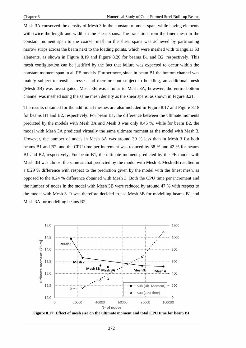
Chapter 8 Numerical Study of Cold-Formed Steel Built-up Beams
372
Mesh 3A conserved the density of Mesh 3 in the constant moment span, while having elements
with twice the length and width in the shear spans. The transition from the finer mesh in the
constant moment span to the coarser mesh in the shear spans was achieved by partitioning
narrow strips across the beam next to the loading points, which were meshed with triangular S3
elements, as shown in Figure 8.19 and Figure 8.20 for beams B1 and B2, respectively. This
mesh configuration can be justified by the fact that failure was expected to occur within the
constant moment span in all FE models. Furthermore, since in beam B1 the bottom channel was
mainly subject to tensile stresses and therefore not subject to buckling, an additional mesh
(Mesh 3B) was investigated. Mesh 3B was similar to Mesh 3A, however, the entire bottom
channel was meshed using the same mesh density as the shear spans, as shown in Figure 8.21.
The results obtained for the additional meshes are also included in Figure 8.17 and Figure 8.18
for beams B1 and B2, respectively. For beam B1, the difference between the ultimate moments
predicted by the models with Mesh 3A and Mesh 3 was only 0.45 %, while for beam B2, the
model with Mesh 3A predicted virtually the same ultimate moment as the model with Mesh 3.
However, the number of nodes in Mesh 3A was around 39 % less than in Mesh 3 for both
beams B1 and B2, and the CPU time per increment was reduced by 38 % and 42 % for beams
B1 and B2, respectively. For beam B1, the ultimate moment predicted by the FE model with
Mesh 3B was almost the same as that predicted by the model with Mesh 3. Mesh 3B resulted in
a 0.29 % difference with respect to the prediction given by the model with the finest mesh, as
opposed to the 0.24 % difference obtained with Mesh 3. Both the CPU time per increment and
the number of nodes in the model with Mesh 3B were reduced by around 47 % with respect to
the model with Mesh 3. It was therefore decided to use Mesh 3B for modelling beams B1 and
Mesh 3A for modelling beams B2.
Figure 8.17: Effect of mesh size on the ultimate moment and total CPU time for beam B1

Chapter 8 Numerical Study of Cold-Formed Steel Built-up Beams
373
Figure 8.18: Effect of mesh size on the ultimate moment and total CPU time for beam B2
Figure 8.19: Mesh 3A configuration in beam B1
Figure 8.20: Mesh 3A configuration in beam B2

Chapter 8 Numerical Study of Cold-Formed Steel Built-up Beams
374
Figure 8.21: Mesh 3B configuration in beam B1
8.3. Detailed FE model: verification
8.3.1 Ultimate moment capacity
The ultimate capacities obtained from the detailed FE models are compared against the
experimental results in Table 8.7 and Table 8.8 for the beams with geometry B1 and B2,
respectively. The tables also include the stabilization settings used to help Abaqus/Standard
achieve a converging solution. The tables show that the detailed FE models were able to provide
a reasonable prediction of the ultimate capacity of the built-up beams, with an average error of
3.98 % and 6.85 % for beams B1 and B2, respectively. It is worth pointing out that for beams
B2 the FE models predicted similar ultimate capacities in the beams with 2 and 3 intermediate
rows of connectors along the constant moment span (less than 2 % difference), as opposed to
the results obtained from the experiments, which showed an average increase of 11 % in the
ultimate capacity of beams B2-3 with respect to beams B2-2.
The moment vs. mid-span deflection curves obtained from the detailed FE models and from the
experiments are plotted in Figure 8.22 and Figure 8.23 for beams B1 and B2, respectively.
Table 8.7: Ultimate moment capacity obtained from tests and detailed FE models for beams B1
Specimen
Test ult.
moment
(kNm)
FEA ult.
moment
(kNm)
FEA/Test Contact
control
Automatic stabilization
DEF AT
B1-0b 11.837 11.701 0.988 2x10⁻⁴ - -
B1-2a 12.509 12.783 1.022 2x10⁻⁴ - -
B1-2b 11.830 13.102 1.108 2x10⁻⁴ - -
B1-3a 13.282 12.849 0.967 2x10⁻⁴ - -
B1-3b 13.007 12.675 0.974 2x10⁻⁴ - -
Avg. 1.012
St. dev. 0.057

Chapter 8 Numerical Study of Cold-Formed Steel Built-up Beams
375
Figure 8.22: Moment vs. mid-span deflection curve obtained from tests and detailed FE models for
beams B1
Table 8.8: Ultimate moment capacity obtained from tests and detailed FE models for beams B2
Specimen
Test ult.
moment
(kNm)
FEA ult.
moment
(kNm)
FEA/Test Contact
control
Automatic stabilization
DEF AT
B2-0a 9.077 9.526 1.049 2x10⁻⁴ - -
B2-0b 8.190 9.630 1.176 2x10⁻⁴ - -
B2-2a 10.413 11.366 1.092 2x10⁻⁴ - -
B2-2b 10.645 11.306 1.062 2x10⁻⁴ - -
B2-3a 11.658 11.510 0.987 2x10⁻⁴ - -
B2-3b 11.740 11.513 0.981 2x10⁻⁴ - -
Avg. 1.058
St. dev. 0.072
Figure 8.23: Moment vs. mid-span deflection curve obtained from tests and detailed FE models for
beams B2

Chapter 8 Numerical Study of Cold-Formed Steel Built-up Beams
376
8.3.2 Deformed shape
The FE models were able to accurately replicate the deformations, including the initial buckled
shape, and the failure mode of the tested beams. As examples, Figure 8.24, Figure 8.26 and
Figure 8.27 compare the deformed shapes obtained from the FE models with those observed
during the test (before and after the peak load) for beams B1-0b, B1-2b and B1-3b, respectively,
while Figure 8.28, Figure 8.29 and Figure 8.30 do the same for beams B2-0b, B2-2b and B2-3b,
respectively. In the figures, the deformed shapes obtained from the FE models before the peak
load was reached is amplified for clarity.
For beam B1-0b, although the experiment showed that the beam failed purely by local buckling,
the deformed shape obtained from the FE model after the peak load showed that the top channel
experienced some flexural-torsional buckling, as shown in Figure 8.24b. However, the moment
vs. deflection curves obtained from the FE model and the experimental test were almost
identical, as shown in Figure 8.22, with a difference in the ultimate moment capacity of only
1.16 %. Close examination of the failure mode of the FE model revealed that failure originated
in the top flanges of the web channels, as a result of local buckling (see Figure 8.25), and that
flexural-torsional buckling of the top channel only occurred after the beam reached its ultimate
moment capacity.
In general, a fairly good agreement was also achieved between the yield line mechanisms
predicted by the FE models and those observed in the tested beams. However, the plastic
mechanism predicted by the FE models often developed in a different location along the
constant moment span.
Figure 8.24: Deformed shape of B1-0b: a) before peak load (amplified); b) after peak load
(b)
(a)

Chapter 8 Numerical Study of Cold-Formed Steel Built-up Beams
377
Figure 8.25: Deformed shape of the web channels of B1-0b at the peak load
Figure 8.26: Deformed shape of B1-2b: a) before peak load (amplified); b) after peak load
Figure 8.27: Deformed shape of B1-0b: a) before peak load (amplified); b) after peak load
(a)
(b)
(a)
(b)

Chapter 8 Numerical Study of Cold-Formed Steel Built-up Beams
378
Figure 8.28: Deformed shape of B2-0b: a) before peak load (amplified); b) after peak load
Figure 8.29: Deformed shape of B2-2b: a) before peak load (amplified); b) after peak load
(a)
(b)
(a)
(b)

Chapter 8 Numerical Study of Cold-Formed Steel Built-up Beams
379
Figure 8.30: Deformed shape of B2-3b: a) before peak load (amplified); b) after peak load
8.3.3 Critical buckling stresses
The out-of-plane deformations of the channel components of beams B1 and B2 due to local
buckling were experimentally recorded with eight potentiometers mounted on two identical
yokes located within the constant moment span, as shown in Figures 8.24-8.30. These out-of-
plane deformations were also extracted from the FE models at the same locations. A comparison
between the out-of-plane deformations obtained experimentally and predicted by the FE models
is shown in Figure 8.31 and Figure 8.32 for two representative beams with geometry B1, and in
Figure 8.33 and Figure 8.34 for two representative beams with geometry B2. In all figures the
out-of-plane deformations are plotted against the total load applied to the beam. Curves
comparing the numerical and experimental out-of-plane deformations for each tested beam are
included in Appendix M.
The load vs. out-of-plane displacement curves were used to calculate the experimental and
numerical critical buckling stresses of the top channel of each tested beam, using the same
assumptions as previously described in Section 4.8.2 of Chapter 4. The critical buckling stresses
obtained from the tests and the respective FE models are reported in Table 8.9 and Table 8.10
for beams B1 and B2, respectively.
For beams B1, Table 8.9 shows that the critical buckling stresses obtained from the FE models
are consistently larger than the experimentally derived ones, with an average difference of
around 30 %. This difference is also evident in Figure 8.31 and Figure 8.32 for the two
(a)
(b)

Chapter 8 Numerical Study of Cold-Formed Steel Built-up Beams
380
representative beams. It is worth pointing out that despite the noticeable difference between the
numerical and experimental critical buckling stresses, the ultimate moment capacity obtained
from the FE models and the tests show a fairly good agreement for all beams with geometry B1.
Figure 8.31: Axial load vs lateral displacements curve of B1-0b obtained from the test and the
detailed FE model
Figure 8.32: Axial load vs lateral displacements curve of B1-2b obtained from the test and the
detailed FE model
Table 8.9: Buckling stresses of the top channel of beams B1 obtained from the tests and the detailed
FE models
Specimen Component
section
Buckling stress
from test
(MPa)
Buckling stress
from FEA
(MPa)
B1-0b T10412-3 170 203
B1-2a T10412-5 170 220
B1-2b T10412-7 154-166 211
B1-3a T10412-9 142 162
B1-3b T10412-11 126-134 201

Chapter 8 Numerical Study of Cold-Formed Steel Built-up Beams
381
For beams B2, the critical buckling stresses of the top channel obtained from the FE models
were slightly larger than those obtained from the tests. However, in this case the agreement was
considerably better than for beams B1, with an average difference between the numerical and
experimental buckling stresses of around 7 %. This good agreement is also revealed in Figure
8.33 and Figure 8.34, which show how the out-of-plane deformations of the top channel
obtained from the FE model follow the deformations recorded by the potentiometers almost
perfectly.
Figure 8.33: Axial load vs lateral displacements curve of B2-2b obtained from the test and the
detailed FE model
Figure 8.34: Axial load vs lateral displacements curve of B2-3b obtained from the test and the
detailed FE model

Chapter 8 Numerical Study of Cold-Formed Steel Built-up Beams
382
Table 8.10: Buckling stresses of the top channel of beams B2 obtained from the tests and the
detailed FE models
Specimen Component
section
Buckling stress
from test
(MPa)
Buckling stress
from FEA
(MPa)
B2-0a T10412-1 127 147
B2-0b T10412-2 120-142 138
B2-2a T10412-3 133-152 152
B2-2b T10412-4 121-136 140
B2-3a T10412-5 133 133
B2-3b T10412-6 128 139
8.4. Simplified FE model: verification
8.4.1 Ultimate moment capacity
The simplified FE models were able to accurately replicate the buckling behaviour of the tested
beams. Table 8.11 and Table 8.12 compare the ultimate moment capacities obtained from the
simplified models against the experimental results for the beams with geometry B1 and B2,
respectively. For beams B1, the average error in the ultimate moment predictions was 3.99 %,
which is virtually the same error as obtained with the detailed FE models, while for beams B2
this value was 7.67 %, which is slightly larger than the average error of 6.85 % obtained with
the detailed FE models. As with the detailed FE models, the simplified FE models predicted
very similar ultimate moment capacities in beams B2 with 2 and 3 intermediate rows of
connectors along the constant moment span, which differed from the experimental observations.
The moment vs. vertical deflection curves obtained from the simplified FE models, as well as
those measured in the experiment are plotted in Figure 8.35 and Figure 8.36 for beams B1 and
B2, respectively.
Table 8.11: Ultimate moment capacity obtained from tests and simplified FE models for beams B1
Specimen
Test ult.
moment
(kNm)
FEA ult.
moment
(kNm)
FEA/Test Contact
control
Automatic stabilization
DEF AT
B1-0b 11.837 11.996 1.013 2x10⁻⁴ - -
B1-2a 12.509 12.814 1.024 2x10⁻⁴ - -
B1-2b 11.830 12.916 1.092 2x10⁻⁴ - -
B1-3a 13.282 12.600 0.949 2x10⁻⁴ - -
B1-3b 13.007 12.731 0.979 2x10⁻⁴ - -
Avg. 1.011
St. dev. 0.054

Chapter 8 Numerical Study of Cold-Formed Steel Built-up Beams
383
Figure 8.35: Moment vs. mid-span deflection curve obtained from tests and simplified FE models
for beams B1
Table 8.12: Ultimate moment capacity obtained from tests and simplified FE models for beams B2
Specimen
Test ult.
moment
(kNm)
FEA ult.
moment
(kNm)
FEA/Test Contact
control
Automatic stabilization
DEF AT
B2-0a 9.077 9.705 1.069 2x10⁻⁴ - -
B2-0b 8.190 9.647 1.178 2x10⁻⁴ - -
B2-2a 10.413 11.545 1.109 2x10⁻⁴ - -
B2-2b 10.645 11.678 1.097 2x10⁻⁴ - -
B2-3a 11.658 11.660 1.000 2x10⁻⁴ - -
B2-3b 11.740 12.148 1.035 2x10⁻⁴ - -
Avg. 1.081
St. dev. 0.062
Figure 8.36: Moment vs. mid-span deflection curve obtained from tests and simplified FE models
for beams B2

Chapter 8 Numerical Study of Cold-Formed Steel Built-up Beams
384
8.4.2 Deformed shape and critical buckling stresses
The simplified FE models were able to predict deformed shapes and failure modes for beams B1
and B2 similar to those predicted by the detailed FE models. In addition, for beams B1 the out-
of-plane deformations in the simplified FE models were in better agreement with those recorded
in the tested beams than in the detailed FE models. Figure 8.41 and Figure 8.42 compare the
out-of-plane deformations obtained from the simplified FE models with those obtained
experimentally for the components of beams B1-0b and B1-2b, respectively. A comparison
involving the predictions obtained from the detailed FE models of the same beams was
previously presented in Figure 8.31 and Figure 8.32. For beams B2, the out-of-plane
deformations predicted by the simplified FE models were very similar to those predicted by the
detailed FE models. For example, Figure 8.39 and Figure 8.40 compare the experimental out-of-
plane deformations with those predicted by the simplified FE models for beams B2-2b and B2-
3b, respectively. The deformations of the same beams were previously compared to the
predictions of the detailed FE models in Figure 8.33 and Figure 8.34. Figures comparing the
experimental out-of-plane deformations with those predicted by the simplified FE models are
included in Appendix M for each tested beam.
The critical buckling stresses of the top channel of beams B1 and B2 derived from the
simplified FE models are listed in Table 8.13 and Table 8.14, respectively. For beams B1 the
agreement between the numerical and the experimental critical buckling stresses was better in
the simplified FE models than in the detailed FE models, with an average difference in the
former of 9 % (compared to around 30 % difference in the latter). For beams B2, the critical
buckling stresses derived from the simplified and detailed FE models were virtually the same,
with an average difference with respect to the experimentally derived ones of around 7 %.
Figure 8.37: Axial load vs lateral displacements of B1-0b obtained from the tests and the simplified
FE models

Chapter 8 Numerical Study of Cold-Formed Steel Built-up Beams
385
Figure 8.38: Axial load vs lateral displacements of B1-2b obtained from the tests and the simplified
FE models
Table 8.13: Buckling stresses of the top channel of beams B1 obtained from the tests and the
simplified FE models
Specimen Component
section
Buckling stress
from test
(MPa)
Buckling stress
from FEA
(MPa)
B1-0b T10412-3 170 161
B1-2a T10412-5 170 155-169
B1-2b T10412-7 154-166 156-189
B1-3a T10412-9 142 146
B1-3b T10412-11 126-134 160
Figure 8.39: Axial load vs lateral displacements of B2-2b obtained from the tests and the simplified
FE models

Chapter 8 Numerical Study of Cold-Formed Steel Built-up Beams
386
Figure 8.40: Axial load vs lateral displacements of B2-3b obtained from the tests and the simplified
FE models
Table 8.14: buckling stresses of the top channel of beams B2 obtained from the tests and the
simplified FE models
Specimen Component
section
Buckling stress
from test
(MPa)
Buckling stress
from FEA
(MPa)
B2-0a T10412-1 127 147
B2-0b T10412-2 120-142 138
B2-2a T10412-3 133-152 152
B2-2b T10412-4 121-136 140
B2-3a T10412-5 133 133
B2-3b T10412-6 128 139
8.5. Parametric study
8.5.1 Effect of fastener modelling
The simplified FE models were used to study the effect of the connector behaviour on the
buckling behaviour and ultimate capacity of CFS built-up beams. To this end additional FE
models were created in which the behaviour of the connectors was modelled using three
different approaches. The ultimate moment capacities obtained with each modelling approach
were then compared with the predictions given by the validated FE models.
The simplest approach to model the connectors consists of using BEAM multi-point constraints
(MPCs). This approach has the advantage of reducing the size of the model. However, since
BEAM MPCs eliminate the degrees of freedom of one of the fastening nodes at the connecting
points, they have the disadvantage that it is not possible to obtain output from the connectors

Chapter 8 Numerical Study of Cold-Formed Steel Built-up Beams
387
(for instance with respect to their internal forces). Moreover, they cannot be used to model more
complex connector behaviour such as slip or bearing deformations of the connecting plates.
The other two approaches which were considered consisted of using connector elements to
model the fasteners, namely HINGE and PLANAR connectors. In the FE model with HINGE
connector elements all CRMs (Components of Relative Motion) between the surfaces were
constrained, apart from the rotational component about the normal to the fastened surfaces,
while in the FE models with PLANAR connector elements all CRMs were constrained apart
from the rotation about the normal to the surfaces and the translational CRMs tangential to the
surfaces. This last modelling approach was similar to the approach used to model the fasteners
in the validated model. However, in this case neither elastic nor plastic behaviour was added to
the tangential CRMs, allowing the fastened surfaces to freely slide relative to each other.
Therefore, the ‘HINGE’ and ‘PLANAR’ models can be seen as idealized extreme opposites in
terms of the surface sliding behaviour.
The ultimate moment capacities obtained from the FE models incorporating HINGE, PLANAR
and MPC approaches, normalized against the predictions given by the validated FE models, are
shown in Figure 8.41 for beams B1 and B2 with 2 and 3 intermediate rows of connectors along
the constant moment span.
Figure 8.41: Ultimate moment comparison for different connector modelling approaches
Figure 8.41 shows that the HINGE and MPC models predict virtually identical ultimate moment
capacities for both built-up geometries and that these predictions are very similar to those given
by the validated FE models, with an average difference of 1 % for beams B1 and 2 % for beams
B2. This can be attributed to the fact that the connectors were not subject to large shear forces
because the simplified FE models were subject to a constant moment. Consequently, shear

Chapter 8 Numerical Study of Cold-Formed Steel Built-up Beams
388
forces in the connectors only originated as a result of local buckling of the components of the
built-up geometry. These shear forces were smaller than the slip force of around 3 kN obtained
from the single lap shear tests on the bolted connectors, as illustrated in Figure 8.42a and Figure
8.42b for representative beams with geometries B1 and B2. Therefore, the relative motion of the
surfaces at the connector points in the validated FE models was negligible.
Figure 8.42: Shear forces in the connectors: a) B1-2a; b) B2-2a
The ultimate moment capacities predicted by the PLANAR models, on the other hand, were
significantly lower than those predicted by the validated FE models, with average differences of
10 % and 11 % for the beams with geometries B1 and B2, respectively. This was due to the fact
that in the PLANAR models, slip between the components of the built-up geometry was
completely unrestrained, and therefore the top channel was not able to restrain the lateral
movement of the top flange of the web channels. As a result, the web channels failed
prematurely in a lateral-distortional buckling mode, as shown in Figure 8.43a and Figure 8.44a
for beams B1-2a and B2-2a, respectively. In the validated FE models, on the other hand, the
built-up beams failed due to local buckling of the components, with global instabilities of the
individual components being prevented by the bolts (see Figure 8.43b and Figure 8.44b for
beam B1-2a and B2-2a, respectively).

Chapter 8 Numerical Study of Cold-Formed Steel Built-up Beams
389
Figure 8.43: Failure mode of beam B1-2a:a) PLANAR model; b) Validated model
Figure 8.44: Failure mode of beam B2-2a:a) PLANAR model; b) Validated model
(a)
(b)
(a)
(b)
Validated FE model
Validated FE model
PLANAR FE model
PLANAR FE model

Chapter 8 Numerical Study of Cold-Formed Steel Built-up Beams
390
8.5.2 Connector spacing and contact interaction
The validated FE models were further used to study the way in which the ultimate capacity of
CFS built-up beams is affected by the connector spacing and by contact between the component
sections. For each built-up geometry, the number of equally spaced rows of intermediate
connectors along the beam (without counting the connectors at the end cross-sections) was
varied from zero to 31. This corresponded to a connector spacing which varied from 1500 mm
to around 50 mm. For each connector spacing, simulations were run with and without contact
interaction between the components of the built-up geometry. In addition, in order to establish
an upper-bound for the moment capacity, corresponding to the connector spacing being reduced
to zero, FE models were created (with and without contact between the components) in which
the connector points were replaced by smeared TIE constrains between the component surfaces
all along the beam length. All the FE models in this study included the initial geometric
imperfections of a representative beam, the material non-linearity obtained from tensile coupons
and the actual connector behaviour as determined from single lap shear tests.
The moment vs. mid-span deflection curves obtained from the FE models for a varying
connector spacing are illustrated in Figure 8.45 and Figure 8.46 for beams B1 and B2,
respectively. Figure 8.45a and Figure 8.46a show the results obtained when contact interaction
between the components of the built-up geometry was activated, while Figure 8.45b and Figure
8.46b show the results obtained when contact was not activated. The failure modes of beams B1
and B2, obtained with and without contact are listed in Table 8.15 for different connector
spacings.
Figure 8.45: Moment vs. mid-span deflection of B1: a) with contact; b) without contact
(b) (a)

Chapter 8 Numerical Study of Cold-Formed Steel Built-up Beams
391
Figure 8.46: Moment vs. mid-span deflection of B2: a) with contact; b) without contact
Table 8.15: Failure modes beams B1 and B2
Beam Failure mode at peak moment
With contact Without contact
Top channel Web channels Built-up Top channel Web channels Built-up
B1-0 L L+LTB - L+F L+LTB -
B1-1 L - - L L+LTB -
B1-3 L L - L L -
B1-7 L L - L L -
B1-15 L L - L L -
B1-31 L L - L L -
B1-Tie L L - L L -
B2-0 - L+LTB - L+F L+LTB -
B2-1 L L - L+F - -
B2-3 L L - L L -
B2-7 L L - L L -
B2-15 L L - L L -
B2-31 L L - L L -
B2-Tie L L - L L -
L = Local buckling; F = Flexural buckling; LTB = Lateral-torsional buckling
Table 8.15 shows that, in beams B1 and B2 without connectors along the constant moment
span, failure of the built-up specimen was triggered as a result of the web channels failing by
interaction of local and lateral-torsional buckling. By activating contact and adding one row of
connectors at mid-span the components were able to mutually prevent each other from
undergoing global instabilities between connector points. In beams B1 and B2 with three or
more rows of intermediate connectors, the connector spacing was small enough to prevent
global buckling of the components between connector points, irrespective of whether contact
was activated or not, and failure occurred as a result of local buckling of the component
sections.
The ultimate moment capacities predicted by the FE models including contact are plotted
against the connector spacing in Figure 8.47a for beams B1 and B2, while the ultimate moment
capacities obtained from the FE models in which contact interaction between the components
was not activated are plotted in Figure 8.47b. In these figures, the ultimate moments are
(a) (b)

Chapter 8 Numerical Study of Cold-Formed Steel Built-up Beams
392
normalized against the predictions given by the models in which the connectors were modelled
with smeared TIE constraints along the beam.
Figure 8.47a and Figure 8.47b show, as could be expected, that preventing global instabilities of
the component sections between connector points resulted in an increase in the ultimate moment
capacity of the built-up specimen. This increase was especially pronounced in the FE models in
which contact between components was not considered. This is due to the fact that the absence
of contact interaction allowed the component sections to buckle individually in a global mode
between connector points without any restraint. In the beams without intermediate connectors,
the web channels buckled in a lateral-torsional buckling mode irrespective of whether contact
was activated or not. However, when contact was not activated, the two web channels buckled
independently from each other, while they were forced to buckle together when contact was
activated, as shown in Figure 8.48 for beam B2.
Figure 8.47a also shows that once the global instabilities of the components between connector
points are completely restrained by a sufficiently small connector spacing, there is a range of
spacings in which the ultimate capacity of the beams does not vary significantly. For example,
reducing the connector spacing from 750 mm to around 94 mm resulted in an increase in the
ultimate capacity of only 10 % and 7 % for beams B1 and B2, respectively.
Figure 8.47: Ultimate load vs. connector spacing for FE models: a) with contact; b) without contact
(a) (b)

Chapter 8 Numerical Study of Cold-Formed Steel Built-up Beams
393
Figure 8.48: Deformed shape of beam B2-0: a) with contact; b) without contact
The initial buckled shape obtained for beams B1 and B2 is shown amplified in Figure 8.49 and
Figure 8.50, respectively, for different connector spacings. The local buckling pattern was most
noticeable in the top channel, while in the web channels it was only visible in the top flange of
the channels, as expected.
In the beams without intermediate connectors the top channel exhibited a regular buckling
pattern along the beam with a half-wave length very close to 110 mm, which is the natural local
buckling half-wave length of the channel. The presence of the web channels forced the top
channel to buckle upwards. This can be clearly appreciated in Figure 8.50 for beams B2. In the
beams with 1 and 3 intermediate rows of connectors, the connector spacing was large enough
for the top channel to buckle generating several half-waves between connector points. However,
the presence of the connectors forced the top channel to adjust its preferred buckle half-wave
length so that the cross-sections containing connectors fell inside a concave buckle. This
imposition obliged the top channel to generate an even number of half-waves between
connector points. Considering the beams with 3 intermediate rows of connectors, neither a half-
wave length of 188 mm, resulting from generating two half-waves between connectors, nor a
half-wave length of 94 mm, resulting from generating four half-waves between connectors, was
optimal for the top channel, which preferred to buckle with a half-wave length of 110 mm, as
shown in Figure 8.51a and Figure 8.51b for beams B1-3 and B2-3, respectively. As a result,
while the top channel buckled with four half-waves between connectors in one of the fields,
(a)
(b)

Chapter 8 Numerical Study of Cold-Formed Steel Built-up Beams
394
with a half-wave length slightly larger than 94 mm, in the adjacent fields the top channel
buckled with two half waves with a half-wave length slightly shorter than 188 mm. The cross-
section containing connectors consequently did no longer exactly coincide with the centre of a
concave buckle, but was slightly shifted towards one side. As Figure 8.51a and Figure 8.51b
show, this buckling pattern with two different half-wave lengths along the beam required a
lower stress than those where the top channel buckled while consistently generating either two
or four half-waves between connectors. A similar explanation applies to the beams with one row
of connectors in the moment span.
As the connector spacing was further reduced the buckles in the top channel became more
regular again. In the beams with 7 intermediate rows of connectors the buckle half-wave length
in the top channel approximately coincided with half the distance between connectors, while in
the beams with 15 intermediate rows of connectors the distance between connectors was almost
the same as the buckle half-wave length of the top channel and the gap between the top channel
and the web channels, which was present in the beams with larger connector spacings, became
almost undetectable. In the beams with 31 intermediate rows of connectors the connector
spacing was smaller than the buckle half-wave length of the top channel, and the connectors
forced the top and web channels to buckle in a synchronous manner. At these short connector
spacings the ultimate capacity of the built-up beams became more sensitive to the distance
between connectors compared to the cases where the connector spacing was larger than the
buckle half-wave length of the components. However, it should be noted that this range of
connector spacings is not practical in construction due to the large amount of labour involved in
assembling specimens with such a large number of connectors.

Chapter 8 Numerical Study of Cold-Formed Steel Built-up Beams
395
Figure 8.49: Amplified buckling deformed shape of beams B1
1 row of connectors
3 rows of connectors
7 rows of connectors
15 rows of connectors
31 rows of connectors
smeared tie constraints
0 rows of connectors
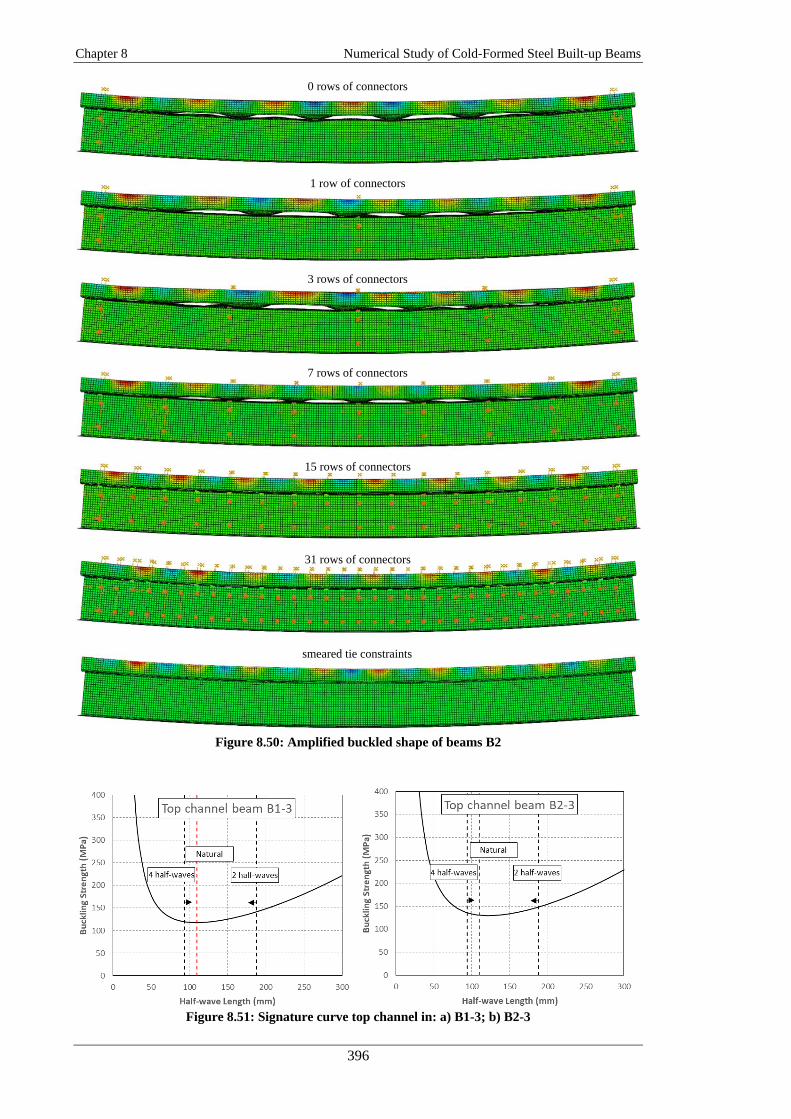
Chapter 8 Numerical Study of Cold-Formed Steel Built-up Beams
396
Figure 8.50: Amplified buckled shape of beams B2
Figure 8.51: Signature curve top channel in: a) B1-3; b) B2-3
1 row of connectors
3 rows of connectors
7 rows of connectors
15 rows of connectors
31 rows of connectors
smeared tie constraints
0 rows of connectors

Chapter 8 Numerical Study of Cold-Formed Steel Built-up Beams
397
The effect of contact between the components on the ultimate capacity of beams B1 and B2 is
illustrated in Figure 8.52, which shows the ratio between the ultimate moment capacities
obtained from the FE models with contact activated and deactivated as a function of the
connector spacing. The figure shows that for the geometries studied the effect of contact was
only important in those beams in which the connector spacing was large enough for the
components to undergo global instability between connector points when no contact was
considered (i.e. beams with zero or one row of connectors). In this case, the different
components in the built-up specimen restrained each other through contact, delaying or even
preventing global instabilities. An example is found in beam B1-1, where contact between the
web channels prevented them from buckling in a lateral-torsional mode. For shorter connector
spacings, on the other hand, the effect of contact became less significant, resulting, on average,
in an increase in the ultimate capacity of less than 5 % for beams B1 and less than 10 % for
beams B2.
Figure 8.52: Effect of contact interaction on the ultimate capacity
8.6. Summary and conclusions
Both detailed and simplified FE models were developed for the 11 built-up CFS beams with two
different cross-sectional geometries presented in Chapter 4, using the software package Abaqus
v.6.14. The beams were assembled with bolts which were modelled using mesh-independent
fasteners. The models included the initial geometric imperfections, as measured on the tested
beams, material non-linearity obtained from tensile coupons extracted from the flat portions and

Chapter 8 Numerical Study of Cold-Formed Steel Built-up Beams
398
the corner regions of the components of the tested beams, and the actual load-elongation
behaviour of the connectors, which was determined from single lap shear tests.
Both the detailed and simplified FE models were validated against the experimental data. The
validation included a comparison of the ultimate moment capacities, the initial buckled shapes
and the critical buckling stresses derived for the top channel of the built-up geometries. The
simplified model was further used in parametric studies to investigate the way in which the
connector modelling approach and connector spacing, as well as contact between components
affect the behaviour and capacity of the built-up beams.
The following conclusions could be drawn from the numerical investigation:
A material modelling study showed that either approximating the actual stress-strain
behaviour in the FE model by a simplified bilinear stress-strain curve or neglecting the
enhancement of the material properties in the corner regions only had a minor effect on
the predicted behaviour and ultimate capacity of the built-up geometries. While the
former simplification resulted in a stiffer post-buckling response and an overestimation
of the ultimate capacity by around 2 %, the latter only affected the ultimate capacity,
underestimating it by approximately the same amount.
Both the detailed and the simplified FE models were able to accurately predict the
initial stiffness of the beams and provided reasonable predictions of their ultimate
moment capacities. For beams B1 the average error in the ultimate moment predictions
given by the detailed and simplified models were virtually the same (around 4 %), while
for beams B2 the predictions given by the detailed model were slightly more accurate
than those given by the simplified one, with an average error of 6.85 % for the former
and 7.67 % for the latter. The detailed and simplified FE models were also able to
predict local buckling patterns similar to those observed in the tested beams. However,
while the critical buckling stresses in the top channel of beam B2 derived from the
detailed FE model were in good agreement with those determined from the tested
beams (with an average error of 7 %), for beams B1 the detailed model consistently
predicted larger critical buckling stresses, with an average error of around 30 %. On the
other hand, the critical buckling stresses derived from the simplified model were in
good agreement with those observed experimentally, with an average difference of 9 %
for beams B1 and 7 % for beams B2.
The ultimate capacities predicted by the validated FE models were in good agreement
with the predictions given by the HINGE and MPC models, in which bolt slip was
prevented. This was attributed to the fact that no shear forces were present in the beams
within the constant moment span. Therefore, shear forces in the connectors only
originated as a result of local buckling of the components and these forces were smaller

Chapter 8 Numerical Study of Cold-Formed Steel Built-up Beams
399
than the bolt slip load. The bolts in beams B1 and B2 were also instrumental in enabling
the top channel to completely restrain the web channels from buckling in a lateral-
torsional mode. This could be verified with the PLANAR model, in which slip without
any resistance was allowed at the connector points. This model predicted ultimate
capacities which were on average around 10 % lower than those predicted by the
validated FE model for beams B1 and B2 as a result of premature global buckling of the
web channels.
The effect of the connector spacing on the ultimate moment capacity of the beams was
found to be important only when the connectors were necessary to restrain global
instabilities of the individual components between connector points. Within the range of
connector spacings where the components buckled in a local mode, reducing the
connector spacing only resulted in a modest increase in the ultimate capacity. For
example, reducing the connector spacing from 750 mm to around 94 mm resulted in an
increase in the ultimate capacity of less than 10 % in both built-up geometries. For
connector spacings shorter than the local buckle half-wave length of the components the
ultimate capacity of the built-up beams became slightly more sensitive to the distance
between connectors. However, this range of connector spacings is impractical for
construction purposes due to the large amount of labour involved.
For the geometries studied contact between the components was seen to be important
mainly when it contributed to partially or completely restraining global instabilities of
the components of the built-up geometry between connector points. When the connector
spacing became small enough to prevent global instabilities of the individual
components the effect of contact became less significant, resulting, on average, in an
increase in the ultimate capacity of less than 5 % for beams B1 and less than 10 % for
beams B2. The effect of contact was also seen to be slightly more important for
connector spacings shorter than the local buckle half-wave length of the components.
However, its effect remained relatively modest.

Chapter 9 Numerical Study of Long Cold-Formed Steel Built-up Columns
400
Chapter 9
Numerical Study of Long Cold-Formed Steel
Built-up Columns
9.1. Introduction
This chapter is devoted to the development of detailed finite element (FE) models of the long
built-up columns presented in Chapter 5. Figure 9.1 illustrates the four different cross-sectional
geometries which were investigated. The columns with geometries 1 and 2 were assembled
using M6 bolts, while the columns with geometries 3 and 4 were assembled using M5.5 self-
drilling screws.
The FE models presented significant convergence issues, which often resulted in the analysis
being terminated before the peak load of the column was reached. These convergence issues
were overcome by adjusting some of the default solution control parameters Abaqus/Standard
uses to solve a non-linear analysis together with adding artificial damping to the model. The
amount of artificial damping introduced into the FE models was determined by carrying out a
stabilization analysis, which paid special attention to the way in which the ultimate capacity of
the columns was affected by the artificial damping forces.
The FE models were verified using the experimental data gathered from the long built-up
columns presented in Chapter 5, which included the ultimate capacity of the column, the
deformed shape after buckling and the critical buckling stresses obtained for some of the
component sections. The validated models were further used to carry out parametric studies
with the aim of investigating the way in which the connector modelling approach and connector
spacing, as well as contact between components affects the buckling response of built-up
columns subject to interaction between cross-sectional buckling of the components, global
instabilities of the components between connector points and global instabilities of the built-up
member as a whole.

Chapter 9 Numerical Study of Long Cold-Formed Steel Built-up Columns
401
Figure 9.1: Built-up cross-sections
9.2. Details of the FE models
The FE models were created using the software package Abaqus v.6.14 (Dassault Systemes,
2014). The columns were discretized using structural shell elements with the default five
integration points through the thickness and using Simpson’s rule. The models were constructed
based on the measured cross-sectional dimensions of the components. They incorporated the
initial geometric imperfections measured on the columns and material non-linearity obtained
from tensile coupons, while the connectors used to assemble the columns were modelled using
mesh-independent fasteners which accounted for their actual behaviour.
Similarly to the tested columns, the numerical models were labelled with the letters ‘LC’ to
indicate that the model corresponded to a long column, and the numbers 1 to 4 to indicate its
cross-sectional geometry (with reference to Figure 9.1). The number of intermediate rows of
connectors along the column was indicated after a hyphen at the end of the label. As an
example, the label ‘LC1-2’ refers to an FE model of a long column with cross-sectional
geometry 1 and two intermediate rows of connectors.
9.2.1 Boundary conditions
The pin-ended boundary conditions in the long columns were simulated by defining a reference
point at each end of the column, which coincided with the rotational axis of the end support.
This axis was located 73.5 mm away from the end cross-section of the column, as illustrated in
Figure 9.2b. Since in the experiments the columns were welded at each end to endplates, BEAM
MPC constraints were used to couple the rotational and translational degrees of freedom of the
nodes of the bottom and top end cross-sections of the column to the degrees of freedom of the
reference points. The boundary conditions were applied to the reference points by constraining

Chapter 9 Numerical Study of Long Cold-Formed Steel Built-up Columns
402
all of their rotational degrees of freedom, apart from the rotational degree of freedom about the
x-axis, as shown in Figure 9.2a. In addition, the bottom reference point also had all of its
translational degrees of freedom restrained, while the top reference point had all of its
translational degrees of freedom restrained apart from the vertical degree of freedom. The
compressive force was applied to the model by imposing a vertical displacement to the top
reference point, with the load eccentricity accounted for by adjusting the position of the
reference points in the y-direction respect to the centroid of the built-up cross-section (see
Figure 9.2 for the axis convention).
Figure 9.2: FE model boundary conditions
9.2.2 Geometric imperfections
All FE models included the initial geometric out-of-plane imperfections as measured on the
tested columns presented in Chapter 5 after the components were assembled into their final
configuration. The imperfections were incorporated into the FE models using a specially
developed Matlab code, which was used to modify the coordinates of the nodes in the input file
(*.inp) of a geometrically perfect FE model generated in Abaqus/Standard.
The imperfection data used in the FE models was recorded by moving a laser displacement
sensor along several lines on each face of each column, as indicated by the arrows in Figure 9.3.
A detailed description of the way in which the out-of-plane imperfections in the tested columns
were recorded is included in Section 5.6.2 of Chapter 5.
On each measured plate element of the built-up cross-sections (i.e. web and flanges of the
components) the imperfections were recorded along four lines. Third order polynomial
(a) (b)

Chapter 9 Numerical Study of Long Cold-Formed Steel Built-up Columns
403
interpolation was therefore carried out to obtain the imperfections at the nodes of the FE model,
as illustrated in Figure 9.4.
Figure 9.3: Location of measured imperfections in stub columns
Figure 9.4: Interpolated imperfection
9.2.3 Material properties
The material behaviour was modelled following the same approach described in Section 7.2.3 of
Chapter 7 using the data obtained from tensile coupons taken from the flat and corner regions of
the channels. This approach to represent the material properties in the FE models is further
referred to as the ‘actual material’ modelling approach. Details of the tensile coupon tests and
full results are provided in Section 5.3 of Chapter 5.
9.2.3.1 Simplified approaches to model material properties
In order to quantify the degree to which the ultimate capacity of the studied built-up geometries
is affected by simplifications in representing the material behaviour in the numerical models, a
series of non-linear analyses were carried out for a representative column belonging to each
built-up geometry using the two simplified material modelling approaches described in Section
7.2.3.1 of Chapter 7, and their ultimate capacities were compared to the predictions given by the
FE models including the actual material properties.

Chapter 9 Numerical Study of Long Cold-Formed Steel Built-up Columns
404
Figure 9.5 and Table 9.1 show that the FE models in which the material properties are
approximated by a bilinear stress-strain curve consistently predict higher ultimate capacities
than the FE models incorporating the actual material properties, with an average increase in the
ultimate load of 5.3 %, and a maximum increase of 8.8 % (for the column with geometry LC3).
On the other hand, the effect of ignoring the enhancement of the mechanical properties in the
corner regions of the FE models was less significant, resulting in an average reduction of the
predicted ultimate capacity of 1.5 %. It is worth pointing out, however, that in the columns
assembled with lipped channels (columns LC3 and LC4) the effect of ignoring the corner
enhancement was noticeably larger than in the other geometries, with a maximum reduction in
the ultimate capacity of 3 % in the columns with geometry LC4. This suggests that, as the
number of corners in a cross-section increases (as may be the case in optimized cross-sections
with edge and intermediate stiffeners), the error in the ultimate load prediction introduced in the
FE model by ignoring the enhancement of the mechanical properties in the corner regions may
not be negligible.
Figure 9.5: Effect of material properties modelling approaches on columns: a) LC1-8a; b) LC2-6a;
c) LC3-2a; d) LC4-3a
(a) (b)
(c) (d)

Chapter 9 Numerical Study of Long Cold-Formed Steel Built-up Columns
405
Table 9.1: Difference in ultimate load with respect to FE model with actual material properties
Column
Difference in ult. load with respect to
actual material properties (%)
Bilinear Without corners
LC1-8a 1.9 -0.7
LC2-6a 4.1 -0.6
LC3-2a 8.8 -1.5
LC4-3a 6.2 -3.0
9.2.4 Contact interaction
Contact between the components of the built-up columns was defined using the finite-sliding
surface-to-surface contact formulation available with the General Contact implementation in
Abaqus/Standard, which allows for arbitrarily large relative motion between the interacting
surfaces, as described in Section 7.2.4 of Chapter 7. Contact between the surfaces was defined
as ‘frictionless’ in the tangential direction, while a ‘hard’ pressure-overclosure behaviour was
approximated in the direction normal to the surfaces using the ‘Augmented Lagrange’ constraint
enforcement method.
In order to reduce the computational cost, contact was only defined between those surfaces of
the components which were likely to interact with each other during the analysis. Figure 9.6
shows the surfaces which were involved in the contact interactions, indicating whether the
surfaces were assigned the master or the slave role in the interaction.
The strain-free adjustment method was used to correct for any possible penetration of the slave
nodes into the master surfaces at the beginning of the analysis, which was likely to occur due to
the introduction of the measured geometric imperfections into the FE model. Since the default
strain-free adjustment available in Abaqus/Standard is designed to only remove small initial
overclosures measuring up to the average thickness of the connected surfaces, the default search
zone for the strain-free adjustment method was increased to 2 mm.
Figure 9.6: Master and slave role in contact interaction

Chapter 9 Numerical Study of Long Cold-Formed Steel Built-up Columns
406
It is worth noting that for built-up column 4 the edges of the plain channel flanges were allowed
to penetrate the flanges of the lipped channels since only the web of the lipped channels was
included in the contact interactions. This option was adopted to avoid edge-to-surface contact,
which was noted to result in significant convergence issues. On the other hand, penetration of
the edges of the plain channel flanges into the lipped channels flanges was noted to only occur
after the columns reached their peak load, and was not considered to affect their buckling
capacity or initial buckling behaviour.
9.2.5 Connector modelling
The bolts and screws used to assemble the components of the built-up columns, as well as the
spot welds which were added at the ends of the columns to ensure a uniform distribution of the
load to all the components, were modelled using mesh-independent fasteners, as described in
Section 7.2.5 of Chapter 7. The fastening points were connected to the neighbouring nodes on
the respective surfaces using the structural coupling method, which was implemented using the
uniform weighting scheme and defining a physical radius for the fastener of 5 mm.
All mesh-independent fasteners were modelled with discrete fasteners. PLANAR connector
elements were used to replicate the behaviour of the bolts and screws used to assemble the
columns, while BEAM connectors were used to simulate the spot welds which were used to
connect the components at each end of the column. The PLANAR connectors were orientated
so that their available rotational component of relative motion (CRM) was normal to the
surfaces in contact and the two available translational CRMs were tangential to the plane of
contact. Elastic and plastic properties, obtained from single lap shear tests, were assigned to the
two available translational CRMs of the PLANAR connectors in order to replicate the actual
behaviour of the screws and bolts.
9.2.6 Type of analysis
The non-linear buckling analysis of the built-up columns was carried out using the General
Static solver available in Abaqus/Standard, with the inclusion of artificial damping to stabilize
the solution. The analyses included geometric and material non-linearity. The time increments
in the analysis were automatically adjusted by Abaqus/Standard using the automatic
incrementation control algorithm.
9.2.7 Overcoming convergence issues in Abaqus/Standard
The unstable character of the non-linear problem, as well as the presence of contact between the
components of the built-up geometry resulted in significant convergence issues, which were

Chapter 9 Numerical Study of Long Cold-Formed Steel Built-up Columns
407
overcome by adjusting some of the solution control parameters, together with adding artificial
damping to the FE models, either through the automatic stabilization or the contact stabilization
schemes available in Abaqus/Standard.
The strategy followed to achieve a convergent solution in all models presented in this chapter
consisted of first running the model using the contact control mechanism together with the non-
default time incrementation control parameters described in Section 7.2.7 of Chapter 7. If the
simulation terminated before the peak load was reached, an additional step was added to the
simulation, in which the contact control mechanism was removed and replaced with the
adaptive automatic stabilization mechanism. Also, in this second step the maximum
displacement correction check was removed by setting Cαn to 1. A description of this solution
control parameter is given in Section 7.2.7 of Chapter 7 together with a discussion about its
effect on the convergent solution. A description of the contact control and adaptive automatic
stabilization mechanism is also given in Section 7.2.7.
The following section presents a stabilization study carried out to determine the appropriate
settings to be used with the contact control and the automatic stabilization schemes to ensure
that the amount of damping introduced into the models was sufficiently low not to significantly
alter the solution.
9.2.8 Stabilization study
9.2.8.1 Contact control
A stabilization study was carried out to ensure that the amount of artificial damping introduced
in the FE models through the contact control mechanism available in Abaqus/Standard was
sufficiently low to have a negligible effect on the final solution. The study was carried out for
one representative column of each built-up geometry. The constant factor Abaqus/Standard uses
to scale the magnitude of the viscous stresses normal to the surfaces in contact was increased
from zero to 8x10⁻⁴. In all models, the ‘tangent fraction’ parameter, which specifies the amount
of artificial damping applied to the relative motion of the surfaces in the tangential direction was
set to zero. This option was chosen because tangential viscous stresses would be likely to absorb
a significant amount of energy when the contact surfaces slip relative to each other.
Table 9.2 lists the ultimate loads obtained for each built-up geometry, as well as the
corresponding value given to the scale factor. Column LC1 was the only geometry where a
converging solution past the peak load could be achieved by only adjusting the solution control
parameters. For the other geometries, a post-peak solution was only possible after activating the
contact control scheme. Figure 9.7a, Figure 9.8a, Figure 9.9a and Figure 9.10a show the ratios
between the energy dissipated through artificial damping (ALLSD) and the total strain energy

Chapter 9 Numerical Study of Long Cold-Formed Steel Built-up Columns
408
(ALLIE) for different values of the constant scale factor, obtained for a representative column
with geometries LC1, LC2, LC3 and LC4, respectively. In the figures, a vertical dashed line
shows the approximate axial deformation at which the column reached its ultimate capacity. The
load-axial shortening curves obtained for different values of the scale factor are shown in Figure
9.7b, Figure 9.8b, Figure 9.9b and Figure 9.10b for a representative column with geometry LC1,
LC2, LC3 and LC4, respectively.
Table 9.2: Ultimate load comparison with contact control schemes
Specimen Stabilization
scheme
Contact
control
Ult. Load
(kN)
LC1-2a No stabilization - 74.95
cc 0.0002 2x10⁻⁴ 74.92
cc 0.0005 5x10⁻⁴ 74.96
cc 0.0008 8x10⁻⁴ 75.37
LC2-2a No stabilization - Divergence
cc 0.0002 2x10⁻⁴ 153.40
cc 0.0005 5x10⁻⁴ 154.07
cc 0.0008 8x10⁻⁴ 154.43
LC3-2a No stabilization - Divergence
cc 0.0002 2x10⁻⁴ 116.11
cc 0.0005 5x10⁻⁴ 116.25
cc 0.0008 8x10⁻⁴ 116.36
LC4-2a No stabilization - Divergence
cc 0.0002 2x10⁻⁴ 112.75
cc 0.0005 5x10⁻⁴ 112.70
cc 0.0008 8x10⁻⁴ 112.91
Table 9.2 shows that for the selected range of values of the scale factor, the ultimate load is not
significantly affected by the contact control mechanism for any of the studied geometries. For
column LC1, the difference in the ultimate load achieved with a scale factor equal to 2x10⁻⁴ was
only 0.04 % relative to the model in which no stabilization was used, while for columns LC2,
LC3 and LC4 the maximum variations in the ultimate load when varying the scale factor from
2x10⁻⁴ to 8x10⁻⁴ were 0.67 %, 0.22 % and 0.19 %, respectively.
As Figures 9.7-9.10 show, the largest amount of artificial damping was introduced in the
column with geometry LC1 at the moment when the plate sections started buckling in a global-
type flexural mode between connectors. It is worth pointing out that this column had only two
intermediate sets of connectors along the column (at a distance of 960 mm), which caused the
plate sections to buckle almost from the onset of loading in the model without stabilization. The
large connector spacings also implied that the forces required to prevent the plate sections from
buckling were relatively small, and therefore in all the FE models in which the contact control
mechanism was activated the viscous forces delayed the onset of global buckling of the plates
between connector points. This is evidenced by the distortion of the load-axial deformation
curve of column LC1 shown in Figure 9.7b. In addition, Figure 9.11 shows the load-lateral
deformation curve of the plate sections at mid-distance between connectors for the different

Chapter 9 Numerical Study of Long Cold-Formed Steel Built-up Columns
409
values of the scale factor. Despite artificial damping delaying the onset of global buckling of the
plate sections between connector points, after the plate buckled the load-lateral deformation
curves obtained for different values of the scale factor converged to the curve obtained from the
FE model in which no artificial damping was added. This explains why, despite the clear
influence of the artificial damping forces on the initial buckling load, the ultimate capacity of
the columns remained almost unaltered.
Based on the results obtained from this stabilization study, it was decided not to use the contact
control mechanism in the LC1 columns with two and three intermediate set of connectors in
order to avoid altering the critical buckling stresses of the plate sections. For the remaining
columns the models were run with the contact control mechanism activated, using a scale factor
equal to 2x10⁻⁴, since this resulted in a negligible change in the ultimate capacity of the studied
geometries.
Figure 9.7: Contact stabilization in columns LC1: a) Dissipated energy over total strain energy; b)
Load-axial shortening curve
Figure 9.8: Contact stabilization in columns LC2: a) Dissipated energy over total strain energy; b)
Load-axial shortening curve

Chapter 9 Numerical Study of Long Cold-Formed Steel Built-up Columns
410
Figure 9.9: Contact stabilization in columns LC3: a) Dissipated energy over total strain energy; b)
Load-axial shortening curve
Figure 9.10: Contact stabilization in columns LC4: a) Dissipated energy over total strain energy; b)
Load-axial shortening curve
Figure 9.11: Load-lateral displacement curves of plate sections in column LC1-2a for different scale
factors

Chapter 9 Numerical Study of Long Cold-Formed Steel Built-up Columns
411
9.2.8.2 Automatic stabilization
In the adaptive automatic stabilization scheme available in Abaqus/Standard the amount of
damping introduced into the model varies for each node of the model and depends on the
‘dissipated energy fraction’ (DEF), the convergence history and the accuracy tolerance (AT).
The DEF is the ratio between the energy dissipated through artificial damping and the total
strain energy in the first increment of the step. It is used by Abaqus/Standard to calculate the
initial static stabilization damping factor. The DEF was set to 2x10⁻⁵ for all the models in which
automatic stabilization was activated. The initial stabilization factor is automatically adjusted
throughout the step based on the convergence history and the accuracy tolerance (AT). To
ensure that the solution predicted by the model was not significantly altered by the artificial
damping introduced through the automatic stabilization scheme, a suitable value of the AT was
determined by carrying out a stabilization study, which included one representative column of
each built-up geometry. In this study the AT was varied from zero (no artificial damping added
to the model) to 8x10⁻³.
The ultimate loads obtained for each built-up geometry, as well as the values given to the DEF
and the AT are reported in Table 9.3, while Figure 9.12a, Figure 9.13a, Figure 9.14a and Figure
9.15a plot the ratio between the energy dissipated through artificial damping (ALLSD) and the
total strain energy (ALLIE) for columns LC1, LC2, LC3 and LC4, respectively. The vertical
dashed line shows the approximate axial deformation at which the column reached its ultimate
capacity. The load-axial shortening curve obtained for the different values of the AT are shown
in Figure 9.12b, Figure 9.13b, Figure 9.14b and Figure 9.15b for columns LC1, LC2, LC3 and
LC4, respectively.
As previously mentioned, only the FE model of the column with geometry LC1 was able to
converge without having to add artificial damping. For this geometry, the addition of artificial
damping forces through the automatic stabilization scheme had a minimal effect on the ultimate
capacity for the chosen range of AT values. For example, setting the AT equal to 2x10⁻³ resulted
in an increase in the ultimate capacity of only 0.04 %, while the increase in the ultimate capacity
as a result of setting the AT equal to 8x10⁻³ was only 0.33 %. Figure 9.12 shows that, for this
geometry, artificial damping is introduced only at the beginning of the loading process, when
the plate sections start buckling, and immediately after the peak load is reached. The ultimate
capacity of the column with geometry LC4 also showed little sensitivity to the addition of
artificial damping forces through the automatic stabilization scheme, with a maximum variation
of 0.56 % over the chosen range of AT values. On the other hand, the ultimate capacity of the
columns with geometries LC2 and LC3 showed a more noticeable sensitivity. For example,
increasing the AT from 2x10⁻³ to 8x10⁻³ in the columns with geometries LC2 and LC3 resulted
in an increase in the ultimate capacities of 7.67 % and 5.71 %, respectively. In these columns

Chapter 9 Numerical Study of Long Cold-Formed Steel Built-up Columns
412
artificial damping was introduced into the model shortly before the ultimate capacity was
reached.
In section 9.2.8.1 it was shown that the ultimate capacities obtained from the FE models when
the contact control mechanism was activated with a scale factor equal to 2x10⁻⁴ were almost
identical to those obtained without adding artificial damping. Since for the columns with
geometries LC2, LC3 and LC4 a converging solution could not be obtained without adding
artificial damping to the FE model, for these columns the ultimate capacity obtained with a
small scale factor of 2x10⁻⁴ was used as a reference to assess the effect of the automatic
stabilization mechanism on the ultimate capacity of the column. This comparison showed that
the increases in the ultimate capacities of the columns with geometries LC2, LC3 and LC4
obtained with the FE models in which the AT was set to 2x10⁻³ were 0.61 %, 1.83 % and 0.33
%, respectively. These errors were considered acceptable, given the great complexity of the
models. Therefore, for all the built-up geometries presented in this chapter, those models
requiring a second step with the automatic stabilization scheme activated in order to achieve a
converging solution past the peak load were defined with an AT equal to 2x10⁻³.
Table 9.3: Ultimate load comparison with automatic stabilization schemes
Specimen Stabilization
scheme DEF AT
Ult. Load
(kN)
LC1-2a
No stabilization - - 74.95
sc 0.002 2x10⁻⁵ 2x10⁻³ 74.98
sc 0.005 2x10⁻⁵ 5x10⁻³ 75.02
sc 0.008 2x10⁻⁵ 8x10⁻³ 75.20
LC2-2a
No stabilization - - Divergence
sc 0.002 2x10⁻⁵ 2x10⁻³ 154.33
sc 0.005 2x10⁻⁵ 5x10⁻³ 160.39
sc 0.008 2x10⁻⁵ 8x10⁻³ 166.17
LC3-2a
No stabilization - - Divergence
sc 0.002 2x10⁻⁵ 2x10⁻³ 118.23
sc 0.005 2x10⁻⁵ 5x10⁻³ 120.47
sc 0.008 2x10⁻⁵ 8x10⁻³ 124.98
LC4-2a
No stabilization - - Divergence
sc 0.002 2x10⁻⁵ 2x10⁻³ 113.12
sc 0.005 2x10⁻⁵ 5x10⁻³ 113..37
sc 0.008 2x10⁻⁵ 8x10⁻³ 113.76

Chapter 9 Numerical Study of Long Cold-Formed Steel Built-up Columns
413
Figure 9.12: Automatic stabilization in columns LC1: a) Dissipated energy over total strain energy;
b) Load-axial shortening curve
Figure 9.13: Automatic stabilization in columns LC2: a) Dissipated energy over total strain energy;
b) Load-axial shortening curve
Figure 9.14: Automatic stabilization in columns LC3: a) Dissipated energy over total strain energy;
b) Load-axial shortening curve

Chapter 9 Numerical Study of Long Cold-Formed Steel Built-up Columns
414
Figure 9.15: Automatic stabilization in columns LC4: a) Dissipated energy over total strain energy;
b) Load-axial shortening curve
9.2.9 Mesh analysis
The long column models were developed using S4R elements with five integration points
through the shell thickness. A mesh analysis was performed to determine a suitable mesh
density, which does not require excessive computational time and does not compromise the
accuracy of the solution. The study was carried out using one representative column of each of
the geometries LC1, LC2 and LC3. Since geometries LC3 and LC4 were assembled using
component sections with the same nominal dimensions, but arranged in a different
configuration, the mesh density obtained for column LC3 was considered to also be applicable
to columns LC4. The columns were modelled using the nominal cross-sectional dimensions of
the components, representative initial geometric imperfections as measured on one of the tested
columns, the non-linear material properties obtained from the tensile coupons, and while
modelling the connectors using HINGE connector elements. For geometries LC1 and LC3, the
columns chosen for the mesh study had a 3 m length and eight intermediate sets of connectors,
while for geometry LC2 the chosen column had a length of 2.5 m and six intermediate sets of
connectors. Both the total CPU time required to run the analysis and the peak load were
considered as criteria in the study.
Four different mesh densities were included for each built-up geometry. The size of the
elements in the flanges and the web of the channels, as well as in the plate section of LC1 was
chosen to be as uniform as possible. The aspect ratio of these elements was kept below 2,
following the recommendations given by Schafer (1997). The number of elements across the
corner region of the channels was varied from two to four. The aspect ratio of the elements
located in these regions was limited to less than 4 (rather than 2) in order to avoid an overly
dense mesh. In the lipped channels, two elements were used across the lips in all the studied
meshes.

Chapter 9 Numerical Study of Long Cold-Formed Steel Built-up Columns
415
Table 9.4, Table 9.6 and Table 9.8 show the number of elements and nodes used in the different
mesh configurations for columns LC1, LC2 and LC3, respectively, while Table 9.5, Table 9.7
and Table 9.9 show the aspect ratios of the meshes studied.
Table 9.4: Mesh configuration for column LC1
Mesh
N of elements N of
nodes Channel Plate column Total
Flange Web Corner Width Length
Mesh 1 2 7 2 9 214 10272 11180
Mesh 2 4 14 2 18 214 18832 19780
Mesh 3 6 21 4 27 429 58344 60200
Mesh 4 7 28 4 36 429 73788 75680
Table 9.5: Mesh aspect ratio in column LC1
Mesh
Aspect ratio
Channels Plates
Flange Web Corner Width
Mesh 1 0.903 0.817 4.000 0.841
Mesh 2 1.805 1.634 4.000 1.682
Mesh 3 1.351 1.223 4.000 1.259
Mesh 4 1.576 1.630 4.000 1.678
Table 9.6: Mesh configuration for columns LC2
Mesh
N of elements N of
nodes Inner Channel Outer Channel column Total
Flange Web Corner Flange Web Corner Length
Mesh 1 1 3 2 2 6 2 179 8234 9000
Mesh 2 3 6 2 4 12 2 179 14320 15120
Mesh 3 5 10 4 7 22 4 358 51552 53132
Mesh 4 7 15 4 10 30 4 358 68020 69646
Table 9.7: : Mesh aspect ratio in columns LC2
Mesh
Aspect ratio
Inner Channels Outer Channels
Flange Web Corner Flange Web Corner
Mesh 1 0.436 0.606 4.000 0.569 0.581 0.436
Mesh 2 1.307 1.213 4.000 1.139 1.163 1.307
Mesh 3 1.089 1.010 4.000 0.996 1.066 1.089
Mesh 4 1.525 1.516 4.000 1.423 1.454 1.525
Table 9.8: Mesh configuration for column LC3
Mesh
N of elements N of
nodes Plain Channel Lipped Channel column Total
Flange Web Corner Flange Web Lip Corner Length
Mesh 1 2 4 2 2 4 2 2 205 13120 14008
Mesh 2 3 9 2 3 8 2 2 205 18450 19364
Mesh 3 4 13 4 5 12 2 4 416 59072 60882
Mesh 4 6 19 4 7 17 2 4 416 74880 76728

Chapter 9 Numerical Study of Long Cold-Formed Steel Built-up Columns
416
Table 9.9: Mesh aspect ratio in columns LC3
Mesh
Aspect ratio
Plain Channels Lipped Channels
Flange Web Corner Flange Web Lip Corner
Mesh 1 0.831 0.530 4.000 0.726 0.583 5.672 4.000
Mesh 2 1.247 1.193 4.000 1.089 1.167 5.672 4.000
Mesh 3 0.819 0.849 4.000 0.895 0.863 2.795 4.000
Mesh 4 1.229 1.241 4.000 1.252 1.222 2.795 4.000
9.2.9.1 Mesh analysis results
The ultimate load and the CPU time required to complete the simulation for the different mesh
configurations considered in the mesh study are listed in Table 9.10, Table 9.11 and Table 9.12
for columns LC1, LC2 and LC3, respectively. The tables also show the total number of
increments Abaqus/Standard needed to complete the simulation and the average CPU time
required for each increment. The CPU times listed in brackets correspond to simulations in
which, although the peak load was reached, the analyses were not completed.
Table 9.10: Effect of the mesh size on the ultimate load and total CPU time for columns LC1
Element
type Mesh
Ultimate
Load (kN)
Total CPU
time (s)
N of
increments
CPU time per
increment (s)
S4R
Mesh 1 88.88 7957 148 54
Mesh 2 89.86 14208 151 94
Mesh 3 87.34 45171 133 340
Mesh 4 87.31 115862 133 871
Table 9.11: Effect of the mesh size on the ultimate load and total CPU time for columns LC2
Element
type Mesh
Ultimate
Load (kN)
Total CPU
time (s)
N of
increments
CPU time per
increment (s)
S4R
Mesh 1 144.63 3045 42 72
Mesh 2 146.81 6437 64 101
Mesh 3 146.10 19655 86 229
Mesh 4 146.08 62718 95 660
Table 9.12: Effect of the mesh size on the ultimate load and total CPU time for columns LC3
Element
type Mesh
Ultimate
Load (kN)
Total CPU
time (s)
N of
increments
CPU time per
increment (s)
S4R
Mesh 1 142.86 31069 514 60
Mesh 2 135.60 39300 443 89
Mesh 3 136.59 163200 446 366
Mesh 4 135.69 (242942) 433 561
The ultimate load and the CPU time per increment are plotted, for each mesh configuration,
against the number of nodes in Figure 9.16, Figure 9.17 and Figure 9.18 for columns LC1, LC2
and LC3, respectively. The figures show that, for all geometries considered, the ultimate load
predictions obtained with Mesh 3 are relatively close to the predictions obtained with the finest

Chapter 9 Numerical Study of Long Cold-Formed Steel Built-up Columns
417
mesh (Mesh 4). For column LC1, the difference between the ultimate load predicted with these
mesh configurations was 0.04 %, while for columns LC2 and LC3 the differences were 0.02 %
and 0.66 %, respectively. This range of accuracy was considered satisfactory given the
complexity of the models and all the models were meshed using a Mesh 3 configuration.
Figure 9.16: Effect of mesh size on the ultimate load and total CPU time for columns LC1
Figure 9.17 Effect of mesh size on the ultimate load and total CPU time for columns LC2

Chapter 9 Numerical Study of Long Cold-Formed Steel Built-up Columns
418
Figure 9.18: Effect of mesh size on the ultimate load and total CPU time for columns LC3
9.3. FE model verification
9.3.1 Ultimate load
Table 9.13, Table 9.14, Table 9.15 and Table 9.16 compare the ultimate loads predicted by the
FE models with those obtained from the tests for columns LC1, LC2, LC3 and LC4,
respectively. The tables also show the stabilization scheme which was used to achieve the
numerical solution.
For columns LC1 and LC2, Table 9.13 and Table 9.14 show that the ultimate loads predicted by
the FE models were consistently lower than those obtained from the tests. For columns LC1 the
numerical ultimate loads were, on average, 3.4 % lower than the experimental ones, while for
columns LC2 the numerical predictions were, on average, 5.5 % lower. A better agreement was
achieved between the numerical and experimental ultimate loads of columns LC3 and LC4, as
shown in Table 9.15 and Table 9.16. For columns LC3, the average difference between the
numerical and experimental ultimate loads was 1.3 %, while for columns LC4 the average
difference was 2.6 %. Excluding columns LC1-2, the numerical models agreed with the test
results in predicting larger ultimate capacities for the columns tested with a load eccentricity of
L/1500 compared to those tested with a load eccentricity of L/1000.
The load vs. axial shortening curves predicted by the FE models and those obtained from the
experiments are shown in Figure 9.19, Figure 9.20, Figure 9.21 and Figure 9.22 for columns
LC1, LC2, LC3, and LC4, respectively. The figures show that the FE models were able to
accurately replicate the initial stiffness as well as the post-buckling stiffness of the column for
all the geometries studied.

Chapter 9 Numerical Study of Long Cold-Formed Steel Built-up Columns
419
Table 9.13: Numerical and experimental ultimate loads of columns LC1
Specimen Test ult.
load (kN)
FEA ult.
load (kN) FEA/Test
Stabilization scheme
Step 1 Step 2
LC1-2a 77.94 75.98 0.975 None sc 0.002
LC1-2b 79.18 75.57 0.954 sc 0.002 -
LC1-3a 79.73 77.85 0.976 None sc 0.002
LC1-3b 81.57 78.32 0.960 None sc 0.002
LC1-8a 89.66 87.28 0.973 cc 0.0001 -
LC1-8b 91.17 87.34 0.958 cc 0.0001 -
Avg. 0.966
St. dev. 0.010
Figure 9.19: Numerical and experimental load vs. axial shortening curves of columns LC1
Table 9.14: Numerical and experimental ultimate loads of columns LC2
Specimen Test ult.
load (kN)
FEA ult.
load (kN) FEA/Test
Stabilization scheme
Step 1 Step 2
LC2-2a 160.90 153.27 0.953 cc 0.0002 -
LC2-2b 171.82 157.47 0.916 cc 0.0002 -
LC2-6a 165.15 157.39 0.953 cc 0.0002 -
LC2-6b 166.88 159.93 0.958 cc 0.0002 -
LC2-4a - 161.35 - cc 0.0002 -
LC2-4b - 164.83 - cc 0.0002 -
Avg. 0.945
St. dev. 0.019

Chapter 9 Numerical Study of Long Cold-Formed Steel Built-up Columns
420
Figure 9.20: Numerical and experimental load vs. axial shortening curves of columns LC2
Table 9.15: Numerical and experimental ultimate loads of columns LC3
Specimen Test ult.
load (kN)
FEA ult.
load (kN) FEA/Test
Stabilization scheme
Step 1 Step 2
LC3-2a 119.04 116.15 0.976 cc 0.0002 -
LC3-2b 123.48 123.40 0.999 cc 0.0002 sc 0.002
LC3-3a 118.88 118.48 0.997 cc 0.0002 -
LC3-3b 122.94 121.26 0.986 cc 0.0002 -
LC3-8a 120.22 122.52 1.019 cc 0.0002 sc 0.002
LC3-8b - 123.99 - cc 0.0002 -
Avg. 0.995
St. dev. 0.016
Figure 9.21: Numerical and experimental load vs. axial shortening curves of columns LC3

Chapter 9 Numerical Study of Long Cold-Formed Steel Built-up Columns
421
Table 9.16: Numerical and experimental ultimate loads of columns LC4
Test ult.
load (kN)
FEA ult.
load (kN) FEA/Test
Stabilization scheme
Step 1 Step 2
LC4-2a 116.53 112.76 0.968 cc 0.0002 -
LC4-2b 117.90 115.04 0.976 cc 0.0002 -
LC4-3a 116.19 113.70 0.979 cc 0.0002 -
LC4-3b 118.57 115.97 0.978 cc 0.0002 sc 0.002
LC4-8a 109.06 117.34 1.076 cc 0.0002 sc 0.002
LC4-8b 119.65 120.13 1.004 cc 0.0002 sc 0.002
Avg. 0.997
St. dev. 0.041
Figure 9.22: Numerical and experimental load vs. axial shortening curves of columns LC4
9.3.2 Deformed shape
In general, the FE models were able to accurately replicate the initial buckled shape of the tested
columns, while for most columns the failure mode and yield line mechanism observed in the
experiments also agreed well with those predicted by the FE models. However, the plastic
deformations predicted by the FE models often concentrated in a location different from the one
observed in the tested columns.
For columns LC1, the experiments showed that the channels buckled in a local mode with 22
half-waves, irrespective of the number of connectors along the column, while the plate sections
buckled outward in each field in columns LC1-2 and LC1-3. This was accurately replicated by
the FE models, as shown in Figure 9.23a and Figure 9.23b for columns LC1-2a and LC1-3a,
respectively. For columns LC1-8 (the columns with eight intermediate sets of connectors) the
experiments showed that the plate sections initially buckled in every other field, while
remaining straight in the adjacent fields. In the corresponding FE model, however, the plate
sections only remained unbuckled in two fields along the column, as shown in Figure 9.23c.

Chapter 9 Numerical Study of Long Cold-Formed Steel Built-up Columns
422
The experiments also showed that in columns LC1-2 failure was triggered by flexural-torsional
buckling of the channels between connectors, which interacted with local buckling of the
channels, global-type flexural buckling of the plates between connectors and flexural buckling
of the whole built-up geometry. This type of failure could only be accurately replicated by the
FE models in column LC1-2b, which was tested with a load eccentricity of L/1500 (Figure
9.24b). For column LC1-2a, which was tested with a load eccentricity of L/1000, the FE models
only predicted a minor participation of flexural-torsional buckling of the channels between
connectors, as shown in Figure 9.24a. In column LC1-3b the channels were also seen
experimentally to fail due to buckling interaction involving flexural-torsional buckling between
connectors, with both channels deforming in a point-symmetric pattern relative to each other.
However, the corresponding FE model predicted the channels to fail predominantly due to
interaction between local buckling and global flexural buckling of the built-up column, as
shown in Figure 9.25a. Columns LC1-3a and LC1-8 failed experimentally due to interaction
between local buckling of the channels, global-type flexural buckling of the plates between
connectors and global flexural buckling of the built-up specimen. The failure mode of these
columns was accurately replicated by the FE models, as shown in Figure 9.25b for column LC1-
8b.
Figure 9.23: Comparison of the buckled shape: a) LC1-2a; b) LC1-3a; c) LC1-8a
(a) (b) (c)

Chapter 9 Numerical Study of Long Cold-Formed Steel Built-up Columns
423
Figure 9.24: Comparison of localized plastic deformations: a) LC1-2a; b) LC1-2b
Figure 9.25: Comparison of localized plastic deformations: a) LC1-3b; b) LC1-8b
(a) (b)
(a) (b)

Chapter 9 Numerical Study of Long Cold-Formed Steel Built-up Columns
424
With respect to columns LC2, the FE models predicted less buckles in the outer channels of
column LC2-2 than the number observed in the tested columns, as shown in Figure 9.26a for
column LC2-2b. This was due to the fact that in the tested columns with geometry LC2 the
flanges of the outer channels were significantly distorted at each end of the column due to the
welding of the endplates, as described in Section 5.5 of Chapter 5. These distortions, which
were not included in the FE models, resulted in buckles with a smaller half-wave length at each
end of the column and therefore the outer channels in the tested columns were able to
accommodate one or two additional buckles. In columns LC2-6 and LC2-4, the outer channels
buckled with two half-waves between connectors in both the FE model and the tested column,
as shown in Figure 9.26b and Figure 9.26c for columns LC2-6a and LC2-4a, respectively. The
FE models only predicted some minor local buckling in the inner channels of columns LC2-6
and LC2-4 shortly before the ultimate load was reached, consistent with the experiments.
Figure 9.27 compares the yield line mechanisms which were observed during the experiments in
columns LC2-2b and LC2-6b with those predicted by the FE models.
Figure 9.26: Comparison of the buckled shape: a) LC2-2b; b) LC2-6a; c) LC2-4a
(b)
(c)
(a)

Chapter 9 Numerical Study of Long Cold-Formed Steel Built-up Columns
425
Figure 9.27: Comparison of localized plastic deformations: a) LC2-2b; b) LC2-6b
In the columns with geometry LC3 the plain channels were experimentally observed to buckle
with eight half-waves between connector points in columns LC3-2, six in columns LC3-3 and
between two and four in columns LC3-8, while the cross-sections containing connectors were
always seen to fall within a concave buckle. The lipped channels, on the other hand, were seen
to buckle in a local mode with between 10 and 12 half-waves between connectors in columns
LC3-2, eight half-waves between connectors in columns LC3-3 and between two and four half-
waves between connectors in columns LC3-8. These buckling patterns were accurately
replicated by the FE models, as shown in Figure 9.28.
Figure 9.29 compares the yield line mechanisms observed during the experiments in columns
LC3-2a and LC3-8a with those predicted by the FE models.
(a) (b)

Chapter 9 Numerical Study of Long Cold-Formed Steel Built-up Columns
426
Figure 9.28: Comparison of the buckled shape: a) LC3-2a; b) LC3-3b; c) LC3-8b
Figure 9.29: Comparison of localized plastic deformations: a) LC3-2a; b) LC3-8a
(a) (b) (c)
(a) (b)

Chapter 9 Numerical Study of Long Cold-Formed Steel Built-up Columns
427
The FE models were also able to accurately replicate the buckled shape of the lipped channels in
columns LC4. The buckled shape of the plain channels of columns LC4 could not be observed
in the experiments and was therefore not compared. Consistent with the experiments, the lipped
channels in the FE models buckled with a half-wave length which ranged from 80 to 90 mm and
the cross-sections containing connectors fell inside a concave buckle. The lipped channels
buckled with between 10 and 12 half-waves between connectors in columns LC4-2, between
eight and ten half-waves between connectors in columns LC4-3 and four half-waves between
connectors in columns LC4-8, as shown in Figure 9.30.
Figure 9.30: Comparison of the buckled shape: a) LC4-2a; b) LC4-3b; c) LC4-8b
Similarly to what was observed in the experiments, the FE models revealed that distortional
buckling of the lipped channels only had a minor participation before the ultimate capacity of
the column was reached. However, the participation predicted by the FE models was even less
significant. Figure 9.31 shows the deformed shape of the lipped channel located on the
compression side of the built-up geometry when the load in the column was around 90 % of the
ultimate capacity for all the columns with geometry LC4.

Chapter 9 Numerical Study of Long Cold-Formed Steel Built-up Columns
428
Figure 9.31: Deformed shape of lipped channel on compression side
A comparison between the yield line mechanisms observed during the experiments and those
predicted by the FE models is shown in Figure 9.32 for columns LC4-2b, LC4-3b and LC4-8b.
Figure 9.32: Comparison of localized plastic deformations: a) LC4-2b; b) LC4-3b; c) LC4-8b
LC4-2a LC4-2b LC4-3a LC4-3b LC4-8a LC4-8b

Chapter 9 Numerical Study of Long Cold-Formed Steel Built-up Columns
429
9.3.3 Critical buckling stresses
The out-of-plane buckling deformations of the different components of the tested columns were
recorded in the experiments using four potentiometers located near the bottom end of the
column, as shown in Figures 9.23-9.32. These out-of-plane deformations were also extracted
from the FE models at the corresponding locations and a comparison is presented in Figure
9.33, Figure 9.34, Figure 9.35 and Figure 9.36 for a representative column with geometry LC1,
LC2, LC3 and LC4, respectively. Curves comparing the experimental and numerical out-of-
plane deformations for each tested column are included in Appendix N.
The experimental and numerical critical buckling stresses of the components of each tested
column were derived from the load vs. out-of-plane displacement curves using the same
assumptions described in Section 5.8.3 of Chapter 5, and are reported in Table 9.17, Table 9.18,
Table 9.19 and Table 9.20 for the columns with geometries LC1, LC2, LC3 and LC4,
respectively.
Figures 9.33-9.36 show that, similarly to what was observed in the experiments, the FE models
predicted that in most columns the component located on the side of the built-up specimen
where global flexural buckling introduced additional compressive stresses buckled before the
twin component located on the opposite side. Therefore the critical buckling stress was taken as
the average value.
Table 9.17 shows that for columns LC1, the average difference between the experimentally
derived critical buckling stresses and those obtained from the FE models was around 20.8 % for
the plates and 4.2 % for the channel sections. The relatively large difference between the
experimental and numerical buckling stresses calculated for the plate sections is due to the fact
that in columns LC1-2 and LC1-3 the plates buckled at very low stresses. In absolute value the
average difference is only 2 MPa. The critical buckling stresses obtained from the FE models
for the channel sections were, on average, 5 % larger than the natural local buckling stress of the
channel considered in isolation. For columns LC2, Table 9.18 shows that, on average, the
numerically derived critical buckling stresses of the outer channels were 12.6 % lower than the
experimentally derived ones and were, on average, 9 % larger than the natural local buckling
stress of outer channel considered in isolation. Table 9.19 also shows that the average difference
between the experimental and numerical buckling stresses in the plain channels of columns LC3
was 13.0 %, with the largest difference (25.5 %) obtained for columns LC3-8. For columns
LC3-2 and LC3-3 the average difference was only 6.8 %. For columns LC4, Table 9.20 shows
that the average difference between the experimentally and numerically derived critical
buckling stresses of the plain channels was 8.3 %. The critical buckling stresses obtained from
the FE models for columns LC3 and LC4 were, on average, 14 % larger than the natural local
buckling stress of the channel considered in isolation.

Chapter 9 Numerical Study of Long Cold-Formed Steel Built-up Columns
430
Figure 9.33: Experimental and numerical axial load vs lateral displacement curves of LC1-3a
Figure 9.34: Experimental and numerical axial load vs lateral displacement curves of LC2-6b
Figure 9.35: Experimental and numerical axial load vs lateral displacement curves of LC3-3a

Chapter 9 Numerical Study of Long Cold-Formed Steel Built-up Columns
431
Figure 9.36: Experimental and numerical axial load vs lateral displacement curves of LC4-3b
Table 9.17: Numerical and experimental buckling stresses of the components of columns LC1
Column
Buckling stress
from test (MPa)
Buckling stress
from FEA (MPa)
Channel Plate Channel Plate
LC1-2a 99 6 97 3
LC1-2b 98 5 90 5
LC1-3a 97 8 93 6
LC1-3b 101 8 95 4
LC1-8a 100 23 102 23
LC1-8b 106 23 103 23
Table 9.18: Numerical and experimental buckling stresses of the components of columns LC2
Column
Buckling stress from
test (MPa)
Buckling stress from
FEA (MPa)
Inner
Channel
Outer
Channel
Inner
Channel
Outer
Channel
LC2-2a - 83 - 66
LC2-2b - 77 - 62
LC2-6a - 74 - 68
LC2-6b - 78 - 76
LC2-4a - 83 - 70
LC2-4b - 76 - 69
Table 9.19: Numerical and experimental buckling stresses of the components of columns LC3
Column
Buckling stress from
test (MPa)
Buckling stress from
FEA (MPa)
Plain
Channel
Lipped
Channel
Plain
Channel
Lipped
Channel
LC3-2a 82 - 69 -
LC3-2b 83 - 78 -
LC3-3a 74 - 73 -
LC3-3b 79 - 76 -
LC3-8a 82-105 99 68 -
LC3-8b 88-109 109 75 -

Chapter 9 Numerical Study of Long Cold-Formed Steel Built-up Columns
432
Table 9.20: Numerical and experimental buckling stresses of the components of columns LC4
Column
Buckling stress from
test (MPa)
Buckling stress from
FEA (MPa)
Plain
Channel
Lipped
Channel
Plain
Channel
Lipped
Channel
LC4-2a 74 - 68 -
LC4-2b 63 - 68 -
LC4-3a 78 - 70 -
LC4-3b 73 - 73 -
LC4-8a 63-85 - 72 -
LC4-8b 67 - 81 -
9.4. Parametric study
9.4.1 Effect of fastener modelling
Additional FE models were created of the built-up columns presented in Chapter 5, in which the
connector behaviour was modelled using either HINGE or PLANAR connector elements,
without adding any elastic or plastic behaviour to the available components of relative motion.
These two connector modelling approaches represent two opposite ends of the spectrum in
terms of surface sliding behaviour. In the former, slip at the connectors is completely prevented
while in the latter infinite and unrestrained slip is allowed. In addition, both modelling
approaches allow free rotation of the fastened surfaces about the axis normal to the surfaces.
The buckling response and ultimate capacities obtained with the ‘HINGE’ and ‘PLANAR’
models were compared to the predictions obtained from the validated FE models in order to
study the effect the connector modelling approach has on the buckling response of CFS built-up
columns subject to buckling of the individual components, as well as global instabilities of the
built-up geometry.
Figure 9.37 shows the ultimate capacities obtained from the HINGE and PLANAR FE models,
normalized against the ultimate loads obtained with the validated FE models for all geometries.
The figure shows that the HINGE FE models predicted almost identical ultimate capacities to
those predicted by the validated FE models. This can be attributed to the low shear forces and
deformations present at the connectors over the load-deformation history of the specimens. This
is illustrated in Figure 9.38 and Figure 9.39, respectively, which show the maximum shear force
and slip at the connectors when the first component buckled and when the ultimate load was
reached. In fact, it has already been shown in Section 7.4.2 of Chapter 7 that the shear forces
which developed at the connector points when the components buckled in a local mode were
relatively small. In the case of the columns assembled with bolts they were typically smaller
than the force which caused the connectors to slip. As Figure 9.38 and Figure 9.39 show, only

Chapter 9 Numerical Study of Long Cold-Formed Steel Built-up Columns
433
columns LC1-8 developed some slip at the connector points after the plate sections buckled in a
global-type flexural mode between connector points. This slip, which was also evident during
the tests from the fact that the plate sections buckled only in some of the fields along the
column, had a small effect on the ultimate capacity of the column, reducing it by around 3 %
with respect to the case where slip was prevented (HINGE FE model), as shown in Figure 9.37.
Global flexural buckling of the built-up geometry as a whole also resulted in small shear forces.
However, this could be attributed to the fact that in these columns slip between the components
at each end of the column was completely prevented. This suggests that if the shear slip between
the components is prevented at the column ends, the shear flexibility of the connectors located
along the column can be ignored when computing the global flexural buckling load of the built-
up column.
Figure 9.37: Ultimate load comparison for different connector modelling approaches
Figure 9.38: Maximum connector slip

Chapter 9 Numerical Study of Long Cold-Formed Steel Built-up Columns
434
Figure 9.39: Maximum connector slip
The PLANAR models, on the other hand, predicted ultimate capacities which were noticeably
lower than those predicted by the validated FE models. For columns LC1 and LC2 the average
reductions in the ultimate capacity were 31 % and 9 %, respectively, while for columns LC3
and LC4 the average reductions in ultimate capacity were 11 % and 23 %, respectively. This
consistent reduction in ultimate capacity was due to the fact that in the PLANAR models some
of the components of each built-up geometry failed prematurely due to global instabilities,
which were not prevented by the connectors as in these FE models slip between the components
of the built-up geometry was completely unrestrained, as shown in Figure 9.40, for a
representative column with geometry LC1, LC2, LC3 and LC4.

Chapter 9 Numerical Study of Long Cold-Formed Steel Built-up Columns
435
Figure 9.40: Failure mode in PLANAR FE model: a) LC1-8a; b) LC2-6a; c) LC3-8a; d) LC4-8a
9.4.2 Connector spacing and contact interaction
The effect which both the connector spacing and contact between the components have on the
ultimate capacity of the four built-up geometries when subject to cross-sectional and global
buckling interaction was investigated by running a series of numerical simulations in which the
number of equally spaced rows of intermediate connectors along the column was varied from
zero to 63, corresponding to a connector spacing which ranged from 2880 mm to 45 mm in
columns LC1, LC3 and LC4 and from 2380 mm to 37 mm in column LC2. For each connector
spacing, the models were run with and without including contact interactions between the
components of the built-up geometry. In addition, both for the models with and without contact
an upper bond of the ultimate capacity was established by considering the case where the
connector spacing was reduced to zero. This was achieved by replacing the connector points
with smeared TIE constraints between the component surfaces along the column length. All
numerical models used in the parametric study included the initial geometric imperfections of a
representative column, the material non-linearity obtained from the tensile coupons and the
actual connector behaviour as determined from single lap shear tests.
(a)
(c)
(b)
(d)

Chapter 9 Numerical Study of Long Cold-Formed Steel Built-up Columns
436
Figure 9.41: Load-axial deformation LC1: a) with contact; b) without contact
Figure 9.42: Load-axial deformation LC2: a) with contact; b) without contact
Figure 9.43: Load-axial deformation LC3: a) with contact; b) without contact
With contact
With contact
With contact
Without contact
Without contact
Without contact
(a)
(a)
(b)
(b)
(a) (b)

Chapter 9 Numerical Study of Long Cold-Formed Steel Built-up Columns
437
Figure 9.44: Load-axial deformation LC4: a) with contact; b) without contact
Figure 9.41, Figure 9.42, Figure 9.43 and Figure 9.44 show the load vs. axial shortening curves
obtained for columns LC1, LC2, LC3 and LC4, respectively, with varying connector spacings
and for the cases where contact was activated or deactivated, while Tables 9.21-9.24 list the
failure modes obtained for each built-up geometry.
Table 9.21: Failure modes in columns LC1
Column
Failure mode at peak load
With contact Without contact
Channels Plates Built-up Channels Plates Built-up
LC1-0 F F - F F -
LC1-1 L+FT F F L+FT F -
LC1-3 L F F L F -
LC1-7 L F F L F F
LC1-15 L* F* F L* F* F
LC1-31 L* F* F L* F* F
LC1-63 L* F* F L* F* -
LC1-Tie L* F* F F -
L = Local buckling; F = Flexural buckling; LTB = Lateral-torsional buckling
*Same buckle half-wave length in each component
Table 9.22: Failure modes in columns LC2
Column
Failure mode at peak load
With contact Without contact
Inner channels Outer channels Built-up Inner channels Outer channels Built-up
LC2-0 FT L F FT L -
LC2-1 - L F - L F
LC2-3 - L F - L F
LC2-7 L L F L L F
LC2-15 L L F L* L* F
LC2-31 L* L* F L* L* F
LC2-63 L* L* F L* L* F
LC2-Tie L* L* F L* L* F
L = Local buckling; F = Flexural buckling; LTB = Lateral-torsional buckling
*Same buckle half-wave length in each component
With contact Without contact
(a) (b)

Chapter 9 Numerical Study of Long Cold-Formed Steel Built-up Columns
438
Table 9.23: Failure modes in columns LC3
Column
Failure mode at peak load
With contact Without contact
Plain channels Lipped channels Built-up Plain channels Lipped channels Built-up
LC3-0 L+F L+FT F L+FT - -
LC3-1 L L F L+F L F
LC3-3 L L F L L F
LC3-7 L L F L L F
LC3-15 L L F L L F
LC3-31 L* L* F L* L* F
LC3-63 L* L* F L* L* F
LC3-Tie L* L* F L* L* F
L = Local buckling; F = Flexural buckling; LTB = Lateral-torsional buckling
*Same buckle half-wave length in each component
Table 9.24: Failure modes in columns LC4
Column
Failure mode at peak load
With contact Without contact
Plain channels Lipped channels Built-up Plain channels Lipped channels Built-up
LC4-0 L+FT L F L+FT - -
LC4-1 L+FT L F L+FT L F
LC4-3 L L F L L F
LC4-7 L L F L L F
LC4-15 L L F L L F
LC4-31 L* L* F L* L* F
LC4-63 L* L* F L L F
LC4-Tie L* L* F L* L* F
L = Local buckling; F = Flexural buckling; LTB = Lateral-torsional buckling
*Same buckle half-wave length in each component
The tables show that when contact was included between the components of geometry LC1,
failure originated due to global instabilities of the channel sections between connector points in
the columns with zero and one intermediate sets of connectors. For geometries LC2 and LC3,
when contact was included, global instabilities of the individual components between connector
points occurred only in those columns with zero rows of intermediate connectors, while for
geometry LC4 the plain channels buckled in a global mode between connector points in the
columns with zero and one row of connectors. As the connector spacing was reduced, in all
geometries the global instabilities of the individual channels were suppressed and they were
only allowed to buckle in a local mode before failure occurred due to global flexural buckling of
the built-up specimen. For relatively large connector spacings each channel in the built-up
specimen buckled in a local mode with a half-wave length close to its natural half-wave length,
while the plate sections in columns LC1 buckled in a global-type flexural mode with a half-
wave length between half the distance and the distance between connectors. When the connector
spacing was further reduced, typically below the shortest natural half-wave length of the
components, the built-up geometry behaved more like a solid cross-section and all components
buckled with the same half-wave length.

Chapter 9 Numerical Study of Long Cold-Formed Steel Built-up Columns
439
Figure 9.45: Ultimate load vs. connector spacing for FE models: a) with contact; b) without contact
The ultimate load predicted by the FE models as a function of the connector spacing for the case
in which contact was activated is plotted Figure 9.45a for each built-up geometry, while Figure
9.45b provides the corresponding information for the case in which contact was not activated.
The ultimate loads are normalized against the predictions given by the models in which the
connectors were modelled with smeared TIE constraints. The figures show that, similar to the
observations obtained from the FE models of the stub columns described in Chapter 7, the
largest sensitivity of the ultimate load to the connector spacing occurs when the connector
spacing is short enough to force the different components of the built-up geometry to buckle
with the same half-wave length. For larger connector spacings, in all columns except LC1, the
load remained almost unaffected by the connector spacing once global instabilities of the
individual channels were restrained. For example, reducing the connector spacing in columns
LC2 from 1190 mm to 149 mm resulted in an increase in the ultimate load of 7 %, while
reducing the connector spacing from 1440 mm to 180 mm in columns LC3 or from 720 mm to
180 mm in columns LC4 resulted in increases in the ultimate load of only 4 % and 3 %,
respectively. For columns LC1, a more noticeable sensitivity of the ultimate load to the
connector spacing was observed. For example, reducing the connector spacing from 720 mm to
360 mm resulted in an increase of the ultimate load of 8 %. As discussed in Section 7.4.2 of
Chapter 7, this is due to the reduction of the half-wave length of the plate sections which
buckled in a global-type flexural mode. Consequently, the load bearing capacity of the plates
was inversely proportional to the square of their effective length.
Figure 9.46 illustrates the effect of contact on the ultimate capacity of each built-up geometry
for different connector spacings. The figure shows the ratio between the peak load obtained
from the FE models in which contact was activated and diactivated for each built-up geometry
and connector spacing. In columns LC2, LC3 and LC4, in which all the components buckled in
a local mode, contact between the components had a modest effect on the ultimate capacity once
the connector spacing was short enough to suppress global instabilities of the individual
components between connector points. For these geometries, the maximum increase in the

Chapter 9 Numerical Study of Long Cold-Formed Steel Built-up Columns
440
ultimate capacity obtained due to the inclusion of contact in the FE models was less than 10 %.
Contact had a sligthly more noticeable effect on the ultimate capacity of columns LC1, resulting
in a maximum increase in the ultimate capacity of 16 %.
Figure 9.46: Effect of contact interaction on the ultimate capacity
9.5. Summary and conclusions
Detailed FE models were developed of the 24 long built-up CFS columns with four different
cross-sectional geometries presented in Chapter 5 using the software package Abaqus v.6.14.
The models incorporated the initial geometric imperfections measured on the tested columns,
the non-linear material properties obtained from tensile coupons, as well as the actual load-
elongation behaviour of the connectors used to assemble the columns, which were modelled
using mesh-independent fasteners.
Convergence issues arising while running the models were overcome by modifying some
solution control parameters and introducing artificial damping through either the contact control
or the automatic stabilization mechanism. A sensitivity analysis was carried out to ensure the
amount of artificial damping introduced into the models was sufficiently low not to alter the
ultimate capacity predicted by the models. The FE models were verified against the
experimental data gathered from the experiments on the long columns presented in Chapter 5,
which included the ultimate capacity, the initial buckled shape of the columns and the critical
buckling stresses determined for some of the components of the built-up geometries. The
validated models were further used in parametric studies to investigate the way in which the
connector modelling approach and the connector spacing, as well as contact between
components affect the buckling response of the long built-up columns.

Chapter 9 Numerical Study of Long Cold-Formed Steel Built-up Columns
441
The most relevant conclusions which were drawn from this numerical investigation are listed
below:
A material modelling study revealed that substituting the actual stress-strain behaviour
by a simplified bilinear stress-strain curve in the FE model resulted in an overestimation
of the ultimate capacity by amounts which ranged from 1.9 % to 8.8 % for the studied
columns. On the other hand, not accounting for the enhancement of the material
properties in the corner regions of the channels had a less significant effect, resulting in
an underestimation of the ultimate capacity of the built-up columns by amounts which
ranged from 0.6 % to 3.0 %.
The validated FE models were able to accurately predict the ultimate capacities of the
tested columns for all the investigated geometries, with average errors of 3.4 % for
columns LC1, 5.5 % for columns LC2, 1.3 % for columns LC3 and 2.6 % for columns
LC4. The FE models were also able to accurately replicate the initial buckled shape of
the tested columns, while for most columns the failure mode and yield line mechanism
observed in the experiments were also seen to agree with those predicted by the FE
models. A fairly good agreement was obtained between the experimentally and
numerically derived critical buckling stresses of the components of each built-up
geometry, with average differences of around 20.8 % and 4.2 % for the plate and
channel sections of columns LC1, 12.6 % for the outer channels of columns LC2, and
13.0 % and 8.3 % for the plain channels of columns LC3 and LC4, respectively. For all
the studied geometries, the numerically derived critical buckling stresses of the channels
were, on average, around 10 % larger than those expected from a finite strip analysis
when the channels were considered in isolation.
The HINGE FE models, in which slip at the connector points was completely
restrained, predicted almost identical ultimate capacities to the validated FE models.
This can be explained by the negligible amount of slip which developed at the
connector points as the built-up columns buckled. As previously shown in Section 7.4.2
of Chapter 7, the shear forces which develop at the connector points as a result of local
buckling of the components are very small. In addition, since slip between the
components was completely restrained at each end of the column, the shear forces at the
connector points resulting from global flexural buckling of the built-up geometry were
minimal. On the other hand, the PLANAR FE models, in which infinite and
unrestrained slip was allowed at the connector points, predicted noticeably lower
ultimate capacities than the validated FE models, due to premature global instabilities of
the components which were not restrained by the connectors.

Chapter 9 Numerical Study of Long Cold-Formed Steel Built-up Columns
442
Regarding the effect of the connector spacing on the ultimate capacity of the built-up
geometries, for the columns assembled from channel sections only (columns LC2, LC3
and LC4), once the connector spacing was short enough to prevent global instabilities of
the channel sections between connector points, there was a wide range of connector
spacings for which the ultimate capacity of the built-up specimen remained almost
unaffected by the connector spacing. In these columns the components buckled with
half-wave lengths independent from each other. As the connector spacing was reduced,
typically below the shortest natural local half-wave length of the components, the built-
up geometry behaved more like a solid cross-section and all components buckled with
the same half-wave length. In this range, the ultimate capacity of the built-up column
showed the largest sensitivity to the connector spacing, displaying an increasing
capacity when the connector spacing was reduced. A similar behaviour was also
observed in columns LC1, in which the plate sections buckled in a global-type flexural
mode. However, in this case, the ultimate capacity of the column still showed a
moderate increase as the connector spacing was reduced, even when the connector
spacing was larger than the natural local buckling half-wave length of the channels.
This increase in the ultimate capacity was due to the reduction of the global buckling
effective length of the plate sections
With respect to the effect of contact on the ultimate capacity of the built-up geometries,
once the connector spacing was short enough to prevent global instabilities of the
individual components between connector points, the increase in ultimate capacity
resulting from the effect of the contact pressure exerted between the components was
generally modest. In columns LC2, LC3 and LC4, in which all the components buckled
in a local mode, contact resulted in a maximum increase in the ultimate capacity of less
than 10 %, while for columns LC1, the maximum increase in the ultimate capacity was
16 %.

Chapter 9 Numerical Study of Long Cold-Formed Steel Built-up Columns
443

Chapter 10 Conclusions and Recommendations
444
Chapter 10
Conclusions and Recommendations
10.1. Summary and conclusions
The main purpose of this study was to develop an improved understanding of the behaviour,
stability and capacity of built-up cold-formed steel members in compression and bending,
paying special attention to the various interactions resulting from buckling of the individual
components in between connector points, cross-sectional instabilities of the components and
global buckling of the built-up member, as well as the role played by the connector spacing in
these interactions. To achieve this, a series of laboratory tests on cold-formed steel built-up
columns and beams were conducted and their behaviour was subsequently replicated and further
studied by means of finite elements simulations. This chapter presents a brief summary of the
work undertaken and reports the main conclusions.
10.1.1 Experimental studies
10.1.1.1 Column and beam tests
20 stub columns with four different built-up geometries were tested between fixed end
conditions. The specimens were each constructed from four individual components, assembled
with either bolts or self-drilling screws at varying spacings. The columns were designed to fail
by cross-sectional instability and buckling of the individual components between connectors,
while excluding global instabilities of the built-up specimen as a whole.
24 long column tests with built-up cross-sectional geometries almost identical to those of the
stub columns and assembled with the same types of connectors were also conducted. The
columns were compressed between pin-ended boundary conditions, while the load was applied
with eccentricities of L/1000 or L/1500. Each built-up geometry was tested with three different
connector spacings, and this time the columns were designed to exhibit global buckling of the

Chapter 10 Conclusions and Recommendations
445
whole column in addition to cross-sectional buckling of the components and possible global
buckling of the components in between connector points.
A series of 12 four-point bending tests was conducted on beams with two different cross-
sectional geometries. The specimens were constructed from three or four channel sections,
connected with bolts at varying spacings, and were designed to fail by local buckling of their
component sections. Lateral restraint was provided at the locations where the concentrated loads
were applied in order to avoid global instability.
The material properties of the test specimens were determined by means of test coupons taken
from the corners and flat portions of the constituent sections, while detailed measurements of
the geometric imperfections of each specimen were carried out using a laser displacement
sensor mounted on a specially designed measuring rig. In addition, the mechanical behaviour of
the connectors used to assemble the built-up specimens was determined by means of single lap
shear tests.
The following are the main conclusions which were drawn from these experiments:
The connectors were observed to rotate and/or translate in order to accommodate the
buckling pattern of the connected components and could not be considered as fixed
points in space. In addition, in some of the columns bolted together from channels and
plate sections, the tests showed clear evidence of slip between the components as a
result of a global-type flexural buckling of the plate sections between connector points.
The buckling pattern of the individual components was seen to be subject to
considerable restraint resulting from the presence of the connectors and contact with the
adjacent components. The amount of restraint depended on the number of connectors,
the built-up configuration and the loading condition.
In the long columns, interaction between global buckling of the built-up specimen and
cross-sectional buckling of the components was evidenced by an amplification of the
amplitude of the buckles of the component located on the most compressed side of the
built-up specimen. This component section was also recorded to buckle slightly before
its twin counterpart located on the opposite side.
By comparing the theoretical buckling stresses of the component sections, calculated
under the assumption that they were isolated from the rest of the specimen, to the
experimental values obtained from the stub column tests, the long column tests and the
beam tests it was observed that the buckling stress of the most slender components was
increased by up to 44 %, 34 % and 54 %, respectively, as a result of the restraint
provided by the remainder of the cross-section.

Chapter 10 Conclusions and Recommendations
446
Both the stub column tests and the long column tests showed that when the cross-
sectional buckling mode of all the components of the built-up geometry is a local mode
(i.e. the columns with geometries 2, 3 and 4), the effect of the connector spacing on the
ultimate capacity of the column is very small or negligible. In the beam tests the
specimens with geometry B1 showed a relatively modest increase in the ultimate
capacity when reducing the connector spacing, while the ultimate capacity of the
specimens with geometry B2 was more significantly affected by the connector spacing.
10.1.1.2 Imperfection measurements of the components of the long columns
An imperfection measuring rig able to perform measurements over a length of 3000 mm was
specifically designed to record the geometric imperfections of the plate and channel sections
used to assemble the long built-up columns. The measuring rig consisted of a laser displacement
sensor moved by two electric motors along high precision guiding bars. The geometric
imperfections of the component sections were recorded along several lines before and after they
were assembled into their final configuration in order to study the effect of the assembly process
on the magnitude and shape of the imperfections. The imperfections recorded on the
components of the built-up geometries were classified into out-of-plane imperfections and
global imperfections.
A simple and inexpensive calibration technique was developed to achieve imperfection
measurements with sufficient accuracy to capture both the global and the cross-sectional
imperfections of the specimens. The technique consisted of using a reflective liquid to create a
virtually perfectly flat surface which could be measured by the laser sensor in order to use it as a
reference surface for all the measurements taken of the specimens.
The following are the main conclusions which were drawn from this study:
The accuracy of the imperfection readings was found to be limited by the out-of-
straightness of the guiding bars along which the laser sensor was moved. After
accounting for this out-of-straightness, the accuracy of the imperfection measurements
was estimated to be ± 0.06 mm over the full 3 m length.
The imperfection measurements recorded on each type of channel section revealed a
similar out-of-plane imperfection profile along the respective web, flanges and lips
before they were assembled into their built-up configuration. This consistency in the
imperfection shape was attributed to the fact that each type of channel section was
presumably fabricated from the same steel coil and followed the same type of cold-
forming process and handling.

Chapter 10 Conclusions and Recommendations
447
The fabrication process was also considered to be responsible for the consistency in the
minor axis global flexural imperfection recorded in all the channels before they were
assembled, which closely resembled a ‘Bow imperfection’ towards the web of the
channel. The major axis global flexural imperfections present in the channels before
they were assembled could be less accurately approximated by a ‘Chamber
imperfection’, with the maximum imperfection amplitude generally not coinciding with
the mid-length of the channel. These global imperfections were significantly smaller
than those recorded about the minor axis of the channels.
By decomposing the out-of-plane imperfections recorded in the channels before they
were assembled into a constant and an undulating component along the channel, it was
found that the constant component may be up to twice as large as the undulating
component. This shows that characterising imperfections related to local or distortional
buckling using the maximum out-of-plane imperfection can yield exceedingly
conservative imperfection values. This is exacerbated by the fact that the profile of the
undulating component will not necessarily resemble the longitudinal shape of the
critical cross-sectional buckling mode of the channel.
Assembling the channels into their final configuration significantly altered the
amplitude and shape of the out-of-plane imperfections along the web of the channels as
a result of direct contact with the adjacent components of the built-up geometry and the
presence of the connectors, or due to rotational compatibility at the junction with the
flanges, which were themselves in contact with or connected to other components. The
former resulting in a greater modification of the out-of-plane imperfections. The
assembly process was found to have a lesser effect on the out-of-plane imperfections
recorded along the flanges of the channels, which in most cases resulted from rotational
compatibility at the web-flange junction.
The assembly process was also found to significantly affect the minor axis global
flexural imperfection of the channels, reducing its magnitude at mid-length by 48 % on
average and in some cases reversing the direction of the global imperfection. The shape
of these imperfections was also affected, resembling less of a sinusoidal bow
imperfection.The effect of the assembly process on the major axis global flexural
imperfections of the channels was less clear, increasing the magnitude of the
imperfections in some cases and reducing it or even inverting it in others.
10.1.1.3 Single lap shear tests
A series of single lap shear tests was carried out to determine the behaviour and the capacity of
the connectors used to assemble the built-up columns and beams. The specimens were

Chapter 10 Conclusions and Recommendations
448
fabricated with the aim of replicating the conditions in the actual built-up members as much as
possible, in terms of dimensions, material properties, fabrication and torque. The connector
behaviour was recorded using LVDTs attached to the test specimens and also using Digital
Image Correlation (DIC), an alternative non-contact measuring technique of which the
reliability was assessed by comparing the results with those obtained from the transducers. The
following conclusions were drawn from this study:
The tests allowed to successfully obtain the load-deformation curves of the connectors,
which were further used as input data in detailed FE models.
Assessment of two DIC algorithms suggested that both algorithms can successfully be
used to measure deformations in CFS sections, provided that the deformations are
contained within a plane.
Out of the two codes assessed, Ncorr v.1.2 showed a significantly higher accuracy than
Jones’ (Jones, 2015) DIC code. Moreover, the accuracy of the measurements obtained
from Ncorr v.1.2 was at least of the same order as the accuracy of the LVDTs.
10.1.2 Numerical studies
Detailed finite element models were developed of the tested built-up beams and columns, which
incorporated the material non-linear behaviour obtained from the tensile coupons, the geometric
imperfections recorded on the test specimens and the connector behaviour obtained from the
single lap shear tests.
The models were validated against the data gathered from the experiments and were further
used in parametric studies to investigate the way in which the connector modelling approach
and the connector spacing, as well as contact between components affect the buckling response
of the built-up specimen.
The main conclusions drawn from the numerical studies are as follows:
A material modelling study revealed that substituting the actual stress-strain behaviour
by a simplified bilinear stress-strain curve in the FE model generally resulted in a
noticeably stiffer post-buckling response and an increase in the ultimate capacity of up
to 8.8 %. The post-buckling stiffness and the ultimate capacity of the specimens were
generally less sensitive to the enhancement of the material properties in the corner
regions.
The FE models were able to provide fairly accurate predictions of the ultimate capacity
of the tested columns and beams for all studied geometries. For the stub columns and
the long columns, the average predicted errors in the ultimate capacity were 3.7 % and

Chapter 10 Conclusions and Recommendations
449
3.2 %, respectively, while for the beams the average error in the ultimate capacity
predicted with a simplified FE model was 5.8 %. The FE models were also able to
replicate the initial buckled shape of the tested specimens for each geometry and
connector spacing, while predicting critical buckling stresses of the components which,
on average, differed by less than 10 % from those experimentally determined.
The FE models showed that the shear forces, which developed at the connectors as a
result of local buckling were sufficiently low not to cause significant slip. Therefore,
preventing slip when modelling the connectors can be expected to lead to accurate
predictions of the ultimate capacity when the individual components buckle in a local
mode, irrespective of whether the specimen is assembled using bolts or screws. On the
other hand, the connectors were found to be instrumental in preventing global
instabilities of the individual components in relatively long specimens. Therefore,
allowing slip without any resistance at the connector points may result in a premature
failure of the built-up specimen.
For the columns and beams assembled only with channel sections, once the connector
spacing was short enough to prevent global instabilities of the channels between
connector points, there was a wide range of connector spacings for which the ultimate
capacity of the built-up specimen was not significantly affected by the connector
spacing. In this range, the components generally buckled with half-wave lengths
independent from each other. In all the studied geometries it was observed that as the
distance between connectors was typically reduced below the shortest buckle half-wave
length of the components, the built-up geometry behaved more like a solid cross-section
and all components buckled with the same half-wave length. In this range, the ultimate
capacity of the built-up specimen became significantly more sensitive to the distance
between connectors, displaying an increasing capacity when the connector spacing was
reduced. However, due to the large amount of labour required to achieve these reduced
connector spacings, it may prove more economical to assume that the connector spacing
does not have an effect on the ultimate capacity of the built-up geometry and to use a
longer connector spacing which is still short enough to prevent global instabilities or
excessive separation of the components between connector points.
For the studied geometries contact between the components was seen to be mainly
important when it contributed to partially or completely restraining global instabilities
of the components of the built-up geometry between connector points. When the
connector spacing became small enough to prevent global instabilities of the individual
components, the effect of contact became less significant, typically resulting in an
increase in the ultimate capacity of less than 10 %. For those specimens in which global
instabilities of the entire member were excluded (i.e. the stub columns and the beams),

Chapter 10 Conclusions and Recommendations
450
the effect of contact was also seen to be slightly more important for connector spacings
shorter than the local buckle half-wave length of the components. However, its effect
remained relatively modest.
10.2. Recommendations for future work
The numerical models developed as part of this research have been proved to accurately
replicate the ultimate capacity and behaviour of the built-up beams and columns investigated.
These FE models can be used in future parametric studies where the material grade, the cross-
sectional dimensions of the components and the overall length of the built-up specimen are
varied in order to cover different local and global slenderness. These additional data points
could then be used to complement the experimental data reported in this thesis to stablish a
potential relationship between the ultimate capacity and relevant key parameters which may
affect it, such as the critical buckling stress or the yield stress of the different components. The
numerical models can also be used together with the geometric imperfection data recorded in
this research to study the effect which the shape and magnitude of geometric imperfections may
have on the ultimate capacity of CFS built-up members.
Regarding the experiments presented in this study, it is worth emphasizing that in the long
column tests, slip between the components at each end of the column was intentionally
suppressed. This decision was taken so that the effect of the connector spacing along the column
could be better studied and to ensure that the load was evenly distributed to all the components
of the built-up specimen. However, it is acknowledged that slip between the components at the
column ends due to global instabilities of the built-up geometry or due to a slight difference in
length between the components may significantly reduce the ultimate capacity of the column.
More research should be directed towards quantifying the degree to which this slip may affect
the ultimate capacity of built-up columns and towards exploring different ways to remove or
limit it. Using spot welds to connect the different components at each end of the column may be
a good way to prevent them from slipping. The operation can be easily applied on site by one
operator and the equipment required is relatively inexpensive. However, research should be
conducted to determine the appropriate number of spot welds to be used. The NAS (AISI,
2016a) specifies that: “The ends of a built-up compression member are connected by a weld
having a length not less than the maximum width of the member or by connectors spaced
longitudinally not more than 4 diameters apart for a distance equal to 1.5 times the maximum
width of the member”. This specification seems excessive, especially if spot welds are used as
connectors, and it is only applicable for built-up members composed of two sections.

Chapter 10 Conclusions and Recommendations
451
The column tests presented in this thesis were designed to exhibit interaction between various
types of buckling modes, including local buckling of the components, global flexural buckling
of the built-up geometry and global buckling of the individual components between connectors.
While distortional buckling was also observed in one of the built-up geometries, its presence
was only minor. Additional tests focusing on interactions involving distortional buckling and
how this is affected by the connector spacing should also be considered. The effect of the
connector spacing on other types of global buckling modes such as torsional or flexural-
torsional buckling of the built-up specimen should be also investigated.
The beam specimens presented in this thesis were tested while providing lateral restraint in
order to avoid lateral-torsional buckling of the built-up specimen. This decision was taken after
considering that in most practical applications the beams are restrained by the presence of the
bridging and a roof or floor. However, there are situations in which this is not the case, and
lateral-torsional buckling of the built-up specimen may interact with cross-sectional buckling of
the components. Experiments should be designed and conducted to study this type of
interaction, as well as the role played by the connector spacing.
In addition, the beams presented in this thesis were tested in a four-point bending configuration,
which resulted in no shear force being introduced in the region of interest. This type of loading
is hardly encountered in practical situations, where beams are typically subjected to a
combination of moment and shear. The interaction effect of bending and shear could be studied
by conducting three-point bending tests, in which the amount of shear can be varied by
changing the span of the beam. Also, tests in which the load is applied to only one individual
component of the beam could be conducted to simulate the case in which a secondary cross-
beam is eccentrically connected to the primary beam, initially transferring its load to a single
component of the built-up specimen. These tests would permit to study the effectiveness of the
load sharing between components as a function of the connector spacing.
Regarding the imperfection measuring rig which was presented in this thesis, a clear
improvement which could significantly reduce the number of scans required to capture the 3D
imperfection profile of the specimens and allow for a direct and easier measurement of the
corner regions of the cross-section would consist of replacing the 1D laser by a 2D laser. More
than one laser sensor could also be mounted on the measuring rig, as shown in Figure 10.1, in
order to further reduce the number of scans required to carry out the measurements. The
direction of the measurements could also be changed so that, instead of taking measurements in
the vertical direction, as in the presented measuring rig, measurements are taken in a horizontal
direction, as shown in Figure 10.2. This would automatically remove the effect of the self-
weight of the specimen from the measurements. Finally, it is worth highlighting the importance
of investing in a motion system for the measuring rig in which all the moving components are
covered and protected from dust. This will help reduce the vibrations while moving the laser

Chapter 10 Conclusions and Recommendations
452
sensor to minimum levels and will prolong the life span of the measuring rig. This is especially
important in cases where the measuring rig has to coexist in an environment with dust
producing materials, such as concrete, which is likely to be the case in a structural laboratory.
Figure 10.1: Arrangements of two 2D laser sensors taking measurements in the vertical direction
Figure 10.2: Arrangements of two 2D laser sensors taking measurements in a horizontal direction

Chapter 10 Conclusions and Recommendations
453

References
454
References
Abbasi, M., Khezri, M. and Rasmussen, K.J.R. (2017), "On extending the direct strength
method to the design of cold ‐ formed steel built ‐ up columns", EUROSTEEL 2017.
Copenhagen, Denmark.
Abbasi, M., Khezri, M., Rasmussen, K.J.R. and Schafer, B.W. (2018) "Elastic buckling analysis
of cold-formed steel built-up sections with discrete fasteners using the compound strip
method", Thin-Walled Structures, 124, 58–71.
Abdel-Rahman, N. and Sivakumaran, K.S. (1997), "Material Properties Models for Analysis of
Cold-Formed Steel Members", Journal of Structural Engineering, 123, 1135–1143.
Àdàny, S. (2004), "Buckling Mode Classification of Members With Open Thin-Walled Cross-
Sections By Using The Finite Strip Method", Report, Johns Hopkins University.
Adany, S. and Schafer, B.W. (2006), "Buckling mode decomposition of single-branched open
cross-section members via finite strip method: Derivation", Thin-Walled Structures, 44,
563.584.
Ádány, S. and Schafer, B.W. (2008), "A full modal decomposition of thin-walled, single-
branched open cross-section members via the constrained finite strip method", Journal of
Constructional Steel Research, 64, 12–29.
Ádány, S. and Schafer, B.W. (2014a), "Generalized constrained finite strip method for thin-
walled members with arbitrary cross-section: Primary modes", Thin-Walled Structures, 84,
150–169.
Ádány, S. and Schafer, B.W. (2014b), "Generalized constrained finite strip method for thin-
walled members with arbitrary cross-section : Secondary modes , orthogonality ,
examples", Thin Walled Structures, 84, 123–133.
AISI (2016a), North American Specification for the Design of Cold-Formed Steel Structural
Members.
AISI (2016b), Commentary on North American Specification for the Design of Cold-Formed
References
455
Steel Structural Members.
Anapayan, T. and Mahendran, M. (2012), "Numerical modelling and design of LiteSteel Beams
subject to lateral buckling", Journal of Constructional Steel Research, 70, 51–64.
Anbarasu, M. (2016), "Local-distortional buckling interaction on cold-formed steel lipped
channel beams", Thin-Walled Structures, 98, 351–359.
Ashraf, M., Gardner, L. and Nethercot, D.A. (2006), "Finite element modelling of structural
stainless steel cross-sections", Thin-Walled Structures, 44, 1048–1062.
Bambach, M.R. and Rasmussen, K.J.R. (2002), "Effective Widths of Unstiffened Elements
Under Combined Compression and Bending", Sixteenth International Specialty
Conference on Cold-Formed Steel Structures, Orlando,Florida USA.
Batista, E.D.M. and Rodrigues, F.G. (1992), "Residual Stress Measurements on Cold-Formed
Profiles", Experimental Techniques, pp. 25–29.
Becque, J. (2008), "The Interaction of Local and Overall Buckling of Cold-Formed Stainless
Steel Columns", PhD thesis, The University of Sidney.
Becque, J. and Rasmussen, K.J.R. (2008), "Numerical Investigation and Design Methods for
Stainless Steel Columns Failing by Interaction of Local and Overall Buckling", Report No
888, The University of Sidney.
Becque, J. and Rasmussen, K.J.R. (2009a), "Numerical Investigation of the Interaction of Local
and Overall Buckling of Stainless Steel I-Columns", Journal of Structural Engineering,
135, 1349–1356.
Becque, J. and Rasmussen, K.J.R. (2009b), "Experimental investigation of local-overall
interaction buckling of stainless steel lipped channel columns", Journal of Constructional
Steel Research, 65, 1677–1684.
Becque, J. and Rasmussen, K.J.R. (2009c), "A numerical investigation of local–overall
interaction buckling of stainless steel lipped channel columns", Journal of Constructional
Steel Research, 65, 1685–1693.
Bernard, E.S., Bridge, R.Q. and Hancock, G.J. (1993), "Tests of Profiled Steel Decks With V-
Stiffeners", Journal of Structural Engineering, 119, 2277–2293.
Bjorhovde, R. (1972), "Deterministic and probabilistic approaches to the strength of steel
columns", PhD thesis, Lehigh University.
Blaber, J., Adair, B. and Antoniou, A. (2015), "Ncorr: Open-Source 2D Digital Image
Correlation Matlab Software", Experimental Mechanics, 55, 1105–1122.

References
456
Bleich, F. (1952), Buckling strength of metal structures, McGraw-Hill Book Company Inc.,
New York.
Brueggen, B. and Ranrseyel, C. (2005), "Capacity of built-up cold-formed steel axial
compression members", Proceeding of the Annual Stability Conference, Missouri, pp. 89–
103.
Bryan, G.H. (1891), "On the Stability of Plane Plate under Thrusts in its own Plate, with
Applications to the “Buckling” of the Sides of a Ship", Proceedings of the London
Mathematical Society, pp. 54–67.
BSI (2008), BS 817:2008 - Specification for surface plates.
Bulson, P.S. (1970), The Stability of Flat Plates, Chatto & Windus, London.
Camotim, D., Silvestre, N., Basaglia, C. and Bebiano, R. (2008), "GBT-based buckling analysis
of thin-walled members with non-standard support conditions", Thin-Walled Structures,
46, 800–815.
CEN (1995), BS EN 10142: 1991 - Specification for Continuously hot-dip zinc coated mild
steel strip and sheet for cold forming - Technical delivery conditions.
CEN (2005), Eurocode 3: Design of steel structures — Part 1-1: Genral rules and rules for
buildings. British Standard Institution.
CEN (2006), Eurocode 3 — Design of steel structures — Part 1-3: General rules —
Supplementary rules for cold-formed members and sheeting. British Standard Institution.
CEN (2009a), Eurocode 3 — Design of steel structures — Part 1-5 : Plated structural elements.
British Standard Institution.
CEN (2009b), BS EN ISO 6892-1:2009 - Metallic materials — Tensile testing — Part 1 :
Method of test at ambient temperature. British Standard Institution.
Chajes, A., Britvec, S.J. and Winter, G. (1963), "Effects of Cold-Straining on Structural Sheet
Steels", Journal of the Structural Division Proceedings of the American Society of Civil
Engineers, 89, 1–32.
Charnvarnichborikarn, P. and Polyzois, D. (1992), "Distortional Buckling of Cold-Formed Steel
Z-Section Columns", Eleventh International Specialty Conference on Cold-Formed Steel
Structures, St. Louis, Missouri, USA.
Cheung, Y.K. (1976), Finite Strip Method in Structural Analysis, Pergamon Press, Oxford.
Craveiro, H.D., Paulo, J., Rodrigues, C. and Laím, L. (2016), "Buckling resistance of axially
loaded cold-formed steel columns", Thin-Walled Structures, 106, 358–375.

References
457
Dai, M. (2017), "The effect of connectors behaviour on the capacity of built-up cold-formed
steel structural elements", The University of Sheffield.
Dassault Systemes (2014), Abaqus 6.14 Analysis User’s Guide: Analysis II, 14.
Davids, A. and Hancock, G. (1986), "Compression Tests of Long Welded I-Section Columns",
American Society of Civil Engineers, 112, 2281–2297.
Davies, J.M. and Leach, P. (1994), "First-order generalised beam theory", Journal of
Constructional Steel Research, 31, 187–220.
Davies, J.M., Leach, P. and Heinz, D. (1994), "Second-order generalised beam theory", Journal
of Constructional Steel Research, 31, 221–241.
Desmond, T.P., Pekoz, T. and Winter, G. (1981), "Intermediate Stiffeners for Thin-Walled
Members", Journal of Structural Engineering. 107, 329–353.
Dilorenzo, G., Portioli, F. and Landolfo, R. (2006), "Experimental Investigation on the Load
Bearing Capacity of Built-up Cold-Formed Steel Beams", Proceedings of International
Colloquium on Stability and Ductility of Steel Structures, Lisbon.
Dinis, P.B. and Camotim, D. (2015), "Cold-formed steel columns undergoing local-distortional
coupling: Behaviour and direct strength prediction against interactive failure", Computers
and Structures, 147, 181–208.
Dinis, P.D. and Camotim, D. (2010), "Local/distortional mode interaction in cold-formed steel
lipped channel beams", Thin-Walled Structures, 48, 771–785.
Dubina, D. and Ungureanu, V. (2000), "Elastic-plastic interactive buckling of thin-walled steel
compression members", Fifteenth International Specialy Conference on Cold-Formed
Steel Structures, St. Louis, Missouri, pp. 223–237.
Dubina, D. and Ungureanu, V. (2002), "Effect of imperfections on numerical simulation of
instability behaviour of cold-formed steel members", Thin-Walled Structures, 40, 239–
262.
Dubina, D., Ungureanu, V. and Landolfo, R. (2012), Design of Cold-Formed Steel Structures -
Eurocode 3: design of Steel Structures Part 1-3: Design of Cold-formed Steel Structures,
ECCS - European Convention for Constructional Steelwork.
ECCS, 1978. European recommendations for steel construction, Publication P022, Experimental
Techniques. Brussels, Belgium.
ECCS TC7 (2009), The Testing of Connections with Mechanical Fasteners in Steel Sheeting
and Sections.

References
458
Fang, P.J. and Winter, G. (1965), "Torsional-flexural buckling of thin-walled open sections",
Report No 320A, Cornell University, Ithaca, NY.
Fisher, G.P. and Bijlaard, P.P. (1953), "Column Strength of H-sections and Square Tubes in
Postbuckling Range of Component Plates", National Advisory Comettee for Aeronautics,
TN 2994.
Fratamico, D.C., Torabian, S., Zhao, X., Rasmussen, K.J.R. and Schafer, B.W. (2018a),
"Experimental study on the composite action in sheathed and bare built-up cold-formed
steel columns", Thin-Walled Structures, 127, 290–305.
Fratamico, D.C., Torabian, S., Zhao, X., Rasmussen, K.J.R. and Schafer, B.W. (2018b),
"Experiments on the global buckling and collapse of built-up cold-formed steel columns",
Journal of Constructional Steel Research, 144, 65–80.
Galambos, T. V. (1998), Guide to stability Design Criteria for Metal Structures, Fifth edit. ed.
John Wiley & Sons, Inc.
Gardner, L. and Nethercot, D.A. (2004), "Numerical Modeling of Stainless Steel Structural
Components — A Consistent Approach", Journal of Structural Engineering, 130, 1586–
1601.
Georgieva, I., Schuerermans, L., Roeck, G. De and Pyl, L. (2011), "Experimental Investigation
of the Deformation of Built-up Members of Cold-formed Steel Profiles", Applied
Mechanics and Materials, 70, 416–421.
Georgieva, I., Schueremans, L. and Pyl, L. (2012a), "Composed columns from cold-formed
steel Z-profiles: Experiments and code-based predictions of the overall compression
capacity", Engineering Structures, 37, 125–134.
Georgieva, I., Schueremans, L., Pyl, L. and Vandewalle, L. (2012b), "Experimental
investigation of built-up double-Z members in bending and compression", Thin-Walled
Structures, 53, 48–57.
Georgieva, I., Schueremans, L., Pyl, L. and Vandewalle, L. (2012c), "Numerical study of built-
up double-Z members in bending and compreassion", Thin-Walled Structures, 60, 85–97.
Gonçalves, R., Ritto-Corrêa, M. and Camotim, D. (2010), "A new approach to the calculation of
cross-section deformation modes in the framework of generalized beam theory",
Computational Mechanics, 46, 759–781.
Goodier, J.N. (1941), "The Buckling of Compressed Bars by Torsion and Flexure", Bulletin,
Cornell University, Engineering Experiment Station, Ithaca, NY.
Graves Smith, T.R. (1967), "The Ultimate Strength of Locally Buckled Columns of Arbitrary

References
459
Length", Proceeding, 18 Symposium on Thin-Walled Structures, Swansea, pp. 35–60.
Hancock, G.J. (1981), "Non-Linear Analysis of Thin Sections in Compression", Journal of the
Structural Division: Proceedings of the ASCE, 107, 455–471.
Hancock, G.J. (1985), "Distortional Buckling of Steel Storage Rack Columns", Journal of
Structural Engineering, 111, 2770–2783.
Hancock, G.J. (1997), "Design for distortional buckling of flexural members", Thin-Walled
Structures, 27, 3–12.
Hancock, G.J., Kwon, Y.B. and Bernard, E.S. (1994), "Strength Design Curves for Thin-Walled
Sections Undergoing Distortional Buckling", Journal of Constructional Steel Research,
31, 169–186.
Hancock, G.J., Rogers, C.A. and Schuster, R.M. (1996), "Comparison of the Distortional
Buckling Method for Flexural Members With Tests", Thirteenth International Specialty
Conference on Cold-Formed Steel Structures, St. Louis, Missouri, USA, pp. 125–140.
Huang, Y. and Young, B. (2014), "The art of coupon tests", Journal of Constructional Steel
Research, 96, 159–175.
Ingvarsson, L. (1975), "Cold-Forming Residual Stresses. Effect on Buckling", In: Proceedings
of the 3rd International Specialty Conference on Cold-Formed Steel Structures.
Jeyaragan, S. and Mahendran, M. (2008a), "Experimental Investigation of the New Built-up
LiteSteel Beams", Fifth International Conference on Thin-Walled Structures, Brisbane,
Australia.
Jeyaragan, S. and Mahendran, M. (2008b), "Numerical Modelling and Design of the New Built-
up LiteSteel Beams", Fifth International Conference on Coupled Instability in Metal
Structures, Sidney, Australia.
Jiahui, Z. (2014), "Cold-Formed Steel Built-Up Compression Members with Longitudinal
Stiffeners", PhD thesis, The University of Hong Kong.
Jones, E.M.C. (2015), Documentation for Matlab-based DIC code.
Kalyanaraman, V., Pekoz, T. and Winter, G. (1977), "Unstiffened Compression Elements",
Journal of the Structural division: Proceedings of the ASCE, 103, 1833–1848.
Karren, K.W. (1967), "Corner Properties of Cold-formed Steel Shapes", Journal of the
Structural Division Proceedings of the American Society of Civil Engineers, 93, 401–432.
Kenneth, W.K. and Winter, G. (1965), "Effects of Cold-Forming on Light-Gage Steel
Members", Report No. 318, Cornell University.

References
460
Kenneth, W.K. and Winter, G. (1967), "Effects of Cold-forming on Light-gage Steel Members",
Journal of the Structural Division Proceedings of the American Society of Civil Engineers,
93, 433–469.
Key, P.W. and Hancock, G.J. (1993), "A Theoretical Investigation of the Column Behaviour of
Cold-Formed Square Hollow Sections", Thin-Walled Structures, pp. 31–64.
Kwon, Y.B. and Hancock, G.J. (1992a), "Design of Channels Against Distortional Buckling",
Eleventh International Specialty Conference on Cold-Formed Steel Structures, St. Louis,
Missouri, USA.
Kwon, Y.B. and Hancock, G.J. (1992b), "Tests of Cold-Formed Channels with Local and
Distortional Buckling", Journal of Structural Engineering, 118, 1786–1803.
Kwon, Y.B. and Hancock, G.J. (1993), "Post-buckling analysis of thin-walled channel sections
undergoing local and distortional buckling", Computers and Structures, 49, 507–516.
Kwon, Y.B., Kim, B.S. and Hancock, G.J. (2009), "Compression tests of high strength cold-
formed steel channels with buckling interaction", Journal of Constructional Steel
Research, 65, 278–289.
Landolfo, R., Mammana, O., Portioli, F., Di Lorenzo, G. and Guerrieri, M.R. (2008), "Laser
welded built-up cold-formed steel beams: Experimental investigations", Thin-Walled
Structures, 46, 781–791.
Landolfo, R., Mammana, O., Portioli, F., Di Lorenzo, G. and Guerrieri, M.R. (2009),
"Experimental investigation on laser welded connections for built-up cold-formed steel
beams", Journal of Constructional Steel Research, 65, 196–208.
Lau, S.C.W. and Hancock, G.J. (1987), "Distortional Buckling Formulas for Channel Columns",
Journal of Structural Engineering, 113, 1063–1078.
Lau, S.C.W. and Hancock, G.J. (1988), "Distortional buckling tests of cold-formed channel
sections", Ninth International Specialty Conference on Cold-Formed Steel Structures, St.
Louis, Missouri, USA, pp. 45–74.
Lau, S.C.W. and Hancock, G.J. (1990), "Inelastic Buckling of Channel Columns in the
Distortional Mode", Thin-Walled Structures, 10, 59–84.
Li, Y., Li, Y., Wang, S. and Shen, Z. (2014), "Ultimate load-carrying capacity of cold-formed
thin-walled columns with built-up box and I section under axial compression", Thin-
Walled Structures, 79, 202–217.
Li, Z., Ádány, S. and Schafer, B.W. (2013), "Modal identification for shell finite element
models of thin-walled members in nonlinear collapse analysis", Thin-Walled Structures,

References
461
67, 15–24.
Li, Z. and Schafer, B.W. (2013), "Constrained Finite Strip Method for Thin-Walled Members
with General End Boundary Conditions", Journal of Engineering Mechanics, 139, 1566–
1576.
Liao, F., Wu, H., Wang, R. and Zhou, T. (2017), "Compression test and analysis of multi-limbs
built-up cold-formed steel stub columns", Journal of Constructional Steel Research, 128,
405–415.
Lorenzo, G. Di, Portioli, F. and Landolfo, R. (2004), "On the Characterization of the Material
Properties for Cold-Formed Steel Members", Fourth International Conference OnThin-
Walled Structures, pp. 251–258.
Lu, Y., Zhou, T., Li, W. and Wu, H. (2017), "Experimental investigation and a novel direct
strength method for cold-formed built-up I-section columns", Thin-Walled Structures, 112,
125–139.
Lundquist, E.E., Stoweix, E.Z. and Schuette, E.H. (1945), "Principles of Moment Distribution
Applied to Stability of Structures Composed of Bars or Plates", Report No. 809, National
Advisory Commetee for Aeronautics.
Marguerre, K. (1938), "Zur Theorie der gekremmter Platte grosser Formaenderung",
Proceedings of 5th Congress for Applied Mechanics, Cambridge.
Martins, A.D., Camotim, D. and Dinis, P.B. (2017), "Local-distortional interaction in cold-
formed steel beams: Behaviour, strength and DSM design", Thin-Walled Structures, 119,
879–901.
Moen, C.D., Igusa, T. and Schafer, B.W. (2008), "Prediction of residual stresses and strains in
cold-formed steel members", Thin-Walled Structures, 46, 1274–1289.
Pastor, M.M., Bonada, J., Roure, F. and Casafont, M. (2013), "Residual stresses and initial
imperfections in non-linear analysis", Engineering Structures, 46, 493–507.
Pastor, M.M., Casafont, M., Bonada, J. and Roure, F. (2014), "Imperfection amplitudes for
nonlinear analysis of open thin-walled steel cross-sections used in rack column uprights",
Thin-Walled Structures, 76, 28–41.
Piyawat, D. (2011), "A Suggested Design Approach for Built-up Cold-Formed Columns Based
on Research Using Nonlinear Finite Element Method", PhD thesis, University of
Oklahoma.
Piyawat, K., Ramseyer, C. and Kang, T.H. (2011), "Nonlinear buckling of built-up cold-formed
sections", International Journal of Theoretical and Applied Multiscale Mechanics, 2, 145–

References
462
164.
Piyawat, K., Ramseyer, C. and Kang, T.H. (2013), "Development of an Axial Load Capacity
Equation for Doubly Symmetric Built-Up Cold-Formed Sections", Journal of Structural
Engineering, 139, 1–13.
Portioli, F., Lorenzo, G. Di, Landolfo, R. and Mazzolani, F.M. (2012), "Contact Buckling
Effects in Built-up Cold-Formed Steel Beams", The 6th International Conference on
Coupled Instabilities in Metal Structures, pp. 1–8.
Puckett, J.A. and Cutkowski, R.M. (1986), "Compound strip method for analysis of plate
systems", Journal of Structural Engineering, 112, 121–138.
Quach, W., Teng, J. and Chung, K. (2004), "Residual stresses in steel sheets due to coiling and
uncoiling: a closed-form analytical solution", Engineering Structures, 26, 1249–1259.
Quach, W.M., Teng, J.G. and Chung, K.F. (2010), "Effect of the manufacturing process on the
behaviour of press-braked thin-walled steel columns", Engineering Structures, 32, 3501–
3515.
Quach, W.M., Teng, J.G. and Chung, K.F. (2006), "Finite element predictions of residual
stresses in press-braked thin-walled steel sections", Engineering Structures, 28, 1609–
1619.
Rasmussen, K.J.R. and Hancock, G.J. (1988), "Geometric Imperfections in Plated Structures
Subject to Interaction between Buckling Modes", Thin-Walled Structures, 6, 433–452.
Rasmussen, K.J.R. and Hancock, G.J. (1992), "Design of Thin-Walled Plain Channel Section
Columns Against Flexural Buckling", First International Specialty Conference on
Coupled Instabilities in Metal Structures.
Rasmussen, K.J.R. and Hancock, G.J. (1993), "Design of Cold-Formed Stainless Steel Tubular
Members. I: Columns", Engineering Structures, 119, 2349–2367.
Rasmussen, K.J.R. (1994), "Design of thin-walled columns with unstiffened flanges",
Engineering Structures, 16, 307–316.
Rasmussen, K.J.R. (2006), "Bifurcation of locally buckled point symmetric columns-Analytical
developments", Thin-Walled Structures, 44, 1161–1174.
Reyes, W. and Guzmán, A. (2011), "Evaluation of the slenderness ratio in built-up cold-formed
box sections", Jorunal of Constructional Steel Research, 67, 929–935.
Rondal, J. (1987), "Residual stresses in cold-rolled profiles", Construction and Building
Materials, 1, 150–164.

References
463
Saint-Venant (1883), "Discussion in Théorie de l ’ élasticité des corps solides" by Clebsch, 704.
Schafer, B.W. (1997), "Cold-Formed Steel Behavior and Design: Analytical and Numerical
Modeling of Elements and Members with Longitudinal Stiffeners", PhD thesis, Cornell
University.
Schafer, B.W. (2000), "Distortional Buckling of Cold-formed Steel Columns", The American
Iron and Steel Institute.
Schafer, B.W. (2002), "Local, Distortional, and Euler Buckling of Thin-Walled Columns",
Journal of Structural Engineering, 128, 289–299.
Schafer, B.W. (2006), "Buckling analysis of cold-formed steel members using CUFSM :
conventional and constrained finite strip methods", 18th International Specialty
Conference on Cold-Formed Steel Structures, Orlando, Florida.
Schafer, B.W. (2011), "Cold-formed steel structures around the world", Steel Construction, 4,
141–149.
Schafer, B.W., Grigoriu, M. and Pekoz, T. (1998), "A probabilistic examination of the ultimate
strength of cold-formed steel elements", Thin-Walled Structures, 31, 271–288.
Schafer, B.W., Li, Z. and Moen, C.D. (2010), "Computational modeling of cold-formed steel",
Thin-Walled Structures, 48, 752–762.
Schafer, B.W. and Pekoz, T. (1998), "Computational modeling of cold-formed steel :
characterizing geometric imperfections and residual stresses", Journal of Constructional
Steel Research, 47, 193–210.
Schafer, B.W. and Pekoz, T. (1998), "Direct Strength Prediction of Cold-Formed Steel
Members Using Numerical Elastic Buckling Solutions", Fourteenth International
Specialty Conference on Cold-Formed Steel Structures, St. Louis, Missouri.
Schafer, B.W. and Pekoz, T. (1999), "Laterally braced cold-formed steel flexural members with
edge stiffened flanges", Journal of Structural Engineering, 125, 118–127.
Schardt, R. (1989), Verallgemeinerte Technische Biegetheorie, Springer, Berlin.
Silvestre, N. and Camotim, D. (2003), "Non-linear generalised beam theory for cold-formed
steel members", International Journal of Structural Stability and Dynamics, 3, 461–490.
Silvestre, N. and Camotim, D. (2003), "GBT buckling analysis of pultruded FRP lipped channel
members", Computers and Structures, 81, 1889–1904.
Silvestre, N., Camotim, D. and Dinis, P.B. (2009), "Direct strength prediction of lipped channel
columns experiencing local-plate/distortional interaction", Advanced Steel Construction, 5,

References
464
49–71.
Sivapathasunderam, J. (2009), "Flexural Behaviour and Design of the New LiteSteel Beams",
PhD thesis, Queensland University of Technology.
Stone, T.A. and LaBoube, R.A. (2005), "Behavior of cold-formed steel built-up I-sections",
Thin-Walled Structures, 43, 1805–1817.
Timoshenko, S.P. (1945), "Theory of bending, torsion and buckling of thin-walled members of
open cross section", Journal of The Franklin Institute, 239, 249–268.
Timoshenko, S.P. and Gere, J.M. (1963), Theory of Elastic Stability, McGraw-Hill.
Van der Neut, A. (1969), "The interaction of local buckling and column failure of thin-walled
compression members", Proceedings 12th International Congress of Applied Mechanics,
pp. 389–399.
Venkataramaiah, K.R. and Roorda, J. (1982), "Analysis of Local Plate Buckling Experimental
Data", Sixth International Specialty Conference on Cold-Formed Steel Structures, St.
Louis, Missouri, pp. 45–73.
Vlasov, V.Z. (1961), Thin-Walled Elastic Beams.
von Karman, T., Sechler, E.E. and Donnell, L.H. (1932), "The Strength of Thin Plates in
Compression", ASME, 54, 53-70.
Walker, A.C. (1975), Design and Analysis of Cold-Formed Sections, International Textbook
Company Ltd., London.
Wang, L. and Young, B. (2015), "Beam tests of cold-formed steel built-up sections with web
perforations", Journal of Constructional Steel Research, 115, 18–33.
Wang, L. and Young, B. (2016a), "Behavior of Cold-Formed Steel Built-Up Sections with
Intermediate Stiffeners under Bending. I: Tests and Numerical Validation", Journal of
Structural Engineering, 142.
Wang, L. and Young, B. (2016b), "Behavior of Cold-Formed Steel Built-Up Sections with
Intermediate Stiffeners under Bending. II: Parametric Study and Design", Journal of
Structural Engineering, 142.
Weng, B.C.C. and White, R.N. (1990), "Residual Stresses in Cold-Bent Thick Steel Plates",
Journal of Structural Engineering, 116, 24–39.
Weng, C.C. and Pekoz, T. (1990), "Residual Stresses in Cold-Formed Steel Members", Journal
of Structural Engineering, 116, 1611–1625.
Whittle, J. and Ramseyer, C. (2009), "Buckling capacities of axially loaded, cold-formed, built-

References
465
up C-channels", Thin-Walled Structures, 47, 190–201.
Yan, J. and Young, B. (2004), "Numerical investigation of channel columns with complex
stiffeners—part I: test verification", Thin-Walled Structures, 42, 883–893.
Yang, D. and Hancock, G.J. (2004), "Compression Tests of High Strength Steel Channel
Columns with Interaction between Local and Distortional Buckling", Journal of Structural
Engineering, 130, 1954–1963.
Yang, D. and Hancock, G.J. (2006), "Numerical Simulation of High-Strength Steel Box-Shaped
Columns Failing in Local and Overall Buckling Modes", Journal of Structural
Engineering, 132, 541–549.
Yap, D.C.Y. and Hancock, G.J. (2008), "Experimental study of complex high-strength cold-
formed cross-shaped steel section", Journal of Structural Engineering, 134, 1322–1333.
Young, B. and Chen, J. (2008), "Design of Cold-Formed Steel Built-Up Closed Sections with
Intermediate Stiffeners", Journal of Structural Engineering, 134, 727–737.
Young, B., Silvestre, N. and Camotim, D. (2013), "Cold-Formed Steel Lipped Channel
Columns Influenced by Local-Distortional Interaction: Strength and DSM Design",
Journal of Structural Engineering, 139, 1059–1074.
Young, B. and Yan, J. (2004), "Numerical investigation of channel columns with complex
stiffeners—part II: parametric study and design", Thin-Walled Structures, 42, 895–909.
Yu, W. (2000), Cold-Formed Steel Design, Third Edit. ed. John Wiley and sons, Inc.
Yu, W. and LaBoube, R.A. (2010), Cold-Formed Steel Design, 4th editio. ed. John Wiley and
Sons, Inc., Hoboken, NJ, USA.
Zandonini, R. (1985), "Stability of compact built-up struts: experimental investigation and
numerical simulation", Construzioni metalliche, No. 4, 1985.
Zeinoddini, V. and Schafer, B.W. (2011), "Global Imperfections and Dimensional Variations in
Cold-Formed Steel Members", International Journal of Structural Stability and Dynamics,
11, 829–854.
Zeinoddini, V. and Schafer, B.W. (2012), "Simulation of geometric imperfections in cold-
formed steel members using spectral representation approach", Thin-Walled Structures,
60, 105–117.
Zhang, J. and Young, B. (2012), "Compression tests of cold-formed steel I-shaped open sections
with edge and web stiffeners", Thin-Walled Structures, 52, 1–11.
Zhang, J.H. and Young, B. (2015), "Numerical investigation and design of cold-formed steel

References
466
built-up open section columns with longitudinal stiffeners", Thin Walled Structures, 89,
178–191.
Zhang, J.H. and Young, B. (2018), "Experimental investigation of cold-formed steel built-up
closed section columns with web stiffeners", Journal of Constructional Steel Research,
147, 380–392.
Zhang, X. and Rasmussen, K.J.R. (2014), "Tests of cold-formed steel portal frames with slender
sections", Steel Construction. 7, 199–203.
Zhao, X., Tootkaboni, M. and Schafer, B.W. (2015), "Development of a Laser-Based Geometric
Imperfection Measurement Platform with Application to Cold-Formed Steel
Construction", Experimental Mechanics, 55, 1779–1790.
Zhao, X., Tootkaboni, M. and Schafer, B.W. (2017), "Laser-based cross-section measurement
of cold-formed steel members: Model reconstruction and application", Thin-Walled
Structures, 120, 70–80.
Ziemian, R.D. (2010), Appendix B - Technical Memoranda of Structural Stability Research
Council.
Copyright © 2022 FDOKUMEN