long-span cold-formed steel single c-section portal frames
400
LONG-SPAN COLD-FORMED STEEL SINGLE C-SECTION PORTAL FRAMES By RINCHEN BE(Civil), MEng(Civil) A thesis submitted in fulfilment of the requirements for the degree of Doctor of Philosophy School of Civil Engineering Faculty of Engineering and Information Technologies The University of Sydney Sydney, Australia October 2018
-
Upload
khangminh22 -
Category
Documents
-
view
1 -
download
0
Transcript of long-span cold-formed steel single c-section portal frames

LONG-SPAN COLD-FORMED STEEL SINGLE C-SECTION PORTAL FRAMES
By
RINCHEN
BE(Civil), MEng(Civil)
A thesis submitted in fulfilment of the requirements for the degree of Doctor of Philosophy
School of Civil Engineering Faculty of Engineering and Information Technologies
The University of Sydney
Sydney, Australia
October 2018

CERTIFICATE OF ORIGINALITY
I hereby certify that this thesis is my own work and that to the best of my knowledge and belief, it contains no material previously published or written by another person, nor material that has been accepted for the award of any other degree or diploma at any educational institution, except where due acknowledgment is made in the thesis.
I also declare that this thesis has been written by me. Any help that I have received in my research work has been duly acknowledged. In addition, I certify that all information sources and literature used has been referenced to the relevant authors.
Rinchen
3 October 2018
i

ABSTRACT
This thesis presents a comprehensive study on long-span cold-formed steel portal frames composed of single C-sections. The study includes the following components: formulation of a nonlinear beam finite element for thin-walled sections, a series of full-scale frame tests and component tests in combination with the detailed finite element modelling followed by the nonlinear analysis and design. The study was aimed at exploring the structural behaviour through experiment and numerical analysis towards developing provisions for the design of cold-formed steel portal frames using Advanced Analysis.
In formulating the beam finite element for general thin-walled open sections, two main challenging effects that must be incorporated are the warping effect arising from the low torsional rigidity and the non-coincident location of the shear centre and the centroid of the cross-sections. Towards achieving this, a nonlinear thin-walled beam element for general open cross-section having seven degrees of freedom was formulated with a local force transformation matrix introduced to account for the eccentric locations of the shear centre and centroid. The developed beam element was successfully implemented for the geometric nonlinear analysis of general thin-walled open sections in the OpenSees framework.
Towards investigating the behaviour and determining the ultimate strength, six full-scale tests on 13.6 m wide by 6.8 m high cold-formed steel single C-section portal frames were conducted with frames subjected to both gravity load and a combination of lateral load and gravity load. Separate tests were performed on the eaves, apex and base connections to establish moment-rotation relations and corresponding flexural stiffness, which were used to represent semi-rigid connections in subsequent frame models comprising beam elements. Coupons from C-sections and connection brackets were tested to determine the respective material properties. To quantify the cross-sectional imperfections, detailed imperfection measurements were carried out on C-sections.
Advanced shell finite element models of the full-scale frames, apex connections, eaves connections and base connections were created with the incorporation of nonlinear material behaviour and contact nonlinearity. Imperfections were also incorporated for the full-scale frame models. The individual bolts used for the connection of components were represented by point-based deformable fasteners. The force-deformation characteristics of the deformable fasteners, which were obtained from separate tests on a series of point fastener connections, were incorporated and successfully implemented in the Advanced Analysis.
The strength of cold-formed steel single C-section portal frames determined by the Direct Strength Method and the Direct Design Method were compared. To account for inherent uncertainties in the strength of CFS portal frames, a system reliability analysis was conducted to derive system resistance factors. It was concluded that the Direct Design Method using Advanced Analysis is the likely future method for the design of cold-formed steel portal frames.
ii
ACKNOWLEDGEMENTS
I would like to express my sincere gratitude to my supervisor Professor Kim J.R. Rasmussen for his advice, guidance and support during my candidature. His patience and encouragement gave me the confidence to overcome many difficulties while doing this research. I extend my sincere gratitude to Professor Gregory J. Hancock for his supervision of Chapter 3 and part of Chapter 6, and sharing his valuable insight into the behaviour of cold-formed steel sections. I would also like to thank my auxiliary supervisor, Associate Professor Hao Zhang for his guidance on the system reliability analysis. They have generously shared their valuable books, which I appreciated very much and am so grateful. Special thanks to the following technical staff of J.W. Roderick Materials and Structures Laboratory at the University of Sydney: Garry Towell for his overall coordination; Paul Burell for his assistance during the setup of Frame Test 2 and for the prompt delivery of lab accessories required for my experiments; Theo Gresley-Daines for his help during the Frame Test 2 installation; Todd Budrodeen for his fabrication of LVDT frames; James Ryder and Paul Bustra for their tireless assistance during the entire period of my experiments in the structural laboratory. I truly appreciated their hard work. Thanks are also to Dr Faham Tahmasebinia for sharing method of using rigid body constraints and to Dr Cao Hung Pham for demonstrating moment application in shell model in Abaqus during the initial stage of my research; Dr Hannah Blum for sharing information regarding her experiments; Le Anh Thi Huynh for assisting with the first coupon tests setup; Dang Khoa Phan for sharing his materials on point-fastener connection tests; Cuong Nguyen Hoai for assisting with the installation of apex connection specimens in the test rig; and Dr Mohannad Mursi for verifying my experimental setups and accuracy of the instrumentation. I am grateful to Alexander Filonov of BlueScope Lysaght for sharing design details of frame connections and for expediting the supply of materials for the experimental tests. I acknowledge the financial support received from various sources: The University of Sydney for providing a USydIS scholarship and subsequently a University of Sydney Postgraduate Award, Centre for Advanced Structural Engineering at the University of Sydney for providing an additional scholarship, and Australian Research Council for funding the research project under its Linkage Project funding scheme LP120200528. I extend my eternal gratitude to my parents for their unconditional love, blessings, and wisdom. Their constant advice and expectations have shaped my life to reach this stage. I also gratefully acknowledge the encouragements extended to me by my siblings and friends. Finally, I thank my wife Sonam Yangden for her moral support and my two sons Jigme Namgyal and Karma Wangchuk for their understanding and patience throughout this research period. I genuinely appreciated your endurance during this research period and love you all.
iii

TABLE OF CONTENTS
CONTENTS PAGE
ABSTRACT .........................................................................................................ii
ACKNOWLEDGEMENTS ............................................................................. iii
TABLE OF CONTENTS .................................................................................. iv
LIST OF FIGURES ........................................................................................... xi
LIST OF TABLES ........................................................................................... xix
ABBREVIATIONS .......................................................................................... xxi
CHAPTER 1. INTRODUCTION .................................................................... 1 1.1 BACKGROUND ................................................................................................................ 1 1.2 PROBLEM STATEMENT ................................................................................................. 1 1.3 OBJECTIVES ..................................................................................................................... 2 1.4 SCOPE ................................................................................................................................ 3 1.5 RESEARCH METHODS ................................................................................................... 3 1.6 THESIS OUTLINE............................................................................................................. 5 1.7 PUBLICATIONS................................................................................................................ 6
CHAPTER 2. LITERATURE REVIEW ........................................................ 7 2.1 GENERAL .......................................................................................................................... 7 2.2 COLD-FORMED STEEL MEMBERS .............................................................................. 7
2.2.1 Material properties .................................................................................................. 7 2.2.2 Twist behaviour of C-sections ................................................................................ 8 2.2.3 Warping behaviour of C-sections ......................................................................... 10
2.2.3.1 Bimoments in thin-walled beams ........................................................... 11 2.2.4 Buckling modes in cold-formed steel members .................................................... 12
2.2.4.1 Local buckling ........................................................................................ 13 2.2.4.2 Distortional buckling .............................................................................. 13 2.2.4.3 Global buckling ...................................................................................... 14 2.2.4.4 Shear buckling ........................................................................................ 14
2.2.5 Post-buckling strength........................................................................................... 14 2.3 COLD-FORMED STEEL PORTAL FRAMES ............................................................... 15
2.3.1 Components of cold-formed steel portal frames ................................................... 15 2.3.2 Past studies on cold-formed steel portal frames .................................................... 16 2.3.3 Portal frame connections ....................................................................................... 20
2.3.3.1 Mechanical fasteners .............................................................................. 20
iv

2.3.3.2 Slip-resistant bolted connections ............................................................ 22 2.3.3.3 Apex and eaves joints ............................................................................. 24 2.3.3.4 Base joint ................................................................................................ 27 2.3.3.5 Secondary connections ........................................................................... 29
2.4 IMPERFECTIONS IN COLD-FORMED STEEL PORTAL FRAMES ......................... 30 2.4.1 Member imperfections .......................................................................................... 31 2.4.2 Frame imperfections ............................................................................................. 32 2.4.3 Integrating imperfection in numerical models ...................................................... 33
2.4.3.1 Scaled eigen buckling modes ................................................................. 33 2.4.3.2 Explicit modelling of initial geometric imperfection ............................. 34 2.4.3.3 Notional horizontal force........................................................................ 34
2.5 ANALYSIS METHODS .................................................................................................. 35 2.5.1 First-order elastic analysis .................................................................................... 36 2.5.2 Elastic stability analysis ........................................................................................ 36 2.5.3 Second order elastic analysis ................................................................................ 37 2.5.4 Plastic analysis ...................................................................................................... 38 2.5.5 Advanced Analysis ............................................................................................... 38
2.6 DESIGN METHODOLOGIES FOR COLD-FORMED STEEL PORTAL FRAMES ... 40 2.6.1 Current design methods ........................................................................................ 40
2.6.1.1 Effective Width Method ......................................................................... 40 2.6.1.2 Direct Strength Method .......................................................................... 40
2.6.2 Direct Design Method using Advanced Analysis ................................................. 41 2.6.2.1 Numerical models................................................................................... 42 2.6.2.2 Reliability-based design ......................................................................... 43
2.7 SUMMARY ...................................................................................................................... 45
CHAPTER 3. FORMULATION FOR THE GEOMETRIC NONLINEAR ANALYSIS OF GENERAL THIN-WALLED SECTIONS ......................... 47 3.1 INTRODUCTION ............................................................................................................ 47 3.2 FORMULATION OF GENERAL THIN-WALLED OPEN SECTION BEAM IN OPENSEES .............................................................................................................................. 48
3.2.1 Coordinate systems ............................................................................................... 48 3.2.1.1 Global coordinate systems...................................................................... 48 3.2.1.2 Local coordinate systems ....................................................................... 49
3.2.2 Elastic beam element ............................................................................................ 50 3.2.2.1 Elastic stiffness relations ........................................................................ 50 3.2.2.2 Modification of torsional rigidity ........................................................... 51
3.2.3 Displacement-based beam element ....................................................................... 51 3.2.3.1 Displacement field .................................................................................. 52 3.2.3.2 Strain-displacement relations ................................................................. 54 3.2.3.3 Stress-strain relations ............................................................................. 57 3.2.3.4 Tangent stiffness matrix ......................................................................... 57
3.2.4 Transformation of element stiffness matrix for general sections .......................... 60
v

3.2.4.1 Transformation matrix ............................................................................ 61
3.2.5 Global stiffness matrix .......................................................................................... 63 3.3 ADAPTION OF BEAM ELEMENT IN OPENSEES ...................................................... 63
3.3.1 OpenSees framework ............................................................................................ 63 3.3.2 Modification of beam elements............................................................................. 64
3.3.2.1 Elastic beam elements ............................................................................ 64 3.3.2.2 Displacement-based beam elements ....................................................... 64
3.4 NUMERICAL EXAMPLES ............................................................................................ 66 3.4.1 Doubly-symmetric sections................................................................................... 67
3.4.1.1 I-section column subjected to compression............................................ 67 3.4.1.2 I-section beam subjected to major axis bending .................................... 72
3.4.2 Monosymmetric sections ...................................................................................... 75 3.4.2.1 Channel column subjected to compression ............................................ 75 3.4.2.2 Channel beam subjected to major axis bending ..................................... 77 3.4.2.3 Channel beam subjected to minor axis bending ..................................... 79 3.4.2.4 Cantilever channel beam subjected to torque at the free end ................. 80
3.4.3 Asymmetric sections ............................................................................................. 82 3.4.3.1 Asymmetric section column subjected to compression ......................... 82 3.4.3.2 Asymmetric section beam subjected to pure bending ............................ 84
3.5 CONCLUSIONS .............................................................................................................. 86
CHAPTER 4. EXPERIMENTAL INVESTIGATION ................................ 87 4.1 INTRODUCTION ............................................................................................................ 87 4.2 FULL-SCALE TESTS ON SINGLE C-SECTION PORTAL FRAMES ........................ 88
4.2.1 Frame geometry .................................................................................................... 88 4.2.2 Initial test preparations .......................................................................................... 91 4.2.3 Frame test series .................................................................................................... 91 4.2.4 Method of installation of test frames .................................................................... 92 4.2.5 Frame connections ................................................................................................ 93
4.2.5.1 Eaves connection .................................................................................... 94 4.2.5.2 Apex connection ..................................................................................... 95 4.2.5.3 Base connection ...................................................................................... 95 4.2.5.4 Purlin connection .................................................................................... 96
4.2.6 Bolting methods for the frame connections .......................................................... 97 4.2.7 Lateral restraint of frames ..................................................................................... 98 4.2.8 Measured frame and section geometry ................................................................. 98
4.2.8.1 Specimen thickness ................................................................................ 99 4.2.8.2 Section and member imperfections ........................................................ 99 4.2.8.3 Global imperfection of test frames ....................................................... 102 4.2.8.4 Other geometric imperfections ............................................................. 104
4.2.9 Loading arrangement .......................................................................................... 104 4.2.10 Instrumentation ................................................................................................... 109 4.2.11 Testing of frames ................................................................................................ 113
vi

4.2.12 Frame test results ................................................................................................ 113
4.2.12.1 General frame behaviour observed during the tests ........................... 113 4.2.12.2 Ultimate load capacity and collapse modes of frames ....................... 115 4.2.12.3 Apex deformation ............................................................................... 118 4.2.12.4 Eaves deformation .............................................................................. 120 4.2.12.5 Flexural-torsional deformation of columns ........................................ 122 4.2.12.6 Local buckling deformation of columns ............................................ 125 4.2.12.7 Fastener deformation .......................................................................... 129 4.2.12.8 Semi-rigid behaviour of base ............................................................. 131
4.3 COUPON TESTS ........................................................................................................... 135 4.3.1 Tests preparation ................................................................................................. 135 4.3.2 Testing of coupons .............................................................................................. 136 4.3.3 Results of coupon tests ........................................................................................ 137
4.4 POINT FASTENER CONNECTION TESTS ................................................................ 139 4.4.1 Slip-resistant bolted connection tests .................................................................. 140
4.4.1.1 Slip-resistance in shear ......................................................................... 141 4.4.1.2 Slip-resistance under torque ................................................................. 144
4.4.2 Screw connection tests ........................................................................................ 146 4.4.3 Snug-tight bolted connection tests ...................................................................... 147
4.5 FRAME CONNECTION TESTS ................................................................................... 149 4.5.1 Eaves connection tests ........................................................................................ 149
4.5.1.1 Eaves connection test setup .................................................................. 151 4.5.1.2 Failure modes ....................................................................................... 154 4.5.1.3 Load-deformation responses ................................................................ 158 4.5.1.4 Simplified moment-rotation relations for eaves connections ............... 161
4.5.2 Apex connection tests ......................................................................................... 162 4.5.2.1 Apex connection test setup ................................................................... 163 4.5.2.2 Test observations .................................................................................. 167 4.5.2.3 Load-displacement responses ............................................................... 169 4.5.2.4 Simplified moment-rotation relations for apex connections ................ 171
4.5.3 Base connection tests .......................................................................................... 172 4.5.3.1 Major axis bending tests ....................................................................... 173 4.5.3.2 Test results ............................................................................................ 175 4.5.3.3 Minor axis bending tests....................................................................... 177 4.5.3.4 Test results ............................................................................................ 179 4.5.3.5 Flexural stiffness and simplified moment-rotation relations ................ 181
4.6 DISCUSSIONS ............................................................................................................... 184
CHAPTER 5. NUMERICAL MODELLING AND ADVANCED ANALYSIS OF SINGLE C-SECTION PORTAL FRAMES ..................... 186 5.1 INTRODUCTION .......................................................................................................... 186 5.2 MATERIAL PROPERTIES ........................................................................................... 187 5.3 FASTENER MODELLING ........................................................................................... 189
vii

5.3.1 Modelling of bolted/screw connections .............................................................. 189 5.3.2 Constitutive relations of point fastener connections ........................................... 189 5.3.3 Validation of fastener behaviour ......................................................................... 190
5.4 FINITE ELEMENT MODELLING OF MAIN FRAME CONNECTIONS.................. 193 5.4.1 Eaves connection................................................................................................. 193
5.4.1.1 Geometry .............................................................................................. 193 5.4.1.2 Numerical model .................................................................................. 193 5.4.1.3 Results .................................................................................................. 194
5.4.2 Apex connection ................................................................................................. 197 5.4.2.1 Geometry .............................................................................................. 197 5.4.2.2 Numerical model .................................................................................. 197 5.4.2.3 Results .................................................................................................. 198
5.4.3 Base connection .................................................................................................. 200 5.4.3.1 Numerical model .................................................................................. 200 5.4.3.2 Results .................................................................................................. 201
5.5 FINITE ELEMENT MODELLING OF CFS PORTAL FRAMES ............................... 202 5.5.1 Geometrical modelling ........................................................................................ 202 5.5.2 Contact modelling ............................................................................................... 204 5.5.3 Element types and meshing................................................................................. 204 5.5.4 Boundary conditions and loading ....................................................................... 205 5.5.5 Initial geometric imperfections ........................................................................... 206 5.5.6 Analysis ............................................................................................................... 208 5.5.7 Comparison of frame tests and FE models ......................................................... 209
5.5.7.1 Frame deformation ............................................................................... 210 5.5.7.2 Fastener deformation ............................................................................ 213
5.5.8 Flexural-torsional deformation of columns......................................................... 214 5.5.9 Effect of fastener behaviour on frame behaviour ................................................ 217
5.6 SOURCE OF UNCERTAINTY IN CFS FRAMES ....................................................... 218 5.7 DISCUSSIONS ............................................................................................................... 219
CHAPTER 6. DESIGN STRENGTH OF COLD-FORMED STEEL PORTAL FRAMES ........................................................................................ 221 6.1 INTRODUCTION .......................................................................................................... 221 6.2 CONVENTIONAL DESIGN METHOD ....................................................................... 222
6.2.1 Design capacity in compression .......................................................................... 222 6.2.2 Design capacity in bending ................................................................................. 224 6.2.3 Design capacity in shear ..................................................................................... 225 6.2.4 Noc and Mo from elastic buckling analysis .......................................................... 226
6.2.4.1 Frame modelling................................................................................... 226 6.2.4.2 Elastic buckling analysis ...................................................................... 228
6.2.5 Noc and Mo based on member effective length .................................................... 228 6.2.6 Finite strip buckling analysis of C-section member............................................ 231 6.2.7 Nominal capacity of CFS portal frames .............................................................. 231
viii
6.2.7.1 Frame analysis ...................................................................................... 231 6.2.7.2 Determination of member capacities .................................................... 232 6.2.7.3 Prediction of frame capacities .............................................................. 233
6.3 DIRECT DESIGN METHOD ........................................................................................ 235 6.3.1 Design strength of CFS single C-section portal frames ...................................... 236
6.4 COMPARISON OF DESIGN RESULTS ...................................................................... 237 6.4.1 Ultimate loads on frames .................................................................................... 237 6.4.2 Moments in eaves and apex connections ............................................................ 238
6.5 SYSTEM RELIABILITY ANALYSIS .......................................................................... 239 6.5.1 Iterative method .................................................................................................. 240
6.5.1.1 System resistance factor and reliability index relations ....................... 243 6.5.2 Non-iterative method .......................................................................................... 246 6.5.3 Comparison of φ -β relations .............................................................................. 247
6.6 DISCUSSIONS ............................................................................................................... 249
CHAPTER 7. CONCLUSIONS ................................................................... 251
REFERENCES ................................................................................................ 256
APPENDIX A. TYPICAL TCL INPUT FILES, TCL PROGRAMS AND MODIFIED OPENSEES SOURCE CODES ............................................... 263 A.1. PROGRAMS FOR THE LARGE DISPLACEMENT ANALYSIS OF THIN-WALLED OPEN CROSS-SECTIONS ................................................................................................... 263
A.1.1 Typical TCL input file ........................................................................................ 263 A.1.2 Function for the discretization of cross-section into fibers ................................. 265 A.1.3 Function for creating nodes and segments from section dimensions .................. 269 A.1.4 Function for the computation of thin-walled open cross-section properties ....... 272 A.1.5 Function for interpolation of sectorial coordinates ............................................. 278 A.1.6 Typical modified source codes in OpenSees ...................................................... 280
A.1.6.1 Class DispBeamColumn3d.cpp ........................................................... 280 A.1.6.2 Class FiberSection3d.cpp .................................................................... 289
A.2. BOUNDARY CONDITIONS FOR WARPING-FREE ENDS IN THIN-WALLED OPEN-SECTION BEAMS UNDERGOING LARGE DISPLACMENT ............................. 292
APPENDIX B. ADDITIONAL MATERIALS FOR FULL-SCALE FRAME TESTS ............................................................................................... 295 B.1. FRAME INSTALLATION PROCEDURE .................................................................... 295 B.2. DIMENSIONS OF EAVES BRACKETS, APEX BRACKETS AND BASE STRAP . 297 B.3. LOAD CELL CALIBRATION ...................................................................................... 301
B.3.1 Load Cell Arrangement ....................................................................................... 302 B.3.2 Calibration Procedure ......................................................................................... 303
B.4. GEOMETRIC IMPERFECTIONS IN COLUMN SPECIMENS .................................. 305 B.5. WEIGHT OF LOADING RIG AND SELF-WEIGHT OF TEST FRAMES ................. 316
ix

B.6. FRAME TESTS - SUPPLEMENTARY RESULTS ...................................................... 319
APPENDIX C. ANCILLIARY TEST RESULTS ........................................ 323 C.1. COUPON TEST DATA AND RESULTS ..................................................................... 323 C.2. POINT FASTENER TEST DATA AND RESULTS ..................................................... 330
C.2.1 Measured dimensions of slip-resistant M16 shear connections .......................... 330 C.2.2 Measured dimensions of slip-resistant M16 moment connections ..................... 331
C.2.2.1 Calculation of torque at the centre of bolt ........................................... 332 C.2.3 Measured dimensions of M8 snug-tight bolted connections .............................. 334 C.2.4 Measured dimensions of the Tek screw connections .......................................... 334
C.3. FRAME CONNECTION DATA AND RESULTS ....................................................... 336 C.3.1 Measurement of initial moment arm for eaves connection ................................. 336 C.3.2 Apex connection test results ............................................................................... 339 C.3.3 Base connection test results ................................................................................ 340
C.3.3.1 Major axis bending tests ...................................................................... 340 C.3.3.2 Minor axis bending tests ...................................................................... 342
C.4. SUMMARY OF EXPERIMENTS CONDUCTED IN THIS RESEARCH .................. 346
APPENDIX D. FINITE ELEMENT MODELLING AND RESULTS ...... 347 D.1. DETERMINATION OF AVERAGE YIELD STRESS OF C-SECTIONS ................... 347 D.2. TYPICAL INPUT FILES FOR APEX CONNECTION MODELS IN ABAQUS ........ 347 D.3. TYPICAL VISCOUS DAMPING ENERGY AND TOTAL STRAIN ENERGY ........ 354 D.4. BUCKLING MODES OF CFS SINGLE C-SECTION PORTAL FRAMES ................ 355 D.5. SECTION PROPERTIES OF C30024 SECTION ......................................................... 356 D.6. FINITE STRIP BUCKLING ANALYSIS OF C30024 SECTION ................................ 358 D.7. FRAME MODELS IN MASTAN2 ................................................................................ 365
D.7.1 Load calculations ................................................................................................ 366 D.7.2 Typical frame model ........................................................................................... 366 D.7.3 Frame buckling modes ........................................................................................ 366 D.7.4 Design action effects ........................................................................................... 368
D.8. GENERIC PROCEDURES FOR THE DESIGN OF CFS PORTAL FRAMES USING DIRECT DESIGN METHOD ............................................................................................... 371
D.8.1 Loads ................................................................................................................... 371 D.8.2 Preliminary member sizing ................................................................................. 371 D.8.3 Geometric modelling........................................................................................... 371 D.8.4 Material Properties .............................................................................................. 372 D.8.5 Geometric imperfections ..................................................................................... 372 D.8.6 Nonlinear analysis and system capacity check ................................................... 372 D.8.7 Serviceability check ............................................................................................ 373
D.9. ADDITIONAL INFORMATION FOR RELIABILITY ANALYSIS ........................... 373 D.9.1 Statistical parameters for fabrication and material ............................................. 373 D.9.2 Matlab script for the system reliability analysis for gravity load combination .. 374 D.9.3 Plots of Ln/Dn versus system resistance factors .................................................. 376
x
LIST OF FIGURES
Figure 2.1 Eccentrically loaded C-section beam (undeformed configuration) .......................... 8 Figure 2.2 Torsional deformation of C-section beam under eccentric loading [24] .................. 9 Figure 2.3 Effects of load eccentricity on the bending strength of C-section beam [25] .......... 9 Figure 2.4 Buckling modes of lipped channel beam in bending [1] ........................................ 13 Figure 2.5 Main structural parts of CFS portal frame .............................................................. 16 Figure 2.6 Elements of CFS single C-section portal frame ..................................................... 16 Figure 2.7 Portal frame geometry of Baigent Hancock [42] ................................................... 17 Figure 2.8 Portal frame layout of Wilkinson and Hancock [45].............................................. 18 Figure 2.9 Portal frame geometry of Lim and Nethercot [9] ................................................... 19 Figure 2.10 Portal frame tests of Zhang et al. [47] .................................................................. 20 Figure 2.11 Failure modes of bolted connection in shear [51] ................................................ 21 Figure 2.12 Failure modes of bolted connection in tension [51] ............................................. 21 Figure 2.13 Tilting and pullout of screw fastener [51] ............................................................ 22 Figure 2.14 Load transmission in a bolted connection: (a) Bearing-type connection; (b) Slip- resistant connection [53] .......................................................................................................... 22 Figure 2.15 Turn-of-nut bolting procedure [53] ...................................................................... 23 Figure 2.16 Some common eaves connections in CFS single C-section portal frames ........... 25 Figure 2.17 Typical apex connections in CFS single C-section portal frames ........................ 26 Figure 2.18 Base joint [68] ...................................................................................................... 28 Figure 2.19 Base joint (BlueScope Lysaght) ........................................................................... 28 Figure 2.20 Modelling of nominally pinned base [43] ............................................................ 29 Figure 2.21 Purlin cleat connections [72] ................................................................................ 30 Figure 2.22 Geometric sectional imperfection [77] ................................................................. 31 Figure 2.23 Equivalent sway and bow imperfection in frame ................................................. 32 Figure 2.24 Structural behaviour [85] ...................................................................................... 35 Figure 2.25 Structural analysis [85] ......................................................................................... 35 Figure 3.1 Global degree of freedom systems ......................................................................... 49 Figure 3.2 Local degree of freedom systems ........................................................................... 49 Figure 3.3 Displacements and rotations of arbitrary thin-walled open cross-section .............. 52 Figure 3.4 Element force system with axial force acting at the shear centre ........................... 61 Figure 3.5 Element force system with axial force acting at the centroid ................................. 61 Figure 3.6 High-level OpenSees objects [19] .......................................................................... 64 Figure 3.7 Fiber representation of channel section .................................................................. 65 Figure 3.8 Dimensions for I, channel and asymmetric sections (in mm) ................................ 67 Figure 3.9 I-section column subjected to compressive load .................................................... 68 Figure 3.10 Torsional buckling behaviour of I-section column in axial compression ............ 69 Figure 3.11 Final deformed state of I-section column (φ=206°) ............................................. 70 Figure 3.12 Flexural buckling behaviour of I-section column subjected to compression ....... 71 Figure 3.13 Deformation of B32OS column model in the post-buckling range ...................... 72 Figure 3.14 I-beam subjected to major axis bending ............................................................... 72
xi

Figure 3.15 End moment versus out-of-plane midspan displacement for I-beam in major axis bending ..................................................................................................................................... 73 Figure 3.16 End moment versus twist angle at midspan for I-beam in major axis bending .... 74 Figure 3.17 Channel column subjected to compression .......................................................... 75 Figure 3.18 Post-buckling behaviour of channel column subjected to compression .............. 76 Figure 3.19 Channel beam subjected to major axis bending ................................................... 78 Figure 3.20 Asymmetric bifurcation of channel beam under major axis bending ................... 78 Figure 3.21 Channel beam subjected to minor axis bending ................................................... 80 Figure 3.22 Post-buckling behaviour of channel beam subjected to minor axis bending ....... 80 Figure 3.23 Cantilever channel beam subjected to torsion at the free end .............................. 81 Figure 3.24 Torsional response of channel beam .................................................................... 81 Figure 3.25 Asymmetric section column subjected to axial compression ............................... 82 Figure 3.26 Load-deformation response of asymmetric section column ................................. 83 Figure 3.27 Post-buckling behaviour of asymmetric section beam subjected to major principal axis bending ............................................................................................................................. 84 Figure 3.28 Post-buckling behaviour of asymmetric section beam subjected to minor principal axis bending .............................................................................................................. 85 Figure 4.1 Test frame layout plan ............................................................................................ 88 Figure 4.2 Frame elevation ...................................................................................................... 89 Figure 4.3 Side elevation of frames on grid 1 and grid 3 ........................................................ 89 Figure 4.4 C-section [71] ......................................................................................................... 90 Figure 4.5 Perspective view of the test frame .......................................................................... 93 Figure 4.6 Main frame connection brackets: (a) Eaves bracket; (b) Zed stiffener; (c) Apex bracket; (d) Base strap ............................................................................................................. 94 Figure 4.7 Eaves connection .................................................................................................... 94 Figure 4.8 Apex connection ..................................................................................................... 95 Figure 4.9 Base connection ...................................................................................................... 95 Figure 4.10 Purlin connection: (a) Original configuration; (b) Deformed configuration ........ 96 Figure 4.11 Cross-bracings at the two ends of frame .............................................................. 98 Figure 4.12 Location of laser points around C-section ............................................................ 99 Figure 4.13 Typical sketch profile of inside of C-section (Specimen T1-C1) ....................... 100 Figure 4.14 Imperfections at two ends of C-section (Specimen T1-C1) ............................... 100 Figure 4.15 Measured imperfection profiles along C-section (Specimen T1-C1) ................. 101 Figure 4.16 Global imperfection measurements .................................................................... 102 Figure 4.17 Measurement of global imperfection profile of a column .................................. 103 Figure 4.18 Location of load points and load spreading system on central frame ................ 104 Figure 4.19 Details of load spreading system ........................................................................ 105 Figure 4.20 Loading bracket connection: (a) Rear side of rafter; (b) Front side of rafter ..... 106 Figure 4.21 Load spreading system on the frame .................................................................. 106 Figure 4.22 Load actuator system .......................................................................................... 107 Figure 4.23 Schematic diagram of frame subjected to horizontal and vertical load .............. 108 Figure 4.24 Arrangement for application of horizontal load ................................................. 108 Figure 4.25 Location of transducers on the central frame ..................................................... 109
xii
Figure 4.26 Transducers at the base of column C3 ................................................................ 110 Figure 4.27 Transducers at the mid-height of column C3 ..................................................... 111 Figure 4.28 Transducers on the south eaves: (a) Transducers installed on the frame; (b) Location of transducers at the eaves; (c) Layout of transducers on the LVDT frame below the eaves ....................................................................................................................................... 111 Figure 4.29 Transducers at the apex ...................................................................................... 112 Figure 4.30 Transducers monitoring relative displacement of connected components: (a) At the junction of apex/eaves bracket and rafter; (b) At the junction of column and base strap 112 Figure 4.31 Typical deformation of test frame. ..................................................................... 114 Figure 4.32 Sign convention adopted for frame deformation ................................................ 114 Figure 4.33 Failure modes of Frame Test 1 and Frame Test 3: (a) Fracture of screw; (b) Bending of eaves bracket ....................................................................................................... 116 Figure 4.34 Failure modes of Frame Test 2: (a) Fracture of screws; (b) Local buckling of rafter R1 near the apex ........................................................................................................... 116 Figure 4.35 Failure modes of Frame Test 4: (a) Bolt bearing; (b) Bending of upper end of column C3 .............................................................................................................................. 117 Figure 4.36:(a) Local buckling of column C3 in Frame Test 5; (b) Local buckling of column C1 in Frame Test 6; (c) Local buckling of rafter R3 in Frame Test 6 ................................... 117 Figure 4.37 Load versus vertical displacement of apex ......................................................... 119 Figure 4.38 In-plane horizontal displacement of south eaves ................................................ 120 Figure 4.39 In-plane horizontal displacement of north eaves ................................................ 120 Figure 4.40 Out-of-plane horizontal displacement of eaves .................................................. 121 Figure 4.41 Flexural-torsional deformation of columns: (a) Column C1, and (b) Column C3 from Frame Test 1; (c) Column C1 and (d) Column C3 from Frame Test 4 ......................... 122 Figure 4.42 Typical displacement of columns at mid-height under gravity load .................. 123 Figure 4.43 Applied load versus twist rotation of columns at 2.5 m above the base plate .... 123 Figure 4.44 Applied load versus twist rotation of columns at 250 mm below the eaves bracket................................................................................................................................................ 124 Figure 4.45 Local buckling deformation of columns C1 and C3 in Frame Test 2 ................ 125 Figure 4.46 Typical local and global deformation profiles of columns below the eaves ...... 126 Figure 4.47 Applied load versus rotation of outside flange (OF) of columns ....................... 126 Figure 4.48 Applied load versus rotation of inside flange (IF) of columns ........................... 127 Figure 4.49 Applied load versus local displacement of web of columns .............................. 127 Figure 4.50 Applied load versus local displacement of outside flange (OF) of columns ...... 128 Figure 4.51 Applied load versus local displacement of inside flange (IF) of columns ......... 128 Figure 4.52 Relative displacements of flanges of rafter and brackets ................................... 129 Figure 4.53 Relative displacements of column flange and base strap ................................... 130 Figure 4.54 Bolt hole deformation in brackets: (a) Eaves bracket; (b) Apex bracket ........... 130 Figure 4.55 Frame deformation: (a) Gravity load only; (b) Lateral load; (c) Lateral load followed by gravity load ........................................................................................................ 132 Figure 4.56 Base moment versus rotation for frames with vertical load only: (a) Frame Test 1; (b) Frame Test 2; (c) Frame Test 4; (d) Frame Test 6 ........................................................... 133
xiii
Figure 4.57 Base moment versus rotation for frames with both vertical and lateral load: (a) Frame Test 3; (b) Frame Test 5.............................................................................................. 134 Figure 4.58 Dimensions of coupon specimen ........................................................................ 136 Figure 4.59 Coupon test setup in MTS tensile testing machine ............................................ 137 Figure 4.60 Stress-strain curve of column coupons (longitudinal direction)......................... 138 Figure 4.61 Stress-strain curve of eaves bracket coupons ..................................................... 138 Figure 4.62 Stress-strain curve of apex bracket coupons ...................................................... 138 Figure 4.63 Slip-resistant bolted connection shear test ......................................................... 141 Figure 4.64 Load versus displacement of M16 bolted connection in shear........................... 142 Figure 4.65 Load versus displacement of individual M16 bolts in shear .............................. 143 Figure 4.66 Tests on slip-resistant M16 bolted connection subjected to torque .................... 144 Figure 4.67 Moment versus relative rotation of M16 bolted connection .............................. 145 Figure 4.68 Screw connection test setup................................................................................ 146 Figure 4.69 Load versus relative displacement of screw connection .................................... 147 Figure 4.70 M8 bolted connection test setup ......................................................................... 148 Figure 4.71 Load versus relative displacement of M8 bolted connection ............................. 148 Figure 4.72 Eaves connections with fastener configuration .................................................. 150 Figure 4.73 Test rig with an eaves connection specimen placed in position ......................... 151 Figure 4.74 Eaves connection test setup details..................................................................... 152 Figure 4.75 Lateral restraints on eaves connection: (a) Dimensions; (b) Setup .................... 153 Figure 4.76 Supports for eaves connection ............................................................................ 154 Figure 4.77 Deformation of specimen EC-1: (a) Twist rotation; (b) Bracket deformation ... 155 Figure 4.78 Deformation of eaves connection: (a) Specimen EC-2; (b) Specimen EC-3 ..... 156 Figure 4.79 Bending of eaves brackets: (a) Specimen EC-1; (b) Specimen EC-2 ................ 157 Figure 4.80 Collapse modes: (a) Specimen EC-1; (b) Specimen EC-2; (c) Specimen EC-3 157 Figure 4.81 Buckling of C-sections: (a) Specimen EC-2; (b) Specimen EC-3 ..................... 157 Figure 4.82 Schematic representation of eaves connection ................................................... 158 Figure 4.83 Force versus vertical displacement of eaves connections .................................. 159 Figure 4.84 Applied load versus horizontal displacement of loaded end of specimens ........ 159 Figure 4.85 Moment-rotation relation of eaves connections ................................................. 160 Figure 4.86 Schematic representation of simplified moment-rotation relation ..................... 161 Figure 4.87 Simplified moment-rotation relations of eaves connection ................................ 162 Figure 4.88 Apex connections with fastener configuration ................................................... 163 Figure 4.89 Apex connection test setup ................................................................................. 164 Figure 4.90 Bracket details of apex connection tests ............................................................. 165 Figure 4.91 Loading arrangement for apex connection tests ................................................. 165 Figure 4.92 Arrangement of lateral restraints for apex connection tests ............................... 166 Figure 4.93 Instrumentation on apex connection specimens ................................................. 167 Figure 4.94 Typical deformations of apex connections: (a) Upward bending of the apex bracket (specimens AC-1); (b) Vertical bending of the web of apex bracket (specimens AC-2); (c) Shearing of screws (specimen AC-3-1); (d) Local buckling at flange-web junction (specimen AC-1-1)................................................................................................................. 168 Figure 4.95 Schematic representation of apex connection .................................................... 169
xiv
Figure 4.96 Applied force versus vertical displacement of apex connections ....................... 169 Figure 4.97 Moment versus rotation of apex connections ..................................................... 170 Figure 4.98 Simplified moment-rotation relations of apex connection ................................. 171 Figure 4.99 Test setup for major axis bending of base connection ....................................... 173 Figure 4.100 Major axis bending of base connection: (a) Column deformation; (b) Bending of base strap and base clamp plate (front and rear view) ........................................................... 174 Figure 4.101 Force versus horizontal displacement of column top in major axis bending ... 175 Figure 4.102 Major axis moment versus rotations above the base of specimen BC-1-1 ....... 175 Figure 4.103 Major axis moment versus rotation above the base of specimen BC-1-2 ........ 176 Figure 4.104 Major axis moment (M1) vs rotations above the base of specimen BC-1-1 .... 176 Figure 4.105 Major axis moment (M1) vs rotations above the base of specimen BC-1-2 .... 177 Figure 4.106 Test setup for the minor axis bending of base connection ............................... 178 Figure 4.107 Bending of column about minor axis: (a) Column deformation; (b) Bending of base strap and clamp plate on the tension side ...................................................................... 178 Figure 4.108 Lateral force versus horizontal displacement of the top end of columns in minor axis bending ........................................................................................................................... 179 Figure 4.109 Minor axis moment versus rotations above the base of specimen BC-2T-1 .... 179 Figure 4.110 Minor axis moment versus rotations above the base of specimen BC-2T-2 .... 180 Figure 4.111 Minor axis moment versus rotations above the base of specimen BC-2C-1 .... 180 Figure 4.112 Base moment (M1) vs rotations above the column base (specimen BC-2T-1) 181 Figure 4.113 Simplified moment-rotation relation of the base connection (for major axis bending) ................................................................................................................................. 182 Figure 4.114 Simplified moment-rotation relation of the base connection (for minor axis bending) ................................................................................................................................. 183 Figure 5.1 Stress-strain relationship: (a) True stress-strain; (b) True stress-plastic strain .... 188 Figure 5.2 M16 bolted connection: (a) in shear; (b) in torque ............................................... 190 Figure 5.3 (a) Screw connection (b) M8 bolted connection .................................................. 190 Figure 5.4 Local coordinate system for connector sections ................................................... 191 Figure 5.5 Finite element model of M16 bolted connection in shear .................................... 192 Figure 5.6 Bolt force versus displacement: (a) Real behaviour; (b) Simplified behaviour ... 192 Figure 5.7 FE model of eaves connection: (a) Specimen EC-1/EC-2; (b) Specimen EC-3 .. 193 Figure 5.8 Load-deformation plot of eaves connection (Specimens EC-1): (a) Moment versus rotation; (b) Force versus vertical displacement .................................................................... 195 Figure 5.9 Load-deformation plot of eaves connection (Specimens EC-2): (a) Moment versus rotation; (b) Force versus vertical displacement .................................................................... 195 Figure 5.10 Load-deformation plot of eaves connection (Specimens EC-3): (a) Moment versus rotation; (b) Force versus vertical displacement ......................................................... 196 Figure 5.11 Typical deformation of eaves connection: (a) von Mises stress distribution; (b) deformation of eaves bracket in the test ................................................................................ 197 Figure 5.12 Numerical model of apex connection (Specimen AC-1) ................................... 197 Figure 5.13 Load-deformation plot of apex connection (specimens AC-1) ......................... 199 Figure 5.14 Load-deformation plot of apex connection (specimens AC-2) .......................... 199 Figure 5.15 Load-deformation plot of apex connection (specimens AC-3) .......................... 200
xv
Figure 5.16 Numerical model of base connection test: (a) front view; (b) rear view ............ 201 Figure 5.17 Moment-rotation of the base: (a) Major axis bending; (b) Minor axis bending . 202 Figure 5.18 Finite element model of test frame ..................................................................... 203 Figure 5.19 Deformable fasteners: (a) in eaves connection; (b) in apex connection ............. 204 Figure 5.20 Support model for central frame: (a) Shell element; (b) Shell element with extruded thickness .................................................................................................................. 205 Figure 5.21 Loading bracket for horizontal load: (a) Shell model; (b) Bracket in test frame206 Figure 5.22 Frame deformation profile (Frame Test 5): (a) Displacement; (b) Rotation ...... 210 Figure 5.23 Force versus vertical displacement of apex for the central frame ...................... 211 Figure 5.24 Horizontal displacements of eaves ..................................................................... 212 Figure 5.25 Twist rotation of column C3............................................................................... 212 Figure 5.26 Bolt force/moment versus displacement/rotation ............................................... 213 Figure 5.27 Flexural-torsional deformation of column C1 .................................................... 214 Figure 5.28 Longitudinal stresses in column C1 below the eaves at elastic load (at 8.8 kN) 216 Figure 5.29 Longitudinal stresses in column C1 below the eaves at ultimate load (at 34.6 kN)................................................................................................................................................ 216 Figure 5.30 Sectorial coordinates at the centroid of element fibers ...................................... 216 Figure 5.31 Prediction of frame behaviour with three types of connector sections .............. 218 Figure 6.1 Schematic frame model with gravity load ............................................................ 227 Figure 6.2 Interaction and loading curves.............................................................................. 234 Figure 6.3 Plot of φs vs β for Case 1 ...................................................................................... 244 Figure 6.4 Plot of φs vs β for Case 2 ...................................................................................... 244 Figure 6.5 Plot of φs vs β for Case 3 ...................................................................................... 244 Figure 6.6 Plot of φs vs β for Case 4 ...................................................................................... 245 Figure 6.7 Plot of weighted φs,w vs β for CFS single C-section portal frames ...................... 248 Figure A.1 Simply supported beam subjected to end moments............................................. 292 Figure A.2 Beam end with boundary condition applied on entire cross-section ................... 293 Figure A.3 Beam end with boundary condition on rigid body element on the cross-section 293 Figure A.4 Comparison of buckling and post-buckling path for I-beam in bending ............. 294 Figure B.1 Base support configuration .................................................................................. 295 Figure B.2 Lifting of the rafters and apex using sling beam ................................................. 296 Figure B.3 Three-dimensional view of Frame Test 6 ............................................................ 297 Figure B.4 Original eaves bracket dimensions (adapted from BlueScope Lysaght) ............. 297 Figure B.5 Original apex bracket dimensions (adapted from BlueScope Lysaght) .............. 298 Figure B.6 Zed stiffener dimensions ...................................................................................... 298 Figure B.7 Base strap dimensions (adapted for experiment) ................................................. 298 Figure B.8 Base strap dimensions (adapted from BlueScope Lysaght) ................................. 299 Figure B.9 Modified eaves connection .................................................................................. 299 Figure B.10 Modified apex connection ................................................................................. 299 Figure B.11 Modified apex bracket dimensions .................................................................... 300 Figure B.12 Modified eaves bracket dimensions ................................................................... 300
xvi
Figure B.13 Purlin cleat dimensions and connection details ................................................. 301 Figure B.14 Fasteners used for the connections: (a) M16 8.8/TF Bolts, galvanized washers and nuts; (b) Lysaght M12 purlin bolts with integrated washers; (c) M8 8.8/S bolts and nuts (upper picture), 5.5 mm diameter Tek screws (lower picture) .............................................. 301 Figure B.15 Base connection elevation ................................................................................. 302 Figure B.16 Base plate dimensions ........................................................................................ 302 Figure B.17 Load cells: (a) Base plate with load cells attached; (b) Load cell arrangement on the base with cover plate removed; (c) Single load cell showing strain gauge attachment; (d) Calibration of load cell........................................................................................................... 303 Figure B.18 Calibration graph for load cells below column C1 ............................................ 304 Figure B.19 Calibration graph for load cells below column C3 ............................................ 304 Figure B.20 Imperfections at two ends of C-section (specimen T1-C3) ............................... 305 Figure B.21 Measured imperfection profiles along C-section (specimen T1-C3) ................. 306 Figure B.22 Imperfections at two ends of C-section (specimen T2-C1) ............................... 307 Figure B.23 Measured imperfection profiles along C-section (specimen T2-C1) ................. 308 Figure B.24 Imperfections at two ends of C-section (specimen T2-C3) ............................... 309 Figure B.25 Measured imperfection profiles along C-section (specimen T2-C3) ................. 310 Figure B.26 Imperfections at two ends of C-section (specimen T3-C1) ............................... 311 Figure B.27 Measured imperfection profiles along C-section (specimen T3-C1) ................. 312 Figure B.28 Imperfections at two ends of C-section (specimen T3-C3) ............................... 313 Figure B.29 Measured imperfection profiles along C-section (specimen T3-C3) ................. 314 Figure B.30 Measurement of weight of bolts ........................................................................ 316 Figure B.31 Applied load versus twist rotation of columns at 240 mm above base plate ..... 319 Figure B.32 Applied load versus in-plane displacement at mid-height of columns .............. 319 Figure B.33 Applied load versus out-of-plane displacement at mid-height of columns ....... 320 Figure B.34 Applied load versus horizontal displacement of apex: (a) In-plane displacement; (b) Out-of-plane displacement ............................................................................................... 320 Figure B.35 Applied load versus out-of-plane displacement of apex of end frame on grid C................................................................................................................................................ 321 Figure B.36 Applied load versus in-plane base rotation of columns ..................................... 321 Figure B.37 Applied load versus reaction at the base of columns ......................................... 322 Figure B.38 Applied load versus base moment of columns about minor axis ...................... 322 Figure C.1 Coupon samples: (a) Original; (b) Sample with zinc coating removed ............... 323 Figure C.2 Stress-strain plots of C-section coupons from longitudinal direction .................. 325 Figure C.3 Stress-strain plots of C-section coupons from transverse direction ..................... 326 Figure C.4 Stress-strain plots of coupons from apex bracket ................................................ 327 Figure C.5 Stress-strain plots of coupons from eaves bracket ............................................... 328 Figure C.6 Necking mode and location on the coupons ........................................................ 329 Figure C.7 Applied load versus vertical displacement of upper end of slip-resistant specimen subject to torque ..................................................................................................................... 333 Figure C.8 Failure of fastener connection test samples: (a) M16 bolted connection; (b) Screw connection .............................................................................................................................. 335
xvii

Figure C.9 Eaves bracket with plate stiffener details ............................................................ 337 Figure C.10 Applied load versus out-of-plane displacement of eaves bracket ...................... 338 Figure C.11 Applied load versus out-of-plane displacement of apex bracket ....................... 339 Figure C.12 Load versus displacement above the column base (specimen BC-1-1)............. 340 Figure C.13 Load versus twist rotation of column (specimen BC-1-1) ................................. 340 Figure C.14 Load versus displacement above the column base (specimen BC-1-2)............. 341 Figure C.15 Load versus twist rotation of column (specimen BC-1-2) ................................. 341 Figure C.16 Load versus displacement above the column base (specimen BC-2T-1) .......... 342 Figure C.17 Load versus twist rotation of column (specimen BC-2T-1) .............................. 342 Figure C.18 Load versus displacement above the column base (Specimen BC-2T-2) ......... 343 Figure C.19 Base moment versus rotations above the column base (specimen BC-2T-2) .... 343 Figure C.20 Load versus twist rotation of column (specimen BC-2T-2) .............................. 344 Figure C.21 Load versus displacement above the column base (specimen BC-2C-1) .......... 344 Figure C.22 Base moment versus rotations above the column base (specimen BC-2C-1) ... 345 Figure C.23 Load versus twist rotation of column (specimen BC-2C-1) .............................. 345 Figure D.1 Comparison of viscous damping energy and total strain energy ......................... 354 Figure D.2 Buckling modes of frames (Frame Test 2) .......................................................... 355 Figure D.3 C30024 section with nodes defining segments .................................................... 356 Figure D.4 Typical frame model ............................................................................................ 365 Figure D.5 Typical frame model (Frame B1) ........................................................................ 366 Figure D.6 Buckling modes for bending (Frame B1) ............................................................ 367 Figure D.7 Frame B1: (a) Axial force diagram; (b) Bending moment diagram .................... 368 Figure D.8 Frame B2: (a) Axial force diagram; (b) Bending moment diagram .................... 369 Figure D.9 Frame B3: (a) Axial force diagram; (b) Bending moment diagram .................... 370 Figure D.10 Plot of φs vs Ln/Dn (Case 1) ............................................................................... 376 Figure D.11 Plot of φs vs Ln/Dn (Case 2) ............................................................................... 377 Figure D.12 Plot of φs vs Ln/Dn (Case 3) ............................................................................... 377 Figure D.13 Plot of φs vs Ln/Dn (Case 4) ............................................................................... 377
xviii

LIST OF TABLES
Table 2.1 Maximum magnitude of cross-sectional imperfection ............................................ 31 Table 3.1 Section properties .................................................................................................... 67 Table 3.2 Comparison of buckling moment for I-beam .......................................................... 74 Table 3.3 Comparison of execution time required for S8R shell and DB model .................... 85 Table 4.1 Nominal dimensions of the C-sections [71, 72] ...................................................... 90 Table 4.2 Frame test series ....................................................................................................... 92 Table 4.3 Mechanical properties of bolts [55, 71] ................................................................... 97 Table 4.4 Measured thickness of the test frame components .................................................. 99 Table 4.5 Global imperfection of the test frames .................................................................. 102 Table 4.6 Column imperfection profile in Frame Test 1 ....................................................... 104 Table 4.7 Details of transducers............................................................................................. 110 Table 4.8 Ultimate load capacity and maximum displacement of frames ............................. 115 Table 4.9 Failure modes of test frames .................................................................................. 115 Table 4.10 Maximum twist rotation of columns .................................................................... 124 Table 4.11 Column base stiffness .......................................................................................... 135 Table 4.12 Coupon test series ................................................................................................ 136 Table 4.13 Mechanical properties of C30024 section and connection brackets .................... 139 Table 4.14 Types of point fastener connection tests .............................................................. 140 Table 4.15 Ultimate capacity of M16 bolted connection ....................................................... 143 Table 4.16 Ultimate capacity of screw connection ................................................................ 147 Table 4.17 Ultimate capacity of M8 bolted connection in shear ........................................... 149 Table 4.18 Eaves connection test series ................................................................................. 150 Table 4.19 Failure modes of eaves connection tests .............................................................. 156 Table 4.20 Ultimate capacities and deformations of eaves connection specimens ............... 160 Table 4.21 Simplified moment-rotation parameters for eaves connection ............................ 161 Table 4.22 Apex connection test series .................................................................................. 163 Table 4.23 Failure modes of apex connection test ................................................................. 168 Table 4.24 Ultimate capacity of apex connection specimens ................................................ 171 Table 4.25 Simplified moment-rotation parameters for apex connection ............................. 172 Table 4.26 Base connection test series .................................................................................. 172 Table 4.27 Elastic flexural stiffness of base connections ...................................................... 182 Table 5.1 Local and distortional buckling imperfections ...................................................... 207 Table 5.2 Comparison of ultimate loads ................................................................................ 209 Table 5.3 Bimoment below the south eaves of column C1 ................................................... 215 Table 6.1 Effective length factors and effective lengths ........................................................ 230 Table 6.2 Elastic global buckling loads and moments ........................................................... 230 Table 6.3 Elastic local, distortional and shear buckling stresses ........................................... 231 Table 6.4 Nominal yield capacity, local buckling, distortional buckling loads (in kN) and moments (kNm) ..................................................................................................................... 232 Table 6.5 Nominal capacities of column C3 .......................................................................... 233 Table 6.6 Design forces and moments ................................................................................... 233
xix

Table 6.7 Ultimate capacities of column C3 .......................................................................... 235 Table 6.8 Comparison of ultimate capacities of CFS portal frames ...................................... 237 Table 6.9 Comparison of moments at the eaves .................................................................... 238 Table 6.10 Comparison of moments at the apex.................................................................... 239 Table 6.11 Statistical data for material, fabrication and professional factors ........................ 242 Table 6.12 Statistical parameters for loads ............................................................................ 242 Table 6.13 Cases for reliability analysis ................................................................................ 243 Table 6.14 System resistance factor φs (Case 1) .................................................................... 245 Table 6.15 System resistance factor φs (Case 2) .................................................................... 245 Table 6.16 System resistance factor φs (Case 3) .................................................................... 246 Table 6.17 System resistance factor φs (Case 4) .................................................................... 246 Table 6.18 System resistance factors based on Equation (6.41) ............................................ 247 Table 6.19 Summary of system resistance factors ................................................................. 248 Table B.1 Column imperfection profile in Frame Test 2....................................................... 315 Table B.2 Column imperfection profile in Frame Test 3....................................................... 315 Table B.3 Column imperfection profile in Frame Test 4....................................................... 315 Table B.4 Column imperfection profile in Frame Test 5....................................................... 315 Table B.5 Column imperfection profile in Frame Test 6....................................................... 316 Table B.6 Self-weight on rafter ............................................................................................. 316 Table B.7 Weight of loading rig ............................................................................................ 317 Table B.8 Self-weight of frame (frame 1 to 5) ...................................................................... 317 Table B.9 Self-weight of frame 6 ......................................................................................... 318 Table C.1 Dimensions of column coupons ............................................................................ 323 Table C.2 Dimensions of apex and eaves bracket coupons ................................................... 323 Table C.3 Mechanical properties of C30024 Section ............................................................ 324 Table C.4 Mechanical properties of eaves and apex brackets ............................................... 324 Table C.5 Measured dimensions M16 bolted shear connection specimens........................... 330 Table C.6 Measured dimensions of M16 moment connection specimens ............................. 331 Table C.7 Measured width and thickness of M8 bolted connection specimens .................... 334 Table C.8 Measured width and thickness of Tek screw connection specimens .................... 334 Table C.9 Measured dimensions of heights of eaves connection specimens ........................ 336 Table C.10 Types and number of experiments performed for this thesis .............................. 346 Table D.1 Section properties of frame members ................................................................... 365 Table D.2 Flexural stiffness of connections in frame ............................................................ 365 Table D.3 Design load and load combinations ...................................................................... 366 Table D.4 Fabrication factor .................................................................................................. 373 Table D.5 Material factors ..................................................................................................... 374
xx

ABBREVIATIONS
CFS Cold-Formed Steel
COV Coefficient of variation
DB Displacement-based Beam element
DDM Direct Design Method
DoF Degree of Freedom
DSM Direct Strength Method
EB Elastic Beam element / Eaves Bracket
FE Finite Element
FOSM First Order Second Moment
GMNIA Geometric and Material Nonlinear Analysis with Imperfections
LB Lip width of SupaCee purlin
LRFD Load and Resistance Factor Design
LVDT Linear Variable Differential Transducers
MIG Metal Inert Gas
MPC Multipoint Constraint
M12 12 mm diameter bolt
M16 16 mm diameter bolt
M20 20 mm diameter bolt
O/A Oval area
PO Partner Organization
RHS Rectangular Hollow Section
SHS Square Hollow Section
xxi
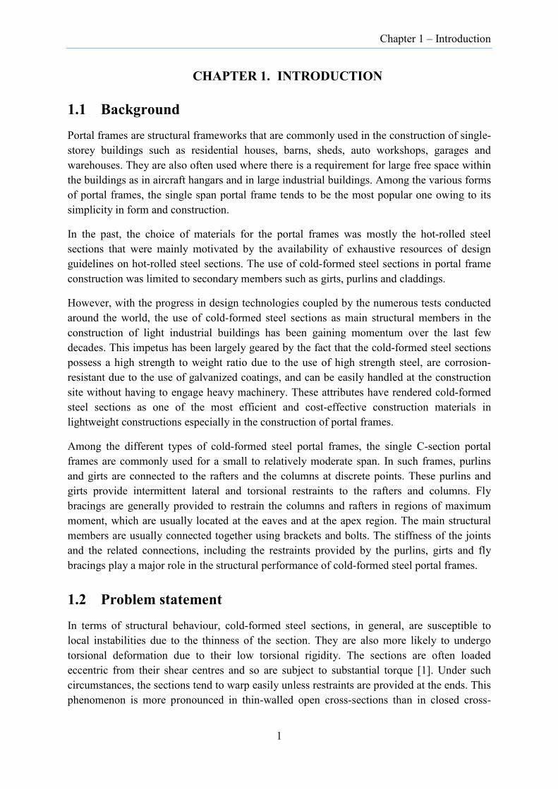
Chapter 1 – Introduction
CHAPTER 1. INTRODUCTION
1.1 Background Portal frames are structural frameworks that are commonly used in the construction of single-storey buildings such as residential houses, barns, sheds, auto workshops, garages and warehouses. They are also often used where there is a requirement for large free space within the buildings as in aircraft hangars and in large industrial buildings. Among the various forms of portal frames, the single span portal frame tends to be the most popular one owing to its simplicity in form and construction.
In the past, the choice of materials for the portal frames was mostly the hot-rolled steel sections that were mainly motivated by the availability of exhaustive resources of design guidelines on hot-rolled steel sections. The use of cold-formed steel sections in portal frame construction was limited to secondary members such as girts, purlins and claddings.
However, with the progress in design technologies coupled by the numerous tests conducted around the world, the use of cold-formed steel sections as main structural members in the construction of light industrial buildings has been gaining momentum over the last few decades. This impetus has been largely geared by the fact that the cold-formed steel sections possess a high strength to weight ratio due to the use of high strength steel, are corrosion-resistant due to the use of galvanized coatings, and can be easily handled at the construction site without having to engage heavy machinery. These attributes have rendered cold-formed steel sections as one of the most efficient and cost-effective construction materials in lightweight constructions especially in the construction of portal frames.
Among the different types of cold-formed steel portal frames, the single C-section portal frames are commonly used for a small to relatively moderate span. In such frames, purlins and girts are connected to the rafters and the columns at discrete points. These purlins and girts provide intermittent lateral and torsional restraints to the rafters and columns. Fly bracings are generally provided to restrain the columns and rafters in regions of maximum moment, which are usually located at the eaves and at the apex region. The main structural members are usually connected together using brackets and bolts. The stiffness of the joints and the related connections, including the restraints provided by the purlins, girts and fly bracings play a major role in the structural performance of cold-formed steel portal frames.
1.2 Problem statement
In terms of structural behaviour, cold-formed steel sections, in general, are susceptible to local instabilities due to the thinness of the section. They are also more likely to undergo torsional deformation due to their low torsional rigidity. The sections are often loaded eccentric from their shear centres and so are subject to substantial torque [1]. Under such circumstances, the sections tend to warp easily unless restraints are provided at the ends. This phenomenon is more pronounced in thin-walled open cross-sections than in closed cross-
1

Chapter 1 – Introduction
sections. Hence, the conventional beam elements having six degrees of freedom at each node may be inadequate to represent the true behaviour of cold-formed steel sections (especially open sections) since the warping degree of freedom is inadvertently missed out from such beam elements. The warping degree of freedom is required to capture the warping displacements in thin-walled sections, and more importantly in single C-sections due to its monosymmetric nature.
The past studies on cold-formed steel (CFS) portal frames comprising single C-sections as members have been generally limited apart from a few research conducted by Baigent and Hancock [2], Mills and LaBoube [3] and Dundu [4]. Most researches have been focussed on CFS portal frames comprising double C-sections connected back-to-back together [5,6,7,8,9,10,11,12,13]. The CFS portal frames, in general, are connected at the eaves, apex and at the base using steel brackets. These joints are semi-rigid in nature [5,9] and hence the strength of CFS portal frames depends largely on the stiffness of these connections. As these joints are semi-rigid, the full rigidity normally assumed in the design practice for CFS portal frames may not be applicable.
Traditionally, the design of CFS portal frames follows a two-step process: analysis followed by member capacity checks. The first-order elastic analysis is usually carried out and moments from the analysis amplified to account for the second-order effect. In some instances, the direct second-order elastic analysis is carried out to obtain design action effects in members. Thereafter, the capacity of each member is checked using currently available design standards such as AS/NZS 4600 [14], AISI S100-16 [15] and EN 1993-1-3 [16]. As the current design methods are member-based with often no linkages between analysis and design apart from the use of effective length factors [17], the trend is to gradually shift towards the system-based design. This new method is a design-by-advanced analysis, which incorporates both the material and geometric nonlinear effects in the structural model and the strength of the whole system, instead of the individual member, can be checked in a single process. However, guidelines for design by advanced analysis for the CFS sections in general and for CFS portal frames in particular, are still at nascent stage at present.
In light of the above, there is a need for the detailed study on the behaviour of cold-formed steel (CFS) single C-section portal frames and associated components through full-scale testing and advanced numerical analysis that would potentially lead to the further development of alternative design methodologies.
1.3 Objectives
This research has been carried out with the following objectives:
1. To develop a formulation for the non-linear beam element with general thin-walled open cross-sections having 7 degrees of freedom within the co-rotational framework of OpenSees (Open System for Earthquake Engineering Simulation).
2

Chapter 1 – Introduction
2. To perform full-scale tests on long-span CFS single C-section portal frames to determine their ultimate strength and to obtain necessary behavioural information for the validation of numerical models.
3. To conduct tests on the apex, eaves and base connections to establish their moment-rotation characteristics and to determine the respective flexural stiffness and strength.
4. To carry out numerical modelling and advanced analysis of the experimental frames and the connections with the incorporation of nonlinear bolted connection behaviour for predicting their ultimate strength and behaviour.
5. To determine the strength of CFS single C-section portal frames using the Direct Strength Method (DSM) towards comparison with the strength predicted by the Direct Design Method (DDM) using Advanced Analysis.
6. To conduct system reliability analysis and derive system resistance factors for the CFS portal frames.
1.4 Scope
This research explores the structural behaviour of long-span CFS single C-section portal frames subjected to gravity load and combination of gravity and lateral load through full-scale experiments, component tests and numerical simulations. For finite element modelling of CFS portal frames, the material properties derived from coupon tests are transformed to true stress and true strain while the behaviour of individual bolted connections, obtained from the component tests, is idealized by the combination of point-based deformable fastener and connector sections. To explore the semi-rigid behaviour of frame connections, both tests and numerical simulation are performed on the eaves, apex and base connections. For the numerical investigation of the behaviour of frames and connections, finite element models are created using shell elements in the widely-used finite element program Abaqus [18]. Determination of frame strength based on the Direct Strength Method (DSM) and the Direct Design Method (DDM) are demonstrated for the CFS single C-section portal frames, highlighting the main processes required for undertaking such design. A system reliability analysis is conducted to derive system resistance factors for the long-span cold-formed steel portal frames.
1.5 Research methods
The following approaches have been adopted to carry out this research:
a) Literature review: The relevant existing knowledge on cold-formed steel portal frames are reviewed to gain an understanding of component behaviour as well as the system behaviour. Particular attention is paid to the structural behaviour of frames, connections and individual structural members. Existing analysis and design methods available for
3
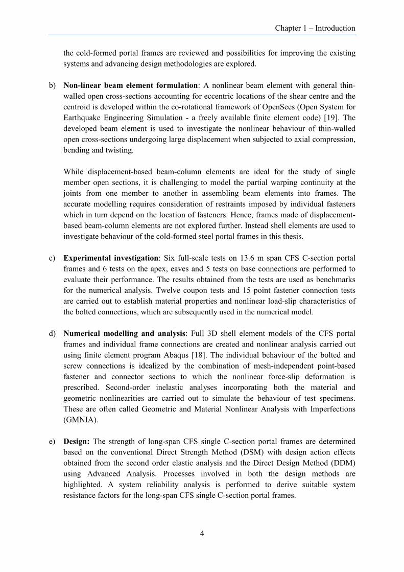
Chapter 1 – Introduction
the cold-formed portal frames are reviewed and possibilities for improving the existing systems and advancing design methodologies are explored.
b) Non-linear beam element formulation: A nonlinear beam element with general thin-
walled open cross-sections accounting for eccentric locations of the shear centre and the centroid is developed within the co-rotational framework of OpenSees (Open System for Earthquake Engineering Simulation - a freely available finite element code) [19]. The developed beam element is used to investigate the nonlinear behaviour of thin-walled open cross-sections undergoing large displacement when subjected to axial compression, bending and twisting. While displacement-based beam-column elements are ideal for the study of single member open sections, it is challenging to model the partial warping continuity at the joints from one member to another in assembling beam elements into frames. The accurate modelling requires consideration of restraints imposed by individual fasteners which in turn depend on the location of fasteners. Hence, frames made of displacement-based beam-column elements are not explored further. Instead shell elements are used to investigate behaviour of the cold-formed steel portal frames in this thesis.
c) Experimental investigation: Six full-scale tests on 13.6 m span CFS C-section portal
frames and 6 tests on the apex, eaves and 5 tests on base connections are performed to evaluate their performance. The results obtained from the tests are used as benchmarks for the numerical analysis. Twelve coupon tests and 15 point fastener connection tests are carried out to establish material properties and nonlinear load-slip characteristics of the bolted connections, which are subsequently used in the numerical model.
d) Numerical modelling and analysis: Full 3D shell element models of the CFS portal
frames and individual frame connections are created and nonlinear analysis carried out using finite element program Abaqus [18]. The individual behaviour of the bolted and screw connections is idealized by the combination of mesh-independent point-based fastener and connector sections to which the nonlinear force-slip deformation is prescribed. Second-order inelastic analyses incorporating both the material and geometric nonlinearities are carried out to simulate the behaviour of test specimens. These are often called Geometric and Material Nonlinear Analysis with Imperfections (GMNIA).
e) Design: The strength of long-span CFS single C-section portal frames are determined
based on the conventional Direct Strength Method (DSM) with design action effects obtained from the second order elastic analysis and the Direct Design Method (DDM) using Advanced Analysis. Processes involved in both the design methods are highlighted. A system reliability analysis is performed to derive suitable system resistance factors for the long-span CFS single C-section portal frames.
4
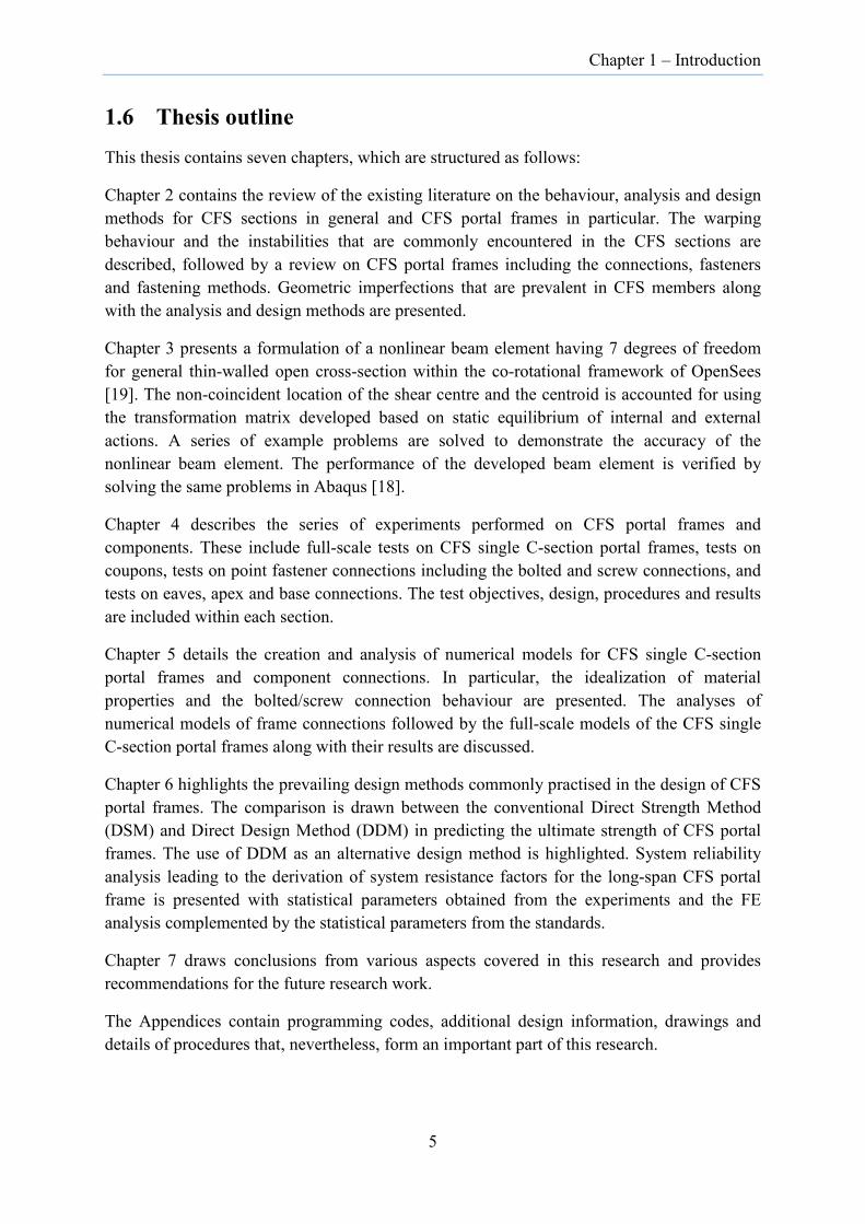
Chapter 1 – Introduction
1.6 Thesis outline
This thesis contains seven chapters, which are structured as follows:
Chapter 2 contains the review of the existing literature on the behaviour, analysis and design methods for CFS sections in general and CFS portal frames in particular. The warping behaviour and the instabilities that are commonly encountered in the CFS sections are described, followed by a review on CFS portal frames including the connections, fasteners and fastening methods. Geometric imperfections that are prevalent in CFS members along with the analysis and design methods are presented.
Chapter 3 presents a formulation of a nonlinear beam element having 7 degrees of freedom for general thin-walled open cross-section within the co-rotational framework of OpenSees [19]. The non-coincident location of the shear centre and the centroid is accounted for using the transformation matrix developed based on static equilibrium of internal and external actions. A series of example problems are solved to demonstrate the accuracy of the nonlinear beam element. The performance of the developed beam element is verified by solving the same problems in Abaqus [18].
Chapter 4 describes the series of experiments performed on CFS portal frames and components. These include full-scale tests on CFS single C-section portal frames, tests on coupons, tests on point fastener connections including the bolted and screw connections, and tests on eaves, apex and base connections. The test objectives, design, procedures and results are included within each section.
Chapter 5 details the creation and analysis of numerical models for CFS single C-section portal frames and component connections. In particular, the idealization of material properties and the bolted/screw connection behaviour are presented. The analyses of numerical models of frame connections followed by the full-scale models of the CFS single C-section portal frames along with their results are discussed.
Chapter 6 highlights the prevailing design methods commonly practised in the design of CFS portal frames. The comparison is drawn between the conventional Direct Strength Method (DSM) and Direct Design Method (DDM) in predicting the ultimate strength of CFS portal frames. The use of DDM as an alternative design method is highlighted. System reliability analysis leading to the derivation of system resistance factors for the long-span CFS portal frame is presented with statistical parameters obtained from the experiments and the FE analysis complemented by the statistical parameters from the standards.
Chapter 7 draws conclusions from various aspects covered in this research and provides recommendations for the future research work.
The Appendices contain programming codes, additional design information, drawings and details of procedures that, nevertheless, form an important part of this research.
5

Chapter 1 – Introduction
1.7 Publications
Conference proceedings
Rinchen, Hancock, G. J. and Rasmussen, K. J. R. (2016). “Formulation for Elastic Stability Analysis of General Thin-walled Open Sections in the OpenSees Framework”, Seventh International Conference on Coupled Instabilities in Metal Structures, Baltimore, USA.
Rasmussen, K.J.R., Blum, H.B. and Rinchen (2018). “Behaviour and design of cold-formed steel portal frames,” Eighth International Conference on Thin-Walled Structures – ICTWS 2018, Lisbon, Portugal.
Journal papers
The following publications will be submitted based on this thesis:
Rinchen, Hancock, G. J. and Rasmussen, K. J. R. (2018). “Geometric nonlinear analysis of thin-walled general open cross-section members”, Thin-Walled Structures (Ready for submission).
Rinchen, and Rasmussen, K. J. R. (2018). “Experiments on long-span cold-formed steel single C-section portal frames”, Journal of Structural Engineering (Ready for submission).
Rinchen, and Rasmussen, K. J. R. (2018). “Numerical modelling of long-span cold-formed steel single C-section portal frames”, Journal of Constructional Steel Research (In preparation).
Rinchen, and Rasmussen, K. J. R. (2018). “Behaviour and numerical modelling of connections in cold-formed steel single C-section portal frames”, Thin-walled Structures (In preparation).
Rinchen, Rasmussen, K. J. R. and Zhang, H. (2018). “Direct Design Method for cold-formed steel single C-section portal frames”, Thin-walled Structures (In preparation).
Research reports
Rinchen, Hancock, G. J. and Rasmussen, K. J. R. (2016). "Formulation and Implementation of General Thin-walled Open-Section Beam-Column Elements in OpenSees." Research Report R961, The University of Sydney, Australia.
6

Chapter 2 – Literature Review
CHAPTER 2. LITERATURE REVIEW
2.1 General Thin-walled cold-formed steel sections are widely used in light gauge constructions such as industrial warehouses, sheds, storage racks and in relatively short-span portal frames apart from their use as secondary structural members. However, in recent years, CFS sections are increasingly used in mid-rise building frames, especially in North America [20]. Innovations in CFS sections are bound to follow as their use continually expands.
However, due to the thinness of the sections, cold-formed steel sections are susceptible to the instability problems that are not normally encountered in hot-rolled sections. Besides this, due to the cold-forming process, the material properties are altered and yield stress distributions across the sections are generally non-uniform. Often the case, cold-formed steel sections have a non-coincident shear centre and centroid resulting in unique structural behaviour.
This chapter begins with a brief review of material properties followed by the discussions on torsional behaviour of single C-sections. Instabilities that are prevalent in CFS sections when subjected to compression, bending and shear are highlighted next. This is followed by the review of CFS portal frames and the frame connections. Types of imperfections prevalent in cold-formed steel members and frames are described next. Different types of analyses are reviewed. This chapter concludes with comments on the available design methods and the use of Advanced Analysis for the design of CFS portal frames.
2.2 Cold-formed steel members
Cold-formed steel portal frames are composed of an assemblage of individual CFS members. An understanding of the fundamentals of the behaviour at the member level is crucial in order to understand the behaviour at the system level. Cold-formed steel sections exhibit unique characteristics that are seldom encountered in hot-rolled steel sections, mainly due to the thinness of the sections and the manufacturing processes.
2.2.1 Material properties
As the cold-formed steel sections have undergone cold reducing (hard rolling) during the manufacturing process, the stress-strain curves for the extracted samples do not exhibit a yield point with a yield plateau [21], instead exhibit gradual yielding. For such type of stress-strain curve, the yield strength is generally taken as the 0.2% proof stress.
While stress-strain relations obtained from the coupon tests are always preferred, it is not possible to conduct coupon tests for every design situation. In such case, Ramberg-Osgood equation [22] find its use in modelling the nonlinear behaviour of the material, which takes the form [23]:
7

Chapter 2 – Literature Review
0.2%
0.002n
Eσ σε
σ
= +
(2.1)
where ε is the strain, σ is the stress, σ0.2% is the 0.2% proof stress, E is the initial elastic modulus and n is the Ramberg-Osgood parameter, which defines the roundness of the elasto-plastic region of the stress-strain curve, is calculated from:
0.2% 0.01%
ln(20)ln( / )
nσ σ
= (2.2)
In cold-formed steel sections, the non-uniform stress distribution resulting from work hardening of corners during the forming process is characterized by a higher yield stress and ultimate tensile strength in the corners (bends) compared to the flat portions [21].
To address this non-uniform yield stress distribution, the current design standards for cold-formed steel structures, such as AS/NZS 4600 [14], AISI S100-16 [15] and EN 1993-1-3 [16], provide guidelines for the computation of average design yield stress of the cross-section, thus allowing the corner strength enhancement to be utilized.
2.2.2 Twist behaviour of C-sections
C-sections, being monosymmetric, possess unique behaviour, especially with regard to torsional deformation. In a single C-section member, due to the eccentric location of the shear centre and centroid, any transverse load which does not pass through the shear centre produces a torsional moment equal to the load times the distance to the shear centre in addition to the bending moment [24]. The twist occurs around the shear centre axis. Figure 2.1 shows the C-section acted upon by the transverse force eccentric from the shear centre. Within the linear elastic range, it can be assumed to be composed of two independent actions: bending and torsion. The resulting deformation is the combination of flexural and torsional deformation (Figure 2.2).
Bending component Torsion component
Figure 2.1 Eccentrically loaded C-section beam (undeformed configuration)
8

Chapter 2 – Literature Review
Figure 2.2 Torsional deformation of C-section beam under eccentric loading [24]
The magnitude of torsional deformation and the strength of the C-section beam depend on the position of the transverse load relative to the shear centre. Based on the series of tests carried out on unbraced simply supported cold-formed steel C-section beam by Put et al. [25] it is reported that the strength of the C-section beam decreases as the load’s eccentricity increases with respect to the shear centre (Figure 2.3). The strength decrease is more pronounced when the load acts outside the shear centre than when it acts on the centroid side.
Figure 2.3 Effects of load eccentricity on the bending strength of C-section beam [25]
9

Chapter 2 – Literature Review
The failure modes are also distinctly different for these two cases. When the load is in between shear centre and centroid, the failure occurs by local buckling of compression flange-web junction as the stress in the compression flange lip is decreased. However, when the load is away from the shear centre, the failure occurs by local buckling of compression flange lip because of the increase in stress within it.
2.2.3 Warping behaviour of C-sections
Another phenomenon that characterizes the behaviour of a single C-section is the cross-sectional warping. Warping is defined by Vlasov [26] as “the distortion of the plane section caused by longitudinal displacement of its points.” Thus, the warping displacement, w at a point in the cross-section in the longitudinal direction of the beam is [26]:
'w ωφ= − (2.3)
where φ′ is the twist defined as the angle of rotation of cross-section per unit length and ω is the sectorial coordinate defined as the longitudinal warping displacement due to unit negative twist (φ′=-1) about the shear centre axis [27].
If warping displacement is unrestrained, the beam undergoes uniform torsion. This induces twisting of component elements due to rotation of the cross-sections about the longitudinal axis. As a result, Saint-Venant shear stresses appear in the cross-section which balances the applied torsion.
The pure shear stress through the thickness of the cross-section is given by:
maxtTJ
τ = ± (2.4)
where t is the thickness, T, the Saint-Venant torque and J, the torsional constant which is usually approximated by:
3
1
13
m
i ii
J b t=
= ∑ (2.5)
for multi-segment thin-walled open cross-sections. In the above expression, bi, ti refers to the width and thickness of the ith plate elements.
If the beam, on the other hand, is restrained against warping, the beam is said to be under non-uniform torsion. Under this circumstance, longitudinal strains develop in the member which generates self-equilibrating normal stresses that vary along the member. These longitudinal stresses are equilibrated by the existence of shear stress in addition to Saint-Venant stress. Thus, the external torsion, T is equilibrated by the combination of Saint-Venant torque, Tv and warping torque, Tω as follows [28]:
vT T Tω= + (2.6)
10

Chapter 2 – Literature Review
Central to the theory of warping of the cross-section is the “bimoment” which is defined as “a pair of equal but opposite bending moments acting in two parallel planes.” The magnitude of bimoment is equal to the product of the distance between parallel planes and the moment on one of them [28].
2.2.3.1 Bimoments in thin-walled beams
Bimoment can arise from two situations viz. the axial load acting at various points on the cross-section and bending moment acting in a plane parallel to the longitudinal axis of the beam. Whether or not a given loading will produce a bimoment in a given thin-walled structure is determined based on the two theorems [28]:
Theorem 1: “A bimoment caused by an external force acting parallel to the longitudinal axis of a beam is equal to the product of this force and the principal sectorial coordinate of the point of its application.”
Mathematically, it is represented by:
B Pω= (2.7)
in which ω is the sectorial coordinate at the point of application of axial load P. For a cross-section acted upon by several axial forces, bimoment can be computed as the summation of the product of individual forces and corresponding sectorial coordinates as follows:
k kk
B Pω=∑ (2.8)
Theorem 2: “A bimoment caused by a bending moment acting in a plane parallel to the longitudinal axis of a beam is equal to a product of this bending moment and the distance of its plane from the shear centre of that beam.”
This can be mathematically represented as:
B Me= (2.9)
where e is the distance of the plane of the moment M from the shear centre.
The longitudinal warping stress induced by the bimoment B at any point s in the cross-section is given as:
( )( ) ss BIωω
ωσ = (2.10)
in which Iω is the warping constant. As is evident from Equation (2.10), the variation of longitudinal stress along a profile of a section caused by bimoment is similar to its principal sectorial coordinates. This stress is by no means trivial, especially in cold-formed steel sections. It can be as high as that of bending stresses in some cases [29].
The warping shear stress induced by the warping torque is given by:
11
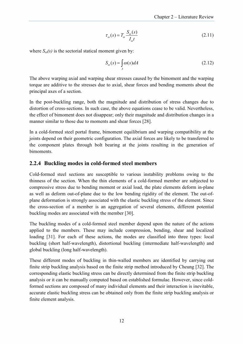
Chapter 2 – Literature Review
( )( ) S ss TI tω
ω ωω
τ = (2.11)
where Sω(s) is the sectorial statical moment given by:
( ) ( )A
S s s dAω ω= ∫ (2.12)
The above warping axial and warping shear stresses caused by the bimoment and the warping torque are additive to the stresses due to axial, shear forces and bending moments about the principal axes of a section.
In the post-buckling range, both the magnitude and distribution of stress changes due to distortion of cross-sections. In such case, the above equations cease to be valid. Nevertheless, the effect of bimoment does not disappear; only their magnitude and distribution changes in a manner similar to those due to moments and shear forces [28].
In a cold-formed steel portal frame, bimoment equilibrium and warping compatibility at the joints depend on their geometric configuration. The axial forces are likely to be transferred to the component plates through bolt bearing at the joints resulting in the generation of bimoments.
2.2.4 Buckling modes in cold-formed steel members
Cold-formed steel sections are susceptible to various instability problems owing to the thinness of the section. When the thin elements of a cold-formed member are subjected to compressive stress due to bending moment or axial load, the plate elements deform in-plane as well as deform out-of-plane due to the low bending rigidity of the element. The out-of-plane deformation is strongly associated with the elastic buckling stress of the element. Since the cross-section of a member is an aggregation of several elements, different potential buckling modes are associated with the member [30].
The buckling modes of a cold-formed steel member depend upon the nature of the actions applied to the members. These may include compression, bending, shear and localized loading [31]. For each of these actions, the modes are classified into three types: local buckling (short half-wavelength), distortional buckling (intermediate half-wavelength) and global buckling (long half-wavelength).
These different modes of buckling in thin-walled members are identified by carrying out finite strip buckling analysis based on the finite strip method introduced by Cheung [32]. The corresponding elastic buckling stress can be directly determined from the finite strip buckling analysis or it can be manually computed based on established formulae. However, since cold-formed sections are composed of many individual elements and their interaction is inevitable, accurate elastic buckling stress can be obtained only from the finite strip buckling analysis or finite element analysis.
12

Chapter 2 – Literature Review
The finite strip buckling analysis does not distinguish between the buckling modes. Hence, the analysis is needed to be repeated over a range of lengths corresponding to buckle half-wavelengths, especially for short wavelength buckling modes [33]. Furthermore, such analysis allows interaction of buckling modes to be captured which are not possible with manual methods.
Figure 2.4 shows the typical buckling curve (often called the signature curve) for the typical C-sections in bending. The insets show four distinct buckled modes of C-sections, which are described in detail in the following paragraph.
Figure 2.4 Buckling modes of lipped channel beam in bending [1]
2.2.4.1 Local buckling
Local buckling is “a mode involving plate flexure alone without transverse deformation of the line or lines of intersection of adjoining plates” [1]. Local buckling is a prominent local instability in a thin-walled structural member which is characterized by a number of ripples or buckles along the walls of a section. Although it does not cause immediate failure, it radically reduces the stiffness of the member against further compression and hastens the ultimate failure [34, 35]. The half-wavelength of local buckling is usually shorter than or equal to the largest dimension of the member under compressive stress. Local buckling is stable in the elastic range and locally buckled members may have substantial post-buckling strength [36].
2.2.4.2 Distortional buckling
Distortional buckling is “a mode of buckling involving a change in cross-sectional shape excluding local buckling” [1]. Distortional bucking involves deformations where part of the
13

Chapter 2 – Literature Review
cross-section (for instance flange) responds rigidly by twisting or translating about a point (flange/web junction) and another part of the cross-section (web) undergoes plate bending [30]. It is a mode of buckling in which the lip stiffener is insufficient to retard the compression flange and attached web from becoming unstable. Distortional buckling can be reduced if lip stiffeners are longer but this is normally outside the jurisdiction of design engineers [37]. The half-wavelength of distortional buckling falls between the half-wavelengths of local and global buckling. It is generally about 3-6 times that of half-wavelength of local buckling [36].
2.2.4.3 Global buckling
Global buckling “involves buckling where the whole cross-section, without distortion, starts to bend laterally (flexural buckling), rotate (torsional buckling), or bend and rotate simultaneously (flexural-torsional buckling)” [30]. This also involves large deformation while the material remains elastic. In other words, failure is not related to the yielding of material but to elastic instability owing to material stiffness and geometry. During global buckling, the cross-section moves as the rigid body without any distortion. The half-wavelength of the global buckling is equal to the unbraced length of the member. Flexural buckling occurs when cold-formed sections are loaded through the shear centre. However, when a column is axially loaded along its centroidal axis, it undergoes flexural-torsional buckling at a lower load than the flexural buckling mode because of the eccentricity of the load from the shear centre [24].
If members are fully braced, lateral torsional buckling gets suppressed and distortional buckling or local buckling normally controls the design.
2.2.4.4 Shear buckling
Shear buckling can be either local or global. Local shear buckling occurs in the slender webs of members when it is subjected to bending or in the wide flanges of sheeting and decking profiles under the effect of diaphragm action. Global shear buckling generally arises when relative lightweight sheeting or lining profiles are subjected to diaphragm action [38].
In recent years, Hancock and Pham [39] investigated thin-walled sections in pure shear using the Semi-Analytical Finite Strip Method and developed a signature curve for the thin-walled sections in a similar fashion to the signature curves for bending and compression.
2.2.5 Post-buckling strength
Cold-formed steel sections have a thickness of individual plate elements several times smaller than their widths. Due to the slenderness of the elements, local buckling can occur well before the yielding of the section. However, the occurrence of local buckling of an element does not necessarily result in reaching its ultimate load-carrying capacity. This is particularly true for those elements that have the lips on its edge which possess greater post-buckling strength [24]. In general, stockier sections have the ability to develop inelastic reserve capacity [40, 41].
14

Chapter 2 – Literature Review
The inelastic reserve capacity has also been observed in the tests of single C-section cold-formed portal frames carried out by Baigent and Hancock [42] in which portal frames failed at significantly higher loads than the first yield loads. The inelastic reserve capacity of the cold-formed steel section can be particularly advantageous in the design of cold-formed steel portal frame structures where deflection limitations can be relaxed such as in agricultural and industrial buildings [40]. However, the maximum post-buckling capacity is limited to 1.25 times the yield strength in accordance with Clause F2.4 of AISI S100-16 [15] thus ensuring the structural safety.
2.3 Cold-formed steel portal frames
Steel portal frames are one of the most efficient and cost-effective structural frameworks that are widely used in the construction of single-story industrial buildings. In particular, cold-formed steel (CFS) portal frames are increasingly used as viable alternatives to the traditional hot-rolled sections for spans in the range of 12 m or more [3, 9]. The advantages of using cold-formed steel sections for portal frames include [9]:
• Sections can be cut to length, pre-punched at the factory to design specifications, marked and delivered to site ready for installation
• Frames can be installed manually without having to mobilize sophisticated machinery resulting in the faster construction
• Cold-formed sections are virtually maintenance-free since they are pre-galvanized • Sections can be efficiently stacked for transportation resulting in reduced
transportation cost • Acquisition costs can be reduced as both main and secondary cold-formed structural
members can be availed from the same manufacturer or supplier
Further, cold-formed steel sections are fully recyclable, making it an ideal and versatile material for constructions.
2.3.1 Components of cold-formed steel portal frames
A typical single span cold-formed steel portal frame building consists of series of portal frames erected at regular bays (Figure 2.5). Each frame, which forms the main structural systems of the building, comprises of columns and rafters connected at the eaves, apex and base through steel brackets (Figure 2.6). The brackets are connected to columns and rafters using bolts. In some cases, screws are also used for the connection besides the bolts.
Purlins and girts spanning between adjacent portal frames are connected to the rafters and columns using cleats. Corrugated roof sheeting is fixed to the purlins while wall cladding is fixed to the girts. Since purlins and girts are connected to the rafters and columns, the load from roof sheeting and wall cladding are ultimately transferred to the columns and rafters in the form of reactive force at discrete connection points. Besides transferring loads to the frame, purlins and girts provide partial translational and rotation restraints to the frames. Fly
15
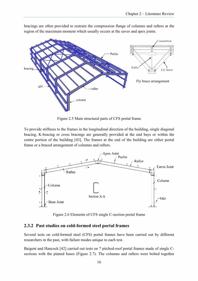
Chapter 2 – Literature Review
bracings are often provided to restrain the compression flange of columns and rafters at the region of the maximum moment which usually occurs at the eaves and apex joints.
Figure 2.5 Main structural parts of CFS portal frame
To provide stiffness to the frames in the longitudinal direction of the building, single diagonal bracing, K-bracing or cross bracings are generally provided at the end bays or within the centre portion of the building [43]. The frames at the end of the building are either portal frame or a braced arrangement of columns and rafters.
Figure 2.6 Elements of CFS single C-section portal frame
2.3.2 Past studies on cold-formed steel portal frames
Several tests on cold-formed steel (CFS) portal frames have been carried out by different researchers in the past, with failure modes unique to each test.
Baigent and Hancock [42] carried out tests on 7 pitched-roof portal frames made of single C-sections with the pinned bases (Figure 2.7). The columns and rafters were bolted together
Fly brace arrangement
16

Chapter 2 – Literature Review
through their webs at the eaves and apex using brackets made from 12 mm thick hot-rolled steel plates. The resulting joints were essentially rigid.
Figure 2.7 Portal frame geometry of Baigent Hancock [42]
The frames were tested under two restraint configurations, each with three different load cases. One set of tests involved testing of frames with external restraints only, and the other set consisted of frames with both external restraints and internal restraints. External restraints were provided on the outside face of frames to simulate the effect of purlins and girts. Internal restraints were provided near the eaves and apex region of the frame to simulate the effect of fly bracing, which prevented lateral movement of the internal flange of the frame. Three loading conditions under which each set of frames tested include gravity load, the lateral load due to the wind in the transverse direction and lateral load due to the wind in the longitudinal direction. All loads were applied as point load coincident with the restraint points.
Frames with both external and internal restraints failed at higher loads than the frames with only external restraints indicating the influence of internal restraints provided by fly bracing on the strength of the frames. The ultimate collapsed loads for both test sets were significantly higher than yield loads, which demonstrated that the cold-formed portal frames have the capacity to carry the load in the post-buckling and post-yielding range. Based on the measurements recorded by the strain gauges, the most highly stressed portions were the flange-web junctions within the cross-section, and the point of initiation of yielding was located below the eave joints.
Kirk [44] tested 6 pairs of CFS portal frames made from the pairs of swagebeam connected back-to-back with spans of 9 m and 12 m. Columns and rafters were connected through their webs to the brackets with bolts. Columns were 3 m high to the eaves and the roof slope was 15 degrees. Frames were tested in pairs with 2.5 m wide bay spacing: first frame with pinned bases and second frame with fixed bases. Bracings were provided to the frame to prevent failure in the out-of-plane direction. Each frame was loaded vertically at purlin positions through a system of steel rods and spreader beams using hydraulic jacks.
17

Chapter 2 – Literature Review
It was reported that for the 12 m span portal frame configuration, the ultimate load of the frame with fixed base was higher by 16% than that of the frame with the pinned base. The failure was due to the buckling of compression flange, which occurred initially at the eaves and subsequently at the apex region.
Wilkinson and Hancock [45] conducted tests on three pinned-base portal frames composed of CFS rectangular hollow sections (RHS) of 150 mm x 50 mm x 4 mm subjected to gravity and wind loads (Figure 2.8).
Figure 2.8 Portal frame layout of Wilkinson and Hancock [45]
While the eaves joints were welded using full penetration butt weld, the apex was bolted using eight M16 high strength structural bolts through the 10 mm thick gusset plates welded to each end of the rafter. The gravity load was applied at the midpoint of rafters using a gravity load simulator while the horizontal load was applied to one of the columns at 2 m above the base by attaching a steel rope to the column and a load cradle to the other end of steel rope. The mode of failures for all frames was the formation of plastic collapse mechanism near the loading point on the rafter and below the eaves. Based on the observation and results, it was pointed out that plastic design is possible for the design of such frames as the connections are sufficiently ductile to undergo required plastic rotations.
Lim and Nethercot [9] carried out a numerical and experimental investigation on the effect of semi-rigid nature of the joints on the behaviour of cold-formed steel portal frames. The frames were made from a double C-section connected back-to-back with pinned base (Figure 2.9). Eaves and apex joints were formed from 3 mm steel brackets bolted to the frame member. Two portal frames differing in joint size (bracket size) were used for the study. The frames were laterally restrained at the locations shown by cross marks in Figure 2.9.
Two approaches were adopted for the numerical modelling: i) beam idealization of the whole frame including the finite size of joints with spring representation for the rigidity of joint and
18

Chapter 2 – Literature Review
ii) full 3D shell element model with beam and spring elements representing the bolts. The numerical results were verified by the full-scale frame tests.
Figure 2.9 Portal frame geometry of Lim and Nethercot [9]
It was reported that joints were semi-rigid, mainly due to the bolt hole elongation that has resulted from the bending moment at the joint. Of the two frame tests, the one with shorter bolt-group length, failed at a load approximately 20% lower than that of a frame having longer bolt-group length due to the development of bimoment [46]. It was also demonstrated that the severe apex deformation can occur due to the semi-rigidity of the joints. Based on the numerical analysis, four components of apex deflections in portal frames were identified [9]:
a. Deflection due to bending of column and rafter b. Deflection due to bolt hole deformation c. Deflection due to in-plane bracket deformation d. Deflection due to shear deformation
Among these, bolt hole deformation contributed the maximum to the total deflections. It was recommended that both serviceability requirements and practical constraints on joint details should be considered while assessing the efficiency of the proposed framing system.
Zhang and Rasmussen [12] and Zhang et al. [47] conducted tests on portal frames made from C-sections connected back-to-back with lateral restraints spaced at 1.35 m to investigate the effects of cross-sectional instability on the overall stability of the frame. Four pitched roof portal frames with pinned bases were tested (Figure 2.10).
While three frames were tested with vertical loads, one frame was tested with a combination of vertical and lateral loads. Both the eaves and apex joints were formed by the bolting of both flanges and webs to the 6 mm thick G350 mild steel gusset plates.
Since the cross-section of the rafters was stockier than that of columns, local buckling occurred in one of the columns near the eaves joint in all the tests when the vertical load reached 50% of the ultimate load. When the load reached close to ultimate state, distortional buckling occurred and frames ultimately failed by the formation of spatial plastic mechanism on the flanges and the webs of one of the columns below the eaves joint. This indicated that distortional buckling stresses were higher than the local buckling stresses. The tests formed
19

Chapter 2 – Literature Review
the basis for the calibration of finite element models that were used for the parametric study on the significance of second order effects caused by local and distortional buckling.
Figure 2.10 Portal frame tests of Zhang et al. [47]
The effect of stress skin diaphragm action from roof sheeting and wall cladding on the portal frame was studied by Mahendran and Moor [48]. Full-scale tests of a 12 m by 12 m portal frame building under various load cases showed that moments and deflections in frames can be reduced and distributed in the presence of cladding and end frame. Significant impact on the reduction of moments was especially noticed when the frame was subjected to lateral load parallel to the frame. Similar tests carried out by Wrzesien and Lim [49] reinforced the beneficial effect of cladding in redistribution of loads, especially under lateral loading. However, the general practice has been that portal frames are analyzed without including the stressed skin effect.
Recently, Blum and Rasmussen [50] tested a series of long-span cold-formed steel portal frames with C-sections connected back-to-back. The frame configuration included variations in the knee connection, sleeve stiffeners in the column and rafters, and loading combinations. It was observed that the ultimate capacity of the frame is sensitive to the stiffness of the knee connection. On the other hand, the inclusion of sleeve stiffeners has minimal impact on the ultimate capacity of the frame. It was also reported that the unbraced frames failed by the lateral-torsional buckling of columns initiated at the knee-to-column connection.
2.3.3 Portal frame connections
2.3.3.1 Mechanical fasteners
Different types of fastening system including welding, bolting, screwing, riveting, clinching, nailing, structural adhesive or other mechanical means are allowed by the code of practice
20

Chapter 2 – Literature Review
such as AS/NZS 4600:2018 [14] for joining the parts of cold-formed steel structures. However, the most commonly used fasteners in the CFS portal frames are bolts and screws although welds are occasionally used to create rigid joints. The welding, however, is not always recommended for use with galvanized cold-formed steel sections owing to the ensuing emission of poisonous gases and destruction of the galvanized coating [9].
While no restriction is placed on the bolt size in codes [14, 15], the general practice is to use bolt size of 12 mm, 16 mm and 20 mm as fasteners in cold-formed steel portal frames. While fasteners are mainly subjected to shear force, they may also experience tension when they are used for the slip-resistant connection. Depending on the connection configuration, various types of connection failures are possible for a point fastener connection. The basic types of failure of thin steel bolted connection subjected to shear and tension are shown in Figure 2.11 and Figure 2.12 respectively.
Figure 2.11 Failure modes of bolted connection in shear [51]
a) Rupture of bolt b) Pull-through failure
Figure 2.12 Failure modes of bolted connection in tension [51]
(Net section rupture) (Tearout)
21

Chapter 2 – Literature Review
Screws are also used as fasteners in the cold-formed steel portal frames besides the bolts. Two main types of screws are available: self-tapping and self-drilling screws. While the self-tapping screws tap their counter thread in a prepared hole, self-drilling screws drill their own holes through the member forming mating threads in one operation [51]. In many cases, washers are integrated with the screws to increase the load-bearing capacity. The size of self-drilling screws used for the connection of cold-formed steel structural members is usually in the range of 4.0 mm to 6.35 mm in diameter [52]. Due to the small size, the failure modes of screw connections are dominated by the tilting and pulling out of the fasteners (Figure 2.13). The other forms of failure: bearing, tearing and shearing of thin members are also prevalent in sheets connected by screws.
Figure 2.13 Tilting and pullout of screw fastener [51]
2.3.3.2 Slip-resistant bolted connections
Bolted connections are generally used for the connection of structural members and joints in CFS portal frames. In such connections, the rigidity of the joint is partly influenced by the method employed to tighten the bolts. For instance, in a bearing-type connection, load is transferred from one plate to another plate by the bearing of bolt on the plate thickness whereas in a friction-type connection (slip-resistant bolted connection), the load is initially transferred by friction developed between the clamped plate and subsequently by bolt bearing on the plate once the friction is overcome (Figure 2.14).
(a)
(b)
Figure 2.14 Load transmission in a bolted connection: (a) Bearing-type connection; (b) Slip- resistant connection [53]
22
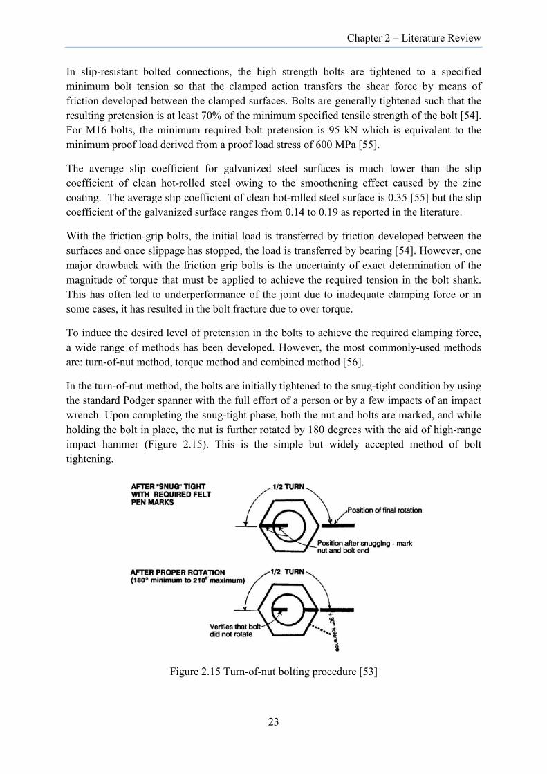
Chapter 2 – Literature Review
In slip-resistant bolted connections, the high strength bolts are tightened to a specified minimum bolt tension so that the clamped action transfers the shear force by means of friction developed between the clamped surfaces. Bolts are generally tightened such that the resulting pretension is at least 70% of the minimum specified tensile strength of the bolt [54]. For M16 bolts, the minimum required bolt pretension is 95 kN which is equivalent to the minimum proof load derived from a proof load stress of 600 MPa [55].
The average slip coefficient for galvanized steel surfaces is much lower than the slip coefficient of clean hot-rolled steel owing to the smoothening effect caused by the zinc coating. The average slip coefficient of clean hot-rolled steel surface is 0.35 [55] but the slip coefficient of the galvanized surface ranges from 0.14 to 0.19 as reported in the literature.
With the friction-grip bolts, the initial load is transferred by friction developed between the surfaces and once slippage has stopped, the load is transferred by bearing [54]. However, one major drawback with the friction grip bolts is the uncertainty of exact determination of the magnitude of torque that must be applied to achieve the required tension in the bolt shank. This has often led to underperformance of the joint due to inadequate clamping force or in some cases, it has resulted in the bolt fracture due to over torque.
To induce the desired level of pretension in the bolts to achieve the required clamping force, a wide range of methods has been developed. However, the most commonly-used methods are: turn-of-nut method, torque method and combined method [56].
In the turn-of-nut method, the bolts are initially tightened to the snug-tight condition by using the standard Podger spanner with the full effort of a person or by a few impacts of an impact wrench. Upon completing the snug-tight phase, both the nut and bolts are marked, and while holding the bolt in place, the nut is further rotated by 180 degrees with the aid of high-range impact hammer (Figure 2.15). This is the simple but widely accepted method of bolt tightening.
Figure 2.15 Turn-of-nut bolting procedure [53]
23

Chapter 2 – Literature Review
In the torque method, a calibrated torque wrench is used for the tightening of the bolts. Due to the difficulty of accounting friction, variations of ±25% in pretension has been measured for identical torque using this method [56]. Hence, this method is prohibited by some guidelines [53].
In the combined method, the bolts are tightened in two stages. Using the torque method, the nut is initially tightened to produce pretension in the bolt about 65% of the yield load. The bolt is then further tightened by half-turn (180 degrees) to induce full pretension.
2.3.3.3 Apex and eaves joints
The apex joint connects two rafters at the ridge while the eaves joint connects rafters to the columns. These joints are usually formed by the connection brackets which are bolted to the columns and rafters. The performance of the portal frame is directly related to the performance of the frame connections [24].
The capacity of these joints depends on the bracket size and thickness and the bolt configuration. Where the bracket thickness is in the order of the member thickness, the resulting joints are semi-rigid in nature. Semi-rigidity of the joint is also attributed to bolt hole elongation due to the bearing of the bolt shank on bracket plates and the local buckling of brackets [9,57]. Bolt hole elongation is defined as the deformation of the bolt hole caused by bearing of the bolt shank against the bolt hole. The main factors that determine the magnitude of bolt hole elongation are [58]:
1. Thickness of the cold-formed steel plate 2. Diameter of bolt-hole 3. Material properties of the cold-formed steel plate 4. Diameter of the bolt 5. Material properties of the bolt 6. Whether the bolt-shank is plain or threaded
The stiffness of the joints can be enhanced either by increasing the bolt-group length or by increasing the number of bolts which require the use of larger brackets. On the other hand, smaller brackets are preferred primarily for the ease of joint installation at the site [59]. Among the joints in portal frames, eaves joint is the highly stressed portion of the portal frame since the maximum bending moment occurs at the eaves joint [60]. In a poorly configured joint, premature local buckling can cause joints to fail well below the bearing capacity of the brackets.
Although several tests were conducted on the joints for portal frames with double C-section joined back-to-back [5, 57, 59, 61] and the joints for closed CFS sections [62, 63, 64], the tests on single C-section joints have been relatively rare, apart from the tests by Mills and LaBoube [65], Dundu and Kemp [60], and BlueScope Lysaght [66].
Baigent and Hancock [42] used 12 mm thick plate to form brackets for the eaves and the apex joint. The single C-section rafters and columns were essentially clamped together in between
24
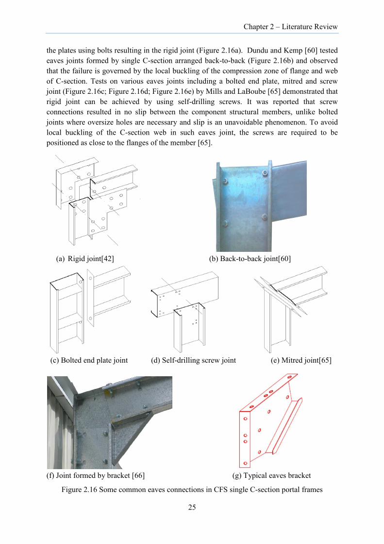
Chapter 2 – Literature Review
the plates using bolts resulting in the rigid joint (Figure 2.16a). Dundu and Kemp [60] tested eaves joints formed by single C-section arranged back-to-back (Figure 2.16b) and observed that the failure is governed by the local buckling of the compression zone of flange and web of C-section. Tests on various eaves joints including a bolted end plate, mitred and screw joint (Figure 2.16c; Figure 2.16d; Figure 2.16e) by Mills and LaBoube [65] demonstrated that rigid joint can be achieved by using self-drilling screws. It was reported that screw connections resulted in no slip between the component structural members, unlike bolted joints where oversize holes are necessary and slip is an unavoidable phenomenon. To avoid local buckling of the C-section web in such eaves joint, the screws are required to be positioned as close to the flanges of the member [65].
(a) Rigid joint[42] (b) Back-to-back joint[60]
(c) Bolted end plate joint (d) Self-drilling screw joint (e) Mitred joint[65]
(f) Joint formed by bracket [66] (g) Typical eaves bracket
Figure 2.16 Some common eaves connections in CFS single C-section portal frames
25

Chapter 2 – Literature Review
BlueScope Lysaght has produced a series of proprietary joints that are widely used in CFS single C-section frames. One such eaves joint is shown in Figure 2.16f. A series of tests on similar eaves joints for C-section profile of 150 mm and 200 mm depth under pure bending [66] indicated that bending capacity of eaves joint is higher under uplift load compared to the bending capacity under gravity load. As intuition might suggests, the bending capacity of the joint also increased with the increase in thickness of the brackets.
Tests on apex joints were conducted by Dubina et al. [57] and Lim and Nethercot [58] for double C-section CFS portal frames. It was reported that in such connections, the failure occurred by buckling of compression flanges near the bracket. Due to the snug-tight conditions, bolt hole elongations were dominant resulting in the overall flexibility of the moment connection.
Mills and LaBoube [65] tested two types of apex joints: welded ridge joint and self-drilling screw ridge joint that are generally used in CFS single C-section portal frames. The tests on welded apex joints resulted in the failure of channel member adjacent to the joint while the weld remained intact. On the other hand, the self-drilling screw apex joints (Figure 2.17a), failed by tilting and shearing of screws [65]. As one would expect, the joint with more screws provided higher capacity than the one that has fewer screws. However, the increase in joint capacity was incommensurate with the increase in screws with the attainment of only 66% higher capacity when the number of screws was doubled.
Typical apex joint used by BlueScope Lysaght in their CFS single C-section portal frames is given in Figure 2.17b, the details of which are elaborated in Section 4.2.5.2.
(a) Screw joint at apex [65]
(b) Apex joint (c) Typical apex bracket
Figure 2.17 Typical apex connections in CFS single C-section portal frames
26
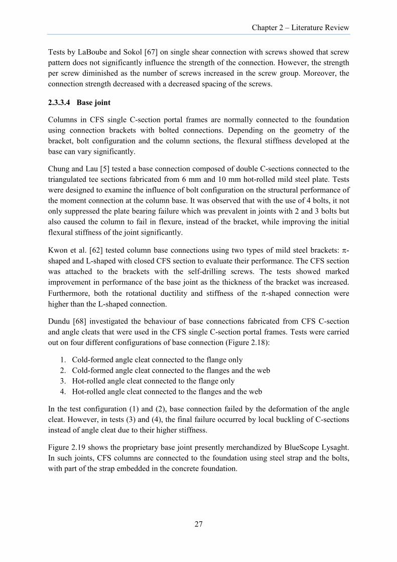
Chapter 2 – Literature Review
Tests by LaBoube and Sokol [67] on single shear connection with screws showed that screw pattern does not significantly influence the strength of the connection. However, the strength per screw diminished as the number of screws increased in the screw group. Moreover, the connection strength decreased with a decreased spacing of the screws.
2.3.3.4 Base joint
Columns in CFS single C-section portal frames are normally connected to the foundation using connection brackets with bolted connections. Depending on the geometry of the bracket, bolt configuration and the column sections, the flexural stiffness developed at the base can vary significantly.
Chung and Lau [5] tested a base connection composed of double C-sections connected to the triangulated tee sections fabricated from 6 mm and 10 mm hot-rolled mild steel plate. Tests were designed to examine the influence of bolt configuration on the structural performance of the moment connection at the column base. It was observed that with the use of 4 bolts, it not only suppressed the plate bearing failure which was prevalent in joints with 2 and 3 bolts but also caused the column to fail in flexure, instead of the bracket, while improving the initial flexural stiffness of the joint significantly.
Kwon et al. [62] tested column base connections using two types of mild steel brackets: π-shaped and L-shaped with closed CFS section to evaluate their performance. The CFS section was attached to the brackets with the self-drilling screws. The tests showed marked improvement in performance of the base joint as the thickness of the bracket was increased. Furthermore, both the rotational ductility and stiffness of the π-shaped connection were higher than the L-shaped connection.
Dundu [68] investigated the behaviour of base connections fabricated from CFS C-section and angle cleats that were used in the CFS single C-section portal frames. Tests were carried out on four different configurations of base connection (Figure 2.18):
1. Cold-formed angle cleat connected to the flange only 2. Cold-formed angle cleat connected to the flanges and the web 3. Hot-rolled angle cleat connected to the flange only 4. Hot-rolled angle cleat connected to the flanges and the web
In the test configuration (1) and (2), base connection failed by the deformation of the angle cleat. However, in tests (3) and (4), the final failure occurred by local buckling of C-sections instead of angle cleat due to their higher stiffness.
Figure 2.19 shows the proprietary base joint presently merchandized by BlueScope Lysaght. In such joints, CFS columns are connected to the foundation using steel strap and the bolts, with part of the strap embedded in the concrete foundation.
27

Chapter 2 – Literature Review
Base connection configuration 1 and 3 Base connection configuration 2 and 4
(Elevation) (Plan)
Figure 2.18 Base joint [68]
Steel Strap
Figure 2.19 Base joint (BlueScope Lysaght)
The main uncertainty with respect to the base connection is the magnitude of flexural rigidity that can be developed at the base. The fixed base is desirable from the serviceability point of view since it reduces lateral frame deflections significantly resulting in substantial savings from the column size. However, the fixed base has a negative impact on the foundation since the moments are required to be transferred along with other forces resulting in larger size of foundation [69]. In design, partial restraints that normally exist at the base are seldom considered. Quite often, the pinned base is assumed for the design purposes.
Towards determining the fixity condition of the cold-formed steel column-bracket foundation system, Reid and Ansourian [70] conducted finite element analysis of the soil-structure interaction by considering a range of subgrade moduli (1MPa to 10,000 MPa) covering the wide spectrum of soil conditions for seven foundation types. It was observed that the rotational stiffness developed at the base for the shallow concrete foundation of thickness 200 mm, normally encountered in light frame constructions, ranged from 2,000 kNm/radian to 15,000 kNm/radian for the subgrade moduli in the range of 1 MPa to 100 MPa. Since the
28

Chapter 2 – Literature Review
rotational stiffness of the base varied widely with the variation of subgrade moduli, it was suggested that the partial fixity condition of the base be modelled by either of the following methods:
i) Adding a stub member at each of the base nodes of the frame whose second moment of area, I= L/(3E)(M/θ) where L and E are the lengths and the elastic modulus of each stub respectively, and M/θ (moment/rotation) is the relevant foundation stiffness. For this purpose, each end of stub member must be restrained against vertical and horizontal translation only (not against rotation); Or
ii) Introducing a rotation spring of stiffness, M/θ for the relevant soil stiffness and
foundation type. In this case too, the base of the frame must be restrained against horizontal and vertical translation.
Reid and Ansourian [70] also carried out field tests to determine moment-rotation relations at the base of a typical portal frame attached to a concrete slab. Typical rotational flexibility of 0.06 radian/kNm was obtained at the base. It was concluded that the rotational flexibility of the base joint was attributed to the flexibility of the column connection at the base alone. The contributions from the rotation of foundation slab and the rotation of column due to the moment-induced curvature near the base were negligibly small.
Koschmidder and Brown [43] suggested using different base fixity for checking serviceability and stability, and ultimate limit states for the portal frames made of hot-rolled sections. It was suggested that the pinned base should be used for the ultimate limit states while the nominally pinned base for the serviceability limit states and stability check.
Nominally pinned base connection can be modelled by using either spring stiffness or dummy member whose length equals to 75% of the column length and pin supported at the ends (Figure 2.20). In both the cases, 10% and 20% of the column stiffness were recommended for the assessment of frame stability and deflection respectively.
Figure 2.20 Modelling of nominally pinned base [43]
2.3.3.5 Secondary connections
Secondary structural members such as purlins and girts, which provide lateral restraint and torsional restraint to the rafters and columns, are connected to them using standard purlin cleats (Figure 2.21). Minimum of two bolts are required for the connection of lapped
29
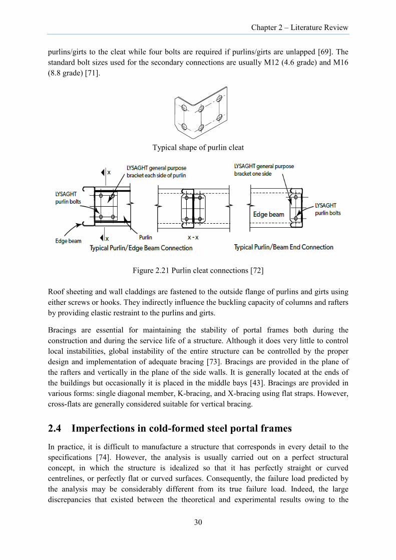
Chapter 2 – Literature Review
purlins/girts to the cleat while four bolts are required if purlins/girts are unlapped [69]. The standard bolt sizes used for the secondary connections are usually M12 (4.6 grade) and M16 (8.8 grade) [71].
Typical shape of purlin cleat
Figure 2.21 Purlin cleat connections [72]
Roof sheeting and wall claddings are fastened to the outside flange of purlins and girts using either screws or hooks. They indirectly influence the buckling capacity of columns and rafters by providing elastic restraint to the purlins and girts.
Bracings are essential for maintaining the stability of portal frames both during the construction and during the service life of a structure. Although it does very little to control local instabilities, global instability of the entire structure can be controlled by the proper design and implementation of adequate bracing [73]. Bracings are provided in the plane of the rafters and vertically in the plane of the side walls. It is generally located at the ends of the buildings but occasionally it is placed in the middle bays [43]. Bracings are provided in various forms: single diagonal member, K-bracing, and X-bracing using flat straps. However, cross-flats are generally considered suitable for vertical bracing.
2.4 Imperfections in cold-formed steel portal frames
In practice, it is difficult to manufacture a structure that corresponds in every detail to the specifications [74]. However, the analysis is usually carried out on a perfect structural concept, in which the structure is idealized so that it has perfectly straight or curved centrelines, or perfectly flat or curved surfaces. Consequently, the failure load predicted by the analysis may be considerably different from its true failure load. Indeed, the large discrepancies that existed between the theoretical and experimental results owing to the
30

Chapter 2 – Literature Review
presence of small imperfection in the structures were initially pointed out by Koiter [75] as early as in 1945.
2.4.1 Member imperfections
The imperfections are broadly classified into three categories: geometric imperfection, material imperfection and mechanical imperfection [76]. Geometric imperfection refers to the deviation of a member from its perfect geometry [77] while the material imperfection refers to the residual stresses or to the yield strength distribution across the section. Mechanical imperfection pertains to the support conditions and loading eccentricities [76]. Geometric imperfections of individual members are mainly due to the manufacturing defects, improper storage and mishandling while the initial residual stresses are introduced during the forming process or initial packaging of steel sheet coils.
Geometric imperfections include bowing, warping, twisting and local deviation which is characterized by dents and regular undulations in the plate [77]. It is broadly classified into two: member imperfection and section imperfection. Member imperfections are characterized by the distortion resulting from the rigid body displacement or rotation of the cross-sections while the section imperfections are associated with the distortion of cross-section resulting from the displacement or rotation of component plates of the cross-section. For the sections with a thickness of less than 3 mm, the maximum geometric sectional imperfection is further categorized into two: a local imperfection in a stiffened element (Type 1) and a deviation from straightness for a stiffened lip or unstiffened flange (Type 2). The maximum magnitudes of the two sectional imperfections are provided in Table 2.1.
Figure 2.22 Geometric sectional imperfection [77]
Table 2.1 Maximum magnitude of cross-sectional imperfection
Imperfection Type Imperfection Maximum w/t
Type 1 0.006w 200
6𝑡𝑒−2𝑡 200
Type 2 t 100 w=width of the plate; t=thickness of the plate
31
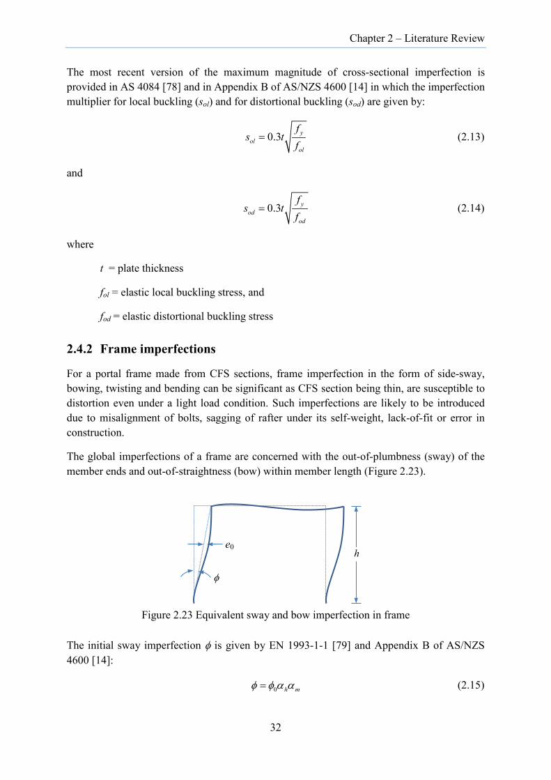
Chapter 2 – Literature Review
The most recent version of the maximum magnitude of cross-sectional imperfection is provided in AS 4084 [78] and in Appendix B of AS/NZS 4600 [14] in which the imperfection multiplier for local buckling (sol) and for distortional buckling (sod) are given by:
0.3 yol
ol
fs t
f= (2.13)
and
0.3 yod
od
fs t
f= (2.14)
where
t = plate thickness
fol = elastic local buckling stress, and
fod = elastic distortional buckling stress
2.4.2 Frame imperfections
For a portal frame made from CFS sections, frame imperfection in the form of side-sway, bowing, twisting and bending can be significant as CFS section being thin, are susceptible to distortion even under a light load condition. Such imperfections are likely to be introduced due to misalignment of bolts, sagging of rafter under its self-weight, lack-of-fit or error in construction.
The global imperfections of a frame are concerned with the out-of-plumbness (sway) of the member ends and out-of-straightness (bow) within member length (Figure 2.23).
Figure 2.23 Equivalent sway and bow imperfection in frame
The initial sway imperfection φ is given by EN 1993-1-1 [79] and Appendix B of AS/NZS 4600 [14]:
0 h mφ φ α α= (2.15)
e0
φ
h
32

Chapter 2 – Literature Review
where:
01
200φ =
2 2 , but 1.03h hh
α α= ≤ ≤
h= height of the columns in metre.
0.5(1 1/ )m mα = +
m= number of vertical members contributing to the horizontal force on the bracing system
The initial local bow imperfections of members for flexural buckling is represented by e0/L [79]:
0eL
(2.16)
where L is the member length. The recommended values of e0/L separately for elastic analysis and inelastic analysis corresponding to different buckling curves are given in EN 1993-1-1 [79].
On the other hand, Clarke et al. [80] have adopted out-of-plumbness imperfection of L/500 and out-of-straightness imperfection of L/1000 for the purpose of Advanced Analysis of the frames. The same values have been included in the Appendix B of AS/NZS 4600 [14] for the Advanced Analysis of CFS frames.
2.4.3 Integrating imperfection in numerical models
Several methods exist for the integration of imperfection in numerical models but the most popular ones are Eigen buckling mode, measured initial geometric imperfection, and notional horizontal force.
2.4.3.1 Scaled eigen buckling modes
One of the most common methods of introducing imperfection is to superimpose eigenmodes which are obtained as relative displacements from the elastic buckling analysis of a structure. Since the imperfections in the shape of the first few buckling modes have a significant influence on the behaviour, they are generally scaled by factors which are computed from the measurements. To implement this method, firstly a classic elastic buckling analysis of a structure is performed assuming the perfect geometry of the structure. Next, the buckling modes are then scaled, combined and added to the perfect geometry of the structure.
Once the scaled buckling modes are superimposed on to the perfect geometry, the non-linear analysis is performed to predict the buckling and post-buckling behaviour of the structure.
33
Chapter 2 – Literature Review
Although the incorporation of imperfection by means of superposition of eigenmodes on to the perfect geometry of the structures lends itself convenient, it has been found that buckling modes are not able to capture the localized dents and deviations which are quite common in practice [81].
2.4.3.2 Explicit modelling of initial geometric imperfection
Another method of introducing imperfection, especially for local sectional imperfections, is by direct perturbation of geometry based on the measured values of imperfections [82].
In this method, the exact measurement of the imperfections is incorporated into the FE models by directly modifying the mesh geometry. The coordinates of the nodes in the finite element mesh are altered so that it matches with the imperfect profile of the structures.
Although this method provides an accurate representation of the imperfect model, it is not practical as it can be applied only to those members for which imperfections have been measured beforehand.
2.4.3.3 Notional horizontal force
The notional horizontal force is another method to circumvent the actual measurement of the imperfection by introducing certain magnitude of the horizontal load in the numerical model of the structure. This method accounts for global imperfection in frames. In this method, a certain portion of gravity load is applied as horizontal loads to the top of each story to account for out-of-plumbness. In a similar fashion, out-of-straightness can be accounted by applying a lateral distributed force along the member or a concentrated force at the mid-height of the member [83].
This method is incorporated in many steel design codes. For instance, AS4100 [55] and AISC 360-10 [84] stipulates notional horizontal force equal to 0.2% of the total design vertical loads exerted at a particular floor level, to be applied at that floor level. EN 1993-1-1[79] recommends the use of equivalent horizontal force equal to φNEd at the top of each column for sway imperfection and uniformly distributed load equal to 8NEdeo,d/L2 on each column for bow imperfection. Here, φ is the initial sway imperfection (Equation (2.15)), NEd is the design value of the compression force in the column, e0,d is the design value of maximum amplitude of an imperfection.
In brief, modelling of geometrical imperfections for frames is much more complicated than for single members. In a CFS portal frame, stress distribution at member ends are likely to be complex compared to the single member structures owing to the discrete location of the fasteners. In such case, the localized effect may be more detrimental compared to the effect of member imperfection. Furthermore, the judicious orientation of imperfection is necessary for frames to be detrimental as certain pattern of imperfection can actually enhance the strength of a perfect frame [80] thereby defeating the whole purpose of modelling imperfection.
34
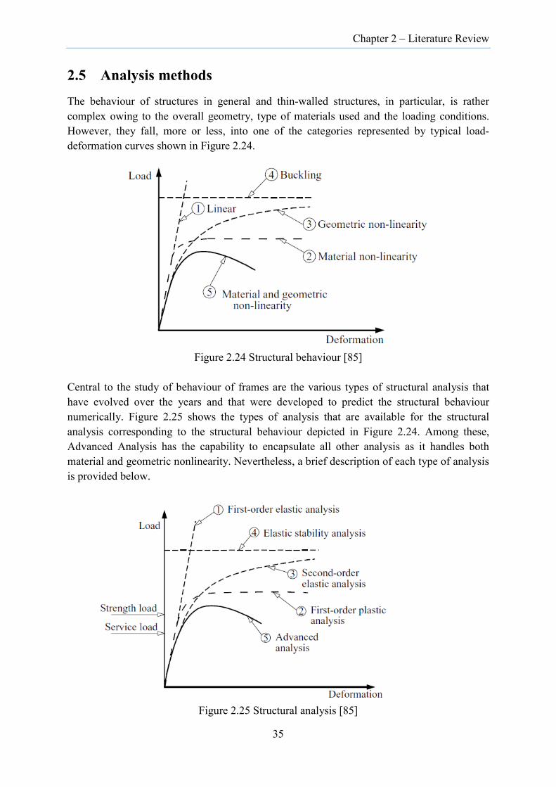
Chapter 2 – Literature Review
2.5 Analysis methods
The behaviour of structures in general and thin-walled structures, in particular, is rather complex owing to the overall geometry, type of materials used and the loading conditions. However, they fall, more or less, into one of the categories represented by typical load-deformation curves shown in Figure 2.24.
Figure 2.24 Structural behaviour [85]
Central to the study of behaviour of frames are the various types of structural analysis that have evolved over the years and that were developed to predict the structural behaviour numerically. Figure 2.25 shows the types of analysis that are available for the structural analysis corresponding to the structural behaviour depicted in Figure 2.24. Among these, Advanced Analysis has the capability to encapsulate all other analysis as it handles both material and geometric nonlinearity. Nevertheless, a brief description of each type of analysis is provided below.
Figure 2.25 Structural analysis [85]
35

Chapter 2 – Literature Review
2.5.1 First-order elastic analysis
The first-order elastic analysis, also called Linear Analysis (LA), is based on the linear elastic constitutive relationships. It ignores any geometrical nonlinearities and associated instability problems [86]. It is characterized by the structural response which is linearly proportional to the applied load. Stiffness relations are formulated based on the undeformed configuration of the structure. Hence, this type of analysis is limited to small displacement. For a linear static analysis, force-deformation relations are defined by an equilibrium equation:
1 =Ku F (2.17)
where K is the stiffness matrix, u1 is the deformation and F the applied loads. Since K is assumed to remain invariant during the course of analysis, the principle of superposition can be applied to simplify the analysis.
For a relatively large loading, the structure tends to have large displacement (geometric nonlinearity) and stresses in the material are increased beyond the elastic limit (material nonlinearity). In such case, force-deformation relations predicted by this analysis may not be representative of the true behaviour of the structure. Although this type of analysis is widely used in the industry irrespective of the type of structures, accuracy becomes questionable, especially with regard to the frames composed of cold-formed steel sections which are often marked by various instabilities.
2.5.2 Elastic stability analysis
Elastic stability analysis, also called Linear Buckling Analysis (LBA), predicts the buckling load of the structure that corresponds to a state of bifurcation of equilibrium of a perfect structure according to [86]:
0[ ]Tb G bλ− =u K K u 0 (2.18)
where K0 is the linear elastic stiffness matrix and KG is the geometric stiffness matrix which accounts for the effect of axial force P on the bending stiffness of the member, λ is the buckling load factor and ub is the buckling modes.
Since the structure is assumed to be perfect, there is no lateral deflection in the structural member until the load reaches the critical load. Upon reaching the critical load, the original configuration of the frame ceases to be stable and with a slight disturbance, the lateral deflection of structures begin to increase without bound.
In other words, at the bifurcation, the stiffness of the structure vanishes. Therefore, critical loads are obtained by solving the eigenvalue problem in which the determinant of the structural stiffness matrix is set to zero as follows:
0| |Gλ− =K K 0 (2.19)
36
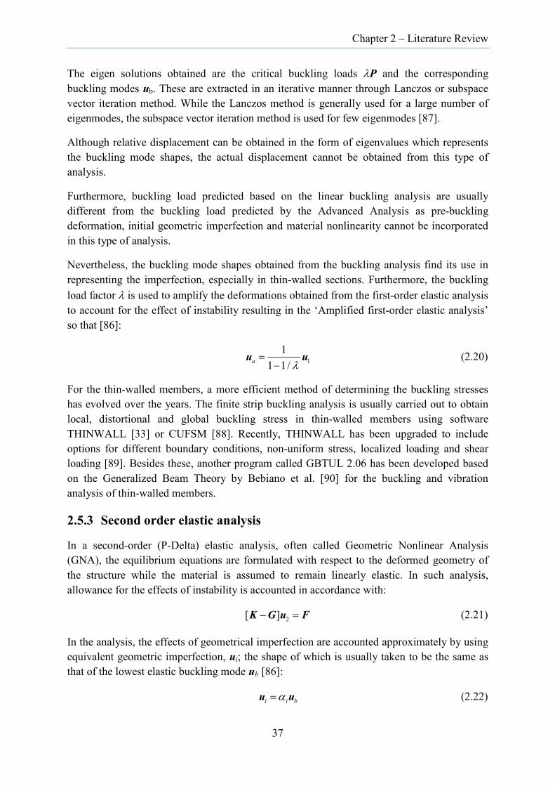
Chapter 2 – Literature Review
The eigen solutions obtained are the critical buckling loads λP and the corresponding buckling modes ub. These are extracted in an iterative manner through Lanczos or subspace vector iteration method. While the Lanczos method is generally used for a large number of eigenmodes, the subspace vector iteration method is used for few eigenmodes [87].
Although relative displacement can be obtained in the form of eigenvalues which represents the buckling mode shapes, the actual displacement cannot be obtained from this type of analysis.
Furthermore, buckling load predicted based on the linear buckling analysis are usually different from the buckling load predicted by the Advanced Analysis as pre-buckling deformation, initial geometric imperfection and material nonlinearity cannot be incorporated in this type of analysis.
Nevertheless, the buckling mode shapes obtained from the buckling analysis find its use in representing the imperfection, especially in thin-walled sections. Furthermore, the buckling load factor λ is used to amplify the deformations obtained from the first-order elastic analysis to account for the effect of instability resulting in the ‘Amplified first-order elastic analysis’ so that [86]:
11
1 1/a λ=
−u u (2.20)
For the thin-walled members, a more efficient method of determining the buckling stresses has evolved over the years. The finite strip buckling analysis is usually carried out to obtain local, distortional and global buckling stress in thin-walled members using software THINWALL [33] or CUFSM [88]. Recently, THINWALL has been upgraded to include options for different boundary conditions, non-uniform stress, localized loading and shear loading [89]. Besides these, another program called GBTUL 2.06 has been developed based on the Generalized Beam Theory by Bebiano et al. [90] for the buckling and vibration analysis of thin-walled members.
2.5.3 Second order elastic analysis
In a second-order (P-Delta) elastic analysis, often called Geometric Nonlinear Analysis (GNA), the equilibrium equations are formulated with respect to the deformed geometry of the structure while the material is assumed to remain linearly elastic. In such analysis, allowance for the effects of instability is accounted in accordance with:
2[ ]− =K G u F (2.21)
In the analysis, the effects of geometrical imperfection are accounted approximately by using equivalent geometric imperfection, ui; the shape of which is usually taken to be the same as that of the lowest elastic buckling mode ub [86]:
i i bα=u u (2.22)
37
Chapter 2 – Literature Review
in which αi is the scaling factor generally provided in the standards. For convenience, the equivalent imperfections are generally replaced by equivalent loads, i i=F Ku resulting in
2[ ] [ ]i i− =K G u F + F (2.23)
As the deformed configuration of the structure is not known in advance and is constantly changing with the applied loads, the force-displacement relationship must be obtained in an iterative manner. Often the load incremental approach is used to obtain the force-deformation response of the structure. In effect, the nonlinear responses are approximated by a series of linear analyses. Because of this, equilibrium of external and internal force must be satisfied through iterations. In here, unlike in the linear elastic analysis, the stiffness matrix is updated at each load step due to the corresponding update of frame of reference to the previous solution.
2.5.4 Plastic analysis
The plastic analysis is applicable to structures which have very small axial forces and instability effects, in which case a sufficient number of plastic hinges must form on the frame to undergo collapse mechanism [86]. This type of analysis is generally limited to the structural frames composed of members having compact sections. The material is assumed to behave linearly elastic–perfectly plastic. It is implicitly assumed that no part of the structure will fail by buckling before the plastic collapse is reached [91]. In the plastic analysis, the maximum moment that the member could carry is the plastic moment capacity of the section and the remaining moment is distributed to the elastic section of the members. The common variation of plastic analysis includes rigid-plastic analysis, 1st order elastic-plastic analysis and 2nd order elastic-plastic analysis which corresponds to the assumption of no elastic deformation, small elastic deformation and large elastic deformation before the progressive formation of plastic hinges at member ends in the structure.
Since the cold-formed steel portal frames have members that are so thin, the plastic analysis will have little relevance in the routine design of structures constructed out of CFS sections.
2.5.5 Advanced Analysis
Advanced Analysis is the second-order inelastic analysis which is used to directly determine the overall strength and stability of a steel framing system [92]. It includes both the geometry and material nonlinearities. Advanced Analysis is also called Geometric and Material Nonlinear Analysis with imperfections (GMNIA). The geometric nonlinearity includes second-order effects (associated with P-∆ and P-δ effects) and (sectional) geometric imperfections while the material nonlinearity includes gradual yielding associated with the influence of residual stresses and flexure [93]. Stiffness degradation due to material yielding in a member is taken into account by using either plastic hinge approach or plastic zone method. Since the strength of the structural systems is directly assessed based on the inclusion of nonlinear effects, the separate checks on the individual member strengths are not
38

Chapter 2 – Literature Review
required thus obviating the need for the calculation of effective length factors, which otherwise is an integral part of the conventional two-step design approach.
The realistic prediction of nonlinear behaviour by the Advanced Analysis depends on the numerical solution strategy used for solving nonlinear equilibrium equations. The exact mathematical representation of the nonlinear behaviour of the structures involves the formulation of equilibrium equations in a deformed configuration which is not normally known in advance [94]. However, the mathematical formulation of full nonlinearity is often difficult and once formulated, is hard to solve. To circumvent this problem, the nonlinear analysis is represented by the piecewise linear analysis in small time steps using incremental load or displacement approach while ensuring static equilibrium is maintained within each time step [95, 96]. Iterations are generally required to achieve the static equilibrium within the time step through the deployment of various nonlinear algorithms with each providing the same solutions.
Several incremental iterative strategies for nonlinear analyses are presented in [97]. Some of the notable nonlinear analysis algorithms include initial stiffness algorithm, tangent stiffness algorithm, and secant stiffness algorithm. The solutions in terms of displacements or forces are sought by using Newton-Raphson or Modified Newton-Raphson technique within each iteration. In the Newton-Raphson method, the tangent stiffness is updated in every cycle of iteration. However, in the modified Newton-Raphson method, the tangent stiffness is updated only at the beginning of iteration and is held constant throughout that particular cycle of iteration [97, 98].
To achieve the force equilibrium within each piecewise linear analysis, either the force-controlled or the displacement-controlled method is used. The choice for the force-controlled or displacement-controlled method depends on the expected behaviour of the structures. If the displacement response is continuously increasing with the corresponding increase of load, force controlled method would generally suffice. On the other hand, if the response is one of gradual softening upon reaching the peak load, displacement-controlled method would be required to advance the solution beyond the maximum point on the load-deflection curve. There are also cases in which the structure suddenly snaps and attains equilibrium at different configuration as in the snap-through problems. In such highly nonlinear structural problems, Riks method [99] or modified Riks method [98] are employed for tracing the load-displacement path.
The real impetus for the successful implementation of Advanced Analysis in the prediction of structural behaviour is the concurrent development of software that are available both commercially and freely. While Abaqus [18] remains one of the widely used commercial software for solving nonlinear structural problems, OpenSees [19], an open source code, is also increasingly being used in recent years. OpenSees is an object-oriented program developed in a modular fashion. It allows customized elements to be developed and linked to its class libraries with minimal interference with the existing classes. Another freely available software that is increasingly being used for the research is MASTAN2 [100]. It has warping functions included in the formulation thus making it attractive for the analysis of CFS frames.
39

Chapter 2 – Literature Review
2.6 Design methodologies for cold-formed steel portal frames
2.6.1 Current design methods
At present, cold-formed steel portal frames are designed based on a two-step process: analysis followed by design. In the first step, either first-order elastic analysis is carried out followed by moment amplification to account for second order effects or second-order elastic analysis is carried out directly to obtain forces and moments in the portal frames. The structure is usually represented by the bar model. In the second step, the capacities of each member are checked based on the current standards (AS/NZS 4600 [14], AISI S100-16 [15] and EN1993-1-3 [16]) member-by-member basis. The process is repeated until the strength and the serviceability requirements are fulfilled.
The design specifications (AS/NZS 4600:2018 and AISI S100-16) for the design of cold-formed steel structures currently include two design methods: Effective Width Method (EWM) and Direct Strength Method (DSM) [101, 102]. EWM was initially developed for the simple sections and has been in use for over 60 years. However, as more and more complex sections were produced in the market, the rigour required to compute the effective width became cumbersome. This has led to the introduction of the Direct Strength Method which does not require lengthy calculations for section properties. Thus, the DSM has rendered itself as convenient and better method at this point of time in the design of cold-formed steel sections besides some limitations.
2.6.1.1 Effective Width Method
In the Effective Width Method, the most severely buckled portions of an element are assumed to be ineffective in resisting load, and the applied compression is resisted by portions situated adjacent to the supported edges. The non-uniform compressive stress distribution in both the stiffened and unstiffened elements is replaced by a uniform stress distribution, which acts only on the effective portion of the buckled plate element [34]. Each plate forming a cross-section is reduced to its effective width and the cross-sectional properties are calculated using the effective width of the sections.
However, the Effective Width Method “ignores the inter-element (e.g. between the flange and the web) equilibrium and compatibility in determining the elastic buckling behaviour, incorporation of competing buckling modes, such as distortional buckling can be awkward, cumbersome iterations are required to determine even basic member strength, and determining the effective sections becomes increasingly complicated as attempts to optimize the sections are made”[101]. Furthermore, the computation of the effective cross-sectional properties depends on the stresses. Thus, it poses formidable tasks if one were to track deformation accurately at each load level in the frame analysis using EWM.
2.6.1.2 Direct Strength Method
Direct Strength Method (DSM) is the design method for cold-formed steel members which uses elastic buckling solutions for the entire member cross sections to give the direct strength
40

Chapter 2 – Literature Review
rather than for elements in isolation [102]. It is an alternative method to the traditional Effective Width Method. In this method, there is no requirement to calculate laborious effective section properties, especially with intermediate stiffeners. The interaction between local and overall modes is taken into account through the use of numerical solutions for elastic buckling. The buckling analysis is usually carried out using computer programs such as THIN-WALL [33] or CUFSM [88] to obtain elastic buckling stresses. The minimum points on the signature curve (Figure 2.4) correspond to local and distortional buckling stresses which are used to calculate the buckling capacities. Accurate member elastic stability is the key idea behind the Direct Strength Method.
With the buckling loads determined by the elastic buckling analysis, the nominal strength of the member under different buckling modes can be determined. The member strength is the minimum of the nominal strength due to local buckling, distortional buckling and global buckling [14, 15].
Although design guidance for members in shear, combined bending and shear, combined axial load and bending and members with holes were absent in the previous version of AS/NZS 4600 [14], it has now been incorporated in the latest version of that standard and also in AISI S100-16 [15]. The primary complication in applying DSM to members with holes is that “holes introduces the potential for interactive buckling modes triggered by the hole size, spacing, geometry, etc.” Since the finite strip method does not account for members with holes, recourse must be had to finite element methods for the elastic buckling analysis, a key ingredient of DSM [101].
A situation where DSM may potentially fail is in the design of structural members with cross-section containing very slender elements. The DSM predicts the member strength based on the member’s elastic buckling loads. If sections of a structural member contain very slender elements, it would result in very low local buckling load. In such case, the strength calculated based on DSM would be overly conservative [30]. To safeguard against such eventualities, Table 7 of new version of AS/NZS 4600 [14] imposes limits on the slenderness of the elements, number of stiffeners and the strength of CFS sections.
2.6.2 Direct Design Method using Advanced Analysis
In the current two-stage design process in which elastic analysis is carried out to determine the design action effects in each member of a structural system, the interaction between the structural system and its members is represented by the effective length factor. The problem with this representation is that it does not provide an accurate indication of the factor against failure as it does not consider the interaction of strength and stability between the member and structural system in a direct manner [17].
Both the EWM and DSM are member-based design. The forces and moments, against which the capacities calculated from these methods are checked, are obtained from either the first-order elastic analysis or the second-order elastic analysis. The capacities are checked member-by-member following a lengthy process. The linkage between the member and the system through the use of effective length concept is still prevalent in these design methods.
41

Chapter 2 – Literature Review
Furthermore, having to deal with enormous equations and conditions somehow belittle the attractiveness of these design methods.
Towards this effect, Advanced Analysis is increasingly looked upon as having the potential to simulate the realistic behaviour of the actual structure and thence base the design of the structural system.
Advanced Analysis is a geometric and material nonlinear analysis with imperfections (GMNIA) in which both the geometric and material nonlinear effects are accounted in the analysis [80]. Provided material nonlinearities, geometric nonlinearities and imperfections are properly modelled, the Advanced Analysis is most capable of predicting the true behaviour of real structures [103]. The main advantage offered by the Advanced Analysis is that separate member capacity checks against code specifications are not required since the stability of members and the structure as a whole is rigorously treated in determining the maximum strength of the structure.
Direct Design Method using Advanced Analysis was first permitted in the 1990 edition of the Australian steel structures standard AS4100 [55] for the frames comprising members with compact section and full lateral restraint. It was apparent that frames consisting of cold-formed steel members were excluded from the domain of Advanced Analysis then. However, with the latest release of AS/NZS 4600:2018 [14], the design by Advanced Analysis was first permitted for the cold-formed steel framing systems. The salient features and essential requirements for the application of Advanced Analysis in CFS frames are highlighted in Appendix B of AS/NZS4600:2018. The main benefit of using Advanced Analysis is - it allows the designer to bypass code design rules, which are generally approximate and somewhat variable in the accuracy and are often difficult to interpret appropriately [104].
2.6.2.1 Numerical models
To enable prediction of the realistic behaviour of the structures using Advanced Analysis, the numerical model must address the influence of finite joint size, joint flexibility, local instabilities, load height within cross-section and effect of secondary structural elements on the frames. A cold-formed steel portal frame, being composed of several components with several parts in contact, demands fuller knowledge in contact mechanics, meshing techniques, numerical analysis and convergence algorithms. In this context, full three-dimensional modelling using shell elements seems to be one of the promising options in capturing deformation and overcoming the drawbacks that are inherent in the stick model widely practised in design offices. Guidance on how to construct finite element models for the CFS sections can be found in [105,106]. Indeed, in recent years, shell element modelling has been implemented by Lim and Nethercot [8], Zhang et al. [107], Cardoso [108] and Hannah [13] for the study of CFS portal frames, mainly with double C-sections connected back-to-back.
At present, the main hurdle in the implementation of Advanced Analysis is imposed by the requirement to solve large stiffness equations, and that too must be repeated several times before the solution in the form of equilibrium path is obtained, which inevitably requires high-performance computing facilities. Such impediment to the wider application of
42

Chapter 2 – Literature Review
Advanced Analysis will, however, slowly phase out especially with the spur in the development of low-cost parallel processing computing facilities.
2.6.2.2 Reliability-based design
In reliability-based design, the Advanced Analysis is carried out in combination with a probabilistic assessment of structural variables to determine the strength of the structure. Such method of strength check has the format similar to Load and Resistance Factor Design (LRFD) [109]:
s n i niR Qφ γ≥∑ (2.24)
in which Rn is the nominal system strength (load-carrying capacity of the whole structural system) predicted by the Advanced Analysis and φs is the system resistance factor (also known as the capacity reduction factor in AS/NZS 4600:2018 [14]) determined by reliability assessment. Here, the load-carrying capacity is obtained by applying incremental loads until a structure reaches its limit state by yielding or buckling [17]. The right-hand side of the Equation (2.24) represents the total loads applied to the structure. The adequacy of the structure can be directly evaluated by comparing the resulting load-carrying capacity φsRn with the total applied factored loads ΣγiQni. For the CFS portal frames, system resistance factor (capacity reduction factor), φs is provided as 0.85 in Table B4 of AS/NZS 4600 [14].
In such Advanced Analysis, the material properties, initial geometric imperfections, residual stresses and loads are treated as random variables [109]. Probabilistic simulations are carried out to derive mean, standard deviation and distribution type for the system strength. Based on these derived parameters together with probabilistic models for dead and live load, reliability index, β can be determined using first-order reliability method. The reliability index, β is a relative measure of safety of a structure. The higher the value the safer is the structure. Since the system resistance factor, φs and reliability index, β are interrelated, one cannot be determined without defining the value of the other. At present, the practice is to fix one of them and derive the other.
A more general approach of determining the relationship between the resistance factor φ and the reliability index β involves establishing the limit state functions and determining the unknowns following the established procedures based on the first-order second-moment (FOSM) reliability method.
For a linear limit state function of the form [110]:
1 2 01
( , ,..., )n
n i ii
g X X X a a X=
= +∑ (2.25)
the reliability index β is given by:
43

Chapter 2 – Literature Review
0
1
2
1( )
i
i
n
i Xi
n
i Xi
a a
a
µβ
σ
=
=
+=
∑
∑ (2.26)
where ai terms are constants and Xi terms are uncorrelated random variables; iXµ and
iXσ are
the corresponding mean and standard deviation.
For a nonlinear limit state function, reliability index β must be determined in an iterative manner which typically involves redefining the limit state function in terms of reduced variables using:
i
i
i Xi
X
XZ
µσ−
= (2.27)
and solving set of (2n+1) simultaneous equations with (2n+1) unknowns (β, α1, α2,…, αn, * * *1 2, ,..., nz z z where
at design point
2
1 at design point
ii
n
k k
gZ
gZ
α
=
−∂∂
= −∂ ∂
∑
(2.28)
i
iX
i i i i
Xg g gZ X Z X
σ∂∂ ∂ ∂= =
∂ ∂ ∂ ∂ (2.29)
2
11
n
iiα
=
=∑ (2.30)
*i iz βα= (2.31)
* * *1 2( , ,..., ) 0ng z z z = (2.32)
One of the most popular methods of solving this set of simultaneous equations is the matrix procedure which consists of the following steps [110]:
1. Formulate the limit state function and relevant parameters for all random variables Xi 2. Obtain an initial design point *
ix by assuming values for n-1 of the random variables Xi and the remaining ones by solving limit state equation, g=0.
3. Determine the reduced variables *iz corresponding to the design point using
* *( ) /i ii i x xz x µ σ= −
44
Chapter 2 – Literature Review
4. Determine the partial derivatives of the limit state function with respect to the reduced variables to obtain vector G:
[ ]1 2evaluated at design point
.... where Tn i
i
gG G G Gz∂
= = −∂
G (2.33)
5. Calculate an estimate of reliability index β :
*
* * * *1 2 where ...
T T
nTz z zβ = =
G z zG G
(2.34)
For linear performance function, Equation (2.34) simplifies to Equation (2.26)
6. Calculate column vector containing the sensitivity factors, α:
T
=G
G Gα (2.35)
7. Determine a new design point in reduced variables for n-1 of the variables using *i iz α β=
8. Determine the corresponding desing points in original coordinates for the n-1 variables * *
i ii x i xx zµ σ= +
9. Obtain the remaining variables (not found in step 7 and 8) by solving g=0 10. Repeat steps 3 to 9 until β and the design point *
ix converge.
Reliability-based design is an emerging technology. A wealth of knowledge already exists for the Advanced Analysis of the hot-rolled steel structures. A similar suite is destined to follow for the cold-formed steel structures. Towards this effect, the reliability analysis has been implemented by Cardoso [108] in the development of a system-reliability based approach for designing CFS portal frames and storage racks.
2.7 Summary
This literature review provided insights into the current state of knowledge on portal frames comprising CFS sections. In particular, various instabilities that are common in CFS sections, imperfections, types of analysis and design and the future trends in design are highlighted.
The past studies on the CFS portal frames and associated connections have been largely on the frames comprising doubly symmetric members formed by connecting channel section back-to-back. The research on CFS single C-section portal frames is relatively rare. The past researches have indicated that the joints in CFS portal frames are generally semi-rigid and the stiffness of the joint is highly dependent on the geometry of the connection bracket, member thickness and the bolt configuration. The bolting method adopted in many connections are
45
Chapter 2 – Literature Review
snug-tight which resulted in significant bolt hole elongation; thus further contributing to the semi-rigidity of the connections.
The behaviour of cold-formed steel members is characterized by instabilities due to the slenderness of the section. Hence, imperfections are likely to be more onerous for the determination of strength in CFS sections than in hot-rolled sections. The prevailing design methods, namely the Effective Width Method and Direct Strength Method, while serving as the contemporary tool for the design of CFS sections, are not without shortcomings. Hence, the Advanced Analysis is seen as an attractive alternative design method that has the potential to radically change design paradigm.
Direct Design Method using Advanced Analysis is a novel approach in which the strength of the whole systems rather than the individual members can be determined with the incorporation of inelasticity of material and geometric nonlinear effects. While its application in the realm of hot-rolled steel frames possessing compact sections is well established, very few have ventured into its application in frames comprising CFS sections. The possible reason for such absence of research in the Advanced Analysis of CFS frames is attributed to the inability of beam elements to capture instabilities that are prevalent in CFS frames unless the numerical models are created using either shell elements or solid elements which then leads to high computational costs. However, with the upsurge of development of high-performance parallel computational algorithms, the design by Advanced Analysis holds promising hope for becoming a robust, routine design for all types of structures including those composed of CFS sections.
46
Chapter 3 – Formulation
CHAPTER 3. FORMULATION FOR THE GEOMETRIC NONLINEAR ANALYSIS OF GENERAL THIN-WALLED SECTIONS
3.1 Introduction The structural behaviour of thin-walled open sections is rather complex owing to their low torsional rigidity and propensity to buckle and warp. Quite often the shear centre and the centroid are non-coincident as in monosymmetric or asymmetric sections. In some sections, such as in channel sections, the shear centre and the centroid are both located outside the material point. Six degrees of freedom commonly used in the solid sections are often not adequate to completely define the deformation of thin-walled open sections, as they are prone to warping. All these factors must be taken into account when formulating the finite element of beams with open cross-sections.
Over the years, several researchers have made significant contributions towards the theoretical and numerical modelling of thin-walled sections. Baigent and Hancock [2] and Hancock [27] formulated the matrix displacement method incorporating the warping torsion for the linear elastic analysis of general thin-walled sections. They also introduced warping as the 7th degree of freedom at the beam ends and successfully implemented for the analysis of single channel-section portal frames. Rasmussen [35] derived the variational equations for general bifurcation analysis of thin-walled members of arbitrary cross-section. Pi and Trahair [111] developed a beam finite element for the prediction of lateral buckling of mono-symmetric beams which included the effect of pre-buckling deformation. In the context of large displacement analysis, Gruttmann et al. [112], Hsiao and Lin [113] and Battini and Pacoste [114] formulated a co-rotational beam element for thin-walled sections with eccentric shear centre and centroid. Alemdar [115] derived the expression for the displacement-based beam element in the co-rotational formulation for the doubly symmetric sections. Recently, Zhang et al. [116] incorporated the warping degree of freedom in OpenSees [19] and used the method for the nonlinear analysis of doubly-symmetric sections.
In the current formulation, the stiffness relations are established for the thin-walled beam elements with general open cross-sections within the co-rotational framework of OpenSees. Two elements, namely an elastic beam element (EB) and a displacement based beam element (DB), are considered. While the EB element is developed only to validate the solution, the focus has been mainly on the DB element. In terms of displacement functions, both the elastic beam elements and the displacement-based beam elements use cubic polynomials as interpolation function for the transverse displacement and the twist, and a linear function for the axial displacement. However, the main difference between EB and DB elements is that the EB elements are formulated with the treatment of each force in isolation and the strain terms used are mostly linear, while the DB elements take account of the nonlinear Green-Lagrange strain in the formulation. DB elements also have the capability to account for distributed plasticity within the section and along the beam length. However, in this chapter, the material is assumed to remain linearly elastic throughout the analysis. The formulations are based on Vlasov’s kinematics [26] in which the cross-section is assumed to retain its
47
Chapter 3 – Formulation
original shape while undergoing overall deformation. The shear deformations due to warping torsion are assumed negligible. As the thin-walled cross-sections are susceptible to warping, a warping degree of freedom is also included in the formulation.
To account for the non-coincident shear centre and centroid of the cross-section, a local transformation matrix is developed to relate the system of forces acting at the shear centre and at the centroid. The beam elements are incorporated in OpenSees and their performance tested through the analysis of doubly symmetric section, singly symmetric section and asymmetric section subjected to axial compression, bending and torsional loading.
In the sections to follow, a brief description of the co-rotational framework along with the coordinate systems adopted for the formulation is presented. The stiffness relations for the EB elements are outlined next, followed by the detailed formulation for the DB elements. The local transformation matrix and the transformation from local to global axis systems are described next. In the end, the various benchmark problems highlighting the performance of the EB and the DB elements are provided.
3.2 Formulation of general thin-walled open section beam in OpenSees
The co-rotational approach of formulating the nonlinear finite element involves the decomposition of motion of the element into rigid body and pure deformational parts through the use of a reference system which continuously rotates and translates with the element [114,117,118]. The rigid body motion of the element is excluded and only the deformational response is considered in the stiffness formulation at the local level. However, the geometric nonlinearity induced by the large rigid body motion is captured in the global coordinate system through the transformation matrices relating local and global response quantities.
One of the main features of the co-rotational formulation is its independence of the derivation of internal forces and tangent stiffness relations at the local system. The mapping from local to global system remains the same for all types of local elements so long as the element has the same number of nodes and degrees of freedom [114].
3.2.1 Coordinate systems
3.2.1.1 Global coordinate systems
In the global coordinate system, the beam element has 7 degrees of freedom (DoFs) at each end: 3 translations, 3 rotations and 1 warping DoF (Figure 3.1). The sign of the rotations follows the right hand rule.
48

Chapter 3 – Formulation
Figure 3.1 Global degree of freedom systems
The global end displacements are represented in vector form as
' '1 1 1 1 1 1 1 2 2 2 2 2 2 2
T
X Y Z b X Y Z bu v w u v wθ θ θ θ θ θ θ θ = U (3.1)
The corresponding global end actions are represented by
' '1 1 1 1 1 1 1 2 2 2 2 2 2 2
T
X Y Z X Y Z b X Y Z X Y Z bF F F M M M M F F F M M M M = F (3.2)
where 𝑀1𝑏′ and 𝑀2𝑏
′ are the bimoments at the beam ends 1 and 2 respectively.
3.2.1.2 Local coordinate systems
In the co-rotational formulation, the rigid body components (translational DoFs) are removed from the element and only the axial, rotational and torsional components are retained in the local coordinate system. Hence, at the local level, the element has only 4 DoFs at each end: 3 rotations and 1 warping DoF, and an axial elongation within the element (Figure 3.2).
Figure 3.2 Local degree of freedom systems
The 9 local displacements are represented in vector form as
49

Chapter 3 – Formulation
' '1 2 3 1 4 5 6 2
T
l l l b l l l b eθ θ θ θ θ θ θ θ = u (3.3)
The corresponding local end actions are
' '1 2 3 1 4 5 6 2
T
l l l b l l l b lM M M M M M M M N = f (3.4)
In the above expressions, θ1𝑏 ′ and θ2𝑏
′ are the end twist; e is the axial deformation, 𝑀1𝑏′ and 𝑀2𝑏
′ are the bimoments at each end. The other notations are self-explanatory. As noted in Figure 3.1 and Figure 3.2, the warping DoF remains constant during the transformation from the local system to global system as warping is in itself a deformational quantity and having an effect only on the local element formulation [116].
3.2.2 Elastic beam element
3.2.2.1 Elastic stiffness relations
The elastic beam element (EB) formulation within the co-rotational framework for the doubly-symmetric sections has been implemented by Alemdar [115] and Zhang et al. [116]. The first order stiffness relations for the elastic beam with coincident shear centre and stiffness are developed by treating individual deformation and corresponding end actions in isolation based on the linear-elastic theory. The stiffness equation relating the end actions and deformation within the local coordinate systems is
l=f k u (3.5)
where f is given by the Equation (3.4), u by the Equation (3.3) and kl by
3 2 3 2
2 2
3 2
12 6 12 66 60 0 0 0 0
5 10 5 104 2
0 0 0 0 0 0 0
4 20 0 0 0 0 0 0
6 4 6 220 0 0 0 0
10 15 10 3012 6 126
0 05 10
w w w w
z z
y y
w w w w
w w wl
EI EI EI EIGJ GJ GJ GJL L L L L L
EI EIL L
EI EI
L LEI EI EI EIGJ GJL GJ GJLL L L LEI EI EIGJ GJL L L L
+ + − + +
+ + − + −
− + − +
=
k3 2
2 2
660 0 0
5 102 4
0 0 0 0 0 0 0
2 40 0 0 0 0 0 0
6 2 6 4 20 0 0 0 0
10 30 10 15
0 0 0 0 0 0 0 0
w
z z
y y
w w w w
EIGJ GJL L
EI EIL L
EI EI
L LEI EI EI EIGJ GJL GJ GJLL L L L
EAL
+ − +
+ − − + +
(3.6)
50
Chapter 3 – Formulation
where E =Elastic modulus, G=Shear modulus, Iz=Second moment of area about z-axis, Iy=Second moment of area about y-axis, Iw=Warping constant, J=Torsional constant, L=Element length, and A=Cross-sectional area of the element. The basis and further details of the derivation can be found in [2, 27, 95].
For the open section beam with eccentric shear centre and centroid, the cross-section transformation derived in Section 3.2.4 is needed to be incorporated prior to the co-rotational transformation. Furthermore, the torsional rigidity GJ is required to be modified to incorporate the Wagner terms for the general EB element, the details of which are provided in the following section.
As the EB element is developed on the basis of linear-elastic theory, nonlinear geometric effects are ignored at the local element level [116]. However, they can be adequately captured during the co-rotational transformation from local to global systems if sufficient number of elements are used along the beam member.
3.2.2.2 Modification of torsional rigidity
For the EB elements to predict the buckling load, the torsional rigidity GJ is required to be modified to include the Wagner effect [119, 120] as follows:
2 2 20 0 0( ) ( )m y y z zGJ GJ N r y z M Mβ β= + + + + + (3.7)
where r0 is given by:
20
y zI Ir
A+
= (3.8)
and βy and βz are the monosymmetry section constants in the respective directions given by:
2 20
2 20
( ) / 2
( ) / 2
y yA
z zA
z y z dA I z
y y z dA I y
β
β
= + −
= + −
∫
∫ (3.9)
In the above, N is the axial force within the element and is negative for a beam in compression; and My and Mz are moments about the principal y-axis and z-axis respectively.
The theoretical basis of this equation can be traced to torsional buckling equations derived by Timonshenko [119] and energy equations by Trahair [120].
3.2.3 Displacement-based beam element
The displacement-based beam element (DB) is a higher order element compared to the elastic beam (EB) element. In the case of DB element, besides the inclusion of normal strains arising from the axial deformation, flexural deformation and warping, it also accounts for the strain contributions arising from the coupling of flexure and torsion. Here the section deformations are determined based on the approximate displacement field and the Principle of Virtual Work is applied to form the equilibrium equations. One underpinning assumption for the DB
51

Chapter 3 – Formulation
element is that the strain developed within the element is considered small while undergoing large displacement and large rotations.
The DB element also possesses the capability to accommodate the spread of material plasticity along the length and within the cross-section of the element. However, this capability is not explored in this study. The stiffness relations for the DB element are discussed next.
3.2.3.1 Displacement field
Consider a case where a typical thin-walled open cross-section undergoes translation followed by a twist rotation about the shear centre axis (Figure 3.3). During this deformation process, the shear centre of the cross-section undergoes displacements u, v and w parallel to the original x-, y-, z-axes, and twist rotation φ about the shear centre axis parallel to the x-axis. Hence the shear centre S translates to S1 and the point P moves to P1 and then finally to P2 because of rotation about the longitudinal axis passing through S1.
Figure 3.3 Displacements and rotations of arbitrary thin-walled open cross-section
The corresponding displacements (up,vp,wp) of a point P(y,z) on the cross-section in the respective x-, y- and z-direction are given by:
( )( )
0
0
' ' ' ' 'p
p
p
u u yv zw yw zv
v v z z
w w y y
ωφ φ φ
φ
φ
= − − + − +
= − −
= + −
(3.10)
where (y0,z0) are the coordinates of the shear centre and ω is the normalized sectorial coordinate with respect to the shear centre. Similar derivation for a different axis system is provided in [120].
52

Chapter 3 – Formulation
The sectorial coordinate (sectorial area) ω is given by [26, 119, 120]:
0 00
s
dsω ω ρ= − ∫ (3.11)
where ρ0 is the perpendicular distance from the shear centre to the tangent to the centreline of the cross-section and s is the distance along the centreline of the cross-section. The sign of ρ0 is taken as positive in a counter-clockwise direction. ω0 is given by:
0 00
1 s
A
ds dAA
ω ρ
= ∫ ∫ (3.12)
The Equation (3.11) satisfies the condition 0.A
dAω =∫
In the co-rotational formulation, the rigid body motion components of deformation are ignored. Hence, the transverse displacement (v, w) and torsional displacement (φ) are expressed in terms of end rotations. Likewise, axial displacement u is expressed in terms of the normal elongation e for the whole length (L) of the beam. Hence, the displacement functions describing the deformations of beam element are given by:
1
1 2 2 5
1 3 2 6' '
1 1 2 1 3 4 4 2
u
v l v l
w l w l
l b l b
u N ev N Nw N N
N N N Nφ φ φ φ
θ θθ θ
φ θ θ θ θ
== += +
= + + +
(3.13)
where Nu1, Nv1, Nv2, Nw1, Nw2, Nφ1, Nφ2, Nφ3 and Nφ4 are respective shape functions given by [115, 95]:
1
2
1 1 2
2 2 4
2 3
1
2 3
3
1
1
1 3 2
3 2
u
v w
v w
xNL
xN N N xL
x xN N N xL L
x xNL L
x xNL L
φ
φ
φ
φ
=
= = = − = = = −
= − +
= −
(3.14)
Here it must be noted that a constant axial deformation and linear curvature distribution are enforced along the beam length. Hence, mesh refinement is required to represent the higher order distribution of deformation.
53

Chapter 3 – Formulation
The displacement functions and end DoFs can be expressed in matrix form as
TuTvTwT
uvw
φφ
=
=
=
=
N uN uN uN u
(3.15)
where
[ ][ ][ ]
1
1 2
1 2
1 2 3 4
0 0 0 0 0 0 0 0
0 0 0 0 0 0 0
0 0 0 0 0 0 0
0 0 0 0 0
Tu u
Tv v v
Tw w w
Tw
N
N N
N N
N N N Nφ φ φ φ
=
=
=
=
N
N
N
N
(3.16)
and u is given by the Equation (3.3).
3.2.3.2 Strain-displacement relations
For large displacement analysis, the longitudinal finite strain at the point P(y,z) on the cross-section is expressed as [35]:
2 2 2
12
p p p pp
u u v wx x x x
ε ∂ ∂ ∂ ∂
= + + + ∂ ∂ ∂ ∂ (3.17)
where x is the longitudinal direction and (u,v,w) are displacements in the (x,y,z) directions respectively. It is assumed the (y,z) are principal axes.
For small gradient of axial displacement strains, this may be approximated by:
2 2
12
p p pp
u v wx x x
ε ∂ ∂ ∂
= + + ∂ ∂ ∂ (3.18)
By substituting the corresponding derivatives of the Equation (3.10) into the Equation (3.18), the axial strain is obtained as:
2 2 2 2 2
0 0
0 0
1 1' '' '' " ( ') ( ') ( ) ( ) ( ')2 2
( ' ') ' ( " ")
p u yv zw v w y y z z
z v y w zv yw
ε ωφ φ
φ φ
= − − + + + + − + −
+ − + − (3.19)
In the above, 𝑢’ is the axial strain due to elongation, 𝑦𝑣” and 𝑧𝑤” are axial strain due to bending about both axes, 𝜔∅′′ is the axial strain contribution from the torsional warping, 𝑧𝑣”∅ and 𝑦𝑤”∅ are axial strain arising due to coupling between bending and torsion, ½𝑣′2 and ½𝑤′2 are the geometric nonlinear effect [115], ½[(𝑦 − 𝑦0)2 + (𝑧 − 𝑧0)2]∅′2 is Wagner term (coupling between axial strain and torsion), and 𝑧0𝑣′∅′ and 𝑦0𝑤′∅′ are geometric
54
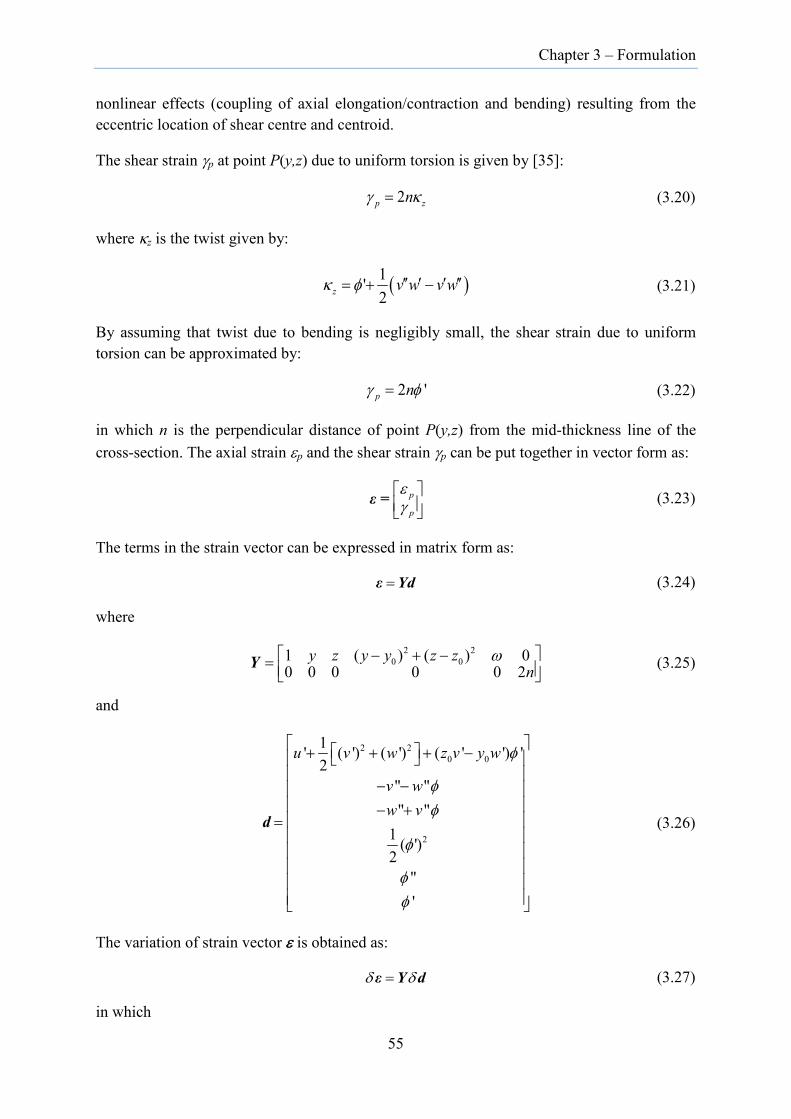
Chapter 3 – Formulation
nonlinear effects (coupling of axial elongation/contraction and bending) resulting from the eccentric location of shear centre and centroid.
The shear strain γp at point P(y,z) due to uniform torsion is given by [35]:
2p znγ κ= (3.20)
where κz is the twist given by:
( )1'2z v w v wκ φ ′′ ′ ′ ′′= + − (3.21)
By assuming that twist due to bending is negligibly small, the shear strain due to uniform torsion can be approximated by:
2 'p nγ φ= (3.22)
in which n is the perpendicular distance of point P(y,z) from the mid-thickness line of the cross-section. The axial strain εp and the shear strain γp can be put together in vector form as:
p
p
εγ
ε = (3.23)
The terms in the strain vector can be expressed in matrix form as:
=ε Yd (3.24)
where
2 2
0 01 ( ) ( ) 00 0 0 0 0 2
y z y y z zn
ω − + −= Y (3.25)
and
2 20 0
2
1' ( ') ( ') ( ' ') '2
" "" "
1 ( ')2
"'
u v w z v y w
v ww v
φ
φφ
φ
φφ
+ + + −
− − − + =
d (3.26)
The variation of strain vector ε is obtained as:
δ δ=ε Y d (3.27)
in which
55
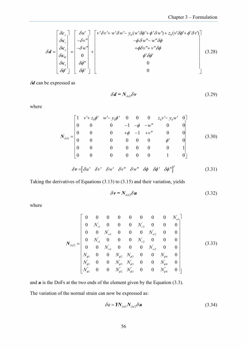
Chapter 3 – Formulation
0 0' ' ' ' ' ( ' ' ' ') ( ' ' ' ')" " "" " "
0 ' '" 0
' ' 0
x
z
y
W
x
u v v w w y w w z v vv w ww v v
δε δ δ δ δφ φ δ δφ φ δδκ δ φδ δφδκ δ φδ δφ
δδκ φ δφδκ δφδφ δφ
+ − + + + − − − − + +
= = +
d (3.28)
δd can be expressed as
1dδδ δd = N v (3.29)
where
0 0 0 0
1
1 ' ' ' ' 0 0 0 ' ' 00 0 0 1 " 0 00 0 0 1 " 0 00 0 0 0 0 0 ' 00 0 0 0 0 0 0 10 0 0 0 0 0 1 0
d
v z w y z v y wwv
δ
φ φφ
φφ
+ − − − − − + − +
=
N (3.30)
[ ]' ' ' " " ' " Tu v w v wδ δ δ δ δ δ δφ δφ δφ=v (3.31)
Taking the derivatives of Equations (3.13) to (3.15) and their variation, yields
2dδδ δv = N u (3.32)
where
'1
' '1 2
' '1 2
' '1 2
2 ' '1 2
1 2 3 4' ' ' '1 2 3 4
'' '' '' ''1 2 3 4
0 0 0 0 0 0 0 00 0 0 0 0 0 00 0 0 0 0 0 00 0 0 0 0 0 00 0 0 0 0 0 0
0 0 0 0 00 0 0 0 00 0 0 0 0
u
v v
w w
v vd
w w
NN N
N NN N
N NN N N NN N N NN N N N
δ
φ φ φ φ
φ φ φ φ
φ φ φ φ
=
N (3.33)
and u is the DoFs at the two ends of the element given by the Equation (3.3).
The variation of the normal strain can now be expressed as:
1 2d dδ δδ δ=ε YN N u (3.34)
56
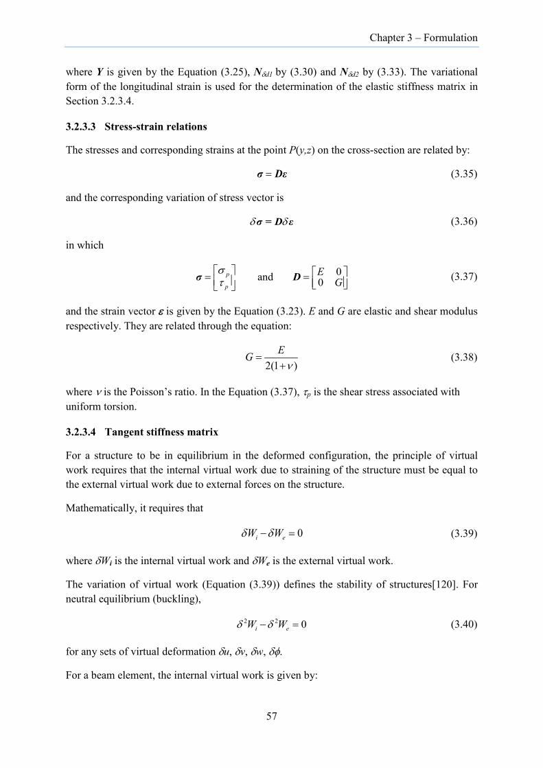
Chapter 3 – Formulation
where Y is given by the Equation (3.25), Nδd1 by (3.30) and Nδd2 by (3.33). The variational form of the longitudinal strain is used for the determination of the elastic stiffness matrix in Section 3.2.3.4.
3.2.3.3 Stress-strain relations
The stresses and corresponding strains at the point P(y,z) on the cross-section are related by:
=σ Dε (3.35)
and the corresponding variation of stress vector is
δ δσ = D ε (3.36)
in which
0and 0p
p
EG
στ = =
σ D (3.37)
and the strain vector ε is given by the Equation (3.23). E and G are elastic and shear modulus respectively. They are related through the equation:
2(1 )
EGν
=+
(3.38)
where ν is the Poisson’s ratio. In the Equation (3.37), τp is the shear stress associated with uniform torsion.
3.2.3.4 Tangent stiffness matrix
For a structure to be in equilibrium in the deformed configuration, the principle of virtual work requires that the internal virtual work due to straining of the structure must be equal to the external virtual work due to external forces on the structure.
Mathematically, it requires that
0i eW Wδ δ− = (3.39)
where δWi is the internal virtual work and δWe is the external virtual work.
The variation of virtual work (Equation (3.39)) defines the stability of structures[120]. For neutral equilibrium (buckling),
2 2 0i eW Wδ δ− = (3.40)
for any sets of virtual deformation δu, δv, δw, δφ.
For a beam element, the internal virtual work is given by:
57

Chapter 3 – Formulation
0
Ti
V
W dVδ = ∫ δε σ (3.41)
and external virtual work by:
Te extWδ δ= u Q (3.42)
Using Equation (3.34), the internal virtual work, δWi can be expressed as
0
0
2 1
2 1
T T T Ti d d
l A
T T Td d f
l
W dA dx
dx
δ δ
δ δ
δ δ
δ
=
=
∫ ∫
∫
u N N Y σ
u N N S (3.43)
Using Equation (3.39), we obtain
0
2 1 int0 or 0δ δδ
− = − = ∫u N N S Q q QT T T
d d f ext extl
dx (3.44)
where the internal force vector qint is:
0
int 2 1T T
d d fl
dxδ δ= ∫q N N S (3.45)
Sf is the vector of section force (stress resultants) expressed as
0
0
2 20 0
1 000 ( ) ( ) 00
0 2
Tf
A
A
dA
yz dAy y z z
n
στ
ω
=
= − + −
∫
∫
S Y σ
(3.46)
0
0
0
0
0
0
2 20 0( ) ( )
2
A
A
A
A
A
A
dA
y dA
z dA
y y z z dA
dA
n dA
σ
σ
σ
σ
ωσ
τ
= − + −
∫∫∫
∫∫∫
(3.47)
58

Chapter 3 – Formulation
whereby,
0
0
0
0
0
0
2 20 0 0
( ) ( )
2
A
zA
yA
A
A
A
N dA
M y dA
M z dA
W y y z z dA
B dA
T n dA
σ
σ
σ
σ
ωσ
τ
=
− =
=
= − + −
=
=
∫
∫
∫
∫
∫
∫
in which N, Mz ,My ,W0, B and T are axial force, bending moment about the z-axis, bending moment about the y-axis, Wagner stress resultant, bimoment and uniform torque at the particular cross-section of the beam.
Using Equation (3.40), the tangent stiffness matrix for a displacement-based beam element can be obtained as
0 0
2 2 T Ti
V V
W dV dVδ δ= +∫ ∫δ ε σ δε σ (3.48)
Substituting Equations (3.35) and (3.36), and the variation of the Equation (3.34) into (3.48), we get
0 0
22 1
T T T Ti d d f
l V
W dx dVδ δδ δ δ δ δ= +∫ ∫u N N S ε D ε (3.49)
The product of δNδd1 and Sf can be further expressed as
1 2d
Tf dδ δδ δ=N S GN u (3.50)
where G is the stability matrix at the local level given by:
0
0
0 0 0
0 0 0 0 0 0 0 00 0 0 0 0 00 0 0 0 0 00 0 0 0 0 0 00 0 0 0 0 0 00 0 0 0 0 00 0 0 0 00 0 0 0 0 0 0 0
y
z
y z
N NzN Ny
MM
M MNz Ny W
−
= −
G (3.51)
Hence, substituting the relevant expressions into the Equation (3.49), we have
59

Chapter 3 – Formulation
0 0 0
22 2 2 1 1 2
T T T T Ti d d d d d d
l l A
W dx dA dxδ δ δ δ δ δδ δ δ = + ∫ ∫ ∫u N GN N N Y DY N N u (3.52)
where the terms within the square bracket represent the elastic stiffness matrix, kl in the local coordinate system. Thus,
0 0
2 2 2 1 1 2T T T
l d d d d t d dl l
dx dxδ δ δ δ δ δ= +∫ ∫k N GN N N k N N (3.53)
where kt is the elastic tangent stiffness matrix given by:
0
Tt
A
dA= ∫k Y DY (3.54)
Upon substituting Y from the Equation (3.25) and D from the Equation (3.37), kt is obtained as
0
2
2 2
2 2
2 2 2 4 2
2 2
2
1 00000
0 0 0 0 0 (4 ) /
tA
y z py y yz p y yz yz z p z zE dAp p y p z p p
y z pG n E
ωωωω
ω ω ω ω ω
=
∫k (3.55)
in which 2 2 20 0( ) ( )p y y z z= − + − .
3.2.4 Transformation of element stiffness matrix for general sections
The stiffness relations of the Equation (3.5) are derived for beam elements with coincident shear centre and centroid. Further, the stiffness relations described in section 3.2.3.4 assumes that force systems relate to the shear centre. Since the thin-walled sections such as single channel sections have an eccentric shear centre and centroid, the above stiffness relations are not directly applicable but required to be transformed prior to the application of co-rotational transformation.
Within the framework of conventional thin-walled beam element formulation, there are seven actions with corresponding displacements at each end of a thin-walled beam element. These include three forces (Fx, Fy, Fz), three moments (Mx, My, Mz) and one bimoment ( '
bM ). In the case of thin-walled beam elements, they do not necessarily act through a common point [27]. The shear forces (Fy, Fz) act through the shear centre with directions parallel to the principal axes, the axial force (Fx) acts along the centroidal axis, the moments (My, Mz) act about the principal axes (y,z) but in planes containing the shear centre, and the torque (Mx) acts about the shear centre axis.
In conformation to the principles of the co-rotational framework, the rigid body motion parts of the end actions are ignored and only the deformational parts are considered at the local
60

Chapter 3 – Formulation
level. Hence, the shear forces (Fy, Fz) are neglected and the axial force (Fx) at two ends are replaced by a single axial force, N within the element. This axial force, N acts through the centroid resulting in uniform axial deformation of the cross-section.
3.2.4.1 Transformation matrix
In the following, a local transformation matrix is derived that relates the state of force system with axial force N acting at the shear centre (Figure 3.4) and at the centroid (Figure 3.5). As observed in the figures, the shear forces (Fy, Fz) have been excluded as befitting to the co-rotational approach of beam element formulation. These forces are, however, recovered at the global level through co-rotational transformation.
Figure 3.4 Element force system with axial force acting at the shear centre
Figure 3.5 Element force system with axial force acting at the centroid
61

Chapter 3 – Formulation
Due to the change in position of the axial force to the centroid, the moments and the bimoments are affected in the original force system. The new end actions are related to the original end actions as follows:
1 1
2 2 0
3 3 0' '1 1
4 4
5 5 0
6 6 0' '2 2
( )( )
( )( )
l l
l l c
l l c
b b c
l l
l l c
l l c
b b c
M MM M N y yM M N z zM M NM MM M N y yM M N z zM M NN N
ω
ω
=
= − −
= + −
= +
=
= + −
= − −
= −
=
(3.56)
where ωc is the sectorial coordinate at the point of application of concentrated axial force, here, in this case, is the centroid. However, if the axial force is applied as a uniform stress, this term is not considered according to the theory of Vlasov [26].
The above set of equations can be arranged in matrix format as
=f Af (3.57)
where
' '1 2 3 1 4 5 6 2, , , , , , , ,
T
l l l b l l l bM M M M M M M M N = f (3.58)
' '1 2 3 1 4 5 6 2, , , , , , , ,
T
l l l b l l l bM M M M M M M M N = f (3.59)
and
0
0
0
0
1 0 0 0 0 0 0 0 00 1 0 0 0 0 0 0 ( )0 0 1 0 0 0 0 0 ( )0 0 0 1 0 0 0 00 0 0 0 1 0 0 0 00 0 0 0 0 1 0 0 ( )0 0 0 0 0 0 1 0 ( )0 0 0 0 0 0 0 10 0 0 0 0 0 0 0 1
c
c
c
c
c
c
y yz z
y yz z
ω
ω
− − + − =
+ − − −
−
A (3.60)
in which f is the force system in the transformed coordinates, f is the force system in the original coordinates, and A is the transformation matrix resulting from the translation of axial force from the shear centre to the centroid of the cross-section. Based on the reciprocal
62

Chapter 3 – Formulation
theorem, it can be concluded that the nodal degrees of freedom after the transformation of axial force to the centroid is
T=u A u (3.61)
Using Equations (3.57) and (3.61), the transformed local stiffness matrix can be expressed as
Tl l=k Ak A (3.62)
3.2.5 Global stiffness matrix
Within the co-rotational framework, the relation between the local and the global variables is obtained [117] as
δ δ=u T U (3.63)
and from the principle of virtual work, the work conjugate relationship between the local frame and the global frame can be expressed as
T Tδ δ=u f U F (3.64)
Substitution of the Equation (3.63) into Equation (3.64) yields
T=F T f (3.65)
which relates the force system in the global coordinates to the local transformed coordinates. The global stiffness relation can be obtained by taking the derivative of the Equation (3.65) as
( =( )
T T
T T T
σ
δ δ δ
δ δδ
= +
= ++
l
F T f T fT Af T Ak A T) U
K K U (3.66)
where Kσ is the geometric stiffness matrix and K is the tangent stiffness matrix in the global coordinate systems. Kσ accounts for the large displacement effects [117]. Thus the global stiffness relation in the co-rotational frame of reference is achieved through the co-rotational transformation matrix T which has a warping degree of freedom included by Zhang et al. [116]. The details of the derivation of the geometric matrix Kσ is given in [117] whereas the tangent stiffness matrix K is provided herein in this chapter and in the research report [121].
3.3 Adaption of beam element in OpenSees
3.3.1 OpenSees framework
OpenSees (Open System for Earthquake Engineering Simulation) is an open-source finite element software framework that was developed by Pacific Earthquake Engineering Research Centre [19]. It is designed for building finite element applications in structural and
63

Chapter 3 – Formulation
geotechnical systems. Within the structural framework, one of the key features of OpenSees is its large displacement analysis capability, which is achieved through the co-rotational transformation integrated within its framework.
OpenSees is developed using object-oriented programming. It is designed in modular form with loose coupling among modules [19]. This allows users and developers in different areas to develop and modify specific modules to build finite element applications with relatively little dependence on other modules. The fundamental objects and their relationships in OpenSees are defined in Figure 3.6.
Figure 3.6 High-level OpenSees objects [19]
The finite element analysis is performed by integrating each module through the scripting language called Tool Command Language (TCL). Hence, the TCL programming language forms an integral part of the successful finite element modelling and analysis in OpenSees.
3.3.2 Modification of beam elements
The formulation of the elastic beam element (EB) and the displacement-based beam (DB) element for the non-symmetric sections are incorporated through the modifications of three files in OpenSees: ElasticBeam3d, DispBeamColumn3d and FiberSection3d. Minor modifications are also made in other interface files.
3.3.2.1 Elastic beam elements
The elastic beam element, that was previously modified to analyze the doubly symmetric thin-walled section [116], was further modified to take account of the general non-symmetric section. Here, the cross-section transformation matrix given by Equation (3.60) was incorporated in the local stiffness relations. Torsional rigidity terms GJ in the stiffness matrix (Equation (3.6)) was replaced by Equation (3.7) wherein the internal axial force and moments were used to compute the modified torsional rigidity (GJ)m.
3.3.2.2 Displacement-based beam elements
The incorporation of the displacement-based beam element in OpenSees required discretization of cross-section into several fibers with each fibre characterized by its centroid,
ModelBuilder Domain Analysis
Recorder
creates the model
stores last converged state and current trial state of model
moves model from converged state to another
records information at converged state for postprocessing
64
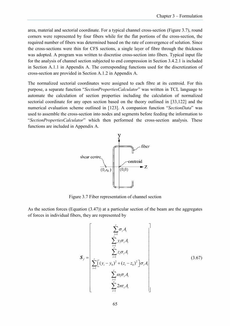
Chapter 3 – Formulation
area, material and sectorial coordinate. For a typical channel cross-section (Figure 3.7), round corners were represented by four fibers while for the flat portions of the cross-section, the required number of fibers was determined based on the rate of convergence of solution. Since the cross-sections were thin for CFS sections, a single layer of fibre through the thickness was adopted. A program was written to discretise cross-section into fibers. Typical input file for the analysis of channel section subjected to end compression in Section 3.4.2.1 is included in Section A.1.1 in Appendix A. The corresponding functions used for the discretization of cross-section are provided in Section A.1.2 in Appendix A.
The normalized sectorial coordinates were assigned to each fibre at its centroid. For this purpose, a separate function “SectionPropertiesCalculator” was written in TCL language to automate the calculation of section properties including the calculation of normalized sectorial coordinate for any open section based on the theory outlined in [33,122] and the numerical evaluation scheme outlined in [123]. A companion function “SectionData” was used to assemble the cross-section into nodes and segments before feeding the information to “SectionPropertiesCalculator” which then performed the cross-section analysis. These functions are included in Appendix A.
Figure 3.7 Fiber representation of channel section
As the section forces (Equation (3.47)) at a particular section of the beam are the aggregates of forces in individual fibers, they are represented by
1
1
1
2 20 0
1
1
1
( ) ( )
2
r
i iir
i i ii
r
i i ii
rf
i i i ii
r
i i iir
i ii
A
y A
z A
y y z z A
A
n A
σ
σ
σ
σ
ωσ
τ
=
=
=
=
=
=
= − + −
∑
∑
∑
∑
∑
∑
S (3.67)
65

Chapter 3 – Formulation
where r refers to the number of fibers, σi is the normal stress, Ai is the area, ωi is the sectorial coordinate, τi is the shear stress, and (yi, zi) are the coordinate of the centroid of the ith fiber of the cross-section.
Similarly, the elastic section tangent stiffness matrix (Equation (3.55)) is represented by
2
1 1 1 1 1
2 2
1 1 1 1 1
2 2
1 1 1 1 1
2 2 2 4
1 1 1 1
0
0
0
r r r r r
i i i i i i i i ii i i i ir r r r r
i i i i i i i i i i i i ii i i i i
r r r r r
i i i i i i i i i i i i it i i i i i
r r r r
i i i i i i i i i ii i i i
A y A z A p A A
y A y A y z A p y A y A
z A y z A z A p z A z AE
p A p y A p z A p A
ω
ω
ω
= = = = =
= = = = =
= = = = =
= = = =
=
∑ ∑ ∑ ∑ ∑
∑ ∑ ∑ ∑ ∑
∑ ∑ ∑ ∑ ∑
∑ ∑ ∑k
2
1
2 2
1 1 1 1 1
0
0
0 0 0 0 0 /
r
i i ii
r r r r r
i i i i i i i i i i i i ii i i i i
p A
A y A z A p A A
GJ E
ω
ω ω ω ω ω=
= = = = =
∑ ∑
∑ ∑ ∑ ∑ ∑
(3.68)
where 2 2 20 0( ) ( )i i ip y y z z= − + − and other terms are defined in relevant sections. The section
forces and stiffness contributions are aggregated along the beam element using a Gauss-Lobatto Integration scheme.
The above two equations along with the other relevant equations and the section transformation matrix are incorporated in the OpenSees files namely displacementColumn3d.cpp and FiberSection3d.cpp. The typical modified sections of the DispBeamColumn3d and FiberSection3d are included in Section A.1.6 in Appendix A.
3.4 Numerical examples
In this section, the buckling and post-buckling behaviour of thin-walled beams and columns with open cross-sections are presented. The solutions are obtained from the OpenSees program that was modified to include the elastic beam element (EB) and displacement-based beam element (DB) outlined in this chapter. The solutions obtained from the OpenSees program are verified by the results obtained from the widely-used finite element software Abaqus [18].
For the purpose of numerical analysis, three sections shown in Figure 3.8, each representative of doubly symmetric, monosymmetric and asymmetric sections are used. The corresponding section properties are given in Table 3.1.
66

Chapter 3 – Formulation
(a) I Section (b) Channel Section (c) Asymmetric Section
Figure 3.8 Dimensions for I, channel and asymmetric sections (in mm)
Table 3.1 Section properties
Properties Units I-Section Channel Section Asymmetric Section
A mm2 741.00 789.28 789.28
Iy’ mm4 2.11 x 10⁵ 5.82 x 10⁵ 5.81 x 10⁵
Iz’ mm4 12.87 x 10⁵ 13.40 x 10⁵ 14.07 x 10⁵
Iω mm6 4.96 x 10⁸ 12.60 x 10⁸ 9.81 x 10⁸
J mm4 2223.0 2367.84 2367.84
(y0,z0) mm (0,0) (0,-63.46) (-8.80,-61.63)
βz mm 0 0 19.65
βy mm 0 155.81 157.12
α degree 0° 0° -2.145° Note: Section properties calculated based on thin-walled theory
For the purpose of analysis, the elastic modulus, E is assumed as 200 GPa and Poisson’s ratio, ν as 0.3. The shear modulus G is given by the Equation (3.38). In all the examples to follow, the linear-elastic material behaviour is assumed.
3.4.1 Doubly-symmetric sections
3.4.1.1 I-section column subjected to compression
A simply supported 6.0 m long I-section column is analyzed for the buckling and post-buckling behaviour when subjected to compressive loads acting through the centroid at the ends. The cross-section of the column is shown in Figure 3.8a. At either end, the column is restrained against transverse displacement and rotation about the longitudinal axis while allowing it to freely displace in the longitudinal direction, rotate about y- and z-axis, and
67
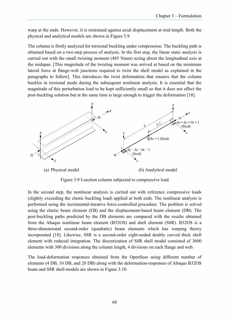
Chapter 3 – Formulation
warp at the ends. However, it is restrained against axial displacement at mid-length. Both the physical and analytical models are shown in Figure 3.9.
The column is firstly analyzed for torsional buckling under compression. The buckling path is obtained based on a two-step process of analysis. In the first step, the linear static analysis is carried out with the small twisting moment (485 Nmm) acting about the longitudinal axis at the midspan. [This magnitude of the twisting moment was arrived at based on the minimum lateral force at flange-web junctions required to twist the shell model as explained in the paragraphs to follow]. This introduces the twist deformation that ensures that the column buckles in torsional mode during the subsequent nonlinear analysis. It is essential that the magnitude of this perturbation load to be kept sufficiently small so that it does not affect the post-buckling solution but at the same time is large enough to trigger the deformation [18].
(a) Physical model (b) Analytical model
Figure 3.9 I-section column subjected to compressive load
In the second step, the nonlinear analysis is carried out with reference compressive loads (slightly exceeding the elastic buckling load) applied at both ends. The nonlinear analysis is performed using the incremental-iterative force-controlled procedure. The problem is solved using the elastic beam element (EB) and the displacement-based beam element (DB). The post-buckling paths predicted by the DB elements are compared with the results obtained from the Abaqus nonlinear beam element (B32OS) and shell element (S8R). B32OS is a three-dimensional second-order (quadratic) beam elements which has warping theory incorporated [18]. Likewise, S8R is a second-order eight-noded doubly curved thick shell element with reduced integration. The discretization of S8R shell model consisted of 3600 elements with 300 divisions along the column length, 4 divisions on each flange and web.
The load-deformation responses obtained from the OpenSees using different number of elements (4 DB, 10 DB, and 20 DB) along with the deformation-responses of Abaqus B32OS beam and S8R shell models are shown in Figure 3.10.
68

Chapter 3 – Formulation
Figure 3.10 Torsional buckling behaviour of I-section column in axial compression
In the figure, the number of elements used for each model is identified by the number before the element type within the legend. Although the EB element could accurately predict the buckling load, it was not able to produce the post-buckling path beyond the certain displacement range due to numerical instability after attaining the buckling load. Hence, the plot corresponding to EB element is not presented. However, its behaviour is found to be similar to that of the Abaqus B32OS beam element.
For the Abaqus S8R shell model, the boundary conditions at the supports were modelled by creating three small areas each at the centre of the web and at the flange-web junctions and assigning rigid body constraints to them. The actual boundary conditions were applied to the reference point on the rigid body regions instead of applying to the entire cross-section. The application of restraint to the entire cross-section has the effect of constraining the ends in the transverse directions to the beam length, thereby stiffening the ends, the details of which are explained in Section A.2 in Appendix A.
Since it was not possible to apply the twisting moment directly to the shell model to introduce initial imperfection, it was simulated by applying a lateral force of magnitude 5 N to the
69
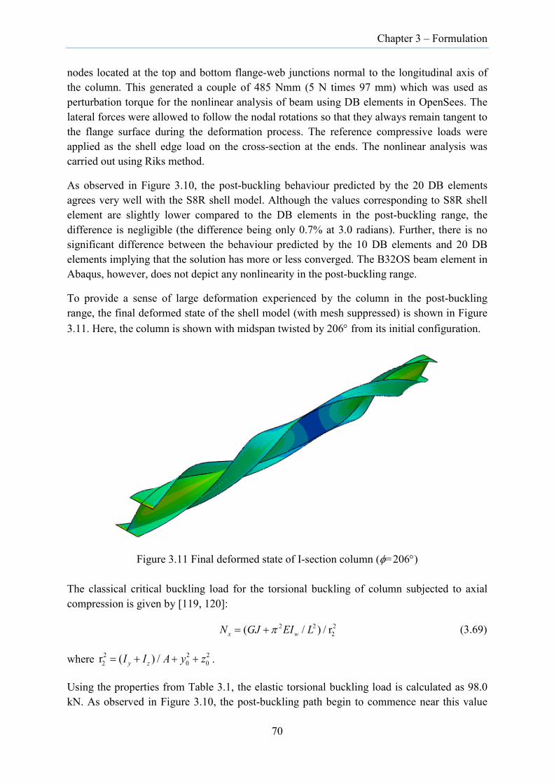
Chapter 3 – Formulation
nodes located at the top and bottom flange-web junctions normal to the longitudinal axis of the column. This generated a couple of 485 Nmm (5 N times 97 mm) which was used as perturbation torque for the nonlinear analysis of beam using DB elements in OpenSees. The lateral forces were allowed to follow the nodal rotations so that they always remain tangent to the flange surface during the deformation process. The reference compressive loads were applied as the shell edge load on the cross-section at the ends. The nonlinear analysis was carried out using Riks method.
As observed in Figure 3.10, the post-buckling behaviour predicted by the 20 DB elements agrees very well with the S8R shell model. Although the values corresponding to S8R shell element are slightly lower compared to the DB elements in the post-buckling range, the difference is negligible (the difference being only 0.7% at 3.0 radians). Further, there is no significant difference between the behaviour predicted by the 10 DB elements and 20 DB elements implying that the solution has more or less converged. The B32OS beam element in Abaqus, however, does not depict any nonlinearity in the post-buckling range.
To provide a sense of large deformation experienced by the column in the post-buckling range, the final deformed state of the shell model (with mesh suppressed) is shown in Figure 3.11. Here, the column is shown with midspan twisted by 206° from its initial configuration.
Figure 3.11 Final deformed state of I-section column (φ=206°)
The classical critical buckling load for the torsional buckling of column subjected to axial compression is given by [119, 120]:
2 2 22( / ) / rx wN GJ EI Lπ= + (3.69)
where 2 2 22 0 0r ( ) /y zI I A y z= + + + .
Using the properties from Table 3.1, the elastic torsional buckling load is calculated as 98.0 kN. As observed in Figure 3.10, the post-buckling path begin to commence near this value
70

Chapter 3 – Formulation
but the exact buckling load is difficult to pinpoint due to the continuous increase of load in the post-buckling range.
The same column is also analyzed for the flexural bucking mode when subjected to axial compressive forces at its ends. Here the initial imperfection is created by performing linear static analysis for a small lateral load (~10 N) acting at the midspan, normal to the longitudinal axis of the column in the weak axis direction. The nonlinear analysis is performed after the application of axial compressive loads at the two ends.
The load-deformation responses describing the post-buckling behaviour of the column modelled with different elements are shown in Figure 3.12.
Figure 3.12 Flexural buckling behaviour of I-section column subjected to compression
It is observed that 4 numbers of DB elements are inadequate to define the post-buckling behaviour although they are sufficient to predict the elastic buckling load. In general, it usually requires element size less than or equal to 200 mm for the convergence of solution. In this particular case, both the B32OS elements and EB elements predicted the post-buckling behaviour exactly same.
All numerical models predicted the elastic buckling load of 11.6 kN, corresponding to the lateral displacement of 280 mm. The theoretical critical buckling load for flexural buckling about the y-axis is 11.57 kN, which was calculated using the expression
71
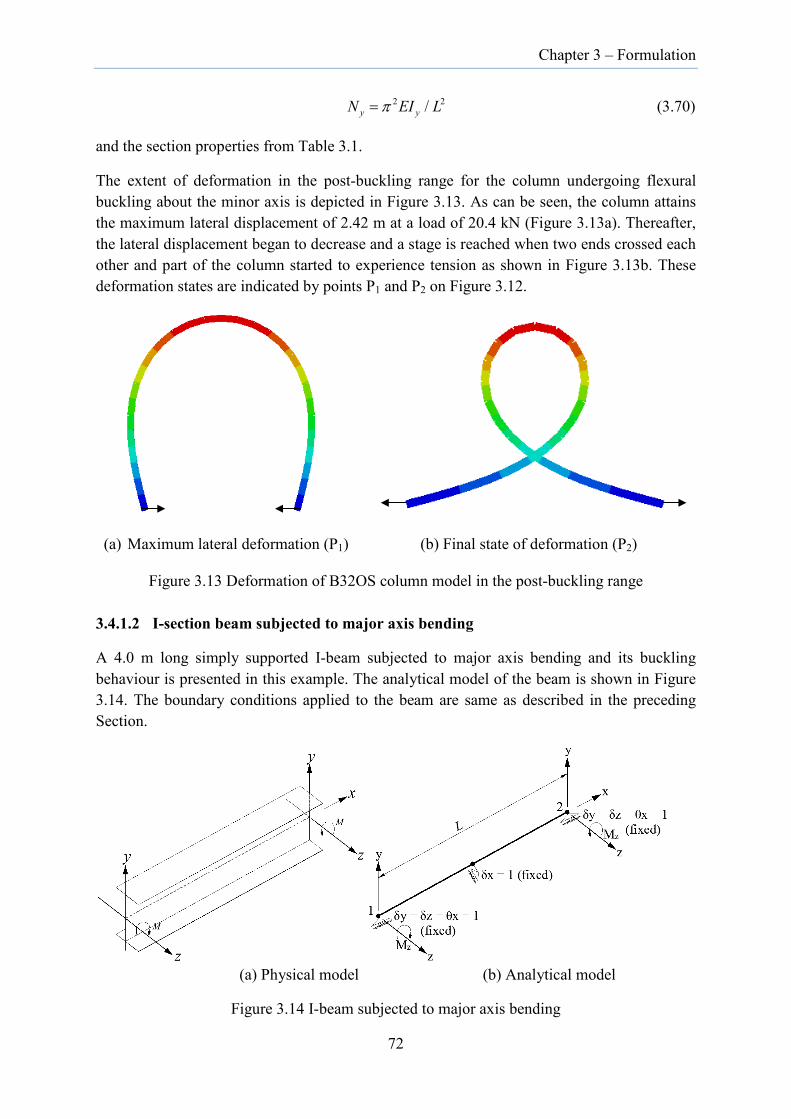
Chapter 3 – Formulation
2 2/y yN EI Lπ= (3.70)
and the section properties from Table 3.1.
The extent of deformation in the post-buckling range for the column undergoing flexural buckling about the minor axis is depicted in Figure 3.13. As can be seen, the column attains the maximum lateral displacement of 2.42 m at a load of 20.4 kN (Figure 3.13a). Thereafter, the lateral displacement began to decrease and a stage is reached when two ends crossed each other and part of the column started to experience tension as shown in Figure 3.13b. These deformation states are indicated by points P1 and P2 on Figure 3.12.
(a) Maximum lateral deformation (P1) (b) Final state of deformation (P2)
Figure 3.13 Deformation of B32OS column model in the post-buckling range
3.4.1.2 I-section beam subjected to major axis bending
A 4.0 m long simply supported I-beam subjected to major axis bending and its buckling behaviour is presented in this example. The analytical model of the beam is shown in Figure 3.14. The boundary conditions applied to the beam are same as described in the preceding Section.
(a) Physical model (b) Analytical model
Figure 3.14 I-beam subjected to major axis bending
72
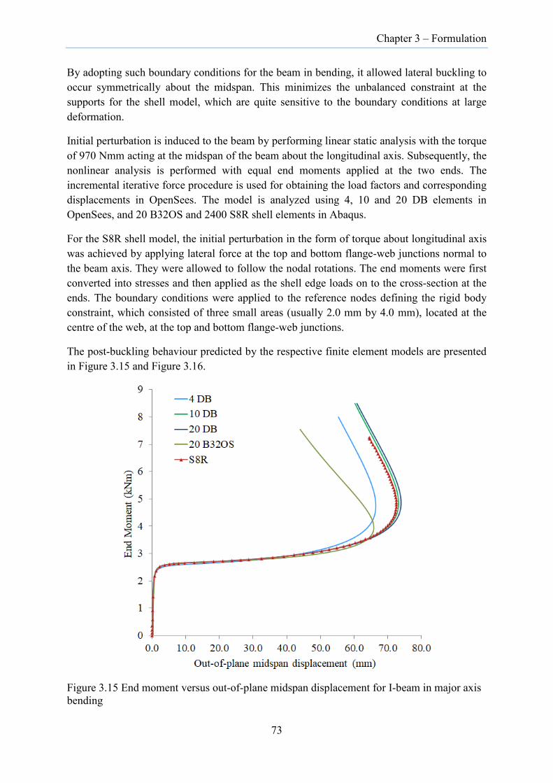
Chapter 3 – Formulation
By adopting such boundary conditions for the beam in bending, it allowed lateral buckling to occur symmetrically about the midspan. This minimizes the unbalanced constraint at the supports for the shell model, which are quite sensitive to the boundary conditions at large deformation.
Initial perturbation is induced to the beam by performing linear static analysis with the torque of 970 Nmm acting at the midspan of the beam about the longitudinal axis. Subsequently, the nonlinear analysis is performed with equal end moments applied at the two ends. The incremental iterative force procedure is used for obtaining the load factors and corresponding displacements in OpenSees. The model is analyzed using 4, 10 and 20 DB elements in OpenSees, and 20 B32OS and 2400 S8R shell elements in Abaqus.
For the S8R shell model, the initial perturbation in the form of torque about longitudinal axis was achieved by applying lateral force at the top and bottom flange-web junctions normal to the beam axis. They were allowed to follow the nodal rotations. The end moments were first converted into stresses and then applied as the shell edge loads on to the cross-section at the ends. The boundary conditions were applied to the reference nodes defining the rigid body constraint, which consisted of three small areas (usually 2.0 mm by 4.0 mm), located at the centre of the web, at the top and bottom flange-web junctions.
The post-buckling behaviour predicted by the respective finite element models are presented in Figure 3.15 and Figure 3.16.
Figure 3.15 End moment versus out-of-plane midspan displacement for I-beam in major axis bending
73

Chapter 3 – Formulation
Figure 3.16 End moment versus twist angle at midspan for I-beam in major axis bending
The critical buckling moment for an I-beam subjected to the major axis bending, which includes the effect of pre-buckling deformation is given by [124]:
2
2
2
2
1
1 1 1
y
cr
y
z z
EIEI GJGJL
ML EI EIGJ
EI EI GJL
ω
ω
ππ
π
+
=
− − +
(3.71)
Based on the Equation (3.71) and the section properties from Table 3.1, the classical buckling moment is calculated and presented along with the numerical solutions in Table 3.2.
Table 3.2 Comparison of buckling moment for I-beam
Solution Type Elastic buckling moment (kNm)
Classical (Equation (3.71)) 2.690
10 DB 2.682 20 DB 2.691
20 B32OS 2.689 S8R shell 2.685
S8R shell* 2.449 *from elastic buckling analysis
74

Chapter 3 – Formulation
In the above Table, the buckling moments from the numerical analyses were determined corresponding to the 15 mm out-of-plane displacement at the midspan. This is the point at which the classical buckling moment (Equation (3.71)) intersects with the graphs. The buckling moment from the Abaqus elastic buckling analysis is lower by 9 percent than the ones predicted by the numerical analyses, as it does not include the pre-buckling deformation.
3.4.2 Monosymmetric sections
3.4.2.1 Channel column subjected to compression
Buckling and post-buckling behaviour of a 6.0 m long simply supported channel column subjected to compressive loads at the two ends is presented. The column with the boundary conditions is shown in Figure 3.17 and the cross-section of the column is shown in Figure 3.8b.
(a) Physical model (b) Analytical model
Figure 3.17 Channel column subjected to compression
A two-step analysis is followed to study the post-buckling behaviour. In the initial step, torsional imperfection is introduced in the model by performing linear static analysis with a small magnitude of torque (485 Nmm) acting at the midspan about the longitudinal axis. In the second step, reference compressive load with magnitude slightly above the buckling load is applied at the two ends and nonlinear analysis is performed with the incremental iterative displacement-controlled procedure. Here, the displacement-controlled method has to be employed, as the load has to pass through the maximum point in the post-buckling range. Use of force-controlled method would result in numerical instability in this case. Since the shear centre is eccentric to the centroid, the shifting of an axial load to the centroid from the shear centre generated a couple equivalents to the axial load times the shear centre distance from the centroid in the OpenSees model. Hence, the couple is applied at each end about the minor axis to account for this eccentricity. These couples act simultaneously with the compressive force at the ends.
75
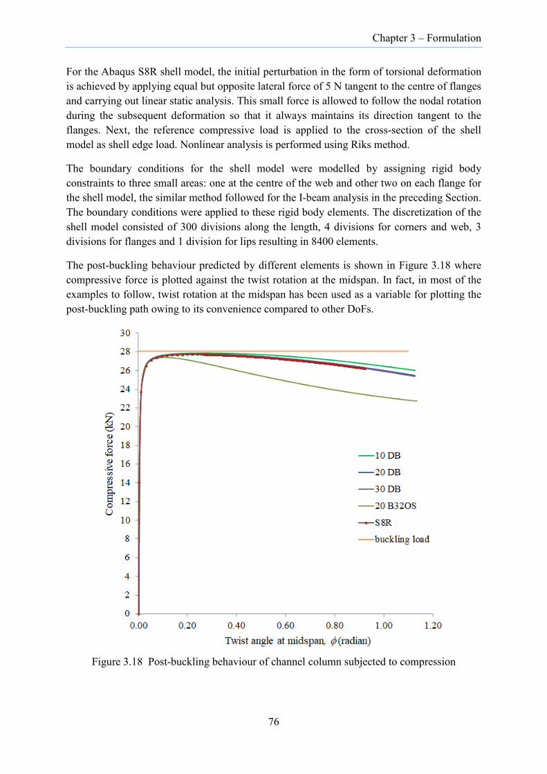
Chapter 3 – Formulation
For the Abaqus S8R shell model, the initial perturbation in the form of torsional deformation is achieved by applying equal but opposite lateral force of 5 N tangent to the centre of flanges and carrying out linear static analysis. This small force is allowed to follow the nodal rotation during the subsequent deformation so that it always maintains its direction tangent to the flanges. Next, the reference compressive load is applied to the cross-section of the shell model as shell edge load. Nonlinear analysis is performed using Riks method.
The boundary conditions for the shell model were modelled by assigning rigid body constraints to three small areas: one at the centre of the web and other two on each flange for the shell model, the similar method followed for the I-beam analysis in the preceding Section. The boundary conditions were applied to these rigid body elements. The discretization of the shell model consisted of 300 divisions along the length, 4 divisions for corners and web, 3 divisions for flanges and 1 division for lips resulting in 8400 elements.
The post-buckling behaviour predicted by different elements is shown in Figure 3.18 where compressive force is plotted against the twist rotation at the midspan. In fact, in most of the examples to follow, twist rotation at the midspan has been used as a variable for plotting the post-buckling path owing to its convenience compared to other DoFs.
Figure 3.18 Post-buckling behaviour of channel column subjected to compression
76

Chapter 3 – Formulation
As observed in Figure 3.18, the post-buckling paths depict the softening behaviour with increasing displacement. The post-buckling path of B32OS significantly deviates from others beyond the buckling load. However, the post-buckling path of DB elements is smooth and decrement is gradual, as is the case of S8R shell model implying the perfect agreement between the two models.
The critical buckling load for a simply supported mono-symmetric section subjected to compressive load and undergoing flexural-torsional buckling is given by [120]:
( ) ( ) ( )
( )
2 2 2 20 0 0
2 2 20 0 0
4 /
2 /
x z x z x z
cr
N N N N N N r r zN
r r z
+ − + − +=
+ (3.72)
in which,
2 2
20
/( ) /
z z
y z
N EI Lr I I A
π=
= + (3.73)
Based on this equation, the critical buckling load for the C-section column is calculated as 28.07 kN. As observed from the graph, all numerical solutions reached the respective peak load (27.77 kN for 30 DB element, 27.41 kN for B32OS element, and 27.73 kN for S8R shell element) and began to decrease as the deformation proceeded further. All these values are lower than the true buckling load computed using Equation (3.72).
3.4.2.2 Channel beam subjected to major axis bending
In this example, a 4.0 m long channel beam is subjected to major axis pure bending with equal moments applied at the two ends (Figure 3.19a). The analytical model is shown in Figure 3.19b. The ends of the beam are free to warp and free to rotate about y- and z-axes while rotation is restrained about the x-axis. The translation in the x-direction is restrained at midspan of the beam. This was arrived at after having noticed the unequal development of stress distribution at the supports in the Abaqus shell model, which was used to verify the post-buckling behaviour of DB elements. By restraining the longitudinal translation at the midspan, it resulted in symmetric deformation of the midspan and developed identical stress distribution at the two supports.
An imperfection is introduced by applying a torque of varying magnitude (depending on the type of deformation examined as explained below) at the midspan of the beam about the longitudinal axis. Next, the reference end moments are applied at the two ends and nonlinear analysis is performed to determine the post-buckling behaviour.
For the S8R shell model, the boundary conditions were similar to the one described in Section 3.4.2.1. However, the discretization of the model consisted of 200 divisions along the length, 4 divisions each at the corners and web, 3 divisions in each flange and 1 division in each lip resulting in 5600 elements for the whole model.
77
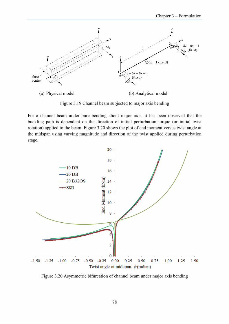
Chapter 3 – Formulation
(a) Physical model (b) Analytical model
Figure 3.19 Channel beam subjected to major axis bending
For a channel beam under pure bending about major axis, it has been observed that the buckling path is dependent on the direction of initial perturbation torque (or initial twist rotation) applied to the beam. Figure 3.20 shows the plot of end moment versus twist angle at the midspan using varying magnitude and direction of the twist applied during perturbation stage.
Figure 3.20 Asymmetric bifurcation of channel beam under major axis bending
78

Chapter 3 – Formulation
The right-side branch of the plot is obtained with an initial positive torque of 2,425 Nmm while the left-side branch for 20 DB and S8R corresponds to a negative torque of 11,640 Nmm. This magnitude of torque was chosen such that it was sufficient to induce small torsional deformation in a shell model during the perturbation stage of the analysis. To observe the influence of initial imperfection magnitude, the initial perturbation torque of 400 Nmm was considered for the plot corresponding to 10 DB element. The equiliribum path shows that the magnitude of initial torque has the effect of shifting the pre-buckling and buckling path for the left-side branch but has negligible effect on the right-side branch and post-buckling path. The plot obtained from the Abaqus B32OS beam model is also presented.
The right-hand side of the plot in Figure 3.20 can be obtained using either force-controlled or displacement-controlled method as the moments are continuously increasing with the increasing deformation. However, for the left-hand side plot, it is necessary to engage Riks method in shell model as it allows the maximum point to pass without undergoing numerical instability and related convergence issue.
While referring to Figure 3.20, it is seen that for the positive initial twist rotation, the equilibrium path is stable as indicated by the rising curve. However, for a negative initial torque at the midspan of the beam, equilibrium path is unstable as indicated by the falling curve. In this case, the load required to maintain equilibrium after buckling decreases with increasing deformation. Further, when the force-controlled method was used, the system became unstable after reaching the peak load and snapped to a very deformed state. The use of arc-length integrator enabled the detection of portions of the imperfect path which the force controlled method was not able to do so in OpenSees model. This asymmetric behaviour of channel section was also observed using the EB model. However, the rate of numerical convergence was slow and worked only with very small (~1 Nmm) initial perturbation torque.
Since post-buckling behaviour of channel beam in major axis bending depends on the sign of initial deformation, it can be surmised that the channel section exhibits asymmetric bifurcation under major axis bending.
3.4.2.3 Channel beam subjected to minor axis bending
The same channel beam used in the above example is bent about the minor axis with equal end moments applied at the two ends. The end moments are applied such that the shear centre side is in tension while the lip is in compression. The boundary conditions along with applied end moments are shown in Figure 3.21. The boundary conditions are similar to the preceding example.
Following the two-step analysis process, the force-deformation responses are obtained from the nonlinear analysis with the displacement-controlled procedure and are plotted in Figure 3.22. The initial perturbation was achieved with the application of torque equal to 485 Nmm applied at the midspan followed by the static analysis. For the S8R shell model, the similar method employed in the preceding examples has been followed for modelling the load and the boundary conditions.
79

Chapter 3 – Formulation
(a) Physical model (b) Analytical model
Figure 3.21 Channel beam subjected to minor axis bending
As observed in Figure 3.22, the post-buckling path predicted by DB element agrees very well up to the twist angle of 1.0 radian. The slight discrepancy beyond this point is due to the difficulty of reproducing the exact boundary condition for the shell model as it is observed to be sensitive in the large displacement range.
Figure 3.22 Post-buckling behaviour of channel beam subjected to minor axis bending
3.4.2.4 Cantilever channel beam subjected to torque at the free end
In this example, a 3.0 m long cantilever channel beam having a cross-sectional dimension similar to Figure 3.8b but with a thickness of 1.5 mm is subjected to end torque (Figure 3.23). Except for the warping DoF, all other DoFs are restrained at the support. The torque is applied at the free end.
80
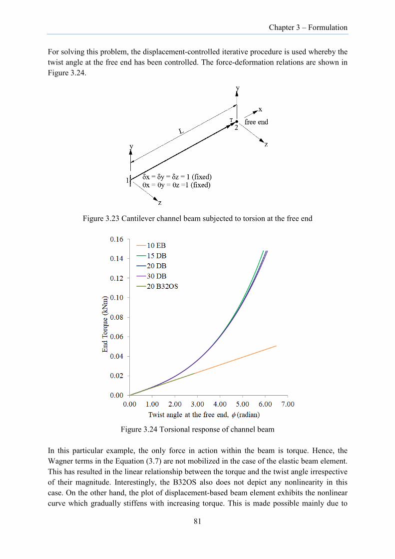
Chapter 3 – Formulation
For solving this problem, the displacement-controlled iterative procedure is used whereby the twist angle at the free end has been controlled. The force-deformation relations are shown in Figure 3.24.
Figure 3.23 Cantilever channel beam subjected to torsion at the free end
Figure 3.24 Torsional response of channel beam
In this particular example, the only force in action within the beam is torque. Hence, the Wagner terms in the Equation (3.7) are not mobilized in the case of the elastic beam element. This has resulted in the linear relationship between the torque and the twist angle irrespective of their magnitude. Interestingly, the B32OS also does not depict any nonlinearity in this case. On the other hand, the plot of displacement-based beam element exhibits the nonlinear curve which gradually stiffens with increasing torque. This is made possible mainly due to
81

Chapter 3 – Formulation
the presence of Wagner term in the strain formulation in the displacement-based element. The similar stiffening behaviour has been observed by Zhang et al. [116] in doubly-symmetric section and by Battini and Pacoste [114] in narrow rectangular sections.
In Figure 3.24, it can be seen that the displacement-based beam elements is capable of predicting the behaviour of beam undergoing large displacement analysis where the torsional effects are significant. It also proves that the co-rotational framework in itself does not produce any non-linearity where the predominant load is torsion. Furthermore, the section undergoes large torsional deformation even with a small magnitude of torsion validating that thin-walled open sections possess very low torsional resistance.
3.4.3 Asymmetric sections
3.4.3.1 Asymmetric section column subjected to compression
To demonstrate the capability of the DB elements in analyzing the thin-walled beam having general cross-sections, a variant of channel section, with upper lips turned upwards has been used as representative of the typical asymmetric sections. In this example, a 6.0 m long column having an asymmetric cross-section (Figure 3.8c) is subjected to a compressive force at its two ends. The boundary conditions are kept same as the model in Figure 3.17. The physical model is shown in Figure 3.25.
Figure 3.25 Asymmetric section column subjected to axial compression
Similar to the process followed in the preceding examples, the initial perturbation in the form of twist was applied at the midspan and the linear static analysis was performed. For the S8R shell model, because of the unequal distance to the top and bottom flange from the centroid, the lateral force of 5.09 N on the centre of the top flange and 4.91 N on bottom flange was applied to cause the initial twist perturbation.
82
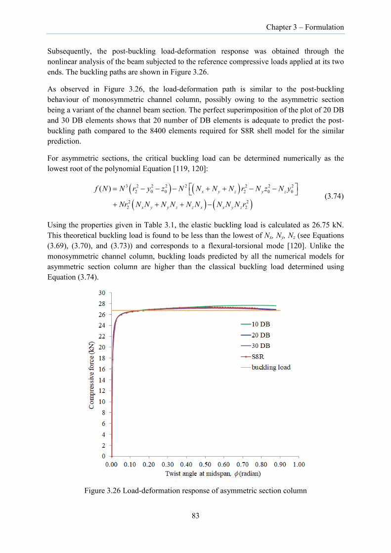
Chapter 3 – Formulation
Subsequently, the post-buckling load-deformation response was obtained through the nonlinear analysis of the beam subjected to the reference compressive loads applied at its two ends. The buckling paths are shown in Figure 3.26.
As observed in Figure 3.26, the load-deformation path is similar to the post-buckling behaviour of monosymmetric channel column, possibly owing to the asymmetric section being a variant of the channel beam section. The perfect superimposition of the plot of 20 DB and 30 DB elements shows that 20 number of DB elements is adequate to predict the post-buckling path compared to the 8400 elements required for S8R shell model for the similar prediction.
For asymmetric sections, the critical buckling load can be determined numerically as the lowest root of the polynomial Equation [119, 120]:
( ) ( )( ) ( )
3 2 2 2 2 2 2 22 0 0 2 0 0
2 22 2
( )
x y z y z
x y y z z x x y z
f N N r y z N N N N r N z N y
Nr N N N N N N N N N r
= − − − + + − −
+ + + − (3.74)
Using the properties given in Table 3.1, the elastic buckling load is calculated as 26.75 kN. This theoretical buckling load is found to be less than the lowest of Nx, Ny, Nz (see Equations (3.69), (3.70), and (3.73)) and corresponds to a flexural-torsional mode [120]. Unlike the monosymmetric channel column, buckling loads predicted by all the numerical models for asymmetric section column are higher than the classical buckling load determined using Equation (3.74).
Figure 3.26 Load-deformation response of asymmetric section column
83

Chapter 3 – Formulation
3.4.3.2 Asymmetric section beam subjected to pure bending
A 4.0 m long beam with an asymmetric cross-section is subjected to bending about its major principal axis. The process of obtaining the numerical solution and the boundary conditions adopted are similar to the monosymmetric channel section in major axis bending.
However, the S8R shell model was transformed through rotation so that the principal axis of the cross-section coincided with the rectangular axis. The load and boundary conditions were applied with respect to the principal axis system. Based on the performance of S8R shell model, the initial twist required to perturb the beam at the onset of nonlinear analysis was determined so that the rotational DoF (about the longitudinal axis at the midspan) was +0.007 radians. The post-buckling path is presented in Figure 3.27.
As observed in Figure 3.27, the post-buckling behaviour predicted by DB element and S8R shell model agrees well.
Figure 3.27 Post-buckling behaviour of asymmetric section beam subjected to major principal axis bending
The same beam is also subjected to the minor axis bending following the similar procedure used for the minor axis bending of channel beam. The beam is bent with the shear centre side in tension. Here the initial twist required to perturb the beam was determined so that the rotational DoF at the midspan of the beam was -0.004 radians. The load-deformation response is plotted in Figure 3.28.
84
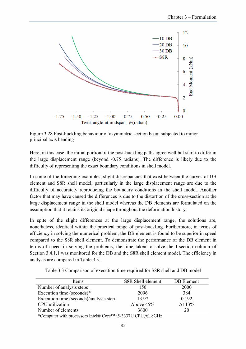
Chapter 3 – Formulation
Figure 3.28 Post-buckling behaviour of asymmetric section beam subjected to minor principal axis bending
Here, in this case, the initial portion of the post-buckling paths agree well but start to differ in the large displacement range (beyond -0.75 radians). The difference is likely due to the difficulty of representing the exact boundary conditions in shell model.
In some of the foregoing examples, slight discrepancies that exist between the curves of DB element and S8R shell model, particularly in the large displacement range are due to the difficulty of accurately reproducing the boundary conditions in the shell model. Another factor that may have caused the differences is due to the distortion of the cross-section at the large displacement range in the shell model whereas the DB elements are formulated on the assumption that it retains its original shape throughout the deformation history.
In spite of the slight differences at the large displacement range, the solutions are, nonetheless, identical within the practical range of post-buckling. Furthermore, in terms of efficiency in solving the numerical problem, the DB element is found to be superior in speed compared to the S8R shell element. To demonstrate the performance of the DB element in terms of speed in solving the problems, the time taken to solve the I-section column of Section 3.4.1.1 was monitored for the DB and the S8R shell element model. The efficiency in analysis are compared in Table 3.3.
Table 3.3 Comparison of execution time required for S8R shell and DB model
Items S8R Shell element DB Element Number of analysis steps 150 2000 Execution time (seconds)* 2096 384 Execution time (seconds)/analysis step 13.97 0.192 CPU utilization Above 45% At 13% Number of elements 3600 20
*Computer with processors Intel® Core™ i5-3337U [email protected]
85

Chapter 3 – Formulation
3.5 Conclusions
Formulation of general thin-walled (open section) beam finite element and its implementation in the OpenSees framework is presented. A simple cross-section transformation matrix relating the axial force acting at the centroid and the shear centre is developed within the local axis system enabling the application of the formulation to the general thin-walled sections.
The displacement-based beam element is capable of handling large deformation with beams having general open cross-sections. Numerical examples demonstrated that DB elements are equally accurate when compared with the Abaqus shell element. The slight discrepancies observed at the large displacement are due to the difficulty of replicating the exact boundary conditions in the shell models. Although elastic beam element is developed based on linear theory and therefore requires more elements for achieving equivalent accuracy, its capability to predict the true buckling load mainly arose from the inclusion of the Wagner effect in the torsional rigidity term.
The B32OS beam element, although predicted the elastic buckling load accurately, is not able to predict the post-buckling behaviour, especially when torsion or initial imperfections in the form of torsional perturbations are involved. Apart from this, its behaviour is similar to the elastic beam element. This has been demonstrated by their perfect agreement in predicting the post-buckling equilibrium path of I-beam undergoing flexural buckling under compression.
As displacement-based beam element is able to analyse the models with great accuracy and with far less time compared to the shell element models, it can be conveniently used for the study of CFS sections undergoing large deformation.
The capability of the displacement-based beam element can be further enhanced by incorporating methods for predicting the local cross-sectional instabilities so that it can be used for the general nonlinear analysis of thin-walled sections undergoing local and/or distortional buckling. Furthermore, the semi-rigid behaviour of CFS joints can be integrated for the prediction of system behaviour of the CFS frames.
86
Chapter 4 – Experiments
CHAPTER 4. EXPERIMENTAL INVESTIGATION
4.1 Introduction The experimental investigations involved designing and testing of full-scale 13.6 m long span CFS single C-section portal frames and their components. The full-scale frame tests were carried out with the following objectives:
i. To observe the structural performance of the existing portal frame configuration ii. To determine the ultimate strength of the existing and modified portal frame
configuration, and iii. To validate the structural behaviour simulated by the numerical models
Towards fulfilling the above objectives, six tests were carried out on CFS single C-section portal frames subjected to gravity load (four tests) and the combination of gravity load and lateral load (two tests).
Besides the full-scale portal frame tests, several ancillary tests (coupon tests, point fastener connection tests, frame connection tests) and imperfection measurements were conducted to gain insight into the behaviour of frame connections and to extract relevant information on material properties, connection characteristics and imperfections for use in numerical models. All full-scale frame tests and ancillary tests were conducted in the J.W. Roderick Materials and Structures Laboratory at The University of Sydney.
Although several tests on portal frames made from cold-formed steel sections had been carried out in the past, the focus had been largely on the CFS portal frames composed of doubly-symmetric sections fabricated by placing two individual C-sections back-to-back [5,6,7,8,9,10,11,12,13]. No full-scale tests on single C-section portal frames had been reported with the exception of early works by Baigent and Hancock [42]. In their work, the joints of portal frames were made rigid, by using 12 mm thick plates bolted to the web of channel section, thereby allowing free warping of flanges at the joints. The span of the frame was 6.25 m and height to eaves was 2.0 m (Figure 2.7). In the present context, CFS single C-section portal frames with semi-rigid joints having a size of 13.6 m long by 6.8 m high are examined.
Hence, towards understanding the structural behaviour of the long-span CFS portal frame made of single C-sections, CFS portal frames consisting of two bays by single span were tested with rafters fully braced by purlins while the columns were unbraced between their ends. Such types of portal frames are ideal for garages and storage sheds where the requirement for vehicular access to the inside of the building precludes the provision of girts in the facades. In fact, adoption of such system for the frame tests was partly stimulated by the desire of the propriety company BlueScope Lysaght to tests such systems for possible use in the construction of large storage sheds with free vehicular access. Of the six frames, one was tested with columns restrained by girts at a spacing of 1.25 m along its height for comparing its behaviour with the behaviour of frames without column restraints.
87
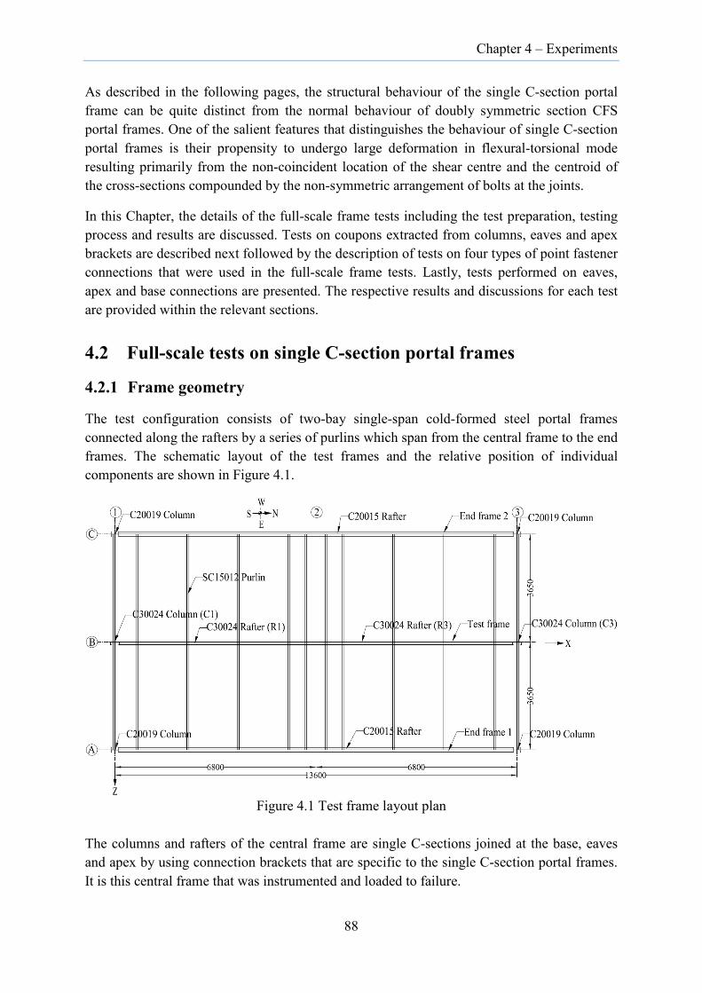
Chapter 4 – Experiments
As described in the following pages, the structural behaviour of the single C-section portal frame can be quite distinct from the normal behaviour of doubly symmetric section CFS portal frames. One of the salient features that distinguishes the behaviour of single C-section portal frames is their propensity to undergo large deformation in flexural-torsional mode resulting primarily from the non-coincident location of the shear centre and the centroid of the cross-sections compounded by the non-symmetric arrangement of bolts at the joints.
In this Chapter, the details of the full-scale frame tests including the test preparation, testing process and results are discussed. Tests on coupons extracted from columns, eaves and apex brackets are described next followed by the description of tests on four types of point fastener connections that were used in the full-scale frame tests. Lastly, tests performed on eaves, apex and base connections are presented. The respective results and discussions for each test are provided within the relevant sections.
4.2 Full-scale tests on single C-section portal frames
4.2.1 Frame geometry
The test configuration consists of two-bay single-span cold-formed steel portal frames connected along the rafters by a series of purlins which span from the central frame to the end frames. The schematic layout of the test frames and the relative position of individual components are shown in Figure 4.1.
Figure 4.1 Test frame layout plan
The columns and rafters of the central frame are single C-sections joined at the base, eaves and apex by using connection brackets that are specific to the single C-section portal frames. It is this central frame that was instrumented and loaded to failure.
88

Chapter 4 – Experiments
The front elevation of the main test frame (frame on grid B) is shown in Figure 4.2 and the side elevation of frames (grid 1 and grid 3) is shown in Figure 4.3. The height to the top of the apex from the base plate is 6.8 m.
Figure 4.2 Frame elevation
Figure 4.3 Side elevation of frames on grid 1 and grid 3
89
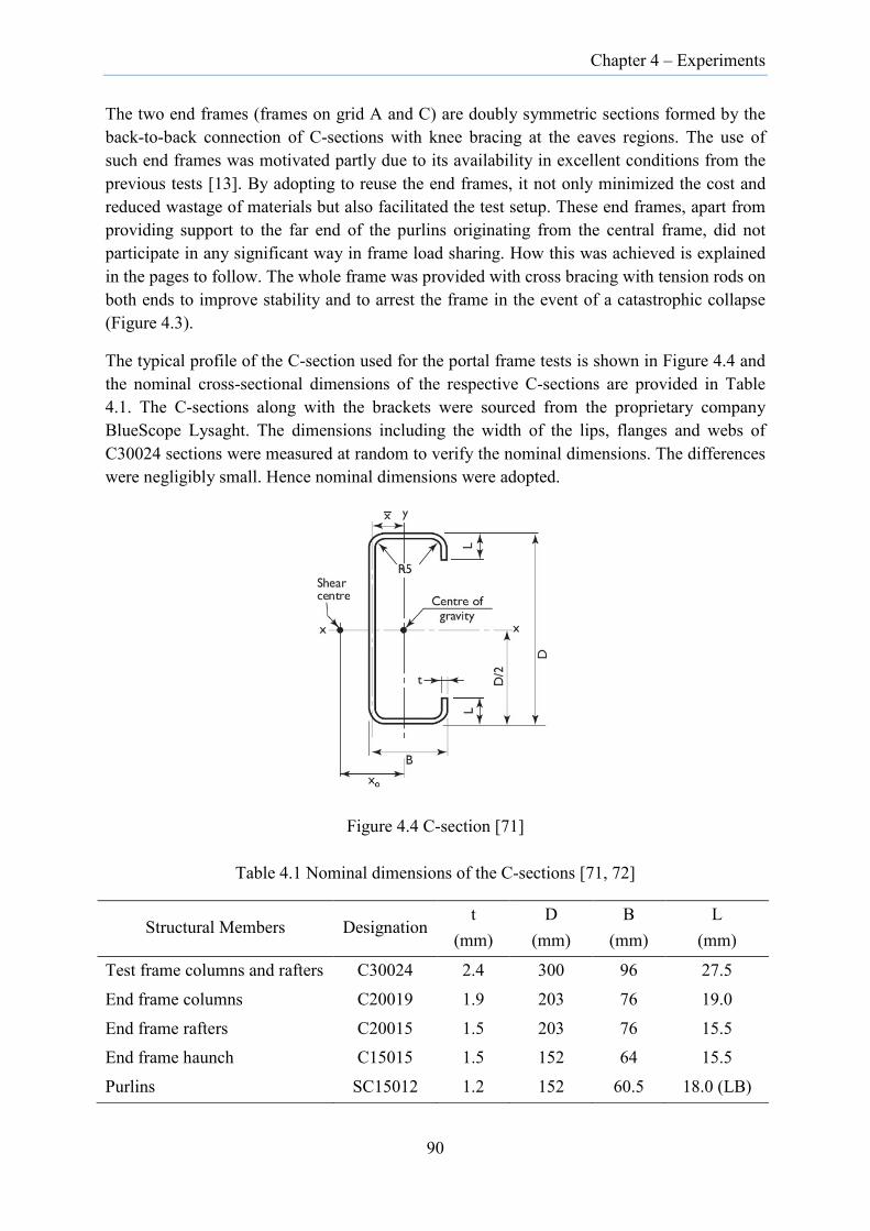
Chapter 4 – Experiments
The two end frames (frames on grid A and C) are doubly symmetric sections formed by the back-to-back connection of C-sections with knee bracing at the eaves regions. The use of such end frames was motivated partly due to its availability in excellent conditions from the previous tests [13]. By adopting to reuse the end frames, it not only minimized the cost and reduced wastage of materials but also facilitated the test setup. These end frames, apart from providing support to the far end of the purlins originating from the central frame, did not participate in any significant way in frame load sharing. How this was achieved is explained in the pages to follow. The whole frame was provided with cross bracing with tension rods on both ends to improve stability and to arrest the frame in the event of a catastrophic collapse (Figure 4.3).
The typical profile of the C-section used for the portal frame tests is shown in Figure 4.4 and the nominal cross-sectional dimensions of the respective C-sections are provided in Table 4.1. The C-sections along with the brackets were sourced from the proprietary company BlueScope Lysaght. The dimensions including the width of the lips, flanges and webs of C30024 sections were measured at random to verify the nominal dimensions. The differences were negligibly small. Hence nominal dimensions were adopted.
Figure 4.4 C-section [71]
Table 4.1 Nominal dimensions of the C-sections [71, 72]
Structural Members Designation t
(mm) D
(mm) B
(mm) L
(mm)
Test frame columns and rafters C30024 2.4 300 96 27.5
End frame columns C20019 1.9 203 76 19.0
End frame rafters C20015 1.5 203 76 15.5 End frame haunch C15015 1.5 152 64 15.5
Purlins SC15012 1.2 152 60.5 18.0 (LB)
90

Chapter 4 – Experiments
The LYSAGHT® C-sections are roll-formed from GALVASPAN steel complying with AS1397-2011 [125] with a minimum yield stress of 450 MPa for sections with base metal thickness of 1.5, 1.9, 2.4 and 3.00 mm. However, for those sections with base metal thickness of 1.2 mm, the minimum yield stress is 500 MPa. All sections are coated with zinc having minimum coating mass of 350 g/m2 [71].
4.2.2 Initial test preparations
To minimize cost and to reduce waste, the materials for the end frames (frames on grid A and C in Figure 4.1) along with the loading rig were reused from the previous tests [13] on CFS portal frames comprising doubly-symmetric C-sections.
However, the column and rafter sections and the connection brackets used for the previous tests were entirely different from the current tests. Hence, it became important to ensure that the overall configuration of the new test setup matched with the previous tests. Towards minimizing lack-of-fit issues, a detailed measurement was carried out on the end frames of the previous tests which included measurement of eaves height, apex height, span, bay spacing, frame sections, loading point location, the end point of purlin and base plate configuration. Detailed measurements were also carried out for the base, knee, apex and eaves brackets for the purpose of numerical modelling described in Chapter 5.
While using the end frames from the previous tests, the central frame (frames on grid B in Figure 4.1) was replaced by the single C-section portal frame which constituted the current tests. Since the single C-section portal frames have a distinctly different size of members and connection brackets compared to the previously tested doubly symmetric section portal frames, the new setup, in particular, required:
• Re-designing of loading points including the load positions on the purlins, • Relocation of purlins to appropriate positions near the apex and the eaves brackets, • Reconfiguration of bolt hole geometry on the base plates, • New design of transducer frames and transducer locations, • Introduction of newly-designed bracket on top of the loading jack to accommodate a
small eccentricity that existed between the load spreading system and the loading jack (resulting from the requirement of force resultants to pass through the eccentric shear centre of the rafter), and
• Adjustment of the height of columns and the length of rafters for the central frame so that the purlins are centrally aligned along the central frame whilst flushing with the top flanges of the end frames as adopted in the previous tests.
4.2.3 Frame test series
In the experimental investigation of single C-section portal frames, six tests were conducted to gain insight into the behaviour of frames and its components, to identify the shortfalls and to explore the possibility of improving the CFS portal frame systems. The six tests included three tests on frames with connection brackets that are currently used in the BlueScope
91
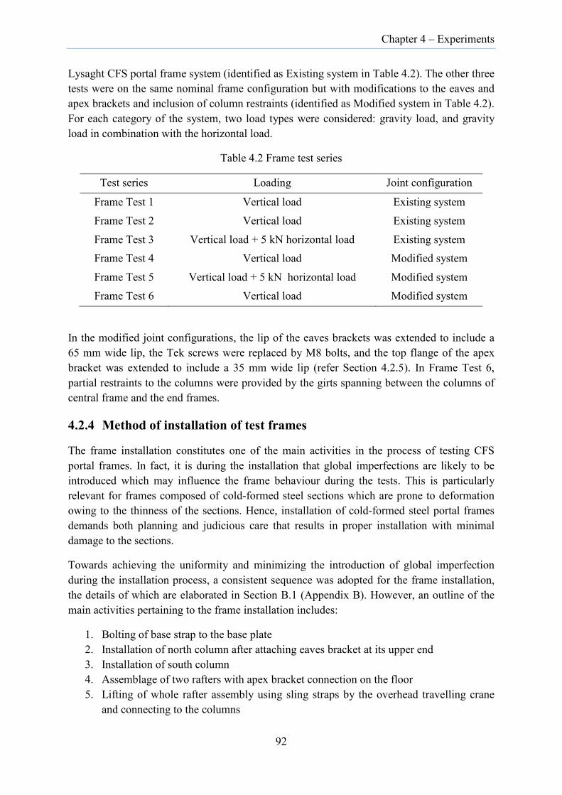
Chapter 4 – Experiments
Lysaght CFS portal frame system (identified as Existing system in Table 4.2). The other three tests were on the same nominal frame configuration but with modifications to the eaves and apex brackets and inclusion of column restraints (identified as Modified system in Table 4.2). For each category of the system, two load types were considered: gravity load, and gravity load in combination with the horizontal load.
Table 4.2 Frame test series
Test series Loading Joint configuration
Frame Test 1 Vertical load Existing system Frame Test 2 Vertical load Existing system
Frame Test 3 Vertical load + 5 kN horizontal load Existing system Frame Test 4 Vertical load Modified system
Frame Test 5 Vertical load + 5 kN horizontal load Modified system
Frame Test 6 Vertical load Modified system
In the modified joint configurations, the lip of the eaves brackets was extended to include a 65 mm wide lip, the Tek screws were replaced by M8 bolts, and the top flange of the apex bracket was extended to include a 35 mm wide lip (refer Section 4.2.5). In Frame Test 6, partial restraints to the columns were provided by the girts spanning between the columns of central frame and the end frames.
4.2.4 Method of installation of test frames
The frame installation constitutes one of the main activities in the process of testing CFS portal frames. In fact, it is during the installation that global imperfections are likely to be introduced which may influence the frame behaviour during the tests. This is particularly relevant for frames composed of cold-formed steel sections which are prone to deformation owing to the thinness of the sections. Hence, installation of cold-formed steel portal frames demands both planning and judicious care that results in proper installation with minimal damage to the sections.
Towards achieving the uniformity and minimizing the introduction of global imperfection during the installation process, a consistent sequence was adopted for the frame installation, the details of which are elaborated in Section B.1 (Appendix B). However, an outline of the main activities pertaining to the frame installation includes:
1. Bolting of base strap to the base plate 2. Installation of north column after attaching eaves bracket at its upper end 3. Installation of south column 4. Assemblage of two rafters with apex bracket connection on the floor 5. Lifting of whole rafter assembly using sling straps by the overhead travelling crane
and connecting to the columns
92

Chapter 4 – Experiments
6. Providing temporary support to the frames by means of purlins installed at the apex and at the eaves regions
7. Tightening of bolts at the apex, eaves and at the base in sequence 8. Installation of additional purlins 9. Installation of transducer frames and transducers 10. Installation of load spreading system 11. Connection of load spreading system to the hydraulic jack 12. Connection of cables from transducers and hydraulic jack to the data logger system
The above sequence implicitly assumes that the base plate and end frames are installed prior to the test frame.
The completed three-dimensional view of the Frame Test 1 depicting the load spreading system and the instrumentations is shown in Figure 4.5. All other frames (Frame Tests 2 to 5) had essentially the same set-up. However, Frame Test 6 had girts as lateral restraints installed on the columns. The completed Frame Test 6 is shown in Figure B.3 in Appendix B.
Figure 4.5 Perspective view of the test frame
4.2.5 Frame connections
The columns and rafters of the central frame were connected at the eaves, apex and base using brackets specific to the single C-section portal frames. Both the eaves and apex brackets had a nominal thickness of 3.0 mm while base strap was 6.0 mm thick. As a result of the relative light gauge of the brackets and relatively small number of fasteners, the connections were semi-rigid. The eaves bracket, zed stiffener, apex bracket and base strap for the existing system of joint configuration are shown in Figure 4.6.
93

Chapter 4 – Experiments
(a) (b) (c) (d)
Figure 4.6 Main frame connection brackets: (a) Eaves bracket; (b) Zed stiffener; (c) Apex bracket; (d) Base strap
4.2.5.1 Eaves connection
The eave connection was formed by bolting column and rafter to the eaves bracket using twelve M16 8.8/TF bolts (Figure 4.7). Two zed stiffeners were placed to clamp the column/rafter with the bracket to enhance the rigidity of the connections. The lip of eaves bracket was fastened to the lips of column/rafter using four 5.5 mm diameter self-drilling Tek screws, while the lips of column/rafter were fastened to the lips of zed stiffener using another two Tek screws each. The relative position of each bolt on the joint is identified by the number from 1 to 12 in Figure 4.7. Similarly, the positions of Tek screws are shown with a number from S1 to S8 on the figure. For detailed dimensions including the fastener locations, see annotation in Appendix B (Figure B.4).
Figure 4.7 Eaves connection
For the modified system of eaves joint configuration, all eight Tek screws were replaced by M8 bolts in addition to increasing the width of eaves bracket lips by 20 mm to provide room for the M8 bolts. The bolts are referenced with the same sign convention (S1-S8) as used for screws in the discussions to follow. For detailed dimensions including the fastener locations, see annotations in Appendix B (Figure B.9, Figure B.12 and Figure B.14).
94
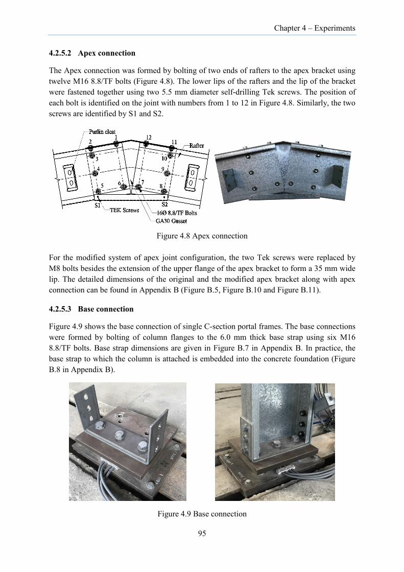
Chapter 4 – Experiments
4.2.5.2 Apex connection
The Apex connection was formed by bolting of two ends of rafters to the apex bracket using twelve M16 8.8/TF bolts (Figure 4.8). The lower lips of the rafters and the lip of the bracket were fastened together using two 5.5 mm diameter self-drilling Tek screws. The position of each bolt is identified on the joint with numbers from 1 to 12 in Figure 4.8. Similarly, the two screws are identified by S1 and S2.
Figure 4.8 Apex connection
For the modified system of apex joint configuration, the two Tek screws were replaced by M8 bolts besides the extension of the upper flange of the apex bracket to form a 35 mm wide lip. The detailed dimensions of the original and the modified apex bracket along with apex connection can be found in Appendix B (Figure B.5, Figure B.10 and Figure B.11).
4.2.5.3 Base connection
Figure 4.9 shows the base connection of single C-section portal frames. The base connections were formed by bolting of column flanges to the 6.0 mm thick base strap using six M16 8.8/TF bolts. Base strap dimensions are given in Figure B.7 in Appendix B. In practice, the base strap to which the column is attached is embedded into the concrete foundation (Figure B.8 in Appendix B).
Figure 4.9 Base connection
95

Chapter 4 – Experiments
To simulate this condition, the base strap was clamped to the upper base plate with the aid of 10 mm thick clamping plate and using three M20 8.8/TF bolts. The upper base plate was connected to the four load cells that were calibrated to provide reactions based on the strain measurement recorded during the tests. These reactions were subsequently used to determine axial load and major and minor axis bending moment at the base. The details of the load cell calibration are presented in Section B.3 (Appendix B). The four load cells were fixed to the lower base plate, which, in turn, was clamped to the I-beam encasted in the concrete floor. This type of connections is neither fixed nor pinned but semi-rigid as described in Section 4.2.12.8. Both the base plate and base plate clamp were cut from 300 grade steel. The details of the base connections are provided in Figure B.15 in Appendix B.
4.2.5.4 Purlin connection
Twenty-four supacee purlins (SC15012) spanned from the central frame to the end frames along the rafters with 12 purlins on each bay (Figure 4.1). They were connected to the web of rafter using custom-made L-shaped purlin cleats (Figure B.13 of Appendix B). Two M12 4.6/S Lysaght purlin bolts with integrated washer were used to fasten the purlin cleat to the web of the rafter while another two bolts were used to connect the purlin to the cleat. The leg of the angle cleat in contact with the web of the rafter was rigidly connected by snug-tightening both M12 bolts to prevent its slip during the tests when the frame is subjected to vertical loading. Figure 4.10 shows the purlin connection in undeformed and deformation configuration.
(a)
(b)
Figure 4.10 Purlin connection: (a) Original configuration; (b) Deformed configuration
At the cleats, purlins were designed to displace without being rotationally restrained which otherwise would transfer reactions to the end frames. This was made possible due to the
96

Chapter 4 – Experiments
combined effect of using slotted bolt holes on the cleats and the method of tightening the purlin bolts. The slotted bolt holes of 16 x 40 mm on the cleats allowed the bolts to slide horizontally without stiffening the purlins during the downward movement of the central frame. This was achieved by snug-tightening only one of the two bolts using a handheld spanner while the second bolt was finger-tightened.
The proper identification of which bolt to be snug-tightened or finger-tightened also played an important role in achieving the desired effect. For this reason, at the cleats on the end frames, the bottom bolt was snug-tightened with spanners while the top bolt was finger-tightened. However, near the central frame, the top bolt was snug-tightened while the bottom bolt was finger-tightened (Figure 4.10a). Figure 4.10b shows the expected deformation of the purlins along with the horizontal displacement of purlin bolts within the slots at the loose connection during the downward deflection of the central frame.
4.2.6 Bolting methods for the frame connections
The mechanical properties of M12 and M16 bolts used for the frame connections along with the bolting method are provided in Table 4.3. M12 bolts were used for the connection of purlins to the cleats and cleats to the web of rafters while M16 bolts were used for the connections at the eaves, apex and base.
Table 4.3 Mechanical properties of bolts [55, 71]
Bolting category
Minimum tensile strength (MPa) Method of bolting
4.6/S 400 Snug tight
8.8/TF 830 Bolts are initially snug-tightened followed by full pretension
While the M12 bolts with integrated washers were tightened using the handheld spanner to achieve the snug-tight condition, the M16 bolts were pretensioned using the turn-of-nut method (refer Section 2.3.3.2 for the description of this method). The main idea was to simulate the bolting procedure often practised at the construction site (as adopted by the BlueScope Lysaght) in the construction of CFS portal frames.
Since the bolt pretension was carried out after the installation of the frame, it was not practical to use a standard Podger hammer to achieve snug-tight condition while working at heights due to difficulty in gaining reactive force. Hence, the effort required to induce bolt rotation to attain snug-tight condition was transferred by a medium-range automatic impact hammer that would achieve the same nut turn. Use of such device not only minimized the variation that would exist in the snug-tightening of bolts with a Podger hammer (depending on the physical effort of a person executing the job) but also was more convenient to use at height.
97

Chapter 4 – Experiments
4.2.7 Lateral restraint of frames
To prevent the frame from out-of-plane instability, the end frame on grid A was restrained against out-of-plane translation at the apex and at a distance of 1.95 m on either side from the apex using 20 mm diameter threaded steel rod bolted to adjacent steel columns.
The frame was also provided with cross-bracing using 16 mm diameter threaded rods of mild steel on grid A1-B1 and A3-B3 on either end of the frames (Figure 4.11). The rods were pin connected at the column base, at the top of the column and at the centre of the cross bracing with the help of custom-made connection cleats.
Figure 4.11 Cross-bracings at the two ends of frame
Such types of cross-bracings often serve the purpose of bracing against lateral load due to wind in real portal frames. However, in the experiment, it was provided with the main purpose of arresting the frame against unintended lateral collapse while conducting the experiment, besides providing lateral restraints to the frame.
4.2.8 Measured frame and section geometry
As imperfections may affect the buckling strength of frames, it is crucial to check the imperfections of the members and the frames.
The dimensions of the C-sections were checked upon delivery of the materials and it was found that the sections generally conformed to the nominal cross-section dimensions. Nonetheless, imperfection measurements for the six columns used for the first three tests were carried out to ascertain the level of deviation of the cross-sections and the overall geometry of the members. The thickness of the C-sections, the brackets (eaves, apex, base straps) and the zed stiffeners were measured to confirm the base metal thickness of the sections required for numerical modelling. Global imperfections were also measured for each test frame before the installation of loading rigs. The details of individual measurement records are described in the following sections.
98
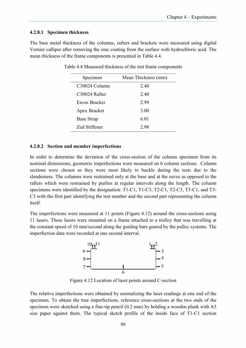
Chapter 4 – Experiments
4.2.8.1 Specimen thickness
The base metal thickness of the columns, rafters and brackets were measured using digital Vernier calliper after removing the zinc coating from the surface with hydrochloric acid. The mean thickness of the frame components is presented in Table 4.4.
Table 4.4 Measured thickness of the test frame components
Specimen Mean Thickness (mm)
C30024 Column 2.40
C30024 Rafter 2.40 Eaves Bracket 2.99
Apex Bracket 3.00
Base Strap 6.01 Zed Stiffener 2.98
4.2.8.2 Section and member imperfections
In order to determine the deviation of the cross-section of the column specimen from its nominal dimensions, geometric imperfections were measured on 6 column sections. Column sections were chosen as they were most likely to buckle during the tests due to the slenderness. The columns were restrained only at the base and at the eaves as opposed to the rafters which were restrained by purlins at regular intervals along the length. The column specimens were identified by the designation: T1-C1, T1-C3, T2-C1, T2-C3, T3-C1, and T3-C3 with the first part identifying the test number and the second part representing the column itself.
The imperfections were measured at 11 points (Figure 4.12) around the cross-sections using 11 lasers. These lasers were mounted on a frame attached to a trolley that was travelling at the constant speed of 10 mm/second along the guiding bars geared by the pulley systems. The imperfection data were recorded at one second interval.
Figure 4.12 Location of laser points around C-section
The relative imperfections were obtained by normalizing the laser readings at one end of the specimen. To obtain the true imperfections, reference cross-sections at the two ends of the specimen were sketched using a fine-tip pencil (0.2 mm) by holding a wooden plank with A3 size paper against them. The typical sketch profile of the inside face of T1-C1 section
99

Chapter 4 – Experiments
(Column C1 in Frame Test 1) at the top section is shown in Figure 4.13 along with the identification of laser positions (1,2, ….,10,11), inside flange (IF) and outside flange (OF).
Figure 4.13 Typical sketch profile of inside of C-section (Specimen T1-C1)
The profiles of the cross-section at the ends were then digitized firstly by electronically scanning the sketch and converting to image form. The image was then processed using Img2CAD (http://www.img2cad.com/) to convert it to dxf format which could be opened in AutoCAD. Once in AutoCAD, the sketch was scaled with an appropriate scale factor to match with the real imperfect cross-section of the specimen at the ends. The true imperfections at the two ends were then obtained by superimposing the perfect cross-section profile onto the imperfect cross-section profile. Thereafter, the true imperfections at the ends were added to the relative imperfections to obtain the magnitude of true imperfections along the length of the specimen. The typical true imperfections at the two ends of the T1-C1 specimen are shown in Figure 4.14 where the imperfect cross-section (solid line profile) is superimposed onto the perfect cross-section (dashed line profile).
The imperfection magnitudes corresponding to the 11 laser points at the two ends of the specimen (T1-C1) are shown in Figure 4.14 with a positive value in the directions indicated by arrows in Figure 4.12. The imperfection profiles along the entire length of the specimen (T1-C1) corresponding to each laser point are shown in Figure 4.15.
Figure 4.14 Imperfections at two ends of C-section (Specimen T1-C1)
100

Chapter 4 – Experiments
Figure 4.15 Measured imperfection profiles along C-section (Specimen T1-C1)
101

Chapter 4 – Experiments
A complete set of imperfections derived for the other five C-sections are provided in Figure B.20 to Figure B.29 in Appendix B. In general, the cross-sectional dimensions of C-section columns were within 1% of their nominal dimensions apart from localized flaring at the ends.
4.2.8.3 Global imperfection of test frames
The columns and rafters in frames are also subjected to global imperfection resulting from the lack-of-fit induced during frame installation. The magnitude of global imperfection can be significantly larger than the standalone member imperfections, especially in the CFS C-sections where the sections are prone to bending and twisting. The typical global imperfections likely to occur in the frame are indicated in Figure 4.16.
For the single C-section portal frame tests, measurements were carried out to determine the misalignment of frames and column twists. This was done right after the completion of frame installations but before the installation of the load spreading system. Measurements included determining the distance to the underside of the apex bracket from the floor level (h), diagonal distance between the top of the base strap to the underside of eaves brackets at the far end (d), and out-of-plumbness of columns and their twist deformation along the length. A laser distance meter was used to measure the longer distances. The details of the measurements are provided in Table 4.5.
Figure 4.16 Global imperfection measurements
Table 4.5 Global imperfection of the test frames
Test Series Out-of-
plumbness of column C1, δ1
Out-of-plumbness of column C3, δ2
Height to the underside of apex
bracket, h
Diagonal distance from base strap to eaves bracket, h
Frame Test 1 12 6 6505 -
Frame Test 2 27 12 6500 14089 Frame Test 3 15 26 6434 14177
Frame Test 4 23 12 6494 14107 Frame Test 5 7 19 6466 14175
Frame Test 6 32 2 6492 14105 Note: Dimensions in mm; positive values of δ1 and δ2 indicate outward global imperfections as shown in Figure 4.16.
h
d
δ1 δ2
Ideal shape
Real shape
102
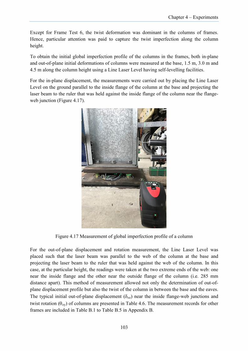
Chapter 4 – Experiments
Except for Frame Test 6, the twist deformation was dominant in the columns of frames. Hence, particular attention was paid to capture the twist imperfection along the column height.
To obtain the initial global imperfection profile of the columns in the frames, both in-plane and out-of-plane initial deformations of columns were measured at the base, 1.5 m, 3.0 m and 4.5 m along the column height using a Line Laser Level having self-levelling facilities.
For the in-plane displacement, the measurements were carried out by placing the Line Laser Level on the ground parallel to the inside flange of the column at the base and projecting the laser beam to the ruler that was held against the inside flange of the column near the flange-web junction (Figure 4.17).
Figure 4.17 Measurement of global imperfection profile of a column
For the out-of-plane displacement and rotation measurement, the Line Laser Level was placed such that the laser beam was parallel to the web of the column at the base and projecting the laser beam to the ruler that was held against the web of the column. In this case, at the particular height, the readings were taken at the two extreme ends of the web: one near the inside flange and the other near the outside flange of the column (i.e. 285 mm distance apart). This method of measurement allowed not only the determination of out-of-plane displacement profile but also the twist of the column in between the base and the eaves. The typical initial out-of-plane displacement (δoz) near the inside flange-web junctions and twist rotation (θoy) of columns are presented in Table 4.6. The measurement records for other frames are included in Table B.1 to Table B.5 in Appendix B.
103

Chapter 4 – Experiments
Table 4.6 Column imperfection profile in Frame Test 1
Height from base
(m)
Colum C1 Column C3 δoz
(mm) θoy
(degree) δoz
(mm) θoy
(degree) 0.00 0 0 0 0 1.50 7 -1.41 11 2.21 3.00 13 -2.61 18 3.61 4.50 15 -3.01 12 2.41
Note: positive direction for θoy follow right-hand rule
4.2.8.4 Other geometric imperfections
While assembling frame components, misfits were observed at the joints, mainly due to the flaring of the column and rafter sections at their ends. This occurred especially at the base and at the apex region. In such cases, the brackets were slightly stretched to allow the column or rafter sections to slide into them. As a result, some tension in the brackets and compression in the columns and rafter sections in the circumferential directions were likely to be introduced. These types of imperfection were difficult to measure, and therefore were ignored.
4.2.9 Loading arrangement
The load spreading system consisted of different lengths of metal strips as vertical hangers and horizontal square hollow steel beams arranged in three layers with the centre of the lowest beam connected to the loading jack (Figure 4.18). The ends of the vertical metal strips and horizontal beams were bolted together as pin connections using threaded rods as bolts.
Figure 4.18 Location of load points and load spreading system on central frame
104

Chapter 4 – Experiments
The vertical loads were applied to the central frame by means of metal strips hung from the brackets that were attached to the purlins on either side of the central frame (Figure 4.19, Figure 4.20). The loading brackets were positioned such that the resultant vertical load passed through the shear centre of the rafter. The purlin, in turn, transferred the load to the web of the rafters of the central frame through the purlin cleats bolted rigidly to its web. The direct application of load onto the rafter would not only cause localized failure at the load application point but also would twist the rafter due to the eccentric location of the shear centre with respect to the centroid. The completed arrangement of the load spreading system on the frame is shown in Figure 4.21.
Figure 4.19 Details of load spreading system
105
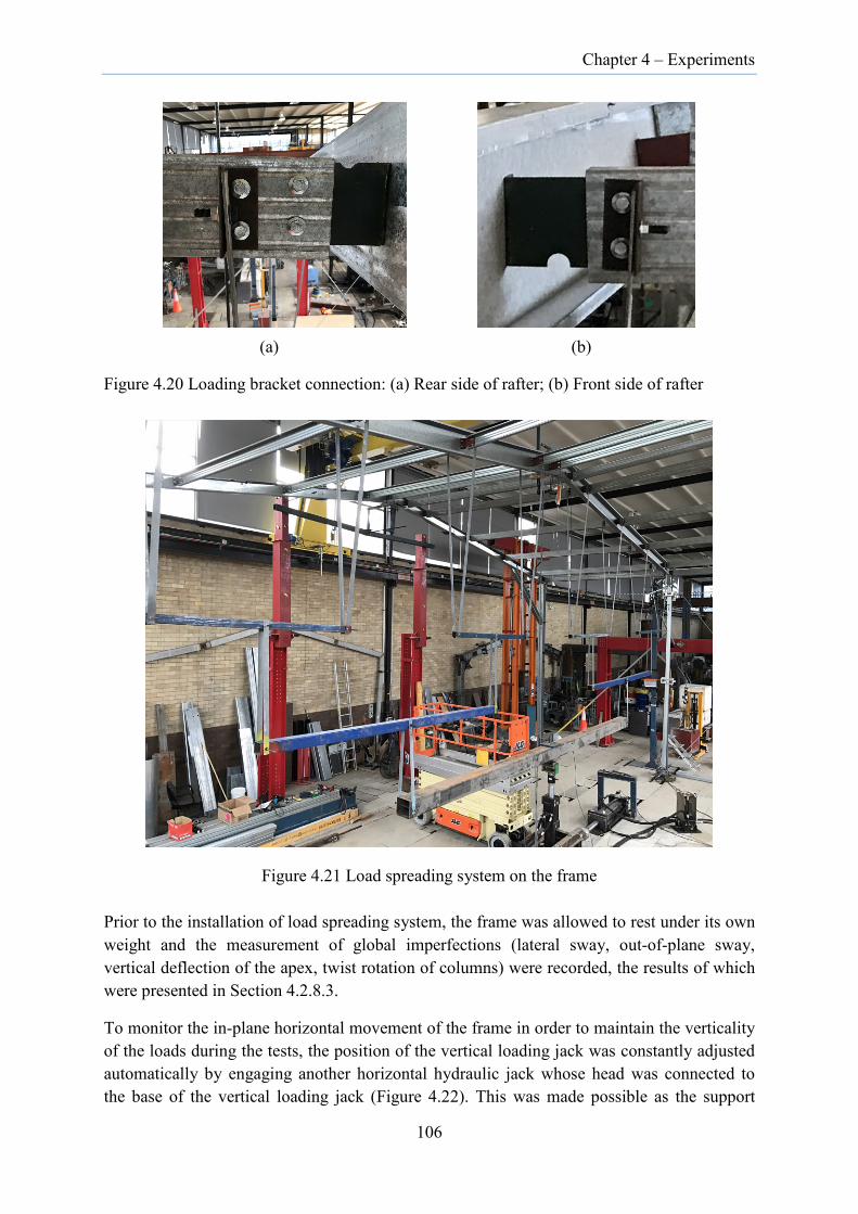
Chapter 4 – Experiments
(a) (b)
Figure 4.20 Loading bracket connection: (a) Rear side of rafter; (b) Front side of rafter
Figure 4.21 Load spreading system on the frame
Prior to the installation of load spreading system, the frame was allowed to rest under its own weight and the measurement of global imperfections (lateral sway, out-of-plane sway, vertical deflection of the apex, twist rotation of columns) were recorded, the results of which were presented in Section 4.2.8.3.
To monitor the in-plane horizontal movement of the frame in order to maintain the verticality of the loads during the tests, the position of the vertical loading jack was constantly adjusted automatically by engaging another horizontal hydraulic jack whose head was connected to the base of the vertical loading jack (Figure 4.22). This was made possible as the support
106

Chapter 4 – Experiments
system for the vertical jack was designed to move horizontally on rollers in the plane of the frame while it was effectively prevented from moving in the vertical and out-of-plane directions.
The information on the horizontal movement of the frame was fed to the horizontal actuator on the floor through the potentiometer that was installed at the apex. While the tip of the needle of the potentiometer bore on the rigid plate attached to the apex bracket, the body of the potentiometer was bolted and tied to the support system hung from the overhead stationary crane. This support system, besides supporting the potentiometer, was also designed to support another three transducers which were placed in three orthogonal directions to measure the frame deformation at the apex.
Figure 4.22 Load actuator system
For the Frame Tests 3 and 5, a constant horizontal load of 5 kN was applied at the north eaves EB3 after the installation of the vertical load spreading system but before connecting the load spreading system to the vertical loading jack, (i.e. before subjecting the frames to incremental vertical loads). The 5 kN horizontal load was kept constant throughout the duration of the tests. Figure 4.23 shows the typical deformation of a frame subjected to combination of gravity and lateral load.
The horizontal load was simulated by hanging two concrete blocks together (495 kg in total weight) with a weighing scale (9 kg) at the end of a steel strand rope whose other end passed over a pulley and was attached to a CFS bracket bolted to the web of north eaves bracket (Figure 4.24). The bracket was fabricated from 2.4 mm thick plate of size 130x110 mm. The
Potentiometer at the apex
Horizontal actuator Vertical loading jack
107

Chapter 4 – Experiments
use of thicker plate would not only stiffen the eaves bracket but also would potentially pinch its web resulting in unwanted premature failure.
Figure 4.23 Schematic diagram of frame subjected to horizontal and vertical load
Figure 4.24 Arrangement for application of horizontal load
To confirm the weight of the frame and the load spreading system recorded by the strain readings from the load cells beneath the base, the weight of the vertical load spreading system was determined by weighing individual component (metal strips, beams, loading brackets, bolts and nuts). Following a similar method, the self-weight of the central frame was also computed. The details are included in Section B.5 in Appendix B.
Attachment of lateral load to the eaves bracket EB3
Scale showing the total horizontal load (in kg) induced by the hanging concrete block
Column C1 Column C3
5 kN
Variable vertical load
108

Chapter 4 – Experiments
4.2.10 Instrumentation
To monitor the deformation of the frame during the tests, linear variable differential transducers (LVDT) having a stroke length of 50 mm, 100 mm and 200 mm were installed at various locations on the central frame. Based on the locations of the transducers, they were categorized into five groups. The location of each group of transducers on the central frame is shown in Figure 4.25. Besides these, a single transducer was also installed at the apex of the end frame on grid C to monitor its out-of-plane displacement during the frame tests. The details of the transducers along with their respective functions are provided in Table 4.7.
Figure 4.25 Location of transducers on the central frame
The typical layout configuration of the transducers at the base, eaves and apex are detailed in Figure 4.26 to Figure 4.30. While the transducers at the base (Figure 4.26) were directly attached to the steel I-beam using magnetic stands, transducers above the ground were supported using either magnetic stands or angle clamps. The magnetic stands were attached to horizontal angle sections which were clamped to vertical RHS posts erected beside each column of the test frames.
Two LVDT frames fabricated from aluminium square hollow sections were attached to each column. The first LVDT frame was located at the centre of the column (2.5 m above the base) to provide bearing surfaces for four transducers that were used for measuring the global deformation (Figure 4.27). The second LVDT frame was located at 250 mm below the eaves bracket to support the five transducers that were used to measure the local deformation of columns. It also provided bearing surfaces for another four transducers measuring global deformation (Figure 4.28).
The three transducers at the apex region (Figure 4.29) were supported by brackets attached to the inverted support that was hung from the overhead crane.
109
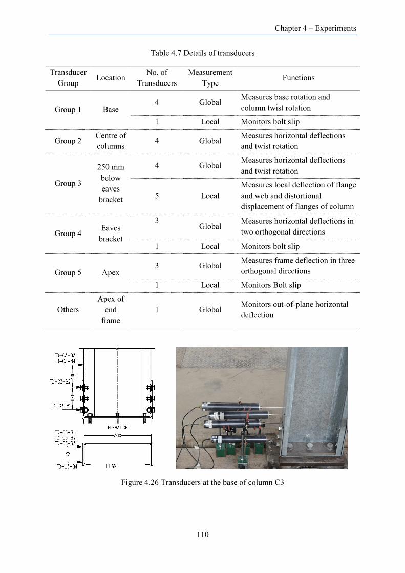
Chapter 4 – Experiments
Table 4.7 Details of transducers
Transducer Group Location No. of
Transducers Measurement
Type Functions
Group 1 Base 4 Global Measures base rotation and
column twist rotation
1 Local Monitors bolt slip
Group 2 Centre of columns 4 Global
Measures horizontal deflections and twist rotation
Group 3
250 mm below eaves
bracket
4 Global Measures horizontal deflections and twist rotation
5 Local Measures local deflection of flange and web and distortional displacement of flanges of column
Group 4 Eaves bracket
3
Global Measures horizontal deflections in two orthogonal directions
1 Local Monitors bolt slip
Group 5 Apex 3 Global Measures frame deflection in three
orthogonal directions
1 Local Monitors Bolt slip
Others Apex of
end frame
1 Global Monitors out-of-plane horizontal deflection
Figure 4.26 Transducers at the base of column C3
110

Chapter 4 – Experiments
Figure 4.27 Transducers at the mid-height of column C3
(a)
(b) (c)
Figure 4.28 Transducers on the south eaves: (a) Transducers installed on the frame; (b) Location of transducers at the eaves; (c) Layout of transducers on the LVDT frame below the eaves
111

Chapter 4 – Experiments
Figure 4.29 Transducers at the apex
Three additional transducers were installed to monitor the relative displacement (slip) of the brackets and rafter/column sections at the apex, eaves and base in some of the later frame tests (Figure 4.30). Of the three transducers, one was placed at the junction of the top flange of rafter and apex bracket while the second one was placed at the junction of the top flange of rafter and south eaves bracket. The third transducer was placed at the junction of the inside flange of column C1 and the base strap. They were directly attached to the frame members using strong adhesive tape while their needle tips bore on aluminium cleats glued to the brackets.
(a) (b)
Figure 4.30 Transducers monitoring relative displacement of connected components: (a) At the junction of apex/eaves bracket and rafter; (b) At the junction of column and base strap
All cables from the transducers were connected to the strain-based Vishay data logger which was monitored and controlled by StrainSmart500 (application software) from the computer terminal. Data were logged at the rate of one data point per second. To facilitate the identification of cables, all of them were tagged with a unique identification number at either end.
112

Chapter 4 – Experiments
4.2.11 Testing of frames
The frames were tested by applying the incremental vertical load using a 250 kN capacity hydraulic jack with a stroke length of 250 mm. After connecting the 200x200x5 SHS loading beam to the hydraulic jack, and having checked the transducers and other connections, the frame tests commenced by applying the incremental vertical load with jack displacement controlled at the rate of 2.0 mm/minute. Such a slow rate was crucial to ensure that the loading was essentially static. The tests were continued until the vertical displacement of the apex was close to 200 mm where the tests were momentarily paused to adjust the transducer position at the apex. This was necessary since the maximum displacement that could be measured by the 200-stroke transducer was 200 mm. By adjusting the position of transducers, it was possible to measure the deflection well beyond the measurement capability of the transducers.
After adjusting the transducers, the test resumed with the same displacement rate. With the exception of Frame Test 3, the frames were unloaded when the vertical jack ran out of travel; the vertical load arrangement was reset and the frame subsequently reloaded to obtain the full pre- and post-ultimate load-displacement response. One of the key observations in the single C-section portal frame tests was the propensity of the members of the frames to undergo large deformations prior to reaching the ultimate load. Hence, displacement transducers were adjusted wherever required by momentarily pausing the tests at various stages of loading. The frame ultimately failed with the sudden change in equilibrium position as described in detail in Section 4.2.12.2. The frames never collapsed totally but continued to sustain load (of much lower magnitude) in the new equilibrium position.
After completing the test, the frames were unloaded and the loading jack was detached from the load spreading system, followed by the removal of transducers. The frame components were dismantled in the reverse order of installation. While dismantling the frame components, great care was taken to avoid straining any parts to enable the post-failure observation and further diagnosis of failure modes.
4.2.12 Frame test results
4.2.12.1 General frame behaviour observed during the tests
As the load was gradually increased, the apex started to deflect vertically and both the columns started to twist in opposite directions to each other. The twisting of columns continued until the attainment of the ultimate load with major deformation occurring above its mid-height. As the loading continued to increase in the non-linear range, the top flange of the apex bracket bent upwards and local buckling deformations began to appear on the web of columns below the eaves. Similar local buckling deformation started to appear within the web of rafters at the apex region. The magnitude of local buckling deformation in the column and rafter webs progressively increased with increasing load. Figure 4.31 shows the typical global and local deformation profile of a frame midway through the tests.
113

Chapter 4 – Experiments
Figure 4.31 Typical deformation of test frame. (Note local buckling of web of column near eaves)
The frames usually reached their ultimate load capacity because of the fracture of screws at the eaves or the formation of a plastic mechanism on the compression web-flange junction of columns. The fracture of screws was often marked by a sudden loud sound and violent shaking of the whole frame. However, the failures due to the local buckling of compression flange-web junction of columns/rafters at the eaves/apex were slow and silent, unlike screw failure. Upon relieving of stresses in frames, the local buckling deformation in the columns and rafters largely disappeared indicating that these deformations were mostly elastic in nature. Nonetheless, in some frames, the columns remained twisted with significant deviation of the cross-section from its original shape at the top end.
To facilitate the explanation of the behaviour of frames through a series of load-displacement plots included in Sections 4.2.12.2 to 4.2.12.6, right-hand rule sign convention as shown in Figure 4.32 is adopted. The direction of arrows indicates the positive values.
Figure 4.32 Sign convention adopted for frame deformation
Column C1 Column
∆ay ∆ex3 ∆ex1
N
Frame
∆ex1 ∆ex3 ∆ax
∆ez1 ∆ez3 ∆az
Rafter
Rafter
Frame Plan
Apex
114

Chapter 4 – Experiments
4.2.12.2 Ultimate load capacity and collapse modes of frames
The ultimate loads attained by test frames along with the maximum vertical displacement of the apex and horizontal displacement of the eaves at collapse are presented in Table 4.8. In Table 4.8, Pu is the ultimate load, ∆ay is the vertical displacement of the apex, and ∆ex1, ∆ex3
are the horizontal displacement of the south eaves (above column C1) and north eaves (above column C3) respectively. The positive displacement directions are indicated in Figure 4.32.
Table 4.8 Ultimate load capacity and maximum displacement of frames
Test Series Pu (kN) ∆ay (mm) ∆ex1 (mm) ∆ex3 (mm)
Frame Test 1 27.2 -371 -54 42
Frame Test 2 31.2 -444 -47 64 Frame Test 3 27.1 -237 +54 139
Frame Test 4 31.4 -388 -29 81 Frame Test 5 30.5 -350 +78(83*) 191
Frame Test 6 34.9 -424 -36 69 *maximum displacement reached during unloading
The collapse of the respective frames usually occurred with the formation of a plastic mechanism or shearing of screws. The details of component failure that initiated the overall collapse of each frame are given in Table 4.9. The corresponding failure modes are shown in Figure 4.33 to Figure 4.36. The components (columns, eaves bracket, and base straps) are identified in Figure 4.2 while fasteners are identified in Figure 4.7 and Figure 4.8. They may be referred to concerning the location of fasteners and understanding of failure modes highlighted in the table below.
Table 4.9 Failure modes of test frames
Test series Failure modes
Frame Test 1
Bending of eaves bracket EB3 (along the line joining bolt 5 and bolt 6 in Figure 4.7), Shearing of screws S2 connecting inside lips of north column C3 and zed stiffener, bending of north column C3 along the bolt line (joining bolts 5 and 6 in Figure 4.7) at the eaves
Frame Test 2
Shearing of two screws (S3 and S4) connecting inside lips of north column C3 and the lip of eaves bracket EB3, bending of eaves bracket EB3 along bolt 5-bolt 6 line, local buckling of rafter R1 near the apex, outward bending of the tip of apex bracket
Frame Test 3 Shearing of screw (S2) connecting the inside lip of north column C3 and zed stiffener, bending of eaves bracket EB3, outward bending of the tip of apex bracket
115

Chapter 4 – Experiments
Test series Failure modes
Frame Test 4 Tearing of inside lip of north column C3 due to bearing of M8 bolt (S2) connecting column lip to zed stiffener, bending of column C3 along the bolt line (bolt 5-bolt 6), bending of eaves bracket EB3
Frame Test 5 Local buckling of north column C3 below the eaves
Frame Test 6 Local buckling of south column C1 below eaves bracket, local buckling of rafter R3 near the apex, bending of eaves bracket EB1, bearing of M8 bolt (S2) connecting zed stiffener to the inside lip of north column C3
(a) (b)
Figure 4.33 Failure modes of Frame Test 1 and Frame Test 3: (a) Fracture of screw; (b) Bending of eaves bracket
(a) (b)
Figure 4.34 Failure modes of Frame Test 2: (a) Fracture of screws; (b) Local buckling of rafter R1 near the apex
116
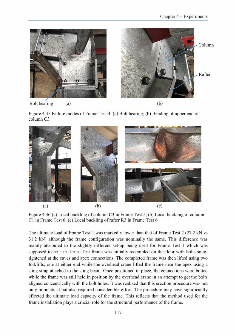
Chapter 4 – Experiments
(a) (b)
Figure 4.35 Failure modes of Frame Test 4: (a) Bolt bearing; (b) Bending of upper end of column C3
(a) (b) (c)
Figure 4.36:(a) Local buckling of column C3 in Frame Test 5; (b) Local buckling of column C1 in Frame Test 6; (c) Local buckling of rafter R3 in Frame Test 6
The ultimate load of Frame Test 1 was markedly lower than that of Frame Test 2 (27.2 kN vs 31.2 kN) although the frame configuration was nominally the same. This difference was mainly attributed to the slightly different set-up being used for Frame Test 1 which was supposed to be a trial run. Test frame was initially assembled on the floor with bolts snug-tightened at the eaves and apex connections. The completed frame was then lifted using two forklifts, one at either end while the overhead crane lifted the frame near the apex using a sling strap attached to the sling beam. Once positioned in place, the connections were bolted while the frame was still held in position by the overhead crane in an attempt to get the bolts aligned concentrically with the bolt holes. It was realized that this erection procedure was not only impractical but also required considerable effort. The procedure may have significantly affected the ultimate load capacity of the frame. This reflects that the method used for the frame installation plays a crucial role for the structural performance of the frame.
Bolt bearing
Column
Rafter
117
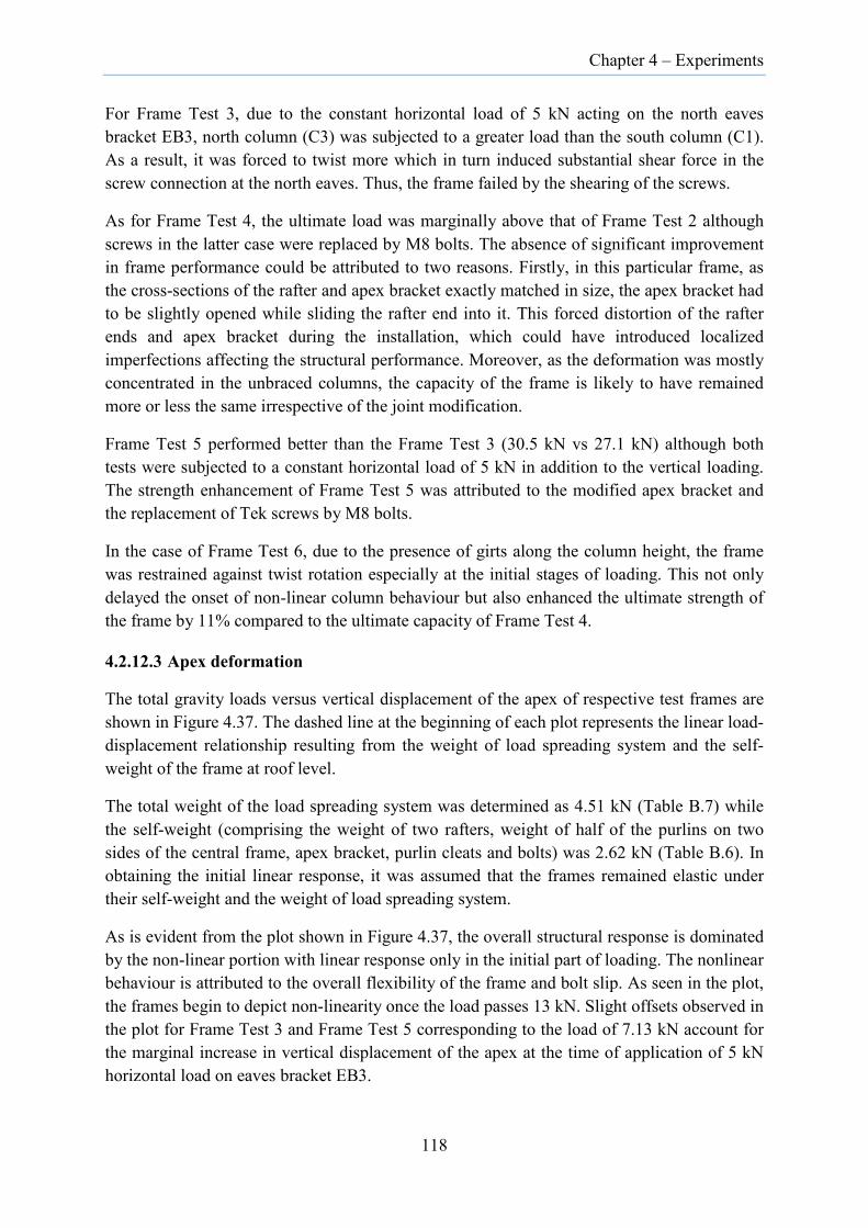
Chapter 4 – Experiments
For Frame Test 3, due to the constant horizontal load of 5 kN acting on the north eaves bracket EB3, north column (C3) was subjected to a greater load than the south column (C1). As a result, it was forced to twist more which in turn induced substantial shear force in the screw connection at the north eaves. Thus, the frame failed by the shearing of the screws.
As for Frame Test 4, the ultimate load was marginally above that of Frame Test 2 although screws in the latter case were replaced by M8 bolts. The absence of significant improvement in frame performance could be attributed to two reasons. Firstly, in this particular frame, as the cross-sections of the rafter and apex bracket exactly matched in size, the apex bracket had to be slightly opened while sliding the rafter end into it. This forced distortion of the rafter ends and apex bracket during the installation, which could have introduced localized imperfections affecting the structural performance. Moreover, as the deformation was mostly concentrated in the unbraced columns, the capacity of the frame is likely to have remained more or less the same irrespective of the joint modification.
Frame Test 5 performed better than the Frame Test 3 (30.5 kN vs 27.1 kN) although both tests were subjected to a constant horizontal load of 5 kN in addition to the vertical loading. The strength enhancement of Frame Test 5 was attributed to the modified apex bracket and the replacement of Tek screws by M8 bolts.
In the case of Frame Test 6, due to the presence of girts along the column height, the frame was restrained against twist rotation especially at the initial stages of loading. This not only delayed the onset of non-linear column behaviour but also enhanced the ultimate strength of the frame by 11% compared to the ultimate capacity of Frame Test 4.
4.2.12.3 Apex deformation
The total gravity loads versus vertical displacement of the apex of respective test frames are shown in Figure 4.37. The dashed line at the beginning of each plot represents the linear load-displacement relationship resulting from the weight of load spreading system and the self-weight of the frame at roof level.
The total weight of the load spreading system was determined as 4.51 kN (Table B.7) while the self-weight (comprising the weight of two rafters, weight of half of the purlins on two sides of the central frame, apex bracket, purlin cleats and bolts) was 2.62 kN (Table B.6). In obtaining the initial linear response, it was assumed that the frames remained elastic under their self-weight and the weight of load spreading system.
As is evident from the plot shown in Figure 4.37, the overall structural response is dominated by the non-linear portion with linear response only in the initial part of loading. The nonlinear behaviour is attributed to the overall flexibility of the frame and bolt slip. As seen in the plot, the frames begin to depict non-linearity once the load passes 13 kN. Slight offsets observed in the plot for Frame Test 3 and Frame Test 5 corresponding to the load of 7.13 kN account for the marginal increase in vertical displacement of the apex at the time of application of 5 kN horizontal load on eaves bracket EB3.
118
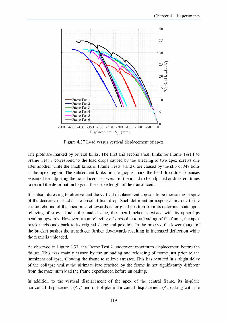
Chapter 4 – Experiments
Figure 4.37 Load versus vertical displacement of apex
The plots are marked by several kinks. The first and second small kinks for Frame Test 1 to Frame Test 3 correspond to the load drops caused by the shearing of two apex screws one after another while the small kinks in Frame Tests 4 and 6 are caused by the slip of M8 bolts at the apex region. The subsequent kinks on the graphs mark the load drop due to pauses executed for adjusting the transducers as several of them had to be adjusted at different times to record the deformation beyond the stroke length of the transducers.
It is also interesting to observe that the vertical displacement appears to be increasing in spite of the decrease in load at the onset of load drop. Such deformation responses are due to the elastic rebound of the apex bracket towards its original position from its deformed state upon relieving of stress. Under the loaded state, the apex bracket is twisted with its upper lips bending upwards. However, upon relieving of stress due to unloading of the frame, the apex bracket rebounds back to its original shape and position. In the process, the lower flange of the bracket pushes the transducer further downwards resulting in increased deflection while the frame is unloaded.
As observed in Figure 4.37, the Frame Test 2 underwent maximum displacement before the failure. This was mainly caused by the unloading and reloading of frame just prior to the imminent collapse, allowing the frame to relieve stresses. This has resulted in a slight delay of the collapse whilst the ultimate load reached by the frame is not significantly different from the maximum load the frame experienced before unloading.
In addition to the vertical displacement of the apex of the central frame, its in-plane horizontal displacement (∆ax) and out-of-plane horizontal displacement (∆az) along with the
119

Chapter 4 – Experiments
out-of-plane displacement (∆efz) of end frame on grid C were also monitored during the tests. The respective plots are included in Figure B.34 and in Figure B.35 in Appendix B.
4.2.12.4 Eaves deformation
Figure 4.38 and Figure 4.39 show the horizontal displacement of the south eaves and north eaves respectively.
Figure 4.38 In-plane horizontal displacement of south eaves
Figure 4.39 In-plane horizontal displacement of north eaves
120
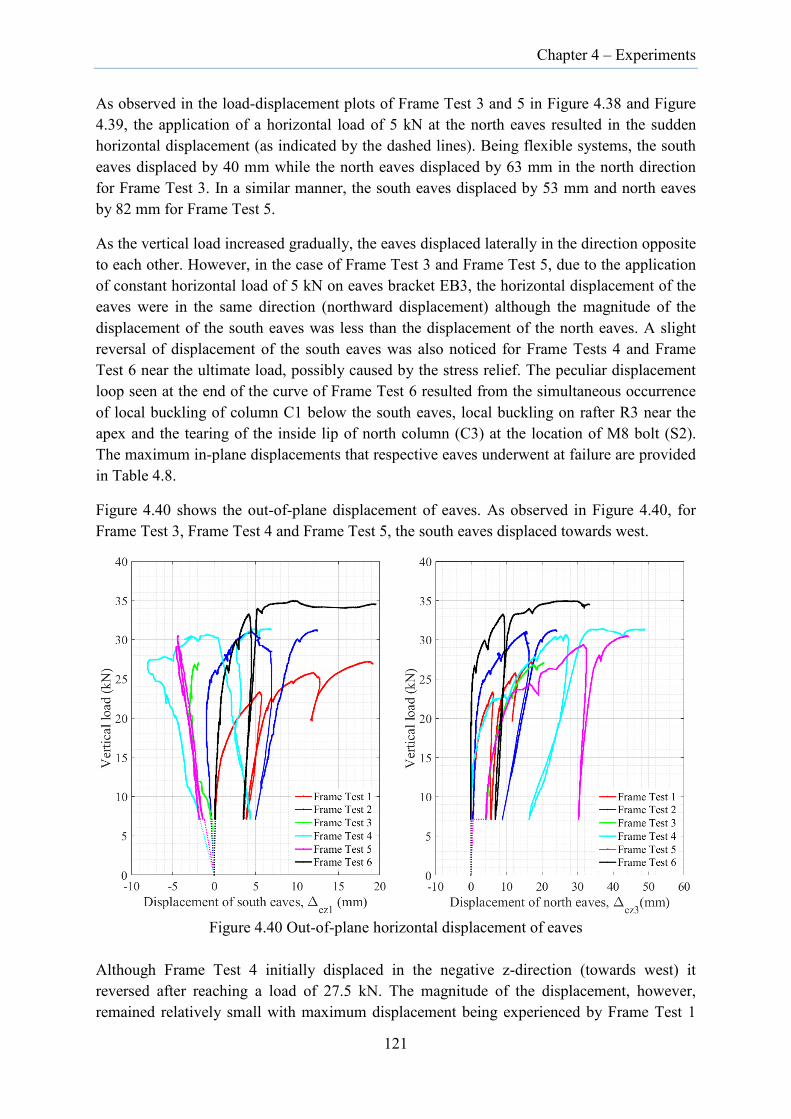
Chapter 4 – Experiments
As observed in the load-displacement plots of Frame Test 3 and 5 in Figure 4.38 and Figure 4.39, the application of a horizontal load of 5 kN at the north eaves resulted in the sudden horizontal displacement (as indicated by the dashed lines). Being flexible systems, the south eaves displaced by 40 mm while the north eaves displaced by 63 mm in the north direction for Frame Test 3. In a similar manner, the south eaves displaced by 53 mm and north eaves by 82 mm for Frame Test 5.
As the vertical load increased gradually, the eaves displaced laterally in the direction opposite to each other. However, in the case of Frame Test 3 and Frame Test 5, due to the application of constant horizontal load of 5 kN on eaves bracket EB3, the horizontal displacement of the eaves were in the same direction (northward displacement) although the magnitude of the displacement of the south eaves was less than the displacement of the north eaves. A slight reversal of displacement of the south eaves was also noticed for Frame Tests 4 and Frame Test 6 near the ultimate load, possibly caused by the stress relief. The peculiar displacement loop seen at the end of the curve of Frame Test 6 resulted from the simultaneous occurrence of local buckling of column C1 below the south eaves, local buckling on rafter R3 near the apex and the tearing of the inside lip of north column (C3) at the location of M8 bolt (S2). The maximum in-plane displacements that respective eaves underwent at failure are provided in Table 4.8.
Figure 4.40 shows the out-of-plane displacement of eaves. As observed in Figure 4.40, for Frame Test 3, Frame Test 4 and Frame Test 5, the south eaves displaced towards west.
Figure 4.40 Out-of-plane horizontal displacement of eaves
Although Frame Test 4 initially displaced in the negative z-direction (towards west) it reversed after reaching a load of 27.5 kN. The magnitude of the displacement, however, remained relatively small with maximum displacement being experienced by Frame Test 1
121

Chapter 4 – Experiments
and Frame Test 6. On the other hand, the north eaves displaced in the positive z-direction in all frame tests. In this case, the maximum displacements were experienced by Frame Tests 4, 5 and 6. The large displacements were the direct consequence of the large local deformation (bending of eaves bracket EB3) especially near the ultimate load in these frame tests.
4.2.12.5 Flexural-torsional deformation of columns
The unique behaviour exhibited by all frames except Frame Test 6 is the gradual twisting of both columns in the direction opposite to each other besides the horizontal displacements as the load is progressively increased. Figure 4.41 shows the flexural-torsional deformation profile of columns from Frame Test 1 and Frame Test 4 – a representative example of a frame with existing joint configuration and modified configuration respectively. In the case of Frame Test 3 and Frame Test 5, which has a constant horizontal load of 5 kN applied on eaves bracket EB3, the twist deformation of the north column (C3) was larger than that of the south column (C1) due to frame sway.
(a) (b) (c) (d)
Figure 4.41 Flexural-torsional deformation of columns: (a) Column C1, and (b) Column C3 from Frame Test 1; (c) Column C1 and (d) Column C3 from Frame Test 4
122
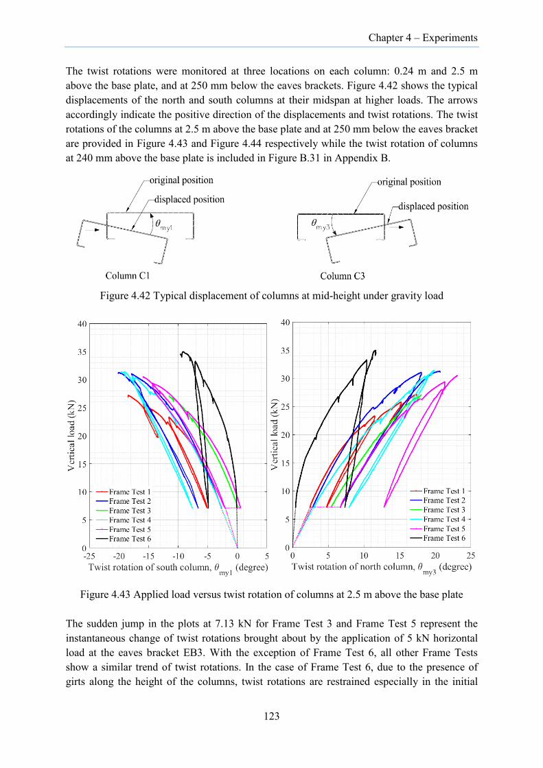
Chapter 4 – Experiments
The twist rotations were monitored at three locations on each column: 0.24 m and 2.5 m above the base plate, and at 250 mm below the eaves brackets. Figure 4.42 shows the typical displacements of the north and south columns at their midspan at higher loads. The arrows accordingly indicate the positive direction of the displacements and twist rotations. The twist rotations of the columns at 2.5 m above the base plate and at 250 mm below the eaves bracket are provided in Figure 4.43 and Figure 4.44 respectively while the twist rotation of columns at 240 mm above the base plate is included in Figure B.31 in Appendix B.
Figure 4.42 Typical displacement of columns at mid-height under gravity load
Figure 4.43 Applied load versus twist rotation of columns at 2.5 m above the base plate
The sudden jump in the plots at 7.13 kN for Frame Test 3 and Frame Test 5 represent the instantaneous change of twist rotations brought about by the application of 5 kN horizontal load at the eaves bracket EB3. With the exception of Frame Test 6, all other Frame Tests show a similar trend of twist rotations. In the case of Frame Test 6, due to the presence of girts along the height of the columns, twist rotations are restrained especially in the initial
123
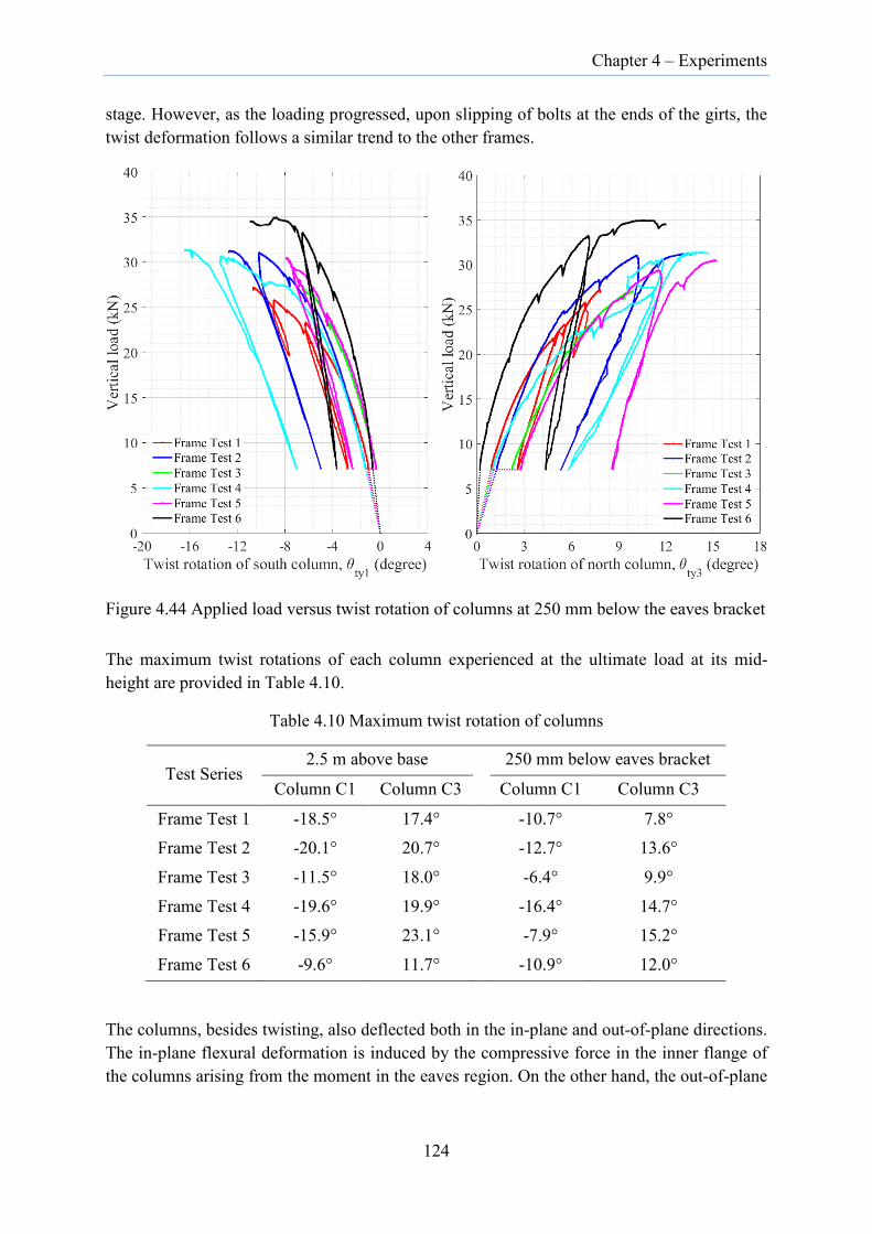
Chapter 4 – Experiments
stage. However, as the loading progressed, upon slipping of bolts at the ends of the girts, the twist deformation follows a similar trend to the other frames.
Figure 4.44 Applied load versus twist rotation of columns at 250 mm below the eaves bracket
The maximum twist rotations of each column experienced at the ultimate load at its mid-height are provided in Table 4.10.
Table 4.10 Maximum twist rotation of columns
Test Series 2.5 m above base 250 mm below eaves bracket
Column C1 Column C3 Column C1 Column C3
Frame Test 1 -18.5° 17.4° -10.7° 7.8° Frame Test 2 -20.1° 20.7° -12.7° 13.6°
Frame Test 3 -11.5° 18.0° -6.4° 9.9°
Frame Test 4 -19.6° 19.9° -16.4° 14.7° Frame Test 5 -15.9° 23.1° -7.9° 15.2°
Frame Test 6 -9.6° 11.7° -10.9° 12.0°
The columns, besides twisting, also deflected both in the in-plane and out-of-plane directions. The in-plane flexural deformation is induced by the compressive force in the inner flange of the columns arising from the moment in the eaves region. On the other hand, the out-of-plane
124

Chapter 4 – Experiments
displacements are due to the axial load acting through the web instead of acting through the centroid.
The overall flexural-torsional buckling of columns is induced by the flexural twisting moment arising from the bimoment, which in turn, originated due to the non-uniform distribution of longitudinal stress across the column sections. Stress gradient within the column section are due to the combined action of bending and axial force in columns and the eccentric distribution of bolts on the eaves brackets. For further details, see Section 5.5.8.
The in-plane displacement (∆mx1, ∆mx3) corresponding to M2 transducer reading and out-of-plane displacement (∆mz1, ∆mz3) corresponding to M3 transducer reading on columns are provided in Figure B.32 and Figure B.33 respectively in Appendix B. The location of M2 and M3 transducers are shown in Figure 4.27.
4.2.12.6 Local buckling deformation of columns
As the loading progressed into the non-linear range, local buckling deformations started to appear in the web of the columns below the eaves. With increasing load, local buckling deformation extended downward towards the mid-height of the column (Figure 4.45). It also appeared in the rafters near the apex upon further loading.
Figure 4.45 Local buckling deformation of columns C1 and C3 in Frame Test 2
The magnitude of buckling deformation was higher near the inner flange-web junction in the columns and at the top flange-web junction in the rafters being subjected to bending. An
125
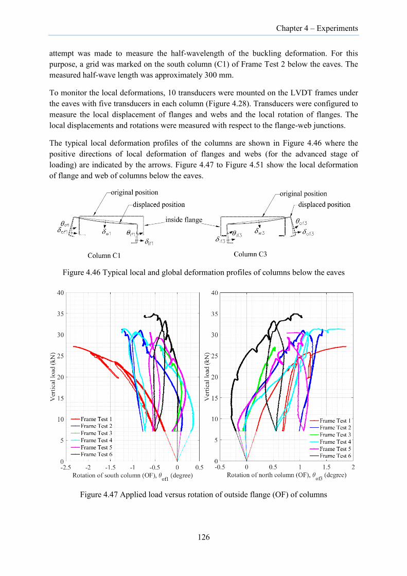
Chapter 4 – Experiments
attempt was made to measure the half-wavelength of the buckling deformation. For this purpose, a grid was marked on the south column (C1) of Frame Test 2 below the eaves. The measured half-wave length was approximately 300 mm.
To monitor the local deformations, 10 transducers were mounted on the LVDT frames under the eaves with five transducers in each column (Figure 4.28). Transducers were configured to measure the local displacement of flanges and webs and the local rotation of flanges. The local displacements and rotations were measured with respect to the flange-web junctions.
The typical local deformation profiles of the columns are shown in Figure 4.46 where the positive directions of local deformation of flanges and webs (for the advanced stage of loading) are indicated by the arrows. Figure 4.47 to Figure 4.51 show the local deformation of flange and web of columns below the eaves.
Figure 4.46 Typical local and global deformation profiles of columns below the eaves
Figure 4.47 Applied load versus rotation of outside flange (OF) of columns
126
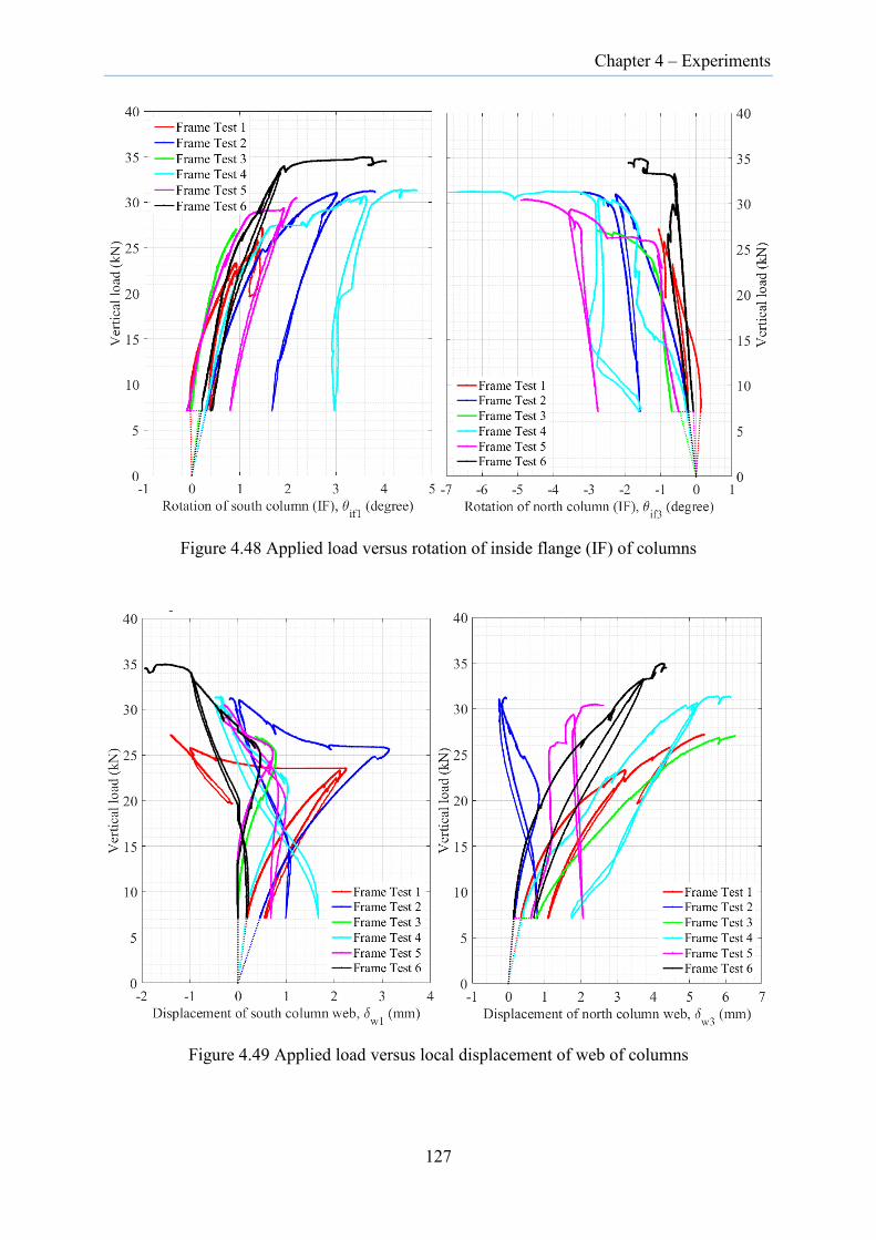
Chapter 4 – Experiments
Figure 4.48 Applied load versus rotation of inside flange (IF) of columns
Figure 4.49 Applied load versus local displacement of web of columns
127
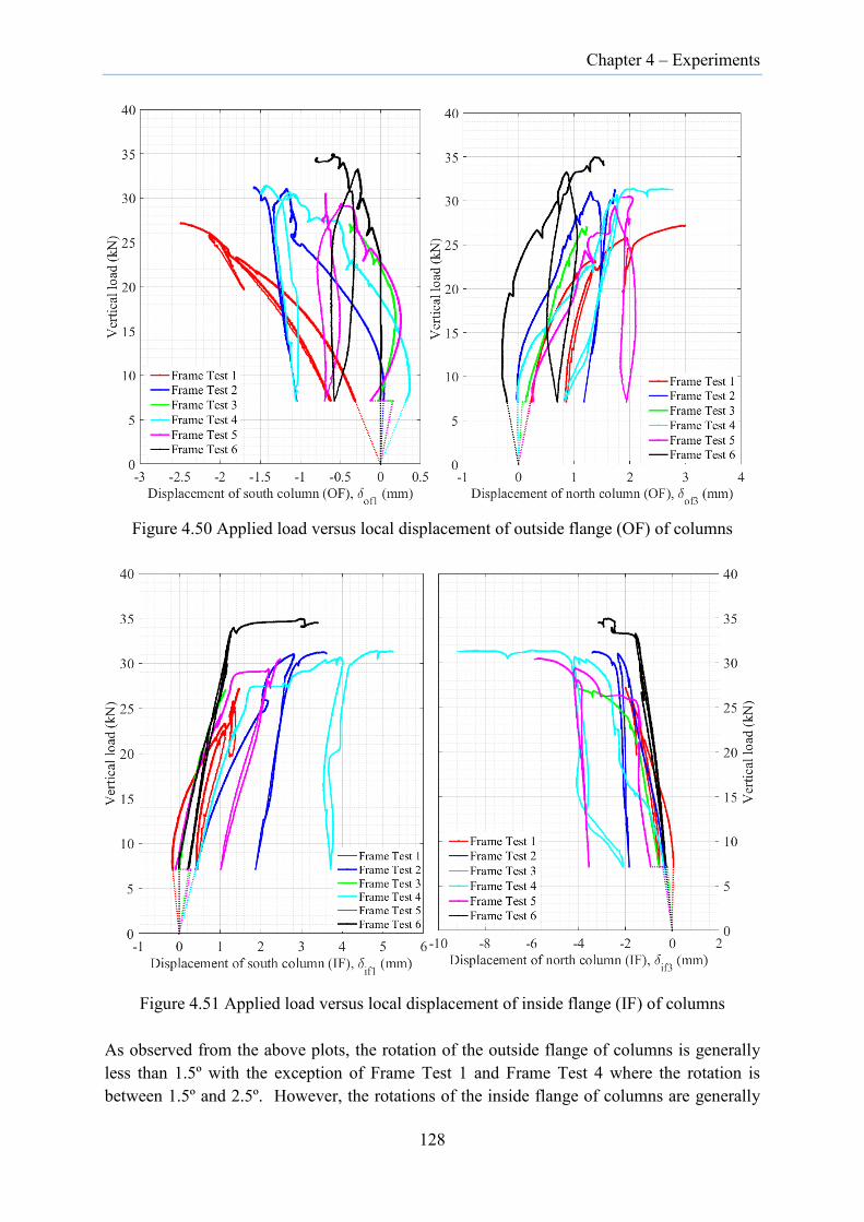
Chapter 4 – Experiments
Figure 4.50 Applied load versus local displacement of outside flange (OF) of columns
Figure 4.51 Applied load versus local displacement of inside flange (IF) of columns
As observed from the above plots, the rotation of the outside flange of columns is generally less than 1.5º with the exception of Frame Test 1 and Frame Test 4 where the rotation is between 1.5º and 2.5º. However, the rotations of the inside flange of columns are generally
128
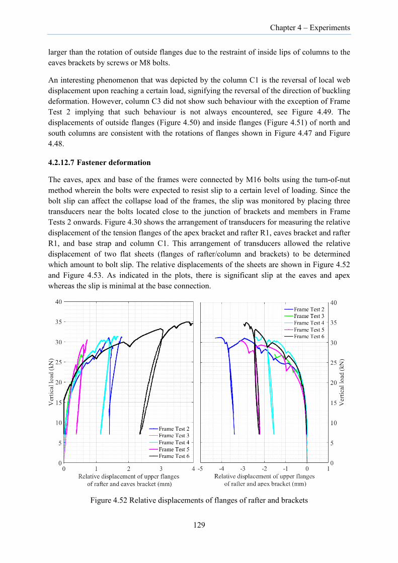
Chapter 4 – Experiments
larger than the rotation of outside flanges due to the restraint of inside lips of columns to the eaves brackets by screws or M8 bolts.
An interesting phenomenon that was depicted by the column C1 is the reversal of local web displacement upon reaching a certain load, signifying the reversal of the direction of buckling deformation. However, column C3 did not show such behaviour with the exception of Frame Test 2 implying that such behaviour is not always encountered, see Figure 4.49. The displacements of outside flanges (Figure 4.50) and inside flanges (Figure 4.51) of north and south columns are consistent with the rotations of flanges shown in Figure 4.47 and Figure 4.48.
4.2.12.7 Fastener deformation
The eaves, apex and base of the frames were connected by M16 bolts using the turn-of-nut method wherein the bolts were expected to resist slip to a certain level of loading. Since the bolt slip can affect the collapse load of the frames, the slip was monitored by placing three transducers near the bolts located close to the junction of brackets and members in Frame Tests 2 onwards. Figure 4.30 shows the arrangement of transducers for measuring the relative displacement of the tension flanges of the apex bracket and rafter R1, eaves bracket and rafter R1, and base strap and column C1. This arrangement of transducers allowed the relative displacement of two flat sheets (flanges of rafter/column and brackets) to be determined which amount to bolt slip. The relative displacements of the sheets are shown in Figure 4.52 and Figure 4.53. As indicated in the plots, there is significant slip at the eaves and apex whereas the slip is minimal at the base connection.
Figure 4.52 Relative displacements of flanges of rafter and brackets
129
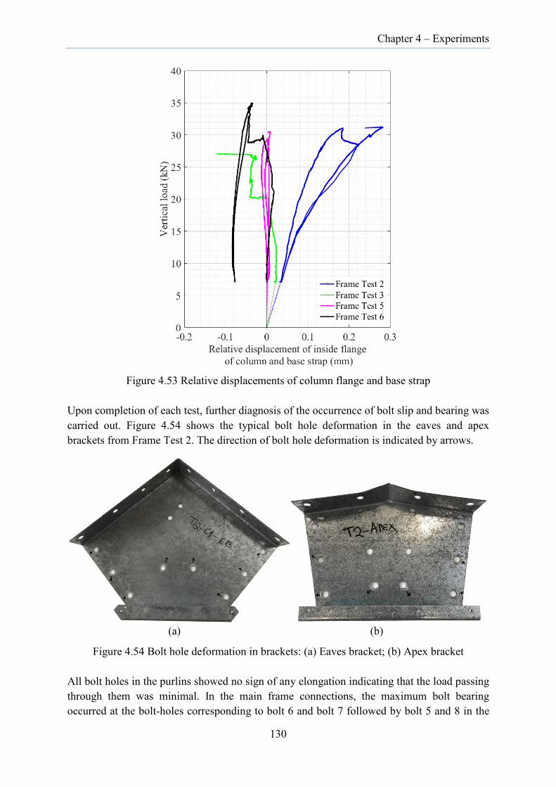
Chapter 4 – Experiments
Figure 4.53 Relative displacements of column flange and base strap
Upon completion of each test, further diagnosis of the occurrence of bolt slip and bearing was carried out. Figure 4.54 shows the typical bolt hole deformation in the eaves and apex brackets from Frame Test 2. The direction of bolt hole deformation is indicated by arrows.
(a) (b)
Figure 4.54 Bolt hole deformation in brackets: (a) Eaves bracket; (b) Apex bracket
All bolt holes in the purlins showed no sign of any elongation indicating that the load passing through them was minimal. In the main frame connections, the maximum bolt bearing occurred at the bolt-holes corresponding to bolt 6 and bolt 7 followed by bolt 5 and 8 in the
130
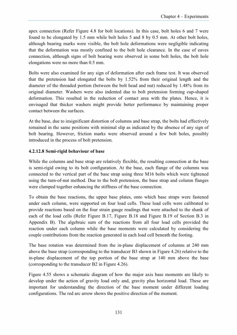
Chapter 4 – Experiments
apex connection (Refer Figure 4.8 for bolt locations). In this case, bolt holes 6 and 7 were found to be elongated by 1.5 mm while bolt holes 5 and 8 by 0.5 mm. At other bolt holes, although bearing marks were visible, the bolt hole deformations were negligible indicating that the deformation was mostly confined to the bolt hole clearance. In the case of eaves connection, although signs of bolt bearing were observed in some bolt holes, the bolt hole elongations were no more than 0.5 mm.
Bolts were also examined for any sign of deformation after each frame test. It was observed that the pretension had elongated the bolts by 1.52% from their original length and the diameter of the threaded portion (between the bolt head and nut) reduced by 1.48% from its original diameter. Washers were also indented due to bolt pretension forming cup-shaped deformation. This resulted in the reduction of contact area with the plates. Hence, it is envisaged that thicker washers might provide better performance by maintaining proper contact between the surfaces.
At the base, due to insignificant distortion of columns and base strap, the bolts had effectively remained in the same positions with minimal slip as indicated by the absence of any sign of bolt bearing. However, friction marks were observed around a few bolt holes, possibly introduced in the process of bolt pretension.
4.2.12.8 Semi-rigid behaviour of base
While the columns and base strap are relatively flexible, the resulting connection at the base is semi-rigid owing to its bolt configuration. At the base, each flange of the columns was connected to the vertical part of the base strap using three M16 bolts which were tightened using the turn-of-nut method. Due to the bolt pretension, the base strap and column flanges were clamped together enhancing the stiffness of the base connection.
To obtain the base reactions, the upper base plates, onto which base straps were fastened under each column, were supported on four load cells. These load cells were calibrated to provide reactions based on the four strain gauge readings that were attached to the shank of each of the load cells (Refer Figure B.17, Figure B.18 and Figure B.19 of Section B.3 in Appendix B). The algebraic sum of the reactions from all four load cells provided the reaction under each column while the base moments were calculated by considering the couple contributions from the reaction generated in each load cell beneath the footing.
The base rotation was determined from the in-plane displacement of columns at 240 mm above the base strap (corresponding to the transducer B3 shown in Figure 4.26) relative to the in-plane displacement of the top portion of the base strap at 140 mm above the base (corresponding to the transducer B2 in Figure 4.26).
Figure 4.55 shows a schematic diagram of how the major axis base moments are likely to develop under the action of gravity load only and, gravity plus horizontal load. These are important for understanding the direction of the base moment under different loading configurations. The red arc arrow shows the positive direction of the moment.
131

Chapter 4 – Experiments
The major axis bending moments developed at the base of respective columns are opposite in direction when the frames are subjected to gravity load only (Figure 4.55a). On the other hand, the frames that are subjected to lateral load develop bending moment in the same direction at the base. However, for the frames initially subjected to horizontal force and subsequently to the vertical load while the initial lateral force being maintained constant, moment reversal occurs at the base of column C1. These observations are relevant to the base moment-rotation relations derived for the test frames.
Figure 4.55 Frame deformation: (a) Gravity load only; (b) Lateral load; (c) Lateral load followed by gravity load
The in-plane major axis base moment-rotation relations for the frames subjected to gravity loads are provided in Figure 4.56 while for frames with vertical load along with a constant horizontal load (of 5 kN acting at the north eaves) are provided in Figure 4.57. For Frame Test 2, the transducer B2 at the base of column C1 malfunctioned during the test and hence only the moment-rotation curve at the base of column C3 is produced for this test. The dashed lines at the starting point of the curves in Figure 4.56 represent the initial moment generated at the base due to the load spreading system installation. However, in Figure 4.57, the dashed lines represent not only the moment generated due to the load spreading system installation but also the additional moment induced when the horizontal load of 5 kN was applied at the north eaves.
As observed in Figure 4.56, the bending moment gradually developed at the column base as the vertical load increased. The initial bending moment developed at the base due to the installation of load spreading system was marginal (less than 1 kNm) in Frame Tests 1, 2 and 4 with the exception of Frame Test 6. As the frame was slightly stiffer due to the presence of girts along the column height, Frame Test 6 developed an initial moment of 1.2 kNm.
However, in the case of frames with the constant horizontal load acting at the north eaves in addition to the vertical loads (Frame Tests 3 and 5), there were significant differences
Column C1 Column C3
(a)
(b) (c)
Positive direction of moment
132

Chapter 4 – Experiments
between the bending moments developed at the base of column C1 and column C3. In this case, although the initial moments generated upon installation of the load spreading system were similar to those for the frames with vertical loads only (Frame Tests 1, 2, 4, 6), the moments generated at the base upon application of the horizontal load of 5 kN were significantly higher (5.7 kNm for column C1 and 5.2 kNm for column C3 in Frame Test 3; 6.72 kNm for column C1 and 6.2 kNm for column C3 in Frame Test 5).
(a) (b)
(c) (d)
Figure 4.56 Base moment versus rotation for frames with vertical load only: (a) Frame Test 1; (b) Frame Test 2; (c) Frame Test 4; (d) Frame Test 6
133
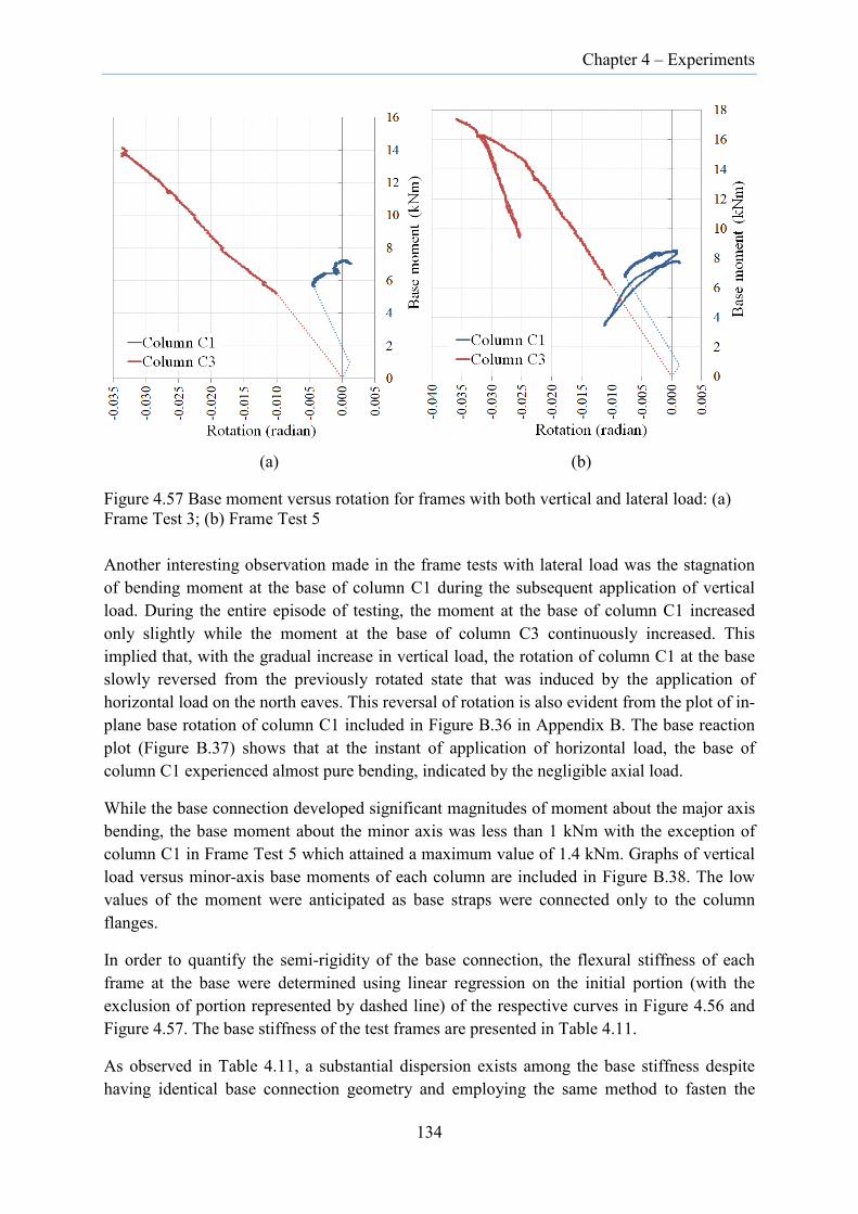
Chapter 4 – Experiments
(a) (b)
Figure 4.57 Base moment versus rotation for frames with both vertical and lateral load: (a) Frame Test 3; (b) Frame Test 5
Another interesting observation made in the frame tests with lateral load was the stagnation of bending moment at the base of column C1 during the subsequent application of vertical load. During the entire episode of testing, the moment at the base of column C1 increased only slightly while the moment at the base of column C3 continuously increased. This implied that, with the gradual increase in vertical load, the rotation of column C1 at the base slowly reversed from the previously rotated state that was induced by the application of horizontal load on the north eaves. This reversal of rotation is also evident from the plot of in-plane base rotation of column C1 included in Figure B.36 in Appendix B. The base reaction plot (Figure B.37) shows that at the instant of application of horizontal load, the base of column C1 experienced almost pure bending, indicated by the negligible axial load.
While the base connection developed significant magnitudes of moment about the major axis bending, the base moment about the minor axis was less than 1 kNm with the exception of column C1 in Frame Test 5 which attained a maximum value of 1.4 kNm. Graphs of vertical load versus minor-axis base moments of each column are included in Figure B.38. The low values of the moment were anticipated as base straps were connected only to the column flanges.
In order to quantify the semi-rigidity of the base connection, the flexural stiffness of each frame at the base were determined using linear regression on the initial portion (with the exclusion of portion represented by dashed line) of the respective curves in Figure 4.56 and Figure 4.57. The base stiffness of the test frames are presented in Table 4.11.
As observed in Table 4.11, a substantial dispersion exists among the base stiffness despite having identical base connection geometry and employing the same method to fasten the
134

Chapter 4 – Experiments
connection parts. The reasons for the variability are not obvious. One of the suspected causes contributing to variability is the difficulty of aligning and maintaining the concentric position of bolts and washers with the bolt holes. Due to the slotted bolt holes (19 mm by 25 mm), the bolts were inadvertently displaced slightly during bolting using turn-of-nut method when a large moment had to be imparted to the nuts by the impact hammer.
Table 4.11 Column base stiffness
Test series Column C1 (kNm/radian)
Column C3 (kNm/radian)
Frame Test 1 713 438 Frame Test 2 - 451 Frame Test 3 297 320 Frame Test 4 576 239 Frame Test 5 481 609 Frame Test 6 843 825
Mean 582 480 COV 0.36 0.44
4.3 Coupon tests The mechanical properties of the cold-formed sections are required for the accurate prediction of structural behaviour during numerical analysis. Hence, towards establishing the material properties and determining the post-yield material behaviour, uniaxial tensile tests were performed on 4 sets of coupons with each set consisting of 3 specimens. The first two sets, each with 3 specimens, were extracted from the centre portion of the web of the column (column C3 from Frame Test 1) while the other two sets, each with 3 specimens, were cut from the flat portion of bottom flanges of the eaves and the apex bracket respectively. Of the two sets extracted from the column, one set belonged to the longitudinal direction and the other set to the transverse direction.
4.3.1 Tests preparation
The specimens were cut to dimensions (Figure 4.58) in accordance with the Australian standard AS 1391:2007 [126]. To avoid superficial work hardening and heating of materials due to cutting, the coupons were cut using a high-precision water-jet laser cutter. The zinc coating on the specimens was removed by immersing them in a trough containing hydrochloric acid. Once the zinc coating was completely removed as indicated by the absence of hydrogen formation (stoppage of bubbles), the specimens were removed, rinsed with water and wiped with rags to dry.
The gauge length along with its midpoint was marked (using a scriber) on each specimen. With a digital Vernier calliper, the base metal thickness and width of each coupon was measured at three locations equidistant from each other within the gauge length. These quantities were subsequently used to compute the tensile stress. The details of coupon tests
135
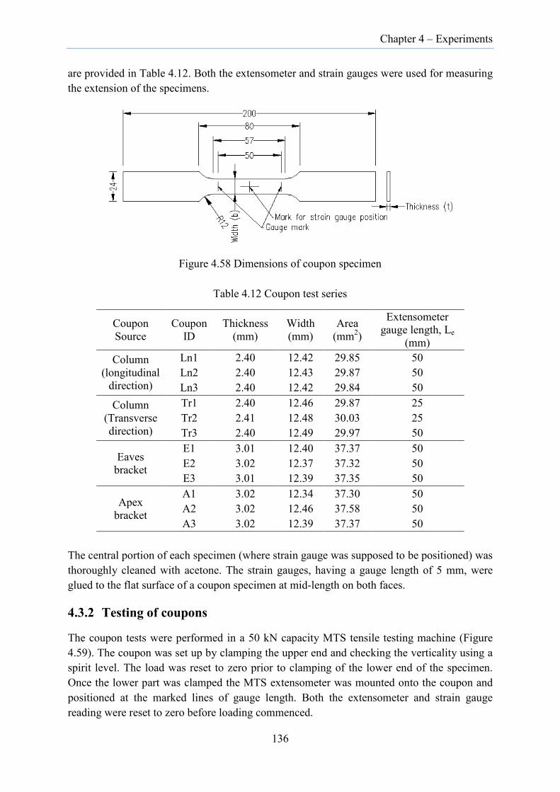
Chapter 4 – Experiments
are provided in Table 4.12. Both the extensometer and strain gauges were used for measuring the extension of the specimens.
Figure 4.58 Dimensions of coupon specimen
Table 4.12 Coupon test series
Coupon Source
Coupon ID
Thickness (mm)
Width (mm)
Area (mm2)
Extensometer gauge length, Le
(mm) Column
(longitudinal direction)
Ln1 2.40 12.42 29.85 50 Ln2 2.40 12.43 29.87 50 Ln3 2.40 12.42 29.84 50
Column (Transverse direction)
Tr1 2.40 12.46 29.87 25 Tr2 2.41 12.48 30.03 25 Tr3 2.40 12.49 29.97 50
Eaves bracket
E1 3.01 12.40 37.37 50 E2 3.02 12.37 37.32 50 E3 3.01 12.39 37.35 50
Apex bracket
A1 3.02 12.34 37.30 50 A2 3.02 12.46 37.58 50 A3 3.02 12.39 37.37 50
The central portion of each specimen (where strain gauge was supposed to be positioned) was thoroughly cleaned with acetone. The strain gauges, having a gauge length of 5 mm, were glued to the flat surface of a coupon specimen at mid-length on both faces.
4.3.2 Testing of coupons
The coupon tests were performed in a 50 kN capacity MTS tensile testing machine (Figure 4.59). The coupon was set up by clamping the upper end and checking the verticality using a spirit level. The load was reset to zero prior to clamping of the lower end of the specimen. Once the lower part was clamped the MTS extensometer was mounted onto the coupon and positioned at the marked lines of gauge length. Both the extensometer and strain gauge reading were reset to zero before loading commenced.
136
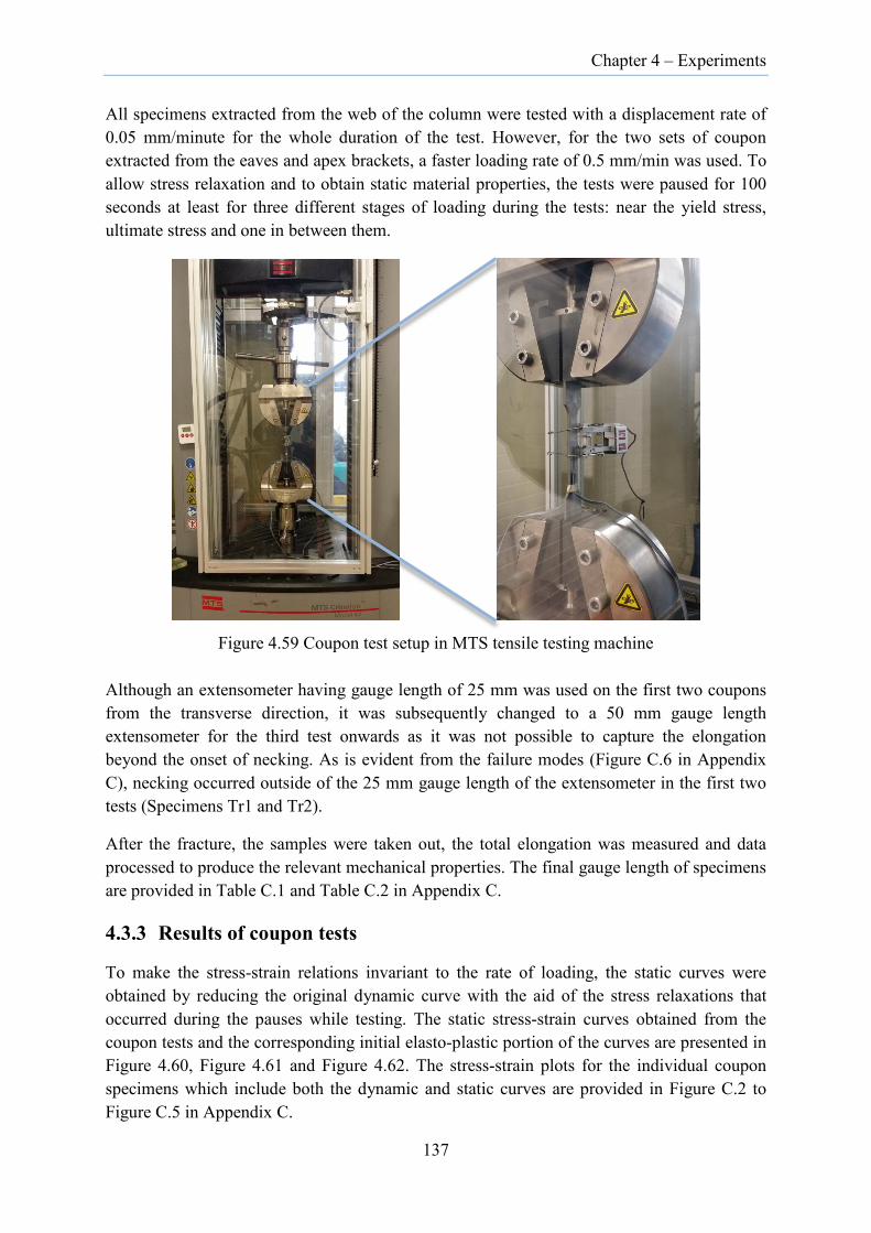
Chapter 4 – Experiments
All specimens extracted from the web of the column were tested with a displacement rate of 0.05 mm/minute for the whole duration of the test. However, for the two sets of coupon extracted from the eaves and apex brackets, a faster loading rate of 0.5 mm/min was used. To allow stress relaxation and to obtain static material properties, the tests were paused for 100 seconds at least for three different stages of loading during the tests: near the yield stress, ultimate stress and one in between them.
Figure 4.59 Coupon test setup in MTS tensile testing machine
Although an extensometer having gauge length of 25 mm was used on the first two coupons from the transverse direction, it was subsequently changed to a 50 mm gauge length extensometer for the third test onwards as it was not possible to capture the elongation beyond the onset of necking. As is evident from the failure modes (Figure C.6 in Appendix C), necking occurred outside of the 25 mm gauge length of the extensometer in the first two tests (Specimens Tr1 and Tr2).
After the fracture, the samples were taken out, the total elongation was measured and data processed to produce the relevant mechanical properties. The final gauge length of specimens are provided in Table C.1 and Table C.2 in Appendix C.
4.3.3 Results of coupon tests
To make the stress-strain relations invariant to the rate of loading, the static curves were obtained by reducing the original dynamic curve with the aid of the stress relaxations that occurred during the pauses while testing. The static stress-strain curves obtained from the coupon tests and the corresponding initial elasto-plastic portion of the curves are presented in Figure 4.60, Figure 4.61 and Figure 4.62. The stress-strain plots for the individual coupon specimens which include both the dynamic and static curves are provided in Figure C.2 to Figure C.5 in Appendix C.
137

Chapter 4 – Experiments
Figure 4.60 Stress-strain curve of column coupons (longitudinal direction)
Figure 4.61 Stress-strain curve of eaves bracket coupons
Figure 4.62 Stress-strain curve of apex bracket coupons
138

Chapter 4 – Experiments
The mechanical properties of the mean of three coupon tests in each group are presented in Table 4.13. In the table, σ0.01% is the stress corresponding to 0.01% strain, σ0.2% is the 0.2% proof stress, σu is the ultimate tensile strength, n is the Ramberg-Osgood parameter which is calculated using Equation (2.2), E is the elastic modulus, εu is the strain corresponding to the ultimate tensile strength and εf is the total strain after fracture. Additional properties can be found in Table C.3 for the C-section column and Table C.4 for the eaves and the apex bracket in Appendix C.
Table 4.13 Mechanical properties of C30024 section and connection brackets
Coupon Source
σ0.01%
(MPa) σ0.2%
(MPa) σu
(MPa) σu/σ0.2% n
E (GPa)
εu
(%) εf
(%)
Column (Long) 414.83 494.95 524.44 1.06 17.11 206.7 6.2 14.0
Column (Trans) 500.17 547.95 565.67 1.03 33.35 219.2 3.2 10.3
Eaves Bracket 473.76 512.61 533.88 1.04 38.04 205.6 5.7 14.0
Apex Bracket 435.24 504.15 527.92 1.05 21.13 208.1 6.5 15.0
The elastic modulus was calculated by constructing a linear regression line through the stress-strain points lying between 90 MPa and 200 MPa corresponding to 20-45% of the nominal yield stress as recommended in [127]. Similarly, the percentage elongation after fracture, εf was calculated based on the original gauge length of 50.0 mm.
As seen in the above stress-strain graphs, the variations among different specimens within each coupon group are hardly discernible until the attainment of ultimate strength. In general, the stress-strain plots of cold-formed steel section are characterized by a rounded transition in the elasto-plastic region followed by a short flat yield plateau before gradually strain-hardening to attain the ultimate strength.
The yield stress and ultimate tensile strength of the coupons from apex and eaves brackets are generally higher than those for the longitudinal coupons of columns. One interesting observation is the existence of a certain degree of anisotropy in material properties in the column as exhibited by the different magnitude of yield stress, ultimate tensile strength, ductility, and elastic modulus in coupons from the two orthogonal directions in the web of the column. Although the strength parameters (yield stress, ultimate tensile strength, and elastic modulus) are higher for the transverse coupons, the ductility is found to be comparatively low.
4.4 Point fastener connection tests
The point fastener connection tests were carried out to obtain relations between the fastener load and the corresponding deformations. Such relationships are required to idealize the behaviour of individual fasteners in the shell finite element model of frames which are described in Chapter 5.
139

Chapter 4 – Experiments
The CFS single C-section portal frames have several types of fasteners connecting various components. These include slip-resistant bolted connections, snug-tight bolted connection and screw connections. In the full-scale frame tests, the eaves, apex and base connections have components fastened together using M16 8.8/TF bolts. In such connections, point fasteners experience either shear force or torque or the combination of both depending on the position of the fastener in the bolt group. Screws were used to fasten lips of the eaves and apex brackets to the lips of columns and rafters. They were also used to fasten lips of columns and rafters to zed stiffeners. In the last three full-scale frame tests, these screw connections were replaced by bolted connections using M8 high-strength bolts.
In the shell element models of CFS single C-section portal frames, each bolted/screw connection is represented by the deformable fasteners which require constitutive relations for 6 DoFs with respect to the chosen frame of reference. The in-plane shear or in-plane moment have greater influence in inducing slip between the two fastened plates than the other force and moment components. Hence, it becomes crucial to derive the constitutive relations corresponding to in-plane shear and in-plane moment. Such constitutive relations for individual fasteners can be directly established based on the point fastener connection tests.
Hence, four series of point fastener connection tests were carried out to establish the load-deformation characteristics of each type of fastener connection. The details of the connection tests are provided in Table 4.14 and the individual tests are described in the following sections.
Table 4.14 Types of point fastener connection tests
Test type Number of specimens Fastener type used Slip-resistant bolted connection in shear 3 M16 8.8/TF bolts
Slip-resistant bolted connection in torque
4 M16 8.8/TF bolts
Screw connection 4 5.5 mm diameter Tek screws Snug-tight bolted connection in shear
4 M8 8.8/S bolts
In all tests, two strips of steel sheet/plate having respective thicknesses of 2.4 mm and 3.0 mm were guillotined from C30024 and C30030 sections which were sourced from BlueScope Lysaght for this sole purpose. The idea of using two dissimilar plate thicknesses was to reproduce the condition of the real point fastener connections in the frame tests.
4.4.1 Slip-resistant bolted connection tests
High-strength structural steel bolts are often used to fasten components in cold-formed steel portal frames. Slip between the sheets is prevented in the serviceability load range by pre-tensioning the bolts to a required torque. Often the turn-of-nut method is used to achieve the bolt pretension, as it is practical and simple to implement on-site.
140

Chapter 4 – Experiments
4.4.1.1 Slip-resistance in shear
Three tests were performed on a slip-resistant bolted connection in shear. The two flat plates were rigidly fastened together using two M16 8.8/TF bolts. The turn-of-nut method was used to tighten the bolts to achieve the desired pretension in the bolts. These tests were representative of the bolted connections at the eaves and apex. In particular, they represented the bolted connection between the flanges of a column or rafter to the flanges of eaves or apex brackets in the test frame where maximum shear forces were likely to occur.
Prior to the bolting of two plates, the areas around the 19 mm diameter bolt-holes were thoroughly cleaned with acetone to remove any dirt and the plates were laid together with bolt holes aligned one above the other. The bolts were placed concentric to the bolt holes after clamping the two plates using G-clamps. However, maintaining the bolts concentric to the bolt holes was not always possible as both bolt and washer tended to displace during the pretension phase. The bolts were tightened by holding the plates in positions using rigid clamps. To prevent the test specimens from slipping at the grip ends during the tests, zinc coating from their ends was removed with hydrochloric acid.
The specimens were tested in a 300 kN capacity Sintech tensile testing machine. The specimens were placed vertically in the test rig with vertical alignment checked using a handheld levelling instrument. The test setup along with the dimensions is shown in Figure 4.63.
Figure 4.63 Slip-resistant bolted connection shear test
141

Chapter 4 – Experiments
To avoid eccentric loading, metallic packing shim of 2.4 mm and 3.0 mm thick was provided at the opposite ends of specimens at the grips as recommended in the standard [128]. To ensure that only the deformation near the bolted portion was captured, displacement transducers were positioned at a distance of 40 mm from the bolt centre, beyond one end of the plates as shown in Figure 4.63. Aluminium angle brackets (of size 50 mm x 50 mm x 3 mm) having a length of 40 mm were glued to the specimen to provide bearing areas for the transducers. Two transducers were placed symmetrically on either flat side of the plates at each reading location. The average reading was used for the calculation of the deformation. To isolate the deformation of individual bolts, additional two transducers were installed in between the two bolts. As it was not possible to place the two central transducers aligned with the centreline of the bolts, they had to be slightly offset laterally.
The tensile tests were conducted by applying a displacement-controlled load with a cross-head displacement rate of 0.5 mm/minute after firmly gripping the ends of the specimen. To ensure that the results obtained are invariant to the rate of loading, the static load-displacement plots were deduced from the load drop that occurred during several pauses of 100 second duration while conducting the tests. Data were logged at the rate of 10 readings per second to capture the transition from no-slip state to the slip-state. The load-deformation relationships of the three connections are presented in Figure 4.64 and the corresponding ultimate capacities of the bolted connection are provided in Table 4.15.
Figure 4.64 Load versus displacement of M16 bolted connection in shear
All specimens failed by fracture of the 2.4 mm thick plate at the location of the upper bolt. The failures were preceded by the significant bearing of bolts on the plates. The failure modes are shown in Figure C.8 in Appendix C.
142

Chapter 4 – Experiments
Table 4.15 Ultimate capacity of M16 bolted connection
Test Specimen Ultimate load (kN) BF-1 80.5 BF-2 79.2 BF-3 81.6 Mean 80.4 COV 0.02
Due to the placement of two additional transducers in between the two bolts, it was possible to isolate deformation at the individual bolt locations. Hence, relative displacements (slip) for each bolt are provided in Figure 4.65 for the three tests along with the mean value. In the figure, the upper bolt is designated as BF-1T, BF-2T, BF-3T and the lower bolt as BF-1B, BF-2B, and BF-3B corresponding to the three tests. The dashed line represents the average value of force-slip relation of the six bolts which are used to idealize the behaviour of the deformable fastener in the numerical model described in Section 5.3.
Figure 4.65 Load versus displacement of individual M16 bolts in shear
In obtaining these plots, the applied shear force was assumed to be equally distributed between the two bolts. The average slip load per bolt was found to be 16.8 kN corresponding to 0.13 mm slip. The slip is defined to have occurred when the relative displacement between two plates is 0.13 mm in accordance with Clause J4 of AS 4100 [55]. As indicated by the increase in slope in the plot, the bolts began to bear on the plates once the bolt-hole clearance of 3.0 mm was fully traversed.
143

Chapter 4 – Experiments
In the full-scale frame tests, the bolts seldom experienced shear force to the extent of plate fracture. In most cases, the deformation of bolts and bolt hole remained insignificantly small apart from the bolt holes in the apex bracket (corresponding to bolts 5, 6, 7 and 8 in Figure 4.8) which underwent bolt-hole elongation of 0.5 mm to 1.5 mm. Hence, the constitutive relation represented by Figure 4.65 for the M16 bolt is more than sufficient to capture the bolt and bolt-hole deformation in the numerical model of CFS portal frames.
4.4.1.2 Slip-resistance under torque
Apart from the shear forces, point fastener may also carry moment while transferring load from one plate to another owing to the bolt pretension which rigidly clamps the two steel plates together. Hence, four tests on slip-resistance of the point fastener subjected to the in-plane torque were conducted to determine the moment-slip rotation characteristics.
The test set-up along with the dimensions are shown in Figure 4.66. Prior to the tests, to ensure that the bolts and washers are concentric to the 19 mm bolt hole, the bolt was initially tightened manually with the force sufficient to hold the plates together. The plates were clamped together using an M16 bolt which was tightened by the turn-of-nut method. Before the specimen was installed in the testing machine, detailed measurements of the distance from the centre of bolts to the pin-hole were taken for all specimens and are presented in Table C.6 in Appendix C.
Figure 4.66 Tests on slip-resistant M16 bolted connection subjected to torque
In the tests, to avoid friction between the gripping plates and the specimen, plates slightly thicker than the thickness of the specimen were placed in between the gripping plates at both ends and the nuts of the two pin bolts were kept loose. Likewise, to prevent etching of plates
F
M,θ
Bolt
144

Chapter 4 – Experiments
at the pin connection at the ends, bolts of 18 mm diameter with a plain shank were used. The inclinometers, which measured the inclination of the two plates, were glued to the plates using double-sided adhesive tape. The inclinometers had a linear range of ±45º and overall range of ±60º.
The test specimens were subjected to a torque at the bolt location by way of a tensile force applied at the pinned connections at its ends. By statics, this resulted in the M16 bolt experiencing shear in addition to the torque as shown in the inset diagram in Figure 4.66. However, the shear force developed at the bolt location was well below the slip load that would have any significant impact on the results. The shear force required to induce slip was above 16 kN as is evident from Figure 4.65, whereas the maximum shear force applied in the tests was 3.10 kN (Figure C.7 in Appendix C).
Based on the initial measurement of the specimens (Table C.6 in Appendix C) and rotation of the two connected plates along with the load and displacement records obtained during the tests, the moment at the fastener point was deduced, the details of which are presented in Section C.2.2.1 in Appendix C. The moment-slip rotation curves of the bolted connection are presented in Figure 4.67. The applied force versus vertical displacement curves of the upper end of the specimen is provided in Figure C.7 in Appendix C.
Figure 4.67 Moment versus relative rotation of M16 bolted connection
In deriving the moment-slip rotation relations, it was implicitly assumed that the deformation of the plates remained small and that the bolt did not undergo large displacement while undergoing rotation. To ensure that this assumption remained valid, the specimens were loaded only to the point where two plates rotated by 22º relative to each other.
145

Chapter 4 – Experiments
4.4.2 Screw connection tests
Four tests were conducted on the screw connection to obtain the force-deformation relationship for incorporation in the numerical model. The configuration of the test specimen along with the test setup is shown in Figure 4.68.
The tests were representative of the screw connection of the lips of eaves/rafter to the lips of eaves/apex brackets in the first three test frames (Frame Test 1, Frame Test 2, and Frame Test 3). However, wider specimens (compared to the lip width of C-sections) were used in these tests to ensure that the failure by bearing or fracture preceded the net section failure, similar to the failure observed in the full-scale frame tests.
The samples were prepared by rigidly clamping two plates (one with 2.4 mm thick and the other with 3.0 mm thick) while 5.5 mm diameter Tek screws were drilled through them. The screws were drilled through the plates with the help of a small handheld rotary hammer drill (18V) as is usually practised at construction sites.
Figure 4.68 Screw connection test setup
Two transducers were placed symmetrically on either flat side of the plates at each reading location. Four aluminium angle brackets were symmetrically glued to the specimen to provide platforms for the transducer needle to bear. The tests were performed in a 300 kN capacity Sintech tensile testing machine by installing the specimen vertically with necessary packing shims at the grip ends to ensure perfect central alignment of the specimens. After having gripped the ends of the specimen, loads were applied with a constant cross-head displacement of 0.5 mm/minute. To make the results invariant to the loading rate, several pauses of 100 second duration were executed during the tests. The static force-deformation response of the screw connection is provided in Figure 4.69 along with the mean value curve.
146

Chapter 4 – Experiments
Figure 4.69 Load versus relative displacement of screw connection
From Figure 4.69, it is seen that the deformation is negligibly small until the load reached 6.5 kN. Thereafter the connection progressively deformed with increasing load until the attainment of the peak load within the range of 0.75 mm and 0.90 mm deformation. All the specimens ultimately failed by the abrupt shearing of screws at the interface of two strips of sheet. The ultimate loads attained by the different specimens are presented in Table 4.16.
Table 4.16 Ultimate capacity of screw connection
Specimens Ultimate load (kN) SC-1 17.4 SC-2 19.8 SC-3 19.4 SC-4 19.9 Mean 19.1 COV 0.06
4.4.3 Snug-tight bolted connection tests
Four tests were conducted on the bolted plate connection with plates fastened by two M8 high strength bolts. These tests were performed to determine the force-deformation relations of bolted connection that was adopted for the last three frame tests (Frame Test 4, Frame Test 5 and Frame Test 6) in replacement of the screw connections used for the original configuration of the eaves and apex connections. The test setup and the connection configuration are shown in Figure 4.70.
147
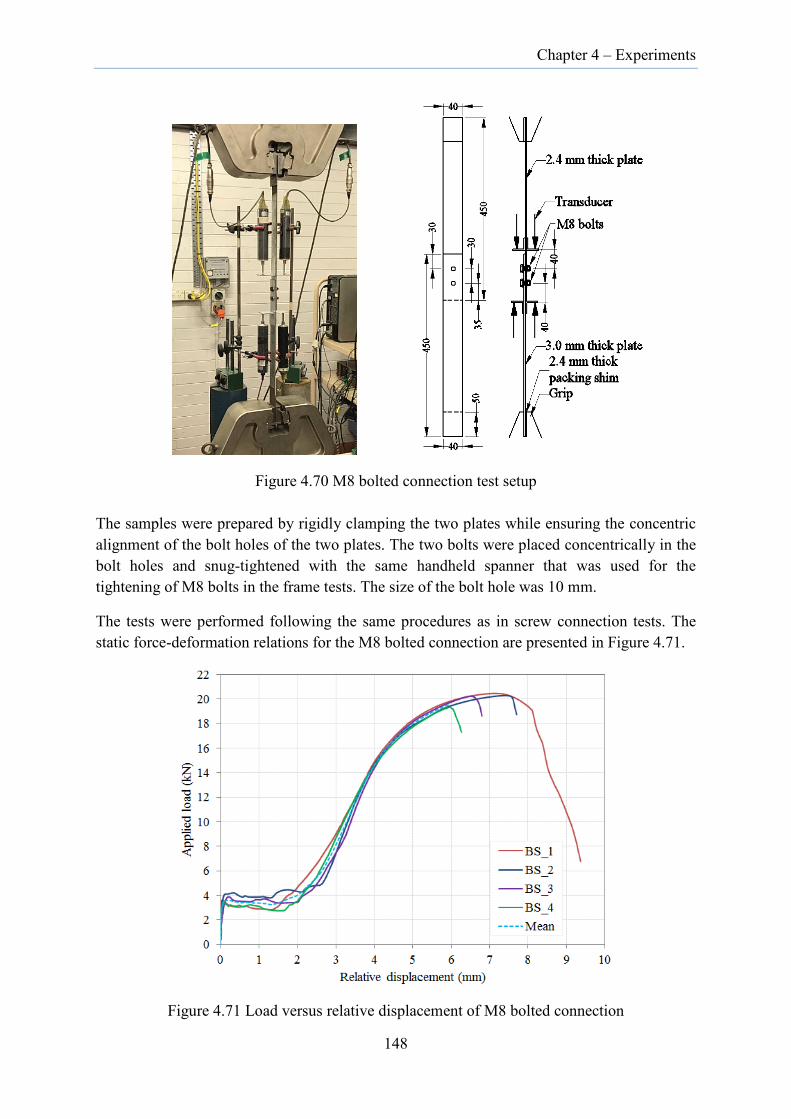
Chapter 4 – Experiments
Figure 4.70 M8 bolted connection test setup
The samples were prepared by rigidly clamping the two plates while ensuring the concentric alignment of the bolt holes of the two plates. The two bolts were placed concentrically in the bolt holes and snug-tightened with the same handheld spanner that was used for the tightening of M8 bolts in the frame tests. The size of the bolt hole was 10 mm.
The tests were performed following the same procedures as in screw connection tests. The static force-deformation relations for the M8 bolted connection are presented in Figure 4.71.
Figure 4.71 Load versus relative displacement of M8 bolted connection
148
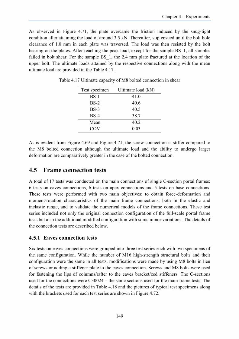
Chapter 4 – Experiments
As observed in Figure 4.71, the plate overcame the friction induced by the snug-tight condition after attaining the load of around 3.5 kN. Thereafter, slip ensued until the bolt hole clearance of 1.0 mm in each plate was traversed. The load was then resisted by the bolt bearing on the plates. After reaching the peak load, except for the sample BS_1, all samples failed in bolt shear. For the sample BS_1, the 2.4 mm plate fractured at the location of the upper bolt. The ultimate loads attained by the respective connections along with the mean ultimate load are provided in the Table 4.17.
Table 4.17 Ultimate capacity of M8 bolted connection in shear
Test specimen Ultimate load (kN) BS-1 41.0 BS-2 40.6 BS-3 40.5 BS-4 38.7 Mean 40.2 COV 0.03
As is evident from Figure 4.69 and Figure 4.71, the screw connection is stiffer compared to the M8 bolted connection although the ultimate load and the ability to undergo larger deformation are comparatively greater in the case of the bolted connection.
4.5 Frame connection tests
A total of 17 tests was conducted on the main connections of single C-section portal frames: 6 tests on eaves connections, 6 tests on apex connections and 5 tests on base connections. These tests were performed with two main objectives: to obtain force-deformation and moment-rotation characteristics of the main frame connections, both in the elastic and inelastic range, and to validate the numerical models of the frame connections. These test series included not only the original connection configuration of the full-scale portal frame tests but also the additional modified configuration with some minor variations. The details of the connection tests are described below.
4.5.1 Eaves connection tests
Six tests on eaves connections were grouped into three test series each with two specimens of the same configuration. While the number of M16 high-strength structural bolts and their configuration were the same in all tests, modifications were made by using M8 bolts in lieu of screws or adding a stiffener plate to the eaves connection. Screws and M8 bolts were used for fastening the lips of columns/rafter to the eaves bracket/zed stiffeners. The C-sections used for the connections were C30024 – the same sections used for the main frame tests. The details of the tests are provided in Table 4.18 and the pictures of typical test specimens along with the brackets used for each test series are shown in Figure 4.72.
149

Chapter 4 – Experiments
Table 4.18 Eaves connection test series
Test series No. of tests Joint details
EC-1 2 Original eaves bracket + 12 M16 8.8/TF bolts + 8 screws
EC-2 2 Modified eaves bracket + 12 M16 8.8/TF bolts + 8 M8 bolts
EC-3 2 Original eaves bracket + 12 M16 8.8/TF bolts + 9 screws + 3 mm thick plate stiffener
EC-1 Connection EC-2 Connection
EC-3 Connection
Figure 4.72 Eaves connections with fastener configuration
Stiffener plate (on rear side)
150
Chapter 4 – Experiments
For the specimen EC-1, 4 screws were used to fasten the lips of the C-sections to the lips of the eaves bracket and 4 screws to fasten the lips of the C-sections to the zed stiffeners. However, for the specimen EC-2, the screws were replaced by 8 M8 bolts. As the lip of the original eaves bracket was not wide enough to accommodate three M8 bolts, a 3.0 mm thick 20 mm wide steel sheet was welded to the edge of the lips. For specimen EC-3, a 3.0 mm thick steel stiffener plate was attached to the rear side of the eaves bracket and a screw was used at the midpoint of lower two bolts (bolt 5 and bolt 8) while keeping all other parts same as for specimen EC-1. The details of the stiffener plate are included in Figure C.9 in Appendix C.
The first test series (EC-1) corresponded to the eaves connection that was adopted for the first three frame tests (Frame Test 1 to Frame Test 3) as described in Section 4.2. Similarly, the second test series (EC-2) corresponded to the modified eaves connection that was used for the last three frame tests (Frame Test 4 to Frame Test 6). The last test series (EC-3) was designed to explore the option of strengthening the joints by adding a stiffener plate on the rear surface of the bracket web as used in EC-1 connection series.
4.5.1.1 Eaves connection test setup
The test specimens were assembled on the floor with all the necessary bolting and screw connection carried out thereon. The test specimens were lifted and installed in the test rig that was specifically designed by the author for the testing of eaves and apex connections with the available material within the structures laboratory. The rig was formed by the assemblage of two beams and columns that were rigidly connected to each other and firmly clamped to the I-beam on the strong floor (Figure 4.73). The rig was also prevented from out-of-plane movement by stabilizing the base using metallic blocks and clamps to the I-beam embedded in the concrete floor. The details of the test setup are shown in Figure 4.74.
Figure 4.73 Test rig with an eaves connection specimen placed in position
151
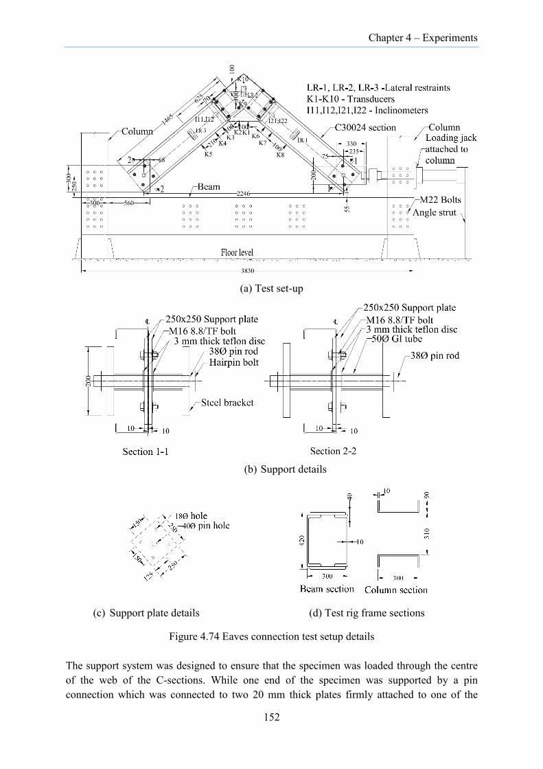
Chapter 4 – Experiments
(a) Test set-up
(b) Support details
(c) Support plate details (d) Test rig frame sections
Figure 4.74 Eaves connection test setup details
The support system was designed to ensure that the specimen was loaded through the centre of the web of the C-sections. While one end of the specimen was supported by a pin connection which was connected to two 20 mm thick plates firmly attached to one of the
152

Chapter 4 – Experiments
columns of the test frame, the other end of the specimen was pin connected to the end of the loading jack using U-shaped plate attached to its head. A high strength steel rod of 38 mm diameter was used as pins.
To prevent out-of-plane displacements, the specimen was restrained laterally using pairs of turnbuckles at three locations: one on the eaves bracket (LR-2) and two on the C-sections (LR-1 and LR-3 shown in Figure 4.74a) on either side of the eaves bracket. The restraint setup is shown in Figure 4.75.
(a)
(b)
Figure 4.75 Lateral restraints on eaves connection: (a) Dimensions; (b) Setup
Figure 4.76 shows the support arrangement for the eaves connection tests. The dimensions and details of each component forming the support system are provided in Figure 4.74b and Figure 4.74c. At the support, the webs of the C-sections were rigidly clamped in between the two steel plates (of size 250 mm x 250 mm x 10 mm) using four M16 high-strength structural bolts to prevent premature bearing failure.
To prevent the specimen from sliding transversely on the pin rod, two galvanized iron tubes of 50.0 mm diameter were inserted between the support bracket and the support steel plates which clamped the web of C-sections (Figure 4.74b). Two 3.0 mm thick circular discs of Teflon plates, each having 65.0 mm outside diameter and 40.0 mm inside diameter, were also inserted in between GI pipes and support plates to minimize friction between them. Furthermore, both the pin rod and the hole on the support plates were lubricated by applying
153
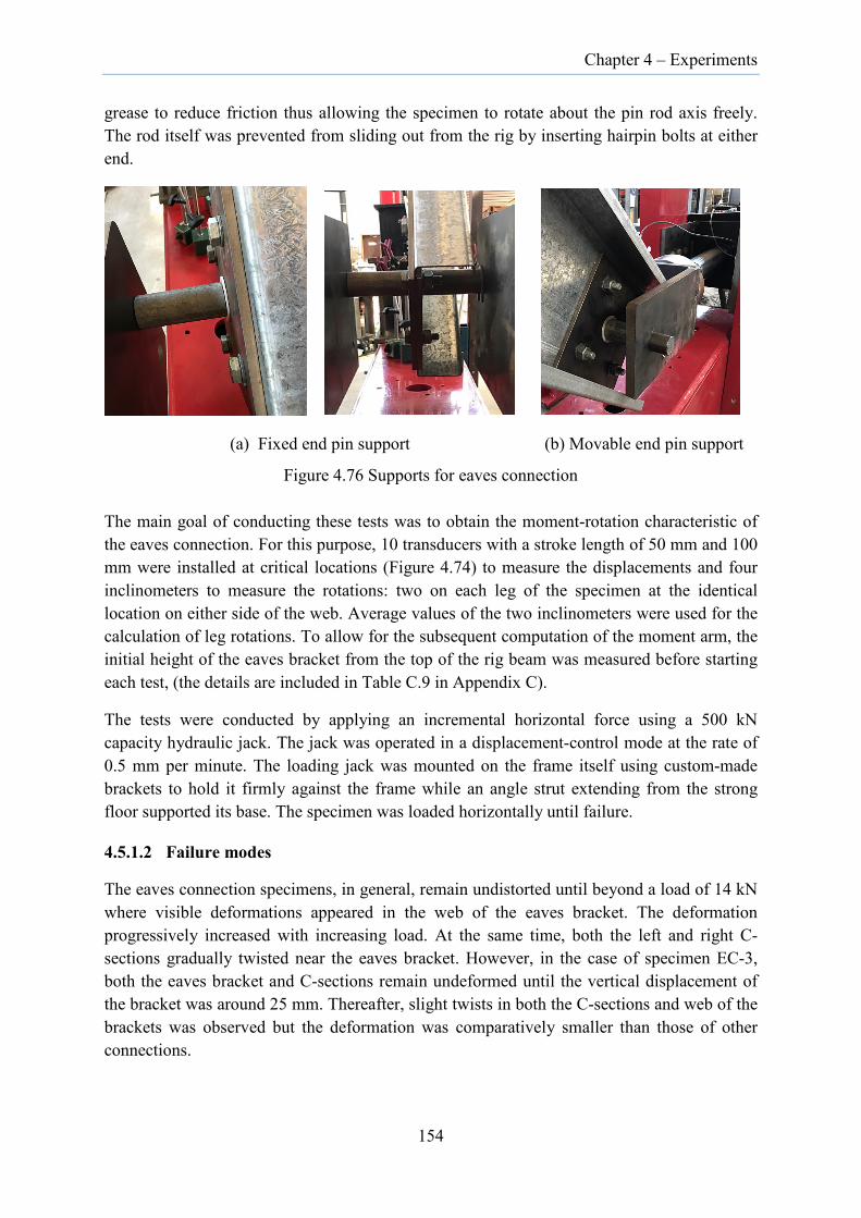
Chapter 4 – Experiments
grease to reduce friction thus allowing the specimen to rotate about the pin rod axis freely. The rod itself was prevented from sliding out from the rig by inserting hairpin bolts at either end.
(a) Fixed end pin support (b) Movable end pin support
Figure 4.76 Supports for eaves connection
The main goal of conducting these tests was to obtain the moment-rotation characteristic of the eaves connection. For this purpose, 10 transducers with a stroke length of 50 mm and 100 mm were installed at critical locations (Figure 4.74) to measure the displacements and four inclinometers to measure the rotations: two on each leg of the specimen at the identical location on either side of the web. Average values of the two inclinometers were used for the calculation of leg rotations. To allow for the subsequent computation of the moment arm, the initial height of the eaves bracket from the top of the rig beam was measured before starting each test, (the details are included in Table C.9 in Appendix C).
The tests were conducted by applying an incremental horizontal force using a 500 kN capacity hydraulic jack. The jack was operated in a displacement-control mode at the rate of 0.5 mm per minute. The loading jack was mounted on the frame itself using custom-made brackets to hold it firmly against the frame while an angle strut extending from the strong floor supported its base. The specimen was loaded horizontally until failure.
4.5.1.2 Failure modes
The eaves connection specimens, in general, remain undistorted until beyond a load of 14 kN where visible deformations appeared in the web of the eaves bracket. The deformation progressively increased with increasing load. At the same time, both the left and right C-sections gradually twisted near the eaves bracket. However, in the case of specimen EC-3, both the eaves bracket and C-sections remain undeformed until the vertical displacement of the bracket was around 25 mm. Thereafter, slight twists in both the C-sections and web of the brackets was observed but the deformation was comparatively smaller than those of other connections.
154
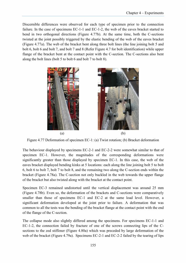
Chapter 4 – Experiments
Discernible differences were observed for each type of specimen prior to the connection failure. In the case of specimens EC-1-1 and EC-1-2, the web of the eaves bracket started to bend in two orthogonal directions (Figure 4.77b). At the same time, both the C-sections twisted at the joint possibly triggered by the elastic bending of the web of the eaves bracket (Figure 4.77a). The web of the bracket bent along three bolt lines (the line joining bolt 5 and bolt 6, bolt 6 and bolt 7, and bolt 7 and 8 (Refer Figure 4.7 for bolt identification) while upper flange of the bracket bent at the contact point with the C-section. The C-sections also bent along the bolt lines (bolt 5 to bolt 6 and bolt 7 to bolt 8).
(a) (b)
Figure 4.77 Deformation of specimen EC-1: (a) Twist rotation; (b) Bracket deformation
The behaviour displayed by specimens EC-2-1 and EC-2-2 were somewhat similar to that of specimen EC-1. However, the magnitudes of the corresponding deformations were significantly greater than those displayed by specimen EC-1. In this case, the web of the eaves bracket displayed bending kinks at 5 locations: each along the line joining bolt 5 to bolt 6, bolt 6 to bolt 7, bolt 7 to bolt 8, and the remaining two along the C-section ends within the bracket (Figure 4.78a). The C-section not only buckled in the web towards the upper flange of the bracket but also twisted along with the bracket at the contact point.
Specimen EC-3 remained undistorted until the vertical displacement was around 25 mm (Figure 4.78b). Even so, the deformation of the brackets and C-sections were comparatively smaller than those of specimens EC-1 and EC-2 at the same load level. However, a significant deformation developed at the joint prior to failure. A deformation that was common to all the tests was the bending of the bracket flange at the contact point with the end of the flange of the C-section.
The collapse mode also slightly differed among the specimens. For specimens EC-1-1 and EC-1-2, the connection failed by fracture of one of the screws connecting lips of the C-sections to the zed stiffener (Figure 4.80a) which was preceded by large deformation of the web of the bracket (Figure 4.79a). Specimens EC-2-1 and EC-2-2 failed by the tearing of lips
155

Chapter 4 – Experiments
of the C-section at the location of the M8 bolt connection to the zed stiffener (Figure 4.80b), which was preceded by buckling of the web of the bracket (Figure 4.79b). For specimen EC-3-1, the failure occurred by the simultaneous fracture of the two screws that were used to fasten the lip of the C-section to the lip of the eaves bracket (Figure 4.80c) while for specimen EC-3-2, failure was due to the fracture of the screw used for fastening the lip of the C-section to the zed stiffener. Bending of the web of the eaves bracket was also observed prior to failure but the web deformation was comparatively smaller than those of specimens EC-1 and EC-2.
(a) (b)
Figure 4.78 Deformation of eaves connection: (a) Specimen EC-2; (b) Specimen EC-3
Another interesting behaviour observed during the tests was the separation of the web of the C-sections from the web of eaves bracket towards the ultimate load (Figure 4.81) due to buckling of the web of the C-sections. In many cases, surfaces in contact began to separate at an early stage and remained permanently deformed even after the failure of specimens. A summary of the failure modes of each specimen is presented in Table 4.19.
Table 4.19 Failure modes of eaves connection tests
Test series Failure modes
EC-1-1 Fracture of screw S7, bending of C-section along the bolt line, web buckling of eaves bracket
EC-1-2 Fracture of screw S2, bending of C-section along the bolt line, web buckling of eaves bracket
EC-2-1 Tearing of C-section lips at the M8 bolts S7, Buckling of C-section, web buckling of eaves brackets
EC-2-2 Tearing of C-section lips at the M8 bolts S7, Buckling of C-section, web buckling of eaves brackets
EC-3-1 Fracture of screws S3 and S4, Bearing of screw S2 onto C-section lips, web buckling of C-sections within the eaves bracket
EC-3-2 Fracture of screw S2, web buckling of C-sections within bracket, bending of eaves bracket
156
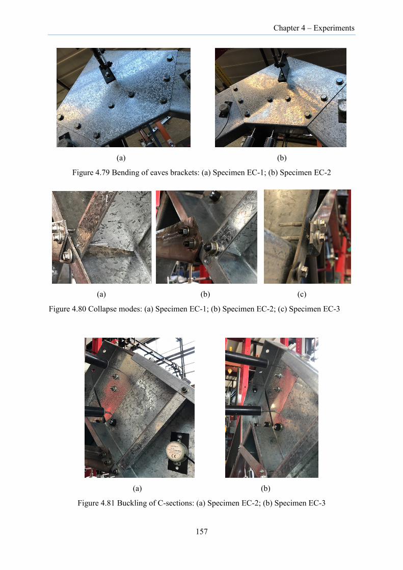
Chapter 4 – Experiments
(a) (b)
Figure 4.79 Bending of eaves brackets: (a) Specimen EC-1; (b) Specimen EC-2
(a) (b) (c)
Figure 4.80 Collapse modes: (a) Specimen EC-1; (b) Specimen EC-2; (c) Specimen EC-3
(a) (b)
Figure 4.81 Buckling of C-sections: (a) Specimen EC-2; (b) Specimen EC-3
157

Chapter 4 – Experiments
4.5.1.3 Load-deformation responses
A schematic diagram of the eaves connection tests subjected to a horizontal force at one end is shown in Figure 4.82. During the tests, the specimen was pushed horizontally causing the specimen end (the one attached to the movable support mounted on the loading jack) to move horizontally towards the other pinned support. As a result, the eaves bracket moved upwards and two legs (C-sections) rotated relative to each other generating bending moment at the eaves bracket.
Figure 4.82 Schematic representation of eaves connection
The vertical displacement v of the eaves joint versus the applied force P is shown in Figure 4.83. Similarly, the horizontal displacement u of the loaded end of the specimen with the applied force P is shown in Figure 4.84. Out-of-plane displacements of the eaves bracket were also monitored during the tests. The load-displacement plots corresponding to transducer K9 and K10 (see Figure 4.74a) are shown in Figure C.10 in Appendix C.
All specimens show a linear response in the initial stage of loading, as shown in Figure 4.87. However, there is no distinct demarcation between the linear and nonlinear behaviour from Figure 4.83 to Figure 4.85 mainly owing to the randomness in the occurrence of bolt slip at the joint. The load dropped momentarily for several specimens after entering the nonlinear range but sustained load for a considerable range of deformation. The use of a plate stiffener on the rear side of the eaves bracket in EC-3 specimens enhanced the ultimate capacity of the joint (Table 4.20) although the improvement in the initial stiffness appeared to be almost nil. The possible cause of such lack of initial stiffness enhancement could be attributed to the inability of the bolt 5 and bolt 8 (see Figure 4.7 for location of bolts) to develop full pretension during bolting as these bolts had to clamp four layers of plates (C-section, zed stiffener, eaves bracket and plate stiffener). Due to this, the major portion of the bolt length was consumed within the thickness of the four layers of plates, as the bolt length was only 30 mm resulting in a reduction of bolt effectiveness.
In all tests, the equilibrium path rises slightly with varying slope prior to attaining the ultimate load followed by the descending branch. This rise in equilibrium path is attributed to the bearing of the main bolts against the bracket. However, the actual failure is brought about not by the bolt bearing on the bracket but rather the fracture of screws (as in specimens EC-1
θ
P P, u
v
M
Pin support
Movable pin support
C-section Centrelin
O
158

Chapter 4 – Experiments
and EC-3) or plate tearing due to the bearing of M8 bolts (as in specimen EC-2) which are a localized event.
Figure 4.83 Force versus vertical displacement of eaves connections
Figure 4.84 Applied load versus horizontal displacement of loaded end of specimens
The moment and the corresponding rotation of the eaves connections are plotted in Figure 4.85. The moment (Mi) at each point was calculated using the following relation
( )0i i iM P h v= + (4.1)
159

Chapter 4 – Experiments
where vi is the vertical displacement of the eaves bracket at each increment of applied force Pi, and h0 is the initial vertical distance from the centreline of the applied force to the point of intersection O of the two centrelines of the C-sections on the eaves bracket (Figure 4.82). The rotation of the joint at the eaves was obtained as the sum of average readings of two inclinometers placed on either side of the eaves bracket (Figure 4.74a).
Figure 4.85 Moment-rotation relation of eaves connections
The ultimate load, ultimate moment and the maximum displacements and rotations at failure are provided in Table 4.20.
Table 4.20 Ultimate capacities and deformations of eaves connection specimens
Test series
Ultimate load, Pu (kN)
Vertical displacement, v (mm)
Ultimate moment, Mu (kNm)
In-plane rotation, θ (rad)
EC-1-1 27.0 34 26.1 0.081
EC-1-2 26.9 32 25.9 0.072
EC-2-1 26.3 57 25.7 0.169
EC-2-2 26.6 57 26.0 0.156
EC-3-1 28.8 43 27.9 0.108
EC-3-2 31.0 43 30.0 0.103
As observed in Table 4.20, a slight increase in the ultimate load and the ultimate moment for EC-3 specimens is visible with the addition of a plate stiffener although the use of M8 bolts (EC-2 specimens) instead of screws has negligible effect on the strength. The force-deformation curves are also marked by several undulations which are the result of buckling or yielding, or asynchronous bolt bearing on plates at the joint. As observed in the above plots
160

Chapter 4 – Experiments
(Figure 4.83, Figure 4.84, Figure 4.85), failure of connections by shearing of screws is marked by an abrupt and sudden load drop whereas the connection failure due to material yielding as in EC-2 specimens is characterized by a gradual load drop.
4.5.1.4 Simplified moment-rotation relations for eaves connections
The moment-rotation curves of each test series can be represented by a single curve which is the mean of the two curves. Based on a linear regression analysis, average curves can be further approximated by a series of linear curves to obtain simplified versions of moment-rotation relations. The schematic representation of the simplified moment-rotation curves is shown in Figure 4.86. The corresponding moment and rotation coordinates along with the flexural stiffness (obtained from the linear regression analysis) within each section of the curve are tabulated in Table 4.21 for the three test series of eaves connection.
Figure 4.86 Schematic representation of simplified moment-rotation relation
Table 4.21 Simplified moment-rotation parameters for eaves connection
Parameters Specimens EC-1 Specimens EC-2 Specimens EC-3 M1 15.1 15.2 13.5 θ1 0.0065 0.0066 0.0065 K1 2330 2315 2091 M2 23.2 23.4 21.0 θ2 0.0244 0.0234 0.0245 K2 449 486 415 M3 25.1 25.6 29.3 θ3 0.0701 0.1204 0.1000 K3 43 24 110 M4 - 22.9 - θ4 - 0.1511 - K4 - -89 -
Note: The units of M, θ and K are kNm, radian and kNm/radian respectively.
M
K4 K3
K1
θ1 θ2 θ3 θ4
M1
M3
M4 M2
K2
θ
161

Chapter 4 – Experiments
Based on the values given in Table 4.21, the simplified moment-rotation relation along with the average value of test results for each test series are plotted in Figure 4.87. The average curves were computed by considering rotation as the independent variable. As the failure of specimen EC-1 and EC-3 was abrupt, the descending branch of the simplified model was not provided.
Figure 4.87 Simplified moment-rotation relations of eaves connection
The failure of eaves connection having screws for the connection of lips is marked by the abrupt shearing of screws resulting in the ultimate failure of the joint while the eaves connection with M8 bolts as a replacement of screws attained the ultimate load after undergoing considerable deformation. The behaviour depicted by the eaves connections is observed to be very similar to that observed in the main frame tests.
While the use of M8 bolts in replacement of Tek screws did not offer any advantage in terms of strength, it nevertheless prevented the abrupt connection failure. This might be especially useful if CFS portal frames were to be constructed in an earthquake-prone area where structural ductility is considered to be of prime importance.
4.5.2 Apex connection tests
Six tests were conducted to establish the force-deformation and in-plane moment-rotation characteristics of the apex connection. They were grouped into three test series with different connection brackets, each consisting of two specimens. The details of the apex connection tests are provided in Table 4.22. Figure 4.88 shows the apex connections with brackets and fastener configuration for each test series.
162

Chapter 4 – Experiments
Table 4.22 Apex connection test series
Test series No. of tests Joint details
AC-1 2 Original apex bracket + 12 M16 8.8/TF bolts + 2 screws
AC-2 2 Modified apex bracket + 12 M16 8.8/TF bolts + 2 M8 bolts
AC-3 2 Modified apex bracket + 12 M16 8.8/TF bolts + 4 screws
AC-1 connection AC-2 connection AC-3 connection
Figure 4.88 Apex connections with fastener configuration
The first test series (specimen AC-1) corresponds to the apex connection of first three frame tests (Frame Test 1 to Frame Test 3 as described in Section 4.2) while the second test series (specimen AC-2) corresponds to the apex connection of the last three frame tests (Frame Test 4 to Frame Test 6). The third test series (specimen AC-3) consists of the modified bracket but using four screws instead of two for fastening the lower lips of the rafters to the lower lip of the apex bracket. As the space on the lower lip of the apex bracket was insufficient to accommodate additional two screws, a 15.0 mm wide strip of 3.0 mm thick plate was welded onto the bracket lip to provide the extra space needed. The third test series was designed to examine the influence of number of screws on the strength of the apex connections.
4.5.2.1 Apex connection test setup
The tests on apex connection were carried out in the same test rig used for the eaves connections. The details of the apex connection test setup are shown in Figure 4.89. The test specimens were assembled on the floor and then bolted using the turn-of-nut method before
163

Chapter 4 – Experiments
being lifted and installed in the rig. To ensure that the specimen was placed centrally with respect to the loading beam, a plumb bob was hung from the centre of the loading beam and the position of the specimen was adjusted until it was aligned centrally.
Figure 4.89 Apex connection test setup
The test specimen was supported on sliding half-round support at the ends. To provide stability at the support and to stiffen the web of the C-sections, support brackets fabricated from 10 mm thick steel plate were attached at the ends (Figure 4.90). The test specimens were loaded vertically at two points: 843.0 mm on either side of the apex (Figure 4.91). The specimens were loaded using the transfer beam attached to the end of the hydraulic jack. To ensure that the load from the hydraulic jack was equally distributed between the two loading points, the transfer beam was pin connected to the hydraulic jack at the midspan.
Furthermore, the loading bracket and the vertical strut of the transfer beam were not directly connected but interfaced by a thin Teflon plate (Figure 4.90c). This arrangement reduced the friction at the interface of the vertical strut and loading bracket and enabled horizontal sliding of the loading brackets away from the centre as the legs of the specimen spread apart. The
164

Chapter 4 – Experiments
loads were applied to the centre of the web of the C-sections by means of a 38 mm diameter pin rod connected to the loading brackets.
(a) Support brackets (b) Loading plate
(c)Loading brackets
Figure 4.90 Bracket details of apex connection tests
Figure 4.91 Loading arrangement for apex connection tests
165

Chapter 4 – Experiments
To prevent premature web buckling at the loading points, two rhombic-shaped loading plates were placed on either side of the web and bolted together using four M16 bolts. Both the pin rod and hole on loading plates were oiled with grease for smooth rotation of the specimen about the pin rod axis during the tests. As in the eaves connection tests, a stopper GI pipe of 50 mm diameter was used on either side of the specimen at the loading points to prevent it from moving laterally on the pin rod. A 3.0 mm thick Teflon disc was placed in between the loading plate and the stopper GI pipe to reduce friction between them. Teflon strips were also placed between the loading bracket and the lips of the C-section.
To prevent the specimen from displacing in the direction normal to the plane of the specimen, lateral restraints were provided on either side of apex bracket and at the two supports (Figure 4.92). The positions of the lateral restraints and the loading points were kept same as the purlin locations near the apex in the main frame tests. The restraints were formed by pairs of turnbuckles attached to the cleats on the C-section and to the cleats at the other supported end (Figure 4.75a).
Figure 4.92 Arrangement of lateral restraints for apex connection tests
To monitor the deformation of the specimen, 12 transducers and 4 inclinometers were installed at critical locations (Figure 4.93). While transducers A1 and A2 were used to obtain the average of the vertical displacement of the apex, transducer pairs A3-A4 and A6-A7 were used to validate the readings of the inclinometers. The readings from transducers A5 and A8 provided comparative displacement of loading points, thus enabling the verification of transfer of equal load to the specimen. Transducers A11 and A12 were installed to check the support settlement if any.
The distances between the supports and loading points and to the centreline of the apex bracket were adjusted and checked before each test. The tests commenced with the application of vertical load through the loading jack with its head controlled to displace vertically at the rate of 0.5 mm per minute. All specimens were loaded to failure. The loading
166

Chapter 4 – Experiments
continued even after attaining the ultimate load so that post-ultimate response could be obtained.
Figure 4.93 Instrumentation on apex connection specimens
4.5.2.2 Test observations
As the loading progressed beyond the elastic range, local buckling deformations appeared in the web of the C-sections with significant deformation near the top flange-web junction. This was accompanied by the upward bending of the tip of the apex bracket (Figure 4.94a). At the same time, the apex bracket bent in the vertical direction with an amplitude of lateral displacement reaching about 10 mm at the centre at the ultimate load in most tests (Figure 4.94b). However, the screws being the weaker fastener, sheared off well before the ultimate load was reached (Figure 4.94c). As the loading approached the ultimate load, local buckling deformation in the web of the C-sections became more pronounced. Local buckling also started to form along the top flange of the C-sections. In general, the specimen attained the ultimate limit state by forming a spatial plastic mechanism at the top flange-web junction of the C-section between the lateral restraint and the loading point (Figure 4.94d). This usually occurred in the range of 270 mm to 350 mm away from the edge of apex bracket. The tests were generally continued until the specimen had undergone considerable post-buckling displacement. Thereafter the tests were stopped as no specific behaviours of interest were observed in the specimens apart from the continual increase of deformation and concurrent drop in load.
While the failure modes of all six specimens were generally similar, there were distinctive features among the specimens. In the AC-1 specimen tests, screws fractured right after traversing the linear range. Although the loads dropped slightly due to the fracture of screws, the specimens continued to carry additional load until reaching the ultimate state. The specimens ultimately failed by the local buckling of the top flange-web junction of one of the C-sections. There were also several instances of slip between the specimen and the half-round block at the supports, especially in the nonlinear loading range. In the case of specimen AC-1-2, twist about the longitudinal axis was observed prior to the ultimate load, mainly triggered by the twisting of the apex bracket due to the fracture of screws.
In specimens AC-2-1 and AC-2-2, the failure was caused by the local buckling of the top flange-web junction of one of the C-sections in between the lateral restraint and the loading point. The two M8 bolts which replaced the screws used for specimen AC-1 sustained the load although a slight bearing deformation was observed at the bolt hole. In the case of
167
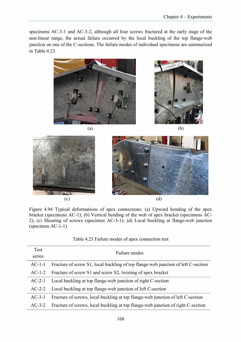
Chapter 4 – Experiments
specimens AC-3-1 and AC-3-2, although all four screws fractured at the early stage of the non-linear range, the actual failure occurred by the local buckling of the top flange-web junction on one of the C-sections. The failure modes of individual specimens are summarized in Table 4.23.
(a) (b)
(c) (d)
Figure 4.94 Typical deformations of apex connections: (a) Upward bending of the apex bracket (specimens AC-1); (b) Vertical bending of the web of apex bracket (specimens AC-2); (c) Shearing of screws (specimen AC-3-1); (d) Local buckling at flange-web junction (specimen AC-1-1)
Table 4.23 Failure modes of apex connection test
Test series Failure modes
AC-1-1 Fracture of screw S1, local buckling of top flange-web junction of left C-section
AC-1-2 Fracture of screw S1 and screw S2, twisting of apex bracket
AC-2-1 Local buckling at top flange-web junction of right C-section
AC-2-2 Local buckling at top flange-web junction of left C-section
AC-3-1 Fracture of screws, local buckling at top flange-web junction of left C-section AC-3-2 Fracture of screws, local buckling at top flange-web junction of right C-section
168

Chapter 4 – Experiments
4.5.2.3 Load-displacement responses
To facilitate the understanding of the structural behaviour, the apex connection is represented by the simple schematic diagram shown in Figure 4.95. The load (P) versus vertical displacement (v) graphs of all specimens are plotted in Figure 4.96. Similarly, the moment (M) versus rotation (θ) graphs are plotted in Figure 4.97. In obtaining the total load on the members, the weight of the two loading brackets along with the pin rods (38.5 kg) was added to the applied load as the loading brackets were directly supported by the specimens.
Figure 4.95 Schematic representation of apex connection
The out-of-plane displacement of the apex bracket was also monitored during the tests. The load-displacement plots corresponding to transducers A9 and A10 (see Figure 4.93) are included in Figure C.11 in Appendix C.
Figure 4.96 Applied force versus vertical displacement of apex connections
θ
v
M
𝑅𝑅
𝑃𝑃2
𝑃𝑃2
𝑅𝑅 0.635 m 0.843 m
O Centreline of C-section Support
10º
169

Chapter 4 – Experiments
Figure 4.97 Moment versus rotation of apex connections
As is evident from Figure 4.96 and Figure 4.97, the initial slopes of all curves are nearly same, implying that the initial stiffness is less affected by the secondary fasteners including screws and M8 bolts. It is only in the nonlinear range that the equilibrium path of each specimen differed significantly. Once the load reached 35 kN, the equilibrium path became nonlinear suggesting the onset of slippage of the M16 bolts. As is evident from the increase in the slope of the equilibrium paths, the specimens began to stiffen midway through the non-linear range owing to the onset of bearing of M8 bolts on the apex bracket.
In the case of specimen AC-1-1, several minor load drops were observed during the test. The drops were caused by the development of Coulomb-type friction between the loading brackets and the half-round supports. In this particular test, the support bracket slipped intermittently as they were not lubricated adequately. This was however redressed in the subsequent tests by adequately lubricating the contact points at the supports.
The load-displacement plots of the four specimens (AC-1-1, AC-1-2, AC-3-1, and AC-3-2) in Figure 4.96 are marked by sudden load drops at two locations corresponding to the shearing of screws. In the case of specimen AC-1-2, this event caused the apex bracket to bend and twist resulting in the twisting of the C-sections. In the case of specimens AC-3-1 and AC-3-2, due to the presence of additional two screws connecting the apex bracket lip to the individual C-sections, the fracture of screws was delayed slightly. Nevertheless, all four screws ultimately fractured with the simultaneous shearing of the left pair of screws followed by the shearing of the right pair of screws at a marginally higher load.
The ultimate load (Pu), the ultimate moment (Mu) and the corresponding vertical displacement (v) and rotations (θ) of the individual tests are provided in Table 4.24. As observed in Table 4.24, there is substantial increase in the ultimate load and the ultimate
170
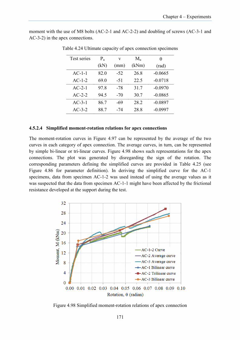
Chapter 4 – Experiments
moment with the use of M8 bolts (AC-2-1 and AC-2-2) and doubling of screws (AC-3-1 and AC-3-2) in the apex connections.
Table 4.24 Ultimate capacity of apex connection specimens
Test series Pu (kN)
v (mm)
Mu (kNm)
θ (rad)
AC-1-1 82.0 -52 26.8 -0.0665 AC-1-2 69.0 -51 22.5 -0.0718 AC-2-1 97.8 -78 31.7 -0.0970 AC-2-2 94.5 -70 30.7 -0.0865 AC-3-1 86.7 -69 28.2 -0.0897 AC-3-2 88.7 -74 28.8 -0.0997
4.5.2.4 Simplified moment-rotation relations for apex connections
The moment-rotation curves in Figure 4.97 can be represented by the average of the two curves in each category of apex connection. The average curves, in turn, can be represented by simple bi-linear or tri-linear curves. Figure 4.98 shows such representations for the apex connections. The plot was generated by disregarding the sign of the rotation. The corresponding parameters defining the simplified curves are provided in Table 4.25 (see Figure 4.86 for parameter definition). In deriving the simplified curve for the AC-1 specimens, data from specimen AC-1-2 was used instead of using the average values as it was suspected that the data from specimen AC-1-1 might have been affected by the frictional resistance developed at the support during the test.
Figure 4.98 Simplified moment-rotation relations of apex connection
171

Chapter 4 – Experiments
Table 4.25 Simplified moment-rotation parameters for apex connection
Parameters Specimens AC-1 Specimens AC-2 Specimens AC-3
M1 14.5 15.3 16.9
θ1 0.0067 0.0073 0.0078
K1 2182 2096 2168
M2 22.8 21.0 26.7
θ2 0.0718 0.0450 0.0891
K2 127 151 123
M3 - 29.6 -
θ3 - 0.0861 -
K3 - 210 - Note: The units of M, θ and K are kNm, radian and kNm/radian respectively.
Among the three types of apex connection specimens, specimens AC-2 performed better in terms of load carrying capacity although the initial stiffness was slightly lower compared to those of specimens AC-1 and AC-3. The shearing of the screws was not the precursor to the attainment of ultimate loads of apex connections (specimens AC-1s and AC-3s) as the connections continued to carry load even after the fracture of screws. Furthermore, the screws tended to shear irrespective of the number of screws being used in the connections. However, the addition of screws had the effect of stiffening the joint and enhancing its strength. In a similar manner, adding a lip to the upper flange of the apex bracket resulted in minimizing vertical bending of the apex bracket and improving its capacity.
4.5.3 Base connection tests
Five tests were carried out to evaluate the flexural stiffness and to establish the moment-rotation characteristics of the base connection used in the full-scale frame tests. While the base connection configuration was nominally the same in all full-scale frame tests, the distinctions among the isolated base connection tests were mainly in terms of the axis of bending of the specimens in two orthogonal directions. The details of the base connection tests are provided in Table 4.26. The specimens BC-1 were subjected to bending about the major axis while specimens BC-2T and BC-2C were bent about the minor axis with the shear centre side in tension and compression respectively.
Table 4.26 Base connection test series
Test series No. of tests Test type
BC-1 2 Major axis bending
BC-2T 2 Minor axis bending
BC-2C 1 Minor axis bending
172

Chapter 4 – Experiments
In the tests, the C-section column was connected to the base strap using six M16 8.8/TF bolts with three bolts connecting each flange of the column to the leg of the base strap. The bolts were tightened using the turn-of-nut method, similar to the procedure adopted for the base connection in the full-scale frame tests. The base strap was clamped to the base plate using three M20 8.8/TF bolts and a 10.0 mm thick steel plate. The 25.0 mm thick base plate was supported by four load cells onto which strain gauges were fastened. The load cells were calibrated to provide reactions based on the strain gauge readings (see Section B.3 of Appendix B).
4.5.3.1 Major axis bending tests
For the major-axis bending tests, the horizontal load was applied at the top of the cantilevered column at a height of 1.8 m from the base using a 100 kN capacity hydraulic jack which was mounted on the test rig frame. The details of the test rig are shown in Figure 4.99.
Figure 4.99 Test setup for major axis bending of base connection
173

Chapter 4 – Experiments
The point of application of the load was located at 45 mm away from the web of the C-section (in proximity of the nominal shear centre) to minimize twisting of the column. The position of the load was determined after running a series of trials on a numerical model with different load positions. The horizontal load was applied through a strut (formed by connecting three flat bars) that was designed to allow rotation at the connected points. The web of the top portion of the column was attached to loading brackets which enabled uniform dispersion of load to the column web.
The displacements and rotations at the base were recorded by 5 transducers and 4 inclinometers (Figure 4.99). Two additional transducers were also installed at the top of the column to monitor twist deformation in the initial stage of loading.
As the loading increased, the column began to rotate about the base with deformation largely concentrated at the base (Figure 4.100a). It was also observed that both the base strap and the 10 mm thick steel clamp plate on the tension side gradually bent along the edge of the washer on the first M20 bolt (that was used to clamp the base strap to the base plate) due to the pull exerted on the tension leg of the base strap (Figure 4.100b). On the compression side, the column flange bore on the base strap corner causing deformation in both. It must be noted that the columns in the frame tests never experienced high magnitude of lateral load to the extent of bending the base clamp.
( a) (b)
Figure 4.100 Major axis bending of base connection: (a) Column deformation; (b) Bending of base strap and base clamp plate (front and rear view)
As the deformation was continuous, the tests were discontinued when the maximum displacement capacity of the loading jack was exhausted. This loading range was sufficient to cover the loading range of the full-scale frame tests.
174
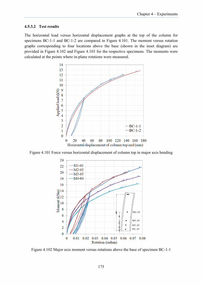
Chapter 4 – Experiments
4.5.3.2 Test results
The horizontal load versus horizontal displacement graphs at the top of the column for specimens BC-1-1 and BC-1-2 are compared in Figure 4.101. The moment versus rotation graphs corresponding to four locations above the base (shown in the inset diagram) are provided in Figure 4.102 and Figure 4.103 for the respective specimens. The moments were calculated at the points where in-plane rotations were measured.
Figure 4.101 Force versus horizontal displacement of column top in major axis bending
Figure 4.102 Major axis moment versus rotations above the base of specimen BC-1-1
175
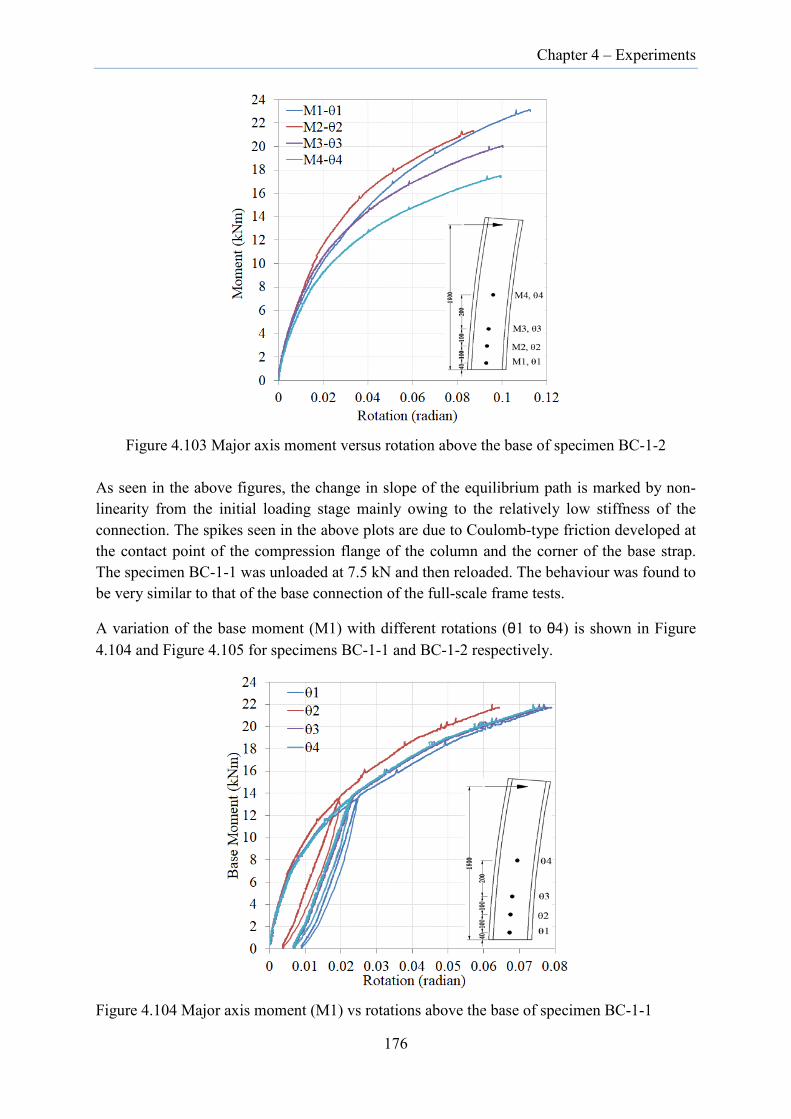
Chapter 4 – Experiments
Figure 4.103 Major axis moment versus rotation above the base of specimen BC-1-2
As seen in the above figures, the change in slope of the equilibrium path is marked by non-linearity from the initial loading stage mainly owing to the relatively low stiffness of the connection. The spikes seen in the above plots are due to Coulomb-type friction developed at the contact point of the compression flange of the column and the corner of the base strap. The specimen BC-1-1 was unloaded at 7.5 kN and then reloaded. The behaviour was found to be very similar to that of the base connection of the full-scale frame tests.
A variation of the base moment (M1) with different rotations (θ1 to θ4) is shown in Figure 4.104 and Figure 4.105 for specimens BC-1-1 and BC-1-2 respectively.
Figure 4.104 Major axis moment (M1) vs rotations above the base of specimen BC-1-1
176

Chapter 4 – Experiments
Figure 4.105 Major axis moment (M1) vs rotations above the base of specimen BC-1-2
It is seen that they also depict a comparable moment-rotation graphs. The other graphs of minor importance pertaining to the relative deformations near the base and twist deformation of column for specimens BC-1-1 and BC-1-2 are shown in Figure C.12 to Figure C.15 in Appendix C.
4.5.3.3 Minor axis bending tests
For the minor axis bending tests, the horizontal load at the top of the vertical column was applied at the centre of the web. Specimens BC-2T-1 and BC-2T-2 were tested with the shear centre side in tension. As the C-section column is non-symmetric about minor axis, specimen BC-2C-1 was tested with shear centre side in compression to observe the difference in behaviour. The details of the test setup along with the location of transducers and inclinometers are given in Figure 4.106.
To capture the relative displacements and twist rotations of the base connection during the tests, four transducers were installed on the web near each flange-web junction and two inclinometers on each flange of the column above the base (Figure 4.106). Additional two transducers were installed at 150 mm apart on the loading bracket to monitor the displacement and rotation of the column at the upper end.
Figure 4.107a shows the deformation of column bent about the minor axis when subjected to lateral loading. As observed in Figure 4.107, the deformation of the column is largely confined to the base. As the lateral load increased, the base strap and the steel plate on the tension side began to bend and in the process gradually separated from the base plate (Figure
177

Chapter 4 – Experiments
4.107b) with separation concentrated near the corners. The tests were discontinued after having exhausted the maximum displacement capacity of the loading jack.
Figure 4.106 Test setup for the minor axis bending of base connection
(a) (b)
Figure 4.107 Bending of column about minor axis: (a) Column deformation; (b) Bending of base strap and clamp plate on the tension side
178
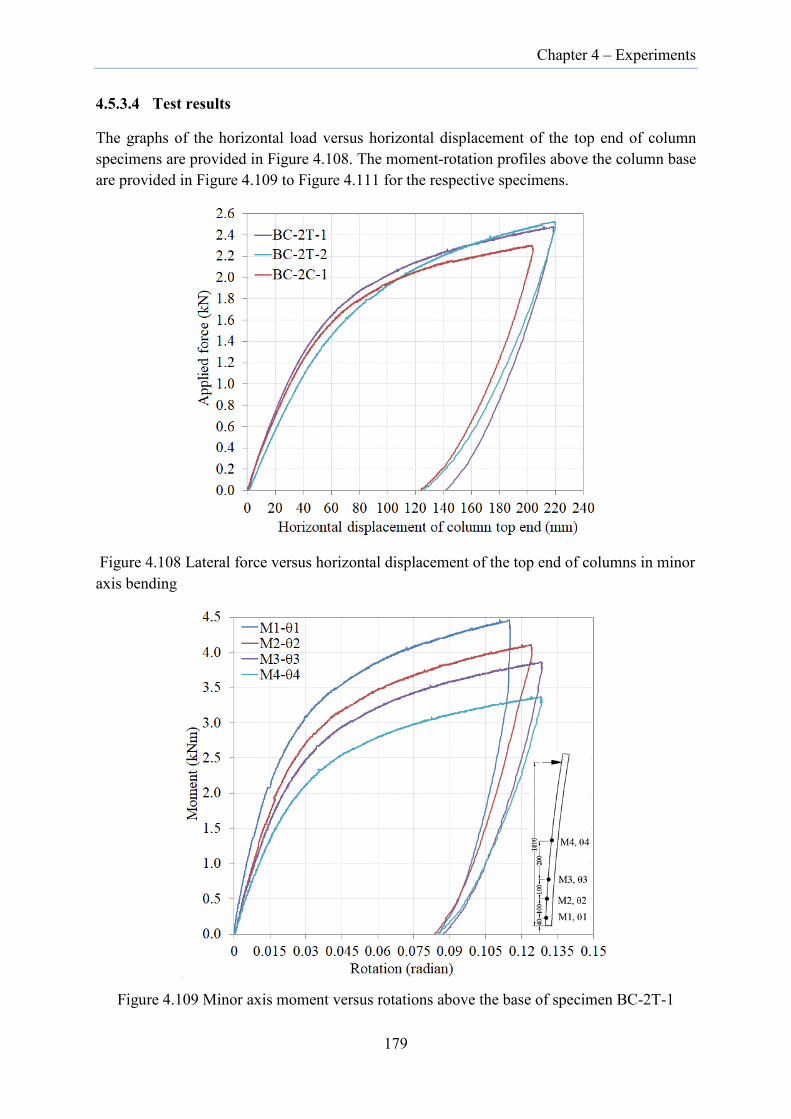
Chapter 4 – Experiments
4.5.3.4 Test results
The graphs of the horizontal load versus horizontal displacement of the top end of column specimens are provided in Figure 4.108. The moment-rotation profiles above the column base are provided in Figure 4.109 to Figure 4.111 for the respective specimens.
Figure 4.108 Lateral force versus horizontal displacement of the top end of columns in minor axis bending
Figure 4.109 Minor axis moment versus rotations above the base of specimen BC-2T-1
179

Chapter 4 – Experiments
Figure 4.110 Minor axis moment versus rotations above the base of specimen BC-2T-2
Figure 4.111 Minor axis moment versus rotations above the base of specimen BC-2C-1
A variation of the base moment (M1) with different rotations (θ1 to θ4) is shown in Figure 4.112 for specimen BC-2T-1, (see Figure C.19 and Figure C.22 in Appendix C for the graphs
180

Chapter 4 – Experiments
of specimens BC-2T-2 and BC-2C-1). It is seen that the moment-rotation relations are nearly identical as the deformation is mostly concentrated at the base. The graphs of relative deformations near the base and twist deformation of column subjected to minor axis bending are shown in Figure C.16 to Figure C.23 in Appendix C.
Figure 4.112 Base moment (M1) vs rotations above the column base (specimen BC-2T-1)
In spite of the column being non-symmetric about the minor axis, the load-deformation plots (Figure 4.108) show no significant differences between the specimens bent with shear centre side in compression and in tension. Such similar behaviour is attributed to the concentration of deformation mostly within the base strap and clamp plate.
4.5.3.5 Flexural stiffness and simplified moment-rotation relations
The initial parts of the moment-rotation plots in Figure 4.102, Figure 4.103, Figure 4.109, Figure 4.110 and Figure 4.111 can be represented by a linear relation, M=Kfθ, in which M is the moment, θ the corresponding rotations and Kf the elastic flexural stiffness. The flexural stiffness, Kf corresponding to various moment-rotation pairs (M1-θ1, M2-θ2, M3-θ3 and M4-θ4) for each specimen are provided in Table 4.27. The flexural stiffness were determined from the figures based on a linear regression analysis by considering moments up to 2 kNm for the major axis moment and 0.5 kNm for the minor axis moment. Beyond these points, the moment-rotation curves become increasingly nonlinear.
181

Chapter 4 – Experiments
Among the four values of flexural stiffness corresponding to the four moment-rotation relations above the base, Kf3 is seen as the best representative of base stiffness since the point, on which the calculation of Kf3 is based, is located right outside the influence of the connection bracket.
Hence, the simplified base moment-rotation characteristics are determined from the average results of two base connection tests in major axis bending and three in minor axis bending corresponding to the M3-θ3 curves. The average value along with the simplified curves is provided in Figure 4.113 for major axis bending and Figure 4.114 for minor axis bending.
Table 4.27 Elastic flexural stiffness of base connections
Specimen Kf1 Kf2 Kf3 Kf4 Bending direction
BC-1-1 1533 1536 1200 1044
Major axis bending BC-1-2 1316 1296 1311 1065
Average 1425 1416 1256 1055
BC-2T-1 227 152 143 124
Minor axis bending BC-2T-2 157 96 92 77 BC-2C-1 178 139 122 98
Average 187 129 119 100
Figure 4.113 Simplified moment-rotation relation of the base connection (for major axis bending)
182
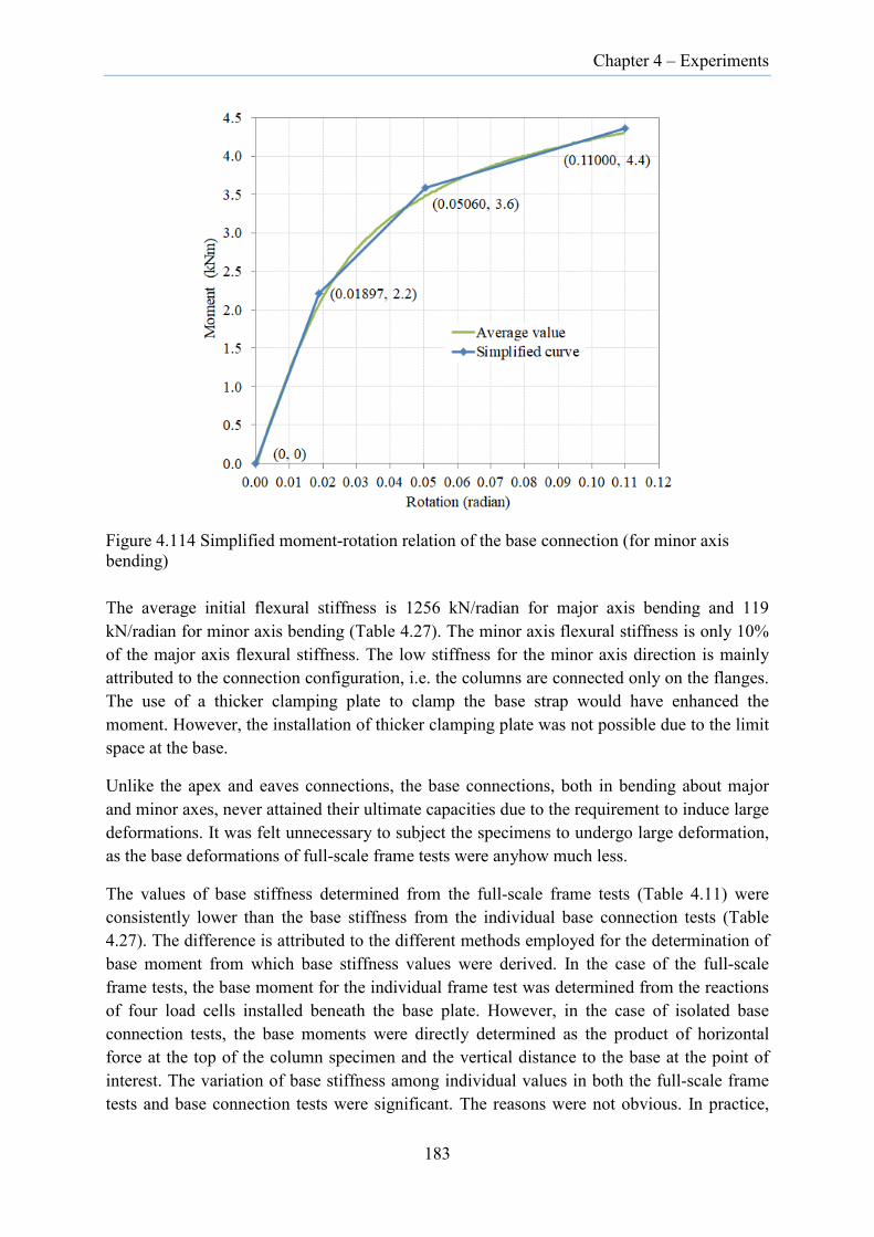
Chapter 4 – Experiments
Figure 4.114 Simplified moment-rotation relation of the base connection (for minor axis bending)
The average initial flexural stiffness is 1256 kN/radian for major axis bending and 119 kN/radian for minor axis bending (Table 4.27). The minor axis flexural stiffness is only 10% of the major axis flexural stiffness. The low stiffness for the minor axis direction is mainly attributed to the connection configuration, i.e. the columns are connected only on the flanges. The use of a thicker clamping plate to clamp the base strap would have enhanced the moment. However, the installation of thicker clamping plate was not possible due to the limit space at the base.
Unlike the apex and eaves connections, the base connections, both in bending about major and minor axes, never attained their ultimate capacities due to the requirement to induce large deformations. It was felt unnecessary to subject the specimens to undergo large deformation, as the base deformations of full-scale frame tests were anyhow much less.
The values of base stiffness determined from the full-scale frame tests (Table 4.11) were consistently lower than the base stiffness from the individual base connection tests (Table 4.27). The difference is attributed to the different methods employed for the determination of base moment from which base stiffness values were derived. In the case of the full-scale frame tests, the base moment for the individual frame test was determined from the reactions of four load cells installed beneath the base plate. However, in the case of isolated base connection tests, the base moments were directly determined as the product of horizontal force at the top of the column specimen and the vertical distance to the base at the point of interest. The variation of base stiffness among individual values in both the full-scale frame tests and base connection tests were significant. The reasons were not obvious. In practice,
183
Chapter 4 – Experiments
the base strap is embedded into the concrete foundation. In principle, the accurate stiffness can be determined by simulating the same condition in the laboratory. However, due to the resource limitations, such establishment of the real concrete foundation was not possible and hence recourse was taken to the best alternative condition. While this did not match the site situation, it nevertheless provided useful information on the flexibility of the base connection.
4.6 Discussions
A series of full-scale tests on long-span cold-formed steel single C-section portal frames along with component tests on the material, fastener connections, and main frame connections have been carried out. Table C.10 in Appendix C summarizes the number of tests, types of tests and associated laboratory activities conducted as part of this research.
Six tests on 13.6 m span by 6.8 m high CFS single C-section portal frames have demonstrated that the flexural-torsional buckling of columns is the dominant structural behaviour. The flexural-torsional buckling deformations in columns were exhibited by all frames especially at the higher loads regardless of the presence of lateral restraints although a stiffness enhancement and much smaller twist rotations were observed when restraints were provided to the columns. The ultimate failure deformations were concentrated at the eaves and the apex and were governed by the type of fasteners used for the connection of the column lips to the connection brackets. In the first three frame tests, the shearing of screws at the eaves usually triggered the failure of the frames whereas in the last three frame tests, the failures were associated with the formation of spatial plastic mechanism because of local buckling below the eaves or near the apex. The strength of the frames with modified joint configuration was slightly higher than the frames with existing proprietary joint configuration. In particular, significant increase in strength was observed in the last frame where columns were braced in the out-of-plane direction with the girts. Hence, to optimize the structural performance, where practically possible, column bracing is essential to reduce twist rotations.
Tests on coupons enabled material behaviour for the C-section, eaves and apex brackets to be compared. Properties derived from the coupon tests indicated that the materials used for the apex and eaves brackets were slightly stiffer and stronger compared to the C-section members. Furthermore, the material properties of the coupons cut from the transverse direction of the web of the C-section showed slightly higher strength and stiffness in relation to the properties of coupons from the longitudinal direction, indicating the existence of a degree of anisotropy in the C-sections.
Tests carried out on point fastener connections allowed the comparison of the behaviour of different types of bolted and screw connections, and extraction of force-displacement characteristics required for the numerical simulation. Tests on slip-resistant bolted connections showed that the pretensioning of bolts could result in a stiffer connection compared to using snug-tightened bolts. The tests also demonstrated that the screw connections possessed stiffness that were higher than those of the M8 bolt connection despite having lower ultimate strength. This explained the reason for the negligible differences in
184

Chapter 4 – Experiments
stiffness shown by the full-scale frame tests with modified joint configuration despite the marginal higher capacities. It is apparent that the fastening of components with pretensioned bolts would enhance the stiffness of the frame connections and minimize bolt-hole elongation, resulting in improved frame performance.
A series of tests on eaves connection, apex connection and base connection were carried out to establish the moment-rotation relations and to determine the flexural stiffness of the respective connections. Certain differences were observed in terms of the failure modes of eaves and apex connections due to the difference in the method employed for testing of specimens. The eaves connections were subjected to two-point load with the lower flange of the eaves bracket (the weaker side of the connection) in compression, whereas the apex connections were subjected to four-point load with the lower flange of the apex bracket (the weaker side of the connection) in tension. In the case of eaves connections, the failures were concentrated in the connection with failure modes associated with the fracture of screws or tearing of lips at the M8 bolt locations although visible local deformation within the eaves bracket as well as in the adjoining members were observed when reaching the ultimate load. On the other hand, in the case of apex bracket, the failures were always in the members associated with local buckling at the compression flange-web junctions. Furthermore, the fracture of screws on the lower flange of the apex bracket was never a precursor to the failure of the joint contrary to the eaves connection where the fracture of screws usually triggered the ultimate failure of the joints and the frames. However, in terms of flexural stiffness and ultimate moment capacity of the joints, there were no significant differences between the eaves and apex connections.
Individual base connection tests demonstrated that they are capable of developing flexural stiffness although the stiffness about the minor axis was minimal. Furthermore, with the localized failure occurring at the base, away from the monosymmetric column section, the minor axis bending stiffness was similar for both bending with the shear centre side in compression and in tension.
Simplified moment-rotation relations and flexural stiffness were derived for the eaves, apex and base connections. These quantities are important parameters in simulating the semi-rigid joints in the frame models represented by the beam elements.
185
Chapter 5 – Numerical Modelling
CHAPTER 5. NUMERICAL MODELLING AND ADVANCED ANALYSIS OF SINGLE C-SECTION PORTAL FRAMES
5.1 Introduction The finite element method is convenient for studying the behaviour of structures. It allows the detailed investigation of the behaviour and caters for parametric studies which are not possible with laboratory tests owing to cost, time and instrument limitations. Once the finite element models are calibrated against laboratory test results, they offer possibilities for carrying out a wide range of parametric studies.
However, unlike the numerical modelling of a single member in which nonlinearity is mostly confined to the material and geometry, and the modelling itself is straightforward in most cases, the numerical modelling of frames demands the incorporation of all three types of nonlinearity: geometric, material and contact with the latter mainly arising from the contact surface interaction of several parts that are inherently present in the frames. Furthermore, numerical modelling of frames consisting of thin-walled sections poses great challenges as they are notoriously flexible and susceptible to buckling. Analysis of such frames is often marked by numerical instabilities and convergence issues.
Despite such challenges, many researchers have analyzed C-section CFS portal frames using finite elements. Baigent and Hancock [42] used the beam elements for the analysis of CFS portal frames with members connected using rigid joints through the channel web. Lim and Nethercot [8] used both beam and shell elements to represent the CFS portal frames composed of doubly-symmetric members formed by C-sections connected back-to-back. In the shell element model, the bolts were idealized using beam elements and bolt hole elongation using spring elements. Spring elements were also used to idealize the semi-rigid behaviour of the joints in the beam element models. Zhang et al. [107] used shell elements to model CFS planar frames comprising doubly-symmetric C-sections but used the moment-rotation characteristics of the semi-rigid connections in lieu of modelling the individual bolts. In modelling the semi-rigid connections, the moment-rotation relation was assigned to in-plane rotational springs located at the intersection of the column and rafter centrelines while considering the bracket to remain rigid at the interface. Recently, Blum [13] used shell elements to model double C-section CFS portal frames with the bolts at the connections idealized by point-based fasteners. The bolts were assumed to remain rigid without slip.
For CFS single C-section portal frames having semi-rigid connections as considered herein, a more general technique was required to overcome the difficulties associated with the eccentricity arising from the non-symmetric bolted configuration at the connections and from the eccentricity between the shear centre and the centroid of the cross-sections. To this effect, the behaviour of individual bolts was idealized using a combination of fastener and deformable connector elements.
This Chapter begins with the description of the representation of nonlinear material behaviour based on the nominal engineering stress-strain relations obtained from the coupon tests.
186
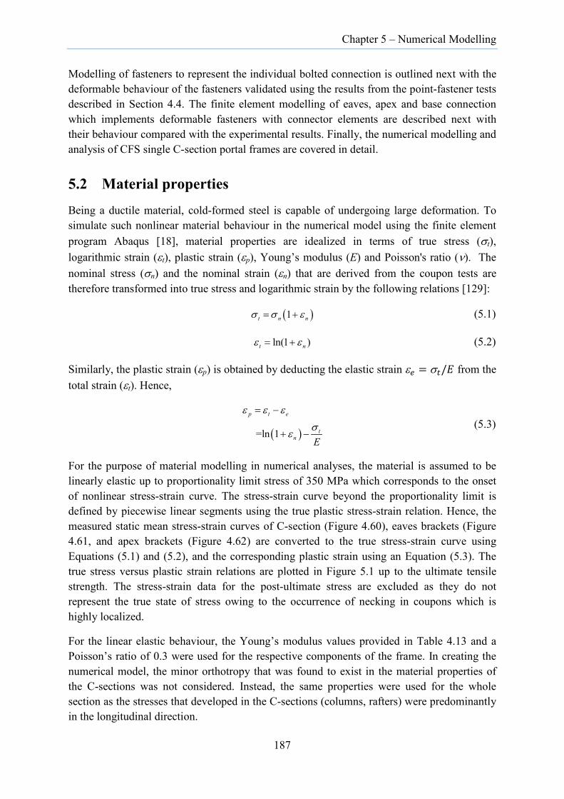
Chapter 5 – Numerical Modelling
Modelling of fasteners to represent the individual bolted connection is outlined next with the deformable behaviour of the fasteners validated using the results from the point-fastener tests described in Section 4.4. The finite element modelling of eaves, apex and base connection which implements deformable fasteners with connector elements are described next with their behaviour compared with the experimental results. Finally, the numerical modelling and analysis of CFS single C-section portal frames are covered in detail.
5.2 Material properties
Being a ductile material, cold-formed steel is capable of undergoing large deformation. To simulate such nonlinear material behaviour in the numerical model using the finite element program Abaqus [18], material properties are idealized in terms of true stress (σt), logarithmic strain (εt), plastic strain (εp), Young’s modulus (E) and Poisson's ratio (ν). The nominal stress (σn) and the nominal strain (εn) that are derived from the coupon tests are therefore transformed into true stress and logarithmic strain by the following relations [129]:
( )1t n nσ σ ε= + (5.1)
ln(1 )t nε ε= + (5.2)
Similarly, the plastic strain (εp) is obtained by deducting the elastic strain ε𝑒 = σ𝑡/𝐸 from the total strain (εt). Hence,
( ) =ln 1
p t e
tn E
ε ε ε
σε
= −
+ − (5.3)
For the purpose of material modelling in numerical analyses, the material is assumed to be linearly elastic up to proportionality limit stress of 350 MPa which corresponds to the onset of nonlinear stress-strain curve. The stress-strain curve beyond the proportionality limit is defined by piecewise linear segments using the true plastic stress-strain relation. Hence, the measured static mean stress-strain curves of C-section (Figure 4.60), eaves brackets (Figure 4.61, and apex brackets (Figure 4.62) are converted to the true stress-strain curve using Equations (5.1) and (5.2), and the corresponding plastic strain using an Equation (5.3). The true stress versus plastic strain relations are plotted in Figure 5.1 up to the ultimate tensile strength. The stress-strain data for the post-ultimate stress are excluded as they do not represent the true state of stress owing to the occurrence of necking in coupons which is highly localized.
For the linear elastic behaviour, the Young’s modulus values provided in Table 4.13 and a Poisson’s ratio of 0.3 were used for the respective components of the frame. In creating the numerical model, the minor orthotropy that was found to exist in the material properties of the C-sections was not considered. Instead, the same properties were used for the whole section as the stresses that developed in the C-sections (columns, rafters) were predominantly in the longitudinal direction.
187
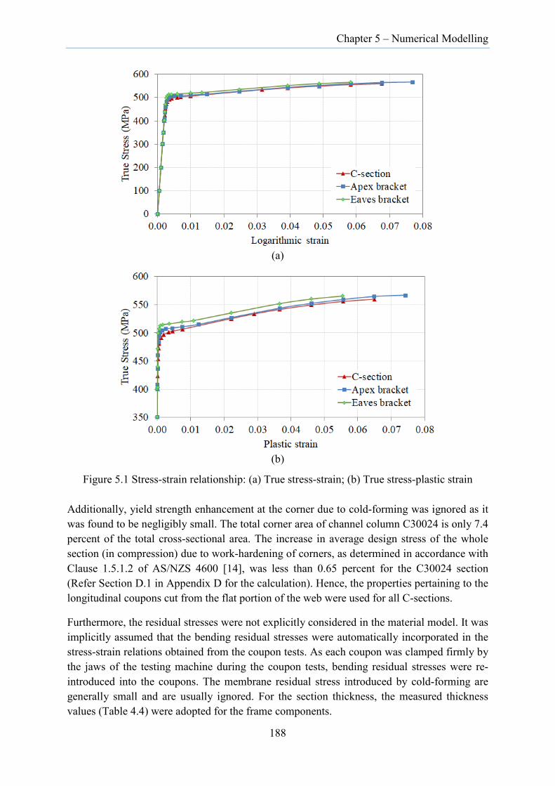
Chapter 5 – Numerical Modelling
(a)
(b)
Figure 5.1 Stress-strain relationship: (a) True stress-strain; (b) True stress-plastic strain
Additionally, yield strength enhancement at the corner due to cold-forming was ignored as it was found to be negligibly small. The total corner area of channel column C30024 is only 7.4 percent of the total cross-sectional area. The increase in average design stress of the whole section (in compression) due to work-hardening of corners, as determined in accordance with Clause 1.5.1.2 of AS/NZS 4600 [14], was less than 0.65 percent for the C30024 section (Refer Section D.1 in Appendix D for the calculation). Hence, the properties pertaining to the longitudinal coupons cut from the flat portion of the web were used for all C-sections.
Furthermore, the residual stresses were not explicitly considered in the material model. It was implicitly assumed that the bending residual stresses were automatically incorporated in the stress-strain relations obtained from the coupon tests. As each coupon was clamped firmly by the jaws of the testing machine during the coupon tests, bending residual stresses were re-introduced into the coupons. The membrane residual stress introduced by cold-forming are generally small and are usually ignored. For the section thickness, the measured thickness values (Table 4.4) were adopted for the frame components.
188

Chapter 5 – Numerical Modelling
5.3 Fastener modelling
5.3.1 Modelling of bolted/screw connections
In the CFS single C-section portal frame tests, columns and rafters were connected to their respective brackets using M16 high strength structural bolts. Their lips were also fastened to the lips of eaves and apex brackets using 5.5 mm diameter Tek screws. Similarly, the purlins were connected to the main frame using purlin cleats. These cleats were connected using M12 bolts.
In the numerical models, the bolt and screw connections were idealized by using mesh-independent point-based fasteners. The fasteners were assigned to the attachment points defined at the location of bolts and screws. The fasteners can be defined by the size, orientation, mass, and the number of sheets to be connected. They can also be located anywhere irrespective of the location of mesh nodes. Each fastener was connected to the surface using a distributing coupling constraint that coupled the displacements and rotations of each fastening point to the average displacement and rotation of the nearby nodes.
The deformable fasteners were assigned with the connector sections to which the connection type was prescribed. The choice of connection type is dependent on the likelihood of which DoFs that would be mobilized during the plate deformation process. In this context, the behaviour of M16 slip-resistant bolts was modelled by the combination of CARTESIAN and CARDAN sections while the behaviour of M8 bolts and screws were modelled by the CARTESIAN section. The CARTESIAN section provides a connection between two nodes that allows translational behaviour in three local Cartesian directions while the CARDAN section provides a rotational connection between two nodes parameterized by Cardan angles. Although the ROTATION connection section also describes the relative rotation about three axes, its use has been discouraged as its finite rotation parameterization is not well-suited for defining connector behaviour in three-dimensional analysis [18].
The actual deformable behaviour of the fasteners was modelled using the combination of connector elasticity and plasticity. While the connector elasticity defined the initial linear elastic portion of the bolt force-slip curve, the connector plasticity represented the nonlinear force-displacement range which included both bolt slip and ply bearing. Connector force components were assumed to be uncoupled in the plasticity model.
5.3.2 Constitutive relations of point fastener connections
The point fastener connection tests, which include slip-resistant bolted connections in shear and in torque, screw connections and snug-tight bolted connections, are described in Section 4.4. The average force-displacement relation of the fastener connections in each category of test is represented by the mean value curve. From this, the load-displacement relation of a single fastener is deduced by assuming that the total shear force is equally distributed between the two fasteners.
189

Chapter 5 – Numerical Modelling
The average nonlinear curves representing the behaviour of the individual fastener can be further simplified to facilitate the computational efficiency using multi-linear curves. The respective curves along with the simplified curves are shown in Figure 5.2 and Figure 5.3.
(a) (b)
Figure 5.2 M16 bolted connection: (a) in shear; (b) in torque
(a) (b)
Figure 5.3 (a) Screw connection (b) M8 bolted connection
5.3.3 Validation of fastener behaviour
In order to demonstrate the performance of the bolted connections idealized by the deformable fasteners, the behaviour of one of the point fastener connection tests described in Section 4.4 is examined after assigning the fasteners with relevant connector sections.
190

Chapter 5 – Numerical Modelling
The connector elasticity and plasticity data that define the behaviour of the fastener are extracted from Figure 5.2 and Figure 5.3. While assigning the connector elasticity and plasticity data, a local coordinate system (Figure 5.4) is adopted to define the relevant DoFs for appropriate assignment of force-displacement relations. For instance, slippage of two plates (shown in Figure 5.4) is likely to be caused by force components acting in the 2 and 3 directions and moment about the 1 direction.
Figure 5.4 Local coordinate system for connector sections
Hence, for M16 bolted connections, the plasticity is assigned to the force components corresponding to the 2, 3 directions (tangent to the plate surfaces) and moment components about the 1 direction while force components corresponding to other DoFs (normal to the plate surfaces) are assumed to remain elastic. For the screw or M8 bolted connections, the moment components are assumed negligible and only the force components are considered. In this case too, plasticity due to ply bearing is considered only in tangential directions while the fastener is assumed to remain elastic in the normal direction.
To demonstrate the performance of the fastener with connector sections, the M16 bolted connection tests described in Section 4.4.1.1 was modelled and analyzed in Abaqus (Figure 5.5). The bolts were not physically modelled but represented by the fastener with connector section to which bolt behaviour was assigned. In modelling the connector sections, two cases of connection behaviour were considered: one represented by the real curve (average curve) and the other by the simplified curve, both shown in Figure 5.2a.
2
4
6
5
1
3
191
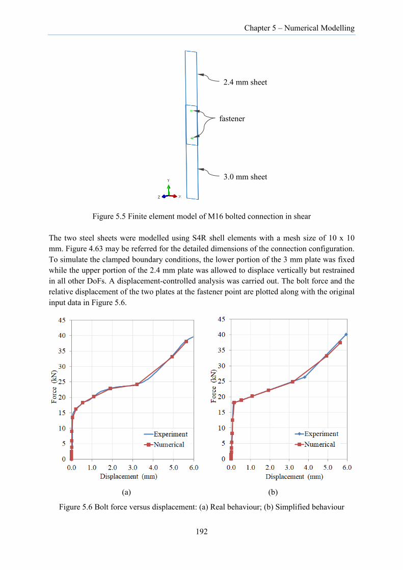
Chapter 5 – Numerical Modelling
Figure 5.5 Finite element model of M16 bolted connection in shear
The two steel sheets were modelled using S4R shell elements with a mesh size of 10 x 10 mm. Figure 4.63 may be referred for the detailed dimensions of the connection configuration. To simulate the clamped boundary conditions, the lower portion of the 3 mm plate was fixed while the upper portion of the 2.4 mm plate was allowed to displace vertically but restrained in all other DoFs. A displacement-controlled analysis was carried out. The bolt force and the relative displacement of the two plates at the fastener point are plotted along with the original input data in Figure 5.6.
(a) (b)
Figure 5.6 Bolt force versus displacement: (a) Real behaviour; (b) Simplified behaviour
fastener
2.4 mm sheet
3.0 mm sheet
192

Chapter 5 – Numerical Modelling
As seen in Figure 5.6, the bolt force and displacement obtained from the numerical analysis accurately traced the original curves, thereby justifying the use of fasteners with connector sections in lieu of the physical modelling of bolts. In the subsequent sections, the behaviour represented by the simplified curves is used for the sake of computational efficiency.
5.4 Finite element modelling of main frame connections
In this section, the main frame connection tests (Section 4.5) were simulated and the behaviour predicted by the nonlinear analysis compared with the experimental results. The main frame connections include apex connection, eaves connection and base connection. The details of the FE models corresponding to each type of connection test are described below.
5.4.1 Eaves connection
5.4.1.1 Geometry
The eaves connection constitutes one of the three main connections in CFS single C-section portal frames. It comprises of two single C-sections, eaves bracket and associated lateral restraints. The overall configuration of the eaves connection along with the detailed dimensions is presented in Section 4.5.1 while the detailed dimensions of the eaves bracket are given in Figure B.4 and Figure B.12 in Appendix B.
5.4.1.2 Numerical model
Figure 5.7 shows the numerical models of eaves connections (EC-1/EC-2 and EC-3), the types of which are identified in Table 4.18 in Section 4.5.1.
(a) (b)
Figure 5.7 FE model of eaves connection: (a) Specimen EC-1/EC-2; (b) Specimen EC-3
The shell finite element model of the eaves connection was created by assembling various parts: two C-sections, eaves bracket, zed stiffeners and cleats. After creating instances of each component at the assembly level, they were translated and rotated to the desired positions.
193

Chapter 5 – Numerical Modelling
The two C30024 C-sections and eaves brackets were modelled using S4R shell elements with a size of 10 mm by 10 mm in general. Four elements were used to model the curved corners while three elements were used for the lips. The relevant steel properties as described in Section 5.2 were assigned to each part. For the L-shaped cleats used for the lateral restraints, the steel properties of the C-section were assigned.
The lateral restraint provided by the turnbuckles in the experiment was modelled using a connector element with axial connector section assigned to it. The axial stiffness (EA/L) required for the axial connector section was computed from the uniform diameter of 12 mm and the elastic properties of steel. The connector elements were connected to the cleats using pin coupling constraint which allowed rotation in any direction but provided restraints against translation in three orthogonal directions.
The pin rod and web stiffener plates at the support and at the loading point were not physically modelled but the constraining effect was taken into account by extending the area of the multipoint constraint (MPC) to be equivalent to the area covered by the plates. The boundary conditions were assigned to the reference nodes of the MPC constraints.
The bolts and screws were modelled using deformable fasteners which were assigned with connector sections. The deformable behaviour of the fasteners was represented by the connector elasticity and plasticity as outlined in Section 5.3. To capture the connection failure resulting from the fracture of screws, damage behaviour was incorporated whereby the damage was initiated once screws experienced forces in excess of 9.55 kN - the ultimate capacity of each screw in shear. The stiffness were degraded using damage evolution with linear stiffness degradation.
At the eaves connection, four main parts are in contact with each other: C-sections, eaves bracket, zed stiffener and lateral-restraint cleat. To account for the interactions among them, surface-to-surface contact pairs were defined with “hard” normal behaviour and with the allowance for separation after contact. In choosing the master-slave surface pairs, the stiffer surface/bigger area or coarse mesh surface were designated as the master surfaces while the softer, smaller or refined meshed surfaces were chosen as the slave surfaces [18].
At the fixed end support, all DoFs were constrained except for the rotational DoFs about the z-axis, while at the movable support, which was connected to the loading jack, the translational DoF in the direction of the y-axis and the rotational DoF about z-axis were released. For the ends of the lateral restraints represented by connector elements, only the translational DoFs were restrained.
5.4.1.3 Results
The nonlinear analysis was performed on the eaves connection models using the displacement-controlled general static procedure. The moment-rotation relations and the support reactions versus upward displacement of the eaves bracket for three types of eaves connections are shown in Figure 5.8 to Figure 5.10. The moments were calculated at the intersection point of the centrelines of two C-sections similar to the moment determined in
194
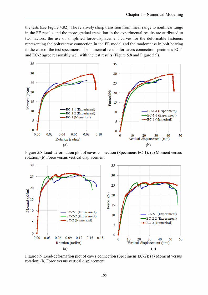
Chapter 5 – Numerical Modelling
the tests (see Figure 4.82). The relatively sharp transition from linear range to nonlinear range in the FE results and the more gradual transition in the experimental results are attributed to two factors: the use of simplified force-displacement curves for the deformable fasteners representing the bolts/screw connection in the FE model and the randomness in bolt bearing in the case of the test specimens. The numerical results for eaves connection specimens EC-1 and EC-2 agree reasonably well with the test results (Figure 5.8 and Figure 5.9).
(a) (b)
Figure 5.8 Load-deformation plot of eaves connection (Specimens EC-1): (a) Moment versus rotation; (b) Force versus vertical displacement
(a) (b)
Figure 5.9 Load-deformation plot of eaves connection (Specimens EC-2): (a) Moment versus rotation; (b) Force versus vertical displacement
195
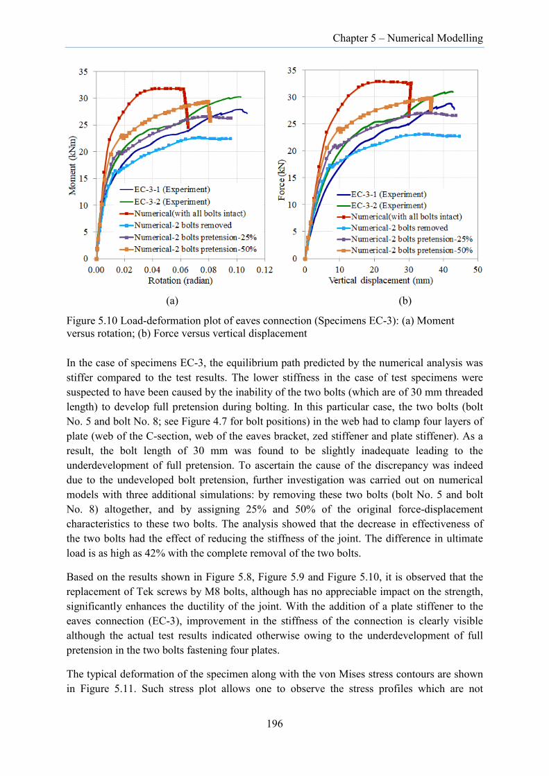
Chapter 5 – Numerical Modelling
(a) (b)
Figure 5.10 Load-deformation plot of eaves connection (Specimens EC-3): (a) Moment versus rotation; (b) Force versus vertical displacement
In the case of specimens EC-3, the equilibrium path predicted by the numerical analysis was stiffer compared to the test results. The lower stiffness in the case of test specimens were suspected to have been caused by the inability of the two bolts (which are of 30 mm threaded length) to develop full pretension during bolting. In this particular case, the two bolts (bolt No. 5 and bolt No. 8; see Figure 4.7 for bolt positions) in the web had to clamp four layers of plate (web of the C-section, web of the eaves bracket, zed stiffener and plate stiffener). As a result, the bolt length of 30 mm was found to be slightly inadequate leading to the underdevelopment of full pretension. To ascertain the cause of the discrepancy was indeed due to the undeveloped bolt pretension, further investigation was carried out on numerical models with three additional simulations: by removing these two bolts (bolt No. 5 and bolt No. 8) altogether, and by assigning 25% and 50% of the original force-displacement characteristics to these two bolts. The analysis showed that the decrease in effectiveness of the two bolts had the effect of reducing the stiffness of the joint. The difference in ultimate load is as high as 42% with the complete removal of the two bolts.
Based on the results shown in Figure 5.8, Figure 5.9 and Figure 5.10, it is observed that the replacement of Tek screws by M8 bolts, although has no appreciable impact on the strength, significantly enhances the ductility of the joint. With the addition of a plate stiffener to the eaves connection (EC-3), improvement in the stiffness of the connection is clearly visible although the actual test results indicated otherwise owing to the underdevelopment of full pretension in the two bolts fastening four plates.
The typical deformation of the specimen along with the von Mises stress contours are shown in Figure 5.11. Such stress plot allows one to observe the stress profiles which are not
196
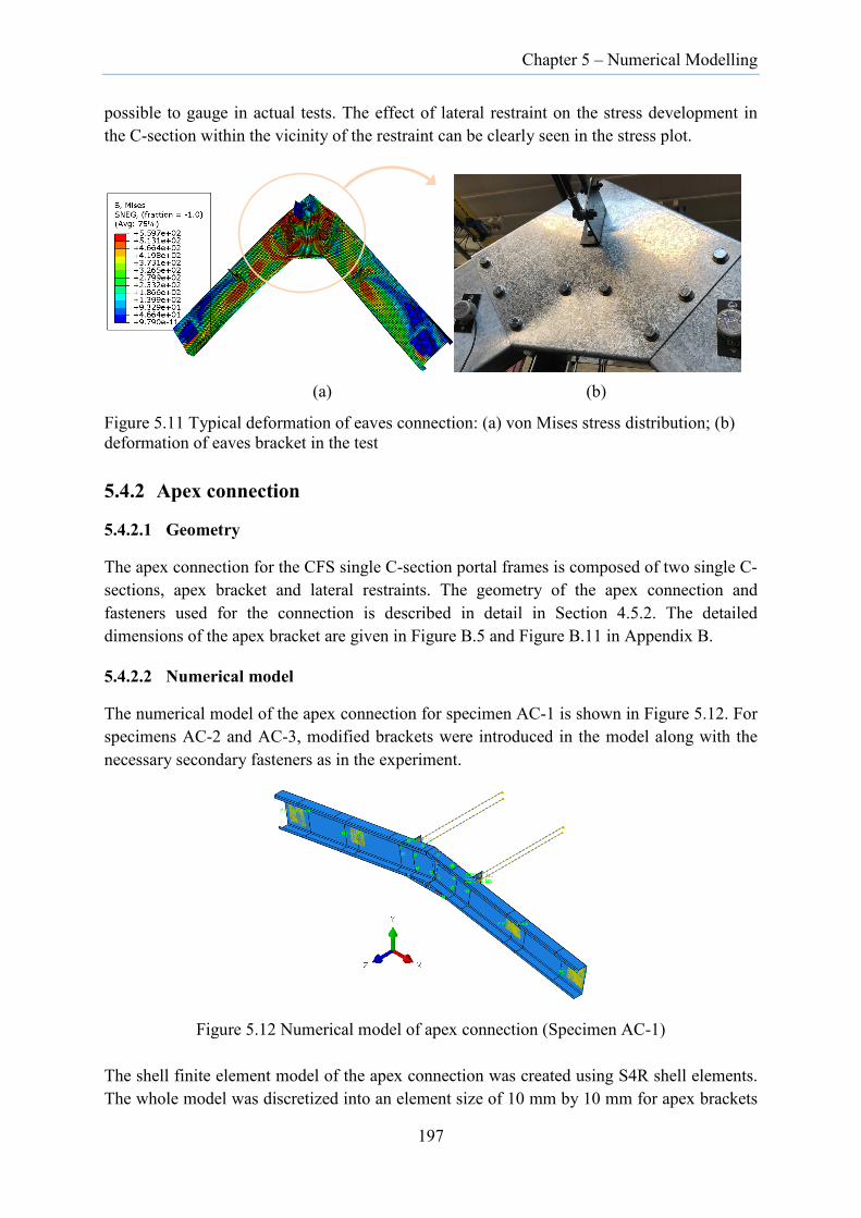
Chapter 5 – Numerical Modelling
possible to gauge in actual tests. The effect of lateral restraint on the stress development in the C-section within the vicinity of the restraint can be clearly seen in the stress plot.
(a) (b)
Figure 5.11 Typical deformation of eaves connection: (a) von Mises stress distribution; (b) deformation of eaves bracket in the test
5.4.2 Apex connection
5.4.2.1 Geometry
The apex connection for the CFS single C-section portal frames is composed of two single C-sections, apex bracket and lateral restraints. The geometry of the apex connection and fasteners used for the connection is described in detail in Section 4.5.2. The detailed dimensions of the apex bracket are given in Figure B.5 and Figure B.11 in Appendix B.
5.4.2.2 Numerical model
The numerical model of the apex connection for specimen AC-1 is shown in Figure 5.12. For specimens AC-2 and AC-3, modified brackets were introduced in the model along with the necessary secondary fasteners as in the experiment.
Figure 5.12 Numerical model of apex connection (Specimen AC-1)
The shell finite element model of the apex connection was created using S4R shell elements. The whole model was discretized into an element size of 10 mm by 10 mm for apex brackets
197

Chapter 5 – Numerical Modelling
and C-sections. The same mesh size was also adopted for the L-shaped brackets used for attaching the lateral restraint. Similar to the eaves connection, the behaviour of each bolt/screw connection was integrated through the fasteners assigned with connector sections, and were placed coincident with the positions of bolts and screws.
To simulate the clamping action provided to the web by the support brackets and the load brackets, all nodes lying within the area bounded by the outermost bolts that clamped the brackets were subject to MPC constraints with a reference node at the centre. To model the boundary conditions at the supports, translational DoF in the x direction and z-axis rotation were released while other DoFs were restrained. Due to the release of translational DoF in the x-direction at the supports, rigid body motion was likely to occur. To prevent such occurrence, the horizontal translational DoF in the x-direction at the midpoint of the apex bracket was restrained.
The turnbuckles used in the experiment for lateral restraint were modelled by connector elements assigned to the axial connector sections. They were connected to the cleats with pin coupling constraints to allow rotation in any direction whilst providing restraints against translational DoFs in respective orthogonal directions. However, the actual lateral restraints were not physically modelled at the supports but the effect of the restraints was implemented by constraining the reference node from moving out-of-plane direction.
For the parts in contact with each other, surface-to-surface contact pairs were defined with hard contact algorithm and allowance for separation after contact. The relevant material properties, as described in Section 5.2, were assigned to the components of apex connections including the L-shaped lateral restraint cleats.The specimens were loaded through the web of the C-sections by defining the reference point for the MPC constraints at the load points. A part of the Abaqus input file for apex connection specimen (AC-2) is provided in Section D.2 in Appendix D.
5.4.2.3 Results
The load-displacement and moment-rotation relations of the apex connection obtained from finite element analysis and the experiment are compared in Figure 5.13, Figure 5.14 and Figure 5.15.
The numerical results and the test results generally agree well with the exception of the AC-1-1 test specimen which showed slightly stiffer behaviour compared to the numerical results. The stiffness increase in this particular case in the test was due to the development of Coulomb-type friction at the supports due to inadequate lubrication. For the specimens AC-1 and AC-3, the lower lips of the C-sections and apex brackets were fastened using Tek screws. The fracture of screws preceding the ultimate load was a common phenomenon in these specimens. Fractures of screws were usually accompanied by the sudden drop in load in the experiment. The numerical analysis could adequately capture this phenomenon as indicated by the sudden small drops in load in the ascending part of the equilibrium paths shown in Figure 5.13 and Figure 5.15.
198
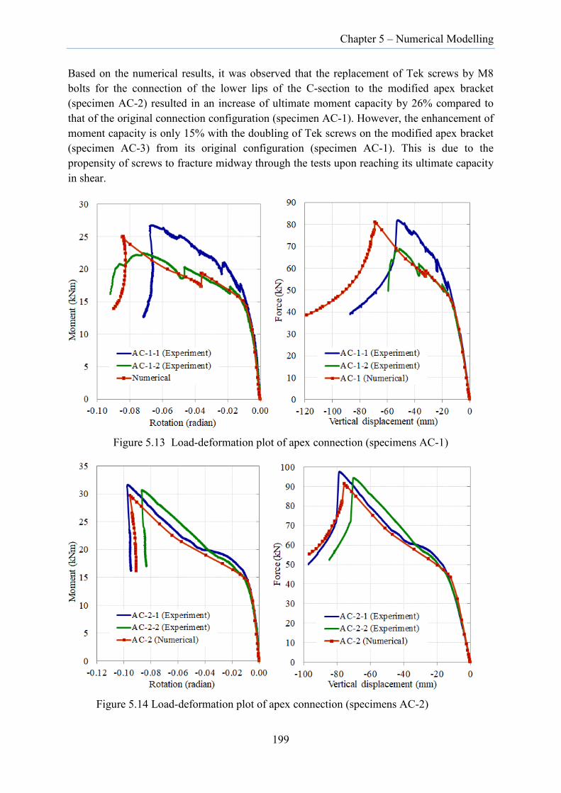
Chapter 5 – Numerical Modelling
Based on the numerical results, it was observed that the replacement of Tek screws by M8 bolts for the connection of the lower lips of the C-section to the modified apex bracket (specimen AC-2) resulted in an increase of ultimate moment capacity by 26% compared to that of the original connection configuration (specimen AC-1). However, the enhancement of moment capacity is only 15% with the doubling of Tek screws on the modified apex bracket (specimen AC-3) from its original configuration (specimen AC-1). This is due to the propensity of screws to fracture midway through the tests upon reaching its ultimate capacity in shear.
Figure 5.13 Load-deformation plot of apex connection (specimens AC-1)
Figure 5.14 Load-deformation plot of apex connection (specimens AC-2)
199
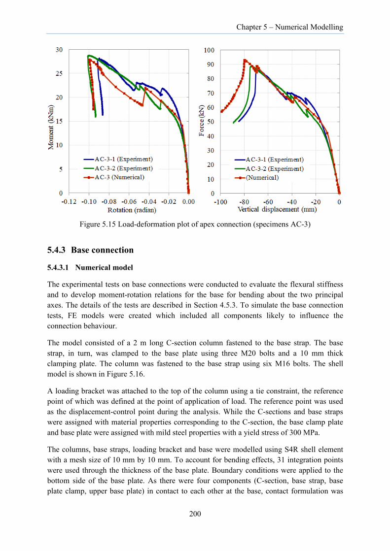
Chapter 5 – Numerical Modelling
Figure 5.15 Load-deformation plot of apex connection (specimens AC-3)
5.4.3 Base connection
5.4.3.1 Numerical model
The experimental tests on base connections were conducted to evaluate the flexural stiffness and to develop moment-rotation relations for the base for bending about the two principal axes. The details of the tests are described in Section 4.5.3. To simulate the base connection tests, FE models were created which included all components likely to influence the connection behaviour.
The model consisted of a 2 m long C-section column fastened to the base strap. The base strap, in turn, was clamped to the base plate using three M20 bolts and a 10 mm thick clamping plate. The column was fastened to the base strap using six M16 bolts. The shell model is shown in Figure 5.16.
A loading bracket was attached to the top of the column using a tie constraint, the reference point of which was defined at the point of application of load. The reference point was used as the displacement-control point during the analysis. While the C-sections and base straps were assigned with material properties corresponding to the C-section, the base clamp plate and base plate were assigned with mild steel properties with a yield stress of 300 MPa.
The columns, base straps, loading bracket and base were modelled using S4R shell element with a mesh size of 10 mm by 10 mm. To account for bending effects, 31 integration points were used through the thickness of the base plate. Boundary conditions were applied to the bottom side of the base plate. As there were four components (C-section, base strap, base plate clamp, upper base plate) in contact to each other at the base, contact formulation was
200

Chapter 5 – Numerical Modelling
enforced with normal contact defined as ‘hard’ while tangential contact was represented by a slip coefficient of 0.18 with penalty friction formulation.
(a) (b)
Figure 5.16 Numerical model of base connection test: (a) front view; (b) rear view
The analysis was carried out using the “static general” and displacement-controlled method. The same model was used to determine the behaviour in bending about the major and minor axes by changing the displacement direction at the controlled reference point.
5.4.3.2 Results
The moment-rotation characteristics for bending about the major and minor axes determined from the output of the FE analysis are presented in Figure 5.17. For major axis bending, the bending moments and corresponding rotations (M1-θ1) obtained from the experiments for specimens BC-1-1 and BC-1-2 (shown in Figure 4.102 and Figure 4.103 in Chapter 4) are compared with the bending moment from the numerical model. Similarly, for minor axis bending, the bending moments and corresponding rotations (M1-θ1) for specimens BT-2T-1, BT-2T-2 and BT-2C-1 (shown in Figure 4.112 in Chapter 4, Figure C.19 and Figure C.22 in Appendix C) are compared with the bending from numerical models. The results agree reasonably well, especially for minor axis bending. For major axis bending, some discrepancy is observed between the behaviours predicted by numerical analysis and the tests. The reason is not obvious as several participating factors are present at the base including slotted bolt holes, possible yielding of components, bending of base straps, frictional resistance between parts in contact to name a few. To observe whether the tangential friction developed at the interface between plates at the base had any influence on the results, analyses were carried out with different slip coefficients. The results showed no major differences in the behaviour with variation in slip coefficient.
For minor axis bending, the analyses were carried out with the shear centre side both in tension and in compression. The results showed a slight increase in stiffness when the
Column C1
201
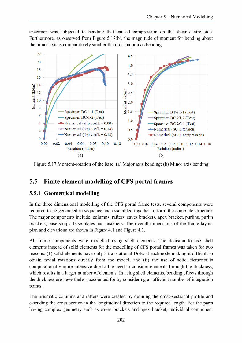
Chapter 5 – Numerical Modelling
specimen was subjected to bending that caused compression on the shear centre side. Furthermore, as observed from Figure 5.17(b), the magnitude of moment for bending about the minor axis is comparatively smaller than for major axis bending.
(a) (b)
Figure 5.17 Moment-rotation of the base: (a) Major axis bending; (b) Minor axis bending
5.5 Finite element modelling of CFS portal frames
5.5.1 Geometrical modelling
In the three dimensional modelling of the CFS portal frame tests, several components were required to be generated in sequence and assembled together to form the complete structure. The major components include: columns, rafters, eaves brackets, apex bracket, purlins, purlin brackets, base straps, base plates and fasteners. The overall dimensions of the frame layout plan and elevations are shown in Figure 4.1 and Figure 4.2.
All frame components were modelled using shell elements. The decision to use shell elements instead of solid elements for the modelling of CFS portal frames was taken for two reasons: (1) solid elements have only 3 translational DoFs at each node making it difficult to obtain nodal rotations directly from the model, and (ii) the use of solid elements is computationally more intensive due to the need to consider elements through the thickness, which results in a larger number of elements. In using shell elements, bending effects through the thickness are nevertheless accounted for by considering a sufficient number of integration points.
The prismatic columns and rafters were created by defining the cross-sectional profile and extruding the cross-section in the longitudinal direction to the required length. For the parts having complex geometry such as eaves brackets and apex bracket, individual component
202

Chapter 5 – Numerical Modelling
plates were initially generated separately and subsequently merged to form the complete parts. Individual components of the frames were created in the assembly module, and assembled by translating and rotating each component to the required location with replication of components where necessary. The thicknesses of the sections were defined using the nominal thickness since the difference between the measured and nominal thickness values of the C-sections and brackets were negligibly small. The full 3D frame model with a single C-section frame at the centre is shown in Figure 5.18.
Figure 5.18 Finite element model of test frame
The end frames are doubly-symmetric sections formed by connecting two individual C-sections back-to-back together. As the end frames were reused from previous tests [13] to provide support to the purlins, they were reproduced in the numerical model to provide an elastic restraint condition to the purlins. To facilitate accurate reproduction of the geometry, each component of the end frames was initially measured from the installed frames, and subsequently verified with the dimensions given in [13].
In the CFS single C-section portal frames, columns and rafters were connected to respective brackets using M16 bolts, Tek screws or M8 bolts while the purlins and cleats were connected using M12 bolts. To simulate the behaviour of the bolted/screw connections, the bolts and screws were idealized using mesh-independent fasteners. They were positioned in the model to coincide with the physical locations of the bolts/screws. The fasteners were assigned with the relevant nonlinear load-displacement relations shown in Figure 5.2 and Figure 5.3.
Typical shell element models of the eaves and apex connections along with the distribution of deformable fasteners are shown in Figure 5.19. These particular figures pertain to the modified eaves and apex connections for the last three frame tests.
203
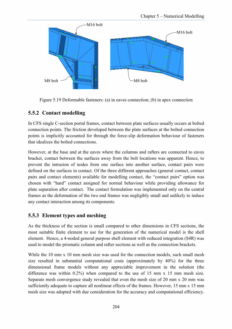
Chapter 5 – Numerical Modelling
Figure 5.19 Deformable fasteners: (a) in eaves connection; (b) in apex connection
5.5.2 Contact modelling
In CFS single C-section portal frames, contact between plate surfaces usually occurs at bolted connection points. The friction developed between the plate surfaces at the bolted connection points is implicitly accounted for through the force-slip deformation behaviour of fasteners that idealizes the bolted connections.
However, at the base and at the eaves where the columns and rafters are connected to eaves bracket, contact between the surfaces away from the bolt locations was apparent. Hence, to prevent the intrusion of nodes from one surface into another surface, contact pairs were defined on the surfaces in contact. Of the three different approaches (general contact, contact pairs and contact elements) available for modelling contact, the “contact pairs” option was chosen with “hard” contact assigned for normal behaviour while providing allowance for plate separation after contact. The contact formulation was implemented only on the central frames as the deformation of the two end frames was negligibly small and unlikely to induce any contact interaction among its components.
5.5.3 Element types and meshing
As the thickness of the section is small compared to other dimensions in CFS sections, the most suitable finite element to use for the generation of the numerical model is the shell element. Hence, a 4-noded general purpose shell element with reduced integration (S4R) was used to model the prismatic column and rafter sections as well as the connection brackets.
While the 10 mm x 10 mm mesh size was used for the connection models, such small mesh size resulted in substantial computational costs (approximately by 40%) for the three dimensional frame models without any appreciable improvement in the solution (the difference was within 0.2%) when compared to the use of 15 mm x 15 mm mesh size. Separate mesh convergence study revealed that even the mesh size of 20 mm x 20 mm was sufficiently adequate to capture all nonlinear effects of the frames. However, 15 mm x 15 mm mesh size was adopted with due consideration for the accuracy and computational efficiency.
M16 bolt
M8 bolt
M16 bolt
M8 bolt
204
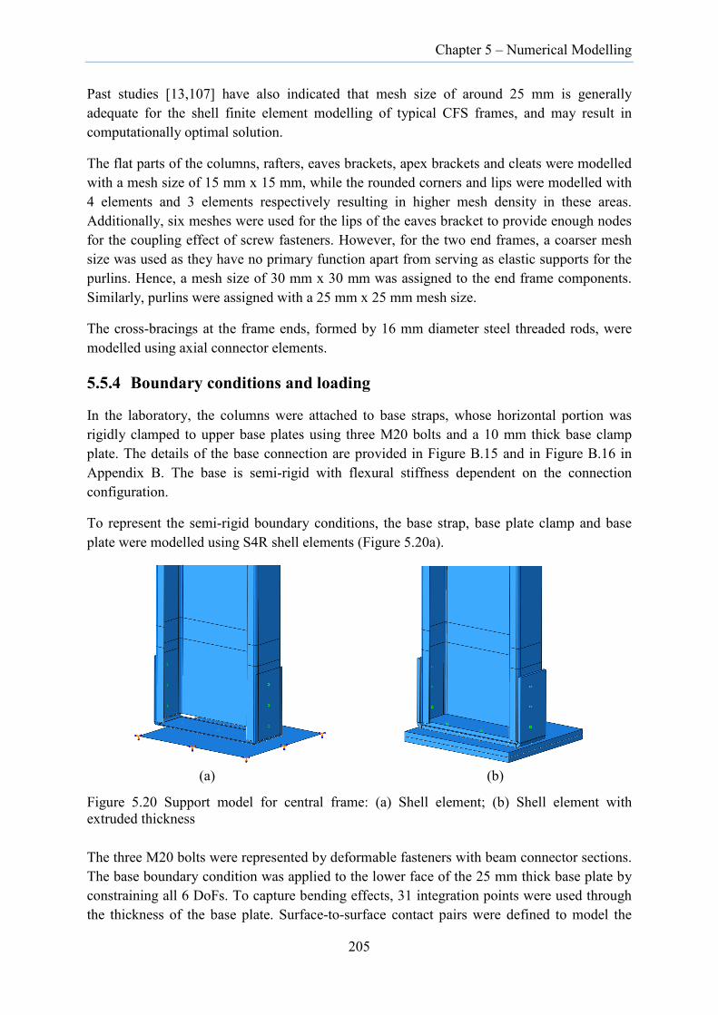
Chapter 5 – Numerical Modelling
Past studies [13,107] have also indicated that mesh size of around 25 mm is generally adequate for the shell finite element modelling of typical CFS frames, and may result in computationally optimal solution.
The flat parts of the columns, rafters, eaves brackets, apex brackets and cleats were modelled with a mesh size of 15 mm x 15 mm, while the rounded corners and lips were modelled with 4 elements and 3 elements respectively resulting in higher mesh density in these areas. Additionally, six meshes were used for the lips of the eaves bracket to provide enough nodes for the coupling effect of screw fasteners. However, for the two end frames, a coarser mesh size was used as they have no primary function apart from serving as elastic supports for the purlins. Hence, a mesh size of 30 mm x 30 mm was assigned to the end frame components. Similarly, purlins were assigned with a 25 mm x 25 mm mesh size.
The cross-bracings at the frame ends, formed by 16 mm diameter steel threaded rods, were modelled using axial connector elements.
5.5.4 Boundary conditions and loading
In the laboratory, the columns were attached to base straps, whose horizontal portion was rigidly clamped to upper base plates using three M20 bolts and a 10 mm thick base clamp plate. The details of the base connection are provided in Figure B.15 and in Figure B.16 in Appendix B. The base is semi-rigid with flexural stiffness dependent on the connection configuration.
To represent the semi-rigid boundary conditions, the base strap, base plate clamp and base plate were modelled using S4R shell elements (Figure 5.20a).
(a) (b)
Figure 5.20 Support model for central frame: (a) Shell element; (b) Shell element with extruded thickness
The three M20 bolts were represented by deformable fasteners with beam connector sections. The base boundary condition was applied to the lower face of the 25 mm thick base plate by constraining all 6 DoFs. To capture bending effects, 31 integration points were used through the thickness of the base plate. Surface-to-surface contact pairs were defined to model the
205
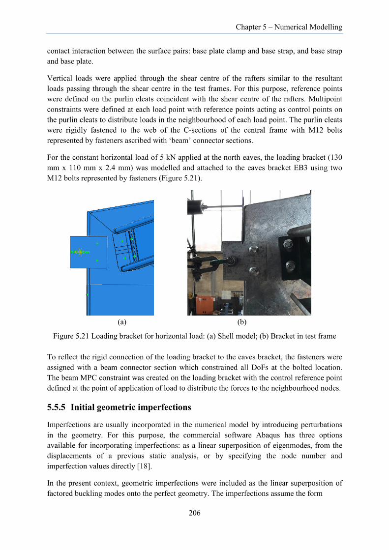
Chapter 5 – Numerical Modelling
contact interaction between the surface pairs: base plate clamp and base strap, and base strap and base plate.
Vertical loads were applied through the shear centre of the rafters similar to the resultant loads passing through the shear centre in the test frames. For this purpose, reference points were defined on the purlin cleats coincident with the shear centre of the rafters. Multipoint constraints were defined at each load point with reference points acting as control points on the purlin cleats to distribute loads in the neighbourhood of each load point. The purlin cleats were rigidly fastened to the web of the C-sections of the central frame with M12 bolts represented by fasteners ascribed with ‘beam’ connector sections.
For the constant horizontal load of 5 kN applied at the north eaves, the loading bracket (130 mm x 110 mm x 2.4 mm) was modelled and attached to the eaves bracket EB3 using two M12 bolts represented by fasteners (Figure 5.21).
(a) (b)
Figure 5.21 Loading bracket for horizontal load: (a) Shell model; (b) Bracket in test frame
To reflect the rigid connection of the loading bracket to the eaves bracket, the fasteners were assigned with a beam connector section which constrained all DoFs at the bolted location. The beam MPC constraint was created on the loading bracket with the control reference point defined at the point of application of load to distribute the forces to the neighbourhood nodes.
5.5.5 Initial geometric imperfections
Imperfections are usually incorporated in the numerical model by introducing perturbations in the geometry. For this purpose, the commercial software Abaqus has three options available for incorporating imperfections: as a linear superposition of eigenmodes, from the displacements of a previous static analysis, or by specifying the node number and imperfection values directly [18].
In the present context, geometric imperfections were included as the linear superposition of factored buckling modes onto the perfect geometry. The imperfections assume the form
206

Chapter 5 – Numerical Modelling
1
N
i i ii
x α=
∆ = ∑ φ (5.4)
where φi is the ith mode shape, αi is the corresponding scale factor and N is the number of modes. The critical buckling modes obtained from an eigenvalue analysis were scaled so that the amplitude matched with the maximum absolute value of the measured imperfections.
For the measured sectional imperfections, the distortional buckling imperfections were determined from the average of the absolute displacement of the flanges, while the local buckling imperfections were determined separately for the web and flanges as the width to thickness ratio of the flange and web were significantly different. The details of the imperfection measurements are covered in Section 4.2.8. The equations used for the calculation of local and distortional buckling imperfections are:
( ), 6 2 1012l webl P P P= − + (5.5)
( ) ( ), 4 3 5 8 7 91 1 12 2 2l flangel P P P P P P
= − + + − +
(5.6)
( )3 5 9 712distortionall P P P P= − + − (5.7)
in which P2, P3,…., P9, P10 are readings at laser points along the cross-sections (Figure 4.12).
Table 5.1 shows the maximum absolute values of the local and the distortional imperfections for the six columns used in the first three frame tests.
Table 5.1 Local and distortional buckling imperfections
Column specimens
Local web (mm)
Local flange (mm)
Distortional (mm)
T1-C1 1.79 0.22 1.44 T1-C3 1.68 0.15 1.88 T2-C1 2.73 0.23 1.72 T2-C3 2.82 0.14 1.49 T3-C1 1.63 0.14 1.64 T3-C3 2.40 0.18 1.38 Mean 2.17 0.18 1.59
While determining the maximum values of the local and distortional imperfections, a 150 mm length of section at either end was excluded on the assumption that, in this region, bolting would have changed the measured imperfection during the frame installation. In addition,
207

Chapter 5 – Numerical Modelling
localized failure in this region was not observed during the tests. The mean value of measured local buckling imperfection in the web is comparable to the local buckling imperfection of 1.92 mm calculated from Equation (2.13).
To observe the trend in the behaviour of the columns, a range of thickness values starting from 2.4 mm to 8 mm was assigned to the columns while assigning a 10 mm thickness to all other sections. A buckling analysis was performed for each thickness. The initial elastic buckling analysis revealed that the global buckling modes were principally a twist deformation of the columns similar to the behaviour observed in the tests. The typical first four buckling modes of columns with an assigned thickness of 4.2 mm are shown in Figure D.2 in Appendix D wherein the first two modes describe a twist deformation of the columns while the remaining two modes describe local buckling of the column webs below the eaves. As is evident from Figure D.2 in Appendix D, in the first and second buckling modes, both columns undergo twist deformation with different amplitude in each mode. This caused numerical difficulties with the application of buckling factors in the linear superposition of buckling modes for imperfection. To circumvent the issue of coupled buckling modes, the twist deformation of each column was isolated in each mode. This was accomplished by assigning the thickness of 4.2 mm to the individual columns in turn while the other column was assigned a thicker section, and performing corresponding buckling analysis. The resulting buckling modes were extracted and combined together along with the local buckling modes. To scale the column twist deformation to the value measured prior to tests, the global imperfection corresponding to the measured column out-of-straightness at 3.0 m above the base of the column (at the point on the web near the inside flange-web junction), was used. The global imperfection amplitudes were derived from the measured twist rotations given in Table 4.5 and in Table B.1 to Table B.5 in Appendix B for respective frames. The values were deduced from measurements carried out right after the frame installation but before the installation of load spreading system.
As the distortional buckling amplitude obtained from the measured imperfections were generally lower than the local buckling amplitudes as shown in
Table 5.1, only the local and global buckling modes were implemented in the FE model. However, buckling factors that would create local buckling imperfection in both the positive and negative transverse directions normal to the web were considered.
5.5.6 Analysis
A static nonlinear analysis was performed for each test frame. A single load step was defined for frames subjected to only vertical loads while three load steps were defined for frames subjected to a combination of lateral load and vertical load. In the latter case, the load steps included initial self-weight (of loading rig, purlins and rafters), horizontal load and vertical load. A “static general” option was used for the static nonlinear analysis of the frames. Where it was not possible to advance the equilibrium path beyond the peak load, the “modified Riks” method was used to obtain post-ultimate equilibrium path. To activate the modified Riks method, the “Restart” option was used upon attainment of the peak load. This
208
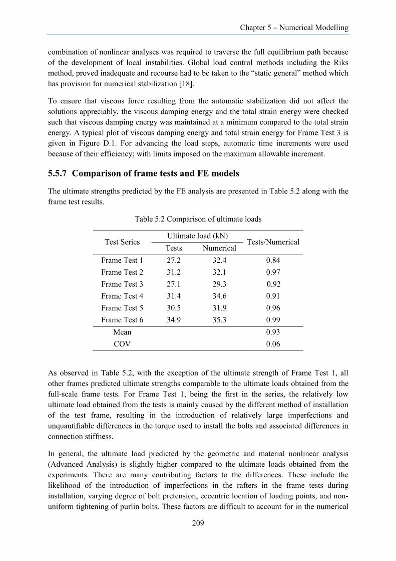
Chapter 5 – Numerical Modelling
combination of nonlinear analyses was required to traverse the full equilibrium path because of the development of local instabilities. Global load control methods including the Riks method, proved inadequate and recourse had to be taken to the “static general” method which has provision for numerical stabilization [18].
To ensure that viscous force resulting from the automatic stabilization did not affect the solutions appreciably, the viscous damping energy and the total strain energy were checked such that viscous damping energy was maintained at a minimum compared to the total strain energy. A typical plot of viscous damping energy and total strain energy for Frame Test 3 is given in Figure D.1. For advancing the load steps, automatic time increments were used because of their efficiency; with limits imposed on the maximum allowable increment.
5.5.7 Comparison of frame tests and FE models
The ultimate strengths predicted by the FE analysis are presented in Table 5.2 along with the frame test results.
Table 5.2 Comparison of ultimate loads
Test Series Ultimate load (kN)
Tests/Numerical Tests Numerical
Frame Test 1 27.2 32.4 0.84 Frame Test 2 31.2 32.1 0.97 Frame Test 3 27.1 29.3 0.92 Frame Test 4 31.4 34.6 0.91 Frame Test 5 30.5 31.9 0.96 Frame Test 6 34.9 35.3 0.99
Mean 0.93 COV 0.06
As observed in Table 5.2, with the exception of the ultimate strength of Frame Test 1, all other frames predicted ultimate strengths comparable to the ultimate loads obtained from the full-scale frame tests. For Frame Test 1, being the first in the series, the relatively low ultimate load obtained from the tests is mainly caused by the different method of installation of the test frame, resulting in the introduction of relatively large imperfections and unquantifiable differences in the torque used to install the bolts and associated differences in connection stiffness.
In general, the ultimate load predicted by the geometric and material nonlinear analysis (Advanced Analysis) is slightly higher compared to the ultimate loads obtained from the experiments. There are many contributing factors to the differences. These include the likelihood of the introduction of imperfections in the rafters in the frame tests during installation, varying degree of bolt pretension, eccentric location of loading points, and non-uniform tightening of purlin bolts. These factors are difficult to account for in the numerical
209

Chapter 5 – Numerical Modelling
model but nevertheless are present in the actual frame tests. Despite these sources of variability, the Advanced Analysis adequately predicted the ultimate loads with high accuracy and uniformity as indicated by the low coefficient of variation of the strength ratio demonstrating its potential use for the design of CFS portal frames.
5.5.7.1 Frame deformation
While the two columns in frames with vertical loads experienced twist deformation of similar magnitude, the columns in frames with lateral load besides vertical load twisted differently with column C3 (north column) twisting more than column C1 (south column). As the frame swayed towards the north due to the application of a horizontal force in the north direction at the north eaves, the column C3 experienced more compressive force resulting in more twist deformation. On the contrary, column C1 underwent minimal twists as it experienced comparatively less compressive force. A typical deformed shape of the finite element model of Frame Test 5 is shown in Figure 5.22. In all the tests, the end frames experienced minimal deformation proving that no significant load was transferred to them from the loading process and that almost entire load was borne by the central frame alone.
( a) (b)
Figure 5.22 Frame deformation profile (Frame Test 5): (a) Displacement; (b) Rotation
The total vertical base reactions from the finite element models along with the vertical loads applied to the test frame versus vertical displacement of the apex are plotted in Figure 5.23 for all test frames. The vertical loads applied to the test frames include self-weight of the rafters, purlins and load spreading system. It can be seen that the behaviour predicted by the Advanced Analysis agrees well with the response of the experimental tests apart from Frame Test 1. For Frame Test 1, the discrepancy between the test results and FE prediction is a result of the different method of installation of test frame as highlighted in Section 4.2.12.2.
The horizontal deflection of the north eaves is plotted for four representative frames along with the horizontal deflections obtained from frame tests in Figure 5.24. Similarly, the twist rotation of column C3 at 2.5 m above the base are plotted in Figure 5.25 for Frame Tests 2 and 3.
210

Chapter 5 – Numerical Modelling
Figure 5.23 Force versus vertical displacement of apex for the central frame
211

Chapter 5 – Numerical Modelling
Figure 5.24 Horizontal displacements of eaves
Figure 5.25 Twist rotation of column C3
212

Chapter 5 – Numerical Modelling
In reality, the transducers measuring the displacements of the frame are fixed in space while the frame continuously deformed under the effect of vertical loading. For frames undergoing large displacements as in this case, the final point of measurement was at a location significantly different from the initial point of measurement. For instance, for the vertical displacement of the apex, the transducer was initially placed underneath the bottom flange of the apex bracket close to its web. Due to the significant deformation of the apex bracket, the final position of the transducer was well away from the initial position on the bottom flange. This precludes an exact comparison between the measured and predicted deformations.
5.5.7.2 Fastener deformation
In the numerical models, the fasteners were assigned nonlinear behaviour in the form of linear elasticity and nonlinear plasticity to the relevant DoFs. The linear elasticity defined the pre-slip state of the bolted connection while the plasticity represented the post-slip state of the bolted connection. In the fastener model, it was assumed that the bolt force normal to the plate surface and the out-of-plane moments remained elastic while in-plane forces and moment were allowed to behave nonlinearly through prescribed force-displacement and moment-rotation relations. In this modelling, the bolt pretension was implicitly accounted in the force-slip deformation relations assigned to the fasteners. The axial forces that developed in the fasteners during the analysis were solely due to the deformation of plates being connected.
To investigate the validity of the assumed uncoupled behaviour among force components in the fastener model, the bolt forces and moments experienced by bolt No. 2 (refer Figure 4.8) at the top flange of the rafter at the apex (where the bolt forces are likely to be high) were monitored. The bolt force and moment versus the corresponding displacement and rotation in three orthogonal directions are given in Figure 5.26.
Figure 5.26 Bolt force/moment versus displacement/rotation
213
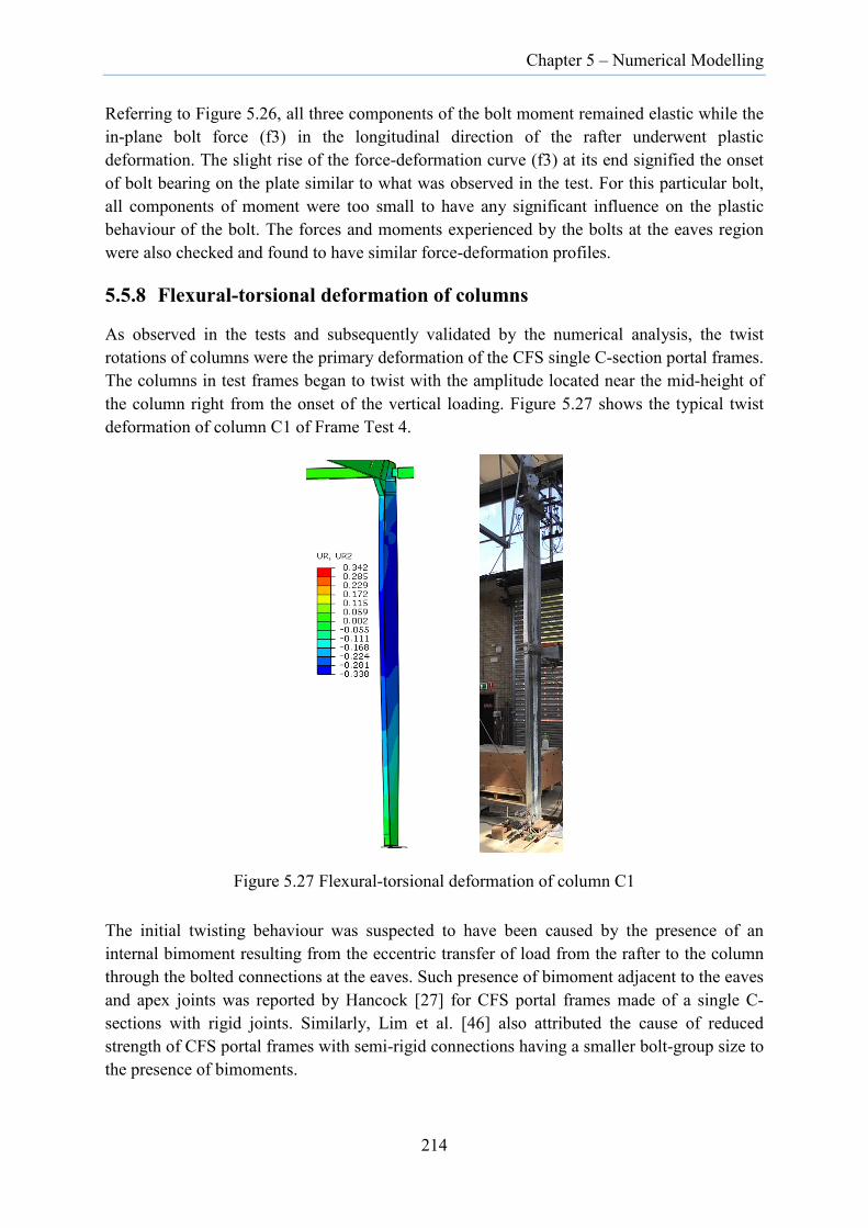
Chapter 5 – Numerical Modelling
Referring to Figure 5.26, all three components of the bolt moment remained elastic while the in-plane bolt force (f3) in the longitudinal direction of the rafter underwent plastic deformation. The slight rise of the force-deformation curve (f3) at its end signified the onset of bolt bearing on the plate similar to what was observed in the test. For this particular bolt, all components of moment were too small to have any significant influence on the plastic behaviour of the bolt. The forces and moments experienced by the bolts at the eaves region were also checked and found to have similar force-deformation profiles.
5.5.8 Flexural-torsional deformation of columns
As observed in the tests and subsequently validated by the numerical analysis, the twist rotations of columns were the primary deformation of the CFS single C-section portal frames. The columns in test frames began to twist with the amplitude located near the mid-height of the column right from the onset of the vertical loading. Figure 5.27 shows the typical twist deformation of column C1 of Frame Test 4.
Figure 5.27 Flexural-torsional deformation of column C1
The initial twisting behaviour was suspected to have been caused by the presence of an internal bimoment resulting from the eccentric transfer of load from the rafter to the column through the bolted connections at the eaves. Such presence of bimoment adjacent to the eaves and apex joints was reported by Hancock [27] for CFS portal frames made of a single C-sections with rigid joints. Similarly, Lim et al. [46] also attributed the cause of reduced strength of CFS portal frames with semi-rigid connections having a smaller bolt-group size to the presence of bimoments.
214

Chapter 5 – Numerical Modelling
In general, an internal bimoment can arise from the longitudinal stresses in the column section if the stress distribution is non-uniform. The internal bimoment is given by [28]:
B dAσω= ∫ (5.8)
in which σ is the longitudinal stress and ω is the sectorial coordinate with respect to the shear centre. For a cross-section discretized into finite elements, it can be approximated by
1
n
i i ii
B Aσ ω=
=∑ (5.9)
where σi is the longitiudinal stress, ωi is the sectorial coordinate at the centroid of elemental area Ai, and n is the number of finite element across the cross-section.
To investigate the existence of a bimoment and whether this was the cause of the twist of the columns observed from the onset of loading, bimoments were calculated using Equation (5.9)at five locations in column C1 (Frame Test 4) below the south eaves corresponding to a vertical load of 8.8 kN (elastic loading range) and at 34.6 kN (ultimate load). The bimoments are shown in Table 5.3.
Table 5.3 Bimoment below the south eaves of column C1
Distance from column base (m)
Bimoment at elastic loading range (kNm2)
Bimoment at ultimate load
(kNm2)
5.067 0.241 0.626
4.537 0.215 0.506
3.997 0.181 0.472 3.757 0.167 0.444
3.502 0.151 0.418
For the calculation of bimoments, the longitudinal stresses were extracted below the eaves corresponding to five sections in column C1. It was presumed that the axial forces transferred to the columns by the bolts at the eaves would have transformed into longitudinal stress immediately below the eaves. Figure 5.28 and Figure 5.29 shows the longitudinal stresses developed at the centroid of each element corresponding to the five sections in column C1 with inset diagram showing its cross-section orientation. The sectorial coordinates at the centroid of each element with respect to the shear centre is plotted in Figure 5.30. The sectorial coordinates and other section properties for the C30024 section were calculated using the TCL program described in Section 3.3.2.2 and is included in Section D.5 in Appendix D.
215
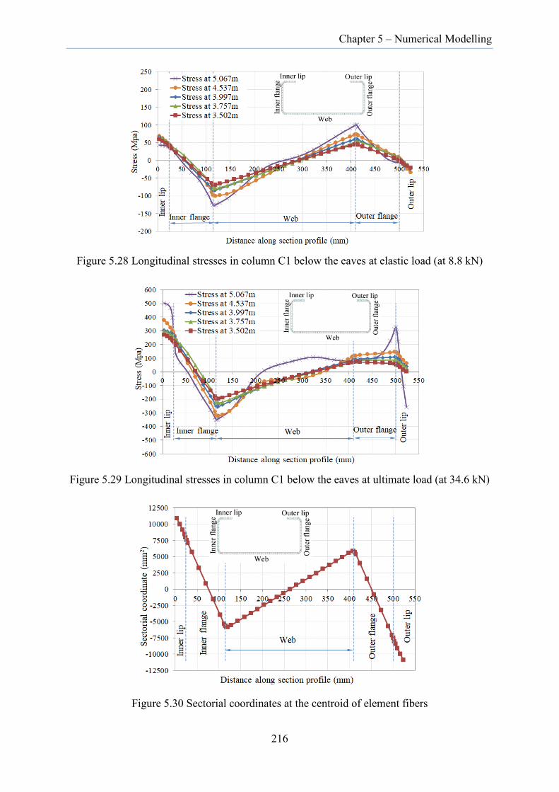
Chapter 5 – Numerical Modelling
Figure 5.28 Longitudinal stresses in column C1 below the eaves at elastic load (at 8.8 kN)
Figure 5.29 Longitudinal stresses in column C1 below the eaves at ultimate load (at 34.6 kN)
Figure 5.30 Sectorial coordinates at the centroid of element fibers
216
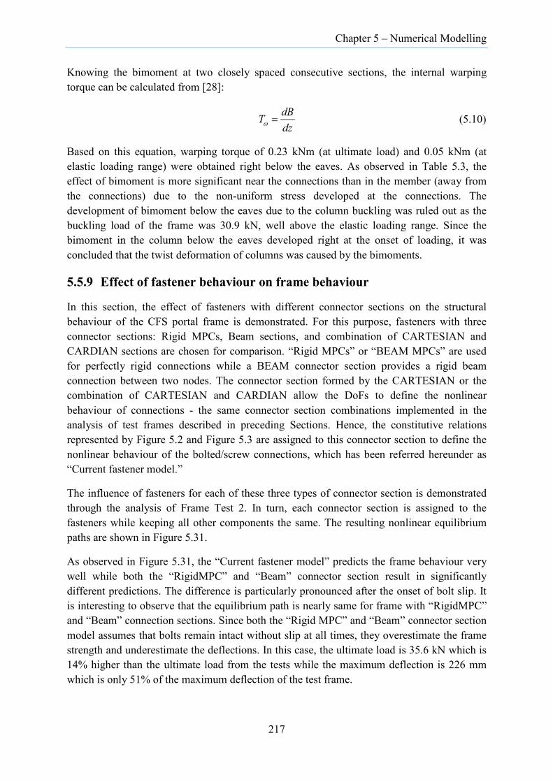
Chapter 5 – Numerical Modelling
Knowing the bimoment at two closely spaced consecutive sections, the internal warping torque can be calculated from [28]:
dBTdzω = (5.10)
Based on this equation, warping torque of 0.23 kNm (at ultimate load) and 0.05 kNm (at elastic loading range) were obtained right below the eaves. As observed in Table 5.3, the effect of bimoment is more significant near the connections than in the member (away from the connections) due to the non-uniform stress developed at the connections. The development of bimoment below the eaves due to the column buckling was ruled out as the buckling load of the frame was 30.9 kN, well above the elastic loading range. Since the bimoment in the column below the eaves developed right at the onset of loading, it was concluded that the twist deformation of columns was caused by the bimoments.
5.5.9 Effect of fastener behaviour on frame behaviour
In this section, the effect of fasteners with different connector sections on the structural behaviour of the CFS portal frame is demonstrated. For this purpose, fasteners with three connector sections: Rigid MPCs, Beam sections, and combination of CARTESIAN and CARDIAN sections are chosen for comparison. “Rigid MPCs” or “BEAM MPCs” are used for perfectly rigid connections while a BEAM connector section provides a rigid beam connection between two nodes. The connector section formed by the CARTESIAN or the combination of CARTESIAN and CARDIAN allow the DoFs to define the nonlinear behaviour of connections - the same connector section combinations implemented in the analysis of test frames described in preceding Sections. Hence, the constitutive relations represented by Figure 5.2 and Figure 5.3 are assigned to this connector section to define the nonlinear behaviour of the bolted/screw connections, which has been referred hereunder as “Current fastener model.”
The influence of fasteners for each of these three types of connector section is demonstrated through the analysis of Frame Test 2. In turn, each connector section is assigned to the fasteners while keeping all other components the same. The resulting nonlinear equilibrium paths are shown in Figure 5.31.
As observed in Figure 5.31, the “Current fastener model” predicts the frame behaviour very well while both the “RigidMPC” and “Beam” connector section result in significantly different predictions. The difference is particularly pronounced after the onset of bolt slip. It is interesting to observe that the equilibrium path is nearly same for frame with “RigidMPC” and “Beam” connection sections. Since both the “Rigid MPC” and “Beam” connector section model assumes that bolts remain intact without slip at all times, they overestimate the frame strength and underestimate the deflections. In this case, the ultimate load is 35.6 kN which is 14% higher than the ultimate load from the tests while the maximum deflection is 226 mm which is only 51% of the maximum deflection of the test frame.
217
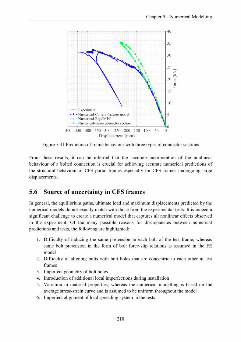
Chapter 5 – Numerical Modelling
Figure 5.31 Prediction of frame behaviour with three types of connector sections
From these results, it can be inferred that the accurate incorporation of the nonlinear behaviour of a bolted connection is crucial for achieving accurate numerical predictions of the structural behaviour of CFS portal frames especially for CFS frames undergoing large displacements.
5.6 Source of uncertainty in CFS frames
In general, the equilibrium paths, ultimate load and maximum displacements predicted by the numerical models do not exactly match with those from the experimental tests. It is indeed a significant challenge to create a numerical model that captures all nonlinear effects observed in the experiment. Of the many possible reasons for discrepancies between numerical predictions and tests, the following are highlighted:
1. Difficulty of inducing the same pretension in each bolt of the test frame, whereas same bolt pretension in the form of bolt force-slip relations is assumed in the FE model
2. Difficulty of aligning bolts with bolt holes that are concentric to each other in test frames
3. Imperfect geometry of bolt holes 4. Introduction of additional local imperfections during installation 5. Variation in material properties; whereas the numerical modelling is based on the
average stress-strain curve and is assumed to be uniform throughout the model 6. Imperfect alignment of load spreading system in the tests
218

Chapter 5 – Numerical Modelling
7. Likelihood of load redistribution in experimental frames especially in the nonlinear displacement range, whereas equal loads are applied to each load point in the numerical model
8. Variation of torque in tightening of purlin bolts in test frames 9. Twisting of rafter caused by unequal distribution of purlins on either side during
installation 10. Strength variation (corner effect) within the cross-sections of members but uniform
material properties are assumed for the whole cross-sections 11. Temperature effect on the measuring instruments
To observe how some of the above factors might influence the strength and stiffness of CFS portal frames, thorough parametric studies, not covered in this thesis, may be warranted.
5.7 Discussions
The nonlinear finite element analysis of long-span CFS single C-section portal frames and associated connections are presented.
The nominal stress-strain relations obtained from coupon tests were transformed into true stress-strain relations to model the nonlinear material behaviour. Bolted and screw connections were idealized by the use of mesh-independent point-based deformable fasteners. To define the characteristics of the deformable fasteners, connector sections were assigned with force-slip relations obtained from the point-fastener connection tests.
The semi-rigid frame connections, which include eaves, apex and base connections, were modelled and nonlinear analyses carried out after incorporating all necessary details including the deformable fasteners, constraints at the loading points and supports, lateral restraints, etc., that reflected the conditions of the respective connection tests in the laboratory. The results obtained from the tests and the FE analyses were compared and found to agree well. From the numerical analyses, both the ultimate strength and the stiffness enhancement of the eaves connection with the addition of plate stiffeners were evident although they were not so apparent from the experimental tests due to the inability of some bolts to develop full pretension. In the case of apex connections using modified brackets, significant improvements were observed with the replacement of Tek screws by M8 bolts or doubling of Tek screws for the connection of the lower lips of the apex bracket to the C-sections.
The long-span CFS single C-section portal frames corresponding to six frame tests were modelled and analysed by incorporating deformable fasteners, constraints, contacts and imperfections. The strength predicted by the Advanced Analysis were in good agreement with the actual strength obtained from the tests. The use of buckling factors that would create local buckling imperfection in both the positive and negative transverse directions normal to the column web were considered. It was found that this had negligible influence on the ultimate strength of frames with values differing within 1.5%. The past studies [13, 107] have also indicated that, for the CFS frames, the initial local and distortional buckling
219
Chapter 5 – Numerical Modelling
imperfections have negligible impact on the strength of a frame unless the imperfections are significantly large. Stress analysis beneath the eaves region revealed the existence of bimoments at the eaves which caused the torsional deformations of columns from the onset of loading and may have precipitated flexural-torsional buckling. Parametric studies on the frame behaviour using different fastener models had proven that choice of correct fastener is crucial for achieving accurate solutions from the numerical models.
The numerical analyses have demonstrated that the torsional buckling deformation of columns is a primary behaviour in CFS single C-section portal frames, affecting frames particularly with unbraced columns. Such deformation being a primary behaviour will be difficult to eliminate altogether. However, it is possible to minimize such deformation by bracing the columns with girts directly attached to the web of columns or reconfiguring the eaves and apex brackets to minimize the introduction of bimoments.
Most importantly, the strength predicted by the Advanced Analysis combined with the actual strength from the frame tests produced valuable statistical information that are useful for undertaking the system reliability analysis for the CFS portal frames.
220

Chapter 6 – Design Methods
CHAPTER 6. DESIGN STRENGTH OF COLD-FORMED STEEL PORTAL FRAMES
6.1 Introduction The determination of structural strength through the design process is one of the key activities in the overall design of any structure. Over the centuries, the design philosophies have evolved from heuristic methods to permissible stress design, and then to limit states design. However, with the spur on the development of parallel computing facilities and as more research is carried out to understand the structural behaviour, there is an ever growing tendency to push the design to the extent that a single step nonlinear analysis alone could predict the strength of the structure without having to go through the lengthy cycle of resizing the structural members to fulfill the codal requirements. In this respect, over the last two decades, there had been widespread growth of research on system-based design mainly for structural systems comprising hot-rolled sections [17, 80, 93, 130, 131, 132].
The system-based design is, however, yet to gain acceptance and become the routine design method for structures. This is even more relevant for the structures comprising cold-formed steel sections where the knowledge base is relatively rare. At present, CFS portal frames are usually designed based on the conventional design methods using Direct Strength Method (DSM) or Effective Width Method (EWM) with the former mostly preferred to the latter one owing to the convenience. However, the EWM is likely to remain in use for a while as traditionally it has been programmed in existing computer design software. In obtaining the design action effects, second-order elastic analysis of a CFS portal frame, represented by beam elements, is usually performed and the capacity is checked member-by-member. In designing CFS portal frames using the DSM, one of the challenges is determining the accurate effective length factor required for the determination of elastic compression member buckling load in flexural, torsional and flexural-torsional buckling (Noc), and elastic lateral-torsional buckling moment (Mo) using codal equations. The CFS portal frames are invariably semi-rigid. For semi-rigid connections, no proper guidance are available for the computation of effective length factors. The prevailing practice is to estimate the effective length factors based on the wide range of methods available for the members with rigid connections.
In this Chapter, the nominal capacities (strength/resistance) of the CFS single C-section portal frames, described in Chapters 4 and 5, are determined based on the conventional design method using the DSM. Two approaches to the determination of elastic compression member buckling load in flexural, torsional and flexural-torsional buckling (Noc), and elastic lateral-torsional buckling moment (Mo) is highlighted followed by the detailed check on members subjected to combined bending and axial compression. The Direct Design Method (DDM) using Advanced Analysis is described next with highlights on its salient features with respect to the CFS portal frames. The ultimate capacities of the CFS single C-section frames based on DSM and DDM are compared. Lastly, the system reliability analysis is conducted to derive system resistance factors (also known as “capacity reduction factors” in AS/NZS 4600:2018 [14]) for the CFS portal frames.
221
Chapter 6 – Design Methods
6.2 Conventional design method
In the conventional design method described herein, the design capacities of members are determined using the DSM in accordance with AS/NZS 4600 [14]. The DSM uses the signature curve to determine the local buckling load (Nol), the local buckling moment (Mol), the distortional buckling load (Nod), the distortional buckling moment (Mod), and the shear local buckling load (Vcr) [31] which are described in the following Sections. In CFS portal frames, the determination of the design capacity of member amounts to strength checking of columns and rafters at the eaves and at the apex region where the design action effects (axial force and moment) are maximum. To facilitate the discussions in the subsequent paragraphs, the relevant equations from AS/NZS 4600 [14] are provided below for the respective sections.
6.2.1 Design capacity in compression
In accordance with Section 7.2.1 of AS/NZS 4600 [14], the nominal member capacity of a member in compression (Nc) is the minimum of the nominal member capacity of a member in compression due to flexural, torsional or flexural-torsional buckling (Nce), local buckling (Ncl) and distortional buckling (Ncd).
The nominal member capacity of a member in compression (Nce) for flexural, torsional or flexural-torsional buckling is given by:
( )2
2
0.658 for 1.5
0.877 for 1.5
cce y c
ce y cc
N N
N N
λ λ
λλ
= ≤
= >
(6.1)
where
/c y ocN Nλ = (6.2)
Noc = least of the elastic compression member buckling load in flexural, torsional and flexural-torsional buckling
= Agfoc
Ny = nominal yield capacity of the member in compression
= Agfy
Ag = gross area of the cross-section
For singly symmetric sections such as a C-section member in a CFS single C-section portal frame, foc is the minimum of foy and foxz where:
222

Chapter 6 – Design Methods
2
2( / )oyey y
Efl rπ
= (6.3)
( ) 21 ( ) 42oxz ox oz ox oz ox ozf f f f f f fββ = + − + −
(6.4)
2
2( / )oxex x
Efl rπ
= (6.5)
2
2 201
1 woz
ez
EIGJfAr GJl
π = +
(6.6)
2 2 2 201 0 0x yr r r x y= + + + (6.7)
2011 ( / )ox rβ = − (6.8)
The nominal member capacity of a member in compression (Ncl) for local buckling and the interaction of local and flexural-torsional buckling is determined as:
0.4 0.4
for 0.776
1 0.15 for 0.776
cl ce l
ol olcl ce l
ce ce
N N
N NN NN N
λ
λ
= ≤
= − >
(6.9)
where
/l ce olN Nλ = (6.10)
Nol = elastic local buckling load
= Agfol
fol = elastic local buckling stress
In a similar manner, the nominal member capacity of a member in compression (Ncd) for distortional buckling is given by:
0.6 0.6
for 0.561
1 0.25 for 0.561
cd y d
od odcd y d
y y
N N
N NN NN N
λ
λ
= ≤
= − >
(6.11)
where
/d y odN Nλ = (6.12)
223
Chapter 6 – Design Methods
Nod = elastic distortional buckling load in compression
= Agfod
fod = elastic distortional buckling stress
6.2.2 Design capacity in bending
For the design capacity of members subjected to bending (Section 7.2.2 of AS/NZS 4600:2018), the nominal member moment capacity (Mb) is the minimum of the nominal member moment capacity due to lateral-torsional buckling (Mbe), local buckling (Mbl) and distortional buckling (Mbd).
The nominal member moment capacity (Mbe) for lateral-torsional buckling for beams without holes is given by:
for 0.56
1010 1 for 2.78 0.569 36
for 2.78
be o o y
ybe y y o y
o
be y o y
M M M M
MM M M M M
MM M M M
= ≤
= − ≥ ≥
= >
(6.13)
where
Mo = elastic lateral-torsional buckling moment
My = Zffy
Zf = full section modulus of the extreme fibre at first yield
The elastic lateral-torsional buckling moment (Mo) for C-sections can be calculated from:
1 for sections bent about the symmetry axis; ando b g o oy ozM C A r f f= (6.14)
2 2
10.5 (0.5 ) ( / / for sections
bent about the centroidal axis normal to the symmetry axis
o s g ox y s y o oz ox TFM C A f C r f f Cβ β = + + (6.15)
where
Cb = Coefficient depending on moment distribution in the laterally unbraced segments
= max
max 3 4 5
12.52.5 3 4 3
MM M M M+ + +
Mmax, M3, M4, M5 = absolute values of the maximum moment, moment at quarter point, moment at mid-point, and moment at three-quarter point respectively of the unbraced segment CTF = Coefficient for unequal end moment
224

Chapter 6 – Design Methods
Cs = Coefficient for moment causing compression or tension on the shear centre side of the centroid
βy = monosymmetry section constant about the y-axis (see Equation (3.9)) The nominal member moment capacity (Mbl) for local buckling and the interaction of local and lateral-torsional buckling is calculated as:
0.4 0.4
for 0.776
1 0.15 for 0.776
bl be l
ol olbl be l
be be
M M
M MM MM M
λ
λ
= ≤
= − >
(6.16)
where
/l be olM Mλ = (6.17)
Mol = elastic local buckling moment
= Zffol
fol = elastic local buckling stress
The nominal member moment capacity (Mbd) for distortional buckling is determined as:
0.5 0.5
for 0.673
1 0.22 for 0.673
bd y d
od odbd y d
y y
M M
M MM MM M
λ
λ
= ≤
= − >
(6.18)
where
/d y odM Mλ = (6.19)
Mod = elastic distortional buckling moment
= Zffod
fod = elastic distortional buckling stress
6.2.3 Design capacity in shear
In accordance with the Section 7.2.3 of AS/NZS 4600 [14], the nominal member shear capacity (Vv) for beams without transverse web stiffeners is given by:
for 0.815
0.815 for 0.815< 1.227
for 1.227
v y v
v cr y v
v cr v
V V
V V V
V V
λ
λ
λ
= ≤
= ≤
= >
(6.20)
225
Chapter 6 – Design Methods
where
/v y crV Vλ = (6.21)
Vy = 0.6Awfy
Aw = area of web element = ht h = depth of the flat portion of web measured along the plane of web t = web thickness fy = design yield stress Vcr = elastic shear buckling force As evident from the Equations (6.3) to (6.6) and Equations (6.14) and (6.15), the determination of elastic buckling load (Noc) for the compression member undergoing flexural, torsional or flexural-torsional buckling and the elastic lateral-torsional buckling moment (Mo), both require the effective lengths (ley, lez) of a member. In the following sections, two methods of obtaining elastic buckling load (Noc) and lateral-torsional buckling moment (Mo) are described.
6.2.4 Noc and Mo from elastic buckling analysis
The monosymmetric section columns buckle either in a flexural mode bending about the minor axis or in a flexural-torsional mode bending about the major axis and torsion [120]. Hence, for frames comprising monosymmetric C-sections, in-plane buckling analysis of a frame would provide incorrect buckling capacity of the C-section columns as it implicitly assumes that the frame is braced in the out-of-plane direction.
6.2.4.1 Frame modelling
For CFS single C-section portal frames, the realistic approach is to carry out elastic buckling analysis in three-dimensional space so that realistic global buckling load and moment can be obtained. In this context, non-commercial computer program MASTAN2 [100] was used to perform elastic buckling analyses for the frame models of CFS single C-section portal frames. The same CFS portal frames, described in Chapter 4 and Chapter 5, were used here.
For this, a beam element model of the central frame in the tests was developed (Figure 6.1). To simplify the model as often practiced in design situations, the end frames and purlins were not modelled but the effect of lateral restraints on the central frame was considered. The lateral supports provided by the purlins were represented by assigning lateral pin supports coinciding with the location of purlins, thus preventing the rafter from displacing out-of-plane direction while allowing it to undergo displacements and torsional rotations in the other directions, similar to the test set-up. In order to represent the test frame in a realistic manner, the stiffness enhancement at the member ends due to the bracket connection was also
226

Chapter 6 – Design Methods
modelled using average properties of the bracket sections which varied from its ends towards the centroid. The columns and rafters were assigned with section properties provided in Table D.1 in Appendix D. For the material properties, Elastic modulus of 206700 MPa (Table 4.13) and Poisson’s ratio of 0.3 was used.
In the experiment, the outside flanges and webs of the C30024 columns and rafters were bolted to the eaves and apex brackets while their inside lips were screwed to the brackets resulting in restraining the warping at the connections. To represent such warping restraint, it was assumed continuous across the element ends in the frame model. However, within the base connection element, warping was assumed free. In the real frame tests, it was neither fully restrained nor completely free but partially restrained as only the flanges of the columns were bolted to the base strap. Since the base strap itself was quite flexible, it was envisioned that the warping free condition at the base would be more realistic.
The supports were restrained against translation in three orthogonal directions while the elastic rotational restraints were imposed on the rotational DoFs by assigning the respective flexural stiffness (Kf,base) about the major and minor axis using flexural stiffness determined from the base connection tests.
To represent the semi-rigid connections at the eaves and apex, the average elastic flexural stiffness (Kf,eaves and Kf,apex), determined from the respective eaves and apex connection tests (Table 4.21 and Table 4.25), were assigned to the member ends at the eaves and apex nodes. The details of the member properties, material properties and the connection properties are provided in Section D.7 in Appendix D.
Figure 6.1 Schematic frame model with gravity load
Rafter
Eaves bracket
Kf,eaves
Kf,apex
Apex bracket
Column
Kf,base Base strap
128 mm
310 mm
5435
mm
13600 mm
10º
227

Chapter 6 – Design Methods
Frame models were categorized into three: Frame B1, Frame B2 and Frame B3. Frame B1 represents the frames with gravity loads (corresponding to Frame Tests 1, 2 and 4) while Frame B2 represents the frames with combination of lateral load and gravity load (corresponding to Frame Tests 3 and 5). Frame B3 represents the frame with gravity load but columns braced in the out-of-plane direction (corresponding to Frame Test 6). The frames were categorized into only three despite six frame tests as no significant differences in design action effects were observed with the slight change in global imperfections among models with same load configurations.
6.2.4.2 Elastic buckling analysis
The main purpose of conducting elastic buckling analysis is to obtain the elastic compression member buckling load in flexural, torsional and flexural-torsional buckling (Noc), and elastic lateral-torsional buckling moment (Mo) for a member in bending.
To obtain the elastic buckling load (Noc) for a column in compression, a vertical concentrated force was applied to a column while no other loads were applied to the rest of the members. However, to obtain the elastic lateral-torsional buckling moment (Mo), the loads were remodeled with application of loads to the nodes coincident with the purlin locations as in the experimental frames. The elastic buckling analyses were performed on respective models. While this method rendered pure elastic buckling load (Noc) in column, the lateral-torsional buckling moment (Mo) was coupled with axial compression in columns. However, the magnitudie of axial compression was relatively small.
The main advantage of this method is that the Noc and Mo required for the design based on DSM were directly obtained without having to resort to the determination of effective length factors. Furthermore, elastic restraints at the member ends due to semi-rigid behaviour of the connections were accounted for in this method. The lowest elastic buckling load (Noc) and lateral-torsional buckling moment (Mo) obtained from the elastic buckling analysis are provided in Table 6.2.
Apart from providing Noc and Mo values, it also provided buckling information of the frames. The first three buckling modes of Frame B1 subjected to both concentrated loads and distributed load on rafters (included in Section D.7.3 in Appendix D) indicated that the column twist is the dominant deformation in CFS single C-section portal frames. The similar buckling behaviour was depicted by the shell models and the full-scale frame tests.
6.2.5 Noc and Mo based on member effective length
In lieu of conducting elastic buckling analysis of frame to obtain Noc and Mo, the readily available expressions for Noc (as given by the classical Equations (6.3) to (6.8) in Section 6.2.1) and for Mo (Equation (6.14) in 6.2.2) may be used. The same expressions can be found in AS/NZS 4600 [14] and in AISI S100-16 [15]. They serve to validate the buckling load and moment obtained from the elastic buckling analysis.
228

Chapter 6 – Design Methods
However, to compute the respective elastic buckling stresses, it requires effective length factors. Computation of accurate effective length factors can be quite complicated as shown in [133] or it can be as simple as adopting it from the assumed idealized end restrained conditions. To simplify the calculations, alignment charts (nomographs) and figures are readily available for members with rigid connections.
However, for the cold-formed steel frames, which has semi-rigid connections, no proper guidelines are available apart from some recommendations provided in Table 17 of Design guide for portal frame steel sheds and garages [134], in the commentary of AS/NZS 4600 [135] and in the commentary section of AISI S100-16 [15]. Based on this, the effective length factors, kex (buckling about major axis), key (buckling about minor axis) and kez (twisting) for the Frames B1, B2 and B3 were determined. The effective length factors are the functions of the stiffness ratios γ at the member ends and is given by [55]:
( )( )
c
eb
IlI
lγ
β=∑∑
(6.22)
where ∑(𝐼 𝑙⁄ )𝑐 and ∑(𝐼 𝑙⁄ )𝑏 are the flexural stiffness at the member ends, and βe is the fixity condition at far end of beam.
The frames were unbraced in-plane but braced in the out-of plane direction by the purlins spanning from the central frame to the two end frames along with the presence of cross-bracings at the two ends.
For the determination of effective length factor, kex, the effective length factor chart for sway frame in AS4100 [55] was used. For this, the stiffness ratio at the top of a column was determined by considering the length of rafter equal to the total developed length of the rafters [43] while the stiffness ratio at the base was determined as the ratio of column flexural stiffness (4EIx/L) about major axis to the average base connection stiffness of 1256 kNm/radian, obtained from Table 4.27. For the cold-formed steel frames, the base stiffness is solely attributed to the connection stiffness at the base (see Section 2.3.3.4).
For the determination of effective length factors, key and kez, the design guide [134] suggests effective length as the length between the adjacent bracing point. For the CFS portal frames considered herein, the adjacent bracing points are the column to rafter connection and column to base connection for Frame B1 and B2 about minor axis. However, for the Frame B3, due to the presence of girts, the effective length ley was taken as 1.25 m, the spacing of the girts. Although, a certain degree of torsional restraints was observed as is evident from Figure 4.43, it was difficult to account in the beam element model in Frame B3. Hence, same effective length lez for the twist in Frame B1 and B2 was adopted.
For determining the key and kez, the benefit of partial fixity at the base instead of assuming pin-end was considered. For this, the stiffness ratio at the base was determined as the ratio of column flexural stiffness (4EIy/L) about minor axis to the average base connection stiffness of 119 kNm/rad (obtained from Table 4.27). The stiffness ratio at the top of the column was
229

Chapter 6 – Design Methods
considered infinite (pinned ended) as no significant rotational restraint was provided by the two purlins bolted to the web of the eaves bracket as explained in Section 4.2.5.4.
Based on the foregoing propositions, the effective length factors for the columns are determined and provided in Table 6.1.
Table 6.1 Effective length factors and effective lengths
Frames Effective length factors Effective lengths (mm)
kex key kez lex ley lez
Frame B1 1.65 0.92 0.92 8968 5000 5000 Frame B2 1.65 0.92 0.92 8968 5000 5000
Frame B3 1.65 1.00 0.92 8968 1250 5000
Based on the calculated effective lengths, the elastic buckling load (Noc) and lateral-torsional buckling moment (Mo) for the north columns (C3 in Figure 4.2) are determined using Equations (6.3) to (6.8) in Section 6.2.1 and Equation (6.14) in Section 6.2.2. The values are provided in Table 6.2 along with the elastic buckling load and buckling moment from the elastic buckling analysis of frames. In the subsequent discussions, the calculations related to Noc and Mo obtained from the elastic buckling analysis are referred as “EBA” and that from the code equations using an effective length approach (method) as “ELM”.
Table 6.2 Elastic global buckling loads and moments
Frame Elastic buckling analysis (EBA)
Effective length method (ELM)
Noc Mo Noc Mo
Frame B1 137.7 38.3 115.6 36.8
Frame B2 137.4 49.7 115.6 47.7 Frame B3 155.8 145.8 115.6 147.1 Note: Units for forces in kN and moments in kNm
For the Frame B2, due to the non-proportional loading, elastic buckling load and lateral-torsional buckling moment were determined in an iterative manner. As seen in Table 6.2, the flexural-torsional buckling load for Frame B3 is higher from the elastic buckling analysis, which reflects the enhancement of buckling strength due to the out-of-plane restraint (and also a small degree of torsional restraint) provided by the girts, whereas the flexural-torsional buckling load calculated using classical equations are same for all three frames. In the ELM case, the flexural-torsional buckling load was calculated based on the minimum of foy and foxz. Since foy is greater than foxz and foxz does not recognize strength enhancement due to column braced in minor axis direction, it has resulted in the same flexural-torsional buckling loads for all frames.
230
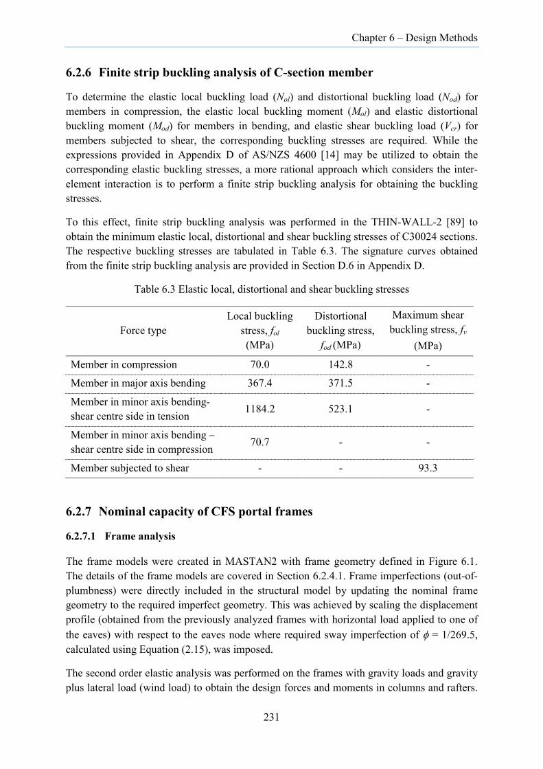
Chapter 6 – Design Methods
6.2.6 Finite strip buckling analysis of C-section member
To determine the elastic local buckling load (Nol) and distortional buckling load (Nod) for members in compression, the elastic local buckling moment (Mol) and elastic distortional buckling moment (Mod) for members in bending, and elastic shear buckling load (Vcr) for members subjected to shear, the corresponding buckling stresses are required. While the expressions provided in Appendix D of AS/NZS 4600 [14] may be utilized to obtain the corresponding elastic buckling stresses, a more rational approach which considers the inter-element interaction is to perform a finite strip buckling analysis for obtaining the buckling stresses.
To this effect, finite strip buckling analysis was performed in the THIN-WALL-2 [89] to obtain the minimum elastic local, distortional and shear buckling stresses of C30024 sections. The respective buckling stresses are tabulated in Table 6.3. The signature curves obtained from the finite strip buckling analysis are provided in Section D.6 in Appendix D.
Table 6.3 Elastic local, distortional and shear buckling stresses
Force type Local buckling
stress, fol (MPa)
Distortional buckling stress,
fod (MPa)
Maximum shear buckling stress, fv
(MPa)
Member in compression 70.0 142.8 -
Member in major axis bending 367.4 371.5 -
Member in minor axis bending-shear centre side in tension 1184.2 523.1 -
Member in minor axis bending – shear centre side in compression 70.7 - -
Member subjected to shear - - 93.3
6.2.7 Nominal capacity of CFS portal frames
6.2.7.1 Frame analysis
The frame models were created in MASTAN2 with frame geometry defined in Figure 6.1. The details of the frame models are covered in Section 6.2.4.1. Frame imperfections (out-of-plumbness) were directly included in the structural model by updating the nominal frame geometry to the required imperfect geometry. This was achieved by scaling the displacement profile (obtained from the previously analyzed frames with horizontal load applied to one of the eaves) with respect to the eaves node where required sway imperfection of φ = 1/269.5, calculated using Equation (2.15), was imposed.
The second order elastic analysis was performed on the frames with gravity loads and gravity plus lateral load (wind load) to obtain the design forces and moments in columns and rafters.
231
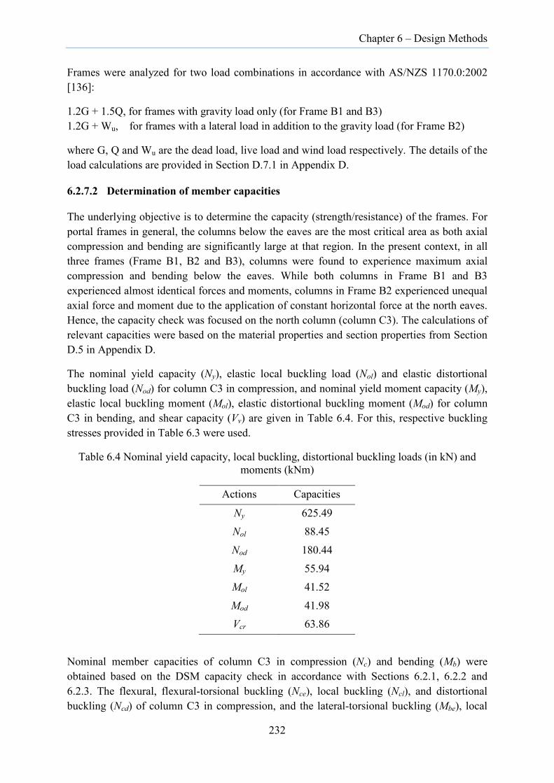
Chapter 6 – Design Methods
Frames were analyzed for two load combinations in accordance with AS/NZS 1170.0:2002 [136]:
1.2G + 1.5Q, for frames with gravity load only (for Frame B1 and B3) 1.2G + Wu, for frames with a lateral load in addition to the gravity load (for Frame B2)
where G, Q and Wu are the dead load, live load and wind load respectively. The details of the load calculations are provided in Section D.7.1 in Appendix D.
6.2.7.2 Determination of member capacities
The underlying objective is to determine the capacity (strength/resistance) of the frames. For portal frames in general, the columns below the eaves are the most critical area as both axial compression and bending are significantly large at that region. In the present context, in all three frames (Frame B1, B2 and B3), columns were found to experience maximum axial compression and bending below the eaves. While both columns in Frame B1 and B3 experienced almost identical forces and moments, columns in Frame B2 experienced unequal axial force and moment due to the application of constant horizontal force at the north eaves. Hence, the capacity check was focused on the north column (column C3). The calculations of relevant capacities were based on the material properties and section properties from Section D.5 in Appendix D.
The nominal yield capacity (Ny), elastic local buckling load (Nol) and elastic distortional buckling load (Nod) for column C3 in compression, and nominal yield moment capacity (My), elastic local buckling moment (Mol), elastic distortional buckling moment (Mod) for column C3 in bending, and shear capacity (Vv) are given in Table 6.4. For this, respective buckling stresses provided in Table 6.3 were used.
Table 6.4 Nominal yield capacity, local buckling, distortional buckling loads (in kN) and moments (kNm)
Actions Capacities
Ny 625.49 Nol 88.45
Nod 180.44
My 55.94 Mol 41.52
Mod 41.98 Vcr 63.86
Nominal member capacities of column C3 in compression (Nc) and bending (Mb) were obtained based on the DSM capacity check in accordance with Sections 6.2.1, 6.2.2 and 6.2.3. The flexural, flexural-torsional buckling (Nce), local buckling (Ncl), and distortional buckling (Ncd) of column C3 in compression, and the lateral-torsional buckling (Mbe), local
232

Chapter 6 – Design Methods
buckling (Mbl) and distortional buckling (Mbd) of column C3 in bending are provided in Table 6.5.
Table 6.5 Nominal capacities of column C3
Design type Items
Frame B1 Frame B2 Frame B3 EBA ELM EBA ELM EBA ELM
Compression
Nce 120.76 101.39 120.50 101.39 136.64 101.39 Ncl 92.50 82.37 92.37 82.37 100.35 82.37 Ncd 261.50 261.50 261.50 261.50 261.50 261.50 Nc 92.50 82.37 92.37 82.37 100.35 82.37
Bending
Mbe 36.94 35.90 47.72 47.93 55.53 55.59 Mbl 32.62 32.00 35.97 38.85 41.52 42.86 Mbd 39.22 39.22 39.22 39.22 39.22 39.22 Mb 32.62 32.00 35.97 38.85 39.22 39.22
Shear Vv 63.86 63.86 63.86 63.86 63.86 63.86
6.2.7.3 Prediction of frame capacities
The design forces and moments in the respective frames were obtained from the second-order elastic analysis corresponding to the load combination given in Section 6.2.7.1. Table 6.6 shows the design compressive forces and moments for column C3 (Refer Section D.7.4 in Appendix D for design action effects).
Table 6.6 Design forces and moments
Frame Compression, N* Bending, M* Shear, V*
Column C3 Column C3 Rafter Frame B1 12.6 19.7 11.7 Frame B2 3.9 11.9 4.1 Frame B3 12.6 19.4 11.7
As the maximum shear force occurred in rafter near the eaves along with the maximum bending moment, the shear strength of the rafter was checked in accordance with the Clause 7.2.3 of AS/NZS 4600 [14] and found to be of less significance.
However, the axial compression and bending moment in the columns were both significant just below the eaves, requiring a check for the interaction of axial compression and bending. As per Clause 7.2.4 of AS/NZS 4600 [14], the combined axial compression and bending must satisfy the following:
***
1.0yx
c c b bx b by
MMNN M Mφ φ φ
+ + ≤ (6.23)
233

Chapter 6 – Design Methods
where φc and φb are capacity reduction factors for compression and bending; Mbx and Mby are nominal member moment capacity about the x- and y-axes; 𝑁∗, 𝑀𝑥
∗, 𝑀𝑦∗ are second-order
design axial compression and design bending moment about the x- and y-axes; and Nc is the nominal member capacity for member in compression. Since the minor axis bending moment is negligibly small, the above interaction equation simplifies to:
* *
1.0c c b b
N MN Mφ φ
+ ≤ (6.24)
As both the section properties and material properties were based on the actual tests, φc and φb are taken as unity. Unity check with design action effects from Table 6.6 and member capacities from Table 6.5 resulted in the values of 0.74 for Frame B1, 0.37 for Frame B2 and 0.63 for Frame B3 suggesting that the design axial forces and moments in Table 6.6 were well below the actual capacities of columns in each frame.
The member capacities of columns in CFS portal frames were determined by satisfying the interaction Equation (6.24) for the combined axial compression and bending actions. The column capacity is found if the sum of two individual quotient in Equation (6.24) is exactly equal to unity for a given load case. Hence, to determine the strength of the frame, additional force-moment pairs (M*, N*) were obtained by analyzing each frame for load combination with magnitude of gravity loads increased in each analysis. The loading line for each frame was constructed. The plot of strength line defined by the Equation (6.24) and the loading lines of columns for three frames are shown in Figure 6.2. The intersection of the loading lines and the strength line define the capacity of the columns in respective frames.
Figure 6.2 Interaction and loading curves
Based on the linear interpolation of points lying on either side of the strength line, the force-moment pairs (𝑁𝑓∗, 𝑀𝑓
∗) corresponding to the ultimate capacities of column C3 are calculated and are provided in Table 6.7.
234
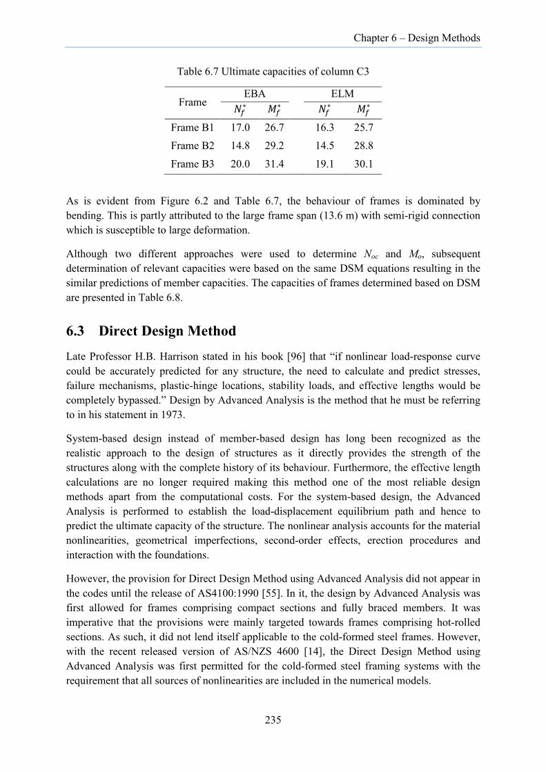
Chapter 6 – Design Methods
Table 6.7 Ultimate capacities of column C3
Frame EBA ELM
𝑁𝑓∗ 𝑀𝑓∗ 𝑁𝑓∗ 𝑀𝑓
∗
Frame B1 17.0 26.7 16.3 25.7 Frame B2 14.8 29.2 14.5 28.8
Frame B3 20.0 31.4 19.1 30.1
As is evident from Figure 6.2 and Table 6.7, the behaviour of frames is dominated by bending. This is partly attributed to the large frame span (13.6 m) with semi-rigid connection which is susceptible to large deformation.
Although two different approaches were used to determine Noc and Mo, subsequent determination of relevant capacities were based on the same DSM equations resulting in the similar predictions of member capacities. The capacities of frames determined based on DSM are presented in Table 6.8.
6.3 Direct Design Method
Late Professor H.B. Harrison stated in his book [96] that “if nonlinear load-response curve could be accurately predicted for any structure, the need to calculate and predict stresses, failure mechanisms, plastic-hinge locations, stability loads, and effective lengths would be completely bypassed.” Design by Advanced Analysis is the method that he must be referring to in his statement in 1973.
System-based design instead of member-based design has long been recognized as the realistic approach to the design of structures as it directly provides the strength of the structures along with the complete history of its behaviour. Furthermore, the effective length calculations are no longer required making this method one of the most reliable design methods apart from the computational costs. For the system-based design, the Advanced Analysis is performed to establish the load-displacement equilibrium path and hence to predict the ultimate capacity of the structure. The nonlinear analysis accounts for the material nonlinearities, geometrical imperfections, second-order effects, erection procedures and interaction with the foundations.
However, the provision for Direct Design Method using Advanced Analysis did not appear in the codes until the release of AS4100:1990 [55]. In it, the design by Advanced Analysis was first allowed for frames comprising compact sections and fully braced members. It was imperative that the provisions were mainly targeted towards frames comprising hot-rolled sections. As such, it did not lend itself applicable to the cold-formed steel frames. However, with the recent released version of AS/NZS 4600 [14], the Direct Design Method using Advanced Analysis was first permitted for the cold-formed steel framing systems with the requirement that all sources of nonlinearities are included in the numerical models.
235

Chapter 6 – Design Methods
6.3.1 Design strength of CFS single C-section portal frames
System-based design resulting in the determination of ultimate strength of each CFS single C-section portal frame tests described in Chapter 4 was already completed in Chapter 5 using Advanced Analysis. The following descriptions, in fact, pertain to the procedures followed for the prediction of strength using Advanced Analysis in Chapter 5.
As CFS portal frames are susceptible to local instabilities and are likely to undergo large deformation, it is crucial to capture such instabilities and related deformation from the numerical model. Hence, a shell element model was adopted for the geometric modelling. This is even more relevant for single C-section portal frames, as the C-sections have non-coincident shear centre and centroid and are prone to flexural-torsional deformation. The initial member sizes were determined based on the conventional design method. The mesh size for the FE model was determined by running models beforehand with different mesh sizes and checking the effect on the ultimate load besides referring to the mesh size used in the past for the similar frame models. The bolted/screw connections were modelled by deformable fasteners with prescribed nonlinear constitutive relations to simulate the actual force-displacement behaviour. The constitutive relations were obtained from separate tests on point fastener connections. The contact formulation was implemented only in places where the severe deformations resulting in the intrusion of nodes from one surface to another surface were evident.
The nonlinear material properties in the form of nonlinear stress-strain relations, Young’s modulus and yield stress were assigned to the respective components which were derived from the coupon tests.
The geometric imperfections were introduced into the shell model through the superposition of first four factored eigenmodes obtained from the elastic buckling analysis. For the global buckling eignmodes, the scale factors were based on the measured amplitude of deformation of the experimental frames while the scale factors for local modes were obtained from the separate imperfection measurement conducted for members before assembling the frame.
Of the six frames, four were analysed for gravity load while two for the combination of lateral and gravity load in correspondence with the loads used in the frame tests. While the lateral load was fixed to a constant value of 5 kN, the magnitude of vertical load at each loading point was computed by equally dividing the ultimate load among 8 load points. In any case, apart from the load distribution, the accuracy of load magnitude was of less concern for the Advanced Analysis as the loads were applied in incremental steps starting from the minimum value and gradually increasing to the maximum applied value. However, accurate determination of loads is necessary to check the structural adequacy in the routine design.
The nonlinear analysis was performed using static general option. Occasionally, the modified Riks option was implemented to traverse the equilibrium path subsequent to the static general option where the static general failed to advance the solution.
236
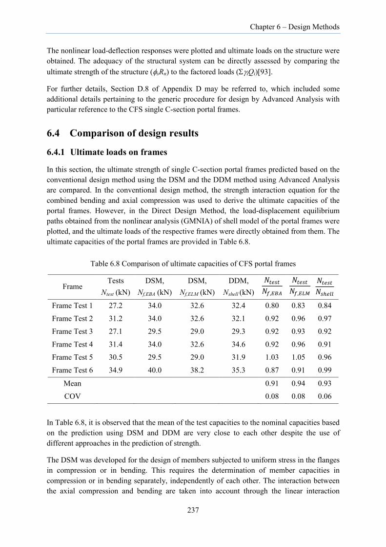
Chapter 6 – Design Methods
The nonlinear load-deflection responses were plotted and ultimate loads on the structure were obtained. The adequacy of the structural system can be directly assessed by comparing the ultimate strength of the structure (φsRn) to the factored loads (ΣγiQi)[93].
For further details, Section D.8 of Appendix D may be referred to, which included some additional details pertaining to the generic procedure for design by Advanced Analysis with particular reference to the CFS single C-section portal frames.
6.4 Comparison of design results
6.4.1 Ultimate loads on frames
In this section, the ultimate strength of single C-section portal frames predicted based on the conventional design method using the DSM and the DDM method using Advanced Analysis are compared. In the conventional design method, the strength interaction equation for the combined bending and axial compression was used to derive the ultimate capacities of the portal frames. However, in the Direct Design Method, the load-displacement equilibrium paths obtained from the nonlinear analysis (GMNIA) of shell model of the portal frames were plotted, and the ultimate loads of the respective frames were directly obtained from them. The ultimate capacities of the portal frames are provided in Table 6.8.
Table 6.8 Comparison of ultimate capacities of CFS portal frames
Frame Tests
Ntest (kN) DSM,
Nf,EBA (kN) DSM,
Nf,ELM (kN) DDM,
Nshell (kN) 𝑁𝑡𝑒𝑠𝑡𝑁𝑓,𝐸𝐵𝐴
𝑁𝑡𝑒𝑠𝑡𝑁𝑓,𝐸𝐿𝑀
𝑁𝑡𝑒𝑠𝑡𝑁𝑠ℎ𝑒𝑙𝑙
Frame Test 1 27.2 34.0 32.6 32.4 0.80 0.83 0.84
Frame Test 2 31.2 34.0 32.6 32.1 0.92 0.96 0.97 Frame Test 3 27.1 29.5 29.0 29.3 0.92 0.93 0.92
Frame Test 4 31.4 34.0 32.6 34.6 0.92 0.96 0.91 Frame Test 5 30.5 29.5 29.0 31.9 1.03 1.05 0.96
Frame Test 6 34.9 40.0 38.2 35.3 0.87 0.91 0.99
Mean 0.91 0.94 0.93 COV 0.08 0.08 0.06
In Table 6.8, it is observed that the mean of the test capacities to the nominal capacities based on the prediction using DSM and DDM are very close to each other despite the use of different approaches in the prediction of strength.
The DSM was developed for the design of members subjected to uniform stress in the flanges in compression or in bending. This requires the determination of member capacities in compression or in bending separately, independently of each other. The interaction between the axial compression and bending are taken into account through the linear interaction
237
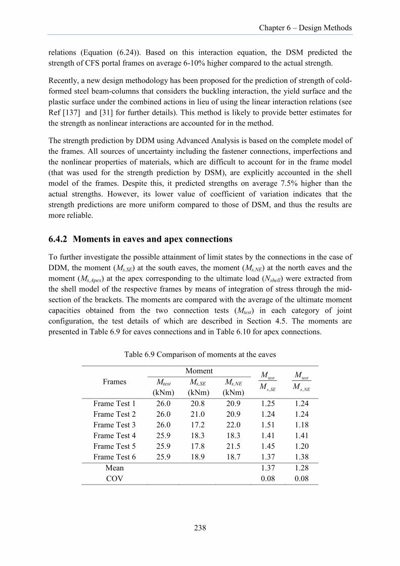
Chapter 6 – Design Methods
relations (Equation (6.24)). Based on this interaction equation, the DSM predicted the strength of CFS portal frames on average 6-10% higher compared to the actual strength.
Recently, a new design methodology has been proposed for the prediction of strength of cold-formed steel beam-columns that considers the buckling interaction, the yield surface and the plastic surface under the combined actions in lieu of using the linear interaction relations (see Ref [137] and [31] for further details). This method is likely to provide better estimates for the strength as nonlinear interactions are accounted for in the method.
The strength prediction by DDM using Advanced Analysis is based on the complete model of the frames. All sources of uncertainty including the fastener connections, imperfections and the nonlinear properties of materials, which are difficult to account for in the frame model (that was used for the strength prediction by DSM), are explicitly accounted in the shell model of the frames. Despite this, it predicted strengths on average 7.5% higher than the actual strengths. However, its lower value of coefficient of variation indicates that the strength predictions are more uniform compared to those of DSM, and thus the results are more reliable.
6.4.2 Moments in eaves and apex connections
To further investigate the possible attainment of limit states by the connections in the case of DDM, the moment (Ms,SE) at the south eaves, the moment (Ms,NE) at the north eaves and the moment (Ms,Apex) at the apex corresponding to the ultimate load (Nshell) were extracted from the shell model of the respective frames by means of integration of stress through the mid-section of the brackets. The moments are compared with the average of the ultimate moment capacities obtained from the two connection tests (Mtest) in each category of joint configuration, the test details of which are described in Section 4.5. The moments are presented in Table 6.9 for eaves connections and in Table 6.10 for apex connections.
Table 6.9 Comparison of moments at the eaves
Frames Moment
,
test
s SE
MM
,
test
s NE
MM
Mtest (kNm)
Ms,SE
(kNm) Ms,NE
(kNm) Frame Test 1 26.0 20.8 20.9 1.25 1.24 Frame Test 2 26.0 21.0 20.9 1.24 1.24 Frame Test 3 26.0 17.2 22.0 1.51 1.18 Frame Test 4 25.9 18.3 18.3 1.41 1.41 Frame Test 5 25.9 17.8 21.5 1.45 1.20 Frame Test 6 25.9 18.9 18.7 1.37 1.38
Mean 1.37 1.28 COV 0.08 0.08
238
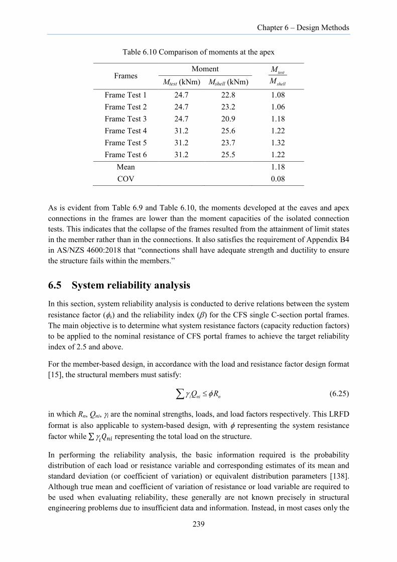
Chapter 6 – Design Methods
Table 6.10 Comparison of moments at the apex
Frames Moment test
shell
MM
Mtest (kNm) Mshell (kNm)
Frame Test 1 24.7 22.8 1.08 Frame Test 2 24.7 23.2 1.06 Frame Test 3 24.7 20.9 1.18 Frame Test 4 31.2 25.6 1.22 Frame Test 5 31.2 23.7 1.32 Frame Test 6 31.2 25.5 1.22
Mean 1.18 COV 0.08
As is evident from Table 6.9 and Table 6.10, the moments developed at the eaves and apex connections in the frames are lower than the moment capacities of the isolated connection tests. This indicates that the collapse of the frames resulted from the attainment of limit states in the member rather than in the connections. It also satisfies the requirement of Appendix B4 in AS/NZS 4600:2018 that “connections shall have adequate strength and ductility to ensure the structure fails within the members.”
6.5 System reliability analysis
In this section, system reliability analysis is conducted to derive relations between the system resistance factor (φs) and the reliability index (β) for the CFS single C-section portal frames. The main objective is to determine what system resistance factors (capacity reduction factors) to be applied to the nominal resistance of CFS portal frames to achieve the target reliability index of 2.5 and above.
For the member-based design, in accordance with the load and resistance factor design format [15], the structural members must satisfy:
i ni nQ Rγ φ≤∑ (6.25)
in which Rn, Qni, γi are the nominal strengths, loads, and load factors respectively. This LRFD format is also applicable to system-based design, with φ representing the system resistance factor while ∑ γ𝑖𝑄𝑛𝑖 representing the total load on the structure.
In performing the reliability analysis, the basic information required is the probability distribution of each load or resistance variable and corresponding estimates of its mean and standard deviation (or coefficient of variation) or equivalent distribution parameters [138]. Although true mean and coefficient of variation of resistance or load variable are required to be used when evaluating reliability, these generally are not known precisely in structural engineering problems due to insufficient data and information. Instead, in most cases only the
239

Chapter 6 – Design Methods
estimates of the mean and coefficient variation of variables are available from the controlled tests [138].
However, in the present context, the statistical parameters for the strength of CFS single C-section portal frames were determined based on the results of full-scale frame tests and the corresponding numerical analysis results along with the data obtained from the coupon tests and measured thickness of the sections. Statistical parameters from AISI S100-16 [15] were also used.
For the reliability analysis of CFS single C-section portal frames subjected to gravity loads, two methods are employed herein: Iterative method and Non-iterative method.
6.5.1 Iterative method
For the CFS portal frames subjected to gravity loads, the ultimate limit state condition that must be fulfilled include the following design equations with action effects on the right-hand side arising from the respective load combinations as per AS/NZS 1170.0:2002 [136]:
1.35s n nR Dφ ≥ (6.26)
1.2 1.5s n n nR D Lφ ≥ + (6.27)
and as per ASCE/SEI 7-10 [139]:
1.4s n nR Dφ ≥ (6.28)
1.2 1.6s n n nR D Lφ ≥ + (6.29)
In the above equations, Dn is the nominal dead load and Ln is the nominal live load. To make it more general, the design equation is written as:
s n d n l nR D Lφ γ γ≥ + (6.30)
where dγ and lγ are dead load and live load factor respectively. In this particular case, the limit state function takes the form
( , , ) ( )g R D L R D L= − + (6.31)
where R is the resistance, D is the dead load and L is the live load. At the limit state surface, g = 0, and the design Equation (6.30) becomes:
s n d n l nR D Lφ γ γ= + (6.32)
Since the statistical data are usually available in terms of the ratio of mean to the nominal parameters instead of individual parameters, the Equation (6.32) can be rewritten in terms of these ratios. Defining Ln/Dn=k, the mean live load (𝐿) to the mean dead load (𝐷) is related by:
240
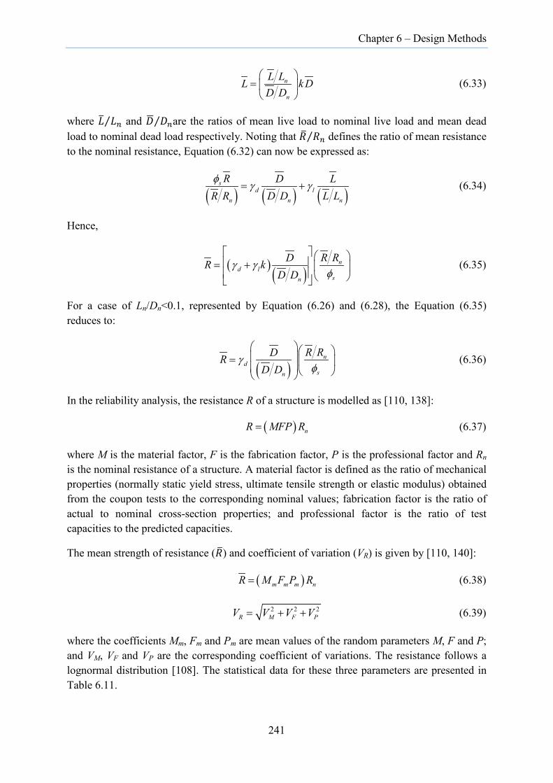
Chapter 6 – Design Methods
n
n
L LL k DD D
=
(6.33)
where 𝐿 𝐿𝑛⁄ and 𝐷 𝐷𝑛⁄ are the ratios of mean live load to nominal live load and mean dead load to nominal dead load respectively. Noting that 𝑅𝑅 𝑅𝑅𝑛⁄ defines the ratio of mean resistance to the nominal resistance, Equation (6.32) can now be expressed as:
( ) ( ) ( )
sd l
n n n
R D LR R D D L Lφ γ γ= + (6.34)
Hence,
( ) ( )n
d lsn
R RDR kD D
γ γφ
= +
(6.35)
For a case of Ln/Dn<0.1, represented by Equation (6.26) and (6.28), the Equation (6.35) reduces to:
( )
nd
sn
R RDRD D
γφ
= (6.36)
In the reliability analysis, the resistance R of a structure is modelled as [110, 138]:
( ) nR MFP R= (6.37)
where M is the material factor, F is the fabrication factor, P is the professional factor and Rn
is the nominal resistance of a structure. A material factor is defined as the ratio of mechanical properties (normally static yield stress, ultimate tensile strength or elastic modulus) obtained from the coupon tests to the corresponding nominal values; fabrication factor is the ratio of actual to nominal cross-section properties; and professional factor is the ratio of test capacities to the predicted capacities.
The mean strength of resistance (𝑅𝑅) and coefficient of variation (VR) is given by [110, 140]:
( )m m m nR M F P R= (6.38)
2 2 2R M F PV V V V= + + (6.39)
where the coefficients Mm, Fm and Pm are mean values of the random parameters M, F and P; and VM, VF and VP are the corresponding coefficient of variations. The resistance follows a lognormal distribution [108]. The statistical data for these three parameters are presented in Table 6.11.
241
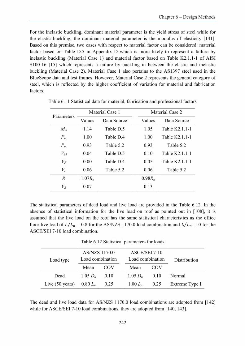
Chapter 6 – Design Methods
For the inelastic buckling, dominant material parameter is the yield stress of steel while for the elastic buckling, the dominant material parameter is the modulus of elasticity [141]. Based on this premise, two cases with respect to material factor can be considered: material factor based on Table D.5 in Appendix D which is more likely to represent a failure by inelastic buckling (Material Case 1) and material factor based on Table K2.1.1-1 of AISI S100-16 [15] which represents a failure by buckling in between the elastic and inelastic buckling (Material Case 2). Material Case 1 also pertains to the AS1397 steel used in the BlueScope data and test frames. However, Material Case 2 represents the general category of steel, which is reflected by the higher coefficient of variation for material and fabrication factors.
Table 6.11 Statistical data for material, fabrication and professional factors
Parameters Material Case 1 Material Case 2
Values Data Source Values Data Source
Mm 1.14 Table D.5 1.05 Table K2.1.1-1 Fm 1.00 Table D.4 1.00 Table K2.1.1-1
Pm 0.93 Table 5.2 0.93 Table 5.2 VM 0.04 Table D.5 0.10 Table K2.1.1-1
VF 0.00 Table D.4 0.05 Table K2.1.1-1
VP 0.06 Table 5.2 0.06 Table 5.2
𝑅𝑅 1.07Rn 0.98Rn
VR 0.07 0.13
The statistical parameters of dead load and live load are provided in the Table 6.12. In the absence of statistical information for the live load on roof as pointed out in [108], it is assumed that the live load on the roof has the same statistical characteristics as the office floor live load of 𝐿 𝐿𝑛⁄ = 0.8 for the AS/NZS 1170.0 load combination and 𝐿 𝐿𝑛⁄ =1.0 for the ASCE/SEI 7-10 load combination.
Table 6.12 Statistical parameters for loads
Load type AS/NZS 1170.0
Load combination ASCE/SEI 7-10
Load combination Distribution Mean COV Mean COV
Dead 1.05 Dn 0.10 1.05 Dn 0.10 Normal Live (50 years) 0.80 Ln 0.25 1.00 Ln 0.25 Extreme Type I
The dead and live load data for AS/NZS 1170.0 load combinations are adopted from [142] while for ASCE/SEI 7-10 load combinations, they are adopted from [140, 143].
242
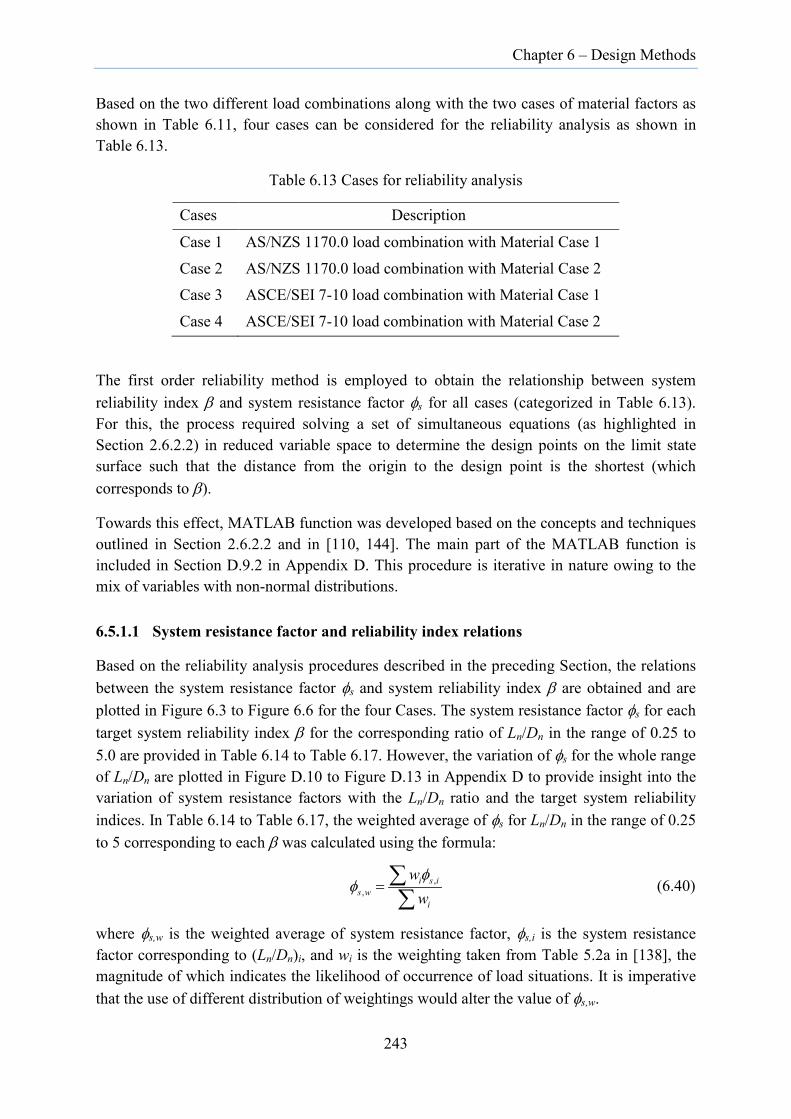
Chapter 6 – Design Methods
Based on the two different load combinations along with the two cases of material factors as shown in Table 6.11, four cases can be considered for the reliability analysis as shown in Table 6.13.
Table 6.13 Cases for reliability analysis
Cases Description
Case 1 AS/NZS 1170.0 load combination with Material Case 1
Case 2 AS/NZS 1170.0 load combination with Material Case 2 Case 3 ASCE/SEI 7-10 load combination with Material Case 1
Case 4 ASCE/SEI 7-10 load combination with Material Case 2
The first order reliability method is employed to obtain the relationship between system reliability index β and system resistance factor φs for all cases (categorized in Table 6.13). For this, the process required solving a set of simultaneous equations (as highlighted in Section 2.6.2.2) in reduced variable space to determine the design points on the limit state surface such that the distance from the origin to the design point is the shortest (which corresponds to β).
Towards this effect, MATLAB function was developed based on the concepts and techniques outlined in Section 2.6.2.2 and in [110, 144]. The main part of the MATLAB function is included in Section D.9.2 in Appendix D. This procedure is iterative in nature owing to the mix of variables with non-normal distributions.
6.5.1.1 System resistance factor and reliability index relations
Based on the reliability analysis procedures described in the preceding Section, the relations between the system resistance factor φs and system reliability index β are obtained and are plotted in Figure 6.3 to Figure 6.6 for the four Cases. The system resistance factor φs for each target system reliability index β for the corresponding ratio of Ln/Dn in the range of 0.25 to 5.0 are provided in Table 6.14 to Table 6.17. However, the variation of φs for the whole range of Ln/Dn are plotted in Figure D.10 to Figure D.13 in Appendix D to provide insight into the variation of system resistance factors with the Ln/Dn ratio and the target system reliability indices. In Table 6.14 to Table 6.17, the weighted average of φs for Ln/Dn in the range of 0.25 to 5 corresponding to each β was calculated using the formula:
,,
i s is w
i
wwφ
φ = ∑∑
(6.40)
where φs,w is the weighted average of system resistance factor, φs,i is the system resistance factor corresponding to (Ln/Dn)i, and wi is the weighting taken from Table 5.2a in [138], the magnitude of which indicates the likelihood of occurrence of load situations. It is imperative that the use of different distribution of weightings would alter the value of φs,w.
243

Chapter 6 – Design Methods
Figure 6.3 Plot of φs vs β for Case 1
Figure 6.4 Plot of φs vs β for Case 2
Figure 6.5 Plot of φs vs β for Case 3
244

Chapter 6 – Design Methods
Figure 6.6 Plot of φs vs β for Case 4
Table 6.14 System resistance factor φs (Case 1)
Ln/Dn Weight
% φs
β=2.5 β=2.75 β=3.0 β=3.25 β=3.5 0.25 0 1.025 0.996 0.970 0.943 0.918 0.5 0 1.066 1.030 0.994 0.959 0.924 1 6 1.078 1.030 0.982 0.936 0.890
1.5 17 1.076 1.020 0.967 0.915 0.865 2 22 1.072 1.013 0.955 0.900 0.848 3 33 1.067 1.002 0.941 0.883 0.828 5 22 1.060 0.991 0.926 0.865 0.808 Weighted φs 1.069 1.007 0.948 0.891 0.838
Table 6.15 System resistance factor φs (Case 2)
Ln/Dn Weight
% φs
β=2.5 β=2.75 β=3.0 β=3.25 β=3.5 0.25 0 0.834 0.802 0.772 0.742 0.714 0.5 0 0.879 0.843 0.808 0.774 0.741 1 6 0.909 0.863 0.819 0.776 0.735
1.5 17 0.915 0.864 0.814 0.767 0.721 2 22 0.916 0.861 0.809 0.758 0.711 3 33 0.916 0.857 0.800 0.747 0.697 5 22 0.914 0.851 0.791 0.736 0.684 Weighted φs 0.915 0.858 0.804 0.752 0.704
245

Chapter 6 – Design Methods
Table 6.16 System resistance factor φs (Case 3)
Ln/Dn Weight
% φs
β=2.5 β=2.75 β=3.0 β=3.25 β=3.5 0.25 0 0.997 0.969 0.941 0.914 0.887 0.5 0 0.995 0.966 0.930 0.893 0.857 1 6 0.981 0.933 0.887 0.842 0.798
1.5 17 0.962 0.910 0.859 0.811 0.765 2 22 0.950 0.895 0.842 0.791 0.744 3 33 0.934 0.876 0.821 0.769 0.720 5 22 0.920 0.859 0.801 0.748 0.697
Weighted φs,w 0.942 0.886 0.832 0.781 0.732
Table 6.17 System resistance factor φs (Case 4)
Ln/Dn Weight
% φs
β=2.5 β=2.75 β=3.0 β=3.25 β=3.5 0.25 0 0.813 0.782 0.752 0.723 0.695 0.5 0 0.834 0.798 0.762 0.728 0.694 1 6 0.831 0.787 0.744 0.702 0.663
1.5 17 0.822 0.773 0.727 0.682 0.640 2 22 0.815 0.763 0.715 0.669 0.625 3 33 0.804 0.751 0.700 0.652 0.608 5 22 0.794 0.738 0.686 0.637 0.591
Weighted φs,w 0.809 0.757 0.707 0.661 0.617
As is evident from Figure 6.3 to Figure 6.6, for larger magnitude of coefficient of variation for resistance, the system reliability index β is quite sensitive to the Ln/Dn ratio. The reduction of β with the increase of system resistance factors is particularly significant for the Ln/Dn ratio less than one. However, for the portal frames, the Ln/Dn ratio is usually in the practical range of 1 to 2 and the weighting for the calculation of weighted φs are assigned zero for the Ln/Dn less than unity. Hence the values corresponding to Ln/Dn ratio of 0.25 and 0.5 has no impact on the φs,w despite its sensitivity to the mean and COV of resistance R.
6.5.2 Non-iterative method
In the calibration of load and resistance factor design of cold-formed steel members and connections, one of the widely used equations that relates the resistance factor φ and the target reliability index β0 is [15]:
2 2 2 2
0( ) M F P P QV V C V Vm m mC M F P e β
φφ − + + += (6.41)
246
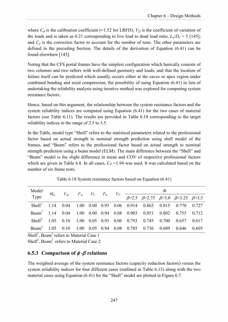
Chapter 6 – Design Methods
where Cφ is the calibration coefficient (=1.52 for LRFD); VQ is the coefficient of variation of the loads and is taken as 0.21 corresponding to live load to dead load ratio, Ln/Dn = 5 [145]; and Cp is the correction factor to account for the number of tests. The other parameters are defined in the preceding Section. The details of the derivation of Equation (6.41) can be found elsewhere [145].
Noting that the CFS portal frames have the simplest configuration which basically consists of two columns and two rafters with well-defined geometry and loads, and that the location of failure itself can be predicted which usually occurs either at the eaves or apex region under combined bending and axial compression, the possibility of using Equation (6.41) in lieu of undertaking the reliability analysis using iterative method was explored for computing system resistance factors.
Hence, based on this argument, the relationship between the system resistance factors and the system reliability indices are computed using Equation (6.41) for the two cases of material factors (see Table 6.11). The results are provided in Table 6.18 corresponding to the target reliability indices in the range of 2.5 to 3.5.
In the Table, model type “Shell” refers to the statistical parameters related to the professional factor based on actual strength to nominal strength prediction using shell model of the frames, and “Beam” refers to the professional factor based on actual strength to nominal strength prediction using a beam model (ELM). The main difference between the “Shell” and “Beam” model is the slight difference in mean and COV of respective professional factors which are given in Table 6.8. In all cases, CP =1.94 was used. It was calculated based on the number of six frame tests.
Table 6.18 System resistance factors based on Equation (6.41)
Model Type
Mm VM Fm VF Pm VP φs
β=2.5 β=2.75 β=3.0 β=3.25 β=3.5
Shell1 1.14 0.04 1.00 0.00 0.93 0.06 0.914 0.863 0.815 0.770 0.727 Beam1 1.14 0.04 1.00 0.00 0.94 0.08 0.903 0.851 0.802 0.755 0.712
Shell2 1.05 0.10 1.00 0.05 0.93 0.06 0.793 0.745 0.700 0.657 0.617 Beam2 1.05 0.10 1.00 0.05 0.94 0.08 0.785 0.736 0.689 0.646 0.605
Shell1, Beam1 refers to Material Case 1 Shell2, Beam2 refers to Material Case 2
6.5.3 Comparison of φ -β relations
The weighted average of the system resistance factors (capacity reduction factors) versus the system reliability indices for four different cases (outlined in Table 6.13) along with the two material cases using Equation (6.41) for the “Shell” model are plotted in Figure 6.7.
247

Chapter 6 – Design Methods
The target reliability index (β0) of 2.5 has been stipulated in [15] for the design of cold-formed steel members and connections. Hence, the system resistance factors (capacity reduction factors) corresponding to the four cases have been determined for achieving β0 of 2.5 for the CFS portal frames and are summarized in Table 6.19.
Figure 6.7 Plot of weighted φs,w vs β for CFS single C-section portal frames
Table 6.19 Summary of system resistance factors
Cases φs
Case 1 1.000
Case 2 0.915 Case 3 0.942
Case 4 0.809
As is evident from Figure 6.7, the value of β is above 2.5 for normal range of φs for Case 1 indicating that the AS/NZS 1170.0 load combination is more than adequate for this particular case. This pertains to the CFS sections that are produced from AS1397 steel. The Case 2 represents a general category of steel used for the design as per AS/NZS 1170.0 load combination. For this, the maximum value of φs is 0.915 to achieve the target reliability index of 2.5. It is also seen that the φs is much lower for ASCE/SEI 7-10 load combination compared to the AS/NZS 1170.0 load combination to achieve similar system reliability. This is attributed to the use of different mean live load to nominal live load ratio and the live load factor in the respective load combinations. As expected, it is observed that the system resistance factors derived from the Equation (6.41) are aligned closer to the system resistance factors derived based on the ASCE/SEI 7-10 load combinations as it was originally developed within that context. This implies that Equation (6.41) cannot be used to derive system resistance factors for all cases.
248

Chapter 6 – Design Methods
Given the availability of a wide range of steel in the market, the system capacity factor for Case 2 and Case 4 seems to be more appropriate for the design of CFS portal frames using AS/NZS 1170.0 and ASCE/SEI 7-10 load combinations respectively.
6.6 Discussions
The design of CFS portal frames based on the conventional design method using DSM is presented leading to the prediction of ultimate capacities of the frames. Towards determining the frame strength, the elastic flexural-torsional buckling load and elastic lateral-torsional buckling moment were determined based on two methods. In the first approach, linear elastic buckling analysis was performed to directly obtain the flexural-torsional buckling load and the lateral-torsional buckling moment thus obviating the need to use the effective length concept. However, in the second approach, classical equations were used to calculate the flexural-torsional buckling load and lateral-torsional buckling moment, which required determination of effective length factors. The prediction based on these two approaches resulted in ultimate capacities that are comparable to each other.
The DSM has been formulated with the objective of predicting member capacity for members subject to uniform stress in the flanges due to compression or bending. For this, the relevant capacities in compression and bending are required to be calculated separately. The interaction of axial compression and bending are accounted through the use of linear interaction equations. However, the development of a new method using normalized failure surface in 3D space that encapsulates all the nonlinear interactions, and that obviates the need to use interaction equation, is already underway towards enhancing the application of DSM in the design of CFS members.
The design features that are relevant to the design by DDM using Advanced Analysis in predicting the nominal strength of CFS portal frames are described. The need for the accurate modelling including the nonlinear constitutive relations for deformable fasteners is emphasized. In particular, use of shell model is recommended as it can capture the local instabilities which are not always possible with the beam element model. The DDM using Advanced Analysis has adequately predicted the frame strength with coefficient of variation of 0.06 (for actual strength to nominal strength) demonstrating the reliability of the predictions. Moments calculated at the eaves and apex based on stress integration showed that member failure had precipitated the frame collapse instead of the localized connection failure, thus fulfilling the requirement of connections to possess higher strength than the member as per AS/NZS 4600. The attractiveness of DDM using Advanced Analysis lies in its capability to capture all nonlinearities in a single-step analysis by which the frame capacities are directly obtained without going through the lengthy member capacity check as is required in DSM case.
To determine the system resistance factors (capacity reduction factors) φs, system reliability analysis for the CFS portal frames subjected to gravity load combinations was conducted. It was revealed that the system resistance factor is sensitive to the mean of resistance represented by the product of the mean of the material, fabrication and professional factors
249
Chapter 6 – Design Methods
and their corresponding coefficient of variation, live load to dead load ratio and the load combinations. The use of statistical parameters for material and fabrication factors from AISI S100-16 [15] resulted in lower system resistance factors than the statistical parameters based on the actual material properties obtained from the coupon tests and the measured thickness of cross-sections. Moreover, for a given target reliability index, the system resistance factors for the ASCE/SEI 7-10 load combination were lower than those of AS/NZS 1170.0 load combination owing to the use of different mean live load to nominal live load ratio and live load combination factor.
However, given the availability of a wide range of steels, it is prudent to use the lower system resistance factors (capacity reduction factors) corresponding to statistical parameters of material and fabrication factors obtained from the specification. Hence, a system resistance factor of φs=0.90 for AS/NZS1170.0 load combination and φs=0.80 for ASCE/SEI 7-10 load combination are recommended for the design of CFS portal frames for achieving the minimum target system reliability, β0 of 2.5.
250

Chapter 7-Conclusions
CHAPTER 7. CONCLUSIONS
A comprehensive study on long-span CFS single C-section portal frames was completed. This included the formulation of beam finite elements for a general thin-walled open cross-section, experiments on full-scale CFS portal frames and components, numerical modelling, design and system reliability analysis of CFS portal frames.
Cold-formed steel portal frames, being composed of slender sections, are likely to undergo large displacements when subjected to vertical and lateral loads. To explore the behaviour at the member level, a displacement-based nonlinear beam element for general thin-walled open cross-sections with seven DoFs at member ends was formulated that could predict the flexural-torsional buckling and post-buckling behaviour of a single member in the large displacement range. Such capability to predict the global behaviour arose from the use of Green’s strain combined with a force transformation matrix that accounts for eccentric locations of the shear centre and the centroid of the cross-section. The performance of the developed displacement-based beam element was demonstrated through the nonlinear analysis of doubly symmetric, monosymmetric and asymmetric sections in axial compression, bending and torsion within the OpenSees framework. The capability of the elastic beam element, which was also formulated along with the displacement-based beam element, was mostly limited to the prediction of the buckling load which resulted from the inclusion of Wagner effect in the torsional rigidity term. As the displacement-based beam element has proven to predict flexural and flexural-torsional behaviour accurately, it can be conveniently used for the geometric nonlinear analysis of thin-walled beams.
A total of six full-scale tests was performed on long-span CFS single C-section portal frames to investigate their behaviour and determine the corresponding ultimate frame strength. All test frames exhibited the dominance of flexural-torsional deformation of columns with maximum deformation largely occurring at the quarter point of their height below the eaves. The failures were mostly concentrated at the eaves and apex regions and were governed by the type of fasteners used for the connection of the member lips to the connection brackets. In the first three tests, the fracture of Tek screws at the north eaves triggered the failure of the frames although the Tek screws at the apex tended to fracture well before the attainment of the ultimate load. The last three frames were tested with the inclusion of minor modifications to the eaves and apex brackets with screws replaced by the bolts on the lips. Besides this, for the last frame test, the columns were braced with girts along their heights resulting in partial restraint to the web laterally and torsionally. With the modified connection configuration, the abrupt failure of the lip connection was not only suppressed but also enhanced the frame strength slightly. The strength increase was significant in the last frame with braced columns indicating that column bracing is essential to reduce twist rotations, where practically possible, to optimize the structural performance.
Besides the full-scale frame tests, tests were conducted on eaves, apex and base connections of CFS single C-section portal frames to establish moment-rotation relations and to determine the flexural stiffness of the respective joints. While the flexural stiffness of the eaves and
251
Chapter 7-Conclusions
apex connections were of the same order of magnitude, the flexural stiffness of the base connection was significantly lower owing to the flexible connection configuration at the base. In general, the flexural stiffness for the base connections about the minor axis was only about one-tenth of the flexural stiffness about the major axis bending. The flexural stiffness derived from the moment-rotation relations are important parameters that find use in representing the semi-rigid behaviour of the connections especially in frames modelled with beam elements.
Tests were also conducted on a series of coupons and point fastener connections to determine material properties of brackets and C-sections and to establish the constitutive relations of the bolted/screw connections. Properties derived from the coupon tests indicated that the materials used for the apex and eaves brackets were slightly stiffer and stronger compared to that used for the C-section members. Tests on point fastener connections showed that the use of pretensioning of bolts or screws can result in a stiffer connection compared to using snug-tightened bolts. Hence, it is apparent that the fastening of components with pretensioned bolts enhances the stiffness of the frame connections and minimizes bolt-hole elongation, resulting in improved frame performance. Such beneficial effects were clearly seen in the frame tests where bolt hole deformations were negligibly small in most cases. However, for this to occur, it is essential to ensure that the bolts are installed to the required tension as per the specification.
Advanced shell finite element models of the test frames and their main connections were created using the commercial finite element software Abaqus. The use of shell elements is advantageous as it can adequately capture local instabilities, which are not normally possible using conventional beam elements. The bolts and screws used for fastening the components were idealized using mesh-independent point-based fasteners with deformable behaviour defined by the constitutive relations obtained from the separate point fastener connection tests. Separate finite element analyses of the eaves and apex connections not only predicted similar behaviour to the respective connection tests but also showed an improvement of joint stiffness and strength with the use of modified connections which was not as apparent from the physical tests, especially with the eaves connections. Similarly, the predictions of the behaviour of base connections were in good agreement with those of the base connection tests especially for bending about the minor axis.
The shell element geometric and material nonlinear analysis with imperfections (GMNIA or Advanced Analysis) of three-dimensional CFS frames not only closely predicted the frame strength obtained from full-scale frame tests but also resulted in load-displacement curves nearly identical to those obtained from full-scale frame tests. The nearly perfect agreement between the actual behaviour and the numerical prediction was partly attributed to the use of point-based deformable fasteners representing bolts and screws. Parametric studies carried out on a same frame with different types of fasteners demonstrated that accurate fastener modelling is necessary to realistically predict the behaviour and to obtain accurate strength predictions. Hence, it is apparent that for the efficient finite element modelling, the connection of frame components using deformable fasteners has proven to be superior to other forms of connections including rigid point-to-point connections. Advanced analysis of full-scale frames showed the dominance of flexural-torsional buckling deformation of
252

Chapter 7-Conclusions
columns similar to what was observed during the respective frame tests. Further check on the longitudinal stress state below the eaves in the south columns verified the existence of a bimoment from the onset of loading which caused the columns to twist. The frame strength obtained from Advanced Analysis along with the actual strength from the full-scale frame tests also established the statistical parameters required for the system reliability analysis of CFS portal frames.
Towards comparing the capacities of CFS single C-section portal frames predicted by the Direct Design Method using Advanced Analysis with that of the conventional design method using the Direct Strength Method, frame members were designed using DSM leading to the prediction of the ultimate capacities of the frames. Although the DSM was formulated with the objective of predicting the member capacity for members under stress resulting from compression or bending, it is capable of predicting the member capacity with reasonable accuracy even for members with non-uniform stress conditions at the ends such as the members in single C-section frames which are subject to bimoments at the connections. Hence, the DSM can be used for the prediction of the capacity of frames provided correct assumptions are made with regard to the determination of the flexural-torsional buckling load and the lateral-torsional buckling moment; the calculations of which are dependent on the member end conditions.
However, the prediction of the nominal strength of CFS portal frames by DDM using Advanced Analysis is based on the complete model of the frames. Uncertainties that are prevalent in design by the DSM, do not occur in the case of the DDM as all aspects of uncertainties including the fastener connections, connection flexibilities, imperfections and nonlinear material properties are explicitly captured in the shell element model of the CFS portal frame. Hence, it presents a more realistic approach to the design of CFS portal frames.
Based on the design process involved in the determination of nominal frame strength by the DSM and DDM, several interesting contrasts can be drawn between the two methods. In the conventional design method using the DSM, the focus is largely on the member capacity check compared to the analysis. However, in the DDM using Advanced Analysis, the focus is on predicting behaviour of the structures through accurate numerical modelling incorporating all nonlinearities. As a result, the nominal strength of the frame is directly obtained in a single-step process without requiring the lengthy process of checking individual member strengths. Because the conventional design method requires member check following the analysis, it involves a two-step process which must be repeated to converge to the required member sections. In essence, the task of performing the design has been shifted to the computer in the case of the DDM using Advanced Analysis whereas more human effort is required in the conventional design method using DSM.
A system reliability analysis for the CFS portal frames subjected to gravity load combinations was conducted to derive system resistance factors. Statistical parameters related to the frame strength were obtained from the full-scale frame tests and the Advanced Analysis of their corresponding numerical models. It was observed that the system resistance factors are sensitive to the mean of the resistance and its coefficient of variation for a given live load to
253

Chapter 7-Conclusions
dead load ratio and load factors. The use of statistical parameters for material and fabrication factors from AISI S100-16 resulted in a lower system resistance factors than the statistical parameters based on the actual material properties obtained from coupon tests and measured thickness of the cross-sections. Furthermore, for a given target reliability index, the system resistance factors for the ASCE/SEI 7-10 load combination were lower than those of AS/NZS 1170.0 load combination owing to the use of different mean live load to nominal live load ratio and live load combination factors. Given the availability of the wide range of steels, it is prudent to use the lower system resistance factors that were derived based on the statistical parameters for material and fabrication factors adopted from the specifications.
In conclusion, the DSM, being adopted in national standards, will prevail as the main design procedure for cold-formed steel portal frames for time being despite some limitations associated with its applicability to the design of frame members. However, with the increase in knowledge base through research, design by the DDM using Advanced Analysis is certain to become the routine design practice, especially with the accelerated development of low-cost parallel computing facilities.
Scope for further research
Further research can be carried out to improve the testing methods, numerical modelling and design process for single C-section portal frames. The following outline are the main areas where enhancement is required to potentially improve the design process of CFS portal frames in general and CFS single C-section portal frames in particular:
1. The capability of the displacement-based beam element can be extended to include local cross-sectional instabilities so that the beam element can be used for the general nonlinear analysis of thin-walled sections undergoing local and/or distortional buckling. Thereafter, the semi-rigid behaviour of CFS joints can be incorporated to enable prediction of system behaviour comprising CFS frames with general cross-sections.
2. One of the challenges of performing the full-scale frame tests is capturing the exact deformation of frames using transducers especially when the frames tend to undergo large deformations. Where transducers were fixed in space, the frame continuously deformed with often the final measuring point of the transducer being in a very different position with respect to the initial location. In such cases, it is difficult to choose particular points on the member as static points for the comparison of results with numerical models. In this respect, an alternative instrumentation that does not need to be fixed in space can be explored that can be simply connected to the frame member and allowed to move along with it whilst recording the deformation. Such instrumentation would record the deformation in a way that can more readily be compared with the deformations predicted by the finite element model.
3. The deformation of eaves and apex brackets were observed to be significant during the tests. The deformations were mainly caused by the eccentric transfer of load from
254
Chapter 7-Conclusions
the rafters to the columns through the bolted connections. Towards improving the connection assembly, options for the reconfiguration of geometry of eaves, apex and base brackets can be explored.
4. The force-deformation relations of the bolted/screw connections were obtained only for the plate thickness and the fasteners that was used in the frame tests. To develop general expressions for the constitutive relations of the point fastener connections, a wider range of tests involving multiple combinations of plate thickness and bolts sizes can be conducted. Alternatively, force-displacement relations can be established based on the numerical modelling of bolts and plate combinations using solid elements.
5. In the finite element model using shell elements, the frame components were connected by deformable fasteners located at the position of bolts and screws. The force and moment components of deformable fasteners were assumed to be uncoupled. To make the deformable fasteners more general, the use of coupled behaviour for fasteners can be examined.
6. Another area where there is need for improvement is in the integration of imperfection in the shell element model of CFS portal frames. Incorporation of imperfection in a detailed manner is not only the most time consuming process but the methods deployed to integrate imperfection vary widely among researchers. It must be understood that the integration of imperfection through the superposition of linear buckling modes is at best approximate for the frames modelled by shell elements. From this perspective, there is compelling reason for simplifying the methods for the integration of imperfection whilst giving due consideration to the accuracy of the method.
7. For the design of CFS portal frames based on the DSM, improvements can be made in the accurate determination of the global buckling load and moment, and the introduction of bimoments at connection points, causing non-uniform stress conditions at the member ends. Seeing that the bimoments were a primary effect, they could potentially be included in the interaction equation to more accurately determine the member design capacity.
255
References
REFERENCES
1. Hancock, G.J., Cold-formed steel structures. Journal of Constructional Steel Research, 2003. 59(4): p. 473-487.
2. Baigent, A.H. and G.J. Hancock, Structural analysis of assemblages of thin-walled members. Engineering Structures, 1982. 4(3): p. 207-216.
3. Mills, J. and R. LaBoube, Self-drilling screw joints for cold-formed channel portal frames, in Sixteenth International Specialty Conference on Cold-Formed Steel Structures, 2002: Orlando, Florida USA.
4. Dundu, M., Design approach of cold-formed steel portal frames. International Journal of Steel Structures, 2011. 11(3): p. 259-273.
5. Chung, K.F. and L. Lau, Experimental investigation on bolted moment connections among cold formed steel members. Engineering Structures, 1999. 21(10): p. 898-911.
6. Elkersh, I., Experimental investigation of bolted cold formed steel frame apex connections under pure moment. Ain Shams Engineering Journal, 2010. 1(1): p. 11-20.
7. Jackson, C., A.M. Wrzesien, R.P. Johnston, A. Uzzaman, and J.B.P. Lim, Effect of reduced joint strength and semi-rigid joints on cold-formed steel portal frames, in 6th International Conference on Coupled Instabilities in Metal Strcutures, , 2012: Glasgow.
8. Lim, J.B.P. and D.A. Nethercot, Finite Element Idealization of a Cold-Formed Steel Portal Frame. Journal of Structural Engineering, 2004. 130(1): p. 78-94.
9. Lim, J.B.P. and D.A. Nethercot, Design and development of a general cold-formed steel portal framing system. The Structural Engineer, 2002. 80(21): p. 31-40.
10. Stratan, A., Z. Nagy, and D. Dubina, Cold-formed steel pitched-roof portal frames of back-to-back plain channel sections and bolted joints, in Eighteenth International Specialty Conference on Cold-Formed Steel Structures, , 2006: Orlando, Florida, U.S.A.
11. Yu, W.K., K.F. Chung, and M.F. Wong, Analysis of bolted moment connections in cold-formed steel beam–column sub-frames. Journal of Constructional Steel Research, 2005. 61(9): p. 1332-1352.
12. Zhang, X. and K. Rasmussen, Tests of cold-formed steel portal frames with slender sections. Steel Construction, 2014. 7(3): p. 199-203.
13. Blum, H.B., Long-span cold-formed steel double channel portal frames, PhD Thesis, 2017: The University of Sydney Australia.
14. Australian/New Zealand Standards, AS/NZS 4600 Cold-formed steel structures. 2018, Sydney, NSW, Australia.
15. American Iron and Steel Institute, North American specification for the design of cold-formed steel structural members. AISI S100-16, 2016.
16. CEN, E., ENV 1993 -1-3 -Eurocode 3: Design of steel structures, Part 1-3: General rules -Supplementary rules for cold-formed thin gauge members and sheeting, in European Committee for Standardization, Brussels, 2006: Belgium.
17. Kim, S.-E., M.-H. Park, and S.-H. Choi, Direct design of three-dimensional frames using practical advanced analysis. Engineering Structures, 2001. 23(11): p. 1491-1502.
18. ABAQUS Analysis User's Guide, Version 6.14, 2014, Dassault Systèmes Simulia USA. 19. Fenves, G.L., F. McKenna, M.H. Scott, and Y. Takahashi. An object-oriented software
environment for collaborative network simulation. in 13th World Conference on Earthquake Engineering. 2004. Canada.
20. Schafer, B.W., Cold‐formed steel structures around the world. Steel Construction, 2011. 4(3): p. 141-149.
21. Hancock, G.J., Design of cold-formed steel structures : to Australian/New Zealand standard AS/NZS 4600:2005. 2007, North Sydney, N.S.W: Australian Steel Institute.
256

References
22. Ramberg, W. and W.R. Osgood, Description of stress-strain curves by three parameters. 1943.
23. Rasmussen, K.J., Full-range stress–strain curves for stainless steel alloys. Journal of constructional steel research, 2003. 59(1): p. 47-61.
24. Hancock, G.J., T. Murray, and D.S. Ellifrit, Cold-Formed Steel Structures to the AISI Specification. 2001: Taylor & Francis.
25. Put, B., Y. Pi, and N. Trahair, Bending and Torsion of Cold-Formed Channel Beams. Journal of Structural Engineering, 1999. 125(5): p. 540-546.
26. Vlasov, V.Z., Thin-walled elastic beams. second ed. 1961, Jerusalem: Israel Program for Scientific Translations.
27. Hancock, G.J., Portal frames composed of cold-formed channel and zed-sections, in Steel Framed Structures - Stability and Strength, R. Narayanan, Editor. 1985, Elsevier Applied Science Publishers: London. p. 241-275.
28. Zbirohowski-Koscia, K., Thin-Walled Beams- From theory to practice. 1967, London: Crosby Lockwood & Son Ltd.
29. Gotluru, B.P., B.W. Schafer, and T. Peköz, Torsion in thin-walled cold-formed steel beams. Thin-Walled Structures, 2000. 37(2): p. 127-145.
30. Chen, H., B. Schafer, and R. LaBoube, Direct Strength Method for Cold-Formed Steel, in STRUCTURE magazine, 2007.
31. Hancock, G.J. Recent Developments in Design for Structural Stability. in Congrès International de Géotechnique–Ouvrages–Structures. 2017. Springer.
32. Cheung, Y.K., Finite strip method in structural analysis. 1st Edition ed. 1976, Oxford; New York: Pergamon Press.
33. Papangelis, J.P. and G.J. Hancock, Computer analysis of thin-walled structural members. Computers & Structures, 1995. 56(1): p. 157-176.
34. Tan, S.H., Channel frames with semi-rigid joints. Computers & Structures, 2001. 79(7): p. 715-725.
35. Rasmussen, K.J.R., Bifurcation of locally buckled members. Thin-Walled Structures, 1997. 28(2): p. 117-154.
36. Macdonald, M., M.A. Heiyantuduwa, and J. Rhodes, Recent developments in the design of cold-formed steel members and structures. Thin-Walled Structures, 2008. 46(7–9): p. 1047-1053.
37. Schafer, B.W., Technical Note on Cold-Formed Steel Construction - Design Aids and Examples for Distortional Buckling, 2008, Cold-Formed Steel Engineers Institute: Washington DC, USA.
38. Davies, J.M., Recent research advances in cold-formed steel structures. Journal of Constructional Steel Research, 2000. 55(1–3): p. 267-288.
39. Hancock, G.J. and C.H. Pham, Shear buckling of channel sections with simply supported ends using the semi-analytical finite strip method. Thin-Walled Structures, 2013. 71: p. 72-80.
40. Maduliat, S., M.R. Bambach, and X.L. Zhao, Inelastic behaviour and design of cold-formed channel sections in bending. Thin-Walled Structures, 2012. 51(0): p. 158-166.
41. Pham, C. and G. Hancock, Experimental Investigation and Direct Strength Design of High-Strength, Complex C-Sections in Pure Bending. Journal of Structural Engineering, 2013. 139(11): p. 1842-1852.
42. Baigent, A.H. and G.J. Hancock, The strength of cold-formed portal frames, in Sixth International Specialty Conference on Cold-Formed Steel Structures, , 1982: Missouri S&T, USA.
43. Koschmidder, D.M. and D.G. Brown, Elastic Design of Single-span Steel Portal Frame Buildings to Eurocode 3. 2012, United Kingdom: Steel Construction Institute.
257

References
44. Kirk, P. Design of a cold formed section portal frame building system. in Eighth international specialty conference on cold-formed steel structures. 1986. Missouri S&T (formerly the University of Missouri-Rolla).
45. Wilkinson, T. and G.J. Hancock, Tests of cold-formed rectangular hollow section portal frames, in Research Report R783, 1999: The University of Sydney, Australia.
46. Lim, J.B., G.J. Hancock, G.C. Clifton, C.H. Pham, and R. Das, DSM for ultimate strength of bolted moment-connections between cold-formed steel channel members. Journal of Constructional Steel Research, 2016. 117: p. 196-203.
47. Zhang, X., K.J. Rasmussen, and H. Zhang, Experimental investigation of locally and distortionally buckled portal frames. Journal of Constructional Steel Research, 2016. 122: p. 571-583.
48. Mahendran, M. and C. Moor, Three-Dimensional Modeling of Steel Portal Frame Buildings. Journal of Structural Engineering, 1999. 125(8): p. 870-878.
49. Wrzesien, A.M., J.B.P. Lim, and R.M. Lawson. Stressed Skin Effects on Cold-Formed Stel Portal Frames with Semi-Rigid Joints. in Proceedings of the 2012 Borneo Engineering Symposium on Cold-formed Steel Innovations 2012. Kuching, Sarawak, Malaysia.
50. Blum, H.B. and K.J.R. Rasmussen, Experiments on long-span cold-formed steel portal frames composed of double channel, in Proceedings of the 7th Internaltion Conference on Coupled Instabilities in Metal Structures, , 2016: Baltimore, Maryland, USA.
51. Dubina, D., V. Ungureanu, and R. Landolfo, Design of Cold-formed Steel Structures. 1st ed. 2012, Berlin: Wiley-VCH Verlag GmbH & Co. KG.
52. Daudet, R.L. and R.A. LaBoube, Shear behavior of self drilling screws used in low ductility steel, in Thirteenth International Specialty Conference on Cold-Formed Steel Structures, 1996: St. Louis, Missouri USA.
53. MDOT, Field Manual for Structural Bolting, M.D.o. Transportation, Editor, 2014. 54. Kulak, G.L., J.W. Fisher, and J.H. Struik, Guide to Design Criteria for Bolted and
Riveted Joints Second Edition ed. 2001. 55. Australian Standard, AS4100:1998 Steel structures, 1998, Standards Australia. 56. Shakya, R. and A. Filonov, Report on Experimental study on slip-resistant joint used in
a portal frame made of cold-formed steels, 2007: BlueScope Steel Lysaght, Chester Hill NSW Australia.
57. Dubina, D., A. Stratan, A. Ciutina, L. Fulop, and Z. Nagy, Performance of ridge and eaves joints in cold-formed steel portal frames, in Seventeenth International Specialty Conference on Cold-Formed Steel Structures, 2004: Orlando, Florida, U.S.A.
58. Lim, J.B.P. and D.A. Nethercot, Stiffness prediction for bolted moment-connections between cold-formed steel members. Journal of Constructional Steel Research, 2004. 60(1): p. 85-107.
59. Lim, J.B.P. and D.A. Nethercot, Ultimate strength of bolted moment-connections between cold-formed steel members. Thin-Walled Structures, 2003. 41(11): p. 1019-1039.
60. Dundu, M. and A.R. Kemp, Strength requirements of single cold-formed channels connected back-to-back. Journal of Constructional Steel Research, 2006. 62(3): p. 250-261.
61. Rhodes, J. and R. Burns, Development of a portal frame system on the basis of component testing, in 18 International Specialty Conference on Cold-Formed Steel Structures, 2006: Florida, USA.
62. Kwon, Y., H. Chung, and G. Kim, Experiments of Cold-Formed Steel Connections and Portal Frames. Journal of Structural Engineering, 2006. 132(4): p. 600-607.
258

References
63. Wilkinson, T. and G.J. Hancock, Tests of knee joints in cold-formed rectangular hollow sections, in Research Report R783, 1999, The University of Sydney, Australia.
64. Dubina, D. and R. Zaharia, Cold-formed steel trusses with semi-rigid joints. Thin-Walled Structures, 1997. 29(1-4): p. 273-287.
65. Mills, J. and R. LaBoube, Self-Drilling Screw Joints for Cold-Formed Channel Portal Frames. Journal of Structural Engineering, 2004. 130(11): p. 1799-1806.
66. BlueScope Lysaght, Ranbuild Deluxe Portal Frame Knee Connection Bending Tests, in Report 5.6.1, 2011: Minchinbury NSW Australia.
67. LaBoube, R. and M. Sokol, Behavior of Screw Connections in Residential Construction. Journal of Structural Engineering, 2002. 128(1): p. 115-118.
68. Dundu, M., Base connections of single cold-formed steel portal frames. Journal of Constructional Steel Research, 2012. 78(0): p. 38-44.
69. Woolcock, S.T., S. Kitipornchai, M.A. Bradford, and G.A. haddad, Design of portal frame buildings - including crane runway beams and monorails. 4th Edition ed, ed. S. Kitipornchai, et al. 2011, North Sydney, N.S.W: Australian Steel Institute.
70. Reid, S. and P. Ansourian, Restraint at base of portal frames, in Investigation Report No S1486, 2006, School of Civil Engineering: The University of Sydney, Australia.
71. BlueScope Lysaght, Zeds and Cees Purlins and Girts - User's Guide for Design and Installation Professionals: Part I, 2014: Minchinbury NSW Australia.
72. BlueScope Lysaght, SupaPurlins -Quick selection guide for open carports in wind regions N2-N4 2014: Minchinbury NSW Australia.
73. Sputo, T. and J.L. Turner, Bracing Cold-Formed Steel Structures; A Design Guide. 2006, Reston, VA: American Society of Civil Engineers. 144 p.
74. Croll, J.G.A. and A.C. Walker, Elements of structural stability. 1972: John Wiley & Sons.
75. Koiter, W.T., A translation of the stability of elastic equilibrium. 1970: Management Information Services.
76. Dubina, D. and V. Ungureanu, Effect of imperfections on numerical simulation of instability behaviour of cold-formed steel members. Thin-walled structures, 2002. 40(3): p. 239-262.
77. Schafer, B. and T. Peköz, Computational modeling of cold-formed steel: characterizing geometric imperfections and residual stresses. Journal of Constructional Steel Research, 1998. 47(3): p. 193-210.
78. Standards Australia, AS4084 Steel storage racking, 2012: Sydney, NSW, Australia. 79. CEN, E., ENV 1993-1-1-Eurocode 3: Design of steel structures-Part 1-1: General rules
and rules for buildings, in European Committee for Standardization, Brussels, 2005: Belgium.
80. Clarke, M.J., R.Q. Bridge, G.J. Hancock, and N.S. Trahair, Advanced analysis of steel building frames. Journal of Constructional Steel Research, 1992. 23(1–3): p. 1-29.
81. Schafer, B.W., Z. Li, and C.D. Moen, Computational modeling of cold-formed steel. Thin-Walled Structures, 2010. 48(10): p. 752-762.
82. Rzeszut, K. and A. Garstecki, Modelling of Initial Geometrical Imperfections in Stability Analysis of Thin-Walled Structures. Journal of Theoretical and Applied Mechanics, 2009. 47(3): p. pp.667-684.
83. Chan, S., H. Huang, and L. Fang, Advanced Analysis of Imperfect Portal Frames with Semirigid Base Connections. Journal of Engineering Mechanics, 2005. 131(6): p. 633-640.
84. AISC, Specification for Structural Steel Buildings (ANSI/AISC 360-10). American Institute of Steel Construction, Chicago-Illinois, 2010.
259
References
85. Trahair, N.S., M.A. Bradford, D. Nethercot, and L. Gardner, The behaviour and design of steel structures to EC3. 2007: CRC Press.
86. Trahair, N.S., Trends in the Analysis and Design of Steel Framed Structures, in Research Report R926, 2012, The University of Sydney, Australia.
87. Bathe, K.-J., Finite element procedures. 2006: Klaus-Jurgen Bathe. 88. Schafer, B.W. and S. Ádány. Buckling analysis of cold-formed steel members using
CUFSM: conventional and constrained finite strip methods. in Eighteenth international specialty conference on cold-formed steel structures. 2006.
89. Nguyen, V.V., G.J. Hancock, and C.H. Pham, Development of the Thin-Wall-2 program for buckling analysis of thin-walled sections under generalized loading, in Eight International Conference on Advances in Steel Structures, 2015: Lisbon, Portugal.
90. Bebiano, R., D. Camotim, and R. Gonçalves, GBTUL 2.0− A New/Improved Version of the GBT-Based Code for the Buckling Analysis of Cold-Formed Steel Members, in 22nd International Specialty Conference on Cold-Formed Steel Structures, 2014: Missouri, USA.
91. Neal, B.G., The plastic methods of structural analysis. 3rd Edition ed. 1963, New York: Wiley.
92. Surovek, A.E., Advanced Analysis in Steel Frame Design: Guidelines for Direct Second-order Inelastic Analysis. 2012: ASCE Publications.
93. Kim, S.-E. and W.-F. Chen, Design guide for steel frames using advanced analysis program. Engineering Structures, 1999. 21(4): p. 352-364.
94. Chen, W.F. and E.M. Lui, Structural stability: theory and implementation. 1987, New York, USA: Elsevier Science Publishing Co.
95. McGuire, W., R.H. Gallagher, and R.D. Ziemian, Matrix Structural Analysis. second ed. 2014, Faculty Books.
96. Harrison, H.B., Computer methods in structural analysis. 1973, New Jersey, USA: Prentice-Hall.
97. Clarke, M.J. and G.J. Hancock, A study of incremental iterative strategies for nonlinear analyses. International Journal for Numerical Methods in Engineering, 1990. 29(7): p. 1365-1391.
98. Crisfield, M., A fast incremental/iterative solution procedure that handles “snap-through”, in Computational Methods in Nonlinear Structural and Solid Mechanics. 1981, Elsevier. p. 55-62.
99. Riks, E., An incremental approach to the solution of snapping and buckling problems. International Journal of Solids and Structures, 1979. 15(7): p. 529-551.
100. Ziemian, R. and W. McGuire, MASTAN2 v3.5 http://www.mastan2.com, 2016. 101. Schafer, B.W., Review: The Direct Strength Method of cold-formed steel member
design. Journal of Constructional Steel Research, 2008. 64(7–8): p. 766-778. 102. Pham, C. and G. Hancock, Direct Strength Design of Cold-Formed Purlins. Journal of
Structural Engineering, 2009. 135(3): p. 229-238. 103. Zhang, H. and K.J.R. Rasmussen, System-based design for steel scaffold structures
using advanced analysis. Journal of Constructional Steel Research, 2013. 89(0): p. 1-8. 104. Trahair, N. and S.-L. Chan, Out-of-plane advanced analysis of steel structures.
Engineering structures, 2003. 25(13): p. 1627-1637. 105. Bakker, M.C.M. and T. Peköz, The finite element method for thin-walled members—
basic principles. Thin-Walled Structures, 2003. 41(2–3): p. 179-189. 106. Sarawit, A.T., Y. Kim, M.C.M. Bakker, and T. Peköz, The finite element method for
thin-walled members-applications. Thin-Walled Structures, 2003. 41(2–3): p. 191-206. 107. Zhang, X., K.J. Rasmussen, and H. Zhang. Structural modeling of cold-formed steel
portal frames. in Structures. 2015. Elsevier.
260

References
108. F. Sena Cardoso, System reliability-based criteria for designing cold-formed steel structures by advanced analysis, PhD Thesis, 2016: The University of Sydney Australia.
109. Shayan, S., K.J.R. Rasmussen, and H. Zhang. System reliability of steel frames designed by inelastic analysis. in Proceedings of the Annual Stability Conference, Structural Stability Council. 2013. St. Louis, Missouri, USA: SSRC.
110. Nowak, A.S. and K.R. Collins, Reliability of structures. 2000: McGraw-Hill. 111. Pi, Y.L. and N.S. Trahair, Prebuckling deflections and lateral buckling. I: theory.
Journal of Structural Engineering, 1992. 118(11): p. 2949-2966. 112. Gruttmann, F., R. Sauer, and W. Wagner, Theory and numerics of three-dimensional
beams with elastoplastic material behaviour. International Journal for Numerical Methods in Engineering, 2000. 48(12): p. 1675-1702.
113. Mo Hsiao, K. and W. Yi Lin, A co-rotational formulation for thin-walled beams with monosymmetric open section. Computer Methods in Applied Mechanics and Engineering, 2000. 190(8–10): p. 1163-1185.
114. Battini, J.-M. and C. Pacoste, Co-rotational beam elements with warping effects in instability problems. Computer Methods in Applied Mechanics and Engineering, 2002. 191(17–18): p. 1755-1789.
115. Alemdar, B.N., Distributed plasticity analysis of steel building structural systems, PhD Thesis, 2001, Georgia Institute of Technology: USA.
116. Zhang, X., K.J.R. Rasmussen, and H. Zhang, Formulation and implementation of three-dimensional doubly symmetric beam-column analyses with warping effect in OpenSees., in Research Report R917, 2011, University of Sydney.
117. Crisfield, M.A., A consistent co-rotational formulation for non-linear, three-dimensional, beam-elements. Computer Methods in Applied Mechanics and Engineering, 1990. 81(2): p. 131-150.
118. Teh, L.H. and M.J. Clarke, Co-rotational and Lagrangian formulations for elastic three-dimensional beam finite elements. Journal of Constructional Steel Research, 1998. 48(2–3): p. 123-144.
119. Timoshenko, S.P. and J.M. Gere, Theory of Elastic Stability. second ed. 1961, Tokyo: McGrawHill-Kogakusha Ltd.
120. Trahair, N.S., Flexural-Torsional Buckling of Structures. first ed. 1993, Melbourne: E & FN Spon. 360.
121. Rinchen, G.J. Hancock, and K.J.R. Rasmussen, Formulation and Implementation of General Thin-walled Open-Section Beam-Column Elements in OpenSees, in Research Report R961, 2016, The University of Sydney, Australia.
122. Pilkey, W., Analysis and Design of Elastic Beams – Computational Methods. 2002: John Wiley & Sons, New York, .
123. Lue, D.M., J.L. Liu, and C.H. Lin, Numerical evaluation on warping constants of general cold-formed steel open sections. International Journal of Steel Structures, 2007. 7(4): p. 297-309.
124. Vacharajittiphan, P., S.T. Woolcock, and N.S. Trahair, Effect of In-Plane Deformation on Lateral Buckling. Journal of Structural Mechanics, 1974. 3(1): p. 29-60.
125. Australian Standard, Continuous hot-dip metallic coated steel sheet and strip-Coatings of zinc and zinc alloyed with aluminium and magnesium, 2011, Standards Australia: Sydney Australia.
126. AS1391, Metallic materials - Tensile testing at ambient temperature. 2007: Standard Australia, Sydney, Australia.
127. Huang, Y. and B. Young, The art of coupon tests. Journal of Constructional Steel Research, 2014. 96: p. 159-175.
261

References
128. Committee on Specifications for the Design of Cold-Formed Steel Structural Members, Test methods for mechanically fastened cold-formed steel connections. 1992.
129. Getting Started with Abaqus: Interactive Edition, Version 6.14, Dassault Systèmes Simulia USA.
130. Ziemian, R., W. McGuire, and G. Deierlein, Inelastic Limit States Design. Part I: Planar Frame Studies. Journal of Structural Engineering, 1992. 118(9): p. 2532-2549.
131. Richard Liew, J.Y., N.M. Punniyakotty, and N.E. Shanmugam, Advanced analysis and design of spatial structures. Journal of Constructional Steel Research, 1997. 42(1): p. 21-48.
132. Liew, J.Y.R., W.F. Chen, and H. Chen, Advanced inelastic analysis of frame structures. Journal of Constructional Steel Research, 2000. 55(1–3): p. 245-265.
133. Duan, L. and W.-F. Chen, Effective length factors of compression members, in Structural Engineering Hancbook. 1999, Ed. Chen Wai-Fah: Boca Raton: CRC Press LLC.
134. Australian Steel Institute, Design Guide - Portal Frames, Steel Sheds and Garages. Second ed. Steel Shed Group Design Guide. 2014.
135. Australian/New Zealand Standards, AS/NZS 4600 Supplement 1:1998 Cold-formed steel structures-Commentary. 2018, Sydney, NSW, Australia.
136. Australian/New Zealand Standards, AS/NZS 1170.0 Structural design actions - Part 0: General Principles, 2002, Standards Australia/Standards Newzealand.
137. Torabian, S., B. Zheng, and B.W. Schafer, Development of a new beam-column design method for cold-formed steel lipped channel members, in Twenty-Second International Specialty Conference on Cold-Formed Steel Structures, 2014: St. Louis, Missouri, USA.
138. Ellingwood, B., T.V. Galambos, J.G. MacGregor, and C.A. Cornell, Development of a probability based load criterion for American National Standard A58: Building code requirements for minimum design loads in buildings and other structures. Vol. 13. 1980: US Department of Commerce, National Bureau of Standards.
139. ASCE. ASCE 7-10: Minimum design loads for buildings and other structures. 2010. American Society of Civil Engineers, Reston, Virginia.
140. Galambos, T.V., Load and resistance factor design. Engineering Journal, AISC, 1981. 18(3): p. 78-84.
141. Yu, W.-w., L.-E. Hsiao, and T.V. Galambos, Load and resistance factor design of cold-formed steel: Calibration of the AISI design provisions. Centre for Cold-Formed Steel Structures Library. 195., 1988.
142. Pham, L., Load combinations and probabilistic load models for limit state codes. Institution of Engineers (Australia) Civ Eng Trans, 1985(1).
143. Ellingwood, B.R., Reliability-based condition assessment and LRFD for existing structures. Structural Safety, 1996. 18(2–3): p. 67-80.
144. Aug, A. and W. Tang, Probability concepts in engineering planning and design, Vol II: Decision, Risk and reliability, 1984, John Wiley & Sons.
145. Yu, W.-w. and T.V. Galambos, Load and resistance factor design of cold-formed steel revised tentative recommendations-load and resistance factor design criteria for cold-formed steel structural members with commentary. Center for Cold-Formed Steel Structures Library. 37, 1985.
262

Appendix A
APPENDIX A. TYPICAL TCL INPUT FILES, TCL PROGRAMS AND MODIFIED OPENSEES SOURCE CODES
A.1. Programs for the large displacement analysis of thin-walled open cross-sections
A.1.1 Typical TCL input file
The TCL input file for the nonlinear analysis of simply supported channel column subjected to compressive forces at the ends is given below. The statements appearing after the # are the comments. # ---------------------------------------------------------------------------- wipe; # clear OpenSees model source Csection.tcl; # loads function that creates fiber section model basic -ndm 3 -ndf 7; # 3 dimensions, 7 DoFs per node set dir FlexuralTorsionalBuckling file mkdir $dir; # create data directory #----------------------- define GEOMETRY -------------------------------------- #Nodes, NodeNumber, xCoord, yCoord, zCoord set NoOfElements 30; set L 6000; # length of beam set incrm [expr $L/$NoOfElements]; for set i $i<[expr $NoOfElements+2] incr i 1 node $i [expr ($i-1)*$incrm] 0 0; #------- define BOUNDARY CONDITIONS (single point constraint)----------- # NodeID, dispX, dispY, dispZ, rotX, rotY, rotZ, Warping DoF fix 1 0 1 1 1 0 0 0; fix 16 1 0 0 0 0 0 0; fix 31 0 1 1 1 0 0 0; #---------------------------- set startNode 1 set middleNode 16 set endNode 31 #------------------- define MATERIALS --------------------------------------------- set IDsteel 1; # assign material tag set Fy 500000; # assign a super large yielding stress to enforce elastic buckling set Es 200000.0; set Bs 0.000001; # strain-hardening ratio (Et/Es) #set R0 15; # 10<R0<20 recommended; controls the transition from elastic to #plastic region on stress-strain curve set poisson 0.3; set G [expr $Es/(2*(1+$poisson))]; set BeamSecTagFiber 1; # assign a tag number to the beam section fiber set SecTagTorsion 70; # assign a tag number to the torsion information of the beam set BeamSecTag 3; uniaxialMaterial Steel01 $IDsteel $Fy $Es $Bs; # build steel01 material
263
Appendix A
#-------- define SECTION DIMENSION AND FIBER DIVISION ---------------- set D 100.0; # Depth set B 75.0; # Flange width set L 16.5; # Lip set t 3.0; # section thickness set r 3.0; # corner radius (to inside face) set nfdw 50; # number of fibers along flat portion of the web set nfbf 40; # number of fibers along flat portion of the flange set nfL 10; # number of fibers along flat portion of the lip set nfC 4; # number of fibers along circumference of corners set nft 1; # number of fibers along thickness direction(=1) set oC 0.0; # sectorial coordinate at the centroid # #------ define FIBER SECTION, TORSION SECTION & TRANSFORMATION ------- set shearCoord [Csection $BeamSecTagFiber $IDsteel $D $B $L $t $r $nfdw $nfbf $nfL $nfC $nft]; set z0 [lindex $shearCoord 0 0]; #z-coord of shear center w.r.t centroid of section set y0 [expr -[lindex $shearCoord 1 0]]; #y-coord of shear center w.r.t centroid of section set J [lindex $shearCoord 2 0]; #Torsional constant set GJ [expr $G*$J]; uniaxialMaterial Elastic $SecTagTorsion $GJ; section Aggregator $BeamSecTag $SecTagTorsion T -section $BeamSecTagFiber; set numIntgrPts 5; # number of integration points along the element set BeamTransfTag 1; # associate a tag to beam transformation geomTransf Corotational $BeamTransfTag 0 0 1; # defines geometric transformation # -----------------------define ELEMENTS --------------------------------------------------- for set i 1 $i<$endNode incr i 1 set elemID $i; set nodeI $i; set nodeJ [expr $i+1] element dispBeamColumn $elemID $nodeI $nodeJ $numIntgrPts $BeamSecTag $BeamTransfTag $y0 $z0 $oC; # ------------------- define initial Perturbation Load-------------------------------------- pattern Plain 1 Linear # NodeID, Fx, Fy, Fz, Mx, My, Mz, Bx load $middleNode 0 0 0 48.5 0 0 0; constraints Plain; # Constraint handler -how it handles boundary conditions numberer Plain; # Renumbers DoF to minimize band-width (optimization) system BandGeneral; # System of equations solver test NormDispIncr 1.0e-8 50 0; algorithm NewtonLineSearch; #use Newton's solution algorithm: updates tangent stiffness at #every iteration integrator LoadControl 1.0 ; analysis Static; analyze 10; loadConst -time 0.0; #maintains the load constant for the reminder of the analysis and resets #the current time to 0 #-------------- define RECORDERS ----------------------------------------------- recorder Node -file $dir/CB_Nx30.out -time -node $middleNode -dof 1 2 3 4 5 6 7 disp;
264
Appendix A
#---------- define second stage main Load (Axial force at the two ends)----------------- set N 1000.0; pattern Plain 2 Linear # NodeID, Fx, Fy, Fz, Mx, My, Mz, Bx load $startNode $N 0 0 0 [expr -$N*$z0] [expr -$N*$y0] 0; load $endNode -$N 0 0 0 [expr $N*$z0] [expr $N*$y0] 0; #--------------------- define ANALYSIS PARAMETERS ---------------------------------- constraints Plain; # how it handles boundary conditions numberer Plain; # renumber dof's to minimize band-width system BandGeneral; # how to store and solve the system of equations in the analysis test NormDispIncr 1.0e-08 50 ; #determine if convergence has been achieved at the end of an #iteration step algorithm Newton; set Dincr 0.0005; set IDctrlNode $middleNode set IDctrlDOF 4 integrator DisplacementControl $IDctrlNode $IDctrlDOF $Dincr; analysis Static ;# define type of analysis - static or transient variable algorithmTypeStatic Newton set ok [analyze 2000]; puts "Finished Analysis" #
A.1.2 Function for the discretization of cross-section into fibers
The following TCL function, extract from the file Csection.tcl, creates the fiber section for lipped channel section with round corners and assign all relevant properties to the fibers proc Csection secID matID D B L t r nfdw nfbf nfL nfC nft #------------------------------------------------------------------------------- # Written by: Rinchen # Date: 3 Oct 2015 # PhD student: University of Sydney, Sydney NSW, Australia #------------------------------------------------------- # Input parameters: # secID - section ID number # matID - material ID number # D = Nominal depth # B = Nominal width of flange # L = Nominal length of lip # t = Nominal thickness of section # r = inside corner radius # nfbf = number of fibers along Top/Bottom flange # nfdw = number of fibers along web # nfL = number of fibers along lip # nfC = number of fibers along the corners (only 4 considered) # nft = number of fibers through thickness (=1 as the section is thin) #-------------------loads TCL math library and dependent files-------------- source C:/Tcl/lib/tcllib1.17/math/math.tcl package require math::linearalgebra
265
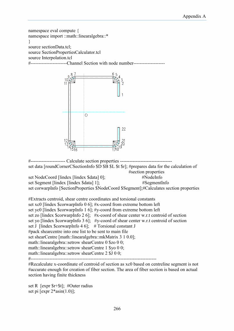
Appendix A
namespace eval compute namespace import ::math::linearalgebra::* source sectionData.tcl; source SectionPropertiesCalculator.tcl source Interpolation.tcl #-----------------------Channel Section with node number--------------------
#---------------------- Calculate section properties --------------------------------- set data [roundCornerCSectionInfo $D $B $L $t $r]; #prepares data for the calculation of #section properties set NodeCoord [lindex [lindex $data] 0]; #NodeInfo set Segment [lindex [lindex $data] 1]; #SegmentInfo set corwarpInfo [SectionProperties $NodeCoord $Segment];#Calculates section properties #Extracts centroid, shear centre coordinates and torsional constants set xc0 [lindex $corwarpInfo 0 6]; #x-coord from extreme bottom left set yc0 [lindex $corwarpInfo 1 6]; #y-coord from extreme bottom left set zo [lindex $corwarpInfo 2 6]; #x-coord of shear center w.r.t centroid of section set yo [lindex $corwarpInfo 3 6]; #y-coord of shear center w.r.t centroid of section set J [lindex $corwarpInfo 4 6]; # Torsional constant J #pack shearcentre into one list to be sent to main file set shearCentre [math::linearalgebra::mkMatrix 3 1 0.0]; math::linearalgebra::setrow shearCentre 0 $zo 0 0; math::linearalgebra::setrow shearCentre 1 $yo 0 0; math::linearalgebra::setrow shearCentre 2 $J 0 0; #-------------------------------------------------------------------------------- #Recalculate x-coordinate of centroid of section as xc0 based on centreline segment is not #accurate enough for creation of fiber section. The area of fiber section is based on actual section having finite thickness set R [expr $r+$t]; #Outer radius set pi [expr 2*asin(1.0)];
266
Appendix A
#Calculate area and coordinate of centroid from extreme left set zc [expr 4/(3*$pi)*($R*$R*$R-$r*$r*$r)/($R*$R-$r*$r)]; set Areatrue [expr ($D-2*($r+$t))*$t+2*($B-2*($r+$t))*$t+2*($L- ($r+$t))*$t+$pi*($R*$R-$r*$r)]; #Area of section set Qc [expr ($D-2*($r+$t))*$t*$t/2+2*($B-2*($r+$t))*$t*$B/2+2*($L-($r+$t))*$t*($B-$t/2)+2*$pi*($R*$R-$r*$r)/4*($R-$zc)+2*$pi*($R*$R-$r*$r)/4*($B-($r+$t)+$zc)]; set zbar [expr $Qc/$Areatrue]; #z-coordinate of centroid from left #------------------ Create fiber cross-section information ----------------- #Coordinates for comptuting fiber size and centroid set y1 [expr $D/2.0] set y2 [expr $y1-$t] set y3 [expr $y2-$r] set y4 [expr $y1-$L] set z1 [expr -$zbar] set z2 [expr $z1+$t] set z3 [expr $z2+$r] set z4 [expr $B+$z1-($t+$r)] set z5 [expr $z4+$r] set z6 [expr $z5+$t] #Calculate length of each fiber at each region: lips, flange, corners and web set dfL [expr ($y3-$y4)/($nfL)] ;#length of each fibre in lip set theta [expr (0.5*$pi)/$nfC]; #angle(radians) subtended by each fiber at the corner set cArea [expr ($R*$R-$r*$r)*$theta/2.0];#area of each corner fiber set dbf [expr ($z4-$z3)/$nfbf]; #length of each fiber in flange set dwf [expr (2.0*$y3)/$nfdw];#length of each fiber in web set NoOfFiber [expr ($nfL+$nfbf)*2+$nfC*4+$nfdw]; #No. of fibers #---------- Assemble coordinate of centroid, area of each fiber --------------- #create matrix to store fiber information set Fib [math::linearalgebra::mkMatrix $NoOfFiber 5 0]; for set i 0 $i<$nfL incr i 1 #Top lip #Fiber No, x,y, Area, warping(to be included later) math::linearalgebra::setrow Fib $i $i 0 0; math::linearalgebra::setrow Fib $i [expr ($z5+$z6)/2.0] 1 1; math::linearalgebra::setrow Fib $i [expr $y4+($dfL/2.0*(2*$i+1))] 2 2; math::linearalgebra::setrow Fib $i [expr $dfL*$t] 3 3; for set i 0 $i<$nfC incr i 1 #Top right corner #Fiber No, x,y, Area, warping(to be included later) set fibNo [expr $i+$nfL] math::linearalgebra::setrow Fib $fibNo $fibNo 0 0; math::linearalgebra::setrow Fib $fibNo [expr $z4+($r+$t/2)*cos($theta/2*(2*$i+1))] 1 1; math::linearalgebra::setrow Fib $fibNo [expr $y3+($r+$t/2)*sin($theta/2*(2*$i+1))] 2 2; math::linearalgebra::setrow Fib $fibNo $cArea 3 3;
267

Appendix A
for set i 0 $i<$nfbf incr i 1 #Top flange set fibNo [expr $i+$nfC+$nfL] math::linearalgebra::setrow Fib $fibNo $fibNo 0 0; math::linearalgebra::setrow Fib $fibNo [expr $z4-($dbf/2*(2*$i+1))] 1 1; math::linearalgebra::setrow Fib $fibNo [expr ($y1+$y2)/2] 2 2; math::linearalgebra::setrow Fib $fibNo [expr $dbf*$t] 3 3; for set i 0 $i<$nfC incr i 1 #Top Left corner #Fiber No, x,y, Area, warping(to be included later) set fibNo [expr $i+$nfC+$nfL+$nfbf] math::linearalgebra::setrow Fib $fibNo $fibNo 0 0; math::linearalgebra::setrow Fib $fibNo [expr $z3+($r+$t/2)*cos($pi/2+$theta/2*(2*$i+1))] 1 1; math::linearalgebra::setrow Fib $fibNo [expr $y3+($r+$t/2)*sin($pi/2+$theta/2*(2*$i+1))] 2 2; math::linearalgebra::setrow Fib $fibNo $cArea 3 3; for set i 0 $i<$nfdw incr i 1 #Web set fibNo [expr $i+2*$nfC+$nfL+$nfbf] math::linearalgebra::setrow Fib $fibNo $fibNo 0 0; math::linearalgebra::setrow Fib $fibNo [expr ($z1+$z2)/2] 1 1; math::linearalgebra::setrow Fib $fibNo [expr $y3-($dwf/2*(2*$i+1))] 2 2; math::linearalgebra::setrow Fib $fibNo [expr $dwf*$t] 3 3; for set i 0 $i<$nfC incr i 1 #Bottom Left corner #Fiber No, x,y, Area, warping(to be included later) set fibNo [expr $i+2*$nfC+$nfL+$nfbf+$nfdw] math::linearalgebra::setrow Fib $fibNo $fibNo 0 0; math::linearalgebra::setrow Fib $fibNo [expr $z3+($r+$t/2)*cos($pi+$theta/2*(2*$i+1))] 1 1; math::linearalgebra::setrow Fib $fibNo [expr -$y3+($r+$t/2)*sin($pi+$theta/2*(2*$i+1))] 2 2; math::linearalgebra::setrow Fib $fibNo $cArea 3 3; for set i 0 $i<$nfbf incr i 1 #Bottom flange set fibNo [expr $i+3*$nfC+$nfL+$nfbf+$nfdw] math::linearalgebra::setrow Fib $fibNo $fibNo 0 0; math::linearalgebra::setrow Fib $fibNo [expr $z3+($dbf/2*(2*$i+1))] 1 1; math::linearalgebra::setrow Fib $fibNo [expr -($y1+$y2)/2] 2 2; math::linearalgebra::setrow Fib $fibNo [expr $dbf*$t] 3 3; for set i 0 $i<$nfC incr i 1 #Bottom right corner #Fiber No, x,y, Area, warping(tobe included later) set fibNo [expr $i+3*$nfC+$nfL+2*$nfbf+$nfdw] math::linearalgebra::setrow Fib $fibNo $fibNo 0 0; math::linearalgebra::setrow Fib $fibNo [expr $z4+($r+$t/2)*cos(3*$pi/2+$theta/2*(2*$i+1))] 1 1; math::linearalgebra::setrow Fib $fibNo [expr -$y3+($r+$t/2)*sin(3*$pi/2+$theta/2*(2*$i+1))] 2 2; math::linearalgebra::setrow Fib $fibNo $cArea 3 3;
268

Appendix A
for set i 0 $i<$nfL incr i 1 #bottom lip set fibNo [expr $i+4*$nfC+$nfL+2*$nfbf+$nfdw] math::linearalgebra::setrow Fib $fibNo $fibNo 0 0; math::linearalgebra::setrow Fib $fibNo [expr ($z5+$z6)/2] 1 1; math::linearalgebra::setrow Fib $fibNo [expr -$y3+($dfL/2*(2*$i+1))] 2 2; math::linearalgebra::setrow Fib $fibNo [expr $dfL*$t] 3 3; #----------------- Interpolate and assign sectorial coordinates to fiber -------------- for set i 0 $i<$NoOfFiber incr i 1 set fId($i) [math::linearalgebra::getelem $Fib $i 0] set f_z($i) [math::linearalgebra::getelem $Fib $i 1]; set f_y($i) [math::linearalgebra::getelem $Fib $i 2] set f_A($i) [math::linearalgebra::getelem $Fib $i 3] set secCoord [Interpolate $Fib $corwarpInfo]; for set i 0 $i<$NoOfFiber incr i 1 set wn($i) [lindex $secCoord $i 1] #------------------------------ Create fiber section--------------------------------------- section Fiber $secID for set i 0 $i<$NoOfFiber incr i 1 fiber $f_y($i) $f_z($i) $f_A($i) $matID $wn($i) $yo $zo; #yLoc, zLoc, Area, materialID, #sectorial coordinate, y_coord, and #z_coord of shear centre return $shearCentre; #returns shear centre coordinate to the main file
A.1.3 Function for creating nodes and segments from section dimensions
The following TCL function, an extract from the file sectionData.tcl, creates notes and segments from the dimension of the cross-section of channel beam for computing section properties
proc roundCornerCSectionInfo D B L t r #------------------------------------------------------------------------------------------- #This procedure returns the node coordinate and element information matrix for channel #section with round corners # #Written by: # Rinchen # PhD student, University of Sydney # Dated: September 2015 # #----------------------------------loads TCL math library---------------------------- source C:/Tcl/lib/tcllib1.17/math/math.tcl; package require math::linearalgebra namespace eval compute
269

Appendix A
namespace import ::math::linearalgebra::* #-------------define coordinates--------------------------
# set NoOfNodes 22; # input number of nodes set NoOfElements [expr $NoOfNodes-1]; set nfC 4; #4 segments at the corner #---------- Define centreline coordinates of nodes with origin at bottom left corner------- set rm [expr $r+0.5*$t] set pi [expr 2*asin(1.0)]; set theta [expr ($pi/2)/$nfC]; #Top lip set Node1x [expr $B-$t]; set Node1y [expr $D-$t-($L-0.5*$t)]; set Node2x [expr $B-$t]; set Node2y [expr $D-$t-$rm]; #Top right corner set Node3x [expr $Node2x-$rm+$rm*cos($theta)]; set Node3y [expr $Node2y+$rm*sin($theta)]; set Node4x [expr $Node2x-$rm+$rm*cos(2*$theta)];set Node4y [expr $Node2y+$rm*sin(2*$theta)]; set Node5x [expr $Node2x-$rm+$rm*cos(3*$theta)];set Node5y [expr $Node2y+$rm*sin(3*$theta)]; #Top flange set Node6x [expr $B-$t-$rm]; set Node6y [expr $D-$t]; set Node7x $rm; set Node7y [expr $D-$t]; #Top left corner set Node8x [expr $rm-$rm*sin($theta)]; set Node8y $Node5y; set Node9x [expr $rm-$rm*sin(2*$theta)]; set Node9y $Node4y; set Node10x [expr $rm-$rm*sin(3*$theta)]; set Node10y $Node3y;
270
Appendix A
#Web set Node11x 0.0; set Node11y $Node2y; set Node12x 0.0; set Node12y $rm; #Bottom left corner set Node13x [expr $rm-$rm*cos($theta)]; set Node13y [expr $rm-$rm*sin($theta)]; set Node14x [expr $rm-$rm*cos(2*$theta)]; set Node14y [expr $rm-$rm*sin(2*$theta)]; set Node15x [expr $rm-$rm*cos(3*$theta)]; set Node15y [expr $rm-$rm*sin(3*$theta)]; #Bottom flange set Node16x $Node7x; set Node16y 0.0; set Node17x $Node6x; set Node17y 0.0; #Bottom right corner set Node18x $Node5x; set Node18y $Node15y; set Node19x $Node4x; set Node19y $Node14y; set Node20x $Node3x; set Node20y $Node13y; #Bottom lip set Node21x $Node2x; set Node21y $Node12y; set Node22x $Node1x; set Node22y [expr $L-0.5*$t]; # #-------- construct nodal coordinate matrix based on the cross-section information ----- # set NodeCoord [math::linearalgebra::mkMatrix $NoOfNodes 3 0.0] for set i 0 $i<$NoOfNodes incr i 1 math::linearalgebra::setelem NodeCoord $i 0 [expr $i+1]; #x-coordinates of nodes: MatrixName, ColumnNo, NodeCoord, min, max for set i 0 $i<$NoOfNodes incr i 1 set j [expr $i+1] math::linearalgebra::setcol NodeCoord 1 [expr "\$Node$j\x"] $i $i; #y-coordinates of nodes for set i 0 $i<$NoOfNodes incr i 1 set j [expr $i+1] math::linearalgebra::setcol NodeCoord 2 [expr "\$Node$j\y"] $i $i; #-------------------- construction Element info matrix---------------------- # set Segment [math::linearalgebra::mkMatrix $NoOfElements 4 0.0] for set i 0 $i<$NoOfElements incr i 1 math::linearalgebra::setelem Segment $i 0 [expr $i+1]; #Define element connection (node i) in column1: colNo,Nodei, min, max for set i 0 $i<$NoOfElements incr i 1 set j [expr $i+1] math::linearalgebra::setcol Segment 1 $j $i $i; #Define element connection (node j) in column 2:colNo, Nodej, min, max
271

Appendix A
for set i 0 $i<$NoOfElements incr i 1 set j [expr $i+2] math::linearalgebra::setcol Segment 2 $j $i $i; #Assign uniform thickness to the section for set i 0 $i<$NoOfElements incr i 1 math::linearalgebra::setcol Segment 3 $t $i $i; return [list $NodeCoord $Segment]
A.1.4 Function for the computation of thin-walled open cross-section properties
The following TCL function, an extract from the file SectionPropertiesCalculator.tcl, computes the section properties of open cross-section based on the input generated by another TCL function provided above. proc SectionProperties NodeCoordinates ElementInfo #--------------------------------------------------------------------------------------- # Written by: Rinchen # Date: 6 Oct 2015 # PhD student: University of Sydney, Sydney NSW, Australia # # Comments: # NodeCoordinates contain nodeNumber, x- and y-coordinate of each node # ElementInfo contains elementNumber, starNode, endNode, segment thickness # Numerical integration schemes follow Simpson's Rule set NodeCoord $NodeCoordinates set Segment $ElementInfo set NoOfNodes [llength $NodeCoordinates] set NoOfElements [llength $ElementInfo] #------Pick up the nodal coordinates corresponding to respective element ends------ for set i 0 $i<$NoOfElements incr i 1 set k [expr $i+1] set segId [math::linearalgebra::getelem $Segment $i 0]; #search indicator set nodei [math::linearalgebra::getelem $Segment $i 1]; #search indicator set nodej [math::linearalgebra::getelem $Segment $i 2]; #search indicator set xi($k) [math::linearalgebra::getelem $NodeCoord [expr $nodei-1] 1]; set yi($k) [math::linearalgebra::getelem $NodeCoord [expr $nodei-1] 2]; set xj($k) [math::linearalgebra::getelem $NodeCoord [expr $nodej-1] 1]; set yj($k) [math::linearalgebra::getelem $NodeCoord [expr $nodej-1] 2]; set tij($k) [math::linearalgebra::getelem $Segment [expr $segId-1] 3]; #-------Calculate segment properties: centroid, area--------------------------- set AreaSec 0.0; set Axc 0.0; set Ayc 0.0;
272

Appendix A
for set i 1 $i<$NoOfNodes incr i 1 set dxi($i) [expr $xi($i)-$xj($i)]; #difference in x-coordinates set dyi($i) [expr $yi($i)-$yj($i)]; #difference in y-coordinates set Lij($i) [expr sqrt($dxi($i)*$dxi($i)+$dyi($i)*$dyi($i))]; #length of segment set Aij($i) [expr $Lij($i)*$tij($i)]; #area of segment set xc($i) [expr ($xi($i)+$xj($i))/2]; #x-coord of centroid of segment set yc($i) [expr ($yi($i)+$yj($i))/2]; #y-coord of centroid of segment set Axc [expr $Axc+$Aij($i)*$xc($i)]; #Sum(A*xc) set Ayc [expr $Ayc+$Aij($i)*$yc($i)]; #Sum (A*yy) set AreaSec [expr $AreaSec+$Aij($i)] #---------Calculate centroid of whole section from the extreme bottom left--------- set xc0 [expr $Axc/$AreaSec]; set yc0 [expr $Ayc/$AreaSec]; #------Calculate second moment of area and polar moment of section w.r.t centroid set Ixx 0.0; set Iyy 0.0; set Ixy 0.0; for set i 1 $i<$NoOfNodes incr i 1 set xii 0.0; set xjj 0.0; set yii 0.0; set yjj 0.0; set xii [expr ($xi($i)-$xc0)]; set xjj [expr ($xj($i)-$xc0)]; set yii [expr ($yi($i)-$yc0)]; set yjj [expr ($yj($i)-$yc0)]; set Ixx [expr $Ixx+($yii*$yii+$yii*$yjj+$yjj*$yjj)*$Lij($i)*$tij($i)/3]; set Iyy [expr $Iyy+($xii*$xii+$xii*$xjj+$xjj*$xjj)*$Lij($i)*$tij($i)/3];
set Ixy [expr $Ixy+(($xii*$yii+$xjj*$yjj)/3+($xii*$yjj+$xjj*$yii)/6)*$Lij($i)*$tij($i)];
#--------Calculate principal moment of area of a whole section---------------- if $Ixy==0.0 set eps 0.000001 else set eps 0.0 ; set delta [expr sqrt(($Ixx-$Iyy)*($Ixx-$Iyy)/4+$Ixy*$Ixy)]; set Ipxx [expr ($Ixx+$Iyy)/2+$delta]; #Imax set Ipyy [expr ($Ixx+$Iyy)/2-$delta]; #Imin set alpha [expr atan(($Ixx-$Ipxx)/($Ixy+$eps))]; #Inclination of principal axes in radians: #+ve for anti-clockwise set pi [expr 2*asin(1.0)]; set alphadeg [expr $alpha*180/$pi]; #--------Transform nodal coordinates to principal axis system------------------- for set i 1 $i<$NoOfNodes incr i 1 set xi0($i) [expr ($yi($i)-$yc0)*sin($alpha)+($xi($i)-$xc0)*cos($alpha)];
273
Appendix A
set yi0($i) [expr ($yi($i)-$yc0)*cos($alpha)-($xi($i)-$xc0)*sin($alpha)]; set xj0($i) [expr ($yj($i)-$yc0)*sin($alpha)+($xj($i)-$xc0)*cos($alpha)]; set yj0($i) [expr ($yj($i)-$yc0)*cos($alpha)-($xj($i)-$xc0)*sin($alpha)]; #---------Calculate sectorial area of segment with respect to centroid--------------- for set i 1 $i<$NoOfNodes incr i 1 set Aoc($i) [expr ($xi0($i)*$yj0($i)-$xj0($i)*$yi0($i))] #------------Compute sectorial coordinate w.r.t centroid------------------------------- # Create matrix to store warping displacement dof at each node at element ends set WarpingCoord [math::linearalgebra::mkMatrix $NoOfElements 3 0] for set i 0 $i<$NoOfElements incr i 1 math::linearalgebra::setelem WarpingCoord $i 0 [expr $i+1]; #Element ID math::linearalgebra::setelem WarpingCoord $i 1 [expr 2*($i+1)-1]; #Warping #displacement dof at node i
math::linearalgebra::setelem WarpingCoord $i 2 [expr 2*($i+1)]; #Warping #displacement dof at node j
#-----------------Construct matrix Cw ([Cw]w=df/dz(Fi))--------------------------- set Cw [math::linearalgebra::mkMatrix [expr 2*$NoOfElements] [expr 2*$NoOfElements] 0] set lastRow [expr 2*$NoOfElements-1]; #Construct NoOfElement rows for element equations in Cw for set i 0 $i<$NoOfElements incr i 1 math::linearalgebra::setelem Cw $i [expr 2*$i] -1.0; math::linearalgebra::setelem Cw $i [expr 2*$i+1] 1.0; #--------------------Construct rows corresponding to compatibility equations in Cw------- set rowNum [expr $NoOfElements-1]; #starting row number for compatibility equations for set i 1 $i<[expr $NoOfElements+1] incr i 1 set found 0 for set j 1 $j<[expr $NoOfElements+1] incr j 1 #compare the occurrence of #each node in ith and jth column set node1 [lindex $Segment [expr $j-1] 1] set node2 [lindex $Segment [expr $j-1] 2] if $i==$node1 | $i==$node2 set found [expr $found+1] if $i==$node1 set ele($found) $j set acol($found) 1
if $found ==1 set windex [lindex $WarpingCoord [expr $ele($found)-1] 1]
274

Appendix A
if $i==$node2 set ele($found) $j set acol($found) 2
if $found ==1 set windex [lindex $WarpingCoord [expr $ele($found)-1] 2]
if $found>1 set colpos1 $windex ; # sets the ith column position in Cw matrix for wi for set k 2 $k<[expr $found+1] incr k 1 set rowNum [expr $rowNum+1]
set colpos2 [lindex $WarpingCoord [expr $ele($k)-1] $acol($k)]; #sets the jth column position for wj
math::linearalgebra::setelem Cw $rowNum [expr $colpos1-1] 1.0; math::linearalgebra::setelem Cw $rowNum [expr $colpos2-1] -1.0; #---------Construct last row for normalized warping equation in Cw------------------- for set i 0 $i<$NoOfElements incr i 1 set j [expr $i+1] math::linearalgebra::setelem Cw $lastRow [expr 2*$i] [expr $Aij($j)/2]; math::linearalgebra::setelem Cw $lastRow [expr 2*$i+1] [expr $Aij($j)/2]; #-------- Construct column vector Fi--------------------------------------------------------- set Fi [math::linearalgebra::mkVector [expr 2*$NoOfElements] 0]; for set i 0 $i<$NoOfElements incr i 1 math::linearalgebra::setelem Fi $i [expr $Aoc([expr $i+1])]; #----Solve for sectorial coordinate w.r.t centroid-------------------------------------------- set omc [math::linearalgebra::solvePGauss $Cw $Fi]; #--------------Assign sectorial coordinate at each end of segment------------------------- for set i 0 $i<$NoOfElements incr i 1 set j [expr $i+1] set wci($j) [math::linearalgebra::getelem $omc [expr 2*$i] 0] set wcj($j) [math::linearalgebra::getelem $omc [expr 2*$i+1] 0] set Iwx 0.0 set Iwy 0.0 for set i 1 $i<[expr $NoOfElements+1] incr i 1
275

Appendix A
set Iwx [expr $Iwx+(($wci($i)*$xi0($i)+$wcj($i)*$xj0($i))/3+($wci($i)*$xj0($i)+$wcj($i)*$xi0($i))/6)*$Lij($i)*$tij($i)]; set Iwy [expr $Iwy+(($wci($i)*$yi0($i)+$wcj($i)*$yj0($i))/3+($wci($i)*$yj0($i)+$wcj($i)*$yi0($i))/6)*$Lij($i)*$tij($i)]; #--------Calculate shear centre w.r.t centroid and in principal axes------------ set xo [expr (-$Ipyy*$Iwy)/(-$Ipxx*$Ipyy)]; set yo [expr ($Ipxx*$Iwx)/(-$Ipxx*$Ipyy)]; #--------Calculate shear centre coordinate w.r.t rectangular axes---------- set Y0 [expr $xo*sin($alpha)+$yo*cos($alpha)+$yc0]; set X0 [expr $xo*cos($alpha)-$yo*sin($alpha)+$xc0]; #----------Calculate sectorial area with respect to shear centre---------- for set i 1 $i<[expr $NoOfElements+1] incr i 1 set j [expr $i+1]
set Aos($i) [expr -(($yj0($i)-$yi0($i))*$xo+($xi0($i)-$xj0($i))*$yo-($xi0($i)*$yj0($i)-$xj0($i)*$yi0($i)))] #-----------------------------Calculate warping constant------------------------ #Calculate normalized sectorial coordinate w.r.t shear centre set Fi0 [math::linearalgebra::mkVector [expr 2*$NoOfElements] 0]; for set i 0 $i<$NoOfElements incr i 1 math::linearalgebra::setelem Fi0 $i [expr $Aos([expr $i+1])]; set om0 [math::linearalgebra::solvePGauss $Cw $Fi0]; #Assemble the sectorial coordinates at the element ends with reversed sign for set i 0 $i<$NoOfElements incr i 1 set j [expr $i+1] set wni($j) [expr -[math::linearalgebra::getelem $om0 [expr 2*$i] 0]]; set wnj($j) [expr -[math::linearalgebra::getelem $om0 [expr 2*$i+1] 0]]; #--------------------Compute warping constant Iw---------------------------- set Iw 0.0 for set i 1 $i<[expr $NoOfElements+1] incr i 1 set Iw [expr $Iw+($wni($i)*$wni($i)+$wni($i)*$wnj($i)+$wnj($i)*$wnj($i))/3*$Lij($i)*$tij($i)]; #Assemble sectorial coordinates corresponding to each node for set i 1 $i<[expr $NoOfNodes+1] incr i 1 for set j 0 $j<$NoOfElements incr j 1
276

Appendix A
set elNo [lindex $Segment $j 0] set node1 [lindex $Segment $j 1] set node2 [lindex $Segment $j 2] if $i == $node1 set wnn($node1) $wni($elNo) if $i == $node2 set wnn($node2) $wnj($elNo) #------- Calculate torsional constant J and monosymmetry parameter betax, betay------- set J 0.0; set betax 0.0; set betay 0.0; for set i 1 $i<[expr $NoOfElements +1] incr i 1 set J [expr $J+$Lij($i)*$tij($i)*$tij($i)*$tij($i)/3] set yiyj [expr $yi0($i)+$yj0($i)] set xixj [expr $xi0($i)+$xj0($i)] set betax [expr $betax+($yi0($i)*($xi0($i)*$xi0($i)+$yi0($i)*$yi0($i))+0.5*$yiyj*($xixj*$xixj+$yiyj*$yiyj)+$yj0($i)*($xj0($i)*$xj0($i)+$yj0($i)*$yj0($i)))*$Aij($i)/6] set betay [expr $betay+($xi0($i)*($xi0($i)*$xi0($i)+$yi0($i)*$yi0($i))+0.5*$xixj*($xixj*$xixj+$yiyj*$yiyj)+$xj0($i)*($xj0($i)*$xj0($i)+$yj0($i)*$yj0($i)))*$Aij($i)/6] set betax [expr $betax/$Ipxx-2.0*$yo] set betay [expr $betay/$Ipyy-2.0*$xo] #Create matrix to store coordinates and warping function at element endI and endJ #Center and torsional constant J information are stored in 7th column if $NoOfElements<6 set NoOfRows 6 else set NoOfRows $NoOfElements ; # ensures #that row is never less than 6 to hold additional data in 7th column! set CoordAndWarping [math::linearalgebra::mkMatrix $NoOfRows 7 0.0]; for set i 0 $i<$NoOfElements incr i 1 set k [expr $i+1] math::linearalgebra::setrow CoordAndWarping $i $xi0($k) 0 0; math::linearalgebra::setrow CoordAndWarping $i $yi0($k) 1 1; math::linearalgebra::setrow CoordAndWarping $i $wni($k) 2 2; math::linearalgebra::setrow CoordAndWarping $i $xj0($k) 3 3; math::linearalgebra::setrow CoordAndWarping $i $yj0($k) 4 4;
277
Appendix A
math::linearalgebra::setrow CoordAndWarping $i $wnj($k) 5 5; math::linearalgebra::setcol CoordAndWarping 6 $xc0 0 0; #x-coord of centroid math::linearalgebra::setcol CoordAndWarping 6 $yc0 1 1; # y -coordinate of centroid math::linearalgebra::setcol CoordAndWarping 6 $xo 2 2; #x-coord of shear center math::linearalgebra::setcol CoordAndWarping 6 $yo 3 3; #y-coord of shear center math::linearalgebra::setcol CoordAndWarping 6 $J 4 4; #Torsional constant math::linearalgebra::setcol CoordAndWarping 6 $alpha 5 5; #orientation of principal axes return $CoordAndWarping; # returns this matrix to other files
A.1.5 Function for interpolation of sectorial coordinates
The following TCL function computes the sectorial coordinate at the centroid of each fiber by linearly interpolating between the sectorial coordinates at the segment ends. proc Interpolate fiberCoordinate SegmentInfo #-------------------------------------------------------------------------- # Written by: Rinchen # Date: 12 Oct 2015 # PhD student: University of Sydney, Sydney NSW, Australia # # Input parameters: # fiberCoordinate contains fiberID, x-,y-coordinates of fiber centroid, Area of fiber # SegmentInfo contains x,y,w coordinates at ith and jth end of segment #------------------------------------------------------------------------------------- set NoOfFiber [llength $fiberCoordinate]; set NoOfElements [llength $SegmentInfo]; #Extract coordinates and warping information at the ends of the segment for set i 0 $i<$NoOfElements incr i 1 set j [expr $i+1] set xi0($j) [lindex $SegmentInfo $i 0]; set yi0($j) [lindex $SegmentInfo $i 1]; set w0i($j) [lindex $SegmentInfo $i 2]; set xj0($j) [lindex $SegmentInfo $i 3]; set yj0($j) [lindex $SegmentInfo $i 4]; set w0j($j) [lindex $SegmentInfo $i 5]; #Extract x,y coordinates of fiber centroid for set i 0 $i<$NoOfFiber incr i 1 set fId($i) [math::linearalgebra::getelem $fiberCoordinate $i 0]; set fx($i) [math::linearalgebra::getelem $fiberCoordinate $i 1]; set fy($i) [math::linearalgebra::getelem $fiberCoordinate $i 2];
278
Appendix A
#Determines the sectorial coordinate at centroid of each fiber set esp 0.1; #set tolerance for numerical roundoff errors for set i 1 $i<[expr $NoOfElements+1] incr i 1 for set j 0 $j<$NoOfFiber incr j 1 if ($fx($j)>=[expr $xi0($i)-$esp] && $fx($j)<=[expr $xj0($i)+$esp]) && ($fy($j)>=[expr $yi0($i)-$esp] && $fy($j)<=[expr $yj0($i)+$esp]) set d sqrt(($fx($j)-$xi0($i))*($fx($j)-$xi0($i))+($fy($j)-$yi0($i))*($fy($j)-$yi0($i))) set dij sqrt(($xj0($i)-$xi0($i))*($xj0($i)-$xi0($i))+($yj0($i)-$yi0($i))*($yj0($i)-$yi0($i))) set w($j) [expr $w0i($i)+$d/$dij*($w0j($i)-$w0i($i))]
if ($fx($j)>=[expr $xi0($i)-$esp] && $fx($j)<=[expr $xj0($i)+$esp]) && ($fy($j)<=[expr $yi0($i)+$esp] && $fy($j)>=[expr $yj0($i)-$esp]) set d sqrt(($fx($j)-$xi0($i))*($fx($j)-$xi0($i))+($fy($j)-$yi0($i))*($fy($j)-$yi0($i))) set dij sqrt(($xj0($i)-$xi0($i))*($xj0($i)-$xi0($i))+($yj0($i)-$yi0($i))*($yj0($i)-$yi0($i))) set w($j) [expr $w0i($i)+$d/$dij*($w0j($i)-$w0i($i))] if ($fx($j)<=[expr $xi0($i)+$esp] && $fx($j)>=[expr $xj0($i)-$esp]) && ($fy($j)>=[expr $yi0($i)-$esp] && $fy($j)<=[expr $yj0($i)+$esp]) set d sqrt(($fx($j)-$xi0($i))*($fx($j)-$xi0($i))+($fy($j)-$yi0($i))*($fy($j)-$yi0($i))) set dij sqrt(($xj0($i)-$xi0($i))*($xj0($i)-$xi0($i))+($yj0($i)-$yi0($i))*($yj0($i)-$yi0($i))) set w($j) [expr $w0i($i)+$d/$dij*($w0j($i)-$w0i($i))]
if ($fx($j)<=[expr $xi0($i)+$esp] && $fx($j)>=[expr $xj0($i)-$esp]) && ($fy($j)<=[expr $yi0($i)+$esp] && $fy($j)>=[expr $yj0($i)-$esp]) set d sqrt(($fx($j)-$xi0($i))*($fx($j)-$xi0($i))+($fy($j)-$yi0($i))*($fy($j)-$yi0($i))) set dij sqrt(($xj0($i)-$xi0($i))*($xj0($i)-$xi0($i))+($yj0($i)-$yi0($i))*($yj0($i)-$yi0($i))) set w($j) [expr $w0i($i)+$d/$dij*($w0j($i)-$w0i($i))] # Assemble sectorial coordinates corresponding to fiber number set fiberSectCoord [math::linearalgebra::mkMatrix $NoOfFiber 2 0]; for set i 0 $i<$NoOfFiber incr i 1 math::linearalgebra::setrow fiberSectCoord $i $i 0 0; math::linearalgebra::setrow fiberSectCoord $i $w($i) 1 1; return $fiberSectCoord; #returns the sectorial coordinates
279

Appendix A
A.1.6 Typical modified source codes in OpenSees
A.1.6.1 Class DispBeamColumn3d.cpp
The major changes made to the class DipsBeamColumn3d are as follows:
DispBeamColumn3d::update(void) int err = 0; crdTransf->update(); // Update the transformation const Vector &v = crdTransf->getBasicTrialDisp();// Get basic deformations double L = crdTransf->getInitialLength(); double oneOverL = 1.0/L; double oneOverLsquare = 1.0/(L*L); double xi[maxNumSections]; beamInt->getSectionLocations(numSections, L, xi); // Loop over the integration points for (int i = 0; i < numSections; i++) Vector e(workArea, 8); double xi1 = xi[i]; double dNv1 = 1.0 + 3.0*xi1*xi1 - 4.0*xi1; double ddNv1 = 6.0*xi1*oneOverL - 4.0*oneOverL; double dNv2 = 3.0*xi1*xi1 - 2.0*xi1; double ddNv2 = 6.0*xi1*oneOverL - 2.0*oneOverL; double dNw1 = dNv1; double ddNw1 = ddNv1; double dNw2 = dNv2; double ddNw2 = ddNv2; double Nf1 = 1.0 - 3.0*xi1*xi1 + 2.0*xi1*xi1*xi1; double dNf1 = 6.0*xi1*xi1*oneOverL - 6.0*xi1*oneOverL; double ddNf1 = 12.0*xi1*oneOverLsquare - 6.0*oneOverLsquare; double Nf2 = xi1*L*(1.0 - xi1)*(1.0 - xi1); double dNf2 = dNv1; double ddNf2 = ddNv1; double Nf3 = 3.0*xi1*xi1 - 2.0*xi1*xi1*xi1; double dNf3 = 6.0*xi1*oneOverL - 6.0*xi1*xi1*oneOverL; double ddNf3 = 6.0*oneOverLsquare - 12.0*xi1*oneOverLsquare; double Nf4 = xi1*xi1*L*(xi1 - 1.0); double dNf4 = dNv2; double ddNf4 = ddNv2; //genearalized strain defined double du = oneOverL*v(8); //u' double dv = dNv1*v(1) + dNv2*v(5); //v' double ddv = ddNv1*v(1) + ddNv2*v(5); //v" double dw = dNw1*v(2) + dNw2*v(6); //w' double ddw = ddNw1*v(2) + ddNw2*v(6); //w" double f = Nf1*v(0) + Nf2*v(3) + Nf3*v(4) + Nf4*v(7); //f double df = dNf1*v(0) + dNf2*v(3) + dNf3*v(4) + dNf4*v(7); //f' double ddf = ddNf1*v(0) + ddNf2*v(3) + ddNf3*v(4) + ddNf4*v(7);//f" //generalized strain assembled to be sent to FiberSection e(0) = du; //u' e(1) = ddv; //v" e(2) = ddw; //w"
280
Appendix A
e(3) = ddf; //f" e(4) = df; //f' e(5) = dv; //v' e(6) = dw; //w' e(7) = f; //f // Set the section deformations err += theSections[i]->setTrialSectionDeformation(e); if (err != 0)
opserr << "DispBeamColumn3d::update() - failed setTrialSectionDeformations()\n";
return err; return 0; const Matrix& DispBeamColumn3d::getTangentStiff() static Matrix kb(9,9); static Matrix N1(6,8); static Matrix N2(8,9); static Matrix N3(8,8); static Matrix kbPart1(9,9); static Matrix Gmax(8,8); static Matrix kbPart2(9,9); static Matrix kf1(9, 9); static Matrix kf2(9, 9); static Matrix T(9, 9); const Vector &v = crdTransf->getBasicTrialDisp(); kb.Zero(); q.Zero(); double L = crdTransf->getInitialLength(); double oneOverL = 1.0/L; double oneOverLsquare=1.0/(L*L); double oneOverLcube=1.0/(L*L*L); double xi[maxNumSections]; beamInt->getSectionLocations(numSections, L, xi); double wt[maxNumSections]; beamInt->getSectionWeights(numSections, L, wt); // Loop over the integration points for (int i = 0; i < numSections; i++) N1.Zero(); N2.Zero(); N3.Zero(); kbPart1.Zero(); kbPart2.Zero(); Gmax.Zero(); kf1.Zero(); kf2.Zero(); T.Zero();
281

Appendix A
double xi1 = xi[i]; double dNv1 = 1.0 + 3.0*xi1*xi1 - 4.0*xi1; double ddNv1 = 6.0*xi1*oneOverL - 4.0*oneOverL; double dNv2 = 3.0*xi1*xi1 - 2.0*xi1; double ddNv2 = 6.0*xi1*oneOverL - 2.0*oneOverL; double dNw1 = dNv1; double ddNw1 = ddNv1; double dNw2 = dNv2; double ddNw2 = ddNv2; double Nf1 = 1.0 - 3.0*xi1*xi1 + 2.0*xi1*xi1*xi1; double dNf1 = 6.0*xi1*xi1*oneOverL - 6.0*xi1*oneOverL; double ddNf1 = 12.0*xi1*oneOverLsquare - 6.0*oneOverLsquare; double Nf2 = xi1*L*(1.0 - xi1)*(1.0 - xi1); double dNf2 = dNv1; double ddNf2 = ddNv1; double Nf3 = 3.0*xi1*xi1 - 2.0*xi1*xi1*xi1; double dNf3 = 6.0*xi1*oneOverL - 6.0*xi1*xi1*oneOverL; double ddNf3 = 6.0*oneOverLsquare - 12.0*xi1*oneOverLsquare; double Nf4 = xi1*xi1*L*(xi1 - 1.0); double dNf4 = dNv2; double ddNf4 = ddNv2; double dv = dNv1*v(1) + dNv2*v(5); //v' double ddv = ddNv1*v(1) + ddNv2*v(5); //v" double dw = dNw1*v(2) + dNw2*v(6); //w' double ddw = ddNw1*v(2) + ddNw2*v(6); //w" double f = Nf1*v(0) + Nf2*v(3) + Nf3*v(4) + Nf4*v(7); //f double df = dNf1*v(0) + dNf2*v(3) + dNf3*v(4) + dNf4*v(7); //f' //Matrix Ndeltad1 & Ndeltad2; Matrix Ndeltad1 incorporates the shear centre eccentricity //-------------------------------------------------------------- N1(0,0) = 1.0; N1(0,1) = dv+z0*df; N1(0,2) = dw - y0*df; N1(0,6) = z0*dv - y0*dw; N1(1,3) = -1.0; N1(1,4) = -f; N1(1,5) = -ddw; N1(2,3) = f; N1(2,4) = -1.0; N1(2,5) =ddv; N1(3,6) = df; N1(4,7) = 1.0; N1(5,6) = 1.0; //-------------------------------------------------------------- N2(0,8) = oneOverL; N2(1,1) = dNv1; N2(1,5) = dNv2; N2(2,2) = dNw1; N2(2,6) = dNw2; N2(3,1) = ddNv1; N2(3,5) = ddNv2; N2(4,2) = ddNw1; N2(4,6) = ddNw2; N2(5,0) = Nf1; N2(5,3) = Nf2; N2(5,4) = Nf3; N2(5,7) = Nf4; N2(6,0) = dNf1; N2(6,3) = dNf2; N2(6,4) = dNf3;
282

Appendix A
N2(6,7) = dNf4; N2(7,0) = ddNf1; N2(7,3) = ddNf2; N2(7,4) = ddNf3; N2(7,7) = ddNf4; //Local transformation matrix - relates axial force acting at shear centre and centroid //T=A^T T(0, 0) = 1.0; T(1, 1) = 1.0; T(2, 2) = 1.0; T(3, 3) = 1.0; T(4, 4) = 1.0; T(5, 5) = 1.0; T(6, 6) = 1.0; T(7, 7) = 1.0; T(8, 8) = 1.0; T(8, 1) = y0; T(8, 2) = -z0; T(8, 3) = omigC; T(8, 5) = -y0; T(8, 6) = z0; T(8, 7) = -omigC; // Get the section tangent stiffness and stress resultant const Matrix &ks = theSections[i]->getSectionTangent(); const Vector &s = theSections[i]->getStressResultant(); N3.addMatrixTripleProduct(0.0, N1, ks, 1.0); kbPart1.addMatrixTripleProduct(0.0, N2, N3, 1.0); //Assembly of stability matrix G Gmax(2, 2) = Gmax(1, 1) = s(0); //P Gmax(5, 4) = Gmax(4, 5) = -s(1); //Mz Gmax(5, 3) = Gmax(3, 5) = s(2); //My Gmax(6, 1) = Gmax(1, 6) = s(0)*z0; //Pz0 Gmax(6, 2) = Gmax(2, 6) = -s(0)*y0; //-Py0 Gmax(6, 6) = s(3); //W kbPart2.addMatrixTripleProduct(0.0, N2, Gmax, 1.0); kf1.addMatrixTripleProduct(0.0, T, kbPart1, 1.0); kf2.addMatrixTripleProduct(0.0, T, kbPart2, 1.0); double wti = wt[i]; for (int j=0; j<9; j++) for (int k=0; k<9; k++) kb(j, k) += kf1(j, k)*L*wti + kf2(j, k)*L*wti; //Assemble internal force vector q static Vector qProduct1(8);
static Vector qProduct2(9); //q(0)=M1x; q(1)=M1z; q(2)=M1y; q(3)=M1x'; q(4)=M2x; q(5)=M2z; q(6)=M2y; q(7)=M2x';q(8)=P
static Vector qProduct3(9); qProduct1.Zero();
283
Appendix A
qProduct2.Zero(); qProduct3.Zero(); qProduct1.addMatrixTransposeVector(0.0, N1, s, 1.0); qProduct2.addMatrixTransposeVector(0.0, N2, qProduct1, 1.0); qProduct3.addMatrixTransposeVector(0.0, T, qProduct2, 1.0); for (int j=0; j<9; j++) q(j) += qProduct3(j)*L*wti; q(0) += q0[0]; q(1) += q0[1]; q(2) += q0[2]; q(3) += q0[3]; q(4) += q0[4]; // Transform to global stiffness K = crdTransf->getGlobalStiffMatrix(kb, q); return K; const Matrix& DispBeamColumn3d::getInitialBasicStiff() static Matrix kb(9,9); static Matrix N1(6,8); static Matrix N2(8,9); static Matrix N3(8,8); static Matrix kbPart1(9,9); static Matrix kbPart2(9,9); static Matrix Gmax(8,8); static Matrix kf1(9, 9); static Matrix kf2(9, 9); static Matrix T(9, 9); kb.Zero();// Zero for integral const Vector &v = crdTransf->getBasicTrialDisp(); double L = crdTransf->getInitialLength(); double oneOverL = 1.0/L; double oneOverLsquare=1.0/(L*L); double oneOverLcube=1.0/(L*L*L); double xi[maxNumSections]; beamInt->getSectionLocations(numSections, L, xi); double wt[maxNumSections]; beamInt->getSectionWeights(numSections, L, wt); // Loop over the integration points for (int i = 0; i < numSections; i++) N1.Zero(); N2.Zero(); N3.Zero(); kbPart1.Zero(); kbPart2.Zero(); Gmax.Zero(); T.Zero(); kf1.Zero();
284

Appendix A
kf2.Zero(); double xi1 = xi[i]; double dNv1 = 1.0 + 3.0*xi1*xi1 - 4.0*xi1; double ddNv1 = 6.0*xi1*oneOverL - 4.0*oneOverL; double dNv2 = 3.0*xi1*xi1 - 2.0*xi1; double ddNv2 = 6.0*xi1*oneOverL - 2.0*oneOverL; double dNw1 = dNv1; double ddNw1 = ddNv1; double dNw2 = dNv2; double ddNw2 = ddNv2; double Nf1 = 1.0 - 3.0*xi1*xi1 + 2.0*xi1*xi1*xi1; double dNf1 = 6.0*xi1*xi1*oneOverL - 6.0*xi1*oneOverL; double ddNf1 = 12.0*xi1*oneOverLsquare - 6.0*oneOverLsquare; double Nf2 = xi1*L*(1.0 - xi1)*(1.0 - xi1); double dNf2 = dNv1; double ddNf2 = ddNv1; double Nf3 = 3.0*xi1*xi1 - 2.0*xi1*xi1*xi1; double dNf3 = 6.0*xi1*oneOverL - 6.0*xi1*xi1*oneOverL; double ddNf3 = 6.0*oneOverLsquare - 12.0*xi1*oneOverLsquare; double Nf4 = xi1*xi1*L*(xi1 - 1.0); double dNf4 = dNv2; double ddNf4 = ddNv2; double dv = dNv1*v(1) + dNv2*v(5); //v' double ddv = ddNv1*v(1) + ddNv2*v(5); //v" double dw = dNw1*v(2) + dNw2*v(6); //w' double ddw = ddNw1*v(2) + ddNw2*v(6); //w" double f = Nf1*v(0) + Nf2*v(3) + Nf3*v(4) + Nf4*v(7); //f double df = dNf1*v(0) + dNf2*v(3) + dNf3*v(4) + dNf4*v(7); //f' //Matrix Ndeltad1 & Ndeltad2 //-------------------------------------------------------------- N1(0, 0) = 1.0; N1(0, 1) = dv + z0*df; N1(0, 2) = dw - y0*df; N1(0, 6) = z0*dv - y0*dw; N1(1, 3) = -1.0; N1(1, 4) = -f; N1(1, 5) = -ddw; N1(2, 3) = f; N1(2, 4) = -1.0; N1(2, 5) = ddv; N1(3, 6) = df; N1(4, 7) = 1.0; N1(5, 6) = 1.0; //-------------------------------------------------------------- N2(0, 8) = oneOverL; N2(1, 1) = dNv1; N2(1, 5) = dNv2; N2(2, 2) = dNw1; N2(2, 6) = dNw2; N2(3, 1) = ddNv1; N2(3, 5) = ddNv2; N2(4, 2) = ddNw1; N2(4, 6) = ddNw2; N2(5, 0) = Nf1; N2(5, 3) = Nf2; N2(5, 4) = Nf3; N2(5, 7) = Nf4; N2(6, 0) = dNf1; N2(6, 3) = dNf2;
285

Appendix A
N2(6, 4) = dNf3; N2(6, 7) = dNf4; N2(7, 0) = ddNf1; N2(7, 3) = ddNf2; N2(7, 4) = ddNf3; N2(7, 7) = ddNf4; //Local transformation matrix //T=A^T; A=Transpose(T) T(0, 0) = 1.0; T(1, 1) = 1.0; T(2, 2) = 1.0; T(3, 3) = 1.0; T(4, 4) = 1.0; T(5, 5) = 1.0; T(6, 6) = 1.0; T(7, 7) = 1.0; T(8, 8) = 1.0; T(8, 1) = y0; T(8, 2) = -z0; T(8, 3) = omigC; T(8, 5) = -y0; T(8, 6) = z0; T(8, 7) = -omigC; // Get the section tangent stiffness and stress resultant const Matrix &ks = theSections[i]->getInitialTangent(); const Vector &s = theSections[i]->getStressResultant(); N3.addMatrixTripleProduct(0.0, N1, ks, 1.0); kbPart1.addMatrixTripleProduct(0.0, N2, N3, 1.0); Gmax(2, 2) = Gmax(1, 1) = s(0); //P Gmax(5, 4) = Gmax(4, 5) = -s(1); //Mz Gmax(5, 3) = Gmax(3, 5) = s(2); //My Gmax(6, 1) = Gmax(1, 6) = s(0)*z0; //Pz0 Gmax(6, 2) = Gmax(2, 6) = -s(0)*y0; //-Py0 Gmax(6, 6) = s(3); //W kbPart2.addMatrixTripleProduct(0.0, N2, Gmax, 1.0); kf1.addMatrixTripleProduct(0.0, T, kbPart1, 1.0);//T^(T)*(kb)*T kf2.addMatrixTripleProduct(0.0, T, kbPart2, 1.0); // Perform numerical integration double wti = wt[i]; for (int j=0; j<9; j++) for (int k=0; k<9; k++) kb(j, k) += kf1(j, k)*L*wti + kf2(j, k)*L*wti; return kb; const Matrix& DispBeamColumn3d::getInitialStiff() const Matrix &kb = this->getInitialBasicStiff(); // Transform to global stiffness
286
Appendix A
K = crdTransf->getInitialGlobalStiffMatrix(kb); return K; const Vector& DispBeamColumn3d::getResistingForce() double L = crdTransf->getInitialLength(); double oneOverLsquare=1.0/(L*L); double oneOverLcube=1.0/(L*L*L); double oneOverL=1.0/L; static Matrix N1(6,8); static Matrix N2(8,9); static Matrix T(9, 9); double xi[maxNumSections]; beamInt->getSectionLocations(numSections, L, xi); double wt[maxNumSections]; beamInt->getSectionWeights(numSections, L, wt); const Vector &v = crdTransf->getBasicTrialDisp(); q.Zero(); // Initialize to zero for integration // Loop over the integration points for (int i = 0; i < numSections; i++) N1.Zero(); N2.Zero(); T.Zero(); double xi1 = xi[i]; double dNv1 = 1.0 + 3.0*xi1*xi1 - 4.0*xi1; double ddNv1 = 6.0*xi1*oneOverL - 4.0*oneOverL; double dNv2 = 3.0*xi1*xi1 - 2.0*xi1; double ddNv2 = 6.0*xi1*oneOverL - 2.0*oneOverL; double dNw1 = dNv1; double ddNw1 = ddNv1; double dNw2 = dNv2; double ddNw2 = ddNv2; double Nf1 = 1.0 - 3.0*xi1*xi1 + 2.0*xi1*xi1*xi1; double dNf1 = 6.0*xi1*xi1*oneOverL - 6.0*xi1*oneOverL; double ddNf1 = 12.0*xi1*oneOverLsquare - 6.0*oneOverLsquare; double Nf2 = xi1*L*(1.0 - xi1)*(1.0 - xi1); double dNf2 = dNv1; double ddNf2 = ddNv1; double Nf3 = 3.0*xi1*xi1 - 2.0*xi1*xi1*xi1; double dNf3 = 6.0*xi1*oneOverL - 6.0*xi1*xi1*oneOverL; double ddNf3 = 6.0*oneOverLsquare - 12.0*xi1*oneOverLsquare; double Nf4 = xi1*xi1*L*(xi1 - 1.0); double dNf4 = dNv2; double ddNf4 = ddNv2; double dv = dNv1*v(1) + dNv2*v(5); //v' double ddv = ddNv1*v(1) + ddNv2*v(5); //v" double dw = dNw1*v(2) + dNw2*v(6); //w' double ddw = ddNw1*v(2) + ddNw2*v(6); //w" double f = Nf1*v(0) + Nf2*v(3) + Nf3*v(4) + Nf4*v(7); //f double df = dNf1*v(0) + dNf2*v(3) + dNf3*v(4) + dNf4*v(7); //f' //Matrix Ndeltad1 & Ndeltad2 //--------------------------------------------------------------
287
Appendix A
N1(0, 0) = 1.0; N1(0, 1) = dv + z0*df; N1(0, 2) = dw - y0*df; N1(0, 6) = z0*dv - y0*dw; N1(1, 3) = -1.0; N1(1, 4) = -f; N1(1, 5) = -ddw; N1(2, 3) = f; N1(2, 4) = -1.0; N1(2, 5) = ddv; N1(3, 6) = df; N1(4, 7) = 1.0; N1(5, 6) = 1.0; //-------------------------------------------------------------- N2(0, 8) = oneOverL; N2(1, 1) = dNv1; N2(1, 5) = dNv2; N2(2, 2) = dNw1; N2(2, 6) = dNw2; N2(3, 1) = ddNv1; N2(3, 5) = ddNv2; N2(4, 2) = ddNw1; N2(4, 6) = ddNw2; N2(5, 0) = Nf1; N2(5, 3) = Nf2; N2(5, 4) = Nf3; N2(5, 7) = Nf4; N2(6, 0) = dNf1; N2(6, 3) = dNf2; N2(6, 4) = dNf3; N2(6, 7) = dNf4; N2(7, 0) = ddNf1; N2(7, 3) = ddNf2; N2(7, 4) = ddNf3; N2(7, 7) = ddNf4; //Local transformation matrix T(0, 0) = 1.0; T(1, 1) = 1.0; T(2, 2) = 1.0; T(3, 3) = 1.0; T(4, 4) = 1.0; T(5, 5) = 1.0; T(6, 6) = 1.0; T(7, 7) = 1.0; T(8, 8) = 1.0; T(8, 1) = y0; T(8, 2) = -z0; T(8, 3) = omigC; T(8, 5) = -y0; T(8, 6) = z0; T(8, 7) = -omigC; // Get section stress resultant const Vector &s = theSections[i]->getStressResultant(); double wti=wt[i]; static Vector qProduct1(8); static Vector qProduct2(9); static Vector qProduct3(9); qProduct1.Zero(); qProduct2.Zero();
288

Appendix A
qProduct3.Zero(); qProduct1.addMatrixTransposeVector(0.0, N1, s, 1.0); qProduct2.addMatrixTransposeVector(0.0, N2, qProduct1, 1.0); qProduct3.addMatrixTransposeVector(0.0, T, qProduct2, 1.0); for (int j=0; j<9; j++) q(j) += qProduct3(j)*L*wti; q(0) += q0[0]; q(1) += q0[1]; q(2) += q0[2]; q(3) += q0[3]; q(4) += q0[4]; // Transform forces Vector p0Vec(p0, 5); P = crdTransf->getGlobalResistingForce(q, p0Vec); P.addVector(1.0, Q, -1.0); return P;
A.1.6.2 Class FiberSection3d.cpp
The changes made to the class FiberSection3d are as follows:
int FiberSection3d::setTrialSectionDeformation (const Vector &deforms) int res = 0; e = deforms;// Generalized strain for (int i = 0; i < 25; i++) // initialize elements of tangent stiffness matrix kData[i] = 0.0; ; for (int i = 0; i < 5; i++) //Initialize elements of stability matrix G sData[i] = 0.0; ; int loc = 0; double d0 = deforms(0);//u' e0 double d1 = deforms(1);//v" e1 double d2 = deforms(2);//w" e2 double d3 = deforms(3);//f" e3 double d4 = deforms(4);//f' e4 double d5 = deforms(5);//v' e5 double d6 = deforms(6);//w' e6 double d7 = deforms(7);//f e7 for (int i = 0; i < numFibers; i++) UniaxialMaterial *theMat = theMaterials[i]; double y = matData[loc++] - yBar; double z = matData[loc++] - zBar; double A = matData[loc++]; double sCoord=matData[loc++];
289

Appendix A
double y0 = matData[loc++]; double z0 = matData[loc++]; double omig = sCoord;// sectorial coordinate double yszs = (y - y0)*(y - y0) + (z - z0)*(z - z0); double strain = d0 - y*(d1 + d2*d7) - z*(d2 - d1*d7) + omig*d3 + 0.5*(d5*d5 + d6*d6) + 0.5*yszs*d4*d4 + (z0*d5 - y0*d6)*d4; // strain at the centroid of fiber double tangent, stress; res += theMat->setTrial(strain, stress, tangent); // get the stress and tangent modulus corresponding to strain double EA = tangent * A; double EAy = y*EA; double EAz = z*EA; double EAyz = EAy*z; //Assemble section stiffness matrix k kData[0] += EA; kData[1] += EAy; kData[2] += EAz; kData[3] += yszs*EA; kData[4] += EA*omig; kData[5] += EAy; kData[6] += EAy * y; kData[7] += EAyz; kData[8] += yszs*EAy; kData[9] += EAy*omig; kData[10] += EAz; kData[11] += EAyz; kData[12] += EAz * z; kData[13] += yszs*EAz; kData[14] += EAz*omig; kData[15] += yszs*EA; kData[16] += yszs*EAy; kData[17] += yszs*EAz; kData[18] += yszs*yszs*EA; kData[19] += yszs*EA*omig; kData[20] += EA*omig; kData[21] += EAy*omig; kData[22] += EAz*omig; kData[23] += yszs*EA*omig; kData[24] += omig*omig*EA; //Assemble section force vector D double fs0 = stress * A; sData[0] += fs0; //P sData[1] += fs0 * y; //Mz sData[2] += fs0 * z; //My sData[3] += fs0 * yszs; //W sData[4] += fs0 * omig; //B return res; const Matrix& FiberSection3d::getInitialTangent(void) static double kInitialData[25] = 0.0 ; static Matrix kInitial(kInitialData, 5, 5);
290

Appendix A
int loc = 0; for (int i = 0; i < numFibers; i++) UniaxialMaterial *theMat = theMaterials[i]; double y = matData[loc++] - yBar; double z = matData[loc++] - zBar; double A = matData[loc++]; double sCoord = matData[loc++]; double y0 = matData[loc++]; double z0 = matData[loc++]; double omig = sCoord; // Assign sectorial coordinate to omig double tangent = theMat->getInitialTangent(); double EA = tangent * A; double yszs = ((y - y0)*(y - y0) + (z - z0)*(z - z0)); double EAy = y*EA; double EAz = z*EA; double EAyz = EAy*z; // section stiffness matrix k kInitialData[0] += EA; kInitialData[1] += EAy; kInitialData[2] += EAz; kInitialData[3] += yszs*EA; kInitialData[4] += EA*omig; kInitialData[5] += EAy; kInitialData[6] += EAy * y; kInitialData[7] += EAyz; kInitialData[8] += yszs*EAy; kInitialData[9] += EAy*omig; kInitialData[10] += EAz; kInitialData[11] += EAyz; kInitialData[12] += EAz * z; kInitialData[13] += yszs*EAz; kInitialData[14] += EAz*omig; kInitialData[15] += yszs*EA; kInitialData[16] += yszs*EAy; kInitialData[17] += yszs*EAz; kInitialData[18] += yszs*yszs*EA; kInitialData[19] += yszs*EA*omig; kInitialData[20] += EA*omig; kInitialData[21] += EAy*omig; kInitialData[22] += EAz*omig; kInitialData[23] += yszs*EA*omig; kInitialData[24] += omig*omig*EA; return kInitial;
291

Appendix A
A.2. Boundary conditions for warping-free ends in thin-walled open-section beams undergoing large displacment
The response of a structure depends on the constraints imposed at the supports. This is especially true for the large displacement analysis of thin-walled open sections with warping free at the ends, modelled using shell elements. In such shell model, it becomes difficult to model the boundary conditions accurately that can simulate the realistic constraints for warping-free ends. The usual method of applying the boundary conditions to the whole cross-section by releasing the longitudinal degree of freedom does not warrant warping-free end as explained below. The explanation is provided with reference to the boundary conditions created for the flexural-torsional buckling analysis of I-section subjected to equal end moments at the ends as in the example described in Section 3.4.1.2.
Consider a case in which a beam is restrained against the displacement in transverse directions and rotation about the longitudinal axis, but allowed to displace in the longitudinal direction and to rotate about the y and z-axis at the ends as depicted in the analytical model in Figure A.1.
(a) Physical model (b) Analytical model
Figure A.1 Simply supported beam subjected to end moments
The response of the beam can be significantly different even with a minor deviation of boundary conditions prevailing at the end supports at the large displacement range. This is demonstrated by considering two cases of boundary conditions applied on the shell model at its end supports: support with restraint applied to the whole cross-section and support with restraint applied to the rigid body areas on the cross-section.
Case 1. Beam constrained by applying boundary conditions to the whole cross-section
Figure A.2 shows the boundary condition (analytical model of Figure A.1b) applied to the whole cross-section of the beam at its ends. In such condition, as the beam undergoes large displacement, the nodes farthest from the centroid are constrained to move parallel to the original beam configuration (Figure A.2b). As a result, the flanges get stretched normal to the
292
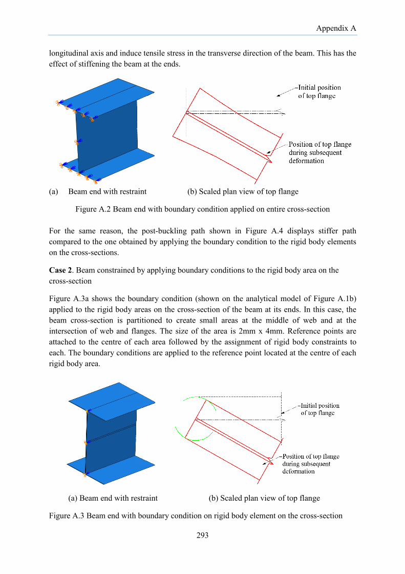
Appendix A
longitudinal axis and induce tensile stress in the transverse direction of the beam. This has the effect of stiffening the beam at the ends.
(a) Beam end with restraint (b) Scaled plan view of top flange
Figure A.2 Beam end with boundary condition applied on entire cross-section
For the same reason, the post-buckling path shown in Figure A.4 displays stiffer path compared to the one obtained by applying the boundary condition to the rigid body elements on the cross-sections.
Case 2. Beam constrained by applying boundary conditions to the rigid body area on the cross-section
Figure A.3a shows the boundary condition (shown on the analytical model of Figure A.1b) applied to the rigid body areas on the cross-section of the beam at its ends. In this case, the beam cross-section is partitioned to create small areas at the middle of web and at the intersection of web and flanges. The size of the area is 2mm x 4mm. Reference points are attached to the centre of each area followed by the assignment of rigid body constraints to each. The boundary conditions are applied to the reference point located at the centre of each rigid body area.
(a) Beam end with restraint (b) Scaled plan view of top flange
Figure A.3 Beam end with boundary condition on rigid body element on the cross-section
293

Appendix A
This method of constraining the beam ends allows free movement of flanges, thus allowing the tips of the flanges to displace along the path described by an arc shown in Figure A.3b. This represents the true warping-free condition at the support. The only drawback with this method is that it requires partitioning of shell models to create the small areas/regions for rigid body constraint resulting in non-uniform mesh size. The influence on the result is however negligible.
Figure A.4 shows the comparison of equilibrium path (end moment versus twist rotation at the midspan) predicted by the shell model with two different types of restraints at the support. The post-buckling path predicted by the displacement-based beam element formulated in Chapter 3 is also provided for the comparison.
Figure A.4 Comparison of buckling and post-buckling path for I-beam in bending
As observed from the above figure, the effect of support condition on the behaviour is negligible at small displacement range. Its effect becomes significant only at large displacement range.
294

Appendix B
APPENDIX B. ADDITIONAL MATERIALS FOR FULL-SCALE FRAME TESTS
B.1. Frame Installation Procedure
The following paragraphs explain the sequence that was followed to install the portal frames in the structural laboratory at The University of Sydney.
Step1. The base plates were fixed to the steel I-beam embedded in the concrete floor by aligning with the previously marked centreline on the top surface of the I-beam. The base plate assemblages were clamped to the I-beam with the aid of four high-strength structural bolts. The base straps were bolted to the upper base plates using three M20 high-strength structural bolts and using 10 mm thick steel plate as clamp.
Figure B.1 Base support configuration
Step 2. An eaves bracket was connected to the first column with bolts in snug-tight condition. The column was lifted and positioned with the base strap. Bolts were inserted and snug tightened after the position of the column was adjusted by checking the vertical alignment in two orthogonal directions using levels. Following a similar process, the second column was installed but without the eaves bracket attached at its top end.
Step 3. The two rafters and apex bracket were assembled on the floor with bolts in snug-tight condition. Sling straps were hung from the ends of horizontal beam and looped around the rafters. The location of the point of attachment was determined in such a way that it caused minimal stress at the apex region. The whole assemblage was gradually lifted while avoiding inducing any twists to the rafter assemblage (Figure B.2). Once lifted into place, one end of the rafter was slid into the eaves bracket that was previously attached to the column top. It was bolted with bolts in snug-tight condition while the rafter assemblage was held in position by the overhead crane.
295
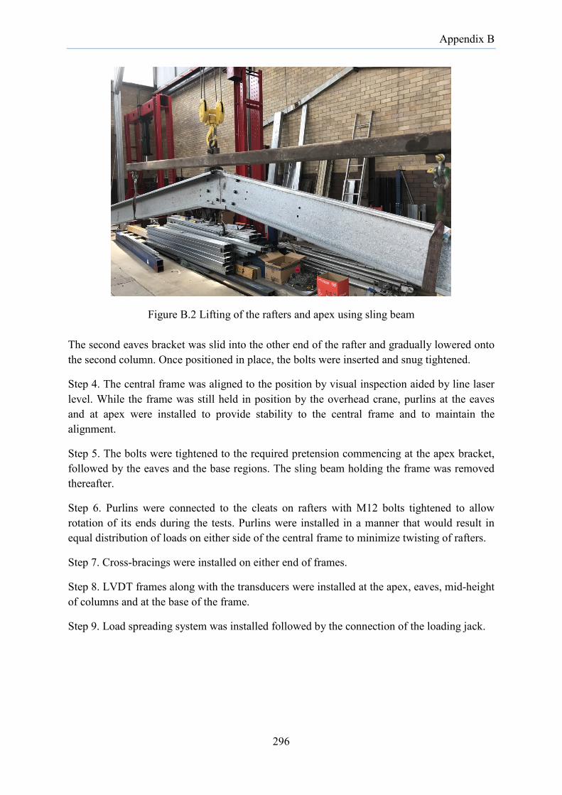
Appendix B
Figure B.2 Lifting of the rafters and apex using sling beam
The second eaves bracket was slid into the other end of the rafter and gradually lowered onto the second column. Once positioned in place, the bolts were inserted and snug tightened.
Step 4. The central frame was aligned to the position by visual inspection aided by line laser level. While the frame was still held in position by the overhead crane, purlins at the eaves and at apex were installed to provide stability to the central frame and to maintain the alignment.
Step 5. The bolts were tightened to the required pretension commencing at the apex bracket, followed by the eaves and the base regions. The sling beam holding the frame was removed thereafter.
Step 6. Purlins were connected to the cleats on rafters with M12 bolts tightened to allow rotation of its ends during the tests. Purlins were installed in a manner that would result in equal distribution of loads on either side of the central frame to minimize twisting of rafters.
Step 7. Cross-bracings were installed on either end of frames.
Step 8. LVDT frames along with the transducers were installed at the apex, eaves, mid-height of columns and at the base of the frame.
Step 9. Load spreading system was installed followed by the connection of the loading jack.
296

Appendix B
Figure B.3 Three-dimensional view of Frame Test 6
B.2. Dimensions of eaves brackets, apex brackets and base strap
Figure B.4 Original eaves bracket dimensions (adapted from BlueScope Lysaght)
297

Appendix B
Figure B.5 Original apex bracket dimensions (adapted from BlueScope Lysaght)
Figure B.6 Zed stiffener dimensions
Figure B.7 Base strap dimensions (adapted for experiment)
298

Appendix B
Figure B.8 Base strap dimensions (adapted from BlueScope Lysaght)
Figure B.9 Modified eaves connection
Figure B.10 Modified apex connection
299

Appendix B
Figure B.11 Modified apex bracket dimensions
Figure B.12 Modified eaves bracket dimensions
300

Appendix B
Figure B.13 Purlin cleat dimensions and connection details
(a) (b) (c)
Figure B.14 Fasteners used for the connections: (a) M16 8.8/TF Bolts, galvanized washers and nuts; (b) Lysaght M12 purlin bolts with integrated washers; (c) M8 8.8/S bolts and nuts (upper picture), 5.5 mm diameter Tek screws (lower picture)
B.3. Load cell calibration
The load cells attached to the base plate were calibrated to provide reactions based on the strains that were recorded during the frame tests. The development of the force-strain relations for the load cells is described below.
301

Appendix B
B.3.1 Load Cell Arrangement
Figure B.15 shows the base connection configuration used for attaching the columns to the floor. The 25 mm thick upper base plate, onto which the base strap is attached, is supported on four cylindrical load cells. Figure B.17 shows the load cell configuration on the base plate. Each load cell is attached with 4 strain gauges, having a gauge length of 5 mm and gauge resistance of 120 Ω (gauge factor of 2.13). These four strain gauges are distributed equidistant from each other around the periphery of the shank of load cells.
Figure B.15 Base connection elevation
Figure B.16 Base plate dimensions
302

Appendix B
(a) (b)
(c) (d)
Figure B.17 Load cells: (a) Base plate with load cells attached; (b) Load cell arrangement on the base with cover plate removed; (c) Single load cell showing strain gauge attachment; (d) Calibration of load cell
B.3.2 Calibration Procedure
Each load cell was subjected to incremental vertical load in the Sintech Tensile Testing Machine. In order to avoid damage to the load cell and to distribute the load equally on the cross-section of the load cell, a smooth cylindrical metallic cushion with movable upper part of hemisphercal-shape was laid on top of load cell. The Sintech loading disc was brought close to the metallic cushion and the load was gradually applied in increment of 1 kN until the load is 10 kN. It was important not to subject the load cell to higher loads lest it yields and renders useless. Each cell was subjected to a vertical load in sequence. An average of the four strain gauge readings in each load cell corresponding to vertical loads are presented in Figure B.18 and Figure B.19.
The linear regression line was run through the four readings to obtain the force-strain relationship, producing
( ) 0.12780 Force kN x microStrain= (B.1)
( ) 0.13260 Force kN x microStrain= (B.2)
303
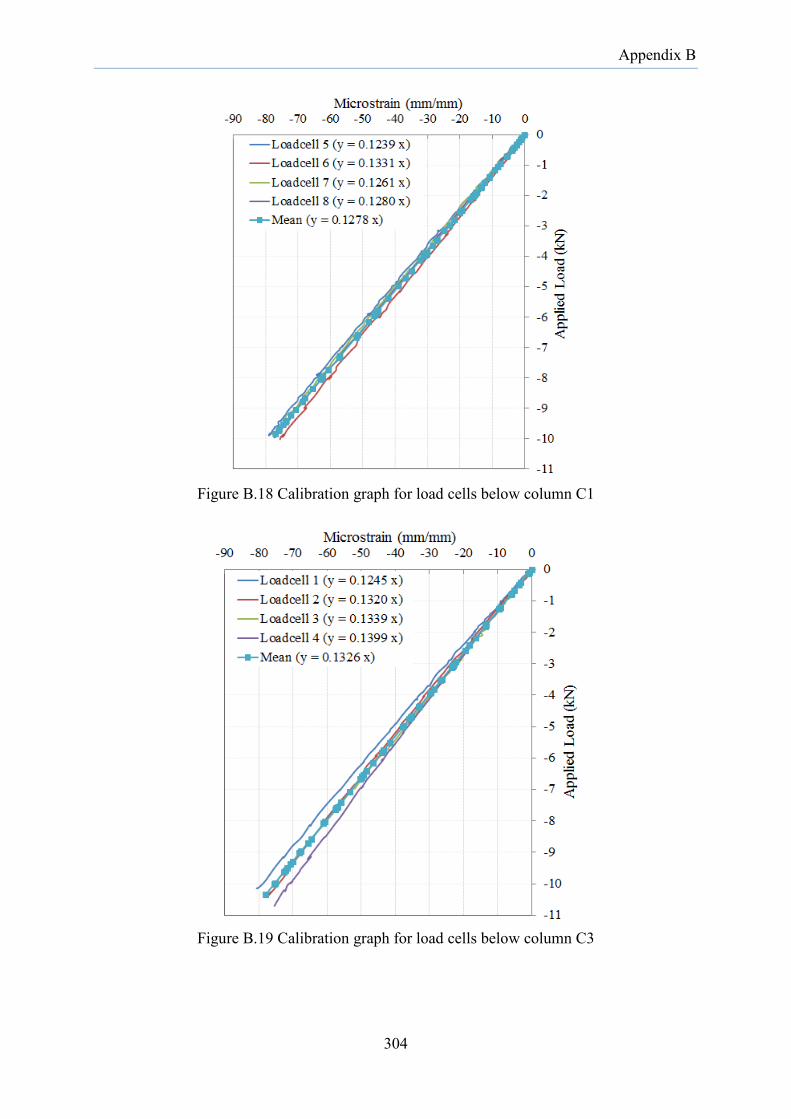
Appendix B
Figure B.18 Calibration graph for load cells below column C1
Figure B.19 Calibration graph for load cells below column C3
304

Appendix B
B.4. Geometric imperfections in column specimens
Figure B.20 Imperfections at two ends of C-section (specimen T1-C3)
305

Appendix B
Figure B.21 Measured imperfection profiles along C-section (specimen T1-C3)
306
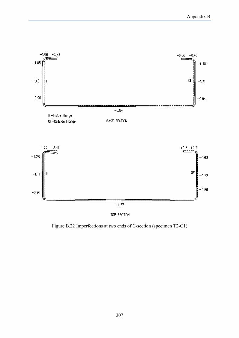
Appendix B
Figure B.22 Imperfections at two ends of C-section (specimen T2-C1)
307
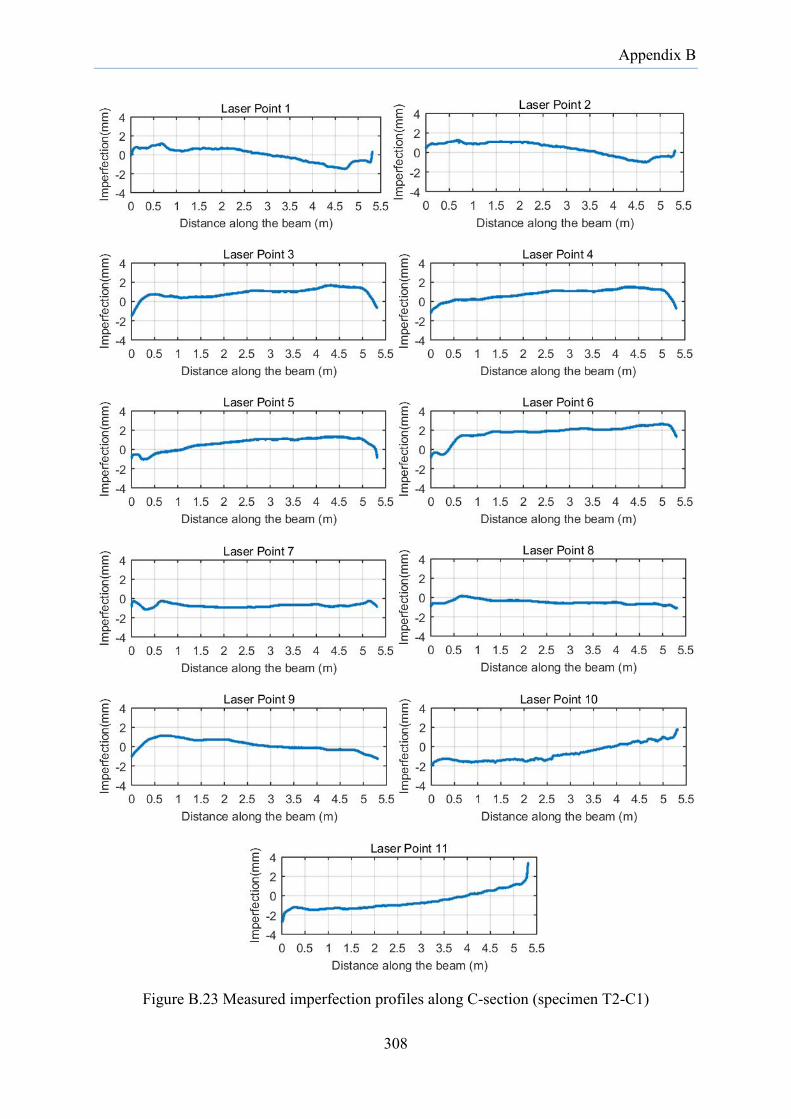
Appendix B
Figure B.23 Measured imperfection profiles along C-section (specimen T2-C1)
308
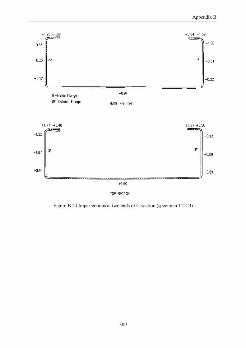
Appendix B
Figure B.24 Imperfections at two ends of C-section (specimen T2-C3)
309

Appendix B
Figure B.25 Measured imperfection profiles along C-section (specimen T2-C3)
310

Appendix B
Figure B.26 Imperfections at two ends of C-section (specimen T3-C1)
311

Appendix B
Figure B.27 Measured imperfection profiles along C-section (specimen T3-C1)
312

Appendix B
Figure B.28 Imperfections at two ends of C-section (specimen T3-C3)
313

Appendix B
Figure B.29 Measured imperfection profiles along C-section (specimen T3-C3)
314
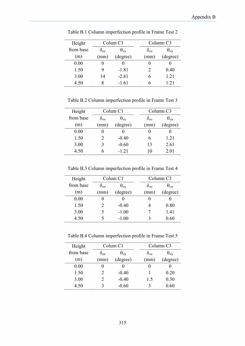
Appendix B
Table B.1 Column imperfection profile in Frame Test 2
Height from base
(m)
Colum C1 Column C3 δoz
(mm) θoy
(degree) δoz
(mm) θoy
(degree) 0.00 0 0 0 0 1.50 9 -1.81 2 0.40 3.00 14 -2.81 6 1.21 4.50 8 -1.61 6 1.21
Table B.2 Column imperfection profile in Frame Test 3
Height from base
(m)
Colum C1 Column C3 δoz
(mm) θoy
(degree) δoz
(mm) θoy
(degree) 0.00 0 0 0 0 1.50 2 -0.40 6 1.21 3.00 3 -0.60 13 2.61 4.50 6 -1.21 10 2.01
Table B.3 Column imperfection profile in Frame Test 4
Height from base
(m)
Colum C1 Column C3 δoz
(mm) θoy
(degree) δoz
(mm) θoy
(degree) 0.00 0 0 0 0 1.50 2 -0.40 4 0.80 3.00 5 -1.00 7 1.41 4.50 5 -1.00 3 0.60
Table B.4 Column imperfection profile in Frame Test 5
Height from base
(m)
Colum C1 Column C3 δoz
(mm) θoy
(degree) δoz
(mm) θoy
(degree) 0.00 0 0 0 0 1.50 2 -0.40 1 0.20 3.00 2 -0.40 1.5 0.30 4.50 3 -0.60 3 0.60
315
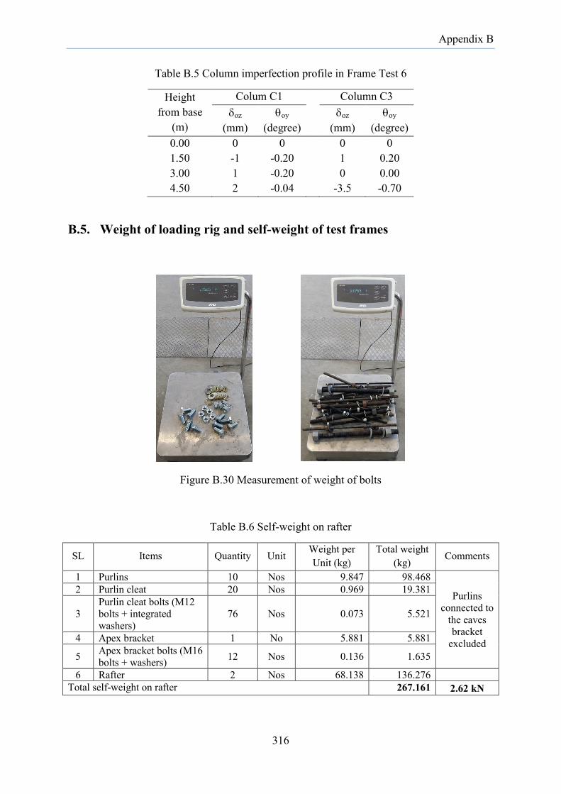
Appendix B
Table B.5 Column imperfection profile in Frame Test 6
Height from base
(m)
Colum C1 Column C3 δoz
(mm) θoy
(degree) δoz
(mm) θoy
(degree) 0.00 0 0 0 0 1.50 -1 -0.20 1 0.20 3.00 1 -0.20 0 0.00 4.50 2 -0.04 -3.5 -0.70
B.5. Weight of loading rig and self-weight of test frames
Figure B.30 Measurement of weight of bolts
Table B.6 Self-weight on rafter
SL Items Quantity Unit Weight per Unit (kg)
Total weight (kg)
Comments
1 Purlins 10 Nos 9.847 98.468
Purlins connected to
the eaves bracket
excluded
2 Purlin cleat 20 Nos 0.969 19.381
3 Purlin cleat bolts (M12 bolts + integrated washers)
76 Nos 0.073 5.521
4 Apex bracket 1 No 5.881 5.881
5 Apex bracket bolts (M16 bolts + washers) 12 Nos 0.136 1.635
6 Rafter 2 Nos 68.138 136.276 Total self-weight on rafter 267.161 2.62 kN
316
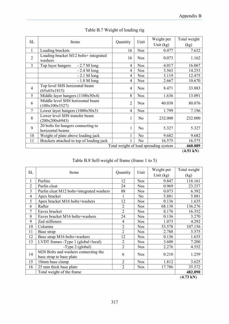
Appendix B
Table B.7 Weight of loading rig
SL Items Quantity Unit Weight per Unit (kg)
Total weight (kg)
1 Loading brackets 16 Nos 0.477 7.632
2 Loading bracket M12 bolts+ integrated washers 16 Nos 0.073 1.162
3 Top layer hangers - 2.7 M long 4 Nos 4.017 16.067 - 2.4 M long 4 Nos 3.563 14.253 - 2.1 M long 4 Nos 3.119 12.475 - 1.8 M long 4 Nos 2.667 10.670
4 Top level SHS horizontal beam (65x65x1815) 4 Nos 8.471 33.883
5 Middle layer hangers (1100x50x4) 8 Nos 1.636 13.091
6 Middle level SHS horizontal beam (100x100x3527) 2 Nos 40.038 80.076
7 Lower layer hangers (1000x50x5) 4 Nos 1.799 7.196
8 Lower level SHS transfer beam (200x200x6943) 1 No 232.000 232.000
9 20 bolts for hangers connecting to horizontal beams 1 No 5.327 5.327
10 Weight of plate above loading jack 1 No 9.682 9.682 11 Brackets attached to top of loading jack 1 No 16.575 16.575
Total weight of load spreading system 460.089 (4.51 kN)
Table B.8 Self-weight of frame (frame 1 to 5)
SL Items Quantity Unit Weight per Unit (kg)
Total weight (kg)
1 Purlins 12 Nos 9.847 118.161 2 Purlin cleat 24 Nos 0.969 23.257 3 Purlin cleat M12 bolts+integrated washers 88 Nos 0.073 6.392 4 Apex bracket 1 No 5.881 5.881 5 Apex bracket M16 bolts+washers 12 Nos 0.136 1.635 6 Rafter 2 Nos 68.138 136.276 7 Eaves bracket 2 Nos 8.176 16.352 8 Eaves bracket M16 bolts+washers 24 Nos 0.136 3.270 9 Zed stiffeners 4 Nos 1.073 4.292
10 Columns 2 Nos 53.578 107.156 11 Base strap 2 Nos 2.788 5.575 12 Base strap M16 bolts+washers 12 Nos 0.136 1.635 13 LVDT frames -Type 1 (global+local) 2 Nos 3.600 7.200 -Type 2 (global) 2 Nos 2.276 4.552
14 M20 Bolts and washers connecting the base strap to base plate 6 Nos 0.210 1.259
15 10mm base clamp 2 Nos 1.812 3.625 16 25 mm thick base plate 2 Nos 17.786 35.572 Total weight of the frame 482.090
(4.73 kN)
317

Appendix B
Table B.9 Self-weight of frame 6
SL Items Quantity Unit Weight per Unit (kg)
Total weight (kg)
1 Purlins 12 Nos 9.847 118.161 2 Purlin cleat 24 Nos 0.969 23.257 3 Purlin cleat M12 bolts+integrated washers 88 Nos 0.073 6.392 4 Apex bracket 1 No 5.881 5.881 5 Apex bracket M16 bolts+washers 12 Nos 0.136 1.635 6 Rafter 2 Nos 68.138 136.276 7 Eaves bracket 2 Nos 8.176 16.352 8 Eaves bracket M16 bolts+washers 24 Nos 0.136 3.270 9 Zed stiffeners 4 Nos 1.073 4.292
10 Columns 2 Nos 53.578 107.156 11 Girts 8 Nos 9.847 78.774 12 Girt cleats 16 Nos 0.969 15.505 13 Girt cleat M12 bolts + washers 48 Nos 0.073 3.487 11 Base strap 2 Nos 2.788 5.575 12 Base strap M16 bolts+washers 12 Nos 0.136 1.635 13 LVDT frames - Type 1 (global+local) 2 Nos 3.600 7.200
- Type 2 (global) 2 Nos 2.276 4.552
14 M20 Bolts and washers connecting the base strap to base plate 6 Nos 0.210 1.259
15 10mm base clamp 2 Nos 1.812 3.625 16 25 mm thick base plate 2 Nos 17.786 35.572 Total weight of the frame 579.855
(5.69 kN)
318

Appendix B
B.6. Frame Tests - supplementary results
Figure B.31 Applied load versus twist rotation of columns at 240 mm above base plate
Figure B.32 Applied load versus in-plane displacement at mid-height of columns
319
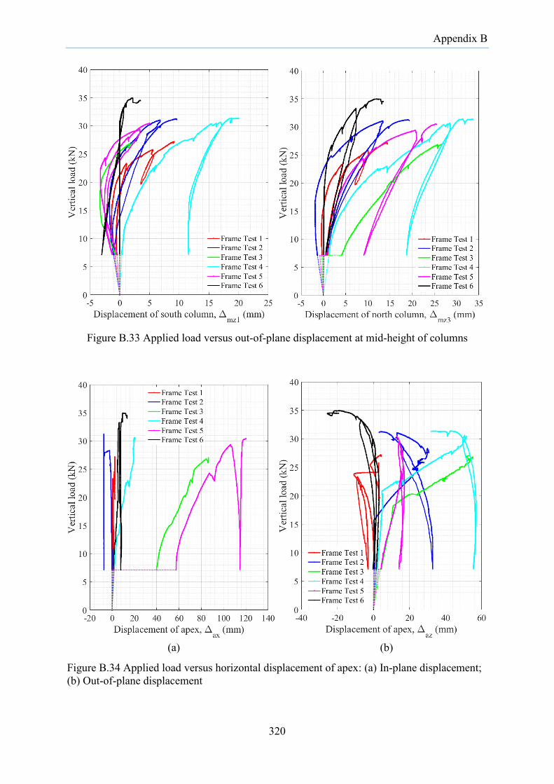
Appendix B
Figure B.33 Applied load versus out-of-plane displacement at mid-height of columns
(a) (b)
Figure B.34 Applied load versus horizontal displacement of apex: (a) In-plane displacement; (b) Out-of-plane displacement
320

Appendix B
Figure B.35 Applied load versus out-of-plane displacement of apex of end frame on grid C
Figure B.36 Applied load versus in-plane base rotation of columns
321
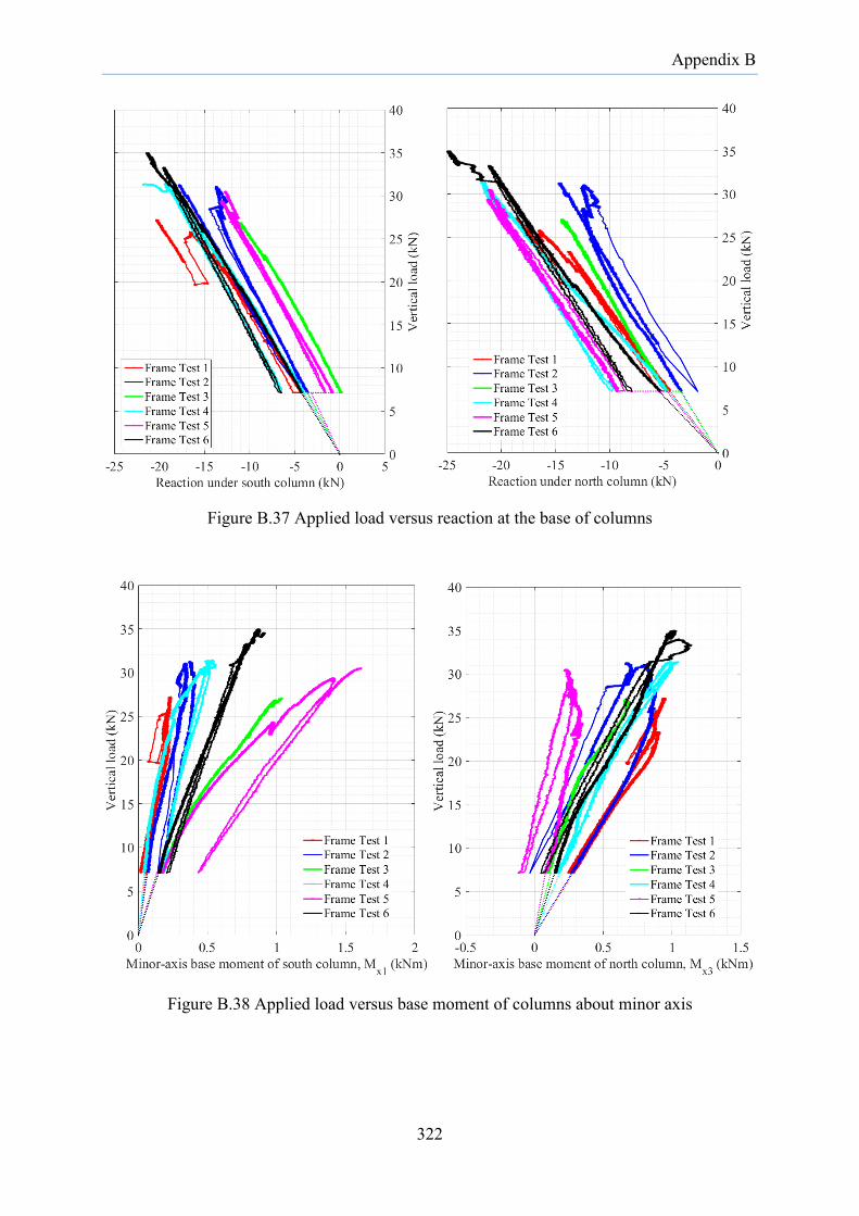
Appendix B
Figure B.37 Applied load versus reaction at the base of columns
Figure B.38 Applied load versus base moment of columns about minor axis
322
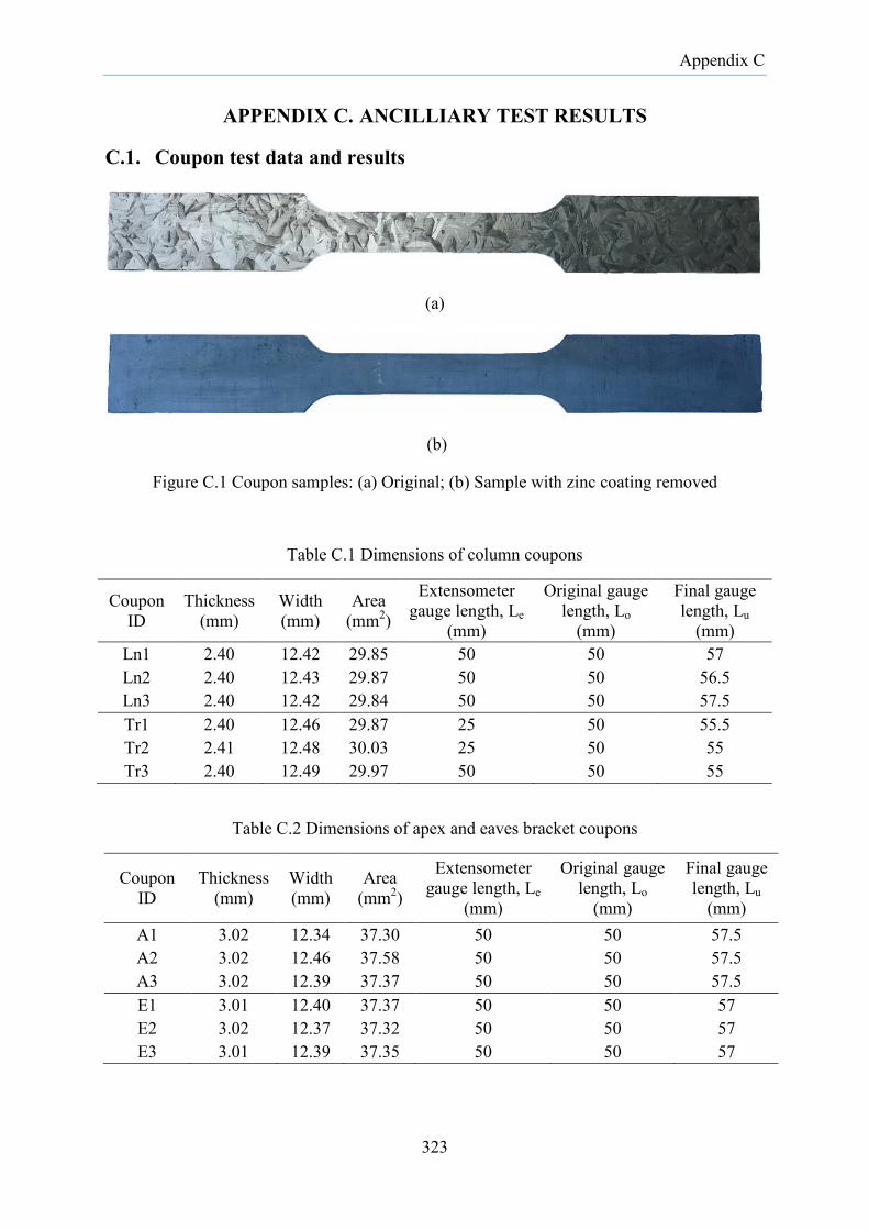
Appendix C
APPENDIX C. ANCILLIARY TEST RESULTS
C.1. Coupon test data and results
(a)
(b)
Figure C.1 Coupon samples: (a) Original; (b) Sample with zinc coating removed
Table C.1 Dimensions of column coupons
Coupon ID
Thickness (mm)
Width (mm)
Area (mm2)
Extensometer gauge length, Le
(mm)
Original gauge length, Lo
(mm)
Final gauge length, Lu
(mm) Ln1 2.40 12.42 29.85 50 50 57 Ln2 2.40 12.43 29.87 50 50 56.5 Ln3 2.40 12.42 29.84 50 50 57.5 Tr1 2.40 12.46 29.87 25 50 55.5 Tr2 2.41 12.48 30.03 25 50 55 Tr3 2.40 12.49 29.97 50 50 55
Table C.2 Dimensions of apex and eaves bracket coupons
Coupon ID
Thickness (mm)
Width (mm)
Area (mm2)
Extensometer gauge length, Le
(mm)
Original gauge length, Lo
(mm)
Final gauge length, Lu
(mm) A1 3.02 12.34 37.30 50 50 57.5 A2 3.02 12.46 37.58 50 50 57.5 A3 3.02 12.39 37.37 50 50 57.5 E1 3.01 12.40 37.37 50 50 57 E2 3.02 12.37 37.32 50 50 57 E3 3.01 12.39 37.35 50 50 57
323
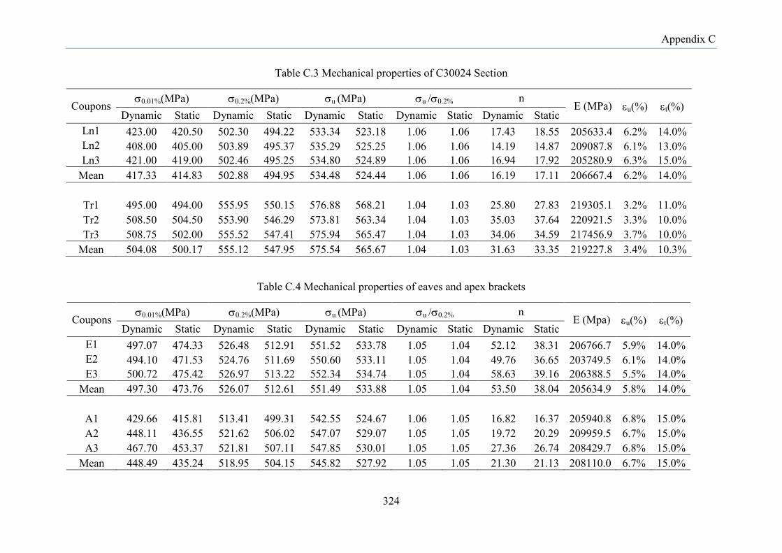
Appendix C
Table C.3 Mechanical properties of C30024 Section
Coupons σ0.01%(MPa) σ0.2%(MPa) σu (MPa) σu /σ0.2% n
E (MPa) εu(%) εt(%) Dynamic Static Dynamic Static Dynamic Static Dynamic Static Dynamic Static
Ln1 423.00 420.50 502.30 494.22 533.34 523.18 1.06 1.06 17.43 18.55 205633.4 6.2% 14.0% Ln2 408.00 405.00 503.89 495.37 535.29 525.25 1.06 1.06 14.19 14.87 209087.8 6.1% 13.0% Ln3 421.00 419.00 502.46 495.25 534.80 524.89 1.06 1.06 16.94 17.92 205280.9 6.3% 15.0%
Mean 417.33 414.83 502.88 494.95 534.48 524.44 1.06 1.06 16.19 17.11 206667.4 6.2% 14.0%
Tr1 495.00 494.00 555.95 550.15 576.88 568.21 1.04 1.03 25.80 27.83 219305.1 3.2% 11.0% Tr2 508.50 504.50 553.90 546.29 573.81 563.34 1.04 1.03 35.03 37.64 220921.5 3.3% 10.0% Tr3 508.75 502.00 555.52 547.41 575.94 565.47 1.04 1.03 34.06 34.59 217456.9 3.7% 10.0%
Mean 504.08 500.17 555.12 547.95 575.54 565.67 1.04 1.03 31.63 33.35 219227.8 3.4% 10.3%
Table C.4 Mechanical properties of eaves and apex brackets
Coupons σ0.01%(MPa) σ0.2%(MPa) σu (MPa) σu /σ0.2% n
E (Mpa) εu(%) εt(%) Dynamic Static Dynamic Static Dynamic Static Dynamic Static Dynamic Static
E1 497.07 474.33 526.48 512.91 551.52 533.78 1.05 1.04 52.12 38.31 206766.7 5.9% 14.0% E2 494.10 471.53 524.76 511.69 550.60 533.11 1.05 1.04 49.76 36.65 203749.5 6.1% 14.0% E3 500.72 475.42 526.97 513.22 552.34 534.74 1.05 1.04 58.63 39.16 206388.5 5.5% 14.0%
Mean 497.30 473.76 526.07 512.61 551.49 533.88 1.05 1.04 53.50 38.04 205634.9 5.8% 14.0%
A1 429.66 415.81 513.41 499.31 542.55 524.67 1.06 1.05 16.82 16.37 205940.8 6.8% 15.0% A2 448.11 436.55 521.62 506.02 547.07 529.07 1.05 1.05 19.72 20.29 209959.5 6.7% 15.0% A3 467.70 453.37 521.81 507.11 547.85 530.01 1.05 1.05 27.36 26.74 208429.7 6.8% 15.0%
Mean 448.49 435.24 518.95 504.15 545.82 527.92 1.05 1.05 21.30 21.13 208110.0 6.7% 15.0%
324
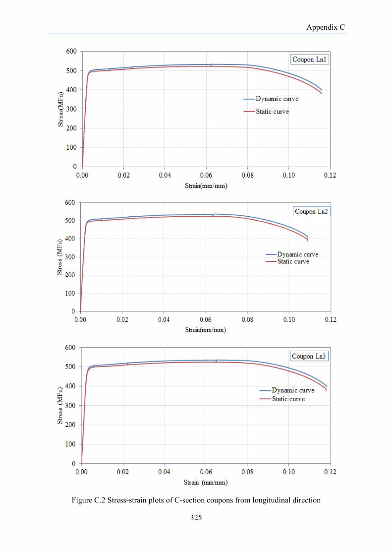
Appendix C
Figure C.2 Stress-strain plots of C-section coupons from longitudinal direction
325
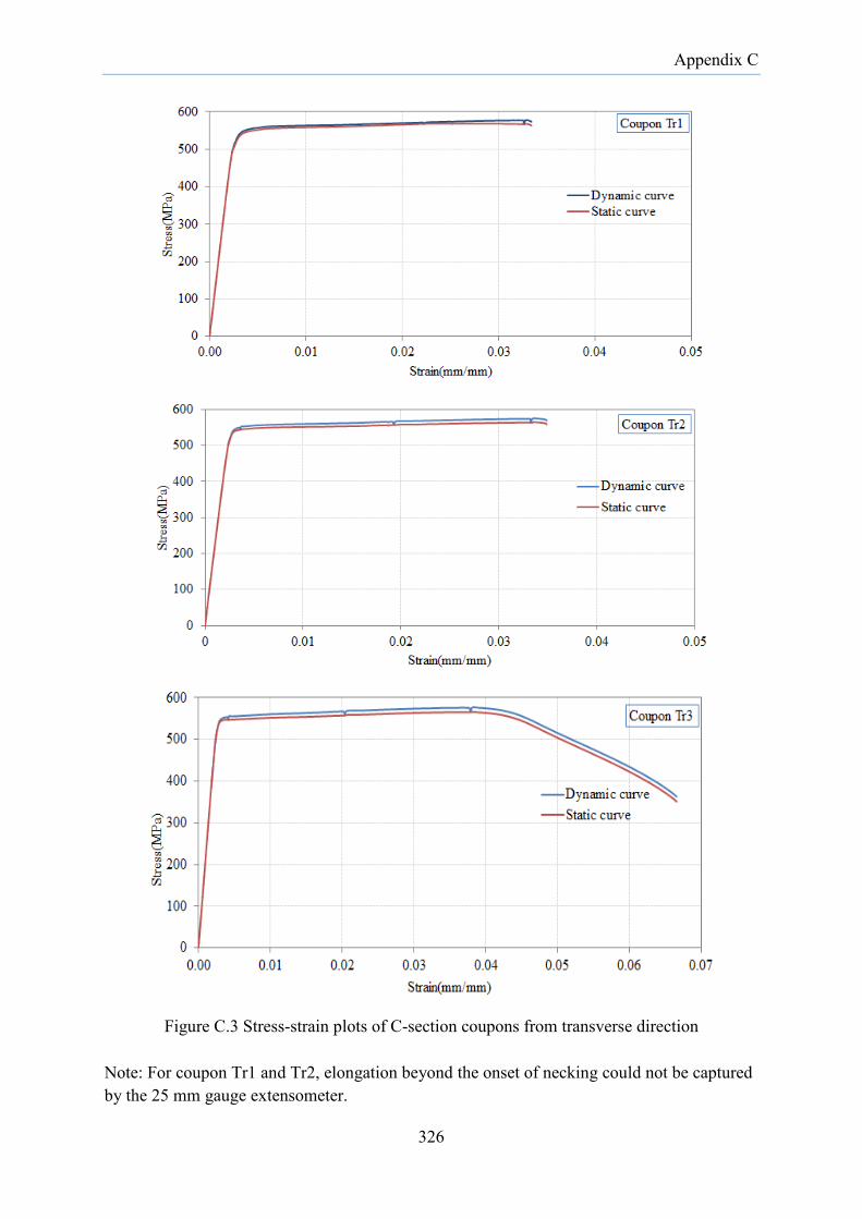
Appendix C
Figure C.3 Stress-strain plots of C-section coupons from transverse direction
Note: For coupon Tr1 and Tr2, elongation beyond the onset of necking could not be captured by the 25 mm gauge extensometer.
326

Appendix C
Figure C.4 Stress-strain plots of coupons from apex bracket
327
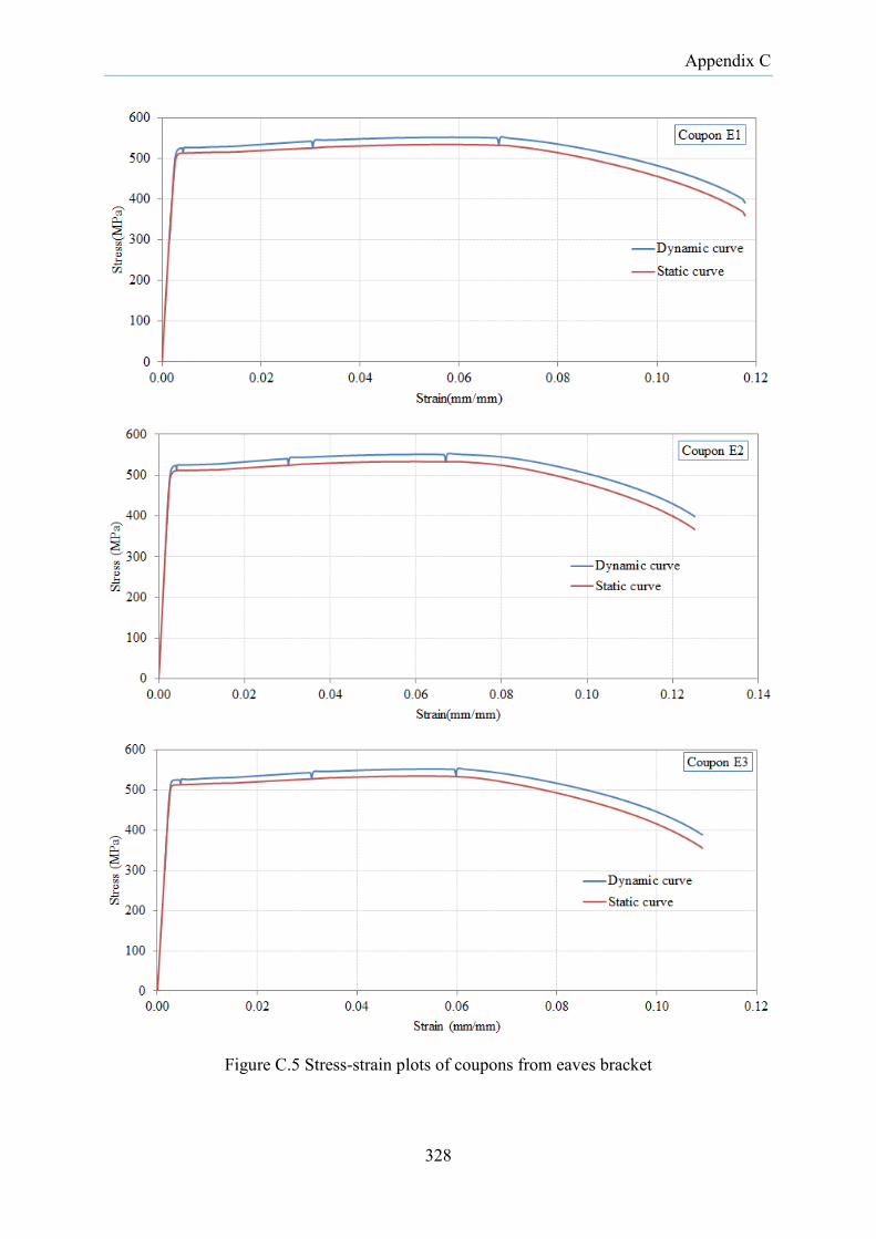
Appendix C
Figure C.5 Stress-strain plots of coupons from eaves bracket
328
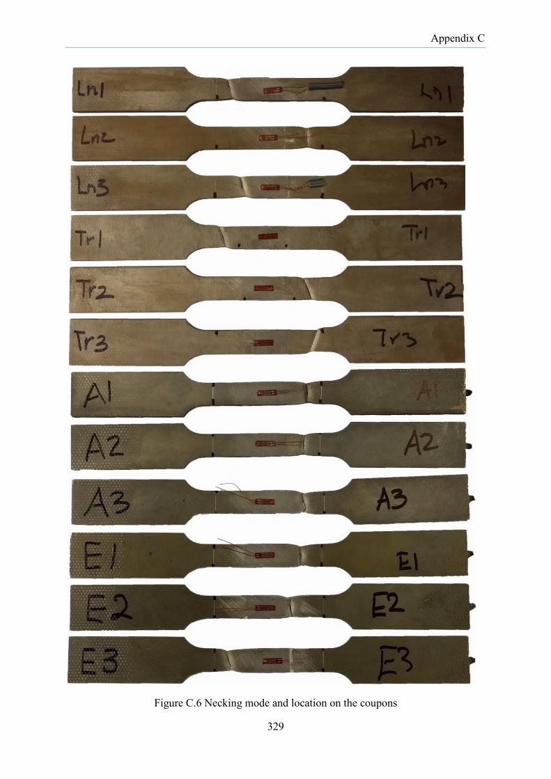
Appendix C
Figure C.6 Necking mode and location on the coupons
329
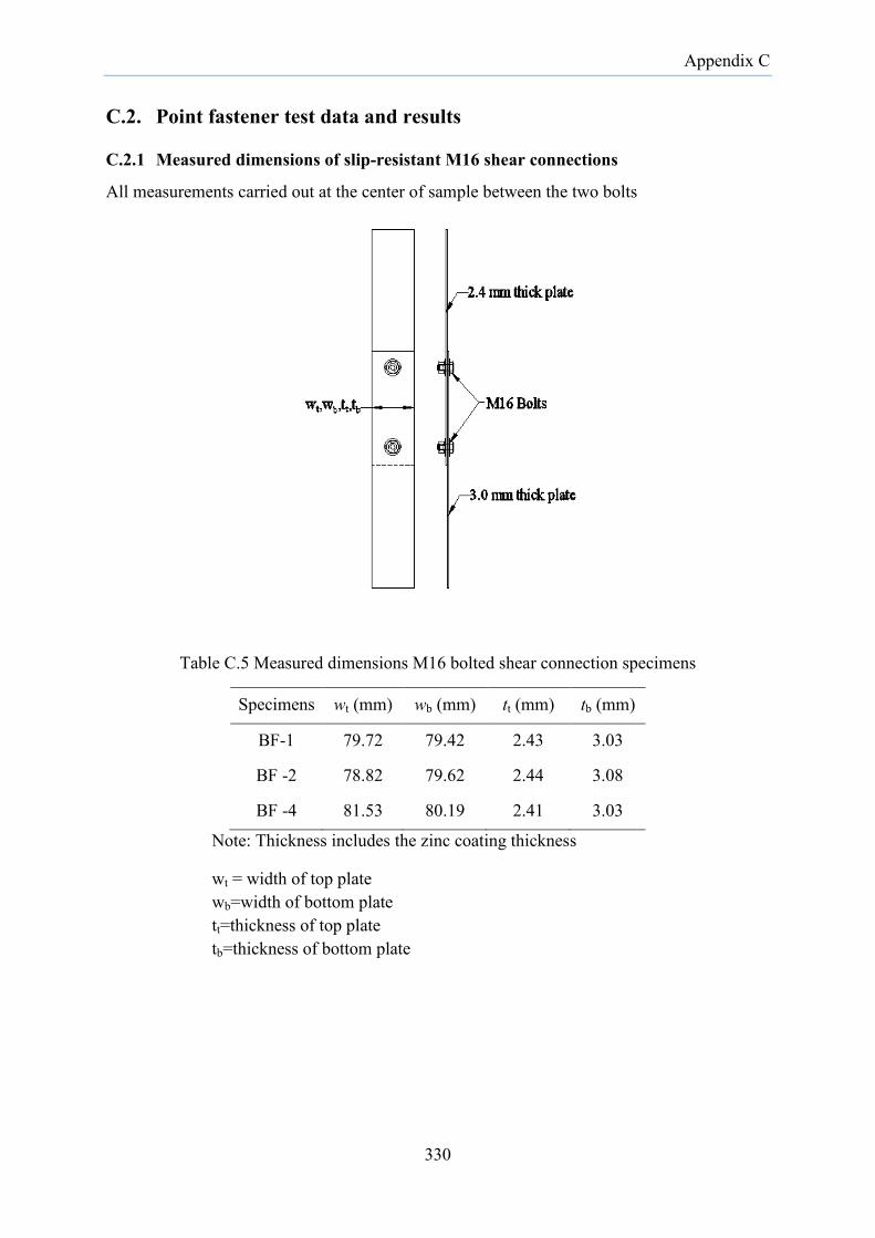
Appendix C
C.2. Point fastener test data and results
C.2.1 Measured dimensions of slip-resistant M16 shear connections
All measurements carried out at the center of sample between the two bolts
Table C.5 Measured dimensions M16 bolted shear connection specimens
Specimens wt (mm) wb (mm) tt (mm) tb (mm)
BF-1 79.72 79.42 2.43 3.03
BF -2 78.82 79.62 2.44 3.08
BF -4 81.53 80.19 2.41 3.03
Note: Thickness includes the zinc coating thickness
wt = width of top plate wb=width of bottom plate tt=thickness of top plate tb=thickness of bottom plate
330
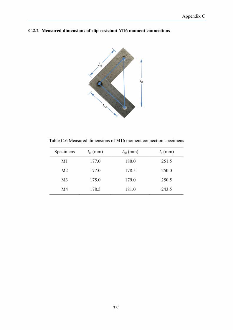
Appendix C
C.2.2 Measured dimensions of slip-resistant M16 moment connections
Table C.6 Measured dimensions of M16 moment connection specimens
Specimens lto (mm) lbo (mm) lo (mm)
M1 177.0 180.0 251.5
M2 177.0 178.5 250.0
M3 175.0 179.0 250.5
M4 178.5 181.0 243.5
lo
lto
lbo
331
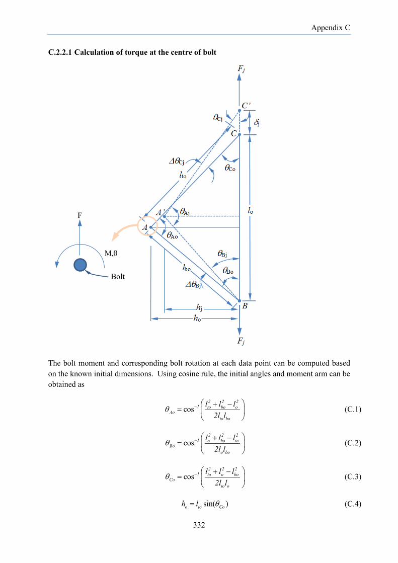
Appendix C
C.2.2.1 Calculation of torque at the centre of bolt
The bolt moment and corresponding bolt rotation at each data point can be computed based on the known initial dimensions. Using cosine rule, the initial angles and moment arm can be obtained as
cos2 2 2
1 to bo oAo
to bo
l l l2l l
θ − + −=
(C.1)
cos2 2 2
1 o bo toBo
o bo
l l l2l l
θ − + −=
(C.2)
cos2 2 2
1 to o boCo
to o
l l l2l l
θ − + −=
(C.3)
sin( )o to Coh l θ= (C.4)
F
M,θ
Bolt
332
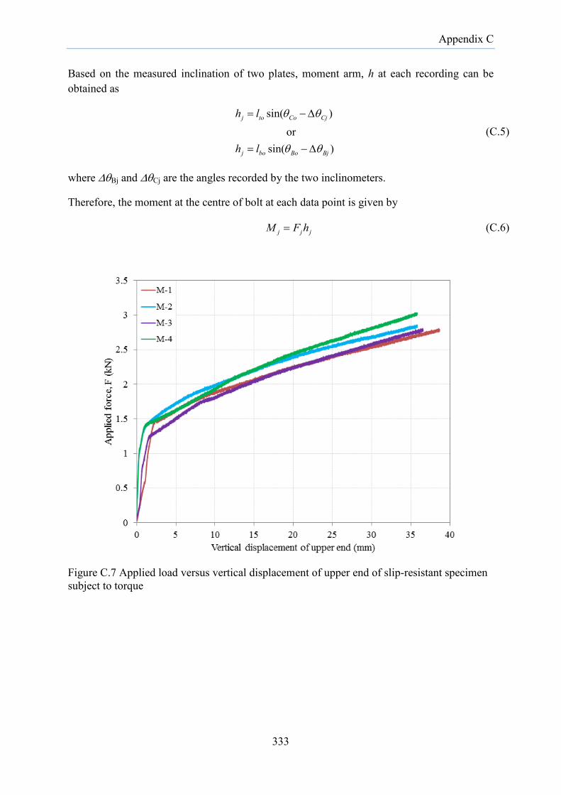
Appendix C
Based on the measured inclination of two plates, moment arm, h at each recording can be obtained as
sin( )
orsin( )
j to Co Cj
j bo Bo Bj
h l
h l
θ θ
θ θ
= −∆
= −∆ (C.5)
where ∆θBj and ∆θCj are the angles recorded by the two inclinometers.
Therefore, the moment at the centre of bolt at each data point is given by
j j jM F h= (C.6)
Figure C.7 Applied load versus vertical displacement of upper end of slip-resistant specimen subject to torque
333
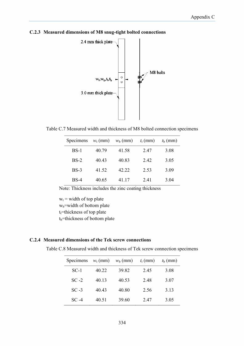
Appendix C
C.2.3 Measured dimensions of M8 snug-tight bolted connections
Table C.7 Measured width and thickness of M8 bolted connection specimens
Specimens wt (mm) wb (mm) tt (mm) tb (mm)
BS-1 40.79 41.58 2.47 3.08
BS-2 40.43 40.83 2.42 3.05
BS-3 41.52 42.22 2.53 3.09
BS-4 40.65 41.17 2.41 3.04
Note: Thickness includes the zinc coating thickness
wt = width of top plate wb=width of bottom plate tt=thickness of top plate tb=thickness of bottom plate
C.2.4 Measured dimensions of the Tek screw connections
Table C.8 Measured width and thickness of Tek screw connection specimens
Specimens wt (mm) wb (mm) tt (mm) tb (mm)
SC-1 40.22 39.82 2.45 3.08
SC -2 40.13 40.53 2.48 3.07
SC -3 40.43 40.80 2.56 3.13
SC -4 40.51 39.60 2.47 3.05
334
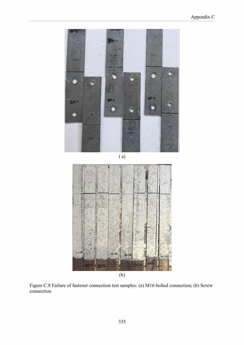
Appendix C
( a)
(b)
Figure C.8 Failure of fastener connection test samples: (a) M16 bolted connection; (b) Screw connection
335

Appendix C
C.3. Frame connection data and results
C.3.1 Measurement of initial moment arm for eaves connection
Table C.9 Measured dimensions of heights of eaves connection specimens
Tests No. h1 (mm) h2 (mm) h3 (mm)
EC-1-1 847 337 250
EC-1-2 844 337 250
EC-2-1 845 337 250
EC-2-2 847 337 250
EC-3-1 840 337 250
EC-3-2 846 337 250
h1 Distance between the underside of eaves bracket to the top of the beam h2 Distance from the underside of eaves bracket to the intersection of column centerlines h3 Distance from the top of the beam to the centerline of load
h1
h3
h2
336

Appendix C
Figure C.9 Eaves bracket with plate stiffener details
337

Appendix C
Figure C.10 Applied load versus out-of-plane displacement of eaves bracket
338
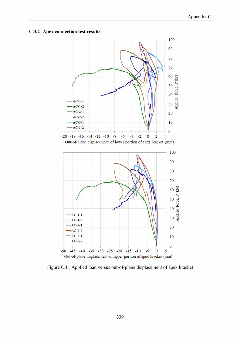
Appendix C
C.3.2 Apex connection test results
Figure C.11 Applied load versus out-of-plane displacement of apex bracket
339

Appendix C
C.3.3 Base connection test results
C.3.3.1 Major axis bending tests
Figure C.12 Load versus displacement above the column base (specimen BC-1-1)
Figure C.13 Load versus twist rotation of column (specimen BC-1-1)
340

Appendix C
Figure C.14 Load versus displacement above the column base (specimen BC-1-2)
Figure C.15 Load versus twist rotation of column (specimen BC-1-2)
341

Appendix C
C.3.3.2 Minor axis bending tests
Figure C.16 Load versus displacement above the column base (specimen BC-2T-1)
Figure C.17 Load versus twist rotation of column (specimen BC-2T-1)
342

Appendix C
Figure C.18 Load versus displacement above the column base (Specimen BC-2T-2)
Figure C.19 Base moment versus rotations above the column base (specimen BC-2T-2)
343

Appendix C
Figure C.20 Load versus twist rotation of column (specimen BC-2T-2)
Figure C.21 Load versus displacement above the column base (specimen BC-2C-1)
344

Appendix C
Figure C.22 Base moment versus rotations above the column base (specimen BC-2C-1)
Figure C.23 Load versus twist rotation of column (specimen BC-2C-1)
345
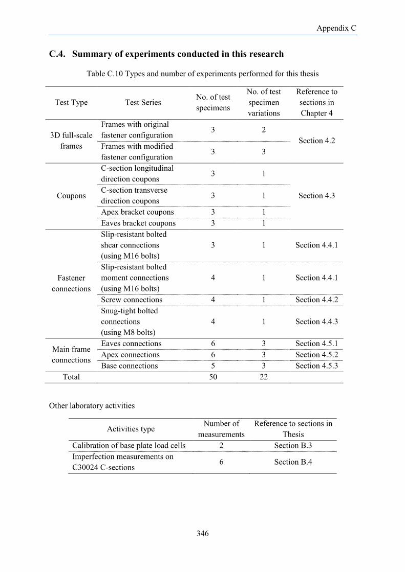
Appendix C
C.4. Summary of experiments conducted in this research
Table C.10 Types and number of experiments performed for this thesis
Test Type Test Series No. of test specimens
No. of test specimen variations
Reference to sections in Chapter 4
3D full-scale frames
Frames with original fastener configuration 3 2
Section 4.2 Frames with modified fastener configuration 3 3
Coupons
C-section longitudinal direction coupons 3 1
Section 4.3 C-section transverse direction coupons 3 1
Apex bracket coupons 3 1 Eaves bracket coupons 3 1
Fastener connections
Slip-resistant bolted shear connections (using M16 bolts)
3 1 Section 4.4.1
Slip-resistant bolted moment connections (using M16 bolts)
4 1 Section 4.4.1
Screw connections 4 1 Section 4.4.2 Snug-tight bolted connections (using M8 bolts)
4 1 Section 4.4.3
Main frame connections
Eaves connections 6 3 Section 4.5.1 Apex connections 6 3 Section 4.5.2 Base connections 5 3 Section 4.5.3
Total 50 22
Other laboratory activities
Activities type Number of measurements
Reference to sections in Thesis
Calibration of base plate load cells 2 Section B.3 Imperfection measurements on C30024 C-sections
6 Section B.4
346
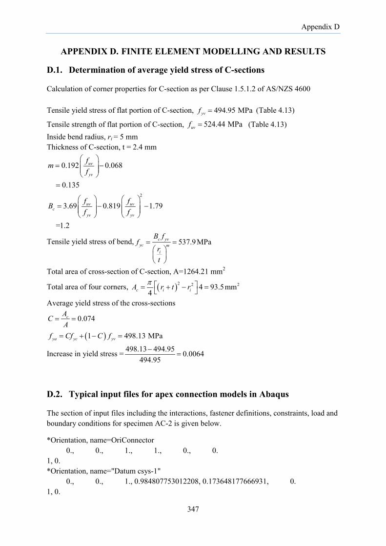
Appendix D
APPENDIX D. FINITE ELEMENT MODELLING AND RESULTS
D.1. Determination of average yield stress of C-sections
Calculation of corner properties for C-section as per Clause 1.5.1.2 of AS/NZS 4600 Tensile yield stress of flat portion of C-section, 494.95 MPayvf = (Table 4.13)
Tensile strength of flat portion of C-section, 524.44 MPauvf = (Table 4.13) Inside bend radius, ri = 5 mm Thickness of C-section, t = 2.4 mm
2
0.192 0.068
0.135
3.69 0.819 1.79
=1.2
= −
=
= − −
uv
yv
uv uvc
yv yv
fmf
f fBf f
Tensile yield stress of bend, 537.9MPac yvyc m
i
B ff
rt
= =
Total area of cross-section of C-section, A=1264.21 mm2
Total area of four corners, ( )2 2 24 93.5mm4c i iA r t rπ = + − =
Average yield stress of the cross-sections
0.074= =cACA
( )1 498.13 MPaya yc yvf Cf C f= + − =
Increase in yield stress = 498.13 494.95 0.0064494.95−
=
D.2. Typical input files for apex connection models in Abaqus
The section of input files including the interactions, fastener definitions, constraints, load and boundary conditions for specimen AC-2 is given below.
*Orientation, name=OriConnector 0., 0., 1., 1., 0., 0. 1, 0. *Orientation, name="Datum csys-1" 0., 0., 1., 0.984807753012208, 0.173648177666931, 0. 1, 0.
347
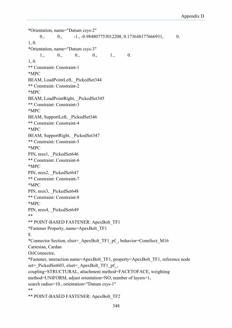
Appendix D
*Orientation, name="Datum csys-2" 0., 0., -1., -0.984807753012208, 0.173648177666931, 0. 1, 0. *Orientation, name="Datum csys-3" 1., 0., 0., 0., 1., 0. 1, 0. ** Constraint: Constraint-1 *MPC BEAM, LoadPointLeft, _PickedSet344 ** Constraint: Constraint-2 *MPC BEAM, LoadPointRight, _PickedSet345 ** Constraint: Constraint-3 *MPC BEAM, SupportLeft, _PickedSet346 ** Constraint: Constraint-4 *MPC BEAM, SupportRight, _PickedSet347 ** Constraint: Constraint-5 *MPC PIN, nres1, _PickedSet646 ** Constraint: Constraint-6 *MPC PIN, nres2, _PickedSet647 ** Constraint: Constraint-7 *MPC PIN, nres3, _PickedSet648 ** Constraint: Constraint-8 *MPC PIN, nres4, _PickedSet649 ** ** POINT-BASED FASTENER: ApexBolt_TF1 *Fastener Property, name=ApexBolt_TF1 8. *Connector Section, elset=_ApexBolt_TF1_pf_, behavior=ConnSect_M16 Cartesian, Cardan OriConnector, *Fastener, interaction name=ApexBolt_TF1, property=ApexBolt_TF1, reference node set=_PickedSet603, elset=_ApexBolt_TF1_pf_, coupling=STRUCTURAL, attachment method=FACETOFACE, weighting method=UNIFORM, adjust orientation=NO, number of layers=1, search radius=10., orientation="Datum csys-1" ** ** POINT-BASED FASTENER: ApexBolt_TF2
348

Appendix D
*Fastener Property, name=ApexBolt_TF2 8. *Connector Section, elset=_ApexBolt_TF2_pf_, behavior=ConnSect_M16 Cartesian, Cardan OriConnector, *Fastener, interaction name=ApexBolt_TF2, property=ApexBolt_TF2, reference node set=_PickedSet604, elset=_ApexBolt_TF2_pf_, coupling=STRUCTURAL, attachment method=FACETOFACE, weighting method=UNIFORM, adjust orientation=NO, number of layers=1, search radius=10., radius of influence=16., orientation="Datum csys-2" ** ** POINT-BASED FASTENER: ApexBolt_Web *Fastener Property, name=ApexBolt_Web 8. *Connector Section, elset=_ApexBolt_Web_pf_, behavior=ConnSect_M16 Cartesian, Cardan OriConnector, *Fastener, interaction name=ApexBolt_Web, property=ApexBolt_Web, reference node set=_PickedSet605, elset=_ApexBolt_Web_pf_, coupling=STRUCTURAL, attachment method=FACETOFACE, weighting method=UNIFORM, adjust orientation=NO, number of layers=1, search radius=10., radius of influence=16., orientation="Datum csys-3" ** ** POINT-BASED FASTENER: ApexScrews *Fastener Property, name=ApexScrews 2.75 *Connector Section, elset=_ApexScrews_pf_, behavior=ConnSect_Screws Cartesian, OriConnector, *Fastener, interaction name=ApexScrews, property=ApexScrews, reference node set=_PickedSet606, elset=_ApexScrews_pf_, coupling= STRUCTURAL, attachment method=FACETOFACE, weighting method=UNIFORM, adjust orientation=NO, number of layers=1, search radius=10., radius of influence=6., orientation="Datum csys-3" ** ** POINT-BASED FASTENER: PurlinCleatBoltCF *Fastener Property, name=PurlinCleatBoltCF 6. *Connector Section, elset=_PurlinCleatBoltCF_pf_ Beam, OriConnector, *Fastener, interaction name=PurlinCleatBoltCF, property=PurlinCleatBoltCF, reference node set=_PickedSet549, elset=_PurlinCleatBoltCF_pf_,
349

Appendix D
coupling= STRUCTURAL, attachment method=FACETOFACE, weighting method=UNIFORM, adjust orientation=NO, number of layers=1, search radius=20., orientation="Datum csys-3" *End Assembly *Connector Behavior, name=ConnSect_Axial *Connector Elasticity, component=1 25111., ** ** MATERIALS ** *Material, name=steelAll *Density 7.85e-06, *Elastic 207000., 0.3 *Plastic 350., 0. 350.68, 7e-06 400.85, 5.5e-05 423.55, 0.000118 453.2, 0.000214 472.73, 0.000349 480.73, 0.00058 491.91, 0.001144 496.79, 0.001897 501.38, 0.003457 503.12, 0.004591 506.54, 0.007499 525.48, 0.02215 533.55, 0.028917 541.61, 0.0366 549.56, 0.046131 555.83, 0.055579 559.72, 0.06495 *Material, name=steelApex *Density 7.85e-06, *Elastic 206000., 0.3 *Plastic 350.7, 0. 400.89, 4e-06 408.84, 1e-05 437.18, 7.2e-05
350

Appendix D
460.52, 0.000158 483.68, 0.000344 493.73, 0.000575 501.58, 0.000915 505.18, 0.001436 507.02, 0.002522 508.73, 0.004502 510.95, 0.007466 515.22, 0.012383 527.18, 0.022129 543.79, 0.036576 552.38, 0.046104 559.24, 0.055549 564.66, 0.064913 566.9, 0.074204 ** ** INTERACTION PROPERTIES ** *Surface Interaction, name=IntProp-1 1., *Surface Behavior, pressure-overclosure=HARD *Connector Behavior, name=ConnSect_M16 *Connector Elasticity, component=1 167012., *Connector Elasticity, component=2 167012., *Connector Elasticity, component=3 167012., *Connector Elasticity, component=4 2.75423e+07, *Connector Elasticity, component=5 2.75423e+07, *Connector Elasticity, component=6 2.75423e+07, *Connector Plasticity, component=1 *Connector Hardening, definition=TABULAR 18016., 0., 0. 26308., 3.69, 0. 40103., 5.84, 0. *Connector Plasticity, component=2 *Connector Hardening, definition=TABULAR 18016., 0., 0. 26308., 3.69, 0. 40103., 5.84, 0.
351

Appendix D
*Connector Plasticity, component=3 *Connector Hardening, definition=TABULAR 18016., 0., 0. 26308., 3.69, 0. 40103., 5.84, 0. *Connector Plasticity, component=4 *Connector Hardening, definition=TABULAR 174618.3, 0, 0 224421.2, 0.059887, 0 267972.4, 0.155423, 0 296600, 0.32366, 0 *Connector Behavior, name=ConnSect_Screws *Connector Elasticity, component=1 92314., *Connector Elasticity, component=2 92314., *Connector Elasticity, component=3 92314., *Connector Plasticity, component=1 *Connector Hardening, definition=TABULAR 3258.4, 0., 0. 3887.91, 2.1292, 0. 17879.5, 4.6716, 0. 20393.3, 6.9647, 0. *Connector Plasticity, component=2 *Connector Hardening, definition=TABULAR 3258.4, 0., 0. 3887.91, 2.1292, 0. 17879.5, 4.6716, 0. 20393.3, 6.9647, 0. *Connector Plasticity, component=3 *Connector Hardening, definition=TABULAR 3258.4, 0., 0. 3887.91, 2.1292, 0. 17879.5, 4.6716, 0. 20393.3, 6.9647, 0. ** ** BOUNDARY CONDITIONS ** ** Name: BC-1 Type: Displacement/Rotation *Boundary _PickedSet395, 2, 2 _PickedSet395, 3, 3 _PickedSet395, 4, 4
352
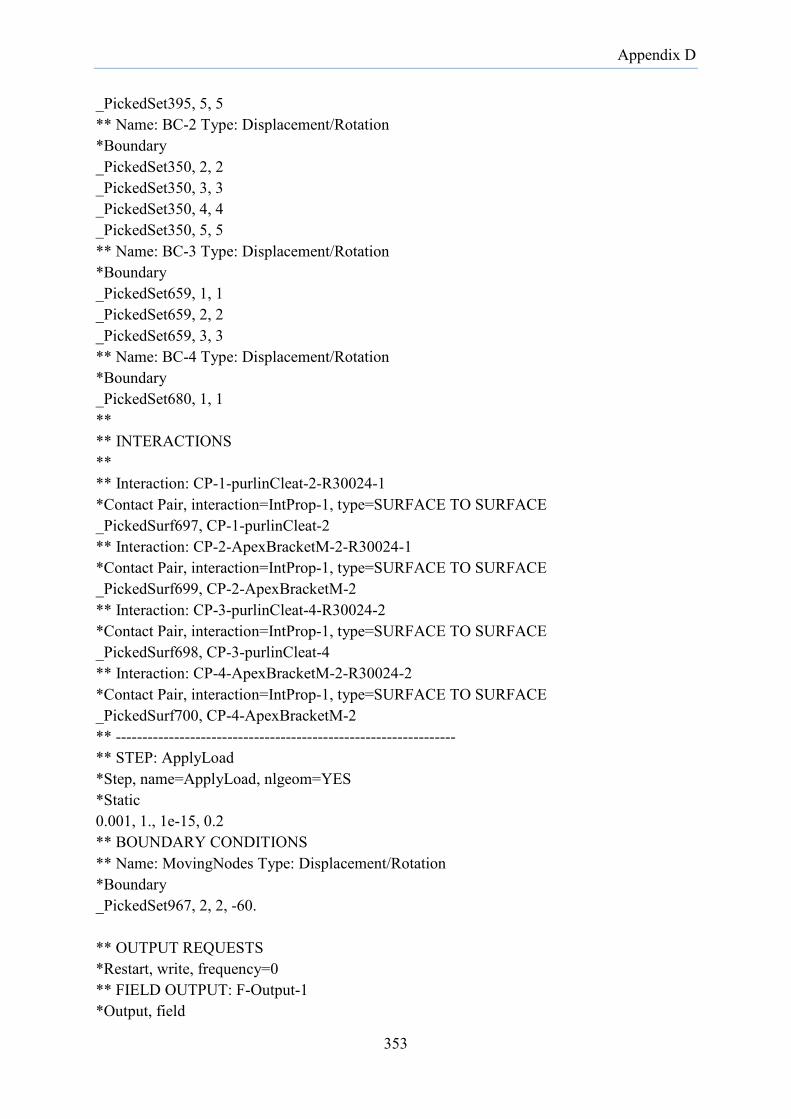
Appendix D
_PickedSet395, 5, 5 ** Name: BC-2 Type: Displacement/Rotation *Boundary _PickedSet350, 2, 2 _PickedSet350, 3, 3 _PickedSet350, 4, 4 _PickedSet350, 5, 5 ** Name: BC-3 Type: Displacement/Rotation *Boundary _PickedSet659, 1, 1 _PickedSet659, 2, 2 _PickedSet659, 3, 3 ** Name: BC-4 Type: Displacement/Rotation *Boundary _PickedSet680, 1, 1 ** ** INTERACTIONS ** ** Interaction: CP-1-purlinCleat-2-R30024-1 *Contact Pair, interaction=IntProp-1, type=SURFACE TO SURFACE _PickedSurf697, CP-1-purlinCleat-2 ** Interaction: CP-2-ApexBracketM-2-R30024-1 *Contact Pair, interaction=IntProp-1, type=SURFACE TO SURFACE _PickedSurf699, CP-2-ApexBracketM-2 ** Interaction: CP-3-purlinCleat-4-R30024-2 *Contact Pair, interaction=IntProp-1, type=SURFACE TO SURFACE _PickedSurf698, CP-3-purlinCleat-4 ** Interaction: CP-4-ApexBracketM-2-R30024-2 *Contact Pair, interaction=IntProp-1, type=SURFACE TO SURFACE _PickedSurf700, CP-4-ApexBracketM-2 ** ---------------------------------------------------------------- ** STEP: ApplyLoad *Step, name=ApplyLoad, nlgeom=YES *Static 0.001, 1., 1e-15, 0.2 ** BOUNDARY CONDITIONS ** Name: MovingNodes Type: Displacement/Rotation *Boundary _PickedSet967, 2, 2, -60. ** OUTPUT REQUESTS *Restart, write, frequency=0 ** FIELD OUTPUT: F-Output-1 *Output, field
353

Appendix D
*Node Output RF, U *Element Output, directions=YES NFORC, S, SF ** HISTORY OUTPUT: H-Output-2 *Output, history *Node Output, nset=ApexNode U1, U2, U3, UR1, UR2, UR3, WARP ** HISTORY OUTPUT: LeftSupportNode *Node Output, nset=LeftSupportNode RF2, ** HISTORY OUTPUT: RightSupportNode *Node Output, nset=RightSupportNode RF2, *End Step
D.3. Typical viscous damping energy and total strain energy
Automatic stabilization solution strategies were used in some of the analysis to control local instabilities in the shell models of the frames. To ensure that the viscous force due to automatic stabilization does not influence the solution, the viscous damping energy (ALLSD) must be maintained at minimum relative to the total strain energy (ALLIE). The figure below shows the plot of ALLSD and ALLIE against the time step for the entire duration of the analysis for Frame Test 3 model.
Figure D.1 Comparison of viscous damping energy and total strain energy
354
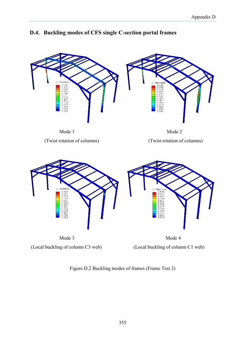
Appendix D
D.4. Buckling modes of CFS single C-section portal frames
Mode 1 Mode 2
(Twist rotation of columns) (Twist rotation of columns)
Mode 3 Mode 4
(Local buckling of column C3 web) (Local buckling of column C1 web)
Figure D.2 Buckling modes of frames (Frame Test 2)
355

Appendix D
D.5. Section properties of C30024 section
Section properties calculated using companion program developed for the analysis of beams described in Chapter 3. All output units are in mm.
Figure D.3 C30024 section with nodes defining segments
Cross-section area: 1263.6142 Second moment and product moment of area about rectangular axes Ix: 16961725.2606 Iy: 1509614.1048 Ixy: 0.0000 Second moment of area about principal axes Ipxx: 16961725.2606 Ipyy: 1509614.1048 Torsion constant, J: 2426.1392788 Warping constant, Iw: 26794702142.0869 Coordinates of centroid from bottom left xc0: 25.0225 yc0: 148.8000 Coordinates of shear centre w.r.t rectangular axes Xs: -41.0102
356

Appendix D
Ys: 148.8000 Coordinates of shear centre in principal axes x0: -66.0327 y0: -0.0000 Orientation of principal axes alpha: 0.000000 radian(0.0000 deg) Monosymmetry section constants betax: -0.0000 betay: 319.6241 Normalized Sectorial coordinate --------------------------------------- Node Sectorial Coordinate --------------------------------------
1 11329.53 2 8623.863 3 8237.182 4 7772.531 5 7298.41 6 6884.758 7 -5197.8 8 -5528.57 9 -5766.66
10 -5878.06 11 -5848.06 12 5848.06 13 5878.062 14 5766.659 15 5528.569 16 5197.802 17 -6884.76 18 -7298.41 19 -7772.53 20 -8237.18 21 -8623.86 22 -11329.5
357
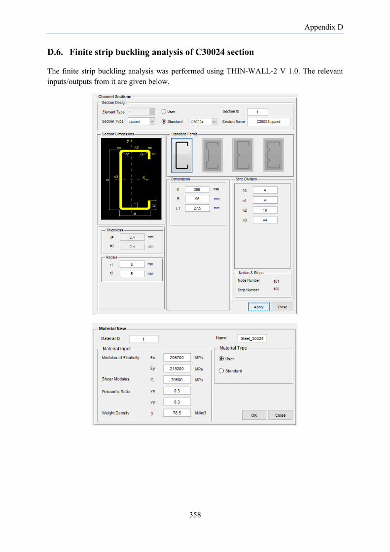
Appendix D
D.6. Finite strip buckling analysis of C30024 section
The finite strip buckling analysis was performed using THIN-WALL-2 V 1.0. The relevant inputs/outputs from it are given below.
358

Appendix D
a) C30024 member subjected to axial compression
359

Appendix D
b) C30024 member subjected to major axis bending moment
360

Appendix D
c) C30024 member subjected to minor axis bending moments
c.1 Shear centre side in compression
361

Appendix D
c.2 Shear centre side in tension
362

Appendix D
363

Appendix D
d) C30024 member subjected to the vertical shear force
364
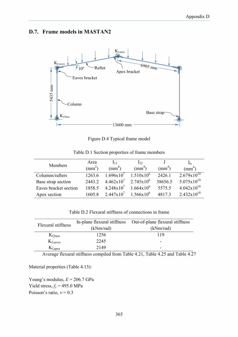
Appendix D
D.7. Frame models in MASTAN2
Figure D.4 Typical frame model
Table D.1 Section properties of frame members
Members Area
(mm2) I11
(mm4) I22
(mm4) J
(mm4) Iω
(mm6) Columns/rafters 1263.6 1.696x10⁷ 1.510x10⁶ 2426.1 2.679x10¹⁰ Base strap section 2443.2 4.462x10⁷ 2.745x10⁶ 38656.5 5.075x10¹⁰ Eaves bracket section 1858.5 4.248x10⁷ 1.664x10⁶ 5575.5 4.042x10¹⁰ Apex section 1605.8 2.447x10⁷ 1.566x10⁶ 4817.3 2.432x10¹⁰
Table D.2 Flexural stiffness of connections in frame
Flexural stiffness In-plane flexural stiffness (kNm/rad)
Out-of-plane flexural stiffness (kNm/rad)
Kf,base 1256 119 Kf,eaves 2245 - Kf,apex 2149 -
Average flexural stiffness compiled from Table 4.21, Table 4.25 and Table 4.27 Material properties (Table 4.13): Young’s modulus, E = 206.7 GPa Yield stress, fy = 495.0 MPa Poisson’s ratio, ν = 0.3
5435
mm
Rafter
Eaves bracket
Kf,eaves
Kf,apex
Apex bracket
Column
Kf,base Base strap
13600 mm
10º
365

Appendix D
D.7.1 Load calculations
Table D.3 Design load and load combinations
Load and load combination Calculations References Dead load: 0.50 mm thick CGI sheeting SC15012 [email protected] kg/m [email protected]/m and fixtures (UDL)
= 0.05 kPa = 2.89x9.81x10-3/1.74 m = 0.0163 kPa =0.12 kN/m
Table A2; Part 1 AS/NZS 1170.1:2002 Lysaght Supacee manual Lysaght Zed and Cee manual
Live load = 0.25 kPa Table 3.2, AS/NZS 1170.1:2002
1.2G +1.5Q = 0.46 kPa (concentrated load) = 0.14 kN/m (UDL)
Clause 4.2.2, AS/NZS 1170.0:2002
Wind load: Minimum design wind speed of 30 m/s assumed
= 0.54 kPa
Clause 2.3; AS/NZS 1170.2:2011
1.2G + Wu = 0.08 kPa (G), 0.14 kN/m (G) = 0.54 kPa (Wu)
Clause 4.2.2, AS/NZS 1170.0:2002
D.7.2 Typical frame model
Figure D.5 Typical frame model (Frame B1)
D.7.3 Frame buckling modes
To observe the column twists in frame models, dummy elements forming C-shape were attached at mid-height of the columns.
366
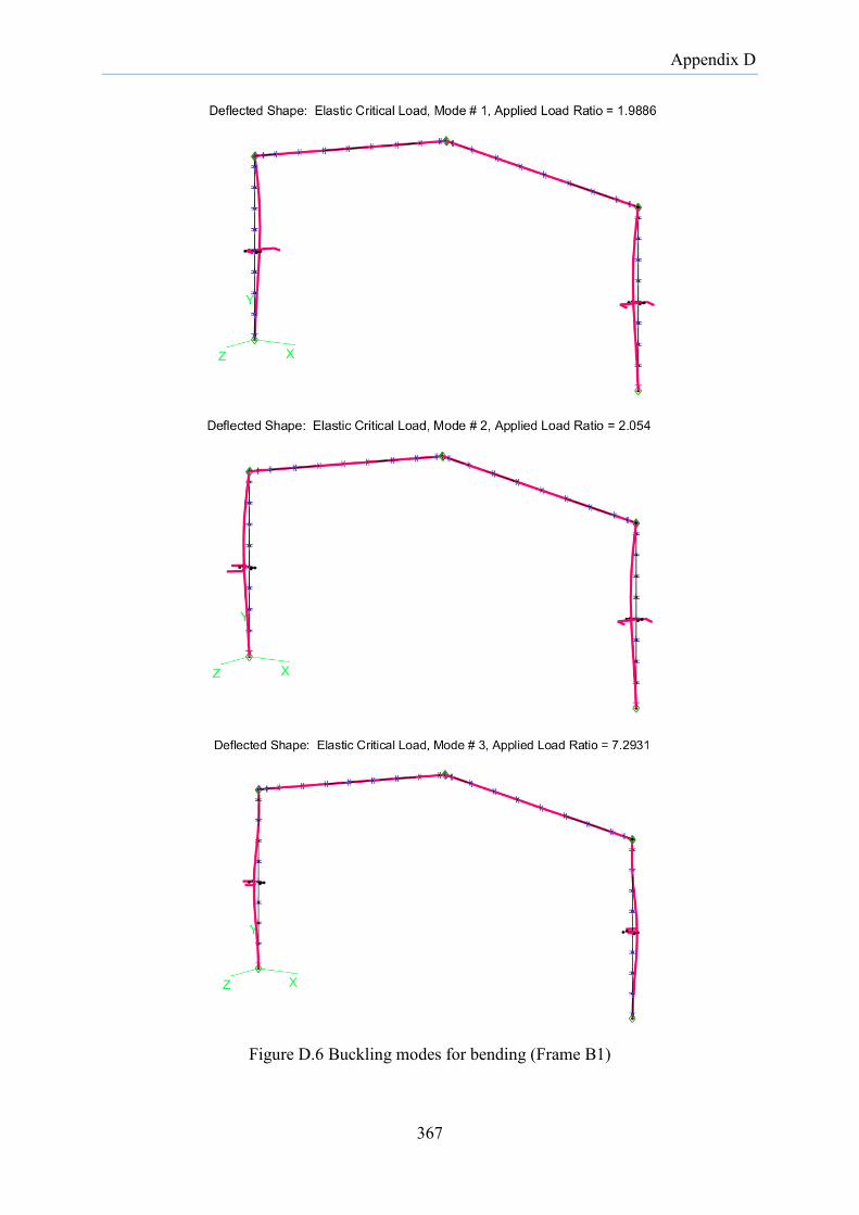
Appendix D
Figure D.6 Buckling modes for bending (Frame B1)
367

Appendix D
D.7.4 Design action effects
Design axial force and bending moment for Frame B1
Load combination: 1.2G+1.5Q
( a)
( b)
Figure D.7 Frame B1: (a) Axial force diagram; (b) Bending moment diagram
368
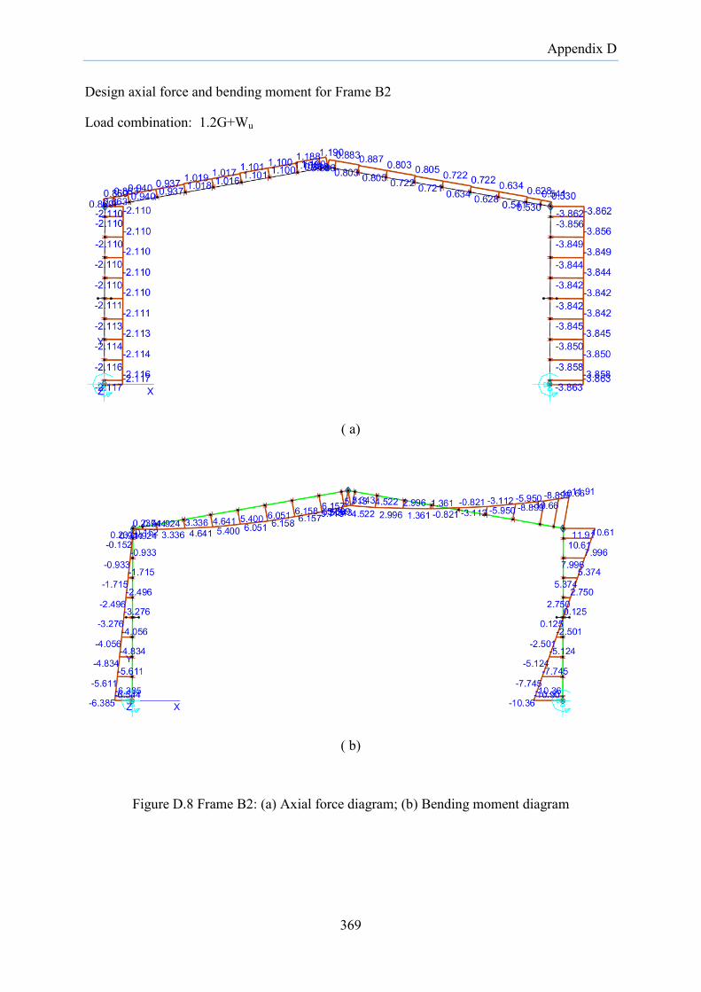
Appendix D
Design axial force and bending moment for Frame B2
Load combination: 1.2G+Wu
( a)
( b)
Figure D.8 Frame B2: (a) Axial force diagram; (b) Bending moment diagram
369
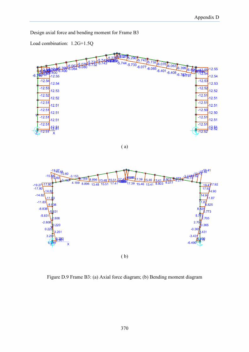
Appendix D
Design axial force and bending moment for Frame B3
Load combination: 1.2G+1.5Q
( a)
( b)
Figure D.9 Frame B3: (a) Axial force diagram; (b) Bending moment diagram
370
Appendix D
D.8. Generic procedures for the design of CFS portal frames using Direct Design Method
D.8.1 Loads
The portal frames are subjected to both the gravity load and horizontal loads. While the gravity loads arise from self-weight of the frame, the weight of purlins and girts, roof sheeting, associated fixtures and live loads, the lateral loads arise from winds and earthquake although seismic loads are seldom an issue in such light structures. Portal frames constructed in alpine zones may also experience seasonal snow loads.
The load on the structures for the advanced analysis must reflect the load distribution and the loading sequence on the real structure. Being a nonlinear analysis, principle of superposition no longer holds true. Hence, each combination of load as per the standard must be applied to the structure in the single step of the analysis. Apart from the load distribution, the accurate magnitude of load is less important in proceeding with the nonlinear analysis as it requires only the reference load. However, accurate determination of loads is necessary to check the structural adequacy.
D.8.2 Preliminary member sizing
To proceed with the advanced analysis, initial member sizes are required. The initial size of members is chosen based on the designer’s experience, thumb rule, based on simplified analysis or adopt the member size based on the similar size from the previously designed structures. Due care must be taken to choose the appropriate initial member size to arrive at the final member sizes without having to re-run the analysis repeatedly. This is crucial as nonlinear analysis of CFS portal frames takes significantly longer time to complete. In this respect, the initial size of rafters can be determined by assuming that it is subjected to gravity loads only while drift requirement can be used to determine initial column size.
D.8.3 Geometric modelling
For the CFS portal frames that are susceptible to local instabilities and are likely to undergo large deformation, it is befitting to use shell element model as opposed to beam element. This is even more relevant for single C-section portal frames, as the C-sections have non-coincident shear centre and centroid and are prone to flexural-torsional deformation. The mesh size for the FE model can be determined based on prior experience or running a separate small model. The bolted/screw connections can be conveniently modelled by deformable fasteners with prescribed nonlinear constitutive relations. To develop the force-displacement characteristics of the point fastener connections, separate physical tests on such connection may be undertaken or solid element model can be created for such connections and analysed to derive the force-displacement relationships. The details of creating the FE model for single C-section portal frames provided in Section 5.5 of Chapter 5 may be referred in this regard.
371
Appendix D
D.8.4 Material Properties
Nonlinear stress-strain relations are generally required to define the material properties. For this, constitutive relations of the material can be developed from coupon tests or adopted from the available data from the past studies. True stress-strain relations are usually required instead of the nominal stress-strain relations in defining the nonlinear material behaviour.
D.8.5 Geometric imperfections
The methods of integrating geometric imperfections in numerical models vary widely requiring a lengthy process, but the most practical way of incorporating imperfections is through the combination of buckled modes obtained from the linear buckling analysis. The first few modes of buckled shapes can be combined by scaling each of them using appropriate scale factors provided in Section 2.4.
How sensitive the structure is to the imperfection can be checked by performing nonlinear analysis without imperfection and comparing the results with that from the imperfect frames.
For the CFS single C-section portal frames tested, as described in Chapter 4, the global deformation mode is column twists rather than the frame sway. As a result, the twist deformations are likely to be more onerous than the sway in such frames. Currently, there are no guidelines available in the standards for the incorporation of twist deformation in frames other than the actual measurement of the twist deformation. Such measurements were carried out in test frames and subsequently incorporated into the numerical models.
D.8.6 Nonlinear analysis and system capacity check
For tracing the non-linear load-displacement behaviour, incremental loads instead of total loads are required. Since the cold-formed steel portal frames are characterized by the local instabilities, small steps are necessary for convergence. For contact non-linearity, the steps must be small enough to avoid convergence issues and at the same time large enough to enhance the analysis speed. The initial increment must be guessed for which it partly depends on the experience and judgment of the designer.
The nonlinear load-deflection response can be plotted and ultimate load on the structure can be obtained. The adequacy of the structural system can be directly assessed by comparing the ultimate strength of the structure (φsRn) to the factored loads (ΣγiQi). For the CFS portal frames, system resistance factor, φs is given as 0.85 in Table B4 of AS/NZS 4600 [14]. The nonlinear analysis and subsequent system capacity check must be carried out for each factored load combination.
If the structural demand is not fulfilled, the highly stressed members can be replaced by the larger size. To identify which member is highly stressed, von Mises stress contours can be plotted to examine the stress distribution in the whole structures. If the structural capacity, on the other hand, exceeds by significant magnitude, the member with least stress can be downsized.
372
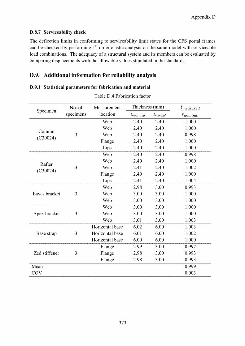
Appendix D
D.8.7 Serviceability check
The deflection limits in conforming to serviceability limit states for the CFS portal frames can be checked by performing 1st order elastic analysis on the same model with serviceable load combinations. The adequacy of a structural system and its members can be evaluated by comparing displacements with the allowable values stipulated in the standards.
D.9. Additional information for reliability analysis
D.9.1 Statistical parameters for fabrication and material
Table D.4 Fabrication factor
Specimen No. of specimens
Measurement location
Thickness (mm) 𝑡𝑚𝑒𝑎𝑠𝑢𝑟𝑒𝑑𝑡𝑛𝑜𝑚𝑖𝑛𝑎𝑙
tmeasured tnominal
Column (C30024) 3
Web 2.40 2.40 1.000 Web 2.40 2.40 1.000 Web 2.40 2.40 0.998
Flange 2.40 2.40 1.000 Lips 2.40 2.40 1.000
Rafter (C30024) 3
Web 2.40 2.40 0.998 Web 2.40 2.40 1.000 Web 2.41 2.40 1.002
Flange 2.40 2.40 1.000 Lips 2.41 2.40 1.004
Eaves bracket 3 Web 2.98 3.00 0.993 Web 3.00 3.00 1.000 Web 3.00 3.00 1.000
Apex bracket 3 Web 3.00 3.00 1.000 Web 3.00 3.00 1.000 Web 3.01 3.00 1.003
Base strap 3 Horizontal base 6.02 6.00 1.003 Horizontal base 6.01 6.00 1.002 Horizontal base 6.00 6.00 1.000
Zed stiffener 3 Flange 2.99 3.00 0.997 Flange 2.98 3.00 0.993 Flange 2.98 3.00 0.993
Mean 0.999 COV 0.003
373

Appendix D
Table D.5 Material factors
Coupon Source
fy,test (MPa)
fy,nom (MPa)
,
,
y test
y nom
ff
Etest (GPa)
Enom (GPa)
test
nom
EE
Column (Long) 494.2 450.0 1.098 205.6 200.0 1.03 495.4 450.0 1.101 209.1 200.0 1.05 495.3 450.0 1.101 205.3 200.0 1.03
Column (Trans) 550.2 450.0 1.223 219.3 200.0 1.10 546.3 450.0 1.214 220.9 200.0 1.10 547.4 450.0 1.216 217.5 200.0 1.09
Eaves Bracket 512.9 450.0 1.140 206.8 200.0 1.03 511.7 450.0 1.137 203.7 200.0 1.02 513.2 450.0 1.140 206.4 200.0 1.03
Apex Bracket 499.3 450.0 1.110 205.9 200.0 1.03 506.0 450.0 1.124 210.0 200.0 1.05 507.1 450.0 1.127 208.4 200.0 1.04
Mean 1.144 1.05 COV 0.041 0.03
D.9.2 Matlab script for the system reliability analysis for gravity load combination % Rinchen % 8 May 2018 % The University of Sydney % This program determines reliability index for a linear limit state % function with non-normal variables % % Notes: Resistance follows lognormal distribution % Dead load follows normal distribution % Live load follows Extreme Type I distribution % % This function was developed in MATLAB R2015b % clc, clearvars format long %----------- Define input---------------------------- % Parameters for resistance distribution mR_Rn=1.07; % mR/Rn (mean R divided by nominal R) VR=0.07; % Coefficient of variation of R % Parameter for dead load distribution mD_Dn=1.05; % mD/Dn (mean dead load divided by nominal dead load) VD=0.1; % Coefficient of variation of dead load % Parameter for live load distribution mL_Ln=0.8; % mL/Ln (mean live load divided by nominal live load) VL=0.25; % Coefficient of variation for live load gammaDead=1.2; % dead load factor
374

Appendix D
gammaDeadSmall=1.35; %dead load factor (for Ln/Dn<0.1) gammaLive=1.5; % live load factor k=[0.25 0.5 1 1.5 2 3 5]; % Ratio of Ln/Dn f=[0.65 0.70 0.75 0.80 0.85 0.90 0.95 1.0]; %System resistance factors % % --------------------------------------------------------------------- mD=1.0; % Mean of dead load set to 1 sD=VD*mD; % standard deviation for j=1:length(k) %range of Ln/Dn ratios for i=1:length(f) % range of system capacity factors % STEP 1: Establish relations based on design equation and variables mL=mL_Ln/mD_Dn*k(j)*mD; % Mean of live load sL=VL*mL; % Std. of live load %Mean of resistance if k(j)<0.1 mR=((gammaDeadSmall)*mD/mD_Dn)*(mR_Rn/f(i)); else mR=((gammaDead+gammaLive*k(j))*mD/mD_Dn)*(mR_Rn/f(i)); end sR=VR*mR; % Std. of resistance % STEP 2: Assume initial design point r=mR; l=mL; % Create the iteration stopping criteria b=10; db=10000; dx=10; while db>0.000001 && dx>0.00001 % STEP 3: Determine equivalent normal mean and standard deviation for initial design points % Statistical parameters of lognormal distribution for resistance R sRe=r*sqrt(log((sR/mR)^2+1)); %Equivalent standard deviation of R mRe=r*(1-log(r)+(log(mR)-(1/2)*log((sR/mR)^2+1)));%Equivalent mean of R % Statistical parameters of extreme type I distribution for live load a=sqrt(pi^2/(6*sL^2)); u=mL-0.5772/a; FL=exp(-exp(-a*(l-u))); %Cumulative distribution function fL=a*exp(-exp(-a*(l-u)))*exp(-a*(l-u));%Probability density function sLe=(1/fL)*normpdf(norminv(FL));%Equivalent standard deviation for live load mLe=l-sLe*norminv(FL); % Equivalent mean for live load % STEP 4: Assemble [G] from -dg/dZi Gr=-sRe; Gd=sD; Gl=sLe; G=[Gr;Gd;Gl];
375
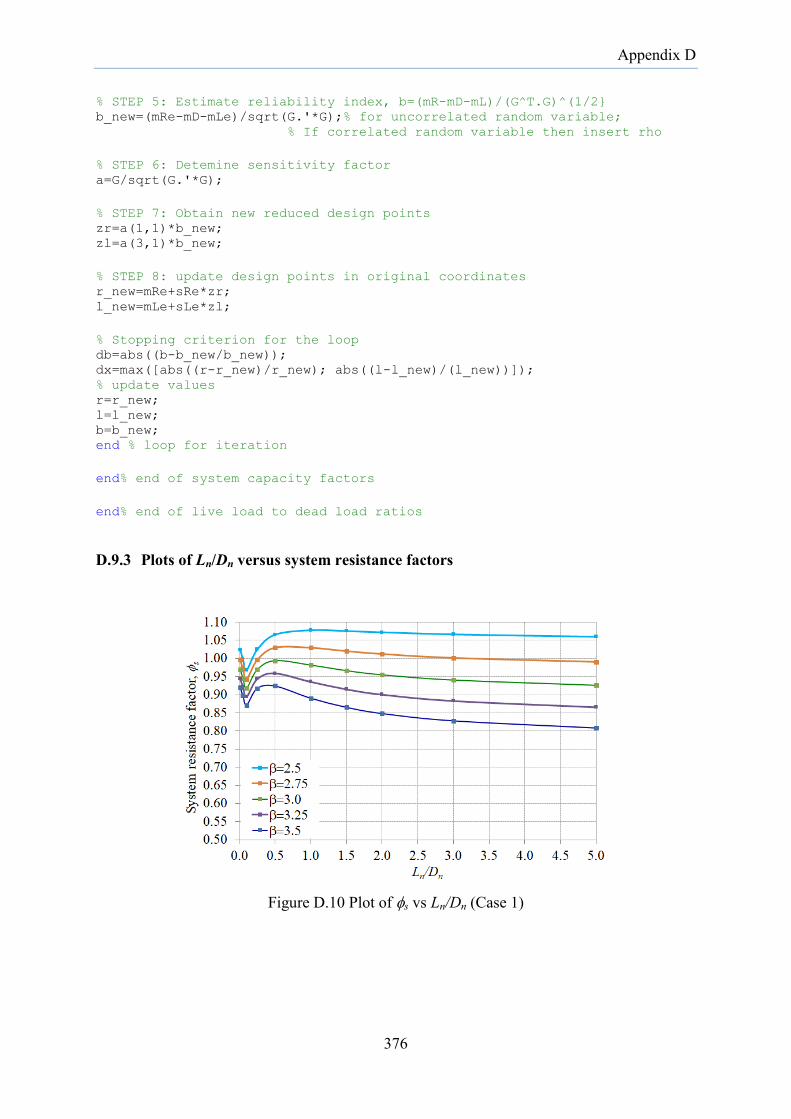
Appendix D
% STEP 5: Estimate reliability index, b=(mR-mD-mL)/(G^T.G)^(1/2 b_new=(mRe-mD-mLe)/sqrt(G.'*G);% for uncorrelated random variable; % If correlated random variable then insert rho % STEP 6: Detemine sensitivity factor a=G/sqrt(G.'*G); % STEP 7: Obtain new reduced design points zr=a(1,1)*b_new; zl=a(3,1)*b_new; % STEP 8: update design points in original coordinates r_new=mRe+sRe*zr; l_new=mLe+sLe*zl; % Stopping criterion for the loop db=abs((b-b_new/b_new)); dx=max([abs((r-r_new)/r_new); abs((l-l_new)/(l_new))]); % update values r=r_new; l=l_new; b=b_new; end % loop for iteration end% end of system capacity factors end% end of live load to dead load ratios
D.9.3 Plots of Ln/Dn versus system resistance factors
Figure D.10 Plot of φs vs Ln/Dn (Case 1)
376

Appendix D
Figure D.11 Plot of φs vs Ln/Dn (Case 2)
Figure D.12 Plot of φs vs Ln/Dn (Case 3)
Figure D.13 Plot of φs vs Ln/Dn (Case 4)
377

Appendix D
End of Appendices
378