arX

iv:0

712.

2280

v3 [

astr

o-ph

] 3

1 Ju

l 200

8

Mon. Not. R. Astron. Soc. 000, 1–13 (2007) Printed 17 January 2014 (MN LATEX style file v2.2)

The assembly bias of dark matter haloes to higher orders

R. E. Angulo⋆, C. M. Baugh†, C. G. Lacey‡,Institute for Computational Cosmology, Department of Physics, University of Durham, South Road, Durham, DH1 3LE, UK.

17 January 2014

ABSTRACT

We use an extremely large volume (2.4h−3Gpc3), high resolution N-body simulationto measure the higher order clustering of dark matter haloes as a function of massand internal structure. As a result of the large simulation volume and the use of anovel “cross-moment” counts-in-cells technique which suppresses discreteness noise,we are able to measure the clustering of haloes corresponding to rarer peaks than waspossible in previous studies; the rarest haloes for which we measure the variance are100 times more clustered than the dark matter. We are able to extract, for the firsttime, halo bias parameters from linear up to fourth order. For all orders measured, wefind that the bias parameters are a strong function of mass for haloes more massivethan the characteristic mass M∗. Currently, no theoretical model is able to reproducethis mass dependence closely. We find that the bias parameters also depend on theinternal structure of the halo up to fourth order. For haloes more massive than M∗,we find that the more concentrated haloes are more weakly clustered than the lessconcentrated ones. We see no dependence of clustering on concentration for haloeswith masses M < M∗; this is contrary to the trend reported in the literature whensegregating haloes by their formation time. Our results are insensitive to whetherhaloes are labelled by the total mass returned by the friends-of-friends group finder orby the mass of the most massive substructure. This implies that our conclusions arenot an artefact of the particular choice of group finding algorithm. Our results willprovide important input to theoretical models of galaxy clustering.

Key words:

1 INTRODUCTION

The spatial distribution of dark matter haloes is not as sim-ple as was once suspected. In the standard theoretical modelfor the abundance and distribution of haloes, the cluster-ing strength of haloes is predicted to be a function of massalone, with more massive haloes displaying stronger clus-tering (e.g. Kaiser 1984; Cole & Kaiser 1989; Mo & White1996). However, recent numerical simulations of hierarchi-cal cosmologies, by covering larger volumes with ever im-proving mass resolution, have been able to reveal subtledependences of halo clustering on other properties such asformation redshift, the internal structure of the halo andits spin (Gao, Springel, & White 2005; Wechsler et al. 2006;Harker et al. 2006; Bett et al. 2007; Wetzel et al. 2007;Jing, Suto, & Mo 2007; Espino-Briones et al. 2007).

The dependence of halo clustering on a second param-eter in addition to mass is generally referred to as assemblybias. However, the nature of the trend in clustering strengthrecovered depends upon the choice of property used to clas-

⋆ E-mail: raul.angulo@durham.ac.uk† E-mail: c.m.baugh@durham.ac.uk‡ E-mail: cedric.lacey@durham.ac.uk

sify haloes of a given mass. Early simulation work failedto uncover a convincing assembly bias signal, as a result ofinsufficient volume and mass resolution, which meant thathalo clustering could be measured for only a narrow rangeof mass and with limited statistics (Lemson & Kauffmann1999; Percival et al. 2003; Sheth & Tormen 2004) The firstclear indication of a dependence of halo clustering on asecond property was uncovered by Gao, Springel, & White(2005). These authors reported that low mass haloes whichform early are more clustered than haloes of the same masswhich form later on. No effect was seen for massive haloes.Wechsler et al. (2006) were able to confirm this result butalso found that halo clustering depends on the density pro-file of the halo, as characterized by the concentration pa-rameter (Navarro, Frenk, & White 1997). The sense of thedependence of clustering strength on concentration changeswith mass. Wechsler et al. found that massive haloes showeda dependence of clustering strength on concentration, withlow concentration haloes being the more strongly clustered(as confirmed by Gao & White 2007, Jing, Suto, & Mo 2007and Wetzel et al. 2007). This trend of clustering strengthwith concentration is reversed for low mass haloes. Al-though formation time and concentration are correlated (e.g.

2 Angulo et al.

Neto et al. 2007), their impact on the clustering of haloesdoes not follow trivially from this correlation, suggestingthat some other parameter may be more fundamental (asargued by Croton, Gao, & White 2007).

Previous studies of assembly bias have focused exclu-sively on the linear bias parameter, which relates the two-point correlations of haloes and dark matter. Measurementsfrom local surveys have shown that galaxies have signifi-cant higher order correlation functions and that the spa-tial distribution of galaxies and haloes is not fully describedby two-point statistics (e.g. Baugh et al. 2004; Croton et al.2004; Nichol et al. 2006; Frith et al. 2006). With large sur-veys planned at higher redshifts, there is a clear need foraccurate models of the higher order clustering of dark mat-ter haloes, and to establish whether or not the higher orderbias parameters depend on other properties in addition tomass.

In this paper we measure the higher order bias pa-rameters of dark matter haloes using a simulation whichcovers a volume more than an order of magnitude largerthan the run analyzed by Gao and collaborators. We use anovel approach to estimate the higher order correlation func-tions of dark matter haloes. Our method builds upon thecross-correlation technique advocated for two-point correla-tions by Jing, Suto, & Mo (2007),Gao & White (2007) andSmith et al. (2007). By considering fluctuations in the den-sity of haloes and dark matter within the same smoothingwindow, we can suppress discreteness noise in our measure-ments. This improved clustering estimator, which uses thecounts-in-cells method, when coupled with the large volumeof our simulation, allows us to recover the bias parametersfrom linear to fourth order, and to study the dependence ofthese parameters on the halo concentration.

In Section 2, we give the theoretical background to thecounts-in-cells technique we use to estimate higher orderclustering and explain how the clustering of haloes relates tothe underlying dark matter at different orders. We also intro-duce the numerical simulations in that section. We presentour results in Section 3 and a summary and discussion inSection 4.

2 THEORETICAL BACKGROUND AND

METHOD

In this Section we give the theoretical background to themeasurements presented in Section 3. We estimate the clus-tering of haloes and dark matter using a counts-in-cells ap-proach. An overview of this method is given in §2.1, in whichwe explain how to obtain expressions for the higher orderauto correlation functions of a density field from the mo-ments of the distribution of counts-in-cells. We also intro-duce the concept of higher order cross correlation functions,which combine fluctuations in two density fields. The con-cept of hierarchical amplitudes, scaling relations betweenhigher order correlation functions and the two-point cor-relation function, is introduced in §2.2. The key theoreticalresults relating the higher order cross correlation functionsof haloes to the two-point function and hierarchical ampli-tudes of the dark matter are given in §2.3. The simulationswe use to measure the clustering of dark matter haloes aredescribed in §2.4.

2.1 The counts in cells approach to measuring

clustering

Here we give a brief overview of the approach of using thedistribution of counts in cells to estimate the higher or-der auto correlation functions of a set of objects. An ex-cellent and comprehensive review of this material is givenby Bernardeau et al. (2002). We first discuss the higher or-der correlation functions for the case of a continuous, un-smoothed density field, then introduce the concept of cross-correlations (§2.1.1), before explaining how these results arechanged in the case of a smoothed distribution of discretepoints (§2.1.2).

2.1.1 Higher order correlations: unsmoothed and

continuous density field

In general, the complete hierarchy of N-point correlationfunctions is required to fully characterize the spatial distri-bution of fluctuations in a density field. An exception tothis occurs for the special case of a Gaussian density field,which can be described completely by its two-point correla-tion function.

The N-point correlation functions are usually writtenin terms of the dimensionless density fluctuation or densitycontrast at a point:

δ(x) = ρ(x)/〈ρ〉 − 1, (1)

where 〈ρ〉 is the mean density; the average is taken overdifferent spatial locations. By definition, 〈δ(x)〉 = 0 when theaverage is taken over a fair sample of the density field. TheN th order moment of the density field, sometimes referredto as a central moment, because δ is a fractional fluctuationaround the mean density, is given by:

µN = 〈δ(x1), . . . , δ(xn)〉, (2)

where, in general, the density fluctuations are correlated atdifferent spatial locations.

The N th order central moments defined in Eq. 2 canbe decomposed into terms which include products of lowerorder moments. This is because there are different permuta-tions of how the N-points can be “connected” or joined to-gether. This idea is illustrated nicely by tree diagrams in thereview by Bernardeau et al. (2002). The terms into whichthe central moments are broken down are called connectedmoments and these cannot be reduced further. In the treediagram language, an N-point connected moment has nodisjoint points; all N-points are linked to one another whenthe spatial averaging is performed. The distinction betweenconnected and unconnected moments may become clearer ifwe write down the decomposition of the unconnected centralmoments up to fifth order:

〈δ2〉 = 〈δ2〉c + 〈δ〉2c (3)

〈δ3〉 = 〈δ3〉c + 3〈δ2〉c〈δ〉c + 〈δ〉3c (4)

〈δ4〉 = 〈δ4〉c + 4〈δ3〉c〈δ〉c + 3〈δ2〉2c (5)

+6〈δ2〉c〈δ〉2c + 〈δ〉4c

〈δ5〉 = 〈δ5〉c + 5〈δ4〉c〈δ〉c + 10〈δ3〉c〈δ2〉c (6)

+10〈δ3〉c〈δ〉2c + 15〈δ2〉2c〈δ〉c

+10〈δ2〉c〈δ〉3c + 〈δ〉5c ,

The assembly bias of dark matter haloes to higher orders 3

where the subscript c outside the angular brackets denotes aconnected moment. Remembering that 〈δ〉 = 0, these equa-tions simplify to:

〈δ2〉 = 〈δ2〉c (7)

〈δ3〉 = 〈δ3〉c (8)

〈δ4〉 = 〈δ4〉c + 3〈δ2〉2c (9)

〈δ5〉 = 〈δ5〉c + 10〈δ3〉c〈δ2〉c. (10)

Hence, for the second and third order moments, there isno difference in practice between the connected and uncon-nected moments.

The N-point auto-correlation functions, ξN , are writtenin terms of the connected moments:

ξN(x1, . . . , xN) = 〈δ(x1), . . . , δ(xN)〉c. (11)

By analogy with the N-point auto correlation functionsof fluctuations in a single density field, we can define the i+j-point cross correlation function of two, co-spatial densityfields, with respective density contrasts given by δ1 and δ2:

ξi,j(x1, . . . , xi ; y1, . . . yj) = (12)

〈δ1(x1), . . . , δ1(xi) δ2(y1), . . . , δ2(yj)〉c.

In the application in this paper, the first index will referto the distribution of dark matter haloes and the secondindex to the dark matter. When the density contrasts areevaluated at the same spatial location, i.e. x1 = . . . = xi =y1 = . . . = yj = 0, the connected moments ξi,j are calledcumulants of the joint probability distribution function ofδ1 and δ2 (and are sometimes denoted as ki,j).

To generate expressions for the higher order correlationfunctions of the cross-correlated density fluctuations, ξi,j ,we will use the method of generating functions (see §3.3.3of Bernardeau et al. 2002). A moment generating functionis defined for the central moments (µi,j) as a power series inδ1 and δ2, which can be written as χ ≡ 〈exp (δ1t1 + δ2t2)〉,where t1 and t2 are random variables. This moment generat-ing function can be related to the cumulant generating func-tion (ψ) for the connected cumulants by (see Bernardeauet al. 2002 for a proof):

ψ(t1, t2) ≡ lnχ(t1, t2). (13)

Then, by taking partial derivatives of ψ and χ evaluated att1 = t2 = 0, one can “generate” the cumulants and moments:

ξi,j(0) = ki,j =∂i+j

∂ti1 ∂tj2

ψ|t1=t2=0 (14)

µi,j =∂i+j

∂ti1 ∂tj2

χ|t1=t2=0 = 〈δi1δ

j2〉. (15)

Following this method we can obtain expressions for thecross-correlation cumulants up to order i+ j = 5, groupingterms of the same order:

k1,1 = µ1,1 (16)

k2,0 = µ2,0 (17)

k3,0 = µ3,0 (18)

k2,1 = µ2,1 (19)

k4,0 = µ4,0 − 3µ2,02 (20)

k3,1 = µ3,1 − 3µ2,0µ1,1 (21)

k2,2 = µ2,2 − µ2,0µ0,2 − 2µ1,12 (22)

k5,0 = µ5,0 − 10µ3,0µ2,0 (23)

k4,1 = µ4,1 − 4µ3,0µ1,1 − 6µ2,0µ2,1 (24)

k3,2 = µ3,2 − µ3,0µ0,2 − 6µ2,1µ1,1 − 3µ2,0µ1,2. (25)

Note that these results are symmetric with respect to ex-changing the indexes and that we have used the fact thatµ1,0 = µ0,1 = 0, since, by construction 〈δ1〉 = 〈δ2〉 = 0.

2.1.2 Higher order correlations: smoothed and discrete

density fields

Sadly, density fluctuations at a point are of little practi-cal use as they cannot be measured reliably, as typicallywe have a finite number of tracers of the density field, i.e.galaxies in a survey or dark matter particles in an N-bodysimulation, and so have a limited resolution view of the den-sity field. Furthermore, estimating the N-point correlationsfor a modern survey or simulation is time consuming andshort cuts are often taken, such as restricting the numberof configurations of points sampled. To overcome both ofthese problems, moments of the smoothed density field canbe computed instead of the point moments.

The smoothed density contrast, δR, is a convolution ofthe density contrast at a point with the smoothing window,WR, which has volume V :

δ(x)R =1

V

∫

dx3′δ(x)WR(x− x′). (26)

Typically, the smoothing window is a spherical top-hat inwhich case WR = 1 for all points within distance R from thecentre of the window and WR = 0 otherwise. After smooth-ing, the cumulants correspond to the i + j-point volume-averaged cross correlation functions:

ξi,j(R) ≡

∫

d3x1 . . . d3xi d3y1 . . .d

3yj (27)

WR(x1) . . .WR(xi)WR(y1) . . .WR(yj)ξi,j .

Eqs. 16-25 are still valid, with the cumulants replaced byvolume-averaged cumulants.

Another issue introduced by the discreteness of the den-sity field is the contribution of Poisson noise to the measure-ments of the cumulants. To take this into account, we canmodify the moment generating function as follows (Peebles1980):

χ(t1, t2) = 〈exp(f1 (t1) + f2 (t2))〉, (28)

f1 = (exp(t1) − t1 − 1) n1 + (exp(t1) − 1) δ1, (29)

f2 = (exp(t2) − t2 − 1) n2 + (exp(t2) − 1) δ2. (30)

Here, n1 and n2 are the mean number of objects in densityfield 1 and density field 2 respectively within spheres of ra-diusR. Using this modified generating function, and definingµ′

i,j = 〈(n1 − n1)i (n2 − n2)

j〉, we obtain the following rela-tions between the volume-averaged, connected i + j-pointcross correlation functions, ξi,j , and the central moments,

4 Angulo et al.

µi,j :

n21 ξ2,0 = µ′

2,0 − n1 (31)

n1n2 ξ1,1 = µ′

1,1 (32)

n22 ξ0,2 = µ′

0,2 − n2 (33)

n31 ξ3,0 = µ′

3,0 + 2n1 − 3µ′

2,0 (34)

n21n2 ξ2,1 = µ′

2,1 − µ′

1,1 (35)

n1n22 ξ1,2 = µ′

1,2 − µ′

1,1 (36)

n32 ξ0,3 = µ′

0,3 + 2n2 − 3µ′

0,2 (37)

n41 ξ4,0 = µ′

4,0 − 6n1 + 11µ′

2,0 − 6µ′

3,0 − 3µ′22,0 (38)

n31n2 ξ3,1 = µ′

3,1 + 2µ′

1,1 − 3µ′

2,1 − 3µ′

1,1µ′

2,0 (39)

n21n

22 ξ2,2 = µ′

2,2 − µ′

1,2 − µ′

2,1 + µ′

1,1 − µ′

2,0µ′

0,2 (40)

−2µ′21,1

n1n32 ξ1,3 = µ′

1,3 + 2µ′

1,1 − 3µ′

1,2 − 3µ′

1,1µ′

0,2 (41)

n42 ξ0,4 = µ′

0,4 − 6n2 + 11µ′

0,2 − 6µ′

0,3 − 3µ′20,2. (42)

Note that these expressions revert to those in the literaturefor autocorrelation moments in the case of either i or j equalto zero (see for instance Baugh et al. 1995). Also note thatin the limit n1 → ∞, n2 → ∞, they correspond to theexpressions given by Eqs. 16-25.

2.2 Hierarchical amplitudes

At this point it is useful to define quantities called hier-archical amplitudes which are the ratio between the N-point, volume-averaged connected moments and the two-point volume-averaged connected moment raised to theN − 1 power:

SN ≡ξN

ξN−12

. (43)

This form is motivated by the expected properties of aGaussian field which evolves due to gravitational instabil-ity (Bernardeau et al. 2002). In the case of small amplitudefluctuations, i.e. on smoothing scales for which ξ2(R) ≪ 1,the SN depend only on the local slope of the linear pertur-bation theory power spectrum of density fluctuations andare independent of time (Juszkiewicz, Bouchet, & Colombi1993; see Bernardeau 1994 for expressions for the SN).Similar scalings, but with different values for the SN, ap-ply in the case of distributions of particles which havenot arisen through gravitational instability, e.g. parti-cles displaced according to Zeldovich approximation (seeJuszkiewicz, Bouchet, & Colombi 1993).

In the case of a Gaussian density field, all of the SN

are equal to zero. Initially, as perturbations grow throughgravitational instability, the two-point connected momentincreases. The distribution of fluctuations soon starts to de-viate from a Gaussian, particularly as voids grow in sizeand cells become empty (δ → −1). Voids evolve more slowlythan overdense regions. There is in principle no limit onhow overdense a cell can become. As a result, the distribu-tion of overdensities becomes asymmetrical or skewed, withthe peak of the distribution moving to negative density con-trasts and a long tail developing to high density contrasts.To first order, this deviation from symmetry is quantified by

the value of S3, which is often referred to as the skewnessof the density field. Higher order moments and hierarchicalamplitudes probe progressively further out into the tails ofthe distribution of density contrasts.

2.3 Higher order correlations: biased tracers

We are now in a position to consider the cross-correlationfunctions for the case of relevance in this paper, when theset of objects making up one of the density fields is localfunction of the second density field; the first density field isa biased tracer of the second. In our application, one densityfield is defined by the spatial distribution of dark matterhaloes and the other by the dark matter. In the case of alocal bias and small perturbations, the density contrast inthe biased tracers (δ1) can be written as an expansion interms of the underlying dark matter density contrast (δ2),as proposed by Fry & Gaztanaga (1993):

δ1(R) =

∞∑

k=0

bkk!δk2 (R), (44)

where the bk are known as bias coefficients; b1 is the linearbias commonly discussed in relation to two point correla-tions. Note that, by construction, we require that 〈δ〉 = 0,which implies b0 = −

∑

∞

k=2〈bk〉/k!. The bk, as we shall see

later, depend on mass but this is suppressed in our notation.Using this bias prescription, and following the treat-

ment Fry & Gaztanaga (1993) used for autocorrelations, wecan write the volume-averaged cross-correlation functions ofdark matter haloes in terms of the two-point volume aver-aged correlation function (ξ0,2) and hierarchical amplitudesof the dark matter, SN:

ξ1,1 = b1ξ0,2 +O(

ξ20,2

)

(45)

ξ2,0 = b21ξ0,2 +O(

ξ20,2

)

(46)

ξ1,2 = b1ξ20,2 (c2 + S3) +O

(

ξ30,2

)

(47)

ξ2,1 = b21ξ20,2 (2 c2 + S3) +O

(

ξ30,2

)

(48)

ξ3,0 = b31ξ20,2 (3 c2 + S3) +O

(

ξ30,2

)

(49)

ξ1,3 = b1ξ30,2 (3S3c2 + S4 + c3) +O

(

ξ40,2

)

(50)

ξ2,2 = b21ξ30,2

(

S4 + 6S3c2 + 2c22 + 2c3)

+O(

ξ40,2

)

(51)

ξ3,1 = b31ξ30,2

(

6c22 + 9S3c2 + S4 + 3c3)

+O(

ξ40,2

)

(52)

ξ4,0 = b41ξ30,2

(

12c22 + 12S3c2 + S4 + 4c3)

+O(

ξ40,2

)

(53)

ξ1,4 = b1ξ40,2(4c2S4 + 6c3S3 + (54)

c4 + S5 + 3c2S23) +O

(

ξ50,2

)

ξ2,3 = b21ξ40,2(12S3c3 + 6S2

3c2 + 12S3c22 + 6c2c3 + (55)

2c4 + S5 + 8c2S4) +O(

ξ52)

ξ3,2 = b31ξ40,2(12c2S4 + 18c3S3 + 18c2c3 + 36c22S3 (56)

+9c2S23 + S5 + 6c32 + 3c4) +O

(

ξ52)

ξ4,1 = b41ξ40,2(4c4 + 24c32 + S5 + 72c22S3 + 16c2S4 + (57)

36c2c3 + 24c3S3 + 12c2S23) +O

(

ξ52)

The assembly bias of dark matter haloes to higher orders 5

ξ5,0 = b51ξ40,2(20c2S4 + 15c2S

23 + 60c32 + 30c3S3 + (58)

5c4 + 120c22S3 + S5 + 60c2c3) +O(

ξ52)

where ck = bk/b1. Note it has been shown that these trans-formations preserve the hierarchical nature of the clustering(Fry & Gaztanaga 1993).

2.4 Numerical Simulations

To make accurate measurements of the higher order clus-tering of dark matter and dark matter haloes, we use theN-body simulations carried out by Angulo et al. (2008).Two simulation specifications were used: i) The BASICC,a high-resolution run which used 14483 particles of mass5.49 × 1011 h−1M⊙ to follow the growth of structure in thedark matter in a periodic box of side 1340h−1Mpc. ii) TheL-BASICC ensemble, a suite of 50 lower resolution runs,which used 4483 particles of mass 1.85×1012 h−1M⊙ in thesame box size as the BASICC. Each L-BASICC run wasevolved from a different realization of the initial Gaussiandensity field. The simulation volume was chosen to allow thegrowth of fluctuations to be modelled accurately on a widerange of scales, including that of the baryonic acoustic oscil-lations (the BASICC acronym stands for Baryonic Acousticoscillation Simulations at the Institute for ComputationalCosmology). The extremely large volume of each box alsomakes it possible to extract accurate measurements of theclustering of massive haloes. The superior mass resolutionof the BASICC run means that it can resolve the haloeswhich are predicted to host the galaxies expected to be seenin forthcoming galaxy surveys. The L-BASICC runs resolvehaloes equivalent to group-sized systems. The independenceof the L-BASICC ensemble runs makes them ideally suitedto the assessment of the impact of cosmic variance on ourclustering measurements.

In both cases, the same values of the basic cosmologicalparameters were adopted, which are broadly consistent withrecent data from the cosmic microwave background and thepower spectrum of galaxy clustering (Sanchez et al. 2006):the matter density parameter, ΩM = 0.25, the vacuum en-ergy density parameter, ΩΛ = 0.75, the normalization ofdensity fluctuations, expressed in terms of the linear the-ory amplitude of density fluctuations in spheres of radius8h−1Mpc at the present day, σ8 = 0.9, the primordial spec-tral index ns = 1, the dark energy equation of state, w = −1,and the Hubble constant, h = H0/(100kms−1Mpc−1) =0.73. The simulations were started from realizations of aGaussian density field set up using the Ze’ldovich approxi-mation (Zel’Dovich 1970). Particles were perturbed from aglass-like distribution (Baugh et al. 1995; White 1994). Thestarting redshift for both sets of simulations was z = 63.The linear perturbation theory power spectrum used to setup the initial density field was generated using the Boltzmancode CAMB (Lewis et al. 2000). The initial density field wasevolved to the present day using a memory efficient versionof GADGET-2 (Springel 2005).

Outputs of the particle positions and velocities werestored from the simulations at selected redshifts. Dark mat-ter haloes were identified using a Friends-of-Friends (FOF)percolation algorithm (Davis et al. 1985) and substructureswithin these were found using a modified version of SUBFIND(Springel et al. 2001). Our default choice is to use the num-

Figure 1. The ratio Vmax/V200 as a function of halo mass forgravitationally bound haloes in the BASICC simulation, which havea minimum of 26 particles. Vmax is the maximum effective circular

velocity of the largest substructure within the halo and V200 isthe effective rotation speed at the radius within which the meandensity is 200 times the critical density, computed using all ofthe particles within this radius. Each panel shows the relationat a different redshift as indicated by the legend. The red linesshow the 20-80 percentile range of the distribution of Vmax/V200

values, and the blue lines show the mean.

ber of particles in a structure as returned by the FOF groupfinder to set the mass of the halo; at the end of Section 3.4we discuss a variation on this to assess the sensitivity ofour results to the group finder. The position of the halo isthe position of the most bound particle in the largest sub-structure, as determined by SUBFIND. In this paper, onlygravitationally bound groups with more than 26 particlesare considered. The SUBFIND algorithm also computes sev-eral halo properties such as the circular velocity profileVc(r) = (GM(r)/r)1/2, Vmax, the maximum value of Vc forthe largest substructure, and V200 = Vc(r200), where r200 isthe radius of a sphere enclosing a volume of mean density 200times the critical density. These properties are calculated us-ing only the particles which are bound to the main subhaloof the FOF halo; i.e. ignoring all of the other substructurehaloes within the FOF halo. In the best resolved haloes, sub-structures other than the largest substructure account for atmost 15% of the total halo mass (Ghigna et al. 1998). Lateron in the paper we will present results for the clustering ofhaloes as a function of mass and a second parameter. Wehave a limited number of output times available to us, so itis not feasible to use the formation time of the halo as thesecond parameter. Instead, we will use the ratio Vmax/V200.Fig. 1 shows Vmax/V200 as a function of halo mass at differ-ent epochs in the BASICC simulation. There is a trend of de-clining Vmax/V200 with increasing halo mass. In cases wherethe density profile of the dark matter halo matches the uni-versal profile advocated by Navarro et al. (1997), Vmax/V200

6 Angulo et al.

depends on the concentration parameter which characterizesthe profile. Haloes in the extreme parts of the distributionof Vmax/V200 also have extreme values of the concentrationparameter (Navarro, Frenk, & White 1997). More massivehaloes tend to have lower values of the concentration pa-rameter and lower values of the velocity ratio Vmax/V200.The ratio Vmax/V200 is easier to extract from the simula-tion, as it does not require a parametric form to be fittedto the density profile. There is a correlation between forma-tion time and concentration parameter, and hence the ra-tio Vmax/V200, albeit with scatter (Navarro, Frenk, & White1997; Zhao et al. 2003).

3 RESULTS

Our ultimate goal is to measure the higher order bias ofdark matter haloes. As described in Section 2, we followa novel approach to do this, employing cross moments be-tween haloes and the dark matter. The first step in this pro-cess is to compute the densities of haloes and dark matteron grids of cubical cells of different sizes1. A natural by-product of this procedure is the higher order clustering ofthe dark matter and haloes in terms of the auto-correlationfunctions. We first present the hierarchical amplitudes esti-mated for the dark matter (§3.1) and haloes (§3.2) using theautocorrelation function higher order moments. In §3.3 weshow the measurements of the cross moments and in §3.4we present the interpretation of these results in terms of thebias parameters.

3.1 Hierarchical amplitudes for the dark matter

Fig. 2 shows the hierarchical amplitudes SN measured forthe dark matter at different redshifts. The upper panelsshow the results in real-space and the lower panels in-clude the effects of redshift space distortions using the dis-tant observer approximation. The points indicate the me-dian value of the hierarchical amplitudes measured in theL-BASICC ensemble and the error bars indicate the vari-ance in these measurements. The lines show the hierarchicalamplitudes predicted by perturbation theory (Bernardeau1994; Juszkiewicz, Bouchet, & Colombi 1993). At the high-est redshift plotted, z = 4, the agreement between the mea-surements made from the simulations and the predictionsof perturbation theory is impressive, covering scales from5h−1Mpc to 100h−1Mpc for S3 and S4. As redshift de-creases, the simulation results for S5 and S6 are slightlyhigher than the perturbation theory predictions. The mea-surements of S3 from the simulations continue to agree withthe perturbation theory predictions, but over a narrowerrange of scales. For smoothing scales on which the variance isless than unity, the hierarchical amplitudes are expected tobe independent of epoch, depending only on the shape of thelinear perturbation theory power spectrum of density fluctu-ations (Juszkiewicz, Bouchet, & Colombi 1993; Bernardeau

1 Tests show that density fluctuations in cubical cells can be read-ily translated into counts in spherical cells by simply setting thevolume of the spherical cell equal to that of the cube. We usecubical cells for speed. The counts are regridded to improve themeasurement of the rare event tails of the count distribution.

1994; Gaztanaga & Baugh 1995). Fig. 2 confirms that thisis the case. As the density field evolves, the measured hi-erarchical amplitudes change remarkably little, particularlywhen one bears in mind that the higher order correlationfunctions change substantially between z = 4 and z = 0.For example, for a cell of radius 50h−1Mpc, the two-pointvolume averaged correlation function increases by a factorof 14 over this redshift interval, and the three-point functionby a factor of 197.

Nevertheless, the simulation results do tend to exceedthe perturbation theory predictions on all scales at all ordersas the density fluctuations grow.

The hierarchical amplitudes measured on small scalesdiffer significantly from the predictions of perturbation the-ory. At z = 4, the simulation results are below the analyt-ical predictions for cell radii smaller than R ∼ 5h−1Mpc.This behaviour is sensitive to the arrangement of particleswhich is perturbed to set up the initial density field. At latertimes, the memory of the initial conditions is erased on smallscales and the measured amplitudes greatly exceed the ex-pectations of perturbation theory. On these scales, the dom-inant contribution to the cross correlation moments is fromparticles within common dark matter haloes. Note that inFig. 2 we do not correct the measured higher order correla-tion functions for Poisson noise, since the initial density fieldwas created by perturbing particles distributed in a glass-like configuration which is sub-Poissonian. Hence, the darkmatter density field is not a random sampling of a contin-uous density field (see Angulo et al. (2008) for an extendeddiscussion of this point). The turnover in the hierarchicalamplitudes seen at small cell radii (e.g. for R < 2h−1Mpc isdue to the finite resolution of the L-BASICC simulations; thehierarchical amplitudes continue to increase in amplitude onsmaller smoothing scales in the BASICC run.

The lower panels of Fig. 2 show the impact of gravi-tationally induced peculiar motions on the hierarchical am-plitudes. We model redshift space distortions using the dis-tant observer approximation, in which peculiar motions per-turb the particle position parallel to one of the co-ordinateaxes. Virialized structures appear elongated when viewed inredshift space. On large scales, coherent bulk flows tend toincrease the amplitude of correlation functions. There is amodest reduction in the amplitude of the hierarchical am-plitudes on large scales. On small scales, there is a dramaticreduction in the magnitude of the SN. The overall impactof the redshift space distortions is to greatly reduce the de-pendence of the hierarchical amplitudes on smoothing scale(see Hoyle et al. 2000).

The estimated error on the measured hierarchical mo-ments is shown in Fig. 3, in which we plot the fractionalerror on SN obtained from the scatter in the measurementsfrom the L-BASICC ensemble. The plot suggests that theskewness of the dark matter can be well measured on allsmoothing scales considered from a volume of the size of theL-BASICC simulation cube. The range of scales over whichrobust measurements can be made of the hierarchical ampli-tudes becomes progressively narrower with increasing order.For example, at z = 0, reliable measurements of S6 are lim-ited to smoothing radii smaller than R ∼ 30h−1Mpc.

The assembly bias of dark matter haloes to higher orders 7

Figure 2. The hierarchical amplitudes (SN) measured for the dark matter as a function smoothing scale, which is plotted in terms ofthe radius of the sphere with the same volume as the cubical cell used. The upper panels show the results in real-space and the lowerpanels show redshift-space. Each panel corresponds to a different redshift as indicated by the legend. The points show the amplitude forthe SN obtained from the L-BASICC ensemble, after taking the ratio of the median correlation functions, as defined by Eq. 43. The errorbars show the scatter in the measurements over the ensemble, obtained by computing SN for each simulation from the ensemble. Errorbars are plotted at smoothing scales for which the fractional error is less than unity; triangles show scales on which the error exceedsunity. In both sets of panels, the dashed lines show the predictions of perturbation theory in real space (see text for details). Note thatno correction for shot noise has been applied to the measured amplitudes. The arrows indicate the cell radius for which the variance inthe counts in cells for the dark matter is equal to unity, which is roughly the scale down to which perturbation theory should be valid;at z = 4, this scale is below R = 1h−1Mpc.

8 Angulo et al.

Figure 3. The fractional scatter, σ(SN)/SN, in the measured hierarchical amplitudes, as estimated from the 50 simulations in theL-BASICC ensemble. Different lines show the scatter for different orders as indicated by the legend.

3.2 The hierarchical amplitudes of dark matter

haloes

The hierarchical amplitudes of dark matter haloes are morecomplicated than those of the dark matter. In addition toa term arising from the evolution of the density field un-der gravitational instability, there is a contribution whichdepends upon height of the peak in the initial density fieldwhich collapses to form the halo (Mo, Jing, & White 1997).For example, if we consider the second and third order auto-correlation functions of haloes given by Eqs. 44 and 47, thenthe skewness for dark matter haloes, SH

3 , is given by:

SH3 =

ξ3,0(

ξ2,0

)2(59)

=3b2b21

+S3

b1. (60)

The gravitational contribution to the skewness, S3, is di-luted by the linear bias factor, b1. In the case of rare peaks,or, equivalently, haloes with masses far in excess of the char-acteristic mass, M∗, at a given redshift, SH

3 approaches anasymptotic value. In this limit, bk ≈ bk1 and so SH

3 ≈ 3; simi-lar arguments for the fourth and fifth order hierarchical am-plitudes yield asymptotic values of SH

4 = 16 and SH5 = 125

(Mo, Jing, & White 1997). Massive haloes at high redshiftcan therefore have non-zero hierarchical amplitudes even ifthe dark matter distribution still has a Gaussian distributionand hence SDM

p = 0.We plot the hierarchical amplitudes of dark mat-

ter haloes in Fig. 4, as a function of the scaled peak

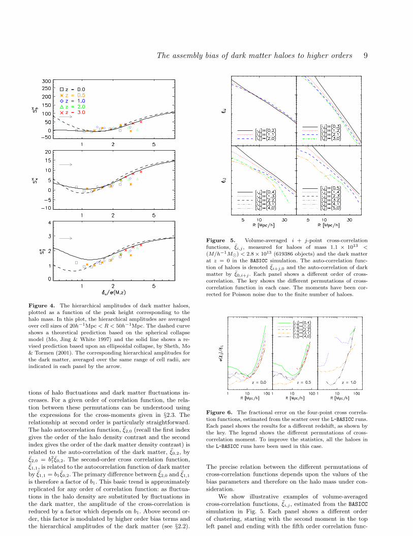
height, δc/σ(M, z). The simulation results are averaged oversmoothing radii of 20h−1Mpc < R < 50h−1Mpc. Thedashed line shows the prediction obtained assuming themass function of Press & Schechter (1974) and the spher-ical collapse model (see Mo, Jing, & White 1997). The solidline shows an improved calculation which uses the ellipsoidalcollapse model and the mass function derived by Sheth et al.(2001). There is some dispersion between the simulation re-sults at different redshifts. The measurements are in rea-sonable agreement with the theoretical predictions for largevalues of δc/σ(M, z). For more modest peaks, the hierarchi-cal amplitudes of haloes averaged on large smoothing scalesshow a dip and are significantly smaller than the amplituderecovered for the dark matter. The strength of this dip ismore pronounced in the measurements from the simulationsthan it is in the theoretical predictions. This discrepancysuggests that the theoretical models do not reproduce thetrend of bias with halo mass for such objects, as we shall seein §3.4.

3.3 Cross-correlation estimates of higher order

clustering

We now switch to estimating cross-correlation functions in-stead of auto-correlation functions. To recap §2, to reducethe impact of discreteness noise on our measurement of haloclustering, we cross-correlate fluctuations in the spatial dis-tribution of haloes with the fluctuation in the dark mat-ter density within the same cell. As the order of the corre-lation function increases, the number of possible permuta-

The assembly bias of dark matter haloes to higher orders 9

Figure 4. The hierarchical amplitudes of dark matter haloes,plotted as a function of the peak height corresponding to thehalo mass. In this plot, the hierarchical amplitudes are averagedover cell sizes of 20h−1Mpc < R < 50h−1Mpc. The dashed curveshows a theoretical prediction based on the spherical collapsemodel (Mo, Jing & White 1997) and the solid line shows a re-vised prediction based upon an ellipsoidal collapse, by Sheth, Mo& Tormen (2001). The corresponding hierarchical amplitudes forthe dark matter, averaged over the same range of cell radii, areindicated in each panel by the arrow.

tions of halo fluctuations and dark matter fluctuations in-creases. For a given order of correlation function, the rela-tion between these permutations can be understood usingthe expressions for the cross-moments given in §2.3. Therelationship at second order is particularly straightforward.The halo autocorrelation function, ξ2,0 (recall the first indexgives the order of the halo density contrast and the secondindex gives the order of the dark matter density contrast) isrelated to the auto-correlation of the dark matter, ξ0,2, byξ2,0 = b21ξ0,2. The second-order cross correlation function,ξ1,1, is related to the autocorrelation function of dark matterby ξ1,1 = b1ξ0,2. The primary difference between ξ2,0 and ξ1,1

is therefore a factor of b1. This basic trend is approximatelyreplicated for any order of correlation function: as fluctua-tions in the halo density are substituted by fluctuations inthe dark matter, the amplitude of the cross-correlation isreduced by a factor which depends on b1. Above second or-der, this factor is modulated by higher order bias terms andthe hierarchical amplitudes of the dark matter (see §2.2).

Figure 5. Volume-averaged i + j-point cross-correlationfunctions, ξi,j , measured for haloes of mass 1.1 × 1013 <(M/h−1M⊙) < 2.8 × 1013 (619386 objects) and the dark matterat z = 0 in the BASICC simulation. The auto-correlation func-tion of haloes is denoted ξi+j,0 and the auto-correlation of darkmatter by ξ0,i+j . Each panel shows a different order of cross-correlation. The key shows the different permutations of cross-correlation function in each case. The moments have been cor-rected for Poisson noise due to the finite number of haloes.

Figure 6. The fractional error on the four-point cross correla-tion functions, estimated from the scatter over the L-BASICC runs.Each panel shows the results for a different redshift, as shown bythe key. The legend shows the different permutations of cross-correlation moment. To improve the statistics, all the haloes inthe L-BASICC runs have been used in this case.

The precise relation between the different permutations ofcross-correlation functions depends upon the values of thebias parameters and therefore on the halo mass under con-sideration.

We show illustrative examples of volume-averagedcross-correlation functions, ξi,j , estimated from the BASICC

simulation in Fig. 5. Each panel shows a different orderof clustering, starting with the second moment in the topleft panel and ending with the fifth order correlation func-

10 Angulo et al.

tion in the bottom right panel. In this plot, the haloes usedhave masses in the range 1.1 × 1013 < (Mhalo/h

−1M⊙) <2.8 × 1013 and the clustering is measured at z = 0. Thetop-left panel of Fig. 5 shows that there is little differencein the amplitude of the second-order correlation function onlarge smoothing scales between the different permutationsof i, j. This implies that for these haloes, the linear biasterm b1 ≈ 1. The correlation functions are, however, differ-ent on small scales. The autocorrelation function of the darkmatter (ξ0,2) is steeper than the autocorrelation of haloes(ξ0,2). The cross-correlation functions are different on largescales for third, fourth and fifth orders. The difference inamplitude is fairly independent of scale for cells with radiiR > 10h−1Mpc. Since the linear bias of this sample of haloesis close to unity, this difference is driven by the higher or-der bias terms and the hierarchical amplitudes of the darkmatter. We plan to model the full behaviour of the cross-correlation functions, including the small scale form, usingthe halo model in a future paper.

One might be concerned that replacing fluctuations inhalo density by fluctuations in dark matter in the higherorder correlation functions leads to a reduction in the clus-tering amplitude (as is indeed apparent in Fig. 5). How-ever, this is more than offset by a reduction in the noiseor scatter of the measurement. The fractional error on themeasurements of the cross-correlation functions is plottedin Fig. 6. The scatter is estimated using the L-BASICC en-semble. Each panel shows the scatter at a different redshift.The cross correlation ξ1,i+j−1 (i.e. one part halo fluctuation,i + j − 1 parts dark matter fluctuation) gives the optimalerror estimate, with a performance comparable to the auto-correlation of the dark matter. At z = 1, it is not possible tomeasure the four-point autocorrelation function of this sam-ple of haloes, even with a box of the size of the L-BASICC

runs. Nevertheless, it is possible to measure the bias factorsrelating the four-point functions of haloes and mass usingthe cross-correlation. Our use of a cross-correlation estima-tor therefore allows us to extend the measurements of thehigher order clustering of haloes to orders and redshifts thatwould not be possible using auto-correlations.

3.4 The bias parameters of dark matter haloes

We now use the cross correlation functions to estimate thelinear and higher order bias parameters of dark matterhaloes. As we demonstrated in the previous section, the bestpossible measurement of the i+ jth order correlation func-tion is obtained when the cross correlation function is madeup of one part fluctuation in halo density and i+ j−1 partsdark matter fluctuation: i.e. in our notation ξ1,i+j−1. Thisapproach, combined with the huge volume of our simula-tion, makes it possible, for the first time, to measure thethird and fourth order bias parameters, and to do so usingnarrow mass bins.

In this section, we use the higher resolution BASICC run,which can resolve the largest dynamic range in halo mass.We use the higher order correlation function measurementsover the range of smoothing radii 15 < (R/h−1Mpc) < 50to estimate the halo bias parameters. The large volume ofthe BASICC simulation means that we can make robust mea-surements of the higher order correlation functions out tolarger smoothing radii than is possible with the smaller Mil-

lennium simulation. The smallest scale we use is set by therequirement that the expansion relating the overdensity inhaloes to the overdensity in dark matter (Eq. 44) is a goodapproximation, i.e. when ξ ≪ 1. The scales we use to extractthe halo bias parameters are considerably larger than thoseGao, Springel & White (2005) and Gao & White (2007)were able to use in the Millennium. We use the simulationoutputs at redshifts of z = 0, 0.5, 1, 2 and 3 to measure theclustering of haloes.

The results for the first, second, third and fourth or-der bias parameters of dark matter haloes are presented inFig. 7. Each panel corresponds to a different order. The up-per half of each panel shows the respective order of biasparameter as a function of halo mass, expressed in terms ofthe peak height corresponding to the halo mass, δc/σ(M, z).The lower half of each panel shows the deviation from thebias parameter extracted for a given mass for samples of the20% of haloes in the mass bin with the highest and low-est values of Vmax/V200, which we are using as a proxy forhalo concentration. Different symbols in the upper panelsshow the measurements at different output redshifts in theBASICC run, as indicated by the key; the same colours areused to draw the lines showing results for samples definedby different Vmax/V200 values at the same output redshiftsin the lower panels.

In Fig. 7, there is remarkably little scatter between theresults obtained from the different output redshifts for thecase of the overall bias as a function of mass. This is en-couraging, as it shows that our results are not affected byresolution (haloes with similar values of δc/σ(M, z) at dif-ferent output times are made up of very different numbers ofparticles). Gao, Springel & White (2005) were able to mea-sure the linear bias parameter up to haloes correspondingto peak heights of 3σ; we are able to extract measurementsfor haloes corresponding to 5σ peaks.

In the upper sub-panels of Fig. 7, we show two the-oretical predictions for the bias parameters of dark mat-ter haloes. The dotted lines show the predictions fromMo, Jing, & White (1997), based on an extension of Press& Schechter’s (1974) theory for abundance of dark mat-ter haloes and the spherical collapse model. The solid linesshow the calculation from Scoccimarro et al. (2001) whichuses the mass function of Sheth & Tormen (1999). Our re-sults tend to agree best with the later, although the mea-surements favour a steeper dependence of bias on peakheight at all orders. For less rare peaks, neither theoret-ical model gives a particularly good fit to the simula-tion results. A similar trend, albeit with more scatter be-tween the results at different output redshifts was foundby Gao, Springel, & White (2005) (see also Wechsler et al.2006; Jing, Suto, & Mo 2007).

Previous studies have reported a dependence of cluster-ing strength on a second halo property besides mass, such ashalo formation time or concentration (Wechsler et al. 2006;Gao & White 2007). We do not have sufficient output timesto make a robust estimate of formation time so we use aproxy for halo concentration instead, Vmax/V200. We findthat the clustering of high peak haloes is sensitive to whetherthe halo has a high or low value of Vmax/V200. The 20% ofhaloes with the lowest values of Vmax/V200 within a givenmass bin (i.e. those with the lowest concentrations) havethe largest linear and second order bias terms. This result

The assembly bias of dark matter haloes to higher orders 11

Figure 7. The bias parameters as a function of halo mass parametrized by ν = δc/σ(M, z). Each plot shows a different order of biasparameter: a) linear bias b1, b) the ratio of the 2nd order bias, b2/b1, c) the ratio of the 3rd order bias, b3/b1 and d) b4/b1. In thelower panel of each plot, the residual bias parameters for the 20% of haloes with the highest or lowest values of Vmax/V200, a proxy forconcentration, are plotted. In the upper panels, symbols show the measurements for different output redshifts, as indicated by the key.The same line colours are used to show the results for different redshifts in the lower panels. In the upper panel of each plot, we plot twotheoretical predictions for the bias parameters, given by Mo, Jing & White (1997) and Scoccimarro et al. (2001).

agrees with previous estimates of the dependence of the lin-ear bias term on halo concentration (Wechsler et al. 2006).

The peak height dependence of the third and fourthorder bias terms for haloes split by Vmax/V200 is more com-plicated. Fig. 7 shows that the third order bias depends onour concentration proxy in a non-monotonic fashion. Thetrend for the fourth order bias is reversed compared withthe results for the first and second order bias parameters:

low concentration haloes have a negative value of the fourthorder bias. We note that it would not be possible to mea-sure a fourth order bias at all using halo auto-correlationfunctions.

One might be concerned that our results could be sen-sitive to the operation of the group finder. In particular, itis well known that the FoF algorithm can sometimes spuri-ously link together distinct haloes into a larger halo, through

12 Angulo et al.

bridges of particles (e.g. Cole & Lacey 1996). We thereforecarried out the exercise of relabelling the mass of each haloby the mass of the largest substructure as determined bySUBFIND. In the rare cases in which haloes are incorrectlylinked into a larger structure, using instead the SUBFIND

mass would result in a significant shift in the mass bin towhich the halo is assigned. Moreover, one would expect thatlow concentration FoF haloes would be more prone to beingbroken up in this way. However, we found no change in ourresults upon following this procedure, demonstrating thatthe trends we find for the dependence of bias on mass andconcentration are robust.

4 SUMMARY AND DISCUSSION

In this paper, we have combined ultra-large volume cosmo-logical simulations with a novel approach to estimating thehigher order correlation functions of dilute samples of ob-jects. The large simulation volume allows us to extract biasparameters on large scales, which follow linear perturba-tion theory more closely, and provides us with large samplesof high mass haloes from which robust clustering measure-ments can be made. The cross-moment counts-in-cells tech-nique we use to estimate the higher order clustering of darkmatter haloes has superior noise performance to traditionalautocorrelation functions, allowing us to probe clusteringto higher orders. These improvements made it possible toextend previous work on the assembly bias of dark matterhaloes in a number of ways. We have been able to extractmeasurements of halo clustering for objects corresponding to5σ peaks, almost twice as high as in earlier studies. We havealso presented, for the first time, estimates of the higher or-der bias parameters of haloes, up to fourth order, and usingnarrow mass bins.

Our results are in qualitative agreement with those inthe literature where they overlap. We find that the linearbias factor, b1, is a strong function of mass, varying byan order of magnitude for peaks ranging in height fromδc/σ(M, z) = 1 to 5. We use the ratio of the maximumof the effective halo rotation speed to the speed at the virialradius, Vmax/V200 as a proxy for halo concentration. Highmass, high Vmax/V200 haloes are less strongly clustered thanthe same mass haloes with low values of Vmax/V200; haloeswith δc/σ(M, z) ∼ 4 display second order clustering thatdiffers by ≈ 25% between the 20% with the lowest values ofVmax/V200 and the 20% of the population with the highestvalues of this ratio.

It is reassuring that we recover a similar dependenceof the linear bias on halo mass when labelling haloes byVmax/V200 as other authors found using the concentrationparameter (Wechsler et al. 2006). This trend is the oppo-site to that recovered when halo samples are split by for-mation time. Gao, Springel, & White (2005) found no de-pendence of the clustering signal on halo formation timefor massive haloes. This is puzzling since formation timeand concentration are correlated, albeit with scatter (e.g.Neto et al. 2007). Croton, Gao, & White (2007) have ar-gued that this suggests that an as yet unknown halo prop-erty is a more fundamental property in terms of determin-ing the clustering strength (for theoretical explanations of

the physical basis of assembly bias see e.g. Zentner 2007;Ariel Keselman & Nusser 2007; Dalal et al. 2008 ).

The second order bias parameter, b2, displays qualita-tively similar dependences on mass and Vmax/V200 to b1 withthe difference that b2 is negative around δc/σ(M,z) ∼ 1.The third and fourth order bias parameters are more com-plicated, being essentially independent of mass until peaksδc/σ(M, z) ∼ 2− 3 are reached, where there is a dip in biasbefore a rapid increase for rarer peaks. The dependence onVmax/V200 is also different at third and fourth order.

We compared our measurements for the bias parame-ters with analytic predictions. For haloes corresponding torare peaks, the trend in linear bias versus peak height isintermediate between the predictions of Mo, Jing, & White(1997), which are based on Press & Schechter’s (1974) the-ory for the abundance of haloes and the spherical collapsemodel, and the calculation of Sheth, Mo & Tormen (2001)and Scoccimarro et al. (2001), based on ellipsoidal collapseand an improved estimate of the halo mass function. Bothanalytic calculations predict a weaker dependence of b1 onpeak height around δc/σ(M, z) ∼ 1 than we find in the sim-ulation. The comparison between the simulation measure-ments and the analytic predictions is similar for b2. For thethird and fourth order bias parameters, the simulation re-sults are in good agreement with the analytic predictionsfor modest peaks. For rare peaks, the bias parameters mea-sured from the similar are again in between the two analyticpredictions.

Observations of clustering are already entering theregime in which our simulation can play an important rolein interpreting the measurements. Existing observations ofhigh redshift quasar clustering suggesting that these ob-jects live in haloes corresponding to ∼ 5 − 6 sigma peaksin the matter distribution at z = 4 (White, Martini & Cohn2007). Future galaxy surveys, due to the volume coveredand number of galaxies targeted, will yield measurementsof clustering with unprecedented accuracy, to higher ordersthan the two-point function. The measurements presentedin this paper will provide invaluable input to future modelsof galaxy clustering based on halo occupation distributionmodels, which have been modified such that galaxy cluster-ing is a function of mass and a second halo property.

ACKNOWLEDGEMENTS

We acknowledge Liang Gao, Shaun Cole and Carlos Frenkfor helpful discussions and Lydia Heck for managing theCosmology Machine at Durham which was used to run thesimulations used in this paper. We also thank Robert Smith,Martin White and Andrew Zentner for useful comments onthe preprint version of this paper. REA is supported bya PPARC/British Petroleum sponsored Dorothy Hodgkinpostgraduate award. CMB is funded by a Royal SocietyUniversity Research Fellowship. This work was supportedin part by a rolling grant from STFC.

REFERENCES

Angulo R., Baugh C. M., Frenk C. S., Lacey C. G., 2008,MNRAS, 383, 755

The assembly bias of dark matter haloes to higher orders 13

Ariel Keselman J., Nusser A., 2007, MNRAS, 382, 1853

Baugh C. M., Gaztanaga E., Efstathiou G., 1995, MNRAS,274, 1049

Baugh C. M., et al., 2004, MNRAS, 351, L44

Bernardeau F., 1994, ApJ, 433, 1

Bernardeau F., Colombi S., Gaztanaga E., Scoccimarro R.,2002, Phys. Rep., 367, 1

Bett P., Eke V., Frenk C. S., Jenkins A., Helly J., NavarroJ., 2007, MNRAS, 376, 215

Cole S., Kaiser N., 1989, MNRAS, 237, 1127

Cole S., Lacey C., 1996, MNRAS, 281, 716

Croton D. J., Gao L., White S. D. M., 2007, MNRAS, 374,1303

Croton D. J., et al., 2004, MNRAS, 352, 1232

Dalal N., White M., Bond J. R., Shirokov A., 2008,arXiv:0803.3453

Davis M., Efstathiou G., Frenk C. S., White S. D. M., 1985,ApJ, 292, 371

Espino-Briones N., Plionis M., Ragone-Figueroa C., 2007,ApJ, 666, 5

Frith W. J., Outram P. J., Shanks T., 2006, MNRAS, 373,759

Fry J. N., Gaztanaga E., 1993, ApJ, 413, 447

Gao L., Springel V., White S. D. M., 2005, MNRAS, 363,L66

Gao L., White S. D. M., 2007, MNRAS, 377, L5

Gaztanaga E., Baugh C. M., 1995, MNRAS, 273, L1

Ghigna S., Moore B., Governato F., Lake G., Quinn T.,Stadel J., 1998, MNRAS, 300, 146

Harker G., Cole S., Helly J., Frenk C., Jenkins A., 2006,MNRAS, 367, 1039

Hoyle F., Szapudi I., Baugh C. M., 2000, MNRAS, 317,L51

Jing Y. P., Suto Y., Mo H. J., 2007, ApJ, 657, 664

Juszkiewicz R., Bouchet F. R., Colombi S., 1993, ApJ, 412,L9

Kaiser N., 1984, ApJ, 284, L9

Lemson G., Kauffmann G., 1999, MNRAS, 302, 111

Lewis A., Challinor A., Lasenby A., 2000, ApJ, 538, 473

Mo H. J., Jing Y. P., White S. D. M., 1997, MNRAS, 284,189

Mo H. J., White S. D. M., 1996, MNRAS, 282, 347

Navarro J. F., Frenk C. S., White S. D. M., 1997, ApJ, 490,493

Neto A. F., et al., 2007, MNRAS, 381, 1450

Nichol R. C., et al., 2006, MNRAS, 368, 1507

Peebles P. J. E., 1980, The large-scale structure of theuniverse. Research supported by the National ScienceFoundation. Princeton, N.J., Princeton University Press,1980. 435 p.

Percival W. J., Scott D., Peacock J. A., Dunlop J. S., 2003,MNRAS, 338, L31

Press W. H., Schechter P., 1974, ApJ, 187, 425

Sanchez A. G., Baugh C. M., Percival W. J., Peacock J. A.,Padilla N. D., Cole S., Frenk C. S., Norberg P., 2006,MNRAS, 366, 189

Sheth R. K., Mo H. J., Tormen G., 2001, MNRAS, 323, 1

Sheth R. K., Tormen G., 1999, MNRAS, 308, 119

Sheth R. K., Tormen G., 2004, MNRAS, 350, 1385

Scoccimarro R., Sheth R. K., Hui L., Jain B., 2001, ApJ,546, 20

Smith R. E., Scoccimarro R., Sheth R. K., 2007,Phys. Rev. D, 75, 063512

Springel V., 2005, MNRAS, 364, 1105Springel V., White S. D. M., Tormen G., Kauffmann G.,2001, MNRAS, 328, 726

Wechsler R. H., Zentner A. R., Bullock J. S., KravtsovA. V., Allgood B., 2006, ApJ, 652, 71

Wetzel A. R., Cohn J. D., White M., Holz D. E., WarrenM. S., 2007, ApJ, 656, 139

White M., Martini P., Cohn, J. D., 2007, arXiv:0711.4109White S. D. M., 1994, arXiv:astro-ph/9410043Zel’Dovich Y. B., 1970, A&A, 5, 84Zentner A. R., 2007, Int. J. Mod. Phys. D., 16, 763Zhao D. H., Mo H. J., Jing Y. P., Borner G., 2003, MNRAS,339, 12