Biogeosciences, 19, 1195–1209, 2022https://doi.org/10.5194/bg-19-1195-2022© Author(s) 2022. This work is distributed underthe Creative Commons Attribution 4.0 License.

Research

article

Testing the effect of bioturbation and species abundance upondiscrete-depth individual foraminifera analysisBryan C. Lougheed1 and Brett Metcalfe2,3

1Department of Earth Sciences, Uppsala University, Uppsala, Sweden2Department of Earth Sciences, Vrije Universiteit Amsterdam, Amsterdam, the Netherlands3Laboratory of Systems and Synthetic Biology, Department of Agrotechnology and Food Sciences,Wageningen University & Research, Wageningen, the Netherlands

Correspondence: Bryan C. Lougheed (bryan.lougheed@geo.uu.se)

Received: 29 July 2021 – Discussion started: 27 September 2021Revised: 20 January 2022 – Accepted: 24 January 2022 – Published: 25 February 2022

Abstract. We used a single foraminifera enabled, holistichydroclimate-to-sediment transient modelling approach tofundamentally evaluate the efficacy of discrete-depth indi-vidual foraminifera analysis (IFA) for reconstructing past seasurface temperature (SST) variability from deep-sea sedi-ment archives, a method that has been used, amongst otherapplications, for reconstructing El Niño–Southern Oscilla-tion (ENSO). The computer model environment allows usto strictly control for variables such as SST, foraminiferaspecies abundance response to SST, as well as depositionalprocesses such as sediment accumulation rate (SAR) and bio-turbation depth (BD) and subsequent laboratory processessuch as sample size and machine error. Examining a num-ber of best-case scenarios, we find that IFA-derived recon-structions of past SST variability are sensitive to all of theaforementioned variables. Running 100 ensembles for eachscenario, we find that the influence of bioturbation upon IFA-derived SST reconstructions, combined with typical samplessizes employed in the field, produces noisy SST reconstruc-tions with poor correlation to the original SST distribution inthe water. This noise is especially apparent for values nearthe tails of the SST distribution, which is the distributionregion of particular interest in the case of, e.g. ENSO. Thenoise is further increased in the case of increasing machineerror, decreasing SAR and decreasing sample size. We alsofind poor agreement between ensembles, underscoring theneed for replication studies in the field to confirm findingsat particular sites and time periods. Furthermore, we showthat a species abundance response to SST could in theorybias IFA-derived SST reconstructions, which can have con-

sequences when comparing IFA-derived SST distributionsfrom markedly different mean climate states. We provide anumber of idealised simulations spanning a number of SAR,sample size, machine error and species abundance scenarios,which can help assist researchers in the field to determine un-der which conditions they could expect to retrieve significantresults.

1 Introduction

1.1 Background

One of the most studied palaeoclimate signal carrier ves-sels within deep-sea sediment cores is the carbonate shellsof planktonic foraminifera (microscopic, single-celled organ-isms), which can record the conditions of the ambient waterthat the foraminifera lived in. These organisms have a lifes-pan of ∼ 1 month, after which their shells sink to, and aredeposited on, the seafloor. Their short lifespan means thatforaminifera microfossil populations retrieved from deep-seasediment archives can, in principle, reflect past monthly seasurface temperature (SST) dynamics, which is key for recon-structing decadal scale climate processes, such as El Niño–Southern Oscillation (ENSO). However, the technical lim-its associated with isotope ratio mass spectrometry analysisof foraminifera has traditionally required that many tens ofsingle foraminifera shells are combined to produce a viablemeasurement, thus averaging out any monthly SST signal.Advances in mass spectrometry have allowed the analysis of

Published by Copernicus Publications on behalf of the European Geosciences Union.

1196 B. C. Lougheed and B. Metcalfe: Bioturbation and species abundance effects upon IFA

single foraminifera shells sizes typically found in planktonicpopulations (Oba and Uomonoto, 1989; Spero and Williams,1990), which has encouraged researchers to carry out amethod commonly referred to as individual foraminiferaanalysis (IFA) to reconstruct SST variability associated with,e.g. ENSO (Koutavas et al., 2006; Leduc et al., 2009). Thismethod can, in principle, allow for the extraction of a rangeof monthly SST values from a given interval of a deep-seasediment archive (i.e. 1 cm discrete depths from a given sedi-ment core). Using the IFA method, a number of foraminiferaare subsampled from a discrete-depth foraminifera popula-tion, after which some form of SST proxy method is appliedto each foraminifera’s carbonate shell to infer individual SSTvalues. Subsequently, an SST distribution can be inferred andused to indicate past SST variability.

The IFA method depends on a major assumption, namelythat the SST distribution generated from the subsampledforaminifera is a faithful representation of the true distri-bution of monthly water SST values for a given time in-terval (i.e. a decadal/centennial/millennial period). However,the ability of discrete-depth IFA to accurately reproduce atime period’s true water SST distribution can be clouded bya number of environmental, biological and logistical issues,which can occur in the water domain (predeposition), sedi-ment archive domain (postdeposition) and laboratory domain(postretrieval).

1.2 Challenges in the water domain

Regarding issues in the water domain, it is possible that aforaminifera species may not continually inhabit a single sur-face water location or water depth, thus giving a noncontin-uous record of SST, which can have consequences for, e.g.ENSO reconstructions (Roche et al., 2018; Metcalfe et al.,2020). Secondly, a species’ abundance through time is notconstant and can be influenced by SST itself, which maybias IFA-derived SST distribution reconstructions, which isespecially relevant in the case of ENSO, which itself influ-ences SST. Similarly, long-term absolute shifts in the overallrange of SST (e.g. from a glacial to an interglacial world)may cause the water’s SST range to shift from one that par-tially overlaps with a species’ preferred temperature rangeto one that fully overlaps with a species’ preferred temper-ature range. In practical terms, this could lead to an IFA-derived artefactual shift from a relatively narrow apparentSST distribution to a relatively wider apparent SST distri-bution, with potential for incorrect interpretation regardingglacial-interglacial SST dynamics.

1.3 Challenges in the sediment domain

Issues associated with the sediment archive domain can fur-ther cloud IFA-derived SST distributions. Specifically, sys-tematic bioturbation of deep-sea sediment archives meansthat individual foraminifera with vastly different ages are

mixed into single discrete-depth sediment intervals, which isa particular challenge in the current state of the art in IFA,which still relies on the average age of a particular sedi-ment interval (i.e. it is not yet feasible to decouple singleplanktonic foraminifera from their discrete depth by system-atically dating individual specimens). This practical limita-tion in turn places an interpretive constraint upon IFA; whenforaminifera from vastly different long-term climate states(i.e. multimillennial) are mixed into the same sediment inter-val, the IFA-derived SST variability reconstructed from thatsediment interval cannot be exclusively assigned to decadalor centennial changes in interannual and intra-annual SSTvariability (Killingley et al., 1981). For these reasons, it isimportant to understand the age distribution of foraminiferacontained within a discrete-depth sediment interval. For ex-ample, it is often assumed that a sediment archive witha sediment accumulation rate (SAR) of, e.g. 5 cm kyr−1

will have a temporal resolution of 1000/5= 200 yr cm−1.This assumption is deceptively supported by the observa-tion that the mean age of such a sediment archive increasesby ∼ 200 yr cm−1. However, downcore increase of discrete-depth mean age is not the same concept as discrete-depth agevariance. The distribution of the age contained within a sin-gle centimetre of sediment core is governed not only by theSAR, but also by the bioturbation depth (BD), the uppermostdepth of the sediment within which bottom dwelling organ-isms actively mix the sediment. Following established under-standing of bioturbation processes (Berger and Heath, 1968;Pisias, 1983; Schiffelbein, 1984), the 1σ age value for a sin-gle cm of sediment core can be approximated, in the exam-ple of a 5 cm kyr−1 sediment core with a representative BDof 10 cm (Boudreau, 1998), as 10/5×1000= 2000 years. Inidealised conditions, the corresponding shape of the age dis-tribution for a discrete-depth interval of sediment core willbe characterised by an exponential distribution with long tailtowards older ages. The average age of the sediment at thetop of the sediment archive will also be similar to the 1σage value, as exhibited in 14C dates of deep-sea core topswhich support a BD of between 5 and 10 cm (Trauth et al.,1997; Henderiks et al., 2002), including for the Pacific (Penget al., 1979; White et al., 2018). It is additionally important toconsider the shape of this distribution when comparing IFA-derived SST from an interval of sediment core (subsampledfrom a population with a exponential age distribution with along tail towards older ages) to observational or model SSTfrom specific periods of climate history (i.e. a uniform inter-val of time).

1.4 Analytical challenges

Finally, issues in the laboratory domain, such as sample sizeand analytical error, can serve to reduce the reproducibilityof the reconstructed SST distribution and cause interpretiveconstraints (Killingley et al., 1981; Schiffelbein and Hills,1984; Thirumalai et al., 2013; Fraass and Lowery, 2017;

Biogeosciences, 19, 1195–1209, 2022 https://doi.org/10.5194/bg-19-1195-2022

B. C. Lougheed and B. Metcalfe: Bioturbation and species abundance effects upon IFA 1197

Dolman and Laepple, 2018; Lougheed, 2020). Some fields,such as foraminifera ecology, recommend a sample size ofat least 300 specimens for sufficient reproducibility to cap-ture an accurate picture of, e.g. species assemblage (Dryden,1931; Patterson and Fishbein, 1989). In the case of IFA, therequired sample size will be sensitive to the research ques-tion. For example, when reconstructing ENSO, sample sizesthat are too small may lead to an interpretation based on in-sufficient data, i.e. brief climate intervals represented by sin-gle foraminifera may be oversampled or undersampled in thesample when compared to their true frequency of occurrencein history. These challenges highlight the need to carry outa simple modelling approach that incorporates conditions ata particular location (SAR, BD, sample size), which can bedone either before or following sample collection.

2 Method

2.1 Experimental design

A computer modelling approach is used, which uniquelyallows all parameters to be known and strictly controlled,thereby allowing us to create an idealised experimental de-sign with minimised degrees of freedom. Such an approachoffers advantages over field-based testing of IFA, where mul-tiple dynamic parameters are unknown, thus leading to in-creased degrees of freedom and limiting the ability to makeinterpretative conclusions about the influence of isolated pa-rameters. Our comprehensive modelling approach incorpo-rates quantitative parameterisations of climate, sediment andlaboratory processes. Such a controlled computer model en-vironment allows us to directly compare a known input wa-ter SST distribution to a reconstructed SST distribution de-rived from the corresponding simulated sediment-based IFA.In this way, we can objectively quantify how well discrete-depth IFA functions in a number of strictly controlled, best-case scenarios, allowing its interpretive capacity for the re-construction of decadal scale SST variability to be evaluatedat the most fundamental level.

2.2 Approach synopsis and model set-up

We carry out a holistic hydroclimate-to-sediment transientmodelling approach to test the suitability of discrete-depthIFA for the reconstruction of SST variability. Crucially, ourapproach includes a quantified representation of both sedi-ment processes (in particular bioturbation) and species abun-dance, thus building upon previous models and simulationestimations of IFA accuracy where such information was notyet included (Leduc et al., 2009; Thirumalai et al., 2013;Fraass and Lowery, 2017). Our modelling approach is car-ried out using an offline coupling of two transient models: asingle-foraminifera sediment accumulation simulator (SEA-MUS; Lougheed, 2020) run at a monthly timestep resolu-tion, forced with monthly SST from the TRACE-21ka cli-

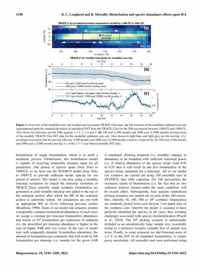
mate model (He, 2011). We investigate a number of best-case scenarios, concentrating on the time period spanningfrom 20 ka (BP 1950) up to and including 1989 CE, assum-ing a hypothetical sediment core location (Fig. 1) at the cen-tre of the Niño 3.4 ENSO region that is used to calculatethe Oceanic Niño Index. While the TRACE-21ka climatemodel does not necessarily fully capture ENSO processes,we choose this location in the model because of its dynamicSST (Fig. 1), which make it an interesting location to testhow inputted monthly SST is reconstructed by the simulatedIFA method. In reality it may or may not be possible to re-trieve a foraminifera-rich sediment core from this site, buthere for the purposes of this theoretical best-case modellingscenario, we assume that it would be possible.

In this study, simulated single foraminifera are incorpo-rated into synthetic sediment archives, the latter of whichemploy best-case sedimentation conditions whereby repre-sentative values for SAR and BD are both kept temporallyconstant. We assume a best-case scenario where foraminiferaperfectly record monthly SST (in this case the TRACE-21kaSST), and we also assume the existence of an ideal proxymethod that allows perfect retrieval of SST data from thesingle foraminifera. In reality, foraminifera may not continu-ously record the water temperature at the surface or indeed atthe same water depth in general, which further complicatesIFA reconstructions of SST dynamics in practice; however,here we seek to test best-case conditions. After carrying outthe sediment archive and bioturbation simulation, syntheticsingle foraminifera are randomly picked from each discrete-depth cm interval of the simulated core, thereby resultingin virtual IFA. The output of the best-case virtual IFA re-trieved from the sediment depth domain can subsequently bedirectly compared to the inputted SST in the time domain(i.e. TRACE-21ka SST), allowing us to evaluate the currentstate of the art in IFA at the most fundamental level.

We summarise the sediment model component (SEA-MUS) in Sect. 2.3, and the climate component (TRACE-21ka) in Sect. 2.4. An overview of our various best-case sce-nario simulations, as well as their associated run parameters,can be found in Sect. 2.5.

2.3 Sediment model component

We model the sedimentation history of single foraminiferausing the SEAMUS sediment accumulation model(Lougheed, 2020). This stochastic model uses the sameestablished understanding of bioturbation (Berger andHeath, 1968; Pisias, 1983; Bard, 2001) that is also incorpo-rated into previous sediment accumulation models (Trauth,1998, 2013; Dolman and Laepple, 2018), but differs inmodel execution in that it is explicitly designed for thepurpose of modelling single foraminifera, thus making ita suitable sediment model for use in this IFA evaluationstudy. Furthermore, the stochastic nature of the model,combined with an ensemble approach, is ideal for simulating

https://doi.org/10.5194/bg-19-1195-2022 Biogeosciences, 19, 1195–1209, 2022

1198 B. C. Lougheed and B. Metcalfe: Bioturbation and species abundance effects upon IFA

Figure 1. Overview of the modelled core site location and associated TRACE-21ka data. (a) The location of the modelled sediment core sitesuperimposed upon the standard deviation of annualised SST from the TRACE-21ka for the 500 year period between 1490 CE and 1989 CE.Also shown for reference are the Niño regions 1+ 2, 3, 3.4 and 4. (b) 100 year (1200 month) and 1000 year (12 000 month) moving meanof the monthly TRACE-21ka SST data for the modelled sediment core site. Also shown in light blue and light grey are the moving ±1σenvelopes associated with the moving 100 year (1200 month) and 1000 year (12 000 month) windows, respectively. (c) 100 year (1200 month)and 1000 year (12 000 month) moving 1σ of the 1.5–7 year filtered monthly SST data.

bioturbation of single foraminifera, which is in itself astochastic process. Furthermore, this bioturbation modelis capable of receiving temporally dynamic input for allparameters. Our period of interest spans from 20 ka to1989 CE, so we have run the SEAMUS model from 30 kato 1989 CE to provide sufficient model spin-up for ourperiod of interest. The model is run here using a monthlytimestep resolution (to match the timestep resolution ofTRACE-21ka), whereby single synthetic foraminifera aregenerated at each monthly timestep and added to the top ofthe sediment archive after which the BD of the sedimentarchive is uniformly mixed. All simulations are run withan appropriate BD of 10 cm, following previous studies(Boudreau, 1998). Some of our model run scenarios assumea temporally constant foraminiferal abundance, in such caseswe assign a constant per timestep foraminifera abundancethat results in 104 foraminifera per centimetre of sediment(i.e. the prescribed per timestep abundance is higher in thecase of higher SAR and vice versa). In the case of modelruns with temporally dynamic foraminifera abundance, theamount of foraminifera per centimetre that will result in 100foraminifera per timestep (i.e. month) for the given SAR

is simulated, allowing temporal (i.e. monthly) changes inabundance to be modelled with sufficient statistical power(i.e. if relative abundance of the species drops from 0.56to 0.55 then it will result in one less foraminifera of thespecies being simulated for a timestep). All of our modelrun scenarios are carried out using 100 ensemble runs inSEAMUS, thus fully capturing (for 100 percentiles) thestochastic nature of bioturbation (i.e. the fact that no twosediment archives formed under the same conditions willbe exactly alike). Subsequently, four separate randomisedpicking scenarios are carried out on each of the 100 ensem-bles, whereby 50, 100, 500 or 104 synthetic foraminiferaare randomly picked from each discrete 1 cm depth slice ofthe synthetic core, whereby the picker is assumed to haveperfectly identified the species in all cases, thus avoidingchallenges associated with species misidentification (Prachtet al., 2019). The 104 picking scenario is intentionallyincluded as an unrealistically large sample size, essentiallyacting as a reference scenario virtually free of sample sizenoise. Finally, in some scenarios we add Gaussian noise of±1 ◦C to the SST of all simulated foraminifera, to mimicproxy uncertainty. All ensemble runs were performed using

Biogeosciences, 19, 1195–1209, 2022 https://doi.org/10.5194/bg-19-1195-2022

B. C. Lougheed and B. Metcalfe: Bioturbation and species abundance effects upon IFA 1199

a Linux computer cluster provided by the Swedish NationalInfrastructure for Computing (SNIC) at the Uppsala Mul-tidisciplinary Centre for Advanced Computational Science(UPPMAX).

2.4 Climate model component

Monthly SST forcing for the SEAMUS model is sourcedfrom the TRACE-21ka transient climate simulation (He,2011), specifically using the surface temperature data for theTRACE-21ka grid cell centred on the coordinates 1.86◦ Nand 146.25◦W. This grid cell, at the centre of the Niño3.4 ENSO region used for calculating the Oceanic Niño In-dex, is ideal for our synthetic core simulation as it is char-acterised by large variation in the model’s interannual sea-sonal surface temperature (Fig. 1a), somewhat analogousto, e.g. ENSO. Furthermore, the grid cell also captures theglacial-interglacial SST transition (Fig. 1b), as well as typicalTRACE-21ka transient changes in ENSO-like SST variabil-ity, as shown by the 1.5–7 year filtered 100 and 1000 yearmoving 1σ of SST (Fig. 1c). This filtering approach haspreviously been used to identify ENSO-like variability inTRACE-21ka for the Niño 3.4 region (Liu et al., 2014).While the model variability is itself of course not a true repli-cation of the real ENSO signal, it nonetheless offers an inter-esting analogous time series of interannual changes in SSTvariability with which to test the efficacy of the IFA methodin reproducing said SST variability.

The TRACE-21ka dataset is the result of a fully cou-pled Community Climate System Model (CCSM3) simula-tion with T31_gx3 grid resolution that uses transient forcingchanges in both greenhouses gases, orbitally driven insola-tion variations, ice sheet evolution (ICE-5G) and associatedmeltwater fluxes for a non-accelerated atmosphere-ocean-seaice-land surface coupling. The TRACE-21ka dataset beginsat 22 ka, whereas our SEAMUS run starts at 30 ka. The rea-son for this difference is that we provide an extra 10 kyr ofspin-up time for the SEAMUS model, which is importantin cases of very low SAR (e.g. ≤ 5 cm kyr−1). In order toprovide SST data for synthetic foraminifera generated be-tween 30 and 22 ka, the oldest 1500 years contained withinthe TRACE-21ka dataset are repeated from 22 to 30 ka. Suchan approach obviously does not represent an accurate pictureof the climate between 30 and 22 ka, but it has no practicalconsequences for the particular purpose of our study, whichis to compare a given climate input signal in the time domainto the subsequent signal recorded by single foraminifera inthe sediment depth domain. Furthermore, our period of studyinterest spans the past 20 kyr.

2.5 Model run settings

We carry out a number of best-case scenarios, with eachscenario being subject to 100 ensemble runs to capture thefull stochastic range resulting from the sedimentation, bio-

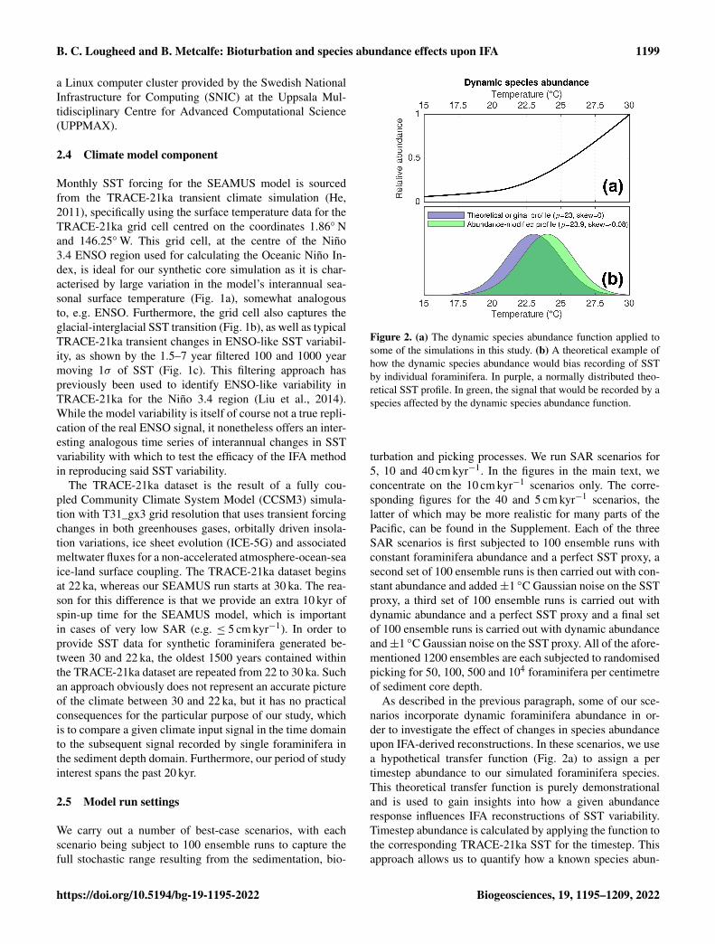
Figure 2. (a) The dynamic species abundance function applied tosome of the simulations in this study. (b) A theoretical example ofhow the dynamic species abundance would bias recording of SSTby individual foraminifera. In purple, a normally distributed theo-retical SST profile. In green, the signal that would be recorded by aspecies affected by the dynamic species abundance function.

turbation and picking processes. We run SAR scenarios for5, 10 and 40 cm kyr−1. In the figures in the main text, weconcentrate on the 10 cm kyr−1 scenarios only. The corre-sponding figures for the 40 and 5 cm kyr−1 scenarios, thelatter of which may be more realistic for many parts of thePacific, can be found in the Supplement. Each of the threeSAR scenarios is first subjected to 100 ensemble runs withconstant foraminifera abundance and a perfect SST proxy, asecond set of 100 ensemble runs is then carried out with con-stant abundance and added±1 ◦C Gaussian noise on the SSTproxy, a third set of 100 ensemble runs is carried out withdynamic abundance and a perfect SST proxy and a final setof 100 ensemble runs is carried out with dynamic abundanceand±1 ◦C Gaussian noise on the SST proxy. All of the afore-mentioned 1200 ensembles are each subjected to randomisedpicking for 50, 100, 500 and 104 foraminifera per centimetreof sediment core depth.

As described in the previous paragraph, some of our sce-narios incorporate dynamic foraminifera abundance in or-der to investigate the effect of changes in species abundanceupon IFA-derived reconstructions. In these scenarios, we usea hypothetical transfer function (Fig. 2a) to assign a pertimestep abundance to our simulated foraminifera species.This theoretical transfer function is purely demonstrationaland is used to gain insights into how a given abundanceresponse influences IFA reconstructions of SST variability.Timestep abundance is calculated by applying the function tothe corresponding TRACE-21ka SST for the timestep. Thisapproach allows us to quantify how a known species abun-

https://doi.org/10.5194/bg-19-1195-2022 Biogeosciences, 19, 1195–1209, 2022

1200 B. C. Lougheed and B. Metcalfe: Bioturbation and species abundance effects upon IFA

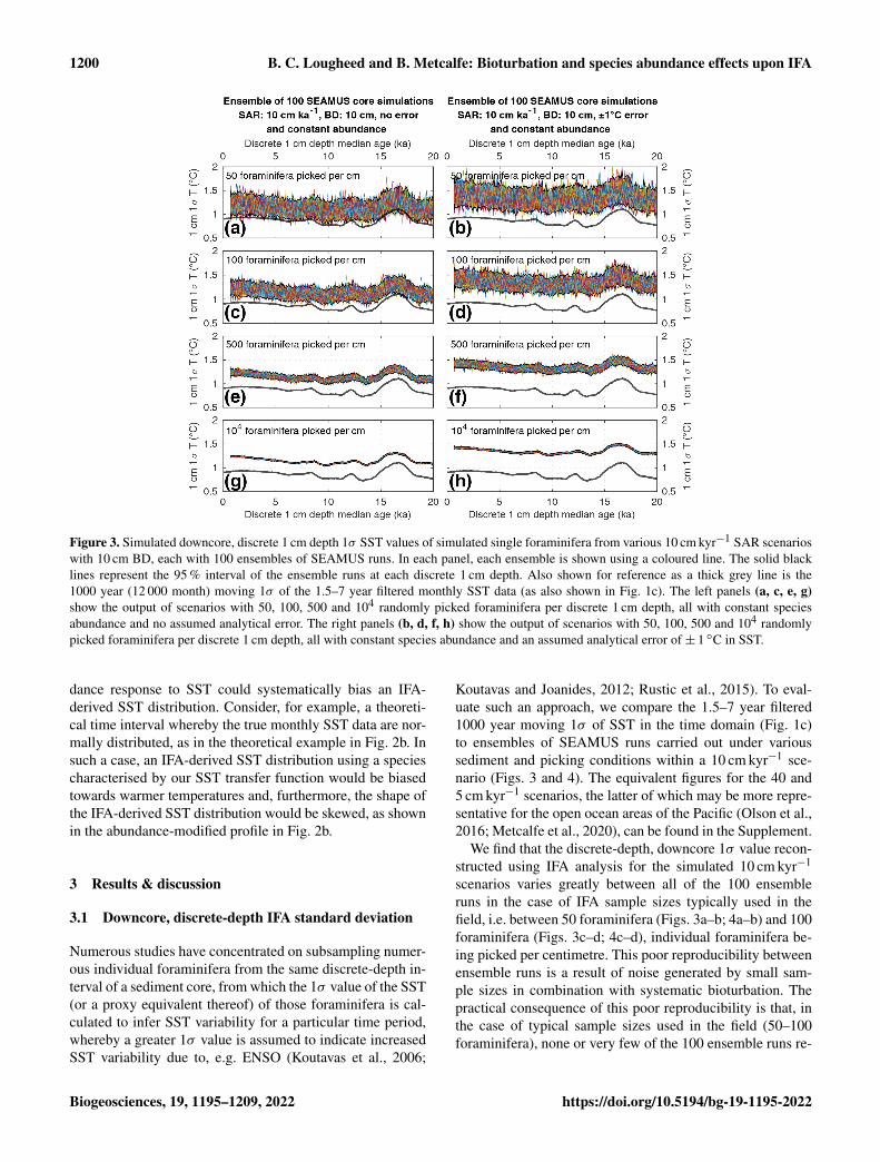
Figure 3. Simulated downcore, discrete 1 cm depth 1σ SST values of simulated single foraminifera from various 10 cm kyr−1 SAR scenarioswith 10 cm BD, each with 100 ensembles of SEAMUS runs. In each panel, each ensemble is shown using a coloured line. The solid blacklines represent the 95 % interval of the ensemble runs at each discrete 1 cm depth. Also shown for reference as a thick grey line is the1000 year (12 000 month) moving 1σ of the 1.5–7 year filtered monthly SST data (as also shown in Fig. 1c). The left panels (a, c, e, g)show the output of scenarios with 50, 100, 500 and 104 randomly picked foraminifera per discrete 1 cm depth, all with constant speciesabundance and no assumed analytical error. The right panels (b, d, f, h) show the output of scenarios with 50, 100, 500 and 104 randomlypicked foraminifera per discrete 1 cm depth, all with constant species abundance and an assumed analytical error of ± 1 ◦C in SST.

dance response to SST could systematically bias an IFA-derived SST distribution. Consider, for example, a theoreti-cal time interval whereby the true monthly SST data are nor-mally distributed, as in the theoretical example in Fig. 2b. Insuch a case, an IFA-derived SST distribution using a speciescharacterised by our SST transfer function would be biasedtowards warmer temperatures and, furthermore, the shape ofthe IFA-derived SST distribution would be skewed, as shownin the abundance-modified profile in Fig. 2b.

3 Results & discussion

3.1 Downcore, discrete-depth IFA standard deviation

Numerous studies have concentrated on subsampling numer-ous individual foraminifera from the same discrete-depth in-terval of a sediment core, from which the 1σ value of the SST(or a proxy equivalent thereof) of those foraminifera is cal-culated to infer SST variability for a particular time period,whereby a greater 1σ value is assumed to indicate increasedSST variability due to, e.g. ENSO (Koutavas et al., 2006;

Koutavas and Joanides, 2012; Rustic et al., 2015). To eval-uate such an approach, we compare the 1.5–7 year filtered1000 year moving 1σ of SST in the time domain (Fig. 1c)to ensembles of SEAMUS runs carried out under varioussediment and picking conditions within a 10 cm kyr−1 sce-nario (Figs. 3 and 4). The equivalent figures for the 40 and5 cm kyr−1 scenarios, the latter of which may be more repre-sentative for the open ocean areas of the Pacific (Olson et al.,2016; Metcalfe et al., 2020), can be found in the Supplement.

We find that the discrete-depth, downcore 1σ value recon-structed using IFA analysis for the simulated 10 cm kyr−1

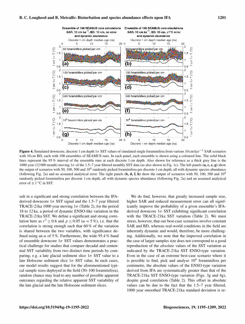
scenarios varies greatly between all of the 100 ensembleruns in the case of IFA sample sizes typically used in thefield, i.e. between 50 foraminifera (Figs. 3a–b; 4a–b) and 100foraminifera (Figs. 3c–d; 4c–d), individual foraminifera be-ing picked per centimetre. This poor reproducibility betweenensemble runs is a result of noise generated by small sam-ple sizes in combination with systematic bioturbation. Thepractical consequence of this poor reproducibility is that, inthe case of typical sample sizes used in the field (50–100foraminifera), none or very few of the 100 ensemble runs re-

Biogeosciences, 19, 1195–1209, 2022 https://doi.org/10.5194/bg-19-1195-2022

B. C. Lougheed and B. Metcalfe: Bioturbation and species abundance effects upon IFA 1201

Figure 4. Simulated downcore, discrete 1 cm depth 1σ SST values of simulated single foraminifera from various 10 cm kyr−1 SAR scenarioswith 10 cm BD, each with 100 ensembles of SEAMUS runs. In each panel, each ensemble is shown using a coloured line. The solid blacklines represent the 95 % interval of the ensemble runs at each discrete 1 cm depth. Also shown for reference as a thick grey line is the1000 year (12 000 month) moving 1σ of the 1.5–7 year filtered monthly SST data (as also shown in Fig. 1c). The left panels (a, c, e, g) showthe output of scenarios with 50, 100, 500 and 104 randomly picked foraminifera per discrete 1 cm depth, all with dynamic species abundance(following Fig. 2a) and no assumed analytical error. The right panels (b, d, f, h) show the output of scenarios with 50, 100, 500 and 104

randomly picked foraminifera per discrete 1 cm depth, all with dynamic species abundance (following Fig. 2a) and an assumed analyticalerror of ± 1 ◦C in SST.

sult in a significant and strong correlation between the IFA-derived downcore 1σ SST signal and the 1.5–7 year filteredTRACE-21ka 1000 year moving 1σ (Table 2), for the period18 to 12 ka, a period of dynamic ENSO-like variation in theTRACE-21ka SST. We define a significant and strong corre-lation here as r2

≥ 0.6 and p ≤ 0.05 (α = 5 %), i.e. that thecorrelation is strong enough such that 60 % of the variationis shared between the two variables, with significance de-fined using an α of 5 %. Furthermore, the wide 95.4 % bandof ensemble downcore 1σ SST values demonstrates a prac-tical challenge for studies that compare decadal and centen-nial SST variability from two distinct time periods by com-paring, e.g. a late glacial sediment slice 1σ SST value to alate Holocene sediment slice 1σ SST value. In such cases,our model results suggest that for the aforementioned typi-cal sample sizes deployed in the field (50–100 foraminifera),random chance may lead to any number of possible apparentoutcomes regarding the relative apparent SST variability ofthe late glacial and the late Holocene sediment slices.

We do find, however, that greatly increased sample size,higher SAR and reduced measurement error can all signif-icantly improve the probability of a given ensemble’s IFA-derived downcore 1σ SST exhibiting significant correlationwith the TRACE-21ka SST variation (Table 2). We muststress, however, that our best-case scenarios involve constantSAR and BD, whereas real-world conditions in the field areinherently dynamic and would, therefore, be more challeng-ing. Additionally, we note that the improved correlation inthe case of larger samples size does not correspond to a goodreproduction of the absolute values of the SST variation asindicated by the TRACE-21ka SST ENSO-type variation.Even in the case of an extreme best-case scenario where itis possible to find, pick and analyse 104 foraminifera percentimetre, the absolute values of the ENSO-type variationderived from IFA are systematically greater than that of theTRACE-21ka SST ENSO-type variation (Figs. 3g and 4g),despite good correlation (Table 2). This offset in absolutevalues can be due to the fact that the 1.5–7 year filtered,1000 year smoothed TRACE-21ka standard deviation is re-

https://doi.org/10.5194/bg-19-1195-2022 Biogeosciences, 19, 1195–1209, 2022

1202 B. C. Lougheed and B. Metcalfe: Bioturbation and species abundance effects upon IFA

Table 1. Overview of SAR and number of picked specimens in select IFA studies (including non-ENSO studies). Region codes are as follows:WEP – western equatorial Pacific; CEP – central equatorial Pacific; EEP – eastern equatorial Pacific; EEI – eastern equatorial Indian Ocean;SIO – southern Indian Ocean; ARA – Arabian Sea. We have estimated the 1σ value of age in 1 cm of sediment based on the SAR and a BDof 10 cm (Boudreau, 1998), using the following calculation based on (Berger and Heath, 1968): BD/SAR× 1000, where SAR is entered incm kyr−1 and BD in cm.

Core(s) Study Region Approximate Estimated 1σ Specimens pickedSAR value of age per discrete

(cm kyr−1) in 1 cm (yr) interval (#)

MGL1208-14MC and 12GC White et al. (2018) CEP ∼ 2.5 4000 70–90ODP 806 Ford et al. (2015) WEP ∼ 3 3300 60–70ODP 849 Ford et al. (2015),

White and Ravelo (2020)EEP ∼ 4 2500 60–70

KNR195-5 MC42 Rustic et al. (2015) EEP ∼ 12 830 55MD02-2529 Leduc et al. (2009) EEP ∼ 40 250 65–90V21-30 Koutavas et al. (2006),

Koutavas and Joanides (2012)EEP ∼ 12 830 50

MD98-2177 Khider et al. (2011) WEP ∼ 70 150 60–90SO189-119KL Thirumalai et al. (2019) EEI ∼ 20 500 55–65SO189-39KL Thirumalai et al. (2019) EEI ∼ 37 270 55–65GeoB 10038-4 Thirumalai et al. (2019) EEI ∼ 9 1100 55–65GeoB 10053-7 Thirumalai et al. (2019) EEI ∼ 35 290 55–65NIOP 905P Ganssen et al. (2011) ARA ∼ 20 500 30–4064PE-174P13 Scussolini et al. (2013) SIO ∼ 1.2 8330 20–30

flecting a different integration of the time than the 1σ dataretrieved from discrete-depth IFA. The former is based ona smoothing of uniform time, whereas the latter representsa population of foraminifera with a long-tailed age distribu-tion. The absolute offset between the two signals is furtherincreased in the case of machine error on the IFA SST anal-ysis (Figs. 3h and 4h), thus highlighting the importance ofaccurately quantifying uncertainties in the analytical process.

3.2 Discrete-depth IFA distribution analysis

Many IFA studies have gone beyond studying discrete depth1σ SST values and have branched into more forensic studiesof the shape of discrete depth SST distributions. These stud-ies have focused on analysing the shape of said distributionusing various statistical tools, including skewness analysis ofhistograms (Leduc et al., 2009; Khider et al., 2011), as wellas quantile–quantile (Q–Q) plots (Ford et al., 2015; Whiteet al., 2018; Thirumalai et al., 2019; Rongstad et al., 2020;White and Ravelo, 2020). Such analyses can reveal apparentshifts in the shape of the downcore IFA-derived SST distri-bution, which the aforementioned studies have attributed toSST changes in the water caused by ENSO-type climate vari-ability.

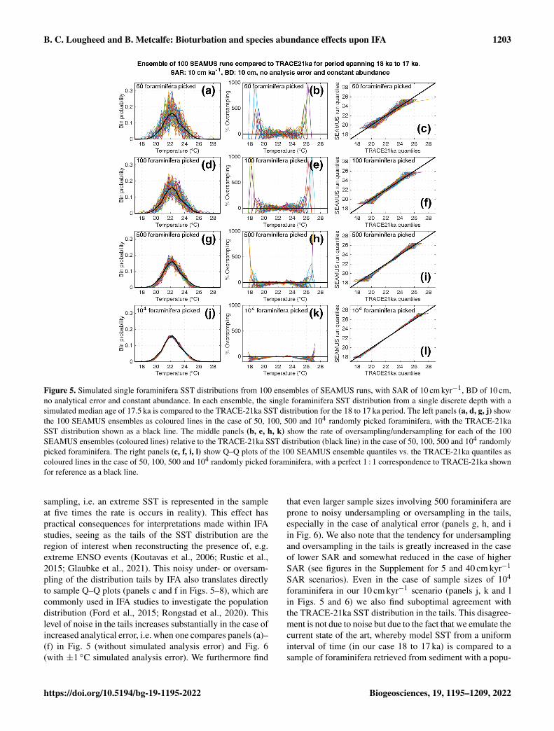
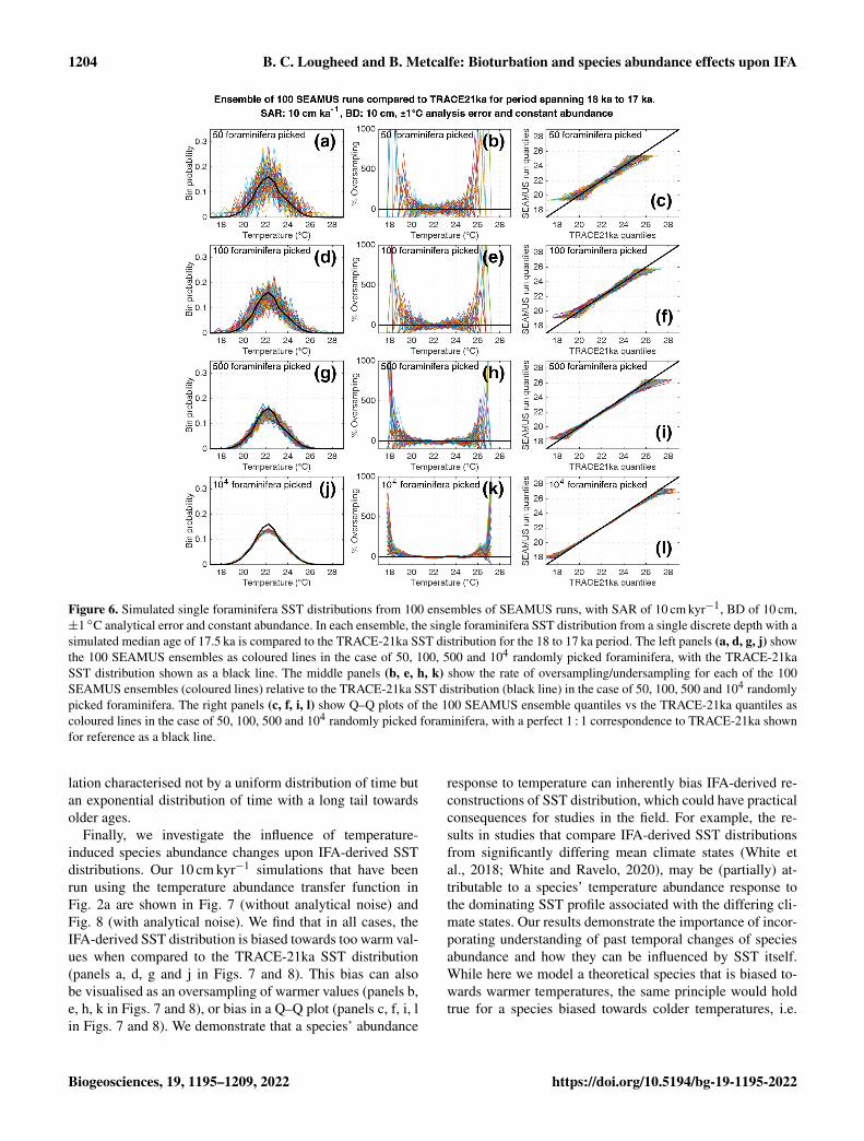
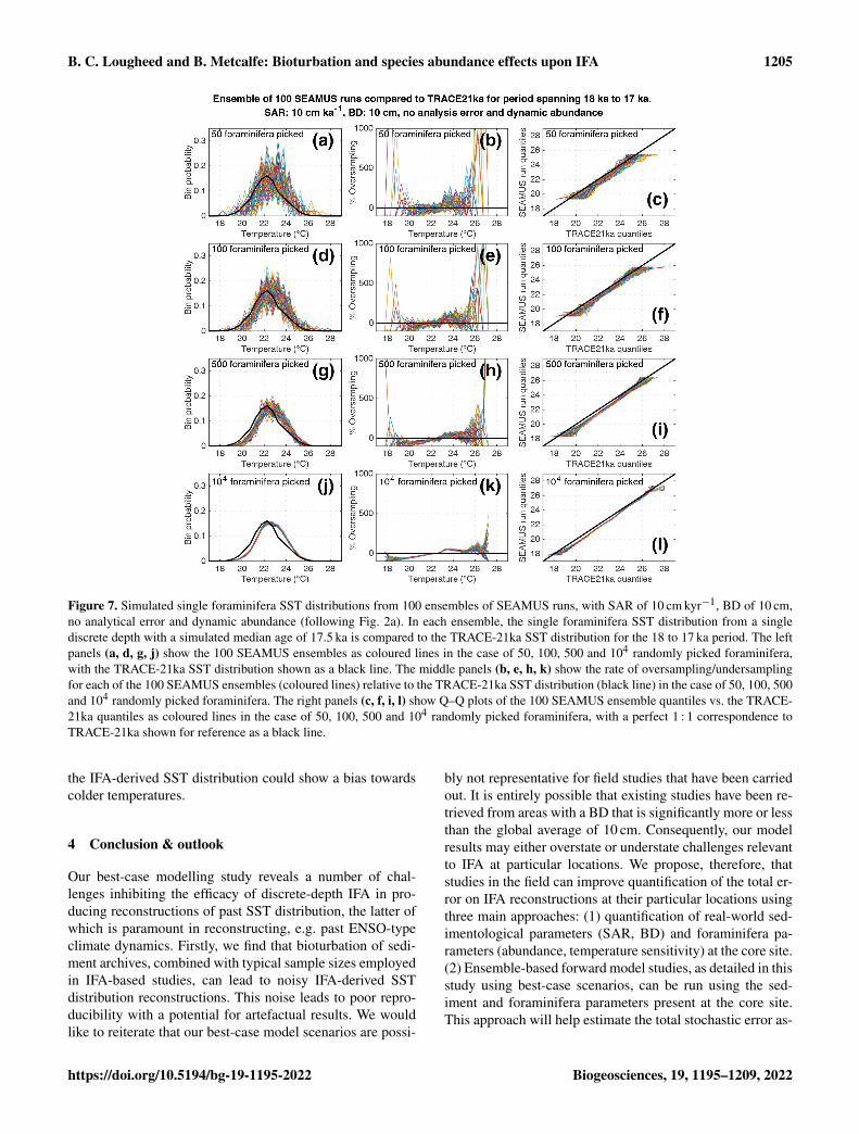
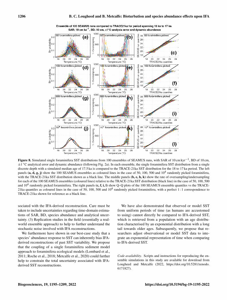
Here, we compare the monthly TRACE-21ka SST data forthe 18 to 17 ka period to our 100 ensembles of simulated IFASST for the 10 cm kyr−1 scenario, taking the 1 cm discrete-depth with a median age closest to 17.5 ka in each ensemble.We show 100 ensembles with no analytical error and con-stant abundance (Fig. 5), 100 ensembles with ±1 ◦C analyt-

ical error and constant abundance (Fig. 6), 100 ensembleswith ±1 ◦C analytical error and dynamic abundance (Fig. 7),and 100 ensembles with ±1 ◦C analytical error and dynamicabundance (Fig. 8). In all cases in our 10 cm kry−1 scenario,we find that sample sizes typically associated with IFA in thefield (50–100 foraminifera, see Table 1) produce high levelsof noise, leading to low reproducibility from one ensemble tothe next (panels a and d in Figs. 5–8). As expected, the 5 and40 cm kyr−1 scenarios (see figures in the Supplement) resultin lower and higher reproducibility, respectably. In practicalterms, these results suggest that if one were to retrieve mul-tiple sediment cores and carry out discrete-depth IFA at thesame coring location, it is possible that different outcomeswould be produced each time, each with suboptimal corre-spondence to the true SST distribution in the water. Further-more, as the level of noise increases with lower SAR, one hasto be additionally careful when comparing IFA results fromsites with markedly different SAR.

We also find that the IFA method has a tendency for noisyoversampling or undersampling of the tails of the true SSTdistribution in the case of typical sample sizes (50–100 spec-imens) used in the field (panels b and e in Figs. 5–8). Thiseffect can be attributed to the fact that there is a low occur-rence of individual foraminifera within the population thatrecord more extreme SST, and small sample sizes are likelyto either miss such foraminifera altogether (i.e.−100 % over-sampling) or, in the case of a single such foraminifera be-ing picked within the sample, significantly over-represent ex-treme SST within the sample (in some cases > 500 % over-

Biogeosciences, 19, 1195–1209, 2022 https://doi.org/10.5194/bg-19-1195-2022

B. C. Lougheed and B. Metcalfe: Bioturbation and species abundance effects upon IFA 1203

Figure 5. Simulated single foraminifera SST distributions from 100 ensembles of SEAMUS runs, with SAR of 10 cm kyr−1, BD of 10 cm,no analytical error and constant abundance. In each ensemble, the single foraminifera SST distribution from a single discrete depth with asimulated median age of 17.5 ka is compared to the TRACE-21ka SST distribution for the 18 to 17 ka period. The left panels (a, d, g, j) showthe 100 SEAMUS ensembles as coloured lines in the case of 50, 100, 500 and 104 randomly picked foraminifera, with the TRACE-21kaSST distribution shown as a black line. The middle panels (b, e, h, k) show the rate of oversampling/undersampling for each of the 100SEAMUS ensembles (coloured lines) relative to the TRACE-21ka SST distribution (black line) in the case of 50, 100, 500 and 104 randomlypicked foraminifera. The right panels (c, f, i, l) show Q–Q plots of the 100 SEAMUS ensemble quantiles vs. the TRACE-21ka quantiles ascoloured lines in the case of 50, 100, 500 and 104 randomly picked foraminifera, with a perfect 1 : 1 correspondence to TRACE-21ka shownfor reference as a black line.

sampling, i.e. an extreme SST is represented in the sampleat five times the rate is occurs in reality). This effect haspractical consequences for interpretations made within IFAstudies, seeing as the tails of the SST distribution are theregion of interest when reconstructing the presence of, e.g.extreme ENSO events (Koutavas et al., 2006; Rustic et al.,2015; Glaubke et al., 2021). This noisy under- or oversam-pling of the distribution tails by IFA also translates directlyto sample Q–Q plots (panels c and f in Figs. 5–8), which arecommonly used in IFA studies to investigate the populationdistribution (Ford et al., 2015; Rongstad et al., 2020). Thislevel of noise in the tails increases substantially in the case ofincreased analytical error, i.e. when one compares panels (a)–(f) in Fig. 5 (without simulated analysis error) and Fig. 6(with ±1 ◦C simulated analysis error). We furthermore find

that even larger sample sizes involving 500 foraminifera areprone to noisy undersampling or oversampling in the tails,especially in the case of analytical error (panels g, h, and iin Fig. 6). We also note that the tendency for undersamplingand oversampling in the tails is greatly increased in the caseof lower SAR and somewhat reduced in the case of higherSAR (see figures in the Supplement for 5 and 40 cm kyr−1

SAR scenarios). Even in the case of sample sizes of 104

foraminifera in our 10 cm kyr−1 scenario (panels j, k and lin Figs. 5 and 6) we also find suboptimal agreement withthe TRACE-21ka SST distribution in the tails. This disagree-ment is not due to noise but due to the fact that we emulate thecurrent state of the art, whereby model SST from a uniforminterval of time (in our case 18 to 17 ka) is compared to asample of foraminifera retrieved from sediment with a popu-

https://doi.org/10.5194/bg-19-1195-2022 Biogeosciences, 19, 1195–1209, 2022

1204 B. C. Lougheed and B. Metcalfe: Bioturbation and species abundance effects upon IFA

Figure 6. Simulated single foraminifera SST distributions from 100 ensembles of SEAMUS runs, with SAR of 10 cm kyr−1, BD of 10 cm,±1 ◦C analytical error and constant abundance. In each ensemble, the single foraminifera SST distribution from a single discrete depth with asimulated median age of 17.5 ka is compared to the TRACE-21ka SST distribution for the 18 to 17 ka period. The left panels (a, d, g, j) showthe 100 SEAMUS ensembles as coloured lines in the case of 50, 100, 500 and 104 randomly picked foraminifera, with the TRACE-21kaSST distribution shown as a black line. The middle panels (b, e, h, k) show the rate of oversampling/undersampling for each of the 100SEAMUS ensembles (coloured lines) relative to the TRACE-21ka SST distribution (black line) in the case of 50, 100, 500 and 104 randomlypicked foraminifera. The right panels (c, f, i, l) show Q–Q plots of the 100 SEAMUS ensemble quantiles vs the TRACE-21ka quantiles ascoloured lines in the case of 50, 100, 500 and 104 randomly picked foraminifera, with a perfect 1 : 1 correspondence to TRACE-21ka shownfor reference as a black line.

lation characterised not by a uniform distribution of time butan exponential distribution of time with a long tail towardsolder ages.

Finally, we investigate the influence of temperature-induced species abundance changes upon IFA-derived SSTdistributions. Our 10 cm kyr−1 simulations that have beenrun using the temperature abundance transfer function inFig. 2a are shown in Fig. 7 (without analytical noise) andFig. 8 (with analytical noise). We find that in all cases, theIFA-derived SST distribution is biased towards too warm val-ues when compared to the TRACE-21ka SST distribution(panels a, d, g and j in Figs. 7 and 8). This bias can alsobe visualised as an oversampling of warmer values (panels b,e, h, k in Figs. 7 and 8), or bias in a Q–Q plot (panels c, f, i, lin Figs. 7 and 8). We demonstrate that a species’ abundance

response to temperature can inherently bias IFA-derived re-constructions of SST distribution, which could have practicalconsequences for studies in the field. For example, the re-sults in studies that compare IFA-derived SST distributionsfrom significantly differing mean climate states (White etal., 2018; White and Ravelo, 2020), may be (partially) at-tributable to a species’ temperature abundance response tothe dominating SST profile associated with the differing cli-mate states. Our results demonstrate the importance of incor-porating understanding of past temporal changes of speciesabundance and how they can be influenced by SST itself.While here we model a theoretical species that is biased to-wards warmer temperatures, the same principle would holdtrue for a species biased towards colder temperatures, i.e.

Biogeosciences, 19, 1195–1209, 2022 https://doi.org/10.5194/bg-19-1195-2022

B. C. Lougheed and B. Metcalfe: Bioturbation and species abundance effects upon IFA 1205

Figure 7. Simulated single foraminifera SST distributions from 100 ensembles of SEAMUS runs, with SAR of 10 cm kyr−1, BD of 10 cm,no analytical error and dynamic abundance (following Fig. 2a). In each ensemble, the single foraminifera SST distribution from a singlediscrete depth with a simulated median age of 17.5 ka is compared to the TRACE-21ka SST distribution for the 18 to 17 ka period. The leftpanels (a, d, g, j) show the 100 SEAMUS ensembles as coloured lines in the case of 50, 100, 500 and 104 randomly picked foraminifera,with the TRACE-21ka SST distribution shown as a black line. The middle panels (b, e, h, k) show the rate of oversampling/undersamplingfor each of the 100 SEAMUS ensembles (coloured lines) relative to the TRACE-21ka SST distribution (black line) in the case of 50, 100, 500and 104 randomly picked foraminifera. The right panels (c, f, i, l) show Q–Q plots of the 100 SEAMUS ensemble quantiles vs. the TRACE-21ka quantiles as coloured lines in the case of 50, 100, 500 and 104 randomly picked foraminifera, with a perfect 1 : 1 correspondence toTRACE-21ka shown for reference as a black line.

the IFA-derived SST distribution could show a bias towardscolder temperatures.

4 Conclusion & outlook

Our best-case modelling study reveals a number of chal-lenges inhibiting the efficacy of discrete-depth IFA in pro-ducing reconstructions of past SST distribution, the latter ofwhich is paramount in reconstructing, e.g. past ENSO-typeclimate dynamics. Firstly, we find that bioturbation of sedi-ment archives, combined with typical sample sizes employedin IFA-based studies, can lead to noisy IFA-derived SSTdistribution reconstructions. This noise leads to poor repro-ducibility with a potential for artefactual results. We wouldlike to reiterate that our best-case model scenarios are possi-

bly not representative for field studies that have been carriedout. It is entirely possible that existing studies have been re-trieved from areas with a BD that is significantly more or lessthan the global average of 10 cm. Consequently, our modelresults may either overstate or understate challenges relevantto IFA at particular locations. We propose, therefore, thatstudies in the field can improve quantification of the total er-ror on IFA reconstructions at their particular locations usingthree main approaches: (1) quantification of real-world sed-imentological parameters (SAR, BD) and foraminifera pa-rameters (abundance, temperature sensitivity) at the core site.(2) Ensemble-based forward model studies, as detailed in thisstudy using best-case scenarios, can be run using the sed-iment and foraminifera parameters present at the core site.This approach will help estimate the total stochastic error as-

https://doi.org/10.5194/bg-19-1195-2022 Biogeosciences, 19, 1195–1209, 2022

1206 B. C. Lougheed and B. Metcalfe: Bioturbation and species abundance effects upon IFA

Figure 8. Simulated single foraminifera SST distributions from 100 ensembles of SEAMUS runs, with SAR of 10 cm kyr−1, BD of 10 cm,±1 ◦C analytical error and dynamic abundance (following Fig. 2a). In each ensemble, the single foraminifera SST distribution from a singlediscrete depth with a simulated median age of 17.5 ka is compared to the TRACE-21ka SST distribution for the 18 to 17 ka period. The leftpanels (a, d, g, j) show the 100 SEAMUS ensembles as coloured lines in the case of 50, 100, 500 and 104 randomly picked foraminifera,with the TRACE-21ka SST distribution shown as a black line. The middle panels (b, e, h, k) show the rate of oversampling/undersamplingfor each of the 100 SEAMUS ensembles (coloured lines) relative to the TRACE-21ka SST distribution (black line) in the case of 50, 100, 500and 104 randomly picked foraminifera. The right panels (c, f, i, l) show Q–Q plots of the 100 SEAMUS ensemble quantiles vs the TRACE-21ka quantiles as coloured lines in the case of 50, 100, 500 and 104 randomly picked foraminifera, with a perfect 1 : 1 correspondence toTRACE-21ka shown for reference as a black line.

sociated with the IFA-derived reconstruction. Care must betaken to include uncertainties regarding time-domain estima-tions of SAR, BD, species abundance and analytical uncer-tainty. (3) Replication studies in the field (essentially a real-world ensemble approach) to help to further understand thestochastic noise involved with IFA reconstructions.

We furthermore have shown in our best-case study that aspecies’ abundance response to SST can inherently bias IFA-derived reconstructions of past SST variability. We proposethat the coupling of a single foraminifera sediment modelapproach to foraminifera ecological models (Lombard et al.,2011; Roche et al., 2018; Metcalfe et al., 2020) could furtherhelp to constrain the total uncertainty associated with IFA-derived SST reconstructions.

We have also demonstrated that observed or model SSTfrom uniform periods of time (as humans are accustomedto using) cannot directly be compared to IFA-derived SST,which is retrieved from a population with an age distribu-tion characterised by an exponential distribution with a longtail towards older ages. Subsequently, we propose that re-searchers adjust observational or model SST data to inte-grate an exponential representation of time when comparingto IFA-derived SST.

Code availability. Scripts and instructions for reproducing the en-semble simulations in this study are available for download fromLougheed and Metcalfe (2022, https://doi.org/10.5281/zenodo.6171827).

Biogeosciences, 19, 1195–1209, 2022 https://doi.org/10.5194/bg-19-1195-2022

B. C. Lougheed and B. Metcalfe: Bioturbation and species abundance effects upon IFA 1207

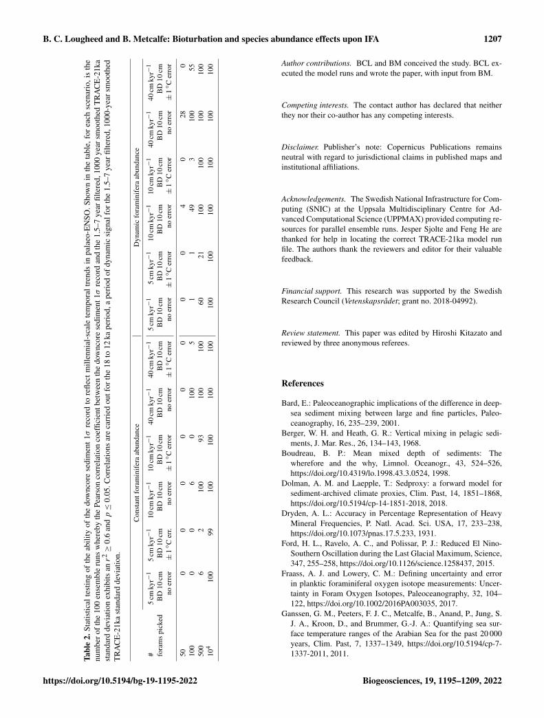
Tabl

e2.

Stat

istic

alte

stin

gof

the

abili

tyof

the

dow

ncor

ese

dim

ent1σ

reco

rdto

refle

ctm

illen

nial

-sca

lete

mpo

ralt

rend

sin

pala

eo-E

NSO

.Sho

wn

inth

eta

ble,

for

each

scen

ario

,is

the

num

bero

fthe

100

ense

mbl

eru

nsw

here

byth

ePe

arso

nco

rrel

atio

nco

effic

ient

betw

een

the

dow

ncor

ese

dim

ent1σ

reco

rdan

dth

e1.

5–7

year

filte

red,

1000

year

smoo

thed

TR

AC

E-2

1ka

stan

dard

devi

atio

nex

hibi

tsanr

2≥

0.6

andp≤

0.05

.Cor

rela

tions

are

carr

ied

outf

orth

e18

to12

kape

riod

,ape

riod

ofdy

nam

icsi

gnal

fort

he1.

5–7

year

filte

red,

1000

-yea

rsm

ooth

edT

RA

CE

-21k

ast

anda

rdde

viat

ion.

Con

stan

tfor

amin

ifer

aab

unda

nce

Dyn

amic

fora

min

ifer

aab

unda

nce

#5

cmky

r−1

5cm

kyr−

110

cmky

r−1

10cm

kyr−

140

cmky

r−1

40cm

kyr−

15

cmky

r−1

5cm

kyr−

110

cmky

r−1

10cm

kyr−

140

cmky

r−1

40cm

kyr−

1

fora

ms

pick

edB

D10

cmB

D10

cmB

D10

cmB

D10

cmB

D10

cmB

D10

cmB

D10

cmB

D10

cmB

D10

cmB

D10

cmB

D10

cmB

D10

cmno

erro

r±

1◦C

err.

noer

ror±

1◦C

erro

rno

erro

r±

1◦C

erro

rno

erro

r±

1◦C

erro

rno

erro

r±

1◦C

erro

rno

erro

r±

1◦C

erro

r

500

00

00

00

04

028

010

00

06

010

05

11

493

100

5550

06

210

093

100

100

6021

100

100

100

100

104

100

9910

010

010

010

010

010

010

010

010

010

0 Author contributions. BCL and BM conceived the study. BCL ex-ecuted the model runs and wrote the paper, with input from BM.

Competing interests. The contact author has declared that neitherthey nor their co-author has any competing interests.

Disclaimer. Publisher’s note: Copernicus Publications remainsneutral with regard to jurisdictional claims in published maps andinstitutional affiliations.

Acknowledgements. The Swedish National Infrastructure for Com-puting (SNIC) at the Uppsala Multidisciplinary Centre for Ad-vanced Computational Science (UPPMAX) provided computing re-sources for parallel ensemble runs. Jesper Sjolte and Feng He arethanked for help in locating the correct TRACE-21ka model runfile. The authors thank the reviewers and editor for their valuablefeedback.

Financial support. This research was supported by the SwedishResearch Council (Vetenskapsrådet; grant no. 2018-04992).

Review statement. This paper was edited by Hiroshi Kitazato andreviewed by three anonymous referees.

References

Bard, E.: Paleoceanographic implications of the difference in deep-sea sediment mixing between large and fine particles, Paleo-ceanography, 16, 235–239, 2001.

Berger, W. H. and Heath, G. R.: Vertical mixing in pelagic sedi-ments, J. Mar. Res., 26, 134–143, 1968.

Boudreau, B. P.: Mean mixed depth of sediments: Thewherefore and the why, Limnol. Oceanogr., 43, 524–526,https://doi.org/10.4319/lo.1998.43.3.0524, 1998.

Dolman, A. M. and Laepple, T.: Sedproxy: a forward model forsediment-archived climate proxies, Clim. Past, 14, 1851–1868,https://doi.org/10.5194/cp-14-1851-2018, 2018.

Dryden, A. L.: Accuracy in Percentage Representation of HeavyMineral Frequencies, P. Natl. Acad. Sci. USA, 17, 233–238,https://doi.org/10.1073/pnas.17.5.233, 1931.

Ford, H. L., Ravelo, A. C., and Polissar, P. J.: Reduced El Nino-Southern Oscillation during the Last Glacial Maximum, Science,347, 255–258, https://doi.org/10.1126/science.1258437, 2015.

Fraass, A. J. and Lowery, C. M.: Defining uncertainty and errorin planktic foraminiferal oxygen isotope measurements: Uncer-tainty in Foram Oxygen Isotopes, Paleoceanography, 32, 104–122, https://doi.org/10.1002/2016PA003035, 2017.

Ganssen, G. M., Peeters, F. J. C., Metcalfe, B., Anand, P., Jung, S.J. A., Kroon, D., and Brummer, G.-J. A.: Quantifying sea sur-face temperature ranges of the Arabian Sea for the past 20 000years, Clim. Past, 7, 1337–1349, https://doi.org/10.5194/cp-7-1337-2011, 2011.

https://doi.org/10.5194/bg-19-1195-2022 Biogeosciences, 19, 1195–1209, 2022

1208 B. C. Lougheed and B. Metcalfe: Bioturbation and species abundance effects upon IFA

Glaubke, R. H., Thirumalai, K., Schmidt, M. W., and Hertzberg,J. E.: Discerning Changes in High-Frequency ClimateVariability Using Geochemical Populations of IndividualForaminifera, Paleoceanogr. Paleocl., 36, e2020PA004065,https://doi.org/10.1029/2020PA004065, 2021.

He, F.: Simulating transient climate evolution of the last deglacia-tion with CCSM 3, PhD thesis, University of Winsconsin, Madi-son, Madison, WI, USA, 2011.

Henderiks, J., Freudenthal, T., Meggers, H., Nave, S., Abrantes,F., Bollmann, J., and Thierstein, H. R.: Glacial–interglacialvariability of particle accumulation in the Canary Basin: atime-slice approach, Deep-Sea Res. Pt. II, 49, 3675–3705,https://doi.org/10.1016/S0967-0645(02)00102-9, 2002.

Khider, D., Stott, L. D., Emile-Geay, J., Thunell, R., and Ham-mond, D. E.: Assessing El Niño Southern Oscillation variabil-ity during the past millennium, Paleoceanography, 26, PA3222,https://doi.org/10.1029/2011PA002139, 2011.

Killingley, J. S., Johnson, R. F., and Berger, W. H.: Oxygen and car-bon isotopes of individual shells of planktonic foraminifera fromOntong-Java plateau, equatorial pacific, Palaeogeogr. Palaeocl.,33, 193–204, https://doi.org/10.1016/0031-0182(81)90038-9,1981.

Koutavas, A. and Joanides, S.: El Niño–Southern Oscillation ex-trema in the Holocene and Last Glacial Maximum, Paleoceanog-raphy, 27, PA4208, https://doi.org/10.1029/2012PA002378,2012.

Koutavas, A., deMenocal, P. B., Olive, G. C., and Lynch-Stieglitz, J.: Mid-Holocene El Niño–Southern Oscillation(ENSO) attenuation revealed by individual foraminifera ineastern tropical Pacific sediments, Geology, 34, 993–996,https://doi.org/10.1130/G22810A.1, 2006.

Leduc, G., Vidal, L., Cartapanis, O., and Bard, E.: Modes of east-ern equatorial Pacific thermocline variability: Implications forENSO dynamics over the last glacial period, Paleoceanography,24, PA3202, https://doi.org/10.1029/2008PA001701, 2009.

Liu, Z., Lu, Z., Wen, X., Otto-Bliesner, B. L., Timmermann,A., and Cobb, K. M.: Evolution and forcing mechanisms ofEl Niño over the past 21,000 years, Nature, 515, 550–553,https://doi.org/10.1038/nature13963, 2014.

Lombard, F., Labeyrie, L., Michel, E., Bopp, L., Cortijo, E.,Retailleau, S., Howa, H., and Jorissen, F.: Modelling plank-tic foraminifer growth and distribution using an ecophysio-logical multi-species approach, Biogeosciences, 8, 853–873,https://doi.org/10.5194/bg-8-853-2011, 2011.

Lougheed, B. C.: SEAMUS (v1.20): a 114C-enabled, single-specimen sediment accumulation simulator, Geosci. Model Dev.,13, 155–168, https://doi.org/10.5194/gmd-13-155-2020, 2020.

Lougheed, B. C. and Metcalfe, B.: Simulation ensembles for:“Testing the effect of bioturbation and species abundance upondiscrete-depth individual foraminifera analysis”, Zenodo [code],https://doi.org/10.5281/zenodo.6171827, 2022.

Metcalfe, B., Lougheed, B. C., Waelbroeck, C., and Roche, D. M.:A proxy modelling approach to assess the potential of extract-ing ENSO signal from tropical Pacific planktonic foraminifera,Clim. Past, 16, 885–910, https://doi.org/10.5194/cp-16-885-2020, 2020.

Oba, T. and Uomonoto, K.: Oxygen and Carbon Isotopic Ratiosof Planktonic Foraminifera in Sediment Traps JT-01 and JT-02,Gekkan Kaiyo, 21, 239–246, 1989.

Olson, P., Reynolds, E., Hinnov, L., and Goswami, A.: Variation ofocean sediment thickness with crustal age, Geochem. Geophy.,17, 1349–1369, https://doi.org/10.1002/2015GC006143, 2016.

Patterson, R. T. and Fishbein, E.: Re-examination of the statisticalmethods used to determine the number of point counts neededfor micropaleontological quantitative research, J. Paleontol., 63,245–248, https://doi.org/10.1017/S0022336000019272, 1989.

Peng, T.-H., Broecker, W. S., and Berger, W. H.: Rates of benthicmixing in deep-sea sediment as determined by radioactive trac-ers, Quaternary Res., 11, 141–149, 1979.

Pisias, N. G.: Geologic time series from deep-sea sediments: Timescales and distortion by bioturbation, Mar. Geol., 51, 99–113,1983.

Pracht, H., Metcalfe, B., and Peeters, F. J. C.: Oxygen isotope com-position of the final chamber of planktic foraminifera providesevidence of vertical migration and depth-integrated growth, Bio-geosciences, 16, 643–661, https://doi.org/10.5194/bg-16-643-2019, 2019.

Roche, D. M., Waelbroeck, C., Metcalfe, B., and Caley, T.:FAME (v1.0): a simple module to simulate the effect ofplanktonic foraminifer species-specific habitat on their oxy-gen isotopic content, Geosci. Model Dev., 11, 3587–3603,https://doi.org/10.5194/gmd-11-3587-2018, 2018.

Rongstad, B. L., Marchitto, T. M., Marks, G. S., Koutavas,A., Mekik, F., and Ravelo, A. C.: Investigating ENSO-Related Temperature Variability in Equatorial Pa-cific Core-Tops Using Mg/Ca in Individual PlankticForaminifera, Paleoceanogr. Paleocl., 35, e2019PA003774,https://doi.org/10.1029/2019PA003774, 2020.

Rustic, G. T., Koutavas, A., Marchitto, T. M., and Linsley, B. K.:Dynamical excitation of the tropical Pacific Ocean and ENSOvariability by Little Ice Age cooling, Science, 350, 1537–1541,2015.

Schiffelbein, P.: Effect of benthic mixing on the information con-tent of deep-sea stratigraphical signals, Nature, 311, 651–653,https://doi.org/10.1038/311651a0, 1984.

Schiffelbein, P. and Hills, S.: Direct assessment of stable iso-tope variability in planktonic foraminifera populations, Palaeo-geogr. Palaeocl., 48, 197–213, https://doi.org/10.1016/0031-0182(84)90044-0, 1984.

Scussolini, P., van Sebille, E., and Durgadoo, J. V.: Paleo Agulhasrings enter the subtropical gyre during the penultimate deglacia-tion, Clim. Past, 9, 2631–2639, https://doi.org/10.5194/cp-9-2631-2013, 2013.

Spero, H. J. and Williams, D. F.: Evidence for seasonallow-salinity surface waters in the Gulf of Mexico overthe last 16,000 years, Paleoceanography, 5, 963–975,https://doi.org/10.1029/PA005i006p00963, 1990.

Thirumalai, K., Partin, J. W., Jackson, C. S., and Quinn, T. M.: Sta-tistical constraints on El Niño Southern Oscillation reconstruc-tions using individual foraminifera: A sensitivity analysis, Pale-oceanography, 28, 401–412, https://doi.org/10.1002/palo.20037,2013.

Thirumalai, K., DiNezio, P. N., Tierney, J. E., Puy, M.,and Mohtadi, M.: An El Niño Mode in the Glacial In-dian Ocean?, Paleoceanogr. Paleocl., 34, 1316–1327,https://doi.org/10.1029/2019PA003669, 2019.

Trauth, M. H.: TURBO: a dynamic-probabilistic simulation to studythe effects of bioturbation on paleoceanographic time series,

Biogeosciences, 19, 1195–1209, 2022 https://doi.org/10.5194/bg-19-1195-2022

B. C. Lougheed and B. Metcalfe: Bioturbation and species abundance effects upon IFA 1209

Comput. Geosci., 24, 433–441, https://doi.org/10.1016/S0098-3004(98)00019-3, 1998.

Trauth, M. H.: TURBO2: A MATLAB simulation to study the ef-fects of bioturbation on paleoceanographic time series, Comput.Geosci., 61, 1–10, https://doi.org/10.1016/j.cageo.2013.05.003,2013.

Trauth, M. H., Sarnthein, M., and Arnold, M.: Bioturbational mix-ing depth and carbon flux at the seafloor, Paleoceanography, 12,517–526, 1997.

White, S. M. and Ravelo, A. C.: Dampened El Niño inthe Early Pliocene Warm Period, Geophys. Res. Lett., 47,e2019GL085504, https://doi.org/10.1029/2019GL085504, 2020.

White, S. M., Ravelo, A. C., and Polissar, P. J.: Dampened El Niñoin the Early and Mid-Holocene Due To Insolation-Forced Warm-ing/Deepening of the Thermocline, Geophys. Res. Lett., 45, 316–326, https://doi.org/10.1002/2017GL075433, 2018.

https://doi.org/10.5194/bg-19-1195-2022 Biogeosciences, 19, 1195–1209, 2022