Testing for the presence of 1/f noise in continuation tapping data

1/f noise in tapping data 1

Canadian Journal of Experimental Psychology (in press)

Testing for the presence of 1/f noise in continuation tapping data

Loïc Lemoine, Kjerstin Torre & Didier Delignières EA 2991, University Montpellier I, France

-

Abstract A number of recent papers have suggested that the series of time intervals produced in

continuation tapping may have fractal properties. This proposition, nevertheless, was only based on the visual appraisal of graphical results, and was not statistically supported. In the present study, we applied the ARMA/ARFIMA modeling procedures proposed by Wagenmakers, Farrell and Ratcliff (2005) to test for the presence of long-range dependencies in continuation tapping data. Our results demonstrate the presence of long-range dependencies in most series and offer strong support for the hypothesis that fluctuations in tapping series are fractal in nature. Key-words: Tapping, variability, 1/f noise, spectral analyses, ARFIMA

________________________________________________ The human motor system possesses a capacity to intentionally produce adaptive rhythmic activities. The cyclic repetition of a pattern of movement, as in locomotion activities, or the synchronization of movements with an external rhythm as in dance, offer examples of this capacity of the motor system to precisely manage the temporal aspects of its functioning. Several authors proposed to give account for this capacity by endowing this system of mechanisms as internal clocks, able to support these activities of production or recognition of temporal intervals (Creelman, 1962; Hoagland, 1933; Treisman, 1963; Treisman, Faulkner & Naish, 1992).

The simplest paradigm for studying these underlying processes is synchronization-continuation tapping. Participants must first synchronize their taps with a periodic signal given by a metronome and then continue tapping in a regular fashion at the same rate once the metronome stops. Analyses focus on the series of inter-tap intervals (I) produced during the continuation phase of the experiment.

The most common model to account for continuation tapping data was proposed by Wing and Kristofferson (1973a). The authors suggest that the production of each interval is based on two independent processes: an internal clock, which provides a series of temporal intervals Ci, and a motor component, responsible for the execution of the tap i at the expiration of the interval Ci. This motor component does not operate instantaneously, and all taps have an assigned motor delay Mi. In terms of both these components, the observed Ii interval is written as:

Ii = Ci + Mi+1 – Mi (1)

- Address for correspondence: Loïc Lemoine, EA 2991 Motor Efficiency and Deficiency, Faculty of Sports and Physical Education, University Montpellier I, 700, avenue du Pic Saint Loup, 34090 Montpellier, France. Tel: +33 (0)6 87 72 90 81, Fax: +33 (0)4 67 41 57 08, Email: [email protected]


In this equation, Ci and Mi are assumed to be uncorrelated white noise processes. On the basis of this model, Wing and Kristofferson made three predictions. The first one is a significant, and negative lag-one autocorrelation in Ii series, bounded between -0.5 and 0, arising from the presence of equivalent terms of motor delay in successive intervals, but of opposite signs. The model suggests that correlations for lag superior to 1 should be close to zero. The second prediction supposes motor variance to be independent of I and constant for any value of I. Conversely, the third expectation is that the internal clock could be suspected to be Weberian: its specific standard deviation should be linearly related to mean interval duration. The Wing-Kristofferson model allows a very simple empirical determination of the variability of each component, according to the following equations:

σ²M = -γI(1) (2)

σ²C = γI(0) + 2γI(1) (3)

where σ²M and σ²C represent the respective variances of M and C, and γI(k) the lag-k autocovariance of I.

These assumptions were experimentally confirmed (Wing & Kristofferson, 1973a, 1973b). Note, nevertheless, that in these experiments, continuation tapping consisted of only about 30 taps.

This model, based on the additive combination of white noise processes, suggests that interval series should be essentially stationary. Nevertheless, in his pioneering work on continuation tapping, Stevens (1886) observed that series comprised both short-term fluctuations, described as a “constant zig-zag”, and longer-term drifts, characterized as “larger and more primary waves”. Such observations are reminiscent of 1/f fluctuations, an ubiquitous feature in biological systems (West & Shlesinger, 1989, 1990), and recently suggested in a number of psychological time series (e.g. Gilden, 2001; Van Orden, Holden, & Turvey, 2003).

Several authors have searched for 1/f behavior in tapping experiments (Chen, Ding, & Kelso, 1997, 2001; Delignières, Lemoine, & Torre, 2004; Gilden, 2001; Gilden, Thornton, & Mallon, 1995; Pressing, & Jolley-Rogers, 1997; M. Yamada,. 1996; Yamada, & Yonera, 2001). In these studies hundreds of successive intervals were collected, and generally a spectral analysis was applied on the resultant series. Figure 1 presents a typical power spectrum, in double logarithmic plot, obtained in these studies. The spectrum is characterized by a linear negative slope in the low frequency region, and a positive slope in the high frequency region.

Gilden et al. (1995) interpreted this kind of results on the basis of the Wing and Kristofferson model. The positive slope in the high frequency region is typical of differenced white noise and could correspond to the contribution of the two terms of motor delay included in the model (Mi - Mi-1). Thus the negative slope, in the low frequency region, should represent the contribution of the cognitive clock (Ci). In order to check this assumption Gilden et al. (1995) simulated series summing 1/f noise and differenced white noise (see Gilden et al., 1995: Figure 1B). These simulated series produced power spectra similar to those obtained in tapping experiments. According to the authors, the negative slope in the low frequency region represents the fractal behavior of the internal clock, and its value gives an evaluation of the characteristic scale invariance of this behavior; the positive slope in the high frequency region is related to the ratio between the 1/f noise and the differenced white noise in the series.


Note that this interpretation invalidated one on the basic assumptions of the Wing and Kristofferson’s model, which considered the cognitive component as a white noise source. Gilden et al. (1995) interpreted this presence of 1/f noise in time interval series as the typical signature of an underlying nonlinear complex system. According to the authors, these results call for a reappraisal of classical psychological models, and the introduction of dynamical systems theory in the study of cognition.

The evidence for 1/f noise in the aforementioned studies was generally based on the visual appraisal of the bi-logarithmic power spectrum, and the obtaining of a roughly linear negative slope, at least in the low frequencies. Nevertheless, the conclusion of the presence of long-range dependence in the series, on the unique basis of this qualitative appraisal, remains problematic. As pointed out by several authors (Pressing & Jolley-Rogers, 1997; Rangarajan & Ding, 2000; Thornton & Gilden, 2005; Wagenmakers, Farrell & Ratcliff, 2004), a number of series, while not possessing any long-range dependence properties, can mimic the characteristic 1/f shape in the bi-logarithmic spectral plot. Wagenmakers et al. (2004) proposed a number of examples of such ambiguous results obtained with short-range dependence processes. An auto-regressive process, for example, is supposed to present in the log-log spectral power a typical flattening in the low frequency region. Its power spectrum, nevertheless, also presents in a wide frequency range a 1/f-like linear trend, and the difference with a genuine 1/f spectrum often lies in two or three ambiguous points in the lowest frequencies.

Short-term processes could constitute a quite plausible alternative hypothesis against long-range dependence. M. Yamada (1996) showed that an auto-regressive model was able to adequately fit the time interval series collected in a continuation tapping experiment. Pressing and Jolley-Rogers (1997) suggested that the 1/f shape in log-log power spectrum described by Gilden et al. (1995) could be only due to series non-stationarity, and claimed for short-term models for timing behavior. More generally, one could conceive continuation tapping as regulated by some correction mechanisms, based on sensory feedback concerning the few

Figure 1: An example of power spectrum in log-log coordinates obtained in a continuationtapping experiment (Yamada & Yonera, 2001).


previously performed taps. Such mechanisms could preserve a stable mean interval value, or correct local deviations, and could be adequately modeled by auto-regressive and/or moving average processes.

As such, the main problem in continuation tapping series is not to assert the presence of dependence in the series, but rather to clarify the nature (short-term vs. long-term) of these dependencies.

This problem was recently addressed by Wagenmakers and colleagues (Farrell, Wagenmakers & Ratcliff, 2005; Wagenmakers, Farrell & Ratcliff, 2004; 2005), who proposed to statistically distinguish between short-range and long-range models on the basis of ARFIMA modeling.

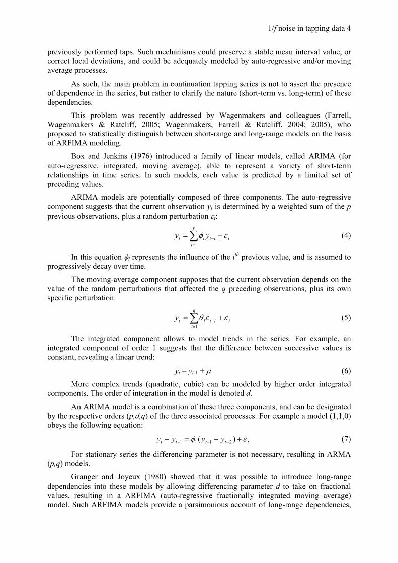
Box and Jenkins (1976) introduced a family of linear models, called ARIMA (for auto-regressive, integrated, moving average), able to represent a variety of short-term relationships in time series. In such models, each value is predicted by a limited set of preceding values.

ARIMA models are potentially composed of three components. The auto-regressive component suggests that the current observation yt is determined by a weighted sum of the p previous observations, plus a random perturbation εt:

∑=

− +=p

ititit yy

1εφ (4)

In this equation φi represents the influence of the ith previous value, and is assumed to progressively decay over time.

The moving-average component supposes that the current observation depends on the value of the random perturbations that affected the q preceding observations, plus its own specific perturbation:

∑=

− +=q

ititity

1εεθ (5)

The integrated component allows to model trends in the series. For example, an integrated component of order 1 suggests that the difference between successive values is constant, revealing a linear trend:

yt = yt-1 + µ (6)

More complex trends (quadratic, cubic) can be modeled by higher order integrated components. The order of integration in the model is denoted d.

An ARIMA model is a combination of these three components, and can be designated by the respective orders (p,d,q) of the three associated processes. For example a model (1,1,0) obeys the following equation:

ttttt yyyy εφ +−=− −−− )( 2111 (7)

For stationary series the differencing parameter is not necessary, resulting in ARMA (p,q) models.

Granger and Joyeux (1980) showed that it was possible to introduce long-range dependencies into these models by allowing differencing parameter d to take on fractional values, resulting in a ARFIMA (auto-regressive fractionally integrated moving average) model. Such ARFIMA models provide a parsimonious account of long-range dependencies,


by the addition of a single parameter to classical ARMA models. Importantly, they allow to simultaneously model short-term processes (by the combination of the p and q parameters), and long-range dependencies through the d parameter, and as such to isolate their respective contributions. Finally, the ARFIMA parameters can be estimated using exact maximum likelihood, allowing testing the significativity of d’s difference from 0. As such, ARFIMA modeling can effectively be used in order to provide statistical evidence for the presence of long-range dependencies in series.

Wagenmakers et al. (2005) recently proposed a complete inferential procedure, based on ARFIMA modeling, for certifying the presence of long-range dependencies in time series. Their method consists in fitting various models to the studied series. Some of these models are ARMA (p,q) models (p and q varying systematically from 0 to 2), which do not contain any long-range serial correlation. The other models are the corresponding ARFIMA (p,d,q) models, differing from the previous ARMA models by the inclusion of the fractional parameter d which represents persistent serial correlations. One supposes that if the series contains long-range dependencies, ARFIMA models should have a better fit than the transient ARMA models. Note that in a previous paper, Wagenmakers et al. (2004) proposed to only contrast an ARMA (1,1) and an ARFIMA (1,d,1) model. The approach proposed in their later paper, based on the test of a wider range of ARMA/ARFIMA models, constitutes an interesting improvement, as the correct specification of parameters p and q allows a better estimation of the long-range estimator d (Taqqu & Teverovsky, 1998; Wagenmakers et al., 2005)

The aim of this study was thus to test for the presence of long-range dependencies in time interval series, collected during a synchronization-continuation experiment. In order to analyze a possible effect of tapping frequency on series’ fluctuations (Kadota, Kudo, & Ohtsuki, 2004; Madison, 2004), two different initial tempi were imposed during the synchronization phase. We tried to go beyond the classical qualitative appraisal of power spectra by applying the ARMA/ARFIMA modeling procedure proposed by Wagenmakers et al. (2005).

Method

Participants

Twelve participants (5 women and 7 men, mean age 32.42 +/-13.77) were involved in the experiment. All were right-handed and no had particular expertise or extensive practice in music. They signed an informed consent form and were not paid for their participation.

Procedure

Participants performed a synchronization-continuation tapping task using the index finger of the right hand. Each trial was composed of two phases. During the first phase participants synchronized their taps with a sequence of regularly spaced auditory signals (bips) emitted by a metronome. After 25 signals the metronome was removed and participants had to continue to tap regularly following the initial tempo. Participants achieved the task starting from two different frequency conditions (1.8Hz and 1.25Hz, corresponding to intervals of 556ms and 800ms), representing the most used frequencies in the literature. The duration of the trials was determined in order to obtain about 1200 successive time intervals during the continuation phase.

Experimental device

The experiment was performed in a quiet room. The auditory signals were provided by a computer-generated metronome. Participants had to tap on a rectangular (2cm X 4cm) plate


fixed on a wood tablet. A switch was set up on the back of the plate and allowed the detection of the occurrence of each tap. Participants could position the tablet so that they could tap comfortably. Their forearm and wrist had to rest on the desk where was fixed the wood tablet. Data were recorded via an A/D converter Nanologger (Digimétrie) towards a 486 processor with a sampling frequency of 511Hz.

Data processing

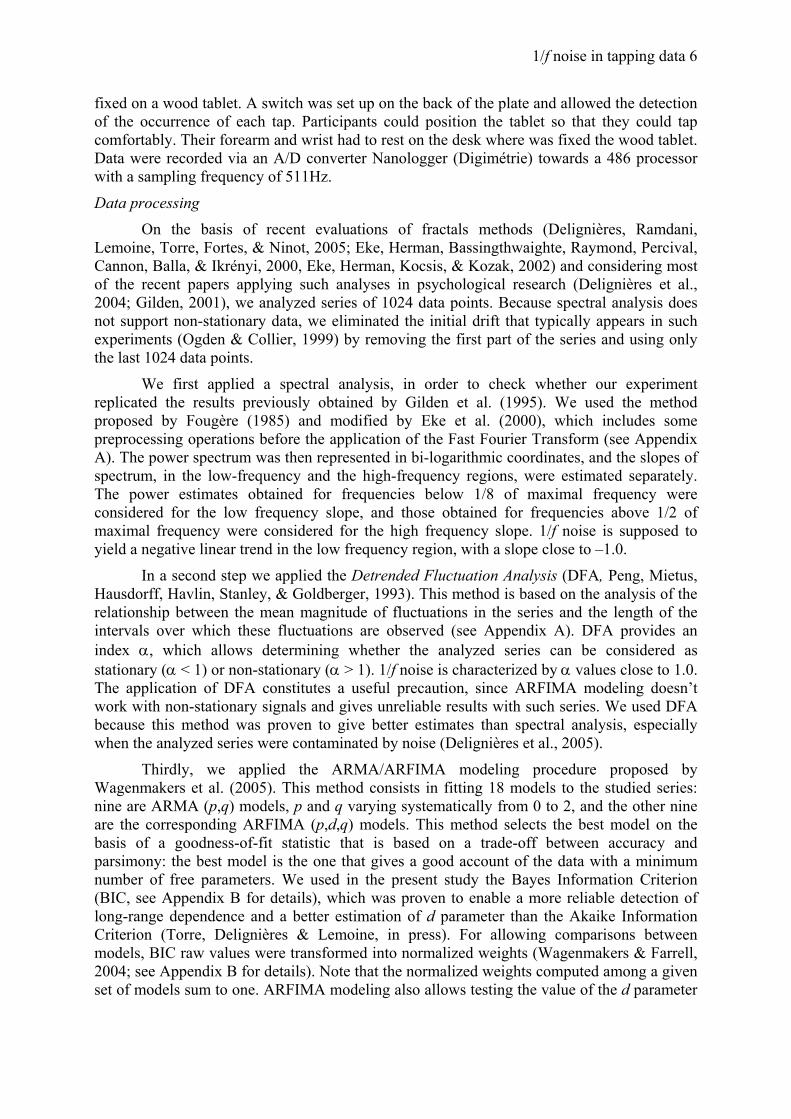
On the basis of recent evaluations of fractals methods (Delignières, Ramdani, Lemoine, Torre, Fortes, & Ninot, 2005; Eke, Herman, Bassingthwaighte, Raymond, Percival, Cannon, Balla, & Ikrényi, 2000, Eke, Herman, Kocsis, & Kozak, 2002) and considering most of the recent papers applying such analyses in psychological research (Delignières et al., 2004; Gilden, 2001), we analyzed series of 1024 data points. Because spectral analysis does not support non-stationary data, we eliminated the initial drift that typically appears in such experiments (Ogden & Collier, 1999) by removing the first part of the series and using only the last 1024 data points.

We first applied a spectral analysis, in order to check whether our experiment replicated the results previously obtained by Gilden et al. (1995). We used the method proposed by Fougère (1985) and modified by Eke et al. (2000), which includes some preprocessing operations before the application of the Fast Fourier Transform (see Appendix A). The power spectrum was then represented in bi-logarithmic coordinates, and the slopes of spectrum, in the low-frequency and the high-frequency regions, were estimated separately. The power estimates obtained for frequencies below 1/8 of maximal frequency were considered for the low frequency slope, and those obtained for frequencies above 1/2 of maximal frequency were considered for the high frequency slope. 1/f noise is supposed to yield a negative linear trend in the low frequency region, with a slope close to –1.0.

In a second step we applied the Detrended Fluctuation Analysis (DFA, Peng, Mietus, Hausdorff, Havlin, Stanley, & Goldberger, 1993). This method is based on the analysis of the relationship between the mean magnitude of fluctuations in the series and the length of the intervals over which these fluctuations are observed (see Appendix A). DFA provides an index α, which allows determining whether the analyzed series can be considered as stationary (α < 1) or non-stationary (α > 1). 1/f noise is characterized by α values close to 1.0. The application of DFA constitutes a useful precaution, since ARFIMA modeling doesn’t work with non-stationary signals and gives unreliable results with such series. We used DFA because this method was proven to give better estimates than spectral analysis, especially when the analyzed series were contaminated by noise (Delignières et al., 2005).

Thirdly, we applied the ARMA/ARFIMA modeling procedure proposed by Wagenmakers et al. (2005). This method consists in fitting 18 models to the studied series: nine are ARMA (p,q) models, p and q varying systematically from 0 to 2, and the other nine are the corresponding ARFIMA (p,d,q) models. This method selects the best model on the basis of a goodness-of-fit statistic that is based on a trade-off between accuracy and parsimony: the best model is the one that gives a good account of the data with a minimum number of free parameters. We used in the present study the Bayes Information Criterion (BIC, see Appendix B for details), which was proven to enable a more reliable detection of long-range dependence and a better estimation of d parameter than the Akaike Information Criterion (Torre, Delignières & Lemoine, in press). For allowing comparisons between models, BIC raw values were transformed into normalized weights (Wagenmakers & Farrell, 2004; see Appendix B for details). Note that the normalized weights computed among a given set of models sum to one. ARFIMA modeling also allows testing the value of the d parameter


estimated from ARFIMA (p,d,q), considering the corresponding ARMA (p,q) model as the null hypothesis.

Two complementary criteria were taken in account for detecting the presence of long-range dependencies in the series: (1) the best model (i.e. the model with the highest weight) should be an ARFIMA (p, d, q), d being significantly different from 0, and (2) the sum of weights of ARFIMA models should be higher than the sum of weights of ARMA models.

Models’ fitting was conducted using the ARFIMA package (Doornik & Ooms, 1999; Ooms & Doornik, 1998) for the matrix computing language Ox (Doornik, 2001). We used, with some minor adaptations, the Ox code provided by Simon Farrell, available at the following web address: http://eis.bristol.ac.uk/~pssaf/ (for details, see Farrell et al., 2005).

Results

The application of spectral analyses resulted in typical spectra, with a negative slope in the low frequency region and for most participants a positive slope in the high frequency region. The mean slope in the low frequency region was -0.93 (SD = 0.25) for the 1.8Hz frequency condition, and –1.05 (SD = 0.25) for the 1.25Hz frequency condition. These mean values were close to the slope expected from 1/f noise, corroborating Gilden et al. (1995)’s results. A one-way repeated-measures ANOVA failed to evidence any statistical difference between the two frequency conditions (F(1,11) = 1.49; p>0.05).

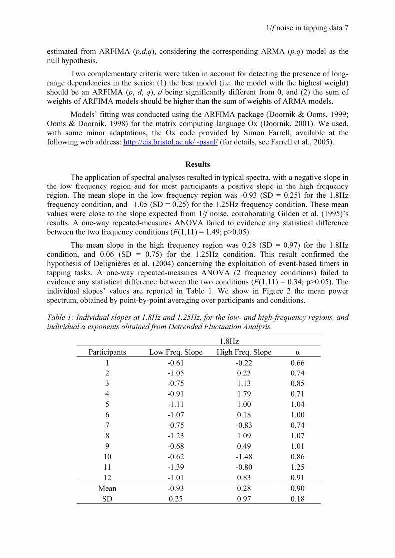
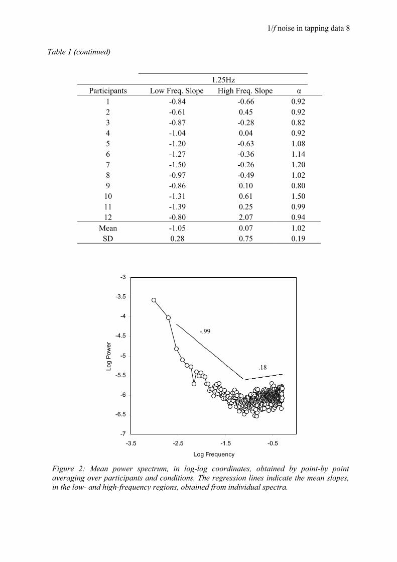
The mean slope in the high frequency region was 0.28 (SD = 0.97) for the 1.8Hz condition, and 0.06 (SD = 0.75) for the 1.25Hz condition. This result confirmed the hypothesis of Delignières et al. (2004) concerning the exploitation of event-based timers in tapping tasks. A one-way repeated-measures ANOVA (2 frequency conditions) failed to evidence any statistical difference between the two conditions (F(1,11) = 0.34; p>0.05). The individual slopes’ values are reported in Table 1. We show in Figure 2 the mean power spectrum, obtained by point-by-point averaging over participants and conditions.

Table 1: Individual slopes at 1.8Hz and 1.25Hz, for the low- and high-frequency regions, and individual α exponents obtained from Detrended Fluctuation Analysis.

1.8Hz Participants Low Freq. Slope High Freq. Slope α

1 -0.61 -0.22 0.66 2 -1.05 0.23 0.74 3 -0.75 1.13 0.85 4 -0.91 1.79 0.71 5 -1.11 1.00 1.04 6 -1.07 0.18 1.00 7 -0.75 -0.83 0.74 8 -1.23 1.09 1.07 9 -0.68 0.49 1.01 10 -0.62 -1.48 0.86 11 -1.39 -0.80 1.25 12 -1.01 0.83 0.91

Mean -0.93 0.28 0.90 SD 0.25 0.97 0.18


Table 1 (continued)

1.25Hz Participants Low Freq. Slope High Freq. Slope α

1 -0.84 -0.66 0.92 2 -0.61 0.45 0.92 3 -0.87 -0.28 0.82 4 -1.04 0.04 0.92 5 -1.20 -0.63 1.08 6 -1.27 -0.36 1.14 7 -1.50 -0.26 1.20 8 -0.97 -0.49 1.02 9 -0.86 0.10 0.80 10 -1.31 0.61 1.50 11 -1.39 0.25 0.99 12 -0.80 2.07 0.94

Mean -1.05 0.07 1.02 SD 0.28 0.75 0.19

-7

-6.5

-6

-5.5

-5

-4.5

-4

-3.5

-3

-3.5 -2.5 -1.5 -0.5

Log Frequency

Log

Pow

er

-.99

.18

Figure 2: Mean power spectrum, in log-log coordinates, obtained by point-by pointaveraging over participants and conditions. The regression lines indicate the mean slopes,in the low- and high-frequency regions, obtained from individual spectra.


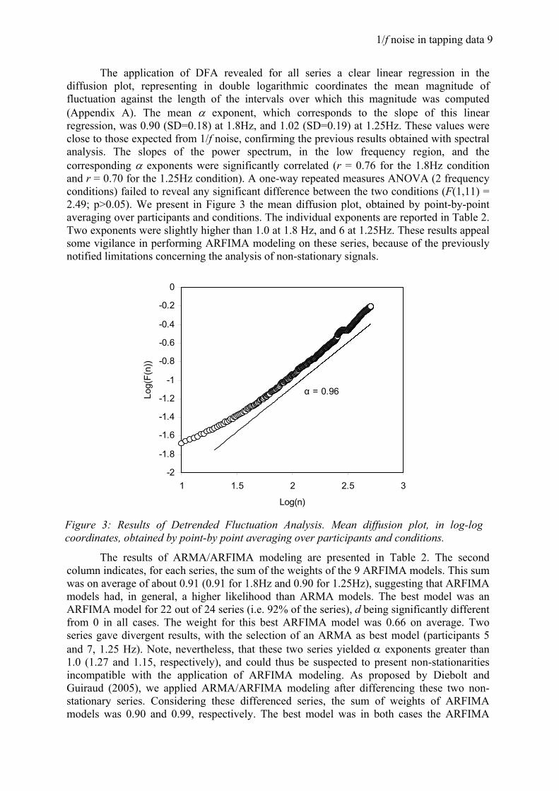
The application of DFA revealed for all series a clear linear regression in the diffusion plot, representing in double logarithmic coordinates the mean magnitude of fluctuation against the length of the intervals over which this magnitude was computed (Appendix A). The mean α exponent, which corresponds to the slope of this linear regression, was 0.90 (SD=0.18) at 1.8Hz, and 1.02 (SD=0.19) at 1.25Hz. These values were close to those expected from 1/f noise, confirming the previous results obtained with spectral analysis. The slopes of the power spectrum, in the low frequency region, and the corresponding α exponents were significantly correlated (r = 0.76 for the 1.8Hz condition and r = 0.70 for the 1.25Hz condition). A one-way repeated measures ANOVA (2 frequency conditions) failed to reveal any significant difference between the two conditions (F(1,11) = 2.49; p>0.05). We present in Figure 3 the mean diffusion plot, obtained by point-by-point averaging over participants and conditions. The individual exponents are reported in Table 2. Two exponents were slightly higher than 1.0 at 1.8 Hz, and 6 at 1.25Hz. These results appeal some vigilance in performing ARFIMA modeling on these series, because of the previously notified limitations concerning the analysis of non-stationary signals.

The results of ARMA/ARFIMA modeling are presented in Table 2. The second column indicates, for each series, the sum of the weights of the 9 ARFIMA models. This sum was on average of about 0.91 (0.91 for 1.8Hz and 0.90 for 1.25Hz), suggesting that ARFIMA models had, in general, a higher likelihood than ARMA models. The best model was an ARFIMA model for 22 out of 24 series (i.e. 92% of the series), d being significantly different from 0 in all cases. The weight for this best ARFIMA model was 0.66 on average. Two series gave divergent results, with the selection of an ARMA as best model (participants 5 and 7, 1.25 Hz). Note, nevertheless, that these two series yielded α exponents greater than 1.0 (1.27 and 1.15, respectively), and could thus be suspected to present non-stationarities incompatible with the application of ARFIMA modeling. As proposed by Diebolt and Guiraud (2005), we applied ARMA/ARFIMA modeling after differencing these two non-stationary series. Considering these differenced series, the sum of weights of ARFIMA models was 0.90 and 0.99, respectively. The best model was in both cases the ARFIMA

-2

-1.8

-1.6

-1.4

-1.2

-1

-0.8

-0.6

-0.4

-0.2

0

1 1.5 2 2.5 3

Log(n)

Log(

F(n)

)

α = 0.96

Figure 3: Results of Detrended Fluctuation Analysis. Mean diffusion plot, in log-logcoordinates, obtained by point-by point averaging over participants and conditions.


(0,d,1), with weights of 0.77 and 0.80, respectively, and estimates for d of about –0.11 and –0.29, respectively.

Table 2: Results of ARMA/ARFIMA modeling. This table reports, for each participant and each condition, the sum of ARFIMA weights, the nature of the best model, the weight of this best model, the estimate of the fractional parameter d, and the results of the inferential test for the significance of d. _________________________________________________________________________

Participants Sum of Best Weight d t prob. ARFIMA model of best weights model _________________________________________________________________________

1 0.89 1,1,1 0.35 0.23 2.46 0.014 2 0.99 0,1,1 0.65 0.41 4.56 0.000 3 0.83 0,1,1 0.66 0.13 1.97 0.049 4 0.92 0,1,1 0.81 0.39 6.26 0.000 5 0.96 0,1,1 0.88 0.45 9.51 0.000 1.8 Hz 6 1.00 2,1,2 0.99 0.42 6.08 0.000 7 0.84 0,1,2 0.62 0.38 4.53 0.000 8 0.78 0,1,1 0.72 0.45 8.58 0.000 9 0.99 1,1,1 0.63 0.34 3.54 0.000 10 0.83 0,1,0 0.44 0.24 10.61 0.000 11 1.00 2,1,2 0.79 0.49 32.14 0.000 12 0.89 1,1,2 0.58 0.42 7.35 0.000 _________________________________________________________________________

1 0.99 0,1,2 0.50 0.28 3.38 0.001 2 0.97 0,1,1 0.82 0.35 6.39 0.000 3 0.97 0,1,1 0.36 0.15 3.09 0.002 4 0.75 0,1,1 0.60 0.44 9.70 0.000 5 0.28 1,0,1 0.58 - - - 1.25 Hz 6 0.98 0,1,1 0.62 0.48 20.95 0.000 7 0.38 1,0,1 0.55 - - - 8 0.94 0,1,1 0.73 0.38 7.38 0.000 9 0.97 0,1,2 0.57 0.40 5.36 0.000 10 0.60 0,1,1 0.55 0.49 26.47 0.000 11 0.87 0,1,1 0.70 0.48 20.39 0.000 12 1.00 1,1,2 0.93 0.39 5.98 0.000 _________________________________________________________________________

In summary the spectral analysis yielded negative slopes in the low frequency region close to 1.0 and positive slopes in the high frequency region, confirming previous results obtained in similar experiments (Delignières et al., 2004; Gilden et al., 1995). DFA analysis reinforced these results with α exponents close to 0.95: series thus were mostly identified as stationary and then that ARFIMA modeling could be applied. Finally the ARMA/ARFIMA modeling evidenced the presence of long term-dependencies in all series, directly for 22 series, and after differencing for two series that, according to DFA, could be suspected to be non-stationary.


Discussion The ARMA/ARFIMA modeling approach proposed by Wagenmakers et al. (2005) was recently questioned by Thornton and Gilden (2005). According to these authors, this method presents a number of theoretical and statistical limitations. The first one is the use of short-term dependence models as null hypothesis. The null hypothesis should represent a plausible alternative in an inferential test, and Thornton and Gilden argued that short-term models did not possess such plausibility in the domain of psychological processes. This could be true for reaction time tasks, which constitute the main focus of Thornton and Gilden’s paper, but this first objection cannot be retained in the present case, as most of the proposed models in the domain of tapping suggest the presence of short-term processes sustaining the regulation of timing behavior. The most classical model for continuous tapping clearly refers to short-term processes (Wing & Kristofferson, 1973a), and as stated in the introduction, a number of propositions aimed at explaining serial correlations in synchronization or continuation tapping on the basis of short-term dependencies, by means of feedback processes (Pressing & Jolley-Rogers, 1997), or short-term memory (M. Yamada, 1996). Thus ARMA models represent an alternative that could justifiably be considered as a null hypothesis.

Another objection pointed out by Thornton and Gilden is that ARFIMA models should always fit data better than ARMA because of the presence of the extra parameter d. This objection could be acceptable if the method was limited to contrasting two models differing only by the addition of the parameter d (see, for example, Wagenmakers et al., 2004). Nevertheless, in the present approach we tried to select the best model within a wider range of candidates, containing 0 to 4 terms for the ARMA models, and 1 to 5 for their ARFIMA counterparts. As can be seen in Table 2, the best model was rarely the most complex. It’s important to keep in mind that the information criterion we used aimed at balancing accuracy and parsimony, and the introduction of an additional parameter was strongly penalized. Torre et al. (in press) showed that the penalty imposed to complex models by BIC led to the selection of quite simple models, and to a better detection rate of long-range dependence. In contrast, the Akaike Information Criterion (AIC) tended to prefer more complex models, and often ARMA models containing several auto-regressive and moving average terms, susceptible to mimic the underlying fractal behavior.

As such, and particularly in the present context, the method proposed by Wagenmakers et al. (2005) seems justifiable and its results can be considered with some assurance. On the basis of a simulation study, Torre et al. (in press) suggested that the hypothesis of the presence of long-range dependencies could be accepted if, considering a set of experimental series, (1) the method selected an ARFIMA as best model for more than 90% of the series, and (2) the mean sum of weights for ARFIMA models was above 0.90. In the present experiment an ARFIMA model was selected for 22 series out of 24 (92%), and considering these 22 series, the mean sum of weights for ARFIMA models was about 0.91. Moreover, the two series primarily classified as ARMA were proven to present long-range dependence on the basis of the analysis of their differenced versions. One can consider that our results met the requirements proposed by Torre et al. (in press) and provide a strong support for the presence of long-range dependence in continuation tapping series. In comparison, Farrell et al. (2005), applying the present method to the experimental series provided by Van Orden et al. (2003), found evidence for an ARFIMA model in 4 series out of 10 in a simple reaction time task, and in 13 series out of 20 in a word naming task. Using AIC, the results were slightly better, with 7 series out of 10, and 14 out of 20, respectively. These results provided a weaker support for the existence of long-range correlation in the studied tasks than the present experiment in continuation tapping. Note that Gilden (2001) also failed to evidence 1/f behavior in reaction time series.


One could wonder, nevertheless, whether these results reflect genuine long-range dependencies in our series or could be determined by the presence of non-stationarities (Pressing and Jolley-Rogers, 1997). As previously indicated, we selected from the collected data the most stationary segment, eliminating the first part where drifts frequently occur. On the basis of both spectral analysis and DFA, we can conclude that most of our series were stationary. And finally, long-range dependencies were detected in all series, including the most stationary.

This experiment confirms the results of several previous studies on tapping (Chen, Ding & Kelso, 1997; Chen, Repp, & Patel, 2002; Gilden et al., 1995; N. Yamada, 1995; M. Yamada, 1996; Yoshinaga, Miyazima & Mitake, 2000), and supports the hypotheses of Gilden et al. (1995): the cognitive component, initially conceived as a white noise source (Wing and Kristofferson; 1973b), has a fractal behavior close to 1/f noise.

We failed to evidence any statistical difference in fractal behavior between the two frequency conditions. This result suggests that the intensity of long-range dependence in the series of intervals produced by event-based timers could be independent on the mean duration of these intervals. Gilden et al. (1995) reported a similar result over a wider range of tapping frequencies (ranging from 0.1 to 3.33 Hz). Nevertheless, a recent experiment working with frequencies ranging from 0.66 to 2.0 Hz showed a significant decrease of long-range dependencies, as tapping frequency increased (Madison, 2004). These divergent results pose an important challenge for future research aiming at deriving models able to reproduce the fractal behavior of event-based timers.

A frequency effect was expected on the slope in high frequency region, due to the evolution of the ratio between the variances of the cognitive and motor components (Gilden et al., 1995). This effect was not obtained, due to the high inter-individual variability of the high-frequency slopes (see Table 1). The two frequencies used in the present experiment could also be too close to induce a significant difference between conditions.

In conclusion, the series of cognitive events produced by the internal clock did not appear as a periodic signal, perturbed by uncorrelated white noise (Wing & Kristofferson, 1973a, 1973b), but exhibits a fractal evolution over time, close to 1/f noise. One of the most attractive hypotheses conceives 1/f fluctuations as the typical signature of self-organized critical states in complex systems (Bak & Chen, 1991; Davidsen & Schuster, 2000; De Los Rios & Zhang, 1999). This assumption is in line with the contemporary approaches in the domains of motor control, cognition sciences, or psychology, which are widely influenced by the theoretical background of nonlinear dynamical systems (Kelso, 1995; Van Gelder, 1998).

Wagenmakers et al. (2004) proposed an alternative hypothesis, based on an adaptation of a classical event-based timer model. In such model, an activation level increases linearly in time, and the reaching of a particular threshold level of activation marks particular moments in time. This event simultaneously resets the activation level, allowing the reiteration of the process (Schöner, 2002). Wagenmakers et al. (2004) assumed that the threshold value could present local non-stationarities, in the form of successive plateaus, due to shifts in strategy over time. Additionally, they suggested that the rate of growth of the activation level could evolve across iterations following an auto-regressive dynamics. They showed, using ARFIMA modeling, that the series of time intervals produced by this quite simple model presented long-range dependencies.

As can be seen, a number of alternative explanations have been proposed in the literature, and the question of the origin of fractal correlation in psychological time series remains an open debate.


References

Bak, P., & Chen, K. (1991). Self-organized criticality. Scientific American, 264, 46-53.

Box, G.E.P., & Jenkins, G.M. (1976). Time series analysis: Forecasting and control. Oakland: Holden-Day.

Chen, Y., Ding, M., & Kelso, J.A.S. (1997). Long memory processes (1/fα type) in human coordination. Physical Review Letters, 79, 4501-4504.

Chen, Y., Ding, M., & Kelso, J.A.S. (2001). Origins of Timing Errors in Human Sensorimotor Coordination. Journal of Motor Behavior, 33, 3-8.

Chen, Y., Repp, B.H., & Patel, A.D. (2002). Spectral decomposition of variability in synchronization and continuation tapping: Comparisons between auditory and visual pacing and feedback conditions. Human Movement Science, 21, 515-532.

Creelman, C.D. (1962). Human discrimination of auditory duration. Journal of Acoustical of Society of America, 34, 582-593.

Davidsen, J., & Schuster, H.G. (2000). 1/fα noise from self-organized critical models with uniform driving. Physical Review E, 62, 6111-6115.

De Los Rios, P., & Zhang Y.C. (1999). Universal 1/f noise from dissipative self-organized criticality models. Physical Review Letters, 82, 472-475.

Delignières, D., Lemoine, L., & Torre, K. (2004). Time intervals production in tapping and oscillatory motion. Human Movement Science, 23, 87-103.

Delignières, D., Ramdani, S., Lemoine, L., Torre, K., Fortes, M., & Ninot, G. (2005). Fractal analysis for short time series : A reassessment of classical methods. Manuscript submitted for publication.

Diebolt, C., & Guiraud, V (2005). A note on long memory time series. Quality & Quantity, 39, 827-836.

Doornik, J.A. (2001). Ox: An Object-Oriented Matrix Language. London: Timberlake Consultants Press.

Doornik, J.A., & Ooms, M. (1999). A package for estimating, forecasting, and simulating Arfima models: Arfima package 1.0 for Ox [On-line]. Available: http://www.doornik.com/download/arfima.pdf

Eke, A., Herman, P., Bassingthwaighte, J.B., Raymond, G.M., Percival, D.B., Cannon, M., Balla, I., & Ikrényi, C. (2000). Physiological time series: distinguishing fractal noises from motions. Pflügers Archives, 439, 403-415.

Eke, A., Hermann, P., Kocsis, L., & Kozak, L.R. (2002). Fractal characterization of complexity in temporal physiological signals. Physiological Measurement, 23, R1-R38.

Farrell, S., Wagenmakers, E.-J., & Ratcliff, R. (2005). ARFIMA time series modeling of serial correlations in human performance. Manuscript submitted for publication.

Fougère, P.F. (1985). On the accuracy of spectrum analysis of red noise processes using maximum entropy and periodogram methods: simulation studies and application to geographical data. Journal of Geographical Research, 90 (A5), 4355-4366.

Gilden, D.L. (2001). Cognitive emissions of 1/f noise. Psychological Review, 108, 33-56.

Gilden, D.L., Thornton, T., & Mallon, M.W. (1995). 1/f noise in human cognition. Science, 267, 1837-1839.


Granger, C.W.J., & Joyeux, R. (1980). An introduction to long-memory models and fractional differencing. Journal of time Series Analysis, 1, 15-29.

Hoagland, H. (1933). The physiological control of judgment of duration: Evidence of a chemical clock. Journal of General Psychology, 9, 267-287.

Kadota, H., Kudo, K., & Ohtsuki, T. (2004). Time-series pattern changes related to movement rate in synchronized human tapping. Neurosciences Letters, 370, 97-101.

Kelso, J.A.S (1995). Dynamics patterns: the self-organization of brain and behavior. Cambridge, MA: MIT Press.

Madison, G. (2004). Fractal modeling of human isochronous serial interval production. Biological Cybernetics, 90, 105, 112.

Ogden, R.T., & Collier, G.L. (1999). On detecting and modeling deterministic drift in long run sequences of tapping data. Communications in Statistics - Theory and Methods, 28, 977-987.

Ooms, M., & Doornik, J.A. (1998). Estimation, simulation and forecasting for fractional autoregressive integrated moving average models. Discussion paper, Econometric Institute, Erasmus University Rotterdam, presented at the fourth annual meeting of the Society for Computational Economics, June 30, 1998, Cambridge, UK.

Peng, C.K., Mietus, J., Hausdorff, J.M., Havlin, S., Stanley, H.E., & Goldberger, AL. (1993). Long-range anti-correlations and non-Gaussian behavior of the heartbeat. Physical Review Letter, 70, 1343-1346.

Pressing, J., & Jolley-Rogers, G. (1997). Spectral properties of human cognition and skill. Biological Cybernetics, 76, 339-347.

Rangarajan, G., & Ding, M. (2000). Integrated approach to the assessment of long range correlation in time series data. Physical Review E, 61(5A), 4991-5001.

Stevens, L.T. (1886). On the time sense. Mind, 11, 393-404.

Schöner, G. (2002). Timing, clocks, and dynamical systems. Brain and Cognition, 48, 31-51.

Taqqu, M.S., & Teverovsky, V. (1998). On estimating the intensity of long-range dependence in finite and infinite variance time series. In R. Adler, R. Feldman, and M.S. Taqqu (Eds.), A practical guide to heavy tails: Statistical techniques and applications (pp. 177-217). Boston: Birkhauser.

Thornton, T.L., & Gilden D.L. (2005). Provenances of correlations in psychophysical data. Psychonomic Bulletin & Review, 12, 403-408.

Torre, K, Delignières, D., & Lemoine, L. (in press). Detection of long-range dependence and estimation of fractal exponents through ARFIMA modeling. British Journal of Statistical and Mathematical Psychology.

Treisman, M. (1963). Temporal discrimination and the indifference interval: Implications for a model of the internal clock. Psychological Monograph, 77, 1-31.

Treisman, M., Faulkner, A., & Naish, P. L. (1992). On the relation between time perception and the timing of motor action: evidence for a temporal oscillator controlling the timing of movement. Quarterly Journal of Experimental Psychology A, 45, 235-63.

Van Gelder, T. (1998). The dynamical hypothesis in cognitive science. Behavioral and Brain Science, 21, 615-665.


Van Orden, G.C., Holden, J.C., & Turvey, M.T. (2003). Self-organization of cognitive performance. Journal of Experimental Psychology: General, 132, 331-350.

Wagenmakers, E.-J., & Farrell, S. (2004). AIC model selection using Akaike weights. Psychonomic Bulletin & Review, 11, 192-196.

Wagenmakers, E.-J., Farrell, S., & Ratcliff, R. (2004). Estimation and interpretation of 1/fα noise in human cognition. Psychonomic Bulletin & Review, 11, 579–615.

Wagenmakers, E.-J., Farrell, S., & Ratcliff, R. (2005). Human cognition and a pile of sand: A discussion on serial correlations and self-organized criticality. Journal of Experimental Psychology: General, 134, 108-116.

West, B.J., & Shlesinger, M.F. (1989). On the ubiquity of 1/f noise. International Journal of Modern Physics B, 3, 795-819.

West, B.J., & Shlesinger, M.F. (1990). The noise in natural phenomena. American Scientist, 78, 40-45.

Wing, A.M., & Kristofferson, A.B. (1973a). The timing of interresponse intervals. Perception and Psychophysics, 13, 455-460.

Wing, A.M., & Kristofferson, A.B. (1973b). Response delays and the timing of discrete motor responses. Perception and Psychophysics, 14, 5-12.

Yamada, M. (1996). Temporal control mechanism in equaled interval tapping. Applied Human Science, 15, 105-110.

Yamada, M., & Yonera, S. (2001). Temporal control mechanism of repetitive tapping with simple rhythmic patterns. Acoustical Science and Technology, 22, 245-252.

Yamada, N. (1995). Nature of variability in rhythmical movement. Human Movement Science, 14, 371-384.

Yoshinaga, H., Miyazima, S., & Mitake, S. (2000). Fluctuation of biological rhythm in finger tapping. Physica A, 280, 582-586.

_______________________________________________

Appendix A

Spectral analysis lowPSD we

We used the lowPSD we method initially proposed by Fougère (1985) and modified by Eke et al. (2000), which includes some preprocessing operations before the application of the Fast Fourier Transform (FFT): First the mean of the series was subtracted from each value, and then a parabolic window was applied: each value in the series was multiplied by the following function:

)²11

2(1)( −+

−=N

jjW for j = 1, 2, …, N. (A1)

This transformation induces a tapering of the series and is supposed to reduce the leakage in the periodogram. Spectral leakage is the term used to describe the loss of power of a given frequency to other frequency bins in the FFT. There are edge effects arising from the discontinuity at the bounds that cause spectral leakage. It implies that windowing in the time domain corresponds to smoothing in the frequency domain. This smoothing reduces sidelobes


associated with the window. Finally, a linear detrending was applied to the resulting series. The FFT algorithm was then applied on the obtained series.

A fractal series is characterized by the following power law:

S(f) ∝ 1/f β (A2)

where β is the spectral exponent, f the frequency and S(f) the correspondent squared amplitude. β is estimated by calculating the negative slope (-β) of the linear regression of log (S(f)) against log f. β equals 0 for white noise, 2 for ordinary Brownian motion, and 1 for 1/f noise. As proposed by Eke et al. (2000) we excluded in the fitting of β the high-frequency power estimates (f > 1/8 of maximal frequency). This method was proven to provide more reliable estimates of the spectral exponent.

Detrended Fluctuation Analysis

DFA is a fractal method that is supposed to be not affected by non-stationarity. The algorithm of DFA consists first in integrating the series y(t), calculating for every t the cumulated sum of the deviations of the mean:

[ ]∑=

−=i

tytyiY

1)()( for i = 1, 2, 3….N (A3)

where N corresponds to series length. This integrated series is then divided in non-overlapping intervals of length n. In each interval, a least squares line is fit to the data (representing the trend in the interval). The Y(t) series is then locally detrended by subtracting to all values the theoretical value Yth(t) given by the regression. For all interval length n, the characteristic magnitude of fluctuation F(n) is calculated by:

[ ]∑=

−=N

kth kYkY

NnF

1

2)()(1)( (A4)

This computation is repeated over all possible interval lengths n (in practice, the shortest length is around 10, and the largest N/2, giving two adjacent intervals). Typically, F(n) increases with interval length n. For fractal series, a power law is expected, as

F(n) ∝ nα (A5)

where α is the scaling exponent. α is estimated by the slope of the graph representing F(n) as a function of n, in log-log coordinates (diffusion plot, see figure 3). α equals 0 for white noise, 1.5 for ordinary Brownian motion, and 1 for 1/f noise.

_________________________________________________

Appendix B

Model selection in ARMA/ARFIMA modeling

The method proposed by Wagenmakers et al. (2005) consists in fitting 18 models to the studied series. Nine of these models are ARMA (p,q) models, p and q varying systematically from 0 to 2. The other nine models are the corresponding ARFIMA (p,d,q) models, differing from the previous ARMA models by the inclusion of the fractional parameter d, representing persistent serial correlations.

Fitting a particular time series involves maximizing the likelihood of a given model with respect to the autocovariance function of the series. Nevertheless, the examination of the


maximum likelihood scores provided by the fitting procedure is not sufficient, as the capacity of models to account for the data is partly related to their number of free parameters. The selection of models has to be based on a trade-off between accuracy and parsimony: the best model is the one that gives a good account of the data with a minimum number of free parameters.

We used in the present paper the Bayes Information Criterion (BIC), defined as:

BIC = -2logL + klogN (B1)

where L represents the maximum likelihood for the model under study, k the number of free parameters in the model, and N the number of observations in the series. As can be seen, the first term rewards accuracy, and the second penalizes the lack of parsimony. The lower the BIC, the better the model.

The raw values of this criterion remain difficult to interpret and to compare between models. Wagenmakers and Farrell (2004) proposed a convenient transformation of the raw values in weights. Consider that the goal is to select the best model among m candidates. The first step is to compute the difference, for each model, between the criterion for this model and for the best model. That is, for the ith model:

∆i(BIC) = BICi – minBIC (B2)

This difference in BIC can then be converted in an estimate of relative likelihood through the following transform :

(B3)

Finally, these relative likelihoods are transformed into weights by normalization (i.e. by division by the sum of the relative likelihood of all models):

(B4)

wi(BIC) can be conceived as the probability for the ith model to be the best model given the data and the set of candidate models (Wagenmakers & Farrell, 2004). Note that the weights computed among a given set of models sum to one.

On the basis of these weights, two criteria could be proposed for detecting the presence of long-range dependence in the series: (1) the best model (i.e. the model with the highest weight) should be an ARFIMA (p, d, q), d being significantly different from 0, and (2) the sum of the weights of the ARFIMA models should be higher than the sum of the weights of the ARMA models.

Torre et al. (2005) showed that BIC gave better results than the Akaike Information Criterion (AIC) initially proposed by Wagenmakers, Farrell and Ratcliff (2004).

∆−∝ )(

21exp)( BICBICL ii

∑=

= m

j

ii

BICLj

BICLBICw

1)(

)()(

Testing for the presence of 1/f noise in continuation tapping data

Documents

Transcript of Testing for the presence of 1/f noise in continuation tapping data