Testing a Random Number Generator - AMS Tesi di Laurea
168
·
-
Upload
khangminh22 -
Category
Documents
-
view
1 -
download
0
Transcript of Testing a Random Number Generator - AMS Tesi di Laurea

Alma Mater Studiorum · Università di Bologna
SCUOLA DI SCIENZE
Corso di Laurea Magistrale in Matematica
Testing a Random Number Generator:
formal properties and automotive application
Tesi di Laurea Magistrale in Crittograa e Probabilità
Relatore:Chiar.ma Prof.ssaGIOVANNACITTI
Correlatore:Chiar.ma Dott.ssaELISABRAGAGLIA
Presentata da:FEDERICOMATTIOLI
III Sessione
Anno Accademico 2017/2018


Introduzione
Lo scopo principale di questa tesi è lo studio di processi casuali in campo automotive.I veicoli moderni, infatti, sono gestiti da centraline (Electronic Control Units: ECUs) checontengono la maggior parte della struttura software del veicolo e sono responsabili dellasicurezza dello stesso nei confronti di attacchi informatici. La maggior parte degli algo-ritmi crittograci è basata sulla generazione di numeri casuali: è quindi necessario che lestringhe generate siano eettivamente casuali. Il metodo di valutazione più riconosciutoe standardizzato, proposto dal National Institute of Standards and Technology (NIST),consiste nell'analizzare sequenze di numeri, costruite dal generatore, attraverso una seriedi test statistici.
I capitoli 2 e 3 costituiscono il nucleo dell'elaborato: qui vengono date le denizionidi processi casuali da un punto di vista probabilistico e con riferimento alla nozionedi entropia. Successivamente, il lavoro si concentra sullo studio della test suite per lavalidazione di Generatori di Numeri Casuali (RNG) proposta dal NIST. La suite con-siste in 15 test, ognuno dei quali analizza le sequenze da una dierente prospettiva. Lasolidità dei test cresce dai primi test (che sono caratterizzati da un bassissimo costo com-putazionale, permettendo di scartare gli RNG meno ecienti) agli ultimi, che studianoproprietà più sosticate dei processi casuali.
I primi test sono basati su proprietà molto semplici delle sequenze casuali, comela probabilità di zero e uno all'interno della sequenza o all'interno di sotto-stringhe(Frequency test e Frequency test within a block), o la probabilità di successioni di bituguali lungo la sequenza o all'interno di sotto-stringhe (Runs test e Runs test within ablock).
Se una sequenza passa questi primi test, viene analizzata con altre classi di test,basati su strumenti matematici più sosticati come ad esempio:
• trasformata di Fourier: il rispettivo test (Spectral test) è in grado di rilevare com-portamenti periodici all'interno della sequenza;
• entropia: le sequenze casuali sono caratterizzate da alti valori entropici, stretta-mente connessi con la comprimibilità della sequenza (Maurer's universal statistical
i

test e Approximate entropy test);
• complessità algoritmica: le sequenza casuali sono sucientemente complesse danon poter essere costruite da semplici algoritmi (Linear complexity test e Serialtest);
• passeggiata aleatoria: la stringa binaria viene identicata come una passeggiataaleatoria di 1 e −1. In quest'ottica le somme parziali dei primi m valori dellasequenza devono essere vicini allo zero (Cumulative sums test) e la sequenza devevisitare ogni stato con la stessa frequenza di una passeggiata aleatoria (Randomexcursion test and Random excursion variant test).
Dal momento che ognuno di questi analizza un diverso comportamento, un unico testnon è suciente per fornire un adeguato responso riguardo la sequenza in oggetto in-oltre, dal momento che lo scopo è quello di validare l'RNG, una sola sequenza non bastaper aermare se le sequenze siano casuali o meno, ma sarà necessario testare un numerosucientemente grande di sequenze attraverso un'adeguata quantità di test.
Con lo scopo di costruire un metodo per valutare, primi tra gli altri, gli RNG con-tenuti all'interno delle centraline, dopo aver analizzato e validato ognuno dei test pro-posti, cercheremo di implementare l'intero schema di validazione in CANoe, un softwareche permette di programmare ed interagire con le ECU, utilizzando, come step intermedi,MatLab e Simulink.
Questo lavoro non sarebbe stato possibile senza l'Azienda Magneti Marelli, che mi hapermesso di svolgere un tirocinio di un anno presso la sede di Bologna, supportato dalCyber Security Systems Architect che mi ha insegnato, tra le altre cose, come è costruitala struttura software dei moderni autoveicoli, cyber security in primis, nonché l'utilizzodei sistemi che verranno analizzati in questa tesi.
ii

Introduction
The main scope of this dissertation is to study random processes in cyber security ofautomotive environment. Indeed modern vehicles are managed by the Electronic Con-trol Units (ECUs), which contains most of the software structure of the vehicle and areresponsible of its security against cyber attacks. Most cryptographical algorithms arebased on generation of random numbers and it is necessary that the generated stringsare truly random. The most standardized evaluation method consists in analyzing se-quences of numbers, built by the generator, through a set of statistical tests, providedby the National Institute of Standards and Technology (NIST).
The core of the thesis are chapters 2 and 3, where we gave the denition of ran-dom process from a probabilistic and entropic point of view. Then we study the suiteproposed by NIST to validate Random Number Generators. The suite consists of 15tests, each one inspecting the sequence from a dierent perspective. The strength oftests increases from rst tests (which have extremely low computational cost and allowto rapidly discard not ecient RNG) to the last ones, which study more sophisticatedproperties of the random process.
The rst tests are based on very simple properties of random sequences as for ex-ample the probability of zeros and ones within the sequence or within any sub-block ofthe sequence (Frequency test and Frequency test within a block), or the probability ofoccurrence of k identical bits within the sequence or any sub-block of it (Runs test andRuns test within a block). If a sequence passes these rst tests, it is submitted to otherclasses of tests, based on more sophisticated mathematical instruments:
• discrete Fourier transform: these tests are able to detect periodic features withinthe sequence which would indicate deviation from randomness (Spectral test);
• notion of entropy, which has high values in random sequences, and is strictly con-nected with non compressibility of the sequence (Maurer's universal statistical testand Approximate entropy test);
• algorithmic complexity: the high complexity of random sequences doesn't permitto build them by simple algorithms (Linear complexity test and Serial test);
iii

• random walk properties: the binary string is identied with a random walk whichattains values 1, −1. Hence the partial sum of the rst m values of the sequencehas to be near zero (Cumulative sums test) and the sequence has to visit each statewith the same frequence of a random walk (Random excursion test and Randomexcursion variant test).
Since each of those analyzes a dierent behavior, a unique test is not adequate togive a response concerning the analyzed sequence and, given the fact that the nal goalis to evaluate the RNG, a single sequence is not enough to say whether or not generatedsequences are random, but it will be necessary to test a great number of sequences, bya commensurate number of tests.
With the purpose to build a method to evaluate, among all, RNGs embedded intoECUs, after studying and validating each proposed test, we will try to implement thewhole validation scheme into CANoe, a software which permits to program and interactwith ECUs, using, as intermediate steps, MatLab and Simulink.
This work wouldn't be possible without theMagneti Marelli Company, which allowedme to carry out a one year traineeship at its Bologna oce, supported by the CyberSecurity Systems Architect which taught me, among other things, how the softwarestructure of modern vehicles is built, cyber security in the rst place, as well as the useof the systems that will be analyzed along this thesis.
iv

Contents
Introduzione i
Introduction iii
1 Random Number Generators in automotive cyber security 11.1 Automotive cyber security . . . . . . . . . . . . . . . . . . . . . . . . . . 1
1.1.1 The ECUs infrastructure . . . . . . . . . . . . . . . . . . . . . . . 11.1.2 Vehicle entry points and hacking . . . . . . . . . . . . . . . . . . 2
1.2 The importance of randomness in cryptography . . . . . . . . . . . . . . 61.2.1 Employment of randomness in automotive . . . . . . . . . . . . . 9
1.3 Random Number Generators . . . . . . . . . . . . . . . . . . . . . . . . . 12
2 The notion of randomness 172.1 Theoretical background . . . . . . . . . . . . . . . . . . . . . . . . . . . . 17
2.1.1 Probability bases . . . . . . . . . . . . . . . . . . . . . . . . . . . 172.1.2 Entropy . . . . . . . . . . . . . . . . . . . . . . . . . . . . . . . . 22
2.2 Characterizations of randomness . . . . . . . . . . . . . . . . . . . . . . . 262.2.1 Probabilistic approach . . . . . . . . . . . . . . . . . . . . . . . . 262.2.2 Information Theory approach . . . . . . . . . . . . . . . . . . . . 272.2.3 Complexity Theory approach . . . . . . . . . . . . . . . . . . . . 312.2.4 Algorithmic Information Theory approach . . . . . . . . . . . . . 34
3 Statistical tests for randomness 373.1 General procedure . . . . . . . . . . . . . . . . . . . . . . . . . . . . . . 37
3.1.1 χ2 goodness-of-t test and incomplete gamma function . . . . . . 403.1.2 Complementary error function . . . . . . . . . . . . . . . . . . . . 45
3.2 Tests . . . . . . . . . . . . . . . . . . . . . . . . . . . . . . . . . . . . . . 473.2.1 The frequency (Monobit) test . . . . . . . . . . . . . . . . . . . . 493.2.2 Frequency test within a block . . . . . . . . . . . . . . . . . . . . 513.2.3 Runs test . . . . . . . . . . . . . . . . . . . . . . . . . . . . . . . 523.2.4 Test for the longest run of ones in a block . . . . . . . . . . . . . 55
v
3.2.5 Binary matrix rank test . . . . . . . . . . . . . . . . . . . . . . . 613.2.6 Discrete Fourier transform (Spectral) test . . . . . . . . . . . . . 653.2.7 Non-overlapping template matching test . . . . . . . . . . . . . . 683.2.8 Overlapping template matching test . . . . . . . . . . . . . . . . . 723.2.9 Maurer's universal statistical test . . . . . . . . . . . . . . . . . . 783.2.10 Linear complexity test . . . . . . . . . . . . . . . . . . . . . . . . 853.2.11 Serial test . . . . . . . . . . . . . . . . . . . . . . . . . . . . . . . 953.2.12 Approximate entropy test . . . . . . . . . . . . . . . . . . . . . . 993.2.13 Cumulative sums (Cusum) test . . . . . . . . . . . . . . . . . . . 1053.2.14 Random excursion test . . . . . . . . . . . . . . . . . . . . . . . . 1103.2.15 Random excursion variant test . . . . . . . . . . . . . . . . . . . . 117
4 Properties of a RNG 1214.1 Second level testing . . . . . . . . . . . . . . . . . . . . . . . . . . . . . . 122
4.1.1 Test for proportion of sequences passing a test . . . . . . . . . . . 1234.1.2 Test for uniformity of P-values . . . . . . . . . . . . . . . . . . . . 125
4.2 Complete testing . . . . . . . . . . . . . . . . . . . . . . . . . . . . . . . 1264.2.1 Set of tests . . . . . . . . . . . . . . . . . . . . . . . . . . . . . . 1264.2.2 Proportion of sequences passing more than one test . . . . . . . . 1274.2.3 Uniformity of P-values from multiple tests . . . . . . . . . . . . . 128
5 Testing ECU's RNG 1315.1 Validation of MatLab codes . . . . . . . . . . . . . . . . . . . . . . . . . 1315.2 CANoe integration of test suite . . . . . . . . . . . . . . . . . . . . . . . 134
5.2.1 Vector CANoe . . . . . . . . . . . . . . . . . . . . . . . . . . . . . 1345.2.2 From MatLab to CANoe . . . . . . . . . . . . . . . . . . . . . . . 1375.2.3 Results from our implementation . . . . . . . . . . . . . . . . . . 140
Conclusions 147
A Examples from implementation 149
Bibliography 155
vi

Chapter 1
Random Number Generators in
automotive cyber security
This chapter is intended to give the reader a main idea of the importance of Ran-dom Number Generators for cryptographic purposes, and in particular for automotivecyber security: an overview of the design of the structure of modern vehicles is providedtogether with examples of usage of random numbers in cryptography. After that, an ex-planation of Random Number Generators types is proposed, in order to give the readerthe framework of this work.
1.1 Automotive cyber security
The structure of modern vehicle allows designers to embed many functions throughsoftware, to make the vehicle more and more ecient and less subject to mechanicalbreakages. This allows to implement many features but, on the other hand, requiresthat the system is protected not only from mechanical threats, but also from hacking.This section is aimed to describe the design of vehicles communication system, togetherwith possible point by which an attacker could interact with it.
1.1.1 The ECUs infrastructure
Modern automobiles are no longer totally mechanical systems, since the largest partof actions and communications, between the user and the car or within the car itself, aremanaged by electronic devices (e.g. if the driver push the brake pedal, the mechanicalaction is registered and electronically sent to the brakes, where the information is pro-cessed and executed by the physical system: that happens not only for brakes, but forthe most part of the behavior of the car). To do that, every part of the vehicle whichhas to perform an action (such as brakes, lightening, steer and the entertaining system)
1
2 1. Random Number Generators in automotive cyber security
or to register values (e.g. emissions, consumptions and temperatures) is provided byan electronic system which is responsible to manage it, called Electronic Control Unit(ECU).
Main examples of ECUs1 are:
• Engine Control Module (ECM): controls the engine by determining the amount offuel to use, the time of ignition and many other parameters concerning the engine;
• Electronic Brake Control Module (EBCM): controls the brake system and the An-tilock Brake System (ABS), formed by pumps and valves, which prevents the brakesto lock in situations of possible sliding;
• Transmission Control Module (TCM): responsible of the transmission and of thegear changing;
• Body Control Module (BCM): controls many functions of the cabin and often worksas a rewall between messages from other ECUs;
• Heating Ventilation, Air Conditioning (HVAC): responsible of cabin environments,such as the temperature.
ECUs don't operate separately, but they are connected each another to share infor-mation, data and parameters which are necessary for the correct conduct of the vehicle.The connections and the internal communications network are usually complaint to theController Area Network standard, the CAN-bus, introduced in 1993 by ISO 118982.The particularity of the CAN-bus is that it is a broadcast communication system: asingle cable is needed to connect a network of ECUs, which are able to see each messageother ECUs send. The communication via CAN allows to reduce cost, complexity andgain in eciency, compared to the corresponding traditional wiring. Figure 1.1 providesan overview of the ECUs system and of the connections between them.
1.1.2 Vehicle entry points and hacking
The multiple connected structure of ECUs permits to make the system more ecientand simpler on one hand, but it also exposes the vehicle, the driver and the manufac-turer to new threats that have to be taken into consideration and prevented. It becomenecessary, then, to embed processes to protect the system. To clarify this problem, we
1Most of ECUs are installed into each vehicle, however dierent manufacturers (OEMs) could decideto embed dierent types in their vehicles.
2Other protocols are the Local Interconnect Network (LIN) and the Ethernet, however they are lessused in automotive due to the low speed of the rst one and to the high cost of the second.

1.1 Automotive cyber security 3
Figure 1.1: ECUs system and CAN-bus connections Credits to www.silicon.it.
shall make some examples of how a malicious attacker could attach the car system.
We can distinguish between two sets of entry points: physical entry points and wire-less connection. Physical entry points are "doors" as for example:
• the OBD-II port: which allows to exchange information by and to the whole vehiclethrough the CAN-bus and to diagnose malfunctions without physically checkingall components or to modify ECUs software. To do that a cable has to be insertedinto the port and connected to a device, such as a computer with a dedicatedtool3. OBD-II port is often situated under the steering wheel: gure 1.2 showsthe appearance of this device. It is clear that an attacker who could access thisport could seriously put at risk driver's health by injecting tampered trac in theinternal network.
• the infotainment system: the interface by which the user can use the radio, playmusic, control wireless connections or access the GPS. The infotainment system iscoupled with an Operating System (e.g. Windows, Linux, Android..) that couldbe subject to wireless or wired modications in order to aect vehicle behavior.
3We will present and use one of them in chapter 5: the CANoe software [70].

4 1. Random Number Generators in automotive cyber security
• CD player, USB, phone docking port: mainly used to interact with the infotainmentsystem, could be a door to enter the system and inject data.
Figure 1.2: The OBD-II port. Credits to www.yourmechanic.com.
Modern vehicles are also provided with many wireless connection which could be usedby an attacker to compromise the system. Examples of wireless entry points are:
• bluetooth: used to pair user's devices, such as a smartphone, to reproduce musicor to use an eventual car speakerphone;
• Radio Frequency Identication (RFID) and Remote Keyless Entry (RKE): deviceswhich, pairing radio signals, permit to remotely open and turn on the vehicle;
• Wi-Fi connection: used, mainly, to communicate between nearby vehicles whichsupport it;
• Global Position System (GPS);
• Digital Audio Broadcasting (DAB);
• Mobile connection (3G,4G): used to connect to OEM's servers, e.g. to remotelyupdate software or to transmit vehicle's data.
We can also classify these connection among short-range (bluetooth), mid-range(RFID and Wi-Fi) and long-range connections (GPS, Internet, DAB and Mobile con-nection).
1.1 Automotive cyber security 5
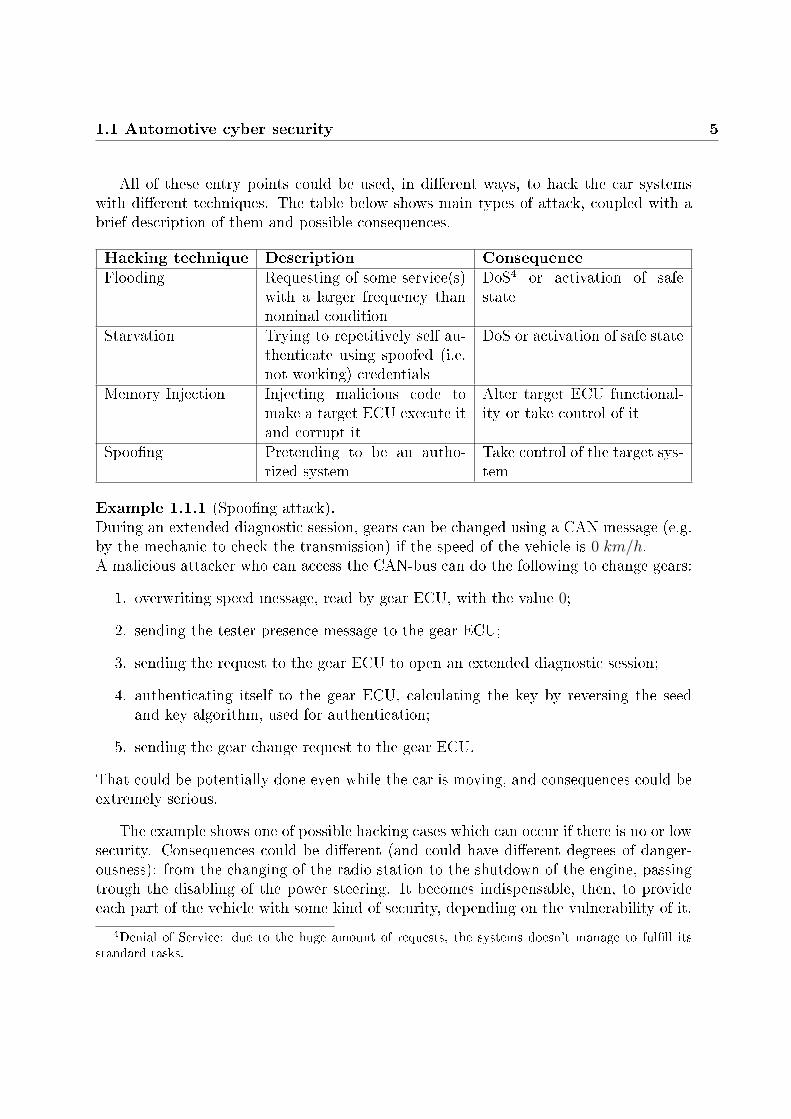
All of these entry points could be used, in dierent ways, to hack the car systemswith dierent techniques. The table below shows main types of attack, coupled with abrief description of them and possible consequences.
Hacking technique Description ConsequenceFlooding Requesting of some service(s)
with a larger frequency thannominal condition
DoS4 or activation of safestate
Starvation Trying to repetitively self au-thenticate using spoofed (i.e.not working) credentials
DoS or activation of safe state
Memory Injection Injecting malicious code tomake a target ECU execute itand corrupt it
Alter target ECU functional-ity or take control of it
Spoong Pretending to be an autho-rized system
Take control of the target sys-tem
Example 1.1.1 (Spoong attack).During an extended diagnostic session, gears can be changed using a CAN message (e.g.by the mechanic to check the transmission) if the speed of the vehicle is 0 km/h.A malicious attacker who can access the CAN-bus can do the following to change gears:
1. overwriting speed message, read by gear ECU, with the value 0;
2. sending the tester presence message to the gear ECU;
3. sending the request to the gear ECU to open an extended diagnostic session;
4. authenticating itself to the gear ECU, calculating the key by reversing the seedand key algorithm, used for authentication;
5. sending the gear change request to the gear ECU.
That could be potentially done even while the car is moving, and consequences could beextremely serious.
The example shows one of possible hacking cases which can occur if there is no or lowsecurity. Consequences could be dierent (and could have dierent degrees of danger-ousness): from the changing of the radio station to the shutdown of the engine, passingtrough the disabling of the power steering. It becomes indispensable, then, to provideeach part of the vehicle with some kind of security, depending on the vulnerability of it.
4Denial of Service: due to the huge amount of requests, the systems doesn't manage to fulll itsstandard tasks.

6 1. Random Number Generators in automotive cyber security
In the order form the bigger to the smaller, it is necessary to take into account the secu-rity of the whole system, of the vehicle, of ECUs and of the Software each ECU carriesand uses: in this dissertation we will focus on the particular aspects which concerns theuse of random numbers.
1.2 The importance of randomness in cryptography
Modern cryptography is based on public algorithms and functions (called crypto-graphic primitives): its whole strength is based on the key and on the unpredictabilityof some values used for encryption, it' here that randomness plays a fundamental role.
The relevance of randomness became more clear if we think that most of modern cryp-tography algorithms and protocols are designed around the Kerckho principle, whichstates that a cryptographic system has to be secure even though everything about thesystem is known, except for the key5. This means that, if we assume that the crypto-graphic structure is well designed, we should measure the strength of the system by thenumber of key an attacker has to guess before he can break it, which also implies thatthe security of the algorithm dangerously decreases if an enemy is able to be aware ofone or more bits of the key.
Random numbers are mainly required in the following cases:
• As cryptographic key in both symmetric and asymmetric algorithm: random num-bers are used as values which dene the transformation of the unencrypted infor-mation (plaintext) into the encrypted one (ciphertext), and vice versa. In moderncryptography, indeed, encryption and decryption algorithms are on public domain,as well as the ciphertexts sender and receiver exchange; the security of the wholeprocess depends, then, on the unguessability of the key: that's why this must de-pend on random values. Most famous examples of algorithms where the key isgenerated by random numbers are AES (symmetric cipher) and RSA (asymmetriccipher).
• In symmetric ciphers (especially stream and block chipers), random numbers areused as initialization vector to make dierent encryptions, even maintaining thesame key which, in this case, doesn't need to be changed each message. Anyway,maintaining the same key for a long time could produce a deterioration of security,so that this modality is used only in the case of a brief-time communication.
5This principle is also known as Shannon's maxim since C. Shannon has independently formulatedit as "the enemy knows the system".

1.2 The importance of randomness in cryptography 7
• Random numbers are used as nonces (number used once) and challenges, to ensurefreshness of messages and authentication (which can be mutual or unilateral) suchas ElGamal, Goldwasser-Micali and McEliece ciphers.
• Digital signature algorithms also need random numbers, to ensure authenticationand non-repudiation, without exposing the message itself to the signer (this typeof signatures are called blind signature schemes, shortly BSS). In this case themessage is made unintelligible (blinded) through a random number, know only bythe author of the message; the blinded message is sent to the entity which as tosign it with is private key, so that no private information are known to the signer.Typical examples are RSA BSS, Elliptic Curve BSS and ElGamal BSS.
• As cryptographic salts, such as as an extra argument used to generate new pass-word, starting from a single master key which remains the same all the time. Thisis typically done in the case the starting key is particularly guessable or to createkey and password that cannot be renegotiated each time.
• Padding is another use of random numbers: some ciphers (particularly block ci-phers) require xed-length messages. In the case the plaintext message doesn'treach the required length, blocks has to be lled with something in order to en-crypt the text and, obviously, removed by the receiver. Padding can be done usingxed values (for example with zeros or by 0x80 followed by zeros), but that couldresult in a leak of information about the message (i.e. an attacker could know some-thing about the message, by analyzing the ciphertext): that could be avoided bypadding using random values. Some examples are Optimal Asymmetric EncryptionPadding (OAEP) and Probabilistic Signature-Encryption Padding (PSEP).
It is clear that the use of not enough random values, or worse of deterministic ones,to perform these schemes could permit an attacker to break the encryption and nd outwhat it hides (plaintext), to impersonate someone else or to access to other people'spersonal information: that could turn out in loss of privacy, theft of money or, in theworst case as in automotive's eld, on put at risk the health of someone else.
We give the following, simple, examples to give the reader a basic idea of how randomnumbers are used.
Example 1.2.1 (The Die-Hellman protocol).The Die-Hellman key exchange is a cryptographic protocol by which two interlocutors(Alice and Bob in the following, as traditionally) can establish a secret shared key over apublic (insecure) channel without the need to know one another or to meet. The sharedkey, produced by this protocol, could be used to encrypt successive communicationsthroughout symmetric cryptography schemes.

8 1. Random Number Generators in automotive cyber security
Let g be a primitive root modulo p, where p is prime. The exchange between Alice(A) and Bob (B) proceeds as follows:
A: chooses a random number a, computes A = ga mod p and sends (g, p, A) to Bob;
B: chooses a random number b, computes B = gb mod p and sends it to Alice;
A: computes KA = Ba mod p;
B: computes KB = Ab mod p.
Alice and Bob, now, have the same key K = KA = KB, since Ba mod p = Ab mod p.
Let's suppose the attacker could intercept the whole speech: he knows A and B, butcouldn't know the key K, since he doesn't know random numbers a and b. Theoreticallyhe could compute, by the discrete logarithm, a and b but that is considered too com-putationally onerous to be dangerous. If the attacker could guess a or b, for exampleif a and b aren't randomly generated, he could impersonate Alice or Bob and see thefollowing encrypted communication or substitute itself to one of the two.
Example 1.2.2 (One-Time Pad (OTP)).Vernam Cipher (often called OTP) is the only cryptographic system which has beenproven (by C. Shannon in [66]) to be secure, since the ciphertext gives absolutely noinformation about the plaintext (this property is said to be perfect secrecy): for thisreason the cipher has been called "the perfect cipher".To encrypt using OTP, one has to generate an innite number of random sequences ofeach possible length and both the sender and the receiver (and no one else) has to ownthose keys.Given the plaintext x1, . . . , xn, a random sequence of the same length has to be chosenas key k1, . . . , kn: the ciphertext is created by an element by element sum yi = xi+ki ∀i.The receiver has to know which is the random sequence the sender used and simplydecrypt by element by element subtraction.Each use, the used key (i.e. the random sequence) has to be destroyed and never usedagain, in order to maintain the perfect secrecy of the cipher.
Notwithstanding the theoretical perfect security of this cipher, the necessity to sharea potentially non-nite number of key (which have to remain secret over time) and toknow which is used each time, the eective practice usability of OTP is very low inmodern cryptography, where the amount of information to encrypt is huge6.
6Anyway, OTP has been used since the early 1900s and registered an exploit in the World War II,where many nations used OTP systems to secure their sensitive trac. [34] provides an interestingreading on these facts, as long as the history of cryptography from its beginning to the time of writing(1967).
1.2 The importance of randomness in cryptography 9
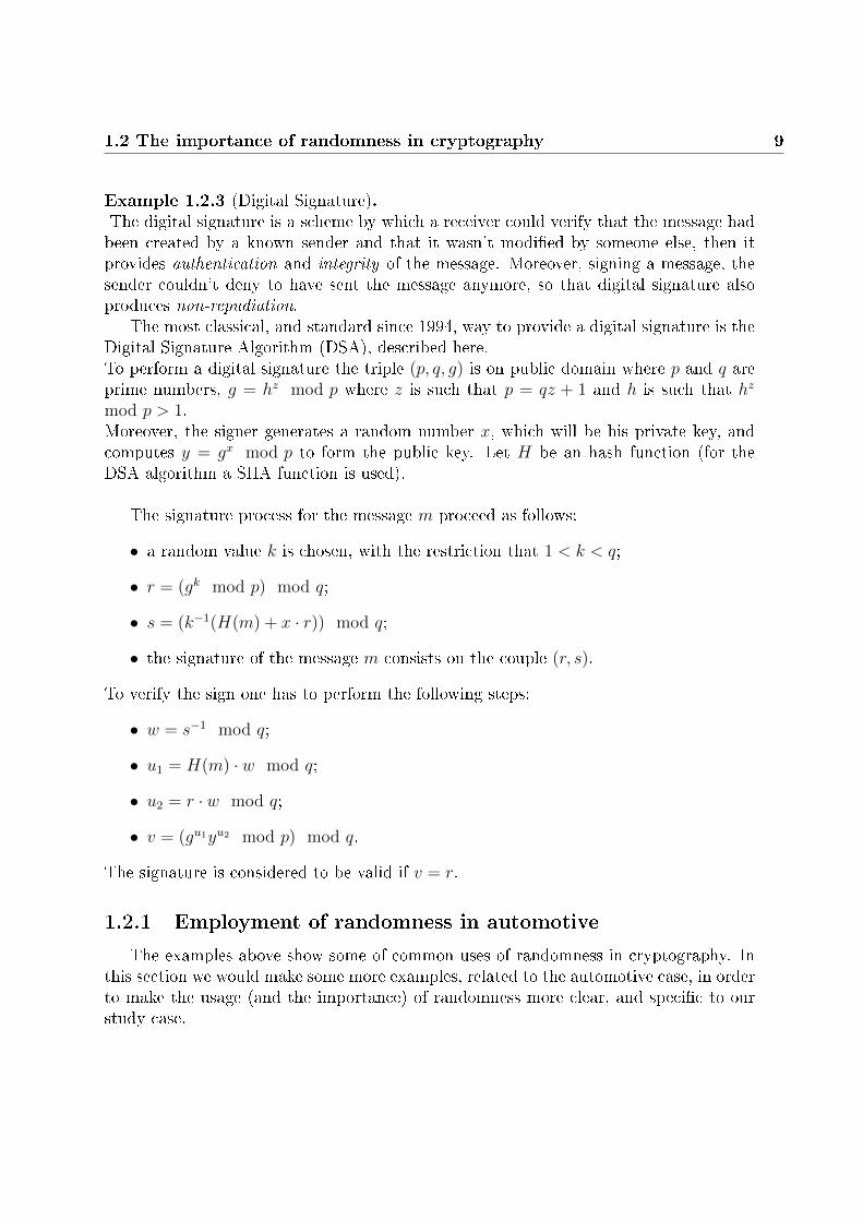
Example 1.2.3 (Digital Signature).The digital signature is a scheme by which a receiver could verify that the message hadbeen created by a known sender and that it wasn't modied by someone else, then itprovides authentication and integrity of the message. Moreover, signing a message, thesender couldn't deny to have sent the message anymore, so that digital signature alsoproduces non-repudiation.
The most classical, and standard since 1994, way to provide a digital signature is theDigital Signature Algorithm (DSA), described here.To perform a digital signature the triple (p, q, g) is on public domain where p and q areprime numbers, g = hz mod p where z is such that p = qz + 1 and h is such that hz
mod p > 1.Moreover, the signer generates a random number x, which will be his private key, andcomputes y = gx mod p to form the public key. Let H be an hash function (for theDSA algorithm a SHA function is used).
The signature process for the message m proceed as follows:
• a random value k is chosen, with the restriction that 1 < k < q;
• r = (gk mod p) mod q;
• s = (k−1(H(m) + x · r)) mod q;
• the signature of the message m consists on the couple (r, s).
To verify the sign one has to perform the following steps:
• w = s−1 mod q;
• u1 = H(m) · w mod q;
• u2 = r · w mod q;
• v = (gu1yu2 mod p) mod q.
The signature is considered to be valid if v = r.
1.2.1 Employment of randomness in automotive
The examples above show some of common uses of randomness in cryptography. Inthis section we would make some more examples, related to the automotive case, in orderto make the usage (and the importance) of randomness more clear, and specic to ourstudy case.

10 1. Random Number Generators in automotive cyber security
Figure 1.3: Digital Signature scheme. Credits to www.docusign.com.
In certain cases the car maker has to ensure that any request to access the CAN-busis made by authorized entity and in particular that critical actions are performed bylegitimate entities:
Example 1.2.4 (Diagnostic authentication (challenge and response)).Apart from troubleshooting, diagnosis communication with vehicle and with ECUs isalso used for more critical tasks, such as reprogramming (ashing) a specic controlunit or updating software. It is crucial, then, to protect the communication betweenthe tester and ECUs against unauthorized persons or equipment. To fulll this need,an authorized tester has to be recognized and authenticated by the system, in order toperform critical actions: that is made by embedding a scheme of authenticated access,which is based on a challenge and response protocol and (possibly) on digital signature,described in example 1.2.3 A tester who has to make critical actions has to perform thefollowing actions:
1. opening a request to the system (i.e. the ECU), which generates a random numberto challenge the tester;
2. the tester encrypts the random number together with a pre-shared secret key, usinga shared algorithm (or a one-way function) and sends the ciphertext back to theECU;

1.2 The importance of randomness in cryptography 11
3. the ECU performs the same encryption and checks if the two values match: if it'sthe case it permits the access.
This process could be even more secure by the use of certicates: in this case the testerhas to ask the OEM (through its PKI7) for the access: the OEM signs a certicate usingits private key; the tester sends the signed certicate to the ECU to request the access.In this case the authentication is performed directly between OEM and ECU, by meansof tester's connection. The OEM signs a certicate reporting tester's identity and sendsit to the ECU, though the tester, to request the access; the ECU sends a chance to theOEM, exploiting tester's connection; the OEM signs the challenge and sends it back tothe ECU, that can validate it and prove the authentication.
Example 1.2.5 (Secure communication).During vehicle activity, ECUs exchange a lot of information between themselves to ensurethe functionality of the whole system. This communications, via CAN-bus, should bechecked to be secure. This is typically done by encrypting sensitive data, by asymmetricor symmetric encryption (e.g. by the use of the Die-Hellman protocol, described inexample 1.2.1).
Each time the vehicle is started, an appointed ECU has to ensure that any other partwasn't modied or replaced (e.g. ECUs or software).
Example 1.2.6 (Component protection).To ensure integrity of the system (i.e. to check if an ECU has been substituted by anunauthorized one), a master ECU performs the following:
1. central ECU extracts a random number and sends it to a target ECU;
2. target ECU appends its unique ID8 to the random number and encrypts it usinga pre-shared key and sends it back;
3. central ECU decrypts the message, checks if the random number is the same itsent and if the ID appears among authorized ECU's IDs (stored into its memory).
Other employment of random numbers are, for example:
• symmetric key generation for ECUs internal usage, such as to encrypt parts ofECU's memory, authentication between ECUs and secure boot;
• asymmetric key generation for authentication;
• digital signature by the RSA-PSS algorithm, which works as in example 1.2.3 butusing RSA to sign, instead of a hash function;
7Public Key Infrastructure by which a third-party could ask the manufacturer to certicate a key.8Identity: its made by an alphanumeric string which is unique for each component.

12 1. Random Number Generators in automotive cyber security
• asymmetric encryption: when the encryption is based on RSA, the padding is oftenmade by random values and it takes the name of Optimal Asymmetric EncryptionPadding (OAEP) and the algorithm takes the name of RSA-OAEP.
To allow ECUs to perform cryptographic functionalities, as the above described,ECUs can be equipped with a specic hardware which fulll all of these needs: anexample is the Hardware Security Module (HSM). HSM guarantees a trusted executionenvironment where cryptography algorithms can be executed and sensitive data stored.
Figure 1.4: Hardware Security Module scheme. This HSM is provided with a TrueRandom Number Generator (TRNG). Credits to www.synopsys.com.
1.3 Random Number Generators
It becomes fundamental to create keys, in the form of strings of digits (numeric oralphanumeric) which can't be uncovered by a possible attacker: that is done by theembedding of Random Number Generators (shortly RNG) in the cryptographic system(for example in the HSM, speaking about ECUs). RNGs are software or hardware (or,in some cases both software and hardware) systems, which generate random numbersas output. The output of an RNG is typically a binary sequence that could have anylength: there exists generators which create decimal or alphanumeric strings, but they'reless used and, in fact, any sequence could be converted in binary, as well as any binarysequence can be converted in any other encoding. For this reason Random Number

1.3 Random Number Generators 13
Generators are also, but rarely, called Random Bit Generators. In this thesis, unlessdierently specied, we will refer to RNGs and to random sequences/strings encodedin binary format. We could distinguish Random Number Generators between Pseudo-Random Number Generators (PRNGs) and True Random Number Generators (TRNGs)depending on the way they create their output.
PRNGs are algorithms which, starting from a short initial value, called seed, producelong sequences by manipulating that value through various mathematical functions insuch a way that output appear random. Some trivial PRNGs were also made by pre-calculated tables from which a long sequence was extracted, depending from the seed.PRNGs can produce sequences which are indistinguishable from really random sequencesin a suitable sense, even though they are, in fact, deterministic. When true randomnessis not required, PRNGs are the most ecient choice, since they don't require any inputbut the seed and they can produce a huge amount of digits in a very short time. Notethat, given a seed, a PRNG will always produce the same sequence as output: this prop-erty of reproducibility, is very useful if one has to simulate or model random phenomena.On the other hand, since the output can be predicted just knowing the seed, PRNGsshouldn't be used when the produced numbers have to be really unpredictable, such aslotteries, gambling, random sampling and security.
When eective unpredictability is required, it becomes necessary to use a TRNG: aRandom Generator which takes values from some source of entropy, which is typically arandom physical phenomena. Some typical source from which randomness is extractedare:
• radioactive source: a radioactive source typically decays at completely unpre-dictable times and that is often simple to register and use. This approach is theone implemented, for example, by the HotBits service of Fourmilab Switzerland(www.fourmilab.ch);
• shot noise: the noise produced by the uctuation of electric current within electriccircuits;
• movement of photons: typically observed while traveling through a semi-transparentmirror, detecting reection and transmission;
• atmospheric noise: atmospheric noise could be picked up by any radio and its easyto be registered. The problem, in this case, is that it has to be detected in situationwhere there is no periodic phenomena. www.random.org follows this approach;
• thermal noise, typically taken from resistors.

14 1. Random Number Generators in automotive cyber security
Obviously, any other physical source could be used to extract digits from, but the ran-domness of the source have to be proved to call that a TRNG. Well designed TRNGcould create high-quality random sequence, however typically TRNG are much slowerthan PRNG since they are related to the physical event.
To fulll the request of a great amount of numbers in a short time, but maintainingthe unpredictability of TRNGs, it is also possible to combine a hardware based RNGto a software based one (i.e. mixing a TRNG and a PRNG together): that type ofRNG is called Hybrid Random Number Generator (HRNG). In this case hardware ex-tract randomness from a physical source of entropy, like TRNGs do, creating a short,unpredictable, sequence; the sequence is then given as input to the software algorithm,which uses it as the seed of a PRNG and extends it to the desired length.By this choice, the produced sequence maintains randomness properties and remainsunpredictable, but can be generated much faster than a classical TRNG. However, thedesign of a HRNG is doubly critical since both the physical entropy source and the al-gorithm has to be well designed and has to work properly.Many manufacturers are taking this path, due to the high demand of eciency requested,while maintaining the unpredictability (in the form of unguessability) feature.
We said that PRNGs are not suitable to use in some application, with cryptographyamong all however, at least theoretically, there exist a small subset of Pseudo RandomNumber Generators which could be used in elds where a TRNG would otherwise berequested: these are called Cryptographically Secure Pseudo-Random Number Generators(CSPRNGs). A PRNG is said to be cryptographically secure if it fulll two requirements:
i) next-bit test: if an attacker knows the rst k bits of a produced random sequence,there is no polynomial-time algorithm which can predict the (k + 1)th bit withmore than 50% of probability;
ii) state compromise extensions: if an attacker guess a part or all of the states of thePRNG, there is no way he can reproduce the stream of random numbers whichwhere produced in previous states (i.e. he can't go backward).
The design of a CSPRNG is hard and most PRNG fail to satisfy one of the two re-quests, however there are many PRNG which have been awarded by the cryptographicallysecure prize: for example the ChaCha20 algorithm (embedded in Mac OS) , the Fortunaalgorithm (Linux) and the CryptGenRandom (Microsoft). Some other CSPRNGs havealso been standardized (in [4] and in [2]), such as Hash_DRBG, HMAC_DRBG andCTR_DRBG.
A well designed RNG has to create sequences which are random by themselves andwhich have no relations with other created sequences. In the following we will present a

1.3 Random Number Generators 15
standardized method to evaluate if a RNG works properly analyzing the behavior of itsoutputs.

16 1. Random Number Generators in automotive cyber security
Chapter 2
The notion of randomness
This chapter will present an overview of the state of the art of randomness denitions.
2.1 Theoretical background
This section consists of a short introduction to the notions of probability which willbe useful to test randomness.
2.1.1 Probability bases
We give, here, some basic denitions we'll use in the following.
Denition 2.1.1 (σ-algebra).Fixed Ω an arbitrary non-empty set, a σ-algebra F over Ω is a family of subsets of Ω s.t.
i) Ω ∈ F ;
ii) if A ∈ F ⇒ Ac ∈ F ;
iii) if (An)n∈N ∈ F ⇒⋃n∈NAn ∈ F .
Denition 2.1.2 (Probability measure).A probability measure on (Ω,F) is a function P : F → [0, 1] such that
i) P (Ω) = 1;
ii) P is σ-additive: if Ann∈N ⊆ F is a countable collection of pairwise disjoint sets,then
P (⋃n∈N
An) =∞∑n=1
P (An).
17

18 2. The notion of randomness
Elements of F are called events and if A ∈ F , the quantity P (A) is said to be theprobability of (the event) A.
Denition 2.1.3 (Probability space).A probability space is a triple (Ω,F , P ) where:
• Ω is an arbitrary non-empty set;
• F is a σ-algebra over Ω;
• P is a probability measure.
Denition 2.1.4 (σ-algebra generated by a subset).Let A be a set of subsets of Ω. Dene
σ(A) = A ⊆ Ω s.t. A ∈ F for all σ-algebras F containing A
σ(A) is a σ-algebra, which is called the σ-algebra generated by A. It is the smallestσ-algebra containing A.
Denition 2.1.5 (Borel σ-algebra).Given d ∈ N. The σ-algebra B = B(Rd) generated by the Euclidean toplogy of Rd iscalled the Borel σ-algebra.
Denition 2.1.6 (Random variable).Let (Ω,F , P ) be a probability space and x the couple (V ,A), where V is a set and A isa σ-algebra. A function X : Ω→ V is called a random variable if X−1(A) ∈ F ∀A ∈ A.X is said to be discrete if V is countable. If V ⊆ R, X is said to be real.The probability that X takes on a value in a measurable set S ⊆ V is written as
P (X ∈ S) = P (ω ∈ Ω|X(ω) ∈ S)
and is called the probability distribution of X.
Denition 2.1.7 (Conditional probability).Let (Ω,F , P ) be a probability space and A,B ∈ F be two events. If P (B) > 0, theconditional probability of A given B (i.e. the probability of A to occur, while B occurs)is dened as
P (A|B) =P (A ∩B)
P (B)
where P (A ∩B) is the probability that both A and B occur.For two random variables X and Y , this denition becomes
P (X ∈ A|Y ∈ B) =P (X ∈ A ∩ Y ∈ B)
P (Y ∈ B).
If two events don't depend one another (we say that they are independent) we have thatP (A ∩B) = P (A)P (B) so that P (A|B) = P (A).

2.1 Theoretical background 19
Remark 2.1.1.From the previous denition, it's easy to obtain the Bayes' theorem, which states thatif A,B ∈ F are two events, than
P (A|B) =P (B|A)P (A)
P (B).
Denition 2.1.8 (Independent random variables).Random variables X1, X2, . . . are said to be independent if for any k ∈ N and for anysequence A1, . . . , Ak ∈ F the equality
P (X1 ∈ A1, . . . , Xk ∈ Ak) = P (X1 ∈ A1) · . . . · P (Xk ∈ Ak)
holds.For discrete random variables X1, X2, . . . this condition simplies to
P (X1 = x1, . . . , Xk = xk) = P (X1 = x1) · . . . · P (Xk = xk)
for any sequence x1, . . . , xk ∈ V.
Denition 2.1.9 (Distribution function).A distribution function µ is a map
µ : B(Rd)→ [0, 1]
dened by
µ(S) =∑x∈S∩A
γd(x) +
∫S
γc(x)dx, S ∈ B
where
• γc, called the probability density function of µ, is a B-mesurable function
γc : Rd → [0,+∞]
such that ∫Rdγc(x)dx =: I ∈ [0, 1]
• γd, called the discrete distribution function of µ, is a function
γd : A→ [0, 1]
where A ⊆ Rd is a countable set, and∑x∈A
γd(x) = 1− I
with the convention that γd(x) = 0 if x ∈ Rd \ A.

20 2. The notion of randomness
In the case that γd ≡ 0, we say that µ is an absolutely continue distribution function.
Denition 2.1.10 (Uniformly distributed random variable).A random variable X that assumes values in a nite set V is said to be uniformly dis-tributed if it assumes all v ∈ V with the same probability.
Denition 2.1.11 (Stochastic process).A stochastic process is a parametrized collection of random variables Xii∈I dened ona probability space (Ω.F , P ) and assuming values in Rn.
Denition 2.1.12 (i.i.d. random variables).Let X and Y be two random variables on the same probability space. If X and Y areindependent as in (2.1.8) and have the same probability distribution, than X and Y aresaid to be independent and identically distributed random variables: in the following we'llshortly say i.i.d..
A stochastic process Xii∈I is said to be an i.i.d. process if random variables thatforms it are.
Denition 2.1.13 (Stationary stochastic process).A stochastic process is said to be stationary if
P (X1 ∈ A1, . . . , Xk ∈ Ak) = P (X1+t ∈ A1, . . . , Xk+t ∈ Ak) ∀k, t ∈ N,∀A1, . . . , Ak ∈ F
For discrete random variables, this condition simplies to
P (X1 = x1, . . . , Xk = xk) = P (X1+t; . . . , Xk+t = xk) ∀x1, . . . , xk ∈ V.
Remark 2.1.2.By denitions, an i.i.d. stochastic process is always stationary.
Denition 2.1.14 (Mean).The mean (or expected value) of a discrete real-valued random variable X is given by
E[X] :=∑x∈V
xP (X = x).
If X is a continue random variable (i.e.∫
Ω|X(ω)|dP (ω) <∞), then its mean is
E[X] :=
∫Ω
X(ω)dP (ω) =
∫RnxdµX(x).
Denition 2.1.15 (Cumulative distribution function).Let X be a real-valued random variable on (Ω,F , P ).The cumulative distribution function of X is the function
FX : R 7→ [0, 1]
s.t. FX(y) = P (X ≤ y), y ∈ R.

2.1 Theoretical background 21
Proposition 2.1.1.If two random variables X, Y : Ω→ R are independent then X, Y ∈ L1(Ω, P ) if and onlyif XY ∈ L1(Ω, P ). In that case we have
E[XY ] = E[X]E[Y ].
Denition 2.1.16 (Variance and standard deviation).Given a random variable X, we can dene its variance and its standard deviation respec-tively as:
V ar(X) := E[E[X]−X]2
σ :=√V ar(X)
Denition 2.1.17 (Ergodic stochastic process).A stationary stochastic process is said to be ergodic if its statistical properties can bededuced from a single, suciently long realization of the stochastic process.
Denition 2.1.18 (Dirac distribution).The Dirac distribution δx0 centered on x0 ∈ R is the distribution with
γc ≡ 0 and γd = 1 on A = x0.
So
δx0(S) =
1 if x0 ∈ S0 if x0 /∈ S.
Denition 2.1.19 (Normal distribution).The real normal distribution N(µ, σ2) of parameters µ ∈ R and σ ≥ 0 is the distributionwhich density is
γc(x) =
0 if σ = 0
1√2πσ2
e−(x−µ)2
2σ2 if σ > 0
and discrete distribution function on A = µ
γd =
1 if σ = 0
0 if σ > 0.
So N(µ, 0) = δµ and, if σ > 0,
N(µ, σ2) =1√
2πσ2
∫S
e−(x−µ)2
2σ2 dx S ∈ B(R).
A particular, and really important special case, is when µ = 0 and σ2 = 1: in this casethe distribution is called Standard Normal distribution and its cumulative distributionfunction is
Φ(x) =1√2π
∫ x
−∞e−t
2/2dt. (2.1)

22 2. The notion of randomness
An extremely useful result for our analysis will be the following
Theorem 2.1.2 (Central limit theorem).Let Xn be a stochastic process of independent and identically distributed random vari-ables, whose mean µ and variance σ2 < +∞. Then the random variable
Zn :=X1 + · · ·+Xn − nµ
σ√n
approaches the Standard Normal Distribution N(0, 1) as n approaches to innity. Inother words, for all a < b we have
limn→∞
P
(a ≤ X1 + · · ·+Xn − nµ
σ√n
≤ b
)= Φ(b)− Φ(a)
where Φ is the cumulative distribution function of the Standard Normal Distribution, asabove.
2.1.2 Entropy
We introduce, now, the concept of entropy, as dened by Shannon [65]. Thanks tothis concept, we can measure the uncertainty of a stochastic source of data or, equiva-lently, the average amount of information content, regardless the object of study.
Let X be a discrete random variable and let P be its probability distribution denedon V = x1, . . . , xM such that P (X = xi) = P (xi) = pi. We want to dene a set offunctions HM : RM → R+ that meets the following axiomes:
i) Monotony: f(M) := HM( 1M, . . . , 1
M) be a strictly increasing function;
ii) Extensiveness: f(LM) = f(L) + f(M) ∀L,M ≥ 1;
iii) Groupability: xed r < M we dene ~q = (qA, qB) s.t. qA =∑r
i=1 pi(⇒ qB = 1− qA =
∑Mi=r+1 pi)
HM(~p) = H2(~q) + qAHr
(p1
qA, . . . ,
prqA
)+ qBHM−r
(pr+1
qB, . . . ,
pMqB
)iv) Continuity.
Theorem 2.1.3 (Shannon).The only function (up to multiplicative constant) which satises the previous axioms is
~p 7→ H(~p) = −cM∑i=1
pi logb pi

2.1 Theoretical background 23
with the convention that 0 log 0 = 0 (which is consistent by the fact that limp→0 p logb1p
=
0). The function H is said to be the entropy function (or simply entropy).
Proof.It's easy to prove that the function H meets the previous axioms, so we'll show the ex-istence and uniqueness of that function.
1. ∀M,k ≥ 1 we can write f(Mk) = f(M · Mk−1) = f(M) + f(Mk−1) using thegroupability property.Iterating the procedure we nd f(Mk) = f(M) + f(Mk−1) = . . . = kf(M)
2. Let's show that ∀M ≥ 1 ∃ c > 0 s.t. f(M) = c logM :if M=1 we have that
f(1) = f(1 · 1) = f(1) + f(1)⇒ f(1) = 0.
If, otherwise, M > 1, one can prove that for all r ≥ 1 exists k ∈ R such that
Mk ≤ 2r ≤Mk+1,
but f(M) = HM( 1M, . . . , 1
M) is a strictly increasing function, so we obtain
f(Mk) ≤ f(2r) ≤ f(Mk+1).
Using the st step
kf(M) ≤ rf(2) ≤ (k + 1)f(M)⇒ k
r≤ f(2)
f(M)≤ k + 1
r,
and the logarithm is strictly increasing too, so
k
r≤ log 2
logM≤ k + 1
r⇒∣∣∣∣ f(2)
f(M)− log 2
logM
∣∣∣∣ ≤ 1
r.
r was arbitrary then, to the limit for r to innity,
f(M) =f(2)
log 2logM = c logM
3. We took uniform pi: let's extend this denition choosing pi = riM∈ Q, i = 1, . . . , N ;
let's divide the element of ~p in groups of ri: each ri element will have a probability

24 2. The notion of randomness
of 1ri
= 1M/pi = 1
M/ riM.
Let's use now the groupability property, obtaining
c logM = f(M) = f(M) = HM
(1
M, . . . ,
1
M
)= H(p1, . . . , pN) +
N∑i=1
piHri
(1
ri, . . . ,
1
ri
)= H(p1, . . . , pN) +
N∑i=1
pic log ri
then
H(p1, . . . , pN) = c
(logM −
N∑i=1
pi log ri
)= c
(−
N∑i=1
pi logriM
)= −c
N∑i=1
pi log pi
We can now extend it to all of R thanks to the continuity axiom.
Remark 2.1.3.The denition is consistent for any base of the logarithm b. Common values of b are 2,the Euler's number e and 10, and the corresponding units of entropy are, respectively,bits, nats and bans.Our purpose is to analyze binary strings: we'll choose b = 2, so that c = 1. In thefollowing we will always use that base, than we'll simply write log, instead of log2.
Remark 2.1.4.By denition we have that H(x) ≥ 0.
Making some examples, we want to to show what we mean for "measure the uncer-tainty" of a source of data
Example 2.1.1.If ~p = (0, . . . , 0, 1, 0, . . . , 0)M we obtain that H(~p) = 0: in the case that the distributionof probability is some of this kind, we don't have any uncertainty.
Example 2.1.2.Let's try to nd which is the event ~p = (p1, . . . , pM) which maximize the entropy H.We consider the function
h : ~p 7→ H(~p) = −M∑i=1
pi log pi
with the constraint that ϕ(~p) =∑M
i=1 pi − 1 = 0. Let's use the Lagrange multipliers:
∂pij(H(~p) + λϕ(~p)) = 0

2.1 Theoretical background 25
− log pj − pj1
pj
1
log 2+ λ = 0⇒ − log pj = λ log 2 = cost.⇒ pj = cost.
pj also has to meet the constrait, so we obtain that pj = 1M.
One can easily see that the uniform vector ~p =(
1M, . . . , 1
M
)is a maximum for the entropy:
in this case we have H(~p) = logM .
Example 2.1.3.If ~p =
(1
M−1, . . . , 1
M−1, 0)M⇒ H(~p) = log(M − 1), so that it's the same as having one
less choice.

26 2. The notion of randomness
2.2 Characterizations of randomness
Many disciplines tried to give a denition of randomness and found dierent waysto call something "random". We are interested in expressing what is a "binary randomstring".
2.2.1 Probabilistic approach
One can formulate the notion of random string in the following way:
Denition 2.2.1 ((Probabilistic) random string).Let Xii∈I be a stochastic process to assume values in V = r1, . . . , rM with probabilityP (ri) = P (rj) ∀i, j.If the process consists on independent and identically distributed (i.i.d.) random vari-ables, then its realization (r1, . . . , rN) ∈ VN is called a random string.
Remark 2.2.1.In the case of a binary string (r1, . . . , rM), ri ∈ V = 0, 1 we can consider the sequenceas a realization of the same random variable X. Obviously, in this case, the probabilitiesare P (0) = P (1) = 1
2as in a coin ip.
The distribution that models the outcomes of an i.i.d. process is known as theBernoulli distribution.
Denition 2.2.2 (Bernoulli distribution).Given p ∈ [0, 1], the Bernoulli distribution function is dened on R and is dened in thefollowing way:
γ(x) =
p if x = 1,
1− p if x = 0,
0 otherwise.
The respective distribution is
B(1,p)(H) =
0 if 0, 1 6∈ H,1 if 0, 1 ∈ H,p if 1 ∈ H, 0 6∈ H,1− p if 0 ∈ H, 1 6∈ H.
If a random variable X has a Bernoulli distribution, then P (X = 1) = p and P (X =0) = 1− p.
Practically speaking, a Bernoulli process is a nite or innite sequence of independentrandom variables X1, X2, . . . such that:

2.2 Characterizations of randomness 27
i) the value of Xi is either "0" or "1", ∀ i;
ii) P (Xi = 1) = p, P (Xi = 0) = 1− p.
So we can rationally model an ideal random string as the realization of a Bernoulliprocess with p = 1
2.
A closely connected, and very useful in the following, distribution is the
Denition 2.2.3 (Binomial distribution).Let n ∈ N and p ∈ [0, 1]. The binomial distribution of parameters n and p is dened bythe distribution function
γ(k) =
(nk
)pk(1− p)n−k if k = 0, 1, . . . , n
0 otherwise.
So if a random variable X has a binomial distribution (by symbols X ∼ Bin(n, p)) wehave
P (X = k) =
(n
k
)pk(1− p)n−k, k = 0, 1, . . . , n.
Example 2.2.1.Typical examples of binomial random variables are:
• the random variable "number of successes in n independent repeted trials withprobability p", which has Bin(n, p) distribution;
• if we suppose to have r objects into n boxes, the random variable "number ofobjects into the rst box" has a Bin(n, 1
r) distribution.
Note that this point of view, nevertheless it provides ideas and characterization ofrandom string, is in fact the main base of all of the following approaches and theories.
2.2.2 Information Theory approach
As we discussed in section (2.1.2), we could give a measure of the uncertainty of asource through the concept of entropy and this uncertainty of the source corresponds tothe amount of information which the data contains.
We modeled a random binary string as a Bernoulli process, i.e. as a sequence ofindependent random variables X1, X2, . . . with P (Xi) = 1
2∀i, so that the information
contained in it is maximum: this means that every single bit of the sequence containsrelevant information. If each single bit of the sequence contains some information, thatimplies that we couldn't compress the string in a relevant way, without losing some ofthe information contained inside it. In the following we try to formalize this idea and to

28 2. The notion of randomness
show that this is strictly connected with the notion of entropy.
Let X = Xii∈I , I ⊆ N be a stochastic process. To express how the entropy growsas soon as the process goes on (i.e. we add bits to the sequence) we can give the following
Denition 2.2.4 (Entropy-rate of a stochastic process).The entropy rate of a stochastic process is dened as
H(X) := limn→∞
H(x1, . . . , xn)
n
if this limit exists.
Using the fact that H(x1, . . . , xn) =∑n
i=1H(xi|x1, . . . , xi−1) one can easily observethat the following holds:
Theorem 2.2.1.If X is a stationary process, than H(X) exists and
H(X) := limn→∞
H(xn|x1, . . . , xn−1).
Example 2.2.2.Let us consider a stochastic process formed by a sequence of i.i.d. random variables. Inthis case it holds that
H(X1, . . . , Xn) = H(X1, . . . , Xn−1) +H(Xn).
Iterating we nd thatH(X1, . . . , Xn) = nH(X1)
since H(Xi) = H(Xj) ∀i, j, so that the entropy rate of this process is exactly
H(X) = limn→∞
H(X1, . . . , Xn)
n=nH(X1)
n= H(X).
Since, as we have seen in previous section, a random sequence is produced by aBernoulli process (which is an i.i.d. process) this is exactly the case of our interest, andthe entropy rate is maximum, since the entropy is.
To compress a sequence we should dene a way to transform elements of it or, inother words, we need a
Denition 2.2.5 (Code).A code C for a random variable X, which takes values on an alphabet χ, is a map
C : χ→ D∗ =⋃n
Dn

2.2 Characterizations of randomness 29
such thatx 7→ C(x),
where D is an alphabet and C(x) is said to be a code word. To each code word we cannaturally associate it's length l(x).
Each code can be extended to nite strings of the alphabet χ through
C∗ : χ∗ → D∗
dened as(x1, . . . , xn) 7→ C∗(x1, . . . , xn) = C(x1) · ... · C(xn).
where · stands for the concatenation.
In the following we will consider the most useful codes which permits to compress/-code and decompress sequences without requiring any other information, i. e. codeswith the following properties:
• Non-singular: if xi 6= xj ⇒ C(xi) 6= C(xj) ∀i, j;
• Prex-free: no code word is prex of other code words, i.e. if c(xi) = α ⇒@j s.t. C(xj) = α ∗ ∗∗.
Codes which satisfy these requirements are called instantaneous or prex code.
To assess the existence of an instantaneous code we can use the following theorem,proved by Kraft in [40]:
Theorem 2.2.2 (Kraft's inequality).If C is an instantaneous code on D, with |D| = D, the set of length l1, . . . , lm is suchthat
∑mi=1D
−li ≤ 1.Vice versa, if the set of length l1, . . . , lm satisfy the inequality ⇒ there exists an in-stantaneous code on D with those length.
Since we are interested in instantaneous codes, this theorem gives us constraints onthe length of code words which permits to study them.We are interested to compress a sequence, i.e. to minimize it's length. Let's consider
Denition 2.2.6 (Average length of the code).If p(x) is the probability of the word x to occur and l(x) is the length of the coded word,the average length of the code is dened as
L(C) =∑x∈χ
p(x)l(x).
A code that minimize the average length is said to be optimal.

30 2. The notion of randomness
We can nd a lower bound for the average length, i.e. we can nd the best per-formance for an instantaneous code, minimizing the average length function, with theconstraints that the length of code words satisfy Kraft's inequality.
Proposition 2.2.3.For each instantaneous code for a random variable X one has
L(C) ≥ HD(X),
where HD(X) is the entropy where the base of the logarithm is D.
Proof.Let's use Lagrange multipliers to minimize the average length with the constraints of theKraft inequality:
J(l1, . . . , lm) =∑i
pili + λ
(∑i
D−li
)where pi and li stands for the probability and length of the i-th symbol of the alphabet.
∂J
∂lk= pk + λ(−logeD ·D−lk) = 0
from which
pk = (λlogD)D−lk .
Now∑pk = 1 and if we suppose
∑D−lk = 1, we obtain
λlogD = 1⇒ λ =1
logD
so that
pk = Dlk ⇔ lk = −logDpk.
Substituting we obtain that the minimum for the average length is L = HD(X).
We can extend this denition to words of any chosen length by dening the
Denition 2.2.7 (Average length per-symbol).If l(x1, . . . , xn) is the length of the code word associate to the word (x1, . . . , xn),
Ln(C) =1
n
∑x1,...,xn
p(x1, . . . , xn)l(x1, . . . , xn)
is said to be the average length per-symbol.

2.2 Characterizations of randomness 31
One can prove that, for an optimal code the following inequality holds:
HD(x1, . . . , xn)
n≤ Ln(C) ≤ HD(x1, . . . , xn) + 1
n
which to the limit n→∞ becomes
H(X) ≤ Ln(C) ≤ H(X).
As we have seen, for a random sequence the entropy rate is, in fact, the entropy of theprocess (which is maximum for random sequences), therefore studying the compressionrate of optimal codes applied to sequences seems to be a good way to test for randomness:this has been done by most of test suites for randomness for long time, since equivalentbut more ecient methods were found. The most used test suites, and especially NIST's,used the LZ78 code or its variants: a universal and optimal code, proposed by Lempel andZiv in [71] and enhanced in [72]. Sequences were eectively compressed, using LZ78 andthe compression rate was analyzed to decide whether or not the sequence was random:due to the high complexity of the compression algorithm and to some weakness of theimplementation, such as constraints on the length of the sequence to test, this test wasremoved in 2004, since the Serial test (test 11) and the Approximate entropy test (test12) produce analogous results.
2.2.3 Complexity Theory approach
In this section, we will present the approach of theory of complexity, introduced byKolmogorov (see [9] for a review) and extended by Chaitin (see for example [12]), whichdenes randomness in terms of the length of the shortest code (called Chaitin computer)that could create the sequence itself. This approach also leads to the sharable idea thatrandomness implies an absence of regularity which is, obviously, strictly connected tothe idea of incompressibility presented by the theory of information.
In this section we will use the concept of partially computable function, typical ofthe algorithmic information theory: a function ϕ : X → Y which is dened on a subsetZ ⊆ X is called a partial function; if dom(ϕ) = X, the function is said to be a totalfunction. A partial function is said to be partially computable function if it can be com-pletely described by an algorithm.
The Chaitin denition of randomness is based on the following
Denition 2.2.8 (Chaitin computer).Let A = a1, . . . , aQ be a sortable alphabet.A computer is a partially computable function C : A∗ × A∗ → A∗.A Chaitin computer is a computer C such that ∀v ∈ A∗ the domain of Cv is prex-free,

32 2. The notion of randomness
with Cv : A∗ → A∗ such that Cv(x) = C(x, v) ∀x ∈ A∗.A (Chaitin) computer C is said to be universal if for each (Chaitin) computer ϕ there isa constant c (which depends on ψ and ϕ) such that if ϕ(x, v) <∞⇒ ∃x′ s.t. ψ(x′, v) =ϕ(x, v) and |x′| ≤ |x|+ c.
As in [11] (Theorem 3.3) one can prove that a (Chaitin) universal computer eectivelyexists. In the sequel we will use ψ to indicate a universal computer and U for a Chaitinuniversal computer and we'll use them to dene complexities of strings.
Denition 2.2.9 (Complexities).a) The Kolmogorov-Chaitin absolute complexity, associated with a computer ϕ isthe function Kϕ : A∗ → N dened as
Kϕ(x) := min|u| s.t. u ∈ A∗, ϕ(u, λ) = x.
If ϕ = ψ we will write K(x) instead of Kψ(x).b) The Chaitin absolute program-size complexity, associated with the Chaitin com-puter C is the function HC : A∗ → N dened as
HC(x) = min|u| s.t. u ∈ A∗, C(u, λ) = x,
and we will write H(x) = HU(x) if the associated computer C is the universal computerU .
According to both denitions, the complexity of a string x is the the length of theshortest string y one has to give as input to a computer to obtain the string x: we canuse this notion as the main quantity to dene randomness. One can prove that the twonotion of complexity are equivalent and that
K(x) ≤ Kϕ(x) +O(1), H(x) ≤ HC(x) +O(1)
for each computer ϕ and for each Chaitin computer C.
Example 2.2.3 (Paradox of randomness).Consider the following binary strings:
x = 00000000000000000000000000000000,
y = 10011001100110011001100110011001,
z = 011010001001101oo101100100010110,
u = 00001001100000010100000010100010,
v = 01101000100110101101100110100101.

2.2 Characterizations of randomness 33
According to the classic probability theory all the previous strings have the same prob-ability, which is 2−32 since they are made of 32 digit which can be 0 or 1, however, ifwe focus on regularity of those, they are extremely dierent: indeed we can express xsimply by "32 zeros", y is "eight time 1001" and z is "0110100010011010 concatenatedwith it's mirror". This example also shows the strict relationship between regularity andcompressibility, since the more a sequence is regular, the more we can compress it.u and v are more cryptically: we can't apparently nd any sort of regularity and we can'texpress them by a shorter formula. Simplistically thinking, this could be considered asthe main idea behind the denition of randomness given by the theory of complexity.
To give a denition of randomness based on complexity, one should prove that, eachtime we choose a length n for the sequence, there is a maximum for the complexity ofstrings of n digits. We will present here the main results which lead to the denition ofrandomness given by Chaitin (see for example [11] for proofs).
Theorem 2.2.4 (Chaitin).Let f : N→ A∗ be an injective, computable function.
• The following inequality holds ∑n≥0
Q−H(f(n)) ≤ 1.
• Let g : N+ → N+ be a computable function, then
i) If∑
n≥1Q−g(n) =∞, then H(f(n)) > g(n) for innitely many n ∈ N+.
ii) If∑
n≥1Q−g(n) <∞, then H(f(n)) ≤ g(n) +O(1).
Using this theorem and choosing g(n) = blogQnc and g(n) = 2blogQnc one can ndthe following bound for the Chaitin complexity of a string of length n on an alphabet ofcardinality Q:
blogQnc < H(string(n)) ≤ 2blogQnc+O(1).
Thanks to this bound we have
Theorem 2.2.5.For every n ∈ N
maxx∈AnH(x) = n+H(string(n)) +O(1).
Since the maximum always exists, we can dene a function Σ : N→ N such that
Σ(n) = maxx∈AnH(x) = n+H(string(n)) +O(1).
A random string of length n could be dened as the string which have the maximalcomplexity among all strings of length n, i.e. the strings x ∈ An such that H(x) ≈ Σ(n)or, in other words, we can give the following

34 2. The notion of randomness
Denition 2.2.10 (Chaitin random string).A string x ∈ A∗ is said to be Chaitin m-random, with m ∈ N, if H(x) ≥ Σ(|x|)−m.x is Chaitin random if it is 0-random.
Moreover, by combinatorial arguments, one can also prove the following result on thenumerosity of Chaitin random strings:
Theorem 2.2.6.For all n ∈ N there exists a constant c > 0 such that
γ(n) = #x ∈ An s.t. H(x) = Σ(|x|) > Qn−c.
This approach is the main focus for the Binary matrix rank test (test 5), the DiscreteFourier transform test (test 6) and for the two test which analyze templates (test 7 and8).
2.2.4 Algorithmic Information Theory approach
The goal of Martin-Löf's theory was to prove that the denitions of randomness givenby Kolmogorov and Chaitin through the theory of complexity are consistent with theclassical probability theory: the strength of his theory is that it includes all known andunknown properties of random sequences.
Let's suppose to have an element x of a general sample space and to test if this elementis typical, i.e. if it belongs to some majority or if it is a special case among that samplespace. Considering all these possible "majorities", an element would be "random" if itlies on the intersection of all majorities or, conversely, it would be "non-random" if thereis some case where it can be considered "particular": this is, basically, the idea if theclassical hypothesis testing we'll explain and use in the following chapter.
Denition 2.2.11 (Martin-Löf test).A set V ⊂ A∗ × N+ is called a Martin-Löf test if the following holds:
i) Vm+1 ⊂ Vm ∀m ≥ 1;
ii) #(An ∩ Vm) < Qn−m/(Q− 1) ∀n ≥ m ≥ 1.
Vm = x ∈ A∗ s.t. (x,m) ∈ V is called a m-section of V . For each m, the set Vm iscalled the critical region at level Q−m/(Q − 1) and we say that a string is "random" atlevel m, with respect to the test V if x /∈ Vm and |x| > m.
Let make, here, two examples to show that tests we'll discuss in the following couldbe analyzed according to this theory.
2.2 Characterizations of randomness 35
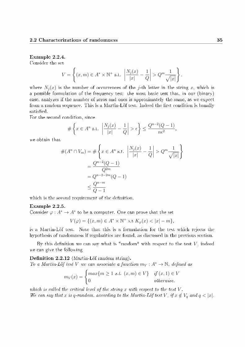
Example 2.2.4.Consider the set
V =
(x,m) ∈ A∗ × N+ s.t.
∣∣∣∣Nj(x)
|x|− 1
Q
∣∣∣∣ > Qm 1√|x|
,
where Nj(x) is the number of occurrences of the j-th letter in the string x, which isa possible formulation of the frequency test: the most basic test that, in our (binary)case, analyzes if the number of zeros and ones is approximately the same, as we expectfrom a random sequence. This is a Martin-Löf test. Indeed the rst condition is banallysatised.For the second condition, since
#
x ∈ An s.t.
∣∣∣∣Nj(x)
|x|− 1
Q
∣∣∣∣ > ε
≤ Qn−2(Q− 1)
nε2,
we obtain that
#(An ∩ Vm) = #
x ∈ An s.t.
∣∣∣∣Nj(x)
|x|− 1
Q
∣∣∣∣ > Qm 1√|x|
=Qn−2(Q− 1)
Q2m
= Qn−2−2m(Q− 1)
≤ Qn−m
Q− 1
which is the second requirement of the denition.
Example 2.2.5.Consider ϕ : A∗ → A∗ to be a computer. One can prove that the set
V (ϕ) = (x,m) ∈ A∗ × N+ s.t Kϕ(x) < |x| −m,
is a Martin-Löf test. Note that this is a formulation for the test which rejects thehypothesis of randomness if regularities are found, as discussed in the previous section.
By this denition we can say what is "random" with respect to the test V , indeedwe can give the following
Denition 2.2.12 (Martin-Löf random string).To a Martin-Löf test V we can associate a function mV : A∗ → N, dened as
mV (x) =
maxm ≥ 1 s.t. (x,m) ∈ V if (x, 1) ∈ V0 otherwise.
which is called the critical level of the string x with respect to the test V .We can say that x is q-random, according to the Martin-Löf test V , if x /∈ Vq and q < |x|.

36 2. The notion of randomness
Chaitin random strings and Martin-Löf's tests are strictly connected, indeed, as in[11], one can prove the following
Theorem 2.2.7.Fixed k ∈ N, almost all Chaitin k-random strings will be declared random by everyMartin-Löf test.

Chapter 3
Statistical tests for randomness
As we have seen, the purpose of a Random Number Generator is to produce sequencesof random digits, if it's a true RNG, or at least that behave as if they are random, in thecase of a PRNG: how could we decide whether a sequence is random? The idea behindstatistical tests is to compare the sequence, output of the RNG, to a sequence which isthe output of an ideal random number generator. Each test inspects the sequence toassess the presence of some specic pattern or behavior which could indicate that thesequence is random. For an ideal random string the property is known a-priori, can bedescribed in probabilistic terms and denes statistic T of each test. Each test gives usmore and more condence of the randomness of the sequence. The purpose is to proposea collection of tests that could cover a suciently large set of defections.
3.1 General procedure
The idea behind the tests is the hypothesis testing: let's x a parameter space Θ,which indexes all possible probability distributions of the observed data. We dene thenull hypothesis H0 as a subset θ0 ∈ Θ which corresponds to special parametric valuesof interest. The so called alternative hypothesis H1 i.e. θ ∈ Θ1 can also be considered:typically the alternative hypothesis corresponds to the complementary one Θ1 = Θ \Θ0.Once the null hypothesis is dened, one tests data to decide if he should maintain orreject his hypothesis, i.e. if the inspected objects belong to the subset Θ0 or to its com-plementary.
In our case of testing randomness, the hypothesis is that the sequence is random andthe alternative one is that it is not, we can give the following
Denition 3.1.1 (Null hypothesis (for randomness)).Let Θ be the set of all possible distributions of a binary sequence, Θ0 the set of distribu-tions of ideal random binary sequence and Θ1 = Θ \Θ0.
37

38 3. Statistical tests for randomness
The null hypothesis H0 : θ ∈ Θ0 is that bits of the observed sequence represent indepen-dent Bernoulli random variables with the probability of success p(1) = p(0) = 1
2
As we said, each statistical test is based on a statistic T : to decide if we should main-tain or reject the null hypothesis, one shall see if the observed statistic T is sucientlyclose to the expected one T0, which is the same statistic under H0. According to that,one should dene a cut-o value to make this decision. This approach leads to
Denition 3.1.2 (Signicance level).The signicance level α is the probability that the null hypothesis is rejected.
This signicance level represents the probability that a "good" generator produced anon-random sequence. α is a-priori dened and empirical results in cryptography showedthat it can be chosen between 0.001 and 0.01. One could also dene the probability thata "bad generator" produced a random sequence; this is the
Denition 3.1.3 (Power of the test).The power of the test β is the probability that the alternative hypothesis H1 is rejected,although is true (i.e. H0 is accepted).
So that, the observer may commit two types of error: judging the generator as a"bad" generator while in fact it eectively generate random numbers, with probabilityα, (we call that type I error) or concluding that the sequence is random (i.e. producedby a "good" random generator) while it's not, with probability β (this will be called typeII error). We summarize possible conclusions in the following table:
CONCLUSIONTRUE SITUATION Accept H0 Reject H0
Data is random (H0 is true) No error Type I errorData is non-random (H0 is false) Type II error No error
The probability β of a type II error is always dicult to express, however α andβ are related to each other: a small α corresponds to a high β and vice versa. Inmost of hypothesis testings, the signicance level α is chosen to be on the order of 0.05,however in cryptography α is commonly set to smaller values (i.e. α ≤ 0.01). Notethat setting, for example, α = 0.01 means that, under randomness hypothesis (i.e. ourdata is eectively random), we expect to reject the null hypothesis in less than 1% ofcases. The existence of these errors shows that evaluating if the observed (empirical)values are suciently close to the expected one it's not enough, because we can fall inone of the previous errors: it's also useful to know how often we obtain the value of thestatistic T(obs) we obtained from our sequence. Assume that the test leads to rejectionof the null hypothesis for large values of a test statistic T (i.e. when T > T0): the maincharacteristic to nd is the

3.1 General procedure 39
Denition 3.1.4 (Empirical signicance level (P-value)).The empirical signicance level, called the P-value, is the probability that the randomvariable T exceeds its observed value T (obs), evaluated under the null hypothesis H0. Informula we can write P-value = P (T > T (obs)|H0).
The advance of this approach is that the null hypothesis is rejected when the P-valueis smaller than α. So, if for each test we compute the P-value we obtain two information:we know if the sequence is random and we get the probability this string is an outputof a truly random generator. By this approach, a P-value which equals to 1 assess thatthe tested sequence has a perfect randomness, while a P-value which equals to zero saysthat our sequence is completely non-random. Chosen a signicance level α, we proceedas follows
• if P-value > α⇒ we accept the null hypothesis or, more precisely, we don't rejectit;
• if P-value < α⇒ we reject the null hypothesis and we conclude that the sequenceis non-random;
• if P-value ≈ α⇒ we don't reject the null hypothesis, but we apply another test.
As consequence, the P-value summarizes the strength of the evidence against thenull hypothesis and gives us a condence level: we can better explain this fact using thefollowing examples
Example 3.1.1.An α = 0.01 indicates that we expect 1 sequence in 100 sequences to be rejected bythe test, if the sequence is in fact random. So, if P-value ≥ 0.01 we consider the stringas random with a condence of 99%; if P-value < 0.01 we consider the sequence asnon-random with a condence of 99%.
Example 3.1.2.Similarly, if α is chosen to be equal to 0.001, if P-value ≥ 0.0001 we consider the stringas random with a condence of 99.9% and, if P-value < 0.001 we consider the sequenceas non random with a condence of 99.9%. Note that α = 0.001 would indicate thatwe expect 1 sequence in 1000 to be rejected by the test even if the sequence is in factrandom.
As we have seen the signicance level we a-priori chose is crucial for our evaluation:a too high value could permit "not-so-good" random number generators to pass tests,even if it doesn't generate random numbers but, on the other hand, a too low α couldbe too compelling and reject even some random sequences.
Since it is not possible to judge a RNG by testing only a sequence, it's importantto make a number of tests that ensures us a good level of condence. As we will see

40 3. Statistical tests for randomness
in section 4.1, the key to reduce the probability of falling on a type I or type II error,and to have a condence level which depends as much as possible on the chosen levelof signicance α is to increase the number of tested sequence to perform a second leveltest. NIST recommends to perform each test on n ∼ 1000 sequences to obtain a level ofsignicance quite close to 1%; as we'll see in the following, since we'll inspect asymptoticproperties,these sequences would have a length on the order of 106 digits. Figure 3.1 sowsan example on the relation that occurs between α, β and the number of tested sequencen: the plot is made for smaller sample size, since it produces a more clear representationof the phenomenon.
Figure 3.1: Connection between power of the test β, level of signicance α and samplesize n. The horizontal line corresponds to α = 0.01 and the 45-degree line correspondsto the minimum of α + β. Credits to [35].
3.1.1 χ2 goodness-of-t test and incomplete gamma function
As we said, each test inspect frequencies of observed objects with the expected statis-tic in random sequences. One of the most common test is the so called chi-squared test(χ2). Once we dened the statistic to inspect, let's suppose that T leads every observa-tion to fall into one of k categories. We take N independent observations: let πi be theexpected probability that each observation falls into i-th category, and let Yi be the ob-served statistic of observations that actually fall into that i-th category, for i = 1, . . . , k.We can dene, and evaluate, the following statistic:
T =k∑i=1
(Yi −Nπi)2
Nπi. (3.1)

3.1 General procedure 41
Remark 3.1.1.By construction we have
Y1 + Y2 + · · ·+ Yk−1 + Yk = N
π1 + π2 + · · ·+ πk−1 + πk = 1
Note that Y1, Y2, . . . , Yk are not completely independent, indeed we can compute Ykusing the previous k− 1 values. In this case we say that our statistic has k− 1 degrees offreedom, i.e. the number of degrees of freedom is one less the number of chosen categories.To evaluate this statistic, we partition the original sequence ε = ε1 . . . εn of length n intoN sub-strings, each of length M (if the length of the sequence can't be exactly divided bychosen M, we can discard the last part since we'll inspect very long strings), obtaining:
ε = ε11 . . . ε1M |ε21 . . . ε2M | . . . |εN1 . . . εNM
For each of these sub-strings we evaluate the frequencies Y1, . . . , Yk of the correspondingstatistic, as described above.
We can now evaluate the statistic in (3.1) which, under the randomness hypothesis,has an approximate χ2-distribution with k − 1 degrees of freedom since it's a sum ofsquares of independent random variables.
We recall, now, the denition of the Euler's gamma function and of the incompletegamma functions in order to provide a property of the P-value:
Denition 3.1.5 (Euler's gamma function).
Γ(s) =
∫ ∞0
es−1e−tdt
Denition 3.1.6 (Incomplete gamma functions).The upper incomplete gamma function is dened as
Γ(s, x) =
∫ ∞x
ts−1e−tdt
and the lower incomplete gamma function is
γ(s, x) =
∫ x
0
ts−1e−tdt.
Proposition 3.1.1.The complementary of the P-value can be expressed in terms of the lower incompletegamma function and of the Euler's gamma function as follows:
limn→∞
P (T ≤ v) = γ
(k − 1
2,v
2
)/Γ
(k − 1
2
)(3.2)
where k − 1 is the number of degrees of freedom, as above.

42 3. Statistical tests for randomness
Proof.First of all we show that the probability that Y1 = y1, . . . , Yk = yk can be seen as
n!
y1! . . . yk!py11 . . . pykk (3.3)
where p1, . . . , pk are the theoretical probabilities.Indeed, since each Ys counts the number of an event, we can assume that the Ys has thevalue ys with the Poisson probability
P (Ys = ys) =e−nps(nps)
ys
ys!.
The Y 's are independent, so
P ((Y1, . . . , Yk) = (y1, . . . , yk)) =k∏s=1
e−nps(nps)ys
ys!,
and the probability that Y1, . . . , Yk = n will be
∑y1+···+yk=ny1,...,yk≥0
k∏s=1
e−nps(nps)ys
ys!=e−nnn
n!.
We can assume, now, that Y1, . . . , Yk are independent except for the condition thatY1 + · · ·+ Yk = n, then the probability that (Y1, . . . , Yk) = (y1, . . . , yk) is(
k∏s=1
e−nps(nps)ys
ys!
)/ (e−nnn
n!
)which equals (3.2). We can therefore consider Y1, . . . , Yk as independent random variableswith Poisson distribution, except for the condition that their sum is xed, and equals n.We make the change of variables
Zs =Ys − nps√
nps,
so that V = Z21 + · · ·+ Z2
k , and the condition Y1 + · · ·+ Yk = n becomes
√p1Z1 + · · ·+√pkZk = 0. (3.4)
Let's consider the (k− 1)-dimensional space S of all vectors (Z1, . . . , Zk) such that (3.4)holds. Using the Central Limit theorem, each Zs has approximately a normal distributionfor large value of n; therefore points in a dierential volume dz2, . . . , dzk of S occur with

3.1 General procedure 43
probability approximately1 proportional to exp(−(z21 + · · ·+ z2
k)/2).The probability that V ≤ v becomes∫
(z1,....zk)∈S∧z21+···+z2k≤vexp(−(z2
1 + · · ·+ z2k)/2)dz2 . . . dzk∫
(z1,...,zk)∈S exp(−(z21 + · · ·+ z2
k)/2)dz2 . . . dzk. (3.5)
The hyperplane (3.4) passes through the origin of the k-dimensional space, so the nu-merator in (3.5) is an integration over the interior of a (k − 1)-dimensional hyperspherecentered at the origin. Applying a generalized change of coordinates, using polar coor-dinates with radius χ and angles ω1, . . . , ωk−2, we can transform (3.5) into∫
χ2≤v e−χ2/2χk−2f(ω1, . . . , ωk−2)dχdω1 . . . dωk−2∫
e−χ2/2χk−2f(ω1, . . . , ωk−2dχdω1 . . . dωk−2
for some function f . Now, the integration over the angles ω1, . . . , ωk−2 gives a constantfactor from numerator and denominator that cancels together. Finally, we obtain theformula ∫ √v
0e−χ
2/2χk−2dχ∫∞0e−χ2/2χk−2dχ
(3.6)
which approximates the probability that T ≤ v.Substituting t = χ2/2 the integral can be expressed in terms of the incomplete gammafunction, obtaining:
limn→∞
P (V ≤ v) = γ
(k − 1
2,v
2
)/Γ
(k − 1
2
). (3.7)
Remark 3.1.2.In the following we'll use the symbol χ2 to express the statistic T in (3.1).
Since we dened the empirical signicance level as the probability of T to exceed theobserved value, to compute the P-value, we need the complementary result, which isobtained by substituting the lower incomplete gamma function by the upper one. Wecan now dene the
Denition 3.1.7 (Complementary incomplete gamma function).The complementary incomplete gamma function igamc is dened as
igamc(s, x) = 1− γ(s, x)
Γ(s)=
Γ(s, x)
Γ(s).
1This step makes the result not an exact value, but only an approximation for large value of n.

44 3. Statistical tests for randomness
Remark 3.1.3.Using the denition above, we can nally write a simple formula for the P-value, in thecase of χ-squared statistics, as
P-value = igamc
(k − 1
2,v
2
)=
1
Γ(v/2)
∫ +∞
v/2
t(k−1)/2−1e−tdt
where k − 1 is the number of degrees of freedom of the χ2 statistic (i.e. k is the numberof classes we are inspecting) and v is its empirical value, obtained from our observationof the sequence through the statistic itself.
We summarize in gure 3.2 the connection between the number of degrees of freedom,the distribution, the chosen level of signicance α and the rejection region.
Figure 3.2: χ2 distribution with 1, 4 and 6 degrees of freedom. Vertical arrows representsthe critical value of the statistic which divides the acceptance and the rejection regions(darker in the gure), that corresponds to values with less probability than α.
As we can see, if χ2 ≤ α, our value will fall into the tail of the distribution whichcorresponds to low values of probability to be in that situation under randomness hy-pothesis, i.e. low P-values will indicate that the sequence shows deviations from theexpected behavior.

3.1 General procedure 45
3.1.2 Complementary error function
According to central limit theorem (Theorem 2.1.2), cumulative sums of a stochasticprocess of independent and identically distributed random variable approaches to Nor-mal Distribution as the number of random variables approaches to innity. Since we canidentify a random string with an i.i.d. stochastic process that theorem gives us anotherinterpretation for studying the string. Indeed, in many tests the theoretical distributionT will have the Normal Distribution: in that cases we could nd the P-value in a simplycomparing the empirical frequencies T (obs) to the Normal Distribution itself. In orderdo so we shall dene the error function and its complementary.
Denition 3.1.8 (Error function).The error function erf (also called Gauss error function) is the function dened as
erf(x) =1√π
∫ x
−xe−t
2
dt =2√π
∫ x
0
e−t2
dt (3.8)
where the second integral comes from the fact that the function is symmetric with respectto the origin.
The error function is the probability of a random variable with normal distributionof mean 0 and variance 1
2of falling in the range [−x, x].
Remark 3.1.4.The cumulative distribution function Φ of the Standard Normal Distribution and theerror function are closely related, indeed we have
Φ(x) =1
2
[1 + erf
(x√2
)].
In the case of a generic normal distribution X with cumulative distribution function F ,mean µ and variance σ2 we can still use this relation in the form
F (x) = Φ
(x− µσ
)=
1
2
[1 + erf
(x− µσ√
2
)]since Y = (X − µ)/σ has a Standard Normal Distribution.
Since we'll be interested in dening in which sense this result is worse than theobserved one, we'll use the following
Denition 3.1.9 (Complementary error function).The complementary error function erfc is dened as
erfc(x) = 1− erf(x) =2√π
∫ ∞x
e−t2
dt

46 3. Statistical tests for randomness
The complementary error function itself, is related with another function which rep-resents the tail distribution of the Standard Normal Distribution, the
Denition 3.1.10 (Q-function).The Q-function is dened as
Q(x) =1√2π
∫ ∞x
exp
(−u
2
2
)du
Q(x) is the probability that a standard normal random variables takes a value largerthan x. So if Y is a normal random variable with mean µ and variance σ2, then X =(Y − µ)/σ has a Standard Normal Distribution and we have
P (Y > y) = P
(X >
x− µσ
)= Q(x),
which is exactly the formulation of the P-value we dened in (3.1.4).
From the denition of the Q-function, and observing that it's an even function, wecan easily see the relation
Q(x) = 1−Q(−x) = 1− Φ(x)
where Φ is the cumulative distribution function of the Standard Normal Distribution.
With the change of variables u2 = 2t2 in the denition of the Q-function, we alsoobtain that
Q(x) =1
2
(2√π
∫ ∞x/√
2
exp(−t2)dt
)=
1
2− 1
2erf
(x√2
)=
1
2erfc
(x√2
)which gives us a relation between the Q-function and the complementary error function.
Remark 3.1.5.According to the above considerations, in tests where statistic has a normal distribution,we'll compute the P-value using the complementary error function erfc.In these cases the P-value will be computed, up to multiplicative constants, as
P-value = erfc
(v − µσ
), (3.9)
where v is the observed statistic, µ is it's mean and σ2 the corresponding variance.

3.2 Tests 47
Figure 3.3: The error function erf can be seen as the probability that a Gaussian randomvariable falls into the into the [−x, x] interval. Conversely, the complementary errorfunction erfc represents the probability that a Gaussian random variable lies outsidethat interval. See [14].
3.2 Tests
In this section we'll study the statistical test suite proposed by the National Instituteof Standard and Technology (NIST) to validate Random Number Generators: the suiteconsists on 15 tests, each of them inspects the sequence from a dierent point of view,trying to detect a dierent weakness of the RNG. We decided to analyze NIST statisticaltests since other test suites, such as the one proposed by the Bundesamt für Sicherheitin der Informationstechnik (BSI), the DieHard test suite or the Crypt-X package, aremostly based on that one.
The complexity, and in a certain sense the strength, of tests increases from rst teststo the last ones so, then even if initial tests could appear trivial, their extremely lowcomputational cost allows to use them to detect most common weakness of RandomNumber Generators which, in general, are not visible to the naked eye, due to the lengthof analyzed sequences.
In the following subsections we'll analyze how tests algorithmically work and, foreach test, we'll study the theory behind it. After that we'll try to understand whichis the best way to use these tests, if some of them are more useful then others and ifwe can choose a battery (or some) to make the testing the most computationally ecient.
First of all we have to make some hypothesis on random binary sequence to be tested,which are based on basic ideas of randomness:

48 3. Statistical tests for randomness
• Uniformity: as we have seen in section (2.2.1) the probability of zeros and ones hasto be the same and it's exactly 1/2 and this occurs at any point of the sequence,regardless of the fact the it has been generated from a true random generator orfrom a pseudo one. That implies that the expected number of zeros or ones, is n/2,where n is the sequence length;
• Scalability: if a sequence is random, then we can extract from it any sub-sequenceand it still has to be random and to pass tests itself;
• Consistency: the behavior of a Random Number Generator has to be consistentwith his starting value (seed). So, to obtain reliable information, it's necessary totest RNG's outputs obtained from dierent seeds (with respect to PRNG, since agood TRNG should not have a predictable seed) .
The 15 tests are:
1. Frequency (Monobit) test;
2. Frequency test within a block;
3. Runs test;
4. Test for the longest run of ones in a block;
5. Binary matrix rank test;
6. Discrete Fourier transform (Spectral) test;
7. Non-overlapping template matching test;
8. Overlapping template matching test;
9. Maurer's "universal statistical" test;
10. Linear complexity test;
11. Serial test;
12. approximate entropy test;
13. Cumulative sums (Cusums) test;
14. Random excursion test;
15. Random excursion variant test.
The theory and the results behind most of the tests are based on asymptotic propertiesor continue distributions, so that reference distributions are derived from the assumptionthat the sequence length is large (all NIST, BSI and DieHard recommend a length of theorder from 103 to 107). Most test can also be computed for small values of n, but resultscould be inappropriate: in this case it should be required an exact distribution that,

3.2 Tests 49
in most cases, is too hard to determine; anyway, better to explain each test we'll useexamples taken from [64] (note that several of them don't satisfy hypothesis on length:the only purpose is to make the test more clear).
We set, here, some notations that will be common to all tests, unless otherwise stated:
• ε = (ε1, . . . , εn) will be the sequence of bit, where εi = 0, 1 ∀i and n is the legthof the sequence;
• some tests require to partition the sequence into sub-blocks: typically, M will bethe length of each block. The n − NM remaining bits will usually be discarded,without loss of strength for the test, as stated in the assumption of scalability; notethat for Maurer's universal test (test 9) the sequence legth will be indicated by L,as Maurer did in his original paper [50];
• χ2 will stand for the the chi-squared statistic, as dened in section (3.1.1);
• K will be the number of degrees of freedom, when it has to be specied as an inputof the test itself;
• α will be the signicance level, as in (3.1.2), and will be taken equal to 0.01 withinthe examples.
3.2.1 The frequency (Monobit) test
Under randomness hypothesis H0, the probability of zero and one is the same then,for a truly random sequence, the number of zeros and ones has to be nearly the same.The test inspects the entire sequence and evaluate the proportion of zeros and ones. If asequence doesn't pass this simple test it won't pass the others with high probability, sincethis provides a great evidence of non-randomness. The following algorithm is consistentfor any sequence length, but to be signicant an n > 100 is recommended.
Algorithmic description
1. Convert the binary sequence ε into a corresponding ±1 sequence X: this can beeciently done by X = 2ε− 1.
2. Compute the proportion of ±1, which consists of 0, 1 in the original string, byadding together bits of the sequence: Sn = X1 + · · ·+Xn.
3. Compute the test statistic sobs = |Sn|√n, which for large values of n has a half normal
distribution, since Sn√nhas a normal distribution.
4. Compute P-value = erfc(Sobs√
2
).

50 3. Statistical tests for randomness
Interpretation of results
A small P-value will occur when there is disproportion between the number of zerosand ones: this corresponds to large values of the statistic Sobs (in particular if there aretoo many ones Sn >> 1 and if there are too many zeros Sn << −1). If the sequence israndom Sobs has to be near zero, since +1 and −1 will cancel one another.
An example
ε = 1011010101 then n = 10.
1. X = 1,−1, 1, 1,−1, 1,−1, 1,−1, 1.
2. Sn = 1− 1 + 1 + 1− 1 + 1− 1 + 1− 1 + 1 = 2.
3. sobs = |2|√10
= 0.632455532.
4. P-value = erfc(
0.632455532√2
)= 0.5270809 > α, so that the sequence is considered
to be random.
P-value = 0.527089 > 0.01, then we don't reject the hypothesis of randomness andproceed with more sophisticated tests.
Mathematical background
Under randomness hypothesis H0 the sequence can be considered as the realizationof a Bernoulli process, i.e. a sequence of random variables where the probability of theoutcomes (0 or 1) equals to 1
2. The test is a direct application of the Central Limit
theorem (Theorem 2.1.2) in the special case of the
Theorem 3.2.1 (De Moivre-Laplace).Let X1, X2, . . . , Xn be a sequence of Bernoulli random variables and let Sn = X1+· · ·+Xn
be their sum.For each a, b ∈ R with a < b we have
limn→∞
P
(a ≤ Sn√
n≤ b
)=
1√2π
∫ b
a
e−x2
2 dx.
In other words, the Normal distribution is a good approximation for the random variabledened by Sn, if n is suciently large.
The approximation provided by the theorem is used to assess the closeness of thefraction of 1's (and 0's) to 1
2.
To follow the denition of the P-value, we can use the theorem to compute
limn→∞
P
(Sn√n≤ z
)=
1√2n
∫ z
−∞e−
x2
2 dx = Φ(z)

3.2 Tests 51
which, for positive z, implies that
P
(|Sn|√n≤ z
)= 2Φ− 1.
In our case z will be the observed value of the statistic sobs = |X1 + · · ·+Xn|/√n and
the P-value can be computed used the complementary error function erfc(sobs/√n) =
2[1− Φ(sobs)].
3.2.2 Frequency test within a block
By the scalability property, under hypothesis of randomness, we have that each sub-sequence of the random sequence has to be random itself so, if we split ε into sub-blocks,the proportion of ones (and zeros) has to be maintained. This test inspects whether thefrequency of ones in each M -bit block of the sequence is approximately M/2. Note thatif M is chosen to be equal to 1 this test degenerates to the rst test, the Frequency test.
Algorithmic description
1. Partition the input sequence into N = bn/Mc sub-blocks and discard the surplus.
2. Compute the proportion of ones into each M − bit block, by
πi =1
M
M∑j=1
εj+M(i−1) for i = 1, . . . ,M .
3. Evaluate the χ-squared statistic for the entire sequence by
χ2(obs) = 4MM∑i=1
(πi −1
2)2
.
4. Compute the P-value using the incomplete gamma function
P-value = igamc
(N
2,χ2(obs)
2
).
Remark 3.2.1.The partition implies that M and N should be such that n ≥ MN . NIST also recom-mends M ≥ 20,M > 0.01n and N < 100.

52 3. Statistical tests for randomness
Interpretation of results
A small P-value will occur when there is a local deviation from the proportion ofzeros and ones within at least one of the blocks (i.e. there are too many zeros or toomany ones).
An example
ε = 0110011010 then n = 10 and we choose M = 3.
1. Partitioning the sequence into N = b nMc = 3 we obtain the blocks 011, 001 and
101. We discard the nal 0.
2. Computing the partition of ones we obtain π1 = 23, π2 = 1
3and π3 = 2
3.
3. The observed statistic will be χ2(obs) = 4·3·((2/3− 1/2)2 + (1/3− 1/2)2 + (2/3− 1/2)2) =1.
4. P-value = igamc(
32, 1
2
)= 0.801252 > α, so the sequence is random.
Mathematical background
As for the Monobit test (3.2.1), this test is focused on the proportion of zeros andones but looks for local deviation from the expected frequency, which is 1
2. The main
theoretical base for this test is the Central Limit theorem (Theorem 2.1.2) but, sincewe divided the sequence into sub-strings, we can compare expected probabilities andobserved frequencies by the χ-squared statistic, as described in section (3.1.1), whichwill have a number of degrees of freedom equal to the number of sub-strings and we canevaluate the P-value using the incomplete gamma function.
3.2.3 Runs test
For this test (and for the "Longest run of ones within a block" test) we shall give thefollowing
Denition 3.2.1 (Run).An uninterrupted sequence of identical bits, bounded after and before by a bit of theopposite value, is said to be a run. The length of a run is the number of equal bits whichform a run; we call a run of length k a k-run. We call the change from zero to one, orvice versa, an oscillation.
Example 3.2.1.The sequence 0111000011 is formed, in the order, by a 1-run of zeros, a 3-run of ones, a4-run of zeros and a 2-run of ones, so it has 4 runs. Note that the number or runs equalsthe number of shifts between 0's and 1's plus one, and vice versa.

3.2 Tests 53
This test focuses on the number of runs of both ones and zeros to determine if they arenearly the same as for a random sequence. In particular, the number of runs correspondsto the frequency of oscillation between zeros and ones: if we have a large number of runswe'll have very frequent oscillations and vice versa. Even if they're obviously connected,this test is not interested on the length of runs, which will be the focus of the subsequentone.
Algorithmic description
1. Compute the proportion of ones through the entire sequence:
λ =1
n
n∑j=1
εj.
2. Evaluate the test statistic
Vn(obs) =n−1∑k=1
r(k) + 1
where r(k) is the function that count jumps between dierent bits
r(k) =
0 if εk = εk + 1
1 otherwise(3.10)
3. Compute P-value as
P-value = erfc
(|Vn(obs)− 2nλ(1− λ)|
2√
2nλ(1− λ)
).
Interpretation of results
A small P-value will occur when there is a great number of runs or when runs aretoo few: this corresponds, respectively, to large or small value of the statistic Vn. Inparticular a large value of Vn would indicate that the oscillation is too fast and a smallvalue that is too slow.
Example 3.2.2.The string 010101010101010101, which is obviously non-random, has too fast oscillation.A 300-bit sequence formed, in the order, by 100 ones, 73 zeroes, 127 ones would havethree runs, whereas we would expect a number of runs close to 150 for a random sequence.

54 3. Statistical tests for randomness
An example
Let's take the 10-bit string ε = 1001101011, so that n = 10.
1. The proportion of ones is λ = 110· (1 + 0 + 0 + 1 + 1 + 0 + 1 + 0 + 1 + 1) = 6
10= 3
5.
2. Vn(obs) = (1 + 0 + 1 + 0 + 1 + 1 + 1 + 1 + 0) + 1 = 7.
3. P-value = erfc(
7−(2·10·3/5·(1−3/5))
2·√
2·10·3/5·(1−3/5)
)= 0.147232 > α, so the sequence is considered
to be random.
Mathematical background
The main basis of this test is the distribution of the total number of runs Vn, which iscomputed by the observation of oscillation among zeros and ones. Let's suppose to havea sequence of length n = n1 + n2, where n1 is the number of 1's and n2 is the number of0's; respectively we call r1 the number of runs of ones and r2 the number of runs of zeros,so that r = r1 + r2 is the total number of runs, then we need the mean and variance ofthe associated distribution Vn.
As we said, Vn can be considered as the sum of indicator variables, by dening therandom variables which corresponds to function (3.10) as
Ik =
1 if the k-th element 6= the (k-1)-th element
0 otherwise
so that Vn = 1 + I2 + · · · + In where Ik are Bernoulli random variables with parameterp = n1n2/
(n2
), and their mean can be easily seen to be
E[Ik] = E[I2k ] =
2n1n2
n(n− 1).
Vn is a combination of Ik so, by linearity, we have
E[Vn] = 1 +n∑k=2
E[Ik] = 1 +2n1n2
n1 + n2
(3.11)
var(Vn) = var
(n∑k=2
Ik
)= (n− 1)var(Ik) +
∑2≤j 6=k≤n
cov(Ij, Ik)
= (n− 1)E[I2k ] +
∑2≤j 6=k≤n
E[IjIk]− (n− 1)2[E[Ik]]2 (3.12)

3.2 Tests 55
and, evaluating the joint moments E[IjIk] in (3.12), we nd that
var(Vn) =2n1n2(2n1n2 − n1 − n2)
(n1 + n2)2(n1 + n2 − 1). (3.13)
Since we are interested to study very large samples, we'll need the asymptotic distri-bution of runs: let's suppose that the sample size n tends to innity in such a way thatn1/n→ λ and n2/n→ λ, with 0 < λ < 1. For n→∞, (3.11) and (3.13) become
limn→∞
E[Vn/n] = 2λ(1− λ) limn→∞
var(Vn/√n) = 4λ2(1− λ)2.
Finally, we can form the standardized random variable
Z =Vn − 2nλ(1− λ)
2√nλ(1− λ)
which, for the Central Limit theorem (Theorem 2.1.2), has a Standard Normal distri-bution, so that we can evaluate the P-value using the complementary error functionerfc.
3.2.4 Test for the longest run of ones in a block
This test is focused on the length of runs along the sequence. The sequence is dividedinto M-bit blocks and the test looks for the longest run of ones into each sub-block.The goal is to determine whether the length of the longest run within the sequenceis consistent from what we expect from a random sequence. We shall note that anirregularity in 1's runs corresponds to an irregularity in 0's runs, so we only need tocheck one of them.
Algorithmic description
1. Partition the input sequence into N = bn/Mc sub-blocks and discard the surplus.Here, M is chosen depending to the sequence length:
Minimum n M128 86272 128
7.5 · 105 104
Note that n < 128 is not permitted, since the test woldn't give reliable result asit is based on asymptotic properties; furthermore, for small values of n we'd beforced to choose short-length sub-sequences, so that this test would be too close tothe previous, and not really useful.

56 3. Statistical tests for randomness
2. Depending onM choose k+1 classes v0, . . . , vk to store the number of runs of onesof xed length:
vi M = 8 M = 128 M = 104
v0 ≤ 1 ≤ 4 ≤ 10v1 2 5 11v2 3 6 12v3 ≥ 4 7 13v4 8 14v5 ≥ 9 15v6 ≥ 16
So, if for example our sequence has length 128 < n ≤ 6272, we'll have the sixclasses v0, . . . , v5 where v0 will be the number of blocks which the longest run ofones is shorter or equal to 4, v1 the number of blocks which the longest run of onesis a 5-length run and so on.
3. Compute the length of the longest run of ones inside each block and computev0, . . . , vk. If we are in the case M = 128 and the longest run of ones in the blockwe are inspecting is 6, we'll increase the value v2 by one; similarly, if the length ofthe longest run of ones is greater than 9, we'll increase v5 by one, and so on.
4. Compute the χ2-statistic comparing obtained frequencies vi and theoretical prob-abilities πi
χ2(obs) =k∑i=0
(vi −Nπi)2
Nπi
which has k degrees of freedom.
5. Compute the P-value using the incomplete gamma function
P-value = igamc
(k
2,χ2(obs)
2
).
Interpretation of results
If the sequence shows clusters of ones the χ2 statistic will be large since, as we will see,the theoretical probabilities of very-long runs are smaller then probabilities of shortestruns. On the other hand, small values of probabilities would indicate that the sequencehas too short runs.
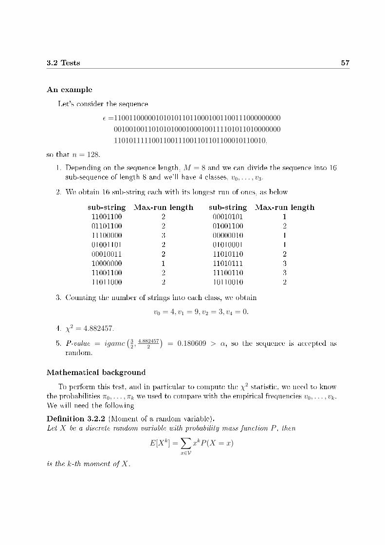
3.2 Tests 57
An example
Let's consider the sequence
ε =11001100000101010110110001001100111000000000
00100100110101010001000100111101011010000000
1101011111001100111001101101100010110010,
so that n = 128.
1. Depending on the sequence length, M = 8 and we can divide the sequence into 16sub-sequence of length 8 and we'll have 4 classes, v0, . . . , v3.
2. We obtain 16 sub-string each with its longest run of ones, as below
sub-string Max-run length sub-string Max-run length11001100 2 00010101 101101100 2 01001100 211100000 3 00000010 101001101 2 01010001 100010011 2 11010110 210000000 1 11010111 311001100 2 11100110 311011000 2 10110010 2
3. Counting the number of strings into each class, we obtain
v0 = 4, v1 = 9, v2 = 3, v4 = 0.
4. χ2 = 4.882457.
5. P-value = igamc(
32, 4.882457
2
)= 0.180609 > α, so the sequence is accepted as
random.
Mathematical background
To perform this test, and in particular to compute the χ2 statistic, we need to knowthe probabilities π0, . . . , πk we used to compare with the empirical frequencies v0, . . . , vk.We will need the following
Denition 3.2.2 (Moment of a random variable).Let X be a discrete random variable with probability mass function P , then
E[Xk] =∑x∈V
xkP (X = x)
is the k-th moment of X.

58 3. Statistical tests for randomness
Denition 3.2.3 (Factorial moment).Let r ∈ N, the r-th factorial moment of a probability distribution or, in other words, ofa random variable X with that probability distribution, is
µr[X] = E[(X)r] = E[X(X − 1)(X − 2) . . . (X − r + 1)]
where E is the mean and
(x)r = x(x− 1)(x− 2) . . . (x− r + 1) =x!
(x− r)!
is the falling factorial, expressed by the Pochammer symbol.
Denition 3.2.4 (Moment generating function).Let X be a discrete random variable with probability mass function p and support S, then
MX(t) = E[etX ] =∑s∈S
etxp(x)
is the moment generating function of X.
Denition 3.2.5 (Factorial moment generating function).Let t ∈ C and X be a real-valued random variable, the factorial moment generatingfunction of the probability distribution of X is
GX(t) = E[tX ].
If X is a discrete random variable, GX(t) is said to be the probability generating functionof X and it's indicated by G(t).
We shall also make some remarks on properties of the factorial moment, for the proofsof which we refer to [18].
Remark 3.2.2.Useful facts are:
i) A trivial observation is that the 1-st (factorial) moment is the expected value.
ii) MX(t) = GX(et).
iii) The moment generating function is related to the cumulative distribution functionby
MX(t) = FX(t) = P (X ≤ t) t ∈ R.
iv) Factorial moments and comulative distribution function are related by the formula
GX(t) = FX(t− 1) =∞∑s=0
ts
s!µ[s].

3.2 Tests 59
If X is a Binomial random variable of parameters n and p. it holds
Remark 3.2.3.
E[(X)r] = (n)rpr.
To model our situation we can think to an urn, containing n balls, r1 white andr2 = n− r1 black. We sequentially extract n balls to form a n-long binary string.
The total number of combination is(n
r1
)=
(n
r2
)=
(n
n− r1
).
We call T the total number of white runs and T0 the total number of white runs whichlength is equal or greater than m+ 1: obviously T ≥ T0. We make use of characteristicrandom variables ai, i = 1, . . . , T such that
ai =
1 if the length of the i-th is ≥ m+ 1
0 otherwise
with each ai attached to the corresponding i-th run. So the probability that any set ofruns j1, . . . , js (suppose that j1 ≤ · · · ≤ js ≤ T ) will be all of length (m+ 1) or more it'sequal to the probability that the product aj1aj2 . . . ajs = 1; for any of the other case theproduct will be 0.
Let's take into account s of T white runs; we remove from them s · m balls andwe impose that r1 − sm ≥ T , so that we'll have (r1 − sm) white balls and r2 blackballs which form T (white) runs. If now we add m balls to each of our s run, we obtainagain r1 +r2 balls which form T white runs where s of them are of length (m+1) or more.
By a simple combinatorial argument we obtain that all the possible arrangements tobe in this situation are (
n− 1
T − 1
)(r2 + 1
T
).
With the assumption that we have a total of T white runs we can compute theexpected value of having s runs which length is ≤ m+ 1, obtaining that
E[aj1 . . . ajs|T ] = E[aj1|T ] · · · · · E[ajs|T ] =
(r1 − sm− 1
T − 1
)/ (r1 − 1
T − 1
)(3.14)
where the rst identity comes from the fact that aji 's are independent (then the expectedvalue of the product is the product of expected values) and the second ones comes from

60 3. Statistical tests for randomness
a direct calculation.
By remark (3.2.3) we also obtain that the s-th factorial moment of T0, which is aBinomial random variable, is
E[(T0)s|T ] = (T )sE[aj1 . . . ajs|T ]. (3.15)
Using the Total Probability theorem and equation (3.14), to obtain the v-th factorialmoment we just have to multiply (3.15) by p(T ) and summing over all T, obtaining
µ[v] =∑T
p(T )E[(T0)v|T ] = (r2 + 1)v
(r − v(m+ 1)
r2
)/ (n
r2
)where (analyzing favorable cases and total cases)
p(T ) =
(r1 − 1
T − 1
)(r2 + 1
T
)/ (r1 + r2
r2
).
Finally, by remark (3.2.2) we obtain that the probability to have an m-run is
P (v ≤ m|r1) = P (T0 = 0) =∑t=0
(−1)tµ[t]
t!=
(n
r2
)−1∑t=0
(−1)t(r2 + 1
t
)(r − t(m+ 1)
r2
).
Turning back to our case, and using the notation of the test, we can use this result toobtain (by the Total Probability theorem)
P (v ≤ m) =M∑r=0
(M
r
)P (v ≤ m|r) 1
2M.
So, now, we can evaluate probabilities π0, . . . , πk of our chosen classes and pre-compute them to embed in the test.
Example 3.2.3.If we divide the sequence into 8-bit block (i.e. M = 8) the theoretical probabilities willbe
Class Probabilityv ≤ 1 π0 = 0.2148v = 2 π1 = 0.3672v = 3 π2 = 0.2305v ≥ 4 π3 = 0.1875
It's important to observe that average cases have bigger probabilities than extreme ones,and the phenomenon is even more observable for biggerM (for example ifM = 104 we'llhave π0 = 0.0882, π2 = 0.2483 and π6 = 0.0727): that is the behaviour one expects froma random sequence.

3.2 Tests 61
3.2.5 Binary matrix rank test
This test analyzes the rank of disjoint matrices created from xed-length sub-stringsof the binary sequence. The purpose is to check whereas this rank is consistent fromwhat expected from a random sequence, i. e. from truly random binary matrices. Sincethe rank corresponds to independence of both rows and columns, this examination leadsto examine linear dependencies through bits of each sub-sequence.
As well as in the NIST statistical test suite, the binary matrix rank test is also partof the DIEHARD battery of test [43], and actually comes from it.
Remark 3.2.4.For this test, we need one more parameterQ, so that the length of sub-blocks will beM ·Q;since the theory of the test, analogously to others, is based on asymptotic properties, Mand Q has to be chosen such that n ≥ 38MQ so that at least 38 matrices are considered.Since if M 6= Q we certainly have |M − Q| dependent vector, our implementation willhave M = Q = 32, so that square matrices are created.
Algorithmic description
1. Partitioning the sequence intoM ·Q-bit sub-sequences we obtain N =⌊
nMQ
⌋blocks
and discard the surplus.From each block ε11, . . . , ε1Q, . . . , εM1, . . . , εMQ form an M × Q matrix, where thei-th row is given by εi1, . . . , εiQ, for i = 1, . . . ,M , i.e. the rst row of each matrixconsists of the rst Q bits of the block, the second row is formed by bits fromQ + 1 to 2Q, and so on till the last row, which consists of the last Q bits of thesub-sequence.
2. For each matrix compute the binary rank Rk, where k = 1, . . . , N . For binary rankwe mean the rank over the nite eld F2.
3. Consider the following 3 classes
• FM = matrices which rank is maximum, i.e. Rl = M
• FM−1 = matrices which rank is maximum −1, i.e. Rl = M − 1
• FM−2 = other matrices
and evaluate the cardinality of each set (for simplicity we'll name these cardinalitiesby the name of the set, so that FM will be the number of matrices of full rank).Observe that FM−2 = N − FM−1 − FM−1.

62 3. Statistical tests for randomness
4. Compute the χ2 statistic as
χ2(obs) =(FM − 0.2888N)2
0.2888N+
(FM−1 − 0.5776N)2
0.5776N+
(FM−3 − 0.1336N)2
0.1336N
5. Compute the P-value = e−χ2(obs)/2.
Interpretation of results
Small P-values will occur when the value of the χ2 statistic is low: this correspondsto deviations from distribution of rank of a truly random sequence. In particular, smallvalues of FM and FM−1 would indicate strong linear dependencies through the sequence.For example, if a binary sequence is created by a shift-register generator formed by lessthan M successive vectors, all created matrices will always have maximum rank while,for truly random data, the proportion of maximum rank should be only about 0.2888.
An example
Let's consider the sequence ε = 01011001001010101101, so that n = 20, and wechoose M = Q = 3.
1. We divide the sequence into N = b 203·3c 9-bit blocs and discard the last two bits (0
and 1).Using the 9-bit created blocks we construct the following 3× 3 two matrices:0 1 0
1 1 00 1 0
0 1 01 0 10 1 1
2. Ranks of the two matrices are R1 = 2 and R2 = 3.
3. We have FM = F3 = 1, since only the second matrix has full rank, FM−1 = F2 = 1(the rst matrix has rank=2), and F3 = 0 since there isn't any matrix with lowerrank.
4. χ2(obs) = (1−0.2888N)2
0.2888N+ (1−0.5776N)2
0.5776N+ (0−0.1336N)2
0.1336N= 0.596953.
5. P-value = e−0.596953/2 = 0.741948 > α so that the sequence is accepted as random.
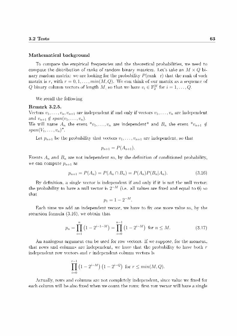
3.2 Tests 63
Mathematical background
To compare the empirical frequencies and the theoretical probabilities, we need tocompute the distribution of ranks of random binary matrices. Let's take an M × Q bi-nary random matrix: we are looking for the probability P (rank=r) that the rank of suchmatrix is r, with r = 0, 1, . . . ,min(M,Q). We can think of our matrix as a sequence ofQ binary column vectors of length M , so that we have vi ∈ FM2 for i = 1, . . . , Q.
We recall the following
Remark 3.2.5.Vectors v1, . . . , vn, vn+1 are independent if and only if vectors v1, . . . , vn are independentand vn+1 /∈ span(v1, . . . , vn).We will name An the event "v1, . . . , vn are independent" and Bn the event "vn+1 /∈span(V1, . . . , vn)".
Let pn+1 be the probability that vectors v1, . . . , vn+1 are independent, so that
pn+1 = P (An+1).
Events An and Bn are not independent so, by the denition of conditioned probability,we can compute pn+1 as
pn+1 = P (An) = P (An ∩Bn) = P (An)P (Bn|An). (3.16)
By denition, a single vector is independent if and only if it is not the null vector:the probability to have a null vector is 2−M (i.e. all values are xed and equal to 0) sothat
p1 = 1− 2−M .
Each time we add an independent vector, we have to x one more value so, by therecursion formula (3.16), we obtain that
pn =n∏i=1
(1− 2i−1−M) =
n−1∏i=0
(1− 2i−M
)for n ≤M . (3.17)
An analogous argument can be used for row vectors. If we suppose, for the moment,that rows and columns are independent, we have that the probability to have both rindependent row vectors and r independent column vectors is
r−1∏i=0
(1− 2i−M
) (1− 2i−Q
)for r ≤ min(M,Q).
Actually, rows and columns are not completely independent, since value we xed foreach column will be also xed when we count the rows: rst row vector will have a single

64 3. Statistical tests for randomness
xed value, second row vector will have 2 xed values and so on till the desired rank r,so our probability becomes
r−1∏i=0
(1− 2i−M
) (1− 2i−Q
)(1− 2i−r)
for r ≤ min(M,Q).
Now, we have xed the min(M,Q) ·min(M,Q) values that concur to the rank of thematrix, but we also have to consider that values outside this sub-matrix remain free tobe either 0 or 1.
Example 3.2.4.Let's suppose that M < Q, and let's look for the maximum rank of the matrix, sor = min(M,Q) = M : by the argument above we'll have that values of the M × Msub-matrix (which values are indicated by aij for i, j = 1, . . . , r = M) and other are free(indicated by *), as follows a11 . . . a1r ∗ ∗ ∗
.... . .
... ∗ . . . ∗aM1 . . . aMr ∗ ∗ ∗
By direct computation one can see that these values are r(Q+M − r)−MQ, so that
the probability to have a random matrix which rank is r is
P (rank=r) = 2r(Q+M−r)−MQ
r−1∏i=0
(1− 2i−M
) (1− 2i−Q
)(1− 2i−r)
for r ≤ min(M,Q). (3.18)
Note that if r = max (i.e. r = min(M,Q)), than r(Q + M − r) −MQ = 0 so thatthe multiplicative factor is 1: extra values are free to be 0 or 1. On the other hand, ifr = 0 we have that r(Q + M − r) −MQ = −MQ and all extra values are xed (themultiplicative factor is 2−MQ.
By the use of formula (3.18) we can compute probabilities to compare with theempirical frequencies: we have M = Q = 32 so, by approximation, we obtain that
pM ≈∞∏j=1
(1− 1
2j
)= 0.2888 . . . ,
pM−1 ≈ 2pM ≈ 0.5776 . . . ,
pM−2 ≈4
9pM ≈ 0.1284 . . .
and all other probabilities are very small (≤ 0.005) if M ≥ 10, so that it wouldn't beuseful to include smaller classes for the statistic.
Finally, we can compute the χ2 statistic and nd the P-value.

3.2 Tests 65
Remark 3.2.6.For this test the P-value is computed by the use of the exponential since, if the number ofclasses (i.e. the number of degrees of freedom) is low, it provides a good approximation of(3.6) and the value is very close to the customary incomplete gamma function which, inthis case, would be igamc (1, χ2(obs)/2). On the other hand, the use of the exponentialis easier and computationally less expensive.
3.2.6 Discrete Fourier transform (Spectral) test
The scope of this test is to detect periodic features through the sequence which wouldindicate deviation from randomness. For periodic features we mean repetitive patternsthat are near each other. To do that we use the discrete Fourier transform (DFT) of thesequence and analyze the pattern of frequencies: we x a bound of 95% on peaks valuesand, to be random, we require that the number of all peaks exceeding this bound isn'tsignicantly dierent from 5%.
For this test we will need the following
Denition 3.2.6 (Discrete Fourier transform).Let x1, . . . , xn be a succession of complex numbers. The discrete Fourier transform (DFT)of the succession is the succession S1, . . . , Sn such that
Sj =n∑k=1
xkei2π
(k−1)n
j (3.19)
=n∑k=1
xkcos(2π(k − 1)
nj) + i
n∑k=1
xksin(2π(k − 1)
nj) (3.20)
where i =√−1 is the imaginary unit.
Algorithmic description
1. Convert the binary sequence ε into a corresponding ±1 sequence X: this can beeciently done by X = 2ε− 1.
2. Apply a discrete Fourier transform to X, obtaining S = DFT (X).S is a sequence of complex variables which represent periodic components of thebinary sequence at dierent frequencies.
3. Let S ′ be the rst half of the obtained sequence S, so that S ′ is a n2-length sequence
of values +1 and -1.Compute the modulus M = abs(S ′) = |S ′| to obtain a sequence of peak heights,as shown in gure 3.4.

66 3. Statistical tests for randomness
4. Compute T =√ln(
10.05
)n the bound of 95% on peaks value.
5. Compute N0 = 0.95 · n2, the expected number of peaks which are less than T.
6. Compute N1, the empirical number of peaks in M which are lass than T.
7. Compute d = N1−N0√n·0.95·0.05/4
.
8. Compute P-value=erfc(|d|√
2
).
Interpretation of results
A small P-value will occur when d is low: that would indicate that there are too manypeaks (i.e. more than 5% of values are above the the bound T ) and, correspondingly, thatthere are not enough values under the bound. This happens when the sequence showstoo many periodic features, compared from what expected from a random sequence.
An example
Let's consider the sequence ε = 1001010011, so that n = 10.
1. X = 1,−1,−1, 1,−1, 1,−1,−1, 1, 1.
2. S = DFT (X) = 0, 1.618+1.175i, 1.382+4.253i,−0.618+1.902i, 3.618−2.628i,−2,3.618 + 2.628i,−0.618− 1.902i, 1.382− 4.253i1.618− 1.175i.
3. M = 0, 2, 4.4721, 2, 4.4721.
4. T = 5.4733.
5. N0 = 4.75.
6. N1 = 5.
7. d = 5−4.75√10·0.95·0.05/4
= 0.725476.
8. P-value=erfc(0.7254/√
2) = 0.468159 > α, so the sequence is accepted as random.

3.2 Tests 67
Mathematical background
To perform this test we need to know what is the distribution of peaks which repre-sents the distribution of the random variable N1 and respectively N0 which representsthe number of peaks not exceeding the 95% threshold in the rst part of the Fouriertransform of the sequence. Note that we only need a half of it, since the discrete Fouriertransform is symmetric.
Let n′ be the length of the rst half sequence (n′ = n2), we can think of N1 as the
sum of n′ random variables which take on the value 1 with probability p = 0.95 and thevalue 0 with probability q = 1 − p = 0.05. Indeed if Yj are random variables such thatYj = 1 if |Sj| < T and |Yj| = 0 otherwise, Yj = 1 with probability p, and Yj = 0 withprobability q, so that the Yjs are Bernoulli random variables: then we can write
N1 =n′∑j=1
Yj.
Since it is the sum of n′ Bernoulli random variable, we can easily compute its expectedvalue as
E[N1] =n′∑i=1
E[Yi] = n′E[Yi] = n′p =n
2p
so that the mean is µ = 0.95 · n2.
We could easily compute the variance in the same way, so that
V ar(N1) =n′∑i=1
V ar(Xi) = nV ar(Xi) = n′pq.
However Kim, Umeno and Hasegawa [36], through numerical simulation found that,even if the expected value found below is a good approximation, the variance tends tobe
σ2 =n′pq
2=npq
4so that the variance we should use to perform the complementary error function isσ2 = n·0.95·0.05
4.
Let's see, now, how to nd the threshold value T so that the number of peaks ex-ceeding it is the 5% of the total: let's write the square modulus of Sj as
|Sj|2 = c2j + s2
j
as (3.20). Under assumption of randomness of xk (which is +1 or -1 for k = 1, . . . , n)we have that cj and sj converge to a normal distribution whit mean zero and variance

68 3. Statistical tests for randomness
σ2 = n/2, so that Y = (cjσ
)2 + (sjσ
)2 converges to a χ2 distribution with 2 degrees offreedom, since it's the sum of 2 independent standard normal random variable, so that
P (Y ) =1
2exp(−Y
2).
If we set Z = Y2, we obtain the distribution
P (Z) = exp(−Z).
We want that the number of peaks above the threshold T is the 5% of the total so,if ZC is the upper bound of the random variable Z, we have
0.05 =
∫ ∞ZC
exp(−Z)dZ = exp(−ZC)
so that ZC = −ln(0.05) = 2.995732274.
By (3.20), we also have that |Sj| =√nZ so, using the bound ZC , we nd that the
threshold isT =
√nZC =
√2.995732274n.
We set the bound T and we found values of the theoretical values of mean andvariance, so we can nd the P-value by the complementary error function using formula(3.9):
P-value = erfc
(|d|√
2
)where d = (N1 −N2)/
√n · 0.95 · 0.05/4.
Figure 3.4 shows the dierence between frequencies of a 4096-bit generated from agood random number generator and the ones from a generator that produces periodicpatterns.
3.2.7 Non-overlapping template matching test
Under assumption of randomness, if we choose a pattern, it has to have the sameprobability of any other pattern of the same length: this is the focus of this test andof the subsequent Overlapping template matching test. This test counts the number ofoccurrences of an aperiodic string and evaluate if that specic pattern occurs more or lessthan expected from a truly random sequence. The test analyzes m bits of the sequence(where m is the length of the chosen pattern): if the pattern is found it slides to thenext m bits, otherwise it slides by only one bit. This is done partitioning the sequenceinto N sub-blocks of length M and the P-value is obtained by the χ2 statistic.
We give the following

3.2 Tests 69
Figure 3.4: While very few magnitudes of the rst sequence exceed the threshold value of95%, represented by the horizontal line, more than 5% do in the second sequence. In thesecond plot a structure of magnitudes is also observable, while we can't see somethinglike that on the rst one. P-values of the rst and the second sequence are, respectively,0.8077 and 0.0001. Credits to [64].

70 3. Statistical tests for randomness
Denition 3.2.7 (Aperiodic patter).We say that a pattern B = ε01, . . . , ε
0m is aperiodic if it doesn't exist a pattern C, shorter
than B, such that B=CC . . . CC ′, where C ′ is a prex of C.
Algorithmic description
First of all we choose an aperiodic template B and let m be its length.
1. The sequence is partitioned into N blocks of length M (possible surplus will bediscarded).
2. For each block count the number Wj of occurrences of B inside the j-th block forj = 1, . . . , N , as follows:
• Compare the rst m bits of the block with B;
• if they're not equal, slide of 1 bit and analyze bits from second to (m+1)-th2;
• if they match, slide of m bits and analyze bits from (m+ 1)-th to 2m-th.
3. Compute theoretical mean µ and variance σ2 as
µ =N −m+ 1
2mσ2 = M
(1
2− 2m− 1
22m
).
4. Compute the observed χ2-statistic as
χ2(obs) =N∑j=1
(Wj − µ)2
σ2.
5. Compute P-value using the incomplete gamma function:
P-value = igamc
(N
2,χ2(obs)
2
).
Remark 3.2.7.Chosen m, this test can be performed for each aperiodic template of length m: forexample if m=2 the only non-periodic templates are 01 and 10, if m = 3 we have 001,011, 100 and 110, but if we choosem = 9 orm = 10 we can perform the test, respectively,for 148 and 284 templates. Note that, each template provides a dierent P-value.
2For eciency purpose is important to compare only one bit at a time, instead of the whole m-bitsblock, so that if the rst bit doesn't match the comparison can straightaway proceed to the following mbits.

3.2 Tests 71
Interpretation of results
A small P-value (i.e. a rejection) is obtained when occurrences of the chosen tem-plate through the sequence are irregular, in particular if there are too many or too fewoccurrences, or if occurrences are located into restricted areas of the sequence.
An example
Let ε = 10100100101110010110, so that n = 20. We take N = 2 and M = 10 andinspect the sequence for the template B = 001 (so m = 3).
1. Partitioning the sequence we obtain the two 10-bits blocks
1010010010, 1110010110.
2. Count occurrences of 001 through blocks; for the rst block we nd the rst oc-currence of B on bits 4-6, and the second one on bits 7-9: note that, as by thealgorithm, bits from 5-7 and 6-8 are not examined, since we slide to bits 7-9 afterthe rst match.We nd W1 = 2 and W2 = 1 (there is only a single occurrence on bits 4-6 in thesecond block).
3. Theoretical mean and variance for m and M of this example are µ = (10 − 3 +1)/23 = 1 and σ2 = 10 ·
(123− 2·3−1
22·3
)= 0.46875.
4. χ2(obs) = (2−1)2+(1−1)2
0.46875= 1+0
0.46875= 2.133333.
5. P-value = igamc(
22, 2.133333
2
)= 0.344154 > α so the sequence is accepted as ran-
dom.
Mathematical background
To perform this test we need to know the theoretical distribution of non-periodicpatterns inside the sequence or simply their mean and variance in order to compute theχ2-distribution.We a-priori choose an aperiodic template B = ε01, . . . , ε
0m as in (3.2.7) of length m.
Example 3.2.5.For m = 4 we have 6 aperiodic patterns: 0001, 0011, 0111, 1000, 1100, 1110.For m = 5 they're 12:00001, 00011, 00101, 01011, 00111, 01111, 11100, 11010, 10100, 1100, 10000, 11110.
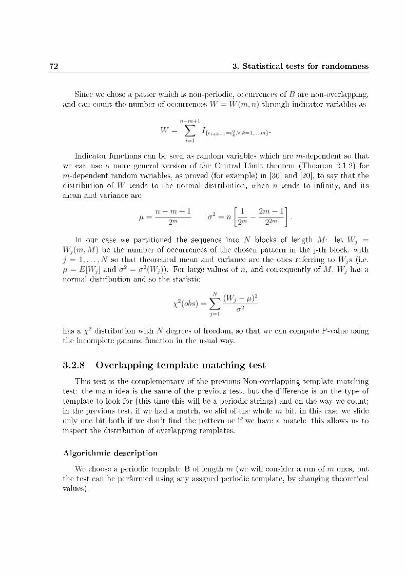
72 3. Statistical tests for randomness
Since we chose a patter which is non-periodic, occurrences of B are non-overlapping,and can count the number of occurrences W = W (m,n) through indicator variables as
W =n−m+1∑i=1
Iεi+k−1=ε0k,∀ k=1,...,m.
Indicator functions can be seen as random variables which are m-dependent so thatwe can use a more general version of the Central Limit theorem (Theorem 2.1.2) form-dependent random variables, as proved (for example) in [30] and [20], to say that thedistribution of W tends to the normal distribution, when n tends to innity, and itsmean and variance are
µ =n−m+ 1
2mσ2 = n
[1
2m− 2m− 1
22m
].
In our case we partitioned the sequence into N blocks of length M : let Wj =Wj(m,M) be the number of occurrences of the chosen pattern in the j-th block, withj = 1, . . . , N so that theoretical mean and variance are the ones referring to Wjs (i.e.µ = E[Wj] and σ
2 = σ2(Wj)). For large values of n, and consequently of M , Wj has anormal distribution and so the statistic
χ2(obs) =N∑j=1
(Wj − µ)2
σ2
has a χ2 distribution with N degrees of freedom, so that we can compute P-value usingthe incomplete gamma function in the usual way.
3.2.8 Overlapping template matching test
This test is the complementary of the previous Non-overlapping template matchingtest: the main idea is the same of the previous test, but the dierence is on the type oftemplate to look for (this time this will be a periodic strings) and on the way we count;in the previous test, if we had a match, we slid of the whole m bit, in this case we slideonly one bit both if we don't nd the pattern or if we have a match: this allows us toinspect the distribution of overlapping templates.
Algorithmic description
We choose a periodic template B of length m (we will consider a run of m ones, butthe test can be performed using any assgned periodic template, by changing theoreticalvalues).

3.2 Tests 73
1. Partition the sequence into N = b nMc blocks of length M (and discard the possible
surplus).
2. For each block count the number of overlapping occurrences of B inside the j-thblock, for j = 1, . . . , N : the window slides each time of 1 bit, i.e. if we're analyzingbits fro k-th to (k +m)-th we'll next analyze bits from k + 1 to k + 1 +m both ifpatterns match or not.To record the number of occurrences in each block, we use classes ν0, . . . , ν5: eachblock, after the check, if we didn't nd occurrences of the template B we incrementν0 by one, if we found 1 occurrence we increment ν1 and so on; ν5 is incrementedif occurrence of B are 5 or more.
3. Compute values of λ and η:
λ =M −m+ 1
2mη =
λ
2.
This values are used to compute theoretical probabilities π0, . . . , π5, which corre-sponds to ν0, . . . , ν5 (if M and m are xed, one can pre-compute these values, aswe did in our implementation).
4. Compute the statistic
χ2(obs) =5∑i=0
(νi −Nπi)2
Nπi
where, if m = 9 and M = 1032 as recommended by NIST, π0 = 0.364091,π1 = 0.185659, π2 = 0.139381, π3 = 0.100571, π4 = 0.0704323 and π5 = 0.139865.Obviously, probabilities for dierent m and M can be computed anyway, as ex-plained in the mathematical background section of this test.
5. Compute P-value using the incomplete gamma function:
P-value = igamc
(5
2,χ2(obs)
2
).
Interpretation of results
A small P-value occurs when the number of periodic occurrences is far from thetheoretical number of them, under randomness hypothesis: in particular this correspondto large values of ν0 or ν5 and, consequently on large values of the statistic.

74 3. Statistical tests for randomness
An example
We test the sequence ε = 10111011110110110100011100101110111110000101101001(so that n = 50) for the template B = 11 (then m = 2), and x M = 10 and N = 5.
1. The partition produces blocks 1011101111, 0110110100, 0111001011, 1011111000,and 0101101001.
2. We count the number of overlapping occurrence of B through blocks. For the rstblock the algorithm will count as follows
Position (bit) Bits Match of B1 - 2 102 - 3 013 - 4 11 X4 - 5 11 X5 - 6 106 - 7 017 - 8 11 X8 - 9 11 X9 - 10 11 X
For the rst block the sequence has ve occurrences of B = 11, then we incrementν5 by one, while ν0 = ν1 = ν2 = ν3 = ν4 = 0.Similarly, block 2 has 2 occurrences of 11, so that ν2 = ν2 + 1 = 1; we have 3occurrences in block 3, so that ν3 is incremented; there are 4 occurrences in block4 and one occurrence in block 5, so that after the examination of all blocks we'llhave ν0 = 0, ν1 = 1, ν2 = 1, ν3 = 1, ν4 = 1, ν5 = 1.
3. λ = (10− 2 + 1)/22 = 2.25 and η = λ/2 = 1.125.
4. Using λ and η we compute the theoretical probabilities which, in this example,will be dierent from the ones in the algorithm section since we have dierent Mand m: we nd π0 = 0.324652, π1 = 0.182617, π2 = 0.142670, π3 = 0.106645, π4 =0.077147 and π5 = 0.166269 (see the Mathematical background section for formulasto compute probabilities).
χ2(obs) =(0− 5 · 0.324652)2
−5 · 0.324652+
1− 5 · 0.182617)2
5 · 0.182617+
(1− 5 · 0.142670)2
5 · 0.142670
+(1− 5 · 0.106645)2
5 · 0.106645+
(1− 5 · 0.077147)2
5 · 0.077147+
(1− 5 · 0.166269)2
5 · 0.166269= 3.167729

3.2 Tests 75
5. P-value = igamc(
52, 3.167729
2
)= 0.274932 > α = 0.01 and we conclude that the
sequence is random.
Mathematical background
The test is based on the distribution of the number of runs of ones which length ism, that can also overlap. Let Wj = Wj(m,n) be the number of those runs in the j-thblock. The key of this test is the computation of the asymptotic distribution ofWj, fromwhich we can evaluate probabilities πi, i = 0, . . . , 5. As proved, in the specic case ofbinary sequences, by Földes in [23] and, in the more general case of sequences createdby any nite alphabet, by Chrysaphinou and Papastravridis in [16], Wjs converges to acompound Poisson distribution, in particular to the so called Pólya-Aeppli distributionwhen (M − m + 1)2−m → λ > 0. The general Pólya-Aeppli distribution models theidea that counted objects occur in clusters, where the number of objects has a Poissondistribution (of parameter θ) and the number of objects per cluster has a geometric dis-tribution of parameter p.
In the following it will be useful this
Denition 3.2.8 (Conuent hypergeometric function).For x ∈ R and a, b ∈ Z the conuent hypergeometric function (also called Kummer'sfunction3) is
1F1[a; c;x] = 1 +a
c1!x+
a(a+ 1)
c(c+ 1)2!x2 + . . .
=∞∑j=0
(a)jxj
(c)jj!
where (a)j = a(a+1) . . . (a+j−1) is the Pochammer's symbol for the ascending factorial.
Remark 3.2.8.The Pólya-Aeppli distribution can be seen in two, equivalent, ways using the Poissondistribution and the geometric distribution, so that if X has a Pólya-Aeppli distributionthen
X ∼ Poisson(θ)∨
Shifted geometric(p) (3.21)
but also, using a non-shifted geometric distribution as
X ∼ Poisson
(θ
p
)∨Geometric(p). (3.22)
3Kummer introduced this function in 1837 as a solution to a dierential equation, called the Kum-mer's dierential equation.
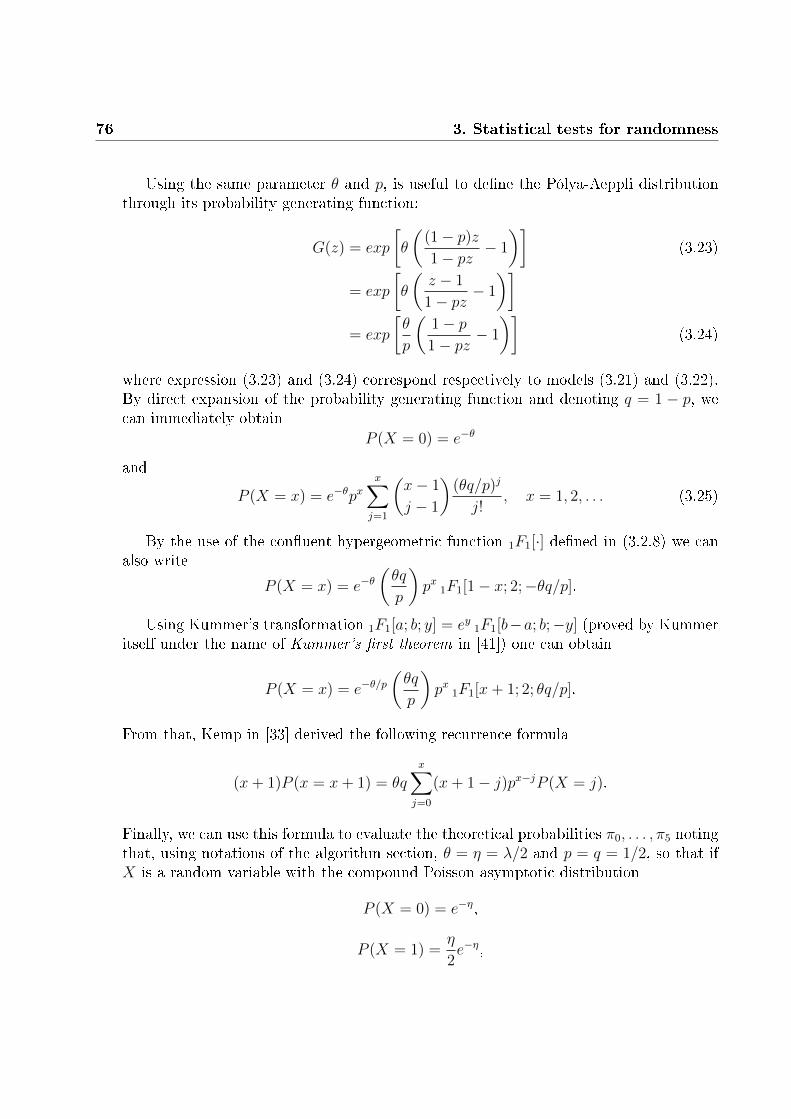
76 3. Statistical tests for randomness
Using the same parameter θ and p, is useful to dene the Pólya-Aeppli distributionthrough its probability generating function:
G(z) = exp
[θ
((1− p)z1− pz
− 1
)](3.23)
= exp
[θ
(z − 1
1− pz− 1
)]= exp
[θ
p
(1− p1− pz
− 1
)](3.24)
where expression (3.23) and (3.24) correspond respectively to models (3.21) and (3.22).By direct expansion of the probability generating function and denoting q = 1 − p, wecan immediately obtain
P (X = 0) = e−θ
and
P (X = x) = e−θpxx∑j=1
(x− 1
j − 1
)(θq/p)j
j!, x = 1, 2, . . . (3.25)
By the use of the conuent hypergeometric function 1F1[·] dened in (3.2.8) we canalso write
P (X = x) = e−θ(θq
p
)px 1F1[1− x; 2;−θq/p].
Using Kummer's transformation 1F1[a; b; y] = ey 1F1[b−a; b;−y] (proved by Kummeritself under the name of Kummer's rst theorem in [41]) one can obtain
P (X = x) = e−θ/p(θq
p
)px 1F1[x+ 1; 2; θq/p].
From that, Kemp in [33] derived the following recurrence formula
(x+ 1)P (x = x+ 1) = θqx∑j=0
(x+ 1− j)px−jP (X = j).
Finally, we can use this formula to evaluate the theoretical probabilities π0, . . . , π5 notingthat, using notations of the algorithm section, θ = η = λ/2 and p = q = 1/2, so that ifX is a random variable with the compound Poisson asymptotic distribution
P (X = 0) = e−η,
P (X = 1) =η
2e−η,

3.2 Tests 77
P (X = 2) =ηe−η
8(η + 2),
P (X = 3) =ηe−η
8
(η2
6+ η + 1
),
P (X = 4) =ηe−η
8
(η3
24+η2
2+
3η
2+ 1
).
We can use above formulas to compute the probabilities π0, . . . π4 and, to evaluatethe probability to have more than four overlapping runs in the block, we can complementthe distribution function obtained in (3.25), obtaining that
P (X > x) = e−ηx∑j=1
ηj
j!∆(j, x)
where
∆(j, x) =x∑k=j
1
2k
(k − 1
j − 1
).
We can nally compute P (X ≥ 5) as
P (X ≥ 5) = P (X = 5) + P (X > 5).
Chosen K + 1 classes X = 0, X = 1, . . . , X = K − 1, X ≥ K , representingthe number of overlapping runs inside blocks, one can compute respective theoreticalprobabilities π0, π1, . . . , πK−1, πK , using above formulas, and compute the value of theχ2-statistic as
χ2(obs) =K∑i=0
(νi −Nπi)2
Nπi
where N is the number of block; after that we can compute the P-value using the in-complete gamma function, as usual.
Supposing to test sequences on the order of 106 bits, we implemented the test forK = 5,m = 9 and M = 1032, as NIST did, so that theoretical probabilities derived byabove formulas are
π0 0.367879π1 0.183939π2 0.137954π3 0.099634π4 0.069935π5 0.140656
.

78 3. Statistical tests for randomness
Values in the above table are the ones NIST inserted in the most recent version oftheir Overlapping template matching test, however Hamano and Kaneko, in [29], provedthat these values are inaccurate since, setting the level of signicance to 1%, the testproduce a rejection rate of 98.8%, instead of the expected 99%.They recomputed probabilities πi, i = 0, . . . , 5 by founding a set of recursive formulas tocompute the number Ti(n) of n-bit sequence with i occurrences of the template B (anm-bit run of ones), so that
πi =
Ti(n)
2nfori = 0, . . . , 4
1−∑4
j=0 πj fori = 5.
By the use of these formulas they computed values of the table below and, testing4 · 104 sequences of length 106 taken from DES (used as a PRNG), showed that valuesproposed by NIST lead to a distribution of rejection rate which is far from the theoreticalone (while, on the other hand, new values ts almost perfectly).
π0 0.364091π1 0.185659π2 0.139381π3 0.100571π4 0.0704323π5 0.166269
.
NIST itself acknowledged that Hamano and Kaneko's values are more correct, but leftthe old ones in the implementation of the test suite. We decided to implement the testusing both values: the rst ones to check the implementation and compare our resultswith NIST's and the second to have a more reliable test for practical purposes.
3.2.9 Maurer's universal statistical test
As we said in section (2.2.2), a truly random sequence has high values of entropy and,for that reason, it couldn't be signicantly compressed (i.e. compressed without losinginformation, contained in the sequence) by any algorithm of compression. Since 2008 atest based on a Lempel-Ziv compressor (an algorithm for data compression proposed byZiv and Lempel in [71]) was included in the NIST statistical test suite, but then it wasremoved due to low eciency, problems on implementation and, primarily, dicult ondening a statistic which can be determined and approximated. However the idea be-hind Maurer's universal statistical test is almost the same: it doesn't try to compress thesequence, as the Lempel-Ziv test proposed in [73] did, but analyzes the per-bit entropy ofthe sequence, which is strictly connected with compressibility. To achieve that, the testexamines the distance (i.e. the number of bit) between matching patterns, since if there

3.2 Tests 79
are a lot of same pattern which are suciently close one-another, one can substitute thepattern with a shorter one and compress the sequence: that is the connection betweendistances and compression.
Maurer, in [50], states that the per-bit entropy is "the correct quality measure for asecret-key source in a cryptographic application" since it's "related to the running timeof enemy's optimal key-search strategy" or to the eective key size of a cipher system.The author also report that, even if this test doesn't detect some specic defection ofthe sequence, it is "able to detect any one of the very general class of statistical defectsthat can be modeled by an ergodic stationary source with nite memory", so that thistest should contain a wide number of standard statistical tests. We recall that, for thistest, we will forget usual notations to conform to the ones Maurer used in the originalpaper, so that the length of block will be L, and the number of blocks will be Q+K.
Algorithmic description
The length of block L and the number of testing blocks Q is chosen depending onthe sequence length, as in the following table:
n L Q = 10 · 2L≥ 387840 6 640≥ 304960 7 1280≥ 2068480 8 2560≥ 4654080 9 5120≥ 10342400 10 10240≥ 22753280 11 20480≥ 49643520 12 40960≥ 107560960 13 81920≥ 231669760 14 163840≥ 496435200 15 327680≥ 1059061760 16 655360
After that, K is set as K = bn/Lc −Q.
The test could be performed for all L, but choosing L ≥ 6 would allow to have everyL-bit pattern into the initialization segment and taking L > 16 would make the test tooslow, since the initialization takes time exponential in L.
1. The sequence is split into two parts: rst Q · L-bits will form the initializationsegment, and the following K · L-bits will form the test segment: any extra bitsare discarded.

80 3. Statistical tests for randomness
Figure 3.5: Partition of the sequence into Q+K block of length L. Credits to [64].
2. Create a table containing each possible L-bit pattern and store the index of thelast occurrence of each of these templates inside the initialization segment: in thefollowing we will call Tj the index of the j-th template of the table. For example ifthe template a appears in s-th block and in t-th block, with s < t, store t as indexof the template a.
3. Scan blocks of the testing sequence: if a block appears into the table, computethe log2 distance between the index of the block and the index of the previousappearance of the template: i.e. if the i-th block matches the j-th template,compute log2(i − Tj). Replace the index Tj into the table with the last index ofthe template i. For each step sum all the distances together into a variable sum(i.e. each step sum = sum+ log2(i− Tj)).
4. Compute the statistic
fn =1
K
Q+K∑i=Q+1
log2(i− Tj) =sum
K.
5. Compute theoretical expected value and standard deviation σ. Expected value andvariance depends only on L so that we can pre-compute them:
L expectedValue variance6 5.2177052 2.9547 6.1962507 3.1258 7.1836656 3.2389 8.1764248 3.31110 9.1723243 3.35611 10.170032 3.384
L expectedValue variance12 11.168765 3.40113 12.168070 3.41014 13.167693 3.41615 14.167488 3.41916 15.167379 3.421

3.2 Tests 81
The theoretical standard deviation is given from
σ = c(L,K)
√variance(L)
K, with c(L,K) = 0.7− 0.8
L+
(4 +
32
L
)K3/L
15.
Compute P-value using the complementary error function:
P-value = erfc
(∣∣∣∣fn − expectedV alue(L)√2σ
∣∣∣∣) .
Remark 3.2.9.In order to make the storing and the computation of step 2 and 3 more ecient, patternsare considered using the decimal value represented (on base 2) by the template itself.For example, if L = 4, the pattern "0010" is stored into the second entry of the storingtable and the pattern "0111" is stored into the 7-th entry. "0000" can be stored intothe last entry of the table or into the rst one: in the second case everything has to beshifted by one.
Interpretation of results
A small P-value (i.e. a rejection of the sequence) occurs when the statistic of distancesfn diers signicantly from the expectedV alue(L): that would indicate that the sequencecan be signicantly compressed, i.e. is not random.
An example
Let ε = 01011010011101010111, then n = 20. Let's take L = 2 and Q = 4 so thatK = bn/Lc −Q = b20/2c − 4 = 6.
1. The sequence is split into an initialization segment 01011010 and a test segment011101010111. No bits are discarded, since Q · L+K · L = 20 = |ε|. L-bit createdblocks are shown in the following tables:
Initialization segmentBlock index Content
1 012 013 104 10
Test segmentBlock index Content
5 016 117 018 019 0110 11

82 3. Statistical tests for randomness
2. Table with L-bit templates and respective index (into the initialization segment)is created:
Template 00 01 10 11Last index 0 2 4 0
3. The sum of distances proceeds as follows:
Block 5: block 5 reports the template ′01′, which last index is 2, so that sum = log2(5−2) = 1.584962501.
Block 6: block 6 reports the template ′11′, which last index is 0, so that sum = sum+log2(6− 0) = 1.584962501 + 2.584962501 = 4.169925002.
Block 7: block 7 reports the template ′01′, which last index is 5, so that sum = sum+log2(7− 5) = 4.169925002 + 1 = 5.169925002.
Block 8: block 8 reports the template ′01′, which last index is 7, so that sum = sum+log2(8− 7) = 5.169925002 + 0 = 5.169925002.
Block 9: block 9 reports the template ′01′, which last index is 8, so that sum = sum+log2(9− 7) = 5.169925002 + 0 = 5.169925002.
Block 10: block 10 reports the template ′11′, which last index is 6, so that sum =sum+ log2(10− 6) = 5.169925002 + 2 = 7.169925002.
During the sum, the table of indexes is updated ad follows:
Iteration L-bit valueblock 00 01 10 114 0 2 4 05 0 5 4 06 0 5 4 67 0 7 4 68 0 8 4 69 0 9 4 610 0 9 4 10
4. The test statistic fn = 7.1699250026
= 1.1949875.
5. For L = 2 expected value and variance can be computed: expectedV alue =
1.5374383 and σ2 = 1.338, then P-value = erfc(∣∣∣1.19498755−1.5374383√
2√
1.338
∣∣∣) = 0.767189 >
α and the sequence is accepted as random.

3.2 Tests 83
Mathematical background
As we have seen in section (3.1.2), in order to perform the complementary errorfunction erfc, we need to know the theoretical distribution of the statistic fn, when datais truly random (i.e. we need to know its mean and variance).Let sN = s1, . . . , sN be the whole (random) sequence of length N , with N = (Q+K)L,we denote the n-th block of length L of the sequence as
bn(sN) = sL(n−1)+1, . . . , sLn for 1 ≤ n ≤ Q+K.
For Q+ 1 ≤ n ≤ Q+K we can dene the function that counts the distance from theprevious template equal to bn(sN) as
An(sN) =
n if @ i ≤ n s.t. bn(SN) = bn−1(sN),
mini ≥ 1 s.t. bN(sN) = bn−i(sN) otherwise.
By this denition we can write the function fn which form the statistic as
fn(sN) =1
K
Q+K∑n=Q+1
log2An(sN).
When it's not strictly necessary, in the following we'll neglect the input argument offunction bn, An, fn and, unless specied, we'll mean that it is sN .
We are ready to compute mean and variance of the function fn (which can obviouslybe seen as a random variable): fn is the average of several random variable, its expectedvalue is equal to the average of the expected values, so that
E[fn] = E[log2An].
The variance of the sum of independent random variables is the sum of variances of them,but our random variables An are not completely independent, so that the variance of fnis smaller; we can write this fact as
var(fn) = c(L,K)2 · var(log2An)
K(3.26)
where the factor c(L,K) denotes the reduction of the variance from the case of com-pletely independent random variables.
Since we are inspecting very long strings, when computing mean and variance, it'sreasonable to assume that Q tends to innity. Let's suppose to have UN = U1, . . . , UN asequence of binary random variable with P (Uj = 1) = P (Uj = 0) = 1/2 ∀j = 1, . . . , N .

84 3. Statistical tests for randomness
For i ≤ 1 we can write the probability to nd a distance between matching patterns ofi as
P (An) =∑b
P (bn = b, bn−1 6= b, . . . , bn−i+1 6= b, bn−i = b).
Under randomness hypothesis the blocks bn are independent and identically distributed,so that probability becomes
P (An = i) =∑b
[P (bn = b)]2 · [1− P (bn = b)]i−1,
but our sequence is binary and symmetric (i.e. it assumes both values 0 and 1 withprobability 1/2), so that
P (An = i) = 2−L(1− 2−L)i−1.
Finally, remembering that we assumed Q→∞, the expected value is
E[fn] = E[log2An] = 2−L∞∑i=1
(1− 2−L)i−1log2i.
Using an analogous argument, the variance of log2An is seen to be
var(log2An) = E[(log2An)2]− (E[log2An])2 = 2−L∞∑i=1
(1− 2−L)i−1(log2i)2 − (E[fn])2.
As we said, if the theoretical mean is exactly the one we just computed, the variance de-pends on the constant c(L,K). Maurer approximated the value by extensive simulationsnding that, for K ≥ 2L, the constant is well approximated by
c(L,K) ≈ 0.7− 0.8
L+
(4 +
32
L
)L−3/L
15.
Knowing the mean and a good approximation of the variance of the statistic fn,we can nally compute P-value using the complementary error function as in the Algo-rithmic description section. As we just seen, even if the expected value is theoreticallycorrect, the variance, and in particular the multiplicative constant c(L,K), is obtainedby simulations. Coron and Naccache, in [17], assess that the approximation for the vari-ance "can make the test 2.67 times more permissive than what theoretically admitted",so that they re-computed the value of c(L,K) by explicit calculation of the variance:to do that, they computed the probability P (An+k = j, An = i) for all possible casesand found a more precise formula for c(L,K). For K ≥ 33 · 2L they found the betterapproximation
c(L,K)2 ≈ d(L) +e(L) · 2L
K(3.27)

3.2 Tests 85
where d(L) and e(L) are functions which take into account dierent case studies on vari-ance of An (i.e. on L).
NIST embedded values of c(L,K) derived by Maurer however, after checking thecorrectness of our code using these ones, we decided to use new approssimations from[17] in order to make the test more precise. Since values of mean and variance remainthe same, we report, in the following table, values of d(L) and e(L) which are necessaryto compute new values of the corrective factor c(L,K), using formula (3.27):
L d(L) e(L)6 0.3489769 0.39413387 0.3631815 0.38132108 0.3732189 0.37301959 0.3800637 0.367711810 0.3845867 0.364369511 0.3874942 0.362297912 0.3893189 0.361033613 0.3904405 0.360273114 0.3911178 0.359821615 0.3915202 0.359557116 0.3917561 0.3594040
so that one can compute the standard deviation as
σ = c(L,K)
√variance(L)
K
and nd the P-value using the complementary error function.
3.2.10 Linear complexity test
This test is focused on the fact that if a random binary sequence has to be un-predictable, it can't be created by a too simple algorithm. In particular the Linearcomplexity test detects if the sequence could be created by a linear feedback shift reg-ister (LFSR) or, alternatively, if the length of this LFSR is long enough to make thesequence random. Indeed random sequences have longer LFSR so that sequences with ashort LFSR can be considered non-random. In other words, the test analyzes whetherthe sequence is complex enough to be considered random.
To better understand the test, we give here the following
Denition 3.2.9 (Feedback Shift Register).A feedback shift register (FSR) of length L is a stage recursive algorithm. At each stage,

86 3. Statistical tests for randomness
a Boolean function f : FL2 7→ F2, called feedback function, generates a bit, taking valuesfrom the previous stage.Starting from an initialization sequence sL−1, . . . , s0 of length L, each step of the algo-rithm, the following operation are performed:
i) the content of stage 0 is given as output and forms part of the output sequence;
ii) the content of stage i is moved to stage i− 1 for each i = 1, . . . , L− 1;
iii) the new content of stage L−1, called feedback bit, is created by the recursive formulasn = f(sn−1, . . . , sn−L) mod 2, for n ≥ L.
At step j ≥ L the sequence s0, s1, . . . , sj−1, sj is created.
Figure 3.6: Scheme for a feedback shift register. At this step the bit sj−L is outputedand added to the sequence. Credits to [51].
A special case of FSR is the
Denition 3.2.10 (Linear Feedback Shift Register).A linear feedback shift register (LFSR) consists of a feedback shift register where thefeedback function f is linear, so that
f(sn−1, . . . , sn−L) =n∑j=1
ajsn−j mod 2. (3.28)
For suitably chosen parameters ai and the initial state sL−1, . . . , s0, sequences createdby a linear feedback shift registers are hardly distinguishable from uniformly distributedrandom sequence, so that LFSRs could be considered a good pseudo-random generators,if the the length L is suciently large: indeed, in this case the generated sequences havea period of 2L−1, while the maximum possible period is 2L − 1, see [58] or [51].
Lemma 3.2.2.A bit sequence u ∈ FN
2 is generated by an LFSR if and only if it is (eventually) periodic.

3.2 Tests 87
This lead us to look for the shortest LFSR that generates a sequence and the following
Denition 3.2.11 (Linear complexity).The linear complexity λ(s) of a bit sequence s ∈ Fn2 is the length of the shortest LFSRthat generates a sequence having s as its rst n terms, where s can be nite or innite.By denition we set λ(s) = 0 if s is formed only by 0s and λ(s) =∞ if s is non-periodic.
Some important fact are the followings:
• The sequence sL = 0, . . . , 0, 1 (formed by L− 1 zeros, followed by an 1) has periodL and linear complexity L.
• For s ∈ FN2 we have 0 ≤ λ(s) ≤ N .
• λ(s) = N ⇔ s = (0, . . . , 0, 1).
• If λ(s) is the linear complexity of s, to predict each following bit of the sequenceone need to know the rst 2λ(s) bits.
Linear complexity can be eciently determined by the Berlakamp-Massey algorithm(BM-algorithm in the sequel). Since we wont use any property of the eld F2, we willwork over an arbitrary eld K and look for the shorter linear generator that generates anite sequence s ∈ KN . As in (3.28) our LFSR is determined by the recursive formula
sk = a1sk−1 + · · ·+ aLsk−L for k = L, . . . , N − 1. (3.29)
From the coecient vector (a1, . . . , aL) ∈ KL we can also consider the polynomial inthe variable T
ϕ(T ) = 1− a1T − . . . aLTL ∈ K[T ],
called feedback polynomial.
We introduce, here, some lemmata, which will be useful for the construction of theBM-algorithm (we refer to [58] for proofs).
Lemma 3.2.3.Let s = (s0, . . . , sn−1) ∈ Kn be a segment of the output of the linear generator describedby (3.29), and let s = (s0, . . . , sn) ∈ Kn+1 be a sequence not generated by the algorithm.Then every homogeneous linear generator of length m ≥ 1 that generates s satisesm ≥ n+ 1− L.
Lemma 3.2.4.For every sequence s ∈ KN we have:
i) λn+1 ≥ λn for all n.

88 3. Statistical tests for randomness
ii) There is a homogeneous linear generator of recursion depth λn that produces (s0, . . . , sn)if and only if λn+1 = λn.
iii) If there is no such generator, then λn+1 ≥ n+ 1− λn.
These two lemmata lead us to the
Theorem 3.2.5 (Massey).Let s ∈ KN , 0 ≤ n ≤ N − 1 and λn+1(s) 6= λn(s). Then
λn(s) ≤ n
2and λn+1 = n+ 1− λn(u).
Proof.The case λn = 0 is trivial, since we have s0 = · · · = sn−1 = 0 and sn = 0, then λn+1 = λnand there's nothing to prove. Otherwise sn 6= 0, then λn+1 = n+ 1 = n+ 1− λn.We can observe that the rst statement follows from the second one since, if λn 6= λn+1,then λn < λn+1, so that 2λn < λn + λn+1 < n+ 1.Let's prove the second statement by induction on n. If n = 0 we have λ0 = 0 and we fallinto the previous case, so let's suppose n ≥ 1.Assuming L := λn ≥ 1, we have
sj = a1sj−1 + · · ·+ aLsj−L for j = L, . . . , n+ 1
and the corresponding feedback polynomial is
ϕ = 1− a1T − · · · − aLTL ∈ K[T ].
We dene the n-th discrepancy as
dn := sn − a1sn−1 − . . . ,−aLsn−L
so that if dn = 0, the generator outputs un as the next element, and there is nothing toprove. Otherwise, if dn 6= 0, let r be the length of the segment before the last increaseof linear complexity, then
t := λr < L, λr+1 = L.
By induction L = r + 1− t and we have the relation
sj = b1sj−1 + · · ·+ btsj−t for j = t, . . . , r − 1.
The corresponding feedback polynomial is
ψ = 1− b1T − · · · − btT t ∈ K[T ]

3.2 Tests 89
and the r-th discrepancy is
dr = sr − b1sr−1 − · · · − btsr−t 6= 0.
If t = 0 we have ψ = 1 and dr = sr.We form now the polynomial
η := ϕ− dndr· T n−r · ψ = 1− c1T − · · · − cmTm ∈ K[T ]
and let's compute the corresponding output. Directly following for j = m, . . . , n− 1 andtaking into account that dn − (dn/dr) · dr for j = n, we have:
sj −m∑i=1
cisj−i = sj −L∑i=1
aisj−i −dndr·
(sj−n+r −
t∑i=1
bisj−n+r−i
)= 0 forj = m, . . . , n.
so that the output is (s0, . . . , dn).
By thatλn+1 ≤ m ≤ maxL, n− r + t = maxL, n+ 1− L,
but we also know that linear complexity is increasing, so that m > L and lemma (3.2.3)tells us that m ≥ n + 1 − L. We obtained that m = n + 1 − L and λn+1 = m, whichconcludes the proof.
Useful consequences of this theorem are that:
• If dn 6= 0 and λn ≤ n2, then λn+1 = n+ 1− λn > λn.
• If s ∈ FN2 is generated by an LFSR of length ≤ L, then such a LFSR may bedetermined from s0, . . . , s2L−1.
The proof of Theorem 3.2.5 gives us an algorithm that builds the LFSR which gen-erates the sequence. We can summarize it as follows:
Algorithm 3.2.6.Given a sequence sN = s0, . . . , sN−1 of length N , initialize ϕ = 1, λ = 0, r = −1, ψ = 1.For n = 0, . . . , N − 1:
d = sn − a1sn−1 − · · · − aLsn−LIf d = 1η = ϕ− d
d′· T n−r · ψ
If l ≤ n2
m = n+ 1− L

90 3. Statistical tests for randomness
t = ll = mψ = ϕr = nd′ = d
ϕ = ηλN(s) = L and ϕ are given as output.
The test uses this algorithm to compute the linear complexity blocks of the observedsequence and compares with the truly random one.
Algorithmic description
1. Partition the sequence into N = b nMc blocks of length M (and discard the possible
remainder).
2. Determine the linear complexity Li of each of the N created blocks through theBerlekamp-Massey algorithm.
3. Compute the theoretical mean as
µ =M
2+
(9 + (−1)M+1
)36
−(M3
+ 29
)2M
.
4. For each block compute the value
Ti = (−1)M · (Li − µ) +2
9.
5. Fixed classes ν0, . . . , ν6 increment them by one in the following way
if Class to incrementTi ≤ −2.5 ν0
−2.5 < Ti ≤ −1.5 ν1
−1.5 < Ti ≤ −0.5 ν2
−0.5 < Ti ≤ 0.5 ν3
0.5 < Ti ≤ 1.5 ν4
1.5 < Ti ≤ 2.5 ν5
Ti > 2.5 ν6
6. Compute the χ2 statistic:
χ2(obs) =K∑i=0
(νi −Nπi)2
Nπi

3.2 Tests 91
where π0 = 0.010417, π1 = 0.03125, π2 = 0.125, π3 = 0.5, π4 = 0.25, π5 = 0.0625,π6 = 0.020833.
7. Compute P-value using the incomplete gamma function:
P-value = igamc
(K
2,χ2(obs)
2
).
Interpretation of results
A small P-value (which leads to a rejection) would occur when observed frequency ofTi are too far from the theoretical probabilities. In particular that would indicate thatthe sequence is locally too simple or, on the other hand, that it has a too high complexityto be eectively random.
An example
Since the rest of the algorithm itself is almost the same of many other algorithms wealready analyzed, this example will focus on the Berlekamp-Massey algorithm, which isthe core (and the algorithmically most complicate part) of the test, and on what the testdoes inside one of the N created blocks.
1. Let's suppose M = 9 and one of the created blocks is sN = 001101110.
2. The Berlekamp-Massey algorithm proceed as follows (rows of the table representsteps of the algorithm):
sNsNsN d ηηη ϕϕϕ L m ψψψ N- - - 1 0 -1 1 00 0 - 1 0 -1 1 10 0 - 1 0 -1 1 21 1 1 1− T 3 3 2 1 31 1 1− T 3 1− T − T 3 3 2 1 40 1 1− T − T 3 1− T − T 2 − T 3 3 2 1 51 1 1− T − T 2 − T 3 1− T − T 2 3 2 1 61 0 1− T − T 2 − T 3 1− T − T 2 3 2 1 71 1 1− T − T 2 1− T − T 2 − T 5 5 7 1− T − T 2 80 1 1− T − T 2 − T 5 1− T 3 − T 5 5 7 1− T − T 2 9
so that the linear complexity of the block is Li = 5.
3. µ = 92
+ (9+(−1)9+1)36
− ( 93
+ 29
)
29= 4.7715.

92 3. Statistical tests for randomness
4. Ti = (−1)9 · (5− 4.7715) + 2/9 = −0.0063.
5. The Ti we found is such that −0.5 ≤ Ti ≤ 0.5, so that ν3 would be incremented byone.
After computing values Ti for each block, one can evaluate the χ2 distribution and ndthe P-value through the incomplete gamma function, as described in the Algorithmicdescription section.
Mathematical background
To perform this test we need to know the distribution of linear complexity λ(s) and,in particular, its mean, since we use it to form the successive statistic Tn.Obviously, aN -bit sequence s = (s0, . . . , sN−1) ∈ FN2 can be extended to s = (s0, . . . , sN) ∈FN+1
2 depending on the bit SN ∈ 0, 1. The Berlekamp-Massey algorithm discussedabove gives us a relation between the linear complexity λ(s) and λ(s), depending on thediscrepancy, that we can simply write as
δ =
0 if the prediction is correct
1 otherwise
where for "prediction" we mean the one the Berlekamp-Massey algorithm do, i.e. if ornot the previous founded LFSR can generate the extendend string s. Theorem 3.2.5 gaveus the following relation
λ(s) =
λ(s) if δ = 0;
λ(s) if δ = 1 and λ(s) > N/2;
N + 1− λ(s) if δ = 1 and λ(s) ≤ N/2.
In order to nd the number µN(L) of sequences of length N which have linear com-plexity L, let's denote
MN(L) := s ∈ FN2 s.t. λ(s) = L,
so that we can think of µN(L) as the cardinality of MN(L). Obviously, we have thefollowing conditions
i) 0 ≤ µn(L) ≤ 2N ,
ii) µN(L) = 0 if L > N ,
iii)∑N
L=0 µN(L) = 2N .
From these considerations we can derive the following
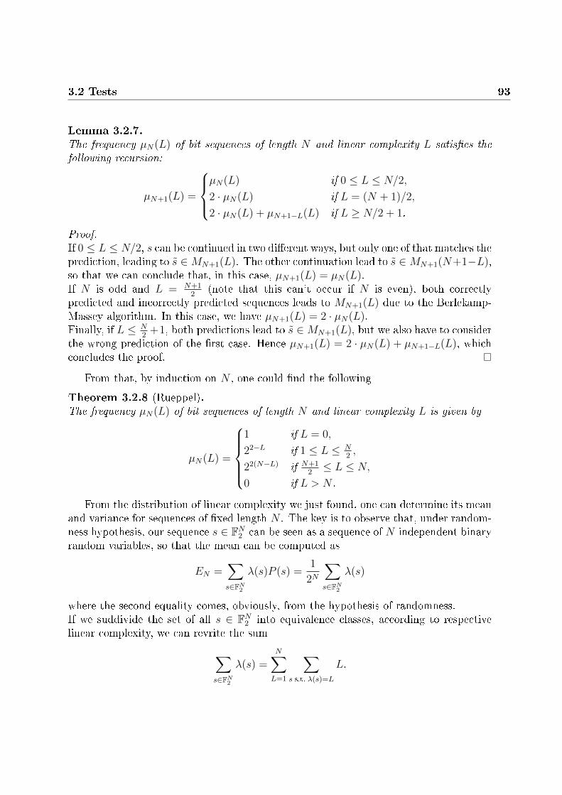
3.2 Tests 93
Lemma 3.2.7.The frequency µN(L) of bit sequences of length N and linear complexity L satises thefollowing recursion:
µN+1(L) =
µN(L) if 0 ≤ L ≤ N/2,
2 · µN(L) if L = (N + 1)/2,
2 · µN(L) + µN+1−L(L) if L ≥ N/2 + 1.
Proof.If 0 ≤ L ≤ N/2, s can be continued in two dierent ways, but only one of that matches theprediction, leading to s ∈MN+1(L). The other continuation lead to s ∈MN+1(N+1−L),so that we can conclude that, in this case, µN+1(L) = µN(L).If N is odd and L = N+1
2(note that this can't occur if N is even), both correctly
predicted and incorrectly predicted sequences leads to MN+1(L) due to the Berlekamp-Massey algorithm. In this case, we have µN+1(L) = 2 · µN(L).Finally, if L ≤ N
2+1, both predictions lead to s ∈MN+1(L), but we also have to consider
the wrong prediction of the rst case. Hence µN+1(L) = 2 · µN(L) + µN+1−L(L), whichconcludes the proof.
From that, by induction on N , one could nd the following
Theorem 3.2.8 (Rueppel).The frequency µN(L) of bit sequences of length N and linear complexity L is given by
µN(L) =
1 if L = 0,
22−L if 1 ≤ L ≤ N2,
22(N−L) if N+12≤ L ≤ N,
0 if L > N .
From the distribution of linear complexity we just found, one can determine its meanand variance for sequences of xed length N . The key is to observe that, under random-ness hypothesis, our sequence s ∈ FN2 can be seen as a sequence of N independent binaryrandom variables, so that the mean can be computed as
EN =∑s∈FN2
λ(s)P (s) =1
2N
∑s∈FN2
λ(s)
where the second equality comes, obviously, from the hypothesis of randomness.If we suddivide the set of all s ∈ FN2 into equivalence classes, according to respectivelinear complexity, we can revrite the sum∑
s∈FN2
λ(s) =N∑L=1
∑s s.t. λ(s)=L
L.

94 3. Statistical tests for randomness
Now each equivalent class contains exactly µN(L) elements, so that
∑s∈FN2
λ(s) =N∑L=1
L · µN(L)
and the expected value becomes
EN =1
2N
N∑L=1
L · µN(L).
By explicitly distinguishing between cases N odd and N even and using the recursiveformulas for µN , as in [62], one can prove the
Theorem 3.2.9 (Rueppel).The expected linear complexity of a sequence s = (s0, . . . , sN−1) of N independent anduniformly distributed binary random variable is given by
EN(L) =N
2+
4 +R2(N)
18− 1
2N
(N
3+
2
9
)and its variance is
V arN(L) =86
81− 1
2N
(14−R2(N)
27N +
82−R2(N)
81
)− 1
22N
(1
9N2 +
4
27N +
4
18
).
Here, and in the following, R2(n) is the parity function: it equals 0 if n is even and 1 ifit's odd.
For moderately large N mean and variance can be approximated as
µN ≈
N2
+ 29
if N is even,N2
+ 518
if N is odd;
σ2 ≈ 86
81,
so that (LN − µN)/σ2 is close to a standard normal variable, and P-values can be foundby
P-value = erfc
(LN − N
2√81/86
).
Though Gustafson et al. in [27] assume that as a good approximation and the linearcomplexity test is embedded in the Crypt-X package [10] in that way, NIST assumes thatthis approximation is too inaccurate due to the dierence on expected value between

3.2 Tests 95
the case of even/odd length, then they decided to adapt the statistic TN to shift thedistribution and make it as symmetric as possible dening
TN = (−1)N(LN − ξN) +2
9
where
ξN =N
2+
4 +R2(N)
18.
The limiting distribution of this random variable T , which only assumes integer values,approximates the normal distribution, but it's still skewed to the right:
P (T = k) =
1
22|k|+1 if k < 0,12
if k = 0,1
22kif k > 0.
From these probabilities we can compute the probabilities of P (T ≥ k > 0) as (3·22k−2)−1
and of P (T ≤ k < 0) as (3 ·22|k|−1)−1, by which we can compute probabilities πi of classesνi of the algorithm, and apply the χ2-test and nd the P-value through the incompletegamma function, as described in section (3.1.1). We shall note that, choosing blocksuciently large (i.e. choosingM suciently large) is really important, in order to makethe approximation the more precise as possible: for this purpose NIST recommends500 ≤M ≤ 5000.
Remark 3.2.10.The choice between the Standard Normal Distribution and the distribution T is relevant,since the dierence on probabilities are relatively large.Comparing the probabilities of chosen classes intervals ν0, . . . , ν6, we nd that, for thestatistic T , probabilities are π0 = 0.010417, π1 = 0.03125, π2 = 0.125, π3 = 0.5, π4 =0.25, π5 = 0.0625, π6 = 0.020833, while the ones from the Standard Normal Distributionwould have been π′0 = 0.0041, π′1 = 0.0432, π′2 = 0.1944, π′3 = 0.3646, π′4 = 0.2863, π′5 =0.0939, π′6 = 0.0135.
3.2.11 Serial test
This test analyzes frequencies of all m-bit patterns of the sequence, counted withoverlapping. m-bit binary patterns are 2m in total and, under randomness assumption,any of them has the same probability to appear as the others, since the distribution asto be uniform. Note that this is a test based on frequency and that, if m is equal to 1,it degenerates to the frequency test (3.2.1).

96 3. Statistical tests for randomness
Algorithmic description
1. Starting from ε = ε1 . . . εn, form an augmented sequence ε′ = ε1 . . . εnε1 . . . , εm−1 byappending the rst m− 1 bits to the end of the sequence.
2. Count the frequency of
• each possible overlapping m-bit block (pattern);
• each possible overlapping (m− 1)-bit block;
• each possible overlapping (m− 2)-bit block.
This will provide:
• vi1,...,im with ij ∈ 0, 1, the number of occurrences of the pattern i1, . . . , imfor all j = 1, . . . ,m;
• vi1,...,im−1 with ij ∈ 0, 1, the number of occurrences of the pattern i1, . . . , im−1
for all j = 1, . . . ,m− 1;
• vi1,...,im−2 with ij ∈ 0, 1, the number of occurrences of the pattern i1, . . . , im−2
for all j = 1, . . . ,m− 2.
3. Compute the statistics
ψ2m =
2m
n
∑i1,...,im
(vi1,...,im −
n
2m
)2
=2m
n
∑i1,...,im
v2i1,...,im
− n;
ψ2m−1 =
2m−1
n
∑i1,...,im−1
(vi1,...,im−1 −
n
2m−1
)2
=2m−1
n
∑i1,...,im−1
v2i1,...,im−1
− n;
ψ2m−2 =
2m−2
n
∑i1,...,im−2
(vi1,...,im−2 −
n
2m−2
)2
=2m−2
n
∑i1,...,im−2
v2i1,...,im−2
− n,
setting, by denition, ψ20 = ψ2
−1 = 0.
4. Compute distances (statistics themselves):
∇ψ2m = ψ2
m − ψ2m−1
∇2ψ2m = ψ2
m − 2ψ2m−1 + ψ2
m−2
5. Compute P-values using the incomplete gamma function:
P-value1 = igamc
(2m−2,
∇ψ2
2
)P-value2 = igamc
(2m−3,
∇2ψ2
2
)

3.2 Tests 97
Interpretation of results
A small P-value occurs when values of the two statistic ∇ψ2m and ∇2ψ2
m are large:that implies that there is large non-uniformity between pattern: some m-bit patternsoccur too many (or too few) times, compared to other m-bit patterns and to what isexpected from a random sequence.
An example
Let ε = 0011011101 be the testing sequence (so that n = 10) and let m = 3.
1. m = 3, then we append the rst m−1 = 2 bits of the sequence to its end, obtainingε′ = 001101110100.
2. Possible 3-bit overlapping templates (2m = 8) are 000, 001, 010, 011, 100, 101, 110and 111 so that respective frequencies are v000 = 0, v001 = 1, v010 = 1, v011 =2, v100 = 1, v101 = 2, v110 = 2, v111 = 0; For the 4 possible 2-bit patterns we havev00 = 1, v01 = 3, v10 = 3, v11 = 3 and (m− 2)-bit frequencies are v0 = 4 and v1 = 6.
3. ψ23 = 23
10(0 + 1 + 1 + 4 + 1 + 4 + 4 + 1)− 10 = 12.8− 10 = 2.8
ψ22 = 22
10(1 + 9 + 9 + 9)− 10 = 11.2− 10 = 1.2
ψ21 = 2
10(16 + 36)− 10 = 10.4− 10 = 0.4.
4. ∇ψ23 = 2.8− 1.2 = 1.6 ∇2ψ2
m = 2.8− 2 · 1.2 + 0.4 = 0.8
5. P-value1 = igamc(2, 1.6
2
)= 0.9057 and P-value2 = igamc
(1, 0.8
2
)= 0.8805. Both
P-values are greater than α = 0.01, then the sequence is accepted as random.
Mathematical background
The serial test uses two dierent types of statistic, the one of ψ2m, ψ
2m−1 and ψ2
m−2
and the statistics of distances ∇ψ2m and ∇2ψ2
m. We will show, here, the reason why ∇ψ2m
and ∇2ψ2m are used instead of ψ2
ν with ν ∈ m,m− 1,m− 2 and we'll prove that usedstatistics have a χ2 distribution, then the incomplete gamma function can be used tond the P-value.
First we used statistics of the form
ψ2m =
2m
n
∑i
(vi −
n
2m
)where, for briefness, we used i to indicate i1, . . . , im. Even though ψ2
m has the form of aχ2 statistic with 2m − 1 degrees of freedom, in fact it hasn't a χ2 distribution (not evenasymptotically) since, as Good proved in [26], one can see that its expected value is
E[ψ2m] = 2m − 1

98 3. Statistical tests for randomness
while the real number of degrees of freedom of ψ2m is strictly minor than 2m − 1, and
the expected value of a χ2 distribution equals the number of degrees of freedom. Thisdepends on the fact that, under randomness hypothesis, we have some restraints onfrequencies. For example, for 2-bit sequences, we have the following two linear restraintson ψ2
2:vi1,0 + vi1,1 = v0,i1 + v1,1i for i1 = 0, 1
i.e. the number of sequence of the form i, 0 or i, 1 has to be the same of the number of0, i or 1, i and, similarly, for sequences of each xed length m. This implies that, in fact,the number of degrees of freedom is not 22− 1 as expected, but only 2, for the example.In general the expected number of degrees of freedom was 2m − 1 but, in fact, they are2m−1, so that the statistic couldn't have a χ2 distribution (see [5] for detailed proof).
To nd a statistic that eectively has a χ2 distribution, the two following statisticsare formed:
∇ψ2m = ψ2
m − ψ2m−1
and∇2ψ2
m = ψ2m − 2ψ2
m−1 + ψ2m−2.
Good in [26] decomposes ψ2m into a sum of normal distributed functions so that ∇ψ2
m
and ∇2ψ2m satisfy the denition of the χ2 distribution. The decomposition is made by
mean of
Denition 3.2.12 (m-dimensional discrete Fourier transform).The m-dimensional mod 2 discrete Fourier transform of a function v = vi is denedby
v∗s =∑i
viω<i,s>,
where ω = exp(2πi/2), i = i1, . . . , im as above and < i, s >= i1s1 + · · · + imsm is thescalar product of vectors i and s.
Observing that the discrete Fourier transformation is linear, one can observe that thetransform of
(vi − n
2m
)is v∗s minus the transform of the constant n
2m. The transform of
the latter is zero, unless s = (0, . . . , 0) when it equals to n; we can also observe thatv∗0 =
∑i vi = n. By previous remarks, using the Rayleigh-Parseval formula (
∑i v
2i =
2−m∑
s v∗sv∗−s) in its discrete version, we nd that∑
i
(vi −
n
2m
)=
1
2m
∑s 6=0
|v∗s |2.
If we classify the 2m vectors s into m + 1 classes depending on how many non-zerovalues they have, we can use the previous formula to rewrite ψ2
m as
nψ2m =
∑d=m
|v∗s |2 + 2∑
d=m−1
|v∗s |2 + · · ·+m∑d=1
|v∗s |2 (3.30)

3.2 Tests 99
where d = j indicates the number of non-zero values of the vector. Bartlett in [5] hasproved that the joint distribution of vi is a asymptotically multivariate normal distribu-tion and, covariances, Good proved that sums in (3.30) have approximately independentχ2 distribution with 2d−2 degrees of freedom, respectively. Following from that ∇ψ2
m and∇2ψ2
m have χ2 distributions with, respectively, 2m−1 and 2m−2 degrees of freedom.
3.2.12 Approximate entropy test
As Maurer's universal statistical test, the approximate entropy test analyzes theentropy of the sequence ε = ε1 . . . εn by the frequencies of m-bit patterns with the onesof (m+ 1)-bit patterns, in analogy with the serial test. Moreover, as in the overlappingtemplate matching test, patterns can overlap.
Algorithmic description
1. Starting from ε = ε1 . . . εn, form an augmented sequence ε′ = ε1 . . . εnε1 . . . , εm−1
by appending the rst m − 1 bits to the end of the sequence: this will create noverlapping sub-sequences of length m to analyze.
2. For each m-bit pattern i count the number of occurrences through the entire se-quence. The count is made in an "overlapping way", i.e. if at j-th step bits fromεj to εj+m−1 are examined, the (j + 1)-th step will analyze bits from εj+1 to εj+m.Let #i be te number of occurrences of the pattern i through the sequence.
3. Compute Cmi = #i
nthe frequency of pattern i inside the sequence, for each possible
i.
4. Compute
ϕm =∑i
πilogπi, where πi = Cmlog2i
;
here i indicates the corresponding decimal value of the string i.
5. Repeat steps from 1 to 4 replacing m by m+ 1, obtaining ϕm+1.
6. Compute the approximate entropy
ApEn(m) = ϕm − ϕm+1.
7. Compute the statistic
χ2(obs) = 2n[log2− ApEn(m)].
8. Compute P-value through the incomplete gamma function:
P-value = igamc
(2m−1,
χ2(obs)
2
).

100 3. Statistical tests for randomness
Interpretation of results
A small P-value will occur when the value of the statistic ApEn(m) is too small ortoo large: the rst case would indicate that the sequence shows strong regularity betweenpattern (i.e. there is no change of entropy between m-bit strings and m+ 1 strings) andthe second one would imply uctuation or irregularity on patterns of the string, and inparticular between patterns of subsequent length.
An example
Let's take the sequence ε = 0100110101, so that n = 10, and m = 3.
1. ε′ = 010011010101, appending the rst m− 1 = 2 bit to the end of the sequence.
2. We count the number of occurrences of the 2m = 23 = 8 possible templates, ndingthat #000 = 0,#001 = 1,#010 = 3,#011 = 1,#100 = 1,#101 = 3,#110 =1,#111 = 0.
3. C3i = #i
10so that C3
000 = 0, C3001 = 0.1, C3
010 = 0.3, C3011 = 0.1, C3
100 = 0.1, C3101 =
0.3, C3110 = 0.1, C3
111 = 0.
4. ϕ3 = 0(log0) + 0.1(log0.1) + 0.3(log0.3) + 0.1(log0.1) + 0.1(log0.1) + 0.3(log0.3) +0.1(log0.1) + 0(log0) = −1.64341772.
5. Let's repeat steps from 1 to 4 by replacing m with m+ 1:
i) m = 4 so that we append the rstm−1 = 3 bits, obtaining ε′ = 0100110101010.
ii) Computed values are #0011 = 1,#0100 = 1,#0101 = 2,#0110 = 1,#1001 =1,#1010 = 3,#1101 = 1 and all the other values are 0.
iii) C40011 = C40100 = C4
0110 = C41001 = C4
1101 = 0.1, C40101 = 0.2, C4
1010 = 0.3, andall other values are zero.
iv) ϕ4 = 0 + 0 + 0 + 0.1(log0.01) + 0.1(log0.01) + 0.2(log0.02) + 0.1(log0.01) + 0 +0 + 0.1(log0.01) + 0.3(log0.03) + 0 + 0 + 0.1(log0.01) + 0 + 0) = −1.83437197.
6. ApEn(3) = ϕ3 − ϕ4 = −1.643418− (−1.834372) = 0.190954.
7. χ2 = 2 · 10 · (0.693147− 0.190954) = 0.502193.
8. P-value= igamc(22, 0.502193
2
)= 0.261961 > α, and the sequence is accepted as
random.

3.2 Tests 101
Mathematical background
The theory behind this test is mostly based on the concept of approximate entropyApEn, introduced by Pincus in [55]. The purpose of approximate entropy is to charac-terize the idea of randomness and study what happens when the sequence grows, one bitafter another. To better understand why the approximate entropy can be used to detectregularity, or irregularity, we shall give the following
Denition 3.2.13 (Distance between two blocks).Let n,m ∈ N \ 0 with m ≤ n, r ∈ R and s = s1, . . . , sn be a sequence of real numbers.Given two blocks of the same length x(i) = si, si+1, . . . , si+m−1 and x(j) of s, the distancebetween blocks x(i) and x(j) is dened as
d(x(i), x(j)) = maxk=1,...,m(|s(i+ k − 1)− s(j + k − 1)|).
The previous notion allows to dene a measure of how blocks of consecutive length(m and m + 1) dier or remain the same through the entire sequence and to measurethe frequency of how often this occurs, by the use of
Cmi (r) =
#j ≤ N −m+ 1 s.t. d(x(i), x(j)) ≤ rN −m+ 1
We can now give the
Denition 3.2.14 (Approximate entropy).
ϕm(r) =1
n−m+ 1
N−m+1∑i=1
logCmi (r)
and the approximate entropy is dened as
ApEn(m, r,N)(s) = ϕm(r)− ϕm+1(r)
with ApEn(0) = −ϕ1.
For completeness we gave denitions for strings with values in R but, in our case, thesequence takes values in 0, 1, so that the distance will only assume values 0 or 1, andcould be dened as
d(x(i).x(j)) =
0 if x(i) = x(j),
1 if x(i) 6= x(j),
and r could only be equal to 1, so that we won't be interested in it anymore. As writtenby Pincus and Huang in [54] "analytic proofs of asymptotic normality and expeciallyexplicit variance estimates for ApEn appear to be extremely dicult", so the key is todene a new type of approximate entropy, which will have the same asymptotic behaviorof the approximate entropy but it is simpler to estimate. Indeed Pincus characterizesrandomness for nite sequences as

102 3. Statistical tests for randomness
Denition 3.2.15 ((m,n)-random sequence).A binary sequence ε of length n is said to be (m,n)-random if
ApEn(m,n)(ε) = maxsApEn(m,n)(s ∈ S),
where S is the set of all possible 2n binary sequences of length n.
Let ε = ε1, . . . , εnε1 . . . , εm−1 be the augmented (or in a certain sense circular) versionof the original string, as we do at the rst step of the algorithm, and let the "modied"version of the empirical distribution be
ϕm =∑
i1,...,im
νi1,...,imlogνi1,...,im ,
where νi1,...,im is the relative frequency of the pattern i1, . . . , im in ε. If ωi1,...,im = nνi1,...,imis the frequency of the pattern, by this denition we have that ωi1,...,im =
∑k ωi1,...,im,k
so that∑
i1,...,imνi1,...,im = n.
We dene the modied approximate entropy as
ApEn(m) = ϕm − ˜ϕm+1.
If we use Jensen's inequality (ψ (∑aixi) ≤
∑aiψ(xi)) with the function ψ which ex-
tends the string, we obtain a rst upper bound for the modied approximate entropy:
ApEn(m) ≤ logs, where s is the cardinality of the set of value, so that in our case s = 2,
so that the largest possible value of ˜ApEn(m) is log2.
On the other hand, we also have that ApEn and ApEn can't dier much, for large valuesof n: if Yi(m) = i1, . . . , im and ν ′i1,...,im = Cm
i , we have
ϕm =∑
i1,...,im
ν ′i1,...,imlogν′i1,...,im
,
then, if ωi1,...,im = (n−m+ 1)ν ′i1,...,im we have that∑i1,...,im
= n−m+ 1
and ωi1,...,im − ω′i1,...,im ≤ m− 1.
We nally obtain that
|νi1,...,im − ν ′i1,...,im| ≤m− 1
n−m+ 1, (3.31)

3.2 Tests 103
which implies that, if m is xed, ApEn(m) and ApEn(m) are close together for largevalues of n.
The last thing we need to know to perform the test is the distribution of the statisticn[log2 − ApEn(m)] since, if we get that, we have the theoretical distribution to useto compute the P-value. Rukhin, in [63], proved that, whether we use the augmentedsequence and the modied approximate entropy or the ones dened by Pincus, we alwayshave that the statistic has a χ2 distribution with (s − 1)sm degrees of freedom. Indeedthe following theorem holds:
Theorem 3.2.10 (Rukhin).For xed m, as n→∞, one has the following convergence in distribution:
2n[logs− ApEn(m)]→ χ2(sm+1 − sm). (3.32)
Also
n[ApEn(m)− ApEn(m)] = O
(1
n
), (3.33)
so that
2n[logs− ApEn(m)]→ χ2(sm+1 − sm).
Proof.Let Zi1,...,im be the dierence between empirical and theoretical probabilities:
Zi1,...,im =√n
(νi1,...,im −
1
sm
);
The vector formed by Zi1,...,im has, by the central limit theorem, asymptotic multivariatedistribution which mean is zero and variance of the form
Σm =1
SmIm −
1
22meme
Tm,
where Im stands for the sm × sm identity matrix and eTm is the vector (1, . . . , 1) whichlength is sm.Chaitin, in [13], showed that
ϕm = −∑
i1,...,im
[1
sm+Zi1,...,im√
n
]·[−mlogs+
smZi1,...,im2n
+O
(1
n3/2
)]∼ mlogs+
sm
2n
∑i1,...,im
Z2i1,...,im
.

104 3. Statistical tests for randomness
Using analogous notations for pattern of length m+ 1 one can easily see that
Zi1,...,im,k =s∑
k=1
Zi1,...,im,k
and
ϕm+1
∑(m+ 1)logs+
sm+1
2n
∑i1,...,im,im+1
Z2i1,...,im,im+1
.
Using the approximations for ϕm and ϕm+1 we have
ϕm − ϕm+1 ∼ logs− sm
2n
∑i1,...,im
(∑k
Zi1,...,im,l
)2
− s∑
i1,...,im,im+1
Z2i1,...,im,im+1
= logs− sm
2nZTQZ
where Q is an sm+1 × sm+1 block-diagonal matrix, formed by sm blocks Q0 which havethe form
Q0 = sI1 − e1eT1 ,
and Z is a normal vector of length sm+1.By spectral decomposition, the quadratic form ZTQZ has the same distribution of∑li1,...,im,im+1W
2i1,...,im,im+1
whereWi1,...,im,im+1 are independent standard normal variables
and li1,...,im,im+1 are the eigenvalues of the matrix Σ1/2QΣ1/2.By direct computing one can see that
Σ1/2m+1 =
1
s(m+1)/2Im+1 −
1
s3(m+1)/2em+1e
Tm+1,
and Σ1/2m+1QΣ
1/2m+1 = 1
sm+1Q.
Directly computing the eigenvalues of Σ1/2m+1QΣ
1/2m+1 one can nd that needed eigenvalues
are equal to s with multiplicity (s− 1)sm and 0 with multiplicity sm, so that
ϕm − ϕm+1 ∼ logs− 1
2nχ2((s− 1)sm)
and
n[logs− ApEn(m)] ∼ 1
2χ2(sm+1 − sm).
Now (3.31) shows that if Z ′i1,...,im =√n[ν ′i1,...,im − s
−m], then |Z ′i1,...,im − Zi1,...,im| ≤ (m−1)√n/(n−m+ 1) and
|ϕm − ϕm| ∼sm
2n
∣∣∣∣∣ ∑i1,...,im
Z2i1,...,im
−∑
i1,...,im
Z ′2i1,...,im
∣∣∣∣∣ ≤ s2m(m− 1)2
2(n−m+ 1)2.

3.2 Tests 105
(3.33) comes directly from that last inequality so that the last convergence in distributionof the statement follows, using (3.32) and (3.33) together.
This theorem, applied to our case where s = 2, tells us that the statistic χ2, computedat step 7 of the algorithm, eectively has a χ2 distribution with 2m degrees of freedom,so that the P-value can be computed using the incomplete gamma function igamc as
P-value = igamc
(2m
2,χ2
2
).
3.2.13 Cumulative sums (Cusum) test
In this test, the sequence is considered as a random walk by transforming the binarystring into a string of −1 and +1. As a random walk, we analyze excursions from zero ofthe walk by computing partial sums and we check if these are too far from zero. Indeedthe random walk created by a truly random sequence tends to stay near zero, since thenumber of zeros and ones has to be approximately the same and the alternation betweenthem has to be relatively fast. Note that a sequence won't pass the test though itsexcursion in too low.
Algorithmic description
1. The sequence is transformed into a string of −1 and +1.
2. Partial sums are computed: this could be done both forward and backward, pro-viding two dierent tests (and P-values):
Forward BackwardS1 = X1 S1 = Xn
S2 = X1 +X2 S2 = Xn +Xn−1
S3 = X1 +X2 +X3 S3 = Xn +Xn−1 +Xn−2...
...Sk = X1 +X2 +X3 + . . .+Xk S3 = Xn +Xn−1 +Xn−2 + . . .+Xn−k+1...
...Sn = X1 + . . .+Xk + . . .+Xn Sn = Xn + . . .+Xk + . . .+X1
Note that, obviously, Sk = Sk−1 +Xk for the forward sum and Sk = Sk−1 +Xn−k+1
for the backward one.
3. Compute the maximal excursion from zero:
z = maxk∈1,...,n
|Sk|.

106 3. Statistical tests for randomness
4. Compute P-value as
P-value = 1−(nz−1)/4∑
k=(−nz +1)/4
[Φ
((4k + 1)z√
n
)− Φ
((4k − 1)z√
n
)]+
(nz−1)/4∑k=(−nz −3)/4
[Φ
((4k + 3)z√
n
)− Φ
((4k + 1)z√
n
)]
where Φ is the cumulative probability distribution function of the Standard Normaldistribution, as dened in (2.1).
Interpretation of results
A small P-value (i.e. a rejection) can occur if 0 and 1 are intermixed too frequently,and this will correspond to small values of the largest excursion z. A large z in theforward testing would indicate that there are too many ones or too many zeros in therst part of the sequence and, on the other hand, that there are too many ones or zerosin the nal part, if the computation is made backwards.
An Example
Let ε = 1011010111 be the test sequence. The test proceeds as follows:
1. X = 1,−1, 1, 1,−1, 1,−1, 1, 1, 1
2. If we compute partial sums in forward mode the computation is:
S1 = 1S2 = 1 + (−1) = 0S3 = 1 + (−1) + 1 = 1S4 = 1 + (−1) + 1 + 1 = 2S5 = 1 + (−1) + 1 + 1 + (−1) = 1S6 = 1 + (−1) + 1 + 1 + (−1) + 1 = 2S7 = 1 + (−1) + 1 + 1 + (−1) + 1 + (−1) = 1S8 = 1 + (−1) + 1 + 1 + (−1) + 1 + (−1) + 1 = 2S9 = 1 + (−1) + 1 + 1 + (−1) + 1 + (−1) + 1 + 1 = 3S10 = 1 + (−1) + 1 + 1 + (−1) + 1 + (−1) + 1 + 1 + 1 = 4
3. z = 4 since 4 it's the largest value reached by partial sums.
4. P-value= 0.4116588 < α and the sequence is accepted as random.
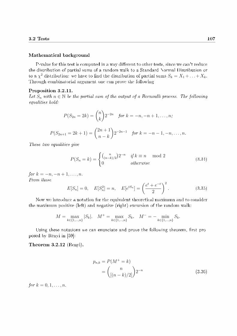
3.2 Tests 107
Mathematical background
P-value for this test is computed in a way dierent to other tests, since we can't reducethe distribution of partial sums of a random walk to a Standard Normal Distribution orto a χ2 distribution: we have to nd the distribution of partial sums Sk = X1 + . . .+Xk.Through combinatorial argument one can prove the following
Proposition 3.2.11.Let Sn with n ∈ N be the partial sum of the output of a Bernoulli process. The followingequalities hold:
P (S2n = 2k) =
(n
k
)2−2n for k = −n,−n+ 1, . . . , n;
P (S2n+1 = 2k + 1) =
(2n+ 1
n− k
)2−2n−1 for k = −n− 1,−n, . . . , n.
These two equalities give
P (Sn = k) =
(n
(n−k)/2
)2−n if k ≡ n mod 2
0 otherwise(3.34)
for k = −n,−n+ 1, . . . , n.From those
E[Sn] = 0, E[S2n] = n, E[etSn ] =
(et + e−t
2
)2
. (3.35)
Now we introduce a notation for the equivalent theoretical maximum and to considerthe maximum positive (left) and negative (right) excursion of the random walk:
M = maxk∈1,...,n
|Sk|, M+ = maxk∈1,...,n
Sk, M− = − mink∈1,...,n
Sk.
Using these notations we can enunciate and prove the following theorem, rst pro-posed by Renyi in [59]:
Theorem 3.2.12 (Renyi).
pn,k = P (M+ = k)
=
(n
[(n− k)/2]
)2−n (3.36)
for k = 0, 1, . . . , n.

108 3. Statistical tests for randomness
Proof.We prove the equality by induction. Let
M+ = max1≤k≤n+1
k∑j=2
Xj
then, for k ≥ 1,
pn+1,k = P (X1 = 1, M+ = k − 1) + P (x1 = −1, M+ = k + 1)
=1
2(pn,k−1 + pn,k+1)
For k = 0, in a similar way
pn+1,0 = P (X1 = −1, M+ ≤ 1) =1
2(pn,1 + pn,0).
We know that p1,0 = p1,1 = 12so that we obtain (3.36) by induction.
The theorem which follows is due to Billingsley: we omit the proof and refer to [6].
Theorem 3.2.13 (Billingsley).For any integers a ≤ 0 ≤ b, a ≤ ν ≤ b we have
pn(a, b, ν) = P (a < −M− ≤M+ < b, Sn = ν)
=∞∑
k=−∞
qn(ν + 2k(b− a))−∞∑
k=−∞
qn(2b− ν + 2k(b− a)) (3.37)
where, for j = −n,−n+ 1, . . . , n,
qn(j) = P (Sn = j) =
(n
(n−j)/2
)2−n if j ≡ n mod 2,
0 otherwise.
A direct consequence of this theorem is the following
Theorem 3.2.14.For any integers a ≤ 0 ≤ b and a ≤ u ≤ ν ≤ b we have
P (a < −z− ≤M+ < b, u < Sn < ν)
=∞∑
k=−∞
P (u+ 2k(b− a) < Sn < ν + 2k(b− a))
−∞∑
k=−∞
P (2b− ν + 2k(b− a) < Sn < 2b− u+ 2k(b− a)), (3.38)

3.2 Tests 109
P (a < −M− ≤M+ < b)
=∞∑
k=−∞
P (a+ 2k(b− a) < Sn < b+ 2k(b− a))
−∞∑
k=−∞
P (b− ν + 2k(b− a) < Sn < b− a+ 2k(b− a)) (3.39)
and
P (M < b) =∞∑
k=−∞
P ((4k − 1)b < Sn < (4k + 1)b)
−∞∑
k=−∞
P ((4k + 1)b < Sn < (4k + 3)b). (3.40)
Proof.(3.38) follows directly from (3.37); (3.39) is the special case of (3.38) with u = a, ν = band (3.14) follows from (3.39) taking a = −b.
Formula (3.40) is what we need, since it is exactly the complementary of the P-valueso, by complementing
P-value = P ( max1≤k≤1
|Sk| ≥ z)
= 1−∞∑
k=−∞
P ((4k − 1)z < Sn < (4k + 1)z)
+∞∑
k=−∞
P ((4k + 1)z < Sn < (4k + 3)z).
As in (3.35) the distribution of Sn has mean µ = 0 and variance σ2 = n, so thatwe can use the Standard Normal cumulative distribution function Φ with z = z/
√n
to compute probabilities of the summations. Obviously, in practice summations aretruncated, however simulations showed that bound proposed in the algorithm provide agood approximation.
Remark 3.2.11.Note that indices k of summations at 4th step of the algorithm would be non-integer,however the theory at the base of the test shows that they must be integers: that's whyindices have to be approximated to obtain truthful results.

110 3. Statistical tests for randomness
3.2.14 Random excursion test
As the previous one, this test considers the binary string as a random walk, inspectingcycles of the walk to check if their behavior is as expected from a true random walk.Cycles of a random walk are dened as
Denition 3.2.16 (Cycle of a random walk).A cycle of a random walk is a sequence of steps (each of length 1) which start from andends at the origin.
The focus is the number of visits of the totality of the cycles to a particular state kand the test checks if this is as expected under hypothesis of randomness. Visits whichare examined are the ones to states −4,−3,−2,−1, 1, 2, 3, 4 producing 8 P-values (onefor each state checked).
Algorithmic description
1. The sequence is transformed into a string of −1 and +1.
2. Partial sums Si are computed to obtain the set S = Sii=1,...,n.
S1 = X1
S2 = X1 +X2
S3 = X1 +X2 +X3...Sk = X1 +X2 +X3 + . . .+Xk...Sn = X1 +X2 +X3 + . . .+Xk + . . .+Xn
3. Create a new sequence S ′ from S by attaching a zero at the beginning and at theend, forming S ′ = 0, S1, S2, . . . , Sn, 0.
4. Let J = #zero crossing in S ′ with the exception of the rst 0. Observe thatJ = #zero crossings = #Cycles.If J < 500 do not perform the test, since it doesn't satisfy the empirical rule forχ2 computations.
5. For each cycle and for each non-zero state (i.e. for −4,−3,−2,−1, 1, 2, 3, 4) countfrequencies of state within each circle.
6. For each state x, and for k = 0, 1, . . . , 5, compute
vk(x) = total number of cycles where state x occurs exactly k times,
with the convention that v5(x) also stores frequencies which are ≥ 5.
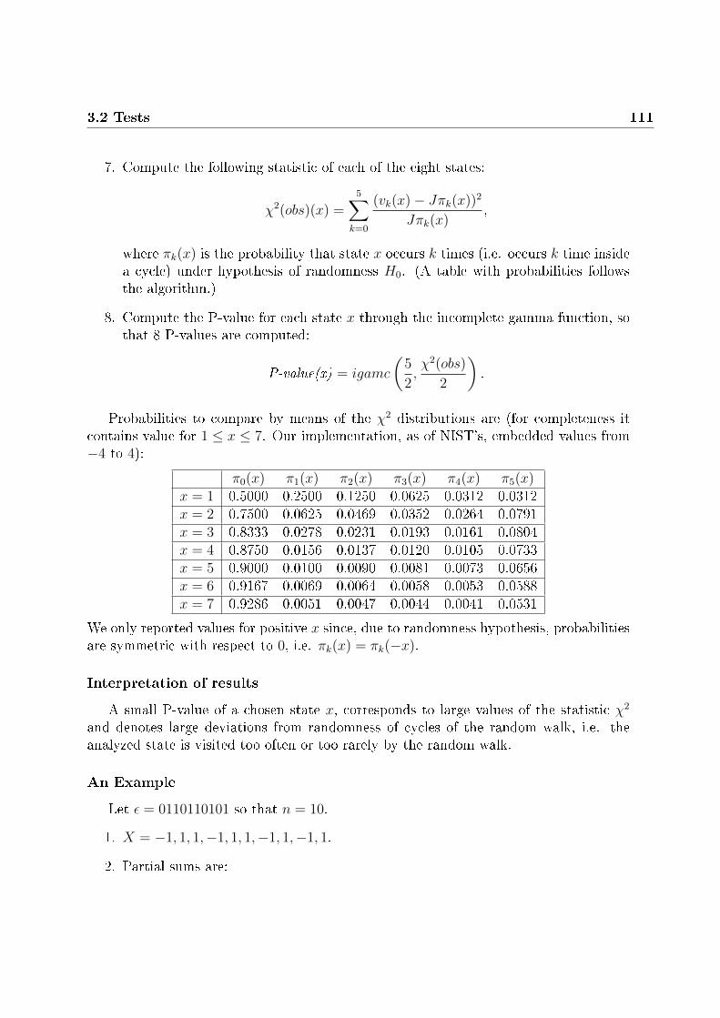
3.2 Tests 111
7. Compute the following statistic of each of the eight states:
χ2(obs)(x) =5∑
k=0
(vk(x)− Jπk(x))2
Jπk(x),
where πk(x) is the probability that state x occurs k times (i.e. occurs k time insidea cycle) under hypothesis of randomness H0. (A table with probabilities followsthe algorithm.)
8. Compute the P-value for each state x through the incomplete gamma function, sothat 8 P-values are computed:
P-value(x) = igamc
(5
2,χ2(obs)
2
).
Probabilities to compare by means of the χ2 distributions are (for completeness itcontains value for 1 ≤ x ≤ 7. Our implementation, as of NIST's, embedded values from−4 to 4):
π0(x) π1(x) π2(x) π3(x) π4(x) π5(x)x = 1 0.5000 0.2500 0.1250 0.0625 0.0312 0.0312x = 2 0.7500 0.0625 0.0469 0.0352 0.0264 0.0791x = 3 0.8333 0.0278 0.0231 0.0193 0.0161 0.0804x = 4 0.8750 0.0156 0.0137 0.0120 0.0105 0.0733x = 5 0.9000 0.0100 0.0090 0.0081 0.0073 0.0656x = 6 0.9167 0.0069 0.0064 0.0058 0.0053 0.0588x = 7 0.9286 0.0051 0.0047 0.0044 0.0041 0.0531
We only reported values for positive x since, due to randomness hypothesis, probabilitiesare symmetric with respect to 0, i.e. πk(x) = πk(−x).
Interpretation of results
A small P-value of a chosen state x, corresponds to large values of the statistic χ2
and denotes large deviations from randomness of cycles of the random walk, i.e. theanalyzed state is visited too often or too rarely by the random walk.
An Example
Let ε = 0110110101 so that n = 10.
1. X = −1, 1, 1,−1, 1, 1,−1, 1,−1, 1.
2. Partial sums are:

112 3. Statistical tests for randomness
S1 = −1 S6 = 2S2 = 0 S7 = 1S3 = 1 S8 = 2S4 = 0 S9 = 1S5 = 1 S10 = 2
and S = −1, 0, 1, 0, 1, 2, 1, 2, 1, 2.
3. The extended random walk is S ′ = 0,−1, 0, 1, 0, 1, 2, 1, 2, 1, 2, 0.
Figure 3.7: Random walk from the example. Credits to [64].
4. After the starting zero, we have J = 3 returns to the origin, since we have zeros inpositions 3, 5 and 12 of the extended walk. We therefore have 3 cycles, consistingof 0,−1, 0, 0, 1, 0 and 0, 1, 2, 1, 2, 1, 2, 0.
5. Counting the frequency of each state we see that the rst cycle has a single occur-rence of −1, the second cycle has one occurrence of 1 and the last one has threeoccurrences of both 1 and 2. The following table provides a more clear visualiza-tion:
State Cycle 1 Cycle 2 Cycle 3x (0,−1,0) (0,1,0) (0,1,2,1,2,1,2,0)-4 0 0 0-3 0 0 0-2 0 0 0-1 1 0 01 0 1 32 0 0 33 0 0 04 0 0 0
6. Computing vk(x) for k = 0, 1, . . . , 5 we have that

3.2 Tests 113
• v0(−1) = 2, since the state −1 occurs exactly 0 time ins two cycles;v1(−1) = 1, since the state −1 occurs exactly one time in 1 cycle;v2(−1) = v3(−1) = v4(−1) = v5(−1) = 0, since the state −1 occurs exactly2, 3, 4,≥ 5 times, respectively, in 0 cycles.
• v0(1) = 1 (the 1 state occurs exactly 0 times in 1 cycle);v1(1) = 1 (the 1 state occurs only once in 1 cycle);v3(1) = 1 (the 1 state occurs exactly three times in 1 cycle);v2(1) = v4(1) = v5(1) = 0 (the 1 state occurs exactly 2, 4,≥ 5 times in 0cycles).
And so on, as in the following table:
State Number of cyclesx 0 1 2 3 4 5-4 3 0 0 0 0 0-3 3 0 0 0 0 0-2 3 0 0 0 0 0-1 2 1 0 0 0 01 1 1 0 1 0 02 2 0 0 1 0 03 3 0 0 0 0 04 3 0 0 0 0 0
7. For the state x = 1 the statistic is
χ2(1) =(1− 3(0.5))2
3(0.5)+
(1− 3(0.25))2
3(0.25)+
(0− 3(0.125))2
3(0.125)+
(1− 3(0.0625))2
3(0.0625)
+(0− 3(0.0312))2
3(0.0312)+
(0− 3(0.0312))2
3(0.0312)= 4.333033.
8. P-value(1)= igamc(
52, 4.333033
2
)= 0.502529 > α and the sequence is accepted as
random, at least for what concerns the state x = 1: analogous computation has tobe done for other values of x to nd other P-values.
Mathematical background
In order to evaluate the χ2 statistic at seventh step of the algorithm, we need toknow the distribution of the number of visit for a random walk and, in particular, weneed theoretical probabilities πj(x) for each state x and for each number of occurrencesj. Let Sk = X1 + . . . ,+Xk be the k-th partial sum of the random walk where Xi
are independent random variables which take values +1 and −1 with probability p and

114 3. Statistical tests for randomness
q = 1 − p respectively. Setting S0 = 0 by denition, let ρ1 < ρ2 < · · · < ρJ be thetimes when the random walk returns to the origin, i.e ρ1 = mink, k > 0 s.t. Sk = 0,ρ2 = mink, k > ρ1j s.t. Sk = 0 . . . .
The respective sequence of excursions will be
(S0, . . . , Sρ1), (Sρ1 , . . . , Sρ2), . . . .
Let J denote the total number of such excursions in the string (corresponding to thenumber of zeros among partial sums Sk), which can be considered as a random variableitself, the limiting distribution of J is widely studied and known (see for example [60])to be
limn→∞
P
(J√n< z
)=
√2
π
∫ z
0
e−u2/2du for z > 0
If J is too small we'd have that the value of the integral is small and then the P-valuewould be small, since
P-value = P (J < J(obs)) ≈√
2
π
∫ J
0
e−u2/2du,
that's why the randomness hypothesis is straight rejected if J < max(0.005√n, 500) at
fourth step of the algorithm and the test doesn't go on.
If the previous, preliminary, test is passed, let ξ(x) be the number of visit to thestate x (with x 6= 0, since this case is already evaluated), during a xed excursion. Thedistribution of ξ(x) is given by the following
Theorem 3.2.15.For p 6= 1/2
P (ξ(x) = 0) = 1− |p− q|∣∣∣1− ( qp)x∣∣∣ (3.41)
and for k = 1, 2, 3, . . .
P (ξ(x) = k) =
|p−q|2
|1−(q/p)x|2
[1− |p−q|
1−(q/p)x
]k−1
p > q, x > 0 or p < q, x < 0,
|p−q|2|1−(p/q)x||1−(p/q)x|
[1− |p−q|
1−(p/q)x
]k−1
p > q, x < 0 or p < q, x > 0.
(3.42)For p = 1/2
P (ξ(x) = 0) = 1− 1
2|x|(3.43)

3.2 Tests 115
and for k ≥ 1
P (ξ(x) = k))1
4x2
(1− 1
2|x|
)k−1
. (3.44)
Proof.First of all we shall observe that if the excursion is nite, then ξ(x) = k, with k ≥ 1,if and only if the random walk Sk reaches the stage x for the rst time, it uctuates(without touching the stage 0) visiting the chosen state k − 1 times and then it returnsto the origin. Observe that if we consider the process Sk − x, that doesn't visit level−x in its rst k − 1 excursions. Taking into account this fact, we can observe that, byindependence of these excursions
p(ξ(x) = k, ρ <∞) = P (ξ(x) > 0)[P (ξ(−x) = 0, ρ <∞)]k−1P (ξ(−x) > 0). (3.45)
Let's suppose, for the moment, that x > 0, then
P (ξ(x) > 0) = P (S1 = 1)P ("x-1 is reached before -1").
The second factor of the right hand side it is equivalent to the probability of winningin the classical gambler's ruin problem with initial capital 1 and total capital x (see forexample [22]), so that
P (ξ(x) > 0) = pq/p− 1
(p/q)x − 1=
q − p(q/p)x − 1
.
Since we are considering a 1-dimensional random walk, to obtain probabilities of sym-metrical (with respect to the origin) stage we can simply swap roles of p and q, obtaining
P (ξ(−x) > 0) =p− q
(p/q)x − 1,
and then
P (ξ(x) > 0) =
∣∣∣∣ p− q(q/p)x − 1
∣∣∣∣ ∀ x,
so that (3.41) is proved since, banally, P (ξ(x) = 0) = 1 − P (ξ(x) > 0). To distinguishcases let's dene I such that
I =
0 if p > q, x < 0 or p < q, x > 0,
1 otherwise,
then
P (ξ(x) = 0, ρ =∞) = (1− I)P (ρ =∞) = (1− I)|p− q|.

116 3. Statistical tests for randomness
By the previous and (3.41), taking into account that P (ξ(x) = 0, ρ < ∞) = P (ξ(x) =0)− P (ξ(x) = 0, ρ =∞), we obtain
P (ξ(x) = 0, ρ <∞) = 1−∣∣∣∣ p− q(q/p)x − 1
∣∣∣∣− (1− I)|p− q|, (3.46)
so that, by substituting it in (3.45), we obtain
P (ξ(x) = k, ρ <∞) = (pq)x(
p− qpx − qx
)2 [1−
∣∣∣∣ p− q(p/q)x − 1
∣∣∣∣− I|p− q|]k−1
.
Now, if the excursion is innite, the case ξ(x) = k occurs if and only if the randomwalk Sk visits the stage x for the rst time, returns to it k − 1 times (without visitingthe origin) and than it continues without visiting both x and 0. Since we're consideringan innite excursion (so that innite time), this case is only possible if x > 0, p > q orx < 0, p < q (i.e. the excursion continues above x, if x > 0, and below x, otherwise).This observation permits us to assert that P (ξ(x) = k, ρ =∞) = 0 if I = 0.Now, taking −x in place of x in (3.46) we obtain
P (ξ(x) = k, ρ =∞) = IP (ξ(x) > 0)(P (ξ(−x) = 0, ρ <∞))k−1P (ρ =∞)
=I(p− q)2
1− (q/p)x
(1−
∣∣∣∣ p− q(p/q)x − 1
∣∣∣∣− |p− q|)k−1
.
Formula (3.42) is obtained by computing P (ξ(x) = k, ρ = ∞) + PI1(ξ(x), ρ < ∞) +PI2(ξ(x), ρ <∞), where I1 and I2 are used here to distinguish between the two possiblecases.Finally, by taking the limit p→∞ in (3.41) and (3.42), one obtains formulas (3.43) and(3.44) respectively.
The case we are interested in is, obviously, the one with p = q = 12: the theorem tells
us that ξ(x) = 0 with probability 1 − 12|x| and that, otherwise (with probability 1
2|x|), it
is a geometric random variable with parameter 12|x| . From this we can easily evaluate its
mean and variance, nding that
E[ξ(x)] = 1, V ar(ξ(x)) = 4|x| − 2. (3.47)
From considerations above, one can also nd that
P (ξ(x) ≤ a+ 1) = 2xP (ξ(x) = a+ 1) =1
|x|
(1− 1
2|x|
)afor a = 0, 1, 2, . . . (3.48)
For each x = −4, . . . ,−1, 1, . . . , 4, formulas (3.44) and (3.48) are used to evaluate prob-abilities πj for j = 0, 1, . . . , 5, which are necessary to compare to empirical frequenciesvj through the χ2 distribution and, after that, to compute P-value using the incompletegamma function igamc.

3.2 Tests 117
3.2.15 Random excursion variant test
Similarly to the previous test, this one focuses on the number of visits of the sequence,considered as a random walk, to dierent states. The purpose is to detect whether thebehavior is compatible with the expected number of visits of a random sequence. Thistest analyzes stages −9,−8, . . . ,−1, 1, . . . , 8, . . . , 9, producing a total of 18 P-values.
Algorithmic description
1. The sequence is transformed into a string of −1 and +1.
2. Partial sums Si are computed to obtain the set S = Sii=1,...,n.
S1 = X1
S2 = X1 +X2
S3 = X1 +X2 +X3...Sk = X1 +X2 +X3 + . . .+Xk...Sn = X1 +X2 +X3 + . . .+Xk + . . .+Xn
3. Create a new sequence S ′ from S by attaching a zero at the beginning and at theend, forming S ′ = 0, S1, S2, . . . , Sn, 0.
4. For each state x, x = −9,−8, . . . ,−1, 1, . . . , 8, 9 compute ξ(x), the total numberof times that state x occurs across all cycles (we indicate the number of cycles, i.e.the number of zero crossing but the rst, with J).
5. For each x compute the P-value using the complementary error function:
P-value(x) = erfc
(|ξ(x)− J |√2J(4|x| − 2)
).
Interpretation of results
As for the previous test, a small P-value occurs when there are strong deviations fromthe expected behavior of the random walk which, under randomness hypothesis, has toform a Gaussian curve.

118 3. Statistical tests for randomness
An Example
Let ε = 0110110101 so that n = 10.
1. X = −1, 1, 1,−1, 1, 1,−1, 1,−1, 1.
2. Partial sums are:
S1 = −1 S6 = 2S2 = 0 S7 = 1S3 = 1 S8 = 2S4 = 0 S9 = 1S5 = 1 S10 = 2
and S = −1, 0, 1, 0, 1, 2, 1, 2, 1, 2.
3. The extended random walk is S ′ = 0,−1, 0, 1, 0, 1, 2, 1, 2, 1, 2, 0.
Figure 3.8: Random walk from the example. Credits to [64].
4. We have J = 3 returns to the origin and the total number of visits at each stateare ξ(−1) = 1, ξ(1) = 4, ξ(2) = 3 and ξ(x) = 0 for all other x.
5. For example, for x = 1, P-value(1) = erfc
(|4−3|√
2·3(4|1|−2)
)= 0.683091 > α and
the sequence is accepted as random, at least for what concerns the state x = 1:analogous computation has to be done for other values of x to nd other P-values.
Mathematical background
Using notations of the "Mathematical background" section of the previous test, let
ξJ(x) = #(visits to stage x during the J-th excursion).
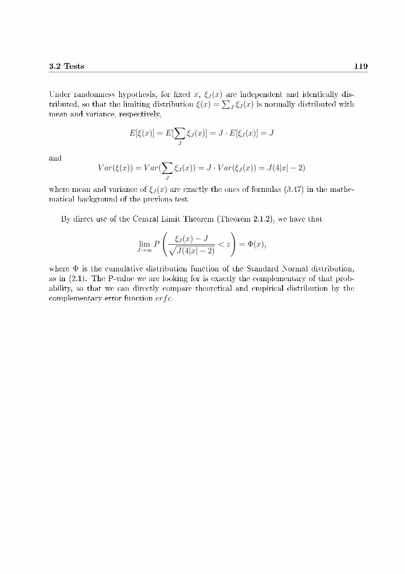
3.2 Tests 119
Under randomness hypothesis, for xed x, ξJ(x) are independent and identically dis-tributed, so that the limiting distribution ξ(x) =
∑J ξJ(x) is normally distributed with
mean and variance, respectively,
E[ξ(x)] = E[∑J
ξJ(x)] = J · E[ξJ(x)] = J
andV ar(ξ(x)) = V ar(
∑J
ξJ(x)) = J · V ar(ξJ(x)) = J(4|x| − 2)
where mean and variance of ξJ(x) are exactly the ones of formulas (3.47) in the mathe-matical background of the previous test.
By direct use of the Central Limit Theorem (Theorem 2.1.2), we have that
limJ→∞
P
(ξJ(x)− J√J(4|x| − 2)
< z
)= Φ(x),
where Φ is the cumulative distribution function of the Standard Normal distribution,as in (2.1). The P-value we are looking for is exactly the complementary of that prob-ability, so that we can directly compare theoretical and empirical distribution by thecomplementary error function erfc.

120 3. Statistical tests for randomness

Chapter 4
Properties of a RNG
In this section we want to study the eciency of a RNG. As discussed in section(3.1), a single test on a single sequence is not enough to assess whether or not an RNGgenerates random sequences. A second level testing is necessary to give a response witha certain level of condence, computing the probability that a truly random sequence sfails one or more tests. For briefness, in this section we will consider each sub-test as adierent test so that we'll have a total of 188 test.
Let's suppose to test a single sequence, which length is consistent with tests require-ments, on k tests. The probability that a truly random sequence s fails a test is α and theprobability that it passes it is it's complementary 1− α, as from our hypothesis, so thatthe probability P (k, k) that k, with k ≤ k, tests are passed has a binomial distribution(2.2.3), so that we obtain
P (k, k) =
(k
k
)(1− α)kαk−k. (4.1)
By this formula, using α = 0.01, the probability that a single sequence passes all the188 tests (by considering each sub-test as a dierent test) is 0.99188 = 0.15 = 15%. Thisshows that we should take into account that, as a test-passing doesn't mean that ourdata is random, a fail doesn't give evidence of non randomness, but multiple tests haveto be performed.
Sýs et al. ([69]) by using 100 GB of data from a good random generator ([19])computed the empirical probability that a sequence fails exactly i test and the empiricalprobability that it fails i or more tests, comparing them with theoretical probabilitiesof formula (4.1). Their analysis was made both in the case that all the 188 test wasapplicable and in the case that Random Excursion test and its Variant were not applicable(since the Random Excursion tests require a sequences which length is on the order of
121
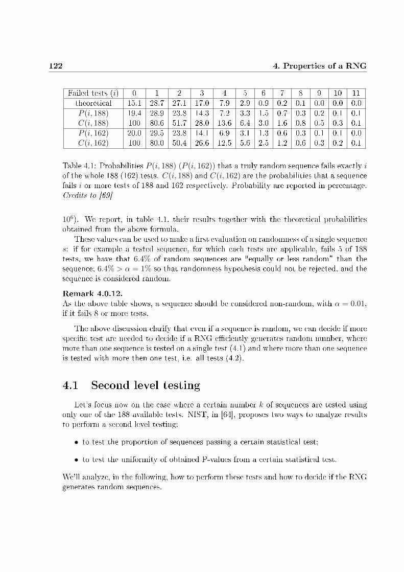
122 4. Properties of a RNG
Failed tests (i) 0 1 2 3 4 5 6 7 8 9 10 11theoretical 15.1 28.7 27.1 17.0 7.9 2.9 0.9 0.2 0.1 0.0 0.0 0.0P (i, 188) 19.4 28.9 23.8 14.3 7.2 3.3 1.5 0.7 0.3 0.2 0.1 0.1C(i, 188) 100 80.6 51.7 28.0 13.6 6.4 3.0 1.6 0.8 0.5 0.3 0.1P (i, 162) 20.0 29.5 23.8 14.1 6.9 3.1 1.3 0.6 0.3 0.1 0.1 0.0C(i, 162) 100 80.0 50.4 26.6 12.5 5.6 2.5 1.2 0.6 0.3 0.2 0.1
Table 4.1: Probabilities P (i, 188) (P (i, 162)) that a truly random sequence fails exactly iof the whole 188 (162) tests. C(i, 188) and C(i, 162) are the probabilities that a sequencefails i or more tests of 188 and 162 respectively. Probability are reported in percentage.Credits to [69]
106). We report, in table 4.1, their results together with the theoretical probabilitiesobtained from the above formula.
These values can be used to make a rst evaluation on randomness of a single sequences: if for example a tested sequence, for which each tests are applicable, fails 5 of 188tests, we have that 6.4% of random sequences are "equally or less random" than thesequence; 6.4% > α = 1% so that randomness hypothesis could not be rejected, and thesequence is considered random.
Remark 4.0.12.As the above table shows, a sequence should be considered non-random, with α = 0.01,if it fails 8 or more tests.
The above discussion clarify that even if a sequence is random, we can decide if morespecic test are needed to decide if a RNG eciently generates random number, wheremore than one sequence is tested on a single test (4.1) and where more than one sequenceis tested with more then one test, i.e. all tests (4.2).
4.1 Second level testing
Let's focus now on the case where a certain number k of sequences are tested usingonly one of the 188 available tests. NIST, in [64], proposes two ways to analyze resultsto perform a second level testing:
• to test the proportion of sequences passing a certain statistical test;
• to test the uniformity of obtained P-values from a certain statistical test.
We'll analyze, in the following, how to perform these tests and how to decide if the RNGgenerates random sequences.

4.1 Second level testing 123
4.1.1 Test for proportion of sequences passing a test
Let's suppose to test k sequences on a certain test and that the number of sequences
passing it is k, whit k ≤ k, so that ν = kkis the proportion of sequences passing the test.
This value has to fall between the condence interval, which is dened by
(1− α)± c√α(1− α)
k, (4.2)
where the value c is the critical value, i.e. the value which splits the domain of ourstatistic between the values which have a probability greater than the signicance levelα and lower than α, as shown in the gure below1, and the term under the square root isthe standard error of the statistic (standard normal, under randomness hypothesis). Thetwo terms together give us the margin of error our analysis has: the more the sequenceswe test, the more this error is small.
Figure 4.1: Standard Normal Distribution and critical values. Credits to [47].
If we choose α = 0.01 and c = 3, as NIST, we have that, to pass a test, the proportionof sequence passing that has to be in the range
0.99± 3
√0.01 · 0.99
k(4.3)
so that if, for example, we are testing k = 1000 sequences, the passing rate has to fallin the interval 0.99± 0.0094392. If the proportion falls outside this interval, we considerthe chosen test not passed by our RNG. We should observe that the value c = 3 is an
1Tables of critical values can be found, for example, in [1] or inhttps://www.itl.nist.gov/div898/handbook/eda/section3/eda3671.htm
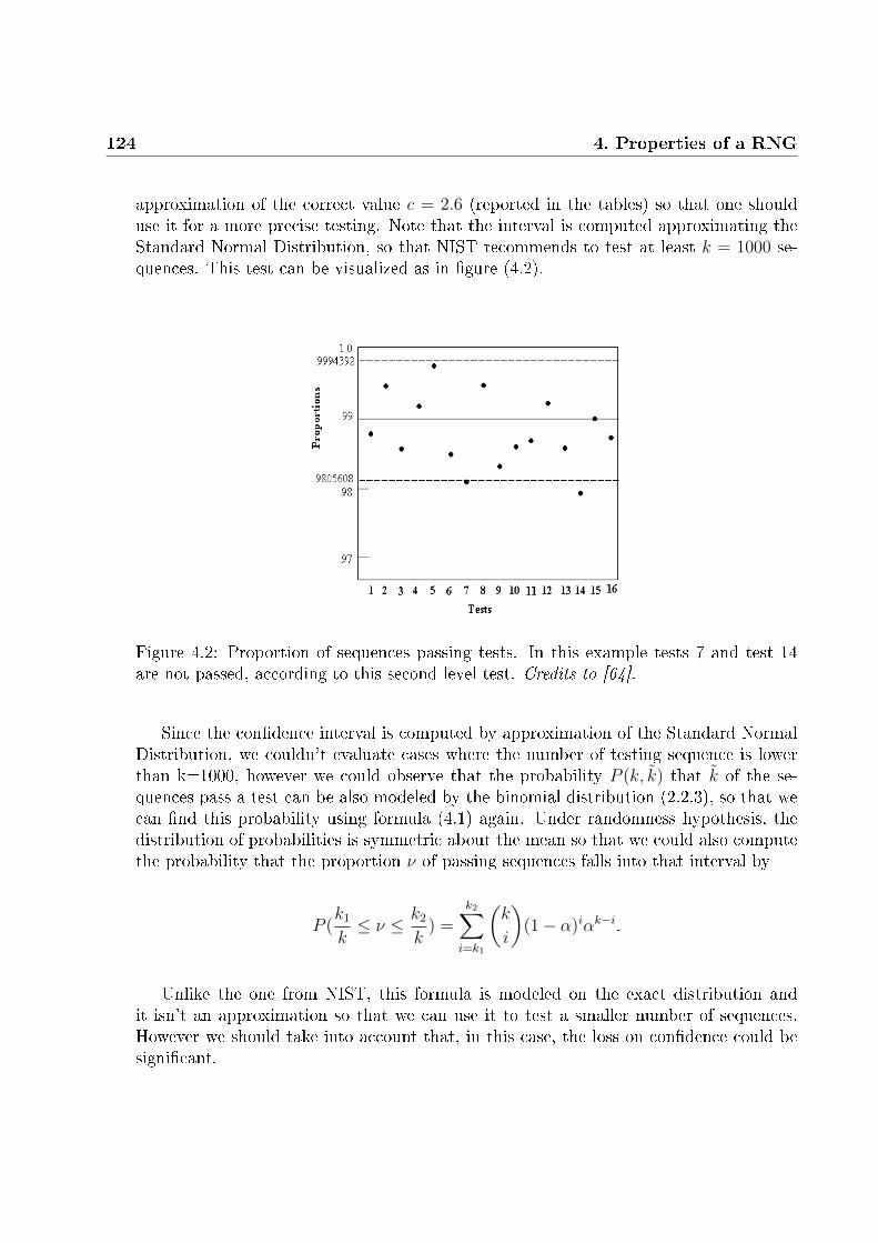
124 4. Properties of a RNG
approximation of the correct value c = 2.6 (reported in the tables) so that one shoulduse it for a more precise testing. Note that the interval is computed approximating theStandard Normal Distribution, so that NIST recommends to test at least k = 1000 se-quences. This test can be visualized as in gure (4.2).
Figure 4.2: Proportion of sequences passing tests. In this example tests 7 and test 14are not passed, according to this second level test. Credits to [64].
Since the condence interval is computed by approximation of the Standard NormalDistribution, we couldn't evaluate cases where the number of testing sequence is lowerthan k=1000, however we could observe that the probability P (k, k) that k of the se-quences pass a test can be also modeled by the binomial distribution (2.2.3), so that wecan nd this probability using formula (4.1) again. Under randomness hypothesis, thedistribution of probabilities is symmetric about the mean so that we could also computethe probability that the proportion ν of passing sequences falls into that interval by
P (k1
k≤ ν ≤ k2
k) =
k2∑i=k1
(k
i
)(1− α)iαk−i.
Unlike the one from NIST, this formula is modeled on the exact distribution andit isn't an approximation so that we can use it to test a smaller number of sequences.However we should take into account that, in this case, the loss on condence could besignicant.

4.1 Second level testing 125
4.1.2 Test for uniformity of P-values
Under randomness hypothesis H0, P-values obtained by dierent sequences by thesame test have to be uniformly distributed, so that this uniformity forms a hypothesisitself, which can be statistically tested. This can be done by a χ2 goodness-of-t test(3.1.1) by splitting the interval [0, 1] which contains P-values into classes (NIST suiteuses 10 classes), compute the frequency Fi of P-values falling into each classes e comparethem by the use of a χ2 statistic, which will have a number of degrees of freedom equalto the number of chosen intervals. By uniformity, if we are examining k P-values (i.e.k sequences), each theoretical frequency will be k/10, so that the statistic will have theform
χ2 =10∑i=1
(Fi − k10
)2
k10
.
As before we can compute the P-value of the statistic by the use of the incompletegamma function, as
P-valueT = igamc(9
2,χ2
2)
and see whether or not this P-values is greater than the signicance level2 αT , whichin this case should be set at 0.0001. If P-valueT < 0.0001 the generator is consideredto create sequence too similar one another, and the test is considered not passed. Weshould note that this test provides a good approximation for k/10 ≥ 5.5, so that at least55 sequences as to be tested to obtain meaningful results.
This test can also be visualized by the use of an histogram, as in gure 4.1.2.
Remark 4.1.1.We should take into account that failing this test doesn't necessarily mean that sequencesare non-random themselves, but that the Random Number Generator is not a goodrandom number generator since it creates sequences which are very similar one another.In other words, even if each sequence could behave as if it's eectively random, inspectingmore sequences together shows evidence that created bits are non-random.
2Note that this signicance level αT refers the second level uniformity testing and it's independentby the level of signicance α one chooses for individual tests

126 4. Properties of a RNG
Figure 4.3: Visualization of the test for the uniformity of P-values. Credits to [64].
4.2 Complete testing
We want to discuss, in this section, the most common and complete case where manysequences are tested using all of the 188 tests of the suite. This nal analysis can beperformed by comparing P-values obtained from a set of tests by a set of sequence, bycomparing the proportion of sequences passing more than one test and by comparing theP-values from the uniformity test.
4.2.1 Set of tests
If we are performing a set of tests on a set of sequences s1, . . . , sk, we should takeinto account that on hypothesis of independence between tests, the probability to faila test is the same of any other test and that the probability of passing more than onetest (i.e. the intersection) factorizes. By this observation, it's clear that we can make anevaluation by the use of the table at the beginning of this chapter as follows:
i) For each test sj, consider the number of tests kj it failed.
ii) Let Cj be the probability that a test fails kj or more tests (the applicability of theRandom Excursion tests should be taken into account), compute the product ofthese probabilities
p =k∏j=1
Cj,
which is the probability that k random sequences are less random than s1, . . . , sk.

4.2 Complete testing 127
iii) If p > α, sequences s1, . . . , sk can be considered random, otherwise the randomnesshypothesis is rejected.
For example, if we are testing two sequences s1 and s2 which failed respectively 1and 2 tests we have that C1 = 0.806 and C2 = 0.504, so that the probability to have twosequences which are less random than the tested one is p = 0.806 · 0.504 = 0.406 > α, sothat the two sequences are considered random.
4.2.2 Proportion of sequences passing more than one test
As we have seen in section (4.1.1), a set of k sequences could be examined througheach test by the evaluation of the proportion of sequences passing that specic test. Inorder to give a more complete answer to the "does my RNG produces random sequences?"question, one should consider if the passing rate of RNG's output of the whole batteryof tests (i.e. the inspection by any point of view) is consistent to what expected froma Random Number Generator which eectively generates random numbers. To do that,one can compare his results to the ones obtained by Sýs et al. in [69] by extensivesimulations on sets of k = 100 and k = 1000 sequences. Results are reported, in thefollowing table, by taking either the constant c of the test as approximated by NIST (i.e.c = 3) and the more accurate value c = 2.6.
Failed tests (i) 0 1 2 3 4 5 6 7 8 9 10 11 12theoretical 15.1 28.7 27.1 17.0 7.9 2.9 0.9 0.2 0.1 0 0 0 0observed 46.9 33.7 14.7 4.3 0.5 0 0 0 0 0 0 0 0C(103, 3) 100 53.1 19.4 4.8 0.5 0 0 0 0 0 0 0 0C(103, 2.6) 100 79.2 48.6 25.2 9.4 3.2 1.2 0.6 0.1 0 0 0 0C(102, 3) 100 95.9 84.3 66.3 45.6 28.1 15.6 8.2 4.1 1.8 0.8 0.3 0.2
Table 4.2: Probabilities that random sequences fail exactly i out of 188 proportion tests,and cumulative probabilities that a set of k = 100 and k = 1000 sequences fail i ormore proportion tests. Cumulative probabilities, obtained by extensive simulations, arecomputed both for c = 3 and c = 2.6. Values are reported in percentage. Credits to [69]
These probabilities can be used to assess the randomness of a set of sequences asfollows: let's suppose to test k = 1000 sequences through the whole battery of tests andto perform the test for proportion to all of them. Assume that 4 tests of proportionare failed: using the constant c = 3 proposed by NIST, the probability to obtain anequivalent or worst case from a good-working RNG is 0.5% which is smaller than thesignicance level α = 1%; tested sequences can be considered non-random. On the otherhand, if we assume the constant c = 2.6, the probability that sequences fail 4 or moretest is 9.4% which is grater than the signicance level α, so that we can consider our

128 4. Properties of a RNG
sequences random. In cases like the one we just proposed is recommended to test anotherset of sequences obtained from the RNG, in order to make a more accurate answer.
Remark 4.2.1.A set of k = 100 sequences should be considered non-random if it fails 11 or more testfor the proportion of sequences passing a test.Similarly, a set of k = 1000 sequences should be considered non-random if it fails 8 ormore test for the proportion of sequences passing a test.Take into account that the more the sequences we test, the more is the condence we havefrom results: to test 1000 sequences is recommended, however, if for some reasons (suchas computation limits) this is not possible, to make this test on a set of 100 sequencesalso produces reliable results.
4.2.3 Uniformity of P-values from multiple tests
Let's suppose to test k = 100 sequences and to make the test for uniformity of P-values (4.1.2) for each of the 188 test, obtaining 188 P-values (i.e. 188 passed/failedresponses). Results can be compared to the probability obtained by Sýs et al. in [69]through extensive simulations on 8192 sets of k = 100 sequences, which are reported inthe following table together with the theoretical probabilities.
Failed tests (i) 0 1 2 3 4 5 6 7 8 9theoretical 15.1 28.7 27.1 17.0 7.9 2.9 0.9 0.2 0.1 0.0observed 11.3 24.8 26.6 19.0 10.8 4.8 1.8 0.5 0.2 0.1
C, αT = 1% 100 88.7 63.9 37.3 18.3 7.5 2.7 0.85 0.33 0.09C, αT = 0.1% 100 21.8 3.1 0 0 0 0 0 0 0C, αT = 0.01% 100 3.3 0.12 0 0 0 0 0 0 0
Table 4.3: Probabilities that 100 random sequences fail exactly i uniformity testsand cumulative probabilities that the set fails i or more uniformity tests for αT =0.01, 0.001, 0.0001 (values are reported in percentage). Note that αT is not the sig-nicance level of individual tests, but the signicance level of the second level uniformitytest. Credits to [69]
If, for example, we test 100 sequences using the whole 188 tests and the uniformitytest is failed for 5 tests (i.e. 5 of the whole 188 P-values obtained from the test foruniformity of P-values are lower than 0.0001) the probability that this occurs for trulyrandom sequences is 0, which is obviously smaller than α = 0.01%, so that the datacould be considered non-random since the tested RNG produces sequences which arenon uniform.
4.2 Complete testing 129
Remark 4.2.2.A set of k = 100 sequences should be considered non-random if it fails 7 or more uni-formity test (with the classical condence level α = 0.01). For smaller condence levels,such as α = 0.001 or α = 0.0001, the maximum number of failed test to consider the setrandom is 2.Testing only 100 sequences through this test could be considered enough since, as dis-cussed in section (4.1.2), this test produces a good characterization of the random gen-erator, however it doesn't bring a real answer on the randomness of the sequences.Anyhow, failing this test should be taken in account, since that indicates that the RNGproduces sequences which could be similar one another, although their behavior couldbe considered random.

130 4. Properties of a RNG

Chapter 5
Testing ECU's RNG
We studied how each of the 15 tests work, we saw how to perform a second leveltesting and how to evaluate whether a certain RNG is working properly or not, ana-lyzing if randomness properties are satised and if generated sequences are sucientlydierent one another. Now we want to describe how we checked the good behavior ofour implementation and how to test the RNG embedded into an ECUs.
The main purpose of our work was to make an implementation which makes possibleto completely test ECU's RNG by simply connect the target ECU to the computer,without the need of any other actions. To do that we decided, rst of all, to implementthe whole test suite by the use of MatLab [48] which allows to perform in the easiestway all mathematical tasks of each test. After that, we embedded the whole test suitein CANoe [70], a software which permits to interact with ECUs: we'll describe this stepin section 5.2. We will report examples of each step of the implementation process inappendix A.
5.1 Validation of MatLab codes
To check our implementation we assumed that the one wrote by NIST in C languageis correct and we compared P-values (and any other output) we obtained from our code tothe ones one obtains testing the same sequences through the NIST test suite, available athttps://csrc.nist.gov/projects/random-bit-generation/documentation-and-software.Due to reproducibility reasons we decided to make the comparison using the binary ex-pansion of some classical values, i.e. π, e,
√2 and
√3, truncated to 106 digits, which is
the recommended length for sequences to test. Figures from 5.1 to 5.4 show the behaviorof P-values for the four sequences and the relative error between our results and NIST's.
As gures show, the error of our implementation is attested between the machine
131

132 5. Testing ECU's RNG
accuracy of MatLab, which is 2.2204 · 10−16, and 10−8. The grater error is obtainedby test 11 and test 12, i.e. the serial test and the approximate entropy test: the errorremains close to the MatLab epsilon and to 10−14 through the whole respective test, sincevalues which carries the error (frequencies vm, vm−1 and vm−2 for test 11 and the value ofthe approximate entropy ApEn) are multiplied, respectively, to 2m = 216 ∼ 0.6 · 105 andto n = 106. According to error analysis theory, this multiplication produces the rising oferrors to our values: anyway, we should observe that, since the level of signicance α istypically chosen as 0.01 or 0.001 and it wouldn't be meaningful to choose a lower value,this error doesn't ruin our implementation since one would always be interested up tothe third or fourth signicant gure.
0 2 4 6 8 10 12 14 1610
−2
10−1
100
PV comparison (pi)
NIST P−ValuesP−Values
0 2 4 6 8 10 12 14 1610
−16
10−15
10−14
10−13
10−12
10−11
10−10
10−9
10−8
Relative Error (pi)
Figure 5.1: P-values and respective relative errors for binary expansion of π.
Remark 5.1.1.Successive implementations (i.e. the Simulink models and their porting into CANoe)were also checked to ensure that each value one obtains using the CANoe implementationis correct: to do that we used values obtained from our MatLab code as the xed pointof the whole process, from single tests to the complete testing of 1000 sequences.

5.1 Validation of MatLab codes 133
0 2 4 6 8 10 12 14 1610
−2
10−1
100
PV comparison (e)
NIST P−ValuesP−Values
0 2 4 6 8 10 12 14 1610
−16
10−15
10−14
10−13
10−12
10−11
10−10
10−9
10−8
Relative Error (e)
Figure 5.2: P-values and respective relative errors for binary expansion of e.
0 2 4 6 8 10 12 14 1610
−2
10−1
100
PV comparison (sqrt2)
NIST P−ValuesP−Values
0 2 4 6 8 10 12 14 1610
−16
10−15
10−14
10−13
10−12
10−11
10−10
10−9
Relative Error (sqrt2)
Figure 5.3: P-values and respective relative errors for binary expansion of√
2
0 2 4 6 8 10 12 14 1610
−2
10−1
100
PV comparison (sqrt3)
NIST P−ValuesP−Values
0 2 4 6 8 10 12 14 1610
−16
10−15
10−14
10−13
10−12
10−11
10−10
10−9
10−8
Relative Error (sqrt3)
Figure 5.4: P-values and respective relative errors for binary expansion of√
3

134 5. Testing ECU's RNG
5.2 CANoe integration of test suite
Once we were sure that our MatLab codes were correct, we decided to bring thatcodes into CANoe and to use those same codes to test ECUs RNG. In this section wewish to give an overview of what CANoe is, how to use MatLab codes through the useof Simulink and Stateow and how to embed and use these things into CANoe.
5.2.1 Vector CANoe
CANoe [70] is a software developed by Vector Informatik GmbH since 1996: it permitsthe user, principally automotive manufacturers and electronic control unit suppliers, tointerface with an individual ECU or to a complete network in order to develop, makeanalysis, test and diagnosis. In particular CANoe can be used both to simulate a CAN-bus network (or a single ECU) without the need to materially build one, at the beginningof the production of a vehicle, and to diagnose malfunctions, when a car shows any typeof issue.
Connecting to a network through CANoe (by the use of a computer or by any otherdedicated hardware which supports it) it is possible to access the CAN-bus in order toread messages which ow in it or to send some to the system. Analogously, connectingan individual ECU allows to interact with it, to simulate the behavior when it is settogether with other ECUs (the software could simulate them) or to (re)program it.
The user interface of CANoe is based on many windows which user can show, hide,move or customize: each of these windows have dierent functionality and permits bothto extract information from the CAN-bus (e.g. to see messages on the bus, to read valuesof interest or to take trace of the telemetry) and to interact with the system (e.g. topush the brake pedal or to move the steering wheel, in a simulated environment or tosend a specic message via CAN-bus, in both simulated or real environment). Figure5.5 shows an example of these windows, together with their use.
Apart from windows showed in gure, another useful window is the measurementsetup window, which permits, on one hand, to choose if the simulation is performed inonline or oine mode and, on the other hand, to choose which value to observe or not; themeasurement setup also manages the saving of logging, i.e. the trace of last measurement.
The most useful window for simulations is the simulation setup window, showed ingure 5.6: it permits to choose the environment of the simulation. This window is fun-damental for development, since it allows the user to build the complete setup he wantsto simulate. Through this window it is possible to add an arbitrary number of blocks :each block represents an element of the environment and could be a node (nodes rep-resent ECUs of the simulated environments), a signal generator (it generates and sends

5.2 CANoe integration of test suite 135
Figure 5.5: CANoe interface example. This example is made of a control interface bywhich user can simulate the ignition, a graphics and data interface by which it is possibleto monitor values of interest (e.g. gear, engine and car speed as in this example), a testerwindow to choose the situation to test, an explorer to choose the object to observe anda trace window to trace messages which run inside of each CAN channel. Credits to [70].

136 5. Testing ECU's RNG
signals to the bus; signals could be random or customized: they are used to simulateextra hardware or bus, in addition to the ones of interest), a replay block (it reproducesa previous simulation, sending the same signals) or logging block (stores signals/mes-sages of interest). These blocks can be connected, in dierent ways, to create the desiredsimulation setup by simulated CAN-bus connections: it is possible to create (and eventu-ally connect) dierent network, where each network is provided of a dedicated CAN-bus(each network can then be interfaced to one or more networks through an ECU whichworks as a gateway). The ECU node, which is the one we are most interested in, is themost customizable one, since it represents the control unit and could simulate each of itsfunctions. It's possible to program each ECU node, dening its tasks, input and output:to do that each ECU node is provided with a script in CAPL1 language.
Figure 5.6: Example of a simulation setup window. This setup is made of four nodeswhich simulate ECUs (each of them endowed with its CAPL script), a signal generatorand a replay block: all of these nodes are connected by a CAN-bus and form a uniquenetwork.
Finally, there is a write window where values from the execution of CAPLs are printedtogether with error in compilation or execution and any other information useful for theuser.
1CAPL is a C-based programming language created by Vector Informatik GmbH: it contains mostof C main functions to which new functions are annexed. CAPL specic functions permit to managethe communication between nodes, e.g. by input and output variables, detecting if external variable arechanged or perform action when an external input is given (e.g. the vehicle is started).

5.2 CANoe integration of test suite 137
5.2.2 From MatLab to CANoe
Since the way to directly communicate with an ECU is the CANoe software, togetherwith a dedicated hardware to connect the ECU and the computer (showed in gure 5.7),we needed to export our MatLab functions to this software in order to use them. CANoeallows users to associate one or more DLLs2 to each ECU node, and call it inside of theCAPL script: this feature permitted us to embed our MatLab functions inside of ourconguration.
Figure 5.7: Vector Base Module: a dedicated hardware used to connect ECUs to acomputer. Credits to [70].
To create DLLs to embed in the CANoe conguration we used Simulink [49], aMatWorks graphical programming environment that permits to create models where op-erations are performed by graphical objects in the form of blocks and arrows: a blockcould stand for a variable, a constant, an operator and so on, while arrows are used toconnect blocks to dene inputs, outputs and relations between them. Simulink, obvi-ously, interface with MatLab: it is possible to use MatLab variables inside the Simuliunkmodel, to send values from the Simulink model to MatLab and also to use user denedMatLab functions through specic blocks (where the function can be wrote in a standardMatLab script). Simulink also interfaces with CANoe, allowing to convert models intoDLLs which could be compiled and used by CANoe (through calls inside of the CAPLscript): this can be done through the Vector CANoe add-on for Simulink, which providesthe cn.tlc target for the compiler (we used the Microsoft Visual C++ compiler [52] toexport Simulink models into DLLs).
Besides compatibility between Simulink and CANoe versions and formats, at thisstep, we had to take into account the limits of each software, in order to make the gen-
2Dynamic-Link Libraries: software libraries which can be dynamically loaded and compiled into aprogram or an executable le in order to execute them as part of the main software itself.

138 5. Testing ECU's RNG
erated DLLs working on CANoe: the main problem we had to overcome was the factthat CANoe couldn't deal with too long variable arrays and sequences we had to testhad to be at least 106 digits long. To overcome the problem we made use of the State-ow logic tool for Simulink: Stateow allows the user to create a nite-state machine3
as a Simulink block (called chart); we inserted a Stateow chart inside of our Simulinkmodel so that CANoe could deal with and send shorter parts of the sequence: the chartaccumulates the sequences till the end and, when it is complete, it sends the completearray to requested test(s).
Another requirement for the building of DLLs from Simulink was that, since gener-ated DLLs use static memory allocation, we couldn't create a model which containedthe whole test suite, so that we had to split tests inside of dierent models (dependingon the size of each test code) and link them all to the CANoe node. Figure 5.8 showscreated DLLs inside of the conguration window for a CANoe node.
Moreover, since Simulink allows to perform the discrete Fourier transform on vectorswhich length is a power of 2 only, our CANoe porting of the test suite requires it too:since, due to the asymptotic theory behind the test, 106 is the minimum allowed lengthwe decided to require a length of 220 = 1048576 for sequence to test, that is the rstpower of 2 value which is greater than 106. This requirement only applies to the testingthrough CANoe (i.e. directly test ECU's RNG): indeed we used 220-long sequences whenwe tested ECU's RNG through the CANoe suite and 106-long strings in other cases,through the MatLab implemetation.
All other tasks are submitted to the CAPL script, inside of CANoe: reading sequencesfrom les (or directly from the ECU), send inputs and outputs to models (that is doneby the use of particular CANoe variables, called system variables4), store results intoles and run the second level testing (also implemented by Simulink models) when asucient number of sequences was tested. After that, the CAPL checks if second leveltestings are passed or not, as described in the previous chapter, and writes nal resultson a le.
The general scheme of a complete testing execution could be summarized as follows:
1. the user chooses how many sequence to test (typically 100 or 1000 sequence arechosen), which test to perform, the desired level of signicance and if he wants to
3A model of computation which passes from a state to another depending on external inputs (e.g. itperforms the next step each time the function is called or each time a variable changes its value etc.).
4System variables are used in CANoe as variables which could be used in the whole conguration:while standard variables can be used inside each CAPL only (i.e. only for a node of the conguration),system variables can be used and modied by each node and sent to external functions, such as DLLs.

5.2 CANoe integration of test suite 139
Figure 5.8: Linked DLLs to a CANoe node. This gure shows the conguration of ourtest suite.
perform the second level testing (in the case he tested enough sequence on everytest);
2. CANoe reads the le which contains the binary sequence to test (or directly readsoutput values of ECU's RNG): a part of it is inserted into a system variables andsent to the DLL (i.e. the model), which waits and accumulate till the desired lengthis reached;
3. the Simulink model executes desired tests and sends results back to CANoe, by theuse of some other system variables.
That is done for each requested test on the whole set of sequences and results are storedinto le.
If the second level testing is requested, the process goes on:
4. results and P-values, of a specic test for all the tested sequences, are red from leswhich contains them and stored into dedicated system variables;
5. system variables are sent to other Simulink models that perform the second leveltesting and send results to CANoe.
This is performed for each test, obtaining 188 results from the test for proportion ofpassing and 188 results from the test for the uniformity of P-values: results are stored

140 5. Testing ECU's RNG
into les.
After that, the CAPL (i.e. CANoe) reads results from this second step and writes ale which contains the nal result (i.e. if or not the RNG passed the complete testing)using bounds of remarks 4.2.1 and 4.2.2, together with information from eventually not-passed tests and possible problems of the Generator.
5.2.3 Results from our implementation
Once we implemented the test suite, we decided to use it to test, apart from theRandom Number Generator embedded into two dierent ECUs, the randi function ofMatLab. This section reports main results of these validations.
randi results
The randi function creates random integers (single values, vectors or matrices)through a Pseudo Random algorithm: the PRNG used for this function is the sameof the rand and randn functions. randi generates values between 1 and the input, sothat to obtain a binary sequence one can use 2 as the max value and subtract it by aunitary vector, so that to generate a 106-length vector one can simply use the commandrandi(2, [106, 1]) − 1. We tested 1000 sequences, performing the whole test suite and,after that, the second level testing, in order to evaluate the goodness of the function.Table 5.1 shows the proportion of passing for each test, stored for type of test (i.e. testcomposed by more sub-tests are reported together)
For 1000 sequences, using bounds of formula (4.3), the proportion test is consideredto be passed if the proportion of passing lies inside the interval [0.9805, 0.9994], so that,to pass the proportion test, at least 981 of 1000 sequences have to pass a single test.In this case, the function randi passed 185 of 188 test for proportion (i.e. more than981 strings on 1000 passed a single test) and 187 of 188 uniformity test so that bothtest were passed and the PRNG embedded in MatLab could be considered to be a welldesigned and good working Random Number Generator (the acceptance ranges for 1000sequences are 180/188 and 182/188, respectively).
Histograms reported in gures 5.9 and 5.10 represent an example for the distributionof P-values of a passed and a failed uniformity test: respectively one of sub-tests of therandom excursion test and one of the sub-test of the non-overlapping template matchingtest (the only one which didn't pass the test for uniformity of P-values). As for the test,P-values are stored into 10 classes between 0 and 1.

5.2 CANoe integration of test suite 141
Test Proportion of passing Uniformity pass rateFrequency 979/1000 1/1Frequency within a block 990/1000 1/1Runs 988/1000 1/1Longest run of ones 990/1000 1/1Matrix rank 987/1000 1/1DFT 994/1000 1/1Non-overlapping 146526/148000 147/148Overlapping 992/1000 1/1Maurer 987/1000 1/1Linear complexity 991/1000 1/1Serial 1982/2000 2/2Approximate Entropy 991/1000 1/1Cumulative sums 1969/2000 2/2Random excursions 7893/8000 8/8Random excursions variant 17786/18000 18/18
Table 5.1: Results from second level testing of randi output: eventual sub-tests areadded together.
Figure 5.9: Histogram for a passed uniformity test: random excursion test (one of the8 sub-tests). The number of P-values into each class is suciently close to a uniformdistribution.

142 5. Testing ECU's RNG
Figure 5.10: Histogram for a failed uniformity test: non-overlapping template matchingtest (one of the whole 148). The number of P-values into each class is far from a uniformdistribution: in particular, compared to other classes, there is a huge disproportionbetween the number of P-values falling into the interval [0.8, 0.9[ (66 P-values).
TRNG results
ECUs at our disposal were provided with a True Random Number Generator, pro-duced by Inneon Technologies [31], of which we was not aware of the structure: in thiscase it's very important to validate the Generator, in order to make sure that everythingworks as it has to do. Moreover, apart from the structure of the TRNG (which couldbe known or unknown), it often happens that RNG's output values are used and pro-cessed by various software functions: it becomes fundamental, then, to ensure that thesefunctions don't spoil produced randomness, for example by adding some recurrences orhidden structures.
Due to the, relatively higher compared to the MatLab PRNG, time to generate ahuge amount of digits and the need to convert these value from binary format to ASCII,we decided to perform the testing on 100 sequences only which length, due to the portingby the use of Simulink (as described in the previous section), was 220.Table 5.2 reports results we obtained from the second level testing applied to ECU'sTRNG, in the same format of results from the randi function.
For 100 sequences, using bounds of formula (4.3), the proportion test is consideredto be passed if the proportion of passing lies inside the interval [0.9641, 1.0159], so that,to pass the proportion test, at least 97 of 100 sequences have to pass a single test.In this case, the TRNG passed 178 of 188 test for proportion and 183 of 188 uniformitytest (the acceptance ranges for 100 sequences are 177/188 and 182/188, respectively), sothat both test were passed and the TRNG could be considered to be a well designed and

5.2 CANoe integration of test suite 143
good working Random Number Generator.
Test Proportion of passing Uniformity pass rateFrequency 99/100 1/1Frequency within a block 95/100 1/1Runs 98/100 1/1Longest run of ones 99/100 1/1Matrix rank 99/100 1/1DFT 96/100 1/1Non-overlapping 14615/14800 145/148Overlapping 99/100 1/1Maurer 100/100 1/1Linear complexity 99/100 1/1Serial 198/200 1/2Approximate Entropy 99/100 1/1Cumulative sums 200/200 2/2Random excursions 792/800 7/8Random excursions variant 1764/1800 17/18
Table 5.2: Results from second level testing of TRNG's output: eventual sub-tests areadded together.
As for the previous, histograms reported in gures 5.11 and 5.12 represent an examplefor the distribution of P-values of a passed and a failed uniformity test: respectively thelinear complexity test and one of the sub-tests of non-overlapping template matchingtest.

144 5. Testing ECU's RNG
Figure 5.11: Histogram for a passed uniformity test: linear complexity test. The numberof P-values into each class is suciently close to a uniform distribution.
Figure 5.12: Histogram for a failed uniformity test: non-overlapping template matchingtest (one of the whole 148). The number of P-values into each class is far from a uniformdistribution: in particular, compared to other classes, there is a disproportion betweenthe number of P-values falling into intervals [0.6, 0.7[ (3 P-values) and [0.8, 0.9[ (23 P-values).

5.2 CANoe integration of test suite 145
PRNG results
We also had the opportunity to test the PRNG embedded into an old ECU whichgenerated numbers using a not performing method. The inspected PRNG generatednumbers between 0 and 255 in hexadecimal format: in order to test them by the testsuite, we converted numbers into binary format and we built 220-long sequences byconcatenating them.
We tested, as for the TRNG, 100 sequences: the PRNG didn't pass the test, sincegenerated sequences passed only 53 of 188 tests for proportion and 44 of 188 uniformitytests. That shows that generated numbers were non-random and that they were similarone another. Table 5.3 reports results from the second level testing.
Test Proportion of passing Uniformity pass rateFrequency 0/100 0/1Frequency within a block 0/100 0/1Runs 0/100 0/1Longest run of ones 75/100 0/1Matrix rank 100/100 1/1DFT 0/100 0/1Non-overlapping 8198/14800 28/148Overlapping 3/100 0/1Maurer 51/100 0/1Linear complexity 100/100 1/1Serial 103/200 1/2Approximate Entropy 0/100 0/1Cumulative sums 0/200 0/2Random excursions 755/800 3/8Random excursions variant 1771/1800 10/18
Table 5.3: Results from second level testing of PRNG's output: eventual sub-tests areadded together.
Histograms reported in gures 5.13 and 5.14 show an example of a passed and a faileduniformity test, respectively: the binary matrix rank test and the longest run of ones ina block test.

146 5. Testing ECU's RNG
Figure 5.13: Histogram for a passed uniformity test: binary matrix rank test. Thenumber of P-values into each class is suciently close to a uniform distribution.
Figure 5.14: Histogram for a failed uniformity test: longest run of ones in a block. Thenumber of P-values into each class is far from a uniform distribution: in particular,compared to other classes, there is a huge disproportion between the number of P-valuesfalling into interval [0, 0.1[ (51 P-values) and other intervals.

Conclusions
We opened this thesis with an overview of the ECUs structure of modern vehicles,focusing on possible entry points and hackings. We described typical use of randomnessin cryptography and, in particular, of how random numbers are used in the cyber secu-rity system of vehicles together with an idea of what a lack on randomness, derived froma problem of the embedded RNG, could imply.
The main aim of this thesis is to study randomness so that we analyzed the generalprocedure to perform a statistical test. That permitted us to focus on the more speciccase of statistical tests for randomness, by describing it and proposing theoretical basesand proofs for each them. Tests are then placed together to obtain the answer we werelooking for, i.e. to know whether or not the RNG is working properly, through a secondlevel testing on previously obtained results.
We nally reached the point where we used all of these information to build a methodto validate RNGs: we did that through MatLab and Simulink, in order to use them intoCANoe. Finally we could use our implementation to, positively, evaluate randomnessof the True Random Number Generator embedded into our ECU and of the MatLab'sPseudo Random Generator.
This constructions obviously has its limits: by this test suite it is impossible todistinguish a Pseudo Random Number Generator from a True one, and that could bea not trivial trouble for cryptographic purposes. Moreover, the 15 tests of this suitecouldn't fulll all possible aspect of randomness (in fact none nite number can do it)so that this suite could be extended, if new tests uncover.
147

148 5. Testing ECU's RNG

Appendix A
Examples from implementation
This appendix is intended to give the reader an example of our implementation, pre-senting two samples of MatLab code for single test (in particular codes described in3.2.11 and 3.2.14) and, after those, an example of one of the Simulink models (the onerelevant to test from 1 to 3: other models are approximately the same).
1 function [R,PVs ,S_obs ,err]= serial_test(s,alpha ,m)
2 % Test 11: Serial test3 % INPUT: s = binary string to test (array)4 % alpha = level of significance5 % m = length of templates to analyze6 % OUTPUT: R = results (#2)7 % PVs = P−value for each statistic (#2)8 % S_obs = values of the statistic (#2)9 % err = error from the execution
10 % RECOMM: choose m < log2(n)−211
12 % default length of window13 if nargin ==2
14 m=16;
15 end
16
17 % pre−allocation of used values18 R=NaN*zeros (2,1);
19 PVs=R;
20 S_obs=R;
21 err=ERRORS.NO_ERROR;
22
23 % sequence is non−empty
149

150 A. Examples from implementation
24 n=length(s);
25 if n==0
26 err=ERRORS.GENERIC;
27 return
28 end
29
30 % form augmented sequence and initialize frequency vectors31 s=vertcat(s,s(1:m-1));
32 vm=zeros (2^m,1);
33 v1=zeros (2^(m-1) ,1);
34 v2=zeros (2^(m-2) ,1);
35
36 % count occurrences37 i=1;
38 while i+m-1<= length(s)
39 if m==0 || m==-1
40 break
41 end
42 % convert patterns into respective decimal value (index)43 index=binvec2dec(s(i:i+m-1))+1;
44 vm(index)=vm(index)+1;
45 i=i+1;
46 end
47 i=1;
48 while i+m-1<= length(s)
49 if m-1==0 || m-1==-1
50 break
51 end
52 index=binvec2dec(s(i:i+m-2))+1;
53 v1(index)=v1(index)+1;
54 i=i+1;
55 end
56 i=1;
57 while i+m-1<= length(s)
58 if m-2==0 || m-2==-1
59 break
60 end
61 index=binvec2dec(s(i:i+m-3))+1;
62 v2(index)=v2(index)+1;
63 i=i+1;
64 end

151
65
66 % compute values of statistics67 psim =0;
68 psi1 =0;
69 psi2 =0;
70 if m~=0 && m~=-1
71 psim =2^m/n*sum(vm.^2)-n;
72 end
73 if m-1~=0 && m-1~=-1
74 psi1 =2^(m-1)/n*sum(v1.^2)-n;
75 end
76 if m-2~=0 && m-2~=-1
77 psi2 =2^(m-2)/n*sum(v2.^2)-n;
78 end
79
80 % compute distances81 nabla=psim -psi1;
82 nabla2=psim -2* psi1+psi2;
83 S_obs (1)=nabla;
84 S_obs (2)=nabla2;
85
86 % compute P−values and check results87 PVs (1)=gammainc(nabla /2 ,2^(m-1)/2,'upper ');
88 PVs (2)=gammainc(nabla2 /2,2^(m-2)/2,'upper ');
89
90 if PVs(1)<alpha
91 R(1)=RESULTS.FAILED;
92 else
93 R(1)=RESULTS.PASSED;
94 end
95
96 if PVs(2)<alpha
97 R(2)=RESULTS.FAILED;
98 else
99 R(2)=RESULTS.PASSED;
100 end

152 A. Examples from implementation
1 function [R,PVs ,S_obs ,err]= random_excursions_test(s,alpha)
2 % Test 14: Random excursions test3 % INPUT: s = binary string to test (vector)4 % alpha = level of significance5 % OUTPUT: R = results (#8)6 % PVs = P−value for each state x (#8)7 % S_obs = values of statistics (#8)8 % error = error from the execution9
10 % pre−allocation of used values11 R=NaN*ones (8,1);
12 PV=R;
13 S_obs=R;
14 err=ERRORS.NO_ERROR;
15
16 % sequence is non−empty17 n=length(s);
18 if n==0
19 err=ERRORS.GENERIC;
20 return
21 end
22
23 % Compute partial sums (random walk)24 s=2*s-ones(size(s)); % 0,1 to −1,125 S=zeros(n,1);
26 S(1)=s(1);
27 for i=2:n
28 S(i)=S(i-1)+s(i);
29 end
30
31 % Compute number of 0s in S2 (i.e. #cycles)32 S2=[0; S; 0];
33 J=nnz(~S2) -1;
34 if J<500 % check on number of cycles35 R=RESULTS.FAILED;
36 return
37 end
38
39 % compute occurrences of values inside each cycle40 table=zeros(8,J);
41 j=1;

153
42 i=2;
43 while j<=J
44 while S2(i)~=0
45 el=S2(i);
46 if el >-5 && el <5
47 if el <0
48 table(el+5,j)=table(el+5,j)+1;
49 else
50 table(el+4,j)=table(el+4,j)+1;
51 end
52 end
53 i=i+1;
54 end
55 i=i+1;
56 j=j+1;
57 end
58
59 % compute frequencies, statistic and P−value for each statex=−4,...,−1,1,...4
60 PVs=zeros (8,1);
61 S_obs=zeros (8,1);
62 for i=1:8
63 v=zeros (6,1);
64 for j=0:4 % compute frequencies65 v(j+1)=sum(table(i,:)==j);
66 end
67 v(6)=sum(table(i,:) >4);
68 p=p_table_aux(i); % pre−allocate probabilities69 chi=chi_stat(v,p,J); % chi−squared statistic70 S_obs(i)=chi;
71 PVs(i)=gammainc(chi/2,5/2,'upper'); % P−values72 if PVs(i)<alpha % results73 R(i)=RESULTS.FAILED;
74 else
75 R(i)=RESULTS.PASSED;
76 end
77 end

154 A. Examples from implementation
Figure A.1: Example of Simulink model. The yellow block is the Stateow chart, wherethe sequence is build from 1000-bit sub-blocks; the red block initializes outputs to −1:if the test is not executed, the only value of an eventual error is updated; blue blockscontain MatLab functions for tests; the gray block updates outputs to the last executedtest.

Bibliography
[1] Abramowitz M. and Stegun I., Handbook of Mathematical Functions, U.S. Govern-ment Printing Oce, Washington, 1967.
[2] ANSI X9.62-2005, Public Key Cryptography for the Financial Services Industry: TheElliptic Curve Digital Signature Algorithm, American National Standard for FinancialServices, 2005.
[3] Baron M. and Rukhin A., Distribution of the Number of Visits for a Random Walk,Communications in Statistics: Stochastic Models Vol. 15, 1999, pp. 593-597.
[4] Barker E. and Kelsey J., NIST Special Publication 800-90A: Recommendation forRandom Number Generation Using Deterministic Random Bit Generators, NationalInstitute of Standards and Technology, 2012.
[5] Bartlett M. S., The frequency goodness of t test for probability chains, Proc. Cam-bridge Philos. Soc. 47. 1951, pp. 86-95.
[6] Billingsley P., Convergence of Probability Measure, J. Wiley, New York, 1968.
[7] Bracewell R. N., The Fourier Transform and Its Applications, McGraw-Hill, NewYork, 1986.
[8] Bragaglia E., Analysis and partial solutions of security problems in automotive envi-ronments, Master's thesis in Mathematics, University of Bologna, 2013.
[9] Burgin M., Generalized Kolmogorov complexity and duality in theory of computations,Notices of the Russian Academy of Sciences, 1982.
[10] Caelli W., Crypt-X package documentation, Tech. Rep., Information Security Re-search, 1992.
[11] Calude C. S., Information and Randomness: An Algorithmic Perspective, Springer-Verlag, 2002, pp. 95-233.
155

156 BIBLIOGRAPHY
[12] Chaitin G., On the Simplicity and Speed of Programs for Computing Innite Sets ofNatural Numbers, Journal of the ACM, 1969, pp. 407-422.
[13] Chaitin G., Randomness and mathematical proof, Scientic American. 1975, pp.47-52.
[14] Chevillard S., The functions erf and erfc computed with arbitrary precision andexplicit error bounds, Information and Computation 216, 2012, pp. 72-95.
[15] Chung K. L., Elementary Probability Theory with Stochastic Processes, Springer-Verlag, New York, 1979, pp. 210-217.
[16] Chrysaphinou O. and Papastavridis O., A Limit Theorem on the Number of Over-lapping Appearances of a Pattern in a Sequence of Independent Trials, ProbabilityTheory and Related Fields Vol. 79, 1988, pp. 129-143.
[17] Coron J-S. and Naccache D., An accurate Evaluation of Maurer's Universal Test,Selected Areas in Cryptography. SAC 1998. Lecture Notes in Computer Science,Springer, Berlin, 1999.
[18] David F. N. and Barton D. E., Combinatorial Chance, Hafner Publishing Co., MewYork, 1962, pp. 228-230.
[19] Department of Physics of Humboldt University and Pico-Quant GmbH: nano-Opticsgroups, QRNG Service, www.qrng.physik.hu-berlin.de.
[20] Diananda P. H., The Central Limit Theorem for m-dependent variables asymptoti-cally stationary to second order, Proc. Camb. phil. Soc. 50, 1954, pp. 92-95
[21] Durrett R., Probability: Theory and Examples, Cambridge University Press, Cam-bridge, 2010.
[22] Feller W., An introduction to probability theory and its applications, J. Wiley, NewYork, 1968.
[23] Földes A., The limit distribution of the length of the longest head-run, PeriodicaMathematica Hungarica Vol. 10, Budapest, 1979, pp. 301-310.
[24] Gibbons J. D. and Chakraborti C., Nonparametric Statistical Inference, MarcelDekker, New York, 2003, pp. 50-58.
[25] Godbole A. P. and Papastavridis S. G., Runs and Patterns in Probability: selectedpapers, Kluwer Academic, Dordrecht, 1994.
[26] Good I. J., The serial test for sampling numbers and other tests for randomness,Proc. Cambridge Philos. Soc. 47, 1952, pp. 276-284.

BIBLIOGRAPHY 157
[27] Gustafson H., Dawson E., Nielsen L. and Caelli W., A computer package for mea-suring the strength of encryption algorithms, Computer and Security 13, 1994, pp.687-697.
[28] Hamano K., The Distribution of the Spectrum for the Discrete Fourier TransformTest Includen in SP800-22, IEICE Trans Fundamentals Vol. E88-A, 2005.
[29] Hamano K. and Kaneko T., The Correction of the Overlapping Template MatchingTest Included in NIST Randomness Test Suite, IEICE Transaction of Electronics,Communications and Computer Sciences Vol. E90-A, 2007, pp. 1788-1792.
[30] Hoeding W. and Robbins H., The Central Limit Theorem for dependent randomvariables, Duke Mathematical Journal 15, 1948, pp. 773-780.
[31] Inneon Technlogies, www.infineon.com.
[32] Johnson N. J., Kotz S. and Kemp A., Discrete Distributions, John Wiley & Sons,New York, 1996, pp. 378-379.
[33] Kemp C. D., 'Stuttering-Poisson' distributions, Journal of the Statistical and SocialEnquiry Society of Ireland Vol. 21, 1967. pp. 151-156.
[34] Khan D., The Codebreakers: The Comprehensive History of Secret Communicationfrom Ancient Times to the Internet, Macmillan Publishers Ltd, 1967.
[35] Kim J., How to Choose the Level of Signicance: A Pedagogical Note, MPRA No.66373, Munich, 2015.
[36] Kim S., Umeno K. and Hasegawa A., Correction of the NIST Statistical Test Suitefor Randomness, IACR Cryptology ePrint Archive, 2004.
[37] Kimberley M., Comparison of two statistical tests for keystream sequences, Elec-tronics Letters. 23, 1987, pp. 365-366.
[38] Knuth D. E., The Art of Computer Programming. Vol 2: Seminumerical Algorithms,Addison-Wesley Professional, Harlow, 1998.
[39] Kovalenko I. N., Distribution of the linear rank of a random matrix, Theory ofProbability and its Applications Vol. 17, 1972, pp. 342-346.
[40] Kraft L. G., A Device for Quantizing Grouping and Coding Amplitude ModulatedPulses, MS Thesis, MIT, Cambridge,1949.
[41] Kummer E. E., Ueber die hypergeometrische Reihe, J. Reine Ang. Math. 35, 1836,pp. 3983.

158 BIBLIOGRAPHY
[42] Maclaren N., Cryptographic Pseudo-random Numbers in Simulation, Cambridge Se-curity Workshop on Fast Software Encryption, Cambridge, 1993, pp. 185-190.
[43] Marsaglia G., DIEHARD statistical Tests, www.stat.fsu.edu/pub/diehard.
[44] Marsaglia G. and Tsay L. H., Matrices and the structure of random number se-quences, Linear Algebra and its Applications. Vol. 67, 1985, pp. 147-156.
[45] Martin-Löf P. E. R., The Denition of Random Sequences, Institute of MathematicalStatistic, Stockholm, 1966, pp. 602-619.
[46] Marton K.,Suchiu A. and Ignat I., Randomness in Digital Cryptography: A Survey,Romanian Journal of Information Science and Technology V. 13, 2010, pp.219-240.
[47] MathBits.com, www.mathbitsnotebook.com.
[48] MathWorks, MatLab, R2013b, www.mathworks.com.
[49] MathWorks, Simulink, V. 8.2, www.mathworks.com.
[50] Maurer U. M., A Universal Statistical Test for Random Bit Generators, Journalof Cryptology. Vol. 5, 1995, pp. 80-105.
[51] Menezes A. J., van Oorscht P. C., Vanstone S. A., Handbook of Applied Cryptogra-phy, CRC Press, Boca Raton, 1997.
[52] Microsoft, Microsoft Visual C++ Compiler, Microsoft Visual Studio 12.0,www.visualstudio.microsoft.com.
[53] Pearson K., On the criterion that a given system of deviations from the probable inthe case of a correlated system of variables is such that it can be reasonably supposedto have arisen from random sampling, Philosophical Magazine. Series 5. 50, 1900, pp.157-175.
[54] Pincus S. and Huang W. M., Approximate entropy, statistical properties and appli-cations, Communications in Statistics, 1992, pp. 3061-3077.
[55] Pincus S. and Singer B. H., Randomness and degrees of irregularity, Proc. Natl.Acad. Sci. USA. Vol. 93, 1996, pp. 2083-2088.
[56] Pincus S. and Kalman R. E., Not all (possibly) random sequences are created equal,Proc. Natl. Acad. Sci. USA. Vol. 94, 1997, pp. 3513-3518.
[57] Pitman J., Probability, New York: Springer-Verlag, New York, 1993, pp. 93-108.

BIBLIOGRAPHY 159
[58] Pommerening K., Lecture Notes of Cryptology curse:www.staff.uni-mainz.de/pommeren/Cryptology.
[59] Renyi A., Foundation of Probability, Holden-Day, San Francisco, 1970.
[60] Revesz P., Random Walk in Random and Non-Random Environments, World Sci-entic, Singapore, 1990.
[61] Rivest R., Shamir A. and Adleman L., A Method for Obtaining Digital Signaturesand Public-Key Cryptosystems, Communications of the ACM. 1978.
[62] Rueppel R. A., Analysis and Design of Stream Ciphers, Springer, New-York, 1986.
[63] Rukhin A., Approximate entropy for testing randomness, Journal of Applied Prob-ability. Vol. 37, 2000.
[64] Rukhin A. et al., A Statistical Test Suite for Random and Pseudorandom NumberGenerators for Cryptographic Applications, NIST SP 800-22 revision 1A, Gaithers-burg, 2010.
[65] Shannon C. E., A Mathematical Theory of Communication, Bell System TechnicalJournal 27, 1948.
[66] Shannon C. E., Communication Theory of Secrecy Systems, Bell System TechnicalJournal. 28, pp. 656715, 1949.
[67] Shum K., Linear Feedback Shift Register, IERG 6120 Coding for distributed storagesystems, 2016, pp. 64-83.
[68] Spitzer F., Principles of random walk, D. Van Nostrand , Princeton, 1964.
[69] Sýs M. et al., On the interpretation of results from the NIST Statistical Test Suite,Romanian Journal of Information Science and Technology V. 18, 2015, pp. 18-32.
[70] Vector Informatik GmbH, CANoe, V. 10.0, www.vector.com.
[71] Ziv J. and Lempel A., A universal algorithm for sequential data compression, IEEETansactions on Information Theory Vol. 23, 1977.
[72] Ziv J. and Lempel A., Compression of Individual Sequences via Variable-Rate Cod-ing, IEEE Tansactions on Information Theory Vol. 24, 1978, pp. 337-343.
[73] Ziv J., Compression, tests for randomness and estimating the statistical model of anindividual sequence, Capocelli R.M. (eds) Sequences, Springer, New-York, 1990.